Embed Size (px)
Citation preview

EFFECT OF MONOMERIC BINDING AFFINITY ON SCAFFOLD
MEDIATED PROTEIN AGGREGATION:
by
Candace Kay Goodman
A dissertation submitted in partial fulfillment
of the requirements for the degree
of
Doctor of Philosophy
in
Chemistry
MONTANA STATE UNIVERSITY
Bozeman, MT
January 2015

©COPYRIGHT
by
Candace Kay Goodman
2015
All Rights Reserved

ii
DEDICATION
This work is dedicated to my baby boy, wonderful husband and entire supportive
family.

iii
ACKNOWLEDGEMENTS
There are many people I have been blessed to interact with and encouraged me in
my decision to attend graduate school and continue through to the bitter end. Thanks to
Greg Gillispie for the inspiration and challenge; whose Socratic methods of teaching
made me into the scientist I am. Thank you to Mary Cloninger for her compassion and
motivation. No matter how terrible I felt before entering her office, I would leave with
hope and inspiration. Greg and Mary are the role models I aspire to be.
I would not have attended college, let alone graduate school if not for my parents.
Thank you Jeff and Laurel Furniss for encouraging and, at times, pushing me to achieve
all I can. Hard work and dedication puts all goals within reach.
As with most dissertations, I would like to thank members of the Cloninger Lab:
Mark Wolfenden for his preliminary work on which the basis of my galectin-3 studies
were performed; Amanda Mattson for her ‘tell it like it is’ nature and beautiful mind;
Anna Michal for our philosophical talks and her attempts at restricting my commitments;
Jessica Ennist for her patience, questions and understanding, and for scolding me when I
did take on additional commitments. And to the boys in the other office-Jon, Harrison,
Sam and Ed. Special thanks are due to Megan Neufield, Jenni Monaco, Nikki Brown and
Jaci Smith: your presence played to my extroverted strengths, I like to think. And Kurt
Peterson at Fluorescence Innovations for help with the plate readers when I needed it.
Mostly, I need to thank my husband and sweet little boy. Thank you Chris, for
cheering me on during the last half mile of this marathon. Thank you Connor for your
love and yes, dinosaurs are “ex-stink”.

iv
TABLE OF CONTENTS
1. INTRODUCTION, BACKGROUND AND RATIONALE ............................................. 1
Assembly Progression in Terms of Binding ....................................................................... 1
Natural Polyvalency: Protein Oligomerization and Repeating Sugar Units ..................... 4
PAMAM Dendrimers as Scaffolds to Study Aggregation ................................................. 7
Review of Aggregation Characterization Methods ............................................................ 8
Summary ............................................................................................................................. 11
Organization ........................................................................................................................ 12
2. FLUORESCENCE LIFETIME SPECTROSCOPY (FLS) ............................................. 14
Introduction to Fluorescence and Fluorescence Lifetime Spectroscopy ........................ 14
Development of Fluorescence Instrumentation to Meet High-
Throughput Demands ................................................................................................ 20
Design of Nova Fluor FLS Plate Readers ................................................................ 23
Collection Modes .......................................................................................... 25
Instrument Calibration and Validation ............................................................................. 26
Wavelength Accuracy and Spectral Responsivity ................................................... 27
Detection System Linearity and Limits of Detection .............................................. 29
Experimental.................................................................................................. 35
Reproducibility .......................................................................................................... 37
Fluorescence Lifetime Standards .............................................................................. 40
Analyzing Fluorescence Lifetime Data .................................................................... 43
Summary ............................................................................................................................. 44
3. APPLICATIONS OF FLUORESCENCE LIFETIME SPECTROSCOPY ................... 45
Introduction and General Considerations in Experiment Design ................................... 45
Application 1: Binding Constant Determination.............................................................. 46
Monomeric Binding of Lactose to Galectin-3 ......................................................... 47
Application 2: Reaction Kinetics ...................................................................................... 52
Application 3: Chemical Denaturation ............................................................................. 57
Summary ............................................................................................................................. 60
4. PROTEIN AGGREGATION MEDIATED BY FUNCTIONALIZED
DENDRIMER SCAFFOLDS ........................................................................................... 62
Background on Protein Models and Dendrimer Functionalization ................................ 62
Concanavalin A.......................................................................................................... 62
Streptavidin ................................................................................................................ 63
Galectin-3 ................................................................................................................... 65

v
TABLE OF CONTENTS - CONTINUED
Functionalized Dendrimer Scaffold.......................................................................... 67
Aggregate Size Characterization ....................................................................................... 68
Dynamic Light Scattering (DLS).............................................................................. 69
Experimental.................................................................................................. 70
Evaluation of DLS Results ........................................................................... 71
Fluorescence Microscopy .......................................................................................... 78
FM Results and Discussion .......................................................................... 79
Kinetics ............................................................................................................................... 87
Inhibition ............................................................................................................................ 97
Stoichiometry ..................................................................................................................... 99
Experimental .............................................................................................................. 99
Precipitation Assay Results and Discussion .......................................................... 100
Summary Comparison of Protein Aggregates ................................................................ 105
5. IMPLICATIONS OF MONOVALENT BINDING AND VALENCY
ON AGGREGATION: SUMMARY AND FUTURE INVESTIGATIONS .............. 107
Particle Growth Theory ................................................................................................... 107
Use of Dendrimers to Understand Forces Involved
in Particle Assembly ................................................................................................ 109
Dendrimer Effects on Particle Growth ................................................................... 110
Contributions of Monomeric Binding Constant, Valency
and Charge on Aggregate Formation ..................................................................... 111
Dendrimers in Disease Control ....................................................................................... 113
Significance of Lectin-Carbohydrate Interactions ................................................. 113
REFERENCES CITED......................................................................................................... 115
APPENDICES ....................................................................................................................... 126
APPENDIX A: List of NovaFluor Data Collection Acronyms
and Definitions .............................................................................. 127
APPENDIX B: Galectin-3 Expression, Purification and Characterization .......... 129

vi
LIST OF TABLES
Table Page
2.1. Lifetimes for R6G, PTP and BCA Decay Curves .......................................... 34
2.2. Sample Preparation and Weight Data for NovaFluor
Linearity Experiment ....................................................................................... 35
2.3. Volumes and Concentration of BCA .............................................................. 36
2.4. Calculated Lifetimes for Reference Dyes ....................................................... 41
3.1. Binding Constants Calculated for Galectin-3 and
Lactose Functionalized Dendrimers ................................................................ 51
3.2. Denaturation Results for Full Length Galectin-3 and
the Carbohydrate Recognition Domain (CRD) .............................................. 60
4.1. Summary of DLS Results for Galectin-3 and Lactose
Functionalized Dendrimer Aggregates ........................................................... 73
4.2. Summary of DLS Results for Con A and Mannose
Functionalized Dendrimer Aggregates ........................................................... 77
4.3. Summary of DLS Results for Streptavidin and Biotin
Functionalized Dendrimer Aggregates ........................................................... 78
4.4. Calibration Equations for Fluorescence Standard Microspheres .................. 80
4.5. Micrograph Characterization of Galectin-3/Lactose
Functionalized Dendrimer Aggregates Following
1 Hour Incubation (remove 220x excess) ....................................................... 81
4.6. Micrograph Characterization of Con A (1 and 4 M)
and Mannose Functionalized Dendrimer Aggregates Following
1 Hour Incubation (remove 220x) ................................................................... 82
4.7. Micrograph Characterization of Con A (1 and 4 M)
and Mannose Functionalized Dendrimer Aggregates Following
26 Hour Incubation (remove 220x) ................................................................. 92

vii
LIST OF TABLES - CONTINUED
Table Page
4.8. Molar Extinction Coefficients for Lactose Functionalized
Dendrimers and Galectin-3 ............................................................................ 103
4.9. Calculated Stiochiometric Ratio of
Galectin-3/Glycodendrimer Sample.............................................................. 103

viii
LIST OF FIGURES
Figure Page
1.1. Monovalent Ligand-Receptor Interaction ....................................................... 2
1.2. Diagram of Proximity/Statistical Effect .......................................................... 3
1.3. Interactions Contributing to Affinity Enhancement
of Multivalent Interactions ............................................................................... 4
1.4. Cellular Multivalent Interactions as Recognition Beacons ............................ 5
1.5. Generation 2 PAMAM Dendrimer .................................................................. 8
2.1. Perrin-Jablonski Diagram of Photon Absorption
and Emission Processes .................................................................................. 15
2.2. Emission Spectra for Native and Denatured CSPI ....................................... 16
2.3. Schematic Showing Conversion from Time-Resolved
to Steady-State Fluorescence ......................................................................... 17
2.4. Diagram of Convoluted Fluorescence Time Decay Spectra ........................ 20
2.5. Histograms Representing the Build-up of the
TCSPC Emission Decay Curves after 1, 20, 500
and 10,000 Photon Events .............................................................................. 22
2.6. Diagram of NovaFluor FLS Plate Readers ................................................... 24
2.7. Labeled Data Matrix Acquired by NovaFluor Instruments ......................... 26
2.8. Normalized Emission Spectra of DPA in Benzene
and Fluorescein in 0.1M NaOH for UV NovaFluor and
Reference Corrected Spectra .......................................................................... 29
2.9. Fluorescence Intensity of Varying Concentrations
of R6G, BSA and PTP .................................................................................... 30
2.10. Normalized Waveforms of Varying Amplitudes for
PTP, R6G and BSA ........................................................................................ 32

ix
LIST OF FIGURES - CONTINUED
Figure Page
2.11. Sample Fits and Residuals for Iterative Reconvolution
of Fluorescence Decay Spectra ...................................................................... 33
2.12. Waveform Overlap and Standard Deviation of
Water Raman Samples Collected Over a 13-month Time Period ............... 38
2.13. Average and Standard Deviation of Rhodamine B, Anthracene,
and Coumarin 480 Waveforms ...................................................................... 39
2.14. Average Normalized BSA Waveform and Standard Deviation .................. 40
3.1. Galectin-3 CRD Crystal Structure ................................................................. 48
3.2. Normalized Free and Lactose-Bound Galectin-3
Fluorescence Waveforms ............................................................................... 49
3.3. Binding Curve for Galectin-3 and Lactose ................................................... 50
3.4. Binding Curves for Galectin-3 and Generation 2
and Generation 6 Lactose Functionalized Dendrimers ................................ 51
3.5. Sample Binding Curves for Galectin-3 and
Lactose and Lactose Functionalized Dendrimers ......................................... 52
3.6. Crystal Structure of Concanavalin A ............................................................. 53
3.7. Fluorescence Waveforms of Free Concanavalin A
and Concanavalin A in Complex with
Mannose Functionalized Dendrimers ............................................................ 54
3.8. Fraction of Concanavalin A Complexed with
Mannose Functionalized Dendrimers from
Fluorescence Lifetime Analysis..................................................................... 55
3.9. Kinetic Profile of Generation 6 Mannose
Functionalized Dendrimers Fit to Equation 12 ............................................. 56
3.10. Kinetic Profile of Generation 3 Mannose
Functionalized Dendrimers Fit to Equation 12 ............................................. 56

x
LIST OF FIGURES - CONTINUED
Figure Page
3.11. Chemical Denaturation Curve of Full Length
and Truncated Galectin-3 ............................................................................... 58
3.12. Free Energy versus Urea Concentration for Full
Length and Truncated Galectin-3 .................................................................. 59
4.1. Crystal Structure of Concanavalin A Displaying Distance
Between Binding Sites ................................................................................... 63
4.2. Crystal Structure of Streptavidin Displaying Distance
Between Binding Sites ................................................................................... 64
4.3. Surface Rendition of Binding Pockets for Biotin Bound
to Streptavidin and Mannose Bound to Concanavalin A ............................. 65
4.4. Crystal Structure of Galectin-3 Carbohydrate
Recognition Domain ....................................................................................... 66
4.5. Ligand Functionalized PAMAM Dendrimers .............................................. 68
4.6. Effective Diameter of Nanoparticles Formed by
Galectin-3 and Lactose Functionalized Dendrimers .................................... 72
4.7. Effective Diameter of Aggregates Formed by
Concanavalin A and Mannose Functionalized Dendrimers ......................... 76
4.8. Calibration Curve of Fluorescent
Microbead Standards ...................................................................................... 80
4.9. Fluorescence Micrographs of Microbead Standards,
Nanoparticles formed by Galectin-3 and Lactose
Functionalized Dendrimers, and Aggregates formed by
Concanavalin A and Mannose Functionalized Dendrimers ......................... 83
4.10. Fluorescence Micrographs of Streptavidin and Biotin
Functionalized Dendrimer Aggregates .......................................................... 85

xi
LIST OF FIGURES - CONTINUED
Figure Page
4.11. Five Minute Kinetic Scan of Concanavalin A and
Mannose Functionalized Dendrimers ............................................................ 89
4.12. Eighty Minute Kinetic Scan of Concanavalin A and
Mannose Functionalized Generation 6 Glycodendrimer ............................. 90
4.13. Sample Micrographs of Concanavalin A and
Mannose Functionalized Dendrimers at 26 Hours ....................................... 91
4.14. Five Minute Kinetic Scan of Galectin-3 and
Lactose Functionalized Dendrimers .............................................................. 93
4.15. Eighty Minute Kinetic Scan of Galectin-3 and
Lactose Functionalized Dendrimers .............................................................. 93
4.16. Twelve hour Kinetic Scan of Galectin-3 and
Lactose Functionalized Dendrimers .............................................................. 94
4.17. Sample Micrographs of Galectin-3 and
Lactose Functionalized Generation 6 Dendrimer at
2, 6 and 14 Hours ............................................................................................ 95
4.18. Sixty Minute Kinetic Scan of Streptavidin and
Biotin Functionalized Dendrimer .................................................................. 97
4.19. Monomeric Sugar Inhibition Curve for Glycodendrimer
Aggregates Formed by Galectin-3 and Concanavalin-A ............................. 98
4.20. UV-Vis Spectra of Lactose Functionalized Dendrimers
and Galectin-3 ............................................................................................... 100
4.21. Absorbance Standard Curves for Galectin-3 and
Lactose Functionalized Dendrimers ............................................................ 101
4.22. Sample UV-Vis Fitted Spectra for Precipitation Assay ............................. 102

xii
ABSTRACT
The intermolecular interactions that occur in a system determine the degree and
duration of the contact. They govern processes from signaling and recognition to
aggregation and tumor formation. The ability to control and affect intermolecular
processes requires an understanding of the assembly process and factors modulating the
assembly, such as the strength of individual interactions (binding affinity) and the
number of interactions between molecules (valency). Functionalized PAMAM
dendrimers were used as nucleating scaffolds to study the significance of intermolecular
interactions on aggregate assembly. Dendrimers functionalized with biotin, lactose and
mannose units spontaneously aggregated when added to the appropriate protein binding
partner (streptavidin, galectin-3, and Concanavalin A, respectively). Aggregates were
characterized to provide insight regarding the effects of binding affinity, protein valency
and concentration on the average diameter, regularity (polydispersity) and kinetics of
aggregate formation. A number of tools were used in this investigation, including
dynamic light scattering (DLS), fluorescence microscopy (FM) and fluorescence lifetime
spectroscopy (FLS). FLS instrumentation was reconfigured to enable high thoughput
formats. A discussion of the validation and re-design of the FLS instrumentation is
included.

1
INTRODUCTION, BACKGROUND AND RATIONALE
Assembly Progression in Terms of Binding
Molecular interactions are responsible for a significant portion of chemical and
biological processes. The binding of small molecules such as drugs and hormones, for
example, can stimulate or inhibit cellular responses. Similarly, addition of phosphate
groups to proteins regulates processes such as transcription, mitosis, apoptosis and
degradation.1, 2, 3
Intermolecular interactions also result in formation of higher order
oligomers, supramolecular complexes and macromolecular assemblies. 4 The existence
of such systems is a consequence of molecular interactions overcoming the entropic
favorability of disassembly. The significance of the interaction depends on the number
and strength of binding events. Engineering of systems able to attenuate or stimulate the
formation of large complexes requires understanding of individual interactions and their
contribution overall. This is especially useful when disease is the result of the created
complex.
Molecular interactions can be classified as monovalent or multivalent based on
the complexity of binding. In the simplest case, monomeric binding, there are two
entities involved each interacting in a one-to-one ratio. Schematically, this is represented
by Figure 1.1 below. 5

2
Figure 1.1. Monovalent interaction between a ligand and receptor (taken from reference
5).
The binding constant, which for most biochemists is expressed as the dissociation
constant, Kd, characterizes the strength of an interaction. Strong, good and weak binding
are thought of as interactions with less than nanomolar, millimolar, and micromolar to
molar dissociation constants, respectively.6 To compensate for the generally weak
binding affinity of monovalent interactions multiple ligand-receptor pairs may form.
Recognizing molecular crowding and the complexity in the composition of cellular and
tissue environments, it seems reasonable to consider multiple ligand-receptor pairs. The
number of ligand-receptor pairs reflects the valency of the system. Multivalent systems
benefit from significant affinity enhancements, typically greater than the sum of
individual affinities.5;7,8
Studies have shown affinity enhancement occurs regardless of
the scaffold architecture selected for ligand display, although more significant increases
in avidity were observed for large, flexible and more densely decorated polymers. 9 The
affinity enhancement is a result of several factors. The presentation of multiple ligands
simultaneously, as done by multivalent frameworks, increases the probability of contact
between receptor and ligand (Figure 1.2 and Figure 1.3, d). This is analogous to
increasing the local concentration and is described as proximity/statistical effects.
Simultaneous binding of two ligands to a single receptor is known as the chelate effect
due to the similarity between this and polydentate ligand binding to a central atom

3
(conventional chelation). The chelate effect can occur as a result of identical interactions
(Figure 1.2) or with two distinct interactions on the same molecule (Figure 1.3, c).
Figure 1.2. Examples of proximity/statistical effect and multivalent binding
characteristic of multi-ligand display using dendritic architectures.10
One consequence of multivalent interactions is crosslinking through the
polymeric scaffold. Crosslinking generally refers to when ionic or covalent bonds tether
polymers to create a complex matrix or network. The physical characteristics such as the
strength and flexibility of the material can be tuned through chemical crosslinking.
Crosslinking occurs at several levels in natural systems, some of which have negative
consequences. In order to design mechanisms to disrupt or interfere with crosslinking an
understanding of the significance of contributing effects (such as statistical and
multivalent effects) must be clarified. The dynamics of the ensemble and the system in
which it’s contained must also be considered. The following discussion elaborates on
naturally observed multivalent systems and the negative crosslinking events that can
occur.

4
Figure 1.3. Interactions contributing to affinity enhancement of multivalent interactions,
specifically speaking to cell-surface interactions. Multivalent ligands can bind to (a)
clustered receptors or (b) recruit nearby receptors. (c) The presence of additional binding
sites within the same receptor demonstrates chelation effects. (d) Enhancement by
increased local concentration of ligand (statistical/proximity effect).11
Natural Polyvalency: Protein Oligomerization and Repeating Sugar Units
Cross linking is present at several levels in natural systems. At the cellular level
cross linking within the extracellular matrix between multivalent receptors and ligands
can result in cellular aggregation or tumor formation.12
Multivalent ligands containing
repeating entities were recognized within the cellular environment as early as 1966.13
The tandem array presentation of sugars can be found on glycoproteins and glycolipids

5
contained in cellular membranes and serve as poly-ligated structures for oligomeric
proteins to engage in multivalent interactions. These carbohydrate-protein interactions
are responsible for cellular recognition (Figure 1.4) and stimulating immune responses.
Not completely understood is the relation between the glycosylation patterns, their
biological role, and their relation to disease.14
For example, over expression of the
glycoprotein mucin 1 (MUC1) has been correlated to poor prognosis in colorectal cancer
suggesting glycoproteins may play a role in this cancer’s progression.15
Kotera et al.
points out the “aberrant glycosylation of mucins by tumor cells has been shown to result
in the differential expression of novel mucin epitopes that are associated with tumors.”16
For this reason, highly glycosylated proteins are candidates for disease biomarkers and
targets in drug delivery systems.17
Figure 1.4: Cellular multivalent interactions as recognition beacons.
Cross-linking also occurs among proteins. It is well known that the polypeptide
subunits participate in homo- and heteromeric interactions. As well stated by Lalonde et
al., these interactions are “…crucial for all levels of cellular function, including
6
architecture, regulation, metabolism and signaling.”18
Longstanding complexes that are
favorable under physiologically relevant concentrations are assigned the native
oligomeric state of a protein. This suggests that the oligomeric state of a protein plays a
role in the function of the protein and that this is a significant property to characterize.
Evolutionarily, oligomerization offers several advantages including diversity in chemical
composition which provides opportunity for additional control (allosterism), and
reduction of errors in peptide sequencing due to the generation of shorter sequences.4
Given that binding constants for monomeric interactions are typically weak,
oligomerization is also a mechanism for proteins to attain increased valency.
Proteins are highly flexible entities, existing in multiple conformations. The
structure of each conformation has a higher propensity for interacting with specific
binding partners, and the population distribution of conformers is hypothesized to shift as
a result of binding.19-21
The concentration dependence of specific protein-protein
interactions implies expression levels could correlate to valency and crosslinking
potential of the system. When the equilibrium of a system is altered, or the protein
becomes misfolded, proteins can increase their ability to associate and cross link.
Crosslinking at this level results in receptor clustering and formation of inclusion bodies,
folding aggregates and amyloid fibers. 22,23
Once in the aggregated state, some proteins
lose the ability to function properly, leading to diseases such as Alzheimer’s, Parkinson’s,
Huntington’s , Type II diabetes and cancer.24, 25
Aggregation in lab settings prevents key
properties from being studied and prevents the study of some proteins altogether.
Synthetic molecules that can mimic multivalent environments can guide our

7
understanding of molecular recognition and signaling processes. Possible treatments for
protein aggregation diseases could ultimately emerge.
PAMAM Dendrimers as Scaffolds to Study Aggregation
Many synthetic multivalent frameworks have been developed for the study of
multivalency and aggregation processes. Gold nanoparticles, quantum dots, star
polymers, linear polymers, hyperbranched polymers, and arrays on surfaces, for example,
have been reported. 11
Given that the free energy of a system results from both enthalpic
and entropic contributions, varying the architecture of a polyvalent scaffold offers
additional tunabilty to the synthetic molecule. Dendrimers are an attractive system from
which to study and mediate protein aggregation because of their highly modular and
systematic nature. Poly(amidoamine) (PAMAM) dendrimers are well-defined, water
soluble, symmetric scaffolds with a controlled and tuneable number of end groups.26
The
number of end groups is dictated by the dendrimer generation and approximately doubles
for each subsequent generation as shown in Figure 1.5. The amine termini can be
functionalized with a variety of molecules, making these scaffolds an excellent choice for
systematic studies of chemical and biological phenomena.27,28

8
Figure 1.5. Generation 2 PAMAM dendrimer.
Review of Aggregation Characterization Methods
Techniques for monitoring protein aggregation include calorimetry, electron
microscopy, light scattering, circular dichroism, surface plasmon resonance, quartz
crystal oscillator, mass spectrometry, fluorescence (using intrinsic and extrinsic probes)
and turbidity. However, most techniques are unable to resolve the multivalent binding
event from cross-linking that causes aggregation. For a complete review of physical
methods to monitor protein aggregation see the supporting information in reference 29.
Each method has an operable concentration range that depends on the limits of detection
and relies on different properties of the interaction to characterize it. Methods such as
turbidity and absorbance are simple and straightforward to measure but distinguishing
size or shape is impossible. Calorimetry uses temperature changes relative to a reference
cell to determine thermodynamic parameters and overall very effectively tracks the

9
effects of large scale aggregation. Calorimetry is incapable of resolving multivalent
interactions from aggregation. Conventional fluorescence techniques rely on signals from
dyes, e.g., Thioflavin T,30
Nile Red,31
and 1-Anilinonaphthalene-8-Sulfonic Acid32
, that
undergo emission shifts as a result of binding to exposed hydrophobic areas and thus are
an indirect measurement of aggregation.33
Electron microscopy (EM) is another example
of an indirect method where the actual measurement is of backscattered electrons
reflecting off the surface of the sample. EM can provide information on the morphology
and size, but the atomic resolution capabilities of EM make attaining accurate
descriptions of the sample distribution difficult (a very high number of images are
required to get a statistically meaningful evaluation). 29
Fluorescence intensity
measurements are susceptible to increased noise and scatter due to aggregation, making it
difficult to evaluate data collected using this method. Therefore, aggregation is likely to
require multiple techniques for full characterization. The research reported here used
three methods in tracking mono- and multivalent interactions: fluorescence lifetime
spectroscopy, dynamic light scattering and fluorescence microscopy.
Fluorescence lifetime spectroscopy (FLS) measures the photon-emitting
relaxation of an electron in a photo-excited molecule. This technique is insensitive to
concentration and is independent of scatter, making it better than conventional
fluorescence intensity measurements. The challenge for FLS is to position the
fluorophore within the system to effectively monitor the aggregation process. Both
binding affinity of a receptor-ligand interaction and the stability of an aggregate
formation can be studied using FLS. Novel instrumentation allows rapid data collection,

10
making this technique desirable for conducting multiparameter experiments. While
fluorescence lifetime can provide information on the strength and duration of an
interaction, the short timescale of typical fluorescence decays prohibit size
characterization of large particles, such as aggregates.
However, if a fluorophore is integrated into the aggregate, fluorescence
microscopy techniques allow direct visualization of the particles. Sensing through
specific attachment of a fluorophore to a protein of interest is not a novel concept.
Attachment either through interaction with dye-labeled antibodies or fusion to a
fluorescent protein, has provided valuable insight regarding expression and localization
of proteins within a cell.34,35
This has been extended to nanoparticle characterization in
vitro and in vivo to determine concentration and metabolism of fluorescently labeled
nanoparticles.36, 37
The benefit of FM over EM is that samples can remain in the liquid
phase and the resolution allows one to sample a greater population of molecules. While it
does not permit the atomic resolution of EM, aggregate morphology can still be evaluated
at the nm-m scale.
Another technique for evaluating the size and population distribution of
aggregates is dynamic light scattering. When light is scattered by spherical, non-
interacting particles, randomly moving according to Brownian motion, the time-
correlated decay rate can be fit to determine molecular diffusion. Approximation of
particle radius comes from assumption that the cubic molecular weight is inversely
proportional to diffusion.38
This method has proven useful in nanoparticle
characterization and polymer assembly.39, 40

11
Summary
Interactions of ligand and receptor molecules are not limited to single entities.
Rather, multivalent systems comprised of a series of ligand/receptor interactions occur
often and are more realistic of nature. The dynamics of the ensemble and the system in
which it’s contained must also be considered.
The ability to create and to study systems from which the effect of valency, the
entropic and enthalpic contributions of multivalent systems, and the tipping factors that
cause interactions to result in disease are significant. Dendrimers are macromolecules
with already proven therapeutic potential, and as such they are effective tools for the
study of multivalent biologically relevant processes.30, 41-44
Increased understanding of
multivalency allows rational design of macromolecules such as dendrimers to be created
to intervene and/or to prevent aggregation diseases. Dendrimers of variable cores and
modifiable endgroups provide the flexibility needed to create disease specific mediators.
Dendrimers can also serve as a mimic of the cellular environment for the study of
multivalent interactions.
The measurement and evaluation of complex multivalent interactions is essential
for understanding biological recognition and signaling processes. Conventional
techniques often have limited utility in the study of multivalent interactions since
processes such as aggregation (energy due to loss of solvation) must be considered.
Research provided in this thesis builds on previous work using PAMAM
dendrimers to mimic the cellular environment and create complex assemblies.
Specifically, investigations of the effect of valency and binding affinity on the nucleation

12
and aggregation of proteins to a functionalized scaffold were conducted. This work is
significant for the remediation of diseases that result from protein aggregation. Light was
the primary vector used in this investigation. Light scattering, light emitted as a form of
energy release, and light as a molecular beacon are all reported here for viewing and
characterizing multicomponent systems involved in complex and multivalent
interactions. The development of new spectroscopic methods and analyses for
multivalent interactions is reported here and holds vast potential for future work.
Organization
Introduction of fluorescence lifetime spectroscopy, the novel direct waveform
recording approach developed by Fluorescence Innovations, and how it can provide a
solution to the need for high-throughput fluorescence lifetime instrumentation are
discussed in the proceeding chapter. Design modifications to previously developed,
cuvette-based instruments to afford a microplate format are shown, along with results
from calibration and validation experiments.
The possible applications of fluorescence lifetime spectroscopy are introduced in
the third chapter, including binding constant determination, chemical denaturation, and
measuring reaction kinetics. It is in this chapter that discussion of multivalent
interactions begins. Studies to (1) determine binding constants for galectin-3 and
different size lactose-functionalized dendrimers, (2) investigate the native
oligomerization state of galectin-3 through chemical denaturation, and (3) characterize

13
aggregation kinetics for mixtures of mannose-functionalized dendrimers and the well
characterized plant lectin Concanavalin A were performed.
Further studies of multivalent systems using dynamic light scattering,
fluorescence microscopy and UV-Vis spectroscopy to evaluate the effect of monomeric
binding constants and valency on the size, morphology and stoichiometry of scaffold-
induced aggregates are the focus of Chapter 4. In addition to the two previously
mentioned systems (Concanavalin A with mannose-functionalized dendrimers and
galectin-3 with lactose functionalized dendrimers), streptavidin and biotin-functionalized
dendrimers were also evaluated.
Chapter 5 provides a summary of the results presented in chapters 3 and 4. The
first section speculates on the role and oligomeric state of galectin-3, followed by
suggestions for additional experiments to further elucidate its function and the effects of
post-translational modifications on function. The final section discusses the potential for
multivalent scaffolds as therapeutic agents in aggregate related diseases and also
discusses suggested assay development for characterizing these molecules.
14
CHAPTER 2
FLUORESCENCE LIFETIME SPECTROSCOPY
Introduction to Fluorescence and Fluorescence Lifetime Spectroscopy
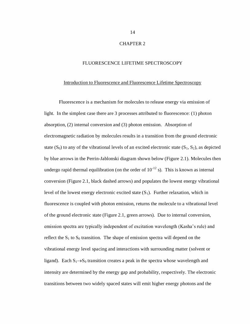
Fluorescence is a mechanism for molecules to release energy via emission of
light. In the simplest case there are 3 processes attributed to fluorescence: (1) photon
absorption, (2) internal conversion and (3) photon emission. Absorption of
electromagnetic radiation by molecules results in a transition from the ground electronic
state (S0) to any of the vibrational levels of an excited electronic state (S1, S2), as depicted
by blue arrows in the Perrin-Jablonski diagram shown below (Figure 2.1). Molecules then
undergo rapid thermal equilibration (on the order of 10-12
s). This is known as internal
conversion (Figure 2.1, black dashed arrows) and populates the lowest energy vibrational
level of the lowest energy electronic excited state (S1). Further relaxation, which in
fluorescence is coupled with photon emission, returns the molecule to a vibrational level
of the ground electronic state (Figure 2.1, green arrows). Due to internal conversion,
emission spectra are typically independent of excitation wavelength (Kasha’s rule) and
reflect the S1 to S0 transition. The shape of emission spectra will depend on the
vibrational energy level spacing and interactions with surrounding matter (solvent or
ligand). Each S1S0 transition creates a peak in the spectra whose wavelength and
intensity are determined by the energy gap and probability, respectively. The electronic
transitions between two widely spaced states will emit higher energy photons and the

15
more probable transitions will create more photons, producing higher signals. Molecules
displaying more structured spectra possess more vibrational energy states.
Figure 2.1: Perrin-Jablonski diagram of photon absorption and emission processes.
Emission spectra are influenced by a fluorophore’s local environment. Solvent
effects, complex formation, energy transfer, etc., can all result in a shift in the emission
spectra. For example Figure 2.2 shows the emission spectra of native (dashed line) and a
denatured form (solid lines) of cottonseed protein isolates (CSPI). Both the alkaline
soluble fraction and total protein isolate, CSPa and CSPI respectively, display an
approximate 15 nm red shift for the solvent exposed, denatured form relative to the native
folded protein isolates. The water soluble cottonseed extract fraction (CSPw) did not
show a spectral response with addition of denaturant suggesting that the tryptophan of
proteins in this fraction were already solvent accessible. 45

16
Figure 2.2. Fluorescence emission spectra of cottonseed protein isolate (CSPI,
black), cottonseed protein water soluble fraction (CSPw, red) and alkali soluble fraction
(CSPa, purple) collected under conditions promoting native (dashed line) and denatured
(solid line) conformations. Shifts to longer wavelengths, as seen for the denatured form
of CSPI and CSPa are commonly observed when fluorophores become solvent exposed. 45
Changes in emission spectra have become a valuable tool for researchers to
observe product formation,46
ligand interactions and characterize segmental motions of a
protein.47
The total shift observed between emission and absorption spectra, caused by
combined effects of internal conversion and the environmental factors listed above, is
known as the Stoke’s shift.
The most common fluorescence signal that is measured is steady-state
fluorescence or fluorescence intensity. Steady-state fluorescence is a measure of the
average number of the photons emitted over a long period of time (typically milliseconds
or seconds), enough time for the system to reach a photoequilibrium. Steady-state
fluorescence measured as a function of emission wavelength is referred to as the emission

17
spectrum (Figure 2.3, b). Likewise, steady-state fluorescence measured as a function of
excitation wavelength is an excitation spectrum.
Fluorescence lifetime (FL), or the time dependent intensity decay of a sample,
reflects the average time a molecule spends in an excited state, and typically occurs on
the order of 0.1-10 ns. Steady-state fluorescence can be determined by integrating the
signal of time-resolved measurements (Figure 2.3). The FL can be acquired by
measuring the intensity decay using a pulsed light source (time-domain), or using the
amplitude and phase changes of an intensity modulated light source (frequency-domain).
Since the instrumentation discussed within is a type of time-domain measurement,
frequency-domain fluorometry will not be discussed and all future references to time-
resolved data implies intensity decays collected in the time domain. Conventionally,
time-resolved data is referred to as a fluorescence decay curve. In this document, a
fluorescence decay curve may also be referred to as a waveform to emphasize the
generality of the measurement for data analyses.
Figure 2.3: Schematic emphasizing (a) steady state fluorescence as the integral of (b)
time-resolved fluorescence.

18
FL is sensitive to alterations in the environment directly surrounding the
fluorophore and can be used as a readout to monitor protein binding, reaction kinetics (in
vitro48 and in vivo49
) and structural changes. Excited molecules return to the ground state
by either radiative or non-radiative pathways. Non-radiative pathways include energy
transfer to the surrounding medium through physical and non-physical means. The
fluorescence lifetime () depends on rates of both radiative () and non-radiative (knr)
processes (Equation 1).
(1)
Electron relaxation from an excited state back to the ground state is a random event;
therefore depopulation of the excited state can be defined by Equation 2,
(2)
where n(t) is the number of molecules in the excited state at time t, and n0 is the total
number of molecules excited (number of molecules excited at t = 0). The intensity
observed can be written as
(3)
Equation 3 assumes that all molecules are excited at the same instant (i.e.,
infinitesimally sharp excitation pulse). Since this is not the case, the width of the
excitation laser pulse must be integrated into the fitting parameters to accurately
determine lifetime. As shown pictorially in Figure 2.4 below, the measured fluorescence
decay curve, N(tk), is the convolution integral of the instrument response function and
fluorescence decay signal. The laser pulse can be represented as a series of
infinitesimally sharp excitation events (orange lines, bottom graph), each exciting a

19
population of fluorophores proportional to the signal strength. The top figure
demonstrates this for a laser profile modeled by three sharp excitation pulses occurring at
times k = 1, k = 2 and k = 3. The first and third pulses are of lower intensity compared to
the second pulse. The total intensity measured (green line, N(tk)) after the first pulse
represents the decay of a relatively small population of fluorophores. The second pulse,
at time k = 2 pushes a larger population of molecules into the excited state and the
observed signal becomes the additive emission from molecules excited by both k = 1 and
k = 2 excitation events. Finally, the third excitation pulse promotes a smaller population
of fluorophores (relative to pulse at k = 2) into the excited state which then emit.
Because the third excitation pulse is less in intensity, the measured signal increase is less
than the signal increase observed following the second excitation pulse. To resolve the
laser profile and fit the fluorescence signal to a sum of exponentials, a mathematical
process known as iterative deconvolution is done.

20
Figure 2.4. Fluorescence data is a combination of the laser pulse profile and fluorescence
emission.50
The measured time dependent intensity, as a result of three infinitesimally
narrow excitation pulses at times t1, t2 and t3, is shown in the top figure. Similarly, the
measured fluorescence intensity profile as a function of time, N(tk), is the additive signal
from many excitation pulses and the resulting emission from all pulses.
The laser profile (a.k.a., instrument response function, IRF) can be measured
directly using a non-fluorescent scattering sample, such as glycogen or silicon beads, or
by measuring the Raman scatter of the solvent. Analysis of lifetime data collected in this
thesis used primarily Raman scattering of a water sample as an IRF in the deconvolution
process.
Development of Fluorescence
Instrumentation to Meet High-Throughput Demands
Due to rapidly growing compound libraries (theoretically ~100 million
compounds)51
and therapeutic targets, the current state of drug development necessitates

21
high-throughput to accelerate formulation. According to a recent review by McGregor
and Hornig, “HTP (high throughput) technology…is crucial for the identification and
validation of novel drug targets and next-generation antivirals.”52
This need has shifted
instrumentation to microfluidic and microplate formats, reducing time and sample
requirements. Fluorescence lifetime is inherently more robust compared to fluorescence
intensity. Fluorescence lifetime is independent of concentration (assuming no change in
state with increasing concentration), volume, slit width, and unaffected by inner filter
effects or laser power fluctuations. These characteristics help reduce false readouts in
assays. Currently available microplate fluorimeters advertising time-resolved capabilities
(Infinite® 200 PRO, PHERAstar® FS, SpectraMax Paradigm Multi-Mode Microplate
Reader) only offer microsecond lifetime acquisition. This is in part due to the
incompatible collection times of nanosecond time resolved instrumentation currently
available.
The most common technique for acquiring time-resolved data on a nanosecond
time scale is time-correlated single photon counting (TCSPC). TCSPC measures the
fluorescence decay by determining the time between excitation and detection of the first
emitted photon, then counts the number of photons detected for specified time intervals.
A histogram of the number of photons counted is built as shown in Figure 2.5, eventually
arriving at the final decay curve.53
To ensure detection of a single photon, the excitation
pulse energy is kept low, typically less than 1 nJ. Due to the statistics of random
emission, TCSPC experiments record 10,000 counts in the peak channel corresponding to
a noise level of approximately 1%.53
To collect this number of photons quickly, the pulse

22
repetition frequency (PRF) of the laser must be high, on the order of 106 Hz. However,
acquisition times for the fastest TCSPC systems still remain outside the limits for high-
throughput applications.
Figure 2.5: Histograms representing the build-up of the TCSPC emission decay curve
after 1, 20, 500 and 10,000 photon events. 53
Direct time-resolved measurements or direct waveform recording (DWR) is
probably the most direct approach to collecting decay information. This method uses a
transient recorder which stores the input from the PMT for digitization.53
The time
resolution is limited to the capabilities of the photodetector and transient recorder,
typically in the nanosecond range. However, for almost all biological and biochemical

23
applications, this is adequate. Fluorescence Innovations, Inc. (FII) has developed
proprietary digitization technology capable of acquiring accurate (0.5%) and precise (1%)
direct time-resolved fluorescence lifetime data in 0.1 ms.54
The high precision is a
consequence of recording thousands of photons for every laser pulse. A detailed
description of the cuvette-based instrument design, components and comparative study to
TCSPC method can be found in reference 54.
The collection times of FII’s technology make it the only nanosecond time-
resolved instrument on the market compatible for high-throughput, microplate formats.
This first section will detail the changes made to FII’s prototype cuvette instrument to
microplate format and the characterization/validation of these instruments.
Design of Nova Fluor FLS Plate Readers
Two fluorescence lifetime spectrophotometers (Vis NovaFluor and UV
NovaFluor) were designed to utilize FII’s technology. Because this technique is not
limited to counting single photons, lower repetition frequencies and more powerful lasers
can be used, resulting in more emitted photons, better photon statistics and shorter
collection times. Both instruments implemented similar design schemes (Figure 2.6),
differences being excitation laser sources and emission wavelength selection.

24
Figure 2.6: Diagram of NovaFluor FLS plate readers. Dye flow cell outlined in green is
specific to the UV NovaFluor. Detection module not shown.
The Vis NovaFluor system contains two passively Q-switched microchip lasers
producing 355/532nm (Teem photonics) and 473 nm (Concepts Research Corporation,
model) excitation. Passively Q-switched lasers eliminate electromagnetic noise that
would otherwise disrupt detection electronics. 54
Highly uniform pulses created by these
lasers (1 ns full width at half maximum, ≤3% pulse-to-pulse deviation) contribute to
extraordinarily high data precision and eliminate the otherwise necessary IRF collection
between samples. The emitted light is collected with an off-axis parabolic mirror

25
(Newport). The appropriate filter (532, 365 and 473 nm long pass filters, Semrock) can
be secured to the lens tube to remove any scattered light. A six position filter wheel
containing 5 bandpass filters provides emission selection and subsequent photodetection
by a PMT (Hamamatsu). The second instrument, UV NovaFluor, contains a high power
(>20 J) 532 nm passively Q-switched laser (Teem photonics, model PNG-002025) that
acts as a pump for a pyrromethane dye (600 M in ethanol) to create a 560-610 nm lasing
output. The output is selected via rotation of a tunable bandpass filter (Semrock), and
subsequently passed through a doubling crystal to produce 285-310 nm excitation (1
J/pulse). Emitted light is again collected with an off-axis parabolic mirror and directed
to a monochromator for emission selection.
Collection Modes. Several types of data can be collected on this instrument. Each
measurement is represented by a three letter acronym. The two terminal letters of almost
all measurement acronyms are TM, representing Time Matrix. This naming was derived
from the measured data matrix which always contains the fluorescence intensity as a
function of time (fluorescence decay curve) in one dimension. The first letter represents
the ‘other variable’ which can be emission wavelength, excitation wavelength, sample,
time (longer time scale, typically seconds), polarization, attenuation, temperature, etc.
Text files containing data are set up to record all parameter settings as shown in Figure
2.7. A definition of each collection acronym is given in Appendix 1.

26
Figure 2.7: Labeled data matrix for data collected using NovaFluor instruments.
Instrument Calibration and Validation
Fluorescence is one of the most common reporters available to researchers, not
only in chemistry but biology and biomedical science. High sensitivity makes
fluorescence a valuable indicator of cell membrane, protein and DNA processes and a
driving force for optical imaging advances.55
Fluorescence has even been used to
visualize tumors in live mice.56
The chemical information reported by a fluorescent
probe is observed and evaluated through changes in fluorescence intensity or quantum
yield, shifts in emission spectra, and alterations in decay kinetics (or lifetime). The
measurement of fluorescence lifetime and intensity data rely on the response of detection
electronics and compatible optics. As well stated by Zenger et al., “objective methods to
assess the quality of data obtained by (fluorescence) measurements are critically

27
important to research scientists, clinical laboratory personnel, and regulatory
reviewers.”57
The fluorescence signal is sensitive to both environmental stimuli (sample
content) and instrumental factors (efficiency/sensitivity of electronics and optics).
Evaluation of instrument inconsistencies come by way of universal standardization
procedures for fluorescence instrumentation.57,58
The fluorescence lifetime plate readers
introduced in the previous section were validated using techniques recommended by the
American Society for Testing and Materials (ASTM) and inferred from reference 59.
The following are results of this validation process.
Wavelength Accuracy
and Spectral Responsivity
Collection of absolute emission spectra is a challenge due to the distortion caused
by both instrumental factors (transmission efficiency and polarization sensitivity of the
monochromator, mirror reflectivity, and PMT sensitivity) and sample-related effects
(such as inner filter effects and competing absorption). The minimum correction required
to compare emission spectra collected on different instruments corrects only for
instrumental factors distorting spectra. Methods of determining instrumental correction
factors include using an irradiation standard with known spectral distribution (such as a
tungsten-halogen lamp) or quantum counters. Since this equipment is typically
unavailable, the most common method to correct emission spectra is to collect spectra
using secondary emission standards and compare this to literature reported values.
Secondary emission standards include (but are not limited to) laser dyes and inorganic
dyes imbedded in a solid substrate.60

28
Emission spectra of fluorescein and 9,10-diphenylantrhacene (DPA) were
measured and compared to reference spectra61
to determine the spectral responsivity of
NovaFluor detection optics. Fluorescein (3.8 mg, 10.1mol) was dissolved in 5 mL 0.1
M NaOH, then diluted 1:1000 for a 2 M stock solution. Similarly, DPA (1.5 mg,
4.5mol) was dissolved in 3 mL benzene and diluted 1:1000 to produce a 1.5 M stock
solution. Fluorescence emission scans on solvents were recorded prior to solution
preparation to check for possible fluorescent contaminations. Stock dye solutions (150
L) were diluted with an equal volume of solvent and scanned (295nm excitation, 400 V
PMT gain, 1 second signal averaging[190 shots], 300-650 nm emission). Final dye
concentrations were 1 and 0.7 M for fluorescein and DPA, respectively.
Overall, the monochromator appears to be well calibrated, with peaks of both
dyes corresponding to that reported (Figure 2.8). The slight variation observed for DPA
spectra could be a result of oxygen quenching (samples were not degassed). The detector
response was slightly lower for wavelengths longer than roughly 550 nm. A majority of
measurements on the UV-NovaFluor will be made at wavelengths below 400 nm. In fact,
the only data collected on this instrument at wavelengths longer than 400 nm thus far are
reported here. Therefore, the need to integrate a correction factor into the software did
not merit the time required to do so.

29
Figure 2.8: Normalized emission spectra of DPA in benzene and fluorescein in 0.1M
NaOH for UV Nova Fluor (blue line) and reference corrected spectra61
(red squares).
Detection System
Linearity and Limits of Detection
The linearity of each instrument was determined by measuring the fluorescence
signal produced at different concentrations of fluorophore. Two of the fluorophores
selected, p-terphenyl (PTP) and Rhodamine 6G (R6G), were standard dyes possessing the
following recommended characteristics: (1) responsive and stable at the selected
excitation wavelength, (2) large quantum yield independent of concentration, (3) and
broad emission spectra.62
The third sample tested was the protein standard bovine serum
albumin (BSA). It was chosen as the representative protein sample simply due to its
availability and stability. Fluorescence intensities for R6G, BSA and PTP are shown as a
function of concentration on both linear and log scales (Figure 2.9). Intensity was
calculated as the integral of the fluorescence decay curve from 0-90 ns.

30
Figure 2.9: Fluorescence intensity of varying concentrations of R6G (a-b) collected on
the Vis NovaFluor, and BSA (c-d) and PTP (e-f) collected on UV Nova Fluor,
respectively. (a), (c), (e) log scale; (b), (d), (f) linear scale.
The upper limit of linearity was defined as the upper point that deviated more than
5% from the straight line fit. The integrated signal shown in Figure 2.9 appears to be
linear for Vis NovaFluor at the range tested (i.e., an upper limit could not be determined
with this data set). Greater variability was observed for signals exceeding 80 mV at the
peak (Figure 2.9, b). This could be a result of pipetting errors, reflecting the sensitivity of
intensity measurements to changes in the volume or path length. Deviation from linearity

31
was observed for the UV NovaFluor instrument for sample concentrations exceeding 6.2
M BSA and 1 M PTP.
The limit of detection (or lower limit of linearity) was determined as the
concentration where the signal deviates by more than twofold from the average percent
deviation (as determined by the middle five data points). Lower limits of detection were
determined to be 1.2 M BSA, 30 nM PTP for the UV NovaFluor instrument. The
visible system had higher sensitivity due to the use of bandpass filters in place of a
monochromator. Bandpass filters transmit between 87-95% of incident light depending
on wavelength compared to 30-50% efficiency of a typical monochromator. The lower
limit of detection of the Vis NovaFluor was determined to be 2.6 nM R6G. The average
straight line deviations for each fluorophore were 3.4%, 4.9% and 1.9% for R6G, PTP
and BSA, respectively.
Time-resolved data is expected to maintain shape regardless of concentration or
signal magnitude. This was verified by directly comparing the overlap of area
normalized waveforms (Figure 2.10), and by iterative reconvolution to determine
lifetimes (Figure 2.11). Deformation of time-resolved data was not observed for either
Vis-NovaFluor or UV-NovaFluor data with peak amplitudes between 7-80 mV and 5-45
mV, respectively. Negligible differences of first moment and lifetime values (iterative
reconvolution with Raman scatter IRF) further support the lack of distortion with
increasing signal (Table 2.1). BSA required a bi-exponential fit as expected for the
fluorescence decay curve of tryptophan containing protein. This was reduced to the

32
average lifetime (Equation 4) which was within the range of literature reported data (6.05
ns63
and 6.77 ns64
).
(4)
Figure 2.10. Normalized waveforms of varying amplitudes for (a) PTP, 4-35 mV, (b)
R6G, 7-91 mV, and (c) BSA, 4-45 mV.

33
Figure 2.11. Sample fits and residuals for iterative reconvolution of fluorescence decay
spectra. (a) PTP (12 waveforms, 60-980 nM), (b) R6G (12 waveforms, 1-10.4 nM) and
(c) BSA (8 waveforms, 0.4-2.9 M).

Table 2.1. Lifetimes for R6G, PTP and BSA decay curves (data represents average of duplicate or triplicate samples). Single
exponential functions sufficiently fit R6G and PTP waveforms. A biexponential fit was required for BSA. The value reported i s the
weighted average lifetime (equation 4).
[R6G] (M) Avg ±
(RSD) [PTP] (M)
Avg ±
(RSD) [BSA] (M)
Avg < ±
(RSD)
1 3.94 ± 0.06 ns
(1.5%) 15.7 NA 0.4
6.66 ± 0.07 ns
(1.0%)
0.80 3.87 ± 0.13 ns
(3.2%) 7.8 NA 1.2
6.55 ± 0.13 ns
(2.0%)
0.60 3.96 ± 0.02 ns
(0.5%) 3.9 NA 2.1
6.56 ± 0.03 ns
(0.4%)
0.50 3.90 ± 0.08 ns
(2.0%) 2.0
1.29 ±0.22 ns
(17%) 2.9
6.57 ± 0.01 ns
(0.2%)
0.40 3.88 ± 0.05 ns
(1.3%) 1.0
1.19 ±0.15 ns
(17%) 3.7
6.65 ± 0.11 ns
(1.7%)
0.30 3.91 ± 0.04 ns
(1.0%) 0.49
1.18 ±0.005 ns
(0.45%) 4.6
6.75 ± 0.001 ns
(0.02%)
0.20 3.92 ± 0.04 ns
(1.0%) 0.25
1.12 ±0.008 ns
(0.76%) 5.4
6.82 ± 0.0008 ns
(0.01%)
0.17 3.90 ± 0.02 ns
(0.5%) 0.12
1.08 ±0.006 ns
(0.51%) 6.2
6.89 ± 0.0002 ns
(0.003%)
0.12 3.86 ± 0.10 ns
(2.7%) 0.061
1.07 ±0.048 ns
(4.48%) 7.0
6.93 ± 0.03 ns
(0.4%)
0.08 3.88 ± 0.08 ns
(2.1%) 0.03
1.18 ±0.005 ns
(0.45%)
0.04 3.84 ± 0.01 ns
(0.30%) 0.015 NA
Overall
(0.08-0.80)
3.90 ± 0.07 ns
(1.70%)
Overall
(0.08-0.80)
1.10 ±0.05 ns
(4.11%)
Overall
(1.2-3.7 M)
6.58 ± 0.08 ns
(1.5%)
34

35
Experimental. Stock Rhodamine 6G (R6G, 7.1 M) was prepared by dissolving
an arbitrary amount in water. The absorbance at 530 nm of a 5x dilution was measured to
determine the concentration (A530 = 0.14, = 116,000 M-1
cm-1
). This sample was diluted
further such that a 300 L sample (approximately 0.4 m path length) produced a signal
close to 100 mV at 532 nm excitation, 610 nm emission (20 nm band pass). Samples were
prepared according to Table 2.2, weighed after each addition, and then transferred to a
quartz microplate (300 L × 3 samples).
Table 2.2 Sample preparation and weight data for Vis NovaFluor linearity experiment.
Well Volume
water (mL)
Volume
R6G (mL)
Weight
water (g)
Weight
R6G
solution (g)
Weight %
(v/v) [R6G]
1, 13, 25 0 1.5 NA NA 100
2, 14, 26 0.30 1.2 0.30 1.213 80
3, 15, 27 0.60 900 0.609 0.908 60
4, 16, 28 0.75 750 0.759 .757 50
5, 17, 29 0.90 600 0.908 0.608 40
6, 18, 30 1.0 500 1.058 0.463 30
7, 19, 31 1.2 300 1.200 0.309 20
8, 20, 32 1.25 0.25 1.249 0.247 17
9, 21, 33 1.3 0.20 1.322 0.183 12
10, 22, 34 1.4 0.10 1.384 0.121 8
11, 23, 35 1.45 0.05 1.459 0.061 4
12, 24, 36 1.5 0 NA NA 0
Scans were recorded using 0.50 s averaging (100 laser pulses), 400 V gain setting
for the photomultiplier tube (PMT), 500 mV digitizer range, 532 nm excitation and 610
nm emission. Water Raman was collected at 556 nm emission (20 nm bandpass) without
either polarizer or 532 nm cutoff scatter filter. Curves were compared by normalization,

36
moment analysis and iterative reconvolution using the Raman scattering as an instrument
response function.
A stock solution of PTP (157 M) was diluted 10 fold with ethanol in a quartz
microplate. Successive dilutions (two fold) were repeated in 11 adjacent wells providing
concentrations of 15.7, 7.8, 3.9, 2.0, 1.0, 0.49, 0.25, 0.12, 0.061, 0.031, and 0.015 M.
Fluorescence decay curves were recorded with UV NovaFluor at 295nm excitation, 350
nm emission, 1.05 s sample averaging (200 shot) and 400 V PMT gain.
Stock BSA (A280 = 0.73, = 43,000 M-1
cm-1
, 17 M) was dissolved in Aquafina
water then diluted according to Table 2.3 (duplicate samples). Waveforms were acquired
at identical settings as for PTP. Seven scans were recorded at varying excitation
attenuation (iris adjustment) to produce roughly 50 mV peak amplitude for BSA samples
between 2.1-7.0 M (data shown in repeatability section).
Table 2.3: Volumes used and corresponding concentration of BSA.
Well Volume H2O
(L)
Volume BSA
solution (L)
[BSA]
(M)
1, 13 200 0 0
2, 14 200 (PBS) 0 0
3, 15 200 5 0.4
4, 16 190 15 1.2
5, 17 180 25 2.1
6, 18 170 35 2.9
7, 19 160 45 3.7
8, 20 150 55 4.6
9, 21 140 65 5.4
10, 22 130 75 6.2
11, 23 120 85 7.0
12, 24 0 0 0

37
Solvent scans were recorded under identical instrument settings to experimental
data prior to adding sample. This was done to verify cleanliness of microplate and
solvent.
Reproducibility
Assessment of data reproducibility provides confidence that any observed changes
are a direct result of the experimental variable being tested. The repeatability of the
NovaFluor instruments was evaluated through three separate experiments.
Day-to-day repeatability was evaluated through collection of water Raman decay
curves collected randomly over 13 months then compared to verify the excitation pulse
width stability of the UV NovaFluor. These waveforms varied in intensity due to
adjustment of an iris preceding the parabolic mirror (refer to Figure 2.6 for instrument
diagram). A significant time shift (0.5 ns) was observed for the water Raman signal
collected April 2013 (unshifted data not shown) which was due to adjustment and
recalibration of the tuning mechanism and doubling crystal. Therefore, waveforms
underwent a waveform overlap procedure to compare the shape of Raman signals. This
procedure matched waveform amplitudes and shifted waveforms in time to provide
maximal overlap. The results of this overlap are shown in Figure 2.12. Excellent stability
was observed for the pulse width over long periods of time.

38
Figure 2.12. Normalized and time shifted Raman waveforms for 5 water samples collected
over a 13 month time period. The standard deviation has been scaled by a factor of 10.
The sample-to-sample repeatability was tested for both UV and Vis NovaFluor
systems using reference solutions. For the Vis NovaFluor, eleven samples of rhodamine B
(RB), anthracene, and coumarin 480 (C480) were scanned using the 532 nm, 355 nm and
473 nm laser sources, respectively. Emission was collected through the 610, 438 and 500
nm bandpass filters for RB, anthracene and C480, respectively. The PMT gain was set to
400 V, and 1.05 s (200 shot) waveform averaging was used. The same waveform overlap
procedure used to evaluate the water Raman shape was applied to compare waveforms for
RB, anthracene, and coumarin 480. Waveforms for each dye were found to be identical
with high precision (Figure 2.13).

39
Figure 2.13. Average (solid line) and standard deviation (dashed line, scaled 100 fold) of
overlapped waveforms for RB (blue), anthracene (red), and C480 (green).
The UV NovaFluor repeatability was evaluated using eight of the waveforms
collected for the linearity study (0.4 mM-6.2mM, duplicate samples). BSA was excited at
295 nm the resulting emission at 340 nm was evaluated. Fluorescence decay curves of
BSA collected on the UV NovaFluor were normalized such that the integrated area under
each waveform was equal. These waveforms were also highly repeatable. The average
relative standard deviation of BSA decay curves at 8 different concentrations (duplicate
samples) was 0.74% for t=18-40ns (Figure 2.14).

40
Figure 2.14: Average (blue) and standard deviation (scaled 10 fold, red) of BSA
waveforms (15 decay curves, 8 concentrations).
The waveform comparisons performed above demonstrate the excellent precision
and stability of the NovaFluor instruments (Figures 2.12-2.14). This high precision is
comparable to the precision observed for cuvette based instruments equipped with the
same technology (Figure S11 of reference 48). This suggests conversion to a microplate
format did not adversely affect the acquired data.
Fluorescence Lifetime Standards
The accuracy of time-resolved fluorescence measurements was evaluated through
comparison of the deconvoluted lifetime values with those reported in the literature for
eight reference dyes. Recommended reference dyes have the characteristics of large
Stokes shifts and quantum yields to avoid problematic interferences such as self
quenching and intermolecular interactions.65
They are readily available in high purity and
soluble in common, high grade solvents. A majority of the dyes selected for this study

41
meet these criteria with the exception of D L-tryptophan, which was selected because it is
the primary, intrinsic fluorophore of proteins. Table 2.4 provides the solvent used, the
appropriate excitation and emission wavelengths range, and literature reported lifetimes
for each fluorophore.
Table 2.4. Calculated lifetimes for reference dyes.
Dye Solvent Excitation/Emission
Wavelength (nm)
Lifetime,
Literature (ns) Ref
Lifetime,
measured (ns)
Anthracene Methanol
295-360/375-442 5.10.3 65 3.900.01ǂ
Ethanol 4.210.02 59 3.990.01ǂ
Fluorescein 0.1M
NaOH 495/517 4.16 66 4.060.07
Coumarin
480 Methanol 390/407-473
1=5.50 ± 0.01
2=0.02 ± 0.004 67
1=5.60 ± 0.02
2=0.04 ± 0.02
DPA Methanol 355/430 8.70.5 65 5.880.04ǂ
Rhodamine
B Water 532/590
1.740.02 65 1.74.01†
1.680.1 68
R6G Water 525/555 4.080.1 68
4.060.05 3.8 0.45 69
PTP Methanol
295/336 1.170.08 65 1.260.01
Ethanol 1.05 59 1.110.05
D L-
tryptophan Water 295/350 3.3 70
1=0.03 ± 0.02
2=3.240.05
ǂ Quenched by molecular oxygen (sample were not de-gassed).
†Reconvolution required biexponential fit (2 = 0.57 ± 0.03 ns)
As shown in Table 2.4, determined lifetimes for fluorescein, rhodamine B, R6G,
PTP and D L-tryptophan are all consistent with published data.
Anthracene and DPA both had significantly shorter than expected lifetimes. These
fluorophores are highly susceptible to oxygen quenching and samples were not degassed.
This is most likely the source of the reduced lifetimes.

42
The biexponential fit necessary for rhodamine B is most likely an artifact of the
IRF. Reconvolution with a Rayleigh scatter IRF collected at a later time provided a good
single exponential fit (1.72 ± 0.01 ns) but required a time shift of 0.08 ns.
The short component of the Coumarin 480 decay curve correlated with that
reported but the long lifetime component was slightly longer. The cause of this is
currently unknown. Coumarins are highly sensitive to their environment, which makes
them excellent chemical sensors.71
It is possible that a trace amount of another solvent,
for example water, was present in the well into which C480 was loaded, and is responsible
for the lifetime difference.
The experimental lifetime of the major component of the tryptophan fluorescence
(2 = 3.24 ns) is consistent with the literature reported data. A second exponential was
required for a good fit which could be a result of a possible contaminant, an inaccurate
IRF, or, due to the absence of an emission polarizer in the UV NovaFluor. The emission
polarizer, when set to the appropriate angle removes rotational bias of the fluorescence
emission. Rotational bias is a consequence of preferential excitation of molecules with
absorption dipoles aligned with the electric vector of the exciting light. This means that
the fluorophores able to absorb light are similarly oriented. Molecules free in solution are
able to rotate during the period between excitation and emission, meaning that the
resulting emission may not have identical orientation as the incident light. Photodetectors
are sensitive to the changes in light polarization and will tend to favor one orientation.
The bias of photodetectors combined with the changes in the orientation of the
fluorophore result in slight shifts in the measured fluorescence decay.

43
Analyzing Fluorescence Lifetime Data
One significant problem with time-resolved data comes in the reduction of decay
curves to a set of parameters. There is a need to select enough parameters to provide an
adequate fit; however, fitting exponentials to too many parameters results in less precise
measurements. (This is not limited to fluorescence decay curves, but rather applies to all
exponential functions.) As a response, alternative methods that involve treating the decay
curve as a spectrum have been developed.
The spectrum approach requires more sophisticated data processing, but
mathematical algorithms to analyze spectral data for the purpose of mixture analysis are
well known. Spectral analyses, where all data points are used in the fitting, originated in
chemometrics but are increasingly being used in spectroscopy.72, 73
Spectral analyses
processes are variously referred to as spectral decomposition74
, spectral deconvolution75
,
spectral unmixing76
, multivariate curve resolution, etc. The choice of name depends in part
on the intended use of the data. Which procedure is most effective may depend on the data
quality. In many cases, the signal changes can be modeled using a weighted linear
combinations of pure responses, as discussed in chapter 3.73
The procedures could be
applied to a variety of spectral data including Raman, absorbance, excitation, emission
and, in this case, the decay spectra.
Conventionally, time-resolved fluorescence is deconvoluted to a set of amplitude
factors and fluorescence decay times. These lifetimes can then be modeled to characterize
the biological or chemical process that is occurring. This method of analysis is
complicated, and sometimes the link between the reaction (or interaction) and

44
fluorescence lifetime is not fully understood. The reason for multiple lifetimes of
tryptophan containing proteins, for example has been77
and continues to be a topic of
debate.78
The high precision of NovaFluor technology permits treatment of the
fluorescence decay as a spectrum, similar to an emission spectra/wavelength-intensity
spectrum. This reduces the noise because it relies on the shape of the curve, which is a
molecular property.
Summary
Fluorescence lifetime spectroscopy offers a versatile platform for evaluating
molecular interactions. A combination of lifetime, intensity and polarization data has the
potential to report on binding, size and relative distances (referring to FRET which was
not discussed but a possible measurement). The need to properly calibrate new
fluorescence based instrumentation is validation necessary to rely on data acquired by the
system. Validation experiments of the UV and Vis NovaFluor plate readers show there
excellent linear response and no waveform distortion was observed as a result in either
electronics or optics.

45
CHAPTER 3
APPLICATIONS OF FLUORESCENCE LIFETIME SPECTROSCOPY
Introduction and General Considerations in Experimental Design
The following summarizes analysis techniques and equations used in the treatment
of fluorescence decay curves as spectra for various applications. Specifically, this chapter
discusses their use in determining binding constants, kinetic rates of reactions, and
thermodynamic stability. This treatment prevents the need for deconvolution. These
analyses rely on the ability to define physical states of the system by the observed lifetime
and are dependent on the distinct lifetimes that exist for each physical state. Decay
curves, or waveforms, can be defined as a linear combination of “state” or “basis”
waveforms when this criterion is met. This is shown for two hypothetical states, X and Y,
each represented by distinct waveforms WX and WY, respectively (equation 5). In this
case, the population of each state is determined by the variable i, and determined by the
coefficients fx,i and fy,i. i can represent ligand concentration, time, temperature, denaturant
concentration, etc.
(5)

46
Application 1:Protein-Ligand Binding Constant Determination
Assuming that there only exists, on average, a single free and bound form of an
intrinsically fluorescent or fluorescently labeled protein, the observed waveform can be
described as the linear combination of waveforms characteristic to each form.
ibbiffi fWfWW ,, (6)
Here Wf, Wb and Wi represent the waveform of free protein, bound protein and protein at
some ligand concentration, i. The fraction of free and bound protein for a given ligand
concentration, i, is represented by ff,i and fb,i, respectively.
The dissociation constant and the law of mass action can relate the fraction of free
and bound protein to the ligand concentration, [L]i and the dissociation constant, Kd by
equations (7) and (8).
id
d
ifLK
Kf
,
(7)
id
i
ibLK
Lf
,
(8)
Substitution of (7) and (8) into (6) results in the following equation:
id
i
b
id
d
fiLK
LW
LK
KWW
(9)
The free spectra and ligand concentrations are measured parameters. If the bound
waveform is unattainable through direct measurements, data extrapolation using a
modified version of equation (6) allows for simultaneous solution of Kd and Wb:

47
i
d
f
i
id
ibL
KW
L
LKWW
(10)
Data sets can be fit using equation 6 and the coefficients ascribed to the free state
modeled with equation 7 to determine Kd. In both fitting techniques, a non-linear least
squares approach was taken to minimize the difference between measured and theoretical
data.
Monomeric Binding
of Lactose to Galecin-3
Galectin-3 is a member of the galectin family of proteins, a family characterized by
their ability to bind -galactoside sugars. Galectin-3 contains three tryptophan residues,
two in its unstructured, N-terminal collagen like domain and one in the binding site of the
C-terminal carbohydrate recognition domain (CRD). Given the position of the tryptophan
residue (Figure 3.1) relative to incoming -galactosides, it was reasonable to believe
binding could be characterized by changes in the intrinsic fluorescence of the protein.

48
Figure 3.1. Crystal structure of galectin-3 CRD (blue) bound to lactose (green).
Tryptophan residue is shown in orange. 79
In this scenario, Wf and Wb from equation 6 above represent the waveforms of free
and lactose bound galectin-3, respectively (Figure 3.2). Wi is the measured fluorescence
decay curve in the presence of a given concentration of lactose, i and is assumed to be a
linear combination of Wf and Wb. The difference between bound and free waveforms is
small but significantly different given the precision of the fluorescence waveform
recording technology used (as discussed in the Reproducibility section of Chapter 2).

49
Figure 3.2. Normalized free (blue and green) and bound waveforms (red and purple) of
galectin-3. The free and bound forms were averaged and the difference of these averages
is shown in light blue (scaled 10 fold).
The coefficients calculated for these two data sets were fit to equation 7 to afford
an average Kd of 49 ± 4 M (Figure 3.3). The calculated Kd was slightly lower than the
binding constants reported for the galectin-3/lactose interaction (0.14 mM-0.22 mM), but
given the variability it seems reasonable.6 Furthermore, shifts were observed in the
emission spectra of galectin-3 upon lactose addition (data not shown) supporting that an
interaction occurred.

50
Figure 3.3. Lactose binding curve for galectin-3. The coefficient corresponding to the
fraction of free galectin-3 (equation 6) from the fluorescence waveform analysis was used.
This experiment was repeated with lactose functionalized dendrimers (generations
2, 4 and 6). The glycodendrimer concentrations were attenuated to match the
concentration of lactose used in the previous study (concentrations of each
glycodendrimer series are shown in Table 3.1). Equation 7 was modified to include a
cooperativity term (n) to compensate for the multivalent nature of the glycodendrimers
used (equation 11).
(11)
Here [GX] represents the concentration of glycodendrimer used.
The effect of the cooperativity term in fitting the binding curve was significant for
G2-lactose functionalized dendrimers but insignificant for G4 and G6 glycodendrimers
(Figure 3.4). When n was not included as a fitting parameter, the resulting Kd was
significantly higher in most cases, with the exception of trial 2 data of G4 glycodendrimer

51
(Table 3.1). The cooperativity term was <1 in most cases, suggesting multiple galectin-3
were bound to a single glycodendrimer.
Figure 3.4. Binding curve for generations 2 (a) and 6 (b) lactose functionalized
dendrimers. Measured data was fit with (dashed line) and without (dotted line) the
cooperativity term, n.
Table 3.1. Binding constants calculated for galectin-3 and lactose functionalized
dendrimers.
Glyco-
dendrimer Trial n
Kd
(M) SSE† Kd (n=1) SSE (n=1)
G2-lactose 1 0.87 20 1.1 32 1.2
2 0.73 36 0.40 126 0.90
3 0.67 15 0.60 52 1.50
G4-lactose 1 0.85 24 2.78 42 2.86
2 1.25 77 0.19 33 0.32
G6-lactose 1 0.81 12 0.64 22 0.78
†SSE is the summed square error
When the cooperativity term is fixed to 1, implying a single galectin-3 binds to a
single glycodendrimer, the binding constant for G2 and G4 lactose dendrimers (70 ± 50
M and 38 ± 6 M, respectively) were similar to monomeric lactose (49 ± 4 M). The
generation 6 glycodendrimer showed a slight enhancement (Figure 3.5 and Table 3.1).
However, more trials are necessary to verify this.

52
In summary, the position of the tryptophan within the binding site of galectin-3
allowed characterization of lactose binding using FLS.
Figure 3.5. Sample binding curves for Galectin-3 with lactose functionalized dendrimers
and monomeric lactose.
Application 2: Reaction Kinetics
In this second study, the change in fluorescence as a function of time following
ligand addition was used to model the kinetics of aggregate formation between
Concanavalin A (Con A) and mannose functionalized PAMAM dendrimers. Con A is a
stable and well characterized plant lectin that binds to -D-mannose and -D-glucose.80
It
contains four tryptophan residues per monomer, most buried within the -sheet motif
(Figure 3.6). One of the four tryptophan residues is located on the most exterior -strand
suggesting that it could be used to report interactions between tetramers (Figure 3.6,
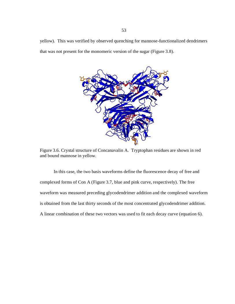
53
yellow). This was verified by observed quenching for mannose-functionalized dendrimers
that was not present for the monomeric version of the sugar (Figure 3.8).
Figure 3.6. Crystal structure of Concanavalin A. Tryptophan residues are shown in red
and bound mannose in yellow.
In this case, the two basis waveforms define the fluorescence decay of free and
complexed forms of Con A (Figure 3.7, blue and pink curve, respectively). The free
waveform was measured preceding glycodendrimer addition and the complexed waveform
is obtained from the last thirty seconds of the most concentrated glycodendrimer addition.
A linear combination of these two vectors was used to fit each decay curve (equation 6).

54
Figure 3.7. Free and complexed waveforms for Con A bound to mannose
glycodendrimers.
In this case, the waveform at time i, Wi, can be represented by mixing the basis
waveforms of the free and complexed Con A (Wf and Wb, respectively). The variable i
now represents time, and b refers to the complexed rather than sugar-bound Con A. The
relative amount of each basis waveform is again determined by the preceding coefficients.
Hence, for any given time i, ffi and fbi identify how much of the free and complexed
waveform, respectively, are present. Consequently, the coefficients reveal the
concentration of each species at a given time (Figure 3.8). At maximal dendrimer
concentration, all Con A is assumed to have entered into a protein-protein interaction, and
this is an approximation.
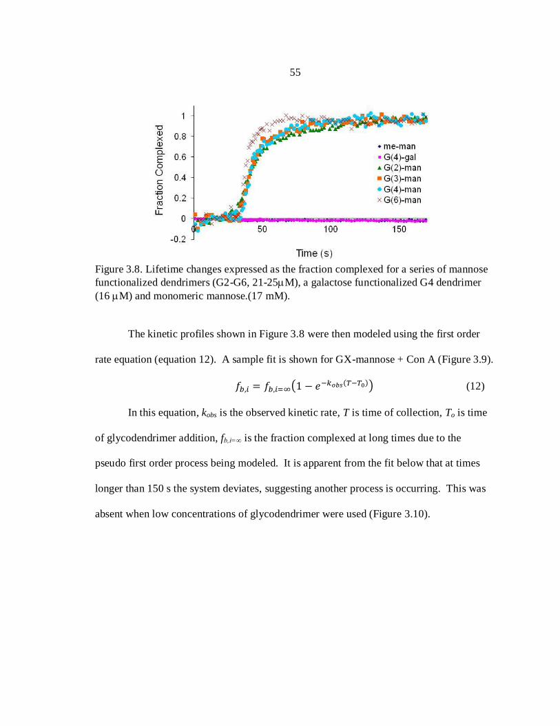
55
Figure 3.8. Lifetime changes expressed as the fraction complexed for a series of mannose
functionalized dendrimers (G2-G6, 21-25M), a galactose functionalized G4 dendrimer
(16 M) and monomeric mannose.(17 mM).
The kinetic profiles shown in Figure 3.8 were then modeled using the first order
rate equation (equation 12). A sample fit is shown for GX-mannose + Con A (Figure 3.9).
(12)
In this equation, kobs is the observed kinetic rate, T is time of collection, To is time
of glycodendrimer addition, fb,i=∞ is the fraction complexed at long times due to the
pseudo first order process being modeled. It is apparent from the fit below that at times
longer than 150 s the system deviates, suggesting another process is occurring. This was
absent when low concentrations of glycodendrimer were used (Figure 3.10).

56
Figure 3.9. Kinetic profile of G6-mannose (65 M) modeled using equation 12.
Figure 3.10. Kinetic profile of G3-mannose (1.8 M) modeled using equation 12 (taken
from supplementary materials of reference 48)
These profiles show similar rates for G2-G4 glycodendrimers and a slight increase
for G6-mannose. The distance between binding sites on Con A is roughly 7 nm (Figure
4.1). Therefore, the increased rate observed for G6-mannose is likely a consequence of
multivalent interactions between it and Con A. Experimental details and kinetic results
can be found in reference 48 or in Chapter 5 of the graduate thesis of Dr. Kristian Schlick.

57
This shows that FLS can be used to track aggregate formation rates by correct
positioning of the fluorophore. Kinetic data were fit using first order assumptions but the
possibility to model more complex scenarios exists.
Application 3: Chemical Denaturation
The ability to track protein denaturation can provide information on the stability of
a protein and factors that affect stability. The pioneering work, led by Nick Pace formed a
foundation of equations to model thermal and chemical denaturation processes.81-84
Stability can be investigated by altering the environment of the protein, say by addition of
potentially stabilizing small molecules, then evaluating the effect on thermodynamic
parameters calculated from denaturation profiles. Collection of denaturation profiles can
be done through a variety of techniques. Examples include circular dichroism, viscosity,
NMR, optical rotation, absorbance and, of course, fluorescence. A recent study on
calcium ion binding to the C2A domain of synaptotagmin (a protein involved in the
regulation and release of neurotransmitters and hormones) combined circular dichroism,
and FLS to determine the mechanistic basis of this domain’s function.85
In this section,
the chemical denaturation curves were collected using FLS as a measure of folded protein
content: the stability contribution of the N-terminal domain on the overall structure of
galectin-3 was evaluated.
For this case, the two ‘state’ waveforms from equation 6, Wf and Wb, represent the
native and unfolded protein respectively. Wi represents the waveform recorded for
varying concentrations, i, of denaturant. A linear combination of the native and denatured

58
waveforms is used, each contributing ff,i and fb,i, respectively, at the specified
concentration i. Figure 3.11 shows the chemical denaturation curve for full length (FL)
and the carbohydrate recognition domain (CRD) of galectin-3. In this experiment urea was
used; another common denaturant is guanidine hydrochloride.
Figure 3.11. Denaturation of FL (blue) and CRD (green) of galectin-3 as a consequence of
urea addition.
Urea shifts the equilibrium between the native and denatured protein to increase
the population of the denatured state (equation 14).
(14)
The equilibrium constant, Keq, reflects the shift and can be related to the Gibb’s
free energy of the system (G°). Since Keq is simply the ratio of native and denatured
forms, G° can be determined using equation 15. This calculation was done for every urea
concentration tested and was plotted as a function of urea concentration (Figure 3.12).
(15)

59
Figure 3.12. Free energy as a function of urea concentration for FL (blue) and CRD
(green) constructs of galectin-3. The bi-phasic nature of FL galectin-3 required two linear
fits; the fit at higher urea concentrations resembles that of the CRD.
Fitting the plot shown in Figure 3.12 provides the thermodynamic information of
the system. Extrapolation to 0 M urea gives the stability of the protein in water (GH2O)
and the point where G° = 0 is the midpoint of the denaturation process. Plots of G
°
versus concentration of denaturant required a two line fit for full length galectin-3, while a
single straight line fit was sufficient for the CRD. The 2nd
phase of the FL profile was
very similar to the CRD, (Table 3.2) suggesting that at higher than 4.5 M urea, any
stabilizing effect of the N-terminal domain is eliminated. If it is assumed that this
stabilization is a result of galectin-3 dimerization (i.e., the G° extrapolation reflects the
stability of binding), the calculated association constant is 9 M.

60
Table 3.2. Denaturation results for full length galectin-3 (FL) and the carbohydrate
recognition domain (CRD).
galectin-3 construct
Denaturation Midpoint (M urea)
GH2O,1
(kJ/mol)† G
H2O,2
(kJ/mol)†
FL 4.34 46.6 28.8
CRD 4.16 47.6 NA
†GH2O,1
and GH2O,2
are from the straight line fits at high and low urea concentrations,
respectively. At high concentrations, the stability enhancement due to the presence of the
N-terminal domain is gone and represents the unfolding of the CRD.
This study shows the applicability of FLS in determining protein stability. Given
that higher concentrations of urea were required to unfold galectin-3, it is assumed that the
N-terminal domain can serve as a stabilizing factor. Further investigation would need to
be done to determine if this stabilization was a result of the N-terminal domain interacting
with the CRD or if the N-terminal domain facilitates oligomerization which is the
stabilizing factor.
Summary
This chapter discussed several studies that use the same technology integrated in
the NovaFluor microplate readers to evaluate thermodynamic and kinetic parameters.
These studies reveal the robust and precise nature of this technology and the sensitivity of
protein tryptophan fluorescence. The basis of the various analyses comes from the ability
to analyze fluorescence decay spectra as linear combinations of basis functions. Typically
one or both basis functions are measured, but this would not be necessary if more complex
algorithms (such as principle component analysis) were used.

61
The FLS studies of glycodendrimer binding to lectin proteins show increased
avidity and possible multivalent interactions (Con A with G6-mannose) as a result of
sugar attachment to the PAMAM scaffold. The tryptophan positioning within the protein
matrix is critical in deciding what parameters can be evaluated. For galectin-3, the
tryptophan lies in the binding site and only the sugar binding event could be characterized.
Con A does not contain a tryptophan in the binding site, so sugar binding did not affect the
fluorescence waveform. However, when another Con A was in close proximity,
quenching was observed. This is likely a result of the tryptophan located on the exterior
-strand being quenched.

62
CHAPTER 4
PROTEIN AGGREGATION MEDIATED BY FUNCTIONALIZED DENDRIMER
SCAFFOLDS
Background on Protein Models and Dendrimer Functionalization
The primary goal of this project was to determine how the strength of binding and
valency of oligomeric proteins affect aggregates formed with multivalent scaffolds. There
are several factors to consider for a multivalent interaction, including (1) monomeric
binding affinity, (2) spacing between binding sites/ligands, (3) valency or number of
binding sites, and (4) induced interactions between similar entities docked in close
proximity. These factors dictate the length of time for an interaction between two
multivalent entities (i.e., kon and koff) and are expected to alter assembly characteristics.
The three protein systems selected for this investigation are described below.
Concanavalin A
Concanavalin A (Con A) is a well-characterized plant lectin (Figure 4.1) that
interacts with cell surface glycoproteins to trigger mitosis86
and apoptosis87
. Its native
quaternary structure consists of four polypeptides oriented in a tetrahedral configuration.
The four monomers each contain a single binding site for -D-mannosyl and -D-
glucosyl groups.80
The sugar binding site is shallow, resulting in a relatively weak (10-3
M) binding affinity for mannose. Multivalency is used in this protein-ligand system to
enhance binding. When the spacing of functionalized dendrimer scaffolds positions
mannose units at distances that meet or exceed the distance between Con A binding sites

63
(6.5 nm) a cooperative process vastly enhances binding avidity (>250 fold).7, 88
Additionally, presentation of mannose in a trimeric form increases the binding affinity
over 100 fold.89,90
This enhancement is greater than that expected from statistical or
proximity effects (see Figure 1.3 for diagram of statistical and proximity effects).
Figure 4.1. Crystal structure for Con A bound to methyl mannose.
89
Streptavidin
Streptavidin is a biotin binding protein secreted from Streptomyces avidinii, and is
commonly used in immunoassays due to its stability and high specificity for biotin.91
The
native oligomeric state for this protein is a tetramer and the distance between binding sites
is approximately 2.5 nm (Figure 4.2).

64
Figure 4.2. Crystal structure for Streptavidin bound to biotin.
92
The monomeric binding affinity for biotin is on the order of 10-14
M. Rather than
containing a shallow binding pocket, as seen for Concanavalin A, the twisted -sheet
structure and flexible loop surround biotin upon entering the binding pocket (Figure 4.3).
X-ray diffraction data reveal that biotin binding alters the -sheet at the dimer interface
creating a more compact, stable structure. 92
It is for these reasons that biotin forms an
almost irreversible interaction with streptavidin.

65
Figure 4.3. Surface rendition of binding pockets for (a) biotin bound by streptavidin and
(b) mannose bound by Con A. Con A has a relatively shallow binding pocket and fewer
hydrogen bonds between oxygen and nitrogen atoms of side chain residues when
compared to streptavidin. The flexible loop regions between -sheets organize around the
biotin molecule within the streptavidin binding site.
Galectin-3
Galectin-3 is a member of the galectin family of proteins. This family is
characterized by their ability to bind -galactoside sugars. The function and exact
mechanism used by galectins for interpreting biological information encoded in glyco-
conjugates remains largely unknown. Expression levels of galectin-3 are highest in innate
immune cells and epithelial cells, and modulation of expression is correlated with certain
bacterial infections92
and increased invasiveness and metastatic potential of several
cancers. 93
Localization to cellular interfaces suggests a role in cell-cell adhesion. 94
The
chimeric structure of galectin-3 contains an unusually long and unstructured N-terminal
domain and a conserved carbohydrate recognition domain (CRD) (Figure 4.4). The
residues within the binding site reorganize water molecules to facilitate binding of -
galactosides..79
The tail domain is highly flexible, is rich in proline and glycine residues,
and is implicated in oligomerization, secretion and signaling activities of galectin-3. 95
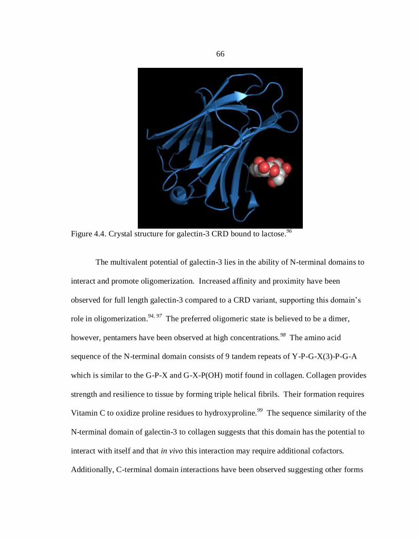
66
Figure 4.4. Crystal structure for galectin-3 CRD bound to lactose.
96
The multivalent potential of galectin-3 lies in the ability of N-terminal domains to
interact and promote oligomerization. Increased affinity and proximity have been
observed for full length galectin-3 compared to a CRD variant, supporting this domain’s
role in oligomerization.94, 97
The preferred oligomeric state is believed to be a dimer,
however, pentamers have been observed at high concentrations.98
The amino acid
sequence of the N-terminal domain consists of 9 tandem repeats of Y-P-G-X(3)-P-G-A
which is similar to the G-P-X and G-X-P(OH) motif found in collagen. Collagen provides
strength and resilience to tissue by forming triple helical fibrils. Their formation requires
Vitamin C to oxidize proline residues to hydroxyproline.99
The sequence similarity of the
N-terminal domain of galectin-3 to collagen suggests that this domain has the potential to
interact with itself and that in vivo this interaction may require additional cofactors.
Additionally, C-terminal domain interactions have been observed suggesting other forms

67
of protein-protein interactions.100
Formation of oligomers having variable oligomerization
states could contribute to the overall function of this lectin, allowing variability in the
distance between carbohydrate binding sites and eliciting specific and distinct responses
based on expression levels.101
Functionalized Dendrimer Scaffold
A series of three ligand functionalized dendrimers of second, third, fourth, and
sixth generation PAMAMs were labeled with mannose, lactose and biotin endgroups
(Figure 4.5). Mannoside and lactoside labeled PAMAM dendrimers were prepared
according to previously reported methods.88, 102
Amanda Mattson graciously synthesized
biotinylated functionalized dendrimer by coupling a biotin containing linker to the
mannose functionalized dendrimers; their synthesis and characterization will be reported
in Amanda Mattson’s doctoral dissertation. All functionalized dendrimers were
characterized using MALDI-TOF MS, 1H and
13C NMR spectrometry.

68
Figure 4.5. Ligand functionalized PAMAM dendrimers. Synthesis and characterization
procedures can be found in References 88 and 102 for mannose and lactose functionalized
dendrimers, respectively.
Aggregate Size Characterization
Spontaneous aggregates were formed when the above ligand-functionalized
PAMAM dendrimers were added to solutions containing the corresponding protein
binding partner. Two primary techniques were used to characterize these aggregates:
dynamic light scattering and fluorescence microscopy. These techniques provided
information regarding the effects of concentration, binding strength and valency on the
size, morphology and population distribution of the particles formed. Micrographs were
taken of fluorescently-labeled proteins incubated with functionalized dendrimers to
directly view aggregates. Dynamic light scattering provided a more rapid technique to
characterize the size and polydispersity of aggregates. Considering the different detection

69
levels of each technique, both methods provided similar results. This chapter briefly
discusses the experimental considerations for each method and reports the results from
these measurements.
Dynamic Light Scattering (DLS)
Dynamic light scattering (DLS) correlates fluctuations of scattered light with time
to calculate hydrodynamic radii and polydispersity of a set of particles. The
autocorrelation function (g(t)) is exponential in nature and fit assuming spherically shaped
particles.
As discussed previously (Methods for Analyzing Fluorescence Lifetime Data,
Chapter 3), fitting exponential decays such as the autocorrelation function is a sensitive
procedure, and various routines are available. The analysis algorithms of the DLS
software fit the autocorrelation function by either (1) expanding the exponential
correlation function via Taylor series expansion then using a normal, linear least squares
fit to determine cumulants; or (2) fitting the exponential directly using a non-linear least
squares fitting algorithm to solve for and amplitude factors. The first method is referred
to as the method of cumulants. Cumulants are coefficients to the Taylor series expansion
and can be related to the intensity correlation decay rate, , and distribution width. NNLS
and CONTIN algorithms make use of the second fitting procedure. In both cases, the
resulting physical parameters (i.e., diameter and polydispersity) are calculated from the
determined variables (cumulants or and amplitude factors).
Both fitting methods provide similar mean values (within 5%), but the method of
cumulants has increased sensitivity to background corrections.103
Similarity was

70
experimentally observed when (1) precautions were taken to minimize background
(filtering all solutions and pre-rinsing cuvettes with filtered buffer), (2) sufficient signals
could be measured, and (3) samples were mostly monodisperse. When these criteria were
not all met, then the method of cumulants did not provide reasonable results, and results
from CONTIN analysis were reported.
Experimental. Samples were prepared at slight, moderate and large molar excess of
protein and incubated for 1 hour at RT. Single scans were recorded prior to addition of
functionalized dendrimers. Triplicate scans were recorded following the one hour
incubation period. The concentration of stock protein samples was determined by
measuring the absorbance at 280 nm and using an 1% of 6.1
98, 13.7, and 10.7 for galectin-
3, Con A and streptavidin, respectively. Sugar functionalized glycodendrimers were
synthesized similar to previous methods102, 104
and stock samples prepared by dissolving
the lyophilized powder in filtered Millipore water to a final concentration of 100, 10 and 1
M. Varying amounts of glycodendrimer were added to the protein solution to give molar
ratios of 3:1, 9:1 and 220:1,protein-to-functionalized dendrimer (see Tables 4.1-4.3 for
concentrations used) and incubated for 1 hour at room temperature. The reported data is
the average of triplicate measurements on 1-6 samples. High relative variances were
obtained for samples where the particle size was too small or too few particles were
present to be detected (counts per seconds were less than 20,000). High relative variances
(greater than 0.5) are characteristic of highly polydisperse samples and could not be fit
well using the method of cumulants.

71
In this study, Con A was resuspended in PBS and then filtered to remove any
insoluble particles. PBS was selected because it is a universal buffer that represents
physiological ionic strength and pH. Since the hydrodynamic radius calculated in light
scattering is ultimately calculated from the ionic mobility, it was important to maintain
this parameter.
Evaluation of DLS Data. Regardless of the amount of excess galectin-3 that was
used, the size and polydispersity of the aggregates were shown to increase with increasing
dendrimer generation (Figure 4.6 and Table 4.1). The largest aggregates were observed for
the 9:1 ratio of galectin-3-to-glycodendrimer, and smaller aggregates were formed when a
large excess or a very small excess of galectin-3 was used. This trend is logical if the
glycodendrimer is serving as the nucleating agent for galectin-3 aggregation. For example,
when the concentration of galectin-3 is comparable to the concentration of
glycodendrimer, then galectin-3 is presented with many different nucleating scaffolds, and
smaller particles are formed. On the other hand, when galectin-3 is present in large excess,
not as many nucleating sites can be incorporated into each aggregate, which causes the
aggregates to be smaller.

72
Figure 4.6. Galectin-3 nanoparticle formed in the presence of compounds 1-4 at (blue)
220 fold excess, (red) 9-fold excess, and (green) 3-fold excess galectin-3. Aggregates size
increases as glycodendrimer generation increases. Largest aggregates are observed for
samples containing 9x molar excess galectin-3.

73
Table 4.1: Summary of DLS results for galectin-3 and lactose functionalized dendrimer
aggregates.
Compound Number [gal-3]
(M)
[dendrimer]
(M)
Effective Dia. (nm)
Relative Variance
Signal (kcps)a
NA 32 0 NRb NRb 14 ± 6
1 0 0.14 NRb NRb 5.5 ± 2.2
0 11.5 NRb NRb 23 ± 0.6
2 0 0.14 NRb NRb 3.2 ± 0.8
0 11.5 2.0 ± 0.4c 42 ± 34d 244 ± 63
3 0 0.14 NRb NRb 3.8 ± 0.8
0 11.5 6.2 ± 1.1c 69 ± 78d 167 ± 5
4 0 0.14 NRb NRb 4.4 ± 0.3
0 11.5 10.6 ± 2.2c 10.6 ± 2.5d 208 ± 8
1
31 0.14 NRb NRb 28 ± 12
31 3.3 364 ± 77 0.21 ± 0.05 60 ± 23
31 11.5 781 ± 88 0.20 ± 0.04 135 ± 28
2
31 0.14 533 ± 72 0.16±0.07 94 ± 24
31 3.3 1744 ± 161 0.17±0.06 282 ± 59
31 11.5 1275 ± 377 0.19±0.07 214 ± 134
3
31 0.14 1177 ± 81 0.19±0.03 385 ± 26
31 3.3 2027 ± 263 0.20±0.10 246 ± 52
31 11.5 871 ± 278 0.25±0.04 292 ± 74
4
31 0.14 1616 ± 111 0.23±0.09 271 ± 73
31 3.3 2269 ± 266 0.23 ± 0.15 249 ± 65
31 11.5 1316 ± 223 0.19 ± 0.08 252 ± 94
2 + 1 mM lactose 31 0.14 NRb NRb 14 ± 2
3 + 1 mM lactose 31 0.14 NRb NRb 17 ± 10
4 + 1mM lactose 31 0.14 NRb NRb 25 ± 11
8 34 0.14 4 ± 3x 13 ± 9b 39 ± 11
NA 34(CRD) 0 NRb NRb 5 ± 0.3
3 34(CRD) 0.14 NRb NRb 10 ± 1 akcps= kilocounts per second. bInsufficient signal to accurately fit, NR = Not reliable result. cMean diameter of major peak (accounts for >99% of distribution population) from CONTIN analysis (cumulant fit inadequate due to the bimodal nature of the sample as evident from high relative variances from this analysis). dRelative variance as reported from CONTIN fit.
A series of control experiments indicate that aggregation is induced by the binding
of galectin-3 to lactose on the dendrimers. Aggregates could not be observed upon

74
addition of compound 8, a mannose functionalized G6 dendrimer. Pre-incubation of
galectin-3 with 1 mM lactose solution completely inhibited aggregate formation in the
presence of glycodendrimers 2-4 (Table 4.1). Experiments using 4 and a truncated form
of galectin-3 showed only a slight increase in the average scattered intensity and did not
result in aggregate formation (Table 4.1). The truncated form of galectin-3 only contains
the carbohydrate recognition domain without the N-terminal domain. No aggregates were
observed for dendrimers 1-4 in solution without addition of galectin-3, and no aggregates
were observed for galectin-3 when glycodendrimers were absent from the solution. Taken
together, these data support aggregate initiation as a response to specific carbohydrate
binding interactions between lectin and glycodendrimer. These data also reveal the
significance of the N-terminal domain in formation of higher order aggregates.
Aggregates of Con A and mannose functionalized dendrimers 5-8 were more
polydispersed than the glycodendrimer/galectin-3 aggregates (Figure 4.7 and Table 4.2).
Significantly lower protein concentrations were required to remain within the specified
limits of detection (LOD) of the DLS instrumentation (2 nm-2 m). A set of experiments
using compound 8 and 220x excess Con A were performed to determine the optimal
protein concentration to characterize nanoparticles using DLS. Samples prepared at 4 M
Con A exceeded instrumental LOD after roughly 40 minutes (Figure 4.12). Scattering of
lower concentration samples produced signals too low for reliable fitting (>20 kcps).
Even at the optimized concentration, aggregates formed at 9:1 and 3:1 molar excess for
compounds 6-8 exceeded the detection limits.

75
In general, by increasing the concentration of glycodendrimers larger aggregates
were formed. The exception to this is compound 8 which showed a maximum aggregate
size at molar ratios of 9:1 protein-to-glycodendrimer. The deviation in the calculated
particle radius for all Con A/ glycodendrimer aggregates is shown in Figure 4.7 to be
large, making it difficult to confidently compare between ratios. The Student T-test
(unpaired, unequal variances) was used to validate the trend observed for compound 8
with Con A. Results for the t-test showed that there were statistically significant
differences between aggregate diameters at 9:1 protein-to-glycodendrimer and 220:1
protein-to-glycodendrimer, and between aggregate diameter at 9:1 protein-to-
glycodendrimer and 3:1 protein-to-glycodendrimer. The calculated t-statistics for both
comparisons were very close to the critical value, demonstrating the high uncertainty of
the radii measurements. Increasing the number of trials would provide higher confidence
that the difference in average diameters is real. Comparison of aggregates between the 3:1
protein-to-glycodendrimer sample and 220:1 protein-to-glycodendrimer sample showed
no significant difference.

76
Figure 4.7. Con A aggregates formed in the presence of compounds 5-8 at 220 (blue), 9
(red) and 3 (green) times molar excess Con A. Larger aggregates are observed for
increasing concentrations of glycodendrimer used with the exception of compound 8
which showed the largest aggregate at 9x molar excess protein.
That the dendrimer mediated aggregation of Con A was a response to sugar
binding events was confirmed by aggregate disassembly in the presence of 16 mM
mannose. A 16-fold higher concentration of the monomeric sugar than was required to
dissolve galectin-3 glycodendrimer aggregates. Given that Con A contains 2 to 4 times
more available binding sites per oligomer and that the multivalent binding for generation 6
dendrimers and Con A is known to significantly increase binding avidity7 this is not an
unreasonable result. This enhanced avidity could also explain the increased polydispersity
of this system. Multivalent interactions prolong the time molecules spend in contact,
meaning that transition from a kinetic to thermodynamic equilibrium state is slow. Fast
assembly has been shown to adversely affect the formation of regular gold
nanoparticles.105
By slowing the kinetics, thermodynamically favored products can result
for each set of interactions resulting in regular growth. DLS measurements assume a

77
spherical particle with isotropic scattering regardless of molecular orientation. Non-
spherical aggregates are likely the source of the increased polydispersity observed for Con
A and mannose functionalized dendrimers.
Table 4.2 Summary of DLS results for Con A and mannose functionalized dendrimer
aggregates.
Compound
Number
[Con A]
(M)
[dendrimer]
(nM)
Effective Dia.
(nm) b
Relative
Variance
Signal
(kcps)a
NA 1 0 NRb NRb 3 ± 1
3.9 0 NRb NRb 23 ± 1
8 0 0.14 NRb NRb 18 ± 1
20 3.3 ± 1.4 0.70±0.02 115 ± 2.6
5 1
4.5 NRb NRb 17 ±5
111 1691 ± 634 0.49 ±0.38 229 ±50
333 1963 ± 1111 1.6 ±3.2 288 ±24
6 1
4.5 558 ± 222 0.13 ±0.12 37 ±8
111 2667 ± 782 0.28 ±0.28 306 ±84
333 3894 ± 1689 0.61 ±1.0 222 ±69
7 1
4.5 686 ± 188 0.13 ±0.11 58 ±7
111 2205 ± 1311 0.49 ±0.74 233 ±87
333 2518 ± 1656 1.8 ±2.9 265 ±92
8 1
4.5 981 ± 601 0.50 ±0.68 139 ±103
111 1828 ± 903 0.24 ±0.28 303 ±178
333 848 ± 233 0.23 ±0.18 301 ±32
8 + 16 mM
mannose 1 4.5 NRb NRb 4 ± 2
Summary of DLS results for Con A and mannosyl dendrimer aggregates. akcps= kilocounts per second. bRecorded from CONTIN analysis due to increased polydispersity yielding unacceptable cumulant fits, NR = Not a reliable result.
Similar results were obtained for Streptavidin/biotin-labeled dendrimer systems.
Aggregates formed non-spherical particles as shown by fluorescence microscopy (Figure
4.10). Results from DLS experiments are shown in Table 4.3 only to afford an indication
of the size variability and high relative variances obtained with streptavidin. The high

78
affinity interaction, combined with the enhanced affinity of sugars displayed on a
polyvalent scaffold prevented aggregates from being disrupted. This statement is
supported by the observation of a structured autocorrelation curve and no appreciable
change in signal upon addition of free biotin.
Table 4.3 Summary of DLS results for Streptavidin and biotin functionalized dendrimer
aggregates.
Compound
Number
[Streptavidin]
(M)
[dendrimer]
(M)
Effective Dia.
(nm) b
Relative
Variance
9 20
0.091 604 ± 930 12 ± 13
2.2 407 ± 264 9 ± 11
6.7 264 ± 409 13 ± 11
12 10
0.045 312 ±250 6 ± 7
1.1 237 ± 364 8 ± 9
3.3 324 ± 161 2 ±1
12 20
0.091 150 ± 39 10 ± 5
2.2 444 ± 89 4 ± 2
6.7 189 ± 135 9 ±6
8 + 1 mM biotin 20 2.2 8895 ± 2615 akcps= kilocounts per second. bRecorded from CONTIN analysis due to increased polydispersity yielding unacceptable cumulant fits
Fluorescence Microscopy (FM)
To confirm the general trends observed in DLS measurements, micrographs of
aggregates containing fluorescently labelled proteins were collected. Skrdla points out
that “...although the fluorescence microscope cannot provide spatial resolution below the
diffraction limit of the respective objects, detection of fluorescing molecules below such
limits is readily achieved.”106
This is in part due to the sensitivity of fluorescence
measurements.

79
FM Results and Discussion. FITC-Con A and FITC-streptavidin (Sigma Aldrich)
were commercially available, and galectin-3 was labeled with AlexaFluor 488 following
the manufacturer’s protocol (brief description can be found in Appendix B).
Functionalized dendrimer samples were added to fluorescently labeled protein samples
using similar protein concentrations and molar ratios of protein-to-glycodendrimer as were
used in the DLS experiments described above. After approximately 1 hour incubation at
room temperature, a 10 L aliquot was removed and mounted for viewing. An Olympus
B61X microscope (100x oil immersion objective) equipped with a CCD camera was used
to capture 20-30 images of fluorescent aggregates. Aggregate size was quantified using
image analysis software (Pixcavator 6.0) in a similar manner to reference 34. Fluorescent
microsphere standards (Dragon Green, Bangs Laboratories, Inc.) were used to create
calibration equations to convert image pixels to particle diameter.
Image processing of standard particles provided a linear relationship between the
reported particle diameter and number of pixels from the computed perimeter variable of
the image analysis software (Figure 4.8, images of fluorescence standards are shown in
Figure 4.9, a-d). Equations and goodness of fit are given in Table 4.4.

80
Figure 4.8. Calibration curve correlating pixel number (perimeter) to particle diameter
Olympus microscopes.
Table 4.4. Calibration equations for fluorescent standard microspheres.
Camera Exposure
time (ms)
Calibration Curve
Equationa
R-squared
value
Olympus
B61X
5b Y=15.94x + 355.8 1.0
10b Y=14.19x + 309.8 0.9988
40 Y=10.79x + 164.9 0.9956 aY represents particle diameter, and x is the number of pixels of the particle perimeter as
quantitated by Pixcavator. b190 nm standard could not be detected and was not included in
the fit.
Initial attempts to use Alexa 488-labelled dendrimers revealed that the
concentration of dendrimer was too low to obtain visible particles (0.14 M dendrimer at
lowest concentration tested). However, Alexa 488-labelled galectin-3 provided viewable
aggregates for the tested ratio of 220:1 protein-to-glycodendrimer. The DLS
measurements of the dye labelled protein and glycodendrimer aggregate reported an
average diameter of 1550 ± 60 nm (single sample, triplicate scans). Therefore, addition of
the dye did not affect the aggregation process. Processing of FM provided similar results
to the unlabelled protein supporting the idea of a large monodispersed population of

81
particles (Table 4.5 and Figure 4.9, e-h). For both methods, the trend of increasing size
and polydispersity with increasing dendrimer generation was observed.
Table 4.5. Micrograph characterization of galectin-3/lactose functionalized dendrimer
aggregates following 1 hour incubation
Compound† Dhyd
(nm)
DN
(nm) DN (nm)
Relative
Variance
DW
(nm) PDI
1 ND 240 47 0.20 253 1.1
2 533 573 71 0.12 587 1.0
3 1177 1331 300 0.23 1402 1.1
4 1616 1788 647 0.36 1904 1.1
†Dendrimers were added at 1/220 the concentration of protein
Dhyd=hydrodynamic radius from DLS measurement
DN=number average diameter
Relative variance = /DN
DW = weighted average diameter =Σ(diameter × frequency); frequency represented as a
percent of total particles sampled
PDI=polydispersity index=DW/DN
ND=not determined
Micrographs of 220 fold excess Con A with mannose functionalized dendrimers
contained a large number of small particles (less than 10 pixels) and a smaller population
of larger particles, as shown in Figure 4.9 (i-l) and summarized in Table 4.6. In some
cases, the relative variances calculated for DLS data collected on these samples were
greater than 0.5 suggesting a multimodal distribution of particles, and the average particle
diameter reveals the bias in favor of larger aggregates. (Table 4.2) Smaller particles were
not consistently observed in DLS measurements, but evident in the Con A glycodendrimer
micrographs suggesting that their presence is real. Taken together, these data support the
view of a polydisperse population of aggregates.
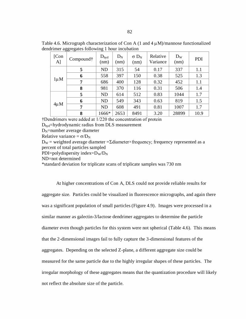
82
Table 4.6. Micrograph characterization of Con A (1 and 4 M)/mannose functionalized
dendrimer aggregates following 1 hour incubation
[Con
A] Compound†
Dhyd
(nm)
DN
(nm) DN
(nm)
Relative
Variance
DW
(nm) PDI
1M
5 ND 315 54 0.17 337 1.1
6 558 397 150 0.38 525 1.3
7 686 400 128 0.32 452 1.1
8 981 370 116 0.31 506 1.4
4M
5 ND 614 512 0.83 1044 1.7
6 ND 549 343 0.63 819 1.5
7 ND 608 491 0.81 1007 1.7
8 1666* 2653 8491 3.20 28899 10.9
†Dendrimers were added at 1/220 the concentration of protein
Dhyd=hydrodynamic radius from DLS measurement
DN=number average diameter
Relative variance = /DN
DW = weighted average diameter =Σdiameter×frequency; frequency represented as a
percent of total particles sampled
PDI=polydispersity index=DW/DN
ND=not determined
*standard deviation for triplicate scans of triplicate samples was 730 nm
At higher concentrations of Con A, DLS could not provide reliable results for
aggregate size. Particles could be visualized in fluorescence micrographs, and again there
was a significant population of small particles (Figure 4.9). Images were processed in a
similar manner as galectin-3/lactose dendrimer aggregates to determine the particle
diameter even though particles for this system were not spherical (Table 4.6). This means
that the 2-dimensional images fail to fully capture the 3-dimensional features of the
aggregates. Depending on the selected Z-plane, a different aggregate size could be
measured for the same particle due to the highly irregular shapes of these particles. The
irregular morphology of these aggregates means that the quantization procedure will likely
not reflect the absolute size of the particle.

83
Figure 4.9: Fluorescence micrograph of fluorescently labelled particles and Microbead
standards. Protein aggregates were captured after ca. 60 minute incubation (RT).
Microbead standards are shown in (a)-(d); (a) 190 nm, inset is a 4x enlargement of
selected area, (b) 520 nm, inset is a 4x enlargement of selected area, (c) 1020 nm and (d)
1900 nm. Alexa 488 labelled galectin-3 (A488gal-3, 31 M) with lactose functionalized
dendrimers (0.14 M) are shown in (e)-(h); (e) A488gal-3 and 1; (f) A488gal-3 and 2; (g)
A488gal-3 and 3; (h) A488gal-3 and 4. FITC labelled Con A (FITC-ConA, 4 M) with
mannose functionalized dendrimers (17 nM are shown in (i)-(l); (i) FITC-ConA and 5; (j)
FITC-ConA and 6; (k) FITC-ConA and 7; (l) FITC-ConA and 8.
Regardless, qualitative comparison of the calculated diameters for lower
generations of mannose functionalized dendrimer did not show any distinguishable trend,

84
while aggregates formed with FITC-Con A and compound 8 appear to be larger (Figure
4.9, l). If the population of small particles mentioned above were excluded from the
number average and weighted average diameter, trends of increasing aggregate size might
emerge. However, since these results would still be of a very qualitative nature, further
analysis was not performed.
The irregular morphology was even more significant for aggregates formed by
FITC-labeled streptavidin and generation 6 biotin-functionalized dendrimers (compound
12, Figure 4.10). The polydispersity of these samples also increased compared to the Con
A and mannose functionalized glycodendrimer aggregates. Comparison of the two higher
concentrations of compound 12 tested (3:1 and 9:1 excess streptavidin), showed no
significant difference in the size or polydispersity of aggregates formed (Figure 4.10, b
and c). The highest concentration of compound 12 (Figure 4.10, c) simply displayed a
higher density of aggregates. Smaller aggregates were observed for the 220 fold excess
streptavidin sample (Figure 4.10, a).

85
Figure 4.10. Series of 3 images of aggregates for varying ratios of streptavidin-to-biotin
dendrimer. (a) 220:1, (b) 9:1, (c) 3:1.
The smaller aggregates observed for the 220:1 streptavidin: biotinylated
glycodendrimer could be a result of fewer binding sites available to crosslink nucleation
sites, resulting in smaller aggregates. It should also be mentioned that the stock solution
of 12 used for the sample containing the lowest concentration of biotinylated
glycodendrimer was 10 times lower than the stock concentration of 12 used in the higher
concentration samples. Since no distinction in size was observed at higher concentrations
of biotinylated glycodendrimer, it is believed that the different stock solutions of
compound 12 used is the primary reason for the observed size difference. The strength of
the biotin-streptavidin interaction forms immediate crosslinks between the protein and

86
biotinylated dendrimers creating a complex and unorganized network. Long-term
rearrangement of these complexes could not be qualitatively observed for DLS
measurements, (Figure 4.18) supporting the hypothesis that aggregates formed by
streptavidin and compound 12 are fixed. This hypothesis needs to be verified by using
additional biotinylated glycodendrimer stocks at varying concentrations, or evaluating the
aggregates formed for the higher concentration biotinylated glycodendrimer samples using
the lower concentration stock. If this hypothesis is true, increasing the concentration of
biotinylated glycodendrimer will not result in larger aggregates, but rather an increased
density of small aggregates.
In summary, the aggregate size of protein/functionalized dendrimer particles
appears to depend on both the ability to participate in multivalent interactions, and the
concentrations of both protein and functionalized dendrimer present. The increased
avidity of streptavidin-biotin and Con A-mannose systems created polydisperse and non-
spherical or irregularly shaped particles. The observed characteristics of higher avidity
systems suggest less mobility of individual particles within the assembly.
Differences in the monomeric binding affinity of the protein-ligand systems appear
to have a lesser affect on the particle morphology and size as compared to the valency of
the protein. This statement is supported by the similarities between Con A and
streptavidin induced aggregates, and the lack of similarity for Con A and galectin-3
aggregates. The monomeric binding affinity of galectin-3 is similar to the monomeric
binding affinity of Con A for mannose. Aggregates of lactose functionalized dendrimers
with galectin-3 displayed a regular, spherical shape, and were relatively monodispersed.

87
The regularity and decreased polydispersity of the galectin-3/lactose functionalized
dendrimer aggregates suggest movement of assembly components to a concise and more
stable particle, and make it distinct from both Con A and streptavidin systems.
Kinetics
The kinetics of aggregate growth for Con A with mannose functionalized
dendrimers could be observed through the uncorrelated light scattering of growing
particles. Changes in light scattering during the first 3-5 minutes were observed for small
dendrimers (generation 2 and 3, Figure 4.11, a and b, respectively) at high concentrations
(110 and 330 nM, Figure 4.11, red and green traces, respectively). At the lowest
concentration of glycodendrimer added, only the generation 6 functionalized dendrimer
displayed a response in the first five minutes (Figure 4.11, d, blue) The fast kinetics of
samples containing higher concentrations of larger glycodendrimers prevented observation
of the initial section of the kinetic curve (Figure 4.11, c and d, red and green traces).
Generation 2 and 3 glycodendrimers, compounds 5 and 6, showed increasing aggregation
rates with increasing glycodendrimer concentration. Rate enhancements as a result of
increasing concentrations could not be evaluated for generation 4 glycodendrimer,
compound 7, since the first part of the curve was not obtained (Figure 4.11, c). The
concentration dependence of generation 6 glycodendrimer, compound 8, showed an initial
rate enhancement as the glycodendrimer concentration was increased from 4.5 nM to 110
nM (Figure 4.11, d, blue and red traces, respectively). However, the aggregate rate at 330
nM was less than the aggregation rate at 110 nM (Figure 4.11, d, red and green traces,

88
respectively). When compared to 7, the aggregation rate for 8 at both 110 and 330 nM
glycodendrimer was reduced. At the lowest concentration of glycodendrimer tested,
changes are only observed for generation 6 mannose functionalized dendrimer.
Of particular interest is the shape of the kinetic profile for 110 nM G2- and G3-
mannose functionalized dendrimer (Figure 4.11, a and b, red traces). This type of
behavior was not observed in previous FLS studies,48
nor was it reported in a recent
publication using real-time surface plasmon resonance measurements to investigate Con A
binding kinetics.107
The lag phase present at early times is typically associated with the
rate of formation of nucleation sites. This is followed by a cooperativity phase,
characteristically containing an increased rate of aggregate growth. Given that Con-A
interactions between oligomers have been observed this second phase may correlate with a
complex that allows protein-protein interactions.

89
Figure 4.11. Initial five-minute DLS scan following addition of varying concentrations of
mannose functionalized dendrimers (4.5 nM, blue; 110 nM, red; 330 nM, green) to Con A
(1 M). (a) Compound 5, (b) 6, (c) 7, (d) 8.
DLS measurements taken at roughly three minute intervals showed continued
growth and increasing polydispersity of aggregates formed with Con A and 8 (Figure
4.12). Enhanced rates and larger aggregates were observed when higher concentrations of
both Con A (4 M compared to 1 M) and 8 (17 nM compared to 4.5 nM) were tested at
the same molar ratio as previous experiments (220 excess Con A).

90
Figure 4.12. Long term kinetics for Con A and compound 8 showing the effect of
concentration on aggregate growth. Error bars represent standard deviation of at least
duplicate scans of 1 M Con A + 4.5 nM 8 (blue) and 4 M Con A + 17 nM 8 (red).
Aggregates formed by Con A/glycodendrimer aggregates were very stable.
Collection of DLS and FM data for FITC-labeled Con A with compounds 5-8 at 26 hours
following glycodendrimer addition show large, polydisperse particles (Figure 4.13 and
Table 4.7). Micrographs a-c of Figure 4.13 and numerical results of Table 4.7 show
maintenance of the observed trend of increasing size with increasing glycodendrimer
generation for compounds 5-7. However, there is a less significant size difference for
compounds 7 and 8 after long periods of time (Figure 4.13, c and d). This may indicate
that the thermodynamic equilibrium of the protein aggregate, in this case, is independent
of the size of the nucleating scaffold, so long as this scaffold permits multivalent
interactions. These results suggest that the protein concentration may play a more
significant role. Aggregates at time points longer than 26 hours would need to be
quantitated to confirm this hypothesis as the trajectory of the smaller glycodendrimer

91
aggregates is currently unknown. Visual observation indicated that samples stored at
room temperature for longer than one week still contained particles.
Figure 4.13. Sample of three fluorescent micrographs of Con A (4 M) + mannose
functionalized dendrimers (17nM) at 26 hours following glycodendrimer addition. (a) 5,
(b) 6, (c) 7, and (d) 8. Samples were protected from light and stored at room temperature
during incubation period.

92
Table 4.7. Micrograph characterization of Con A (1 and 4 M)/mannose functionalized
dendrimer aggregates following 26 hour incubation (220× excess Con A)
[Con A] Compound† Dhyd
(nm)*
DN
(nm) DN
(nm) Rel Var
DW
(nm) PDI
1M
5 437 505 274 0.54 646 1.3
6 1475 931 736 0.79 1550 1.7
7 1743 887 729 0.82 1487 1.7
8 831 648 463 0.71 1048 1.6
4M
5 ND 1289 1633 1.27 3327 2.6
6 ND 2893 8269 2.86 25900 9.0
7 ND 1851 1676 0.91 3363 1.8
8 1513 4126 5371 1.30 11001 2.7
†Dendrimers were added at 1/220 the concentration of protein
*Standard deviation for all DLS measurements were >200 nm and most were >600 nm
meaning numbers presented have little significance.
Dhyd=hydrodynamic radius from DLS measurement
DN=number average diameter
Rel Var = Relative variance = /DN
DW = weighted average diameter =Σdiameter×frequency; frequency represented as a
percent of total particles sampled
PDI=polydispersity index=DW/DN
ND=not determined
In contrast to the stability observed for aggregates of Con A/mannose
functionalized dendrimers, galectin-3 and lactose functionalized dendrimers appeared to
disassemble several hours following glycodendrimer addition. DLS data showed
decreasing signals in the first five minute scan (Figure 4.14). There are two possible
causes for the observed signal reduction. The aggregates could be combining, producing a
smaller number of large aggregates or the aggregates could be disassembling. Analysis of
the autocorrelation functions showed increasing aggregate size regardless of
glycodendrimer size for several hours (Figure 4.15), suggesting that a smaller number of
large particles are forming.

93
Figure 4.14. Initial five-minute DLS scan following addition of lactose functionalized
dendrimers (0.14 M) to galectin-3 (31 M). Compound 1 (blue), 2 (red), 3 (green), and 4
(purple). Incident light was adjusted to 200-400 kcps for compounds 2-4.
Figure 4.15. One hour kinetic profile for 31 M galectin-3 + 0.14 M lactose
glycodendrimer compounds 2 (red), 3 (blue), and 4 (green).

94
However, extended DLS measurements (Figure 4.16) and micrographs taken at 2,
4, 6 and 14 hours following addition of compound 4 provided further evidence for
shrinking and disassembly of large particles (Figure 4.17). The initial several hour growth
phase was followed by a period of disassembly. Disassembly was supported by the
observation of decreasing aggregate diameter of galectin-3 and 4 for both DLS and FM
methods.
Figure 4.16. Effective diameter of aggregates formed by addition of compound 4 to
galectin-3 (different colors represent individual trials).

95
Figure 4.17. Sample of three fluorescent micrographs of galectin-3 + 4 at (a) 2 hours, (b) 6
hours, (c) 14 hours and (d) 26 hours following glycodendrimer addition. Samples were
protected from light and stored at room temperature.
Disassembly of galectin-3/glycodendrimer aggregates could be a result of the high
entropic cost of ordering the N-terminal domain, thereby restricting its motion. Similar in
nature to polyvalent ligands connected by a flexible framework, the enthalpic gain of
binding does not, in all cases, compensate for the loss of motion in flexible regions of a

96
molecule. Whitesides alludes to the consequence of increasing entropy in his statement
regarding the design of polyvalent ligands,
“Incomplete understanding of the entropy in the design of polyvalent
molecules that are less effective or only marginally more effective than
their monovalent counterparts. The many bivalent systems joined by
flexible linkers (e.g. oligo9ethylene glycol) or polymethylene) provide
examples of systems that can almost be guaranteed to fail for entropic
reasons.” 5
While Whitesides is referring to the entropy of long, flexible linkers between
ligands, the same would hold true for oligomeric receptors held together by flexible
domains.
Streptavidin and biotinylated glycodendrimers 9-12 rapidly formed complex
aggregates. The formation of aggregates occurred too rapidly to be characterized by
methods employed. Additionally, the highly polydisperse and irregular nature of these
aggregates make any quantitative conclusion he nature of this aggregate a simple
conjecture. A sample kinetic profile acquired for DLS results is shown for compound 12
and streptavidin at 220 fold excess in Figure 4.18. The large error bars of these data
reveal the difficulty of making any type of qualitative or quantitative comparison.

97
Figure 4.18. One hour kinetic profile for streptavidin (220 fold excess) and compound 12.
Inhibition
Inhibition of functionalized dendrimer mediated nanoparticles with the monomeric
ligand was tracked using DLS. (Figure 4.19) Samples were pre-incubated with
monomeric ligand, then glycodendrimer constructs were added and the diameter of the
nanoparticles was determined. The alternative method of titrating monomeric ligand into
preformed particles could not be used as galectin-3 aggregates are held together weakly,
and addition of water alone disrupted the interaction (data not shown).

98
Figure 4.19: Inhibition curves for galectin-3+4 (blue) and Con A + 8 (green). Data
represents average of three scans recorded at 1 hour incubation of triplicate samples.
The IC50 of monomeric mannose required to disrupt aggregates of Con-A and 8
was approximately 20 times higher than the monomeric lactose required to disrupt
aggregates formed by galectin-3 and 4 (6.5 and 0.28 mM, respectively). Given that these
two proteins have comparable affinities for their preferred carbohydrate, the IC50
differences were ascribed to the higher valency associated with Con A.
An enhancement factor, , was introduced by Whitesides, et al. that related the
monomeric binding affinity, Kmono, to polyvalent binding avidities calculated via ELISA
assay, KELISA, by the following expression:
5
(16)
If the IC50
value calculated above is considered synonymous to KELISA then the ratio of
terms for galectin-3 relative to Con A is 0.04, and reflects a less favorable avidity
enhancement for the galectin-3 aggregates compared to that of Con A. The lack of

99
cooperativity for the galectin-3 system likely contributes to the eventual disassembly of
these particles. The assumption of a proportional relationship between IC50
and KELISA
comes from knowing that both values represent the system where the assay response is
half the maximum expected response.
Stoichiometry
The stoichiometric ratios of galectin-3/glycodendrimer aggregates were
determined to evaluate the protein clustering ability of the glycodendrimer system.
Conventionally, this is done by separating the precipitate through centrifugation,
dissolution of the precipitate, and measuring the absorbance at 280 nm to quantitate the
amount of protein.104, 108
This was not possible for the galectin-3 system studied. The
particles were too small and the centrifugal force required to pellet exceeded the ability of
available equipment. An alternative method was designed to filter the precipitate after an
hour incubation and quantitate both protein and glycodendrimer components of the filtrate
using UV-Vis spectra.
Experimental
Galectin-3 glycodendrimer nanoparticles of varying size spontaneously assembled
upon mixing with compounds 1-4 (0.14, 3.4 and 11.5 M) with galectin-3 (31 M). DLS
and microscopy results show that for compounds 2-4 a majority of these particles exceed
400 nm, suggesting filtration with a 220 nm pore size diameter should be efficient means
to separate aggregates. Following incubation at room temperature for 1 hour,
nanoparticles were removed by filtration with 0.22 m Millipore syringe tip filters

100
(PVDF, 4 mm diameter). Particles were then disassembled and washed from filter with -
lactose (300 L, 10 mM, washed over filter 3 times). UV-Vis spectra (190 nm-350 nm,
SpectraMax Plus 384, Molecular Devices) were recorded for the pre-filtered solution,
filtrate and lactose wash. These spectra were fit to predetermined glycodendrimer and
galectin-3 spectra using a least squares method to determine the stoichiometric ratio.
Precipitation Assay Results and Discussion
The figure below compares the area normalized glycodendrimer and galetin-3 UV-
Vis spectra. The spectral shapes were concentration independent for the range listed
(Figure 4.20). Molar extinction coefficients for galectin-3 and glycodendrimers were
calculated from the slope of absorbance versus concentration plot at 240 nm (Figure 4.21,
top) and 280 nm (Figure 4.21, bottom).
Figure 4.20. UV-Vis spectra of lactose functionalized dendrimer and galectin-3 samples.
Error bars represent 3 of 3-7 spectra

101
Figure 4.21. Absorbance standard curves for galectin-3 (blue diamonds), 1 (red squares),
2 (green triangles), 3 (purple crosses), 4 (blue crosses) at (a) 240 nm and (b) 280 nm.
Quantization of galectin-3 and glycodendrimer aggregates was done via fitting
UV-Vis data for the lactose wash with the above spectra using equation (16), as shown in
Figure 4.22. The coefficients, D and G correspond to relative amounts of glycodendrimer
and galectin-3, respectively. The coefficients were converted to molar concentrations
using the determined molar extinction coefficient (Table 4.8) before calculating the ratio
of galectin-3-to-glycodendrimer (Table 4.9).
(16)
Here, As is the measured absorbance spectra of the glycodendrimer/galecin-3
sample, Ad and Ag are the dendrimer and galectin-3 spectrum, respectively, D is a scalar
representing the relative amount of glycodendrimer, and G is a scalar representing the
relative amount of galectin-3. Sample spectra with fits are shown in Figure 4.22.

102
Figure 4.22. Sample-fitted spectra for the lactose wash of galectin-3 and 3.4 M (a)
Galectin-3 + 1, (b) Galectin-3 + 2, (c) Galectin-3 + 3, and (d) Galectin-3 + 4
glycodendrimer added. Measured data (blue squares), fitted data (purple crosses),
glycodendrimer component (red squares), and galectin-3 component (green triangle).
This process worked well for samples where an appreciable amount of signal could
be observed for both components. When one component was in large excess, as in the
case with aggregates formed by galectin-3 and 11.5 M 4, the minor component could not
be determined confidently (Table 4.9). Use of an extrinsic fluorophore to label the minor
component should provide the sensitivity needed to circumvent this problem.

103
Table 4.8: Molar extinction coefficients
Sample ϵ240 nm (M-1
cm-1
) ϵ280 nm (M-1
cm-1
)
1 151000 2700
2 435000 15700
3 747000 15200
4 2256000 51600
Galectin-3 22400 18000
Table 4.9: Calculated stoichiometric ratio of galectin-3:glycodendrimer
Sample [dendrimer] (M)
0.014 3.4 11.5
1 23 ± 3 9 ± 5 3 ± 0.6
2 32 ± 15 11 ± 2 5 ± 1.6
3 56 ± 17 12 ± 2 3 ± 1.3
4 57 ± 8 12 ± 3 ND
The stoichiometric ratios of galectin-3 and lactose functionalized aggregates that
were determined by the method described above are shown in Tables 4.9. Samples
containing lower stoichiometric ratios of galectin-3-to-glycodendrimer (3:1 and 9:1
stoichiometric excess of galectin-3) revealed similar stoichiometries to the sample makeup
within the aggregate. In other words, the average number of galectin-3 molecules in the
nanoparticles was equivalent to the ratio of excess galectin-3 molecules in solution. This
was not the case for samples containing a large excess of galectin-3 relative to the
glycodendrimer scaffold. All calculated stoichiometries for aggregates formed in the
presence of 220 molar excess galectin-3 were substantially less than 220. As expected, an
increasing trend in the stoichiometric ratio of galectin-3-to-glycodendrimer was observed
with increasing glycodendrimer size for compounds 1-3. This shows that the larger the
molecular scaffold, the greater number of entities that can bind to the scaffold.

104
Interestingly, the saturation value of galectin-3 for compounds 4 and 6 were similar.
There are two possible explanations for the saturation of galectin-3 molecules with
glycodendrimer size for 4 and 6. The first is that even though total surface area of 6 is
approximately 2 fold higher than the surface area of 4, the thermodynamically favored
equilibrium state at 1 hour is similar for both 4 and 6. The kinetics of galectin-3 and 6
aggregates are fastest for this generation of glycodendrimer, increasing the likelihood of
disordered nucleation sites. This could create a situation where multiple carbohydrate
endgroups are unbound within the core of the aggregate, resulting in a lower than expected
stoichiometric ratio.
Another possibility is that electrostatic repulsion is greater for galectin-3 with 6.
For most lactose functionalized dendrimers, the remaining, unfunctionalized amines
account for roughly 25% of the total number of endgroups. However, in the
functionalized G6 construct, approximately half of the terminal amines remain. The pI of
galectin-3, calculated using EXPASY was determined to be 8.6, suggesting the protein
contains an overall positive charge under the solution conditions of the experiment. The
increasingly positive surface of 6 compared to lower generations of lactose functionalized
dendrimers exerts a larger repulsive force on the bound galectin-3 molecules. Lactose
functionalized dendrimers efficiently interacted with negatively charged dodecylsulfate
molecules and could be pulled through an SDS polyacrylamide gel (data not shown). This
partially supports the idea of a positively charged surface for lactose functionalized
dendrimers. This hypothesis could also be confirmed by evaluating the surface charge of
both galectin-3 and glycodendrimer components via zeta-potential measurements.

105
Summary Comparison of Protein Aggregates
The quaternary structure of a protein is likely to impact the nanoparticle formed
via PAMAM scaffold mediated protein aggregation. The quaternary structures of Con A
and streptavidin are similar in that both are tetrahedral, while galectin-3 is most likely a
dimer or a less defined oligomer. Thus, direct comparisons between Con A and
streptavidin were made to determine the affect of the monovalent binding association on
assemblage.
Similarities in the particle morphology and polydispersity for Con A and
streptavidin systems suggest that the enhanced avidity of higher order oligomer systems
causes irregular morphology and increased polydispersities. The increased oligomeric
state of the protein creates a higher valency system, assuming each binding site remains
accessible upon oligomerization. This enhanced avidity resulted in slower moving (Con A
and mannose glycodendrimer) and even stagnant (streptavidin and biotinylated
glycodendrimer) assemblies.
The most notable difference between streptavidin and Con A systems was
observed in the kinetics of aggregate assembly. The 100 billion fold enhanced monomeric
binding affinity of streptavidin relative to Con A resulting in dramatically increased
aggregation rates. Streptavidin and biotin functionalized dendrimer aggregates formed
instantaneously while Con A and mannose functionalized dendrimers continued to grow
for at least 26 hours.
Galectin-3 and Con A, on the other hand, have similar binding affinity but
different valencies, making their comparison quite useful to determine the affect of the

106
valency and binding site orientation on aggregation. There appears to be a fast and slow
process for galectin-3 and Con-A systems. This has been previously modeled via SPR
measurements of immobilized Con A with mannosyl and glucosyl decorated 2-4th
generation gallic acid−triethylene glycol dendrimers.107
These authors ascribe the rapid
initial association to the initial sugar-binding event which was enhanced for generation 3
and 4 glycodendrimers. The slower second phase has been attributed to the rearrangement
of these aggregates. Continual growth was also observed for Con A.
Galectin-3 and lactose functionalized aggregates appeared to form more rapidly
than Con A and mannose functionalized aggregates. Rather than continually growing,
galectin-3/glycodendrimer aggregates appear to undergo an initial growth phase followed
with eventual denucleation and dissolution. The cause of the disassembly process is
currently unknown, and further studies will need to be done to characterize the assembly
with time.

107
CHAPTER 5
IMPLICATIONS OF MONOVALENT BINDING AND VALENCY ON
AGGREGATION BEHAVIOR: OVERARCHING SUMMARY AND FUTURE
INVESTIGATIONS
The ability to understand and manipulate polyvalent interactions would allow us to
control diseases where polyvalent interactions result in catastrophe. In many cases, the
catastrophe comes in the form of crosslinking between entities resulting in aggregation.
Aggregation prevents the protein from functioning properly, and sometimes these
aggregates cannot be broken down by conventional, physiological means. The first step to
control these systems or to create systems that interfere with these processes is
characterization. There are two aggregation phenomena that would be useful if
characterized. The first being the forces driving the interaction, and the second being the
identification of assembly progression. In other words, it would be desirable to know
what conditions contribute to cause nucleation, and does particle growth occur through
monomer addition or combination of nuclei. PAMAM dendrimers offer a tunable and
characteristically favorable scaffold that can be used in understanding the significance of
forces involved in particle formation.
Particle Growth Theory
The process of molecular assembly to form nanoparticles is a topic of debate and
appears to depend on the individual conditions of each system. Classical nucleation
theory describes an initial nucleation event where free monomers come together to form
nuclei. Nuclei act as an activated state once reaching a critical size, and the instability of

108
the activated state results in growth to a thermodynamically equilibrated state. Aggregates
smaller than the critical size are unstable and disassemble to their monomer form.109
The
particles larger than the critical size are stabilized by reduction of the overall surface area-
to-volume ratio. A single large aggregate, whose volume is equal to the sum of the
volumes of several smaller particles, has a smaller exposed surface area compared to the
total surface area of the smaller particles. The interfacial curvature of the solid to liquid
phase is greater for large particles resulting in lower stress and a lower energy system.
The process of particle assembly to reduce the overall interfacial volume is known as
Ostwald ripening, and typically increases the heterogeneity of the sample. 110
While
classical nucleation theory cannot provide accurate descriptions of the kinetic processes of
nanoparticle formation, it is capable of predicting the steady-state conditions required for
monodispersed nanoparticles.105
Particle growth kinetics have been modeled under the
assumption that growth results due to the addition of monomers to the nucleation site.29
Data is fit using monomer association and dissociation rates. Most equations modeling
monomer addition include nucleation parameters, or an additional term describing the
nucleation event. However, some models such as the reversible association model used by
Eisenberg, et al. and Thusius, et al. only consider the concentration of protein in monomer
and polymer forms.111-113
The critical nucleation size and nucleation rate of the system are dependent on the
attractive and repulsive intermolecular forces of the system. These forces include charge
based interactions, hydrogen bonding, dipole-dipole or dipole-induced interactions (van
der Waals), and interactions due to the hydrophobic effect. Particle growth depends on
109
the attractive forces of the system compensating for and overcoming the repulsive forces
of the systems. While all interactions have the possibility of occurring for each
component, the relative strength of the interaction determines its contribution to the
overall system. In other words, some of these interactions may be too weak to be
considered relevant. For example, in the DVLO model ranks van der Waals, charge and
“acid-base” interactions as the most significant interactions. The DVLO model for
molecular colloidal adhesion defines the spontaneity of assemblage using a free energy
term. The free energy is a combination of van der Waals interactions (GvdW
), charge
based interactions (Gdl) and “acid-base” interactions (G
AB).
109
Use of Dendrimers to Understand
Forces Involved in Particle Assembly
The studies herein use functionalized dendrimers as nucleation sites. The
dendrimer acts as a stability factor in the aggregate assembly. Additional attractive forces
occur between protein and functionalized dendrimer to force protein molecules in close
proximity. Characteristically, these aggregates may or may not reflect protein aggregation
in the cellular environment because the aggregates created are heterogeneous ensembles of
dendrimer and protein entities, but they are realistic of protein interactions at the cell
surface environment. At the cellular surface, proteins can be post-translationally modified
to contain multiple epitopes of a single molecule, one example being polyglycated
membrane proteins.
The process of molecules coming together, interacting in a multivalent fashion,
and then assembling into a nanoparticle is driven by attractive forces. The first event is

110
the monomeric binding event, which is closely followed by a multivalent binding event, so
long as the proximity of ligands allow binding to multiple receptors. The strength of the
multivalent event, determines the time two entities are associated with one another, and
depend on the valency of the components.
Dendrimer Effects on Particle Growth
In theory, the use of functionalized dendrimers to mediate protein aggregates could
facilitate or adversely affect the nucleation event. Functionalized dendrimers were
designed to provide a scaffold that has affinity for the protein counterparts. Therefore, the
functionalized dendrimers have the ability to recruit proteins, bring them into close
proximity, and possibly induce protein-protein interactions. The degree of attraction is
determined through the mono- and polyvalent interactions between scaffold and protein
(see section Assembly Progression in terms of Binding in Chapter 1 for more information
on polyvalent binding). The nucleation ability would depend on the competition between
protein-protein interactions and protein-ligand interactions of the functionalized
dendrimer/protein environment. When both the protein-ligand and protein-protein
interactions are cooperative then the functionalized dendrimers could serve to enhance
nucleation. In this situation, the functionalized dendrimer would effectively recruit
proteins, then these proteins could interact with one another to create a higher valency
receptor. The increased valency would enhance the overall avidity between the protein
“cluster” and functionalized dendrimer, and increase the interaction time. Increasing the
interaction time would increase the probability for additional proteins to dock to the
glycodendrimer scaffold and interact with the protein “cluster”. This cycle could continue

111
until either all available protein has been complexed, or until equilibrium between
complexed and free protein is achieved.
There is also the possibility of functionalized dendrimer constructs to negatively
affect nucleation rate. In this scenario, the protein-ligand interaction must be more
favorable than the enhanced avidity observed as a consequence of protein-protein
interactions. The forces holding protein oligomers together are less favorable than the
energy of protein-ligand binding. Therefore, the probability of nucleation is decreased
when the system contains an excess of ligated scaffolds and the protein-protein
interactions are weak.
Contributions of Monomeric Binding
Constant, Valency and Charge on Aggregate Formation
The monovalent interaction dominates and the mobility of entities within a
molecular assembly is lost in cases where the monovalent association constant is very
high. Loss of mobility was also observed for systems of increased avidity as a result of
multivalent interactions. The greater the number of interactions that occur to hold
molecules together, the higher the avidity and the longer the two are associated.
The structure of Con A and streptavidin aggregates formed in the presence of
polyvalent dendrimer constructs were polydisperse and morphologically irregular. An
extensive network of protein-glycodendrimer complexes resulted when increasing
nucleation sites were made available. The primary difference observed between
streptavidin and Con A aggregates was the rate at which they formed. Aggregates of
Streptavidin and biotin functionalized dendrimers formed rapidly, and either did not

112
require a nucleation event or the nucleation event occurred to quickly to be observed.
Classical polymerization appeared true for the Con A and mannose functionalized
dendrimer system. A lag period was observed in which the mannose functionalized
dendrimers facilitated Con A nucleation, and based on the aggregate morphology, the
nucleation sites combined in the growing aggregate. Even though the monovalent
binding affinity of Con A for mannose would suggest possible rearrangement of the
particles, the enhanced avidity due to multivalent interactions between Con A and
mannose functionalized dendrimers appears to prevent any particle rearrangement.
Galectin-3 and Con A have similar monomeric binding affinities yet exist at
distinct oligomeric states. Comparing galectin-3 and Con A systems reveal the
importance of the valency of the system. Results showed that glycodendrimer induced
Con A aggregates were slower to form but had superior stability, while galectin-3
aggregates formed very quickly but disappeared over time.
For the Con A system, it is speculated that the charge based interactions are
attractive under the experimental conditions of the experiment. The dendrimers are
expected to have an overall positive charge, based on the pKa of the unlabeled terminal
amines. Con A tetramers are expected to be slightly negatively charged based on the
calculated pI of the protein. There is the possibility of reducing the avidity by altering the
charge of either component of the system. Altering the charge of the Con A tetramer
could be done by changing the buffer system used. However, Con A is known to dimerize
at pH values below 5.10
Therefore it would be easier to modify the glycodendrimer
system to create either a neutral or negatively charges species to investigate the role of the

113
charge based interactions. The charge of the PAMAM dendrimers could be moderated by
capping the terminal amines with a neutral tether.
Dendrimers in Disease Control
Dendritic, multivalent systems provide a method of targeting, drug delivery, and
ultimately disease control. The disease can be pathogen-based or amyloidogenic. In
pathogen-based diseases the enhanced avidity of multivalent frameworks provides a
means of higher specificity in binding (detecting pathogens). In amyloidogenic diseases,
multivalency offers a means to break up and interfere with the amyloidogenic process,
ultimately preventing aggregation. The multivalent scaffolds developed must have certain
characteristics in order to be FDA approved. The scaffold must be non-toxic, soluble,
effective, show minimal interference, and must be eventually excreted. PAMAM
dendrimers have been shown to contain many of these properties depending on the
exterior functionalization. Additionally, PAMAM dendrimers are systematically grown
using a two-step synthesis procedure creating a tunable and regular framework.
Significance of Lectin-Carbohydrate Interactions
Patterns of cell-surface carbohydrates change during development, differentiation,
oncogenesis and metastasis. These changes are believed to be involved in signaling
pathways and cell recognition. A link exists between binding to specific glycans and the
resulting signaling response. Characteristically, monomers binding to these carbohydrate
components are weak and non-specific. Polyvalency is one mechanism that is used in
nature to increase the binding affinity or avidity of protein carbohydrate interactions, but

114
polyvalency does not explain the specificity of the interaction. The specificity, and
resulting signaling response, may arise from the protein-protein interactions that occur
after the carbohydrate-docking event. In other words, the carbohydrates act as a
nucleation site enabling proteins to come together. The polyvalency of glycan-containing
scaffolds amplifies binding making the interaction specific and causing a specific
biological response. This type of interaction is commonly seen in pathogen and cell
recognition and the immune response. Using tunable glycodendrimers to mimic this
environment provides a mechanism to study carbohydrate mediated interactions.

115
REFERENCES CITED

116
1. Amano, T., Nakamizo, A., Mishra, S. K., Gumin, J., Shinojima, N., Sawaya, R.,
and Lang, F. F. (2009) Simultaneous phosphorylation of p53 at serine 15 and 20
induces apoptosis in human glioma cells by increasing expression of pro-apoptotic
genes, Journal of Neuro-Oncology 92, 357-371.
2. Ferrero, M., Ferragud, J., Orlando, L., Valero, L., del Pino, M. S., Farras, R., and
de Mora, J. F. (2011) Phosphorylation of AIB1 at Mitosis Is Regulated by
CDK1/CYCLIN B, Plos One 6, 12.
3. Olsen, J. V., Blagoev, B., Gnad, F., Macek, B., Kumar, C., Mortensen, P., and
Mann, M. (2006) Global, in vivo, and site-specific phosphorylation dynamics in
signaling networks, Cell 127, 635-648.
4. Ali, M. H., and Imperiali, B. (2005) Protein oligomerization: How and why,
Bioorganic & Medicinal Chemistry 13, 5013-5020.
5. Mammen, M., Choi, S. K., and Whitesides, G. M. (1998) Polyvalent interactions in
biological systems: Implications for design and use of multivalent ligands and
inhibitors, Angewandte Chemie-International Edition 37, 2755-2794.
6. Klyosov, A., Vitczak, Z., and Platt, D. (2008) Galectins, John Wiley & Sons, Inc.,
New Jersey.
7. Woller, E. K., and Cloninger, M. J. (2002) The lectin-binding properties of six
generations of mannose-functionalized dendrimers, Organic Letters 4, 7-10.
8. Wolfenden, M. L., and Cloninger, M. J. (2005) Mannose/glucose-functionalized
dendrimers to investigate the predictable tunability of multivalent interactions,
Journal of the American Chemical Society 127, 12168-12169.
9. Gestwicki, J. E., Cairo, C. W., Strong, L. E., Oetjen, K. A., and Kiessling, L. L.
(2002) Influencing receptor-ligand binding mechanisms with multivalent ligand
architecture, Journal of the American Chemical Society 124, 14922-14933.
10. Mangold, S. L., and Cloninger, M. J. (2006) Binding of monomeric and dimeric
Concanavalin A to mannose-functionalized dendrimers, Organic & Biomolecular
Chemistry 4, 2458-2465.
11. Kiessling, L. L., Gestwicki, J. E., and Strong, L. E. (2000) Synthetic multivalent
ligands in the exploration of cell-surface interactions, Current Opinion in
Chemical Biology 4, 696-703.
12. Levental, K. R., Yu, H., Kass, L., Lakins, J. N., Egeblad, M., Erler, J. T., Fong, S.
F. T., Csiszar, K., Giaccia, A., Weninger, W., Yamauchi, M., Gasser, D. L., and
Weaver, V. M. (2009) Matrix Crosslinking Forces Tumor Progression by
Enhancing Integrin Signaling, Cell 139, 891-906.

117
13. Green, D. E., and Perdue, J. F. (1966) Membranes as Expressions of Repeating
Units, Proceedings of the National Academy of Sciences of the United States of
America 55, 1295-&.
14. Varki, A. (1993) Biological Roles of Oligosaccharides - All of the Theories are
Correct, Glycobiology 3, 97-130.
15. Niv, Y. (2008) MUC1 and colorectal cancer pathophysiology considerations,
World Journal of Gastroenterology 14, 2139-2141.
16. Kotera, Y., Fontenot, J. D., Pecher, G., Metzgar, R. S., and Finn, O. J. (1994)
Humoral Immunity Against a Tandem Repeat Epitope of Human Mucin MUC-1 in
Sera from Breast, Pancreatic, and Colon-Cancer Patients, Cancer Research 54,
2856-2860.
17. Arcinas, A., Yen, T. Y., Kebebew, E., and Macher, B. A. (2009) Cell Surface and
Secreted Protein Profiles of Human Thyroid Cancer Cell Lines Reveal Distinct
Glycoprotein Patterns, Journal of Proteome Research 8, 3958-3968.
18. Lalonde, S., Ehrhardt, D. W., Loque, D., Chen, J., Rhee, S. Y., and Frommer, W.
B. (2008) Molecular and cellular approaches for the detection of protein-protein
interactions: latest techniques and current limitations, Plant Journal 53, 610-635.
19. Kumar, S., Ma, B. Y., Tsai, C. J., Sinha, N., and Nussinov, R. (2000) Folding and
binding cascades: Dynamic landscapes and population shifts, Protein Science 9,
10-19.
20. Ma, B. Y., Kumar, S., Tsai, C. J., and Nussinov, R. (1999) Folding funnels and
binding mechanisms, Protein Engineering 12, 713-720.
21. Tsai, C. J., Kumar, S., Ma, B. Y., and Nussinov, R. (1999) Folding funnels,
binding funnels, and protein function, Protein Science 8, 1181-1190.
22. Simons, K., and Toomre, D. (2000) Lipid rafts and signal transduction, Nature
Reviews Molecular Cell Biology 1, 31-39.
23. Fink, A. L. (1998) Protein aggregation: folding aggregates, inclusion bodies and
amyloid, Folding & Design 3, R9-R23.
24. Vasan, S., Foiles, P., and Founds, H. (2003) Therapeutic potential of breakers of
advanced glycation end product-protein crosslinks, Archives of Biochemistry and
Biophysics 419, 89-96.
25. Lee, A. S., Galea, C., DiGiammarino, E. L., Jun, B., Murti, G., Ribeiro, R. C.,
Zambetti, G., Schultz, C. P., and Kriwacki, R. W. (2003) Reversible amyloid
118
formation by the p53 tetramerization domain and a cancer-associated mutant,
Journal of Molecular Biology 327, 699-709.
26. Newkome, G. R., Moorefield, C. N., and Vögtle, F. (2001) Dendrimers and
dendrons : concepts, syntheses, applications, Wiley-VCH, Weinheim ; New York.
27. Cloninger, M. J. (2002) Biological applications of dendrimers, Current Opinion in
Chemical Biology 6, 742-748.
28. Lee, C. C., MacKay, J. A., Frechet, J. M. J., and Szoka, F. C. (2005) Designing
dendrimers for biological applications, Nature Biotechnology 23, 1517-1526.
29. Morris, A. M., Watzky, M. A., and Finke, R. G. (2009) Protein aggregation
kinetics, mechanism, and curve-fitting: A review of the literature, Biochimica Et
Biophysica Acta-Proteins and Proteomics 1794, 375-397.
30. Klajnert, B., Cortijo-Arellano, M., Cladera, J., and Bryszewska, M. (2006)
Influence of dendrimer's structure on its activity against amyloid fibril formation,
Biochemical and Biophysical Research Communications 345, 21-28.
31. Demeule, B., Gurny, R., and Arvinte, T. (2007) Detection and characterization of
protein aggregates by fluorescence microscopy, International Journal of
Pharmaceutics 329, 37-45.
32. Bhat, S. A., and Bano, B. (2014) Conformational behaviour and aggregation of
chickpea cystatin in trifluoroethanol: Effects of epicatechin and tannic acid,
Archives of biochemistry and biophysics 562, 51-61.
33. Hawe, A., Sutter, M., and Jiskoot, W. (2008) Extrinsic fluorescent dyes as tools for
protein characterization, Pharmaceutical Research 25, 1487-1499.
34. Michel, A. K., Nangia-Makker, P., Raz, A., and Cloninger, M. J. (2014) Lactose-
Functionalized Dendrimers Arbitrate the Interaction of Galectin-3/MUC1
Mediated Cancer Cellular Aggregation, Chembiochem : a European journal of
chemical biology 15, 2106-2112.
35. Giepmans, B. N. G., Adams, S. R., Ellisman, M. H., and Tsien, R. Y. (2006)
Review - The fluorescent toolbox for assessing protein location and function,
Science 312, 217-224.
36. Roding, M., Deschout, H., Braeckmans, K., and Rudemo, M. (2013) Measuring
absolute nanoparticle number concentrations from particle count time series,
Journal of Microscopy 251, 19-26.
37. Cheng, S. H., Li, F. C., Souris, J. S., Yang, C. S., Tseng, F. G., Lee, H. S., Chen,
C. T., Dong, C. Y., and Lo, L. W. (2012) Visualizing Dynamics of Sub-Hepatic

119
Distribution of Nanoparticles Using Intravital Multiphoton Fluorescence
Microscopy, Acs Nano 6, 4122-4131.
38. Pecora, R. (2000) Dynamic light scattering measurement of nanometer particles in
liquids, Journal of Nanoparticle Research 2, 123-131.
39. Panacek, A., Kvitek, L., Prucek, R., Kolar, M., Vecerova, R., Pizurova, N.,
Sharma, V. K., Nevecna, T., and Zboril, R. (2006) Silver colloid nanoparticles:
Synthesis, characterization, and their antibacterial activity, Journal of Physical
Chemistry B 110, 16248-16253.
40. Lynn, D. M., and Langer, R. (2000) Degradable poly(beta-amino esters):
Synthesis, characterization, and self-assembly with plasmid DNA, Journal of the
American Chemical Society 122, 10761-10768.
41. Pourianazar, N. T., Mutlu, P., and Gunduz, U. (2014) Bioapplications of
poly(amidoamine) (PAMAM) dendrimers in nanomedicine, Journal of
Nanoparticle Research 16.
42. Majoros, I. J., Williams, C. R., and Baker, J. R. (2008) Current dendrimer
applications in cancer diagnosis and therapy, Current Topics in Medicinal
Chemistry 8, 1165-1179.
43. Baird, E. J., Holowka, D., Coates, G. W., and Baird, B. (2003) Highly effective
poly(ethylene glycol) architectures for specific inhibition of immune receptor
activation, Biochemistry 42, 12739-12748.
44. Ottaviani, M. F., Cangiotti, M., Fiorani, L., Fattori, A., Wasiak, T., Appelhans, D.,
and Klajnert, B. (2012) Kinetics of Amyloid and Prion Fibril Formation in the
Absence and Presence of Dense Shell Sugar-Decorated Dendrimers, Current
Medicinal Chemistry 19, 5907-5921.
45. He, Z. Q., Uchimiya, M., and Cao, H. P. (2014) Intrinsic Fluorescence Excitation-
Emission Matrix Spectral Features of Cottonseed Protein Fractions and the Effects
of Denaturants, Journal of the American Oil Chemists Society 91, 1489-1497.
46. Bohren, K. M., Vonwartburg, J. P., and Wermuth, B. (1987) Kinetics of Carbonyl
Reductase from Human-Brain, Biochemical Journal 244, 165-171.
47. Zhou, T. Q., and Rosen, B. P. (1997) Tryptophan fluorescence reports nucleotide-
induced conformational changes in a domain of the ArsA ATPase, Journal of
Biological Chemistry 272, 19731-19737.
48. Schlick, K. H., Lange, C. K., Gillispie, G. D., and Cloninger, M. J. (2009)
Characterization of Protein Aggregation via Intrinsic Fluorescence Lifetime,
Journal of the American Chemical Society 131, 16608-+.

120
49. Holub, O., Seufferheld, M. J., Govindjee, C. G., Heiss, G. J., and Clegg, R. M.
(2007) Fluorescence lifetime imaging microscopy of Chlamydomonas reinhardtii:
non-photochemical quenching mutants and the effect of photosynthetic inhibitors
on the slow chlorophyll fluorescence transient, Journal of Microscopy-Oxford 226,
90-120.
50. Lakowicz, J. R. (2006) Principles of fluorescence spectroscopy, 3rd ed., Springer,
New York.
51. Sundberg, S. A. (2000) High-throughput and ultra-high-throughput screening:
solution- and cell-based approaches, In Current Opinion in Biotechnology, pp 47-
53, Elsevier.
52. Hornig, J., and McGregor, A. (2014) Design and development of antivirals and
intervention strategies against human herpesviruses using high-throughput
approach, Expert Opinion on Drug Discovery 9, 891-915.
53. (2008) Standardization and Quality Assurance in Fluorescence Measurements I:
Techniques, Standardization and Quality Assurance in Fluorescence
Measurements I: Techniques 05, 1-496.
54. Muretta, J. M., Kyrychenko, A., Ladokhin, A. S., Kast, D. J., Gillispie, G. D., and
Thomas, D. D. (2010) High-performance time-resolved fluorescence by direct
waveform recording, Review of Scientific Instruments 81, 8.
55. Dean, K. M., and Palmer, A. E. (2014) Advances in fluorescence labeling
strategies for dynamic cellular imaging, Nature Chemical Biology 10, 512-523.
56. Yamauchi, K., Yang, M., Jiang, P., Xu, M. X., Yamamoto, N., Tsuchiya, H.,
Tomita, K., Moossa, A. R., Bouvet, M., and Hoffman, R. M. (2006) Development
of real-time subcellular dynamic multicolor imaging of cancer-cell trafficking in
live mice with a variable-magnification whole-mouse imaging system, Cancer
Research 66, 4208-4214.
57. Vogt, R. F., Jr., Marti, G. E., and Zenger, V. (2008) Quantitative Fluorescence
Calibration: a Tool for Assessing the Quality of Data Obtained by Fluorescence
Measurements, Standardization and Quality Assurance in Fluorescence
Measurements I: Techniques 05, 3-31.
58. International, A. (2014) ASTM E2719-09, In Standard Guide for Fluorescence--
Instrument Calibration and Qualification, ASTM International, West
Conshohocken, PA.
59. Lakowicz, J. R. (2006) Principles of fluorescence spectroscopy, 3rd ed., Springer,
New York.

121
60. Gardecki, J. A., and Maroncelli, M. (1998) Set of secondary emission standards for
calibration of the spectral responsivity in emission spectroscopy, Applied
Spectroscopy 52, 1179-1189.
61. Lakowicz, J., R. (2006) Principles of fluorescence spectroscopy, 3rd ed., Springer,
New York.
62. International, A. (2013) ASTM E578-07, In Standard Test Method for Linearity of
Fluorescence Measuring Systems, ASTM International, West Conshohocken, PA.
63. Albani, J. R. (2014) Origin of Tryptophan Fluorescence Lifetimes. Part 2:
Fluorescence Lifetimes Origin of Tryptophan in Proteins, Journal of Fluorescence
24, 105-117.
64. Ghosh, S., Paul, B. K., and Chattopadhyay, N. (2014) Interaction of cyclodextrins
with human and bovine serum albumins: A combined spectroscopic and
computational investigation, Journal of Chemical Sciences 126, 931-944.
65. Boens, N., Qin, W. W., Basaric, N., Hofkens, J., Ameloot, M., Pouget, J., Lefevre,
J. P., Valeur, B., Gratton, E., Vandeven, M., Silva, N. D., Engelborghs, Y.,
Willaert, K., Sillen, A., Rumbles, G., Phillips, D., Visser, A., van Hoek, A.,
Lakowicz, J. R., Malak, H., Gryczynski, I., Szabo, A. G., Krajcarski, D. T., Tamai,
N., and Miura, A. (2007) Fluorescence lifetime standards for time and frequency
domain fluorescence spectroscopy, Analytical Chemistry 79, 2137-2149.
66. Zhang, X. F., Zhang, J. L., and Liu, L. M. (2014) Fluorescence Properties of
Twenty Fluorescein Derivatives: Lifetime, Quantum Yield, Absorption and
Emission Spectra, Journal of Fluorescence 24, 819-826.
67. Yip, R. W., Wen, Y. X., and Szabo, A. G. (1993) Decay Associated Fluorescence-
Spectra of Coumarin-1 and Coumarin-102 - Evidence for a 2-State Solvation
Kinetics in Organic-Solvents, Journal of Physical Chemistry 97, 10458-10462.
68. Magde, D., Rojas, G. E., and Seybold, P. G. (1999) Solvent dependence of the
fluorescence lifetimes of xanthene dyes, Photochemistry and Photobiology 70,
737-744.
69. Alfano, R. R., Shapiro, S. L., and Yu, W. (1973) Effect of soap on the fluorescent
lifetime and quantum yield of rhodamine 6G in water, In Optics Communications,
pp 191-192, Elsevier.
70. Vekshin, N. (2002) Photonics of Biopolymers, Springer-Verlag, Berlin.
71. Jones, G., Jackson, W. R., Choi, C., and Bergmark, W. R. (1985) Solvent Effects
on Emission Yield and Livetime for Coumarin Laser-Dyes - Requirements for a
Rotatory Decay Mechanism, Journal of Physical Chemistry 89, 294-300.

122
72. Liu, S. M., Kokot, S., and Will, G. (2009) Photochemistry and chemometrics-An
overview, Journal of Photochemistry and Photobiology C-Photochemistry Reviews
10, 159-172.
73. de Juan, A., and Tauler, R. (2003) Chemometrics applied to unravel
multicomponent processes and mixtures - Revisiting latest trends in multivariate
resolution, Analytica Chimica Acta 500, 195-210.
74. Kasimova, M. R., Grigiene, J., Krab, K., Hagedorn, P. H., Flyvbjerg, H.,
Andersen, P. E., and Moller, I. M. (2006) The free NADH concentration is kept
constant in plant mitochondria under different metabolic conditions, Plant Cell 18,
688-698.
75. Kania, A., and Fiedor, L. (2006) Steric control of bacteriochlorophyll ligation,
Journal of the American Chemical Society 128, 454-458.
76. Thaler, C., and Vogel, S. S. (2006) Quantitative linear unmixing of CFP and YFP
from spectral images acquired with two-photon excitation, Cytometry Part A 69A,
904-911.
77. Doering, K., Meder, G., Hinnenberger, M., Woelcke, J., Mayr, L. M., and
Hassiepen, U. (2009) A Fluorescence Lifetime-Based Assay for Protease Inhibitor
Profiling on Human Kallikrein 7, Journal of Biomolecular Screening 14, 1-9.
78. Pan, C.-P., Muino, P. L., Barkley, M. D., and Callis, P. R. (2011) Correlation of
Tryptophan Fluorescence Spectral Shifts and Lifetimes Arising Directly from
Heterogeneous Environment, Journal of Physical Chemistry B 115, 3245-3253.
79. Saraboji, K., Hakansson, M., Genheden, S., Diehl, C., Qvist, J., Weininger, U.,
Nilsson, U. J., Leffler, H., Ryde, U., Akke, M., and Logan, D. T. (2012) The
Carbohydrate-Binding Site in Galectin-3 Is Preorganized To Recognize a
Sugarlike Framework of Oxygens: Ultra-High-Resolution Structures and Water
Dynamics, Biochemistry 51, 296-306.
80. Bittiger, H., and Schnebli, H. P. (1976) Concanavalin A as a Tool, Bittiger, H. and
H. P. Schnebli (Ed.). Concanavalin a as a Tool. Xv+639p. Illus. John Wiley and
Sons: New York, N.Y., USA; London, England. Isbn 0-471-01350-1, V-639.
81. Pace, C. N. (1990) Conformational Stability of Globular-Proteins, Trends in
Biochemical Sciences 15, 14-17.
82. Pace, C. N., Shirley, B. A., McNutt, M., and Gajiwala, K. (1996) Forces
contributing to the conformational stability of proteins, Faseb Journal 10, 75-83.
83. Pace, C. N. (1990) Measuring and Increasing Protein Stability, Trends in
Biotechnology 8, 93-98.

123
84. Pace, C. N. (1975) The Stability of Globular Proteins, Critical Reviews in
Biochemistry 3, 1-43.
85. Gauer, J. W., Sisk, R., Murphy, J. R., Jacobson, H., Sutton, R. B., Gillispie, G. D.,
and Hinderliter, A. (2012) Mechanism for Calcium Ion Sensing by the C2A
Domain of Synaptotagmin I, Biophysical Journal 103, 238-246.
86. Singh, R. S., Tiwary, A. K., and Kennedy, J. F. (1999) Lectins: Sources, activities,
and applications, Critical Reviews in Biotechnology 19, 145-178.
87. Cribbs, D. H., Kreng, V. M., Anderson, A. J., and Cotman, C. W. (1996) Cross-
linking of concanavalin a receptors on cortical neurons induces programmed cell
death, Neuroscience 75, 173-185.
88. Woller, E. K., Walter, E. D., Morgan, J. R., Singel, D. J., and Cloninger, M. J.
(2003) Altering the strength of lectin binding interactions and controlling the
amount of lectin clustering using mannose/hydroxyl-functionalized dendrimers,
Journal of the American Chemical Society 125, 8820-8826.
89. Bouckaert, J., Hamelryck, T. W., Wyns, L., and Loris, R. (1999) The crystal
structures of Man(alpha 1-3)Man(alpha 1-0)Me and Man(alpha 1-6)Man(alpha 1-
0)Me in complex with concanavalin A, Journal of Biological Chemistry 274,
29188-29195.
90. Lis, H., and Sharon, N. (1998) Lectins: Carbohydrate-specific proteins that
mediate cellular recognition, Chemical Reviews 98, 637-674.
91. Dundas, C. M., Demonte, D., and Park, S. (2013) Streptavidin-biotin technology:
improvements and innovations in chemical and biological applications, Applied
Microbiology and Biotechnology 97, 9343-9353.
92. Weber, P. C., Ohlendorf, D. H., Wendoloski, J. J., and Salemme, F. R. (1989)
Structural Origins of High-Affinity Biotin Binding to Streptavidin, Science 243,
85-88.
93. Danguy, A., Camby, I., and Kiss, R. (2002) Galectins and cancer, Biochimica Et
Biophysica Acta-General Subjects 1572, 285-293.
94. Nieminen, J., Kuno, A., Hirabayashi, J., and Sato, S. (2007) Visualization of
galectin-3 oligomerization on the surface of neutrophils and endothelial cells using
fluorescence resonance energy transfer, Journal of Biological Chemistry 282,
1374-1383.
95. Dumic, J., Dabelic, S., and Flogel, M. (2006) Galectin-3: An open-ended story,
Biochimica Et Biophysica Acta-General Subjects 1760, 616-635.

124
96. Saraboji, K., Hakansson, M., Diehl, C., Nilsson, U. J., Leffler, H., Akke, M., and
Logan, D. T. (2011) 3ZSJ: Crystal structure of Human Galectin-3 CRD in complex
with Lactose at 0.86 angstrom resolution, Protein Data Bank.
97. Hirabayashi, J., Hashidate, T., Arata, Y., Nishi, N., Nakamura, T., Hirashima, M.,
Urashima, T., Oka, T., Futai, M., Muller, W. E. G., Yagi, F., and Kasai, K. (2002)
Oligosaccharide specificity of galectins: a search by frontal affinity
chromatography, Biochimica Et Biophysica Acta-General Subjects 1572, 232-254.
98. Ahmad, N., Gabius, H. J., Andre, S., Kaltner, H., Sabesan, S., Roy, R., Liu, B. C.,
Macaluso, F., and Brewer, C. F. (2004) Galectin-3 precipitates as a pentamer with
synthetic multivalent carbohydrates and forms heterogeneous cross-linked
complexes, Journal of Biological Chemistry 279.
99. Stone, N., and Meister, A. (1962) Function of Ascorbic Acid in Conversion
of Proline to Collagen Hydroxyproline, Nature 194, 555-&.
100. Lepur, A., Salomonsson, E., Nilsson, U. J., and Leffler, H. (2012) Ligand Induced
Galectin-3 Protein Self-association, Journal of Biological Chemistry 287, 21751-
21756.
101. Yang, J., and Hlavacek, W. S. (2011) Scaffold-mediated nucleation of protein
signaling complexes: Elementary principles, Mathematical Biosciences 232, 164-
173.
102. Goodman, C. K., Wolfenden, M. L., Nangia-Makker, P., Michel, A. K., Raz, A.,
and Cloninger, M. J. (2014) Multivalent scaffolds induce galectin-3 aggregation
into nanoparticles, Beilstein Journal of Organic Chemistry 10, 1570-1577.
103. Bargeron, C. B. (1974) Analysis of intensity correlation spectra of mixtures
ofpolystyrene latex spheres: comparison of direct least squares fitting with the
method of cumulants, The Journal of Chemical Physics 60, 2516-2519.
104. Wolfenden, M. L., and Cloninger, M. J. (2006) Carbohydrate-functionalized
dendrimers to investigate the predictable tunability of multivalent interactions,
Bioconjugate Chemistry 17, 958-966.
105. Skrdla, P. J. (2012) Roles of Nucleation, Denucleatiion, Coarsening, and
Aggregation Kinetics in Nanoparticle Preparations and Neurological Disease,
Langmuir 28, 4842-4857.
106. Spring, K. R., and Davidson, M. W. (2000-2013) Introduction to Fluorescence
Microscopy, Nikon Microscopy U,
http://www.microscopyu.com/articles/fluorescence/fluorescenceintro.html.

125
107. Munoz, E. M., Correa, J., Riguera, R., and Fernandez-Megia, E. (2013) Real-Time
Evaluation of Binding Mechanisms in Multivalent Interactions: A Surface Plasmon
Resonance Kinetic Approach, Journal of the American Chemical Society 135,
5966-5969.
108. Khan, M. I., Mandal, D. K., and Brewer, C. F. (1991) Interactions of
Concanavalin-A with Glycoproteins - A Quantitative Precipitation Study of
Concanavalin-A with the Soybean Agglutinin, Carbohydrate Research 213, 69-77.
109. Hermansson, M. (1999) The DLVO theory in microbial adhesion, Colloids and
Surfaces B-Biointerfaces 14, 105-119.
110. Voorhees, P. W. (1992) Ostwald Ripening of 2-Phase Mixtures, Annual Review of
Materials Science 22, 197-215.
111. Eisenber.H. (1971) Glutamate Dehydrogenase - Anatomy of a Regulatory Enzyme,
Accounts of Chemical Research 4, 379.
112. Thusius, D. (1975) Mechanism of Bovine Liver Glutamate-Dehydrogenase Self-
Assembly.2. Simulation of Relaxation Spectra for an Open Linear Polymerization
Proceeding via a Sequential Addition of Monomer Units, Journal of Molecular
Biology 94, 367-383.
113. Reisler, E., Pouyet, J., and Eisenber.H. (1970) Molecular Weights, Association,
and Frictional Resistance of Bovine Liver Glutamate Dehydrogenase at Low
Concentrations - Equilibrium and Velocity Sedimentation, Light-Scattering
Studies, and Settling Experiments with Macroscopic Models of Enzyme Oligomer,
Biochemistry 9, 3095.
114. Nangia-Makker, P., Balan, V., and Raz, A. (2012) Galectin-3-Binding and
Metastasis, Methods in Molecular Biology, 251-266.
115. Ahmad, N., Gabius, H. J., Sabesan, S., Oscarson, S., and Brewer, C. F. (2004)
Thermodynamic binding studies of bivalent oligosaccharides to galectin-1,
galectin-3, and the carbohydrate recognition domain of galectin-3, Glycobiology
14, 817-825.
116. Molecular Probes Handbook, A Guide to Fluorescent Probes and Labeling
Technologies, 11th ed.

126
APPENDICES

127
APPENDIX A
LIST OF NOVAFLUOR DATA COLLECTION ACRONYMS AND DEFINITION

128
Real-time Data
Collects and displays fluorescence decay curves at designated settings for a single
sample. This type of collection allows users to optimize settings by viewing the resulting
signal change in real-time. Only a single waveform can be saved from this measurement.
WTM: Wavelength-Time Matrix
WTM refers to wavelength time matrix and measures the time-resolved
information at a range of emission wavelengths and a fixed excitation wavelength.
KIN: Kinetic KIN refers to a kinetic measurement in which a series of waveforms are collected
at time intervals determined by the averaging selected. The time required to acquire a
single waveform at the selected averaging is determined by the pulse repitition frequency
of the laser and time to transfer and digitize the signal. Approximate values are calculated
by the software (Figure A1). This mode is excellent for studying kinetics of interactions
occurring on the second to minute time scale.
STM: Series-time Matrix
Collects a designated number of fluorescence decay curves for a single well at
fixed excitation, emission, temperature, attenuation and polarization settings. This type of
measurement allows users to view time dependent changes in the fluorescence (binding
kinetics, photochemistry).
WTM: Emission Wavelength-time Matrix
Collects fluorescence decay curves at various emission wavelengths. The
integrated intensity plot provides what is conventionally known as the emission spectra.
XTM: Excitation Wavelength-time Matrix
Collects fluorescence decay curves at various excitation wavelengths. The
integrated intensity of this type of measurement is conventionally known as an excitation
spectrum.
MVM: Multi-Variable Matrix
This collection mode combines 2 of the above measurements into a single scan.
Most commonly, it combines a sample-time matrix with one of the other modes. For
example, if you would like to collect an emission spectrum for an entire plate, this mode
would be used.

129
APPENDIX B
GALECTIN-3 EXPRESSION, PURIFICATION AND CHARACTERIZATION

130
Expression and Purification. Galectin-3 was expressed in E. coli transformed with the
pGEX-6p-Galectin-3 vector and purified according to previous methods.114
The bacteria
were grown overnight (37°C, 250 rpm) in YT/AMP media then transferred to 1 L
YT/AMP media and grown until the OD600 reached 1.2 (1-2 hours). At this point, 1 mL of
100 mM IPTG was added and incubation continued for another 4-5 hours. Bacteria were
harvested by centrifuging for 15 minutes at 4000 rpm. Resuspended pellets (20% w/w in
1x PBS) were microfluidized then centrifuged at 9000 rpm for 10 minutes. The
supernatant was incubated (1 hour, 4°C) with 0.25 mL Glutathione Sepharose (GS) 4B
beads (50% w/w in PBS, GE Healthcare) per 12 mL supernatant. These were centrifuged
(2000 rpm, 5 min) and washed 2-3 times with 3 mL 1x PBS then once with 1 mL cleavage
buffer (50 mM Tris-HCl pH 7, 150 mM NaCl, 1 mM EDTA, 1 mM DTT). Overnight
incubation (4°C) in 0.920 mL cleavage buffer and 0.080 mL PreScission Protease (GE
Healthcare) cleaved protein product from sepharose. The protein solution was removed
following centrifugation (2000 rpm, 5 min), then beads were washed twice with 1x PBS to
remove all galectin-3. The three protein solutions were combined, then this solution was
further purified using a lactose sepharose affinity column, with 0.2 M lactose
displacement from the column followed by extensive dialysis in PBS (200 mL, 4-6 hours,
on ice, switching buffer 2-3 times). As observed in Figure B.1 below, a high molecular
weight band is observed for samples that are not subjected to the final affinity column
purification (Lane 5) and for more weakly bound protein (PBS wash, Lane 6). The purity
of the final galectin-3 product was verified by SDS-PAGE gel (15% agarose, 10 L
protein loaded), as shown in Lane 1 of the figure below.
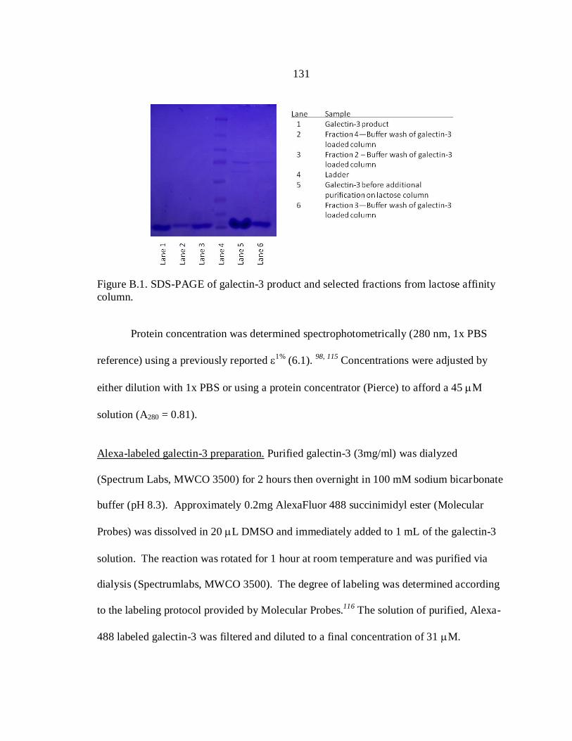
131
Figure B.1. SDS-PAGE of galectin-3 product and selected fractions from lactose affinity
column.
Protein concentration was determined spectrophotometrically (280 nm, 1x PBS
reference) using a previously reported 1%
(6.1). 98, 115
Concentrations were adjusted by
either dilution with 1x PBS or using a protein concentrator (Pierce) to afford a 45 M
solution (A280 = 0.81).
Alexa-labeled galectin-3 preparation. Purified galectin-3 (3mg/ml) was dialyzed
(Spectrum Labs, MWCO 3500) for 2 hours then overnight in 100 mM sodium bicarbonate
buffer (pH 8.3). Approximately 0.2mg AlexaFluor 488 succinimidyl ester (Molecular
Probes) was dissolved in 20 L DMSO and immediately added to 1 mL of the galectin-3
solution. The reaction was rotated for 1 hour at room temperature and was purified via
dialysis (Spectrumlabs, MWCO 3500). The degree of labeling was determined according
to the labeling protocol provided by Molecular Probes.116
The solution of purified, Alexa-
488 labeled galectin-3 was filtered and diluted to a final concentration of 31 M.