Electrical and Computer Engineering Transistor-Level

Use Asymptotic Waveform Evaluation Method onTransistor-Level Timing Analysis

Zhong Wang

Electrical and Computer Engineering

University of Toronto

Oct 12, 2001

[email protected]

http://www.eecg.toronto.edu/˜zwang

Synthesis Reading Group Copyrightc© Zhong Wang, Oct 2001, ECE, Univ. of Toronto 1

Outline

Motivation

Previous work

Problems of Spice

AWE(Asymptotic Waveform Evaluation)

Results


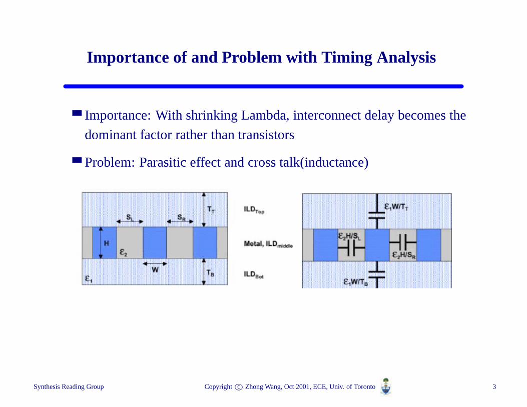
Importance of and Problem with Timing Analysis

Importance: With shrinking Lambda, interconnect delay becomes the

dominant factor rather than transistors

Problem: Parasitic effect and cross talk(inductance)


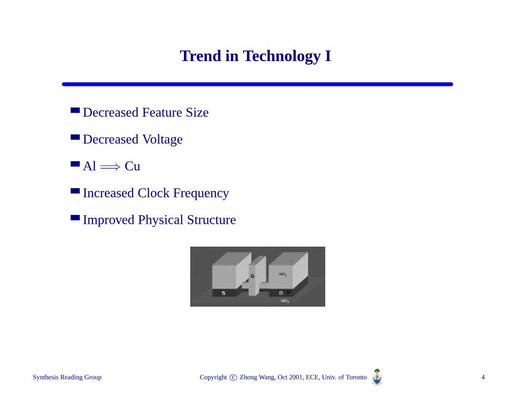
Trend in Technology I

Decreased Feature Size

Decreased Voltage

Al =⇒ Cu

Increased Clock Frequency

Improved Physical Structure


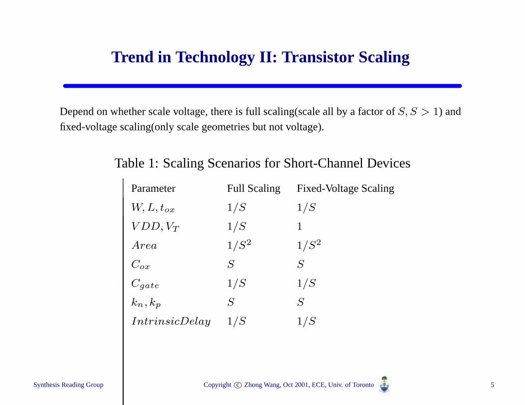
Trend in Technology II: Transistor Scaling

Depend on whether scale voltage, there is full scaling(scale all by a factor ofS, S > 1) and

fixed-voltage scaling(only scale geometries but not voltage).

Table 1: Scaling Scenarios for Short-Channel Devices

Parameter Full Scaling Fixed-Voltage Scaling

W, L, tox 1/S 1/S

V DD, VT 1/S 1

Area 1/S2 1/S2

Cox S S

Cgate 1/S 1/S

kn, kp S S

IntrinsicDelay 1/S 1/S


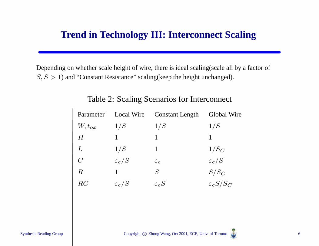
Trend in Technology III: Interconnect Scaling

Depending on whether scale height of wire, there is ideal scaling(scale all by a factor of

S, S > 1) and “Constant Resistance” scaling(keep the height unchanged).

Table 2: Scaling Scenarios for Interconnect

Parameter Local Wire Constant Length Global Wire

W, tox 1/S 1/S 1/S

H 1 1 1

L 1/S 1 1/SC

C εc/S εc εc/S

R 1 S S/SC

RC εc/S εcS εcS/SC


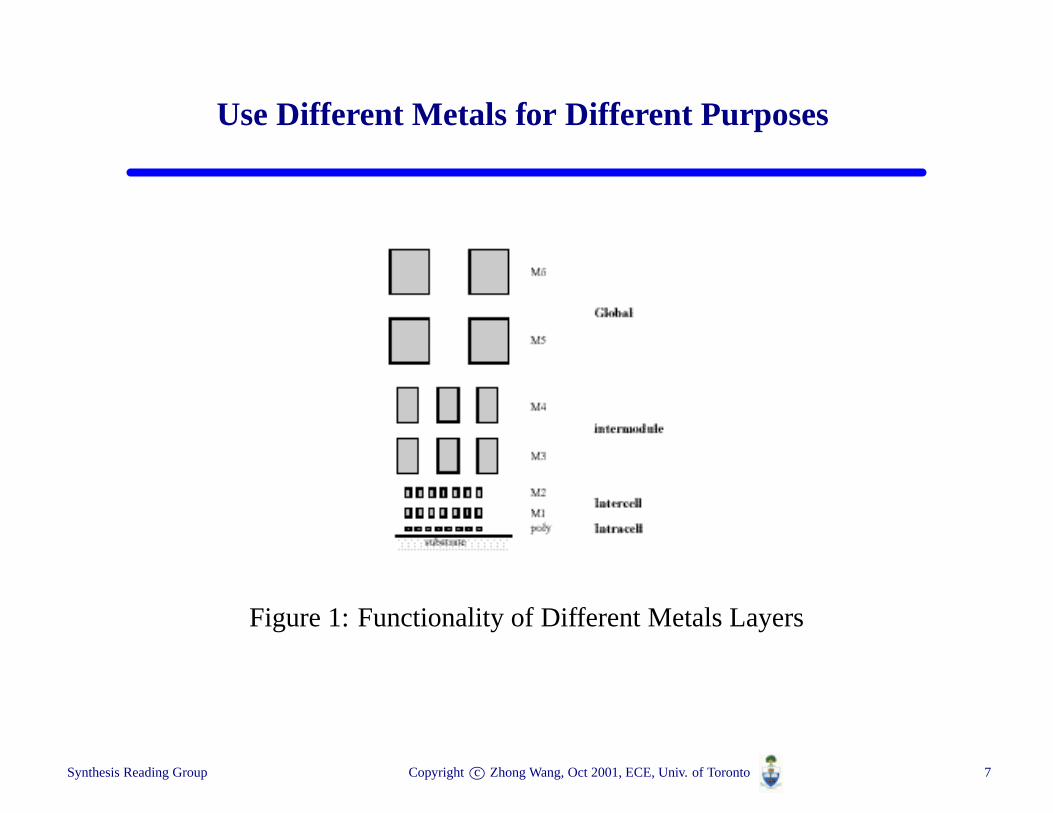
Use Different Metals for Different Purposes

Figure 1: Functionality of Different Metals Layers


Problem of Spice in Timing Analysis

Overuse: prohibitive long run time

Dynamic timing analysis: need test pattern

Accurate spice model of DSM technology

Not easy to be embedded.


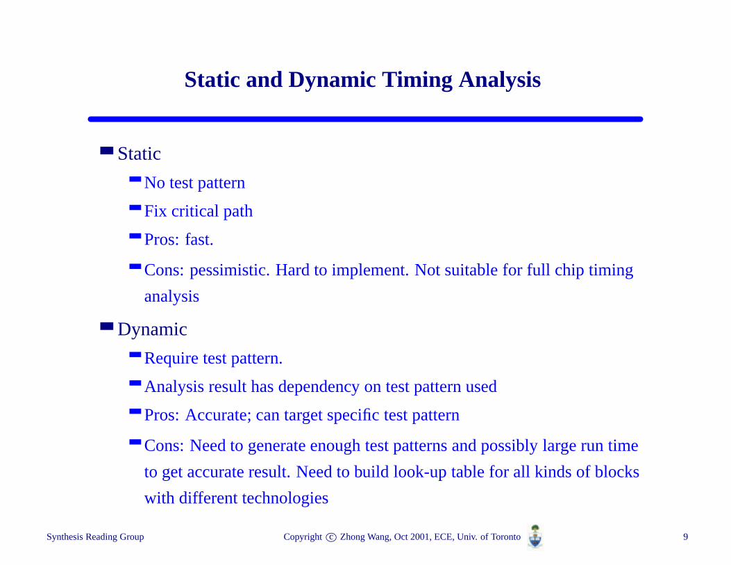
Static and Dynamic Timing Analysis

Static

No test pattern

Fix critical path

Pros: fast.

Cons: pessimistic. Hard to implement. Not suitable for full chip timing

analysis

Dynamic

Require test pattern.

Analysis result has dependency on test pattern used

Pros: Accurate; can target specific test pattern

Cons: Need to generate enough test patterns and possibly large run time

to get accurate result. Need to build look-up table for all kinds of blocks

with different technologies


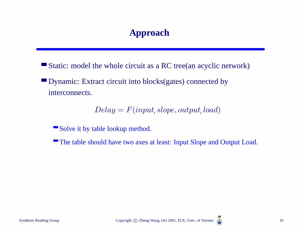
Approach

Static: model the whole circuit as a RC tree(an acyclic network)

Dynamic: Extract circuit into blocks(gates) connected by

interconnects.

Delay = F (input slope, output load)

Solve it by table lookup method.

The table should have two axes at least: Input Slope and Output Load.


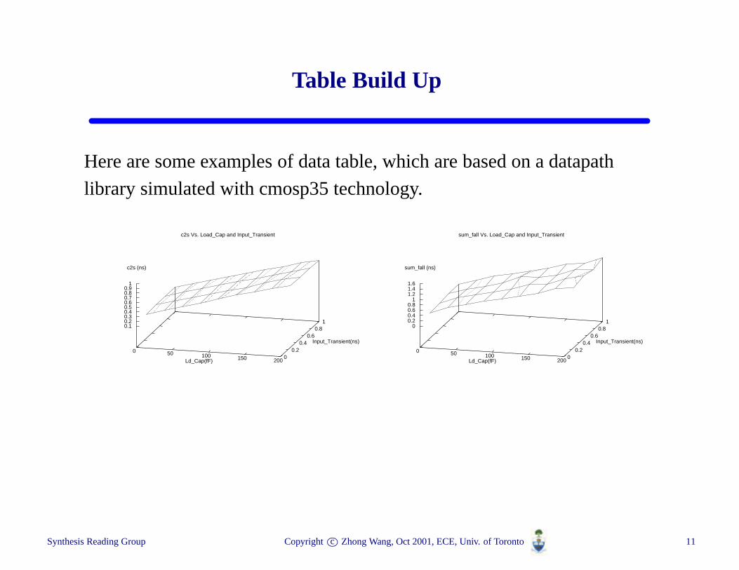
Table Build Up

Here are some examples of data table, which are based on a datapath

library simulated with cmosp35 technology.

c2s Vs. Load_Cap and Input_Transient

0 50 100 150 200Ld_Cap(fF)0

0.20.4

0.60.8

1

Input_Transient(ns)

0.10.20.30.40.50.60.70.80.9

1

c2s (ns)

sum_fall Vs. Load_Cap and Input_Transient

0 50 100 150 200Ld_Cap(fF)0

0.20.4

0.60.8

1

Input_Transient(ns)

00.20.40.60.8

11.21.41.6

sum_fall (ns)


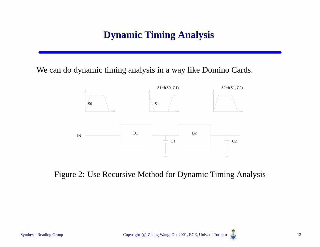
Dynamic Timing Analysis

We can do dynamic timing analysis in a way like Domino Cards.

INB1 B2

C1 C2

S0 S1

S1=f(S0, C1) S2=f(S1, C2)

Figure 2: Use Recursive Method for Dynamic Timing Analysis


Use AWE(Asymptotic Waveform Evaluation) Method forSTA

“Asymptotic Waveform Evaluation for Timing Analysis”, Pillage,

L.T. and Rohrer, R.A. IEEE Transaction on CAD,April, 1990.

For Interconnect delay analysis

1000 times faster than Spice but maintain an accuracy of with 10% of

Spice

Limit: mid frequency; linear RLC: floating capacitors, grounded

resistors, inductors and linear controlled source.


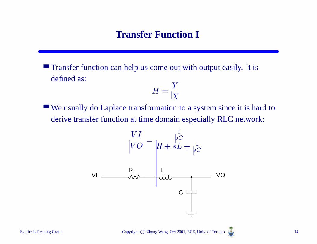
Transfer Function I

Transfer function can help us come out with output easily. It isdefined as:

H =Y

X

We usually do Laplace transformation to a system since it is hard toderive transfer function at time domain especially RLC network:

V I

V O=

1sC

R + sL + 1sC

VI VOR L

C


Transfer Function II

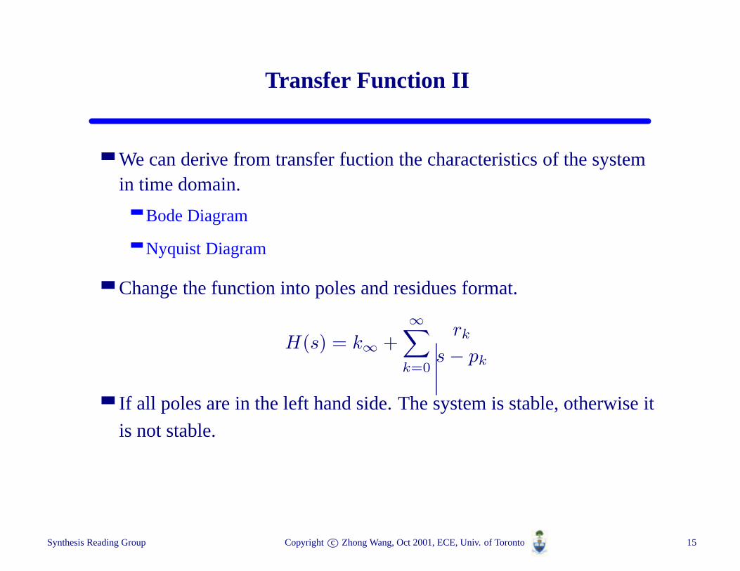
We can derive from transfer fuction the characteristics of the systemin time domain.

Bode Diagram

Nyquist Diagram

Change the function into poles and residues format.

H(s) = k∞ +∞∑

k=0

rk

s − pk

If all poles are in the left hand side. The system is stable, otherwise it

is not stable.


Time Domain to Frequency Domain

For linear circuit, if C and G stands for capacitor(and inductor) and

admittance matrix respectively, there is:

CX0 = −GX + bu

Y = 1T X

Do Laplace transformation and define

H(s) = Y (s)/U(s) = k∞ +∑

j=1kj

s−p−j

= 1T(I + sA + s2A2 + . . .)r

=∑∞

k=0 mksk

as the transfer function.pj are the poles. Continue to do Taylor

expansion.


Moment Matching

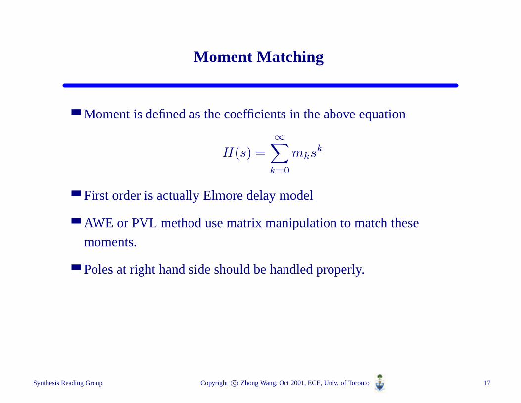
Moment is defined as the coefficients in the above equation

H(s) =∞∑

k=0

mksk

First order is actually Elmore delay model

AWE or PVL method use matrix manipulation to match these

moments.

Poles at right hand side should be handled properly.


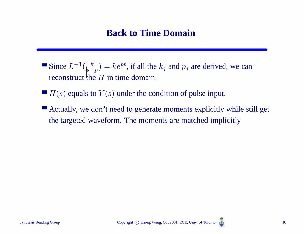
Back to Time Domain

SinceL−1( ks−p) = kept, if all the kj andpj are derived, we can

reconstruct theH in time domain.

H(s) equals toY (s) under the condition of pulse input.

Actually, we don’t need to generate moments explicitly while still get

the targeted waveform. The moments are matched implicitly


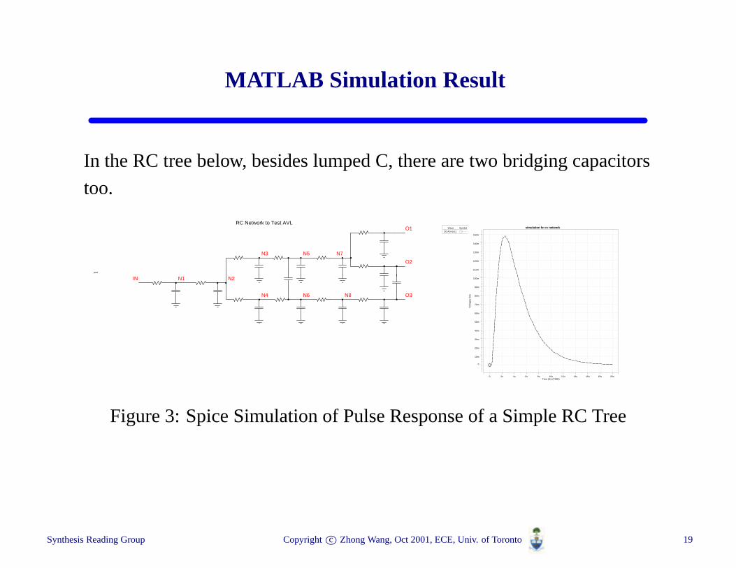
MATLAB Simulation Result

In the RC tree below, besides lumped C, there are two bridging capacitors

too.

IN

O1

O2

O3

RC Network to Test AVL

N1 N2

N3

N4

N5

N6

N7

N8

1

Symbol Wave

D0:A0:v(o1)

Vol

tage

s (li

n)

0

10m

20m

30m

40m

50m

60m

70m

80m

90m

100m

110m

120m

130m

140m

150m

Time (lin) (TIME)0 2u 4u 6u 8u 10u 12u 14u 16u 18u 20u

simulation for rc network

Figure 3: Spice Simulation of Pulse Response of a Simple RC Tree


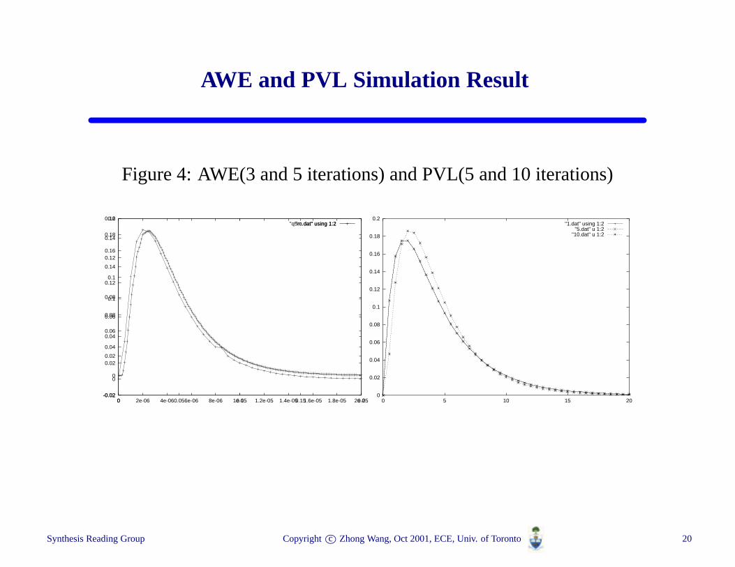
AWE and PVL Simulation Result

Figure 4: AWE(3 and 5 iterations) and PVL(5 and 10 iterations)

-0.02

0

0.02

0.04

0.06

0.08

0.1

0.12

0.14

0.16

0.18

0.2

0 0.05 0.1 0.15 0.2

"q5m.dat" using 1:2

-0.02

0

0.02

0.04

0.06

0.08

0.1

0.12

0.14

0.16

0 2e-06 4e-06 6e-06 8e-06 1e-05 1.2e-05 1.4e-05 1.6e-05 1.8e-05 2e-05

"rc.dat" using 1:2

0

0.02

0.04

0.06

0.08

0.1

0.12

0.14

0.16

0.18

0.2

0 5 10 15 20

"1.dat" using 1:2"5.dat" u 1:2

"10.dat" u 1:2


Problem with AWE

Poles at right hand side

Usually cannot just increase iteration number to get better result

Use PVL(Pade Approximation via the Lanczos Process)

More accurate higher order approximation

Not sensitive to poles at right hand side

Does not increase complexity

Hurwitz Table Method

Incremental and Hierarchical


Practical Problem

Extraction of DSM technology layout

Passivity and Stability

Hierarchical and Incremental

Matrix Manipulation

Moment Preserving Modeling Reduction

Model Reduction based on Frequency


Documents

Electrical and Computer Engineering Transistor-Level