Embed Size (px)
Citation preview
(4.2)
Equations in One Space Variable
INTRODUCTION
In Chapt~r 1 we discussed methods for solving IVPs, whereas in Chapters 2 and3 boundary-value problems were treated. This chapter combines the techniquesfrom these chapters to solve parabolic partial differential equations in one spacevariable.
CLASSifiCATION Of PARTIAL DiffERENTIAL EQUATIONS
Consider the most general linear partial differential equation of the second orderin two independent variables:
Lw = awxx + 2bwxy + CWyy + dwx + ewy + fw = g (4.1)
where a, b, C, d, e, f, g are given functions of the independent variables andthe subscripts denote partial derivatives. The principal part of the operator Lis
a2 a2 a2
a-+2b--+c-ax2 ax ay ay2
Primarily, it is the principal part, (4.2), that determines the properties of thesolution of the equation Lw = g. The partial differential equation Lw - g = 0
127
128 Parabolic Partial Differential Equations in One Space Variable
is classified as:
HyperbOliC} {> °Parabolic according as b2
- ac = °Elliptic < ° (4.3)
where b2 - ac is called the discriminant of L. The procedure for solving eachtype of partial differential equation is different. Examples of each type are:
Wxx + W yy = 0, e.g., Laplace's equation, which is elliptic
e.g., wave equation, which is hyperbolic
e.g., diffusion equation, which is parabolic
An equation can be of mixed type depending upon the values of the parameters,e.g.,
YWxx + Wyy = 0,(Tricomi's equation) {
y < 0, hyperbolicy = 0, parabolic,U > 0, elliptic
To each of the equations (4.1) we must adjoin appropriate subsidiaryrelations, called boundary and/or initial conditions, which serve to complete theformulation of a "meaningful problem." These conditions are related to thedomain in which (4.1) is to be solved.
METHOD OF LINES
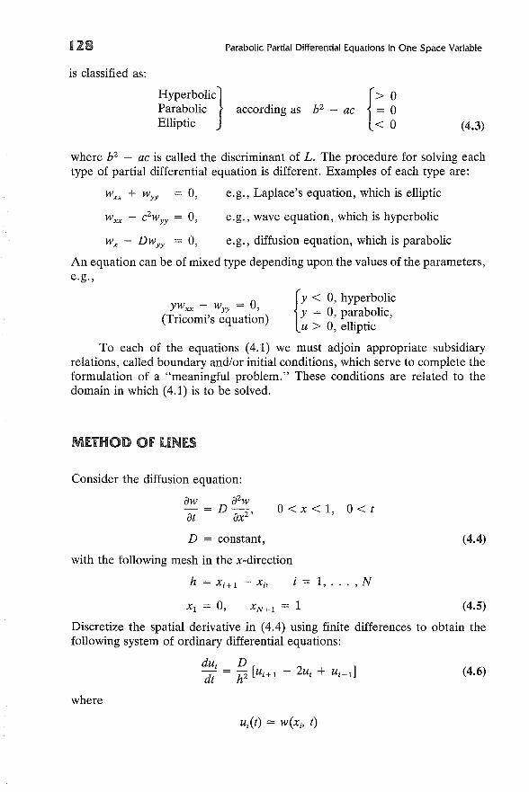
Consider the diffusion equation:
aw = D a2wat ax2 '
°< x < 1, 0< t
D constant, (4.4)
with the following mesh in the x-direction
i = 1, ... ,N
(4.5)
(4.6)
Discretize the spatial derivative in (4.4) using finite differences to obtain thefollowing system of ordinary differential equations:
duo Dd/ = h2 [Ui+l - 2ui + ui-d
where
ult) = W(Xi' t)
Method of Lines 129
Thus, the parabolic PDE can be approximated by a coupled system of ODEsin t. This technique is called the method of lines (MOL) [1] for obvious reasons.To complete the formulation we require knowledge of the subsidiary conditions.The parabolic PDE (4.4) requires boundary conditions atx = °and x = 1, andan initial condition at t = 0. Three types of boundary conditions are:
Dirichlet, e.g., weD, t) = 8l(t)
Neumann, e.g., wi1, t) = gz(t)
Robin, e.g., aw(O, t) + I3wx (O, t) = git) (4.7)
In the MOL, the boundary conditions are incorporated into the discretizationin the x-direction while the initial condition is used to start the associated IVP.
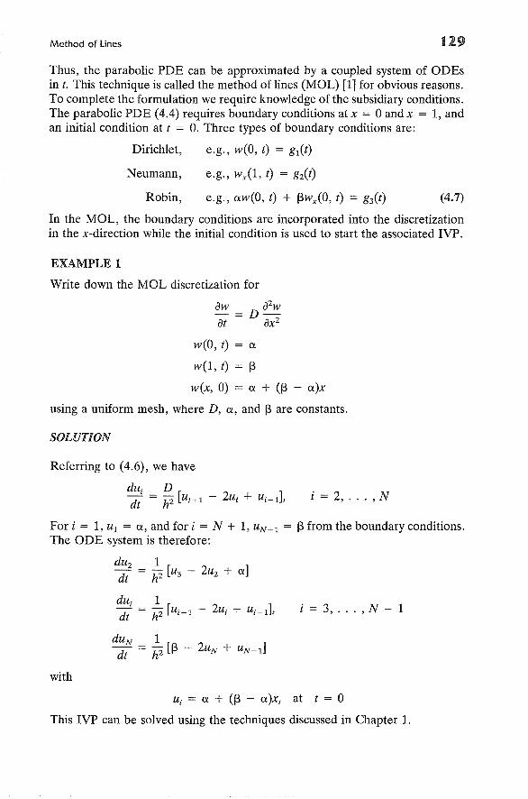
EXAMPLE 1
Write down the MOL discretization for
aw = D azwat axz
weD, t) = a
w(l, t) = 13
w(x, 0) = a + (13 - a)x
using a uniform mesh, where D, a, and 13 are constants.
SOLUTION
Referring to (4.6), we have
du Ddt' = hZ [u;+1 - 2u; + u;-d, i = 2, ... ,N
i = 3, ... ,N - 1
For i = 1, U 1 = a, and for i = N + 1, UN+l = 13 from the boundary conditions.The ODE system is therefore:
duz 1dt = hZ [u3 - 2uz + a]
duo 1dr' = hZ [U;+l - 2u; + u;-d,
with
u; = a + (13 - a)x; at t = °This IVP can be solved using the techniques discussed in Chapter 1.
130 Parabolic Partial Differential Equations in One Space Variable
The method of lines is a very useful technique since IVP solvers are in amore advanced stage of development than other types of differential equationsolvers. We have outlined the MOL using a finite difference discretization. Otherdiscretization alternatives are finite element methods such as collocation andGalerkin methods. In the following sections we will first examine the MOL usingfinite difference methods, and then discuss finite element methods.
FINITE DIffERENCES
Low-Order Time Approximations
Consider the diffusion equation (4.4) with
w(O, t) = 0
w(l, t) = 0
w(x, 0) = f(x)
which can represent the unsteady-state diffusion of momentum, heat, or massthrough a homogeneous medium. Discretize (4.4) using a uniform mesh to give:
duo Dd/ = h2 [Ui+l - 2ui + ui-d, i = 2, ... , N
(4.8)
where Ui = f(xi), i = 2, ... ,N at t = O. If the Euler method is used to integrate(4.8), then with
we obtain
j = 0,1, ...
or
where
Ui,j+l - Ui,j DI::i.t = h2 [Ui+1,j - 2 i ,j + Ui-1,j]
Ui,j+l = (1 - 2T)Ui ,j + T(Ui+1,j + Ui-l,)
(4.9)
AtT = h2 D
and the error in this formula is O(At + h2) (At from the time discretization, h2
from the spatial discretization). At j = 0 all the u/s are known from the initialcondition. Therefore, implementation of (4.9) is straightforward:
Finite Differences 131
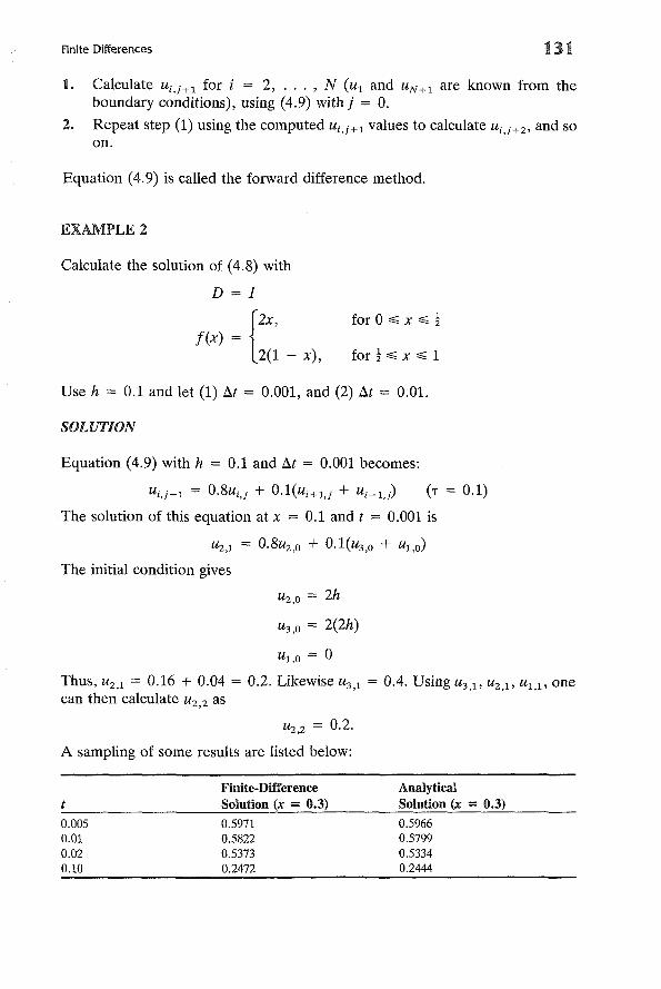
1. Calculate Ui,j+1 for i = 2, ... , N (u l and UN+l are known from theboundary conditions), using (4.9) with j = O.
2. Repeat step (1) using the computed Ui,j+l values to calculate Ui ,j+2, and soon.
Equation (4.9) is called the forward difference method.
EXAMPLE 2
Calculate the solution of (4.8) with
D = 1
{
2X'f(x) =
2(1 - x),
for 0,;:.;; x ,;:.;; ~
for ~ ,;:.;; x ,;:.;; 1
Use h = 0.1 and let (1) At = 0.001, and (2) f:.t = 0.01.
SOLUTION
Equation (4.9) with h = 0.1 and At = 0.001 becomes:
Ui,j+l = 0.8ui,j + O.l(Ui+l,j + Ui-1,j) (1' = 0.1)
The solution of this equation at x = 0.1 and t = 0.001 is
U2,1 = 0.8~,o + 0.1(u3,o + Ul,O)
The initial condition gives
U2,O = 2h
U3,O = 2(2h)
U1,O = 0
Thus, U2 ,1 = 0.16 + 0.04 = 0.2. Likewise U3 ,1 = 0.4. Using U3 ,1' U2 ,1' UI,l' onecan then calculate U 2 ,2 as
~,2 = 0.2.
A sampling of some results are listed below:
0.0050.010.Q20.10
Finite-DifferenceSolution (x = 0.3)
0.59710,58220.53730.2472
AnalyticalSolution (x = 0.3)
0.59660.57990.53340.2444
132
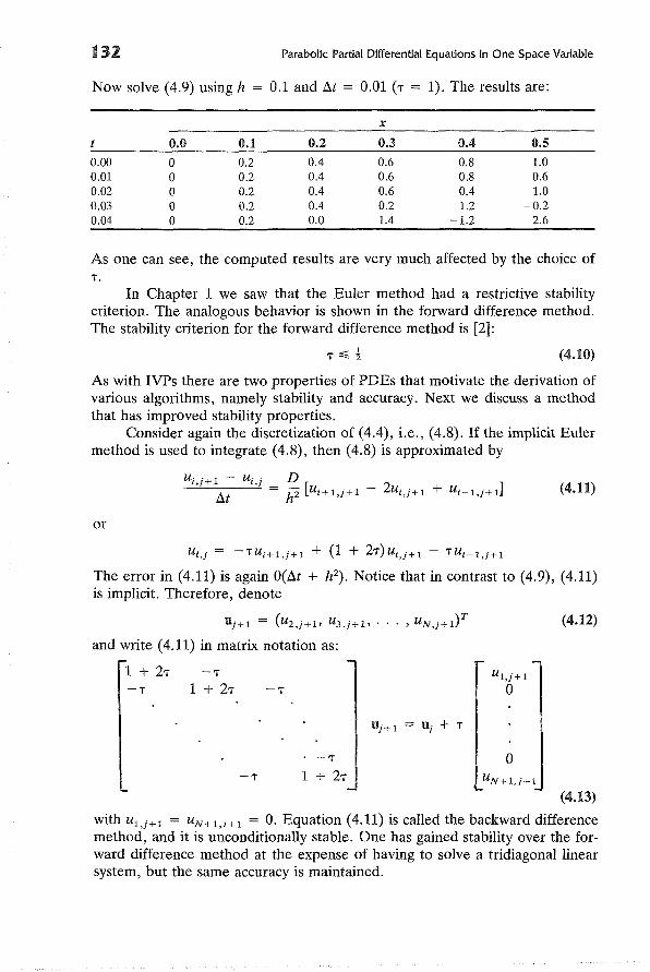
Now solve (4.9) using h
Parabolic Partial Differential Equations in One Space Variable
0.1 and I1t = 0.01 (r = 1). The results are:
x
t 0.0 0.1 0.2 0.3 0.4 0.50.00 0 0.2 0.4 0.6 0.8 1.00.01 0 0.2 0.4 0.6 0.8 0.60.02 0 0.2 0.4 0.6 0.4 1.00.03 0 0.2 0.4 0.2 1.2 -0.20.04 0 0.2 0.0 1.4 -1.2 2.6
As one can see, the computed results are very much affected by the choice ofT.
In Chapter 1 we saw that the Euler method had a restrictive stabilitycriterion. The analogous behavior is shown in the forward difference method.The stability criterion for the forward difference method is [2]:
(4.10)
As with IVPs there are two properties of PDEs that motivate the derivation ofvarious algorithms, namely stability and accuracy. Next we discuss a methodthat has improved stability properties.
Consider again the discretization of (4.4), i.e., (4.8). If the implicit Eulermethod is used to integrate (4.8), then (4.8) is approximated by
or
Ui,j+l - Ui,j DI1t = h2 [Ui+l,j+l - 2ui ,j+l + Ui-1,j+d
Ui,j = -TUi+l,j+l + (1 + 2T)Ui ,j+l - TUi-1,j+l
(4.11)
The error in (4.11) is again O(l1t + h2). Notice that in contrast to (4.9), (4.11)is implicit. Therefore, denote
-T
and write (4.11) in matrix notation as:
1 + 2T -T-T 1 + 2T
-T
1 + 2T
U1,j+l
o
oUN+1,j+l
(4.12)
(4.13)
with U1,j+l UN+1,i+l = O. Equation (4.11) is called the backward differencemethod, and it is unconditionally stable. One has gained stability over the forward difference method at the expense of having to solve a tridiagonal linearsystem, but the same accuracy is maintained.
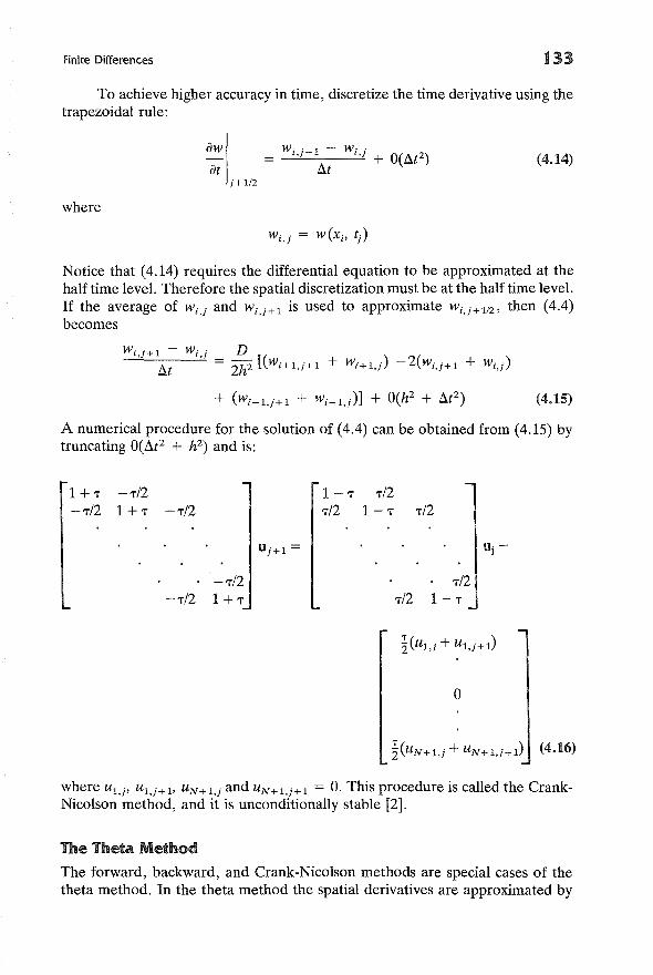
Finite Differences t33
To achieve higher accuracy in time, discretize the time derivative using thetrapezoidal rule:
where
aWat
j+1/Z
(4.14)
Notice that (4.14) requires the differential equation to be approximated at thehalf time level. Therefore the spatial discretization must be at the half time level.If the average of Wi,j and Wi,j+l is used to approximate Wi,j+l/Z' then (4.4)becomes
Wi,j+l - w· . DI1t ',J = 2hz [(Wi+1,j+l + Wi+1,j) -2(wi,j+l + Wi,j)
(4.15)
A numerical procedure for the solution of (4.4) can be obtained from (4.15) bytruncating O(LltZ + hZ) and is:
1 + 'T -'T12- 'T12 1 + 'T -'T12
1-'T'T12
'T121-'T 'T12
u·]
-'T12-'T12 1+'T
'T12'T12 1 - 'T
o
~(UN+l,j + UN+1,j+l) (4.16)
where U1,j' U1,j+v UN+l,j and UN+l,j+l = O. This procedure is called the CrankNicolson method, and it is unconditionally stable [2].
The Theta Method
The forward, backward, and Crank-Nicolson methods are special cases of thetheta method. In the theta method the spatial derivatives are approximated by
134 Parabolic Partial Differential Equations in One Space Variable
the following combination at the j and j + 1 time levels:
iPu _ 2 (1 )"2-2 - 80x u i J"+l + - 8 uxui J"ax' ,
where
U"+l " - 2u" " + U,"-l,J"02 _',J ',JxUi,j - h2
For example, (4.4) is approximated by
U i ,j+1 - Ui,j = D[802 u" " (1 8)02 ]I5..t x ',J+1 + - xUi,j
or in matrix form
(4.17)
(4.18)
[1 - (1 - 8)1"1]U j (4.19)
where
1 = identity matrix
2 -1
-1 2
J=
-1-1 2
(4.20)
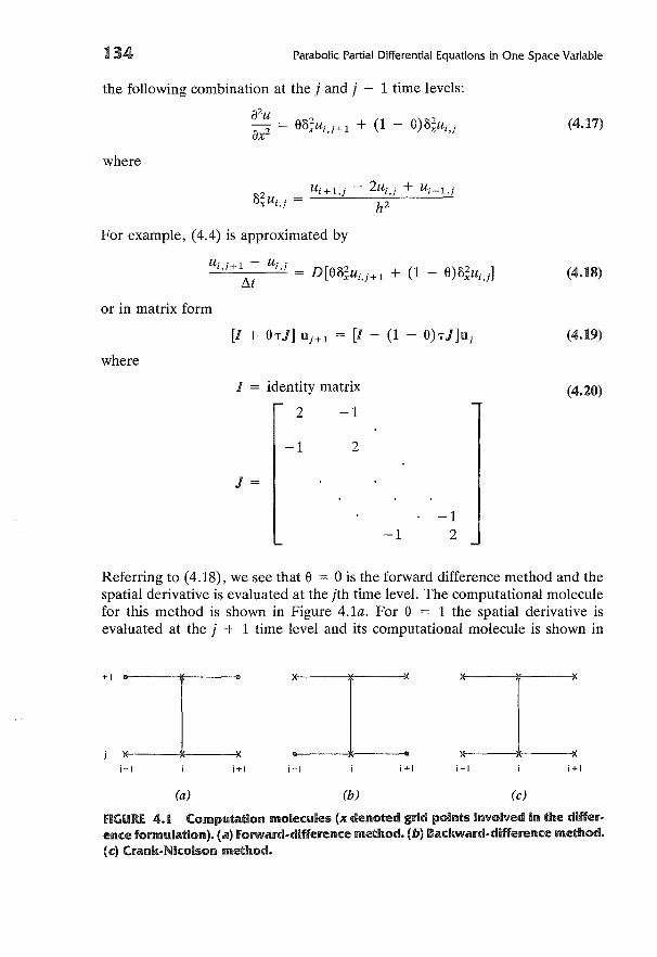
Referring to (4.18), we see that 8 = 0 is the forward difference method and thespatial derivative is evaluated at the jth time level. The computational moleculefor this method is shown in Figure 4.1a. For 8 = 1 the spatial derivative isevaluated at the j + 1 time level and its computational molecule is shown in
+1
i-I
(a)
;+1 i-I
(b)
;+1 i-I
(c)
i+1
FIGURE 4.. Computation molecules (x denoted grid points involved in the difference formulation). (a) Forward-difference method. (b) Backward-difference method.(c) Crank-Nicolson method.
Finite Differences 135
Figure 4.1b. The Crank-Nicolson method approximates the differential equationat the j + ~ time level (computational molecule shown in Figure 4.1c) andrequires information from six positions. Since 8 = t the Crank-Nicolson methodaverages the spatial derivative between j and j + 1 time levels. Theta may lieanywhere between zero and one, but for values other than 0, 1, and ~ there isno direct correspondence with previously discussed methods. Equation (4.19)can be written conveniently as:
or
uj + 1 = [1 + 81"1]-1 [1 - (1 - 8) 1"1] u j (4.21)
(4.22)
Boundary and Initial Conditions
Thus far, we have only discussed Dirichlet boundary conditions. Boundary conditions expressed in terms of derivatives (Neumann or Robin conditions) occurvery frequently in practice. If a particular problem contains flux boundary conditions, then they can be treated using either of the two methods outlined inChapter 2, i.e., the method of false boundaries or the integral method. As anexample, consider the problem of heat conduction in an insulated rod with heatbeing convected "in" at x = °and convected "out" at x = 1. The problem canbe written as
aT aZTpC- = k-Pat axz
T = To at t = 0, for 0< x < 1
where
aT- k- = h1(T1 - T) at x = °
ax
aT-k- = hz(T - Tz) at x = 1
ax
T = dimensionless temperature
To = dimensionless initial temperature
pCp = density times the heat capacity of the rod
h1, hz = convective heat transfer coefficients
T1, Tz = dimensionless reference temperatures
k = thermal conductivity of the rod
(4.23)
136 Parabolic Partial Differential Equations in One Space Variable
Using the method of false boundaries, at x = 0
aT-k- = h1(T1 - T)ax
becomes
Solving for Uo gives
A similar procedure can be used at x = 1 in order to obtain
2h2UN + 2 = k t:u(T2 - UN + 1) + UN
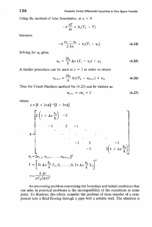
Thus the Crank-Nicolson method for (4.23) can be written as:
wherec = [I + hA]-l[I - hAl
(4.24)
(4.25)
(4.26)
(4.27)
A=
-1 2 -1
-1 2
-2
An interesting problem concerning the boundary and initial conditions thatcan arise in practical problems is the incompatibility of the conditions at somepoint. To illustrate this effect, consider the problem of mass transfer of a component into a fluid flowing through a pipe with a soluble wall. The situation is
Finite Differences 137
I' L ,
- FLUID VELOCITY
t t t t t t t t t t t t t
Fluid entersat a uniformcompositionwith molefraction ofcomponent A,
YA1 ______-L......I-.L-.L-L.....J--L---I.--L-L-L-...I-...I.-.L--'-- _
Soluble coating an wall maintains liquidcomposition Y~ next to the wall surface.
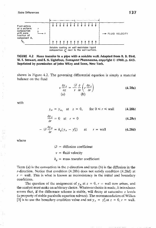
fiGURE. 4.2 Mass transfer in a pipe with a solubie wall. Adapted from R. B. Bird,W. E. Stewart, and Eo N. Lightfoot, Transport Phenomena, copyright © 1960, p. 643.Reprinted by permission of John Wiley and Sons, New York.
shown in Figure 4.2. The governing differential equation is simply a materialbalance on the fluid
vayA= 0 ~ (r ayA)az r ar ar
(a) (b)
(4.28a)
with
YA = YA , at z = 0, for °~ r ~ wall (4. 28b)
aYA = ° at r = °ar (4.28c)
at r = wall (4.28d)
where
o = diffusion coefficient
v = fluid velocity
kg = mass transfer coefficient
Term (a) is the convection in the z-direction and term (b) is the diffusion in ther-direction. Notice that condition (4.28b) does not satisfy condition (4.28d) atr = wall. This is what is known as inconsistency in the initial and boundaryconditions.
The question of the assignment of YA at z = 0, r = wall now arises, andthe analyst must make an arbitrary choice. Whatever choice is made, it introduceserrors that, if the difference scheme is stable, will decay at successive z levels(a property of stable parabolic equation solvers). The recommendation of Wilkes[3] is to use the boundary condition value and set YA = Y~ at z = 0, r = wall.
138
EXAMPLE 3
Parabolic Partial Differential Equations in One Space Variable
A fluid (constant density p and viscosity fL) is contained in a long horizontalpipe of length L and radius R. Initially, the fluid is at rest. At t = 0, a pressuregradient (Po - PL)/L is imposed on the system. Determine the unsteady-statevelocity profile V as a function of time.
SOLUTION
The governing differential equation is
p aV = Po - PL + fL!..i (r av)at L r ar ar
with
v=o at t = 0, for 0 :%; r :%; R
av = 0 at r = 0, for t ~ 0arV=o at r = R, for t ~ 0
Define
r~ =
R
T) = (Po - PL)R2
then the governing PDE can be written as
aT) = 4 + !..i (~ aT))aT ~ a~ a~
T) = 0 at T = 0, for 0 :%; ~ :%; 1
a1] = 0 at ~ = 0, for T ~ 0a~
1] = 0 at ~ = 1, for T ~ 0
At T ---? 00 the system attains steady state, 1]0C" Let
The steady-state solution is obtained by solving
1 d ( d1]oc)o = 4 + ~ d~ ~ d~
Finite Differences
with
1]00 = 0 at £ = 1
a1]oo = 0 at £ = 0a£
and is 1]00 = 1 - £2. Therefore
a<l> = ! ~ (£ a<l»a'T £a£ a£
with
a<l> = 0 at £ = 0, for'T ;:?; 0a£
<1>=0 at £ = 1, for 'T ;:?; 0
<I> = 1 - £2 at 'T = 0, for 0 ~ £ ~ 1
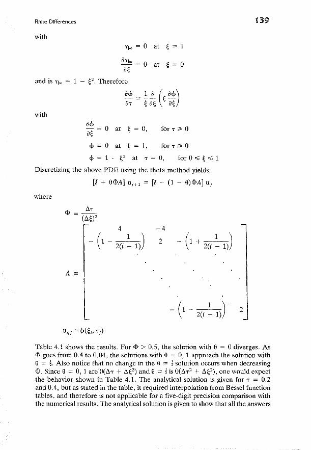
Discretizing the above PDE using the theta method yields:
[1 + e<PA] Uj+l = [1 - (1 - e)<pA] uj
where
139
A=
-4
2 _(1 + __1__)2(i - 1)
Table 4.1 shows the results. For <P > 0.5, the solution with e = 0 diverges. As<P goes from 0.4 to 0.04, the solutions with e = 0, 1 approach the solution withe = 1. Also notice that no change in the e = 1solution occurs when decreasing<P. Since e = 0,1 areO(A'T + A£2) and e = 1is 0(A'T2 + A£2), one would expectthe behavior shown in Table 4.1. The analytical solution is given for 'T = 0.2and 0.4, but as stated in the table, it required interpolation from Bessel functiontables, and therefore is not applicable for a five-digit precision comparison withthe numerical results. The analytical solution is given to show that all the answers
140 Parabolic Partial Differential Equations in One Space Variable
TABLE 4.1 Computed <l> Values Using the Theta Method~ = 0.4
fl> = 0.4 fl> = 0.04
'I' 6=0 6=1 6=! 6=0 6=1 6=!
0.2 0.27192 0.27374 0.27283 0.27274 0.27292 0.272830.4 0.85394( -1) 0.86541( -1) 0.85967( -1) 0.8591O( -1) 0.86025( -1) 0.85968( -1)0.8 0.84197(-2) 0.86473( -2) 0.85332(-2) 0.85218(-2) 0.85446(-2) 0.85332(-2)
Analyticalt0.27230.8567( -1)
t Solution required the use of Bessel functions, and interpolation of tabular data will produce errors in thesenumbers.
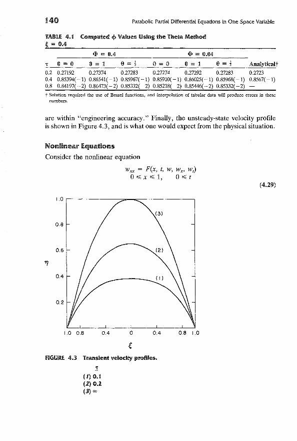
are within "engineering accuracy." Finally, the unsteady-state velocity profileis shown in Figure 4.3, and is what one would expect from the physical situation.
Nonlinear EquationsConsider the nonlinear equation
W xx = F(x, t, w, wx ' wt)
o~ x ~ 1, 0 ~ t
(4.29)
1.0 r-------~-~------__,
0.8
0.6
0.4
0.2
1.0 0.8 0.4 o 0.4 0.8 1.0
fiGURE 4.3 Transient velocity profiles.
(1) 0.1(2) 0.2(3) 00
Finite Differences 141
(4.30)
with w(O, t), w(l, t), and w(x, 0) specified. The forward difference methodwould produce the following difference scheme for (4.29):
2 _ ( ui,i+l - Ui,i)8x ui ,i - F Xi' ti, Ui,i' ilXUi,i' ilt
where
If the time derivative appears linearly, (4.30) can be solved directly. This isbecause all the nonlinearities are evaluated at the jth level, for which the nodevalues are known. The stability criterion for the forward difference method isnot the same as was derived for the linear case, and no generalized explicitcriterion is available. For "difficult" problems implicit methods should be used.The backward difference and Crank-Nicolson methods are
and
1 2( (Ui,i+1 + Ui,i28x Ui,i+l + Ui,) = F Xi' ti +1/2, 2
Ui,i+\ -t Ui,i)~ilx (u i , i + 1 + U i , i ), --'-''---''l.l----'-'"-
(4.31)
(4.32)
Equations (4.31) and (4.32) lead to systems of nonlinear equations that must besolved at each time step. This can be done by a Newton iteration.
To reduce the computation time, it would be advantageous to use methodsthat handle nonlinear equations without iteration. Consider a special case of(4.29), namely,
Wxx = !lex, t, w)wt + f2(X, t, w)wx + f3(X, t, w) (4.33)
A Crank-Nicolson discretization of (4.33) gives
with
= h i +1I2 (Ui'i+~~ Ui,i)
+ hi+1I2 ilx
(Ui,i+12+ Ui,i) + f~i+1/2 (4.34)
(u· . 1 + u· .)
f i,i+ 1/2 _ .(: l,J+ l,Jn - in Xi' ti + 1/2 , 2 ' n = 1,2,3.
Equation (4.34) still leads to a nonlinear system of equations that would requirean iterative method for solution. If one could estimate ui,i+1/2' by ui,i+1/2 say,
142 Parabolic Partial Differential Equations in One Space Variable
and use it in
1 1)2 ( U . .) = t-iJ+1/2(Ui,j+1 - Ui,j)2' x U i ,j+1 + ',j 1 At
- (u .. 1 + U· .)+ t~j+1I2 Ax l,j+ 2 ',j
where
+ h j+
1I2
(4.35)
then there would be no iteration. Douglas and Jones [4] have considered thisproblem and developed a predictor-corrector method. They used a backwarddifference method to calculate Cti,j+1I2:
1)2 - -Ii j Cti,j+1/2 - Ui,j fi j A - fi j, ";,1+," - i (~t) + i ,u;,I+'" + i'
where
(4.36)
The procedure is to predict Ui,j+1/2 from (4.36) (this requires the solutionof one tridiagonal linear system) and to correct using (4.35) (which also requiresthe solution of one tridiagonal linear system). This method eliminates the nonlinear iteration at each time level, but does require that two tridiagonal systemsbe solved at each time level. Lees [5] introduced an extrapolated Crank-Nicolsonmethod to eliminate the problem of solving two tridiagonal systems at each timelevel. A linear extrapolation to obtain Ui,j+ 112 gives
Ct· '+1/2 = U· . + ~ (u· . - U· '-1)l,] l.J 1,J l,j
or
Cti,j + 1/23Ui ,j - U i ,j-1
2(4.37)
Notice that Cti ,j+1I2 is defined directly for j > 1. Therefore, the procedure is tocalculate the first time level using either a forward difference approximation orthe predictor-corrector method of Douglas and Jones, then step in time using(4.35) with Cti,j + 1/2 defined by (4.37). This method requires the solution of onlyone tridiagonal system at each time level (except for the first step), and thuswould require less computation time.
Inhomogeneous Media
Problems containing inhomogeneities occur frequently in practical situations.Typical examples of these are an insulated pipe-i.e., interfaces at the insidefluid-inside pipewall, outside pipewall-inside insulation surface, and the outside
Finite Differences 143
insulation surface-outside fluid-or a nuclear fuel element (refer back to Chapter2). In this case, the derivation of the PDE difference scheme is an extension ofthat which was outlined in Chapter 2 for ODEs.
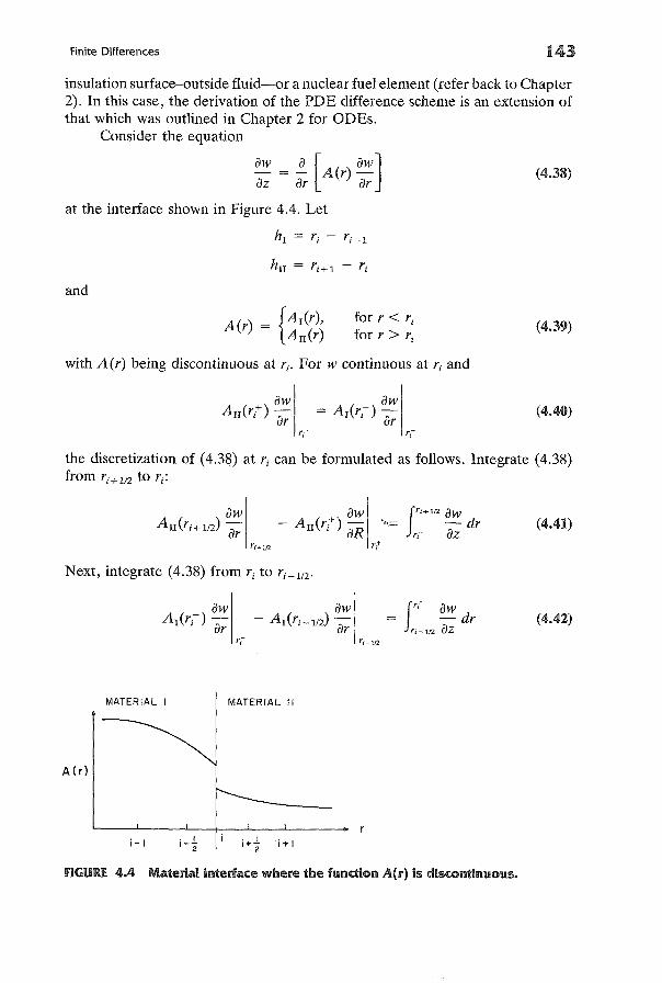
Consider the equation
ow 0 [ ow]- = - A(r)-uz or orat the interface shown in Figure 4.4. Let
and
(4.38)
A(r) = {A1(r),AlI(r)
for r < rj
for r > r i(4.39)
with A(r) being discontinuous at rj. For w continuous at r j and
+ owAlI(rj )ar (4.40)
the discretization of (4.38) at r j can be formulated as follows. Integrate (4.38)from ri+ liZ to r j :
+ aw jr'+112 aw- AlI(ri ) .oR "".= - dr
u r,+ azrt
(4.41)
Next, integrate (4.38) from r j to rj-1/Z '
rj-1I2
jr,- aw= -dr
r'-1I2 az(4.42)
A(r)
MATERIAL I MATERIAL II
i-I • 11--
2
FIGURE 4.4 Material interface where the function A(l') is discontinuous.
144 Parabolic Partial Differential Equations in One Space Variable
Now, add (4.42) to (4.41) and use the continuity condition (4.40) to give
fr;+112 aw
= -drr'-112 aZ
ri-l/2
(4.43)
Approximate the integral in (4.43) by
fr'+112 aw aw 1 aw
- dr = - (ri+l/Z - r i - lIZ) = -2(hr + hn ) ri-112 az az az
(4.44)
If a Crank-Nicolson formulation is desired, then (4.43) and (4.44) would give
Ui,j+l - Ui,j 1 {An (ri + 1/z)Llz = hI + hn hn (Ui+l,j+l + Ui+l)
(4.45)
Notice that if hI = hn and AI = An, then (4.45) reduces to the standard secondorder correct Crank-Nicolson discretization. Thus the discontinuity of A(r) istaken into account.
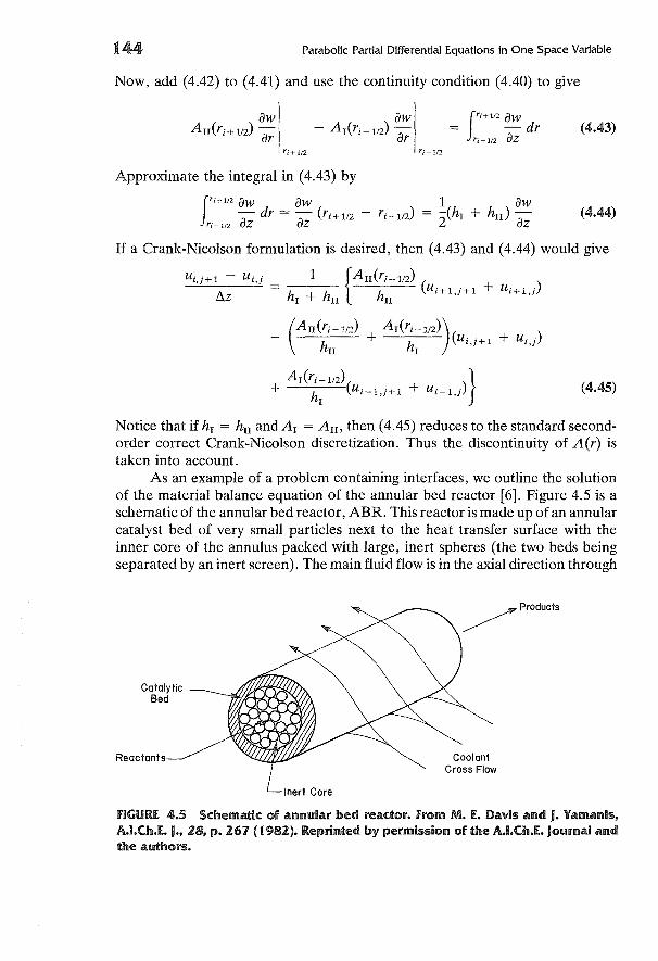
As an example of a problem containing interfaces, we outline the solutionof the material balance equation of the annular bed reactor [6]. Figure 4.5 is aschematic of the annular bed reactor, ABR. This reactor is made up of an annularcatalyst bed of very small particles next to the heat transfer surface with theinner core of the annulus packed with large, inert spheres (the two beds beingseparated by an inert screen). The main fluid flow is in the axial direction through
CatalyticBed
Reactants CoolantCross Flow
FIGURE. 4.5 Schematic of annular bed reactor. From M. E. Davis and J. Yamanis,A.I.Ch.E. J., 28, p. 267 (1982). Reprinted by permission ofthe A.I.Ch.E. Journal andthe authors.
Finite Differences 145
the core, where the inert packing promotes radial transport to the catalyst bed.If the effects of temperature, pressure, and volume change due to reaction onthe concentration and on the average velocity are neglected and mean propertiesare used, the mass balance is given by
"at _VI az
(a)
[Am An] ~ ~ (rD at)Re Sc r ar ar
(b)
+ [~: ~n}2 4> 2R(f)
(c) (4.46)
where the value of 1 or 0 for ~1 and ~2 signifies the presence or absence of aterm from the above equation as shown below
Core Screen Bed
with
1o
oo
o-1
t = dimensionless concentration
z = dimensionless axial coordinate
r = dimensionless radial coordinate
Am, An = aspect ratios (constants)
Re = Reynolds number
Sc = Schmidt number
D = dimensionless radial dispersion coefficient
4> = Thiele modulus
R(f) = dimensionless reaction rate function.
Equation (4.46) must be complemented by the appropriate boundary and initialconditions, which are given by
at r = 0at = 0ar
Dc atl = Dsc atl at r = rscar c ar sc
Dsc atl = DB atl at r = r Bar sc ar B
at = 0 at r = 1ar
(centerline)
(core-screen interface)
(screen-bed interface)
(wall)
t = 1 at z = 0, for 0 ~ r ~ 1
146 Parabolic Partial Differential Equations in One Space Variable
Notice that in (4.46), term (a) represents the axial convection and therefore isnot in the equation for the screen and bed regions, while term (c) representsreaction that only occurs in the bed, i.e., the equation changes from parabolicto elliptic when moving from the core to the screen and bed. Also, notice thatD is discontinuous at r sc and rB • This problem is readily solved by the use of anequation of the form (4.45). Equation (4.46) becomes
81
[Ui ,j+1 :z Ui ,j-1] [Am An] 1 ~ {ri + 1/z D i + 1/Z
= Re Sc hI + hrr
ri
hrr
(Ui + 1,j+1
(ri+1/Z Di+lIZ + r i - 1/Z D i - lIZ) ( . . . .)+ Ui + 1 ) - h h U"j+1 + U"j
rr I
(4.47)
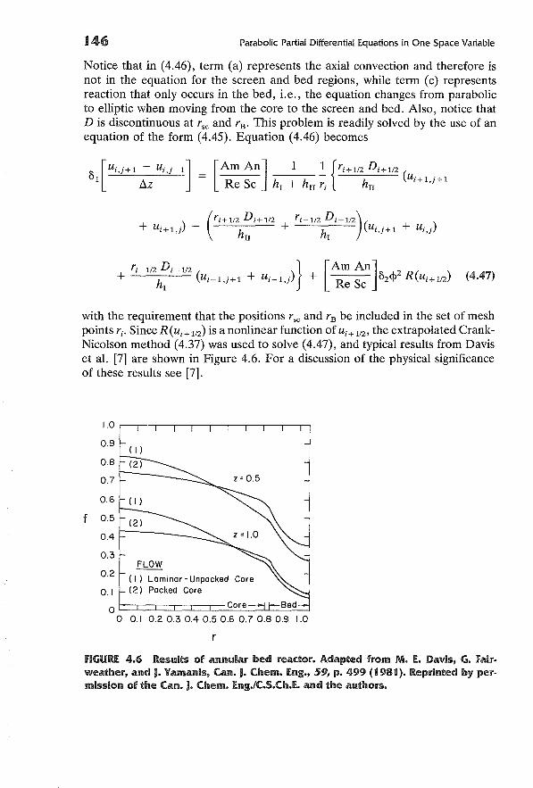
with the requirement that the positions r sc and rB be included in the set of meshpoints rio Since R(Ui+ liZ) is a nonlinear function of Ui+ liZ' the extrapolated CrankNicolson method (4.37) was used to solve (4.47), and typical results from Daviset al. [7] are shown in Figure 4.6. For a discussion of the physical significanceof these results see [7].
1.0
0.9
0.8
0.7
0.6
f 0.5
0.4
0.3
0.2FLOW
( I) Laminar - Unpacked
0.1 (2) Packed Core
00 0.1
r
flGURf. 4.6 Results of annular bed reactor. Adapted from M. E. Davis, G. fairweather, and J. Yamanis, Can. J. Chem. Eng., 59, p. 499 (1981). Reprinted by permission of the Can. J. Chem. Eng.lC.S.Ch.E. and the authors.
Finite Differences 147
(4.48)
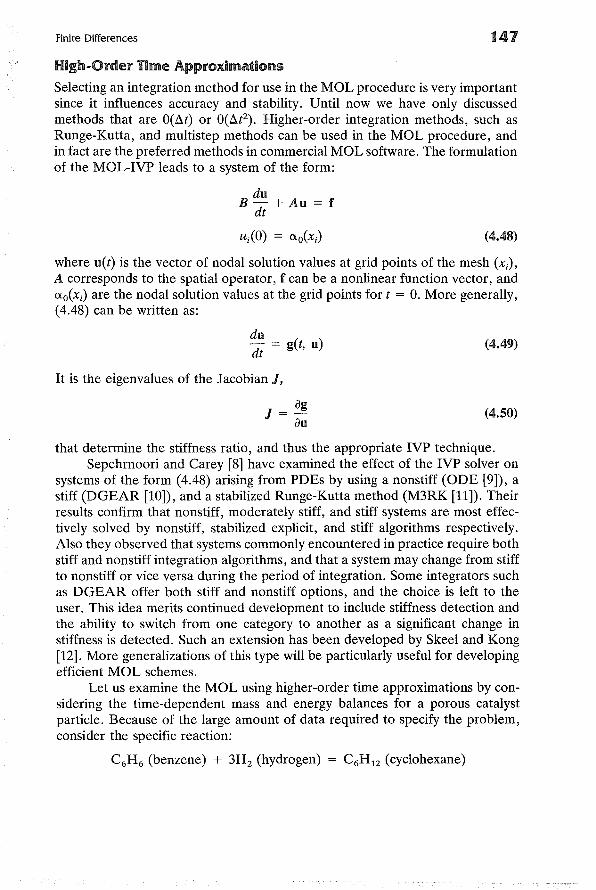
High-Order Time Approximations
Selecting an integration method for use in the MOL procedure is very importantsince it influences accuracy and stability. Until now we have only discussedmethods that are O(6.t) or O(6.tZ). Higher-order integration methods, such asRunge-Kutta, and multistep methods can be used in the MOL procedure, andin fact are the preferred methods in commercial MOL software. The formulationof the MOL-IVP leads to a system of the form:
duB - + Au = f
dt
uJO) = <Xo(xi)
where u(t) is the vector of nodal solution values at grid points of the mesh (Xi),A corresponds to the spatial operator, f can be a nonlinear function vector, and<Xo(xi) are the nodal solution values at the grid points for t = O. More generally,(4.48) can be written as:
dudt = g(t, u)
It is the eigenvalues of the Jacobian J,
J = agau
(4.49)
(4.50)
that determine the stiffness ratio, and thus the appropriate IVP technique.Sepehrnoori and Carey [8] have examined the effect of the IVP solver on
systems of the form (4.48) arising from PDEs by using a nonstiff (ODE [9]), astiff (DGEAR [10]), and a stabilized Runge-Kutta method (M3RK [11]). Theirresults confirm that nonstiff, moderately stiff, and stiff systems are most effectively solved by nonstiff, stabilized explicit, and stiff algorithms respectively.Also they observed that systems commonly encountered in practice require bothstiff and nonstiff integration algorithms, and that a system may change from stiffto nonstiff or vice versa during the period of integration. Some integrators suchas DGEAR offer both stiff and nonstiff options, and the choice is left to theuser. This idea merits continued development to include stiffness detection andthe ability to switch from one category to another as a significant change instiffness is detected. Such an extension has been developed by Skeel and Kong[12]. More generalizations of this type will be particularly useful for developingefficient MOL schemes.
Let us examine the MOL using higher-order time approximations by considering the time-dependent mass and energy balances for a porous catalystparticle. Because of the large amount of data required to specify the problem,consider the specific reaction:
C6H 6 (benzene) + 3Hz (hydrogen) = C6H 12 (cyclohexane)
148 Parabolic Partial Differential Equations in One Space Variable
(4.51)
(hydrogen)
(benzene)
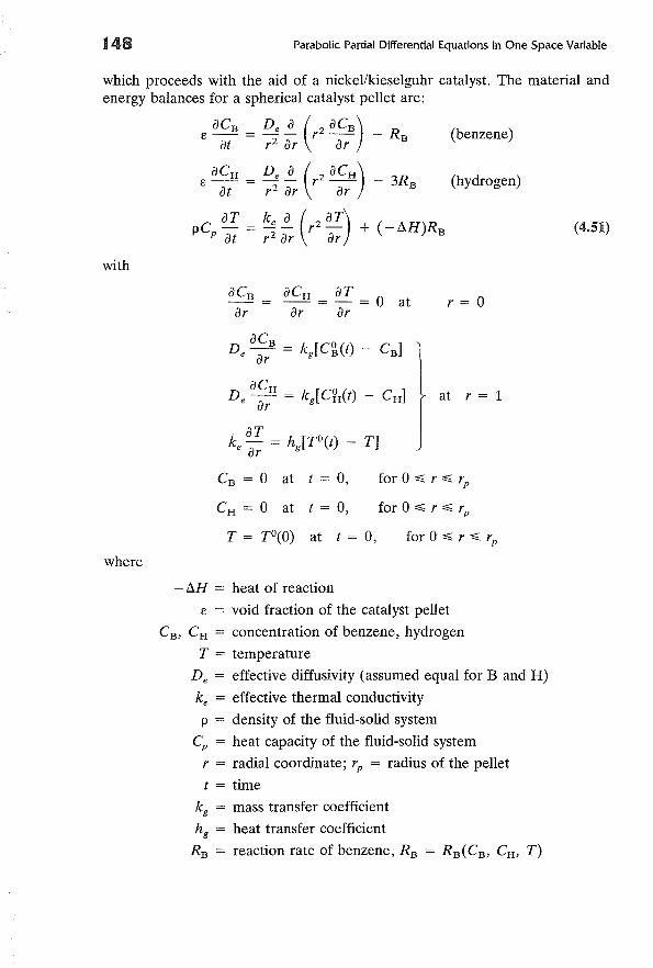
which proceeds with the aid of a nickel/kieselguhr catalyst. The material andenergy balances for a spherical catalyst pellet are:
E aCB = De ~ (r2 aCB ) - RBat r2 ar ar
E aCH = De ~ (r2 aCH) - 3RBat r2 ar ar
aT ke a ( aT)pC - = -- r2 - + (-AH)R Bp at r2 ar ar
with
aCB = aCH = aT = ° atar ar ar r = °
De a~H = kg[C~(t) - CH ]
. aTke a; = hg[TO(t) - T]
at r = 1
CB = ° at t = 0,
CH = ° at t = 0, for °"'S r "'S rp
T = TO(O) at t = 0, for °"'S r "'S rp
where
- AH = heat of reaction
E = void fraction of the catalyst pellet
CB , CH = concentration of benzene, hydrogen
T = temperature
De = effective diffusivity (assumed equal for B and H)
ke = effective thermal conductivity
p = density of the fluid-solid system
Cp = heat capacity of the fluid-solid system
r = radial coordinate; rp = radius of the pellet
t = time
kg = mass transfer coefficient
hg = heat transfer coefficient
RB = reaction rate of benzene, RB = RB(CB, CH , T)
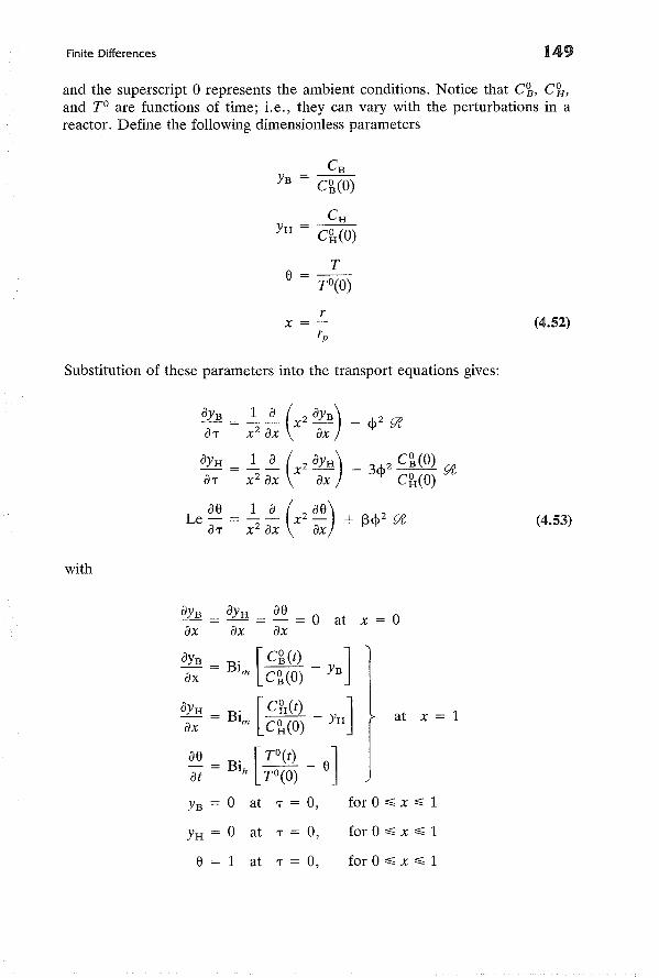
Finite Differences 149
and the superscript 0 represents the ambient conditions. Notice that C~, CfJ-I,and TO are functions of time; i.e., they can vary with the perturbations in areactor. Define the following dimensionless parameters
-~YB - C~(O)
CHYH = C~(O)
Te = TO(O)
Substitution of these parameters into the transport equations gives:
ae 1 a ( ae)Le - = - - x 2 - + ~<!>2 9taT x2 ax ax
with
aYB = aYH = ae = 0 at x = 0ax ax ax
(4.52)
(4.53)
at x = 1
YB = 0 at T = 0,
YH = 0 at T = 0,
e = 1 at T = 0,
for 0 ~ x ~ 1
for 0 ~ x ~ 1
for 0 ~ x ~ 1
150
where
Parabolic Partial Differential Equations in One Space Variable
2
<1>2 = C~~;)De RB(C~(O), C~(O), TO(O)) (Thiele modulus squared)
p = De ( - LlH)C~(O) (Prater number)keTO(O)
(Lewis number)
DetT=-
r~E
Bim
= rpkg
De
B. rphgIh =
ke
(dimensionless time)
(mass Biot number)
(heat Biot number)
(4.54)
For the benzene hydrogenation reaction, the reaction rate function is [13]:
Peatk K exp [(QR:rE
)]PBPH
RB =
1 + K exp (R~T)PBwhere
k = 3207 gmole/(sec'atm'gcat)K = 3.207 X 10⁻⁸ atm- 1
Q = 16,470 callgmole
E = 13,770 cal/gmole
Rg = 1.9872 call(gmoleoK)
Peat = 1.88 g/cm3
Pi = partial pressure of component i
Noticing that
Ci Pi (TO(O))Yi = q(O) = P?(O) -r/LJ [(1 1)] 2 __[~l_+_K_P--,~:::...;(--,-O)_e-"xp--,(~(X=l),,--]_YL· = exp (X2 - - 6 YBYH
6 [1 + KP~(O) exp (~l) YB6]
(4.55)
Finite Differences
where
a - Q1 - R
gTO(O)
a _ ..o..::(Q=----_E--'-)2 - R
gTO(O)
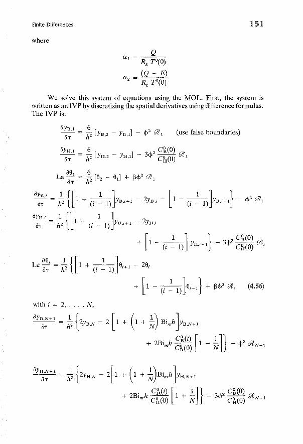
151
(use false boundaries)
We solve this system of equations using the MOL. First, the system iswritten as an IVP by discretizing the spatial derivatives using difference formulas.The IVP is:
aYB,l _ 6 2----a;- - h2 [YB,2 - YB,d - <I> 9(1
aYH,l _ 6 2 C~(O)----a;- - h2 [YH,2 - YH,l] - 3<1> C~(O) 9(1
ae 6Le _1 = h
2[e2 - e1] + 13<1>2 9( 1
aT
a~~'i = ~2 {[1 + (i ~ 1)}B,i+1 - 2YB,i +
a~:'i = ~2 {[1 + (i ~ 1)}H,i+1 - 2YH,i
[ 1] }_3.1,.2 C~(O) 9(.+ 1 - (i _ 1) YH,i-1 't' C~(O) I
Le ~; = ~2 {[1 + (i ~ 1)]ei + 1 - 2ei
+ [1 - (i ~ 1)Jei-1} + 13<1>29(i (4.56)
with i = 2, ... , N,
aYB,N+1 = ~ {2 - 2[1 +aT h2 YB,N
aYH,N+1 1{ [( 1).]aT = h2 2YH,N - 2 1 + 1 + N Blmh YH,N+1
. C~(t) [ 1]} 2 C~(O)+ 2Blmh CMO) 1 + IV - 3<1> C~(O) flP N + 1
151 Parabolic Partial Differential Equations in One Space Variable
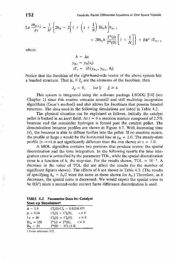
Le aeN + 1 = ~ {2e - 2[1 +aT h2 N
where
h = Ax
YB,i = YB(Xi)
[7(. = [7(. (YB' YH' e.)1 ,1' ,1' 1
Notice that the Jacobian of the right-hand-side vector of the above system hasa banded structure. That is, if Jij are the elements of the Jacobian, then
for Ii - jl ;;,: 4
This system is integrated using the software package LSODE [14] (seeChapter 1) since this routine contains nonstiff and stiff multistep integrationalgorithms (Gear's method) and also allows for Jacobians that possess bandedstructure. The data used in the following simulations are listed in Table 4.2.
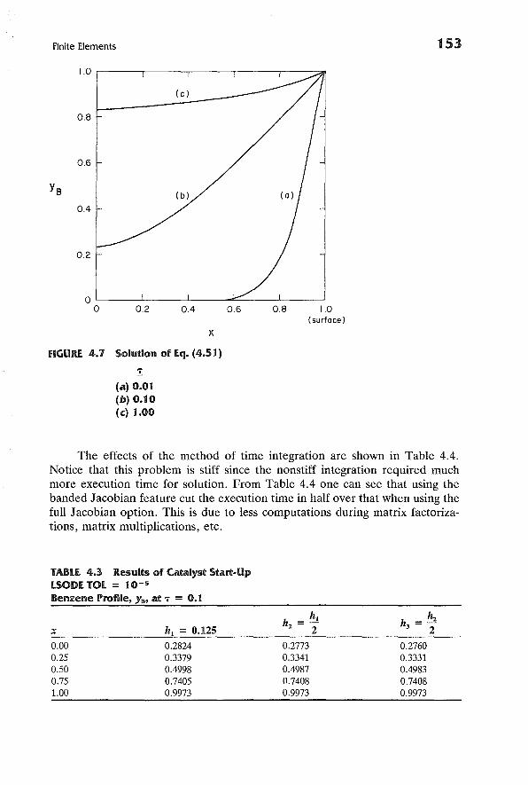
The physical situation can be explained as follows. Initially the catalystpellet is bathed in an inert fluid. At t = aa reaction mixture composed of 2.5%benzene and the remainder hydrogen is forced past the catalyst pellet. Thedimensionless benzene profiles are shown in Figure 4.7. With increasing time(T), the benzene is able to diffuse further into the pellet. If no reaction occurs,the profile at large T would be the horizontal line at YB = 1.0. The steady-stateprofile (T-i>OO) is not significantly different than the one shown at T = 1.0.
A MOL algorithm contains two portions that produce errors: the spatialdiscretization and the time integration. In the following results the time integration error is controlled by the parameter TaL, while the spatial discretizationerror is a function of h, the step-size. For the results shown, TaL = 10-5 • Adecrease in the value of TaL did not affect the results (to the number ofsignificant figures shown). The effects of h are shown in Table 4.3. (The resultsof specifying h4 = h3/2 were the same as those shown for h3 .) Therefore, as hdecreases, the spatial error is decreased. We would expect the spatial error tobe O(h2
) since a second-order correct finite difference discretization is used.
TABU 4.2 Parameter Data for CatalystStart-up Simulationt
q, = 1.0 C\'.(O)/C~ = 0.025/0.975
f3 = 0.04 C\'.(t) = q(O), t ~ 0
Le = 80 C~(t) = C~(O), t ~ 0Bim = 350 TO(t) = TO(O) , t ~ 0Bih = 20 TO(O) = 373.15 K
t From reference [15].
Finite Elements
1.0 ,.-------,.----,--------,.----,------::All
153
(c)
0.8
0.6
(b)
0.4
0.2
O'--------'------.l.---=-----'------'o 0.2 0.4 0.6 0.8 1.0
(surface)
x
fiGURE. 4.7 Solution of Eq. (4.51)
!(a) 0.01(b) 0.10(c) 1.00
The effects of the method of time integration are shown in Table 4.4.Notice that this problem is stiff since the nonstiff integration required muchmore execution time for solution. From Table 4.4 one can see that using thebanded Jacobian feature cut the execution time in half over that when using thefull Jacobian option. This is due to less computations during matrix factorizations, matrix multiplications, etc.
TABLE 4.3 Results of Catalyst Start-UpLSODE TOL = 10- 5
Benzene Profile, Yn, at 'T = 0.1
h _ hI hzh3 =-X hI = 0.125 z - 2 2
0.00 0.2824 0.2773 0.27600.25 0.3379 0.3341 0.33310.50 0.4998 0.4987 0.49830.75 0.7405 0.7408 0.74081.00 0.9973 0.9973 0.9973
154 Parabolic Partial Differential Equations in One Space Variable
TABLE 4.4 further Results of CatalystStart-Up150D£ TOt = 10-5
h = 0.0625
Execution TimeRatio
Nonstiff methodStiff method
(full Jacobian)Stiff method
(banded Jacobian)
T = 0.1
7.872.30
1.00
T = 1.0
50.982.24
1.00
fiNITE ELEMENTS
In the following sections we will continue our discussion of the MOL, but willuse finite element discretizations in the space variable. As in Chapter 3, we willfirst present the Galerkin method, and then proceed to outline collocation.
Galerkin
Here, the Galerkin methods outlined in Chapter 3 are extended to parabolicPDEs. To solve a PDE, specify the piecewise polynomial approximation (ppapproximation) to be of the form:
m
u(x, t) 2: uj(t)<I>j(x)j=l
(4.57)
Notice that the coefficients are now functions of time. Consider the PDE:
with
aw a [ aw]at = ax a(x, w) ax ' 0< x < 1, t> 0 (4.58)
w(x, 0) = woCx)
w(O, t) = 0
w(l, t) = 0
If the basis functions are chosen to satisfy the boundry conditions, then the weakform of (4.58) is
(a(x, w) ~:' <1>;) + (aa~' <l>i) = 0 i = 1, ... m (4.59)
Finite Elements 155
The MOL formulation for (4.58) is accomplished by substituting (4.57) into(4.59) to give
i = 1, ... ,m
Thus, the IVP (4.60) can be written as:
Ba'(t) + D(a)a(t) = 0
with
Ba(O) 13where
Di,j = (a <1>; , <1>;)
Bi,j = (<I>j' <l>i)13 = [(wo, <1>1), (wo, <1>2), ..• , (wo, <l>m))T
(4.60)
(4.61)
(4.62)
In general this problem is nonlinear as a result of the function a in thematrix D. One could now use an IVP solver to calculate a(t). For example, ifthe trapezoidal rule is applied to (4.61), the result is:
[an+1 an]B l:i.t + D(an+1/2)an+1
/2 = 0
with
where
tn = n l:i.t
an = a(tn)
a n + 1/2 =2
Since the basis <l>i is local, the matrices Band D are sparse. Also, recall that theerror in the Galerkin discretization is O(hk ) where k is the order of the approximating space. Thus, for (4.62), the error is 0(l:i.t2 + hk ), since the trapezoidalrule is second-order accurate. In general, the error of a Galerkin-MOL discretization is O(l:i.tP + hk ) where p is determined by the IVP solver. In the followingexample we extend the method to a system of two coupled equations.
EXAMPLE 4
A two-dimensional model is frequently used to describe fixed-bed reactors thatare accomplishing highly exothermic reactions. For a single independent reaction
156 Parabolic Partial Differential Equations in One Space Variable
a material and energy balance is sufficient to describe the reactor. These continuity equations are:
r af = pe[~ (r af)] + 131r9P(f, e)
az ar ar
ae [a ( ae)]r - = Bo - r - + I37.r9P(f, e)az ar ar
with
f = e = 1 at z = 1, for 0 < r < 1
af = ae = 0 at r = 0, for 0 < z < 1ar ar
where
aear
-Bi(e - ew) at r = 1, for 0 < Z < 1
z = dimensionless axial coordinate, 0 ~ z ~ 1
r = dimensionless radial coordinate, 0 ~ r ~ 1
f = dimensionless concentration
e = dimensionless temperature
ew = dimensionless reactor wall temperature
9P = dimensionless reaction rate function
Bi, Pe, Bo, 131, 132 = constants
These equations express the fact that the change in the convection is equal tothe change in the radial dispersion plus the change due to reaction. The boundarycondition for e at r = 1 comes from the continuity of heat flux at the reactorwall (which is maintained at a constant value of ew). Notice that these equationsare parabolic PDE's, and that they are nonlinear and coupled through the reaction rate function. Set up the Galerkin-MOL-IVP.
SOLUTION
Let
m
u(x, z) ~ a/z)<j>/x) = f(x, z)j=l
m
vex, z) = ~ "Yj(z)<j>j(x) = e(x, z)j=l
Finite Elements 151
such that
m
u(X, 0) = 2: aj(O)<I>/X) = 1.0j=1
m
VeX, 0) = 2: 'Yj(O)<I>j(X) = 1.0j=1
The weak form of this problem is
(:~, <1» = Pe [r :~<I>{ - G~ <1>:) ] + ~1( YG, <l>i)
G:, <l>i) = Bo [r ~~<I>{ - G~, <1>:) ] + ~2( YG,<I>i)
i= 1, ... ,m
where
(a, b) = fal abr dr
The boundary conditions specify that
r = 0)(:~ = 0 at r = 1 and r = 0)
(ae- = 0 atar
r at <l>i 11 = 0ar 0
r ae <l>i 11 - Bi (e - ew )<I>i(1)ar 0
Next, substitute the pp-approximations for t and e into the weak forms of thecontinuity equations to give
j~1 a; (z)(<I>j' <1>;) = -Pe [j~1 aj(z)(<I>;, <1>;)] + ~1(.Yi, <l>i)
j~1 'Y;(z)(<I>j' <l>i) = -Bo [Bi C~1 'Yj<l>/1) - ew ) <l>i(1)
+ j~1 'Y/z)(<I>;, <1>;)] + ~2(.Yi, <l>i)' i = 1, ... ,m
where
158
Denote
Parabolic Partial Differential Equations in One Space Variable
Ci,j = (<pj, <Pi)
Di,j = (<p;, <Pi)
Bi,j = <pi(l)<pj(l)
tlJi = (9t , <p;)
The weak forms of the continuity equations can now be written as:
COl.' - Pe DOl. + 131'"
C'Y' -Bo [Bi (B'Y - ew $(l)) + D'Y] + 13z'"
with 01.(0) and 'Y(O) known. Notice that this system is a set of IVPs in thedependent variables 01. and 'Y with initial conditions 01.(0) and 'Y(O). Since thebasis <Pi is local, the matrices B, C, and D are sparse. The solution of this systemgives OI.(t) and 'Y(t) , which completes the specification of the pp-approximationsu and v.
From the foregoing discussions one can see that there are two componentsto any Galerkin-MOL solution, namely the spatial discretization procedure andthe IVP solver. We defer further discussions of these topics and that of Galerkinbased software until the end of the chapter where it is covered in the sectionon mathematical software.
CollocationAs in Chapter 3 we limit out discussion to spline collocation at Gaussian points.To begin, specify the pp-approximation to be (4.57), and consider the PDE:
with
aw ( aw aZw)-- xtw--at - f " 'ax' axz ' 0< x < 1, t> 0 (4.63)
where
w = wo(x) at t = 0'hW + f3 lw' = "Il(t) at x = 01] zW + f3zw' = "Iz(t) at x = 1
i = 1,2
According to the method of spline collocation at Gaussian points, we requirethat (4.57) satisfy the differential equation at (k - M) Gaussian points persubinterval, where k is the degree of the approximating space and M is the orderof the differential equation. Thus with the mesh
o = Xl < Xz < ... < Xe+l 1 (4.64)
Finite Elements 159
Eq. (4.63) becomes
j~l u; (t)<!>j(x;) = t(X;, t, j~l u/t)<!>j(x;), j~l Uj(t)<!>; (x;), j~l Uj(t)<!>" (x;) )
i = 1, ... , m - 2 (4.65)
where
m = (k - M}e + 2
M = 2
We now have m - 2 equations in m unknown coefficients uj • The last twoequations necessary to specify the pp-approximation are obtained by differentiating the boundary conditions:
m m
'll1 L u; (t)<!>/O) + (31 L U; (t)<!>; (0) = -y~ (t)j=l j=lm m
'll2 L U; (t)<!>j(1) + (32 L U; (t)<!>; (1) = -y;(t)j=l j=l
This system of equations can be written as
Aa' (t) = F(t, a)
a(O) = a owhere
A = left-hand side of (4.65) and (4.66)
F = right-hand side of (4.65) and (4.66)
and a o is given by:
(4.66)
(4.67)
m
L Uj(O)<!>j(xi) = Wo(X;) ,j=l
1 = 1, ... ,m
Since the basis <!>j is local, the matrix A will be sparse. Equation (4.67) can nowbe integrated in time by an IVP solver. As with Galerkin-MOL, the errorproduced from collocation-MOL is O(LltP + hk) where p is specified by the IVPsolver and k is set by the choice of the approximating space. In the followingexample we formulate the collocation method for a system of two coupledequations.
EXAMPLE 5
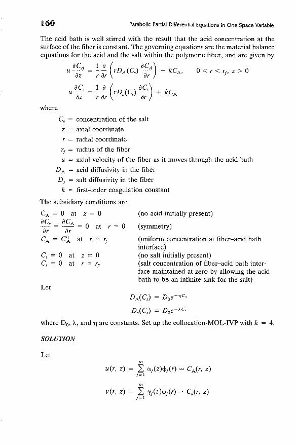
A polymer solution is spun into an acidic bath, where the diffusion of acid intothe polymeric fiber causes the polymer to coagulate. We wish to find the concentration of the acid (in the fiber), CA , along the spinning path. The coagulationreaction is
Polymer + acid -i> coagulated polymer + salt
160 Parabolic Partial Differential Equations in One Space Variable
The acid bath is well stirred with the result that the acid concentration at thesurface of the fiber is constant. The governing equations are the material balanceequations for the acid and the salt within the polymeric fiber, and are given by
u aCA = ! ~ (rD (C) acA ) - kCaz r ar A s ar A, 0 < r < rf' z > 0
u acs = ! ~ (rDs(Cs) acs) + kCAaz r ar ar
where
(no acid initially present)
(symmetry)
(uniform concentration at fiber-acid bathinterface)(no salt initially present)(salt concentration of fiber-acid bath interface maintained at zero by allowing the acidbath to be an infinite sink for the salt)
Cs = 0 at z = 0Cs = 0 at r = rf
Cs = concentration of the salt
z = axial coordinate
r = radial coordinate
rf = radius of the fiber
u = axial velocity of the fiber as it moves through the acid bath
DA = acid diffusivity in the fiber
Ds = salt diffusivity in the fiber
k = first-order coagulation constant
The subsidiary conditions are
CA = 0 at z = 0acs aCA- = -- = 0 at r = 0ar arCA = Cs... at r = rf
Let
where Do, A, and'f) are constants. Set up the collocation-MOL-IVP with k = 4.
SOLUTION
Letm
u(r, z) 2: uj(z)<j>j(r) = CA(r, z)j=l
m
vCr, z) = 2: )'j(z)<j>j(r) = CsCr, z)j=l
Finite Elements
such that
for
m
u(r, 0) = L Uj(O)<pj(r) = 0j=l
m
vCr, 0) = L 'Yj(O)<pj(r) = 0j=l
161
o = Xl < Xz < ... < Xe < Xe+l = rf
Since k = 4 and M = 2, m = 2(e + 1) and there are two collocation pointsper subinterval, 'Til and 'TiZ, i = 1, ... , e. For a given subinterval i, the collocation equations are
for s = 1, 2, where
DA('Tis) = Do exp [ -11 C~l 'Y/Z)<Pj('TiS)) ]
Dbis) = Do exp [ -A. (~l 'Yj (Z)<pj ('TiS)) ]
At the boundaries we have the following:
m m
L U; (Z)<p; (0) = L 1'; (Z)<p; (0) = 0j=l j=l
m
L U; (Z)<P/rf) = C~,j=l
m
L 'Y;(Z)<Pkf) = 0j=l
The 4e equations at the collocation points and the four boundary equations give4(( + 1) equations for the 4(( + 1) unknowns Uj(z) and 'Yj(Z) ,j = 1, . . . , 2(e + 1). This system of equations can be written as
AljI' = F(a(z), ')'(z))ljI(O) = Q
162
where
Parabolic Partial Differential Equations in One Space Variable
Q = [0, ... , 0, C~L OFA = sparse matrix
F(a(z), 'Y(z)) = nonlinear vector
a(z) = [U1(Z), , um(z))T
'Y(z) = b1(Z), , 'Vm(z))T
\fJ(z) = [U1(Z), 'V1(Z), U2(Z), 'Viz), ... , um(z), 'Vm(z)F
The solution of the IVP gives aCt) and 'Y(t), which completes the specificationsof the pp-approximations u and v.
As with Galerkin-MOL, a collocation-MOL code must address the problems of the spatial discretization and the "time" integration. In the followingsection we discuss these problems.
MATHEMATICAL SOfTWARE
A computer algorithm based upon the MOL must include two portions: thespatial discretization routine and the time integrator. If finite differences areused in the spatial discretization procedure, the IVP has the form shown in(4.49), which is that required by the IVP software discussed in Chapter 1. AMOL algorithm that uses a finite element method for the spatial discretizationwill produce an IVP of the form:
A(y, t)y' = g(y, t) (4.68)
Therefore, in a finite element MOL code, implementation of the IVP softwarediscussed in Chapter 1 required that the implicit IVP [Eq. (4.68)] be convertedto its explicit form [Eq. (4.49)]. For example, (4.68) can be written as
where
y'=A- 1g
A-I = inverse of A
(4.69)
This problem can be avoided by using the IVP solver GEARIB [16] or its updateLSODI [14], which allows for the IVP to be (4.68) where A and ag/ay are banded,and are the implicit forms of the GEAR/GEARB [17,18] or LSODE [14] codes.
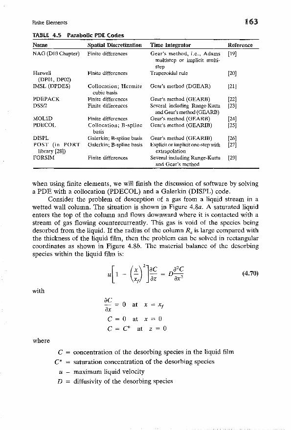
Table 4.5 lists the parabolic PDE software and outlines the type of spatialdiscretization and time integration for each code. Notice that each of the majorlibraries-NAG, Harwell, and IMSL-eontain PDE software. As is evident fromTable 4.5, the overwhelming choice of the time integrator is the Gear method.This method allows for stiff and nonstiff equations and has proven reliable overrecent years (see users guides to GEAR [16], GEARB [17], and LSODE [14]).Since we have covered the MOL using finite differences in greater detail than
Finite Elements
TABLE 4.5 Parabolic POE Codes
163
Name
NAG (D03 Chapter)
Harwell(DP01, DP02)
IMSL (DPDES)
PDEPACKDSS/2
MOLlOPDECOL
DISPLPOST (in PORT
library [28])FORSIM
Spatial Discretization
Finite differences
Finite differences
Collocation; Hermitecubic basis
Finite differencesFinite differences
Finite differencesCollocation; B-spline
basisGalerkin; B-spline basisGalerkin; B-spline basis
Finite differences
Time Integrator
Gear's method, i.e., Adamsmultistep or implicit multistep
Trapezoidal rule
Gear's method (DGEAR)
Gear's method (GEARB)Several including Runge-Kutta
and Gear's method (GEARB)Gear's method (GEARB)Gear's method (GEARIB)
Gear's method (GEARIB)Explicit or implicit one-step with
extrapolationSeveral including Runge-Kutta
and Gear's method
Reference
[19]
[20]
[21]
[22][23]
[24][25]
[26][27]
[29]
when using finite elements, we will finish the discussion of software by solvinga PDE with a collocation (PDECOL) and a Galerkin (DISPL) code.
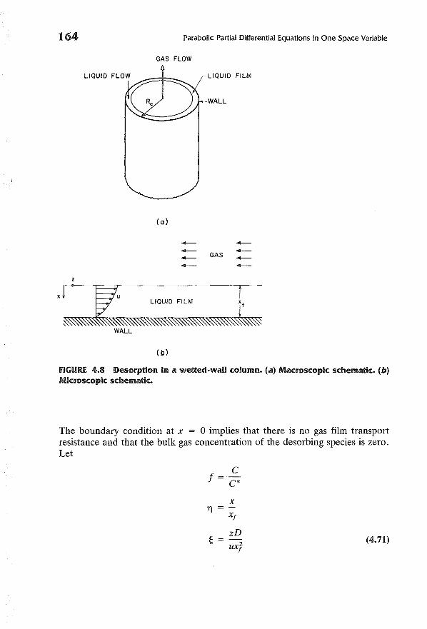
Consider the problem of desorption of a gas from a liquid stream in awetted wall column. The situation is shown in Figure 4.8a. A saturated liquidenters the top of the column and flows downward where it is contacted with astream of gas flowing countercurrently. This gas is void of the species beingdesorbed from the liquid. If the radius of the column Rc is large compared withthe thickness of the liquid film, then the problem can be solved in rectangularcoordinates as shown in Figure 4.8b. The material balance of the desorbingspecies within the liquid film is:
U[l (~r]~~a2c
(4.70)D-ax2
with
ac0 at x = xfax
C=O at x = 0
C = C* at z = 0
where
c = concentration of the desorbing species in the liquid film
C* saturation concentration of the desorbing species
U = maximum liquid velocity
D diffusivity of the desorbing species
164 Parabolic Partial Differential Equations in One Space Variable
GAS FLOW
(0)
LIQUID FILM
WALL
z
~
~
~-- GAS
~-~~
.~~~Xf
WALL
(b)
fiGURE. 4.8 Desorption in a wetted-wall column. (<1) Macroscopic schematic. (11)Microscopic schematic.
The boundary condition at x = 0 implies that there is no gas film transportresistance and that the bulk gas concentration of the desorbing species is zero.Let
cf =·c*
xT] =
xf
~zD
(4.71)-ux2
f
Mathematical Software
Substituting (4.71) into (4.70) gives:
(1 _ 1)2) af = a2f
a~ a1)2
af = 0 at 1) = 1a1)
f = 0 at 1) = 0
f = 1 at z = 0
165
(4.72)
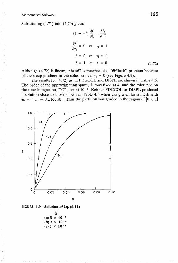
Although (4.72) is linear, it is still somewhat of a "difficult" problem becauseof the steep gradient in the solution near 1) = 0 (see Figure 4.9).
The results for (4.72) using PDECOL and DISPL are shown in Table 4.6.The order of the approximating space, k, was fixed at 4, and the tolerance onthe time integration, TOL, set at 10- 6 • Neither PDECOL or DISPL produceda solution close to those shown in Table 4.6 when using a uniform mesh with1); - 1);-1 = 0.1 for all i. Thus the partition was graded in the region of [0,0.1]
1.0 .------,--~-__,_--__r-=-___,r__-__,
0.8
0.6
f
0.4
0.2
0.02 0.04 0.06 0.08 0.10
fiGURE 4.9 Solution of Eq. (4.72)
~(a) 5 x 10⁻⁵
(b) 3 x 10⁻⁴
(c) 1 X 10⁻³
166 Parabolic Partial Differential Equations in One Space Variable
TABLE 4.6 Results of (q. (4.72)1] = 0.01, k = 4, TOt = (-6)
PDECOL DISPL
5( -5) 0.6827 0.68283( -4) 0.3169 0.31681( - 3) 0.1768 0.1769'ITI: 0 = 'TJI < 'TJ2 < 'TJII = 0.1
0.1 = 'TJII < 'TJ12 < < 'TJ20 = 1.0'IT2: 0 = 'TJI < 'TJ2 < < 'TJ21 = 0.1
0.1 = 'TJ21 < 'TJ22 < 'TJ30 = 1.0
0.68390.31690.1769'TJi - 'TJi-1 = 0.01'TJi - 'TJi-1 = 0.1'TJi - 'TJi-l = 0.005'TJi - 'TJi-1 = 0.1
0.68280.31680.1769
as specified by 'lT1 and 'lTz in Table 4.6. Further mesh refinements in the regionof [0, 0.1] did not cause the solutions to differ from those shown for 'lTz. Fromthese results, one can see that PDECOL and DISPL produced the same solutions. This is an expected result since both codes used the same approximatingspace, and the same tolerance for the time integration.
The parameter of engineering significance in this problem is the Sherwoodnumber, Sh, which is defined as
where
Sh (4.73)
311
1 = 2: 0 (1 - 1]Z)f dTf (4.74)
Table 4.7 shows the Sherwood numbers for various ~ (calculated from the solutions of PDECOL using 'lTz). Also, from this table, one can see that the resultscompare well with those published elsewhere [30].
TABLE 4.7 further Results oHq. (4.72)
~ Sh* Sh (PDECOL)
5( -5) 80.75 80.731( -4) 57.39 57.383( -4) 33.56 33.555( -4) 26.22 26.228( -4) 20.95 20.941( - 3) 18.85 18.84
* From Chapter 7 of [30].
Mathematical Software
PROBLEMS
167
1. A diffusion-convection problem can be described by the following PDE:
as a2 s as'11.- 0< x < 1, t> °at ax2 ax'
with
S(O, t) = 1,
as- (1, t) = 0,ax
sex, 0) = 0,
t> °t> °O<x<l
where A = constant.(a) Discretize the space variable, x, using Galerkin's method with the
Hermite cubic basis and set up the MOL-IVP.
(b) Solve the IVP generated in (a) with A = 25.
Physically, the problem can represent fluid, heat, or mass flow in whichan initially discontinuous profile is propagated by diffusion and convection,the latter with a speed of A.
2. Given the diffusion-convection equation in Problem 1:
(a) Discretize the space variable, x, using collocation with the Hermitecubic basis and set up the MOL-IVP.
(b) Solve the IVP generated in (a) with A = 25.
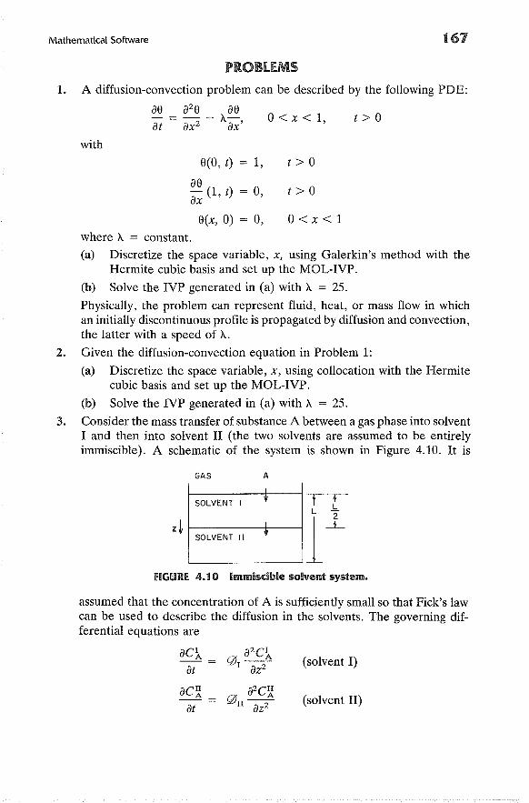
3. Consider the mass transfer of substance A between a gas phase into solventI and then into solvent II (the two solvents are assumed to be entirelyimmiscible). A schematic of the system is shown in Figure 4.10. It is
GAS A
SOLVENT I' t +
zt L *----J1L
1~OLVENT II •
fiGURE 4.10 Immiscible solvent system.
assumed that the concentration of A is sufficiently small so that Fick's lawcan be used to describe the diffusion in the solvents. The governing differential equations are
ac~ a2c~(solvent I)0-at I az2
ac~ = a2c~(solvent II)0 n -
2-at az
168 Parabolic Partial Differential Equations in One Space Variable
where
e~ = concentration of A in region i (moles/cm3)
o i = diffusion coefficient in region i (cmz/s)
t = time (s)
with
e~ = e~ = 0 at t = 0
ae~-- = 0 at z = Laz
ae~0 u -z- ataz
Lz=-
2
e~ = e~ at z = L/2 (distribution coefficient = 1)
P = HeI at z = 0 (pA = partial pres.sure of A in)A A the gas phase; H IS a constant
Compute the concentration profile of A in the liquid phase from t = 0to steady state when PA = 1 atm and H = 104 atm/(moles'cm3), forDr/Du = 1.0.
4. Compute the concentration profile of A in the liquid phase (from Problem3) using DI/Du = 10.0 and DI/Du = 0.1. Compare these profiles to thecase where DI/Du = 1.0.
5*. Diffusion and adsorption in an idealized pore can be represented by thePDEs:
ac aZc- = D-z - [ka (1 - f)c - kdfJ, 0< x < 1, t> 0at ax
~ f3[ka (1 - f)c - kdfJat
with
c(O, t) = 1, t> 0
ac- (1, t) = 0, t> 0ax
c(x, 0) = f(x, 0) = 0 0<x<1
Problems
where
169
c = dimensionless concentration of adsorbate in the fluid within thepore
f = fraction of the pore covered by the adsorbate
x = dimensionless spatial coordinate
ka = rate constant for adsorption
k d = rate constant for desorption
D, f3 = constants
Let D = f3 = ka = 1 and solve the above problem with ka/kd = 0.1, 1.0,and 10.0. From these results, discuss the effect of the relative rate ofadsorption versus desorption.
6*. The time-dependent material and energy balances for a spherical catalystpellet can be written as (notation is the same as was used in the sectionFinite Differences-High-Order Time Approximations):
- <\>29(
with
where
ay = ae = ° at x = °ax axy = e = 1 at x = 1
y = 0, e = 1 at 'T = 0, for all x
(first order)
Let <\> = 1.0, f3 = 0.04, 'Y = 18, and solve this problem using:
(a) Le = 10
(b) Le = 1
(c) Le = 0.1
Discuss the physical significance of each solution.
170 Parabolic Partial Differential Equations in One Space Variable
7*. Froment [31] developed a two-dimensional model for a fixed-bed reactorwhere the highly exothermic reactions
k 1 k2
o-xylene--p.~phthalic anhydride - CO2 , CO, H20(A) "'" (B) (C)
k3 ~CO2 , CO, H20
(C)
were occurring on a vanadium catalyst. The steady-state material andenergy balances are:
aXI = Pe [a2XI + ! aXI]
az ar2 r ar
aX2 = Pe [a2X2 + ! aX2]
az ar2 r ar
ae = Bo [a2e + ! ae]
az ar2 r ar
with
0< r < 1, O<z<l
O<z<l
Xl = X2 = 0 and e = eo at z = 0,
aXI aX2 ae- = - = - = 0 at r = 0,ar ar ar
O<r<l
aXI = aX2 = 0ar ar
where
d ae B' ( )an - = 1 e - ew at r= 1,ar O<z<l
Xl = fractional conversion to B
X2 = fractional conversion to C
e = dimensionless temperature
z = dimensionless axial coordinate
r = dimensionless radial coordinate
R I = k l (l - Xl - x2) - k 2x I
R2 = k2xI + k3(1 - Xl - X2)Pe, Bo = constants
13i = constants, i = 1, 2, 3
Bi = Biot number
ew = dimensionless wall temperature
Problems 171
Froment gives the data required to specify this system of PDEs, and oneset of his data is given in Chapter 8 of [30] as:
where
Pe = 5.76,
131 = 5.106,
Bo = 10.97,
I3z = 3.144,
Bi = 2.5
133 = 11.16
with
i = 1,2,3
a1 = -1.74,
"'11 = 21.6,
a z = -4.24,
"'Iz = 25.1,
a3 = -3.89
"13 = 22.9
Let ew = eo = 1 and solve the reactor equations with:
(a) al = -1.74
(b) a1 = - 0.87
(c) a1 = - 3.48
Comment on the physical implications of your results.
8*. The simulation of transport with chemical reaction in the stratospherepresents interesting problems, since certain reactions are photochemical,i.e., they require sunlight to proceed. In the following problem let C1
denote the concentration of ozone, 03' Cz denote the concentration ofoxygen singlet, 0, and C3 denote the concentration of oxygen, Oz (assumedto be constant). If z specifies the altitude in kilometers, and a Fickianmodel of turbulent eddy diffusion (neglecting convection) is used to describe the transport of chemical species, then the continuity equations ofthe given species are
aC1 = ~[K ac1] + R 30 < z < 50, 0< t
at az az 1,
acz = ~ [K acz] + Rzat az az
with
aC1 (30, t) = acz (30, t) = 0, t > °az az
aC1 (50, t) = acz (50, t) = 0, t > °az az
C1(z, 0) = 106"'1(z) , 30 ~ z ~ 50
Cz(z, 0) = 101z"'l(z), 30 ~ z ~ 50
112 Parabolic Partial Differential Equations in One Space Variable
where
K =exp [~]R 1 = - k 1C1C3 - k ZC1Cz + 2k3(t)C3 + kit)Cz
Rz =k1C1C3 - k ZC1CZ - kit)Cz
C3 =3.7 x 10¹⁶
k1 =1.63 X 10- 16
k z =4.66 X 10- 16
klt) = { exp [Sin-(~t)l for sin (wt) > 0, i = 3,4
0, for sin (wt) ~ 0,
V3 =22.62
V4 =7.601
1T
W = 43,200
[ ]z [ ]4Z - 40 1 z - 40
-y(z) = 1 - 10 + 2 10
Notice that the reaction constants k3(t) and k4(t) build up to a peak atnoon (t = 21,600) and are switched off from sunset (t = 43,200) to sunrise(t = 86,400). Thus, these reactions model the diurnal effect. Calculate theconcentration of ozone for a 24-h time period, and compare your resultswith those given in [26].
REfERENCES
1. Liskovets, O. A., "The Method of Lines," J. Diff. Eqs., 1, 1308 (1965).
2. Mitchell, A. R., andD. F. Griffiths, The Finite Difference Method in PartialDifferential Equations, Wiley, Chichester (1980).
3. Wilkes, J. 0., "In Defense of the Crank-Nicolson Method," A.I.Ch.E.J., 16, 501 (1970).
4. Douglas, J., Jr., and B. F. Jones, "On Predictor-Corrector Method forNonlinear Parabolic Differential Equations," J. Soc. Ind. Appl. Math.,11, 195 (1963).
Problems 173
5. Lees, M., "An Extrapolated Crank-Nicolson Difference Scheme for QuasiLinear Parabolic Equations," in Nonlinear Partial Differential Equations,W. F. Ames (ed.), Academic, New York (1967).
6. Davis, M. E., "Analysis of an Annular Bed Reactor for the Methanationof Carbon Oxides," Ph.D. Thesis, Univ. of Kentucky, Lexington (1981).
7. Davis, M. E., G. Fairweather and J. Yamanis, "Annular Bed ReactorMethanation of Carbon Dioxide," Can. J. Chern. Eng., 59, 497 (1981).
8. Sepehrnoori, K., and G. F. Carey, "Numerical Integration of SemidiscreteEvolution Systems," Comput. Methods Appl. Mech. Eng., 27, 45 (1981).
9. Shampine, L. F., and M. K. Gordon, Computer Solution of OrdinaryDifferential Equations: The Initial Value Problem, Freeman, San Francisco(1975).
10. International Mathematics and Statistics Libraries Inc., Sixth Floor-NBCBuilding, 7500 Bellaire Boulevard, Houston, Tex.
11. Verwer, J. G., "Algorithm 553-M3RK, An Explicit Time Integrator forSemidiscrete Parabolic Equations," ACM TOMS, 6, 236 (1980).
12. Skeel, R. D., and A. K. Kong, "Blended Linear Multistep Methods,"ACM TOMS. Math. Software, 3, 326 (1977).
13. Kehoe, J. P. C., and J. B. Butt, "Kinetics of Benzene Hydrogenation bySupported Nickel at Low Temperature," J. Appl. Chern. Biotechnol., 22,23 (1972).
14. Hindmarsh, A. c., "LSODE and LSODI, Two New Initial Value OrdinaryDifferential Equation Solvers," ACM SIGNUM Newsletter, December(1980).
15. Kehoe, J. P. c., and J. B. Butt, "Transient Response and Stability of aDiffusionally Limited Exothermic Catalytic Reaction," 5th InternationalReaction Engineering Symposium, Amsterdam (1972).
16. Hindmarsh, A. C., "GEARIB: Solution of Implicit Systems of OrdinaryDifferential Equations with Banded Jacobian," Lawrence Livermore Laboratory Report UCID-30103 (1976).
17. Hindmarsh, A. c., "GEAR: Ordinary Differential Equation System Solver,"Lawrence Livermore Laboratory Report UCID-30001 (1974).
18. Hindmarsh, A. C., "GEARB: Solution of Ordinary Differential EquationsHaving Banded Jacobians," Lawrence Livermore Laboratory Report UCID30059 (1975).
19. Dew, P. M., and Walsh, J. E., "A Set of Library Routines for SolvingParabolic Equations in One Space Variables," ACM TOMS, 7, 295 (1981).
20. Harwell Subroutine Libraries, Computer Science and Systems Division ofthe United Kingdom Atomic Energy Authority, Harwell, England.
21. Sewell, G., "IMSL Software for Differential Equations in One SpaceVariable," IMSL Tech. Report No. 8202 (1982).
174 Parabolic Partial Differential Equations in One Space Variable
22. Sincovec, R. F., and N. K. Madsen, "PDEPACK: Partial DifferentialEquations Package Users Guide," Scientific Computing Consulting Services, Colorado Springs, Colo. (1981).
23. Schiesser, W., "DDS/2-An Introduction to the Numerical Method ofLines Integration of Partial Differential Equations," Lehigh Univ., Bethlehem, Pa. (1976).
24. Hyman, J. M., "MOLID: A General-Purpose Subroutine Package for theNumerical Solution of Partial Differential Equations," Los Alamos Scientific Laboratory Report LA-7595-M, March (1979).
25. Madsen, N. K., and R. F. Sincovec, "PDECOL, General CollocationSoftware for Partial Differential Equations," ACM TOMS, 5, 326 (1979).
26. Leaf, G. K., M. Minkoff, G. D. Byrne, D. Sorensen, T. Blecknew, andJ. Saltzman, "DISP: A Software Package for One and Two Spatially Dimensioned Kinetics-Diffusion Problems," Report ANL-77-12, ArgonneNational Laboratory, Argonne, Ill. (1977).
27. Schryer, N. L., "Numerical Solution of Time-Varying Partial DifferentialEquations in One Space Variable," Computer Science Tech. Report 53,Bell Laboratories, Murray Hill, N.J. (1977).
28. Fox, P. A., A. D. Hall, and N. L. Schryer, "The PORT MathematicalSubroutine Library," ACM TOMS, 4, 104 (1978).
29. Carver, M., "The FORSIM VI Simulation Package for the AutomaticSolution of Arbitrarily Defined Partial Differential and/or Ordinary Differential Equation Systems," Rep. AECL-5821, Chalk River Nuclear Laboratories, Ontario, Canada (1978).
30. Villadsen, J., and M. L. Michelsen, Solution of Differential Equation Modelsby Polynomial Approximation, Prentice-Hall, Englewood Cliffs, N.J. (1978).
31. Froment, G. F., "Fixed Bed Catalytic Reactors," Ind. Eng. Chern., 59,18 (1967).
BIBLIOGRAPHY
An overview offinite diffrence and finite element methods for parabolic partial differentialequations in time and one space dimension has been given in this chapter. For additionalor more detailed information, see the following texts:
Finite Difference
Ames, W. F., Nonlinear Partial Differential Equations in Engineering, Academic, NewYork (1965).
Ames, W. F., ed., Nonlinear Partial Differential Equations, Academic, New York (1967).
Problems 175
Ames, W. F., Numerical Methods for Partial Differential Equations, 2nd ed., Academic,New York (1977).
Finlayson, B. A., Nonlinear Analysis in Chemical Engineering, McGraw-Hill, New York(1980).
Forsythe, G. E., and W. R. Wason, Finite Difference Methods for Partial DifferentialEquations, Wiley, New York (1960).
Issacson, 1., and H. B. Keller, Analysis ofNumerical Methods, Wiley, New York (1966).
Mitchell, A. R., and D. F. Griffiths, The Finite Difference Method in Partial DifferentialEquations, Wiley, Chichester (1980).
finite Element
Becker, E. B., G. F. Carey, and J. T. Oden, Finite Elements: An Introduction, PrenticeHall, Englewood Cliffs, N.J. (1981).
Fairweather, G., Finite Element Galerkin Methods for Differential Equations, MarcelDekker, New York (1978).
Mitchell, A. R., and D. F. Griffiths, The Finite Difference Method in Partial DifferentialEquations, Wiley, Chichester (1980). Chapter 5 discusses the Galerkin method.
Mitchell, A. R., and R. Wait, The Finite Element Method in Partial Differential Equations,Wiley, New York (1977).
Strang, G., and G. J. Fix, An Analysis of the Finite Element Method, Prentice-Hall,Englewood Cliffs, N.J. (1973).


![[aiesec] [ivp] proposal](https://img.pdfslide.net/doc/110x75/568c0eea1a28ab955a923c70/aiesec-ivp-proposal.jpg)