1

2014-01-21

Minyi Zhong minyi.zhong@uni-jena.de Moritz Eßlinger moritz.esslinger@uni-jena.de Herbert Gross herbert.gross@uni-jena.de Friedrich Schiller University Jena Institute of Applied Physics Albert-Einstein-Str. 15 07745 Jena

Examples Practiced in Lectures

Advanced Optical Design

Contents 1 Introduction (none) ................................................................................................................................ 2

2 Optimization I ......................................................................................................................................... 2

2.1 System layout with ideal lenses ..................................................................................................... 2

2.2 Delano Diagram ............................................................................................................................. 3

2.3 Insertion of Finite Lens Thickness ................................................................................................. 6

3 Optimization II ........................................................................................................................................ 9

3.1 Influence of initial system .............................................................................................................. 9

3.2 Influence of criteria selection ....................................................................................................... 11

4 Optimization III ..................................................................................................................................... 13

4.1 Achromate ................................................................................................................................... 13

4.2 Mirror constrained beam shaping ................................................................................................ 17

5 Structural modifications ....................................................................................................................... 21

5.1 Adding a lens ............................................................................................................................... 21

5.2 Removing a lens .......................................................................................................................... 23

6 Aberrations and Performance (none) .................................................................................................. 27

7 Aspheres and Freeforms ..................................................................................................................... 27

7.1 Forbes Aspheres ......................................................................................................................... 27

7.2 Aspherical cylindrical lens ........................................................................................................... 29

7.3 Aspherical Singlet ........................................................................................................................ 32

8 Field flattening ..................................................................................................................................... 34

8.1 Field lens flattener ....................................................................................................................... 34

8.2 Pair of thick meniscus lenses ...................................................................................................... 40

9 Chromatic correction ........................................................................................................................... 43

9.1 Apochromate ............................................................................................................................... 43

9.2 Correction with Burried Surface ................................................................................................... 47

10 Special Topics ................................................................................................................................. 52

10.1 Skew spherical aberration ........................................................................................................... 52

2

10.2 Endoscope system ...................................................................................................................... 54

11 Higher order aberration ................................................................................................................... 58

11.1 High-NA Collimator ...................................................................................................................... 58

11.2 Induced aberrations ..................................................................................................................... 63

12 Advanced optimization strategies .................................................................................................... 64

12.1 Optimization of Insensitivity ......................................................................................................... 64

12.2 Global Optimization ..................................................................................................................... 69

13 Mirror systems ................................................................................................................................. 74

13.1 Astigmatism of oblique curved Mirrors ........................................................................................ 74

13.2 Cassegrain telescope .................................................................................................................. 79

1.1 Hybrid DOE .................................................................................................................................. 82

1.2 Correction with diffractive lens ..................................................................................................... 88

1.3 Tolerance sensitivity .................................................................................................................... 91

1.4 Tolerancing a splitted achromate ................................................................................................ 94

1 Introduction (none)

2 Optimization I

2.1 System layout with ideal lenses

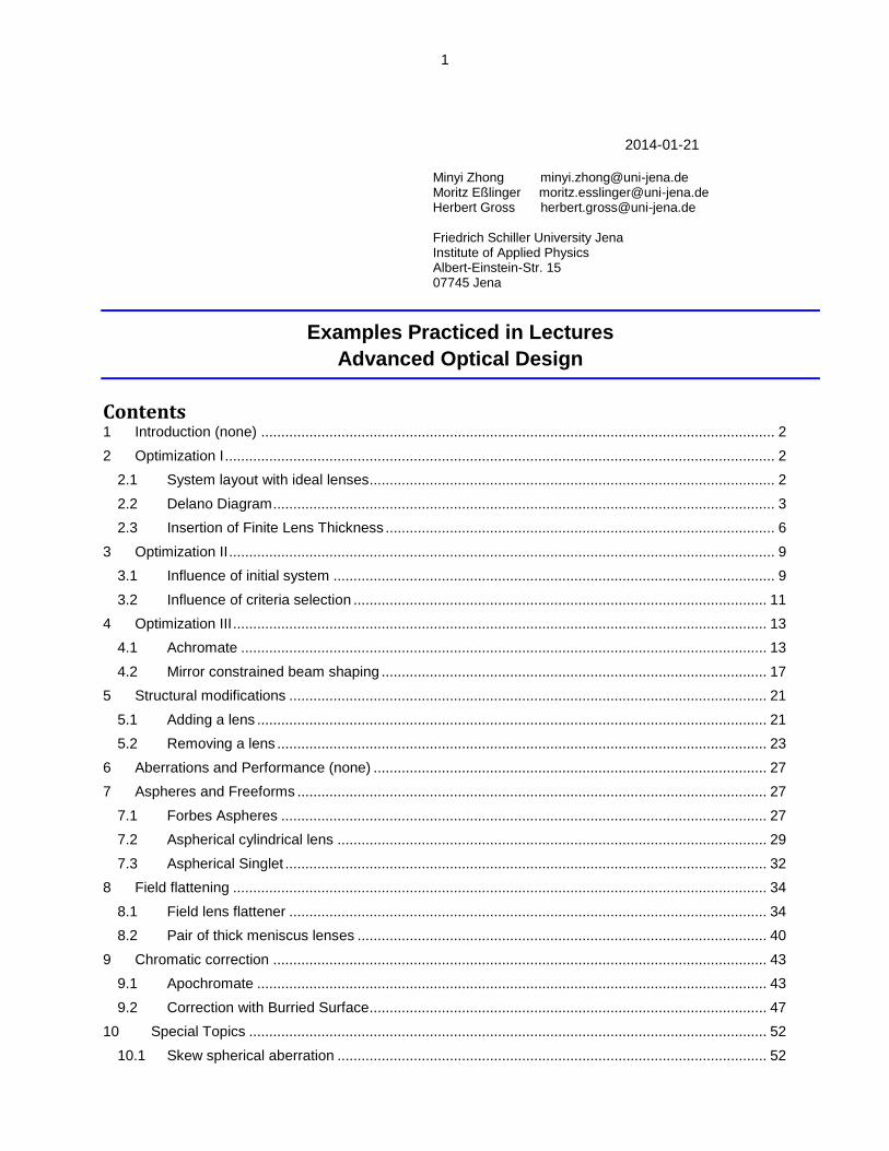
A collimated laser beam with wavelength 1.064 m and diameter D = 2 mm should be expanded by a Kepler-type afocal telescope made of ideal lenses with a first focallength f1 = 50 mm and a factor of 5. The enlarged collimated beam is then focussed down by a cylindrical lens with focal length f = 100 mm to get a line focus. a) Setup the system described above by ideal lenses b) Show the line focus graphically Solution: a)

3

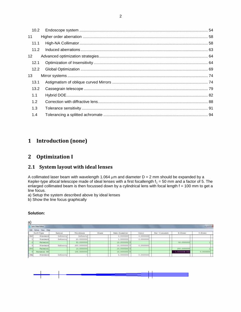
The ideal lens can also bemodelled as an ABCD-system. b) Spot diagram, more points, scale fixed, bad resolution A footprint is an alternative option.

It has to be noted, that the footprint only gives the line pattern, if the diameter of the final image plane is fixed to the corresponding finite vaue, e.g. 10 mm. Due to the perfect system property, otherwise the diameter in the image plane are near to zero.

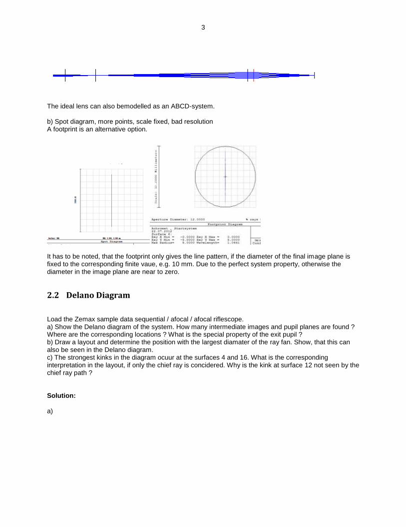
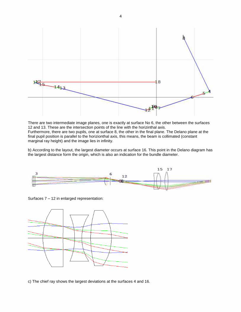
2.2 Delano Diagram Load the Zemax sample data sequential / afocal / afocal riflescope. a) Show the Delano diagram of the system. How many intermediate images and pupil planes are found ? Where are the corresponding locations ? What is the special property of the exit pupil ? b) Draw a layout and determine the position with the largest diamater of the ray fan. Show, that this can also be seen in the Delano diagram. c) The strongest kinks in the diagram ocuur at the surfaces 4 and 16. What is the corresponding interpretation in the layout, if only the chief ray is concidered. Why is the kink at surface 12 not seen by the chief ray path ? Solution: a)

4

There are two intermediate image planes, one is exactly at surface No 6, the other between the surfaces 12 and 13. These are the intersection points of the line with the horizinthal axis. Furthermore, there are two pupils, one at surface 8, the other in the final plane. The Delano plane at the final pupil position is parallel to the horizionthal axis, this means, the beam is collimated (constant marginal ray height) and the image lies in infinity. b) According to the layout, the largest diameter occurs at surface 16. This point in the Delano diagram has the largest distance form the origin, which is also an indication for the bundle diameter.

Surfaces 7 – 12 in enlarged representation:

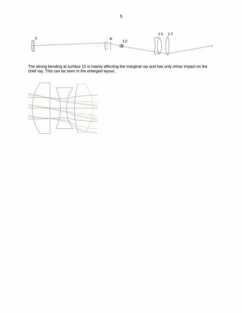
c) The chief ray shows the largest deviations at the surfaces 4 and 16.

5

The strong bending at surface 12 is mainly affecting the marginal ray and has only minar impact on the chief ray. This can be seen in the enlarged layout.

6

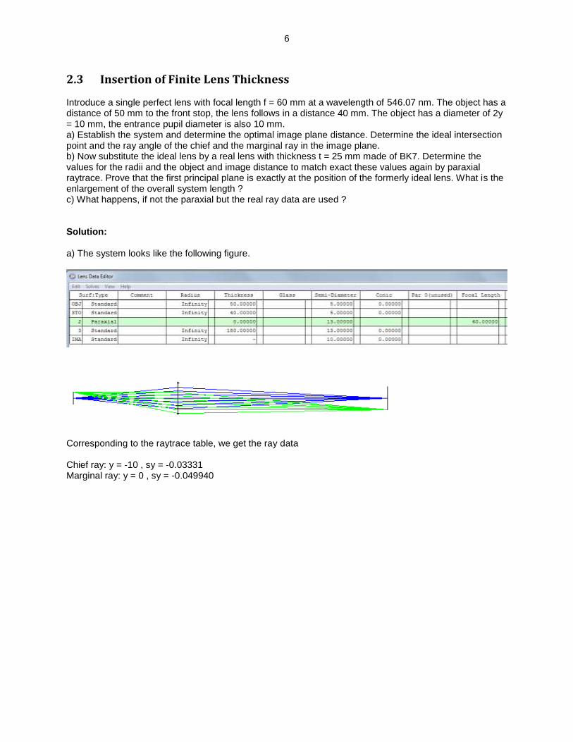
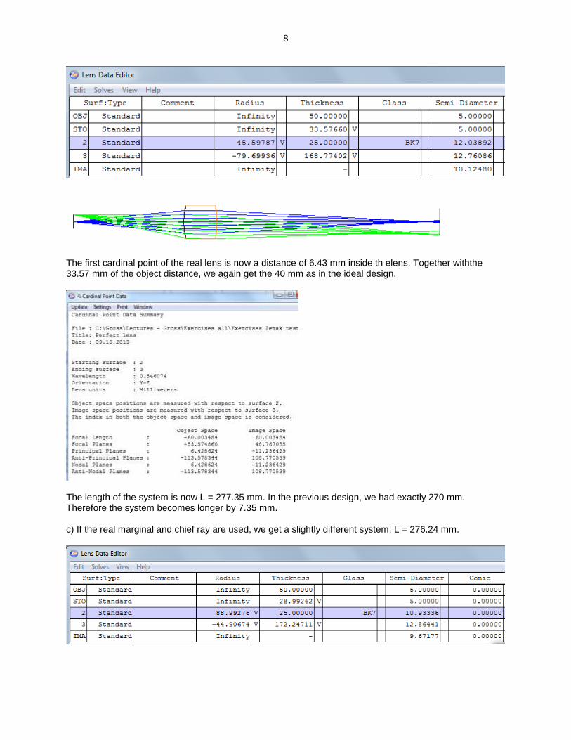
2.3 Insertion of Finite Lens Thickness Introduce a single perfect lens with focal length f = 60 mm at a wavelength of 546.07 nm. The object has a distance of 50 mm to the front stop, the lens follows in a distance 40 mm. The object has a diameter of 2y = 10 mm, the entrance pupil diameter is also 10 mm. a) Establish the system and determine the optimal image plane distance. Determine the ideal intersection point and the ray angle of the chief and the marginal ray in the image plane. b) Now substitute the ideal lens by a real lens with thickness t = 25 mm made of BK7. Determine the values for the radii and the object and image distance to match exact these values again by paraxial raytrace. Prove that the first principal plane is exactly at the position of the formerly ideal lens. What is the enlargement of the overall system length ? c) What happens, if not the paraxial but the real ray data are used ? Solution: a) The system looks like the following figure.

Corresponding to the raytrace table, we get the ray data Chief ray: y = -10 , sy = -0.03331 Marginal ray: y = 0 , sy = -0.049940

7

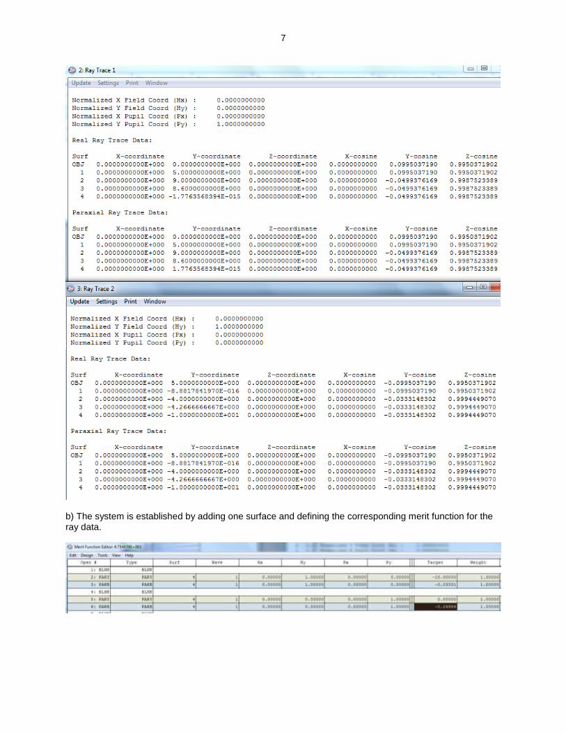
b) The system is established by adding one surface and defining the corresponding merit function for the ray data.

8

The first cardinal point of the real lens is now a distance of 6.43 mm inside th elens. Together withthe 33.57 mm of the object distance, we again get the 40 mm as in the ideal design.

The length of the system is now L = 277.35 mm. In the previous design, we had exactly 270 mm. Therefore the system becomes longer by 7.35 mm. c) If the real marginal and chief ray are used, we get a slightly different system: L = 276.24 mm.

9

The problem with this solution is, that now the residual aberrations aretaken into account and the solution is no longer perfect near to the axis.

3 Optimization II

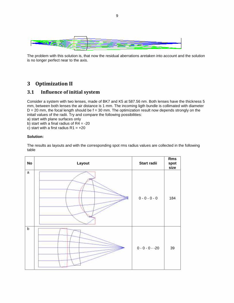
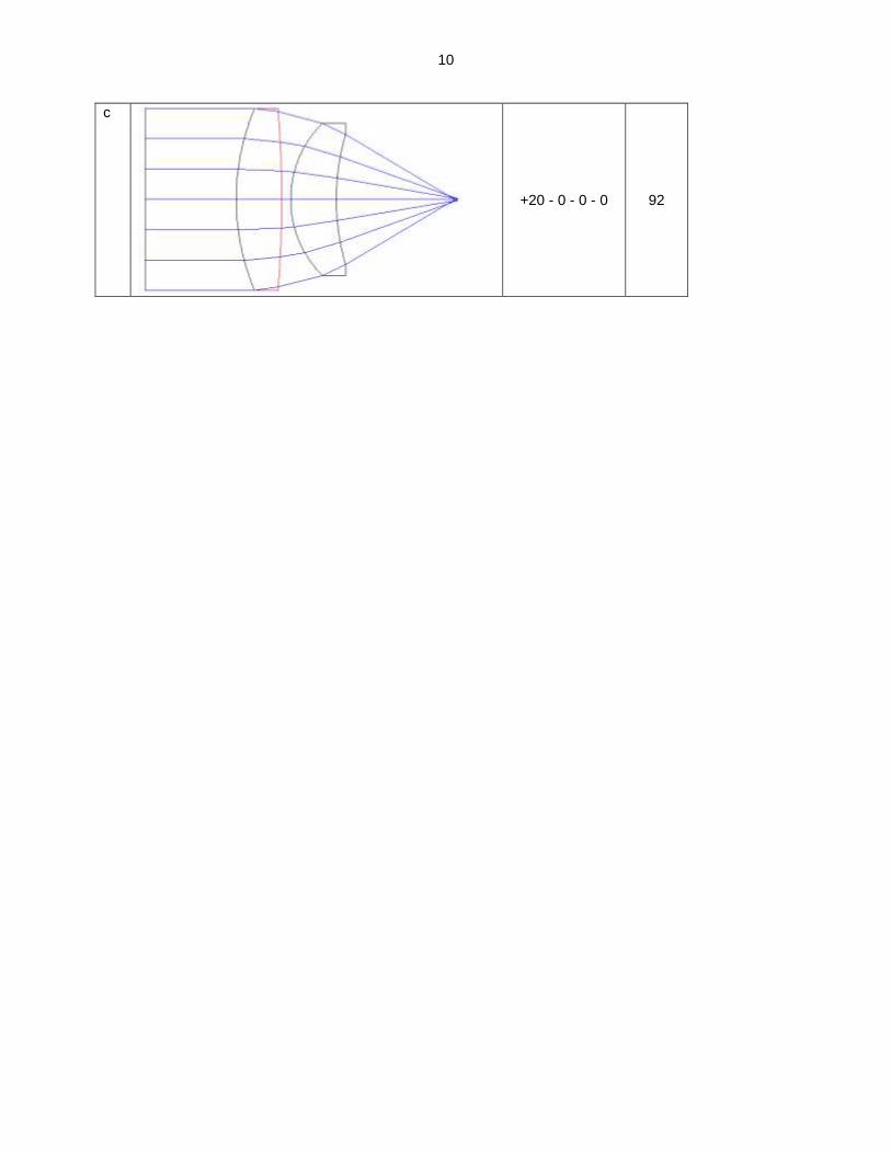
3.1 Influence of initial system Consider a system with two lenses, made of BK7 and K5 at 587.56 nm. Both lenses have the thickness 5 mm, between both lenses the air distance is 1 mm. The incoming ligth bundle is collimated with diameter D = 20 mm, the focal length should be f = 30 mm. The optimization result now depends strongly on the initail values of the radii. Try and compare the following possibilities: a) start with plane surfaces only b) start with a final radius of R4 = -20 c) start with a first radius R1 = +20 Solution: The results as layouts and with the corresponding spot rms radius values are collected in the following table

No Layout Start radii Rms spot size

a

0 - 0 - 0 - 0 184

b

0 - 0 - 0 - -20 39

10

c

+20 - 0 - 0 - 0 92

11

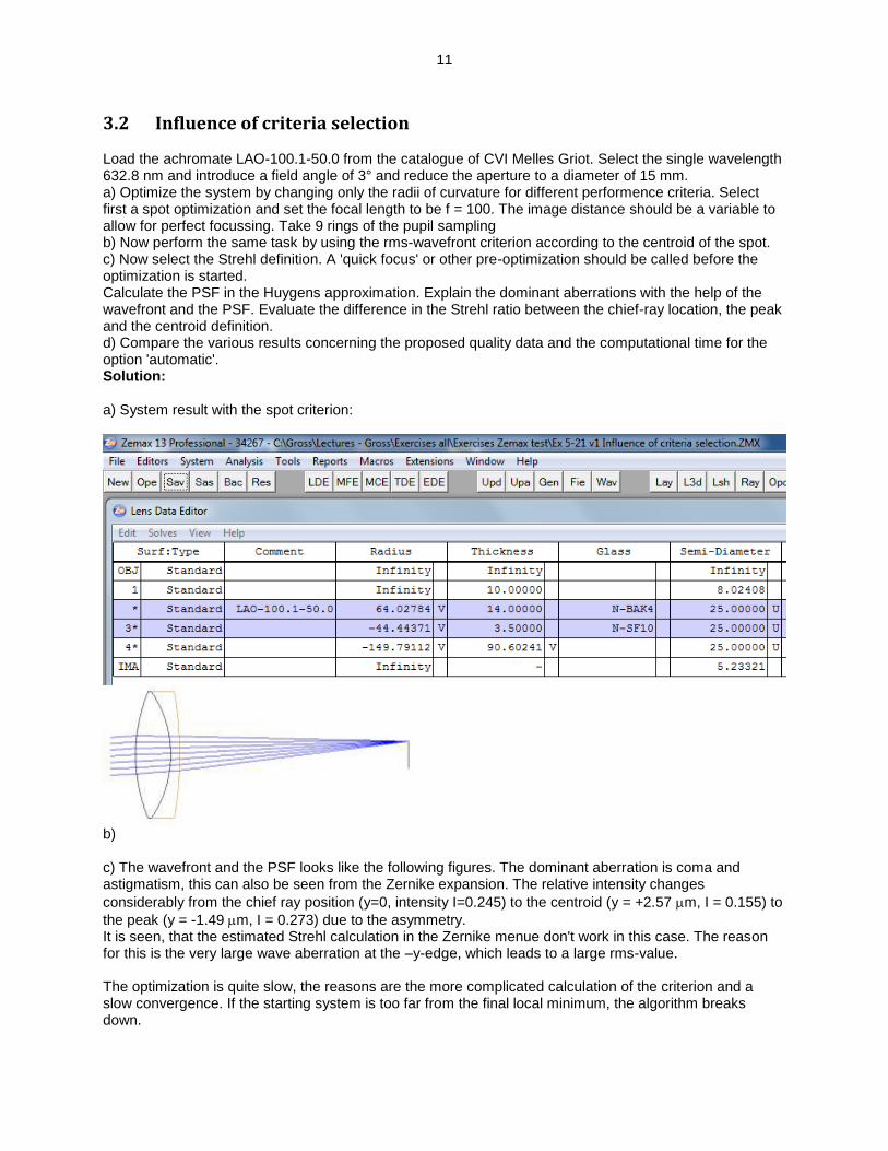
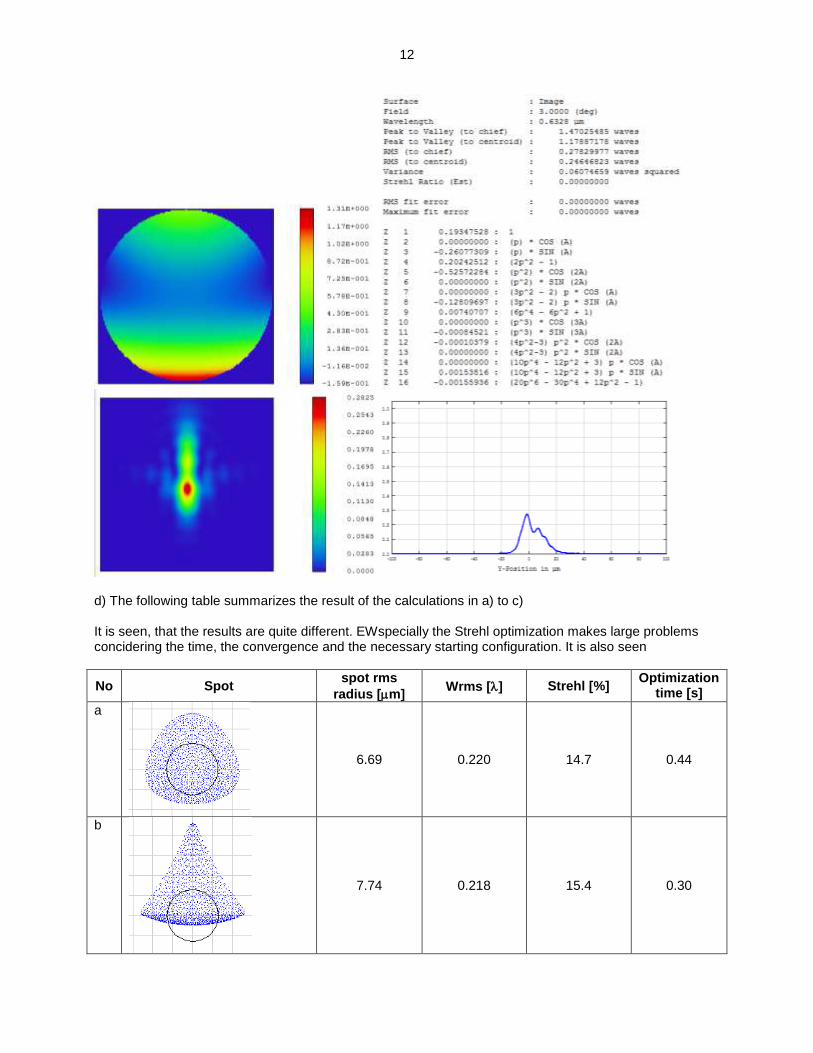
3.2 Influence of criteria selection Load the achromate LAO-100.1-50.0 from the catalogue of CVI Melles Griot. Select the single wavelength 632.8 nm and introduce a field angle of 3° and reduce the aperture to a diameter of 15 mm. a) Optimize the system by changing only the radii of curvature for different performence criteria. Select first a spot optimization and set the focal length to be f = 100. The image distance should be a variable to allow for perfect focussing. Take 9 rings of the pupil sampling b) Now perform the same task by using the rms-wavefront criterion according to the centroid of the spot. c) Now select the Strehl definition. A 'quick focus' or other pre-optimization should be called before the optimization is started. Calculate the PSF in the Huygens approximation. Explain the dominant aberrations with the help of the wavefront and the PSF. Evaluate the difference in the Strehl ratio between the chief-ray location, the peak and the centroid definition. d) Compare the various results concerning the proposed quality data and the computational time for the option 'automatic'. Solution: a) System result with the spot criterion:

b) c) The wavefront and the PSF looks like the following figures. The dominant aberration is coma and astigmatism, this can also be seen from the Zernike expansion. The relative intensity changes

considerably from the chief ray position (y=0, intensity I=0.245) to the centroid (y = +2.57 m, I = 0.155) to

the peak (y = -1.49 m, I = 0.273) due to the asymmetry. It is seen, that the estimated Strehl calculation in the Zernike menue don't work in this case. The reason for this is the very large wave aberration at the –y-edge, which leads to a large rms-value. The optimization is quite slow, the reasons are the more complicated calculation of the criterion and a slow convergence. If the starting system is too far from the final local minimum, the algorithm breaks down.

12

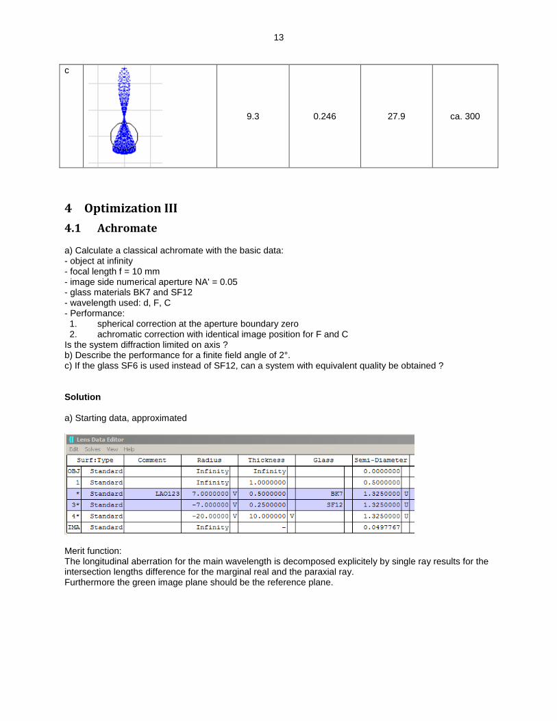
d) The following table summarizes the result of the calculations in a) to c) It is seen, that the results are quite different. EWspecially the Strehl optimization makes large problems concidering the time, the convergence and the necessary starting configuration. It is also seen

No Spot spot rms

radius [m] Wrms [] Strehl [%]

Optimization time [s]

a

6.69 0.220 14.7 0.44

b

7.74 0.218 15.4 0.30

13

c

9.3 0.246 27.9 ca. 300

4 Optimization III

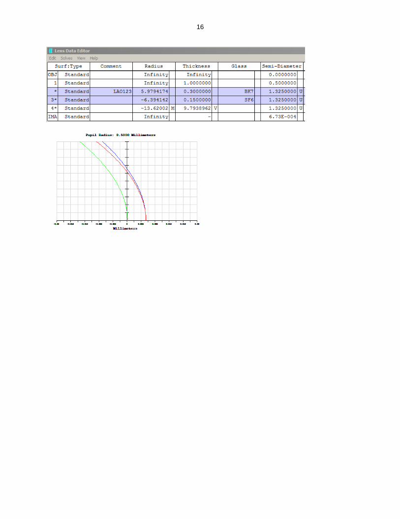
4.1 Achromate a) Calculate a classical achromate with the basic data: - object at infinity - focal length f = 10 mm - image side numerical aperture NA' = 0.05 - glass materials BK7 and SF12 - wavelength used: d, F, C - Performance: 1. spherical correction at the aperture boundary zero 2. achromatic correction with identical image position for F and C Is the system diffraction limited on axis ? b) Describe the performance for a finite field angle of 2°. c) If the glass SF6 is used instead of SF12, can a system with equivalent quality be obtained ? Solution a) Starting data, approximated

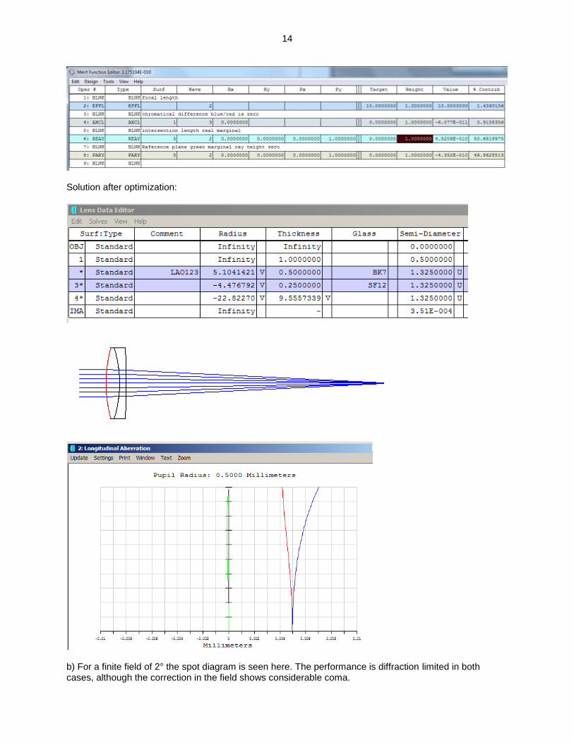
Merit function: The longitudinal aberration for the main wavelength is decomposed explicitely by single ray results for the intersection lengths difference for the marginal real and the paraxial ray. Furthermore the green image plane should be the reference plane.

14

Solution after optimization:

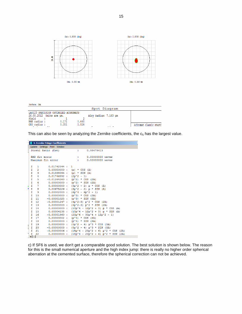
b) For a finite field of 2° the spot diagram is seen here. The performance is diffraction limited in both cases, although the correction in the field shows considerable coma.

15

This can also be seen by analyzing the Zernike coefficients, the c5 has the largest value.

c) If SF6 is used, we don't get a comparable good solution. The best solution is shown below. The reason for this is the small numerical aperture and the high index jump: there is really no higher order spherical aberration at the cemented surface, therefore the spherical correction can not be achieved.

16

17

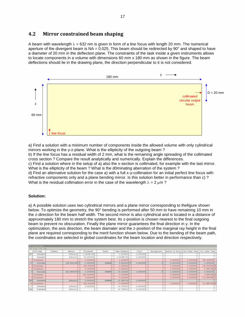
4.2 Mirror constrained beam shaping

A beam with wavelength = 632 nm is given in form of a line focus with length 20 mm. The numerical aperture of the divergent beam is NA = 0.025. This beam should be redirected by 90° and shaped to have a diameter of 20 mm in the deflection plane. The constraints of the task inside a given instruments allows to locate components in a volume with dimensions 60 mm x 180 mm as shown in the figure. The beam deflections should lie in the drawing plane, the direction perpendicular to it is not considered.

line focus

180 mm

60 mm

D = 20 mmcollimated

circular output

beam

y

z

a) Find a solution with a minimum number of components inside the allowed volume with only cylindrical mirrors working in the y-z-plane. What is the ellipticity of the outgoing beam ? b) If the line focus has a residual width of 2 mm, what is the remaining angle spreading of the collimated cross section ? Compare the result analytically and numerically. Explain the differences. c) Find a solution where in the setup of a) also the x-section is collimated, for example with the last mirror. What is the ellipticity of the beam ? What is the d0minating aberration of the system ? d) Find an alternative solution for the case a) with a full x-y-collimation for an initial perfect line focus with refractive components only and a plane bending mirror. Is this solution better in performance than c) ?

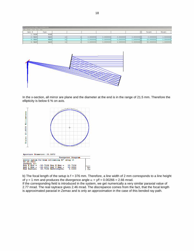
What is the residual collimation error in the case of the wavelength = 2 m ? Solution: a) A possible solution uses two cylindrical mirrors and a plane mirror corresponding to thefigure shown below. To optimize the geometry, the 90° bending is performed after 50 mm to have remaining 10 mm in the z-direction for the beam half width. The second mirror is also cylindrical and is located in a distance of approximately 180 mm to stretch the system best. Its z-position is chosen nearest to the final outgoing beam to prevent no obscuration. Finally the plane mirror guarantees the final direction in y. In the optimization, the axis direction, the beam diamater and the z-position of the marginal ray height in the final plane are required corresponding to the merit function shown below. Due to the bending of the beam path, the coordinates are selected in global coordinates for the beam location and direction respectively.

18

In the x-section, all mirror are plane and the diameter at the end is in the range of 21.5 mm. Therefore the ellipticity is below 6 % on axis.

b) The focal length of the setup is f = 376 mm. Therefore, a line width of 2 mm corresponds to a line height

of y = 1 mm and produces the divergence angle = y/f = 0.00266 = 2.66 mrad. If the corresponding field is introduced in the system, we get numerically a very similar paraxial value of 2.77 mrad. The real raytrace gives 2.46 mrad. The discrepance comes from the fact, that the focal length is approximated paraxial in Zemax and is only an approximation in the case of this bended ray path.

19

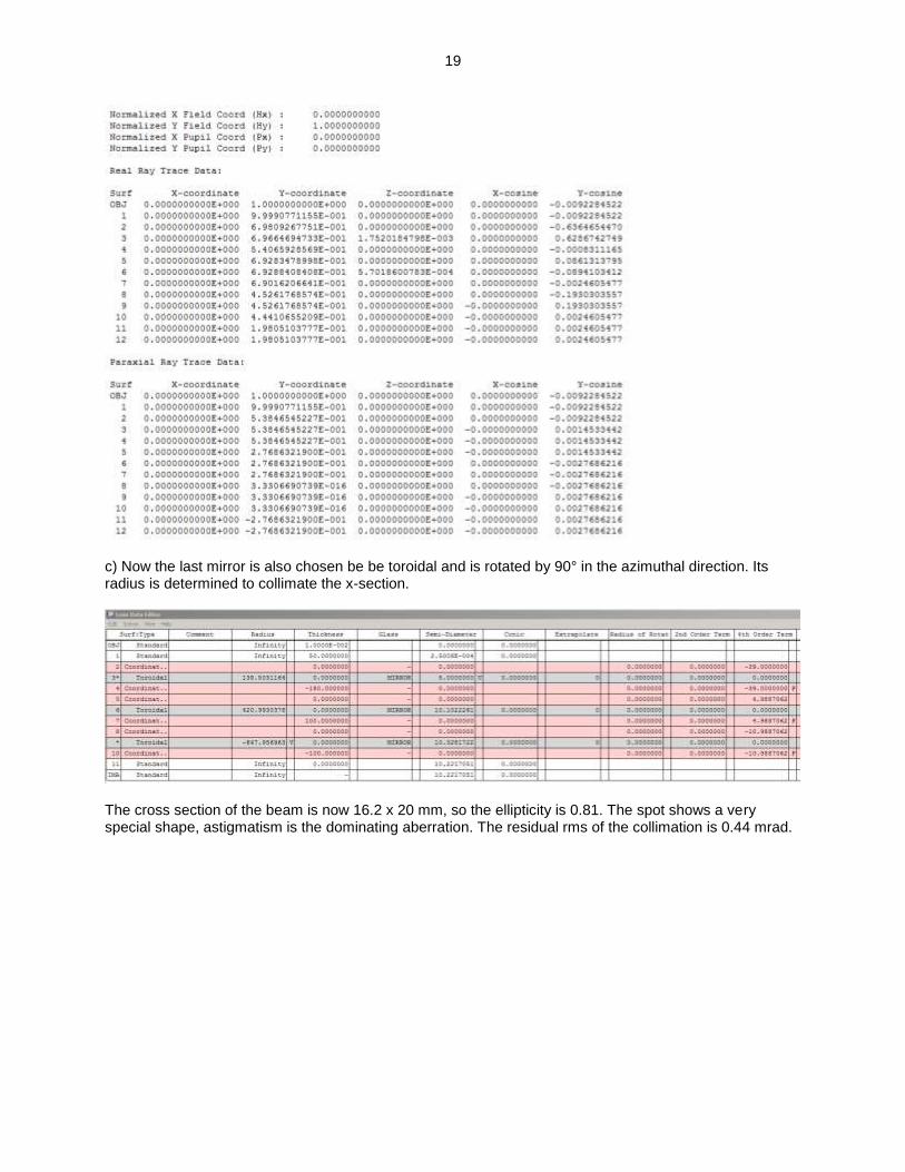
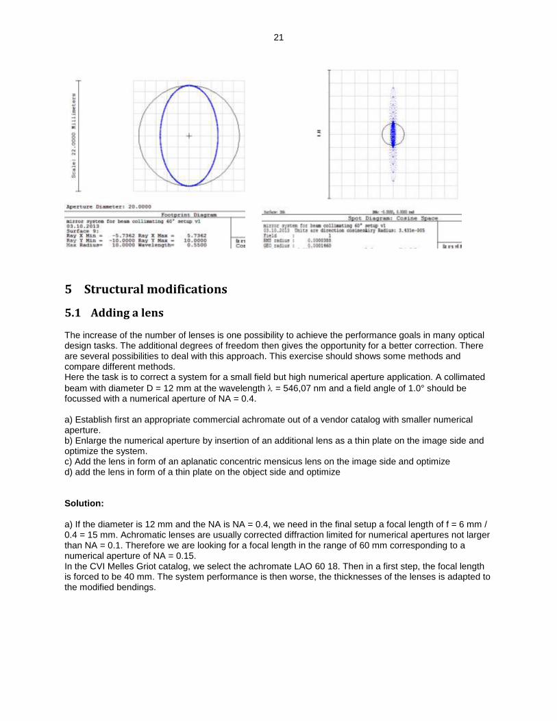
c) Now the last mirror is also chosen be be toroidal and is rotated by 90° in the azimuthal direction. Its radius is determined to collimate the x-section.

The cross section of the beam is now 16.2 x 20 mm, so the ellipticity is 0.81. The spot shows a very special shape, astigmatism is the dominating aberration. The residual rms of the collimation is 0.44 mrad.

20

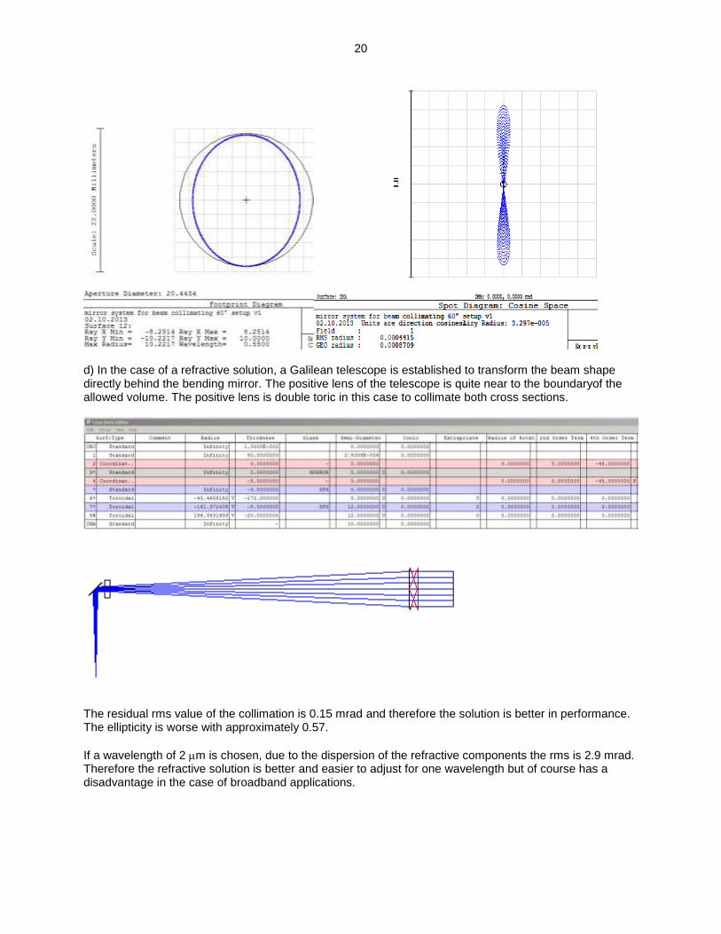
d) In the case of a refractive solution, a Galilean telescope is established to transform the beam shape directly behind the bending mirror. The positive lens of the telescope is quite near to the boundaryof the allowed volume. The positive lens is double toric in this case to collimate both cross sections.

The residual rms value of the collimation is 0.15 mrad and therefore the solution is better in performance. The ellipticity is worse with approximately 0.57.

If a wavelength of 2 m is chosen, due to the dispersion of the refractive components the rms is 2.9 mrad. Therefore the refractive solution is better and easier to adjust for one wavelength but of course has a disadvantage in the case of broadband applications.

21

5 Structural modifications

5.1 Adding a lens The increase of the number of lenses is one possibility to achieve the performance goals in many optical design tasks. The additional degrees of freedom then gives the opportunity for a better correction. There are several possibilities to deal with this approach. This exercise should shows some methods and compare different methods. Here the task is to correct a system for a small field but high numerical aperture application. A collimated

beam with diameter D = 12 mm at the wavelength = 546,07 nm and a field angle of 1.0° should be focussed with a numerical aperture of NA = 0.4. a) Establish first an appropriate commercial achromate out of a vendor catalog with smaller numerical aperture. b) Enlarge the numerical aperture by insertion of an additional lens as a thin plate on the image side and optimize the system. c) Add the lens in form of an aplanatic concentric mensicus lens on the image side and optimize d) add the lens in form of a thin plate on the object side and optimize Solution: a) If the diameter is 12 mm and the NA is NA = 0.4, we need in the final setup a focal length of f = 6 mm / 0.4 = 15 mm. Achromatic lenses are usually corrected diffraction limited for numerical apertures not larger than NA = 0.1. Therefore we are looking for a focal length in the range of 60 mm corresponding to a numerical aperture of NA = 0.15. In the CVI Melles Griot catalog, we select the achromate LAO 60 18. Then in a first step, the focal length is forced to be 40 mm. The system performance is then worse, the thicknesses of the lenses is adapted to the modified bendings.

22

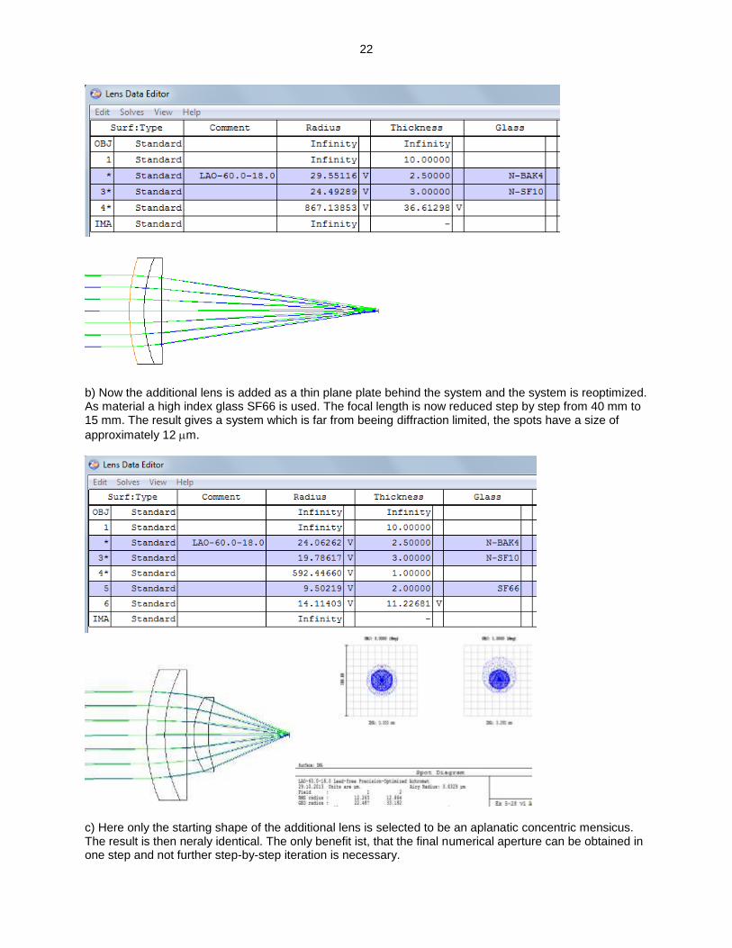
b) Now the additional lens is added as a thin plane plate behind the system and the system is reoptimized. As material a high index glass SF66 is used. The focal length is now reduced step by step from 40 mm to 15 mm. The result gives a system which is far from beeing diffraction limited, the spots have a size of

approximately 12 m.

c) Here only the starting shape of the additional lens is selected to be an aplanatic concentric mensicus. The result is then neraly identical. The only benefit ist, that the final numerical aperture can be obtained in one step and not further step-by-step iteration is necessary.

23

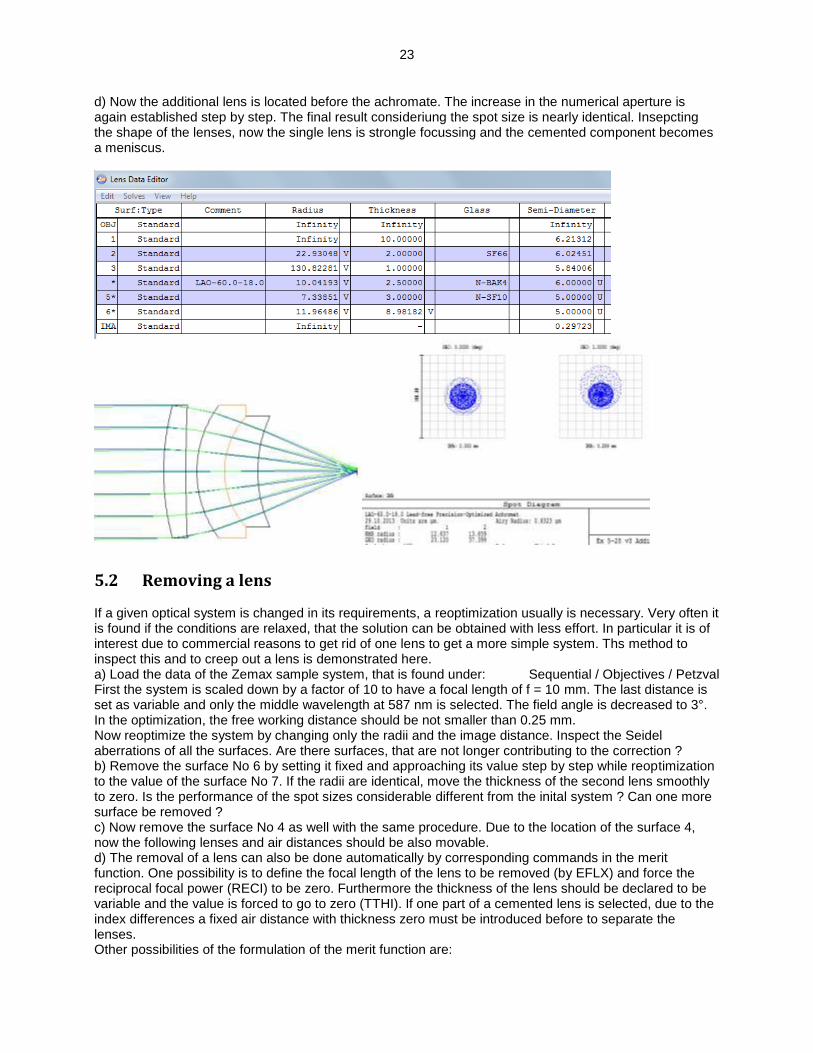
d) Now the additional lens is located before the achromate. The increase in the numerical aperture is again established step by step. The final result consideriung the spot size is nearly identical. Insepcting the shape of the lenses, now the single lens is strongle focussing and the cemented component becomes a meniscus.

5.2 Removing a lens If a given optical system is changed in its requirements, a reoptimization usually is necessary. Very often it is found if the conditions are relaxed, that the solution can be obtained with less effort. In particular it is of interest due to commercial reasons to get rid of one lens to get a more simple system. Ths method to inspect this and to creep out a lens is demonstrated here. a) Load the data of the Zemax sample system, that is found under: Sequential / Objectives / Petzval First the system is scaled down by a factor of 10 to have a focal length of f = 10 mm. The last distance is set as variable and only the middle wavelength at 587 nm is selected. The field angle is decreased to 3°. In the optimization, the free working distance should be not smaller than 0.25 mm. Now reoptimize the system by changing only the radii and the image distance. Inspect the Seidel aberrations of all the surfaces. Are there surfaces, that are not longer contributing to the correction ? b) Remove the surface No 6 by setting it fixed and approaching its value step by step while reoptimization to the value of the surface No 7. If the radii are identical, move the thickness of the second lens smoothly to zero. Is the performance of the spot sizes considerable different from the inital system ? Can one more surface be removed ? c) Now remove the surface No 4 as well with the same procedure. Due to the location of the surface 4, now the following lenses and air distances should be also movable. d) The removal of a lens can also be done automatically by corresponding commands in the merit function. One possibility is to define the focal length of the lens to be removed (by EFLX) and force the reciprocal focal power (RECI) to be zero. Furthermore the thickness of the lens should be declared to be variable and the value is forced to go to zero (TTHI). If one part of a cemented lens is selected, due to the index differences a fixed air distance with thickness zero must be introduced before to separate the lenses. Other possibilities of the formulation of the merit function are:

24

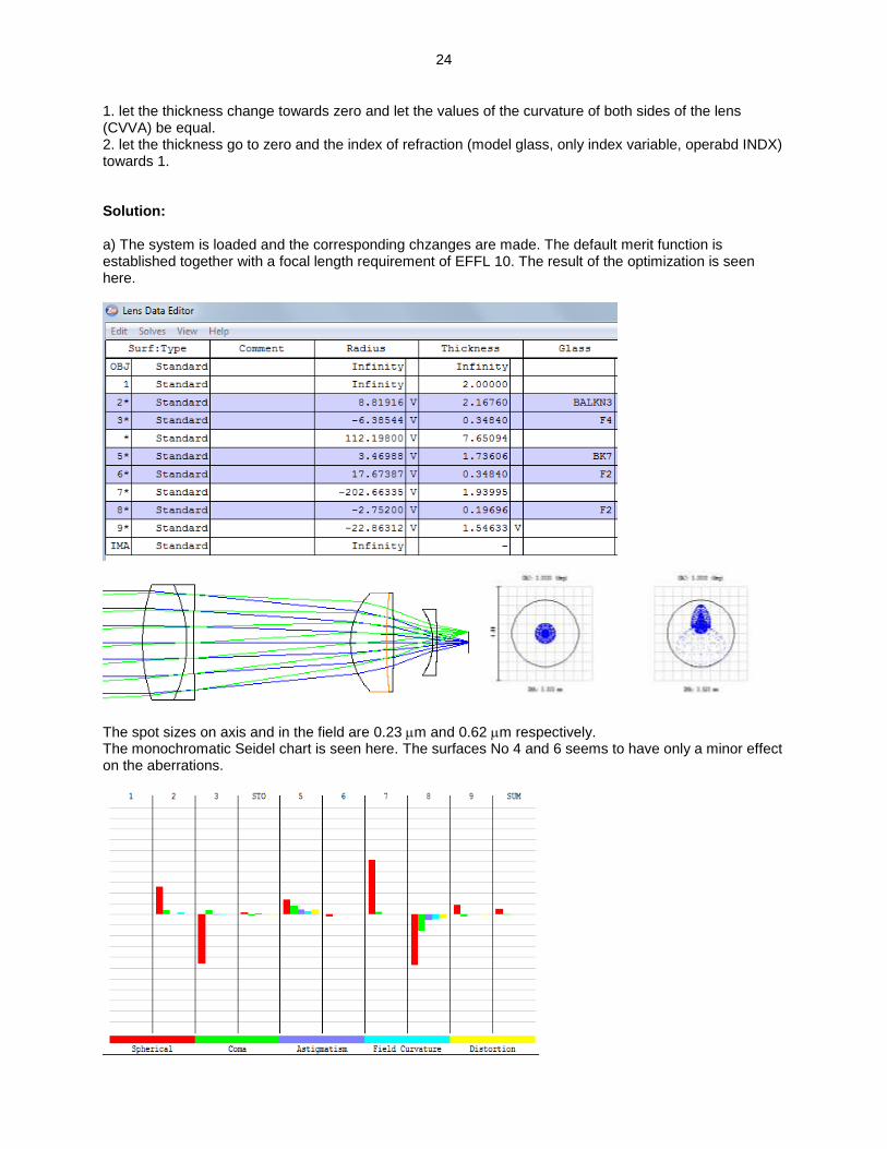
1. let the thickness change towards zero and let the values of the curvature of both sides of the lens (CVVA) be equal. 2. let the thickness go to zero and the index of refraction (model glass, only index variable, operabd INDX) towards 1. Solution: a) The system is loaded and the corresponding chzanges are made. The default merit function is established together with a focal length requirement of EFFL 10. The result of the optimization is seen here.

The spot sizes on axis and in the field are 0.23 m and 0.62 m respectively. The monochromatic Seidel chart is seen here. The surfaces No 4 and 6 seems to have only a minor effect on the aberrations.

25

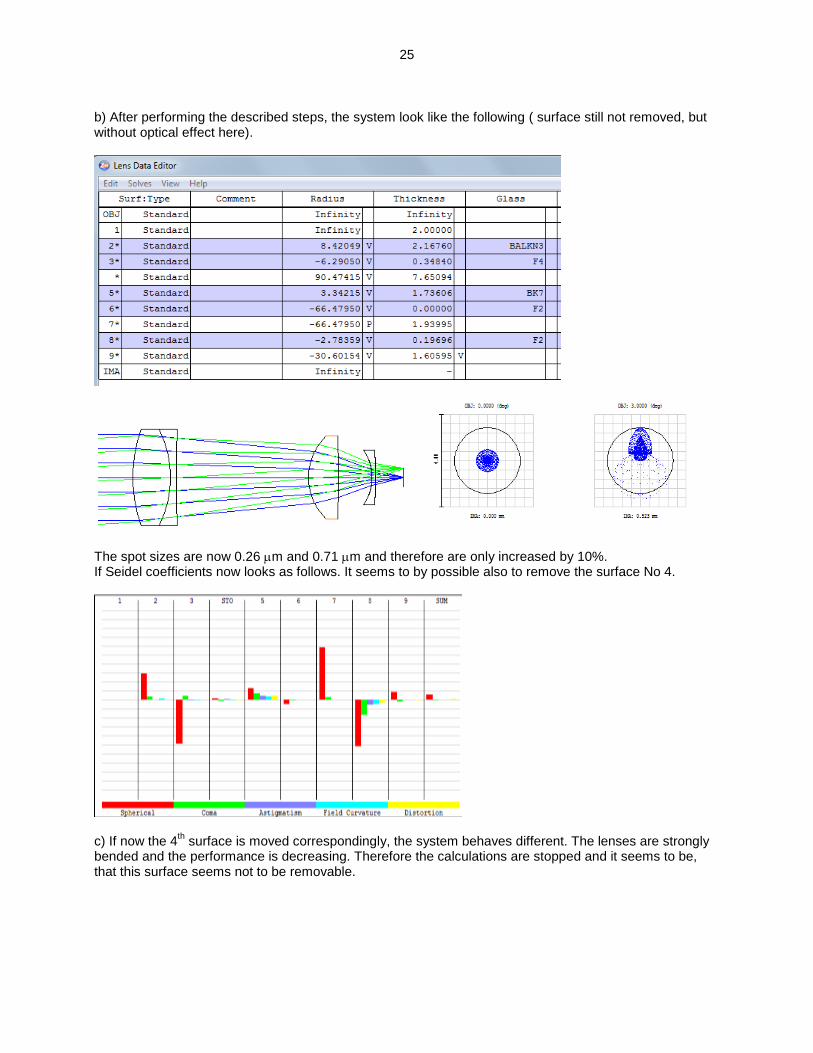
b) After performing the described steps, the system look like the following ( surface still not removed, but without optical effect here).

The spot sizes are now 0.26 m and 0.71 m and therefore are only increased by 10%. If Seidel coefficients now looks as follows. It seems to by possible also to remove the surface No 4.

c) If now the 4

th surface is moved correspondingly, the system behaves different. The lenses are strongly

bended and the performance is decreasing. Therefore the calculations are stopped and it seems to be, that this surface seems not to be removable.

26

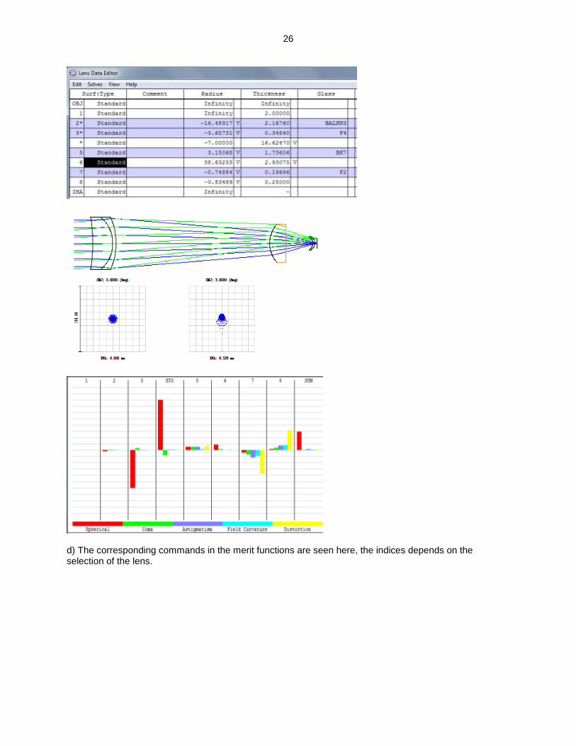
d) The corresponding commands in the merit functions are seen here, the indices depends on the selection of the lens.

27

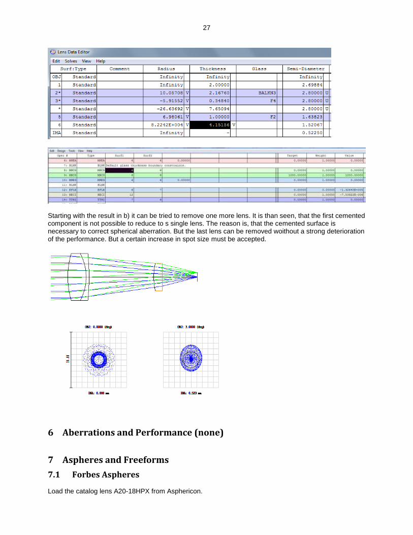
Starting with the result in b) it can be tried to remove one more lens. It is than seen, that the first cemented component is not possible to reduce to s single lens. The reason is, that the cemented surface is necessary to correct spherical aberration. But the last lens can be removed woithout a strong deterioration of the performance. But a certain increase in spot size must be accepted.

6 Aberrations and Performance (none)

7 Aspheres and Freeforms

7.1 Forbes Aspheres Load the catalog lens A20-18HPX from Asphericon.

28

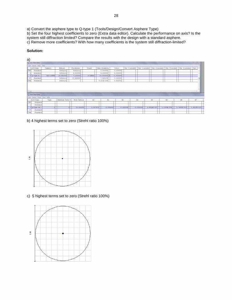
a) Convert the asphere type to Q-type 1 (Tools/Design/Convert Asphere Type) b) Set the four highest coefficients to zero (Extra data editor). Calculate the performance on axis? Is the system still diffraction limited? Compare the results with the design with a standard asphere. c) Remove more coefficients? With how many coefficients is the system still diffraction-limited? Solution: a)

b) 4 highest terms set to zero (Strehl ratio 100%)

c) 5 highest terms set to zero (Strehl ratio 100%)

29

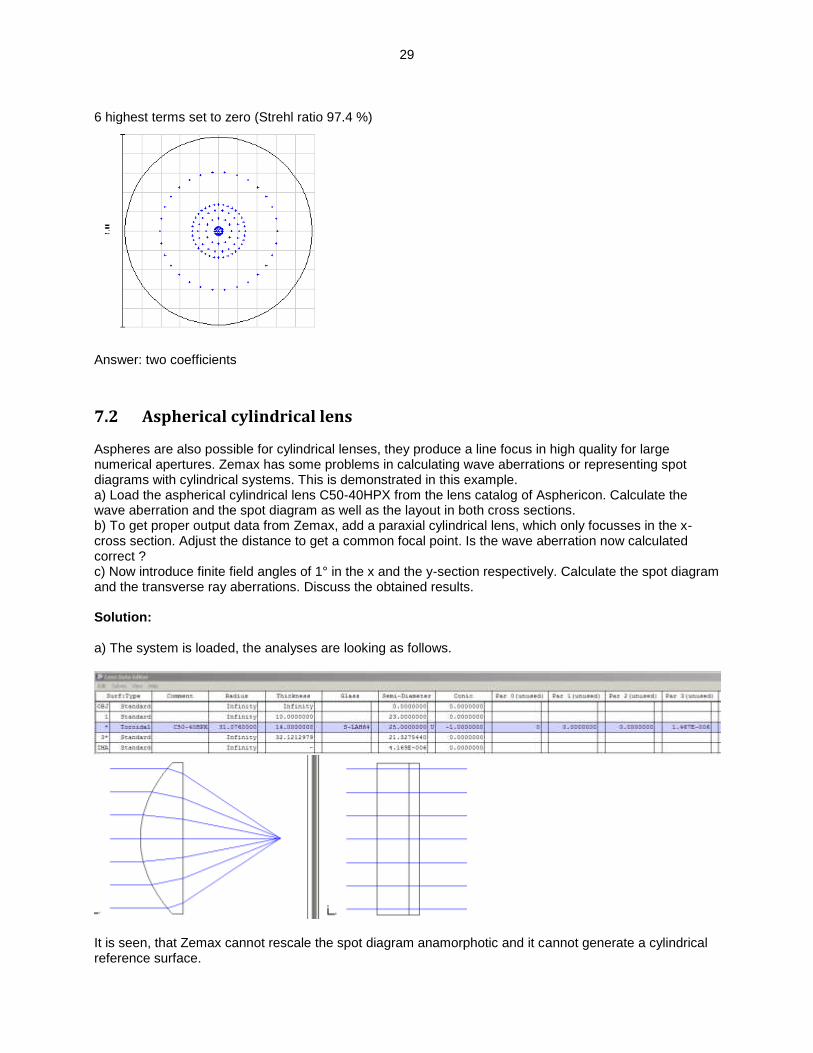
6 highest terms set to zero (Strehl ratio 97.4 %)

Answer: two coefficients

7.2 Aspherical cylindrical lens Aspheres are also possible for cylindrical lenses, they produce a line focus in high quality for large numerical apertures. Zemax has some problems in calculating wave aberrations or representing spot diagrams with cylindrical systems. This is demonstrated in this example. a) Load the aspherical cylindrical lens C50-40HPX from the lens catalog of Asphericon. Calculate the wave aberration and the spot diagram as well as the layout in both cross sections. b) To get proper output data from Zemax, add a paraxial cylindrical lens, which only focusses in the x-cross section. Adjust the distance to get a common focal point. Is the wave aberration now calculated correct ? c) Now introduce finite field angles of 1° in the x and the y-section respectively. Calculate the spot diagram and the transverse ray aberrations. Discuss the obtained results. Solution: a) The system is loaded, the analyses are looking as follows.

It is seen, that Zemax cannot rescale the spot diagram anamorphotic and it cannot generate a cylindrical reference surface.

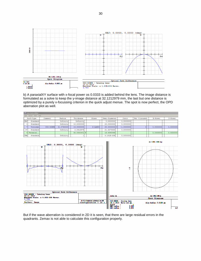
30

b) A paraxialXY surface with x-focal power os 0.0333 is added behind the lens. The image distance is formulated as a solve to keep the y-image distance at 32.1212979 mm, the last but one distance is optimized by a purely x-focussing criterion in the quick adjust menue. The spot is now perfect, the OPD aberration plot as well.

But if the wave aberration is considered in 2D it is seen, that there are large residual errors in the quadrants. Zemax is not able to calculate this configuration properly.

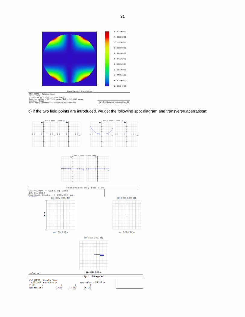
31

c) if the two field points are introduced, we get the following spot diagram and transverse aberratiosn:

32

The finite field in y-direction produces coma as expected for an asphere in the y-section. The field in the x-section produces a small amount of defocus, although the spot diagram looks strange.

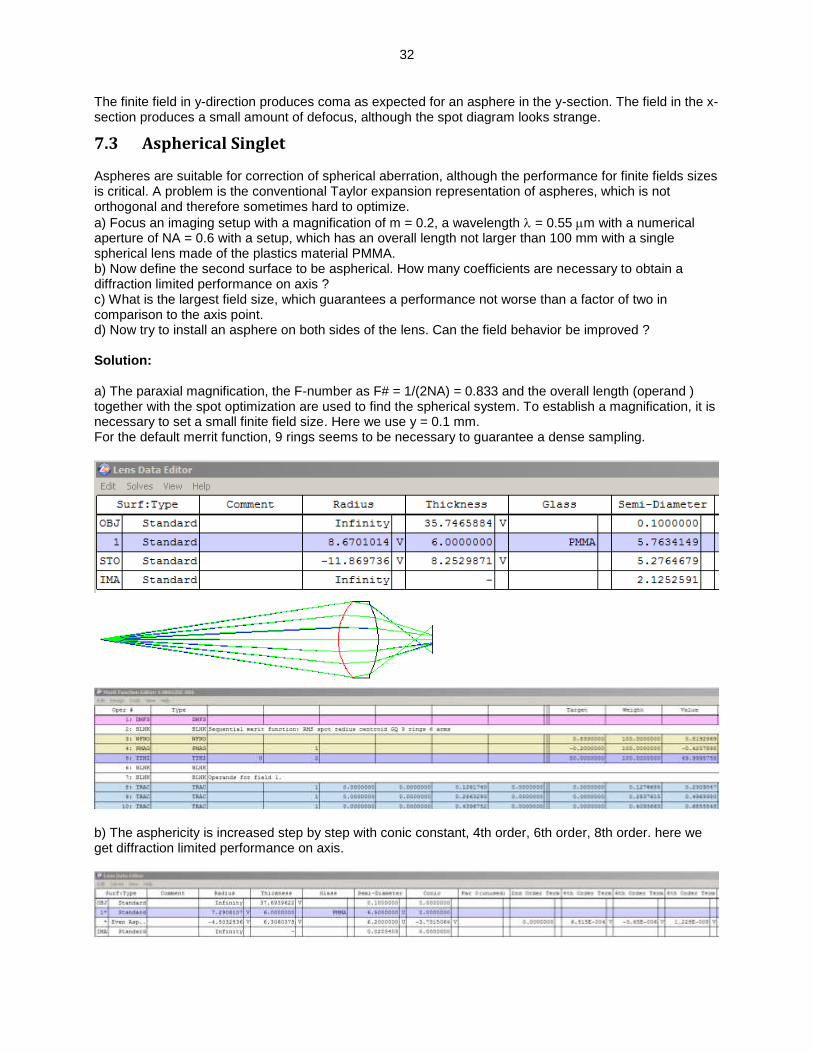
7.3 Aspherical Singlet Aspheres are suitable for correction of spherical aberration, although the performance for finite fields sizes is critical. A problem is the conventional Taylor expansion representation of aspheres, which is not orthogonal and therefore sometimes hard to optimize.

a) Focus an imaging setup with a magnification of m = 0.2, a wavelength = 0.55 m with a numerical aperture of NA = 0.6 with a setup, which has an overall length not larger than 100 mm with a single spherical lens made of the plastics material PMMA. b) Now define the second surface to be aspherical. How many coefficients are necessary to obtain a diffraction limited performance on axis ? c) What is the largest field size, which guarantees a performance not worse than a factor of two in comparison to the axis point. d) Now try to install an asphere on both sides of the lens. Can the field behavior be improved ? Solution: a) The paraxial magnification, the F-number as F# = 1/(2NA) = 0.833 and the overall length (operand ) together with the spot optimization are used to find the spherical system. To establish a magnification, it is necessary to set a small finite field size. Here we use y = 0.1 mm. For the default merrit function, 9 rings seems to be necessary to guarantee a dense sampling.

b) The asphericity is increased step by step with conic constant, 4th order, 6th order, 8th order. here we get diffraction limited performance on axis.

33

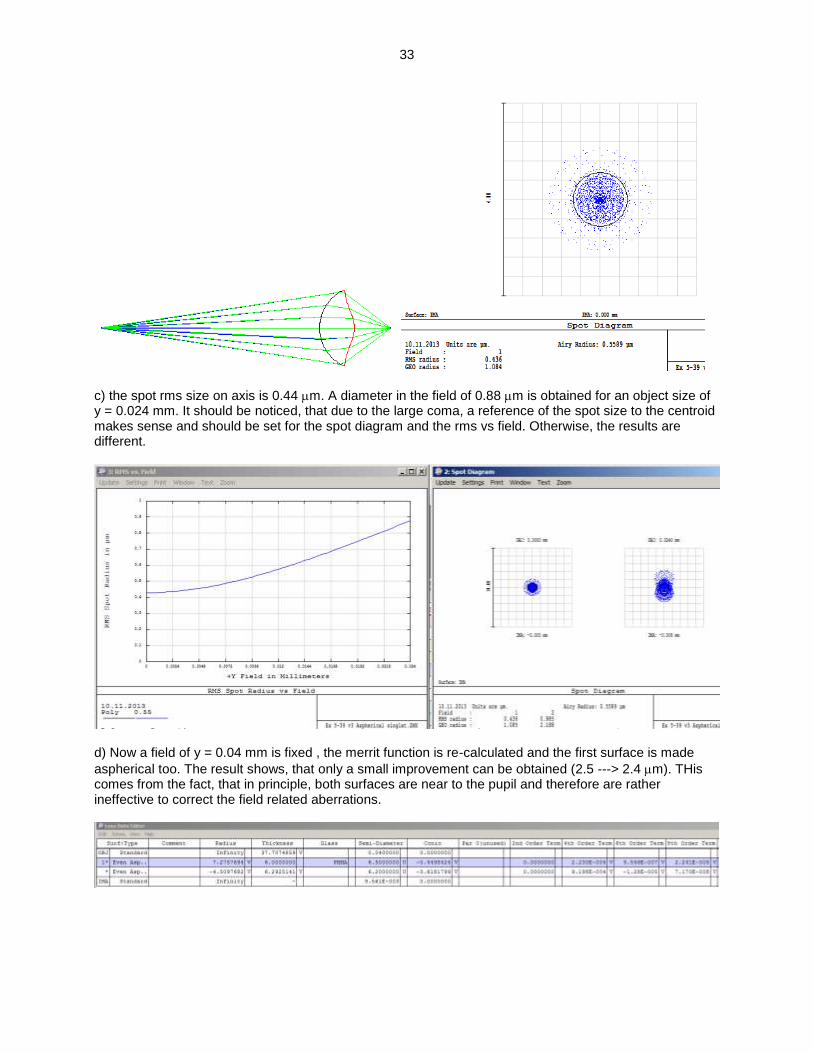
c) the spot rms size on axis is 0.44 m. A diameter in the field of 0.88 m is obtained for an object size of y = 0.024 mm. It should be noticed, that due to the large coma, a reference of the spot size to the centroid makes sense and should be set for the spot diagram and the rms vs field. Otherwise, the results are different.

d) Now a field of y = 0.04 mm is fixed , the merrit function is re-calculated and the first surface is made

aspherical too. The result shows, that only a small improvement can be obtained (2.5 ---> 2.4 m). THis comes from the fact, that in principle, both surfaces are near to the pupil and therefore are rather ineffective to correct the field related aberrations.

34

8 Field flattening

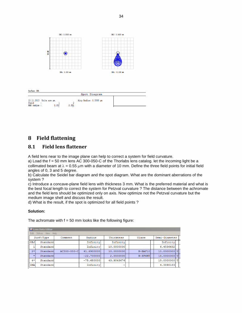
8.1 Field lens flattener A field lens near to the image plane can help to correct a system for field curvature. a) Load the f = 50 mm lens AC 300-050-C of the Thorlabs lens catalog. let the incoming light be a

collimated beam at = 0.55 m with a diameter of 10 mm. Define the three field points for initial field angles of 0, 3 and 5 degree. b) Calculate the Seidel bar diagram and the spot diagram. What are the dominant aberrations of the system ? c) Introduce a concave-plane field lens with thickness 3 mm. What is the preferred material and what is the best focal length to correct the system for Petzval curvature ? The distance between the achromate and the field lens should be optimized only on axis. Now optimize not the Petzval curvature but the medium image shell and discuss the result. d) What is the result, if the spot is optimized for all field points ? Solution: The achromate with f = 50 mm looks like the following figure:

35

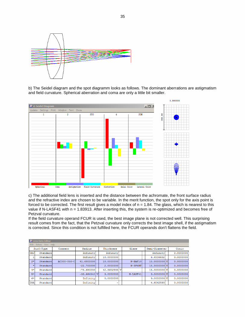
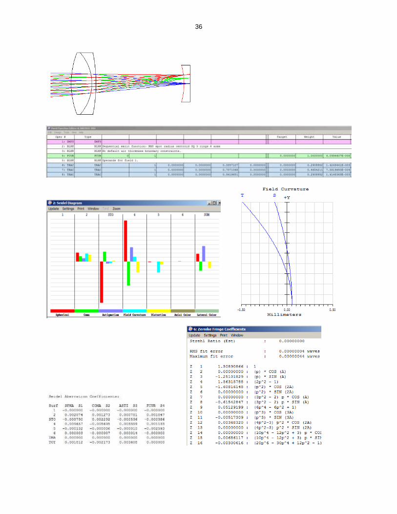
b) The Seidel diagram and the spot diagramm looks as follows. The dominant aberrations are astigmatism and field curvature. Spherical aberration and coma are only a little bit smaller.

c) The additional field lens is inserted and the distance between the achromate, the front surface radius and the refractive index are chosen to be variable. In the merit function, the spot only for the axis point is forced to be corrected. The first result gives a model index of n = 1.84. The glass, which is nearest to this value if N-LASF41 with n = 1.83913. After inserting this, the system is re-optimized and becomes free of Petzval curvature. If the field curvature operand FCUR is used, the best image plane is not corrected well. This surprising result comes from the fact, that the Petzval curvature only corrects the best image shell, if the astigmatism is corrected. Since this condition is not fulfilled here, the FCUR operands don't flattens the field.

36

37

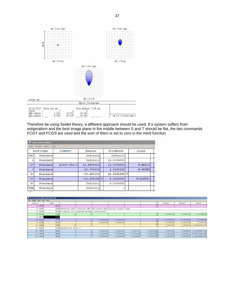
Therefore be using Seidel theory, a different approach should be used. If a system suffers from astigmatism and the best image plane in the middle between S and T should be flat, the two commands FCGT and FCGS are used and the sum of them is set to zero in the merit function.

38

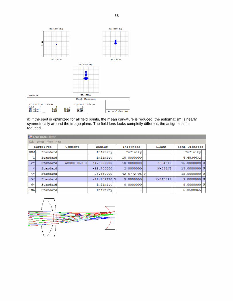
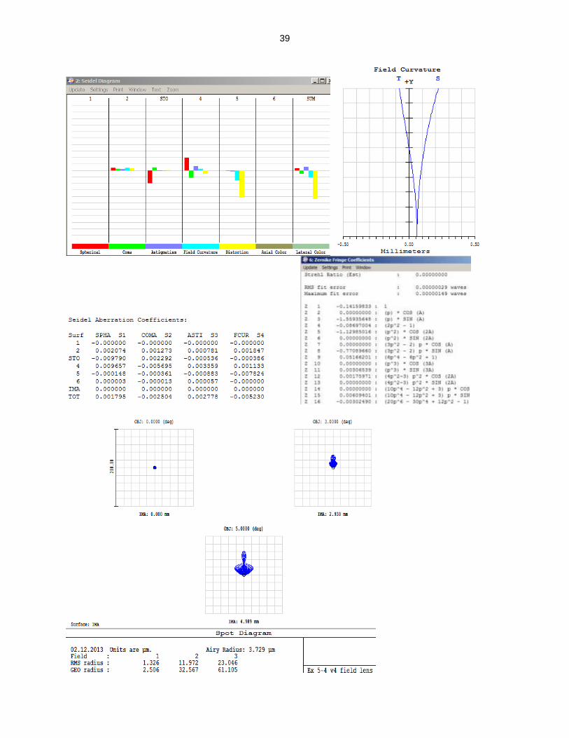
d) If the spot is optimized for all field points, the mean curvature is reduced, the astigmatism is nearly symmetrically around the image plane. The field lens looks completly different, the astigmatism is reduced.

39

40

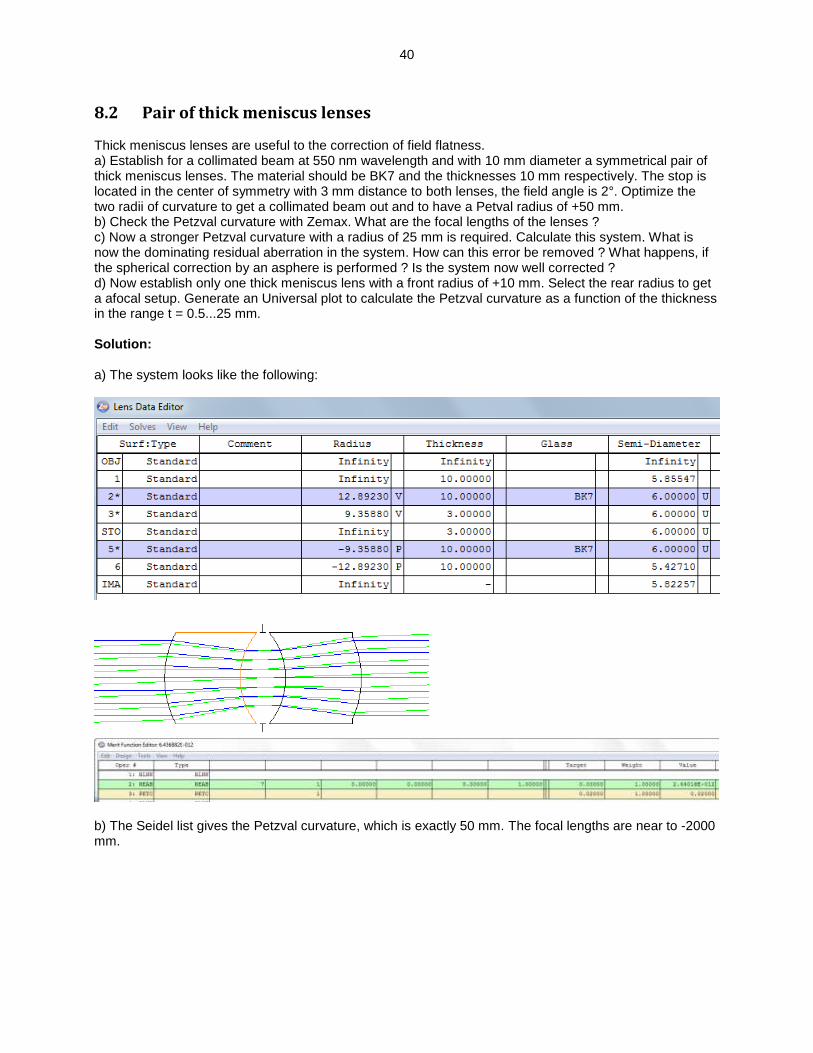
8.2 Pair of thick meniscus lenses Thick meniscus lenses are useful to the correction of field flatness. a) Establish for a collimated beam at 550 nm wavelength and with 10 mm diameter a symmetrical pair of thick meniscus lenses. The material should be BK7 and the thicknesses 10 mm respectively. The stop is located in the center of symmetry with 3 mm distance to both lenses, the field angle is 2°. Optimize the two radii of curvature to get a collimated beam out and to have a Petval radius of +50 mm. b) Check the Petzval curvature with Zemax. What are the focal lengths of the lenses ? c) Now a stronger Petzval curvature with a radius of 25 mm is required. Calculate this system. What is now the dominating residual aberration in the system. How can this error be removed ? What happens, if the spherical correction by an asphere is performed ? Is the system now well corrected ? d) Now establish only one thick meniscus lens with a front radius of +10 mm. Select the rear radius to get a afocal setup. Generate an Universal plot to calculate the Petzval curvature as a function of the thickness in the range t = 0.5...25 mm. Solution: a) The system looks like the following:

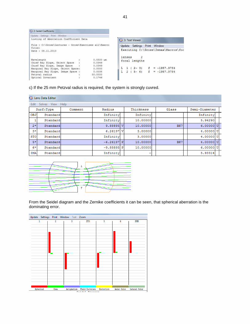
b) The Seidel list gives the Petzval curvature, which is exactly 50 mm. The focal lengths are near to -2000 mm.

41

c) If the 25 mm Petzval radius is required, the system is strongly cuvred.

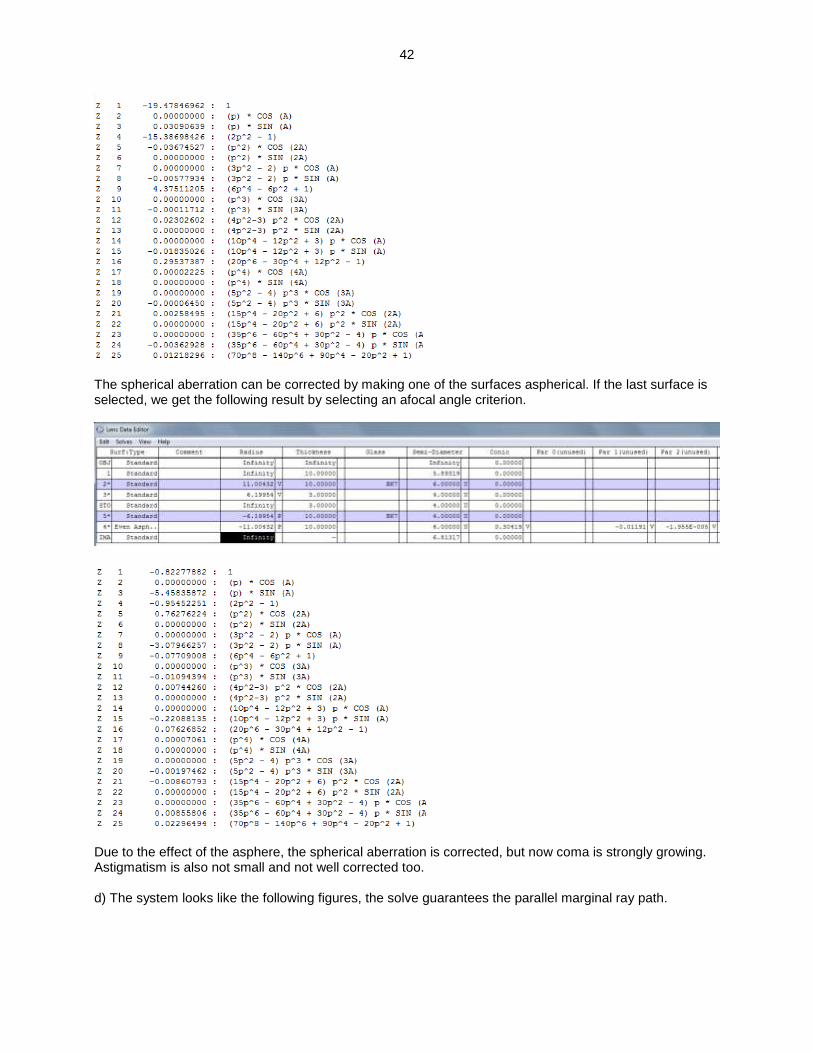
From the Seidel diagram and the Zernike coefficients it can be seen, that spherical aberration is the dominating error.

42

The spherical aberration can be corrected by making one of the surfaces aspherical. If the last surface is selected, we get the following result by selecting an afocal angle criterion.

Due to the effect of the asphere, the spherical aberration is corrected, but now coma is strongly growing. Astigmatism is also not small and not well corrected too. d) The system looks like the following figures, the solve guarantees the parallel marginal ray path.

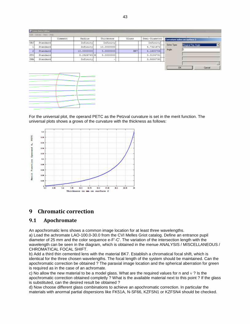
43

For the universal plot, the operand PETC as the Petzval curvature is set in the merit function. The universal plots shows a grows of the curvature with the thickness as follows:

9 Chromatic correction

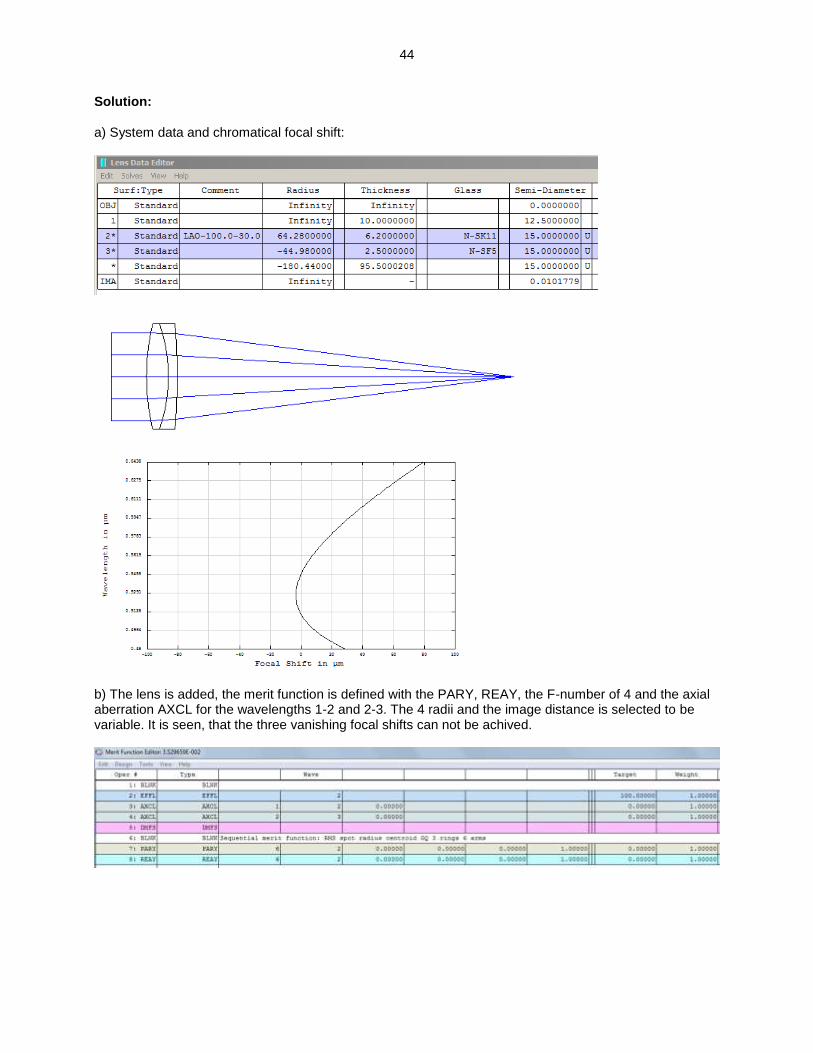
9.1 Apochromate An apochromatic lens shows a common image location for at least three wavelengths. a) Load the achromate LAO-100.0-30.0 from the CVI Melles Griot catalog. Define an entrance pupil diameter of 25 mm and the color sequence e-F'-C'. The variation of the intersection length with the wavelength can be seen in the diagram, which is obtained in the menue ANALYSIS / MISCELLANEOUS / CHROMATICAL FOCAL SHIFT. b) Add a third thin cemented lens with the material BK7. Establish a chromatical focal shift, which is identical for the three chosen wavelengths. The focal length of the system should be maintained. Can the apochromatic correction be obtained ? The paraxial image location and the spherical aberration for green is required as in the case of an achromate.

c) No allow the new material to be a model glass. What are the required values for n and ? Is the apochromatic correction obtained completly ? What is the available material next to this point ? If the glass is substituted, can the desired result be obtained ? d) Now choose different glass combinations to achieve an apochromatic correction. In particular the materials with anormal partial dispersions like FK51A, N-SF66, KZFSN1 or KZFSN4 should be checked.

44

Solution: a) System data and chromatical focal shift:

b) The lens is added, the merit function is defined with the PARY, REAY, the F-number of 4 and the axial aberration AXCL for the wavelengths 1-2 and 2-3. The 4 radii and the image distance is selected to be variable. It is seen, that the three vanishing focal shifts can not be achived.

45

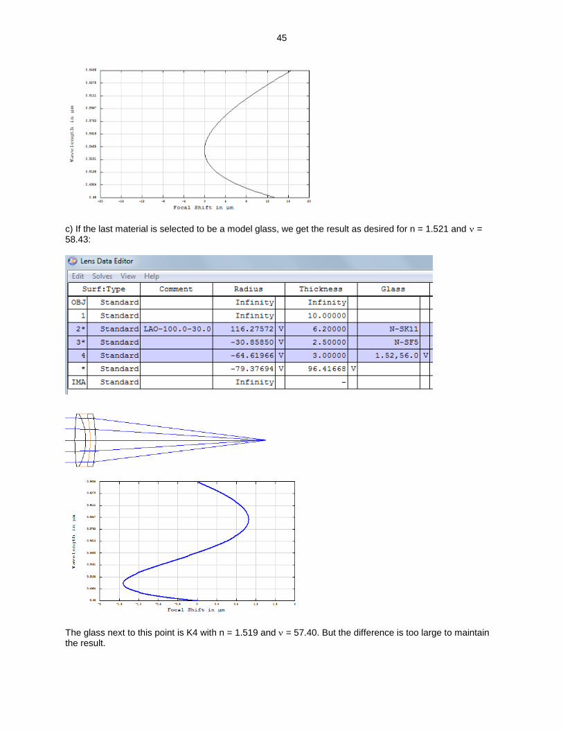
c) If the last material is selected to be a model glass, we get the result as desired for n = 1.521 and = 58.43:

The glass next to this point is K4 with n = 1.519 and = 57.40. But the difference is too large to maintain the result.

46

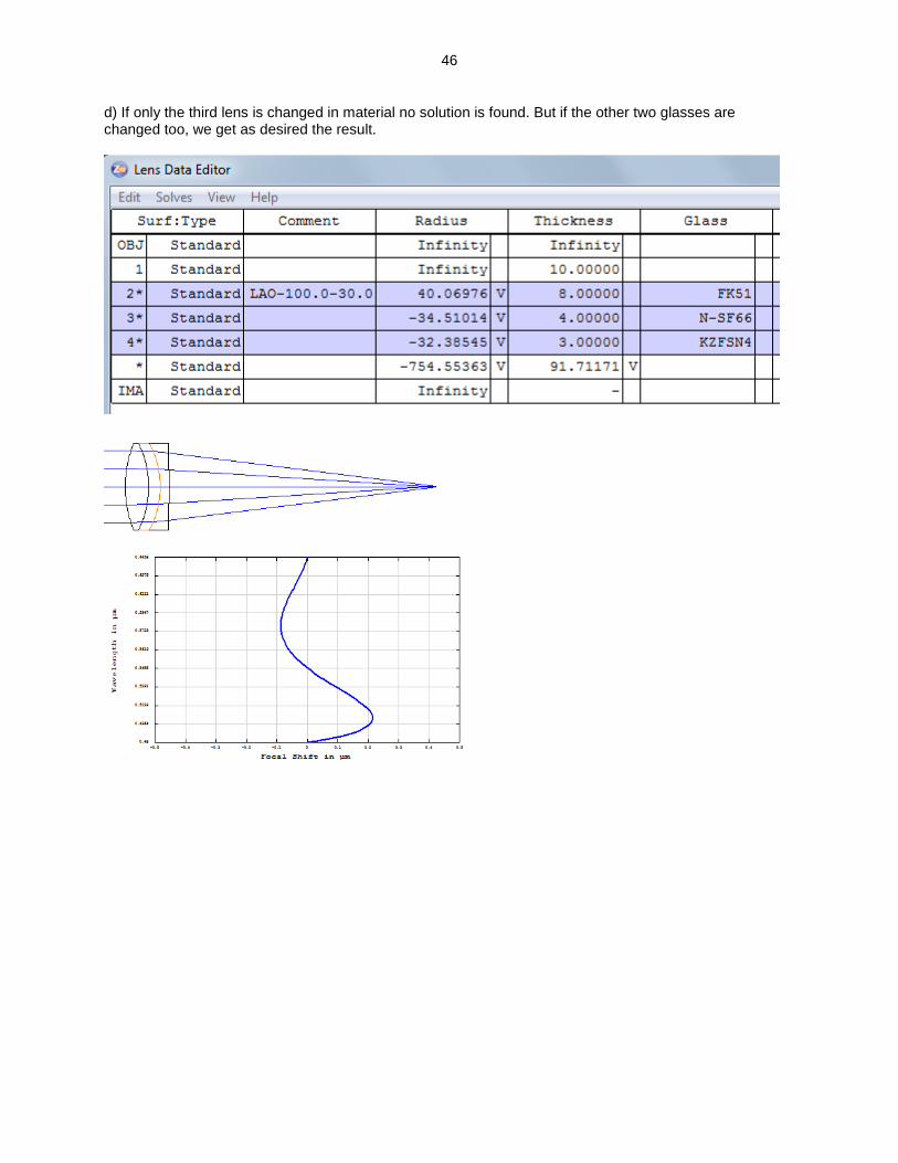
d) If only the third lens is changed in material no solution is found. But if the other two glasses are changed too, we get as desired the result.

47

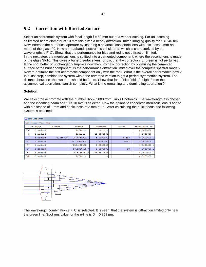
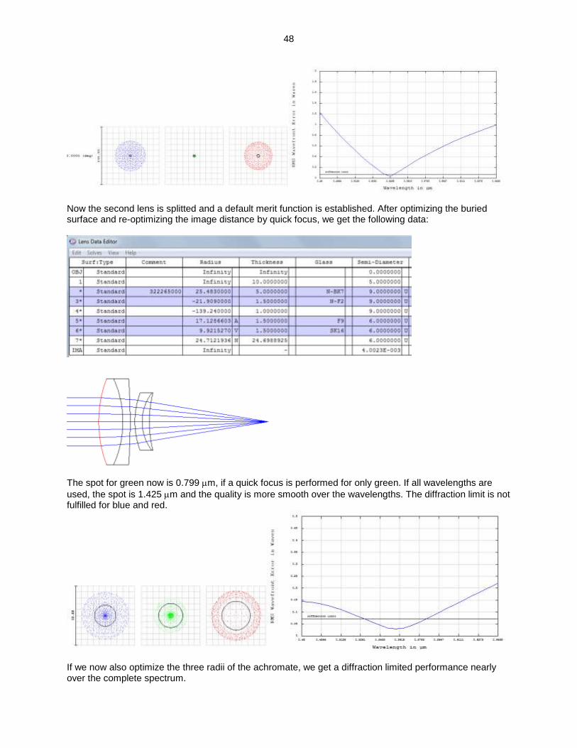
9.2 Correction with Burried Surface Select an achromatic system with focal length f = 50 mm out of a vendor catalog. For an incoming

collimated beam diameter of 10 mm this gives a nearly diffraction limited imaging quality for = 546 nm. Now increase the numerical aperture by inserting a aplanatic concentric lens with thickness 3 mm and made of the glass F9. Now a broadband spectrum is considered, which is characterized by the wavelengths e F' C'. Show, that the performance for blue and red is not diffraction limited. In the next step, the meniscus lens is splitted into a cemented component, where the second lens is made of the glass SK16. This gives a burierd surface lens. Show, that the correction for green is not perturbed. Is the spot better or unchanged ? Improve now the chromatic correction by optimizing the cemented surface of the burier component. Is the performance diffraction limited over the complete spectral range ? Now re-optimize the first achromatic component only with the radii. What is the overall performance now ? In a last step, combine the system with a the reversed version to get a perfect symmetrical system. The distance between the two parts should be 2 mm. Show that for a finite field of height 3 mm the asymmetrical aberrations vanish completly. What is the remaining and dominating aberration ? Solution: We select the achromate with the number 322265000 from Linois Photonics. The wavelength e is chosen and the incoming beam aperture 10 mm is selected. Now the aplanatic concentric meniscus lens is added with a distance of 1 mm and a thickness of 3 mm of F9. After calculating the quick focus, the following system is obtained:

The wavelength combination e F' C' is selected. It is seen, that the system is diffraction limited only near

the green line. Spot rms value for the e-line is D = 0.858 m.

48

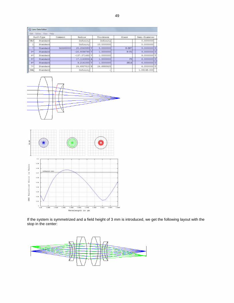
Now the second lens is splitted and a default merit function is established. After optimizing the buried surface and re-optimizing the image distance by quick focus, we get the following data:

The spot for green now is 0.799 m, if a quick focus is performed for only green. If all wavelengths are

used, the spot is 1.425 m and the quality is more smooth over the wavelengths. The diffraction limit is not fulfilled for blue and red.

If we now also optimize the three radii of the achromate, we get a diffraction limited performance nearly over the complete spectrum.

49

If the system is symmetrized and a field height of 3 mm is introduced, we get the following layout with the stop in the center:

50

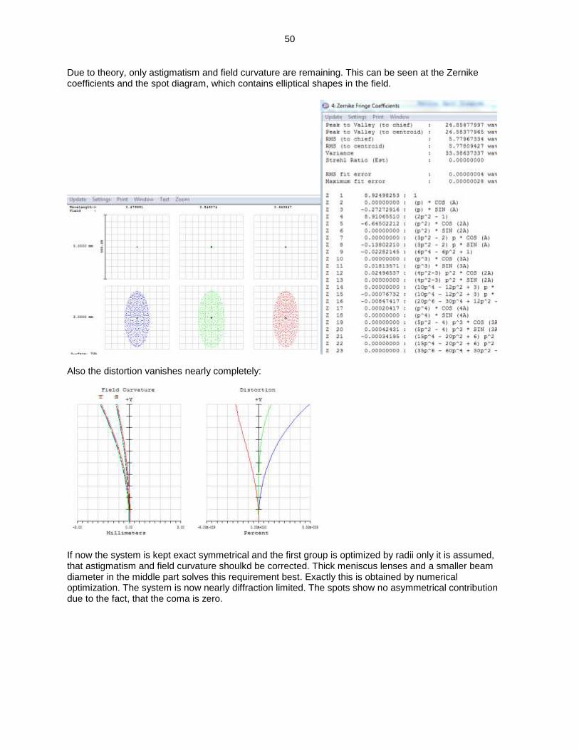
Due to theory, only astigmatism and field curvature are remaining. This can be seen at the Zernike coefficients and the spot diagram, which contains elliptical shapes in the field.

Also the distortion vanishes nearly completely:

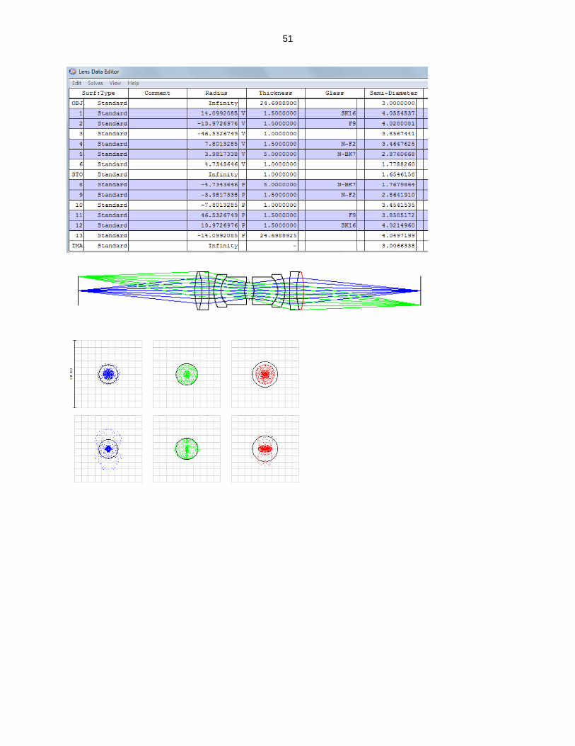
If now the system is kept exact symmetrical and the first group is optimized by radii only it is assumed, that astigmatism and field curvature shoulkd be corrected. Thick meniscus lenses and a smaller beam diameter in the middle part solves this requirement best. Exactly this is obtained by numerical optimization. The system is now nearly diffraction limited. The spots show no asymmetrical contribution due to the fact, that the coma is zero.

51

52

10 Special Topics

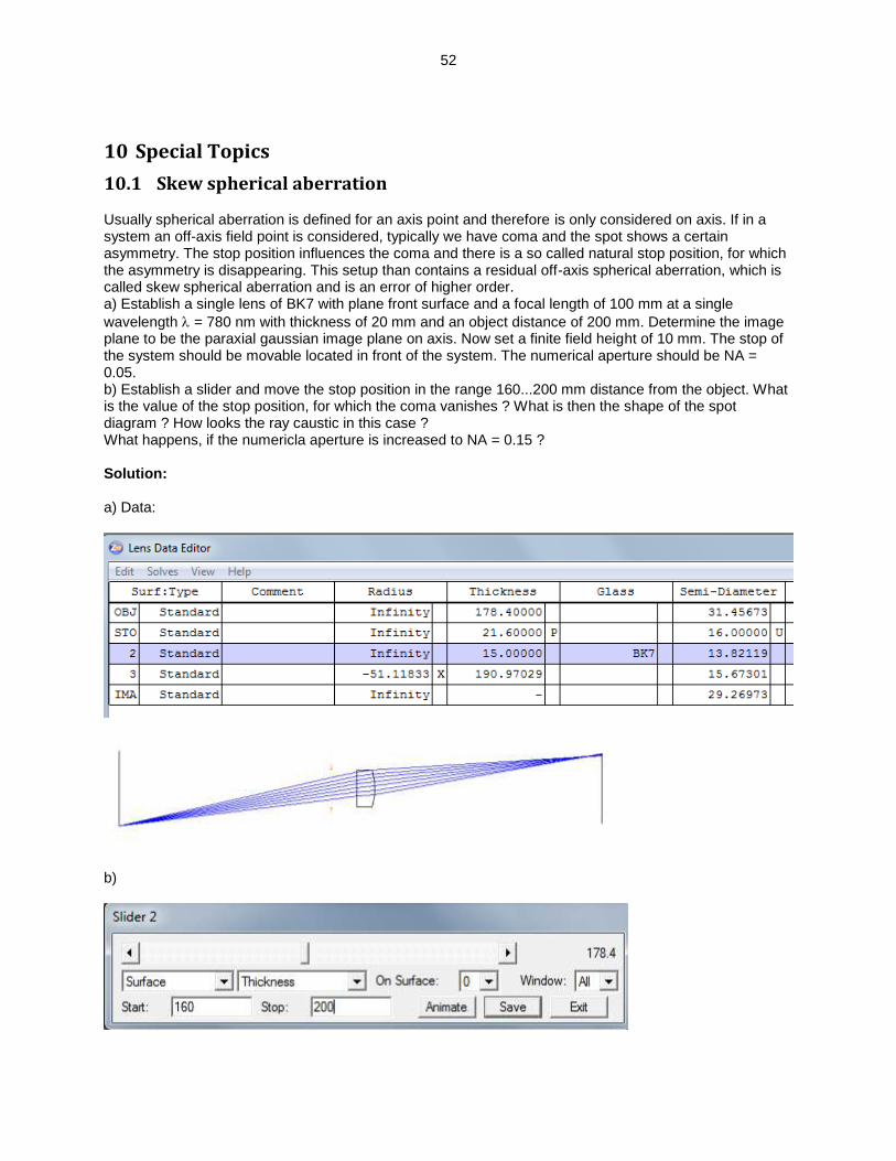
10.1 Skew spherical aberration Usually spherical aberration is defined for an axis point and therefore is only considered on axis. If in a system an off-axis field point is considered, typically we have coma and the spot shows a certain asymmetry. The stop position influences the coma and there is a so called natural stop position, for which the asymmetry is disappearing. This setup than contains a residual off-axis spherical aberration, which is called skew spherical aberration and is an error of higher order. a) Establish a single lens of BK7 with plane front surface and a focal length of 100 mm at a single

wavelength = 780 nm with thickness of 20 mm and an object distance of 200 mm. Determine the image plane to be the paraxial gaussian image plane on axis. Now set a finite field height of 10 mm. The stop of the system should be movable located in front of the system. The numerical aperture should be NA = 0.05. b) Establish a slider and move the stop position in the range 160...200 mm distance from the object. What is the value of the stop position, for which the coma vanishes ? What is then the shape of the spot diagram ? How looks the ray caustic in this case ? What happens, if the numericla aperture is increased to NA = 0.15 ? Solution: a) Data:

b)

53

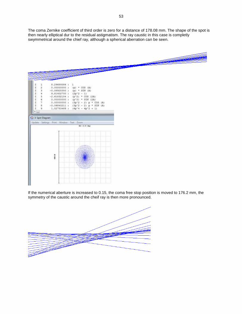
The coma Zernike coefficient of third order is zero for a distance of 178.08 mm. The shape of the spot is then nearly elliptical dur to the residual astigmatism. The ray caustic in this case is completly swymmetrical around the chief ray, although a spherical aberration can be seen.

If the numerical aberture is increased to 0.15, the coma free stop position is moved to 176.2 mm, the symmetry of the caustic around the cheif ray is then more pronounced.

54

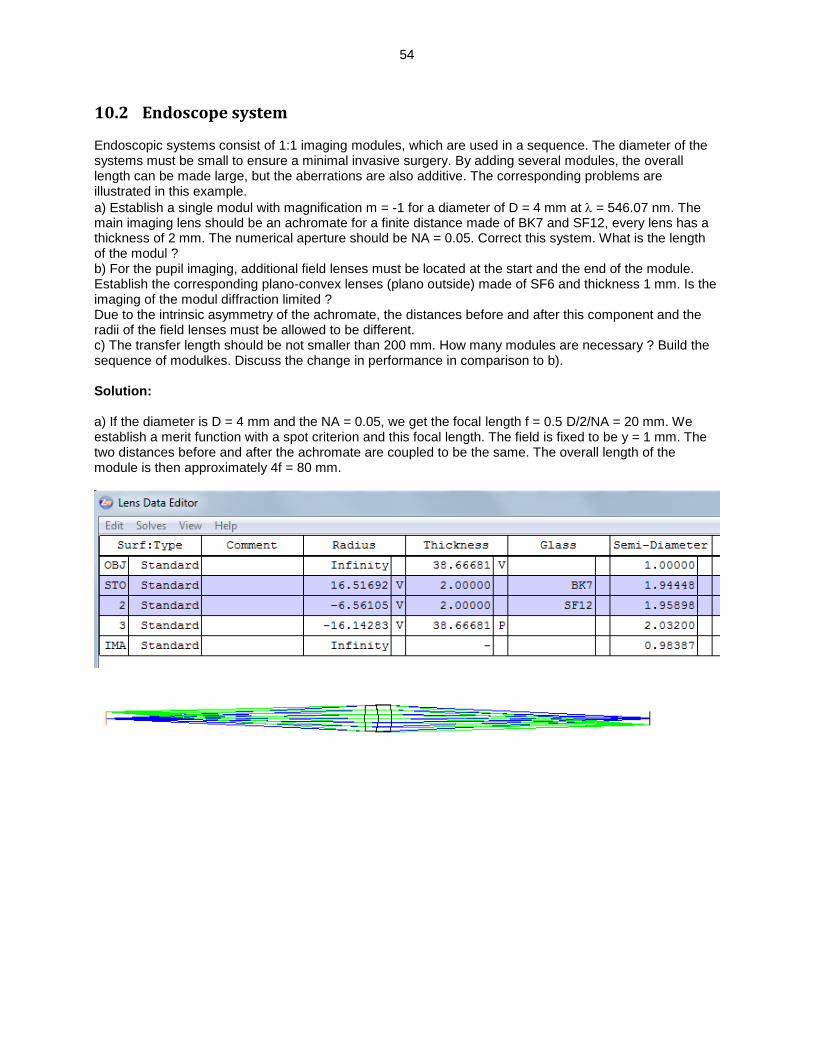
10.2 Endoscope system Endoscopic systems consist of 1:1 imaging modules, which are used in a sequence. The diameter of the systems must be small to ensure a minimal invasive surgery. By adding several modules, the overall length can be made large, but the aberrations are also additive. The corresponding problems are illustrated in this example.

a) Establish a single modul with magnification m = -1 for a diameter of D = 4 mm at = 546.07 nm. The main imaging lens should be an achromate for a finite distance made of BK7 and SF12, every lens has a thickness of 2 mm. The numerical aperture should be NA = 0.05. Correct this system. What is the length of the modul ? b) For the pupil imaging, additional field lenses must be located at the start and the end of the module. Establish the corresponding plano-convex lenses (plano outside) made of SF6 and thickness 1 mm. Is the imaging of the modul diffraction limited ? Due to the intrinsic asymmetry of the achromate, the distances before and after this component and the radii of the field lenses must be allowed to be different. c) The transfer length should be not smaller than 200 mm. How many modules are necessary ? Build the sequence of modulkes. Discuss the change in performance in comparison to b). Solution: a) If the diameter is D = 4 mm and the NA = 0.05, we get the focal length f = 0.5 D/2/NA = 20 mm. We establish a merit function with a spot criterion and this focal length. The field is fixed to be y = 1 mm. The two distances before and after the achromate are coupled to be the same. The overall length of the module is then approximately 4f = 80 mm.

55

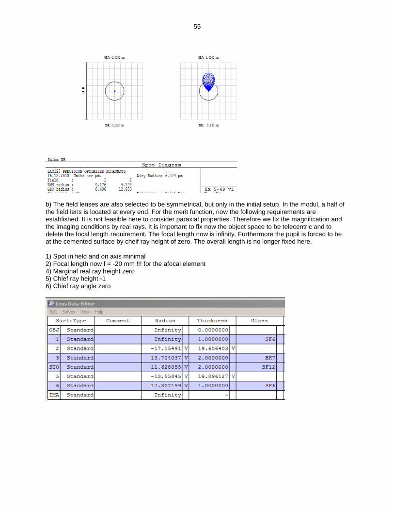
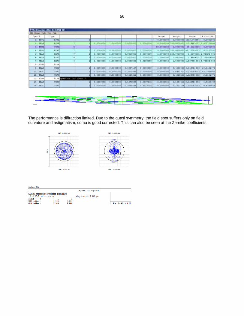
b) The field lenses are also selected to be symmetrical, but only in the initial setup. In the modul, a half of the field lens is located at every end. For the merit function, now the following requirements are established. It is not feasible here to consider paraxial properties. Therefore we fix the magnification and the imaging conditions by real rays. It is important to fix now the object space to be telecentric and to delete the focal length requirement. The focal length now is infinity. Furthermore the pupil is forced to be at the cemented surface by cheif ray height of zero. The overall length is no longer fixed here. 1) Spot in field and on axis minimal 2) Focal length now f = -20 mm !!! for the afocal element 4) Marginal real ray height zero 5) Chief ray height -1 6) Chief ray angle zero

56

The performance is diffraction limited. Due to the quasi symmetry, the field spot suffers only on field curvature and astigmatism, coma is good corrected. This can also be seen at the Zernike coefficients.

57

c) By adding 3 systems, we get a length of 240 mm. The performance is also good, but no longer diffraction limited.

58

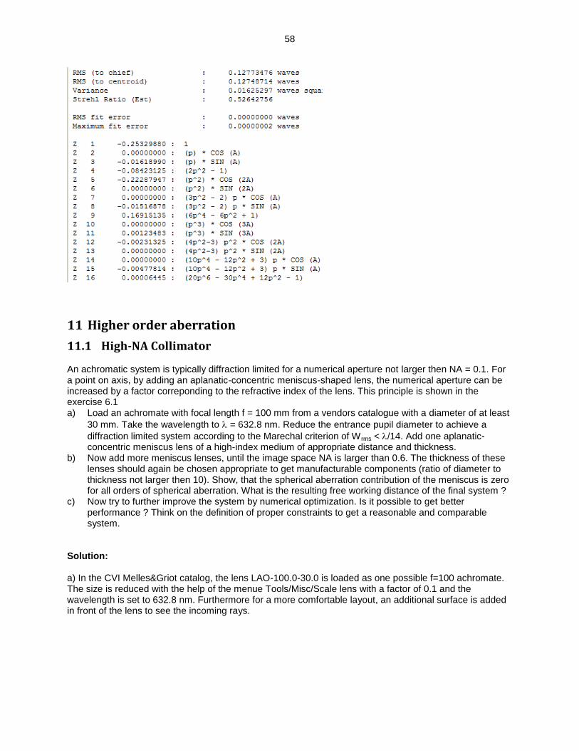
11 Higher order aberration

11.1 High-NA Collimator An achromatic system is typically diffraction limited for a numerical aperture not larger then NA = 0.1. For a point on axis, by adding an aplanatic-concentric meniscus-shaped lens, the numerical aperture can be increased by a factor correponding to the refractive index of the lens. This principle is shown in the exercise 6.1 a) Load an achromate with focal length f = 100 mm from a vendors catalogue with a diameter of at least

30 mm. Take the wavelength to = 632.8 nm. Reduce the entrance pupil diameter to achieve a

diffraction limited system according to the Marechal criterion of W rms < /14. Add one aplanatic-concentric meniscus lens of a high-index medium of appropriate distance and thickness.

b) Now add more meniscus lenses, until the image space NA is larger than 0.6. The thickness of these lenses should again be chosen appropriate to get manufacturable components (ratio of diameter to thickness not larger then 10). Show, that the spherical aberration contribution of the meniscus is zero for all orders of spherical aberration. What is the resulting free working distance of the final system ?

c) Now try to further improve the system by numerical optimization. Is it possible to get better performance ? Think on the definition of proper constraints to get a reasonable and comparable system.

Solution: a) In the CVI Melles&Griot catalog, the lens LAO-100.0-30.0 is loaded as one possible f=100 achromate. The size is reduced with the help of the menue Tools/Misc/Scale lens with a factor of 0.1 and the wavelength is set to 632.8 nm. Furthermore for a more comfortable layout, an additional surface is added in front of the lens to see the incoming rays.

59

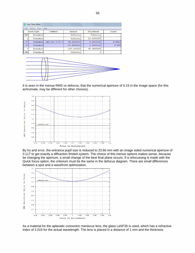
It is seen in the menue RMS vs defocus, that the numerical aperture of 0.15 in the image space (for this achromate, may be different for other choices).

By try and error, the entrance pupil size is reduced to 23.66 mm with an image sided numerical aperture of 0.117 to get exactly a diffraction limited system. The choice of this menue options makes sense, because be changing the aperture, a small change of the best final plane occurs. If a refocussing is made with the Quick focus option, the criterium must be the same in the defocus diagram. There are small differences between a spot and a wavefront optimization.

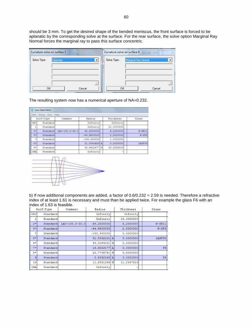
As a material for the aplanatic concentric meniscus lens, the glass LaSF35 is used, which has a refractive index of 2.015 for the actual wavelength. The lens is placed in a distance of 1 mm and the thickness

60

should be 3 mm. To get the desired shape of the bended meniscus, the front surface is forced to be aplanatic by the corresponding solve at the surface. For the rear surface, the solve option Marginal Ray Normal forces the marginal ray to pass this surface concentric.

The resulting system now has a numerical aperture of NA=0.232.

b) If now additional components are added, a factor of 0.6/0.232 = 2.59 is needed. Therefore a refractive index of at least 1.61 is necessary and must than be applied twice. For example the glass F6 with an index of 1.63 is feasible.

61

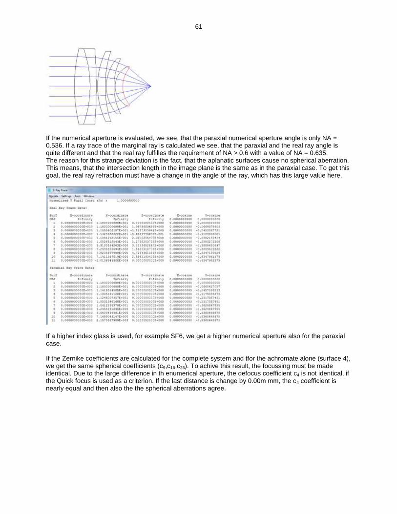
If the numerical aperture is evaluated, we see, that the paraxial numerical aperture angle is only NA = 0.536. If a ray trace of the marginal ray is calculated we see, that the paraxial and the real ray angle is quite different and that the real ray fulfilles the requirement of NA > 0.6 with a value of NA = 0.635. The reason for this strange deviation is the fact, that the aplanatic surfaces cause no spherical aberration. This means, that the intersection length in the image plane is the same as in the paraxial case. To get this goal, the real ray refraction must have a change in the angle of the ray, which has this large value here.

If a higher index glass is used, for example SF6, we get a higher numerical aperture also for the paraxial case. If the Zernike coefficients are calculated for the complete system and tfor the achromate alone (surface 4), we get the same spherical coefficients (c9,c16,c25). To achive this result, the focussing must be made identical. Due to the large difference in th enumerical aperture, the defocus coefficient c4 is not identical, if the Quick focus is used as a criterion. If the last distance is change by 0.00m mm, the c4 coefficient is nearly equal and then also the the spherical aberrations agree.

62

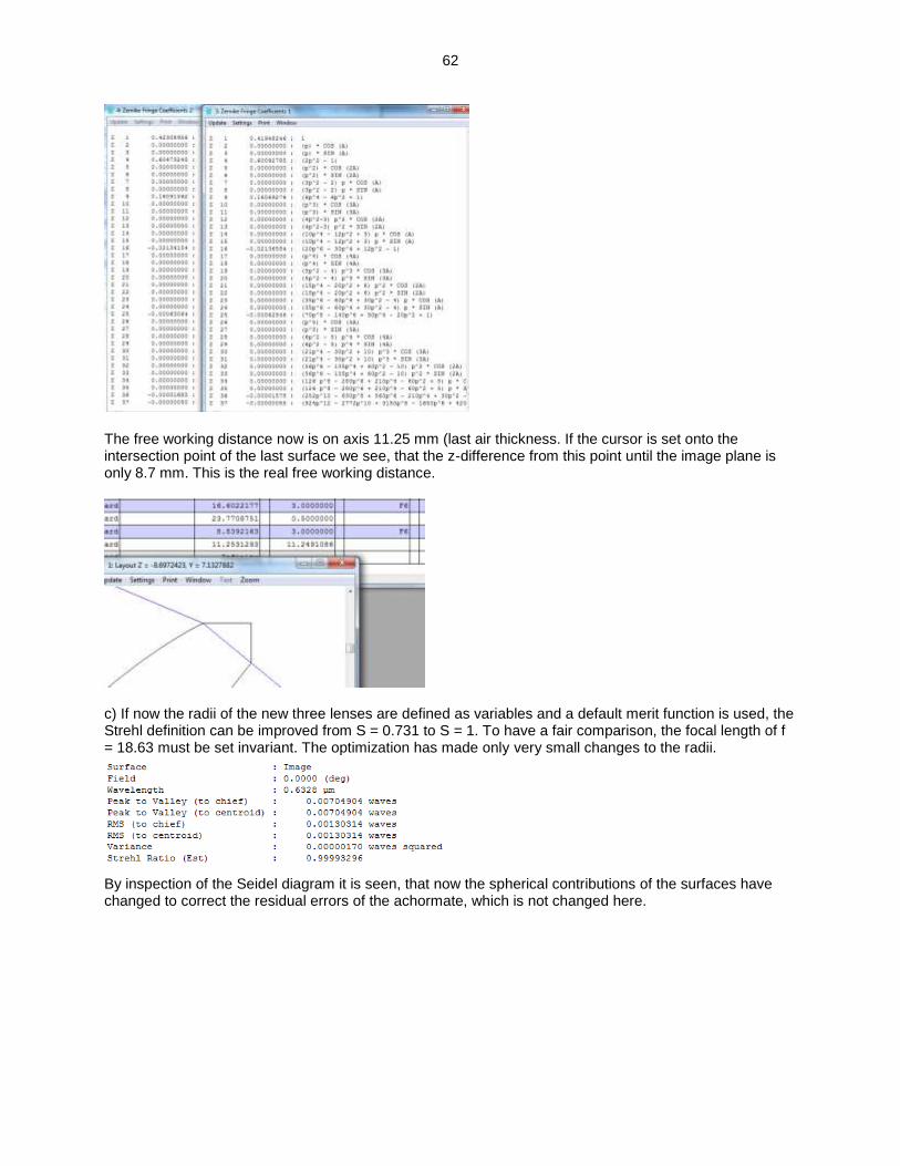
The free working distance now is on axis 11.25 mm (last air thickness. If the cursor is set onto the intersection point of the last surface we see, that the z-difference from this point until the image plane is only 8.7 mm. This is the real free working distance.

c) If now the radii of the new three lenses are defined as variables and a default merit function is used, the Strehl definition can be improved from S = 0.731 to S = 1. To have a fair comparison, the focal length of f = 18.63 must be set invariant. The optimization has made only very small changes to the radii.

By inspection of the Seidel diagram it is seen, that now the spherical contributions of the surfaces have changed to correct the residual errors of the achormate, which is not changed here.

63

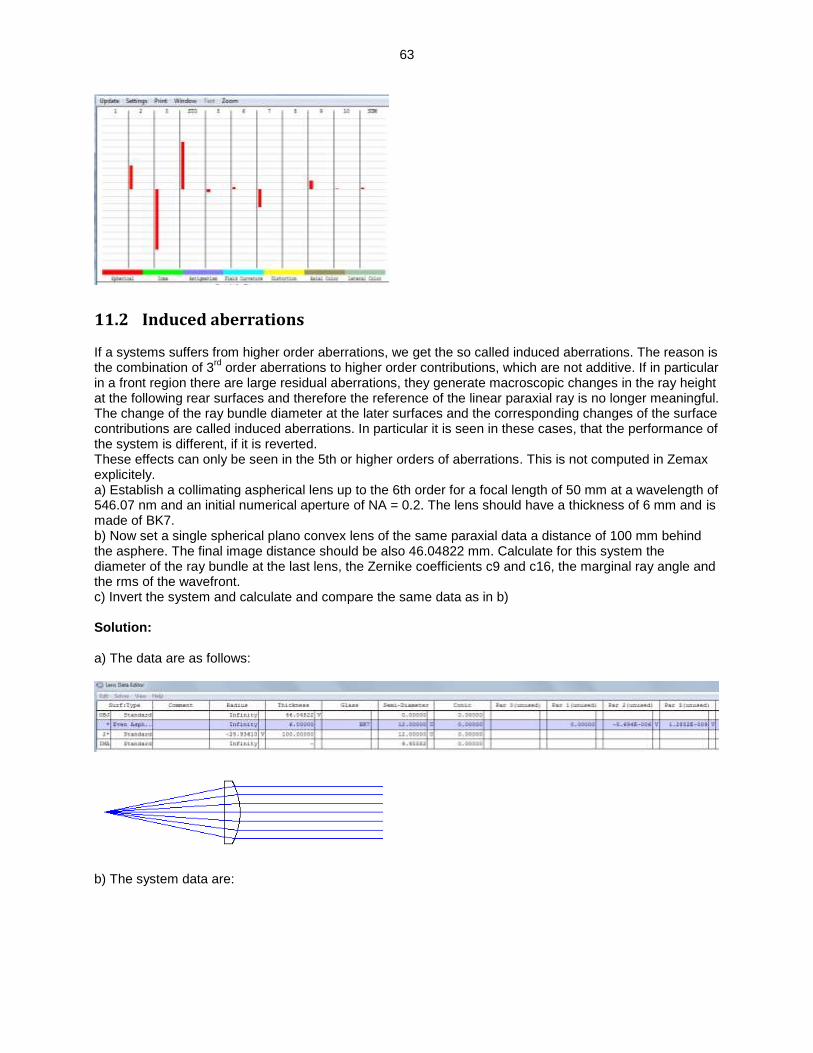
11.2 Induced aberrations If a systems suffers from higher order aberrations, we get the so called induced aberrations. The reason is the combination of 3

rd order aberrations to higher order contributions, which are not additive. If in particular

in a front region there are large residual aberrations, they generate macroscopic changes in the ray height at the following rear surfaces and therefore the reference of the linear paraxial ray is no longer meaningful. The change of the ray bundle diameter at the later surfaces and the corresponding changes of the surface contributions are called induced aberrations. In particular it is seen in these cases, that the performance of the system is different, if it is reverted. These effects can only be seen in the 5th or higher orders of aberrations. This is not computed in Zemax explicitely. a) Establish a collimating aspherical lens up to the 6th order for a focal length of 50 mm at a wavelength of 546.07 nm and an initial numerical aperture of NA = 0.2. The lens should have a thickness of 6 mm and is made of BK7. b) Now set a single spherical plano convex lens of the same paraxial data a distance of 100 mm behind the asphere. The final image distance should be also 46.04822 mm. Calculate for this system the diameter of the ray bundle at the last lens, the Zernike coefficients c9 and c16, the marginal ray angle and the rms of the wavefront. c) Invert the system and calculate and compare the same data as in b) Solution: a) The data are as follows:

b) The system data are:

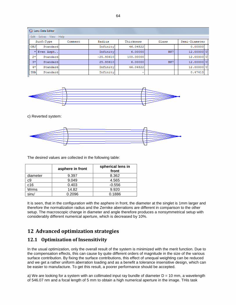
64

c) Reverted system:

The desired values are collected in the following table:

asphere in front spherical lens in

front

diameter 9.397 8.362

c9 9.049 4.565

c16 0.403 -0.556

Wrms 14.82 9.920

sinu' 0.2096 0.1886

It is seen, that in the configuration with the asphere in front, the diameter at the singlet is 1mm larger and therefore the normalization radius and the Zernike aberrations are different in comparison to the other setup. The macroscopic change in diameter and angle therefore produces a nonsymmetrical setup with considerably different numerical aperture, which is decreased by 10%.

12 Advanced optimization strategies

12.1 Optimization of Insensitivity In the usual optimization, only the overall result of the system is minimized with the merit function. Due to the compensation effects, this can cause by quite different orders of magnitude in the size of the various surface contribution. By fixing the surface contributions, this effect of unequal weighting can be reduced and we get a rather uniform aberration loading and as a benefit a tolerance insensitive design, which can be easier to manufacture. To get this result, a poorer performance should be accepted. a) We are looking for a system with an collimated input ray bundle of diameter D = 10 mm, a wavelength of 546.07 nm and a focal length of 5 mm to obtain a high numerical aperture in the image. THis task

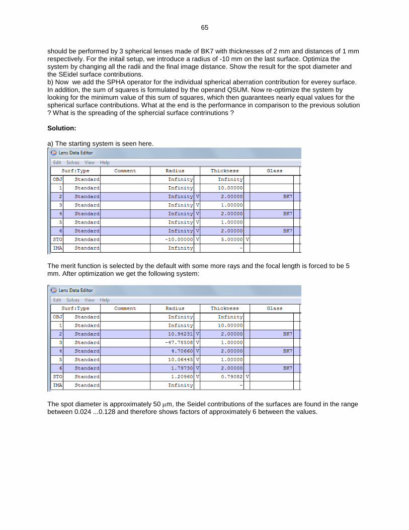
65

should be performed by 3 spherical lenses made of BK7 with thicknesses of 2 mm and distances of 1 mm respectively. For the initail setup, we introduce a radius of -10 mm on the last surface. Optimiza the system by changing all the radii and the final image distance. Show the result for the spot diameter and the SEidel surface contributions. b) Now we add the SPHA operator for the individual spherical aberration contribution for everey surface. In addition, the sum of squares is formulated by the operand QSUM. Now re-optimize the system by looking for the minimum value of this sum of squares, which then guarantees nearly equal values for the spherical surface contributions. What at the end is the performance in comparison to the previous solution ? What is the spreading of the sphercial surface contrinutions ? Solution: a) The starting system is seen here.

The merit function is selected by the default with some more rays and the focal length is forced to be 5 mm. After optimization we get the following system:

The spot diameter is approximately 50 m, the Seidel contributions of the surfaces are found in the range between 0.024 ...0.128 and therefore shows factors of approximately 6 between the values.

66

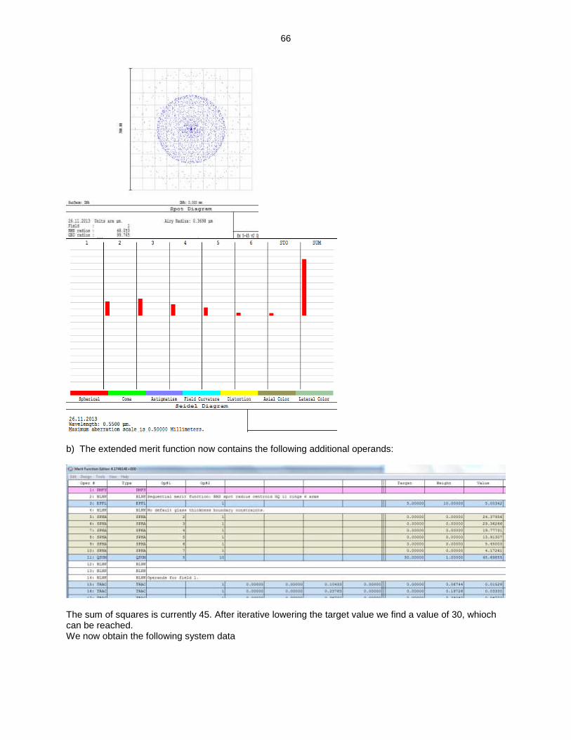
b) The extended merit function now contains the following additional operands:

The sum of squares is currently 45. After iterative lowering the target value we find a value of 30, whioch can be reached. We now obtain the following system data

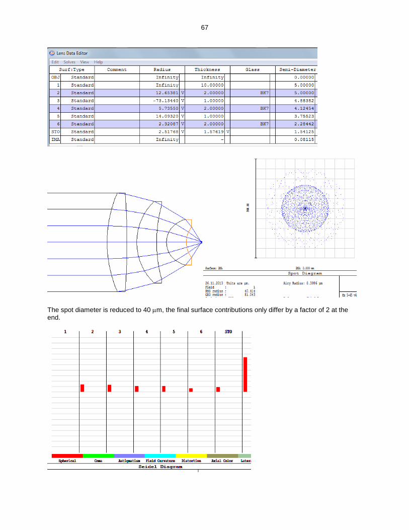
67

The spot diameter is reduced to 40 m, the final surface contributions only differ by a factor of 2 at the end.

68

It is seen by further reducing the target value for the sum of squares of the surface contribution, that the optimizations increases the focal length, which is not desired. This last iterative procedure can also be obtained by the Operand MINN, which looks for the minimum value of the sum of squares.

69

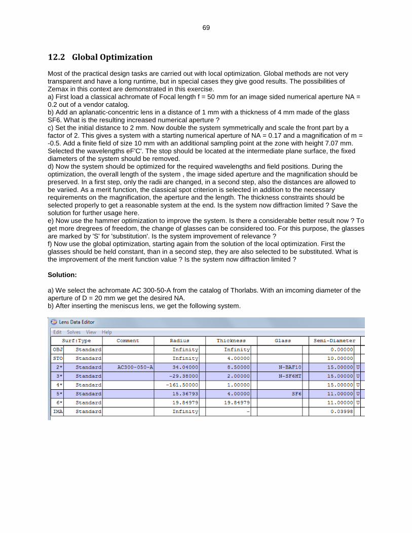
12.2 Global Optimization Most of the practical design tasks are carried out with local optimization. Global methods are not very transparent and have a long runtime, but in special cases they give good results. The possibilities of Zemax in this context are demonstrated in this exercise. a) First load a classical achromate of Focal length f = 50 mm for an image sided numerical aperture NA = 0.2 out of a vendor catalog. b) Add an aplanatic-concentric lens in a distance of 1 mm with a thickness of 4 mm made of the glass SF6. What is the resulting increased numerical aperture ? c) Set the initial distance to 2 mm. Now double the system symmetrically and scale the front part by a factor of 2. This gives a system with a starting numerical aperture of NA = 0.17 and a magnification of m = -0.5. Add a finite field of size 10 mm with an additional sampling point at the zone with height 7.07 mm. Selected the wavelengths eF'C'. The stop should be located at the intermediate plane surface, the fixed diameters of the system should be removed. d) Now the system should be optimized for the required wavelengths and field positions. During the optimization, the overall length of the system , the image sided aperture and the magnification should be preserved. In a first step, only the radii are changed, in a second step, also the distances are allowed to be variied. As a merit function, the classical spot criterion is selected in addition to the necessary requirements on the magnification, the aperture and the length. The thickness constraints should be selected properly to get a reasonable system at the end. Is the system now diffraction limited ? Save the solution for further usage here. e) Now use the hammer optimization to improve the system. Is there a considerable better result now ? To get more dregrees of freedom, the change of glasses can be considered too. For this purpose, the glasses are marked by 'S' for 'substitution'. Is the system improvement of relevance ? f) Now use the global optimization, starting again from the solution of the local optimization. First the glasses should be held constant, than in a second step, they are also selected to be substituted. What is the improvement of the merit function value ? Is the system now diffraction limited ? Solution: a) We select the achromate AC 300-50-A from the catalog of Thorlabs. With an imcoming diameter of the aperture of D = 20 mm we get the desired NA. b) After inserting the meniscus lens, we get the following system.

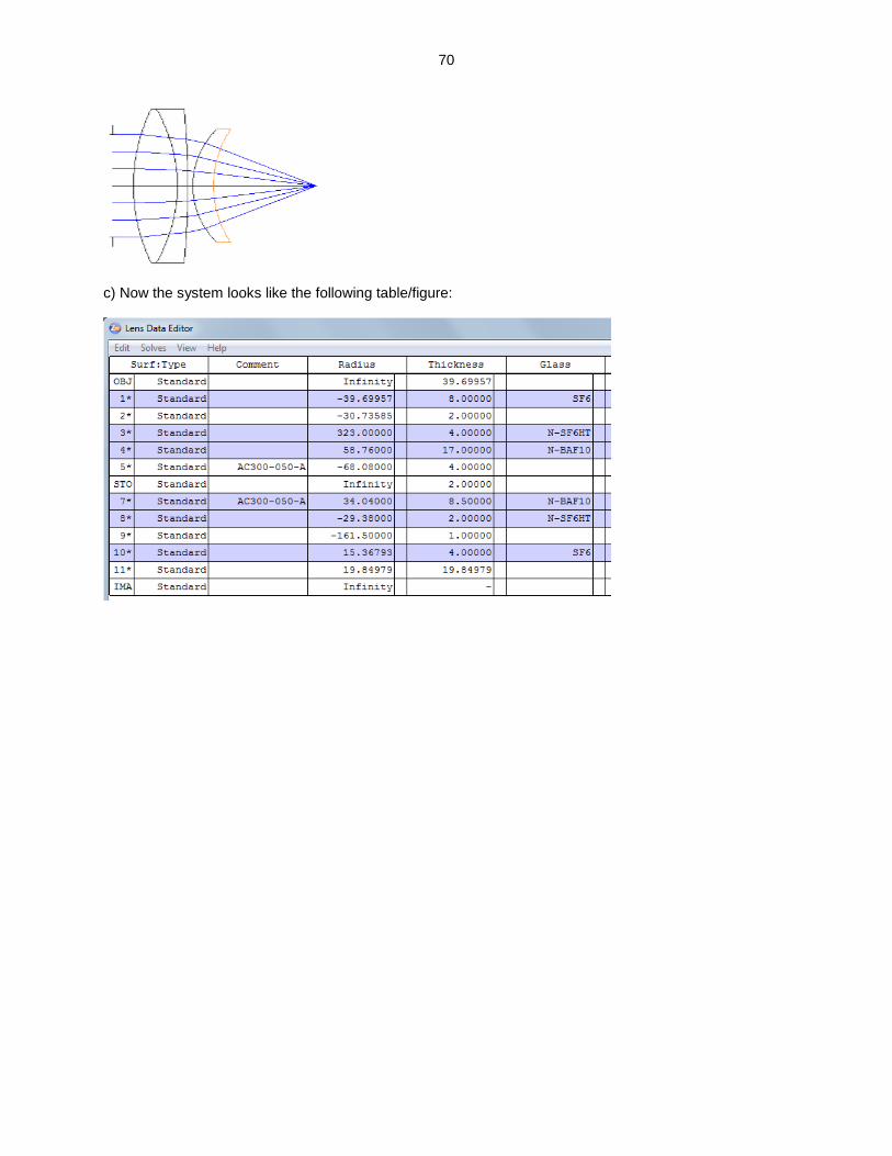
70

c) Now the system looks like the following table/figure:

71

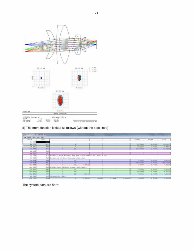
d) The merit function lokkas as follows (without the spot lines)

The system data are here:

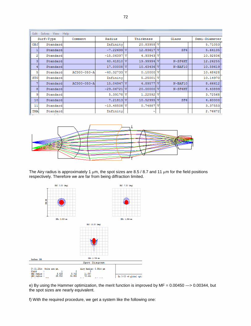
72

The Airy radius is approximately 1 m, the spot sizes are 8.5 / 8.7 and 11 m for the field positions respectively. Therefore we are far from being diffraction limited.

e) By using the Hammer optimization, the merit function is improved by MF = 0.00450 ---> 0.00344, but the spot sizes are nearly equivalent. f) With the required procedure, we get a system like the following one:

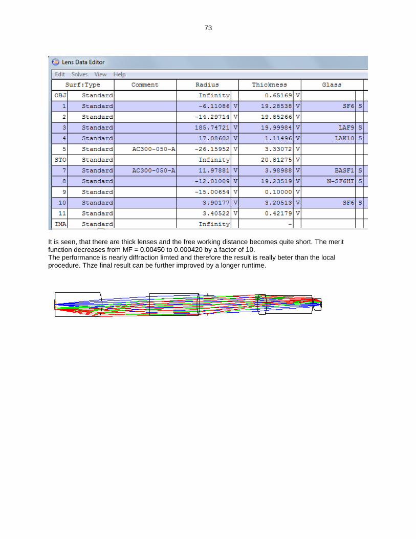
73

It is seen, that there are thick lenses and the free working distance becomes quite short. The merit function decreases from MF = 0.00450 to 0.000420 by a factor of 10. The performance is nearly diffraction limted and therefore the result is really beter than the local procedure. Thze final result can be further improved by a longer runtime.

74

13 Mirror systems

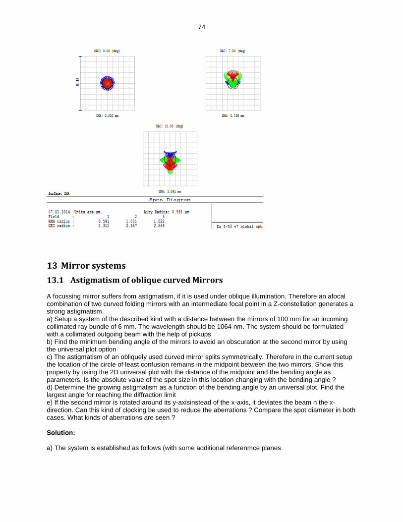
13.1 Astigmatism of oblique curved Mirrors A focussing mirror suffers from astigmatism, if it is used under oblique illumination. Therefore an afocal combination of two curved folding mirrors with an intermediate focal point in a Z-constellation generates a strong astigmatism. a) Setup a system of the described kind with a distance between the mirrors of 100 mm for an incoming collimated ray bundle of 6 mm. The wavelength should be 1064 nm. The system should be formulated with a collimated outgoing beam with the help of pickups b) Find the minimum bending angle of the mirrors to avoid an obscuration at the second mirror by using the universal plot option c) The astigmatism of an obliquely used curved mirror splits symmetrically. Therefore in the current setup the location of the circle of least confusion remains in the midpoint between the two mirrors. Show this property by using the 2D universal plot with the distance of the midpoint and the bending angle as parameters. Is the absolute value of the spot size in this location changing with the bending angle ? d) Determine the growing astigmatism as a function of the bending angle by an universal plot. Find the largest angle for reaching the diffraction limit e) If the second mirror is rotated around its y-axisinstead of the x-axis, it deviates the beam n the x-direction. Can this kind of clocking be used to reduce the aberrations ? Compare the spot diameter in both cases. What kinds of aberrations are seen ? Solution: a) The system is established as follows (with some additional referenmce planes

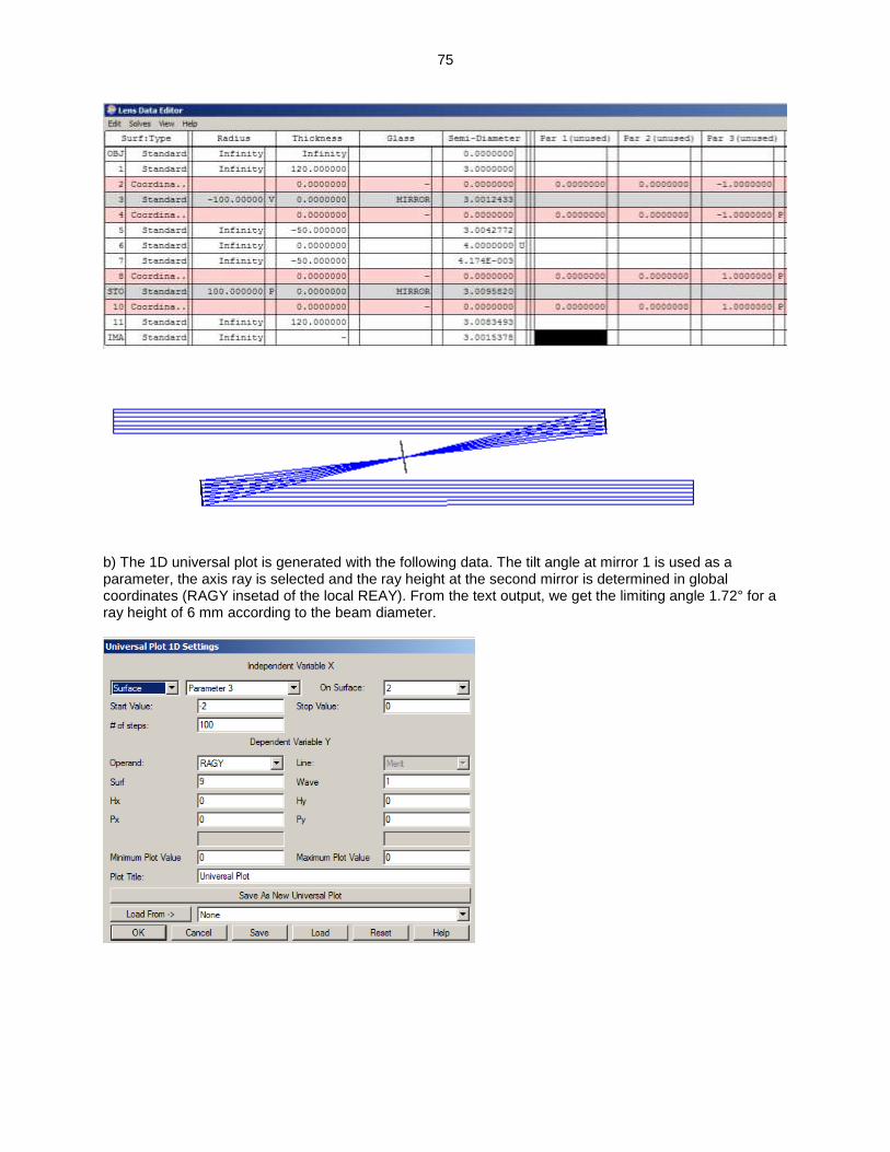
75

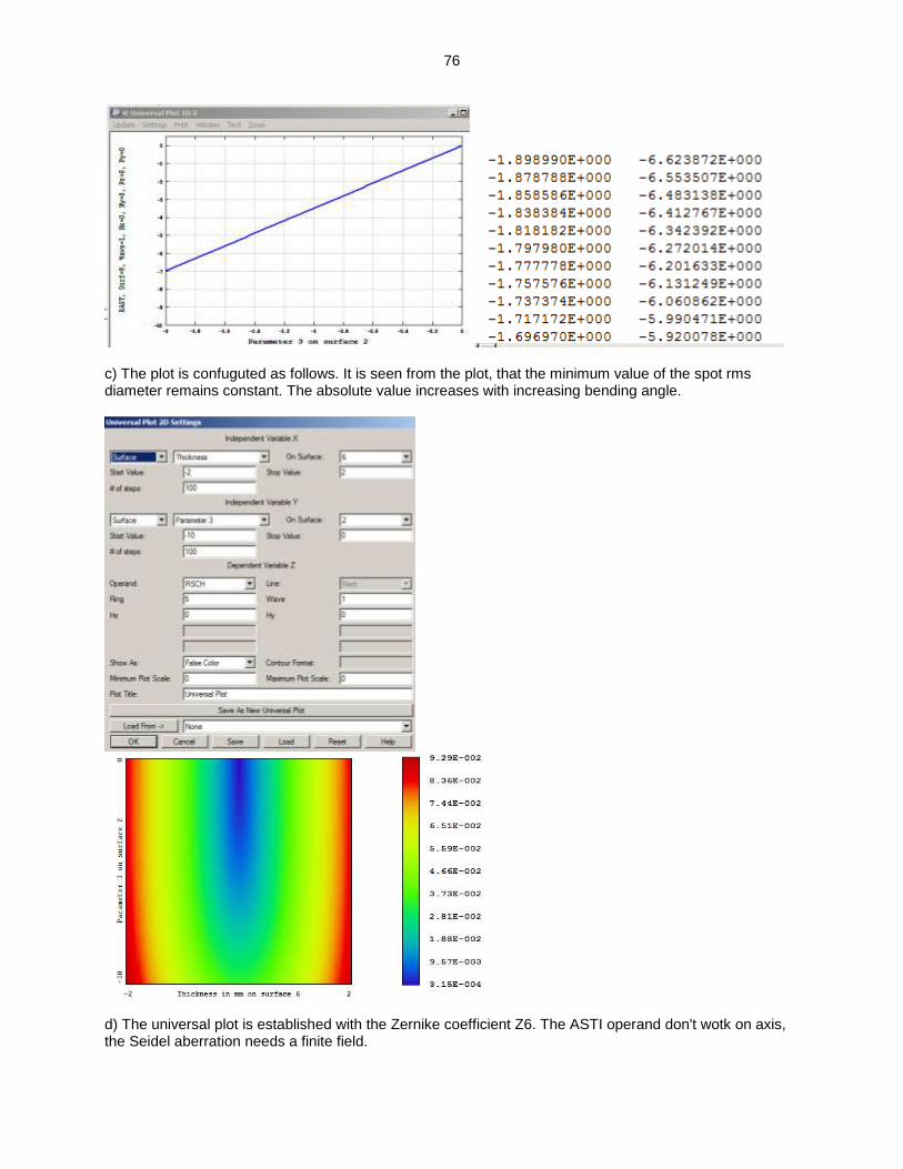
b) The 1D universal plot is generated with the following data. The tilt angle at mirror 1 is used as a parameter, the axis ray is selected and the ray height at the second mirror is determined in global coordinates (RAGY insetad of the local REAY). From the text output, we get the limiting angle 1.72° for a ray height of 6 mm according to the beam diameter.

76

c) The plot is confuguted as follows. It is seen from the plot, that the minimum value of the spot rms diameter remains constant. The absolute value increases with increasing bending angle.

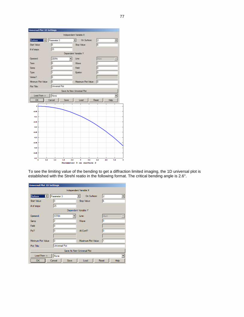
d) The universal plot is established with the Zernike coefficient Z6. The ASTI operand don't wotk on axis, the Seidel aberration needs a finite field.

77

To see the limiting value of the bending to get a diffraction limited imaging, the 1D universal plot is established with the Strehl reatio in the following format. The critical bending angle is 2.6°.

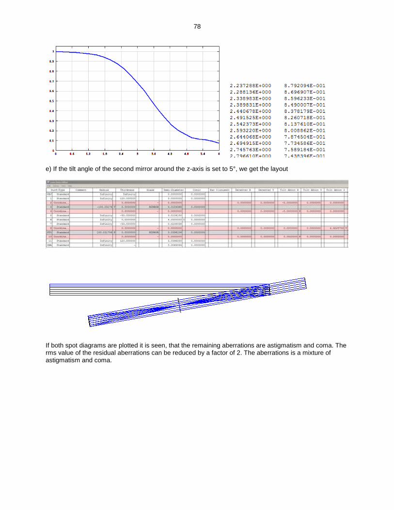
78

e) If the tilt angle of the second mirror around the z-axis is set to 5°, we get the layout

If both spot diagrams are plotted it is seen, that the remaining aberrations are astigmatism and coma. The rms value of the residual aberrations can be reduced by a factor of 2. The aberrations is a mixture of astigmatism and coma.

79

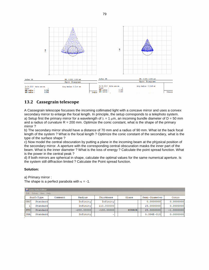
13.2 Cassegrain telescope A Cassegrain telescope focusses the incoming collimated light with a concave mirror and uses a convex secondary mirror to enlarge the focal length. In principle, the setup corresponds to a telephoto system.

a) Setup first the primary mirror for a wavelength of = 1 m, an incoming bundle diameter of D = 50 mm and a radius of curvature R = 200 mm. Optimize the conic constant, what is the shape of the primary mirror ? b) The secondary mirror should have a distance of 70 mm and a radius of 90 mm. What ist the back focal length of the system ? What is the focal length ? Optimize the conic constant of the secondary, what is the type of the surface shape ? c) Now model the central obscuration by putting a plane in the incoming beam at the phjysical position of the secondary mirror. A aperture with the corresponding central obscuration masks the inner part of the beam. What is the inner diameter ? What is the loss of energy ? Calculate the point spread function. What is the power in the central peak ? d) If both mirrors are spherical in shape, calculate the optimal values for the same numerical aperture. Is the system still diffraction limited ? Calculate the Point spread function. Solution: a) Primary mirror :

The shape is a perfect parabola with = -1.

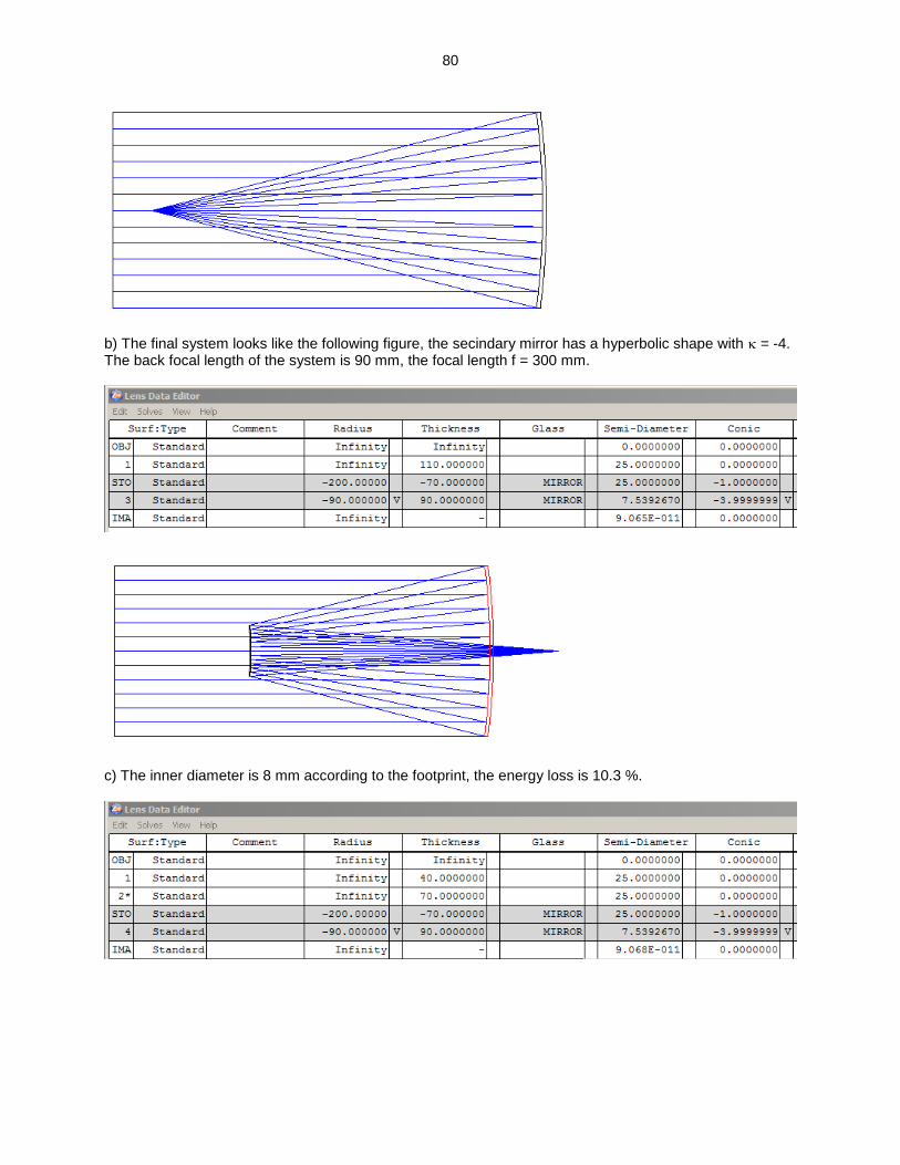
80

b) The final system looks like the following figure, the secindary mirror has a hyperbolic shape with = -4. The back focal length of the system is 90 mm, the focal length f = 300 mm.

c) The inner diameter is 8 mm according to the footprint, the energy loss is 10.3 %.

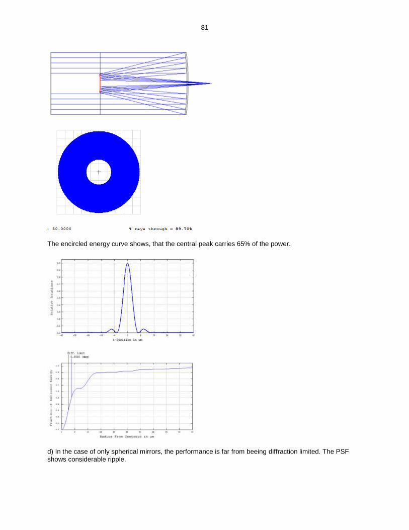
81

The encircled energy curve shows, that the central peak carries 65% of the power.

d) In the case of only spherical mirrors, the performance is far from beeing diffraction limited. The PSF shows considerable ripple.

82

14 Diffractive Elements

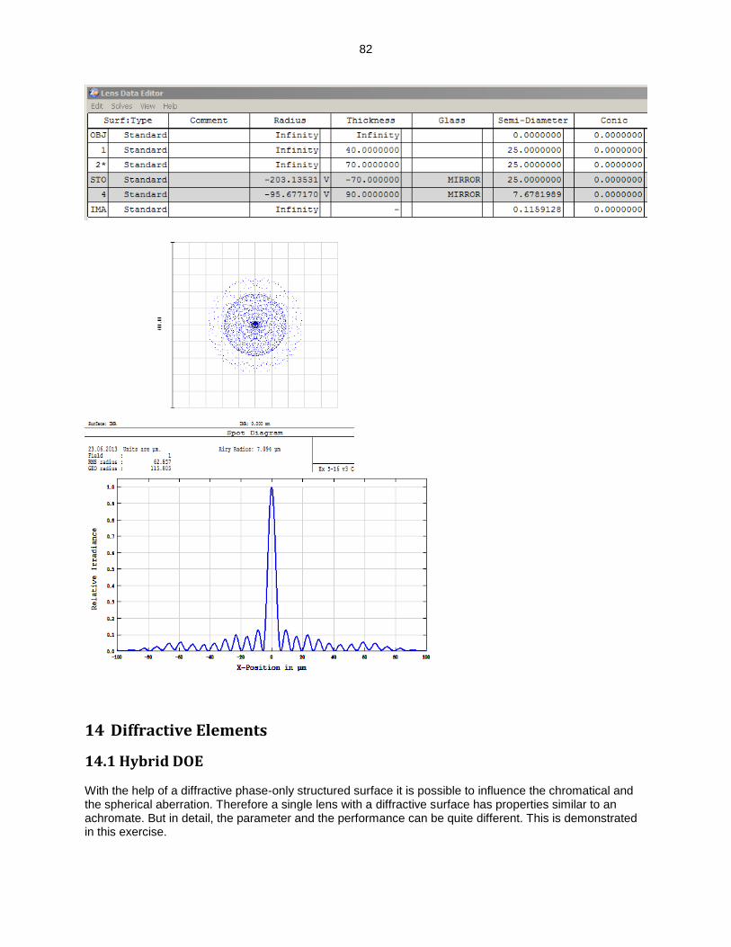
14.1 Hybrid DOE With the help of a diffractive phase-only structured surface it is possible to influence the chromatical and the spherical aberration. Therefore a single lens with a diffractive surface has properties similar to an achromate. But in detail, the parameter and the performance can be quite different. This is demonstrated in this exercise.

83

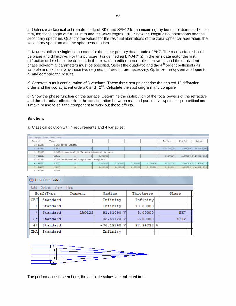
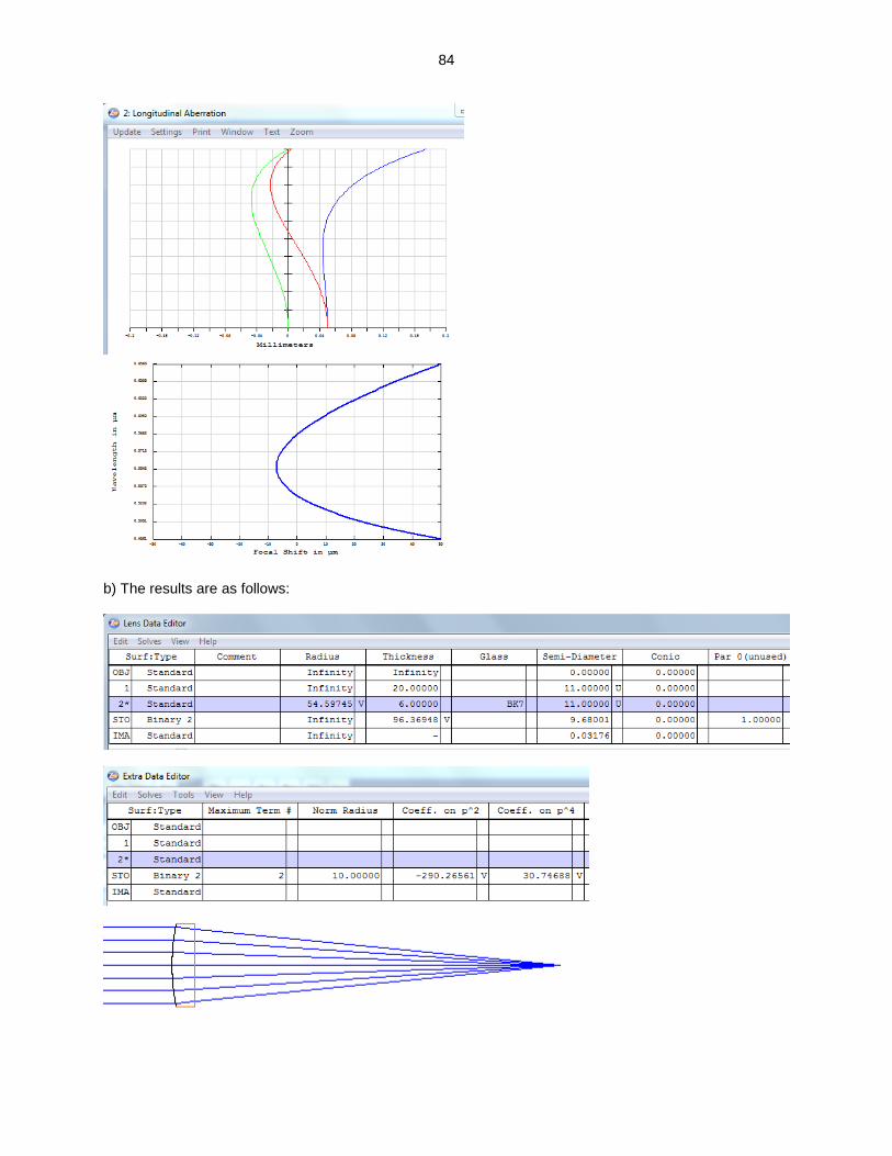
a) Optimize a classical achromate made of BK7 and SAF12 for an incoming ray bundle of diameter D = 20 mm, the focal length of f = 100 mm and the wavelengths FdC. Show the longitudinal aberrations and the secondary spectrum. Quantify the values for the residual aberrations of the zonal spherical aberration, the secondary spectrum and the spherochromatism. b) Now establish a singlet component for the same primary data, made of BK7. The rear surface should be plane and diffractive. For this purpose, it is defined as BINARY 2, in the lens data editor the first diffraction order should be defined. In the extra data editor, a normalization radius and the equivalent phase polynomial parameters must be specified. Select the quadratic and the 4

th order coefficients as

variable and explain, why these two degrees of freedom are necessary. Optimize the system analogue to a) and compare the results. c) Generate a multiconfiguration of 3 versions. These three setups describe the desired 1

st diffraction

order and the two adjacent orders 0 and +2nd

. Calculate the spot diagram and compare. d) Show the phase function on the surface. Determine the distribution of the focal powers of the refractive and the diffractive effects. Here the consideration between real and paraxial viewpoint is quite critical and it make sense to split the component to work out these effects. Solution: a) Classical solution with 4 requirements and 4 variables:

The performance is seen here, the absolute values are collected in b)

84

b) The results are as follows:

85

The peak values of the the three main residual aberrations are listed together with the classical achromate in the following table. It is seen: 1. the hybrid has a considerably larger secondary spectrum 2. the hybrid has a very small zonal spherical aberration 3. the hybrid has a larger spherochromatism The reasons for 1. + 3. is the extreme small Abbe number of the diffractive surface. In the case of the singlet, a bending of the lens can not be used to correct spherical aberration, if the DOE shoul be located on a plane surface. Therefore to be comparable with the achromate, the 4

th order

polynomial is necessary to fulfill this goal. The 4th order then is capable to correct spherical aberration

must better.

classical achromate Hybrid DOE

Secondary spectrum 60 m 153 m

spherical zone 47 m 1.3 m

spherochromatism 171 m 290 m

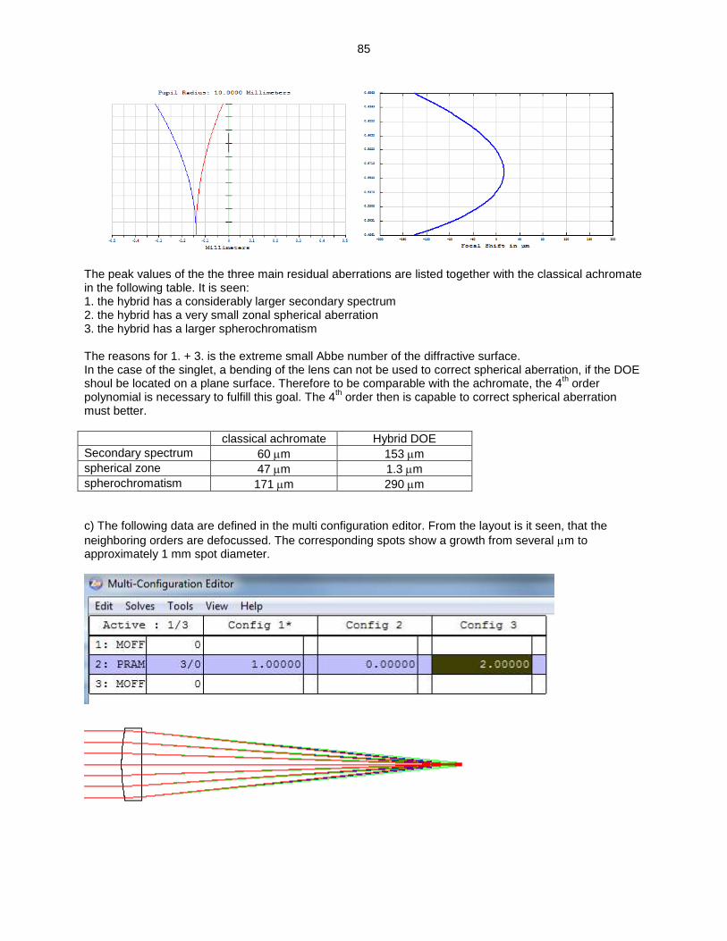
c) The following data are defined in the multi configuration editor. From the layout is it seen, that the

neighboring orders are defocussed. The corresponding spots show a growth from several m to approximately 1 mm spot diameter.

86

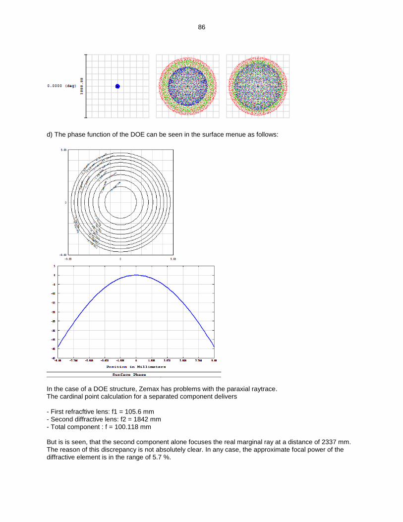
d) The phase function of the DOE can be seen in the surface menue as follows:

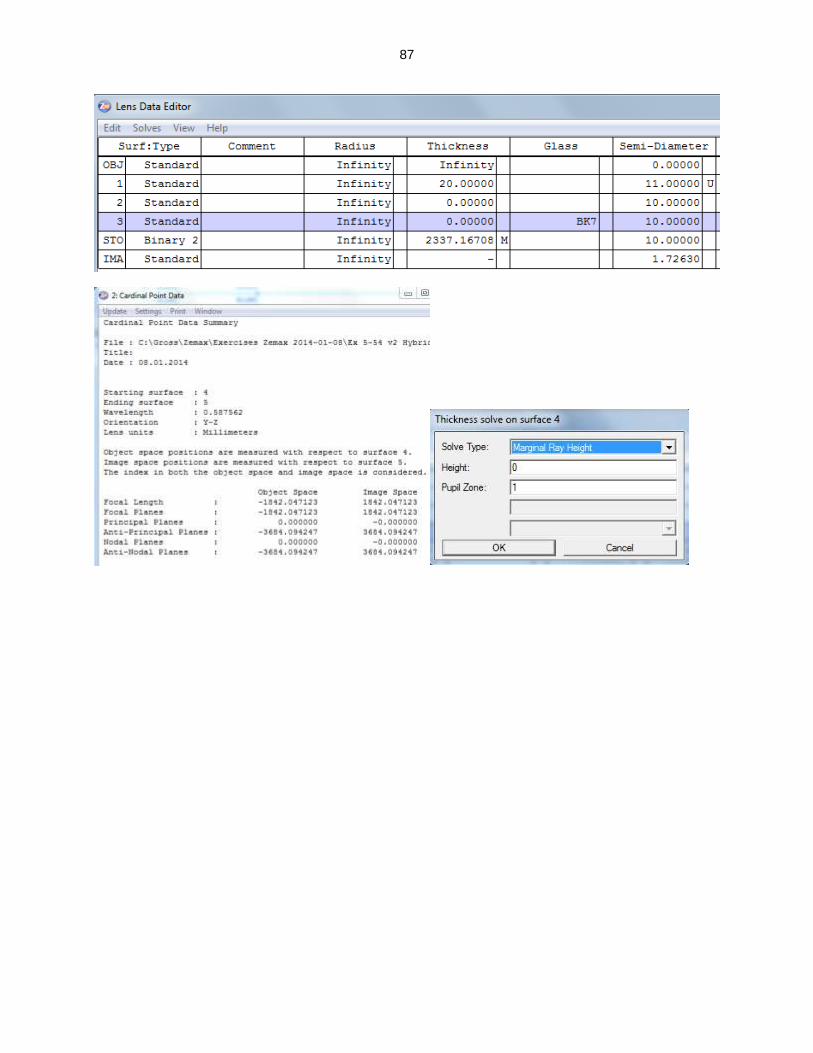
In the case of a DOE structure, Zemax has problems with the paraxial raytrace. The cardinal point calculation for a separated component delivers - First refracftive lens: f1 = 105.6 mm - Second diffractive lens: f2 = 1842 mm - Total component : f = 100.118 mm But is is seen, that the second component alone focuses the real marginal ray at a distance of 2337 mm. The reason of this discrepancy is not absolutely clear. In any case, the approximate focal power of the diffractive element is in the range of 5.7 %.

87

88

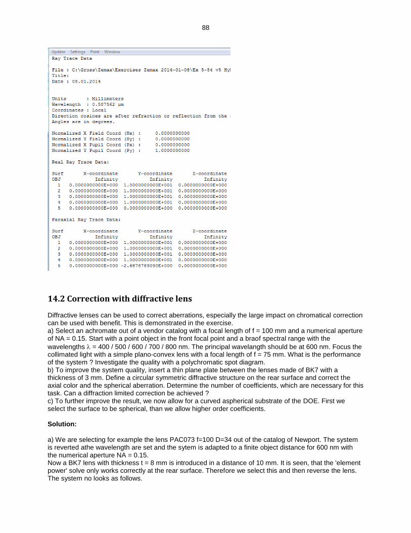
14.2 Correction with diffractive lens Diffractive lenses can be used to correct aberrations, especially the large impact on chromatical correction can be used with benefit. This is demonstrated in the exercise. a) Select an achromate out of a vendor catalog with a focal length of f = 100 mm and a numerical aperture of NA = 0.15. Start with a point object in the front focal point and a braof spectral range with the

wavelengths = 400 / 500 / 600 / 700 / 800 nm. The principal wavelangth should be at 600 nm. Focus the collimated light with a simple plano-convex lens with a focal length of f = 75 mm. What is the performance of the system ? Investigate the quality with a polychromatic spot diagram. b) To improve the system quality, insert a thin plane plate between the lenses made of BK7 with a thickness of 3 mm. Define a circular symmetric diffractive structure on the rear surface and correct the axial color and the spherical aberration. Determine the number of coefficients, which are necessary for this task. Can a diffraction limited correction be achieved ? c) To further improve the result, we now allow for a curved aspherical substrate of the DOE. First we select the surface to be spherical, than we allow higher order coefficients. Solution: a) We are selecting for example the lens PAC073 f=100 D=34 out of the catalog of Newport. The system is reverted athe wavelength are set and the sytem is adapted to a finite object distance for 600 nm with the numerical aperture NA = 0.15. Now a BK7 lens with thickness t = 8 mm is introduced in a distance of 10 mm. It is seen, that the 'element power' solve only works correctly at the rear surface. Therefore we select this and then reverse the lens. The system no looks as follows.

89

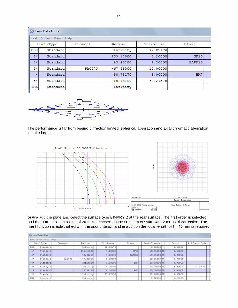
The performance is far from beeing diffraction limited, spherical aberration and axial chromatic aberration is quite large.

b) We add the plate and select the surface type BINARY 2 at the rear surface. The first order is selected and the normalization radius of 20 mm is chosen. In the first step we start with 2 terms of correction. The merit function is established with the spot criterion and in addition the focal length of f = 46 mm is required.

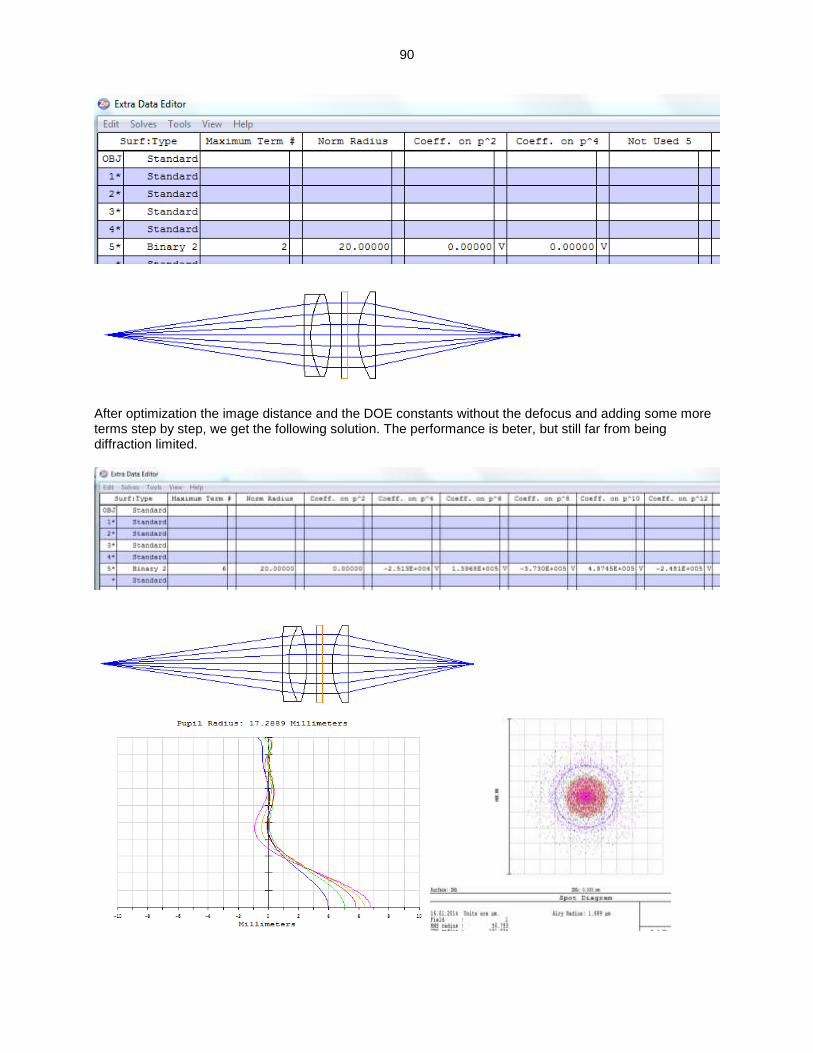
90

After optimization the image distance and the DOE constants without the defocus and adding some more terms step by step, we get the following solution. The performance is beter, but still far from being diffraction limited.

91

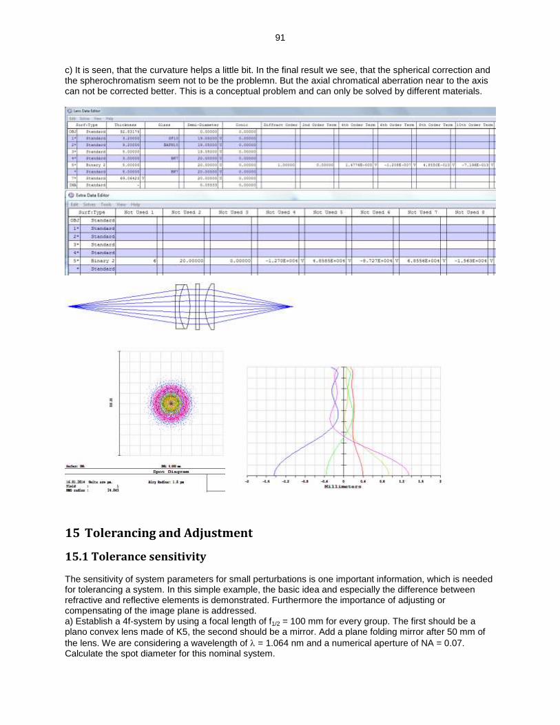
c) It is seen, that the curvature helps a little bit. In the final result we see, that the spherical correction and the spherochromatism seem not to be the problemn. But the axial chromatical aberration near to the axis can not be corrected better. This is a conceptual problem and can only be solved by different materials.

15 Tolerancing and Adjustment

15.1 Tolerance sensitivity The sensitivity of system parameters for small perturbations is one important information, which is needed for tolerancing a system. In this simple example, the basic idea and especially the difference between refractive and reflective elements is demonstrated. Furthermore the importance of adjusting or compensating of the image plane is addressed. a) Establish a 4f-system by using a focal length of f1/2 = 100 mm for every group. The first should be a plano convex lens made of K5, the second should be a mirror. Add a plane folding mirror after 50 mm of

the lens. We are considering a wavelength of = 1.064 nm and a numerical aperture of NA = 0.07. Calculate the spot diameter for this nominal system.

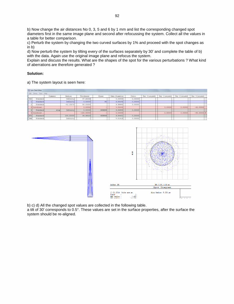
92

b) Now change the air distances No 0, 3, 5 and 6 by 1 mm and list the corresponding changed spot diameters first in the same image plane and second after refocussing the system. Collect all the values in a table for better comparison. c) Perturb the system by changing the two curved surfaces by 1% and proceed with the spot changes as in b) d) Now perturb the system by tilting every of the surfaces separately by 30' and complete the table of b) with the data. Again use the original image plane and refocus the system. Explain and discuss the results. What are the shapes of the spot for the various perturbations ? What kind of aberrations are therefore generated ? Solution: a) The system layout is seen here:

b) c) d) All the changed spot values are collected in the following table. a tilt of 30' corresponds to 0.5°. These values are set in the surface properties, after the surface the system should be re-aligned.

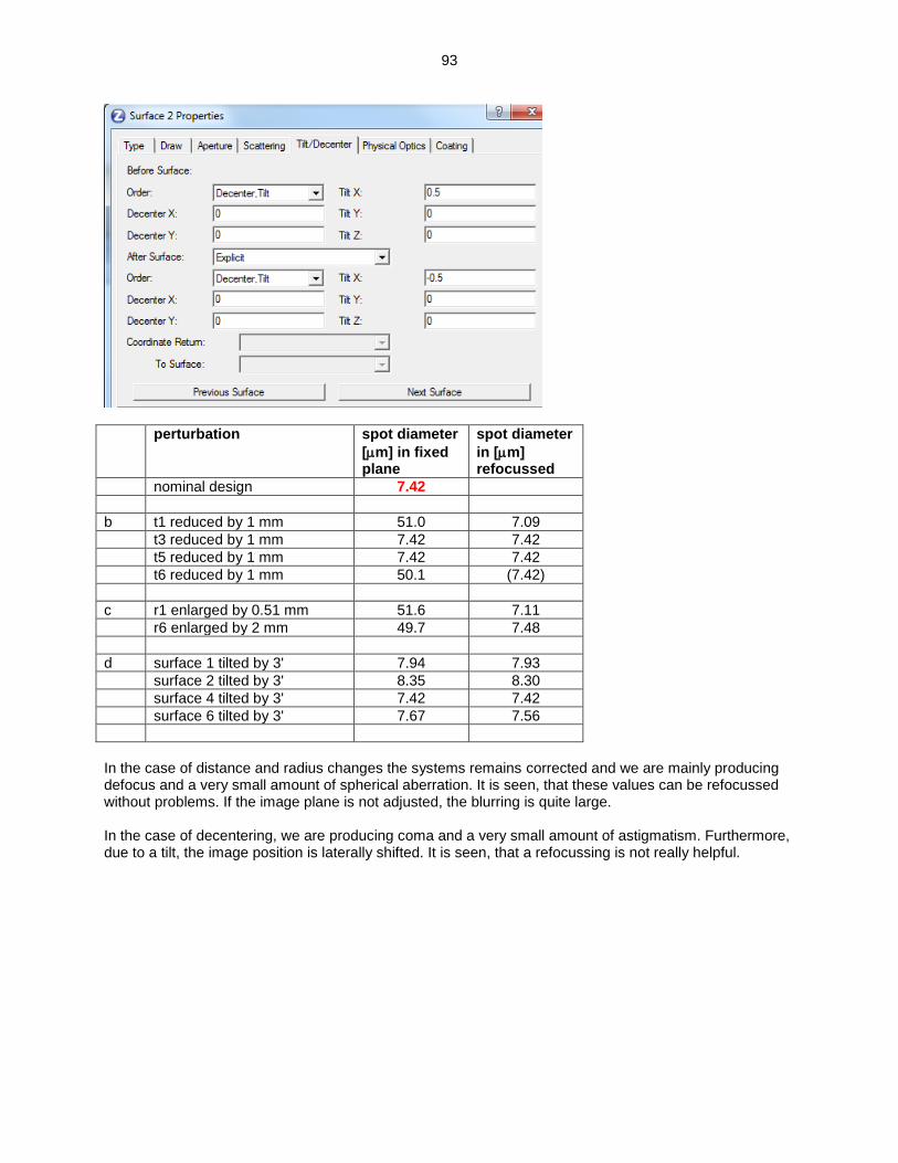
93

perturbation spot diameter

[m] in fixed plane

spot diameter

in [m] refocussed

nominal design 7.42

b t1 reduced by 1 mm 51.0 7.09

t3 reduced by 1 mm 7.42 7.42

t5 reduced by 1 mm 7.42 7.42

t6 reduced by 1 mm 50.1 (7.42)

c r1 enlarged by 0.51 mm 51.6 7.11

r6 enlarged by 2 mm 49.7 7.48

d surface 1 tilted by 3' 7.94 7.93

surface 2 tilted by 3' 8.35 8.30

surface 4 tilted by 3' 7.42 7.42

surface 6 tilted by 3' 7.67 7.56

In the case of distance and radius changes the systems remains corrected and we are mainly producing defocus and a very small amount of spherical aberration. It is seen, that these values can be refocussed without problems. If the image plane is not adjusted, the blurring is quite large. In the case of decentering, we are producing coma and a very small amount of astigmatism. Furthermore, due to a tilt, the image position is laterally shifted. It is seen, that a refocussing is not really helpful.

94

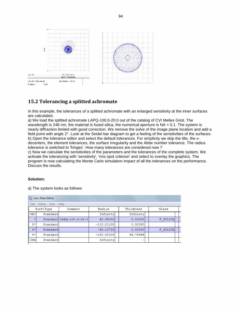
15.2 Tolerancing a splitted achromate In this example, the tolerances of a splitted achromate with an enlarged sensitivity at the inner surfaces are calculated. a) We load the splitted achromate LAPQ-100.0-20.0 out of the catalog of CVI Melles Griot. The wavelength is 248 nm, the material is fused silica, the numerical aperture is NA = 0.1. The system is nearly diffraction limited with good correction. We remove the solve of the image plane location and add a field point with angle 2°. Look at the Seidel bar diagram to get a feeling of the sensitivities of the surfaces. b) Open the tolerance editor and select the default tolerances. For simplicity we skip the tilts, the x-decenters, the element tolerances, the surface irregularity and the Abbe number tolerance. The radius tolerance is switched to 'fringes'. How many tolerances are considered now ? c) Now we calculate the sensitivities of the parameters and the tolerances of the complete system. We activate the tolerancing with 'sensitivity', 'rms spot criterion' and select to overlay the graphics. The program is now calculating the Monte Carlo simulation impact of all the tolerances on the performance. Discuss the results. Solution: a) The system looks as follows:

95

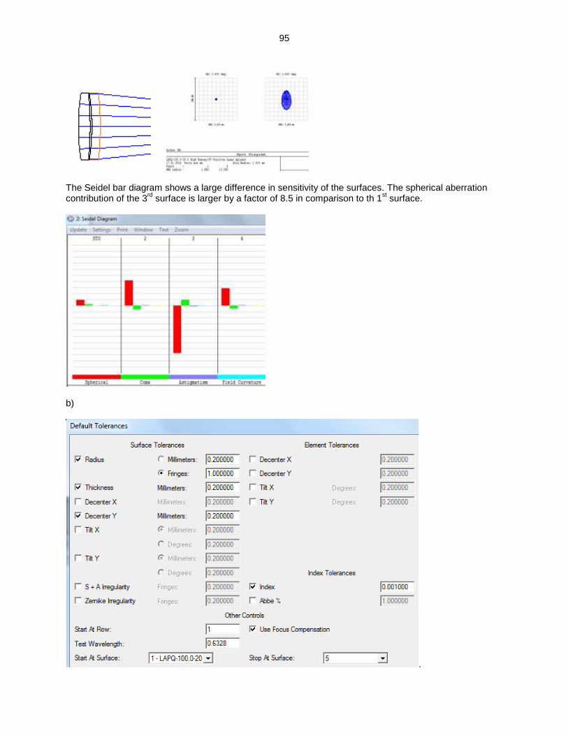
The Seidel bar diagram shows a large difference in sensitivity of the surfaces. The spherical aberration contribution of the 3

rd surface is larger by a factor of 8.5 in comparison to th 1

st surface.

b)

.

96

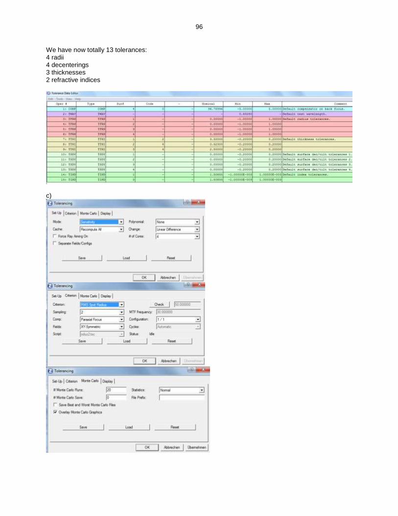
We have now totally 13 tolerances: 4 radii 4 decenterings 3 thicknesses 2 refractive indices

c)

97

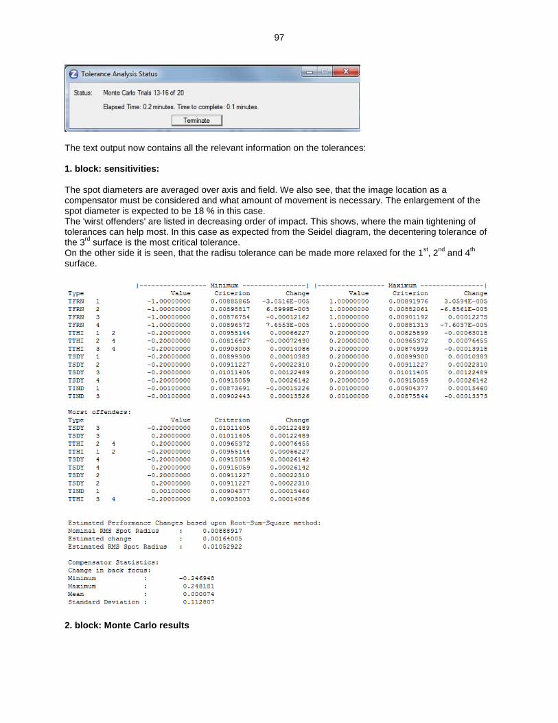
The text output now contains all the relevant information on the tolerances: 1. block: sensitivities: The spot diameters are averaged over axis and field. We also see, that the image location as a compensator must be considered and what amount of movement is necessary. The enlargement of the spot diameter is expected to be 18 % in this case. The 'wirst offenders' are listed in decreasing order of impact. This shows, where the main tightening of tolerances can help most. In this case as expected from the Seidel diagram, the decentering tolerance of the 3

rd surface is the most critical tolerance.

On the other side it is seen, that the radisu tolerance can be made more relaxed for the 1st, 2

nd and 4

th

surface.

2. block: Monte Carlo results

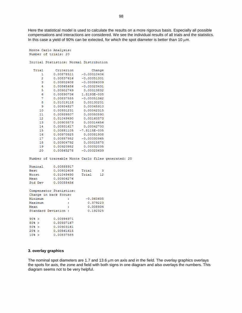
98

Here the statistical model is used to calculate the results on a more rigorous basis. Especially all possible compensations and interactions are considered. We see the individual results of all trials and the statistics.

In this case a yield of 90% can be extected, for which the spot diameter is better than 10 m.

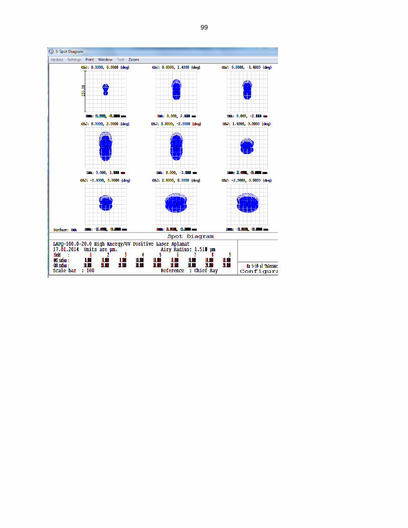
3. overlay graphics

The nominal spot diameters are 1.7 and 13.6 m on axis and in the field. The overlay graphics overlays the spots for axis, the zone and field with both signs in one diagram and also overlays the numbers. This diagram seems not to be very helpful.

99