Embed Size (px)
Citation preview
Explaining Sudden Spikes in Global
Risk1
Philippe Bacchetta
University of Lausanne
CEPR
Eric van Wincoop
University of Virginia
NBER
November 9, 2010
1We would like to thank Martina Insam for able research assistance, Michael Dev-
ereux and Fabio Ghironi for their comments, as well as other participants at the ECB
conference “What Future for Financial Globalization?” for questions and comments. We
gratefully acknowledge financial support from the National Science Foundation (grant
SES-0649442), the Hong Kong Institute for Monetary Research, the National Centre
of Competence in Research “Financial Valuation and Risk Management” (NCCR FIN-
RISK), and the Swiss Finance Institute.
Abstract
The sharp drop in equity prices across the globe during the 2008 financial crisis
coincides with a spike in equity price risk (VIX) of similar magnitude across a broad
set of developing and developed countries. This spike in risk across many countries
appears unrelated to a sudden shift in fundamentals and does not appear to be the
result of a transmission of shocks across countries through financial markets. In
this paper we provide an explanation for this phenomenon by developing a model
that allows for the possibility of large self-fulfilling shifts in risk. This builds on
Bacchetta, Tille and van Wincoop (2010), who develop the concept of risk panics in
a closed economy framework. During such a panic a weak macro variable becomes
a focal point (coordination device) for a self-fulfilling increase in perceived risk.
We show that when macro fundamentals have a limited impact on equity prices
during normal times, the risk panic will impact countries very similarly.

1 Introduction
The financial panic in the Fall of 2008 lead to a sharp drop in equity prices and an
increase in perceived risk around the world. It has been widely documented that
the magnitude of the equity price decline was broadly similar across the globe.
What is perhaps less known is that the spike in asset price risk, as measured by
implied volatility measures (e.g., VIX in the US), was also of similar magnitude
across a broad set of countries. This is illustrated in Figure 1 for a group of
12 developed and developing countries.1 The close co-movement in equity prices
during this period was clearly related to the co-movement in risk. Beyond the
recent crisis, there is a substantial econometric literature which has shown that
asset price volatility co-moves significantly across countries, especially during high
volatility periods.2
Two features stand out regarding the global spike in risk during recent financial
crises. First, it is hard to attribute to a sudden shift in fundamentals. The health
of leveraged financial institutions was weak during the panic in the Fall of 2008,
but had gradually deteriorated for at least a year prior to that. The same can be
said for the spike in global risk during the Spring of 2010 that has been associated
with the health of the Greek public sector. The fiscal problems in Greece had
developed for a long time and did not suddenly arise in the Spring of 2010. The
second feature is that the global spike in risk does not appear to be the result of a
transmission of shocks across countries through financial linkages. As documented
by Rose and Spiegel (2010) and Kamin and Pounder (2010), there is no evidence
that countries with larger cross-border financial linkages to the United States saw
a bigger drop in equity prices during the 2008 crisis.
The goal of this paper is to develop a framework that is consistent with these
stylized facts. We aim to develop a model that generates a sharp spike in risk
simultaneously across the globe, that is not the result of sudden large fundamental
shocks, and whose global dimension is not associated with the transmission of
shocks through financial markets. In our model a global risk panic takes the form
of a self-fulfilling increase in risk perceptions around the world that occurs when a
1Data sources are reported in Appendix C.2See for example Edwards and Susmel (2001), Beirne et al. (2009) or Diebold and Yilmaz
(2009). Soriano and Climent (2006) provide a survey of this literature.
1
particularly weak macro variable in some country becomes the sudden focal point
of the market.
The paper builds on Bacchetta, Tille, and van Wincoop (2010), from here on
BTW, who develop the concept of risk panics in a closed economy context. BTW
show that as long as asset demand depends on asset price risk, self-fulfilling shifts
in risk are possible. In this case there is a dynamic mapping of risk into itself,
because the risk associated with the future asset price depends on uncertainty
about future risk. During a risk panic, a weak fundamental suddenly takes on the
additional role of a coordination device for the self-fulfilling shift in risk. BTW
show that the weaker the fundamental, the larger is the panic.
Some of the recent literature on financial contagion, which we review in Section
2, has explained the co-movement in equity prices during recent crises with the
co-movement in risk premia. This focus is well placed as it is hard to argue that
either of the two other asset pricing determinants, the risk-free rate and expected
dividends, can account for the equity price co-movement. But movements in risk
play little or no role in the risk premia considered in the literature.
In this paper we also attribute equity price co-movement to co-movement in risk
premia. But, motivated by the stylized facts presented in the opening paragraphs,
we depart from the recent literature along three important dimensions. First, in
our model fluctuations in risk premia (and especially their spikes during a panic)
are explicitly linked to fluctuations in asset price risk itself. This is motivated by
the sharp increase in equity price risk across the globe during the recent crises,
as documented in Figure 1. Understanding the fluctuations in asset price risk,
and their commonality across countries, then becomes the central aspect of our
analysis.
Second, in our theory the co-movement in equity price risk is not a result of
the transmission of a shock in one country to other countries. Rather, some event
draws the attention of investors around the globe to a variable (or set of variables)
in a particular country, such as the health of financial institutions in the United
States or fiscal debt in Greece. When this variable is particularly weak, it can lead
to a simultaneous panic across the globe, with a widespread increase in perceived
equity price risk and drop in equity prices. This aspect of our model is consistent
with the fact that regular transmission channels through financial markets do not
appear to have played a central role.
2
Third, in our model a panic generates entirely self-fulfilling shifts in risk and
equity prices while the recent contagion literature relies on shocks to observed
macro fundamentals (i.e., technology shocks). As emphasized above, the panic in
the Fall of 2008 came quite unexpectedly and is hard to attribute to a sudden large
shock to macro fundamentals.
We want to emphasize that our model is not aimed at providing a full account
of what happened during the 2008 panic. Most observers would argue that a key
aspect of the crisis was a run on wholesale bank deposits (e.g. through repo con-
tracts), an aspect that is entirely absent from our model. Security complexity
issues and adverse selection combined to generate a sharp increase in haircuts on
many asset backed securities, reducing their values and making them effectively in-
eligible as collateral. We believe that it is important to distinguish what happened
in the equity market from what happened to asset backed securities. Security
complexity issues did not apply to equity and only a small fraction of the equity
market was held by these leveraged financial institutions. Moreover, when global
risk more than tripled in the Spring of 2010, there was no bank panic at all. There
just needs to be some variable, or set of variables, that becomes a natural focal
point of the market and generates a level of “fear” that implies a self-fulfilling
increase in perceived risk. It is no wonder that the VIX is often referred to as the
“fear factor”.
The particular model that we use to derive our results is sufficiently stylized to
allow for a closed form analytical solution. This makes the mechanisms at work
easier to understand for what is otherwise a quite difficult topic. We consider a two-
country model where investors trade equity claims with exogenous and stochastic
dividends. Two simplifying assumptions are an OLG structure and a constant
interest rate on bonds. BTW show that relaxing the latter assumption is not
central to risk panics.
The only stochastic fundamental is the dividend on equity. The role this fun-
damental plays during a panic is as a coordination device for a self-fulfilling shift
in risk. As emphasized by BTW, the precise nature of the macro variable that be-
comes the focal point for a risk panic is not so important. They show that results
are similar when the key macro fundamental is the net worth of leveraged financial
institutions, which fits more closely to the 2008 crisis. Focusing on stochastic div-
idends as the only source of macro shocks has the advantage of making the model
3

more standard and analytically tractable.
We analyze the factors that determine how much individual countries are af-
fected by the global panic. An important dimension is the hedging property of a
country asset with respect to the global portfolio. If assets have similar hedging
properties, their price collapse in a panic will be of similar magnitude. We show
that a condition for these hedging properties to be similar is that macro funda-
mentals have limited explanatory power for equity prices during normal times. In
that case a global risk panic can affect countries similarly.
The remainder of the paper is organized as follows. Section 2 reviews the
recent literature on financial contagion. Section 3 describes the model. Section 4
discusses the solution for the world equity price and global risk panics. Section
5 discusses the solution of the equity prices of the two countries. It particularly
it focuses on how a global risk panic affects the countries individually. Section 6
concludes.
2 Related Literature
In this section we discuss two related literatures. The first is the recent literature
on financial contagion. The second is the general literature on multiple equilibria
and self-fulfilling shifts in expectations.
2.1 Recent Financial Contagion Literature
The recent financial crisis has spurred renewed interest in the issue of financial
contagion.3 The vast existing literature4 is being extended, drawing lessons from
recent events. This renewed interest in contagion is not surprising as movements
in equity prices across the globe were highly synchronized during the Fall of 2008.
A striking feature however, especially in light of Figure 1, is that the theoretical
literature gives little attention to asset price risk. Co-movement of asset prices is
not associated in the literature with co-movements of risk.
3There is no precise or agreed-upon definition of contagion, but we think of it as a situation
where a shock in one country affects other countries through various channels.4See Dornbusch et al. (2000) or Karolyi (2003) for surveys.
4
Nonetheless the recent crisis has lead the literature to put more emphasis on
common shifts in risk premia to explain asset price co-movements. These shifts
in risk premia are not associated with asset price risk itself, but rather operate
through wealth effects often due to financial frictions. This channel was suggested
by Calvo (1999) in the context of the Russian virus and later by Krugman (2008) to
explain the co-movement of equity prices during the recent crisis.5 More formally
in general equilibrium frameworks, this channel of contagion appears in Gromb
and Vayanos (2002), Kyle and Xiong (2001) and Pavlova and Rigobon (2008).
To understand this wealth channel, assume that the Home equity price goes
down, for example due to a negative earnings shock. This reduces the wealth of
Home investors, which reduces their demand for Foreign equity through a wealth
effect. Similarly, to the extent that Foreign investors hold Home equity, it also
reduces their wealth, which again reduces demand for Foreign equity. This leads
to a drop in the Foreign equity price. Risk premia and wealth are related as
reduced wealth implies that the holdings of risky assets increase relative to wealth.
This leads to higher risk premia.
This explanation for contagion during the recent crisis has an important limi-
tation though. The contagion relies critically on the presence of large cross-border
asset holdings. However, Rose and Spiegel (2010) and Kamin and Pounder (2010)
find that larger cross-border asset exposure to the U.S. did not increase the extent
to which stock prices were affected by the crisis. This has lead to a search for
additional contagion channels operating through risk premia that do not depend
on the extent of cross-border asset holdings.6
Dedola and Lombardo (2010) develop a model where financial intermediaries
charge an “external finance premium” to investors, which is basically a risk pre-
mium. As investors’ wealth decreases (negative technology shock), a higher risk
premium on both Home and Foreign equity implies a common drop in their prices.
The extent of equity price risk does not affect the finance premium, which is only
5In Calvo (1999), price movements are exacerbated by imperfect information by investors.
See King and Wadwhani (1990) or Calvo and Mendoza (2000) for models explaining contagion
based on limited information.6While Rose and Spiegel (2010) and Kamin and Pounder (2010) consider the impact of the
crisis on stock prices across countries, most of the empirical literature on contagion in the recent
financial crises focuses on the impact on real variables like output growth. See for example Lane
and Milesi-Ferretti (2010), Imbs (2010), or Giannone et al. (2010).
5

an exogenous function of wealth. A similar mechanism is present in Devereux
and Yetman (2010) and Mendoza and Quadrini (2010). In Devereux and Yetman
(2010) investors face a leverage or borrowing constraint. A lower wealth implies a
tighter constraint and higher risk premia on all risky assets held by investors. This
is because the borrowing constraint makes no distinction between the riskiness of
Home versus Foreign equity.
In these papers the implied risk premia are the same for Home and Foreign
equity independently of the extent of cross-border asset holdings. However, this
is essentially by assumption as the finance premium or the borrowing constraint
makes no distinction between the riskiness of Home and Foreign assets. In reality
borrowing constraints depend on the riskiness of the assets held by investors as
well as their exposure to individual assets. This is true both for collateralized
and uncollateralized lending. Risk premia will then differ across assets. Conta-
gion through wealth effects will again depend on the extent of cross-border asset
holdings. For example, a drop in Home wealth should raise risk premia on Foreign
stock more when Home investors allocate more of their wealth to Foreign equity
and are therefore more at risk of default with a drop in Foreign equity prices.
A few papers do examine the impact of shocks to uncertainty occurring on
one asset. For example, Fostel and Geneakoplos (2008) present a model where an
increase in uncertainty in a developed country’s assets leads to a price decline in
emerging country asset prices. Schinasi and Smith (2000) examine the impact of
a volatility increase in one asset under various portfolio rules and determine when
contagion occurs. These papers, however, consider exogenous changes in risk and
do not lead to co-movement in asset price risk.
2.2 Self-Fulfilling Expectations
Also related is the broader literature on self-fulfilling shifts in expectations. In this
literature there is a coordination of beliefs among agents, such that a common shift
in beliefs leads to actions of all agents that make the change in expectations self-
fulfilling. In terms of asset prices, there are many applications of this phenomenon
for both stock prices and exchange rates.7
7In particular, there is a large literature with self-fulfilling speculative attacks on currencies,
e.g., see Obstfeld (1986) or Aghion et al. (2004).
6
There can also be contagion across countries associated with self-fulfilling shifts
in beliefs. For example, Masson (1999) argues that a currency crisis in one country
can trigger a self-fulfilling shift in beliefs in another country that leads to a currency
crisis there. Similarly, there can be simultaneous bank runs in multiple countries
due to self-fulfilling shifts in beliefs. Allen and Gale (2000) examine contagion in
a Diamond-Dybvig model. Although they do not analyze self-fulfilling shifts in
beliefs, it is well known that they can arise in this context. There can either be a
common self-fulfilling shift in beliefs across countries or a self-fulfilling bank run in
one country that is transmitted to other countries through cross-country linkages
between banks.
In this paper there are also self-fulfilling shifts in beliefs, but a key distinction is
that beliefs are associated with asset price risk. This is critical as we wish to explain
the global spike in risk that is common across many countries. Related, but quite
different from what we do here, is a small literature in which self-fulfilling shifts
in beliefs about risk can occur due to an interaction between risk and liquidity.
This occurs in limited participation models such as Pagano (1989), Allen and Gale
(1994) and Jeanne and Rose (2002). When agents believe that risk is high, market
participation is low. This implies low market liquidity, which leads to a large price
response to asset demand shocks and therefore high risk.8
In this paper the self-fulfilling shift in beliefs about risk is of a very different
nature. In the high risk equilibrium risk is time-varying, while it is constant in the
limited participation models. This connects better to the recent financial crises
during which there was a spike not only in the level but also the volatility of the
VIX. The possibility of a high risk equilibrium is not associated with the interaction
between risk and liquidity, but rather is the result of the dynamic nature of the
model where risk today depends on uncertainty about risk tomorrow. A shift to
the high risk equilibrium implies a self-fulfilling shift in beliefs about the entire
stochastic process of risk. This process is linked to that of a macro fundamental.
This fits closely to what we have seen during recent crises. For example, the VIX
fluctuated significantly during the Greek debt crisis with every bit of information
about a possible bailout package.
8This phenomenon is not limited to limited participation models of asset prices. For other
applications see Bacchetta and van Wincoop (2006) and Walker and Whiteman (2007).
7
3 A Simple Two-Country Portfolio Choice Model
In this section we describe a simple two-country portfolio choice model. Each
country, Home and Foreign, is inhabited by two-period overlapping generations of
consumers-investors with mean-variance preferences. They allocate their portfolio
between bonds, Home stocks and Foreign stocks.9 Financial markets are perfectly
integrated. The only uncertainty comes from Home and Foreign shocks that affect
dividends. In this section, we derive the optimal portfolios and the equilibrium
conditions for equity prices. The equilibria themselves are discussed in the next
two sections.
3.1 Optimal Portfolios
The model complexity is kept to a strict minimum so that it can be solved an-
alytically. We denote the Home and Foreign countries respectively H and F. In
both countries the overlapping generations of investors are born with wealth W .10
They invest it in equity and bonds and consume the return on their investment
when old. The total number of agents is n in the Home country and 1− n in the
Foreign country.
The bond pays an exogenous constant gross return R. This implicitly assumes
that there is a risk-free technology with a constant real return R that is in infinite
supply. This short-cut assumption allows us to derive a closed form solution to
the model.11 Equity consists of a claim on trees with stochastic dividends of
respectively ZH,t and ZF,t in the Home and Foreign countries. The per capita
capital stock (number of trees) in both countries is K. Equity prices are QH,t and
QF,t. Home and Foreign equity returns from t to t+ 1 are then
RH,t+1 =ZH,t+1 +QH,t+1
QH,t
(1)
9There is no distinction between Home and Foreign bonds as it is a single good economy.10As discussed in BTW, the assumption of OLG with initial endowments contributes to simplify
the analysis by reducing the number of state variables. However, numerical analysis shows that
relaxing this assumption does not affect fundamentally the results.11In BTW we relax it in a closed economy setting by introducing a time-varying interest rate
solved from bond market equilibrium. While this requires a numerical solution as a result of the
non-linearities that it generates, it does not fundamentally alter the findings.
8

RF,t+1 =ZF,t+1 +QF,t+1
QF,t
(2)
The only source of uncertainty in the model is with respect to dividends:
ZH,t = Z +mAH,t (3)
ZF,t = Z +mAF,t (4)
where Z is a positive constant, m is a non-negative parameter, and AH,t and AF,t
are Home and Foreign macro variables. The formulation of (3) and (4) allows
us to vary the fundamental role of the macro variables AH,t and AF,t in affecting
asset payoffs. As m becomes smaller, both dividends and asset prices become less
affected by fundamental shocks. When m = 0, the variables AH,t and AF,t no longer
affect dividends. They then becomes pure sunspots that have no fundamental role
in the model. The macro variables follow an AR process:
Ai,t+1 = ρAi,t + εi,t+1 (5)
i = H,F . The innovations εH,t+1 and εF,t+1 have symmetric distributions with
mean zero. Their variance is σ2 and their correlation is ρHF . Also assume that
vart(ε2i,t+1) = ω2, i = H,F .
Investors from both countries born at time t maximize a mean-variance utility
over their portfolio return:
EtRpt+1 − 0.5γvart(R
pt+1) (6)
As explained in BTW, the adoption of mean-variance preferences is a simplifying
device to make asset demand, and therefore asset prices, depend on future asset
price risk. This will also be the case when we introduce financial constraints in an
expected utility framework, such as value-at-risk or margin constraints, but the
resulting setup will be far more complex. As we will see, the link between asset
prices and future asset price risk is key to generating self-fulfilling shifts in risk.
The two countries are perfectly integrated, so that they choose the same port-
folio allocation and have the same portfolio returns:
Rpt+1 = αH,tRH,t+1 + αF,tRF,t+1 + (1− αH,t − αF,t)R (7)
where αi,t denotes the portfolio share invested in equity from country i.
9
The equity market clearing conditions are
αH,tW = QH,tnK (8)
αF,tW = QF,t(1− n)K (9)
3.2 Equilibrium Conditions for Equity Prices
Maximization of (6) with respect to αH,t and αF,t gives
αH,t =1
γ
vart(RF,t+1)Et(RH,t+1 −R)− covt(RH,t+1, RF,t+1)Et(RF,t+1 −R)
vart(RH,t+1)vart(RF,t+1)− covt(RH,t+1, RF,t+1)2(10)
αF,t =1
γ
vart(RH,t+1)Et(RF,t+1 −R)− covt(RH,t+1, RF,t+1)Et(RH,t+1 −R)
vart(RH,t+1)vart(RF,t+1)− covt(RH,t+1, RF,t+1)2(11)
Write the excess payoff on stocks as ri,t+1 = Qi,t+1+Zi,t+1−RQi,t for i = H,F .
Substituting the portfolio expressions (10)-(11) into the market clearing conditions
(8)-(9) then gives
vart(rF,t+1)EtrH,t+1 − covt(rH,t+1, rF,t+1)EtrF,t+1 =
γnK
W
(vart(rH,t+1)vart(rF,t+1)− covt(rH,t+1, rF,t+1)2
)(12)
vart(rH,t+1)EtrF,t+1 − covt(rH,t+1, rF,t+1)EtrH,t+1 =
γ(1− n)K
W
(vart(rH,t+1)vart(rF,t+1)− covt(rH,t+1, rF,t+1)2
)(13)
In solving the model we will use the approach proposed by Aoki (1981), first
analyzing world aggregates and then differences across countries. Define the world
equity price as QW,t+1 = nQH,t+1 + (1−n)QF,t+1 and the global dividend payment
as ZW,t+1 = nZH,t+1 + (1− n)ZF,t+1. The excess payoff on a world equity claim is
then
rW,t+1 = nrH,t+1 + (1− n)rF,t+1 = QW,t+1 + ZW,t+1 −RQW,t
Writing (12)-(13) jointly in vector notation and then pre-multiplying them with
the matrix vart(rH,t+1) covt(rH,t+1, rF,t+1)
covt(rH,t+1, rF,t+1) vart(rF,t+1)
gives
EtrH,t+1 =γK
Wcovt(rH,t+1, rW,t+1) (14)
EtrF,t+1 =γK
Wcovt(rF,t+1, rW,t+1) (15)
10
The equilibrium expected excess payoff on equity, which is a risk premium, depends
on the covariance with the excess payoff on the world equity claim.12
Taking the weighted sum of (14) and (15), with weights n and 1 − n, as well
as their simple difference, gives
EtrW,t+1 =γK
Wvart(rW,t+1) (16)
Et(rH,t+1 − rF,t+1) =γK
Wcovt(rH,t+1 − rF,t+1, rW,t+1) (17)
These two equations are key to solving for the equilibrium asset prices. (16) tells
us that the risk premium on the global equity position depends on the variance
of the global excess payoff. Equation (17) simply says that investors demand a
higher expected excess payoff on the equity that has a higher covariance with the
world. Risk premia also depend on risk aversion γ, on the asset supply K and on
wealth W , but they are constant in the analysis.
Returning to our notation in terms of equity prices, if we define QD,t = QH,t−QF,t as the difference in equity price, (16)-(17) become
Et(QW,t+1 + ZW,t+1)−RQW,t =γK
Wvart(QW,t+1 + ZW,t+1) (18)
Et(QD,t+1 + ZD,t+1)−RQD,t =γK
Wcovt(QD,t+1 + ZD,t+1, QW,t+1 + ZW,t+1) (19)
Using (18) and (19) we now solve for QW,t and QD,t as a function of the state
variables AH,t and AF,t. This also gives the solution for the equity prices of the
individual countries. In the next section we focus on the world price QW,t, while
we examine individual prices in Section 5.
4 World Equity Price: Multiple Equilibria and
Panics
The solution for the world equity price can be obtained from (18) alone. This
equation is the same as the equilibrium in the closed economy model of BTW,
12These last two equations imply the familiar capital asset pricing model. Using that rW,t+1 =
nrH,t+1 + (1 − n)rF,t+1, they can be written as Etri,t+1 = βiEtrw,t+1 for i = H,F , where
βi = covt(ri,t+1, rw,t+1)/vart(rW,t+1).
11

where agents can invest in a single stock and in bonds. Not surprisingly, the
nature of the equilibria resulting from (18) is the same as in BTW. There are three
types of equilibria: a pure fundamental equilibrium, sunspot-like equilibria, and
equilibria that allow for self-fulfilling switches between low and high risk states.
We first describe the basic mechanism behind the multiplicity of equilibria and
then discuss the three types of equilibria.
4.1 Basic Mechanism
A key feature of equation (18) is that the price QW,t at time t is related to the
variance of the price at time t + 1, vart(QW,t+1). Equation (18) can be rewritten
as:
QW,t =1
REtZW,t+1 +
1
REtQW,t+1 −
γK
W
1
Rvart(QW,t+1 + ZW,t+1) (20)
The asset price today depends not only on expectations and on risk associated
with future dividends, but also on risk associated with the future world equity
price itself. Define this risk as Riskt = vart(QW,t+1). It is this dependence of the
equity price on risk associated with its future level that creates the possibility of
multiple equilibria and self-fulfilling shifts in risk.
QW,t depends negatively on Riskt. But sinceQW,t+1 in turn depends on Riskt+1,
Riskt depends on uncertainty associated with Riskt+1. Risk does not just depend
on uncertainty about future dividends, but also on uncertainty about future risk
itself. The fact that risk depends on uncertainty about future risk gives rise to
a degree of freedom about the process of risk. This leads to multiple equilibria,
characterized by different beliefs about the process of risk. It also gives rise to the
possibility of self-fulfilling shifts in beliefs about the process of risk.
In the remainder of this section we discuss the three types of equilibria that
are possible. First, there is a fundamental equilibrium in which agents believe that
risk is constant. Second, there is a sunspot-like equilibrium where beliefs about
risk are tied to a macro fundamental.13 In this case the macro fundamental has a
dual role as a fundamental (in this model by affecting the dividend on assets) and
as a coordination device for beliefs about risk. The latter role is entirely separate
from the fundamental role and is made possible by the degree of freedom about
risk perceptions due to the dynamic link between future risk and current risk.
13The terminology of sunspot-like equilibria was first introduced by Manuelli and Peck (1992).
12

In our model this dual role can be played by AH,t or AF,t or some linear combina-
tion, each generating a different sunspot-like equilibrium. For illustrative purposes,
in what follows we will only consider sunspot-like equilibria where AH,t plays this
dual role. While dividends are the only fundamentals in our simple model, BTW
show that other fundamentals, such as the net worth of leveraged institutions, can
take on this dual role as well. In principle, any macro variable can take on the
role as coordination device for beliefs about risk. During the recent European debt
crisis, one can argue that the Greek debt played such a role.
The third type of equilibrium is a switching equilibrium, which allows for self-
fulfilling switches between the fundamental equilibrium and the sunspot-like equi-
librium. During this switch there is a self-fulfilling shift in beliefs about the process
of risk. When a switch occurs from the fundamental to the sunspot-like equilib-
rium, we speak of a risk panic. Risk then spikes and more so when the fundamental
is weak. We now turn to a detailed description of each of these three equilibria.
4.2 Fundamental Equilibrium
First consider an equilibrium where the world equity price is linear in the two
fundamentals:14
QW,t = QW + vWHAH,t + vWFAF,t (21)
where QW , vWH and vWF are constants to be solved. This implicitly assumes that
perceived risk is constant over time. Using (21), we can compute the expectation
and variance of QW,t+1 + ZW,t+1. Notice that the variance is constant in this case.
Substituting the result into (18), and equating on the left and the right hand side
the constant term, the term linear in AH,t and the term linear in AF,t, allows us
to solve for the three unknown parameters.
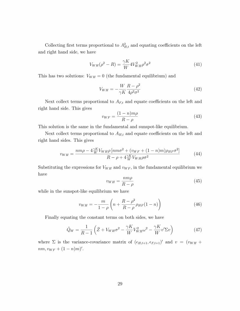
The solution is (see Appendix A for details of the algebra and for an expression
for the constant term QW ):
vWH =nmρ
R− ρ (22)
vWF =(1− n)mρ
R− ρ (23)
14In considering such stationary equilibria, we automatically rule out rational bubbles.
13
so that
QW,t = QW +mρ
R− ρAW,t (24)
where AW,t+1 = nAH,t+1 + (1 − n)AF,t+1. The world equity price depends on the
world dividend, whose impact is larger the higher the persistence ρ of dividend
shocks. We call this the fundamental equilibrium. The coefficient on AW,t goes to
zero as we let m→ 0, in which case AW,t no longer plays a fundamental role (does
not affect the global dividend).
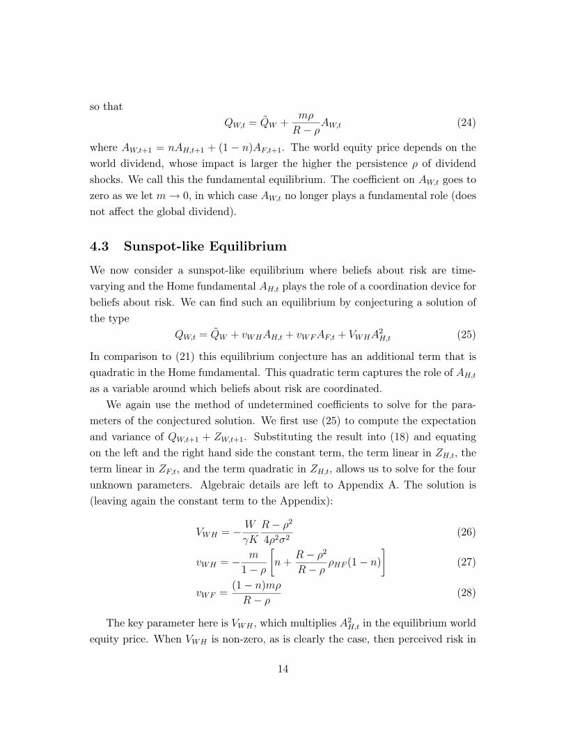
4.3 Sunspot-like Equilibrium
We now consider a sunspot-like equilibrium where beliefs about risk are time-
varying and the Home fundamental AH,t plays the role of a coordination device for
beliefs about risk. We can find such an equilibrium by conjecturing a solution of
the type
QW,t = QW + vWHAH,t + vWFAF,t + VWHA2H,t (25)
In comparison to (21) this equilibrium conjecture has an additional term that is
quadratic in the Home fundamental. This quadratic term captures the role of AH,t
as a variable around which beliefs about risk are coordinated.
We again use the method of undetermined coefficients to solve for the para-
meters of the conjectured solution. We first use (25) to compute the expectation
and variance of QW,t+1 + ZW,t+1. Substituting the result into (18) and equating
on the left and the right hand side the constant term, the term linear in ZH,t, the
term linear in ZF,t, and the term quadratic in ZH,t, allows us to solve for the four
unknown parameters. Algebraic details are left to Appendix A. The solution is
(leaving again the constant term to the Appendix):
VWH = − W
γK
R− ρ24ρ2σ2
(26)
vWH = − m
1− ρ
[n+
R− ρ2R− ρ ρHF (1− n)
](27)
vWF =(1− n)mρ
R− ρ (28)
The key parameter here is VWH , which multiplies A2H,t in the equilibrium world
equity price. When VWH is non-zero, as is clearly the case, then perceived risk in
14
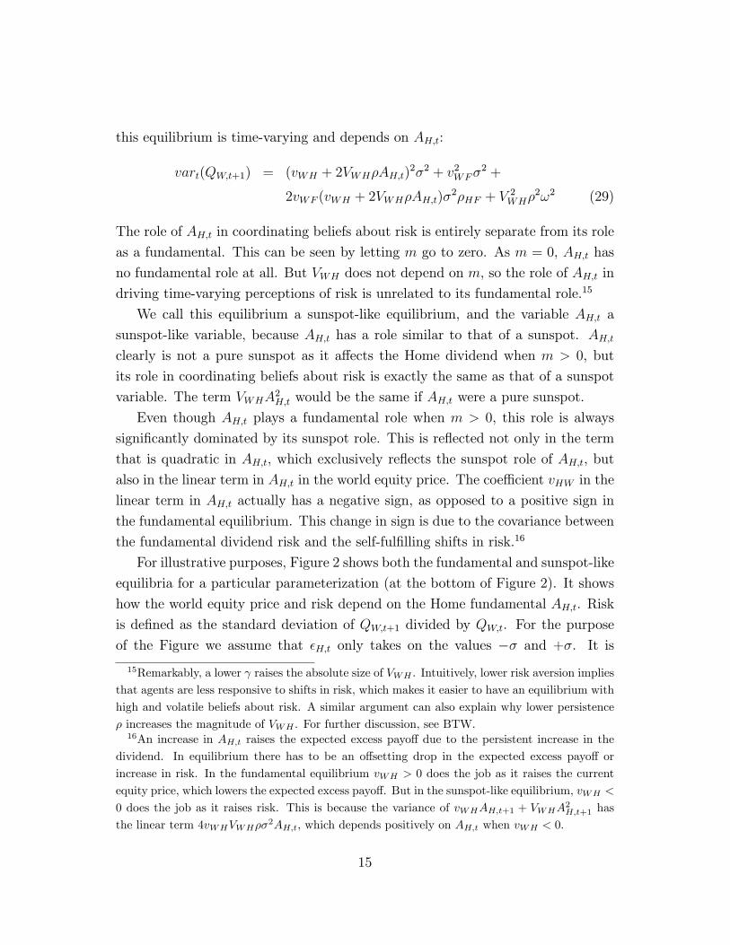
this equilibrium is time-varying and depends on AH,t:
vart(QW,t+1) = (vWH + 2VWHρAH,t)2σ2 + v2WFσ
2 +
2vWF (vWH + 2VWHρAH,t)σ2ρHF + V 2
WHρ2ω2 (29)
The role of AH,t in coordinating beliefs about risk is entirely separate from its role
as a fundamental. This can be seen by letting m go to zero. As m = 0, AH,t has
no fundamental role at all. But VWH does not depend on m, so the role of AH,t in
driving time-varying perceptions of risk is unrelated to its fundamental role.15
We call this equilibrium a sunspot-like equilibrium, and the variable AH,t a
sunspot-like variable, because AH,t has a role similar to that of a sunspot. AH,t
clearly is not a pure sunspot as it affects the Home dividend when m > 0, but
its role in coordinating beliefs about risk is exactly the same as that of a sunspot
variable. The term VWHA2H,t would be the same if AH,t were a pure sunspot.
Even though AH,t plays a fundamental role when m > 0, this role is always
significantly dominated by its sunspot role. This is reflected not only in the term
that is quadratic in AH,t, which exclusively reflects the sunspot role of AH,t, but
also in the linear term in AH,t in the world equity price. The coefficient vHW in the
linear term in AH,t actually has a negative sign, as opposed to a positive sign in
the fundamental equilibrium. This change in sign is due to the covariance between
the fundamental dividend risk and the self-fulfilling shifts in risk.16
For illustrative purposes, Figure 2 shows both the fundamental and sunspot-like
equilibria for a particular parameterization (at the bottom of Figure 2). It shows
how the world equity price and risk depend on the Home fundamental AH,t. Risk
is defined as the standard deviation of QW,t+1 divided by QW,t. For the purpose
of the Figure we assume that εH,t only takes on the values −σ and +σ. It is
15Remarkably, a lower γ raises the absolute size of VWH . Intuitively, lower risk aversion implies
that agents are less responsive to shifts in risk, which makes it easier to have an equilibrium with
high and volatile beliefs about risk. A similar argument can also explain why lower persistence
ρ increases the magnitude of VWH . For further discussion, see BTW.16An increase in AH,t raises the expected excess payoff due to the persistent increase in the
dividend. In equilibrium there has to be an offsetting drop in the expected excess payoff or
increase in risk. In the fundamental equilibrium vWH > 0 does the job as it raises the current
equity price, which lowers the expected excess payoff. But in the sunspot-like equilibrium, vWH <
0 does the job as it raises risk. This is because the variance of vWHAH,t+1 + VWHA2H,t+1 has
the linear term 4vWHVWHρσ2AH,t, which depends positively on AH,t when vWH < 0.
15

important that the distribution is bounded as AH,t itself is then bounded as well
(here between plus and minus σ/(1− ρ)), which is needed to assure that the asset
price is positive in all states.
In the sunspot-like equilibrium the equity price and risk are clearly much more
sensitive to AH,t. The additional risk leads to a lower world equity price than under
the fundamental equilibrium for all possible values of AH,t. At the extreme values
of AH,t (on either side) there are very high beliefs about risk and correspondingly
low equity prices.
4.4 Switching Equilibria and Global Risk Panics
We refer to the third type of equilibrium as a switching equilibrium. This equi-
librium is the main focus of this paper. It is closely related to the fundamental
and sunspot-like equilibria discussed so far. In a switching equilibrium, there are
occasional self-fulfilling switches between low and high risk states. The low risk
state is similar to the fundamental equilibrium and the high risk state is similar to
the sunspot-like equilibrium. We assume that the switch between low and high risk
states is driven by a Markov process. With probability p1 we are in the low risk
state tomorrow when we are in the low risk state today. Similarly, with probability
p2 we are in the high risk state tomorrow if we are in the high risk state today.
When p1 = p2 = 1, we always remain in the same state, leading to the funda-
mental and sunspot-like equilibria discussed above. When we lower the probabil-
ities below one, agents need to take into account that we may switch to another
state when computing expectations and risk. The low and high risk states then
no longer correspond exactly to the fundamental and sunspot-like equilibria. For
example, risk is higher in the low risk state than in the fundamental equilibrium
as there is now a possibility of switching to the high risk state. The relationship
between the equity price and the state variables remains as in (25), but ones needs
to separately solve for the coefficients in the low and high risk states.
BTW solve for such switching equilibria. Here we take a somewhat simpler
approach, with the benefit of the findings in BTW. They show that the solution is
a continuous function of the probabilities. As p1 = p2 approaches 1, the low and
high risk states approach respectively the fundamental and sunspot-like equilibria.
Using this finding, we consider the low risk state to be the fundamental equilibrium
16
and the high-risk state the sunspot-like equilibrium. This is infinitesimally close
to the true equilibrium when p1 = p2 are very close to 1. While the probabilities
of switching are then very small, we can still consider the impact of a switch. This
approach has the advantage that we already know what the low and high risk
states are. For larger switching probabilities (lower values of p1 and p2) a solution
can only be obtained numerically. The qualitative results remain similar though.
A risk panic involves a self-fulfilling switch from the low risk state to the high
risk state. At the moment the panic happens there is an immediate increase in
perceived risk, coordinated around AH,t. In Figure 2 this is the jump in risk from
the broken line (fundamental equilibrium) to the solid like (sunspot-like equilib-
rium). At the time of the panic the fundamental itself does not change. Rather,
it suddenly takes on the additional role of a variable around which beliefs about
risk are coordinated. As we can see from Figure 2, the increase in risk can be very
large, particularly when the fundamental is either very weak or very strong.
We consider the latter case less realistic in practice as sharp increases in risk
usually happen when the market is concerned about a bad fundamental. It would
be more realistic to assume that the switching probabilities are a function of the
fundamental itself, with the probability of a switch to the high risk state being
larger when the fundamental is weaker. That would avoid a large risk panic when
the fundamental is strong. It would also avoid the strange result of a drop in equity
prices when the fundamental improves, which happens in Figure 2 for positive
values of AH,t. We nonetheless abstract from this element of realism here in order
to maintain analytic tractability. We not only keep p1 and p2 fixed, but only
consider risk panics for the case where they are infinitesimally close to 1.
Figure 2 shows that the drop in the world equity price can be very large when
the panic happens at a time that the fundamental is weak. This is also illustrated
in Figure 3, which shows what happens to the world equity price and risk as a
result of the panic that happens at the time that the macro fundamental (Home
dividend) is at its weakest, i.e., is equal to −0.1.17 We assume that in period 6
the world economy switches to the high risk state, where it stays until period 10.
Before and after that we are in the low risk state. The panic leads to a 48% drop
in the world equity price. This is caused by an increase in world equity price risk
17This value comes from the fact that εH,t = −σ = −0.01 and ρ = 0.9.
17
from 0.4% to 14%. Of course, dependent on the parameters one can get even larger
or smaller risk panics. For example, if we lower Z from 0.5 to 0.4, the panic leads
to a 61% drop in the world equity price and risk increases from 0.5% to 23%.18
5 The Impact of the Global Risk Panic on Indi-
vidual Countries
The previous section described how global asset prices could collapse because of a
risk panic. An important question is how the individual countries are affected by
the panic. This is the question that we address in this section.
5.1 Country Prices and Covariance
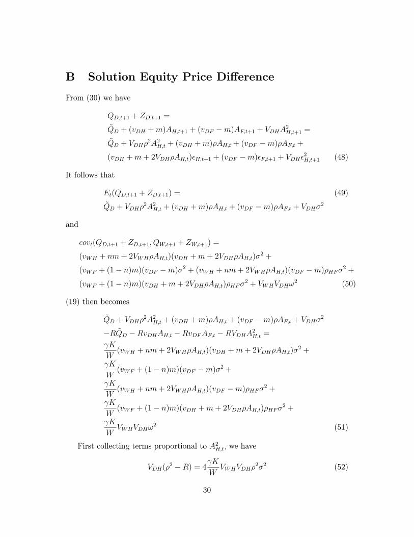
To look at the different price reactions, we need to determine QD,t from (19). We
will consider the following solution:
QD,t = QD + vDHAH,t + vDFAF,t + VDHA2H,t (30)
As in the previous section, we assume that only the Home dividend AH,t can
coordinate self-fulfilling shifts in risk.
To determine the parameters in (30) we take the following steps. First, we con-
jecture (30). Then we compute the expectation of QD,t+1 + ZD,t+1 and covariance
between QD,t+1 + ZD,t+1 and QW,t+1 + ZW,t+1. Substituting the result in (19), we
can solve for the 4 parameters in the conjecture (30) for QD,t. Together with QW,t
this gives the equity price of both countries: the Home and Foreign equity prices
are respectively QH,t = QW,t + (1−n)QD,t and QF,t = QW,t−nQD,t. Details of the
algebra are left to Appendix B. We first discuss the fundamental equilibrium and
then turn to sunspot-like equilibria and switching equilibria featuring risk panics.
In the fundamental equilibrium we have VDH = 0, vDH = mρ/(R − ρ) and
vDF = −mρ/(R − ρ). The expressions for the equity prices of the two countries
18While our aim here is certainly not to draw precise quantitative comparisons to the recent
crisis, we should point out that the numbers that we reported in Figure 1 for the VIX cannot be
directly compared to those reported here for risk. The VIX numbers are risk measures that are
multiplied by the square root of 12 in order to annualize them. For example, a VIX of 80 implies
that equity price risk over the next month is 23%.
18

then become
QH,t =1
R− 1
Z − ( mR
R− ρ
)2γK
WσHW
+mρ
R− ρAH,t (31)
QF,t =1
R− 1
Z − ( mR
R− ρ
)2γK
WσFW
+mρ
R− ρAF,t (32)
where σiW = cov(εi,t+1, εW,t+1), i = H,F , is the covariance between the Home
(Foreign) and world dividend innovation. The latter is defined as εW,t+1 = nεH,t+1+
(1− n)εF,t+1. It is natural to assume that σiW > 0. Two points are worth making
with regards to this fundamental equilibrium. First, the constant terms depend on
the covariance of the dividend innovation with the world dividend innovation. The
higher is this covariance, the riskier the asset and therefore the lower the price.
Second, equity prices only depend on domestic dividend innovations. Thus, there
is no contagion of shocks across countries. This is because we have shut down the
regular channels of contagion through the interest rate and wealth. Both are held
constant.
Sunspot-like equilibria can also be computed following the solution method
discussed above. Appendix B computes the values of the four unknown parameters
of the conjecture (30) forQD,t. The impact of the Foreign fundamentalAF,t remains
the same in the sunspot-like equilibrium as in the fundamental equilibrium. This
reflects the fact that the Foreign dividend only plays a pure fundamental role (by
assumption). The impact of the Home fundamental AH,t is more complex as it
coordinates beliefs about risk in the sunspot-like equilibrium.
In order to understand what drives the solution of asset prices as a function
AH,t, it is useful to consider equation (19). It equates the difference in the excess
payoff on Home and Foreign equity to the difference in their respective risk premia.
Integrating forward, and ruling out bubbles, we have
QD,t =mρ
R− ρAD,t −γK
W
∞∑i=1
1
RiEtcovt+i−1(QD,t+i + ZD,t+i, QW,t+i + ZW,t+i) (33)
This equation holds both in the fundamental and sunspot-like equilibrium. A
risk panic involves a switch from the fundamental equilibrium to the sunspot-like
equilibrium. Since AD,t does not change during the panic, the change in QD,t
19
during the panic is equal to
∆QD,t = −γKW
∞∑i=1
1
Ri∆Etcovt+i−1(QD,t+i + ZD,t+i, QW,t+i + ZW,t+i) (34)
When ∆QD,t differs from 0, the panic affects the asset prices of the two countries
differently.
Equation (34) implies that the panic affects the two countries differently to
the extent that it affects the relative riskiness of the assets differently. This in
turn depends on how it affects the covariance between the equity payoffs of the
individual countries and the global payoff. If this covariance rises more for the
Home than the Foreign country, so that the covariance between QD,t+1 + ZD,t+1
and QW,t+1 + ZW,t+1 increases, then risk increases more in the Home country and
its equity price drops more during the panic.
Write ∆cov as the change in the covariance between QD,t+1 + ZD,t+1 and
QW,t+1 + ZW,t+1 from the fundamental to the sunspot-like equilibrium. Using the
results from Appendix B, we can write this as
∆cov =Rm
R− ρ(1− ρHF )σ2(vWH − vWH)− ρm
1− ρσHW (vDH − vDH) +
2ρ
[Rm
R− ρ(1− ρHF )σ2VWH −ρm
1− ρσHWVDH + (vDH − vDH)σ2VWH
]AH,t +
4ρ2σ2VWHVDHA2H,t (35)
where a bar stands for the value of the parameter in the fundamental equilibrium.
While (35) may appear a complicated expression at first, we will see that it pro-
vides insight into the various mechanisms that determine how much the individual
countries are affected by the panic.
5.2 Two Factors Determining the Impact of Global Panic
on Individual Countries
At a general level, two factors determine how much the individual countries are
affected by the crisis: (1) an indeterminacy and (2) differences in fundamental
hedging properties.
We show in Appendix B that VDH is indeterminate in the sunspot-like equi-
librium. While we know the coefficient on A2H,t for the global equity price, how
20
this average coefficient for the global price divides across the two assets is not
determinate. This indeterminacy is due to another type of self-fulfilling beliefs.
If agents believe that the Home country will be more affected by the panic, then
their beliefs will be fulfilled in equilibrium.
This can be seen from (35). If the Home equity price depends more negatively
on A2H,t, which happens when VDH < 0, then the relative risk of Home equity
during the panic depends more positively on A2H,t (recall that VWH < 0). This in
turn justifies a more negative coefficient on A2H,t in the equilibrium Home equity
price. To put it another way, when the Home equity price depends more negatively
on A2H,t in the sunspot-like equilibrium, the covariance with the world equity price
depends more positively on A2H,t.19 This increases its risk as a function of A2H,t,
which in turn justifies the more negative coefficient on A2H,t in the Home equity
price.
The second factor that determines how much the individual countries are af-
fected by the global panic is associated with the fundamental hedging properties
of the assets. An asset is a more attractive hedge against global risk when its
payoff covaries less with the global payoff. The fundamental payoff on an asset is
the payoff in the fundamental equilibrium, when there are no self-fulfilling shifts in
risk. As we have seen, the payoff in the fundamental equilibrium only depends on
the asset’s dividend. A higher covariance between the dividend of an asset and the
global payoff in the sunspot-like equilibrium implies a weaker hedge. This leads to
a larger impact of the panic.
In order to illustrate these points more precisely and obtain a better under-
standing of the role of the parameters in driving the results, we first consider the
case where the macro variables AH,t and AF,t have a large fundamental role (m is
large) and then the case where they play a small fundamental role (m close to 0).
We will argue that the latter is more realistic.
5.3 Large Fundamental Role of Macro Variables
In the case where m is much above zero, so that the macro variables have a large
fundamental role, we obtain two results. First, the impact of the indeterminacy on
19This is because the world equity price also depends negatively on A2H,t and the variance of
A2H,t+1 depends positively on A2H,t.
21
the equilibrium prices is limited. Second, the fundamental hedging properties of
the assets are such that the panic affects the Home country more than the Foreign
country.
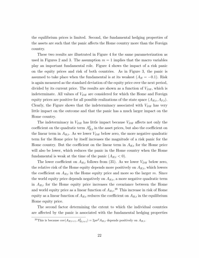
These two results are illustrated in Figure 4 for the same parameterization as
used in Figures 2 and 3. The assumption m = 1 implies that the macro variables
play an important fundamental role. Figure 4 shows the impact of a risk panic
on the equity prices and risk of both countries. As in Figure 3, the panic is
assumed to take place when the fundamental is at its weakest (AH = −0.1). Risk
is again measured as the standard deviation of the equity price over the next period,
divided by its current price. The results are shown as a function of VDH , which is
indeterminate. All values of VDH are considered for which the Home and Foreign
equity prices are positive for all possible realizations of the state space (AH,t, AF,t).
Clearly, the Figure shows that the indeterminacy associated with VDH has very
little impact on the outcome and that the panic has a much larger impact on the
Home country.
The indeterminacy in VDH has little impact because VDH affects not only the
coefficient on the quadratic term A2H,t in the asset prices, but also the coefficient on
the linear term in AH,t. As we lower VDH below zero, the more negative quadratic
term for the Home price by itself increases the magnitude of a risk panic for the
Home country. But the coefficient on the linear term in AH,t for the Home price
will also be lower, which reduces the panic in the Home country when the Home
fundamental is weak at the time of the panic (AH,t < 0).
The lower coefficient on AH,t follows from (35). As we lower VDH below zero,
the relative risk of the Home equity depends more positively on AH,t, which lowers
the coefficient on AH,t in the Home equity price and more so the larger m. Since
the world equity price depends negatively on AH,t, a more negative quadratic term
in AH,t for the Home equity price increases the covariance between the Home
and world equity price as a linear function of AH,t.20 This increase in risk of Home
equity as a linear function of AH,t reduces the coefficient on AH,t in the equilibrium
Home equity price.
The second factor determining the extent to which the individual countries
are affected by the panic is associated with the fundamental hedging properties
20This is because cov(AH,t+1, A2H,t+1) = 2ρσ2AH,t depends positively on AH,t.
22
of the assets. This leads to a larger impact of the panic in the Home country.
The expression for ∆cov in (35) provides some understanding of these hedging
properties. Assume for now that vDH = vDH , so that the relative size of the linear
coefficients remains the same as in the fundamental equilibrium (the deviation of
vDH from vDH in equilibrium only serves to amplify the results that we are about
to describe). Then, since vWH < vWH and VWH < 0, it follows from (35) that
both the constant term and the coefficient on AH,t are negative in the expression
for ∆cov.
At AH,t = 0, the risk panic then makes the Home equity a relatively better
hedge against global risk, leading to a smaller drop in the Home equity price.
The negative linear coefficient on AH,t in ∆cov implies that the weaker the Home
fundamental at the time of the panic (the more negative AH,t), the less attractive
the Home equity as a hedge against global risk as a result of the panic. This leads
to a larger risk panic in the Home country.21 We find that unless AH,t is very close
to 0, the second effect dominates, leading to a larger panic in the Home country.
The intuition for these findings is associated with the extent to which the
dividend of the equities is a hedge against the global risk faced by the agents in
the sunspot-like equilibrium. Since vWH < 0 in the high risk equilibrium, this
reduces the relative risk of the Home equity as its dividend becomes negatively
correlated with vWHAH,t, making it a better hedge against global risk and reducing
the relative size of the panic in the Home country.
The quadratic term in the global equity price is VWHA2H,t. As VWH < 0,
the covariance of this term with the Home dividend, 2mρVWHσ2AH,t, depends
negatively on AH,t. This increases the relative risk of the Home asset when AH,t < 0
and more so the more negative AH,t. When the Home fundamental is sufficiently
weak this causes a larger drop in the Home equity price during the panic.
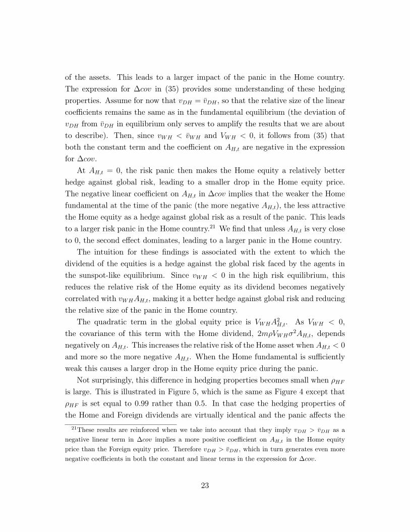
Not surprisingly, this difference in hedging properties becomes small when ρHF
is large. This is illustrated in Figure 5, which is the same as Figure 4 except that
ρHF is set equal to 0.99 rather than 0.5. In that case the hedging properties of
the Home and Foreign dividends are virtually identical and the panic affects the
21These results are reinforced when we take into account that they imply vDH > vDH as a
negative linear term in ∆cov implies a more positive coefficient on AH,t in the Home equity
price than the Foreign equity price. Therefore vDH > vDH , which in turn generates even more
negative coefficients in both the constant and linear terms in the expression for ∆cov.
23
covariance with the global payoff virtually the same across the two assets.
The size of the country that is the focal point for the panic does not matter
much in these results. Even if the Home country is small relative to the global
economy, it remains the case that the risk panic is much larger in the Home country.
For example, setting n = 0.1 and VDH = 0, risk increases 55% and 12% in the
Home and Foreign country respectively, while their respective equity prices drop
by 80% and 46%.
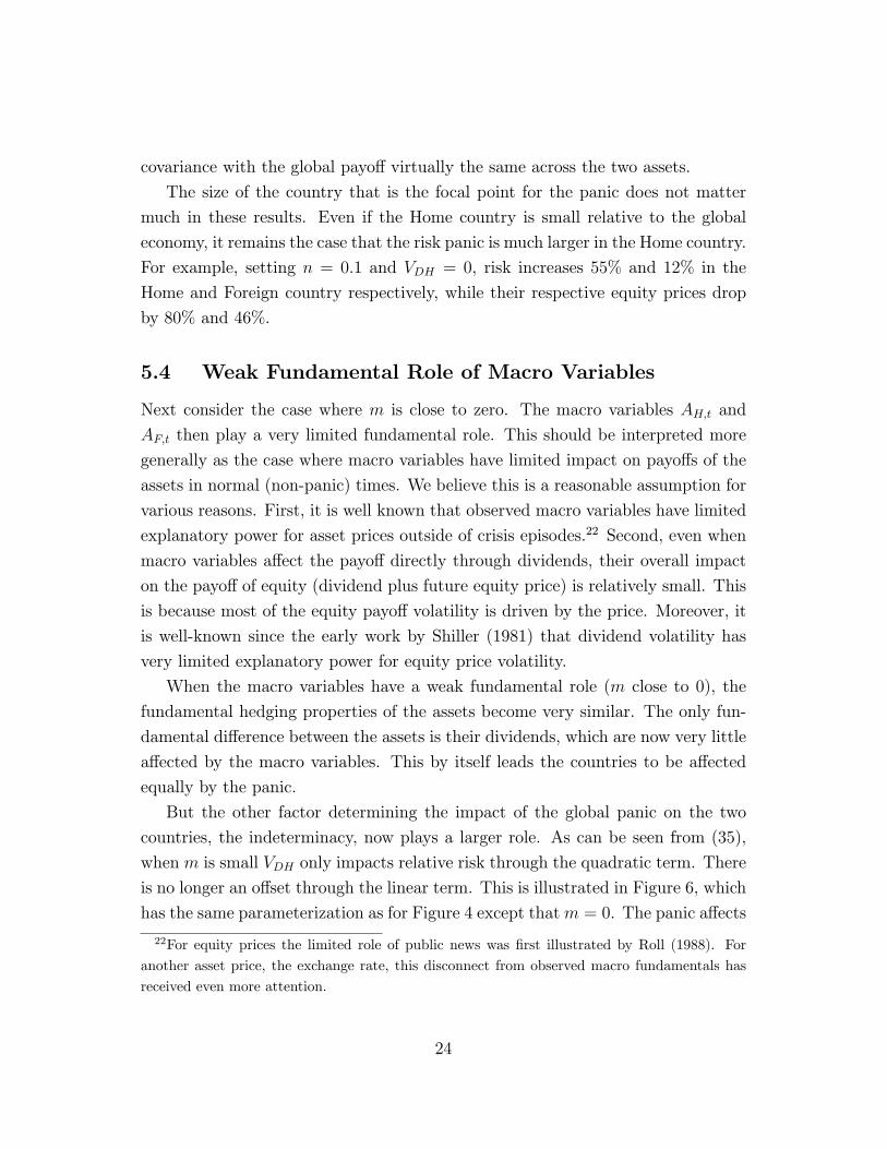
5.4 Weak Fundamental Role of Macro Variables
Next consider the case where m is close to zero. The macro variables AH,t and
AF,t then play a very limited fundamental role. This should be interpreted more
generally as the case where macro variables have limited impact on payoffs of the
assets in normal (non-panic) times. We believe this is a reasonable assumption for
various reasons. First, it is well known that observed macro variables have limited
explanatory power for asset prices outside of crisis episodes.22 Second, even when
macro variables affect the payoff directly through dividends, their overall impact
on the payoff of equity (dividend plus future equity price) is relatively small. This
is because most of the equity payoff volatility is driven by the price. Moreover, it
is well-known since the early work by Shiller (1981) that dividend volatility has
very limited explanatory power for equity price volatility.
When the macro variables have a weak fundamental role (m close to 0), the
fundamental hedging properties of the assets become very similar. The only fun-
damental difference between the assets is their dividends, which are now very little
affected by the macro variables. This by itself leads the countries to be affected
equally by the panic.
But the other factor determining the impact of the global panic on the two
countries, the indeterminacy, now plays a larger role. As can be seen from (35),
when m is small VDH only impacts relative risk through the quadratic term. There
is no longer an offset through the linear term. This is illustrated in Figure 6, which
has the same parameterization as for Figure 4 except that m = 0. The panic affects
22For equity prices the limited role of public news was first illustrated by Roll (1988). For
another asset price, the exchange rate, this disconnect from observed macro fundamentals has
received even more attention.
24
the two countries equally when VDH = 0. But the indeterminacy associated with
VDH now has a big impact on how the panic affects the two countries.
Nonetheless a good case can be made for VDH = 0 as a plausible outcome.
First, any deviation from VDH = 0 is entirely arbitrary. While it is possible for
investors to believe that the panic should affect one country more than the other,
there is no a priori reason for this to be the case as the assets are not different in
any fundamental way.
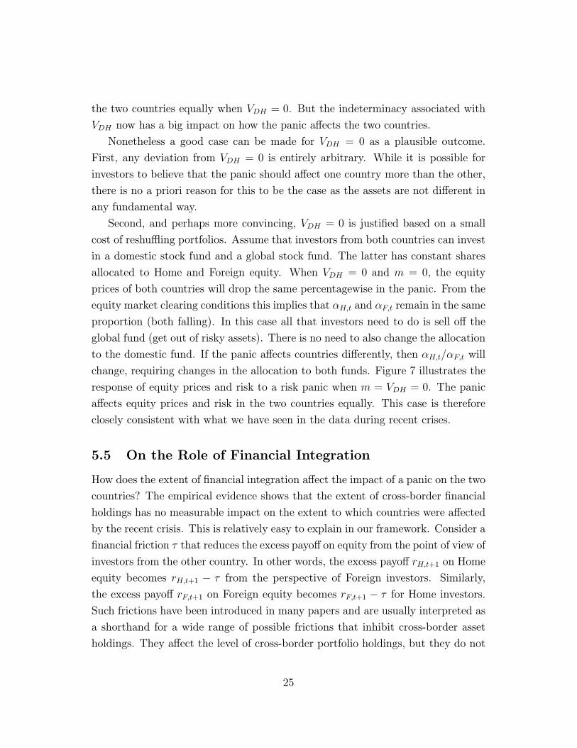
Second, and perhaps more convincing, VDH = 0 is justified based on a small
cost of reshuffling portfolios. Assume that investors from both countries can invest
in a domestic stock fund and a global stock fund. The latter has constant shares
allocated to Home and Foreign equity. When VDH = 0 and m = 0, the equity
prices of both countries will drop the same percentagewise in the panic. From the
equity market clearing conditions this implies that αH,t and αF,t remain in the same
proportion (both falling). In this case all that investors need to do is sell off the
global fund (get out of risky assets). There is no need to also change the allocation
to the domestic fund. If the panic affects countries differently, then αH,t/αF,t will
change, requiring changes in the allocation to both funds. Figure 7 illustrates the
response of equity prices and risk to a risk panic when m = VDH = 0. The panic
affects equity prices and risk in the two countries equally. This case is therefore
closely consistent with what we have seen in the data during recent crises.
5.5 On the Role of Financial Integration
How does the extent of financial integration affect the impact of a panic on the two
countries? The empirical evidence shows that the extent of cross-border financial
holdings has no measurable impact on the extent to which countries were affected
by the recent crisis. This is relatively easy to explain in our framework. Consider a
financial friction τ that reduces the excess payoff on equity from the point of view of
investors from the other country. In other words, the excess payoff rH,t+1 on Home
equity becomes rH,t+1 − τ from the perspective of Foreign investors. Similarly,
the excess payoff rF,t+1 on Foreign equity becomes rF,t+1 − τ for Home investors.
Such frictions have been introduced in many papers and are usually interpreted as
a shorthand for a wide range of possible frictions that inhibit cross-border asset
holdings. They affect the level of cross-border portfolio holdings, but they do not
25
affect the marginal trade-offs. Changes in expected payoffs still lead to the same
portfolio shifts for both Home and Foreign investors.
While a larger τ reduces cross-border asset holdings, it has no effect on the
magnitude of the global panic and how much it affects the two countries. The
friction τ only affects the constant term in the equity price solutions. For both the
fundamental and sunspot-like equilibria it changes the mean of QW by −2n(1 −n)τ/(R − 1) and the mean of QD by −(1 − 2n)τ/(R − 1). Our model therefore
does not necessarily generate any relationship between cross-border asset holdings
and the extent to which countries are affected by the panic.
More fundamentally, the debate about the role of cross-border asset holdings
is relevant when financial contagion is due to the transmission of shocks. One
can imagine that a shock in one country has a larger impact on other countries if
financial linkages are stronger. But in our model the impact of a panic on individual
countries does not occur through the transmission of shocks, so that the magnitude
of financial linkages is not a determining factor. Rather, what coordinates the panic
across countries is an event that suddenly draws attention of investors all over the
world to a weak fundamental somewhere. This weak fundamental, by becoming
a common focal point of attention by investors everywhere, leads to a widespread
self-fulfilling increase in risk perceptions.
6 Conclusion
The paper is motivated by the sharp increase in equity price risk across many coun-
tries during recent financial crises. Remarkably, the magnitude of this increase in
perceived risk is very similar across countries and is associated with a similar drop
in equity prices across many countries. Moreover, the extent of cross-border finan-
cial linkages appears to have little impact on how much countries were affected.
In addition, all of this appears to have happened without sudden large shocks to
fundamentals.
In order to shed light on this phenomenon, we have developed a theory of
risk panics that has the following features. First, there is a sharp increase in risk
and a drop in equity prices in all countries. Second, the panic does not spread
across countries through financial linkages but is rather the result of a coordinated
increase in risk perceptions all over the world due to an event that draws the
26
attention to a particularly weak macro variable somewhere in the world. Third,
the global panic is not caused by a change in any fundamental, but is rather the
result of a self-fulfilling increase in perceived risk that is coordinated by a weak
fundamental.
We have shown that the panic tends to be larger in the country whose macro
fundamental becomes the focal point of the self-fulfilling increase in risk. But when
observed macro variables have a limited impact on equity prices in normal times,
as observed in the data, we have shown that the panic can affect countries very
similarly, as seen in the recent crises. Both the spike in risk and the drop in the
equity price will then be similar.
While we have offered one explanation for the huge spike in risk associated with
equity prices, and the very similar magnitude of this panic across the world, this
topic deserves a lot more attention in future research. Not much work has been
done in macroeconomics in understanding what drives such substantial changes in
risk, let alone the common pattern across the globe in this regard. We hope that
this will change in the future, putting us in a position to have a horse race among
competing theories.
27

Appendix
A Solution World Equity Price
In this Appendix we derive the solution for the world equity price in Section 4.
Start with the conjecture (25)
QW,t = QW + vWHAH,t + vWFAF,t + VWHA2H,t (36)
Note that this also includes the fundamental equilibrium as a special case, where
VWH = 0. We need to compute the expectation and variance of QW,t+1 + ZW,t+1.
We have
QW,t+1 + ZW,t+1 =
QW + Z + (vWH + nm)AH,t+1 + (vWF + (1− n)m)AF,t+1 + VWHA2H,t+1 =
QW + Z + VWHρ2A2H,t + (vWH + nm)ρAH,t + (vWF + (1− n)m)ρAF,t +
(vWH + nm+ 2VWHρAH,t)εH,t+1 + (vWF + (1− n)m)εF,t+1 + VWHε2H,t+1 (37)
It follows that
Et(QW,t+1 + ZW,t+1) = (38)
QW + Z + VWHρ2A2H,t + (vWH + nm)ρAH,t + (vWF + (1− n)m)ρAF,t + VWHσ
2
and
vart(QW,t+1 + ZW,t+1) =
(vWH + nm+ 2VWHρAH,t)2σ2 + (vWF + (1− n)m)2σ2 +
2(vWH + nm+ 2VWHρAH,t)(vWF + (1− n)m)ρHFσ2 + V 2
WHω2 (39)
Substituting these results into (18), we have
QW + Z + VWHρ2A2H,t + (vWH + nm)ρAH,t + (vWF + (1− n)m)ρAF,t + VWHσ
2
−RQW −RvWHAH,t −RvWFAF,t −RVWHA2H,t =
γK
W(vWH + nm+ 2VWHρAH,t)
2σ2 +γK
W(vWF + (1− n)m)2σ2 +
γK
W2(vWH + nm+ 2VWHρAH,t)(vWF + (1− n)m)ρHFσ
2 +γK
WV 2WHω
2 (40)
28
Collecting first terms proportional to A2H,t and equating coefficients on the left
and right hand side, we have
VWH(ρ2 −R) =γK
W4V 2
WHρ2σ2 (41)
This has two solutions: VWH = 0 (the fundamental equilibrium) and
VWH = − W
γK
R− ρ24ρ2σ2
(42)
Next collect terms proportional to AF,t and equate coefficients on the left and
right hand side. This gives
vWF =(1− n)mρ
R− ρ (43)
This solution is the same in the fundamental and sunspot-like equilibrium.
Next collect terms proportional to AH,t and equate coefficients on the left and
right hand sides. This gives
vWH =nmρ− 4γK
WVWHρ [nmσ2 + (vWF + (1− n)m)ρHFσ
2]
R− ρ+ 4γKWVWHρσ2
(44)
Substituting the expressions for VWH and vWF , in the fundamental equilibrium we
have
vWH =nmρ
R− ρ (45)
while in the sunspot-like equilibrium we have
vWH = − m
1− ρ
(n+
R− ρ2R− ρ ρHF (1− n)
)(46)
Finally equating the constant terms on both sides, we have
QW =1
R− 1
(Z + VWHσ
2 − γK
WV 2WHω
2 − γK
Wv′Σv
)(47)
where Σ is the variance-covariance matrix of (εH,t+1, εF,t+1)′ and v = (vWH +
nm, vWF + (1− n)m)′.
29
B Solution Equity Price Difference
From (30) we have
QD,t+1 + ZD,t+1 =
QD + (vDH +m)AH,t+1 + (vDF −m)AF,t+1 + VDHA2H,t+1 =
QD + VDHρ2A2H,t + (vDH +m)ρAH,t + (vDF −m)ρAF,t +
(vDH +m+ 2VDHρAH,t)εH,t+1 + (vDF −m)εF,t+1 + VDHε2H,t+1 (48)
It follows that
Et(QD,t+1 + ZD,t+1) = (49)
QD + VDHρ2A2H,t + (vDH +m)ρAH,t + (vDF −m)ρAF,t + VDHσ
2
and
covt(QD,t+1 + ZD,t+1, QW,t+1 + ZW,t+1) =
(vWH + nm+ 2VWHρAH,t)(vDH +m+ 2VDHρAH,t)σ2 +
(vWF + (1− n)m)(vDF −m)σ2 + (vWH + nm+ 2VWHρAH,t)(vDF −m)ρHFσ2 +
(vWF + (1− n)m)(vDH +m+ 2VDHρAH,t)ρHFσ2 + VWHVDHω
2 (50)
(19) then becomes
QD + VDHρ2A2H,t + (vDH +m)ρAH,t + (vDF −m)ρAF,t + VDHσ
2
−RQD −RvDHAH,t −RvDFAF,t −RVDHA2H,t =
γK
W(vWH + nm+ 2VWHρAH,t)(vDH +m+ 2VDHρAH,t)σ
2 +
γK
W(vWF + (1− n)m)(vDF −m)σ2 +
γK
W(vWH + nm+ 2VWHρAH,t)(vDF −m)ρHFσ
2 +
γK
W(vWF + (1− n)m)(vDH +m+ 2VDHρAH,t)ρHFσ
2 +
γK
WVWHVDHω
2 (51)
First collecting terms proportional to A2H,t, we have
VDH(ρ2 −R) = 4γK
WVWHVDHρ
2σ2 (52)
30

In the fundamental equilibrium, where VWH = 0, it follows that VDH = 0. After
substituting (42), it follows that (52) holds for all values of VDH in the sunspot-like
equilibrium. Next collecting terms proportional to AF,t, we find
vDF = − mρ
R− ρ (53)
This holds both in the fundamental and sunspot-like equilibrium.
Next collecting terms proportional to AH,t, we have
vDH =mρ− 2ργK
W(η1VDH + η2VWH)
R− ρ+ 2γKWVWHρσ2
(54)
where
η1 = (vWH + nm)σ2 + (vWF + (1− n)m)ρHFσ2 (55)
η2 = mσ2 + (vDF −m)ρHFσ2 (56)
In the fundamental equilibrium where VWH = VDH = 0, it follows that
vDH =mρ
R− ρ (57)
In the sunspot-like equilibrium vDH depends on VDH , which is indeterminate.
When VDH = 0 we have
vDH = mρ2 +R− R−ρ2
R−ρ RρHF
R(2ρ− 1)− ρ2 (58)
This uses the value for vDF in the expression for η2 and the expression for VWH .
Finally, collecting constant terms, we have
QD =1
R− 1
(VDHσ
2 − γK
WVWHVDHω
2 − γK
Wv′1Σv2
)(59)
where v1 = (vWH + nm, vWF + (1− n)m)′ and v2 = (vDH +m, vDF −m)′.
31

C Implied Volatility Indices
Country Source
Belgium Datastream
Full name: BEL 20 Volatility
Computed from: BEL 20 Index options, 1 month
Canada Montreal Exchange
Full name: MX Implied Volatility Index
Computed from: CDN S&P/TSX60 Fund, 1 month
France Datastream
Full name: CAC 40 Volatility
Computed from: CAC 40 Index options, 1 month
Germany Datastream
Full name: VDAX - NEW
Computed from: DAX Index options traded at Eurex, 1 month
India National Stock Exchange of India
Full name: India VIX
Computed from: NIFTY Index options, 1 month
Japan CSFI, University of Osaka
Full name: CSFI - VXJ
Computed from: Nikkei 225 Index options, 1 month
Mexico Mexican Derivatives Exchange
Full name: VIMEX
Computed from: IPC options traded at MexDer, 3 months
Netherlands Datastream
Full name: AEX Volatility
Computed from: AEX Index options, 1 month
South Africa Johannesburg Stock Exchange
Full name: SAVI Top40
Computed from: FTSE/JSE Top40 Index options, 3 months
South Korea Korea Exchange
Full name: VKOSPI
Computed from: KOSPI200 Index options, 1 month
Switzerland Swiss Exchange
Full name: VSMI
Computed from: SMI options traded at Eurex, 1 month
U.S.A. Datastream
Full name: CBOE - VIX
Computed from: S&P 500 index options, 1 month
32
References
[1] Aghion, Philippe, Philippe Bacchetta, and Abhijit Banerjee (2004), “A Cor-
porate Balance-Sheet Approach to Currency Crises,” Journal of Economic
Theory 119, 6-30.
[2] Allen, Franklin and Douglas Gale (1994), “Limited Market Participation and
Volatility of Asset Prices,” American Economic Review 84, 933-955.
[3] Allen, Franklin, and Douglas Gale (2000), ”Financial Contagion,” Journal of
Political Economy 108, 1-33.
[4] Aoki, M. (1981), Dynamics Analysis of Open Economies, Academic Press,
New York.
[5] Bacchetta, Philippe and Eric van Wincoop (2006), “Can Information Hetero-
geneity Explain the Exchange Rate Determination Puzzle?,” American Eco-
nomic Review 96, 552-576.
[6] Bacchetta, Philippe, Cedric Tille, and Eric van Wincoop (2010), “Self-
fulfilling Risk Panics,” NBER Working Paper No. 16159.
[7] Beirne, John, Guglielmo Maria Caporale, Marianne Schulze-Ghattas, and
Nicola Spagnolo (2009), ”Volatility Spillovers and Contagion from Mature
to Emerging Stock Markets,” European Central Bank Working Paper No.
1113.
[8] Bekaert, Geert and Campbell R. Harvey (1995), ”Time-Varying World Market
Integration,” Journal of Finance 50, 403-444.
[9] Calvo, Guillermo A. (1999), ”Contagion in Emerging Markets: When Wall
Street Is a Carrier,” mimeo.
[10] Calvo, Guillermo A. and Enrique G. Mendoza (2000), ”Rational Contagion
and the Globalization of Securities Markets,” Journal of International Eco-
nomics 51, 79-113.
[11] Dedola, Luca and Giovanni Lombardo (2010), ”Financial Frictions, Financial
Integration and the International Propagation of Shocks,” mimeo.
[12] Devereux, M.B. and J. Yetman (2010), “Financial Deleveraging and the In-
ternational Transmission of Shocks,” NBER Working Paper No. 16226.
33
[13] Diebold, Francis X. and Kamil Yilmaz (2009), Measuring Financial Asset
Return and Volatility Spillovers, with Application to Global Equity Markets,”
The Economic Journal 119, 158—171.
[14] Dornbusch, Rudiger, Yung Chul Park, and Stijn Claessens (2000), ”Contagion:
Understanding How It Spreads,” The World Bank Research Observer 15, 177-
97.
[15] Edwards, Sebastian and Raul Susmel (2001), ”Volatility Dependence, and
Contagion in Emerging Equity Markets,” Journal of Development Economics
66(2), 505-32.
[16] Fostel, Ana and John Geanakoplos (2008), “Leverage Cycles and the Anxious
Economy,” American Economic Review 98(4), 1211-1244.
[17] Giannone, Domenico, Michele Lenza, and Lucrezia Reichlin (2010) “Market
Freedom and the Global Recession,” ECARES working paper 2010-020.
[18] Gromb, Denis and Dimitri Vayanos (2002), “Equilibrium and Welfare in Mar-
kets with Financially Constrained Arbitrageurs,” Journal of Financial Eco-
nomics 66, 361-407.
[19] Imbs, Jean (2010), ”The First Global Recession in Decades,” mimeo.
[20] Jeanne, Olivier and Andrew K. Rose (2002), “Noise Trading and Exchange
Rate Regimes,” Quarterly Journal of Economics 77, 537-569.
[21] Kamin, Steven B. and Laurie Pounder (2010), ”How Did a Domestic Housing
Slump Turn into a Global Financial Crisis?” Federal Reserve Board Interna-
tional Finance Discussion Paper No. 994.
[22] Karolyi, G. Andrew (2003), ”Does International Financial Contagion Really
Exist?” International Finance 6:2, 179—199.
[23] King, Mervin, Enrique Sentana and Sushil Wadhwani (1994), “Volatility and
Links between National Stock Markets,” Econometrica 62 (4), 901-933.
[24] King, Mervin and Sushil Wadhwani (1990), “Transmission of Volatility be-
tween Stock Markets,” Review of Financial Studies 3(1), 5-33.
[25] Krugman, Paul (2008), ”The International Finance Multiplier,” mimeo.
[26] Kyle, Albert S. and Wei Xiong (2001), “Contagion as a Wealth Effect,” The
Journal of Finance 56(4), 1401-1440.
34

[27] Lane, Philip R., and Gian Maria Milesi-Ferretti (2010) “The Cross-Country
Incidence of the Global Crisis,” IMF Economic Review 58(2), forthcoming.
[28] Manuelli, Rodolfo E. and James Peck (1992), “Sunspot-like Effects of Random
Endowments,” Journal of Economic Dynamics and Control 16, 193-206.
[29] Mendoza, Enrique and Vincenzo Quadrini (2010), ”Financial Globalization,
Financial Crises and Contagion,” Journal of Monetary Economics, forthcom-
ing.
[30] Masson, Paul (1999), ”Contagion: Macroeconomic Models with Multiple
Equilibria,” Journal of International Money and Finance 18, 587—602.
[31] Obstfeld, Maurice (1986), ’Rational and self-fulfilling balance-of-payments
crises,’ American Economic Review 76, 72-81.
[32] Pagano, Marco (1989), “Endogenous Market Thinness and Stock Price
Volatility,” Review of Economic Studies 56, 269-288.
[33] Pavlova, Anna and Roberto Rigobon (2008), “The Role of Portfolio Con-
straints in the International Propagation of Shocks,” Review of Economic
Studies 75, 1215-1256.
[34] Roll, Richard (1988), “R2,” Journal of Finance 43 (2), 541-566.
[35] Rose, Andrew and Mark Spiegel (2010), “The Causes and Consequences of
the 2008 Crisis: International Linkages and American Exposure,” Pacific Eco-
nomic Review 15, 340-363.
[36] Schinasi, Garry J. and R. Todd Smith (2000), “Portfolio Diversification,
Leverage, and Financial Contagion,” IMF Staff Papers 47, 159-176.
[37] Shiller, Robert J. (1981), “Do Stock Prices Move Too Much to be Justified
by Subsequent Changes in Dividends?,” American Economic Review 71(3),
421-436.
[38] Soriano, Pilar and Francisco Climent (2006), “Volatility Transmission Models:
A Survey,” Revista de Economıa Financiera, N.10, 32-81.
[39] Walker, Todd B. and Charles H. Whiteman (2007), “Multiple Equilibria in a
Simple Asset Pricing Model, ” Economic Letters 97(3), 191-196.
35
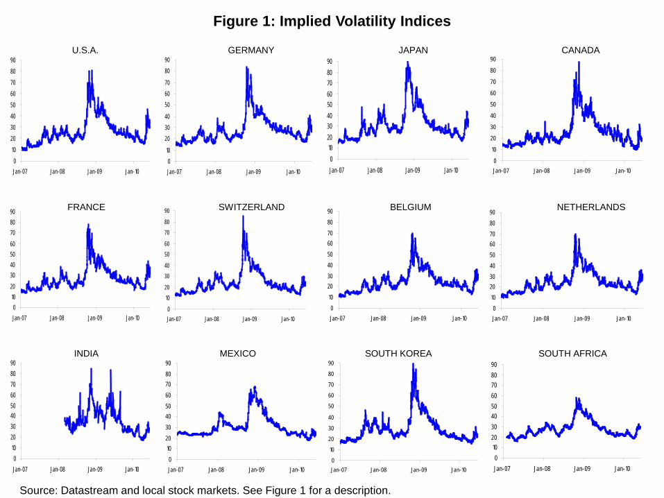
010
2030405060708090
Jan-07 Jan-08 Jan-09 Jan-10
010
2030405060708090
Jan-07 Jan-08 Jan-09 Jan-10
010
2030405060708090
Jan-07 Jan-08 Jan-09 Jan-10
Source: Datastream and local stock markets. See Figure 1 for a description.
Figure 1: Implied Volatility Indices
010
203040
506070
8090
Jan-07 Jan-08 Jan-09 Jan-100
10
20
30
40
50
60
70
80
90
Jan-07 Jan-08 Jan-09 Jan-10
0
1020
3040
5060
7080
90
Jan-07 Jan-08 Jan-09 Jan-10
010
2030405060708090
Jan-07 Jan-08 Jan-09 Jan-10
010
2030405060708090
Jan-07 Jan-08 Jan-09 Jan-100
102030405060708090
Jan-07 Jan-08 Jan-09 Jan-10
010
2030405060708090
Jan-07 Jan-08 Jan-09 Jan-100
10
20
30
40
50
60
70
80
90
Jan-07 Jan-08 Jan-09 Jan-10
010
2030405060708090
Jan-07 Jan-08 Jan-09 Jan-10
U.S.A. JAPAN CANADAGERMANY
FRANCE SWITZERLAND NETHERLANDSBELGIUM
INDIA SOUTH KOREA SOUTH AFRICAMEXICO
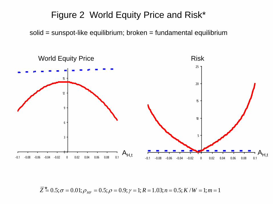
0
3
6
9
12
15
-0.1 -0.08 -0.06 -0.04 -0.02 0 0.02 0.04 0.06 0.08 0.1
Figure 2 World Equity Price and Risk*
0
5
10
15
20
25
-0.1 -0.08 -0.06 -0.04 -0.02 0 0.02 0.04 0.06 0.08 0.1
1;1/;5.0;03.1;1;9.0;5.0;01.0;5.0 ========= mWKnRZ HF γρρσ*
AH,t AH,t
solid = sunspot-like equilibrium; broken = fundamental equilibrium
World Equity Price Risk
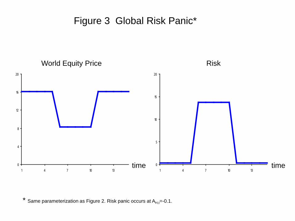
0
4
8
12
16
20
1 4 7 10 13
Figure 3 Global Risk Panic*
* Same parameterization as Figure 2. Risk panic occurs at AH,t=-0.1.
time
World Equity Price Risk
0
5
10
15
20
1 4 7 10 13time

0
20
40
60
80
-700 -600 -500 -400 -300 -200 -100 0 100
Figure 4 Impact Risk Panic Across Countries—Role of VDH *
% Drop Equity prices During Panic Increase in Risk During Panic
0
10
20
30
40
-700 -600 -500 -400 -300 -200 -100 0 100
* The parameterization is the same as in Figure 2. The risk panic occurs at AH,t=-0.1.
HomeHome
Foreign
Foreign
VDH VDH

0
20
40
60
80
-300 -200 -100 0 100 200
Figure 5 Impact Risk Panic Across Countries— =0.99*
% Drop Equity prices During Panic Increase in Risk During Panic
0
10
20
30
40
-300 -200 -100 0 100 200
* Other than ρHF=0.99, the parameterization is the same as in Figure 2. The risk panic occurs at AH,t=-0.1.
Home
HomeForeign
Foreign
VDH VDH
HFρ
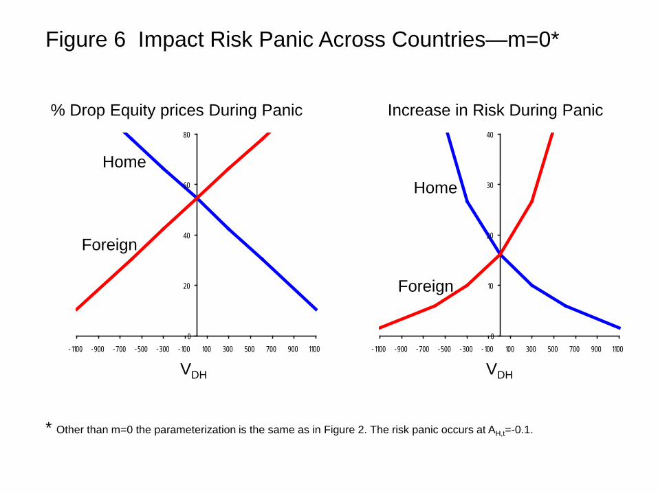
0
20
40
60
80
-1100 -900 -700 -500 -300 -100 100 300 500 700 900 1100
Figure 6 Impact Risk Panic Across Countries—m=0*
% Drop Equity prices During Panic Increase in Risk During Panic
0
10
20
30
40
-1100 -900 -700 -500 -300 -100 100 300 500 700 900 1100
* Other than m=0 the parameterization is the same as in Figure 2. The risk panic occurs at AH,t=-0.1.
HomeHome
Foreign
Foreign
VDH VDH
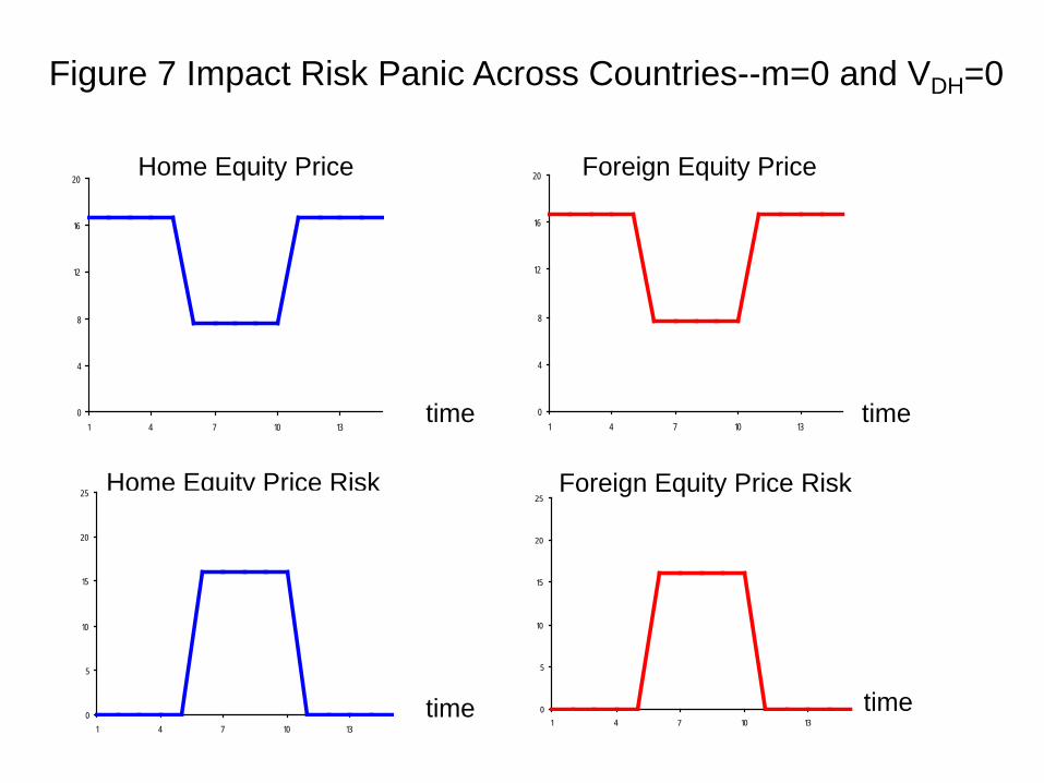
0
4
8
12
16
20
1 4 7 10 13
Figure 7 Impact Risk Panic Across Countries--m=0 and VDH=0
time
Home Equity Price
Home Equity Price Risk
0
5
10
15
20
25
1 4 7 10 13
time
0
4
8
12
16
20
1 4 7 10 13
Foreign Equity Price
0
5
10
15
20
25
1 4 7 10 13
timetime
Foreign Equity Price Risk