Embed Size (px)
DESCRIPTION
VALIDITY OF HIGH-SCHOOL GRADES
Citation preview
Research & Occasional Paper Series: CSHE.6.07
UNIVERSITY OF CALIFORNIA, BERKELEYhttp://cshe.berkeley.edu/
VALIDITY OF HIGH-SCHOOL GRADES IN PREDICTING STUDENT SUCCESS BEYOND THE FRESHMAN YEAR:
High-School Record vs. Standardized Tests as Indicators of Four-Year College Outcomes*
Saul GeiserCenter for Studies in Higher Education
University of California, Berkeley
Maria Veronica SantelicesGraduate School of Education
University of California, Berkeley
Copyright 2007 Saul Geiser and Maria Veronica Santelices, all rights reserved.
ABSTRACTHigh-school grades are often viewed as an unreliable criterion for college admissions, owing to differences in grading standards across high schools, while standardized tests are seen as methodologically rigorous, providing a more uniform and valid yardstick for assessing student ability and achievement. The present study challenges that conventional view. The study finds that high-school grade point average (HSGPA) is consistently the best predictor not only of freshman grades in college, the outcome indicator most often employed in predictive-validity studies, but of four-year college outcomes as well. A previous study, UC and the SAT (Geiser with Studley, 2003),demonstrated that HSGPA in college-preparatory courses was the best predictor of freshman grades for a sample of almost 80,000 students admitted to the University of California. Because freshman grades provide only a short-term indicator of college performance, the present study tracked four-year college outcomes, including cumulative college grades and graduation, for the same sample in order to examine the relative contribution of high-school record and standardized tests in predicting longer-term college performance. Key findings are: (1) HSGPA is consistently the strongestpredictor of four-year college outcomes for all academic disciplines, campuses and freshman cohorts in the UC sample; (2) surprisingly, the predictive weight associated with HSGPA increases after the freshman year, accounting for a greater proportion of variance in cumulative fourth-year than first-year college grades; and (3) as an admissions criterion, HSGPA has less adverse impact than standardized tests on disadvantaged and underrepresented minority students. The paper concludes with a discussion of the implications of these findings for admissions policy and argues for greater emphasis on the high-school record, and a corresponding de-emphasis onstandardized tests, in college admissions.
* The study was supported by a grant from the Koret Foundation.
Geiser and Santelices: VALIDITY OF HIGH-SCHOOL GRADES 2
CSHE Research & Occasional Paper Series
Introduction and Policy Context
This study examines the relative contribution of high-school grades and standardized admissions tests in predicting students’ long-term performance in college, including cumulative grade-point average and college graduation. The relative emphasis on grades vs. tests as admissions criteria has become increasingly visible as a policy issue at selective colleges and universities, particularly in states such as Texas and California, where affirmative action has been challenged or eliminated.
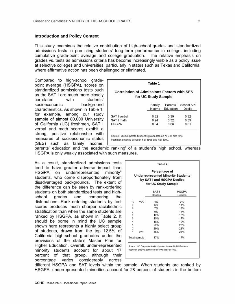
Compared to high-school grade-point average (HSGPA), scores on standardized admissions tests such as the SAT I are much more closely correlated with students’ socioeconomic background characteristics. As shown in Table 1, for example, among our study sample of almost 80,000 University of California (UC) freshmen, SAT I verbal and math scores exhibit a strong, positive relationship with measures of socioeconomic status (SES) such as family income, parents’ education and the academic rankingi of a student’s high school, whereas HSGPA is only weakly associated with such measures.
As a result, standardized admissions tests tend to have greater adverse impact than HSGPA on underrepresented minorityii
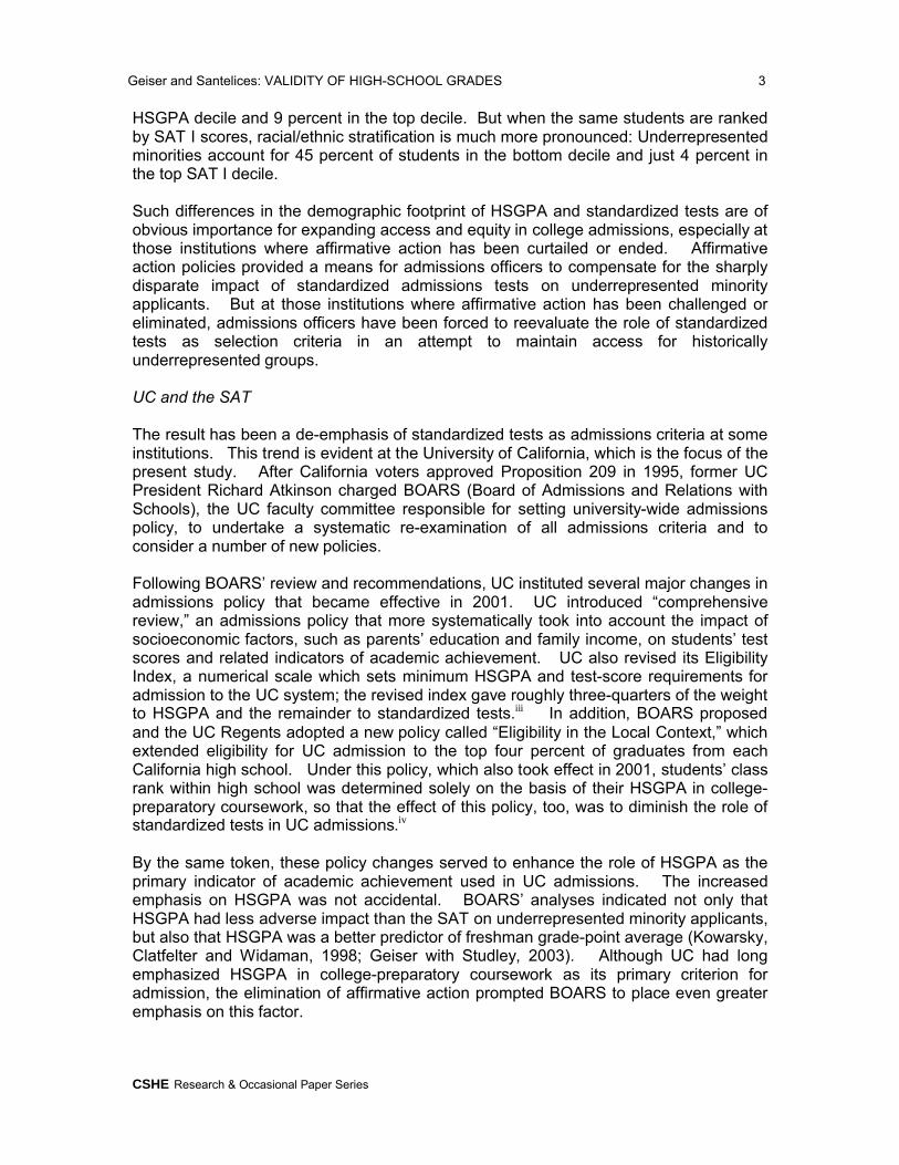
students, who come disproportionately from disadvantaged backgrounds. The extent of the difference can be seen by rank-ordering students on both standardized tests and high-school grades and comparing the distributions. Rank-ordering students by test scores produces much sharper racial/ethnic stratification than when the same students are ranked by HSGPA, as shown in Table 2. It should be borne in mind the UC sample shown here represents a highly select group of students, drawn from the top 12.5% of California high-school graduates under the provisions of the state’s Master Plan for Higher Education. Overall, under-represented minority students account for about 17 percent of that group, although their percentage varies considerably across different HSGPA and SAT levels within the sample. When students are ranked by HSGPA, underrepresented minorities account for 28 percent of students in the bottom
Family Parents' School APIIncome Education Decile
SAT I verbal 0.32 0.39 0.32SAT I math 0.24 0.32 0.39HSGPA 0.04 0.06 0.01
Source: UC Corporate Student System data on 79,785 first-time
freshmen entering between Fall 1996 and Fall 1999.
Correlation of Admissions Factors with SES
Table 1
for UC Study Sample
SAT I HSGPADeciles Deciles
10 (high) 4% 9%9 6% 11%8 7% 13%7 9% 14%6 12% 16%5 15% 17%4 18% 19%3 22% 20%2 29% 23%1 (low) 45% 28%
Total sample 17% 17%
Source: UC Corporate Student System data on 79,785 first-time
freshmen entering between Fall 1996 and Fall 1999.
Table 2
for UC Study Sample
Percentage ofUnderrepresented Minority Students
by SAT I and HSGPA Deciles
Geiser and Santelices: VALIDITY OF HIGH-SCHOOL GRADES 3
CSHE Research & Occasional Paper Series
HSGPA decile and 9 percent in the top decile. But when the same students are ranked by SAT I scores, racial/ethnic stratification is much more pronounced: Underrepresented minorities account for 45 percent of students in the bottom decile and just 4 percent in the top SAT I decile.
Such differences in the demographic footprint of HSGPA and standardized tests are of obvious importance for expanding access and equity in college admissions, especially at those institutions where affirmative action has been curtailed or ended. Affirmative action policies provided a means for admissions officers to compensate for the sharply disparate impact of standardized admissions tests on underrepresented minority applicants. But at those institutions where affirmative action has been challenged or eliminated, admissions officers have been forced to reevaluate the role of standardized tests as selection criteria in an attempt to maintain access for historically underrepresented groups.
UC and the SAT
The result has been a de-emphasis of standardized tests as admissions criteria at some institutions. This trend is evident at the University of California, which is the focus of the present study. After California voters approved Proposition 209 in 1995, former UC President Richard Atkinson charged BOARS (Board of Admissions and Relations with Schools), the UC faculty committee responsible for setting university-wide admissions policy, to undertake a systematic re-examination of all admissions criteria and to consider a number of new policies.
Following BOARS’ review and recommendations, UC instituted several major changes in admissions policy that became effective in 2001. UC introduced “comprehensive review,” an admissions policy that more systematically took into account the impact of socioeconomic factors, such as parents’ education and family income, on students’ test scores and related indicators of academic achievement. UC also revised its Eligibility Index, a numerical scale which sets minimum HSGPA and test-score requirements for admission to the UC system; the revised index gave roughly three-quarters of the weight to HSGPA and the remainder to standardized tests.iii In addition, BOARS proposed and the UC Regents adopted a new policy called “Eligibility in the Local Context,” which extended eligibility for UC admission to the top four percent of graduates from each California high school. Under this policy, which also took effect in 2001, students’ class rank within high school was determined solely on the basis of their HSGPA in college-preparatory coursework, so that the effect of this policy, too, was to diminish the role of standardized tests in UC admissions.iv
By the same token, these policy changes served to enhance the role of HSGPA as the primary indicator of academic achievement used in UC admissions. The increased emphasis on HSGPA was not accidental. BOARS’ analyses indicated not only that HSGPA had less adverse impact than the SAT on underrepresented minority applicants, but also that HSGPA was a better predictor of freshman grade-point average (Kowarsky, Clatfelter and Widaman, 1998; Geiser with Studley, 2003). Although UC had long emphasized HSGPA in college-preparatory coursework as its primary criterion for admission, the elimination of affirmative action prompted BOARS to place even greater emphasis on this factor.
Geiser and Santelices: VALIDITY OF HIGH-SCHOOL GRADES 4
CSHE Research & Occasional Paper Series
But the diminished emphasis on SAT scores in favor of HSGPA and other factors has not been without its critics. De-emphasizing tests led inevitably to the admission of some students with poor test scores, as the then-Chair of the UC Regents, John Moores, demonstrated in a controversial analysis of UC Berkeley admission data in 2002 (Moores, 2003). Lower test scores among some admitted students also caused misgivings among those concerned with collegiate rankings in national publications such as US News and World Report, which tend to portray even small annual fluctuations in average test scores as indicators of changing institutional quality and prestige.
At the root of critics’ concerns is the widespread perception of standardized tests as providing a single, common yardstick for assessing academic ability, in contrast to high-school grades, which are viewed as a less reliable indicator owing to differences in grading standards across high schools. Testing agencies such as the College Board, which owns and administers the SAT, do little to discourage this perception:
The high school GPA … is an unreliable variable, although typically used in studies of predictive validity. There are no common grading standards across schools or across courses in the same school (Camara and Michaelides, 2005:2; see also Camara, 1998).
Researchers affiliated with the College Board also frequently raise concerns about grade inflation, which is similarly viewed as limiting the reliability of HSGPA as a criterion for college admissions:
As more and more college-bound students report GPAs near or above 4.0, highschool grades lose some of their value in differentiating students, and course rigor, admissions test scores, and other information gain importance in college admissions (Camara, Kimmel, Scheuneman and Sawtell, 2003:108).
Standardized tests, in contrast, are usually portrayed as exhibiting greater precision and methodological rigor than high-school grades and thus providing a more reliable and consistent measure of student ability and achievement. Given these widespread and contrasting perceptions of test scores and grades, it is understandable that UC’s de-emphasis of standardized tests in favor of HSGPA and other admissions factors would cause misgivings among some critics.
For those who share this commonly-held view of standardized tests, it often comes as a surprise to learn that high-school grades are in fact better predictors of freshman grades in college, although this fact is well known to college admissions officers and those who conduct research on college admissions. The superiority of HSGPA over standardized tests has been established in literally hundreds of “predictive validity” studies undertaken by colleges and universities to examine the relationship between their admissions criteria and college outcomes such as freshman grades. Freshman GPA is the most frequently used indicator of college success in such predictive-validity studies, since that measure tends to be more readily available than other outcome indictors.
Predictive-validity studies undertaken at a broad range of colleges and universities show that HSGPA is consistently the best predictor of freshman grades. Standardized test scores do add a statistically significant increment to the prediction, so that the combination of HSGPA and test scores predicts better than HSGPA alone. But HSGPA accounts for the largest share of the predicted variation in freshman grades. Useful
Geiser and Santelices: VALIDITY OF HIGH-SCHOOL GRADES 5
CSHE Research & Occasional Paper Series
summaries of the results of the large number of predictive-validity studies that have been undertaken over the past several decades can be found in Morgan (1989) and Hezlett et al. (2001).
Research Focus
The present study is a follow-up to an earlier study entitled, UC and the SAT: Predictive Validity and Differential Impact of the SAT I and SAT II at the University of California(Geiser with Studley, 2003). That study confirmed that HSGPA in college-preparatory courses is the best predictor of freshman grades for students admitted to the University of California. In addition, the study found that, after HSGPA, achievement-type tests such as the SAT II – particularly the SAT II Writing Test -- were the next-best predictor of freshman grades and were consistently superior to aptitude-type tests such as the SAT I in that regard. UC and the SAT was influential in the College Board’s recent decision to revise the SAT I in the direction of a more curriculum-based, achievement-type test and to include a writing component.v
Since UC and the SAT was published, new research questions have emerged. The first concerns the outcome indicators employed as measures of student “success” in college. Like the great majority of other predictive-validity studies, UC and the SAT employed freshman grade-point average as its primary outcome criterion for assessing the predictive validity of HSGPA and standardized tests, but questions have been raised about whether the study findings can be generalized to other, longer-term outcomes. Many have criticized the narrowness of freshman grades as a measure of college “success” and have urged use of alternative outcome criteria such as graduation rates or cumulative grade-point average in college.vi
This study makes use of UC’s vast longitudinal student database to track four-year college outcomes for the sample of almost 80,000 freshmen included in the original study of UC and the SAT. Do high-school grades and standardized test scores predict longer-term as well as short-term college outcomes, and if so, what is the relative contribution of these factors to the prediction?
A second important issue concerns variations across organizational units -- academic disciplines, campuses and freshman cohorts -- in the extent to which high-school grades and standardized test scores predict college performance. Some have raised questions about whether standardized tests might be better predictors of college performance in certain disciplines -- particularly in the “hard” sciences and math-based disciplines -- so that SAT scores should continue to be emphasized as an admissions criterion in those fields (Moores, 2003). Others have criticized UC and the SAT for aggregating results across campuses, suggesting that the findings of the earlier study might be spurious insofar as they may confound within-campus with between-campus effects (Zwick, Brown and Sklar, 2004).
To address such concerns, this study employs multilevel modeling of the UC student data to estimate the extent to which group-level effects, such as those associated with academic disciplines or campuses, may affect the predictive validity of high-school grades, standardized test scores and other student-level admissions factors.
Geiser and Santelices: VALIDITY OF HIGH-SCHOOL GRADES 6
CSHE Research & Occasional Paper Series
Data and Methodology
Sample
The sample consisted of 79,785 first-time freshmen who entered UC over the four-year period from Fall 1996 through Fall 1999 and for whom complete admissions data were available. This is essentially the same sample employed in the earlier study of UC and the SAT except for the addition of missing student files from the UC Riverside campus that were not available at the time of the earlier study.vii Data on each student were drawn from UC’s Corporate Student Database, which tracks all students after point of entry based on periodic data uploads from the UC campuses into the UC corporate data system.
Predictor Variables
The main predictor variables considered in the study were high-school grade-point average and standardized test scores. The HSGPA used in this analysis was an “unweighted” grade-point average, that is, a GPA “capped” at 4.0 and calculated without additional grade-points for Advanced Placement (AP) or honors-level courses. Previous research by the present authors has demonstrated that an unweighted HSGPA is a consistently better predictor of college performance than an honors-weighted HSGPA (Geiser and Santelices, 2006). Standardized test scores considered in the analysis consisted of students’ scores on each of the five tests required for UC admission during the period under study: SAT I verbal and math (or ACT equivalent), SAT II Writing and Mathematics, and a SAT II third subject test of the student’s choosing. viii
In addition to these academic variables, the analysis also controlled for students’ socioeconomic and demographic characteristics, including family income, parents’ education, and the Academic Performance Index (API) of students’ high schools. These controls were introduced for two reasons. First, UC explicitly takes such factors into account in admissions decisions, giving extra consideration for applicants from poorer families and disadvantaged schools. Although the extra consideration given to applicants from such backgrounds is known to correlate inversely, to some degree, with college outcomes, such factors are formally considered in the admissions process and should therefore be included in any analyses of the validity of UC admissions criteria.
Second and equally important, omission of socioeconomic background factors can lead to significant overestimation of the predictive power of academic variables, such as SAT scores, that are correlated with socioeconomic advantage. A recent and authoritative study by Princeton economist Jesse Rothstein, using UC data, found that SAT scores often serve as a “proxy” for student background characteristics:
The results here indicate that the exclusion of student background characteristics from prediction models inflates the SAT’s apparent validity, as the SAT score appears to be a more effective measure of the demographic characteristics that predict UC FGPA [freshman grade-point average] than it is of preparedness conditional on student background. … [A] conservative estimate is that traditional methods and sparse models [i.e., those that do not take into account student background characteristics] overstate the SAT’s importance to predictive accuracy by 150 percent (Rothstein, 2004).
Geiser and Santelices: VALIDITY OF HIGH-SCHOOL GRADES 7
CSHE Research & Occasional Paper Series
The present analysis controlled for socioeconomic background factors in order to minimize such “proxy” effects and derive a truer picture of the actual predictive weights associated with various academic admissions factors.ix
Finally, it is important to note several kinds of predictor variables that were notconsidered here. Given that the present study is concerned with the predictive validity of admissions criteria, we have deliberately ignored the role of other factors -- such as financial, social and academic support in college -- which may significantly affect graduation or other college outcomes but which come into play during the course ofstudents’ undergraduate careers. The present study is limited to assessing the long-term predictive validity of academic and other factors known at point of college admission.
Outcome Measures
The study employed two main indicators of long-term “success” in college: Four-year graduation and cumulative GPA.
Graduation is obviously an important indicator of student success in college, although there are several different ways in which this outcome can be measured. The measure employed here is four-year graduation, that is, whether a student graduates within the normative time-to-degree of four years. This measure differs, for example, from the gross graduation rate, that is, the proportion of students who graduate at any point after admission. About 78 percent of all entering freshman ultimately go on to graduate from UC, but only about 40 percent graduate within four years, according to recent UC data. Average time-to-degree at UC is about 4.3 years, indicating that many students require at least one extra term to graduate. The graduation rate increases to about 70 percent after five years and to about 78 percent after six years, after which it does not increase appreciably – students who do not graduate after six years tend not to graduate at all.x
Four-year graduation was chosen as an outcome measure for both methodological and policy reasons. Because the sample included freshmen cohorts entering UC over a multi-year period from 1996 to1999, gross graduation rates for the earlier cohorts were somewhat higher than for the later cohorts, an artifact of the shorter period of time that students in the later cohorts had to complete their degrees. Using four-year graduation rates permitted a fairer comparison across cohorts insofar as all students in the sample had the same number of years to meet the criterion. Four-year graduation rates also appeared the more appropriate measure on policy grounds. UC, like other public universities, has recently been under considerable pressure from state government authorities to improve student “throughput” and to encourage more students to “finish in four” as a means of achieving budgetary savings.xi Graduating within the normative time-to-degree of four years can thus be considered a “success” from that policy standpoint as well.xii
Geiser and Santelices: VALIDITY OF HIGH-SCHOOL GRADES 8
CSHE Research & Occasional Paper Series
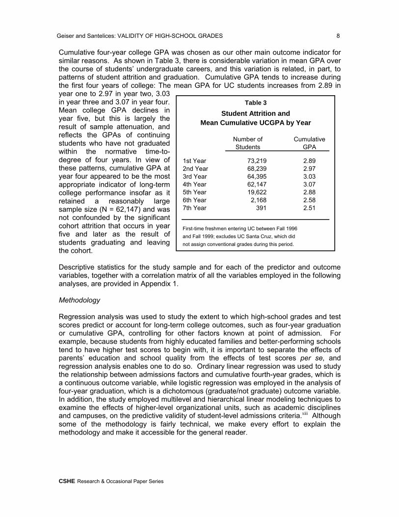
Cumulative four-year college GPA was chosen as our other main outcome indicator for similar reasons. As shown in Table 3, there is considerable variation in mean GPA over the course of students’ undergraduate careers, and this variation is related, in part, to patterns of student attrition and graduation. Cumulative GPA tends to increase during the first four years of college: The mean GPA for UC students increases from 2.89 in year one to 2.97 in year two, 3.03 in year three and 3.07 in year four. Mean college GPA declines in year five, but this is largely the result of sample attenuation, and reflects the GPAs of continuing students who have not graduated within the normative time-to-degree of four years. In view of these patterns, cumulative GPA at year four appeared to be the most appropriate indicator of long-term college performance insofar as it retained a reasonably large sample size (N = 62,147) and was not confounded by the significant cohort attrition that occurs in year five and later as the result of students graduating and leaving the cohort.
Descriptive statistics for the study sample and for each of the predictor and outcome variables, together with a correlation matrix of all the variables employed in the following analyses, are provided in Appendix 1.
Methodology
Regression analysis was used to study the extent to which high-school grades and test scores predict or account for long-term college outcomes, such as four-year graduation or cumulative GPA, controlling for other factors known at point of admission. For example, because students from highly educated families and better-performing schools tend to have higher test scores to begin with, it is important to separate the effects of parents’ education and school quality from the effects of test scores per se, and regression analysis enables one to do so. Ordinary linear regression was used to study the relationship between admissions factors and cumulative fourth-year grades, which is a continuous outcome variable, while logistic regression was employed in the analysis of four-year graduation, which is a dichotomous (graduate/not graduate) outcome variable. In addition, the study employed multilevel and hierarchical linear modeling techniques to examine the effects of higher-level organizational units, such as academic disciplines and campuses, on the predictive validity of student-level admissions criteria.xiii Although some of the methodology is fairly technical, we make every effort to explain the methodology and make it accessible for the general reader.
Number of CumulativeStudents GPA
1st Year 73,219 2.892nd Year 68,239 2.973rd Year 64,395 3.034th Year 62,147 3.075th Year 19,622 2.886th Year 2,168 2.587th Year 391 2.51
First-time freshmen entering UC between Fall 1996
and Fall 1999; excludes UC Santa Cruz, which did
not assign conventional grades during this period.
Student Attrition andMean Cumulative UCGPA by Year
Table 3
Geiser and Santelices: VALIDITY OF HIGH-SCHOOL GRADES 9
CSHE Research & Occasional Paper Series
Organization of Report
Section I of the report presents findings on the relative contribution of high-school grades and standardized admissions tests in predicting cumulative fourth-year grade-point average at UC. Section II compares the predictive validity of HSGPA and test scores between the first and fourth year of college and reports a surprising finding, namely, that the predictive validity of admissions factors actually improves over the four years of college, accounting for a greater proportion of the variance in cumulative fourth-year college GPA than freshman GPA; possible explanations for this phenomenon are considered. Section III then utilizes multilevel and hierarchical linear modeling to examine the extent to which clustering of students within campuses, academic disciplines and other higher-level organizational units may affect the predictive validity of student-level admissions factors. Section IV examines the relative contribution of HSGPA and test scores in predicting four-year graduation from UC. The paper concludes with a discussion of the implications of our findings for admissions policy.
I. Validity of Admissions Factors in Predicting Cumulative Fourth-Year GPA
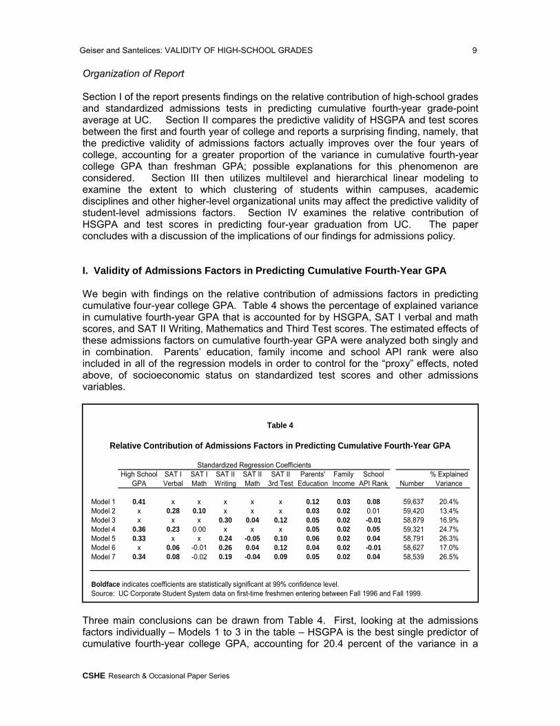
We begin with findings on the relative contribution of admissions factors in predicting cumulative four-year college GPA. Table 4 shows the percentage of explained variance in cumulative fourth-year GPA that is accounted for by HSGPA, SAT I verbal and math scores, and SAT II Writing, Mathematics and Third Test scores. The estimated effects of these admissions factors on cumulative fourth-year GPA were analyzed both singly and in combination. Parents’ education, family income and school API rank were also included in all of the regression models in order to control for the “proxy” effects, noted above, of socioeconomic status on standardized test scores and other admissions variables.
Three main conclusions can be drawn from Table 4. First, looking at the admissions factors individually – Models 1 to 3 in the table – HSGPA is the best single predictor of cumulative fourth-year college GPA, accounting for 20.4 percent of the variance in a
High School SAT I SAT I SAT II SAT II SAT II Parents' Family School % ExplainedGPA Verbal Math Writing Math 3rd Test Education Income API Rank Number Variance
Model 1 0.41 x x x x x 0.12 0.03 0.08 59,637 20.4%Model 2 x 0.28 0.10 x x x 0.03 0.02 0.01 59,420 13.4%Model 3 x x x 0.30 0.04 0.12 0.05 0.02 -0.01 58,879 16.9%Model 4 0.36 0.23 0.00 x x x 0.05 0.02 0.05 59,321 24.7%Model 5 0.33 x x 0.24 -0.05 0.10 0.06 0.02 0.04 58,791 26.3%Model 6 x 0.06 -0.01 0.26 0.04 0.12 0.04 0.02 -0.01 58,627 17.0%Model 7 0.34 0.08 -0.02 0.19 -0.04 0.09 0.05 0.02 0.04 58,539 26.5%
Boldface indicates coefficients are statistically significant at 99% confidence level.Source: UC Corporate Student System data on first-time freshmen entering between Fall 1996 and Fall 1999.
Standardized Regression Coefficients
Relative Contribution of Admissions Factors in Predicting Cumulative Fourth-Year GPA
Table 4
Geiser and Santelices: VALIDITY OF HIGH-SCHOOL GRADES 10
CSHE Research & Occasional Paper Series
model that also includes socioeconomic background variables (Model 1, right-hand column). SAT II scores, including students’ scores on the SAT II Writing, Math and Third Subject Test (Model 3), are the next-best predictor, accounting for 16.9 percent of the variance. Students’ scores on the SAT I verbal and math tests (Model 2) rank last, accounting for just 13.4 percent of the variance in cumulative fourth-year college grades, controlling for socioeconomic background variables.xiv
Second, it is evident that using the admissions factors in combination – Models 4 to 7 –explains more of the variance in cumulative college grades than is possible with any one admissions factor alone. Thus, all of the predictor variables combined – HSGPA, SAT I and SAT II scores together with socioeconomic background variables (Model 7) –account for 26.5 percent of the variance in cumulative fourth-year college GPA for the overall UC sample, the largest percentage of explained variance for any of the models. Note also the size of the additional increment provided by test scores: After taking HSGPA into account, test scores increase the explained variance by about 6 percentage points, from 20.4 percent (Model 1) to 26.5 percent (Model 7).
Third, looking at the pattern of standardized coefficients within the body of Table 4, it is evident that HSGPA and SAT II Writing scores have the greatest predictive weight, controlling for other factors. Standardized regression coefficients, or “beta weights,” show the number of standard deviations that a dependent variable (in this case fourth-year college GPA) changes for each one-standard deviation change in a given predictor variable, controlling for all other variables in the regression equation. As the above table shows, HSGPA has the largest predictive weight, 0.34, followed by SAT II Writing scores, 0.19, while the weights for all of the other variables are considerably smaller.
These findings are consistent with those for first-year college grades reported originallyin UC and the SAT: HSGPA and SAT II Writing scores are the strongest predictors of both cumulative college grades and freshman grades, and other standardized test scores, though statistically significant in many cases, have considerably less predictive weight after controlling for student background characteristics.
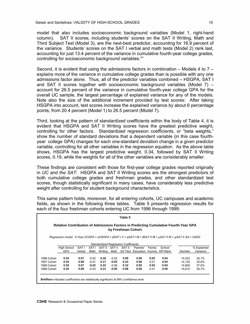
This same pattern holds, moreover, for all entering cohorts, UC campuses and academic fields, as shown in the following three tables. Table 5 presents regression results for each of the four freshman cohorts entering UC from 1996 through 1999:
High School SAT I SAT I SAT II SAT II SAT II Parents' Family School % ExplainedGPA Verbal Math Writing Math 3rd Test Education Income API Rank Number Variance
1996 Cohort 0.34 0.07 -0.02 0.18 -0.02 0.09 0.05 0.02 0.04 14,022 26.1%1997 Cohort 0.34 0.08 -0.01 0.17 -0.04 0.10 0.06 0.01 0.04 14,102 25.8%1998 Cohort 0.33 0.07 -0.02 0.22 -0.06 0.10 0.05 0.03 0.04 14,605 27.6%1999 Cohort 0.34 0.08 -0.03 0.21 -0.05 0.08 0.05 0.01 0.05 15,810 26.7%
Boldface indicates coefficients are statistically significant at 99% confidence level.
Regression model: 4-Year UCGPA = αHSGPA + βSAT I V + φSAT I M + θSAT II W + μSAT II M + ψSAT II 3rd + ΩSES
Table 5
Standardized Regression Coefficients
Relative Contribution of Admissions Factors in Predicting Cumulative Fourth-Year GPAby Freshman Cohort
Geiser and Santelices: VALIDITY OF HIGH-SCHOOL GRADES 11
CSHE Research & Occasional Paper Series
Looking at the standardized coefficients in the body of Table 5, it is evident that HSGPA has the greatest predictive weight in all entering cohorts, while SAT II Writing scores are consistently the second-best predictor of fourth-year college grades. Somewhat weaker but still statistically significant, the SAT II Third Test has the next-greatest predictive weight in all cases, followed by SAT I verbal scores. The two math tests – both the SAT I and the SAT II – are not statistically significant predictors of fourth-year grades in most cases, after controlling for other factors.
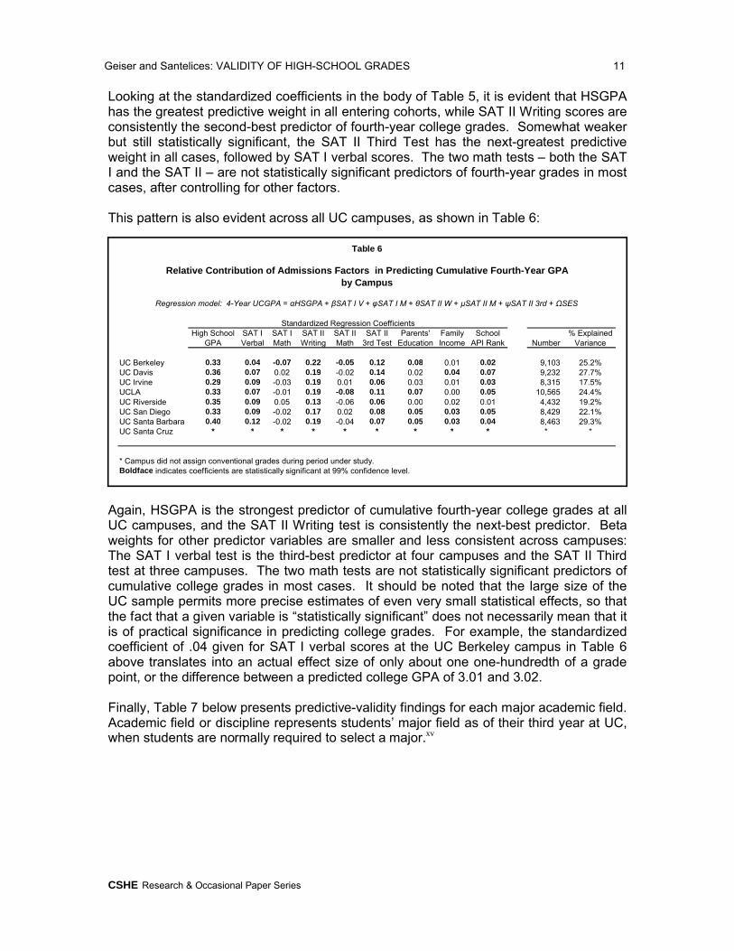
This pattern is also evident across all UC campuses, as shown in Table 6:
Again, HSGPA is the strongest predictor of cumulative fourth-year college grades at all UC campuses, and the SAT II Writing test is consistently the next-best predictor. Beta weights for other predictor variables are smaller and less consistent across campuses: The SAT I verbal test is the third-best predictor at four campuses and the SAT II Third test at three campuses. The two math tests are not statistically significant predictors of cumulative college grades in most cases. It should be noted that the large size of the UC sample permits more precise estimates of even very small statistical effects, so that the fact that a given variable is “statistically significant” does not necessarily mean that it is of practical significance in predicting college grades. For example, the standardized coefficient of .04 given for SAT I verbal scores at the UC Berkeley campus in Table 6above translates into an actual effect size of only about one one-hundredth of a grade point, or the difference between a predicted college GPA of 3.01 and 3.02.
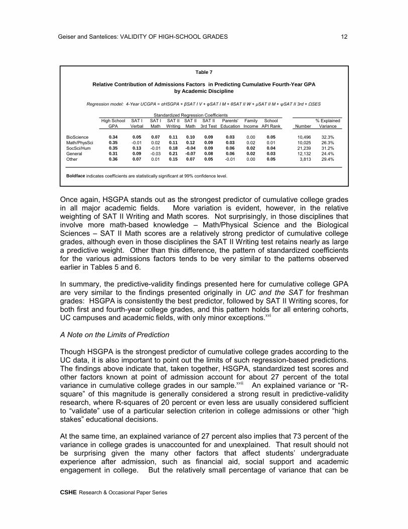
Finally, Table 7 below presents predictive-validity findings for each major academic field. Academic field or discipline represents students’ major field as of their third year at UC, when students are normally required to select a major.xv
High School SAT I SAT I SAT II SAT II SAT II Parents' Family School % ExplainedGPA Verbal Math Writing Math 3rd Test Education Income API Rank Number Variance
UC Berkeley 0.33 0.04 -0.07 0.22 -0.05 0.12 0.08 0.01 0.02 9,103 25.2%UC Davis 0.36 0.07 0.02 0.19 -0.02 0.14 0.02 0.04 0.07 9,232 27.7%UC Irvine 0.29 0.09 -0.03 0.19 0.01 0.06 0.03 0.01 0.03 8,315 17.5%UCLA 0.33 0.07 -0.01 0.19 -0.08 0.11 0.07 0.00 0.05 10,565 24.4%UC Riverside 0.35 0.09 0.05 0.13 -0.06 0.06 0.00 0.02 0.01 4,432 19.2%UC San Diego 0.33 0.09 -0.02 0.17 0.02 0.08 0.05 0.03 0.05 8,429 22.1%UC Santa Barbara 0.40 0.12 -0.02 0.19 -0.04 0.07 0.05 0.03 0.04 8,463 29.3%UC Santa Cruz * * * * * * * * * * *
* Campus did not assign conventional grades during period under study.Boldface indicates coefficients are statistically significant at 99% confidence level.
Table 6
Standardized Regression Coefficients
Relative Contribution of Admissions Factors in Predicting Cumulative Fourth-Year GPAby Campus
Regression model: 4-Year UCGPA = αHSGPA + βSAT I V + φSAT I M + θSAT II W + μSAT II M + ψSAT II 3rd + ΩSES
Geiser and Santelices: VALIDITY OF HIGH-SCHOOL GRADES 12
CSHE Research & Occasional Paper Series
Once again, HSGPA stands out as the strongest predictor of cumulative college grades in all major academic fields. More variation is evident, however, in the relative weighting of SAT II Writing and Math scores. Not surprisingly, in those disciplines that involve more math-based knowledge – Math/Physical Science and the Biological Sciences – SAT II Math scores are a relatively strong predictor of cumulative college grades, although even in those disciplines the SAT II Writing test retains nearly as large a predictive weight. Other than this difference, the pattern of standardized coefficients for the various admissions factors tends to be very similar to the patterns observed earlier in Tables 5 and 6.
In summary, the predictive-validity findings presented here for cumulative college GPA are very similar to the findings presented originally in UC and the SAT for freshman grades: HSGPA is consistently the best predictor, followed by SAT II Writing scores, for both first and fourth-year college grades, and this pattern holds for all entering cohorts, UC campuses and academic fields, with only minor exceptions.xvi
A Note on the Limits of Prediction
Though HSGPA is the strongest predictor of cumulative college grades according to the UC data, it is also important to point out the limits of such regression-based predictions. The findings above indicate that, taken together, HSGPA, standardized test scores and other factors known at point of admission account for about 27 percent of the total variance in cumulative college grades in our sample.xvii An explained variance or “R-square” of this magnitude is generally considered a strong result in predictive-validity research, where R-squares of 20 percent or even less are usually considered sufficient to “validate” use of a particular selection criterion in college admissions or other “high stakes” educational decisions.
At the same time, an explained variance of 27 percent also implies that 73 percent of the variance in college grades is unaccounted for and unexplained. That result should not be surprising given the many other factors that affect students’ undergraduate experience after admission, such as financial aid, social support and academic engagement in college. But the relatively small percentage of variance that can be
High School SAT I SAT I SAT II SAT II SAT II Parents' Family School % ExplainedGPA Verbal Math Writing Math 3rd Test Education Income API Rank Number Variance
BioScience 0.34 0.05 0.07 0.11 0.10 0.09 0.03 0.00 0.05 10,496 32.3%Math/PhysSci 0.35 -0.01 0.02 0.11 0.12 0.09 0.03 0.02 0.01 10,025 26.3%SocSci/Hum 0.35 0.13 -0.01 0.18 -0.04 0.09 0.06 0.02 0.04 21,239 31.2%General 0.31 0.09 -0.03 0.21 -0.07 0.08 0.06 0.02 0.03 12,132 24.4%Other 0.36 0.07 0.01 0.15 0.07 0.05 -0.01 0.00 0.05 3,813 29.4%
Boldface indicates coefficients are statistically significant at 99% confidence level.
Table 7
Standardized Regression Coefficients
Relative Contribution of Admissions Factors in Predicting Cumulative Fourth-Year GPAby Academic Discipline
Regression model: 4-Year UCGPA = αHSGPA + βSAT I V + φSAT I M + θSAT II W + μSAT II M + ψSAT II 3rd + ΩSES
Geiser and Santelices: VALIDITY OF HIGH-SCHOOL GRADES 13
CSHE Research & Occasional Paper Series
explained by HSGPA, standardized tests and other factors known at point of admission necessarily limits the accuracy of any predictions based on those factors. This is especially true where, as is often the case in admissions decision-making, one is attempting to predict individual outcomes rather than group outcomes or averages for large samples of individuals.
An example will illustrate the point: Take an individual applicant whom, based on all of the predictor variables we have considered thus far -- HSGPA, SAT I and SAT II scores, parental education, family income and school API rank – is predicted to achieve a cumulative college GPA of 3.0, or a B average. Because the above variables account for only a relatively small fraction of the total variance in cumulative GPA, however, the error bands around the prediction are relatively large. At the “95 percent confidence level,” the statistical standard most often employed in social-science research, the error band surrounding the prediction is plus or minus .79 grade points. What this means, in other words, is that we can be “95 percent confident” that the student’s actual college GPA will fall somewhere within a range between 2.21, or a C average, and 3.79, or an A-minus average. While perhaps better than nothing, the high degree of uncertainty surrounding the prediction limits its usefulness in making comparisons among individual applicants.
In the same example, it is also worth noting what standardized test scores contribute to the prediction. For the same student with a predicted college GPA of 3.0, dropping test scores from the regression equation expands the 95% confidence interval to plus or minus .82 grade points, compared to .79 grade points when test scores are counted.xviii While this difference is “significant” in a statistical sense, as a practical matter the uncertainty surrounding the prediction remains high and underscores the need for admissions officers to exercise great caution in using test scores to decide individual cases.xix
II. Prediction of First-Year vs. Cumulative Fourth-Year College GPA
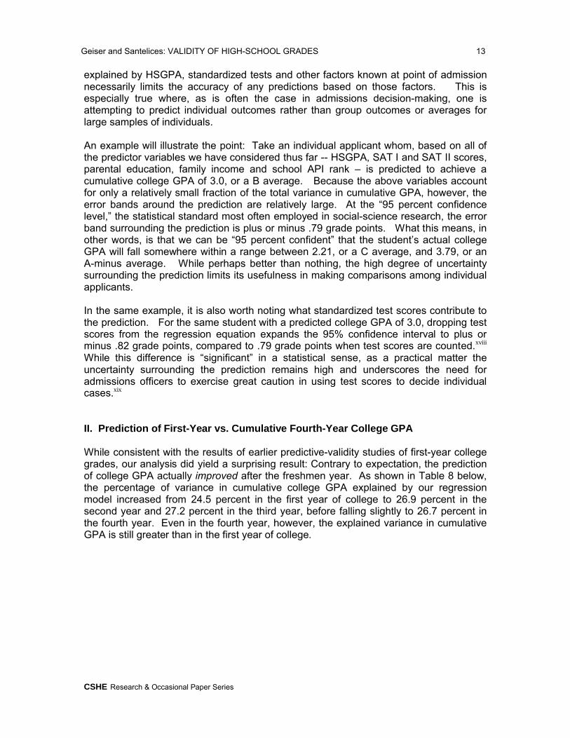
While consistent with the results of earlier predictive-validity studies of first-year college grades, our analysis did yield a surprising result: Contrary to expectation, the prediction of college GPA actually improved after the freshmen year. As shown in Table 8 below, the percentage of variance in cumulative college GPA explained by our regression model increased from 24.5 percent in the first year of college to 26.9 percent in the second year and 27.2 percent in the third year, before falling slightly to 26.7 percent in the fourth year. Even in the fourth year, however, the explained variance in cumulative GPA is still greater than in the first year of college.
Geiser and Santelices: VALIDITY OF HIGH-SCHOOL GRADES 14
CSHE Research & Occasional Paper Series
Note that the above results are limited to the same sample of students – those who completed all four years at UC and for whom complete data were available on all of the covariates – so that the finding cannot be attributed to sample attrition or similar confounding effects. Although one would expect the predictive power of admissions criteria to weaken over the course of students’ undergraduate careers as other, more proximate factors take hold (e.g., financial aid, social support, and academic engagement in college), in fact the variance in cumulative college GPA explained by factors known at point of admission increases over the course of students’ undergraduate careers.
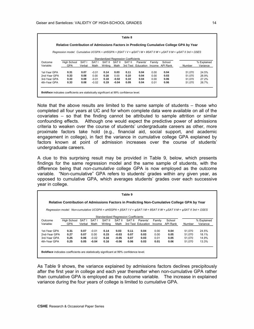
A clue to this surprising result may be provided in Table 9, below, which presents findings for the same regression model and the same sample of students, with the difference being that non-cumulative college GPA is now employed as the outcome variable. “Non-cumulative” GPA refers to students’ grades within any given year, as opposed to cumulative GPA, which averages students’ grades over each successive year in college.
As Table 9 shows, the variance explained by admissions factors declines precipitously after the first year in college and each year thereafter when non-cumulative GPA rather than cumulative GPA is employed as the outcome variable. The increase in explained variance during the four years of college is limited to cumulative GPA.
Outcome High School SAT I SAT I SAT II SAT II SAT II Parents' Family School % ExplainedVariable: GPA Verbal Math Writing Math 3rd Test Education Income API Rank Number Variance
1st-Year GPA 0.31 0.07 -0.01 0.14 0.03 0.11 0.04 0.00 0.04 51,070 24.5%2nd-Year GPA 0.27 0.07 0.00 0.15 -0.03 0.07 0.03 0.00 0.05 51,070 18.1%3rd-Year GPA 0.25 0.06 -0.02 0.16 -0.05 0.07 0.03 0.01 0.05 51,070 14.9%4th-Year GPA 0.25 0.05 -0.04 0.16 -0.06 0.06 0.03 0.01 0.06 51,070 13.3%
Boldface indicates coefficients are statistically significant at 99% confidence level.
Table 9
Relative Contribution of Admissions Factors in Predicting Non-Cumulative College GPA by Year
Regression model: Non-cumulative UCGPA = αHSGPA + βSAT I V + φSAT I M + θSAT II W + μSAT II M + ψSAT II 3rd + ΩSES
Standardized Regression Coefficients
Outcome High School SAT I SAT I SAT II SAT II SAT II Parents' Family School % ExplainedVariable: GPA Verbal Math Writing Math 3rd Test Education Income API Rank Number Variance
1st-Year GPA 0.31 0.07 -0.01 0.14 0.03 0.11 0.04 0.00 0.04 51,070 24.5%2nd-Year GPA 0.33 0.08 0.00 0.16 0.00 0.10 0.04 0.00 0.03 51,070 26.9%3rd-Year GPA 0.33 0.08 -0.01 0.18 -0.02 0.10 0.04 0.00 0.06 51,070 27.2%4th-Year GPA 0.33 0.08 -0.02 0.19 -0.04 0.09 0.04 0.01 0.06 51,070 26.7%
Boldface indicates coefficients are statistically significant at 99% confidence level.
Standardized Regression Coefficients
Relative Contribution of Admissions Factors in Predicting Cumulative College GPA by Year
Regression model: Cumulative UCGPA = αHSGPA + βSAT I V + φSAT I M + θSAT II W + μSAT II M + ψSAT II 3rd + ΩSES
Table 8
Geiser and Santelices: VALIDITY OF HIGH-SCHOOL GRADES 15
CSHE Research & Occasional Paper Series
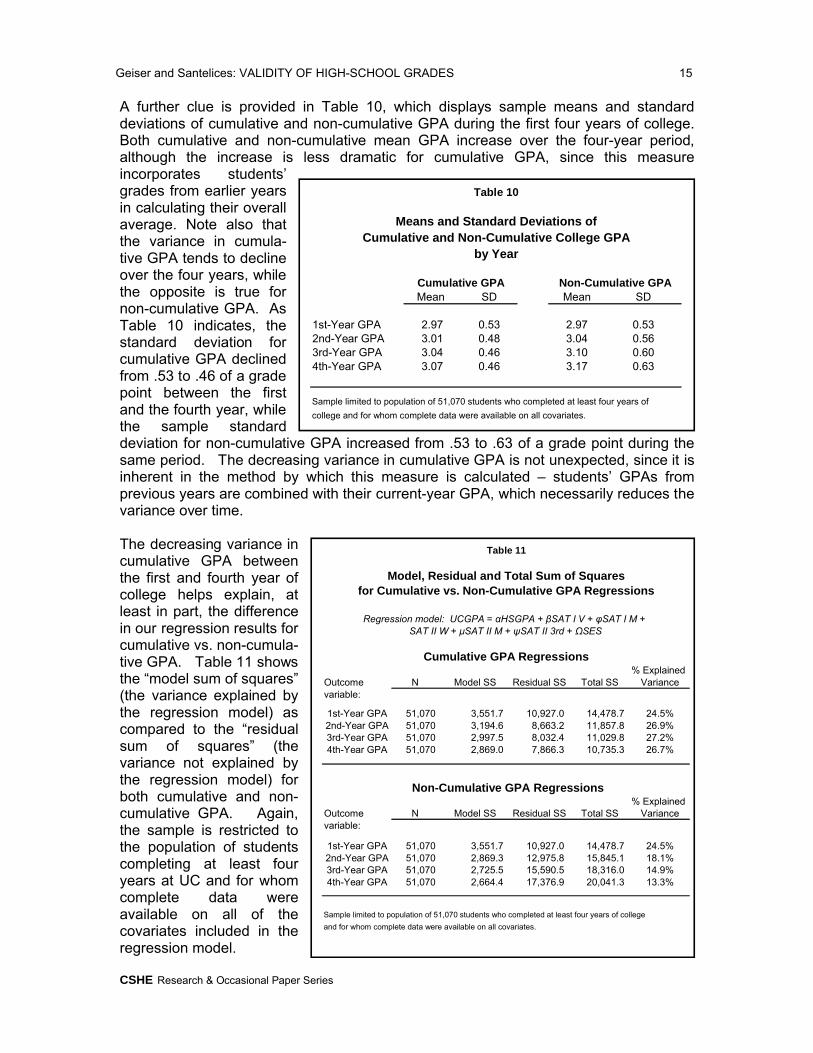
A further clue is provided in Table 10, which displays sample means and standard deviations of cumulative and non-cumulative GPA during the first four years of college.Both cumulative and non-cumulative mean GPA increase over the four-year period, although the increase is less dramatic for cumulative GPA, since this measure incorporates students’ grades from earlier years in calculating their overall average. Note also that the variance in cumula-tive GPA tends to decline over the four years, while the opposite is true for non-cumulative GPA. As Table 10 indicates, the standard deviation for cumulative GPA declined from .53 to .46 of a grade point between the first and the fourth year, while the sample standard deviation for non-cumulative GPA increased from .53 to .63 of a grade point during the same period. The decreasing variance in cumulative GPA is not unexpected, since it is inherent in the method by which this measure is calculated – students’ GPAs from previous years are combined with their current-year GPA, which necessarily reduces the variance over time.
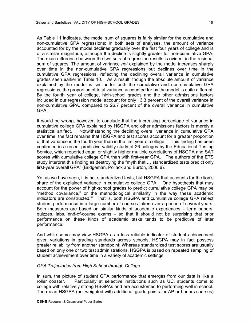
The decreasing variance in cumulative GPA between the first and fourth year of college helps explain, at least in part, the difference in our regression results for cumulative vs. non-cumula-tive GPA. Table 11 shows the “model sum of squares” (the variance explained by the regression model) as compared to the “residual sum of squares” (the variance not explained by the regression model) for both cumulative and non-cumulative GPA. Again, the sample is restricted to the population of students completing at least four years at UC and for whom complete data were available on all of the covariates included in the regression model.
% ExplainedOutcome N Model SS Residual SS Total SS Variancevariable:
1st-Year GPA 51,070 3,551.7 10,927.0 14,478.7 24.5%2nd-Year GPA 51,070 3,194.6 8,663.2 11,857.8 26.9%3rd-Year GPA 51,070 2,997.5 8,032.4 11,029.8 27.2%4th-Year GPA 51,070 2,869.0 7,866.3 10,735.3 26.7%
% ExplainedOutcome N Model SS Residual SS Total SS Variancevariable:
1st-Year GPA 51,070 3,551.7 10,927.0 14,478.7 24.5%2nd-Year GPA 51,070 2,869.3 12,975.8 15,845.1 18.1%3rd-Year GPA 51,070 2,725.5 15,590.5 18,316.0 14.9%4th-Year GPA 51,070 2,664.4 17,376.9 20,041.3 13.3%
Sample limited to population of 51,070 students who completed at least four years of college
and for whom complete data were available on all covariates.
Model, Residual and Total Sum of Squares
Non-Cumulative GPA Regressions
Cumulative GPA Regressions
Table 11
for Cumulative vs. Non-Cumulative GPA Regressions
SAT II W + μSAT II M + ψSAT II 3rd + ΩSESRegression model: UCGPA = αHSGPA + βSAT I V + φSAT I M +
Mean SD Mean SD
1st-Year GPA 2.97 0.53 2.97 0.532nd-Year GPA 3.01 0.48 3.04 0.563rd-Year GPA 3.04 0.46 3.10 0.604th-Year GPA 3.07 0.46 3.17 0.63
Sample limited to population of 51,070 students who completed at least four years of
college and for whom complete data were available on all covariates.
Means and Standard Deviations of
Table 10
Non-Cumulative GPACumulative GPA
by YearCumulative and Non-Cumulative College GPA
Geiser and Santelices: VALIDITY OF HIGH-SCHOOL GRADES 16
CSHE Research & Occasional Paper Series
As Table 11 indicates, the model sum of squares is fairly similar for the cumulative and non-cumulative GPA regressions: In both sets of analyses, the amount of variance accounted for by the model declines gradually over the first four years of college and is of a similar magnitude, although the decline is slightly greater for non-cumulative GPA. The main difference between the two sets of regression results is evident in the residual sum of squares: The amount of variance not explained by the model increases sharply over time in the non-cumulative GPA regressions but declines over time in the cumulative GPA regressions, reflecting the declining overall variance in cumulative grades seen earlier in Table 10. As a result, though the absolute amount of variance explained by the model is similar for both the cumulative and non-cumulative GPA regressions, the proportion of total variance accounted for by the model is quite different. By the fourth year of college, high-school grades and the other admissions factors included in our regression model account for only 13.3 percent of the overall variance in non-cumulative GPA, compared to 26.7 percent of the overall variance in cumulative GPA.
It would be wrong, however, to conclude that the increasing percentage of variance in cumulative college GPA explained by HSGPA and other admissions factors is merely a statistical artifact. Notwithstanding the declining overall variance in cumulative GPA over time, the fact remains that HSGPA and test scores account for a greater proportion of that variance in the fourth year than in the first year of college. This finding has been confirmed in a recent predictive-validity study of 26 colleges by the Educational Testing Service, which reported equal or slightly higher multiple correlations of HSGPA and SAT scores with cumulative college GPA than with first-year GPA. The authors of the ETS study interpret this finding as destroying the “myth that … standardized tests predict only first-year overall GPA” (Bridgeman, Pollack and Burton, 2006:6).
Yet as we have seen, it is not standardized tests, but HSGPA that accounts for the lion’s share of the explained variance in cumulative college GPA. One hypothesis that may account for the power of high-school grades to predict cumulative college GPA may be “method covariance,” or the methodological similarity in the way these academic indicators are constructed.xx That is, both HSGPA and cumulative college GPA reflect student performance in a large number of courses taken over a period of several years. Both measures are based on similar kinds of academic experiences – term papers, quizzes, labs, end-of-course exams – so that it should not be surprising that prior performance on these kinds of academic tasks tends to be predictive of later performance.
And while some may view HSGPA as a less reliable indicator of student achievement given variations in grading standards across schools, HSGPA may in fact possess greater reliability from another standpoint: Whereas standardized test scores are usually based on only one or two test administrations, HSGPA is based on repeated sampling of student achievement over time in a variety of academic settings.
GPA Trajectories from High School through College
In sum, the picture of student GPA performance that emerges from our data is like a roller coaster. Particularly at selective institutions such as UC, students come to college with relatively strong HSGPAs and are accustomed to performing well in school. The mean HSGPA (not weighted with additional grade points for AP or honors courses)
Geiser and Santelices: VALIDITY OF HIGH-SCHOOL GRADES 17
CSHE Research & Occasional Paper Series
for our sample of entering freshmen was 3.52. But the first year or two in college is a difficult transition period for many students who must adjust not only to the more rigorous academic standards of college but often as well to the experience of being away from home for the first time. Most students who drop out of college tend to do so during this period, and even among those who persist, mean GPAs plummet well below what students have become accustomed to earning in high school: Mean first-year college GPA for our sample was 2.97.
After this transition period, however, the undergraduate years tend to show steady improvement in GPA performance for most students, even approaching the levels that students achieved earlier in high school. Mean cumulative GPA for our sample increased to 3.01 in the second year, 3.04 in the third year and 3.07 in the fourth year at UC, and the increase was even greater for non-cumulative GPA. In part this upward trajectory may simply reflect self-selection, as students sort themselves and migrate into the types of college courses and majors in which they can perform well. But the data also suggest another possible explanation: Because cumulative college GPA, like HSGPA, is based on repeated sampling of student performance over time in a variety of academic settings, cumulative GPA in the fourth year of college tends to be a less variable and possibly more reliable indicator of students’ true ability and achievement than their first-year grades. As a result, the capacity of HSGPA to predict cumulative GPA tends to be consistent or even improve slightly over the four years of college. While a definitive test of this hypothesis must await future research, the present data leave no doubt that high-school grades are consistently the strongest predictor of college grades throughout the undergraduate years.
III. Multilevel Analysis of Predictive-Validity Findings
The analyses presented thus far have dealt primarily with the validity of student-level admissions factors in predicting 4-year college outcomes. We turn next to an examination of the effects of higher-level groupings, such as campuses and academic disciplines, on the predictive validity of student-level criteria. Because students are clustered within different campuses, academic disciplines and entering freshman cohorts, and because their entry into such higher-level groupings may be systematically related to admissions factors – e.g., students admitted at more selective campuses may have higher HSGPAs, on average – it is possible that group-level effects could account in part for the relationships we have observed at the student level between admissions factors and four-year college outcomes. Indeed, some critics of the earlier study upon which the present research is based have gone so far as to suggest that the relationship we have observed between student-level admissions criteria and college outcomes may be entirely an artifact of such group-level effects:
[UC and the SAT] aggregated data over seven UC campuses, four freshman cohorts (1996 through 1999), or both … . Combining data from different groups of individuals can obscure relationships among variables or produce spurious evidence of such relationships. The phenomenon is known in statistical jargon as confounding within-group effects with between-group effects. An example is the following: Suppose that there is no correlation between test scores or college grades at either Campus A or Campus B (i.e., no within-school effect). At Campus B, however, both grades and test scores tend to be higher than at Campus A – a between-school effect. If the data from the two schools are
Geiser and Santelices: VALIDITY OF HIGH-SCHOOL GRADES 18
CSHE Research & Occasional Paper Series
combined and the correlation recalculated, there will appear to be a correlation between test scores and grades, but the association will be due entirely to the fact that, at Campus B, both grades and test scores are higher than at Campus A (Zwick, Brown and Sklar, 2004).
The simplest way to test whether such group-level effects are at play is to examine the relationship between student-level admissions factors and college outcomes not only for the overall, aggregate sample, but also within each campus, academic discipline and freshman cohort. Those analyses have been presented earlier in this paper. The analyses show the same consistent pattern: HSGPA is the strongest predictor of both first and fourth-year college grades, and this pattern holds for all UC campuses, academic disciplines and entering freshman cohorts, without exception.
Another, more sophisticated technique for examining group-level effects is known as multilevel or hierarchical linear modeling, a relatively new methodology that has become increasingly popular in the research literature (Bryk and Raudenbush, 1992; Rabe-Hesketh and Skrondal, 2005). Among other uses, multilevel modeling enables researchers to partition the variation in any outcome variable of interest – in our case, cumulative college GPA – into within-group and between-group components.
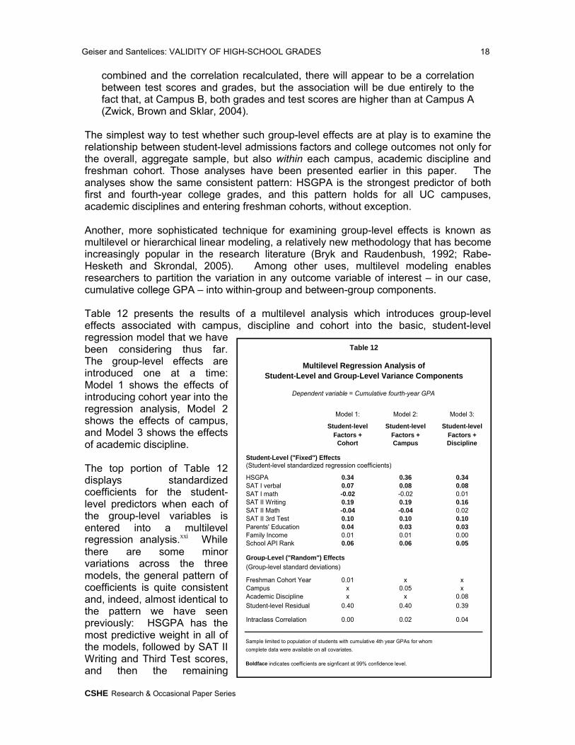
Table 12 presents the results of a multilevel analysis which introduces group-level effects associated with campus, discipline and cohort into the basic, student-level regression model that we have been considering thus far. The group-level effects are introduced one at a time: Model 1 shows the effects of introducing cohort year into the regression analysis, Model 2 shows the effects of campus, and Model 3 shows the effects of academic discipline.
The top portion of Table 12 displays standardized coefficients for the student-level predictors when each of the group-level variables is entered into a multilevel regression analysis.xxi While there are some minor variations across the three models, the general pattern of coefficients is quite consistent and, indeed, almost identical to the pattern we have seen previously: HSGPA has the most predictive weight in all of the models, followed by SAT II Writing and Third Test scores, and then the remaining
Model 1: Model 2: Model 3:
Student-level Student-level Student-levelFactors + Factors + Factors +
Cohort Campus Discipline
Student-Level ("Fixed") Effects(Student-level standardized regression coefficients)
HSGPA 0.34 0.36 0.34SAT I verbal 0.07 0.08 0.08SAT I math -0.02 -0.02 0.01SAT II Writing 0.19 0.19 0.16SAT II Math -0.04 -0.04 0.02SAT II 3rd Test 0.10 0.10 0.10Parents' Education 0.04 0.03 0.03Family Income 0.01 0.01 0.00School API Rank 0.06 0.06 0.05
Group-Level ("Random") Effects(Group-level standard deviations)
Freshman Cohort Year 0.01 x xCampus x 0.05 xAcademic Discipline x x 0.08Student-level Residual 0.40 0.40 0.39
Intraclass Correlation 0.00 0.02 0.04
Sample limited to population of students with cumulative 4th year GPAs for whom
complete data were available on all covariates.
Boldface indicates coefficients are signficant at 99% confidence level.
Dependent variable = Cumulative fourth-year GPA
Table 12
Multilevel Regression Analysis ofStudent-Level and Group-Level Variance Components
Geiser and Santelices: VALIDITY OF HIGH-SCHOOL GRADES 19
CSHE Research & Occasional Paper Series
student-level variables trail in the same order of importance that we have observed in earlier analyses.
The more interesting results appear in the bottom part of Table 12, which displays group-level effects. The numbers for cohort year, campus and academic discipline represent the amount of variation in our outcome variable, cumulative fourth-year college GPA, that is accounted for by these higher-level groupings after controlling for measured differences among groups in student-level characteristics (i.e., HSGPA, SAT II Writing scores, etc.). The variation is expressed in standard deviations. As the table indicates, the variation associated with cohort year is quite small, only about one one-hundredth of a standard deviation in cumulative fourth-year GPA. The variation associated with campus is somewhat larger, .05 standard deviations, and the variation associated with academic discipline is larger still, .08 standard deviations.xxii
But the variation associated with these group-level effects pales in comparison to that associated with the “student-level residual,” which is about .4 standard deviations in all three models in Table 12. The student-level residual represents that portion of the total variance in cumulative college GPA that is attributable neither to group-level effects nor to measured student-level characteristics such as HSGPA and test scores, but instead is attributable to other, unmeasured student-level characteristics not specified in the model. Such unmeasured characteristics might include personality traits such as perseverance or intellectual curiosity, for example, that are related to student performance in college, or other kinds of academic ability that are not necessarily captured by HSGPA and standardized tests. The large size of the student-level residual in comparison with any of the group-level effects indicates that student-level characteristics are much more important in determining college outcomes.
The same point is underscored by the “intraclass correlations” at the bottom of Table 12. The intraclass correlation is a statistic that ranges from zero to one and measures the “closeness” of observations within groups relative to the closeness of observations between groups, when student-level measures are held constant. The statistic can also be interpreted to represent the proportion of “residual” variance – i.e., the variance in college grades that is not attributable to measured student-level characteristics –attributable to group-level effects (Rabe-Hesketh and Skrondal, 2005).xxiii
The intraclass correlation of .00 for cohort year indicates that this group-level variable accounts for zero percent of the residual variance in college grades when other student-level measures are held constant. The intraclass correlations associated with campus and academic discipline are somewhat greater if still relatively small. The intraclass correlation associated with campus is .02, accounting for about two percent of the residual variance, while the intraclass correlation associated with academic discipline is .04, or about four percent of the residual variance in cumulative college grades not explained by other student-level admissions measures.xxiv Although the proportion of residual variance accounted for by academic discipline and campus is non-trivial, it is relatively small in comparison with the proportion of both explained variance and residual variance at the student level.
Geiser and Santelices: VALIDITY OF HIGH-SCHOOL GRADES 20
CSHE Research & Occasional Paper Series
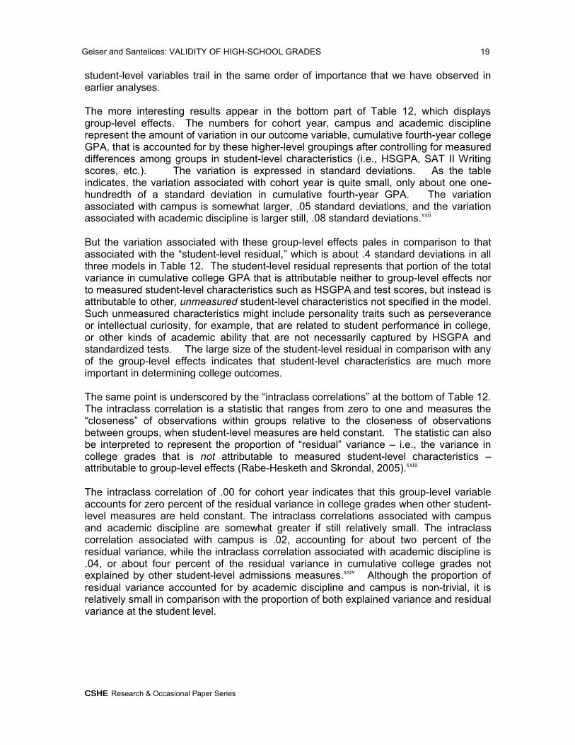
It is still possible, however, for even relatively small “between-group” effects to influence the magnitude and direction of the relationship between admissions criteria and college outcomes at the student level. The most straightforward way to test for this possibility is to introduce academic discipline, campus and cohort year as categorical variables within our original regression model. When this is done, the resulting regression coefficients for HSGPA, test scores and other student-level predictors can be interpreted as representing the purely “within-group” effects of these variables, after accounting for “between-group” effects. Those results are presented in Table 13.
The left-hand column in Table 13, labeled “Model A,” displays regression results for the student-level factors only, while the right-hand column, “Model B,” shows results when group-level variables are introduced into the regression model. Note that inclusion of group-level variables increases the explained variance from 26.4 percent to 30.8 percent, as we would expect from the previous findings in Table 12 on the variance associated with group-level effects.
The regression coefficients for cohort year, campus and academic discipline in Table 13 represent the effects of each particular category in comparison to the reference category within each group. For example, the coefficient of .25 for Social Science/Humanities indicates that cumulative college GPA is higher, on average, by .25 standard deviations for students in that major than for students in the reference category, Mathematics/Physical Science, controlling for other factors.xxv Getting good grades is less difficult, in other words, in the social sciences than in the hard sciences, other things being equal. Note also the campus coefficients in Table13, which indicate that cumulative college
Model A Model B
Only
HSGPA 0.34 0.37SAT I verbal 0.08 0.07SAT I math -0.02 0.01SAT II Writing 0.19 0.17SAT II Math -0.04 0.02SAT II 3rd Test 0.10 0.11Parents' Education 0.04 0.03Family Income 0.01 0.01School API Rank 0.06 0.05
1996 Cohort x (reference)1997 Cohort x -0.011998 Cohort x -0.011999 Cohort x -0.02
Berkeley x (reference)Davis x -0.01Irvine x 0.08Los Angeles x 0.00Riverside x 0.05San Diego x -0.01Santa Barbara x 0.09
Math/Phys Sci x (reference)Biological Sci x 0.11SocSci/Humanities x 0.25General/Undeclared x 0.09Other x 0.11
Number of Cases 53,217 53,217
% Explained Variance 26.4% 30.8%
Sample limited to population of students with cumulative 4th-year GPAs for whom
complete data were available on all covariates.
Boldface indicates coefficients are signficant at 99% confidence level.
Standardized Regression CoefficientsFor Student-Level Factors Before and After
Inclusion of Group-Level Variables
Table 13
Variables
Dependent variable: Cumulative fourth-year GPA
Student-LevelFactors
Student-Level + Group-Level
Geiser and Santelices: VALIDITY OF HIGH-SCHOOL GRADES 21
CSHE Research & Occasional Paper Series
GPAs at the Irvine, Riverside and Santa Barbara campuses are significantly higher, on average, than at the reference category, Berkeley, UC’s flagship campus.
But the key point, for our purposes, is the pattern the regression coefficients among the student-level variables in the top part of Table 13. If it is true that our predictive-validity findings are the spurious result of “confounding of within-group effects with between-group effects,” as some have suggested (Zwick, Brown and Sklar, 2004), then one would expect to observe a decline in the magnitude of the student-level regression coefficients between Model A, which shows results for the aggregate, pooled sample, and Model B, which includes group-level predictors within the regression model and thus represents the purely “within-group” effect. But this is not the case. Both the pattern and magnitude of the student-level regression coefficients are quite similar, if not identical, in the two models. In fact, the coefficient for our main student-level predictor, HSGPA, actually increases from .34 to .37 standard deviations after cohort year, campus and academic discipline are entered into the regression model and the purely “within-group” effect of HSGPA can be observed. Once again, the peculiar power and robustness of HSGPA as a predictor of college outcomes is evident.xxvi
IV. Prediction of Four-Year College Graduation
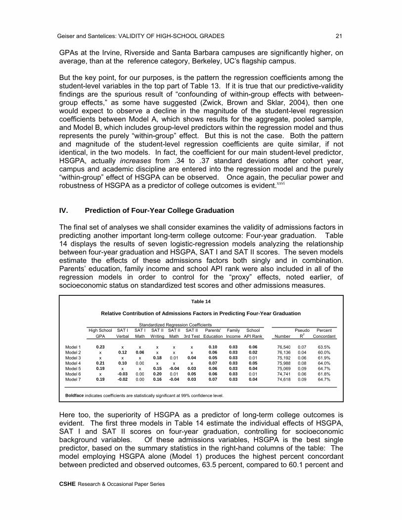
The final set of analyses we shall consider examines the validity of admissions factors in predicting another important long-term college outcome: Four-year graduation. Table 14 displays the results of seven logistic-regression models analyzing the relationship between four-year graduation and HSGPA, SAT I and SAT II scores. The seven models estimate the effects of these admissions factors both singly and in combination. Parents’ education, family income and school API rank were also included in all of the regression models in order to control for the “proxy” effects, noted earlier, of socioeconomic status on standardized test scores and other admissions measures.
Here too, the superiority of HSGPA as a predictor of long-term college outcomes is evident. The first three models in Table 14 estimate the individual effects of HSGPA, SAT I and SAT II scores on four-year graduation, controlling for socioeconomic background variables. Of these admissions variables, HSGPA is the best single predictor, based on the summary statistics in the right-hand columns of the table: The model employing HSGPA alone (Model 1) produces the highest percent concordant between predicted and observed outcomes, 63.5 percent, compared to 60.1 percent and
High School SAT I SAT I SAT II SAT II SAT II Parents' Family School Pseudo PercentGPA Verbal Math Writing Math 3rd Test Education Income API Rank Number R2
Concordant
Model 1 0.23 x x x x x 0.10 0.03 0.06 76,540 0.07 63.5%Model 2 x 0.12 0.06 x x x 0.06 0.03 0.02 76,136 0.04 60.0%Model 3 x x x 0.18 0.01 0.04 0.05 0.03 0.01 75,192 0.06 61.9%Model 4 0.21 0.10 0.00 x x x 0.07 0.03 0.05 75,988 0.08 64.0%Model 5 0.19 x x 0.15 -0.04 0.03 0.06 0.03 0.04 75,069 0.09 64.7%Model 6 x -0.03 0.00 0.20 0.01 0.05 0.06 0.03 0.01 74,741 0.06 61.8%Model 7 0.19 -0.02 0.00 0.16 -0.04 0.03 0.07 0.03 0.04 74,618 0.09 64.7%
Boldface indicates coefficients are statistically significant at 99% confidence level.
Standardized Regression Coefficients
Relative Contribution of Admissions Factors in Predicting Four-Year Graduation
Table 14
Geiser and Santelices: VALIDITY OF HIGH-SCHOOL GRADES 22
CSHE Research & Occasional Paper Series
61.9 percent respectively, for the models which employ SAT I and SAT II scores alone (Models 2 and 3).xxvii
Looking at the remaining models in Table 14 (Models 4 through 7), it is evident that using HSGPA in combination with test scores yields better prediction than any one variable alone, although the incremental improvement in prediction that results from adding test scores is relatively modest: Model 5, which adds SAT II scores to HSGPA, produces the largest incremental improvement in prediction over Model 1, increasing the percent concordant from 63.5 percent to 64.7 percent. However, once HSGPA and SAT II scores are entered into the regression (Model 5), adding SAT I scores (Model 7) produces no incremental improvement in prediction, which remains at 64.7 percent.xxviii
The relative weight of HSGPA compared with that of other admissions measures in predicting four-year graduation is also evident in the standardized regression coefficients in the body of Table 14.xxix Model 7, which incorporates all of the admissions factors we have been considering, permits us to see the relative weight for each factor while controlling simultaneously for all of the other factors. Once again we see the familiar pattern observed throughout this study: HSGPA has the greatest predictive weight followed by SAT II Writing scores. Of the remaining SAT component tests, only the SAT II Third Test retains a positive and statistically significant relationship with four-year graduation, controlling for other factors.
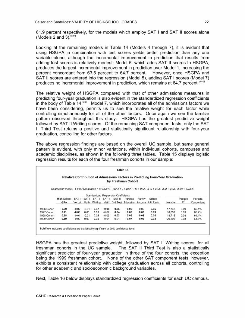
The above regression findings are based on the overall UC sample, but same general pattern is evident, with only minor variations, within individual cohorts, campuses and academic disciplines, as shown in the following three tables. Table 15 displays logistic regression results for each of the four freshman cohorts in our sample:
HSGPA has the greatest predictive weight, followed by SAT II Writing scores, for all freshman cohorts in the UC sample. The SAT II Third Test is also a statistically significant predictor of four-year graduation in three of the four cohorts, the exception being the 1999 freshman cohort. None of the other SAT component tests, however, exhibits a consistent relationship with college graduation across all cohorts, controlling for other academic and socioeconomic background variables.
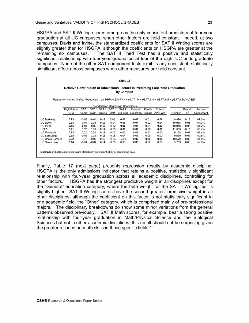
Next, Table 16 below displays standardized regression coefficients for each UC campus.
High School SAT I SAT I SAT II SAT II SAT II Parents' Family School Pseudo PercentGPA Verbal Math Writing Math 3rd Test Education Income API Rank Number R2
Concordant
1996 Cohort 0.20 -0.02 -0.01 0.17 -0.05 0.05 0.06 0.02 0.05 17,742 0.09 65.1%1997 Cohort 0.21 -0.05 0.00 0.16 -0.02 0.04 0.08 0.03 0.03 18,052 0.09 65.2%1998 Cohort 0.18 -0.01 -0.01 0.16 -0.03 0.03 0.05 0.03 0.04 18,715 0.08 64.1%1999 Cohort 0.19 -0.02 0.00 0.16 -0.04 0.01 0.07 0.03 0.03 20,109 0.08 64.3%
Boldface indicates coefficients are statistically significant at 99% confidence level.
Table 15
Standardized Regression Coefficients
Relative Contribution of Admissions Factors in Predicting Four-Year Graduationby Freshman Cohort
Regression model: 4-Year Graduation = αHSGPA + βSAT I V + φSAT I M + θSAT II W + μSAT II M + ψSAT II 3rd + ΩSES
Geiser and Santelices: VALIDITY OF HIGH-SCHOOL GRADES 23
CSHE Research & Occasional Paper Series
HSGPA and SAT II Writing scores emerge as the only consistent predictors of four-year graduation at all UC campuses, when other factors are held constant. Indeed, at two campuses, Davis and Irvine, the standardized coefficients for SAT II Writing scores are slightly greater than for HSGPA, although the coefficients on HSGPA are greater at the remaining six campuses. The SAT II Third Test has a positive and statistically significant relationship with four-year graduation at four of the eight UC undergraduate campuses. None of the other SAT component tests exhibits any consistent, statistically significant effect across campuses when other measures are held constant.
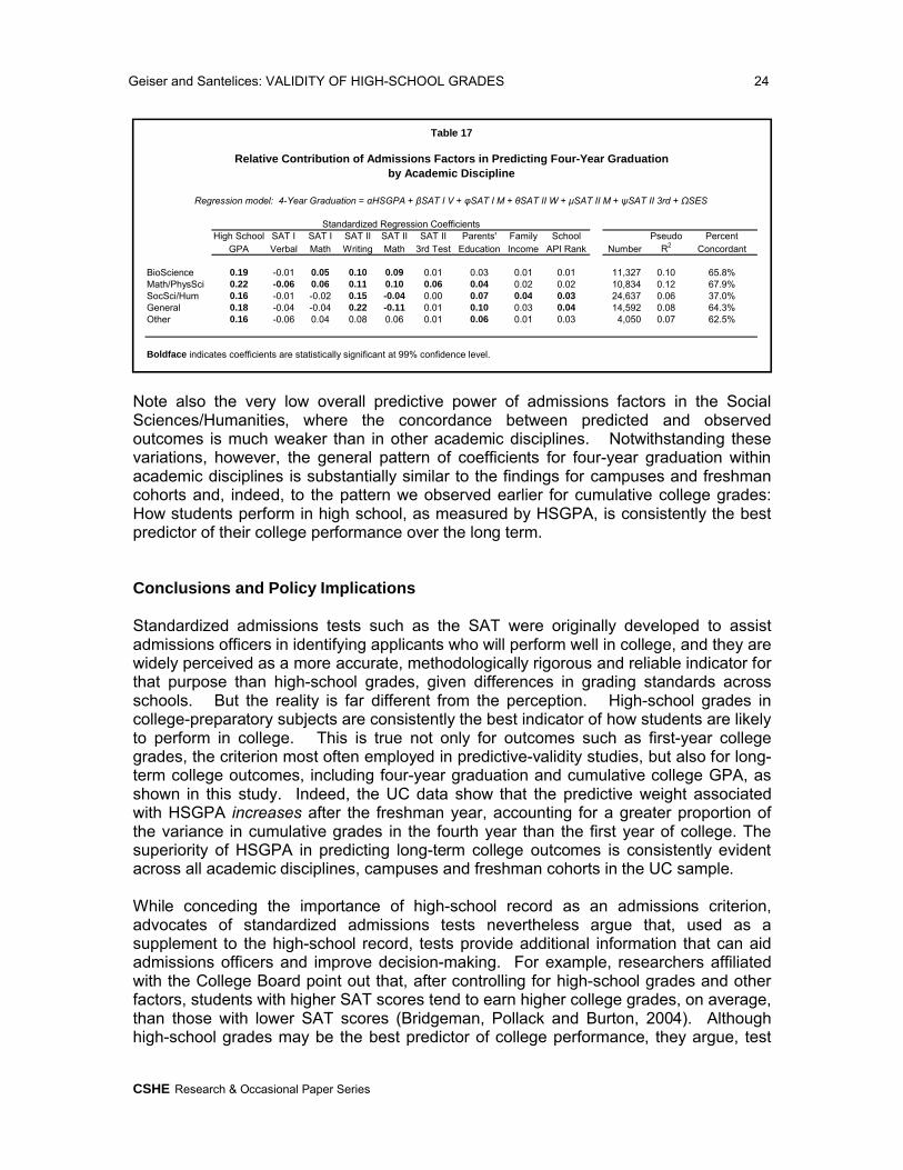
Finally, Table 17 (next page) presents regression results by academic discipline. HSGPA is the only admissions indicator that retains a positive, statistically significant relationship with four-year graduation across all academic disciplines, controlling for other factors. HSGPA has the strongest predictive weight in all disciplines except forthe “General” education category, where the beta weight for the SAT II Writing test is slightly higher. SAT II Writing scores have the second-greatest predictive weight in all other disciplines, although the coefficient on this factor is not statistically significant in one academic field, the “Other” category, which is comprised mainly of pre-professional majors. The disciplinary breakdowns do show some minor variations from the general patterns observed previously. SAT II Math scores, for example, bear a strong positive relationship with four-year graduation in Math/Physical Science and the Biological Sciences but not in other academic disciplines; this result should not be surprising given the greater reliance on math skills in those specific fields.xxx
High School SAT I SAT I SAT II SAT II SAT II Parents' Family School Pseudo PercentGPA Verbal Math Writing Math 3rd Test Education Income API Rank Number R2 Concordant
UC Berkeley 0.23 -0.03 -0.01 0.13 0.05 0.05 0.06 0.01 0.06 9,976 0.12 67.0%UC Davis 0.18 -0.04 0.05 0.19 -0.04 0.06 0.04 0.02 0.04 10,958 0.08 64.3%UC Irvine 0.16 -0.05 -0.02 0.17 -0.02 0.06 0.04 0.01 0.03 10,048 0.05 61.2%UCLA 0.21 0.02 0.00 0.17 -0.03 0.03 0.09 0.02 0.03 11,565 0.11 66.4%UC Riverside 0.23 0.02 0.00 0.12 -0.02 0.02 0.02 0.03 0.00 6,168 0.08 63.4%UC San Diego 0.18 -0.03 0.03 0.15 -0.05 0.04 0.05 0.05 0.02 9,580 0.07 62.8%UC Santa Barbara 0.22 0.01 -0.02 0.12 -0.03 -0.01 0.07 0.05 0.05 10,570 0.09 64.6%UC Santa Cruz 0.14 -0.04 -0.04 0.11 -0.03 0.03 0.05 0.02 0.03 5,753 0.03 59.0%
Boldface indicates coefficients are statistically significant at 99% confidence level.
Table 16
Standardized Regression Coefficients
Relative Contribution of Admissions Factors in Predicting Four-Year Graduationby Campus
Regression model: 4-Year Graduation = αHSGPA + βSAT I V + φSAT I M + θSAT II W + μSAT II M + ψSAT II 3rd + ΩSES
Geiser and Santelices: VALIDITY OF HIGH-SCHOOL GRADES 24
CSHE Research & Occasional Paper Series
Note also the very low overall predictive power of admissions factors in the Social Sciences/Humanities, where the concordance between predicted and observed outcomes is much weaker than in other academic disciplines. Notwithstanding these variations, however, the general pattern of coefficients for four-year graduation within academic disciplines is substantially similar to the findings for campuses and freshman cohorts and, indeed, to the pattern we observed earlier for cumulative college grades: How students perform in high school, as measured by HSGPA, is consistently the best predictor of their college performance over the long term.
Conclusions and Policy Implications
Standardized admissions tests such as the SAT were originally developed to assist admissions officers in identifying applicants who will perform well in college, and they are widely perceived as a more accurate, methodologically rigorous and reliable indicator for that purpose than high-school grades, given differences in grading standards across schools. But the reality is far different from the perception. High-school grades in college-preparatory subjects are consistently the best indicator of how students are likely to perform in college. This is true not only for outcomes such as first-year college grades, the criterion most often employed in predictive-validity studies, but also for long-term college outcomes, including four-year graduation and cumulative college GPA, as shown in this study. Indeed, the UC data show that the predictive weight associated with HSGPA increases after the freshman year, accounting for a greater proportion of the variance in cumulative grades in the fourth year than the first year of college. The superiority of HSGPA in predicting long-term college outcomes is consistently evident across all academic disciplines, campuses and freshman cohorts in the UC sample.
While conceding the importance of high-school record as an admissions criterion, advocates of standardized admissions tests nevertheless argue that, used as a supplement to the high-school record, tests provide additional information that can aid admissions officers and improve decision-making. For example, researchers affiliated with the College Board point out that, after controlling for high-school grades and other factors, students with higher SAT scores tend to earn higher college grades, on average, than those with lower SAT scores (Bridgeman, Pollack and Burton, 2004). Although high-school grades may be the best predictor of college performance, they argue, test
High School SAT I SAT I SAT II SAT II SAT II Parents' Family School Pseudo PercentGPA Verbal Math Writing Math 3rd Test Education Income API Rank Number R2 Concordant
BioScience 0.19 -0.01 0.05 0.10 0.09 0.01 0.03 0.01 0.01 11,327 0.10 65.8%Math/PhysSci 0.22 -0.06 0.06 0.11 0.10 0.06 0.04 0.02 0.02 10,834 0.12 67.9%SocSci/Hum 0.16 -0.01 -0.02 0.15 -0.04 0.00 0.07 0.04 0.03 24,637 0.06 37.0%General 0.18 -0.04 -0.04 0.22 -0.11 0.01 0.10 0.03 0.04 14,592 0.08 64.3%Other 0.16 -0.06 0.04 0.08 0.06 0.01 0.06 0.01 0.03 4,050 0.07 62.5%
Boldface indicates coefficients are statistically significant at 99% confidence level.
Table 17
Standardized Regression Coefficients
Relative Contribution of Admissions Factors in Predicting Four-Year Graduationby Academic Discipline
Regression model: 4-Year Graduation = αHSGPA + βSAT I V + φSAT I M + θSAT II W + μSAT II M + ψSAT II 3rd + ΩSES
Geiser and Santelices: VALIDITY OF HIGH-SCHOOL GRADES 25
CSHE Research & Occasional Paper Series
scores add significantly to the prediction, so that the combination of test scores and high-school record provides better prediction than either factor alone (Camara and Echternacht, 2000; Burton and Ramist, 2001). Or as one admissions officer from a highly selective college put it, “They’re especially useful for evaluating the rural Midwestern kid who’s No. 1 in a graduating class of nine at a high school you don’t know.”xxxi
The UC data confirm that standardized tests do yield a small, but statistically significant improvement in predicting long-term college outcomes, beyond that which is provided by HSGPA or other variables known at point of admission.xxxii The problem, however, is that, even when test scores and high-school record are combined, the overall level of prediction provided by these factors is relatively limited. The most fully-specified prediction model presented in this study, including both student-level and group-level factors in the regression equation, indicates that HSGPA, SAT scores and other factors known at admission together account for only about 30 percent of the total variance in cumulative college grades -- leaving 70 percent unaccounted for and unexplained.xxxiii That result should not be surprising given the many other factors that affect students’ undergraduate experience after admission, such as financial aid, social support and academic engagement in college. But the relatively small proportion of variance that can be explained by factors known at admission necessarily limits the accuracy of predictions based on those factors.
The limits of prediction are especially evident when attempting to predict individual outcomes rather than group outcomes or averages for large samples of students. Predicted outcomes for individual students, based only on factors known at admission, are subject to considerable uncertainty and wide error bands. For example, the error band around predicted GPA for any given student was plus or minus .77 grade points, at the 95 percent confidence level, in our best-fitting prediction model.xxxiv What this means, in other words, is that for a student projected to have a cumulative GPA of 3.0, or a B average, we can be “95 percent confident” that their actual college GPA will fall somewhere in a range between a C and an A.
Nor do test scores add an appreciable increment in predicting individual outcomes. When both SAT I and SAT II scores are dropped from the same prediction model, the error band expands slightly to plus or minus .80 grade points at the 95 percent confidence level, compared to .77 grade points when tests are included. While this difference is “statistically significant,” as a practical matter the uncertainty surrounding the prediction remains high in either event. Though it may be true “on average” that higher SAT scores are associated with higher college GPAs, controlling for other factors, this is not necessarily true in individual cases. These considerations underscore the need for admissions officers to exercise great caution in using either standardized tests or high-school grades to project how particular applicants from particular high schools may perform in college.
Beyond Prediction
But the superiority of the high-school record over standardized tests extends beyond its predictive value alone, insofar as prediction is possible, and HSGPA has other important advantages as an admissions criterion. High-school grades are much less closely correlated with student socioeconomic characteristics than standardized tests. Within the UC sample, for example, HSGPA is only weakly correlated with family income,
Geiser and Santelices: VALIDITY OF HIGH-SCHOOL GRADES 26
CSHE Research & Occasional Paper Series
parents’ education and school API rank, whereas SAT scores bear a strong, positive relationship to each of these measures. As a result, HSGPA tends to have less adverse impact than standardized admissions tests on underrepresented minority applicants, who come disproportionately from disadvantaged backgrounds. Such differences in the demographic footprint of HSGPA and standardized tests are of obvious importance for expanding access and equity in “high stakes” admissions, especially at those colleges and universities where affirmative action has been curtailed or ended.
Moreover, high-school grades possess another advantage as an admissions criterion that, while less tangible, is no less important. This concerns the social meaningassociated with grades and tests. Standardized admissions tests such as the SAT reflect student performance in a single, three-hour (now four-hour) sitting, usually in the middle of the junior year of high school. Such tests are designed to tap “generalized reasoning abilities” thought to predict success in college, although it is known that test scores also reflect test-preparation, repeat test-taking and other “test-wise” strategies aimed at boosting scores. Test-taking strategies aside, performing well on the SAT is generally regarded as an indicator of “merit,” in the sense of academic ability or aptitude for learning.
High-school grades, in contrast, reflect students’ cumulative performance over a period of years in a variety of subjects. In calculating HSGPA, selective institutions such as UC count only performance in college-preparatory subjects -- courses that university faculty regard as essential prerequisites for college-level work and that research hasshown to be highly correlated with college outcomes (Adelman, 1999). Fittingly, students who perform well on this measure are said to have “earned” good grades; though raw intellectual ability is important, other student qualities such as motivation, personal discipline and perseverance are also critical for achieving and maintaining a strong GPA over the four years of high school. In this sense, HSGPA connotes an alternative and older meaning of “merit,” albeit one that remains vital for college admissions: “to earn or deserve; to be entitled to reward or honor.”
Though high-school record is the best predictor of college performance, its importance as a selection criterion reflects a broader philosophy of college admissions that calls into question the value of prediction itself. As a selection criterion, HSGPA shifts attention from predicted performance in college to demonstrated achievement in high school. As against an approach that seeks to assess generalized reasoning abilities or aptitude for learning, emphasis on HSGPA focuses on the mastery of specific skills and knowledge required for college-level work. Even if high-school record had less predictive value, its use as a college-admissions criterion would still be defensible and appropriate insofar as it affirms the value of demonstrated academic achievement.
In the final analysis, the case for emphasizing high-school grades over standardized tests as an admissions criterion rests not only on its greater predictive power, but also on a recognition of the limits of prediction. Given our limited ability to predict college outcomes, it is essential that admissions criteria exhibit “content” and “face validity” as well as “predictive validity,” that is, that the criteria bear a direct and transparent relationship to college-level work. Insofar as standardized tests continue to be used, a strong case can be made for curriculum-based, achievement-type tests, since those tests not only have predictive value but also measure knowledge and skills that are unquestionably important in college or in particular college majors. But these sameconsiderations argue most strongly for greater emphasis on the high-school record, and
Geiser and Santelices: VALIDITY OF HIGH-SCHOOL GRADES 27
CSHE Research & Occasional Paper Series
a corresponding de-emphasis on standardized tests, in college admissions. High-school grades provide a fairer, more equitable and ultimately more meaningful basis for admissions decision-making and, despite their reputation for “unreliability,” remain the best available indicator with which to hazard predictions of student success in college.
References
Adelman, C. (1999). Answers in a Toolbox: Academic Intensity, Attendance Patterns, and Bachelor’s Degree Attainment. Washington, D.C.: U.S. Department of Education, Office of Educational Research and Improvement.
American Educational Research Association, American Psychological Association, and National Council on Measurement in Education. (1985). Standards for Educational and Psychological Testing. Washington, DC: American Psychological Association.
Bridgeman, B., Pollack, J. and N. Burton. (2004). “Understanding what SAT reasoning test scores add to high school grades: A straightforward approach.” College Board Research Report No. 2004-4. New York: College Board.
Bridgeman, B., Pollack, J. and N. Burton. (2006). “Predicting cumulative grades in college courses: Exploring the Myths.” Paper presented at the annual meeting of the national Council on Measurement in Education, April, 2006. Princeton, NJ: Educational Testing Service.
Brown, T. and R. Zwick. (2006). “Using hierarchical linear models to describe first-year grades at the University of California.” Paper presented at National Council on Measurement in Education annual meeting. San Francisco, CA.
Burton, N. and L. Ramist. (2001). “Predicting success in college: SAT studies of classes graduating since 1980.” College Board Research Report No. 2001-02. New York: College Board.
Bryk, A. and S. Raudenbush. (1992). Hierarchical Linear Models: Applications and Data Analysis Methods. Newbury Park: Sage.
Camara, W. (1998). “High school grading policies.” College Board Research Note No. RN-04, May 1998. New York: College Board.
Camara, W., Kimmel, E., Scheuneman, J. and E. Sawtell. (2003). “Whose grades are inflated?” College Board Research Report No. 2003-4. New York: College Board.
Camara, W., and G. Echternacht. (2000). “The SAT I and high school grades: Utility in predicting success in college.” College Board Report No. RN-10. New York: College Board.
Geiser and Santelices: VALIDITY OF HIGH-SCHOOL GRADES 28
CSHE Research & Occasional Paper Series
Camara, W. and M. Michaelides. (2001). “AP use in admissions: A response to Geiser and Santelices.” College Board Research Note, May 11, 2005. Downloaded from http://www.collegeboard.com/research/pdf/051425Geiser_050406.pdf.
Geiser, S., and Santelices, M.V. (2006). “The role of Advanced Placement and honors courses in college admissions.” In P. Gandara, G. Orfield and C. Horn (Eds.), Expanding Opportunity in Higher Education (pp. 75-114). Albany, NY: SUNY Press.
Geiser, S., with R. Studley. (2003). “UC and the SAT: Predictive validity and differential impact of the SAT I and the SAT II at the University of California.” Educational Assessment, 8(1), 1-26.
Hamilton, L. (1992). Regression with Graphics: A Second Course in Applied Statistics. Belmont, CA: Duxbury Press.
Hezlett, S., Kuncel, N., Vey, A., Ones, D., Campbell, J. & Camara, W. (2001). “The effectiveness of the SAT in predictive success early and late in college: A comprehensive meta-analysis.” Paper presented at the annual meeting of the National Council of Measurement in Education, Seattle, WA.
Kowarsky, J., Clatfelter, D. and K. Widaman. (1998). “Predicting university grade-point average in a class of University of California freshmen: An assessment of the validity of GPA and test scores as indicators of future academic performance.” Institutional research paper. Oakland, CA: University of California Office of the President.
Moores, J. (2003). “A preliminary report on the University of California, Berkeley admission process for 2002.” Oakland, CA: UC Office of the President: Downloaded from http://www.universityofcalifornia.edu/news/compreview/mooresreport.pdf.
Morgan, R. (1989). “Analysis of the predictive validity of the SAT and high school grades from 1976 to 1983.” College Board Report No. 89-7. New York: College Board.
National Research Council. (1999). High Stakes: Testing for Tracking, Promotion, and Graduation. Washington, DC: National Academies Press.
Rabe-Hesketh, S. and A. Skrondal. (2005). Multilevel and Longitudinal Modeling Using Stata. College Park, Texas: Stata Press.
Rothstein, J. (2004). “College performance predictions and the SAT." Journal of Econometrics, volume 121, 297-317.
Wilson, K. (1983). “A review of research on the prediction of academic performance after the freshman year.” College Board Report No. 83-2. New York: College Board.
Zwick, R., Brown, T. & J. Sklar. (2004). “California and the SAT: A reanalysis of University of California admissions data.” Center for Studies in Higher Education, Research & Occasional Paper Series. Berkeley, CA.
Zwick, R. (Ed.) (2004). Rethinking the SAT: The Future of Standardized Testing in University Admissions. New York and London: Routledge Farmer.
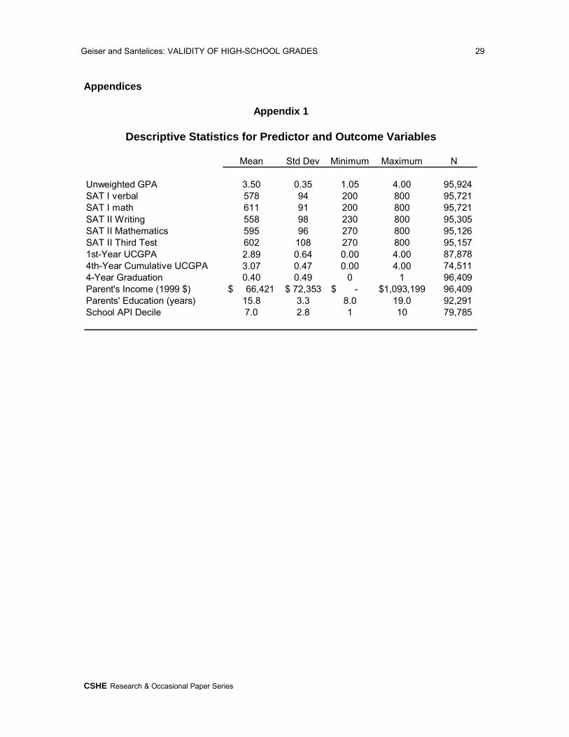
Geiser and Santelices: VALIDITY OF HIGH-SCHOOL GRADES 29
CSHE Research & Occasional Paper Series
Appendices
Mean Std Dev Minimum Maximum N
Unweighted GPA 3.50 0.35 1.05 4.00 95,924 SAT I verbal 578 94 200 800 95,721 SAT I math 611 91 200 800 95,721 SAT II Writing 558 98 230 800 95,305 SAT II Mathematics 595 96 270 800 95,126 SAT II Third Test 602 108 270 800 95,157 1st-Year UCGPA 2.89 0.64 0.00 4.00 87,878 4th-Year Cumulative UCGPA 3.07 0.47 0.00 4.00 74,511 4-Year Graduation 0.40 0.49 0 1 96,409 Parent's Income (1999 $) 66,421$ 72,353$ -$ 1,093,199$ 96,409 Parents' Education (years) 15.8 3.3 8.0 19.0 92,291 School API Decile 7.0 2.8 1 10 79,785
Descriptive Statistics for Predictor and Outcome Variables
Appendix 1
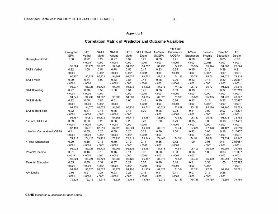
Geiser and Santelices: VALIDITY OF HIGH-SCHOOL GRADES 30
CSHE Research & Occasional Paper Series
Unweighted GPA
SAT I Verbal
SAT I Math
SAT II Writing
SAT II Math
SAT II Third Exam
1st-Year UCGPA
4th-Year Cumulative
UCGPA4-Year
GraduationParent's Income
Parents' Education
API Decile
Unweighted GPA 1.00 0.22 0.29 0.27 0.32 0.22 0.39 0.41 0.20 0.01 0.05 -0.03<.0001 <.0001 <.0001 <.0001 <.0001 <.0001 <.0001 <.0001 0.0015 <.0001 <.0001
95,924 95,277 95,277 94,941 94,752 94,787 87,493 74,215 95,924 95,924 91,960 79,524 SAT I Verbal 0.22 1.00 0.54 0.78 0.50 0.47 0.33 0.35 0.15 0.16 0.39 0.21
<.0001 <.0001 <.0001 <.0001 <.0001 <.0001 <.0001 <.0001 <.0001 <.0001 <.000195,277 95,721 95,721 94,707 94,575 94,572 87,313 74,123 95,721 95,721 91,625 79,215
SAT I Math 0.29 0.54 1.00 0.53 0.86 0.45 0.28 0.26 0.13 0.13 0.32 0.27337<.0001 <.0001 <.0001 <.0001 <.0001 <.0001 <.0001 <.0001 <.0001 <.0001 <.0001
95,277 95,721 95,721 94,707 94,575 94,572 87,313 74,123 95,721 95,721 91,625 79,215 SAT II Writing 0.27 0.78 0.53 1.00 0.51 0.45 0.36 0.39 0.19 0.16 0.37 0.23219
<.0001 <.0001 <.0001 <.0001 <.0001 <.0001 <.0001 <.0001 <.0001 <.0001 <.000194,941 94,707 94,707 95,305 94,863 94,865 87,028 73,990 95,305 95,305 91,279 78,927
SAT II Math 0.32 0.50 0.86 0.51 1.00 0.46 0.29 0.26 0.12 0.11 0.27 0.25987<.0001 <.0001 <.0001 <.0001 <.0001 <.0001 <.0001 <.0001 <.0001 <.0001 <.0001
94,752 94,575 94,575 94,863 95,126 94,711 86,824 73,819 95,126 95,126 91,105 78,763 SAT II Third Test 0.22 0.47 0.45 0.45 0.46 1.00 0.28 0.28 0.11 0.02 0.07 0.16221
<.0001 <.0001 <.0001 <.0001 <.0001 <.0001 <.0001 <.0001 <.0001 <.0001 <.000194,787 94,572 94,572 94,865 94,711 95,157 86,869 73,849 95,157 95,157 91,135 78,788
1st-Year UCGPA 0.39 0.33 0.28 0.36 0.29 0.28 1.00 0.79 0.35 0.08 0.18 0.11461<.0001 <.0001 <.0001 <.0001 <.0001 <.0001 <.0001 <.0001 <.0001 <.0001 <.0001
87,493 87,313 87,313 87,028 86,824 86,869 87,878 74,446 87,878 87,878 84,127 73,219 4th-Year Cumulative UCGPA 0.41 0.35 0.26 0.39 0.26 0.28 0.79 1.00 0.42 0.08 0.18 0.10607
<.0001 <.0001 <.0001 <.0001 <.0001 <.0001 <.0001 <.0001 <.0001 <.0001 <.000174,215 74,123 74,123 73,990 73,819 73,849 74,446 74,511 74,511 74,511 71,334 62,147
4-Year Graduation 0.20 0.15 0.13 0.19 0.12 0.11 0.35 0.42 1.00 0.06 0.11 0.07057<.0001 <.0001 <.0001 <.0001 <.0001 <.0001 <.0001 <.0001 <.0001 <.0001 <.0001
95,924 95,721 95,721 95,305 95,126 95,157 87,878 74,511 96,409 96,409 92,291 79,785 Parent's Income 0.01 0.16 0.13 0.16 0.11 0.02 0.08 0.08 0.06 1.00 0.33 0.15067
0.0015 <.0001 <.0001 <.0001 <.0001 <.0001 <.0001 <.0001 <.0001 <.0001 <.000195,924 95,721 95,721 95,305 95,126 95,157 87,878 74,511 96,409 96,409 92,291 79,785
Parents' Education 0.05 0.39 0.32 0.37 0.27 0.07 0.18 0.18 0.11 0.33 1.00 0.25522<.0001 <.0001 <.0001 <.0001 <.0001 <.0001 <.0001 <.0001 <.0001 <.0001 <.0001
91,960 91,625 91,625 91,279 91,105 91,135 84,127 71,334 92,291 92,291 92,291 76,691 API Decile -0.03 0.21 0.27 0.23 0.26 0.16 0.11 0.11 0.07 0.15 0.26 1
<.0001 <.0001 <.0001 <.0001 <.0001 <.0001 <.0001 <.0001 <.0001 <.0001 <.000179,524 79,215 79,215 78,927 78,763 78,788 73,219 62,147 79,785 79,785 76,691 79,785
Correlation Matrix of Predictor and Outcome Variables
Appendix 2
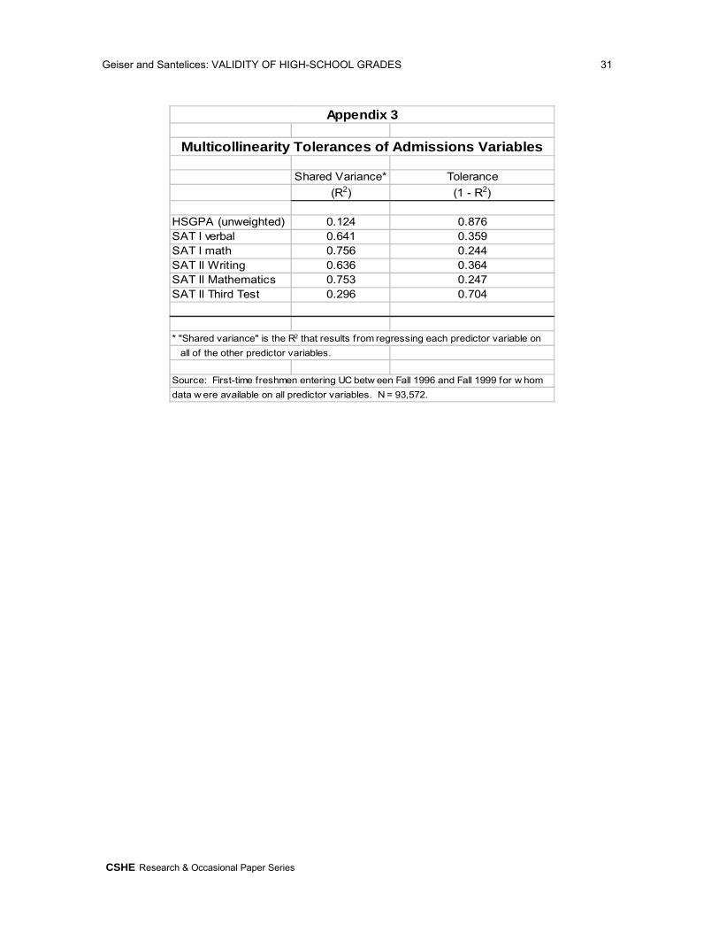
Geiser and Santelices: VALIDITY OF HIGH-SCHOOL GRADES 31
CSHE Research & Occasional Paper Series
Shared Variance* Tolerance
(R2) (1 - R2)
HSGPA (unweighted) 0.124 0.876SAT I verbal 0.641 0.359SAT I math 0.756 0.244SAT II Writing 0.636 0.364SAT II Mathematics 0.753 0.247SAT II Third Test 0.296 0.704
* "Shared variance" is the R2 that results from regressing each predictor variable on
all of the other predictor variables.
Source: First-time freshmen entering UC betw een Fall 1996 and Fall 1999 for w hom
data w ere available on all predictor variables. N = 93,572.
Multicollinearity Tolerances of Admissions Variables
Appendix 3
Geiser and Santelices: VALIDITY OF HIGH-SCHOOL GRADES 32
CSHE Research & Occasional Paper Series
NOTES
i Academic Performance Index (API) is a measure of school quality developed by the California Department of Education and is closely associated with socioeconomic, racial/ethnic, and other demographic differences among students who attend them. For example, 87 percent of students attending California schools in the lowest API decile are underrepresented minorities (Chicano/Latinos, African Americans and American Indians), compared to just 17 percent among schools in the top decile. ii Underrepresented minorities refer to racial/ethnic groups which historically have had low participation rates in higher education: African American, American Indian, and Chicano/Latino students.iii The new UC Eligibility Index introduced in 2001 also doubled the weight given to SAT II Achievement test scores in comparison to SAT I verbal and reasoning test scores, based on regression analyses conducted by BOARS which showed that the SAT II had approximately twice the weight of SAT I scores in predicting freshman grade-point average among UC students (Kowarsky, Clatfelter and Widaman, 1998).iv The ELC policy did require applicants to submit standardized test results as a condition of admission, but the scores were not used in determining class rank.v A useful summary of the research and events leading up to the recently-introduced changes in the SAT is provided in R. Zwick, Rethinking the SAT: The Future of Standardized Testing in University Admissions. New York and London: RoutledgeFarmer, 2004.vi Relatively few studies of the predictive validity of admissions criteria have examined long-term college outcomes, and those studies have generally involved small samples. For useful summaries of long-term predictive-validity studies conducted before 1980, see Wilson (1983), and for studies after 1980, see Burton and Ramist (2001)vii The original study sample was missing data for freshman entering UC Riverside in 1997 and 1998, due to a faulty upload of campus data into the UC Corporate Student System.viii UC’s standardized test requirements for freshman admissions were revised effective fall 2006 to reflect the changes in the SAT I and the incorporation of the SAT II Writing Test into the SAT I, as well as other changes such as the incorporation of higher-level mathematics into that test. UC now requires students to take either the new SAT I or the ACT plus writing, together with two other SAT II Subject Tests in areas of the student’s choosing.ix The socioeconomic variables included in the regressions were years of education for the highest educated parent, log of parental income in 1999 dollars and school API decile, which was treated as a continuous variable for reasons of convenience. Data on family income and parents’ education are drawn from information provided by students on the UC admissions application. UC has periodically conducted analyses comparing family income data from the admissions application with that from the UC financial aid application, which is subject to audit. Those analyses show that, while there are sometimes substantial differences in the data reported for individual students, mean incomes for most population groups are quite similar across the two data sources. The logarithm of family income is used here to take into account the diminishing marginal effects of income on UCGPA and other variables. That is, a $10,000 increase in income is likely to have a larger effect for a student whose family earns $35,000 annually than for a student whose family earns $135,000. Use of the log of income is standard
Geiser and Santelices: VALIDITY OF HIGH-SCHOOL GRADES 33
CSHE Research & Occasional Paper Series
practice in economic research. API scores for each high school are based on ratings developed by the California Department of Education.x Graduation data are from UC Office of the President website:http://www.ucop.edu/sas/infodigest03/Data_Freshmen.pdf.
xiA summary description of the efforts at each UC undergraduate campus to accelerate time-to-degree may be found in “Programs to assist students to graduate within four years” at the UC Office of the President website:http://www.ucop.edu/planning/finishinfour00.pdf.
xii It should be noted that undergraduate programs in engineering often require five years of study. Because it was difficult reliably to identify students in specific engineering programs in the UC systemwide database, those students were retained in the sample. Their inclusion should not appreciably affect any findings presented here, however, because of their relatively small number.xiiiAll of the predictor variables employed in the study were tested for multicollinearity. Multicollinearity is sometimes encountered in admissions research and refers to situations where predictor variables are too closely interrelated. At the extreme, when 90% or more of the variance among predictor variables is shared, regression results can become unstable and prevent one from isolating the effects of individual variables. A diagnostic statistic known as “tolerance,” or the proportion of variance not shared among the predictor variables, can be used to test for multicollinearity; as a rule of thumb, tolerance must be at least .1 to .2 for stable regression results (Hamilton, 1992:133-135). All of the predictor variables employed in this study exhibited acceptable tolerances as shown in Appendix 3. xiv Socioeconomic background variables by themselves account for 4.1% of the explained variance in cumulative fourth-year college GPA for the overall UC sample.xv The disciplinary variable employed in this study differs from that used in the earlier study of UC and the SAT in that the earlier study used students’ intended major as of their freshman year. Because students frequently change intended majors up until their junior year, when they are required actually to select a major, the indicator for academic discipline employed here is undoubtedly more accurate than that used in the earlier study, which was limited to predicting first-year college outcomes.xvi In response to the earlier findings in UC and the SAT on the predictive efficacy of the SAT II Writing test, the College Board has now revised the SAT I to incorporate a Writing test, among other changes. xvii Model 7, Table 4.xviii Interestingly, the confidence interval was even wider for first-year than for fourth-year GPA. At the 95 percent confidence level, the interval for freshman GPA was plus or minus 1.09 grade points for a regression model that included all of the student-level predictors presented here, and plus or minus 1.12 grade points when SAT scores were dropped from that model. The reasons for the improvement in prediction of cumulative GPA after the first year are discussed in the following section.xix Some predictive-validity studies make statistical adjustments for range restriction, i.e., the fact that, among applicants to selective institutions such as UC, only those with high test scores tend to be admitted, and as a result, there is a limited range of scores among admitted students with which to assess the utility of standardized tests in predicting college outcomes. Researchers associated with the College Board advocate making statistical adjustments to deal with this problem by estimating what the results might have been if all SAT takers attended college, and those researchers typically report regression results larger than those shown here (e.g.,Camara and Echternacht, 2000;
Geiser and Santelices: VALIDITY OF HIGH-SCHOOL GRADES 34
CSHE Research & Occasional Paper Series
Burton and Ramist, 2001). This study eschews such statistical estimates, however, for three reasons. First, the estimates are based on statistical assumptions that cannot be empirically verified, including the assumptions of linearity (the relationship between test scores and college grades is assumed to be linear and identical across the observed and unobserved ranges of the data) and homoscedasticity (the variance in the outcome variable is assumed to be the same across the observed and unobserved ranges). Second, where statistical adjustments are based on the range of test scores among the national population of SAT takers rather the applicant pool at a particular institution, they can overstate the true value of standardized tests for admissions officers. At highly competitive institutions such as UC, range restriction occurs not only among the pool of admitted students but among the applicant pool as well, and tests are used to select from among an already highly selective, high-achieving pool of applicants. A fundamental maxim of “high stakes” testing is that tests should be validated for the specific purpose for which they are used (AERA, 1985; National Research Council, 1999), and adjusting predictive-validity coefficients for selective colleges and universities based on the national population of SAT takers seems inappropriate for that reason. Finally, range restriction is less an issue at UC because of its eligibility requirements, which set minimum test-score and HSGPA standards in order for students to apply for regular admission, with the result that the variance in test scores among admitted students is not greatly dissimilar to that of applicants. Thus, the standard deviation of SAT I scores among admitted students in our sample was .90 that of applicants, and for SAT II scores the ratio was .92. (Interestingly, the ratio of standard deviations between admitted students and applicants was lowest for HSGPA, .82, suggesting that range restriction may more affect high-school grades than test scores, at least in the UC sample.) For all of these reasons, the present study avoids statistical adjustments and presents only observed validity coefficients and explained variances.xx We are indebted to Professor Michael Brown of UC Santa Barbara for suggesting this hypothesis, although he is in no way responsible for the interpretation offered here.xxi Student-level or “level-1” effects are known as “fixed effects” in the language of multilevel analysis because they are assumed to be measured without error, e.g., a student’s SAT score is assumed to be the true score for that student. Group-level or “level-2” effects, in contrast, are known as “random effects” insofar as they are assumed to be sample values drawn from a larger population and thus to vary randomly around the true population mean. xxii As shown previously in Table 10, our sample standard deviation in cumulative fourth-year GPA was .46 grade points, so that .08 standard deviations, for example, is equivalent to .08 x .46 = .0368, or about four one-hundredths of a grade point.xxiii As shown earlier in Table 4, measured student-level characteristics account for about 27 percent of the variance in cumulative college grades, leaving 73 percent as unexplained or “residual” variance.xxiv For readers familiar with multilevel or hierarchical linear modeling, a “two-way error components analysis” was also performed, introducing “cross random effects” for campus and academic discipline. Introducing random effects for campus and academic discipline simultaneously into the analysis produced an intraclass correlation of .04 for discipline and .02 for campus, similar to the one-way results in Table 12. xxv Introducing any mutually exclusive set of categories in regression analysis requires that one category be excluded, since the excluded category can be derived from the remaining categories (e.g., if a student is not female, then they must be male) and therefore yields no additional information. The excluded category thus becomes the
Geiser and Santelices: VALIDITY OF HIGH-SCHOOL GRADES 35
CSHE Research & Occasional Paper Series
reference point for the remaining categorical variables, and the regression coefficients for the remaining variables are interpreted in relation to the reference category. xxvi In a later study, Brown and Zwick employed multilevel modeling techniques with the UC sample to estimate the effects of group-level variables on the predictive validity of HSGPA. Their results showed that although “random” or group-level effects on the predictive validity of HSGPA did vary by campus and freshman cohort, such effects appeared to account for less than one percent of the residual variance in first-year grades (Brown and Zwick, 2006, Tables 2 and 3). xxvii In logistic regression, which predicts dichotomous, “yes/no” outcomes, there is no precise counterpart to the coefficient of determination, or R2, used in ordinary linear regression to represent the proportion of variance in a continuous numerical outcome variable, such as college GPA, that is “explained” by a given prediction model. Some statisticians have proposed various “pseudo R2” measures, none of which is entirely satisfactory; Nagelkerke’s “maximum-rescaled R2”, a standard SAS output, is used here. The second statistic, “percent concordant,” is based on a rank correlation of observed responses and predicted probabilities and indicates the percentage of all pairs of observations in which the predicted and observed outcomes are the same. The pseudo R2 and percent concordant statistics are reported here in place of the log-likelihood statistics more often reported in logistic-regression analyses in order to make the results more accessible to the statistically unsophisticated reader. Log-likelihood comparisons could not be made for the regression models in Table 14, in any case, since not all of the models are nested nor are the number of observations the same for all models.xxviii This finding is consistent with previous findings reported in UC and the SAT which showed that, after HSGPA and SAT II scores are considered, SAT I scores provide little or no additional information with which to predict first-year college grades (Geiser with Studley, 2003, Table 2). xxix Technical note: The standardized logistic regression coefficients shown in this and the following tables were calculated in SAS by multiplying the raw regression coefficient for a given predictor variable by standard deviation of that variable divided by π/3.xxx Note the similar pattern of regression coefficients for SAT II Math scores in predicting cumulative GPA within both Math/Physical Science and Biological Science shown earlier in Table 7. xxxi Quoted in New York Times, August 31, 2006, p. 1, “Students’ paths to small colleges can bypass SAT.”xxxii Compare Models 1 and 7 in Tables 4 and 14. xxxiii Model B, Table 13.xxxiv Model B, Table 13.