Embed Size (px)
Citation preview
ANA MARIA DOMINGOS NOBRE
INTEGRATED ECOLOGICAL-ECONOMIC
MODELLING AND ASSESSMENT APPROACH FOR
COASTAL ECOSYSTEM MANAGEMENT
Thesis submitted to the Faculty of Sciences and
Technology, New University of Lisbon, for the degree
of Doctor of Philosophy in Environmental Sciences.
Dissertação apresentada para obtenção do Grau de
Doutor em Ciências do Ambiente, pela Universidade
Nova de Lisboa, Faculdade de Ciências e Tecnologia.
LISBOA
Agosto 2009

i
Acknowledgments
I am grateful to all the people that direct and indirectly contributed to this work:
I am particularly thankful to my supervisor, J.G. Ferreira for guidance and support; above all,
I cannot express my gratitude for his mentoring since early stage of my work at his research
group.
To João Nunes, for being always a step ahead, sharing his experience and critical opinion; and
most of all for initiating me into the research work.
Suzanne Bricker, for being so supportive of my ideas, for manuscript revision; and specially
for inspiring me about what an assessment methodology should be.
To the SPEAR team, for the collaboration and integrated modelling work. In particular, I
thank to Josephine K. Musango and Martin de Wit, for collaboration, insights and valuable
comments on the economics of aquaculture.
I am grateful to Amir Neori and Deborah Robertson-Andersson, for being so receptive about
developing the integrative work for quantifying an ecologically balanced view of mariculture
and for collaboration to further develop the case study. Additionally, I thank Amir Neori for
discussions and for valuable comments that improved the work presented in this thesis.
To Lia Vasconcelos and her discussion group for participation in their multidisciplinary
sessions and for the valuable comments they provided about key presentations of my work in
particular the preparation of my defence.
To Robert Grove for valuable information about kelp restoration project.
I thank all manuscript co-authors for contributing to the work that is presented herein. I am
also thankful to the anonymous reviewers and Gavin Maneveldt for valuable comments that
considerably improved the manuscripts which are part of this thesis.
To colleagues and friends from FCT especially for the healthy day-to-day companionship
over the years: Jota, Andrea, Changbo, Teresa, Micas, Camille, Yongjin, Grosso, Norma,
Lourenço, Sol, Pacheco, Akli and Maria João.
To Filomena Gomes for the kind support on the administrative issues.
Finally to my family, for everything and for the example about the meaning of persistence and
determination; and off course for the patience, support and special treats that still made the
Summer worthwhile.
ii
The coastal ecosystem modelling work presented in this thesis was developed in the context
of the European Union, Sixth Framework Programme FP6-2002-INCO-DEV-1 SPEAR
(INCO-CT-2004-510706) project, which provided the means, such as data and modelling
tools, for developing the integrated model.
Financial support was provided by the Portuguese Foundation for Science and Technology
(FCT) as a Ph.D. scholarship (SFRH/BD/25131/2005) and funding for participating in several
conferences which were crucial for dissemination and progress of the work developed in this
thesis.
iii
Abstract
Over the past few decades, policy-makers have defined new instruments to address coastal
ecosystem degradation. Emerging coastal management frameworks highlight the use of the
best available knowledge about the ecosystem to manage coastal resources and maintain
ecosystem’s services. Progress is required, however, in translating data into useful knowledge
for environmental problem solving. This thesis aims to contribute to research assessing
changes in coastal ecosystems and benefits generated due to management actions (or to the
lack thereof). The overall objectives are to assess the ecological and economic impacts of
existing management programmes, as well as future response scenarios and to translate the
outcomes into useful information for managers.
To address these objectives, three different approaches were developed:
A multilayered ecosystem model
A multilayered ecosystem model was developed to simulate management scenarios that
account for the cumulative impacts of multiple uses of coastal zones. This modelling field is
still at an early stage of development and is crucial, for instance, to simulate the impacts of
aquaculture activities on the ecosystem, accounting for multiple farms and their interactions
with other coastal activities. The multilayered ecosystem model is applied in this thesis to test
scenarios designed to improve water quality and manage aquaculture.
An ecological-economic assessment methodology (∆DPSIR approach)
The Differential Drivers-Pressure-State-Impact-Response (∆DPSIR) approach further
develops the integrated approach by providing an explicit link between ecological and
economic information related to the use and management of coastal ecosystems. Furthermore,
the ∆DPSIR approach provides a framework to synthesise scientific data into useful
information for the evaluation of previously adopted policies and future response scenarios.
The ∆DPSIR application is tested using different datasets and scales of analysis, including: (i)
assessment of the ecological-economic impacts of the scenarios at the waterbody/watershed
level, using the multilayered ecosystem model outputs, and (ii) evaluation of the ecological-
economic effects of aquaculture options at the individual aquaculture level, using data from
an abalone farm. These are two important scale of analysis for the development of an
ecosystem approach to aquaculture.
iv
A dynamic ecological-economic model (MARKET model)
One of the missing links in ecosystem modelling is with economics. The MARKET model
was developed to simulate the feedbacks between the ecological-economic components of
aquaculture production. This model was applied to simulate shellfish production in a given
ecosystem under different assumptions for price and income growth rates and the maximum
available area for cultivation. Further application of the MARKET model at a wider scale
might be useful for understanding the ecological and economic limitations on global
aquaculture production.
This integrated ecological-economic modelling and assessment approach can be further
applied to address new coastal management issues, such as coastal vulnerability to natural
catastrophes. It can also support implementation of current legislation and policies, such as
the EU Integrated Coastal Zone Management recommendation or the development of River
Basin Management Plans following the EU Water Framework Directive requirements. On the
other hand, the approach can address recurring coastal management needs, such as the
assessment of the outcomes of past or on-going coastal management plans worldwide, in
order to detect symptoms of the overuse and misuse of coastal ecosystems.
v
Resumo
Ao longo das últimas décadas, os decisores políticos têm definido novos instrumentos para
combater a degradação dos ecossistemas costeiros. Abordagens emergentes de gestão de
ecossistemas costeiros salientam o uso do melhor conhecimento disponível sobre o
ecossistema para a gestão dos recursos costeiros. Desenvolvimentos são necessários para
sintetizar dados em informação relevante para a resolução de problemas ambientais. Esta tese
visa contribuir para a investigação sobre a avaliação de alterações nos ecossistemas costeiros
e nos benefícios que estes geram devido a medidas de gestão (ou a falta delas). Os objectivos
gerais são avaliar os impactes ecológicos e económicos de medidas de gestão adoptadas
anteriormente, bem como, de cenários de resposta; e traduzir os resultados em informações
úteis para os gestores.
Para atingir os objectivos definidos foram desenvolvidas três metodologias:
Um modelo de ecossistema multicamadas
O modelo de ecossistema multicamadas é desenvolvido para simular cenários de gestão que
integram os impactes cumulativos dos múltiplos usos das zonas costeiras. Esta é uma área da
modelação do ecossistema ainda numa fase inicial de desenvolvimento e crucial para, por
exemplo, simular os impactos das actividades aquícolas no ecossistema de forma a incluir a
interacção entre diversas unidades de produção e com outras actividades costeiras. O modelo
de ecossistema multicamadas é aplicado para testar cenários concebidos para melhorar a
qualidade da água e gestão da aquacultura.
Uma metodologia de avaliação ecológica-económica (∆DPSIR)
A metodologia ‘Differential Drivers-Pressure-State-Impact-Response’ (∆DPSIR) adiciona
uma vantagem à abordagem integrada através da ligação explícita entre informação ecológica
e económica relacionada com o uso e gestão de sistemas costeiros. Adicionalmente, o
∆DPSIR fornece uma abordagem para sintetizar os dados científicos em informações
relevantes para gestores sobre a avaliação de políticas adoptadas no passado e de cenários
para o futuro. A aplicação do ∆DPSIR é testada usando diferentes tipos de dados e escalas de
análise, incluindo: (i) avaliação do impacto ecológico-económico dos cenários à escala da
massa de água/bacia hidrográfica usando os resultados do modelo multicamadas, e (ii)
avaliação dos efeitos ecológico-económicos de diferentes opções da aquacultura a nível de
uma unidade de produção individual usando os dados de uma aquacultura de abalone. Estas
vi
são duas escalas de análise importantes para o desenvolvimento de uma abordagem de
ecossistema para a aquacultura.
Um modelo ecológico-económico dinâmico (MARKET)
Uma das limitações dos modelos de ecossistema é a ligação com a economia. O modelo
MARKET foi desenvolvido para simular o feedback entre as componentes ecológica e
económica da produção aquícola. Foi aplicado para simular a produção de bivalves num
determinado ecossistema, considerando diferentes pressupostos para as taxas de crescimento
de preço e de salários, e para a área máxima disponível para o cultivo. A aplicação do modelo
MARKET à escala mais ampla pode ser útil para compreender as limitações ecológicas e
económicas da produção de aquacultura a nível mundial.
Esta abordagem integrada ecológico-económica de modelação e avaliação pode ser utilizada
para responder a novas questões de gestão das zonas costeiras; tais como a vulnerabilidade a
catástrofes naturais. Pode também ser usada para a implementação de legislação e políticas,
tais como a recomendação Europeia sobre a Gestão Integrada das Zonas Costeira, ou o
desenvolvimento dos Planos de Gestão de Bacia Hidrográfica conforme indicado na Directiva
Quadro da Água. Por outro lado, a abordagem desenvolvida pode também responder a
necessidades recorrentes dos gestores, nomeadamente avaliar os resultados de planos de
gestão costeira já finalizados ou a decorrer, com o intuito de detectar os sintomas visíveis de
abuso e mau uso dos ecossistemas costeiros.
vii
Abbreviations
∆DPSIR, Differential Drivers-Pressures-State-Impact-Response
ASSETS, Assessment of Estuarine Trophic Status model
BOD5, Five-day biochemical oxygen demand
Chl-a, Chlorophyll-a
CZM, Coastal Zone Management
DIN, Dissolved Inorganic Nitrogen
DO, Dissolved oxygen
DPSIR, Drivers-Pressures-State-Impact-Response
DSS, Decision Support Systems
EAA, Ecosystem Approach to Aquaculture
EBM, ecosystem-based management
EC, Eutrophic Condition index of the ASSETS model
EU, European Union
EBM, Ecosystem-Based Management
FO, Future Outlook index of the ASSETS model
GES, Good Environmental Status
GHG, Greenhouse gas
GIS, Geographic Information System
GNP, Gross National Product
GPP, Gross Primary Production
HAB, Harmful algal bloom
ICM, Integrated Coastal Management
ICZM, Integrated Coastal Zone Management
IEA, Integrated Environmental Assessment
IF, Influencing Factors index of the ASSETS model
IMF, International Monetary Fund
IMTA, Integrated Multi-Trophic Aquaculture
LCA, Life-Cycle Assessment
MARKET, Modeling Approach to Resource economics decision-maKing in EcoaquaculTure
MSFD, Marine Strategy Framework Directive
N, Nitrogen
NEEA, USA National Estuarine Eutrophication Assessment
NEP, USA National Estuary Program
NPP, Net Primary Production
P, Phosphorus
viii
PEQ, Population equivalent
PEV, Partial Ecosystem Value
POM, Particulate Organic Matter
PPP, Purchasing Power Parity
RS, Remote Sensing
SAV, Submerged Aquatic Vegetation
SCI, Science Citation Index
SPM, Suspended Particulate Matter
SWAT, Soil and Water Assessment Tool model
TEV, Total Economic Value
TFW, Total Fresh Weight
USA, United States of America
USD, U.S. dollar
UWWTD, Urban Waste Water Treatment Directive
WFD, European Water Framework Directive
WWTP, Wastewater treatment plant
Symbols
∆DPSIR – economic quantification VDrivers, Value of the drivers
VDriversEcosyst, Value of the drivers in the coastal ecosystem
VDriversExternal, economic value of the activities both in the catchment
VEcosystem, Value of the ecosystem
VImpact, Value of the impact on the ecosystem
VManagement, Economic value of management
VResponse, Value of the response
VDirectUse, Direct use value of the ecosystem
VIndirectUse, Indirect use value of the ecosystem
VNonUse, Non-use value of the ecosystem
VExternalities, Value of the environmental externalities
Simple nutrient mass balance model Fsea, nutrient source - nutrients from seawater
Fabalone, nutrient source - net nutrient production in the abalone tanks
ix
Ffertilizer, nutrient source - seaweed fertilization
Falgae, nutrient sink - nutrient sinks include seaweed nutrient uptake
Feffluent, nutrient sink - nutrient discharge to the sea
ruptake, nutrient uptake rate
Frecirculation, is the nutrient mass in seaweed effluents that re-enters into the system
Fabalone2algae, is the nutrient mass outflow from the abalone tanks to the seaweed ponds.
euptake, is the seaweed nutrient removal efficiency (%) that corresponds to the proportion of nutrients removed relative to the available nutrients
MARKET model SimP, Simulation period
ts, Simulation timestep
tsecol, Ecological timestep
tsecon, Economic timestep
Ecological system µ, Mortality rate
A, Cultivation area
G, Annual growth rate
g, Scope for growth
HB, Harvestable biomass
MaxA, Maximum cultivation area
N, Number of individuals
nseed, Seeding density
s, Weight class
sp, Seeding period
tp, Cultivation cycle
w, Ecosystem model seed weight
Economic system DK, Depreciation of capital
DQ, Desired production
FC, Fixed costs
IKL, Interest on capital loan
K, Capital
L, Labour
LD, Local demand
MC, Marginal costs
MPK, Marginal productivity of capital
x
MPL, Marginal productivity of labour
MR, Marginal revenue
NP, Net profit
P, Price
Q, Shellfish production
TCQ, Total cost of shellfish production
TCQ+1, Total cost of producing one more unit
UVCL Unit labour cost
VC, Variable costs
VCL, Labour costs
VCM, Maintenance costs
VCO, Other variable costs
df, Depreciation fraction
dp, Depreciation period
ed, Price elasticity of demand
ey, Income elasticity of demand
mf, Maintenance Fraction
r, Interest rate
RCQ, Desired change in production
rd, Demand growth rate
RK, Changes in labour inputs
RL, Changes in labour inputs
rcq, annual change rate in production
rp, Price growth rate
ry, Per capita income growth rate
αK, Elasticity of capital
αL, Elasticity of labour
xi
Authorship declaration for published work
Part of the work presented in this dissertation was previously published/submitted as articles
in peer-reviewed International journals:
Nobre, A., 2009. An ecological and economic assessment methodology for coastal
ecosystem management. Environmental Management, 44(1): 185-204.
Nobre, A.M., Ferreira, J.G., 2009. Integration of ecosystem-based tools to support
coastal zone management. Journal of Coastal Research, SI 56: 1676-1680.
Nobre, A.M., Musango, J.K., de Wit M.P., Ferreira, J.G. 2009. A dynamic ecological-
economic modeling approach for aquaculture management. Ecological Economics,
68(12): 3007-3017.
Nobre, A.M., Ferreira, J.G., Nunes, J.P., Yan, X., Bricker, S., Corner, R., Groom, S.,
Gu, H., Hawkins, A.J.S., Hutson, R., Lan, D., Lencart e Silva, J.D., Pascoe, P., Telfer,
T., Zhang, X., Zhu, M., Assessment of coastal management options by means of
multilayered ecosystem models. Estuarine Coastal and Shelf Science, In Press.
Nobre, A.M., Robertson-Andersson, D., Neori, A., Sankar, K., Ecological-economic
assessment of aquaculture options: comparison between monoculture and integrated
multi-trophic aquaculture. Submitted to Aquaculture.
Nobre, A.M., Bricker, S.B., Ferreira, J.G., Yan, X., de Wit, M., Nunes, J.P., Integrated
environmental modelling and assessment of coastal ecosystems, application for
aquaculture management. Submitted to Coastal Management.
I hereby declare that as the first author of the above mentioned manuscripts, provided the
major contribution to the research and technical work developed, to the interpretation of the
results and to the preparation of the manuscripts.

xii
xiii
List of contents
Acknowledgments i
Abstract iii
Resumo v
Abbreviations vii
Symbols viii
List of figures xvii
List of tables xix
Índice de figuras xxi
Índice de quadros xxiii
CHAPTER 1. INTRODUCTION 1
1.1 Background 2 1.1.1 Coastal management challenge: addressing emerging coastal zone problems 2
Integrated Coastal Zone Management (ICZM) 2 Ecosystem-Based Management (EBM) 5 Ecosystem Approach to Aquaculture (EAA) 7
1.1.2 Role of science for coastal management 8 Increase of knowledge about complex coastal processes 9 Tools to communicate science to managers 9 Interaction of coastal environment and socio-economics 10
1.2 Thesis overview 11 1.2.1 Objectives 11 1.2.2 Study sites 13 1.2.3 Thesis outline 15
CHAPTER 2. MULTILAYERED ECOSYSTEM MODELLING 19
Assessment of coastal management options by means of multilayered ecosystem models 21 INTRODUCTION 21 METHODOLOGY 25
Study site and data 25 Multilayered ecosystem model 28
Catchment sub-model 33 Hydrodynamic sub-model 35 Aquatic resource sub-model 36 Biogeochemical sub-model 37
Coastal management options simulation 38 Definition of scenarios 38 Development scenario implementation and interpretation 39
xiv
RESULTS 40 Ecosystem simulation 40 Development scenarios 46
DISCUSSION 49 CONCLUSIONS 51
CHAPTER 3. INTEGRATED ECOLOGICAL-ECONOMIC ASSESSMENT 53
An ecological and economic assessment methodology for coastal ecosystem management 55 INTRODUCTION 55 METHODOLOGY 57
DPSIR framework 57 Characterization stage 58 Quantification stage 58 Overview stage 59
Case Study: site and data description 60 Data collection and analysis 61
Characterization stage of the ∆DPSIR 62 Ecological assessment of the ∆DPSIR 64
Pressure 64 State 65 Pressure, ∆State and Impact State 67
Economic assessment of the ∆DPSIR 68 Value of the drivers 71 Value of the ecosystem 71 Value of the response 72 Value of the impact on the ecosystem 72 Economic value of management 73
Spatial and Temporal Scope 74 RESULTS AND DISCUSSION 74
Characterization stage 74 Quantification stage 76
Drivers 76 Pressure 77 State 78 Response 79 Impact 79 Overview stage 81
CONCLUSIONS 83
CHAPTER 4. ECOSYSTEM APPROACH TO AQUACULTURE 85
4.1 Waterbody/watershed level assessment: evaluation of model scenarios 86
Integrated environmental modelling and assessment of coastal ecosystems, application for aquaculture management 87
INTRODUCTION 87 METHODOLOGY 89
General approach 89 Case study site and data 90
Data description and analysis 91 Scenarios 93
ASSETS model application 93 Influencing factors - IF 94 Eutrophic condition - EC 94 Future outlook - FO 94 ASSETS application to ecosystem model outputs 94
Differential Drivers-Pressure-State-Impact-Response application 95 Drivers 95 Pressures 96 State 96
xv
Impact 97 Response 98 Overview 98
RESULTS AND DISCUSSION 99 Eutrophication assessment of Xiangshan Gang 99
Data-based application 99 Assessment of simulated scenarios 101
Integrated ecological-economic assessment 103 Drivers 103 Pressures 103 State and Impact 104 Response 108
Overview of the integrated environmental-economic assessment 108 CONCLUSIONS 111
4.2 Farm level assessment: IMTA evaluation using real farm data 113
Ecological-economic assessment of aquaculture options: comparison between monoculture and integrated multi-trophic aquaculture 115
INTRODUCTION 115 METHODOLOGY 117
General approach 117 Case study site and data 119 Differential Drivers-Pressure-State-Impact-Response application to the case study 120
Drivers 121 Pressures 122 State 124 Impact 124 Response 125
A Nutrient mass balance model for the recirculating system 125 RESULTS AND DISCUSSION 128
Drivers 129 Pressures 130
Nutrient discharge 130 Harvesting of natural kelp beds 131 CO2 balance 131
State and Impact 131 Response 133 Managing nutrient limitation due to seaweed expansion 133
Nutrient mass balance in I & J, Cape Cultured Abalone Pty, Ltd. farm 133 Nutrient mass balance in Seaor Marine Ltd. farm 133 Insights from the nutrient mass balance model 134
DISCUSSION 134 Social relevance 135
CONCLUSION 136
CHAPTER 5. ECOLOGICAL-ECONOMIC DYNAMIC MODELLING 137
A dynamic ecological-economic modeling approach for aquaculture management 139 INTRODUCTION 139 METHODOLOGY 141
Conceptual approach 141 Ecological and economic limits 142
Case study: site and data description 143 Model implementation 145
Ecological component 146 Economic component 149 Decision component 154
Model assessment and scenario definition 156 RESULTS 157 DISCUSSION 160 CONCLUSIONS 162
xvi
CHAPTER 6. INTEGRATION OF ECOSYSTEM-BASED TOOLS 163
Integration of ecosystem-based tools to support coastal zone management 165 INTRODUCTION 165 GENERAL APPROACH 166
Integration of ecosystem-based tools 166 Case study 167
REMOTE SENSING 167 GEOGRAPHIC INFORMATION SYSTEMS 168 CATCHMENT MODELING 169 COASTAL ECOSYSTEM MODELING 169 ECONOMIC VALUATION 170 ASSESSMENT METHODOLOGIES 171 CONCLUDING REMARKS 173
CHAPTER 7. GENERAL DISCUSSION 175
7.1 Integrated ecological-economic modelling and assessment approach 176
7.2 Concluding remarks about the study sites 179
7.3 Conclusions 183
REFERENCES 185
xvii
List of figures
FIGURE 1.1. STUDY SITES. 13 FIGURE 1.2. THESIS ORGANISATION. 15 FIGURE 2.1. XIANGSHAN GANG AND CATCHMENT AREA CHARACTERISATION. 26 FIGURE 2.2. INTEGRATED CATCHMENT-BAY MODELLING APPROACH FOR COASTAL ECOSYSTEM MANAGEMENT:
MODEL COMPONENTS AND ECOSYSTEM-BASED TOOLS. 28 FIGURE 2.3. CATCHMENT MODEL OUTPUTS AND COMPARISON WITH DATA: A) MEASURED AND SIMULATED
DISSOLVED INORGANIC NITROGEN (DIN) FOR FUXI AND YANGONGXI RIVERS; B) ESTIMATED AND SIMULATED NITROGEN EXPORT; C) SIMULATED MONTHLY RUNOFF COMPARED WITH RAINFALL; AND D) NITROGEN LOADS FROM DIFFUSE AND POINT SOURCES. 34
FIGURE 2.4. STANDARD SIMULATION OUTPUTS FOR AN INNER BOX (BOX 3, HUANGDUN BAY) AND A MIDDLE BOX (BOX 10), PLOTTED WITH AVERAGE DAILY DATA (JUNE2005/JUNE2006) AND CORRESPONDING STANDARD DEVIATION: PHYTOPLANKTON BIOMASS, DISSOLVED INORGANIC NITROGEN (DIN), PHOSPHATE, SUSPENDED PARTICULATE MATTER (SPM) MATTER AND PARTICULATE ORGANIC MATTER (POM). 41
FIGURE 2.5. STANDARD SIMULATION OUTPUTS FOR PHYTOPLANKTON PLOTTED WITH AVERAGE DAILY DATA (JUNE2005/JUNE2006) AND CORRESPONDING STANDARD DEVIATION FOR BOXES 1, 3, 4, 6, 7, 9, 10. 42
FIGURE 2.6. STANDARD SIMULATION OUTPUTS FOR BOX 3 (IN GREY) AND BOX 11 (IN BLACK) FOR: OYSTER PRODUCTION (STANDING STOCK, TOTAL BIOMASS); MASS LOSS DUE TO REPRODUCTION, FAECES AND EXCRETION; AND KEY ENVIRONMENTAL VARIABLES AFFECTING OYSTER GROWTH, I.E. PHYTOPLANKTON BIOMASS, PARTICULATE ORGANIC MATTER (POM) AND WATER TEMPERATURE. PEAKS ARE INDICATED WITH LETTERS P#, POM#, ML# FOR PHYTOPLANKTON, POM AND MASS LOSS, RESPECTIVELY. THE STRIPES SUPERIMPOSED IN THE SHELLFISH PRODUCTION PLOTS INDICATE THE TIME SNAPSHOTS THAT CORRESPOND TO THE PEAKS, HARVESTING AND SEEDING. 43
FIGURE 2.7. STANDARD SIMULATION OUTPUTS FOR SHELLFISH HARVEST AND COMPARISON WITH DATA (IN T YEAR-
1). 44 FIGURE 2.8. SENSITIVITY ANALYSIS OF THE COASTAL ECOSYSTEM TO THE TEMPORAL RESOLUTION OF THE
CATCHMENT MODEL OUTPUTS FOR AN INNER BOX (BOX 3, HUANGDUN BAY), A MIDDLE BOX (BOX 6), AND AN OUTER BOX (BOX 12): DISSOLVED INORGANIC NITROGEN (DIN), PHOSPHATE, PHYTOPLANKTON BIOMASS AND PARTICULATE ORGANIC MATTER (POM). (STRAIGHT LINES IN THE PLOTS INDICATE AVERAGE VALUE FOR DIN AND PHOSPHATE, AND 90-PERCENTILE FOR PHYTOPLANKTON). 45
FIGURE 2.9. SCENARIO SIMULATION OUTPUTS FOR AN INNER BOX (BOX 3, HUANGDUN BAY), A MIDDLE BOX (BOX 6), AND AN OUTER BOX (BOX 12): DISSOLVED INORGANIC NITROGEN (DIN), PHOSPHATE, PHYTOPLANKTON BIOMASS, HARVESTED SHELLFISH AND SHELLFISH PRODUCTIVITY (CALCULATED AS THE RATIO OF TOTAL WEIGHT OF SHELLFISH HARVESTED TO TOTAL WEIGHT OF SEEDING). 47
FIGURE 2.10. SHELLFISH PRODUCTIVITY, CALCULATED AS THE RATIO OF TOTAL WEIGHT OF SHELLFISH HARVESTED TO TOTAL WEIGHT OF SEEDING. 49
FIGURE 3.1. ∆DPSIR CONCEPTUAL MODEL: CHARACTERIZATION (STAGE 1), QUANTIFICATION (STAGE 2), AND OVERVIEW (STAGE 3) STAGES. 57
FIGURE 3.2. SCHEMATIC REPRESENTATION OF THE CHARACTERIZATION STAGE OF THE ∆DPSIR APPROACH. 58 FIGURE 3.3. SCHEMATIC PRESENTATION OF THE QUANTIFICATION STAGE OF THE ∆DPSIR APPROACH. A)
ASSESSMENT IN A GIVEN YEAR AND B) ASSESSMENT OF THE CHANGES IN A GIVEN PERIOD. 58 FIGURE 3.4. SCENARIOS FOR THE EVOLUTION OF ECOLOGICAL AND ECONOMIC INDICATORS: A) SUSTAINABLE
SCENARIO, B) OVEREXPLOITATION SCENARIO, C) RESTORATION/REMEDIATION SCENARIO, D) NO MANAGEMENT SCENARIO. 60
FIGURE 3.5. LAND USE AND OCCUPATION IN RIA FORMOSA AND ITS CATCHMENT AREA. 61 FIGURE 3.6. RIA FORMOSA ECOLOGICAL MODEL RESULTS FROM NOBRE ET AL. (2005). A) MODEL BOXES, B)
MACROALGAL GROWTH AS FUNCTION OF NUTRIENT LOADS, C) DISSOLVED OXYGEN CONCENTRATION 67 FIGURE 3.7. ∆DPSIR ECONOMIC ASSESSMENT. 69 FIGURE 3.8. DRIVER PRODUCTION, LABOR FORCE AND OCCUPIED AREA IN RIA FORMOSA AND ITS CATCHMENT. 76 FIGURE 3.9. PRESSURE QUANTIFICATION: A) NITROGEN (N) AND PHOSPHORUS (P) LOADS GENERATED BY THE
DRIVERS, AND B) BIOCHEMICAL OXYGEN DEMAND (BOD5) AND POPULATION EQUIVALENTS (PEQ) OF THE DRIVERS’ WASTEWATER. 77
FIGURE 3.10. DATA USED FOR STATE QUANTIFICATION OF BIVALVE PRODUCTION: A) ESTIMATED PRODUCTION RATES GIVEN BY A LOCAL AQUACULTURE ASSOCIATION AND B) CLASSIFICATION OF BIVALVE PRODUCTION AREAS BASED ON ANNUAL AVERAGE VALUES OF FAECAL COLIFORMS. 78
FIGURE 3.11 ∆DPSIR RESULTS IN ∆T: VIMPACT FOR THE THREE SCENARIOS CONSIDERED FOR THE CALCULATION OF VEXTERNALITIES AS DEFINED IN TABLE 3.11. 80
FIGURE 3.12. ∆DPSIR RESULTS IN ∆T: VMANAGEMENT FOR THE THREE SCENARIOS CONSIDERED FOR THE CALCULATION OF VEXTERNALITIES AS DEFINED IN TABLE 11. 81
FIGURE 3.13. ∆DPSIR SYNTHESIS: ECOLOGICAL AND ECONOMIC CHANGES IN DRIVERS, PRESSURE AND STATE. 81
xviii
FIGURE 4.1. DIAGRAM OF THE INTEGRATED ENVIRONMENTAL MODELLING AND ASSESSMENT APPROACH FOR COASTAL ECOSYSTEMS. 90
FIGURE 4.2. XIANGSHAN GANG CHARACTERIZATION: BATHYMETRY; SAMPLING STATIONS; AQUACULTURE STRUCTURES AND PRODUCTION; WATERSHED SUB-BASIN LIMITS AND LAND USE; AND MODEL BOXES. 91
FIGURE 4.3. DIFFERENTIAL DPSIR APPLICATION TO EVALUATE SIMULATED SCENARIOS. 95 FIGURE 4.4. PRESSURE CHANGE: A) NUTRIENT LOAD (RESEARCH LEVEL); B) CATCHMENT-AQUACULTURE SOURCES
CONTRIBUTION USING IF INDEX OF THE ASSETS MODEL (MANAGEMENT LEVEL). 104 FIGURE 4.5. SHELLFISH PRODUCTIVITY PER BOX EXPRESSED AS THE AVERAGE PHYSICAL PRODUCT (APP: RATIO OF
TOTAL WEIGHT OF SHELLFISH HARVESTED TO TOTAL WEIGHT OF SEEDING), FOR CHINESE OYSTER, RAZOR CLAM, MANILA CLAM AND MUDDY CLAM. 105
FIGURE 4.6. ECOSYSTEM STATE CLASSIFICATION OF NUTRIENTS AND CHL-A PER BOX FOR STANDARD SIMULATION AND INDICATION OF CHANGES AS SIMULATED IN EACH SCENARIO. 106
FIGURE 4.7. APPLICATION OF THE DIFFERENTIAL DPSIR TO EVALUATE THE SEAWEED ROLE IN IMTA. 119 FIGURE 4.8. NUTRIENT MASS BALANCE MODEL FOR SETTING 3 (RECIRCULATING IMTA SYSTEM WITH 12 SEAWEED
PONDS TO BE IMPLEMENTED IN THE I & J FARM). 126 FIGURE 4.9. NUTRIENT MASS BALANCE MODEL ESTIMATES OF % OF FERTILIZER REQUIRED FOR SEAWEED
PRODUCTION IN THE I & J FARM AS A FUNCTION OF TARGET YIELD. 133 FIGURE 5.1. MARKET CONCEPTUAL MODEL: ECOLOGICAL-ECONOMIC INTERACTIONS IN MARICULTURE. 141 FIGURE 5.2. XIANGSHAN GANG MAP AND PHYSICAL DATA. 143 FIGURE 5.3. DECISION MODEL IMPLEMENTATION: LOGICAL TEST FOR DECISION ABOUT INCREASE, DECREASE OR
MAINTAINING CURRENT PRODUCTION. 155 FIGURE 5.4. SIMULATION RESULTS FOR STANDARD SCENARIO, SCENARIO 1 AND SCENARIO 2 FOR: A) LOCAL
DEMAND (LD), B) SHELLFISH PRODUCTION (Q), C) MARGINAL COST AND REVENUE (MC AND MR) AND D) NET PROFIT (NP). 158
FIGURE 5.5. SIMULATION RESULTS FOR STANDARD SCENARIOS, SCENARIO 3 AND SCENARIO 4 FOR: A) LOCAL DEMAND (LD), B) SHELLFISH PRODUCTION (Q), C) MARGINAL COST AND REVENUE (MC AND MR) AND D) NET PROFIT (NP). 159
FIGURE 6.1. INTEGRATION OF TOOLS FOR COASTAL ECOSYSTEM MANAGEMENT. 166 FIGURE 6.2. RIA FORMOSA LAND COVER CLASSIFICATION RESULTS. 168
xix
List of tables
TABLE 1.1. OVERVIEW OF MAJOR ICZM INITIATIVES WORLDWIDE. 3 TABLE 1.2. EXAMPLES OF EVALUATION OF THE EFFECTIVENESS OF ICZM PROGRAMMES. 5 TABLE 1.3. KEY STAGES OF THE INTEGRATED ECOLOGICAL-ECONOMIC MODELLING AND ASSESSMENT
METHODOLOGY DEVELOPMENT. 12 TABLE 2.1. EXAMPLES OF MODELLING TOOLS USED FOR THE APPLICATION OF LEGISLATION AND MANAGEMENT
PROGRAMMES WORLDWIDE. 23 TABLE 2.2. SYNTHESIS OF DATASET USED IN THE INTEGRATED MODELLING APPROACH FOR THE XIANGSHAN
GANG. DATA SOURCE: SPEAR PROJECT (FERREIRA ET AL., 2008B) UNLESS INDICATED. 27 TABLE 2.3. MAIN EQUATIONS FOR CATCHMENT, HYDRODYNAMIC, AQUATIC RESOURCES AND BIOGEOCHEMICAL
SUB-MODEL STATE VARIABLES. 29 TABLE 2.4. ECOSYSTEM MODEL FORCING FUNCTIONS FOR XIANGSHAN GANG STANDARD SIMULATION. 31 TABLE 2.5. ECOSYSTEM MODEL PARAMETERS FOR XIANGSHAN GANG STANDARD SIMULATION. 32 TABLE 2.6. AMPLITUDE AND PHASE OF THE HARMONIC CONSTITUENTS: COMPARISON BETWEEN OBSERVED AND
SIMULATED VALUES. 35 TABLE 2.7. CORRELATION BETWEEN MEASUREMENTS AND SIMULATION OF SHELLFISH INDIVIDUAL WEIGHT AND
LENGTH, USING PEARSON PRODUCT-MOMENT CORRELATION COEFFICIENT (R). 37 TABLE 2.8. SCENARIO DEFINITION (PERCENTAGE CHANGES COMPARED WITH STANDARD SIMULATION ARE SHOWN
IN BRACKETS AND ITALICS). 46 TABLE 3.1. LEGISLATIVE AND POLICY INSTRUMENTS ADOPTED WORLDWIDE FOR COASTAL ECOSYSTEM
MANAGEMENT. 56 TABLE 3.2. DATA DESCRIPTION. 62 TABLE 3.3. CORRESPONDENCE BETWEEN MOST COMMON DRIVERS WITH RESPECTIVE PRESSURE INDICATORS AND
WITH ECOLOGICAL STATE INDICATORS. 63 TABLE 3.4. EXAMPLE OF PRESSURE INDICATORS AT THE RESEARCH AND MANAGEMENT LEVELS FOR THE LOSS OF
NATURAL HABITAT AREAS. 65 TABLE 3.5. STATE CLASSIFICATION TOOLS USED TO INFORM MANAGERS 66 TABLE 3.6. ECONOMIC ASSESSMENT VARIABLES OF THE ∆DPSIR 68 TABLE 3.7. ∆DPSIR COMPLEX ECONOMIC APPROACH. 70 TABLE 3.8. ∆DPSIR SIMPLE ECONOMIC APPROACH. 70 TABLE 3.9. CHARACTERIZATION OF THE DRIVERS, STATE INDICATORS AND PRESSURE INDICATORS IN RIA
FORMOSA 75 TABLE 3.10. QUANTIFICATION OF DRIVERS IN RIA FORMOSA AND ITS CATCHMENT (CHANGES BETWEEN 1985 AND
1995). 76 TABLE 3.11. POSSIBLE MANAGEMENT ACTION COSTS NECESSARY TO AVOID ABNORMAL CLAM MORTALITY. 80 TABLE 4.1. SYNTHESIS OF DATASET USED IN THE INTEGRATED MODELLING AND ASSESSMENT APPROACH. DATA
COMPILED FROM CHAPTER 2 WORK, OTHERWISE REFERENCE IS PROVIDED. 92 TABLE 4.2. SCENARIO DEFINITION. 93 TABLE 4.3. XIANGSHAN GANG EUTROPHIC CONDITION (EC) CLASSIFICATION, BASED ON DATA. 100 TABLE 4.4. EXAMPLE OF HAB EVENTS IN XIANGSHAN GANG (ZOFB, 2008). 101 TABLE 4.5. SYNTHESIS OF ASSETS APPLICATION TO MODEL OUTPUTS AND COMPARISON WITH DATA-BASED
APPLICATION. 102 TABLE 4.6. DRIVERS QUANTIFICATION: FISH AND SHELLFISH AQUACULTURE PRODUCTION (TONNAGE AND NET
PROFIT). 103 TABLE 4.7. VALUE OF ENVIRONMENTAL EXTERNALITIES: AVOIDED COSTS DUE TO FISH CAGE REDUCTION (IN
SCENARIOS 1 AND 3) AND WWTP COSTS (IN SCENARIOS 2 AND 3). 107 TABLE 4.8. ECONOMIC IMPACTS OF THE SHIFT FROM THE STANDARD SIMULATION TO EACH SCENARIO. 108 TABLE 4.9. SYNTHESIS OF THE ECOLOGICAL AND ECONOMIC VARIABLES OF THE DIFFERENTIAL DPSIR ANALYSIS
FOR THE SHIFT FROM STANDARD SIMULATION TO EACH SCENARIO. 109 TABLE 4.10. SETTINGS ADOPTED FOR THE APPLICATION OF THE DIFFERENTIAL DPSIR TO THE I & J FARM. 120 TABLE 4.11. RUNNING COSTS OF I & J FARM WHEN PRODUCING ABALONE IN MONOCULTURE USING A FLOW-
THROUGH SYSTEM (SETTING 1) (COMPILED FROM ROBERTSON-ANDERSSON (2007)). 121 TABLE 4.12. GENERAL INDICATORS OF PRESSURE EXERTED ON THE COASTAL ECOSYSTEM BY AQUACULTURE OF
ABALONE, SEAWEED AND FISH. 122 TABLE 4.13. WATER QUALITY AND WATER FLOW IN THE MONOCULTURE (SETTING 1) AND IMTA SYSTEM (SETTING
2) FOR THE I & J FARM (COMPILED AND COMBINED FROM ROBERTSON-ANDERSSON (2007), ROBERTSON-ANDERSSON ET AL. (2008), SANKAR (2009)). 123
TABLE 4.14. I & J SEAWEED POND INVESTMENT COSTS (COMPILED FROM ROBERTSON-ANDERSSON (2007)). 125 TABLE 4.15. SYNTHESIS OF THE DIFFERENTIAL DPSIR APPLICATION TO THE I & J FARM. 128
xx
TABLE 4.16. QUANTIFICATION OF THE ECOLOGICAL AND ECONOMIC VARIABLES OF THE DIFFERENTIAL DPSIR FOR THE I & J FARM. 129
TABLE 4.17. ADDITIONAL COSTS ASSOCIATED WITH THE SEAWEED PONDS AND SAVINGS THAT RESULT FROM THE SHIFTING OF MONOCULTURE (SETTING 1) TO THE IMTA (SETTINGS 2 AND 3) IN THE I & J FARM. 130
TABLE 4.18. NUTRIENT SOURCES AND SINKS FOR THE I & J FARM IN (I) A FLOW-THROUGH 120 TON ABALONE MONOCULTURE SYSTEM AND (II) A 120 TON ABALONE AND SEAWEED (FOUR PONDS) IMTA SYSTEM. 130
TABLE 4.19. NUTRIENT SOURCE AND SINK PREDICTIONS FOR I & J FARM: (I) FOR THE PROJECTED 120 TON ABALONE FARM COMBINED WITH TWELVE SEAWEED PONDS (360 TON) IN A RECIRCULATING SYSTEM; AND (II) FOR A SENSITIVITY ANALYSIS FOR THE NUTRIENT REMOVAL EFFICIENCY, WHERE IS TESTED EUPTAKE VALUES FROM THE LITERATURE (75% FOR N AND 12.5% FOR P) INSTEAD OF USING VALUES FROM SETTING 2 (53% FOR N AND 5% FOR P). 131
TABLE 4.20. NUTRIENT BUDGET IN SEAOR MARINE LTD IMTA FARM COMBINING FISH, SEAWEED AND ABALONE (COMPILED FROM NEORI ET AL. (1998, 2004)). 134
TABLE 5.1. CASE STUDY SOCIO-ECONOMIC INDICATORS. COMPILED FROM FAO (2005) AND NBSC (2007). 144 TABLE 5.2. MARKET MODEL PARAMETERS. 145 TABLE 5.3. INITIAL VALUE OF MARKET MODEL VARIABLES. 146 TABLE 5.4. SCENARIOS ANALYZED IN THE MARKET MODEL. 157
xxi
Índice de figuras
FIGURA 1.1. LOCAIS DE ESTUDO. 13FIGURA 1.2. ORGANIZAÇÃO DA TESE. 15FIGURA 2.1. CARACTERIZAÇÃO DE XIANGSHAN GANG E SUA BACIA HIDROGRÁFICA. 26FIGURA 2.2. ABORDAGEM INTEGRADA DE SIMULAÇÃO DA BACIA HIDROGRÁFICA E DO ECOSISTEMA COSTEIRO.
28
FIGURA 2.3. RESULTADOS DO MODELO DE BACIA HIDROGRÁFICA E COMPARAÇÃO COM OS DADOS: A) AZOTO INORGÂNICO DISSOLVIDO PARA OS RIOS FUXI E YANGONGXI (DADOS E SIMULAÇAO); ESTIMATIVA E SIMULAÇAO DA EXPORTAÇÃO DE AZOTO; C) ESCORRÊNCIA MENSAL EM COMPARAÇÃO COM A PRECIPITAÇÃO; E D) CARGAS DE AZOTO DE FONTES DIFUSAS E PONTUAIS.
34
FIGURA 2.4. RESULTADOS DO MODELO PARA UMA CAIXA INTERIOR (BOX 3, HUANGDUN BAY) E UMA CAIXA INTERMÉDIA (BOX 10), MÉDIA DIÁRIA CALCULADA A PARTIR DOS DADOS (JUN2005/JUL2006) E CORRESPONDENTE DESVIO PADRÃO: BIOMASSA DE FITOPLÂNCTON, AZOTO INORGÂNICO DISSOLVIDO (DIN), FOSFATO, MATÉRIA PARTICULADA EM SUSPENSÃO (SPM) E MATÉRIA ORGÂNICA EM SUSPENSÃO (POM).
41
FIGURA 2.5. RESULTADOS DO MODELO PARA FITOLÂNCTON, MÉDIA DIÁRIA CALCULADA A PARTIR DOS DADOS (JUN2005/JUL2006) E CORRESPONDENTE DESVIO PADRÃO, PARA AS CAIXAS 1, 3, 4, 6, 7, 9, 10.
42
FIGURA 2.6. RESULTADOS DO MODELO PARA A CAIXA 3 (EM CINZENTO) E A CAIXA 11 (EM PRETO) PARA: PRODUÇÃO DE OSTRAS (STOCK, BIOMASSA TOTAL, COLHEITA), PERDA DE MASSA DEVIDO À REPRODUÇÃO, FEZES E EXCREÇÃO; E PRINCIPAIS VARIÁVEIS AMBIENTAIS QUE AFECTAM O CRESCIMENTO DA OSTRA (BIOMASSA DE FITOPLÂNCTON, MATÉRIA PARTÍCULADA ORGÂNICA E TEMPERATURA DA ÁGUA).
43
FIGURA 2.7. RESULTADOS DO MODELO: PRODUÇÃO DE BIVALVES E COMPARAÇÃO COM OS DADOS (EXPRESSO EM T ANO-1).
44
FIGURA 2.8. ANÁLISE DE SENSIBILIDADE DO ECOSSISTEMA COSTEIRO À RESOLUÇÃO TEMPORAL DOS OUTPUTS DO MODELO DE BACIA, PARA UMA CAIXA INTERIOR (BOX 3, HUANGDUN BAY), UMA CAIXA INTERMÉDIA (CAIXA 6), E UMA CAIXA EXTERIOR (BOX 12): AZOTO INORGÂNICO DISSOLVIDO (DIN), FOSFATO, CONCENTRAÇÃO DE FITOPLÂNCTON E MATÉRIA ORGÂNICA PARTÍCULADA (POM). (LINHAS RECTAS NOS GRÁFICOS INDICAM O VALOR MÉDIO DE DIN E FOSFATO, E O PERCENTIL 90 PARA O FITOPLÂNCTON).
45
FIGURA 2.9. RESULTADOS DA SIMULAÇÃO DOS CENÁRIOS PARA UMA CAIXA INTERIOR (BOX 3, HUANGDUN BAY), UMA CAIXA INTERMÉDIA (CAIXA 6) E UMA CAIXA EXTERIOR (BOX 12): AZOTO INORGÂNICO DISSOLVIDO (DIN), FOSFATO, MATÉRIA ORGÂNICA PARTICULADA (POM), BIOMASSA DE FITOPLÂNCTON, BIOMASSA DE BIVALVES COLHIDA E PRODUTIVIDADE DOS BIVALVES.
47
FIGURA 2.10. PRODUTIVIDADE DOS BIVALVES EXPRESSA COMO A RAZÃO ENTRE BIOMASSA COLHIDA E BIOMASSA SEMEADA.
49
FIGURA 3.1. MODELO CONCEPTUAL ∆DPSIR: CARACTERIZAÇÃO (ETAPA 1), QUANTIFICAÇÃO (ETAPA 2), E SÍNTESE (ETAPA 3).
57
FIGURA 3.2. REPRESENTAÇÃO ESQUEMÁTICA DA ETAPA DE CARACTERIZAÇÃO DO ∆DPSIR. 58FIGURA 3.3. REPRESENTAÇÃO ESQUEMÁTICA DA ETAPA DE QUANTIFICAÇÃO DO ∆DPSIR. A) AVALIAÇÃO PARA UM DETERMINADO ANO, B) AVALIAÇÃO DAS ALTERAÇÕES NUM DADO PERÍODO.
58
FIGURA 3.4. CENÁRIOS DE EVOLUÇÃO ECOLÓGICA-ECONÓMICA: A) CENÁRIO SUSTENTÁVEL, B) CENÁRIO DE SOBRE-EXPLORAÇÃO, C) CENÁRIO DE REMEDIAÇÃO, D) CENÁRIO DE FALTA DE GESTÃO.
60
FIGURA 3.5. OCUPAÇÃO E USO DA SUPERFÍCIE NA RIA FORMOSA E BACIA HIDROGRÁFICA. 61FIGURA 3.6. RESULTADOS DO MODELO ECOLÓGICO DA RIA FORMOSA A PARTIR DE NOBRE ET AL. (2005). A) CAIXAS DO MODELO, B) CRESCIMENTO DE MACROALGAS EM FUNÇÃO DAS CARGAS DE NUTRIENTES, C), CONCENTRAÇÃO DE OXIGÉNIO DISSOLVIDO.
67
FIGURA 3.7. ANÁLISE ECONÓMICA DO ∆DPSIR. 69FIGURA 3.8. PRODUÇÃO DAS ACTIVIDADES ECONÓMICAS, TRABALHO E ÁREA OCUPADA NA RIA FORMOSA E BACIA HIDROGRÁFICA.
76
FIGURA 3.9. QUANTIFICAÇÃO DA PRESSÃO: A) CARGAS DE AZOTO (N) E FÓSFORO (P) GERADAS PELAS ACTIVIDADES; E B) CARÊNCIA BIOQUÍMICA DE OXIGÉNIO (BOD5) E POPULAÇÃO EQUIVALENTE (PEQ) DAS ÁGUAS RESIDUAIS.
77
FIGURA 3.10. DADOS UTILIZADOS PARA A QUANTIFICAÇÃO DA PRODUÇÃO DE BIVALVES. A) TAXAS DE PRODUÇÃO ESTIMADAS POR UMA ASSOCIAÇÃO LOCAL DE AQUACULTURA, E B) CLASSIFICAÇÃO DAS ZONAS DE PRODUÇÃO DE BIVALVES BASEADA EM VALORES MÉDIOS ANUAIS DE COLIFORMES FECAIS.
78
FIGURA 3.11. RESULTADOS DO ∆DPSIR EM ∆T: VIMPACT PARA OS TRÊS CENÁRIOS CONSIDERADOS PARA O CÁLCULO DE VEXTERNALITIES COMO DEFINIDO NA TABELA 3.11.
70
FIGURA 3.12. RESULTADOS DO ∆DPSIR EM ∆T: VMANAGEMENT PARA OS TRÊS CENÁRIOS CONSIDERADOS 81
xxii
PARA O CÁLCULO DE VEXTERNALITIES COMO DEFINIDO NA TABELA 11. FIGURA 3.13. SÍNTESE DO ∆DPSIR: ALTERAÇÕES ECOLÓGICAS E ECONÓMICAS NAS ACTIVIDADES, PRESSÃO E ESTADO.
81
FIGURA 4.1. ESQUEMA DA ABORDAGEM INTEGRADA DE MODELAÇÃO E AVALIAÇÃO PARA ECOSSISTEMAS COSTEIROS.
90
FIGURA 4.2. CARACTERIZAÇÃO DE XIANGSHAN GANG: BATIMETRIA; ESTAÇÕES DE AMOSTRAGEM, ESTRUTURAS DE AQUACULTURA E PRODUÇÃO; LIMITES DAS SUB-BACIAS HIDROGRÁFICAS E USO DO SOLO; CAIXAS DO MODELO.
91
FIGURA 4.3. APLICAÇÃO DO ∆DPSIR PARA AVALIAR CENÁRIOS SIMULADOS. 95FIGURA 4.4. ALTERAÇÕES NA PRESSÃO: A) CARGA DE NUTRIENTES (NÍVEL DE PESQUISA); B) ESTIMATIVA DA CONTRIBUIÇÃO DAS FONTES DE DA BACIA HIDROGRÁFICAS E AQUACULTURA USANDO O ÍNDICE IF DO MODELO ASSETS (NÍVEL DE GESTÃO).
104
FIGURA 4.5. PRODUTIVIDADE DOS BIVALVES POR CAIXA EXPRESSA COMO A RAZÃO ENTRE A BIOMASSA COLHIDA ANUALMENTE E SEMEADA ANUALMENTE PARA A OSTRA CHINESA, LINGUEIRÃO, AMEIJOA JAPÓNICA E ‘MUDDY CLAM’.
105
FIGURA 4.6. CLASSIFICAÇÃO DOS NUTRIENTES E CHL-A POR CAIXA PARA A SIMULAÇÃO STANDARD E INDICAÇÃO DAS ALTERAÇÕES SIMULADAS EM CADA CENÁRIO.
106
FIGURA 4.7. APLICAÇÃO DO ∆DPSIR PARA AVALIAR O PAPEL DAS MACROALGAS EM IMTA. 119FIGURA 4.8. MODELO DE BALANÇO DE MASSA DE NUTRIENTES PARA O SISTEMA DE RECIRCULAÇÃO DO CENÁRIO 3.
126
FIGURA 4.9. ESTIMATIVAS DO MODELO DE BALANÇO DE MASSA DE NUTRIENTES SOBRE A % DE FERTILIZANTE NECESSÁRIA PARA A PRODUÇÃO DAS MACROALGAS EM FUNÇÃO DA COLHEITA PRETENDIDA.
133
FIGURA 5.1. MODELO CONCEPTUAL MARKET: INTERACÇÕES ECOLOGÍCAS-ECONÓMICAS EM AQUACULTURA MARINHA.
141
FIGURA 5.2. MAPA DE XIANGSHAN GANG E CARACTERIZAÇÃO FÍSICA. 143FIGURA 5.3. TESTE LÓGICO PARA DECISÃO SOBRE AUMENTAR, DIMINUIR OU MANTER A PRODUÇÃO ACTUAL. 155FIGURA 5.4. RESULTADOS DA SIMULAÇÃO PARA O CENÁRIO STANDARD, CENÁRIO 1 E CENÁRIO 2 PARA: A) PROCURA LOCAL (LD), B) PRODUÇÃO DE BIVALVES (Q), C) CUSTO E RECEITA MARGINAL (MC E MR) E D) LUCRO (NP).
158
FIGURA 5.5. RESULTADOS DA SIMULAÇÃO PARA O CENÁRIO STANDARD, CENÁRIO 3 E CENÁRIO 4 PARA: A) PROCURA LOCAL (LD), B) PRODUÇÃO DE BIVALVES (Q), C) CUSTO E RECEITA MARGINAL (MC E MR) E D) LUCRO (NP).
159
FIGURA 6.1. INTEGRAÇÃO DE FERRAMENTA PARA A GESTÃO DE ECOSSISTEMAS COSTEIROS. 166FIGURA 6.2. RESULTADOS SOBRE A CLASSIFICAÇÃO DE USO DO SOLO DA BACIA DE DRENAGEM DA RIA FORMOSA.
168
xxiii
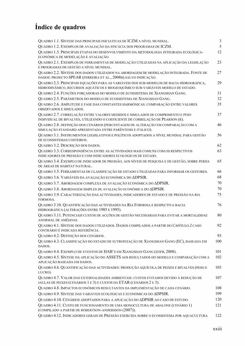
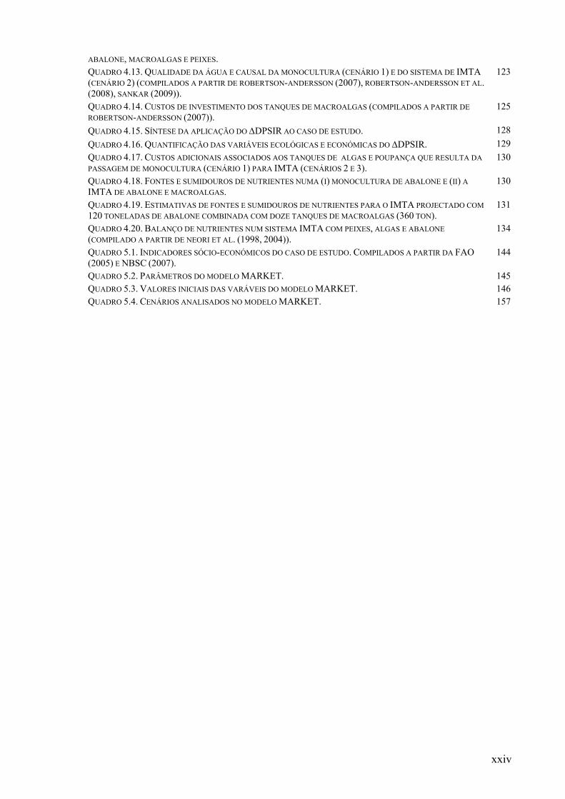
Índice de quadros
QUADRO 1.1. SÍNTESE DAS PRINCIPAIS INICIATIVAS DE ICZM A NÍVEL MUNDIAL. 3QUADRO 1.2. EXEMPLOS DE AVALIAÇÃO DA EFICÁCIA DOS PROGRAMAS DE ICZM. 5QUADRO 1.3. PRINCIPAIS ETAPAS DO DESENVOLVIMENTO DA METODOLOGIA INTEGRADA ECOLÓGICA-ECONÓMICA DE MODELAÇÃO E AVALIAÇÃO.
12
QUADRO 2.1. EXEMPLOS DE FERRAMENTAS DE MODELAÇÃO UTILIZADAS NA APLICAÇÃO DA LEGISLAÇÃO E PROGRAMAS DE GESTÃO A NÍVEL MUNDIAL.
23
QUADRO 2.2. SÍNTESE DOS DADOS UTILIZADOS NA ABORDAGEM DE MODELAÇÃO INTEGRADA. FONTE DE DADOS: PROJECTO SPEAR (FERREIRA ET AL., 2008B) SALVO INDICAÇÃO.
27
QUADRO 2.3. PRINCIPAIS EQUAÇÕES PARA AS VARIÁVEIS DOS SUB-MODELOS DE BACIA HIDROGRÁFICA, HIDRODINÂMICO, RECURSOS AQUÁTICOS E BIOGEOQUÍMICO SUB-VARIÁVEIS MODELO DE ESTADO.
29
QUADRO 2.4. FUNÇÕES FORÇADORAS DO MODELO DE ECOSSISTEMA DE XIANGSHAN GANG. 31QUADRO 2.5. PARÂMETROS DO MODELO DE ECOSSISTEMA DE XIANGSHAN GANG. 32QUADRO 2.6. AMPLITUDE E FASE DAS CONSTANTES HARMÓNICAS: COMPARAÇÃO ENTRE VALORES OBSERVADOS E SIMULADOS.
35
QUADRO 2.7. CORRELAÇÃO ENTRE VALORES MEDIDOS E SIMULADOS DE COMPRIMENTO E PESO INDIVIDUAL DE BIVALVES, UTILIZANDO O COEFICIENTE DE CORRELAÇÃO DE PEARSON (R).
37
QUADRO 2.8. DEFINIÇÃO DOS CENÁRIOS (PERCENTAGEM DE ALTERAÇÃO EM COMPARAÇÃO COM A SIMULAÇÃO STANDARD APRESENTADA ENTRE PARÊNTESIS E ITÁLICO).
46
QUADRO 3.1. INSTRUMENTOS LEGISLATIVOS E POLÍTICOS ADOPTADOS A NÍVEL MUNDIAL PARA GESTÃO DE ECOSSISTEMAS COSTEIROS.
56
QUADRO 3.2. DESCRIÇÃO DOS DADOS. 62QUADRO 3.3. CORRESPONDÊNCIA ENTRE AS ACTIVIDADES MAIS COMUNS COM OS RESPECTIVOS INDICADORES DE PRESSÃO E COM INDICADORES ECOLÓGICOS DE ESTADO.
63
QUADRO 3.4. EXEMPLO DE INDICADOR DE PRESSÃO, AOS NÍVEIS DE PESQUISA E DE GESTÃO, SOBRE PERDA DE ÁREAS DE HABITAT NATURAL.
65
QUADRO 3.5. FERRAMENTAS DE CLASSIFICAÇÃO DE ESTADO UTILIZADAS PARA INFORMAR OS GESTORES. 66QUADRO 3.6. VARIÁVEIS DA AVALIAÇÃO ECONÓMICA DO ∆DPSIR. 68QUADRO 3.7. ABORDAGEM COMPLEXA DE AVALIAÇÃO ECONÓMICA DO ∆DPSIR. 70QUADRO 3.8. ABORDAGEM SIMPLES DE AVALIAÇÃO ECONÓMICA DO ∆DPSIR. 70QUADRO 3.9. CARACTERIZAÇÃO DAS ACTIVIDADES, INDICADORES DE ESTADO E DE PRESSÃO NA RIA FORMOSA.
75
QUADRO 3.10. QUANTIFICAÇÃO DAS ACTIVIDADES NA RIA FORMOSA E RESPECTIVA BACIA HIDROGRÁFICA (ALTERAÇÕES ENTRE 1985 E 1995).
76
QUADRO 3.11. POTENCIAIS CUSTOS DE ACÇÕES DE GESTÃO NECESSÁRIAS PARA EVITAR A MORTALIDDAE ANORMAL DE AMÊIJOAS.
80
QUADRO 4.1. SÍNTESE DOS DADOS UTILIZADOS. DADOS COMPILADOS A PARTIR DO CAPÍTULO 2 CASO CONTRÁRIO É INDICADA REFERÊNCIA.
92
QUADRO 4.2. DEFINIÇÃO DOS CENÁRIOS. 93QUADRO 4.3. CLASSIFICAÇÃO DO ESTADO DE EUTROFIZAÇÃO DE XIANGSHAN GANG (EC), BASEADA EM DADOS.
100
QUADRO 4.4. EXEMPLO DE EVENTOS DE HAB’S EM XIANGSHAN GANG (ZOFB, 2008). 101QUADRO 4.5. SÍNTESE DA APLICAÇÃO DO ASSETS AOS RESULTADOS DO MODELO E COMPARAÇÃO COM A APLICAÇÃO BASEADA EM DADOS.
102
QUADRO 4.6. QUANTIFICAÇÃO DAS ACTIVIDADES: PRODUÇÃO AQUÍCOLA DE PEIXES E BIVALVES (PESO E LUCRO).
103
QUADRO 4.7. VALOR DAS EXTERNALIDADES AMBIENTAIS: CUSTOS EVITADOS DEVIDO À REDUÇÃO DE JAULAS DE PEIXES (CENÁRIOS 1 E 3) E CUSTOS DA ETAR (CENÁRIOS 2 E 3).
107
QUADRO 4.8. IMPACTOS ECONÓMICOS RESULTANTES DA IMPLEMENTAÇÃO DE CADA CENÁRIO. 108QUADRO 4.9. SÍNTESE DAS VARIÁVEIS ECOLÓGICAS E ECONÓMICAS DO ∆DPSIR. 109QUADRO 4.10. CENÁRIOS ADOPTADOS PARA A APLICAÇÃO DO ∆DPSIR AO CASO DE ESTUDO. 120QUADRO 4.11. CUSTO DE FUNCIONAMENTO DE UMA MONOCULTURA DE ABALONE (CENÁRIO 1) (COMPILADO A PARTIR DE ROBERTSON-ANDERSSON (2007)).
121
QUADRO 4.12. INDICADORES GERAIS DE PRESSÃO EXERCIDA SOBRE O ECOSSISTEMA POR AQUACULTURA 122
xxiv
ABALONE, MACROALGAS E PEIXES. QUADRO 4.13. QUALIDADE DA ÁGUA E CAUSAL DA MONOCULTURA (CENÁRIO 1) E DO SISTEMA DE IMTA (CENÁRIO 2) (COMPILADOS A PARTIR DE ROBERTSON-ANDERSSON (2007), ROBERTSON-ANDERSSON ET AL. (2008), SANKAR (2009)).
123
QUADRO 4.14. CUSTOS DE INVESTIMENTO DOS TANQUES DE MACROALGAS (COMPILADOS A PARTIR DE ROBERTSON-ANDERSSON (2007)).
125
QUADRO 4.15. SÍNTESE DA APLICAÇÃO DO ∆DPSIR AO CASO DE ESTUDO. 128QUADRO 4.16. QUANTIFICAÇÃO DAS VARIÁVEIS ECOLÓGICAS E ECONÓMICAS DO ∆DPSIR. 129QUADRO 4.17. CUSTOS ADICIONAIS ASSOCIADOS AOS TANQUES DE ALGAS E POUPANÇA QUE RESULTA DA PASSAGEM DE MONOCULTURA (CENÁRIO 1) PARA IMTA (CENÁRIOS 2 E 3).
130
QUADRO 4.18. FONTES E SUMIDOUROS DE NUTRIENTES NUMA (I) MONOCULTURA DE ABALONE E (II) A IMTA DE ABALONE E MACROALGAS.
130
QUADRO 4.19. ESTIMATIVAS DE FONTES E SUMIDOUROS DE NUTRIENTES PARA O IMTA PROJECTADO COM 120 TONELADAS DE ABALONE COMBINADA COM DOZE TANQUES DE MACROALGAS (360 TON).
131
QUADRO 4.20. BALANÇO DE NUTRIENTES NUM SISTEMA IMTA COM PEIXES, ALGAS E ABALONE (COMPILADO A PARTIR DE NEORI ET AL. (1998, 2004)).
134
QUADRO 5.1. INDICADORES SÓCIO-ECONÓMICOS DO CASO DE ESTUDO. COMPILADOS A PARTIR DA FAO (2005) E NBSC (2007).
144
QUADRO 5.2. PARÂMETROS DO MODELO MARKET. 145QUADRO 5.3. VALORES INICIAIS DAS VARÁVEIS DO MODELO MARKET. 146QUADRO 5.4. CENÁRIOS ANALISADOS NO MODELO MARKET. 157


Chapter 1, INTRODUCTION
1
Chapter 1. Introduction
This chapter presents the frame of reference for the work developed and provides an overview
of the thesis. The first part reviews the coastal management challenge and the role of science
in addressing emerging coastal zone problems. The second part describes the thesis
objectives, presents the study sites used to develop the work and outlines the thesis structure.
Chapter 1, INTRODUCTION
2
1.1 Background
1.1.1 Coastal management challenge: addressing emerging coastal zone problems
Coastal zones comprise important ecosystems (MA, 2005), which generate goods and
services with a high economic value (Ledoux and Turner, 2002). As a result, a strip 100 km
wide along the coastline contains nearly 40% of the world population and 61% of the gross
world product (MA, 2005). Anthropogenic pressures increasingly compromise, directly and
indirectly, the important benefits generated by coastal systems (MA, 2005; Costanza and
Farley, 2007). The main human threats to coastal areas include: loss of natural habitats, loss in
biodiversity and cultural diversity, decline in water quality, vulnerability to global changes
such as predicted sea level rise, increased negative impacts of coastal disasters, the diversity
of human activities, competition for space and seasonal variations in pressure (Ehler et al.,
1997; Fabbri, 1998; Humphrey et al., 2000; MA, 2005; Costanza and Farley, 2007).
Therefore, sustainable development of coastal zones constitutes a challenge for stakeholders
with a role in coastal management.
Integrated Coastal Zone Management (ICZM)
Policy-makers worldwide have defined policy and legislative instruments to address the
emerging coastal zone problems (Clark, 1996; Borja, 2006; Ducrotoy and Elliott, 2006). One
of the more widely known and applied is the Integrated Coastal Zone Management (ICZM)
approach. ICZM is defined as a dynamic management process that brings together the human
and the ecological dimensions to promote the sustainable use, development and protection of
coastal zones (Clark, 1996; Olsen, 2003; Forst, 2009). Managers worldwide have adopted
ICZM within different contexts: 1) to address specific environmental problems emerged in
coastal zones or to manage coastal vulnerability to natural hazards and climate change (Clark,
1996; Krishnamurthy et al., 2008); 2) either at national or local levels, as exemplified by
NRMMC (2006) and Lewis III et al. (1999), respectively; 3) following a top-down approach
or based on a community-based initiative (Cicin-Sain and Knecht, 1998; Lewis III, et al.,
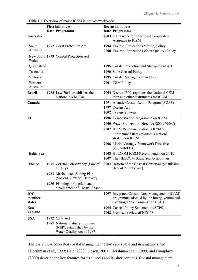
1999; Belfiore, 2000; Kearney et al., 2007). Table 1.1 presents an overview of worldwide
coastal management initiatives. Although such synthesis is reductionist about coastal
management efforts, it illustrates that ICZM initiatives appeared about four decades ago and
that some countries are currently adopting new programmes.
Chapter 1, INTRODUCTION
3
Table 1.1. Overview of major ICZM initiatives worldwide. First initiatives Recent initiatives Date Programme Date Programme Australia 2003 Framework for a National Cooperative
Approach to ICZM South Australia
1972 Coast Protection Act
19942000
Environ. Protection (Marine) Policy Environ. Protection (Water Quality) Policy
New South Wales
1979 Coastal Protection Act
Queensland 1995 Coastal Protection and Management Act Tasmania 1996 State Coastal Policy Victoria 1995 Coastal Management Act 1995 Western Australia
2001 CZM Policy
Brazil 1988 Law 7661, establishes the National CZM Plan
2004 Decree 5300, regulates the National CZM Plan and other instruments for ICZM
Canada 199119972002
Atlantic Coastal Action Program (ACAP) Oceans Act Oceans Strategy
EU 1996 Demonstration programme on ICZM 2000 Water Framework Directive (2000/60/EC) 2002 ICZM Recommendation 2002/413/EC
For member states to adopt a National strategy on ICZM.
2008 Marine Strategy Framework Directive (2008/56/EC)
Baltic Sea 20032007
HELCOM ICZM Recommendation 24/10 The HELCOM Baltic Sea Action Plan
France 1975 Coastal Conservancy (Law of 10 July)
2002 Reform of the Coastal Conservancy's mission (law of 27 February)
1983 Marine Area Zoning Plan (SMVM) (law of 7 January)
1986 Planning, protection, and development of Coastal Space
IOC member states
1997 Integrated Coastal Area Management (ICAM) programme adopted by the Intergovernmental Oceanographic Commission (IOC)
New Zealand
19942008
Coastal Policy Statement (NZCPS) Proposed review of NZCPS
USA 1972 1987
CZM Act National Estuary Program (NEP), established by the Water Quality Act of 1987
The early USA concerted coastal management efforts are stable and in a mature stage
(Hershman et al., 1999; Hale, 2000; Gibson, 2003). Hershman et al. (1999) and Humphrey
(2000) describe the key features for its success and its shortcomings. Coastal management
Chapter 1, INTRODUCTION
4
programmes on a European scale are more recent (Humphrey et al., 2000; Shipman and
Stojanovic, 2007). The various EU policies and directives emerged as complementary
instruments the most important being (Borja, 2006; Ducrotoy and Elliott, 2006; 2008): the
Water Framework Directive (WFD) of 2000, the ICZM recommendation of 2002 and the
Marine Strategy Framework Directive (MSFD) of 2008. Table 1.1 shows only a brief sample
of the programmes adopted within EU. The individual EU member states have different
approaches to coastal management with a variety and complexity of coastal management
initiatives and legislations (Gibson, 2003; Rupprecht Consult and IOI, 2006; Shipman and
Stojanovic 2007). For detailed coastal management initiatives within and across member
states refer to van Alphen (1995), Barragán (2003), Eremina and Stetsko (2003), Pickaver
(2003), Veloso-Gomes et al. (2003), Anker et al. (2004), Taveira Pinto and Paskoff (2004),
Astron (2005), Enemark (2005), Smith and Potts (2005), DOENI (2006), Rupprecht Consult
and IOI (2006), WAG (2007), Deboudt et al. (2008), DEFRA (2008). Clark (1996), Kay et al.
(1997), Cicin-Sain and Knecht (1998), Hale (2000) and Krishnamurthy et al. (2008) provide
detailed ICZM case studies developed worldwide.
For individual ICZM programmes to evolve, comprehensive evaluations are required. It is
important that ICZM program output evaluation is combined with ‘state-of-the-coast’
information to show, for instance, whether new program goals may be needed and to allow an
ICZM program to evolve to an improved version (Olsen et al., 1997; Hershman et al., 1999;
Stojanovic et al., 2004; Billé, 2007). However, most of the evaluation efforts focus on
measuring the evolution of the ICZM process outputs (Olsen, 2003; Pickaver et al., 2004;
Stojanovic et al., 2004; Billé, 2007). Worldwide and independently of maturity of the ICZM
process, there is a lack of measurements of its effectiveness, i.e. of the consequent changes in
the state of the coastal systems, its resources and associated benefits (Knecht et al., 1996,
1997; Kay et al., 1997; Olsen et al., 1997; Hershman et al., 1999; Humphrey et al., 2000;
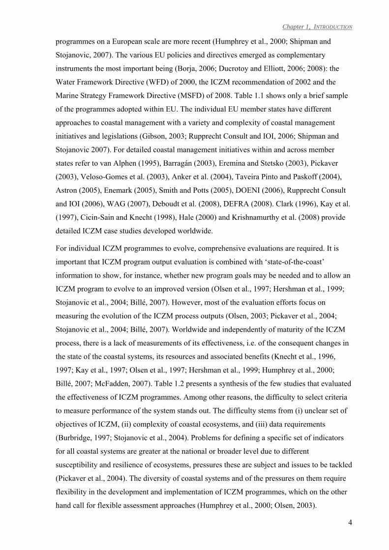
Billé, 2007; McFadden, 2007). Table 1.2 presents a synthesis of the few studies that evaluated
the effectiveness of ICZM programmes. Among other reasons, the difficulty to select criteria
to measure performance of the system stands out. The difficulty stems from (i) unclear set of
objectives of ICZM, (ii) complexity of coastal ecosystems, and (iii) data requirements
(Burbridge, 1997; Stojanovic et al., 2004). Problems for defining a specific set of indicators
for all coastal systems are greater at the national or broader level due to different
susceptibility and resilience of ecosystems, pressures these are subject and issues to be tackled
(Pickaver et al., 2004). The diversity of coastal systems and of the pressures on them require
flexibility in the development and implementation of ICZM programmes, which on the other
hand call for flexible assessment approaches (Humphrey et al., 2000; Olsen, 2003).
Chapter 1, INTRODUCTION
5
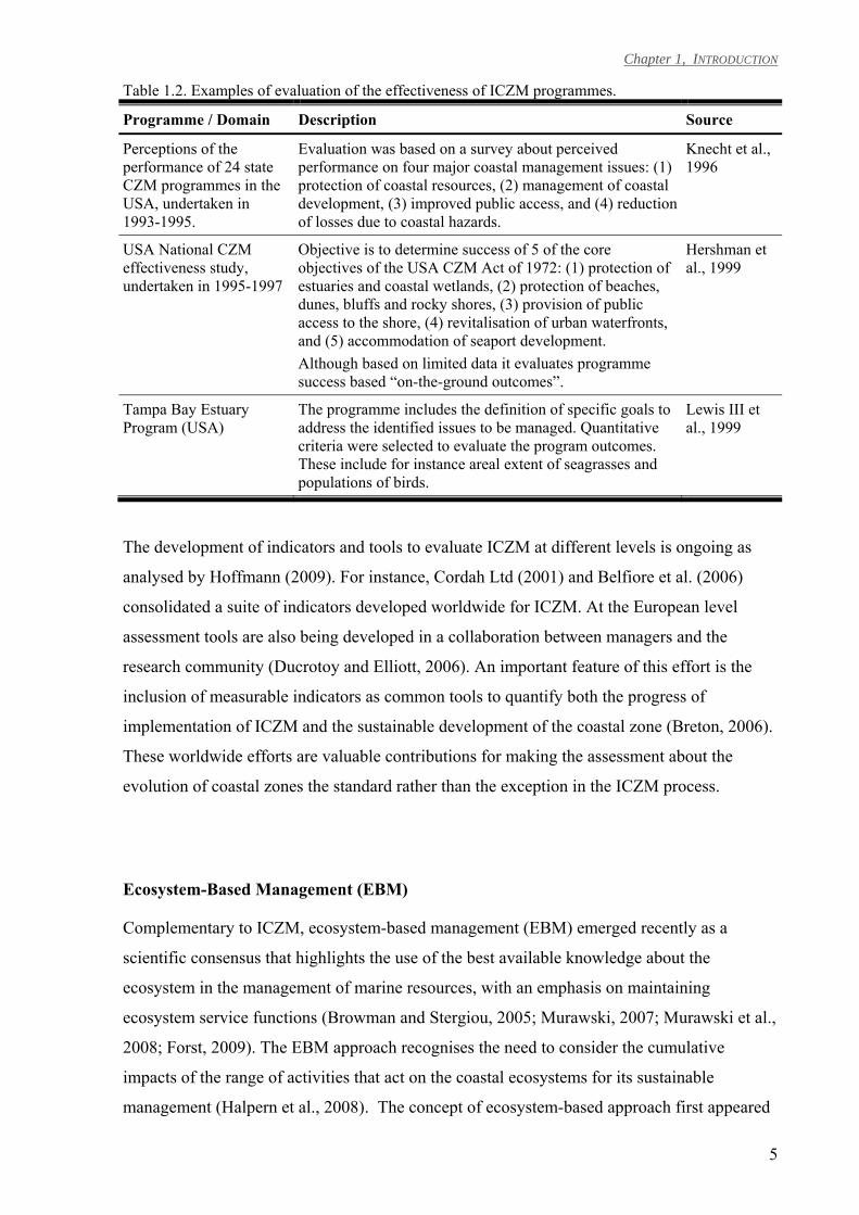
Table 1.2. Examples of evaluation of the effectiveness of ICZM programmes.
Programme / Domain Description Source
Perceptions of the performance of 24 state CZM programmes in the USA, undertaken in 1993-1995.
Evaluation was based on a survey about perceived performance on four major coastal management issues: (1) protection of coastal resources, (2) management of coastal development, (3) improved public access, and (4) reduction of losses due to coastal hazards.
Knecht et al., 1996
USA National CZM effectiveness study, undertaken in 1995-1997
Objective is to determine success of 5 of the core objectives of the USA CZM Act of 1972: (1) protection of estuaries and coastal wetlands, (2) protection of beaches, dunes, bluffs and rocky shores, (3) provision of public access to the shore, (4) revitalisation of urban waterfronts, and (5) accommodation of seaport development. Although based on limited data it evaluates programme success based “on-the-ground outcomes”.
Hershman et al., 1999
Tampa Bay Estuary Program (USA)
The programme includes the definition of specific goals to address the identified issues to be managed. Quantitative criteria were selected to evaluate the program outcomes. These include for instance areal extent of seagrasses and populations of birds.
Lewis III et al., 1999
The development of indicators and tools to evaluate ICZM at different levels is ongoing as
analysed by Hoffmann (2009). For instance, Cordah Ltd (2001) and Belfiore et al. (2006)
consolidated a suite of indicators developed worldwide for ICZM. At the European level
assessment tools are also being developed in a collaboration between managers and the
research community (Ducrotoy and Elliott, 2006). An important feature of this effort is the
inclusion of measurable indicators as common tools to quantify both the progress of
implementation of ICZM and the sustainable development of the coastal zone (Breton, 2006).
These worldwide efforts are valuable contributions for making the assessment about the
evolution of coastal zones the standard rather than the exception in the ICZM process.
Ecosystem-Based Management (EBM)
Complementary to ICZM, ecosystem-based management (EBM) emerged recently as a
scientific consensus that highlights the use of the best available knowledge about the
ecosystem in the management of marine resources, with an emphasis on maintaining
ecosystem service functions (Browman and Stergiou, 2005; Murawski, 2007; Murawski et al.,
2008; Forst, 2009). The EBM approach recognises the need to consider the cumulative
impacts of the range of activities that act on the coastal ecosystems for its sustainable
management (Halpern et al., 2008). The concept of ecosystem-based approach first appeared
Chapter 1, INTRODUCTION
6
in the 1970’s, not specifically related with coastal zones (Slocombe, 1993). Grumbine (1994)
and Slocombe (1998) review the origins and principles of EBM and provide lessons for
implementing it. An important feature that both authors highlight is that EBM is about
integrating environment and development. They emphasise that in the real systems humans
are within rather than separated from nature. Slocombe (1998) suggests that an effective EBM
(i) starts with a synthesis of information for future research and management, (ii) monitors
features to follow changes, (iii) uses local knowledge, and (iv) is practical, and if resources
are limited it needs to focus research on knowledge that is meaningful to management. The
definition of operational goals is an important challenge for EBM implementation, according
to Slocombe (1998). In one of the first references of EBM for coastal zones, Imperial and
Hennessey (1996) identified the USA National Estuary Program (NEP) as a promising
ecosystem-based approach to managing estuaries. The particularity of NEP is to focus on
solutions for problems identified on each estuary (Imperial and Hennessey, 1996). For each
estuary is implemented a comprehensive conservation and management plan which contains
an action plan to address problems identified and a monitoring programme to measure
effectiveness of activities. Furthermore, the plan sets the funding and the institutional context
to implement the estuarine programmes. At the European level, there are also several
examples of EBM, for example for the Baltic Sea, North Sea and Wadden Sea (Enemark,
2005; HELCOM, 2007; Ducrotoy and Elliott, 2008). In Canada, the Atlantic Coastal Action
Program (ACAP) is an ecosystem and community-based approach to integrated planning and
management of the environment that has unique features such as the power sharing among
stakeholders (McNeil et al., 2006). The Environment Canada launched it in 1991 and the
process consists of development and implementation of management plans, partnership
building, local involvement and action and scientific research to improve and maintain the
environmental integrity of coastal communities (McNeil et al., 2006). The ACAP established
an alternative process to environmental and socio-economic management of coastal zones
involving interested stakeholders since the beginning to identify problems and solutions. The
evaluation of ACAP focuses on the environmental results and consists of accounting the
measures adopted and avoided the avoided pressures, e.g., area of enhanced wildlife habitat or
weight of mercury eliminated from waste stream. According to Environment Canada, the
ACAP is effective on an ecosystem basis (McNeil et al., 2006).
Chapter 1, INTRODUCTION
7
Ecosystem Approach to Aquaculture (EAA)
Sustainable development of mariculture represents a particular challenge for coastal
ecosystem and resources managers for the combination of the following reasons (GESAMP,
2001):
Aquaculture relevance for food security (Ahmed and Lorica, 2002);
Rapid growth of aquaculture industry (Duarte et al., 2007a) estimated as about 8.8%
per annum since 1970 (FAO 2006);
Generalised concern that the increasing demand for aquaculture can drive coastal
degradation, such as habitat loss, pollution, overexploitation of fisheries for fishmeal
and oil, due to unsustainable aquaculture practices (MA, 2005);
Some aquaculture solutions, including those of extractive species (Neori et al., 2004),
are advocated for mitigating some of aquaculture’s impacts on coastal ecosystems, for
instance cultivation of seaweeds and shellfish (Ferreira et al., 2007a; Gren et al., 2009;
Stephenson, et al., 2009);
Aquaculture aesthetic impacts cause conflicts with other users of coastal zones
(Dempster and Sanchez-Jerez, 2008; Gibbs, 2009);
Impacts of aquaculture activities are cumulative among farms and additive to the
impacts of other development pressures in the coastal zone, consequently aquaculture
development must be addressed beyond the individual farm level, at the ecosystem
level (GESAMP, 2001; Ferreira et al., 2008a; Soto et al., 2008);
The future of the aquaculture industry relies on sustainable coastal development
because ultimately it depends on healthy coastal waters (GESAMP, 2001).
For the above-mentioned reasons an ecosystem approach to aquaculture (EAA), integrated
with management of other coastal developments, is required for sustaining aquaculture
expansion (GESAMP, 2001; FAO, 2007; Soto et al., 2008). According to FAO, EAA is
defined as: “An ecosystem approach to aquaculture (EAA) strives to balance diverse societal
objectives, by taking account of the knowledge and uncertainties of biotic, abiotic and human
components of ecosystems including their interactions, flows and processes and applying an
integrated approach to aquaculture within ecologically and operationally meaningful
boundaries. The purpose of EAA should be to plan, develop and manage the sector in a
manner that addresses the multiple needs and desires of societies, without jeopardizing the
options for future generations to benefit from the full range of goods and services provided by
aquatic ecosystems.” (FAO, 2007).
Chapter 1, INTRODUCTION
8
1.1.2 Role of science for coastal management
The complexity of the phenomena occurring in coastal ecosystems and their management
requires the interaction among managers and researchers of a range of disciplines (Fabbri,
1998). The effective integration of science with management is important for better policy
formulation and policy-making for achievement of both environmental and development
needs and goals (Slocombe, 1993; Peirce, 1998; Turner, 2000; Cheong, 2008). Currently the
role of applied environmental science to support coastal management and address legal
requirements is increasing (Ducrotoy and Elliott, 2006). In order to communicate science to
managers, researchers must follow a problem-oriented approach and distil the outputs into
accessible and useful information for managers (Nobre et al., 2005; Dennison, 2008;
Hoffmann, 2009). Such an approach calls for the integration of scientific methodologies and
disciplines across different scales (IMPRESS, 2003; McFadden, 2007). In particular, the
adoption of an EAA poses several challenges to the scientific community (GESAMP, 2001;
Soto et al., 2008). For instance, guidance about more sustainable aquaculture options at the
farm level (Neori et al., 2004; Robertson-Andersson et al., 2008; Ayer and Tyedmers, 2009)
and understanding of cumulative impacts within coastal ecosystem for determination of, for
instance, carrying capacity with respect to aquaculture activity (Ferreira, et al. 2008a).
Overall, ecosystem-based tools capable of providing insights about complex ecological
processes and interaction with socio-economic systems are valuable to support the sustainable
use of high demanded coastal zones. The most commonly applied tools include (Cicin-Sain
and Knecht, 1998; Neal et al., 2003): spatial modelling tools, such as geographical
information systems (GIS) and remote sensing; catchment and coastal ecosystem modelling;
participatory work with stakeholders; integrated environmental assessment, benefit-cost
studies and economic valuation. The aim of these tools is to provide information to the
decision-making process or its evaluation and not to replace decision-makers (Van Kouwen et
al., 2008). The enhanced understanding scientific methodologies provide can be particularly
useful in conflict resolution processes inherent to ICZM (Fabbri, 1998; McCreary et al.,
2001). The development of integrative tools requires the interaction of all stakeholders in
order to ensure (Cicin-Sain and Knecht, 1998; Van Kouwen et al., 2008) that (i) tools address
relevant issues for coastal management, and (ii) managers can use the tools and their outputs.
The state-of-the-art about ecosystem-based tools is detailed in Chapter 6.
There are three major research areas to support ICZM and EBM: (i) increase of knowledge
about complex coastal processes, such as the cumulative impacts of coastal zone multiple
Chapter 1, INTRODUCTION
9
pressures, (ii) development of tools to communicate science to managers, and (iii) interaction
of coastal environment and socio-economics. These research areas are discussed below.
Increase of knowledge about complex coastal processes
A knowledge gap highlighted as crucial for coastal management is to understand the
cumulative impacts of natural and anthropogenic pressures on coastal ecosystem state, and on
the goods and services these areas provide (Halpern et al., 2008). Ecological modelling is
recognised as an important tool for coastal management, which can contribute for
understanding coastal ecosystem processes including the above mentioned research gap
(Turner, 2000; Fulton et al., 2003; Greiner, 2004; Hardman-Mountford et al., 2005;
Murawski, 2007; Forst, 2009). In particular, more recently the requirement for models at the
ecosystem level capable of simulating the cumulative impacts of multiple uses has been
highlighted (Fulton et al., 2003; Ferreira et al., 2008a). Nevertheless, modelling approaches
that are able to simulate the cumulative impacts of coastal activities on these ecosystems are
still at an early stage of development. Such developments are particularly important for
determination of ecological carrying capacity required for the sustainable expansion of
aquaculture (Ferreira et al., 2008a; Dempster and Sanchez-Jerez, 2008; Soto et al., 2008).
Chapter 2 provides further details about contributions of ecosystem modelling and state-of-
the-art of relevant modelling approaches.
Tools to communicate science to managers
Integration and synthesis of complex knowledge from different disciplines into useful
information to coastal managers and the public at large is a progressing and challenging field
to environmental scientists (Harris, 2002; McNie, 2007; Cheong, 2008). Integrated
Environmental Assessment (IEA) methodologies can enhance communication between
scientists and policy-makers, since those methodologies aim to present an interdisciplinary
synthesis of scientific knowledge (Tol and Vellinga, 1998; Harris, 2002). IEA outcomes
normally provide insight regarding complex phenomena, which can guide decision-making
and policy development for ecological resources management (Toth and Hizsnyik 1998). The
Drivers-Pressure-State-Impact-Response (DPSIR) is a well-known IEA framework (Peirce,
1998) used to communicate science to coastal managers and in particular to bridge the
science-management scales gap (Elliott, 2002). Chapter 3 further reviews the use of IEA
frameworks for coastal management. Ecological modelling in particular can benefit from the
integration with IEA methodologies to distil the outcomes of complex models into useful
information for managers (Nobre et al., 2005). A review about integration of IEA
Chapter 1, INTRODUCTION
10
methodologies with ecological models is presented in Chapter 4 (Section 4.1). Because it
involves human interpretation, one of the IEA caveats is subjectivity and dependence on the
analyst point of view (Tol and Vellinga, 1998). That is a criticism specifically pointed out to
the DPSIR approach (Svarstad et al., 2008). Tol and Vellinga (1998) recommend that for the
use of IEA full potential the methodologies for integrating knowledge need to improvement.
Specifically for the DPSIR, Svarstad et al. (2008) suggest the expansion of the framework to
incorporate social and economic concerns, rather than just report about the state of the
environment.
At the EU level several tools are being developed, specifically to support implementation of
coastal management related legislation and policy (Ducrotoy and Elliott, 2006). Specific
examples include: (i) GIS as a decision support tool to be used in the development of the
National Strategy for ICZM of the Catalan coast following the EU recommendation (Sardá et
al., 2005), (ii) GIS use for division of ecosystems into homogenous management units as
required by the WFD (Ferreira et al., 2006; Balaguer et al., 2008), (iii) tool to assist in the
classification of marine angiosperms, one of the WFD biological elements for coastal and
transitional waters (Best et al., 2007), (iv) benthic community-based biotic indices to evaluate
ecosystem status and condition, in support of WFD implementation (Pinto et al., 2009). Borja
et al. (2008) reviews at the worldwide level, existing integrative assessment tools capable to
support recent legislation developed in several nations to address ecological quality or
integrity.
A particular area where efforts need to be developed is the production of methodologies to
assess the impacts of the ICZM initiatives on coastal ecosystems (Olsen et al., 1997),
including the changes in the benefits these generate. Chapter 3 presents existing
methodologies that aim to support sound-decision making.
Interaction of coastal environment and socio-economics
Understanding the linkages between the natural and anthropogenic systems is crucial for
ICZM and EBM (Turner, 2000; Westmacott, 2001; Boissonnas et al., 2002; Bowen and Riley,
2003; Cheong, 2008). Firstly, the aim of ICZM is to promote the sustainable development of
coastal ecosystems including both ecological and socio-economic components. Secondly,
coastal management and planning must account for the ‘costs’ of resource degradation.
Finally, the measurement of the effectiveness of ICZM initiatives must screen not only the
consequent changes on the ecological state of the ecosystem but also changes of the socio-
economic benefits generated in coastal areas. In particular, economic valuation methods are
Chapter 1, INTRODUCTION
11
crucial to account for ecosystem goods and services in decision-making (Boissonnas et al.,
2002; Lal, 2003; Farber et al., 2006; Costanza and Farley, 2007).
The DPSIR approach results of the effort to integrate the natural and anthropogenic systems,
and to combine science with management (Cheong, 2008). DPSIR is a widely used
conceptual framework for integrated coastal management that provides a conceptual scheme
of how socio-economic activities interact with the natural systems (Elliott, 2002; Ledoux and
Turner, 2002; Bowen and Riley, 2003; IMPRESS, 2003; Bidone and Lacerda, 2004; GTOS,
2005; Hofmann et al., 2005; Scheren et al., 2004; Borja et al., 2006; Nobre, 2009). In simple
terms, the DPSIR establishes the link between the human activities (‘Drivers’), corresponding
loads (‘Pressures’), resulting changes of the ‘State’ of the ecosystem (i.e. the ‘Impact’) and
the actions adopted by the coastal managers and decision-makers (Response). However, this
IEA methodology lacks the formal definition of a consistent linkage between ecological and
economic indicators over time (Nobre, 2009). The DPSIR approach and the interaction
between the natural and anthropogenic systems is further analysed in Chapter 3.
Additionally, the inclusion of the economic component in dynamic ecological models is
required in order to simulate the feedback between the ecological and socio-economic
systems (Bockstael et al., 1995; Nobre et al., 2009). First attempts to integrate the ecological
and economic models date back to the 1960’s (Westmacott, 2001). Currently integrated
ecological-economic modelling is an evolving discipline that has increased recently
(Drechsler et al., 2007). Several difficulties exist, such as the difference in scales at which
normally these two systems are simulated or analysed (Nijkamp and van den Bergh 1997;
Turner, 2000; Drechsler and Watzold, 2007; Nobre et al., 2009). Existing efforts for
integration of ecological and economic models are detailed in Chapter 5.
1.2 Thesis overview
1.2.1 Objectives
Anthropogenic activity is generating a negative feedback through the significant direct and
indirect socio-economic benefits provided by coastal ecosystems; increasing human pressure
on coastal zones (Boissonnas et al., 2002) is causing degradation and consequently decreases
the benefits that these ecosystems deliver (Bowen and Riley, 2003; MA, 2005; Costanza and
Farley, 2007). Emerging coastal management frameworks use the best available knowledge
about the ecosystem to manage marine resources and functions (Fluharty, 2005; Murawski,
2007; Forst, 2009). More progress is needed regarding the process of translating data into
Chapter 1, INTRODUCTION
12
useful knowledge for environmental problem solving, and this is also true with regards to
coastal zones (Dennison, 2008). Managers and policy-makers require analytical and
assessment methodologies capable of (i) generating understanding about coastal ecosystems
and their interaction with the socio-economic system, and (ii) synthesising research outcomes
into useful information in order to define effective responses and evaluate previously adopted
actions (McNie, 2007; Stanners et al., 2008).
This thesis aims to contribute to research on the assessment of changes in coastal ecosystems
and in benefits generated due to management actions (or lack of actions). The overall
objectives are to (i) assess the ecological and economic impacts of previously adopted policies
as well as future response scenarios, and (ii) translate the outcomes into useful information for
stakeholders with a management role.
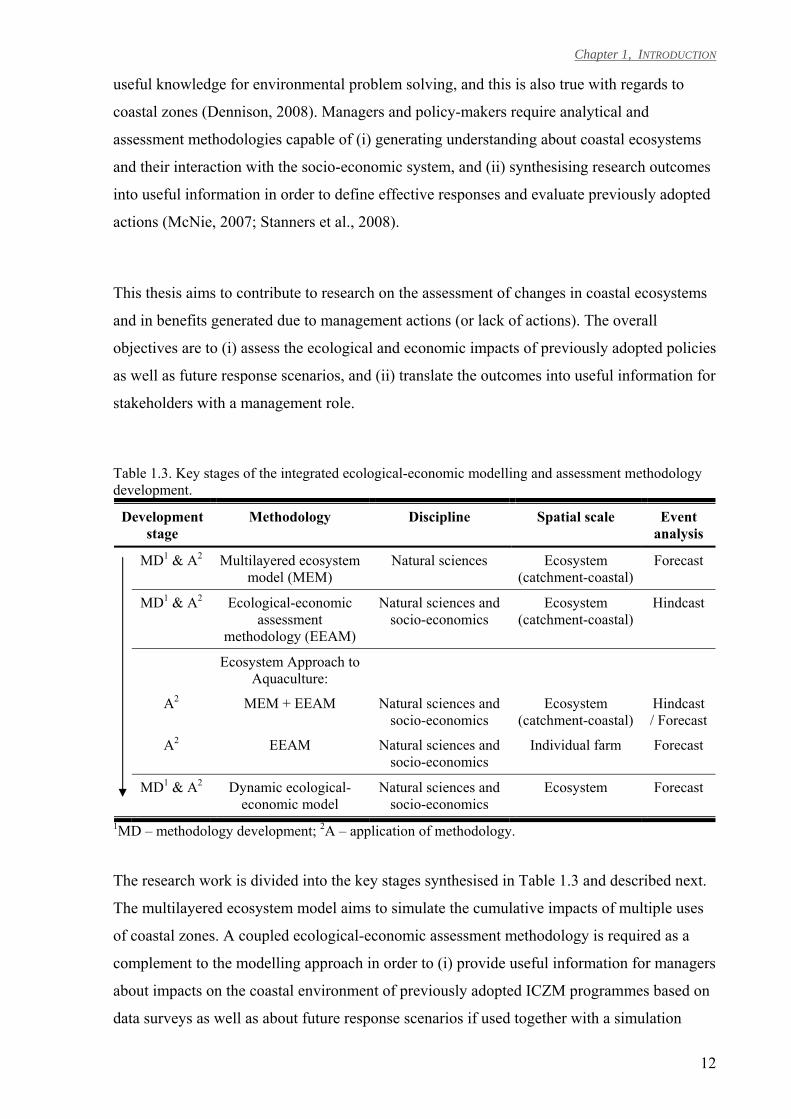
Table 1.3. Key stages of the integrated ecological-economic modelling and assessment methodology development.
Development stage
Methodology Discipline Spatial scale Event analysis
MD1 & A2 Multilayered ecosystem model (MEM)
Natural sciences Ecosystem (catchment-coastal)
Forecast
MD1 & A2 Ecological-economic assessment
methodology (EEAM)
Natural sciences and socio-economics
Ecosystem (catchment-coastal)
Hindcast
Ecosystem Approach to Aquaculture:
A2 MEM + EEAM Natural sciences and socio-economics
Ecosystem (catchment-coastal)
Hindcast / Forecast
A2 EEAM Natural sciences and socio-economics
Individual farm Forecast
MD1 & A2 Dynamic ecological-economic model
Natural sciences and socio-economics
Ecosystem Forecast
1MD – methodology development; 2A – application of methodology.
The research work is divided into the key stages synthesised in Table 1.3 and described next.
The multilayered ecosystem model aims to simulate the cumulative impacts of multiple uses
of coastal zones. A coupled ecological-economic assessment methodology is required as a
complement to the modelling approach in order to (i) provide useful information for managers
about impacts on the coastal environment of previously adopted ICZM programmes based on
data surveys as well as about future response scenarios if used together with a simulation
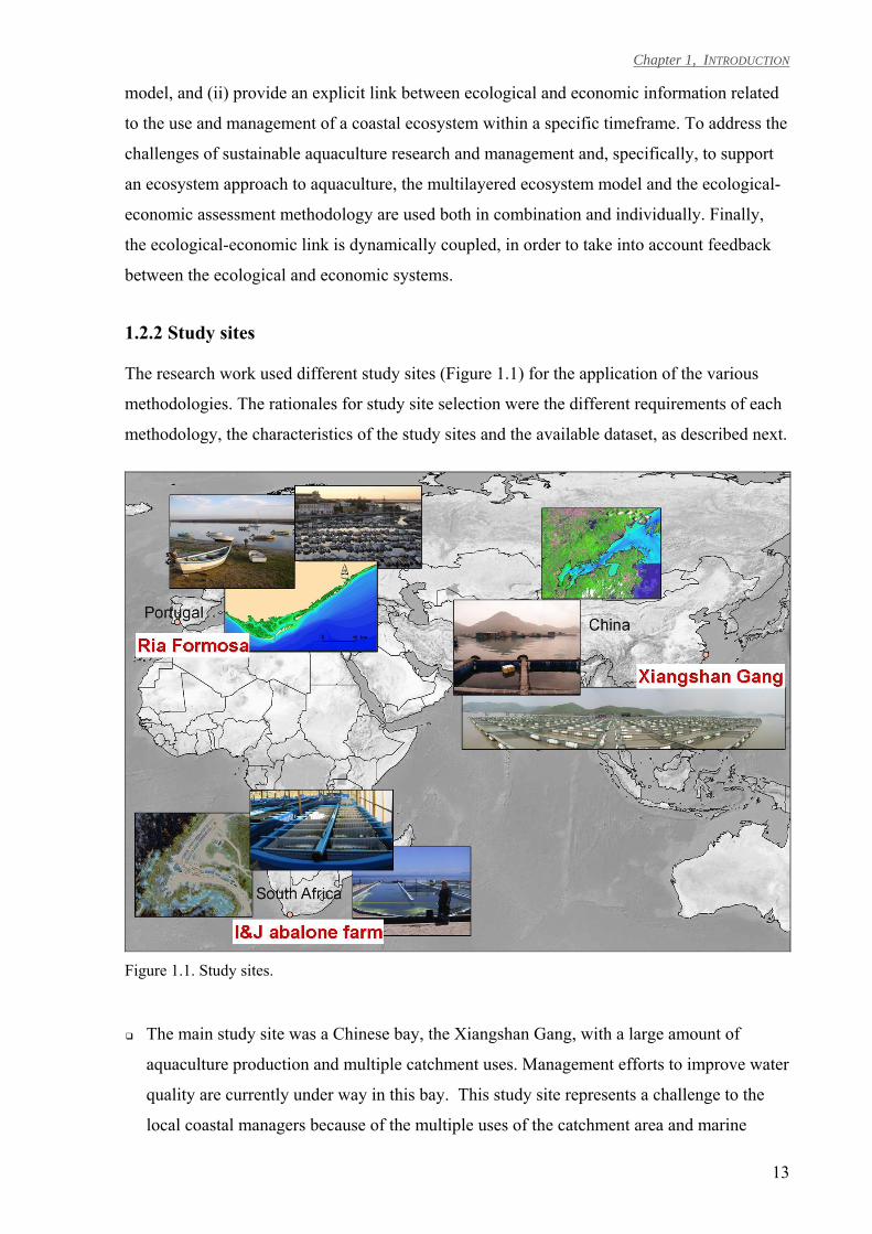
Chapter 1, INTRODUCTION
13
model, and (ii) provide an explicit link between ecological and economic information related
to the use and management of a coastal ecosystem within a specific timeframe. To address the
challenges of sustainable aquaculture research and management and, specifically, to support
an ecosystem approach to aquaculture, the multilayered ecosystem model and the ecological-
economic assessment methodology are used both in combination and individually. Finally,
the ecological-economic link is dynamically coupled, in order to take into account feedback
between the ecological and economic systems.
1.2.2 Study sites
The research work used different study sites (Figure 1.1) for the application of the various
methodologies. The rationales for study site selection were the different requirements of each
methodology, the characteristics of the study sites and the available dataset, as described next.
Figure 1.1. Study sites.
The main study site was a Chinese bay, the Xiangshan Gang, with a large amount of
aquaculture production and multiple catchment uses. Management efforts to improve water
quality are currently under way in this bay. This study site represents a challenge to the
local coastal managers because of the multiple uses of the catchment area and marine
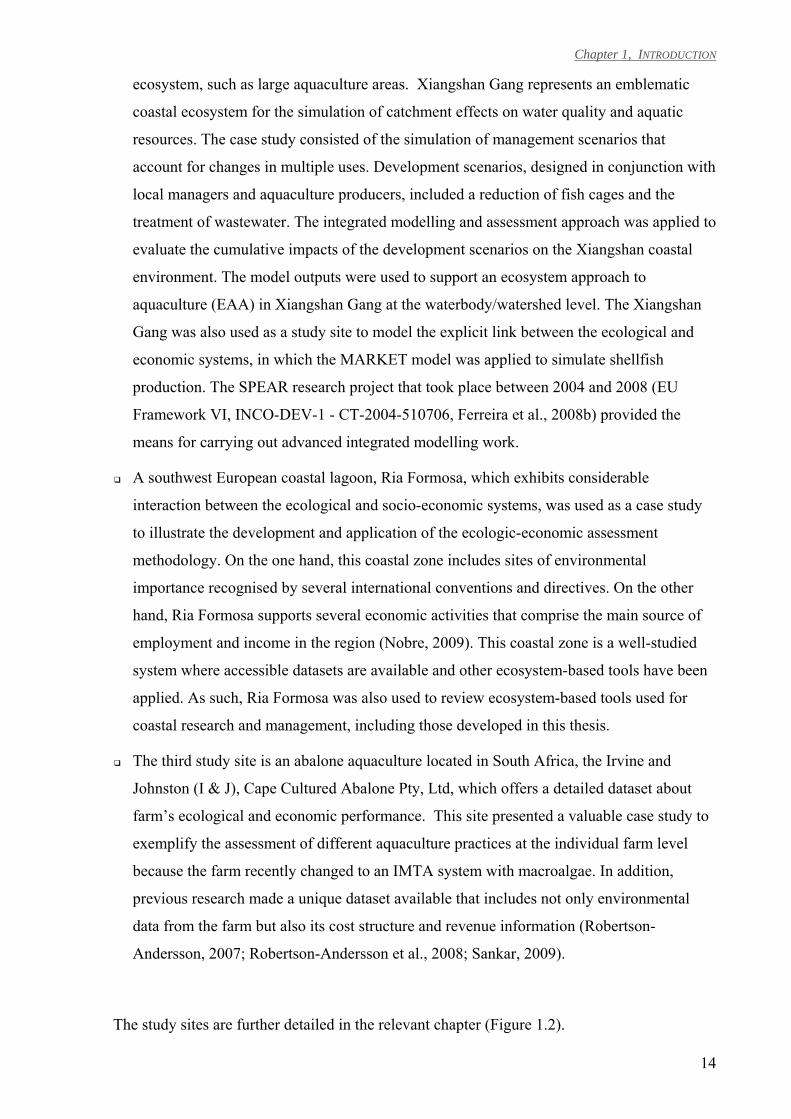
Chapter 1, INTRODUCTION
14
ecosystem, such as large aquaculture areas. Xiangshan Gang represents an emblematic
coastal ecosystem for the simulation of catchment effects on water quality and aquatic
resources. The case study consisted of the simulation of management scenarios that
account for changes in multiple uses. Development scenarios, designed in conjunction with
local managers and aquaculture producers, included a reduction of fish cages and the
treatment of wastewater. The integrated modelling and assessment approach was applied to
evaluate the cumulative impacts of the development scenarios on the Xiangshan coastal
environment. The model outputs were used to support an ecosystem approach to
aquaculture (EAA) in Xiangshan Gang at the waterbody/watershed level. The Xiangshan
Gang was also used as a study site to model the explicit link between the ecological and
economic systems, in which the MARKET model was applied to simulate shellfish
production. The SPEAR research project that took place between 2004 and 2008 (EU
Framework VI, INCO-DEV-1 - CT-2004-510706, Ferreira et al., 2008b) provided the
means for carrying out advanced integrated modelling work.
A southwest European coastal lagoon, Ria Formosa, which exhibits considerable
interaction between the ecological and socio-economic systems, was used as a case study
to illustrate the development and application of the ecologic-economic assessment
methodology. On the one hand, this coastal zone includes sites of environmental
importance recognised by several international conventions and directives. On the other
hand, Ria Formosa supports several economic activities that comprise the main source of
employment and income in the region (Nobre, 2009). This coastal zone is a well-studied
system where accessible datasets are available and other ecosystem-based tools have been
applied. As such, Ria Formosa was also used to review ecosystem-based tools used for
coastal research and management, including those developed in this thesis.
The third study site is an abalone aquaculture located in South Africa, the Irvine and
Johnston (I & J), Cape Cultured Abalone Pty, Ltd, which offers a detailed dataset about
farm’s ecological and economic performance. This site presented a valuable case study to
exemplify the assessment of different aquaculture practices at the individual farm level
because the farm recently changed to an IMTA system with macroalgae. In addition,
previous research made a unique dataset available that includes not only environmental
data from the farm but also its cost structure and revenue information (Robertson-
Andersson, 2007; Robertson-Andersson et al., 2008; Sankar, 2009).
The study sites are further detailed in the relevant chapter (Figure 1.2).
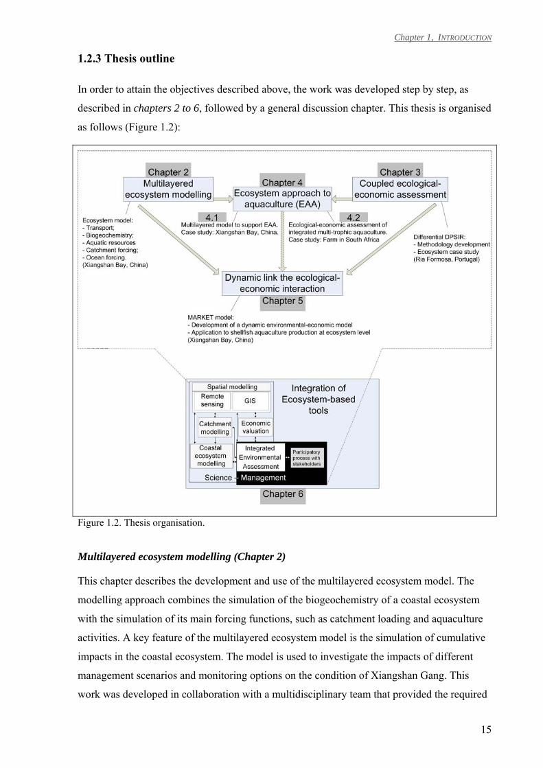
Chapter 1, INTRODUCTION
15
1.2.3 Thesis outline
In order to attain the objectives described above, the work was developed step by step, as
described in chapters 2 to 6, followed by a general discussion chapter. This thesis is organised
as follows (Figure 1.2):
Figure 1.2. Thesis organisation.
Multilayered ecosystem modelling (Chapter 2)
This chapter describes the development and use of the multilayered ecosystem model. The
modelling approach combines the simulation of the biogeochemistry of a coastal ecosystem
with the simulation of its main forcing functions, such as catchment loading and aquaculture
activities. A key feature of the multilayered ecosystem model is the simulation of cumulative
impacts in the coastal ecosystem. The model is used to investigate the impacts of different
management scenarios and monitoring options on the condition of Xiangshan Gang. This
work was developed in collaboration with a multidisciplinary team that provided the required
Chapter 1, INTRODUCTION
16
sub-models for the catchment, hydrodynamic and aquatic resources simulation (Ferreira et al.,
2008b).
Integrated ecological-economic assessment (Chapter 3)
This chapter introduces the differential DPSIR (∆DPSIR) methodology, an adaptation of the
general DPSIR approach (Nobre, 2009). The ∆DPSIR includes an explicit linkage between
ecology and economy within a specific timeframe. This assessment methodology is developed
as a tool to analyse the relationship between the ecosystem state and the use of aquatic
resources. The ∆DPSIR aims to provide the scientific-based information required by
managers and decision-makers to evaluate the ecological and economic impacts of previously
adopted policies, as well future response scenarios, on the coastal environment. The
application of the ∆DPSIR is illustrated through an analysis of developments in a southwest
European coastal lagoon between 1985 and 1995.
Ecosystem approach to aquaculture (Chapter 4)
This chapter integrates the work developed in Chapters 2 and 3 to develop an ecosystem
approach to aquaculture (EAA). The relevant scales for the EAA application are (Soto et al.,
2008) (1) the farm level, (2) the waterbody and respective watershed/aquaculture zone, and
(3) the global, market-trade scale. Herein, two case studies are presented to evaluate
aquaculture options at the waterbody/watershed level and at the farm level:
4.1 Waterbody/watershed level assessment: evaluation of model scenarios
The application of the ecosystem model outputs and the ∆DPSIR to evaluate
development scenarios at the waterbody/watershed level is illustrated in this
section.
4.2 Farm level assessment: evaluation of real data
Herein, a detailed dataset is analysed to evaluate aquaculture options at the farm
level. The ∆DPSIR is applied to quantify the ecological and economic benefits of
shifting from an abalone monoculture to an abalone-seaweed integrated multi-
trophic aquaculture (IMTA).
Chapter 1, INTRODUCTION
17
Ecological-economic dynamic modelling (Chapter 5)
The dynamical link between the ecological and economic components is described in this
chapter (Nobre et al., 2009). A coupled ecological-economic model has been developed for
simulation of aquaculture production. First, the Modelling Approach to Resource economics
decision-maKing in EcoaquaculTure (MARKET) was developed as a conceptual framework.
Second, the MARKET approach was implemented to integrate an aquatic resources model
with an economic model in the context of shellfish production in a Chinese coastal
embayment. This work included inputs from an economic team for the definition of the
economic functions for the case study (Nobre et al., 2009).
Integration of ecosystem-based tools (Chapter 6)
This chapter presents state-of-the-art ecosystem-based tools used for coastal research and
management, including those developed in this thesis (Nobre and Ferreira, 2009). A
consolidated demonstration of the application of such tools for coastal management is carried
out using the Ria Formosa and catchment area as a case study.

Chapter 1, INTRODUCTION
18
Chapter 2. Multilayered ecosystem modelling
Context
As mentioned in Chapter 1, improving knowledge about complex coastal processes requires
that the coastal ecosystem be modelled with tools capable of simulating the cumulative
impacts of multiple uses. Such developments are still at an early stage but are potentially
important for the sustainable expansion of aquaculture. For instance, they could allow for
calculation of ecosystem carrying capacity that accounts for effects of multiple farms and
other coastal activities on the ecosystem.
Summary
This chapter describes the multilayered ecosystem model and its application to Xiangshan
Gang, a Chinese coastal bay with large aquaculture production and multiple catchment uses,
where management efforts to improve water quality are underway. This integrated modelling
approach combines the simulation of the biogeochemistry of a coastal ecosystem with the
simulation of its main forcing functions, such as catchment loading and aquaculture activities.
The case study consists of simulation scenarios designed together with local managers and
aquaculture producers that account for changes in multiple uses. The integrated modelling
approach is applied to simulate the cumulative effects of the reduction of fish cages and
treatment of wastewater on the Xiangshan Gang coastal environment.
Chapter 2, MULTILAYERED ECOSYSTEM MODELLING
20
This chapter corresponds to a manuscript currently in second-stage
review in Estuarine Coastal and Shelf Science:
Assessment of coastal management options by means of multilayered
ecosystem models, by Nobre, A.M., Ferreira, J.G., Nunes, J.P., Yan,
X., Bricker, S., Corner, R., Groom, S., Gu, H., Hawkins, A.J.S.,
Hutson, R., Lan, D., Lencart e Silva, J.D., Pascoe, P., Telfer, T., Zhang,
X., Zhu, M.
Chapter 2, MULTILAYERED ECOSYSTEM MODELLING
21
Assessment of coastal management options by means of multilayered ecosystem models
INTRODUCTION
Coastal zones provide considerable benefits to society while at the same time human activities
exert pressure on coastal ecosystems, therefore threatening those same benefits (Nobre, 2009).
To promote the sustainable use of coastal zone resources an ecosystem approach is of
considerable value, firstly in understanding the causal relationships between environmental
and socio-economic systems, and the cumulative impacts of the range of activities developed
in coastal ecosystems (Soto et al., 2008; Nobre and Ferreira, 2009), and secondly to manage
coastal resources and biodiversity (Browman and Stergiou, 2005; Murawski et al., 2008).
Marine Ecosystem-Based Management (EBM) is an emerging scientific consensus
complementary to Integrated Coastal Zone Management (ICZM). EBM highlights the need to
use the best available knowledge about the ecosystem in order to manage marine resources,
with an emphasis on maintaining ecosystem service functions (Browman and Stergiou, 2005;
Murawski, 2007; Murawski et al., 2008). In particular, improved planning and management
of aquaculture production is highlighted as one of the sustainability issues related to coastal
zone development and management that must urgently be addressed (GESAMP, 2001).
Recently, several initiatives have occurred to support the development of an Ecosystem
Approach to Aquaculture (EAA), which aims to integrate aquaculture within the wider
ecosystem in order to promote the sustainability of the industry (Soto et al., 2008).
Ecosystem modelling is a powerful tool that can contribute the required scientific grounding
for the adoption of such an Ecosystem-Based Management approach (Fulton et al., 2003;
Greiner, 2004; Hardman-Mountford et al., 2005; Murawski, 2007). Specifically, modelling
can be useful to: (i) provide insights about ecological interactions within the ecosystem
(Raillard and Ménesguen, 1994; Plus et al., 2003; Dowd, 2005; Grant et al., 2008; Sohma et
al., 2008; Dumbauld et al., 2009), (ii) estimate the cumulative impacts of multiple activities
operating on a given coastal area at an integrated catchment - marine ecosystem scale (Soto et
al., 2008), and (iii) evaluate the susceptibility of an ecosystem to pressures by means of
scenario simulation (Hofmann et al., 2005; Nobre et al., 2005; Roebeling et al., 2005;
Marinov et al., 2007; Ferreira et al., 2008a). James (2002), Fulton et al. (2003), and Moll and
Radach (2003) have reviewed ecological models used in the simulation of the hydrodynamics
and biogeochemistry of aquatic ecosystems. Such models vary widely according to their
target application. For instance, aquaculture carrying capacity models can be developed at the
farm scale (e.g., Ferreira et al., 2007a; Cromey et al., 2009; Ferreira et al., 2009) or at the
Chapter 2, MULTILAYERED ECOSYSTEM MODELLING
22
ecosystem scale (e.g., Dowd, 2005; Ferreira et al., 2008a). These models can focus on specific
features of the environment such as seston biodeposition (Cromey et al., 2009; Weise et al.,
2009), or can integrate the ecosystem biogeochemistry (Plus et al., 2003; Dowd, 2005; Grant
et al., 2008; Ferreira et al., 2008a). Ecological models can also focus on how the
environmental parameters affect the physiology of cultured species (e.g., Raillard and
Ménesguen, 1994; Gangnery et al., 2004) or how aquaculture production affects the
ecosystem as a whole (e.g., Grant et al. 2008; Weise et al. 2009). The role of models in
evaluating the ‘disturbances’ caused by bivalve mariculture on coastal systems may be
especially important in the USA where increasing regulations are in some cases being
implemented on the basis of a rather strict interpretation of the precautionary principle, with a
consequent restriction of aquaculture activities (Dumbauld et al., 2009). Concurrently,
substantial efforts are also ongoing on the simulation of interactions between catchment and
coast, for instance the work developed under the EuroCat (‘European catchments, catchment
changes and their impact on the coast’) research project (Salomons and Turner, 2005). The
work presented by Artioli et al. (2005), Hofmann et al. (2005) and Nikolaidis et al. (2009)
exemplifies the existing modelling approaches including the interface between the biophysical
and socio-economic models for the catchment and coastal systems.
Overall, if a model is to contribute to an Ecosystem-Based Management approach, it should
integrate the range of key processes relevant to the questions asked, and thus allow simulation
of the resulting cumulative impacts of human activities. For instance, to assist in the
determination of ecological carrying capacity of aquaculture production, a model must
include inputs from the multiple aquaculture farms situated in a given ecosystem and include
simulation of other relevant activities, for example those within the catchment area that affect
the coastal ecosystem such as agriculture and wastewater discharge and eventual treatment
(Soto et al., 2008). Additionally, and particularly important for management, is the use of
models for scenario simulation (Roebeling et al., 2005). This practice implies that
management-relevant scenarios are developed to test changes in multiple uses or to explore
impacts of global environmental changes (Hofmann et al., 2005; Nobre et al., 2005; Marinov
et al., 2007; Ferreira et al., 2008a). This type of approach is crucial for EBM and requires
close interaction with managers, decision-makers, and ecosystem and resource users (Ledoux
et al., 2005; Nunneri and Hofmann, 2005). In addition, ecosystem stakeholders must be able
to understand the information that models provide and also contribute information on the
issues to be managed, so that model development addresses their particular needs. Ecological
modelling was introduced as a management tool in the 1970’s (Jørgensen and Bendoricchi,
2001); since then modelling tools have often proven useful in supporting the application and
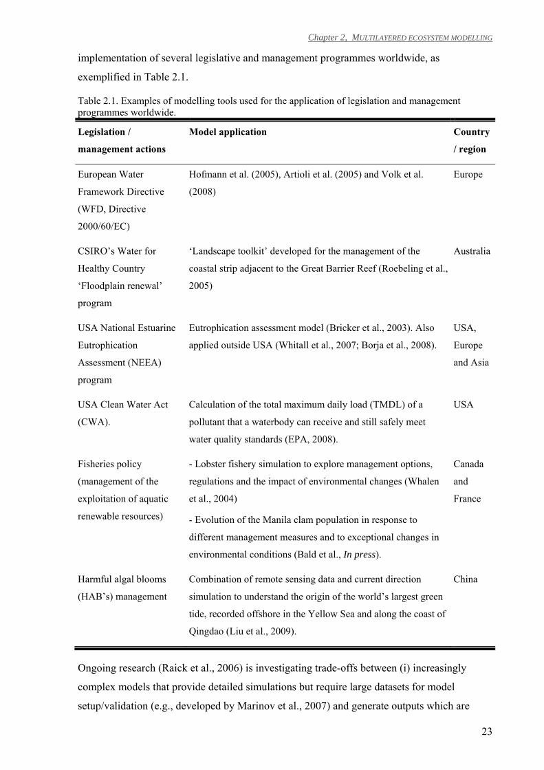
Chapter 2, MULTILAYERED ECOSYSTEM MODELLING
23
implementation of several legislative and management programmes worldwide, as
exemplified in Table 2.1.
Table 2.1. Examples of modelling tools used for the application of legislation and management programmes worldwide.
Legislation /
management actions
Model application Country
/ region
European Water
Framework Directive
(WFD, Directive
2000/60/EC)
Hofmann et al. (2005), Artioli et al. (2005) and Volk et al.
(2008)
Europe
CSIRO’s Water for
Healthy Country
‘Floodplain renewal’
program
‘Landscape toolkit’ developed for the management of the
coastal strip adjacent to the Great Barrier Reef (Roebeling et al.,
2005)
Australia
USA National Estuarine
Eutrophication
Assessment (NEEA)
program
Eutrophication assessment model (Bricker et al., 2003). Also
applied outside USA (Whitall et al., 2007; Borja et al., 2008).
USA,
Europe
and Asia
USA Clean Water Act
(CWA).
Calculation of the total maximum daily load (TMDL) of a
pollutant that a waterbody can receive and still safely meet
water quality standards (EPA, 2008).
USA
Fisheries policy
(management of the
exploitation of aquatic
renewable resources)
- Lobster fishery simulation to explore management options,
regulations and the impact of environmental changes (Whalen
et al., 2004)
- Evolution of the Manila clam population in response to
different management measures and to exceptional changes in
environmental conditions (Bald et al., In press).
Canada
and
France
Harmful algal blooms
(HAB’s) management
Combination of remote sensing data and current direction
simulation to understand the origin of the world’s largest green
tide, recorded offshore in the Yellow Sea and along the coast of
Qingdao (Liu et al., 2009).
China
Ongoing research (Raick et al., 2006) is investigating trade-offs between (i) increasingly
complex models that provide detailed simulations but require large datasets for model
setup/validation (e.g., developed by Marinov et al., 2007) and generate outputs which are
Chapter 2, MULTILAYERED ECOSYSTEM MODELLING
24
difficult to synthesise and interpret; and (ii) simple models that due to generalisation of
processes or resolution may fail to capture important ecosystem features (e.g., McKindsey et
al., 2006). A promising intermediate approach, whereby different models running at different
scales can be integrated in order to optimise the trade-offs between complex and simple
models, has been developed by Ferreira et al. (2008a, 2008b). Model integration can be
implemented by (i) coupling offline upscaled outputs of detailed hydrodynamic models with
ecological box models (Raillard and Ménesguen, 1994; Nobre et al., 2005; Ferreira et al.,
2008a); or (ii) explicitly integrating models with different time steps, which is particularly
important if there is a need to take into account feedback between the models, as is the case of
ecological-economic simulations (Nobre et al., 2009). The advantages of such an intermediate
approach include: (i) running multi-year ecosystem models without the computational
limitations reported for detailed models (Grant et al., 2008); (ii) fewer data requirements for
model setup (Ferreira et al., 2008a); and (iii) running coarser models at the end of the
modelling chain, that present a higher level of information, which are more suitable to inform
decision-makers (Ferreira et al., 2008a), and may be better suited to provide highly
aggregated information used to drive management-oriented screening models. The main
challenges for model integration include: (i) the model coupling can be time-consuming,
given that it implies either processing the model outputs according to the format of the
downstream model inputs or understanding the various model architectures for programming
the code for communication between models; (ii) offline coupling does not allow dynamic
feedback between models; and (iii) online coupling forces scientists and managers to interact
towards a common definition of the problem and the identification of the underlying
variables, which often requires a broader understanding of different disciplines. The
development of integrative tools that simulate the catchment and the biogeochemistry of
coastal waters, including cultivated species, is at an early stage, and there are only a few such
simulations of management scenarios at the catchment-coastal scale (e.g., Marinov et al.,
2007; Ferreira et al., 2008b).
In order to contribute to this development, a multilayered catchment-coastal modelling
approach is described below, which optimizes these trade-offs through the use of a
comprehensive set of models operating at different levels of complexity and geographical
scales. China provides an opportunity for an emblematic case study, given that its coastal
areas exhibit rapid economic growth (10% average increase of GDP over 1995-2005), which
is causing conflict among its multiple uses (Cao and Wong, 2007). Furthermore, Chinese
shellfish aquaculture production (including clams, oysters, mussels, scallops, cockles and
arkshells) increased at an average annual rate of about 28% since 1990, and in 2007
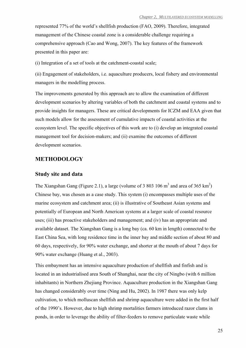
Chapter 2, MULTILAYERED ECOSYSTEM MODELLING
25
represented 77% of the world’s shellfish production (FAO, 2009). Therefore, integrated
management of the Chinese coastal zone is a considerable challenge requiring a
comprehensive approach (Cao and Wong, 2007). The key features of the framework
presented in this paper are:
(i) Integration of a set of tools at the catchment-coastal scale;
(ii) Engagement of stakeholders, i.e. aquaculture producers, local fishery and environmental
managers in the modelling process.
The improvements generated by this approach are to allow the examination of different
development scenarios by altering variables of both the catchment and coastal systems and to
provide insights for managers. These are critical developments for ICZM and EAA given that
such models allow for the assessment of cumulative impacts of coastal activities at the
ecosystem level. The specific objectives of this work are to (i) develop an integrated coastal
management tool for decision-makers; and (ii) examine the outcomes of different
development scenarios.
METHODOLOGY
Study site and data
The Xiangshan Gang (Figure 2.1), a large (volume of 3 803 106 m3 and area of 365 km2)
Chinese bay, was chosen as a case study. This system (i) encompasses multiple uses of the
marine ecosystem and catchment area; (ii) is illustrative of Southeast Asian systems and
potentially of European and North American systems at a larger scale of coastal resource
uses; (iii) has proactive stakeholders and management; and (iv) has an appropriate and
available dataset. The Xiangshan Gang is a long bay (ca. 60 km in length) connected to the
East China Sea, with long residence time in the inner bay and middle section of about 80 and
60 days, respectively, for 90% water exchange, and shorter at the mouth of about 7 days for
90% water exchange (Huang et al., 2003).
This embayment has an intensive aquaculture production of shellfish and finfish and is
located in an industrialised area South of Shanghai, near the city of Ningbo (with 6 million
inhabitants) in Northern Zhejiang Province. Aquaculture production in the Xiangshan Gang
has changed considerably over time (Ning and Hu, 2002). In 1987 there was only kelp
cultivation, to which molluscan shellfish and shrimp aquaculture were added in the first half
of the 1990’s. However, due to high shrimp mortalities farmers introduced razor clams in
ponds, in order to leverage the ability of filter-feeders to remove particulate waste while
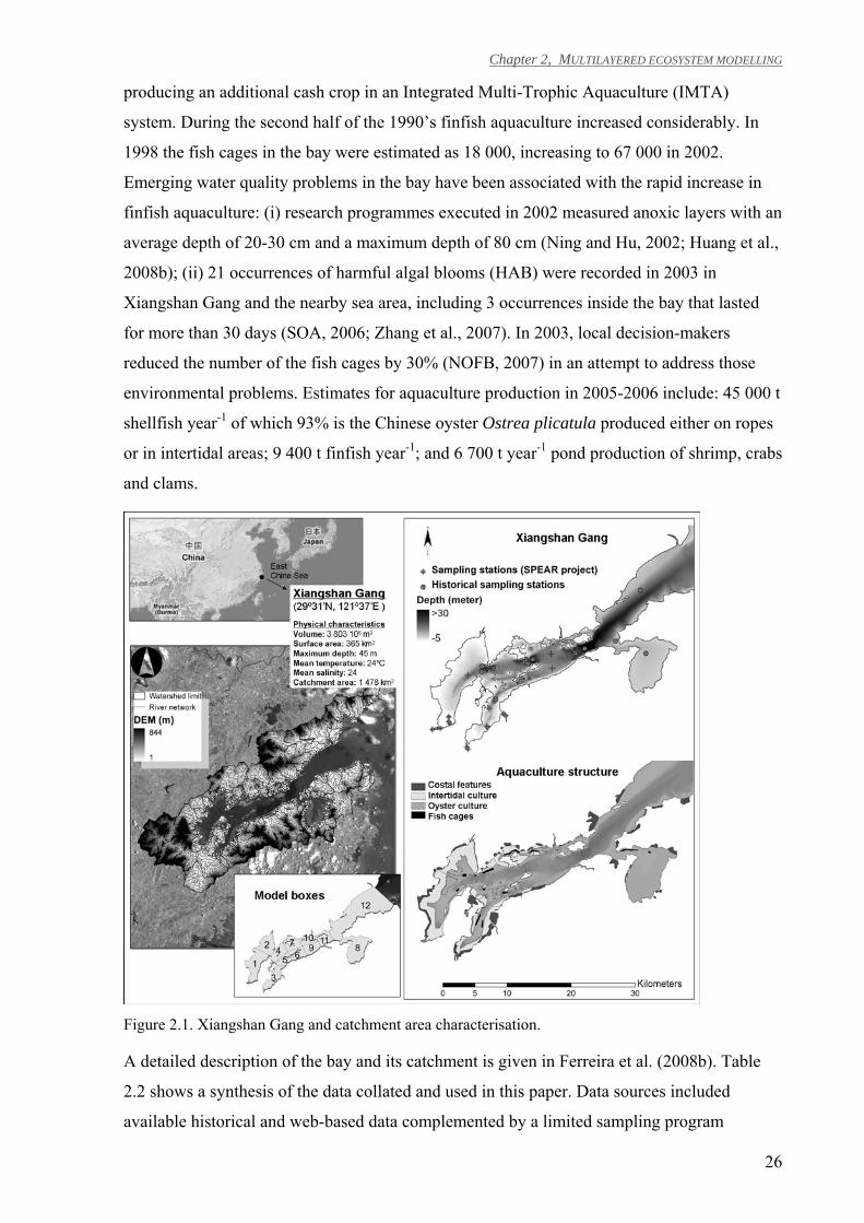
Chapter 2, MULTILAYERED ECOSYSTEM MODELLING
26
producing an additional cash crop in an Integrated Multi-Trophic Aquaculture (IMTA)
system. During the second half of the 1990’s finfish aquaculture increased considerably. In
1998 the fish cages in the bay were estimated as 18 000, increasing to 67 000 in 2002.
Emerging water quality problems in the bay have been associated with the rapid increase in
finfish aquaculture: (i) research programmes executed in 2002 measured anoxic layers with an
average depth of 20-30 cm and a maximum depth of 80 cm (Ning and Hu, 2002; Huang et al.,
2008b); (ii) 21 occurrences of harmful algal blooms (HAB) were recorded in 2003 in
Xiangshan Gang and the nearby sea area, including 3 occurrences inside the bay that lasted
for more than 30 days (SOA, 2006; Zhang et al., 2007). In 2003, local decision-makers
reduced the number of the fish cages by 30% (NOFB, 2007) in an attempt to address those
environmental problems. Estimates for aquaculture production in 2005-2006 include: 45 000 t
shellfish year-1 of which 93% is the Chinese oyster Ostrea plicatula produced either on ropes
or in intertidal areas; 9 400 t finfish year-1; and 6 700 t year-1 pond production of shrimp, crabs
and clams.
Figure 2.1. Xiangshan Gang and catchment area characterisation.
A detailed description of the bay and its catchment is given in Ferreira et al. (2008b). Table
2.2 shows a synthesis of the data collated and used in this paper. Data sources included
available historical and web-based data complemented by a limited sampling program
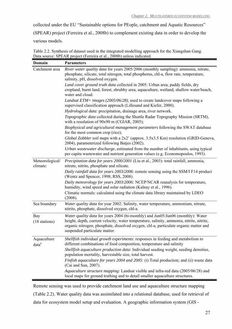
Chapter 2, MULTILAYERED ECOSYSTEM MODELLING
27
collected under the EU “Sustainable options for PEople, catchment and Aquatic Resources”
(SPEAR) project (Ferreira et al., 2008b) to complement existing data in order to develop the
various models.
Table 2.2. Synthesis of dataset used in the integrated modelling approach for the Xiangshan Gang. Data source: SPEAR project (Ferreira et al., 2008b) unless indicated. Domain Parameters Catchment area River water quality data for years 2005/2006 (monthly sampling): ammonia, nitrate,
phosphate, silicate, total nitrogen, total phosphorus, chl-a, flow rate, temperature, salinity, pH, dissolved oxygen.
Land cover ground truth data collected in 2005: Urban area, paddy fields, dry cropland, burnt land, forest, shrubby area, aquaculture, wetland, shallow water/beach, water and cloud.
Landsat ETM+ images (2005/06/28), used to create landcover maps following a supervised classification approach (Lillesand and Kiefer, 2000).
Hydrological data: precipitation, drainage area, river network. Topographic data collected during the Shuttle Radar Topography Mission (SRTM),
with a resolution of 90x90 m (CGIAR, 2005); Biophysical and agricultural management parameters following the SWAT database
for the most common crop (rice); Global Zobbler soil maps with a 2x2’ (approx. 3.5x3.5 Km) resolution (GRID-Geneva,
2004), parameterized following Batjes (2002). Urban wastewater discharge, estimated from the number of inhabitants, using typical
per capita wastewater and nutrient generation values (e.g. Economopoulos, 1993).
Meteorological/ climate:
Precipitation data for years 2000/2001 (Liu et al., 2003): total rainfall, ammonia, nitrate, nitrite, phosphate and silicate. Daily rainfall data for years 2003/2006: remote sensing using the SSM/I F14 product (Wentz and Spencer, 1998; RSS, 2008). Daily meteorology for years 2003/2006: NCEP/NCAR reanalysis for temperature, humidity, wind speed and solar radiation (Kalnay et al., 1996). Climatic normals: calculated using the climate data library maintained by LDEO (2008).
Sea boundary Water quality data for year 2002: Salinity, water temperature, ammonium, nitrate, nitrite, phosphate, dissolved oxygen, chl-a.
Bay (18 stations)
Water quality data for years 2004 (bi-monthly) and Jun05/Jun06 (monthly): Water height, depth, current velocity, water temperature, salinity, ammonia, nitrite, nitrite, organic nitrogen, phosphate, dissolved oxygen, chl-a, particulate organic matter and suspended particulate matter.
Aquaculture dataa
Shellfish individual growth experiments: responses in feeding and metabolism to different combinations of food composition, temperature and salinity Shellfish aquaculture production data: Individual seeding weight, seeding densities, population mortality, harvestable size, total harvest. Finfish aquaculture for years 2004 and 2005: (i) Total production; and (ii) waste data (Cai and Sun, 2007). Aquaculture structure mapping: Landsat visible and infra-red data (2005/06/28) and local maps for ground truthing and to detail smaller aquaculture structures.
Remote sensing was used to provide catchment land use and aquaculture structure mapping
(Table 2.2). Water quality data was assimilated into a relational database, used for retrieval of
data for ecosystem model setup and evaluation. A geographic information system (GIS -
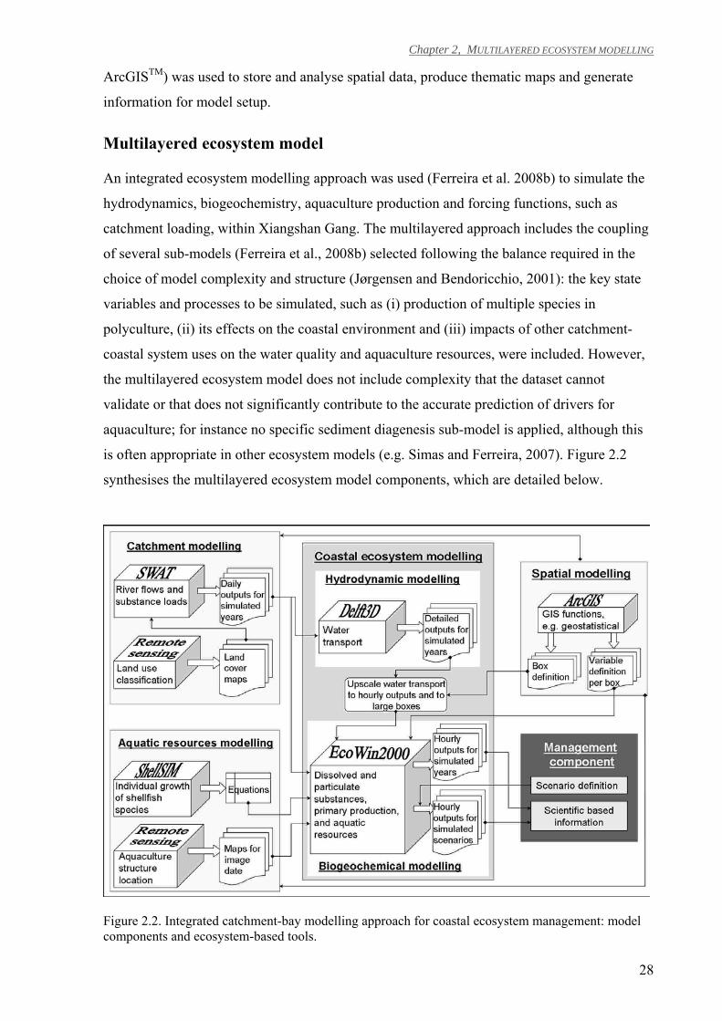
Chapter 2, MULTILAYERED ECOSYSTEM MODELLING
28
ArcGISTM) was used to store and analyse spatial data, produce thematic maps and generate
information for model setup.
Multilayered ecosystem model
An integrated ecosystem modelling approach was used (Ferreira et al. 2008b) to simulate the
hydrodynamics, biogeochemistry, aquaculture production and forcing functions, such as
catchment loading, within Xiangshan Gang. The multilayered approach includes the coupling
of several sub-models (Ferreira et al., 2008b) selected following the balance required in the
choice of model complexity and structure (Jørgensen and Bendoricchio, 2001): the key state
variables and processes to be simulated, such as (i) production of multiple species in
polyculture, (ii) its effects on the coastal environment and (iii) impacts of other catchment-
coastal system uses on the water quality and aquaculture resources, were included. However,
the multilayered ecosystem model does not include complexity that the dataset cannot
validate or that does not significantly contribute to the accurate prediction of drivers for
aquaculture; for instance no specific sediment diagenesis sub-model is applied, although this
is often appropriate in other ecosystem models (e.g. Simas and Ferreira, 2007). Figure 2.2
synthesises the multilayered ecosystem model components, which are detailed below.
Figure 2.2. Integrated catchment-bay modelling approach for coastal ecosystem management: model components and ecosystem-based tools.
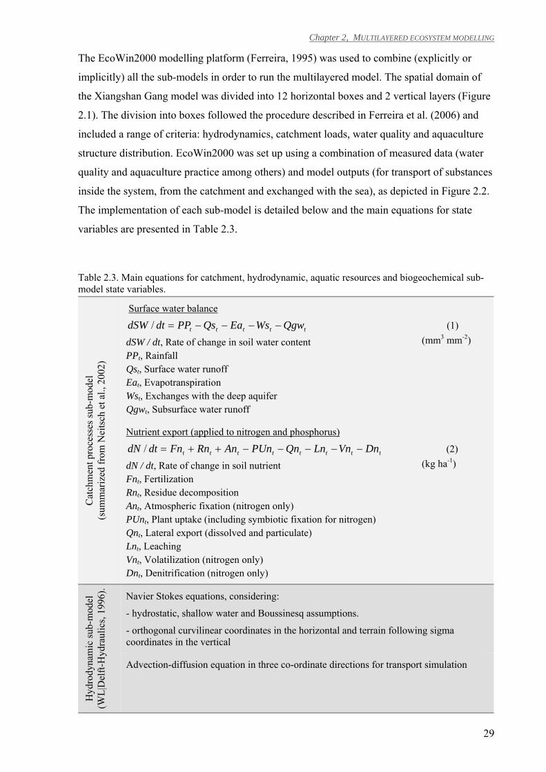
Chapter 2, MULTILAYERED ECOSYSTEM MODELLING
29
The EcoWin2000 modelling platform (Ferreira, 1995) was used to combine (explicitly or
implicitly) all the sub-models in order to run the multilayered model. The spatial domain of
the Xiangshan Gang model was divided into 12 horizontal boxes and 2 vertical layers (Figure
2.1). The division into boxes followed the procedure described in Ferreira et al. (2006) and
included a range of criteria: hydrodynamics, catchment loads, water quality and aquaculture
structure distribution. EcoWin2000 was set up using a combination of measured data (water
quality and aquaculture practice among others) and model outputs (for transport of substances
inside the system, from the catchment and exchanged with the sea), as depicted in Figure 2.2.
The implementation of each sub-model is detailed below and the main equations for state
variables are presented in Table 2.3.
Table 2.3. Main equations for catchment, hydrodynamic, aquatic resources and biogeochemical sub-model state variables.
Cat
chm
ent p
roce
sses
sub-
mod
el
(sum
mar
ized
from
Nei
tsch
et a
l., 2
002)
Surface water balance
ttttt QgwWsEaQsPPdtdSW −−−−=/ (1)
dSW / dt, Rate of change in soil water content PPt, Rainfall Qst, Surface water runoff Eat, Evapotranspiration Wst, Exchanges with the deep aquifer Qgwt, Subsurface water runoff
(mm3 mm-2)
Nutrient export (applied to nitrogen and phosphorus)
tttttttt DnVnLnQnPUnAnRnFndtdN −−−−−++=/ (2)
dN / dt, Rate of change in soil nutrient Fnt, Fertilization Rnt, Residue decomposition Ant, Atmospheric fixation (nitrogen only) PUnt, Plant uptake (including symbiotic fixation for nitrogen) Qnt, Lateral export (dissolved and particulate) Lnt, Leaching Vnt, Volatilization (nitrogen only) Dnt, Denitrification (nitrogen only)
(kg ha-1)
Hyd
rody
nam
ic su
b-m
odel
(W
L|D
elft-
Hyd
raul
ics,
1996
). Navier Stokes equations, considering:
- hydrostatic, shallow water and Boussinesq assumptions.
- orthogonal curvilinear coordinates in the horizontal and terrain following sigma coordinates in the vertical
Advection-diffusion equation in three co-ordinate directions for transport simulation
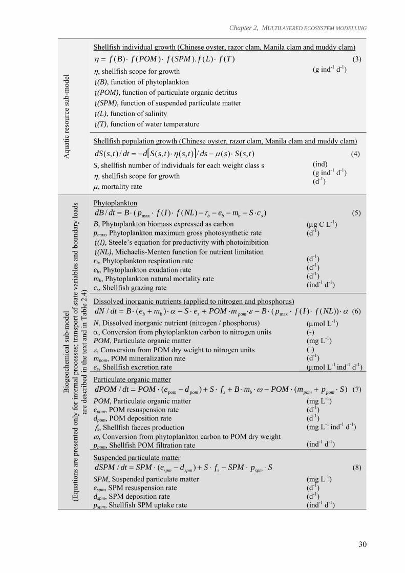
Chapter 2, MULTILAYERED ECOSYSTEM MODELLING
30
Aqu
atic
reso
urce
sub-
mod
el
Shellfish individual growth (Chinese oyster, razor clam, Manila clam and muddy clam) )()().()()( TfLfSPMfPOMfBf ⋅⋅⋅=η (3)
η, shellfish scope for growth ƒ(B), function of phytoplankton ƒ(POM), function of particulate organic detritus ƒ(SPM), function of suspended particulate matter ƒ(L), function of salinity ƒ(T), function of water temperature
(g ind-1 d-1)
Shellfish population growth (Chinese oyster, razor clam, Manila clam and muddy clam)
[ ] ),()(/),(),(/),( tsSsdststsSddttsdS ⋅−⋅−= µη (4) S, shellfish number of individuals for each weight class s η, shellfish scope for growth µ, mortality rate
(ind) (g ind-1 d-1) (d-1)
Bio
geoc
hem
ical
sub-
mod
el
(Equ
atio
ns a
re p
rese
nted
onl
y fo
r int
erna
l pro
cess
es; t
rans
port
of st
ate
varia
bles
and
bou
ndar
y lo
ads
are
desc
ribed
in th
e te
xt a
nd in
Tab
le 2
.4)
Phytoplankton ))()((/ max sbbb cSmerNLfIfpBdtdB ⋅−−−−⋅⋅⋅= (5)
B, Phytoplankton biomass expressed as carbon pmax, Phytoplankton maximum gross photosynthetic rate ƒ(I), Steele’s equation for productivity with photoinibition ƒ(NL), Michaelis-Menten function for nutrient limitation rb, Phytoplankton respiration rate eb, Phytoplankton exudation rate mb, Phytoplankton natural mortality rate cs, Shellfish grazing rate
(µg C L-1) (d-1) (d-1) (d-1) (d-1) (ind-1 d-1)
Dissolved inorganic nutrients (applied to nitrogen and phosphorus) αεα ⋅⋅⋅⋅−⋅⋅+⋅+⋅+⋅= ))()(()(/ max NLfIfpBmPOMeSmeBdtdN pomsbb (6)
N, Dissolved inorganic nutrient (nitrogen / phosphorus) α, Conversion from phytoplankton carbon to nitrogen units POM, Particulate organic matter ε, Conversion from POM dry weight to nitrogen units mpom, POM mineralization rate es, Shellfish excretion rate
(µmol L-1)(-)
(mg L-1)
(-) (d-1) (µmol L-1 ind-1 d-1)
Particulate organic matter )()(/ SpmPOMmBfSdePOMdtdPOM pompombspompom ⋅+⋅−⋅⋅+⋅+−⋅= ω (7)
POM, Particulate organic matter epom, POM resuspension rate dpom, POM deposition rate ƒs, Shellfish faeces production ω, Conversion from phytoplankton carbon to POM dry weight ppom, Shellfish POM filtration rate
(mg L-1) (d-1) (d-1) (mg L-1 ind-1 d-1) (ind-1 d-1)
Suspended particulate matter SpSPMfSdeSPMdtdSPM spmsspmspm ⋅⋅−⋅+−⋅= )(/ (8)
SPM, Suspended particulate matter espm, SPM resuspension rate dspm, SPM deposition rate pspm, Shellfish SPM uptake rate
(mg L-1) (d-1) (d-1) (ind-1 d-1)
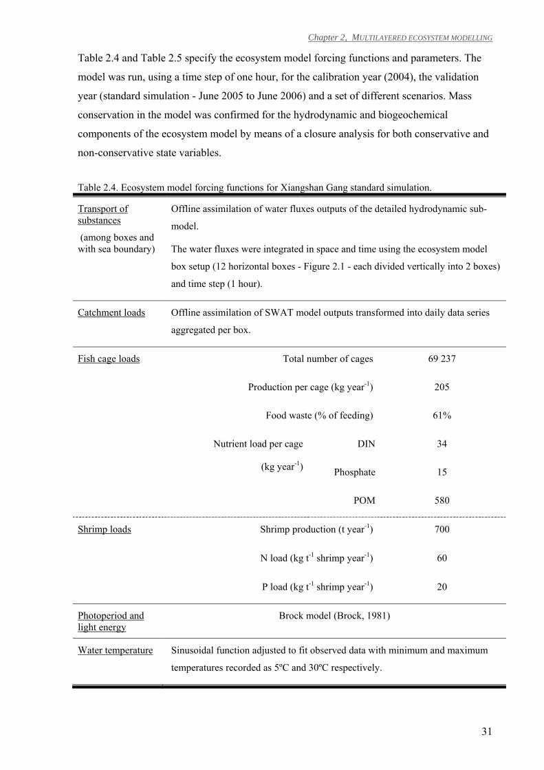
Chapter 2, MULTILAYERED ECOSYSTEM MODELLING
31
Table 2.4 and Table 2.5 specify the ecosystem model forcing functions and parameters. The
model was run, using a time step of one hour, for the calibration year (2004), the validation
year (standard simulation - June 2005 to June 2006) and a set of different scenarios. Mass
conservation in the model was confirmed for the hydrodynamic and biogeochemical
components of the ecosystem model by means of a closure analysis for both conservative and
non-conservative state variables.
Table 2.4. Ecosystem model forcing functions for Xiangshan Gang standard simulation.
Transport of substances
(among boxes and with sea boundary)
Offline assimilation of water fluxes outputs of the detailed hydrodynamic sub-
model.
The water fluxes were integrated in space and time using the ecosystem model
box setup (12 horizontal boxes - Figure 2.1 - each divided vertically into 2 boxes)
and time step (1 hour).
Catchment loads Offline assimilation of SWAT model outputs transformed into daily data series
aggregated per box.
Fish cage loads Total number of cages 69 237
Production per cage (kg year-1) 205
Food waste (% of feeding) 61%
Nutrient load per cage
(kg year-1)
DIN 34
Phosphate 15
POM 580
Shrimp loads Shrimp production (t year-1) 700
N load (kg t-1 shrimp year-1) 60
P load (kg t-1 shrimp year-1) 20
Photoperiod and light energy
Brock model (Brock, 1981)
Water temperature Sinusoidal function adjusted to fit observed data with minimum and maximum
temperatures recorded as 5ºC and 30ºC respectively.
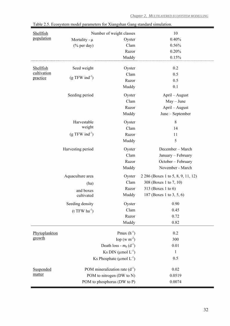
Chapter 2, MULTILAYERED ECOSYSTEM MODELLING
32
Table 2.5. Ecosystem model parameters for Xiangshan Gang standard simulation.
Shellfish population
Number of weight classes 10 Mortality - µ (% per day)
Oyster 0.40% Clam 0.56% Razor 0.20%
Muddy 0.15%
Shellfish cultivation practice
Seed weight
(g TFW ind-1)
Oyster 0.2 Clam 0.5 Razor 0.5
Muddy 0.1
Seeding period Oyster April – August Clam May – June Razor April – August
Muddy June – September
Harvestable weight
(g TFW ind-1)
Oyster 8 Clam 14 Razor 11
Muddy 5
Harvesting period Oyster December – March Clam January – February Razor October – February
Muddy November - March
Aquaculture area
(ha)
and boxes cultivated
Oyster 2 286 (Boxes 1 to 5, 8, 9, 11, 12) Clam 308 (Boxes 1 to 7, 10) Razor 313 (Boxes 1 to 6)
Muddy 187 (Boxes 1 to 3, 5, 6)
Seeding density
(t TFW ha-1)
Oyster 0.90 Clam 0.45 Razor 0.72
Muddy 0.82
Phytoplankton growth
Pmax (h-1) 0.2 Iop (w m-2) 300
Death loss - mb (d-1) 0.01 Ks DIN (µmol L-1) 1
Ks Phosphate (µmol L-1) 0.5
Suspended matter
POM mineralization rate (d-1) 0.02 POM to nitrogen (DW to N) 0.0519
POM to phosphorus (DW to P) 0.0074
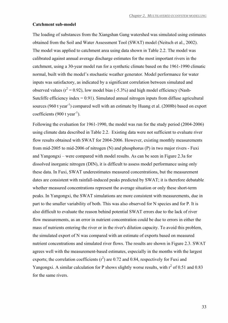
Chapter 2, MULTILAYERED ECOSYSTEM MODELLING
33
Catchment sub-model
The loading of substances from the Xiangshan Gang watershed was simulated using estimates
obtained from the Soil and Water Assessment Tool (SWAT) model (Neitsch et al., 2002).
The model was applied to catchment area using data shown in Table 2.2. The model was
calibrated against annual average discharge estimates for the most important rivers in the
catchment, using a 30-year model run for a synthetic climate based on the 1961-1990 climatic
normal, built with the model’s stochastic weather generator. Model performance for water
inputs was satisfactory, as indicated by a significant correlation between simulated and
observed values (r2 = 0.92), low model bias (-5.3%) and high model efficiency (Nash-
Sutcliffe efficiency index = 0.91). Simulated annual nitrogen inputs from diffuse agricultural
sources (960 t year-1) compared well with an estimate by Huang et al. (2008b) based on export
coefficients (900 t year-1).
Following the evaluation for 1961-1990, the model was run for the study period (2004-2006)
using climate data described in Table 2.2. Existing data were not sufficient to evaluate river
flow results obtained with SWAT for 2004-2006. However, existing monthly measurements
from mid-2005 to mid-2006 of nitrogen (N) and phosphorus (P) in two major rivers - Fuxi
and Yangongxi – were compared with model results. As can be seen in Figure 2.3a for
dissolved inorganic nitrogen (DIN), it is difficult to assess model performance using only
these data. In Fuxi, SWAT underestimates measured concentrations, but the measurement
dates are consistent with rainfall-induced peaks predicted by SWAT; it is therefore debatable
whether measured concentrations represent the average situation or only these short-term
peaks. In Yangongxi, the SWAT simulations are more consistent with measurements, due in
part to the smaller variability of both. This was also observed for N species and for P. It is
also difficult to evaluate the reason behind potential SWAT errors due to the lack of river
flow measurements, as an error in nutrient concentration could be due to errors in either the
mass of nutrients entering the river or in the river's dilution capacity. To avoid this problem,
the simulated export of N was compared with an estimate of exports based on measured
nutrient concentrations and simulated river flows. The results are shown in Figure 2.3. SWAT
agrees well with the measurement-based estimates, especially in the months with the largest
exports; the correlation coefficients (r2) are 0.72 and 0.84, respectively for Fuxi and
Yangongxi. A similar calculation for P shows slightly worse results, with r2 of 0.51 and 0.83
for the same rivers.
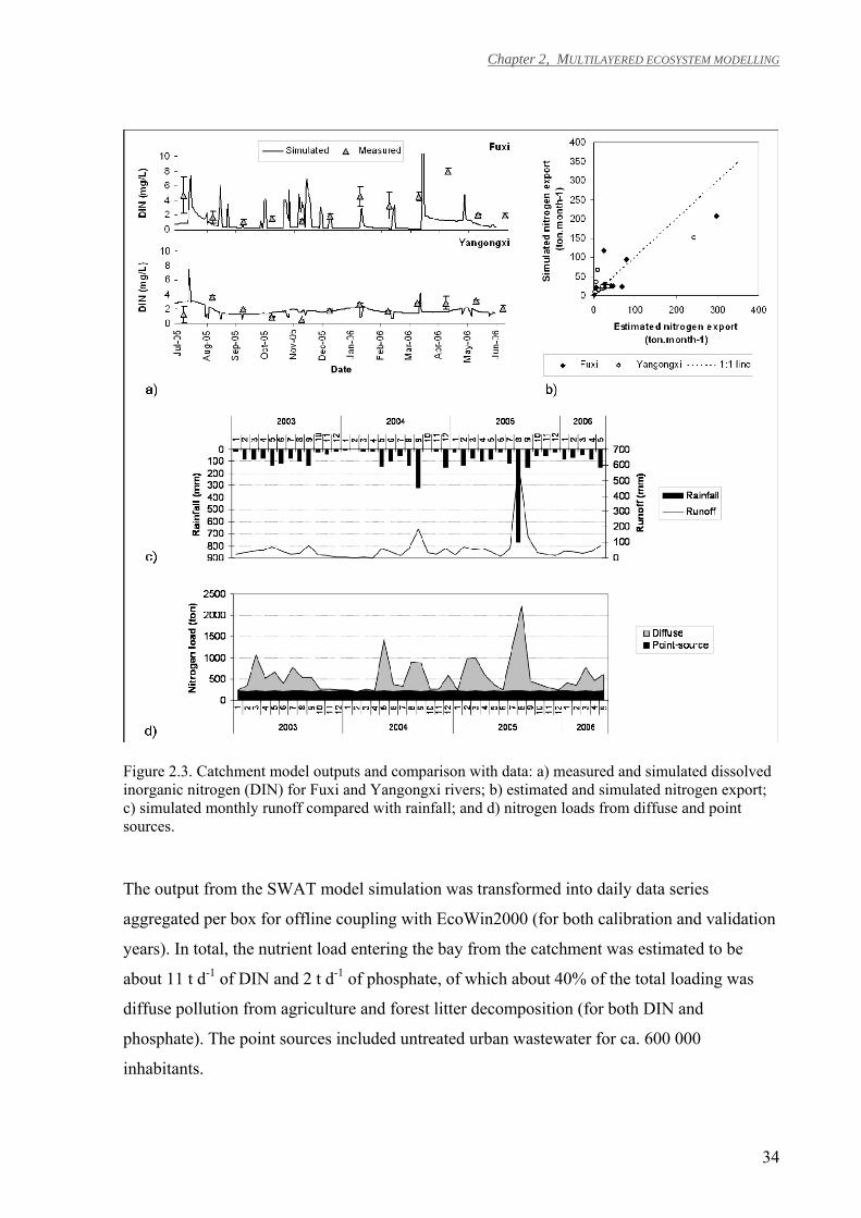
Chapter 2, MULTILAYERED ECOSYSTEM MODELLING
34
Figure 2.3. Catchment model outputs and comparison with data: a) measured and simulated dissolved inorganic nitrogen (DIN) for Fuxi and Yangongxi rivers; b) estimated and simulated nitrogen export; c) simulated monthly runoff compared with rainfall; and d) nitrogen loads from diffuse and point sources.
The output from the SWAT model simulation was transformed into daily data series
aggregated per box for offline coupling with EcoWin2000 (for both calibration and validation
years). In total, the nutrient load entering the bay from the catchment was estimated to be
about 11 t d-1 of DIN and 2 t d-1 of phosphate, of which about 40% of the total loading was
diffuse pollution from agriculture and forest litter decomposition (for both DIN and
phosphate). The point sources included untreated urban wastewater for ca. 600 000
inhabitants.
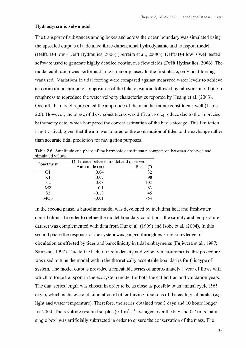
Chapter 2, MULTILAYERED ECOSYSTEM MODELLING
35
Hydrodynamic sub-model
The transport of substances among boxes and across the ocean boundary was simulated using
the upscaled outputs of a detailed three-dimensional hydrodynamic and transport model
(Delft3D-Flow - Delft Hydraulics, 2006) (Ferreira et al., 2008b). Delft3D-Flow is well tested
software used to generate highly detailed continuous flow fields (Delft Hydraulics, 2006). The
model calibration was performed in two major phases. In the first phase, only tidal forcing
was used. Variations in tidal forcing were compared against measured water levels to achieve
an optimum in harmonic composition of the tidal elevation, followed by adjustment of bottom
roughness to reproduce the water velocity characteristics reported by Huang et al. (2003).
Overall, the model represented the amplitude of the main harmonic constituents well (Table
2.6). However, the phase of these constituents was difficult to reproduce due to the imprecise
bathymetry data, which hampered the correct estimation of the bay’s storage. This limitation
is not critical, given that the aim was to predict the contribution of tides to the exchange rather
than accurate tidal prediction for navigation purposes.
Table 2.6. Amplitude and phase of the harmonic constituents: comparison between observed and simulated values.
Constituent Difference between model and observed Amplitude (m) Phase (º)
O1 0.04 32K1 0.07 -90N2 0.03 103M2 0.1 -83S2 -0.13 45
MO3 -0.01 -54
In the second phase, a baroclinic model was developed by including heat and freshwater
contributions. In order to define the model boundary conditions, the salinity and temperature
dataset was complemented with data from Hur et al. (1999) and Isobe et al. (2004). In this
second phase the response of the system was gauged through existing knowledge of
circulation as effected by tides and baroclinicity in tidal embayments (Fujiwara et al., 1997;
Simpson, 1997). Due to the lack of in situ density and velocity measurements, this procedure
was used to tune the model within the theoretically acceptable boundaries for this type of
system. The model outputs provided a repeatable series of approximately 1 year of flows with
which to force transport in the ecosystem model for both the calibration and validation years.
The data series length was chosen in order to be as close as possible to an annual cycle (365
days), which is the cycle of simulation of other forcing functions of the ecological model (e.g.
light and water temperature). Therefore, the series obtained was 3 days and 10 hours longer
for 2004. The resulting residual surplus (0.1 m3 s-1 averaged over the bay and 0.7 m3 s-1 at a
single box) was artificially subtracted in order to ensure the conservation of the mass. The
Chapter 2, MULTILAYERED ECOSYSTEM MODELLING
36
detailed flow fields were scaled up and converted into a data series of water fluxes between
boxes and across the sea boundary with a one hour time step and coupled offline with
EcoWin2000 (see e.g., Ferreira et al., 2008a).
Aquatic resource sub-model
The simulated aquatic resources included Ostrea plicatula (Chinese oyster), Sinonvacula
constricta (razor clam), Tapes philippinarum (Manila clam) and Tegillarca granosa (muddy
clam) production. The equations for shellfish aquaculture production were explicitly
integrated into the ecosystem model using a four step approach (Ferreira et al., 2008a): (i) use
of a shellfish individual growth model (ShellSIM - http://www.shellsim.com); (ii) coupling of
the individual growth model with a demographic model to simulate the population (Ferreira et
al., 1997); (iii) integration of the population growth model with an aquaculture practice model
which implements the seeding of the population biomass and harvesting of the marketable
cohorts for a given production cycle (Ferreira et al., 1997); and (iv) use of a multiple-
inheritance object-oriented approach (Nunes et al., 2003) to extend to multiple species in
polyculture. ShellSIM simulates feeding, metabolism and individual growth in contrasting
environments for different shellfish species, as exemplified for Chlamys farreri by Hawkins
et al. (2002). In the ShellSIM model, removal of particulate organic matter (phytoplankton
and detritus) by shellfish is determined through the individual growth models for the bivalves.
It is a function of several environmental drivers, including salinity, temperature, suspended
particulate matter (SPM) and the food sources themselves, and is additionally driven by
allometry. These drivers are used to determine filtration, pre-ingestive selection, ingestion and
assimilation. The individual growth model was calibrated for Chinese oyster, razor clam and
muddy clam under local conditions (Ferreira et al., 2008b). As shown in Table 2.7 there is a
statistically significant relationship between the individual model results and observations for
shellfish wet weight and shell length. For the simulation of the Manila clam individual
growth, the model used in Ferreira et al. (2007a) was applied. The population growth is
simulated using a demographic model based on ten weight classes. The demographic model is
a widely used model (Ferreira et al., 1997; Nunes et al., 2003; Nobre et al., 2005; Ferreira et
al., 2007a) based on a conservation equation (Eq. 4, Table 2.3) discretised in weight classes.
The food (phytoplankton and detritus) removed by the population is scaled for each weight
class on the basis of the number of individuals in the class; compliance with the Courant
condition is ensured, such that, in the case of numerical instability, the food supply (and
therefore the growth potential) is reduced by adjusting the filtration rate. Changes in the
population structure derive from the simulation of the individual growth of one animal (Eq. 3,
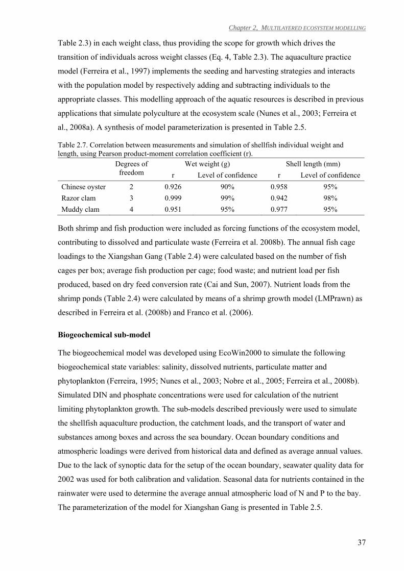
Chapter 2, MULTILAYERED ECOSYSTEM MODELLING
37
Table 2.3) in each weight class, thus providing the scope for growth which drives the
transition of individuals across weight classes (Eq. 4, Table 2.3). The aquaculture practice
model (Ferreira et al., 1997) implements the seeding and harvesting strategies and interacts
with the population model by respectively adding and subtracting individuals to the
appropriate classes. This modelling approach of the aquatic resources is described in previous
applications that simulate polyculture at the ecosystem scale (Nunes et al., 2003; Ferreira et
al., 2008a). A synthesis of model parameterization is presented in Table 2.5.
Table 2.7. Correlation between measurements and simulation of shellfish individual weight and length, using Pearson product-moment correlation coefficient (r).
Degrees of freedom
Wet weight (g) Shell length (mm) r Level of confidence r Level of confidence
Chinese oyster 2 0.926 90% 0.958 95% Razor clam 3 0.999 99% 0.942 98% Muddy clam 4 0.951 95% 0.977 95%
Both shrimp and fish production were included as forcing functions of the ecosystem model,
contributing to dissolved and particulate waste (Ferreira et al. 2008b). The annual fish cage
loadings to the Xiangshan Gang (Table 2.4) were calculated based on the number of fish
cages per box; average fish production per cage; food waste; and nutrient load per fish
produced, based on dry feed conversion rate (Cai and Sun, 2007). Nutrient loads from the
shrimp ponds (Table 2.4) were calculated by means of a shrimp growth model (LMPrawn) as
described in Ferreira et al. (2008b) and Franco et al. (2006).
Biogeochemical sub-model
The biogeochemical model was developed using EcoWin2000 to simulate the following
biogeochemical state variables: salinity, dissolved nutrients, particulate matter and
phytoplankton (Ferreira, 1995; Nunes et al., 2003; Nobre et al., 2005; Ferreira et al., 2008b).
Simulated DIN and phosphate concentrations were used for calculation of the nutrient
limiting phytoplankton growth. The sub-models described previously were used to simulate
the shellfish aquaculture production, the catchment loads, and the transport of water and
substances among boxes and across the sea boundary. Ocean boundary conditions and
atmospheric loadings were derived from historical data and defined as average annual values.
Due to the lack of synoptic data for the setup of the ocean boundary, seawater quality data for
2002 was used for both calibration and validation. Seasonal data for nutrients contained in the
rainwater were used to determine the average annual atmospheric load of N and P to the bay.
The parameterization of the model for Xiangshan Gang is presented in Table 2.5.
Chapter 2, MULTILAYERED ECOSYSTEM MODELLING
38
The pelagic variables in the model were calibrated against a historical time series for 2004
(Table 2.2). Due to lack of historical data, the annual average of the validation year was used
for SPM and particulate organic matter (POM). The model was run for the validation year
using the same parameters employed for the calibration year but adjusting the data series for
forcing functions and the initial conditions to simulate the period from June 2005 to June
2006. Model performance was evaluated by comparing the model outputs of the standard
simulation with the water quality and aquaculture production data for the validation period.
Coastal management options simulation
Definition of scenarios
The development scenarios were defined as a result of the participatory work among
stakeholders carried out during the SPEAR project (Ferreira et al., 2008b). Several
stakeholder meetings were held involving modellers, local fishery and environmental
managers and aquaculture producers. The capabilities of the modelling tools to support
catchment and aquaculture management were explained to the local managers and producers.
In addition, the issues of concern to the local managers and producers were discussed with the
modelling team. The participatory work among stakeholders culminated with a clear set of
scenarios defined by the Xiangshan Gang managers and aquaculture producers. The scenarios
to be simulated by the multilayered ecosystem modelling framework comprise: (i) a reduction
of fish cages corresponding to a 38% reduction in total fish production (Scenario 1); (ii) an
extension of wastewater treatment to the entire population (Scenario 2); and (iii) a
simultaneous reduction of fish cages and extended wastewater treatment (Scenario 3). These
scenarios are important for the evaluation of nutrient abatement strategies defined by
managers to improve water quality in Xiangshan Gang. From a management perspective, the
scientific assessment of such scenarios also provides guidelines/grounding for future
aquaculture policy and for eutrophication control.
Using SWAT model outputs with different timesteps an additional scenario was run to test the
consequences of different temporal resolution of forcing functions on simulated results.
Monitoring of substance loadings from the adjacent catchment area are often used as forcing
for coastal ecosystem models. However, this is often restricted to a few locations within the
watershed and to a few sampling occasions over the year. In this work the use of SWAT
model enabled the application of detailed forcing in space and time for catchment loads and to
test the sensitivity analysis of the coastal ecosystem to the temporal resolution of the
catchment model outputs. The scenario includes running the standard simulation using
Chapter 2, MULTILAYERED ECOSYSTEM MODELLING
39
monthly, rather than of daily, data series of the SWAT model outputs. This scenario
exemplifies how the multilayered ecosystem model can be used in the future to further
explore a larger research issue about monitoring data requirements and optimal temporal
resolutions to use in the models.
Development scenario implementation and interpretation
The reduction of fish cages (scenarios 1 and 3) was implemented assuming that the decrease
in nutrient loading is proportional to the decrease in fish production. The impact of
wastewater treatment (scenarios 2 and 3) on the exports of N, P and sediment from urban
areas was calculated following Burks and Minnis (1994). Table 2.8 synthesises the
corresponding substance loading used to simulate each scenario.
A comparison of the results obtained for the different scenarios was performed and the
interpretation of the outcomes was guided by means of:
(i) Influencing Factors (IF) from the ASSETS eutrophication model (Bricker et al., 2003) to
interpret the influence of catchment and aquaculture loads on eutrophication; The IF index
calculates the pressure on the system as a combination of the nutrient loading with the system
susceptibility to eutrophication (flushing and dilution factors) (Bricker at al., 2008). Bricker et
al. (2003, 2008) calculates the relative magnitude of the different sources considering inputs
from watershed (manageable anthropogenic sources) and ocean (background sources)
boundaries. For the IF application to Xiangshan Gang, aquaculture and watershed are together
considered manageable anthropogenic sources. Details on the IF calculation are provided by
Bricker et al. (2003) and a computer application is freely available online
(http://www.eutro.org/register) to perform the calculations;
(ii) The threshold of chl-a 90-percentile values as defined in the ASSETS model (Bricker et
al. 2003) to assess the level of expression of the phytoplankton symptom;
(iii) Chinese sea water quality standards (National Standard of People’s Republic of China,
1997) for DIN and phosphate to assess the compliance with desirable water quality objectives
set by decision-makers for the bay; and
(iv) Shellfish productivity, given as the ratio of total weight of shellfish harvested to total
weight of seed, also known as average physical product (APP, Jolly and Clonts, 1993), to
interpret the changes in the ecosystem use due to scenario implementation.
Chapter 2, MULTILAYERED ECOSYSTEM MODELLING
40
RESULTS
Ecosystem simulation
Figure 2.3c and Figure 2.3d show catchment model results for runoff and N loading into
Xiangshan Gang, from diffuse (agricultural) and point (urban sewage) sources. N inputs have
two annual peaks, in early spring and early summer, which can be related to both the
fertilisation of rice (which is harvested twice per year in this region) and the annual rainfall
and runoff patterns. This pattern was also found for particulate matter and P loads. The large
input peak in August 2005 is an exceptional occurrence, mostly caused by typhoon Matsa on
August 5th. The major sources for N, according to the model results are urban sewage
discharges (56%); agricultural, namely fertilization in rice crops (27%); and rangelands,
mostly detritus decomposition from forests (17%). P followed a similar pattern, with 60%
coming from urban sewage discharge and the remainder from agricultural and natural sources.
Figure 2.4 shows the results of the coastal ecosystem model for the pelagic variables in an
inner location (Box 3) and a location in the middle of the bay (Box 10), which represents the
outermost box with sampling data. The ecosystem model outputs for DIN and phytoplankton
compare reasonably well with collected data, as exemplified for boxes 3 and 10 in Figure 2.4.
The DIN peak observed around day 120 in Box 3 is not reproduced, possibly due to an
underestimation of the loads for that period (from catchment or from aquaculture) or due to a
local phenomenon that does not represent the average for the box. In contrast, the model
outputs for phytoplankton exhibit peaks not seen in the data. In particular, the sampling point
immediately before day 180 shows a very low value for phytoplankton, whereas the model
simulates high phytoplankton concentrations. A combination of three factors can justify this
occurrence: (i) high natural variability of phytoplankton (Rantajärvi et al., 1998), not captured
by the sampling window; (ii) phytoplankton dynamics are ruled by complex set of factors
difficult to simulate in dynamic ecological models, such as species succession (Arhonditsis et
al., 2007); and (iii) the model outputs represent an uniform value for a box, and thus cannot
account for the variability in that area, given that for most boxes data coverage for validation
includes only one sampling station (Figure 2.1); for box 3 in particular there are 2 stations, the
remaining stations are for rivers or from the historical dataset used for calibration). With
regard to phosphate, the data do not indicate a particular pattern, and in general the model
overestimates observed phosphate concentrations. This might be due to an overestimate of
phosphate loads from either i) fish cages, given that fish aquaculture is the major source of
this nutrient (Table 2.8) together with the fact that an average annual load is considered due to
the lack of temporally detailed data on fish cage loading; or ii) from the catchment, which as
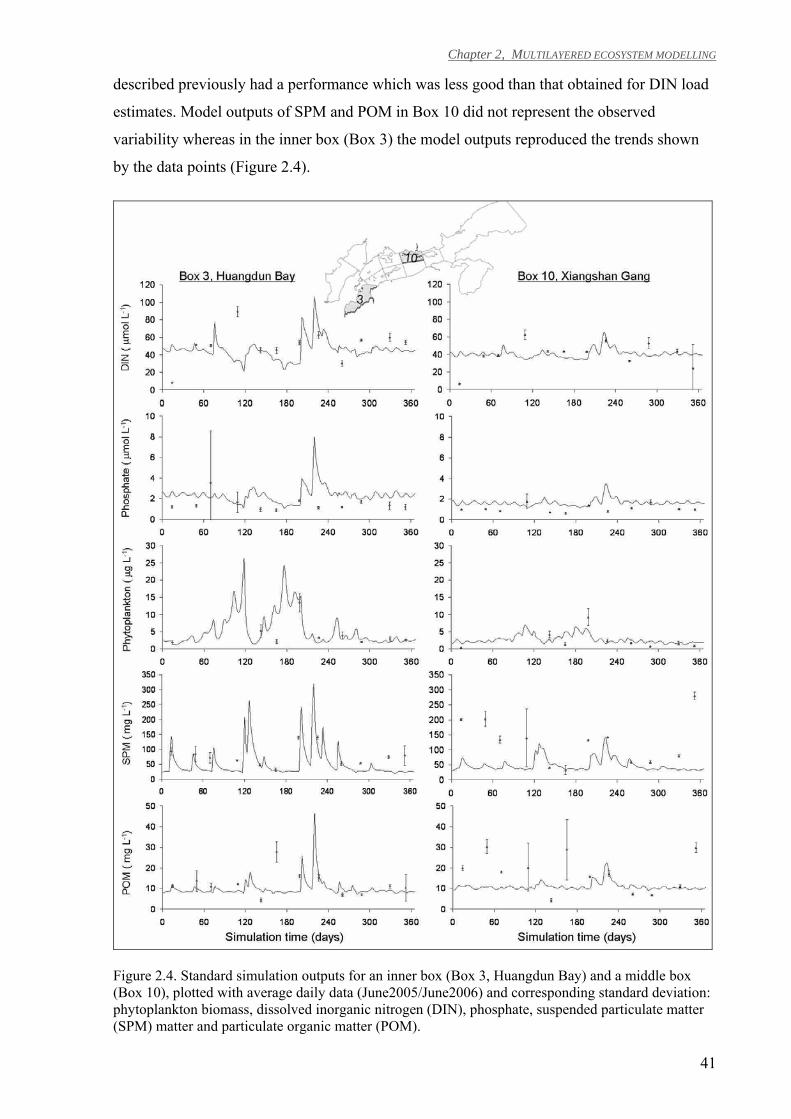
Chapter 2, MULTILAYERED ECOSYSTEM MODELLING
41
described previously had a performance which was less good than that obtained for DIN load
estimates. Model outputs of SPM and POM in Box 10 did not represent the observed
variability whereas in the inner box (Box 3) the model outputs reproduced the trends shown
by the data points (Figure 2.4).
Figure 2.4. Standard simulation outputs for an inner box (Box 3, Huangdun Bay) and a middle box (Box 10), plotted with average daily data (June2005/June2006) and corresponding standard deviation: phytoplankton biomass, dissolved inorganic nitrogen (DIN), phosphate, suspended particulate matter (SPM) matter and particulate organic matter (POM).
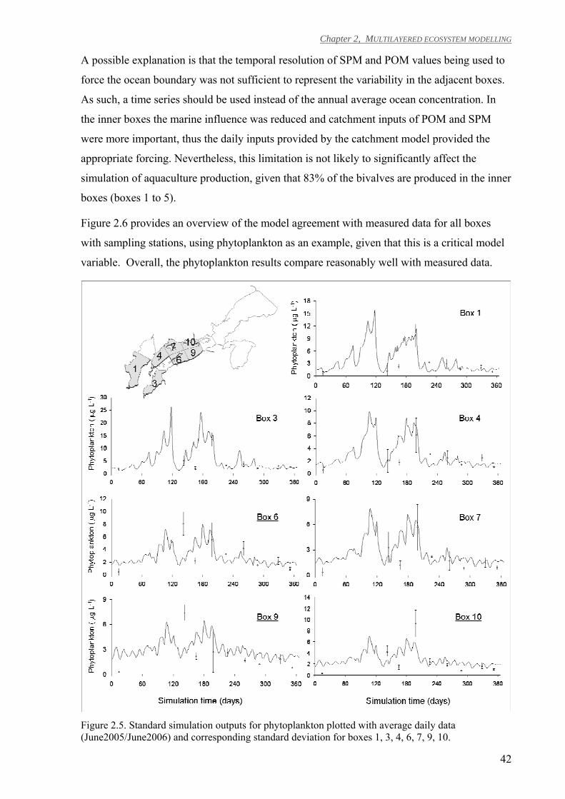
Chapter 2, MULTILAYERED ECOSYSTEM MODELLING
42
A possible explanation is that the temporal resolution of SPM and POM values being used to
force the ocean boundary was not sufficient to represent the variability in the adjacent boxes.
As such, a time series should be used instead of the annual average ocean concentration. In
the inner boxes the marine influence was reduced and catchment inputs of POM and SPM
were more important, thus the daily inputs provided by the catchment model provided the
appropriate forcing. Nevertheless, this limitation is not likely to significantly affect the
simulation of aquaculture production, given that 83% of the bivalves are produced in the inner
boxes (boxes 1 to 5).
Figure 2.6 provides an overview of the model agreement with measured data for all boxes
with sampling stations, using phytoplankton as an example, given that this is a critical model
variable. Overall, the phytoplankton results compare reasonably well with measured data.
Figure 2.5. Standard simulation outputs for phytoplankton plotted with average daily data (June2005/June2006) and corresponding standard deviation for boxes 1, 3, 4, 6, 7, 9, 10.
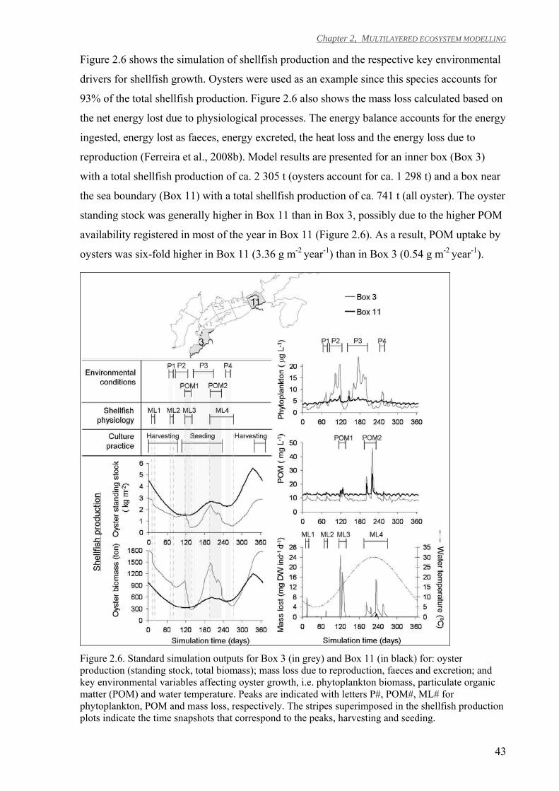
Chapter 2, MULTILAYERED ECOSYSTEM MODELLING
43
Figure 2.6 shows the simulation of shellfish production and the respective key environmental
drivers for shellfish growth. Oysters were used as an example since this species accounts for
93% of the total shellfish production. Figure 2.6 also shows the mass loss calculated based on
the net energy lost due to physiological processes. The energy balance accounts for the energy
ingested, energy lost as faeces, energy excreted, the heat loss and the energy loss due to
reproduction (Ferreira et al., 2008b). Model results are presented for an inner box (Box 3)
with a total shellfish production of ca. 2 305 t (oysters account for ca. 1 298 t) and a box near
the sea boundary (Box 11) with a total shellfish production of ca. 741 t (all oyster). The oyster
standing stock was generally higher in Box 11 than in Box 3, possibly due to the higher POM
availability registered in most of the year in Box 11 (Figure 2.6). As a result, POM uptake by
oysters was six-fold higher in Box 11 (3.36 g m-2 year-1) than in Box 3 (0.54 g m-2 year-1).
Figure 2.6. Standard simulation outputs for Box 3 (in grey) and Box 11 (in black) for: oyster production (standing stock, total biomass); mass loss due to reproduction, faeces and excretion; and key environmental variables affecting oyster growth, i.e. phytoplankton biomass, particulate organic matter (POM) and water temperature. Peaks are indicated with letters P#, POM#, ML# for phytoplankton, POM and mass loss, respectively. The stripes superimposed in the shellfish production plots indicate the time snapshots that correspond to the peaks, harvesting and seeding.
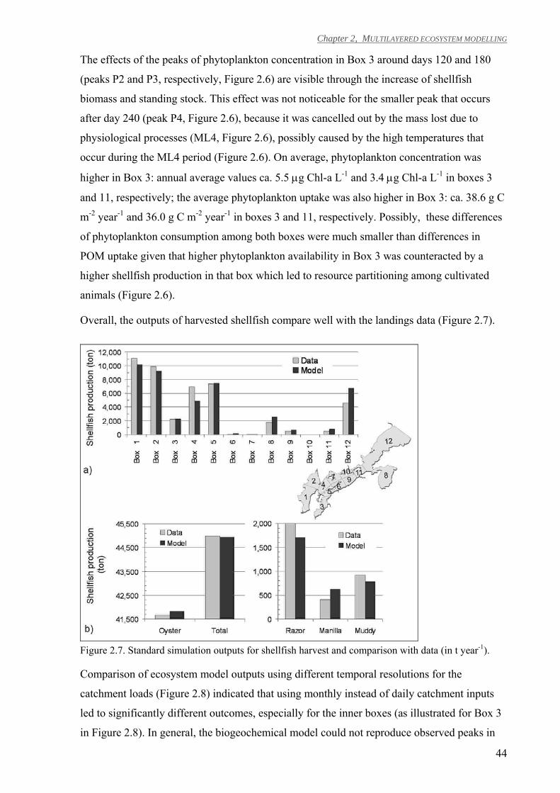
Chapter 2, MULTILAYERED ECOSYSTEM MODELLING
44
The effects of the peaks of phytoplankton concentration in Box 3 around days 120 and 180
(peaks P2 and P3, respectively, Figure 2.6) are visible through the increase of shellfish
biomass and standing stock. This effect was not noticeable for the smaller peak that occurs
after day 240 (peak P4, Figure 2.6), because it was cancelled out by the mass lost due to
physiological processes (ML4, Figure 2.6), possibly caused by the high temperatures that
occur during the ML4 period (Figure 2.6). On average, phytoplankton concentration was
higher in Box 3: annual average values ca. 5.5 µg Chl-a L-1 and 3.4 µg Chl-a L-1 in boxes 3
and 11, respectively; the average phytoplankton uptake was also higher in Box 3: ca. 38.6 g C
m-2 year-1 and 36.0 g C m-2 year-1 in boxes 3 and 11, respectively. Possibly, these differences
of phytoplankton consumption among both boxes were much smaller than differences in
POM uptake given that higher phytoplankton availability in Box 3 was counteracted by a
higher shellfish production in that box which led to resource partitioning among cultivated
animals (Figure 2.6).
Overall, the outputs of harvested shellfish compare well with the landings data (Figure 2.7).
Figure 2.7. Standard simulation outputs for shellfish harvest and comparison with data (in t year-1).
Comparison of ecosystem model outputs using different temporal resolutions for the
catchment loads (Figure 2.8) indicated that using monthly instead of daily catchment inputs
led to significantly different outcomes, especially for the inner boxes (as illustrated for Box 3
in Figure 2.8). In general, the biogeochemical model could not reproduce observed peaks in
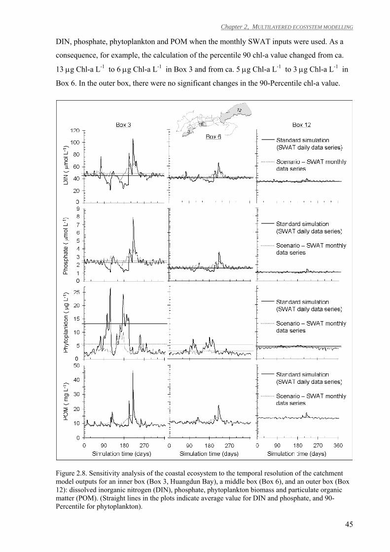
Chapter 2, MULTILAYERED ECOSYSTEM MODELLING
45
DIN, phosphate, phytoplankton and POM when the monthly SWAT inputs were used. As a
consequence, for example, the calculation of the percentile 90 chl-a value changed from ca.
13 µg Chl-a L-1 to 6 µg Chl-a L-1 in Box 3 and from ca. 5 µg Chl-a L-1 to 3 µg Chl-a L-1 in
Box 6. In the outer box, there were no significant changes in the 90-Percentile chl-a value.
Figure 2.8. Sensitivity analysis of the coastal ecosystem to the temporal resolution of the catchment model outputs for an inner box (Box 3, Huangdun Bay), a middle box (Box 6), and an outer box (Box 12): dissolved inorganic nitrogen (DIN), phosphate, phytoplankton biomass and particulate organic matter (POM). (Straight lines in the plots indicate average value for DIN and phosphate, and 90-Percentile for phytoplankton).
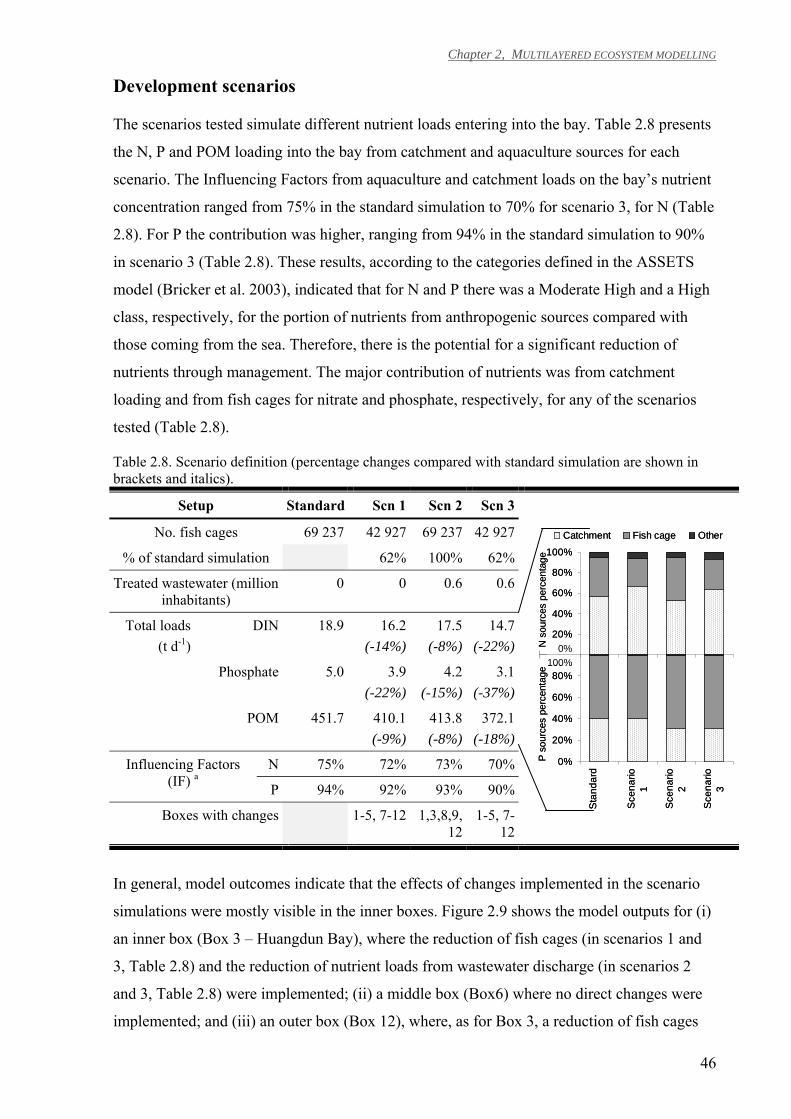
Chapter 2, MULTILAYERED ECOSYSTEM MODELLING
46
Development scenarios
The scenarios tested simulate different nutrient loads entering into the bay. Table 2.8 presents
the N, P and POM loading into the bay from catchment and aquaculture sources for each
scenario. The Influencing Factors from aquaculture and catchment loads on the bay’s nutrient
concentration ranged from 75% in the standard simulation to 70% for scenario 3, for N (Table
2.8). For P the contribution was higher, ranging from 94% in the standard simulation to 90%
in scenario 3 (Table 2.8). These results, according to the categories defined in the ASSETS
model (Bricker et al. 2003), indicated that for N and P there was a Moderate High and a High
class, respectively, for the portion of nutrients from anthropogenic sources compared with
those coming from the sea. Therefore, there is the potential for a significant reduction of
nutrients through management. The major contribution of nutrients was from catchment
loading and from fish cages for nitrate and phosphate, respectively, for any of the scenarios
tested (Table 2.8).
Table 2.8. Scenario definition (percentage changes compared with standard simulation are shown in brackets and italics).
Setup Standard Scn 1 Scn 2 Scn 3
No. fish cages 69 237 42 927 69 237 42 927
% of standard simulation 62% 100% 62%
Treated wastewater (million inhabitants)
0 0 0.6 0.6
Total loads (t d-1)
DIN 18.9 16.2 (-14%)
17.5 (-8%)
14.7 (-22%)
Phosphate 5.0 3.9 (-22%)
4.2 (-15%)
3.1 (-37%)
POM 451.7 410.1 (-9%)
413.8 (-8%)
372.1 (-18%)
Influencing Factors (IF) a
N 75% 72% 73% 70%
P 94% 92% 93% 90%
Boxes with changes 1-5, 7-12 1,3,8,9,12
1-5, 7-12
In general, model outcomes indicate that the effects of changes implemented in the scenario
simulations were mostly visible in the inner boxes. Figure 2.9 shows the model outputs for (i)
an inner box (Box 3 – Huangdun Bay), where the reduction of fish cages (in scenarios 1 and
3, Table 2.8) and the reduction of nutrient loads from wastewater discharge (in scenarios 2
and 3, Table 2.8) were implemented; (ii) a middle box (Box6) where no direct changes were
implemented; and (iii) an outer box (Box 12), where, as for Box 3, a reduction of fish cages
0%
20%
40%
60%
80%
100%
Catchment Fish cage Other
0%
20%
40%
60%
80%
100%
Sta
ndar
d
Sce
nario
1
Sce
nario
2
Sce
nario
3
0%100%
N s
ourc
es p
erce
ntag
eP
sou
rces
per
cent
age
0%
20%
40%
60%
80%
100%
Catchment Fish cage Other
0%
20%
40%
60%
80%
100%
Sta
ndar
d
Sce
nario
1
Sce
nario
2
Sce
nario
3
0%100%
N s
ourc
es p
erce
ntag
eP
sou
rces
per
cent
age
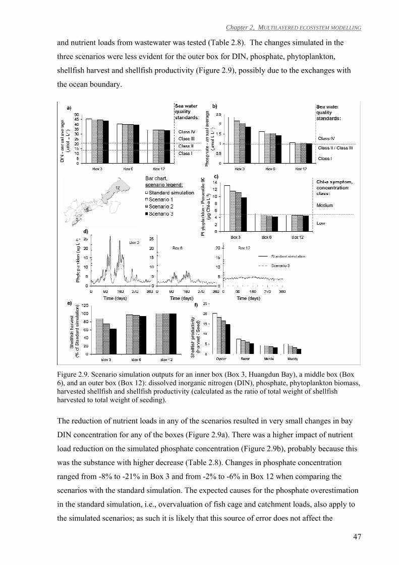
Chapter 2, MULTILAYERED ECOSYSTEM MODELLING
47
and nutrient loads from wastewater was tested (Table 2.8). The changes simulated in the
three scenarios were less evident for the outer box for DIN, phosphate, phytoplankton,
shellfish harvest and shellfish productivity (Figure 2.9), possibly due to the exchanges with
the ocean boundary.
Figure 2.9. Scenario simulation outputs for an inner box (Box 3, Huangdun Bay), a middle box (Box 6), and an outer box (Box 12): dissolved inorganic nitrogen (DIN), phosphate, phytoplankton biomass, harvested shellfish and shellfish productivity (calculated as the ratio of total weight of shellfish harvested to total weight of seeding).
The reduction of nutrient loads in any of the scenarios resulted in very small changes in bay
DIN concentration for any of the boxes (Figure 2.9a). There was a higher impact of nutrient
load reduction on the simulated phosphate concentration (Figure 2.9b), probably because this
was the substance with higher decrease (Table 2.8). Changes in phosphate concentration
ranged from -8% to -21% in Box 3 and from -2% to -6% in Box 12 when comparing the
scenarios with the standard simulation. The expected causes for the phosphate overestimation
in the standard simulation, i.e., overvaluation of fish cage and catchment loads, also apply to
the simulated scenarios; as such it is likely that this source of error does not affect the
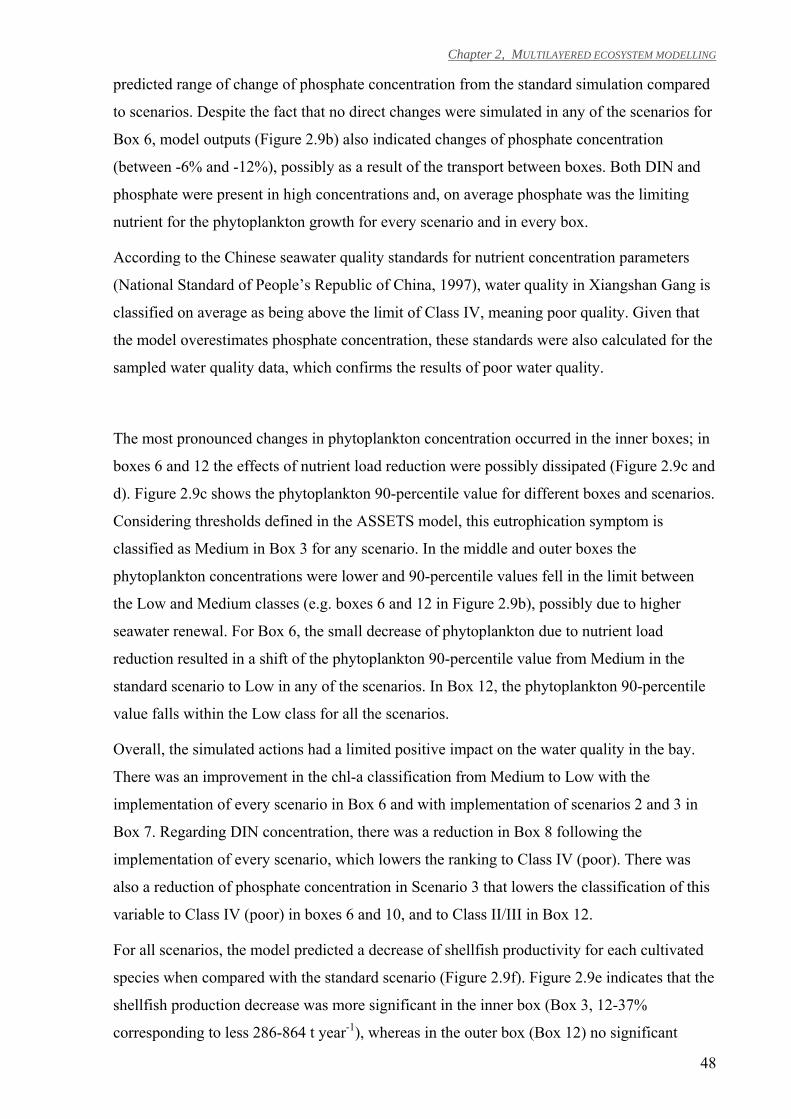
Chapter 2, MULTILAYERED ECOSYSTEM MODELLING
48
predicted range of change of phosphate concentration from the standard simulation compared
to scenarios. Despite the fact that no direct changes were simulated in any of the scenarios for
Box 6, model outputs (Figure 2.9b) also indicated changes of phosphate concentration
(between -6% and -12%), possibly as a result of the transport between boxes. Both DIN and
phosphate were present in high concentrations and, on average phosphate was the limiting
nutrient for the phytoplankton growth for every scenario and in every box.
According to the Chinese seawater quality standards for nutrient concentration parameters
(National Standard of People’s Republic of China, 1997), water quality in Xiangshan Gang is
classified on average as being above the limit of Class IV, meaning poor quality. Given that
the model overestimates phosphate concentration, these standards were also calculated for the
sampled water quality data, which confirms the results of poor water quality.
The most pronounced changes in phytoplankton concentration occurred in the inner boxes; in
boxes 6 and 12 the effects of nutrient load reduction were possibly dissipated (Figure 2.9c and
d). Figure 2.9c shows the phytoplankton 90-percentile value for different boxes and scenarios.
Considering thresholds defined in the ASSETS model, this eutrophication symptom is
classified as Medium in Box 3 for any scenario. In the middle and outer boxes the
phytoplankton concentrations were lower and 90-percentile values fell in the limit between
the Low and Medium classes (e.g. boxes 6 and 12 in Figure 2.9b), possibly due to higher
seawater renewal. For Box 6, the small decrease of phytoplankton due to nutrient load
reduction resulted in a shift of the phytoplankton 90-percentile value from Medium in the
standard scenario to Low in any of the scenarios. In Box 12, the phytoplankton 90-percentile
value falls within the Low class for all the scenarios.
Overall, the simulated actions had a limited positive impact on the water quality in the bay.
There was an improvement in the chl-a classification from Medium to Low with the
implementation of every scenario in Box 6 and with implementation of scenarios 2 and 3 in
Box 7. Regarding DIN concentration, there was a reduction in Box 8 following the
implementation of every scenario, which lowers the ranking to Class IV (poor). There was
also a reduction of phosphate concentration in Scenario 3 that lowers the classification of this
variable to Class IV (poor) in boxes 6 and 10, and to Class II/III in Box 12.
For all scenarios, the model predicted a decrease of shellfish productivity for each cultivated
species when compared with the standard scenario (Figure 2.9f). Figure 2.9e indicates that the
shellfish production decrease was more significant in the inner box (Box 3, 12-37%
corresponding to less 286-864 t year-1), whereas in the outer box (Box 12) no significant
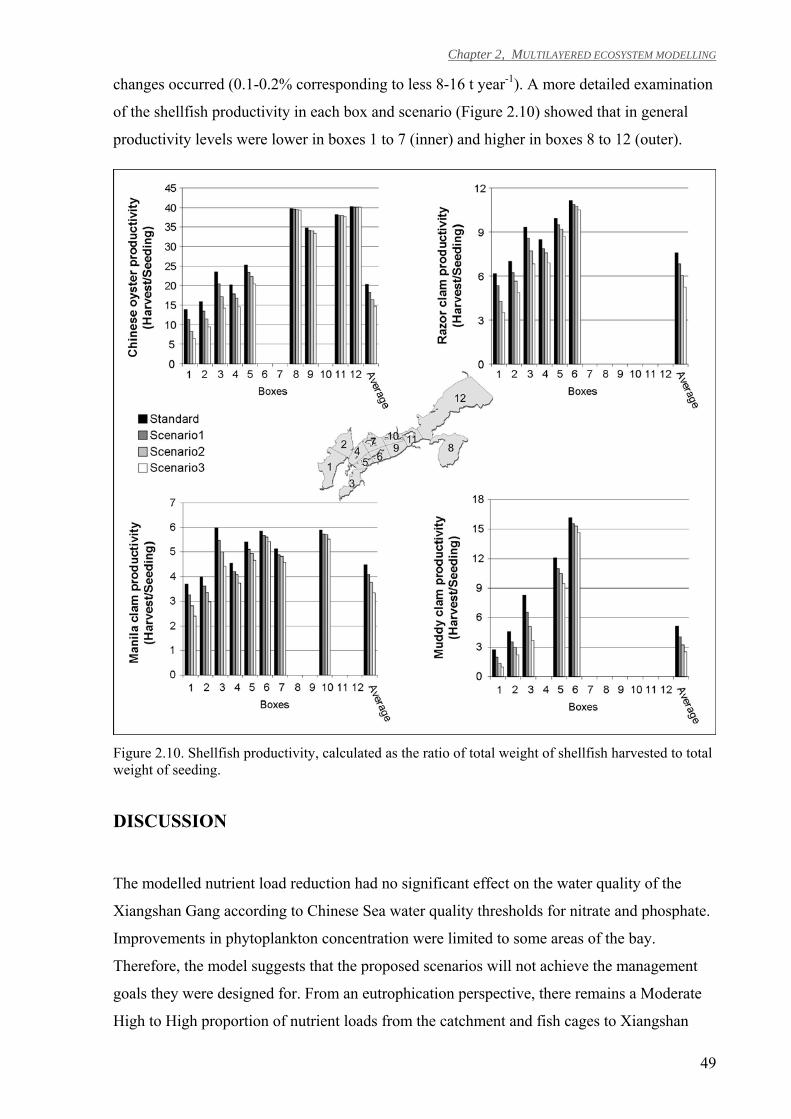
Chapter 2, MULTILAYERED ECOSYSTEM MODELLING
49
changes occurred (0.1-0.2% corresponding to less 8-16 t year-1). A more detailed examination
of the shellfish productivity in each box and scenario (Figure 2.10) showed that in general
productivity levels were lower in boxes 1 to 7 (inner) and higher in boxes 8 to 12 (outer).
Figure 2.10. Shellfish productivity, calculated as the ratio of total weight of shellfish harvested to total weight of seeding.
DISCUSSION
The modelled nutrient load reduction had no significant effect on the water quality of the
Xiangshan Gang according to Chinese Sea water quality thresholds for nitrate and phosphate.
Improvements in phytoplankton concentration were limited to some areas of the bay.
Therefore, the model suggests that the proposed scenarios will not achieve the management
goals they were designed for. From an eutrophication perspective, there remains a Moderate
High to High proportion of nutrient loads from the catchment and fish cages to Xiangshan
Chapter 2, MULTILAYERED ECOSYSTEM MODELLING
50
Gang that need to be managed. Future work using this multilayered ecosystem model includes
the definition of further scenarios, using the SWAT model to assess how different land use
management practices may impact the bay. Likewise, future scenarios might include the
adoption of different aquaculture practices such as described by Ayer and Tyedmers (2009) to
decrease the wastes from fish cages. The model outputs indicated that the nutrients and POM
provided by fish cages and wastewater are sustaining shellfish growth in the inner boxes. In
the scenarios that test a decrease of these substances (Table 2.8), shellfish production
decreases (Figure 2.9e,f and Figure 2.10). The estimated total loss of harvested shellfish was
between 4 600 t year-1 and 12 700 t year-1, corresponding to a relative decrease in the range of
10-28%, and to a loss of annual revenue between 555 and 1 500 thousand Euro. Those effects
are predicted to be more evident in the inner section of the Xiangshan Gang because of: (i)
higher water residence times, in the range of 60 to 80 days; and (ii) higher competition for
food resources given that cultivation areas in boxes 1 to 5 represented 89% of the total
shellfish cultivation area, whereas these boxes accounted only for 34% of the total bay area.
As such, and based on the analysis in Figure 2.10, it is advisable to reallocate part of the
shellfish culture towards the mouth of the embayment, in particular for the Chinese oyster and
muddy clam. Such measures should be adopted in parallel to the reduction of substance
loading into the bay in order to minimize the reduction in shellfish production.
Notwithstanding, it is suggested that a cost-benefit analysis should be carried out to analyse
the economic and environmental viability of alternative sources of income for the local
community that might compensate for any decrease in aquaculture activities. A combined
environmental and economic strategic assessment is even more important given that the
Xiangshan Gang area is considered as a key area to promote sustainable development of the
Ningbo municipality. Planning includes a balance between its protection and its use, to take
advantage of ecological and marine resources (Ningbo Municipal People's Government,
2006). Expected uses include the entertainment and tourism industries, modern fishing and
international logistics such as harbour activities.
The multilayered ecosystem model presented in this paper can be used to simulate further
nutrient and aquaculture management scenarios in Xiangshan Gang, and in particular to test
varying nutrient loads from catchment and aquaculture sources in order to determine the
nutrient load level required to meet water quality targets for the bay. On this basis, an
indication of the various management options available for such load reduction and
corresponding costs could be provided.
Chapter 2, MULTILAYERED ECOSYSTEM MODELLING
51
Although harmful algal blooms are a severe problem in the Xiangshan Gang and adjacent
ocean (ZOFB, 2008), due to the complex and uncertain causes of HAB and the chaotic nature
of these events (Huppert, et al., 2005; Huang et al., 2008a) HAB simulation is not included in
the ecosystem model. While some observations indicate that many red tides originate in the
East China Sea, some have developed inside the bay (Long et al., 2008; ZOFB, 2008). Severe
economic losses were associated with these incidents, either as a result of shellfish and finfish
mortalities due to toxic algae or to interdiction of seafood sales from the affected areas
(ZOFB, 2008). The increase of HAB’s in China since 2000 may be associated with an
increase of fish cages (Wang, 2002), but given the uncertainty about causes of HAB’s in
Xiangshan Gang, it is speculative whether a reduction of nutrient discharge might cause a
reduction of the occurrence of HAB’s inside the bay and a consequent reduction in
aquaculture closure time due to toxin contamination and/or death of cultivated organisms. A
clear understanding about the origin and the triggering mechanisms of the HAB’s in the
Xiangshan Gang is required for determining the management possibilities. Monitoring of
HAB events is recommended, in particular research about causative and sustaining factors for
HAB, which can be applied for managing aquaculture sites subject to these events (Babaran et
al., 1998).
The comparison of ecosystem model results using different temporal resolutions for the
catchment loads illustrates the importance of the SWAT catchment model in providing a
temporally distributed estimate of water and nutrient loadings from catchments into coastal
systems, for different outlets. These issues should be further explored. A detailed sampling
program together with the catchment modelling should be used to guide on the amount of
catchment monitoring data and temporal resolution to use in coastal ecosystem models.
Likewise, similar research should be carried out for ocean boundary conditions and
aquaculture loads.
CONCLUSIONS
The outcomes obtained for Xiangshan Gang indicate that multilayered ecosystem models can
play a key role in Integrated Coastal Zone Management and for the adoption of an ecosystem-
based approach to marine resource management. The present case study also indicates that the
integration of ecosystem-based tools can be used to fill data gaps, improve the
temporal/spatial detail of the setup datasets, and provide guidance to monitoring programmes.
The multilayered ecosystem modelling approach is appropriate to support management of
coastal and estuarine systems worldwide including the assessment of cumulative impacts of
Chapter 2, MULTILAYERED ECOSYSTEM MODELLING
52
activities developed in these zones. Overall, the modelling approach presented in this paper
can be helpful for the implementation of legislation and other regulatory instruments. For
instance, it can contribute towards the implementation of the European Marine Strategy
Framework Directive (Directive 2008/56/EC), for analysing scenarios designed to achieve the
‘good environmental status’ (GES) in coastal waters.
To maximize the potential benefits of multilayered ecosystem models, a natural development
is the application of aggregated results in simple screening models for management, and the
coupling of this kind of ecological model to socio-economic models, in order to more
effectively address the interactions between natural and social systems.
Chapter 3. Integrated ecological-economic assessment
Context
The preceding chapter describes the development of an integrated ecosystem model and its
application for simulating scenarios designed together with local managers to test potential
measures to improve water quality in a Chinese embayment.
Further efforts are needed to translate the complex model results into knowledge useful for
managers. Likewise, after implementing a set of measures, either to address a specific
problem or in the context of a broader ICZM programme, managers need to assess the
effectiveness of their actions.
Summary
This chapter presents a methodology to provide scientific-based information required by
managers and decision-makers to evaluate previously adopted policies as well as future
response scenarios. The method described here consists of an adaptation of the Drivers-
Pressure-State-Impact-Response methodology, named differential DPSIR (∆DPSIR). The
∆DPSIR approach further develops the multilayered ecosystem model by explicitly linking
ecological and economic information related to the use and management of a coastal
ecosystem within a specific timeframe. The application of ∆DPSIR is illustrated through an
analysis of developments in a southwest European coastal lagoon between 1985 and 1995.
The results are presented herein. Furthermore, the methodology was made available online at
http://www.salum.net/ddpsir/.
Chapter 3, INTEGRATED ECOLOGICAL-ECONOMIC ASSESSMENT
54
This chapter corresponds to the published manuscript:
Nobre, A., 2009. An ecological and economic assessment methodology
for coastal ecosystem management. Environmental Management,
44(1): 185-204.
(For consistency with published version this chapter is written in
American English)
Chapter 3, INTEGRATED ECOLOGICAL-ECONOMIC ASSESSMENT
55
An ecological and economic assessment methodology for coastal ecosystem management
INTRODUCTION
Coastal zones are important areas that provide provisioning, regulating and recreational
services to coastal populations and have a high economic value (Costanza et al., 1997;
Ledoux and Turner, 2002). Boissonnas et al. (2002) estimate that the services provided by
coastal environments and wetlands make up 43% of the world’s ecosystem services.
However, the benefits that these ecosystems generate are threatened by society’s own activity.
Population settlement in coastal areas is responsible for increasing pressure on these
ecosystems (Boissonnas et al., 2002), resulting in severe consequences, such as (1)
eutrophication related problems (Bricker et al., 2003; Ferreira et al., 2007b), (2) degradation
of natural habitat areas (Cicin-Sain and Belfiore, 2005; Ortiz-Lozano et al., 2005), and (3)
water quality degradation and sedimentation due to non-sustainable aquaculture production
(Gibbs, 2004; Bondad-Reantaso et al., 2005). Negative changes in natural systems directly
feed back on the socio-economic system that relies on the coastal ecosystem’s goods and
services (Bowen and Riley, 2003). This can result in (1) economic losses, as exemplified by
Islam and Tanaka (2004) for the fisheries industry and by Lipton and Hicks (2003) for
recreational fishing, or (2) an increase in the negative impacts of coastal disasters (Costanza
and Farley, 2007).
Managers and policy-makers face the challenge of adopting responses to reverse the general
trend of coastal ecosystem degradation and biodiversity loss. New legislative and policy
instruments have been defined worldwide over the past few decades (Table 3.1). In order for
decision-makers to gain insight into the performance of their responses, the management and
science scales paradox should be addressed (Nijkamp and van den Bergh, 1997; Elliott,
2002). This implies the need for the application of scientific methodologies across different
scales to enable understanding of ecosystem behavior (IMPRESS, 2003; Ferreira et al., 2005).
Additionally, research results must be aggregated across a broader scale so that they may be
useful to managers and they must integrate with the social sciences (Turner, 2000; Boissonnas
et al., 2002; Lal, 2003). Bridging this scale gap requires integrated methodologies, such as the
Driver-Pressure-State-Impact-Response (DPSIR) framework (Luiten, 1999; Ledoux and
Turner, 2002; Bowen and Riley, 2003).
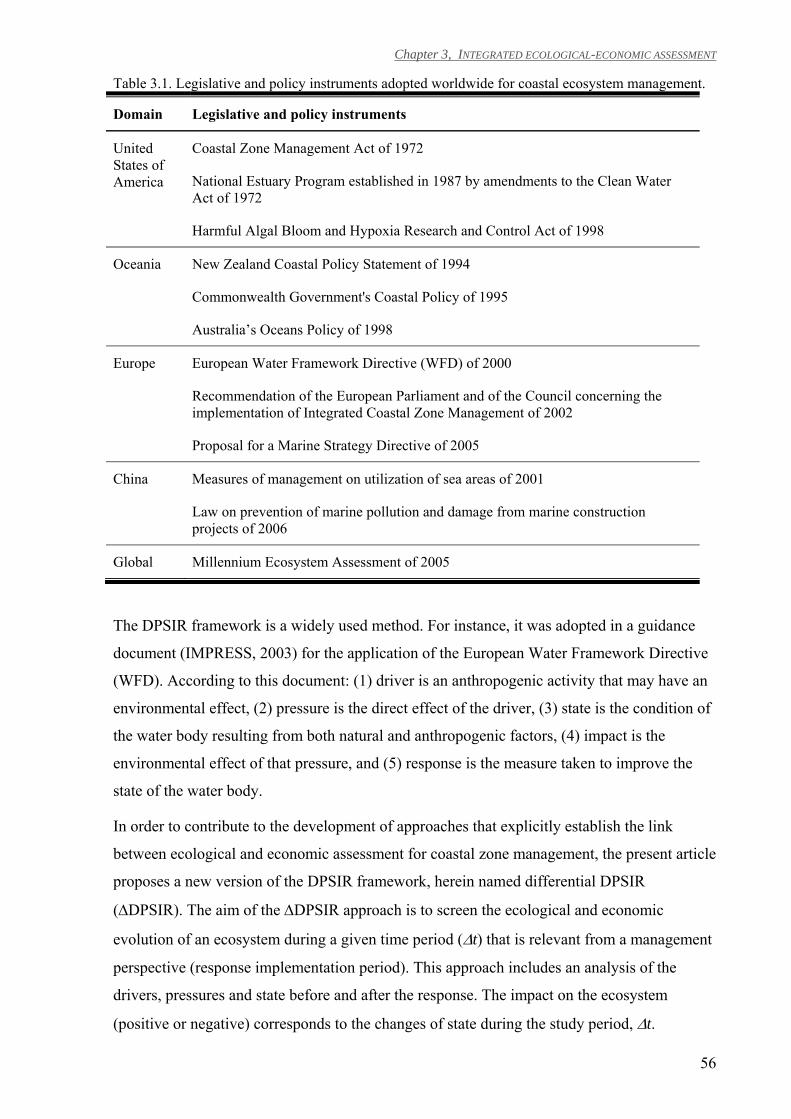
Chapter 3, INTEGRATED ECOLOGICAL-ECONOMIC ASSESSMENT
56
Table 3.1. Legislative and policy instruments adopted worldwide for coastal ecosystem management.
Domain Legislative and policy instruments
United States of America
Coastal Zone Management Act of 1972
National Estuary Program established in 1987 by amendments to the Clean Water Act of 1972
Harmful Algal Bloom and Hypoxia Research and Control Act of 1998
Oceania New Zealand Coastal Policy Statement of 1994
Commonwealth Government's Coastal Policy of 1995
Australia’s Oceans Policy of 1998
Europe European Water Framework Directive (WFD) of 2000
Recommendation of the European Parliament and of the Council concerning the implementation of Integrated Coastal Zone Management of 2002
Proposal for a Marine Strategy Directive of 2005
China Measures of management on utilization of sea areas of 2001
Law on prevention of marine pollution and damage from marine construction projects of 2006
Global Millennium Ecosystem Assessment of 2005
The DPSIR framework is a widely used method. For instance, it was adopted in a guidance
document (IMPRESS, 2003) for the application of the European Water Framework Directive
(WFD). According to this document: (1) driver is an anthropogenic activity that may have an
environmental effect, (2) pressure is the direct effect of the driver, (3) state is the condition of
the water body resulting from both natural and anthropogenic factors, (4) impact is the
environmental effect of that pressure, and (5) response is the measure taken to improve the
state of the water body.
In order to contribute to the development of approaches that explicitly establish the link
between ecological and economic assessment for coastal zone management, the present article
proposes a new version of the DPSIR framework, herein named differential DPSIR
(∆DPSIR). The aim of the ∆DPSIR approach is to screen the ecological and economic
evolution of an ecosystem during a given time period (∆t) that is relevant from a management
perspective (response implementation period). This approach includes an analysis of the
drivers, pressures and state before and after the response. The impact on the ecosystem
(positive or negative) corresponds to the changes of state during the study period, ∆t.
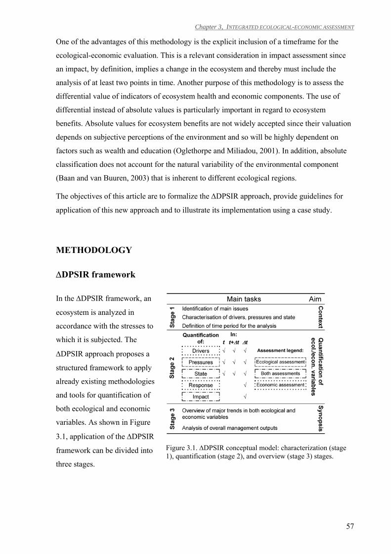
Chapter 3, INTEGRATED ECOLOGICAL-ECONOMIC ASSESSMENT
57
One of the advantages of this methodology is the explicit inclusion of a timeframe for the
ecological-economic evaluation. This is a relevant consideration in impact assessment since
an impact, by definition, implies a change in the ecosystem and thereby must include the
analysis of at least two points in time. Another purpose of this methodology is to assess the
differential value of indicators of ecosystem health and economic components. The use of
differential instead of absolute values is particularly important in regard to ecosystem
benefits. Absolute values for ecosystem benefits are not widely accepted since their valuation
depends on subjective perceptions of the environment and so will be highly dependent on
factors such as wealth and education (Oglethorpe and Miliadou, 2001). In addition, absolute
classification does not account for the natural variability of the environmental component
(Baan and van Buuren, 2003) that is inherent to different ecological regions.
The objectives of this article are to formalize the ∆DPSIR approach, provide guidelines for
application of this new approach and to illustrate its implementation using a case study.
METHODOLOGY
∆DPSIR framework
In the ∆DPSIR framework, an
ecosystem is analyzed in
accordance with the stresses to
which it is subjected. The
∆DPSIR approach proposes a
structured framework to apply
already existing methodologies
and tools for quantification of
both ecological and economic
variables. As shown in Figure
3.1, application of the ∆DPSIR
framework can be divided into
three stages.
Figure 3.1. ∆DPSIR conceptual model: characterization (stage 1), quantification (stage 2), and overview (stage 3) stages.
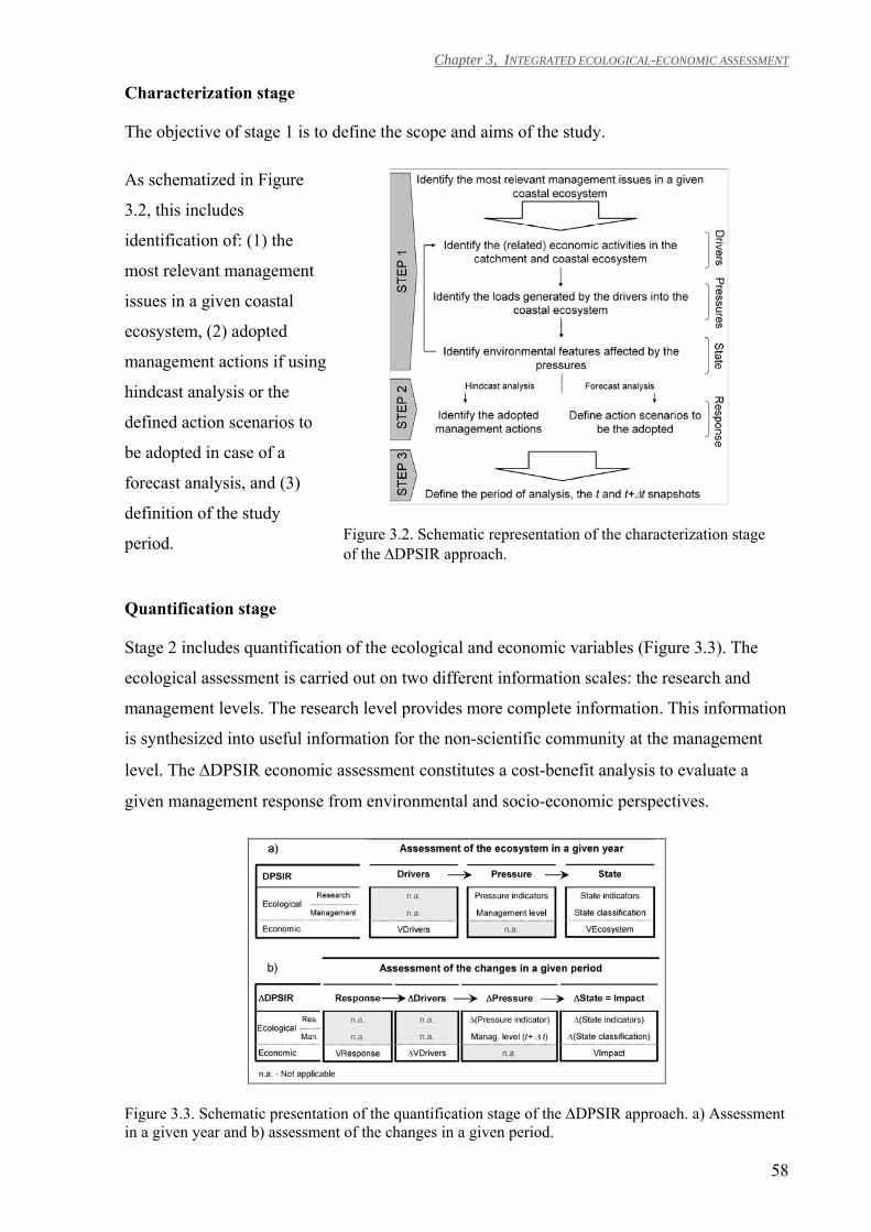
Chapter 3, INTEGRATED ECOLOGICAL-ECONOMIC ASSESSMENT
58
Characterization stage
The objective of stage 1 is to define the scope and aims of the study.
As schematized in Figure
3.2, this includes
identification of: (1) the
most relevant management
issues in a given coastal
ecosystem, (2) adopted
management actions if using
hindcast analysis or the
defined action scenarios to
be adopted in case of a
forecast analysis, and (3)
definition of the study
period.
Figure 3.2. Schematic representation of the characterization stage of the ∆DPSIR approach.
Quantification stage
Stage 2 includes quantification of the ecological and economic variables (Figure 3.3). The
ecological assessment is carried out on two different information scales: the research and
management levels. The research level provides more complete information. This information
is synthesized into useful information for the non-scientific community at the management
level. The ∆DPSIR economic assessment constitutes a cost-benefit analysis to evaluate a
given management response from environmental and socio-economic perspectives.
Figure 3.3. Schematic presentation of the quantification stage of the ∆DPSIR approach. a) Assessment in a given year and b) assessment of the changes in a given period.
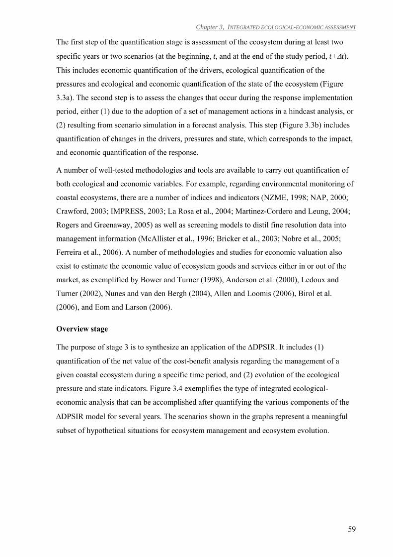
Chapter 3, INTEGRATED ECOLOGICAL-ECONOMIC ASSESSMENT
59
The first step of the quantification stage is assessment of the ecosystem during at least two
specific years or two scenarios (at the beginning, t, and at the end of the study period, t+∆t).
This includes economic quantification of the drivers, ecological quantification of the
pressures and ecological and economic quantification of the state of the ecosystem (Figure
3.3a). The second step is to assess the changes that occur during the response implementation
period, either (1) due to the adoption of a set of management actions in a hindcast analysis, or
(2) resulting from scenario simulation in a forecast analysis. This step (Figure 3.3b) includes
quantification of changes in the drivers, pressures and state, which corresponds to the impact,
and economic quantification of the response.
A number of well-tested methodologies and tools are available to carry out quantification of
both ecological and economic variables. For example, regarding environmental monitoring of
coastal ecosystems, there are a number of indices and indicators (NZME, 1998; NAP, 2000;
Crawford, 2003; IMPRESS, 2003; La Rosa et al., 2004; Martinez-Cordero and Leung, 2004;
Rogers and Greenaway, 2005) as well as screening models to distil fine resolution data into
management information (McAllister et al., 1996; Bricker et al., 2003; Nobre et al., 2005;
Ferreira et al., 2006). A number of methodologies and studies for economic valuation also
exist to estimate the economic value of ecosystem goods and services either in or out of the
market, as exemplified by Bower and Turner (1998), Anderson et al. (2000), Ledoux and
Turner (2002), Nunes and van den Bergh (2004), Allen and Loomis (2006), Birol et al.
(2006), and Eom and Larson (2006).
Overview stage
The purpose of stage 3 is to synthesize an application of the ∆DPSIR. It includes (1)
quantification of the net value of the cost-benefit analysis regarding the management of a
given coastal ecosystem during a specific time period, and (2) evolution of the ecological
pressure and state indicators. Figure 3.4 exemplifies the type of integrated ecological-
economic analysis that can be accomplished after quantifying the various components of the
∆DPSIR model for several years. The scenarios shown in the graphs represent a meaningful
subset of hypothetical situations for ecosystem management and ecosystem evolution.
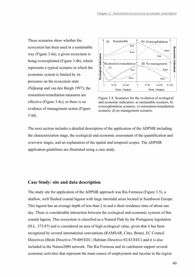
Chapter 3, INTEGRATED ECOLOGICAL-ECONOMIC ASSESSMENT
60
These scenarios show whether the
ecosystem has been used in a sustainable
way (Figure 3.4a); a given ecosystem is
being overexploited (Figure 3.4b), which
represents a typical scenario in which the
economic system is limited by its
pressures on the ecosystem state
(Nijkamp and van den Bergh 1997); the
restoration/remediation measures are
effective (Figure 3.4c); or there is no
evidence of management action (Figure
3.4d).
Figure 3.4. Scenarios for the evolution of ecological and economic indicators: a) sustainable scenario, b) overexploitation scenario, c) restoration/remediation scenario, d) no management scenario.
The next section includes a detailed description of the application of the ∆DPSIR including:
the characterization stage, the ecological and economic assessment of the quantification and
overview stages, and an explanation of the spatial and temporal scopes. The ∆DPSIR
application guidelines are illustrated using a case study.
Case Study: site and data description
The study site for application of the ∆DPSIR approach was Ria Formosa (Figure 3.5), a
shallow, well flushed coastal lagoon with large intertidal areas located in Southwest Europe.
This lagoon has an average depth of less than 2 m and a short residence time of about one
day. There is considerable interaction between the ecological and economic systems of this
coastal lagoon. This ecosystem is classified as a Natural Park by the Portuguese legislation
(D.L. 373/87) and is considered an area of high ecological value, given that it has been
recognized by several international conventions (RAMSAR, Cites, Bonn), EC Council
Directives (Birds Directive-79/409/EEC; Habitats Directive-92/43/EEC) and it is also
included in the Natura2000 network. The Ria Formosa and its catchment support several
economic activities that represent the main source of employment and income in the region.
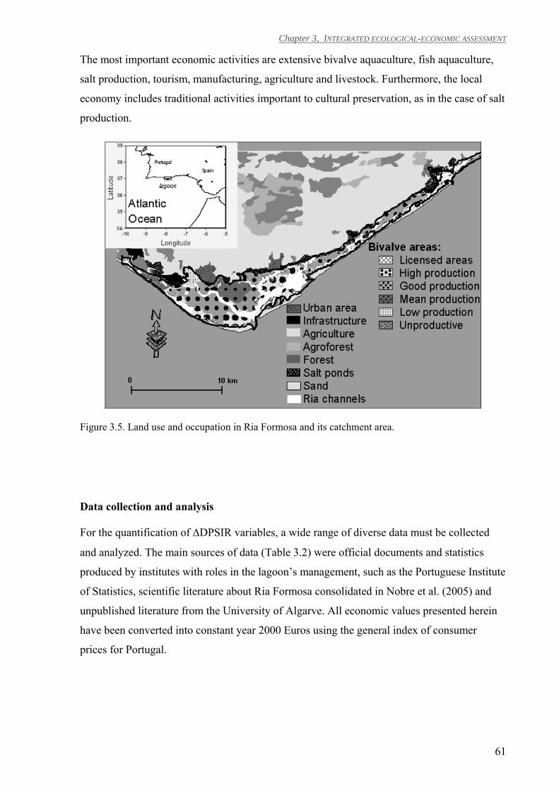
Chapter 3, INTEGRATED ECOLOGICAL-ECONOMIC ASSESSMENT
61
The most important economic activities are extensive bivalve aquaculture, fish aquaculture,
salt production, tourism, manufacturing, agriculture and livestock. Furthermore, the local
economy includes traditional activities important to cultural preservation, as in the case of salt
production.
Figure 3.5. Land use and occupation in Ria Formosa and its catchment area.
Data collection and analysis
For the quantification of ∆DPSIR variables, a wide range of diverse data must be collected
and analyzed. The main sources of data (Table 3.2) were official documents and statistics
produced by institutes with roles in the lagoon’s management, such as the Portuguese Institute
of Statistics, scientific literature about Ria Formosa consolidated in Nobre et al. (2005) and
unpublished literature from the University of Algarve. All economic values presented herein
have been converted into constant year 2000 Euros using the general index of consumer
prices for Portugal.
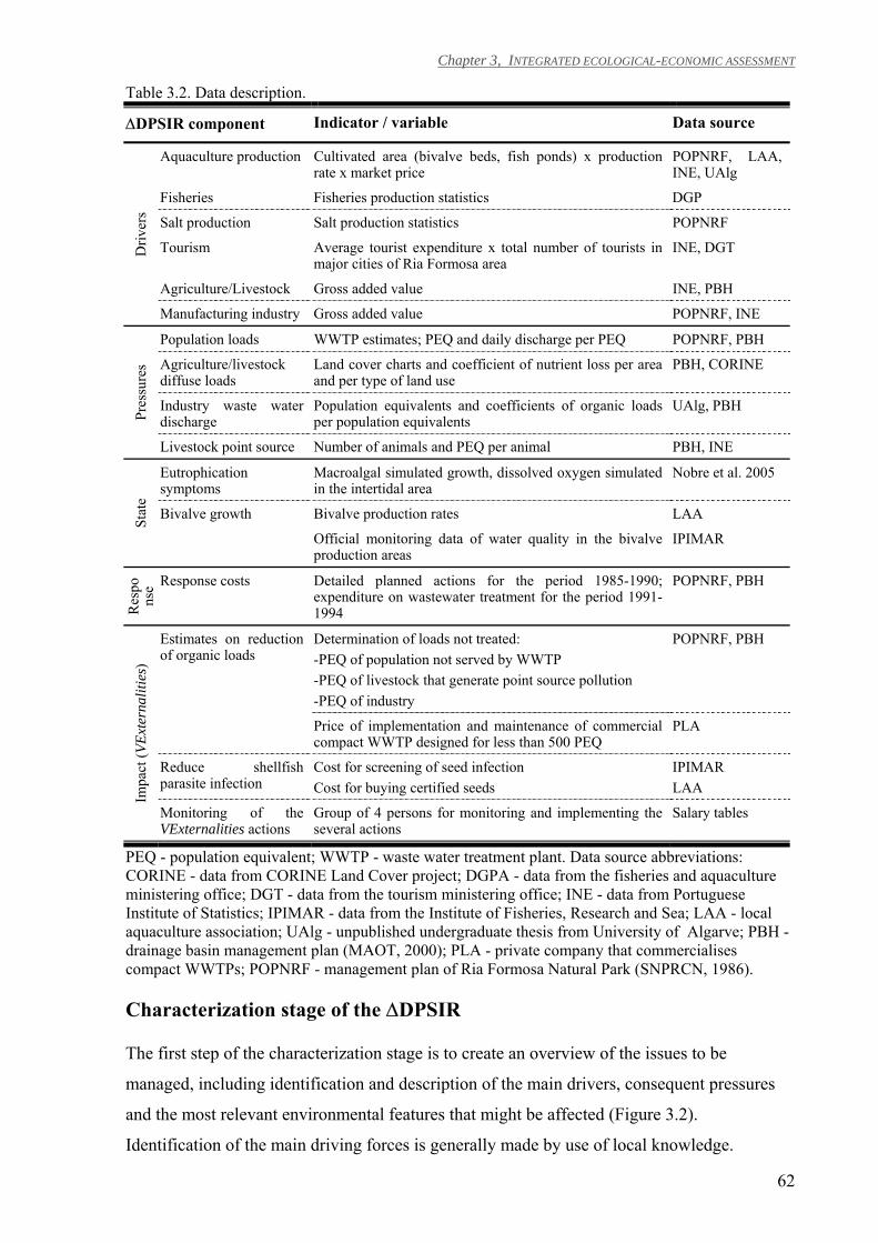
Chapter 3, INTEGRATED ECOLOGICAL-ECONOMIC ASSESSMENT
62
Table 3.2. Data description.
∆DPSIR component Indicator / variable Data source D
river
s Aquaculture production Cultivated area (bivalve beds, fish ponds) x production
rate x market price POPNRF, LAA, INE, UAlg
Fisheries Fisheries production statistics DGP
Salt production Salt production statistics POPNRF
Tourism Average tourist expenditure x total number of tourists in major cities of Ria Formosa area
INE, DGT
Agriculture/Livestock Gross added value INE, PBH
Manufacturing industry Gross added value POPNRF, INE
Pres
sure
s
Population loads WWTP estimates; PEQ and daily discharge per PEQ POPNRF, PBH
Agriculture/livestock diffuse loads
Land cover charts and coefficient of nutrient loss per area and per type of land use
PBH, CORINE
Industry waste water discharge
Population equivalents and coefficients of organic loads per population equivalents
UAlg, PBH
Livestock point source Number of animals and PEQ per animal PBH, INE
Stat
e
Eutrophication symptoms
Macroalgal simulated growth, dissolved oxygen simulated in the intertidal area
Nobre et al. 2005
Bivalve growth Bivalve production rates LAA
Official monitoring data of water quality in the bivalve production areas
IPIMAR
Res
pons
e Response costs Detailed planned actions for the period 1985-1990; expenditure on wastewater treatment for the period 1991-1994
POPNRF, PBH
Impa
ct (V
Exte
rnal
ities
)
Estimates on reduction of organic loads
Determination of loads not treated: -PEQ of population not served by WWTP -PEQ of livestock that generate point source pollution -PEQ of industry
POPNRF, PBH
Price of implementation and maintenance of commercial compact WWTP designed for less than 500 PEQ
PLA
Reduce shellfish parasite infection
Cost for screening of seed infection Cost for buying certified seeds
IPIMAR LAA
Monitoring of the VExternalities actions
Group of 4 persons for monitoring and implementing the several actions
Salary tables
PEQ - population equivalent; WWTP - waste water treatment plant. Data source abbreviations: CORINE - data from CORINE Land Cover project; DGPA - data from the fisheries and aquaculture ministering office; DGT - data from the tourism ministering office; INE - data from Portuguese Institute of Statistics; IPIMAR - data from the Institute of Fisheries, Research and Sea; LAA - local aquaculture association; UAlg - unpublished undergraduate thesis from University of Algarve; PBH - drainage basin management plan (MAOT, 2000); PLA - private company that commercialises compact WWTPs; POPNRF - management plan of Ria Formosa Natural Park (SNPRCN, 1986).
Characterization stage of the ∆DPSIR
The first step of the characterization stage is to create an overview of the issues to be
managed, including identification and description of the main drivers, consequent pressures
and the most relevant environmental features that might be affected (Figure 3.2).
Identification of the main driving forces is generally made by use of local knowledge.
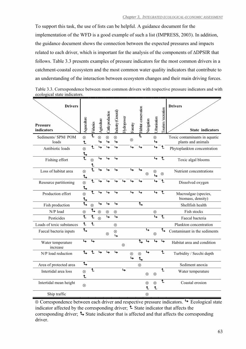
Chapter 3, INTEGRATED ECOLOGICAL-ECONOMIC ASSESSMENT
63
To support this task, the use of lists can be helpful. A guidance document for the
implementation of the WFD is a good example of such a list (IMPRESS, 2003). In addition,
the guidance document shows the connection between the expected pressures and impacts
related to each driver, which is important for the analysis of the components of ∆DPSIR that
follows. Table 3.3 presents examples of pressure indicators for the most common drivers in a
catchment-coastal ecosystem and the most common water quality indicators that contribute to
an understanding of the interaction between ecosystem changes and their main driving forces.
Table 3.3. Correspondence between most common drivers with respective pressure indicators and with ecological state indicators.
Drivers
Pressure indicators Aq
uacu
lture
Fishe
ries
Agric
ulture
Cattle
prod
uctio
n
Indus
try (G
enera
l)
Hydro
powe
r
Fores
try
Habit
at co
nserv
ation
Navig
ation
Urba
nisati
on
Touri
sm / r
ecrea
tion
Drivers
State indicators
Sediments/ SPM/ POM loads
⊗
⊗ ⊗ ⊗ ⊗ ⊗ Toxic contaminants in aquatic plants and animals
Antibiotic loads ⊗
Phytoplankton concentration
Fishing effort ⊗
Toxic algal blooms
Loss of habitat area ⊗
⊗ ⊗ ⊗ Nutrient concentrations
Resource partitioning ⊗
Dissolved oxygen
Production effort ⊗
Macroalgae (species, biomass, density)
Fish production ⊗ Shellfish health N/P load ⊗ ⊗ ⊗ ⊗ ⊗ Fish stocks Pesticides ⊗ Faecal bacteria
Loads of toxic substances ⊗ Plankton concentration Faecal bacteria inputs ⊗ ⊗ ⊗
Contaminant in the sediments
Water temperature increase
⊗ Habitat area and condition
N/P load reduction ⊗ ⊗ Turbidity / Secchi depth
Area of protected area ⊗ Sediment anoxia Intertidal area loss ⊗
⊗ ⊗
Water temperature
Intertidal mean height ⊗ ⊗ ⊗ Coastal erosion
Ship traffic ⊗
⊗ Correspondence between each driver and respective pressure indicators. Ecological state indicator affected by the corresponding driver; State indicator that affects the corresponding driver; State indicator that is affected and that affects the corresponding driver.
Chapter 3, INTEGRATED ECOLOGICAL-ECONOMIC ASSESSMENT
64
The next step is identification of response actions that have been adopted in the case of a
hindcast analysis or definition of management action scenarios in the case of a forecast
analysis (Figure 3.2). If the ecosystem is subject to management policies, a set of laws (e.g.
Urban Waste Water Treatment Directive, UWWTD, 91/271/EEC or Nitrates Directive, ND,
91/676/EEC), policies (e.g. DOENI, 2006) or economic instruments (e.g. Romstad, 2003;
Zylicz, 2003; Hatton MacDonald et al., 2004) are planned and enforced by managers or policy
makers according to the evaluation of the state of the ecosystem. These responses can be
targeted at the catchment region, the coastal ecosystem or both, and have a precautionary or
remedial nature. For ecosystems that are not subject to management, a null response must be
considered.
Finally, during the characterization stage, the appropriate timeframe for application of the
∆DPSIR must be defined (Figure 3.2). The evaluation can be either a hindcast analysis (in
order to assess changes that have already occurred in the ecosystem due to a given
management response) or a forecast analysis (in order to predict changes that result from the
simulation of management scenarios). Definition of the appropriate time period for the
analysis must take into account the possibility that some of the pressures might only be
evident in impacts with a time lag of several years (IMPRESS, 2003).
In the Ria Formosa case study, the characterization stage was elaborated based on the
Management Plan of Ria Formosa Natural Park (SNPRCN, 1986), local community
knowledge and the scientific literature. The most outstanding issues are symptoms of benthic
eutrophication and high clam mortality. Further details, including definition of the period of
analysis, are provided in the results section.
Ecological assessment of the ∆DPSIR
The ecological assessment is done by quantifying (1) the loads (pressure), (2) the
biogeochemical quality of the ecosystem (state), and (3) their changes (∆Pressure and ∆State,
i.e., impact) due to a given management response to a given problem or research topic (Figure
3.3).
Pressure
Since the same magnitude of pressure is likely to produce different effects in different
ecosystems (e.g. due to susceptibility), it is important to identify the significant pressures
(those that are likely to affect the ecosystem state). The quantification of pressures is dealt
with at the research level, for example, by determining the annual load of nitrogen from the
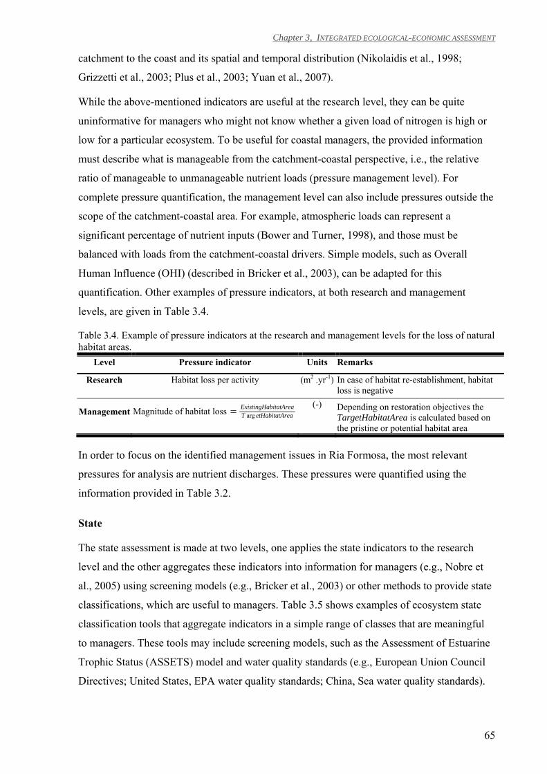
Chapter 3, INTEGRATED ECOLOGICAL-ECONOMIC ASSESSMENT
65
catchment to the coast and its spatial and temporal distribution (Nikolaidis et al., 1998;
Grizzetti et al., 2003; Plus et al., 2003; Yuan et al., 2007).
While the above-mentioned indicators are useful at the research level, they can be quite
uninformative for managers who might not know whether a given load of nitrogen is high or
low for a particular ecosystem. To be useful for coastal managers, the provided information
must describe what is manageable from the catchment-coastal perspective, i.e., the relative
ratio of manageable to unmanageable nutrient loads (pressure management level). For
complete pressure quantification, the management level can also include pressures outside the
scope of the catchment-coastal area. For example, atmospheric loads can represent a
significant percentage of nutrient inputs (Bower and Turner, 1998), and those must be
balanced with loads from the catchment-coastal drivers. Simple models, such as Overall
Human Influence (OHI) (described in Bricker et al., 2003), can be adapted for this
quantification. Other examples of pressure indicators, at both research and management
levels, are given in Table 3.4.
Table 3.4. Example of pressure indicators at the research and management levels for the loss of natural habitat areas.
Level Pressure indicator Units Remarks
Research Habitat loss per activity (m2 .yr-1) In case of habitat re-establishment, habitat loss is negative
Management Magnitude of habitat loss reaetHabitatATbitatAreaExistingHa
arg=(-) Depending on restoration objectives the
TargetHabitatArea is calculated based on the pristine or potential habitat area
In order to focus on the identified management issues in Ria Formosa, the most relevant
pressures for analysis are nutrient discharges. These pressures were quantified using the
information provided in Table 3.2.
State
The state assessment is made at two levels, one applies the state indicators to the research
level and the other aggregates these indicators into information for managers (e.g., Nobre et
al., 2005) using screening models (e.g., Bricker et al., 2003) or other methods to provide state
classifications, which are useful to managers. Table 3.5 shows examples of ecosystem state
classification tools that aggregate indicators in a simple range of classes that are meaningful
to managers. These tools may include screening models, such as the Assessment of Estuarine
Trophic Status (ASSETS) model and water quality standards (e.g., European Union Council
Directives; United States, EPA water quality standards; China, Sea water quality standards).
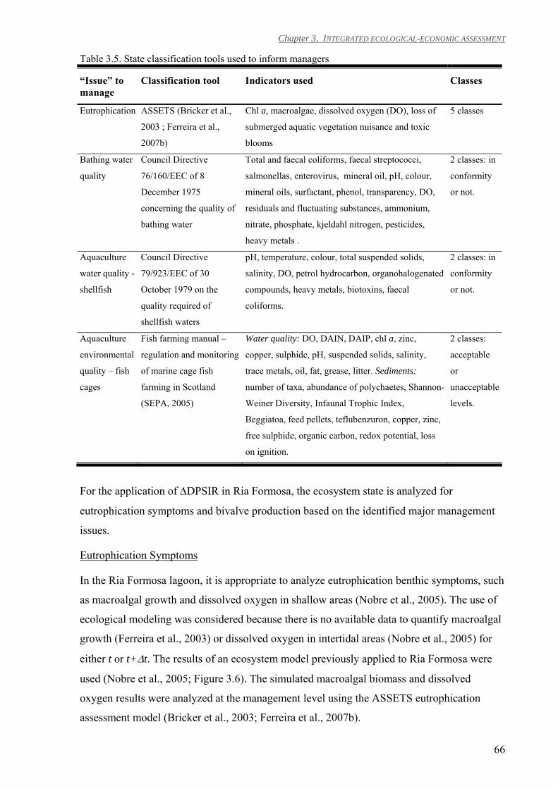
Chapter 3, INTEGRATED ECOLOGICAL-ECONOMIC ASSESSMENT
66
Table 3.5. State classification tools used to inform managers
“Issue” to manage
Classification tool Indicators used Classes
Eutrophication ASSETS (Bricker et al.,
2003 ; Ferreira et al.,
2007b)
Chl a, macroalgae, dissolved oxygen (DO), loss of
submerged aquatic vegetation nuisance and toxic
blooms
5 classes
Bathing water
quality
Council Directive
76/160/EEC of 8
December 1975
concerning the quality of
bathing water
Total and faecal coliforms, faecal streptococci,
salmonellas, enterovirus, mineral oil, pH, colour,
mineral oils, surfactant, phenol, transparency, DO,
residuals and fluctuating substances, ammonium,
nitrate, phosphate, kjeldahl nitrogen, pesticides,
heavy metals .
2 classes: in
conformity
or not.
Aquaculture
water quality -
shellfish
Council Directive
79/923/EEC of 30
October 1979 on the
quality required of
shellfish waters
pH, temperature, colour, total suspended solids,
salinity, DO, petrol hydrocarbon, organohalogenated
compounds, heavy metals, biotoxins, faecal
coliforms.
2 classes: in
conformity
or not.
Aquaculture
environmental
quality – fish
cages
Fish farming manual –
regulation and monitoring
of marine cage fish
farming in Scotland
(SEPA, 2005)
Water quality: DO, DAIN, DAIP, chl a, zinc,
copper, sulphide, pH, suspended solids, salinity,
trace metals, oil, fat, grease, litter. Sediments:
number of taxa, abundance of polychaetes, Shannon-
Weiner Diversity, Infaunal Trophic Index,
Beggiatoa, feed pellets, teflubenzuron, copper, zinc,
free sulphide, organic carbon, redox potential, loss
on ignition.
2 classes:
acceptable
or
unacceptable
levels.
For the application of ∆DPSIR in Ria Formosa, the ecosystem state is analyzed for
eutrophication symptoms and bivalve production based on the identified major management
issues.
Eutrophication Symptoms
In the Ria Formosa lagoon, it is appropriate to analyze eutrophication benthic symptoms, such
as macroalgal growth and dissolved oxygen in shallow areas (Nobre et al., 2005). The use of
ecological modeling was considered because there is no available data to quantify macroalgal
growth (Ferreira et al., 2003) or dissolved oxygen in intertidal areas (Nobre et al., 2005) for
either t or t+∆t. The results of an ecosystem model previously applied to Ria Formosa were
used (Nobre et al., 2005; Figure 3.6). The simulated macroalgal biomass and dissolved
oxygen results were analyzed at the management level using the ASSETS eutrophication
assessment model (Bricker et al., 2003; Ferreira et al., 2007b).
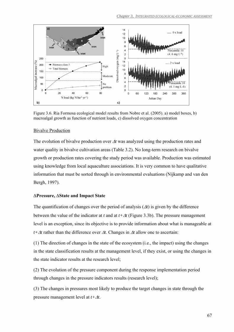
Chapter 3, INTEGRATED ECOLOGICAL-ECONOMIC ASSESSMENT
67
Figure 3.6. Ria Formosa ecological model results from Nobre et al. (2005). a) model boxes, b) macroalgal growth as function of nutrient loads, c) dissolved oxygen concentration
Bivalve Production
The evolution of bivalve production over ∆t was analyzed using the production rates and
water quality in bivalve cultivation areas (Table 3.2). No long-term research on bivalve
growth or production rates covering the study period was available. Production was estimated
using knowledge from local aquaculture associations. It is very common to have qualitative
information that must be sorted through in environmental evaluations (Nijkamp and van den
Bergh, 1997).
∆Pressure, ∆State and Impact State
The quantification of changes over the period of analysis (∆t) is given by the difference
between the value of the indicator at t and at t+∆t (Figure 3.3b). The pressure management
level is an exception, since its objective is to provide information about what is manageable at
t+∆t rather than the difference over ∆t. Changes in ∆t allow one to ascertain:
(1) The direction of changes in the state of the ecosystem (i.e., the impact) using the changes
in the state classification results at the management level, if they exist, or using the changes in
the state indicator results at the research level;
(2) The evolution of the pressure component during the response implementation period
through changes in the pressure indicators results (research level);
(3) The changes in pressures most likely to produce the target changes in state through the
pressure management level at t+∆t.
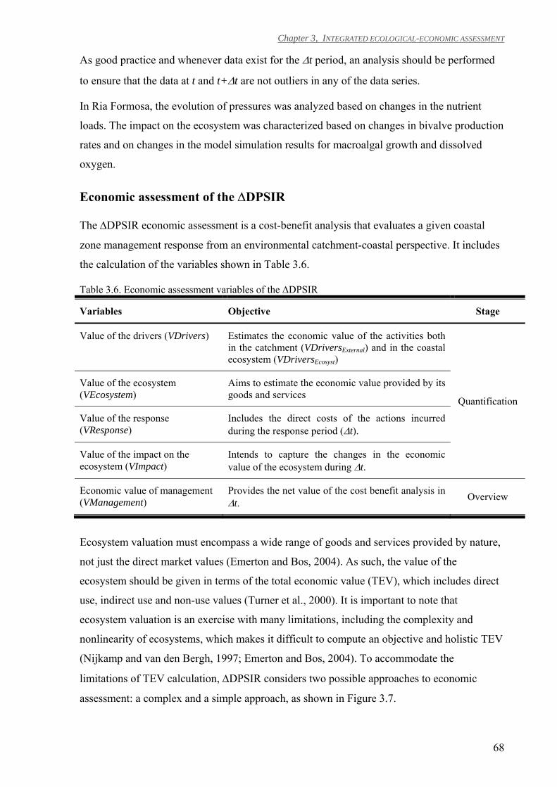
Chapter 3, INTEGRATED ECOLOGICAL-ECONOMIC ASSESSMENT
68
As good practice and whenever data exist for the ∆t period, an analysis should be performed
to ensure that the data at t and t+∆t are not outliers in any of the data series.
In Ria Formosa, the evolution of pressures was analyzed based on changes in the nutrient
loads. The impact on the ecosystem was characterized based on changes in bivalve production
rates and on changes in the model simulation results for macroalgal growth and dissolved
oxygen.
Economic assessment of the ∆DPSIR
The ∆DPSIR economic assessment is a cost-benefit analysis that evaluates a given coastal
zone management response from an environmental catchment-coastal perspective. It includes
the calculation of the variables shown in Table 3.6.
Table 3.6. Economic assessment variables of the ∆DPSIR
Variables Objective Stage
Value of the drivers (VDrivers) Estimates the economic value of the activities both in the catchment (VDriversExternal) and in the coastal ecosystem (VDriversEcosyst)
Quantification
Value of the ecosystem (VEcosystem)
Aims to estimate the economic value provided by its goods and services
Value of the response (VResponse)
Includes the direct costs of the actions incurred during the response period (∆t).
Value of the impact on the ecosystem (VImpact)
Intends to capture the changes in the economic value of the ecosystem during ∆t.
Economic value of management (VManagement)
Provides the net value of the cost benefit analysis in ∆t. Overview
Ecosystem valuation must encompass a wide range of goods and services provided by nature,
not just the direct market values (Emerton and Bos, 2004). As such, the value of the
ecosystem should be given in terms of the total economic value (TEV), which includes direct
use, indirect use and non-use values (Turner et al., 2000). It is important to note that
ecosystem valuation is an exercise with many limitations, including the complexity and
nonlinearity of ecosystems, which makes it difficult to compute an objective and holistic TEV
(Nijkamp and van den Bergh, 1997; Emerton and Bos, 2004). To accommodate the
limitations of TEV calculation, ∆DPSIR considers two possible approaches to economic
assessment: a complex and a simple approach, as shown in Figure 3.7.
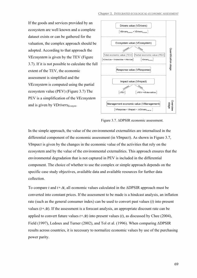
Chapter 3, INTEGRATED ECOLOGICAL-ECONOMIC ASSESSMENT
69
If the goods and services provided by an
ecosystem are well known and a complete
dataset exists or can be gathered for the
valuation, the complex approach should be
adopted. According to that approach the
VEcosystem is given by the TEV (Figure
3.7). If it is not possible to calculate the full
extent of the TEV, the economic
assessment is simplified and the
VEcosystem is computed using the partial
ecosystem value (PEV) (Figure 3.7) The
PEV is a simplification of the VEcosystem
and is given by VDriversEcosyst.
Figure 3.7. ∆DPSIR economic assessment.
In the simple approach, the value of the environmental externalities are internalised in the
differential component of the economic assessment (in VImpact). As shown in Figure 3.7,
VImpact is given by the changes in the economic value of the activities that rely on the
ecosystem and by the value of the environmental externalities. This approach ensures that the
environmental degradation that is not captured in PEV is included in the differential
component. The choice of whether to use the complex or simple approach depends on the
specific case study objectives, available data and available resources for further data
collection.
To compare t and t+∆t, all economic values calculated in the ∆DPSIR approach must be
converted into constant prices. If the assessment to be made is a hindcast analysis, an inflation
rate (such as the general consumer index) can be used to convert past values (t) into present
values (t+∆t). If the assessment is a forecast analysis, an appropriate discount rate can be
applied to convert future values t+∆t) into present values (t), as discussed by Chee (2004),
Field (1997), Ledoux and Turner (2002), and Tol et al. (1996). When comparing ∆DPSIR
results across countries, it is necessary to normalize economic values by use of the purchasing
power parity.
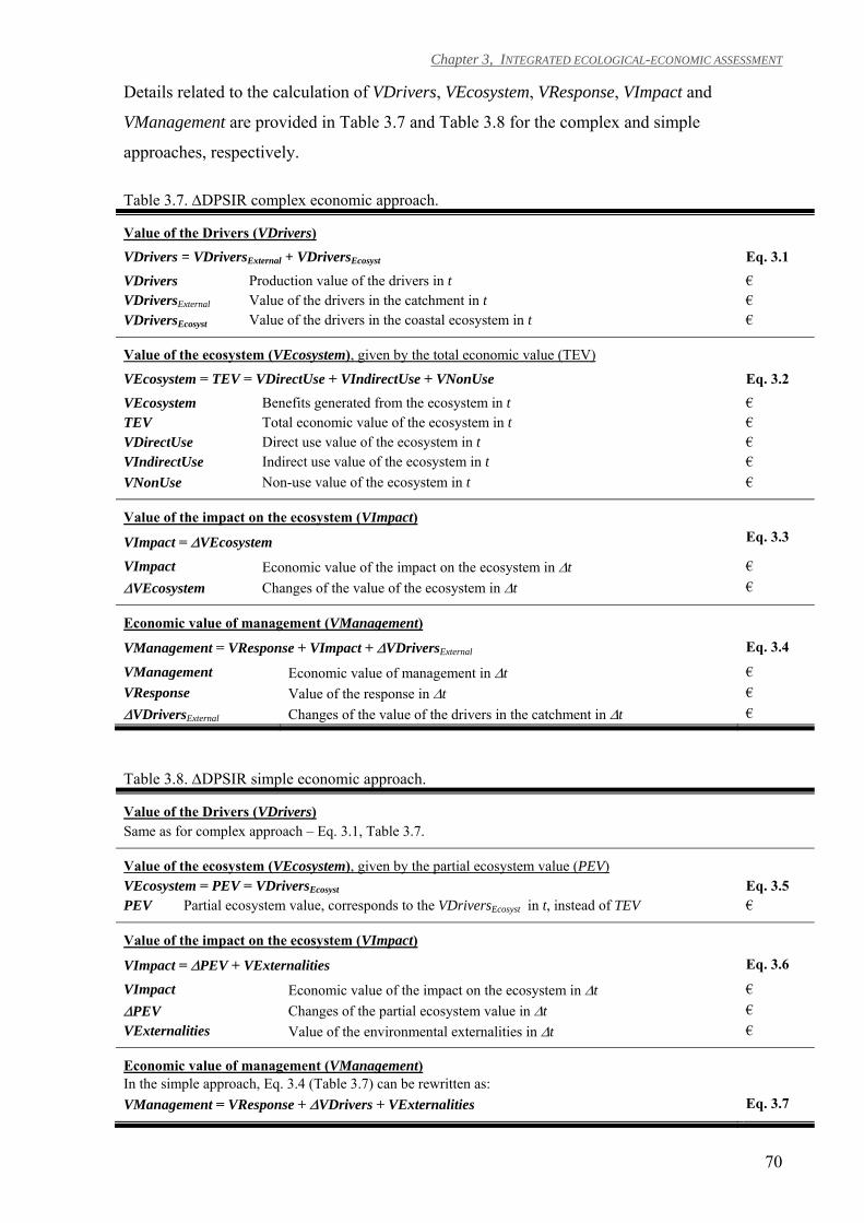
Chapter 3, INTEGRATED ECOLOGICAL-ECONOMIC ASSESSMENT
70
Details related to the calculation of VDrivers, VEcosystem, VResponse, VImpact and
VManagement are provided in Table 3.7 and Table 3.8 for the complex and simple
approaches, respectively.
Table 3.7. ∆DPSIR complex economic approach.
Value of the Drivers (VDrivers)
VDrivers = VDriversExternal + VDriversEcosyst Eq. 3.1
VDrivers Production value of the drivers in t € VDriversExternal Value of the drivers in the catchment in t € VDriversEcosyst Value of the drivers in the coastal ecosystem in t €
Value of the ecosystem (VEcosystem), given by the total economic value (TEV)
VEcosystem = TEV = VDirectUse + VIndirectUse + VNonUse Eq. 3.2
VEcosystem Benefits generated from the ecosystem in t € TEV Total economic value of the ecosystem in t € VDirectUse Direct use value of the ecosystem in t € VIndirectUse Indirect use value of the ecosystem in t € VNonUse Non-use value of the ecosystem in t €
Value of the impact on the ecosystem (VImpact)
VImpact = ∆VEcosystem Eq. 3.3
VImpact Economic value of the impact on the ecosystem in ∆t € ∆VEcosystem Changes of the value of the ecosystem in ∆t €
Economic value of management (VManagement)
VManagement = VResponse + VImpact + ∆VDriversExternal Eq. 3.4
VManagement Economic value of management in ∆t € VResponse Value of the response in ∆t € ∆VDriversExternal Changes of the value of the drivers in the catchment in ∆t €
Table 3.8. ∆DPSIR simple economic approach.
Value of the Drivers (VDrivers) Same as for complex approach – Eq. 3.1, Table 3.7.
Value of the ecosystem (VEcosystem), given by the partial ecosystem value (PEV) VEcosystem = PEV = VDriversEcosyst Eq. 3.5 PEV Partial ecosystem value, corresponds to the VDriversEcosyst in t, instead of TEV €
Value of the impact on the ecosystem (VImpact)
VImpact = ∆PEV + VExternalities Eq. 3.6
VImpact Economic value of the impact on the ecosystem in ∆t € ∆PEV Changes of the partial ecosystem value in ∆t € VExternalities Value of the environmental externalities in ∆t €
Economic value of management (VManagement) In the simple approach, Eq. 3.4 (Table 3.7) can be rewritten as: VManagement = VResponse + ∆VDrivers + VExternalities Eq. 3.7
Chapter 3, INTEGRATED ECOLOGICAL-ECONOMIC ASSESSMENT
71
Value of the drivers
The value of the drivers (VDrivers, Eq. 3.1 in Table 3.7) includes: (1) the value of economic
activities that impact a coastal ecosystem but are not sustained by it (VDriversExternal); and (2)
the value of activities that depend on the coastal ecosystem (VDriversEcosyst). VDrivers
corresponds to the sum of the production values for these activities. If such information is not
available, the value of the economic activities may be estimated based on proxies, such as the
number of workers or the level of output/production. In the case of agriculture, this can be
estimated based upon the cultivated area and the average production value per area. The
specific method will depend on the available information, but the same method must be
applied for both t and t+∆t. Also, when comparing results between ecosystems, it is important
to verify which of the approaches was used. ∆VDrivers is given by the difference between
VDriverst and VDriverst+∆t. In a hindcast application of the ∆DPSIR, this value is calculated
based on data; in a forecast analysis, VDriverst+∆t is calculated based on scenario predictions,
such as those provided by Ferreira et al. (2007a) for aquaculture productivity and by Lipton
and Hicks (2003) for recreational fishing. In some cases, especially in forecast analyzes,
∆VDrivers can represent a measure of opportunity costs, as in the following conceptual
example: If the ∆DPSIR is employed to analyze a set of response actions designed to improve
water quality in a coastal ecosystem, which includes the reduction of economic activities in
the catchment; then ∆VDriversExternal (which measures the reduction of the economic value of
these activities) corresponds to the opportunity cost of the management strategy.
In Ria Formosa, the drivers listed in Table 3.9 were considered. Whenever possible, official
statistics for production values were used to determine the activity economic value; however,
proxies were used for cases of aquaculture production and tourism (as described in Table 3.2).
Value of the ecosystem
There are a number of well-known techniques that may be used to calculate components of
TEV: market prices, production function approaches, surrogate market approaches, cost-based
approaches and stated preference approaches (Emerton and Bos, 2004). Söderqvist et al.
(2004) provided several case studies that exemplify how several economic components of the
∆DPSIR approach may be calculated. In cases where it is possible to calculate the TEV, the
complex approach for ∆DPSIR economic assessment is used (Eq. 3.2 in Table 3.7).
Subjectivity of the existing valuation methods for calculating components of the TEV is
known (Chee, 2004; Driml, 1997; Nunes and van den Bergh, 2001); however, their systematic
Chapter 3, INTEGRATED ECOLOGICAL-ECONOMIC ASSESSMENT
72
application to the same ecosystem over time can lead to an objective differential value of the
ecosystem (∆VEcosystem). Nevertheless, it is often not possible to calculate the full TEV.
For cases in which the full TEV cannot be calculated, application of the simple ∆DPSIR
approach is recommended (Figure 3.7). Following this approach, VEcosystem is given by
VDriversEcosyst, and is therefore named the PEV (Eq. 3.5 in Table 3.8). Non-market natural
capital is accounted for in the differential component and is assimilated in VImpact, through
determination of the value of the environmental externalities during the study period.
Due to data limitations, the simple ∆DPSIR approach was applied to Ria Formosa (Eq. 3.5 in
Table 3.8). VDriversEcosyst was calculated considering the activities listed in Table 3.9 that
depend on the coastal ecosystem.
Value of the response
The costs of implementing a response must be carefully defined so as not to duplicate costs
already included in ∆VDrivers. For example, if construction of waste water treatment plants
(WWTP) is among the response actions for improving water quality and these costs are
already included in the drivers, they should not be included in VResponse. The Tillamook Bay
National Estuary Project Action Plans (TBNEP, 1999) provides a good example of the items
that should be included in VResponse, especially in the case of restoration scenarios. If the
∆DPSIR approach is applied to a forecast analysis, i.e., to test different management
scenarios, VResponse can be calculated based on models (Brady, 2003; Gren and Folmer,
2003).
For the Ria Formosa case study, the response costs (VResponse) were calculated based on
data described in Table 3.2.
Value of the impact on the ecosystem
In the ∆DPSIR framework, the aim of VImpact is to give a quantified measure of the changes
in the economic value of an ecosystem, including the market and non-market value of natural
capital. Theoretically, the most straightforward way to calculate VImpact would be to estimate
the TEV at t and t+∆t and calculate the difference between the two values (∆DPSIR complex
approach). However, as explained previously, in some cases it is only possible to estimate the
economic value of activities that depend on the coastal ecosystems. Despite this, managers
require information regarding changes in the ecosystem that are not captured in the market.
An alternative approach is proposed (∆DPSIR simple approach) where the value of the
environmental externalities (VExternalities) is calculated. For instance, if there was a decrease
Chapter 3, INTEGRATED ECOLOGICAL-ECONOMIC ASSESSMENT
73
in the state of the ecosystem during ∆t and the pressures are known, the cost of the necessary
actions to avoid the environmental degradation or the costs to replace the loss of ecosystem
functions should be calculated (VExternalities). Examples of estuarine, coastal and marine
ecosystem restoration actions are given by Elliott et al. (2007). For cases in which man-made
capital is not able to compensate for functions provided by the ecosystem or critical natural
thresholds are irreversibly reached (Ledoux and Turner, 2002), VExternalities must be flagged
and marked as not determinable (n.d.). The VExternalities calculation varies from case to
case. For example, if the observed changes in state correspond to an increase of
eutrophication symptoms due to urban wastewater discharges, the costs of building or
improving an already existing WWTP would be a proxy for VExternalities. In addition, if the
symptoms were also due to agricultural runoff, the costs could be estimated by modeling
approaches, such as the simulated scenarios for nutrient load reduction presented by Elofsson
(2003).
The two options for VImpact calculation are as follows: the complex approach (Eq. 3.3 in
Table 3.7), where it is calculated based on the change in TEV, which accounts for changes in
the direct, indirect and non-use values; the simple approach (Eq. 3.6 in Table 3.8), where it is
calculated based on the change in PEV, plus the value of the environmental externalities
(VExternalities). A positive VImpact value reflects a positive economic impact of the response
on the ecosystem, and vice versa.
The economic component of the impact (VImpact) in Ria Formosa was calculated based on
changes in PEV and the value of the environmental externalities (VExternalities). For the
calculation of VExternalities in Ria Formosa, a list of the actions required to avoid the most
relevant negative ecological changes was developed. The costs for implementing these actions
were calculated and used to compute the VExternalities, based on data described in Table 3.2.
Economic value of management
The economic value of management (VManagement, Eq. 3.4 in Table 3.7) provides an overall
balance between (1) the direct costs of the response actions (VResponse), (2) the changes in
the value of the ecosystem (VImpact), and (3) the impacts to the local economic activities in
the catchment (∆VDriversExternal). This economic variable is quantified in the overview stage
(stage 3) of the ∆DPSIR and aims to provide a synopsis of the ∆DPSIR economic assessment.
Chapter 3, INTEGRATED ECOLOGICAL-ECONOMIC ASSESSMENT
74
Spatial and Temporal Scope
The analysis of ecological processes in the coastal zone generally implies temporal
resolutions of seconds to days in scientific studies and much longer (years) for management
purposes. In the ∆DPSIR framework, the ecosystem is analyzed for a given year and the
changes are evaluated after the response implementation period, which normally spans several
years. The economic and ecological analyzes for a given year are made using data or
simulation results with yearly, monthly, daily or even smaller time steps, depending on the
available data. The difference in timescales can be addressed by upscaling the detailed results
into the relevant scales of the upstream processes, as exemplified by Nobre et al. (2005): (1)
for simulating the transport of substances in large-scale ecosystem models, and (2) to distil
the model results into information for managers using screening models (e.g. McAllister et
al., 1996; Bricker et al., 2003).
The spatial extent includes processes that occur in the catchment and their effects on coastal
ecosystems. The results for managers should be presented at a coarse scale for the entire
ecosystem or divided into large bodies of water, as required by several management
instruments (Ferreira et al., 2006). This requires a scientific background that ranges from very
detailed hydrodynamics (resolved with a temporal resolution of seconds and with a spatial
resolution of a grid of millions of cells) to less detailed ecological resolution.
RESULTS AND DISCUSSION
Characterization stage
The period between 1985 and 1995 corresponds to the implementation period of a set of
actions defined in the Management Plan of Ria Formosa Natural Park (SNPRCN, 1986).
During these years, a significant number of WWTPs were built or improved (15 out of a total
of 27). The most important management issues identified in the Ria Formosa regarding that
period are seasonal variation of the local human population and a decrease in clam stocks.
Tourism during the high season increased by 100% and 150% the resident population in 1985
and 1995, respectively, which made management and operation of WWTP difficult (MAOT,
2000). The decrease in clam stocks in the mid 1980s resulted from the appearance of the
parasite Perkinsus atlanticus (Azevedo, 1989). The decreased production affected the socio-
economy of the local population, since the local clam species (Ruditapes decussatus) is a
highly valued commodity (Matias et al., 2008), of which Ria Formosa contributes ca. 90% of
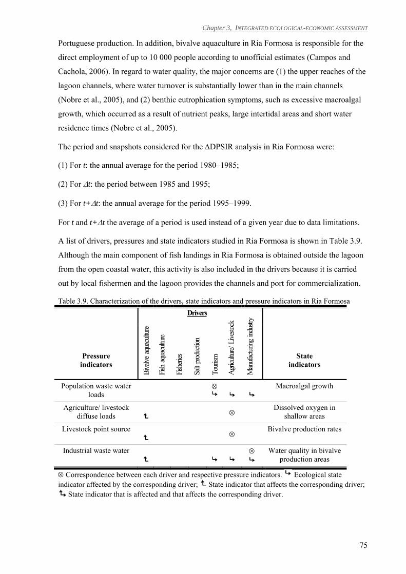
Chapter 3, INTEGRATED ECOLOGICAL-ECONOMIC ASSESSMENT
75
Portuguese production. In addition, bivalve aquaculture in Ria Formosa is responsible for the
direct employment of up to 10 000 people according to unofficial estimates (Campos and
Cachola, 2006). In regard to water quality, the major concerns are (1) the upper reaches of the
lagoon channels, where water turnover is substantially lower than in the main channels
(Nobre et al., 2005), and (2) benthic eutrophication symptoms, such as excessive macroalgal
growth, which occurred as a result of nutrient peaks, large intertidal areas and short water
residence times (Nobre et al., 2005).
The period and snapshots considered for the ∆DPSIR analysis in Ria Formosa were:
(1) For t: the annual average for the period 1980–1985;
(2) For ∆t: the period between 1985 and 1995;
(3) For t+∆t: the annual average for the period 1995–1999.
For t and t+∆t the average of a period is used instead of a given year due to data limitations.
A list of drivers, pressures and state indicators studied in Ria Formosa is shown in Table 3.9.
Although the main component of fish landings in Ria Formosa is obtained outside the lagoon
from the open coastal water, this activity is also included in the drivers because it is carried
out by local fishermen and the lagoon provides the channels and port for commercialization.
Table 3.9. Characterization of the drivers, state indicators and pressure indicators in Ria Formosa
Pressure indicators
Biva
lve a
quac
ulture
Fish
aqua
cultu
re
Drivers
Agric
ulture
/ Live
stock
Man
ufactu
ring
indus
try
State indicators
Fishe
ries
Salt
produ
ction
Touri
sm
Population waste water loads ⊗
Macroalgal growth
Agriculture/ livestock diffuse loads
⊗ Dissolved oxygen in
shallow areas
Livestock point source
⊗ Bivalve production rates
Industrial waste water
⊗ Water quality in bivalve
production areas
⊗ Correspondence between each driver and respective pressure indicators. Ecological state indicator affected by the corresponding driver; State indicator that affects the corresponding driver;
State indicator that is affected and that affects the corresponding driver.
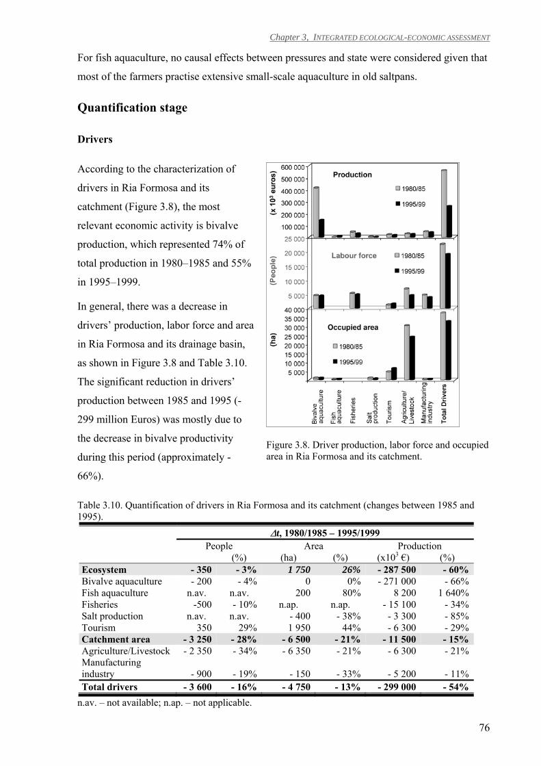
Chapter 3, INTEGRATED ECOLOGICAL-ECONOMIC ASSESSMENT
76
For fish aquaculture, no causal effects between pressures and state were considered given that
most of the farmers practise extensive small-scale aquaculture in old saltpans.
Quantification stage
Drivers
According to the characterization of
drivers in Ria Formosa and its
catchment (Figure 3.8), the most
relevant economic activity is bivalve
production, which represented 74% of
total production in 1980–1985 and 55%
in 1995–1999.
In general, there was a decrease in
drivers’ production, labor force and area
in Ria Formosa and its drainage basin,
as shown in Figure 3.8 and Table 3.10.
The significant reduction in drivers’
production between 1985 and 1995 (-
299 million Euros) was mostly due to
the decrease in bivalve productivity
during this period (approximately -
66%).
Figure 3.8. Driver production, labor force and occupied area in Ria Formosa and its catchment.
Table 3.10. Quantification of drivers in Ria Formosa and its catchment (changes between 1985 and 1995).
∆t, 1980/1985 – 1995/1999 People Area Production (%) (ha) (%) (x103 €) (%)
Ecosystem - 350 - 3% 1 750 26% - 287 500 - 60%Bivalve aquaculture - 200 - 4% 0 0% - 271 000 - 66%Fish aquaculture n.av. n.av. 200 80% 8 200 1 640%Fisheries -500 - 10% n.ap. n.ap. - 15 100 - 34%Salt production n.av. n.av. - 400 - 38% - 3 300 - 85%Tourism 350 29% 1 950 44% - 6 300 - 29%Catchment area - 3 250 - 28% - 6 500 - 21% - 11 500 - 15%Agriculture/Livestock - 2 350 - 34% - 6 350 - 21% - 6 300 - 21%Manufacturing industry - 900 - 19% - 150 - 33% - 5 200 - 11%Total drivers - 3 600 - 16% - 4 750 - 13% - 299 000 - 54%
n.av. – not available; n.ap. – not applicable.
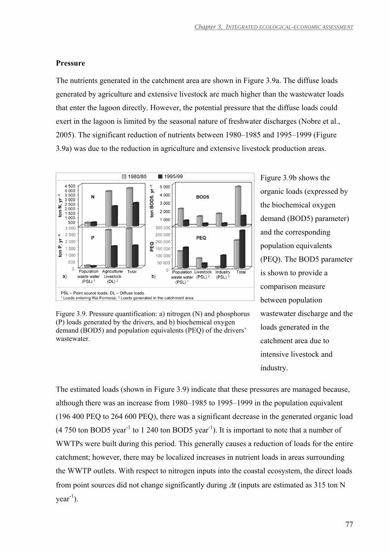
Chapter 3, INTEGRATED ECOLOGICAL-ECONOMIC ASSESSMENT
77
Pressure
The nutrients generated in the catchment area are shown in Figure 3.9a. The diffuse loads
generated by agriculture and extensive livestock are much higher than the wastewater loads
that enter the lagoon directly. However, the potential pressure that the diffuse loads could
exert in the lagoon is limited by the seasonal nature of freshwater discharges (Nobre et al.,
2005). The significant reduction of nutrients between 1980–1985 and 1995–1999 (Figure
3.9a) was due to the reduction in agriculture and extensive livestock production areas.
Figure 3.9b shows the
organic loads (expressed by
the biochemical oxygen
demand (BOD5) parameter)
and the corresponding
population equivalents
(PEQ). The BOD5 parameter
is shown to provide a
comparison measure
between population
wastewater discharge and the
loads generated in the
catchment area due to
intensive livestock and
industry.
Figure 3.9. Pressure quantification: a) nitrogen (N) and phosphorus (P) loads generated by the drivers, and b) biochemical oxygen demand (BOD5) and population equivalents (PEQ) of the drivers’ wastewater.
The estimated loads (shown in Figure 3.9) indicate that these pressures are managed because,
although there was an increase from 1980–1985 to 1995–1999 in the population equivalent
(196 400 PEQ to 264 600 PEQ), there was a significant decrease in the generated organic load
(4 750 ton BOD5 year-1 to 1 240 ton BOD5 year-1). It is important to note that a number of
WWTPs were built during this period. This generally causes a reduction of loads for the entire
catchment; however, there may be localized increases in nutrient loads in areas surrounding
the WWTP outlets. With respect to nitrogen inputs into the coastal ecosystem, the direct loads
from point sources did not change significantly during ∆t (inputs are estimated as 315 ton N
year-1).
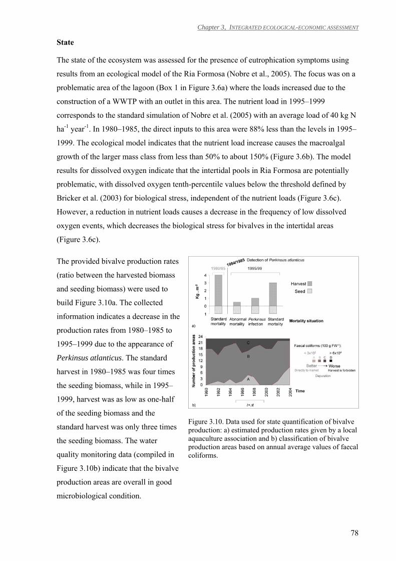
Chapter 3, INTEGRATED ECOLOGICAL-ECONOMIC ASSESSMENT
78
State
The state of the ecosystem was assessed for the presence of eutrophication symptoms using
results from an ecological model of the Ria Formosa (Nobre et al., 2005). The focus was on a
problematic area of the lagoon (Box 1 in Figure 3.6a) where the loads increased due to the
construction of a WWTP with an outlet in this area. The nutrient load in 1995–1999
corresponds to the standard simulation of Nobre et al. (2005) with an average load of 40 kg N
ha-1 year-1. In 1980–1985, the direct inputs to this area were 88% less than the levels in 1995–
1999. The ecological model indicates that the nutrient load increase causes the macroalgal
growth of the larger mass class from less than 50% to about 150% (Figure 3.6b). The model
results for dissolved oxygen indicate that the intertidal pools in Ria Formosa are potentially
problematic, with dissolved oxygen tenth-percentile values below the threshold defined by
Bricker et al. (2003) for biological stress, independent of the nutrient loads (Figure 3.6c).
However, a reduction in nutrient loads causes a decrease in the frequency of low dissolved
oxygen events, which decreases the biological stress for bivalves in the intertidal areas
(Figure 3.6c).
The provided bivalve production rates
(ratio between the harvested biomass
and seeding biomass) were used to
build Figure 3.10a. The collected
information indicates a decrease in the
production rates from 1980–1985 to
1995–1999 due to the appearance of
Perkinsus atlanticus. The standard
harvest in 1980–1985 was four times
the seeding biomass, while in 1995–
1999, harvest was as low as one-half
of the seeding biomass and the
standard harvest was only three times
the seeding biomass. The water
quality monitoring data (compiled in
Figure 3.10b) indicate that the bivalve
production areas are overall in good
microbiological condition.
Figure 3.10. Data used for state quantification of bivalve production: a) estimated production rates given by a local aquaculture association and b) classification of bivalve production areas based on annual average values of faecal coliforms.
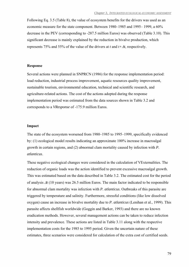
Chapter 3, INTEGRATED ECOLOGICAL-ECONOMIC ASSESSMENT
79
Following Eq. 3.5 (Table 8), the value of ecosystem benefits for the drivers was used as an
economic measure for the state component. Between 1980–1985 and 1995– 1999, a 60%
decrease in the PEV (corresponding to -287.5 million Euros) was observed (Table 3.10). This
significant decrease is mainly explained by the reduction in bivalve production, which
represents 75% and 55% of the value of the drivers at t and t+∆t, respectively.
Response
Several actions were planned in SNPRCN (1986) for the response implementation period:
load reduction, industrial process improvement, aquatic resources quality improvement,
sustainable tourism, environmental education, technical and scientific research, and
agriculture-related actions. The cost of the actions adopted during the response
implementation period was estimated from the data sources shown in Table 3.2 and
corresponds to a VResponse of -175.9 million Euros.
Impact
The state of the ecosystem worsened from 1980–1985 to 1995–1999, specifically evidenced
by: (1) ecological model results indicating an approximate 100% increase in macroalgal
growth in certain regions, and (2) abnormal clam mortality caused by infection with P.
atlanticus.
These negative ecological changes were considered in the calculation of VExternalities. The
reduction of organic loads was the action identified to prevent excessive macroalgal growth.
This was estimated based on the data described in Table 3.2. The estimated cost for the period
of analysis ∆t (10 years) was 26.5 million Euros. The main factor indicated to be responsible
for abnormal clam mortality was infection with P. atlanticus. Outbreaks of this parasite are
triggered by temperature and salinity. Furthermore, stressful conditions (like low dissolved
oxygen) cause an increase in bivalve mortality due to P. atlanticus (Lenihan et al., 1999). This
parasite affects shellfish worldwide (Goggin and Barker, 1993) and there are no known
eradication methods. However, several management actions can be taken to reduce infection
intensity and prevalence. These actions are listed in Table 3.11 along with the respective
implementation costs for the 1985 to 1995 period. Given the uncertain nature of these
estimates, three scenarios were considered for calculation of the extra cost of certified seeds.
Chapter 3, INTEGRATED ECOLOGICAL-ECONOMIC ASSESSMENT
80
Table 3.11. Possible management action costs necessary to avoid abnormal clam mortality.
Abnormal clam mortality due P. atlanticus
Actions to reduce infection intensity and prevalence Costs in 2000 constant prices (x 103 €)
Good screening of seed infection Examination and sampling costs: 41
Extra cost for buying certified seeds Scenario Cost ∆t1 All seeds from outside RF 250 000 ∆t2 Seed scarcity in RF 100 000 ∆t3 No extra costs 0
Lower population densities No implementation costs: 0
Improve D.O. in clam beds (same action as for macroalgal growth)
Reduction of nutrient loads: 26 500
Optimise conditions in depuration plants No implementation costs: 0
The salary of the workforce (estimated as 0.48 million Euros for ∆t) required to monitor the
implementation of management actions was also included for calculation of VExternalities.
Estimates of VExternalities are presented in Figure 3.11 for the three action scenarios
considered in Table 3.11.
The economic value of the impact was estimated using Eq. 3.6 (Table 3.8) and is presented in
Figure 3.11 for the three scenarios of VExternalities. VImpact assumed a negative value due
to the reduction in VDriversEcosyst and the negative value of VExternalities. The analysis of
economic impact indicates that expenditure of the value estimated in VExternalities may have
reduced the economic loss of bivalve production, which, according to Table 3.10, represents
94% of the estimated losses of VDriversEcosyst.
VExternalities represents
between 49% (in scenario ∆t1) to
9% (in scenario ∆t3) of VImpact
(Figure 3.11). These estimates
indicate that if 49% (in scenario
∆t1) to 9% (in scenario ∆t3) of
the value of the economic impact
had been spent, the loss of
ecological value during ∆t may
have been reduced to a range
between 51% (in scenario ∆t1)
and 91% (in scenario ∆t3).
Figure 3.11 ∆DPSIR results in ∆t: VImpact for the three scenarios considered for the calculation of VExternalities as defined in Table 3.11.
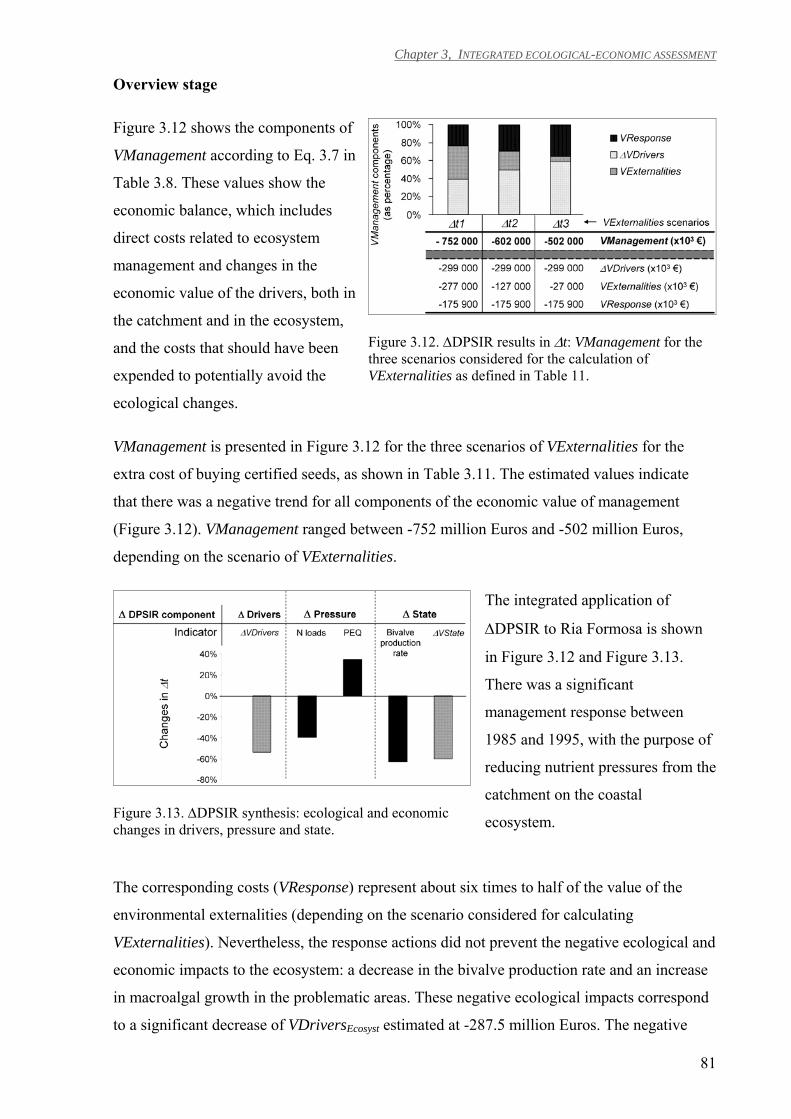
Chapter 3, INTEGRATED ECOLOGICAL-ECONOMIC ASSESSMENT
81
Overview stage
Figure 3.12 shows the components of
VManagement according to Eq. 3.7 in
Table 3.8. These values show the
economic balance, which includes
direct costs related to ecosystem
management and changes in the
economic value of the drivers, both in
the catchment and in the ecosystem,
and the costs that should have been
expended to potentially avoid the
ecological changes.
Figure 3.12. ∆DPSIR results in ∆t: VManagement for the three scenarios considered for the calculation of VExternalities as defined in Table 11.
VManagement is presented in Figure 3.12 for the three scenarios of VExternalities for the
extra cost of buying certified seeds, as shown in Table 3.11. The estimated values indicate
that there was a negative trend for all components of the economic value of management
(Figure 3.12). VManagement ranged between -752 million Euros and -502 million Euros,
depending on the scenario of VExternalities.
The integrated application of
∆DPSIR to Ria Formosa is shown
in Figure 3.12 and Figure 3.13.
There was a significant
management response between
1985 and 1995, with the purpose of
reducing nutrient pressures from the
catchment on the coastal
ecosystem. Figure 3.13. ∆DPSIR synthesis: ecological and economic changes in drivers, pressure and state.
The corresponding costs (VResponse) represent about six times to half of the value of the
environmental externalities (depending on the scenario considered for calculating
VExternalities). Nevertheless, the response actions did not prevent the negative ecological and
economic impacts to the ecosystem: a decrease in the bivalve production rate and an increase
in macroalgal growth in the problematic areas. These negative ecological impacts correspond
to a significant decrease of VDriversEcosyst estimated at -287.5 million Euros. The negative
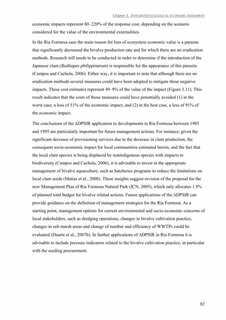
Chapter 3, INTEGRATED ECOLOGICAL-ECONOMIC ASSESSMENT
82
economic impacts represent 80–220% of the response cost, depending on the scenario
considered for the value of the environmental externalities.
In the Ria Formosa case the main reason for loss of ecosystem economic value is a parasite
that significantly decreased the bivalve production rate and for which there are no eradication
methods. Research still needs to be conducted in order to determine if the introduction of the
Japanese clam (Ruditapes philippinarum) is responsible for the appearance of this parasite
(Campos and Cachola, 2006). Either way, it is important to note that although there are no
eradication methods several measures could have been adopted to mitigate these negative
impacts. These cost estimates represent 49–9% of the value of the impact (Figure 3.11). This
result indicates that the costs of those measures could have potentially avoided (1) in the
worst case, a loss of 51% of the economic impact, and (2) in the best case, a loss of 91% of
the economic impact.
The conclusions of the ∆DPSIR application to developments in Ria Formosa between 1985
and 1995 are particularly important for future management actions. For instance, given the
significant decrease of provisioning services due to the decrease in clam production, the
consequent socio-economic impact for local communities estimated herein, and the fact that
the local clam species is being displaced by nonindigenous species with impacts to
biodiversity (Campos and Cachola, 2006), it is advisable to invest in the appropriate
management of bivalve aquaculture, such as hatcheries programs to reduce the limitations on
local clam seeds (Matias et al., 2008). These insights suggest revision of the proposal for the
new Management Plan of Ria Formosa Natural Park (ICN, 2005), which only allocates 1.9%
of planned total budget for bivalve related actions. Future applications of the ∆DPSIR can
provide guidance on the definition of management strategies for the Ria Formosa. As a
starting point, management options for current environmental and socio-economic concerns of
local stakeholders, such as dredging operations, changes in bivalve cultivation practice,
changes in salt marsh areas and change of number and efficiency of WWTPs could be
evaluated (Duarte et al., 2007b). In further applications of ∆DPSIR in Ria Formosa it is
advisable to include pressure indicators related to the bivalve cultivation practice, in particular
with the seeding procurement.
Chapter 3, INTEGRATED ECOLOGICAL-ECONOMIC ASSESSMENT
83
CONCLUSIONS
The ∆DPSIR framework is a powerful tool for integrated coastal management that can
support realistic decision-making that accounts for the value of the environmental
externalities. It can be particularly useful for the evaluation of management and policy
scenarios according to cost and effectiveness criteria. The ∆DPSIR approach includes key
concepts for an integrated ecosystem analysis, namely: (1) explicit simulation of the link
between ecological and economic systems, and (2) inclusion of a temporal component for
comparison of the ecosystem in t and t+∆t, which is crucial for the assessment of the benefits
and impacts of the ecosystem. This approach allows for an analysis of the economic
consequences of changes in environmental quality. In addition, the ∆DPSIR approach may
stimulate discussion of possible links between management and science, which is required for
sound decision-making and contributes to a better understanding of the management/science
scale paradox.
Application of the ∆DPSIR was illustrated through an analysis of developments in the Ria
Formosa coastal lagoon between 1985 and 1995. The value of economic activities dependent
on the lagoon suffered a significant reduction (ca. –60%) over that period, mainly due to a
decrease in bivalve production. During that decade the pressures from the catchment area
were managed (ca. 176 million Euros), mainly through the building of WWTP’s.
Nevertheless, the ecosystem state worsened with respect to abnormal clam mortalities due to a
parasite infection and to benthic eutrophication symptoms in specific problematic areas. The
negative economic impacts during the decade were estimated between -565 and -315 million
Euros of which 9–49% represent the cost of the environmental externalities. The evaluation of
past developments suggests that future management actions should focus on reducing the
limitation on local clam (Ruditapes decussatus) seeds, with positive impacts expected for both
the socio-economy of the local population as well on biodiversity.
The ∆DPSIR should be applied to a range of ecosystems with different problems and different
levels of monitoring in order to ascertain its usefulness and to compare the results. Further
validation of this approach is necessary to verify its ability to consistently translate ecological
and economic outputs into information that is useful to managers. Furthermore, future work
should include the development of a social component for the ∆DPSIR in order to monitor
changes in social indicators, such as employment and per capita income, which result from
implementation of the policies or changes in economic activity.

Chapter 3, INTEGRATED ECOLOGICAL-ECONOMIC ASSESSMENT
84
Chapter 4. Ecosystem approach to aquaculture
Context
The aquaculture industry is an important socio-economic activity: (i) it is one of the fastest
growing animal food-producing industries (6.1 % increase from 2004 to 2006 – FAO, 2009),
(ii) it contributes for food security, particularly in developing countries (Ahmed and Lorica,
2002; Kaliba et al., 2007), and (iii) it can generate employment and other economic benefits
for local communities (Ahmed and Lorica, 2002; Kaliba et al., 2007). Aquaculture is expected
to increase to meet increasing demand for fish, given the strong likelihood that wild fisheries
will remain stagnant (FAO, 2009). However, aquaculture production is slowing (FAO, 2009).
The development of sustainable aquaculture calls for an integrated ecosystem approach (FAO,
2007; Soto et al., 2008), known as the ecosystem approach to aquaculture (EAA, as explained
in Chapter 1). EAA considers three scales of analysis: (i) the waterbody/watershed level, (ii)
the individual farm level, and (iii) the global market-trade level.
Summary
This chapter uses the methodologies developed in chapters 2 and 3 to illustrate their
application to EAA at two of the relevant levels of analysis. The first part of this chapter uses
the ∆DPSIR approach to carry out an ecological-economic assessment, at the
waterbody/watershed level, of the scenarios simulated with the multilayered ecosystem
model. The second part provides a detailed ecological-economic analysis of aquaculture
options at the farm level, by means of the ∆DPSIR.
4.1 Waterbody/watershed level assessment: evaluation of model scenarios
Context
The analysis of aquaculture at the ecosystem level is essential, primarly, because of the
feedbacks between this industry and coastal ecosystem. For instance, production depends on
the good condition of the ecosystem, which aquaculture itself may compromise (GESAMP,
2001; Islam, 2005). Second, an ecosystem-level analysis is required because coastal
ecosystems are characterised by complex ecological interactions and are subject to a
multiplicity of driving forces generated in the catchment, inside the waterbody and also from
the sea boundary (Ferreira et al., 2008a).
Summary
Chapter 2 presents the multilayered ecosystem model for simulating the cumulative impacts
of multiple uses of coastal zones. Chapter 3 describes the ∆DPSIR methodology developed
for the ecological-economic assessment of the effectiveness of coastal management actions.
In this chapter, the multilayered ecosystem model and the ∆DPSIR are applied together, with
the objective of synthesising the scenario simulation outputs into useful information for
sustainable aquaculture development at the ecosystem level. Furthermore, this chapter extends
the ∆DPSIR testing carried out in Chapter 3 by using it to evaluate management scenarios, as
opposed to evaluation of past management responses by means of data analysis.
Chapter 4.1, ECOSYSTEM APPROACH TO AQUACULTURE: WATERBODY/WATERSHED LEVEL
87
Integrated environmental modelling and assessment of coastal ecosystems, application for aquaculture management
INTRODUCTION
Sustainable use and development of coastal areas represent a challenge to coastal managers as
detailed in the Chapter 1. As discussed previously, in chapters 1 and 2, ecological modelling
is a powerful tool to assist coastal management. In many integrated environmental
assessments (IEA’s), not specifically related with coastal management, a large effort focused
on development of simulation models (Peirce, 1998). IEA consists on the interdisciplinary
synthesis of scientific knowledge to provide insight regarding complex phenomena, namely to
guide on decision-making and policy development to address environmental problems and for
ecological resources management (Peirce, 1998; Toth and Hizsnyik, 1998). There are many
possible roles for models in IEA, as for instance: (i) understanding behaviour of complex
system; (ii) scenarios analysis; and (iii) quantifying uncertainty of integrated assessment
(Peirce, 1998). A wide range of models exist whereby the spatial and temporal resolutions, the
features of the system included in the model and the level of detail at which they are
simulated, the computational and numeric complexity are adapted to the specific needs of
each case (as further discussed in Chapter 2). Integrated assessment and modelling is required
in order to adopt a comprehensive analysis of the system including its feedbacks (Harris,
2002). To be useful for managers, independently of the complexity degree of model, the
generated outputs need to be translated into meaningful information to managers and other
stakeholders (Harris, 2002; Nobre et al., 2005). For instance while there are many coastal
ecosystem models, few efforts exist for communicating its output for managers with concrete
solutions for coastal problems. For that purpose a multidisciplinary approach that synthesises
scientific-based information to managers is required.
IEA frameworks are normally applied for organizing and structuring information to facilitate
analysis and assessment of environmental data (Stanners et al., 2008). IEA can also be used to
analyse and synthesise ecological models into meaningful information for coastal managers.
For instance, Liu et al. (2008) proposes a framework to make integrated modelling efforts
useful for managers; whereby one of the steps includes assessing and comparing impacts of
defined scenarios. The Drivers-Pressure-State-Impact-Response (DPSIR) is a conceptual IEA
approach widely used for management of coastal systems. The DPSIR was previously used to
Chapter 4.1, ECOSYSTEM APPROACH TO AQUACULTURE: WATERBODY/WATERSHED LEVEL
88
guide on reporting of catchment-coastal ecosystem models to compare nutrient loading
scenarios (Artioli et al., 2005; Hofmann et al., 2005; Salomons and Turner, 2005). This
conceptual approach establishes a causal link between (Elliott, 2002, Borja et al., 2006,
Stanners et al., 2008; Nobre, 2009): human activities (Drivers), the direct effects that these
generate (Pressures), the resulting condition of the ecosystems at a given moment in time
(State), the variation of the State of the ecosystem as a result of the Pressures during a given
time period (Impact), the management actions and policies that cause a change of the Drivers
(Response). In particular, the differential DPSIR (∆DPSIR – developed in Chapter 3)
provides an explicit link between the ecological and economic quantification of the D-P-S-I-R
components. Other set of IEA approaches is targeted to assess specific environmental issues.
For instance, the increase of visible effects of coastal eutrophication worldwide enhanced the
need for assessment tools for management of eutrophication process (Vidal et al., 1999). The
ASSETS approach (Bricker et al., 2003; 2008) exemplifies an eutrophication assessment
model applied worldwide (Whitall et al., 2007; Borja et al., 2008). This is one of US
governmental tool to guide on eutrophication management in about 140 coastal systems over
the entire US coast (Bricker et al., 2008).
The sustainability of aquaculture industry is a current challenge for managers of coastal
ecosystems and of aquatic resources. While better management practices must be
implemented at the farm level the analysis of the aquaculture impacts must be carried out at
the ecosystem level; mainly because the individual farm effects are cumulative in relation to
other farms in the same ecosystem and to other coastal activities (GESAMP, 2001; Soto et al.,
2008). The use of simulation models coupled with IEA approaches can be particularly
important for mariculture managers to adopt the emerging concept of an ecosystem approach
to aquaculture (EAA – FAO, 2007; Soto et al., 2008). Firstly, simulation models provide
understanding about coastal ecosystems and interactions with aquaculture activities. For
instance McKindsey et al. (2006) and Ferreira et al. (2008a) illustrate the importance of using
ecosystem models for determining aquaculture carrying capacity. Particularly important are
integrated modelling approaches, such as the multilayered ecosystem model developed in
Chapter 2 that allows for the assessment of cumulative impacts of coastal activities at the
ecosystem level. Secondly, the IEA approaches are useful to distil the generated outputs to
managers and to compare the impacts estimated due to simulated management scenarios. For
instance, the simulated effects of changes of nutrient loading into a shallow lagoon are
synthesised concerning eutrophication status using the ASSETS screening model (Nobre et
al., 2005). The nutrient loading into coastal systems from fish wastes represents an important
Chapter 4.1, ECOSYSTEM APPROACH TO AQUACULTURE: WATERBODY/WATERSHED LEVEL
89
aquaculture related problem to be tackled, since not only is it an eutrophication source
compromising water quality but also limits the expansion of aquaculture itself (Islam, 2005).
Therefore, the application of a similar approach to investigate impacts of scenarios designed
to manage fish aquaculture wastes is highly relevant for EAA. Furthermore, the use of an IEA
approach such as the ∆DPSIR can extend the scenario analysis by assessing both the
ecological and economic impacts of the management options.
The overall aim of this chapter is to present an approach that couples coastal ecosystem
modelling with integrated environmental assessment methodologies. The focus of this work is
to support the development of an ecosystem approach to aquaculture management including
interactions with substance loading from the watershed. The integrated environmental
modelling and assessment approach is illustrated using the Xiangshan Gang, China. The
simulated scenarios defined by the bay stakeholders as described in Chapter 2 are herein
analysed and compared using the ∆DPSIR developed in Chapter 3. The objectives of this
work are to: (i) assess the eutrophication condition of a coastal bay and analyse the impacts of
simulated scenarios on bay eutrophic state; (ii) assess the ecological and economic impacts of
the management scenarios; and (iii) provide information about the adoption of an EAA and
about options for sustainable coastal management of the bay.
METHODOLOGY
General approach
The integrated environmental modelling and assessment approach consists in using IEA
methodologies to evaluate ecosystem model outputs for different scenarios (Figure 4.1). For
this work the outputs of the multilayered ecosystem model developed in Chapter 2 are used.
The model runs include simulation of scenarios that comprise changes of aquaculture and
catchment pressure.
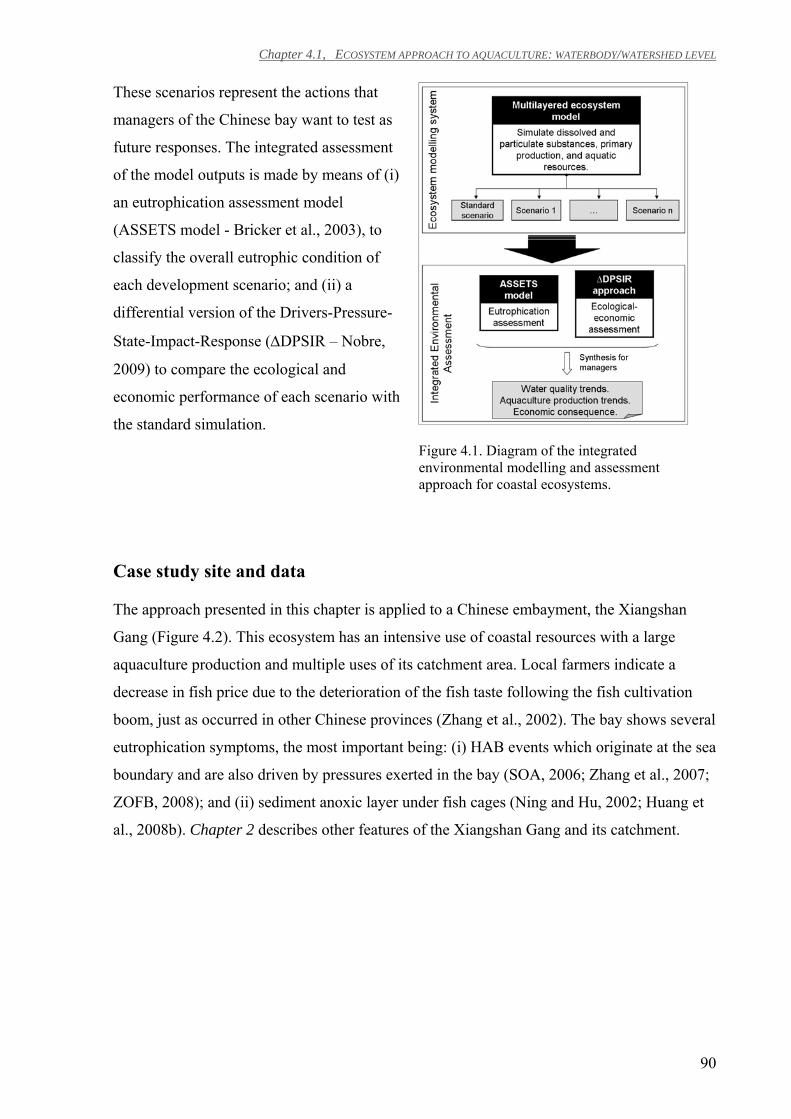
Chapter 4.1, ECOSYSTEM APPROACH TO AQUACULTURE: WATERBODY/WATERSHED LEVEL
90
These scenarios represent the actions that
managers of the Chinese bay want to test as
future responses. The integrated assessment
of the model outputs is made by means of (i)
an eutrophication assessment model
(ASSETS model - Bricker et al., 2003), to
classify the overall eutrophic condition of
each development scenario; and (ii) a
differential version of the Drivers-Pressure-
State-Impact-Response (∆DPSIR – Nobre,
2009) to compare the ecological and
economic performance of each scenario with
the standard simulation.
Figure 4.1. Diagram of the integrated environmental modelling and assessment approach for coastal ecosystems.
Case study site and data
The approach presented in this chapter is applied to a Chinese embayment, the Xiangshan
Gang (Figure 4.2). This ecosystem has an intensive use of coastal resources with a large
aquaculture production and multiple uses of its catchment area. Local farmers indicate a
decrease in fish price due to the deterioration of the fish taste following the fish cultivation
boom, just as occurred in other Chinese provinces (Zhang et al., 2002). The bay shows several
eutrophication symptoms, the most important being: (i) HAB events which originate at the sea
boundary and are also driven by pressures exerted in the bay (SOA, 2006; Zhang et al., 2007;
ZOFB, 2008); and (ii) sediment anoxic layer under fish cages (Ning and Hu, 2002; Huang et
al., 2008b). Chapter 2 describes other features of the Xiangshan Gang and its catchment.
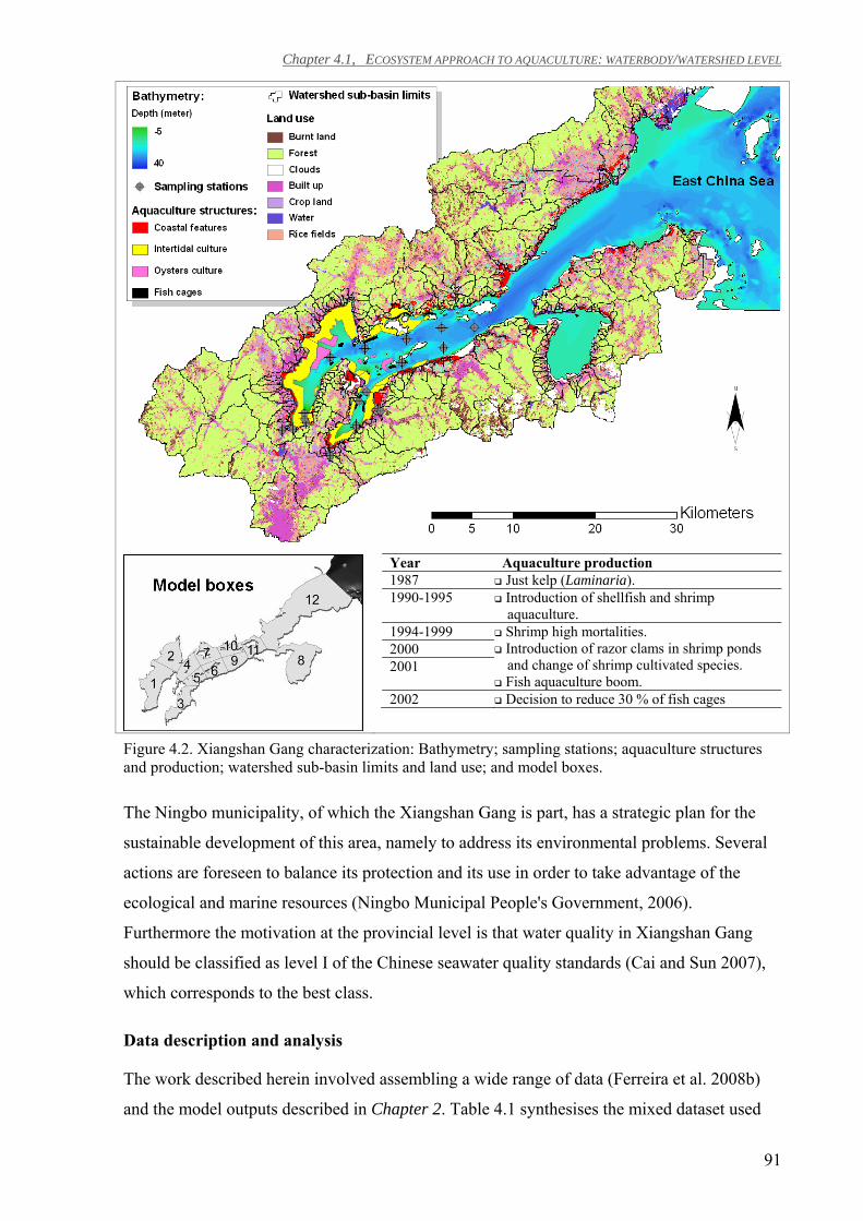
Chapter 4.1, ECOSYSTEM APPROACH TO AQUACULTURE: WATERBODY/WATERSHED LEVEL
91
Year Aquaculture production 1987 Just kelp (Laminaria). 1990-1995 Introduction of shellfish and shrimp
aquaculture. 1994-1999 Shrimp high mortalities.
Introduction of razor clams in shrimp ponds and change of shrimp cultivated species.
Fish aquaculture boom.
2000 2001
2002 Decision to reduce 30 % of fish cages
Figure 4.2. Xiangshan Gang characterization: Bathymetry; sampling stations; aquaculture structures and production; watershed sub-basin limits and land use; and model boxes.
The Ningbo municipality, of which the Xiangshan Gang is part, has a strategic plan for the
sustainable development of this area, namely to address its environmental problems. Several
actions are foreseen to balance its protection and its use in order to take advantage of the
ecological and marine resources (Ningbo Municipal People's Government, 2006).
Furthermore the motivation at the provincial level is that water quality in Xiangshan Gang
should be classified as level I of the Chinese seawater quality standards (Cai and Sun 2007),
which corresponds to the best class.
Data description and analysis
The work described herein involved assembling a wide range of data (Ferreira et al. 2008b)
and the model outputs described in Chapter 2. Table 4.1 synthesises the mixed dataset used
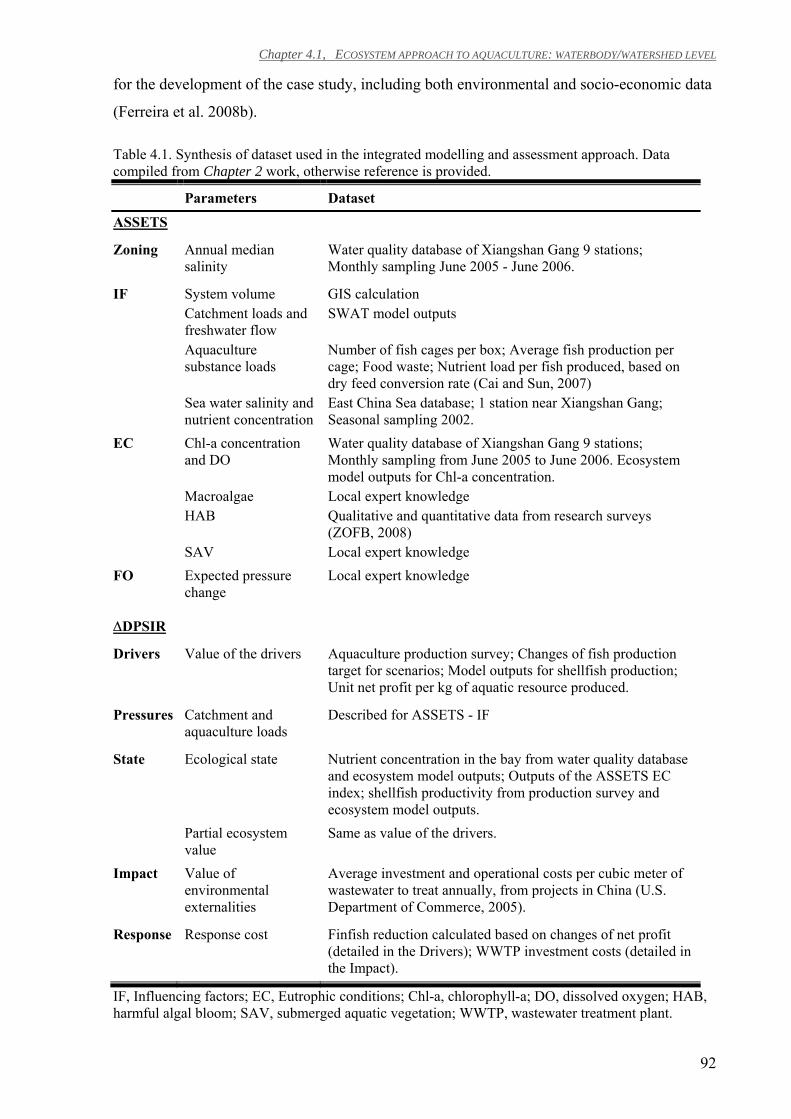
Chapter 4.1, ECOSYSTEM APPROACH TO AQUACULTURE: WATERBODY/WATERSHED LEVEL
92
for the development of the case study, including both environmental and socio-economic data
(Ferreira et al. 2008b).
Table 4.1. Synthesis of dataset used in the integrated modelling and assessment approach. Data compiled from Chapter 2 work, otherwise reference is provided.
Parameters Dataset
ASSETS
Zoning Annual median salinity
Water quality database of Xiangshan Gang 9 stations; Monthly sampling June 2005 - June 2006.
IF System volume GIS calculation Catchment loads and
freshwater flow SWAT model outputs
Aquaculture substance loads
Number of fish cages per box; Average fish production per cage; Food waste; Nutrient load per fish produced, based on dry feed conversion rate (Cai and Sun, 2007)
Sea water salinity and nutrient concentration
East China Sea database; 1 station near Xiangshan Gang; Seasonal sampling 2002.
EC Chl-a concentration and DO
Water quality database of Xiangshan Gang 9 stations; Monthly sampling from June 2005 to June 2006. Ecosystem model outputs for Chl-a concentration.
Macroalgae Local expert knowledge HAB Qualitative and quantitative data from research surveys
(ZOFB, 2008) SAV Local expert knowledge FO Expected pressure
change Local expert knowledge
∆DPSIR
Drivers Value of the drivers Aquaculture production survey; Changes of fish production target for scenarios; Model outputs for shellfish production; Unit net profit per kg of aquatic resource produced.
Pressures Catchment and aquaculture loads
Described for ASSETS - IF
State Ecological state Nutrient concentration in the bay from water quality database and ecosystem model outputs; Outputs of the ASSETS EC index; shellfish productivity from production survey and ecosystem model outputs.
Partial ecosystem value
Same as value of the drivers.
Impact Value of environmental externalities
Average investment and operational costs per cubic meter of wastewater to treat annually, from projects in China (U.S. Department of Commerce, 2005).
Response Response cost Finfish reduction calculated based on changes of net profit (detailed in the Drivers); WWTP investment costs (detailed in the Impact).
IF, Influencing factors; EC, Eutrophic conditions; Chl-a, chlorophyll-a; DO, dissolved oxygen; HAB, harmful algal bloom; SAV, submerged aquatic vegetation; WWTP, wastewater treatment plant.
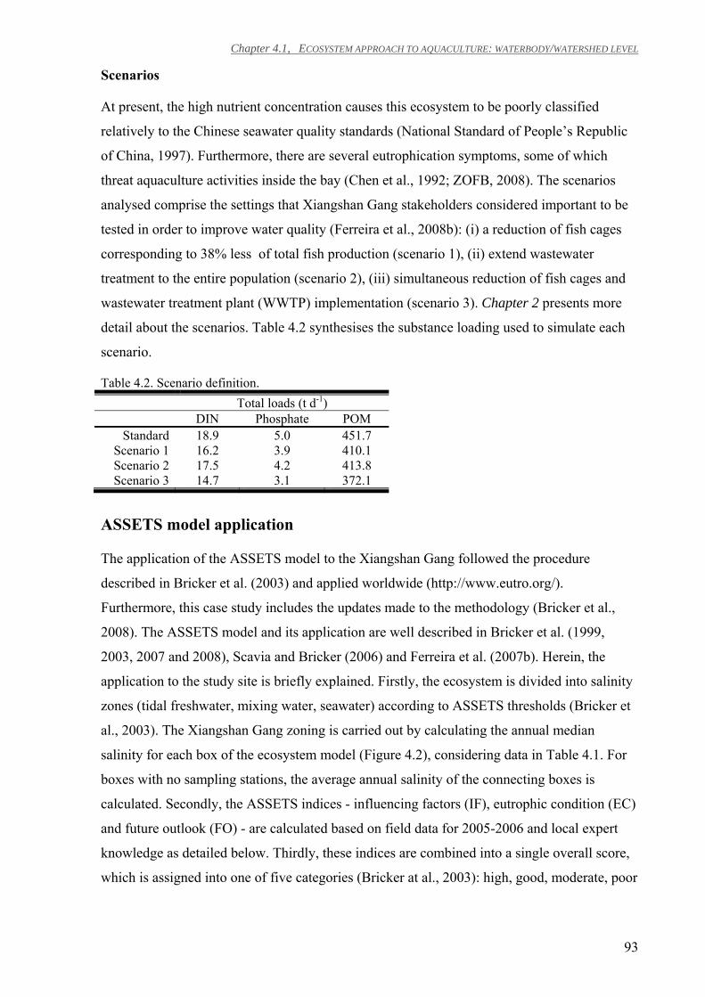
Chapter 4.1, ECOSYSTEM APPROACH TO AQUACULTURE: WATERBODY/WATERSHED LEVEL
93
Scenarios
At present, the high nutrient concentration causes this ecosystem to be poorly classified
relatively to the Chinese seawater quality standards (National Standard of People’s Republic
of China, 1997). Furthermore, there are several eutrophication symptoms, some of which
threat aquaculture activities inside the bay (Chen et al., 1992; ZOFB, 2008). The scenarios
analysed comprise the settings that Xiangshan Gang stakeholders considered important to be
tested in order to improve water quality (Ferreira et al., 2008b): (i) a reduction of fish cages
corresponding to 38% less of total fish production (scenario 1), (ii) extend wastewater
treatment to the entire population (scenario 2), (iii) simultaneous reduction of fish cages and
wastewater treatment plant (WWTP) implementation (scenario 3). Chapter 2 presents more
detail about the scenarios. Table 4.2 synthesises the substance loading used to simulate each
scenario.
Table 4.2. Scenario definition. Total loads (t d-1) DIN Phosphate POM
Standard 18.9 5.0 451.7 Scenario 1 16.2 3.9 410.1 Scenario 2 17.5 4.2 413.8 Scenario 3 14.7 3.1 372.1
ASSETS model application
The application of the ASSETS model to the Xiangshan Gang followed the procedure
described in Bricker et al. (2003) and applied worldwide (http://www.eutro.org/).
Furthermore, this case study includes the updates made to the methodology (Bricker et al.,
2008). The ASSETS model and its application are well described in Bricker et al. (1999,
2003, 2007 and 2008), Scavia and Bricker (2006) and Ferreira et al. (2007b). Herein, the
application to the study site is briefly explained. Firstly, the ecosystem is divided into salinity
zones (tidal freshwater, mixing water, seawater) according to ASSETS thresholds (Bricker et
al., 2003). The Xiangshan Gang zoning is carried out by calculating the annual median
salinity for each box of the ecosystem model (Figure 4.2), considering data in Table 4.1. For
boxes with no sampling stations, the average annual salinity of the connecting boxes is
calculated. Secondly, the ASSETS indices - influencing factors (IF), eutrophic condition (EC)
and future outlook (FO) - are calculated based on field data for 2005-2006 and local expert
knowledge as detailed below. Thirdly, these indices are combined into a single overall score,
which is assigned into one of five categories (Bricker at al., 2003): high, good, moderate, poor
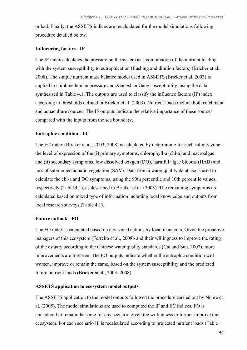
Chapter 4.1, ECOSYSTEM APPROACH TO AQUACULTURE: WATERBODY/WATERSHED LEVEL
94
or bad. Finally, the ASSETS indices are recalculated for the model simulations following
procedure detailed below.
Influencing factors - IF
The IF index calculates the pressure on the system as a combination of the nutrient loading
with the system susceptibility to eutrophication (flushing and dilution factors) (Bricker at al.,
2008). The simple nutrient mass balance model used in ASSETS (Bricker et al. 2003) is
applied to combine human pressure and Xiangshan Gang susceptibility, using the data
synthesised in Table 4.1. The outputs are used to classify the influence factors (IF) index
according to thresholds defined in Bricker et al. (2003). Nutrient loads include both catchment
and aquaculture sources. The IF outputs indicate the relative importance of these sources
compared with the inputs from the sea boundary.
Eutrophic condition - EC
The EC index (Bricker at al., 2003; 2008) is calculated by determining for each salinity zone
the level of expression of the (i) primary symptoms, chlorophyll-a (chl-a) and macroalgae;
and (ii) secondary symptoms, low dissolved oxygen (DO), harmful algae blooms (HAB) and
loss of submerged aquatic vegetation (SAV). Data from a water quality database is used to
calculate the chl-a and DO symptoms, using the 90th percentile and 10th percentile values,
respectively (Table 4.1), as described in Bricker et al. (2003). The remaining symptoms are
calculated based on mixed type of information including local knowledge and outputs from
local research surveys (Table 4.1).
Future outlook - FO
The FO index is calculated based on envisaged actions by local managers. Given the proactive
managers of this ecosystem (Ferreira et al., 2008b and their willingness to improve the rating
of the estuary according to the Chinese water quality standards (Cai and Sun, 2007), more
improvements are foreseen. The FO outputs indicate whether the eutrophic condition will
worsen, improve or remain the same, based on the system susceptibility and the predicted
future nutrient loads (Bricker at al., 2003; 2008).
ASSETS application to ecosystem model outputs
The ASSETS application to the model outputs followed the procedure carried out by Nobre et
al. (2005). The model simulations are used to computed the IF and EC indices. FO is
considered to remain the same for any scenario given the willingness to further improve this
ecosystem. For each scenario IF is recalculated according to projected nutrient loads (Table
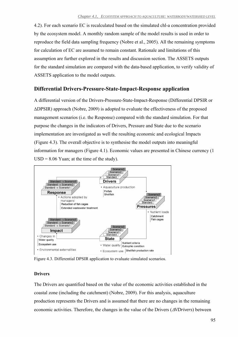
Chapter 4.1, ECOSYSTEM APPROACH TO AQUACULTURE: WATERBODY/WATERSHED LEVEL
95
4.2). For each scenario EC is recalculated based on the simulated chl-a concentration provided
by the ecosystem model. A monthly random sample of the model results is used in order to
reproduce the field data sampling frequency (Nobre et al., 2005). All the remaining symptoms
for calculation of EC are assumed to remain constant. Rationale and limitations of this
assumption are further explored in the results and discussion section. The ASSETS outputs
for the standard simulation are compared with the data-based application, to verify validity of
ASSETS application to the model outputs.
Differential Drivers-Pressure-State-Impact-Response application
A differential version of the Drivers-Pressure-State-Impact-Response (Differential DPSIR or
∆DPSIR) approach (Nobre, 2009) is adopted to evaluate the effectiveness of the proposed
management scenarios (i.e. the Response) compared with the standard simulation. For that
purpose the changes in the indicators of Drivers, Pressure and State due to the scenario
implementation are investigated as well the resulting economic and ecological Impacts
(Figure 4.3). The overall objective is to synthesise the model outputs into meaningful
information for managers (Figure 4.1). Economic values are presented in Chinese currency (1
USD = 8.06 Yuan; at the time of the study).
Figure 4.3. Differential DPSIR application to evaluate simulated scenarios.
Drivers
The Drivers are quantified based on the value of the economic activities established in the
coastal zone (including the catchment) (Nobre, 2009). For this analysis, aquaculture
production represents the Drivers and is assumed that there are no changes in the remaining
economic activities. Therefore, the changes in the value of the Drivers (∆VDrivers) between
Chapter 4.1, ECOSYSTEM APPROACH TO AQUACULTURE: WATERBODY/WATERSHED LEVEL
96
the standard simulation and each scenario are quantified based on the change of the net profit
of the activities that depend on the ecosystem (∆VDriversEcosyst) while change of the value
of the activities on the catchment (∆VDriversExternal) equals to zero. The aquaculture net
profit for each scenario and standard simulation is estimated based on: (i) the fish weight
production and the simulated weight production of shellfish; and (ii) the net profit per unit
produced, which is obtained based on an aquaculture economic survey for finfish, oyster, and
clams (de Wit et al., 2008). The shellfish species simulated in the multilayered ecosystem
model are Ostrea plicatula (Chinese oyster), Sinonvacula constricta (razor clam), Tapes
philippinarum (Manila clam) and Tegillarca granosa (muddy clam), as detailed in Chapter 2.
The finfish production is a forcing function of the model that contributes with dissolved and
particulate wastes (as explained in Chapter 2). Scenarios 1 and 3 implement the change of
fish cages that managers want to test.
Pressures
The significant Pressures to monitor are the discharge of nutrients from the catchment and
aquaculture. These are estimated based on the multilayered ecosystem model developed in
Chapter 2. In order to inform managers about the significance of the loads (from an
eutrophication perspective) the outputs of the IF index of the ASSETS model are used. A high
score of IF index indicates that control measures can be adopted at the catchment-estuary
level, while a low score indicates nutrient reduction actions should be taken at a wider level or
are not manageable.
State
The ecological State corresponds to the condition of the aquatic ecosystem resulting from
both natural and anthropogenic factors. The State of the ecosystem is analysed considering
relevant environmental and ecological criteria:
(i) The nutrient (DIN and phosphate) criteria following Chinese seawater quality standards
(National Standard of People’s Republic of China, 1997). The simulated annual averages of
DIN and phosphate concentration are classified according to the thresholds defined in the
standards for these parameters. A monthly random sample of the model results for the day
time is used in order to reproduce the field data sampling frequency.
(ii) The eutrophication condition (EC) index of the ASSETS model is used for the
classification of the Xiangshan Gang eutrophic state, as detailed previously.
Chapter 4.1, ECOSYSTEM APPROACH TO AQUACULTURE: WATERBODY/WATERSHED LEVEL
97
(iii) The shellfish productivity, given as the average physical product (APP) as defined by
Jolly and Clonts (1993), is used as a proxy for the ecosystem use. APP calculation consists of
dividing the total weight of shellfish harvested by the total weight of seeding.
The calculation of the ecosystem total economic value (TEV) is beyond the scope of this
study. Herein, the partial ecosystem value (PEV) is calculated following the simple approach
of the ∆DPSIR (Nobre, 2009). The PEV corresponds to the value of the Drivers that depend
on the ecosystem (VDriversEcosyst) as calculated in the Drivers section.
Impact
The ecological Impact corresponds to the effect of the anthropogenic pressures in the State of
the ecosystem and corresponds to the changes in the State at a given time period or between
simulation scenarios (Nobre, 2009). The ecological Impact is calculated based on the
variation in the (i) nutrients classification according to the Chinese seawater quality standards,
(ii) eutrophic condition as determined with the EC index of the ASSETS model, and (iii)
shellfish productivity.
The corresponding economic Impact (Nobre, 2009) is calculated based on i) changes of the
partial ecosystem value given as the value of the Drivers that depend of the ecosystem
(VDriversEcosyst, as calculated in the Drivers section), and on ii) the value of environmental
externalities (VExternalities). The economic Impact component of the Differential DPSIR
aims to provide a measure of the direct changes on the economic activities that depend of the
ecosystem as well the indirect effects that are not captured in the those activities
(environmental externalities). In this analysis, the environmental externalities concerning the
shift from the standard simulation to each scenario correspond to the total nutrient load
reduction, due to both the fish cage reduction and the WWTP implementation. The avoided
costs for treating downstream an equivalent amount of nutrients (Farber et al., 2006)
correspond to the VExternalities. Data about several WWTP projects in China and respective
investments (Table 4.1) provided the investment and operational costs of effluent treatment.
Although the WWTP implementation represents a cost for the municipality, thus is accounted
as a Response cost, it must also be accounted here as a positive environmental externality.
The average investment and operational costs are given expressed per cubic meter (U.S.
Department of Commerce, 2005): 4 163 Yuan per cubic meter of total capacity to treat
annually and 0.7 Yuan per cubic meter of wastewater to treat, respectively. As such the fish
nutrient load reduction is converted into equivalent wastewater flow to treat annually
considering the nitrogen (N) and phosphorus (P) removal estimated for the WWTP (Ferreira
et al., 2008b): 12.3 mg N L-1 and 2.8 mg P L-1. The fish cage nutrient reduction (Table 4.2)
Chapter 4.1, ECOSYSTEM APPROACH TO AQUACULTURE: WATERBODY/WATERSHED LEVEL
98
converts into about an equivalent wastewater avoided to treat annually of 81 million m3,
considering the N load, and 66 million m3, considering the P load. A precautionary approach
is adopted, therefore the larger volume of wastewater avoided to treat is chosen. Calculation
of the investment cost per annum considered 30-year depreciation for the WWTP facility.
Response
The Response is characterised by the measures that the local stakeholders defined in each
scenario. The corresponding costs are the production losses due to reduction of the finfish
cages in scenarios 1 and 3, and the WWTP investment and operational costs in scenarios 2
and 3. It is assumed that the cost for the reduction of the fish cages is equivalent to the net
profit that would be obtained by the fish farmers if production is maintained at the standard
level. Calculation of the fish aquaculture net profit is detailed previously in the Drivers
section. The WWTP related costs are calculated based on several WWTP projects in China
and respective investments (U.S. Department of Commerce, 2005) as detailed previously in
the economic Impact section for calculation of the VExternalities.
Overview
The overall economic gain or loss in adopting each scenario (VManagement) is calculated by
means of a balance between: (i) the direct costs related to ecosystem management
(VResponse), (ii) the resulting changes in the economic value of the drivers (including only
shellfish production given that the finfish cage reduction is an adopted measure and thus is
already accounted in the VResponse), and (iii) the value of the environmental externalities
(VExternalities). This synthesis value reflects not only the Impacts caused by the simulated
Response actions on the Drivers economic value but also on the indirect value of
environmental effects, while accounts for the costs required to implement the Response.
Like any modelling exercise, the application of IEA approaches (the ASSETS and the
∆DPSIR) to interpret modelling outputs presents limitations. The most outstanding on this
particular case study regards HAB events. The ecosystem model excludes HAB simulation
due to the lack of underlying deterministic knowledge about the complexity of its causes and
its chaotic behaviour (Huppert, et al., 2005; Huang et al., 2008a). Consequently, the changes
that occur in any of the simulated scenarios regarding HAB events are not predicted.
Therefore, and based on the fact that HAB’s are occurring at least since 1992 in Xiangshan
Gang (Chen et al., 1992) it is assumed that the HAB symptom for ASSETS calculation
Chapter 4.1, ECOSYSTEM APPROACH TO AQUACULTURE: WATERBODY/WATERSHED LEVEL
99
remained constant. Likewise, the economic Impacts due to changes in aquaculture closure
owing to HAB’s are assumed to suffer no changes.
RESULTS AND DISCUSSION
Eutrophication assessment of Xiangshan Gang
Data-based application
The majority of the Xiangshan Gang classifies as seawater zone (276 km2) corresponding to
boxes 4 to 12. The remaining area (84 km2) of this coastal embayment classifies as mixing
water and corresponds to boxes 1 to 3.
Influencing Factors (IF): The influence from aquaculture and catchment loads on the bay’s
nutrient concentration is moderate high for N and high for P. These IF ratings indicate large
nutrient loads compared to the system dilution and flushing potential, which on the other hand
points towards a large potential for nutrient reduction from a catchment-bay management
perspective.
Eutrophic Condition (EC): Table 4.3 synthesises the EC calculation. For primary symptoms
problems are observed concerning the level of expression of chl-a in the mixing and seawater
zones. In the mixing zone a high level of expression is obtained given that the chl-a 90th
percentile values fall within the range for medium eutrophic conditions and that occur with a
high spatial coverage. In the seawater zone a moderate level of expression is obtained given
that two out of six stations register medium eutrophic conditions and all the remaining fall
below the 5 µg L-1 threshold. The frequency of the chl-a problems in both zones is considered
periodic, given the seasonal phytoplankton peaks observed in the bay on previous years. For
macroalgae no problems are reported since only cultivated biomass is registered in both
zones. Concerning secondary symptoms, there are no problems with low DO concentrations
given that calculated 10th percentile value for both zones are higher than the threshold
adopted as indicative of biological stress (Bricker et al., 2003). SAV symptom is ambiguous
to classify because Xiangshan Gang is a highly modified ecosystem, where most of its
intertidal and near shore area is converted into aquaculture areas, so no inferences can be done
regarding the loss of those habitats as a result of euthrophication process. On the other hand
measurements of the sediment below fish cage, carried out on research programmes in 2002,
estimate anoxic layers with an average depth of 20-30 cm and a maximum depth of 80 cm
(Ning and Hu, 2002; Huang et al., 2008b).
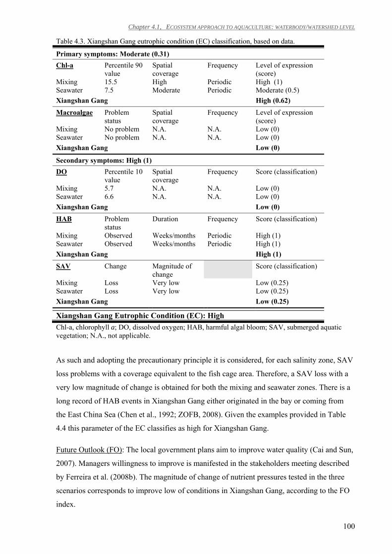
Chapter 4.1, ECOSYSTEM APPROACH TO AQUACULTURE: WATERBODY/WATERSHED LEVEL
100
Table 4.3. Xiangshan Gang eutrophic condition (EC) classification, based on data.
Primary symptoms: Moderate (0.31) Chl-a Percentile 90
value Spatial coverage
Frequency Level of expression (score)
Mixing 15.5 High Periodic High (1) Seawater 7.5 Moderate Periodic Moderate (0.5) Xiangshan Gang High (0.62)
Macroalgae Problem status
Spatial coverage
Frequency Level of expression (score)
Mixing No problem N.A. N.A. Low (0) Seawater No problem N.A. N.A. Low (0) Xiangshan Gang Low (0)
Secondary symptoms: High (1) DO Percentile 10
value Spatial coverage
Frequency Score (classification)
Mixing 5.7 N.A. N.A. Low (0) Seawater 6.6 N.A. N.A. Low (0) Xiangshan Gang Low (0)
HAB Problem status
Duration Frequency Score (classification)
Mixing Observed Weeks/months Periodic High (1) Seawater Observed Weeks/months Periodic High (1) Xiangshan Gang High (1)
SAV Change Magnitude of change
Score (classification)
Mixing Loss Very low Low (0.25) Seawater Loss Very low Low (0.25) Xiangshan Gang Low (0.25)
Xiangshan Gang Eutrophic Condition (EC): High Chl-a, chlorophyll a; DO, dissolved oxygen; HAB, harmful algal bloom; SAV, submerged aquatic vegetation; N.A., not applicable.
As such and adopting the precautionary principle it is considered, for each salinity zone, SAV
loss problems with a coverage equivalent to the fish cage area. Therefore, a SAV loss with a
very low magnitude of change is obtained for both the mixing and seawater zones. There is a
long record of HAB events in Xiangshan Gang either originated in the bay or coming from
the East China Sea (Chen et al., 1992; ZOFB, 2008). Given the examples provided in Table
4.4 this parameter of the EC classifies as high for Xiangshan Gang.
Future Outlook (FO): The local government plans aim to improve water quality (Cai and Sun,
2007). Managers willingness to improve is manifested in the stakeholders meeting described
by Ferreira et al. (2008b). The magnitude of change of nutrient pressures tested in the three
scenarios corresponds to improve low of conditions in Xiangshan Gang, according to the FO
index.
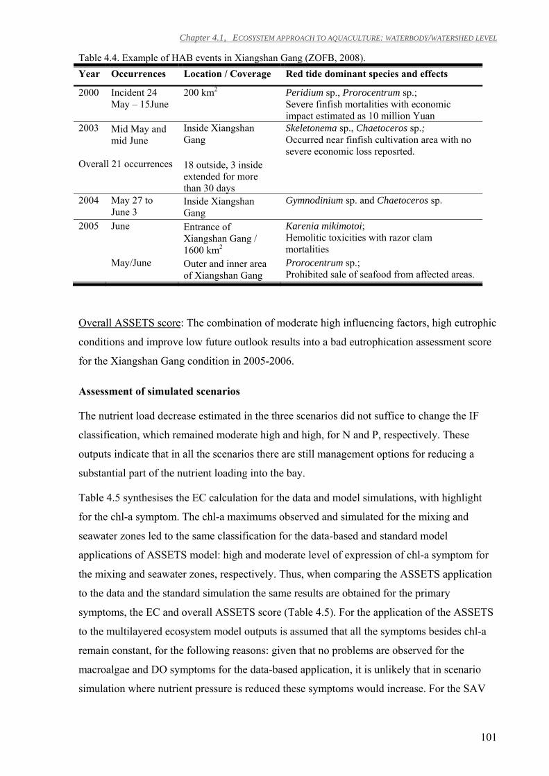
Chapter 4.1, ECOSYSTEM APPROACH TO AQUACULTURE: WATERBODY/WATERSHED LEVEL
101
Table 4.4. Example of HAB events in Xiangshan Gang (ZOFB, 2008). Year Occurrences Location / Coverage Red tide dominant species and effects
2000 Incident 24 May – 15June
200 km2 Peridium sp., Prorocentrum sp.; Severe finfish mortalities with economic impact estimated as 10 million Yuan
2003 Mid May and mid June
Inside Xiangshan Gang
Skeletonema sp., Chaetoceros sp.; Occurred near finfish cultivation area with no severe economic loss reposrted.
Overall 21 occurrences 18 outside, 3 inside extended for more than 30 days
2004 May 27 to June 3
Inside Xiangshan Gang
Gymnodinium sp. and Chaetoceros sp.
2005 June Entrance of Xiangshan Gang / 1600 km2
Karenia mikimotoi; Hemolitic toxicities with razor clam mortalities
May/June Outer and inner area of Xiangshan Gang
Prorocentrum sp.; Prohibited sale of seafood from affected areas.
Overall ASSETS score: The combination of moderate high influencing factors, high eutrophic
conditions and improve low future outlook results into a bad eutrophication assessment score
for the Xiangshan Gang condition in 2005-2006.
Assessment of simulated scenarios
The nutrient load decrease estimated in the three scenarios did not suffice to change the IF
classification, which remained moderate high and high, for N and P, respectively. These
outputs indicate that in all the scenarios there are still management options for reducing a
substantial part of the nutrient loading into the bay.
Table 4.5 synthesises the EC calculation for the data and model simulations, with highlight
for the chl-a symptom. The chl-a maximums observed and simulated for the mixing and
seawater zones led to the same classification for the data-based and standard model
applications of ASSETS model: high and moderate level of expression of chl-a symptom for
the mixing and seawater zones, respectively. Thus, when comparing the ASSETS application
to the data and the standard simulation the same results are obtained for the primary
symptoms, the EC and overall ASSETS score (Table 4.5). For the application of the ASSETS
to the multilayered ecosystem model outputs is assumed that all the symptoms besides chl-a
remain constant, for the following reasons: given that no problems are observed for the
macroalgae and DO symptoms for the data-based application, it is unlikely that in scenario
simulation where nutrient pressure is reduced these symptoms would increase. For the SAV
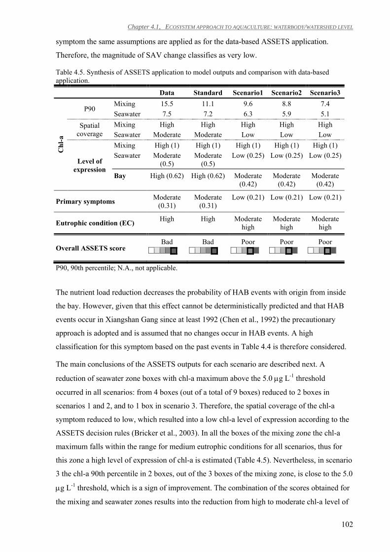
Chapter 4.1, ECOSYSTEM APPROACH TO AQUACULTURE: WATERBODY/WATERSHED LEVEL
102
symptom the same assumptions are applied as for the data-based ASSETS application.
Therefore, the magnitude of SAV change classifies as very low.
Table 4.5. Synthesis of ASSETS application to model outputs and comparison with data-based application.
Data Standard Scenario1 Scenario2 Scenario3
Chl
-a
P90 Mixing 15.5 11.1 9.6 8.8 7.4 Seawater 7.5 7.2 6.3 5.9 5.1
Spatial coverage
Mixing High High High High High Seawater Moderate Moderate Low Low Low
Level of expression
Mixing High (1) High (1) High (1) High (1) High (1) Seawater Moderate
(0.5) Moderate
(0.5) Low (0.25) Low (0.25) Low (0.25)
Bay High (0.62) High (0.62) Moderate (0.42)
Moderate (0.42)
Moderate (0.42)
Primary symptoms Moderate (0.31)
Moderate (0.31)
Low (0.21) Low (0.21) Low (0.21)
Eutrophic condition (EC) High High Moderate high
Moderate high
Moderate high
Overall ASSETS score Bad
Bad
Poor
Poor
Poor
P90, 90th percentile; N.A., not applicable.
The nutrient load reduction decreases the probability of HAB events with origin from inside
the bay. However, given that this effect cannot be deterministically predicted and that HAB
events occur in Xiangshan Gang since at least 1992 (Chen et al., 1992) the precautionary
approach is adopted and is assumed that no changes occur in HAB events. A high
classification for this symptom based on the past events in Table 4.4 is therefore considered.
The main conclusions of the ASSETS outputs for each scenario are described next. A
reduction of seawater zone boxes with chl-a maximum above the 5.0 µg L-1 threshold
occurred in all scenarios: from 4 boxes (out of a total of 9 boxes) reduced to 2 boxes in
scenarios 1 and 2, and to 1 box in scenario 3. Therefore, the spatial coverage of the chl-a
symptom reduced to low, which resulted into a low chl-a level of expression according to the
ASSETS decision rules (Bricker et al., 2003). In all the boxes of the mixing zone the chl-a
maximum falls within the range for medium eutrophic conditions for all scenarios, thus for
this zone a high level of expression of chl-a is estimated (Table 4.5). Nevertheless, in scenario
3 the chl-a 90th percentile in 2 boxes, out of the 3 boxes of the mixing zone, is close to the 5.0
µg L-1 threshold, which is a sign of improvement. The combination of the scores obtained for
the mixing and seawater zones results into the reduction from high to moderate chl-a level of
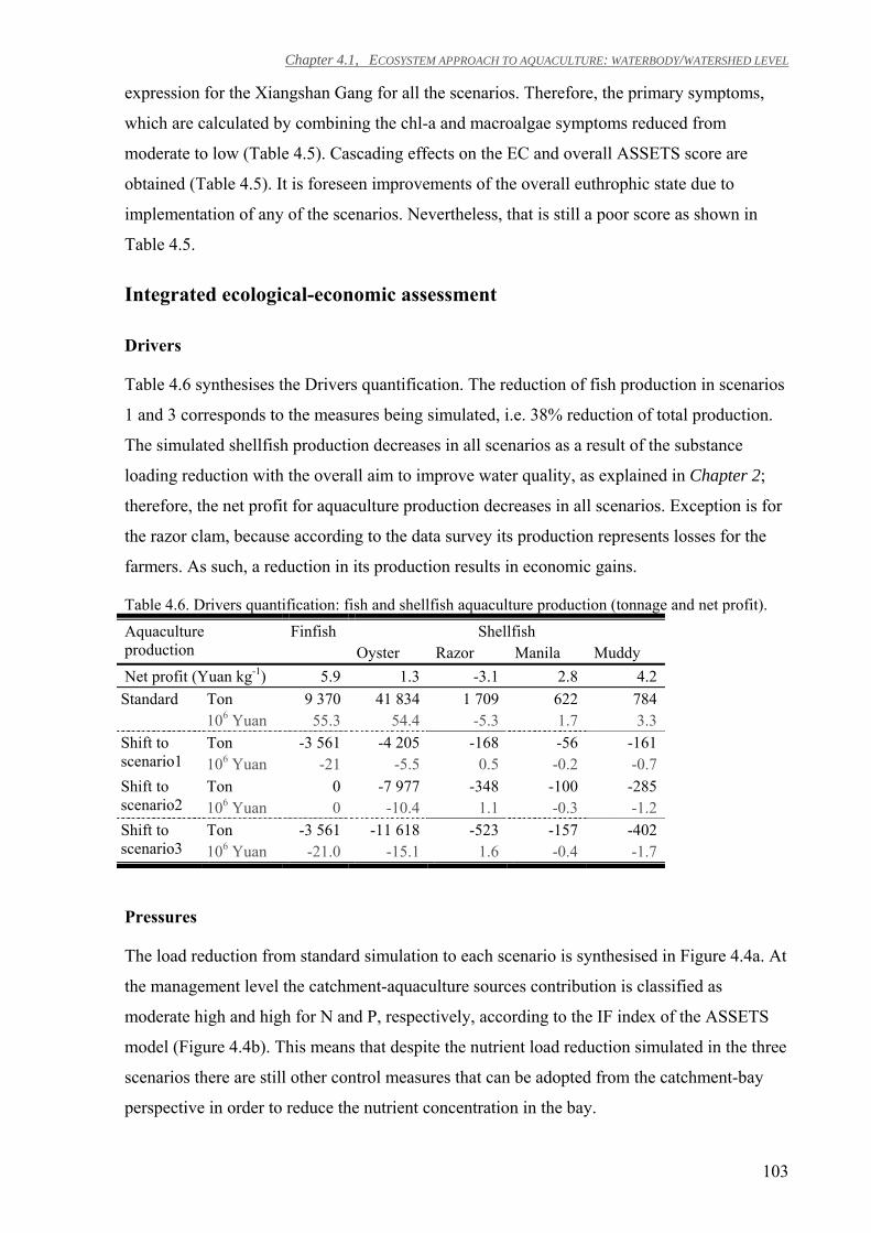
Chapter 4.1, ECOSYSTEM APPROACH TO AQUACULTURE: WATERBODY/WATERSHED LEVEL
103
expression for the Xiangshan Gang for all the scenarios. Therefore, the primary symptoms,
which are calculated by combining the chl-a and macroalgae symptoms reduced from
moderate to low (Table 4.5). Cascading effects on the EC and overall ASSETS score are
obtained (Table 4.5). It is foreseen improvements of the overall euthrophic state due to
implementation of any of the scenarios. Nevertheless, that is still a poor score as shown in
Table 4.5.
Integrated ecological-economic assessment
Drivers
Table 4.6 synthesises the Drivers quantification. The reduction of fish production in scenarios
1 and 3 corresponds to the measures being simulated, i.e. 38% reduction of total production.
The simulated shellfish production decreases in all scenarios as a result of the substance
loading reduction with the overall aim to improve water quality, as explained in Chapter 2;
therefore, the net profit for aquaculture production decreases in all scenarios. Exception is for
the razor clam, because according to the data survey its production represents losses for the
farmers. As such, a reduction in its production results in economic gains.
Table 4.6. Drivers quantification: fish and shellfish aquaculture production (tonnage and net profit).
Aquaculture production
Finfish Shellfish Oyster Razor Manila Muddy
Net profit (Yuan kg-1) 5.9 1.3 -3.1 2.8 4.2 Standard Ton 9 370 41 834 1 709 622 784
106 Yuan 55.3 54.4 -5.3 1.7 3.3 Shift to scenario1
Ton -3 561 -4 205 -168 -56 -161 106 Yuan -21 -5.5 0.5 -0.2 -0.7
Shift to scenario2
Ton 0 -7 977 -348 -100 -285 106 Yuan 0 -10.4 1.1 -0.3 -1.2
Shift to scenario3
Ton -3 561 -11 618 -523 -157 -402 106 Yuan -21.0 -15.1 1.6 -0.4 -1.7
Pressures
The load reduction from standard simulation to each scenario is synthesised in Figure 4.4a. At
the management level the catchment-aquaculture sources contribution is classified as
moderate high and high for N and P, respectively, according to the IF index of the ASSETS
model (Figure 4.4b). This means that despite the nutrient load reduction simulated in the three
scenarios there are still other control measures that can be adopted from the catchment-bay
perspective in order to reduce the nutrient concentration in the bay.
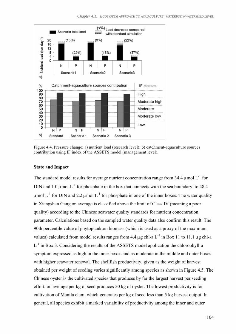
Chapter 4.1, ECOSYSTEM APPROACH TO AQUACULTURE: WATERBODY/WATERSHED LEVEL
104
Figure 4.4. Pressure change: a) nutrient load (research level); b) catchment-aquaculture sources contribution using IF index of the ASSETS model (management level).
State and Impact
The standard model results for average nutrient concentration range from 34.4 µmol L-1 for
DIN and 1.0 µmol L-1 for phosphate in the box that connects with the sea boundary, to 48.4
µmol L-1 for DIN and 2.2 µmol L-1 for phosphate in one of the inner boxes. The water quality
in Xiangshan Gang on average is classified above the limit of Class IV (meaning a poor
quality) according to the Chinese seawater quality standards for nutrient concentration
parameter. Calculations based on the sampled water quality data also confirm this result. The
90th percentile value of phytoplankton biomass (which is used as a proxy of the maximum
values) calculated from model results ranges from 4.4 µg chl-a L-1 in Box 11 to 11.1 µg chl-a
L-1 in Box 3. Considering the results of the ASSETS model application the chlorophyll-a
symptom expressed as high in the inner boxes and as moderate in the middle and outer boxes
with higher seawater renewal. The shellfish productivity, given as the weight of harvest
obtained per weight of seeding varies significantly among species as shown in Figure 4.5. The
Chinese oyster is the cultivated species that produces by far the largest harvest per seeding
effort, on average per kg of seed produces 20 kg of oyster. The lowest productivity is for
cultivation of Manila clam, which generates per kg of seed less than 5 kg harvest output. In
general, all species exhibit a marked variability of productivity among the inner and outer
Chapter 4.1, ECOSYSTEM APPROACH TO AQUACULTURE: WATERBODY/WATERSHED LEVEL
105
boxes (Figure 4.5). The Chinese oyster productivity, for instance, varies from 14, in Box 1, to
40, in Box 12. An exception is for instance the Manila clam. The highest productivity occurs
in Box 3 (ca. 6), which is even slightly higher than in Box 10.
Figure 4.5. Shellfish productivity per box expressed as the average physical product (APP: ratio of total weight of shellfish harvested to total weight of seeding), for Chinese oyster, razor clam, Manila clam and muddy clam.
The change of the ecosystem State predicted in each scenario when compared with the
standard simulation corresponds to the ecological Impact and is detailed herein. The State
classification per box is shown in Figure 4.6 for the standard simulation and each scenario,
thus providing an image of the State evolution regarding the nutrients and chl-a criteria. The
simulated actions had a limited Impact on the State classification regarding nutrient
concentration in the bay. No changes are estimated for DIN. For phosphate there are
improvements with implementation of scenario 3 in boxes 6 and 12, which shifted into Class
IV and into Class II/III, respectively, when compared with standard simulation (Figure 4.6).
Nevertheless, and more important than to estimate the Impact of nutrient load reduction in the
bay nutrient concentration is to examine the eutrophication symptoms (Bricker et al., 2003).
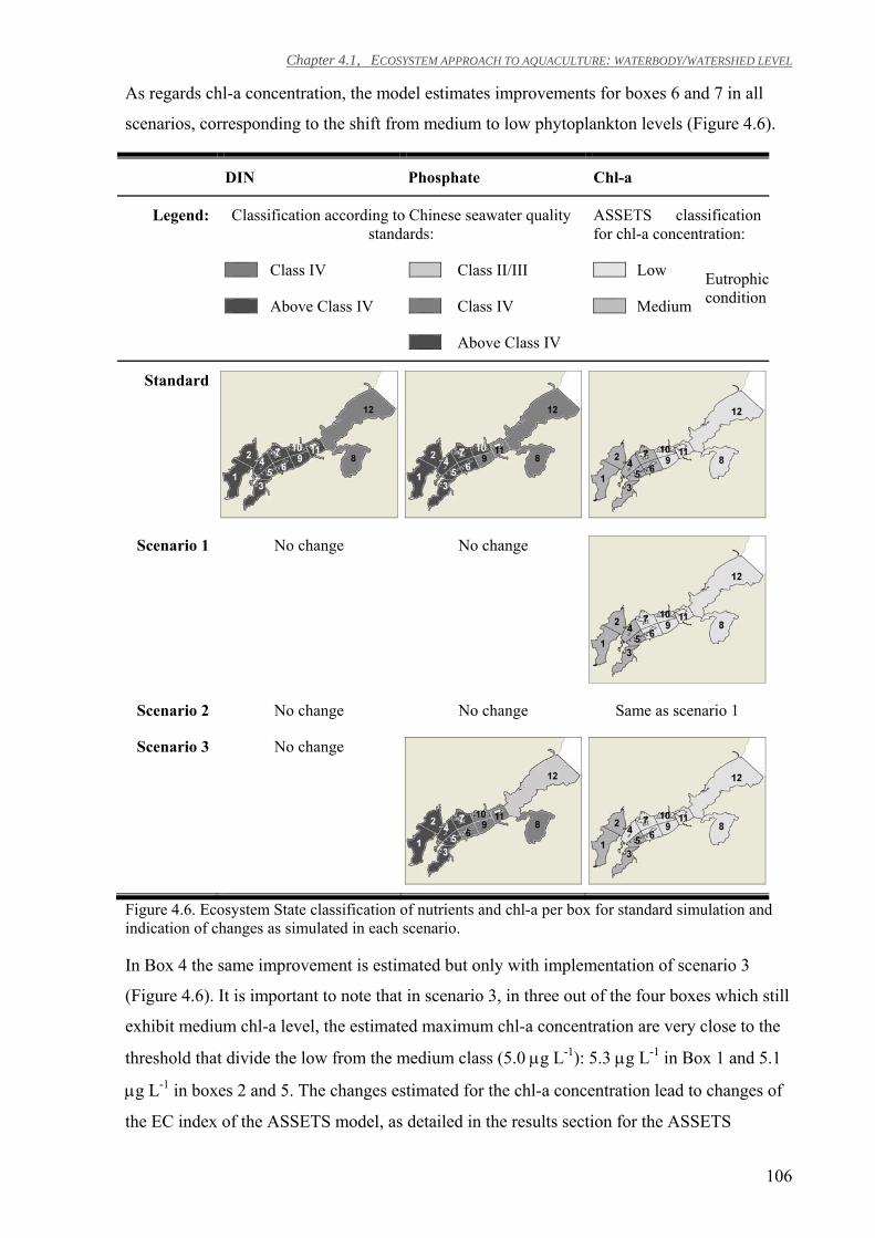
Chapter 4.1, ECOSYSTEM APPROACH TO AQUACULTURE: WATERBODY/WATERSHED LEVEL
106
As regards chl-a concentration, the model estimates improvements for boxes 6 and 7 in all
scenarios, corresponding to the shift from medium to low phytoplankton levels (Figure 4.6).
DIN Phosphate Chl-a
Legend: Classification according to Chinese seawater quality standards:
ASSETS classification for chl-a concentration:
Class IV
Class II/III
Low Eutrophic condition
Above Class IV
Class IV
Medium
Above Class IV
Standard
Scenario 1 No change No change
Scenario 2 No change No change Same as scenario 1
Scenario 3 No change
Figure 4.6. Ecosystem State classification of nutrients and chl-a per box for standard simulation and indication of changes as simulated in each scenario.
In Box 4 the same improvement is estimated but only with implementation of scenario 3
(Figure 4.6). It is important to note that in scenario 3, in three out of the four boxes which still
exhibit medium chl-a level, the estimated maximum chl-a concentration are very close to the
threshold that divide the low from the medium class (5.0 µg L-1): 5.3 µg L-1 in Box 1 and 5.1
µg L-1 in boxes 2 and 5. The changes estimated for the chl-a concentration lead to changes of
the EC index of the ASSETS model, as detailed in the results section for the ASSETS
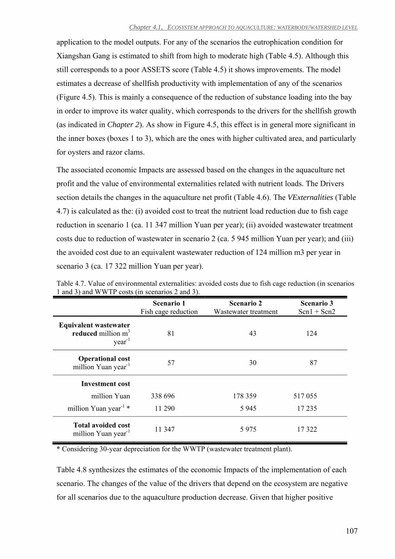
Chapter 4.1, ECOSYSTEM APPROACH TO AQUACULTURE: WATERBODY/WATERSHED LEVEL
107
application to the model outputs. For any of the scenarios the eutrophication condition for
Xiangshan Gang is estimated to shift from high to moderate high (Table 4.5). Although this
still corresponds to a poor ASSETS score (Table 4.5) it shows improvements. The model
estimates a decrease of shellfish productivity with implementation of any of the scenarios
(Figure 4.5). This is mainly a consequence of the reduction of substance loading into the bay
in order to improve its water quality, which corresponds to the drivers for the shellfish growth
(as indicated in Chapter 2). As show in Figure 4.5, this effect is in general more significant in
the inner boxes (boxes 1 to 3), which are the ones with higher cultivated area, and particularly
for oysters and razor clams.
The associated economic Impacts are assessed based on the changes in the aquaculture net
profit and the value of environmental externalities related with nutrient loads. The Drivers
section details the changes in the aquaculture net profit (Table 4.6). The VExternalities (Table
4.7) is calculated as the: (i) avoided cost to treat the nutrient load reduction due to fish cage
reduction in scenario 1 (ca. 11 347 million Yuan per year); (ii) avoided wastewater treatment
costs due to reduction of wastewater in scenario 2 (ca. 5 945 million Yuan per year); and (iii)
the avoided cost due to an equivalent wastewater reduction of 124 million m3 per year in
scenario 3 (ca. 17 322 million Yuan per year).
Table 4.7. Value of environmental externalities: avoided costs due to fish cage reduction (in scenarios 1 and 3) and WWTP costs (in scenarios 2 and 3). Scenario 1 Scenario 2 Scenario 3 Fish cage reduction Wastewater treatment Scn1 + Scn2
Equivalent wastewater reduced million m3
year-1 81 43 124
Operational cost million Yuan year-1 57 30 87
Investment cost
million Yuan 338 696 178 359 517 055
million Yuan year-1 * 11 290 5 945 17 235
Total avoided cost million Yuan year-1 11 347 5 975 17 322
* Considering 30-year depreciation for the WWTP (wastewater treatment plant).
Table 4.8 synthesizes the estimates of the economic Impacts of the implementation of each
scenario. The changes of the value of the drivers that depend on the ecosystem are negative
for all scenarios due to the aquaculture production decrease. Given that higher positive
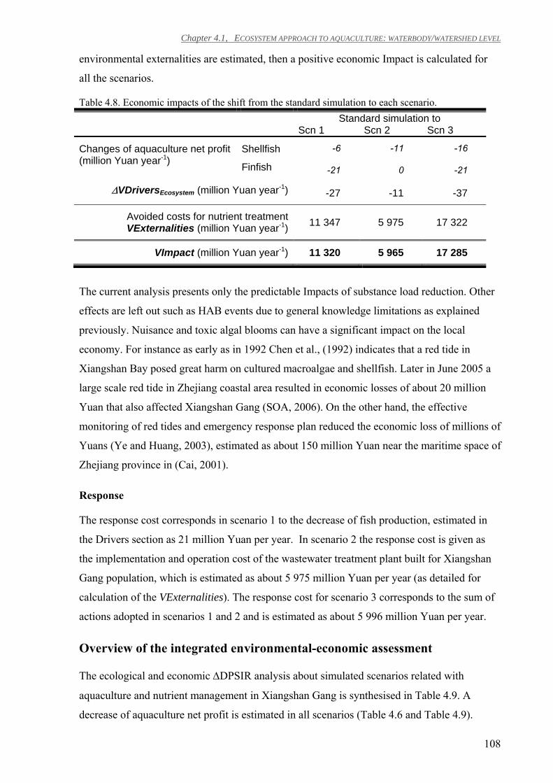
Chapter 4.1, ECOSYSTEM APPROACH TO AQUACULTURE: WATERBODY/WATERSHED LEVEL
108
environmental externalities are estimated, then a positive economic Impact is calculated for
all the scenarios.
Table 4.8. Economic impacts of the shift from the standard simulation to each scenario. Standard simulation to Scn 1 Scn 2 Scn 3
Changes of aquaculture net profit (million Yuan year-1)
Shellfish -6 -11 -16
Finfish -21 0 -21
∆VDriversEcosystem (million Yuan year-1) -27 -11 -37
Avoided costs for nutrient treatment VExternalities (million Yuan year-1) 11 347 5 975 17 322
VImpact (million Yuan year-1) 11 320 5 965 17 285
The current analysis presents only the predictable Impacts of substance load reduction. Other
effects are left out such as HAB events due to general knowledge limitations as explained
previously. Nuisance and toxic algal blooms can have a significant impact on the local
economy. For instance as early as in 1992 Chen et al., (1992) indicates that a red tide in
Xiangshan Bay posed great harm on cultured macroalgae and shellfish. Later in June 2005 a
large scale red tide in Zhejiang coastal area resulted in economic losses of about 20 million
Yuan that also affected Xiangshan Gang (SOA, 2006). On the other hand, the effective
monitoring of red tides and emergency response plan reduced the economic loss of millions of
Yuans (Ye and Huang, 2003), estimated as about 150 million Yuan near the maritime space of
Zhejiang province in (Cai, 2001).
Response
The response cost corresponds in scenario 1 to the decrease of fish production, estimated in
the Drivers section as 21 million Yuan per year. In scenario 2 the response cost is given as
the implementation and operation cost of the wastewater treatment plant built for Xiangshan
Gang population, which is estimated as about 5 975 million Yuan per year (as detailed for
calculation of the VExternalities). The response cost for scenario 3 corresponds to the sum of
actions adopted in scenarios 1 and 2 and is estimated as about 5 996 million Yuan per year.
Overview of the integrated environmental-economic assessment
The ecological and economic ∆DPSIR analysis about simulated scenarios related with
aquaculture and nutrient management in Xiangshan Gang is synthesised in Table 4.9. A
decrease of aquaculture net profit is estimated in all scenarios (Table 4.6 and Table 4.9).
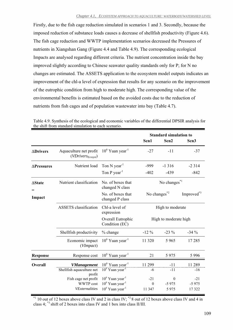
Chapter 4.1, ECOSYSTEM APPROACH TO AQUACULTURE: WATERBODY/WATERSHED LEVEL
109
Firstly, due to the fish cage reduction simulated in scenarios 1 and 3. Secondly, because the
imposed reduction of substance loads causes a decrease of shellfish productivity (Figure 4.6).
The fish cage reduction and WWTP implementation scenarios decreased the Pressures of
nutrients in Xiangshan Gang (Figure 4.4 and Table 4.9). The corresponding ecological
Impacts are analysed regarding different criteria. The nutrient concentration inside the bay
improved slightly according to Chinese seawater quality standards only for P; for N no
changes are estimated. The ASSETS application to the ecosystem model outputs indicates an
improvement of the chl-a level of expression that results for any scenario on the improvement
of the eutrophic condition from high to moderate high. The corresponding value of the
environmental benefits is estimated based on the avoided costs due to the reduction of
nutrients from fish cages and of population wastewater into bay (Table 4.7).
Table 4.9. Synthesis of the ecological and economic variables of the differential DPSIR analysis for the shift from standard simulation to each scenario.
Standard simulation to Scn1 Scn2 Scn3
∆Drivers Aquaculture net profit (VDriversEcosyst)
106 Yuan year-1 -27 -11 -37
∆Pressures Nutrient load Ton N year-1 -999 -1 316 -2 314 Ton P year-1 -402 -439 -842
∆State
=
Impact
Nutrient classification No. of boxes that changed N class
No changes*1
No. of boxes that changed P class
No changes*2 Improved*3
ASSETS classification Chl-a level of expression
High to moderate
Overall Eutrophic Condition (EC)
High to moderate high
Shellfish productivity % change -12 % -23 % -34 %
Economic impact (VImpact)
106 Yuan year-1 11 320 5 965 17 285
Response Response cost 106 Yuan year-1 21 5 975 5 996
Overall VManagement 106 Yuan year-1 11 299 -11 11 289 Shellfish aquaculture net
profit 106 Yuan year-1 -6 -11 -16
Fish cage net profit 106 Yuan year-1 -21 0 -21 WWTP cost 106 Yuan year-1 0 -5 975 -5 975 VExternalities 106 Yuan year-1 11 347 5 975 17 322
*1 10 out of 12 boxes above class IV and 2 in class IV; *2 8 out of 12 boxes above class IV and 4 in class 4; *3 shift of 2 boxes into class IV and 1 box into class II/III.
Chapter 4.1, ECOSYSTEM APPROACH TO AQUACULTURE: WATERBODY/WATERSHED LEVEL
110
The value of environmental externalities surpasses the negative change of the drivers that
depend on the ecosystem (Table 4.8); therefore a positive economic Impact is estimated
(Table 4.9). The Response cost for the planned action in scenario 1 is 2 orders of magnitude
lower than for scenarios 2 and 3. These two scenarios account for the implementation and
operation of a WWTP (estimated as about 5 975 million Yuan per year), while in scenario 1
the response cost corresponds to the closure of 38% of finfish aquaculture net profit
(estimated as about 21 million Yuan per year). The overall economic balance (VManagement)
estimates a similar gain for scenarios 1 and 3 and a loss for scenario 2 (Table 4.9). The
VManagement represents the outcome of the balance between (i) the aquaculture net profit
decrease (due to the fish aquaculture reduction and decrease of shellfish productivity), (ii) the
response costs (including only the WWTP costs to avoid the double-accounting of the fish
aquaculture net profit decrease), and (iii) the quantifiable environmental externalities. In
scenario 2 the VExternalities cancel out the Response cost leading to a negative overall
balance. Therefore, the negative balance corresponds to the reduction of shellfish
productivity. In scenarios 1 and 3, the positive balance is mainly due to the avoided costs for
treatment of fish effluents.
Herein, and based on the integrated modelling and assessment approach recommendations
about improving water quality and minimize aquaculture production decrease are presented.
To start with, in a follow up work and based on the current set of models the modelling teams
could provide estimates about the reduction targets required to reach the aimed water quality
condition. Future actions to improve water quality in Xiangshan Gang should include
extended stakeholder meetings to define further nutrient reduction measures; namely, related
with agriculture practice, which are not explored in the current modelling exercise. The
catchment model of the multilayered modelling system (detailed in Chapter 2) could assist
the determination of the most effective measures. Alternatively to current options about
decreasing fish cages it might be interesting to make a cost-benefit analysis to evaluate other
fish cultivation practices; namely, in integrated multi-trophic aquaculture (IMTA) systems in
land-based ponds (as discussed in the second part of this chapter for an abalone-seaweed
IMTA) or fish cages with a floating bag system (Ayer and Tyedmers, 2009). A benefit of the
land ponds is that it allows disconnection from the bay during HAB events. An intermediate
measure might be to re-establish massive kelp or other seaweeds cultivation, especially near
fish cage areas, in order to reduce loading of dissolved nutrients into the bay. Until late 1980’s
kelp was the major aquatic resource produced in the bay. The seaweed replacement by other
aquatic resources and in particular the fish cultivation boom in the second half of the 1990’s is
believed to be related with several of the HAB events (Feng et al, 2004). Feng et al. (2004)
Chapter 4.1, ECOSYSTEM APPROACH TO AQUACULTURE: WATERBODY/WATERSHED LEVEL
111
illustrates the ecological and economic advantages of restoring the vast kelp cultivation. To
minimize the expected effects of decrease of substance loads into the decline of shellfish
production, the outputs of the approach suggest the displacement of part of the shellfish
production in order to distribute cultivation areas more evenly over the bay. For instance 89%
of the total shellfish cultivation area is located in boxes 1 to 5, which correspond to only about
34% of the total Xiangshan area. In general, the shift of part of the shellfish culture from the
up- to downstream area of the bay is advisable. For instance, Chinese oyster productivity is
almost 3 times higher in Box 12 than in Box 1. As such, a fraction of Box 1 oyster production
(which concentrates 22 % of total oyster production) should be distributed over other boxes.
This action might require wider zoning efforts for the bay in order to optimize and harmonize
space allocation between several coastal uses.
If further management actions for water quality improvement are to be adopted, the wider side
effects related with the water quality improvement must be accounted in the economic
analysis; such as the development of other coastal uses such as tourism and recreational
fisheries, which can diversify the source of income in the region.
The monitoring of HAB events, in particular for determining the origin (if from inside the bay
or from outside) and the triggering mechanisms is recommended for the management of the
Xiangshan Gang eutrophic condition. Babaran et al. (1998) exemplify how research about
initiating and triggering mechanisms that cause HAB’s can be applied for managing
aquaculture sites subject to these events. Roelke and Buyukates (2001) provide example about
establishing preventive management schemes based on an early-warning indicator
monitoring. Additionally, for future cost-benefit analysis the appraisal of detailed economic
impacts of HAB events on aquaculture production is recommended.
CONCLUSIONS
The synthesis of model outputs using IEA methodologies provides useful insights for
managers about what is expectable to change in water quality and ecosystem state as a result
of simulation scenarios. In particular the use of the ∆DPSIR enabled an estimate of the
ecological-economic impacts of the tested management solutions. The comparison among
scenario outputs provided insights for the adoption of future policy and research. The use of
∆DPSIR is enhanced by using together other IEA approaches, more targeted that can provide
classification of ecosystem status regarding specific problems. In this case study, the ASSETS
screening model played a crucial role to understand the effects of changes of nutrient loading
Chapter 4.1, ECOSYSTEM APPROACH TO AQUACULTURE: WATERBODY/WATERSHED LEVEL
112
(from both catchment and aquaculture activities) in the eutrophic condition of bay. There are
nevertheless limitations inherent to any modelling exercise given the incomplete
representation of reality. For instance, relevant variables for the environmental assessment
might be left out given the complexity and current knowledge of processes to be simulated,
such as HAB events. In such cases, if possible is recommended to fill modelling gaps based
on expert knowledge, rather than overlook the effect (Peirce, 1998). Notwithstanding, the
scenario prediction besides providing insights to managers concerning the variables simulated
in the ecosystem model, can also assist the planning of the impact assessment evaluations of
future coastal management actions. Namely, to identify the relevant variables/indicators for
the characterisation and analysis of the: (i) catchment and coastal activities, (ii) relevant
pressures, and (iii) ecological features to monitor.
The design of the integrated modelling and assessment approach for a specific case study
must be tailored to address the needs of managers and other stakeholders of the ecosystem.
This is an essential step to ensure that the relevant local issues are included in the modelling
and thus that the overall approach is useful. Actions adopted by managers after the application
of an integrated modelling and assessment approach, should be followed by monitoring to: (i)
assess the consequent impacts; (ii) verify the modelling predictions; and (iii) contribute to
knowledge specially to fulfil modelling gaps.
The case study developed in this chapter lays the groundwork for more complex applications
of the integrated environmental modelling and assessment approach elsewhere. The subject
analysed herein is highly relevant for the integrated management of coastal zones given the
existing challenges to promote sustainable aquaculture development and the management of
nutrient loading from coastal activities. In particular, the case study illustrated the usefulness
of the integrated environmental modelling and assessment approach to assist the development
of an ecosystem approach to aquaculture.
4.2 Farm level assessment: IMTA evaluation using real farm data
Context
The previous part of this chapter analysed the multilayered ecosystem model scenarios to
support the development of EAA at the waterbody/catchment level. The analysis of
aquaculture at the individual farm level is also important for the development of EAA.
Aquaculture has been mostly associated with negative impacts, mostly due to unsustainable
cultivation practices (Paez-Osuna et al., 1999; Feng et al., 2004; Xu et al., 2007). However,
depending on the aquaculture practice and cultivated species, aquaculture can also generate
environmental benefits (Neori et al., 2004; Newell, 2004; Žydelis et al., 2008; Gren et al.,
2009). The adoption of best management practices (BMPs) for new and existing farms is
important to minimize the potential negative impacts on water quality and ecosystem
deterioration, while potentially leading to increasing profit margins, as exemplified by
Valderrama and Engle (2002) for shrimp aquaculture.
Summary
This chapter illustrates the application of the ∆DPSIR for the ecological-economic assessment
of aquaculture options at the farm level. An abalone farm located in South Africa is used to
exploit the detailed dataset about its environmental and economic performance. The case
study consists of assessing the ecological-economic effects of the abalone-seaweed IMTA on
the farm’s performance and the corresponding environmental externalities.
Chapter 4.2, ECOSYSTEM APPROACH TO AQUACULTURE: FARM LEVEL
114
This section corresponds to the manuscript submitted to Aquaculture:
Ecological-economic assessment of aquaculture options: comparison
between monoculture and integrated multi-trophic aquaculture, by
Nobre, A.M., Robertson-Andersson, D., Neori, A., Sankar, K.
(For consistency with submitted version this chapter is written in
American English)
Chapter 4.2, ECOSYSTEM APPROACH TO AQUACULTURE: FARM LEVEL
115
Ecological-economic assessment of aquaculture options: comparison between monoculture and integrated multi-trophic aquaculture
INTRODUCTION
Aquaculture has grown at an average annual rate of 8.8% since 1970, with an increase in the
production of seafood (excluding plants) of about 8 fold up to 2004 (FAO, 2006).
Sustainability issues related to socially and environmentally irresponsible aquaculture
practices reported for certain cultivation systems have generated concerns about the industry,
particularly highly industrialized and intensified monoculture farms (Paez-Osuna et al., 1999;
GESAMP, 2001; Islam, 2005; Xu et al., 2007; Allsopp et al., 2008). Because of their impact
on the environment and of their negative feedbacks on the aquaculture operations, the
expansion of aquaculture has been limited (GESAMP, 2001; Islam, 2005; Gibbs, 2009). The
broader public is generally unaware of the benefits that aquaculture can generate to the
environment (Newell, 2004; Lindahl et al., 2005; Ferreira et al., 2007a; Rice, 2008; Žydelis et
al., 2008) and to society (promotion of poverty reduction through employment, higher income
and food security – FAO, 2005; Msuya, 2006; Troell et al., 2006; Kaliba et al., 2007;
Robertson-Andersson et al., 2008). Given the importance of food security on the one hand
(Ahmed and Lorica, 2002), and given the negative ecological-economic impacts of poorly
conceived aquaculture practices on the other hand (Islam, 2005), an integrated planning and
management of aquaculture is required (GESAMP, 2001). Furthermore, external benefits of
socially and environmentally responsible (sustainable) aquaculture can have direct economic
value, since consumers have been showing increased awareness of, and preference for,
sustainable seafood harvesting (FAO, 2006). The main technological approaches that have
been developed to meet environmental concerns (Refstie et al., 2001; Neori et al., 2004;
Gutierrez-Wing and Malone, 2006) include: (i) improved feed and water management, (ii)
water recirculating systems, (iii) bacterial biofilters and (iv) extractive species (filter feeders,
detritivores and macroalgae).
More recently, the integration of fed species and extractive species in the modern form of
polyculture called integrated multi-trophic aquaculture (IMTA, also known as 'partitioned
aquaculture' and 'aquaponics'), has been developed to ease environmental concerns because it
addresses issues of both productivity and nutrient loading into the environment (Neori et al.,
2004; FAO, 2006; WGEIM, 2006; Abreu et al., 2009; Buschmann et al., 2009; Troell et al.,
2009). IMTA has been gaining recognition as a sustainable approach to aquaculture because
Chapter 4.2, ECOSYSTEM APPROACH TO AQUACULTURE: FARM LEVEL
116
of its combination of environmental, economic and social advantages (Whitmarsh et al., 2006;
Ridler et al., 2007; Allsopp et al., 2008). A key component of IMTA is the use of macroalgae:
while taking up dissolved inorganic nutrients (nitrogen and phosphorus), the produced algal
biomass is a renewable protein-enriched feed to other cultivated species, and a product on its
own (Chopin et al., 2001). Abalone farming is an aquaculture industry that can particularly
benefit from the implementation of IMTA with marine macroalgae (seaweeds), which are the
natural abalone food. South Africa, the third largest abalone producer in the world (Gordon
and Cook, 2004), has begun implementing IMTA with the seaweed Ulva lactuca L. and the
abalone Haliotis midae L. (Robertson-Andersson et al., 2008). This move has largely emerged
for the following reasons:
(i) Demand for natural stocks of South African kelp as feed for abalone is approaching the
maximum sustainable yield of the concession areas (Troell et al., 2006) and insufficient
access by some farms to wild kelp beds (Bolton, 2006; Smit et al., 2007; Hwang et al., 2009).
(ii) Diets of mixed algal species accelerate abalone growth rates relative to single-species
diets (Naidoo et al., 2006; Dlaza et al., 2008).
(iii) Cultivation of seaweeds in the farm's abalone effluent allows water recirculation and
reduces nutrient discharge into the environment (Robertson-Andersson, 2007).
(iv) A land based seaweed facility allows the abalone farm to disconnect itself from the sea
for extended periods by water recirculation through seaweed ponds during red tides and oil
spills (Robertson-Andersson, 2007).
Aquaculture, like other uses of marine resources where the environmental and the socio-
economic systems are intertwined, require for its sustainable development information about
the ecological and economic impacts of different practices. This implies communication
between the scientific, management and policy-making communities, and the integration
among disciplines using mutually understandable concepts (GESAMP, 2001). The Drivers-
Pressure-State-Impact-Response (DPSIR) approach is a potential analytical framework for
determining the impacts of aquaculture options. This approach has been applied to assist in
the evaluation of environmental impacts and of ecosystem management approaches (Stanners
et al., 2008). In particular, the DPSIR has been widely used to report about quantification of
the impacts of human activities on coastal activities (Borja et al., 2006; Elliott, 2002;
IMPRESS 2003; Nobre, 2009). The DPSIR is a conceptual framework for integrated
environmental assessment that provides (i) a systematic view of the socio-economic and
environmental interactions and (ii) a reporting framework to policy-makers and public
(Bowen and Riley, 2003; Ledoux and Turner, 2002; Nobre, 2009). The application of the
Chapter 4.2, ECOSYSTEM APPROACH TO AQUACULTURE: FARM LEVEL
117
DPSIR is based on the use of indicators (Stanners et al., 2008). It facilitates the structuring of
data following the causal chain D-P-S-I-R: Drivers are the anthropogenic activities generating
Pressures that perturb the State of the ecosystem, thus causing an Impact on the ecosystem,
which calls for management and policy-making Responses to improve the State of the
ecosystem (Borja et al., 2006; IMPRESS 2003). A recent version of the DPSIR, the
Differential DPSIR (∆DPSIR), establishes an explicit link between the ecological and the
economic systems and screens the evolution of ecological and economic variables over time
or between simulated scenarios (Nobre, 2009). The ∆DPSIR approach provides a tool for the
assessment of changes in environmental quality and consequent effects on the economic
system, including on the value of anthropogenic activities and of the ecosystem (Nobre,
2009).
The aim of the work presented herein is to couple ecological and economic information to
support resource managers in the assessment of the ecological and economic impacts of
aquaculture operations. This paper uses the integration of seaweed production in the abalone
industry in the form of IMTA as a case study, and the ∆DPSIR framework (Nobre, 2009) as
an approach to evaluate the ecological and economic impacts. The objectives are to:
(i) Assess the environmental and economic impacts to the main stakeholders of the shift from
abalone monoculture to IMTA with seaweeds using data from a farm located in South Africa
(Roberston-Andersson, 2007; Roberston-Andersson et al., 2008; Sankar, 2009).
(ii) Carry out a mass balance analysis to manage nutrient limitation due to seaweed expansion
in the South African farm. Includes data analyzes from an Israeli IMTA farm with abalone,
fish and seaweeds (Neori and Shpigel, 2006) to provide guidance on possible solutions for the
sustainable management of the nutrient limitation that occurs when expanding the seaweed
production.
METHODOLOGY
General approach
The ∆DPSIR methodology (Nobre, 2009) is applied to evaluate aquaculture options. The
∆DPSIR includes quantification of ecological and economic variables. The ecological
assessment includes quantification of indicators of Pressure, State, and Impact. The economic
assessment consists in a cost-benefit analysis to evaluate a given Response from an
environmental and economic perspective; includes quantification of the value of the divers, of
the ecosystem, of the impact, of the response and the economic value of management (Nobre,
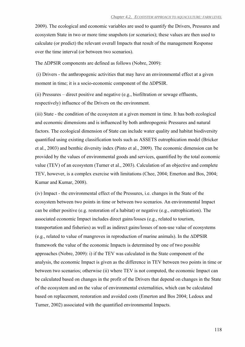
Chapter 4.2, ECOSYSTEM APPROACH TO AQUACULTURE: FARM LEVEL
118
2009). The ecological and economic variables are used to quantify the Drivers, Pressures and
ecosystem State in two or more time snapshots (or scenarios); these values are then used to
calculate (or predict) the relevant overall Impacts that result of the management Response
over the time interval (or between two scenarios).
The ∆DPSIR components are defined as follows (Nobre, 2009):
(i) Drivers - the anthropogenic activities that may have an environmental effect at a given
moment in time; it is a socio-economic component of the ∆DPSIR.
(ii) Pressures – direct positive and negative (e.g., biofiltration or sewage effluents,
respectively) influence of the Drivers on the environment.
(iii) State - the condition of the ecosystem at a given moment in time. It has both ecological
and economic dimensions and is influenced by both anthropogenic Pressures and natural
factors. The ecological dimension of State can include water quality and habitat biodiversity
quantified using existing classification tools such as ASSETS eutrophication model (Bricker
et al., 2003) and benthic diversity index (Pinto et al., 2009). The economic dimension can be
provided by the values of environmental goods and services, quantified by the total economic
value (TEV) of an ecosystem (Turner et al., 2003). Calculation of an objective and complete
TEV, however, is a complex exercise with limitations (Chee, 2004; Emerton and Bos, 2004;
Kumar and Kumar, 2008).
(iv) Impact - the environmental effect of the Pressures, i.e. changes in the State of the
ecosystem between two points in time or between two scenarios. An environmental Impact
can be either positive (e.g. restoration of a habitat) or negative (e.g., eutrophication). The
associated economic Impact includes direct gains/losses (e.g., related to tourism,
transportation and fisheries) as well as indirect gains/losses of non-use value of ecosystems
(e.g., related to value of mangroves in reproduction of marine animals). In the ∆DPSIR
framework the value of the economic Impacts is determined by one of two possible
approaches (Nobre, 2009): i) if the TEV was calculated in the State component of the
analysis, the economic Impact is given as the difference in TEV between two points in time or
between two scenarios; otherwise (ii) where TEV is not computed, the economic Impact can
be calculated based on changes in the profit of the Drivers that depend on changes in the State
of the ecosystem and on the value of environmental externalities, which can be calculated
based on replacement, restoration and avoided costs (Emerton and Bos 2004; Ledoux and
Turner, 2002) associated with the quantified environmental Impacts.
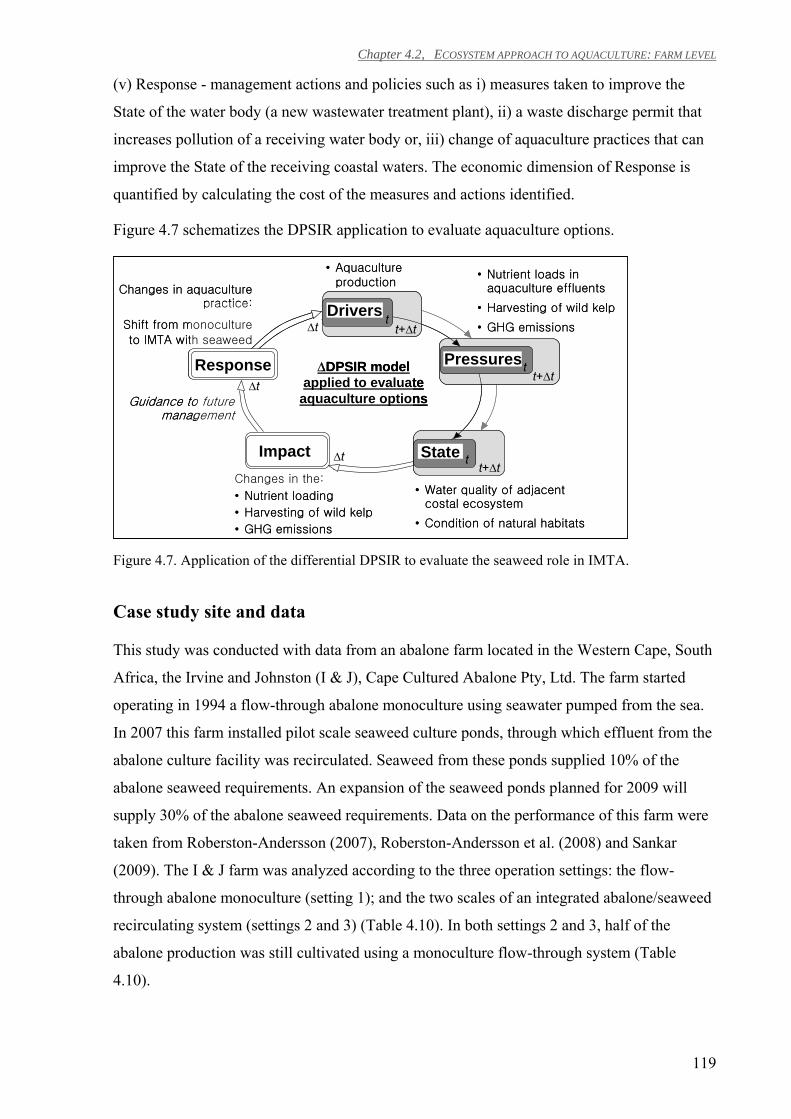
Chapter 4.2, ECOSYSTEM APPROACH TO AQUACULTURE: FARM LEVEL
119
(v) Response - management actions and policies such as i) measures taken to improve the
State of the water body (a new wastewater treatment plant), ii) a waste discharge permit that
increases pollution of a receiving water body or, iii) change of aquaculture practices that can
improve the State of the receiving coastal waters. The economic dimension of Response is
quantified by calculating the cost of the measures and actions identified.
Figure 4.7 schematizes the DPSIR application to evaluate aquaculture options.
Figure 4.7. Application of the differential DPSIR to evaluate the seaweed role in IMTA.
Case study site and data
This study was conducted with data from an abalone farm located in the Western Cape, South
Africa, the Irvine and Johnston (I & J), Cape Cultured Abalone Pty, Ltd. The farm started
operating in 1994 a flow-through abalone monoculture using seawater pumped from the sea.
In 2007 this farm installed pilot scale seaweed culture ponds, through which effluent from the
abalone culture facility was recirculated. Seaweed from these ponds supplied 10% of the
abalone seaweed requirements. An expansion of the seaweed ponds planned for 2009 will
supply 30% of the abalone seaweed requirements. Data on the performance of this farm were
taken from Roberston-Andersson (2007), Roberston-Andersson et al. (2008) and Sankar
(2009). The I & J farm was analyzed according to the three operation settings: the flow-
through abalone monoculture (setting 1); and the two scales of an integrated abalone/seaweed
recirculating system (settings 2 and 3) (Table 4.10). In both settings 2 and 3, half of the
abalone production was still cultivated using a monoculture flow-through system (Table
4.10).
• Aquaculture production
t+∆t
t+∆tDrivers t
t+∆tPressures t
State tImpact
∆DPSIR model applied to evaluate
aquaculture options
Response
• Nutrient loads in aquaculture effluents
• Harvesting of wild kelp
• GHG emissions
• Water quality of adjacent costal ecosystem
• Condition of natural habitats
∆t
∆t
∆t
Changes in the:
• Nutrient loading
• Harvesting of wild kelp
• GHG emissions
Guidance to future management
Changes in aquaculture practice:
Shift from monoculture to IMTA with seaweed
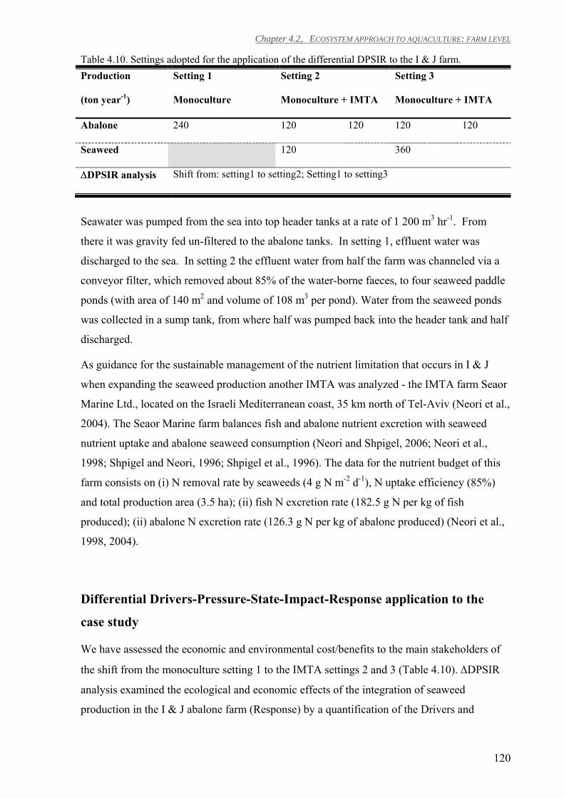
Chapter 4.2, ECOSYSTEM APPROACH TO AQUACULTURE: FARM LEVEL
120
Table 4.10. Settings adopted for the application of the differential DPSIR to the I & J farm. Production Setting 1 Setting 2 Setting 3
(ton year-1) Monoculture Monoculture + IMTA Monoculture + IMTA
Abalone 240 120 120 120 120
Seaweed 120 360
∆DPSIR analysis Shift from: setting1 to setting2; Setting1 to setting3
Seawater was pumped from the sea into top header tanks at a rate of 1 200 m3 hr-1. From
there it was gravity fed un-filtered to the abalone tanks. In setting 1, effluent water was
discharged to the sea. In setting 2 the effluent water from half the farm was channeled via a
conveyor filter, which removed about 85% of the water-borne faeces, to four seaweed paddle
ponds (with area of 140 m2 and volume of 108 m3 per pond). Water from the seaweed ponds
was collected in a sump tank, from where half was pumped back into the header tank and half
discharged.
As guidance for the sustainable management of the nutrient limitation that occurs in I & J
when expanding the seaweed production another IMTA was analyzed - the IMTA farm Seaor
Marine Ltd., located on the Israeli Mediterranean coast, 35 km north of Tel-Aviv (Neori et al.,
2004). The Seaor Marine farm balances fish and abalone nutrient excretion with seaweed
nutrient uptake and abalone seaweed consumption (Neori and Shpigel, 2006; Neori et al.,
1998; Shpigel and Neori, 1996; Shpigel et al., 1996). The data for the nutrient budget of this
farm consists on (i) N removal rate by seaweeds (4 g N m-2 d-1), N uptake efficiency (85%)
and total production area (3.5 ha); (ii) fish N excretion rate (182.5 g N per kg of fish
produced); (ii) abalone N excretion rate (126.3 g N per kg of abalone produced) (Neori et al.,
1998, 2004).
Differential Drivers-Pressure-State-Impact-Response application to the
case study
We have assessed the economic and environmental cost/benefits to the main stakeholders of
the shift from the monoculture setting 1 to the IMTA settings 2 and 3 (Table 4.10). ∆DPSIR
analysis examined the ecological and economic effects of the integration of seaweed
production in the I & J abalone farm (Response) by a quantification of the Drivers and
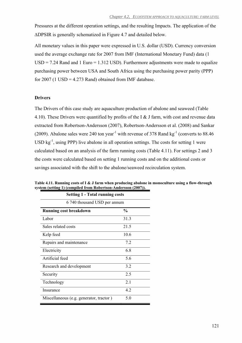
Chapter 4.2, ECOSYSTEM APPROACH TO AQUACULTURE: FARM LEVEL
121
Pressures at the different operation settings, and the resulting Impacts. The application of the
∆DPSIR is generally schematized in Figure 4.7 and detailed below.
All monetary values in this paper were expressed in U.S. dollar (USD). Currency conversion
used the average exchange rate for 2007 from IMF (International Monetary Fund) data (1
USD = 7.24 Rand and 1 Euro = 1.312 USD). Furthermore adjustments were made to equalize
purchasing power between USA and South Africa using the purchasing power parity (PPP)
for 2007 (1 USD = 4.273 Rand) obtained from IMF database.
Drivers
The Drivers of this case study are aquaculture production of abalone and seaweed (Table
4.10). These Drivers were quantified by profits of the I & J farm, with cost and revenue data
extracted from Robertson-Andersson (2007), Robertson-Andersson et al. (2008) and Sankar
(2009). Abalone sales were 240 ton year-1 with revenue of 378 Rand kg-1 (converts to 88.46
USD kg-1, using PPP) live abalone in all operation settings. The costs for setting 1 were
calculated based on an analysis of the farm running costs (Table 4.11). For settings 2 and 3
the costs were calculated based on setting 1 running costs and on the additional costs or
savings associated with the shift to the abalone/seaweed recirculation system.
Table 4.11. Running costs of I & J farm when producing abalone in monoculture using a flow-through system (setting 1) (compiled from Robertson-Andersson (2007)).
Setting 1 - Total running costs
6 740 thousand USD per annum
Running cost breakdown %
Labor 31.3
Sales related costs 21.5
Kelp feed 10.6
Repairs and maintenance 7.2
Electricity 6.8
Artificial feed 5.6
Research and development 3.2
Security 2.5
Technology 2.1
Insurance 4.2
Miscellaneous (e.g. generator, tractor ) 5.0
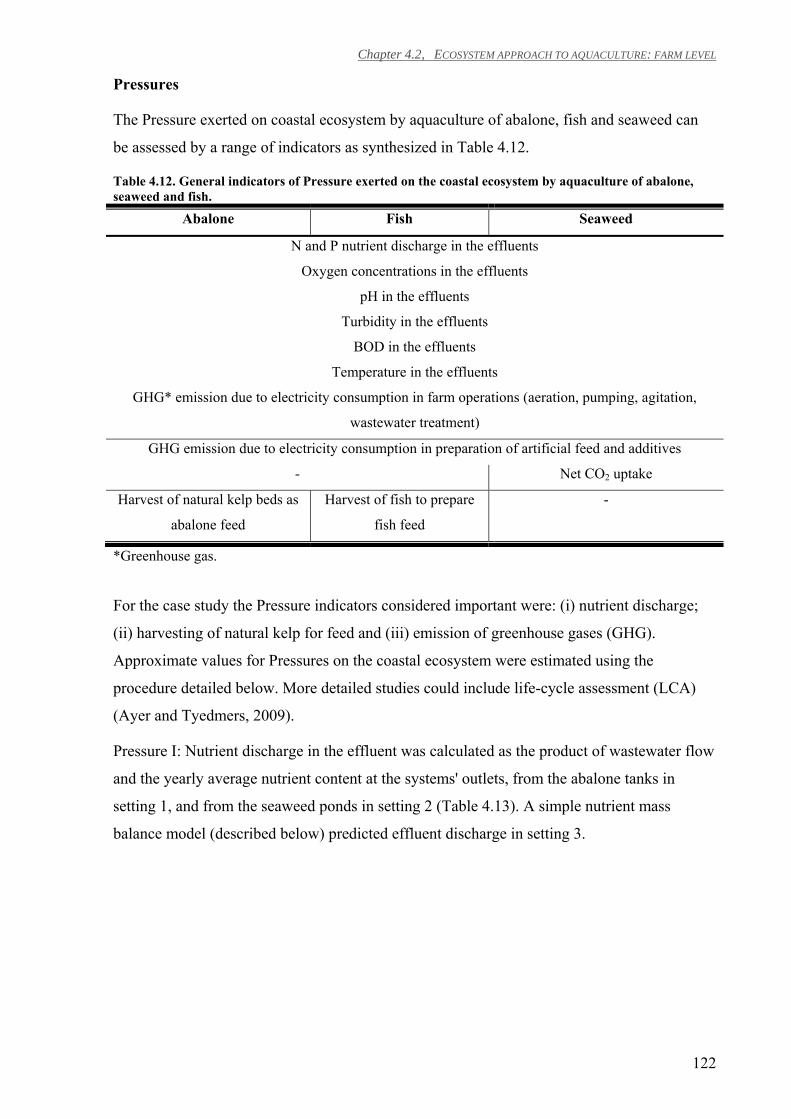
Chapter 4.2, ECOSYSTEM APPROACH TO AQUACULTURE: FARM LEVEL
122
Pressures
The Pressure exerted on coastal ecosystem by aquaculture of abalone, fish and seaweed can
be assessed by a range of indicators as synthesized in Table 4.12.
Table 4.12. General indicators of Pressure exerted on the coastal ecosystem by aquaculture of abalone, seaweed and fish.
Abalone Fish Seaweed
N and P nutrient discharge in the effluents
Oxygen concentrations in the effluents
pH in the effluents
Turbidity in the effluents
BOD in the effluents
Temperature in the effluents
GHG* emission due to electricity consumption in farm operations (aeration, pumping, agitation,
wastewater treatment)
GHG emission due to electricity consumption in preparation of artificial feed and additives
- Net CO2 uptake
Harvest of natural kelp beds as
abalone feed
Harvest of fish to prepare
fish feed
-
*Greenhouse gas.
For the case study the Pressure indicators considered important were: (i) nutrient discharge;
(ii) harvesting of natural kelp for feed and (iii) emission of greenhouse gases (GHG).
Approximate values for Pressures on the coastal ecosystem were estimated using the
procedure detailed below. More detailed studies could include life-cycle assessment (LCA)
(Ayer and Tyedmers, 2009).
Pressure I: Nutrient discharge in the effluent was calculated as the product of wastewater flow
and the yearly average nutrient content at the systems' outlets, from the abalone tanks in
setting 1, and from the seaweed ponds in setting 2 (Table 4.13). A simple nutrient mass
balance model (described below) predicted effluent discharge in setting 3.
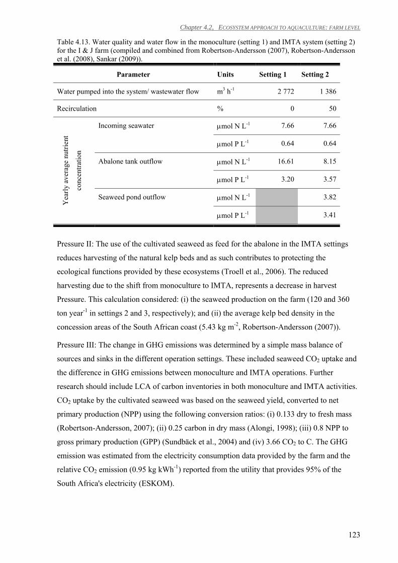
Chapter 4.2, ECOSYSTEM APPROACH TO AQUACULTURE: FARM LEVEL
123
Table 4.13. Water quality and water flow in the monoculture (setting 1) and IMTA system (setting 2) for the I & J farm (compiled and combined from Robertson-Andersson (2007), Robertson-Andersson et al. (2008), Sankar (2009)).
Parameter Units Setting 1 Setting 2
Water pumped into the system/ wastewater flow m3 h-1 2 772 1 386
Recirculation % 0 50
Yea
rly a
vera
ge n
utrie
nt
conc
entra
tion
Incoming seawater µmol N L-1 7.66 7.66
µmol P L-1 0.64 0.64
Abalone tank outflow µmol N L-1 16.61 8.15
µmol P L-1 3.20 3.57
Seaweed pond outflow µmol N L-1 3.82
µmol P L-1 3.41
Pressure II: The use of the cultivated seaweed as feed for the abalone in the IMTA settings
reduces harvesting of the natural kelp beds and as such contributes to protecting the
ecological functions provided by these ecosystems (Troell et al., 2006). The reduced
harvesting due to the shift from monoculture to IMTA, represents a decrease in harvest
Pressure. This calculation considered: (i) the seaweed production on the farm (120 and 360
ton year-1 in settings 2 and 3, respectively); and (ii) the average kelp bed density in the
concession areas of the South African coast (5.43 kg m-2, Robertson-Andersson (2007)).
Pressure III: The change in GHG emissions was determined by a simple mass balance of
sources and sinks in the different operation settings. These included seaweed CO2 uptake and
the difference in GHG emissions between monoculture and IMTA operations. Further
research should include LCA of carbon inventories in both monoculture and IMTA activities.
CO2 uptake by the cultivated seaweed was based on the seaweed yield, converted to net
primary production (NPP) using the following conversion ratios: (i) 0.133 dry to fresh mass
(Robertson-Andersson, 2007); (ii) 0.25 carbon in dry mass (Alongi, 1998); (iii) 0.8 NPP to
gross primary production (GPP) (Sundbäck et al., 2004) and (iv) 3.66 CO2 to C. The GHG
emission was estimated from the electricity consumption data provided by the farm and the
relative CO2 emission (0.95 kg kWh-1) reported from the utility that provides 95% of the
South Africa's electricity (ESKOM).
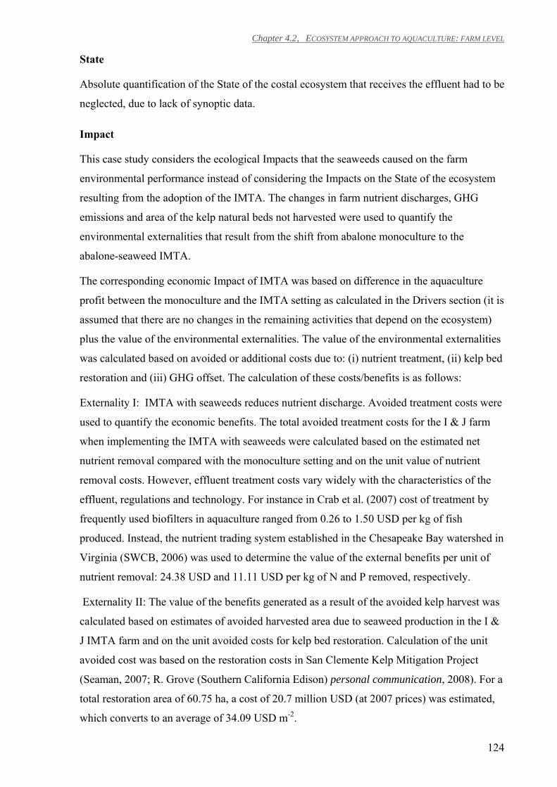
Chapter 4.2, ECOSYSTEM APPROACH TO AQUACULTURE: FARM LEVEL
124
State
Absolute quantification of the State of the costal ecosystem that receives the effluent had to be
neglected, due to lack of synoptic data.
Impact
This case study considers the ecological Impacts that the seaweeds caused on the farm
environmental performance instead of considering the Impacts on the State of the ecosystem
resulting from the adoption of the IMTA. The changes in farm nutrient discharges, GHG
emissions and area of the kelp natural beds not harvested were used to quantify the
environmental externalities that result from the shift from abalone monoculture to the
abalone-seaweed IMTA.
The corresponding economic Impact of IMTA was based on difference in the aquaculture
profit between the monoculture and the IMTA setting as calculated in the Drivers section (it is
assumed that there are no changes in the remaining activities that depend on the ecosystem)
plus the value of the environmental externalities. The value of the environmental externalities
was calculated based on avoided or additional costs due to: (i) nutrient treatment, (ii) kelp bed
restoration and (iii) GHG offset. The calculation of these costs/benefits is as follows:
Externality I: IMTA with seaweeds reduces nutrient discharge. Avoided treatment costs were
used to quantify the economic benefits. The total avoided treatment costs for the I & J farm
when implementing the IMTA with seaweeds were calculated based on the estimated net
nutrient removal compared with the monoculture setting and on the unit value of nutrient
removal costs. However, effluent treatment costs vary widely with the characteristics of the
effluent, regulations and technology. For instance in Crab et al. (2007) cost of treatment by
frequently used biofilters in aquaculture ranged from 0.26 to 1.50 USD per kg of fish
produced. Instead, the nutrient trading system established in the Chesapeake Bay watershed in
Virginia (SWCB, 2006) was used to determine the value of the external benefits per unit of
nutrient removal: 24.38 USD and 11.11 USD per kg of N and P removed, respectively.
Externality II: The value of the benefits generated as a result of the avoided kelp harvest was
calculated based on estimates of avoided harvested area due to seaweed production in the I &
J IMTA farm and on the unit avoided costs for kelp bed restoration. Calculation of the unit
avoided cost was based on the restoration costs in San Clemente Kelp Mitigation Project
(Seaman, 2007; R. Grove (Southern California Edison) personal communication, 2008). For a
total restoration area of 60.75 ha, a cost of 20.7 million USD (at 2007 prices) was estimated,
which converts to an average of 34.09 USD m-2.
Chapter 4.2, ECOSYSTEM APPROACH TO AQUACULTURE: FARM LEVEL
125
Externality III: The cost/benefit associated with the change in the GHG emission was
estimated using the voluntary carbon market system and the estimated GHG emissions of the
I & J farm. The average applicable offset rate (14.27 Euro per ton CO2, which converts to
about 18.72 USD per ton CO2) was calculated based on data of 90 providers (Carbon Catalog,
2008).
Response
The Response is a socio-economic component of the ∆DPSIR analysis (Nobre, 2009) and in
this case study equals the cost of the measures adopted by the farm managers to set up
settings 2 and 3. Estimates were based on Robertson-Andersson (2007) data about seaweed
pond investment costs (Table 4.14). Calculation of the Response cost per annum considered
10-year depreciation for the concrete structure and 5-year for other components.
Table 4.14. I & J seaweed pond investment costs (compiled from Robertson-Andersson (2007)). Paddle pond costs USD
Concrete 9 361
Other components (e.g. electric motor) 4 645
Paddle wheels (shared by two ponds) 8 031
Total investment USD
4 ponds 78 858
12 ponds 236 574
A Nutrient mass balance model for the recirculating system
A simple two compartment abalone-seaweed mass balance model was developed to predict
the nutrient discharge for the projected expansion of the seaweed ponds in setting 3 (Figure
4.8). The nutrient sources include the nutrients from seawater (Fsea), the net nutrient
production in the abalone tanks (Fabalone) and the seaweed fertilization (Ffertilizer). The nutrient
sinks include seaweed nutrient uptake (Falgae) and nutrient discharge to the sea (Feffluent).
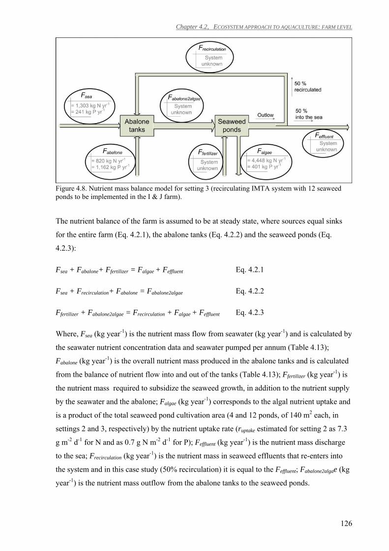
Chapter 4.2, ECOSYSTEM APPROACH TO AQUACULTURE: FARM LEVEL
126
Figure 4.8. Nutrient mass balance model for setting 3 (recirculating IMTA system with 12 seaweed ponds to be implemented in the I & J farm).
The nutrient balance of the farm is assumed to be at steady state, where sources equal sinks
for the entire farm (Eq. 4.2.1), the abalone tanks (Eq. 4.2.2) and the seaweed ponds (Eq.
4.2.3):
Fsea + Fabalone+ Ffertilizer = Falgae + Feffluent Eq. 4.2.1
Fsea + Frecirculation+ Fabalone = Fabalone2algae Eq. 4.2.2
Ffertilizer + Fabalone2algae = Frecirculation + Falgae + Feffluent Eq. 4.2.3
Where, Fsea (kg year-1) is the nutrient mass flow from seawater (kg year-1) and is calculated by
the seawater nutrient concentration data and seawater pumped per annum (Table 4.13);
Fabalone (kg year-1) is the overall nutrient mass produced in the abalone tanks and is calculated
from the balance of nutrient flow into and out of the tanks (Table 4.13); Ffertilizer (kg year-1) is
the nutrient mass required to subsidize the seaweed growth, in addition to the nutrient supply
by the seawater and the abalone; Falgae (kg year-1) corresponds to the algal nutrient uptake and
is a product of the total seaweed pond cultivation area (4 and 12 ponds, of 140 m2 each, in
settings 2 and 3, respectively) by the nutrient uptake rate (ruptake estimated for setting 2 as 7.3
g m-2 d-1 for N and as 0.7 g N m-2 d-1 for P); Feffluent (kg year-1) is the nutrient mass discharge
to the sea; Frecirculation (kg year-1) is the nutrient mass in seaweed effluents that re-enters into
the system and in this case study (50% recirculation) it is equal to the Feffluent; Fabalone2algae (kg
year-1) is the nutrient mass outflow from the abalone tanks to the seaweed ponds.
Chapter 4.2, ECOSYSTEM APPROACH TO AQUACULTURE: FARM LEVEL
127
Furthermore, Ffertilizer can be defined as the nutrients required for the seaweed maximal yield
minus the other nutrient sources for the seaweed ponds:
Ffertilizer = Falgae/euptake – Fabalone2algae Eq. 4.2.4
Where, euptake is the seaweed nutrient removal efficiency (%) that corresponds to the
proportion of nutrients removed relative to the available nutrients. euptake was estimated for
setting 2 as 53% for N and 5% for P.
For setting 3 it is assumed that values for Fsea, Fabalone, ruptake and euptake are the same as in
setting 2.
Considering the above assumptions and Eq. 4.2.2, Eq. 4.2.3 and Eq. 4.2.4 the model may be
defined as a system of four equations with the following four unknowns (Figure 4.8):
Ffertilizer = Falgae/euptake - (Fsea + Frecirculation+ Fabalone) Eq. 4.2.5
Fabalone2algae = Fsea + Frecirculation+ Fabalone Eq. 4.2.6
Frecirculation = (Ffertilizer + Fabalone2algae - Falgae)/2 Eq. 4.2.7
Feffluent = Frecirculation Eq. 4.2.8
The solution to the system can be defined as:
Ffertilizer = Falgae*[(1+ euptake)/2*euptake] - Fsea - Fabalone Eq. 4.2.9
Fabalone2algae = Fsea + (Falgae/2) * (1/euptake -1) + Fabalone Eq. 4.2.10
Frecirculation = Falgae/2 * (1/ euptake -1) Eq. 4.2.11
Feffluent = Falgae/2 * (1/ euptake -1) Eq. 4.2.12
Here, Eq. 4.2.9 calculates the quantity of fertilizer required for the planned seaweed
production and Eq. 4.2.12, the farm's nutrient discharge.
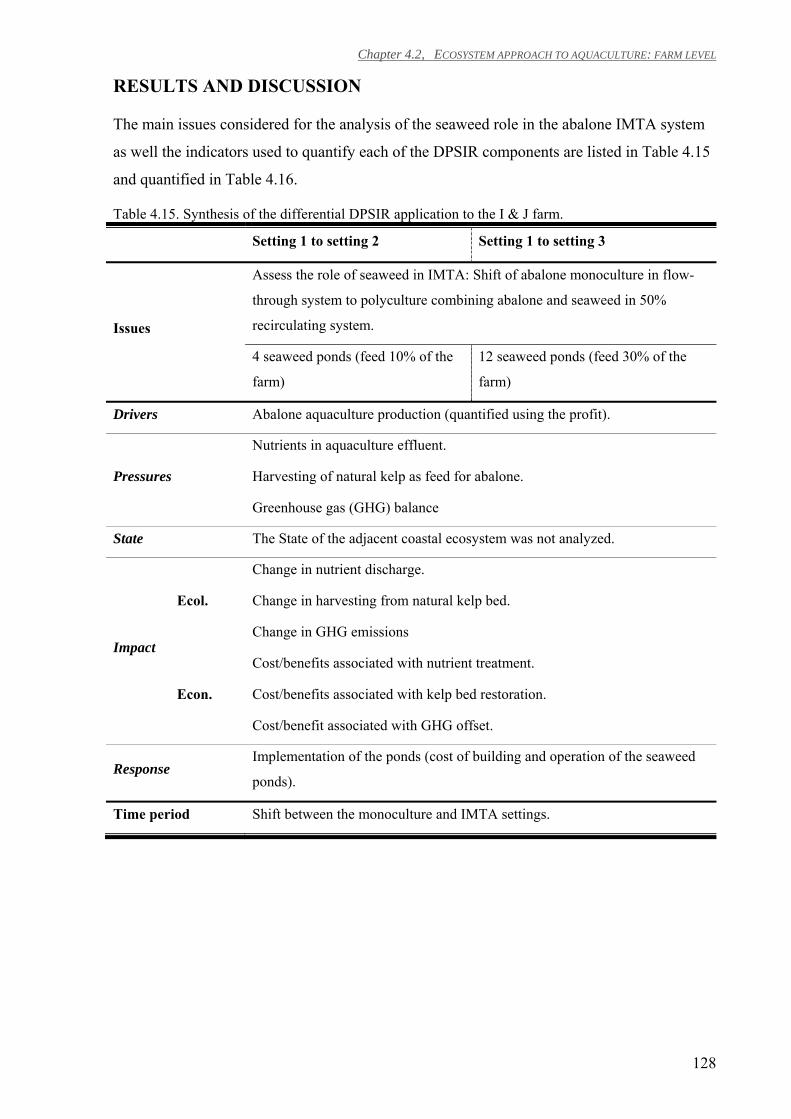
Chapter 4.2, ECOSYSTEM APPROACH TO AQUACULTURE: FARM LEVEL
128
RESULTS AND DISCUSSION
The main issues considered for the analysis of the seaweed role in the abalone IMTA system
as well the indicators used to quantify each of the DPSIR components are listed in Table 4.15
and quantified in Table 4.16.
Table 4.15. Synthesis of the differential DPSIR application to the I & J farm.
Setting 1 to setting 2 Setting 1 to setting 3
Issues
Assess the role of seaweed in IMTA: Shift of abalone monoculture in flow-
through system to polyculture combining abalone and seaweed in 50%
recirculating system.
4 seaweed ponds (feed 10% of the
farm)
12 seaweed ponds (feed 30% of the
farm)
Drivers Abalone aquaculture production (quantified using the profit).
Pressures
Nutrients in aquaculture effluent.
Harvesting of natural kelp as feed for abalone.
Greenhouse gas (GHG) balance
State The State of the adjacent coastal ecosystem was not analyzed.
Impact
Ecol.
Change in nutrient discharge.
Change in harvesting from natural kelp bed.
Change in GHG emissions
Econ.
Cost/benefits associated with nutrient treatment.
Cost/benefits associated with kelp bed restoration.
Cost/benefit associated with GHG offset.
Response Implementation of the ponds (cost of building and operation of the seaweed
ponds).
Time period Shift between the monoculture and IMTA settings.
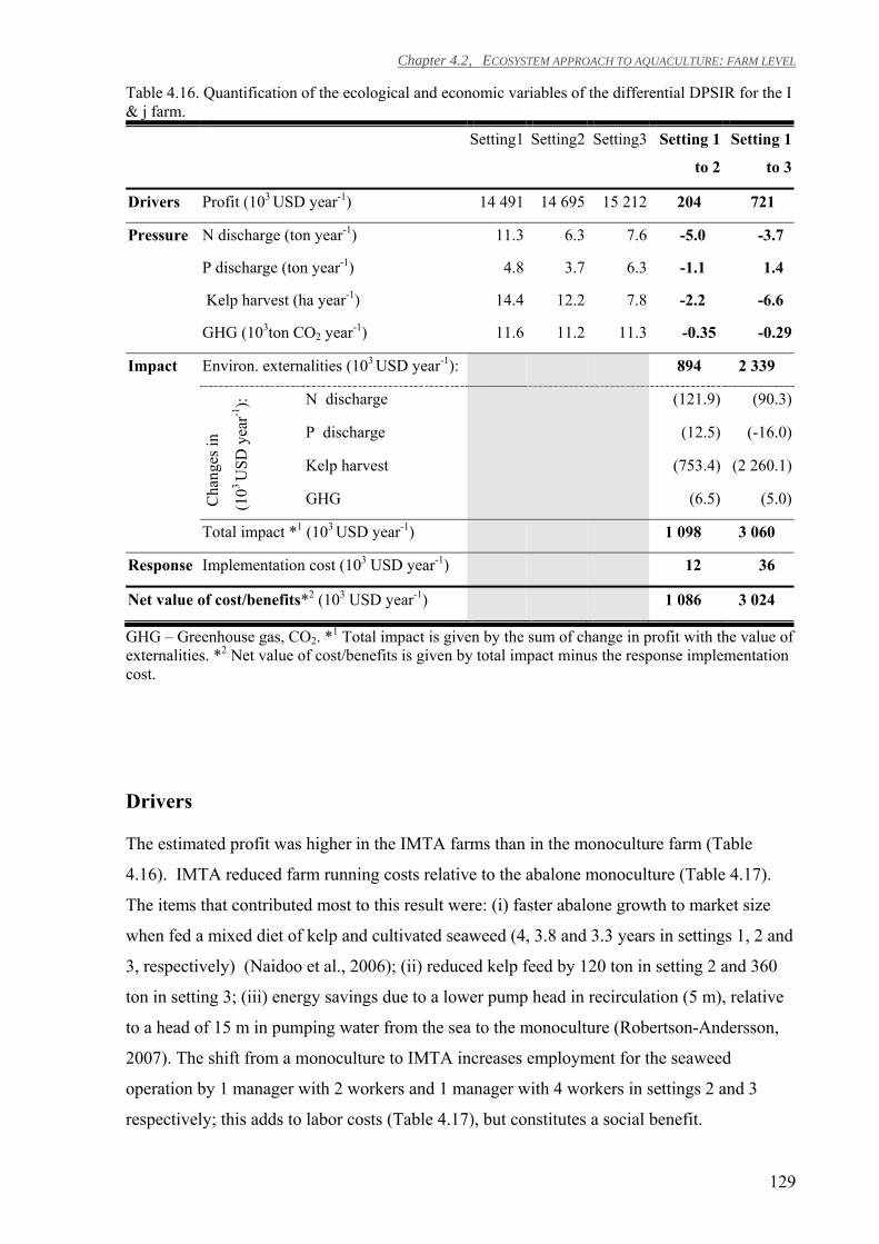
Chapter 4.2, ECOSYSTEM APPROACH TO AQUACULTURE: FARM LEVEL
129
Table 4.16. Quantification of the ecological and economic variables of the differential DPSIR for the I & j farm.
Setting1 Setting2 Setting3 Setting 1
to 2
Setting 1
to 3
Drivers Profit (103 USD year-1) 14 491 14 695 15 212 204 721
Pressure N discharge (ton year-1) 11.3 6.3 7.6 -5.0 -3.7
P discharge (ton year-1) 4.8 3.7 6.3 -1.1 1.4
Kelp harvest (ha year-1) 14.4 12.2 7.8 -2.2 -6.6
GHG (103ton CO2 year-1) 11.6 11.2 11.3 -0.35 -0.29
Impact Environ. externalities (103 USD year-1): 894 2 339
Cha
nges
in
(103
USD
yea
r-1):
N discharge (121.9) (90.3)
P discharge (12.5) (-16.0)
Kelp harvest (753.4) (2 260.1)
GHG (6.5) (5.0)
Total impact *1 (103 USD year-1) 1 098 3 060
Response Implementation cost (103 USD year-1) 12 36
Net value of cost/benefits*2 (103 USD year-1) 1 086 3 024
GHG – Greenhouse gas, CO2. *1 Total impact is given by the sum of change in profit with the value of externalities. *2 Net value of cost/benefits is given by total impact minus the response implementation cost.
Drivers
The estimated profit was higher in the IMTA farms than in the monoculture farm (Table
4.16). IMTA reduced farm running costs relative to the abalone monoculture (Table 4.17).
The items that contributed most to this result were: (i) faster abalone growth to market size
when fed a mixed diet of kelp and cultivated seaweed (4, 3.8 and 3.3 years in settings 1, 2 and
3, respectively) (Naidoo et al., 2006); (ii) reduced kelp feed by 120 ton in setting 2 and 360
ton in setting 3; (iii) energy savings due to a lower pump head in recirculation (5 m), relative
to a head of 15 m in pumping water from the sea to the monoculture (Robertson-Andersson,
2007). The shift from a monoculture to IMTA increases employment for the seaweed
operation by 1 manager with 2 workers and 1 manager with 4 workers in settings 2 and 3
respectively; this adds to labor costs (Table 4.17), but constitutes a social benefit.
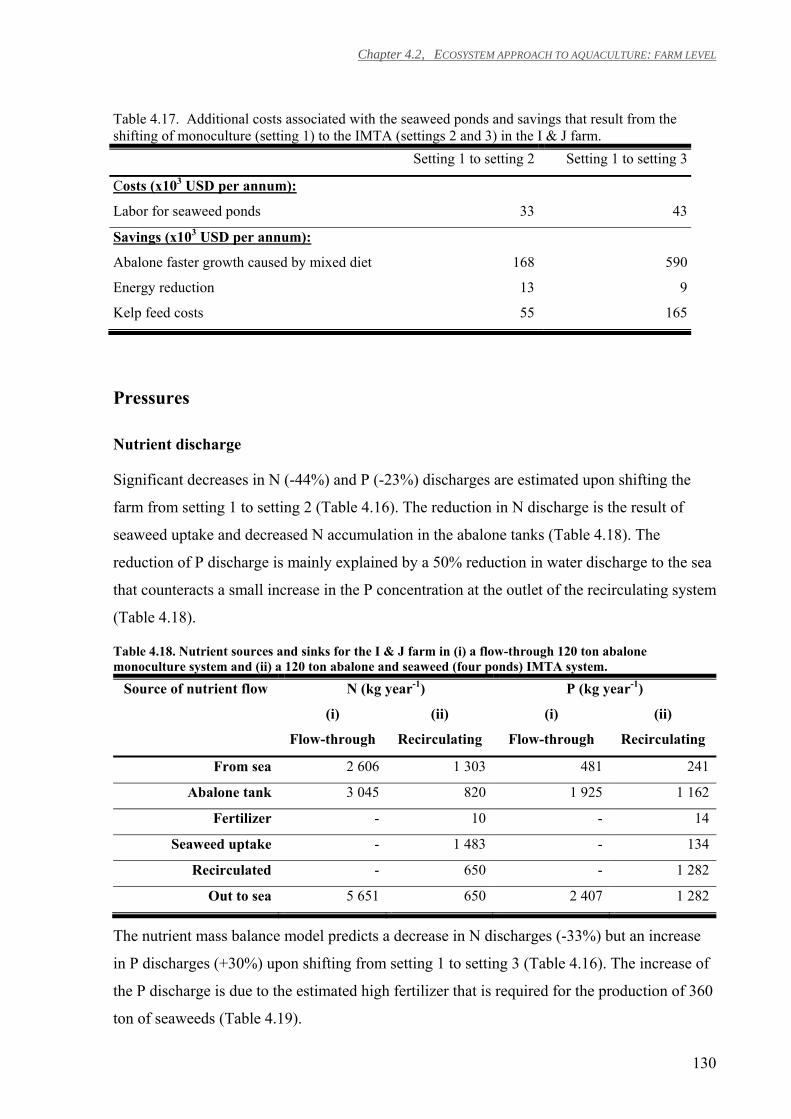
Chapter 4.2, ECOSYSTEM APPROACH TO AQUACULTURE: FARM LEVEL
130
Table 4.17. Additional costs associated with the seaweed ponds and savings that result from the shifting of monoculture (setting 1) to the IMTA (settings 2 and 3) in the I & J farm. Setting 1 to setting 2 Setting 1 to setting 3
Costs (x103 USD per annum):
Labor for seaweed ponds 33 43
Savings (x103 USD per annum):
Abalone faster growth caused by mixed diet 168 590
Energy reduction 13 9
Kelp feed costs 55 165
Pressures
Nutrient discharge
Significant decreases in N (-44%) and P (-23%) discharges are estimated upon shifting the
farm from setting 1 to setting 2 (Table 4.16). The reduction in N discharge is the result of
seaweed uptake and decreased N accumulation in the abalone tanks (Table 4.18). The
reduction of P discharge is mainly explained by a 50% reduction in water discharge to the sea
that counteracts a small increase in the P concentration at the outlet of the recirculating system
(Table 4.18).
Table 4.18. Nutrient sources and sinks for the I & J farm in (i) a flow-through 120 ton abalone monoculture system and (ii) a 120 ton abalone and seaweed (four ponds) IMTA system.
Source of nutrient flow N (kg year-1) P (kg year-1)
(i)
Flow-through
(ii)
Recirculating
(i)
Flow-through
(ii)
Recirculating
From sea 2 606 1 303 481 241
Abalone tank 3 045 820 1 925 1 162
Fertilizer - 10 - 14
Seaweed uptake - 1 483 - 134
Recirculated - 650 - 1 282
Out to sea 5 651 650 2 407 1 282
The nutrient mass balance model predicts a decrease in N discharges (-33%) but an increase
in P discharges (+30%) upon shifting from setting 1 to setting 3 (Table 4.16). The increase of
the P discharge is due to the estimated high fertilizer that is required for the production of 360
ton of seaweeds (Table 4.19).
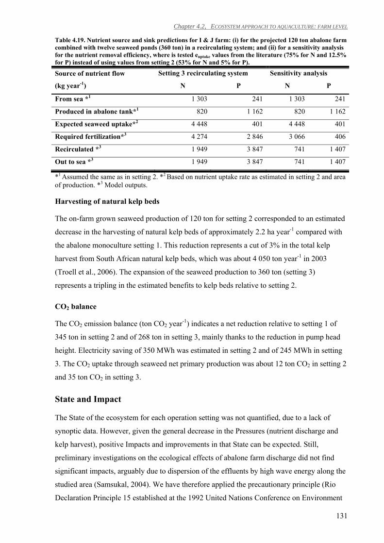
Chapter 4.2, ECOSYSTEM APPROACH TO AQUACULTURE: FARM LEVEL
131
Table 4.19. Nutrient source and sink predictions for I & J farm: (i) for the projected 120 ton abalone farm combined with twelve seaweed ponds (360 ton) in a recirculating system; and (ii) for a sensitivity analysis for the nutrient removal efficiency, where is tested euptake values from the literature (75% for N and 12.5% for P) instead of using values from setting 2 (53% for N and 5% for P).
Source of nutrient flow
(kg year-1)
Setting 3 recirculating system Sensitivity analysis
N P N P
From sea *1 1 303 241 1 303 241
Produced in abalone tank*1 820 1 162 820 1 162
Expected seaweed uptake*2 4 448 401 4 448 401
Required fertilization*3 4 274 2 846 3 066 406
Recirculated *3 1 949 3 847 741 1 407
Out to sea *3 1 949 3 847 741 1 407
*1 Assumed the same as in setting 2. *2 Based on nutrient uptake rate as estimated in setting 2 and area of production. *3 Model outputs.
Harvesting of natural kelp beds
The on-farm grown seaweed production of 120 ton for setting 2 corresponded to an estimated
decrease in the harvesting of natural kelp beds of approximately 2.2 ha year-1 compared with
the abalone monoculture setting 1. This reduction represents a cut of 3% in the total kelp
harvest from South African natural kelp beds, which was about 4 050 ton year-1 in 2003
(Troell et al., 2006). The expansion of the seaweed production to 360 ton (setting 3)
represents a tripling in the estimated benefits to kelp beds relative to setting 2.
CO2 balance
The CO2 emission balance (ton CO2 year-1) indicates a net reduction relative to setting 1 of
345 ton in setting 2 and of 268 ton in setting 3, mainly thanks to the reduction in pump head
height. Electricity saving of 350 MWh was estimated in setting 2 and of 245 MWh in setting
3. The CO2 uptake through seaweed net primary production was about 12 ton CO2 in setting 2
and 35 ton CO2 in setting 3.
State and Impact
The State of the ecosystem for each operation setting was not quantified, due to a lack of
synoptic data. However, given the general decrease in the Pressures (nutrient discharge and
kelp harvest), positive Impacts and improvements in that State can be expected. Still,
preliminary investigations on the ecological effects of abalone farm discharge did not find
significant impacts, arguably due to dispersion of the effluents by high wave energy along the
studied area (Samsukal, 2004). We have therefore applied the precautionary principle (Rio
Declaration Principle 15 established at the 1992 United Nations Conference on Environment
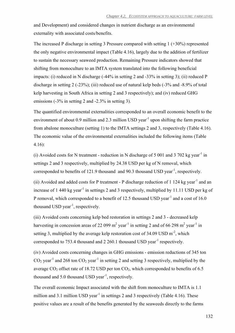
Chapter 4.2, ECOSYSTEM APPROACH TO AQUACULTURE: FARM LEVEL
132
and Development) and considered changes in nutrient discharge as an environmental
externality with associated costs/benefits.
The increased P discharge in setting 3 Pressure compared with setting 1 (+30%) represented
the only negative environmental impact (Table 4.16), largely due to the addition of fertilizer
to sustain the necessary seaweed production. Remaining Pressure indicators showed that
shifting from monoculture to an IMTA system translated into the following beneficial
impacts: (i) reduced in N discharge (-44% in setting 2 and -33% in setting 3); (ii) reduced P
discharge in setting 2 (-23%); (iii) reduced use of natural kelp beds (-3% and -8.9% of total
kelp harvesting in South Africa in setting 2 and 3 respectively); and (iv) reduced GHG
emissions (-3% in setting 2 and -2.3% in setting 3).
The quantified environmental externalities corresponded to an overall economic benefit to the
environment of about 0.9 million and 2.3 million USD year-1 upon shifting the farm practice
from abalone monoculture (setting 1) to the IMTA settings 2 and 3, respectively (Table 4.16).
The economic value of the environmental externalities included the following items (Table
4.16):
(i) Avoided costs for N treatment - reduction in N discharge of 5 001 and 3 702 kg year-1 in
settings 2 and 3 respectively, multiplied by 24.38 USD per kg of N removal, which
corresponded to benefits of 121.9 thousand and 90.3 thousand USD year-1, respectively.
(ii) Avoided and added costs for P treatment - P discharge reduction of 1 124 kg year-1 and an
increase of 1 440 kg year-1 in settings 2 and 3 respectively, multiplied by 11.11 USD per kg of
P removal, which corresponded to a benefit of 12.5 thousand USD year-1 and a cost of 16.0
thousand USD year-1, respectively.
(iii) Avoided costs concerning kelp bed restoration in settings 2 and 3 - decreased kelp
harvesting in concession areas of 22 099 m2 year-1 in setting 2 and of 66 298 m2 year-1 in
setting 3, multiplied by the average kelp restoration cost of 34.09 USD m-2, which
corresponded to 753.4 thousand and 2 260.1 thousand USD year-1 respectively.
(iv) Avoided costs concerning changes in GHG emissions - emission reductions of 345 ton
CO2 year-1 and 268 ton CO2 year-1 in setting 2 and setting 3 respectively, multiplied by the
average CO2 offset rate of 18.72 USD per ton CO2, which corresponded to benefits of 6.5
thousand and 5.0 thousand USD year-1, respectively.
The overall economic Impact associated with the shift from monoculture to IMTA is 1.1
million and 3.1 million USD year-1 in settings 2 and 3 respectively (Table 4.16). These
positive values are a result of the benefits generated by the seaweeds directly to the farms
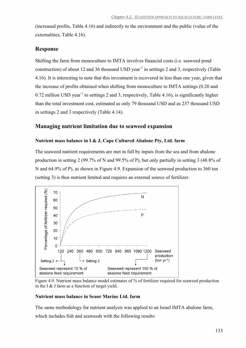
Chapter 4.2, ECOSYSTEM APPROACH TO AQUACULTURE: FARM LEVEL
133
(increased profits, Table 4.16) and indirectly to the environment and the public (value of the
externalities, Table 4.16).
Response
Shifting the farm from monoculture to IMTA involves financial costs (i.e. seaweed pond
construction) of about 12 and 36 thousand USD year-1 in settings 2 and 3, respectively (Table
4.16). It is interesting to note that this investment is recovered in less than one year, given that
the increase of profits obtained when shifting from monoculture to IMTA settings (0.20 and
0.72 million USD year-1 to settings 2 and 3, respectively, Table 4.16), is significantly higher
than the total investment cost, estimated as only 79 thousand USD and as 237 thousand USD
in settings 2 and 3 respectively (Table 4.14).
Managing nutrient limitation due to seaweed expansion
Nutrient mass balance in I & J, Cape Cultured Abalone Pty, Ltd. farm
The seaweed nutrient requirements are met in full by inputs from the sea and from abalone
production in setting 2 (99.7% of N and 99.5% of P), but only partially in setting 3 (48.8% of
N and 64.9% of P), as shown in Figure 4.9. Expansion of the seaweed production to 360 ton
(setting 3) is thus nutrient limited and requires an external source of fertilizer.
Figure 4.9. Nutrient mass balance model estimates of % of fertilizer required for seaweed production in the I & J farm as a function of target yield.
Nutrient mass balance in Seaor Marine Ltd. farm
The same methodology for nutrient analysis was applied to an Israel IMTA abalone farm,
which includes fish and seaweeds with the following results:
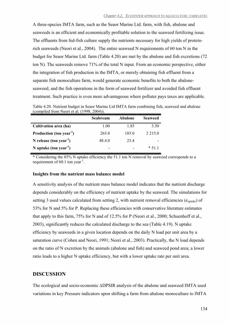
Chapter 4.2, ECOSYSTEM APPROACH TO AQUACULTURE: FARM LEVEL
134
A three-species IMTA farm, such as the Seaor Marine Ltd. farm, with fish, abalone and
seaweeds is an efficient and economically profitable solution to the seaweed fertilizing issue.
The effluents from fed-fish culture supply the nutrients necessary for high yields of protein-
rich seaweeds (Neori et al., 2004). The entire seaweed N requirements of 60 ton N in the
budget for Seaor Marine Ltd. farm (Table 4.20) are met by the abalone and fish excretions (72
ton N). The seaweeds remove 71% of the total N input. From an economic perspective, either
the integration of fish production in the IMTA, or merely obtaining fish effluent from a
separate fish monoculture farm, would generate economic benefits to both the abalone-
seaweed, and the fish operations in the form of seaweed fertilizer and avoided fish effluent
treatment. Such practice is even more advantageous where polluter pays taxes are applicable.
Table 4.20. Nutrient budget in Seaor Marine Ltd IMTA farm combining fish, seaweed and abalone (compiled from Neori et al. (1998, 2004)). Seabream Abalone Seaweed
Cultivation area (ha) 1.00 1.85 3.50
Production (ton year-1) 265.0 185.0 2 215.0
N release (ton year-1) 48.4.0 23.4 -
N uptake (ton year-1) - - * 51.1
* Considering the 85% N uptake efficiency the 51.1 ton N removal by seaweed corresponds to a requirement of 60.1 ton year-1.
Insights from the nutrient mass balance model
A sensitivity analysis of the nutrient mass balance model indicates that the nutrient discharge
depends considerably on the efficiency of nutrient uptake by the seaweed. The simulations for
setting 3 used values calculated from setting 2, with nutrient removal efficiencies (euptake) of
53% for N and 5% for P. Replacing these efficiencies with conservative literature estimates
that apply to this farm, 75% for N and of 12.5% for P (Neori et al., 2000; Schuenhoff et al.,
2003), significantly reduces the calculated discharge to the sea (Table 4.19). N uptake
efficiency by seaweeds in a given location depends on the daily N load per unit area by a
saturation curve (Cohen and Neori, 1991; Neori et al., 2003). Practically, the N load depends
on the ratio of N excretion by the animals (abalone and fish) and seaweed pond area; a lower
ratio leads to a higher N uptake efficiency, but with a lower uptake rate per unit area.
DISCUSSION
The ecological and socio-economic ∆DPSIR analysis of the abalone and seaweed IMTA used
variations in key Pressure indicators upon shifting a farm from abalone monoculture to IMTA
Chapter 4.2, ECOSYSTEM APPROACH TO AQUACULTURE: FARM LEVEL
135
with seaweeds. In general, the incorporation of seaweeds decreased the Pressures caused by
the abalone production. The environmental benefits included reduction in nitrogen discharge
into the sea, reduction in harvest of natural kelp harvesting and reduction in CO2 emissions.
Depending on the upscaling setting, phosphorus discharge could increase due to fertilization
of the seaweeds; this could, however, be neutralized by integrating the production of other
organism such as fish in the IMTA. The overall economic gain, thanks to adopting the IMTA
design compared with an abalone monoculture, is valued at 1.1 million or 3.0 million USD
year-1, depending on the scale of the seaweed facility. These values represent the outcome of
the balance between the farm direct benefits expressed as increased profit, the implementation
costs of the seaweed ponds and the quantifiable environmental externalities that arise due to
the shift from abalone monoculture to IMTA with seaweeds. The external environmental
benefits contribute about 80% of the economic gains upon shifting to the IMTA, which means
that the increase in profitability to the farms brings even larger benefits to the environment
and the public. From both ecological and economic perspectives, the benefits associated with
the shift from monoculture to the IMTA increases with an increase in seaweed production.
However, the expansion of the on-farm grown seaweeds should be carefully designed in order
to efficiently address the resulting nutrient limitations. The balanced three-species IMTA farm
in Israel provides an example on how to manage nutrient limitation. In that case the on-farm
grown seaweeds receive all the additional nutrients from the fish effluents.
Social relevance
Aquaculture can accrue social benefits in employment, income and food security, particularly
important to poor, rural coastal communities worldwide (Ahmed and Lorica, 2002; Katranidis
et al., 2003; Kaliba et al., 2007). The South African abalone farm case study exemplifies the
positive impact an aquaculture industry can have on local communities. The I & J farm
employs 5.5% of the men and 1.5% of the women from the local communities of Blompark,
Groeneweldskerma and Masakhane (CSS, 2005, Robertson-Andersson, 2007). These
communities are characterized by high unemployment (85.7%), with more than 50% of the
labor force being unskilled and semi skilled, using criteria as defined by Lewis (2001)
(Robertson-Andersson, 2007). This is particularly relevant where unemployment is not only
an economic issue but also a critical socio-political issue (Kingdon and Knight, 2003; Evett,
2006): four in every ten adults of working age in South Africa are unemployed or have no
access to or means of earning an income (Evett, 2006). According to Lewis (2001), the
overall unemployment in South Africa in 2000 was above 36% and 50% in unskilled and
semi-skilled workers respectively. The direct permanent employment in the South African
Chapter 4.2, ECOSYSTEM APPROACH TO AQUACULTURE: FARM LEVEL
136
abalone industry has a large local impact in previously disadvantaged coastal communities,
where any increase in employment is valuable. A more detailed analysis is still required to
determine the full cascade of social impacts that the IMTA approach can have. In particular,
and in order to complement the present ecological-economic assessment, future analysis
should focus on the social cost/benefits of the IMTA settings compared with the monoculture
production.
CONCLUSION
The application of the ∆DPSIR to the present case study indicates that the shift from abalone
monoculture to IMTA with seaweeds increases the farm profitability and brings even larger
benefits to the environment and the public, through reduced Pressures on the adjacent coastal
ecosystem and increased employment. As the cost of energy increases and where pollution
taxes are adopted, the economic incentives for the implementation of IMTA farms, compared
with monoculture abalone farms, are likely to mount. From a social and environmental
perspective, the three-species IMTA with fish, abalone and seaweeds produces more value
and resources for human consumption while still managing the waste produced. This outcome
should be considered by industry and regulators involved with the current expansion in
abalone culture worldwide. The present ∆DPSIR analysis can help owners and regulatory
officials in balancing the design of the farm with respect to nutrient mass balance towards
reduced negative environmental externalities. As kelp is reaching limits of sustainable
harvesting, particularly in kelp concession areas with high abalone farm concentrations, and
with the forceful socio-economic incentives quantified in the present paper, it can be expected
that two- and three-species IMTA farms will become the industry norm, rather than the
exception.
The estimates of the economic value of the environmental externalities obtained by the
∆DPSIR analysis provide the aquaculture industry, the coastal zone and resource managers an
indication of the benefits to farms and society by implementation of ecologically balanced
IMTA farms, relative to monoculture systems. More such analyses should be undertaken on
other aquaculture practices and for other species of fish, shrimp, shellfish and macroalgae.
Likewise, the ∆DPSIR could be applied to compare the ecological and economic impacts of
fisheries vs. aquaculture. Those studies should include a detailed quantification of aquaculture
industry impacts on the entire cascade of employment and income of local communities.
Chapter 5. Ecological-economic dynamic modelling
Context
One of the missing links in ecosystem modelling is economics. Integration with economics
for scenario testing is important to help define the focus of management measures. Dynamic
ecological-economic modelling is required to simulate the feedbacks between the ecological
and economic systems. Insights provided by the outcomes of such modelling tools are
important for coastal management. For instance, with limited resources, is important to
prioritize actions that bring larger benefits to the public and at the same time allow the
development of private activities.
Summary
This chapter presents the MARKET model, which dynamically couples the ecological and
economic components of aquaculture production. The model is herein applied to simulate
shellfish production in a Chinese bay under different assumptions for price and income
growth rates and the maximum area available for shellfish cultivation.
Chapter 5, ECOLOGICAL-ECONOMIC DYNAMIC MODELLING
138
This chapter corresponds to the published manuscript:
Nobre, A.M., J.K. Musango, M.P. de Wit, Ferreira, J.G., 2009. A
dynamic ecological-economic modeling approach for aquaculture
management. Ecological Economics. DOI:
10.1016/j.ecolecon.2009.06.019.
(For consistency with published version this chapter is written in
American English)
Chapter 5, ECOLOGICAL-ECONOMIC DYNAMIC MODELLING
139
A dynamic ecological-economic modeling approach for aquaculture management
INTRODUCTION
Global consumption of finfish and shellfish as food has doubled since 1973. Evidence
suggests that the large increase in the aquatic resources production in recent decades has
resulted from the enormous growth in seafood demand in the developing countries (Delgado
et al., 2003). China is the largest aquaculture producer in the world, with an average annual
growth rate from 1980 to 2004 of 15 % (Gíslason et al., 2006), and the only nation where
farmed production exceeds wild catch (Sanchez et al., 2007). In 2006, 68 % of total aquatic
production in China was from aquaculture (FAO, 2009). The development of aquaculture in
China has had a positive impact in terms of its contribution to nutrition, employment, and
improvement in socio-economic status of both rural and urban communities (FAO, 2004).
About 4.3 million rural workers are directly employed in aquaculture with an annual per
capita net income of 8 667 Yuan (which converts to 1 075 USD considering the exchange rate
at the time of study, 1 USD = 8.06 Yuan) (FAO, 2005). Given the significance of aquaculture
in China, changes in mariculture production due to changes in economic inputs or biophysical
variability have a wider socio-economic impact on communities.
Just like any other food-producing sector in the world, aquaculture relies on renewable and
non-renewable resources. Sustainable development and management of aquaculture thus
requires an appropriate understanding of the conflicts and interactions between the resource
use and its users. Such understanding contributes to improve governance in resource use,
which is an important prerequisite of the sector’s sustainability and one of the objectives of
building an ecosystem approach to aquaculture (EAA) (Soto et al., 2008). Aquaculture is
considered as the “solution” for bridging the supply and demand gap of aquatic food globally.
There is however concern about the negative environmental impacts that some aquaculture
practices can exert on coastal resources and ecosystems (Tovar et al., 2000; Xu et al., 2007).
The carrying capacity of the coastal ecosystem can represent a limit to the increase in
aquaculture production. Depending on culture practices, this might be related to space
limitations, availability of food resources or on the environmental capacity to assimilate
aquaculture generated wastes (Sequeira et al., 2008). Apart from ecological limitations there
are also economic cost limitations to production, illustrated through an analysis of the
marginal cost in relation to marginal revenue (Gravelle and Rees, 1993). An economic
Chapter 5, ECOLOGICAL-ECONOMIC DYNAMIC MODELLING
140
analysis of aquaculture production must be based on realistic production cost and income
projections that account for these economic limitations.
The focus of aquaculture management is often on maximizing the output and not the profit,
which is not only economically inefficient, but carries unnecessary ecological risks. If the
goals of sustainable aquaculture development are to be achieved, then there is need to
understand both ecological and economic limitations. Aquaculture operations depend directly
on the availability and quality of the marine resources and environment. If the marine
ecosystem is overexploited the negative impacts will be felt in aquaculture farming operations
and by all other downstream activities dependent on aquatic resources farming. This is
particularly important for a country such as China that accounts for 68 % of the world aquatic
production, and where some of the marine ecosystems have a high percentage of reclaimed
areas for aquaculture, e.g., 77 % of the coastal usable area of Xiamen is occupied by
aquaculture activities (Xue, 2005).
To ensure sustainable aquaculture production, it is crucial to understand the ecological and
economic limits beyond which mariculture becomes less efficient. Dynamic modeling can
provide a tool that facilitates the understanding of the complex feedbacks between ecological
and economic aspects of aquaculture production. Resource managers and policymakers have
come to understand that the sustainability of ecological and economic systems is tightly
coupled (GESAMP, 2001). However, the complexity of the interactions may make informed
resource decision-making extremely difficult, particularly given the dynamic nature of
ecosystems and the difference in the scale of analysis of ecological and economic systems.
The integration between ecological and economic models is currently a developing discipline
(Drechsler et al., 2007). Several conflicts were identified (Bockstael et al., 1995; Drechsler
and Watzold, 2007) that explain the decoupling of these two disciplines, namely: (i) the scales
of analysis; (ii) the communication/understanding between ecology and economics; and (iii)
the implicit assumptions of each one.
In recent years there was an increase in the development of integrated ecological-economic
models (Drechsler et al., 2007). According to Bulte and van Kooten (1999), Armstrong
(2007) and Drechsler et al. (2007) these models tend to be less complex than the
biological/ecological models alone. Jin et al. (2003) categorize ecological-economic models
into 3 groups: (i) bioeconomic model approach; (ii) integration of complex environmental and
economic models; and (iii) linear models, for instance the coupling of linear economic input-
output model with a food web model.
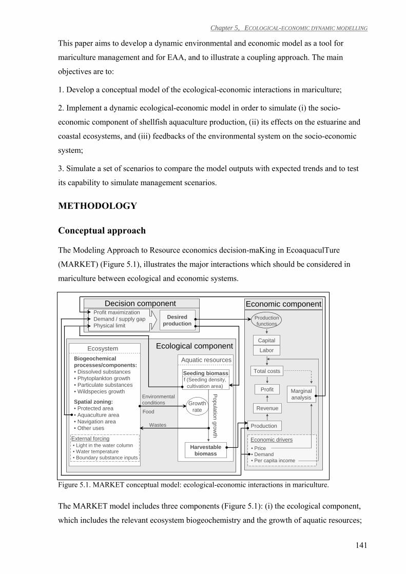
Chapter 5, ECOLOGICAL-ECONOMIC DYNAMIC MODELLING
141
This paper aims to develop a dynamic environmental and economic model as a tool for
mariculture management and for EAA, and to illustrate a coupling approach. The main
objectives are to:
1. Develop a conceptual model of the ecological-economic interactions in mariculture;
2. Implement a dynamic ecological-economic model in order to simulate (i) the socio-
economic component of shellfish aquaculture production, (ii) its effects on the estuarine and
coastal ecosystems, and (iii) feedbacks of the environmental system on the socio-economic
system;
3. Simulate a set of scenarios to compare the model outputs with expected trends and to test
its capability to simulate management scenarios.
METHODOLOGY
Conceptual approach
The Modeling Approach to Resource economics decision-maKing in EcoaquaculTure
(MARKET) (Figure 5.1), illustrates the major interactions which should be considered in
mariculture between ecological and economic systems.
Figure 5.1. MARKET conceptual model: ecological-economic interactions in mariculture.
The MARKET model includes three components (Figure 5.1): (i) the ecological component,
which includes the relevant ecosystem biogeochemistry and the growth of aquatic resources;
Production
Total costs
Revenue
Profit
Capital
Labor
Marginal analysis Environmental
conditions
Ecological component
Economic componentDecision component
External forcing
Ecosystem
Aquatic resourcesBiogeochemical processes/components:• Dissolved substances• Phytoplankton growth• Particulate substances• Wildspecies growth
• Light in the water column• Water temperature• Boundary substance inputs
Seeding biomassf (Seeding density,
cultivation area)
Harvestablebiomass
Population grow
th
GrowthrateFood
Economic drivers
Profit maximizationDemand / supply gapPhysical limit
Desired production
Wastes
• Price• Demand• Per capita income
Production functions
Spatial zoning:• Protected area• Aquaculture area• Navigation area• Other uses Production
Total costs
Revenue
Profit
Capital
Labor
Marginal analysis Environmental
conditions
Ecological component
Economic componentDecision component
External forcing
Ecosystem
Aquatic resourcesBiogeochemical processes/components:• Dissolved substances• Phytoplankton growth• Particulate substances• Wildspecies growth
• Light in the water column• Water temperature• Boundary substance inputs
Seeding biomassf (Seeding density,
cultivation area)
Harvestablebiomass
Population grow
th
GrowthrateFood
Economic drivers
Profit maximizationDemand / supply gapPhysical limit
Desired production
Wastes
• Price• Demand• Per capita income
Production functions
Spatial zoning:• Protected area• Aquaculture area• Navigation area• Other uses
Chapter 5, ECOLOGICAL-ECONOMIC DYNAMIC MODELLING
142
(ii) the economic component, which invests capital and labor for the production of the aquatic
resources; and (iii) the decision component, which determines the desired production for the
next production cycle. The three components interact as follows (Figure 5.1):
At the beginning of a production cycle, the ecological component is used to determine the
seeding biomass corresponding to the desired production for that cycle and to allocate the
required cultivation space. The ecosystem water quality and environmental conditions are
used to calculate the scope for growth of the cultivated species. In parallel, the aquatic
resource production affects the biogeochemistry of the ecosystem, either through waste
generation and/or uptake of particulate and dissolved substances, depending on species and
culture practice. The adult individuals are subsequently harvested and transferred to the
economic component at the end of the production cycle, and the harvested biomass is used by
this module to calculate the revenue generated. Concurrently, in the economic component the
production inputs, such as labor and capital required to produce the desirable yield (as
calculated in the decision component), are determined and used to calculate the production
cost. In addition, the economic component determines the marginal cost and marginal revenue
in order to inform the decision component about profitability. The decision component then
determines the changes in the desired production for the next cycle based on the following
criteria: (i) profit maximization, based on the comparison of marginal cost and marginal
revenue; (ii) the gap between demand and supply, based on the comparison of the local
demand against shellfish production, in order to monitor if the market can absorb an increase
in production or if there is already a surplus; and (iii) physical limit, in order to ensure that the
cultivation area does not exceed the maximum available area for aquaculture, as defined by
ecosystem managers.
Ecological and economic limits
The ecosystem carrying capacity and economic production capacity can be limited by the
following factors:
1. Space limitation, which is defined by stakeholders with respect to allocation of ecosystem
area to cultivation and other uses.
2. Food limitation (in the case of extensive aquaculture), which is a function of available
ecosystem resources, cultivation densities and practices. It affects the growth rate of aquatic
resources.
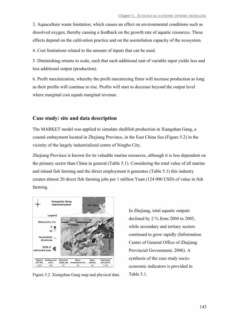
Chapter 5, ECOLOGICAL-ECONOMIC DYNAMIC MODELLING
143
3. Aquaculture waste limitation, which causes an effect on environmental conditions such as
dissolved oxygen, thereby causing a feedback on the growth rate of aquatic resources. These
effects depend on the cultivation practice and on the assimilation capacity of the ecosystem.
4. Cost limitations related to the amount of inputs that can be used.
5. Diminishing returns to scale, such that each additional unit of variable input yields less and
less additional output (production).
6. Profit maximization, whereby the profit maximizing firms will increase production as long
as their profits will continue to rise. Profits will start to decrease beyond the output level
where marginal cost equals marginal revenue.
Case study: site and data description
The MARKET model was applied to simulate shellfish production in Xiangshan Gang, a
coastal embayment located in Zhejiang Province, in the East China Sea (Figure 5.2) in the
vicinity of the largely industrialized centre of Ningbo City.
Zhejiang Province is known for its valuable marine resources, although it is less dependent on
the primary sector than China in general (Table 5.1). Considering the total value of all marine
and inland fish farming and the direct employment it generates (Table 5.1) this industry
creates almost 20 direct fish farming jobs per 1 million Yuan (124 000 USD) of value in fish
farming.
In Zhejiang, total aquatic outputs
declined by 2 % from 2004 to 2005,
while secondary and tertiary sectors
continued to grow rapidly (Information
Center of General Office of Zhejiang
Provincial Government, 2006). A
synthesis of the case study socio-
economic indicators is provided in
Table 5.1. Figure 5.2. Xiangshan Gang map and physical data.
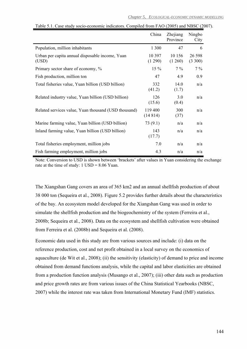
Chapter 5, ECOLOGICAL-ECONOMIC DYNAMIC MODELLING
144
Table 5.1. Case study socio-economic indicators. Compiled from FAO (2005) and NBSC (2007).
China Zhejiang Province
Ningbo City
Population, million inhabitants 1 300 47 6
Urban per capita annual disposable income, Yuan (USD)
10 397 (1 290)
10 156 (1 260)
26 598 (3 300)
Primary sector share of economy, % 15 % 7 % 7 %
Fish production, million ton 47 4.9 0.9
Total fisheries value, Yuan billion (USD billion) 332 (41.2)
14.0 (1.7)
n/a
Related industry value, Yuan billion (USD billion) 126 (15.6)
3.0 (0.4)
n/a
Related services value, Yuan thousand (USD thousand) 119 400 (14 814)
300 (37)
n/a
Marine farming value, Yuan billion (USD billion) 73 (9.1) n/a n/a
Inland farming value, Yuan billion (USD billion) 143 (17.7)
n/a n/a
Total fisheries employment, million jobs 7.0 n/a n/a
Fish farming employment, million jobs 4.3 n/a n/a
Note: Conversion to USD is shown between ‘brackets’ after values in Yuan considering the exchange rate at the time of study: 1 USD = 8.06 Yuan.
The Xiangshan Gang covers an area of 365 km2 and an annual shellfish production of about
38 000 ton (Sequeira et al., 2008). Figure 5.2 provides further details about the characteristics
of the bay. An ecosystem model developed for the Xiangshan Gang was used in order to
simulate the shellfish production and the biogeochemistry of the system (Ferreira et al.,
2008b; Sequeira et al., 2008). Data on the ecosystem and shellfish cultivation were obtained
from Ferreira et al. (2008b) and Sequeira et al. (2008).
Economic data used in this study are from various sources and include: (i) data on the
reference production, cost and net profit obtained in a local survey on the economics of
aquaculture (de Wit et al., 2008); (ii) the sensitivity (elasticity) of demand to price and income
obtained from demand functions analysis, while the capital and labor elasticities are obtained
from a production function analysis (Musango et al., 2007); (iii) other data such as production
and price growth rates are from various issues of the China Statistical Yearbooks (NBSC,
2007) while the interest rate was taken from International Monetary Fund (IMF) statistics.
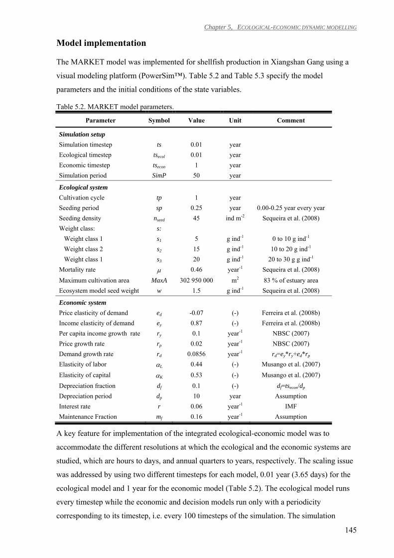
Chapter 5, ECOLOGICAL-ECONOMIC DYNAMIC MODELLING
145
Model implementation
The MARKET model was implemented for shellfish production in Xiangshan Gang using a
visual modeling platform (PowerSim™). Table 5.2 and Table 5.3 specify the model
parameters and the initial conditions of the state variables.
Table 5.2. MARKET model parameters.
Parameter Symbol Value Unit Comment
Simulation setup Simulation timestep ts 0.01 year Ecological timestep tsecol 0.01 year Economic timestep tsecon 1 year Simulation period SimP 50 year
Ecological system Cultivation cycle tp 1 year Seeding period sp 0.25 year 0.00-0.25 year every year Seeding density nseed 45 ind m-2 Sequeira et al. (2008) Weight class: s: Weight class 1 s1 5 g ind-1 0 to 10 g ind-1 Weight class 2 s2 15 g ind-1 10 to 20 g ind-1 Weight class 1 s3 20 g ind-1 20 to 30 g g ind-1 Mortality rate µ 0.46 year-1 Sequeira et al. (2008) Maximum cultivation area MaxA 302 950 000 m2 83 % of estuary area Ecosystem model seed weight w 1.5 g ind-1 Sequeira et al. (2008)
Economic system Price elasticity of demand ed -0.07 (-) Ferreira et al. (2008b) Income elasticity of demand ey 0.87 (-) Ferreira et al. (2008b) Per capita income growth rate ry 0.1 year-1 NBSC (2007) Price growth rate rp 0.02 year-1 NBSC (2007) Demand growth rate rd 0.0856 year-1 rd=ey*ry+ed*rp Elasticity of labor αL 0.44 (-) Musango et al. (2007) Elasticity of capital αK 0.53 (-) Musango et al. (2007) Depreciation fraction df 0.1 (-) df=tsecon/dp Depreciation period dp 10 year Assumption Interest rate r 0.06 year-1 IMF Maintenance Fraction mf 0.16 year-1 Assumption
A key feature for implementation of the integrated ecological-economic model was to
accommodate the different resolutions at which the ecological and the economic systems are
studied, which are hours to days, and annual quarters to years, respectively. The scaling issue
was addressed by using two different timesteps for each model, 0.01 year (3.65 days) for the
ecological model and 1 year for the economic model (Table 5.2). The ecological model runs
every timestep while the economic and decision models run only with a periodicity
corresponding to its timestep, i.e. every 100 timesteps of the simulation. The simulation
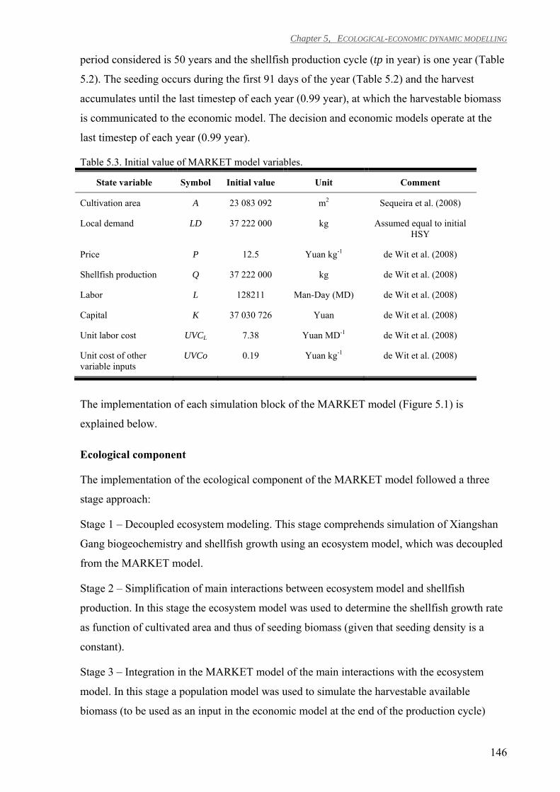
Chapter 5, ECOLOGICAL-ECONOMIC DYNAMIC MODELLING
146
period considered is 50 years and the shellfish production cycle (tp in year) is one year (Table
5.2). The seeding occurs during the first 91 days of the year (Table 5.2) and the harvest
accumulates until the last timestep of each year (0.99 year), at which the harvestable biomass
is communicated to the economic model. The decision and economic models operate at the
last timestep of each year (0.99 year).
Table 5.3. Initial value of MARKET model variables.
State variable Symbol Initial value Unit Comment
Cultivation area A 23 083 092 m2 Sequeira et al. (2008)
Local demand LD 37 222 000 kg Assumed equal to initial HSY
Price P 12.5 Yuan kg-1 de Wit et al. (2008)
Shellfish production Q 37 222 000 kg de Wit et al. (2008)
Labor L 128211 Man-Day (MD) de Wit et al. (2008)
Capital K 37 030 726 Yuan de Wit et al. (2008)
Unit labor cost UVCL 7.38 Yuan MD-1 de Wit et al. (2008)
Unit cost of other variable inputs
UVCo 0.19 Yuan kg-1 de Wit et al. (2008)
The implementation of each simulation block of the MARKET model (Figure 5.1) is
explained below.
Ecological component
The implementation of the ecological component of the MARKET model followed a three
stage approach:
Stage 1 – Decoupled ecosystem modeling. This stage comprehends simulation of Xiangshan
Gang biogeochemistry and shellfish growth using an ecosystem model, which was decoupled
from the MARKET model.
Stage 2 – Simplification of main interactions between ecosystem model and shellfish
production. In this stage the ecosystem model was used to determine the shellfish growth rate
as function of cultivated area and thus of seeding biomass (given that seeding density is a
constant).
Stage 3 – Integration in the MARKET model of the main interactions with the ecosystem
model. In this stage a population model was used to simulate the harvestable available
biomass (to be used as an input in the economic model at the end of the production cycle)
Chapter 5, ECOLOGICAL-ECONOMIC DYNAMIC MODELLING
147
based on the seeding input (obtained from the decision model output at the beginning of each
production cycle) and on the shellfish growth rate (obtained from stage 2).
Stage 1 - Decoupled ecosystem model
An ecosystem model, developed with the widely used EcoWin2000 modeling platform
(Ferreira, 1995; Nunes et al., 2003; Nobre et al., 2005; Sequeira et al., 2008), was applied to
simulate the key biogeochemical features of Xiangshan Gang as well as shellfish aquaculture
(Ferreira et al., 2008b; Sequeira et al., 2008). The spatial domain of the model was divided
into 24 compartments (12 horizontal x 2 vertical layers). The catchment loads (dissolved
nutrients and particulate matter) and fish cage wastes were simulated as a forcing function
(Ferreira et al., 2008b). The transport of substances was simulated using an offline data series
of water fluxes between boxes and across the sea boundaries, provided by a detailed
hydrodynamic model (Ferreira et al., 2008b). In each box the main state variables simulated
were dissolved inorganic nutrients (nitrogen and phosphorus), suspended particulate matter,
phytoplankton biomass, shellfish individual scope for growth and population dynamics,
following the approach described for instance in Ferreira et al. (2008a).
For the simulation of feedbacks between the economic and environmental components, both
the economic and the decision models should be coupled with the ecosystem model, although
in the current implementation of the MARKET model simulations were made in decoupled
mode.
Stage 2 - Simplification of main interactions between ecosystem model and shellfish
production
In order to implement the ecological component of the MARKET model the main interactions
between the ecosystem model and the aquatic resources production were simplified. It was
considered that these are represented by (i) the seeding biomass (i.e. the cultivation area
assuming that the seeding density is a constant) and (ii) the resulting growth of the bivalves.
The decoupled ecosystem model of the bay (Sequeira et al., 2008) was run in order to
determine the shellfish growth rate as a function of the cultivated area. Several cultivation
areas were used to run the ecosystem model using the same setup for the remaining initial
state variables, parameters and boundary conditions. Therefore, the simulation accommodates
the potential food availability constraints due to an increase in the number of filter feeders. It
was found that the growth rate is inversely proportional to the cultivated area (Eq. 5.1).
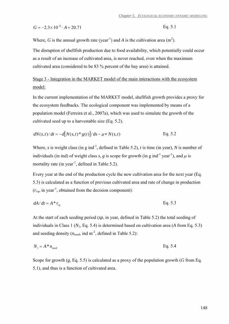
Chapter 5, ECOLOGICAL-ECONOMIC DYNAMIC MODELLING
148
71.20103.2 8 +⋅×−= − AG Eq. 5.1
Where, G is the annual growth rate (year-1) and A is the cultivation area (m2).
The disruption of shellfish production due to food availability, which potentially could occur
as a result of an increase of cultivated area, is never reached, even when the maximum
cultivated area (considered to be 83 % percent of the bay area) is attained.
Stage 3 - Integration in the MARKET model of the main interactions with the ecosystem
model:
In the current implementation of the MARKET model, shellfish growth provides a proxy for
the ecosystem feedbacks. The ecological component was implemented by means of a
population model (Ferreira et al., 2007a), which was used to simulate the growth of the
cultivated seed up to a harvestable size (Eq. 5.2).
[ ] ),(/)(*),(/),( tsNdstgtsNddttsdN ∗−−= µ Eq. 5.2
Where, s is weight class (in g ind-1, defined in Table 5.2), t is time (in year), N is number of
individuals (in ind) of weight class s, g is scope for growth (in g ind-1 year-1), and µ is
mortality rate (in year-1, defined in Table 5.2).
Every year at the end of the production cycle the new cultivation area for the next year (Eq.
5.3) is calculated as a function of previous cultivated area and rate of change in production
(rcq, in year-1, obtained from the decision component):
cqrAdtdA */ = Eq. 5.3
At the start of each seeding period (sp, in year, defined in Table 5.2) the total seeding of
individuals in Class 1 (N1, Eq. 5.4) is determined based on cultivation area (A from Eq. 5.3)
and seeding density (nseed, ind m-2, defined in Table 5.2):
seednAN *1 = Eq. 5.4
Scope for growth (g, Eq. 5.5) is calculated as a proxy of the population growth (G from Eq.
5.1), and thus is a function of cultivated area.
Chapter 5, ECOLOGICAL-ECONOMIC DYNAMIC MODELLING
149
wGg *= Eq. 5.5
Where, w (in g ind-1, defined in Table 5.2) is the average individual seed weight used in the
ecosystem model.
At the end of the year the individuals accumulated in the harvestable classes (N2+N3, as
calculated from Eq. 5.2) are converted into the harvestable biomass (HB, in kg, Eq. 5.6):
β*)**( 3322 sNsNHB += Eq. 5.6
Where, β is the conversion from g to kg.
Current implementation of the ecological model assumes that decisions to change production
are implemented through changes in the cultivation biomass. On the other hand, the changes
in the cultivation biomass affect the growth of shellfish (due to food availability) and
consequently the harvestable biomass. At this stage of development, the ecosystem feedbacks
are implicitly included in the MARKET model through the shellfish growth. Future
developments of the model will include explicit integration of the economic and decision
systems into the ecosystem model in order to monitor shellfish biodeposition as well as the
role of filter-feeders on phytoplankton uptake. Phytoplankton removal equates to the
reduction of coastal eutrophication symptoms, providing an additional ecosystem service.
Economic component
In each simulation year, the decision model calculates the desired production rate,
communicates it to the economic model and thus drives the change in the production inputs
(Figure 5.1). The economic component of the MARKET model is divided into sub-models
that simulate: (i) the harvest of the available biomass determined by the ecological model, (ii)
the production inputs (labor and capital), (iii) the corresponding production cost, (iv) the
generated revenue and net profit of the bivalve production for a given year, and (vi) the
marginal cost and marginal revenue in order to provide information required by the decision
model. The implementation of the economic model also includes simulation of the exogenous
functions that drive the aquatic resource production, namely: (i) price, (ii) household income,
and (iii) local demand. Both the economic drivers and sub-models are further detailed below.
Economic drivers:
The economic drivers are implemented following standard economic theory. A rise in income
is expected to positively influence the demand for fish and aquatic products and an increase in
price is expected to negatively influence the demand for aquatic species and aquatic products
Chapter 5, ECOLOGICAL-ECONOMIC DYNAMIC MODELLING
150
(Jolly and Clonts, 1993). In the model the changes in demand (rd, in year-1) are determined by
changes in the income and prices, as defined in Table 5.2. Both the price elasticity of demand
(ed, Table 5.2) and income elasticity of demand (ey, Table 5.2) were obtained from a national
level demand function analysis (Ferreira et al., 2008b). This model assumes that the changes
of the local demand follow the changes of the national demand, as information to derive local
level demand functions was not available. The local demand (LD, in kg) forcing function (Eq.
5.7) is initialized considering the local consumption data as the initial local demand (Table
5.3).
LDrdtdLD d ∗=/ Eq. 5.7
The local farmers are assumed to be price takers, whereby the aquatic product prices are
determined by the global market. The changes in the domestic price reflect the Chinese
inflation rate for the period 1995-2006. The yearly average including outliers is 2.8 %, while
when excluded, the average is 1.5 % (NBSC, 2007). A constant price growth rate (rp, in year-
1) of 2 % per year was therefore assumed based on the averaged inflation data. The price (P,
in Yuan kg-1) forcing function is given by Eq. 5.8:
PrdtdP p ∗=/ Eq. 5.8
In addition to price and demand the economic model is also forced by the annual growth of
the per capita income (ry, in year-1). The per capita income growth rate is used to calculate the
changes in the demand (rd), as defined in Table 5.2, and is also used to force the changes of
the unit labor cost as defined in Eq. 5.23. A constant per capita income growth rate of 10 %
per year was assumed based on the real per capita income growth data (NBSC, 2007).
Production sub-model:
The shellfish production (Q, in kg) for a given year (Eq. 5.9), is based on the desired
production determined for that year and is limited by the harvestable biomass simulated in the
ecological system (HB, in kg, Eq. 5.6). Thus, herein we assume that the harvest shellfish yield
equals to the shellfish production.
),( HBDQMinQ = Eq. 5.9
Where, DQ (in kg), is the desired production determined for that year, which was calculated
in the previous year as the desired production for the next cycle, following Eq. 5.32, in the
decision system.
Chapter 5, ECOLOGICAL-ECONOMIC DYNAMIC MODELLING
151
Production inputs sub-model:
This sub-model examines the capital and labor input levels resulting from the changes in the
desired production:
LRdtdL =/ Eq. 5.10
KRdtdK =/ Eq. 5.11
Where, L (in Man-Day) is the labor used for the production and is calculated based on the
required changes in labor inputs (RL, in Man-Days year-1); K (in Yuan) represents the assets
used in production and is calculated based on the required changes in the value of capital (RK,
in Yuan year-1).
The changes in both labor (RL, Eq. 5.12) and capital (RK, Eq. 5.13) are determined as a
function of the desired change in production (RCQ, in kg year-1, calculated in the decision
model, Eq. 5.31) and respectively on the marginal productivity of labor (MPL, in kg Man-
Days-1) and on the marginal productivity of capital (MPK, in kg Yuan-1):
LCQL MPRR /= Eq. 5.12
KCQK MPRR /= Eq. 5.13
Where, MPL and MPK are determined following Eq. 5.14 and Eq. 5.15, respectively, as
defined in Yunhua et al. (1998).
LQMP LL /∗=α Eq. 5.14
KQMP KK /∗=α Eq. 5.15
Where, αL and αK (dimensionless, Table 5.2) are the elasticity of labor and capital,
respectively, and were determined based on the production function (Musango et al., 2007)
defined in Eq. 5.16:
16.1ln53.0ln44.0ln +∗+∗= KLQ Eq. 5.16
Chapter 5, ECOLOGICAL-ECONOMIC DYNAMIC MODELLING
152
Production cost sub-model:
The production cost sub-model determines the total cost of shellfish production (TCQ, in
Yuan, Eq. 5.17) as the sum of the fixed cost (FC, in Yuan) and the variable cost (VC, in
Yuan):
VCFCTCQ += Eq. 5.17
Where, FC and VC are calculated following Eq. 5.18 and Eq. 5.21, respectively.
IKLDKFC += Eq. 5.18
Where, FC is given by the depreciation of capital (DK, in Yuan) and by the interest on capital
loan (IKL, in Yuan). DK and IKL are given by Eq. 5.19 and Eq. 5.20, respectively.
KdDK f ∗= Eq. 5.19
Where, df (dimensionless) represents the depreciation fraction (Table 5.2).
KrIKL ∗= Eq. 5.20
Where, r (year-1) is the interest rate (Table 5.2).
The variable cost includes the labor cost (VCL), the maintenance cost (VCM) and other variable
costs (VCO), all are expressed in Yuan:
OML VCVCVCVC ++= Eq. 5.21
The labor cost is calculated based on the labor and on the unit labor cost (UVCL, in Yuan
Man-Day-1):
LL UVCLVC ∗= Eq. 5.22
The unit labor cost changes as a function of the per capita income growth rate (ry, in year-1,
defined in Table 5.2):
LyL UVCrdtdUVC */ = Eq. 5.23
The maintenance cost is determined as a fraction (mf, defined in Table 5.2) of the capital (K)
as defined in a local economic survey (de Wit et al., 2008) and following Eq. 5.24:
Chapter 5, ECOLOGICAL-ECONOMIC DYNAMIC MODELLING
153
KmVC fM *= Eq. 5.24
The other variable costs include costs of feeding, seeding and interest on loan among others.
This variable is calculated based on the shellfish production (Q, in kg, Eq. 5.9) and on the unit
cost of other variables (UVCO, in Yuan kg-1):
OO UVCQVC *= Eq. 5.25
The unit cost of other variables changes as a function of the price growth rate (rp, in year-1,
defined in Table 5.2):
OpO UVCrdtdUVC */ = Eq. 5.26
Net profit sub-model:
The dynamics of net profit (NP, in Yuan, Eq. 5.27) are determined by the revenue (derived
from the dynamics of production output and price) and the total cost incurred (which includes
fixed and variable costs):
)()*( VCFCPQNP +−= Eq. 5.27
Marginal cost and revenue sub-model:
For each economic timestep the marginal cost (MC, in Yuan kg-1) is determined as the
increase in total cost that results of producing an additional unit of shellfish:
QTCMC ∆∆= / Eq. 5.28
For calculation of MC we consider an output increment of one kg of shellfish (∆Q = 1 kg).
Thus, for every one unit of additional Q, Eq. 5.28 reduces to:
QQ TCTCMC −= +1 Eq. 5.29
Where, TCQ+1 (in Yuan) is the total cost to produce Q+1, and TCQ (Eq. 5.17) the total cost as
calculated previously for Q. TCQ+1 is calculated using the production cost sub-model (Eq.
5.17 to Eq. 5.26) to compute the cost of the inputs (labor and capital) needed to produce Q+1.
On the other hand, the required labor and capital to produce the additional output are
determined by multiplying one kg of shellfish by the inverse of marginal productivity of labor
Chapter 5, ECOLOGICAL-ECONOMIC DYNAMIC MODELLING
154
(LMP
1 which expresses as Man-Days kg-1) and the inverse of marginal productivity of capital
(KMP
1 which expresses as Yuan kg-1), respectively.
Assuming that the shellfish farmers are price takers, the marginal revenue (MR, in Yuan kg-1)
was equated to the price of shellfish (P, in Yuan kg-1, Eq. 5.8).
PMR= Eq. 5.30
Both marginal cost (MC) and marginal revenue (MR) are used by the decision model for
calculation of the profit maximization criteria.
Decision component
The decision component is the engine of the MARKET model. This simulation block
determines the production in the following year, therefore driving both the ecological and
economic components. In the MARKET model it is assumed that the farmers’ decision is
based on (i) the profit maximization, (ii) the gap between demand and supply, and (iii) the
available area for aquaculture activities, i.e. the physical limits. Each of the three criteria is
further detailed below:
i) Profit maximization: the local farmers are assumed to be perfectly rational and that their
interest in aquaculture production is to maximize individual profit. Therefore, they will aim to
increase production only up to an output level whereby marginal cost equals marginal
revenue. In this analysis, the farm managers are assumed to have knowledge on the cost and
demand functions facing the shellfish production and about other actors in the system.
Although none of these conditions are likely to be met in reality, these provide a baseline
economic decision-making rule to maximize profit in order to test the application of the
MARKET model. Both marginal cost and marginal revenue values are provided by the
economic model (Eq. 5.29 and Eq. 5.30). If the marginal revenue is greater than the marginal
cost (MR > MC) the decision model defines an increase in desired production for the next
period and the inverse occurs when the marginal revenue is less than the marginal cost (MR <
MC). If the marginal revenue equals marginal cost (MR = MC) then the model decides to
maintain the desired production for the next period at current production level.
ii) Demand / supply gap: is calculated as the difference between the local demand and the
shellfish production, both given by the economic model (Eq. 5.7 and Eq. 5.9). It indicates
whether the demand is met by production (if Q ≥ LD), or if the market can absorb an increase
in production (if Q < LD).
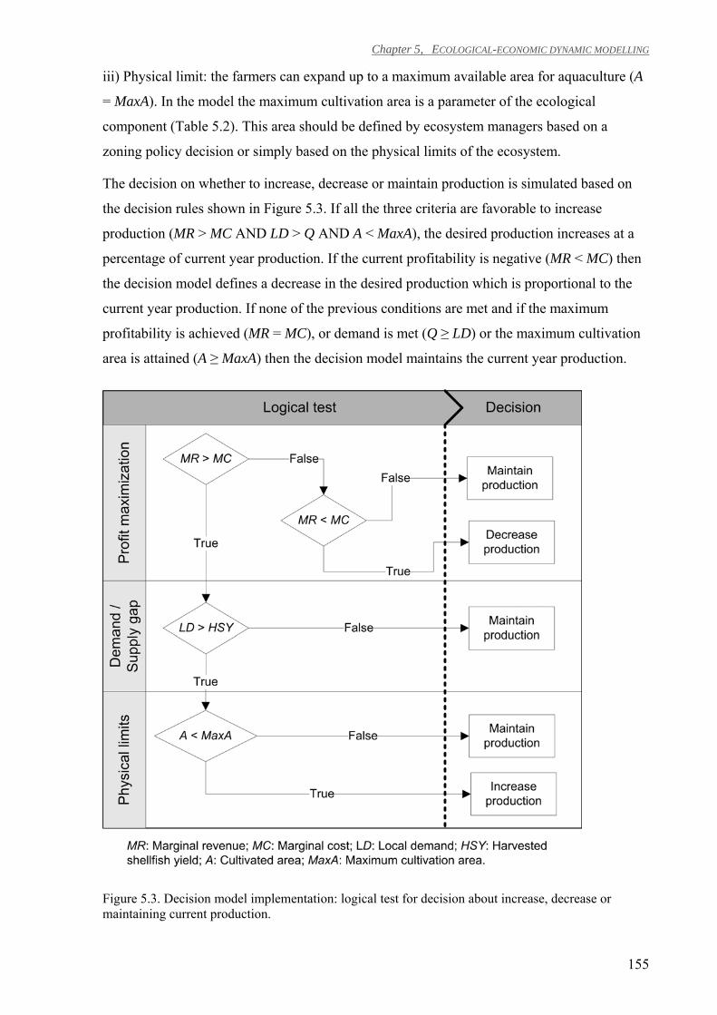
Chapter 5, ECOLOGICAL-ECONOMIC DYNAMIC MODELLING
155
iii) Physical limit: the farmers can expand up to a maximum available area for aquaculture (A
= MaxA). In the model the maximum cultivation area is a parameter of the ecological
component (Table 5.2). This area should be defined by ecosystem managers based on a
zoning policy decision or simply based on the physical limits of the ecosystem.
The decision on whether to increase, decrease or maintain production is simulated based on
the decision rules shown in Figure 5.3. If all the three criteria are favorable to increase
production (MR > MC AND LD > Q AND A < MaxA), the desired production increases at a
percentage of current year production. If the current profitability is negative (MR < MC) then
the decision model defines a decrease in the desired production which is proportional to the
current year production. If none of the previous conditions are met and if the maximum
profitability is achieved (MR = MC), or demand is met (Q ≥ LD) or the maximum cultivation
area is attained (A ≥ MaxA) then the decision model maintains the current year production.
Figure 5.3. Decision model implementation: logical test for decision about increase, decrease or maintaining current production.
Chapter 5, ECOLOGICAL-ECONOMIC DYNAMIC MODELLING
156
The change in the quantity that aquaculture managers want to produce in the next cycle, i.e.
the desired change in production (RCQ, in kg year-1), is calculated as a fraction of current year
production by means of Eq. 5.31:
cqCQ rQR ∗= Eq. 5.31
Where, Q (in kg) represents the current year production and is calculated in the economic
model (Eq. 5.9); rcq (in year-1), is the annual change rate in production and is conditioned by
the decision whether to increase, decrease or maintain production (according to Figure 5.3 and
as explained above). Depending on the decision taken rcq is given as:
(i) If decision is to increase production, then the rate of change in production is 10 % per year
of current production (rcq = 0.1 year-1);
(ii) If decision is to decrease production, then the rate of change in production is -30 % per
year of current production (rcq = -0.3 year-1);
(iii) If decision is to maintain production, then the rate of change in production is 0 % per
year of current production (rcq = 0.0 year-1).
Further research is needed to understand how this decision is normally taken in the real world
in order to improve the definition of the rate of change in production.
The desired production for the next cycle (DQ, in kg) is then given by current production (Q)
and by the desired change in production for the next cycle (RCQ*tp):
tpRQDQ CQ ∗+= Eq. 5.32
Where, tp (in year) is the shellfish production cycle period (defined in Table 5.2).
Model assessment and scenario definition
At this stage of development and given the deterministic nature of the MARKET model, it
cannot incorporate the randomness involved in decisions by individual farmers. In addition, it
does not integrate the complex dynamics that govern for instance a policy change that decides
a shift from shellfish to finfish or macroalgal production. In order to validate the MARKET
model at that level, a very specific dataset would be required: a data series of both economic
production and environmental factors for a given ecosystem where the main changes in
aquaculture production are only constrained by the ecological and economic factors in a
perfectly rational way.
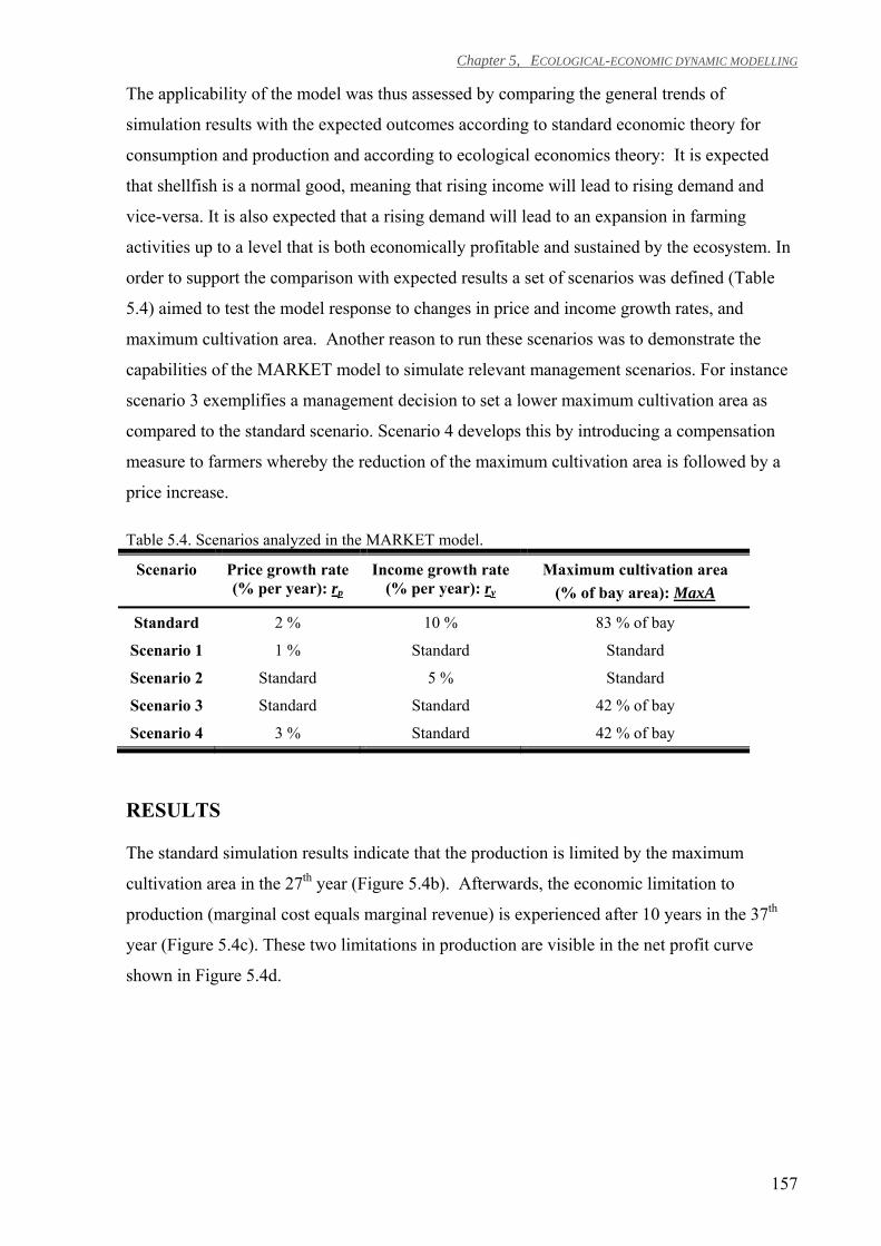
Chapter 5, ECOLOGICAL-ECONOMIC DYNAMIC MODELLING
157
The applicability of the model was thus assessed by comparing the general trends of
simulation results with the expected outcomes according to standard economic theory for
consumption and production and according to ecological economics theory: It is expected
that shellfish is a normal good, meaning that rising income will lead to rising demand and
vice-versa. It is also expected that a rising demand will lead to an expansion in farming
activities up to a level that is both economically profitable and sustained by the ecosystem. In
order to support the comparison with expected results a set of scenarios was defined (Table
5.4) aimed to test the model response to changes in price and income growth rates, and
maximum cultivation area. Another reason to run these scenarios was to demonstrate the
capabilities of the MARKET model to simulate relevant management scenarios. For instance
scenario 3 exemplifies a management decision to set a lower maximum cultivation area as
compared to the standard scenario. Scenario 4 develops this by introducing a compensation
measure to farmers whereby the reduction of the maximum cultivation area is followed by a
price increase.
Table 5.4. Scenarios analyzed in the MARKET model.
Scenario Price growth rate (% per year): rp
Income growth rate (% per year): ry
Maximum cultivation area (% of bay area): MaxA
Standard 2 % 10 % 83 % of bay
Scenario 1 1 % Standard Standard
Scenario 2 Standard 5 % Standard
Scenario 3 Standard Standard 42 % of bay
Scenario 4 3 % Standard 42 % of bay
RESULTS
The standard simulation results indicate that the production is limited by the maximum
cultivation area in the 27th year (Figure 5.4b). Afterwards, the economic limitation to
production (marginal cost equals marginal revenue) is experienced after 10 years in the 37th
year (Figure 5.4c). These two limitations in production are visible in the net profit curve
shown in Figure 5.4d.
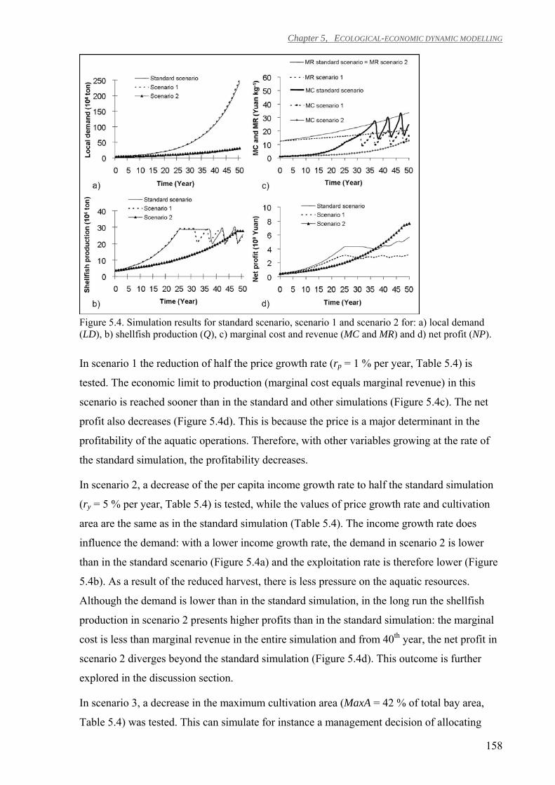
Chapter 5, ECOLOGICAL-ECONOMIC DYNAMIC MODELLING
158
Figure 5.4. Simulation results for standard scenario, scenario 1 and scenario 2 for: a) local demand (LD), b) shellfish production (Q), c) marginal cost and revenue (MC and MR) and d) net profit (NP).
In scenario 1 the reduction of half the price growth rate (rp = 1 % per year, Table 5.4) is
tested. The economic limit to production (marginal cost equals marginal revenue) in this
scenario is reached sooner than in the standard and other simulations (Figure 5.4c). The net
profit also decreases (Figure 5.4d). This is because the price is a major determinant in the
profitability of the aquatic operations. Therefore, with other variables growing at the rate of
the standard simulation, the profitability decreases.
In scenario 2, a decrease of the per capita income growth rate to half the standard simulation
(ry = 5 % per year, Table 5.4) is tested, while the values of price growth rate and cultivation
area are the same as in the standard simulation (Table 5.4). The income growth rate does
influence the demand: with a lower income growth rate, the demand in scenario 2 is lower
than in the standard scenario (Figure 5.4a) and the exploitation rate is therefore lower (Figure
5.4b). As a result of the reduced harvest, there is less pressure on the aquatic resources.
Although the demand is lower than in the standard simulation, in the long run the shellfish
production in scenario 2 presents higher profits than in the standard simulation: the marginal
cost is less than marginal revenue in the entire simulation and from 40th year, the net profit in
scenario 2 diverges beyond the standard simulation (Figure 5.4d). This outcome is further
explored in the discussion section.
In scenario 3, a decrease in the maximum cultivation area (MaxA = 42 % of total bay area,
Table 5.4) was tested. This can simulate for instance a management decision of allocating
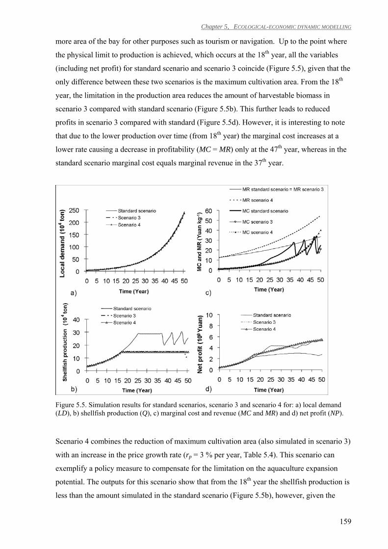
Chapter 5, ECOLOGICAL-ECONOMIC DYNAMIC MODELLING
159
more area of the bay for other purposes such as tourism or navigation. Up to the point where
the physical limit to production is achieved, which occurs at the 18th year, all the variables
(including net profit) for standard scenario and scenario 3 coincide (Figure 5.5), given that the
only difference between these two scenarios is the maximum cultivation area. From the 18th
year, the limitation in the production area reduces the amount of harvestable biomass in
scenario 3 compared with standard scenario (Figure 5.5b). This further leads to reduced
profits in scenario 3 compared with standard (Figure 5.5d). However, it is interesting to note
that due to the lower production over time (from 18th year) the marginal cost increases at a
lower rate causing a decrease in profitability (MC = MR) only at the 47th year, whereas in the
standard scenario marginal cost equals marginal revenue in the 37th year.
Figure 5.5. Simulation results for standard scenarios, scenario 3 and scenario 4 for: a) local demand (LD), b) shellfish production (Q), c) marginal cost and revenue (MC and MR) and d) net profit (NP).
Scenario 4 combines the reduction of maximum cultivation area (also simulated in scenario 3)
with an increase in the price growth rate (rp = 3 % per year, Table 5.4). This scenario can
exemplify a policy measure to compensate for the limitation on the aquaculture expansion
potential. The outputs for this scenario show that from the 18th year the shellfish production is
less than the amount simulated in the standard scenario (Figure 5.5b), however, given the
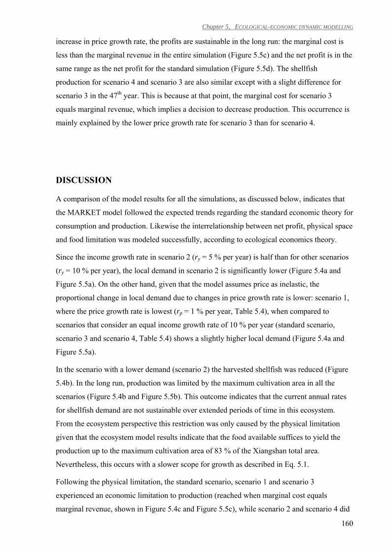
Chapter 5, ECOLOGICAL-ECONOMIC DYNAMIC MODELLING
160
increase in price growth rate, the profits are sustainable in the long run: the marginal cost is
less than the marginal revenue in the entire simulation (Figure 5.5c) and the net profit is in the
same range as the net profit for the standard simulation (Figure 5.5d). The shellfish
production for scenario 4 and scenario 3 are also similar except with a slight difference for
scenario 3 in the 47th year. This is because at that point, the marginal cost for scenario 3
equals marginal revenue, which implies a decision to decrease production. This occurrence is
mainly explained by the lower price growth rate for scenario 3 than for scenario 4.
DISCUSSION
A comparison of the model results for all the simulations, as discussed below, indicates that
the MARKET model followed the expected trends regarding the standard economic theory for
consumption and production. Likewise the interrelationship between net profit, physical space
and food limitation was modeled successfully, according to ecological economics theory.
Since the income growth rate in scenario 2 (ry = 5 % per year) is half than for other scenarios
(ry = 10 % per year), the local demand in scenario 2 is significantly lower (Figure 5.4a and
Figure 5.5a). On the other hand, given that the model assumes price as inelastic, the
proportional change in local demand due to changes in price growth rate is lower: scenario 1,
where the price growth rate is lowest (rp = 1 % per year, Table 5.4), when compared to
scenarios that consider an equal income growth rate of 10 % per year (standard scenario,
scenario 3 and scenario 4, Table 5.4) shows a slightly higher local demand (Figure 5.4a and
Figure 5.5a).
In the scenario with a lower demand (scenario 2) the harvested shellfish was reduced (Figure
5.4b). In the long run, production was limited by the maximum cultivation area in all the
scenarios (Figure 5.4b and Figure 5.5b). This outcome indicates that the current annual rates
for shellfish demand are not sustainable over extended periods of time in this ecosystem.
From the ecosystem perspective this restriction was only caused by the physical limitation
given that the ecosystem model results indicate that the food available suffices to yield the
production up to the maximum cultivation area of 83 % of the Xiangshan total area.
Nevertheless, this occurs with a slower scope for growth as described in Eq. 5.1.
Following the physical limitation, the standard scenario, scenario 1 and scenario 3
experienced an economic limitation to production (reached when marginal cost equals
marginal revenue, shown in Figure 5.4c and Figure 5.5c), while scenario 2 and scenario 4 did
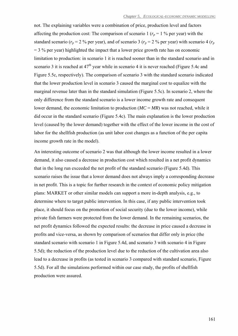
Chapter 5, ECOLOGICAL-ECONOMIC DYNAMIC MODELLING
161
not. The explaining variables were a combination of price, production level and factors
affecting the production cost: The comparison of scenario 1 (rp = 1 % per year) with the
standard scenario (rp = 2 % per year), and of scenario 3 (rp = 2 % per year) with scenario 4 (rp
= 3 % per year) highlighted the impact that a lower price growth rate has on economic
limitation to production: in scenario 1 it is reached sooner than in the standard scenario and in
scenario 3 it is reached at 47th year while in scenario 4 it is never reached (Figure 5.4c and
Figure 5.5c, respectively). The comparison of scenario 3 with the standard scenario indicated
that the lower production level in scenario 3 caused the marginal cost to equalize with the
marginal revenue later than in the standard simulation (Figure 5.5c). In scenario 2, where the
only difference from the standard scenario is a lower income growth rate and consequent
lower demand, the economic limitation to production (MC = MR) was not reached, while it
did occur in the standard scenario (Figure 5.4c). The main explanation is the lower production
level (caused by the lower demand) together with the effect of the lower income in the cost of
labor for the shellfish production (as unit labor cost changes as a function of the per capita
income growth rate in the model).
An interesting outcome of scenario 2 was that although the lower income resulted in a lower
demand, it also caused a decrease in production cost which resulted in a net profit dynamics
that in the long run exceeded the net profit of the standard scenario (Figure 5.4d). This
scenario raises the issue that a lower demand does not always imply a corresponding decrease
in net profit. This is a topic for further research in the context of economic policy mitigation
plans: MARKET or other similar models can support a more in-depth analysis, e.g., to
determine where to target public intervention. In this case, if any public intervention took
place, it should focus on the promotion of social security (due to the lower income), while
private fish farmers were protected from the lower demand. In the remaining scenarios, the
net profit dynamics followed the expected results: the decrease in price caused a decrease in
profits and vice-versa, as shown by comparison of scenarios that differ only in price (the
standard scenario with scenario 1 in Figure 5.4d, and scenario 3 with scenario 4 in Figure
5.5d); the reduction of the production level due to the reduction of the cultivation area also
lead to a decrease in profits (as tested in scenario 3 compared with standard scenario, Figure
5.5d). For all the simulations performed within our case study, the profits of shellfish
production were assured.
Chapter 5, ECOLOGICAL-ECONOMIC DYNAMIC MODELLING
162
CONCLUSIONS
The MARKET model allows for an integrated dynamic analysis of (i) the demand for
mariculture products, (ii) economic production and cost limiting factors, (iii) the biological
growth of aquatic resources, (iv) interactions with the environmental conditions and (iv) the
spatial limitations of culture in coastal ecosystems. Our approach can contribute to
mariculture management and for implementation of an ecosystem approach to aquaculture
(EAA).
Simulation of shellfish production in a Chinese embayment was chosen as a case study
illustrating the implementation of the MARKET model. A key feature of the model
implementation was to incorporate the different time scales at which the ecological and
economic systems function. In this study, we have used several management scenarios to
show that the model reproduces the expected trends and provides further insights. In all the
scenarios, production in the long run does not meet increasing demand. In this case study the
physical limitation of the bay was the first limiting factor for all the scenarios, that is, space is
expected to impose limitations on production before it becomes less profitable to expand
production. Overall, the MARKET model can help to understand the succession of the
limiting factors in mariculture industry and whether the production can meet the demand for
aquatic resources.
The MARKET model can be widely applied, provided that case-specific information exists on
shellfish demand, price, income, production functions, physical area available for cultivation,
and environmental conditions that have an effect on the growth of aquatic resources and are
affected by its production. It is recommended that future MARKET model developments
include: (i) an improvement of the decision model, in particular for decisions by farmers
about changes of production level, (ii) explicit dynamic coupling with an ecosystem model,
and (iii) implementation for other aquaculture species and culture practices, especially those
that normally raise more concerns related with environmental management, such as finfish
monoculture.
Chapter 6. Integration of ecosystem-based tools
Context
The preceding Chapters 2 to 5 present different methodologies for (i) integrated simulation of
coastal ecosystems, (ii) ecological-economic assessment of the effectiveness of response
actions, and (iii) dynamic ecological-economic modelling of aquaculture production in coastal
ecosystems.
Summary
This chapter presents the integrated application of these and a wider spectrum of ecosystem-
based tools for coastal ecosystem research and management, such as geographic information
systems, remote sensing and economic valuation methods. This chapter illustrates the
application of such a set of tools to support coastal management, using a coastal lagoon
located in southwest Europe as a case study.
Chapter 6, INTEGRATION OF ECOSYSTEM-BASED TOOLS
164
This chapter corresponds to the published manuscript:
Nobre, A.M and Ferreira, J.G., 2009. Integration of ecosystem-based
tools to support coastal zone management. Journal of Coastal Research,
SI 56: 1676-1680.
(For consistency with published version this chapter is written in
American English)
Chapter 6, INTEGRATION OF ECOSYSTEM-BASED TOOLS
165
Integration of ecosystem-based tools to support coastal zone management
INTRODUCTION
Coastal zones exhibit complex interactions at different levels: (i) they are under influence of a
great variety of pressures at the interface between land and sea, (ii) they are subject to
feedback effects between natural and human systems (Turner et al. 2003), (iii) they exhibit
complex relationships between the physical and biological processes – in particular estuaries
are characterized by complex ecological feedbacks (Bergamasco et al., 2003). Coastal zones
are highly productive and provide significant direct and indirect socio-economic benefits, e.g.
food, biodiversity, nutrient cycling, climate regulation, recreation, culture and amenity (MA,
2005). As a result coastal zones concentrate 40% of the world population and 61% of world’s
total GNP (MA, 2005). However, their misuse is causing degradation and consequently
decreases of the services that these coastal ecosystems deliver (MA, 2005). The Millennium
Assessment (MA, 2005) also indicates impact on human health: of the annual cost due to
coastal water pollution (16 billion USD) a large proportion is related to human health.
To address coastal zone problems, ecosystem-based management (EBM) and integrated
coastal management (ICM) are required (Browman and Stergiou, 2005; Murawski et al.,
2008). ICM is a well established approach (GESAMP, 1996; Cicin-Sain and Knecht, 1998)
defined as a dynamic process for the management of the use, development and protection of
the coastal zone (Murawski et al., 2008). It consists of an integrated approach from different
perspectives (GESAMP, 1996). EBM is an emerging scientific consensus (Murawski et al.,
2008), defined as the use of the best available knowledge about the ecosystem to manage
marine resources (Fluharty, 2005). The integration of (i) science with management and (ii)
natural with social sciences, is critical for effective governance of coastal zones (Cheong,
2008).
The role of science is to provide the insights and information required to support managers
and decision makers (GESAMP, 1996; Browman and Stergiou, 2005). This implies the use of
scientific applications that enable (i) the understanding of biogeochemical processes, (ii)
interaction of ecological and socio-economic components, and (iii) synthesis and
communication of complex outputs to managers. The integration of tools, such as geographic
information systems (GIS), ecological modeling of catchment and coastal systems, economic
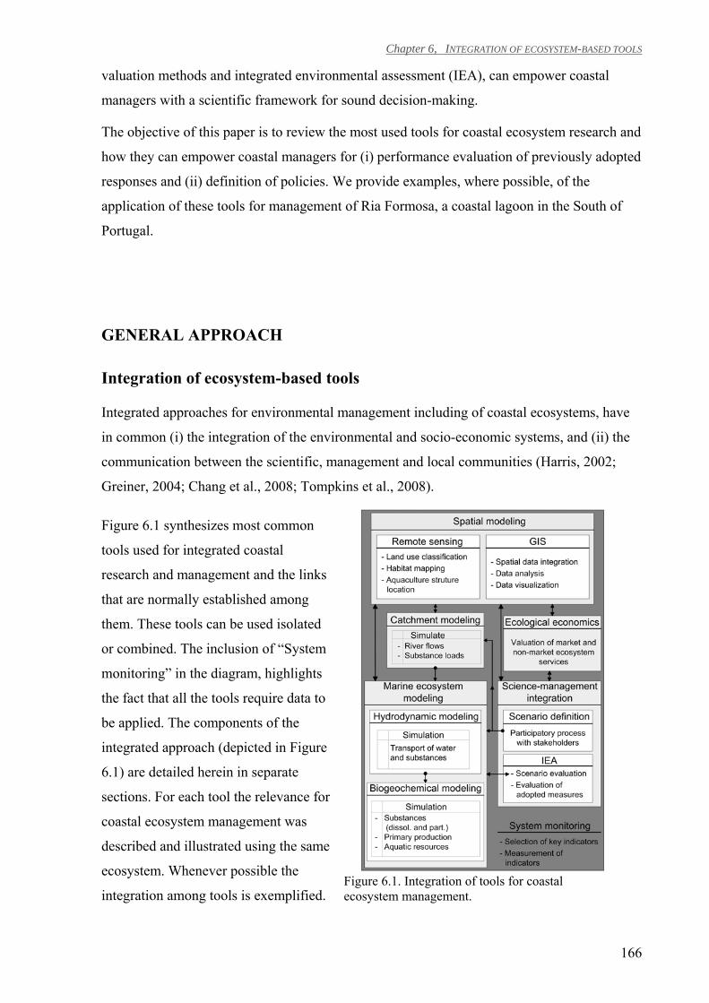
Chapter 6, INTEGRATION OF ECOSYSTEM-BASED TOOLS
166
valuation methods and integrated environmental assessment (IEA), can empower coastal
managers with a scientific framework for sound decision-making.
The objective of this paper is to review the most used tools for coastal ecosystem research and
how they can empower coastal managers for (i) performance evaluation of previously adopted
responses and (ii) definition of policies. We provide examples, where possible, of the
application of these tools for management of Ria Formosa, a coastal lagoon in the South of
Portugal.
GENERAL APPROACH
Integration of ecosystem-based tools
Integrated approaches for environmental management including of coastal ecosystems, have
in common (i) the integration of the environmental and socio-economic systems, and (ii) the
communication between the scientific, management and local communities (Harris, 2002;
Greiner, 2004; Chang et al., 2008; Tompkins et al., 2008).
Figure 6.1 synthesizes most common
tools used for integrated coastal
research and management and the links
that are normally established among
them. These tools can be used isolated
or combined. The inclusion of “System
monitoring” in the diagram, highlights
the fact that all the tools require data to
be applied. The components of the
integrated approach (depicted in Figure
6.1) are detailed herein in separate
sections. For each tool the relevance for
coastal ecosystem management was
described and illustrated using the same
ecosystem. Whenever possible the
integration among tools is exemplified. Figure 6.1. Integration of tools for coastal ecosystem management.
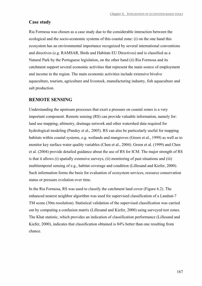
Chapter 6, INTEGRATION OF ECOSYSTEM-BASED TOOLS
167
Case study
Ria Formosa was chosen as a case study due to the considerable interaction between the
ecological and the socio-economic systems of this coastal zone: (i) on the one hand this
ecosystem has an environmental importance recognized by several international conventions
and directives (e.g. RAMSAR, Birds and Habitats EU Directives) and is classified as a
Natural Park by the Portuguese legislation, on the other hand (ii) Ria Formosa and its
catchment support several economic activities that represent the main source of employment
and income in the region. The main economic activities include extensive bivalve
aquaculture, tourism, agriculture and livestock, manufacturing industry, fish aquaculture and
salt production.
REMOTE SENSING
Understanding the upstream processes that exert a pressure on coastal zones is a very
important component. Remote sensing (RS) can provide valuable information, namely for:
land use mapping, altimetry, drainage network and other watershed data required for
hydrological modeling (Pandey et al., 2005). RS can also be particularly useful for mapping
habitats within coastal systems, e.g. wetlands and mangroves (Green et al., 1999) as well as to
monitor key surface water quality variables (Chen et al., 2004). Green et al. (1999) and Chen
et al. (2004) provide detailed guidance about the use of RS for ICM. The major strength of RS
is that it allows (i) spatially extensive surveys, (ii) monitoring of past situations and (iii)
multitemporal sensing of e.g., habitat coverage and condition (Lillesand and Kiefer, 2000).
Such information forms the basis for evaluation of ecosystem services, resource conservation
status or pressure evolution over time.
In the Ria Formosa, RS was used to classify the catchment land cover (Figure 6.2). The
enhanced nearest neighbor algorithm was used for supervised classification of a Landsat-7
TM scene (30m resolution). Statistical validation of the supervised classification was carried
out by computing a confusion matrix (Lillesand and Kiefer, 2000) using surveyed test zones.
The Khat statistic, which provides an indication of classification performance (Lillesand and
Kiefer, 2000), indicates that classification obtained is 84% better than one resulting from
chance.
Chapter 6, INTEGRATION OF ECOSYSTEM-BASED TOOLS
168
Figure 6.2. Ria Formosa land cover classification results.
GEOGRAPHIC INFORMATION SYSTEMS
GIS can be used for spatial data integration (e.g. bathymetry, sampling stations, habitat area,
catchment land use), data analysis (e.g. calculation of waterbody volume and area, thematic
mapping such as interpolation of sampling station data, zoning) and data visualization (e.g., of
the generated thematic maps). These capabilities make it a useful tool for ICM (Douven et al.,
2003; Tolvanen and Kalliola, 2008) either as a data generator (if used to extract data for other
tools, e.g. setup ecological models) or as an ‘end in itself’ (if used for communicating
information to managers). GIS can integrate with other applications as e.g., ecological
models, by offline coupling, whereby the model receives some of its input data from the GIS,
or using a tighter integration whereby both the model and GIS share a common interface and
communicate directly (Fedra, 1996). Sardá et al. (2005), illustrates the integration of data into
GIS, and its use for data processing and visualization targeted to managers. The use of
embedded GIS basic functions into Decision Support Systems (DSS) can empower managers
by enabling to manipulate, display and analyze spatial data and models (Fedra, 1996).
Another example of GIS use for ICM is to support marine spatial planning for the
implementation of relevant legislation (Gilliland and Laffoley, 2008; Maes, 2008). Examples
are provided by (i) Cheong (2008) for the delineation of Exclusive Economic Zones required
by the Law of the Sea Convention of 1982, (ii) Ferreira et al. (2006) for the division of
Chapter 6, INTEGRATION OF ECOSYSTEM-BASED TOOLS
169
transitional and coastal waters into waterbodies as determined by the Water Framework
Directive (WFD, 2000/60/CE) and (iii) Boyes et al. (2007) for zoning based on legislation
applicable within the Irish Sea.
For Ria Formosa there are several examples of the use of GIS for ICM, namely (i) zoning of
Ria Formosa for the application of WFD as described by Ferreira et al. (2006) and (ii)
identification of conflicting uses by the Natural Park authority (ICN, 2005). Existing spatially
distributed data (either produced by research institutes, universities or local managers) could
be compiled for the development of a DSS to support local managers to implement existing
and develop future plans.
CATCHMENT MODELING
Integrated land use catchment modeling emerged as a requirement from policy makers and
managers to understand the feedback between changing land use and changing environmental
conditions (Veldkamp and Verburg, 2004). Several studies were developed to understand the
effects of land use policy on the environmental and socio-economic systems (Veldkamp and
Verburg, 2004; Macleod et al., 2007). Furthermore, information about catchment pressures is
of paramount importance to simulate the downstream coastal ecosystems (Neal et al., 2003).
In particular, estimates of substance loads entering from the catchment are required to
simulate the biogeochemical conditions of the coastal water bodies. Depending on objectives
and available data simpler or more complex approaches can be used: direct estimation
techniques, simple export coefficient methods or more complex catchment models
(McGuckin et al., 1999; Letcher et al., 2002; Endreny and Wood, 2003; Pandey et al., 2005;
Wade et al., 2005). The advantage of catchment models is that they allow for scenario
simulation of catchment land use. This can be integrated with coastal ecosystem models to
determine the impact of the catchment loads.
In the case of Ria Formosa, the runoff is concentrated in the winter months (ca. 71%). Loads
entering into this coastal system have been calculated based on river water quality and flow
data together with waste water discharge data (MAOT, 2000; Ferreira et al., 2003). However,
it is desirable to apply catchment models to determine daily nutrient and sediment loads as
well to test relevant management scenarios and respective impacts.
COASTAL ECOSYSTEM MODELING
For the simulation of estuarine and coastal ecosystems there are a large number of models of
varying complexity, regarding spatial and temporal scales, components of the ecosystem and
Chapter 6, INTEGRATION OF ECOSYSTEM-BASED TOOLS
170
processes included (Fulton et al., 2003). Model development normally depends on the
research objectives. Recently the use of ecosystem modeling to assist ICM became an
emerging requirement (Fulton et al., 2003; Nobre et al., 2005). In particular modeling can be
useful to overcome data limitations and to simulate scenarios. For instance ecological
modeling can play an important role for the implementation of the WFD (de Jonge, 2007).
The development of ecological models usually implies integration with some of the other
tools in review, at least for the model setup and forcing with boundary conditions (Fedra,
1996; Neal et al., 2003).
In the Ria Formosa several models have been applied at different levels, namely a detailed
hydrodynamic model and an ecosystem box model that simulate transport, nutrient cycling,
primary production and secondary production (bivalves) (Nobre et al. 2005). The ecosystem
model was run to simulate different scenarios relevant for eutrophication management.
ECONOMIC VALUATION
Ecosystem valuation aims to estimate the total and marginal value of the ecosystem services
(both the market and the non-market components). There are several difficulties in placing an
economic value on natural assets and specially of calculating an absolute economic value of
ecosystems (Costanza et al., 1997; Ledoux and Turner, 2002). Nevertheless, it is of crucial
importance that an effort is made to calculate the changes caused on human welfare due to the
changes that affect ecosystem functioning (Costanza et al., 1997). Valuation can be regarded
as a policy tool in the sense that it enables an accounting of ecosystem goods and services,
together with the market services, in decision-making and management of coastal systems
(Barbier et al., 1996; Costanza et al., 1997; Ledoux and Turner, 2002). There is a variety of
economic valuation methods broadly categorized either as revealed preference methods (such
as hedonic pricing, travel cost or replacement cost) or as stated preference methods (such as
contingent valuation and choice experiment), each with advantages and limitations depending
on the application. Ledoux and Turner (2002) and Birol et al. (2006) provide a review of the
application of such methods for water resources management.
Given the ecological importance of the Ria Formosa and the benefits it generates, it would be
appropriate to conduct such a valuation exercise. Considering the economic activities that
depend on this ecosystem (aquaculture, fisheries, tourism and salt production) an average
benefit of 338 million Euros year-1 (2000 prices) is estimated. This value corresponds to the
average net profit generated by these activities for the period between 1980 and 1999 (Nobre,
2009). Updated and more detailed studies are required to capture other direct and indirect use
Chapter 6, INTEGRATION OF ECOSYSTEM-BASED TOOLS
171
values. Particularly important is to estimate the values associated with the wetland area (ca.
17 % of Ria Formosa Natural Park area) given the range of benefits this type of ecosystem
provides, i.e. food resources, flood water retention, groundwater recharge/discharge and
nutrient abatement (Acharya, 2000). Detailed guidelines to carry out such studies are provided
by Barbier et al. (1996). In order to estimate an approximate range, the wetlands potential
value was evaluated using values provided by Ghermandi et al. (2008), ca. 100 to 10 000
USD (2003) ha-1 yr-1, based on an extensive review of economic value estimates of wetlands
worldwide. The estimated value of wetlands in Ria Formosa ranges between 0.30 and 29.54
million Euro yr-1 (2000 prices) (USD conversion to Euros was based on the Consumer Price
Index rate from the Bureau of Labor Statistics and currency conversion from the IMF).
ASSESSMENT METHODOLOGIES
Integrated Environmental Assessment (IEA) methodologies can be broadly defined as
interdisciplinary approaches targeted to guide decision-makers and managers about
environmental problems, and in more general terms for natural resources management (Toth
and Hizsnyik, 1998). IEA methodologies are by themselves integrative tools (Cheong, 2008)
that promote the interaction of ecological and socio-economic disciplines or simply the
synthesis of complex information to managers. The Drivers-Pressure-State-Impact-Response
(DPSIR) is one such tool that has been widely applied to synthesize natural and socio-
economic sciences for marine policy formulation (Cheong, 2008) and for ICM (Ledoux and
Turner, 2002). For the application of assessment approaches the selection of key indicators is
critical (Håkanson and Blenckner, 2008). Borja et al. (2008) reviews existing methodologies
to assess ecosystem ecological status in order to address legislation adopted worldwide for
management of ecological quality or integrity.
Ferreira et al. (2003) exemplifies the use of an IEA methodology to inform managers about
eutrophication status in Ria Formosa. The work carried out concluded that there is a moderate
low eutrophic condition, for which the main symptom identified is periodic blooms of
macroalgae in some locations of Ria Formosa (Ferreira et al., 2003). Further research
investigated the effects of nutrient loading scenarios on the eutrophic state of Ria Formosa by
coupling the eutrophication assessment methodology with the ecosystem ecological model
(Nobre et al. 2005). The eutrophication assessment methodology used was the USA National
Estuarine Eutrophication Assessment (NEEA) method and its successor the ASSETS
screening model (Bricker et al., 2003).
Chapter 6, INTEGRATION OF ECOSYSTEM-BASED TOOLS
172
The case study presented by Nobre (2009) exemplifies how an IEA approach could support
the strategic management of Ria Formosa natural resources from both ecological and socio-
economic perspectives: The comparison of drivers, pressures and ecosystem state in two
different periods (1980/85 and 1995/99) indicates that although there was a significant
management response (namely the construction of waste water treatment plants), the negative
economic impacts represented 80% to 220% of the response cost (Nobre, 2009). The decrease
of the economic benefits was mainly due to the decrease of bivalve production, which is
believed to be related to the appearance of a parasite (Campos and Cachola, 2006).
Aquaculture production in Ria Formosa presently accounts for 47% of the Portuguese
mariculture products and it is estimated that bivalve aquaculture alone is responsible for the
direct employment of 4 500 people (ICN, 2005) or up to 10 000 according to unofficial
estimates (Campos and Cachola, 2006). Ruditapes decussatus is the local clam species and its
production in Ria Formosa is highly significant (ca. 90% of Portuguese production, in 2001).
This species is highly priced (Matias et al., 2008), however, it is being displaced by the
Manila clam Ruditapes philippinarum (Campos and Cachola, 2006). Notwithstanding the
incentives for conservation of local clam, the stipulated activities in Ria Formosa Natural Park
Management Plan preview for bivalve related management an amount that represents 1.9% of
planned total budget (ICN, 2005). Results and information synthesized herein, suggest that is
advisable to invest in the proper management of bivalve aquaculture and natural beds with a
special emphasis on the seeding procurement or development of local hatcheries, which might
have a positive effect on (i) mitigating disease introduction (Nobre, 2009), (ii) limiting the
introduction of alien species (Campos and Cachola, 2006) and (iii) on Ruditapes decussatus
seed availability (Matias et al., 2008).
It is advisable that the relevant authorities should define a set of indicators to monitor
effectiveness of the goals established in the several management plans that exist for this
ecosystem, the most important being: (i) Management Plan of Coastal Zone between
Vilamoura e Vila Real de Santo António approved through Resolution No. 103/2005 of 27
June 2005, focus on the strip of land 500m wide from the seawater baseline and on the marine
area limited by the 30m bathymetric line, (ii) Ria Formosa Natural Park Management Plan
approved through Regulatory Decree No. 2/91 of 24 January 1991 and currently is under
revision, focus on Ria Formosa lagoon ecosystem, and (iii) Hidrographic basin plans of the
Algarve streams approved through Regulatory Decree No. 12/2002 of 9 March 2002, focus on
the drainage basin of several streams encompassing Ria Formosa catchment area.
Chapter 6, INTEGRATION OF ECOSYSTEM-BASED TOOLS
173
CONCLUDING REMARKS
This paper describes a range of tools that can be used to provide coastal managers with
scientifically based information for performance evaluation of previously adopted responses
as well as future management policies. In order to capitalize on the use of these tools and their
integration a tighter iterative collaboration at the ecosystem level between managers and
scientists is required, whereby the former should provide the latter with specific management
objectives or goals for conservation of a given ecosystem and the services it delivers
(Rosenberg and McLeod, 2005). This approach asks scientists for: (i) suggestions about how
to achieve those objectives within budget and timeframe constraints, and (ii) monitoring tools
to assess the performance of policies adopted. Scientists engaged in this process should focus
on addressing the management needs and communicating the information in an
understandable and accessible away (Tribbia and Moser, 2008). Nevertheless, there are
always uncertainties associated with scientific knowledge and predictions. These should be
acknowledged, particularly with respect to accuracy, but without holding the ecosystem-based
management process.

Chapter 6, INTEGRATION OF ECOSYSTEM-BASED TOOLS
174

Chapter 7. General discussion
This chapter presents a general discussion on the work developed in this thesis. This
discussion consolidates the outcomes of the work presented in chapters 2 to 6. The first part
discusses the methodological developments, both individually and in terms of how they
complement each other. The second part discusses the use of several study sites and the main
conclusions for each. The third part presents final conclusions.
Chapter 7, GENERAL DISCUSSION
176
7.1 Integrated ecological-economic modelling and assessment approach
The integrated ecological-economic modelling and assessment approach consists of
complementary approaches developed to assess the coastal ecosystem at different scales and
translate scientific-based information into meaningful knowledge for managers. Some of the
developments contribute novel methodologies for integrated coastal zone management
(ICZM) and, in particular, support an ecosystem approach to aquaculture. The main
methodologies include:
A multilayered ecosystem model: simulates the cumulative impacts of multiple uses of
coastal zones. This approach combines the simulation of the biogeochemistry of a
coastal ecosystem with the simulation of its main forcing functions, such as catchment
loading and aquaculture activities;
A coupled ecological-economic assessment methodology – the ∆DPSIR approach
(http://www.salum.net/ddpsir/): informs managers and decision-makers about the
ecological and economic impacts of previously adopted ICZM programmes as well as
about future response scenarios. The key feature of the ∆DPSIR is to provide an
explicit link between ecological and economic information related to the use and
management of a coastal ecosystem within a specific timeframe;
A Modelling Approach to Resource economics decision-maKing in EcoaquaculTure –
the MARKET model: provides understanding of the ecological and economic limits
beyond which mariculture becomes less efficient. The key feature of the MARKET
model is that it dynamically simulates the ecological and economic interactions.
Overall, the multilayered ecosystem model can provide valuable insights to ICZM, for
instance, as regards management scenarios that account for the cumulative impacts of
multiple uses of coastal zones. This approach can be particularly useful if managers are
engaged in the process, in which case it requires the explanation of the model capabilities and
limitations to managers and of the management requirements to the modelling team. Scenario
testing can help managers design the most effective measures for attaining their goals. After
implementing a set of measures, for instance, in the context of an ICZM programme,
Chapter 7, GENERAL DISCUSSION
177
managers need to be able to assess the outcomes of the initiative in order to follow an
adaptative management approach. The ∆DPSIR provides a framework to accomplish this
evaluation. One of the case studies of this thesis illustrates the application of the ∆DPSIR
approach and exemplifies how this methodology can support the strategic management of
natural resources in a coastal lagoon from both ecological and economic perspectives. The
approach is further extended in another case study in which the ∆DPSIR methodology is
applied to evaluate scenarios simulated with the multilayered ecosystem model. The
application of this combined modelling and assessment approach explicitly links the
ecological and economic information about the aquatic resource use and management options
simulated for the coastal ecosystem. Overall, the ∆DPSIR application is tested using different
datasets and scales of analysis: (i) to analyse past management of a coastal lagoon, based on
data; (ii) to evaluate impacts of management scenarios on a coastal bay, based on model
outputs; (iii) and to assess the performance of an individual aquaculture farm. Finally, the
MARKET model explicitly couples ecological and economic interactions for aquaculture
production. A key feature of the coupled ecological-economic model implementation is the
incorporation of the different time scales at which the ecological and economic systems
function. The MARKET model further develops the multilayered ecosystem model and the
∆DPSIR approach, both of which cannot dynamically simulate the feedbacks between the
ecological and economic systems.
In this work, the described methodologies are applied to address a current management
challenge. The focus of the work is on dealing with the challenges of sustainable mariculture
development; mainly due to its socio-economic importance and complex interactions with the
environmental system. The multilayered ecosystem model is applied to test scenarios
designed to improve water quality and manage aquaculture. The model outputs are analysed
using the ∆DPSIR approach to assess the ecological-economic impacts of the scenarios on
aquaculture production at the waterbody/watershed level. Additionally, the ∆DPSIR approach
is used to evaluate the ecological-economic effects of different aquaculture practice options at
the individual farm level, which is other important scale of analysis for the development of an
ecosystem approach to aquaculture. Finally, the MARKET model is applied to dynamically
simulate the interactions between the ecological and economic systems to understand the
ecological and economic limits beyond which mariculture becomes less efficient.
Chapter 7, GENERAL DISCUSSION
178
The integrated ecological-economic modelling and assessment approach for management of
coastal ecosystems presents several limitations, which include:
Limitations inherent to ecological/ecosystem modelling:
• Ecological modelling, and thus scenario simulation, is limited to the variables for
which there exists comprehensive knowledge;
• For known processes, there are complex interactions that cannot be accounted for in an
ecosystem model;
• The degree of model complexity, regarding spatial/temporal resolution, is limited to a
level that allows a manageable treatment of results, which implies that only averaged
values are obtained.
Limitations inherent to integrated assessment:
• Integrated assessments, for instance the DPSIR, do not generate neutral knowledge
(Svarstad et al., 2008); rather, the results depend on the analyst’s point of view. For
that reason, when performing such assessments, it is important to engage all
stakeholders.
Limitations inherent to integrating the natural and socio-economic system:
• Ecosystem valuation has a number of limitations, not only methodological but also
moral (Hampicke, 1999; Emerton and Bos, 2004). For a number of reasons, is difficult
to compute an objective and holistic total economic value of a given ecosystem
(Nijkamp and van den Bergh 1997);
• The stochastic nature of decisions by individual farmers and the complex dynamics that
govern, for instance, a policy change, are difficult to incorporate in a dynamic model.
As such, the MARKET model allows for scenario testing under restricted assumptions.
When working with modelling and assessment methodologies to support coastal management,
it is important to identify the above-mentioned limitations in order to avoid the misconception
that science can address all coastal problems and questions made by managers. However, all
these methodologies have useful applications, as presented throughout this thesis. The
ecosystem-based management approach takes into account the balance between scientific
limitations and capabilities to address management needs. It endorses the use of the best
available knowledge about the ecosystem to manage coastal resources and maintain its
services; thus promoting an adaptative understanding about ecosystem processes to respond to
uncertainties (Murawski, 2007).
Chapter 7, GENERAL DISCUSSION
179
7.2 Concluding remarks about the study sites
This section presents the consolidated conclusions about each study site:
Xiangshan Gang exemplifies a South East Asian coastal ecosystem characterised by (i)
multiple human pressures, in particular large aquaculture production areas, and (ii) ongoing
management efforts to improve water quality in order to diversify the uses, such as promoting
tourism. Major outcomes of the research include:
The assessment of the trophic condition of the bay results in a poor estimated score for
the implementation of any scenario. The improvement of water quality will require
broader actions than those tested in the modelling exercise. There is still a high to
moderate high proportion of anthropogenic nutrient sources that can be reduced;
Harmful algal bloom events are the most relevant eutrophication symptom in
Xiangshan Gang. Management of this complex phenomenon requires further research
and monitoring, including a systematic analysis about the origin of the occurrences,
triggering mechanisms and detailed economic impacts;
Further actions to decrease pressure on the coastal ecosystem should also include land
use change of the catchment area. The multilayered ecosystem model can assist
managers in testing the effects of different land cover and agriculture practice on the
bay water quality and aquaculture production;
A solution with potential ecological and economic gains is to re-establish kelp or other
seaweed cultivation in order to reduce dissolved nutrient concentration in the bay;
In the simulated scenarios, the reduction of emissions from wastewater and fish cages
causes a reduction in shellfish production of about 8% to 47%, depending on the
scenario;
Chapter 7, GENERAL DISCUSSION
180
The MARKET model indicates that production in the long run does not meet
increasing demand. If aquaculture reduction is not an option, because substance
loading, which provides food for shellfish, will decrease as a result of further water
quality improvement plans, an ecosystem approach is required to optimise growth
conditions:
o Displace the shellfish culture to areas of the bay with best growth conditions.
For instance, model outputs estimate that Chinese oyster productivity is almost
3 times higher in the downstream area of the bay than in the inner part;
o Integrate shellfish production near fish cage areas, in order to sustain shellfish
food resources even if, at the ecosystem level, the substances might be
reduced;
o Where integrated aquaculture in the embayment is not desirable or possible, in-
land integrated multi-trophic aquaculture (IMTA) systems might be an option.
Integration of the insights provided by the model outputs with spatial zoning tools
might assist in optimizing the location of competing and synergistic activities;
Model improvements should include better simulation of the bay hydrodynamics,
detailed data series for the sea boundary inputs, extended spatial coverage of the water
sampling network inside the bay, detailed data series of fish cage inputs and full
mapping of aquaculture structures and practices;
In the long run and from a broad society perspective, the costs incurred to take some of
these actions might be paid back by the avoided costs of restoring ecosystems and
improved food security.
Chapter 7, GENERAL DISCUSSION
181
Ria Formosa exemplifies western shallow coastal systems, with a conservation value
protected by several international conventions/directives and a coastal community
characterised by low population density with a high degree of socio-economic interaction
with the lagoon. The most important management issues identified in the Ria Formosa for the
period analysed (1985 to 1995), were seasonal variations of the local human population and a
decrease in clam stocks. The major outcomes of the research include:
A comparison of drivers, pressures and ecosystem state in two different periods
(1980/85 and 1995/99) indicates that although there was a significant management
response (such as the construction of waste water treatment plants), the ecosystem state
worsened in terms of abnormal clam mortalities due to a parasite and benthic
eutrophication symptoms in specific problematic areas. The corresponding negative
economic impacts represent 80% to 220% of the response cost;
The value of economic activities dependent on the lagoon suffered a significant
reduction (ca. -60%). The decrease of the economic benefits was mainly due the
decrease of bivalve production, a consequence of the abnormal clam mortalities. The
social consequences are also relevant given that bivalve aquaculture production is
responsible for the direct employment of about 4 500 to 10 000 people;
The local clam species (Ruditapes decussatus) is highly priced, and its production in
Ria Formosa is significant compared with total national production. However, it is
being displaced by the Manila clam (Ruditapes philippinarum);
Evaluation of these events indicates that future management policies should focus on
conservation of the local clam, a step that should result in positive impacts to both the
local socio-economy and biodiversity;
Notwithstanding, the activities stipulated in the Ria Formosa Natural Park Management
Plan include an amount for bivalve related management that represents 1.9% of
planned total budget;
Future actions should invest in the proper management of bivalve aquaculture and
natural beds with a special emphasis on the seeding procurement or development of
local hatcheries, which might have a positive effect on (i) mitigating disease
introduction, (ii) limiting the introduction of alien species, and (iii) on local clam seed
availability (Matias et al., 2008);
Chapter 7, GENERAL DISCUSSION
182
The relevant authorities should also define a set of indicators to monitor the
effectiveness of the goals established in the various management plans that exist for
this ecosystem.
The Irvine and Johnston (I & J), Cape Cultured Abalone Pty, Ltd farm illustrates the shift of
an abalone monoculture in a flow-through system into an abalone-seaweed IMTA with
recirculation. This case study is relevant not only for other Southern African abalone farms,
which together are the largest abalone producers outside Asia (783 ton per year), but also for
land-based farms located elsewhere and for other species, such as fish or shrimp. The major
outcomes of the ∆DPSIR application include:
The comparison of monoculture with both IMTA settings indicates an overall
economic gain of between 1.1 and 3.0 million U.S. dollar per annum. This range of
values reflects the effects of adopting IMTA on (i) economic value of drivers, i.e.
farm's profit, (ii) value of environmental externalities, and (iii) implementation costs;
The environmental benefits include reduction in nitrogen discharge into the sea,
reduction in the harvest of natural kelp and reduction in CO2 emissions. Alone, these
represent about 80 % of the estimated overall gains;
The ∆DPSIR analysis suggests that the value of the benefits to the public by adopting
the IMTA designs were larger than the gains in the farm's profitability;
The benefits associated with shifting from a monoculture to the IMTA increase with an
increase in seaweed production. However, the resulting nutrient limitation should be
addressed;
One solution is the three-species IMTA with fish, abalone and seaweeds. This system
produces more value and resources for human consumption while still managing the
waste produced;
The abalone-seaweed case provided a convenient IMTA system, given that while
seaweeds act as nutrient biofilters, they are also the natural abalone feed. For other
species, the generated algal biomass can be converted into other products, such as
energy, fertilizers or pharmaceuticals; a similar study might also be conducted using
other extractive species, such as filter-feeders.

Chapter 7, GENERAL DISCUSSION
183
7.3 Conclusions
Research about the ecological and economic assessment of coastal ecosystems is important
because (i) of the importance of and high demand for coastal zones, (ii) the symptoms of
overuse and misuse of these ecosystems, and (iii) the need for methodologies to evaluate the
outcomes of coastal management initiatives and to support coastal planning.
The specific problem addressed in this work is the assessment of changes of the ecosystem
state and their interactions with the anthropogenic system. This thesis provides a methodology
to assess the impacts of management responses and multiple coastal zone uses on the
ecosystem state and generated benefits. The study focuses on the challenges of sustainable
aquaculture research and management. Despite the limitations described above, the integrated
ecological-economic approach for management of coastal ecosystems contributes new
knowledge for addressing the following research needs:
Simulation of the cumulative impacts of multiple uses of coastal zones;
Management-oriented assessment of ecological and economic impacts on coastal
ecosystems;
Dynamic simulation of ecological-economic interactions of mariculture production.
The results obtained for the different case studies illustrate this method’s application for
assessing the ecological and economic impacts of management responses and scenarios
simulated to test management actions. The outcomes of the approach were synthesised into
information for managers. The integrated approach was applied to analyse aquaculture
production at both the ecosystem and farm levels. The outcomes illustrated the usefulness of
this approach for assisting the development of an ecosystem approach to aquaculture, as
advocated by FAO (FAO, 2007; Soto et al., 2008). Furthermore, the simulation of the
feedbacks between the ecological and economic systems supported the dynamic analysis of (i)
the demand for aquaculture products, (ii) economic production and cost-limiting factors, (iii)
the growth of aquatic resources, (iv) interactions with environmental conditions, and (iv) the
spatial limitations of culture in coastal ecosystems.
Chapter 7, GENERAL DISCUSSION
184
Future applications must include the interaction and communication with stakeholders of the
ecosystem, preferably at earlier stages. Such procedures will contribute to the definition of
evaluation criteria in the development of management programmes. Additionally, they will
ensure that the relevant variables for managers and resource users are included in the
modelling frameworks. Early interaction should be followed up with iterative communication
between researchers, stakeholders with a management role and users of the goods and
services of an ecosystem.
The methodology developed in this thesis can be further applied to address new coastal
management issues, such as coastal vulnerability to natural catastrophes. It can also support
implementation of current legislation and policies, such as the EU ICZM recommendation or
the development of River Basin Management Plans following the requirements of the EU
Water Framework Directive. On the other hand, it can be used to address recurring issues,
such as the assessment of the outcomes of past or on-going coastal management plans.
REFERENCES
185
References
Abreu, M. H., Varela, D. A., Henríquez, L., Villarroel, A., Yarish, C., Sousa-Pinto, I. and Buschmann, A. H., 2009. Traditional vs. Integrated Multi-Trophic Aquaculture of Gracilaria chilensis C. J. Bird, J. McLachlan & E. C. Oliveira: Productivity and physiological performance. Aquaculture, 293(3-4): 211-220.
Acharya, G., 2000. Approaches to valuing the hidden hydrological services of wetland ecosystems. Ecological Economics, 35:63-74.
Ahmed, M., Lorica, M.H., 2002. Improving developing country food security through aquaculture development - lessons from Asia. Food Policy, 27(2):125-141.
Allen, B.P., Loomis, J.B., 2006. Deriving values for the ecological support function of wildlife: an indirect valuation approach. Ecological Economics, 56:49–57.
Allsopp, M., Johnston, P., Santillo, D., 2008. Challenging the aquaculture industry on sustainability. Greenpeace International, Netherlands, 24 pp.
Alongi, D.M., 1998. Coastal ecosystem processes. CRC Press, Boca Raton, 419 pp.
Anderson, D.M., Hoagland, P., Kaoru, Y., White, A.W., 2000. Estimated annual economic impacts from harmful algal blooms (HABs) in the United States. Woods Hole Oceanographic Institute Technical Report, WHOI-2000-11, 101 pp.
Anker, H.T., Nellemann, V., Sverdrup-Jensen, S., 2004. Coastal zone management in Denmark: ways and means for further integration. Ocean & Coastal Management, 47(9-10): 495-513.
Arhonditsis, G.B., Stow, C.A., Paerl, H.W., Valdes-Weaver, L.M., Steinberg, L.J., Reckhow, K.H., 2007. Delineation of the role of nutrient dynamics and hydrologic forcing on phytoplankton patterns along a freshwater-marine continuum. Ecological Modelling, 208: 230-246.
Armstrong, C.W., 2007. A note on the ecological-economic modelling of marine reserves in fisheries. Ecological Economics, 62: 242-250.
Artioli, Y., Bendoricchio, G., Palmeri, L., 2005. Defining and modelling the coastal zone affected by the Po river (Italy). Ecological Modelling, 184(1): 55-68.
Astron, 2005. Seas the Opportunity: A Strategy for the Long Term Sustainability of Scotlands Coasts and Seas. Scottish Executive, Edinburgh. 47 pp.
Ayer, N.W., Tyedmers, P.H., 2009. Assessing alternative aquaculture technologies: life cycle assessment of salmonid culture systems in Canada. Journal of Cleaner Production, 17(3):362-373.
Azevedo, C., 1989. Fine structure of Perkinsus atlanticus n. sp. (Apicomplexa, Perkinsea) parasite of the clam Ruditapes decussatus from Portugal. Journal of Parasitology 75:627–635.
Baan, P.J.A., van Buuren, J.T., 2003. Testing of indicators for the marine and coastal environment in Europe. Part 3: Present state and development of indicators for eutrophication,
REFERENCES
186
hazardous substances, oil and ecological quality. Technical report No 86. European Environment Agency, 65 pp.
Babaran, R.P., Espinosa, R.A., Abalos, T.U., 1998. Initiating and triggering mechanisms causing harmful algal blooms. Journal of Shellfish Research, 17(5): 1623-1626.
Balaguer, P., Sardá, R., Ruiz, M., Diedrich, A., Vizoso, G., Tintoré, J., 2008. A proposal for boundary delimitation for integrated coastal zone management initiatives. Ocean & Coastal Management, 51(12): 806-814.
Bald, J., Sinquin, A., Borja, A., Caill-Milly, N., Duclercq, B., Dang, C., de Montaudouin, X., 2009. A system dynamics model for the management of the Manila clam, Ruditapes philippinarum (Adams and Reeve, 1850) in the Bay of Arcachon (France). Ecological Modelling, In Press.
Barbier, E.B., Acreman, M.C., Knowler, D., 1996. Economic valuation of wetlands: a guide for policy makers and planners. Ramsar Convention Bureau, Gland, Switzerland.
Barragán, J.M., 2003. Coastal zone management in Spain (1975-2000). Journal of Coastal Research, 19: 314-325.
Batjes, N.H., 2002. Soil parameter estimates for the soil types of the world for use in global and regional modelling (version 2.1; July 2002). ISRIC report 2002/02c, International Food Policy Research Institute (IFPRI) e International Soil Reference and Information Centre (ISRIC), Wageningen.
Belfiore, S., 2000. Recent developments in coastal management in the European Union. Ocean & Coastal Management, 43(1):123-135.
Belfiore, S., Barbière, J., Bowen, R., Cicin-Sain, B., Ehler, C., Mageau, C., McDougall, D., Siron, R., 2006. A handbook for measuring the progress and outcomes of integrated coastal and ocean management. Heileman, S. (Eds). IOC Manuals and Guides, 46; ICAM Dossier, 2. Paris, UNESCO. 224 pp.
Bergamasco, A., De Nat, L., Flindt, M.R., Amos, C.L., 2003. Interactions and feedbacks among phytobenthos, hydrodynamics, nutrient cycling and sediment transport in estuarine ecosystems. Continental Shelf Research, 23:1715-41.
Best, M., Massey, A.,Prior, A., 2007. Developing a saltmarsh classification tool for the European Water Framework Directive. Marine Pollution Bulletin, 55(1-6):205-214.
Bidone, E.D., Lacerda, L.D., 2004. The use of DPSIR framework to evaluate sustainability in coastal areas. Case study: Guanabara Bay basin, Rio de Janeiro, Brazil. Regional Environmental Change, 4(1):5-16.
Billé, R., 2007. A dual-level framework for evaluating integrated coastal management beyond labels. Ocean & Coastal Management, 50(10):796-807.
Birol, E., Karousakis, K., Koundouri, P., 2006. Using economic valuation techniques to inform water resources management: A survey and critical appraisal of available techniques and an application. Science of The Total Environment, 365:105-122.
Bockstael, N., Costanza, R., Strand, I., Boynton, W., Bell, K., Wainger, L., 1995. Ecological economic modeling and valuation of ecosystems. Ecological Economics, 14:143-159.
REFERENCES
187
Boissonnas, J., Connolly, N., Mantoura, F., D’Ozouville, L., 2002. Integrating Marine Science in Europe. European Science Foundation Marine Board, 148 pp.
Bolton, J.J., 2006. Do we have the vision to integrate our marine aquaculture? South African Journal of Science, 102:57-58.
Bondad-Reantaso, M.G., Subasinghe, R.P., Arthur, J.R., Ogawa, K., Chinabut, S., Adlard, R., Tan, Z., Shariff, M., 2005. Disease and health management in Asian aquaculture. Veterinary and parasitology, 132:249–272.
Borja, A., 2006. The new European Marine Strategy Directive: Difficulties, opportunities, and challenges. Marine Pollution Bulletin, 52(3):239-242.
Borja, A., Galparsoro, I., Solaun, O., Muxika, I., Tello, E.M., Uriarte, A., Valencia, V., 2006. The European Water Framework Directive and the DPSIR, a methodological approach to assess the risk of failing to achieve good ecological status. Estuarine, Coastal and Shelf Science, 66(1-2):84-96.
Borja, A., Bricker, S.B., Dauer, D.M., Demetriades, N.T., Ferreira, J.G., Forbes, A.T., Hutchings, P., Jia, X., Kenchington, R., Marques, J.C. and Zhu, C., 2008. Overview of integrative tools and methods in assessing ecological integrity in estuarine and coastal systems worldwide. Marine Pollution Bulletin, 56:1519-1537.
Bowen, R.E., Riley, C., 2003. Socio-economic indicators and integrated coastal management. Ocean & Coastal Management, 46:299-312.
Bower, B.T., Turner, R.K., 1998. Characterising and analysing benefits from integrated coastal management (ICM). Ocean and Coastal Management, 38:41–66.
Boyes, S.J., Elliott, M., Thomson, S.M., Atkins, S., Gilliland, P., 2007. A proposed multiple-use zoning scheme for the Irish Sea: An interpretation of current legislation through the use of GIS-based zoning approaches and effectiveness for the protection of nature conservation interests. Marine Policy, 31:287-298.
Brady, M., 2003. The relative cost-efficiency of arable nitrogen management in Sweden. Ecological Economics 47:53–70.
Breton, F., 2006. Report on the use of the ICZM indicators from the WG-ID. A contribution to the ICZM evaluation. Version 1.“indicators and data” working group (WG-ID) of the European ICZM expert group. 63 pp.
Bricker, S.B., Clement, C.G., Pirhalla, D.E., Orlando, S.P. and Farrow, D.R.G., 1999. National Estuarine Eutrophication Assessment. Effects of Nutrient Enrichment in the Nation's Estuaries. NOAA - National Ocean Service, Special Projects Office and the National Centers for Coastal Ocean Science, Silver Spring.
Bricker, S.B., Ferreira, J.G., Simas, T., 2003. An integrated methodology for assessment of estuarine trophic status. Ecological Modelling, 169:39-60.
Bricker, S., Longstaff, B., Dennison, W., Jones, A., Boicourt, K., Wicks, C., Woerner, J., 2007. Effects of Nutrient Enrichment in the Nation's Estuaries: A Decade of Change, National Estuarine Eutrophication Assessment Update. NOAA Coastal Ocean Program Decision Analysis Series No. 26. National Centers for Coastal Ocean Science, Silver Spring, MD.
REFERENCES
188
Bricker, S.B., Longstaff, B., Dennison, W., Jones, A., Boicourt, K., Wicks, C., Woerner, J., 2008. Effects of nutrient enrichment in the nation's estuaries: A decade of change. Harmful Algae, 8(1):21-32.
Brock, T.D., 1981. Calculating solar radiation for ecological studies. Ecological Modelling, 14:1-9.
Browman, H.I., Stergiou, K.I. (Eds.), 2005. Politics and socio-economics of ecosystem-based management of marine resources. Marine Ecology Progress Series, 300:241-296.
Bulte, E.H., van Kooten, G.C., 1999. Metapopulation dynamics and stochastic bioeconomic modeling. Ecological Economics, 30:293-299.
Burbridge, P.R., 1997. A generic framework for measuring success in integrated coastal management. Ocean & Coastal Management, 37(2): 175-189.
Burks, B.D., Minnis, M.M., 1994. Onsite Wastewater Treatment Systems. Hogarth House, Madison.
Buschmann, A. H., Cabello, F., Young, K., Carvajal, J., Varela, D. A. and Henríquez, L., 2009. Salmon aquaculture and coastal ecosystem health in Chile: Analysis of regulations, environmental impacts and bioremediation systems. Ocean & Coastal Management, 52(5): 243-249.
Cai, Y., 2001. Xiangshan Harbor Red Tide Emergency Monitoring and Disaster Precaution Technique. In 2nd International Conference on Harmful Algae Mitigation and Mitigation (HAMM): November 12-16, 2001, Qingdao, China.
Cai, H., Sun, Y., 2007. Management of Marine Cage Aquaculture. Environmental Carrying Capacity Method Based on Dry Feed Conversion Rate. Environmental Science and Pollution Research, 14:463-469.
Campos, C., Cachola, R.A., 2006. The introduction of the Japanese Carpet Shell in coastal lagoon systems of the Algarve (south Portugal): a food safety concern. Internet Journal of Food Safety, 8:1-2.
Cao, W., Wong, M.H., 2007. Current status of coastal zone issues and management in China: A review. Environment International, 33: 985-992.
Carbon Catalog, http://www.carboncatalog.org/, data searched on 21st November 2008
CGIAR, Consultative Group on International Agricultural Research. 2005. CGIAR-CSI SRTM 90m DEM Digital Elevation Database. Consortium for Spatial Information, Consultative Group on International Agricultural Research. Available online at: http://srtm.csi.cgiar.org/.
Chang, Y.C., Hong, F.W., Lee, M.T., 2008. A system dynamic based DSS for sustainable coral reef management in Kenting coastal zone, Taiwan. Ecological Modelling, 211:153-168.
Chee, Y.E. 2004. An ecological perspective on the valuation of ecosystem services. Biological Conservation, 120:549-565.
REFERENCES
189
Chen, Q., Zhang, Y., Ekroos, A., Hallikainen, M., 2004. The role of remote sensing technology in the EU water framework directive (WFD). Environmental Science & Policy, 7:267-276.
Chen, Y.Q., Rong, P., Wu, X.J., 1992. Environment of the East China Sea Area and Its CoastaI Economic Development. Science and Technology Review, 9:30-32.
Cheong, S.M., 2008. A new direction in coastal management. Marine Policy, 32:1090-1093.
Chopin, T., Buschmann, A.H., Halling, C., Troell, M., Kautsky, N., Neori, A., Kraemer, G.P., Zertuche-Gonzalez, J.A., Yarish, C., Neefus, C., 2001. Integrating seaweeds into marine aquaculture systems: a key toward sustainability. Journal of Phycology, 37:975-986.
Cicin-Sain, B., Knecht, R.W., 1998. Integrated Coastal and Ocean Management: Concepts and Practices. Island Press, Washington, DC.
Cicin-Sain, B., Belfiore, S., 2005. Linking marine protected areas to integrated coastal and ocean management: a review of theory and practice. Ocean and Coastal Management, 48:847–868.
Clark, J.R., 1996. Coastal zone management handbook. Lewis/CRC Publishers, Boca Raton, Florida. 694 pp.
Cohen, I., Neori, A., 1991. Ulva lactuca biofilters for marine fishponds effluents. Botanica Marina, 34:475–82.
Cordah Ltd, 2001. Indicators to monitor the progress of integrated coastal zone management: A review if worldwide practice. Scottish Executive Central Research Unit. 54 pp.
Costanza, R., D'Arge, R., De Groot, R., Farber, S., Grasso, M., Hannon, B., Limburg, K., Naeem, S., O'Neill, R.V., Paruelo, J., Raskin, R.G., Sutton, P., Van Den Belt, M., 1997. The value of the world's ecosystem services and natural capital. Nature, 387:253-260.
Crab, R., Avnimelech, Y., Defoirdt, T., Bossier, P., Verstraete, W., 2007. Nitrogen removal techniques in aquaculture for a sustainable production. Aquaculture, 270:1-14.
Costanza, R., Farley, J., 2007. Ecological economics of coastal disasters: Introduction to the special issue. Ecological Economics 63: 249-253.
Crawford, C., 2003. Environmental management of marine aquaculture in Tasmania, Australia. Aquaculture, 226:129–138.
Cromey, C.J., Nickell, T.D., Treasurer, J., Black, K.D., Inall, M., 2009. Modelling the impact of cod (Gadus morhua L.) farming in the marine environment - CODMOD. Aquaculture, 289:42-53.
CSS (Central Statistical Service). 2005. October Household Survey 2001: Central Statistical Service, Pretoria.
de Jonge, V.N., 2007. Toward the application of ecological concepts in EU coastal water management. Marine Pollution Bulletin, 55:407-414.
de Wit, M.P., Jiao, H., Luo, Q., Musango, J.K., Yan, X., Ye, C., Zhang, X., Zhang, Z., Zhu, M., 2008. Notes on production, costs and revenue in selected Chinese aquaculture systems:
REFERENCES
190
Results from an economic survey. CSIR Report: CSIR/NRE/RBSD/ER/2008/0024/C, Stellenbosch, South Africa.
Deboudt, P., Dauvin, J.C., Lozachmeur, O., 2008. Recent developments in coastal zone management in France: The transition towards integrated coastal zone management (1973-2007). Ocean & Coastal Management, 51(3):212-228.
DEFRA (Department for Environment Food and Rural Affairs), 2008. A strategy for promoting an integrated approach to the management of coastal areas in England. 48 pp.
Delft Hydraulics, 2006. Delft3D-FLOW, a simulation program for hydrodynamic flows and transports in2 and 3 dimensions. User manual. Version 3.11.
Delgado, C.L., Wada, N., Rosegrant, M.W., Meijer, S., Ahmed, M., 2003. Outlook for fish 2020: Meeting global demand. International Food Policy Research Institute (IFPRI) 2020 Vision Food Policy Report.
Dempster, T., Sanchez-Jerez, P., 2008. Aquaculture and coastal space management in Europe: An ecological perspective. In: M. Holmer, K. Black, C. M. Duarte, N. Marbà, I. Karakassis (eds.), Aquaculture in the ecosystem. Springer. 326 pp.
Dennison, W.C., 2008. Environmental problem solving in coastal ecosystems: A paradigm shift to sustainability. Estuarine, Coastal and Shelf Science, 77(2):185-196.
Dlaza, T.S., Maneveldt, G.W., Viljoen, C., 2008. Growth of post-weaning abalone Haliotis midae fed commercially available formulated feeds supplemented with fresh wild seaweed. African Journal of Marine Science, 30(1):199–203.
DOENI (Department of the Environment in Northern Ireland), 2006. An Integrated Coastal Zone Management Strategy for Northern Ireland 2006 - 2026. 86 pp.
Douven, W.J.A.M., Buurman, J.J.G., Kiswara, W., 2003. Spatial information for coastal zone management: the example of the Banten Bay seagrass ecosystem, Indonesia. Ocean & Coastal Management, 46:615-634.
Dowd, M., 2005. A bio-physical coastal ecosystem model for assessing environmental effects of marine bivalve aquaculture. Ecological Modelling, 183:323-346.
Drechsler, M., Grimm, V., Mysiak, J., Watzold, F., 2007. Differences and similarities between ecological and economic models for biodiversity conservation. Ecological Economics, 62:232-241.
Drechsler, M., Watzold, F., 2007. Ecological-economic modelling for the sustainable use and conservation of biodiversity. Ecological Economics, 62:03-206.
Driml, S.M., 1997. Bringing ecological economics out of the wilderness. Ecological Economics, 23:145–153.
Duarte, C.M., Marbá, N., Holmer, M., 2007a. Rapid domesticationof marine species. Science, 316: 382-383.
Duarte, P., Azevedo, B., Ribeiro, C., Pereira, A., Falcão, M., Serpa, D., Bandeira, R., Reia, J., 2007b. Management oriented mathematical modelling of Ria Formosa (South Portugal). Transitional Waters Monographs, 1:13–51.
REFERENCES
191
Ducrotoy, J.P., Elliott, M., 2006. Recent developments in estuarine ecology and management. Marine Pollution Bulletin, 53(1-4):1-4.
Ducrotoy, J.P., Elliott, M., 2008. The science and management of the North Sea and the Baltic Sea: Natural history, present threats and future challenges. Marine Pollution Bulletin, 57(1-5):8-21.
Dumbauld, B.R., Ruesink, J.L., Rumrill, S.S., 2009. The ecological role of bivalve shellfish aquaculture in the estuarine environment: A review with application to oyster and clam culture in West Coast (USA) estuaries. Aquaculture, 290:196-223.
Economopoulos, A.P., 1993. Assessment of Sources of Air, Water, and Land Pollution: A Guide to Rapid Source Inventory Techniques and Their Use in Formulating Environmental Control Strategies. World Health Organization, Geneva.
Ehler, C.N., Cicin-Sain, B., Knecht, R., South, R., Weiher, R., 1997. Guidelines to assist policy makers and managers of coastal areas in the integration of coastal management programs and national climate-change action plans. Ocean & Coastal Management, 37:7-27.
Elliott, M. 2002. The role of the DPSIR approach and conceptual models in marine environmental management: an example for offshore wind power. Marine Pollution Bulletin, 44(6):iii-vii.
Elliott, M., Burdon, D., Hemingway, K.L., Apitz, S.E., 2007. Estuarine, coastal and marine ecosystem restoration: Confusing management and science—a revision of concepts. Estuarine Coastal and Shelf Science, 74(3):349–366.
Elofsson, K., 2003. Cost-effective reductions of stochastic agricultural loads to the Baltic Sea. Ecological Economics, 47:13–31.
Emerton, L., Bos, E., 2004. Value: Counting Ecosystems as an Economic Part of Water Infrastructure. IUCN, Gland, Switzerland and Cambridge, UK. 88 pp.
Endreny, T.A., Wood, E.F., 2003. Watershed Weighting of Export Coefficients to Map Critical Phosphorous Loading Areas. Journal of the American Water Resources Association, 39:165–181.
Enemark, J., 2005. The Wadden Sea protection and management scheme--towards an integrated coastal management approach? Ocean & Coastal Management, 48: 996-1015.
Eom, Y.S., Larson, D.M., 2006. Improving environmental valuation estimates through consistent use of revealed and stated preference information. Journal of Environmental Economics and Management, 52:501-516.
EPA (U.S. Environmental Protection Agency), 2008. Handbook for Developing Watershed TMDLs. U.S. Environmental Protection Agency, Office of Wetlands, Oceans, and Watersheds.. Draft December 2008. Avalaible at: http://www.epa.gov/OWOW/TMDL/, last accessed on 29 September.
Eremina, T.R., Stetsko, E.V., 2003. Legal provision for integrated coastal zone management. Textbook published by Russian State Hydrometeorological University (RSHU), based on UNESCO/CSI related project on Sustainable Coastal Development in the White Sea - Barents
REFERENCES
192
Sea Region. Available at: http://www.unesco.org/csi/act/russia/legalpro1.htm, last accessed on July 2009.
Evett, K. 2006. Our Future for life: sustainable job creation. Highbury Monarch Communications Pty. Cape Town. South Africa. 242pp.
Fabbri, K.P., 1998. A methodology for supporting decision making in integrated coastal zone management. Ocean & Coastal Management, 39(1-2): 51-62.
FAO (Food and Agriculture Organization), 2009. Fishery statistical collections, Global aquaculture production 1950-2007. Available online: http://www.fao.org/fishery/statistics/global-aquaculture-production/en, searched on 6th May 2009.
FAO, 2004. The State Of World Fisheries and Aquaculture (SOFIA) 2004. FAO Fisheries Department, Rome. 153 pp.
FAO. 2005. National Aquaculture Sector Overview - China. Text by Shuping, C., FAO Fisheries and Aquaculture Department. Rome.
FAO. 2006. State of World Aquaculture, FAO Fisheries Technical Paper No. 500. FAO Fisheries and Aquaculture Department, Rome, 134 pp.
FAO, 2007. The state of world fisheries and aquaculture, 2006. FAO Fisheries and Aquaculture Department. 180 pp.
FAO, 2009. The State Of World Fisheries and Aquaculture (SOFIA) 2008. FAO Fisheries Department, Rome. 196 pp.
Farber, S., Costanza, R., Childers, D. L., Erickson, J., Gross, K., Grove, M., Hopkinson, C. S., Kahn, J., Pincetl, S., Troy, A., Warren, P., Wilson, M., 2006. Linking Ecology and Economics for Ecosystem Management. Bioscience, 56(2):121-133.
Fedra, K., 1996. Distributed models and embedded GIS: Integration strategies and case studies. In: Goodchild, M.F., Steyaert, L.T., Parks, B.O., Johnston, C., Maidment, D., Crane, M. and Glendinning, S. (eds.). GIS and environmental modeling: Progress and research issues. John Wiley & Sons, Inc., pp. 413-417.
Feng, Y., Hou, L., Ping, N., Ling, T., Kyo, C., 2004. Development of mariculture and its impacts in Chinese coastal waters. Reviews in Fish Biology and Fisheries, 14:1-10
Ferreira J.G., 1995. ECOWIN - an object-oriented ecological model for aquatic ecosystems. Ecological Modelling, 79:21-34.
Ferreira, J. G., Duarte, P., Ball, B., 1997. Trophic capacity of Carlingford Lough for oyster culture - analysis by ecological modelling. Aquatic ecology, 31(4): 361-378.
Ferreira, J.G., Simas T., Nobre A., Silva M.C., Shifferegger K., Lencart-Silva J., 2003. Identification of sensitive areas and vulnerable zones in transitional and coastal Portuguese systems. INAG, Portuguese Water Institute and IMAR, Institute of Marine Research, Portugal, 131 pp.
Ferreira, J.G., Andersson, H.C., Corner, R., Groom, S., Hawkins, A.J.S., Hutson, R., Lan, D., Nauen, C., Nobre, A.M., Smits, J., Stigebrandt, A., Telfer, T., de Wit, M., Yan, X., Zhang,
REFERENCES
193
X.L., Zhu, M.Y., 2005. SPEAR, Sustainable options for people, catchment and aquatic resources. IMAR—Institute of Marine Research, Portugal, 71 pp. Available at http://www.biaoqiang.org/
Ferreira, J.G., Nobre, A.M., Simas, T.C., Silva, M.C., Newton, A., Bricker, S.B., Wolff, W.J., Stacey, P.E., Sequeira, A, 2006. A methodology for defining homogeneous water bodies in estuaries - Application to the transitional systems of the EU Water Framework Directive. Estuarine Coastal Shelf Science, 66:468-482.
Ferreira, J.G., Hawkins, A.J.S., Bricker, S.B., 2007a. Management of productivity, environmental effects and profitability of shellfish aquaculture - the Farm Aquaculture Resource Management (FARM) model. Aquaculture, 264:160-174.
Ferreira, J.G., Bricker, S.B., Simas, T.C., 2007b. Application and sensitivity testing of a eutrophication assessment method on coastal systems in the United States and European Union. Journal of Environmental Management, 84(4):433-445.
Ferreira, J.G., Hawkins, A.J.S., Monteiro, P., Moore, H., Service, M., Pascoe, P.L., Ramos, L., Sequeira, A., 2008a. Integrated assessment of ecosystem-scale carrying capacity in shellfish growing areas. Aquaculture, 275(1-4):138-151.
Ferreira, J.G., Andersson, H.C., Corner, R.A., Desmit, X., Fang, Q., de Goede, E.D., Groom, S.B, Gu, H., Gustafsson, B.G., Hawkins, A.J.S., Hutson, R., Jiao, H., Lan, D., Lencart-Silva, J., Li, R., Liu, X., Luo, Q., Musango, J.K., Nobre, A.M., Nunes, J.P., Pascoe, P.L., Smits, J.G.C., Stigebrandt, A., Telfer, T.C., de Wit, M.P., Yan, X., Zhang, X.L., Zhang, Z., Zhu, M.Y., Zhu, C.B., Bricker, S.B., Xiao, Y., Xu, S., Nauen, C., Scalet, M., 2008b. SPEAR. Sustainable Options for People, Catchment and Aquatic Resources. IMAR-Institute of Marine Research. 184 pp.
Ferreira, J.G., A. Sequeira, A.J.S. Hawkins, A. Newton, T. Nickell, R. Pastres, J. Forte, A. Bodoy, S.B. Bricker, 2009. Analysis of coastal and offshore aquaculture: application of the FARM model to multiple systems and shellfish species. Aquaculture, 292, 129-138.
Field, B.C., 1997. Environmental economics, an introduction, 2nd edn. McGraw-Hill, Singapore, 496 pp.
Fluharty, D., 2005. Evolving ecosystem approaches to management of fisheries in the USA. Marine Ecology Progress Series, 300:248–253.
Forst, M.F., 2009. The convergence of Integrated Coastal Zone Management and the ecosystems approach. Ocean & Coastal Management, 52(6):294-306.
Franco, A.R., Ferreira, J.G., Nobre, A.M., 2006. Development of a growth model for penaeid shrimp. Aquaculture, 259:268-277.
Fujiwara, T., Sanford, L.P., Nakatsuji, K., Sugiyama, Y., 1997. Anti-cyclonic circulation driven by the estuarine circulation in a gulf type ROFI. Journal of Marine Systems, 12:1-4.
Fulton, E.A., Smith, D.M., Johnson, C.R., 2003. Effect of complexity on marine ecosystem models. Marine Ecology Progress Series, 253:1-16.
REFERENCES
194
Gangnery, A., Bacher, C., Buestel, D., 2004. Modelling oyster population dynamics in a Mediterranean coastal lagoon (Thau, France): sensitivity of marketable production to environmental conditions. Aquaculture, 230:323-347.
GESAMP (IMO/FAO/UNESCO-IOC/WMO/WHO/IAEA/UN/UNEP Joint Group of Experts on the Scientific Aspects of Marine Environmental Protection). 1996. The contributions of science to coastal zone management. Reports and Studies, 61: 66p.
GESAMP (IMO/FAO/UNESCO-IOC/WMO/WHO/IAEA/UN/UNEP Joint Group of Experts on the Scientific Aspects of Marine Environmental Protection). 2001a. Planning and management for sustainable coastal aquaculture development. GESAMP Reports and Studies, 68: 90pp.
Ghermandi, A., van den Bergh, J.C.J.M., Brander, L.M., de Groot, H.L.F., Nunes, P.A.L.D., 2008. The economic value of wetland conservation and creation: a meta-analysis. FEEM (Fondazione Eni Enrico Mattei) working paper, 25pp.
Gibbs, M.T., 2004. Interactions between bivalve shellfish farms and fishery resources. Aquaculture, 240:267–296.
Gibbs, M.T. 2009. Implementation barriers to establishing a sustainable coastal aquaculture sector. Marine Policy, 33(1):83-89.
Gibson, J., 2003. Integrated Coastal Zone Management Law in the European Union. Coastal Management, 31(2):127-136.
Gilliland, P.M., Laffoley, D., 2008. Key elements and steps in the process of developing ecosystem-based marine spatial planning. Marine Policy, 32:787-796.
Gíslason, A., Shen, B.L.Y., Halldórsson, V., 2006. Glitnir seafood industry report - China. Glitnir Seafood Team. 50 pp.
Goggin, C.L., Barker, S.C., 1993. Phylogenetic position of the genus Perkinsus (Protista, Apicomplexa) based on small subunit ribosomal RNA. Molecular and Biochemical Parasitology, 60:65-70.
Gordon, R., Cook, P.A., 2004. World abalone fisheries and aquaculture update: supply and market dynamics. Journal of Shellfisheries Research, 23:935-939.
Grant, J., Bacher, C., Cranford, P. J., Guyondet, T., Carreau, M., 2008. A spatially explicit ecosystem model of seston depletion in dense mussel culture. Journal of Marine Systems, 73: 155-168.
Gravelle, H., Rees, R., 1993. Microeconomics. 2nd edition. Longman, London & New York. 752 pp.
Green, E.P., Mumby, P.J., Edwards, A.J., Clark, C.D., 1999. The Remote Sensing Handbook for Tropical Coastal Management, UNESCO Publishing.
Greiner, R., 2004. Systems framework for regional-scale integrated modelling and assessment. Mathematics and Computers in Simulation, 64:41-51.
REFERENCES
195
Gren, I.M., Folmer, H., 2003. Cooperation with respect to cleaning of an international water body with stochastic environmental damage: the case of the Baltic Sea. Ecological Economics, 47:33–42.
Gren, I.M., Lindahl, O., Lindqvist, M., 2009. Values of mussel farming for combating eutrophication: An application to the Baltic Sea. Ecological Engineering, 35(5):935-945.
GRID-Geneva: Global Resource Information Database, Geneva office. 2004. FAO – UNESCO soil map of the world; 130 soil types (grid version). United Nations Environment Programme, Division of Early Warning and Assessment, Genebra. Available online at: www.grid.unep.ch/
Grizzetti, B., Bouraoui, F., Granlund, K., Rekolainen, S., Bidoglio, G., 2003. Modelling diffuse emission and retention of nutrients in the Vantaanjoki watershed (Finland) using the SWAT model. Ecological Modelling, 169:25–38.
Grumbine, E.R., 1994. What is ecosystem management? Conservation Biology, 8(1): 27-38.
GTOS ( Global Terrestrial Observing System), 2005. Coastal GTOS - Strategic design and phase 1 implementation plan. Global Terrestrial Observing System, Food and Agriculture Organization of the United Nations Rome. 108 pp.
Gutierrez-Wing, M.T., Malone, R.F., 2006. Biological filters in aquaculture: Trends and research directions for freshwater and marine applications. Aquacultural Engineering, 34(3):163-171.
Håkanson, L., Blenckner, T., 2008. A review on operational bioindicators for sustainable coastal management-Criteria, motives and relationships. Ocean & Coastal Management, 51:43-72.
Hale, L.Z., 2000. Achieving Integration in Coastal Management: The Challenge of Linking National and Local Levels of Government. Korea Observer, 30(4):671-690.
Halpern, B.S., McLeod, K.L., Rosenberg, A.A., Crowder, L.B., 2008. Managing for cumulative impacts in ecosystem-based management through ocean zoning. Ocean & Coastal Management, 51(3):203-211.
Hampicke, U., 1999. The limits to economic valuation of biodiversity. International Journal of Social Economics, 26: 158-173.
Hardman-Mountford, N.J., Allen, J.I., Frost, M.T., Hawkins, S.J., Kendall, M.A., Mieszkowska, N., Richardson, K.A., Somerfield, P.J., 2005. Diagnostic monitoring of a changing environment: An alternative UK perspective. Marine Pollution Bulletin, 50:1463-1471.
Harris, G., 2002. Integrated assessment and modelling: an essential way of doing science. Environmental Modelling & Software, 17(3):201-207.
Hatton MacDonald, D., Connor, J., Morrison, M., 2004. Economic instruments for managing water quality in New Zealand. Final report for the NZ Ministry for the environment. S/03/1393. CSIRO Land and Water, 73 pp.
Hawkins, A.J.S., Duarte, P., Fang, J.G., Pascoe, P.L., Zhang, J.H., Zhang, X.L., Zhu, M.Y., 2002. A functional growth model of responsive suspension-feeding and growth in bivalve
REFERENCES
196
shellfish, configured and validated for the scallop Chlamys farreri during culture in China. Journal of Experimental Marine Biology and Ecology, 281:13-40.
HELCOM, 2007. The HELCOM Baltic Sea Action Plan. HELCOM Ministerial Meeting. Krakow, Poland, 15 November 2007. 101 pp
Hershman, M.J., Good, J.W., Bernd-Cohen, T., Goodwin, R.F., Lee, V., Pogue, P., 1999. The Effectiveness of Coastal Zone Management in the United States. Coastal Management, 27(2): 113-138.
Hoffmann, J., 2009. Indicators for an ICZM. Experience with a problem-oriented approach. Journal of Coastal Conservation, DOI 10.1007/s11852-009-0052-0.
Hofmann, J., Behrendt, H., Gilbert, A., Janssen, R., Kannen, A., Kappenberg, J., Lenhart, H., Lise, W., Nunneri, C., Windhorst, W., 2005. Catchment-coastal zone interaction based upon scenario and model analysis: Elbe and the German Bight case study. Regional Environmental Change, 5:54-81.
Huang S., Lou, H., Xie, Y., Hu, J., 2003. Hydrodynamic Environment and its effects in the Xiangshan Bay. International Conference on Estuaries and Coasts, November 9-11, 2003, Hangzhou, China.
Huang, D.W., Wang, H.L., Feng, J.F., Zhu, Z.W., 2008a. Modelling algal densities in harmful algal blooms (HAB) with stochastic dynamics. Applied Mathematical Modelling, 32:1318-1326.
Huang, X.Q., Wang, J.H., Jiang, X.S., 2008b. Marine environmental capacity and pollution control in Xiangshan Gang. China Ocean Press. 348pp.
Humphrey, S., Burbridge, P., Blatch, C., 2000. US lessons for coastal management in the European Union. Marine Policy, 24(4):275-286.
Huppert, A., Blasius, B., Olinky, R., Stone, L., 2005. A model for seasonal phytoplankton blooms. Journal of Theoretical Biology, 236:276-290.
Hur, H.B., Jacobs, G.A., Teague, W.J., 1999. Monthly Variations of Water Masses in the Yellow and East China Seas. Journal of Oceanography, 55:171-184.
Hwang, E.K., Baek, J.M., Park, C.S., 2009. The mass cultivation of Ecklonia stolonifera Okamura as a summer feed for the abalone industry in Korea. Journal of Applied Phycology. DOI 10.1007/s10811-009-9402-4.
ICN (National Nature Conservation Institute), 2005. Plano de Ordenamento do Parque Natural da Ria Formosa. Estudos de caracterização, diagnóstico e programa de execução (In Portuguese).
Imperial, M.T., Hennessey, T. M., 1996. An ecosystem-based approach to managing estuaries: An assessment of the National Estuary program. Coastal Management, 24:115-139.
IMPRESS (working group 2.1. for the identification of pressures and assessment of impacts). 2003. Analysis of Pressures and Impacts. Guidance document No 3. Common Implementation Strategy for the Water Framework Directive (2000/60/EC). Office for Official Publications of the European Communities, Luxembourg. 157 pp.
REFERENCES
197
Information Center of General Office of Zhejiang Provincial Government, 2006. The Economic Development of Zhejiang Province. The People’s Government of Zheijang Province.
Islam, Md.S., Tanaka, M., 2004. Impacts of pollution on coastal and marine ecosystems including coastal and marine fisheries and approach for management: a review and synthesis. Marine Pollution Bulletin, 48:624–649.
Islam, M., 2005. Nitrogen and phosphorus budget in coastal and marine cage aquaculture and impacts of effluent loading on ecosystem: review and analysis towards model development. Marine Pollution Bulletin, 50(1):48-61.
Isobe A., Fujiware, E., Chang, P., Sugimatsu, K., Shimizu, M., Matsuno, T., Manda, A., 2004. Intrusion of Less Saline Shelf Water into the Kuroshio Subsurface Layer in the East China Sea. Journal of Oceanography, 60:853-863.
James, I.D., 2002. Modelling pollution dispersion, the ecosystem and water quality in coastal waters: a review. Environmental Modelling & Software, 17:363-385.
Jin, D., Hoagland, P., Dalton, T.M., 2003. Linking economic and ecological models for a marine ecosystem. Ecological Economics, 46:367-385.
Jolly, C.M., Clonts, H.A., 1993. Economics of aquaculture. Haworth Press, USA. 319 pp.
Jørgensen, S.E., Bendoricchio, G., 2001. Fundamentals of ecological modelling, 3rd edition. Developments in Environmental Modelling 21. Elsevier, Netherlands. 530 pp.Kaliba, A., Ngugi, C., Mackambo, J., Osewe, K., Senkondo, E., Mnembuka, B., Amisah, S., 2007. Potential effect of aquaculture promotion on poverty reduction in Sub-Saharan Africa. Aquaculture International, 15:445-459.
Kalnay, E., Kanamitsu, M., Kistler, R., Collins, W., Deaven, D., Gandin, L., Iredell, M., Saha, S., White, G., Woollen, J., Zhu, Y., Chelliah, M., Ebisuzaki, W., Higgins, W., Janowiak, J., Mo, K.C., Ropelewski, C., Wang, J., Leetmaa, A., Reynolds, R., Jenne, R., Joseph, D., 1996. The NCEP/NCAR 40-year reanalysis project, Bull. Amer. Meteor. Soc., 77:437-470.
Katranidis, S., Nitsi, E., Vakrou, A., 2003. Social acceptability of aquaculture development in coastal areas: the case of two Greek islands. Coastal Management, 31:37-53.
Kay, R., Eliot, I., Panizza, V., Donaldson, B., 1997. Reforming coastal management in Western Australia. Ocean & Coastal Management, 35(1):1-29.
Kearney, J., Berkes, F., Charles, A., Pinkerton, E., Wiber, M., 2007. The Role of Participatory Governance and Community-Based Management in Integrated Coastal and Ocean Management in Canada. Coastal Management, 35(1):79-104.
Kingdon, G.G., Knight, J., 2003. Well-being poverty versus income poverty and capabilities poverty. Global Poverty Reduction Group, Centre for the Study of African Economies, University of Oxford. 32 pp.
Knecht, R.W., Cicin-Sain, B., Fisk, G.W., 1996. Perceptions of the performance of state coastal zone management programs in the United States. Coastal Management, 24(2):141-163.
REFERENCES
198
Knecht, R.W., Archer, J., 1993. “Integration” in the US coastal zone management program, Ocean & Coastal Management, 21:183–200.
Knecht, R.W., Cicin-Sain, B., Fisk, G.W., 1997. Perceptions of the performance of state coastal zone management programs in the United States. II. Regional and state comparisons. Coastal Management, 25(3):325-343.
Krishnamurthy, R.R., Kannen, A., Ramanathan, A.L., Tinti, S., Glavovic, B.C., Green, D.R., Han, Z., Agardy, T.S. (Eds.), 2008. Integrated Coastal Zone Management - The Global Challenge. Research Publishing, Singapore, Chennai.
Kumar, M., Kumar, P., 2008. Valuation of the ecosystem services: A psycho-cultural perspective. Ecological Economics, 64:808-819.
La Rosa, T., Mirto, S., Mazzola, A., Maugeri, T.L., 2004. Benthic microbial indicators of fish farm impact in a coastal area of the Tyrrhenian Sea. Aquaculture, 230:153–167.
Lal, P., 2003. Economic valuation of mangroves and decision-making in the Pacific. Ocean & Coastal Management, 46(9-10):823-844.
LDEO, Lamont-Doherty Earth Observatory. 2008. IRI/LDEO Climate Data Library. The Earth Institute, University of Columbia. Available online at: http://iridl.ldeo.columbia.edu/.
Ledoux, L., Turner, R.K., 2002. Valuing ocean and coastal resources: a review of practical examples and issues for further action. Ocean & Coastal Management, 45:583-616.
Ledoux, L., Beaumont, N., Cave, R., Turner, R.K., 2005. Scenarios for integrated river catchment and coastal zone management. Regional Environmental Change, 5:82-96.
Lenihan, H.S., Micheli, F., Shelton, S.W., Peterson, C.H., 1999, The influence of multiple environmental stressors on susceptibility to parasites: an experimental determination with oysters. Limnology and Oceanography, 44:910-924.
Letcher, R.A., Jakeman, A.J., Calfas, M., Linforth, S., Baginska, B., Lawrence, I., 2002. A comparison of catchment water quality models and direct estimation techniques. Environmental Modelling & Software, 17:77-85.
Lewis III, R.R., Clark, P.A., Fehring, W.K., Greening, H.S., Johansson, R.O., Paul, R.T., 1999. The Rehabilitation of the Tampa Bay Estuary, Florida, USA, as an Example of Successful Integrated Coastal Management. Marine Pollution Bulletin, 37(8-12):468-473.
Lewis, J., 2001. Policies to Promote Growth and Employment in South Africa, Discussion Paper 16, Southern Africa Department, World Bank, Washington, D.C. 103 pp.
Lillesand, T.M., Kiefer, R.W., 2000. Remote sensing and image interpretation. 4th edition. John Wiley & Sons, Inc, New York.
Lindahl, O., Hart, R., Hernroth, B., Kollberg, S., Loo, L.O., Olrog, L., Rehnstam-Holm, A.S., Svensson, J., Svensson, S., Syversen, U., 2005. Improving Marine Water Quality by Mussel Farming: A Profitable Solution for Swedish Society. AMBIO: A Journal of the Human Environment, 34:131-138.
Lipton, D.W., Hicks, R., 2003. The cost of stress: Low dissolved oxygen and recreational striped bass (Morone saxatilis) fishing in the Patuxent River. Estuaries, 26:310–315.
REFERENCES
199
Liu, C.L., Chen, H.T., Ren, H.B., Zhang, G.S., 2003. Nutrient elements in wet deposition (precipitation) from the Yellow Sea and the East China Sea regions. Marine Environmental Science (China), 22:26-30.
Liu, Y., Gupta, H., Springer, E., Wagener, T., 2008. Linking science with environmental decision making: Experiences from an integrated modeling approach to supporting sustainable water resources management. Environmental Modelling & Software, 23:846-858.
Liu, D., Keesing, J.K., Xing, Q., Shi, P., 2009. World's largest macroalgal bloom caused by expansion of seaweed aquaculture in China. Marine Pollution Bulletin, 58(6): 888-895.
Long, H., Zhou, Y., Yu, Y.F., Fu, G.J., 2008. Analyses on harmful algal blooms in Zhejiang coastal waters from 2001 to 2007. Marine Environmental Science 27, S1-S4.
Luiten, H., 1999. A legislative view on science and predictive models. Environmental Pollution, 100:5-11.
MA (Millennium Ecosystem Assessment). 2005. Global Assessment reports. Volume 1: Current state and trends. Chapter 19: Coastal systems. Island Press, Washington, DC.
Macleod, C.J.A., Scholefield, D., Haygarth, P.M., 2007. Integration for sustainable catchment management. Science of The Total Environment, 373:591-602.
Maes, F., 2008. The international legal framework for marine spatial planning. Marine Policy, 32:797-810.
MAOT (Ministério do Ambiente e do Ordenamento do Território) (2000) Plano de Bacia Hidrogra´fica das Ribeiras do Algarve - Caracterização Geral da Bacia Hidrográfica, 1ª Fase - Análise e Diagnóstico da Situação de Referência, Volume III. Ministério do Ambiente e do Ordenamento do Território: Instituto da Água e Direcção Regional do Ambiente do Algarve (in Portuguese).
Marinov, D., Galbiati, L., Giordani, G., Viaroli, P., Norro, A., Bencivelli, S., Zaldivar, J.M., 2007. An integrated modelling approach for the management of clam farming in coastal lagoons. Aquaculture, 269:306-320.
Martinez-Cordero, F., Leung, P., 2004. Sustainable aquaculture and producer performance: measurement of environmentally adjusted productivity and efficiency of a sample of shrimp farms in Mexico. Aquaculture, 241:249–268.
Matias, D., Joaquim, S., Leitão, A., Massapina, C., 2008. Effect of geographic origin, temperature and timing of broodstock collection on conditioning, spawning success and larval viability of Ruditapes decussatus (Linné, 1758). Aquaculture International, doi: 10.1007/s10499-008-9197-3.
McAllister, T.L., Overton, M.F., Brill, J., 1996. Cumulative impact of marinas on estuarine water quality. Environmental Management, 20:385-396.
McCreary, S., Gamman, J., Brooks, B., Whitman, L., Bryson, R., Fuller, B., McInerny, A., Glazer, R., 2001. Applying a Mediated Negotiation Framework to Integrated Coastal Zone Management. Coastal Management, 29(3):183-216.
McFadden, L., 2007. Governing Coastal Spaces: The Case of Disappearing Science in Integrated Coastal Zone Management. Coastal Management, 35(4):429-443.
REFERENCES
200
McGuckin, S.O., Jordan, C., Smith, R.V., 1999. Deriving phosphorus export coefficients for corine land cover types. Water Science and Technology, 39:47-53.
McKindsey, C.W., Thetmeyer, H., Landry, T., Silvert, W., 2006. Review of recent carrying capacity models for bivalve culture and recommendations for research and management. Aquaculture, 261:451-462.
McNeil, T. C., Rousseau, F. R. and Hildebrand, L. P., 2006. Community-Based Environmental Management in Atlantic Canada: The Impacts and Spheres of Influence of the Atlantic Coastal Action Program. Environmental Monitoring and Assessment, 113(1): 367-383.
McNie, E.C., 2007. Reconciling the supply of scientific information with user demands: an analysis of the problem and review of the literature. Environmental Science & Policy, 10(1):17-38.
Moll, A., Radach, G., 2003. Review of three-dimensional ecological modelling related to the North Sea shelf system. Progress in Oceanography, 57:175-217.
Msuya, F.E., 2006. The impact of seaweed farming on the social and economic structure of seaweed farming communities in Zanzibar, Tanzania. In A.T. Critchley, M. Ohno and D.B Largo (Eds), World Seaweed Resources, Version: 1.0. 27 pp.
Murawski, S.A., 2007. Ten myths concerning ecosystem approaches to marine resource management. Marine Policy 31, 681-690.
Murawski, S., Cyr, N., Davidson, M., Hart, Z., NOAA, Balgos, M., Wowk, K., Cicin-Sain, B., Global Forum, 2008. Policy brief on achieving EBM and ICM by 2010 and progress indicators. 4th Global Conference on Oceans, Coast, and Islands: Advancing Ecosystem Management and Integrated Coastal and Ocean Management in the Context of Climate Change. April 7-11, 2008, Hanoi, Vietnam. 70p.
Musango, J.K., de Wit, M.P., Lombard, J.P., Gu, H., Luo, Q., Ye, C., Zhang, X., Zhang, Z., Zhu, M., 2007. Estimating production functions in selected Chinese Aquaculture production systems. CSIR Report: CSIR/NRE/RBSD/ER/2007/0169/C, Stellenbosch, South Africa.
Naidoo, K., Maneveldt, G., Ruck, K., Bolton, J.J., 2006. A comparison of various seaweed-based diets and formulated feed on growth rate of abalone in a land-based aquaculture system. Journal of Applied Phycology, 18:437-443.
NAP (Australian National Action Plan for Salinity and Water Quality), 2000. Monitoring and evaluation: resource condition indicators. Estuarine, Coastal and marine habitat integrity. Natural Resource Management (NRM) Fact sheets, 18 pp.
National Standard of People’s Republic of China, 1997. Sea water quality standard, GB3097-1997.
NBSC, National Bureau of Statistics of China, 2007. China Statistical Yearly Data. Available online: http://www.stats.gov.cn/english/statisticaldata/yearlydata/, searched on 4th December 2007.
REFERENCES
201
Neal, C., Leeks, G.J.L., Millward, G.E., Harris, J.R.W., Huthnance, J.M., Rees, J.G., 2003. Land-ocean interaction: processes, functioning and environmental management from a UK perspective: an introduction. The Science of the Total Environment, 314-316:3-11.
Neitsch, S.L., Arnold, J.G., Kiniry, J.R., Williams, J.R., Kiniry, K.W., 2002. Soil and Water Assessment Tool theoretical documentation. TWRI report TR-191, Texas Water Resources Institute, College Station.
Neori, A., Shpigel, M., 2006. An integrated system for farming fish, seaweed and abalone (a solicited contribution). In: CAB International Aquaculture Compendium.Wallingford, UK.
Neori, A., Ragg, L.C., Shpigel, M., 1998. The integrated culture of seaweed, abalone, fish and clams in modular intensive land-based systems: II. Performance and nitrogen partitioning within an abalone (Haliotis tuberculata) and macroalgae culture system. Aquacultural Engineering, 17(4):215-239.
Neori, A., Shpigel, M., Ben-Ezra, D., 2000. A sustainable integrated system for culture of fish, seaweed and abalone. Aquaculture, 186(3-4):279-291.
Neori, A., Msuya, F.E., Shauli, L., Schuenhoff, A., Kopel, F., Shpigel, M., 2003. A novel three-stage seaweed (Ulva lactuca) biofilter design for integrated mariculture. Journal of Applied Phycology, 15:543-553.
Neori, A., Chopin, T., Troell, M., Buschmann, A.H., Kraemer, G.P., Halling, C., Shpigel, M., Yarish, C., 2004. Integrated aquaculture: rationale, evolution and state of the art emphasizing seaweed biofiltration in modern mariculture. Aquaculture, 231:361-391.
Newell, R.I.E., 2004. Ecosystem influences of natural cultivated populations of suspension-feeding bivalve molluscs: a review. Journal of Shellfisheries Research, 23:51-61.
Nijkamp, P., van den Bergh, J.C.J.M., 1997. New advances in economic modelling and evaluation of environmental issues. European Journal of Operational Research, 99:180-196.
Nikolaidis, N.P., Heng, H., Semagin, R., Clausen, J.C., 1998, Non-linear response of a mixed land use watershed to nitrogen loading. Agriculture, Ecosystems & Environment, 67:251-265.
Nikolaidis, N.P., Karageorgis, A.P., Kapsimalis, V., Drakopoulou, P., Skoulikidis, N., Behrendt, H., Levkov, Z., 2009. Management of nutrient emissions of Axios River catchment: Their effect in the coastal zone of Thermaikos Gulf, Greece. Ecological Modelling, 220:383-396.
Ning, X.R., Hu, X.G., 2002. Aquaculture ecology and carrying capacity assessment in Xiangshan Harbour. Beijing: Ocean Press, pp92-93.
Ningbo Municipal People's Government, 2006. The Eleventh Five-Year Plan. Chapter VI. Accelerating the Advancement of Urbanization, and Promoting harmonious Progress of Different Areas. Available at http://english.ningbo.gov.cn/col/col450/index.html, last access at October 2008.
Nobre, A.M., 2009. An ecological and economic assessment methodology for coastal ecosystem management. Environmental Management, 44(1):185-204.
Nobre, A.M, Ferreira, J.G., 2009. Integration of ecosystem-based tools to support coastal zone management. Journal of Coastal Research, SI 56:1676-1680.
REFERENCES
202
Nobre A.M., Ferreira, J.G., Newton, A., Simas, T., Icely, J.D., Neves, R., 2005. Management of coastal eutrophication: Integration of field data, ecosystem-scale simulations and screening models. Journal of Marine Systems, 56:375-390.
Nobre, A.M., Musango, J.K., de Wit, M.P., Ferreira, J.G., 2009. A dynamic ecological-economic modeling approach for aquaculture management. Ecological Economics. DOI: 10.1016/j.ecolecon.2009.06.019.
NOFB, Ningbo Ocean and Fisheries Bureau. 2007. Distribution plan of fish cages in Xiangshan Bay. 25pp.
NRMMC (National Resource Management Ministerial Council), 2006. National cooperative approach to Integrated Coastal Zone Management. Framework and implementation plan. NRMMC, Department of the Environment and Heritage, Canberra, ACT. 57 pp.
Nunes, J.P., Ferreira, J.G., Gazeau, F., Lencart-Silva, J., Zhang, X.L., Zhu, M.Y., Fang, J.G., 2003. A model for sustainable management of shellfish polyculture in coastal bays. Aquaculture, 219:257-277.
Nunes, P.A.L.D., van den Bergh, J.C.J.M., 2001. Economic valuation of biodiversity: sense or nonsense? Ecological Economics, 39:203-222.
Nunes, P.A.L.D, van den Bergh, J.C.J.M., 2004. Can People Value Protection against Invasive Marine Species? Evidence from a Joint TC–CV Survey in the Netherlands. Environmental & Resource Economics, 28:517-532.
Nunneri, C., Hofmann, J., 2005. A participatory approach for Integrated River Basin Management in the Elbe catchment. Estuarine, Coastal and Shelf Science, 62:521-537.
NZME (New Zealand Ministry for the Environment), 1998. Environmental performance indicators. Summary of proposed indicators for the marine environment. Ref. ME296, 32 pp.
Oglethorpe, D.R., Miliadou, D., 2001. Economic valuation of the non-use attributes of a wetland: a case-study for Lake Kerkini. Journal of Environmental Planning and Management, 43:755-767.
Olsen, S., Tobey, J., Kerr, M., 1997. A common framework for learning from ICM experience. Ocean & Coastal Management, 37(2):155-174.
Olsen, S.B., 2003. Frameworks and indicators for assessing progress in integrated coastal management initiatives. Ocean & Coastal Management, 46(3-4):347-361.
Ortiz-Lozano, L., Granados-Barba, A., Solís-Weiss, V., García-Salgado, M.A., 2005. Environmental evaluation and development problems of the Mexican Coastal Zone. Ocean and Coastal Management, 48:161–176.
Paez-Osuna, F., Guerrero-Galvan, S.R., Ruiz-Fernandez, A.C., 1999. Discharge of Nutrients from Shrimp Farming to Coastal Waters of the Gulf of California. Marine Pollution Bulletin, 38(7):585-592.
Pandey, V.K., Panda, S.N., Sudhakar, S., 2005. Modelling of an Agricultural Watershed using Remote Sensing and a Geographic Information System. Biosystems Engineering, 90:331-347.
REFERENCES
203
Peirce, M., 1998. Computer-based models in Integrated Environmental Assessment. Technical report no. 14. European Environment Agency. 63 pp.
Pickaver, A.H., Gilbert, C., Breton, F., 2004. An indicator set to measure the progress in the implementation of integrated coastal zone management in Europe. Ocean & Coastal Management, 47(9-10):449-462.
Pickaver, A., 2003. Integrated Coastal Zone Management in the Baltic States - State of the Art Report. EUCC - The Coastal Union. 93 pp.
Pinto, R., Patrício, J., Baeta, A., Fath, B.D., Neto, J.M., Marques, J.C., 2009. Review and evaluation of estuarine biotic indices to assess benthic condition. Ecological Indicators, 9:1-25.
Plus, M., Chapelle, A., Lazure, P., Auby, I., Levavasseur, G., Verlaque, M., Belsher, T., Deslous-Paoli, J.-M., Zaldivar, J.-M., Murray, C. N., 2003. Modelling of oxygen and nitrogen cycling as a function of macrophyte community in the Thau lagoon. Continental Shelf Research, 23:1877-1898.
Raick C., Soetaert, K., Grégoire, M., 2006. Model complexity and performance: How far can we simplify? Progress in Oceanography, 70:27-57.
Raillard, O., Ménesguen, A., 1994. An ecosystem box model for estimating the carrying capacity of a macrotidal shellfish system. Marine Ecology Progress Series, 115:117-130.
Rantajärvi, E., Olsonen, R., Hällfors, S., Leppänen, J. M., Raateoja, M., 1998. Effect of sampling frequency on detection of natural variability in phytoplankton: unattended high-frequency measurements on board ferries in the Baltic Sea. ICES Journal of Marine Science, 55:697-704.
Refstie, S., Storebakken, T., Baeverfjord, G., Roem, A.J., 2001. Long-term protein and lipid growth of Atlantic salmon (Salmo salar) fed diets with partial replacement of fish meal by soy protein products at medium or high lipid level. Aquaculture, 193(1-2):91-106.
Rice, M.A., 2008. Environmental effects of shellfish aquaculture in the Northeast. Northeastern Regional Aquaculture Center Publication, 105:1-6.
Ridler, N., Wowchuk, M., Robinson, B., Barrington, K., Chopin, T., Robinson, S., Page, F., Reid, G., Szemerda, M., Sewuster, J. and Boyne-Travis, S., 2007. Integrated Multi-Trophic Aquaculture (IMTA): A potential strategic choice for farmers. Aquaculture Economics & Management, 11(1): 99-110.
Robertson-Andersson, D.V., 2007. Biological and economical feasibility studies of using Ulva lactuca (Chlorophyta) in recirculating systems in abalone farming. Doctoral dissertation, University of Cape Town, South Africa.
Robertson-Andersson, D.V., Potgieter, M., Hansen, J., Bolton, J.J., Troell, M., Anderson, R.J., Halling, C., Probyn, T., 2008. Integrated seaweed cultivation on an abalone farm in South Africa. Journal of Applied Phycology, 20(5):579-595.
Roebeling, P.C., Bohnet, I., Smith, M., Westcott, D., Kroon, F., Hartcher, M., Hodgen, M., Vleeshouwer, J., 2005. Landscapes Toolkit for triple-bottom-line assessment of land use scenarios in Great Barrier Reef catchments. MODSIM 2005 International Congress on
REFERENCES
204
Modelling and Simulation. Modelling and Simulation Society of Australia and New Zealand, December 2005, 711-717.
Roelke, D., Buyukates, Y., 2001. The Diversity of Harmful Algal Bloom-Triggering Mechanisms and the Complexity of Bloom Initiation. Human and Ecological Risk Assessment: An International Journal, 7(5):1347-1362.
Rogers, S.I., Greenaway, B., 2005. A UK perspective on the development of marine ecosystem indicators. Marine Pollution Bulletin, 50:9–19.
Romstad, E., 2003. Team approaches in reducing nonpoint source pollution. Ecological Economics, 47:71-78.
Rosenberg, A.A., McLeod, K.L., 2005. Implementing ecosystem-based approaches to management for the conservation of ecosystem services. Marine Ecology Progress Series, 300:270–275.
RSS, Remote Sensing Systems, 2008. Special Sensor Microwave/Imager (SSM/I) data products. Remote Sensing Systems, Santa Rosa. Available online at: http://www.ssmi.com/.
Rupprecht Consult, IOI (International Ocean Institute), 2006. Evaluation of Integrated Coastal Zone Management (ICZM) in Europe - Final Report. European Commission.
Salomons, W., Turner, K., 2005. Catchment-coastal region research. Regional Environmental Change, 5:50-53.
Samsukal, P., 2004. A preliminary study of effluent water quality of land-based abalone farms in South Africa. Masters thesis. The Norwegian College of Fisheries Science, University of Tromsø Norway.
Sanchez, J., Xinping, W., Han, A., 2007. China, Peoples Republic of Fishery products. Global Agriculture Information Network, Report no. CH7094, USDA Foreign Agricultural Service.
Sankar, K., 2009. Effects of formulated feed fortification with kelp (Ecklonia maxima (Osbeck) Papenfuss) on the South African abalone (Haliotis midae) in terms of growth, water quality and cultivation system. Masters thesis. University of Cape Town, South Africa.
Sardá, R., Avila, C., Mora, J., 2005. A methodological approach to be used in integrated coastal zone management processes: the case of the Catalan Coast (Catalonia, Spain). Estuarine, Coastal and Shelf Science, 62(3):427-439.
Scavia, D., Bricker, S.B., 2006. Coastal eutrophication assessment in the United States. Biogeochemistry, 79:187-208.
Scheren, P.A.G.M., Kroeze, C., Janssen, F.J.J.G., Hordijk, L., Ptasinski, K.J., 2004. Integrated water pollution assessment of the Ebrie Lagoon, Ivory Coast, West Africa. Journal of Marine Systems, 44(1-2):1-17.
Schuenhoff, A., Shpigel, M., Lupatsch, I., Ashkenazi, A., Msuya, F.E., Neori, A., 2003. A semi-recirculating, integrated system for the culture of fish and seaweed. Aquaculture, 221:167-181.
Seaman, W. 2007. Artificial habitats and the restoration of degraded marine ecosystems and fisheries. Hydrobiologia, 580:143-155.
REFERENCES
205
SEPA (Scottish Environment Protection Agency), 2005. Marine fish farm manual: regulation and monitoring of marine cage fish farming in Scotland—a manual of procedures.
Sequeira A., Ferreira, J.G., Hawkins, A.J.S., Nobre, A., Lourenço, P., Zhang, X.L., Yan, X., Nickell, T., 2008. Trade-offs between shellfish aquaculture and benthic biodiversity: A modelling approach for sustainable management. Aquaculture, 274:313-328.
Shipman, B., Stojanovic, T., 2007. Facts, Fictions, and Failures of Integrated Coastal Zone Management in Europe. Coastal Management, 35(2):375-398.
Shpigel, M., Neori, A., Marshall, A., 1996. The suitability of several introduced species of abalone (gastropoda: haliotidae) for land-based culture with pond grown seaweed in Israel. The Israeli Journal of Aquaculture - Bamidgeh, 48:192-200.
Shpigel, M., Neori, A., 1996. Abalone and seaweeds intensive cultivation in integrated land-based mariculture system: I. Proposed design and cost analyses. Aquacultural Engineering, 15:313-326.
Simas, T.C., Ferreira, J.G., 2007. Nutrient enrichment and the role of salt marshes in the Tagus estuary (Portugal). Estuarine, Coastal and Shelf Science, 75, 393-407.
Simpson, J.H., 1997. Physical processes in the ROFI regime. Journal of Marine Systems, 12:1-4.
Slocombe, D., 1993. Environmental planning, ecosystem science, and ecosystem approaches for integrating environment and development. Environmental Management, 17(3):289-303.
Slocombe, D.S., 1998. Lessons from experience with ecosystem-based management. Landscape and Urban Planning, 40(1-3):31-39.
Smit A.J., Robertson-Andersson, D.V., Peall, S., Bolton, J.J., 2007. Dimethylsulfoniopropionate (DMSP) accumulation in abalone Haliotis midae (Mollusca: Prosobranchia) after consumption of various diets, and consequences for aquaculture. Aquaculture, 269:377-389.
Smith, H.D., Potts, J., 2005. Managing Britain's marine and coastal environment, towards a sustainable future. Routledge and the National Maritime Museum. 309 pp.
SNPRCN (Serviço Nacional de Parques, Reservas e Conservação da Natureza) (1986) Plano de Ordenamento do Parque Natural da Ria Formosa (in Portuguese).
SOA (State Oceanic Administration China). 2006. Annual report of marine environment quality in China. 75 pp.
Söderqvist, T., Eggert, H., Olsson, B., Soutukorva, A., 2004. Economic valuation for sustainable development in the Swedish coastal zone. Ambio, 34:169–175.
Sohma, A., Sekiguchi, Y., Kuwae, T., Nakamura, Y., 2008. A benthic-pelagic coupled ecosystem model to estimate the hypoxic estuary including tidal flat - Model description and validation of seasonal/daily dynamics. Ecological Modelling, 215:10-39.
Soto, D., Aguilar-Manjarrez, J., Hishamunda, N. (Eds.), 2008. Building an ecosystem approach to aquaculture. FAO/Universitat de les Illes Balears Expert Workshop. 7–11 May
REFERENCES
206
2007, Palma de Mallorca, Spain. FAO Fisheries and Aquaculture Proceedings. No. 14. Rome, FAO. 2008. 221 pp.
Stanners, D., Bosch, P., Dom, A., Gabrielsen, P., Gee, D., Martin, J., Rickard, L.; Weber, J. L., 2008. Frameworks for environmental assessment and indicators at the EEA. In: T. Hak, B. Moldan, A. L. Dahl (eds.), Sustainability Indicators: A Scientific Assessment. Island Press. 127-144 pp.
Stephenson, K., Aultman, S., Metcalfe, T., Miller, A., 2009. An evaluation of nutrient trading options in Virginia: A role for agriculture? In Southern Agricultural Economics Association Annual Meeting, Atlanta, Georgia, January 31-February 3, 2009.
Stojanovic, T., Ballinger, R.C., Lalwani, C.S., 2004. Successful integrated coastal management: measuring it with research and contributing to wise practice. Ocean & Coastal Management, 47(5-6):273-298.
Sundbäck, K., Linares, F., Larson, F., Wulff, A., Engelsen, A., 2004. Benthic nitrogen fluxes along a depth gradient in a microtidal fjord: The role of denitrification and microphytobenthos. Limnology and Oceanography, 49(4):1095-1107.
Svarstad, H., Petersen, L.K., Rothman, D., Siepel, H., WStzold, F., 2008. Discursive biases of the environmental research framework DPSIR. Land Use Policy, 25(1):116-125.
SWCB (State Water Control Board). 2006. General Virginia pollutant discharge elimination system (VPDES) Watershed permit regulation for total nitrogen and phosphorus discharges and nutrient trading in Chesapeake Bay Watershed in Virginia. 9 VAC 25-820-10 et seq. Effective: November 1, 2006. Virginia Department of Environmental Quality. 19pp.
Taveira Pinto, F., Paskoff, R., 2004. The practice of coastal zone management in Portugal. Journal of Coastal Conservation, 10(1):147-158.
TBNEP (Tillamook Bay National Estuary Project), 1999. Restoring the balance—Comprehensive Conservation and Management Plan for Tillamook Bay, Oregon. Garibaldi, Oregon: Tillamook County Performance Partnership under Cooperative Agreement CE-980127-01 with the U.S. Environmental Protection Agency, 382 pp.
Tol, R.S.J., Klein, R.J.T., Jansen, H.M.A., Verbruggen, H., 1996. Some economic considerations on the importance of proactive integrated coastal zone management. Ocean and Coastal Management, 32:39-55.
Tol, R., Vellinga, P., 1998. The European Forum on Integrated Environmental Assessment. Environmental Modeling and Assessment, 3(3):181-191.
Tolvanen, H., Kalliola, R., 2008. A structured approach to geographical information in coastal research and management. Ocean & Coastal Management, 51:485-494.
Tompkins, E.L., Few, R., Brown, K., 2008. Scenario-based stakeholder engagement: Incorporating stakeholders preferences into coastal planning for climate change. Journal of Environmental Management, 88:1580-1592.
Toth, F., Hizsnyik, E., 1998. Integrated environmental assessment methods: Evolution and applications. Environmental Modeling and Assessment, 3:193-207.
REFERENCES
207
Tovar, A., Moreno, C., Manuel-Vez, M.P., Garcia-Vargas, M., 2000. Environmental impacts of intensive aquaculture in marine waters. Water Resources, 34(1):334-342.
Tribbia, J., Moser, S.C., 2008. More than information: what coastal managers need to plan for climate change. Environmental Science & Policy, 11:315-328.
Troell, M., Robertson-Andersson, D., Anderson, R.J., Bolton, J.J., Maneveldt, G., Halling, C., Probyn, T., 2006. Abalone farming in South Africa: An overview with perspectives on kelp resources, abalone feed, potential for on-farm seaweed production and socio-economic importance. Aquaculture, 257:266-281.
Troell, M., Joyce, A., Chopin, T., Neori, A., Buschmann, A. H. and Fang, J. G., 2009. Ecological engineering in aquaculture - Potential for integrated multi-trophic aquaculture (IMTA) in marine offshore systems. Aquaculture, In Press, doi:10.1016/j.aquaculture.2009.09.010.
Turner, R.K., 2000. Integrating natural and socio-economic science in coastal management. Journal of Marine Systems, 25(3-4):447-460.
Turner, R.K., van den Bergh, J.C.J.M., Söderqvist, T., Barendregt, A., van der Straaten, J., Maltby, E., van Ierland, E.C., 2000. Ecological-economic analysis of wetlands: scientific integration for management and policy. Ecological Economics, 35:7–23.
Turner, R.K., Paavola, J., Cooper, P., Farber, S., Jessamy, V., Georgiou, S., 2003. Valuing nature: lessons learned and future research directions. Ecological Economics, 46:493-510.
U.S. Department of Commerce, 2005. Water supply and wastewater treatment market in China. U.S. Department of Commerce, International Trade Administration. Washington, D.C., 105 pp. Available at http://www.ita.doc.gov, last access at October 2008.
Valderrama, D., Engle, C.R., 2002. Economics of better management practices (BMP) for semi-intensive shrimp farms in Honduras and shrimp cooperatives in Nicaragua. Report prepared under the World Bank, NACA, WWF and FAO consortium program on shrimp farming and the environment. Work in progress for public discussion. Published by the Consortium. 53pp.
van Alphen, J., 1995. The Voordelta integrated policy plan: administrative aspects of coastal zone management in the Netherlands. Ocean & Coastal Management, 26(2): 133-150.
Van Kouwen, F., Dieperink, C., Schot, P., Wassen, M., 2008. Applicability of Decision Support Systems for Integrated Coastal Zone Management. Coastal Management, 36(1):19-34
Veldkamp, A., Verburg, P.H., 2004. Modelling land use change and environmental impact. Journal of Environmental Management, 72:1-3.
Veloso-Gomes, F., Taveira-Pinto, F., Cassar, M., 2003. Portuguese coastal zones and the new coastal management plans. Journal of Coastal Conservation, 9(1):25-34.
Vidal, M., Duarte, C. M., Sbnchez, M.C., 1999. Coastal Eutrophication Research in Europe: Progress and Imbalances. Marine Pollution Bulletin, 38(10):851-854.
Volk, M., Hirschfeld, J., Dehnhardt, A., Schmidt, G., Bohn, C., Liersch, S., Gassman, P. W., 2008. Integrated ecological-economic modelling of water pollution abatement management options in the Upper Ems River Basin. Ecological Economics, 66:66-76.
REFERENCES
208
Wade, A.J., Whitehead, P.G., Jarvie, H.P., Neal, C., Prior, H., Johnes, P.J., 2004. Nutrient monitoring, simulation and management within a major lowland UK river system: the Kennet. Mathematics and Computers in Simulation, 64:307-17.
WAG (Welsh Assembly Government), 2007. Making the Most of Wales' Coast – the Integrated Coastal Zone Management Strategy for Wales. 32 pp.
Wang, F.B., 2002. The water pollution introduced by aquaculture using net-cage and countermeasures controlling of it. Marine Sciences (China), 26:24-26.
Weise, A.M., Cromey, C.J., Callier, M.D., Archambault, P., Chamberlain, J., McKindsey, C.W., 2009. Shellfish-DEPOMOD: Modelling the biodeposition from suspended shellfish aquaculture and assessing benthic effects. Aquaculture, 288:239-253.
Wentz, F.J., Spencer, R.W., 1998. SSM/I Rain Retrievals within a Unified All-Weather Ocean Algorithm. Journal of the Atmospheric Sciences, 55:1613-1627.
Westmacott, S., 2001. Developing decision support systems for integrated coastal management in the tropics: Is the ICM decision-making environment too complex for the development of a useable and useful DSS? Journal of Environmental Management, 62:55-74.
WGEIM (ICES Working Group on Environmental Interactions of Mariculture), 2006. Report of the working group on environmental interactions of mariculture (WGEIM). ICES WGEIM Report 2006, ICES Mariculture Committee, ICES CM 2006/MCC:03, Ref. ACME. 201 pp.
Whalen, J., Uljee, I., White, R., Neis, B., Engelen, G., 2004. An individual based model of the lobster fishery in St. John Bay, Newfoundland, Canada, Research Institute for Knowledge Systems, Maastricht. 87pp.
Whitall, D., Bricker, S., Ferreira, J., Nobre, A., Simas, T., Silva, M., 2007. Assessment of Eutrophication in Estuaries: Pressure-State-Response and Nitrogen Source Apportionment. Environmental Management, 40:678-690.
Whitmarsh, D.J., Cook, E.J., Black, K.D., 2006. Searching for sustainability in aquaculture: An investigation into the economic prospects for an integrated salmon-mussel production system. Marine Policy, 30:293-298.
WL|Delft-Hydraulics (1996). Delft3D-FLOW User Manual Version 3.05. Delft, Netherlands, WL|Delft Hydraulics, 614 pp.
Xu, Z., Lin, X., Lin, Q., Yang, Y., Wang, Y., 2007. Nitrogen, phosphorus, and energy waste outputs of four marine cage-cultured fish fed with trash fish. Aquaculture, 263:130-141.
Xue, G., 2005. China and international fisheries law and policy. Publications on Ocean Development, 50. Martinus Nijhoff Publishers, Leiden, Boston, 326 pp.
Ye, S.F., Huang, X.Q., 2003. HABs in East China Sea:Surveillance and monitoring. Marine environmental Science, 22(2):10-14.
Yuan, D., Lin, B., Falconer, R.A., Tao, J., 2007. Development of an integrated model for assessing the impact of diffuse and point source pollution on coastal waters. Environmental Modelling & Software 22(6):871-879.
REFERENCES
209
Yunhua, L., Beng, C.S., Wenzhi, L., 1998. Education, experience and productivity of labor in China's township and village enterprises: the case of Jiangsu province. China Economic Review, 9(1):47-58.
Zhang, C.L., Liu, J.F., Li, Y.C., Chen, Z., 2002. Analysing the present condition and countermeasure of cultured large yellow croaker Pseudosciaena crocea in Fujian Province. Journal of the Shanghai Fisheries University, 11(1):77-83.
Zhang, L.L., Jiang, X.S., Cai, Y.H., Li, Z.E., 2007. Comprehensive assessment of the situation of water quality at the red tide monitoring area of Xiangshan Harbor in recent four years. Transaction of Oceanology and Limnology, 4:98-103.
ZOFB, Zhejiang Ocean and Fisheries Bureau. 2008. Bulletin of Marine Environment in Zhejiang Province in 2007. pp40.
Žydelis, R., Esler, D., Kirk, M., Boyd, W.S., 2008. Effects of off-bottom shellfish aquaculture on winter habitat use by molluscivorous sea ducks. Aquatic Conservation: Marine and Freshwater Ecosystems. DOI: 10.1002/aqc.977.
Zylicz, T., 2003. Instruments for water management at the drainage basin scale. Ecological Economics, 47:43–51.