IPS Chapter 5

© 2012 W.H. Freeman and Company

5.1: The Sampling Distribution of a Sample Mean

5.2: Sampling Distributions for Counts and

Proportions

Sampling Distributions

Sampling Distributions5.1 The Sampling Distribution of a Sample Mean

© 2012 W.H. Freeman and Company

Objectives

5.1 Sampling distribution of a sample mean

The mean and standard deviation of

For normally distributed populations

The central limit theorem

Weibull distributions

x

Reminder: the two types of data

QuantitativeSomething that can be counted or measured and then averaged across individuals in the population (e.g., your height, your age, your IQ score)

CategoricalSomething that falls into one of several categories. What can becounted is the proportion of individuals in each category (e.g., your gender, your hair color, your blood type—A, B, AB, O).

How do you figure it out? Ask: What are the n individuals/units in the sample (of size “n”)?

What is being recorded about those n individuals/units?

Is that a number ( quantitative) or a statement ( categorical)?

Reminder: What is a sampling distribution?

The sampling distribution of a statistic is the distribution of all

possible values taken by the statistic when all possible samples of a

fixed size n are taken from the population. It is a theoretical idea—we

do not actually build it.

The sampling distribution of a statistic is the probability distributionof that statistic.

Sampling distribution of the sample meanWe take many random samples of a given size n from a population with mean µ and standard deviation σ.

Some sample means will be above the population mean µ and some will be below, making up the sampling distribution.

Sampling distribution of “x bar”

Histogram of some sample

averages

Sampling distribution of x bar

µ

σ/√n

For any population with mean µ and standard deviation σ:

The mean, or center of the sampling distribution of , is equal to the population mean µ : .

The standard deviation of the sampling distribution is σ/√n, where n is the sample size : .

x µx = µ

σ x = σ / n

Mean of a sampling distribution of

There is no tendency for a sample mean to fall systematically above or

below µ, even if the distribution of the raw data is skewed. Thus, the mean

of the sampling distribution is an unbiased estimate of the population mean

µ — it will be “correct on average” in many samples.

Standard deviation of a sampling distribution of

The standard deviation of the sampling distribution measures how much the

sample statistic varies from sample to sample. It is smaller than the standard

deviation of the population by a factor of √n. Averages are less

variable than individual observations.

x

x

For normally distributed populationsWhen a variable in a population is normally distributed, the sampling

distribution of for all possible samples of size n is also normally

distributed.

If the population is N(µ, σ)

then the sample means

distribution is N(µ, σ/√n).Population

Sampling distribution

x

IQ scores: population vs. sample

In a large population of adults, the mean IQ is 112 with standard deviation 20. Suppose 200 adults are randomly selected for a market research campaign.

The distribution of the sample mean IQ is:

A) Exactly normal, mean 112, standard deviation 20

B) Approximately normal, mean 112, standard deviation 20

C) Approximately normal, mean 112 , standard deviation 1.414

D) Approximately normal, mean 112, standard deviation 0.1

C) Approximately normal, mean 112 , standard deviation 1.414

Population distribution : N(µ = 112; σ = 20)

Sampling distribution for n = 200 is N(µ = 112; σ /√n = 1.414)

, P(z < −3) = 0.0013 ≈ 0.1%

Note: Make sure to standardize (z) using the standard deviation for the sampling distribution.

Application

Hypokalemia is diagnosed when blood potassium levels are below 3.5mEq/dl. Let’s assume that we know a patient whose measured potassium levels vary daily according to a normal distribution N(µ = 3.8, σ = 0.2).

If only one measurement is made, what is the probability that this patient will be misdiagnosed with Hypokalemia?

z =(x − µ)

σ=

3.5 − 3.80.2

= −1.5 , P(z < −1.5) = 0.0668 ≈ 7%

Instead, if measurements are taken on 4 separate days, what is the probability of a misdiagnosis?

z =(x − µ)σ n

=3.5 − 3.80.2 4

= −3

The central limit theoremCentral Limit Theorem: When randomly sampling from any population with mean µ and standard deviation σ, when n is large enough, the sampling distribution of is approximately normal: ~ N(µ, σ/√n).

Population with strongly skewed

distribution

Sampling distribution of

for n = 2 observations

Sampling distribution of

for n = 10 observations

Sampling distribution of

for n = 25 observations

x

x x

x

Practical note

Large samples are not always attainable.

Sometimes the cost, difficulty, or preciousness of what is studied drastically limits any possible sample size.

Blood samples/biopsies: No more than a handful of repetitions are acceptable. Oftentimes, we even make do with just one.

Opinion polls have a limited sample size due to time and cost ofoperation. During election times, though, sample sizes are increased for better accuracy.

Not all variables are normally distributed.Income, for example, is typically strongly skewed.

Is still a good estimator of µ then?x

Income distribution

Let’s consider the very large database of individual incomes from the Bureau of Labor Statistics as our population. It is strongly right skewed.

We take 1000 SRSs of 100 incomes, calculate the sample mean for each, and make a histogram of these 1000 means.

We also take 1000 SRSs of 25 incomes, calculate the sample mean for each, and make a histogram of these 1000 means.

Which histogram corresponds to

samples of size 100? 25?

In many cases, n = 25 isn’t a huge sample. Thus,

even for strange population distributions we can

assume a normal sampling distribution of the

mean and work with it to solve problems.

How large a sample size?

It depends on the population distribution. More observations arerequired if the population distribution is far from normal.

A sample size of 25 is generally enough to obtain a normal sampling distribution from a strong skewness or even mild outliers.

A sample size of 40 will typically be good enough to overcome extreme skewness and outliers.

Sampling distributions

Atlantic acorn sizes (in cm3)

— sample of 28 acorns:

Describe the histogram. What do you assume for the population distribution?

What would be the shape of the sampling distribution of the mean:

For samples of size 5?

For samples of size 15?

For samples of size 50?

0

2

4

6

8

10

12

14

1.5 3 4.5 6 7.5 9 10.5 More

Acorn sizesFr

eque

ncy

Any linear combination of independent normal random variables isalso normally distributed.

More generally, the central limit theorem is valid as long as we are sampling many small random events, even if the events have different distributions (as long as no one random event dominates the others).

Why is this cool? It explains why the normal distribution is so common.

Further properties

Example: Height seems to be determined

by a large number of genetic and

environmental factors, like nutrition. The

“individuals” are genes and environmental

factors. Your height is a mean.

Weibull distributionsThere are many probability distributions beyond the binomial and

normal distributions used to model data in various circumstances.

Weibull distributions are used to model time to failure/product lifetime and are common in engineering to study product reliability.

Product lifetimes can be measured in units of time, distances, or number of

cycles for example. Some applications include:

Quality control (breaking strength of products and parts, food shelf life)

Maintenance planning (scheduled car revision, airplane maintenance)

Cost analysis and control (number of returns under warranty, delivery time)

Research (materials properties, microbial resistance to treatment)

Density curves of three members of the Weibull family describing a different type of product time to failure in manufacturing:

Infant mortality: Many products fail immediately and the remainders last a long time. Manufacturers only ship the products after inspection.

Early failure: Products usually fail shortly after they are sold. The design or production must be fixed.

Old-age wear out: Most products wear out over time, and many fail at about the same age. This should be disclosed to customers.

Sampling Distributions5.2 Sampling Distributions For Counts and Proportions

© 2012 W. H. Freeman and Company

Objectives

5.2 Sampling distributions for counts and proportions

Binomial distributions for sample counts

Binomial distributions in statistical sampling

Binomial mean and standard deviation

Sample proportions

Normal approximation

Binomial formulas

Binomial distributions for sample counts

Binomial distributions are models for some categorical variables,

typically representing the number of successes in a series of n trials.

The observations must meet these requirements:

The total number of observations n is fixed in advance.

Each observation falls into just 1 of 2 categories: success and failure.

The outcomes of all n observations are statistically independent.

All n observations have the same probability of “success,” p.

We record the next 50 births at a local hospital. Each newborn is either a

boy or a girl; each baby is either born on a Sunday or not.

We express a binomial distribution for the count X of successes among nobservations as a function of the parameters n and p: B(n,p).

The parameter n is the total number of observations.

The parameter p is the probability of success on each observation.

The count of successes X can be any whole number between 0 and n.

A coin is flipped 10 times. Each outcome is either a head or a tail.

The variable X is the number of heads among those 10 flips, our count

of “successes.”

On each flip, the probability of success, “head,” is 0.5. The number X of

heads among 10 flips has the binomial distribution B(n = 10, p = 0.5).

Applications for binomial distributions

Binomial distributions describe the possible number of times that a particular event will occur in a sequence of observations.

They are used when we want to know about the occurrence of an event, not its magnitude.

In a clinical trial, a patient’s condition may improve or not. We study the number of patients who improved, not how much better they feel.

Is a person ambitious or not? The binomial distribution describes the number of ambitious persons, not how ambitious they are.

In quality control we assess the number of defective items in a lot of goods, irrespective of the type of defect.

Imagine that coins are spread out so that half

of them are heads up, and half tails up.

Close your eyes and pick one. The

probability that this coin is heads up is 0.5.

Likewise, choosing a simple random sample (SRS) from any population is not

quite a binomial setting. However, when the population is large, removing a

few items has a very small effect on the composition of the remaining

population: successive observations are very nearly independent.

However, if you don’t put the coin back in the pile, the probability of picking up

another coin and having it be heads up is now less than 0.5. The successive

observations are not independent.

Binomial distribution in statistical sampling

A population contains a proportion p of successes. If the population is

much larger than the sample, the count X of successes in an SRS of

size n has approximately the binomial distribution B(n, p).

The n observations will be nearly independent when the size of the

population is much larger than the size of the sample. As a rule of

thumb, the binomial sampling distribution for counts can be used

when the population is at least 20 times as large as the sample.

Reminder: Sampling variability

Each time we take a random sample from a population, we are likely to

get a different set of individuals and calculate a different statistic. This

is called sampling variability.

If we take a lot of random samples of the same size from a given

population, the variation from sample to sample—the sampling distribution—will follow a predictable pattern.

Calculations

In Minitab,Menu/Calc/

Probability Distributions/Binomial

Choose “Probability” for theprobability of a given number ofsuccesses P(X = x)

Or “Cumulative probability” for the density function P(X ≤ x)

The probabilities for a Binomial distribution can be calculated by using software.

Software commands: Excel:=BINOMDIST (number_s, trials, probability_s, cumulative)

Number_s:

number of successes in trials.

Trials:

number of independent trials.

Probability_s:

probability of success on each trial.

Cumulative:

a logical value that determines the form of the function.

TRUE, or 1, for the cumulativeP(X ≤ Number_s)

FALSE, or 0, for the probability function P(X = Number_s).

Binomial mean and standard deviation

The center and spread of the binomial

distribution for a count X are defined by

the mean µ and standard deviation σ:

)1( pnpnpqnp −=== σµ

Effect of changing p when n is fixed.a) n = 10, p = 0.25

b) n = 10, p = 0.5

c) n = 10, p = 0.75

For small samples, binomial distributions

are skewed when p is different from 0.5.0

0.05

0.1

0.15

0.2

0.25

0.3

0 1 2 3 4 5 6 7 8 9 10

Number of successes

P(X=

x)

0

0.05

0.1

0.15

0.2

0.25

0.3

0 1 2 3 4 5 6 7 8 9 10

Number of successes

P(X=

x)

0

0.05

0.1

0.15

0.2

0.25

0.3

0 1 2 3 4 5 6 7 8 9 10

Number of successes

P(X

=x) a)

b)

c)

We often write q as 1 – p.

Color blindness

The frequency of color blindness (dyschromatopsia) in the Caucasian American male population is estimated to be about 8%. We take a random sample of size 25 from this population.

The population is definitely larger than 20 times the sample size, thus we can approximate the sampling distribution by B(n = 25, p = 0.08).

What is the probability that five individuals or fewer in the sample are color blind?

Use Excel’s “=BINOMDIST(number_s,trials,probability_s,cumulative)”

P(x ≤ 5) = BINOMDIST(5, 25, .08, 1) = 0.9877

What is the probability that more than five will be color blind? P(x > 5) = 1 − P(x ≤ 5) =1 − 0.9877 = 0.0123

What is the probability that exactly five will be color blind?P(x = 5) = BINOMDIST(5, 25, .08, 0) = 0.0329

0%

5%

10%

15%

20%

25%

30%

0 2 4 6 8 10 12 14 16 18 20 22 24

Number of color blind individuals (x)

P(X

= x

)

Probability distribution and histogram for the number

of color blind individuals among 25 Caucasian males.

x P(X = x) P(X <= x) 0 12.44% 12.44%1 27.04% 39.47%2 28.21% 67.68%3 18.81% 86.49%4 9.00% 95.49%5 3.29% 98.77%6 0.95% 99.72%7 0.23% 99.95%8 0.04% 99.99%9 0.01% 100.00%

10 0.00% 100.00%11 0.00% 100.00%12 0.00% 100.00%13 0.00% 100.00%14 0.00% 100.00%15 0.00% 100.00%16 0.00% 100.00%17 0.00% 100.00%18 0.00% 100.00%19 0.00% 100.00%20 0.00% 100.00%21 0.00% 100.00%22 0.00% 100.00%23 0.00% 100.00%24 0.00% 100.00%25 0.00% 100.00%

B(n = 25, p = 0.08)

What are the mean and standard deviation of the count

of color blind individuals in the SRS of 25 Caucasian

American males?

µ = np = 25*0.08 = 2

σ = √np(1 − p) = √(25*0.08*0.92) = 1.36

p = .08n = 10

p = .08n = 75

0

0.05

0.1

0.15

0.2

0 1 2 3 4 5 6 7 8 9 10 11 12 13Number of successes

P(X

=x)

0

0.1

0.2

0.3

0.4

0.5

0 1 2 3 4 5 6

Number of successes

P(X

=x)

µ = 10*0.08 = 0.8 µ = 75*0.08 = 6

σ = √(10*0.08*0.92) = 0.86 σ = √(75*0.08*0.92) = 3.35

What if we take an SRS of size 10? Of size 75?

Sample proportionsThe proportion of “successes” can be more informative than the count. In statistical sampling the sample proportion of successes, , is used to estimate the proportion p of successes in a population.

For any SRS of size n, the sample proportion of successes is:

nX

np ==

sample in the successes ofcount ˆ

In an SRS of 50 students in an undergrad class, 10 are Hispanic:= (10)/(50) = 0.2 (proportion of Hispanics in sample)

The 30 subjects in an SRS are asked to taste an unmarked brand of coffee and rate it “would buy” or “would not buy.” Eighteen subjects rated the coffee “would buy.”

= (18)/(30) = 0.6 (proportion of “would buy”)

p̂

p̂

p̂

If the sample size is much smaller than the size of a population with proportion p of successes, then the mean and standard deviation of

are:

nppp pp

)1(ˆˆ

−== σµ

Because the mean is p, we say that the sample proportion in an SRS is an

unbiased estimator of the population proportion p.

The variability decreases as the sample size increases. So larger samples

usually give closer estimates of the population proportion p.

p̂

Normal approximationIf n is large, and p is not too close to 0 or 1, the binomial distribution can be

approximated by the normal distribution N(µ = np, σ2 = np(1 − p)). Practically,

the Normal approximation can be used when both np ≥10 and n(1 − p) ≥10.

If X is the count of successes in the sample and = X/n, the sample proportion

of successes, their sampling distributions for large n, are:

X approximately N(µ = np,σ2 = np(1 − p))

is approximately N (µ = p, σ2 = p(1 − p)/n)

p̂

p̂

Sampling distribution of the sample proportion

The sampling distribution of is never exactly normal. But as the sample size increases, the sampling distribution of becomes approximately normal.

The normal approximation is most accurate for any fixed n when p is close to 0.5, and least accurate when p is near 0 or near 1.

p̂p̂

Color blindness

The frequency of color blindness (dyschromatopsia) in the Caucasian American male population is about 8%.

We take a random sample of size 125 from this population. What is the probability that six individuals or fewer in the sample are color blind?

Sampling distribution of the count X: B(n = 125, p = 0.08) np = 10P(X ≤ 6) = BINOMDIST(6, 125, .08, 1) = 0.1198 or about 12%

Normal approximation for the count X: N(np = 10, √np(1 − p) = 3.033)P(X ≤ 6) = NORMDIST(6, 10, 3.033, 1) = 0.0936 or 9%Or z = (x − µ)/σ = (6 −10)/3.033 = −1.32 P(X ≤ 6) = 0.0934 from Table A

The normal approximation is reasonable, though not perfect. Here p = 0.08 is not close to 0.5 when the normal approximation is at its best.

A sample size of 125 is the smallest sample size that can allow use of the normal approximation (np = 10 and n(1 − p) = 115).

00.020.040.060.080.1

0.120.14

0 5 10 15 20 25

Count of successes

P(X

=x)

Binomial Normal approx.

0

0.01

0.02

0.03

0.04

0.05

0 20 40 60 80 100 120 140

Count of successes

P(X=

x)

Binomial Normal approx.

0

0.05

0.1

0.15

0.2

0.25

0 1 2 3 4 5 6 7 8 9 10 11 12

Count of successes

P(X=

x)

Binomial Normal approx.

Sampling distributions for the color blindness example.

n = 50

n = 125 n =1000

The larger the sample size, the better the normal approximation suits the binomial distribution.

Avoid sample sizes too small for np or n(1 − p) to reach at least 10 (e.g., n = 50).

The normal distribution is a better approximation of the binomial

distribution, if we perform a continuity correction where x’ = x + 0.5 is

substituted for x, and P(X ≤ x) is replaced by P(X ≤ x + 0.5).

Why? A binomial random variable is a discrete variable that can only

take whole numerical values. In contrast, a normal random variable is

a continuous variable that can take any numerical value.

P(X ≤ 10) for a binomial variable is P(X ≤ 10.5) using a normal approximation.

P(X < 10) for a binomial variable excludes the outcome X = 10, so we exclude the entire interval from 9.5 to 10.5 and calculate P(X ≤ 9.5) when using a normal approximation.

Normal approximation: continuity correction

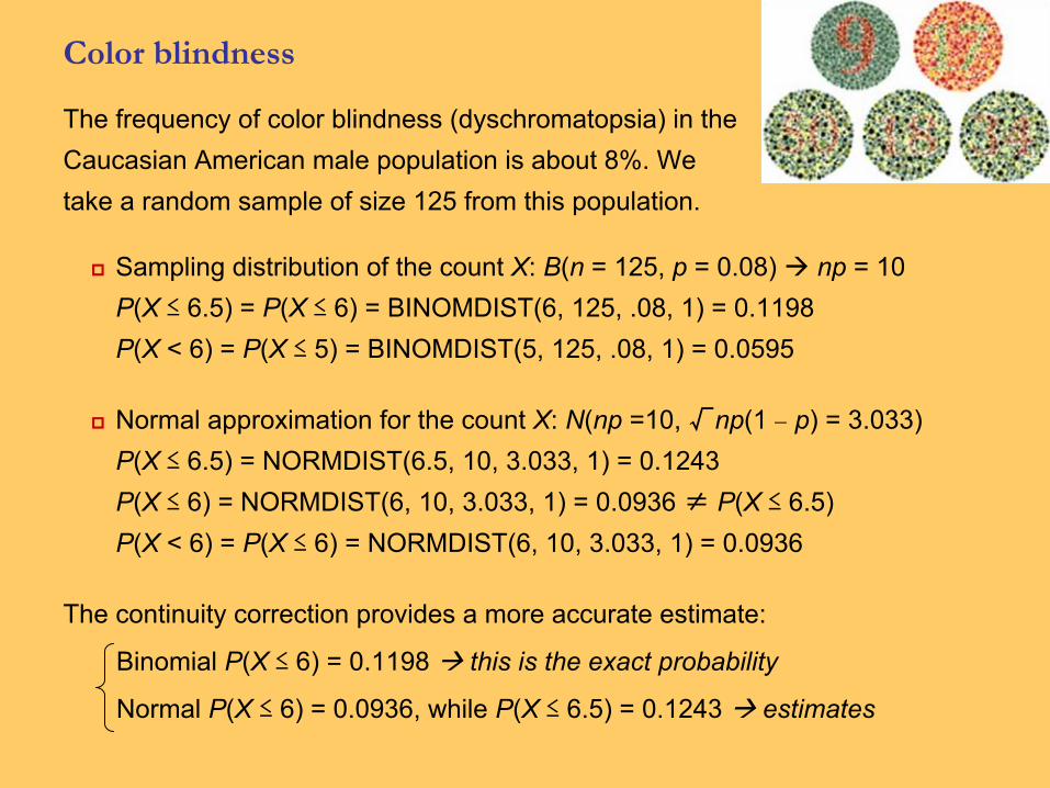
Color blindness

The frequency of color blindness (dyschromatopsia) in the Caucasian American male population is about 8%. We take a random sample of size 125 from this population.

Sampling distribution of the count X: B(n = 125, p = 0.08) np = 10P(X ≤ 6.5) = P(X ≤ 6) = BINOMDIST(6, 125, .08, 1) = 0.1198 P(X < 6) = P(X ≤ 5) = BINOMDIST(5, 125, .08, 1) = 0.0595

Normal approximation for the count X: N(np =10, √np(1 − p) = 3.033)P(X ≤ 6.5) = NORMDIST(6.5, 10, 3.033, 1) = 0.1243P(X ≤ 6) = NORMDIST(6, 10, 3.033, 1) = 0.0936 ≠ P(X ≤ 6.5) P(X < 6) = P(X ≤ 6) = NORMDIST(6, 10, 3.033, 1) = 0.0936

The continuity correction provides a more accurate estimate:

Binomial P(X ≤ 6) = 0.1198 this is the exact probability

Normal P(X ≤ 6) = 0.0936, while P(X ≤ 6.5) = 0.1243 estimates

Binomial formulas

The number of ways of arranging k successes in a series of n

observations (with constant probability p of success) is the number of

possible combinations (unordered sequences).

This can be calculated with the binomial coefficient:

)!(!!

knknn

k −=

Where k = 0, 1, 2, ..., or n.

Binomial formulas

The binomial coefficient “n_choose_k” uses the factorial notation “!”.

The factorial n! for any strictly positive whole number n is:

n! = n × (n − 1) × (n − 2) × · · · × 3 × 2 × 1

For example: 5! = 5 × 4 × 3 × 2 × 1 = 120

Note that 0! = 1.

Calculations for binomial probabilities

The binomial coefficient counts the number of ways in which k successes can be arranged among n observations.

The binomial probability P(X = k) is this count multiplied by the probability of any specific arrangement of the k successes:

X P(X)

0

1

2

…

k

…

n

nC0 p0qn = qn

nC1 p1qn-1

nC2 p2qn-2

…

nCx pkqn-k

…

nCn pnq0 = pn

Total 1

knk ppnkkXP −−

== )1()(

The probability that a binomial random variable takes any

range of values is the sum of each probability for getting

exactly that many successes in n observations.

P(X ≤ 2) = P(X = 0) + P(X = 1) + P(X = 2)

Color blindness

The frequency of color blindness (dyschromatopsia) in the

Caucasian American male population is estimated to be

about 8%. We take a random sample of size 25 from this population.

What is the probability that exactly five individuals in the sample are color blind?

Use Excel’s “=BINOMDIST(number_s,trials,probability_s,cumulative)”

P(x = 5) = BINOMDIST(5, 25, 0.08, 0) = 0.03285

P(x = 5) = 53,130 * 0.0000033 * 0.1887 = 0.03285

P(x = 5) =n!

k!(n − k)!pk (1 − p)n −k =

25!5!(20)!

0.085(0.92)20

P(x = 5) =21*22*23*24 *25

1*2* 3* 4 *50.085(0.92)20

Alternate Slides

The following slides offer alternate software

output data and examples for this presentation.

Calculations

InJMP,Highlight a column,click the column triangle ( ), and click formula to open the box on the right.Select Discrete Probability

Choose “Binomial Probability” for the probability of a given number ofsuccesses P(X = x)

Or “Binomial Distribution” for the density function P(X ≤ x)Enter values for p, n and x as shown

in the diagram.Click “OK.”P(X≤x) is illustrated.

The probabilities for a Binomial distribution can be calculated by using software.

Color blindness

The frequency of color blindness (dyschromatopsia) in the

Caucasian American male population is estimated to be

about 8%. We take a random sample of size 20 from this population.

What is the probability that exactly five individuals in the sample are color blind?

Use JMPs: Probability Binomial Probability (0.08, 20, 5)

P(x= 5) = Binomial Probability (0.08, 20, 5) = 0.0145 – or use Table C

P(x= 5) = (n! / k!(n −k)!)pk(1 −p)n-k = (20! / 5!(15)!) 0.0850.9215

P(x= 5) = (16*17*18*19*20 / 1*2*3*4*5) 0.0850.9215

P(x= 5) = 15,504 * 0.0000033 * 0.286297 = 0.0145

Color blindness

The frequency of color blindness (dyschromatopsia) in the Caucasian American male population is estimated to be about 8%. We take a random sample of size 20 from this population.

The population is definitely larger than 20 times the sample size, thus we can approximate the sampling distribution by B(n = 20, p = 0.08).

What is the probability that five individuals or fewer in the sample are color blind?

Use JMPs: Probability Binomial Distribution (0.08, 20, 5)

P(x≤ 5) = Binomial Distribution(0.08, 20, 5) = 0.9962

What is the probability that more than five will be color blind?P(x> 5) = 1 −P(x≤ 5) =1 − 0.9962 = 0.0038

What is the probability that exactly five will be color blind?P(x= 5) = Binomial Probability (0.08, 20, 5) = 0.0145 – or use Table C

Probability distribution and histogram for the number

of color blind individuals among 20 Caucasian males.

B(n = 20, p = 0.08)

What are the mean and standard deviation of the count

of color blind individuals in the SRS of 25 Caucasian

American males?

µ = np = 20*0.08 = 1.6

σ = √np(1 −p) = √(20*0.08*0.92) = 1.213

p = .08n = 10

p = .08n = 75

0

0.05

0.1

0.15

0.2

0 1 2 3 4 5 6 7 8 9 10 11 12 13Number of successes

P(X

=x)

0

0.1

0.2

0.3

0.4

0.5

0 1 2 3 4 5 6

Number of successes

P(X

=x)

µ = 10*0.08 = 0.8 µ = 75*0.08 = 6

σ = √(10*0.08*0.92) = 0.86 σ = √(75*0.08*0.92) = 3.35

What if we take an SRS of size 10? Of size 75?

Color blindness

The frequency of color blindness (dyschromatopsia) in the

Caucasian American male population is estimated to be

about 8%. We take a random sample of size 20 from this population.

What is the probability that exactly five individuals in the sample are color blind?

Use JMPs: Probability Binomial Probability (0.08, 20, 5)

P(x= 5) = Binomial Probability (0.08, 20, 5) = 0.0145 – or use Table C

P(x= 5) = (n! / k!(n −k)!)pk(1 −p)n-k = (20! / 5!(15)!) 0.0850.9215

P(x= 5) = (16*17*18*19*20 / 1*2*3*4*5) 0.0850.9215

P(x= 5) = 15,504 * 0.0000033 * 0.286297 = 0.0145