Is the Aggregate Investor Reluctant to Realise Losses ...faculty.haas.berkeley.edu/odean/Papers current versions...Is the Aggregate Investor Reluctant to Realise Losses? 425 period,

European Financial Management, Vol. 13, No. 3, 2007, 423–447doi: 10.1111/j.1468-036X.2007.00367.x

Is the Aggregate Investor Reluctant toRealise Losses? Evidence from Taiwan

Brad M. BarberGraduate School of Management, University of California, Davis, CA 95616, USAE-mail: [email protected]

Yi-Tsung LeeDepartment of Accounting, National Chengchi University, Taipei, TaiwanE-mail: [email protected]

Yu-Jane LiuDepartment of Finance, Guanghua School, Peking University, China and Department of FinanceNational Chengchi University, Taipei, TaiwanE-mail: [email protected]

Terrance OdeanHaas School of Business, University of California, Berkeley, CA 94720, USAE-mail: [email protected]

Abstract

We ask whether the typical investor and the aggregate investor exhibit a biasknown as the disposition effect, the tendency to sell investments that are held fora profit at a faster rate than investments held for a loss. We analyse all tradingactivity on the Taiwan Stock Exchange (TSE) for the five years ending in 1999.Using a dataset that contains all trades (over one billion) and the identity ofevery trader (nearly four million), we find that in aggregate, investors in Taiwanare about twice as likely to sell a stock if they are holding that stock for a gainrather than a loss. Eighty-four percent of all Taiwanese investors sell winners ata faster rate than losers. Individuals, corporations, and dealers are reluctant torealise losses, while mutual funds and foreigners, who together account for lessthan 5% of all trades (by value), are not.

Keywords: individual investors; institutional investors; disposition effect; prospecttheory.

JEL classification: G11

We are grateful to the Taiwan Stock Exchange for providing the data used in this study.Michael Bowers provided phenomenal computing support, which made this project possible.Terrance Odean is grateful for the financial support of the National Science Foundation(Grant 0222107).

C© 2007 The AuthorsJournal compilation C© 2007 Blackwell Publishing Ltd, 9600 Garsington Road, Oxford OX4 2DQ, UK and 350 Main Street, Malden, MA02148, USA.

424 Brad M. Barber, Yi-Tsung Lee, Yu-Jane Liu and Terrance Odean

Most clients, however, will not sell anything at a loss. They don’t want to give up thehope of making money on a particular investment, or perhaps they want to get evenbefore they get out . . .. Investors are also reluctant to accept and realise losses becausethe very act of doing so proves that their first judgment was wrong . . . Investors whoaccept losses can no longer prattle to their loved ones, ‘Honey, it’s only a paper loss.Just wait. It will come back’.

Leroy GrossThe Art of Selling Intangibles: How to Make your Million( $ ) by Investing OtherPeople’s Money

1. Introduction

Do the psychologically motivated trading biases that clearly affect some investors, affectenough investors so as to potentially influence asset prices? Are these biases restrictedto a less sophisticated, less wealthy minority of investors, or are they the norm? Inthis paper, we ask whether the typical investor and the aggregate investor exhibit a biasknown as the disposition effect, the tendency to sell investments that are held for a profitat a faster rate than investments held for a loss.

We answer this question in the context of the Taiwanese stock market. We analyseall trading activity on the Taiwan Stock Exchange (TSE) for the five years endingin 1999. Using a dataset that contains all trades (over one billion) and the identityof every trader (nearly four million), we are able to quantify the extent to whichinvestors sell losers and winners (relative to the opportunities to sell each). We definea winner as a stock that has increased in value since its purchase and a loser as astock that has declined in value since its purchase. In aggregate, investors in Taiwanare about twice as likely to sell a stock if they are holding that stock for a gainrather than a loss. Furthermore, 85% of all investors sell winners at a faster rate thanlosers.

In auxiliary analyses, we find the following empirical results:

1. We categorise investors into five broad categories: individuals, corporations, domes-tic mutual funds, foreigners, and dealers. Individuals, corporations, and dealers arereluctant to realise losses, while mutual funds and foreigners, who together accountfor less than 5% of all trades (by value), are not.

2. Short sellers are reluctant to realise losses. We analyse short sales and documentsimilar patterns to those found for long positions; investors are reluctant to realiselosses from short sales (i.e., buying to close a short position following priceappreciation).

3. Both men and women are reluctant to realise losses. Consistent with Barber andOdean (2001), men trade more actively than women. However, the reluctance torealise losses is of similar magnitude for men and women.

4. The willingness to sell losers increases following strong market returns.5. The disposition effect does not lead to momentum in Taiwanese stock returns.

Our results are consistent with a growing body of empirical work which documentsthat investors are reluctant to realise their losses. In contrast to prior studies, whichanalyse the decisions of a relatively small sample of investors or a relatively short time

C© 2007 The AuthorsJournal compilation C© 2007 Blackwell Publishing Ltd, 2007

Is the Aggregate Investor Reluctant to Realise Losses? 425

period, we analyse the complete transactions of all investors for a five-year period inthe world’s 12th largest financial market.1

The plan of the paper is as follows. In section 2, we describe related research. Insection 3, we describe the institutional details of the TSE, data, and methods. We presentresults in section 4, discuss implications in section 5, and make concluding remarks insection 6.

2. Related Research

Shefrin and Statman (1985) propose that a combination of mental accounting (Thaler,1985) and of utility functions similar to those described in Kahneman and Tversky’sProspect Theory (1979) leads investors to more readily sell stock investments held fora gain than those held for a loss. Due to mental accounting, investors focus on gainsand losses from individual stock positions rather than focusing on portfolio returns ortotal wealth levels. Due to Prospect Theory-like utility functions, investors may preferthe risks of continuing to own a stock that they would otherwise have sold if that stockis currently held for a loss.

For some investors, the tendency to hold losers may be driven on a more basic levelthan probabilities of gains and losses. We live in a world in which most decisions arejudged ex post and most people find it psychologically painful to acknowledge theirmistakes. When a stock is sold for a loss, it becomes, irrevocably, an (ex post) mistake.A stock that one continues to hold for a loss, however, still might turn out to be a good(ex post) decision. Thus by continuing to hold onto their losers, investors postpone, andpotentially avoid, admitting their mistakes.

Several empirical studies test this application of prospect theory to investments. Odean(1998) analyses the trades of 10,000 accounts at a discount brokerage between the years1987 and 1993. He documents that winners are sold at roughly twice the rate of losersand shows that this phenomenon is not explained by taxes, rebalancing, or transactioncosts. Barber and Odean (1999) confirm this result using data from the same discountbroker, but different accounts, for the period 1991–1996. Using the same dataset, Dharand Zhu (2006) document that the disposition effect is stronger for less sophisticatedinvestors. Shapira and Venezia (2001) analyse the round-trip trades of about 4,000Israeli investors during 1994; consistent with the predictions of prospect theory, losersare held two to three times longer than winners. Analysing trades of all Finnish investorsfor approximately two years ending in January 1997, Grinblatt and Keloharju (2001)conclude that Finnish investors are less likely to sell a stock held for a capital loss.Using logit regressions, they document this result in aggregate (weighting each tradeequally) for five investor categories: households, non-financial corporations, financialand insurance companies, and government and non-profit institutions.2 Jackson (2004)reports that individual investors in Australia sell more actively after positive returns andbuy less actively after negative returns; the first of these phenomena is consistent with

1 The Economist Pocket World in Figures (London: Profile Books, 2002), p. 62.2 While Grinblatt and Keloharju (2001) also have data for foreign investors, they are unableto classify enough foreign sales as capital gains or losses to run their analysis. Due to theirshorter time period and lower turnover rates, they are able to classify only 8% of all investors’sales while we classify 73%.



the disposition effect. Studies have also found evidence of the disposition effect in theexercise of company stock options (Heath et al., 1999), residential housing (Genesoveand Mayer, 2001), and professional futures traders (Locke and Mann, 2001). Finally,Coval and Shumway (2005) report that market makers in Treasury Bond futures takeon additional risk after experiencing recent losses – behaviour consistent with ProspectTheory and the disposition effect.

In work related to the disposition effect, Barber et al. (2006) find that investors aremore likely to purchase a stock that they previously sold if the stock is currently tradingat a lower price. They argue that an investor who sells and repurchases at a lower pricefeels good about these transactions, while an investor who repurchases at a higher pricethan he sold regrets having sold in the first place. To avoid this regret, investors avoidrepurchasing for a higher price. Odean (1998) reports that investors are more likely tobuy additional shares of a stock that has dropped in price since purchased than a stockthat has appreciated. Again, a desire to avoid regret may explain this behaviour.

We contribute to understanding of the disposition effect by analysing all trades madeon the TSE from 1995 to 1999. We are able to document that the tendency to hold lossesis exhibited by Taiwanese traders in aggregate as well as by the vast majority of thesetraders on an individual level. This extensive data set and (relatively) long time periodenable us to provide compelling evidence that the both the typical and the aggregateinvestor are reluctant to realise losses.

3. Background, Data and Methods

3.1. Taiwan market rules

Before proceeding, it is useful to describe the Taiwan Stock Exchange (TSE). TheTSE operates in a consolidated limit order book environment where only limit ordersare accepted. During the regular trading session, from 9:00 a.m. to noon during oursample period, buy and sell orders can interact to determine the executed price subjectto applicable automatching rules. Minimum tick sizes are set by the TSE and varydepending on the price of the security. Effective 2 November 1993, all securities listedon the TSE are traded by automatching through TSE’s Fully Automated SecuritiesTrading (‘FAST’) system. During our sample period, trades can be matched one to twotimes every 90 seconds throughout the trading day. Orders are executed in strict priceand time priority. An order entered into the system at an earlier time must be executedin full before an order at the same price entered at a later time is executed. Althoughmarket orders are not permitted, traders can submit aggressive price-limit orders toobtain matching priority. During our study period, there is a daily price limit of 7% ineach direction and a trade-by-trade intraday price limit of two ticks from the previoustrade price.

The TSE caps commissions at 0.1425% of the value of a trade. Some brokers offerlower commissions for larger traders, though we are unable to document the prevalenceof these price concessions. Taiwan also imposes a transaction tax on stock sales of 0.3%.Capital gains (both realised and unrealised) are not taxed, while cash dividends are taxedat ordinary income tax rates for domestic investors and at 20% for foreign investors.Corporate income is taxed at a maximum rate of 25%, while personal income is taxedat a maximum rate of 40%.



Table 1

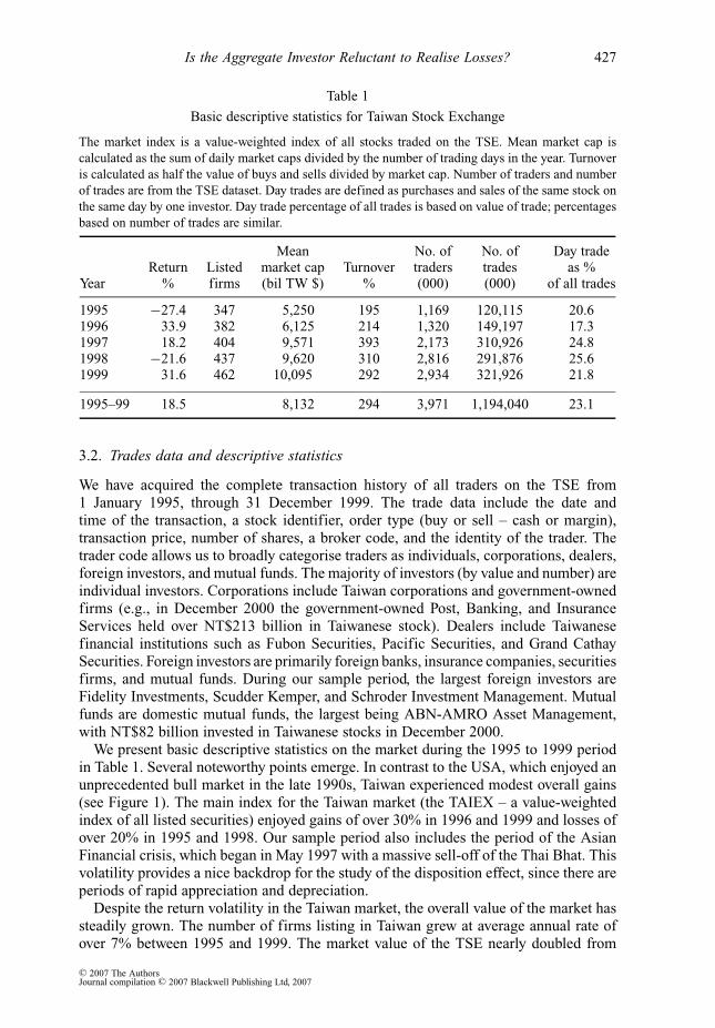
Basic descriptive statistics for Taiwan Stock Exchange

The market index is a value-weighted index of all stocks traded on the TSE. Mean market cap is

calculated as the sum of daily market caps divided by the number of trading days in the year. Turnover

is calculated as half the value of buys and sells divided by market cap. Number of traders and number

of trades are from the TSE dataset. Day trades are defined as purchases and sales of the same stock on

the same day by one investor. Day trade percentage of all trades is based on value of trade; percentages

based on number of trades are similar.

Mean No. of No. of Day tradeReturn Listed market cap Turnover traders trades as %

Year % firms (bil TW $) % (000) (000) of all trades

1995 −27.4 347 5,250 195 1,169 120,115 20.61996 33.9 382 6,125 214 1,320 149,197 17.31997 18.2 404 9,571 393 2,173 310,926 24.81998 −21.6 437 9,620 310 2,816 291,876 25.61999 31.6 462 10,095 292 2,934 321,926 21.8

1995–99 18.5 8,132 294 3,971 1,194,040 23.1

3.2. Trades data and descriptive statistics

We have acquired the complete transaction history of all traders on the TSE from1 January 1995, through 31 December 1999. The trade data include the date andtime of the transaction, a stock identifier, order type (buy or sell – cash or margin),transaction price, number of shares, a broker code, and the identity of the trader. Thetrader code allows us to broadly categorise traders as individuals, corporations, dealers,foreign investors, and mutual funds. The majority of investors (by value and number) areindividual investors. Corporations include Taiwan corporations and government-ownedfirms (e.g., in December 2000 the government-owned Post, Banking, and InsuranceServices held over NT$213 billion in Taiwanese stock). Dealers include Taiwanesefinancial institutions such as Fubon Securities, Pacific Securities, and Grand CathaySecurities. Foreign investors are primarily foreign banks, insurance companies, securitiesfirms, and mutual funds. During our sample period, the largest foreign investors areFidelity Investments, Scudder Kemper, and Schroder Investment Management. Mutualfunds are domestic mutual funds, the largest being ABN-AMRO Asset Management,with NT$82 billion invested in Taiwanese stocks in December 2000.

We present basic descriptive statistics on the market during the 1995 to 1999 periodin Table 1. Several noteworthy points emerge. In contrast to the USA, which enjoyed anunprecedented bull market in the late 1990s, Taiwan experienced modest overall gains(see Figure 1). The main index for the Taiwan market (the TAIEX – a value-weightedindex of all listed securities) enjoyed gains of over 30% in 1996 and 1999 and losses ofover 20% in 1995 and 1998. Our sample period also includes the period of the AsianFinancial crisis, which began in May 1997 with a massive sell-off of the Thai Bhat. Thisvolatility provides a nice backdrop for the study of the disposition effect, since there areperiods of rapid appreciation and depreciation.

Despite the return volatility in the Taiwan market, the overall value of the market hassteadily grown. The number of firms listing in Taiwan grew at average annual rate ofover 7% between 1995 and 1999. The market value of the TSE nearly doubled from



$0.0

$0.2

$0.4

$0.6

$0.8

$1.0

$1.2

$1.4

$1.6

19950105 19950615 19951117 19960430 19960930 19970312 19970812 19980122 19980714 19981223 19990616 19991201

Fig. 1. Growth of $1 invested in Taiwan Index on 31 December 1994.

1995 to 1999 – growing from NT$ 5.2 trillion (US$ 198 billion) in 1995 to over NT$10 trillion (US$ 313 billion) in 1999.3 At the end of 1999, the Taiwan market ranked asthe 12th largest financial market in the world, though it was only slightly greater than2% of the total US market.

Turnover in the TSE is remarkably high – averaging 292% annually during oursample period.4 In contrast, turnover on the New York Stock Exchange averaged 69%during the same period.5 The number of traders and number of trades grew dramaticallyduring our sample period. For the five-year period, we analyse more than one billiontrades.

Day trading is also prevalent in Taiwan. We define day trading as the purchase andsale of the same stock on the same day by an investor. Over our sample period, daytrading accounted for 23% of the total dollar value of trading volume. The majority ofday trading (64%) involves the purchase and sale of the same number of shares in astock (i.e., most day trades yield no net change in ownership at the close of the day).6

Individual investors dominate the Taiwan market. According to the 2000 Taiwan StockExchange Factbook (Table 24), individual investors accounted for between 56 and 59%of total stock ownership during our sample period. Taiwan corporations owned between17 and 23% of all stocks, while foreigners owned between 7 and 9%. At the end of 2000,

3 The $TW/$US exchange rate reached a low of 24.5 and a high of 34.7 betweenJanuary 1995 and December 1999.4 We calculate turnover as half the sum of buys and sells in each year divided by the averagedaily market cap for the year.5 NYSE Factbook 2000, p. 99.6 See Barber et al. (2005) for a comprehensive analysis of day trading in Taiwan.



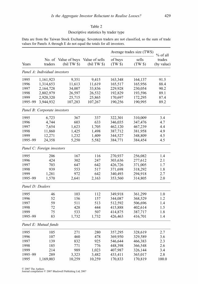
Table 2

Descriptive statistics by trader type

Data are from the Taiwan Stock Exchange. Seventeen traders are not classified, so the sum of trade

values for Panels A through E do not equal the totals for all investors.

Average trades size (TW$)% of all

No. of Value of buys Value of sells of buys sells tradesYears traders (bil TW $) (bil TW $) (TW $) (TW $) (by value)

Panel A: Individual investors

1995 1,161,923 9,351 9,415 163,348 164,137 91.51996 1,314,653 11,613 11,619 165,517 165,956 88.41997 2,164,728 34,007 33,836 229,928 230,054 90.21998 2,802,979 26,597 26,532 192,829 193,596 89.11999 2,920,320 25,715 25,865 170,697 172,295 87.41995–99 3,944,932 107,283 107,267 190,256 190,995 89.2

Panel B: Corporate investors

1995 6,723 367 337 322,301 310,009 3.41996 4,744 603 633 346,035 347,476 4.71997 7,654 1,623 1,705 462,120 467,239 4.41998 11,860 1,425 1,498 387,712 381,958 4.91999 12,271 1,232 1,409 344,527 348,809 4.51995–99 24,358 5,250 5,582 384,771 384,454 4.5

Panel C: Foreign investors

1995 206 167 116 270,937 256,082 1.41996 424 302 247 303,636 277,612 2.11997 703 647 642 426,726 371,005 1.71998 939 553 517 371,698 318,292 1.81999 1,281 972 642 340,493 294,918 2.71995–99 1,570 2,641 2,163 353,560 314,805 2.0

Panel D: Dealers

1995 46 103 112 349,918 361,299 1.01996 52 156 157 344,087 368,529 1.21997 59 511 513 512,592 506,696 1.41998 72 428 444 415,888 402,614 1.51999 75 533 507 414,875 387,717 1.81995–99 83 1,732 1,732 426,463 416,701 1.4

Panel E: Mutual funds

1995 105 271 280 357,295 328,619 2.71996 107 460 478 369,950 329,589 3.61997 139 832 925 546,644 466,383 2.31998 185 771 776 448,398 366,548 2.61999 214 989 1,023 407,987 326,144 3.41995–99 289 3,323 3,482 433,411 365,017 2.81995 1,169,003 10,259 10,259 170,833 170,819 100.0



Table 2

Continued.

Average trades size (TW$)% of all

No. of Value of buys Value of sells of buys sells tradesYears traders (bil TW $) (bil TW $) (TW $) (TW $) (by value)

Panel F: All investors

1996 1,319,980 13,134 13,134 176,066 176,055 100.01997 2,173,287 37,624 37,624 242,017 242,011 100.01998 2,816,047 29,799 29,799 204,189 204,187 100.01999 2,934,176 29,496 29,496 183,247 183,247 100.01995–99 3,971,249 120,312 120,312 201,524 201,519 100.0

Taiwan’s population reached 22.2 million; 6.8 million Taiwanese (31%) had opened abrokerage account.

In Table 2, we present the total value of buys and sells for each investor group by year.As can be seen in the last column of the table, individual investors account for roughly90% of all trading volume and place trades that are roughly half the size of those madeby the four other groups (corporations, dealers, foreigners, and mutual funds). Each ofthe remaining groups accounts for less than 5% of total trading volume.

Obviously, individual investors are very active traders in Taiwan. Some back-of-the-envelope calculations using data on the percentage ownership and trading for eachinvestor group, we estimate that annual turnover for the individual investor group rangesbetween 308 and 630% annually from 1995 to 1999.7

3.3. Methods

We wish to investigate whether investors are reluctant to realise loses. To test the nullhypothesis that investors are equally likely to realise gains and losses, we calculate adaily hazard rate for the realisation of gains and losses. In general, on each day we breakup an investor’s portfolio into stocks held for gains and stocks held for losses. We thenanalyse the selling activity of the investor and calculate the proportion of his winnerssold and the proportion of his losers sold.

Specifically, by going through each investor’s trading records in chronological order,we construct a portfolio of individual stocks for which the purchase date and price areknown. (See the appendix for the details of portfolio construction.) For stocks sold, thesales price for the stock is compared to its average purchase price to determine whetherthat stock was sold for a gain or a loss. Each stock that was in that portfolio at thebeginning of that day but was not sold is considered to be a paper (unrealised) gain orloss. We compare the stock’s daily high and low price to the average purchase price ofthe stock and categorise paper positions as gains, losses, or indeterminate (if the averagepurchase price falls between the daily high and low price). Our counts of the value andnumber of gains and losses realised are incremented daily (regardless of whether a sale

7 For example, in 1995 the individual investor group accounted for 91.5% of all trades and58.1% of stock ownership. Given annual market turnover of 195%, this implies that turnoverfor individual investors was 308%: (91.5/58.1) × 195.



0%

10%

20%

30%

40%

50%

60%

19950106 19950617 19951120 19960502 19961002 19970314 19970814 19980203 19980716 19981228 19990621 19991203

Fig. 2. Positions constructed from trades data as a percentage of total TSE marketcapitalisation

took place). Then, for each trader we calculate two ratios:

Proportion of gains realised (PGR) = Realised gains

Realised gains + Paper gains;

Proportion of losses realised (PLR) = Realised losses

Realised losses + Paper losses.

A large difference in the proportion of gains realised (PGR) and the proportion of lossesrealised (PLR) indicates that this investor preferred realising gains rather than losses(relative to his opportunity to realise each).8

Since we construct positions for each investor based on his trades, the constructedpositions grow through our sample period. Because turnover on the TSE is quitehigh, the growth in positions occurs fairly quickly. By the end of 1995 constructedpositions represent roughly 25% of total market capitalisation, while at the end of 1999,constructed positions represent roughly half of total market capitalisation (see Figure 2).We are unable to construct positions for shares that are not traded. Though marketwideturnover is very high, nearly half of all shares in this market do not trade during ourfive year period.

8 Our methodology follows that introduced in Odean (1998) with one important difference.Because of computing resource constraints, Odean evaluated an investor’s paper gains andpaper losses only for days on which the investor made a sale, while we do so every day.Thus our PGR and PLR calculations are equivalent to daily hazard rates at which winnersand losers are sold. Direct comparisons of PGR and PLR across investors holding differingportfolio sizes can be made using our methodology, but not the earlier methodology.



To establish statistical significance, we use two approaches. First, we calculate thedifference between PGR and PLR for each investor. We calculate the mean differenceacross investors within a particular investor group (individuals, corporations, dealers,foreigners, or mutual funds). Statistical significance is based on the mean differenceand the cross-sectional standard deviation of the difference.

Second, we separately sum realised gains, realised losses, paper gains, and paperlosses across all investors and across each investor group on each calendar day. Thisallows us to calculate the difference between PGR and PLR on a particular day. Wethen calculate the mean difference across days for investors within a particular group(individuals, corporations, dealers, foreigners, or mutual funds). Statistical significanceis based on the mean difference over time and the time-series standard deviation of thedifference. The time-series standard deviations are calculated using the Newey-Westcorrection for autocorrelation.

4. Results

4.1. Cross-sectional results

In Table 3, Panel A, we present the total value of paper gains, paper losses, realisedgains, and realised losses for all investors and by investor type. Each field is summedacross investors and over time. These values are used to calculate the proportion of gainsrealised (PGR) and the proportion of losses realised (PLR) in Table 3, Panel B. First,consider the results for all investors (in the last column of Table 3, Panel B). Gains arerealised at a daily rate of 2.9%, while losses are realised at a daily rate of 1.4% – lessthan half the rate for gains. In aggregate, investors are roughly twice as likely to sella winner rather than a loser, providing strong support for the notion that the aggregateinvestor is reluctant to realise losses.9 To formally test whether investors are reluctant torealise losses, we separately calculate PGR and PLR for each investor and then averageacross investors. These results are presented in the last column of Table 3, Panel C. Forthe average investor, the proportion of gains realised is 9.4%, while the proportion oflosses realised is only 2.3%. The difference in PGR and PLR (7.1%) is reliably positive(p < 0.01). (The fact that these values are greater than those obtained when summingacross investors and over time indicates that relative to the positions they hold, smallinvestors tend to trade more actively than large investors.) Furthermore, 84% of allinvestors realise gains at a faster rate than losses (i.e., PGR > PLR).

Our results by investor type indicate individuals, corporations, and dealers preferto sell winners rather than losers. These results are similar regardless of whether weaggregate across investors and over time (Panel B) or average across investors (PanelC). In contrast, foreign investors and domestic mutual funds do not prefer to sell winnersrather than losers. When we average across investors, we are unable to reject the nullhypothesis that PGR equals PLR for foreigners, while domestic mutual funds display amodest preference for selling losers rather than winners (p < 0.05).

9 PGR and PLR can be interpreted as daily turnover rates for gains and losses, respectively.When multiplied by the number of trading days in the year (on average, 279 in Taiwan),annual turnover is 809% for gains and 396% for losses. These figures are much higher thanthe turnover rates reported in Table 1 since we construct positions for only those who trade.As reported in Figure 2, we do not construct positions for roughly half of the market. Theseinfrequent traders pull down marketwide turnover.



Tab

le3

Pro

port

ion

of

gai

ns

real

ised

(PG

R)

and

pro

port

ion

of

loss

esre

alis

ed(P

LR

)by

inves

tor

type

On

each

day

,in

ves

tor,

and

stock

,pap

ergai

ns

repre

sent

the

tota

lva

lue

of

unre

alis

edca

pit

algai

ns

rela

tive

toth

eav

erag

epurc

has

epri

cefo

rth

est

ock

.P

aper

gai

ns

are

sum

med

acro

ssd

ays,

sto

cks,

and

inves

tors

.P

aper

loss

es,

real

ised

gai

ns,

and

real

ised

loss

esar

eca

lcu

late

dsi

mil

arly

(see

Ap

pen

dix

).

Indiv

idual

Mu

tual

All

inves

tors

Corp

ora

teF

ore

igner

sD

eale

rsfu

nd

sin

ves

tors

Num

ber

of

inves

tors

3064,9

55

13,0

45

1,4

83

81

24

83

07

9,8

29

Pane

lA

:To

tal

valu

eof

PG

,P

L,

RG

,an

dR

L($

TW

tril

lion

)

Pap

ergai

ns

(PG

)966.4

6318.9

8259.6

521.1

11

43.3

31

74

0.8

9

Pap

erlo

sses

(PL

)1

639.4

6317.5

199.3

928.3

97

5.9

62

16

1.2

4

Rea

lise

dgai

ns

(RG

)4

5.7

02.6

81.2

11.0

01.9

25

2.5

5

Rea

lise

dlo

sses

(RL

)27.8

20.9

90.6

70.5

01.1

83

1.1

8

Pane

lB

:P

GR

and

PL

Rba

sed

onag

greg

ated

valu

esof

PG

,P

L,

RG

,an

dR

L

%gai

ns

real

ised

:P

GR

=R

G/(P

G+

RG

)4.3

90.8

30.4

64.5

41.3

22.9

3

%lo

sses

real

ised

:P

LR

=R

L/(P

L+

RL

)1.6

70.3

10.6

71.7

31.5

31.4

2

PG

R−

PL

R2.7

20.5

2−0

.21

2.8

2−0

.21

1.5

1

Pane

lC

:M

ean

PG

Ran

dP

LR

acro

ssin

vest

ors

%gai

ns

real

ised

:P

GR

=R

G/(P

G+

RG

)9.4

35.0

11.0

07.3

31.4

99.4

0

%lo

sses

real

ised

:P

LR

=R

L/(P

L+

RL

)2.3

31.1

71.1

52.5

81.7

52.3

2

PG

R−

PL

R7.1

0∗∗

∗3.8

4∗∗

∗−0

.15

4.7

5∗∗

∗−0

.26

∗∗7.0

8∗∗

∗

Per

centa

ge

of

inves

tors

wh

ere

84.4

∗∗∗

55.5

∗∗∗

32.2

∗∗∗

91.4

∗∗∗

30.6

∗∗∗

84.2

∗∗∗

PG

R>

PL

R(c

alcu

late

dusi

ng

valu

eso

ftr

ades

)

Per

centa

ge

of

inves

tors

wh

ere

85.7

∗∗∗

57.3

∗∗∗

36.9

∗∗∗

93.8

∗∗∗

55.2

85.5

∗∗∗

PG

R>

PL

R(c

alcu

late

dusi

ng

num

ber

sof

trad

es)

∗∗∗

-re

liab

lydif

fere

nt

from

zero

(or

50%

)at

the

1%

signif

ican

cele

vel

.



4.2. Results by gender

Though it would be interesting to explore the relation between the disposition effect anddemographic characteristics, we have data on only one demographic variable – gender.Of the 3.1 million individual investors for whom we are able to calculate PGR and PLR,1.7 million (55%) are women and 1.4 million (45%) are men. In contrast, 51% of theTaiwan population is male. Though it may seem unusual that there are more women thanmen who invest in the TSE market, we suspect this is largely a cultural phenomenon. InTaiwan, it is not unusual for women to buy and sell stocks after shopping at the market.This practice has become so prevalent in Taiwan that many brokerages market directly tothis female clientele. In Taiwan, brokerage houses are lavish venues for trading stocks,which offer comfortable seating, tea, and VIP rooms for frequent traders.

In Table 4, we present the mean value of PGR, PLR, and the difference for menand women. Both men and women prefer to sell winners rather than losers. Thoughthe difference between PGR and PLR is greater for men than women (7.19 and 7.02,respectively), the ratio of PGR to PLR is greater for women than men (4.7 and 3.6,respectively). Thus, though men realise gains at a faster rate than women (PGR isgreater for men), they exhibit a somewhat lower preference for realising gains ratherthan losses (the ratio of PGR to PLR is less for men). The fact that men realise bothgains and losses at a faster rate than women is consistent with the results in Barber andOdean (2001), which uses data from a large US discount broker to document that mentrade more actively than women.

4.3. Time-series results

As described previously, we sum paper gains, paper losses, realised gains, and realisedlosses across investors for a particular day. We then calculate a daily value for theproportion of gains realised (PGR) and the proportion of losses realised (PLR). InTable 5, we present the results of our time-series analysis. Panel A contains the meandaily value of PGR; Panel B contains the mean daily value of PLR; Panel C containsthe difference (PGR less PLR).

Consider first the results for all investors – presented in the last column of Table 5.PGR exceeds PLR in each year that we analyse and is reliably positive in each individual

Table 4

Mean PGR and PLR for women and men

For each day, investor, and stock, paper gains represent the total value of unrealised capital gains

relative to the average purchase price for the stock. Paper gains are summed across days, stocks, and

investors. Paper losses, realised gains, and realised losses are calculated similarly (see Appendix).

Men Women

Number 1408,737 1655,513

% gains realised: PGR = RG/(PG + RG) 10.00 8.95% losses realised: PLR = RL/(PL + RL) 2.81 1.92PGR − PLR 7.02∗∗∗ 7.19∗∗∗

Percentage of investors where PGR > PLR 83∗∗∗ 85∗∗∗

∗∗∗ - reliably different from zero (or 50%) at the 1% significance level.



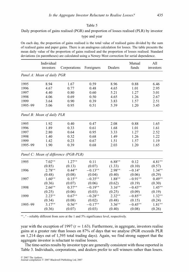
Table 5

Daily proportion of gains realised (PGR) and proportion of losses realised (PLR) by investor

type and year

On each day, the proportion of gains realised is the total value of realised gains divided by the sum

of realised gains and paper gains. There is an analogous calculation for losses. The table presents the

mean daily value of the proportion of gains realised and the proportion of losses realised. Standard

deviations (in parentheses) are calculated using a Newey-West correction for serial dependence.

Individual Mutual Allinvestors Corporations Foreigners Dealers funds investors

Panel A: Mean of daily PGR

1995 8.94 1.67 0.59 8.96 0.88 6.461996 4.67 0.77 0.48 4.65 1.01 2.951997 4.40 0.80 0.60 5.21 1.27 3.011998 4.06 0.69 0.50 4.65 1.26 2.671999 3.64 0.90 0.39 3.83 1.57 2.511995–99 5.06 0.95 0.51 5.39 1.20 3.45

Panel B: Mean of daily PLR

1995 1.92 0.40 0.47 2.08 0.88 1.651996 1.89 0.33 0.61 1.68 1.01 1.611997 2.80 0.64 0.95 3.33 1.27 2.521998 1.40 0.32 0.68 1.49 1.26 1.221999 1.42 0.23 0.67 1.51 1.57 1.191995–99 1.90 0.39 0.68 2.03 1.20 1.65

Panel C: Mean of difference (PGR-PLR)

1995 7.02∗∗ 1.27∗∗ 0.11 6.88∗∗ 0.12 4.81∗∗(0.85) (0.13) (0.07) (1.33) (0.10) (0.57)

1996 2.78∗∗ 0.44∗∗ −0.13∗∗ 2.98∗∗ −0.14∗ 1.34∗∗(0.48) (0.08) (0.04) (0.40) (0.06) (0.29)

1997 1.60∗∗ 0.15∗∗ −0.35∗∗ 1.88∗∗ −0.91∗∗ 0.49∗∗(0.36) (0.07) (0.06) (0.62) (0.19) (0.30)

1998 2.66∗∗ 0.37∗∗ −0.19∗∗ 3.16∗∗ −0.43∗∗ 1.45∗∗(0.25) (0.06) (0.03) (0.25) (0.09) (0.19)

1999 2.23∗∗ 0.67∗∗ −0.28∗∗ 2.32∗∗ −0.85∗∗ 1.32∗∗(0.34) (0.08) (0.02) (0.48) (0.15) (0.24)

1995–99 3.17∗∗ 0.56∗∗ −0.17∗∗ 3.36∗∗ −0.45∗∗ 1.81∗∗(0.36) (0.07) (0.03) (0.40) (0.08) (0.26)

∗∗, ∗ - reliably different from zero at the 1 and 5% significance level, respectively.

year with the exception of 1997 (t = 1.63). Furthermore, in aggregate, investors realisegains at a greater rate than losses on 87% of days that we analyse (PGR exceeds PLRon 1,214 days out of 1,395 total trading days). Again, we find strong support that theaggregate investor is reluctant to realise losses.

The time-series results by investor type are generally consistent with those reported inTable 3. Individuals, corporations, and dealers prefer to sell winners rather than losers.



These results are quite robust across years. In contrast, with the exception of 1995 –the first year in our analysis, foreign investors and domestic mutual funds prefer to selllosers rather than winners.

4.4. Short sales

The analysis of short sales provides a natural test of the robustness of our results. Ifinvestors are reluctant to realise losses, they should prefer to cover short positions whenstocks have declined in value and maintain short positions when stocks increase in value.During our sample period, only individual investors and corporations were allowed toshort stocks; foreigners, domestic mutual funds, and dealers were precluded from doingso. We are able to identify approximately 330,000 individuals and 1,100 corporationsthat sold short during our sample period.

A short position is classified as a paper gain if the stock’s price is below the average(short) sales price and a paper loss if the stock’s price is above the average (short)sales price. As for long positions, we sum paper gains, paper losses, realised gains, andrealised losses across investors for a particular day. We then calculate a daily value forthe proportion of gains realised (PGR) and the proportion of losses realised (PLR). InTable 6, we present the results of our time-series analysis. Panel A contains the meandaily value of PGR; Panel B contains the mean daily value of PLR; Panel C containsthe difference (PGR less PLR).

For the full sample period, both individuals and corporations prefer to cover short salesat a gain (i.e., following price declines), rather than at a loss. The results for individualsare robust across each of the five years that we analyse, though, in 1998 and 1999,corporations have no reliable preference for selling winning or losing short positions.

Cross-sectional analyses similar to those reported for long positions in Table 3 confirmthe time-series results. The average corporation and the average individual prefer tosell winning, rather than losing, short positions. In addition, 71% of individuals sellwinning short positions at a faster rate than losing short positions. However, only halfof corporations do so (indicating the tendency to sell winning short positions is lesssystematic across corporations).

We also analyse the short-selling of individuals by gender. Men are somewhat morelikely to sell short than women; 13% of men sell short, while 9% of women do so. Bothmen and women prefer to cover short positions for a gain rather than a loss.

4.5. Market movements and the disposition effect

The time-series of PGR and PLR during a five-year period when the Taiwan stock marketexperienced prolonged periods of significant appreciation and depreciation afford us theopportunity to analyse the relation between market movements and the propensity tosell winners and losers.

There are at least two reasons we expect to observe a relation between broad marketmovements and PGR (or PLR). First, it is likely that investors’ reference points changeas prices change. Throughout our analysis, we have considered the purchase price asthe reference point for establishing gains and losses. However, following periods ofappreciation in the market, investors are likely to view some stocks that are held for again as losers. For example, if the market has appreciated by 20% and investors hold astock that has only appreciated by 10%, some investors are likely to view the investment



Table 6

Short positions: daily proportion of gains realised (PGR) and proportion of losses realised

(PLR) by investor type and year

On each day, the proportion of gains realised is the total value of realised gains divided by the sum

of realised gains and paper gains. There is an analogous calculation for losses. The table presents the

mean daily value of the proportion of gains realised and the proportion of losses realised. Standard

deviations (in parentheses) are calculated using a Newey-West correction for serial dependence.

Individual investors Corporations All investors

Panel A: Mean of daily PGR

1995 12.79 10.56 12.741996 7.67 5.91 7.631997 11.39 9.73 11.271998 4.87 0.93 4.671999 2.40 0.37 2.291995–99 7.78 5.47 7.68

Panel B: Mean of daily PLR

1995 7.89 5.65 7.851996 3.64 1.81 3.601997 3.23 1.29 3.161998 2.57 1.12 2.511999 1.67 0.55 1.611995–99 3.72 2.01 3.67

Panel C: Mean of difference (PGR-PLR)

1995 4.90∗∗ 4.92∗∗ 4.89∗∗(0.83) (1.74) (0.84)

1996 4.02∗∗ 4.09∗∗ 4.03∗∗(0.66) (1.16) (0.67)

1997 8.16∗∗ 8.45∗∗ 8.11∗∗(1.51) (3.40) (1.54)

1998 2.30∗∗ −0.19 2.17∗∗(0.54) (0.16) (0.52)

1999 0.72∗∗ −0.17 0.68∗∗(0.22) (0.09) (0.22)

1995–99 4.06∗∗ 3.47∗∗ 4.01∗∗(0.55) (0.96) (0.56)

as a loss, since the stock has underperformed the market. If this is the case, we wouldexpect PGR to decrease following periods of appreciation, since we incorrectly classifysome perceived losses as gains. Analogously, following periods of depreciation, wewould expect PLR to increase, since we incorrectly classify some perceived gains aslosses.

Second, heterogeneity in the tendency to sell winners and losers across investorswill lead to a relation between broad market movements and PGR (or PLR). Our prior



analyses reveal just such heterogeneity – corporations, individuals, and dealers prefer tosell winners rather than losers, while foreigners and domestic mutual funds do not preferto do so. This heterogeneity will cause PGR and PLR to decrease following periods ofappreciation and increase following periods of depreciation.10

To analyse these effects, we estimate a simple time-series regression using weeklyvalues of PGR and PLR. Weekly values are obtained by summing paper gains, paperlosses, realised gains, and realised losses across the week. We then estimate the followingthree time-series regressions:

PG Rt = a +8∑

i=1

bi PG Rt−i+8∑

i=1

cirt−i+et

P L Rt = a +8∑

i=1

bi P L Rt−i+8∑

i=1

cirt−i+et

(PG R

P L R

)t

= a +8∑

i=1

bi

(PG R

P L R

)t−i

+8∑

i=1

cirt−i+et

where a, b, and c are coefficient estimates, rt is the weekly return on the market, andet is an error term. We include eight lags of the dependent variable, since empiricallypartial autocorrelations beyond eight lags are indistinguishable from zero.

The results of this analysis are presented in Table 7. Consider first the results forthe ratio (PGR/PLR) for long positions (panel A). There is strong evidence that thepropensity to sell winners, relative to losers, declines following strong market returns.The coefficient estimates on lagged market returns are generally negative – reliablyso for lags of one to three weeks. Furthermore, we can comfortably reject the nullhypothesis that the sum of the coefficients on lagged returns is equal to zero. Whenwe separately analyse PGR and PLR, as anticipated, we find that lagged returns arenegatively related to PGR. This is consistent with both changing reference points andheterogeneity in the willingness to sell winners. However, we find that PLR is positivelyrelated to past return (with the exception of lag length eight).

To test the robustness of these results, we also estimate analogous time-seriesregressions for PGR and PLR based on short positions (Table 7, Panel B). Note that thepredicted relation between past returns and PGR (or PLR) is precisely the opposite of that

10 To understand the effects of this heterogeneity, consider a simple example where the marketconsists of two investors – one who prefers to sell winners at twice the rate of losers and asecond who sells winners and losers at an equal rate. For simplicity, assume both investorssell 10% of their portfolio. Following a period of appreciation, assume both investors holdportfolios comprised of $80 of gains and $20 of losses. The investors with no preference forselling winners or losers sells $8 of gains and $2 of losses, while the investor who prefersto sell winners at twice the rate of losers sells $8.89 of gains and $1.11 of losses. Acrossthe two investors, the proportion of gains realised (PGR) is ($8 + $8.89)/$160 = 0.106,while the proportion of losses realised is ($2 + $1.11)/$40 = 0.078. Now consider a periodfollowing depreciation, where both investors hold portfolios comprised of $20 of gains and$80 of losses. The investor with no preference for selling winners and losers sells $2 of gainsand $8 of losses, while the investor who prefers to sell winners at twice the rate of loserssells $3.33 of gains and $6.67 of losses. Thus, PGR is ($2 + $3.33)/$40 = 0.133 and PLRis ($8 + $6.67)/$160 = 0.092. Note that PGR and PLR are both lower following periods ofappreciation.



Table 7

Time-series relation of weekly market returns and proportion of gains realised (PGR), the

proportion of losses realised (PLR), and the ratio of PGR to PLR: 1995–99

The dependent variable is alternately (1) the weekly proportion of gains realised, (2) the weekly

proportion of losses realised (PLR), and (3) the ratio of PGR to PLR. Independent variables include

eight weekly lags of the dependent variable and eight lags of weekly market returns (log returns − r):

PG Rt = a +8∑

i=1

bi PG Rt−i +8∑

i=1

cirt−i + ei

There are analogous equations for PLR and PGR/PLR. The sample period begins in the 20th

week of 1995 and ends in the last week of 1999 (241 weekly observations). Test statistics are

calculated using a Newey-West correction for serial dependence.

Dependent variable

PGR/PLR PGR PLR

Coef. t-stat Coef. t-stat Coef. t-stat

Panel A: Regression results for long positions

Intercept 0.296 2.45∗∗ 0.005 2.23∗∗ 0.002 2.22∗∗Lag length: Lagged dependent variable:

1 0.575 5.61∗∗∗ 0.642 6.27∗∗∗ 0.896 8.81∗∗∗2 0.237 2.43∗∗ 0.055 0.50 −0.248 −1.89∗3 0.194 1.86∗ 0.279 2.46∗∗ 0.335 2.75∗∗∗4 −0.269 −1.87∗ −0.122 −0.88 −0.107 −0.975 0.066 0.54 −0.067 −0.57 −0.036 −0.276 −0.001 −0.01 −0.008 −0.09 −0.030 −0.397 −0.007 −0.07 0.041 0.25 0.104 1.208 0.092 1.08 0.036 0.32 −0.021 −0.33

Lagged market returns

1 −9.323 −3.13∗∗∗ −0.056 −1.14 0.059 5.23∗∗∗2 −9.055 −4.74∗∗∗ −0.058 −1.94∗ −0.001 −0.193 −4.270 −1.85∗ −0.055 −1.72∗ 0.014 2.01∗∗4 −0.812 −0.38 −0.045 −1.62 −0.007 −0.625 1.353 0.44 0.049 1.32 0.003 0.386 −3.638 −1.46 −0.052 −2.14∗∗ −0.006 −0.737 −1.180 −0.49 −0.012 −0.43 0.007 0.798 −0.921 −0.42 −0.033 −1.07 −0.014 −2.10∗∗

Adj. R-Sq. (%) 68.9 61.2 80.8

Wald Test:8∑

i=1

ci = 0 29.05∗∗∗ 9.04∗∗∗ 7.10∗∗∗

for long positions, thus providing a natural test of the robustness of our results for longpositions. Consistent with the results for long positions, we find that the propensity tosell winners declines following poor market returns for short positions, PGR is positivelyrelated to past market returns, and PLR is negatively related to past market returns.



Table 7

Continued.

Dependent variable:

PGR/PLR PGR PLR

Coef. t-stat Coef. t-stat Coef. t-stat

Panel B: Regression results for short positions

Intercept 0.233 1.63 0.003 1.01 0.003 2.39∗∗Lag length: Lagged dependent variable:

1 0.600 6.99∗∗∗ 0.540 5.07∗∗∗ 0.647 6.67∗∗∗2 −0.129 −1.11 0.094 0.85 −0.008 −0.073 0.373 2.55∗∗ 0.317 2.87∗∗∗ 0.237 2.58∗∗4 −0.178 −1.57 0.012 0.16 −0.159 −1.285 0.064 0.61 −0.115 −1.17 0.136 1.356 0.068 0.61 0.018 0.19 −0.007 −0.077 0.135 1.72∗ 0.003 0.03 0.035 0.358 −0.048 −0.60 0.068 0.74 0.019 0.23

Lagged market returns

1 10.910 4.94∗∗∗ 0.282 3.16∗∗∗ −0.059 −2.12∗∗2 4.186 1.79∗ 0.129 2.30∗∗ −0.025 −1.253 4.094 1.70∗ 0.034 0.56 −0.051 −2.17∗∗4 2.982 1.46 0.095 1.94∗ 0.005 0.235 3.009 1.21 −0.020 −0.37 −0.006 −0.386 4.761 2.05∗∗ 0.080 1.42 −0.013 −0.757 2.172 1.07 0.019 0.32 0.015 0.988 −2.243 −1.31 −0.121 −2.23∗∗ −0.032 −1.81∗

Adj. R-Sq. (%) 66.9 75.4 83.5

Wald Test:8∑

i=1

ci = 0 30.57∗∗∗ 12.27∗∗∗ 8.73∗∗∗

∗∗∗, ∗∗, ∗ - significant at the 1, 5, and 10% level (two-tailed test)

In summary, there is strong evidence that the propensity to sell winners declines fol-lowing periods of appreciation (or depreciation for short positions). Both heterogeneityin the willingness to sell winners across investors and changing reference points wouldyield this result. Neither explains why the proportion of losses realised (PLR) increasesfollowing periods of appreciation (or depreciation for short positions). One possibleexplanation – not tested here – is that as the market appreciates, many stock positionsheld for losses appreciate, though not to the break even point. Some investors may besatisfied getting out of a losing position at a better price than they could have gotten aweek or two earlier.

5. Discussion and Implications

We have provided strong evidence that the typical and the aggregate investor prefer tosell winners rather than losers. In this section we discuss the possible implications ofthis finding for returns and volume.



5.1. Returns

Grinblatt and Han (2002) and Weber and Zuckel (2002) develop models wherein someinvestors prefer to sell winners and hold losers. Disposition investors have higherdemand for losing stocks than winning stocks, ceteris paribus. In these models, since thedemand for stocks by other investors is not perfectly elastic, stocks underreact to publicinformation and generate momentum in stock returns. Thus, the disposition effect isproposed as a potential explanation of the momentum profits documented by Jegadeeshand Titman (1993) and Rouwenhorst (1998). Grinblatt and Han (2002) and Goetzmannand Massa (2003) provide empirical support for the link between the disposition effectand momentum profits in the USA.

Given the strong tendency for Taiwanese investors to realise winners rather thanlosers, the Grinblatt–Han and the Weber–Zuckel models predict the presence of a strongmomentum effect in Taiwan. To investigate this prediction, we construct momentumportfolios for Taiwan as in Jegadeesh and Titman (1993) for the period 1981–2002. Ineach month, stocks are sorted into quintiles based on their returns in the prior k months(where k = 1, 3, or 6). The quintile with the highest returns during the formation periodis labelled the winner portfolio, while the quintile with the lowest returns is labelled theloser portfolio. Portfolio returns are calculated assuming a holding period of j months(where j = 1, 3, or 6). Portfolio returns are value-weighted, though the results arequalitatively similar when we equal weight returns.

The results of this analysis are presented in Table 8, Panel A. There are no reliablemomentum profits in Taiwan. Our momentum results are consistent with those of Honget al. (2003) and Hameed and Kusnadi (2002), who both find no evidence of momentumprofits in Taiwan. Hameed and Kusnadi find no statistically significant momentumprofits from 1981 to 1994 for Taiwan, Malayasia, Singapore, Hong Kong, South Korea,and Thailand. Thus a widespread and strong disposition effect in Taiwan is not sufficientto generate momentum in the cross-section of stock returns. This result casts doubt onGrinblatt and Han’s contention that the disposition effect is the cause of momentum inthe USA.

While we are sympathetic to the notion that the disposition effect may contribute tomomentum profits, we conjecture that there is also an important countervailing effect –the tendency for investors to be trend chasers who buy stocks with strong past returns.Using trade data from a discount broker and retail broker in the USA, Barber et al. (2006)document that, on average, investors prefer to buy stocks with strong past returns (seealso Odean, 1999). If some investors prefer to sell winners, while some (perhaps thesame) investors prefer to buy winners, the pricing implications of these two biases willdepend on the relative sise of the two groups who exhibit them and the intensity of theirpreferences.

5.2. Volume

If the aggregate investor prefers to sell winners rather than losers, ceteris paribus, volumewill almost certainly increase following periods of significant appreciation. When themajority of stocks are held for gains, the aggregate investor is more willing to sell.(Though the propensity to sell winners declines following periods of appreciation, thisdecrease is more than offset by the greater proportion of the market being held forgains.)

To investigate this conjecture, we estimate a simple vector autoregression using weekly(log) market returns and weekly turnover for the TSE for the period January 1981 to May



Tab

le8

The

month

lyre

turn

san

dtu

rnov

erfo

rsh

ort

-ter

mm

om

entu

mst

rate

gie

s:1981–2002

Inea

chm

on

th,

sto

cks

are

sort

edin

toq

uin

tile

sb

ased

on

thei

rre

turn

sin

the

pri

or

km

on

ths

(wh

ere

k=

1,

3,

or

6).

Th

eq

uin

tile

wit

hth

eh

igh

est

retu

rns

du

rin

g

the

form

atio

np

erio

dis

lab

elle

dth

ew

inn

erp

ort

foli

o,

wh

ile

the

qu

inti

lew

ith

the

low

est

retu

rns

isla

bel

led

the

low

erp

ort

foli

o.

InP

anel

A,

po

rtfo

lio

retu

rns

are

calc

ula

ted

assu

min

ga

ho

ldin

gp

erio

do

fj

mo

nth

s(w

her

ej=

1,

3,

or

6).

InP

anel

B,

po

rtfo

lio

turn

over

sar

eca

lcu

late

dov

erh

old

ing

per

iod

so

fj

mo

nth

s(w

her

ej

=1

,3

,o

r6

).P

ort

foli

ore

turn

san

dtu

rnov

erra

tes

bo

thar

eva

lue-

wei

gh

ted

.

Pane

lA

Valu

e-w

eigh

ted

port

foli

ore

turn

Port

foli

os

form

edon

the

bas

isof

pas

tre

turn

sin

pri

or

1m

onth

3m

onth

s6

month

s

Hold

ing

per

iod:

Win

ner

Lose

rW

inner

-lose

rW

inner

Lose

rW

inner

-lose

rW

inner

Lose

rW

inner

-lose

r

1m

th0.0

175

0.0

107

0.0

068

(1.1

4)

0.0

155

0.0

175

−0.0

020

(−0.3

0)

0.0

156

0.0

158

−0.0

002

(−0.0

2)

3m

ths

0.0

165

0.0

142

0.0

023

(0.6

4)

0.0

147

0.0

164

−0.0

017

(−0.3

2)

0.0

160

0.0

173

−0.0

013

(−0.2

1)

6m

ths

0.0

167

0.0

147

0.0

020

(0.8

2)

0.0

169

0.0

182

−0.0

013

(−0.2

8)

0.0

168

0.0

180

−0.0

012

(−0.2

4)

Pane

lB

:Va

lue-

wei

ghte

dpo

rtfo

lio

turn

over

Port

foli

os

form

edon

the

bas

isof

pas

tre

turn

sin

pri

or

1m

onth

3m

onth

s6

month

s

Hold

ing

per

iod:

Win

ner

Lose

rW

inner

-lose

rW

inner

Lose

rW

inner

-lose

rW

inner

Lose

rW

inner

-lose

r

1m

th0.3

245

0.2

241

0.1

004

(4.8

9)

0.3

235

0.2

187

0.1

048

(4.4

7)

0.3

188

0.2

322

0.0

866

(3.2

4)

3m

ths

0.2

661

0.2

047

0.0

614

(5.5

7)

0.2

826

0.2

130

0.0

696

(4.0

0)

0.2

942

0.2

273

0.0

669

(3.0

2)

6m

ths

0.2

465

0.2

042

0.0

423

(5.2

9)

0.2

594

0.2

120

0.0

473

(3.2

7)

0.2

726

0.2

230

0.0

496

(2.6

6)

t-st

atis

tics

are

inpar

enth

eses



-0.1%

0.0%

0.1%

0.2%

0.3%

0.4%

0.5%

0.6%

0.7%

0.8%

0.9%

1 3 5 7 9 11 13 15 17 19 21 23 25 27 29 31 33 35 37 39 41 43 45 47 49 51

Week

Fig. 3. Generalised impulse response function of weekly turnover to one standard errorshock to (log) market return

The impulse response function is estimated using a vector autoregression of weekly turnover and

weekly (log) market returns with four lags. The generalised impulse response function is calculated as

described in Pesaran and Shin (1998).

2003. Weekly turnover is defined as total dollar volume divided by beginning-of-weekmarket capitalisation. Mean weekly turnover during this period is 4.7% (244% annualturnover), while median turnover is 4% (208% annual turnover).

Not surprisingly, preliminary analyses reveal strong time-series dependence inturnover, but weak time-series dependence in market returns. We estimate a VAR withfour lags of market returns and four lags of turnover.11 Granger causality tests fromthis simple VAR indicate innovations to market returns increase turnover (p < 0.01).In Figure 3, we present the generalised impulse response of a one standard error shockto returns on turnover. The effect of returns on turnover is immediate and persistsfor almost one year. The short-term effect (roughly 0.7%) is also economically large –approximately 15% of the unconditional mean of weekly turnover. When we decomposethe variance of turnover into that attributable to innovations in market returns andinnovations in turnover, between 20 and 30% of the variation in turnover is attributableto innovations in market returns. In summary, there is strong support for the conjecturethat innovations to market returns increase turnover.

Our VAR results are qualitatively similar to those of Statman et al. (2006) for the USmarket; they document that innovations to market returns increase turnover in the USmarket. Though they recognise the potential importance of the disposition effect, they

11 We choose four lags based on the Schwartz lag length criterion. Our results are not sensitiveto the choice of lag length.



emphasise self-attribution bias as the primary factor underlying this relation. Investorswith a self-attribution bias attribute their successes to their own abilities and failures toexogenous factors. Thus, when the market performs well, investors who attribute theirstrong returns to their own abilities are likely to become overconfident and, thus, trademore (Gervais and Odean, 2001).

We are unable to differentiate these competing explanations for the observed relationbetween market returns and marketwide turnover. However, the explanations yieldsomewhat different predictions for the cross-section of turnover. The disposition effectpredicts that turnover will be greatest for stocks with the strongest recent returns, whileself-attribution driven turnover is likely to be less stock specific. To investigate thispossibility, we calculate turnover for each of the momentum portfolios constructed inthe previous section. As reported in Table 8, we find that the quintile of stocks with thegreatest recent returns experiences much higher subsequent turnover than the quintilewith the lowest recent returns. This result is consistent with the disposition effect.However, it may also be caused, in part, by buyer driven trades chasing good recentperformance.

6. Conclusion

We analyse all trades made on the Taiwan Stock Exchange between 1995 and 1999 andprovide strong evidence that, in aggregate and individually, investors have a dispositioneffect; that is, investors prefer to sell winners and hold losers. The disposition effectexists for both long and short positions, for both men and women (to roughly the samedegree), and tends to decline following periods of market appreciation.

Eighty-five percent of all Taiwanese investors sell winners at a faster rate thanlosers. The only two investor types that do not do so, mutual funds and foreigninvestors, account for less than 5% of all trades. Clearly a bias that is so widespreadand shared by some, though not all, institutional investors has the potential to affectasset prices and trading volume. Some researchers have proposed that the dispositioneffect might explain the profitability of momentum strategies. However, we find littleevidence of momentum profits in Taiwan, despite the strong marketwide preferencefor selling winners rather than losers. Possibly, the tendency of Taiwanese investors tochase performance offsets any pricing effects of their preference to sell winners. Therelationship between returns and subsequent trading volume, both for the market and atthe individual stock level, is completely consistent with the disposition effect. Followingperiods of price appreciation, the willingness to sell increases. Our empirical analysesindicate marketwide turnover increases following periods of appreciation. In addition,stocks with strong recent returns experience higher subsequent turnover than stocks withpoor recent returns.

We live in a world where decisions – even those for which chance plays a largerole – are judged on outcomes. Most investors who buy and sell individual securitieshave little or no ability to distinguish future winners and losers. They do, however,have the ability to put off the day of reckoning. The typical and the aggregate investorpostpone selling losing investments because they, like the rest of us, hate to admit theirmistakes.



Appendix

Details of the calculation of paper gains, paper losses, realised gains, and realisedlosses

The daily positions of each trader are built up based on her trading activity. Consider thecase of long positions. The counting of paper gains and paper losses begins on the dayfollowing the purchase of the security. (If the first trade in a stock is a sale, the sale isignored.) On days with no sales, paper positions are recorded as follows: if the averagepurchase price of the shares is less than the low for the day, a paper gain is recorded. Ifthe average purchase price is greater than the high for the day, a paper loss is recorded.If the average purchase price is between the high and low for the day, the position isassigned to an indeterminate category. The value of the paper position is recorded asthe shares held times the prior day’s closing price. If a position is sold on a day, the saleis recorded as a realised gain if the sales price exceeds the average purchase price, arealised loss if the sales price is less than the average purchase price, and indeterminateif the sales price and average purchase price are equal. On days when investors sell part,but not all, of their outstanding shares (i.e., a partial sale), we record both paper andrealised values. The shares sold are recorded as a realised gain, realised loss, or realisedindeterminate in the same manner as complete sales. The unsold portion of the positionis recorded as a paper gain, paper loss, or paper indeterminate by comparing the averagepurchase price to the sales price of shares sold. Examples of these calculations for onestock are presented in Table A1.

We define day trading as the purchase and sale of the same stock on the same day.If a stock is bought and sold on the same day, we net out the trading activity for theday and treat the net balance as one purchase or one sale. For example, if an investorbought 2000 and sold 1000 shares of a stock on the same day, we would treat this as apurchase of 1000 shares. Conversely, if the investor bought 1000 shares and sold 2000shares, we would treat this as a sale of 1000 shares. In the majority of cases (64%), daytrading results in no net balance.

Short sales and short purchases (i.e., purchases that cover short positions) are codedas such in the trade data. Thus, the calculation of paper and realised values for shortpositions is completely analogous to that for long positions. Occasionally, we observeshort sales when an investor has an outstanding long position in the same stock. In thesecases, we treat the short sale as a regular sale, rather than tracking a separate long andshort position for the same stock. Similarly, we also observe long purchases when aninvestor has an outstanding short position in the same stock. In these cases, we treatthe long purchase as a short purchase, rather than tracking a separate long and shortposition for the same stock.

References

Barber, B. M., Lee, Y.-T., Liu, Y.-J. and Odean, T., ‘Do individual day traders make money? Evidence

from Taiwan’, SSRN Working Paper, http://ssrn.com/abstract=529063, 2005.

Barber, B. M. and Odean, T., ‘The courage of misguided convictions: the trading behavior of individual

investors’, Financial Analysts Journal, Vol. 55, No. 6, 1999, pp. 41–55.

Barber, B. M. and Odean, T., ‘Boys will be boys: gender, overconfidence, and common stock

investment’, Quarterly Journal of Economics, Vol. 116, No. 1, 2001, pp. 261–92.



Tab

leA

1

Sam

ple

calc

ula

tion

of

pap

eran

dre

alis

edva

lues

for

trad

esin

one

stock

Pap

erlo

sses

are

po

siti

on

sh

eld

for

alo

ss.

Pap

erlo

sses

are

det

erm

ined

byco

mp

arin

gth

eav

erag

ep

urc

has

ep

rice

toth

eh

igh

and

low

pri

ces

for

the

day

.O

nd

ays

wit

hn

osa

les,

the

valu

eo

fp

aper

po

siti

on

sis

calc

ula

ted

asth

eb

egin

nin

g-o

f-d

aysh

are

bal

ance

tim

esth

ecl

osi

ng

pri

cefr

om

the

pri

or

day

.O

nd

ays

wit

hp

arti

alsa

les,

pap

erp

osi

tio

ns

are

cate

go

rise

dan

dre

cord

edu

sin

gth

esa

les

pri

ceo

fsh

ares

sold

.T

he

calc

ula

tio

ns

for

pap

erin

det

erm

inat

ear

ean

alog

ou

sto

tho

sefo

rp

aper

loss

es.

This

trad

erhad

no

pap

ergai

ns.

Rea

lise

dlo

sses

are

sale

sfo

ra

loss

,an

dre

alis

edgai

ns

are

sale

sfo

ra

gai

n.

Rea

lise

dgai

ns

and

loss

esar

edet

erm

ined

byco

mp

arin

g

the

sale

sp

rice

sto

the

aver

age

pu

rch

ase

pri

ce.

Th

eva

lues

of

real

ised

gai

ns

and

loss

esar

eca

lcu

late

das

the

sale

sp

rice

tim

essh

ares

sold

.

Buys

Sal

esS

har

ebal

ance

Dai

lypri

ces(

$)

Purc

h.

Sal

eA

v.purc

h.

Pap

erP

aper

Rea

l.R

eal.

Shar

epri

ce($

)S

har

epri

ce($

)B

egin

End

pri

ce($

)H

igh

Low

Cl.

loss

($)

indet

er($

)gai

n($

)lo

ss($

)

19980219

1,0

00

63.0

01,0

00

63.0

64.5

62.0

62.0

19980220

1,0

00

59.5

1,0

00

2,0

00

61.3

63.0

59.5

63.0

62,0

00

19980221

2,0

00

65.0

2,0

00

067.0

64.0

67.0

130,0

00

19980223

00

68.5

65.0

66.0

19980224

00

68.5

63.5

65.5

19980225

1,0

00

61.0

01,0

00

61.0

67.5

61.0

61.0

19980226

1,0

00

1,0

00

61.0

63.5

61.0

62.5

61,0

00

19980227

1,0

00

1,0

00

61.0

64.5

59.0

61.0

62,5

00

19980302

1,0

00

60.0

1,0

00

2,0

00

60.5

62.5

59.0

59.5

61,0

00

19980303

1,0

00

56.0

2,0

00

3,0

00

59.0

58.5

55.5

56.5

119,0

00

19980304

1,0

00

57.5

3,0

00

2,0

00

59.0

58.5

53.5

54.0

115,0

00

57,5

00

19980305

1,0

00

55.0

2,0

00

3,0

00

57.7

56.5

54.0

56.0

108,0

00

19980306

1,0

00

57.0

3,0

00

2,0

00

57.7

59.5

54.0

58.0

114,0

00

57,0

00

19980307

2,0

00

57.0

2,0

00

057.7

60.0

55.0

55.0

114,0

00



Barber, B. M., Odean, T. and Strahilevitz, M., ‘Once burned, twice shy: how naı̈ve learning

and couterfactuals affect the repurchase of stocks previously sold’, SSRN Working Paper,

http://ssrn.com/abstract=611267, 2006.

Barber, B. M., Odean, T. and Zhu, N., ‘Systematic noise’, SSRN Working Paper:


Coval, J. D. and Shumway, T., ‘Do behavioral biases affect prices?’, Journal of Finance, Vol. 61, No.

1, 2005, pp. 1–34.

Dhar, R. and Zhu, N., ‘Up close and personal: an individual level analysis of the disposition effect’,

Management Science, forthcoming 2006.

Genesove, D. and Mayer, C., ‘Nominal loss aversion and seller behavior: evidence from the housing

market’, Quarterly Journal of Economics, Vol. 116, No. 4, 2001, pp. 1233–60.

Gervais, S. and Odean, T., ‘Learning to be overconfident’, Review of Financial Studies, Vol. 14, No.

1, 2001, pp. 1–27.

Goetzmann, W. N. and Massa, M., ‘Disposition matters: volume, volatility and price impact of a behav-

ioral bias’, Yale ICF Working Paper No. 03–01. Available at SSRN: http://ssrn.com/abstract=377043,

2003.

Grinblatt, M. and Han, B., 2002, ‘The disposition effect and momentum’, NBER Working PaperNo. W8734. Available at SSRN: http://ssrn.com/abstract=298258, 2003.

Grinblatt, M. and Keloharju, M., ‘What makes investors trade?’, Journal of Finance, Vol. 56, 2001,

pp. 589–616.

Hameed, A. and Kusnadi, Y., ‘Momentum strategies: evidence from Pacific Basin stock markets’,

Journal of Financial Research, Vol. 25, No. 3, 2002, pp. 383–97.

Heath, C., Huddart, S. and Lang, M., ‘Psychological factors and security option exercise’, QuarterlyJournal of Economics, Vol. 114, No. 2, 1999, pp. 601–27.

Hong, D., Lee, C. M. C. and Swaminathan, B., ‘Earnings momentum in international markets’, CornellWorking Paper (2003).

Jackson, A., ‘The aggregate behaviour of individual investors’, SSRN Working Paper,


Jegadeesh, N. and Titman, S., ‘Returns to buying winners and selling losers: implications for stock

market efficiency’, Journal of Finance, Vol. 48, 1993, pp. 65–91.

Kahneman, D. and Tversky, A., ‘Prospect theory: an analysis of decision under risk’, Econometrica,

Vol. 46, 1979, pp. 171–85.

Locke, P. and Mann, S., ‘Do professional traders exhibit loss realisation aversion?’, SSRN WorkingPaper, http://ssrn.com/abstract=251942, 2001.

Odean, T., ‘Are investors reluctant to realize their losses?’, Journal of Finance, Vol. 53, 1998,

pp. 1775–98.

Odean, T., ‘Do investors trade too much?’, American Economic Review, Vol. 89, 1999, pp. 1279–98.

Rouwenhorst, K. G., ‘International momentum strategies’, Journal of Finance, Vol. 53, No. 1, 1998,

pp. 267–84.

Shapira, Z. and Venezia, I., ‘Patterns of behavior of professionally managed and independent investors’,

Journal of Banking and Finance, Vol. 25, 2001, pp. 1573–87.

Shefrin, H. and Statman, M., ‘The disposition to sell winners too early and ride losers too long: theory

and evidence’, Journal of Finance, Vol. 40, 1985, pp. 777–90.

Statman, M., Thorley, S. and Vorkink, K., ‘Investor overconfidence and trading volume’, Review ofFinancial Studies, Vol. 19, No. 4, 2006, pp. 1531–65.

Thaler, R., ‘Mental accounting and consumer choice’, Marketing Science, Vol. 3, 1985, pp. 199–214.

Weber, M. and Zuchel, H., ‘The disposition effect and momentum’, SFB 504 discussion paper 01–26,

2002.


Documents

Is the Aggregate Investor Reluctant to Realise Losses ...faculty.haas.berkeley.edu/odean/Papers current versions...Is the Aggregate Investor Reluctant to Realise Losses? 425 period,