Embed Size (px)
Citation preview

Editorial Board
I
JAQM Editorial Board Editors Ion Ivan, Academy of Economic Studies, Romania Claudiu Herteliu, Academy of Economic Studies, Romania Gheorghe Nosca, Association for Development through Science and Education, Romania Editorial Team Adrian Visoiu, Academy of Economic Studies, Romania Catalin Boja, Academy of Economic Studies, Romania Cristian Amancei, Academy of Economic Studies, Romania Cristian Toma, Academy of Economic Studies, Romania Dan Pele, Academy of Economic Studies, Romania Erika Tusa, Academy of Economic Studies, Romania Eugen Dumitrascu, Craiova University, Romania Irina Isaic, Academy of Economic Studies, Romania Marius Popa, Academy of Economic Studies, Romania Mihai Sacala, Academy of Economic Studies, Romania Miruna Mazurencu Marinescu, Academy of Economic Studies, Romania Nicu Enescu, Craiova University, Romania Sara Bocaneanu, Academy of Economic Studies, Romania Manuscript Editor Lucian Naie, IBM Romania

Advisory Board
II
JAQM Advisory Board Alexandru Isaic-Maniu, Academy of Economic Studies, Romania Anatol Godonoaga, Academy of Economic Studies of Moldova Bogdan Ghilic Micu, Academy of Economic Studies, Romania Catalin Balescu, National University of Arts, Romania Constanta Bodea, Academy of Economic Studies, Romania Constantin Mitrut, Academy of Economic Studies, Romania Cristescu Marian-Pompiliu, Lucian Blaga University, Romania Cristian Pop Eleches, Columbia University, USA Dan Petrovici, Kent University, UK Daniel Teodorescu, Emory University, USA Dumitru Marin, Academy of Economic Studies, Romania Dumitru Matis, Babes-Bolyai University, Romania Gabriel Badescu, Babes-Bolyai University, Romania Gabriel Popescu, Academy of Economic Studies, Romania Gherghe Nosca, Association for Development through Science and Education, Romania Gheorghe Sabau, Academy of Economic Studies, Romania Ilie Costas, Academy of Economic Studies of Moldova Ilie Tamas, Academy of Economic Studies, Romania Ioan I. Andone, Al. Ioan Cuza University, Romania Ion Bolun, Academy of Economic Studies of Moldova Ion Ciuca, Politechnica University of Bucharest, Romania Ion Ivan, Academy of Economic Studies, Romania Ion Gh. Rosca, Academy of Economic Studies, Romania Ion Smeureanu, Academy of Economic Studies, Romania Irinel Burloiu, Intel Romania Kim Viborg Andersen, Institut for Informatik, Copenhagen Business School, Denmark Manoj V. Pradhan, Morgan Stanley - London Research Division, UK Mihaela Muntean, Western University Timisoara, Romania Nicolae Tapus, University Politehnica of Bucharest, Romania Nicolae Tomai, Babes-Bolyai University, Romania Oprea Dumitru, Ioan Cuza University, Romania Ovidiu Artopolescu, Microsoft Romania Panagiotis Sinioros, Technical Education Institute, Piraeus, Greece Perran Penrose, Independent, Connected with Harvard University, USA and London University, UK Peter Nijkamp, Free University De Boelelaan, The Nederlands Radu Macovei, University of Medicine Carol Davila, Romania Radu Serban, Academy of Economic Studies, Romania Recep Boztemur, Middle East Technical University Ankara, Turkey Stefan Nitchi, Babes-Bolyai University, Romania Tudorel Andrei, Academy of Economic Studies, Romania Valentin Cristea, Politechnica University of Bucharest, Romania Valter Cantino, Universita Degli Studi Di Torino, Italy Vergil Voineagu, Academy of Economic Studies, Romania Victor Croitoru, University Politehnica of Bucharest, Romania Victor Ploae, Ovidius University, Romania Victor Valeriu Patriciu, Military Technical Academy, Romania Victor Voicu, University of Medicine Carol Davila, Romania Viorel Gh. Voda, Mathematics Institute of Romanian Academy, Romania
Contents
III
Page Reliability and Quality Control – Practice and Experience
Cezar VASILESCU Optimal Redundancy Allocation for Information Management Systems 1 Marian Pompiliu CRISTESCU Specific Aspects of Financial and Accountancy Software Reliability 17 Radu CONSTANTINESCU, Ioan Mihnea IACOB Capability Maturity Model Integration 31 Ion IVAN, Adrian PIRVULESCU, Paul POCATILU, Iulian NITESCU Software Quality Verification Through Empirical Testing 38 Gheorghe NOSCA, Adriean PARLOG A Model for Evaluating the Software Reliability Level 61 Eugen DUMITRASCU, Marius POPA Evaluating the Effects of the Optimization on the Quality of Distributed Applications
70
Cosmin TOMOZEI Internet Databases in Quality Information Improvement 83 Mihai POPESCU Evaluating the Effects of the Optimization on the Quality of Distributed Applications
89
Software Analyses
Adrian COSTEA On Measuring Software Complexity 98 Victor Valeriu PATRICIU, Calin Marin VADUVA, Octavian Gheorghe MORARIU, Marius VANCA, Olivian Daniel TOFAN
Modeling the Audit in IT Distributed Applications 109 Adrian VISOIU Performance Criteria for Software Metrics Model Refinement 118 Felician ALECU Performance Analysis of Parallel Algorithms 129
Contents
IV
Page Experimental Design
Blanca VELÁZQUEZ, Victor MARTINEZ-LUACES, Adriana VÁZQUEZ Valerie DEE, Hugo MASSALDI
Experimental Design Techniques Applied to Study of Oxygen Consumption in a Fermenter
135
Theoretical Approaches
Alexandru ISAIC-MANIU, Viorel Gh. VODA Aspects on Statistical Approach of Population Homogeneity 142 Applied Methods
Nicolae-Iulian ENESCU Finding GPS Coordinates on a Map Using PDA 150 Virgil CHICHERNEA Interactive Methods Used in Graduate Programs 171 Macroeconomic Inquires
Gheorghe ZAMAN, Zizi GOSCHIN, Ion PARTACHI, Claudiu HERTELIU The Contribution of Labour and Capital to Romania’s and Moldova’s Economic Growth
179
Reviews
Gheorghe NOSCA Adrian COSTEA, “Computational Intelligence Methods for Quantitative Data Mining”, PhD Thesis
186
Reliability and Quality Control – Practice and Experience
1
OPTIMAL REDUNDANCY ALLOCATION FOR INFORMATION MANAGEMENT SYSTEMS
Cezar VASILESCU1 PhD, Associate Professor National Defense University, Bucharest, Romania E-mail: [email protected]
Abstract: Reliability allocation requires defining reliability objectives for individual subsystems in order to meet the ultimate goal of reliability. Individual reliability objectives set for software development must lead to an adequate ratio of time-length, level of difficulty and risks, as well as decrease development process total cost. Thus, redundancy ensures meeting the reliability request by introducing a sufficient quantity of spare equipment. But in the same time, this solution leads to an increase in weight, size and cost. The aim of this paper is the investigation of reliability allocation to specific sets of software applications (AST) under the circumstances of minimizing development and implementation costs by using the Rome Research Laboratory methodology and by complying with the conditions of costs minimization triggered by the introduction of redundancies [GHITA 00]. The paper analyses the ways in which the software reliability allocation gradual methodology can be extended. It also analyses the issue of optimal system design in terms of reliability allocation by using instruments of mathematical programming and approaches the variation of reliability and system cost by taking into account the redundancy introduced in the system. This paper is also going to provide an example of calculus which uses a representative software system and illustrates the methodology of optimal allocation of specific sets of software applications reliability. Key words: Reliability allocation; Optimal redundancy; Increase of software applications reliability; Application software tools
Introduction
Reliability allocation requires defining reliability objectives for individual subsystems in order to meet the ultimate goal of reliability. Individual reliability objectives set for software development must lead to an adequate ratio of time-length, level of difficulty and risks, as well as decrease development process total cost.
Thus, redundancy ensures meeting the reliability request by introducing a sufficient quantity of spare equipment. But in the same time, this solution leads to an increase in

Reliability and Quality Control – Practice and Experience
2
weight, size and cost. In this respect, software reliability allocation gradual methodology [ROME 97]2 can be extended to include the approach used in [GHITA 96]. The latter analyses the issue of optimal system design in terms of reliability allocation by using instruments of mathematical programming and approaches the variation of reliability and system cost by taking into account the redundancy introduced in the system.
Consequently, the aim of this paper is the investigation of reliability allocation to specific sets of software applications (AST) under the circumstances of minimizing development and implementation costs by using the Rome Research Laboratory methodology and by complying with the conditions of costs minimization triggered by the introduction of redundancies [GHITA 00].
Before proceeding any further some theoretical clarifications are needed. Firstly, reliability allocation as viewed by [ROME 97] refers to allotting reliability specifications at system level to software module level (be there a non-redundant configuration). Reliability allocation as viewed by [GHITA 00] refers to the optimal allocation of redundancy in order to reach the reliability level set through reliability specifications. In conclusions, the complementarity of the two approaches is worth mentioning.
Secondly, within the context of information management systems, the term redundancy refers both to the existence of several specific sets of software applications (AST) developed and designed independently and which have the same functions, and to testing and upgrading these sets.
All this considered, this paper is also going to provide an example of calculus which uses a representative software system and which illustrates the idea of the possibility of merging the two methodologies. Moreover, the conclusion that is to be drawn is that the modeling of the AST reliability increase by technological means (i.e. by testing and upgrading the software) and by redundancy is a necessity.
The Increase of Software Applications Reliability through Redundancy
The hypothesis underlying the analysis of the software reliability increase of the information management systems is that these systems are part of those systems that are fault-tolerant. In this respect, ‘redundancy’ (viewed as the use within a system of more elements than necessary for its functioning in order to have the system run flawlessly even in the presence of breakdowns/failures [SERB 96]) is the basic element that assures the reliability of these systems. Other elements may concern hardware or software subsystems and can be traced at any level, starting from individual components up to the whole system (hardware and/ software).
With regard to reliability, the information management systems software has a hierarchical functional partition, beginning with the Mission Specific Tools Set (MSTS), Software Applications sets (AST) and the software modules within them, all of which including redundant components and mechanisms to reestablish the functioning.
The basic methods from the fault tolerance theory for the hardware field can be adapted and applied to the software of the information management systems. Thus, in order to assure its tolerance to failures, encoding logical functions by using redundant codes, error recognition and error removal by screening faults with the help of multiple (redundant) software modules installed in different system equipments or functional reconfiguration of

Reliability and Quality Control – Practice and Experience
3
the system by activating a spare software element that is to replace the failed element can be used.
These methods underlie the suggestions made by the information management systems designers to use the following basic forms of redundant software architectures (forms that assure an increase in reliability regardless of the hierarchical functional level - MSTS, AST, software module):
- The triple modular redundancy. It includes three identical functional modules that carry out similar tasks. Their results are subject to the process known as ‘voting’ that screens a possible erroneous functioning of one of the modules.
- Duplication with comparison. It is based on two functional modules that assure carrying out similar tasks. If due to their parallel functioning results (outputs) differ, diagnosis procedures are carried out to identify the faulty module.
- Dynamic redundancy. It contains several modules with similar functions. However, only a part of the functions are operational, whereas the other is on stand-by. When a failure is identified the ones on stand-by become operational and take over the tasks of the faulty ones. All these three basic forms of redundant software architectures are to be found in
the implementation of the specific sets of software applications (AST). In order to evaluate the latter’s reliability performance this paper starts from the
hypothesis that screening faults is instantaneous and that the faults of the individual copies of ASTs are independent. Moreover, I am to employ reliability logical models conventionally represented in a way similar to those specific to the evaluation of the reliability functions for redundant hardware structures.
The following examples display the evaluation of AST reliability performance using as bibliography the evaluation of reliability functions of redundant structures [SERB 96]. Example 1 The triple modular redundancy made up of identical ASTs
The triple modular redundancy is made up of three identical ASTs where ( )tRAST
is their reliability function and a voter where ( )tRV is its reliability function. The reliability
function of the triple modular redundancy can be modeled by starting from the logical reliability model (fig. 1)
AST2
AST3
AST1
V
RAST(t)
RAST(t)
RAST(t)
RV(t)
Figure 1. The reliability logical model for the triple modular redundancy

Reliability and Quality Control – Practice and Experience
4
For a good functioning of the software system, at least 2 ASTs and the V voter must
function correctly. The functioning probability of the redundant system under discussion is given by the
general formula [SERB 96] for k-out-of-n systems:
( ) ( ) ( )( ) ⎥⎦
⎤⎢⎣
⎡−×= ∑
=
−n
ki
iniinV tRtRCtRR 1
which is
( ) ( ) ( )( )32 23 tRtRtRR ASTASTV −×=
Example 2 The triple modular redundancy made up of non- identical ASTs
The three ASTs perform the same functions but they are different in terms of design and implementation. The reliability logical model is similar to the one in fig. 1, with the
observation that the ASTs have different reliabilities which are given the notation ( )tRiAST .
In order to calculate the reliability function the method of exhaustive enumeration of system states is used. In table 1 the probabilities of correct functioning of the system and the probabilities associated to these events are presented.
Table 1. The probabilities of good functioning of the system with non-identical ASTs
Seq. The events assuring the good
functioning The probability of the event
1. 321 ASTASTAST ∩∩ ( ) ( ) ( )tRtRtR ASTASTAST 321××
2. −
∩∩ 321 ASTASTAST ( ) ( ) ( )( )tRtRtR ASTASTAST 3211−××
3. 221 ASTASTAST ∩∩
−
( ) ( )( ) ( )tRtRtR ASTASTAST 3211 ×−×
4. 321 ASTASTAST ∩∩
− ( )( ) ( ) ( )tRtRtR ASTASTAST 321
1 ××−
The good functioning of the system is assured by joining all four events. They are
incompatible with one another and thus the probability of the good functioning of the triple modular redundancy is:
( ) ( ) ( ) ( ) ( ) ( ) ( ) ( )( )[( ) ( )( ) ( ) ( )( ) ( ) ( )]
( ) ( ) ( ) ( ) ( ) ( ) ( )[( ) ( ) ( )]tRtRtR
tRtRtRtRtRtRtR
tRtRtRtRtRtR
tRtRtRtRtRtRtRtR
ASTASTAST
ASTASTASTASTASTASTV
ASTASTASTASTASTAST
ASTASTASTASTASTASTV
321
323121
321321
321321
2-
11
1
××
−×+×+×=
=××−+×−×+
+−××+××=
In the two examples, the modeling of the reliability function of the AST
redundancies does not take into account the instances of error-compensation. Consequently,

Reliability and Quality Control – Practice and Experience
1
OPTIMAL REDUNDANCY ALLOCATION FOR INFORMATION MANAGEMENT SYSTEMS
Cezar VASILESCU1 PhD, Associate Professor National Defense University, Bucharest, Romania E-mail: [email protected]
Abstract: Reliability allocation requires defining reliability objectives for individual subsystems in order to meet the ultimate goal of reliability. Individual reliability objectives set for software development must lead to an adequate ratio of time-length, level of difficulty and risks, as well as decrease development process total cost. Thus, redundancy ensures meeting the reliability request by introducing a sufficient quantity of spare equipment. But in the same time, this solution leads to an increase in weight, size and cost. The aim of this paper is the investigation of reliability allocation to specific sets of software applications (AST) under the circumstances of minimizing development and implementation costs by using the Rome Research Laboratory methodology and by complying with the conditions of costs minimization triggered by the introduction of redundancies [GHITA 00]. The paper analyses the ways in which the software reliability allocation gradual methodology can be extended. It also analyses the issue of optimal system design in terms of reliability allocation by using instruments of mathematical programming and approaches the variation of reliability and system cost by taking into account the redundancy introduced in the system. This paper is also going to provide an example of calculus which uses a representative software system and illustrates the methodology of optimal allocation of specific sets of software applications reliability. Key words: Reliability allocation; Optimal redundancy; Increase of software applications reliability; Application software tools
Introduction
Reliability allocation requires defining reliability objectives for individual subsystems in order to meet the ultimate goal of reliability. Individual reliability objectives set for software development must lead to an adequate ratio of time-length, level of difficulty and risks, as well as decrease development process total cost.
Thus, redundancy ensures meeting the reliability request by introducing a sufficient quantity of spare equipment. But in the same time, this solution leads to an increase in

Reliability and Quality Control – Practice and Experience
2
weight, size and cost. In this respect, software reliability allocation gradual methodology [ROME 97]2 can be extended to include the approach used in [GHITA 96]. The latter analyses the issue of optimal system design in terms of reliability allocation by using instruments of mathematical programming and approaches the variation of reliability and system cost by taking into account the redundancy introduced in the system.
Consequently, the aim of this paper is the investigation of reliability allocation to specific sets of software applications (AST) under the circumstances of minimizing development and implementation costs by using the Rome Research Laboratory methodology and by complying with the conditions of costs minimization triggered by the introduction of redundancies [GHITA 00].
Before proceeding any further some theoretical clarifications are needed. Firstly, reliability allocation as viewed by [ROME 97] refers to allotting reliability specifications at system level to software module level (be there a non-redundant configuration). Reliability allocation as viewed by [GHITA 00] refers to the optimal allocation of redundancy in order to reach the reliability level set through reliability specifications. In conclusions, the complementarity of the two approaches is worth mentioning.
Secondly, within the context of information management systems, the term redundancy refers both to the existence of several specific sets of software applications (AST) developed and designed independently and which have the same functions, and to testing and upgrading these sets.
All this considered, this paper is also going to provide an example of calculus which uses a representative software system and which illustrates the idea of the possibility of merging the two methodologies. Moreover, the conclusion that is to be drawn is that the modeling of the AST reliability increase by technological means (i.e. by testing and upgrading the software) and by redundancy is a necessity.
The Increase of Software Applications Reliability through Redundancy
The hypothesis underlying the analysis of the software reliability increase of the information management systems is that these systems are part of those systems that are fault-tolerant. In this respect, ‘redundancy’ (viewed as the use within a system of more elements than necessary for its functioning in order to have the system run flawlessly even in the presence of breakdowns/failures [SERB 96]) is the basic element that assures the reliability of these systems. Other elements may concern hardware or software subsystems and can be traced at any level, starting from individual components up to the whole system (hardware and/ software).
With regard to reliability, the information management systems software has a hierarchical functional partition, beginning with the Mission Specific Tools Set (MSTS), Software Applications sets (AST) and the software modules within them, all of which including redundant components and mechanisms to reestablish the functioning.
The basic methods from the fault tolerance theory for the hardware field can be adapted and applied to the software of the information management systems. Thus, in order to assure its tolerance to failures, encoding logical functions by using redundant codes, error recognition and error removal by screening faults with the help of multiple (redundant) software modules installed in different system equipments or functional reconfiguration of

Reliability and Quality Control – Practice and Experience
3
the system by activating a spare software element that is to replace the failed element can be used.
These methods underlie the suggestions made by the information management systems designers to use the following basic forms of redundant software architectures (forms that assure an increase in reliability regardless of the hierarchical functional level - MSTS, AST, software module):
- The triple modular redundancy. It includes three identical functional modules that carry out similar tasks. Their results are subject to the process known as ‘voting’ that screens a possible erroneous functioning of one of the modules.
- Duplication with comparison. It is based on two functional modules that assure carrying out similar tasks. If due to their parallel functioning results (outputs) differ, diagnosis procedures are carried out to identify the faulty module.
- Dynamic redundancy. It contains several modules with similar functions. However, only a part of the functions are operational, whereas the other is on stand-by. When a failure is identified the ones on stand-by become operational and take over the tasks of the faulty ones. All these three basic forms of redundant software architectures are to be found in
the implementation of the specific sets of software applications (AST). In order to evaluate the latter’s reliability performance this paper starts from the
hypothesis that screening faults is instantaneous and that the faults of the individual copies of ASTs are independent. Moreover, I am to employ reliability logical models conventionally represented in a way similar to those specific to the evaluation of the reliability functions for redundant hardware structures.
The following examples display the evaluation of AST reliability performance using as bibliography the evaluation of reliability functions of redundant structures [SERB 96]. Example 1 The triple modular redundancy made up of identical ASTs
The triple modular redundancy is made up of three identical ASTs where ( )tRAST
is their reliability function and a voter where ( )tRV is its reliability function. The reliability
function of the triple modular redundancy can be modeled by starting from the logical reliability model (fig. 1)
AST2
AST3
AST1
V
RAST(t)
RAST(t)
RAST(t)
RV(t)
Figure 1. The reliability logical model for the triple modular redundancy

Reliability and Quality Control – Practice and Experience
4
For a good functioning of the software system, at least 2 ASTs and the V voter must
function correctly. The functioning probability of the redundant system under discussion is given by the
general formula [SERB 96] for k-out-of-n systems:
( ) ( ) ( )( ) ⎥⎦
⎤⎢⎣
⎡−×= ∑
=
−n
ki
iniinV tRtRCtRR 1
which is
( ) ( ) ( )( )32 23 tRtRtRR ASTASTV −×=
Example 2 The triple modular redundancy made up of non- identical ASTs
The three ASTs perform the same functions but they are different in terms of design and implementation. The reliability logical model is similar to the one in fig. 1, with the
observation that the ASTs have different reliabilities which are given the notation ( )tRiAST .
In order to calculate the reliability function the method of exhaustive enumeration of system states is used. In table 1 the probabilities of correct functioning of the system and the probabilities associated to these events are presented.
Table 1. The probabilities of good functioning of the system with non-identical ASTs
Seq. The events assuring the good
functioning The probability of the event
1. 321 ASTASTAST ∩∩ ( ) ( ) ( )tRtRtR ASTASTAST 321××
2. −
∩∩ 321 ASTASTAST ( ) ( ) ( )( )tRtRtR ASTASTAST 3211 −××
3. 221 ASTASTAST ∩∩
−
( ) ( )( ) ( )tRtRtR ASTASTAST 3211 ×−×
4. 321 ASTASTAST ∩∩
− ( )( ) ( ) ( )tRtRtR ASTASTAST 321
1 ××−
The good functioning of the system is assured by joining all four events. They are
incompatible with one another and thus the probability of the good functioning of the triple modular redundancy is:
( ) ( ) ( ) ( ) ( ) ( ) ( ) ( )( )[( ) ( )( ) ( ) ( )( ) ( ) ( )]
( ) ( ) ( ) ( ) ( ) ( ) ( )[( ) ( ) ( )]tRtRtR
tRtRtRtRtRtRtR
tRtRtRtRtRtR
tRtRtRtRtRtRtRtR
ASTASTAST
ASTASTASTASTASTASTV
ASTASTASTASTASTAST
ASTASTASTASTASTASTV
321
323121
321321
321321
2-
11
1
××
−×+×+×=
=××−+×−×+
+−××+××=
In the two examples, the modeling of the reliability function of the AST
redundancies does not take into account the instances of error-compensation. Consequently,

Reliability and Quality Control – Practice and Experience
5
the probability of the event to have m failures in 1AST , n < m failures in 2AST , r < n
failures in 3AST and the three ASTs to function:
( ) ( ) ( ) ( ) ( ) ( )!!! rttR
nttR
mttRP
r
AST
n
AST
m
ASTλλλ
××=
where ( )λ is the failure rate of an AST.
There is a number of mnrP permutations for the triple (m, n, r) with a view to
identifying the errors of the three ASTs:
⎪⎩
⎪⎨
⎧
>>==
===
rnm 6,rn sau ,3
,1nm
rnmPmnr
Each triple is associated with a r,n,mPr conditioned probability defined as:
“The AST system functions correctly if it contains m, n or r errors’, where m can be set to any value, n < m and r < n.
Consequently, the reliability function of the AST is calculated according to the relation:
( ) ( ) ( ) ( ) ( ) ( ) ( )
( ) ( )∑∑∑
∑∑∑∞
= = =
++
∞
= = =
××=
==
0 0 0,,
3
0 0 0,,
!!!Pr
!!!Pr
m
m
n
n
r
rnm
rnmmnrAST
r
AST
n
ASTm
m
n
n
r
m
ASTrnmmnr
rnmtPtR
rttR
nttR
mttRPtR
λ
λλλ
( ) ( ) ( ) ( )
( )∑∑∑
∑∞
= = =
++
∞
=
××+
++=
1 1 0,,
10,0,00
330,0,0000
!!!Pr
!PrPr
m
m
n
n
r
rnm
rnmmnr
m
m
mmASTAST
rnmtP
mtPtRtRPtR
λ
λ
By acknowledging that for software systems there is an exponential repartition for
run time, for which ( ) tAST etR λ−= , it results:
( )( )∑ ∑
∞
=
∞
=+==
0 1 !1
!1
m m
m
AST mt
mt
tRλλ
or
( ) ( )( )tR
tRmt
AST
AST
m
m −=∑
∞
=
1!1
λ
By replacing, it results:
( ) ( ) ( ) ( )( ) ( ) ( )∑∑∑∞
= = =
++
××+−+=
1 1 0,,
323
!!!Pr13
m
m
n
n
r
rnm
rnmmnrASTASTASTAST rnmtPtRtRtRtRtR λ

Reliability and Quality Control – Practice and Experience
6
Example 3 Dynamic redundancy
Be there a dynamic redundancy made up of two ASTs, a basic (functional) one - AST1 and a spare one - AST2. The spare AST can be functioning or on stand-by and can be identical (or not) with the functional one.
The following notations are to be used:
− ( )tRAST 1 - the reliability function of the basic AST;
− ( )tRAST 2 - the reliability function of the spare functioning AST;
− ( )tR rAST 2 - the reliability function of the spare standby AST.
The logical model of the dynamic redundancy is presented in fig. 2.
AST2
AST1
RAST1(t)
RAST2(t)
RC
Figure 2. The logical reliability model of the dynamic redundancy
The dynamic redundancy can successfully function on long-term if the following events take place:
1. AST1 (basic AST) functions well for the (0, t) time duration; for the probability of this
event we give the notation ( )tRAST11Pr = ;
2. AST2 fails at time moment t<ττ where, ; AST (spare AST) is in proper functioning
condition and it works well for the time interval ( )t,τ .
The probability of AST failure within the infinite small time interval ( )τττ d+, is
( ) ττ df , and the probability of AST1 at the τ moment and of the AST2 functioning from the
τ moment until the t moment, with AST2 in functioning condition at the τ moment is:
( ) ( ) ( ) ττττ dtRRf ASTAST R−
22
If t<< τ0 , the probability of the 2Pr composed event is:
( ) ( ) ( )∫ −=t
ASTAST dtRRfR
02 22
Pr ττττ
The two events are incompatible. Thus, the probability of a good functioning of the dynamic redundancy is:
( ) ( ) ( ) ( ) ( )∫ −+=t
ASTASTAST dtRRftRtRR
0221
ττττ
Reliability and Quality Control – Practice and Experience
7
The Optimal Allocation of Application Software Redundancies
The problem of reliability allocation issues during the stage of provisional reliability evaluation. The paper [GHITA 00] offers solutions for the optimal allocation of reliability for general situations by tackling the topic of “objects made up component equipments” and puts forward a way of choosing the type of redundancy that best meets the reliability requirement.
In what follows I would like to deal with the issue of adapting the methodology of reliability allocation to the reliability of specific sets of software applications and to present a methodology- adequate calculation program that would enable solving case studies.
The first thing under consideration is the problem of availability allocation (adapted after [SERB 96]) if the IT system is designed as a serial connection of (parallel) redundancies of subsystems.
Usually, system design starts by introducing a minimum number of functionally necessary equipments in its structure. The resulting structure is, from the reliability point of view, a serial one. Since serial structures have the lowest reliability, they may not meet reliability requirements and, consequently, the designer is to increase system reliability starting from redundancy in the number of elements.
By giving the notation of ( )ii mD to the availability of equipment number “i”,
equipment which has "mi" redundant (same type of) equipments and the notation of m=(ml, m2, ..., mn) to redundancy at product level, where n is the number of equipments, it results that D(m) is expressed as:
∏=
=n
iiDD
1
Availability calculation ( )ii mD depends on the type of redundancy practiced
(redundancy through the design of parallel systems, “r out of n”, or by using spare equipment).
In the first two alternatives, redundant equipments work under the same conditions as basic equipment does. On the one hand, that assures a technically easier solution. However, the issuing reliability is less good compared to the last alternative.
For this alternative of “parallel” redundancy
( ) 111 +−−= imii dD
for mi = 0, it results Di = di
ii
iid
μλλ+
=
where Di is the availability of an equipment of type “i”. Through redundancy, the reliability requirements can be met by introducing
enough spare equipment. Nonetheless, weight, size and cost increase. If we give the notation of C (m) to the cost of redundant equipments within the
system, the latter is calculated as follows:
( ) ( )∑=
=n
iii mcmC
1*
where ci is the cost of an equipment of type “i”.

Reliability and Quality Control – Practice and Experience
8
From the cost relation it results that the function increases monotonously as against any component mi. Of all solutions, the one that meets the reliability condition at the lowest cost must be chosen.
In conclusion, the problem of the optimal design of the system is formulated as follows: “of all m redundant solutions, one must find the solution that minimizes the cost C(m), be there a restriction, in which D= D(m) is calculated in accordance with the relations above”.
The reliability requests for AST can be expressed as follows: *PPAST ≥ or
*DD KK
AST≥
where
− ASTP is the probability of good functioning;
− ASTDK is the availability coefficient;
− *P and *DK are the minimum values of reliability indicators.
The reliability requirement can be thus met by [GHITA 96] [GHITA 00]:
a) increasing system’s components reliability;
b) increasing (improving) system’s reparability;
c) using some reliability redundancies. The third alternative is going to be discussed in more details in the following
paragraphs. Usually software design starts from the basic principle of a minimum and
functionally necessary number of modules within the system. Reliability analysis points out that the latter is a serial structure of low reliability. Reliability increase during the design stage is done by having a redundancy introduced as far as the number of modules is concerned.
If ( )iiAST mP is the notation for the probability of good functioning of an iAST
that has im redundant modules of the same type and the redundancy at the level of the
whole set of ASTs is given the notation ( )nmmmm ..., , , 21= , where n represents the
number of ASTs, it results that ( )mPAST is expressed through the relation:
( ) ( )∏=
=n
iiiASTAST mPmP
1.
Calculating probabilities ( )iiAST mP depends on the type of redundancy
employed: − redundancy by designing systems of parallel software modules; − redundancy by designing systems of “r out of n” software modules; − the use of spare software. The last alternative has the advantage of assuring a reliability increase superior to
the other two for which the systems of redundant software modules work in the same manner as the basic ones.

Reliability and Quality Control – Practice and Experience
9
The probability of an iAST good functioning for the first two alternatives of
redundancy is:
( ) ( )∑=
−++ −=
n
rk
kmi
ki
kmiiAST
ii
PPCmP 11 1
where
iP - probability of good functioning of a model of type i;
ti
ieP λ−= (an exponential repartition law follows);
with iλ - failure intensity of the module type i and t - mission duration.
If r=1 the system is of a parallel type and if r>1 the system is of an r-out- of- n type. As for the redundancy through spare software modules, each module together with
the im redundant modules forms a kit that fails when the im +1 modules fail.
In this case, the probability to have an exact number of k failures is calculated as follows:
( ) ( ) ( ) tkiii
ietkPkP λλν −=== ,
where
iλ - failure intensity of modules;
iν - number of type i failed modules.
But ( ) ( )iiiiAST mPmP ≤= ν , thus resulting the relation:
( ) ( ) ( ) !/0
ketmPi
im
k
tkiiiAST ∑
=
−= λλ
The previous formula is valid if we are to accept the hypothesis according to which failure and module replacement is instantaneously done through a spare module and that
probability equals 1. By having the calculus formulas the good functioning of iAST analyzed
it results that they are monotonously increasing functions. In conclusion, regardless of the P* level, there is the possibility of reaching the desired reliability level by including enough redundant software modules.
( )
( ) 1lim
si 1lim
=
=
∞→
∞→
mP
mP
ASTm
iiASTmi
However, one observation must be made in this respect: by introducing any number of redundant software modules within the structure of an AST, its complexity and cost automatically increase. In all software systems, total cost reduction is an efficiency criterion unanimously accepted. Consequently, an optimal equilibrium between the desired reliability for an AST, the number of redundant software modules and the cost of this activity needs to be reached. In the general concept of “cost” we include the design/ development costs, software maintenance/ exploitation costs and downtime costs.
By giving the cost of introducing within AST the redundant modules the notation
( )mC AST , its value can be estimated as follows:
Reliability and Quality Control – Practice and Experience
10
( ) ∑=
=n
iiiAST mcmC
1,
where ic is the cost of a module of type i. From the cost relation it results that the function
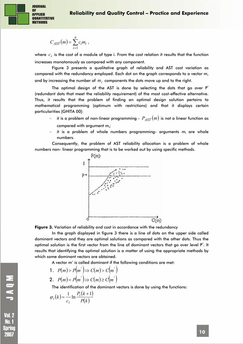
increases monotonously as compared with any component. Figure 3 presents a qualitative graph of reliability and AST cost variation as
compared with the redundancy employed. Each dot on the graph corresponds to a vector m,
and by increasing the number of im components the dots move up and to the right.
The optimal design of the AST is done by selecting the dots that go over P* (redundant dots that meet the reliability requirement) of the most cost-effective alternative. Thus, it results that the problem of finding an optimal design solution pertains to mathematical programming (optimum with restrictions) and that it displays certain particularities [GHITA 00]:
− it is a problem of non-linear programming - ( )mPAST is not a linear function as
compared with argument mi; − it is a problem of whole numbers programming- arguments mi are whole
numbers. Consequently, the problem of AST reliability allocation is a problem of whole
numbers non- linear programming that is to be worked out by using specific methods.
Figure 3. Variation of reliability and cost in accordance with the redundancy
In the graph displayed in figure 3 there is a line of dots on the upper side called dominant vectors and they are optimal solutions as compared with the other dots. Thus the optimal solution is the first vector from the line of dominant vectors that go over level P*. It results that identifying the optimal solution is a matter of using the appropriate methods by which some dominant vectors are obtained.
A vector m’ is called dominant if the following conditions are met:
1. ( ) ( ) ( ) ( )'' mCmCmPmP >⇒>
2. ( ) ( ) ( ) ( )'' mCmCmPmP ≥⇒=
The identification of the dominant vectors is done by using the functions:
( ) ( )( )kPkP
ck i
ii
1ln1 +
=ϕ

Reliability and Quality Control – Practice and Experience
11
which evaluate the probability increase per unit of cost for a component with k
redundancies. All procedures are workable if the functions ( )kiϕ are convex and for the
previously mentioned structures (r- out- of- n systems or spare ones) ( )kiϕ are convex.
The procedure below supplies a line of dominant vectors
( ) ( ) ( ) ( )( )kmkmkmkm n ..., , , 21= , k=1, 2, …, N in which
1. m(1)= (0, 0, …, 0) 2. m(k+1) is recurrently deduced as follows
( ) ( )( ) ( ) Iidaca 1
Iidaca 11≠=+=+=+
kmkmkmkm
ii
ii
where I is the index number that maximizes function ( )kiϕ ; (if there are more
indices I, in order to obtain maximum possible one of them is selected as index I); 3. Algorithm stall results from:
( )( ){ }*:min PkmPkN ≥=
In conclusion, the procedure leads to a line of dominant vectors deduced one from the other by adding one unit for each argument that reaches the greatest increase in probability per unit of cost.
The chain begins with the identical null vector and ends with the first vector that meets the reliability condition (C). This procedure supplies a chain of dominant vectors that does not necessarily include all possible dominant vectors between the identical invalid
vector and vector ( )km . Consequently, it does not always supply an optimal solution, but a
quasi-optimal one. The procedure has the advantage of completely taking algorithm form and of being easy to implement on a computer. Its main disadvantage resides in the fact that it starts from vector (0, 0, ..., 0) and thus a number of steps must be taken towards finding the first dominant vector that meets the reliability and cost requests.
A more direct method (with fewer steps) towards obtaining a chain of dominant vectors is the one recommended in [BARLOW 92] and which involves using one of the following procedures. Procedure 1
It is similar to the procedure previously described and it helps determine the whole chain of dominant vectors by starting from vector (0, 0, ..., 0) and successively introducing redundancies in accordance with the increase criterion. Procedure 2
It is an operational alternative that helps determine one dominant vector
( )**1
* ,..., mnnn = that corresponds to the imposed level of probability *P . It is based on the
particularity that lets probability *P be, there is a constant value so that all the components
of the dominant vector *n meet the condition:
( ) ( ){ }** :min Pkkn ii δϕ <= .
Since functions ( )kiϕ are positive and monotonously decreasing and ( ) 0* >Pδ ,
the previous relation always assures finding components *in . The advantage of this
procedure consists in directly supplying vector *n that corresponds to the imposed

Reliability and Quality Control – Practice and Experience
12
probability level *P . The disadvantage lies not in offering any clue as to the manner of
choosing the constant value ( )*Pδ , which is done through successive trials.
Procedure 3 It consists in joining previous procedures by using their advantages. If a level of
probability *P is imposed, an estimate value for the constant ( )*Pδ and its corresponding
dominant vector ( )δn are established through successive trials, so that ( )( ) *, PntP <δ by
using procedure 2.
Once ( )δn is established, by using procedure 1 the chain of dominant vectors is
established in its turn until the dominant vector *n that meets condition ( ) **, PntP ≥ is
obtained.
Case Study: The Methodology of Optimal Allocation of AST Reliability
In this sub-chapter we give an example that illustrates the methodology of optimal allocation of AST reliability [VASILESCU 05] by using the optimized method of dominant vectors calculation that was explained in detail in the previous paragraphs (procedures 1-3).
AST1(1) AST2(1) AST3(1)
AST1(k) AST2(k) AST3(k)
AST1(m1) AST2(m2) AST3(m3)
Modulul 1 (AST1)
.
...
.
.
Modulul 2 (AST2)
Modulul 3 (AST3)
Figure 4. Specific set of software applications (AST) with
redundancies at the software modules level In order to set the basis of this calculus, here are the initial data of the problem. We
analyze an IT system, in which a command and control activity is supported through a specific set of software applications (AST) consisting of three software modules (figure 4).
Table 3 depicts the failure intensities and their specific costs. Table 3. Specific set of software applications - initial data
I ASTiλ (hour-1) ASTic (u.c.)
1 0,0008 200 2 0,0005 300 3 0,0003 250
Reliability and Quality Control – Practice and Experience
13
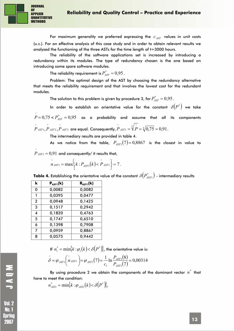
For maximum generality we preferred expressing the ASTc values in unit costs
(u.c.). For an effective analysis of this case study and in order to obtain relevant results we analyzed the functioning of the three ASTs for the time length of t=3000 hours.
The reliability of the software applications set is increased by introducing a redundancy within its modules. The type of redundancy chosen is the one based on introducing some spare software modules.
The reliability requirement is 0,95* =ASTP .
Problem: The optimal design of the AST by choosing the redundancy alternative that meets the reliability requirement and that involves the lowest cost for the redundant modules.
The solution to this problem is given by procedure 3, for 0,95* =ASTP .
In order to establish an orientative value for the constant ( )*Pδ we take
75,0^
=P < 0,95* =ASTP as a probability and assume that all its components
3
^
2
^
1
^,, ASTASTAST PPP are equal. Consequently, 91,075,033 ^
1^
=== PP AST .
The intermediary results are provided in table 4.
As we notice from the table, ( ) 8867,071 =ASTP is the closest in value to
91,01
^=ASTP and consequently/ it results that,
( ) 7:max 1
^
11
^=
⎭⎬⎫
⎩⎨⎧ <= ASTASTAST PkPkn .
Table 4. Establishing the orientative value of the constant ( )*1ASTPδ - intermediary results
k PAST1(k) RAST1(k)
0 0,0082 0,0082 1 0,0395 0,0477 2 0,0948 0,1425 3 0,1517 0,2942 4 0,1820 0,4763 5 0,1747 0,6510 6 0,1398 0,7908 7 0,0959 0,8867 8 0,0575 0,9442
If ( ) ( ){ }** :min Pkkn ii δϕ <= , the orientative value is:
( ) ( )( ) 00314,078ln17
1
1
111
^
1
^===⎟
⎠⎞
⎜⎝⎛=
AST
ASTASTASTAST P
Pc
n ϕϕδ
By using procedure 2 we obtain the components of the dominant vector *n that
have to meet the condition:
( ) ( ){ }** :min Pkkn ASTiASTi δϕ <= ,

Reliability and Quality Control – Practice and Experience
14
As a result, the first 2ASTϕ that meets the previous condition is ( ) 000260,082 =ASTϕ ,
namely the first 3ASTϕ that meets the previous condition is ( ) 000179,063 =ASTϕ . It results the
dominant vector ( )6,8,7^
=n with its corresponding probability 95,063,0^
<=P .
Moreover, by employing the rule of increase from procedure 1 the result is the
chain of dominant vectors presented in table 5 and their corresponding values ( )nP and
( )nC .
Table 5. Chain of dominant vectors
ASTn
1ASTn 2ASTn 3ASTn ( )nP ( )nC
7 8 6 0,639351 5300 7 9 6 0,790611 5600 7 10 6 0,889451 5900 7 11 6 0,946202 6200 8 11 6 0,975635 6400
We notice that the first dominant vector that meets the condition ( ) 95,0* ≥nP at
the lowest cost is ( )6,11,8=ASTn , whereas its corresponding probability is ( ) 975,0=nP at
the cost of ( ) 6400=nC u.c.
We also observe that by using procedure 3 we needed 5 steps to obtain the result, whereas for the procedure 1 we would have needed 21 extra steps.
In order to implement formulas and do the calculations we used Microsoft Excel due to the possibility it offers to introduce initial data in a rapid manner, and also because of the elegant and explicit layout for the results provided by its spreadsheets.
Excel spreadsheet cells explanation: • D4:D6 - intensity of failures in the modules that were given the notations AST1, AST2
and AST3; • E4:E6 - modules specific cost; • H3 - mission duration in hours; • B9:B21 - number of redundant modules introduced; • D9:D21 (H9:H21, L9:L21) - values of modules reliability; for example, cell D10
contains the formula =D9+POWER($F$4*$D$4*$H$3;B10)/FACT(B10)*EXP(-($F$4*$D$4*$H$3));
• E9:E21 (I9:I21, M9:M21) - values of the reliability increase for modules per unit cost; for example, cell E10 contains the formula =(1/$E$4)*LN((D11/D10));
• C25:E25 (C29:E29) - chains of dominant vectors; for example, cell C26 contains the formula =IF(MAX(E17;I17;M17)=E17;C25+1;C25);
• F25:F29 - values of overall AST reliability; for example, cell F25 contains the formula =D16*H16*L16; G25:G29 - values of overall AST costs; for example, cell G25 contains the formula
=C25*$E$4+D25*$E$5+E25*$E$6.

Reliability and Quality Control – Practice and Experience
15
Figure 6. Optimal allocation of the AST reliability by using the
method of calculating the dominant vectors- results

Reliability and Quality Control – Practice and Experience
16
In conclusion, in order to meet the imposed reliability requirement a specific set of
software applications tools is needed. The latter includes: eight modules type one, eleven modules type two and six modules type three. The cost of the AST is 6400 unit cost. References 1. BARLOW, R., PROSCHAN, F. Mathematical Theory of Reliability, John Wiley, New York, 1998 2. GHITA, A., IONESCU, V. Metode de calcul în fiabilitate, Editura Academiei Tehnice Militare,
Bucharest, 1996 3. GHITA, A., IONESCU, V., BICA, M. Metode de calcul în mentenabilitate, Editura Academiei
Tehnice Militare, Bucharest, 2000 4. SERB, A. Sisteme de calcul tolerante la defectari Editura Academiei Tehnice Militare,
Bucharest, 1996 5. VASILESCU, C. Alocarea optima a fiabilitatii seturilor specifice de aplicatii software din
sistemele C4ISR, The 10th International Scientific Conference, Academia Fortelor Terestre, Sibiu, November 24-26, 2005
6. *** System and Software Reliability Assurance Notebook, produced for Rome Laboratory, New York, 1997
7. *** TR-92-52 - Software Reliability Measurement and Test Integration Techniques, produced for Rome Laboratory, New York, 1992
1 Cezar Vasilescu has graduated the Faculty of Electronics and Information Science within the Military Technical Academy - Bucharest in 1997. He holds a PhD diploma in Computer Science from 2006. He has graduated in 2003 the Advanced Management Program organized by National Defense University of Washington D.C., USA. Also, he has received the US Department of Defense Chief Information Officer (CIO) certification from the Information Resources Management College of Washington D.C. Currently he is the head of the IT&C Office within the Regional Department of Defense Resources Management Studies - Brasov and associate professor at the National Defense University - Bucharest. He is the author of more than 30 journal articles and scientific presentations at conferences in the fields of hardware/software reliability, command and control systems and information resources management. He has coordinated as program manager the activity of establishing in Romania of an international educational program in the field of information resources management, in collaboration with universities from USA. Beside his research activity, he has coordinated “Train the Trainers” and “Educate the Educators” activities with international participation. Main published books: - Information Management, Military Technical Academy Publishing House, Bucharest, 2006. - Information Technology for Management, Regional Center of Defense Resources Management Publishing House, Brasov, 2001. 2 Codifications of references: [BARLOW 98] BARLOW, R., PROSCHAN, F. Mathematical Theory of Reliability, John Wiley, New York,
1998 [GHITA 96] GHITA, A., IONESCU, V. Metode de calcul în fiabilitate, Editura Academiei Tehnice Militare,
Bucharest, 1996 [GHITA 00] GHITA, A., IONESCU, V., BICA, M. Metode de calcul în mentenabilitate, Editura Academiei
Tehnice Militare, Bucharest, 2000 [ROME 92] *** TR-92-52 - Software Reliability Measurement and Test Integration Techniques,
produced for Rome Laboratory, New York, 1992 [ROME 97] *** System and Software Reliability Assurance Notebook, produced for Rome Laboratory,
New York, 1997 [SERB 96] SERB, A. Sisteme de calcul tolerante la defectari Editura Academiei Tehnice Militare,
Bucharest, 1996 [VASILESCU 05] VASILESCU, C. Alocarea optima a fiabilitatii seturilor specifice de aplicatii software din
sistemele C4ISR, The 10th International Scientific Conference, Academia Fortelor Terestre, Sibiu, November 24-26, 2005

Reliability and Quality Control – Practice and Experience
17
SPECIFIC ASPECTS OF FINANCIAL AND ACCOUNTANCY SOFTWARE RELIABILITY
Marian Pompiliu CRISTESCU PhD, University Professor “Lucian Blaga” University of Sibiu, Romania E-mail: [email protected]
Abstract: The target of the present trend of the software industry is to design and develop more reliable software, even if, in the beginning, this requires larger costs necessary to obtain the level of reliability. It has been found that in the case of software which contain large amounts of components - financial and accounting software are also included here – the actions taken to increase the level of reliability in the operational stage induces a high level of costs. This one is superior to the one that involves obtaining systems of software with an adequate reliability, before releasing them on the market and before using them. Before taking into account the material and financial aspects that involve obtaining the adequate reliability, we must consider the social effects that occur because of the lack of reliability of software. The conclusion is that, if we begin with the idea that a system of accounting software is a fitted and well structured ensemble of different components – from a constructive point of view – which satisfy interconnected needs, the reliability of the entire system depends directly on the reliability of each component. Key words: software reliability; software metrics; object-oriented software; error; fault; failure; financial and accountancy software
1. Introduction
The main method used in building complex systems is abstractization. A system is built on levels; level B is made out of components from level A. But at the same time, components from level B are used as if they were atoms, independently, to build level C and so on.
An important subject in the theory of reliability is the construction of more reliable software, from components which are more or less reliable. If a system works only when every component is functional, it is impossible to build a complex system because the reliability decreases exponential with the amount of components.
Certain classes of programmes, such as those from air traffic controls and supervision of nuclear power plants, need a high reliability level. In critical programmes, the architects of the systems take into consideration the possibility of failure, which they treat in the software

Reliability and Quality Control – Practice and Experience
18
A system of programmes, from a static point of view, appears as a function f defined
through X, with values in Y – of final results. Function YXf →: represents in a static way
the system of programmes and is: • a partial function, if for every x∈ X there is a value y ∈ Y so as y=f(x); • a total function, if for every x∈ X there is a value y ∈ Y so as y=f(x).
In conclusion the total function correspond to a system of programmes that allows the solving of a problem for every initial data, and the partial function corresponds to a system of programmes which supplies us with solutions of certain sets of values.
A system of financial and accounting programmes is identified with a complex process, made out of many subprocesses, based on the rivalling model. This means separating different tasks into performing processes which are parallel different. Figure 1 presents the way such a system of programmes is structured.
A problem which is dealt with by using the calculator is represented through a calculating function, an algorithm. The same function is evaluated by a set of algorithms. There are functions that cannot be evaluated by algorithms.
Figure 1. The tree of interconnected components
The structure is dynamical, which means that new performing processes are created or old ones are finished, according to the will of the user. The lines from the figure show the component which is being used and the using component, and the way we look at the tree is from top to bottom.
Between the components there are no implicit connections once these are appealed in the system, but if one wishes, a connection can be made. In this way a total control can be restored over every component of the system. If the example of figure 1 is analysed, we can see that the components A, C, E and F are interconnected; therefore the connection works both ways, no matter if component C has established the connection or component E or F.
Economical procedures and especially those from the financial and accounting field are recognised as having a high level of complexity. The difficulty associated with the solutions of simple problems united is smaller than the one associated to the initial complex problem. The architecture of the system expresses the way the system is entirely organized in components named subsystems. The interaction is produced through the exchange of the performing control. In the case of sequential programmes, the control belongs to only one module. The software architecture also includes information regarding the necessary time needed to perform every module.
The financial and accounting programmes are made out of subsystems; each is made out of smaller subsystems; the lowest level is achieved by modules. A subsystem is a package of connected classes, operations, associations, events and restrictions. These are identified by the services offered; services are groups of functions with the same goal.
Reliability and Quality Control – Practice and Experience
19
A system of financial and accounting programmes offers a multitude of services through its components. The goal is to satisfy the users` needs for a long period of time and at a high quality level. The possibilities that the given functions are correctly executed for some time by the system are done through the help of reliability. The reliability of the system is determined by the reliability of the components, the number of components and the structure of the system.
2. Stimulating the reliability of the financial and accounting systems
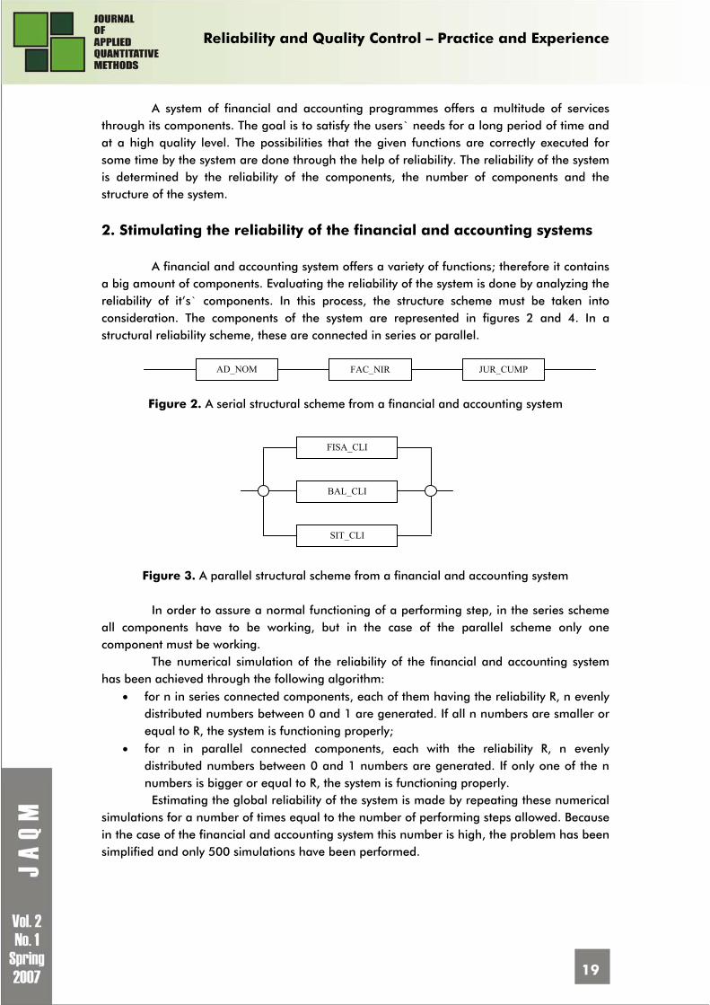
A financial and accounting system offers a variety of functions; therefore it contains a big amount of components. Evaluating the reliability of the system is done by analyzing the reliability of it’s` components. In this process, the structure scheme must be taken into consideration. The components of the system are represented in figures 2 and 4. In a structural reliability scheme, these are connected in series or parallel.
Figure 2. A serial structural scheme from a financial and accounting system
Figure 3. A parallel structural scheme from a financial and accounting system
In order to assure a normal functioning of a performing step, in the series scheme all components have to be working, but in the case of the parallel scheme only one component must be working.
The numerical simulation of the reliability of the financial and accounting system has been achieved through the following algorithm:
• for n in series connected components, each of them having the reliability R, n evenly distributed numbers between 0 and 1 are generated. If all n numbers are smaller or equal to R, the system is functioning properly;
• for n in parallel connected components, each with the reliability R, n evenly distributed numbers between 0 and 1 numbers are generated. If only one of the n numbers is bigger or equal to R, the system is functioning properly. Estimating the global reliability of the system is made by repeating these numerical
simulations for a number of times equal to the number of performing steps allowed. Because in the case of the financial and accounting system this number is high, the problem has been simplified and only 500 simulations have been performed.
AD_NOM FAC_NIR JUR_CUMP
FISA_CLI
BAL_CLI
SIT_CLI

Reliability and Quality Control – Practice and Experience
20
a). The numerical simulating programme of performing components connected in series
n = [150,300]; % number of simulations R = 0,8; % reliability of the components m = 3; % number of series connected components for j = 1 : length(n)
k = 0; for I = 1 : n(j) x = row(1,m); if all(x<=R) k = k + 1; else end
end f(1,j) = k / n(1,j); % reliability end
b). The numerical simulating programme of performing components connected in parallel
n = [150,300]; % number of simulations R = 0,8; % reliability of the components m = 3; % number of parallel connected components for j = 1 : length(n)
k = 0; for I = 1 : n(j) x = row(1,m); if any(x<=R) k = k + 1; else end
end f(1,j) = k / n(1,j); % reliability end
c). The global simulating programme of 500 performed simulations n = 500; R1 = 0,8;R2 = 0,92;
F1 = row(n,1); F2 = row(n,1); N = length(F); % number of functions fprintf(The reliability of the system is %3.2f\n',N/n)
The first programme takes figure 2 into consideration and uses components with
the reliability R=0,8. The second treats the case of figure 3 and also uses components with the reliability R=0,8. In order to compare the calculated reliability, a number of 150 and 300 simulations have been conducted. The third programme takes into consideration a series structure made out of two components, the first reliability R1=0,8, and the second reliability R2=0,92.
After the first programme performed, the reliability obtained was: [0,5200 0,5000]. After the second programme performed, these values of the reliability were offered:
[0,9920 0,9960].

Reliability and Quality Control – Practice and Experience
21
After the third programme performed, this value was obtained: The reliability of the system is 0,74. In practice it was been discovered that for financial and accounting programmes
which contain a big number of components, using the series and parallel scheme does not assure a high level of reliability. Therefore, a mixed structure that combines the advantages of both types is used. In figures 4.a and 4.b two specific cases of such mixed structures are presented. These are frequently used for financial and accounting evidences.
4.a
4.b
Figure 4.a, b Mixed structural schemes The following reliability calculations are used in both cases: in the first case, from figure 4.a, the reliability is given by the relationship:
( )∏ ∏= =
−−=n
ii
n
iiim RRRR
1 1
1 (1)
for figure 4.b the reliability is given by the relationship:
( ) ( )∏ ∏= =
−+−−=n
i
n
iiiim RRRR
1 1
111 (2)
Because the complexity level of these schemes is very high, the very difficult
necessity of simplification the structure function appears. In specialized literature [SZYP02]1, [PHAM00], [DAVI03] different methods of reducing the structure of the function and calculating the reliability of mixed structural schemes are presented. According to the method presented in [GORO97], the components of a financial and accounting system must be grouped regarding to the way they are situated in the serial or parallel graph and so, we get a primary level of a programming group. This group is formed by components which are connected in series or parallel. A new group on the next hierarchical scale follows and this procedure is continued until a single series or parallel structure of n levels is formed, where levels of n-1 components are displayed. These methods have a low applicability rate due to a set of assumptions on which it relies and too many calculations.
FISAEC
FISAIM
CALC_RUL BAL_SIT
P_ORE
P_ZILE
SAL_RLZ CALC_CO

Reliability and Quality Control – Practice and Experience
22
3. Using modern programming techniques to increase the reliability of financial and accounting software
The technique of object oriented modeling is a methodology used to develop
financial and accounting software by using a collection of predefined techniques and noting conventions. It follows the entire life cycle which contains: analysing, designing, implementation and testing. These are followed by the stage in which it is used, when the maintenance and improvements on the system are done, to ensure the reliability needs imposed by the client.
For the development of accounting programming objects, two approaches are practiced: quick prototypization and the development of the entire life cycle. In the quick prototypization a small part of the system is initially developed, after this it is improved through gradual improvements of the specification and implementation, until it becomes robust.
The development methodology of software designed for financials and accountings is firstly characterized by the analyzing and projection steps, whereas the implementation and testing steps rely on the first. The analysis process has as a result a formed model which contains three essential aspects of the system: the objects and the relationships that exist between them, the dynamic flow between the orders and the functional transformation of data, using certain restrictions. Therefore the OMT methodology is bases on three models directed towards the object:
• the object oriented model – describes the static structure of data; • the dynamic model – describes the temporal relationships of orders, • the functional model – describes the functional relationships between values.
The programming technique frequently used is chosen on criteria such as error and performance tolerance. In [KICM00] it is told that the extension of the traditional library of stopping points is easy to do, so as this one is able to notice more directions from the same process. A multidirectional set library of stopping points, which works at a processing level, must save all directions for a verification point and to restore each of them when it is restarted.
In [TEOD01] it has been demonstrated that this mechanism of stopping points increases the flexibility and efficiency of the error tolerance schemes. Due to these characteristics it is used in the development of financial and accounting systems, in order to increase the efficiency of the tests and to raise the reliability level.
To exemplify the way this mechanism is used, an accounting programming system which, for error tolerance, uses the distributing algorithm of coming and going – present in [KICM00], is taken into consideration.
As a consequence of the existing relationships, the functions of the programming system become interdependent. If one of them fails, the algorithm determines which of the functions is dependent on the one that failed, and these must be performed backwards from the last stopping point. This solution is suboptimal when every function is multidirectional. In practice, it has been observed that only the paths dependent on the failing function must be performed backwards and the others remain unchanged. When establishing stopping points and backward points the following aspects are taken into consideration:
• the minimum frequency of performance for registering the dependencies and other information about the performance of the programme;

Reliability and Quality Control – Practice and Experience
23
• the procedure for establishing selective testing points by using the information and the guiding points so as to develop the restore algorithm;
• the selective backwards algorithm based on guiding points. To demonstrate how to use the stopping point and backward point technique in
order to increase the reliability of financial and accounting software based on object oriented modeling, two arguments are taken into account:
• investigating the way group stopping points, for isolated groups of objects and communication ways of the programme, are established;
• investigating the way in which certain performing ways from a programme can be performed backwards in a selective way and others continue to be performed; during this period the general well being of the programming system is preserved.
Developing error tolerance schemes at a high level involves the usage of selective algorithms. In [ROMA03] it is said that the conventional models, that coordinate the process of restoring, after errors of interacting components are detected, must be implemented at the top of selective algorithms.
By using these techniques, the results obtained due to the growth in error tolerance and, therefore, of the reliability, indicate the fact that using selective schemes at processing levels is better than using techniques based on check points and also using recovery schemes when the number of current functions or error numbers are high.
4. Developing high reliability for object-oriented software The software developing process is schematized through the next stages: system
feasibility studying, problem analysing, designing, codification and system testing. For a procedural programme system these stages correspond to a “warerfall”
pattern. This means that the system is divided into substages and each requirement is previously known so that the tasks are performed one by one.
In the development of bookkeeping software based on this technology the starting point consists of recognizing the requirements of the matter. Therefore, an initial version is designed and then, as the requirements are better defined, the system is completed by adding new components or the existing ones are improved.
Adopting the evolutionary developing design leads to obtaining intermediate forms of the system, called prototypes. These resemble versions of the final form that are improved in time, as the developing process continues. Such an approach allows the client’s effective control over the system’s final version; the changes that occur in the client’s requirements are accepted even if the analysis and design are in an advanced stage. The client’s implication in the development process allows setting components and important sequences of execution. This determines the diminishing of the testing effort and implicitly of the costs and reliability increase.
Based on the evolutionary model, the development stages of the programming system are performed with every frequentation and the resulted prototype is evaluated for detecting the errors which are corrected in the next frequentation. In the system feasibility study stage the clients demands are clearly defined and through the client’s implication a solution are chosen from the existent ones.

Reliability and Quality Control – Practice and Experience
24
The architecture of the software for bookkeeping is divided in a number of components that consist of one or more objects. These components are collections of objects which collaborate for producing a service set. Each component is described by: functions, internal objects, external objects with which interfaces also interact. It is because of the interface that a component looks like a “black box” that shows only the entrances and emergences.
The testing stage involves the validation of the system results from the previous phases. The organisation of the designing process of the programme systems oriented toward objects involves the existence of different levels of testing. This includes the testing of methods, classes and modules, being based on an established initial plan that is finalised by testing the entire system. Object-oriented technology is used for testing the software and its main effect consists of improving the quality. A new programme system contains reused objects that have already been tested and have an appropriate reliability level. The result is that the testing effort is minimised and the reliability increases. In this case, the testing is aimed toward new components and especially toward the critical ones.
Modularity is another important facility, frequently used for developing programme systems designed for financial bookkeeping and it is based on object modeling. It allows an easier detection of software errors. The repairing process of these systems is also improved by establishing better connections between software items and real objects. As a result of this facility programme systems are divided in autonomous components. This has important effects on the human resources involved in the development and there, on the costs. The structure and organisation procedures of these resources are defined according to the defining manner of the components as well as the integration manner in the whole system.
It is recommended that these components should be developed by interfunctional teams that integrate analysis, designing, codification and testing abilities so that the development of each component is to be accomplished individually. In order to increase the functionality level, the assembly of different components must be done by groups of professionals that are in charge with the testing process of the entire programme system.
Practically it has been uncertain because of the limited resources of the companies which develop programme systems for bookkeeping; some of these recommendations are not followed. Therefore, in most cases the assembly of the components and testing the entire system is made by the same people that have taken part in the analysis, designing and codification phases. Thereby, they sometimes have a subjective vision upon the development process that leads to the decreasing of the ability to detect errors in the initial phases. In this kind of situations, the programme systems are moved to the operational stage, although their reliability level is low. The exploitation costs of these systems are rather high, and the users are not satisfied with the quality of the offered services.
In order to investigate the actual spreading of object-oriented technology among the producers of software destined to keep a financial-accountancy record and to analyse the characteristics of these practices on the software market, along the years, many actions have been undertaken. One of these is represented by the straw poll made by a branch of IBM in 2004. This was based on a questionnaire sent by e-mail and distributed at conferences. The questionnaire was divided into 3 sections: technology, development process and cost.

Reliability and Quality Control – Practice and Experience
25
Based on the results of the straw poll, the weight of the object-oriented software production in the total financial-accountancy software production has been determined. This aspect is shown in figure 5.
Figure 5. Grouping software producers according to the production of object-oriented software level (Source: http://www.garavelli/poliba/docs.html)
Using the object-oriented technology is in many situations delayed by the high costs
required by the preparation. According to the dates, in only 8% of the companies the programmers who have always worked corresponding to this technology represent more than 80%, while in 57% of cases more than two thirds of the personnel has been converted to work on the basis of the principles of object-oriented technology.
Concerning spreading the methods of object orientation in the phases of analysis and designing of the software development process, it has been observed that 35% of the companies do not use any kind of methodology at all. These results were compared to those in section 3 of the questionnaire which refers to the exploitation costs of developed programme systems. It has been established that the costs level for those companies which do not use any kind of methodology is 27% higher compared to those who use object-oriented methodology and 16% compared to those which use the classical object-oriented methodology. 75% of the companies use prototypes during the process of software development. The degree of prototypes use is shown in figure 6.
Figure 6. Using prototypes
(Source: http://www.garavelli/poliba/docs.htm)

Reliability and Quality Control – Practice and Experience
26
Analysing the data has shown the fact that using the inter-functioning teams in the process of development is very frequent (68%). For 53% of the companies the size of the team depends on the complexity of the programming system, and for 33%, on its` size. In 69% of the cases the team consists of employees with different abilities, but in 19% of the cases the abilities of the members are homogeneous. The results also show that only 20% of companies use a system of metrics to control the quality, and 64% do not use any kind of metrics.
In figure 6 we can see that the frequency of prototyping is very high for 38% of them, when 24% is dependent on the product, and 13% depends on the client.
The companies questioned were asked for their opinion regarding the improvement of the reliability, as a consequence of four key influential factors which were placed on a scale of 0 to 3. The analysis showed that important factors were considered the development of reusable components (2,38), reusage of the existing components (2,26) or using innovative technological software (2,23). Reusing parts is considered to be the most efficient way of making reliability grow and this is why 66% of the companies produce own software components, designed for future reuse. The reusable components are produced during the development of a specific programming system (50%) or as a result of current activities (23%). Only 16% of companies do not use these reusable components in the process of improvement of the reliability of their software.
Because of this data, the majority of companies that develop software designed to keep the financial and accounting evidence use the technique of object orientation. Using reusable components represents a decisive factor in the process of reducing costs and improving the reliability. To evaluate the reliability of the software of many companies, adequate metrics and models are used.
The cost, from the total of sales that are formed when acquiring these components is smaller than 10%, for most companies (69%), whereas for 19% of companies it is smaller than 20%, growing until 30% for a percentage (12%) of the companies.
5. Specific aspects of the reliability of accounting software The following factors determine the importance of the study of the reliability of
programmes: • the growth in the complexity of the functioning programmes, as a result of them
being included in big software, and of the important functions that these must realize; the consequence is a growth in the cost of the user, in case of errors;
• high expectations regarding the quality of software; • the complexity of the exploitation needs; • growing cost of exploitation and maintenance. One of the characteristics of the annual production of software consists of creating
and developing complex systems – from the functional point of view. The programmes are parts of such complex systems; therefore they must match the general conditions of the system. The incorrect function of one of them, may lead to false results. The growing needs related to the functioning quality of programmes and of the systems, find their source, for example, in: a high flexibility, maintainability, portability, integrity, etc. Firstly, these needs must be satisfied in the previous steps, which precede the current exploitation of the product

Reliability and Quality Control – Practice and Experience
27
by the user. When the programming system in the hands of the beneficiary is operational, only its` quality must be confirmed.
The growth in the costs of exploitation and maintenance of software is mostly determined by a lack of the reliability of the programmes it consists of.
In practice it has been discovered that, in the development stage, between the costs of development and the level of reliability of accounting software there is a tight bond; the components that need a high level of reliability have bigger costs in order to achieve this goal.
Testing is a method of improving the reliability of accounting software. A high level of reliability is achieved when the time span in which the testing is done is high and when the test are refined. The testing process involves human and material resource, and an increase in the testing efforts generates a growth in the costs of high level reliability components.
In order to study these connected relationships, three components of the programming system CONTGEST have been analysed. Each component had a specific level of reliability, according to its` operational profile. The time of the tests was record. A specific level for the cost had been attributed to the components, according to the total costs. The characteristics recorded are shown in table 1. Table 1. The characteristics of the components of the programming system CONTGEST
Component Time of testing (h) Costs (%) Reliability (%)
AD_NOM 51 27 76
ST_NOM 37 15 70
MOD_NOM 82 58 81
By analysing the data presented in table 1, we can observe that between the
reliability and the time of testing there is nonlinear dependence. Figure 7 shows the relationship existing between these characteristics. We can see that the time of testing is not the only factor that influences the reliability and this is why other factors must be taken into consideration.
Figure 7. The relationship between the reliability and the time of testing for the
components of the programming system CONTGEST
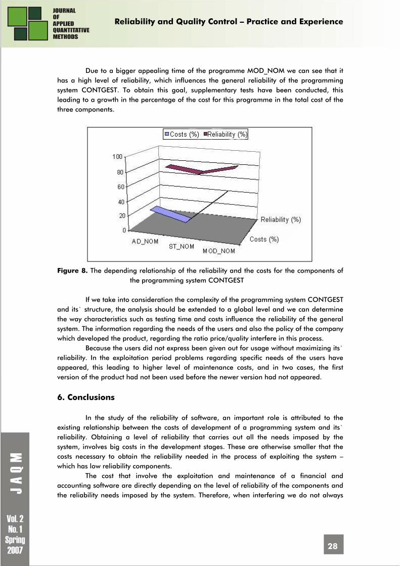
Reliability and Quality Control – Practice and Experience
28
Due to a bigger appealing time of the programme MOD_NOM we can see that it
has a high level of reliability, which influences the general reliability of the programming system CONTGEST. To obtain this goal, supplementary tests have been conducted, this leading to a growth in the percentage of the cost for this programme in the total cost of the three components.
Figure 8. The depending relationship of the reliability and the costs for the components of the programming system CONTGEST
If we take into consideration the complexity of the programming system CONTGEST and its` structure, the analysis should be extended to a global level and we can determine the way characteristics such as testing time and costs influence the reliability of the general system. The information regarding the needs of the users and also the policy of the company which developed the product, regarding the ratio price/quality interfere in this process.
Because the users did not express been given out for usage without maximizing its` reliability. In the exploitation period problems regarding specific needs of the users have appeared, this leading to higher level of maintenance costs, and in two cases, the first version of the product had not been used before the newer version had not appeared.
6. Conclusions
In the study of the reliability of software, an important role is attributed to the existing relationship between the costs of development of a programming system and its` reliability. Obtaining a level of reliability that carries out all the needs imposed by the system, involves big costs in the development stages. These are otherwise smaller that the costs necessary to obtain the reliability needed in the process of exploiting the system – which has low reliability components.
The cost that involve the exploitation and maintenance of a financial and accounting software are directly depending on the level of reliability of the components and the reliability needs imposed by the system. Therefore, when interfering we do not always

Reliability and Quality Control – Practice and Experience
29
achieve noticeable effects. There are cases where if we distinguish an error, others are generated.
If we take into consideration the variety and complexity of accounting situations that the programming system must deal with, the result is that efficiency is given firstly by the way they respond to the needs of the user. When the interferences caused by flaws are rare, the system is said to be more efficient – from every point of view. The frequency of errors and therefore the level of reliability represent signs of loyalty regarding the efficiency of the programming system.
References 1. Chillarege R., Kao W., Condit R. Defect Type and its Impact on the Growth Curve, Proceedings
International Conference on Software Engineering, May 2004 2. Cristescu M. Modelarea fiabilitatii sistemelor de programe, PhD. Thesis, Bucharest, 2003 3. Davis A.M. Software Requirements: Objects, Functions, and States, Prentice-Hall, Saddle
River, New Jersey, 2003 4. Goron S. Fiabilitatea softului, RISOPRINT Publishing House, Cluj-Napoca, 1997 5. Ivan I., Saha P. Quality characteristics of The Internet Applications, in DIGITAL ECONOMY -
The Proceedings Of The Sixth International Conference On Economic Informatics, Bucharest, May 2003
6. Kim S., Clark J.A. and McDermid J. A. Class mutation: mutation testing for object-oriented programs, in Proceedings of the NetObjectDays - Conference on Object-Oriented Software Systems, 2000
7. Pham H. Software Reliability, Springer, 2000 8. Schneidewind N.F. Life Cycle Core Knowledge Requirements for Software Reliability
Measurement, The R & M Engineering Journal, Volume 23 No. 2, June 2003 9. Schneidewind N. F. Software Quality Control and Prediction Model for Maintenance, Annals
of Software Engineering 9, 2000 10. Simao R., and Belchior A. Quality Characteristics for Software Components: Hierarchy and
Quality Guides, in Component-Based Software Quality: Methods and Techniques, LNCS 2693, pp. 188-211, 2003
11. Szyperski C. Component Software Beyond Object-Oriented Programming, Addison-Wesley and ACM Press, 2002
12. Teodorescu L., Ivan I. Managementul calităţii software, INFOREC Publishing House, Bucharest, 2001
1 Codifications of references: [CHIL04] Chillarege R., Kao W., Condit R. Defect Type and its Impact on the Growth Curve,
Proceedings International Conference on Software Engineering, May 2004 [CRIS03] Cristescu M. Modelarea fiabilitatii sistemelor de programe, PhD. Thesis, Bucharest, 2003 [DAVI03] Davis A.M. Software Requirements: Objects, Functions, and States, Prentice-Hall, Saddle
River, New Jersey, 2003 [GORO97] Goron S. Fiabilitatea softului, RISOPRINT Publishing House, Cluj-Napoca, 1997 [IVAN03] Ivan I., Saha P. Quality characteristics of The Internet Applications, in DIGITAL ECONOMY
- The Proceedings Of The Sixth International Conference On Economic Informatics, Bucharest, May 2003
[KICM00] Kim S., Clark J.A. and McDermid J. A. Class mutation: mutation testing for object-oriented programs, in Proceedings of the NetObjectDays - Conference on Object-Oriented Software Systems, 2000
[PHAM00] Pham H. Software Reliability, Springer, 2000 [SCHN03] Schneidewind N.F. Life Cycle Core Knowledge Requirements for Software Reliability
Measurement, The R & M Engineering Journal, Volume 23 No. 2, June 2003 [SCHN00] Schneidewind N. F. Software Quality Control and Prediction Model for Maintenance,
Annals of Software Engineering 9, 2000

Reliability and Quality Control – Practice and Experience
30
[SIBE03] Simao R., and Belchior A. Quality Characteristics for Software Components: Hierarchy and
Quality Guides, in Component-Based Software Quality: Methods and Techniques, LNCS 2693, pp. 188-211, 2003
[SZYP02] Szyperski C. Component Software Beyond Object-Oriented Programming, Addison-Wesley and ACM Press, 2002
[TEOD01] Teodorescu L., Ivan I. Managementul calităţii software, INFOREC Publishing House, Bucharest, 2001

Reliability and Quality Control – Practice and Experience
31
CAPABILITY MATURITY MODEL INTEGRATION
Radu CONSTANTINESCU PhD Candidate, University Assistant Academy of Economic Studies, Bucharest, Romania E-mail: [email protected] Web page: http:// www.raduconstantinescu.ase.ro
Ioan Mihnea IACOB
Abstract: In this paper we present an introduction to, and an overview to the CMMI process model, that appeared from the need to address generic, company-wide, organizational issues for a wider range of activity domains, providing a flexible framework that allows further ‘plug-in’ extensions to be added. Key words: process; capability maturity model; process areas
Introduction
In an attempt to improve the way organizations and companies organize and do business, many models, standards and methodologies have been developed. Unfortunately, the majority of these models are meant to improve specific activities for specific organizations only and do not take a systematic approach to the general problems that most organizations are facing. Such models have been created for software developing companies – Software Engineering Institute's (SEI) Capability Maturity Model for Software (SW-CMM) focuses on software engineering organizations; others concentrate on systems engineering – Electronic Industries Alliance's (EIA) Systems Engineering Capability Model (SECM). As mentioned earlier, those models can improve specific activities and are less useful addressing organization-wide issues.
In an attempt to minimize the aforementioned problems, CMMI comes in with general guidelines and models that transcend disciplines, addressing the entire product life cycle from conception, development, delivery and maintenance. Moreover, the model is conceived as a core, onto which further extensions can be added.

Reliability and Quality Control – Practice and Experience
32
Process Models There are several dimensions an organization can focus on to improve its business.
Figure 1 illustrates the three critical dimensions that organizations typically focus on: people, procedures and methods, tools and equipment.
People
A
D
EC
B
Procedures and methods
Tools and equipment
Process
Figure 1. The Three Critical Dimensions
The three critical dimensions are held together through the processes used in the
organization. A process is defined by IEEE as “a sequence of steps performed for a given
purpose”. As the CMMI model puts it, evaluating the efficiency of an organization can be reduced to evaluating the efficiency of its processes, and introduces as a measure of an organization’s efficiency the maturity levels.
In case of immature organizations, processes are improvised by practitioners, the process descriptions are not rigorously followed nor enforced and the organization performance is highly dependent on current practitioners. The mature organizations’ processes have descriptions consistent with the way the work actually gets done; they are defined, documented and continuously improved. Mature organizations’ processes are visibly supported by managers, are well controlled and there is constructive use of product and process measurement, and are institutionalized, meaning that the organization builds an infrastructure that contains effective, usable and consistently applied processes.
A process model is a structured collection of practices that describe the
characteristics of effective processes. It provides its users with a common language and a shared vision.

Reliability and Quality Control – Practice and Experience
33
Capability Maturity Models Capability maturity models (CMMs) focus on improving processes in an
organization. They contain the essential elements of effective processes for one or more disciplines and describe an evolutionary improvement path from ad hoc, immature processes to disciplined, mature processes with improved quality and effectiveness.
The CMM Integration project was formed in order to outrun the problem of using multiple CMMs. Three source models were combined:
1. The Capability Maturity Model for Software (SW-CMM) v2.0 2. The Systems Engineering Capability Model (SECM) 3. The Integrated Product Development Capability Maturity Model (IPD-CMM)
The intent of CMMI is to provide a CMM that covers product and service development and maintenance but also provides an extensible framework so that new bodies of knowledge can be added. Currently, four bodies of knowledge are available when planning process improvement using CMMI:
• Systems engineering • Software engineering • Integrated product and process development • Supplier sourcing
Disciplines, which are the discussed bodies of knowledge, are addressed by the process areas associated with them and by model components called discipline amplifications. A process area is a cluster of related best practices in an area that, when implemented collectively, satisfies a set of goals considered important for making significant improvement in that area.
For systems engineering, the CMMI identifies 22 theoretical process areas: 1. Causal Analysis and Resolution 2. Configuration Management 3. Decision Analysis and Resolution 4. Integrated Project Management (the first two specific goals) 5. Measurement and Analysis 6. Organizational Innovation and Deployment 7. Organizational Process Definition 8. Organizational Process Focus 9. Organizational Process Performance 10. Organizational Training 11. Product Integration 12. Project Monitoring and Control 13. Project Planning 14. Process and Product Quality Assurance 15. Quantitative Project Management 16. Requirements Development 17. Requirements Management 18. Risk Management 19. Supplier Agreement Management 20. Technical Solution 21. Validation 22. Verification

Reliability and Quality Control – Practice and Experience
34
In the case of software engineering organizations, the process areas listed for systems engineering remain the same. The only difference in the CMMI model is that the discipline amplifications for software engineering receive special emphasis.
In case of improving the integrated product and process development processes, there are two additional process areas as in the systems engineering discipline and additional best practices in the Integrated Project Management process area. These two additional process areas are:
• Integrated Teaming • Organizational Environment for Integration
In case of improving the source selection processes, there are the same process areas as in systems engineering with one additional process area, Integrated Supplier Management. The discipline amplifications for supplier sourcing receive special emphasis.
In case of improving multiple disciplines, the model architect has to choose from the process areas listed under all of the relevant disciplines and pay attention to all of the discipline amplifications for those disciplines.
CMM Approaches: Representations The CMMI model provides its users two approaches to process improvement; these
are the so-called “model representations”, which can be thought of as two different views of the same data, which is the CMMI model.
The continuous representation offers a detailed image of an organization’s processes. It will allow an organization to evaluate process areas individually, and it is the representation commonly used in process improvement, because it allows identifying and focusing on trouble spots, and measuring improvement progress on a finer-grained scale.
For each process area, capability levels are used to measure the improvement path from an unperformed process to an optimizing process. Capability levels cannot be skipped, and are built one on top of another: the capability level X contains inherently the requirements of the capability level X-1. The first capability level, CL0 contains no requirements, but it is rather defined by the lack of any of the performance characteristics required at the first appraisable capability level. The last capability level, CL5 can be seen as an assurance for lasting, continuous self improvement in that specific process area. The CMMI’s six capability levels are represented in Table 1. Table 1. Capability Levels Identifier Capability Level
0 Incomplete 1 Performed 2 Managed 3 Defined 4 Quantitatively Managed 5 Optimizing
Using the continuous representation implies a good understanding of dependencies
among the process areas, since the intrinsic interconnections between them might require a certain capability level for another process area before another reaches a targeted capability

Reliability and Quality Control – Practice and Experience
35
level. This representation organizes the process areas from a lucrative point of view in four basic categories:
• Support: contains processes that do not have an external / commercial output, but provide the foundation on which the rest of the organization can perform an efficient activity
• Engineering: contains processes that “do the work” - perform the actual work of the organization
• Project Management: contains processes that coordinate to efficiency the “actual work” of the organization
• Process Management: contains processes that set paths for the entire organization
Table 2 represents the process areas in the continuous representation.
Table 2. Continuous representation Category Process Area
Process Management Organizational Process Focus (OPF) Organizational Process Definition (OPD) Organizational Training (OT) Organizational Process Performance (OPP) Organizational Innovation and Deployment (OID)
Project Management Project Planning (PP) Project Monitoring and Control (PMC) Supplier Agreement Management (SAM) Integrated Project Management (IPM) Risk Management (RSKM) Integrated Teaming (IT) Integrated Supplier Management (ISM) Quantitative Project Management (QPM)
Engineering Requirements Management (REQM) Requirements Development (RD) Technical Solution (TS) Product Integration (PI) Verification (VER) Validation (VAL)
Support Configuration Management (CM) Process and Product Quality Assurance (PPQA) Measurement and Analysis (MA) Decision Analysis and Resolution (DAR) Organizational Environment for Integration (OEI) Causal Analysis and Resolution (CAR)
The staged representation offers a view at the organization level, providing a
measure for the entire organization. It is less detailed than the continuous representation, but it provides a higher-level view of the entire organization, and a simple, straightforward, easily understandable label, with more direct commercial / business implications. The staged representation will provide as a standardized measure the entire organization’s maturity level.
Just as processes capability levels, the maturity levels are built one on top of each other, so a level cannot be ‘skipped’, and a superior maturity level has, intrinsically, the

Reliability and Quality Control – Practice and Experience
36
maturity requirements of the inferior maturity levels. As a difference, the first level in the staged representation is maturity level 1 – ML1, but the concept behind the first level stays the same: this first level is rather characterized by a lack of complying to the requirements of the first appraisable maturity level. The maturity levels are represented in Table 3. Table 3. Maturity Levels Identifier Maturity Level Meaning 1 Initial “Do the work” 2 Managed 3 Defined 4 Quantitatively Managed 5 Optimizing
There is a strong relationship between the two representations, not only in terms of
levels naming. Any maturity level implies that in the continuous representation a group of process areas have reached certain capability levels
The staged representation offers a roadmap to efficiently focus on improving process and process areas, with milestones for bringing the entire organization in a coherent and uniform way from the initial level to the optimizing level, ensuring a robust incremental improvement. Achieving a maturity level sets a solid basis for the entire organization improvement towards the next maturity level.
The staged representation is also seen as a good choice when starting a process improvement initiative lacking precise directions towards the areas that need improvement. More than a decade of research and experience in the software community has shown that this is the enduring path to be followed when improving organization-wide. Table 4 represents the process areas in the staged representation.
Table 4. Staged representation
Level Focus Process Areas Optimizing Continuous Process
Improvement Organizational Innovation and Deployment (OID) Causal Analysis and Resolution (CAR)
Quantitatively Managed
Quantitative Management Organizational Process Performance (OPP) Quantitative Project Management (QPM)
Defined Process Standardization Requirements Development (RD) Technical Solution (TS) Product Integration (PI) Verification (VER) Validation (VAL) Organizational Process Focus (OPF) Organizational Process Definition (OPD) Organizational Training (OT) Integrated Project Management (IPM) Risk Management (RSKM) Integrated Teaming (IT) Integrated Supplier Management (ISM) Decision Analysis and Resolution (DAR) Organizational Environment for Integration (OEI)
Managed Basic Project Management Requirements Management (REQM)

Reliability and Quality Control – Practice and Experience
37
Project Planning (PP) Project Monitoring and Control (PMC) Supplier Agreement Management (SAM) Measurement and Analysis (MA) Process and Product Quality Assurance (PPQA) Configuration Management (CM)
Initial
Conclusions CMMI provides an interconnected and hence stable model, with more detailed
coverage of the product life cycle than other process-improvement alternative products. CMMI assimilates the experience of an entire community, and many lessons learned during the development, maintenance, and usage of the source models from which it was developed, addressing some problems found, for example, in both the Software CMM and the SECM.
CMMI joins software engineering and systems engineering into product engineering, therefore providing organizations with a powerful integrated toolset. It promotes collaboration between systems engineering and software engineering, helping organizations focus on the end product and its associated processes. It allows for flexibility in implementing the model to better suit an organization’s business objectives, allowing at the same time for common terminology, architecture, and appraisal methods.
Even though the initial focus of CMMI was on product and service engineering, CMMI was designed for other disciplines as well, thereby supporting enterprise-wide process improvement.
References 1. Ahern, D. M., Aaron C., Turner R. CMMI Distilled: A Practical Introduction to Integrated
Process Improvement, Addison Wesley, 2003 Second Edition
2. Carnegie Mellon Software Engineering Information Repository, Carnegie Mellon Software Engineering Institute, https://seir.sei.cmu.edu/seir/
3. Carnegie Mellon Software Engineering Institute Official CMMI Web Page http://www.sei.cmu.edu/cmmi/
4. Chrissis, M. B., Konrad, M., Shrum, S. CMMI: Guidelines for Process Integration and Product Improvement, Addison Wesley, 2003

Reliability and Quality Control – Practice and Experience
38
SOFTWARE QUALITY VERIFICATION THROUGH EMPIRICAL TESTING
Ion IVAN1 PhD, University Professor, Department of Economic Informatics Academy of Economic Studies, Bucharest, Romania Author of more than 25 books and over 75 journal articles in the field of software quality management, software metrics and informatics audit. His work focuses on the analysis of quality of software applications. E-mail: [email protected] , Web page: http://www.ionivan.ro
Adrian PIRVULESCU BRD - Groupe Société Générale, Bucharest, Romania Bachelor Degree in Economic Computer Science from Academy of Economic Studies, Bucharest, Romania E-mail: [email protected]
Paul POCATILU PhD, University Lecturer, Department of Economic Informatics Academy of Economic Studies, Bucharest, Romania E-mail: [email protected]
Iulian NITESCU Student of Faculty of Cybernetics, Statistics and Economic Computer Science, Academy of Economic Studies, Bucharest, Romania E-mail: [email protected]
Abstract: Included is research that contributes to raising the quality of programs written in C/C++. Empirical testing was tackled. The empirical nature is characterized by the partial quality of its elements, the absence of systematic behavior in the process and the idea of random attempts at program behavior. Empirical testing methods are used the program as a black box view, as well as for the source code. Software testing at source level pursues raising the tree-like coverage associated with the code. There are known indicators for quantifying the test methods and measuring their efficiency upon programs by an empirical approach, as well as measuring the program quality level. Key words: software testing; empirical measurements; software quality; indicators

Reliability and Quality Control – Practice and Experience
39
1. Introduction
This section presents fundamental concepts for software testing. The objective for testing is to establish the unconformities between the specification
and the final software product. The performance of the product is brought out by more comprehensive testing, if the product is well constructed. If the software product is not well constructed, the depth of testing brings out deficiencies in the source code.
Included in the test objectives is testing whether or not all the data is read. If we have a file with n articles, we have to check whether all the n articles are read. If we have a matrix with m lines and n columns, we check whether the m lines and n columns are used in calculations and if the m * n elements are also used in calculations. For partial testing, lists of elements that are not part of the processing process are constructed.
The test has to establish if the processing is done as stated in the specifications. The processing algorithm implies a series of steps. The test checks whether for each element in the file, matrix or sequence, all the steps are applied.
The testing methodology has the particularity of checking whether the processing is complete and correct. There is a series of control keys. Intermediate and final results are checked to see if the imposed criteria are satisfied.
Through the testing process all the unconformities between what the software product has to offer and what is written in its specification are established. In practice, the following situations are encountered:
correct specification, correct software; the analyst understood the problem at hand and the formalized definition included in the specification is correct and complete; the programmers have followed the criteria in the specification and each part in the specification has a correspondence to a module or code sequence in the program;
correct specification, incorrect software; the analyst understood the problem at hand and the formalized definition included in the specification is correct and complete, but the programmers did not follow the criteria in the specification;
incorrect specification, correct software; the analyst did not understand the problem at hand and the specification definition is incorrect or incomplete; the programmers intervened upon the specification requirements, thus the final program is correct;
incorrect specification, incorrect software; the analyst did not understand the problem at hand and the specification definition is incorrect or incomplete; the programmers have followed the criteria in the specification and each part in the specification has a correspondence to a module or code sequence in the program resulting in the program functioning incorrectly or incompletely.
In all cases, the testing re-establishes the truth, for the purpose of bringing the software product back on track towards the defined development, for the objective it was made.
Syntax errors appear during compilation. These are grouped on different levels - from warnings to fatal errors. Construction errors appear at link editing, runtime and result interpretation. Empirical testing has a partial behavior and is carried out in the following stages: analysis, projection, programming and module integration. Empirical testing is an auto-validation process as well as a global process. Disadvantages of empirical testing are

Reliability and Quality Control – Practice and Experience
40
related to the work volume and the impossibility of improving over a certain limit of software quality.
Empirical testing is carried out by the program makers and then by the program users. As a starting point, it has input data and expected results. In the case where there are correlations between results (unvaried elements), empirical testing will have to emphasize the extent to which these correlations are made.
Empirical testing can be oriented towards a positive aspect, which emphasizes what the program computes, or the extent to which the program computes what it was meant to, or a negative aspect, in which case the control examples are chosen in a way that will bring out what the program doesn’t do. Control examples that make up the empiric lot for testing reflect the testing process developer’s capacity.
Empirical testing is necessary for software products sold on key, without clear documentation or those belonging to a class that doesn’t include rigorous testing. Also, empirical testing is specific in those situations where the user always solves the desired problems with the same data structures and there are no variations to the size and data grouping accuracy. Empirical testing is not specific to software development, integration and reusing.
Any problem to be solved can be expressed by different levels of complexity. Each level has a specific volume and an input data structure. Empirical testing does not assume a gradual approach, complete to those levels, but the introduction of test examples, in the extent to which these appear in books, sale of products or by partially copying files from an extended database. The test examples are the actual problems to be solved.
If the multitudes of test examples are systematically constructed form a mosaic, the empirical test examples can be compared to a mosaic that is missing enough plates. However, the theme, subject and characters can be intuited or reconstructed.
The classical approaches looking at software testing from (Myers GJ, 1979; Beizer B, 1990), as well as Hutcheson ML 2003; Patton R. 2001), touch on the empirical nature of software testing.
In (Ivan I, Pocatilu P 1999), empirical testing was looked at from the programs as black boxes view, without taking into account the source code. In (Ivan I, Teodorescu L, Pocatilu P, 2000), research results are presented on the way in which software quality can be improved through testing.
This article develops empirical testing on software and shows the way in which, through empirical testing, the quality level of software is influenced. For measuring these levels, indicators are proposed for quantifying the testing process, as well as for measuring the quality level associated with the program.
In the article there is research done through the CNCSIS Framework for the estimation of object oriented prototypes software testing costs and Models for the estimation of e-business application’ s costs grants.
Section 2 looks at empirical testing of software through the black box prism. In section 3 we look at empirical testing at the source code level. In section 4, methods for quantifying the testing process are presented. Section 5 is dedicated to measuring software quality. Section 6 presents a series of experimental results obtained by the authors. Conclusions for the research carried out are presented in section 7.

Reliability and Quality Control – Practice and Experience
41
2. The black-box approach to programs
The program has to be viewed as a black-box (Fig. 1). From documentation, from the way in which interfaces are conceived, comes the input data structure. The way in which processing is done, what processing is done, what the secondary effects are, do not represent an essential part of empirical testing.
Program
I E
Figure 1. The program viewed as a black-box
The objective of empirical testing is showing that the program is good, working or not good, in which case the situations where the program does not offer required results are identified. Empirical testing in the case of the black bock approach is concentrated upon the following three important areas:
input data level processing level output data level (results). The input data level is used to check if the program accepts as input data, data that
defines the problem. Situations are identified where the demand of data exceeds the supply, the demand is less than the supply and in the best case, where there is equality between what the programs wants as input and what is offered.
At the processing level, all the algorithm steps are completely traversed, with an interruption at a certain point of execution or in different points, with connections between offered data and the point at which interruption occurs.
At output level – program results – what is wanted is the identification of structurally incomplete results, structurally complete results but incorrect, and also, the situation where results are good qualitatively without being able to further comment upon their effective correctitude.
In the case where the program is considered as a black box, it is imperative to carry out a study on the qualitative nature of the processing level, as there is no access to the program components, to the algorithms.
Numerous programs computing economical problems (accounting books, forecasts) for variables such as Gross National Produce (GNP), price (Pr), would only have to deal with strictly positive numbers. This is why the appearance of negative or null values in a forecast model for estimating GNP or Pr indicates the existence of some processing errors, or errors in the conceptual scheme of the model.
The black box associated with the program allows the bookkeeping of the functional part of the program - what processing is carried out, what processing is not carried out or is not correctly carried out.
For example, the program PRELM is considered, which carries out a series of processes leading to a matrix with a particular structure (Fig. 2).

Reliability and Quality Control – Practice and Experience
42
Figure 2. Resulting matrix for the PRELM program
For the following set of input data: a=1, b=2, c=3, x=10, y=11, u=100 and
w=110, if program P displays a table, the first things to check are: if the 4th order identity sub-matrix exists in the upper left corner of the matrix; if the 5th column is populated exclusively by the a value; if the 3rd order null sub-matrix exists in the bottom right corner; if -1 is on the 2nd column on lines 5 to 8; if on line 1, columns 6 and 7, there are values for x, respectively y, and in the 8th
column there is their sum; if on line 2 and 3, columns 6 and 7 there is the u value, respectively w, on the 8th
column, line 2 there is their sum, and their difference should be on column 8, line 3;
if 1 is on the 4th column, line 5, and 0 on lines 6, 7 and 8; if on the 1st column, on lines 5, 6, 7 and 8 there is the a value multiplied by 4, 3,
2, respectively 1; if on column 3, lines 5, 6, 7 and 8 there are values for 1/a, 2/a, ¾, respectively
4/a. Not knowing the program, the control examples are collected randomly, at most
introducing the criteria for the currently appearing situation (in the processing) frequency. At first these control examples have small dimensions, to permit manual verifications. For example the function that computes the inverse of a matrix will be called with a 4 lines by 4 columns matrix as input data. In the absence of possibilities for verifying A*A-1=U, where:
A is the matrix to invert; A-1 is the inverse of A; U is the identity matrix (or unit matrix)
the example is either taken from a book where values for A and A-1 have been presented, or is constructed ad-hoc.
Empirical testing also takes into account examples of specific situations. Coming back to the inverse of a matrix function, the input is supplied as a matrix with two identical lines and the behavior of the program is examined.

Reliability and Quality Control – Practice and Experience
43
In the case where program P is integrated into an application for current usage, empirical testing consists of constructing copies of files that are already being exploited and extracting/actualizing information from these copies (Fig. 3). In this case the current database is protected, eliminating the risk of uncontrolled deterioration of it.
Fn
F2 …
Fj
F1
Fi Copying
P Result
Testing
Assembly of existent files
Figure 3. Empirical testing of a program to integrate into an application in current use Empirical testing has to be carried out so that is can produce sufficient information
that will lead to accepting or rejecting the use of this program for current use. The program viewed as a black box is appreciated for carrying out the desired
processing or not doing so. For the multitude of test examples considered, appreciation by Yes or No will suffice. Weighted percentages for correct results and total number of program runs are also described.
Consider the program that carries out certain tasks and the following test examples: E1, E2, ..., En. After running the program with test data, in k situations correct results were obtained, and in k-n situations incorrect results were obtained. If the k-n test examples, in which incorrect results were obtained, belong to a limited group of topologies, it can be concluded that the k situations cover a diverse and large enough area of different problem types. However, if the k examples belong to a single group of problems then it can be concluded that the program cannot cover a wide enough area of situations.
In the case where the specifications were not correctly understood, the basis for describing the algorithm was incorrect, but the program is accepted even though in reality the results are not 100% accurate because of erroneous foundations (specifications). When the results printed in books are incorrect, even though the program is correct, it may be rejected.
3. Structural approach to programs
Any construction can have a graph structure associated with it in which the nodes are instructions, sequences of instructions or procedures. The arcs show the succession of instruction execution, and succession of procedures.

Reliability and Quality Control – Practice and Experience
44
There are situations where tree structures are associated with programs. In figure 4, there is a representation of the PMIN4 program tree structure, whose objective is to determine the minimum value between a, b, c and d.
a>b no yes
a>c b>c
no yes no yes
a>d c>d b>d c>d no yes no yes no yes no yes
min=a min=d min=c min=d min=b min=d min=c min=d
Figure 4. Tree structure associated with the PMIN4 program for choosing the minimum element.
Consider the program PGEN2M written in C/C++ that generates two matrixes and
prints them on the screen:
void main() { int i,j,n,x[10][10],y[10][10];
printf("n="); scanf("%i",&n); for (i=0;i<n;i++) for (j=0;j<n;j++) {
x[i][j]=i+j; y[i][j]=i*j;
} for (i=0;i<n;i++)
for (j=0;j<n;j++) printf("%i ",x[i][j]); for (i=0;i<n;i++)
for (j=0;j<n;j++) printf("%i ",y[i][j]);
}
The graph associated with PGEN2M is represented in figure 5.

Reliability and Quality Control – Practice and Experience
45
R e a d n
i= 0
i< n
j= 0
y e s
j< n
y e s
jixij +=
jiyij ∗=
j= j+ 1
i= i+ 1
n o
n o
i= 0
i< n
j= 0
j< n
y e s
y e s
p r in t i jx
j= j+ 1
n o
i= 0
n o
i= i+ 1
i< n
y e sj= 0
j< n
p r in t i jy
j= j+ 1
i= i+ 1
n o y e s
n o
s to p
Figure 5. The graph associated with PGEN2M that generates two matrixes
To completely test the program means to define test data that will pass by every node in the graph at execution. In the above example, for 1 ≤ n < 10 all the nodes in the graph are visited. If the condition 1 ≤ n < 10 is true, for values n<1 and n ≥ 10, the error part in figure 6 is traversed.

Reliability and Quality Control – Practice and Experience
46
read n
1≤ n < 10 no yes
Error message
CODE
Figure 6. Program sequence for validating that variable n is within the limits
If a software product is organized on modules arranged in a tree-like structure (Fig.
7), to test the product would mean to define such sets of test data that will activate all branches of the tree, line by line.
Figure 7. Software organized in modules
The multitude of paths for the program in figure 7 is: d1: {M0,M1,M4} d2: {M0,M1,M5} d3: {M0,M2} d4: {M0,M3,M6} d5: {M0,M3,M7} d:6 {M0,M3,M8}. In the situation where a software product has a different structure than the tree-like
one, through adequate transformations a tree structure is obtained. For example, in figure 9, by the multiplication of the M4 module, a tree structure is obtained starting from the one in figure 8.
Figure 8. Graph structure of software product

Reliability and Quality Control – Practice and Experience
47
Figure 9. Tree structure obtained by the multiplication of the module
Even in the case of structures where there are conditional loops, a tree structure is
assigned using conventions for processing the cyclic behavior. For example, the graph
associated with the program that evaluates the expression }{min20 ii
xe≤≤
= is shown in figure
10.
i=0
e= ix
i≤ 2
no yes ix > 1+ix no yes e= 1+ix
i=i+1
write e
stop
Figure 10. Graph with tree structure with known number of loops
For the graph with a known number of loops from figure 10, the tree structure associated with it is presented in figure 11. The arcs represented by dotted lines are the non activated instructions of the program.

Reliability and Quality Control – Practice and Experience
48
i=0
e= ix
i ≤ 2 no yes
write e e > 1x no yes
stop i=i+1 e = 1x i ≤ 2 i=i+1
no yes e > 2x i ≤ 2
write e no yes no yes write e e = 2x write e e > 2x stop no da yes
stop write e stop write e e = 2x
stop stop write e
stop
Figure 11. Tree structure corresponding to a finite number of loops
For an unknown number of loops, corresponding to the following sequence:
s=0; for (i=0;i<n;i++) s+=x[i]; printf("%i",s);
the resulting structure is as shows in figure 12.

Reliability and Quality Control – Practice and Experience
49
s=0
i<n no yes write s s+=x[i]
i++
i<n no yes write s s+=x[i]
i++
i<n
i<n no yes
write s s+=x[i]
i++
write s
Figure 12. Tree structure representing an undefined number of loops
Working on a tree structure allows for carrying out more complete testing. Programs that solve more complex problems in economics, industry, transportation and commerce have a lot of levels, and the number of leafs for the tree structure is of the order of thousands, which in turn means generating test data in the order of thousands.
4. Quantifying testing processes
Consider a tree structure S associated with program P, organized on k levels. At the first level, the root level, there is a single node n1. At the second level there are n2 nodes, at the third level there are n3 nodes, and so on. On the last level, where the leafs are, the number of nodes is nk.
The total number of nodes NT associated with the structure is therefore:
∑=
=k
iiT n N
1

Reliability and Quality Control – Practice and Experience
50
The number of data sets Nset represents an important indicator because it offers an overview on the volume of processing specific to the testing.
The diversity of test sets Dset is an indicator that shows the measure of how the testing process has the capacity to cover an area as wide as possible of the tree. There is a maximum diversity and a relative diversity. The maximum diversity Dmax represents the number of leafs in the tree. The relative diversity Drel is defined as:
maxDDD set
rel =
If Drel converges to 1, it means that the testing process is complete. The testing level Lt shows the position of the last node in the tree reached. Lmax
represents the level at which the leafs of the tree are situated. The relative level Lrel shows the degree of depth traversal of the tree:
maxLLL t
rel =
The degree of coverage Ga shows the weighted percentage of nodes from the tree reached in the testing process Na in the total number of nodes NT of the tree structure:
T
Aa N
NG =
The relative activation frequencies of leafs in the tree structure are tightly tied to the specifics of the problem to be solved.
For the tree structure in figure 13, the leafs a, b, c, d and e have the activation frequencies fa, fb, fc, fd and fe.
bf efdfcfaf
Figure 13. Tree structure organized on 3 levels
The weighted coverage degree Gap is calculated as follows:
∑
∑
=
== n
ii
n
iii
ap
f
fG
1
1α

Reliability and Quality Control – Practice and Experience
51
where:
if represents the activation frequency of node i in the tree structure, and
iα is 1 if node i is activated in the testing process and 0 otherwise.
This indicator assumes an analysis of the input data for the problem that is currently solved for each beneficiary. The testing process takes into account this information, however, by limiting resources it has it’s own strategy that only in special cases overlaps with the real mode of exploitation of the program, as it happens for example when the testing is done for passenger flights software, for nuclear reactors, for space flights, where risks have a major significance.
There are a number of ways to interpret the test results. In a first variant, the concept all or nothing is used. With this method, after testing of program P with data
sets kSDSDSD ,...,, 21 is complete, the qualifier iβ is considered, with 1=iβ (accepted) if for
data set iSD the program P being tested gives correct and complete results, and 0=iβ as
rejected, if after testing program P with iSD data set there are errors. Table 1 is constructed:
Table 1. Test results using the accepted/rejected qualifier for the program
Data set Qualifier β
SD1
1β
SD2
2β
… …
SDi
iβ
… …
SDk
kβ
Total
∑=
=k
iiT
1
β
The ratio kTGC = is calculated which corresponds to the weighted percentage of
the data sets whose results were correct. The data sets differ in structure and generate
different effects with respect to the processing. If data set iSD activates certain sequences in
the program with complexity iC , then the ratio
∑
∑
=
== k
ii
k
iii
CP
C
CG
1
1
β is calculated, which allows
for a better overview of the test process.
These indicators are used in section 6 for establishing the way in which program PEC2 was tested.

Reliability and Quality Control – Practice and Experience
52
5. Software quality planning
The experience in using and developing software products imposes rules on planning for its quality. There are numerous software products currently in use.
Consider m domains of usage: mDDD ,...,, 21 . Domain iD contains
programs 1iP , 2iP ,…, irP which are permanently used. Each has its own quality level, that is
1iIQ , 2iIQ ,…, irIQ . ijIQ is the aggregate indicator for the quality of program ijP . While
using program ijP the advantages and disadvantages the program has are highlighted due
to the initial quality level the program was endowed with. Consider:
efijIQ - the effective quality level of program ijP
plijIQ - the planned quality level of program ijP
neijIQ - the user required necessary quality level for program ijP .
If efijIQ > pl
ijIQ > neijIQ while the program is in use, the user has a high level of
satisfaction, thus program ijP is offering special facilities or special behaviors, above the
expectations of the user.
If efijIQ > pl
ijIQ = neijIQ , the user is satisfied that the product is functioning with
efijIQ > ne
ijIQ . If efijIQ > pl
ijIQ < neijIQ it means that at the planning stage, the user’s needs
have not been fully studied. If efijIQ < pl
ijIQ < neijIQ , then the situation is at it’s worst.
It follows that experience comes in to correct levels plIQ so
that ktpl
ijtpl
ijtpl
ij IQIQIQ ++ <<< )(...)()( 1 . When a new software product is constructed for use
in domain iD at a moment kt + , the demands for ktpl
ijIQ +)( , rj ,...,2,1= are analyzed, and
decisions are made to work in planning with average or maximum levels. In the hypothesis where maximum levels are used and in the case
where neij
plij
efij IQIQIQ ≥≥ , for products irii PPP ,...,, 21 , the quality characteristics
rCCC ,...,, 21 are considered, which are measured as in table 2:
Table 2. Measuring effective levels of quality characteristics Program
1C 2C ... jC ...
rC
1iP . . . . . .
2iP . . . . . .
… … … … … … …
ikP . . . ikjα . .
… … … … … … …
irP . . . . . .

Reliability and Quality Control – Practice and Experience
53
In table 2, variables ikjα , represent the level of quality characteristics jC for
program ikP . The maximum levels are chosen for characteristics { }ikjrkij αα
<≤= maxmax where r
represents the number of programs from domain iD . It follows that the planned levels for
the new product are for characteristics rCCC ,...,, 21 , respectively maxmax2
max1 ,...,, rααα .
Natural selection principles also apply in the software field. For the problem on calculating the inverse of a matrix, characteristics C1 –
complexity and C2 – robustness are considered, together with programs 1PX ,
2PX ,..., 10PX , for which data is collected in the following tables:
Table 3. Marks associated with the qualifiers associated with characteristics C1 and C2
Qualifier ikjα C1 Qualifier C2 Marks
very high very good 10 high good 7 average satisfying 5
low unsatisfying 2
Qualifiers used for complexity and robustness are presented in table 4.
Table 4. Quality characteristics associated with the program for inverting a matrix
Program 1C 2C
PX1 10 7
PX2 5 7
PX3 7 7
PX4 2 5
PX5 5 5
PX6 10 10
PX7 7 10
PX8 5 7
PX9 7 2
PX10 7
5
Consider the programs for which the qualifier for complexity is very high or high,
and also for which the qualifier for robustness if very good or good, and then calculate the mean complexity, and mean robustness. These then become planned levels for the type of program that deals with inverting matrixes.
For the importance coefficient p1=0.4 associated to complexity and p2=0,6
associated to robustness, the aggregate indicator for quality aC can be calculated for the
ten programs, from which the results in table 5 can be obtained.

Reliability and Quality Control – Practice and Experience
54
Table 5. Aggregate indicator for quality
Program 1C 2C 2211 ** CpCpCa +=
PX1 10 7 8,2
PX2 5 7 6,2
PX3 7 7 7
PX4 2 5 3,8
PX5 5 5 5
PX6 10 10 10
PX7 7 10 8,8
PX8 5 7 6,2
PX9 7 2 4
PX10 7
5
5,8
On the basis of the aggregate indicator for quality the planned level for program
quality is identified. This means that inside software companies, the program behavior is noted, so that classes can be made as homogeneous as possible on different problem types, and to be able to obtain the planned levels.
In the case of some products, their behavior with users is noted, measurements of effective characteristics are taken, and thus, levels that become planned levels are associated through similarities to other applications with the same level of complexity or that are in the same area of usage.
6. Experimental results
For easing the development of the experimental part, the well known problem of solving a second order equation has been chosen. The testing of any other program is done in a similar way.
The program considered reads three floating point numbers a, b and c. These are
interpreted as the coefficients for any equation of order <=2 of the form 02 =++ cbxax . Program PEC2 calculates the solutions to the equation in the case that they exist, complex or real, or shows a message corresponding to different situations - if the problem doesn’t have a solution or is undetermined.
The code for program PEC2 is written in C/C++: #include "stdafx.h" #include <stdio.h> #include <math.h> void ecuatie(float a,float b,float c,float *x1,float *x2,float *re1, float *im1, float *re2,float *im2,int *path) { float delta; if(a==0) if(b==0) if(c==0) *path=1; else *path=2; else if(c==0) { *x1=0;

Reliability and Quality Control – Practice and Experience
55
*path=3; } else { *x1=-c/b; *path=4; } else if(b==0) if(c==0) { *x1=0; *x2=0; *path=5; } else if (-c/a>0) { *x1=sqrt(-c/a); *x2=-sqrt(-c/a); *path=6; } else { *im1=sqrt(c/a); *im2=-sqrt(c/a); *path=7; } else if(c==0) { *x1=0; *x2=-b/a; *path=8; } else { delta=b*b-4*a*c; if(delta>0) { *x1=(-b+sqrt(delta))/(2*a); *x2=(-b-sqrt(delta))/(2*a); *path=9; } else if(delta==0) { *x1=-b/(2*a); *x2=*x1; *path=10; } else { *re1=-b/(2*a); *im1=(sqrt(-delta))/(2*a); *re2=-b/(2*a); *im2=(-sqrt(-delta))/(2*a); *path=11; } } } void main() { char s[200], s1[200]; float a,b,c,x1,x2,re1,re2,im1,im2; int path; FILE *f, *f1; printf("Nume fisier de intrare: "); gets(s);

Reliability and Quality Control – Practice and Experience
56
printf("Nume fisier de iesire: "); gets(s1); f=fopen(s, "r"); f1=fopen(s1, "w"); while (!feof(f)) { fscanf(f,"%f %f %f", &a, &b, &c); ecuatie(a,b,c,&x1,&x2,&re1,&im1,&re2,&im2,&path); switch (path) { case 1: fprintf(f1, "Nedeterminare\n");break; case 2: fprintf(f1, "Ecuatia nu are solutii\n");break; case 3: fprintf(f1, "%f\n",x1);break; case 4: fprintf(f1, "%f\n",x1);break; case 5: fprintf(f1, "%f %f\n",x1,x2);break; case 6: fprintf(f1, "%f %f\n",x1,x2);break; case 7: fprintf(f1, "%fi %fi\n",im1,im2);break; case 8: fprintf(f1, "%f %f\n",x1,x2);break; case 9: fprintf(f1, "%f %f\n",x1,x2);break; case 10:fprintf(f1, "%f %f\n", x1,x2);break; case 11:printf(f1,"%f+%fi%f+%fi\n",re1,im1,re2,im2);break; } } fclose(f); fclose(f1);
}
The tree structure in figure 14 is associated to program PEC2:
Read a
a==0
b==0 b==0
c==0
noyes
Read b
Read c
yes no
c==0
yes no
UndeterminedEq. Doesn’t havesolution
yes no
x1=0
x1=-c/b
Write x1
yes no
c==0 c==0
yes no
x1=0
x2=0
-c/a>0
yes no
x1=sqrt(-c/a)
x2=-sqrt(-c/a)
x1=sqrt(c/a)*i
x2=-sqrt(c/a)*i
noyes
x1=0
x2=-b/a
D=b*b-4*a*c
D>0
noyes
x1=-b+sqrt(D)/2*a
x2=-b-sqrt(D)/2*a
D=0
noyes
x1=-b/2*a
x2=x1
x1=-b+i*sqrt(-D)/2*a
x2=-b-i*sqrt(-D)/2*a
Path 1 Path 2
Path 3 Path 4
Path 5
Path 6 Path 7
Path 8
Path 9
Path 10 Path 11
Write x1
Write x1,x2
Write x1,x2 Write x1,x2
Write x1,x2
Write x1,x2
Write x1,x2 Write x1,x2
Figure 14. Tree structure associated with program PEC2 for calculating the solution to a
second order equation.

Reliability and Quality Control – Practice and Experience
57
The tree structure has k =12 levels. The number of nodes for each level is 1n =1;
2n = 1; 3n = 1; 4n =1; 5n =2; 6n =4; 7n =8; 8n =7; 9n =6; 10n =5; 11n =3; 12n =2. The
total number of nodes is TN =31 nodes and there are 11 paths corresponding to the 11
leafs. The complexities of the paths from the root to the leafs are calculated using
Halstead’s formula: 222121 loglog nnnnC += , with 1n = number of operands and 2n =
number of operators. The total complexity TC , is calculated as a sum of the complexities for
all the paths. In table 6 there are complexities calculated for each path. Table 6. Complexities of paths for program PEC2 Path Complexity path1
48 path2 52,53 path3 71,27 path4 91,36 path5 91,13 path6 150,84 path7 145,04 path8 112,11 path9 282,21 path10 250,92 path11
413,19 Total 1708,6
For the test process to be complete, it is necessary for the relative diversity of the
data sets relD to be 1, which means that the diversity of test sets setD has to cover the
maximum diversity corresponding to the number of leafs. For example, if the test data sets from table 7 are considered, these cover the whole tree area, so that the degree of coverage
aG is 100%. In this case, the degree of depth traversal relL is equal to 1.
Table 7. Test data sets associated to program PEC2
Data set Associated values SD1
(0,0,0)
SD2 (0,0,7)
SD3 (0,5,0)
SD4 (0,2,4)
SD5 (1,0,0)
SD6 (1,0,-3)
SD7 (2,0,1)
SD8 (1,2,0)
SD9 (1,-1,-2)
SD10 (1,2,1)
SD11 (1,1,1)
For calculating the weighted degree of coverage apG , the activation frequencies of
the tree leafs have to be settled. For this, state variables are introduced into the program,

Reliability and Quality Control – Practice and Experience
58
which count the activation of leaf nodes. These indicators show to what extent the program testing is conclusive.
To accomplish the program testing, the test data sets are read from a text file as input, and the obtained results are saved in an output text file. A complete test for an application is impossible to accomplish both theoretically and practically. Tests that maximize the probability of discovering important processes in the application have to be devised.
To accomplish the program testing, the test data sets are read from a text file as input, and the obtained results are saved in an output text file. The obtained results by running the program with the data from table 7 are presented in figure 15.
Figure 15. Results obtained from running PEC2 with the considered test data
The test is run, and table 8 results:
Table 8. Results from testing program PEC2
Data set Qualifier β Complexity
SD1 1 48
SD2 1 52,53
SD3 1 71,27
SD4 1 91,36
SD5 1 91,13
SD6 1 150,84
SD7 1 145,04
SD8 1 112,11
SD9 1 282,21
SD10 1 250,92
SD11 1 413,19
Total 11 1708,6
The weighted indicator CG is calculated for data sets whose results have been
correct using the qualifier accepted/rejected and the indicator CPG on the basis of path

Reliability and Quality Control – Practice and Experience
59
complexity, thus the level of program quality results. On the basis of the results we have
CG = CPG = 1, which means that the test is correct and complete.
7. Conclusions
The software quality of input data, results, processes, is emphasized by testing. Empirical testing has a special role because it is the only way to check the quality of very complex software applications. At present there is a lack of software to assist the symbolic testing for such applications. The correctness is automatically emphasized for very restrictive classes of applications.
Empirical testing is the practitioner’s instrument for seeing how good or how bad a software product, database or the result of his/her application is. The only thing that needs to be done is to find techniques and methods based on empirical testing, that are built in such a way as to maximize the efficiency of the software testing process.
The empirical nature is characterized by partial quality of its elements, the absence of systematic behavior in the process and the idea of random attempts of program behavior.
The accumulated experience and joining the effort with the test results are the fundamentals of improvement in empirical testing. The dynamic behavior is concerned with the number of data sets, their diversity, and the summation of transformations that are produced in the testing process to obtain as much information as possible about the quality of the application.
In the future, experimental results and data series from tests will have to be included in models for software and database costs.
Empirical testing is at the hands of all users. Beta versions of software products are empirically tested on a very large user base.
Empirical testing was used in research for an informatics system for crediting operations in a bank. This system had a very high complexity. References 1. Beizer, B. Software Testing Techniques – Second Edition, Van Nostrad Reinhold, New York,
1990 2. Cazan D., Ivan I. Metrici de calitate ale sistemelor informatice, Revista Informatica
Economica, vol. 8, nr. 3, pp.123—128, September 2004 3. Chan, W. K., Chen T. Y., Tse, T. H. An Overview of Integration Testing Techniques of
Object-Oriented Programs, Proceedings of the 2nd ACIS Annual International Conference on Computer and Information Science, (ICIS 2002), Mt. Pleasant, Michigan, 2002
4. Chen, T.Y., Yu, Y.T. On the expected number of failures detected by subdomain testing and random testing, IEEE Transactions on Software Engineering, vol. 22, No. 2, February 1996, pp 109--119.
5. Hutcheson M.L. Software Testing Fundamentals: Methods and Metrics, John Wiley & Sons, 2003
6. Ivan, I, Pocatilu, P. Testarea Software Orientat Obiect, Editura INFOREC, Bucharest, 1999 7. Ivan, I., Popescu, M., Sinioros, P., Simion, F. Metrici Software, Editura INFOREC, Bucharest, 1999 8. Ivan, I., Teodorescu, L., Pocatilu, P. Cresterea calitatii software prin testare, Revista Q-media,
vol. 2, nr. 5, pp. 20—24, 2000

Reliability and Quality Control – Practice and Experience
60
9. Ivan, I., Pocatilu, P., Stanca, C., Mihai, T. Data Certification, Proceeding of the 2000 MIT Conference on Information Quality, 2000
10. Ivan, I., Pocatilu, P., Sinioros, P. Testarea aplicatiilor de e-business, Proceedings of SIMPEC 2000 International Conference, vol. 2, Brasov, Transylvania University, pp. 172—177, November 2000
11. Ivan, I., Toma, C. Testarea interfetelor om-calculator, Revista Romana de Informatica si Automatica, vol. 13, nr. 2, pp. 22—29, 2003
12. Ivan, I., Pocatilu, P. Testarea automata a aplicatiilor software specializate, Revista Informatica Economica, vol. VIII, nr. 2, pp.116—120, June 2004
13. Ivan, I., Boja, C. Metode statistice in analiza software, Editura ASE, Bucharest, 2004 14. McGregor, J.D. Quality Assurance: An overview of testing, Journal of Object-Oriented
Programming, vol.9, No. 8, 1997 15. McGregor, J.D. Testing – Is It a Phase, an Activity or a Lifestyle?, Journal of Object-Oriented
Programming, Vol. 13, No. 1, March/April 2000, pp. 36--39 16. Myers, G. J.The Art of Software Testing, John Wiley & Sons, New York, 1979 17. Myers, G. J. The Art of Software Testing, Second Edition, Revised and Updated by Tom
Badgett and Todd M. Thomas with Corey Sandler, John Wiley & Sons, 2004 18. Olaru, M. Managementul calitatii, Editura Economiaă, Bucharest, 1999 19. Pocatilu, P., Ungureanu, D. Managementul procesului de testare software, Revista Romana
de Informatica si Automatica, vol. 13, nr. 2, 2003, pp. 15-21 20. Pocatilu, P. Costurile testarii software, Editura ASE, Bucharest, 2004 21. Pocatilu, P. Testarea programelor Java cu JUnit, Informatica Economica, vol. IX, nr. 2(34),
2005, pp. 51-55, June 2005 22. Pocatilu, P. Using test cases in distributed application testing, in Proceedings of SIMPEC 2005
International Conference, Brasov, May 20-21, 2005, pp. 255--261 23. Patton, R. Software testing, SAMS Publishing House, USA, 2001
1 Ion IVAN has graduated the Faculty of Economic Computation and Economic Cybernetics in 1970, he holds a PhD diploma in Economics from 1978 and he had gone through all didactic positions since 1970 when he joined the staff of the Bucharest Academy of Economic Studies, teaching assistant in 1970, senior lecturer in 1978, assistant professor in 1991 and full professor in 1993. Currently he is full Professor of Economic Informatics within the Department of Economic Informatics at Faculty of Cybernetics, Statistics and Economic Informatics from the Academy of Economic Studies. He is the author of more than 25 books and over 75 journal articles in the field of software quality management, software metrics and informatics audit. His work focuses on the analysis of quality of software applications. He is currently studying software quality management and audit, project management of IT&C projects. He received numerous diplomas for his research activity achievements. For his entire activity, the National University Research Council granted him in 2005 with the national diploma, Opera Omnia. He has received multiple grants for research, documentation and exchange of experience at numerous universities from Greece, Ireland, Germany, France, Italy, Sweden, Norway, United States, Holland and Japan. He is distinguished member of the scientific board for the magazines and journals like: - Economic Informatics; - Economic Computation and Economic Cybernetics Studies and Research; - Romanian Journal of Statistics He has participated in the scientific committee of more than 20 Conferences on Informatics and he has coordinated the appearance of 3 proceedings volumes for International Conferences. From 1994 he is PhD coordinator in the field of Economic Informatics. He has coordinated as a director more than 15 research projects that have been financed from national and international research programs. He was member in a TEMPUS project as local coordinator and also as contractor in an EPROM project.

Reliability and Quality Control – Practice and Experience
61
A MODEL FOR EVALUATING THE SOFTWARE RELIABILITY LEVEL
Gheorghe NOSCA1 PhD, Association for Development through Science and Education, Bucharest, Romania E-mail: [email protected] Adriean PARLOG2 PhD, Defence National University, Bucharest, Romania E-mail: [email protected]
Abstract: The COTS utilization in the software development is one of the nowadays software production characteristics. This paper proposes a generic model for evaluating a software reliability level. The model can be, also, used to evaluate any quality characteristics level. Key words: software reliability; software quality; complex system theory; structure function; graph; simulation; Boolean operator
1. Theoretical approach
The model is developed using the complex system theory. The software system is made up of some modules, and each module reliability level is known. The model is very useful in case of using COTS.
A complex software system was taken into consideration to build the model, and the following complex system structural properties have been taken into consideration:
P1– the system is coherent if its functional structure is down up, and each element is important;
P2 – an element i, i∈Φ, is less important if Φ(1i,x) = Φ(0i, x); ∀( i,x) P3– a system made up of m components, having the functional structure Φ has the
following property:
x1∧x2∧ ... ∧xm ≤ Φ(x) ≤ x1∨x2∨... ∨xm ∈{0,1}.
This means that the considered characteristic is bounded as follow: - down, if all the structural components are optimum; - upper, if at least one component is optimum;

Reliability and Quality Control – Practice and Experience
62
P4 - let us consider K = {1,2, …, m}
K0(x) ) ={i, xi = 0} K1 (x) = {i, xi = 1}.
A vector X with Φ (x) = 1, having as correspondent Ci (x) is called path. P5 – a path is minim if for each y < x, y(i) < x(i), i=1, 2, ..., m). In other words, a minim path is a minim succession of elements that assure, for
example, the system reliability. It is taken into consideration the software system functional structure:
S = Φ (x1, x2, ..., xm)
and it is intended to establish a relationship R = h(p1, p2, ..., pm), among the levels of modules characteristics.
Let us consider a system having m components x1, x2, …, xm
A Boolean operator T is defined as follow:
- ( ) ii xxT = , i = 1, 2, ...,m
- ( ) ( ) ( ) ( ) mmmm xxxxxxxTxxxxTxxTxxxT ............,...,, 2121112121121 ∨∨⋅∨=⋅⋅⋅= −
- ( ) ( ) ( ) ( ) mmm xxxxTxTxTxxxT ⋅⋅⋅=⋅=∨∨∨ ......... 212121
The following algorithm is attached:
STEP 1: The system is presented as graph, and its structure function is established: Φ = D1∨ D2 ∨ ... ∨Dm , where: D1 , D2 , ..., Dm are minimum paths. STEP 2: Calculate Fi = D1 ∨ D2 ∨ ... ∨ D , 1 ≤ i ≤ m, eliminating fram D1, D2, ..., Di-1 the elements common for the peers (D1, Di ), (D2,Di), ..., (Di-1, Di). STEP 3: Calculate T(Fi) şi Di ⋅T(Fi), 1 ≤ i < m
STEP 4: Calculate ( )( )∑=
⋅=m
iii FTDR
1 the quality characteristic indicator, where are
attached ii px → , ii qx →
As example we consider a software structure shown in Figure 1.

Reliability and Quality Control – Practice and Experience
63
STEP 1: The structure function is shown below: Φ = ABDG∨ACEG∨ABFEG∨ACFDG STEP 2: F1 = 0 F2 = D1 = ABDG, and are eliminated the common elements from (ABDG, ACEG), that means A and G. F2 = BD F3 = D1∨D2; the common elements from (D1, D3); (D2,D3) (ABDG, ABFEG); (ACEG, ABFEG), are eliminated, and the result is
F3 = D∨C F4 = B∨E∨BE STEP 3: Calculate T(Fi):
( ) 01 =FT
( ) ( ) DBBBDTFT ⋅∨=⋅=2
( ) ( ) CDCDTFT ⋅=∨=3
( ) ( ) ( ) ( ) ( ) ( )EBBEBBETETBTBEEBTFT ×××=×=∨∨=4
Calculate, further, Di⋅T(Fi)
( ) ( ) ABDGDTDFTD ==×=× 1111 0
A
C B
D
G
F
Figure 1. The software strucure
E

Reliability and Quality Control – Practice and Experience
64
( ) ( ) ( )DBBACEGDBBDFTD ∨=∨×=× 222
( ) ( ) ( )CDABFEGCDDFTD ⋅=∨×=× 333
( ) ( )[ ]EBBEBACDFGFTD ⋅∨⋅=× 44
STEP 4: Calculate the indicator of the considered characteristic, let us say the reliability.
( ) ( ) ( )[ ]( ) ( )EBBEbGFDCacDGFEBADBBGECAGDBA
i
m
ii
qqqqqpppppqqpppppqqqpppppppp
EBBEBACDFGCDABFEGDBBACEGABDGFTDR
+++++=
=∨+⋅+∨+== ∑=
)(:1
This model is a theoretical base for a simulation model, in order to estimate the
reliability of a software complex system. The indicator calculated at STEP 4 is an adimensional indicator of the system characteristic. It is an aggregated indicator obtained taken into consideration the characteristics of the component modules.
2. A simulation algorithm
A simulation algorithm for evaluating the system chosen characteristic level it is presented below.
STEP 1: Initialize the algorithm for generating the random numbers uniform distributed within the interval (0,1). STEP 2: Initialize the algorithm for generating the coefficients of the modules
characteristics. The general characteristic iGC can be evaluated.
STEP 3: Generate the level of the component modules characteristics (pi) comparing iGC with αi., where αi is given.
STEP 4: Calculate the characteristic level of each module.
3. Algorithm for calculating the structure function
Let us consider the software system with m components. Its attached graph has k nodes.
STEP 1: Build the connections matrix, C(k,k), attached to the graph. STEP 2: Add the unit matrix, I (k,k). to the connections matrix. STEP 3: Eliminate the first column and the last line from C. With the remaining lines and columns is built the determinant D, having the rank k – 1. STEP 4: Developing the determinant, it is obtained the structure function.
Let us consider the example from Figure 1, having attached the graph shown in Figure 2.

Reliability and Quality Control – Practice and Experience
65
The graph subcomponents are A, B, ..., J, and its nodes are V1, V2, ..., V9.
( )
0000000000000000000000000
00000000000000000000000000000000000000000000000
9,9
IH
GF
ED
CBA
C =
Calculate C(9, 9) + I(9, 9) The result is a matrix with 8 lines and 8 columns. The following determinant is
attached to the above mentioned matrix.:
IH
GF
ED
CBA
10000000100000
00100000001000000010000000100000010000000
Develop the determinant
V1 V2
A
B
C
V4
E
V6
G
V8
I
V9
H V7F V5 D V3
J
Figure 2. The system structure graph

Reliability and Quality Control – Practice and Experience
66
IH
GF
ED
CB
A
100000010000
00100000010000001000000100000
× =
= =××+××
IH
GF
ED
CA
IH
GF
ED
BA
1000001000
00100000100000000001
1000001000
00100000100000100000
=××+×××=
IH
GF
E
CA
IH
GF
E
DBA
10000100
001000010000
10000100
001000000001
=×××+×××=
IH
GF
ECAH
GF
DBA
100010
000001
1100010
001000
=×××+××××=IH
GECA
IH
GFDBA
1001
00
1000
01
=×××+××××=I
GECA
IH
FDBA1
010
= A × B × D × F × H + A × C × E × G × I

Reliability and Quality Control – Practice and Experience
67
Further we propose an algorithm to evaluate the global quality, taken into consideration the characteristics quality.
4. Algorithm for evaluating the global quality
STEP 1: Calculate max...,,2,1, JjC jG = , where:
jGC - the global quality of the module j
Jmax – the maximum number of iterations for calculating the CG for a module, taking into consideration the simulated values for the coefficients that appear in the module.
STEP 2: Calculate max
1
max
J
CC
J
j
jG
ig
∑== , where i = 1, 2, ..., m.
Assuming that the characteristic of the component modules is independent from stochastic point of view, these modules are: operational or non operational.
The following algorithm is used to estimate the general indicator of the system: STEP 1: Define structure graph attached to the system. STEP 2: Define the function structure. STEP 3: i = 1 STEP 4: l = 1 STEP 5: k = 1
STEP 6: Calculate kGC
STEP 7: k = k + 1; if k < n, continue with STEP 6, else STEP 8.
STEP 8: Calculate n
CC
n
k
kG
lG
∑== 1
STEP 9: If llGC α< , then l
G
l
Cc
α= , and generate u ∈ (0, ½),
else l
lGC
cα
= , and generate u ∈ (1/2, 1).
STEP 10: If u < c, then xl = 0, else xl = 1. STEP 11: l = l + 1; if l < m, then continue with STEP 5, else STEP 12. STEP 12: Calculate the status Si = Φ(x). STEP 13: i = i + 1; if i < n, then continue with STEP 4, else STEP 14.
STEP 14: n
SR
n
ii∑
== 1
The structured logical schema is presented in Figure 3. The variables have the
significations presented in text.

Reliability and Quality Control – Practice and Experience
68
The each module quality characteristic is supposed known. In the case the software is built with reusable components, already tested in use, the characteristic level is known. In other cases there are used methods as experts’ judgments, simulation etc.
START
Define structure
Calculate
G, N, αi, i =
i = 1
i > n
e = 1
e > m k=1
k >n
Generate weigths
Calculate kGC
( )( ) nkvC lG /∑=
elGC α<
( ) RGCkV =
k = k + 1
lGe CC /α= e
lGCC α/=
U ∈ (0, U ∈
U< C xl = 0 xl = 1
l = l +
R = Σ Si / n
STOP
Si = Φ (x)
I = i + 1
N Y
Y N
Y
N
Y
N
N
Y
N Y
s = 1
Figure 3. A Simulation Model
In conclusion the proposed model is a generic one, that can be utilized to assess the
reliability of a complex system made up of modules, and the modules reliabilities are known.

Reliability and Quality Control – Practice and Experience
69
Bibliography
1. Dudewicz, E.J. Mishra, and S.N. Modern Mathematical Statistics, John Wiley & Sons, Inc., New York, 1988
2. Elsayed, E. Reliability Engineering, Addison Wesley, Reading, MA, 1996 3. Kececioglu, D. Reliability Engineering Handbook, Volume 1, Prentice Hall, Inc., New Jersey,
1991 4. Kececioglu, D. Maintainability, Availability, & Operational Readiness Engineering, Volume
1, Prentice Hall PTR, New Jersey, 1995 5. Knuth, D.E. The Art of Computer Programming: Volume 2 - Seminumerical Algorithms,
Third Edition, Addison-Wesley, 1998 6. L'Ecuyer, P. Communications of the ACM, Vol. 31, pp.724-774, 1988 7. L'Ecuyer, P. Proceedings of the 2001 Winter Simulation Conference, pp.95-105, 2001 8. Mann, N.R., Schafer R.E. and Singpurwalla N.D. Methods for Statistical Analysis of Reliability
and Life Data, John Wiley & Sons, Inc., New York, 1974 9. Meeker, W.Q. and Escobar L.A. Statistical Methods for Reliability Data, John Wiley & Sons,
Inc., New York, 1998 10. Mettas, A. Reliability Allocation and Optimization for Complex Systems, Proceedings of the
Annual Reliability & Maintainability Symposium, 2000 11. Nelson, W. Applied Life Data Analysis, John Wiley & Sons, Inc., New York, 1982 12. Nosca, Gh. Metode si tehnici de optimizare a costului calitatii produselor program, PhD
Dissertation, Academy of Economic Studies, Bucharest, 2003 13. Parlog, A.. Sistem de modele de simulere, PhD Dissertation, Higher Military Studies Academy,
Bucharest, 1994 14. Peters, E.E. Fractal Market Analysis: Applying Chaos Theory to Investment & Economics,
John Wiley & Sons, 1994 15. Press, W.H., S.A. Teukolsky, W.T. Vetterling and B.R. Flannery, Numerical Recipes in C: The Art
of Scientific Computing, Second Edition, Cambridge University Press, 1988 16. ReliaSoft Corporation, Life Data Analysis Reference, ReliaSoft Publishing, Tucson, Arizona, 1997 17. Tillman, F.A., Hwang, C.L. and Kuo, W., Optimization of Systems Reliability, Marcel Dekker,
Inc., 1980
1 Gheorghe Nosca graduated Mechanical Faculty at Military Technical Academy in 1981, and Cybernetics, Statistics and Informatics Economics Faculty at Academy of Economics Studies in 1992. He obtained his PhD degree in Economics, Cybernetics and Statistics Economics specialty in 2003. He is currently researcher at Association for Development through Science and Education. He has published (in co-operation) 3 books, 16 articles in informatics journals. He has taken part in about 20 national and international conferences and symposiums. His research interests include data quality, data quality management, software quality cost, informatics audit, and competitive intelligence. 2 Adriean Parlog graduated Economic Cybernetics and Statistics Faculty, specialized in economic cybernetics at the Academy of Economics Studies, in 1979. He obtained his Ph.D. degree in Military Science in 1994. He has also graduated post academics courses in Romania and abroad, specialized in information quality management, conflict prevention and diplomacy. He is currently associate professor at Defense National University and guest professor at Lucian Blaga University and at the National School of Political and Administrative Studies. He has published two books, more than 30 articles in scientific journals. He has taken part in about 30 national and international conferences and symposiums. He has taken part in designing and developing very complex Information Systems. His research interests include information system development, data quality, data quality management, modeling, simulation and optimization.

Reliability and Quality Control – Practice and Experience
70
EVALUATING THE EFFECTS OF THE OPTIMIZATION ON THE QUALITY OF DISTRIBUTED APPLICATIONS
Eugen DUMITRASCU1 PhD Candidate, University Assistant, Computer Systems and Communications Department, Faculty of Automation, Computers and Electronics University of Craiova, Craiova, Romania E-mail: [email protected] Marius POPA2 PhD, University Lecturer, Economic Informatics Department Academy of Economic Studies, Bucharest, Romania PhD Dissertation Title: Methods and techniques used in the qualitative evaluation of the data (2005) E-mail: [email protected] Abstract: In this paper, we present the characteristic features of distributed applications. We also enumerate the modalities of optimizing them and the factors that influence the quality of distributed applications, as well as the way they are affected by the optimization processes. Moreover, we enumerate the quality characteristics of distributed applications and a series of evaluation’s indicators of quality for varied structures of distributed applications. Key words: optimization; quality; distributed applications
1. Distributed applications A distributed application or a global application implies the access of data from
many nodes of a computers network. The components are being executed on different nodes, on different platforms that are connected to the network.
The term “distributed application” has three aspects: • the application A, whose functionality is divided in n components, A1, A2, …, An,
n∈N, n>1 that interact and cooperate together; each component is a distributed application or a process;
• the components Ai are autonomous entities that run on different computers; • the components Ai change information through network. The distributed applications are those in which many beneficiaries or users that are
in different points of territory, access definite resources for computer network to solve a problem. The modern conceptions for banking transactions, inter-banking transactions, realization of e-commerce activities, training activities, informing activities, testing of knowledge activities, concluded the on-line contracts, these are just few of the distributed applications that must characterize the information society. Development philosophies for e-

Reliability and Quality Control – Practice and Experience
71
learning, e-government, e-business, for virtual organizations and the implementation of new work forms are based on the principles of distributed applications.
The particularities of distributed applications are: • strong interfaces that permit using them by a very diverse number of citizens; • high generality degree that permits large number of persons to solve their own
problems; • friendly interfaces that permit the elimination of input data errors and the
abandon of utilization; • levels of security which guarantee that the system of transactions is operational; • levels of access that convenient resolve the problem of security with the problem
of transparency; • high level of correctness and reliability; • the guarantee for recording sufficient information that give the possibility to
reconstitute the information route; • the components of any distributed application contain two important parts:
application part and communication part; some components contain a special part named administrative part with control role and manage role of components;
• high degree of modularity and the possibility of extensibility through addition or elimination of some software or hardware components;
• the possibility of many more users to share the resources; • a large availability in case of fault of some components; • fault tolerance. The importance of distributed applications is bigger and bigger in the information
society. In these days almost any application is realized distributely.
2. The optimization of distributed applications The optimization, in most general meaning, is the process of modifying a product
for bringing it in a more important form in relation with one or many estimation criteria and makes that product the best from the technical, economical and social point of view, in comparison with other products that are part of same category.
The aim of optimizing software products is to make them faster, more efficient, more reliable, easy to use, ease to maintain, that occupy little space on disc and consume few resources.
The software optimization is the art or the science to modify a software program, to become efficient, to use one or few computer resources, few memory, to occupy little space on disc and the run time of operations to be short.
The optimization of programs represents one of the directions towards which the implementers of software products orientate in parallel with growing the complexity and the variety of these products. There are many aspects of this process on the programs, among which we mention the following:
• minimizing the time of execution (or run time); • optimizing the size of operands; • optimizing the source code; • minimizing the assignation of resources.

Reliability and Quality Control – Practice and Experience
72
The optimization is the concept according to which, from set of possible solutions to a problem, is chosen that solution that verifies a performance criterion.
There are two important categories of optimizing programs from the point of view of implementing algorithms:
a) using a better algorithm, that means to replace an algorithm with a better one, but that does not prevent the understanding or the ulterior modification of the program;
b) improving the implementation of the algorithm that is already used, to favor the particularities of the framework in what the program runs or in favor of the characteristics of programs’ data; the optimization leads to a difficult understanding or to a modification of the program in the future; it also, decreases the portability of the program on different hardware or software architectures.
A rule of optimizing programs that is considered as the “first law of optimization” is not to try optimizing the program, strictly speaking of modifying an existing program, until it works correctly.
The problem of the minimum corresponds to the situation in which the performance criterion leads to the choice of a solution from possible solutions, for which that criterion has the lowest value.
The problem of maximum corresponds to the situation in which the performance criterion leads to the choice of a solution from possible solutions, for which that criterion has the biggest value.
The single-criterion optimization presupposes choosing from a set of criteria a single criterion and extracting from possible solutions, that solution which satisfies best that criterion.
The multi-criterion optimization presupposes extracting that solution that satisfies simultaneously many criteria of performance.
In the case of distributed applications, to optimize means to define a set of distributed applications’ structures or a set of variant distributed applications which differ by the:
• disposition of the elements; • topologies and modalities of connection; • allocated resources for construction elements; • levels or layers from architecture; • implemented functions of processing; • level of quality of the obtained characteristics; • cost of realization; • duration of realization.
and the choice from this finite set of that distributed application that satisfies the considered criterion of performance.
If a new variant will appear, we will go further into evaluating the criterion of
performance and setting a new optimal solution. There are situations in which a new variant doesn’t change anything, the old optimal solution still remains optimal.
Criteria of optimum: • the minimization of prices; • the maximization of the degree of satisfying the users;

Reliability and Quality Control – Practice and Experience
73
• the minimization of the transaction’s duration; • the maximization of the variety of the clients’ requests.
3. Quality characteristics of distributed applications The quality characteristics are emphasized in different stages from life cycle of
distributed application. These characteristics are general characteristics and special characteristics. Two special characteristics of distributed applications are synchronization and integration.
The general characteristics of a distributed application are: • correct functionality of distributed applications’ components in a securitize and
interoperable mode; • reliability that maintains the level of application performance in given conditions
and for a long period of time. The based attributes of these characteristics are: fault tolerance and recoverability of date affected from diverse errors of application;
• usability from different users; • efficiency of application given by time behavior and used resource behavior; • maintainability that refers to the effort needed for certain modifications; • portability that permits the application to run on different systems; • interoperability with other distributed applications or systems; • studied complexity in correlation with other characteristics as reliability, stability
or maintainability; • flexibility in special case of web distributed applications. This flexibility, from the
web server for databases point of view, is given by the capacity to incorporate data from accessed databases in web pages;
• security that offers a safer way of information in network, using cryptographic support, read/write rights, protected access by password, etc.
Nowadays, distributed applications refer more and more to the mobility characteristics of users due to exponential progress of mobile communication technologies.
The mobile communications technologies facilitate the interchange of data between users, irrespective of their geographic location. A special importance is given by the form of data represented, form that is determined by the storage capacity and the processing of the mobile devices.
For instance, the exchanged information between the members of a project team has diverse formats of representation. The format of representating the information has an important role for interpreting the data by the members of that team project. In order to offer a content of high quality, the security models and templates were developed taking into consideration the mobile multimedia content [BOJA06]3.
The new forms of communication between users are the result of the technological progress over the last decade. The personal digital assistances, computers with wireless technology help us to realize an improvement in the real time management. The decisions in real time presuppose a good communication between the team members on basis of the represented information in adequate format [BOJA06].

Reliability and Quality Control – Practice and Experience
74
The use of multimedia format is the result of the last evolutions in the information technology domain. The security of the multimedia content implies the progress of security models and templates.
Digital Right Management (DRM) is a specification that designate a set of standards for certain characteristics of business and management models. The use of the media object downloaded from a server is inspected by the providers and by the operators of informational content. The mobile management of projects implies the use of mobile devices. The communication technology is provided by a third organization that has to ensure a high level of quality for paid services by the owner of the project for mobile management [BOJA06].
We define the rules for using the media objects. A single media object has associated with it different rights with different prices. Digital Right Management sells rights to use the media objects and doesn’t sell the media object itself.
There are two ways to provided the rights to users, [www1]: - the delivery with the media object; - sending rights separately in the media content. In table 1, we present the media types MIME (Multipurpose Internet Mail
Extensions) for objects, regarding their representation of Digital Rights Management message format [BOJA06]. Table 1. MIME media types
DRM Methods Media MIME types Forward-lock application/vnd.oma.drm.message Combined delivery application/vnd.oma.drm.message
application/vnd.oma.drm.rights+xml Separated delivery application/vnd.oma.drm.rights+xml
application/vnd.oma.drm.rights+wbxml application/vnd.oma.drm.content
The message Digital Right Management is based on a composite MIME type in
which one or many objects are combined into a single one. The complex system of communication and transfer has the following
characteristics: - processes the important quantities of data; - takes the decisions in short time; - communicates the information, the results and the decisions in short time
between the users; - simulates the complex situations; - estimates the final or partial results. Alongside with the satisfaction of the quality requirements by ensuring the quality
characteristics of the mobile applications mobile, the profit and the time are two factors that emphasize the success of implementation of the distributed applications using the newer technologies of the Information Society.

Reliability and Quality Control – Practice and Experience
75
4. Indicators for estimating the quality of distributed applications We define a set of quality indicators for distributed applications. These are different
from a define structure to another by the specific characteristics that each structure has. a) Quality Indicators for client-server applications There is a set of indicators that estimate the quality of these applications, these
indicators are determined by computing them by the server application or by the client application, such as:
• the number of servers (INS) indicates the number of server applications, in case a client-server application uses more servers;
• the number of clients (INC) connected to server, or the number of different clients that access the server application;
• maximum number of clients (INCmax) that the server supports, in case a server application has a limit in that meaning;
• the completeness of a server (ICS) is a measure that shows the coverage of connected clients, facing a maximum number of clients
maxNC
NCCS I
II =
• the completeness of distributed application is a measure given by the sum of the completenesses of each server, in case the application has more servers
∑=
=NS
i
I
iCSC II
1
• the number of logical correlations (ICL) between client and server information; • the number of changed messages (IMCS) between client and server, in some cases
it measures the number of changed messages between clients (IMCC); • the number of client’s requests to server (ICCS); • the number of responses given by server to client (IRSC); • average time life cycle of application is the fraction between work length (DL) of
an application and the number of fault of application (nc)
ncDT L
V =
• the security level of application is given by the number of attacks (na) of different application in time unit (IGS)
TnaIGS Δ
=
• the portability degree (IGP) of application is given by the number of systems that the client-server application runs.
b) Quality indicators for multi-level applications These indicators are the same with those indicators described for client-server
applications and where we only add a few indicators for the others levels of application. Like

Reliability and Quality Control – Practice and Experience
76
the previous model, these indicators are computed by the server application or by the client application. These supplementary indicators are:
• the number of changed messages between client and the intermediate level or levels (IMCI);
• the number of changed messages between server and the intermediate level or levels (IMSI);
• the number of client requests to intermediate levels (ICCI); • the number of responses given by the server to intermediate levels (IRSI); • the number of transactions (IT) in time unit realized by the server level with
storage data level. c) Quality indicators for web applications There are 14 indicators or metrics for this type of application: subject, proportion,
depth, cohesiveness, accuracy, source, maintenance, frequency, availability, authority, presentation, information-to-noise ratio (useful information), writing quality, popularity. From this list the following 6 as being widely used:
• frequency – indicates how recent a page was updated, is measured as the time past from last update or modification of the document
uai TT −=ν
where, Ti = initial time Tua = the last update time
• availability – indicates the number of incomplete (broken) links on the web
page, is calculated like a fraction between these links and the total numbers of links it contains from page
NTLNLIDisp =
where, NLI = the broken links NTL = the total numbers of links
• information-to-noise ratio (useful information) – we measure the useful information content from the web page for a given dimension, and it is computed as the total number of tokens divided by the size of the document
DimNTSIU =
where, NTS = total numbers of tokens after processing Dim = the size of the document
• authority – indicates the reputation of the organization realized by the web page • popularity – indicates the number of links of other sites that are mentioned by
this page • cohesiveness – indicates the degree in which the page content is emphasizeded
by a certain theme

Reliability and Quality Control – Practice and Experience
77
d) Quality indicators for e-commerce application The indicators for estimating the quality of e-commerce applications are:
• the authentication grade indicates the number of information requested for authentifying a client: username, password, last name, first name, address, the card number, card type, the data card expiry, etc. For facilitating the authentication, we use for example unique codes for identifying persons like personal numeric code;
• the security degree is given by the number of users that accessed the application without passing through the authentication phase or those who used false authentication information. This indicator must be null for secured application;
• the degree of data’s actuality; • the number of transaction in time unit (hour, day, week, month, year); • the number of sells in time unit; • the number of transactions done by a certain person or user in the time unit. The last three indicators reveal clearly the quality of application because an e-
commerce application is qualitative if these indicators are bigger. This means that the application was accessed by many users and the products or commercial services are of good quality. Also, it does comparative statistics on long periods of time and for that it sees if the application improved the quality or not on that period. In this way the indicators must be stored and archived on long periods of time.
e) Quality indicators for mobile applications The quality of these applications is estimated by the indicators or metrics for
distributed applications on multi-levels. A mobile application is considered a client-server application on three levels: on first level it is the client application that works on portable devices and that is a graphic interface, a many times web interface, based on WAP protocol, the second level or middleware level contains applications that run on different servers for instance web servers, or a mobile application server, the third level contains the storage data level or diverse databases.
We enumerate some indicators for estimating a quality of mobile applications: • the graphic quality of applications that refers to the displayed mode of a user
interface of a mobile application. In this domain a series of standards, protocols and even virtual machines for mobile applications have appeared;
• the degree of communicating with a remote server is given by the number of accesses in the time unit of mobile client application to server. The mobile applications didn’t have to be connected permanently to a network and that is why we measure only the number of the accesses to the network;
• the access time at the wireless network; • the synchronizational degree with different and varied mobile applications.
5. Experimental results
We will present some experimental results on a distributed web application, used in identifying persons. The application searches a person in many distributed databases and on the same server or on the different remote servers.

Reliability and Quality Control – Practice and Experience
78
The identification of the person is done by the first and last names or by Personal Numeric Code (PNC). In the cases where there are many persons with same first and last names the identification is not unique and for that it is efficient to search by PNC, that is a unique code and represents the primary key in any table from a database with persons.
Dealing with a web application, the client is a web interface that connects to a database for searching persons.
For a good understanding of the usefulness of this application, let us give a real example. Let’s suppose you want to search a person into a database from a city or a county. If that person is not in this county or city the search won’t have any results. In this case, it searches in the databases from others counties. So, it is clear that we need a distributed application which a client, for instance a web browser, can access, by web server, other databases from other servers located remotely. In this case, all databases must contain at least a table with the same structure or similar with that table with persons from the local database, to permit the client to send the data that he asked for, for instance the personal data of a person like: PNC, First name, Last name, Sex, Birth data, Address, Email, Phone.
The structure of the application is represented in figure Fig.1.
Figure 1. The structure of a web application for identifying a person
We measure the afferent indicators for this type of application. This application is a
multi-level application. INS = m INC = n INCmax = maximum number of clients that the server supports
WEB Server
SERVER APPLICATI
PHP
DB1
SQL
MySQL Server
Apache Server
Local Server
WEB Server
Server Application
PHP
DBm
SQL
MySQL Server
Apache Server
Remote Server
INTERNET
WEB Browser
Client 1
WEB Browser
Client 2
WEB Browser
Client n
HTTP
HTTP
HTTP
HTTP
HTTP

Reliability and Quality Control – Practice and Experience
79
The application is tested on Windows and Linux operating systems using diverse browsers as Internet Explorer, Netscape or Mozilla, so, the portability degree for server is IGPserver = 2 and for client is IGPclient = 2.
The tests are realized for 4 servers therefore m=4 and for 10 client stations so n=10.
INS = 4 INC = 10 It is considered for each server INCmax =10. In the maximum case of having connected all clients:
11010
max ==CSI
In the minimum case of having connected a single client:
1.0101
min ==CSI
a) The single-criterion optimization We consider a single quality characteristic for measuring an indicator namely the
number of transactions realized on a time unit. From here, we derive the transactions volumes on that time unit for each server. The servers have different configurations. We note those with S1, S2, S3, S4 the used servers.
The servers will be ordered by the volumes of transactions performed in a time unit noted UT. The server with maximum level will be chosen for identifying the optimal server, from the realized transactions point of view. S1 S2 S3 S4
Number of transactions in time unit UT
100 345 215 300
After the ascending ordering, we will obtain:
S1 S3 S4 S2
Number of transactions in time unit UT
100 215 300 345
It is observed that the most performed server is S2 who realized the greatest
number of transactions on the time unit UT. b) The multi-criterion optimization We test the identification of a person using many data for selecting him/her from
the databases. The selection criteria are by PNC, by last name, by last name and first name. We identify the optimal searching technique with a minimum number of results. The tests

Reliability and Quality Control – Practice and Experience
80
will be done by many clients, each of them wanting to find the same person using different criteria.
The client C1 searches the person by PNC, the client C2 searches the person by the last name, and the client C3 searches the person by the last name and the first name. In the table with the results, it will be written the number of results found in the databases. If a criterion is not used, we write -.
Server S1 S2 S3 S4 Sel.crit.
Client
PNC Last Name
Last Name and First
Name
PNC Last Name
Last Name and First
Name
PNC Last Name
Last Name and First
Name
PNC Last Name
Last Name
and First
Name
Total no. of results
C1 1 - - 0 - - 0 - - 0 - - 1 C2 - 20 - - 10 - - 2 - - 7 - 39 C3 - - 10 - - 1 - - 0 - - 1 12
Min 0 0 0 0 0 0 0 0 0 0 0 0 1 Max 1 20 10 0 10 1 0 2 0 0 7 1 39
We observe that for finding a person in the databases, we need to search by the
field that identifies that person as unique, for instance the PNC. In this case, if the value PNC is valid and existing, then there will be a single result. In the case of searching fields that do not identify in unique mode a person, it is better to choose more fields of selection simultaneously to have a minimum of results.
6. Conclusions
The Information Society is characterized by implementing the applications that address to the public at large. All these applications come to support the citizen as users for equipments and services from ICT (Information and Communication Technology).
In most cases, the applications from the information society domain are applications that require using the computer, the software through communication network, therefore through telephones or computers networks.
Having at our disposition a computers network, the most important thing is the communication of application in this network through changing information. In all industrial, economical, finance-banking or telecommunication branches, the used applications are in large parts distributed applications.
In software industry, a series of methods, techniques and solutions are being developed for optimizing products. An important role in the optimization of software products is played by the computer architecture and performances that run the program, especially the own processor, and operating system that administrates the resources of the entire computer.
The optimization of distributed applications means to define some structure of applications with their own characteristics, where we apply different criteria for optimization and determination some minimum or maximum values for certain metrics or for certain quality indicators.
Nowadays, the processors have evolved and are being designed using pipeline technologies that presuppose the superposition of some phases from executing instructions. This technique goes to an optimal execution of run time of programs.

Reliability and Quality Control – Practice and Experience
81
Although the key role is played by the processor of the computer in optimizing the applications, the compiler of the programming language in which the program is written plays a very important role also. A part of the modern compilers contain in their optimazing structure levels of code optimization and levels for obtaining generated code in an optimal form.
However, the programmer has the most important role in the program’s optimization, through him work experience with that language. The choice of optimal algorithm that reduces the execution time is an important necessity for the optimization process.
In developing any software product, there must not be neglected the optimization phase, that must by applied always after developing the program and to ensure that this one works without errors. The necessity of optimization is determined after the testing, estimating and analyzing process of the software product.
References 1. Boja, C., Popa, M. Managementul mobil de proiecte, Informatica Economica, 2006 2. ISO8402 International Standard – Quality, Vocabulary, Genève, Switzerland, 1986 3. ISO/IEC 9126 International Standard – Information Technology – Software product
evaluation – Quality characteristics and guidelines for their use, Genève, Switzerland, 1991
4. ISO 9000 Part 3 - Quality management and quality assurance standards – Guidelines for the application of ISO 9001 to the development, supply and maintenance of software, Genève, Switzerland, 1991
5. Ivan, I., Pocatilu, P., Cazan, D. Practica dezvoltării software în limbaje de asamblare, Editura Economica, Bucharest, 2002
6. Ivan, I., Boja, C., Metode Statistice în Analiza Software, Editura ASE, Bucharest, 2004 7. Ivan, I., Sinioros, P., Popescu, M., Simion, F. Metrici software, Editura inforec, Bucharest, 1997 8. Teodorescu, L., Ivan, I. Managementul Calitatii Software, Editura INFOREC, Bucharest, 2001 9. www.forum.nokia.com
1 Eugen Dumitrascu graduated in July 2000the Faculty of Automation, Computers and Electronics at the University of Craiova. From 2001 he is PhD student at the Academy of Economic Studies, Faculty of Cybernetics, Statistics and Economic Informatics on optimization of distributed applications. He is author and coauthor of more than 20 journal articles and scientific presentations at conferences, and coauthor of three books. He is CISCO instructor at Regional Academy OAO RoEduNet Craiova in Java and IT Essentials domains. His work focuses on the computer architecture, logical design of the digital computers, assembler, programming techniques, high level programming languages, databases and software testing. He participated in many research projects (TEMPUS, MINERVA, Leonardo da Vinci, CNCSIS) with Romanian and abroad universities. He collaborate with many IT&C Companies for developing some software projects. 2 Marius Popa is lecturer in Economic Informatics Department, Academy of Economic Studies of Bucharest. He published over 30 articles in journals and magazines in computer science, informatics and statistics fields, over 35 papers presented at national and international conferences, symposiums and workshops. He is the author of one book and he is coauthor of three books. In November 2005, he finished the doctoral stage, and his PhD thesis has the title Methods and techniques used in the qualitative evaluation of the data. His interest domains are: data and software quality, software engineering and project management. 3 Codifications of references: [BOJA06] Boja, C., Popa, M. Managementul mobil de proiecte, Informatica Economica, 2006 [ISO86] ISO8402 International Standard – Quality, Vocabulary, Genève, Switzerland, 1986

Reliability and Quality Control – Practice and Experience
82
[ISO91a] ISO/IEC 9126 International Standard – Information Technology – Software
product evaluation – Quality characteristics and guidelines for their use, Genève, Switzerland, 1991
[ISO91b] ISO 9000 Part 3 - Quality management and quality assurance standards – Guidelines for the application of ISO 9001 to the development, supply and maintenance of software, Genève, Switzerland, 1991
[IVAN02] Ivan, I., Pocatilu, P., Cazan, D. Practica dezvoltării software în limbaje de asamblare, Editura Economica, Bucharest, 2002
[IVAN04] Ivan, I., Boja, C., Metode Statistice în Analiza Software, Editura ASE, Bucharest, 2004 [IVAN97] Ivan, I., Sinioros, P., Popescu, M., Simion, F. Metrici software, Editura inforec, Bucharest,
1997 [TEOD01] Teodorescu, L., Ivan, I. Managementul Calitatii Software, Editura INFOREC, Bucharest,
2001 [www1] www.forum.nokia.com
Reliability and Quality Control – Practice and Experience
83
INTERNET DATABASES IN QUALITY INFORMATION IMPROVEMENT
Cosmin TOMOZEI University Assistant, Mathematics and Computer Science Department, Faculty of Science University of Bacau, Bacau, Romania E-mail: [email protected] Abstract: Even though many important companies are reluctant into deploying their databases on the Internet, being too concerned about security, we would like to demonstrate that they shouldn’t be worried too much about it, but to try to provide information in real-time to management, boards or people who travel on companies interests. However, security is one of the most important factors that should be offered to websites and databases on the Internet. If we consider one of information quality metrics, the time between the sending of the message and the receiving, it can decrease considerably thanks to a secure, normalized and non-redundant database. Another direction of our study is the interdisciplinary approach, including the cooperation between management science, information technology and quantitative analysis in order to provide a perspective for improving information’s quality. Key words: data protection; redundancy; data integrity; flexibility; economic efficiency; reliability
Internet databases, concepts and technologies
In the last decade, databases have been mostly Internet oriented, Oracle or SQL Server providing opportunities for web developers to use them in their applications. Companies, due to globalization also oriented their Information Systems to a distributed approach, available for users, target groups from all over the world due to Internet connections or remote connections. Such an application we developed for the Chamber of Commerce and Industry Bacau with the main purpose to help the management to store and update their activities and offer support in the process of decision making.
Formerly, when a department needed information from the database, it would have been compulsory to ask the IT department to retrieve it from the information system and the answer would have come in a few days, due to the amount of activities in which the department was already involved. Now, anyone can do his own duties via Internet applications, the software giving them specific answers and information in real time. As a result, the gap between the solicitation of data and the time of response has been reduced to almost zero.

Reliability and Quality Control – Practice and Experience
84
The economic efficiency is another important approach because the main objective of any economic entity is to be efficient, profitable and to gain market success. Efficiency and success are strongly connected with a solid, non-redundant, fast moving and secure information system. However, some of the activities cannot be published on the outside network without being protected from any kind of intrusion attempt or unauthorized access. For such a reason, we did our best to maintain protection, security and integrity as main priorities.
In Information Theory, redundancy is defined as the number of bits used to transmit a message minus the number of bits of actual information. Data compression is the most important way to eliminate the unwanted redundancy. On the other hand, Database Theory defines redundancy as the degree of data multiplication, which can be accepted if it doesn’t exceed a certain level so as to become uncontrolled.
However, in distributed systems redundancy appears due to data replication, if such a project approach is designed by the analyst.
Replication is the process in which two or more databases communicate transferring data and information. Even though it may look like information cloning the difference between cloning and replication consisting in the fact that a replication server is supervising the data transfer (replication server eg IBM DataPropagator™ for iSeries™, V8.1 ) .Every database is updated when updates or modifications are made on one replica.
Data Integrity has been also very important in our approach, and it has been taken into consideration by both sides:
- entity integrity, meaning that the primary key columns for each table must contain a unique value.
- referential integrity, each value in a foreign key column must exist as a primary key of the table it references.
Furthermore, the security is also assured by granting access on the database, to read, write, insert, update or delete data depending on the role that the user has. The database administrator, in our case the IT analyst from the Information Technology Department is the one entitled to create user accounts and to offer them specific rights.
Consequently, a unique password and username is provided to every user for working on the database after the process of authentication. For example, the department of Business Information as administrator of the business information system, offering advice to companies about business opportunities, creating and supporting contacts and partnerships between companies as well as offering support for the development of the economic region, is enabled to make daily updates to the databases. The employees of the Department of Business Information are also responsible for the correctness and the accuracy of the data.
Internet database quality metrics
The first step in database design is data modeling which realizes the link between the end-users and the software solution that becomes useful for them. The concordance (agreement) is a metric which compares the results of a specific prototype to the initial objectives. Even though it represents a small fraction of the entire development process, it is very important to spend enough time and resources for data modeling.

Reliability and Quality Control – Practice and Experience
85
It is also very important that this stage of the process should not remain just a theoretical approach but actually to be implemented and followed on the other steps of application development. Software engineers, application developers and analysts are focusing mainly on the code elaboration related quality metrics, process modeling and data analysis not being as much taken into account as the above mentioned factors. In [PIGECA06]1 there are some proposals of data models. The model should also be validated, audited before continuing the next steps.
Project complexity is defined as
E ( )∑=
=n
i
CiE
1
where n represents the number of entities of the project, C>1. The complexity of the entity is represented by ‘i’
iii FDE *=
iD - data architecture complexity;
iF - functional complexity;
iD = )**( ii NFDAbFDAaRi + ,
Ri - the number of relationships(associations) FDAi - the number of functional dependencies NFDAi- the number of non functional dependencies.
Data modeling, relationships and dependencies are all shown in our application in the database diagram 1, which describes the entity-relationship model of our application.
Accuracy measures if the database entities are correct and all the errors have been removed from the model.
Accuracy is defined by the triplet (Entity , Feature, Value), Et=(en,fe,va). En - database entity (which has its origins in the conceived model , such as data table; Fe - a property of the entity; Va - a quantitative or qualitative measurement of the entity.
The more accuracy increases the minimum difference between the actual value(val) and the correct value (val’) is.
Err= 'valval −
should minimum if not zero. That leads us to the idea that
Min(ERR)=Min|,
1 1 i
n
i
n
ii valval∑ ∑
= =
− | (*)
for each entity. It is also important to mention that data conversions are very useful but they should
be followed by verifications. One of the instruments that makes data transformation easier is the data adapter. If the data provided by the web controls value field is string type , and the field in the table related to that control is int type, data conversion is compulsory to prevent errors.
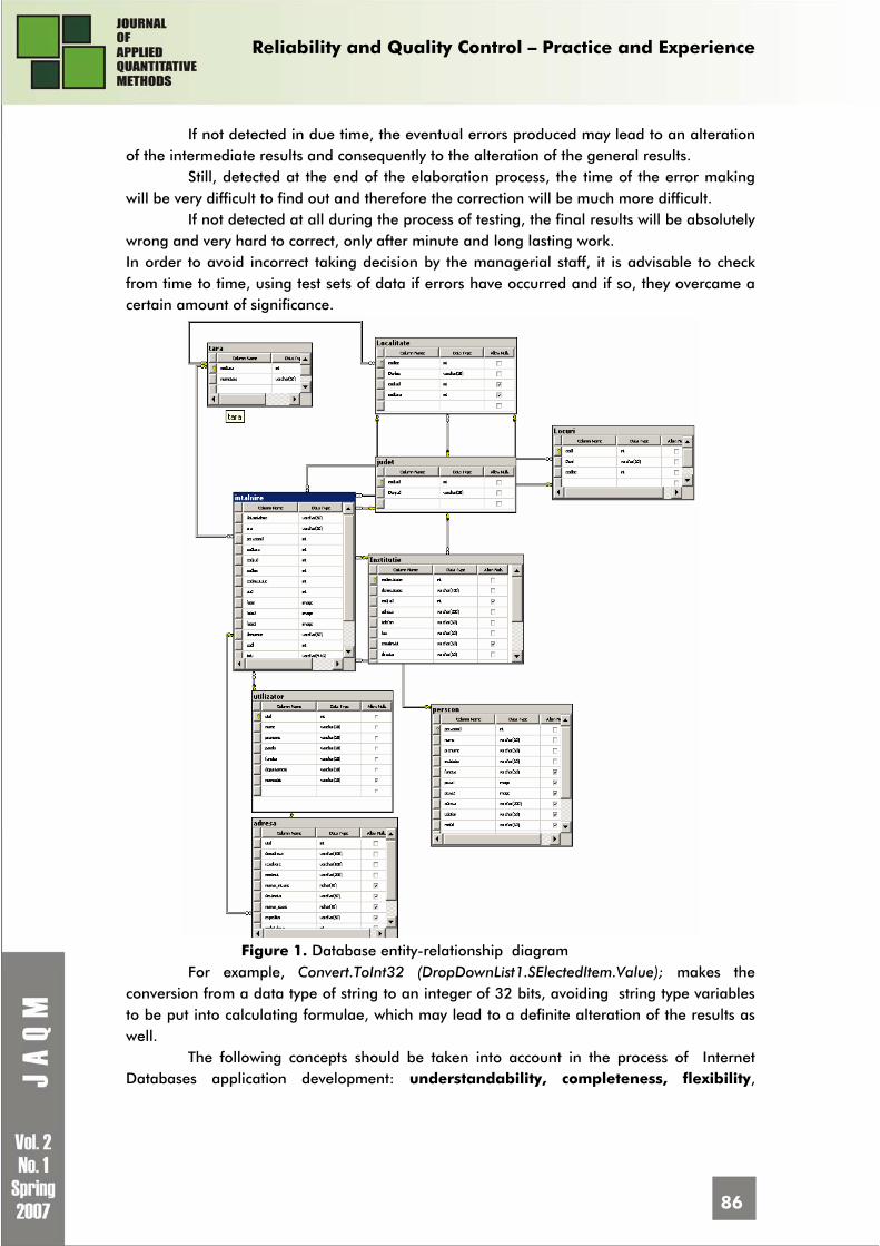
Reliability and Quality Control – Practice and Experience
86
If not detected in due time, the eventual errors produced may lead to an alteration of the intermediate results and consequently to the alteration of the general results.
Still, detected at the end of the elaboration process, the time of the error making will be very difficult to find out and therefore the correction will be much more difficult.
If not detected at all during the process of testing, the final results will be absolutely wrong and very hard to correct, only after minute and long lasting work. In order to avoid incorrect taking decision by the managerial staff, it is advisable to check from time to time, using test sets of data if errors have occurred and if so, they overcame a certain amount of significance.
Figure 1. Database entity-relationship diagram
For example, Convert.ToInt32 (DropDownList1.SElectedItem.Value); makes the conversion from a data type of string to an integer of 32 bits, avoiding string type variables to be put into calculating formulae, which may lead to a definite alteration of the results as well.
The following concepts should be taken into account in the process of Internet Databases application development: understandability, completeness, flexibility,

Reliability and Quality Control – Practice and Experience
87
reliability and data protection. The last concept has been dealt with in the first chapter of the article.
Understandability involves that developers should think from user perspectives and try to empathize with his problems, technological fear and rejection of the new. When changes are made, the target group is trained to cooperate with the new application.
Completeness is another important web database quality metric. An application is complete when all the items from the model (such as the tables and columns from the database diagram) correspond to the user requirements. At every step (prototype) it is recommended to study if the stage is complete and if is not there should be made some corrections. In our application, there have been omitted some user requirements such as the storage of official letters that are very important for the business meetings. A table was added and it has been related to the other tables in the relational model. Problems also appear if the end user requirements are not well defined , which leads the development team to confusion. The target group must be interviewed in the development process to find out that the partial outputs are accurate.
The application is also flexible. Flexibility makes an application economically efficient. The number of changes in the future is not supposed to be very big and also changes must be easy to accomplish. The more the application is flexible, the lower cost of changing and upgrading is.
It is also very important for the application to be reliable during the life cycle. We hope that our application would maintain all its functions and procedures for a long period of time without any irremediable, beyond repair errors. It is desired that it would work for a long period of time. The index of reliability is
ndatndatI c
r =
where
cndat represents the number of datasets that generated the results;
ndat , the total number of datasets. A good application is realized when the indicator has the value greater than 0,78.
The target group consists of the employees of each department of the Chamber; they have been interviewed from the beginning and on the course of the entire development process. The predictive test results have been included in the table 1. Table 1. The target group’s predictive test results
Department No of users No of queries Good responses
Updates Errors
Business Information 5 35 30 2 2
Fairs and Exhibitions 12 50 46 8 3
Human Resources 3 35 33 4 0
Public relations 5 70 69 3 0
There are 25 users which made 190 queries in one week. Average queries per
employee is 190/25=7,6 queries per user. The number of good responses is 178. The index of reliability is 0,93 meaning that the software application is very good .

Reliability and Quality Control – Practice and Experience
88
Conclusions
This paper related some theoretical themes, studied by many authors in computer science, with the role of describing the quality aspects of web relational databases .
The statistic calculations are important for each software metric on all stages of the project realization because they show the exact level of precision and report the percentage in which the initial objectives have been realized.
It is also useful to relate statistic results from each step to the next step of the project, every step, including analysis and data modeling having the same significance level for the objective’s realizations.
Economic efficiency must also be achieved by making a reliable application that would help the managerial board to take appropriate decisions and not to put them in difficulty.
The study is also interdisciplinary, because of the different approaches, economic, technical and social. In the future, the employees will have to answer to questions, about the usability of the programs and the development team will take them into consideration.
References 1. Arsanjani, A. Empowering the Business Analyst for on Demand Computing, IBM Systems
Journal, Vol.44, nr.1, 2005 2. Block, E., Hiemstra, D., Choenni, S. Predicting the cost quality trade off for information
retrieval queries: Facilitating Databases and query optimization, www.utwente.nl, 21.11.2006
3. IBM Info center, www.publib.boulder.ibm.com, 28.11.2006 4. Ivan, I., Popa, M., Popescu, Al. The Aggregation of the Text Entities, Economic Computation
and Economic Cybernetics Studies and Research 38, no. 1-4, 2004, pag.37–50 5. Ivan, I., Saha, P. Quality Characteristics of the Internet Applications, Software 2003 - ASE
Printing House, 2004 6. Ivan, I., Visoiu, A. Economic Models Basis, ASE Publishing House, Bucharest, 2005 7. Platini, M., Genaro, M., Calero, C. Data Model metrics, www.uclm.es, 20.11.2006
1 Codifications of references:
[ARSA05] Arsanjani, A. Empowering the Business Analyst for on Demand Computing, IBM Systems Journal, Vol.44, nr.1, 2005
[BLOHI06] Block, E., Hiemstra, D., Choenni, S. Predicting the cost quality trade off for information retrieval queries: Facilitating Databases and query optimization, www.utwente.nl, 21.11.2006
[IVSA03] Ivan, I., Saha, P. Quality Characteristics of the Internet Applications, Software 2003 - ASE Printing House, 2004
[IVPO04] Ivan, I., Popa, M., Popescu, Al. The Aggregation of the Text Entities, Economic Computation and Economic Cybernetics Studies and Research 38, no. 1-4, 2004, pag.37–50
[IVVI05] Ivan, I., Visoiu, A. Economic Models Basis, ASE Publishing House, Bucharest, 2005 [PIGECA06] Platini, M., Genaro, M., Calero, C. Data Model metrics, www.uclm.es, 20.11.2006 [www1] IBM Info center, www.publib.boulder.ibm.com, 28.11.2006

Reliability and Quality Control – Practice and Experience
89
1
kk M
kk
p λ
λ=
=
∑
SOFTWARE RELIABILITY FROM THE FUNCTIONAL TESTING PERSPECTIVE
Mihai POPESCU PhD, Senior Lecturer Military Technical Academy, Bucharest, Romania E-mail: [email protected]
Abstract: The metrics proposed in this paper give a methodological framework in the field of the functional testing for the software programs. The probability of failure for software depends of the number of residual defects; obvious the detection of these depends very much of data test used, that are conforming with a operational profile. But it’s the same true that a linear source code, that have a lot of instructions, but a sequential structure, is easier tested and debugged than a code with alternative control structures. Key words: software; reliability; functional testing; metrics
1. A metric of the complexity
There are very much specialists in the field that say the probability of failure for
software depends of the number of residual defects; obvious the detection of these depends very much of data test used, that are conforming with a operational profile.
But it’s the same true that a linear source code, that have a lot of instructions, but a sequential structure, is easier tested and debugged than a code with alternative control structures.
That explains why I defined in [POPE02]1 failure aprioristic probabilities (pk) of software modules across with theirs cyclomatic complexity.
The choosing of the computing way for the probability pk is determined by the available data and by the estimation and prediction models for reliability.
A usual weight computing formulas for failure aprioristic probabilities of the modules is (1):
(1)

Reliability and Quality Control – Practice and Experience
90
: kloc
k
TlocT
p⎛ ⎞⎜ ⎟⎝ ⎠
where λk=failure intensity of module k, that is calculated by formulas:
kkk IMer /** ωλ = (2)
Where: Me=4,2*10 7− Musa rate for failures exposure; r = processor speed (istructions/s) – can be established from benchmarking programs or from the technical characteristics given by the sale man;
kω = number of failures contained by the software module k. It can be
determined in according to [ROME97], transforming source instructions written in a program language in function points and than determining the number of failures in according to CMM level (Capability Maturity Model) selected;
kI = number of executable code lines k * expanded rate [ROME97].
This paragraph wants to deduct new metrics for complexity and reliability based on functional theory. For this goal, we’ll note with:
Ti=duration of test i; θj= average duration for locating/recovery of the module j . Appropriate, we’ll define the duration for locating/recovery of the a failure module
being a random discrete variable, called Tloc, having the next repartition law : , where: Tlock= duration for locating/recovery cumulated on the branch k of the tree associated to the program P; Pk= failure aprioristic probability of the module k.
For the locating tree of failure modules from fig.2, obtained based on the program structure proposed in fig. 1, we’ll have the next repartition law for the random discrete variable Tloc : T4+T5 T4+T5 T4+T5 T4+T5 T4+T5
+T2+θ1 +θ2 +T2+θ3 +θ4 +θ5 Tloc= p1 p2 p3 p4 p5
Appropriate, we’ll have the average duration of locating/recovery for module Tloc_med, the next expression :
Tloc_med= (T4+T5+ T2+θ1)p1 + (T4+T5+θ2)p2+(T4+T5+T2+θ3)p3 + +(T4+T5+θ4)p4+(T4+T5+θ5)p5 (3)

Reliability and Quality Control – Practice and Experience
91
Figure 1. The decomposition of a program in modules for testing We define variable Πk like: (4) It can observe that Πk has the next properties:
1) Πk>0; 2) , that means the weight of the module k in the testing and recovery of module k,versus of the N program modules.
Fixing a duration for locating/recovery, T0loc_med, to accomplish a mission by
software, the program must be written to satisfy the condition: We can observe, in the same time, that descended sorting Πk values on can see the modules with a big duration for testing/locating of the singular failures, these modules could be redesigned, eventually. If we call E the number of residual defects from program, than:
_
;kloc kk
loc med
T pT
⋅Π =
11
N
kk =
Π =∑
0_ _ .loc med loc medT T≤

Reliability and Quality Control – Practice and Experience
92
Tloc_gen_med=E Tloc_med . (5) If Ti=1, ∀i and θj=1, ∀j, we have: Tloc_med=Mloc_med, and we’ll get the number of steps to locate failure modules. The using of these metrics has the next advantages:
- gives a better reflection of the locating and fixing mechanism for the defects contained in software (based on functional testing);
- gives value to the performances of the testing tools and to the skill of the debugging personal;
- offers a good support to software products designers, signaling the modules that need a bigger testing/locating time, suggesting even theirs redesign.
2. Case study
I’ll compute the average duration of locating (3) and general average duration of locating (5) based on the methodology proposed at 1. and on the structure of the modules tree from fig. 1.
According to this structure, we’ll start from the next information that we know about the modules and functions (table 2). Table 2. Information known about software modules
Module Name
Functions Number of executable instructions
function/module
Probability of execution
function/module
Programming Language
M1 ⎯ 3 1 C++
M2 push(z); z ∈ [1,50]
15 1 C++
M3 ⎯ 4 1 C++
M4 push(z),top(z), pop(z); z ∈ [1,50]
push(z) - 15 pop() - 10 top(z) - 5
pop() – 0.8 top(z) – 0.1
push(z) – 0.1
C++ C++ C++
M5 push(z),pop(), top(z);z ∈ [1,50]
push(z) - 15 pop() - 10 top(z) - 5
push(z) – 0.8 top(z) – 0.1 pop() – 0.1
C++ C++ C++
For this goal, we proceed the next steps: 1°)The calculation of the modules’ failure aprioristic probabilities with (3) and (4) formulas. We admit the hypothesis that software will be executed on a 2 MIPS computer, meaning r=2000000, and CMM level is 3, a common used level for IT companies [PAUL93]. With the explanations given for (2) and with information obtained from [POPE02], we’ll have:
⋅

Reliability and Quality Control – Practice and Experience
93
=1ω 3 : 53 * 1.63 = 0.923 defects;
=2ω 15 : 53 * 1.63 = 0.461 defects;
=3ω 4 : 53 * 1.63 = 0.123 defects;
=4ω (15+10+5) : 53 * 1.63 = 0.923 defects;
=5ω (15+10+5) : 53 * 1.63 = 0.923 defects;
=1I (3 source lines) * (object instructions/source line) = 18 object instructions;
=2I (15 source lines) * (6 object instructions/source line) = 90 object instructions;
=3I (4 source lines) * (6 object instructions/source line) = 24 object instructions;
=4I (30 source lines) * (6 object instructions/source line) = 180 object instructions;
=5I (30 source lines) * (6 object instructions/source line) = 180 object instructions;
Replacing these values, we’ll have:
11 ωλ ∗∗= Mer / defectsdefectfailures
ondnsinstructioI 092.0102.4
sec2000000 7
1 ∗⎟⎟⎠
⎞⎜⎜⎝
⎛⋅∗= −
/18 = 0.0042 ond
defectssec
( ) ;sec
0044.024123.07103.420000002 onddefects
=∗−∗∗=λ
;sec
044.024123.0*)7102.4(20000003 onddefects
=−⋅∗=λ
;sec
045.0180923.0)7102.4(20000004 onddefects
=∗−⋅∗=λ
ond
defectssec
045.0180923.0)7102.4(20000005 =∗−⋅∗=λ ;
;sec
0219.054321 onddefects
=++++ λλλλλ
The value a little big for the failure intensity is explained by the big number of instructions contained by modules and by r value(2 MIPS), big enough. Applying formula(1), we have:
;193.00219.00042.05
111 === ∑
=iip λλ
;196.00219.00043.00219.022 === λp
;201.00219.00044.00219.033 === λp
;205.00219.00045.00219.044 === λp
.205.00219.00045.00219.055 === λp

Reliability and Quality Control – Practice and Experience
94
According to the values of these probabilities, FIAB program [GHIT96] displays failure tree from fig. 2.
Figure 2. Locating tree of defect modules 2°) The determination of average duration for locating/testing of the
modules
To determine iT time we take in account the probability of execution of each
function and the results testing made in according with the specifications for that function. That is:
,__*)____(mod__
1j
fnr
jjji fexpfspraptestfdurataT
i
∑=
+= (6)
where:
ifnr mod__ = number of functions from module i tested;
=jfexp __ probability of execution of function j;
=jfdurata _ execution time of function j;
=jfspraptest ___ testing time of function j results in according with the
specifications; We established the next values T.U.(Unites of Time) for used functions(table 3):
Table 3. Execution and testing times in according with the specifications and the times for locating/recovery for the functions used in modules Function Name Execution Time Testing time in according
with the specifications Average
locating/recovery time Push(z) 30 T.U. 20 T.U. 300 T.U. Pop( ) 25 T.U.. 20 T.U. 250 T.U. Top (z) 20 T.U.. 15 T.U. 100 T.U.
5V
2V 4V
2V 4M
2M 5M
3M 1M
0 1
1
1
10 0
0

Reliability and Quality Control – Practice and Experience
95
Starting from formulas:
,__*)____(mod__
1j
fnr
jjji fexpfspraptestfdurataT
i
∑=
+= (see 6)
∑=
=ifnr
jji frestlocdurata
mod__
1___θ (7),
where:
=jfrestlocdurata ___ locating/recovery time of function j in module i,
we’ll have:
=1T execution time for 3 source instructions(6 T. U.) + testing time in according with
the specifications (0 T. U.) = 6 T. U.);
=1θ 1 T. U. (a simple instruction if.... then ….else);
=2T (30 T. U. + 20 T. U.) *1 = 50 T. U.;
3002 =θ T. U.;
=3T (7 T. U.+ 0 T. U.) = 7 T. U.;
=3θ 1 T. U. ( a simple instruction if …then…else);
=4T (30+20) ⋅ 0,1+(25+20)⋅ 0,8 +(20+15)⋅ 0,1=50⋅0.1+45⋅0.8+35⋅0,1 = 44.5 T.
U.;
=4θ 300 ⋅ 0,1+250⋅0,8+100⋅0,1 = 240 T. U.;
=5T (30+20)⋅ 0,8+(25+20)⋅0,1+(20+15)⋅ 0,1 = 50⋅0,8+45⋅0,1+35⋅0,1 = 48 T.
U.;
=5θ 300⋅0,8+250⋅0,1+250⋅0,1 = 290 T. U.
For the locating tree of defect modules from fig. 2, we’ll have the next repartition law for the
discreet random variable T loc :
54321
5435215
5452425242
ppppp
TT
TTTTTTTTTT
Tlocθθθθθ +++++++
+++++
=

Reliability and Quality Control – Practice and Experience
96
..2495,282
205.0)290485,44(205,0)2404850(201.0)1485.4450(196.0)3004850(193.0)1485.4450()()(
)()()(
55544452
33542225211542_
UT
pTTpTT
pTTTpTTpTTTT medloc
=⋅+++⋅+++⋅++++⋅+++⋅+++=⋅+++⋅+++
⋅++++⋅+++⋅+++=
θθ
θθθ
3°) The determination of average testing and locating/recovery duration of the modules, using the residual number of defects into a program, with formula (5):
medlocmedlocmedgenloc TTET _54321___ )( ⋅++++=⋅= ωωωωω
=(0.092+0,461+0,123+0,923+0.923)*282,2495 = 2,522*282,2495 ≈ 711,833 T.U.
4°) The determination of the weights and theirs importance (formula 4):
098,02495,2826955,27)( _11542_111 ==⋅+++=⋅=Π medlocmedloc TpTTTTpTloc θ ;
=⋅=Π medlocTpTloc _222 276,02495,282008,78)( _2252 ==⋅++ medlocTpTT θ ;
102,02495,282/8435,28)( _33542_233 ==⋅+++=⋅=Π medlocmedloc TpTTTTpTloc θ ;
=⋅=Π medlocTpTloc _444 245,02495,28229.69)( _4452 ==⋅++ medlocTpTT θ ;
=⋅=Π medlocTpTloc _555 278,02495,2824125,78)( _5554 ==⋅++ medlocTpTT θ .
The decrease row of kΠ values is:
13425 ,,,, ΠΠΠΠΠ , and this means that the module with the most locating/testing time is
M5 and the module with the least locating/testing time is M1, this thing allowing to designers and programmers to redesign and grow the performances of critical modules(regarding of testing/recovery times).
3. General conclusions The metrics proposed in this paper give a methodological framework in the field of the functional testing for the software programs. These metrics have the next capabilities: − give a good understanding for functional testing and locate/recovery mechanism of the software modules of a program;
− give a better appraisal to the performances of the testing tools and to the skill of the debugging personal(by locating/recovery time of a function into a module);
− identify the modules that need a big locating/testing time (by decrease sorting of the weights), asking a possible redesign for the intensive resources modules.

Reliability and Quality Control – Practice and Experience
97
Bibliography 1. Boehm, J., Saib, B. Error Seeding Technique Specification, Prepared under Contract Number
NAS 2-10550 by Hughes Aircraft Company, Fullerton and General Research Corporation, Santa Barbara, California, USA, 1980
2. Ghita, A., Ionescu, V. Metode de calcul in fiabilitate, Course, Technical Military Academy, Bucharest, 1996
3. Goron, S., Fiabilitatea Produselor Program, Universitatea Babes-Bolyai, Cluj-Napoca, Ed. Risoprint, 2000
4. Paulk, M., Curtis, B., s.o., Capability Maturity Model for Software, Version 1.1, Software Engineering Institute, Carnegie Mellon University, Pittsburg, Pensylvania, USA, 1993
5. Popescu, M., Managementul Fiabilitatii Aplicatiilor Software Militare, PhD Dissertation, Technical Military Academy, Bucharest, 2002
6. System and Software Reliability Assurance Notebook, Produced for Rome Laboratory, New York, 1997
1 Codifications of references: [BOEH81] Boehm, J., Saib, B. Error Seeding Technique Specification, Prepared under Contract Number
NAS 2-10550 by Hughes Aircraft Company, Fullerton and General Research Corporation, Santa Barbara, California, USA, 1980
[GHIT96] Ghita, A., Ionescu, V. Metode de calcul in fiabilitate, Course, Technical Military Academy, Bucharest, 1996
[GORO00] Goron, S., Fiabilitatea Produselor Program, Universitatea Babes-Bolyai, Cluj-Napoca, Ed. Risoprint, 2000
[PAUL93] Paulk, M., Curtis, B., s.o., Capability Maturity Model for Software, Version 1.1, Software Engineering Institute, Carnegie Mellon University, Pittsburg, Pensylvania, USA, 1993
[POPE02] Popescu, M., Managementul Fiabilitatii Aplicatiilor Software Militare, PhD Dissertation, Technical Military Academy, Bucharest, 2002
[ROME97] System and Software Reliability Assurance Notebook, Produced for Rome Laboratory, New York, 1997

Software Analyses
98
ON MEASURING SOFTWARE COMPLEXITY
Adrian COSTEA1 PhD, University Lecturer Academy of Economic Studies, Bucharest, Romania E-mail: [email protected] Web page: http://www.abo.fi/~acostea
Abstract: In this paper we measure one internal measure of software products, namely software complexity. We present one method to determine the software complexity proposed in literature and we try to validate the method empirically using 10 small programs (the first five are written in Pascal and the last five in C++). We have obtained results which are intuitively correct, that is we have obtained higher values for average structural complexity and total complexity for the programs which “look” more complex than the others, not only in terms of length of program but also in terms of the contained structures. Key words: software; complexity; measurement
1. Introduction
Software quality is the degree to which software possesses a desired combination of attributes such as maintainability, testability, reusability, complexity, reliability, interoperability, etc. (IEEE, 1992). In other words, quality of software products can be seen as an indirect measure and is a weighted combination of different software attributes which can be directly measured. Moreover, many practitioners believe that there is a direct relationship between internal and external software product attributes. For example, a lower software complexity (seen here as a structural complexity) could lead to a greater software reliability (Fenton & Pfleeger, 1997).
Measuring complexity of software products was, and still is, a widely distributed research subject. The scope of studying it was to control the levels of the external attributes of software via internal attributes, like complexity is. The most well-known internal attribute is software length. Another is complexity. While in the case of length is a quite well defined consensus about the ways the length should be measured, in the case of complexity is still a lot of confusion. It is not wrong to say that there is a relationship between complexity and the length of the program. But, all authors agree that when measuring complexity one should take into account something different from length and length at the same time. This approach was followed in Törn et al. (1999) where a new measure of software complexity called structural complexity is derived. In the literature there are several measures of complexity, the most used ones being: • length defined as the number of lines of codes and

Software Analyses
99
• McCabe’s cyclomatic complexity which measures something else than just length:
dne +=+−= 12ν where ν is the cyclomatic complexity of the flowgraph f, e is the number of edges, n the
number of nodes, and d is the number of predicate nodes of f. The longer the program is, the more predicate nodes it has. This leads to normal
conclusion that McCabe’s cyclomatic number is strongly correlated with length. The problem with McCabe’s cyclomatic number is that is not a “good” measure of complexity, since smaller programs (in terms of lines of code) are much more complex in terms of their intrinsic functions. In order to eliminate the correlation, some authors proposed other measures such as complexity density defined as the ratio of cyclomatic complexity to thousand of lines of code (Gil & Kemerer, 1991).
McCabe (1976) proposed a derived complexity measure called essential complexity measure ( νe ): me −=νν where ν is the cyclomatic number and m represents the number of sub-flowgraphs of f that are D-structured primes (Fenton & Pfleeger, 1997, p. 288).
Bache (1990) proposed a series of axioms and a number of measures that satisfy the axioms, the VINAP measures, to characterize the software complexity. Woodward et al. (1979) proposed the so-called knot measure that is defined as the total number of points at which control-flow lines cross.
When measuring software complexity we have to be very cautious on which metrics we use. The authors in Törn et al. (1999) state that one can obtain wrong result if he/she compares two different programs using one complexity measure and other two using another one. Another problem raised by the authors is that of establishing acceptable axioms for complexity measures. The failure to realize the existence of different views about complexity leads to conflicting axioms.
Next we present an overview of the software complexity model proposed in Törn et al. (1999), and then, we apply this methodology on some example programs in order to empirically validate it.
Methodology The model to calculate the total complexity of a piece of software (p) is as follows:
)()()( pcplpe =
where e(p) is the total complexity, l(p) is the length of the software, and c(p) is the average
structural complexity. For a collection of software units },...,,{ 21 npppP = we calculate c(P)
as the average of the individual units complexity:
∑
∑
=
=== n
ii
n
iii
n
pl
pcplpppcPc
1
121
)(
)()(),...,,()(

Software Analyses
100
The individual unit lengths and total complexities are additive. So, if we add them we obtain the length of the collection (l(P)) and, respectively, the total complexity of the collection (e(P)).
In Törn et al. (1999) the authors use the above equations for the software collections and define new formulas that use some constants. The constants are different from one control structure to the other. Next we give the three formulas (sequence, choice, iteration) for average structural complexity using these constants:
),...,,();...;;( 2121 nsn pppccpppc = - sequence
),,()( qpbccifc if= - choice: “if b then p else q”
),()( pbccwhilec do= - iteration: “while b do p”
In general, when applying the model we consider 5.13.11.1 =<=<= doifs ccc
which is intuitive since we assign to the more complex structure a greater importance when calculating the complexity.
We can have the same reasoning (adding some constants) when we calculate the
lengths of different control structures. For example: ),,()( qpbllifl if += . For simplification
(when applying the methodology for our example programs) we will consider all these
constants zero ( 0==== dgodoif llll ).
Using these formulas the complexity of any program can be computed given the lengths and average complexities of the smallest parts (atoms): assignment statement, expressions, procedure calls and goto’s. In our experiment we consider all these to have the value of 1 (as it is suggested in Törn et al. (1999)).
The unique feature of the model resides in the fact that no other complexity model found in literature has such a two dimensional structure in representing the complexity. Also, the theoretical properties of the model that cover unstructuredness, sequencing, nesting, modularization and layout are intuitively correct. In order to be able to apply the methodology we have to write the programs in “node representation”. Using this representation, decision nodes, assignment statements and goto nodes are given as: (b la ca), (n la ca), and (go la ca) respectively, where la and ca are the length and complexity of the atoms.
In the next section we apply this methodology on some example programs and try to validate it empirically.
Results
We start the empirical evaluation by testing the complexity of some basic structures (p) and changes of the basic structures (p’):
Sequential structure: Let p = {a;b}, where a, b are simple assignment statements. Then this can be
written using the “node notation” as: (S(n 1 1)(n 1 1)) = (n 2 1.1) =>l = 2; c = 1.1 and e = 2.2.

Software Analyses
101
Now let p’ = {a;b;c}, where a, b, c are simple statements (assignment statements or defining statements). Then, in node notation the structure will be (s(n11)(n11)(n11)) = (n 3 1.1*(1+1+1)/3) = (n 3 1.1) => l = 3, c =1.1 and e = 3.3.
Conclusion: p’ is more complex than p. It is obvious that the average complexity or the complexity density is equal for p and p’, since both structures consists only of program nodes. But the total complexity of p’ is greater than the total complexity of p.
Choice structure (IF a then p else q): Let p = (If a then b else c), where a is a decision node and b, c are simple
statements (program nodes). In node notation this will be written as: (if (b 1 1) (n 1 1) (n 1 1)) = (n 3 1.3*(1+1+1)/3) = (n 3 1.3) => l = 3, c = 1.3 and
e = 3.9. Let p’=(If (a and b) then c else d), where a, b are decision nodes (Boolean
expressions) and c, d are program nodes. Using node notation: (if (b 2 1) (n 1 1) (n 1 1)) = (n 4 1.3) =>l = 4, c = 1.3 and e = 5.2. Now let p’’ = (If a then (b and c) else d), where a is a decision node and b, c, d are
program nodes. Using node notation: (if (b 1 1) (s(n 1 1) (n 1 1))(n 1 1)) = (if (b 1 1) (n 2 1.1) (n 1 1)) = (n 4
1.3*(2+2.2)/4) = (n 4 1.365) => l = 4, e = 1.365 and e = 5.46. Conclusion: p’’ is more complex than p’, which is more complex than p. Here the
average complexity or complexity density is the same for p and p’. It is right because the both structures p and p’ are basic, with the only difference that the decision node in p’ is of length 2. In the p’’ structure is included a sequential structure, which has the average complexity 1.1. This will increase the average complexity of if structure, and implicitly the total complexity.
Iteration structure (Do-while)
Let p = (While a do b), where a is a decision node and b is a program node. In node notation this is written as: (do (b 1 1) (n 1 1)) = (n 2 1.5). That is, the complexity density c=1.5 and the overall complexity e=3, and the length is l = 2.
Now let p’ = (While a do (b and c)). In node notation, the structure will be: (do (b 1 1) (s(n 1 1) (n 1 1))). This will be written further on as: (do (b 1 1) (n 2 1.1)) = (n 3 1.5*(1+2.2)/3) = (n 3 1.6). This means that the
average complexity (complexity density) is c=1.6, the length of the structure is l=3, and the overall complexity is e=4.8.
Conclusion: p’ is more complex than p. The complexity density of p’ is greater than that of p, and also the overall complexity of p’(e’=4.8) is greater that that of p (e=3).
Then we collected 10 programs for which we computed the values (l, c, e). The programs and the calculations are:

Software Analyses
102
1st Program program ex1; var x: integer; procedure p(y:integer); begin writeln(Y:3); if y>3 then begin write('123'); writeln; end end; begin x:=3; while x<=5 do begin p(x); x:=x+1 end; end.
(s(n 1 1) (n 1 1) (s(n 1 1) (do(b 1 1) (s(n 1 1) (if(b 1 1) (s(n 1 1) (n 1 1) ) ) (n 1 1) ) ) ) )
The average structural complexity c = 1.947. The program length l = 9 Overall complexity e = 17.52. 2nd Program program ex2; var counter: integer; begin counter:=1; while counter<20 do begin write('We are inthe loop, wainting'); write('for the counter to reach 20. It is', counter:4); writeln; counter:=counter+2; end; end.
(s(n 1 1) (n 1 1) (s(n 1 1) (do(b 1 1) (s(n 1 1) (n 1 1) (n 1 1) (n 1 1) ) ) ) )
The average structural complexity c = 1.65. The program length l = 8 Overall complexity e = 13.211 3rd Program program ex3; const string_size=30; type low_set=set of 'a'..'z'; var data_set: low_set ; storage: string[string_size]; index: 1..string_size; print_group:string[26]; begin data_set:=[]; print_group:='';
(s(n 1 1) (n 1 1) (n 1 1) (n 1 1) (n 1 1) (n 1 1) (n 1 1) (s(n 1 1) (n 1 1) (n 1 1)

Software Analyses
103
storage:='This is a set for test'; index:=1; while index<=length(storage) do begin if storage[index] in ['a'..'z'] then if storage[index] in data_set then writeln(index:4, ' ',storage[index],' is already in the set') else begin data_set:=data_set+[storage[index]]; print_group:=print_group+storage[index]; writeln(index:4,'',storage[index],' added to group, complete group= ',print_group); end; else writeln(index:4,' ',storage[index],' is not a lower case letter'); index:=index+1; end; end.
(n 1 1) (do(b 1 1) (s(if(b 1 1) (if(b 1 1) (n 1 1) (s(n 1 1) (n 1 1) (n 1 1) ) ) (n 1 1) ) (n 1 1) ) ) ) )
The average structural complexity c = 1.97 The program length l = 20 Overall complexity e = 39.425 4th Program program ex4; var index, count: integer; checkerboard: array[1..8]of array[1..8] of integer; value: array[1..8,1..8] of integer; begin index:=1; while index<=8 do begin count:=1; while count<=8 do begin checkerboard[index,count]:=index+3*count; value[index,count]:=index+2*checkerboard[index,count]; count:=count+1; end; index:=index+1; end; writeln('Output of checkerboard'); writeln; index:=1; while index<=8 do begin count:=1; while count<=8 do begin write(checkerboard[index,count]:7); count:=count+1; end; writeln; index:=index+1; end; value[3,5]:=-1; value[3,6]:=3; value[3,7]:=2; count:=1; while count<=3 do begin writeln;
(s(n 1 1) (n 1 1) (n 1 1) (n 1 1) (s(n 1 1) (do(b 1 1) (s(n 1 1) (do(b 1 1) (s(n 1 1) (n 1 1) (n 1 1) ) ) (n 1 1) ) ) (n 1 1) (n 1 1) (n 1 1) (do(b 1 1) (s(n 1 1) (do(b 1 1) (s(n 1 1) (n 1 1) ) ) (n 1 1) (n 1 1) ) ) (n 1 1) (n 1 1) (n 1 1)

Software Analyses
104
count:=count+1; end; writeln('output of value'); writeln; count:=1; while count<=8 do begin index:=1; while index<=8 do begin write(value[count,index]:7); index:=index+1; end; writeln; count:=count+1; end; end.
(n 1 1) (do(b 1 1) (s(n 1 1) (n 1 1) ) ) (n 1 1) (n 1 1) (n 1 1) (do(b 1 1) (s(n 1 1) (do(b 1 1) (s(n 1 1) (n 1 1) ) ) (n 1 1) (n 1 1) ) ) ) )
The average structural complexity c = 1.97 The program length l = 39, Overall complexity e = 76.98 5th Program Program ex5; var index, count: integer; checkerboard: array[1..8]of array[1..8] of integer; value: array[1..8,1..8] of integer; begin index:=1; while index<=8 do begin count:=1; while count<=8 do begin checkerboard[index,count]:=index+3*count; value[index,count]:=index+2*checkerboard[index,count]; count:=count+1; end; index:=index+1; end; writeln('Output of checkerboard'); writeln; index:=1; while index<=8 do begin count:=1; while count<=8 do begin write(checkerboard[index,count]:7); count:=count+1; end; writeln; index:=index+1; end; count:=1; while count<=3 do begin writeln; count:=count+1;
(s(n 1 1) (n 1 1) (n 1 1) (n 1 1) (s(n 1 1) (do(b 1 1) (s(n 1 1) (do(b 1 1) (s(n 1 1) (n 1 1) (n 1 1) ) ) (n 1 1) ) ) (n 1 1) (n 1 1) (n 1 1) (do(b 1 1) (s(n 1 1) (do(b 1 1) (s(n 1 1) (n 1 1) ) ) (n 1 1) (n 1 1) ) ) (n 1 1)

Software Analyses
105
end; writeln('output of value'); writeln; count:=1; while count<=8 do begin index:=1; while index<=8 do begin write(value[count,index]:7); index:=index+1; end; writeln; count:=count+1; end; end.
(do(b 1 1) (s(n 1 1) (n 1 1) ) ) (n 1 1) (n 1 1) (n 1 1) (do(b 1 1) (s(n 1 1) (do(b 1 1) (s(n 1 1) (n 1 1) ) ) (n 1 1) (n 1 1) ) ) ) )
The average structural complexity c = 2.27 The program length l = 36 Overall complexity e = 81.81
As a first observation, when comparing the results obtained for the 4th program with those for the 5th program, we can state that even the length of the program 5 is lower that the length of program 4 (36<39), the average complexity of program 5 is greater than that of program 4 (2.27>1.97). This is true and intuitively explained by the fact that the density of complex structures in program 5 is greater than that in program 4. The difference in size (39-36) is explained by the three assignment statements (value[3,5]:=-1; value[3,6]:=3; value[3,7]:=2;) which appear only in program 4 and have a lower value for complexity.
This shows that taking just length as a complexity measure is not a correct way to evaluate the quality of a software product of being complex or not. Even though the length is high, it is possible that the program is easily readable and easy to maintain, if it consists of few complex and nested structures and much many simple statements. 6th Program void merge(apvector<int> &a, int first, int mid, int last) { int aPtr=first, bPtr=mid+1, cPtr=first; int total=last-first+1, loop; bool doneA = false, doneB = false; apvector<int> c(a.length()); for (loop=1; loop<=total; loop++) { if (doneA) { c[cPtr] = a[bPtr];
bPtr++; } else if (doneB) { c[cPtr] = a[aPtr];
(s (n 1 1) // aPtr = … (n 1 1) // bPtr = … (n 1 1) // cPtr = … (n 1 1) // total = … (n 1 1) //doneA = false (n 1 1) // doneB = false (n 1 1) // constructor call (n 1 1) // loop = 1 (do (b 1 1) (s (if (b 1 1) (s (n 1 1) (n 1 1) )

Software Analyses
106
aPtr++; } else if (a[aPtr] < a[bPtr]) { c[cPtr] = a[aPtr];
aPtr++; }
else { c[cPtr] = a[bPtr]; bPtr++;
} cPtr++;
if (aPtr > mid) doneA = true; if (bPtr > last) doneB = true;
} for (loop=first; loop<=last; loop++) a[loop] = c[loop]; }
(if (b 1 1) (s (n 1 1) (n 1 1) ) (if (b 1 1) (s (n 1 1) (n 1 1) ) (s (n 1 1) (n 1 1) ) ) ) ) (n 1 1) (if (b 1 1) (n 1 1) ) (if (b 1 1) (n 1 1) ) (n 1 1) ) // close do (n 1 1) // loop = first (do (b 1 1) (s (n 1 1) (n 1 1) // loop++ ) )
) // close s
The average structural complexity c = 2.3. The program length l = 30. Overall complexity e = 69. 7th Program void quickSort (apvector<int> &list, int first, int last){ int g = first, h = last; int midIndex, dividingValue; midIndex = (first + last) / 2; dividingValue = list[midIndex]; do { while (list[g] < dividingValue) g++; while (list[h] > dividingValue) h--; if (g <= h) { swap(list[g], list[h]); g++; h--; } } while (g < h); if (h > first) quickSort (list,first,h); if (g < last) quickSort (list,g,last); }
(s (n 1 1) (n 1 1) (n 1 1) (n 1 1) (do (b 1 1) (s (do (b 1 1) (n 1 1) ) (do (b 1 1) (n 1 1) ) (if (b 1 1) (s (n 1 1) (n 1 1) (n 1 1) ) ) // close if ) // close s ) // close do
) // close s

Software Analyses
107
The average structural complexity c = 1.93. The program length l = 17. Overall complexity e = 32.8075. 8thProgram void mergeSort(apvector<int> &list, int first, int last) { int mid; if (first == last) last++; else if (1 == last - first) { if (list[first] > list[last]) swap (list[first], list[last]); } else { mid = (first+last) / 2; mergeSort (list, first, mid); mergeSort (list, mid+1, last); merge (list, first, mid, last); } }
(if (b 1 1) (n 1 1) (if (b 1 1) (if (b 1 1) (n 1 1) ) (s (n 1 1) (n 1 1) (n 1 1) (n 1 1) ) // close if ) // close if )// close if
The average structural complexity c = 1.79. The program length l = 9. Overall complexity e = 16.12. 9th Program void insertionSort (apvector<int> &list) { int pos; for( int i=1; i<list.length(); ++i ) { pos = i; while( (pos>0) && ( list[pos-1]>list[pos] ) ) { swap( list[pos-1], list[pos] ); pos--; } } }
(s (n 1 1) // i=1 (do (b 2 1) // function call (s (n 1 1) (do (b 2 1) (s (n 1 1) (n 1 1) ) ) (n 1 1) // ++i ) // close s ) // close do
) // close s
The average structural complexity c = 1.76. The program length l = 9. Overall complexity e = 15.83. 10th Program void screenOutput (const apvector<int> &nums) { cout << setiosflags( ios :: right ); for( int x=0; x<nums.length(); ++x ) { if( x%12 == 0 ) cout << endl; cout << setw(6) << nums[x] << " "; }
(s (n 1 1) (n 1 1) // x=0 (do (b 2 1) // function call (s (if (b 2 1) // length = 2 // 1 from x%12 // 1 from x%12 == 0 (n 1 1)

Software Analyses
108
} ) // close if (n 3 1) // display 3 times (n 1 1) // ++x ) // close s ) // close do
) // close s
The average structural complexity c = 1.8035. The program length l = 11. Overall complexity e = 19.8385.
Some of the last five programs are procedures which implement different kinds of sorting (quick sort, insertion, sort, merge sort). We have to mention that in the last five programs we did not take into consideration the variables declarations when calculating the complexity. Also when we transformed “for” structure in “do” structure we have followed the rule:
for (i=0; i<n; i++) equivalent with (n 1 1) // i = 0 (do (b 1 1)
…. (n 1 1) // i++
) // close do
We have obtained results which are intuitively correct, that is we have obtained
higher values for average structural complexity and total complexity for the programs which “look” more complex than the others, not only in terms of length of program but also in terms of the contained structures.
References 1. Bache R. Graph Theory Models of Software, PhD thesis, South Bank University, London, 1990. 2. Fenton N.E. and Pfleeger S.L. Software Metrics - A Rigorous & Practical Approach,
International Thomson Computer Press, London 1997 (Second edition) 3. Gill G. K. and Kemerer C.F. Cyclomatic Complexity Density and Software Maintenance, IEEE
Transanctions on Software Engineering, SE-17: 1284-1288, 1991 4. IEEE – IEEE Standard 1061-1992 Standard for a Software Quality Metrics Methodology, New
York: Institute of Electrical and Electronics Engineers, 1992 5. McCabe T. A Software Complexity Measure, IEEE Transactions on Software Engineering SE-2(4):
308-320, 1976 6. Törn A., Andersson T. and Enholm K. A Complexity Metrics Model For Software, South African
Computer Journal 24, November 1999, 40-48 7. Woodward M.R., Hennell M.A. and Hedley D. A measure of control flow complexity in
program text, IEEE Transactions on Software Engineering, SE-5(1): 45-50, 1979
1 Adrian COSTEA hold a PhD from Turku Centre for Computer Science Research interests: Data Mining Techniques for Decision Support Financial Benchmarking Economic/Financial Performance Classification Models Economic/Financial/Process Variable Predictions Further interests: Software reliability models

Software Analyses
109
MODELING THE AUDIT IN IT DISTRIBUTED APPLICATIONS
Victor-Valeriu PATRICIU PhD, University Professor Department of Computer Engineering Military Technical Academy, Bucharest, Romania E-mail: [email protected]
Calin Marin VADUVA Technical University of Cluj-Napoca, Cluj-Napoca, Romania Co-author of books: Security in Electronic Commerce (2000); Java Programming (1999), Theory of Information Transmission - Laboratory Course (1996) E-mail: [email protected]
Octavian MORARIU Student, Technical University of Cluj-Napoca, Cluj-Napoca, Romania E-mail: [email protected]
Marius VANCA Bachelor Degree form Babes-Bolyai University, Cluj Napoca, Romania Fortech, Cluj Napoca, Romania E-mail: [email protected] Olivian Daniel TOFAN PhD Candidate, Assistant Researcher, Department of Mathematics and Computer Science Babes Bolyai University, Cluj Napoca, Romania E-mail: [email protected]
Abstract: Quality in software is always an important and forever an "in vogue" topic, especially if we talk about complex distributed IT systems. In the context of the software quality, reliability of the software is a fundamental aspect. If we are talking about critical software solutions, we may not imagine any failure in the software, we may not imagine that some data has been lost or some operation has been done in the wrong way. In this context an important feature that should be build in the software is the audit capabilities of the software. Any application that adheres to a certain quality level must implement a solid audit module in order to be compliant with modern standards. There is no way to prove that the software operates in the right way except auditing the important actions executed by the software. The aim of this paper is to define the requirements for auditing and to propose a solution for implementing them in a software system. The paper starts from the description of the requirements for audit, goes on with a presentation of original concepts in the field and presents in the end the practical approach for implementation of the solution in a real software system. Key words: modeling; IT audit; distributed applications

Software Analyses
110
1. Introduction
The audit module of a Software System provides the means to record all actions
performed both by the direct users of the system and by the system itself. A complete audit system must record not only the actions that were performed, but also the states of the objects affected by those actions. All the information is stored in a chronological way, so tracking and rollback are always possible on system object states. The audit module is a vital part of reliability and security the system as it provides the information regarding all the actions and modifications performed on objects in a structured manner, unlike logging.
From the audit point of view, an action is defined as a specific piece of functionality of the software system. Execution of an action implies some kind of processing or a transformation to be applied on a dataset. An object will be defined as a set of attributes, where an attribute is a unique name-value pair.
2. Audit requirements
There are two types of requirements for an audit module. The first type is represented by the functionality requirements. Any audit module should implement the following minimum requirements:
- Record actions performed trough the system - Record object states - Provide means to retrieve audit data - Provide means to track the history of an object - Provide means to detect any external change of data
Along with these functional requirements there are some security related requirements: - Audit data must be stored in a secure manner - Continuous audit must be assured, no gaps allowed - Compliancy and integration with standards
In the following section each requirement will be discussed for a better understanding.
Record actions performed trough the system represents the base feature for an audit module. This requirement is implemented even in the simplest logging systems. However, if with the logging systems (used mostly for debugging) there isn’t a universal format, for an audit system the information recorded should be consistent. This requirement raises a challenge for application architects as it usually require a common point for all actions performed by the users, or by the system itself. This common point can be defined as a dispatcher. A well-designed application usually contains such a dispatcher, used also as main authorization point.
In order to be able to have a history tracking feature and a rollback option for a software system, the audit module must record all object states. When an object is modified by an action there are usually three states to be recorded: initial state (OBJ_PRE),

Software Analyses
111
ideal state (OBJ_IDEAL) and result state (OBJ_RES). The initial state represents the state of the object before the operation is performed. The ideal state is the final state of the object if the operation is successful. The result state is the final state of the object, regardless of the result of the operation. This document is assuming that the operations, like in real world, can have tree outcomes: successful, failed or partially successful.
At all times the audit module must provide means to retrieve audit data. A user of the software system, having the necessary authorization must be able at any time to query the audit module for information regarding actions and objects.
The audit module must also provide means to track the history of an object. This implies searching all the saved states and actions related to a specific object, and build a chronological report based on the obtained data-set.
The audit should provide means to detect external changes of data. The data managed by the software systems is usually stored in a data base or in other information repository. This means that if someone has access direct to this repository may change directly the information. It is practical impossible to audit these operations as long as they may not be intercepted by our audit system, but the audit module should detect if such a “break” appears.
The most important security requirement for an audit module is to store the audit data in a secure manner. The audit module must guarantee that only authorized users can access the information stored. Also, no external modification on the audit data must be permitted. In this way the audit data will be authentic.
Continuous audit must be assured. During the whole life cycle of the application objects a full audit must be maintained. The audit module can allow no gaps in the chronological line.
3. Architecture
There are two solutions for implementing an audit module: - First one uses hooks to integrate in an given application, intercepting the strategic
calls, also known as an external audit system; - The second one provides a set of interfaces and relies on the application to explicit
invoke audit methods, also known as an internal audit system. Even if this article focuses on the last approach, we may consider this model as a
base for implementation of the first approach. One aspect that has been considered by us in the future is migration from the second approach to the first approach using the ideas/concepts from aspect programming. Nevertheless this would be the subject addressed by further work.
In this section is presented the high-level architecture on an audit system. Each sub-module will be presented in detail later in this article. The diagram will show the main interfaces of the audit module and also the relations between sub-modules.

Software Analyses
112
Figure 1. Audit Module Architecture Diagram
The audit module will record two types of information:
• Action execution: the user U has executed the action A at time T. Along with this basic information, that should identify an action type audit entry, some other details need to be recorded: context in witch the action was executed (network information, application information), a possible reason or description for the action and the outcome of the action (successful, failed or partially successful).
• Object modification: if an object is modified at some point, regardless of the initiator of the modification (a user, a batch job, another application), three states of the object must be recorded as defined in the previous section. There are cases when not all three states are relevant, for example if an object is created or deleted. In those cases the OBJ_PRE and the OBJ_RES states will be empty. For a better understanding of the audit sub-modules, the following section will
describe in more detail the functionality for each: • Audit interface –This interface is providing the methods for recording an action
execution or an object change. The application’s main dispatcher will basically use this interface. As presented at the beginning of this section, this article is assuming that the audit module will be developed as a part of the software system. Considering this approach, an explicit call to the audit module will be required for recording and action execution or the modification of an object. Considering that all kinds of actions and objects in the application must be recorded, this interface must be flexible enough to cope with this requirement.
• Reporting interface – This interface will expose the reporting functionality provided by the audit module. In production systems the quantity of data stored and managed by the audit module will be huge. Usually the main problem in audit reporting is filtering the relevant data from the whole amount of recordings. The audit module
Audit Module (AUD)
Reporting interface
Data access level
Secure audit data storage
Audit interface
Action audit submodule
Object audit submodule
Tracking submodule
Initialization & configuration submodule
Diff submodule

Software Analyses
113
must be able to generate reports based on all kind or criteria: all actions for a specific user, history of a specific object, and so on. This interface will also provide the means to retrieve the differences in object states at some given times.
• Action audit sub-module – implements the audit interface, providing the methods for recording action related events. Information about the user that executes the action and the outcome of the action will be added to the recording at this level.
• Object audit sub-module – implements the persistence related business for the objects before and after a modification is performed on the object. Two methods will be implemented at this level: auditBefore(operation,OBJ_PRE,OBJ_IDEAL) and auditAfter(operation,OBJ_IDEAL,OBJ_REAL). As another responsibility for this sub-module we can mention the possibility of data encryption/decryption for stored objects. We must consider a sever performance penalty because of this requirement. This must be considered from the design stage because may affect considerably the reporting feature. .
• Tracking sub-module – this module will implement the standard queries to retrieve the most relevant information. Along with this standard reports this module must be able to perform user defined, custom, queries and reports.
• Diff sub-module – for a specific object this module will be able to identify and report the differences between two states of the object at given moments in time. This module will be responsible for retrieving and comparing the object states.
• Initialization and configuration sub-module – An important part of an audit system is the configuration and initialization section. A tight integration is required with the host operating system for performance and standard compliance reasons and so a strong initialization and configuration module is required. This module will manage the credentials for secure connections to the storage systems and will implement all the high-availability features for the audit subsystem. Also, as only some types or objects and only a subset of actions are relevant for being recorded, the configuration module will provide action and object filtering configuration. This module is also responsible to create the database structure use for auditing using the information stored in configuration files (e.g. xml files), information that defines the structure (metadata) of the auditable object.
4. Recording format
This section will define the format required to record actions and objects in the storage system.
Action record format – The following attributes define the format for action type records:
• actionID – the unique identifier for the action performed. • actionType – in data management application there are three main
operation types: new – creation of a new object, update – modification of an existing object, delete – terminate the life-cycle of an object.
• timestampStart – start time for action execution. • timestampEnd – end time for action execution. • auditSrcID – the source module identifier that requested the audit
operation.

Software Analyses
114
• userID – the unique identifier of the user that performed the action. • subjectID – the unique identifier of the process or task that requested the
audit recording. • result – the actual result of the action execution. • description – description of the action. • dynamicAttributes – For greater flexibility a dynamic map of attributes can
be specified for some actions. This map will contain name-value pairs with action specific data.
Object record format – Along with actions auditing, related objects would be recorded with a different format. In real-life applications, objects can become quite complex. This record format should be flexible enough to allow saving all kinds of objects. For each object modification three records will be saved:
• Initial state – OBJ_PRE – This is the state of the object just before the operation is executed. The upper level will retrieve the original object state before the operation is executed. This record will be empty only if the operation executed is of type „new”.
• Ideal state – OBJ_IDEAL – represents the ideal state. This should be identical to result state if the operation is successful and identical to initial state if the operation fails.
• Result state – OBJ_REAL – represents the result state of the object. This state will be empty only if the operation executed is of type „delete” and is successful.
For implementing this model, each object should have a formal description available. Objects can be implemented as lists of attributes, where each attribute has the following metadata:
- data-type description - persistence-type description - value (or multiple values)
Considering these assumptions the format is as following: • objectID – unique identifier for the object. • objectType – type of the object. This will be the link to the data-type
description. • objectVersion – version number. Incremented after each operation. • globalChangedNumber – a global change log number. • objectData – multiple fields, name-value pairs.
5. Workflow diagram
The following diagram describes the main workflow for the audit module, for a single operation or for a group of operations.
The audit process can be divided as a sequence of steps, linked together as in the workflow diagram above. From a high level view the audit of one single operation suppose: the audit initiation, execution of the operation and finish the audit. As a continuous audit chronological line must be assured the audit transaction concept will be used during implementation. The transaction facilitates the recording of operations data even in the case of system breakdown and restart.

Software Analyses
115
Figure 1. Audit Module Workflow Diagram
Figure 2. Audit Module Workflow Diagram As another observation, there are cases when a series of operations are triggered
by a single user action (for example the case when the user deletes a list of objects). In this case all operations must be performed in a transaction fashion. The same approach must be extended to the audit functionality, so one audit transaction should be used to record all operations from the group.
The detailed steps from the audit procedure are: 1. Initialize audit transaction. If there is no audit transaction initialized it is assumed
that only one operation will be audited. One unique identifier is allocated for this audit transaction to allow later reference to it.
2. For each single operation, the corresponding audit procedure is initialized. One unique identifier is also allocated for this.
3. Once the audit of the operation is initialized, the current state of the operated object is recorded. This suppose: the persistence layer inquiry to obtain the current values of the object properties, create the auditable object and record it in the audit data storage.
Start audit transaction
Init audit operation
Audit operation
Finish audit operation
Com
mit
audit
Init audit transacti
Init audit operatio
Retrieve current object
Record current
Notification
Execution
Record ideal
Record final
Finish audit
Commit changes
More operations?
No Yes

Software Analyses
116
4. In case the operation that is going to be performed is a modification of the object, the ideal state is recorded – that is the state of the object which is expected after the operation is executed.
5. At this point the caller should notify the audit module that the execution of the operation will start. The operation start timestamp is recorded.
6. Operation execution. 7. The operation end timestamp is recorded. The obtained object state (for object
modification operations) is recorded. The operation result is also recorded. 8. The operation audit is ended. 9. In case a group of operations are audited, the steps 2-8 are repeated for each single
operation from the group. 10. The audit transaction is committed.
6. Conclusion
The Audit module of one application keeps a “picture” of the full history of the system life. This recorded information may be used at any point in time to analyze and understand system failures, problems or states, to check the reliability of the system and to assure the application is working and conforming to certain quality standards. It provides a systematic measurable technical assessment of the application. Worldwide companies consider the audit of the systems they use a mission-critical function. The current paper intended to offer a practical approach for implementing such a module covering most of the features requested by a real world application. The solution proposed has not been only presented as a concept but additional has been successfully validated in different distributed applications (n’tier systems, web applications). Nevertheless we may consider that the approach presented may also be improved in the following areas: improve the usability of the module (the developer should integrate the module easier), ensure a high level availability and performance of the audit module. These will be the subject of further research and further practical implementations.
Bibliography 1. An Implementation Guide for AS/400 Security and Auditing:Including C2,Cryptography,
Communications,and PC Connectivity, Document Number: GG24-4200-00, International Technical Support Organization / Rochester Center, June 1994
2. Chandramouli, R., Sandhu, R. Role-based access control features in commercial database management systems, Proceedings of the NIST–NSA National (USA) Computer Security Conference, 1998, Pages 503–511.
3. Ferraiolo, D., Kuhn, R., Chandramouli, R. Role-based access control, Artech House computer security series
4. Gamman, E. Design Patterns: Elements of Reusable Object-Oriented Software, Addison-Wesley, 1995
5. Gong, L. Inside Java 2 Platform Security: Architecture, API Design and Implementation, Addison Wesley Longman, Inc., 1999
6. HP OpenVMS Guide to System Security - Security for the System Administrator, Added Protection for System Data and Resources, Ch. 9 Security Auditing http://h71000.www7.hp.com/doc/732FINAL/aa-q2hlg-te/00/00/80-con.html
7. Linux Audit-Subsystem Design Documentation

Software Analyses
117
8. McGraw, G. and Felten, E. User Authentication and Authorization in the Java Platform Sun JAAS - Securing Java, John Wiley and Sons, 1999
9. Oracle9i Database Concepts Release 2 (9.2). Part Number A96524-01, Ch 24 Auditing http://download-west.oracle.com/docs/cd/B10501_01/server.920/a96524/c25audit.htm
10. Patriciu, V. V. Securitatea informatică în Unix şi Internet, Ed. Tehnica, Bucharest, 1998 11. Patriciu, V. V., Pietroseanu, M. E., Bica, I., Vaduva, C., Voicu, N. Security in Electronic
Commerce, Editura All, 2000 12. Rehman, R. Intrusion Detection Systems with Snort Advanced IDS Techniques Using Snort,
Apache, MySQL, PHP, and ACID, Pearson Education, Inc. Publishing as Prentice Hall PTR, Upper Saddle River, New Jersey, 2003
13. Tofan, O. D., Vaduva, C. Permission Management in Distributed Applications, The 31st International Conference “Modern Technologies in XXI century”, Bucharest, November, 2005
14. Vaduva, C., Patriciu, V. V., Tofan, O. D. Authorization framework for distributes systems, Proceedings of International Conference, "Communications2006", Bucharest, Romania, 2006
15. Vaduva, C., Tofan, O. D. Security Architectures in Distributed Systems, The 31st International Conference “Modern Technologies in XXI century”, Bucharest, November, 2005
16. Windley, P. Digital Identity, O'Reilly , 2005

Software Analyses
118
PERFORMANCE CRITERIA FOR SOFTWARE METRICS MODEL REFINEMENT
Adrian VISOIU1 PhD Candidate, Assistant Lecturer, Economic Informatics Department, Academy of Economic Studies, Bucharest, Romania E-mail: [email protected] Abstract: In this article, the refinement process is presented with respect to model list building using model generators. Performance criteria for built models are used to order the model lists according to the needs of modelling. Models are classified by means of performance and complexity. An aggregated indicator based on the two factors is proposed and analysed in model list ordering. A software structure for model refinement is presented. A case study shows practical aspects of using the aggregated indicator in model refinement. Key words: software; metrics; modelling; performance criteria
1. Model design concepts
The software metrics refinement is the process of building models for software metrics estimation and choosing among them those who explain the studied phenomenon. Choosing a certain model has to underlie on objective criteria such as statistical performance and expression complexity.
A set P containing the programs P1, P2 ,..., Pn is considered. A software quality system has the characteristics C1, C2 ..., Cm. For a certain characteristic Cj, several models, denoted by Mj1, Mj2 ..., Mjk, are built in order to estimate its level.
These models have the following form: Mjh: yj=fjh(X1, X2, ..., Xr).
When building the analytical form of fjh(), variables, coefficients and operators are taken into account.
A large series of analytical expressions associated to software quality characteristics assessing processes are built. The model for estimating software developing effort E in man hours, for implementing a software product with KLOC thousands of source lines, has the expression: E(KLOC)=a+b KLOCc.
As the feasibility of automated recording of influence factors levels for a certain characteristic Cj increases, premises arise for building more complex analytical expressions containing large number of variables and a large number of operators. That is why the differences between models should be studied and quantified.

Software Analyses
119
The objective of software metrics estimation is prognosis for the values of the studied variables and using that information as underlying for management decisions at software project management level.
2. Model refinement process
In the context of model generation, the refinement process is described as follows. Consider the dataset S and a model generator G. The set of models generated by G to fit the dataset S is LM. The model set LM is characterized by the following:
• the number of models is large • models have a variety of values for the performance criterion ranging from the worst
fitting model to the best fitting model • models have a variety of values for the complexity, ranging from the most simple
expressions to very complex ones • the best fitting models are not compulsory the most complex ones, and also, the
simplest models are not the worst in explaining the studied phenomenon. The refinement process takes the set LM of generated models and produces a new
model set LM' containing less models from the initial set. The models are chosen to meet certain criteria. The main criterion a model must meet is its capacity to explain the studied phenomenon. This is achieved using statistical performance indicators such as the sum of squared differences or R2. Model complexity is also taken into account as the expressions used in practice need to be simple and easy to explain and interpret.
The sum of squared differences is an absolute measure of the quality of a model. Consider that the studied variable, Y, has n entries in the dataset, denoted by yi. The estimated values using a model are denoted by ŷi. The sum of squared differences is obtained by:
SS = ∑=
n
i 1(yi-ŷi)2
This statistical performance indicator shows the unexplained variance. Its value is always positive and grows with the size of the data series. In the context of model generation it can be used for model comparison as long as the length of the data series is the same for all models. To remove this deficiency the standard error of differences SE is computed as
SE = 2−n
SS
In the following sections, the sum of squared differences SS is used as the dataset used in estimation is the same for all models and comparison can be done using this indicator. For the same dataset, if a model M1 has a lower SS value than another model M2, the M1 model explains better the studied phenomenon.
An analytical expression for a model M contains different elements whose number of apparitions are used in measuring its complexity using a Halstead software metric: C(M)=n1 log n1+n2 log n2 , where n1 - number of operands, variables and coefficients; n2- number of operators.

Software Analyses
120
For the model: y = a x + b x3 + c u3 + d the table 1 is built. Table 1. Number of apparitions for operands and operators Operands Frequency x 2 u 1 a 1 b 1 c 1 d 1 y 1 3 2 n1 10 Operators * 3 + 3 ()α 2 n2 8
The complexity C is given by the relation: C = n1 log2 n1 + n2 log2 n2 = 10 log2 10 + 8 log2 8=57.21928095
It is desired, that models used in practice to be simple and easy to interpret, leading to low complexity expressions.
The refinement process using model generators is described by the following diagram shown in figure 1.
Figure 1. The model refinement process
The refinement process takes the following steps: - the dataset is built; it contains data series for the dependent variable and independent variables
Dataset D1,D2,...
Analytical expression generation Parameter
estimation
Model list ordering
model variables list of
model structures
Modelbase M1,M2,...
list of models
list of refined models
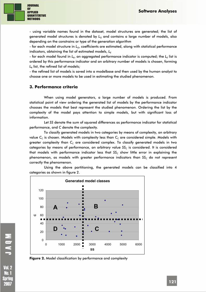
Software Analyses
121
- using variable names found in the dataset, model structures are generated; the list of generated model structures is denoted by LG and contains a large number of models, also depending on the constrains or type of the generation algorithm - for each model structure in LG, coefficients are estimated, along with statistical performance indicators, obtaining the list of estimated models, LE - for each model found in LE, an aggregated performance indicator is computed; the LE list is ordered by this performance indicator and an arbitrary number of models is chosen, forming LR list, the refined list of models; - the refined list of models is saved into a modelbase and then used by the human analyst to choose one or more models to be used in estimating the studied phenomenon.
3. Performance criteria
When using model generators, a large number of models is produced. From statistical point of view ordering the generated list of models by the performance indicator chooses the models that best represent the studied phenomenon. Ordering the list by the complexity of the model pays attention to simple models, but with significant loss of information.
Let SS denote the sum of squared differences as performance indicator for statistical performance, and C denote the complexity.
To classify generated models in two categories by means of complexity, an arbitrary value CC is chosen. Models with complexity less than CC are considered simple. Models with greater complexity than CC are considered complex. To classify generated models in two categories by means of performance, an arbitrary value SSC is considered. It is considered that models with performance indicator less that SSC show little error in explaining the phenomenon, as models with greater performance indicators than SSC do not represent correctly the phenomenon.
Using the above partitioning, the generated models can be classified into 4 categories as shown in figure 2.
Generated model classes
0
20
40
60
80
100
120
0 1000 2000 3000 4000 5000 6000
SS
C
A B
CD
Figure 2. Model classification by performance and complexity

Software Analyses
122
The models shown in figure 1 have certain characteristics: A - complex models that explain the phenomenon; they are usually models with very good statistical performance B - complex models but weak in explaining the phenomenon; they usually include many factors that do not have influence, and analytical expression include many operands and functions that do not express correctly the connection between factors C - simple models but weak in explaining the phenomenon; usually, they do not include enough factors, and use simple operands and functions D - simple models that explain the phenomenon; it is desired that the models used to be from this category. It is obvious that an aggregated indicator is required to take into account both
considered aspects of a model, the statistical performance and expression complexity. This is achieved by using an utility function associated to the model f(c,s), a two variable function, where c denotes the complexity of the model's analytical expression and s denotes the statistical performance indicator.
Consider that the value of the aggregated performance indicator must be minimized, e.g. the sum of squared differences. This leads to ascending ordered model lists by this indicator. The main properties of the function are:
- the function increases with the growth of complexity; the more operands and operators an expression has, its complexity grows; model generators that use only statistical performance to order the generated model lists, usually create long analytical expressions; the complexity is a criterion that has to be minimized; - if the statistical performance indicator is to be minimized (e.g. the sum of squared differences), the function that computes the aggregated indicator value must increase while the factor raises. The aggregated performance indicator is used only in the refinement of models. It
is not intended to replace the statistical performance indicators. Its purpose is to help the analyst to order model lists accordingly to his needs.
Such an indicator is the weighted performance indicator PM given by: PM = SSM
p . CMq
where SSM – SS indicator for model M; CM – complexity of M. p – coefficient of importance for statistical indicator q - coefficients of importance for expression complexity This indicator has the properties exposed above. For example, for p=1 and q=0,
the indicator becomes the same with SS. Setting different values for p and q, the importance of the two factors is modified.
4. Software for model refinement
Model refinement is achieved using dedicated software. Modelbases create the context for model refinement offering specific instruments for modeling and integrating aspects of modeling activity.
Modelbases are complex software constructions offering functions for:

Software Analyses
123
• defining, retrieving and updating models • modeling applications management • estimation and validation of coefficients • automated model generation from existing datasets • dataset management
A representation of the modelbase structure detailing the model generator branch is presented in figure 3.
Figure 3. Modelbase structure with emphasis on model generators
Model generators are modelbase instruments that build model structures from a
given class using variables found in the dataset given as input. Model classes group models with the same structure, e.g. linear models, linear models with lagged variables, nonlinear models. For each class a model generator is developed. Each dataset contains data series for the recorded variables. The endogenous variable is specified and the generator builds analytical expressions using influence factors. For each model structure, coefficients are estimated and a performance indicator is computed. The resulting model list is ordered by the performance indicator. The analyst chooses between the best models an appropriate form that later will be used in estimating the studied characteristic.
The nonlinear model generator is intended for building nonlinear models for software metrics estimation. The algorithm is based on generating expressions in polish form using a combinatorial method.
An expression is built up of operands and operators. In this case, operands are represented by independent variables and coefficients. Operators consist of elementary operations and other functions.
Consider the multiplication operator, *, and two operands. a and b. The operation a*b can be viewed as the result of a function, multiply, that has the form: multiply(a ,b) = a*b, where a ,b are real numbers
In the same manner other operations are treated, building plus(a, b) = a +b power(a, b) = a b log(a ,b) = log a b
Modelbase
Model management
Model generators
Dataset management
Linear model generator
Lagged variables model
generator
Nonlinear model
generator

Software Analyses
124
This representations permits rephrasing of expressions, for example, given the expression: a + b * c + d e, it is equivalent with plus ( plus ( a , multiply (b , c) ) , power ( d , e ) ).
Simplifying, it can be written as: + + a * b c ^ d e, where ^ denotes rising to power operation.
It is observed that this form corresponds to the polish notation, and has several advantages:
• it is easy to evaluate such an expression using a stack and pushing element by element in reverse order as long as that element is an operand or popping and operating a number of operands when the element is an operator and then pushing the result back on the stack; the value that remains on the stack is the value of the expression
• it is easy to build an expression directly in polish notation and when needed to be reconstructed an ordinary form. In order to build an expression directly in polish notation, expression elements are
separated into sets. Let the set containing the influence factors symbolic names be denoted by V. Let the
set containing the operators be denoted by O. Let CO denotes the set {q} where q marks the apparition of a coefficient in the expression. The set of expression elements is the reunion E=V U CO U O. Consider the model: TIME_DEV = a * CC b * PR c + d where
• studied variable: TIME_DEV, the time needed to develop a software module • influence factors: CC – the cyclomatic complexity of module assessed at design time,
PR – the rating of the programmer assigned to this activity; V={CC , PR} • operators: O = {+, *, ^} • coefficients : {a, b, c, d} The equivalent polish notation is: + * a * ^ CC b ^ PR c d.
The nonlinear model generator uses internally the above representation of models. Using a combinatorial algorithm expressions are built directly in polish form. The parameters for this process are:
• the operand set, V • the coefficient set, CO • the operator set, O • the maximum length of the stack • the maximum complexity of the generated expression
The model generation is an important step in the refinement process. The nonlinear model generator is suitable for modeling as the phenomena do not always follow linear laws.

Software Analyses
125
5. Experimental results
Consider the model that estimates the time required for fixing a defect from a program module taking into account its severity and the number of code lines estimated to be modified or added:
FIX_HOURS = f(LOC_COUNT, SEVERITY) where
FIX_HOURS – the endogenous variable to be estimated, measured by man hours LOC_COUNT – estimated number of lines of code involved in the fix SEVERITY – the severity of the defect, between 1 and 5
The sets taken into account are: • S = {plus, multiply, power} • V = { LOC_COUNT, SEVERITY }
It observed that only addition, multiplication and raising to power operations are permitted.
Using a nonlinear model generator with specific constraints the list of generated models is filtered and reduced in size. Constraints limit consecutive raising to power operations, consecutive operations on coefficients and a maximum stack dimension of 13. Consider the dataset D described in table 2. Table 2. Dataset used for model generation No. FIX_HOURS SEVERITY SLOC_COUNT
1 1 2 4 2 1 2 10 3 1 3 1 4 1 3 2 5 2 2 15 6 3 3 15 7 40 5 200
....
102 8 3 2 103 20 2 265 104 30 5 20
The list of generated models is presented in table 3.
Table 3. List of generated models for the selected dataset ID Expression
M1 2.86*SEVERITY+0.284*LOC_COUNT-3.394 M2 1.115*10-4*SEVERITY7.781 M3 1.196*LOC_COUNT0.753-0.134 M4 1.125*(SEVERITY*LOC_COUNT)0.601-0.898 M5 1.081*SEVERITY0.036*LOC_COUNT0.763+0.082 M6 0.321*SEVERITY2.204+0.501*LOC_COUNT0.891+0.253 M7 (2.877*SEVERITY+0.833*LOC_COUNT)0.814-2.827
For CC = 23 and SSC = 2.00 the generated models classify as presented in figure 4.

Software Analyses
126
Model classification
1.921; 35.161.939; 27.11
1.978; 12.75
3.503; 6.75
1.978; 27.11
1.964; 19.6 2.194; 19.6
05
10152025303540
0 1 2 3 4
SS
C
SSc=2.000
Cc = 23
Figure 4. Generated models classification
Ordering model lists by statistical performance indicator is done when model performance is the main objective of the analysis. The list of models, ordered by statistical performance indicator SS, given as output is shown in table 4. Table 4. Models ordered by statistical performance indicator SS
ID Expression SS
(104 units)
C
M6 0.321*SEVERITY2.204+0.501*LOC_COUNT0.891+0.253 1.921 35.16 M7 (2.877*SEVERITY+0.833*LOC_COUNT)0.814-2.827 1.939 27.11 M1 2.86*SEVERITY+0.284*LOC_COUNT-3.394 1.964 19.60 M3 1.196*LOC_COUNT0.753-0.134 1.978 12.75 M5 1.081*SEVERITY0.036*LOC_COUNT0.763+0.082 1.978 27.11 M4 1.125*(SEVERITY*LOC_COUNT)0.601-0.898 2.194 19.60 M2 1.115*10-4*SEVERITY7.781 3.503 6.75
As seen in table 4 the best model that estimates FIX_HOURS is M6, taking into account only the quality of estimation. However, it has the greatest complexity among all the rest, and uses five coefficients and two variables. Other models with resembling performance are M7, M1, M3, M5.
Ordering the list by the weighted indicator PM with parameters p=3 and q=1, M3 becomes eligible. It has few parameters and a single variable that is easy to obtain data for. It uses only a variable to asses the phenomenon. The results are shown in table 5. Table 5. Models ordered by aggregated indicator with p=3 and q=1
ID Expression SS (104 units) C
PM p=3 q=1
M3 1.196*LOC_COUNT0.753-0.134 1.978 12.75 98.67089 M1 2.86*SEVERITY+0.284*LOC_COUNT-3.394 1.964 19.60 148.4843 M7 (2.877*SEVERITY+0.833*LOC_COUNT)0.814-2.827 1.939 27.11 197.6346 M4 1.125*(SEVERITY*LOC_COUNT)0.601-0.898 2.194 19.60 206.9979 M5 1.081*SEVERITY0.036*LOC_COUNT0.763+0.082 1.978 27.11 209.8014 M6 0.321*SEVERITY2.204+0.501*LOC_COUNT0.891+0.253 1.921 35.16 249.2476 M2 1.115*10-4*SEVERITY7.781 3.503 6.75 290.1511

Software Analyses
127
The parameter setting shown in table 5 pays more attention to model performance. It is recommended that analysts use such settings when the studied phenomenon do not offer clues for the form of the link between the variables.
The p and q parameters are used to increase or decrease the importance of factors. Different values for p and q offer different list orderings according to analyst's interest. For example, the list ordering for p=1 and q=2 is shown in table 6. Table no.6 Models ordered by aggregated indicator with p=1 and q=2
ID Expression SS
(104 units)
C PM p=1 q=2
M2 1.115*10-4*SEVERITY7.781 3.503 6.75 159.6054 M3 1.196*LOC_COUNT0.753-0.134 1.978 12.75 321.5486 M1 2.86*SEVERITY+0.284*LOC_COUNT-3.394 1.964 19.60 754.4902 M4 1.125*(SEVERITY*LOC_COUNT)0.601-0.898 2.194 19.60 842.8470 M7 (2.877*SEVERITY+0.833*LOC_COUNT)0.814-2.827 1.939 27.11 1425.0721 M5 1.081*SEVERITY0.036*LOC_COUNT0.763+0.082 1.978 27.11 1453.7353 M6 0.321*SEVERITY2.204+0.501*LOC_COUNT0.891+0.253 1.921 35.16 2374.7894
The parameter setting shown above pays attention to very simple models. In this case simplicity is more valuated than performance. This kind of setting is recommended only when there is a clue that the link between the studied variables follows a simple expression.
Subsequent updates on the database require that periodical estimation of coefficients to track changes.
The best models obtained are stored and operated on using the modelbase.
5. Conclusions
The refinement process is guided by the analyst according to his needs. This process is complex and operates on model sets. Model sets are built by model generators using the datasets that are to by analyzed.
Performance criteria are needed to choose among the models. The analyst uses these criteria to order generated model lists.
The most important criterion for list ordering is the statistical performance. The model is used to explain a phenomenon and predict evolution when giving certain inputs. Ordering the model lists by this criterion gives access to the best models and it is recommended to use it when precision is a critical aspect of the modeling activity.
Model complexity is a criterion that orders the models according to their structure. It is incorrect to use the complexity alone when ordering model lists.
The aggregated performance indicator is a solution to combine both studied aspects of a model. The analyst can set parameter settings that give separate importance to performance and complexity. The purpose of using the aggregated performance indicator is to obtain simple models but with minimum loss of information in explaining the studied phenomenon.
On the other hand, the analyst is required to interpret results, to asses different variants. A group of models from the top of the ordered list are chosen and used. It is important to validate the models assessing their performance over time or using other datasets.
Software Analyses
128
The aggregated performance indicator does not replace statistical performance indicators. It is intended to be used only in the context of model generation.
Bibliography 1. Boja, C., Ivan, I. Metode statistice în analiza software, Editura ASE, Bucharest, 2004 2. Ivan, I., Popescu, M. Metrici software, Editura Inforec, Bucharest, 1999 3. Ivan, I., Visoiu, A. Baza de modele economice, Editura ASE, Bucharest, 2005 4. Jalote, P. Software Project Management in Practice, Addison Wesley, 2002 5. Toma, C., Ivan, I., Popa, M., Boja, C. Data Metrics Properties, Proceedings of International
Symposium October 22-23, Iasi, 2004, p. 45-56 6. Visoiu, A., Garais, G. Nonlinear model structure generator for software metrics estimation,
The 37th International Scientific Symposium of METRA, Bucharest, May, 26th - 27th, 2006, Ministry of National Defence, published on CD
7. Visoiu, A., Ivan, I. Rafinarea metricilor software, Economistul, supliment Economie teoretica si aplicativa, nr.1947 (2973), 29 august 2005
1 Adrian Visoiu graduated the Bucharest Academy of Economic Studies, the Faculty of Cybernetics, Statistics and Economic Informatics. He has a master degree in Project Management. He is a PhD student at Doctoral School of Bucharest Academy of Economic Studies in the field of Economic Informatics. He is an assistant lecturer in the Economic Informatics Department of the Bucharest Academy of Economic Studies. He published 7 articles and he is coauthor of “Baza de modele economice” book.

Software Analyses
129
PERFORMANCE ANALYSIS OF PARALLEL ALGORITHMS
Felician ALECU1 PhD, University Lecturer, Economic Informatics Department, Academy of Economic Studies, Bucharest, Romania E-mail: [email protected] Abstract: A grid is a collection of individual machines. The goal is to create the illusion of a powerful computer out of a large collection of connected systems sharing resources. Some resources may be used by all users of the grid while others may have specific restrictions. The most common resource is computing cycles provided by the processors. Grid computing represents unlimited opportunities in terms of business and technical aspects. The main reason of parallelization a sequential program is to run the program faster. The first criterion to be considered when evaluating the performance of a parallel program is the speedup used to express how many times a parallel program works faster than the corresponding sequential one used to solve the same problem. When running a parallel program on a real parallel system there is an overhead coming from processors load imbalance and from communication times needed for changing data between processors and for synchronization. This is the reason why the execution time of the program will be greater than the theoretical value. Key words: grid computing; grid network; parallel processing; performance analysis; parallel speedup; parallel efficiency
The performance of parallel algorithms executed on multiprocessor systems
The first criterion taken into consideration when the performances of the parallel systems are analyzed is the speedup used to express how many times a parallel program works faster than a sequential one, where both programs are solving the same problem. The most important reason of parallelization a sequential program is to run the program faster.
The speedup formula is
p
s
TT
S =
where - Ts is the execution time of the fastest sequential program that solves the
problem;

Software Analyses
130
- Tp is the execution time of the parallel program used to finalize the same problem.
If a parallel program is executed on a computer having p processors, the highest value that can be obtained for the speedup is equal with the number of processors from the system. The maximum speedup value could be achieved in an ideal multiprocessor system where there are no communication costs and the workload of processors is balanced. In such a system, every processor needs Ts/p time units in order to complete its job so the speedup value will be as the following:
p
pTT
Ss
s ==
There is a very simple reason why the speedup value cannot be higher than p – in such a case, all the system processors could be emulated by a single sequential one obtaining a serial execution time lower than Ts. But this is not possible because Ts represents the execution time of the fastest sequential program used to solve the problem.
According to the Amdahl law, it is very difficult, even into an ideal parallel system, to obtain a speedup value equal with the number of processors because each program, in terms of running time, has a fraction α that cannot be parallelized and has to be executed sequentially by a single processor. The rest of (1 - α) will be executed in parallel.
The parallel execution time and the speedup will become:
pTTT ssp /)1( αα −⋅+⋅=
1)1(/)1(1
/)1( +−⋅=
−+=
−⋅+⋅==
pp
ppTTT
TT
Sss
s
p
s
ααααα
When ∞→p , we have
α1lim =
∞→S
p
The maximum speedup that could be obtained running on a parallel system a program with a fraction α that cannot be parallelized is 1/α, no matter of the number of processors from the system.
For example, if a program fraction of 20% cannot be parallelized on a four processors system, the parallel execution time and the speedup will be equal with:
sssp TTTT ⋅=⋅+⋅= 4.04/8.02.0
5.24.0
14.0
==⋅
=s
s
TT
S
The parallel execution time will be 40% of the serial execution time and the parallel program will be only 2.5 times faster than the sequential one because 20% of the program cannot be parallelized (figure 1). The maximum speedup that we can obtain is 1/0.2 = 5 and this means that the parallel execution time will never be shorter than 20% of the sequential execution time even in a system with an infinite number of processors.
Amdahl low concludes it is very important to identify the fraction of a program than cannot be parallelized and to minimize it.

Software Analyses
131
The parallel efficiency quantifies the number of the valuable operations performed by the processors during the parallel program execution. The parallel efficiency could be expressed as the following:
pSE =
where S is the speedup and p represents the number of the processors from the system.
Figure 1. Parallel execution on an ideal system
Due to the fact the speedup value is lower than the number of processors, the
parallel efficiency will be always located between 0 and 1. Another important indicator is the execution cost representing the total processor
time used to solve the problem. For a parallel application, the parallel cost could be calculated according with the following formula:
pp TpC ⋅=
For a sequential program, its cost (sequential cost) will be equal with the total execution time:
ss TC =
For this reason, the parallel efficiency could be also expressed as the following:
p
s
p
sp
s
CC
TpT
pT
T
pSE =
⋅===
Finally, the supplementary cost of parallel processing indicates the total processor times spent for secondary operations not directly connected with the main purpose of the program that is executed. Such a cost cannot be identified for a sequential program.
spspl TTpCCC −⋅=−=sup
The figure 2 presents the way in which a parallel program will be executed on a real 4 processor system. This time, the program contains a fraction of 20% that cannot be
P1 P4 P3 P2 P1
100% sequential
Sequential execution Parallel execution
20% sequential
20% 20% 20% 20%

Software Analyses
132
parallelized, the load of the processors is not balanced and the communications times are not neglected anymore.
The source of this type of cost is represented by the following elements: - load imbalance – is generated by the unbalanced tasks that are assigned to
different processors. In such a case, some processors will finish the execution earlier so they need to wait in an idle state for the other tasks to be completed. Also, the presence of a program fraction that cannot be parallelized generates load imbalance because this portion of code should be executed by a single processor in a sequential manner.
- supplementary calculations – generated by the need to compute some value locally even if they are already calculated by another processor that is, unfortunately, busy at the time when these data are necessary.
- communication and synchronization between processors – the processors need to communicate each others in order to obtain the final results. Also, there are some predefined execution moments when some processors should synchronize their activity.
Figure 2. Parallel execution on a real system
In order to obtain a faster program, we can conclude we need to reduce to the
minimum the fraction that cannot be parallelized, to assure the load balance of the tasks at the processor level and also to minimize the times dedicated for communication and synchronization.
The performance of parallel algorithms executed on grid systems A grid is a collection of machines that contribute any combination of resources as a
whole. Basically, grid computing represents a new evolutionary level of distributed computing. It tries to create the illusion of a virtual single powerful computer instead of a large collection of individual systems connected together. These systems are sharing various resources like computing cycles, data storage capacity using unifying file systems over
P1 P4 P3 P2 P1
100% sequential
Sequential execution Parallel execution
20% sequential
~20% ~20% ~20% ~20%

Software Analyses
133
multiple machines, communications, software and licenses, special equipments and capacities.
The use of the grid is often born from a need for increased resources of some type. Grids can be built in all sizes, ranging from just a few machines in a department to groups of machines organized in hierarchy spanning the world. The simplest grid consists of just few machines, all of the same hardware architecture and same operating system, connected on a local network. Some people would call this a cluster implementation rather than a grid. The next step is to include heterogeneous machines but within the same organization. Such a grid is also referred to as an intragrid. Security becomes more important as more organizations are involved. Sensitive data in one department may need to be protected from access by jobs running for other departments. Dedicated grid machines may be added to increase the service quality. Over time, a grid may grow to cross organization boundaries and may be used for common interest projects. This is known as an intergrid.
We will consider a parallel program that is executed in a time of pT on a grid
network composed by p computers numbered from 1 to p. Also, the sequential execution
time of the program on an individual station will be isT .
The speedup of a parallel program that runs on the cluster of stations can be computed by dividing the best sequential time by the parallel one:
p
is
pi
grid TT
S 1min ==
The individual computers of the grid network are not identical so they will have different processing powers. The ratio between the power of an ordinary computer and the most powerful one can be expressed can be expressed by the formula:
is
js
pj
i TT
P 1min == , i = 1..p
Each proportion will satisfy the following relation: 1≤iP .
Based on these ratios, we can calculate the heterogeneity factor of the computers being part of the cluster of stations by using the differences in power that exist between them:
p
PHF
p
ii∑
=
−= 1
)1(
During a program execution, the degree of parallelism will vary and this will generate the load imbalance of the processors from the system. Basically, the degree of parallelism is equal with the number of processors that are participating to the program execution.
The average degree of parallelism is defined as being the average number of stations that were active during the entire execution of the program, as the following:
p
p
i
ip
m T
TGP
∑== 1

Software Analyses
134
where ipT represents how much time the station i was active.
The speedup formula can be now obtained based on the heterogeneity of the stations that are part of the grid network and using the average degree of parallelism of the program that is executed:
)1( GEGPS mgrid −⋅= .
In conclusion in order to obtain a faster parallel program, there is the need to
reduce to the minimum the fraction that cannot be parallelized, to assure the load balance of the tasks at the processors level and also to minimize the amount of data used for communication and synchronization.
References 1. Grama, A. et al, An Introduction to Parallel Computing: Design and Analysis of Algorithms,
Addison Wesley, 2nd edition, 2003 2. Gropp, W. et al, The Sourcebook of Parallel Computing, Morgan Kaufmann, 2002 3. Jordan, H. F., Jordan, H. E. Fundamentals of Parallel Computing, Prentice Hall, 2002 4. Joseph, J., Fellenstein, C., Grid Computing, Prentice Hall, 2003 5. Ladd, S., Guide to Parallel Programming, Springer-Verlag, 2004 6. Tanenbaum, A. S. Distributed Operating Systems, Prentice Hall, 1995 7. Wyrzykowski, R., Parallel Processing And Applied Mathematics, Springer, 2004
1 Alecu Felician has graduated the Faculty of Cybernetics, Statistics and Economic Informatics in 2000 and he holds a PhD diploma in Economics from 2006. Currently he is lecturer of Economic Informatics within the Department of Economic Informatics at Faculty of Cybernetics, Statistics and Economic Informatics from the Academy of Economic Studies. He is the author of more than 20 journal articles in the field of parallel computers, grid computing and distributed processing.

Experimental Design
135
EXPERIMENTAL DESIGN TECHNIQUES APPLIED TO STUDY OF
OXYGEN CONSUMPTION IN A FERMENTER1
Blanca VELÁZQUEZ MSc, Department of Biotechnology Development Institute of Hygiene, Faculty of Medicine, University of the Republic of Uruguay Av. Alfredo Navarro 3051, C.P. 11600. Montevideo, Uruguay E-mail: [email protected] Víctor MARTÍNEZ-LUACES Chemical Engineer and University Professor, Institute of Chemical Engineering, Faculty of Engineering, University of the Republic of Uruguay, Av. Julio Herrera y Reissig 565, C.P. 11300. Montevideo, Uruguay E-mail: [email protected]
Adriana VÁZQUEZ Chemical Engineer, Department of Bioengineering Institute of Chemical Engineering, Faculty of Engineering, University of the Republic of Uruguay, Av. Julio Herrera y Reissig 565, C.P. 11300. Montevideo, Uruguay E-mail: [email protected] Valerie DEE PhD, Department of Biotechnology Development Institute of Hygiene, Faculty of Medicine, University of the Republic of Uruguay Av. Alfredo Navarro 3051, C.P. 11600. Montevideo, Uruguay E-mail: [email protected]
Hugo MASSALDI PhD, University Professor, Department of Biotechnology Development Institute of Hygiene, Faculty of Medicine, University of the Republic of Uruguay Av. Alfredo Navarro 3051, C.P. 11600. Montevideo, Uruguay E-mail: [email protected]
Abstract: The dependence of the volumetric rate of oxygen consumption on the variables agitation and air flow, was studied in a laboratory scale fermenter. A 22 factorial experimental design, with four axial points and four replicates of the central point, was used. The coefficients for the two-variables, quadratic model were calculated. The 'fit' of the model with the empirical data was studied using a lack of fit test. The surface response methodology was used to maximize the dependent variable, volumetric rate of oxygen consumption. The response surface obtained showed an absolute maximum on the domain’s boundary, consistent with theoretical considerations indicating that a relative maximum inside the domain was impossible. This approach allowed us to derive a model to predict volumetric rate of oxygen consumption in a standard laboratory fermenter, as a function of agitation and air flow, i.e., the two variables selected. Key words: surface response methodology; volumetric rate of oxygen consumption

Experimental Design
136
Introduction
Production of recombinant proteins is most economical when there is a high cell concentration in the fermenter and the protein product is also expressed at a high level. Aerobic or facultative anaerobic cells in culture require adequate transfer of oxygen from the gaseous phase (usually air, or air enriched with oxygen) to the liquid phase, where the cells consume oxygen for respiration. In lab experiments with flasks, oxygen supply is typically achieved by flask stirring with a high ratio of air to liquid flask volume, which often becomes a significant parameter (Martínez et al., 2006). Aeration and agitation are carried out in the fermenter to provide the culture with oxygen, and to some extent to stabilize physicochemical parameters. In aerobic fermentations, oxygen supply may become a limiting factor, especially in very large-scale systems. Oxygen is not very soluble (its saturation concentration in water is 7 mg L-1 when air is bubbled through it at 1 atm. at 30ºC) (Bailey and Ollis, 1986). Its rate of solubilization is a function of several factors: the area of the gas-liquid interphase, temperature, contact time, composition of the culture medium, cell density and cell activity, among others (Pirt, 1975).
In a given system, some factors, such as temperature, are pre-set or are easily controlled in order to achieve optimum conditions. Therefore, the contact area, the contact time, and agitation are the most important variables determining oxygen transfer (Werman and Wilki, 1973). Oxygen supplied into the fermenter by air flow and agitation becomes limited as time goes on, due to alterations in the medium. There are therefore two separate factors that often determine how long the culture can continue. The first factor is the demand for oxygen, which requires more or less oxygen in solution in the culture medium, according to the requirements of the cells. The second factor is the capacity of the system to transfer oxygen into the liquid phase. Demand for oxygen in the culture is determined by cell concentration, the specific growth rate, and oxygen transfer into the medium, and is satisfied by oxygen in the culture medium entering the cells (Calam and Russell, 1973). Oxygen transfer is limited by the velocity of air bubbles through the culture medium, and the velocity of oxygen transport into cells. It is important to use appropriate experimental design to discover the oxygen transfer potential of the fermenter, according to its operating conditions (Phillips and Johnson, 1961).
In our work, we have studied the variation in volumetric rate of oxygen consumption (kLaCL*) of the culture as a function of agitation and air flow. From a statistical point of view, this implies studying a real function with two independent variables, preferably using the surface response methodology (S.R.M.) (Montgomery, 2005). We used a linear regression model with two variables, and the following terms: an independent term, two linear terms, two pure quadratic terms, and an interaction term. The main reason for choosing this model was our interest in studying two effects: curvature and interaction between variables. In order to adjust the parameters of this model to our data, the experiment was properly designed with replicate data points so as to be able to estimate error. We chose the Box-Wilson design (Box and Wilson, 1951), commonly called central composite design (CCD), in our case with four centerpoint runs (Montgomery, 2005).
Our aim was to obtain a well-validated quadratic model which would allow prediction of kLaCL* values, in a fermenter, as a function of air flow and agitation, within the

Experimental Design
137
working limits of those variables. This approach should be useful for the future evaluation of recombinant streptolysin-O (Velázquez et al., 2005) production in a fermenter.
Materials and methods
Determination of the volumetric rate of oxygen consumption. A 3-litre fermenter (Bio Flo III, Batch-Continuous Fermenter, New Brunswick Scientific, Edison, N.J., U.S.A.) was used with a working volume of 2 litres of water. The fermenter was automatically controlled by software (AFS-BioCommand Bioprocessing Software, version 2.60; New Brunswick Scientific). Volumetric rate of oxygen consumption (kLaCL*) was determined by oxidation of S2O3
2- to SO4 2- in the presence of metal ions (Co 2+ or Cu 2+) as the catalyst (Wernan and Wilki, 1973). The determination was carried out in 2 litres of distilled water at 37ºC, with 20 g/L S2O3
2- and 1.5 g/L CuSO4 as catalyst. For each assay, the rotation speed of the agitator was adjusted, and air flow was also adjusted, according to the settings pre-determined by the experimental design (50 - 450 r.p.m. for agitation and 0.500 – 4.000 L/min. for air flow). Samples of 5 mL were taken for analysis at different time-points (from t = 0 and at intervals of 5 to 15 minutes) until all the sulfite had been oxidized.
Experimental Design. With the volumetric rate of oxygen consumption (kLaCL*) results, surface response studies were carried out using a 22 factorial experimental design,
with four axial points ((±α, 0) and (0, ±α), where α = 2 ) and four replicates of the
central point, totaling 12 experiments (Montgomery, 2005). The coded values of the
independent variables were: -α, 1, 0 (central point), +1, +α (Table 1). The experimental
plan is shown in Table 2 for the coded values in Table 1. Table 1. Coded values of independent variables. Coded levels used in experimental design for S.R.M. of kLaCL* in fermenter.
Levels Variable Symbol
-α -1 0 +1 +α Agitation (r.p.m.) X1 50 109 250 392 450
Air flow (L/min.) X2 0.500 0.836 2.250 3.660 4.000
Table 2. Experimental plan for SRM study of kLaCL*. Values of independent variables agitation (r.p.m) and air flow (L/min.) for determining kLaCL* in the fermenter, coded as in Table 1.
Experiment Nº Agitation (x1) Air flow (x2) 1 -1 -1 2 +1 -1 3 -1 +1 4 +1 +1 5 0 0 6 0 0 7 -α 0 8 +α 0 9 0 -α
10 0 +α 11 0 0 12 0 0

Experimental Design
138
Analysis of the proposed model. Analysis of the model proposed for the observed data, and calculation of its coefficients, were carried out using the Statistica version 4.5 software (Statsoft). For preliminary assessment of the model's fit, correlation coefficient R and its square, R2, were used (Montgomery, 2005). The statistical significance of the parameters of the model was determined by Student's t test and corroborated by Fisher's F test (Montgomery, 2005). In this test, the higher the critical value of t and the lower the value of p, the greater the effect or significance of the coefficient in the model (Montgomery, 2005). Subsequently, the goodness of fit of the model was examined by the lack of fit (L.O.F.) test (Draper and Smith, 1998). There were 5 degrees of freedom in our full quadratic model. Twelve experiments were carried out, with n-1 degrees of freedom. The degrees of freedom of the error were calculated by difference as always. Finally, the surface response methodology (Montgomery, 2005) was used to find the maximum volumetric rate of oxygen consumption (kLaCL*).
Results
Determination of the coefficients for the model of volumetric rate of oxygen consumption (kLaCL*) as a function of agitation and air flow. Table 3 shows experimental values for volumetric rate of oxygen consumption, and those calculated according to the following quadratic model: y = β0 + β1 X1 + β2 X2 + β11 X1
2 + β22 X22 + β12 X1X2
where y is the predicted value of volumetric rate of oxygen consumption (kLaCL*) (mmol/L/h) X1= agitation (r.p.m.) in coded form X2= air flow (L/min.) in coded form y = 15.50014 + 22.58148 X1 + 6.43198 X2 + 13.12500 X1
2 - .87500 X22 + 4.00000 X1X2.
Table 3. Comparison of experimental and calculated values of kLaCL*. Experimental values of kLaCL* were obtained by the sulfite oxidation method. Calculated values of kLaCL* were obtained from the regression equation y = β0 + β1 X1 + β2 X2 + β11 X1
2 + β22 X22 + β12
X1X2
Agitation (r.p.m.) Air flow (L/min.)
Experimental kLaCL*
(mmol /L/h)
Calculated kLaCL * (mmol /L/h)
109 0.836 5.00 +/- 0.08 2.74
392 0.836 35.00 +/- 0.87 39.90
109 3.660 10.00 +/- 0.15 7.60
392 3.660 56.00 +/- 1.87 60.76
250 2.250 12.00 +/- 0.01 15.50
250 2.250 16.00 +/- 0.27 15.50
50 2.250 6.00 +/- 0.10 9.81
450 2.250 80.00 +/- 4.00 73.68
250 0.500 6.00 +/- 3.00 4.65
250 4.000 24.00 +/- 0.61 22.85
250 2.250 17.00 +/- 0.28 15.50
250 2.250 17.00 +/- 0.28 15.50

Experimental Design
139
Correlation and parameter significance. Results showed that the model fitted with the experimental values in the ranges of the variables studied. Multiple regression analysis results were R = 0.9885 and R2 = 0.9770, indicating a high degree of correlation between the experimental values and those predicted by the model.
Table 4 shows Student's t test applied to individual coefficients in the model, to test their significance. Coefficients β1, β2 and β11 were statistically significant at a 95% confidence level. These are the coefficients for the linear terms for air flow and agitation, and for the quadratic term of agitation.
Table 4. Linear and quadratic coefficients estimated for the quadratic model. Estimated values and probability levels according to Student´s t test. Coefficient Effect on model Student´s t
(5 d.f.) Probability level
(p)
β1 22.58148 13.56670 .000039
β2 6.43198 3.86426 .011829
β11 13.12500 7.05288. .000886 β22 -.87500 -.47019 .658013 β12 4.00000 1.69929 .150014
Table 5 shows analysis of variance (ANOVA) for Fisher's F test. The calculated value
of F was greater than the tabulated value (F1,5 = 6.61), in the case of the coefficients β1, β2 and β11, being significant at the 95% confidence level. However, the F values for coefficients β22 and β12 were not significant. It can be concluded from these results that agitation is the most significant factor in determining volumetric rate of oxygen consumption, followed by the quadratic term for agitation, and thirdly by the air flow. Table 5. Analysis of variance (ANOVA) for regression model of kLaCL* as a function of agitation and air flow. Significance of the model coefficients (NS: not significance at 95 %, S: significance at 95%).
Goodness of fit and response surface of the model. A lack of fit (L.O.F) test
was performed and the results are shown in Table 6. Table 6. ANOVA for L.O.F. test.
Source of variation
Sum of squares
Degrees of
Freedom
Mean squares
F p-value Signifi-cance level
β1 4079.384 1 4079.384 184.0555 .000039 S β2 330.963 1 330.963 14.9325 .011829 S β11 1102.500 1 1102.500 49.7431 .000886 S β22 4.900 1 4.900 .2211 .658013 NS β12 64.000 1 64.000 2.8876 .150014 NS
Residual 110.819 5 22.164
Item Degrees of Freedom Sum of squares Mean squares
Model 5 5658.50775 1131.70155 Error 6 132.15892 22.02649 Total 11 5790.66667

Experimental Design
140
A statistic value F = 51.38 can be obtained by dividing mean squares of model by mean squares of error (Table 6). This value was compared with the critical region [8.75, +∞), obtained by using the F function table, with 5 degrees of freedom for the model and 6 degrees of freedom for the error, with a significance level of α = 0.01. Thus, the 'fit' of the model was statistically significant at the 99% confidence level. The surface response methodology applied to the experimental conditions tested identified a maximum volumetric rate of oxygen consumption of 89.88 mmol/L/h. This maximum corresponded to the coded values of 1.5 for agitation and air flow, that is, 462 r.p.m. and 4.100 L/min. respectively. Thus the maximum is achieved at the highest values of both variables, within the experimental ranges (450 r.p.m and 4.000 L/min. respectively) (Figure 1).
Figure 1. S.R.M. for kLaCL* values. kLaCL* as a function of agitation and air flow (coded values as in Table 1).
Discussion and conclusions
The experimental design chosen was appropriate for estimating the coefficients in a full quadratic regression with two independent variables. In our particular case, we concluded that the 'fit' of the model to the experimental data was statistically significant at the 99% confidence level. However, some of the individual coefficients of the model equation were not significant, even at the 95% confidence level. The non significant coefficients were: the quadratic term for air flow (β22) and the one for the interaction between agitation and air flow (β12). The implication from the bioengineering point of view is that the most important variable to take into account in ensuring adequate volumetric rate of oxygen consumption (kLaCL* ) in cultures in a fermenter, is agitation. However, the biological needs of the microorganism must be met in order to maximize the yield of the desired

Experimental Design
141
recombinant protein, so air flow must also be taken into account, as a complementary variable. From the statistical point of view, the above could suggest applying a significance test for a sub-model (Rencher, 2000), in order to examine 'goodness of fit' with a simpler model in which the quadratic term for air flow and the interaction term are excluded.
The obtained surface corresponding to the full quadratic model might be further explored by increasing the experimental values of both air flow and agitation.
The absolute maximum for volumetric rate of oxygen consumption that we found was located at the vertex of the region, corresponding to the highest values of the variables. Since the function kLaCL* increases with respect to both air flow and to agitation, a relative maximum inside the domain cannot be expected (Banks, 1980). The results of the S.R.M. performed (Figure 1) are totally consistent with the above theoretical consideration. If the same procedure is carried out to search for another maximum, using higher values for air flow and agitation, we would expect a surface response similar to Figure 1, i.e., with the function increasing with both variables, and an absolute maximum at the boundary of the domain. It would be convenient to use a maximum slope method for this exploration (Montgomery, 2005). For this purpose, determining the maximum slope as a function of the variables of the model would be useful.
References 1. Bailey, J. E. and Ollis, D. F., Biochemical engineering fundamentals; 457-500. 2nd Edition,
McGraw-Hill Book Co. New York, U.S.A, 1986 2. Banks, G. T. , Scale-up of fermentation process, Top. Enzyme Ferment. Biotechnol. 3, 170-266,
1980 3. Box, G. E. and Wilson, K. B., On the Experimental Attainment of Optimum Conditions,
Journal of the Royal Statistical Society, Series B, 13, 1-45, 1951 4. Calam, C. T. and Russell, D. W., Microbial aspects of fermentation process development, J.
Appl. Chem. Biotechnol. 23, 225-237, 1973 5. Draper, N. R. and Smith, H., Applied Regression Analysis, 47-55. J Wiley & Sons, New York,
U.S.A, 1998 6. Martínez, V., Guineo, G., Velázquez, B., Chabalgoity, J. A. and Massaldi, H., Bifactorial design
applied recombinant protein expressions, Journal Data Science, 4, 247-255, 2006 7. Montgomery, D. C., Design and Analysis of Experiments; 405-458. 6th Edition, J. Wiley &
Sons. New Jersey, U.S.A, 2005 8. Phillips, D. H. and Johnson, M. J., Oxygen transfer in fermentations, Sci. Rep. Ist. Super.
Sanita, 1, 1 90-195, 1961 9. Pirt, S. J., Principles of Microbe and Cell cultivation, 4-15. 1st. Edition, Blackwell Scientific
Publications, London, U.K, 1975 10. Rencher, A. C., Linear Models in Statistics, 170-213. John Wiley & Sons, New York, U.S.A, 2000 11. Velázquez, B., Massaldi, H., Battistoni, J. and Chabalgoity, J. A., Construction and expression of
recombinant Streptolysin-O; pre-evaluations of it use in immunoassays, Clinical Laboratory Diagnostic Immunology, 12, 683-684, 2005
12. Wernan, W. C. and Wilki, C. R., New method for evaluation of dissolved oxygen response for Kla determination, Biotech. Bioeng.,15, 571, 1973
1 To whom correspondence should be addressed: E-mail: [email protected] Phone: +(598) 2 4871288 ext. 1122 Fax: +(598) 2 4873073

Theoretical Approaches
142
ASPECTS ON STATISTICAL APPROACH OF POPULATION HOMOGENEITY
Alexandru ISAIC-MANIU PhD, University Professor, Department of Statistics and Economic Prognosis University of Economic Studies, Bucharest, Romania (Co)Author of the books: Proiectarea statistica a experimentelor (2006), Enciclopedia calitatii (2005), Dictionar de statistica generala (2003), Statistica pentru managementul afacerilor (2000), Metoda Weibull (1983) E-mail: [email protected], Web page: http://www.amaniu.ase.ro
Viorel Gh. VODĂ PhD, Senior Scientific Researcher, Institute of Mathematical Statistics and Applied Mathematics of the Romanian Academy, Bucharest, Romania Co-author of the books: Proiectarea statistica a experimentelor (2006), Dictionar de statistica generala (2003), Manualul calitatii (1997) E-mail: [email protected] Abstract: In this article we emphasize the manner in which this statistical indicator - the variation coefficient (v) - could help the inference on measurable characteristics generated by technological processes. Our interest lies upon the so-called SPC- Statistical Process Control; the main result obtained is the following: if the coefficient of variation is known, then the statistical distribution of capability index is of ALPHA-type distribution (Družinin). We also put into light some links between (v) and Taguchi’s quality loss function. Key words: variation coefficient; signal-to-noise ratio; Alpha distribution; capability index; quality loss function
1. Introduction
It is well-known that when we desire to compare the spread (dispersion) in two sets of data if we choose to do this straightforwardly by comparing the two standard deviations - this may lead to fallacious conclusions. This may be due to the fact that the variables/characteristics involved are measured in different units. Furthermore, if the same unit of measurement is employed, one may still see a large difference between the two means.
Such situations may occur with data obtained from various areas of interest - from technology to biostatistics.
To deal with cases like those, we need a measure (an indicator) of relative variation rather than absolute variation. The coefficient of variation, which expresses the standard deviation as a percentage of the mean, is just such an indicator: since the mean and standard deviation have the same measurement unit (as the original data, in fact) this coefficient of variation is independent of any unit of measurement.

Theoretical Approaches
143
Theoretically, if X is a measurable characteristic - that is a continuous random
variable (c.r.v.) with finite mean-value and variance ( ) ( )( )+∞<+∞< x,x VarE , then the
ratio
( )( ) ,xE
xVarV = where ( ) 0xE ≠ (1)
is the coefficient of variation (c.v.) associated to X. Let us notice that the request for finitude is mandatory since there are distributions for which this condition is not fullfiled. For instance, the Cauchy distribution:
( ) Rπ
f ∈+
⋅= x,x1
11x:x 2 (2)
“has no average value” - since
( ) ( ) ( ) ∞−∞=∞−∞+
+=+
=⋅= ∫∫ 22 x1ln
21x
x1x2
21xxx
ππ RR
ddfxE (a “senseless” form)
(3) or in the case of inverse Rayleigh variable:
( ) ( ) 0a,0x,x/aexpax2a;x: 23 >>−= −fX (4)
where the variance is ( ) +∞=xVar (see Treyer, 1976 [17] or Bârsan-Pipu et al., 1999 [2]).
2. Some properties related to sample coefficient of variation
As it is well-known, in practice we work with the sample coefficient of variation V , that is:
x/SV = , where ∑= ixn1x and ( ) ( )∑ −−= 1n/xxS 22
i (5)
On the other hand, some authors (see Mc. Kay, 1932 [13] consider also the form:
x/SV 00 = , where and ( )∑ −= n/xxS 220 i (6)
which provides that the statistics ( )20
20 V1/VB +⋅ where ( )2V/11nB += is chi-square
distributed with (n-1) degrees of freedom ( )21n−χ .
Johnson and Welch (1940, [12]) proved that V/n has a non-central t-distribution
with ( )1n − degrees of freedom and V/n as noncentrality parameter and the underlying
variable x is normally distributed ( )2,N σμ .
F.N. David (1949 [3]) gave some approximations to the first four moments of V ,
assuming that x has a normal variance and the mean value of μσ= /V is not (very) large.
Iglewicz, Myers and Howe (1968 [9]) provided some approximations for the
percentiles pV of V , assuming also normality of X and imposing to the value of V, the

Theoretical Approaches
144
restriction 5.0V ≤ . The percentiles are obtained from the equation { } p1VVobPr p −=≤
via 2p;1n−χ - the quantiles of chi-squared distribution.
Two years later the same Iglewicz and Myers (1970 [10]) gave a simpler version of
pV as:
( ) ( )pnpnp BnnV ;12
;12 /1/ˆ −− −⋅−≈ χχ (7)
where B has been defined above. Ivan and Văduva in a paper in Romanian (see [11, 1969]) proposed a series
expansion of the density of V as follows:
( ) ( )( )
( )( ) ( )
∑∞
= ++
−
+
⎟⎠⎞
⎜⎝⎛ +
+Γ⋅⋅⋅
Γ⋅−
=0 2
12
21
2
x1
21
!22x
2/2/exp2,;x
K K
K K
Kf γ
γ
γδ
γπδδγ
where σμδγ /,1 nn =−= and ( )•Γ is the well-known Gamma function. Their
formula - in spite of the fact that is an “exact” one, is very cumbersome to use.
Warren (1982 [19 ] proposes the use of the exact relationship of V to noncentral t, or better - he says - the normal approximation to noncentral t.
Anders Hald (1952, [ 8 ]) considered a normal variable ( )2,N σμ with known μσ /=V and
proved that one may deduce the following approximations:
( ) VVE ≈ and ( ) ( ) ( )22
V211n2
VVVar +−
≈ (8)
where n is the sample size used to estimate ,n: i1∑−=μ xx ix being the sample
measurements on ( )2,σμN∈Χ .
For large n and small values of V, the sample coefficient of variation may be
considered as approximately normally distributed with mean V and variance ( )1n2/V2 − .
We discarded the term ( )1n/V4 − which is negligible in the above assumptions.
3. Some new inferences
Let X be a measurable quality characteristic of class ( )2,N σμ , where μσ= /V is
assumed to be known (V = V0 - a positive value). Therefore, μ=σ 0V and the law becomes:
( ) ( )( )
⎭⎬⎫
⎩⎨⎧
μμ−
−⋅πμ
=μ 220
2
00 V2
exp2V
1,V;f:X xx (9)
0,0,x 0 >>∈ VR μ
The parameter μ is easily estimated by the sample mean x and therefore
x⋅=σ 0Vˆ , where ∑−= i1nn xx .

Theoretical Approaches
145
It is important to notice that MLE (Maximum Likelihood Estimator) for μ in this case
has a “ugly” form and it is obtained as the positive root of a second degree equation (a
similar case when we have the law ( )λλ,N - that is mean value is equal to the variance,
has been investigated in Stoichiţoiu-Vodă, 2002, [ 16, page 255 ]).
Tziafetas (1989, [ 18, page 965 ]) states that if ( )2,Nx σμ∈ then its associated
Gini’s coefficient G has the value ( ) π⋅μσ / - in our case π0V . Let us remember that
Corrado Gini (1884 - 1965) has proposed in 1912 (see [ 7 ]) what is called now “Gini coefficient” which is in fact half of the relative mean difference:
( )∑∑= =
−−
=n
1i
n
1jji1nn
1G xx (10)
which is an even location free statistic (see Patel and Read 1996 [ 15 ] page 280). H.A. David (1968 [ 43 ]) discovered that (10) does appear in an old paper of
Friedrich Robert Helmert (1843 - 1917) published 1876 in a German astronomical journal (see also David and Edwards, 2001, [ 5 ] for an English version of Helmert’s article).
According to Zítek (1954 [ 20 ]), Helmert’s statistic has been used by the astronomer Halger von Andrae in 1872 as an estimator of the so-called “probable error”
( )σ⋅6745,0 as:
( ) ( )[ ]
( )i
2/n
1iW1i2n
1nnˆ ⋅+−
−π
=σ ∑=
where [n/2] is the largest integer in n/2 and W(i) is the quasi-range of order i, namely
( ) ( ) ( )i1ini xxW −= +− , where ( ) ( ) ( )n21 xxx ≤≤≤ K are ordered sample values.
It is important to notice that from an economical point of view, a known coefficient of variation in the normal case is not of much use since this means that the measure of income inequality (or wealthy inequality) is always constant - which is not the case in real life (there is a paper in this respect belonging to Gini himself: “Measurement of inequality and incomes” published in 1921 - see Morgan, 1962 [ 14 ]).
The assumption of a known V is useful in process capability theory. Let [ LSL, USL ] be the interval of specifications imposed to the characteristic X (LSL = Lower Specifications Limit; USL = Upper Specifications Limit) and therefore, the potential index of the process is:
μ⋅⎟⎟⎠
⎞⎜⎜⎝
⎛ −=
σ−
=1
V6LSLUSL
6LSLUSLCp
0
(11)
since we did assume that ( )0V/V 0 >=μσ= . The estimator of Cp is hence:
x1K
x1
V6LSLUSLpC
0
⋅=⋅⎟⎟⎠
⎞⎜⎜⎝
⎛ −= (12)
where k is the constant ( ) 0V6/LSLUSL −
It follows that the inference on pC is transferred to the inference on x/1 - that is
on the reciprocical of x - the sample average (where 0x > ).
Since x is normally distributed ( )n/,N 2σμ , we may write:

Theoretical Approaches
146
( ) ( )
( ) ,V2
nexp2V
n
n/2exp
2nn/,,f
20
2
0
2
22
⎭⎬⎫
⎩⎨⎧
μμ−
−πμ
=⎭⎬⎫
⎩⎨⎧
σμ−
−πσ
=σμ
x
xx
, 0,0 >μ>x (13)
The distribution of x/1 has to be evaluated now:
⎭⎬⎫
⎩⎨⎧ ≤−=
⎭⎬⎫
⎩⎨⎧ <=
⎭⎬⎫
⎩⎨⎧ <
u1xobPr1x
u1obPru
x1obPr (14)
where we did assume that .0x > Therefore, we have:
( ) ( )∫−=⎭⎬⎫
⎩⎨⎧ ≤−=
u
dxnxfu
xobuF/1
0
2,;11Pr1 σμ (15)
where if we take the derivative, we obtain the density function of the variable :x/1
( ) ( ) ( ) 0,v,0u,v2
u1n
expu2v
nuFuf 0220
2
20
>μ>
⎪⎪⎭
⎪⎪⎬
⎫
⎪⎪⎩
⎪⎪⎨
⎧
μ
⎟⎠⎞
⎜⎝⎛ μ−
−⋅⋅πμ
=′= (16)
Hence, we did reach the following (interesting-we dare to say) result, namely:
The distribution of the estimated potential index pC in the case when the
variation coefficient is known, is of Družinin Alpha type distribution (see Dorin et al, 1994 [ 6 ], p. 110 - 117) - that is the distribution of a left truncated normal variable, the truncation point being
0,0 =>= ττ xxx
Another intervention of V in capability evaluation is the following: let x be a
measurable characteristic, normally distributed with unknown V and consider that we have
only one specification, namely LSL = 0. In this case, the capability index pkC is:
⎟⎠⎞
⎜⎝⎛⋅==
⎭⎬⎫
⎩⎨⎧
=sx
31
s3LSL-x
s3USL-x
,s3
LSL-xminCpk (17)
that is ( ) ( ),v/13/1Cpk ⋅= where xs/v = . This “inverse” ( )v/1 is known as signal-to-noise
ratio (the empirical one), used by Genichi Taguchi (see [ 1 ]) in his theory of experimentation. Taguchi also considered the so-called average-loss function associated to quality,
that is ( ) ( )[ ]2TyEkyL −⋅= where y is a measured value of the characteristic and T is its
target value (or “optimal” value). In practice, we deal with
( ) ( )[ ]22 TysEkyL −+⋅= (18)

Theoretical Approaches
147
where ( ) ninsn iii ,1,y,yy,yy 2121 =−== ∑ ∑−− are measured value and k - a
constant depending on the actual problem investigated.
If T = 0, then ( ) [ ]⎥⎥⎦
⎤
⎢⎢⎣
⎡⎟⎠⎞
⎜⎝⎛+=+=
2222
sy1ksskyL y and we see that 2v/1 appears:
( ) ( )[ ]22 v1/1ksyL += (19)
If V is known (V = V0), the loss-function depends only on variability (s). On the
other hand, if we have Ty = , then:
( ) ( )222
222 vyk
ysykskyL ⋅⋅=⎟⎟
⎠
⎞⎜⎜⎝
⎛⋅=⋅= (20)
which means that the loss-function depends only on location ( )y if V is known.
Taguchi states that if y is very close to the target value (T), then, the standard
deviation could be expressed as:
yTss0 ⋅= (we have ss0 ≈ if yT ≈ ) (21)
and hence, the loss-function becomes ( ) 2VTKyL ⋅⋅= .
Since the statistics y and 2s are independent, we may write:
( )[ ] ( ) ⎟⎟⎠
⎞⎜⎜⎝
⎛⋅⋅=⎟⎟
⎠
⎞⎜⎜⎝
⎛⋅⋅= 2
222
22
y1EsEKT
ysETKyLE (22)
Since in general, we have ( )xE1
x1E >⎟⎠⎞
⎜⎝⎛
, we obtain finally the inequality:
( )[ ] ( )( )2
22
yEsEKTyLE ⋅≥ (23)
If the characteristic is normal ( )2,N σμ , the mean-values of sample statistics 2y and 2s are already known and are found in Patel - Read (1996, [ 15 ]).
Practical conclusions are the following:
(i) if the process is perfectly centered on the mean-value (which is just the target value), the loss is null (the ideal case); (ii) the loss cannot be infinitely large: it is more or less significant - depending on the distance of the characteristic’s values from its target (this distance may appear also due to the uncertainty in measurements); (iii) if the variation coefficient is known, the loss-function depends on variability or location - and this fact is a consequence of the particular choice of that loss-function.

Theoretical Approaches
148
4. The use of V for parameter estimation
If we have an arbitrary continuous random variable x with
( ) ( )21 ,R,,θ;f θθ=θ∈xx as its density function which involves usually two unknown
parameters 21 andθθ , in most of the cases, V - the coefficient variation depends only on one
of these parameters (this is not the case of the normal law!). For instance, if we consider the log-normal law:
( ) [ ] 0,,0,2/)(lnexpπ2
1μ,σ;f: 222 >>−−= σμσμσ
xxx
xx (24)
since ( ) ( )2/expxE 2σ+μ= and ( ) ( ) ( )2/exp1Var 22
σ+μ⋅−= σex
we have
( )( ) 1
EVar
V2
−== σex
x (25)
which depends only on ( )σ .
If we take X as a modified Gamma variable (see Dorin et al., 1994, page 110):
( ) ( ) ( ) 0k,,0,/kexpk,;f:1
>≥−Γ
⎟⎠⎞
⎜⎝⎛=
−
θθθ
θ xxk
xkxXk
(26)
where
( ) ∫∞
−=Γ0
1-k duuk ue (Gamma function)
we have ( ) ( ) k/Var,E 2θ=θ= xx and hence k1/V = .
This property - namely the dependence on only one of the distribution’s parameters - allows the use of V to estimate both these parameters, as follows:
(i) tabulate the quantity ( )kgV = - as in the previous case k1/V =
(Gamma) or ( ) 1eσgV2
−== σ (log - normal) a.s.o. for a suitable range of
values for k, σ, etc.;
(ii) draw a random sample nxxx ,,, 21 K from X population and compute the
sample coefficient of variation x/sV = ;
(iii) search in the table, the obtained value of V and read the corresponding
value of k or σ or whatever parameter may be there: this value is the estimation of
σ for instance in log - normal law. - say σ ;
(iv) equating E(x) with the sample mean x , one obtains the relationship:
{ }2/ˆexpx 2σ+μ= (27)
where from an estimation of μ is extracted:
2/xlnˆ 2σ−=μ (28)

Theoretical Approaches
149
The procedure is valid for any distribution for which V depends only on one parameter: Weibull, Gama, Alpha one some examples. Normal law as we know does not
fulfill this request since μσ= /V and Beta variable is another case.
References 1. Alexis, J. Metoda Taguchi în practica industriala. Planuri de experiente (translation from
French), Editura TEHNICA, Bucuresti, Colectia MQM, 1999 2. Barsan-Pipu, N., Isaic-Maniu, Al. and Voda, V. Gh. Defectarea. Modele statistice cu aplicatii,
Editura ECONOMICA, Bucuresti, 1999 3. David, F. N. Note on the application of Fisher’s K-statistics, Biometrika, vol. 36, pag. 389 –
393, 1949 4. David, M., A. Gini’s mean difference rediscovered, Biometrika, vol. 36, pag. 232 – 240, 1968 5. David, H. A. and Edwards, A.W.F. Annotated Readings in the History of Statistics, Springer
Verlag, Berlin-New York, 2001 6. Dorin, Al. C., Isaic-Maniu, Al. and Voda, V. Gh. Probleme statistice ale fiabilitatii, Editura
ECONOMICA, Bucuresti, 1994 7. Gini, C. Variabilità e Mutabilitá, Tipografia di Paolo Cuppini, Bologna, 1912 8. Hald, A. Statistical Theory with Engineering Applications, John Wiley and Sons, Inc., New
York, 1952 9. Iglewicz, B., Myers, R.H. and Howe, R. B. On the percentage points of the sample coefficient
of variation, Biometrika, vol. 55, pag. 580 – 581, 1968 10. Iglewicz, B. and Myers, R.H. Comparisons of approximations to the percentage points of the
sample coeficient of variation, Technometrics, Vol. 12, pag. 166-169, 1970 11. Ivan, C. and Văduva, I. Asupra repartiţiei coeficientului de variabilitate, Stud. Cerc. Mat. tom
21, nr. 7, pag. 1047 – 1062, 1969 12. Johnson, N. L. and Welch, B. L. Applications of the non-central t distribution, Biometrika, vol.
31, pag. 362 – 389, 1940 13. McKay, A. Distribution of the coefficient of variation and the extended „t” distribution, J.
Roy. Statist. So. vol. 95, pag. 695 – 698, 1932 14. Morgan, J. The anatomy of income distribution, The Review of Economics and Statistics, vol.
44, pag 270 – 283, 1962 15. Patel, J. K. and Read, C. B. Handbook of the Normal Distribution (second edition, revised
and expanded), Marcel Dekker Inc., New York, 1996 16. Stoichiţoiu, D. G. and Vodă, V. Gh. The same mean-value and variance - some theoretical
and practical consequences in product quality and realiability analysis, Proceedngs of the 8th Int. Conf. „Quality, Reliability Mainteinablity”, edited by Eurocer Building, SRAC, 2002
17. Treyer, V. N. Vseobschye termofluctuantzyonnye osnovy kineticheskoy teorii dolgovechnosty i nadežnosty mashin i priborov, STAQUAREL ‚76, Prague, vol. I, pag. 261 – 268, 1976
18. Tziafetas, G. N. A formula for the Gini coefficient and its decomposition, Biometrical Journal (Akad. Verlag – Berlin), vol. 31, nr. 9, pag. 961 – 967, 1989
19. Warren, W. G. On the adequacy of the chi-squared approximations for the coefficient of variation, Communications in Statistics, Ser. B., vol. 11, pag. 659 – 666, 1982
20. Zitek, Fr. O pewnych estymatorach odchylenia standardowego, Zastosowania Matematyki (Warszawa), vol. I, nr. 4, pag. 342 – 353, 1954

Applied Methods
150
FINDING GPS COORDINATES ON A MAP USING PDA
Nicolae-Iulian ENESCU1 PhD Candidate, University Assistant, Computer Systems and Communications Department, Faculty of Automation, Computers and Electronics University of Craiova, Craiova, Romania E-mail: [email protected] Abstract: The purpose is defining algorithms for the elaboration of GPS coordinates using the PDA. The C++ and C# programming languages have been used for this. A software was elaborated which: runs on PDAs that have Windows Mobile 2003 OS, assumes GPS information and implements algorithms for establishing the coordinates on a map represented as a TIF image. The precision for the coordinates is less than 10 meter. The program was tested and used by a Japanese Company. Key words: PDA; GPS; coordinates; map; algorithms
Requests
A software application was desired that should run on PDA with GPS antenna attached. The application must locate the GPS coordinates on a map from Japan.
The coordinates known by longitude and latitude must be established over a given image in TIF format which can represent a map with scale 1:200000 or 1:25000. The maps contain information in their headers that refer to the map limits. This data includes the left-top and right-bottom coordinates of the corners, the dimensions of width and height in pixels and the lengths of the maps. It was necessary an algorithm that would also allow map synchronization when the user goes beyond the limits of the current map.
Informatics solution
As a result of many PDAs (on the Japanese market) having Windows Mobile OS, the informatics solution for implementing the requests was to use .NET CF C# with Microsoft Visual Studio .NET 2003. Due to .NET CF having some limitations in loading a TIF image, a dynamic library for the module that loads and saves a TIF image was built in C++ with Microsoft eMbedded Visual C++ 4.
Because the program needed additional functions that are not in .NET CF there was used an application framework named “Smart Device Framework 1.2” which enriches and extends the .NET Compact Framework. There are many new class libraries and controls, along with all the existing class libraries and controls, available free on www.opwnnetcf.org.

Applied Methods
151
Algorithms Map algorithms Algorithm for Map Index
200000 and 25000 maps structure is mesh type. It is called “Standard Area Mesh”. This is the standard way to divide an area by constant intervals of longitude and latitude.
In the case of Japan, the latitude and longitude used since 2002 are WGS84 type, but the map data stored in the application map is Tokyo Datum type. The “Standard Area Mesh” has 3 levels. 1) The 1st Area Block (Primary Area Division or the First Mesh)
The Primary Area Division is made by dividing Japan into rectangles with the width of 1-degree longitude and height of 2/3-degree latitude (1º X 40’).
The 1st Area Block has a correspondent area of 6,400km2, which is the area of 1 unit from 1:200000 map. Each unit has a correspondent 1:200000 map image.
The mesh code for the 1st area is 4 digits long. The value is composed from 2 parts of 2 digits each.
The first 2 digits are obtained by multiplying the south edge latitude degrees with 1.5.
The next 2 digits are obtained by subtracting the west edge longitude degrees with 100.
2) The 2nd Area Block (Secondary Area Division or the Second Mesh)
Dividing the 1st area division vertically – horizontally by 8 makes the 2nd area. Each unit is 7’ 30” X 5’ and corresponds to 1 unit of the 1:25000 map, which has an area of 100 km2.

Applied Methods
152
The mesh code for the 2nd area division is a 2-digit code. The first digit is numbered from 0 for south edge to 7 for north, along longitude line. The second digit is numbered from 0 to west edge to 7 for east edge, along latitude line.
3) The 3rd Area Block (Third Area Division or the Base Mesh)
Dividing the 2nd area division vertically – horizontally by 10 makes the 3rd area. Each unit is 45” X 30” and it corresponds to an area of 1 km2.
The mesh code for the 3rd area division is a 2 digits code. The first digit is numbered from 0 for south edge to 9 for north edge, along longitude line. The second digit is numbered from 0 for west edge to 9 for east edge, along latitude line.
The 3rd Area Division is called the “Base Mesh”.
Algorithm for map management
The major concern is that there are irregular maps and the maps have a trapezoidal shape instead of a rectangular one as we might expect. The first step towards a good map joining quality is to adjust the maps’ shape.
The program must cut images exactly on the edges of the map. The problem was that the images are not rectangles, and the information about the corners is not accurate. In

Applied Methods
153
order to solve those problems the application must find the real map corners and must transform the maps in rectangles using affine transformation.
Real corners
(75, 75) – map info (77, 77) – real corner
In theory, every map image

Applied Methods
154
should have a 2-pixel width boundary, gray colored. Unfortunately this is not always true. There are many cases when the boundary line is missing, or is only 1-pixel width or the color is not gray.
The program searches the real corner by checking the color of pixels.
The two arrows show the direction of searching. Every pixel, starting from the file
boundary, is checked to see if it has a color different than Black (text color), Brown (heights), White (none).
There are 2 directions: one for finding the “X” coordinate and the other for finding the “Y” coordinate. The same procedure is used for all the 4 corners.
There are a couple of conditions to be met in order to decide if a pixel contributes to the real corner:
• the search is done separately on the line and on the column; • if a pixel has the Gray color we assume that it is on the map border; • if a pixel has a different color than Gray, Black and White, we assume that the
border is missing and that the pixel is where the map starts. The next 10 (10 is a number experimentally issued) pixels’ color is checked to be sure they are image pixels.
• if the distance between the default value and the found value is bigger than 15 pixels, than the default value is kept.
GPS Algorithms
This section provides guidance in the implementation of measurement processing algorithms. The discussions include:
− Mathematical constants used in GPS position determination computations. − The GPS parity algorithm implementation to permit the user to detect demodulation
errors within the decoded navigation message. − Interpretation of the satellite transmitting URA parameter. − Satellite position determination using broadcast ephemeris parameters. − Correction of the code phase time received from the satellite with respect to both
satellite code phase offset and relativistic effects.

Applied Methods
155
− Compensation for the effects of satellite group delay differential. − Correction for ionospheric propagation delay. − Performing time transfer to UTC.
Mathematical Constants
The speed of light used for generating the data described in the above paragraphs is:
c = 2.99792458 x 10⁸ meters per second which is the official WGS-84 speed of light. The user should use the same value for the speed of light in computations. Other WGS-84 constants the user is required to use for satellite ephemeris calculations are: μ = 3.986005 x 10¹⁴ meters3 / sec2 WGS-84 value of the Earth's universal gravitational parameter Ωe= 7.2921151467 x 10⁻⁵ rad / sec WGS-84 value of the Earth's rotation rate
The sensitivity of the satellite's antenna phase center position to small perturbations in most ephemeris parameters is extreme. The sensitivity of position to the parameters (A)1/2, Crc and Crs is about one meter/meter. The sensitivity of position to the angular rate parameters is on the order of 108 meters/semicircle, and to the angular rate parameters is on the order of 1012 meter/semicircle/second. Because of this extreme sensitivity to angular perturbations, the value of π used in the curve fit is given here. π is a mathematical constant, the ratio of a circle's circumference to its diameter. Here π is taken as
π= 3.1415926535898 Parity Algorithm
The user must perform error detection of the decoded navigation data using the parity algorithm equations provided in Table 1. Figure 1 presents an example flow chart that defines one way of recovering data (dn) and checking parity. The parity bit D*30 is used for recovering raw data. The parity bits D*29 and D*30, along with the recovered raw data (dn) are modulo-2 added in accordance with the equations appearing in Table 1 for D25 . . . D30, which provide computed parity to compare with transmitted parity D25 . . . D30. Table 1. Parity Encoding Equations

Applied Methods
156
where: d1, d2, . . . . d24 are the source data bits the symbol (*) is used to identify the last 2 bits of the previous word of the subframe, D25, . . . . D30 are the computed parity bits D1, D2, D3, . . . . D29, D30 are the bits transmitted by the satellite, and ⊕ is the "Modulo-2" or "Exclusive-Or" operation. User Range Accuracy (URA)
The URA reported in the navigation message will correspond to the maximum value anticipated during each subframe fit interval with uniform SA levels invoked. Referring to the decimal equivalent of the transmitted four-bit binary number as N -- with N a positive integer in the range of 0 through 15 -- the accuracy value is defined to mean "no better than X meters", in accordance with the following relationships:
− If the value of N is 6 or less, X = 2(1 + N/2), − If the value of N is 6 or more, but less than 15, X = 2(N-2), − N = 15 will indicate the absence of an accuracy prediction and will advise the SPS
user to use that satellite at the user's own risk. For N = 1, 3, and 5, X is rounded to 2.8, 5.7, and 11.3 meters respectively; the
above relationships yield integer values of X for all other values of N. Using these values of X the user may utilize a look-up table approach for interpreting the URA message.
Figure 1. Example Flow Chart for User Implementation of Parity Algorithm

Applied Methods
157
User Algorithm for Ephemeris Determination The user will compute the ECEF coordinates of position for the phase center of each
satellite's L-Band antenna utilizing a variation of the equations shown in Table 2. Subframes 2 and 3 parameters are Keplerian in appearance; the values of these parameters, however, are obtained via a least squares curve fit of the predicted ephemeris for the phase center of the satellite's antenna (time-position quadruples; t, x, y, z). a. Coordinate System
The equations given in Table 2 provide the satellite's antenna phase center position in the WGS-84 Earth-Centered Earth-Fixed reference frame defined as follows: ORIGIN = Earth's center of mass* Z-AXIS = Parallel to the direction of the CONVENTIONAL INTERNATIONAL ORIGIN (CIO)
for polar motion, as defined by the BUREAU INTERNATIONAL DE L'HEURE (BIH) on the basis of the latitudes adopted for the BIH stations**
X-AXIS = Intersection of the WGS-84 reference meridian plane and the plane of the mean astronomic equator, the reference meridian being parallel to the zero meridian defined by the BUREAU INTERNATIONAL DE L'HEURE (BIH) on the basis of the longitudes adopted for the BIH stations***
Y-AXIS = Completes a right-handed Earth-Centered, Earth-Fixed orthogonal coordinate system, measured in the plan of the mean astronomic equator 90 degrees east of the X-axis***
* Geometric center of WGS-84 ellipsoid ** Rotation axis of WGS-84 ellipsoid *** X, Y axis of WGS-84 ellipsoid b. Geometric Range Correction
When computing the geometric range, the user will account for the effects due to earth rotation rate (reference Table 2) during the time of signal propagation so as to evaluate the path delay in an inertially stable coordinate system. Specifically, if the user
works in Earth-fixed coordinates the user should add (−ΩeyΔt ,ΩexΔt,0) to the position
estimate (x, y, z). Application of Correction Parameters
In order to properly account for satellite clock bias and propagation delays, the user receiver must perform corrections to observed pseudo range measurements. The pseudo range is defined as:
PRmeasured = c(treceived - ttransmitted) where PRmeasured = measured pseudo range treceived = time that ranging measurement was received at the user location ttransmitted = time that ranging signal was transmitted from the satellite Group Delay Application
The SPS user who utilizes the L1 frequency will modify the code phase offset with the equation:
where TGD is provided to the user as subframe 1 data.

Applied Methods
158
Table 2. Elements of Coordinate Systems

Applied Methods
159
Satellite Clock Correction The polynomial defined in the following allows the user to determine the effective
satellite PRN code phase offset referenced to the phase center of the satellite antennas (Δtsv) with respect to GPS system time (t) at the time of data transmission.
The coefficients transmitted in the subframe 1 describe the offset apparent to the control segment two-frequency receivers for the interval of time in which the parameters are transmitted. This estimated correction accounts for the deterministic satellite clock error characteristics of bias, drift and aging, as well as for the satellite implementation characteristics of group delay bias and mean differential group delay. Since these coefficients do not include corrections for relativistic effects, the user's equipment must determine the requisite relativistic correction. Accordingly, the offset given below includes a term to perform this function.
The user will correct the time received from the satellite with the equation (in seconds)
t = tsv − (Δt sv)L1 (1) where t = GPS system time (seconds), t sv = effective SV PRN code phase time at message transmission time (seconds), (Δt sv) L1 = SV PRN code phase time offset (seconds). The satellite PRN code phase offset is given by
(Δt sv )L1 = af0 + af1(t - toc) + af2(t - toc)2 + Δtr - TGD (2) where af0, af1, and af2 are the polynomial coefficients given in subframe 1, toc is the clock data reference time in seconds, and Δtr is the relativistic correction term (seconds) which is given by
Δtr = F e (A)1/2 sin Ek The orbit parameters (e, A, Ek) used here are described in discussions of data
contained in subframes 2 and 3, while F is a constant whose value is F = -2 (μ)1/2 / c2 = - 4.442807633 (10)-10 sec / (meter)1/2
Note that equations (1) and (2), as written, are coupled. While the coefficients af0, af1, and af2 are generated by using GPS time as indicated in equation (2), sensitivity of tsv to t is negligible. This negligible sensitivity will allow the user to approximate t by tsv in equation (2). The value of t must account for beginning or end of week crossovers. That is, if the quantity t - toc is greater than 302,400 seconds, subtract 604,800 seconds from t. If the quantity t - toc is less than -302,400 seconds, add 604,800 seconds to t. Ionospheric Model
The SPS user should correct the time received from the satellite for ionospheric effect by utilizing parameters contained in page 18 of subframe 4 in the model given below. It is estimated that the use of this model will provide at least a 50 percent reduction in the SPS user's RMS error due to ionospheric propagation effects.
The ionospheric correction model is given by

Applied Methods
160
F = 1.0 + 16.0[0.53 - E]3 and αn and βn are the satellite transmitted data words with n = 0, 1, 2, and 3. Other equations that must be solved are
The terms used in computation of ionospheric delay are as follows: - Satellite Transmitted Terms
αn the coefficients of a cubic equation representing the amplitude of the vertical delay
(4 coefficients = 8 bits each) βn the coefficients of a cubic equation representing the period of the model
(4 coefficients = 8 bits each) - Receiver Generated Terms
E elevation angle between the user and satellite (semi-circles) A azimuth angle between the user and satellite, measured clockwise positive
from the true North (semi-circles) φu user geodetic latitude (semi-circles) WGS-84 λu user geodetic longitude (semi-circles) WGS-84 GPS time receiver computed system time

Applied Methods
161
- Computed Terms x phase (radians) F obliquity factor (dimensionless) t local time (sec)
φm geomagnetic latitude of the earth projection of the ionospheric intersection point (mean ionospheric height assumed 350 km) (semicircles)
λi geomagnetic latitude of the earth projection of the ionospheric intersection point (semi-circles)
φi geomagnetic latitude of the earth projection of the ionospheric intersection point (semi-circles)
ψ earth's central angle between user position and earth projection of ionospheric intersection point (semi-circles)
Universal Coordinated Time (UTC)
Depending on the relationship of the effectivity date to the user's current GPS time, the following three different UTC/GPS-time relationships exist:
a. Whenever the effectivity time indicated by the WNLSF and the DN values is not in the past (relative to the user's present time), and the user's present time does not fall in the timespan which starts at DN + 3/4 and ends at DN + 5/4, the UTC/GPS-time relationship is given by
tUTC = (tE - ΔtUTC) {Modulo 86400 seconds} where tUTC is in seconds and
ΔtUTC = ΔtLS + A0 + A1 (tE - tot + 604800 (WN - WNt)), (seconds); tE = GPS time as estimated by the user on the basis of correcting tsv for factors described in previous paragraph as well as for ionospheric and SA (dither) effects; ΔtLS = delta time due to leap seconds; A0 and A1 = constant and first order terms of polynomial; tot = reference time for UTC data; WN = current week number (derived from subframe 1); WNt = UTC reference week number.
The estimated GPS time (tE) is in seconds relative to end/start of week. The reference time for UTC data (tot) is referenced to the start of that week whose number (WNt). The WNt value consists of the eight LSBs of the full week number. The user must account for the truncated nature of this parameter as well as truncation of WN, WNt, and WLSF due to rollover of the full week number. The absolute value of the difference between the untruncated WN and WNt values will not exceed 127.
b. Whenever the user's current time falls within the timespan of DN + 3/4 to DN + 5/4, proper accommodation of the leap second event with a possible week number transition is provided by the following expression for UTC:
tUTC = W [Modulo (86400 + ΔtLSF − ΔtLS)] , (seconds); where
W = (tE − ΔtUTC − 43200) [Modulo 86400] + 43200 , (seconds); and the definition of ΔtUTC (as given in "a" above) applies throughout the transition period. Note that when a leap second is added, unconventional time values of the form 23: 59: 60.xxx are encountered. Some user equipment may be designed to approximate UTC by decrementing the running count of time within several seconds after the event, thereby

Applied Methods
162
promptly returning to a proper time indication. Whenever a leap second event is encountered, the user equipment must consistently implement carries or borrows into any year/week/day counts.
c. Whenever the effectivity time of the leap second event, as indicated by the WNLSF and DN values, is in the "past" (relative to the user's current time), the relationship previously given for tUTC in "a" above is valid except that the value of ΔtLSF is substituted for ΔtLS. The CS will coordinate the update of UTC parameters at a future upload so as to maintain a proper continuity of the tUTC time scale.
Implementation for the solution The application is built around the Multiple Document Interface (MDI) specification.
The purpose of this application is providing the user a tool to interact with map images. The images are TIF files and represent maps of all regions in Japan. There are two (2) kinds of maps the application can work with. The classification is based on the map scale specification and these are 1:200000 and 1:25000. The information in the TIF file can have 2 types of organization: - by strips (see figure 2) - by tiles (see figure 3) Both types are supported.
Figure 2. TIF Strip Organization

Applied Methods
163
Because the PDA memory is limited, not the entire TIF file is loaded in the main
memory. Only an image of 900x900 pixels is kept in the main memory. This image is named “Working data”.
When the user drags the map outside of the “Working data” image, then this image is updated with a new sub-zone of the TIF map. When this happens, the hour glass cursor appears on the screen for a short time.
For each TIF file organization (strips or tiles) there is an algorithm to extract a “Working data” sub-zone.
In the above picture a “Cij” element is referred to as the color element (pixel) at the row i and column j in a certain strip. Li is referred to as the line(row) i in a strip.
A strip contains one or more lines of pixels. When a “Working data” covers a strip, the entire strip is loaded from the file and then only the necessary zone is extracted from the strip. A “Working data” zone can cover one or more strips – all of them are read from the file. This leads to slow performance if the TIF file has a big width. For this reason, the TIF tile organization is preferred because it is much faster.
Figure 3. TIF Tile Organization

Applied Methods
164
The tile number increases from left to right and from top to bottom. Each tile has a fixed number of rows and columns. These parameters are
established when the map is exported. The “Cij” elements are referred to as color elements (pixels) in a tile.
A working data can cover one or more tiles. Only the covered tiles are loaded from
the file and after that only the area of interest is kept in the main memory. The tile organization is faster than the strip organization because less information has to be loaded from the file at each “Working data” update.
In the program, for configuring the GPS and receiving GPS sentences it was used the framework “Smart Device Framework 1.2”.
The next three figures represent the main screens of the program used for: set GPS
characteristics, display GPS information and find GPS coordinates on a TIF map.
Figure 4. Screen from application
used for GPS Settings
Figure 5. Screen from application used for displaying GPS Information

Applied Methods
165
Figure 6. Screen for finding GPS coordinates on map
About PDA Personal digital assistants (PDAs) are handheld devices that were originally
designed as personal organisers, but became much more versatile over the years. PDAs have many uses: calculating, use as a clock and calendar, playing computer games, accessing the Internet, sending and receiving e-mail, use as a radio or stereo, video recording, recording notes, use as an address book, GPS and use as a spreadsheet. Newer PDAs also have both color screens and audio capabilities, enabling them to be used as mobile phones (smartphone), web browsers or media players. Many PDAs can access the Internet, intranets or extranets via Wi-Fi, or Wireless Wide-Area Networks (WWANs). One of the most significant PDA characteristic is the presence of a touch screen.
Touch screen PDAs, including Windows Pocket PC devices, usually have a detachable stylus that can be used on the touch screen. Interaction is then done by tapping the screen to activate buttons or menu choices, and dragging the stylus to, for example, highlight text.
Text input is usually done in one of two ways: • Using a virtual keyboard, where a keyboard is shown on the touch screen. Input
is done by tapping the letters. • Using letter or word recognition, where letters or words are written on the touch
screen, and then "translated" to letters in the currently activated text field. Despite rigorous research and development projects, this data input method still requires much patience from the user since it tends to be rather inaccurate.
The currently major PDA operating systems are: • Palm OS - owned by PalmSource

Applied Methods
166
• Windows Mobile (Pocket PC), (based on the Windows CE kernel) - owned by Microsoft
• RIM for the BlackBerry - owned by Research In Motion • Many operating systems based on the Linux kernel - free (not owned by any
company). These include: • GPE - Based on GTK+/X11 • OPIE user interface/Qtopia - based on Qt/E Qtopia is developed by
Trolltech, OPIE is a fork of Qtopia developed by volunteers • Symbian OS (formerly EPOC) owned by Ericsson, Motorola, Panasonic, Nokia,
Samsung, Siemens and Sony Ericsson Many PDAs run using a variation of the ARM architecture (usually denoted by the
Intel XScale trademark). This encompasses a class of RISC microprocessors that are widely used in mobile devices and embedded systems, and its design was influenced strongly by a popular 1970s/1980s CPU, the MOS Technology 6502.
About GPS The Global Positioning System, usually called GPS, is the only fully-functional
satellite navigation system. A constellation of more than two dozen GPS satellites broadcasts precise timing signals by radio, allowing any GPS receiver (abbreviated to GPSr) to accurately determine its location (longitude, latitude, and altitude) in any weather, day or night, anywhere on Earth.
GPS has become a vital global utility, indispensable for modern navigation on land, sea, and air around the world, as well as an important tool for map-making and land surveying. GPS also provides an extremely precise time reference, required for telecommunications and some scientific research, including the study of earthquakes. GPS receivers can also gauge altitude and speed with a very high degree of accuracy. Calculating positions
To calculate its position, a receiver first needs to know the precise time. To do this, it uses an internal crystal oscillator-based clock that is continually updated by the signals being sent in L1 from various satellites. At that point the receiver identifies the visible satellites by the distinct pattern in their C/A codes. It then looks up the ephemeris data for each satellite, which was captured from the NM and stored in memory. This data is used in a formula that calculates the precise location of the satellites at that point in time.
Finally the receiver must calculate the time delay to each satellite. To do this, it produces an identical C/A sequence from a known seed number. The time delay is calculated by increasingly delaying the local signal and comparing it to the one received from the satellite; at some point the two signals will match up, and that delay is the time needed for the signal to reach the receiver. The delay is generally between 65 and 85 milliseconds. The distance to that satellite can then be calculated directly, the so-called pseudorange.
The receiver now has two key pieces of information: an accurate estimate of the position of the satellite, and an accurate measurement of the distance to that satellite. This tells the receiver that it lies on the surface of an imaginary sphere whose radius is that distance. To calculate the precise position, at least four such measurements are taken simultaneously. This places the receiver at the intersection of the four imaginary spheres. Since the C/A pattern repeats every millisecond, it can only be used to place the user within

Applied Methods
167
300 kilometers (180 mi). Thus the multiple measurements are also needed to determine whether the receiver has lined up its internal C/A code properly, or is "one off".
The calculation of the position of the satellite, and thus the time delay and range to it, all depend on the accuracy of the local clock. The satellites themselves are equipped with extremely accurate atomic clocks, but this is not economically feasible for a receiver. Instead, the system takes redundant measurements to re-capture the correct clock information.
To understand how this works, consider a local clock that is off by 0.1 microseconds, or about 30 meters (100 ft) when converted to distance. When the position is calculated using this clock, the range measurements to each of the satellites will read 30 meters too long. In this case the four spheres will not overlap at a point, instead each sphere will intersect at a different point, resulting in several potential positions about 30 meters apart. The receiver then uses a mathematical technique to calculate the clock error that would produce this offset, in this case 0.1 microseconds, adjusts the range measurements by this amount, and then updates the internal clock to make it more accurate.
This technique can be applied with any four satellites. Commercial receivers therefore attempt to "tune in" to as many satellites as possible, and repeatedly make this correction. In doing so, clock errors can be reduced almost to zero. In practice, anywhere from six to ten measurements are taken in order to round out errors, and civilian receivers generally have 10 to 12 channels in total.
Calculating a position with the P(Y) signal is generally similar in concept, assuming one can decrypt it. The encryption is essentially a safety mechanism; if a signal can be successfully decrypted, it is reasonable to assume it is a real signal being sent by a GPS satellite. In comparison, civil receivers are highly vulnerable to spoofing since a set of navigationally consistent C/A signals can be generated using readily available off the shelf signal generators. Even if the victim receiver incorporates RAIM features it will still "buy in' to the spoofing signals since RAIM only checks to make sure the signals make sense from a navigational perspective.
Accuracy
Best case. The position calculated by a GPS receiver relies on three accurate measurements: the current time, the position of the satellite, and the time delay for the signal. Errors in the clock signal can be reduced using the method above, meaning that the overall accuracy of the system is generally based on the accuracy of the position and delay.
The measurement of the delay requires the receiver to "lock onto" the same sequence of bits being sent from the satellite. This can be made relatively accurate by timing comparing the rising or trailing edges of the bits. Modern electronics can lock the two signals to about 1% of a bit time, or in this case about 1% of a microsecond. Since light travels at 299,792,458 m/s, this represents an error of about 3 meters (10 ft), the minimum error possible given the timing of the C/A signal.
This can be improved by using the higher-speed P(Y) signal, assuming the same 1% accuracy in locking the retrieved P-code to the internally generated version. In this case the same calculation results in an accuracy of about 30 centimeters (1 ft). Since the P-code repeats at 10.23 MHz, it has a "repeat range" of about 30 kilometers (20 mi). This explains the terminology; when using the P-code, it was first necessary to calculate a coarse position with the C/A code in order to determine how to line up the P-code with the internally generated copy.

Applied Methods
168
Atmospheric effects. One of the biggest problems for GPS accuracy is that changing atmospheric conditions change the speed of the GPS signals unpredictably as they pass through the ionosphere. The effect is minimized when the satellite is directly overhead and becomes greater toward the horizon, since the satellite signals must travel through the greater "thickness" of the ionosphere as the angle increases. Once the receiver's rough location is known, an internal mathematical model can be used to estimate and correct for the error.
Because ionospheric delay affects the speed of radio waves differently based on their frequencies, the second frequency band (L2) can be used to help eliminate this type of error. Some military and expensive survey-grade civilian receivers can compare the difference between the P(Y) signal carried in the L1 and L2 frequencies to measure atmospheric delay and apply precise corrections. This correction can be applied even without decrypting the P(Y) signal, as long as the encryption key is the same on both channels. In order to make this easier, the U.S. Government has added a new civilian signal on L2, called L2C, starting with the Block IIR-M satellites. The first Block IIR-M was launched in 2005. It allows a direct comparison of the L1 and L2 signals for ionospheric correction.
The effects of the ionosphere are generally slow-moving and can easily be tracked. The effects for any particular geographical area can be easily calculated by comparing the GPS-measured position to a known surveyed location. This correction, say, "10 meters to the east" is also valid for other receivers in the same general location. Several systems send this information over radio or other links to the receivers, allowing them to make better corrections than a comparison of L1 and L2 alone could.
The amount of humidity in the air also has a delaying effect on the signal, resulting in errors similar to those generated in the ionosphere but located much closer to the ground in the troposphere. The areas affected by these problems tend to be smaller in area and faster moving than the billows in the ionosphere, making accurate correction for these effects more difficult.
Multipath effects. GPS signals can also be affected by multipath issues, where the radio signals reflect off surrounding terrain; buildings, canyon walls, hard ground, etc. This delay in reaching the receiver causes inaccuracy. A variety of receiver techniques, most notably narrow correlator spacing, have been developed to mitigate multipath errors. For long delay multipath, the receiver itself can recognize the wayward signal and discard it. To address shorter delay multipath from the signal reflecting off the ground, specialized antennas may be used. This form of multipath is harder to filter out since it is only slightly delayed as compared to the direct signal, causing effects almost indistinguishable from routine fluctuations in atmospheric delay.
Multipath effects are much less severe in dynamic applications such as cars and planes. When the GPS antenna is moving, the false solutions using reflected signals quickly fail to converge and only the direct signals result in stable solutions.
Ephemeris and clock errors. The navigation message from a satellite is sent out only every 12.5 minutes. In reality, the data contained in these messages tends to be "out of date" by an even larger amount. Consider the case when a GPS satellite is boosted back into a proper orbit; for some time following the maneuver, the receiver’s calculation of the satellite's position will be incorrect until it receives another ephemeris update. Additionally, the amount of accuracy sent in the ephemeris is limited by the bandwidth; using the data from the satellites alone limits its accuracy.

Applied Methods
169
Further, while it is true that the onboard clocks are extremely accurate, they do suffer from clock drift. This problem tends to be very small, but may add up to 2 meters (6 ft) of inaccuracy.
These sorts of errors are even more "stable" than ionospheric problems and tend to change on the order of days or weeks, as opposed to minutes. This makes correcting for these errors fairly simple by sending out a more accurate almanac on a separate channel.
Conclusions
GPS allows receivers to accurately calculate their distance from the GPS satellites. The receivers do this by measuring the time delay between when the satellite sent the signal and the local time when the signal was received. This delay, multiplied by the speed of light, gives the distance to that satellite. The receiver also calculates the position of the satellite based on information periodically sent in the same signal. By comparing the two, position and range, the receiver can discover its own location.
Several "real world" effects intrude and degrade the accuracy of the system. These are outlined in the table below (Table 3), with descriptions following. When all of these effects are added up, GPS is typically accurate to about 15 meters (50 ft). Table 3. Sources of GPS error
Source Effect
Ionospheric effects ± 5 meter
Ephemeris errors ± 2.5 meter
Satellite clock errors ± 2 meter
Multipath distortion ± 1 meter
Tropospheric effects ± 0.5 meter
Numerical errors ± 1 meter or less
Differential GPS (DGPS) helps correct these errors. The basic idea is to gauge GPS
inaccuracy at a stationary receiver station with a known location. Since the DGPS hardware at the station already knows its own position, it can easily calculate its receiver's inaccuracy. The station then broadcasts a radio signal to all DGPS-equipped receivers in the area, providing signal correction information for that area. In general, access to this correction information makes DGPS receivers much more accurate than ordinary receivers.
The most essential function of a GPS receiver is to pick up the transmissions of at least four satellites and combine the information in those transmissions with information in an electronic almanac, all in order to figure out the receiver's position on Earth. Once the receiver makes this calculation, it can tell you the latitude, longitude and altitude (or some similar measurement) of its current position.

Applied Methods
170
References 1. Federal Aviation Administration, FAA WAAS fact-sheet, EGNOS, the European equivalent, went
on-line in 2005.
2. Hydrographic Journal. Developments in Global Navigation Satellite Systems. April 2002.
3. United States Department of Defense. Announcement of Initial Operational Capability. December 8, 1993.
4. National Archives and Records Administration. U.S. Global positioning system policy. March
29, 1996.
5. Federal Highway Administration. Nationwide DGPS Program Fact Sheet. 6. Office of Science and Technology Policy. Presidential statement to stop degrading GPS. May
1, 2000.
7. HowStuffWorks. How GPS Receivers Work. 8. Dana, Peter H. GPS Orbital Planes. August 8, 1996. 9. USNO. NAVSTAR Global Positioning System. 10. NMEA NMEA 2000 11. Rizos, Chris. University of New South Wales. GPS Satellite Signals. 1999. 12. Physics Today. Relativity and GPS. May 2002. 13. Deines, Uncompensated relativity effects for a ground-based GPSA receiver, Position
Location and Navigation Symposium, 1992. Record. '500 Years After Columbus — Navigation Challenges of Tomorrow'. IEEE PLANS '92.
14. United States Naval Research Laboratory. National Medal of Technology for GPS. November 21, 2005
15. Phrack. Issue 0x3c (60), article 13. December 28, 2002. 16. GPS World. The hunt for an unintentional GPS jammer. January 1, 2003. 17. Ruley, John. AVweb. GPS jamming. February 12, 2003. 18. Space Environment Center. SEC Navigation Systems GPS Page. August 26, 1996. 19. American Forces Press Service. CENTCOM charts progress. March 25, 2003. 20. Peter H. Dana: Global Positioning System Overview — Large amount of technical information
and discussion. 21. Simplified explanation of GPS at howstuffworks.com 22. GPS SPS Signal Specification, 2nd Edition — The official (civilian) signal specification. 23. Satellite Navigation: GPS & Galileo (PDF) — 16-page paper about the history and working of
GPS, touching on the upcoming Galileo 24. History of GPS, including information about each satellite's configuration and launch. 25. The GPS Joint Program Office (GPS JPO) — Responsible for designing and acquiring the
system on behalf of the US Government. 26. University of New Brunswick, In Simple Terms, How Does GPS Work?
1 Nicolae - Iulian Enescu is Teaching Assistant at the Computer Systems and Communications Department at the Faculty of Automation, Computers and Electronics, University of Craiova, Romania. In July 2000 he graduated the Faculty of Automation, Computers and Electronics at the University of Craiova. From 2001 he is PhD student at the Academy of Economic Studies, Faculty of Cybernetics, Statistics and Economic Informatics. He is author and coauthor of more than 20 journal articles and scientific presentations at conferences, and coauthor of 3 books. His work focuses on the data communication, assembler, programming techniques, high level programming languages, databases and software testing. He collaborate with many IT&C Companies for developing some software projects.

Applied Methods
171
INTERACTIVE METHODS USED IN GRADUATE PROGRAMS
Virgil CHICHERNEA1 PhD, University Professor, Management Information Systems Department, Romanian American University, B-dul Expozitiei no. 1B, Sector 1, Bucharest, Romania E-mail: [email protected] Abstract: Any professional act will lead to a significant change. How can one make students understand “managing change” as a consequence or as an intended objective? “DECISION IN CASCADE” – is a Management Computational Game for the Education of University Master Students and Junior Executive – simulates five economic functions: research and development, production, purchases and sales, personnel, finance and accounting of five to nine companies operating on a free market. The program package handles a data base of the modelled companies and provides reports on sales by types of markets, on the output of the company , personnel, raw materials in stock, production costs, innovation and research. Key words: Management game; stochastic simulation models; program package; research & development; production; purchases & sales; personnel; finance & accounting
1. Introduction
The management game "DECISIONS IN CASCDE" is using in teaching and development purposes of the future managers. This game is a sensitive instrument for measuring the cumulative effects of the decision sets, spread over time, concerning all the activities going on in the enterprise departments (research and development, production, purchase and sales, personnel, finance and accounting). This is a competition computational game. The number of the participant teams is request: ( 2 to 9 teams : implicit is 3).
The file JOC1.DBF contains the data bases from 9 enterprises and their economical results from 4 quarter. The game start with the quarter no. 5. ( Please read BRIEF DESCRIPTION and HELP). After end of quarter no.4 all enterprises have the equal results. In this moment the game start. In run example the Enterprise no.3 at the end of quarter no.6 is bankruptcy. WHY?? Try to solve this problem. (Modify decisions and simulation for quarter no.5 and no.6.
Although the quality of a management simulation cannot only be determining by the number of the simulated function, most important is the question how these functions are integrated in the whole system of the game.

Applied Methods
172
2. Game structure
The computer simulation into “ DECISION IN CASCADE” management game is based on both deterministic and stochastic elements which can be reduced to the depiction of pure deterministic interdependencies in order to adapt to the education of the participants which of course may vary.
The integration of the economic functions in “ DECISION IN CASCADE” is carried out with the help of two aspects:
a) In the game, the situation of competition of five enterprises is simulated, and b) The enterprises are able to participate in five different markets.
We hope you will find this didactical software use-full and pleasant instrument.
Personnel Suppliers Enterprises Products Markets S1 E1 P1 M1 S2 E2 P2 M2 S3 E3 P3 M3 S4 E4 E7 M4 S5 E5 E8 M5 S6 E6 E9 Procurement Research &Development Production Sales Financing
3. Simulation models
“ DECISION IN CASCADE” allows the simulation of three to nine enterprises which are competing in five markets with up to two products. The enterprises are represented by five groups which have the task of forming the management and make strategic decisions relative to the functions of the enterprise. The economic –mathematical models and the program package associated with it make it possible to study the evolution of the company as a system within a planning period (t+1). The simulate and quantity the effects of various decisions made within that interval. The data contained in the company data base show a normal performance to date of the respective company. The data offer information on: market potential, money assets, existing manpower, raw materials inventories, results of research and development, financial position of the modeled company the trainees are expected to mange.
The package contains the menu for HELP (trainer’s manual and supplies), PARAMETRES (the number of teams, the language used, the type of printer etc.) HISTORY (enterprise evolution), DECISION, SIMULATION REPORT (the results of simulation), QUIT.

Applied Methods
173
The program package contains five mathematical models in which all the relevant data (decision and data of data base) is integrated to evaluate the evolution of the companies as a system. In this context, the following simulation models are used:
a) Simulation model (deterministic) for production functions: The modeled company develops, manufactures and sells products. The products are
manufactured in a technological process that has two stages. In stage one the mixture is prepared, while in stage two the mixture is processed into finished products. Both production divisions have two groups of identical machines. Planning can be done by the following methods:
1. The quantities of products to be made are set up and accordingly the requirements of resources (manpower; raw materials; production capacities etc.)
2. Taking into account the various factors of the production proces,the lowest level resource (bottlenecks) is specified and then the quantity of products to be made is set up function of these bottlenecks.
Here are the main elements of the production process:
- Raw materials (there are seven types of raw materials which are acquired on a quarterly basis. Storing costs are charged, the storehouse capacity could be increased thought investments).
- Manpower (there are three categories of personnel available to operate four type of manpower for each type of machine is sought, expressed as a percentage of the total number of employees; existing manpower can be trained and upgraded).
- Finished products, these are defined according to: product name, specific raw materials consumption per unit, productivity (number of units/hour), product quality expressed through numeric values assignment to each of the product attributes (color, design, appearance, etc.);
- Production capacities (for groups of machines , two by two identical – each machine has an input, an output and a transfer function);
- Production Plan for machine groups (product quantity/machine (PQ)) is calculated to the formula:

Applied Methods
174
PQ= Tef * W Where Tef is actual running time ( total time minus time for maintenance) and W =
machine productivity (units/hour). b) Simulation models (stochastic) for research and development
Activity for research and development Fixed assets: 4 groups of machine, storehouses of raw material, semi-finished products, finished products enterprise buildings . During the game, it is possible to change the layout of machines, to extend the warehouses or to build new buildings.
The modeled company owns fixed assets as follows: company buildings; four groups of machines to produce semi-finished and finished products; ware-houses for raw materials, semi-finished and finished products. During the game, it is possible to replace machinery, to expand storage and build new buildings (houses, canteens, kindergartens etc.) . Research work will be performed on contract by specialized institute. The value of research work outcome depends on the allocated funds ( the qualitative parameters of new product are available in the research report supplied by the program package ) The new product can be phased-in immediately, and its is possible to advertise for it.
c) Simulation model (stochastic) for personnel activity: In the course of the game various personnel activities can occur such as: hiring,
leaving for another enterprise, scheduling holidays, updating courses by groups of workers. The duration of a worker's holiday is 3 weeks a year; The holiday is given compulsorily and it is entered in the decision form as follows: 1 worker is on holiday for 3 weeks; there are 12 weeks in a quarter, therefore value 1 entered in the form means that 4 workers were on holiday in that quarter; In the modelled enterprise if a worker does not go on his holidays in due time (1 year since the date of the previous holidays) he is automatically transferred to another unit; Any increase in the number of workers during a quarter cannot be more than maximum 10 % of the number of workers in a group; Overtime is paid according to a differentiated criterion; There are inter-conditionings in distributing the workers to be hired (an increase in worker's number in one enterprise is detrimental to another enterprise; i.e. the number of the latter decreases). Hourly wages by groups of workers is the same as in the previous period.

Applied Methods
175
The company can hire and fire personnel, can grant rest leaves and can upgrade groups of personnel. The increase in the number of personnel during one quarter cannot exceed 10 percent of the total number of personnel existing in three groups. There are internal policies regulating the hiring of manpower by each of the two to nine companies. The labour situation (actual employees and potential employees) is very sensitive to the conditions offered by each company (wages, rest leaves, upgrading courses, social welfare, housing, canteens, kindergartens, rate of extra time pay, financial position of the company). A change in these parameters will make manpower migrate from one company to another. The management council must provide the necessary conditions to stabilize and attract manpower).
d) Simulation models ( stochastic) for purchase and sales The models associated with sales involved competition. Each company distributes its
products to four categories of markets. Selling prices are different in the four different types of markets and are fluctuating freely. Finished products are delivery for four categories of markets: Home Markets; ZONE I, ZONE II; ZONE III. Selling prices are differentiated by the four categories of markets and have the same value as in the previous period; Total demand is at random and it is influenced by marketing (advertising, prices, market information) and seasonal factors. Sales stochastic model (interactive). Advertising effect is not direct, but it has a dynamic evolution in a longer interval of time. Storing and transport costs are shown by trainer.
The management councils set prices according to the distribution policy they wish to
adopt for each market segment. Total demand in every market (market potential) is available and is influenced by marketing efforts (advertising, level of price, information on the market) and by season factors. The associated economic- mathematical model is a stochastic model. The amount of products sold to various market sectors depends on the company’s market effort, on quality of products as well as a probability factor expressed by a coefficient close to the one which represents a random factor of the market. The effect of advertising is not immediate. It has a dynamic evolution in the following intervals (quarters).

Applied Methods
176
f) Simulation model (deterministic) for finance and accounting activity: The financial operations of the 2 to 9 companies modeled in the game are
performed automatically by the program package. A part of the financial operations are executed by the program (e.g. payments, quarterly balance sheet, expenditure balance sheet by product); Quarterly production expenditures (costs) include direct production costs and overhead charges of the period; The difference between the value of sales and the costs represents the benefit, or losses, if the case. A profitable enterprise may not, at a certain moment, be able to settle its payments. In such circumstances the bank grants a loan at 4 % interest. At the end round of the game ( decision- making period equal three mounts) the profit for every company is calculated. Any company may, at a certain moment, be unable to make payments. In such cases a loan can be granted by bank. Each company can obtain a loan only twice throughout the duration of the game. Repeated negative results cause bankruptcy. All data referring to the state of each modelled company for every quarter are stored in the data base of the program package. This enables the analysis of results obtained from running the decisions made during each round and the correction of decision with long term effects. The decision-making parameters of the game, grouped by functions of the modelled company are as follows: Production (36 parameters); Distribution (30 parameters); Research and Development (3 parameters); Personnel (28 parameters); Finance and Accounting ( 16 parameters).
g) Simulation period The simulation of a period begin with a phase of decision-making by the three to
nine groups [enterprises]. These decisions can be fed directly into the computer or be formalized in writing on a decision sheet and be handed to the director.
One version allows at the same time a “pre-simulation” of decision that are taken,
which then can be taken over by the director for the actual simulation. Before the director starts the simulation , he has possibility to inspect the decisions of the groups for the current period and modify the economic conditions. The simulation can be started. At the end of each period the enterprises received reports.

Applied Methods
177
3. Reports
The report handed to each at the end of each period contains approximately 12 pages. They can be printed or viewed on the screen. The report is organised as follows:
- report of purchase and stock - a report of production, haulage and stock for finished products - a report of research and development, if necessary with suggestions for a product-
variation or innovation - market statistics - required information on market - report of personnel - report of cash flow - contribution margin accounting per product - profit and loss account - a balance sheet
In the following table shows all functions that can be found in MANAGER
1. business functions Procurement; Sales, Research and Development
Production, Finance, Personnel 2. way of proceeding Deterministic, stochastic, interactive 3. number of participants Max. 30 in five groups 4. maximum number of simulated periods
15 periods (one period represent one business quarter
5. number of decision parameters For participants :125 per period For director : 52 per period
6. Pre-simulation Possible with the help of player version 7. data capture With the help of decision sheets or player disks 8. EDP – equipment Minim 1 PC with printer , when operating with player version: 6
PC’s with printer 9. target group Junior executive, university students majoring in business
economies (from 3rd year on)
4. Technical aspects
“ DECISION IN CASCADE” requires an IBM-compatible PC, WINDOWS version system and a hard disk. The operation can be done with the help of the mouse. There are menus and input [templates] and explanation [help] function. For the implementing of the program, CLIPPER , a programming language, was used.
5. The strategic value of gaming simulation: What is the purpose of the game? What are the risks for education? What
educational value does gaming simulation acquire in the process of education when it highlights the hazard significance of decisions? How does gaming simulation relate not only to the theory – and therefore the probability theory – but also to the entrepreneurship theory, to the studies on learning, to the educational technologies, to virtual realities?

Applied Methods
178
The management game has two attributes: co-operation and individual education. Co-operation, which stands out as the winning strategy in competition games. Individuality of education: if each person has to have a particular individuality, as it happens in the case of role playing. It means that the value of the human person and his right to self-determination must be recognised. So, not only must we have teaching imparted through gaming simulation, but also education, meant as an interactive relationship between those who know and those who have to learn.
Reports, in the forms of display or listing, are produced in Romanian, English, French, and file text can be translated in any language. The package is accompanied by a work kit consisting of: trainer’s manual, managing team manual, listings on the evaluation of companies, forms for filling un the decisions.
References
1. Chichernea, V. Business Game Managing Team Manual 2. Chichernea, V. Sisteme Suport de Decizie, Editura Print Group, 2006 3. Chichernea, V. Business Game in Management Development, Managing change with cases,
simulation, game and other interactive methods. , Needham Boston MA, 02192-1218 USA, Edited by Hans E. Klain , 1991
1 Curently Virgil Chichernea is full professor and dean at Management Information Department within the Romanian American University, Bucharest. He is the author of more 20 books and over 90 journal articles in the field of e-learning; mathematical modeling, object oriented design; simulation models and decision theory. He received grants for research, documentation and technical assistance from United Kingdom; Germany; Czechoslovakia; Hungary; China; Israel and he was visiting professor at James Madison University, Virginia, U.S.A. He is a member of international associations WACRA - World Association for Case Method Research & Application – Boston, U.S.A. He has coordinated over 20 research projects and provided technical assistance for many economic information projects.

Macroeconomic Inquires
179
THE CONTRIBUTION OF LABOUR AND CAPITAL TO
ROMANIA’S AND MOLDOVA’S ECONOMIC GROWTH
Gheorghe ZAMAN1 PhD, University Professor, Dean - Faculty of Finance “Spiru Haret” University Director of Institute of National Economy, Bucharest, Romania President of Romania’s General Association of Economists (AGER) Correspondent Member of Romanian Academy of Science E-mail: [email protected]
Zizi GOSCHIN2 PhD, University Professor Academy of Economic Studies, Bucharest, Romania E-mail: [email protected]
Ion PARTACHI3 PhD, University Professor Chief of the Department “Statistics and Economic Forecasting” Academy of Economic Studies of Moldova, Kishinev, Republic of Moldova E-mail: [email protected]
Claudiu HERTELIU PhD, University Assistant, Department of Statistics and Econometrics University of Economic Studies, Bucharest, Romania Co-author of the books: Sistemul national de indicatori pentru educatie (2005), Finantarea invatamantului preuniversitar de stat (2000) E-mail: [email protected], Web page: http://www.hertz.ase.ro
Abstract: In the present research we have used the Cobb-Douglas production function in its classical form for analyzing Romania’s and Moldova’s economic growth in relation to the intensity of using capital and labour as determinants of the production and GDP level and structure. Key words: Production function; capital; labour; sustainable development
Our research is based on one of the most famous production functions, the Cobb-Douglas function, formulated in 1928 by the American economist Paul Douglas and the mathematician Charles W. Cobb. In our opinion, the theoretical-methodological and practical significance of the utilization of the Cobb-Douglas production function on the macroeconomic level consists in the opportunity to analyse the economic growth in relation to the capital intensity and labour intensity as determinants of the production and GDP level and structure.
Initially, we based our analysis on the classical form of the Cobb-Douglas production function:
,βα LAKY = 0, >βα (1)

Macroeconomic Inquires
180
where: Y - output; K - capital production factor; L - labour production factor; A, α, β - function parameters (constant) The α and β parameters measure the amount of output generated by capital and
labour. In a way, the two constant parameters may be assimilated to sui generis elasticity coefficients. If α + β = 1, the production function is called homothetic and implies constant return to scale; for example, by doubling the consumption of either factor, the production doubles as well. The A constant expresses the overall efficiency of the production factors.
The application of the Cobb-Douglas model to the economy of Romania and the Republic of Moldova involves both determining the contribution of capital and labour to the GDP of both countries and a comparison by time and country of the size of the production function parameters.
The available statistics for Romania’s and Moldova’s economy provide the corresponding territorial statistical series for analyses based on the Cobb-Douglas production function, in accordance with the cross-section analysis. We advance the working hypothesis that each territorial unit (district) has a relatively autonomous economy whose main aggregates of the production factors, labour and capital, form a compound quite representative for the whole economy, even if there are territorial differences within a certain range, higher as absolute values and lower as relative values. To estimate the parameters of the Cobb-Douglas production function for Romania’s and Moldova’s economy we considered the following primary data:
1. The turnover of the non-agricultural sectors (industry, constructions, trade and other services), as an expression of the output achieved by the statistically recorded territorial units (Romania’s and Moldova’s districts). 2. The amount of gross investments in non-agricultural sectors, by district, as an approximation of the capital production function factor, K, in relation to both the results of the fixed assets in function and their multiplying effect in the future. We are aware that this indicator only partially reflects the capital factor. At present, the official statistics do not provide data on tangible assets by districts in Romania, while in Moldova data on the value of the fixed assets by district are available. 3. The number of personnel employed in non-agricultural sectors represents the labour factor, L.
The statistical data on the model indicators (explained and explanatory variables) concerning Romania’s districts and Bucharest and Moldova’s districts and Kishinev are for the years 2002, 2003 and 2004. The statistical analysis of the three variables (turnover, investments/fixed assets and personnel) over the three years reveals a relatively homogenous distribution of the values of the statistical series terms, as proved by the moderate values of the variation coefficients. The homogeneity of the statistical distribution could be higher for each data series if Bucharest, in the case of Romania, and Kishinev in the case of Moldova, were excluded from the analysis, as their values are much beyond the national average of all indicators, which might distort the structural regularity of the territorial statistical distribution. Another comment on the descriptive statistical analysis is that the number of employed personnel is the variable showing the most uniform distribution throughout the country.
The estimation of the Cobb-Douglas production function, based on the primary data concerning the turnover, gross investments/fixed assets and number of employees was made by means of the STATISTICA software and the Simplex and Quasi-Newton method, preferred for its higher accuracy [Ştefănescu, 2004]. Table 1 shows the values of the Cobb-Douglas production function parameters in 2002, 2003 and 2004.

Macroeconomic Inquires
181
Table 1. Parameters calculated for Romania and Moldova 2002* 2003 2004 Parameter
Romania Moldova Romania Moldova* Romania Moldova α 0.626 0.662 0.621 0.666 0.558 0.665 β 0.374 0.338 0.511 0.334 0.538 0.453 A 3.22 44.60 0.710 52.69 1.020 13.45
* The homothetic form of the production function (α + β=1) is considered. The quality of the model is checked by statistical methods for each year. The
explained variation ranges between 95% and 99.5%; the Fisher test proved the model validity and the Durbin-Watson test showed that the errors were self-correlated. Also, positive results were produced by the Fisher test of homoscedasticity (the residual variation is constant).
What concerns us to a great extent are the results produced by the model and the economic policy conclusions after the analysis of the production function coefficients. Therefore, the parameters estimated by means of the model may help to determine the contribution of the capital (K) and labour (L) production factors to the output, Y (Table 2).
Table 2. The capital and labour contribution to the output
2002 2003 2004 Factor contribution
to the output (%)
Romania Moldova Romania Moldova Romania Moldova
K 62.6 66.2 54.7 66.6 50.9 59.5 L 37.4 33.8 45.3 33.4 49.1 40.5
The conclusions drawn after the application of the Cobb-Douglas production
function with two factors – labour and capital – to Romania and Moldova in 2002, 2003 and 2004 refer mainly to the significantly lower contribution (but increasing year by year) of the labour factor to the total results (turnover) and the relatively high contribution of the investments/fixed assets to the economic growth of the two countries at the present development stage. The contribution of the labour factor to the economic growth is higher and increases faster in Romania than in Moldova, but the discrepancy between the two countries is moderate.
The lower contribution of the labour factor in Moldova may also be explained by the fact that the workforce, in general, and the “brain”, in special, played a major role in the capital contribution growth, of course, in relative terms, which did not necessarily imply an exceptional qualitative component. As for Romania, affected by the same brain drain, the existing labour potential – higher than that of Moldova – was influenced by the phenomenon to a lower extent, although the unfavorable effects could be serious on long term.
To support strategymaking for sustainable economic development, the size of the above parameters provides elements for making decisions in support of a high rate of formation of the fixed capital, provided that it has a high utilization efficiency.
Empiric studies came to conclusions similar to ours, using either time series or territorial series. For example, Karagianis, Palivos and Papageorgiou (2004), using data on 82 countries over 28 years, estimated by means of a VES production function the contribution of the production factors to the GDP. The results showed that the contribution of the capital factor accounted for 66.7%, that of the labour factor was 32.05% and the non-included technical progress reached 1.17%. The above results were very close to the previous ones concerning Romania’s and Moldova’s economy.
Another more specific form of the classical Cobb-Douglas production function includes, besides the labour and capital factors, the residual factor, λ, that expresses the influence of technical progress, be it included or non-included. While the non-included technical progress acts uniformly and undistinctly by means of the production factor, components, the included technical progress acts distinctly by means of the different components of the two production factors: labour and capital. The action of the included

Macroeconomic Inquires
182
technical progress is stronger in relation to the new generation of production factors. The economic-mathematical models frequently include production functions with included technical progress of a neutral type: Hicks - type functions implying that the technical progress acts by means of two production factors, the Harrod-type functions implying that the influence of the technical progress is exerted through labour, and the Sollow-type functions implying that the influence of the technical progress is exerted through capital.
The Cobb-Douglas production function with Hicks-type technical progress is the following:
teLKY λβα −= , (2)
where α, β, λ > 0, the λ parameter is the expression of technical progress and t is
the time variation. Trying to be as close to reality as possible, the production function model was
refined by several changes with a view to the following: 1. Increasing the number of factors by including in the analysis the technological progress, intermediate consumption (material expenditure), etc. as well as dividing the classical production factors into components, such as unskilled/skilled labour or tangible/intangible assets. An example is the following model:
∑=
−−⋅⋅=N
jjXLKAY
1
1)( βαβα (3)
where α + β < 1, α, β > 0 and Xj represent the material consumption in the production. 2. Multi-output production functions. 3. Complementary factor production functions. 4. Replacing the constant elasticity of substitution (CES) hypothesis with the variable elasticity of substitution (VES) hypothesis.
The CES production functions, introduced by the American economists K. Arrow,
H. Chenery and R. Sollow are homogenous linear ones, characterized by constant elasticity of substitution. Their general form is expressed by the relation:
ρρρ αα /1])1([ −−− −+= LKAY , ρ > -1, 0 < α < 1, A > 1 (4)
where: A – constant, expresses the integral efficiency of the production factors; ρ – substitution parameter; α – constant, measures the capital contribution to the output. It is a first degree homogenous function: the modification in some proportion of the
capital, K, and labour, L, the output, Y, varies in the same proportion. The form of the VES production function is:
νααν αβ )1(][ −+= KLAKY , (5) where A, α, β, ν are constant; ν stands for the variation in the elasticity of
substitution. Thus, if ν = 1, the function (5) presents a constant elasticity of substitution, and if
additionally β = 0, we obtain the Cobb-Douglas production function. Another trend in the development of the production function model is research on
the integration in forms quite suitable for the contemporary growth of the natural capital

Macroeconomic Inquires
183
and natural resources whose assessment and prospective estimation at the present time are an area of scientific debate and creativeness. Human capital is part of the national wealth, which sheds new light on the complementarity of the resource advantage theory, competition theory and sustainability theory which is clearly and directly connected with the self-sustained growth theory, steady-state growth models and infinite horizon growth (Ramsey) models.
Another development of the production function models is related to the contribution of workforce migration on national and international scales, which, as experts say, will increase in the future due to the favorable action of several factors: low transport cost, rapid communication and information means, governmental and regional policies for the immigrants' integration, increasing number of agreements between countries concerning the temporary workforce migration, etc. In our opinion, a factor of major scientific and practical interest in this category of models is brain drain and associated phenomena, such as brain gain, brain loss and brain circulation, clearly connected with the new paradigm of the human capital contribution to global economic growth, to reviewing the means for filling the economic, technological and scientific gap among the countries and leap-frogging of the development stages.
Conclusions
To our knowledge, it is the first time in Romania and Moldova that the Cobb-
Douglas model calculation at the macroeconomic level in the cross-section variant provides such positive results that comply with all usual statistical tests.
The most relevant conclusion concerns the importance of the capital (the technological level of the machinery, equipment and tools) for the economic growth, which ensures the proper endowment of the workforce whose training, retraining and productivity should increase for the effective utilization of the new technologies that imply more employed workforce involved in the lifelong learning.
As the investment increases, upgrading requires a higher training level dependent on the information technology and, implicitly, on the increasing workforce contribution to the GDP. The R&D and intellectual capital are turned to good account by the labour factor, as revealed by the increasing share of the intangible assets (sometimes, up to 80%) in all assets of the companies. It is one of the facts showing the transition to the knowledge-based economy, on the one hand, and, along with the development of the endogenous economic growth models by Romer (1986) and Lucas (1989), the rejection of the idea that the capital/labour ratio is an essential endogenous variable, on the other hand.
The formulation of the contemporary economic growth theory is aimed at separating and particularizing the influences of the entire set of internal factors related to the innovation, institutional effectiveness, education, spillover and spinoff, as these factors are included in the intangible assets of the economy and, of course, show the contribution of the intellectual (human) capital, which is a new perspective regarding the fundamental and applied economic research.
The estimation of the parameters of the Cobb-Douglas production function reveals, according to our analysis, that the classical form of the production functions is the first step in analyzing the multitude of quantitative and qualitative production factors specific, on the one hand, to a certain level of economic-social development and, on the other hand, to the common denominator of the information economy and society based on knowledge, of the globalization and necessity to ensure the sustainability of the economic-social development.
The Cobb-Douglas production function could be a very useful tool for decision-making at different levels of the economic aggregation, by combining the static analysis and dynamic analysis of the influence factors, based on the hypothesis of the CES and VES production function; according to our research, the main role in the substitution is played by capital, in its broad sense, supported by highly-skilled workforce, which changes substantially the ratio of physical work to the scientific creation work, the simple work to the complex one, as well as of the routine work to the innovative one, by adding new

Macroeconomic Inquires
184
management and organization schemes, as required by the expanding business networks, the market globalization and the economic development sustainability.
The outcome of our research suggests to carry on the investigation by distinguishing between the contribution of the stage-based factor and the economic-social development of countries, and the economic-social convergence and non-convergence of countries. As the capital contribution is higher in the developed countries than in Romania and Moldova is, of course, a challenge and, at the same time, a benchmark not only in the theoretical-methodological field, but also in the policy and decision making on short, medium and long terms.
Selective bibliography
1. Ariga, J.M. Internalising Environmental Quality in Simple Endogenous Growth Model, University of Maryland, 2002
2. Aghion, Ph., Howitt P. Endogenous Growth Theory, MIT Press, 1998 3. Ben-Gad, M. Importing Human Capital: Immigration in the Endogenous Growth Model,
University of Haifa, 2003 4. Grossman, T., Helpman E. Innovation and Growth in the Global Economy, MIT Press, 1991 5. Karagianis, G., Palivos, T., Papageorgiou, C. Variable Elasticity of Substitution and Economic
Growth: Theory and Evidence, Department of Economics, University of Macedonia, Greece, 2004
6. Klump, R., and O. de La Grandville Economic Growth and the Elasticity of Substitution, American Economic Review 90, p. 282-291, 2000
7. Lovell, C.A.K. CES and VES Production Functions in a Cross-Section Context, Journal of Political Economy 81, p. 705-720, 1973
8. Lucas, R.E. On the Mechanics of Economic Development, Journal of Monetary Economics 22, p. 3-42, 1988
9. Romer, P.M. Increasing Returns and Long-Run Growth, Journal of Political Economy, volume 94, p. 1002-1037, 1986
10. Romer, P.M. Endogenous Technological Change, Journal of Political Economy, 1990 11. Sato, R. and Hoffman F. Production Functions with Variable Elasticity of Substitution: Some
Analysis and Testing, Review of Economics and Statistics 50, p. 453-460, 1968 12. Stiglitz J.E. Growth with Exhaustible Natural Resources. The Competitive Economy, Review
of Economic Studies, volume 41, p. 130-152. 13. Stefanescu, S. Solutionarea unui model de regresie neliniara utilizat în economie, Revista
Studii si Cercetari de Calcul Economic si Cibernetica Economica, nr.3/2004, p.59-69, 2004
14. Zaman, Gh., Goschin, Z., Herteliu, C. Analysis of the Correlation between the GDP Evolutions and the Capital and Labour Factors in Romania, Romanian Journal of Economic Forecasting, p. 5-21, 2005
15. Zellner, A., Ryu, H. Alternative Functional Forms for Production, Cost and Returns to Scale Functions, Journal of Applied Econometrics 13, p. 101-127, (1998
1 Main publications:
- Restructurarea societatilor comerciale (Restructuring of SOE’s), Colecţia „Metode, tehnici, instrumente, Editor Tribuna Economică, Bucureşti, 1996; - State Enterprise Restructuring in Bulgaria, Romania and Albania, GOREX Press, edited by Mitko Dimitrov, Sofia, Bulgaria, 1997; - Blocaje în economia de tranzţie a României (Blockage of the Romania’s transition economy), Editura Tehnică, Bucureşti, 1997; - Environmental Protection Management at Microlevel (Comparison of the Experience between the Southern European Market and Transition Economies), EchoTechTrans publishing, 1998;

Macroeconomic Inquires
185
- Societatea informaţională – societatea cunoaşterii, Concepte, soluţii şi strategii pentru România (Information Society-Knowledge-Based Society. Concepts and strategies in Romania. Education and lifelong learning), Editura Expert, Bucureşti, 2001; - Evolutii structurale ale exportului in Romania (Structural Evolution of Export in Romania), Publishing House „Expert”, 2003; - Evolutii structurale ale exportului in Romania, Model de prognoză a exportului şi importului pe ramuri CAEN (Structural Evolutions of Romania’s Exports), Editura „Expert”, Bucureşti, 2004; - Science and Technology Policy Lessons for CEE Countries, Publishing House „Expert”, Bucharest, 2005; - National Human Development Report 1995-1999, Romania, Aspects of Education Reforms, UNDP, 2005; - Transferul tehnologic şi investiţiile – priorităţi ale dezvoltării durabile, CIDE, Bucureşti, 2007.
2 Zizi Goschin is professor of Statistics and Regional Statistics at the Academy of Economic Studies of Bucharest. She is also a senior scientific researcher at the Institute of National Economy. Recent books (co-author):
- Transferul tehnologic şi investiţiile-priorităţi ale dezvoltării durabile, Academia Română-INCE, editat de CIDE, 2007. - Creativitate şi inovare. Experienţe europene, CIDE, Colecţia Biblioteca economică, 2006. - Statistică. Teorie şi aplicaţii, Editura ASE, 2006. - Întreprinderi mici şi mijlocii în România. Inovare şi competitivitate în context european, Editura Expert, 2005. - Statistică. Teorie şi aplicaţii, Editura Expert, Bucureşti, 2005. - Statistică economică, Editura Tribuna Economică, Bucureşti, 2004. - Statistică economică. Lucrări aplicative, Editura Tribuna Economică, Bucureşti, 2004. - Evaluări ale dezvoltării durabile în România, Editura ASE, 2003. - Cercetarea ştiinţifică. Efecte economico-sociale în România, Colecţia Biblioteca Economică, CIDE, Academia Română, 2003. - Resursele umane în România. Mobilitatea teritorială, Editura ASE, 2002.
3 Main publications:
- Moldova (Statistiical system)/ EUROSTAT-Chisinau; Studiu comparativ privind statistica/ TACIS PCA Chisinau, 2002; - The role of statistics in a democratic society – (co-authors D.Stefanescu, Il. Dumitrescu) – The annals of Academy of Economic Studies of Moldova, 2nd Vol., Chisinau, 2004; - The reflection of international statistical standards at the discipline “Socio-economic Statistics” for the financial-banking field – (co-author S.Caraivanova) – International Conference: the apposition of financial system at the conditions of European integration, April, 1-2nd, 2004, Chisinau, 2004; - How is the statistics perceived in the actual modern society? – (co-author D.Jemna) Scientific-didactical review “Economica”, nr.1(49)/2005, Chisinau, 2005; - The role of statistics in a democratic society – (co-author E.Jaba) – The annals of Academy of Economic Studies of Moldova, 3rd Vol., Chisinau, 2005; - Third poverty reduction strategies forum for CIS-7 Countries (Azerbaijan, Armenia, Georgia, Kyrgyz Republic, Moldova, Tajikistan, Uzbekistan, Almaty, Kazakhstan), 2002.

Reviews
186
Gheorghe NOSCA1 PhD, Association for Development through Science and Education, Bucharest, Romania E-mail: [email protected] Key words: Business Intelligence; Computational Intelligence Methods; Knowledge Discovery; Data Mining; Economic/Financial Performance Benchmarking; Prediction of Process Control Variables
PhD Thesis Review on
"COMPUTATIONAL INTELLIGENCE METHODS FOR QUANTITATIVE DATA MINING"
by Adrian COSTEA
“Computational intelligence methods for quantitative data mining " was
elaborated by Adrian Costea, under supervision of Professor Barbro Back, Institute for Advanced Management Systems Research, Abo Akedemi University, Turku, Finland, and it was presented for public criticism on the 2nd of October 2006, with the permission of the Faculty of Economics and Social Sciences at Abo Akedemi University.
The thesis's main objectives are to investigate the benefits of introducing Computational Intelligence methods to address business problems such as economic/financial performance benchmarking of countries/companies, and to explore the use of Artificial Neural Network for process variable prediction.
In order to fulfill these objectives, Mr. Adrian Costea, explores, combine, improve and compare different methods
The author investigates the use of different Computational Intelligence (CI) methods to address different business problems. The CI methods employed are from the field of Artificial Intelligence (decision tree induction, neural network in the form of self-organizing maps and multilayer perceptions), evolutionary computation (genetic algorithms), and fuzzy logic. Classical statistical methods (e.g. C-Means, multinomial logic regression) are used as comparation methods.
This dissertation contributes to related research by exploring and combining the above mentioned methods for performing data mining tasks.
The structure of the thesis includes a first part, RESEARCH SUMMARY, and a second part ORIGINAL RESEARCH PUBLICATIONS.
The introduction presents the research context, motivation for the study, aim of the study and research questions. The author presents, also, the related works, and their relevance for the study.
In the second chapter Mr. Adrian Costea present the research methodology. There are presented some of well known research framework within the field of Information Systems and Social Science. It is, also, positioned the research by adopting a pluralistic

Reviews
187
research strategy emphasizing constructivism and following a number of specific guidelines for constructive research approaches.
The knowledge discovery process, in general, and the data mining process, in particular, are described in the third chapter. There are, also, shown both quantitative and qualitative data mining techniques, together with agent technology. Next, it stresses the importance of quantitative data mining methods and enumerates some of the most important areas of applicability for the former ones.
Chapter four presents some key business problems that can be addressed through quantitative data mining: economic/financial performance benchmarking, and the prediction of process variables. It also presents related research that addressed these business problems.
The fifth chapter, that is the most important in terms of research contribution, presents series of computational intelligence approaches to address the problems of economic/financial performance benchmarking and process control variables prediction. It compares the advantages and disadvantages of statistics, decision trees, neural networks, fuzzy logic and genetic algorithms when applied to assessing comparatively the economic/financial performance of countries/companies. A series of improvements in the algorithmic part of the discovery process is presented: a modified version of the FCM algorithm, new ways of validating the SOMS, new ways of training the neural networks. Different technical problems related to the implementation of different computational intelligent methods are addressed. It is, also, discussed the need for hybrid approaches to solving data mining classification tasks.
Chapter six applies the methods described in the previous chapter using a number of experiments: the economic performance benchmarking of Central-Eastern European countries; the financial performance benchmarking of the most important companies from two large industry sectors – the pulp-and-paper and telecommunications sector; the prediction of process control variables for the glass manufacturing process at Schott, a glass manufacturer from Germany.
The last chapter summarizes the managerial implications and the contributions of our research in performing data mining tasks. The limitations of and the future directions for the study are, also, presented.
The authors' researches are based on the results of the original experiments, published in the following papers, presented in the second part:
• A Conceptual Model for Multiagent Knowledge Building System • A Two-Level Approach to Making Class Predictions • Combining Clustering and Classification Techniques for Financial
Performance • A Weightening FCM Algorithm for Clusterization of Companies as to their
Financial Performances • Assessing the Predictive Performance of ANN-based classifiers Based on
Different Data Processing Methods Distributions and Training Mechanisms. The thesis includes the original and valorous results of a young researcher and it is a
mark for his future as a scientist.
1 A short presentation of Gheorghe Nosca is available at p. 69 of JAQM current issue.