Kernels & Kernelization

Ken Kreutz-Delgado

(Nuno Vasconcelos)

Winter 2012 — UCSD — ECE 174A

2

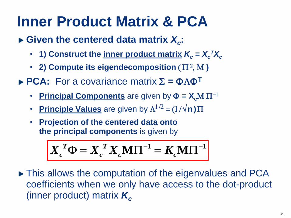
Inner Product Matrix & PCA Given the centered data matrix Xc:

• 1) Construct the inner product matrix Kc = XcTXc

• 2) Compute its eigendecomposition ( 2, M )

PCA: For a covariance matrix = LT

• Principal Components are given by = XcM -1

• Principle Values are given by L1/2 = (1 / n )

• Projection of the centered data onto the principal components is given by

This allows the computation of the eigenvalues and PCA coefficients when we only have access to the dot-product (inner product) matrix Kc

1 1M M

T T

c cc cX X X K

- - = =

3

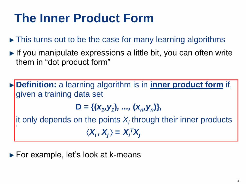
The Inner Product Form

This turns out to be the case for many learning algorithms

If you manipulate expressions a little bit, you can often write them in “dot product form”

Definition: a learning algorithm is in inner product form if, given a training data set

D = {(x1,y1), ..., (xn,yn)},

it only depends on the points Xi through their inner products i

Xi , Xj = Xi

TXj

For example, let’s look at k-means

4

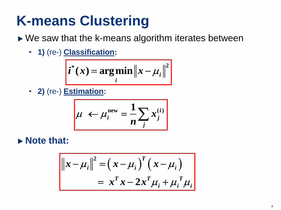
K-means Clustering We saw that the k-means algorithm iterates between

• 1) (re-) Classification:

• 2) (re-) Estimation:

Note that:

2*( ) argmin

ii

i x x = -

new ( )1

i

i j

j

xn

=

( ( 2

2

T

i i i

T T T

i i i

x x x

x x x

- = - -

= -

5

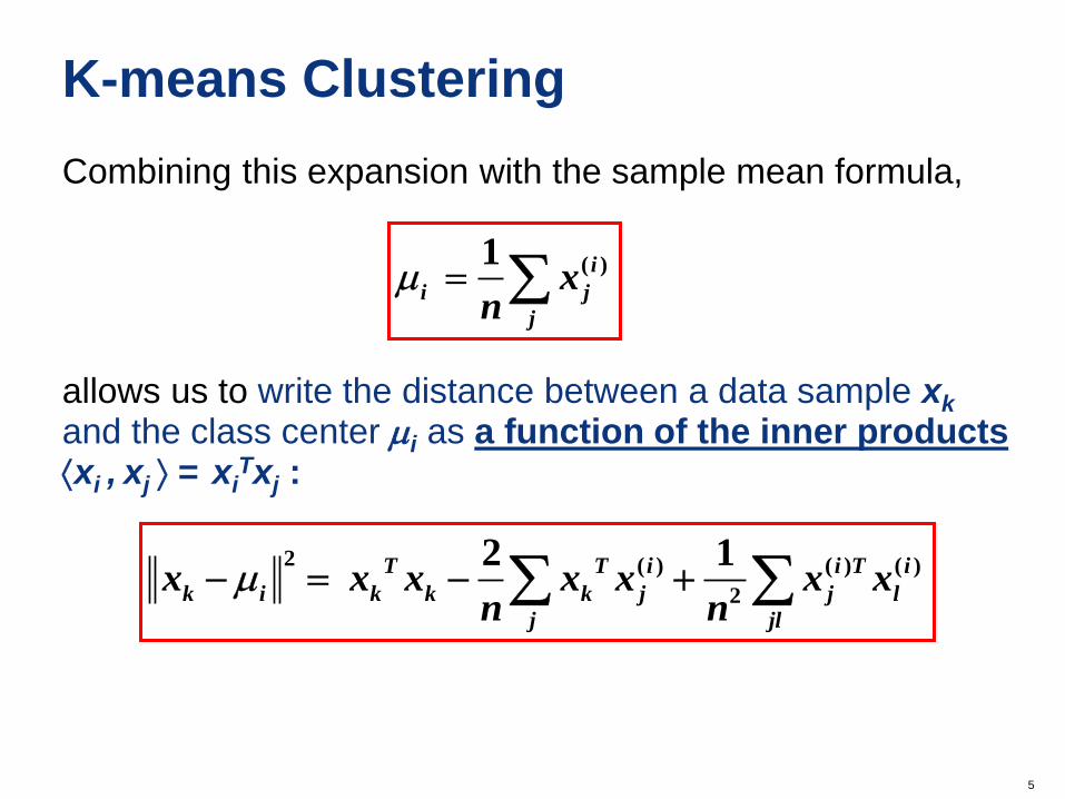
K-means Clustering

Combining this expansion with the sample mean formula,

allows us to write the distance between a data sample xk and the class center i as a function of the inner products xi

, xj = xiTxj :

( )1 i

i j

j

xn

=

2 ( ) ( ) ( )

2

2 1

T T i i T i

k i k k k j j l

j jl

x x x x x x xn n

- = -

6

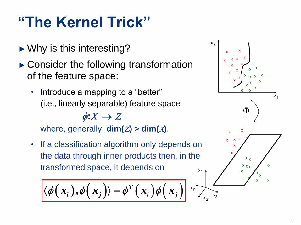
“The Kernel Trick”

Why is this interesting?

Consider the following transformation of the feature space:

• Introduce a mapping to a “better”

(i.e., linearly separable) feature space

:X Z

where, generally, dim(Z) > dim(X).

• If a classification algorithm only depends on

the data through inner products then, in the

transformed space, it depends on

x

x

x

x

x

x x

x

x x

x

x

o

o

o

o

o

o o

o

o o

o

o

x 1

x 2

x

x

x

x

x

x x

x

x x

x

x

o

o

o

o

o

o o

o

o o

o

o x 1

x 3 x 2

x n

( ( ( ( ,T

i j i jx x x x =

7

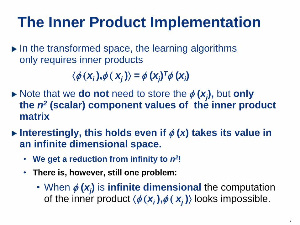
The Inner Product Implementation

In the transformed space, the learning algorithms only requires inner products

(xi ), ( xj ) = (xj)

T (xi)

Note that we do not need to store the (xj), but only the n2 (scalar) component values of the inner product matrix

Interestingly, this holds even if (x) takes its value in an infinite dimensional space.

• We get a reduction from infinity to n2!

• There is, however, still one problem:

• When (xj) is infinite dimensional the computation of the inner product (xi

), ( xj ) looks impossible.

8

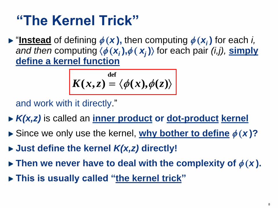
“The Kernel Trick”

“Instead of defining (x ), then computing (xi ) for each i,

and then computing (xi ), ( xj ) for each pair (i,j), simply

define a kernel function and work with it directly.”

K(x,z) is called an inner product or dot-product kernel

Since we only use the kernel, why bother to define (x )?

Just define the kernel K(x,z) directly!

Then we never have to deal with the complexity of (x ).

This is usually called “the kernel trick”

def

( , ) ( ), ( )K x z x z =

9

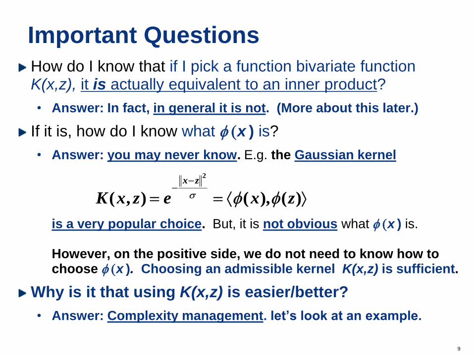
Important Questions

How do I know that if I pick a function bivariate function K(x,z), it is actually equivalent to an inner product?

• Answer: In fact, in general it is not. (More about this later.)

If it is, how do I know what (x ) is?

• Answer: you may never know. E.g. the Gaussian kernel

is a very popular choice. But, it is not obvious what (x ) is. However, on the positive side, we do not need to know how to choose (x ). Choosing an admissible kernel K(x,z) is sufficient.

Why is it that using K(x,z) is easier/better?

• Answer: Complexity management. let’s look at an example.

2

( ), ( )( , )

x z

x zK x z e -

-

= =

10

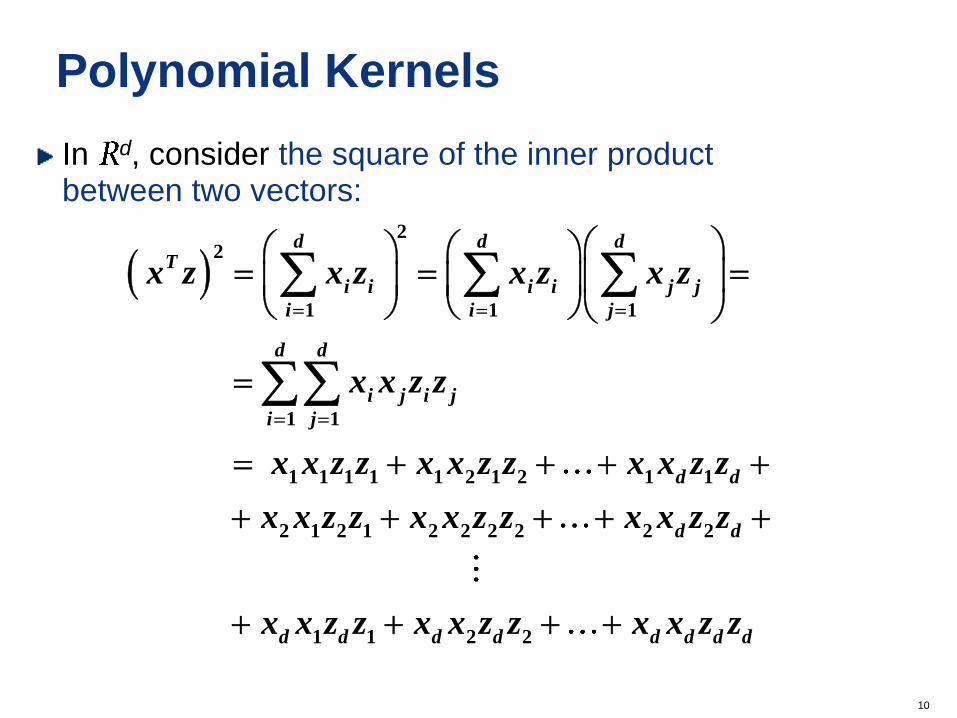
Polynomial Kernels

In d, consider the square of the inner product between two vectors:

( 2

2

1 1 1

1 1

1 1 1 1 1 2 1 2 1 1

2 1 2 1 2 2 2 2 2 2

d d dT

i i i i j j

i i j

d d

i j i j

i j

d d

d d

x z x z x z x z

x x z z

x x z z x x z z x x z z

x x z z x x z z x x z z

= = =

= =

= = =

=

=

1 1 2 2

d d d d d d d d

x x z z x x z z x x z z

11

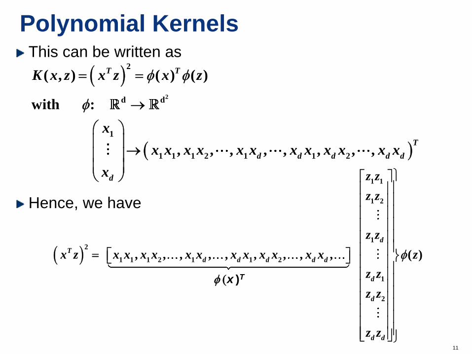
Polynomial Kernels This can be written as

Hence, we have

(

1 1

1 2

12

1 1 1 2 1 1 2

1

2

, , , , , , , , , ( )

d

T

d d d d d

d

d

d d

z z

z z

z z

x z x x x x x x x x x x x x z

z z

z z

z z

=

(x )T

(

(

2

2

d d

1

1 1 1 2 1 1 2

( , ) ( ) ( )

with :

, , , , , , , ,

T T

T

d d d d d

d

K x z x z x z

x

x x x x x x x x x x x x

x

= =

12

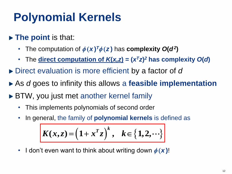
Polynomial Kernels

The point is that:

• The computation of (x )T (z ) has complexity O(d 2)

• The direct computation of K(x,z) = (xTz)2 has complexity O(d)

Direct evaluation is more efficient by a factor of d

As d goes to infinity this allows a feasible implementation

BTW, you just met another kernel family

• This implements polynomials of second order

• In general, the family of polynomial kernels is defined as

• I don’t even want to think about writing down (x )!

( ( , ) 1 , 1,2,k

TK x z x z k=

13

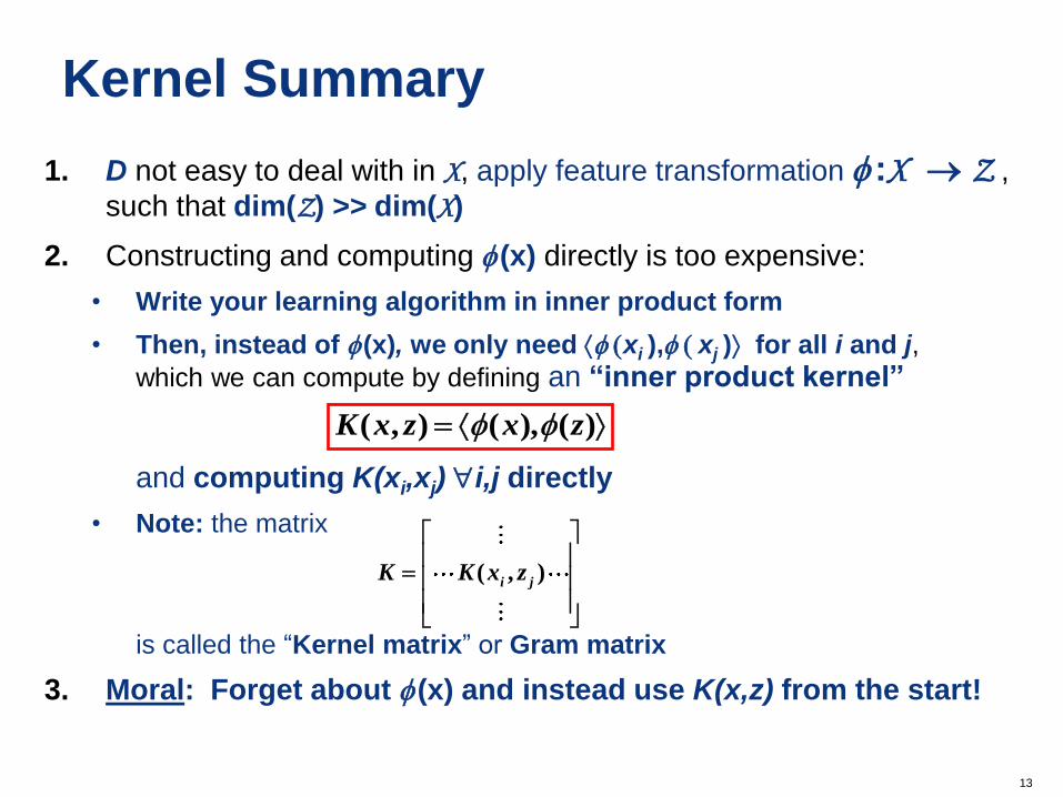
Kernel Summary

1. D not easy to deal with in X, apply feature transformation :X Z , such that dim(Z) >> dim(X)

2. Constructing and computing (x) directly is too expensive:

• Write your learning algorithm in inner product form

• Then, instead of (x), we only need (xi ), ( xj ) for all i and j,

which we can compute by defining an “inner product kernel” and computing K(xi,xj) "i,j directly

• Note: the matrix is called the “Kernel matrix” or Gram matrix

3. Moral: Forget about (x) and instead use K(x,z) from the start!

( , ) ( ), ( )K x z x z =

( , )i j

K K x z

=

14

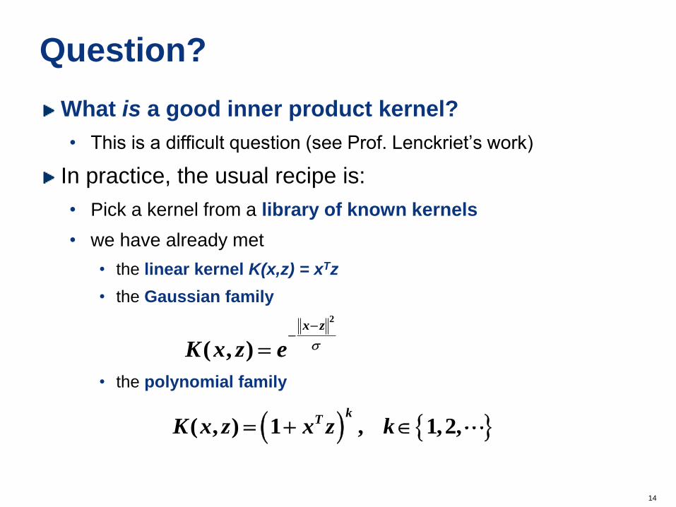
Question?

What is a good inner product kernel?

• This is a difficult question (see Prof. Lenckriet’s work)

In practice, the usual recipe is:

• Pick a kernel from a library of known kernels

• we have already met

• the linear kernel K(x,z) = xTz

• the Gaussian family

• the polynomial family

2

( , )

x z

K x z e

--

=

( ( , ) 1 , 1,2,k

TK x z x z k=

15

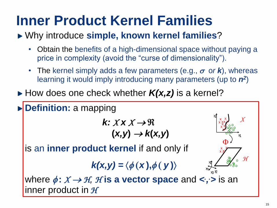
Inner Product Kernel Families Why introduce simple, known kernel families?

• Obtain the benefits of a high-dimensional space without paying a price in complexity (avoid the “curse of dimensionality”).

• The kernel simply adds a few parameters (e.g., or k), whereas learning it would imply introducing many parameters (up to n2)

How does one check whether K(x,z) is a kernel?

Definition: a mapping

k: X x X

(x,y) k(x,y)

is an inner product kernel if and only if

k(x,y) = (x ), ( y )

where : X H, H is a vector space and <.,.> is an inner product in H

x x

x

x

x

x x x

x x x x

o o

o

o

o o o o

o o o o

x 1

x 2

x x

x

x

x

x x x

x x x x

o o

o

o

o o o o

o o o o x 1

x 3 x 2 x n

X

H

16

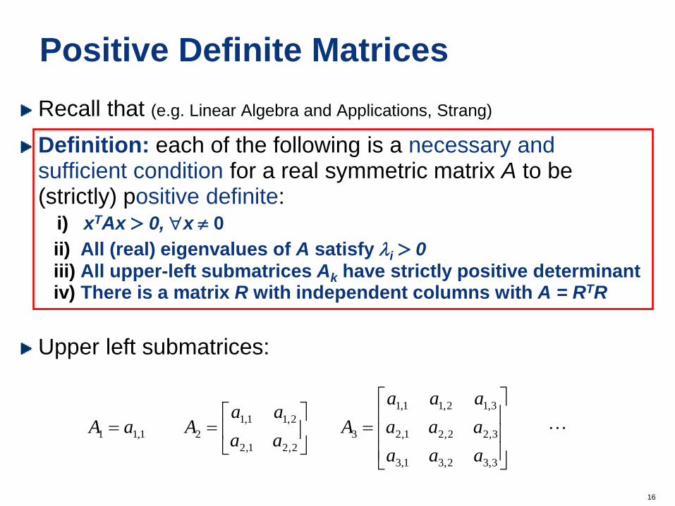
Positive Definite Matrices

Recall that (e.g. Linear Algebra and Applications, Strang)

Definition: each of the following is a necessary and sufficient condition for a real symmetric matrix A to be (strictly) positive definite: i) xTAx > 0, "x 0

ii) All (real) eigenvalues of A satisfy li > 0 iii) All upper-left submatrices Ak have strictly positive determinant iv) There is a matrix R with independent columns with A = RTR

Upper left submatrices:

3,32,31,3

3,22,21,2

3,12,11,1

3

2,21,2

2,11,1

21,11

=

==

aaa

aaa

aaa

Aaa

aaAaA

17

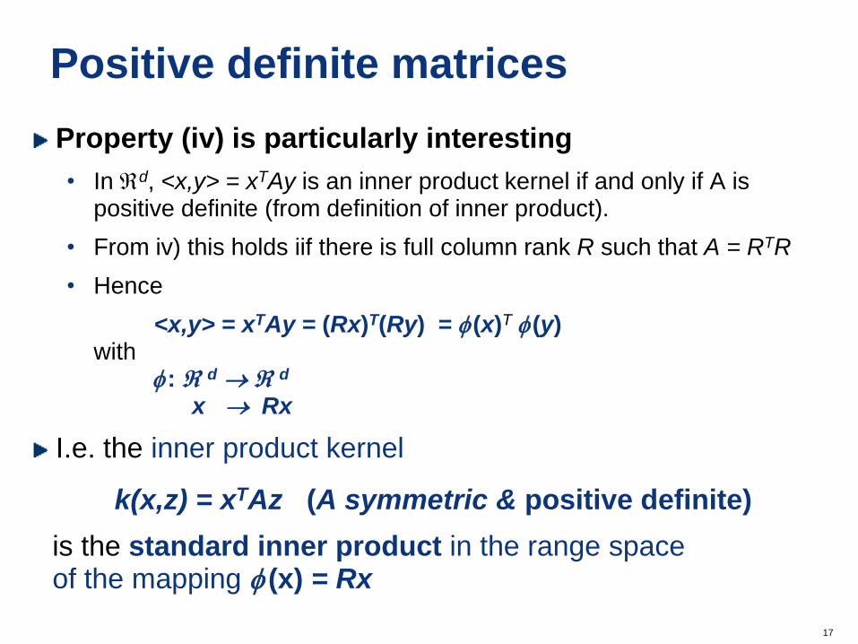
Positive definite matrices

Property (iv) is particularly interesting

• In d, <x,y> = xTAy is an inner product kernel if and only if A is positive definite (from definition of inner product).

• From iv) this holds iif there is full column rank R such that A = RTR

• Hence

<x,y> = xTAy = (Rx)T(Ry) = (x)T (y) with : d d x Rx

I.e. the inner product kernel

k(x,z) = xTAz (A symmetric & positive definite)

is the standard inner product in the range space of the mapping (x) = Rx

18

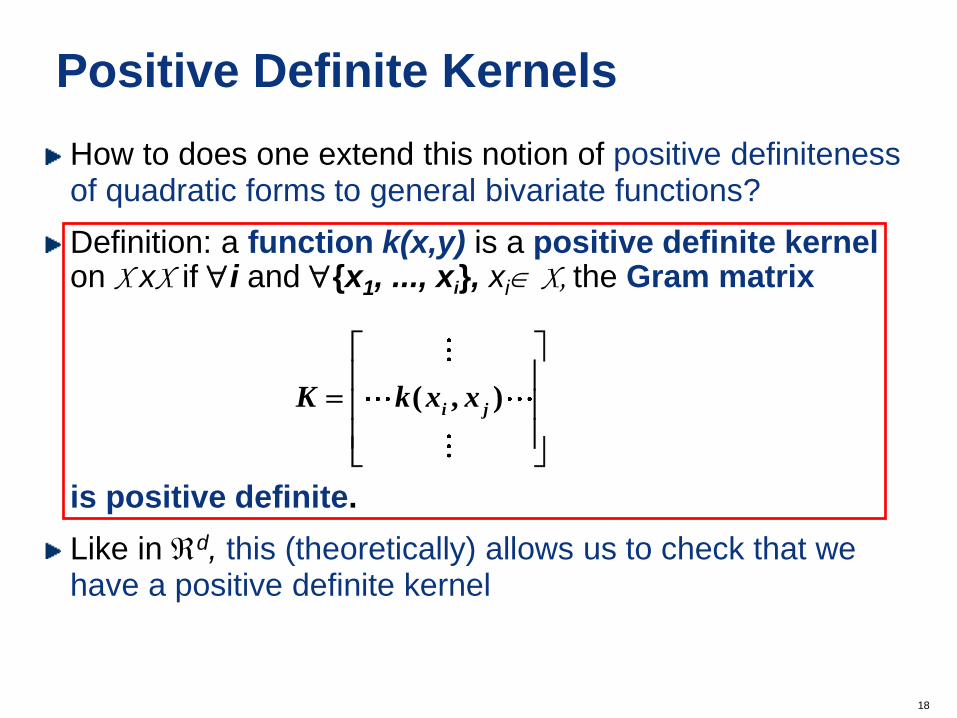
How to does one extend this notion of positive definiteness of quadratic forms to general bivariate functions?

Definition: a function k(x,y) is a positive definite kernel on X xX if "i and "{x1, ..., xi}, xi X, the Gram matrix

is positive definite.

Like in d, this (theoretically) allows us to check that we have a positive definite kernel

Positive Definite Kernels

( , )i j

K k x x

=

19

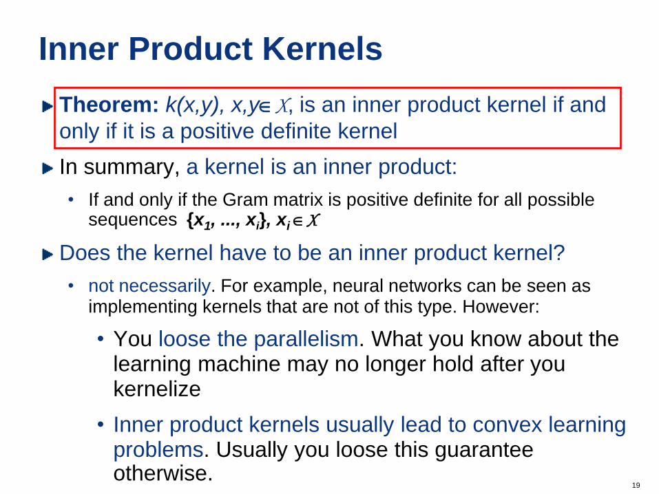
Inner Product Kernels

Theorem: k(x,y), x,yX, is an inner product kernel if and

only if it is a positive definite kernel

In summary, a kernel is an inner product:

• If and only if the Gram matrix is positive definite for all possible sequences {x1, ..., xi}, xi X

Does the kernel have to be an inner product kernel?

• not necessarily. For example, neural networks can be seen as implementing kernels that are not of this type. However:

• You loose the parallelism. What you know about the learning machine may no longer hold after you kernelize

• Inner product kernels usually lead to convex learning problems. Usually you loose this guarantee otherwise.

20

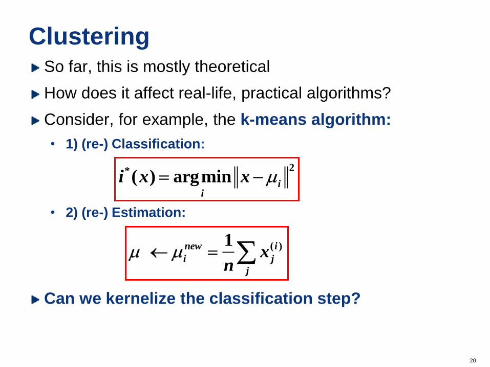
Clustering So far, this is mostly theoretical

How does it affect real-life, practical algorithms?

Consider, for example, the k-means algorithm:

• 1) (re-) Classification:

• 2) (re-) Estimation:

Can we kernelize the classification step?

2*( ) argmin

ii

i x x = -

( )1

new i

i j

j

xn

=

21

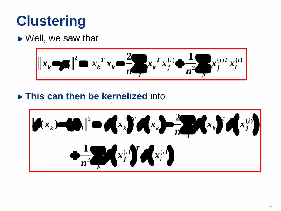
Clustering Well, we saw that

This can then be kernelized into

( ( ( (

( (

2 ( )

( ) ( )

2

2)

1

(

T T i

k k k k j

j

Ti i

j l

l

i

j

x x x x xn

x xn

- = -

2 ( ) ( ) ( )

2

2 1

T T i i T i

k i k k k j j l

j jl

x x x x x x xn n

- = -

22

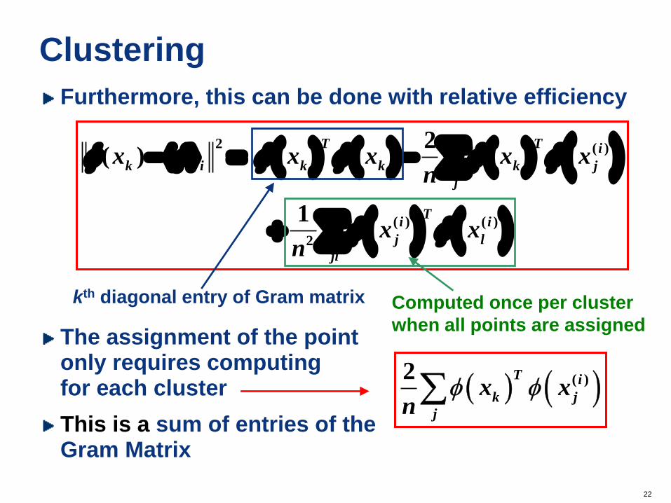
Clustering

Furthermore, this can be done with relative efficiency

The assignment of the point only requires computing for each cluster

This is a sum of entries of the Gram Matrix

( ( ( (

( (

2 ( )

( ) ( )

2

2)

1

(

T T i

k i k k k j

j

Ti i

j l

jl

x x x x xn

x xn

- = -

kth diagonal entry of Gram matrix Computed once per cluster

when all points are assigned

( ( ( )2 T i

k j

j

x xn

23

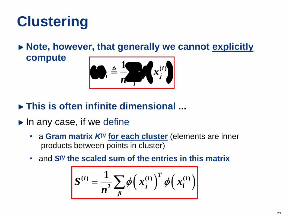
Clustering

Note, however, that generally we cannot explicitly compute

This is often infinite dimensional ...

In any case, if we define

• a Gram matrix K(i) for each cluster (elements are inner products between points in cluster)

• and S(i) the scaled sum of the entries in this matrix

( ( )1i

i

j

j

xn

( ( ( ) ( ) ( )

2

1 Ti i i

j l

jl

S x xn

=

24

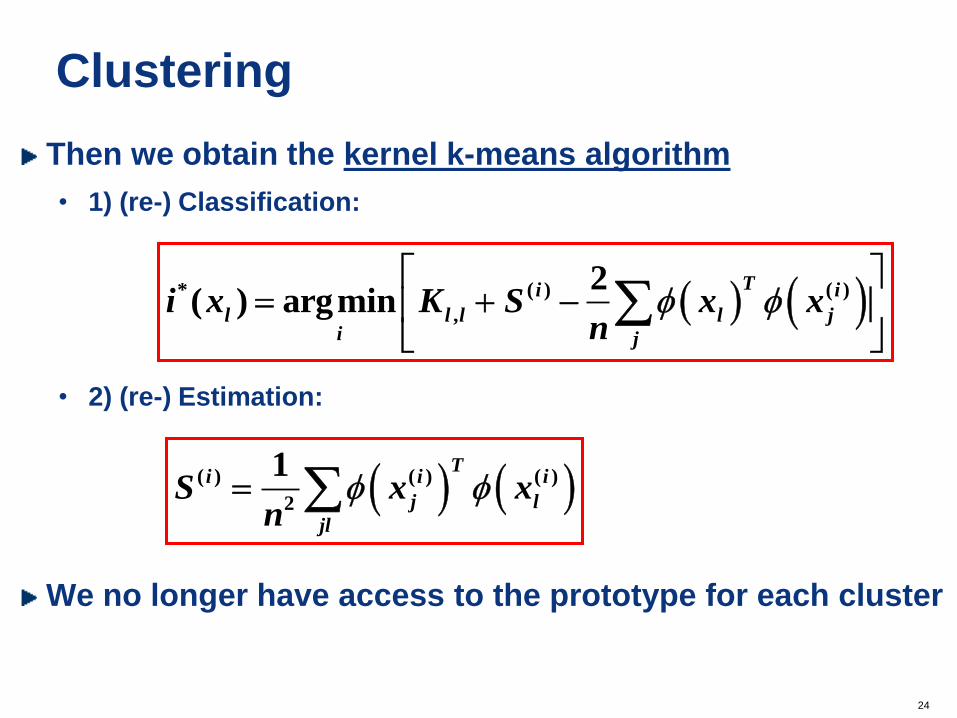
Clustering

Then we obtain the kernel k-means algorithm

• 1) (re-) Classification:

• 2) (re-) Estimation:

We no longer have access to the prototype for each cluster

( ( ( ) ( ) ( )

2

1 Ti i i

j l

jl

S x xn

=

( ( * ( ) ( )

,

2( ) argmin

Ti i

l l l l ji j

i x K S x xn

= -

25

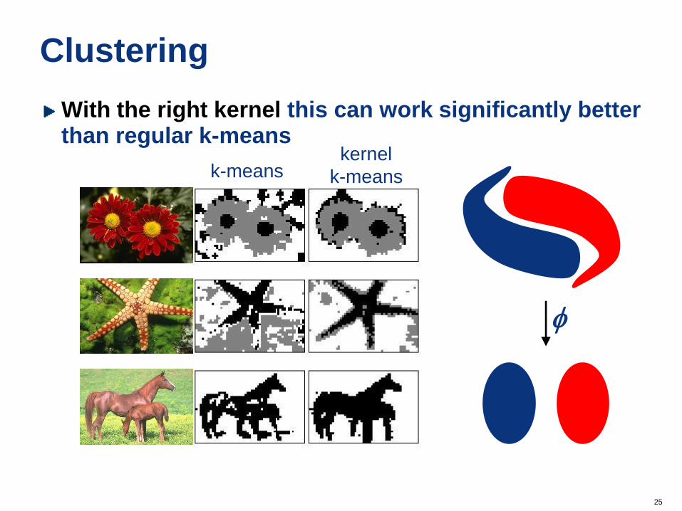
Clustering

With the right kernel this can work significantly better than regular k-means

k-means kernel

k-means

26

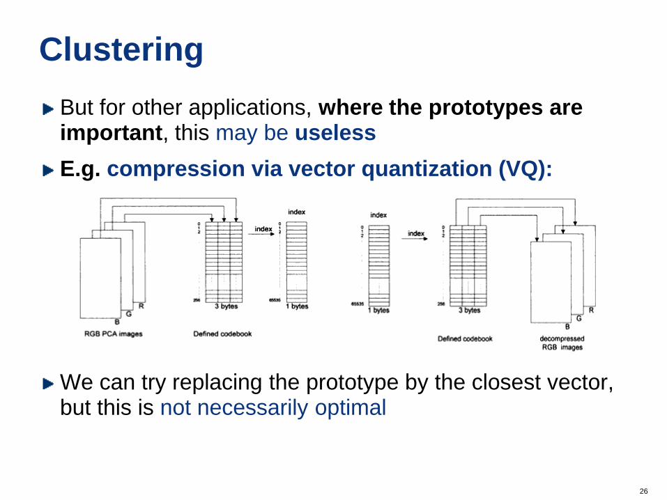
Clustering

But for other applications, where the prototypes are important, this may be useless

E.g. compression via vector quantization (VQ):

We can try replacing the prototype by the closest vector, but this is not necessarily optimal

27

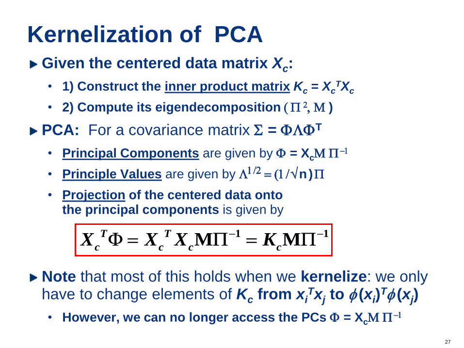
Kernelization of PCA Given the centered data matrix Xc:

• 1) Construct the inner product matrix Kc = XcTXc

• 2) Compute its eigendecomposition ( 2, M )

PCA: For a covariance matrix = LT

• Principal Components are given by = XcM -1

• Principle Values are given by L1/2 = (1 / n )

• Projection of the centered data onto the principal components is given by

Note that most of this holds when we kernelize: we only have to change elements of Kc from xi

Txj to (xi)T (xj)

• However, we can no longer access the PCs = XcM -1

1 1M M

T T

c cc cX X X K

- - = =

28

Kernel Methods

Most learning algorithms can be kernelized

• Kernel Principal Component Analysis (PCA)

• Kernel Linear Discriminant Analysis (LDA)

• Kernel Independent Analysis (ICA)

• Etc.

As in kernalized k-means clustering, sometimes we loose some of the features of the original algorithm

But the performance is frequently better

The canonical application:

The Support Vector Machine (SVM)

29

END