Embed Size (px)
Citation preview

1
1
School of Computer Science
Learning generalized linear models and tabular CPT of
structured full BN
Probabilistic Graphical Models (10Probabilistic Graphical Models (10--708)708)
Lecture 9, Oct 15, 2007
Eric XingEric XingReceptor A
Kinase C
TF F
Gene G Gene H
Kinase EKinase D
Receptor BX1 X2
X3 X4 X5
X6
X7 X8
Receptor A
Kinase C
TF F
Gene G Gene H
Kinase EKinase D
Receptor BX1 X2
X3 X4 X5
X6
X7 X8
X1 X2
X3 X4 X5
X6
X7 X8
Reading: J-Chap. 7,8.
Eric Xing 2
Grade for hw 1
Project proposal
Questions

2
Eric Xing 3
Linear RegressionLet us assume that the target variable and the inputs are related by the equation:
where ε is an error term of unmodeled effects or random noise
Now assume that ε follows a Gaussian N(0,σ), then we have:
iiT
iy εθ += x
⎟⎟⎠
⎞⎜⎜⎝
⎛ −−= 2
2
221
σθ
σπθ )(exp);|( i
Ti
iiyxyp x
Eric Xing 4
Logistic Regression (sigmoid classifier)
The condition distribution: a Bernoulli
where µ is a logistic function
We can used the brute-force gradient method as in LR
But we can also apply generic laws by observing the p(y|x) is an exponential family function, more specifically, a generalized linear model!
yy xxxyp −−= 11 ))(()()|( µµ
xTex
θµ
−+=
11)(

3
Eric Xing 5
Exponential familyFor a numeric random variable X
is an exponential family distribution with natural (canonical) parameter η
Function T(x) is a sufficient statistic.Function A(η) = log Z(η) is the log normalizer.Examples: Bernoulli, multinomial, Gaussian, Poisson, gamma,...
{ }{ })(exp)(
)(
)()(exp)()|(
xTxhZ
AxTxhxp
T
T
ηη
ηηη1
=
−= XnN
Eric Xing 6
Multivariate Gaussian Distribution
For a continuous vector random variable X∈Rk:
Exponential family representation
Note: a k-dimensional Gaussian is a (d+d2)-parameter distribution with a (d+d2)-element vector of sufficient statistics (but because of symmetry and positivity, parameters are constrained and have lower degree of freedom)
( )
( )( ){ }Σ−Σ−Σ+Σ−=
⎭⎬⎫
⎩⎨⎧ −Σ−−
Σ=Σ
−−−
−
logtrexp
)()(exp),(
/
//
µµµπ
µµπ
µ
12111
21
2
1212
21
21
21
TTTk
Tk
xxx
xxxp
( )[ ] ( )[ ]( )[ ]
( )( ) 2
221
112211
21
121
21
1211
211
2
2/)(
log)(trlog)(vec;)(
and ,vec,vec;
k
TT
T
xh
AxxxxT
−
−
−−−−
=
−−−=Σ+Σ=
=
Σ−=Σ==Σ−Σ=
π
ηηηηµµη
ηµηηηµη
Moment parameter
Natural parameter

4
Eric Xing 7
Multinomial distributionFor a binary vector random variable
Exponential family representation
),|(multi~ πxx
⎭⎬⎫
⎩⎨⎧
== ∑k
kkx
Kxx xxp
K
πππππ lnexp)( L21
21
[ ]
1
1
0
1
1
1
=
⎟⎠
⎞⎜⎝
⎛=⎟
⎠
⎞⎜⎝
⎛−−=
=
⎥⎦⎤
⎢⎣⎡
⎟⎠⎞⎜
⎝⎛=
∑∑=
−
=
)(
lnln)(
)(
;ln
xh
eA
xxTK
k
K
kk
K
k
kηπη
ππη
⎭⎬⎫
⎩⎨⎧
⎟⎠
⎞⎜⎝
⎛−+⎟⎟
⎠
⎞⎜⎜⎝
⎛∑−
=
⎭⎬⎫
⎩⎨⎧
⎟⎠
⎞⎜⎝
⎛−⎟
⎠
⎞⎜⎝
⎛−+=
∑∑
∑∑∑−
=
−
=−
=
−
=
−
=
−
=
1
1
1
111
1
1
1
1
1
1
11
11
K
kk
K
k kKk
kk
K
kk
K
k
KK
kk
k
x
xx
ππ
π
ππ
lnlnexp
lnlnexp
Eric Xing 8
Why exponential family?Moment generating property
{ }{ }
[ ])()(
)(exp)()(
)(exp)()(
)()(
)(log
xTE
dxZ
xTxhxT
dxxTxhdd
Z
Zdd
ZZ
dd
ddA
T
T
=
=
=
==
∫
∫
ηη
ηηη
ηηη
ηηη1
1
{ } { }
[ ] [ ][ ])(
)()(
)()()(
)(exp)()()(
)(exp)()(
xTVarxTExTE
Zdd
Zdx
ZxTxhxTdx
ZxTxhxT
dAd
2
TT
=−=
−= ∫∫2
22
2 1 ηηηη
ηηη
η
5
Eric Xing 9
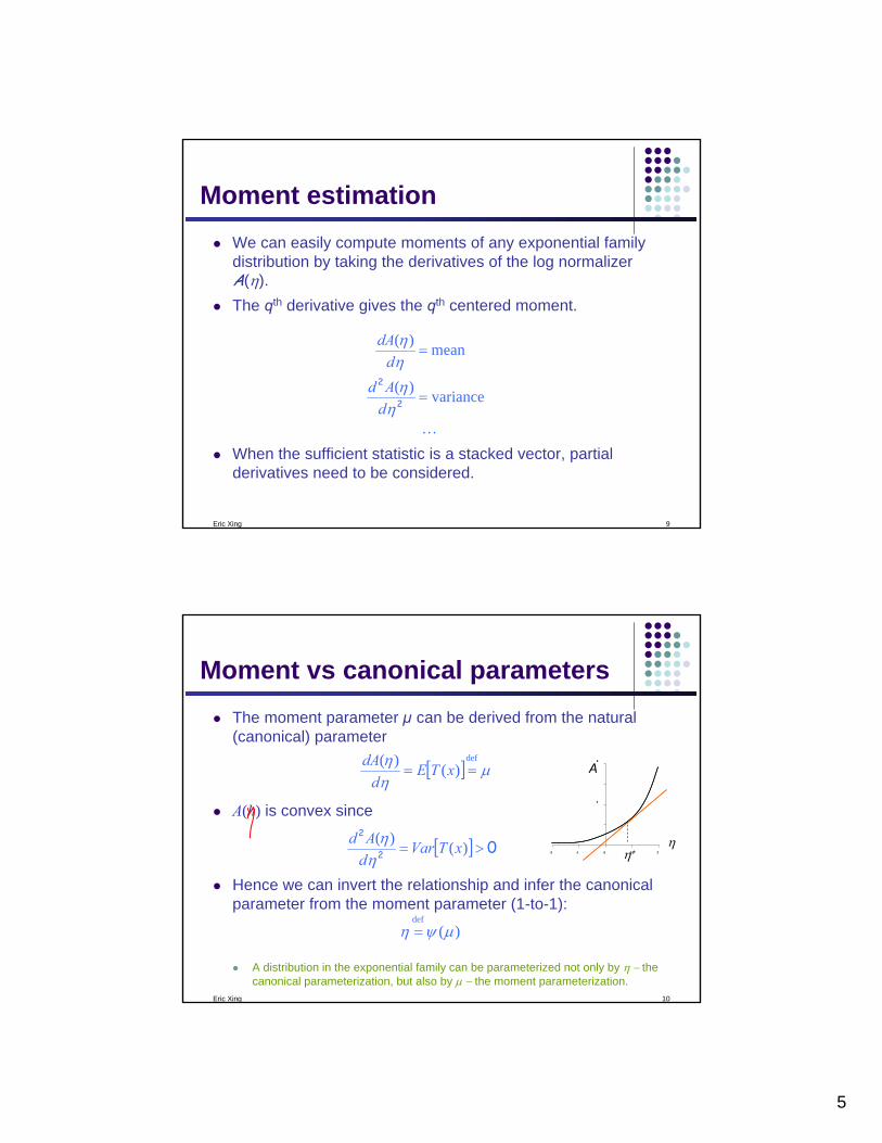
Moment estimationWe can easily compute moments of any exponential family distribution by taking the derivatives of the log normalizerA(η).The qth derivative gives the qth centered moment.
When the sufficient statistic is a stacked vector, partial derivatives need to be considered.
L
variance)(
mean)(
=
=
2
2
ηηηη
dAdddA
Eric Xing 10
Moment vs canonical parametersThe moment parameter µ can be derived from the natural (canonical) parameter
A(h) is convex since
Hence we can invert the relationship and infer the canonical parameter from the moment parameter (1-to-1):
A distribution in the exponential family can be parameterized not only by η − the canonical parameterization, but also by µ − the moment parameterization.
[ ] µηη def
)()(== xTE
ddA
[ ] 02
2
>= )()( xTVardAdη
η
)(def
µψη =
4
8
-2 -1 0 1 2
4
8
-2 -1 0 1 2
A
ηη∗

6
Eric Xing 11
MLE for Exponential FamilyFor iid data, the log-likelihood is
Take derivatives and set to zero:
This amounts to moment matching.We can infer the canonical parameters using
{ }
∑ ∑
∏
−⎟⎠
⎞⎜⎝
⎛+=
−=
n nn
Tn
nn
Tn
NAxTxh
AxTxhD
)()()(log
)()(exp)(log);(
ηη
ηηηl
)(
)()(
)()(
∑
∑
∑
=
=∂
∂
⇒
=∂
∂−=
∂∂
nnMLE
nn
nn
xTN
xTN
A
ANxT
1
1
0
µ
ηη
ηη
η
)
l
)( MLEMLE µψη )) =
Eric Xing 12
SufficiencyFor p(x|θ), T(x) is sufficient for θ if there is no information in Xregarding θ yeyond that in T(x).
We can throw away X for the purpose pf inference w.r.t. θ .
Bayesian view
Frequentist view
The Neyman factorization theorem
T(x) is sufficient for θ if
T(x) θX ))(|()),(|( xTpxxTp θθ =
T(x) θX ))(|()),(|( xTxpxTxp =θ
T(x) θX
))(,()),(()),(,( xTxxTxTxp 21 ψθψθ =
))(,()),(()|( xTxhxTgxp θθ =⇒

7
Eric Xing 13
ExamplesGaussian:
Multinomial:
Poisson:
( )[ ]( )[ ]
( ) 2211
21
1211
2 /)(
log)(vec;)(
vec;
k
T
T
xh
AxxxxT
−
−
−−
=
Σ+Σ=
=
Σ−Σ=
π
µµη
µη
∑∑ ==⇒n
nn
nMLE xN
xTN
111 )(µ
[ ]
1
1
0
1
1
1
=
⎟⎠
⎞⎜⎝
⎛=⎟
⎠
⎞⎜⎝
⎛−−=
=
⎥⎦⎤
⎢⎣⎡
⎟⎠⎞⎜
⎝⎛=
∑∑=
−
=
)(
lnln)(
)(
;ln
xh
eA
xxTK
k
K
kk
K
k
kηπη
ππη
∑=⇒n
nMLE xN1µ
!)(
)()(
log
xxh
eAxxT
1=
==
==
ηλη
λη
∑=⇒n
nMLE xN1µ
Eric Xing 14
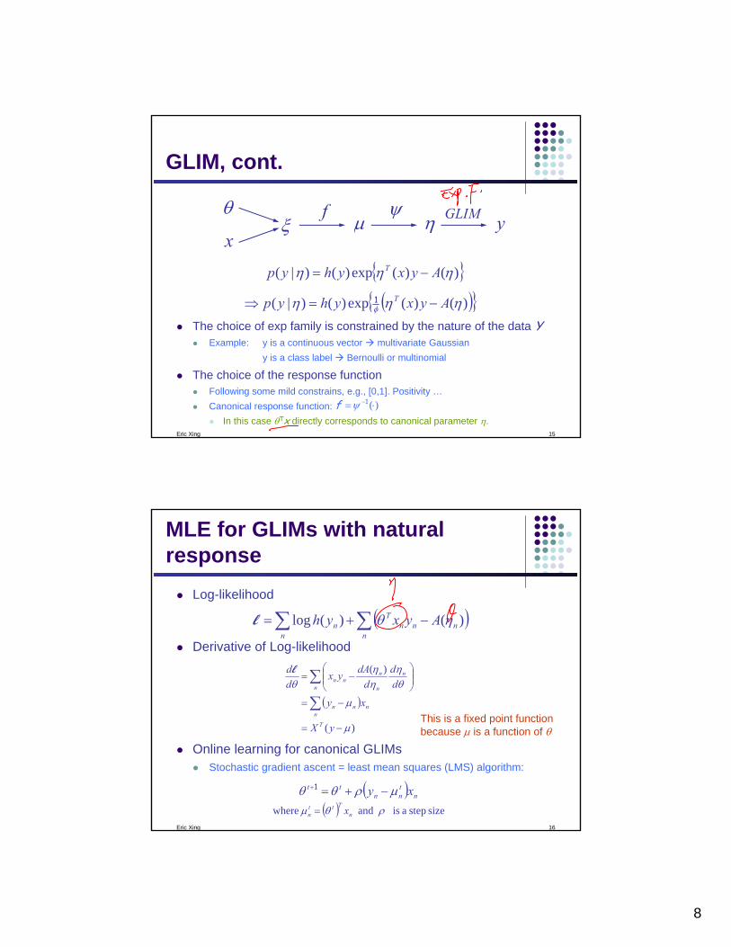
Generalized Linear Models (GLIMs)
The graphical modelLinear regressionDiscriminative linear classificationCommonality:
model Ep(Y)=µ=f(θTX)What is p()? the cond. dist. of Y.What is f()? the response function.
GLIMThe observed input x is assumed to enter into the model via a linear combination of its elementsThe conditional mean µ is represented as a function f(ξ) of ξ, where f is known as the response functionThe observed output y is assumed to be characterized by an exponential family distribution with conditional mean µ.
Xn
YnN
xTθξ =
8
Eric Xing 15
GLIM, cont.
The choice of exp family is constrained by the nature of the data YExample: y is a continuous vector multivariate Gaussian
y is a class label Bernoulli or multinomial
The choice of the response functionFollowing some mild constrains, e.g., [0,1]. Positivity …Canonical response function:
In this case θTx directly corresponds to canonical parameter η.
( ){ })()(exp)()|( ηηη φ Ayxyhyp T −=⇒ 1
)(⋅= −1ψf
{ })()(exp)()|( ηηη Ayxyhyp T −=
ηψfθ
xµξ yGLIM
Eric Xing 16
MLE for GLIMs with natural response
Log-likelihood
Derivative of Log-likelihood
Online learning for canonical GLIMsStochastic gradient ascent = least mean squares (LMS) algorithm:
( )∑ ∑ −+=n n
nnnT
n Ayxyh )()(log ηθl
( )
)(
)(
µ
µ
θη
ηη
θ
−=
−=
⎟⎟⎠
⎞⎜⎜⎝
⎛−=
∑
∑
yX
xy
dd
ddAyx
dd
T
nnnn
n
n
n
nnn
l
This is a fixed point function because µ is a function of θ
( ) ntnn
tt xy µρθθ −+=+1
( ) size step a is and where ρθµ nTtt
n x=

9
Eric Xing 17
Batch learning for canonical GLIMs
The Hessian matrix
where is the design matrix and
which can be computed by calculating the 2nd derivative of A(ηn)
( )
WXX
xxddx
dd
ddx
ddxxy
dd
dddH
T
nT
nTn
n n
nn
Tn
n n
nn
nTn
nn
nnnTT
−=
=−=
−=
=−==
∑
∑
∑∑
θηηµ
θη
ηµ
θµµ
θθθ
since
l2
[ ]TnxX =
⎟⎟⎠
⎞⎜⎜⎝
⎛=
N
N
dd
ddW
ηµ
ηµ ,,diag K
1
1
⎥⎥⎥⎥
⎦
⎤
⎢⎢⎢⎢
⎣
⎡
−−−−
−−−−−−−−
=
nx
xx
XMMM
2
1
⎥⎥⎥⎥
⎦
⎤
⎢⎢⎢⎢
⎣
⎡
=
ny
yy
yM
v 2
1
Eric Xing 18
Recall LMSCost function in matrix form:
To minimize J(θ), take derivative and set to zero:
( ) ( )yy
yJ
T
n
ii
Ti
vv −−=
−= ∑=
θθ
θθ
XX
x
2121
1
2)()( ⎥⎥⎥⎥
⎦
⎤
⎢⎢⎢⎢
⎣
⎡
−−−−
−−−−−−−−
=
nx
xx
XMMM
2
1
⎥⎥⎥⎥
⎦
⎤
⎢⎢⎢⎢
⎣
⎡
=
ny
yy
yM
v 2
1
( )
( )
( )0
221
22121
=−=
−+=
∇+∇−∇=
+−−∇=∇
yXXX
yXXXXX
yyXyXX
yyXyyXXXJ
TT
TTT
TTTT
TTTTTT
v
v
vvv
vvvv
θ
θθ
θθθ
θθθθ
θθθ
θθ
trtrtr
tryXXX TT v=⇒ θ
The normal equations
( ) yXXX TT v1−=*θ
⇓

10
Eric Xing 19
Iteratively Reweighted Least Squares (IRLS)
Recall Newton-Raphson methods with cost function J
We now have
Now:
where the adjusted response is
This can be understood as solving the following " Iteratively reweighted least squares " problem
JHttθθθ ∇−= −+ 11
WXXH
yXJT
T
−=
−=∇ )( µθ
( ) [ ]( ) ttTtT
tTttTtT
tt
zWXXWX
yXXWXXWX
H
1
1
11
−
−
−+
=
−+=
∇+=
)( µθ
θθ θ l
( ) )( tttt yWXz µθ −+=−1
)()(minarg θθθθ
XzWXz Tt −−=+1
( ) yXXX TT v1−=*θ
Eric Xing 20
Example 1: logistic regression (sigmoid classifier)
The condition distribution: a Bernoulli
where µ is a logistic function
p(y|x) is an exponential family function, with mean:
and canonical response function
IRLS
yy xxxyp −−= 11 ))(()()|( µµ
)()( xex ηµ −+
=1
1
[ ] )(| xexyE ηµ −+
==1
1
xTθξη ==
⎟⎟⎟
⎠
⎞
⎜⎜⎜
⎝
⎛
−
−=
−=
)(
)(
)(
NN
W
dd
µµ
µµ
µµηµ
1
1
1
11
O
11
Eric Xing 21
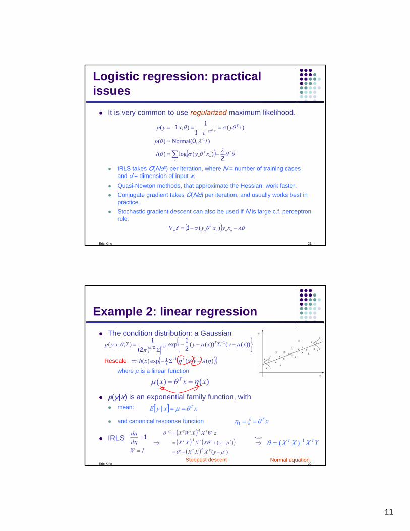
Logistic regression: practical issues
It is very common to use regularized maximum likelihood.
IRLS takes O(Nd3) per iteration, where N = number of training cases and d = dimension of input x.Quasi-Newton methods, that approximate the Hessian, work faster.Conjugate gradient takes O(Nd) per iteration, and usually works best in practice.Stochastic gradient descent can also be used if N is large c.f. perceptronrule:
( ) θθλθσθ
λθ
θσθθ
T
nn
Tn
Txy
xyl
Ip
xye
xyp T
2
01
11
1
−=
=+
=±=
∑
−
−
)(log)(
),(Normal~)(
)(),(
( ) λθθσθ −−=∇ nnnT
n xyxy )(1l
Eric Xing 22
Example 2: linear regressionThe condition distribution: a Gaussian
where µ is a linear function
p(y|x) is an exponential family function, with mean:
and canonical response function
IRLS
)()( xxx T ηθµ ==
[ ] xxyE Tθµ ==|
xTθξη ==1
IWdd
=
= 1ηµ
( )( ){ })()(exp)(
))(())((exp),,( //
ηη
µµπ
θ
Ayxxh
xyxyxyp
T
Tk
−Σ−⇒
⎭⎬⎫
⎩⎨⎧ −Σ−−
Σ=Σ
−
−
121
1212 2
12
1
( )( ) ( )
( ) )(
)(tTTt
ttTT
ttTtTt
yXXX
yXXXX
zWXXWX
µθ
µθ
θ
−+=
−+=
=
−
−
−+
1
1
11
⇒∞→
⇒t
YXXX TT 1−= )(θ
Steepest descent Normal equation
Rescale

12
Eric Xing 23
ClassificationGenerative and discriminative approach
Q
X
Q
X
RegressionLinear, conditional mixture, nonparametric
X Y
Density estimationParametric and nonparametric methods
µ,σ
XX
Simple GMs are the building blocks of complex BNs
24
School of Computer ScienceAn (incomplete)
genealogy of graphical
models
The structures of most GMs (e.g., all listed here), are not learned from data, but designed by human.
But such designs are useful and indeed favored because thereby human knowledge are put into good use …

13
Eric Xing 25
MLE for general BNsIf we assume the parameters for each CPD are globally independent, and all nodes are fully observed, then the log-likelihood function decomposes into a sum of local terms, one per node:
∑ ∑∏ ∏ ⎟⎠
⎞⎜⎝
⎛=⎟⎟
⎠
⎞⎜⎜⎝
⎛==
i ninin
n iinin ii
xpxpDpD ),|(log),|(log)|(log);( ,,,, θθθθ ππ xxl
X2=1
X2=0
X5=0
X5=1
Eric Xing 26
Earthquake
Radio
Burglary
Alarm
Call
∏=
==M
ii ixpp
1
)|()( πxxXFactorization:
ji
kii x
jkixp
πθπ x
x|
)|( =
Local Distributions defined by, e.g., multinomial parameters:
How to define parameter prior?
Assumptions (Geiger & Heckerman 97,99):
Complete Model EquivalenceGlobal Parameter IndependenceLocal Parameter IndependenceLikelihood and Prior Modularity
? )|( Gp θ

14
Eric Xing
Global Parameter IndependenceFor every DAG model:
Local Parameter IndependenceFor every node:
∏=
=M
iim GpGp
1
)|()|( θθ
Earthquake
Radio
Burglary
Alarm
Call
∏=
=i
ji
ki
q
jxi GpGp
1|
)|()|(π
θθx
independent of)( | YESAlarmCallP =θ
)( | NOAlarmCallP =θ
Global & Local Parameter Independence
Eric Xing
Provided all variables are observed in all cases, we can perform Bayesian update each parameter independently !!!
sample 1
sample 2
M
θ2|1θ1 θ2|1
X1 X2
X1 X2
Global ParameterIndependence
Local ParameterIndependence
Parameter Independence,Graphical View

15
Eric Xing 29
Which PDFs Satisfy Our Assumptions? (Geiger & Heckerman 97,99)
Discrete DAG Models:
Dirichlet prior:
Gaussian DAG Models:
Normal prior:
Normal-Wishart prior:
∏∏∏∑
=Γ
Γ=
kk
kk
kk
kk
kk CP 1-1- )()(
)()( αα θαθ
α
αθ
)(Multi~| θπ jxi i
x
),(Normal~| Σµπ jxi i
x
⎭⎬⎫
⎩⎨⎧ −Ψ−−
Ψ=Ψ − )()'(exp
||)(),|( // νµνµ
πνµ 1
212 21
21
np
{ }
. where
,WtrexpW),(),|W( /)(/
1
212
21
−
−−
Σ=⎭⎬⎫
⎩⎨⎧ ΤΤ=Τ
W
nww
wwncp αααα
( ),)(,Normal),,|( 1−= WW µµ ανανµp
Eric Xing 30
MLE for general BNsIf we assume the parameters for each CPD are globally independent, and all nodes are fully observed, then the log-likelihood function decomposes into a sum of local terms, one per node:
∑ ∑
∏ ∏
⎟⎠
⎞⎜⎝
⎛=
⎟⎟⎠
⎞⎜⎜⎝
⎛=
=
i niin
n iiin
i
i
xp
xp
DpD
),|(log
),|(log
)|(log);(
,
,
θ
θ
θθ
π
π
x
x
l

16
Eric Xing 31
Consider the distribution defined by the directed acyclic GM:
This is exactly like learning four separate small BNs, each of which consists of a node and its parents.
Example: decomposable likelihood of a directed model
),,|(),|(),|()|()|( 132431311211 θθθθθ xxxpxxpxxpxpxp =
X1
X4
X2 X3
X4
X2 X3
X1X1
X2
X1
X3
Eric Xing 32
MLE for BNs with tabular CPDsAssume each CPD is represented as a table (multinomial) where
Note that in case of multiple parents, will have a composite state, and the CPD will be a high-dimensional tableThe sufficient statistics are counts of family configurations
The log-likelihood is
Using a Lagrange multiplier to enforce , we get:
)|(def
kXjXpiiijk === πθ
iπX
∑=n
kn
jinijk ixxn π,,
def
∑∏ ==kji
ijkijkkji
nijk nD ijk
,,,,
loglog);( θθθl
1=∑j ijkθ ∑=
kjikij
ijkMLijk n
n
,','
θ

17
Eric Xing 33
MLE and Kulback-Leiblerdivergence
KL divergence
Empirical distribution
Where δ(x,xn) is a Kronecker delta function
Maxθ(MLE) Minθ(KL)
( ) ∑=x xp
xqxqxpxqD)()(log)()(||)(
∑=
=N
nnxxN
xp1
1 ),()(~ defδ
≡( )
);(
)|(log)(~log)(~
)|(log)(~)(~log)(~)|(
)(~log)(~)|(||)(~
DN
C
xpN
xpxp
xpxpxpxpxpxpxpxpxpD
nn
x
xx
x
θ
θ
θθ
θ
l1
1
+=
−=
−=
=
∑∑
∑∑
∑
Eric Xing 34
Consider a time-invariant (stationary) 1st-order Markov modelInitial state probability vector:
State transition probability matrix:
The joint:
The log-likelihood:
Again, we optimize each parameter separatelyπ is a multinomial frequency vector, and we've seen it beforeWhat about A?
Parameter sharing
X1 X2 X3 XT…
Aπ
)(def
11 == kk Xpπ
)|(def
11 1 === −it
jtij XXpA
∏∏= =
−=T
t tttT XXpxpXp
2 2111 )|()|()|( : πθ
∑∑∑=
−+=n
T
ttntn
nn AxxpxpD
211 ),|(log)|(log);( ,,, πθl

18
Eric Xing 35
Learning a Markov chain transition matrix
A is a stochastic matrix: Each row of A is multinomial distribution.So MLE of Aij is the fraction of transitions from i to j
Application: if the states Xt represent words, this is called a bigram language model
Sparse data problem:If i j did not occur in data, we will have Aij =0, then any futher sequence with word pair i j will have zero probability. A standard hack: backoff smoothing or deleted interpolation
1=∑ j ijA
∑ ∑∑ ∑
= −
= −=•→
→=
n
T
titn
jtnn
T
titnML
ijx
xxi
jiA2 1
2 1
,
,,
)(#)(#
MLiti AA •→•→ −+= )(~
λλη 1
Eric Xing 36
Bayesian language modelGlobal and local parameter independence
The posterior of Ai · and Ai' · is factorized despite v-structure on Xt, because Xt-1 acts like a multiplexerAssign a Dirichlet prior βi to each row of the transition matrix:
We could consider more realistic priors, e.g., mixtures of Dirichlets to account for types of words (adjectives, verbs, etc.)
X1 X2 X3 XT…
Ai ·π Ai' ·
βα
…
A
)(# where,)(
)(#)(#
),,|( ',
,def
•→+=−+=
+•→+→
==i
Ai
jiDijpA
i
ii
MLijikii
i
kii
Bayesij β
βλλβλ
ββ
β 1

19
Eric Xing 37
Example: HMM: two scenariosSupervised learning: estimation when the “right answer” is known
Examples: GIVEN: a genomic region x = x1…x1,000,000 where we have good
(experimental) annotations of the CpG islandsGIVEN: the casino player allows us to observe him one evening,
as he changes dice and produces 10,000 rolls
Unsupervised learning: estimation when the “right answer” is unknown
Examples:GIVEN: the porcupine genome; we don’t know how frequent are the
CpG islands there, neither do we know their compositionGIVEN: 10,000 rolls of the casino player, but we don’t see when he
changes dice
QUESTION: Update the parameters θ of the model to maximize P(x|θ) --- Maximal likelihood (ML) estimation
Eric Xing 38
Recall definition of HMMTransition probabilities between any two states
or
Start probabilities
Emission probabilities associated with each state
or in general:
A AA Ax2 x3x1 xT
y2 y3y1 yT...
... ,)|( , jiit
jt ayyp === − 11 1
( ) .,,,,lMultinomia~)|( ,,, I∈∀=− iaaayyp Miiiitt K211 1
( ).,,,lMultinomia~)( Myp πππ K211
( ) .,,,,lMultinomia~)|( ,,, I∈∀= ibbbyxp Kiiiitt K211
( ) .,|f~)|( I∈∀⋅= iyxp iitt θ1

20
Eric Xing 39
Supervised ML estimationGiven x = x1…xN for which the true state path y = y1…yN is known,
Define:Aij = # times state transition i→j occurs in yBik = # times state i in y emits k in x
We can show that the maximum likelihood parameters θ are:
What if x is continuous? We can treat as N×Tobservations of, e.g., a Gaussian, and apply learning rules for Gaussian …
∑∑ ∑∑ ∑ ==
•→→
== −
= −
' ',
,,
)(#)(#
j ij
ij
n
T
titn
jtnn
T
titnML
ij AA
y
yyi
jia2 1
2 1
∑∑ ∑∑ ∑ ==
•→→
==
=
' ',
,,
)(#)(#
k ik
ik
n
T
titn
ktnn
T
titnML
ik BB
y
xyi
kib1
1
( ){ }NnTtyx tntn :,::, ,, 11 ==
Eric Xing 40
Supervised ML estimation, ctd.Intuition:
When we know the underlying states, the best estimate of θ is the average frequency of transitions & emissions that occur in the training data
Drawback:Given little data, there may be overfitting:
P(x|θ) is maximized, but θ is unreasonable0 probabilities – VERY BAD
Example:Given 10 casino rolls, we observe
x = 2, 1, 5, 6, 1, 2, 3, 6, 2, 3y = F, F, F, F, F, F, F, F, F, F
Then: aFF = 1; aFL = 0bF1 = bF3 = .2; bF2 = .3; bF4 = 0; bF5 = bF6 = .1

21
Eric Xing 41
PseudocountsSolution for small training sets:
Add pseudocountsAij = # times state transition i→j occurs in y + RijBik = # times state i in y emits k in x + Sik
Rij, Sij are pseudocounts representing our prior beliefTotal pseudocounts: Ri = ΣjRij , Si = ΣkSik ,
--- "strength" of prior belief, --- total number of imaginary instances in the prior
Larger total pseudocounts ⇒ strong prior belief
Small total pseudocounts: just to avoid 0 probabilities --- smoothing
This is equivalent to Bayesian est. under a uniform prior with "parameter strength" equals to the pseudocounts