This is a version of a publication

in

Please cite the publication as follows:

DOI:

Copyright of the original publication:

This is a parallel published version of an original publication.This version can differ from the original published article.

published by

Classification of intraday S&P500 returns with a Random Forest

Lohrmann Christoph, Luukka Pasi

Lohrmann, C., Luukka, P. (2019). Classification of intraday S&P500 returns with a RandomForest. International Journal of Forecasting, vol. 35, iss. 1, pp. 390-407. DOI: 10.1016/j.ijforecast.2018.08.004

Final draft

Elsevier

International Journal of Forecasting

10.1016/j.ijforecast.2018.08.004

© 2018 International Institute of Forecasters.

1

1 Introduction

1.1 Background

The ability to predict the stock market accurately is of pivotal interest to investors, stakeholders,

researchers and even governments (Fadlalla & Amani, 2014). For instance, investors use forecasts as a

tool for making investment decisions (Lu & Wu, 2011), to identify opportunities and challenges in a

market (Enke, Grauer, & Mehdiyev, 2011) and to generate trading strategies (Krauss, Do, & Huck,

2017; Leigh, Purvis, & Ragusa, 2002; Leung, Daouk, & Chen, 2000). Many forecast models assume

that the past can be analyzed in order to approximate future stock market movements (Guerard Jr.,

2013). The two main forms of analysis that are deployed for generating investment strategies are

technical and fundamental analysis. Technical analysis focuses on the market price dynamics and

trading volume behavior in order to predict the future behavior of a stock or financial market (Leigh et

al., 2002). The technical approach follows the assumption that the price patterns that have occurred in

the past repeat and will continue to occur in the future and, therefore, can be used to predict future

price movements (Bodie, Kane, & Marcus, 2009; Fama, 1965b). It can be regarded as a pattern

recognition problem (Felsen, 1975; Guo, Wang, Liu, & Yang, 2014). In contrast, fundamental analysis

assumes that stock prices are predicated on fundamental data. Fundamental analysis uses information

such as company-specific earnings and prospects to predict future cash flows and the company’s value

to forecast future stock price movements (Bodie et al., 2009; Leigh et al, 2002).

However, the efficient market hypothesis (EMH) states that market prices follow a random walk and

therefore cannot be forecasted based on past market movements and behaviors (Leigh et al., 2002).

The efficient market hypothesis (EMH), introduced by Eugene Fama in 1970, defines a financial

market as ‘efficient’ if it reflects the available information fully (Fama, 1970). One form of financial

market that is related to stock markets via the concept of information efficiency is the prediction

market, which can be regarded as a new form of betting market (Page, 2012), as traders on prediction

markets are effectively betting on the outcome of a certain event. The payoff from this bet depends on

the outcome of that future event (Wolfers & Zitzewitz, 2004). The price setting occurs between

traders, as on a financial market, and in the case of well-calibrated traders may be considered as an

estimate of the probability of the event (Page, 2012). A central aspect for financial markets, including

prediction markets, is information efficiency, which refers to the fact that information is incorporated

in and reflected by a price, and that no market participant is able to influence the market price directly

(Vaughan Williams & Reade, 2016). However, prediction markets also show irrationality and

anomalies that are common for other financial markets, such as price misalignments (Rothschild &

Pennock, 2014) and the tendency to overweight low-probability events and underweight events that

are almost certain to occur (Wolfers & Zitzewitz, 2004). Consequently, prediction markets show many

parallels to financial stock markets. To a certain extent, stock markets can also be interpreted as

2

prediction markets, as Fama (1965a) showed that they reflect the effects of information on past events,

as well as on events that are expected to happen. Moreover, Fama (1970) stated that market efficiency

does not have to be violated by the fact that investors disagree on the implications of the available

information, as long as no investor can consistently beat the market. As a consequence, a financial

market such as a stock market can incorporate and represent the different opinions of investors who

disagree on the implications of the available information and trade on their beliefs in order to achieve a

profit.

Various different strategies have been developed over the years for forecasting stock prices and

returns. These strategies include support vector machines (Guo-qiang, 2011; Guo et al., 2014), neural

network models (Altay & Satman, 2005; Fadlalla & Amani, 2014), the random subspace classifier

(Zhora, 2005), systems incorporating genetic algorithms (Kim, Han, & Lee, 2004; Leigh et al., 2002)

and case-based reasoning (Chun & Park, 2005). Cao and Tay (2001) use a support vector machine to

forecast the S&P500 daily index between 1993 and 1995 by transforming the data into five-day

relative difference in percentage (RDP) values, and use lagged RDP values and technical indicators for

the prediction. Their model obtains better forecasting results in terms of normalized mean squared

errors (NMSE) than a backpropagation neural network. Kim (2003) also used support vector machines

on daily data from the Korean stock exchange (KOSPI) from 1989 to 1998. He deployed 12 common

technical indicators and found the SVM to outperform the benchmark neural network and the CBR

model, obtaining results that were compatible with those of Cao and Tay (2001). Kim et al. (2004)

used a hybrid integration mechanism with a fuzzy genetic algorithm that encompasses nine technical

indicators such as the moving average, the relative strength index (RSI) and the stochastic %D. Their

approach can generate accurate results for the prediction of the Korean stock index KOSPI.

Subsequent research by Kim, Min, and Han (2006) used five technical indicators from weekly KOSPI

index data from 1990 to 2001 to address this as a four-class classification problem. They combined

knowledge obtained from a neural network and human experts for a genetic algorithm and were able

to outperform the benchmark methods. However, the data set used for this research was rather small,

with only 312 weekly observations. Teixeira and De Oliveira (2010) built a method for automatic

stock trading based on a k-nearest-neighbor classifier, with the inputs to the model including closing

prices, trading volumes and technical indicators such as moving averages, the RSI, stochastics and

Bollinger bands. For daily data from 1998 to 2009 for 15 stocks from the Sao Paulo stock exchange,

they managed to achieve profits after transaction costs for 12 of the 15 stocks. For the two-class

problem, they accomplished these profits even though the accuracy of the KNN classifier was well

below 50%. Nyberg (2013) used monthly data from 1957 to 2010, encompassing both technical and

fundamental data (e.g. industrial production and unemployment), to predict bear and bull markets for

the S&P500. Using a dynamic probit model, they were able to produce predictions for these two types

of market sentiments that were superior to those from a static model. Bhaduri and Saraogi (2010)

investigated stock and bond markets with a probit model with the aim of identifying bull and bear

3

markets and finding a relationship between yield spreads and these market states. They use a proxy for

the Indian stock market from 1996 to 2008 (monthly) to find entry and exit points to the market, and

achieve returns in excess of those of a conventional buy-and-hold strategy. Guo et al. (2014) used 39

features, including the open price, high price, low price, moving averages, momentum terms, RSI,

stochastic %K and %D, MACD, momentum and other technical indicators, to forecast the Shanghai

stock market and the Dow Jones index. Their model outperformed the two other models that they

compared their classifier with. Fadlalla and Amani (2014) used 10 features to predict the Qatar Stock

Exchange closing price, including simple and weighted moving averages, RSI, MACD, stochastic %K

and %D momentum, and the commodity channel index. Their neural network outperformed an

ARIMA model on the given dataset. The study by Karymshakov & Abdykaparov (2012) on

forecasting price movements of the Istanbul Stock Exchange (ISE) included a currency exchange rate,

the gold price, common technical indicators such as moving averages and price information such as

the high and low prices of the ISE during a trading day. O’Connor and Madden (2006) constructed a

neural network for forecasting the Dow Jones Industrial Average Index and incorporated fundamental

factors including currency exchange rates and commodity prices (crude oil). They report an accurate

model performance. Research by Lendasse, De Bodt, Wertz, and Verleysen (2000) deployed external

variables such as other stock market indices, exchange rates and interest rates, combined with

technical indicators of the daily Belgian Bel 20 stock index, to predict the sign of the change up to five

days in the future. Niaki and Hoseinzade (2013) included 27 financial and economic factors in their

analysis for forecasting the direction of the daily S&P500 and were able to outperform a buy-and-hold

strategy. Moreover, Zhong and Enke (2017) included the factors of Niaki and Hoseinzade (2013)

among the variables in their study for forecasting the direction of the closing price of the SPDR S&P

500 ETF. Their variables encompassed 60 financial and economic factors, including the trading

volume of the SPDR S&P 500 ETF, interest and exchange rates, commodity prices, other stock market

indices and common technical indicators. Their results show that they are able to outperform the

benchmarks, including a buy-and-hold strategy, significantly in terms of risk-adjusted returns.

Some authors attempted to identify a pattern for the classification of transformed technical indicators

into features that represent a trading signal/ strategy in order to better classify returns. Leigh et al.

(2002) deployed a combination of a genetic algorithm and a neural network that attempted to use the

“bull flag” pattern to predict the NYSE Composite Index. They forecast stock prices successfully and

showed a violation of the weak-form EMH. Chang and Wu (2015) used daily data from 15 US stocks

between 2008 and 2012 to compute 32 technical indicators. Using kernel-based feature extraction to

identify trading signals, and their stock trading model with SVR, they reached a higher profitability

than the other dimensionality-reduction methods with this classifier. Patel, Shah, Thakkar, and

Kotecha (2015) extracted trend deterministic data from 10 technical indicators for two stocks and two

stock indices (CNX Nifty and S&P Bombay Stock Exchange Sensex) from daily data from 2003 to

4

2012. They showed that the performances of all of the prediction models in their study improved when

the technical indicators were converted into trend deterministic data.

Overall, previous research and momentum anomalies (Leigh et al., 2002) have indicated that both

fundamental factors and technical indicators can be integrated successfully into a trading strategy.

1.2 Objectives

The objective of this paper is to use feature selection together with the ensemble classifier random

forest to build a classification model for predicting the open-to-close returns of one of the main equity

indices, the S&P500, in a four-class setting. Subsequently, a more detailed analysis of the feature

importance will be conducted to gain a better understanding of which features are relevant for the

prediction task. The classifier and its result on the feature subset from the feature selection will then be

used as the basis of several trading strategies. These trading strategies will be derived from the four

classes related to the magnitude of the S&P500 open-to-close returns, and their performances will be

benchmarked against a buy-and-hold strategy. Finally, the contributions of the four classes in the

prediction to the trading strategies will be investigated.

The remaining paper is structured as follows: Section 2 discusses the methods, including the feature

selection algorithm, and Section 3 depicts the data set and the application of the methodology to it.

Section 4 presents the results for the random forest classifier and the analysis of the feature importance

and the investment strategies, which are evaluated critically with respect to the buy-and-hold strategy

and the contributions of the predicted classes to the returns in Section 5.

2 Methodology

2.1 Entropy measures

Entropy can be regarded as a “measure of the degree of fuzziness” (De Luca & Termini, 1972).

Furthermore, De Luca and Termini (1972) described it as the average information contained in a

dataset that is available when making a decision.

This paper will apply the entropy measures defined by De Luca and Termini (1972) and Parkash,

Sharma, and Mahajan (2008) for feature selection. This entropy measure can be defined as (De Luca

& Termini, 1972):

,

(1)

where is the membership degree of to the fuzzy set A. The entropy measures

introduced by Parkash et al. (2008) are related to the concept of weighted entropy (Belis & Guiasu,

1968), and are defined as follows:

5

(2)

.

(3)

The shape of the entropy function values is illustrated in Figure 1. The characteristic that all three

entropy measures share is that they reach their maximums at an input of 0.5, while their minimums are

reached at inputs of 0 and 1. The idea of an entropy measure is that a small entropy value, which is

reached with an input close to 0 or 1, represents certainty and structure, while low entropy values,

which occur for inputs close to 0.5, suggest uncertainty and a low level of informativity (Yao, Wong,

& Butz, 1999). This aspect can be used for classification tasks in combination with similarity. Since

the outputs obtained with both entropy measures of Parkash et al. (2008) are the same for the same

input values, it is sufficient to consider only the first measure (see Eq. (6)) in what follows.

Figure 1: Comparison of different entropy measures.

Imagine a simple classification problem where four observations are available. The observations

belong to one of two classes and contain two features that are independent of each other, as is

presented in Table 1.

Table 1: Example observations.

Observation Feature 1 Feature 2 Class

X1 5 10 1

X2 5.2 30 1

X3 5.1 50 2

X4 4.9 70 2

6

After scaling the observation values of each feature to the unit interval with max–min-scaling, the

observations and ideal vectors can be illustrated as in Figure 2. It is apparent from Figure 2 that the

scaled feature values vary strongly within each class for the first feature and considerably less for the

second feature. Moreover, the classes for the first scaled feature overlap, whereas those for the second

feature take values in a different range of values.

Following the logic of the feature selection algorithm proposed by Luukka (2011), the first step is to

calculate an ideal vector for each class that aims to characterize each class well (Luukka,

Saastamoinen, & Könönen, 2001). An ideal vector should differ between classes so that it can

discriminate between these classes well.

There exist several ways of computing ideal vectors, with the arithmetic mean being one of the earliest

methods. An ideal vector can also be calculated with more generalized mean operators such as the

generalized mean, the Bonferroni mean or ordered weighted averaging (OWA).

Using the generalized mean, the ideal vector for a class Ci is:

,

(4)

where is the value of the ideal vector for class i for feature d and refers to the number of

observations that belong to class i. For this simple example, m = 1, so that the ideal vector is simply

the class mean for each feature.

The second step is the calculation of the similarity between each ideal vector and each observation

, with j = 1 to n. This is carried out by computing the similarities between the observation and the

ideal vector:

, (5)

where, for simplicity, p is set to 1. Using Eq. (1) for De Luca and Termini entropy, entropy values for

each feature d can be obtained as

.

(6)

The entropy value for each feature, which is the sum of the two entropy values for that feature in

the two classes, indicates which feature should be removed. The removal decision is based on the idea

that small entropy values refer to regularities and structure in a dataset, while high entropy values

7

indicate randomness (Yao, Wong, & Butz, 1999). This means that entropy can show whether data are

characterized by uncertainty or are informative (Luukka, 2007).

Figure 2: Scaled example observations.

Observation Feature 1 Feature 2 Class

O1 0.33 0 1

O2 1 0.33 1

O3 0.67 0.67 2

O4 0 1 2

v1 0.67 0.17 1

v2 0.33 0.83 2

More specifically, fuzzy entropy measures can be used to determine the relevance of features (Luukka,

2011). For feature removal, the feature that has the highest entropy value and, therefore, is assumed to

be least informative, will be removed; thus, for the given example, feature 2 would be removed.

Table 2: Example similarity and entropy values

Similarity Feature 1 Feature 2 Class

S(x1,v1) 0.67 0.83 1

S(x2,v1) 0.67 0.83 1

S(x3,v1) 1.00 0.50 1

S(x4,v1) 0.33 0.17 1

S(x1,v2) 1.00 0.17 2

S(x2,v2) 0.33 0.50 2

S(x3,v2) 0.67 0.83 2

S(x4,v2) 0.67 0.83 2

H(d, Class1) 1.91 2.04 1

H(d, Class 2) 1.91 2.04 2

H(d) 3.82 4.09

This example illustrates how entropy can be included in the feature selection so as to remove less

informative features. However, a closer look suggests that the proposed feature removal for the given

example is not a good choice with respect to the classification accuracy. Assuming that the

observations in this example are a representative sample of the underlying population, it is obvious

that the feature space for feature 2 can be split into distinct regions for the decision making, whereas

8

feature 1 shows a clear overlap in the values that this feature takes in the two different classes. In

simple terms, the second feature allows an observation to be assigned to one of the classes without

uncertainty, but the first feature does not. Thus, the removal of the second feature will lead to a

deterioration in the classification with these observations. However, as this simple example has

illustrated, this shortcoming can be overcome by using a scaling factor for the entropies that takes into

account the distance between a feature value of one ideal vector and the corresponding feature values

of all other ideal vectors (Lohrmann, Luukka, Jablonska-Sabuka, & Kauranne, 2018). Feature

selection based on fuzzy similarity and entropy measures (FSAE), which uses a scaling factor for the

entropy values, is discussed in more detail in the subsequent section.

2.2 Fuzzy similarity and entropy measure (FSAE) based feature selection

Feature selection using fuzzy similarity and entropy measures (FSAE) using scaled entropy was

introduced by Lohrmann et al. (2018), and has its origin in the algorithm developed by Luukka (2011).

This feature selection algorithm is designed as a filter method, and in particular a feature ranking

method, but can also be used as a wrapper; for instance, together with a similarity classifier. It is based

on the idea of using scaled fuzzy entropy measures on similarity values to determine the importance of

features. First, the similarity is calculated, where 0 implies complete dissimilarity of an

observation to the ideal vector while 1 emphasizes the highest degree of similarity. Second, the

entropy values for similarities are computed. Similarities of 0 or 1 will lead to the lowest entropies,

which emphasizes high informativeness. On the other hand, a similarity close to 0.5 results in the

highest entropy value and signals uncertainty. This idea is applied to a classification problem in order

to calculate the similarity of features from observations with the ideal vector of each class and

determine their entropy values. This entropy value will be low if the feature is highly informative and

high if the uncertainty of the feature is high (Luukka, 2011). In addition, a scale factor for the entropy

values is used to emphasize the distances among the ideal vectors of the classes. Using the scale factor

on the entropy has the desirable property that distinct features of ideal vectors decrease the entropy

value, while the entropy values of features where the ideal vectors are close remain at their initial level

or decrease only slightly. In other words, if a feature on average has largely different values in one

class from those in all other classes, this results in a smaller entropy value. In this case, the scaled

entropy will indicate that the feature is more informative.

In generalized form, the scaling factor SF can be denoted as

. (7)

The numerator determines the sum of the absolute distances of the ideal vector value for feature d for

class i to all other classes (in the most simple case with l = 1).

9

The scaled entropy SE for a feature d for all classes is calculated based on Eq. (6) for the entropy and

Eq. (7) for the scaling factor:

.

(8)

The result of the FSAE filter is a scaled entropy value for each feature. Since high scaled entropy

values indicate uncertainty, the features with the lowest scaled entropy values are most important for

distinguishing between classes. For the feature selection, the user specifies which number of features

(denoted k) should be kept, and subsequently only uses the k features with the lowest scaled entropy

values. The underlying assumption is that this removes features that do not contribute to the deviation

among classes (Luukka, 2011).

For the simple example presented in Section 2.1, the use of the scaled entropy (SE) changes the feature

removal from feature 2 to feature 1.

Table 3: Example of scaled entropy.

Entropy Feature 1 Feature 2

H(d) 3.82 4.09

SE(d) 2.55 1.36

The second feature has a higher degree of informativity than the first, since the distance between the

values of the ideal vectors of the two classes is larger for this feature than for the first feature. The

scaling factor accounts for this interclass distance, which led to the decision to remove feature 1

instead.

The feature importance based on the scaled entropy values determined by the FSAE filter method can

be presented in an intuitive form between [0,1] by dividing the scaled entropy by the sum of scaled

entropy values, subtracting this value from 1, and standardizing the resulting feature importance vector

to [0,1].

. (9)

The feature importance will be close to one for informative features, while uninformative and

irrelevant features will show feature importance values of close or equal to zero.

This feature selection method was chosen because it showed results that were competitive with those

of the most common feature selection methods, is intuitive in its use and is computationally

10

inexpensive (Lohrmann, Luukka, Jablonska-Sabuka, & Kauranne, 2018). Moreover, using a feature

ranking method allows the feature importance values to be analyzed for a single feature as well as for

a group of features.

3 Application of our methodology to the data

3.1 Data

The dataset that is analysed in this paper consists of time series obtained from Yahoo Finance (2017).

The time horizon for the training and testing of the classifier is from 10/11/2010 to 04/29/2016, and

the time period selected for the out-of-sample forecast is from 05/2/2016 to 3/28/2018. The dependent

variable is the daily open-to-close return of the S&P500 index from the opening price to the closing

price of a single trading day. The feature dataset includes seven financial market indices, two market

ETFs, six indices and ETFs related to sectors and commodities, three currency time series, seven time

series related to interest rates, yields and yield spreads, nine technical indicators, and the VIX index.

The seven financial market indices encompass large indices such as the S&P500 (US), the STOXX50

(EU), the Hang Seng (C), the Nikkei225 (J), the FTSE100 (UK), and the DAX (GER). Moreover, it

contains the Russel 2000, which is an index premised on firms with small market capitalization in the

US. The two market exchange traded funds (ETF) are intended to represent large- and medium-

capitalized emerging market companies (iShares MSCI Emerging Markets; see BlackRock, 2017a),

and to track the performances of large-, medium- and small-capitalized firms worldwide (Vanguard

Total World Stock ETF; see Morningstar, 2017).

Commodities and materials are represented by the United States Commodity Index and the SPDR

S&P U.S. Materials Select Sector UCITS ETF, respectively. The former is supposed to reflect the

performance of a portfolio of commodity futures, which represents the energy, precious metals,

industrial metals, grains, livestock and softs sectors (USCF, 2017). The latter aims to track the

performance of American large-capitalized material firms within the S&P500 (State Street Global

Advisors (SPDR), 2017b). These features are intended to capture the influence of the commodities and

materials sector on the American economy, and thus, on the American stock market. The SPDR Gold

Shares ETF is the largest physically backed gold ETF, and tracks mainly long exposure to gold. This

ETF is included because commodities, especially gold, can indicate future inflation, and their price

volatility is believed to have negative consequences for financial markets (Baur, 2012), which may

have a severe impact on the US economy (Gokmenoglu & Fazlollahi, 2015). The iPath S&P GSCI

Crude Oil Total Return Index concentrates its exposure on the S&P GSCI Crude Oil Total Return

Index, which is a benchmark for the total return accomplished in the crude oil market (S&P Dow

Jones Indices, 2017). This index is used to incorporate the impact of changes in the crude oil market

on financial markets, as the oil price can have an extensive impact on both the economy and financial

markets (Gokmenoglu & Fazlollahi, 2015). Three additional factors are the exchange rates of the USD

11

to the Yen (Japan), the Euro (EU) and the Yuan (China), which reflect the attractiveness of US exports

and its purchasing power with respect to imports for the US economy relative to its largest trading

partners. We also integrate the relevance of the financial sector for the S&P500 index by including the

Financial Select Sector ETF and the iShares MSCI Europe Financials. The former is supposed to track

the investment results of large financial companies in the US that are listed in the S&P 500 (State

Street Global Advisors (SPDR), 2017a), while the latter attempts to track the performance of an index

of European equities in the financial sector (BlackRock, 2017b).

The category encompassing interest rates and yields contains the CBOE 10-year interest rate, the 30-

year Treasury yield (US), the 5-year Treasury yield (US) and the 13-week Treasury bill (US). The

CBOE 10-year interest rate is a time series of the Chicago Board Options Exchange that represents

interest rate options for the 10-year Treasury note (Chicago Board Options Exchange, 2017). The

short-term 13-week Treasury bill (US) will also be used as a proxy for the 13-week yield for the

calculation of two of the yield spreads. From the three yield curves, the 30-year-to-5-year yield spread,

the 30-year-to-13-weeks yield spread, and the 5-year-to-13-weeks yield spread are computed as

additional time series. No 10-year yield curve is available from Yahoo Finance, but a 30-year yield

curve and a 5-year yield curve are used instead, in addition to the 13-week one. This follows the

convention of using a short-term government yield curve and a long-term one of at least several years

for the calculation of yield spreads (Bhaduri & Saraogi, 2010; Nyberg, 2013; Rudebusch & Williams,

2009). Research has indicated that yield spreads contain useful information in relation to the

contraction and expansion of the economy, and therefore they might also be of relevance for

predicting a stock market index (Rudebusch & Williams, 2009). Finally, the authors use the VIX as an

additional financial time series to represent the market sentiment. The volatility index VIX is included

in the features because it can be regarded as a barometer for investor sentiment in the market (Rossilo,

Giner, & de la Fuente, 2014).

In general, our choice of features is in line with previous research that has used at least a subset of

these features, such as lagged index data, technical indicators, the oil price, exchange rates, the gold

price, or short- and long-term interest rates/yields (Krollner, Vanstone, & Finnie, 2010).

For each of these time series, the closing and opening prices, daily high and low values and volumes

are downloaded if available. These data are included in the feature dataset because price and volume

information are the major components in technical analysis (Achelis, 1995). Moreover, the daily range

values of the indices are derived from their daily high and low values. The range indicates the

maximum daily variation in the price series. For each time series, we also calculate the returns

between the opening and the respective closing prices, which are the changes that occur during the

trading day, as well as the returns between the closing and opening prices, reflecting the price changes

during the times when no trading is occurring.. Table 4 lists all features for the classification problem.

12

The remaining features are technical indicators, including the changes in the 1-, 3-, 5- and 10-day

momentums, the relative strength index (RSI), the moving average convergence–divergence (MACD),

moving averages (MA) and Bollinger bands (Di Lorenzo, 2013; Hurwitz & Marwala, 2011). The

technical indicators MACD, RSI and Bollinger bands are transformed into trading signals instead of

just using their values directly. A comparable approach was pursued by Patel, Shah, Thakkar, &

Kotecha (2015), who referred to this as trend deterministic data and found that this transformation led

to a significantly higher classification accuracy than using the technical indicators in their original

form. The transformation into signals follows common trading rules. An RSI of less than 30 takes a

value of 1 (oversold/buy signal), an RSI of over 70 takes a value of 0 (overbought/sell signal), and an

RSI between 30 and 70 takes a value of 0.5. For the MACD, the feature is assigned a value of 1 if the

MACD (26 days EMA/12 days MA) is smaller than the signal line (exponential moving average

(EMA), 9 days), which indicates to buy, and a value of zero if the MACD exceeds the signal line. If

the MACD equals the signal line, the feature takes on a value of 0.5 (Achelis, 1995).

Table 4: List of features.

Dependent variable

S&P500 Open-close return

Features

Time series

S&P500 - Close-open return Δ (%) High Δ (%) Low Δ (%) Volume Δ (%) Range

DAX Open-close return Close-open return Δ (%) High Δ (%) Low - Δ (%) Range

Nikkei225 Open-close return Close-open return Δ (%) High Δ (%) Low Δ (%) Volume Δ (%) Range

iShares MSCI Emerging Markets Open-close return Close-open return Δ (%) High Δ (%) Low Δ (%) Volume Δ (%) Range

Vanguard Total World Stock ETF Open-close return Close-open return Δ (%) High Δ (%) Low Δ (%) Volume Δ (%) Range

Hang Seng Open-close return Close-open return Δ (%) High Δ (%) Low Δ (%) Volume Δ (%) Range

FTSE 100 Open-close return Close-open return Δ (%) High Δ (%) Low Δ (%) Volume Δ (%) Range

STOXX 50 Open-close return Close-open return - - - -

Russell 2000 Open-close return Close-open return Δ (%) High Δ (%) Low Δ (%) Volume Δ (%) Range

VIX S&P500 Open-close return Close-open return Δ (%) High Δ (%) Low - Δ (%) Range

SPDR Gold Shares ETF Open-close return Close-open return Δ (%) High Δ (%) Low Δ (%) Volume Δ (%) Range

United States Commodity Index Open-close return Close-open return Δ (%) High Δ (%) Low Δ (%) Volume Δ (%) Range

Materials Select Sector SPDR

ETF Open-close return Close-open return Δ (%) High Δ (%) Low Δ (%) Volume Δ (%) Range

iPath S&P GSCI Crude Oil Open-close return Close-open return Δ (%) High Δ (%) Low Δ (%) Volume Δ (%) Range

Financial Select Sector Open-close return Close-open return Δ (%) High Δ (%) Low Δ (%) Volume Δ (%) Range

iShares MSCI Europe Financials Open-close return Close-open return Δ (%) High Δ (%) Low Δ (%) Volume Δ (%) Range

CBOE Interest Rate 10 Year Open-close return Close-open return Δ (%) High Δ (%) Low - Δ (%) Range

Treasury Yield 30 Years Open-close return Close-open return Δ (%) High Δ (%) Low - Δ (%) Range

Treasury Yield 5 Years Open-close return Close-open return Δ (%) High Δ (%) Low - Δ (%) Range

13 Week Treasury Bill Open-close return Close-open return Δ (%) High Δ (%) Low - Δ (%) Range

JPY / USD Exchange Rate Open-close return Close-open return Δ (%) High Δ (%) Low - Δ (%) Range

EUR / USD Exchange Rate Open-close return Close-open return Δ (%) High Δ (%) Low - Δ (%) Range

13

CNY / USD Exchange Rate Open-close return Close-open return Δ (%) High Δ (%) Low - Δ (%) Range

Technical indicators and yield spreads

Δ (%) Spread Treasury 30y – 5y Δ (%) momentum (1d) MACD (26d, 12d, Signal 9d) Mov.Avg. (5d)

Δ (%) Spread Treasury 30y – 13w Δ (%) momentum (3d) Bollinger (2 Std) Mov.Avg. (10d)

Δ (%) Spread Treasury 5y – 13w Δ (%) momentum (5d) RSI (14d)

Δ (%) momentum (10d)

Lastly, the Bollinger bands feature is assigned a value of 1 if the signal line crosses the lower

Bollinger band from below (buy signal), a value of 0 if the signal line crosses the upper Bollinger band

from above (sell signal), and 0.5 if the signal line is within the lower and upper Bollinger bands (Di

Lorenzo, 2013).

When the initial time series are downloaded from Yahoo Finance, volume time series for which no

information can be downloaded and where the entire feature download consists of zeros are removed.

For the remaining features, missing values are replaced by the last previously known value to avoid

biasing the time series with future values that are yet unknown (e.g. through interpolation). Moreover,

the rank of the data set is calculated in order to check the features for multicollinearity, with the

objective of removing features that are highly correlated with other features in the dataset, which

essentially means that this feature does not provide any additional information for the classification.

However, no features have to be removed here since no multicollinearity is present in the dataset.

After this procedure, the training and testing dataset contains 1373 observations and the dataset for the

forecasting period consists of 481 observations for all 136 features. Finally, the features are

normalized to the unit interval . The time series to be classified is the open-to-close return of the

S&P 500. The open-to-close returns are split into four classes according to their daily magnitudes.

Table 5 lists the classes for both the training/testing and forecast periods.

Table 5: Classes for the S&P 500 closing returns.

S&P 500 closing return Class Training and testing Forecast period

Observations in % Observations in %

Larger than 0.5% 1 345 25.13% 59 12.27%

Between 0.5% and 0.0% 2 399 29.06% 199 41.37%

Between 0.0% and –0.5% 3 339 24.69% 172 35.76%

Smaller than –0.5% 4 290 21.12% 51 10.60%

The idea is to create distinct groups for ‘strong positive’, ‘slightly positive’, ‘slightly negative’ and

‘strong negative’ returns. The proportions of the four classes are similar in the training and testing

data, but more unbalanced in the forecast period, with slightly positive and slightly negative returns

14

being the majority classes and higher-magnitude returns having smaller numbers of observations. The

classification of the daily S&P data into four classes is one of the aspects that differentiates the

approach pursued in this paper from most of the existing literature. Kim et al. (2006) used a four-class

approach, but on weekly data for the Korean KOSPI index. Patel et al. (2015) worked with their trend

deterministic features on a binary class case, but mentioned that a setting with more categories is also

worth exploring.

Another aspect that is worth mentioning is that all of the information presented can be downloaded

without cost, and is available easily to potential investors and researchers.

3.2 Training procedure

The first step is feature selection for the initial 136 features in the data set, and for that purpose we use

the FSAE filter method. Each feature is ranked according to FSAE based on its scaled entropy value

(in ascending order). Initially, we calculate the performance using a simple similarity classifier with all

features, and one feature will be removed in each step, that with the next lowest rank. This procedure

is conducted using the FSAE with different combinations of entropy measures and l-parameters. Each

setup is tested for different values of the p (from 1 to 8) and m (from 1 to 6) parameters, and we report

only the accuracies for the p and m values that lead to the highest mean accuracy for each combination

of entropy and l-parameter. Finally, we choose the setup of the entropy and l-parameter that appears

most suitable in terms of performance and number of features removed.

With this setup, the main classifier in this study, the random forest (Breiman, 2001), will be used

together with the FSAE to determine which features should be removed. The random forest is an

ensemble classifier that trains multiple decision trees and combines their results in order to assign

observations to a class (Adele, Cutler, & Stevens, 2012). This procedure is supposed to avoid the

common problem of single decision trees, which tend to overfit data easily if their parameters are not

set suitably. Other advantages of this model include its ability to model interactions between features

and its robustness to outlier values for features (Hastie, Tibshirani, & Friedman, 2009). Here, the

random forest will consist of 50 decision trees. As was demonstrated by Breiman (2001), the choice of

the number of decision trees can be as desired, since the generalization error is converging to a limit.

Random forests have been applied successfully in a variety of different applications (Adele et al.,

2012), including the classification of financial time series. Khaidem, Saha, and Dey (2016) used a

random forest in a context comparable to that in this paper, using technical indicators but considering

the prediction of stock returns, and reported high classification results. Recently, Zhang, Cui, Xu, Li,

and Li (2018) used a random forest in their stock price trend prediction system and demonstrated its

ability to outperform a KNN classifier, support vector machines and an artificial neural network.

In order to find a model with limited complexity and a good generalization ability for previously

unseen observations, noise can be added during the training procedure (Özesmi, Tan, & Özesmi,

15

2006). Since noise is supposed to prevent a model from being overfitted to the given observations,

adding noise should make the learning algorithm less sensitive to the variation in the features for

reasonable amounts of noise, thus preventing overfitting (Matsuoka, 1992; Özesmi et al., 2006). In this

paper, the authors add independently and uniformly distributed noise to the features before using the

random forest algorithm with FSAE for the feature selection. The idea behind this proceeding is that

using a certain amount of noise should make the choice of features more robust and reliable.

Once more, the classifier, in this case the random forest, will be used first with all features, then

features will be removed iteratively based on their ranking from the FSAE feature selection. For this

purpose, the entire testing and training time series (with 1373 observations) is split using the hold-out

method into 70% of observations for training and the remaining 30% for testing. The use of stratified

sampling ensures that the training and test data consist of observations from all four return classes and

in proportions that represent the classes. Noise is added to the training data solely to ensure that the

result generalizes to the actually observed test data, not to fit the perturbed data. The magnitude of the

noise added at each iteration is varied from +/– 0 standard deviations (Std) up to +/– 4 Std, by steps of

1 Std. The standard deviation is determined based on the feature values of all observations. The level

of noise that is added is random, but is limited in each step to +/– the number of standard deviations

for that level of noise. The only exception is when adding noise to the technical indicators and the

trading strategies premised on these indicators. Since these indicators all depend on the price series, it

would be inconsistent and implausible to perturb them separately rather than perturbing the underlying

stock price series. Thus, we inject the trading strategies with noise by perturbing the underlying

S&P500 closing price series according to the standard deviation of the S&P500 index (from +/– 0 up

to +/– 4 Std), then determine the technical indicators and trading strategy values afterwards. In each

iteration, and therefore for each feature subset, the data set is split 20 times and for each split, the

perturbed training data is used for the FSAE feature ranking and the noise-free testing set with the

random forest is used for the evaluation of the performance for the feature subset. The test accuracy is

averaged over the 20 runs for a feature subset. After removing the features iteratively according to

their ranks and computing the mean accuracy for each of these subsets, we select the feature subset

that results in the highest mean accuracy on the test data.

The second step of the training procedure is classification. The feature subset determined previously

will be deployed for the classification with the random forest, while four other classification

algorithms, the k-nearest neighbour algorithm (KNN; see Cover & Hart, 1967), the naive Bayes

classifier (Russell & Norvig, 2009), decision trees (Breiman, Friedman, Stone, & Olshen, 1984) and a

similarity classifier (Luukka et al., 2001), will be applied as benchmarks for the classification

accuracy. The classifier with the highest classification accuracy will be used as the basis for the

evaluation of four different strategies that are conceptualized according to the four classes that were

created for the classification problem. These strategies are depicted in detail in the next section. The

returns generated with these strategies (after transaction costs) are then determined for the test set and

16

validated with the separate data set for the forecast period. The out-of-sample forecast data set is used

with the trading strategies that are premised on the best classification model’s predictions in order to

validate the performance against a buy-and-hold strategy. All of the calculations are implemented

using MATLAB™ software.

4 Results

The results for the different setups of the FSAE filter for feature selection show that most algorithms

are capable of identifying features that are redundant or of small relevance for the classification. Table

6 lists the results with the similarity classifier for the choice of the FSAE setup. The best performance

accuracy, 44.78%, is accomplished with the entropy measure of De Luca and Termini (1972) and an l-

parameter of 1. However, the combination of Parkash et al. (2008) entropy and l = 1 leads to a

comparable accuracy of 44.38%, but with only 64 features instead of 121. Since almost the same

performance as the most accurate approach can be achieved with only slightly over half the number of

features, the approach with Parkash et al. (2008) entropy and l = 1 is more suitable for further analysis.

Table 6: Classification results with feature selection (before noise injection).

Approach Parameter Entropy No. of

features

Features

removed

Avg.

performance

Variance

(in %) p m

Sim - 136 None 44.73% 0.05 % 2 2

Sim + FSAE l = 1 De Luca & Termini 121 15 44.78% 0.03 % 5 3

Sim + FSAE l = 1 Parkash et al. 64 72 44.38% 0.05 % 3 1

Sim + FSAE l = 2 De Luca & Termini 119 17 43.06% 0.06 % 2 2

Sim + FSAE l = 2 Parkash et al. 120 16 42.91% 0.05 % 3 2

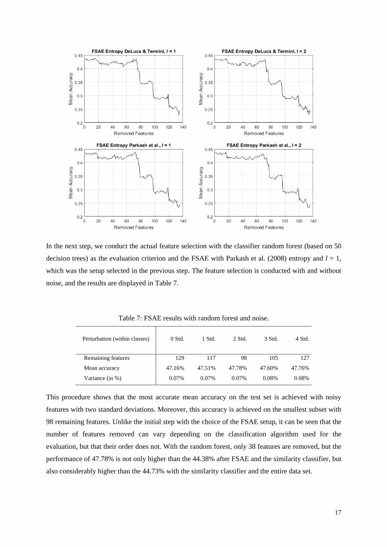
Figure 3 shows that, for all FSAE setups, the performance initially decreases, but then has a peak or

secondary peak at around 70 removed features. This stresses that all setups work well, but using

Parkash et al. (2008) entropy and l = 1, which found the best performance at this peak of around 70

removed features, is the most suitable choice of these setups.

Figure 3: Results for FSAE setups.

17

In the next step, we conduct the actual feature selection with the classifier random forest (based on 50

decision trees) as the evaluation criterion and the FSAE with Parkash et al. (2008) entropy and l = 1,

which was the setup selected in the previous step. The feature selection is conducted with and without

noise, and the results are displayed in Table 7.

Table 7: FSAE results with random forest and noise.

Perturbation (within classes) 0 Std. 1 Std. 2 Std. 3 Std. 4 Std.

Remaining features 129 117 98 105 127

Mean accuracy 47.16% 47.51% 47.78% 47.60% 47.76%

Variance (in %) 0.07% 0.07% 0.07% 0.08% 0.08%

This procedure shows that the most accurate mean accuracy on the test set is achieved with noisy

features with two standard deviations. Moreover, this accuracy is achieved on the smallest subset with

98 remaining features. Unlike the initial step with the choice of the FSAE setup, it can be seen that the

number of features removed can vary depending on the classification algorithm used for the

evaluation, but that their order does not. With the random forest, only 38 features are removed, but the

performance of 47.78% is not only higher than the 44.38% after FSAE and the similarity classifier, but

also considerably higher than the 44.73% with the similarity classifier and the entire data set.

18

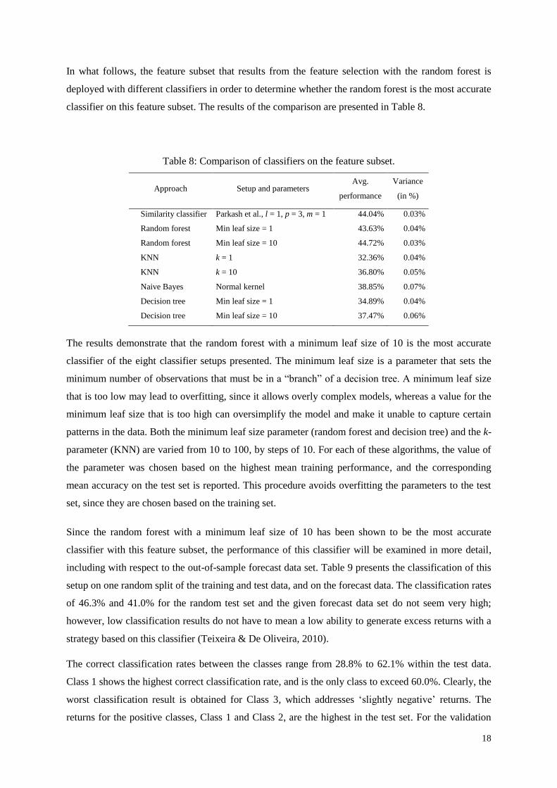
In what follows, the feature subset that results from the feature selection with the random forest is

deployed with different classifiers in order to determine whether the random forest is the most accurate

classifier on this feature subset. The results of the comparison are presented in Table 8.

Table 8: Comparison of classifiers on the feature subset.

Approach Setup and parameters Avg.

performance

Variance

(in %)

Similarity classifier Parkash et al., l = 1, p = 3, m = 1 44.04% 0.03%

Random forest Min leaf size = 1 43.63% 0.04%

Random forest Min leaf size = 10 44.72% 0.03%

KNN k = 1 32.36% 0.04%

KNN k = 10 36.80% 0.05%

Naive Bayes Normal kernel 38.85% 0.07%

Decision tree Min leaf size = 1 34.89% 0.04%

Decision tree Min leaf size = 10 37.47% 0.06%

The results demonstrate that the random forest with a minimum leaf size of 10 is the most accurate

classifier of the eight classifier setups presented. The minimum leaf size is a parameter that sets the

minimum number of observations that must be in a “branch” of a decision tree. A minimum leaf size

that is too low may lead to overfitting, since it allows overly complex models, whereas a value for the

minimum leaf size that is too high can oversimplify the model and make it unable to capture certain

patterns in the data. Both the minimum leaf size parameter (random forest and decision tree) and the k-

parameter (KNN) are varied from 10 to 100, by steps of 10. For each of these algorithms, the value of

the parameter was chosen based on the highest mean training performance, and the corresponding

mean accuracy on the test set is reported. This procedure avoids overfitting the parameters to the test

set, since they are chosen based on the training set.

Since the random forest with a minimum leaf size of 10 has been shown to be the most accurate

classifier with this feature subset, the performance of this classifier will be examined in more detail,

including with respect to the out-of-sample forecast data set. Table 9 presents the classification of this

setup on one random split of the training and test data, and on the forecast data. The classification rates

of 46.3% and 41.0% for the random test set and the given forecast data set do not seem very high;

however, low classification results do not have to mean a low ability to generate excess returns with a

strategy based on this classifier (Teixeira & De Oliveira, 2010).

The correct classification rates between the classes range from 28.8% to 62.1% within the test data.

Class 1 shows the highest correct classification rate, and is the only class to exceed 60.0%. Clearly, the

worst classification result is obtained for Class 3, which addresses ‘slightly negative’ returns. The

returns for the positive classes, Class 1 and Class 2, are the highest in the test set. For the validation

19

dataset, the accuracies range between 23.8% for Class 3 and 55.8% for Class 2. Only for the ‘strong

positive’ Class 1 is the classification accuracy considerably lower than on the test set, at 40.7%

compared to 62.1%. Simplifying things by considering the results from the perspective of an investor,

who will probably focus mainly on whether the predicted returns are positive or negative, the correct

classification rates can differ considerably from those of the single classes. The correct classification

rates for positive and negative returns for the data are 75.2% and 35.9%. This is worse than the result

for the test data, and indicates a clearly higher ability of the classifier to predict positive returns

correctly. The low negative prediction is burdened by the low classification rate in Class 3, which

accounts for more than three times as many observations as Class 4. In conclusion, the classifier for

the validation dataset seems to be more accurate at determining positive returns, but performs more

poorly at predicting the negative return classes.

Table 9: Classification results for training, test and forecast data.

Test Class 1 Class 2 Class 3 Class 4

62.1 % 54.6 % 18.8 % 48.3 %

46.3 % Positive Negative

82.40 % 50.00 %

Forecast Class 1 Class 2 Class 3 Class 4

40.7 % 55.8 % 23.8 % 41.2 %

41.0 % Positive Negative

75.2 % 35.9 %

We will attempt to obtain a better understanding of the decision-making abilities of the classifier by

discussing the features with the lowest scaled entropy values, since low entropy corresponds to high

informativity. As Figure 4 illustrates, the S&P500 Momentum terms, currency exchange rates, the

European stock market and the United States Commodity Index (USCI) possess the highest

information content. Three of the top four features for predicting the S&P500 open-to-close return are

related to the change in momentum. The remaining features consist of the exchange rates USD/Yuan

and USD/EUR, the European STOXX 50 open-to-close return and the change in the low value of the

USCI.

Figure 4: Top 10 lowest scaled entropy values.

20

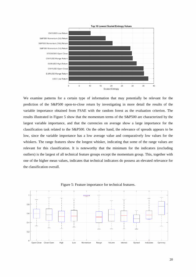
We examine patterns for a certain type of information that may potentially be relevant for the

prediction of the S&P500 open-to-close return by investigating in more detail the results of the

variable importance obtained from FSAE with the random forest as the evaluation criterion. The

results illustrated in Figure 5 show that the momentum terms of the S&P500 are characterized by the

largest variable importance, and that the currencies on average show a large importance for the

classification task related to the S&P500. On the other hand, the relevance of spreads appears to be

low, since the variable importance has a low average value and comparatively low values for the

whiskers. The range features show the longest whisker, indicating that some of the range values are

relevant for this classification. It is noteworthy that the minimum for the indicators (excluding

outliers) is the largest of all technical feature groups except the momentum group. This, together with

one of the higher mean values, indicates that technical indicators do possess an elevated relevance for

the classification overall.

Figure 5: Feature importance for technical features.

21

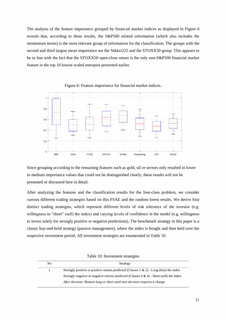
The analysis of the feature importance grouped by financial market indices as displayed in Figure 6

reveals that, according to these results, the S&P500 related information (which also includes the

momentum terms) is the most relevant group of information for the classification. The groups with the

second and third largest mean importance are the Nikkei225 and the STOXX50 group. This appears to

be in line with the fact that the STOXX50 open-close return is the only non-S&P500 financial market

feature in the top 10 lowest scaled entropies presented earlier.

Figure 6: Feature importance for financial market indices.

Since grouping according to the remaining features such as gold, oil or sectors only resulted in lower

to medium importance values that could not be distinguished clearly, these results will not be

presented or discussed here in detail.

After analyzing the features and the classification results for the four-class problem, we consider

various different trading strategies based on this FSAE and the random forest results. We derive four

distinct trading strategies, which represent different levels of risk tolerance of the investor (e.g.

willingness to “short” (sell) the index) and varying levels of confidence in the model (e.g. willingness

to invest solely for strongly positive or negative predictions). The benchmark strategy in this paper is a

classic buy-and-hold strategy (passive management), where the index is bought and then held over the

respective investment period. All investment strategies are enumerated in Table 10.

Table 10: Investment strategies

No Strategy

1 Strongly positive or positive returns predicted (Classes 1 & 2) - Long (buy) the index

Strongly negative or negative returns predicted (Classes 3 & 4) - Short (sell) the index

After decision: Remain long or short until next decision requires a change

22

2 Strongly positive returns predicted (Class 1) - Long (buy) the index

Strongly negative returns predicted (Class 4) - Short (sell) the index

After decision: Remain long or short until next decision requires a change

3 Strongly positive returns predicted (Class 1) - Long (buy) the index

Strongly negative or negative returns predicted (Classes 3 & 4) - Short (sell) the index

After decision: Remain long or short until next decision requires a change

4 Strongly positive or positive returns predicted (Classes 1 & 2) - Long (buy) the index

Strongly negative returns predicted (Class 4) - Short (sell) the index

After decision: Remain long or short until next decision requires a change

5 Benchmark: buy-and-hold - Long (buy) the index at start of period and retain

It is important to mention that only the index returns are regarded in the subsequent analysis of the

returns; no dividends of the underlying stocks are included.

For the comparison to a buy-and-hold strategy, various different levels of transaction costs are

considered. Transaction costs can be incorporated either as a percentage of the underlying trade (e.g.

Pätäri & Vilska, 2014) or as a fixed amount in a certain currency (e.g. Teixeira & De Oliveira, 2010),

and can vary considerably from country to country (Domowitz, Glen, & Madhavan, 2001). In this

study, both approaches will be used – a fixed amount in US dollars that can be expected to be paid to a

broker in the US, as well as a low percentage of the underlying trade value. Using both approaches

ensures that our results can be compared to other existing and future findings more easily. For the first

approach, the transaction cost varied between $10 and $20, which is within the range of transaction

costs that an investor can expect for an order at a broker to purchase a stock or financial instrument

(Nasdaq, 2017). The percentage-based transaction costs are set at 0.1%, 0.2%, 03% and 0.4%, to

incorporate low to medium levels of transaction costs.

In addition, it is assumed that no capital or gains are withdrawn during the investment period

considered. Since the S&P500 open-to-close return is the dependent variable, the results of the

strategies assume that the financial instruments used track the S&P500 as closely as possible. This

may be by buying all, or at least the majority, of the shares in the proportions that represent the firms

in the S&P500, by investing in an exchange traded fund (ETF) that attempts to replicate the behavior

of the S&P500, or potentially by using a suitable financial derivative. An ETF is an inexpensive

alternative for tracking a certain market or sector, and can also be bought at a broker (Bodie et al.,

2009). It is crucial for some of the strategies presented here that ETFs can be sold short (Bodie et al.,

2009). If an investor deploys an ETF to follow one of the strategies presented here, it must be taken

into account that, in addition to broker costs for the purchase of the ETF, costs are also incurred for the

ETF itself. Thus, investors should consider that the performance numbers presented here need to be

reduced by any additional cost such as the total expense ratio (TER) of the ETF, which is commonly

rather low (Bodie et al., 2009).

23

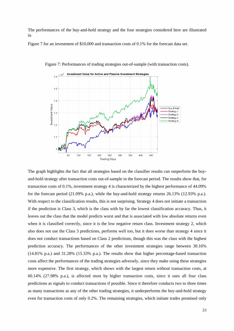
The performances of the buy-and-hold strategy and the four strategies considered here are illustrated

in

Figure 7 for an investment of $10,000 and transaction costs of 0.1% for the forecast data set.

Figure 7: Performances of trading strategies out-of-sample (with transaction costs).

The graph highlights the fact that all strategies based on the classifier results can outperform the buy-

and-hold strategy after transaction costs out-of-sample in the forecast period. The results show that, for

transaction costs of 0.1%, investment strategy 4 is characterized by the highest performance of 44.09%

for the forecast period (21.09% p.a.), while the buy-and-hold strategy returns 26.13% (12.93% p.a.).

With respect to the classification results, this is not surprising. Strategy 4 does not initiate a transaction

if the prediction is Class 3, which is the class with by far the lowest classification accuracy. Thus, it

leaves out the class that the model predicts worst and that is associated with low absolute returns even

when it is classified correctly, since it is the low negative return class. Investment strategy 2, which

also does not use the Class 3 predictions, performs well too, but it does worse than strategy 4 since it

does not conduct transactions based on Class 2 predictions, though this was the class with the highest

prediction accuracy. The performances of the other investment strategies range between 30.16%

(14.81% p.a.) and 31.28% (15.33% p.a.). The results show that higher percentage-based transaction

costs affect the performances of the trading strategies adversely, since they make using these strategies

more expensive. The first strategy, which shows with the largest return without transaction costs, at

60.14% (27.98% p.a.), is affected most by higher transaction costs, since it uses all four class

predictions as signals to conduct transactions if possible. Since it therefore conducts two to three times

as many transactions as any of the other trading strategies, it underperforms the buy-and-hold strategy

even for transaction costs of only 0.2%. The remaining strategies, which initiate trades premised only

24

on a subset of the classes, show fewer transactions and are therefore less sensitive to changes in the

transaction costs. For investments of $10.000 and $50.000, the performances again depend on the

transaction costs, with the returns logically being higher the lower the value of the transaction costs, as

the costs are in proportion to the investment amount.

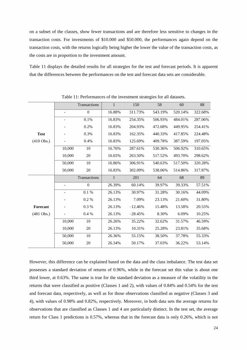
Table 11 displays the detailed results for all strategies for the test and forecast periods. It is apparent

that the differences between the performances on the test and forecast data sets are considerable.

Table 11: Performances of the investment strategies for all datasets.

Test

(410 Obs.)

Transactions 1 150 58 60 88

- 0 16.88% 311.73% 543.19% 520.14% 322.68%

- 0.1% 16.83% 254.35% 506.93% 484.01% 287.06%

- 0.2% 16.83% 204.93% 472.68% 449.95% 254.41%

- 0.3% 16.83% 162.35% 440.33% 417.85% 224.48%

- 0.4% 16.83% 125.69% 409.78% 387.59% 197.05%

10,000 10 16.76% 287.61% 530.36% 506.92% 310.65%

10,000 20 16.65% 263.50% 517.52% 493.70% 298.62%

50,000 10 16.86% 306.91% 540.63% 517.50% 320.28%

50,000 20 16.83% 302.09% 538.06% 514.86% 317.87%

Forecast

(481 Obs.)

Transactions 1 201 64 68 89

- 0 26.39% 60.14% 39.97% 39.33% 57.51%

- 0.1 % 26.13% 30.97% 31.28% 30.16% 44.09%

- 0.2 % 26.13% 7.09% 23.13% 21.60% 31.80%

- 0.3 % 26.13% –12.46% 15.48% 13.58% 20.55%

- 0.4 % 26.13% –28.45% 8.30% 6.09% 10.25%

10,000 10 26.26% 35.22% 32.62% 31.57% 46.59%

10,000 20 26.13% 10.31% 25.28% 23.81% 35.68%

50,000 10 26.36% 55.15% 38.50% 37.78% 55.33%

50,000 20 26.34% 50.17% 37.03% 36.22% 53.14%

However, this difference can be explained based on the data and the class imbalance. The test data set

possesses a standard deviation of returns of 0.96%, while in the forecast set this value is about one

third lower, at 0.63%. The same is true for the standard deviation as a measure of the volatility in the

returns that were classified as positive (Classes 1 and 2), with values of 0.84% and 0.54% for the test

and forecast data, respectively, as well as for those observations classified as negative (Classes 3 and

4), with values of 0.98% and 0.82%, respectively. Moreover, in both data sets the average returns for

observations that are classified as Classes 1 and 4 are particularly distinct. In the test set, the average

return for Class 1 predictions is 0.57%, whereas that in the forecast data is only 0.26%, which is not

25

even half. We find comparable results for the average return for Class 4 predictions, with –0.73% on

the test set versus –0.20% on the forecast set, which is not even a third of the magnitude. This

discrepancy between the results in the test and forecast data sets is due to the fact that the predictions

in Classes 1 and 4 contribute most to the returns achieved by any of the trading strategies depicted.

The effect is amplified by the fact that the forecast data set is more unbalanced, with fewer

observations in Classes 1 and 4, whose correct prediction could boost the returns of the strategy. As a

consequence, the difference between the results in the test and forecast sets is considerable, but

plausible after further investigation. Moreover, the returns achieved by the trading strategies clearly

depend on the market volatility and returns.

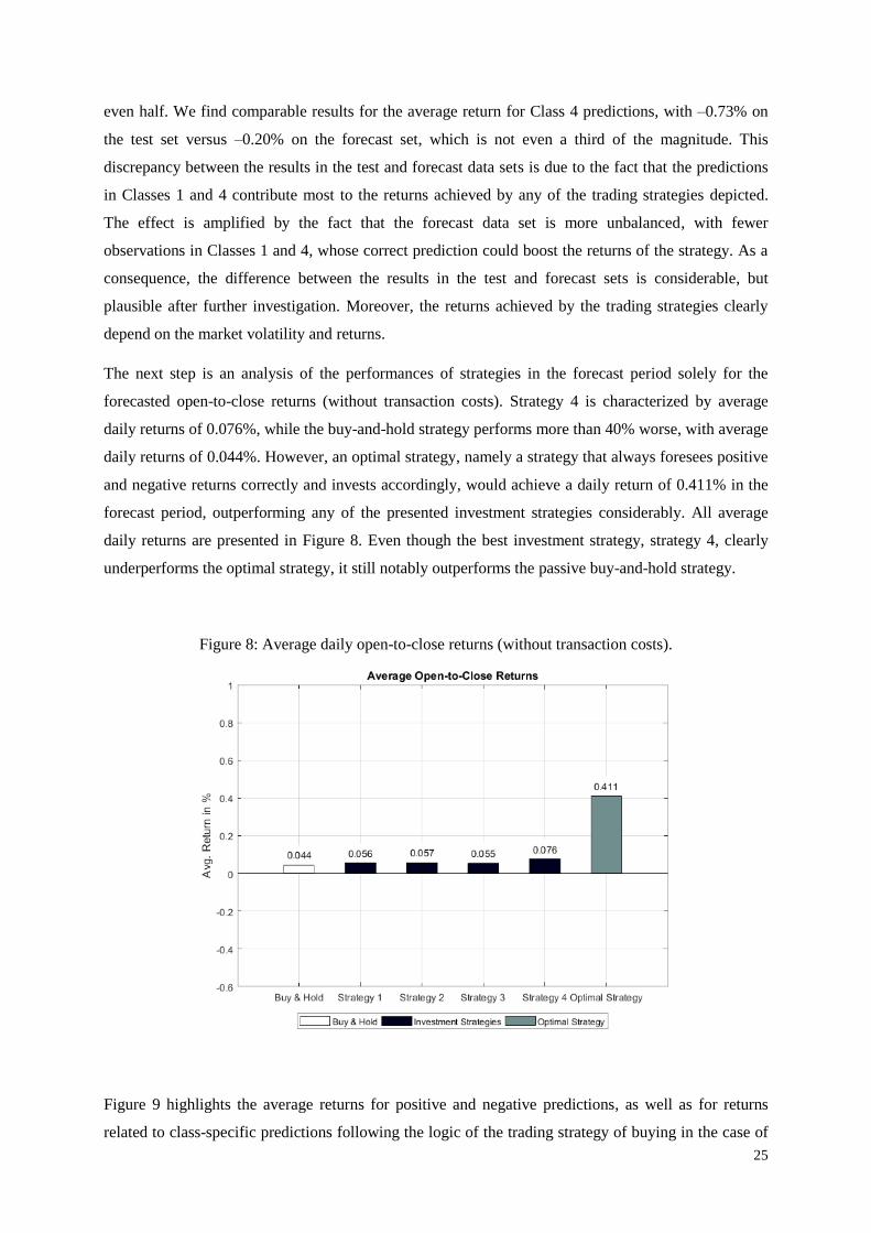
The next step is an analysis of the performances of strategies in the forecast period solely for the

forecasted open-to-close returns (without transaction costs). Strategy 4 is characterized by average

daily returns of 0.076%, while the buy-and-hold strategy performs more than 40% worse, with average

daily returns of 0.044%. However, an optimal strategy, namely a strategy that always foresees positive

and negative returns correctly and invests accordingly, would achieve a daily return of 0.411% in the

forecast period, outperforming any of the presented investment strategies considerably. All average

daily returns are presented in Figure 8. Even though the best investment strategy, strategy 4, clearly

underperforms the optimal strategy, it still notably outperforms the passive buy-and-hold strategy.

Figure 8: Average daily open-to-close returns (without transaction costs).

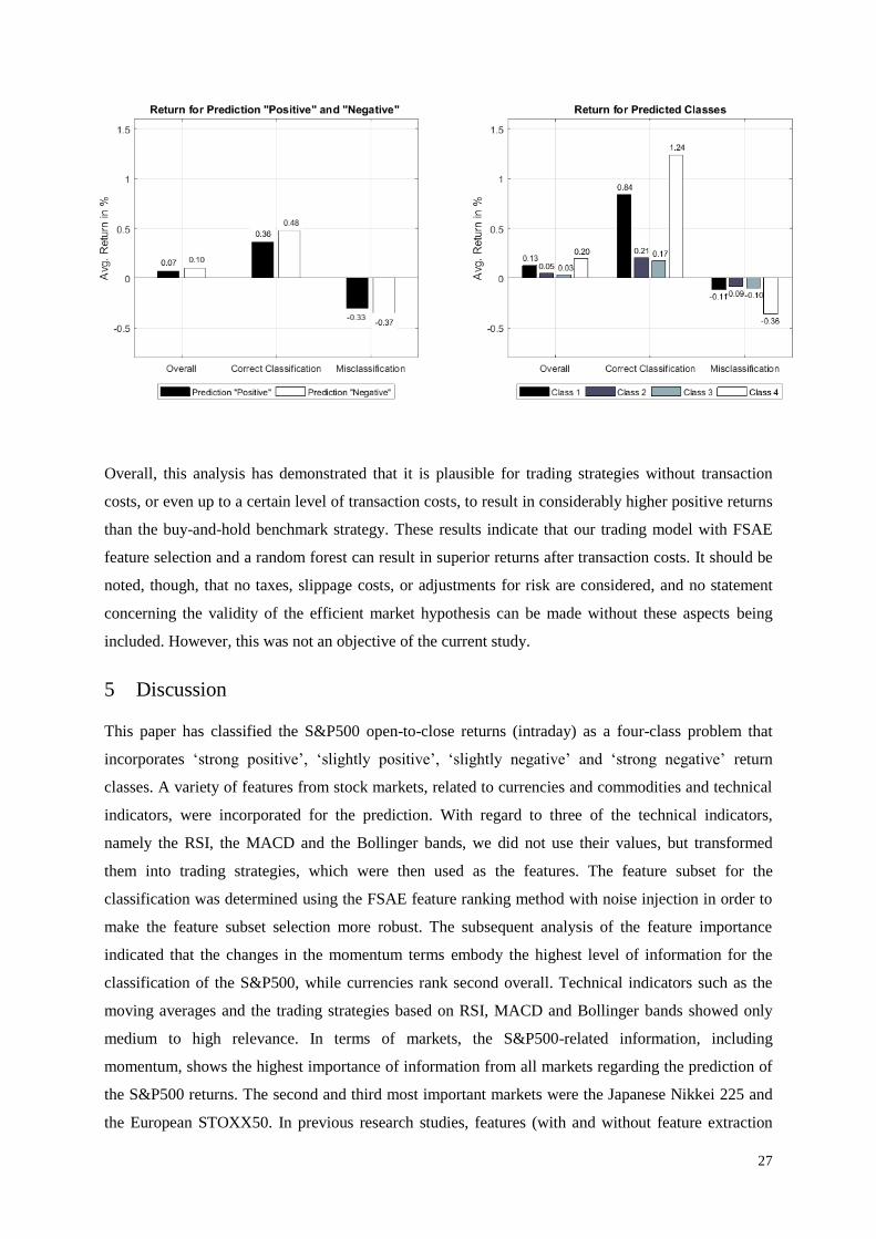
Figure 9 highlights the average returns for positive and negative predictions, as well as for returns

related to class-specific predictions following the logic of the trading strategy of buying in the case of

26

a Class 1 or Class 2 classification and selling short in the case of a predicted Class 3 or Class 4. The

first graph shows that the prediction of the negative classes (Class 3 and Class 4) accounts for a higher

average return than the positive classes in the forecast period. Moreover, it stresses that the correct

prediction of the positive and negative classes (0.36% and 0.48%) is higher in magnitude than the

average return of misclassifying the direct counterparts of these two return directions (–0.33% and –

0.37%).

The second graph in Figure 9 highlights the average class-specific returns overall, in the cases of both

correct classification and misclassifications. The graph illustrates two relevant aspects of the

classification result. The first is that, for all classes, the returns are higher in magnitude in the case of

correct classification than when a misclassification occurs. This contributes to the fact that the average

return overall is positive for all classes. In particular, all predicted classes lead to positive returns on

average. In simple terms, if the classifier predicts a class for a daily return, following this prediction

will lead to a positive return on average – even though the prediction may be incorrect.

The second aspect that this graph highlights is the difference between the average returns for the

classes with ‘strong positive’ (Class 1) and ‘strong negative’ (Class 4) predicted returns, as opposed to

those with ‘slightly positive’ and ‘slightly negative’ returns (Classes 2 and 3). In the case of correct

classifications, the average returns of Classes 1 and 4 (at 0.84% and 1.24%) are considerably higher

than those of the two other classes. This result is intuitive, given that correct classification means that

the returns for Classes 1 and 4 are respectively larger than 0.5% and smaller than –0.5% (larger than

0.5% for the trading strategy that sells short). The noticeable impact of this higher average return is

that the negative return in the case of a misclassification apparently does not entirely compensate for

the positive return from a correct classification. This results not only in positive average returns for

Classes 1 and 4 overall (independently of whether the classification is correct or not), but also in

considerably higher average returns than those for Classes 3 and 4. Predicting ‘strong positive’ returns

(Class 1) leads to more than double the average return of ‘slightly positive’ returns (Class 2). The

pattern is seen even more strongly for negative returns, where the prediction of ‘strong negative’

returns (Class 4) results in an average return that is more than 6 times that of a classification of

‘slightly negative’ returns (Class 3). The considerably smaller numbers of observations from Classes 1

and 4 in the forecast data set are part of the reason why the average returns for the positive and

negative returns in the first graph are positive but considerably lower than the average returns for these

classes.

Figure 9: Performances for all predictions for trading (Strategy 1).

27

Overall, this analysis has demonstrated that it is plausible for trading strategies without transaction

costs, or even up to a certain level of transaction costs, to result in considerably higher positive returns

than the buy-and-hold benchmark strategy. These results indicate that our trading model with FSAE

feature selection and a random forest can result in superior returns after transaction costs. It should be

noted, though, that no taxes, slippage costs, or adjustments for risk are considered, and no statement

concerning the validity of the efficient market hypothesis can be made without these aspects being

included. However, this was not an objective of the current study.

5 Discussion

This paper has classified the S&P500 open-to-close returns (intraday) as a four-class problem that

incorporates ‘strong positive’, ‘slightly positive’, ‘slightly negative’ and ‘strong negative’ return

classes. A variety of features from stock markets, related to currencies and commodities and technical

indicators, were incorporated for the prediction. With regard to three of the technical indicators,

namely the RSI, the MACD and the Bollinger bands, we did not use their values, but transformed

them into trading strategies, which were then used as the features. The feature subset for the

classification was determined using the FSAE feature ranking method with noise injection in order to

make the feature subset selection more robust. The subsequent analysis of the feature importance

indicated that the changes in the momentum terms embody the highest level of information for the

classification of the S&P500, while currencies rank second overall. Technical indicators such as the

moving averages and the trading strategies based on RSI, MACD and Bollinger bands showed only

medium to high relevance. In terms of markets, the S&P500-related information, including

momentum, shows the highest importance of information from all markets regarding the prediction of

the S&P500 returns. The second and third most important markets were the Japanese Nikkei 225 and

the European STOXX50. In previous research studies, features (with and without feature extraction

28

and selection) have commonly been used simply for classification, without examining in more detail

their feature importance for the class labels / event prediction for the future state of the financial

market. In future research, our results for the feature importance must be validated and analyzed with

respect to their generalizability to other equity markets.

The classification of the feature subset was conducted using the random forest classifier, and

contrasted with the performances of different setups of the KNN algorithm, decision trees, naive

Bayes and the similarity classifier. The mean classification accuracy was demonstrated to be the

highest for the random forest model. It is noteworthy that the prediction rates for the four classes differ

considerably. The subsequent use of four different trading strategies showed that trading based on only

a subset of the predicted classes can be more profitable than following all predictions. In particular,

using only predictions of Classes 1, 2 and 4 led to the highest return for the forecasting period, since

the classification accuracy for Class 3 was clearly the lowest and the average return from using this

class prediction was also comparatively low. Another essential finding of this research is that the

contributions of the classes to the returns of the trading strategies vary. Predictions on a ‘buy’ decision

for the ‘strong positive’ Class 1 or a ‘sell’ for the ‘strong negative’ Class 4 have overall (correct

classifications and misclassifications) multiple times higher returns than those on the ‘slightly

positive’ and ‘slightly negative’ return classes (Classes 2 and 3). In other words, using the two extreme

classes with returns that are far from zero in absolute terms contributes most to the trading strategies

on average. Since most previous research has simply used a binary classification problem with only

upward and downward movements being considered, this finding can help to shed light on the way in

which using more event outcomes for the classification, rather than merely simple upward or

downward movements, can improve the benefit of a trading strategy (or a bet on an event). This

finding needs to be validated in future research. It will be also of interest to see whether this pattern is

observed for the forecasts of other financial markets and whether the prediction of the extreme classes

can result in higher average returns or payoffs in other contexts too.

6 Acknowledgements

This research would like to acknowledge the funding received from the Finnish Strategic Research

Council, grant number 313396 / MFG40 Manufacturing 4.0.

7 References

Achelis, S. B. (1995). Technical analysis from A to Z (2nd ed.). New York: McGraw-Hill.

Adele, C., Cutler, D. R., & Stevens, J. R. (2012). Random forests. In Ensemble machine learning:

methods and applications (pp. 157–175). Springer.

Altay, E., & Satman, M. H. (2005). Stock market forecasting: artificial neural network linear

regression comparison in an emerging market. Journal of Financial Management and Analysis,

29

18(2), 18–33.

Baur, D. G. (2012). Asymmetric volatility in the gold market. Journal of Alternative Investments,

14(4), 26–38.

Belis, M., & Guiasu, S. (1968). A quantitative-qualitative measure of information in cybernetic

systems. IEEE Transactions on Information Theory, 14(4), 593–594.

Bhaduri, S., & Saraogi, R. (2010). The predictive power of the yield spread in timing the stock market.

Emerging Markets Review, 11(3), 261–272.

BlackRock. (2017a). iShares MSCI emerging markets ETF. Retrieved May 20, 2017, from

https://www.ishares.com/us/products/239637/EEM.

BlackRock. (2017b). iShares MSCI Europe financials ETF. Retrieved April 30, 2017, from

https://www.ishares.com/us/products/239645/ishares-msci-europe-financials-etf.

Bodie, Z., Kane, A., & Marcus, A. J. (2009). Investments (8th ed.). Irwin: McGraw-Hill.

Breiman, L. (2001). Random forests. Machine Learning, 45(1), 5–32.

Breiman, L., Friedman, J., Stone, C. J., & Olshen, R. A. (1984). Classification and regression trees.

Wadsworth International Group.

Cao, L., & Tay, F. E. H. (2001). Financial forecasting using support vector machines.

Neurocomputing, 1(2), 1–36.

Chang, P. C., & Wu, J. L. (2015). A critical feature extraction by kernel PCA in stock trading model.

Soft Computing, 19(5), 1393–1408.

Chicago Board Options Exchange (2017). CBOE interest rate 10 year. Retrieved May 20, 2017, from

http://www.cboe.com/delayedquote/advanced-charts?ticker=TNX

Chun, S.-H., & Park, Y.-J. (2005). Dynamic adaptive ensemble case-based reasoning: application to

stock market prediction. Expert Systems with Applications, 28, 435–443.

Cover, T., & Hart, P. (1967). Nearest neighbor pattern classification. IEEE Transactions on

Information Theory, 13(1), 21–27.

De Luca, A., & Termini, S. (1972). A definition of a nonprobabilistic entropy in the setting of fuzzy

sets theory. Information and Control, 20, 301–312.

Di Lorenzo, R. (2013). Basic technical analysis of financial markets. A modern approach. Milan:

Springer Italia.

Domowitz, I., Glen, J., & Madhavan, A. (2001). Liquidity, volatility and equity trading costs across

countries and over time. International Finance, 4(2), 221–255.

30

Enke, D., Grauer, M., & Mehdiyev, N. (2011). Stock market prediction with multiple regression, fuzzy

type-2 clustering and neural networks. Procedia Computer Science, 6, 201–206.

Fadlalla, A., & Amani, F. (2014). Predicting next day closing price of Qatar Exchange Index using

technical indicators and artificial neural network. Intelligent Systems in Accounting, Finance and

Management, 21, 209–223.

Fama, E. F. (1965a). Random walks in stock market prices. Financial Analysts Journal, 21(5), 55–59.

Fama, E. F. (1965b). The behavior of stock market prices. The Journal of Business, 38(1), 34–105.

Fama, E. F. (1970). Efficient capital markets: a review of theory and empirical work. Journal of

Finance, 25(2), 383–417.

Felsen, J. (1975). Learning pattern recognition techniques applied to stock market forecasting. IEEE

Transactions on Systems, Man, and Cybernetics, 5(6), 583–594.

Gokmenoglu, K. K., & Fazlollahi, N. (2015). The interactions among gold, oil, and stock market:

evidence from S&P500. Procedia Economics and Finance, 25, 478–488.

Guerard Jr., J. B. (2013). Introduction to financial forecasting in investment analysis. New York:

Springer ScienceBusiness Media.

Guo-qiang, X. (2011). The optimization of share price prediction model based on support vector

machine. In International Conference on Control, Automation and Systems Engineering (CASE)

(pp. 1–4).

Guo, Z., Wang, H., Liu, Q., & Yang, J. (2014). Fusion based forecasting model for financial time

series. PLoS ONE, 9(6), 1–13.

Hastie, T., Tibshirani, R., & Friedman, J. (2009). The elements of statistical learning: data mining,

inference, and prediction. Springer Series in Statistics (Vol. 2).

Hurwitz, E., & Marwala, T. (2011). Suitability of using technical indicator-based strategies as

potential strategies within intelligent trading systems. In IEEE International Conference on

Systems, Man, and Cybernetics (SMC) (pp. 80–84).

Karymshakov, K., & Abdykaparov, Y. (2012). Forecasting stock index movement with artificial

neural networks: the case of İstanbul stock exchange. Trakya University Journal of Social

Science, 14(2), 231–242.

Khaidem, L., Saha, S., & Dey, S. R. (2016). Predicting the direction of stock market prices using

random forest. Applied Mathematical Finance, 1(5), 1–20.

Kim, K. (2003). Financial time series forecasting using support vector machines. Neurocomputing,

31

55(1–2), 307–319.

Kim, M.-J., Min, S.-H., & Han, I. (2006). An evolutionary approach to the combination of multiple

classifiers to predict a stock price index. Expert Systems with Applications, 31(2), 241–247.

Kim, M. J., Han, I., & Lee, K. C. (2004). Hybrid knowledge integration using the fuzzy genetic

algorithm: prediction of the Korea Stock Index. Intelligent Systems in Accounting, Finance and

Management, 12, 43–60.

Krauss, C., Do, X. A., & Huck, N. (2017). Deep neural networks, gradient-boosted trees, random

forests: statistical arbitrage on the S&P 500. European Journal of Operational Research, 259,

689–702.

Krollner, B., Vanstone, B., & Finnie, G. (2010). Financial time series forecasting with machine

learning techniques: a survey. In European Symposium on Artificial Neural Networks:

Computational and Machine Learning (pp. 25–30).

Leigh, W., Purvis, R., & Ragusa, J. M. (2002). Forecasting the NYSE composite index with technical

analysis, pattern recognizer, neural network, and genetic algorithm: a case study in romantic

decision support. Decision Support Systems, 32, 361–377.

Lendasse, A., De Bodt, E., Wertz, V., & Verleysen, M. (2000). Non-linear financial time series

forecasting – application to the Bel 20 stock market index. European Journal of Economic and

Social Systems, 14(1), 81–91.

Leung, M. T., Daouk, H., & Chen, A.-S. (2000). Forecasting stock indices: a comparison of

classification and level estimation models. International Journal of Forecasting, 16(2), 173–190.

Lohrmann, C., Luukka, P., Jablonska-Sabuka, M., & Kauranne, T. (2018). Supervised feature

selection with a combination of fuzzy similarity measures and fuzzy entropy measures. Expert

Systems with Applications, 110, 216–236.

Lu, C.-J., & Wu, J.-Y. (2011). An efficient CMAC neural network for stock index forecasting. Expert

Systems with Applications, 38(12), 15194–15201.

Luukka, P. (2007). Similarity classifier using similarity measure derived from Yu’s norms in

classification of medical data sets. Computers in Biology and Medicine, 37, 1133–1140.

Luukka, P. (2011). Feature selection using fuzzy entropy measures with similarity classifier. Expert

Systems with Applications, 38, 4600–4607.

Luukka, P., Saastamoinen, K., & Könönen, V. (2001). A classifier based on the maximal fuzzy

similarity in the generalized Lukasiewicz-structure. In 10th IEEE International Conference on

Fuzzy Systems.

32

Matsuoka, K. (1992). Noise injection into inputs in back-propagation-learning. IEEE Transactions on

Systems, Man, and Cybernetics: Systems, 22(3), 436–440.

Morningstar (2017). Vanguard total world stock index fund ETF. Retrieved from

http://www.morningstar.co.uk/uk/etf/snapshot/snapshot.aspx?id=0P0000G5T2.

Nasdaq (2017). Start investing with only $1,000. Retrieved April 30, 2017, from

http://www.nasdaq.com/investing/start-investing-1000.stm.

Niaki, S. T. A., & Hoseinzade, S. (2013). Forecasting S&P 500 index using artificial neural networks

and design of experiments. Journal of Industrial Engineering International, 9(1), 1–9.

Nyberg, H. (2013). Predicting bear and bull stock markets with dynamic binary time series models.

Journal of Banking and Finance, 37(9), 3351–3363.

O’Connor, N., & Madden, M. G. (2006). A neural network approach to predicting stock exchange

movements using external factors. Knowledge-Based Systems, 19(5), 371–378.

Özesmi, S. L., Tan, C. O., & Özesmi, U. (2006). Methodological issues in building, training, and

testing artificial neural networks in ecological applications. Ecological Modelling, 195(1–2), 83–

93.

Page, L. (2012). “It ain’t over till it’s over.” Yogi Berra bias on prediction markets. Applied

Economics, 44(1), 81–92.

Parkash, O., Sharma, P., & Mahajan, R. (2008). New measures of weighted fuzzy entropy and their

applications for the study of maximum weighted fuzzy entropy principle. Information Sciences,

178, 2389–2395.

Patel, J., Shah, S., Thakkar, P., & Kotecha, K. (2015). Predicting stock and stock price index

movement using trend deterministic data preparation and machine learning techniques. Expert

Systems with Applications, 42(1), 259–268.

Pätäri, E., & Vilska, M. (2014). Performance of moving average trading strategies over varying stock

market conditions: the Finnish evidence. Applied Economics, 46(24), 2851–2872.

Rossilo, R., Giner, J., & de la Fuente, D. (2014). The effectiveness of the combined use of VIX and

support vector machines on the prediction of S&P 500. Neural Computing and Applications, 25,

321–332.

Rothschild, D., & Pennock, D. M. (2014). The extent of price misalignment in prediction markets.

Algorithmic Finance, 3(1–2), 3–20.

Rudebusch, G. D., & Williams, J. C. (2009). Forecasting recessions: The puzzle of the enduring power

of the yield curve. Journal of Business and Economic Statistics, 27(4), 492–503.

33

Russell, S., & Norvig, P. (2009). Artificial intelligence: a modern approach (3rd ed.). Prentice Hall.

S&P Dow Jones Indices. (2017). S&P GSCI CRUDE OIL. Retrieved April 10, 2017, from

https://us.spindices.com/indices/commodities/sp-gsci-crude-oil.

State Street Global Advisors (SPDR). (2017a). SPDR S&P U.S. financials select sector UCITS ETF.

Retrieved May 5, 2017, from https://fi.spdrs.com/en/professional/etf/spdr-sp-us-financials-select-

sector-ucits-etf-ZPDF-GY?cid=1365706.

State Street Global Advisors (SPDR). (2017b). SPDR S&P U.S. materials select sector UCITS ETF.

Retrieved May 5, 2017, from https://fi.spdrs.com/en/professional/etf/SPDR-SP-US-Materials-

Select-Sector-UCITS-ETF-ZPDM-GY.

Teixeira, L. A., & De Oliveira, A. L. I. (2010). A method for automatic stock trading combining

technical analysis and nearest neighbor classification. Expert Systems with Applications, 37(10),

6885–6890.

USCF. (2017). United States commodity index fund. Retrieved May 5, 2017, from

http://www.uscfinvestments.com/usci.

Vaughan Williams, L., & Reade, J. J. (2016). Prediction markets, social media and information

efficiency. Kyklos, 69(3), 518–556.

Wolfers, J., & Zitzewitz, E. (2004). Prediction markets. Journal of Economic Perspectives, 18(2),

107–126.

Yahoo Finance (2017). Selected time series. Retrieved from https://finance.yahoo.com/.

Yao, Y. Y., Wong, S. K., & Butz, C. J. (1999). On information-theoretic measures of attribute

importance. In PacificAsia Conference on Knowledge Discovery and Data Mining (pp. 133–

137).

Zhang, J., Cui, S., Xu, Y., Li, Q., & Li, T. (2018). A novel data-driven stock price trend prediction

system. Expert Systems with Applications, 97, 60–69.

Zhong, X., & Enke, D. (2017). Forecasting daily stock market return using dimensionality reduction.

Expert Systems with Applications, 67, 126–139.

Zhora, D. V. (2005). Data preprocessing for stock market forecasting using random subspace classifier

network. In Proceedings of International Joint Conference on Neural Networks, Montreal,

Canada (pp. 2549–2554).