Embed Size (px)
Citation preview

Long-Term Results from Evaluation of Advanced New Construction Packages in Test Homes: Martha’s Vineyard, Massachusetts Dave Stecher, Katherine Allison, and Duncan Prahl IBACOS, Inc.
October 2012

NOTICE
This report was prepared as an account of work sponsored by an agency of the United States government. Neither the United States government nor any agency thereof, nor any of their employees, subcontractors, or affiliated partners makes any warranty, express or implied, or assumes any legal liability or responsibility for the accuracy, completeness, or usefulness of any information, apparatus, product, or process disclosed, or represents that its use would not infringe privately owned rights. Reference herein to any specific commercial product, process, or service by trade name, trademark, manufacturer, or otherwise does not necessarily constitute or imply its endorsement, recommendation, or favoring by the United States government or any agency thereof. The views and opinions of authors expressed herein do not necessarily state or reflect those of the United States government or any agency thereof.
Available electronically at http://www.osti.gov/bridge
Available for a processing fee to U.S. Department of Energy and its contractors, in paper, from:
U.S. Department of Energy Office of Scientific and Technical Information
P.O. Box 62 Oak Ridge, TN 37831-0062
phone: 865.576.8401 fax: 865.576.5728
email: mailto:[email protected]
Available for sale to the public, in paper, from: U.S. Department of Commerce
National Technical Information Service 5285 Port Royal Road Springfield, VA 22161 phone: 800.553.6847
fax: 703.605.6900 email: [email protected]
online ordering: http://www.ntis.gov/ordering.htm
Printed on paper containing at least 50% wastepaper, including 20% postconsumer waste

iii
Long-Term Results from Evaluation of Advanced New Construction Packages in Test Homes: Martha’s Vineyard, Massachusetts
Prepared for:
The National Renewable Energy Laboratory
On behalf of the U.S. Department of Energy’s Building America Program
Office of Energy Efficiency and Renewable Energy
15013 Denver West Parkway
Golden, CO 80401
NREL Contract No. DE-AC36-08GO28308
Prepared by:
Dave Stecher, Katherine Allison, and Duncan Prahl
IBACOS, Inc.
2214 Liberty Avenue
Pittsburgh, PA 15222
NREL Technical Monitor: Michael Gestwick
Prepared under Subcontract No. KNDJ-0-40341-00
October 2012

iv
[This page left blank]
v
Contents List of Figures ............................................................................................................................................ vi List of Tables .............................................................................................................................................. vi Definitions .................................................................................................................................................. vii Executive Summary ................................................................................................................................. viii Acknowledgments ................................................................................................................................... viii 1 Introduction and Background ............................................................................................................. 1
1.1 Purpose and Research Questions .........................................................................................2 2 Mathematical and Modeling Methods ................................................................................................. 4 3 Experimental Methods ......................................................................................................................... 8 4 Results ................................................................................................................................................. 12 5 Discussion ........................................................................................................................................... 23 6 Conclusions ........................................................................................................................................ 26 7 References .......................................................................................................................................... 27
vi
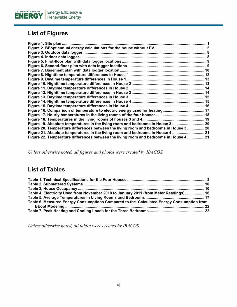
List of Figures Figure 1. Site plan ....................................................................................................................................... 1 Figure 2. BEopt annual energy calculations for the house without PV ................................................ 5 Figure 3. Outdoor data logger ................................................................................................................... 8 Figure 4. Indoor data logger....................................................................................................................... 8 Figure 5. First-floor plan with data logger locations ............................................................................... 9 Figure 6. Second-floor plan with data logger locations .......................................................................... 9 Figure 7. Basement plan with data logger location ............................................................................... 10 Figure 8. Nighttime temperature differences in House 1 ...................................................................... 12 Figure 9. Daytime temperature differences in House 1 ......................................................................... 13 Figure 10. Nighttime temperature differences in House 2 .................................................................... 13 Figure 11. Daytime temperature differences in House 2 ....................................................................... 14 Figure 12. Nighttime temperature differences in House 3 .................................................................... 14 Figure 13. Daytime temperature differences in House 3 ....................................................................... 15 Figure 14. Nighttime temperature differences in House 4 .................................................................... 15 Figure 15. Daytime temperature differences in House 4 ....................................................................... 16 Figure 16. Comparison of temperature to electric energy used for heating ....................................... 17 Figure 17. Hourly temperatures in the living rooms of the four houses ............................................. 18 Figure 18. Temperatures in the living rooms of houses 3 and 4 .......................................................... 19 Figure 19. Absolute temperatures in the living room and bedrooms in House 3 .............................. 20 Figure 20. Temperature differences between the living room and bedrooms in House 3 ................ 20 Figure 21. Absolute temperatures in the living room and bedrooms in House 4 .............................. 21 Figure 22. Temperature differences between the living room and bedrooms in House 4 ................ 21
Unless otherwise noted, all figures and photos were created by IBACOS.
List of Tables Table 1. Technical Specifications for the Four Houses .......................................................................... 2 Table 2. Submetered Systems ................................................................................................................. 10 Table 3. House Occupancy ...................................................................................................................... 10 Table 4. Electricity Used from November 2010 to January 2011 (from Meter Readings) .................. 16 Table 5. Average Temperatures in Living Rooms and Bedrooms ....................................................... 17 Table 6. Measured Energy Consumptions Compared to the Calculated Energy Consumption from
BEopt Modeling .................................................................................................................................. 22 Table 7. Peak Heating and Cooling Loads for the Three Bedrooms.................................................... 22
Unless otherwise noted, all tables were created by IBACOS.
vii
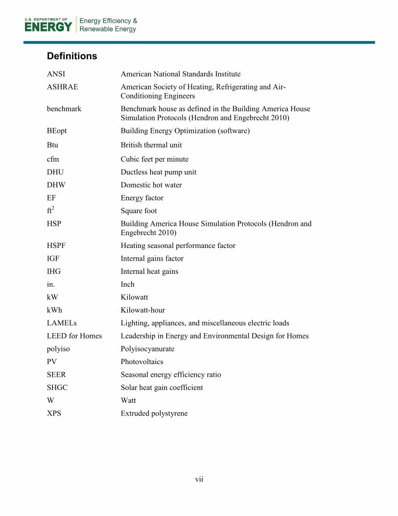
Definitions
ANSI American National Standards Institute
ASHRAE American Society of Heating, Refrigerating and Air-Conditioning Engineers
benchmark Benchmark house as defined in the Building America House Simulation Protocols (Hendron and Engebrecht 2010)
BEopt Building Energy Optimization (software)
Btu British thermal unit
cfm Cubic feet per minute
DHU Ductless heat pump unit
DHW Domestic hot water
EF Energy factor
ft2 Square foot
HSP Building America House Simulation Protocols (Hendron and Engebrecht 2010)
HSPF Heating seasonal performance factor
IGF Internal gains factor
IHG Internal heat gains
in. Inch
kW Kilowatt
kWh Kilowatt-hour
LAMELs Lighting, appliances, and miscellaneous electric loads
LEED for Homes Leadership in Energy and Environmental Design for Homes
polyiso Polyisocyanurate
PV Photovoltaics
SEER Seasonal energy efficiency ratio
SHGC Solar heat gain coefficient
W Watt
XPS Extruded polystyrene

viii
Executive Summary
This report presents a cold climate project that examines the relationships among very energy efficient single-family residential thermal enclosures, room-to-room temperature variations, and simplified space conditioning systems. The project was developed, designed, and built by South Mountain Company and is located in West Tisbury, Massachusetts, on the island of Martha’s Vineyard. This project allowed investigators to compare room-to-room temperatures in four virtually identical houses that were all built to the same construction standard. Each of the four all-electric homes has a single ductless heat pump unit (DHU) located in the main living space with a single programmable thermostatic control built into the unit. Each bedroom and the main bathroom have radiant electric resistance panels with individual nonprogrammable thermostatic controls that occupants can turn on and off for their comfort. Results indicate that temperature fluctuations in the living room resulting from aggressive setup and setback of the DHU may contribute to fewer hours when the bedroom temperatures are within +2°F of the living room temperatures, compared to houses without setback. Solar gains in the living room, along with opening and closing doors, appear to have a significant impact on room-to-room temperature differences, as would be expected. Setback strategies do not appear to save energy but do contribute to significant temperature variations.
Acknowledgments
The authors thank the South Mountain Company for developing, designing, and constructing this innovative project (including the energy systems); for coordinating access to the houses; and for supporting data collection activities. The authors also thank the residents of the houses, who allowed the authors to record the data and endured the inconvenience of monthly meter readings, and Matt Coffey for diligently collecting the data. Finally, the authors thank the U.S. Department of Energy’s Building America Program for funding this research.

1
1 Introduction and Background
In 2010 IBACOS identified a project designed and built by South Mountain Company in West Tisbury, Massachusetts, on the island of Martha’s Vineyard that was nearing completion and was aligned with ongoing research into the application of simplified space conditioning systems in highly insulated houses. The community consists of eight all-electric two- and three-bedroom (1,251 and 1,447 ft2, respectively) Cape Cod style houses built in a cluster development as shown in Figure 1. Houses 1, 2, 3, and 4 in Figure 1 all have identical three-bedroom floor plans. Each of these four all-electric homes has a single ductless heat pump unit (DHU) located in the main living space with a single programmable thermostatic control built into the unit. Each bedroom and the main bathroom have radiant electric resistance panels with individual nonprogrammable thermostatic controls that the occupants can turn on and off for their comfort.
Figure 1. Site plan
Courtesy of South Mountain Company, used with permission All houses are highly insulated and very airtight. Each has earned a platinum rating from the U.S. Green Building Council’s Leadership in Energy and Environmental Design for Homes (LEED for Homes) program. IBACOS was not involved in the design or specifications of the houses. South Mountain Company has been designing and building energy efficient houses for more than 30 years. Abrams (2011) contains a comprehensive description of the project and its technical features, which also is available on the South Mountain Company website. Table 1 gives the general specifications for the all-electric houses.
2
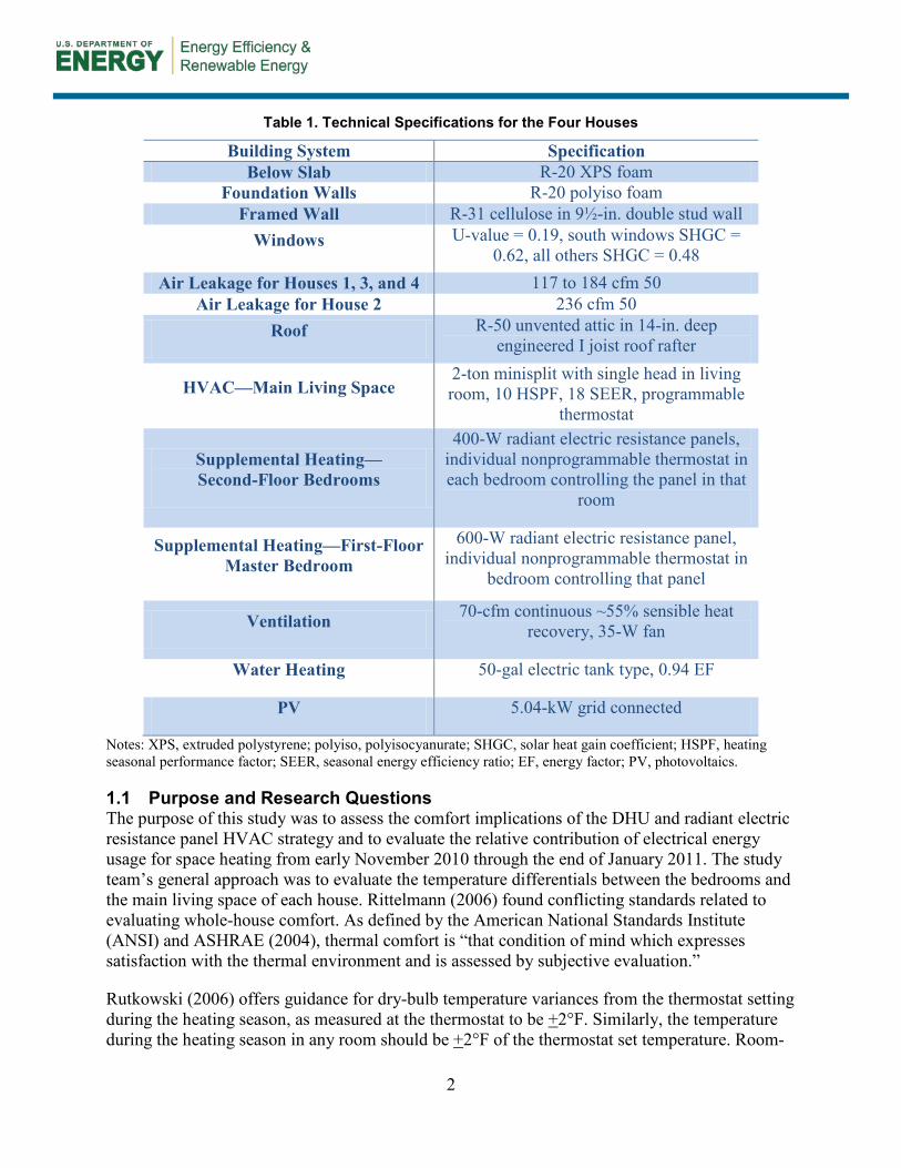
Table 1. Technical Specifications for the Four Houses
Building System Specification Below Slab R-20 XPS foam
Foundation Walls R-20 polyiso foam Framed Wall R-31 cellulose in 9½-in. double stud wall
Windows U-value = 0.19, south windows SHGC = 0.62, all others SHGC = 0.48
Air Leakage for Houses 1, 3, and 4 117 to 184 cfm 50 Air Leakage for House 2 236 cfm 50
Roof R-50 unvented attic in 14-in. deep engineered I joist roof rafter
HVAC—Main Living Space 2-ton minisplit with single head in living room, 10 HSPF, 18 SEER, programmable
thermostat
Supplemental Heating— Second-Floor Bedrooms
400-W radiant electric resistance panels, individual nonprogrammable thermostat in each bedroom controlling the panel in that
room
Supplemental Heating—First-Floor Master Bedroom
600-W radiant electric resistance panel, individual nonprogrammable thermostat in
bedroom controlling that panel
Ventilation 70-cfm continuous ~55% sensible heat recovery, 35-W fan
Water Heating 50-gal electric tank type, 0.94 EF
PV 5.04-kW grid connected
Notes: XPS, extruded polystyrene; polyiso, polyisocyanurate; SHGC, solar heat gain coefficient; HSPF, heating seasonal performance factor; SEER, seasonal energy efficiency ratio; EF, energy factor; PV, photovoltaics.
1.1 Purpose and Research Questions The purpose of this study was to assess the comfort implications of the DHU and radiant electric resistance panel HVAC strategy and to evaluate the relative contribution of electrical energy usage for space heating from early November 2010 through the end of January 2011. The study team’s general approach was to evaluate the temperature differentials between the bedrooms and the main living space of each house. Rittelmann (2006) found conflicting standards related to evaluating whole-house comfort. As defined by the American National Standards Institute (ANSI) and ASHRAE (2004), thermal comfort is “that condition of mind which expresses satisfaction with the thermal environment and is assessed by subjective evaluation.”
Rutkowski (2006) offers guidance for dry-bulb temperature variances from the thermostat setting during the heating season, as measured at the thermostat to be +2°F. Similarly, the temperature during the heating season in any room should be +2°F of the thermostat set temperature. Room-

3
to-room temperature differences or floor-to-floor temperature differences should be no greater than 4°F in the heating season. Air temperature is only one factor in measuring overall thermal comfort (ASHRAE 2004), but Rittelmann (2006) found that, in well-insulated houses with low-emissivity windows, air temperature and mean radiant temperature track fairly closely, except when the windows are experiencing direct solar gain.
In this project, the study team sought to answer several key research questions related to thermal comfort in very energy efficient houses. Because of the stage at which the project was identified (roughly 4 months after occupancy), detailed instrumentation was not possible. Using some low-cost data collection strategies in conjunction with the electromechanical submetering that South Mountain Company installed as part of the project’s construction, however, the study team felt that reasonable insight into these questions could be gained. The primary questions were as follows:
1. What is the room-to-room temperature difference between the main space with the DHU and the individual bedrooms with radiant electric resistance panels?
2. What is the impact of thermostat setback/setup of the DHU on bedroom temperatures?
3. What are the correlations among the temperature at the main DHU; the gross overall energy consumption for heating; and the breakdowns among the DHU, the radiant electric resistance panels, and internal gains from all other electricity used during the study period?
The purpose of this investigation was not to compare modeled to actual energy consumption but to better understand the dynamics of multizone heating strategies and associated energy consumption.

4
2 Mathematical and Modeling Methods
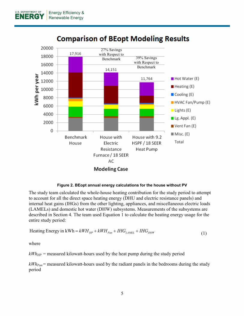
The three-bedroom house (1,447 ft2 above grade, 784 ft2 below grade conditioned floor area) was modeled in BEopt (Building Energy Optimization) software (Version 1.1).1 The study team conducted the modeling to evaluate projected energy efficiency compared to the Building America benchmark using the House Simulation Protocols (HSPs) of Hendron and Engebrecht (2010). This was done primarily to validate that the strategy chosen by South Mountain Company met key source energy savings criteria for the Building America Program, not to try to predict actual energy consumption for end uses. BEopt 1.1 does not have DHUs or radiant electric resistance panels as options in the equipment libraries, nor does it have the capability to model zoned or hybrid heating systems. The study investigators evaluated two different scenarios to demonstrate the range of predicted energy consumption for heating. The first was a ducted forced air system with an electric furnace and an 18 SEER air-conditioning unit, completely within the conditioned space. The other was the same ducted forced air system with a 9.2 HSPF/18 SEER air source heat pump, also completely within the conditioned space.
Figure 2 shows the modeling calculations for the annual energy consumption of the house without PV. BEopt calculated 27% source energy savings with the electric resistance furnace and 39% savings with the heat pump. No modeling was performed to evaluate the projected room-to-room temperature differences between the main living space with the heat pump and the bedrooms when the radiant electric resistance panels were not being used. BEopt modeling assumed that the whole house was heated and cooled using the DHU or the electric resistance furnace. Modeling also assumed a uniform space temperature throughout the house.
1 See http://beopt.nrel.gov/ for more information.
5
Figure 2. BEopt annual energy calculations for the house without PV
The study team calculated the whole-house heating contribution for the study period to attempt to account for all the direct space heating energy (DHU and electric resistance panels) and internal heat gains (IHGs) from the other lighting, appliances, and miscellaneous electric loads (LAMELs) and domestic hot water (DHW) subsystems. Measurements of the subsystems are described in Section 4. The team used Equation 1 to calculate the heating energy usage for the entire study period:
DHWLAMELPanHP IHGIHGkWHkWH +++= kWh in Energy Heating (1)
where
kWhHP = measured kilowatt-hours used by the heat pump during the study period
kWhPan = measured kilowatt-hours used by the radiant panels in the bedrooms during the study period
27% Savings with Respect to
Benchmark 39% Savings with Respect to
Benchmark
6
IHGLAMEL = calculated internal gains in kilowatt-hours from measured LAMELs during the study period
IHGDHW = calculated internal gains in kilowatt-hours from measured DHW in gallons during the study period.
The additional whole-house contribution of the sensible internal gains from ventilation fan and LAMEL electric usage was estimated for each house using an internal gains factor (IGF). The IGF in Equation 2 is the percentage of sensible load considered to be contributing to satisfying the heating loads, using the equations found in the HSPs (Hendron and Engebrecht 2010):
∑∑=
LAMEL
LAMELfractSens
BB
IGF
(2)
where
∑BSens fract LAMEL = sum of the sensible load fractions of benchmark LAMELs from the equations in the HSPs
∑BLAMEL = sum of site kilowatt-hours for benchmark LAMELs.
For the house size (2,231 ft2 conditioned floor area) and the number of bedrooms, the IGF was calculated as
%.66kWh 7104kWh 4657
=
The IGF was then applied to each house to estimate the internal gains using Equation 3:
∑ ×= IGFkWhIHG LAMELNovJanLAMEL (3)
where kWhLAMEL is the calculated LAMEL use per month for the study period in kilowatt-hours. The kWhLAMEL was calculated by subtracting the electric readings of each of the submeters from the whole-house utility meter reading.
Using Equation 4, the study team also estimated the whole-house contribution of the sensible internal gains from the DHW system:
Btu 3413kWh 1
daygalNCTH
dayBtuNCTH
×
×= ∑ ActNovJanDHW gpMo
DHW
IHGIHG (4)
where

7
IHGDHW = internal heat gain from the DHW system losses for the entire study period in site kilowatt-hours
NCTHIHGBtu/day = new construction test home daily internal DHW heat gain from the HSPs (Hendron and Engebrecht 2010) in British thermal units
NCTHDHWgal/day = new construction test home daily DHW usage from the HSPs (Hendron and Engebrecht 2010) in gallons
gpMoAct = measured DHW gallons in the study houses over the course of the study period.
8
3 Experimental Methods
The study team used the data collected for comparisons of variations in temperature between the main living space and rooms not actively conditioned by the DHU. The impact of independently controlled electric resistance heaters in each room was also evaluated. Validation of whole-house energy savings was outside the scope of this study.
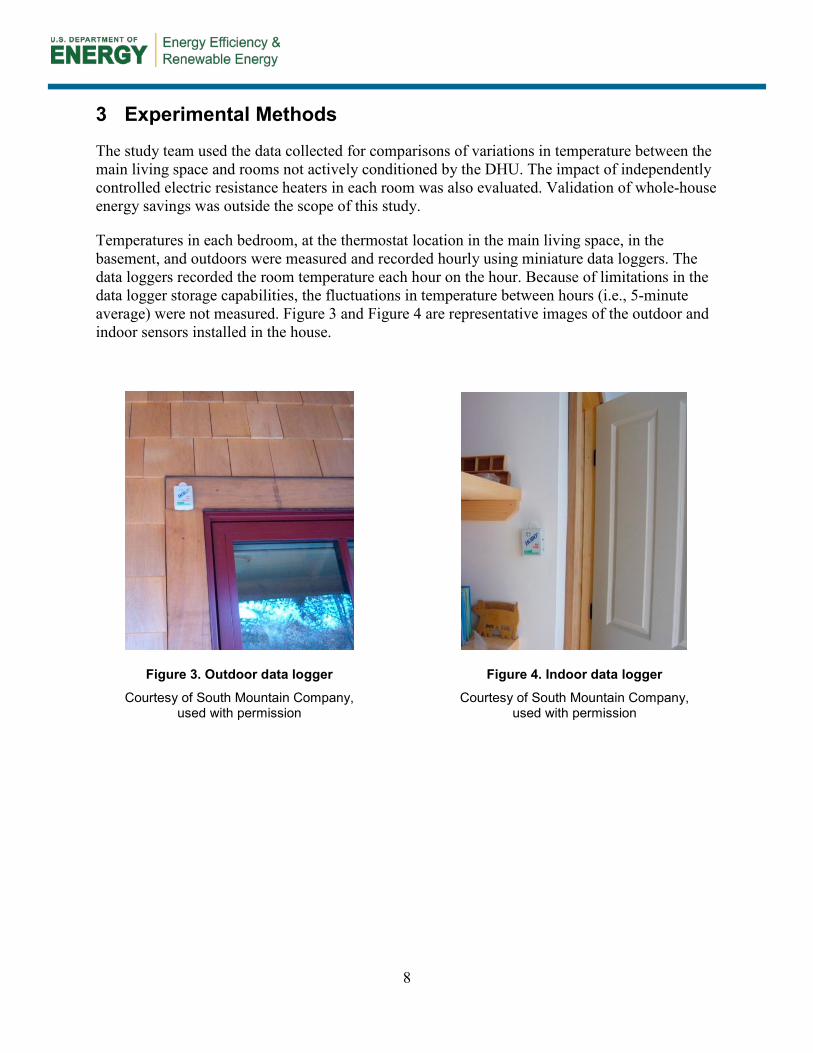
Temperatures in each bedroom, at the thermostat location in the main living space, in the basement, and outdoors were measured and recorded hourly using miniature data loggers. The data loggers recorded the room temperature each hour on the hour. Because of limitations in the data logger storage capabilities, the fluctuations in temperature between hours (i.e., 5-minute average) were not measured. Figure 3 and Figure 4 are representative images of the outdoor and indoor sensors installed in the house.
Figure 3. Outdoor data logger
Courtesy of South Mountain Company, used with permission
Figure 4. Indoor data logger
Courtesy of South Mountain Company, used with permission

9
Sensor locations throughout the house are shown in Figure 5, Figure 6, and Figure 7.
Figure 5. First-floor plan with data logger locations
Courtesy of South Mountain Company, used with permission
Figure 6. Second-floor plan with data logger locations
Courtesy of South Mountain Company, used with permission
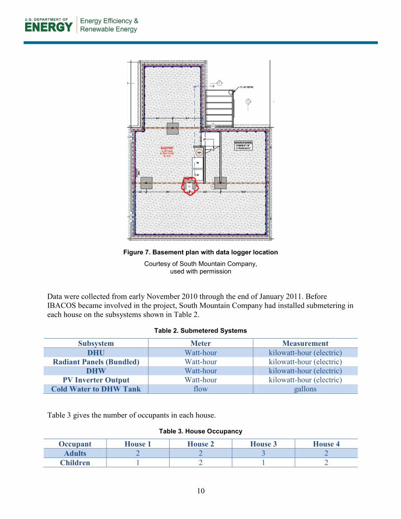
10
Figure 7. Basement plan with data logger location
Courtesy of South Mountain Company, used with permission
Data were collected from early November 2010 through the end of January 2011. Before IBACOS became involved in the project, South Mountain Company had installed submetering in each house on the subsystems shown in Table 2.
Table 2. Submetered Systems
Subsystem Meter Measurement DHU Watt-hour kilowatt-hour (electric)
Radiant Panels (Bundled) Watt-hour kilowatt-hour (electric) DHW Watt-hour kilowatt-hour (electric)
PV Inverter Output Watt-hour kilowatt-hour (electric) Cold Water to DHW Tank flow gallons
Table 3 gives the number of occupants in each house.
Table 3. House Occupancy
Occupant House 1 House 2 House 3 House 4 Adults 2 2 3 2
Children 1 2 1 2

11
One of the residents in the community collected the watt-hour and flow meter readings each month. The data loggers for temperature measurements were launched at the beginning of the study period and downloaded once at the end of the study period. The data loggers collected the room temperature once each hour. No attempt was made to record the door open/closed state of the bedroom doors in the houses. Two temperature data loggers failed in two of the houses: an east second-floor bedroom data logger in House 1 and a west second-floor bedroom data logger in House 2.
Before IBACOS became involved, South Mountain Company offered a prize to any resident who could achieve net zero annual energy use. As reported by Rosenbaum (2011), two of the eight houses reached net zero annual consumption. One of the houses that achieved net zero was also one of the houses in this study group. The other three houses in this study group had the highest total site energy consumption of all eight houses.

12
4 Results
The study team analyzed temperature data to compare the temperature at the thermostat location to the temperature in each of the bedrooms. Rutkowski (2009) recommends that the temperatures in rooms other than where the thermostat is located should be no more than +2°F of the temperature at the thermostat. For the study period, temperatures in the bedrooms were sorted into hourly bins in 2°F increments above or below the thermostat temperature. The temperature data were further disaggregated into day (8:00 a.m. to 7:00 p.m.) and night (8:00 p.m. to 7:00 a.m.), which represented the 12 hourly temperature readings taken by the data loggers. These were used to analyze differences in temperatures when the bedrooms were presumed to be normally unoccupied (day) and occupied (night), respectively. Investigators also analyzed the electric consumption for the study period for heat pump use, radiant electric resistance panel use, and sensible internal gains.
Results for House 1 from 8:00 p.m. to 7:00 a.m. and 8:00 a.m. to 7:00 p.m. are shown in Figure 8 and Figure 9, respectively.
Figure 8. Nighttime temperature differences in House 1

13
Figure 9. Daytime temperature differences in House 1
Results for House 2 from 8:00 p.m. to 7:00 a.m. and 8:00 a.m. to 7:00 p.m. are shown in Figure 10 and Figure 11, respectively.
Figure 10. Nighttime temperature differences in House 2

14
Figure 11. Daytime temperature differences in House 2
Results for House 3 from 8:00 p.m. to 7:00 a.m. and 8:00 a.m. to 7:00 p.m. are shown in Figure 12 and Figure 13, respectively.
Figure 12. Nighttime temperature differences in House 3
15
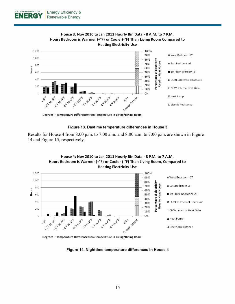
Figure 13. Daytime temperature differences in House 3
Results for House 4 from 8:00 p.m. to 7:00 a.m. and 8:00 a.m. to 7:00 p.m. are shown in Figure 14 and Figure 15, respectively.
Figure 14. Nighttime temperature differences in House 4

16
Figure 15. Daytime temperature differences in House 4
Table 4 gives the electric and DHW consumption for the houses during the study period (November 2010 through January 2011).
Table 4. Electricity Used from November 2010 to January 2011 (from Meter Readings)
End Use House 1 House 2 House 3 House 4 kWhHP 813 kWh 582 kWh 737 kWh 391 kWh kWhPan 379 kWh 906 kWh 311 kWh 514 kWh
kWhLAMEL 711 kWh 1,395 kWh 1,013 kWh 1,745 kWh kWhDHW 480 kWh 1,171 kWh 989 kWh 1,067 kWh GalDHW 1,770 gal 5,860 gal 4,280 gal 5,050 gal
The study team aggregated the data to evaluate the percentage of time during which the bedrooms were no more than +2°F of the temperature at the thermostat and the percentage of time the bedrooms were in each of the other incremental 2°F bins above or below the thermostat temperature (i.e., the –4°F to –2°F bin combined with the +2°F to +4°F bin). Figure 16 shows the comparison of these percentages to the electric energy used for heating during the study period, which is a combination of direct meter readings and calculated contributions as described in Section 4.

17
Figure 16. Comparison of temperature to electric energy used for heating
Table 5 shows the average temperatures in the living rooms and bedrooms of the four houses from November 2010 through January 2011.
Table 5. Average Temperatures in Living Rooms and Bedrooms
Room House 1 House 2 House 3 House 4 Living Room 69.4°F 71.8°F 70.0°F 68.8°F
First-Floor Bedroom 62.0°F 68.7°F 65.2°F 63.6°F Second-Floor East Bedroom Failed sensor 68.5°F 64.6°F 67.0°F Second-Floor West Bedroom 65.5°F Failed sensor 65.1°F 67.2°F
18
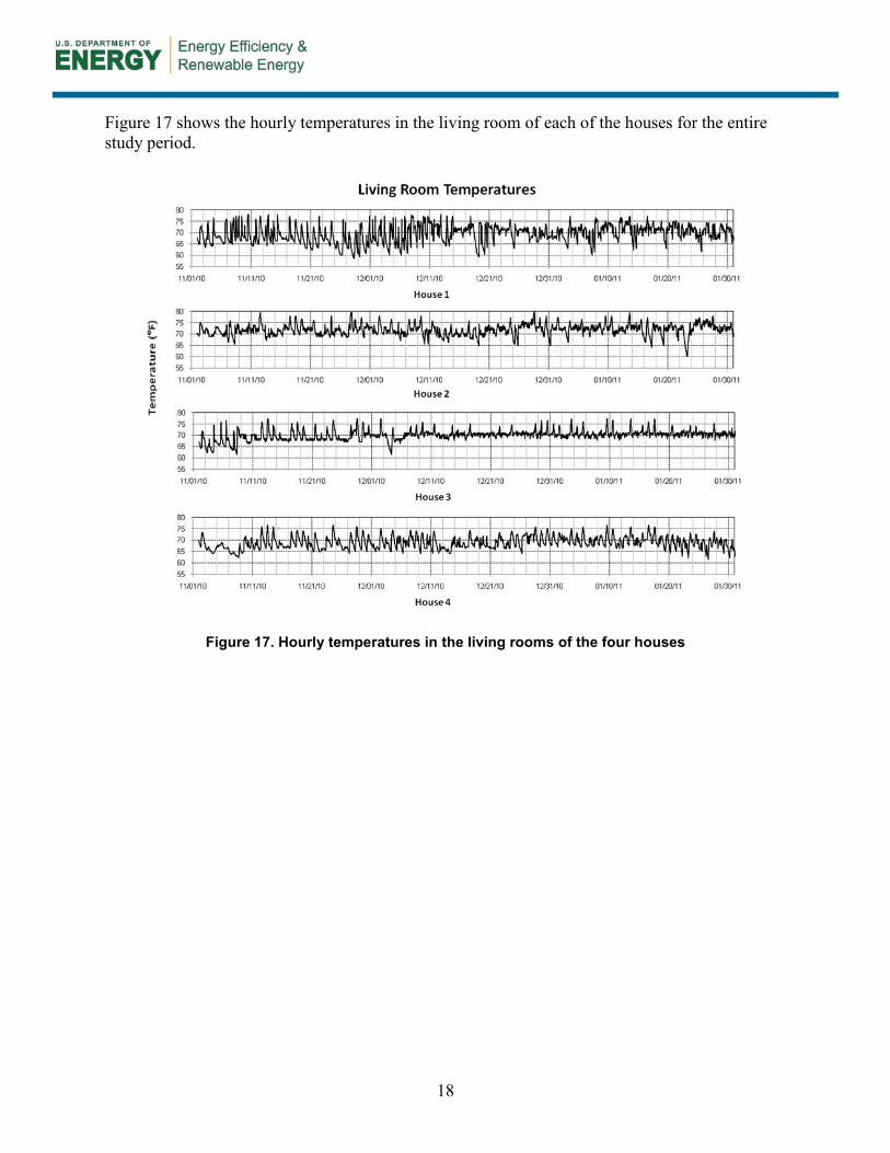
Figure 17 shows the hourly temperatures in the living room of each of the houses for the entire study period.
Figure 17. Hourly temperatures in the living rooms of the four houses
19
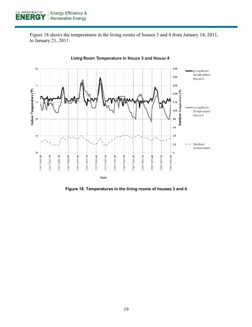
Figure 18 shows the temperatures in the living rooms of houses 3 and 4 from January 14, 2011, to January 21, 2011.
Figure 18. Temperatures in the living rooms of houses 3 and 4
20
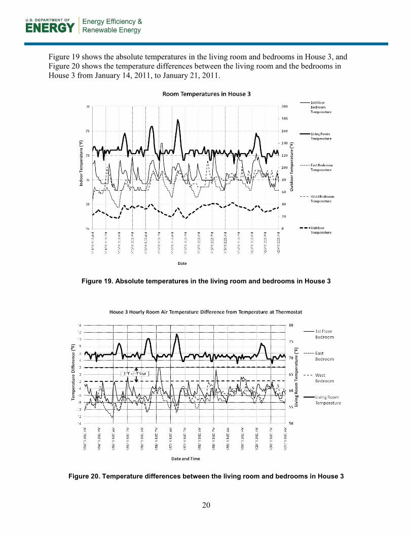
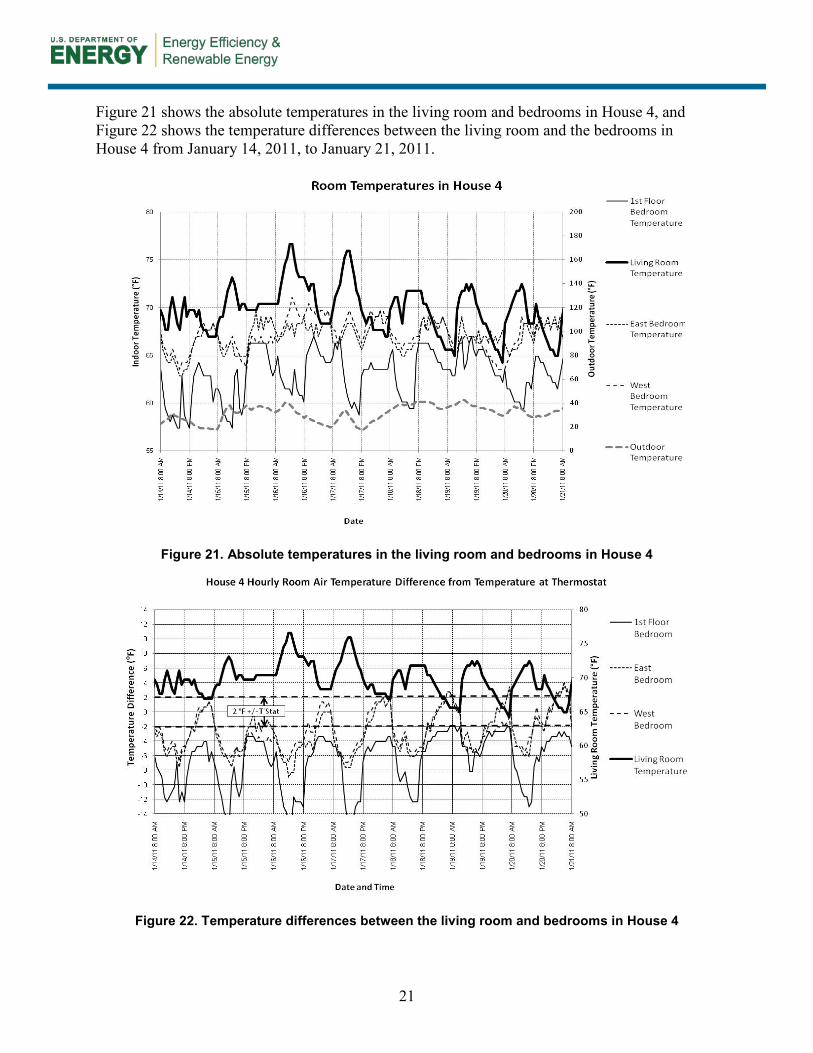
Figure 19 shows the absolute temperatures in the living room and bedrooms in House 3, and Figure 20 shows the temperature differences between the living room and the bedrooms in House 3 from January 14, 2011, to January 21, 2011.
Figure 19. Absolute temperatures in the living room and bedrooms in House 3
Figure 20. Temperature differences between the living room and bedrooms in House 3
21
Figure 21 shows the absolute temperatures in the living room and bedrooms in House 4, and Figure 22 shows the temperature differences between the living room and the bedrooms in House 4 from January 14, 2011, to January 21, 2011.
Figure 21. Absolute temperatures in the living room and bedrooms in House 4
Figure 22. Temperature differences between the living room and bedrooms in House 4
22
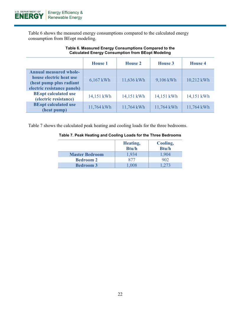
Table 6 shows the measured energy consumptions compared to the calculated energy consumption from BEopt modeling.
Table 6. Measured Energy Consumptions Compared to the Calculated Energy Consumption from BEopt Modeling
House 1 House 2 House 3 House 4
Annual measured whole-house electric heat use
(heat pump plus radiant electric resistance panels)
6,167 kWh 11,636 kWh 9,106 kWh 10,212 kWh
BEopt calculated use (electric resistance) 14,151 kWh 14,151 kWh 14,151 kWh 14,151 kWh
BEopt calculated use (heat pump) 11,764 kWh 11,764 kWh 11,764 kWh 11,764 kWh
Table 7 shows the calculated peak heating and cooling loads for the three bedrooms.
Table 7. Peak Heating and Cooling Loads for the Three Bedrooms
Heating, Btu/h
Cooling, Btu/h
Master Bedroom 1,934 1,904 Bedroom 2 877 902 Bedroom 3 1,008 1,273
23
5 Discussion
Although the data from houses 1 and 3 and houses 2 and 4 have similar characteristics, houses 1 and 2 are not included in the detailed temperature analysis because they are each missing temperature data from one upstairs bedroom as discussed in Section 2. House 1 achieved an annual net zero energy consumption (Rosenbaum 2011).
Houses 3 and 4 had similar absolute total heating electricity consumption despite very different heat pump and resistance heat amounts. House 3 used 1,048 kWh of total electricity during the study period, 737 kWh at the heat pump and 311 kWh at the resistance heaters, accounting for 59% of the heat contribution per Equation 1. House 4 used 980 kWh of total electricity during the study period, 466 kWh at the heat pump and 514 kWh at the resistance heaters, accounting for 43% of the heat contribution per Equation 1. Per Equation 2, houses 3 and 4 used the equivalent of 668 kWh (38% of total heat kilowatt-hours) and 1,152 kWh (54% of total heat kilowatt-hours) of electric resistance from the internal gains associated with the electricity used for LAMELs, respectively. As shown in Figure 16, houses 1 and 3 and houses 2 and 4 showed similar trends with respect to the distribution of electricity use for the heat pump, radiant electric resistance panels, and the electricity attributable to the LAMEL internal gains.
The hourly sampled temperature differences between each of the bedrooms and the living room in each house were categorized into 2°F temperature bins as shown in Figure 16. House 3 had greater total electricity use and greater heat pump operation, and the temperatures in the bedrooms were within +2°F of the temperature in the living room 20% of the time and within +4°F 41% of the time. In House 4, with lower total electricity use but more resistance heat use and a significantly higher LAMEL contribution, bedrooms were within +2°F of the temperature in the living room 30% of the time and within +4°F 60% of the time.
To better understand these percentages, look at the differences in the apparent heating system setup/setback strategy employed in houses 3 and 4, as shown in Figure 17. House 3 appears to be operated with a “set it and forget it” mentality for the DHU and setback/setup for the radiant electric resistance panels, although the east bedroom and the master bedroom were observed to frequently fall below the set-point temperature, indicating that the panels had been completely turned off.
House 4 appears to have been operated in a completely different manner. The DHU unit was operated with daily setback and setup, frequently with the setback temperature apparently turned off. This caused dramatic temperature swings in the living room. The radiant electric resistance panels were operated in the same way, with the temperature apparently set anywhere from approximately 66°F to 70°F when needed and set to off when not needed. Figure 20 and Figure 22 show the impact of this strategy on the +2°F comfort band. The temperature difference is not attributable to the DHU equalizing temperatures in the upstairs bedrooms; instead, it is the downward temperature drift in the living room that brings the temperatures closer together.
Also note that houses 1 and 3 had similar average living room temperatures and similar total heating energy consumption, but the aggressive setback strategy yielded significant fluctuations in temperatures in House 1. This may result from occupant comfort desires, but the data from
24
Table 4 and Table 5 do not indicate that a setback strategy will save energy in houses with these thermal enclosure characteristics and space conditioning systems.
All four houses showed a trend toward cooler bedrooms during the day compared to the night, which can be expected based on typical occupancy patterns (i.e., bedrooms are generally not used during the day).
Another factor that drives the temperature differences is the sun-tempered design of these houses. The living room is the dominant area that receives solar gain, and, as such, the temperature in that space was seen to rise by more than 7°F over the course of a sunny day. This response was not as dramatic in the bedrooms, and, in some cases, the rooms with doors that were apparently closed dropped in temperature while the living room was rising in temperature.
The frequency of door operation was not explicitly measured, but it appears that the impact of door closure can be observed from the data. January 17 appears to be a sunny day, based on the rise in the living room temperatures in houses 3 and 4, as shown in Figure 18. Figure 21 shows that the second-floor east and west bedrooms in House 4 have a similar rise in temperature as the living room, but the first-floor bedroom temperature drops dramatically during the day. Conversely, Figure 19 shows that, in House 3, all bedroom temperatures rise as the living room temperature rises. This indicates that the first-floor bedroom in House 4 was either intentionally cooled by opening windows or, more likely, was isolated from the main body of the house by closing the door. The first-floor bedroom is on the north side of the house; therefore, even on a sunny day, it would not be expected to receive any appreciable solar gain. This pattern appears repeatedly in the data set.
With the heating strategy of a single DHU located in the main living space and radiant electric resistance panels in each bedroom controlled by individual thermostatic controls, the occupants’ behavior of leaving bedroom doors open or closed has a significant impact on room-to-room temperatures. The study team suspects that the houses with greater electric resistance heat use had the bedroom doors closed for longer periods of time, but these houses also appear to be operated with aggressive setup and setback schedules. Based on work by Prahl (2006), keeping the first floor at a steady temperature in an energy efficient house with a point source fuel fired heater helps to maintain more consistent temperatures in the upstairs bedrooms when the doors are open. Further study to evaluate the temperature differences relative to door-open versus door-closed status would be valuable in removing the impact of occupant behavior on the temperature data.
The role of the LAMELs in these houses is impossible to accurately evaluate; however, even with the assumptions used, LAMELs appear to be a large contributing factor. The distribution of these loads throughout the house and their relative use are unclear. In houses this small and this well insulated, the contribution of these “mini space heaters” can have significant localized impacts, such as waste heat from cooking and entertainment devices, among others. A more detailed inventory of actual devices and usage patterns would be needed for deeper analysis to identify specific drivers of the relative temperature differences from room to room in these houses.

25
Based on the bedroom load calculations, fan-assisted air transfer from the main living space to the bedrooms could be an alternative strategy. Assuming that the temperature at the ceiling is 5°F higher than the thermostat set point because of stratification in the room, approximately 350 cfm of air from the main living space would meet the peak heating load for the master bedroom or bedrooms 2 and 3 combined (350 cfm × 5°F × 1.085 = 1,899 Btu/h). The three bedrooms could be “heated” with two low sone inline fans (one for the master bedroom, one for the other two bedrooms) that draw approximately 95 W each. House 3 used between 42 and 152 kWh per month for electric resistance heat. This translates to equivalent run times of approximately 7 to 24 hours per day for the fans. This indicates a strategy that encourages a modest but acceptable level of stratification in the main space and adequately sized transfer fans with intakes located where air temperature is predicted to be the highest. This approach may be as (or more) effective than individual radiant panels at maintaining uniform temperatures in an energy efficient way. IBACOS is investigating this strategy as part of its ongoing research in laboratory homes through the Building America program.
Finally, these data show that, above all, personal comfort is relative. Different people have different comfort and privacy needs and operate their heating systems and houses in different ways, whether for energy savings, comfort, or both. South Mountain Company has not received any comfort complaints from the occupants of these homes.
26
6 Conclusions
Four identical houses built in West Tisbury, Massachusetts, showed a wide range of energy use for space heating from early November 2010 through the end of January 2011. The DHU and the radiant electric resistance panels were estimated to have provided 43% to 71% of the electric energy needed for space heating, with almost all of the remainder being satisfied by internal gains attributed to LAMELs. Temperature measurements indicate that, with increased use of the radiant electric resistance panels in the bedrooms, temperatures were (not surprisingly) closer to the living room temperature where the DHU was located. Temperature excursions resulting from aggressive setup and setback of the DHU may contribute to higher percentages of time where the bedrooms were within +2°F of the living room because the living room temperature dropped closer to the temperatures of the bedrooms. In the two houses with complete temperature data sets, the bedrooms were within +2°F of the living room temperature no more than 30% of the time. Solar gains in the living room also appear to drive wider temperature swings. Opening and closing doors appears to have a significant impact on room-to-room temperature differences, as would be expected. Energy consumption between two houses with similar average living room temperatures but very different setback schedules had very similar heat pump and electric resistance energy consumption during the study period.
After accounting for the electrical output of the 5.04-kW PV system, House 1 achieved an annual net zero energy consumption. This house also demonstrated significant temperature swings in the living space, where the DHU was located, and significant temperature variations between the bedrooms and the living room.
27
7 References
Abrams, J. (2011). “High-Performance Homes on a Budget.” Journal of Light Construction (January); pp. 39–46. http://www.jlconline.com/building-envelope/high-performance-homes-on-a-budget.aspx. Accessed August 2011. Also available at http://www.southmountain.com/press-and-media. Accessed October 2012.
ASHRAE (2004). “ANSI/ASHRAE Standard 55-2004, Thermal Environmental Conditions for Human Occupancy.” Atlanta, GA: ASHRAE.
Hendron, R.; Engebrecht, C. (2010). Building America House Simulation Protocols. NREL/TP-550-49426. Golden, CO: National Renewable Energy Laboratory.
Prahl, D. (2007). “Small Homes, Excellent Enclosures, Almost No Heating System—Fact or Fiction?” Proceedings of the Thermal Enclosure of Buildings X Conference, Clearwater, FL, December 2–7, 2007. Atlanta, GA: ASHRAE.
Rittelmann, W. (2006). “A Systemic Short-Term Field Test for Residential HVAC Thermal Comfort Performance.” Proceedings of the 2006 ACEEE Summer Study on Energy Efficiency in Buildings, August 13–18, 2006. Washington, D.C.: ACEEE. pp. 1-260 – 1-271
Rosenbaum, M. (2011). Zero-Net Possible? Yes! Energy Performance of Eight Homes at Eliakim’s Way. West Tisbury, MA: South Mountain Company.
Rutkowski, H. (2009). Manual D—Residential Duct Systems. 3rd edition, Version 1. Arlington, VA: Air Conditioning Contractors of America. Rutkowski, H. (2006). Manual J—Residential Load Calculation. 8th edition, Version 2. Arlington, VA: Air Conditioning Contractors of America.

DOE/GO-102012-3494 ▪ October 2012
Printed with a renewable-source ink on paper containing at least 50% wastepaper, including 10% post-consumer waste.