MATH 571 — Mathematical Models of Financial Derivatives

Topic 1 – Introduction to Derivative Instruments

1.1 Basic derivative instruments: bonds, forward contracts, swaps

and options

1.2 Rational boundaries of option values

1.3 Early exercise policies of American options

1

1.1 Basic derivative instruments: bonds, forward contracts,

swaps and options

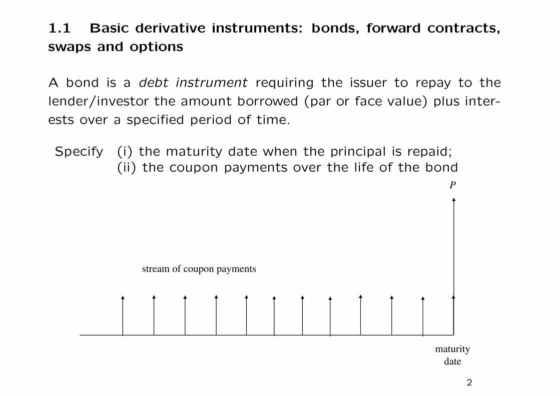
A bond is a debt instrument requiring the issuer to repay to the

lender/investor the amount borrowed (par or face value) plus inter-

ests over a specified period of time.

Specify (i) the maturity date when the principal is repaid;(ii) the coupon payments over the life of the bond

maturity

date

stream of coupon payments

P

2

• The coupon rate offered by the bond issuer represents the cost

of raising capital. It depends on the prevailing risk free interest

rate and the creditworthiness of the bond issuer. It is also af-

fected by the values of the embedded options in the bond, like

conversion right in convertible bonds.

• Assume that the bond issuer does not default or redeem the

bond prior to maturity date, an investor holding this bond un-

til maturity is assured of a known cash flow pattern. This is why

bond products are also called Fixed Income Products/Derivatives.

Pricing of a bond

Based on the current information of the interest rates (yield

curve) and the embedded option provisions, find the cash amount

that the bond investor should pay at the current time so that

the deal is fair to both counterparties.

3

Features in bond indenture

1. Floating rate bond

The coupon rates are reset periodically according to some pre-

determined financial benchmark, like LIBOR + spread, where

LIBOR is the LONDON INTER-BANK OFFERED RATE.

2. Amortization feature – principal repaid over the life of the bond.

3. Callable feature (callable bonds)

The issuer has the right to buy back the bond at a specified

price. Usually this call price falls with time, and often there

is an initial call protection period wherein the bond cannot be

called.

4

4. Put provision – grants the bondholder the right to sell back to

the issuer at par value on designated dates.

5. Convertible bond – gives the bondholder the right to exchange

the bond for a specified number of shares of the issuer’s firm.

? Bond holders can take advantage of the future growth of the

issuer’s company.

? Issuer can raise capital at a lower cost.

6. Exchangeable bond – allows the bondholder to exchange the

bond par for a specified number of common stocks of another

corporation.

5

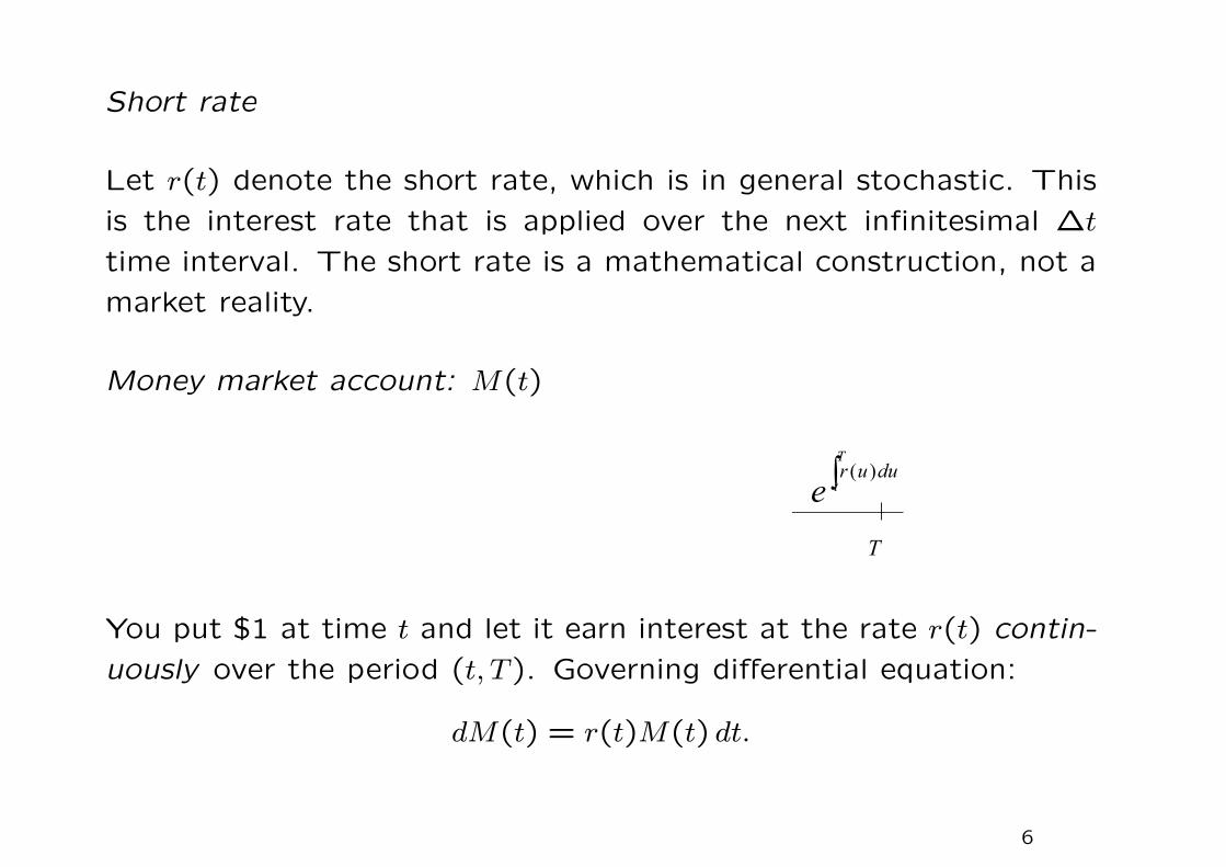
Short rate

Let r(t) denote the short rate, which is in general stochastic. This

is the interest rate that is applied over the next infinitesimal ∆t

time interval. The short rate is a mathematical construction, not a

market reality.

Money market account: M(t)

t T

T

t

duur

e)(

You put $1 at time t and let it earn interest at the rate r(t) contin-

uously over the period (t, T ). Governing differential equation:

dM(t) = r(t)M(t) dt.

6

∫ T

t

dM(u)

M(u)=

∫ T

tr(u) du

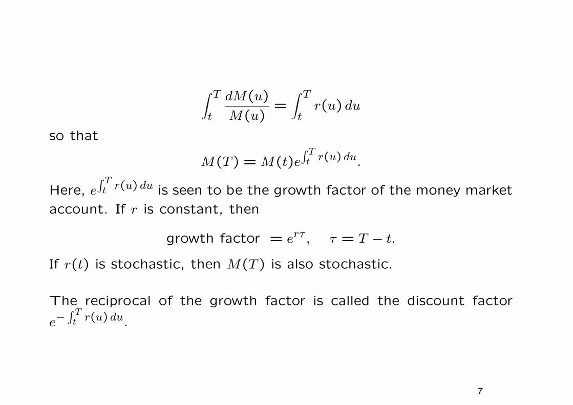
so that

M(T ) = M(t)e∫ Tt r(u) du.

Here, e∫ Tt r(u) du is seen to be the growth factor of the money market

account. If r is constant, then

growth factor = erτ , τ = T − t.

If r(t) is stochastic, then M(T ) is also stochastic.

The reciprocal of the growth factor is called the discount factor

e−∫ Tt r(u) du.

7

Discount bond price

t T

) $1

τ = T − t = time to bond’s maturity

The price that an investor on the zero-coupon (discount) bond with

unit par is willing to pay at time t if the bond promises to pay him

back $1 at a later time (maturity date) T .

This fair value is called the discount bond price B(t, T ), which is

given by the expectation of the discount factor based on current in-

formation: Et

[e−

∫ Tt r(u) du

]. If r is constant, then B(t, T ) = e−rτ , τ =

T − t.

8

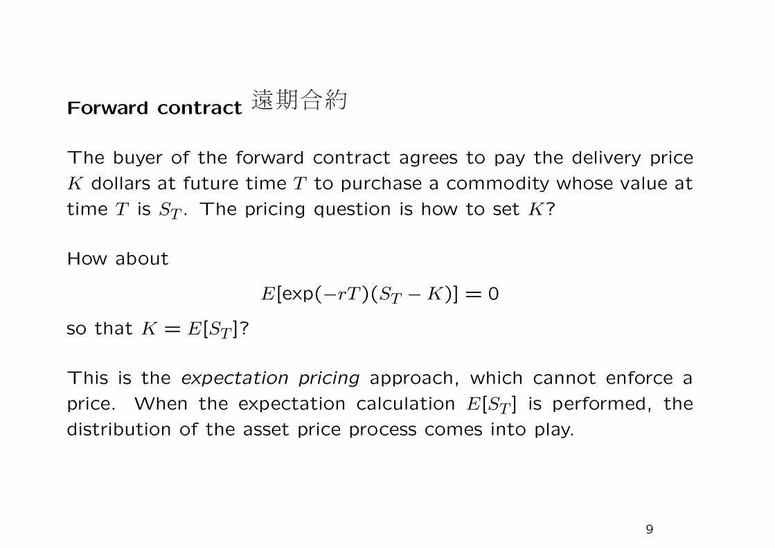
Forward contract

The buyer of the forward contract agrees to pay the delivery price

K dollars at future time T to purchase a commodity whose value at

time T is ST . The pricing question is how to set K?

How about

E[exp(−rT )(ST −K)] = 0

so that K = E[ST ]?

This is the expectation pricing approach, which cannot enforce a

price. When the expectation calculation E[ST ] is performed, the

distribution of the asset price process comes into play.

9

Objective of the buyer:

To hedge against the price fluctuation of the underlying commodity.

• Intension of a purchase to be decided earlier, actual transaction

to be done later.

• The forward contract needs to specify the delivery price, amount,

quality, delivery date, means of delivery, etc.

Potential default of either party (counterparty risk): writer or buyer.

10

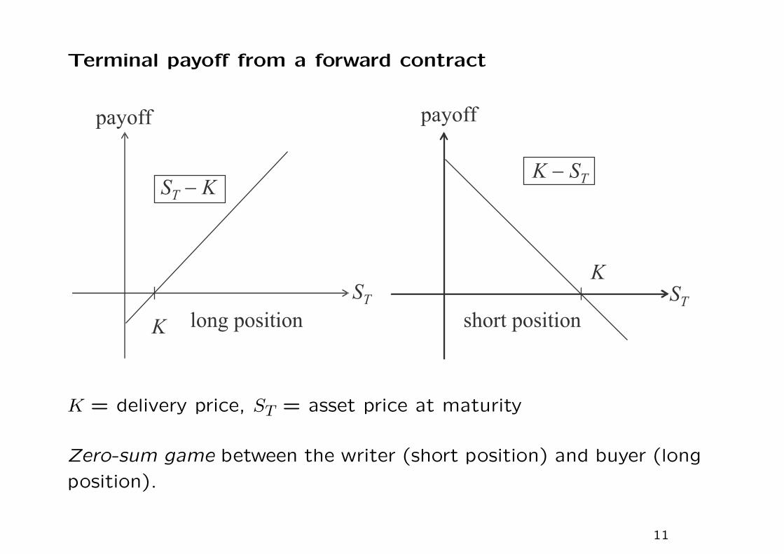
Terminal payoff from a forward contract

K = delivery price, ST = asset price at maturity

Zero-sum game between the writer (short position) and buyer (long

position).

11

Forward contracts have been extended to include underlying assets

other than physical commodities, e.g. on exchange rate of foreign

currency or interest rate instrument (like bonds) or stock index.

Hang Seng index futures

• The underlying is the Hang Seng index.

• One index point corresponds to $50.

Settlement

• On the last but one trading day at the end of the month.

• Take the average of the index value at 5-minute intervals as the

settlement value.

12

Is the forward price related to the expected price of the commodity

on the delivery date? Provided that the underlying asset can be

held for hedging by the writer, then

forward price

= spot price + cost of fund + storage cost︸ ︷︷ ︸cost of carry

• Cost of fund is the interest accrued over the period of the for-

ward contract.

• Cost of carry is the total cost incurred to acquire and hold the

underlying asset, say, including the cost of fund and storage

cost.

• Dividends paid to the holder of the asset are treated as negative

contribution to the cost of carry.

13

Numerical example on arbitrage

– spot price of oil is US$19

– quoted 1-year forward price of oil is US$25

– 1-year US dollar interest rate is 5% pa

– storage cost of oil is 2% per annum, paid at maturity

Any arbitrage opportunity? Yes

Sell the forward and expect to receive US$25 one year later. Borrow

$19 now to acquire oil, pay back $19(1+0.05) = $19.95 a year later.

Also, one needs to spend $0.38 = $19× 2% as the storage cost.

total cost of replication (dollar value at maturity)

= spot price + cost of fund + storage cost

= $20.33 < $25 to be received.

Close out all positions by delivering the oil to honor the forward. At

maturity of the forward contract, guaranteed riskless profit = $4.67.

14

Value and price of a forward contract

Let f(S, τ) = value of forward, F (S, τ) = forward price,

τ = time to expiration,

S = spot price of the underlying asset.

Further, we let

B(τ) = value of an unit par discount bond with time to maturity τ

• If the interest rate r is constant and interests are compounded

continuously, then B(τ) = e−rτ .

• Assuming no dividend to be paid by the underlying asset and no

storage cost.

We construct a “static” replication of the forward contract by a

portfolio of the underlying asset and bond.

15

Portfolio A: long one forward and a discount bond with par value K

Portfolio B: one unit of the underlying asset

Both portfolios become one unit of asset at maturity. Let ΠA(t)

denote the value of Portfolio A at time t. Note that ΠA(T ) = ΠB(T ).

By the “law of one price”,∗, we must have ΠA(t) = ΠB(t). The

forward value is given by

f = S −KB(τ).

The forward price is defined to be the delivery price which makes

f = 0, so K = S/B(τ). Hence, the forward price is given by

F (S, τ) = S/B(τ) = spot price + cost of fund.

∗Suppose ΠA(t) > ΠB(t), then an arbitrage can be taken by selling Portfolio Aand buying Portfolio B. An upfront positive cash flow is resulted at time t butthe portfolio values are offset at maturity T .

16

Discrete dividend paying asset

D = present value of all dividends received from holding the asset

during the life of the forward contract.

We modify Portfolio B to contain one unit of the asset plus bor-

rowing of D dollars. The loan of D dollars will be repaid by the

dividends received by holding the asset. We then have

f + KB(τ) = S −D

so that

f = S − [D + KB(τ)].

Setting f = 0 to solve for K, we obtain F = (S −D)/B(τ).

The “net” asset value is reduced by the amount D due to the

anticipation of the dividends. Unlike holding the asset, the holder

of the forward will not receive the dividends. As a fair deal, he

should pay a lower delivery price at forward’s maturity.

17

Cost of carry

Additional costs to hold the commodities, like storage, insurance,

deterioration, etc. These can be considered as negative dividends.

Treating U as −D, we obtain

F = (S + U)erτ ,

U = present value of total cost incurred during the remaining life of

the forward to hold the asset.

Suppose the costs are paid continuously, we have

F = Se(r+u)τ ,

where u = cost per annum as a proportion of the spot price.

In general, F = Sebτ , where b is the cost of carry per annum. Let q

denote the continuous dividend yield per annum paid by the asset.

With both continuous holding cost and dividend yield, the cost of

carry b = r + u− q.

18

Forward price formula with discrete carrying costs

Suppose an asset has a holding cost of c(k) per unit in period k,

and the asset can be sold short. Suppose the initial spot price is S.

The theoretical forward price F is

F =S

d(0, M)+

M−1∑

k=0

c(k)

d(k, M),

where d(0, k)d(k, M) = d(0, M).

The terms on the right hand side represent the future value at

maturity of the total costs required for holding the underlying asset

for hedging. Note that holding costs can be visualized as negative

dividends.

19

Proportional carrying charge

Forward contract written at time 0 and there are M periods until

delivery. The carrying charge in period k is qS(k − 1), where q is a

proportional constant. Show that the forward price is

F =S(0)/(1− q)M

d(0, M).

• We expect the forward price increases when the carrying charges

become higher.

20

Borrow αS(0) dollars at current time to buy α units of assets and

long one forward. Here, α is to be determined.

Sell out q portion of asset at each period in order to pay for the

carrying charge. After M period, α units becomes α(1− q)M .

The goal is to make available one unit of the asset for delivery at

maturity. We set α(1− q)M to be one and obtain α =1

(1− q)M.

The portfolio of longing the forward with delivery price K and a

bond with par K is equivalent to long α units of the asset. This

gives

f + Kd(0, M) = αS(0).

By setting f = 0 to obtain the forward price K, we obtain

K =S(0)

(1− q)M

/d(0, M).

21

Futures contracts

A futures contract is a legal agreement between a buyer (seller) and

an established exchange or its clearing house in which the buyer

(seller) agrees to take (make) delivery of a financial entity at a

specified price at the end of a designated period of time. Usually

the exchange specifies certain standardized features.

Mark to market the account

Pay or receive from the writer the change in the futures price

through the margin account so that payment required on the ma-

turity date is simply the spot price on that date.

Credit risk is limited to one-day performance period

22

Roles of the clearinghouse

• Eliminate the counterparty risk through the margin account.

• Provide the platform for parties of a futures contract to unwind

their position prior to the settlement date.

Margin requirements

Initial margin – paid at inception as deposit for the contract.

Maintenance margin – minimum level before the investor is re-

quired to deposit additional margin.

23

Example (Margin)

Suppose that Mr. Chan takes a long position of one contract in

corn (5,000 kilograms) for March delivery at a price of $2.10 (per

kilogram). And suppose the broker requires margin of $800 with a

maintenance margin of $600.

• The next day the price of this contract drops to $2.07. This

represents a loss of 0.03 × 5,000 = $150. The broker will take

this amount from the margin account, leaving a balance of $650.

The following day the price drops again to $2.05. This repre-

sents an additional loss of $100, which is again deducted from

the margin account. As this point the margin account is $550,

which is below the maintenance level.

• The broker calls Mr. Chan and tells him that he must deposit at

least $250 in his margin account, or his position will be closed

out.

24

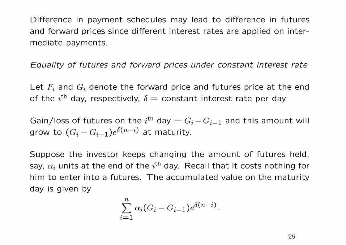
Difference in payment schedules may lead to difference in futures

and forward prices since different interest rates are applied on inter-

mediate payments.

Equality of futures and forward prices under constant interest rate

Let Fi and Gi denote the forward price and futures price at the end

of the ith day, respectively, δ = constant interest rate per day

Gain/loss of futures on the ith day = Gi−Gi−1 and this amount will

grow to (Gi −Gi−1)eδ(n−i) at maturity.

Suppose the investor keeps changing the amount of futures held,

say, αi units at the end of the ith day. Recall that it costs nothing for

him to enter into a futures. The accumulated value on the maturity

day is given byn∑

i=1

αi(Gi −Gi−1)eδ(n−i).

25

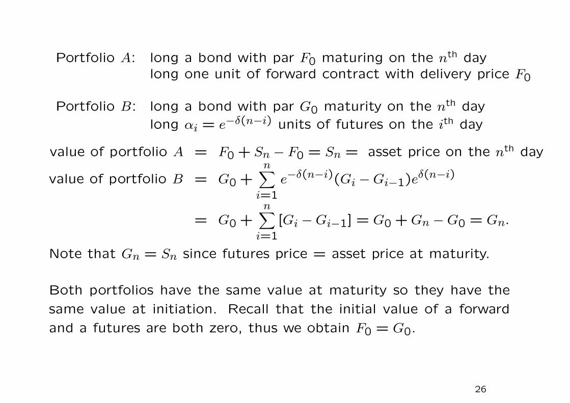
Portfolio A: long a bond with par F0 maturing on the nth daylong one unit of forward contract with delivery price F0

Portfolio B: long a bond with par G0 maturity on the nth day

long αi = e−δ(n−i) units of futures on the ith day

value of portfolio A = F0 + Sn − F0 = Sn = asset price on the nth day

value of portfolio B = G0 +n∑

i=1

e−δ(n−i)(Gi −Gi−1)eδ(n−i)

= G0 +n∑

i=1

[Gi −Gi−1] = G0 + Gn −G0 = Gn.

Note that Gn = Sn since futures price = asset price at maturity.

Both portfolios have the same value at maturity so they have the

same value at initiation. Recall that the initial value of a forward

and a futures are both zero, thus we obtain F0 = G0.

26

Proposition 1

Consider an asset with a price S̃T at time T . The futures price of

the asset, Gt,T , is the time-t spot price of an asset which has a

payoff

S̃T

Bt,t+1B̃t+1,t+2 · · · B̃T−1,T

at time T . Note that quantities with “tilde” at top indicate stochas-

tic variables.

Proof We start with 1Bt,t+1

long futures contracts at time t. The

gain/loss from the futures position day τ earns/pays the overnight

rate 1B̃τ,τ+1

. Also, invest Gt,T in a one-day risk free bond and roll the

cash position over on each day at the one-day rate. The investment

of Gt,T is equivalent to the price paid to acquire the asset.

27

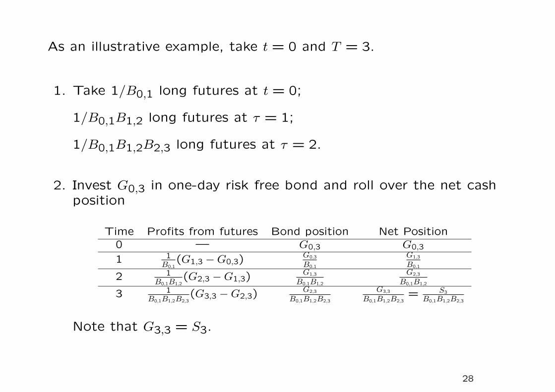
As an illustrative example, take t = 0 and T = 3.

1. Take 1/B0,1 long futures at t = 0;

1/B0,1B1,2 long futures at τ = 1;

1/B0,1B1,2B2,3 long futures at τ = 2.

2. Invest G0,3 in one-day risk free bond and roll over the net cashposition

Time Profits from futures Bond position Net Position0 — G0,3 G0,3

1 1B0,1

(G1,3 −G0,3)G0,3

B0,1

G1,3

B0,1

2 1B0,1B1,2

(G2,3 −G1,3)G1,3

B0,1B1,2

G2,3

B0,1B1,2

3 1B0,1B1,2B2,3

(G3,3 −G2,3)G2,3

B0,1B1,2B2,3

G3,3

B0,1B1,2B2,3= S3

B0,1B1,2B2,3

Note that G3,3 = S3.

28

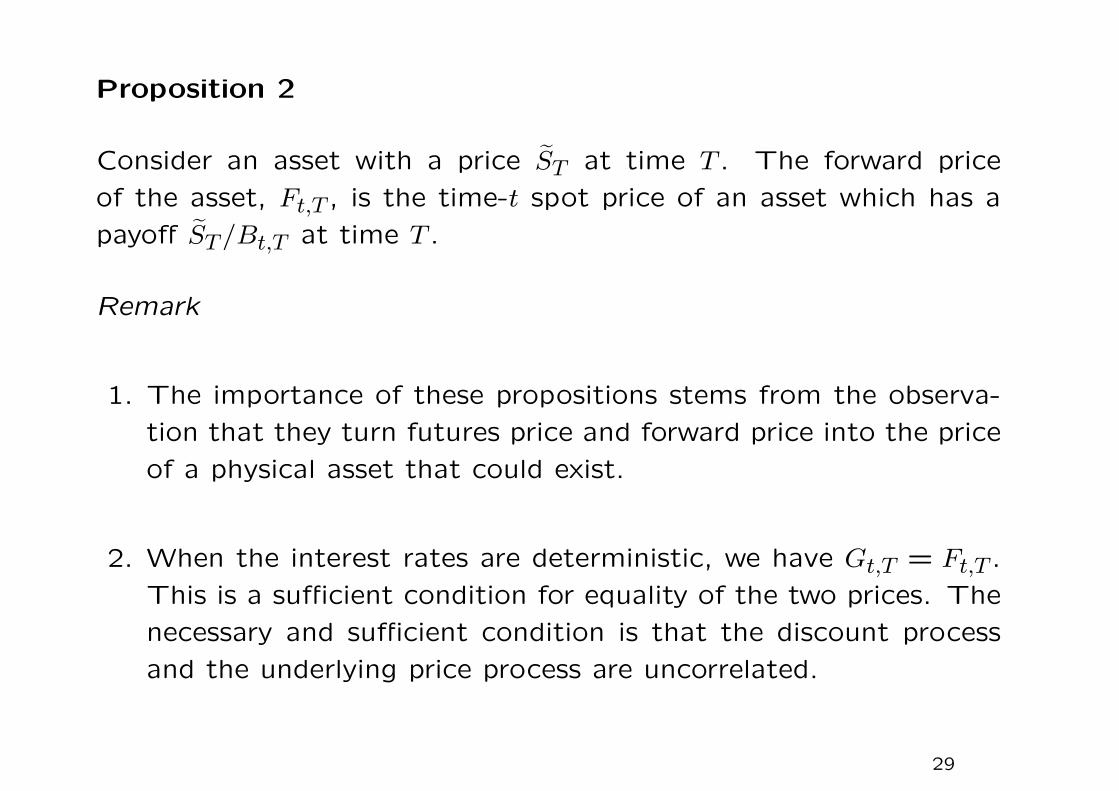
Proposition 2

Consider an asset with a price S̃T at time T . The forward price

of the asset, Ft,T , is the time-t spot price of an asset which has a

payoff S̃T/Bt,T at time T .

Remark

1. The importance of these propositions stems from the observa-

tion that they turn futures price and forward price into the price

of a physical asset that could exist.

2. When the interest rates are deterministic, we have Gt,T = Ft,T .

This is a sufficient condition for equality of the two prices. The

necessary and sufficient condition is that the discount process

and the underlying price process are uncorrelated.

29

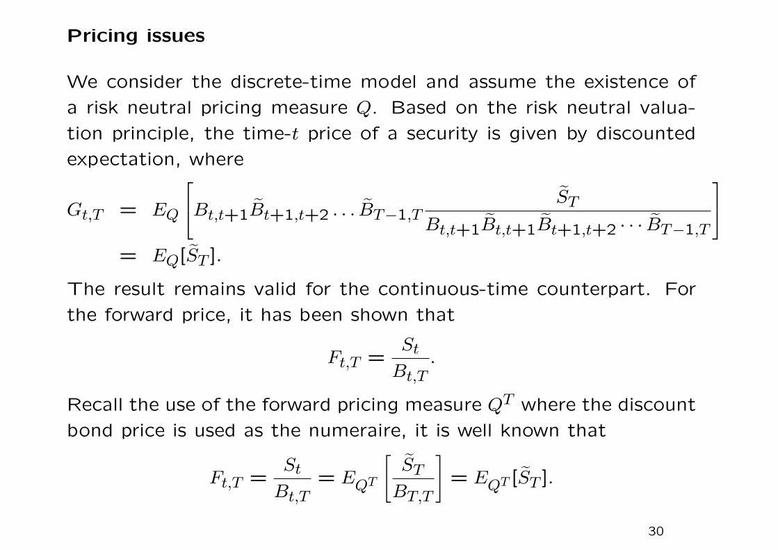
Pricing issues

We consider the discrete-time model and assume the existence of

a risk neutral pricing measure Q. Based on the risk neutral valua-

tion principle, the time-t price of a security is given by discounted

expectation, where

Gt,T = EQ

Bt,t+1B̃t+1,t+2 . . . B̃T−1,T

S̃T

Bt,t+1B̃t,t+1B̃t+1,t+2 · · · B̃T−1,T

= EQ[S̃T ].

The result remains valid for the continuous-time counterpart. For

the forward price, it has been shown that

Ft,T =St

Bt,T.

Recall the use of the forward pricing measure QT where the discount

bond price is used as the numeraire, it is well known that

Ft,T =St

Bt,T= EQT

[S̃T

BT,T

]= EQT [S̃T ].

30

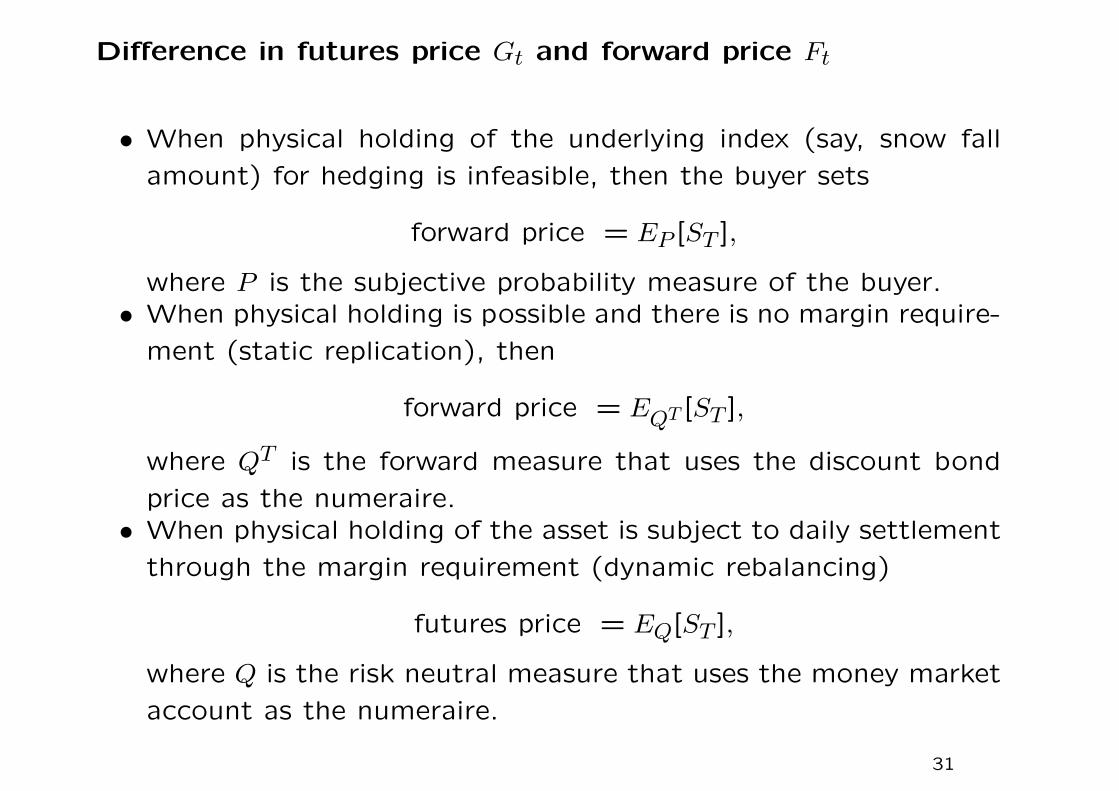
Difference in futures price Gt and forward price Ft

• When physical holding of the underlying index (say, snow fall

amount) for hedging is infeasible, then the buyer sets

forward price = EP [ST ],

where P is the subjective probability measure of the buyer.• When physical holding is possible and there is no margin require-

ment (static replication), then

forward price = EQT [ST ],

where QT is the forward measure that uses the discount bond

price as the numeraire.• When physical holding of the asset is subject to daily settlement

through the margin requirement (dynamic rebalancing)

futures price = EQ[ST ],

where Q is the risk neutral measure that uses the money market

account as the numeraire.

31

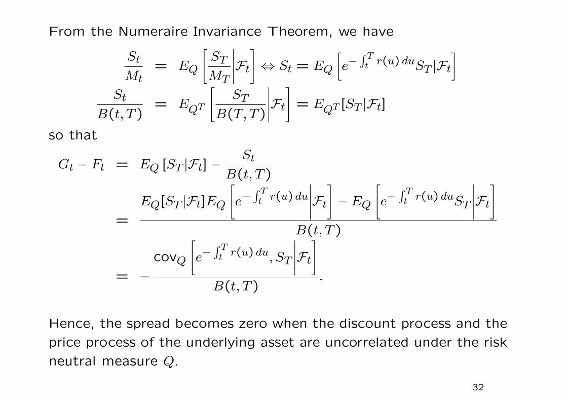
From the Numeraire Invariance Theorem, we have

St

Mt= EQ

[ST

MT

∣∣∣∣∣Ft

]⇔ St = EQ

[e−

∫ Tt r(u) duST |Ft

]

St

B(t, T )= EQT

[ST

B(T, T )

∣∣∣∣∣Ft

]= EQT [ST |Ft]

so that

Gt − Ft = EQ [ST |Ft]−St

B(t, T )

=

EQ[ST |Ft]EQ

[e−

∫ Tt r(u) du

∣∣∣∣∣Ft

]− EQ

[e−

∫ Tt r(u) duST

∣∣∣∣∣Ft

]

B(t, T )

= −covQ

[e−

∫ Tt r(u) du, ST

∣∣∣∣∣Ft

]

B(t, T ).

Hence, the spread becomes zero when the discount process and the

price process of the underlying asset are uncorrelated under the risk

neutral measure Q.

32

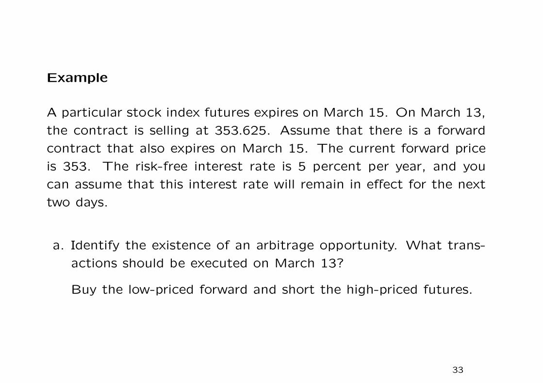
Example

A particular stock index futures expires on March 15. On March 13,

the contract is selling at 353.625. Assume that there is a forward

contract that also expires on March 15. The current forward price

is 353. The risk-free interest rate is 5 percent per year, and you

can assume that this interest rate will remain in effect for the next

two days.

a. Identify the existence of an arbitrage opportunity. What trans-

actions should be executed on March 13?

Buy the low-priced forward and short the high-priced futures.

33

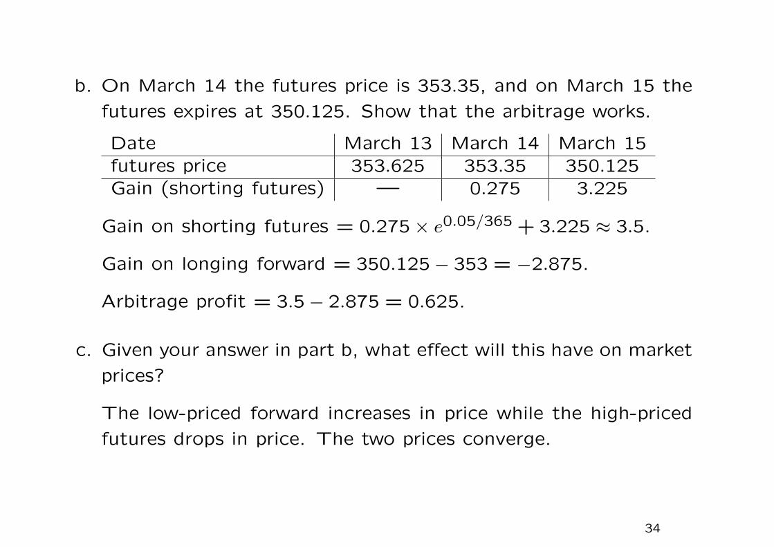
b. On March 14 the futures price is 353.35, and on March 15 the

futures expires at 350.125. Show that the arbitrage works.

Date March 13 March 14 March 15futures price 353.625 353.35 350.125Gain (shorting futures) — 0.275 3.225

Gain on shorting futures = 0.275× e0.05/365 + 3.225 ≈ 3.5.

Gain on longing forward = 350.125− 353 = −2.875.

Arbitrage profit = 3.5− 2.875 = 0.625.

c. Given your answer in part b, what effect will this have on market

prices?

The low-priced forward increases in price while the high-priced

futures drops in price. The two prices converge.

34

Index futures arbitrage

If the delivery price is higher than the no-arbitrage price, arbitrage

profits can be made by buying the basket of stocks that is underlying

the stock index and shorting the index futures contract.

Difficulties in actual implementation and associated costs

1. Require significant amount of capital e.g. Shorting 2,000 Hang

Seng index futures requires the purchase of 2.5 billion worth of

stock (based on Hang Seng Index of 25,000 and $50 for each

index point).

2. Timing risk

Stock prices move quickly, there exist time lags in the buy-in

and buy-out processes.

35

3. Settlement

The unwinding of the stock positions must be done in 47 steps

on the settlement date.

4. Stocks must be bought or sold in board lot. One can only

approximate the proportion of the stocks in the index calculation

formula.

5. Dividend amounts and dividend payment dates of the stocks are

uncertain. Note that dividends cause the stock price to drop

and affect the index value.

6. Transaction costs in the buy-in and buy-out of the stocks; and

interest losses in the margin account.

36

Currency forward

The underlying is the exchange rate X, which is the domestic cur-

rency price of one unit of foreign currency.

rd = constant domestic interest rate

rf = constant foreign interest rate

Portfolio A: Hold one currency forward with delivery price K

and a domestic bond of par K maturing on the

delivery date of forward.

Portfolio B: Hold a foreign bond of unit par maturing on the

delivery date of forward.

Let ΠA(t) and ΠA(T ) denote the value of Portfolio A at time t and

T , respectively.

37

Remark

Exchange rate is not a tradable asset. However, it comes into

existence when we convert the price of the foreign bond (tradeable

asset) from the foreign currency world into the domestic currency

world.

On the delivery date, the holder of the currency forward has to

pay K domestic dollars to buy one unit of foreign currency. Hence,

ΠA(T ) = ΠB(T ), where T is the delivery date.

Using the law of one price, ΠA(t) = ΠB(t) must be observed at the

current time t.

38

Note that

Bd(τ) = e−rdτ , Bf(τ) = e−rfτ ,

where τ = T − t is the time to expiry. Let f be the value of the

currency forward in domestic currency,

f + KBd(τ) = XBf(τ),

where XBf(τ) is the value of the foreign bond in domestic currency.

By setting f = 0,

K =XBf(τ)

Bd(τ)= Xe(rd−rf)τ .

We may recognize rd as the cost of fund and rf as the dividend

yield. This result is the well known Interest Rate Parity Relation.

39

Bond forward

The underlying asset is a zero-coupon bond of maturity T2 with a

settlement date T1, where t < T1 < T2.

The holder pays the delivery price F of the bond forward on the

forward maturity date T1 to receive a bond with par value P on the

maturity date T2.

40

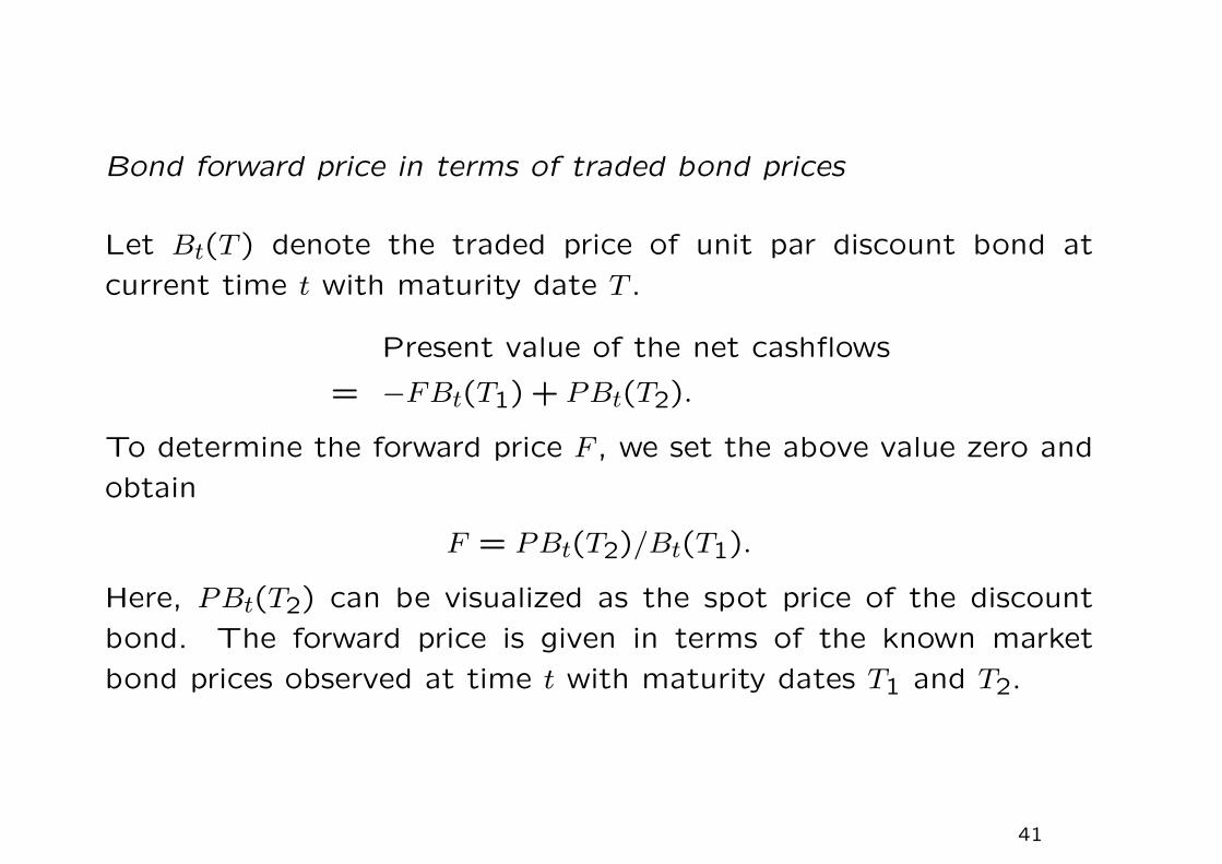
Bond forward price in terms of traded bond prices

Let Bt(T ) denote the traded price of unit par discount bond at

current time t with maturity date T .

Present value of the net cashflows

= −FBt(T1) + PBt(T2).

To determine the forward price F , we set the above value zero and

obtain

F = PBt(T2)/Bt(T1).

Here, PBt(T2) can be visualized as the spot price of the discount

bond. The forward price is given in terms of the known market

bond prices observed at time t with maturity dates T1 and T2.

41

Forward on a coupon-paying bond

The underlying is a coupon-paying bond with maturity date TB.

Note that the bond is a traded security whose value changes with

respect to time.

6c7

TB

Let TF be the delivery date of the bond forward, where TF < TB. Let

ti be the coupon payment date of the bond on which deterministic

coupon ci is paid. Let t be the current time, where t < TF < TB.

Some of the coupons have been paid at earlier times. Let F be the

forward price, the amount paid by the forward contract holder at

time TF to buy the bond.

42

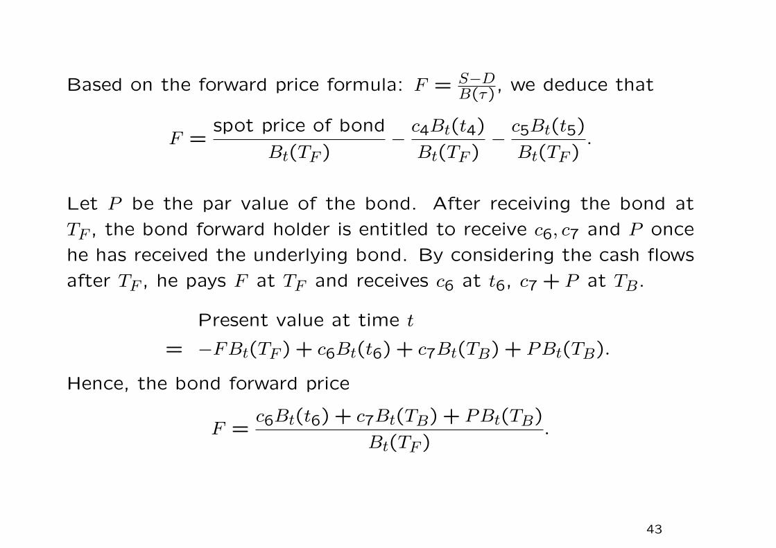
Based on the forward price formula: F = S−DB(τ), we deduce that

F =spot price of bond

Bt(TF )− c4Bt(t4)

Bt(TF )− c5Bt(t5)

Bt(TF ).

Let P be the par value of the bond. After receiving the bond at

TF , the bond forward holder is entitled to receive c6, c7 and P once

he has received the underlying bond. By considering the cash flows

after TF , he pays F at TF and receives c6 at t6, c7 + P at TB.

Present value at time t

= −FBt(TF ) + c6Bt(t6) + c7Bt(TB) + PBt(TB).

Hence, the bond forward price

F =c6Bt(t6) + c7Bt(TB) + PBt(TB)

Bt(TF ).

43

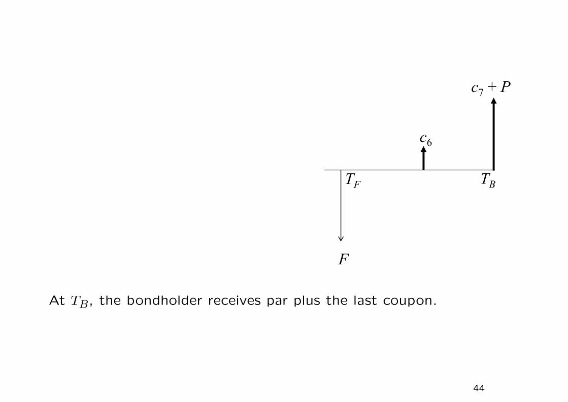
5

F

TF

TB

c7+ P

c6

At TB, the bondholder receives par plus the last coupon.

44

Example — Bond forward

• A 10-year bond is currently selling for $920.

• Currently, hold a forward contract on this bond that has a de-

livery date in 1 year and a delivery price of $940.

• The bond pays coupons of $80 every 6 months, with one due

6 months from now and another just before maturity of the

forward.

• The current interest rates for 6 months and 1 year (compounded

semi-annually) are 7% and 8%, respectively (annual rates com-

pounded every 6 months).

• What is the current value of the forward?

45

Let d(0, k) denote the discount factor over the (0, k) semi-annual

period. Consider the future value of the cash flows associated with

holding the bond one year later and payment of F0 under the forward

contract. The current forward price of the bond

F0 =spot price

d(0,2)− c(1)d(0,1)

d(0,2)− c(2)d(0,2)

d(0,2)

= 920(1.04)2 − 80(1.04)2

1.035− 80(1.04)2

(1.04)2= 831.47.

The difference in the forward prices is discounted to the present

value. The current value of the forward contract = 831.47−940(1.04)2

=

−100.34.

46

Implied forward interest rate

The forward price of a forward on a discount bond should be related

to the implied forward interest rate R(t;T1, T2). The implied forward

rate is the interest rate over [T1, T2] as implied by time-t discount

bond prices. The bond forward buyer pays F at T1 and receives P

at T2 and she is expected to earn R(t;T1, T2) over [T1, T2], so

F [1 + R(t;T1, T2)(T2 − T1)] = P.

Together with

F = PBt(T2)/Bt(T1),

we obtain

R(t;T1, T2) =1

T2 − T1

[Bt(T1)

Bt(T2)− 1

].

47

Forward rate agreement (FRA)

The FRA is an agreement between two counterparties to exchange

floating and fixed interest payments on the future settlement date

T2.

• The floating rate will be the LIBOR rate L[T1, T2] as observed

on the future reset date T1.

Question

Should the fixed rate be set equal to the implied forward rate over

the same period as observed today?

48

Determination of the forward price of LIBOR

L[T1, T2] = LIBOR rate observed at future time T1

for the accrual period [T1, T2]

K = fixed rate

N = notional of the FRA

Cash flow of the fixed rate receiver

49

Cash flow of the fixed rate receiver

t T T1 2

reset date settlement date

floating rate[ ] is

reset at

L T , T

T1 2

1

collect

from maturity bond

N + NK(T - T )

T -2 2

2

collectat from

-maturity bond;

invest in bankaccount earning

[ , ] rate

of interest

NT

T

L T T

1

1

1 2

collect( , )

( - )

N + NL T T

T T1 2

2 1

50

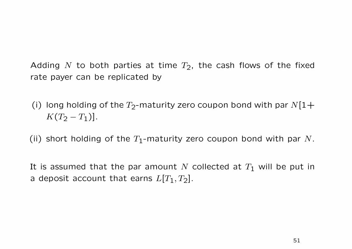
Adding N to both parties at time T2, the cash flows of the fixed

rate payer can be replicated by

(i) long holding of the T2-maturity zero coupon bond with par N [1+

K(T2 − T1)].

(ii) short holding of the T1-maturity zero coupon bond with par N .

It is assumed that the par amount N collected at T1 will be put in

a deposit account that earns L[T1, T2].

51

Comparison between bond forward and FRA

52

Value of the replicating portfolio at the current time

= N{[1 + K(T2 − T1)]Bt(T2)−Bt(T1)}.

We find K such that the above value is zero.

K =1

T2 − T1

[Bt(T1)

Bt(T2)− 1

]

︸ ︷︷ ︸forward rate over [T1, T2]

.

The fair fixed rate K is seen to be the forward price of the LIBOR

rate L[T1, T2] over the time period [T1, T2].

53

Interest rate swaps

In an interest swap, the two parties agree to exchange periodic

interest payments.

• The interest payments exchanged are calculated based on some

predetermined dollar principal, called the notional amount.

• One party is the fixed-rate payer and the other party is the

floating-rate payer. The floating interest rate is based on some

reference rate (the most common index is the LONDON IN-

TERBANK OFFERED RATE, LIBOR).

54

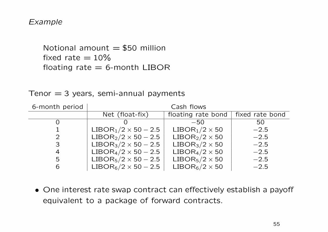
Example

Notional amount = $50 millionfixed rate = 10%floating rate = 6-month LIBOR

Tenor = 3 years, semi-annual payments

6-month period Cash flowsNet (float-fix) floating rate bond fixed rate bond

0 0 −50 501 LIBOR1/2× 50− 2.5 LIBOR1/2× 50 −2.52 LIBOR2/2× 50− 2.5 LIBOR2/2× 50 −2.53 LIBOR3/2× 50− 2.5 LIBOR3/2× 50 −2.54 LIBOR4/2× 50− 2.5 LIBOR4/2× 50 −2.55 LIBOR5/2× 50− 2.5 LIBOR5/2× 50 −2.56 LIBOR6/2× 50− 2.5 LIBOR6/2× 50 −2.5

• One interest rate swap contract can effectively establish a payoff

equivalent to a package of forward contracts.

55

A swap can be interpreted as a package of cash market instruments

– a portfolio of forward rate agreements.

• Buy $50 million par of a 3-year floating rate bond that pays

6-month LIBOR semi-annually.

• Finance the purchase by borrowing $50 million for 3 years at

10% interest rate paid semi-annually.

The fixed-rate payer has a cash market position equivalent to a long

position in a floating-rate bond and a short position in a fixed rate

bond (borrowing through issuance of a fixed rate bond).

56

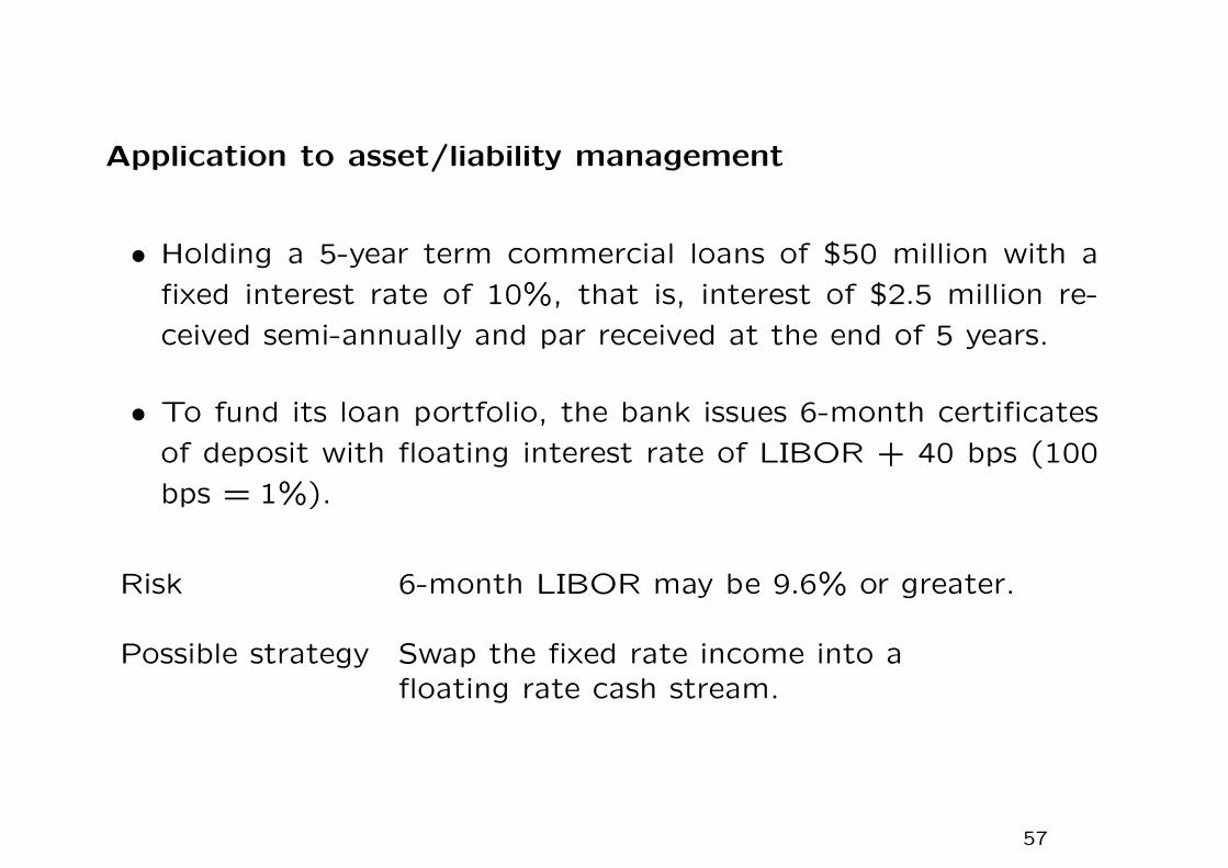
Application to asset/liability management

• Holding a 5-year term commercial loans of $50 million with a

fixed interest rate of 10%, that is, interest of $2.5 million re-

ceived semi-annually and par received at the end of 5 years.

• To fund its loan portfolio, the bank issues 6-month certificates

of deposit with floating interest rate of LIBOR + 40 bps (100

bps = 1%).

Risk 6-month LIBOR may be 9.6% or greater.

Possible strategy Swap the fixed rate income into afloating rate cash stream.

57

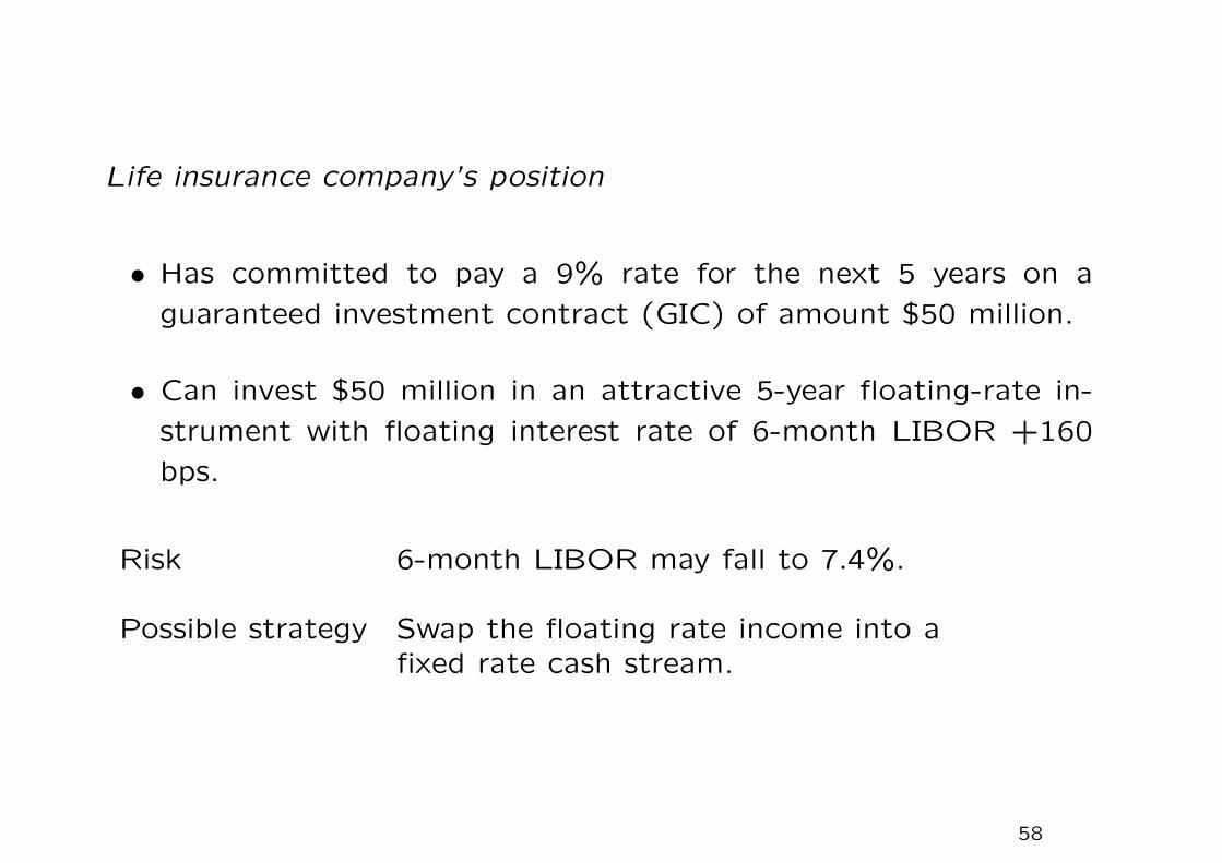
Life insurance company’s position

• Has committed to pay a 9% rate for the next 5 years on a

guaranteed investment contract (GIC) of amount $50 million.

• Can invest $50 million in an attractive 5-year floating-rate in-

strument with floating interest rate of 6-month LIBOR +160

bps.

Risk 6-month LIBOR may fall to 7.4%.

Possible strategy Swap the floating rate income into afixed rate cash stream.

58

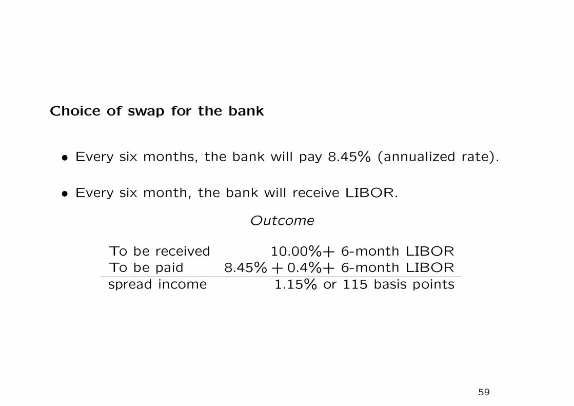
Choice of swap for the bank

• Every six months, the bank will pay 8.45% (annualized rate).

• Every six month, the bank will receive LIBOR.

Outcome

To be received 10.00%+ 6-month LIBORTo be paid 8.45% + 0.4%+ 6-month LIBORspread income 1.15% or 115 basis points

59

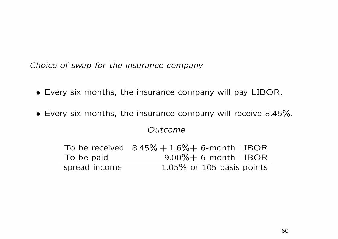
Choice of swap for the insurance company

• Every six months, the insurance company will pay LIBOR.

• Every six months, the insurance company will receive 8.45%.

Outcome

To be received 8.45% + 1.6%+ 6-month LIBORTo be paid 9.00%+ 6-month LIBORspread income 1.05% or 105 basis points

60

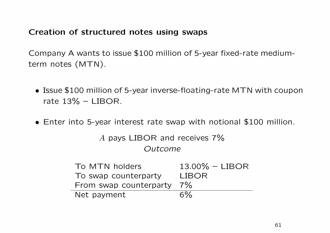
Creation of structured notes using swaps

Company A wants to issue $100 million of 5-year fixed-rate medium-

term notes (MTN).

• Issue $100 million of 5-year inverse-floating-rate MTN with coupon

rate 13% – LIBOR.

• Enter into 5-year interest rate swap with notional $100 million.

A pays LIBOR and receives 7%

Outcome

To MTN holders 13.00% – LIBORTo swap counterparty LIBORFrom swap counterparty 7%Net payment 6%

61

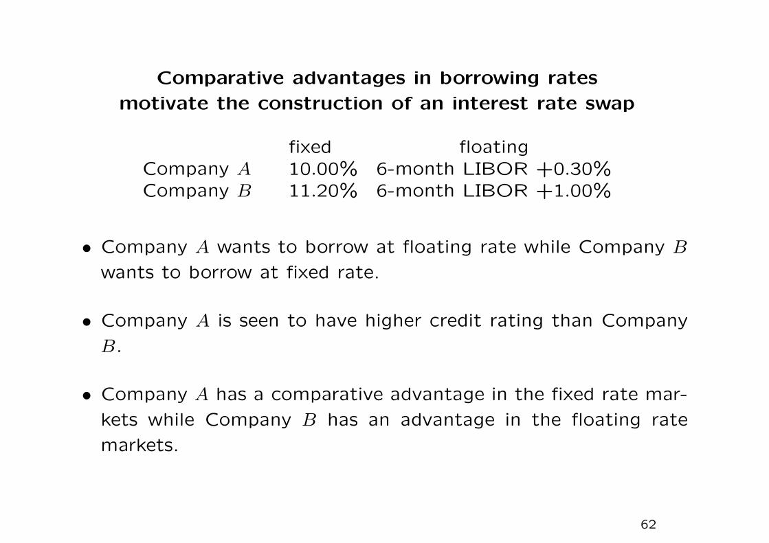
Comparative advantages in borrowing rates

motivate the construction of an interest rate swap

fixed floatingCompany A 10.00% 6-month LIBOR +0.30%Company B 11.20% 6-month LIBOR +1.00%

• Company A wants to borrow at floating rate while Company B

wants to borrow at fixed rate.

• Company A is seen to have higher credit rating than Company

B.

• Company A has a comparative advantage in the fixed rate mar-

kets while Company B has an advantage in the floating rate

markets.

62

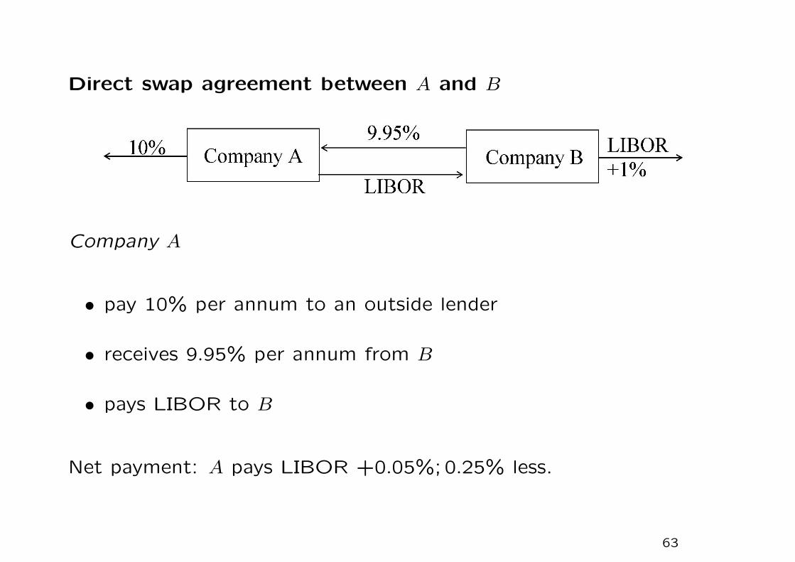
Direct swap agreement between A and B

Company A

• pay 10% per annum to an outside lender

• receives 9.95% per annum from B

• pays LIBOR to B

Net payment: A pays LIBOR +0.05%;0.25% less.

63

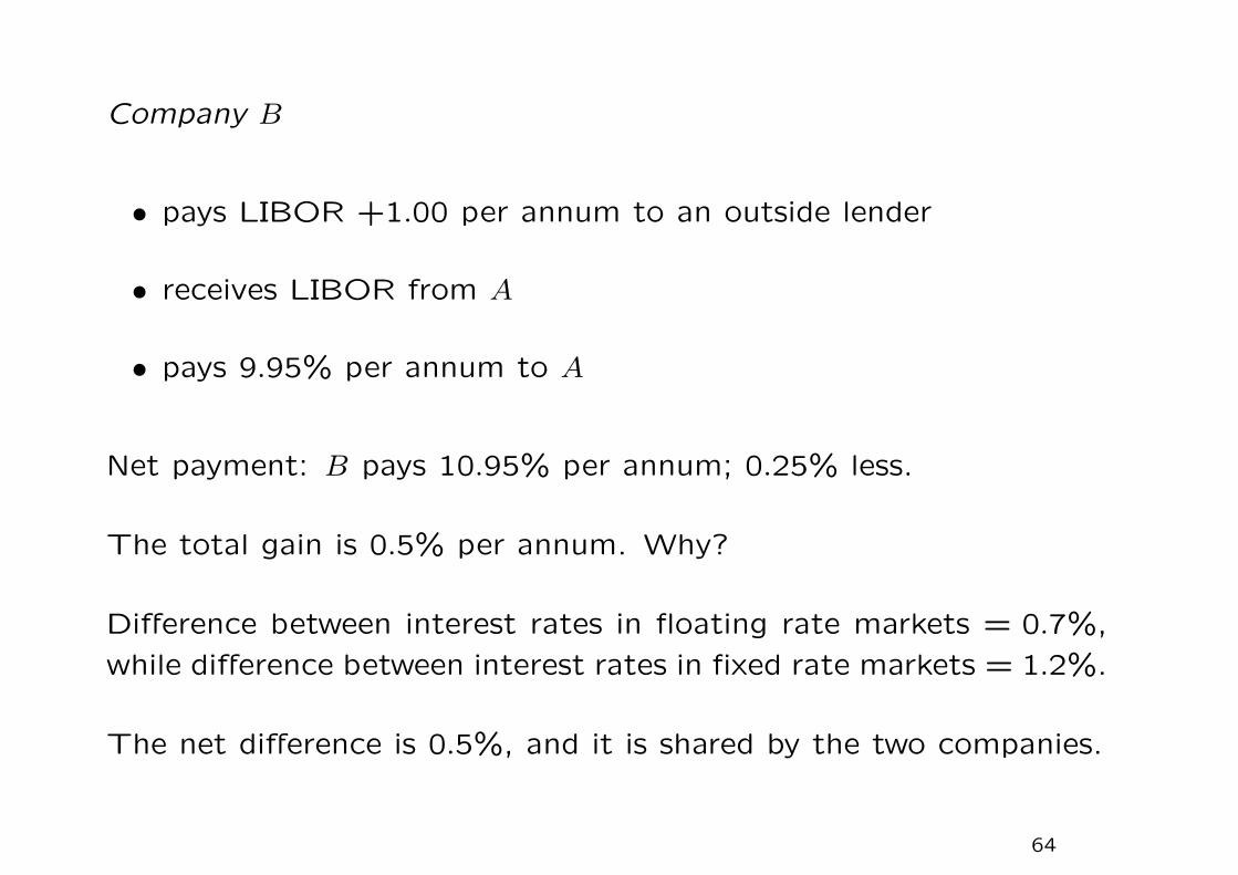
Company B

• pays LIBOR +1.00 per annum to an outside lender

• receives LIBOR from A

• pays 9.95% per annum to A

Net payment: B pays 10.95% per annum; 0.25% less.

The total gain is 0.5% per annum. Why?

Difference between interest rates in floating rate markets = 0.7%,

while difference between interest rates in fixed rate markets = 1.2%.

The net difference is 0.5%, and it is shared by the two companies.

64

Interest rate swap using financial intermediary

Net gain to A = 0.2%

Net gain to B = 0.2%

Net gain to the financial intermediary = 0.1%. The financial inter-

mediary has to bear the counterparty risks of the two companies.

The settlement clauses of interest rate swaps upon default can be

quite complicated.

• The financial institution has two separate contracts. If one of

the companies defaults, the financial institution still has to honor

its agreement with the other company.

65

Exploiting comparative advantages

• Initial motivation for the interest rate swap market was bor-

rower exploitation of “credit arbitrage” opportunities because

of differences between the quality spread between the lower-

and higher-rated credits in the floating and fixed rate loans.

Query As with any arbitrage opportunity, the more it is exploited,

the smaller it becomes.

Explanation The difference in quality spread persists due to dif-

ferences in regulations and tax treatment in different

countries.

66

Valuation of interest rate swaps

• When a swap is entered into, it typically has zero value.

• Valuation involves finding the fixed swap rate K such that the

fixed and floating legs have equal value at inception.

• Consider a swap with payment dates t1, t2, · · · , tn (tenor struc-

ture) set in the term of the swap. Li−1 is the LIBOR observed

at ti−1 but payment is made at ti. Write δi ≈ ti − ti−1 as the

accrual period over [ti−1, ti].

• The fixed payment at ti is KNδi while the floating payment at

ti is Li−1Nδi, i = 1,2, · · ·n. Here, N is the notional.

67

Day count convention

For the 30/360 day count convention of the time period (D1, D2]

with D1 excluded but D2 included, the year fraction is

max(30− d1,0) + min(d2,30) + 360× (y2 − y1) + 30× (m2 −m1 − 1)

360where di, mi and yi represent the day, month and year of date Di, i =

1,2.

For example, the year fraction between Feb 27, 2006 and July 31,

2008

=30− 27 + 30 + 360× (2008− 2006) + 30× (7− 2− 1)

360

=33

360+ 2 +

4

12.

68

Replication of cash flows

• The fixed payment at ti is KNδi. The fixed payments are

packages of discount bonds with par KNδi at maturity date

Ti, i = 1,2, · · · , n.

• To replicate the floating leg payments at current time t, t < T0,

we long T0-maturity discount bond with par N and short Tn-

maturity discount bond with par N . The N dollars collected

at T0 can generate the floating leg payments Li−1Nδi at all

Ti, i = 1,2, · · · , n. The remaining N dollars at Tn is used to pay

the par of the Tn-maturity bond.

• Let B(t, T ) be the time-t value of the discount bond with ma-

turity t.

69

• Sum of percent value of the floating leg payments

= N [B(t, T0)−B(t, Tn)];

sum of present value of fixed leg payments

= NKn∑

i=1

δiB(t, Ti).

The swap rate K is given by equating the present values of the two

sets of payments:

K =B(t, T0)−B(t, Tn)∑n

i=1 δiB(t, Ti).

The interest rate swap reduces to a FRA when n = 1. As a check,

we obtain

K =B(t, T0)−B(t, T1)

(T1 − T0)B(t, T1).

70

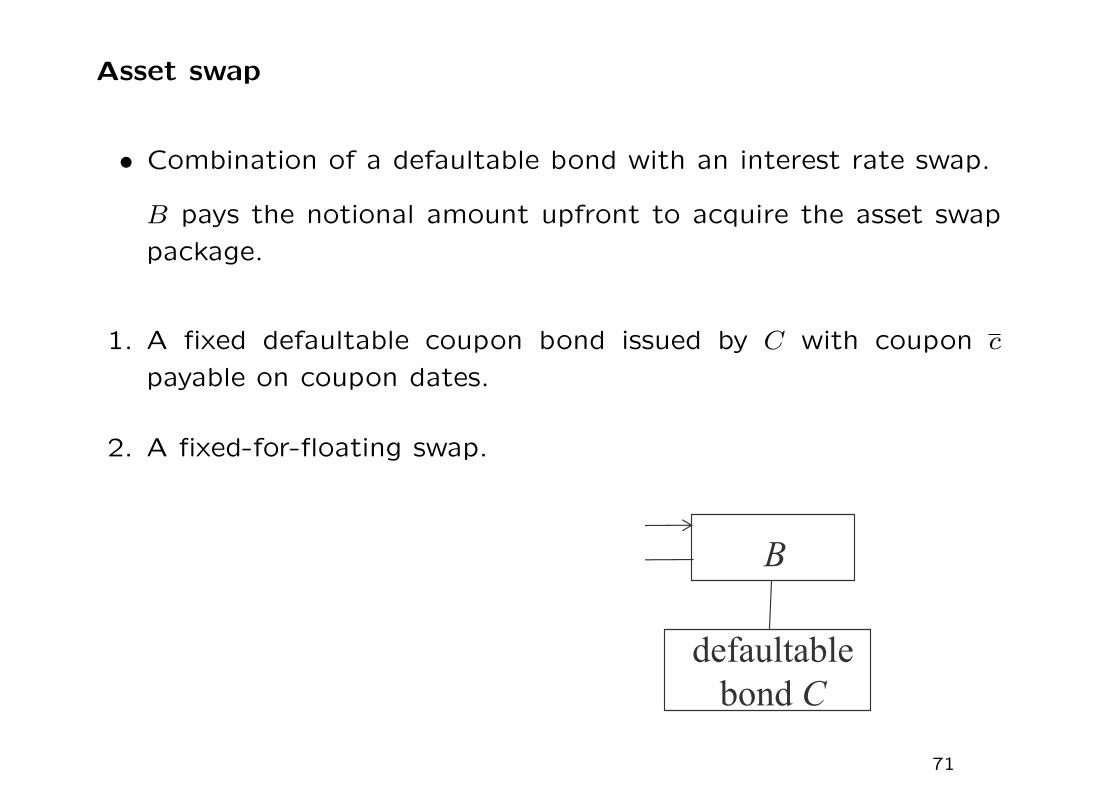
Asset swap

• Combination of a defaultable bond with an interest rate swap.

B pays the notional amount upfront to acquire the asset swap

package.

1. A fixed defaultable coupon bond issued by C with coupon c

payable on coupon dates.

2. A fixed-for-floating swap.

A B

LIBOR +

defaultable

bond Cis adjusted to ensure that the asset swap

71

The asset swap spread sA is adjusted to ensure that the asset swap

package has an initial value equal to the notional.

Remarks

1. Asset swaps are more liquid than the underlying defaultable

bond.

2. An asset swaption gives B the right to enter an asset swap

package at some future date T at a predetermined asset swap

spread sA.

72

Hedge based pricing – approximate hedge and replication strate-

gies

Provide hedge strategies that cover much of the risks involved in

credit derivatives – independent of any specific pricing model.

Basic instruments

1. Default free bond

C(t) = time-t price of default-free bond with fixed-coupon c

B(t, T ) = time-t price of default-free zero-coupon bond

2. Defaultable bond

C(t) = time-t price of defaultable bond with fixed-coupon c

73

3. Interest rate swap

s(t) = forward swap rate at time t of a standard fixed-for-floating

=B(t, tn)−B(t, tN)

A(t; tn, tN), t ≤ tn

where A(t; tn, tN) =N∑

i=n+1

δiB(t, ti) = value of the annuity pay-

ment stream paying δi on each date ti. The first swap payment

starts on tn+1 and the last payment date is tN .

The forward swap rate is market observable. It may occur that

the swap rate markets may not agree exactly with the bond

markets.

74

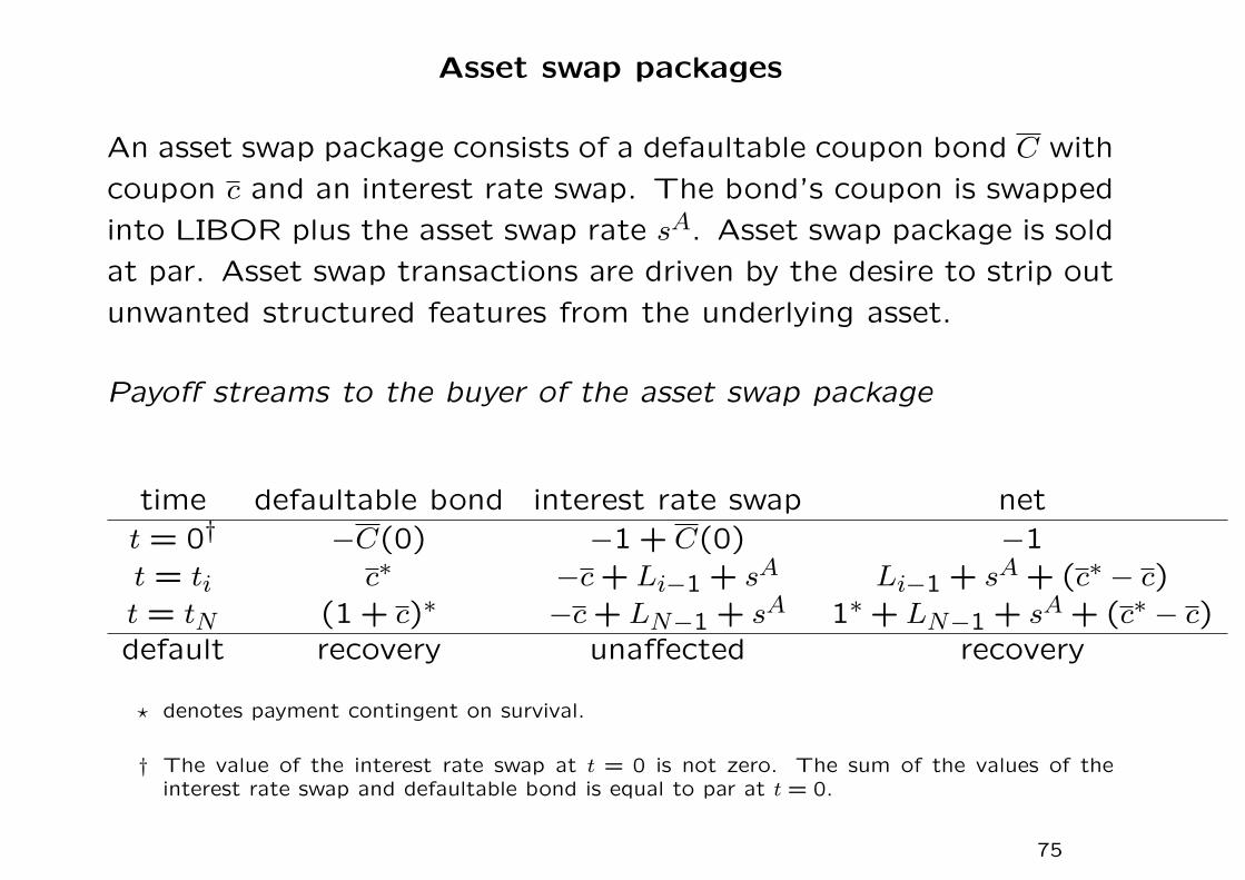
Asset swap packages

An asset swap package consists of a defaultable coupon bond C with

coupon c and an interest rate swap. The bond’s coupon is swapped

into LIBOR plus the asset swap rate sA. Asset swap package is sold

at par. Asset swap transactions are driven by the desire to strip out

unwanted structured features from the underlying asset.

Payoff streams to the buyer of the asset swap package

time defaultable bond interest rate swap nett = 0† −C(0) −1 + C(0) −1t = ti c∗ −c + Li−1 + sA Li−1 + sA + (c∗ − c)t = tN (1 + c)∗ −c + LN−1 + sA 1∗ + LN−1 + sA + (c∗ − c)default recovery unaffected recovery

? denotes payment contingent on survival.

† The value of the interest rate swap at t = 0 is not zero. The sum of the values of theinterest rate swap and defaultable bond is equal to par at t = 0.

75

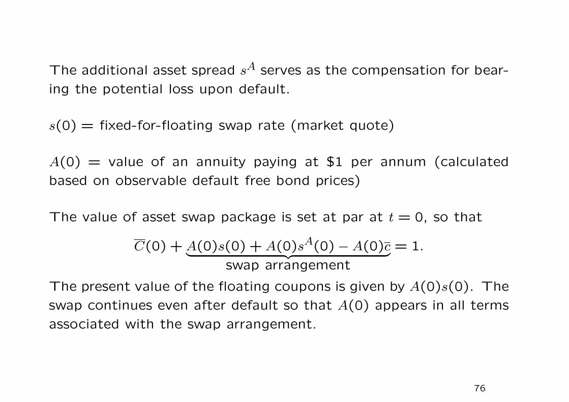
The additional asset spread sA serves as the compensation for bear-

ing the potential loss upon default.

s(0) = fixed-for-floating swap rate (market quote)

A(0) = value of an annuity paying at $1 per annum (calculated

based on observable default free bond prices)

The value of asset swap package is set at par at t = 0, so that

C(0) + A(0)s(0) + A(0)sA(0)−A(0)c︸ ︷︷ ︸swap arrangement

= 1.

The present value of the floating coupons is given by A(0)s(0). The

swap continues even after default so that A(0) appears in all terms

associated with the swap arrangement.

76

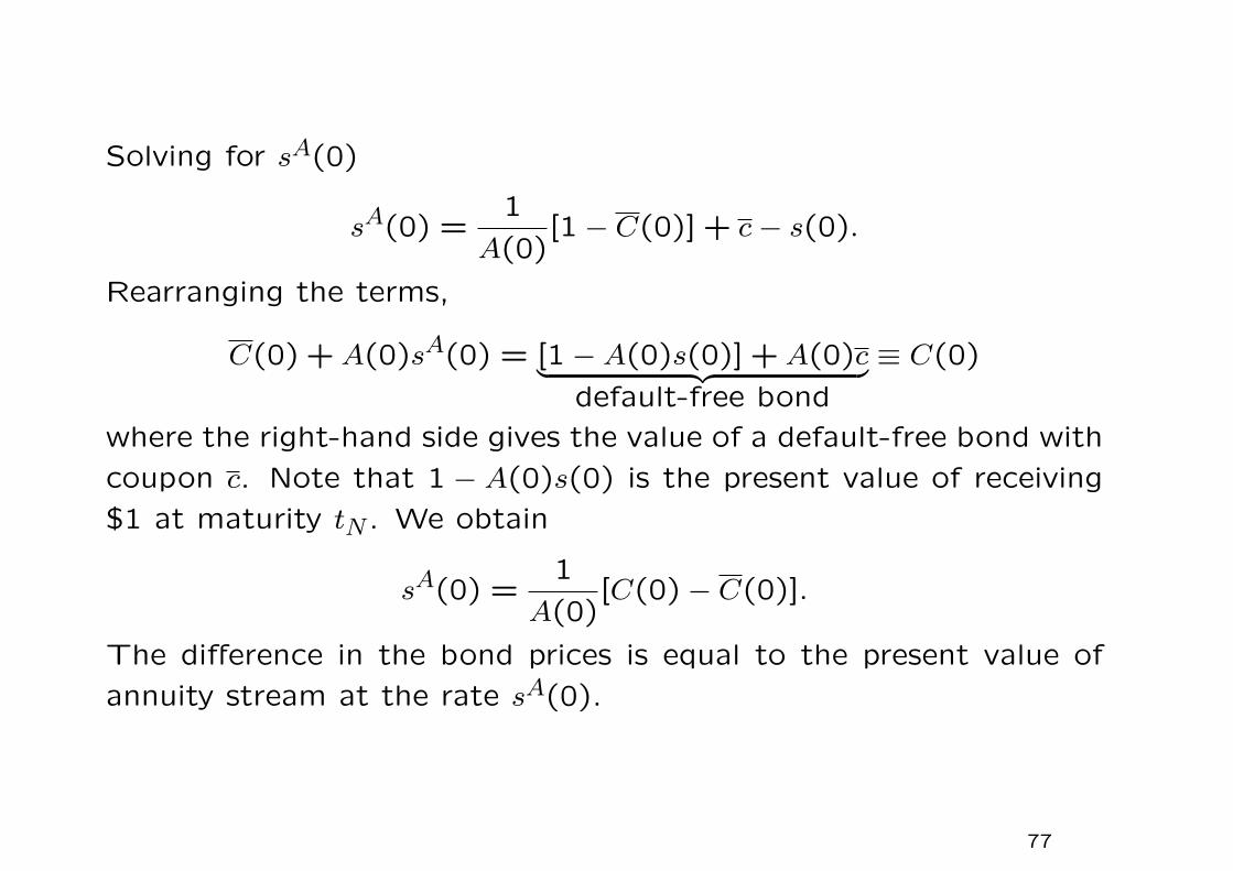
Solving for sA(0)

sA(0) =1

A(0)[1− C(0)] + c− s(0).

Rearranging the terms,

C(0) + A(0)sA(0) = [1−A(0)s(0)] + A(0)c︸ ︷︷ ︸default-free bond

≡ C(0)

where the right-hand side gives the value of a default-free bond with

coupon c. Note that 1 − A(0)s(0) is the present value of receiving

$1 at maturity tN . We obtain

sA(0) =1

A(0)[C(0)− C(0)].

The difference in the bond prices is equal to the present value of

annuity stream at the rate sA(0).

77

Alternative proof

A combination of the non-defaultable counterpart (bond with coupon

rate c) plus an interest rate swap (whose floating leg is LIBOR while

the fixed leg is c) becomes a par floater. Hence, the new asset pack-

age should also be sold at par.

The buyer is guaranteed to receive LIBOR floating rate interests

plus par. We have

C(0) =

PV $1 at tn︷ ︸︸ ︷1−A(0)s(0)+A(0)c

while A(0)s(0)−A(0)c gives the value of the interest rate swap.

78

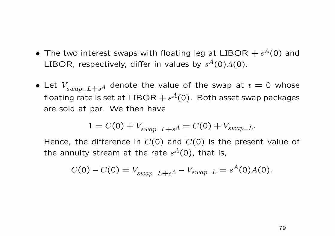
• The two interest swaps with floating leg at LIBOR + sA(0) and

LIBOR, respectively, differ in values by sA(0)A(0).

• Let Vswap−L+sA denote the value of the swap at t = 0 whose

floating rate is set at LIBOR + sA(0). Both asset swap packages

are sold at par. We then have

1 = C(0) + Vswap−L+sA = C(0) + Vswap−L.

Hence, the difference in C(0) and C(0) is the present value of

the annuity stream at the rate sA(0), that is,

C(0)− C(0) = Vswap−L+sA − Vswap−L = sA(0)A(0).

79

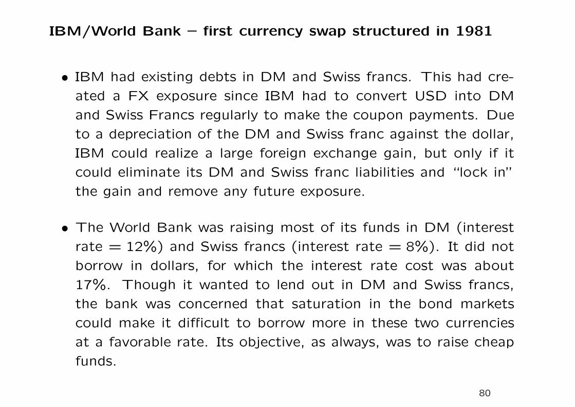
IBM/World Bank – first currency swap structured in 1981

• IBM had existing debts in DM and Swiss francs. This had cre-

ated a FX exposure since IBM had to convert USD into DM

and Swiss Francs regularly to make the coupon payments. Due

to a depreciation of the DM and Swiss franc against the dollar,

IBM could realize a large foreign exchange gain, but only if it

could eliminate its DM and Swiss franc liabilities and “lock in”

the gain and remove any future exposure.

• The World Bank was raising most of its funds in DM (interest

rate = 12%) and Swiss francs (interest rate = 8%). It did not

borrow in dollars, for which the interest rate cost was about

17%. Though it wanted to lend out in DM and Swiss francs,

the bank was concerned that saturation in the bond markets

could make it difficult to borrow more in these two currencies

at a favorable rate. Its objective, as always, was to raise cheap

funds.

80

81

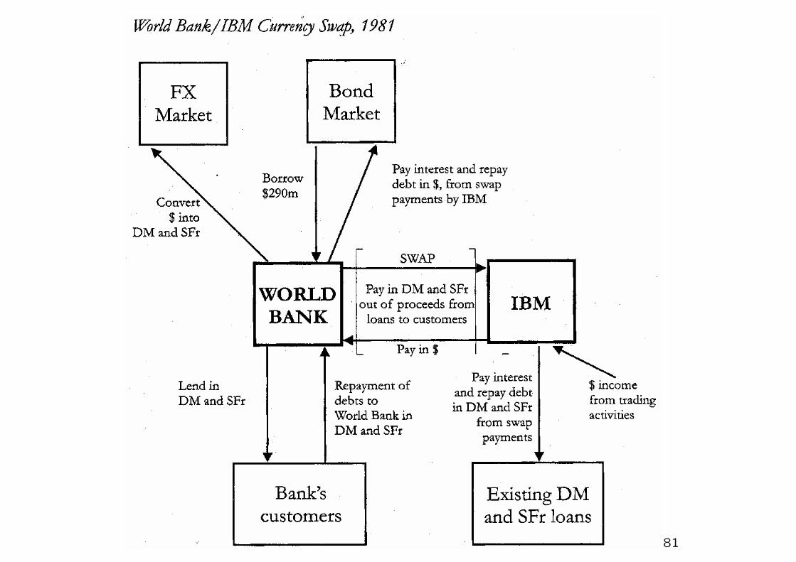
• IBM was willing to take on dollar liabilities and made dollar

payments (periodic coupons and principal at maturity) to the

World Bank since it could generate dollar income from normal

trading activities.

• The World Bank could borrow dollars, convert them into DM

and SFr in FX market, and through the swap take on payment

obligations in DM and SFr.

1. The foreign exchange gain on dollar appreciation is realized by

IBM through the negotiation of a favorable swap rate in the

swap contract.

2. The swap payments by the World Bank to IBM were scheduled

so as to allow IBM to meet its debt obligations in DM and SFr.

82

Under the currency swap

• IBM pays regular US coupons and US principal at maturity.

• World Bank pays regular DM and SFr coupons together with

DM and SFr principal at maturity.

Now IBM converted its DM and SFr liabilities into USD, and the

World Bank effectively raised hard currencies at a cheap rate. Both

parties achieved their objectives!

83

Financial options

• A call (or put) option is a contract which gives the holder the

right to buy (or sell) a prescribed asset, known as the underlying

asset, by a certain date (expiration date) for a predetermined

price (commonly called the strike price or exercise price).

• The option is said to be exercised when the holder chooses to

buy or sell the asset.

• If the option can only be exercised on the expiration date, then

the option is called a European option.

• If the exercise is allowed at any time prior to the expiration date,

then it is called an American option

84

Terminal payoff

• The terminal payoff from the long position (holder’s position)

of a European call is then

max(ST −X,0).

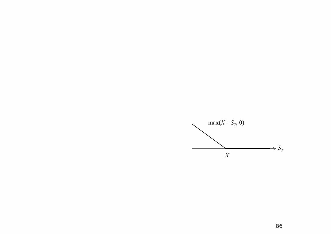
• The terminal payoff from the long position in a European put

can be shown to be

max(X − ST ,0),

since the put will be exercised at expiry only if ST < X, whereby

the asset worth ST is sold at a higher price of X.

85

put payoff

ST

X

max(X – ST, 0)

86

Questions and observations

What should be the fair option premium (usually called option price

or option value) so that the deal is fair to both writer and holder?

What should be the optimal strategy to exercise prior the expiration

date for an American option?

At least, the option price is easily seen to depend on the strike price,

time to expiry and current asset price. The less obvious factors for

the pricing models are the prevailing interest rate and the degree of

randomness of the asset price, commonly called the volatility .

87

Hedging

• If the writer of a call does not simultaneously own any amount

of the underlying asset, then he is said to be in a naked position.

• Suppose the call writer owns some amount of the underlying

asset, the loss in the short position of the call when asset price

rises can be compensated by the gain in the long position of the

underlying asset.

• This strategy is called hedging, where the risk in a portfolio is

monitored by taking opposite directions in two securities which

are highly negatively correlated.

• In a perfect hedge situation, the hedger combines a risky op-

tion and the corresponding underlying asset in an appropriate

proportion to form a riskless portfolio.

88

Swaptions – Product nature

• The buyer of a swaption has the right to enter into an interest

rate swap by some specified date. The swaption also specifies

the maturity date of the swap.

• The buyer can be the fixed-rate receiver (put swaption) or the

fixed-rate payer (call swaption).

• The writer becomes the counterparty to the swap if the buyer

exercises.

• The strike rate indicates the fixed rate that will be swapped

versus the floating rate.

• The buyer of the swaption either pays the premium upfront or

can be structured into the swap rate.

89

Uses of swaptions

Used to hedge a portfolio strategy that uses an interest rate swap

but where the cash flow of the underlying asset or liability is uncer-

tain.

Uncertainties come from (i) callability, eg, a callable bond or mort-

gage loan, (ii) exposure to default risk.

Example

Consider a S & L Association entering into a 4-year swap in which

it agrees to pay 9% fixed and receive LIBOR.

• The fixed rate payments come from a portfolio of mortgage

pass-through securities with a coupon rate of 9%. One year

later, mortgage rates decline, resulting in large prepayments.

• The purchase of a put swaption with a strike rate of 9% would

be useful to offset the original swap position.

90

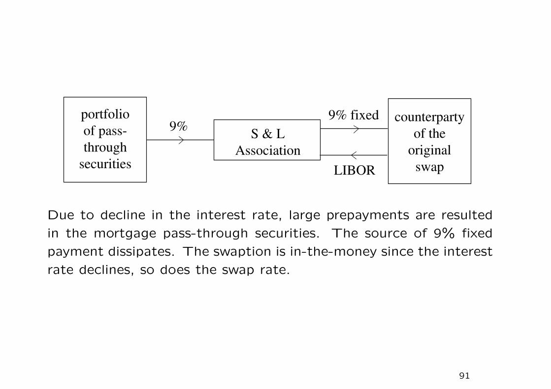
Due to decline in the interest rate, large prepayments are resulted

in the mortgage pass-through securities. The source of 9% fixed

payment dissipates. The swaption is in-the-money since the interest

rate declines, so does the swap rate.

91

By exercising the put swaption, the S & L Association receives a

fixed rate of 9%

92

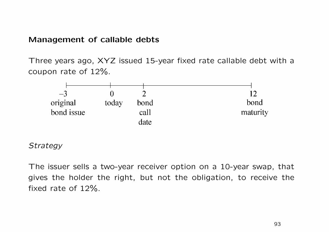
Management of callable debts

Three years ago, XYZ issued 15-year fixed rate callable debt with a

coupon rate of 12%.

Strategy

The issuer sells a two-year receiver option on a 10-year swap, that

gives the holder the right, but not the obligation, to receive the

fixed rate of 12%.

93

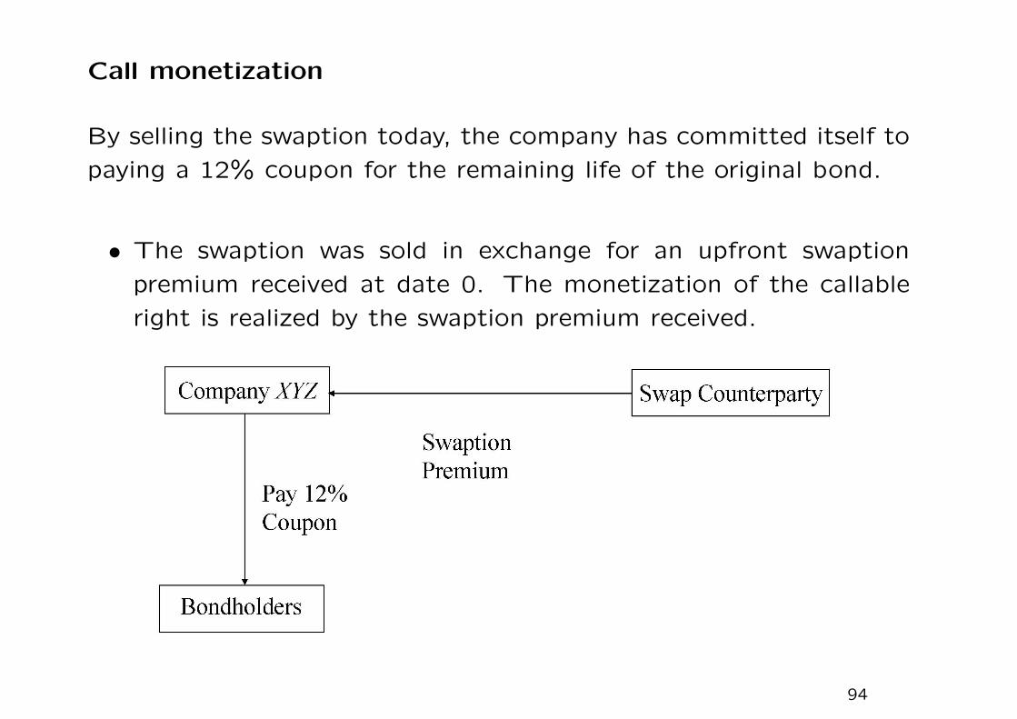
Call monetization

By selling the swaption today, the company has committed itself to

paying a 12% coupon for the remaining life of the original bond.

• The swaption was sold in exchange for an upfront swaption

premium received at date 0. The monetization of the callable

right is realized by the swaption premium received.

94

Call-Monetization cash flow: Swaption expiration date

swap rate ≥ 12% (swap counterparty does not exercise)

swap rate < 12% (swap counterparty exercises)

95

Disasters for Company XY Z

• The fixed rate on the 10-year swap is below 12% in two years

but its debt refunding rate in the capital market is above 12%

(due to credit deterioration)

• The company would be forced to enter into a swap that it does

not want while it may liquidate the original debt liabilities posi-

tion at a disadvantage and not be able to refinance its borrowing

profitably.

96

1.2 Rational boundaries for option values

• We do not specify the probability distribution of the movement

of the asset price so that the fair option value cannot be derived.

• Mathematical properties of the option values as functions of the

strike price X, asset price S and time to expiry τ are derived.

• We study the impact of dividends on these rational boundaries.

• The optimal early exercise policy of American options on a non-

dividend paying asset can be inferred from the analysis of these

bounds on option values.

• The relations between put and call prices (called the put-call

parity relations) are also deduced.

97

Non-negativity of option prices

All option prices are non-negative, that is,

C ≥ 0, P ≥ 0, c ≥ 0, p ≥ 0,

as derived from the non-negativity of the payoff structure of option

contracts.

If the price of an option were negative, this would mean an option

buyer receives cash up-front. He is guaranteed to have a non-

negative terminal payoff. In this way, he can always lock in a riskless

profit.

98

Intrinsic values of American options

• max(S−X,0) and max(X−S,0) are commonly called the intrinsic

value of a call and a put, respectively.

• Since American options can be exercised at any time before

expiration, their values must be worth at least their intrinsic

values, that is,

C(S, τ ;X) ≥ max(S −X,0)

P (S, τ ;X) ≥ max(X − S,0).

• Suppose C is less than S−X when S ≥ X, then an arbitrageur can

lock in a riskless profit by borrowing C + X dollars to purchase

the call and exercise it immediately to receive the asset worth

S. The riskless profit would be S −X − C > 0.

99

American options are worth at least their European counterparts

An American option confers all the rights of its European coun-

terpart plus the privilege of early exercise. The additional privilege

cannot have negative value.

C(S, τ ;X) ≥ c(S, τ ;X)

P (S, τ ;X) ≥ p(S, τ ;X).

• The European put value can be below the intrinsic value X − S

at sufficiently low asset value and the value of a European call

on a dividend paying asset can be below the intrinsic value S−X

at sufficiently high asset value.

100

Values of options with different dates of expiration

Consider two American options with different times to expiration τ2and τ1 (τ2 > τ1), the one with the longer time to expiration must

be worth at least that of the shorter-lived counterpart since the

longer-lived option has the additional right to exercise between the

two expiration dates.

C(S, τ2;X) > C(S, τ1;X), τ2 > τ1,

P (S, τ2;X) > P (S, τ1;X), τ2 > τ1.

The above argument cannot be applied to European options due to

lack of the early exercise privilege.

101

Values of options with different strike prices

c(S, τ ;X2) < c(S, τ ;X1), X1 < X2,

C(S, τ ;X2) < C(S, τ ;X1), X1 < X2.

and

p(S, τ ;X2) > p(S, τ ;X1), X1 < X2,

P (S, τ ;X2) > P (S, τ ;X1), X1 < X2.

Values of options at varying asset value levels

c(S2, τ ;X) > c(S1, τ ;X), S2 > S1,

C(S2, τ ;X) > C(S1, τ ;X), S2 > S1;

and

p(S2, τ ;X) < p(S1, τ ;X), S2 > S1,

P (S2, τ ;X) < P (S1, τ ;X), S2 > S1.

102

Upper bounds on call and put values

• A call option is said to be a perpetual call if its date of expiration

is infinitely far away. The asset itself can be considered as an

American perpetual call with zero strike price plus additional

privileges such as voting rights and receipt of dividends, so we

deduce that S ≥ C(S,∞; 0).

S ≥ C(S,∞; 0) ≥ C(S, τ ;X) ≥ c(S, τ ;X).

• The price of an American put equals the strike value when the

asset value is zero; otherwise, it is bounded above by the strike

price.

X ≥ P (S, τ ;X) ≥ p(S, τ ;X).

103

Lower bounds on the values of call options on a non-dividend paying

asset

Portfolio A consists of a European call on a non-dividend paying

asset plus a discount bond with a par value of X whose date of

maturity coincides with the expiration date of the call. Portfolio B

contains one unit of the underlying asset.

Asset value at expiry ST < X ST ≥ XPortfolio A X (ST −X) + X = STPortfolio B ST ST

Result of comparison VA > VB VA = VB

The present value of Portfolio A (dominant portfolio) must be equal

to or greater than that of Portfolio B (dominated portfolio). If oth-

erwise, an arbitrage opportunity can be secured by buying Portfolio

A and selling Portfolio B.

104

Write B(τ) as the price of the unit-par discount bond with time to

expiry τ . Then

c(S, τ ;X) + XB(τ) ≥ S.

Together with the non-negativity property of option value.

c(S, τ ;X) ≥ max(S −XB(τ),0).

The upper and lower bounds of the value of a European call on a

non-dividend paying asset are given by (see Figure)

S ≥ c(S, τ ;X) ≥ max(S −XB(τ),0).

105

106

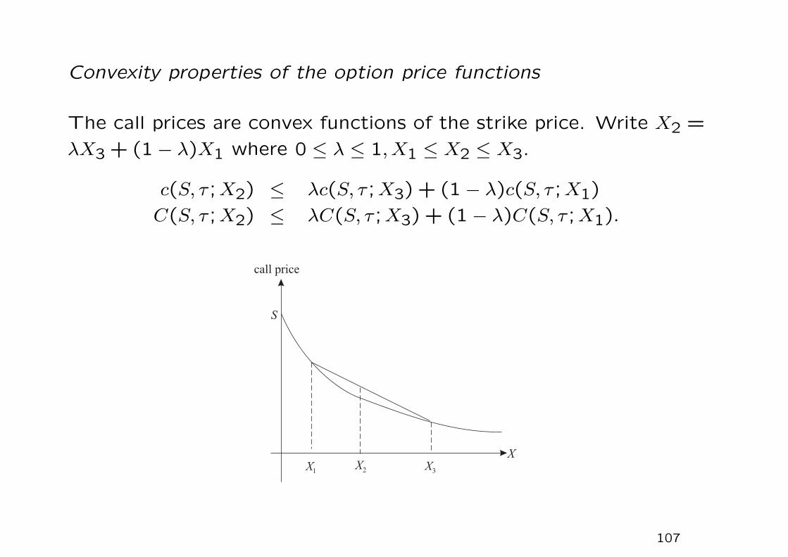
Convexity properties of the option price functions

The call prices are convex functions of the strike price. Write X2 =

λX3 + (1− λ)X1 where 0 ≤ λ ≤ 1, X1 ≤ X2 ≤ X3.

c(S, τ ;X2) ≤ λc(S, τ ;X3) + (1− λ)c(S, τ ;X1)

C(S, τ ;X2) ≤ λC(S, τ ;X3) + (1− λ)C(S, τ ;X1).

107

Consider the payoffs of the following two portfolios at expiry. Port-

folio C contains λ units of call with strike price X3 and (1−λ) units

of call with strike price X1, and Portfolio D contains one call with

strike price X2.

Since VC ≥ VD for all possible values of ST , Portfolio C is dominant

over Portfolio D. Therefore, the present value of Portfolio C must

be equal to or greater than that of Portfolio D.

• The drop in call value for one dollar increase in the strike price

should be less than one dollar. The loss in the terminal payoff

of the call due to the increase in the strike price is realized only

when the call expires in-the-money. Indeed,

∣∣∣∣∣∂c

∂X

∣∣∣∣∣ ≤ B(τ). The

factor B(τ) appears since the potential loss of paying extra one

dollar in the strike price occurs at maturity so its present value

is B(τ).

108

Payoff at expiry of Portfolios C and D.

Asset valueat expiry

ST ≤ X1 X1 ≤ ST ≤ X2 X2 ≤ ST ≤ X3 X3 ≤ ST

Portfolio C 0 (1− λ)(ST −X1) (1− λ)(ST −X1) λ(ST −X3) +(1− λ)(ST −X1)

Portfolio D 0 0 ST −X2 ST −X2

Result ofcomparison

VC = VD VC ≥ VD VC ≥ V ∗D VC = VD

* Recall X2 = λX3 + (1− λ)X1, and observe

(1− λ)(ST −X1) ≥ ST −X2

⇔ X2 − (1− λ)X1 ≥ λST

⇔ X3 ≥ ST .

109

• There is no factor involving τ , so the result also holds even when

the calls in the two portfolios are exercised prematurely. Hence,

the convexity property also holds for American calls.

• By changing the call options in the above two portfolios to the

corresponding put options, it can be shown that European and

American put prices are also convex functions of the strike price.

• By using the linear homogeneity property of the call and put

option functions with respect to the asset price and strike price,

one can show that the call and put prices (both European and

American) are convex functions of the asset price.

110

Impact of dividends on the asset price

• When an asset pays a certain amount of dividend, we can use

no arbitrage argument to show that the asset price is expected

to fall by the same amount (assuming there exist no other fac-

tors affecting the income proceeds, like taxation and transaction

costs).

• Suppose the asset price falls by an amount less than the dividend,

an arbitrageur can lock in a riskless profit by borrowing money

to buy the asset right before the dividend date, selling the asset

right after the dividend payment and returning the loan.

111

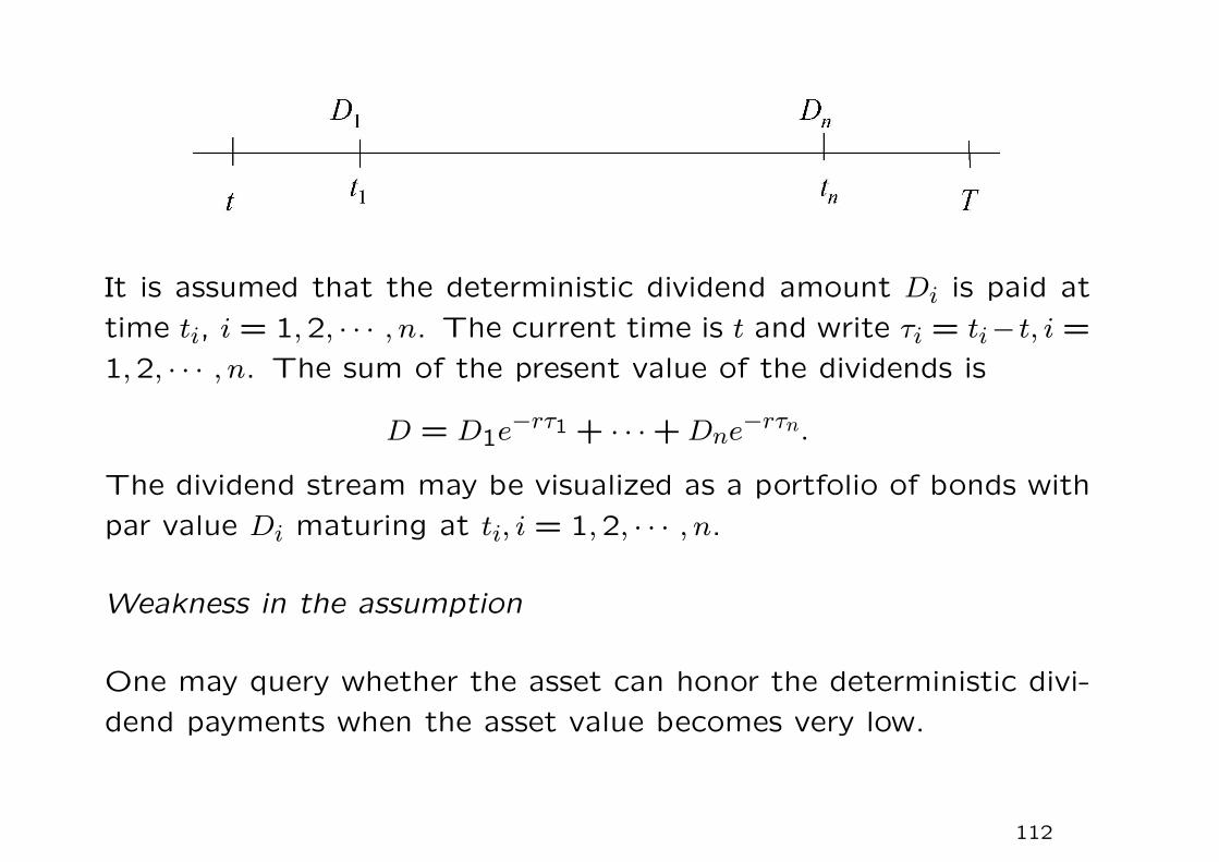
It is assumed that the deterministic dividend amount Di is paid at

time ti, i = 1,2, · · · , n. The current time is t and write τi = ti− t, i =

1,2, · · · , n. The sum of the present value of the dividends is

D = D1e−rτ1 + · · ·+ Dne−rτn.

The dividend stream may be visualized as a portfolio of bonds with

par value Di maturing at ti, i = 1,2, · · · , n.

Weakness in the assumption

One may query whether the asset can honor the deterministic divi-

dend payments when the asset value becomes very low.

112

Impact of dividends on the lower bound on a European call value

and the early exercise policy of an American call option.

• Portfolio B is modified to contain one unit of the underlying

asset and a loan of D dollars of cash (in the form of a portfolio

of bonds as specified earlier). At expiry, the value of Portfolio

B will always become ST since the loan of D will be paid back

during the life of the option using the dividends received.

• Since VA ≥ VB at expiry, hence the present value of Portfolio A

must be at least as much as that of Portfolio B. Together with

the non-negativity property of option values, we obtain

c(S, τ ;X, D) ≥ max(S −XB(τ)−D,0).

113

• When S is sufficiently high, the European call almost behaves

like a forward whose value is S−D−XB(τ). Recall the put-call

parity relation: c = p + S −D −XB(τ), so

p(S, τ ;X, D) → 0 as S →∞.

• Since the call price is lowered due to the dividends of the under-

lying asset, it may be possible that the call price becomes less

than the intrinsic value S − X when the lumped dividend D is

deep enough.

• The necessary condition on D such that c(S, τ ;X, D) may fall

below the intrinsic value S −X is given by

S −X > S −XB(τ)−D or D > X[1−B(τ)].

If D does not satisfy the above condition, it is never optimal to

exercise the American call prematurely.

114

When D > X[1 − B(τ)], the lower bound S − D − XB(τ) becomes

less than the intrinsic value S − X. As S → ∞, the European call

price curve falls below the intrinsic value line.

115

• The American call must be sufficiently deep in-the-money so

that the chance of regret on early exercise is low.

• Since there will be an expected decline in asset price right after

a discrete dividend payment, the optimal strategy is to exercise

right before the dividend payment so as to capture the dividend

paid by the asset.

• The holder of a put option gains when the asset price drops after

a discrete dividend is paid since the put value is a decreasing

function of the asset price. The American put holder would

never optimally early exercise right before the dividend date.

116

Bounds on puts

The bounds for American and European puts can be shown to be

P (S, τ ;X, D) ≥ p(S, τ ;X, D) ≥ max(XB(τ) + D − S,0).

• When XB(τ) + D < X ⇔ D < X[1 − B(τ)], the lower bound

XB(τ)−S may become less than the intrinsic value X−S when

the put is sufficiently deep in-the-money (corresponding to low

value for S). Since it is sub-optimal for the holder of an Ameri-

can put option when the put value falls below the intrinsic value,

the American put should be exercised prematurely.

• The presence of dividends makes the early exercise of an Amer-

ican put option less likely since the holder loses the future divi-

dends when the asset is sold upon exercising the put.

117

Put-call parity relations

For a pair of European put and call options on the same underlying

asset and with the same expiration date and strike price, we have

p = c− S + D + XB(τ).

When the underlying asset is non-dividend paying, we set D = 0.

• The first portfolio involves long holding of a European call, a

cash amount of D + XB(τ) and short selling of one unit of the

asset.

• The second portfolio contains only one European put.

• The cash amount D in the first portfolio is used to compensate

the dividends due to the short position of the asset.

• At expiry, both portfolios are worth max(X − ST ,0).

118

Since both options are European, they cannot be exercised prior to

expiry. Hence, both portfolios have the same value throughout the

life of the options.

• The parity relation cannot be applied to American options due

to their early exercise feature.

Lower and upper bounds on the difference of the prices of American

call and put options

First, we assume the underlying asset to be non-dividend paying.

Since P > p and C = c, and putting D = 0,

C − P < S −XB(τ),

giving the upper bound on C − P .

119

• Consider the following two portfolios: one contains a European

call plus cash of amount X, and the other contains an American

put together with one unit of underlying asset.

If there were no early exercise of the American put prior to maturity,

the terminal value of the first portfolio is always higher than that

of the second portfolio. If the American put is exercised prior to

maturity, the second portfolio’s value becomes X, which is always

less than c + X. The first portfolio dominates over the second

portfolio, so we have

c + X > P + S.

Further, since c = C when the asset does not pay dividends, the

lower bound on C − P is given by

S −X < C − P.

120

Combining the two bounds, the difference of the American call and

put option values on a non-dividend paying asset is bounded by

S −X < C − P < S −XB(τ).

• The right side inequality: C − P < S − XB(τ) also holds for

options on a dividend paying asset since dividends decrease call

value and increase put value.

• The left side inequality has to be modified as: S−D−X < C−P .

• Combining the results, the difference of the American call and

put option values on a dividend paying asset is bounded by

S −D −X < C − P < S −XB(τ).

121

1.3 Early exercise policies of American options

Non-dividend paying asset

• At any moment when an American call is exercised, its value

immediately becomes max(S −X,0). The exercise value is less

than max(S−XB(τ),0), the lower bound of the call value if the

call remains alive.

• This implies that the act of exercising prior to expiry causes a

decline in value of the American call. To the benefit of the

holder, an American call on a non-dividend paying asset will not

be exercised prior to expiry. Since the early exercise privilege is

forfeited, the American and European call values should be the

same.

• For an American put, it may become optimal to exercise prema-

turely when S falls to sufficiently low value, provided that the

dividends are not sufficiently deep.

122

Dividend paying asset

• When the underlying asset pays dividends, the early exercise of

an American call prior to expiry may become optimal when (i)

S is very high and (ii) the dividends are sizable. Under these

circumstances, it then becomes more attractive for the investor

to acquire the asset rather than holding the option.

– When S is high, the chance of regret of early exercise is low;

equivalently, the insurance value of holding the call is lower.

– When the dividends are sizable, it is more attractive to hold

the asset directly instead of holding the call.

• For an American put, when D is sufficiently high, it may become

non-optimal to exercise prematurely even at very low value of S

(even when the put is very deep-in-the-money).

123

American call on an asset with discrete dividends

• Since the holder of an American call on an asset with discrete

dividends will not receive any dividend in between dividend times,

so within these periods, it is never optimal to exercise the Amer-

ican call.

• It may be optimal to exercise the American call immediately

before the asset goes ex-dividend. What are the necessary and

sufficient conditions?

124

One-dividend model – Amount of D is paid out at td

• If the American call is exercised at t−d , the call value becomes

S−d −X. If there is no early exercise, then the asset price drops

to S+d = S−d −D right after the dividend payout.

• It behaves like an ordinary European option for t > t+d . This is

because when there is no further dividend, it becomes always

non-optimal to exercise the American call.

• The lower bound of the one-dividend American call value at t+dis the same lower bond for a European call, which is given by

S+d −Xe−r(T−t+d ), where T − t+d is the time to expiry.

• By virtue of the continuity of the call value across the dividend

date, the lower bound B for the call value at time t−d should also

be equal to B = S+d −Xe−r(T−td) = (S−d −D)−Xe−r(T−td).

125

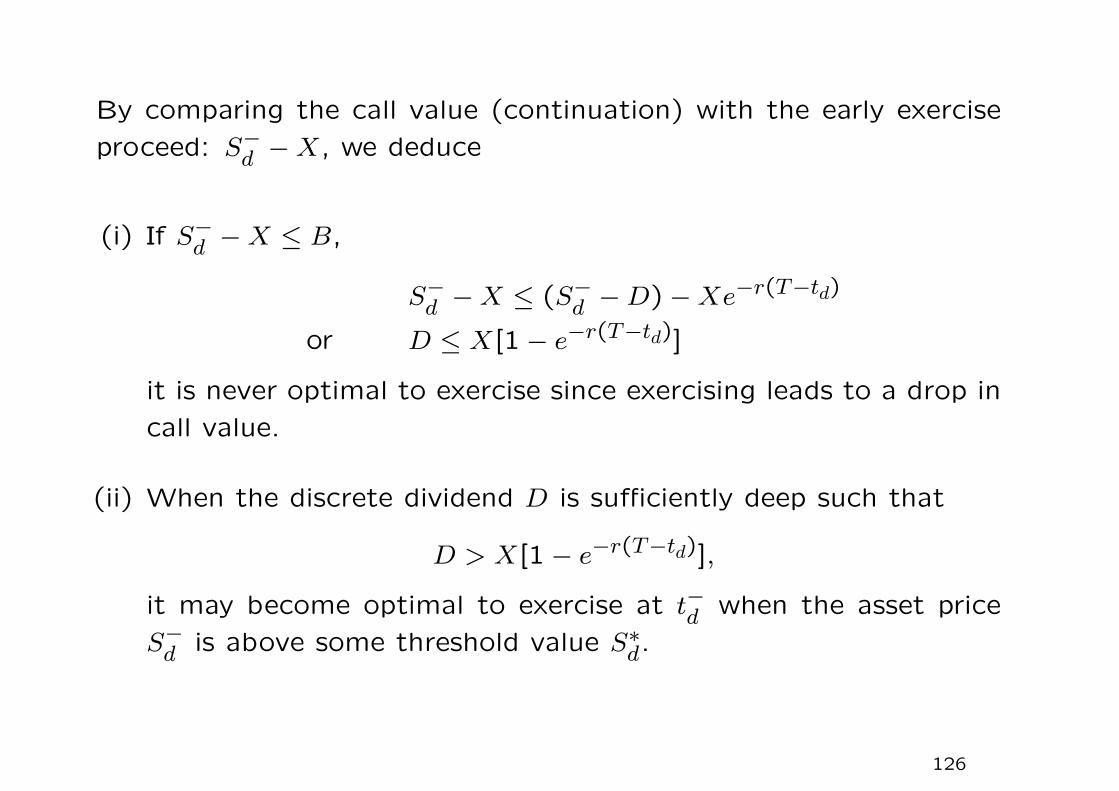
By comparing the call value (continuation) with the early exercise

proceed: S−d −X, we deduce

(i) If S−d −X ≤ B,

S−d −X ≤ (S−d −D)−Xe−r(T−td)

or D ≤ X[1− e−r(T−td)]

it is never optimal to exercise since exercising leads to a drop in

call value.

(ii) When the discrete dividend D is sufficiently deep such that

D > X[1− e−r(T−td)],

it may become optimal to exercise at t−d when the asset price

S−d is above some threshold value S∗d.

126

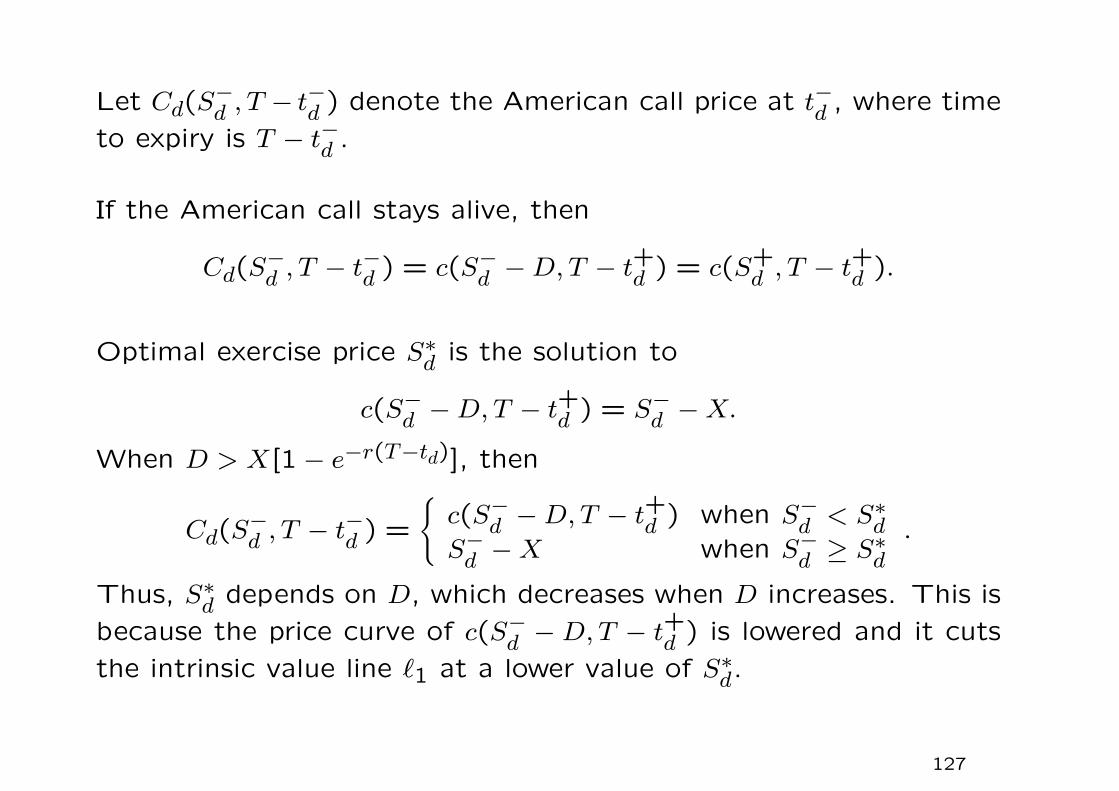
Let Cd(S−d , T − t−d ) denote the American call price at t−d , where time

to expiry is T − t−d .

If the American call stays alive, then

Cd(S−d , T − t−d ) = c(S−d −D, T − t+d ) = c(S+

d , T − t+d ).

Optimal exercise price S∗d is the solution to

c(S−d −D, T − t+d ) = S−d −X.

When D > X[1− e−r(T−td)], then

Cd(S−d , T − t−d ) =

{c(S−d −D, T − t+d ) when S−d < S∗dS−d −X when S−d ≥ S∗d

.

Thus, S∗d depends on D, which decreases when D increases. This is

because the price curve of c(S−d −D, T − t+d ) is lowered and it cuts

the intrinsic value line `1 at a lower value of S∗d.

127

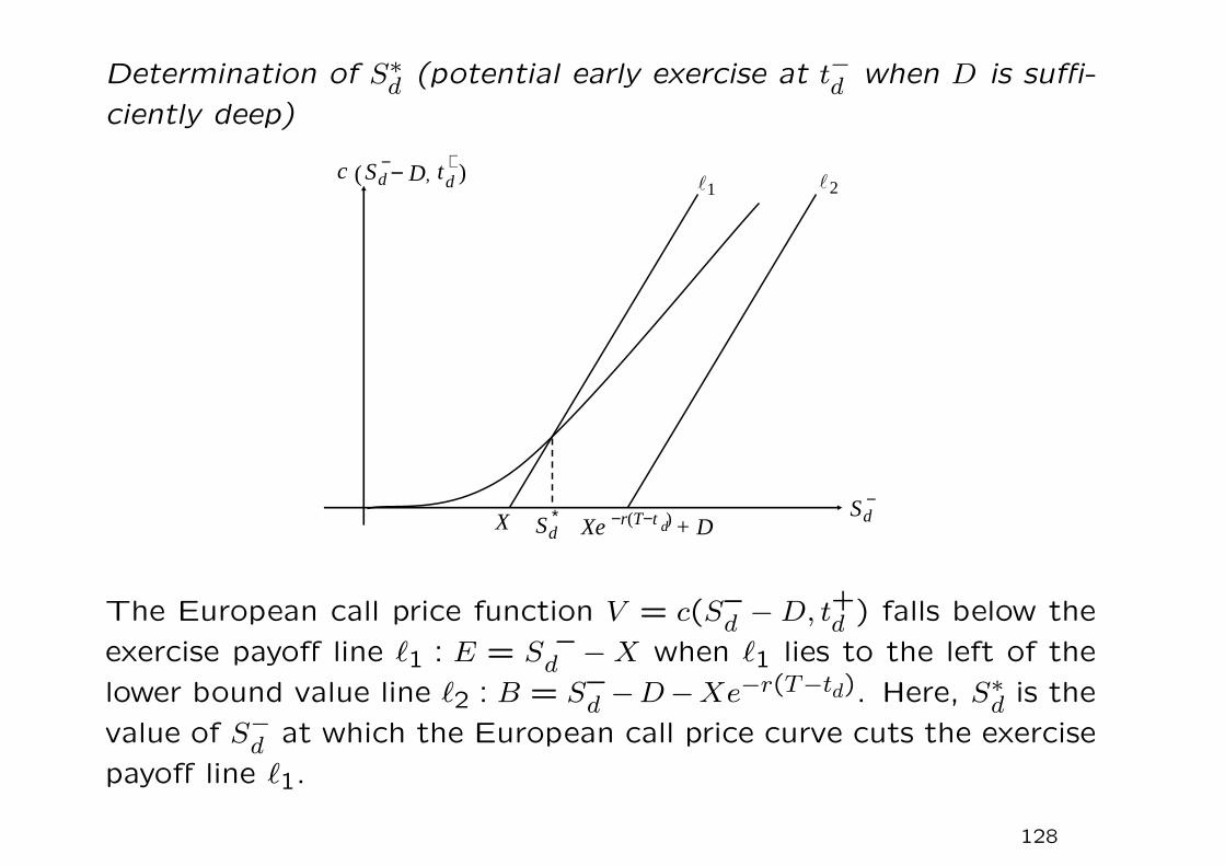
Determination of S∗d (potential early exercise at t−d when D is suffi-

ciently deep)

− D,(−d )+

dtSc

X

1l 2l

dS −

dS ∗ Xe + D−r(T−t )d

The European call price function V = c(S–d −D, t+d ) falls below the

exercise payoff line `1 : E = S –d −X when `1 lies to the left of the

lower bound value line `2 : B = S–d −D−Xe−r(T−td). Here, S∗d is the

value of S−d at which the European call price curve cuts the exercise

payoff line `1.

128

Summary of early exercise policies of American calls

• With no dividends, the decision of early exercise of an American

option (call or put) depends on the competition between the

time value of X and the loss of insurance value associated with

the holding of the option.

• Early exercise of non-dividend paying American call is non-optimal

since this leads to the loss of insurance value of the call plus the

loss of time value of X.

• For an American call on a discrete dividend paying asset, it may

become optimal to exercise at time right before the ex-dividend

time, provided that the dividend amount is sizable and the call

is sufficiently deep in-the-money. The critical asset price is a

decreasing function of the size of dividend. Early exercise at a

lower asset price level leads to a greater loss of insurance value

but the loss is offset by the more sizable dividend received.

129

Continuous dividend model

Under constant dividend yield q, the dividend amount received during

(t, t+dt) from holding one unit of asset is qSt dt. Also, e−q(T−t) unit

of the asset at time t will become one unit at time T through

accumulation of the dividends into purchase of the asset.

Why do we consider dividend yield model?

• It is considered as a continuous approximation to the discrete

dividends model. Otherwise, pricing under the discrete n-dividend

model requires the joint distribution of asset prices at all divi-

dend dates: Std1, Std2

, · · · , Stdn.

• The foreign money market account, which serves as the under-

lying asset in exchange options, earns the foreign interest rate

rf as dividend yield.

130

S X-

Se X-qt

- e-qt

c S, ; X, q( )t

S

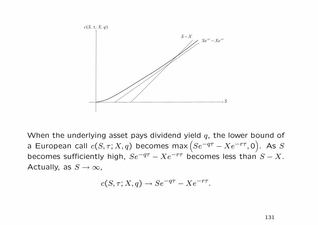
When the underlying asset pays dividend yield q, the lower bound of

a European call c(S, τ ;X, q) becomes max(Se−qτ −Xe−rτ ,0

). As S

becomes sufficiently high, Se−qτ −Xe−rτ becomes less than S −X.

Actually, as S →∞,

c(S, τ ;X, q) → Se−qτ −Xe−rτ .

131

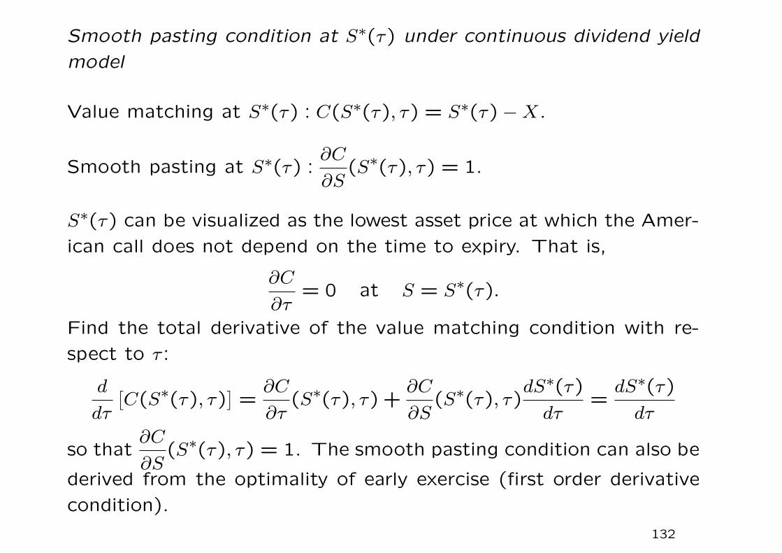
Smooth pasting condition at S∗(τ) under continuous dividend yield

model

Value matching at S∗(τ) : C(S∗(τ), τ) = S∗(τ)−X.

Smooth pasting at S∗(τ) :∂C

∂S(S∗(τ), τ) = 1.

S∗(τ) can be visualized as the lowest asset price at which the Amer-

ican call does not depend on the time to expiry. That is,

∂C

∂τ= 0 at S = S∗(τ).

Find the total derivative of the value matching condition with re-

spect to τ :

d

dτ

[C(S∗(τ), τ)

]=

∂C

∂τ(S∗(τ), τ) +

∂C

∂S(S∗(τ), τ)dS∗(τ)

dτ=

dS∗(τ)dτ

so that∂C

∂S(S∗(τ), τ) = 1. The smooth pasting condition can also be

derived from the optimality of early exercise (first order derivative

condition).

132

American call on a continuous dividend yield paying asset

The option price curve of a longer-lived American call will be above

that of its shorter-lived counterpart for all values of S. The upper

price curve cuts the intrinsic value tangentially at a higher critical

asset value S∗(τ). Hence, S∗(τ) for an American call is an increasing

function of τ .

133

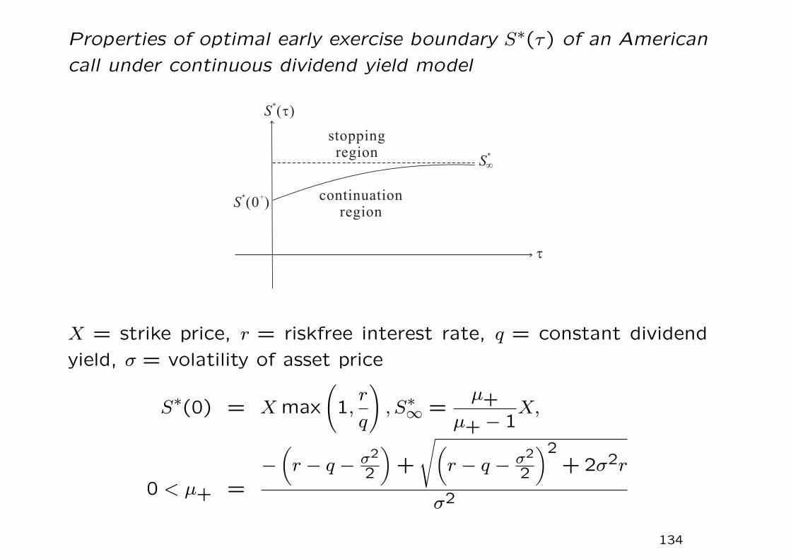
Properties of optimal early exercise boundary S∗(τ) of an American

call under continuous dividend yield model

X = strike price, r = riskfree interest rate, q = constant dividend

yield, σ = volatility of asset price

S∗(0) = X max

(1,

r

q

), S∗∞ =

µ+

µ+ − 1X,

0 < µ+ =−

(r − q − σ2

2

)+

√(r − q − σ2

2

)2+ 2σ2r

σ2

134

Stopping region = {(S, τ) : S ≥ S∗(τ)}, inside which the American

call should be optimally exercised. When S < S∗(τ), it is optimal

for the holder to continue holding the American call option.

1. S∗(τ) is monotonically increasing with respect to τ with

S∗(0+) = X max

(1,

r

q

)and S∗∞ =

µ+

µ+ − 1X. The determination

of S∗∞ requires a pricing model of the perpetual American call

option.

2. S∗(τ) is a continuous function of τ when the asset price process

is continuous.

3. S∗(τ) ≥ X for τ ≥ 0

Suppose S∗ < X, then the early exercise proceed S∗(τ) − X

becomes negative. This must be ruled out.

135

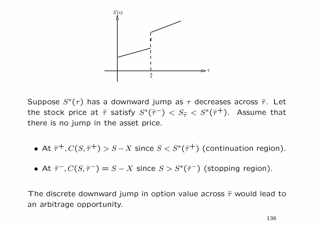
Suppose S∗(τ) has a downward jump as τ decreases across τ̃ . Let

the stock price at τ̃ satisfy S∗(τ̃−) < Sτ̃ < S∗(τ̃+). Assume that

there is no jump in the asset price.

• At τ̃+, C(S, τ̃+) > S−X since S < S∗(τ̃+) (continuation region).

• At τ̃−, C(S, τ̃−) = S −X since S > S∗(τ̃−) (stopping region).

The discrete downward jump in option value across τ̃ would lead to

an arbitrage opportunity.

136

Asymptotic behavior of S∗(0+) of an American call

At time close to expiry, the insurance value is negligible. It then

suffices to determine the optimal early exercise policy by considering

only the tradeoff between the gain in dividend and loss in the time

value of the strike price.

(i) q < r

The American call is kept alive when X < S <r

qX. This is

derived from the financial intuition that within a short time in-

terval δt prior to expiry, the dividend qSδt earned from holding

the asset is less than the interest rXδt earned from depositing

the amount X in a bank to earn interest at the rate r.

Hence, for q < r, limτ→0+

S∗(τ) =r

qX.

137

American call on non-dividend paying asset

In particular, when q = 0, S∗(τ) → ∞ as τ → 0+. Since S∗(τ) is

monotonically increasing with respect to τ , so

S∗(τ) →∞ for all values of τ.

This agrees with the earlier conclusion that it is always non-optimal

to exercise an American call prematurely when q = 0.

138

(ii) q ≥ r

In this case,r

qX becomes less than X. We argue that S(0+) ≤

X. Assume the contrary, suppose S∗(0+) > X so that the Amer-

ican call is still alive when X < S < S∗(0+) at time close to

expiry. Now, since q ≥ r and S > X, the loss in dividend amount

qSδt not earned is more than the interest amount rXδt earned.

This represents a non-optimal early exercise policy.

Together with the condition: S∗(0+) ≥ X, we must have

limτ→0+

S∗(τ) = X for q ≥ r.

139

In summary,

limτ→0+

S∗(τ) =

{ rqX q < r

X q ≥ r

= X max

(1,

r

q

).

• When q ≥ r, an American call which is optimally held to expira-

tion will have zero value at expiration.

• At expiry τ = 0, the American call option will be exercised

whenever S ≥ X and so S∗(0) = X. Hence, for q < r, there is a

jump of discontinuity of S∗(τ) at τ = 0.

140

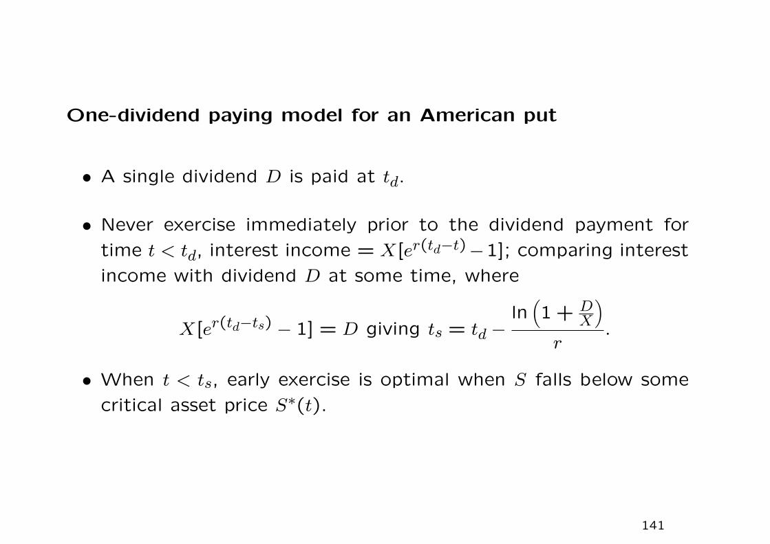
One-dividend paying model for an American put

• A single dividend D is paid at td.

• Never exercise immediately prior to the dividend payment for

time t < td, interest income = X[er(td−t)−1]; comparing interest

income with dividend D at some time, where

X[er(td−ts) − 1] = D giving ts = td −ln

(1 + D

X

)

r.

• When t < ts, early exercise is optimal when S falls below some

critical asset price S∗(t).

141

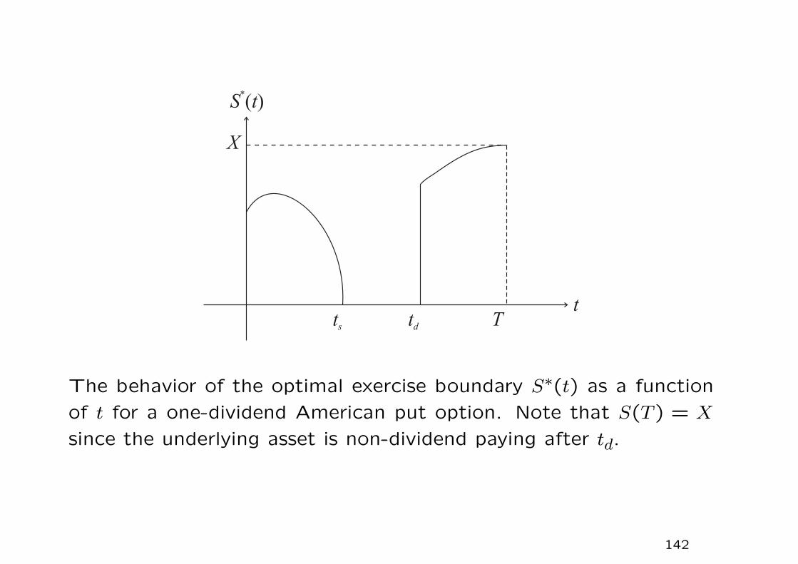
The behavior of the optimal exercise boundary S∗(t) as a function

of t for a one-dividend American put option. Note that S(T ) = X

since the underlying asset is non-dividend paying after td.

142

In summary, the optimal exercise boundary S∗(t) of the one-dividend

American put model exhibits the following behavior.

(i) When t < ts, S∗(t) first increases then decreases smoothly with

increasing t until it drops to the zero value at ts.

(ii) S∗(t) stays at the zero value in the interval [ts, td].

(iii) When t ∈ (td, T ], S∗(t) is a montonically increasing function of t

with S∗(T ) = X.

143

Here, td < t1 < t2 < T . The put price curve at time t1 intersects

the intrinsic value line tangentially at S∗(t1). We observe: S∗(t1) <

S∗(t1) < X.

144