Max Löffler, Sebastian Siegloch

8952 2021

March 2021

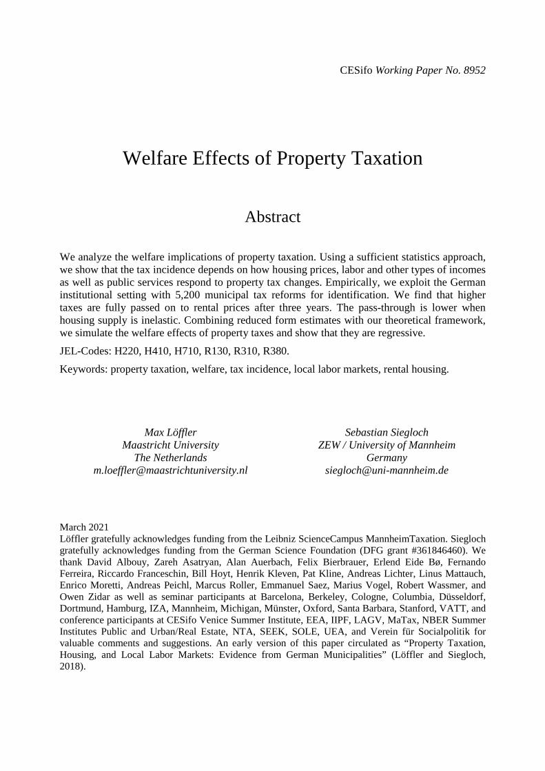
Welfare Effects of Property Taxation Max Löffler, Sebastian Siegloch

Impressum:

CESifo Working Papers ISSN 2364-1428 (electronic version) Publisher and distributor: Munich Society for the Promotion of Economic Research - CESifo GmbH The international platform of Ludwigs-Maximilians University’s Center for Economic Studies and the ifo Institute Poschingerstr. 5, 81679 Munich, Germany Telephone +49 (0)89 2180-2740, Telefax +49 (0)89 2180-17845, email [email protected] Editor: Clemens Fuest https://www.cesifo.org/en/wp An electronic version of the paper may be downloaded · from the SSRN website: www.SSRN.com · from the RePEc website: www.RePEc.org · from the CESifo website: https://www.cesifo.org/en/wp

mailto:[email protected]

https://www.cesifo.org/en/wp

http://www.ssrn.com/

http://www.repec.org/

https://www.cesifo.org/en/wp

CESifo Working Paper No. 8952

Welfare Effects of Property Taxation

Abstract We analyze the welfare implications of property taxation. Using a sufficient statistics approach, we show that the tax incidence depends on how housing prices, labor and other types of incomes as well as public services respond to property tax changes. Empirically, we exploit the German institutional setting with 5,200 municipal tax reforms for identification. We find that higher taxes are fully passed on to rental prices after three years. The pass-through is lower when housing supply is inelastic. Combining reduced form estimates with our theoretical framework, we simulate the welfare effects of property taxes and show that they are regressive.

JEL-Codes: H220, H410, H710, R130, R310, R380.

Keywords: property taxation, welfare, tax incidence, local labor markets, rental housing.

Max Löffler

Maastricht University The Netherlands

[email protected]

Sebastian Siegloch ZEW / University of Mannheim

Germany [email protected]

March 2021 Löffler gratefully acknowledges funding from the Leibniz ScienceCampus MannheimTaxation. Siegloch gratefully acknowledges funding from the German Science Foundation (DFG grant #361846460). We thank David Albouy, Zareh Asatryan, Alan Auerbach, Felix Bierbrauer, Erlend Eide Bø, Fernando Ferreira, Riccardo Franceschin, Bill Hoyt, Henrik Kleven, Pat Kline, Andreas Lichter, Linus Mattauch, Enrico Moretti, Andreas Peichl, Marcus Roller, Emmanuel Saez, Marius Vogel, Robert Wassmer, and Owen Zidar as well as seminar participants at Barcelona, Berkeley, Cologne, Columbia, Düsseldorf, Dortmund, Hamburg, IZA, Mannheim, Michigan, Münster, Oxford, Santa Barbara, Stanford, VATT, and conference participants at CESifo Venice Summer Institute, EEA, IIPF, LAGV, MaTax, NBER Summer Institutes Public and Urban/Real Estate, NTA, SEEK, SOLE, UEA, and Verein für Socialpolitik for valuable comments and suggestions. An early version of this paper circulated as “Property Taxation, Housing, and Local Labor Markets: Evidence from German Municipalities” (Löffler and Siegloch, 2018).

1 Introduction

Property taxes account for about one third of total capital tax revenues in the United Statesand the European Union (Zucman, 2015). Despite over a century of economic research, ourunderstanding of the effects of property taxes is still in a “sad state” (Oates and Fischel,2016, p. 415). This assessment seems particularly true when it comes to the welfare effectsof property taxation. Theoretically, two competing views on the incidence of the propertytax—the new view vs. the benefit view—offer very different answers to the question of whobears the burden of property taxes. Empirically, institutional settings and data availability makeidentification challenging: long (and wide) panels of local property tax rates and housing priceshave been relatively scarce, clean policy variation is hard to isolate with frequent, non-randomre-assessments of property values, and property taxes and expenditures on important localpublic goods and services oftentimes move simultaneously.

We add to the understanding of the incidence1 of property taxes by exploiting the institutionalsetting in Germany, where municipalities adjust tax rates, while tax bases remain fixed andproperty tax revenues are of secondary importance for local public services. Leveraging microdata on offered rents and house prices we derive clean estimates on the direct effect of propertytaxes on the price of housing. We feed these quasi-experimental estimates into a novel sufficientstatistic representation of commonly used spatial equilibrium models to calculate the welfareeffects of property taxes across the distribution.

The paper consists of three parts. In the first, theoretical part, we suggest a sufficient statisticsapproach to analyze the incidence of the property tax. Starting from a simple and generalutility function, where a household can be (a combination of) a renter, landlord, and firm owner,we rely on standard envelope conditions and Roy’s identity to show that marginal utility effectsof a change in property taxes depend on three factors: the pass-through of the tax on the priceof housing, the effect of higher taxes on local public goods, and general equilibrium effectson other markets.2 Which other markets are affect depends on how the model is specified.We demonstrate the sufficient statistics properties of our framework by connecting it to therecent literature specifying structural spatial equilibrium models in labor, public, and urbaneconomics (Kline, 2010, Moretti, 2011, Ahlfeldt et al., 2015, Suárez Serrato and Zidar, 2016).In this class of models, the sufficient statistics formula of the welfare effect of property taxestypically also depends on the general equilibrium effects on local labor markets as captured bywages and firm profits.

In the second, empirical part, we use the German institutional set-up as a laboratory toestimate the relevant elasticities that determine the incidence of the property tax. Germanmunicipalities may autonomously adjust local property tax rates (Grundsteuer) via municipality-specific scaling factors to a federal tax rate. Each year, more than ten percent of the 8,481 WestGerman municipality change their local property tax rate, resulting in a large amount of tax

1 Throughout the paper, we use the term incidence to describe the welfare effects of property taxation. We refer toprice effects as pass-through. In a simple model, pass-through and incidence can be identical.

2 For the empirical implementation, we use the term public goods in a broad sense, referring to all expenditureson publicly provided goods and services independent of whether they are non-excludable and/or non-rival.

2

reforms that we can exploit for identification. Important for identification, this is the onlychannel through which municipalities can influence the tax burden. Assessed property valuesremain fixed over time; new buildings are assessed by authorities at the (higher) state levelbased on historical price indices. All other rules determining the tax base are set at the federallevel. We demonstrate that property tax changes are not systematically driven by housingmarket shocks or local business cycles. Instead, municipalities increase taxes to consolidate thefiscal balance. While revenues increase after a tax reform, there is little significant effect onlocal public expenditures as municipalities improve their fiscal balance.

We combine administrative data on the universe of municipalities and their local propertytax rates with detailed microdata on rental prices from ImmobilienScout24 (the German Zillow)between 2007 and 2020 and various other commercial and administrative data sources onhousing and labor markets. We implement a series of event studies exploiting the within-municipality variation in tax rates over time to estimate reduced form effects of property taxeson housing and labor prices as well as municipal expenditures as a proxy for responses of localpublic goods. The event study designs enable us to assess the dynamics of the treatment effects.In addition, we can test the exogeneity of tax reforms by investigating pre-reform trends. Inthe absence of a pre-trend, the identifying assumption is that there is no systematic regionalfactor driving both municipal property tax rates and outcome variables. We explicitly testthis assumption. In our baseline, we account for annual shocks at the level of the commutingzone (CZ). We assess the sensitivity of our estimates by controlling for local shocks at less(e.g., state) or more detailed (e.g., county) levels of aggregation and confirm that our estimatesare robust as soon as we account for local shocks at a sufficiently low geographical level.Moreover, we show that estimates are very stable when including (lagged) local business cyclevariables (GDP, unemployment, population) as controls. Based on these findings, we calculatebounds in the spirit of Oster (2019) and show that unobservables are unlikely to render ourestimates insignificant. Last, we use a peculiarity arising from the fiscal equalization schemesimplemented at each respective German federal state to set up an instrumental variablesapproach, which again yields similar findings.

Our reduced form results are as follows: We show that gross rents increase moderately in theshort run implying that part of the tax burden is on the landlord. In the medium run, startingthree years after a tax hike, gross rents further increase to a level implying a full pass-throughof the property tax on gross rents. We test for various heterogeneous effects, finding that thepass-through is higher in municipalities that have (i) a lower share of developed land, (ii) alower share of physically undevelopable land, (iii) smaller population levels, (iv) a highershare of private (rather than public) housing. In line with Saiz (2010), these findings point atdifferences in housing supply elasticities driving the results, as supply should be less elastic indensely populated areas with a higher share of land unusable for additional construction. Wefurther show that neither local wages nor firm profits are affected by property tax increases.Municipal expenditures do not increase following a tax increase—if anything there is a slightdecrease.

In the third part of the paper, we combine the theoretical framework with the empirical

3

reduced form findings to assess the welfare effects of property taxation. The sufficient statisticsapproach allows us to go beyond representative agent representations to calculate the relativeburden of the tax increase. We can implement the predicted welfare effects at the householdlevel directly using rich distributional household-level data from the German Income andExpenditure Survey. This approach enables us to not only provide average statements on theincidence of property taxes but to study the welfare effects over the full distribution of Germanhouseholds.

We find that property taxes are regressive. Utility losses due to a one percentage pointincrease in the property tax are relatively larger for households at the bottom of the distributionand increase inequality in consumption. Households from the first decile have relative utilitylosses of around 1.1 percent, while households in the top decile lose only around 0.3 percent.This pattern already emerges when using only the partial-equilibrium textbook model of taxincidence that abstracts from general equilibrium effects on wages, business incomes or publicgoods. The full general equilibrium model leads to similar welfare losses at the ends of thedistribution but smaller negative effects in the middle. Running counterfactual simulations weshow that property taxes could be progressive, i.e., the utility loss would increase in householdconsumption, if there was zero pass-through from landlords to renters.

Related Literature. Our paper speaks to various strands of the literature. Empirically, weprovide reduced form evidence on the effects of property taxes on housing prices usingadministrative tax data from German municipalities and microdata on housing prices. Wethereby add to the existing empirical literature on the pass-through of the property tax on rents,which has predominantly focused on the United States. The previous literature has offered awide range of estimates for the pass-through of property taxes on rents: Orr (1968, 1970, 1972),Heinberg and Oates (1970), Hyman and Pasour (1973), Dusansky et al. (1981), and Carrolland Yinger (1994) estimate that between 0–115 percent of the tax is shifted onto renters. Ourresults also show the dynamics of the property tax incidence in the short and medium run,which is particularly important for housing markets (England, 2016). We find that propertytax increases lead to lower house prices, which is evidence of capitalization into house values(Palmon and Smith, 1998, de Bartolomé and Rosenthal, 1999). Last, the observed decrease inbuilding permits offers evidence that property tax increases reduce housing investments, aneffect also demonstrated by Lyytikäinen (2009) for Finland and Lutz (2015) for the state of NewHampshire in the U.S.

Theoretically, we provide a new perspective on the incidence of property taxation by lookingthrough the lens of a local labor market model. These models, which have become the“workhorse of the urban growth literature” (Glaeser, 2009, p. 25), extend the Rosen-Robackmodel (Rosen, 1979, Roback, 1982) to account for location-specific preferences of workersand differential productivity of firms, relaxing the perfect mobility assumption in traditionalmodels (Moretti, 2011, Kline and Moretti, 2014, Suárez Serrato and Zidar, 2016, Fajgelbaumet al., 2019). We add to the literature by introducing a sufficient statistics approach (Chetty,2009, Kleven, 2021) and pointing out the empirical responses that are necessary to quantify the

4

incidence of property taxation. Within this framework, it is easy to increase the complexityof the underlying model from a partial textbook incidence model to a full-fledged spatialequilibrium model with location-specific preferences of mobile workers with a general utilityfunction (Albouy and Stuart, 2020), location-specific productivity of mobile firms that aresubject to the property tax, a construction sector (Ahlfeldt et al., 2015), absent or non-absentlandlords as well as endogenous fiscal and non-fiscal amenities (Diamond, 2016, Brülhart et al.,2021).

Our results inform the long-standing debate of the capital tax (or new) view vs. benefitview. The capital tax view adopts a general equilibrium perspective in closed economy andargues that the national average burden of the property tax is borne by capital owners, i.e.,typically richer landlords (Mieszkowski, 1972, Mieszkowski and Zodrow, 1989). Hence, the taxis progressive. We deviate from the assumption of a fixed capital stock in the economy andassume global capital markets and perfect mobility of capital such that higher property taxesmay reduce the overall housing capital stock in the society, a channel that has been neglectedin the previous literature (Oates and Fischel, 2016). The benefit view builds on a Tiebout (1956)model with perfect zoning and mobile individuals, who choose among municipalities offeringdifferent combinations of tax rates and local public goods (Hamilton, 1975, 1976). The tax isequivalent to a user fee for local public services. We add three results to the debate. First, anincrease in property taxes decreases utility across the income distribution. Second, a very highpreference for local public good would be needed to turn results welfare-neutral. Third, theproperty tax is regressive, i.e., the utility losses are higher for poorer households rather thanricher landlords.

Finally, we touch upon a literature that studies the value and optimal provision of local publicgoods (Samuelson, 1954). In the United States, the most important type of local public goodsfinanced through property taxes is public schooling and there is a large literature studyingthe valuation of housing amenities—most often local school quality (see, e.g., Bradbury et al.,2001, Bayer et al., 2007, Cellini et al., 2010, Ferreira, 2010, Boustan, 2013). Brülhart et al. (2021)study the case of Switzerland, where local (income) tax revenues are mostly spent on schoolsas well. Schönholzer and Zhang (2017) show that residents also value other types of localamenities, most notably public security. In Germany, both schools and police are financedat the state level. While German municipalities do spend part of their property tax revenueswithin their local jurisdictions, we exploit a setting where the public good channel is arguablyless important relative to the effects on local housing and labor markets.

The remainder of this paper is organized as follows. In Section 2 we set up the theoreticalframework. Section 3 provides the institutional background of property taxation in Germanyand information on the used data. We set up our empirical model in Section 4 and presentreduced-form results in Section 5. Section 6 discusses the welfare effects of the tax. Section 7concludes.

5

2 Modeling the Welfare Effects of Property Taxation

In this section, we propose a general framework to quantify the welfare effects of propertytaxes. In Section 2.1, we describe our framework to characterize the household-level welfarecosts of local property tax increases. In Section 2.2, we explain in detail the links to otherapproaches in the literature, notably the large literature on spatial equilibrium models (Eppleand Sieg, 1999, Kline, 2010, Moretti, 2011, Ahlfeldt et al., 2015, Suárez Serrato and Zidar, 2016).

2.1 Household Welfare in Spatial Equilibrium Models

The economy consists of a continuum of households i ∈ H who choose to live in one out ofmany small cities across the country (indexed by c). Cities differ in size, productivity, and localamenities gc, which includes both geographical amenities such as sunshine hours and localpublic goods like safety, parks or infrastructure. Municipalities levy a property tax tc on realestate and land, and use (parts of) the revenues for public good provision. Cities vary in thepre-tax price of housing per square meter rc (producer price) and thus also in the tax-inclusiveconsumer price denoted by rC

c .We assume that households derive utility from local amenities gc, housing consumption hi,

and composite good consumption xi. Households have different preferences ui(hi, xi, gc) andcharacteristics, including occupation, disposable income yi, and also household composition.The budget constraint is given by rC

c hi + xi = yi, with the price of the composite good beingnormalized to one. Households maximize utility and we denote household i’s indirect utilityfunction by vi(rC

c , yi, gc). Assuming that the economy is in equilibrium (with the correspondingequilibrium prices and quantities indicated by superscript stars) we derive the following result:

Proposition 1 (Household Welfare). The money-metric effect of a small increase in city c’s propertytax tc on household i’s utility is given by:

drC∗ dy∗ dg∗ ∂v /∂g∆Wi = −h∗ c i g c g i

i + + δ δ =dtc dt i with i . (1)

c dtc ∂vi/∂y

This proposition follows directly from the envelope theorem and Roy’s identity (see Ap-pendix C.1 for a formal derivation). The welfare consequences of a small tax increase forhousehold i are governed by three effects: (i) the pass-through of tax increases on gross-of-taxhousing expenditures, (ii) the impact on household income, and (iii) the change in local publicgood provision. The latter effect is weighted according to household i’s relative preference forpublic vs. private goods. Importantly, following from the standard envelope condition, changesin behavior have no first-order consequences for utility as long as tax reforms are small.

The outlined framework provides a direct mapping between theory and empirical appli-cations while imposing minimal structure on the economy. Proposition 1 characterizes thewelfare implications of property tax increases in terms of estimable sufficient statistics (Chetty,2009, Kleven, 2021), namely the reduced-form effects of property taxes on equilibrium rents,incomes, and local public good provision. In Section 5, we estimate the effects of property taxchanges, exploiting the institutional setting in Germany with numerous small tax reforms at

6

the local level. We connect theory and empirics to simulate the welfare effects of tax increasesat the household level in Section 6.

Partial Equilibrium Model. The result in Proposition 1 nests the standard textbook modelof tax incidence in a partial equilibrium setting. To see this, consider a world with only twohouseholds R and L, and abstract from public goods. Household R has fixed income andconsumes housing h at price rC

c . Household L lives abroad and receives rental income yL = rchfrom renting out real estate to R. The loss in household R’s utility after introducing propertytaxes tc increases (i) in the amount of floor space rented and (ii) the pass-through of taxes onconsumer price rents. Similarly, landlord L’s welfare loss depends on (i) the amount of floorspace rented out and (ii) the pass-through of taxes on net rents, i.e., producer prices. Withquasi-linear preferences in consumption, these welfare effects are equivalent to changes inconsumer and producer surplus, respectively.

Local Public Goods. We extend the partial model by incorporating a key mechanism of thebenefit view of property taxation, where taxes act like user fees for local public services (Hamilton,1976). A standard partial-equilibrium analysis would neglect the fact that municipalities aroundthe world use property taxes to finance local public goods. The welfare consequences ofproperty tax reforms thus crucially depend on the use of the tax revenues. This idea is reflectedin the third part on the right-hand side of the equation in Proposition 1: if tax increases translateinto higher levels of local public good provision (dg∗c /dtc > 0), households are compensatedfor higher costs-of-living (in proportion to their relative preferences for public goods, g

δi ). Ifrent increases and public good provision exactly offset each other, property taxes will have noimpact on household welfare. Households could then move across municipalities to find theirpreferred mix of taxes and amenities (Tiebout, 1956).

General Equilibrium Effects. The proposed framework further differs from the textbook modelby incorporating potential interactions with other markets. A classic example highlighted inthe capital tax view of property taxation are general-equilibrium effects on the capital market(Mieszkowski, 1972). With property taxes reducing the after-tax yield on capital in the housingmarket, capital owners are expected to shift their investment to other, more profitable uses.This shift away from the housing sector reduces the demand for construction services and landfor building, potentially hurting workers and owners of construction companies as well asland owners. Higher costs for commercial real estate also create an incentive for local firmsto substitute towards other production factors. Under certain conditions (e.g., a fixed capitalsupply in the economy), property tax increases may also reduce the overall return on capital andthus capital incomes. Such equilibrium effects on different markets would trigger additionalwelfare effects that need to be taken into account. We subsume these general-equilibriumeffects in the proposition above via their impact on household income (dy∗i /dtc). Importantly,these effects are likely heterogeneous among the population as some households suffer whileothers gain depending on household characteristics and the nature of these spillovers.

7

Mobility Across Space. The third departure from the standard tax incidence model lies in thespatial dimension—studying mobile agents locating in one out of many small cities—which isvery similar to the local labor market and spatial equilibrium literature (see, e.g., Redding andRossi-Hansberg, 2017, for a survey). Assuming that households, firms, and capital are mobileacross space gives rise to further equilibrium responses and capitalization effects in local pricesand incomes. One prime example for such a spatial equilibrium mechanism is the assumptionof labor mobility (Brueckner, 1981). If workers can avoid a city’s rising property tax by movingto another place, local firms will have to pay a compensating differential for workers to stay inthe city (in a model without commuting, dy∗i /dtc > 0). The capitalization of tax increases inlocal equilibrium prices and incomes will then depend strongly on the degree of mobility ofthe different agents in the economy. Proposition 1 reflects the welfare impact of these variousmechanisms in the reduced-form effects on rents drC∗

c /dtc and incomes dy∗i /dtc.

2.2 Relation to Standard Spatial Equilibrium Models

The outlined framework characterizes the welfare effects of property tax changes using anumber of reduced-form effects as sufficient statistics. We argue that the proposed approachmakes four contributions. First, the framework introduced above is very general. Structuralapproaches have been criticized for, e.g., relying heavily on Cobb-Douglas utility functions orspecific distributions of taste parameters (Proost and Thisse, 2019, Albouy and Stuart, 2020).The sufficient statistics approach allows to abstract from specific functional forms of householdutility, firm production, and construction activity. We only assume differentiability, separability,and positive and decreasing marginal utilities.

Second, the generalized approach allows for an arbitrary level of heterogeneity in householdcharacteristics, choices, and preferences, which have been assumed homogeneous in manyprevious applications. For example, households may combine different occupations and receiveincome from various sources at the same time in our framework, whereas workers, firm owners,and landlords have been modeled as distinct representative agents before. We also abstainfrom the usual requirement that firm owners and landlords are absent from the city.

Third, we provide a micro-founded derivation of welfare effects that can be quantified atthe household level or aggregated using social marginal welfare weights (Saez and Stantcheva,2016). The theoretical framework can be applied to conduct straightforward counterfactualsimulations of welfare effects using household microdata (see Section 6). The previous literaturehad to rely on more restrictive formulations and stylized welfare evaluations given the limiteddegree of heterogeneity in order to keep the model analytically tractable.

Fourth, sufficient statistics approaches are very convenient when being used in a setting withclean quasi-experimental variation that enables researchers to estimate causal reduced-formeffects of a policy change (Chetty, 2009, Kleven, 2021). In the context of this study, the reduced-form estimates can be directly plugged into Proposition 1 to calculate the welfare effects with aminimal model structure.

8

A Structural Representation. The drawback of sufficient statistics approaches is that it is notpossible to quantify equilibrium prices and quantities, and analyze the mechanisms behind thewelfare effects by studying comparative statics (Chetty, 2009). For these exercises, we need astructural representation of the underlying model and corresponding additional assumptions.In Appendix A, we recast our model economy in a fully specified structural framework (seeAppendices A.1–A.3). We build on Suárez Serrato and Zidar (2016), whose model includesmobile workers and firms with idiosyncratic location preferences and location-firm specificproductivity shifters, respectively; firms operate under monopolistic competition and havenon-zero profits. We augment this model in two dimensions. First, we add a constructionsector as in Ahlfeldt et al. (2015) to model the supply of real estate in more detail. Second,we endogenize the public good provision by modeling local governments which use propertytax revenues to fund local public goods (similar to Fajgelbaum et al., 2019). We solve thismodel analytically and derive theoretical predictions on the welfare effects for the differentrepresentative agents, i.e., workers, firm owners, and landlords. By virtue of the sufficientstatistics, the structural welfare predictions correspond closely to the results of Proposition 1(see Appendix A.4 for a detailed comparison).

Comparative Statics. Looking at the model mechanisms, we provide an intuition on thesign and size of the reduced-form effects in Proposition 1 using the structural representation(see Appendix A.5 for a thorough discussion). The impact of tax increases on gross housingcosts per m2 (drC∗

c /dtc) can be decomposed in two effects: (i) the direct effect measuring thepass-through that depends on the housing supply and demand elasticities as in the textbookincidence model, and (ii) an indirect effect operating through the transmission of tax revenuesinto local public good provision and the capitalization of public goods in local rents. The moremobile households are and the more elastic housing demand, the lower the direct pass-throughof tax increases in consumer prices, and the stronger the reduction in net rents. The indirecteffect counteracts the decrease in housing demand triggered by the tax increase, therebyalleviating the reduction in net-of-tax rents.

We model income from three sources in the Appendix (cf. dy∗i /dtc in Proposition 1). First,landlord income changes proportionally to the change in producer prices, i.e., net rents.Decreasing net rents thus translates into lower profits for landlords. Second, we model theeffect on workers’ wage earnings, which is theoretically ambiguous and depends on the degreeto which firms (i) have to compensate workers to keep them in the city and (ii) reduce theirlabor demand in response to rising input factor costs. Third, the impact on firms’ profitsultimately also depends on whether labor demand or supply are more elastic.

3 Institutions and Data

We rely on the institutional setting of local property taxation in Germany to identify thesufficient statistics needed to quantify the household level welfare effects. Section 3.1 describesthe relevant features of property taxation in Germany. Section 3.2 gives an overview on the

9

data used in our empirical analysis.

3.1 Property Taxation in Germany

The German property tax (Grundsteuer B) is a one-rate tax that applies to the land and builtstructures. Residential and commercial properties are both subject to the same property taxregulations. The tax rate is levied by the municipality and local property tax revenues areone of the most important revenue sources for German municipalities, amounting to a total of12 billion EUR for all municipalities in 2013. Importantly, the only thing municipalities canadjust is the local tax rate. All other legal regulations of the property tax, i.e., the definition ofthe tax base, as well as legal norms regarding the property assessment, are set at the federallevel and have been unchanged for decades.3

The property tax liability is calculated according to the following formula:

Tax Liability = Assessed Value× Federal Tax Rate×Municipal Scaling Factor . (2)︸︷︷︸Local Property Tax Rate

We discuss the different elements of the formula below.

Assessed Values. The property value (Einheitswert) is assessed by the state tax offices (notby the municipality) when the property is built and, importantly, remains fixed over time.The last general assessment of property values in Germany took place in 1964. In order tomake the assessment comparable for new buildings, property valuation is based on pricesas of 1964 using historical rent indices. There is no regular reassessment of properties to adjustthe assessed value to current market values or inflation. Neither are assessed values updatedwhen the property is sold. Reassessments only occur if the owner creates a new buildingor substantially improves an existing structure on her land.4 As a consequence, assessedvalues differ from current market values. The average assessed value for West German homeswas 39,136 EUR in 2013, roughly a fifth of the reported current market value (EVS, 2013).Assessment notices do not provide any detail on how specific parts of the building contributeto the assessed value. This practice makes the assessment barely transparent for house owners,landowners, and renters. There is also no deduction for mortgage payments or debt services inthe German property tax.

Federal Tax Rates. The federal tax rate (Grundsteuermesszahl) is set at 0.35 percent for allproperty types in West Germany with only two exceptions. First, the federal tax rate forsingle-family homes is 0.26 percent up to the value of 38,347 EUR; and 0.35 percent for everyeuro the assessed value exceeds this threshold. Second, the federal tax rate for two-familyhouses is 0.31 percent.

3 See Spahn (2004) for a more detailed discussion. All legal regulations can be found in the Grundsteuergesetz.4 The improvement has to concern the “hardware” of the property, such as adding a floor. Maintaining the roof or

installing a new kitchen does not lead to a reassessment. Lock-in effects or assessment limits are thus not anissue in the German context other than in some U.S. states (see, e.g., Ferreira, 2010, Bradley, 2017).

10

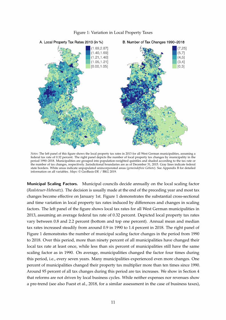
https://www.gesetze-im-internet.de/grstg_1973/index.html

Figure 1: Variation in Local Property Taxes

Notes: The left panel of this figure shows the local property tax rates in 2013 for all West German municipalities, assuming afederal tax rate of 0.32 percent. The right panel depicts the number of local property tax changes by municipality in theperiod 1990–2018. Municipalities are grouped into population-weighted quintiles and shaded according to the tax rate orthe number of tax changes, respectively. Jurisdictional boundaries are as of December 31, 2015. Gray lines indicate federalstate borders. White areas indicate unpopulated unincorporated areas (gemeindefreie Gebiete). See Appendix B for detailedinformation on all variables. Maps: © GeoBasis-DE / BKG 2019.

Municipal Scaling Factors. Municipal councils decide annually on the local scaling factor(Realsteuer-Hebesatz). The decision is usually made at the end of the preceding year and most taxchanges become effective on January 1st. Figure 1 demonstrates the substantial cross-sectionaland time variation in local property tax rates induced by differences and changes in scalingfactors. The left panel of the figure shows local tax rates for all West German municipalities in2013, assuming an average federal tax rate of 0.32 percent. Depicted local property tax ratesvary between 0.8 and 2.2 percent (bottom and top one percent). Annual mean and mediantax rates increased steadily from around 0.9 in 1990 to 1.4 percent in 2018. The right panel ofFigure 1 demonstrates the number of municipal scaling factor changes in the period from 1990to 2018. Over this period, more than ninety percent of all municipalities have changed theirlocal tax rate at least once, while less than six percent of municipalities still have the samescaling factor as in 1990. On average, municipalities changed the factor four times duringthis period, i.e., every seven years. Many municipalities experienced even more changes. Onepercent of municipalities changed their property tax multiplier more than ten times since 1990.Around 95 percent of all tax changes during this period are tax increases. We show in Section 4that reforms are not driven by local business cycles. While neither expenses nor revenues showa pre-trend (see also Fuest et al., 2018, for a similar assessment in the case of business taxes),

11

we show below that municipalities use the reform to reshuffle the structure of their finances,even decreasing expenditures in the short run (up to three years after the reform).

Statutory Incidence and Ancillary Costs. The statutory incidence of the property tax ison the property owner, i.e., the landlord. However, a salient legal regulations on operatingcosts (Betriebskostenverordnung) stipulates that property taxes for rental housing are part of theancillary costs that renters have to pay to their landlords on top of net rents. By this regulation,landlords are directed to include the tax payments in the ancillary bill that renters receive atthe end of each year. Other typical ancillary costs are fees for garbage collection, water supply,or janitor and cleaning services.

Municipal Revenues and Local Public Goods. Property (and business) tax revenues are animportant source of revenue for German municipalities because they are the only instrumentsat the disposal of municipalities to raise tax revenues. In 2013, the average (median) annualrevenues of municipalities was 2,691 (2,353) euro per capita. 28% of the revenues are comingfrom local business and property taxes that are directly controlled by the municipalities. Percapita property tax revenues average to 155 euro (21% of local taxes).5 Compared to theU.S., revenues raised at the state and local level are much lower in Germany. According tothe U.S. Census Bureau, state and local revenue per capita amounted to 7,000 dollars percapita—with 5,000 dollars p.c. coming from taxes and about 17% thereof from property taxes.

The lower amount of municipal revenues are reflected on the expenditure side. In Germany,local jurisdictions are much less important when it comes to public services. Unlike in the U.S.,important types of public goods such as schooling, police, or high and freeways are financed atthe level of the states or the federal level. About 80% of the expenditures are spent on keepingup the usual administrative duties, that is to pay municipal employees, maintain the existingbuildings, co-finance public firms (waste, energy, and public transport) and cover housing costsof welfare recipients as mandated by federal law. About 15% of the expenditures are used forinvestment projects, rebuilding the city hall, replacing street lamps or extending parks.

Given that (i) local property taxes make up only 5% of total municipal revenues, (ii) publicgoods provided by the municipality are of second order compared to the U.S., and (iii) only asmall share of municipal expenditures will affect the stock of local public goods, we conjecturethat the local public good channel is of secondary importance in the context of Germany. Weconfirm this empirically, both in terms of reduced form evidence (Section 5) and when usingour theoretical model to run counterfactual simulations (Section 6).

3.2 Data and Descriptive Statistics

We combine housing market microdata with administrative data on the fiscal and economicsituation of German municipalities, and administrative wage and employment data fromsocial security registers. Based on these sources, we construct an annual panel data set for

5 Other important revenues come from federal level taxes. Municipalities receive a share of the personal incometax revenues and the value added tax revenues, based on the number of tax payers.

12

the universe of all 8,423 West German municipalities spanning the years from 2007 to 2018.6

This section gives an overview on the data used for our empirical analysis and the estimationsample. Appendix B provides more details on the definition and the sources of all variables.

Housing Market Microdata. Our main data source is a microdata set with real-estate ad-vertisements covering apartments and houses offered for rent and for sale on the platformImmobilienScout24 (the German Zillow). This website is by far the largest online real estateplatform in Germany. The data includes real-estate advertisements from 2007 until 2020,yielding on average more than three million ads per year. The data is provided by the researchdata center FDZ Ruhr at RWI (Boelmann and Schaffner, 2019).

The most important information we extract from this data set is the consumer price ofhousing. As common for data from internet platforms prices are offered and not transactionprices. Our main variable is the gross-of-tax rent per square meter, which includes property taxpayments and all other ancillary costs (Bruttowarmmiete).7 Besides prices, the dataset contains avast set of characteristics such as the living space, the number of rooms, the quality, and theconstruction year. In order to generate a comparable measure of rental and sales prices persquare meter, we focus on apartments with a living space between 40 and 100 square metersand houses with a living space of 100 to 200 square meters, roughly dropping properties belowthe 10th and above 90th percentiles for both dwelling types. Moreover, we drop propertieswith unrealistic prices per square meter (bottom and top 0.5 percent) and unrealistic reportedancillary cost to net rent ratio. Last, the data contains information on the location of theadvertised object including municipality identifiers. This regional information allows us to linkads to the corresponding municipalities, the respective property tax rates, and various otherfiscal and economic indicators.

German Municipality Data. We compile a comprehensive municipality-year panel usingdata from various administrative sources. The largest part of this municipality-level datais provided by Federal Statistical Office and the Statistical Offices of the Länder. The mostimportant variable in the context of this study are municipal property tax rates since the 1990s.In addition, we make use of additional economic and fiscal indicators. We use municipalbudgets to back out business profits at the level of the municipality. Furthermore, our datainclude municipal annual expenditures as a proxy for local public goods. We also observeannual population figures, land use within the municipality, and statistics about the owners ofthe local housing stock (cross-sectional data on types of landlords).

Besides data from the Statistical Offices, we compile data on the local number of individualsregistered as unemployed as well as county-level GDP to proxy and control for fluctuations

6 We exclude East Germany from our analysis for two reasons. First, there has been a substantial amount ofmunicipal mergers within East Germany from the mid-1990s until the late 2000s, which induces measurementerror in the main regressors (Fuest et al., 2018). Second, the federal tax rate in East Germany is different fromWest Germany (cf. Section 3). This implies that the same increase in the local scaling factor would lead todifferent increases in the total property tax rate in East and West Germany. However, we also test the sensitivityof our results to this exclusion and find that results are similar when including East Germany (see Section 5.4).

7 We also study offered sales prices as an outcome, but clearly transacted and offered price should differ morewhen it comes to real-estate sales, so our main focus will be on rental housing.

13

in the local business cycle. We make use of social security data provided by Institute forEmployment Research (IAB) on municipal-level average wages. Annual wages are based onthe universe of workers subject to social security. Last, the Federal Institute for Research onBuilding, Urban Affairs and Spatial Development provides us with definitions of commutingzones that are defined according to commuting flows (Arbeitsmarktregionen).

Estimation Sample. We combine housing market and municipality data to build an estimationsample with municipality-year observations spanning the period from 2008 to 2015. The sampleperiod is narrower than the original data coverage since we include leads and lags of propertytax rate changes as main explanatory variable (see Section 4.1). In the baseline sample, werequire a minimum number of 15 rental ads per municipality-year cell to be included inthe sample, which leaves us with around 1,500 municipalities per year. In Section 5.4, weexperiment with the minimum number of ads per municipality and year and show that ourresults are robust to various alternative thresholds.

Appendix Table B.2 provides descriptive statistics of our baseline sample listing all outcomevariables, main regressors, and control variables used in the empirical analysis.

4 Empirical Strategy

4.1 Empirical Model

As derived from the theoretical framework, we are interested in the effects of property taxes onthe following outcome variables: rents, incomes, and municipal expenditures. We make use ofan event study design similar to Suárez Serrato and Zidar (2016) to investigate the effects ofproperty tax changes with j̄ lags and j leads of the treatment variable. Using the distributed-lagrepresentation in a first-differences setting, our empirical model is given by:

j̄

∆ ln Ym,t = ∑ γj∆PropertyTaxRatem,t−j + ψ∆Xm,t + θr,t + εm,t, (3)j=−j+1

where we regress the first difference of outcome variable Y (in logs) in municipality m,commuting zone r, and year t on leads and lags of year-to-year changes in the local propertytax rate, ∆PropertyTaxRatem,t. Municipal control variables, which are included depending onthe specification (see below), are denoted by Xm,t. In the baseline specification, we includeleads and lags of the local business tax rate, the other tax instrument at the disposal of Germanmunicipalities. The error term is denoted by εm,t.

This specification is equivalent to using a standard event study where treatment indicators fortax changes are scaled with the size of the tax change and treatment indicators at the endpointsof the effect window (j = −j, j̄) are binned (Schmidheiny and Siegloch, 2020). First-differencingwipes out time-invariant municipal confounders. The model further includes commutingzone-by-year fixed effects θr,t, controlling flexibly for annual shocks at the level of commutingzones (CZ, Arbeitsmarktregionen).

14

Since equation (3) is specified as a distributed-lag model, we need to cumulate the resultingestimates γ̂j of year-to-year effects over j to make them interpretable in a canonical event studylogic. We thus sum the distributed-lag estimates to recover the treatment effect estimates β̂ j

relative to the pre-treatment period. Normalizing effects to one period prior to the propertytax reform, i.e., setting β̂−1 = 0, treatment effect estimates β̂ j can be uniquely recovered: −1−∑ γ − ≤ ≤ − k=j+1 ̂k if j j 2

β̂ j = 0 if j = −1 (4) j ¯∑ γ̂k if 0 ≤= j ≤k 0 j.

The event-study nature of the empirical setup enables us to investigate dynamic treatmenteffects of property taxes on the respective outcomes and thereby account for lagged responsesand potential delays in housing market adjustment (England, 2016). Our baseline specificationincludes four leads and lags, i.e., j = 4 and j̄ = 4, respectively. We calculate the average of thetwo last estimates, β̂ and β̂3 4, to provide a take-away number of the medium-run impact ofproperty tax changes on the respective outcomes. The choice of the event window is determinedby data availability over time. Our baseline specification is a compromise between the length ofthe event window and statistical power. We experimented with other event window definitions,finding very similar results (see Section 5.4).

Inference is based on cluster-robust standard errors accounting for arbitrary correlationof unobserved components within municipalities over time. The results are not sensitive towhether we allow for clustering at the municipal level or the level of commuting zones.

4.2 Identifying Variation and Identification Challenges

The identifying variation is coming from around 5,200 tax reforms. In order to obtain causalestimates, we need pre-trends to be flat and statistically indistinguishable from zero. While thefirst differences setup controls for time-invariant confounders, our estimates are biased if localshocks affect both municipal fiscal policies and the respective outcomes.

A first important question in this regard is why municipalities change tax rates. In order topartly answer this question, we inspect what happens to municipal revenues and expendituresafter an increase in the property tax rate. Panels A and B of Appendix Figure C.7 shows thatproperty tax revenues increase instantaneously and persistently as one would expect giventhe rather inelastic tax base. Overall, total revenues increase slightly and according to theshare of property taxes in total revenues (cf. Section 3.1). Next, we turn to the expenditureside. Strikingly, Panel C of Appendix Figure C.7 shows decreasing total expenditures in thefirst three years after a reform, which is mostly driven by decreases in ongoing expenditureslike personnel (Panel D) and investments. At the same time municipalities increase spendingon debt services (Panel E). These measures lead to an increase in the fiscal balance (inversehyperbolic sine transformed) as shown in Panel F of Appendix Figure C.7. In summary,municipalities raise taxes to increase long-run fiscal balances while there is no significant effecton local public good expenditures.

15

Importantly, we do not detect any significant pre-trend in the fiscal variables, which wouldviolate our identifying assumption. We provide four further tests to challenge our identifyingassumption (see Section 5.2 for the results).

(1) Flexible Controls for Local Shocks. Our baseline model includes a rich set of CZ-by-yearfixed effects, controlling flexibly for local shocks at the level of 201 commuting zones. Toassess the relevance of confounders at the local level and the robustness of our results, we runseveral alternative specifications accounting for region-by-year fixed effects at higher and lowergeographical levels. We start out with the least demanding empirical model including pureyear fixed effects, i.e., only absorbing common shocks at the national level. We then introducestate-by-year fixed effects (there are eight states in the main sample). Next we account forshocks at the level of 28 administrative districts (NUTS II, Regierungsbezirke), followed by aspecification accounting for shocks at the level of the 72 metropolitan statistical areas (MSA,Raumordnungsregionen). We also estimate a more demanding specification with separate fixedeffects for each of the 315 counties (Kreise). Results are very similar across specifications oncewe account for MSA-by-year fixed effects.

(2) Testing for Municipal Confounders. Flexible regional time trends can only account forshocks at the respective level but will not detect shocks occurring even more locally withinmunicipalities. A major concern is that such local municipality-specific business cycles driveboth municipal property tax rates and local housing market outcomes. We directly test thismechanism using municipal unemployment, GDP per capita at the county level, and municipalpopulation levels as outcome variables in the event study regression in equation (3). AppendixFigure C.6 shows flat pre-trends for all three outcomes. Analogously, pre-trends for municipalrevenues or expenditures are flat (see Appendix Figure C.7). Moreover, we run additionalsensitivity analyses by adding the same local business cycle measures as (lagged) controlvariables to our baseline specification. Results are robust to the inclusion of business cyclecontrols.

(3) Assessing the Role of Selection on Unobservables. While municipal business cycle are theprime suspect for confounding variables at the local level, there might be other, unobservableconfounders that bias our estimates. In order to assess the sensitivity of our empirical results,we follow Oster (2019) and calculate bounds comparing how estimates and goodness-of-fit measures change when including local business cycle controls. These bounds indicatethe robustness of our baseline estimates with regard to unobserved confounders of similarimportance. Again, the implied bounds are very close to our main estimates.

(4) Instrumental Variables. In the baseline empirical model, we exploit the substantialvariation in property tax rates within municipalities over time to identify treatment effects.While tax reforms are never truly exogenous, the tests discussed above are intended to validate

16

the identification strategy by assessing whether tax reforms are systematically driven bychanges in the housing market, local business cycles, or other local shocks.

As a fourth and alternative endogeneity check, we purify the variation in local tax rates byapplying an instrumental variables strategy. To this end, we exploit a specific feature of theGerman system of fiscal federalism. Each state has its own fiscal equalization scheme throughwhich resources are redistributed across municipalities within states (see, e.g., Buettner, 2006).In each state, municipalities receive transfers depending on their fiscal need relative to theirfiscal capacity. Fiscal need refers to the mandatory public services a municipality has todeliver and are largely determined by municipal population size. Fiscal capacity measures amunicipality’s ability to raise tax revenues. To assess this capacity, the property tax base ofa municipality is multiplied with a standard tax rate instead of the actual one (and similarlyfor the local business tax).8 This standard tax rate is common for all municipalities within astate and supposed to reflect the average local tax rate in this state. As municipal tax ratesincrease over time (cf. Section 3.1), standard tax rates typically increase during our sampleperiod as well—in some states annually and formula-based, in others in an unsystematic anddiscretionary rhythm.9

This fiscal equalization mechanism creates two incentives for local policymakers. First, oncestates raise their standard tax rates, they incentivize subordinate municipalities to increaselocal tax rates as well (see Egger et al., 2010, Baskaran, 2014, Rauch and Hummel, 2016, whostudy these incentive effects in the context of the German fiscal equalization schemes). Second,since fiscal equalization transfers are calculated based on relative differences within the state,increases in the state-wide standard tax rates create an additional incentive depending on therelative differences between standard and actual tax rates. The higher the new standard taxrate relative to a municipalities’ actual one, the stronger the incentive for subsequent local taxincreases (see Appendix C.2 for a formal theoretical discussion of both predictions).

We exploit these two incentives to construct our instrument as follows:

StandardTaxRate − PropertyTaxRateIVm,t = StandardTaxRateIncrease s,t m,t−1

s,t · (5)PropertyTaxRatem,t−1

The instrument interacts a dummy variable indicating an increase in state s’s standard tax ratein year t with a measure capturing the relative difference between the new standard tax rateand the old local tax rate in municipality m in year t− 1. Although the instrument still relieson a municipality-specific component, we argue that the implied shock is exogenous from thestandpoint of local policymakers for three reasons. First, municipalities are small and atomisticcompared to the size and number of municipalities per state. On average, there are around1,000 municipalities per state, and no single municipality is dominating within states. Second,the instrument exploits only the relative difference between standard and local property tax

8 The standard tax rate is composed of the federal tax rate and a state-level standard scaling factor (see equation (2)).State-specific standard tax rates are known as Fiktive Hebesätze, Nivellierungshebesätze, or Durchschnittshebesätze.

9 We exclude the states of Baden-Württemberg and Saarland from this part of the analysis as the former didnot change its standard tax rate in past decades and the latter implemented a large-scale municipal fiscalconsolidation program at the same time, making it impossible to isolate the effects of standard tax rate changes.

17

rates, i.e., cross-sectional variation across municipalities rather than changes at the local level.Third, we fix local property tax rates in the year before the increase in the standard tax rate,which further alleviates the potential for endogenous responses at the local level.

We formally estimate the following distributed-lag model as first stage event study:

j̄

∆PropertyTaxRatem,t = ∑ ηj IVm,t−j + δ∆Xm,j + ζr,t + εm,t, (6)j=−j+1

where we again sum estimates η̂j over years j to recover the cumulative treatment effectsrelative to the pre-reform period (similar to equation (4)). Appendix Figure C.1 shows theresulting first-stage relationship confirming the theoretical predictions. After an increase in thestate-wide standard tax rate, municipalities respond by increasing their own property tax rateswithin the next three years and leveling off thereafter. Effects are stronger for municipalitieswith larger relative differences between the new standard tax rate and their old own tax rate.The medium-run estimate is equal to 0.49 (and statistically significant with standard error 0.06),which implies that local property tax rates increase by half a percentage point for each onepercentage point increase in the relative difference to the standard tax rate. As expected, thefigure also shows that local property tax rates decline in the instrument prior to standard taxrate increases. Note that this pre-trend emerges by construction of the instrument.10 We showbelow that the implied IV estimates are very similar to our baseline measure.

5 Reduced-Form Effects of Property Tax Changes

This section presents the reduced-form effects of property tax changes using the outlinedempirical approach. In Section 5.1 we present the baseline results for the effect of property taxeson rental prices. We test the identification in Section 5.2. Next we investigate heterogeneouseffects in Section 5.3. Finally, Section 5.4 presents several robustness checks.

5.1 Property Taxes and Rental Prices

Figure 2 shows the baseline result for the effect of property taxes on gross rents, that is thetax-inclusive consumer price of housing. The event study graph shows small and flat pre-treatment trends, which are statistically indistinguishable from zero. At the time of the taxchange, indicated by the solid vertical line, gross rents first increase slightly to an effect sizeof 0.01 and then converge to an estimate of 0.03 three to four years after the tax reform.

These log-level estimates imply that a one percentage point increase in the local propertytax rate (which corresponds roughly to an 80 percent increase in the tax rate) leads to athree percent increase in gross rents. We compare these point estimates to the average ratio

10 Consider two municipalities A and B in the same state experiencing an increase in the state-wide stan-dard tax rate in some year t. Four years before this reform, A and B had the same property tax rate,PropertyTaxRateA

t− =4 PropertyTaxRateBt−4. Municipality B raised its tax rate subsequently, such that in the

pre-reform year, municipality A had a lower property tax rate, i.e., PropertyTaxRateAt− <1 PropertyTaxRateB

t−1.It follows that IVA,t > IVB,t and we should see a declining pre-trend relative to the pre-reform year t− 1.

18

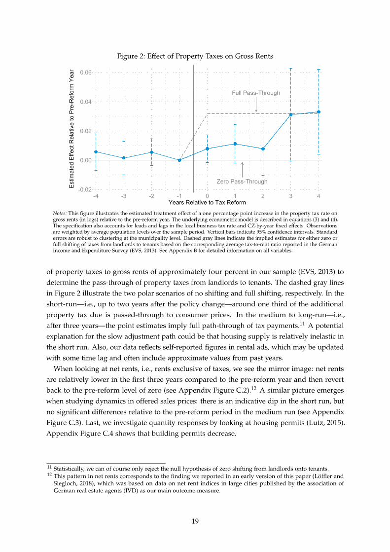
Figure 2: Effect of Property Taxes on Gross Rents

Zero Pass-Through

Full Pass-Through

-0.02

0.00

0.02

0.04

0.06Es

timat

ed E

ffect

Rel

ativ

e to

Pre

-Ref

orm

Yea

r

-4 -3 -2 -1 0 1 2 3 4Years Relative to Tax Reform

Notes: This figure illustrates the estimated treatment effect of a one percentage point increase in the property tax rate ongross rents (in logs) relative to the pre-reform year. The underlying econometric model is described in equations (3) and (4).The specification also accounts for leads and lags in the local business tax rate and CZ-by-year fixed effects. Observationsare weighted by average population levels over the sample period. Vertical bars indicate 95% confidence intervals. Standarderrors are robust to clustering at the municipality level. Dashed gray lines indicate the implied estimates for either zero orfull shifting of taxes from landlords to tenants based on the corresponding average tax-to-rent ratio reported in the GermanIncome and Expenditure Survey (EVS, 2013). See Appendix B for detailed information on all variables.

of property taxes to gross rents of approximately four percent in our sample (EVS, 2013) todetermine the pass-through of property taxes from landlords to tenants. The dashed gray linesin Figure 2 illustrate the two polar scenarios of no shifting and full shifting, respectively. In theshort-run—i.e., up to two years after the policy change—around one third of the additionalproperty tax due is passed-through to consumer prices. In the medium to long-run—i.e.,after three years—the point estimates imply full path-through of tax payments.11 A potentialexplanation for the slow adjustment path could be that housing supply is relatively inelastic inthe short run. Also, our data reflects self-reported figures in rental ads, which may be updatedwith some time lag and often include approximate values from past years.

When looking at net rents, i.e., rents exclusive of taxes, we see the mirror image: net rentsare relatively lower in the first three years compared to the pre-reform year and then revertback to the pre-reform level of zero (see Appendix Figure C.2).12 A similar picture emergeswhen studying dynamics in offered sales prices: there is an indicative dip in the short run, butno significant differences relative to the pre-reform period in the medium run (see AppendixFigure C.3). Last, we investigate quantity responses by looking at housing permits (Lutz, 2015).Appendix Figure C.4 shows that building permits decrease.

11 Statistically, we can of course only reject the null hypothesis of zero shifting from landlords onto tenants.12 This pattern in net rents corresponds to the finding we reported in an early version of this paper (Löffler and

Siegloch, 2018), which was based on data on net rent indices in large cities published by the association ofGerman real estate agents (IVD) as our main outcome measure.

19

5.2 Probing Identification

While the estimated pre-trends are reassuringly flat in our baseline specification, we furthertest whether the treatment effects in Figure 2 depict the causal effect of property tax changes.As discussed in Section 4.2, we run four major checks. We present the resulting estimates ofthese tests in Figure 4. To improve readability, we summarize pre-treatment effects (leads of upto four years prior to a tax change), and medium-run effects (three to four years after a policychange) by calculating the average over the respective estimates. All corresponding event studygraphs are presented in Appendix C.3.

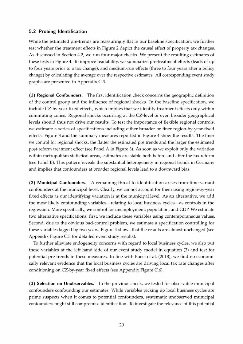
(1) Regional Confounders. The first identification check concerns the geographic definitionof the control group and the influence of regional shocks. In the baseline specification, weinclude CZ-by-year fixed effects, which implies that we identify treatment effects only withincommuting zones. Regional shocks occurring at the CZ-level or even broader geographicallevels should thus not drive our results. To test the importance of flexible regional controls,we estimate a series of specifications including either broader or finer region-by-year-fixedeffects. Figure 3 and the summary measures reported in Figure 4 show the results. The finerwe control for regional shocks, the flatter the estimated pre trends and the larger the estimatedpost-reform treatment effect (see Panel A in Figure 3). As soon as we exploit only the variationwithin metropolitan statistical areas, estimates are stable both before and after the tax reform(see Panel B). This pattern reveals the substantial heterogeneity in regional trends in Germanyand implies that confounders at broader regional levels lead to a downward bias.

(2) Municipal Confounders. A remaining threat to identification arises from time-variantconfounders at the municipal level. Clearly, we cannot account for them using region-by-yearfixed effects as our identifying variation is at the municipal level. As an alternative, we addthe most likely confounding variables—relating to local business cycles—as controls in theregression. More specifically, we control for unemployment, population, and GDP. We estimatetwo alternative specifications: first, we include these variables using contemporaneous values.Second, due to the obvious bad-control problem, we estimate a specification controlling forthese variables lagged by two years. Figure 4 shows that the results are almost unchanged (seeAppendix Figure C.5 for detailed event study results).

To further alleviate endogeneity concerns with regard to local business cycles, we also putthese variables at the left hand side of our event study model in equation (3) and test forpotential pre-trends in these measures. In line with Fuest et al. (2018), we find no economi-cally relevant evidence that the local business cycles are driving local tax rate changes afterconditioning on CZ-by-year fixed effects (see Appendix Figure C.6).

(3) Selection on Unobservables. In the previous check, we tested for observable municipalconfounders confounding our estimates. While variables picking up local business cycles areprime suspects when it comes to potential confounders, systematic unobserved municipalconfounders might still compromise identification. To investigate the relevance of this potential

20

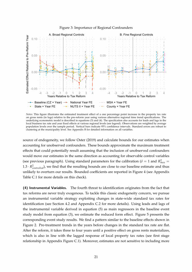
Figure 3: Importance of Regional Confounders

-0.05

0.00

0.05

0.10

Estim

ated

Effe

ct R

elat

ive

to P

re-R

efor

m Y

ear


Baseline (CZ × Year) National Year FEState × Year FE NUTS II × Year FE

A. Broad Regional Controls

-0.05

0.00

0.05

0.10


MSA × Year FECounty × Year FE

B. Fine Regional Controls

Notes: This figure illustrates the estimated treatment effect of a one percentage point increase in the property tax rateon gross rents (in logs) relative to the pre-reform year using various alternative regional time trend specifications. Theunderlying econometric model is described in equations (3) and (4). The specification also accounts for leads and lags in thelocal business tax rate and year fixed effects at various regional levels (see legend). Observations are weighted by averagepopulation levels over the sample period. Vertical bars indicate 95% confidence intervals. Standard errors are robust toclustering at the municipality level. See Appendix B for detailed information on all variables.

source of endogeneity, we follow Oster (2019) and calculate bounds for our estimates whenaccounting for unobserved confounders. These bounds approximate the maximum treatmenteffects that could potentially result assuming that the inclusion of unobserved confounderswould move our estimates in the same direction as accounting for observable control variables(see previous paragraph). Using standard parameters for the calibration (δ = 1 and R2

max =

1.3 R2· controlled), we find that the resulting bounds are close to our baseline estimate and thusunlikely to overturn our results. Bounded coefficients are reported in Figure 4 (see AppendixTable C.1 for more details on this check).

(4) Instrumental Variables. The fourth threat to identification originates from the fact thattax reforms are never truly exogenous. To tackle this classic endogeneity concern, we pursuean instrumental variable strategy exploiting changes in state-wide standard tax rates foridentification (see Section 4.2 and Appendix C.2 for more details). Using leads and lags ofthe instrumental variable derived in equation (5) as main regressors in the baseline eventstudy model from equation (3), we estimate the reduced form effect. Figure 5 presents thecorresponding event study results. We find a pattern similar to the baseline effects shown inFigure 2. Pre-treatment trends in the years before changes in the standard tax rate are flat.After the reform, it takes three to four years until a positive effect on gross rents materializes,which is also in line with the lagged response of local property tax rates (see first stagerelationship in Appendix Figure C.1). Moreover, estimates are not sensitive to including more

21

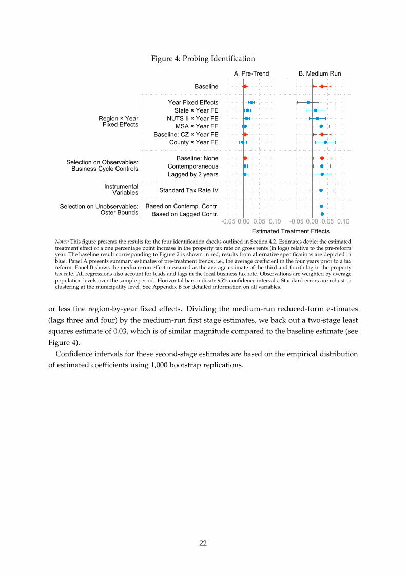
Figure 4: Probing Identification

Region × YearFixed Effects

Selection on Observables:Business Cycle Controls

Selection on Unobservables:Oster Bounds

InstrumentalVariables

Baseline

Year Fixed EffectsState × Year FE

NUTS II × Year FEMSA × Year FE

Baseline: CZ × Year FECounty × Year FE

Baseline: NoneContemporaneousLagged by 2 years

Standard Tax Rate IV

Based on Contemp. Contr.Based on Lagged Contr.

-0.05 0.00 0.05 0.10 -0.05 0.00 0.05 0.10

A. Pre-Trend B. Medium Run

Estimated Treatment Effects Notes: This figure presents the results for the four identification checks outlined in Section 4.2. Estimates depict the estimatedtreatment effect of a one percentage point increase in the property tax rate on gross rents (in logs) relative to the pre-reformyear. The baseline result corresponding to Figure 2 is shown in red, results from alternative specifications are depicted inblue. Panel A presents summary estimates of pre-treatment trends, i.e., the average coefficient in the four years prior to a taxreform. Panel B shows the medium-run effect measured as the average estimate of the third and fourth lag in the propertytax rate. All regressions also account for leads and lags in the local business tax rate. Observations are weighted by averagepopulation levels over the sample period. Horizontal bars indicate 95% confidence intervals. Standard errors are robust toclustering at the municipality level. See Appendix B for detailed information on all variables.

or less fine region-by-year fixed effects. Dividing the medium-run reduced-form estimates(lags three and four) by the medium-run first stage estimates, we back out a two-stage leastsquares estimate of 0.03, which is of similar magnitude compared to the baseline estimate (seeFigure 4).

Confidence intervals for these second-stage estimates are based on the empirical distributionof estimated coefficients using 1,000 bootstrap replications.

22

Figure 5: Effect of Standard Tax Rate Changes on Gross Rents

-0.04

-0.02

0.00

0.02

0.04

0.06R

educ

ed F

orm

Effe

ct o

n G

ross

Ren

ts

-4 -3 -2 -1 0 1 2 3 4Years Relative to Standard Tax Rate Reform

Baseline (Commuting Zone-by-Year) MSA-by-Year County-by-Year

Notes: This figure illustrates the estimated reduced-form effect of the standard tax rate IV defined in equation (5) on grossrents (in logs) relative to the year before a standard tax rate increase. The underlying econometric model is analogousto equations (3) and (4). The specification also accounts for leads and lags in the local business tax rate and CZ-by-yearfixed effects. Observations are weighted by average population levels over the sample period. Municipalities in the statesBaden-Württemberg and Saarland are excluded from the estimation sample. Vertical bars indicate 95% confidence intervals.Standard errors are robust to clustering at the municipality level. See Appendix B for detailed information on all variables.

5.3 Heterogeneous Effects

In this section we study heterogeneous effects by municipality type. To this end, we groupmunicipalities according to different indicators and interact these indicator variables with allleads and lags of the property tax rate in equation (3).13 We follow the studies by Saiz (2010)and Hilber and Vermeulen (2016) and investigate whether the pass-through to consumer pricescan be explained with differences in local housing supply constraints. To this end, we use twomeasures of physical supply constraints (in 2007). First, we use the share of already developedland relative to the total developable area of a municipality. While this measure yields a proxyfor the availability of land for new construction, it is driven by past housing supply and hencepotentially endogenous. To address this concern, we secondly group municipalities accordingto their share of physically undevelopable land (i.e., areas that are undevelopable becausethey are wetland, water bodies, wasteland, or mining areas). Panels A and B of Figure 6present the corresponding results. We find stronger price effects in less supply-constrainedmunicipalities (blue) and hardly any pass-through in municipalities with more severe housingsupply restrictions (red). This pattern is in line with the standard tax incidence prediction, i.e.,that the pass-through to consumer prices increases with the housing supply elasticity.

Next we test for heterogeneous effects by municipal size. Larger cities are typically also more

13 The different group indicators are not independent from each other (e.g., think of supply constraints and citysize). Heterogeneity patterns should thus be taken as suggestive evidence for different types of municipalities.

23

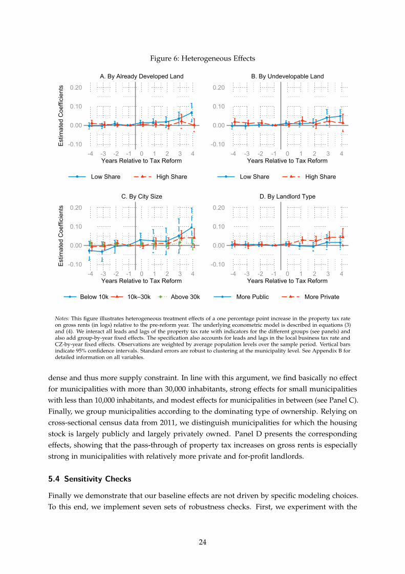
Figure 6: Heterogeneous Effects

-0.10

0.00

0.10

0.20

Estim

ated

Coe

ffici

ents


Low Share High Share

A. By Already Developed Land

-0.10

0.00

0.10

0.20


Low Share High Share

B. By Undevelopable Land

-0.10

0.00

0.10

0.20

Estim

ated

Coe

ffici

ents


Below 10k 10k–30k Above 30k

C. By City Size

-0.10

0.00

0.10

0.20


More Public More Private

D. By Landlord Type

Notes: This figure illustrates heterogeneous treatment effects of a one percentage point increase in the property tax rateon gross rents (in logs) relative to the pre-reform year. The underlying econometric model is described in equations (3)and (4). We interact all leads and lags of the property tax rate with indicators for the different groups (see panels) andalso add group-by-year fixed effects. The specification also accounts for leads and lags in the local business tax rate andCZ-by-year fixed effects. Observations are weighted by average population levels over the sample period. Vertical barsindicate 95% confidence intervals. Standard errors are robust to clustering at the municipality level. See Appendix B fordetailed information on all variables.

dense and thus more supply constraint. In line with this argument, we find basically no effectfor municipalities with more than 30,000 inhabitants, strong effects for small municipalitieswith less than 10,000 inhabitants, and modest effects for municipalities in between (see Panel C).Finally, we group municipalities according to the dominating type of ownership. Relying oncross-sectional census data from 2011, we distinguish municipalities for which the housingstock is largely publicly and largely privately owned. Panel D presents the correspondingeffects, showing that the pass-through of property tax increases on gross rents is especiallystrong in municipalities with relatively more private and for-profit landlords.

5.4 Sensitivity Checks

Finally we demonstrate that our baseline effects are not driven by specific modeling choices.To this end, we implement seven sets of robustness checks. First, we experiment with the

24

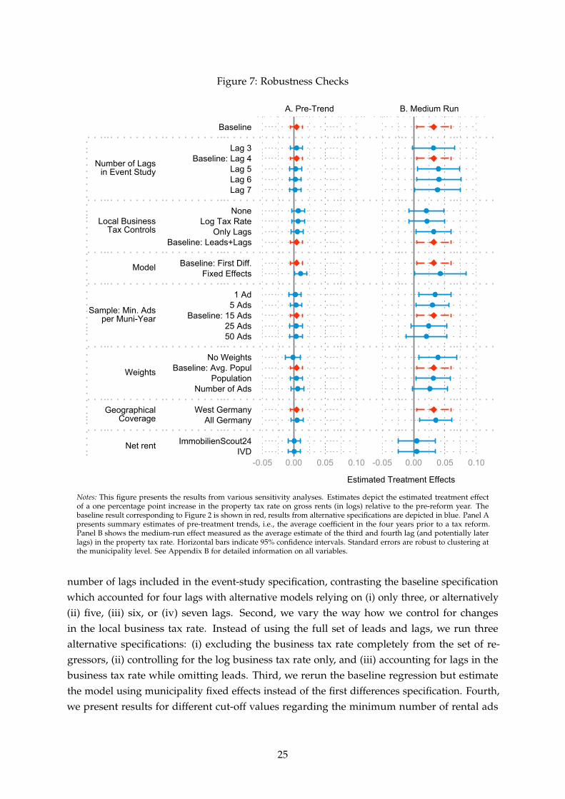
Figure 7: Robustness Checks

Number of Lagsin Event Study

Local BusinessTax Controls

Model

Sample: Min. Adsper Muni-Year

GeographicalCoverage

Net rent

Weights

Baseline

Lag 3Baseline: Lag 4

Lag 5Lag 6Lag 7

NoneLog Tax Rate

Only LagsBaseline: Leads+Lags

Baseline: First Diff.Fixed Effects

1 Ad5 Ads

Baseline: 15 Ads25 Ads50 Ads

No WeightsBaseline: Avg. Popul

PopulationNumber of Ads

West GermanyAll Germany

ImmobilienScout24IVD

-0.05 0.00 0.05 0.10 -0.05 0.00 0.05 0.10

A. Pre-Trend B. Medium Run

Estimated Treatment Effects

Notes: This figure presents the results from various sensitivity analyses. Estimates depict the estimated treatment effectof a one percentage point increase in the property tax rate on gross rents (in logs) relative to the pre-reform year. Thebaseline result corresponding to Figure 2 is shown in red, results from alternative specifications are depicted in blue. Panel Apresents summary estimates of pre-treatment trends, i.e., the average coefficient in the four years prior to a tax reform.Panel B shows the medium-run effect measured as the average estimate of the third and fourth lag (and potentially laterlags) in the property tax rate. Horizontal bars indicate 95% confidence intervals. Standard errors are robust to clustering atthe municipality level. See Appendix B for detailed information on all variables.

number of lags included in the event-study specification, contrasting the baseline specificationwhich accounted for four lags with alternative models relying on (i) only three, or alternatively(ii) five, (iii) six, or (iv) seven lags. Second, we vary the way how we control for changesin the local business tax rate. Instead of using the full set of leads and lags, we run threealternative specifications: (i) excluding the business tax rate completely from the set of re-gressors, (ii) controlling for the log business tax rate only, and (iii) accounting for lags in thebusiness tax rate while omitting leads. Third, we rerun the baseline regression but estimatethe model using municipality fixed effects instead of the first differences specification. Fourth,we present results for different cut-off values regarding the minimum number of rental ads

25

per municipality-year cell. We compare our baseline threshold of 15 ads to four alternativelimits: (i) one ad, (ii) five ads, (iii) 25 ads, or (iv) 50 ads. Fifth, we vary the weights employedin the regression (baseline: average population levels over the sample period) and test threealternative weighting procedures: (i) discarding weights, (ii) using annual population levels,and (iii) weighting by the number of rental ads in a municipality per year. Sixth, we extendthe estimation sample and include municipalities in East Germany (baseline: West Germanyonly). Finally, we test whether the medium-run effect on net rents in our estimation sampleand in the alternative IVD dataset are indeed zero, implying full pass-through from landlordsto tenants if the producer price excluding taxes remains unaffected (Löffler and Siegloch, 2018).

For each of these checks, we present summary estimates of the pre trends as well as themedium-run effects after three or more years. Figure 7 presents the corresponding results. Theplot illustrates that our findings are robust with respect to these tests. Medium-run estimateshover around our baseline estimate and are statistically significantly different from zero inmost cases. Pre-trends are notably flat in virtually all specifications with only one exception:the fixed effects model. This small but significant difference is driven by the binned endpointat the fourth lead, i.e., reflecting some difference four or more years prior to tax reforms. Allunderlying event study results are presented in Appendix Figures C.8–C.13.

6 Welfare Simulations

In this section, we feed the reduced-form evidence into our theoretical framework to simulatethe welfare effects of property taxation. We start by explaining how we implement thesimulation in Section 6.1. In Section 6.2, we present the corresponding results and showhow property taxes affect household welfare. Finally, we run counterfactual simulations toinvestigate the welfare effects of property taxation in different institutional contexts (Section 6.3).

6.1 Data and Calibration

We base our simulation on the 2013 wave of the German Income and Expenditure Survey(EVS, 2013), a representative cross-sectional household study conducted every five years by theGerman Federal Statistical Office. In line with the empirical analysis in Section 5, we focus onrespondents from West Germany, which leaves us with a sample of |H| = 32,458 households.14

The survey includes information on the household context, incomes from various sources, andbasic housing characteristics, in particular the tenancy status and square meter of the mainresidence. In addition, the Federal Statistical Office reports rental payments for renters andimputed rents as well as property tax payments in case of owner-occupied housing.

Equation (7) yields the starting point for the empirical implementation of Proposition 1. Werewrite the money-metric change in household i’s utility in response to an increase in the

14 We perform all simulations at the household level accounting for household sampling weights and using theOECD-modified equivalence scale to adjust for differences in household size throughout our analysis.

26

property tax rate as:

∆Wi = −hi∆rCi + ∆yL

i + ∆yW F g ∈ Hi + ∆yi + δi ∆g, for i , (7)

where hi denotes the observed floor area of household i’s apartment or house. The operator ∆indicates simulated changes in gross per m2 housing prices rC

i , landlord income yLi , wage

earnings yWi , business income yF

i , and public good provision g, respectively.We provide more details on the empirical implementation of the different components in

Table 1. Panel A illustrates how the simulated changes of equation (7) relate to the reduced-form evidence on the effects of a one percentage point increase in the property tax rate. Panel Bshows the estimates for the different semi-elasticities used in the simulation. These estimatesrepresent medium-run effects using the model from equations (3)–(4) and gross rents, averagewages in the municipality, and profits of local firms, and municipal expenditures as outcomes(in logs). Precisely, we calculate the implied medium-run semi-elasticities from the respectiveevent studies, averaging the estimated coefficients in years three and four after a tax change.

As discussed in Section 2.1, the household welfare effect consists of three components: First,we simulate the impact of property tax changes on housing expenditures hirC

i using reportedliving space and gross rents from the data and the semi-elasticity of gross rents with respectto a one percentage point increase in the property tax rate estimated in Section 5. In case ofowner-occupied housing, we simulate the change in tax payments based on imputed rents.

Second, we account for changes in household income. To predict the impact on rentalincome, ∆yL

i , we multiply the estimated semi-elasticity of gross rents with respect to theproperty tax rate by observed total landlord income and subtract landlords’ additional propertytax payments using the average tax-to-rent ratio from the data. Since additional landlord incomeis subject to income taxation, we further multiply this figure by the marginal net-of-income-taxrate to arrive at the change in net rental income.

In addition to landlord income, household income effects also include changes in wagesand business income (see equation (7)). We estimate the effects of property taxes on these twooutcomes using our empirical model defined in equations (3) and (4). Appendix Figure C.14shows the corresponding results. Overall, wages and business incomes are hardly affected byproperty tax changes, medium-run effects are close to zero (see also the summary estimates inPanel B of Table 1). Based on the estimate for wages, we simulate the change in household’searnings, ∆yW

i , using observed wage income and the marginal tax wedges from income taxesand social-security contributions. Similarly, we predict the change in business income, ∆yF

i ,based on the estimated semi-elasticity of profits with respect to the property tax rate, reportedself-employment income, and the marginal net-of-income tax rate.

The third component concerns the transmission of property taxes in public good provision,denoted by ∆g. To simulate the welfare effects of changes in local public goods, we need theaverage municipal expenditures per capita (EUR 2,463 in 2013) and the semi-elasticity estimateof municipal expenditures per capita with respect to the property tax rate (see Panel C ofAppendix Figure C.7 and the summary estimate in Panel B of Table 1).15 In order to transform15 We proxy locally provided public services using per capita expenditures of the municipality, which is a common

27

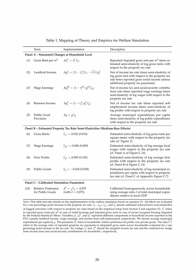
Table 1: Mapping of Theory and Empirics for Welfare Simulation

Term Implementation Description

Panel A – Simulated Changes at Household Level

(1) Gross Rent per m2 ∆rCi = rC

i ε̂rC Reported/imputed gross rent per m2 times es-timated semi-elasticity of log gross rents withrespect to the property tax rate

(2) Landlord Income ∆yLi = ([1− τ I

i ] ε̂rC − t/r) yLi Net of income tax rate times semi-elasticity of

log gross rent with respect to the property taxrate times reported gross rental income (minusadditional property tax payments)

(3) Wage Earnings ∆yWi = (1− τW

i ) yWi ε̂yW Net of income tax and social-security contribu-

tions rate times reported wage earnings timessemi-elasticity of log wages with respect to theproperty tax rate

(4) Business Income ∆yFi = (1− τ I

i ) yFi ε̂yF Net of income tax rate times reported self-

employment income times semi-elasticity oflog profits with respect to property tax rate

(5) Public GoodProvision

∆g = g ε̂g Average municipal expenditures per capitatimes semi-elasticity of log public expenditureswith respect to the property tax rate

Panel B – Estimated Property Tax Rate Semi-Elasticities (Medium-Run Effects)

(6) Gross Rents ε̂rC = 0.032 (0.014) Estimated semi-elasticity of log gross rents persquare meter with respect to the property taxrate (cf. Figure 2)

(7) Wage Earnings ε̂yW = 0.006 (0.009) Estimated semi-elasticity of log average localwages with respect to the property tax rate(cf. Panel A of Figure C.14)

(8) Firm Profits ε̂yF = 0.009 (0.145) Estimated semi-elasticity of log average firmprofits with respect to the property tax rate(cf. Panel B of Figure C.14)

(9) Public Goods ε̂g = −0.034 (0.038) Estimated semi-elasticity of log municipal ex-penditures per capita with respect to propertytax rate (cf. Panel C of Appendix Figure C.7)

Panel C – Calibrated Simulation Parameters

(10) Relative Preferencefor Public Goods

δgi = δ

1−δ = 0.079(with δ = 0.073)

Calibrated homogeneously across householdsusing average ratio δ of total municipal expen-ditures relative to local GDP

Notes: This table provides details on the implementation of the welfare simulation based on equation (7). All effects are evaluatedfor a one percentage point increase in the property tax rate. ε̂rC , ε̂yW , ε̂yF , and ε̂g denote estimated reduced-form semi-elasticities

of logged outcomes with respect to property tax rates based on the empirical setup from Section 5 and equation (3). rCi refers

to reported gross rents per m2 in case of rental housing and imputed gross rents in case of owner-occupied housing (imputedby the Federal Statistical Office). Variables yL

i , yWi , and yF

i represent different components of household income reported in theEVS, namely landlord income, wage earnings, and income from self-employment, respectively. We denote average municipal

gexpenditures per capita by g. The parameter δi refers to households’ relative preference for public over private goods. The ratio t/rrefers to the average ratio of reported property tax payments to (imputed) gross rents across households evaluated for a onepercentage point increase in the tax rate. Tax wedges Iτi and Wτi denote the marginal income tax rate and the combined tax wedgefrom income taxes and social-security contributions for household i, respectively.

28

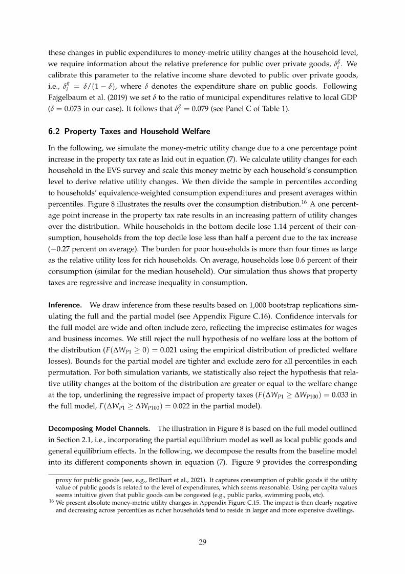
these changes in public expenditures to money-metric utility changes at the household level,we require information about the relative preference for public over private goods, g

δi . Wecalibrate this parameter to the relative income share devoted to public over private goods,i.e., g

δ = δ/(1 − δ)i , where δ denotes the expenditure share on public goods. FollowingFajgelbaum et al. (2019) we set δ to the ratio of municipal expenditures relative to local GDP(δ = 0.073 in our case). It follows that g

δ =i 0.079 (see Panel C of Table 1).

6.2 Property Taxes and Household Welfare

In the following, we simulate the money-metric utility change due to a one percentage pointincrease in the property tax rate as laid out in equation (7). We calculate utility changes for eachhousehold in the EVS survey and scale this money metric by each household’s consumptionlevel to derive relative utility changes. We then divide the sample in percentiles accordingto households’ equivalence-weighted consumption expenditures and present averages withinpercentiles. Figure 8 illustrates the results over the consumption distribution.16 A one percent-age point increase in the property tax rate results in an increasing pattern of utility changesover the distribution. While households in the bottom decile lose 1.14 percent of their con-sumption, households from the top decile lose less than half a percent due to the tax increase(−0.27 percent on average). The burden for poor households is more than four times as largeas the relative utility loss for rich households. On average, households lose 0.6 percent of theirconsumption (similar for the median household). Our simulation thus shows that propertytaxes are regressive and increase inequality in consumption.

Inference. We draw inference from these results based on 1,000 bootstrap replications sim-ulating the full and the partial model (see Appendix Figure C.16). Confidence intervals forthe full model are wide and often include zero, reflecting the imprecise estimates for wagesand business incomes. We still reject the null hypothesis of no welfare loss at the bottom ofthe distribution (F(∆WP1 ≥ 0) = 0.021 using the empirical distribution of predicted welfarelosses). Bounds for the partial model are tighter and exclude zero for all percentiles in eachpermutation. For both simulation variants, we statistically also reject the hypothesis that rela-tive utility changes at the bottom of the distribution are greater or equal to the welfare changeat the top, underlining the regressive impact of property taxes (F(∆WP1 ≥ ∆WP100) = 0.033 inthe full model, F(∆WP1 ≥ ∆WP100) = 0.022 in the partial model).

Decomposing Model Channels. The illustration in Figure 8 is based on the full model outlinedin Section 2.1, i.e., incorporating the partial equilibrium model as well as local public goods andgeneral equilibrium effects. In the following, we decompose the results from the baseline modelinto its different components shown in equation (7). Figure 9 provides the corresponding

proxy for public goods (see, e.g., Brülhart et al., 2021). It captures consumption of public goods if the utilityvalue of public goods is related to the level of expenditures, which seems reasonable. Using per capita valuesseems intuitive given that public goods can be congested (e.g., public parks, swimming pools, etc).

16 We present absolute money-metric utility changes in Appendix Figure C.15. The impact is then clearly negativeand decreasing across percentiles as richer households tend to reside in larger and more expensive dwellings.

29

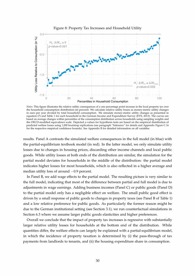
Figure 8: Property Tax Increases and Household Utility

H0: ΔWP1 ≥ 0p-value=0.021

H1: ΔWP1 ≥ ΔWP100

p-value=0.033

-1.5

-1.0

-0.5

0.0U

tility

Los

s R

elat

ive

to C

onsu

mpt

ion

(in %

)

0 20 40 60 80 100Percentiles in Household Consumption

Notes: This figure illustrates the relative utility consequences of a one percentage point increase in the local property tax overthe household consumption distribution (in percent). We calculate relative utility losses as money-metric utility changesin euro per year divided by total household consumption. We simulate money-metric utility changes as presented inequation (7) and Table 1 for each household in the German Income and Expenditure Survey (EVS, 2013). The curves arebased on average changes within percentiles of the consumption distribution across households using sampling weights andthe OECD-modified equivalence scale. Depicted p-values for hypothesis tests are based on the empirical distribution ofpredicted welfare losses using 1,000 bootstrap replications (see paragraph “Inference” for details and Appendix Figure C.16for the respective empirical confidence bounds). See Appendix B for detailed information on all variables.

results. Panel A contrasts the simulated welfare consequences in the full model (in blue) withthe partial-equilibrium textbook model (in red). In the latter model, we only simulate utilitylosses due to changes in housing prices, discarding other income channels and local publicgoods. While utility losses at both ends of the distribution are similar, the simulation for thepartial model deviates for households in the middle of the distribution: the partial modelindicates higher losses for most households, which is also reflected in a higher average andmedian utility loss of around −0.9 percent.

In Panel B, we add wage effects to the partial model. The resulting picture is very similar tothe full model, indicating that most of the difference between partial and full model is due toadjustments in wage earnings. Adding business incomes (Panel C) or public goods (Panel D)to the partial model only has a negligible effect on welfare. The small public good effect isdriven by a small response of public goods to changes in property taxes (see Panel B of Table 1)and a low relative preference for public goods. As particularly the former reason might bedue to the German institutional setting (see Section 3.1), we run counterfactual simulations inSection 6.3 where we assume larger public goods elasticities and higher preferences.

Overall we conclude that the impact of property tax increases is regressive with substantiallylarger relative utility losses for households at the bottom end of the distribution. Whilequantities differ, the welfare effects can largely be explained with a partial-equilibrium model,in which the incidence of property taxation is determined by (i) the pass-through of taxpayments from landlords to tenants, and (ii) the housing expenditure share in consumption.

30

Figure 9: Decomposition of Welfare Effects

-1.5

-1.0

-0.5

0.0

Rel

ativ

e U

tility

Los

s (in

%)

0 20 40 60 80 100

A. Partial Model vs. Full Model

-1.5

-1.0

-0.5

0.0

0 20 40 60 80 100

B. Partial Model with Wage Earnings Channel

-1.5

-1.0

-0.5

0.0

Rel

ativ

e U

tility

Los

s (in

%)


C. Partial Model with Firm Profit Channel

-1.5

-1.0

-0.5

0.0


D. Partial Model with Public Goods Channel

Full Model (Baseline) Partial Model Intermediate Model

Notes: This figure illustrates the utility consequences of a one percentage point increase in the local property tax over thedistribution of household consumption (in percent). Panel A depicts the full model combining housing market responsesas well as local public good responses and adjustments in wage earnings and business incomes (in blue). In red, thepanel illustrates the partial equilibrium model based on housing market adjustments only. Panel B–D present intermediatescenarios, enriching the partial model by compensating wage responses (Panel B), business profit adjustments (Panel C), orlocal public goods adjustments (Panel D), respectively, and discarding other channels. We simulate money-metric utilitychanges as presented in equation (7) and Table 1 for each household in the German Income and Expenditure Survey (EVS,2013) and normalize by total household consumption. The depicted curves are based on average utility changes withinpercentiles of the consumption distribution across households using sampling weights and the OECD-modified equivalencescale. See Appendix B for detailed information on all variables.

Sensitivity Checks. The simulations are based on a set of modeling assumptions. In Ap-pendix C.5, we provide a detailed discussion of the different assumptions and the sensitivity ofour results to modeling choices. In particular, we assess to what extent our results differ when(i) using alternative ways to calculate the additional tax burden, (ii) scaling by household in-come instead of consumption, (iii) employing different tax schedule imputations, (iv) includingEast Germany as well, and (v) using different calibrations for the relative valuation of publicvs. private goods. Results are rather insensitive to these robustness checks and if anythingyield more regressive results compared to the baseline simulation.

6.3 Counterfactual Simulations

In a last step, we run various counterfactual scenarios. First, we ask how the welfare effects ofproperty tax increases would change if we imposed a zero pass-through of taxes from landlords

31

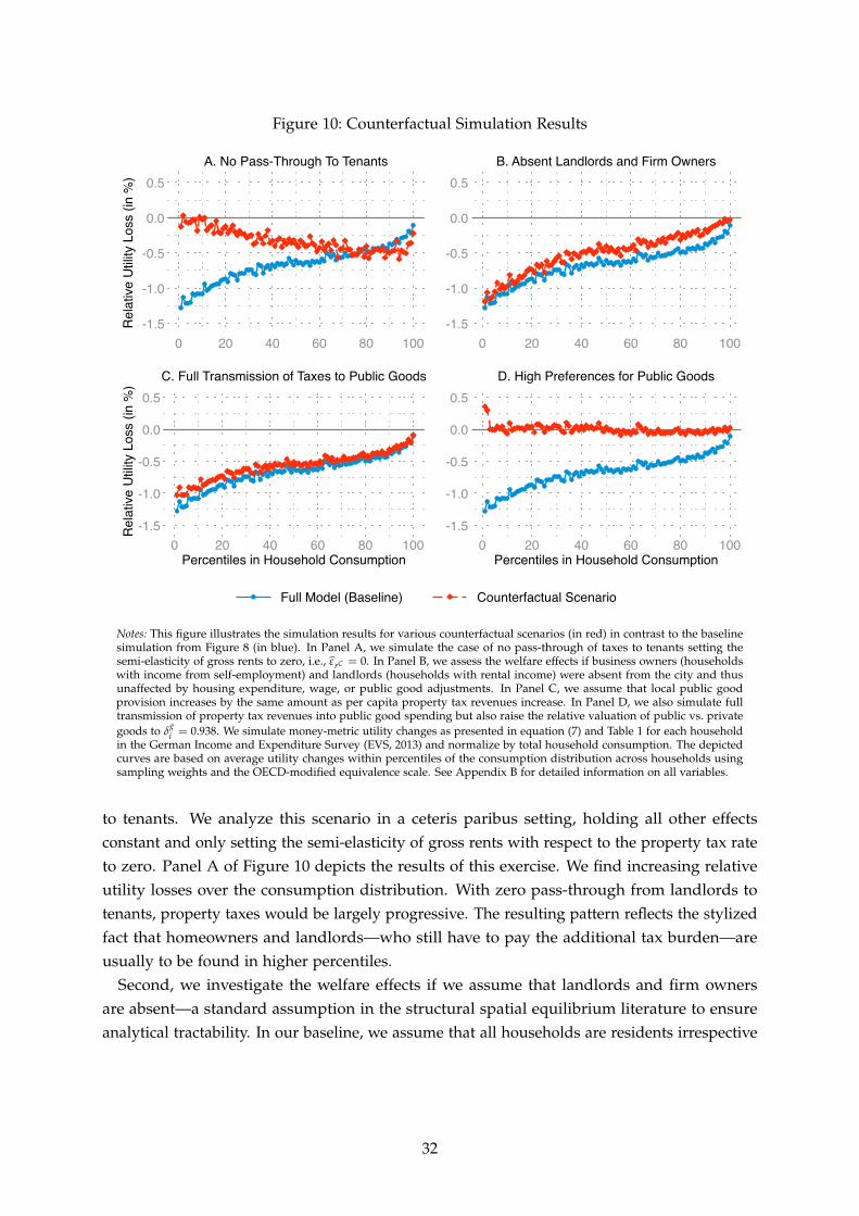
Figure 10: Counterfactual Simulation Results

-1.5

-1.0

-0.5

0.0

0.5

Rela

tive

Utilit

y Lo

ss (i

n %

)

0 20 40 60 80 100

A. No Pass-Through To Tenants

-1.5

-1.0

-0.5

0.0

0.5

0 20 40 60 80 100

B. Absent Landlords and Firm Owners

-1.5

-1.0

-0.5

0.0

0.5

Rela

tive

Utilit

y Lo

ss (i

n %

)


C. Full Transmission of Taxes to Public Goods

-1.5

-1.0

-0.5

0.0

0.5


D. High Preferences for Public Goods

Full Model (Baseline) Counterfactual Scenario

Notes: This figure illustrates the simulation results for various counterfactual scenarios (in red) in contrast to the baselinesimulation from Figure 8 (in blue). In Panel A, we simulate the case of no pass-through of taxes to tenants setting thesemi-elasticity of gross rents to zero, i.e., ε̂rC = 0. In Panel B, we assess the welfare effects if business owners (householdswith income from self-employment) and landlords (households with rental income) were absent from the city and thusunaffected by housing expenditure, wage, or public good adjustments. In Panel C, we assume that local public goodprovision increases by the same amount as per capita property tax revenues increase. In Panel D, we also simulate fulltransmission of property tax revenues into public good spending but also raise the relative valuation of public vs. private

ggoods to δ =i 0.938. We simulate money-metric utility changes as presented in equation (7) and Table 1 for each householdin the German Income and Expenditure Survey (EVS, 2013) and normalize by total household consumption. The depictedcurves are based on average utility changes within percentiles of the consumption distribution across households usingsampling weights and the OECD-modified equivalence scale. See Appendix B for detailed information on all variables.

to tenants. We analyze this scenario in a ceteris paribus setting, holding all other effectsconstant and only setting the semi-elasticity of gross rents with respect to the property tax rateto zero. Panel A of Figure 10 depicts the results of this exercise. We find increasing relativeutility losses over the consumption distribution. With zero pass-through from landlords totenants, property taxes would be largely progressive. The resulting pattern reflects the stylizedfact that homeowners and landlords—who still have to pay the additional tax burden—areusually to be found in higher percentiles.

Second, we investigate the welfare effects if we assume that landlords and firm ownersare absent—a standard assumption in the structural spatial equilibrium literature to ensureanalytical tractability. In our baseline, we assume that all households are residents irrespective

32

of whether they are workers, business owners, or landlords.17 In the counterfactual scenario,we now assume that (i) households with positive rental income are only affected via changesin rental income, and (ii) households with income from self-employment only by changes inbusiness profits; we set all other channels to zero for these households. Panel B of Figure 10shows the corresponding results. While this alternative scenario has little impact at the bottomof the distribution, it reduces the utility losses for most households in the middle and upperpart of the distribution, yielding a more regressive impact of the tax.

Third, we impose the counterfactual assumption that additional property tax revenues arefully transmitted into higher public good spending. Based on average municipal per-capitaproperty tax revenues and the estimated semi-elasticity of tax revenues with respect to a onepercentage point increase in the tax rate, we simulate annual municipal public good spendingto increase by 87 EUR per capita (cf. Panel B of Appendix Figure C.7). Panel C of Figure 10illustrates the simulation results along the distribution of consumption expenditures. Asexpected, relative utility losses are smaller for all percentiles and particularly so at the lowerend of the distribution. However, the resulting pattern is still regressive and qualitatively quitesimilar to our baseline simulation.

The reason for the small effect of the counterfactual shown in Panel C is that the relativepreference for local public goods in the baseline model is low. While we used a revealed prefer-ence approach following Fajgelbaum et al. (2019) to calibrate the public good preference, wemight underestimate individuals’ preferences for public goods if the local public expendituresover GDP share is inefficiently low and the public good is under-provided. This would clearlylead to an underestimate of the utility gains associated with a higher public good level asimplied by the benefit view (Tiebout, 1956, Hamilton, 1976). To assess the relevance of thispossibility, we simulate a counterfactual scenario in which we calibrate the parameter g

δi suchthat resulting utility changes average to zero (see Panel D of Figure 10), which correspondsto the assumption maintained in the benefit view of property taxation. It turns out that therelative preferences would have to be as high as g

δ =i 0.938, i.e., an order of magnitude largerthan our baseline calibration and more than three times as large as the upper bound estimatein Fajgelbaum et al. (2019). Municipal expenditures would have to make up for almost half oflocal GDP to explain such high preferences via the revealed preferences approach.

7 Conclusion

We study the welfare effects of property taxation. We propose a new theoretical angle on thisquestion by using a local labor market model in the spirit of Ahlfeldt et al. (2015) and Kline andMoretti (2014). We show that the incidence of property taxation can easily be derived using asufficient statistics approach, in which the welfare effects of the tax depend on the changesin the price of housing, public goods, and various sources of income like wages, business orlandlord income that might be affected by property taxes. In a next step, we estimate these

17 This is still an approximation given the heterogeneity in where households work, earn business income, rent outdwellings, or consume public goods. The EVS survey includes no information on the respective locations.

33

behavioral responses exploiting the German institutional setting of property taxation, in whichwe observe more than 5,200 property tax reforms over the period 2007–2018. Specifically, thereis no re-assessment of housing values and public goods financed by local property taxes play aminor role. We find that property taxes are fully passed through to rental prices after threeyears. This central finding is robust to various sensitivity checks, including an IV strategy anda test for selection on unobservables. Wages, business incomes, and local public goods are onlyweakly affected by changes in the property tax rate.

In a last step, we combine the sufficient statistics formula with our quasi-experimentalreduced-form evidence. Our simple welfare expression enables us to go beyond a representativeagent approach and simulate the welfare effects of property taxes across the income distributiontaking into account that households can simultaneously be renters, landlords, workers, andbusiness owners. We find that property taxes are regressive with poorer households showingan up to four times larger welfare loss following an increase in the property tax comparedto rich households. We also show that a partial equilibrium model that only focuses on theprice of housing reproduces the welfare prediction of the full fledged spatial equilibriummodel reasonably well. Last, we run a counterfactual scenario in which we increase theimportance of local public goods—both by assuming a higher responsiveness and increasingthe relative preferences for those goods. While the regressive nature of property taxes issomewhat alleviated, we show that we would need unrealistically high preferences for localpublic goods to fully make up for the utility losses induced by the price effects of a propertytax increase.

34

References

Ahlfeldt, G. M., S. J. Redding, D. M. Sturm, and N. Wolf (2015). “The Economics of Density:Evidence From the Berlin Wall”. Econometrica 83.6, pp. 2127–2189.

Albouy, D. and B. Stuart (2020). “Urban Population and Amenities: The Neoclassical Model ofLocation”. International Economic Review 61.1, pp. 127–158.

Baskaran, T. (2014). “Identifying Local Tax Mimicking With Administrative Borders and aPolicy Reform”. Journal of Public Economics 118, pp. 41–51.

Bayer, P., F. Ferreira, and R. McMillan (2007). “A Unified Framework for Measuring Preferencesfor Schools and Neighborhoods”. Journal of Political Economy 115.4, pp. 588–638.

Boelmann, B. and S. Schaffner (2019). “FDZ Data Description: Real-Estate Data for Germany(RWI-GEO-RED) – Advertisements on the Internet Platform ImmobilienScout24”. RWIProjektberichte.

Boustan, L. P. (2013). “Local Public Goods and the Demand for High-Income Municipalities”.Journal of Urban Economics 76.3, pp. 71–82.

Bradbury, K. L., C. J. Meyer, and K. E. Case (2001). “Property Tax Limits, Local Fiscal Behavior,and Property Values: Evidence from Massachusetts Under Proposition 2 1/2”. Journal ofPublic Economics 80.2, pp. 287–311.

Bradley, S. (2017). “Inattention to Deferred Increases in Tax Bases: How Michigan Homebuyersare Paying for Assessment Limits”. Review of Economics and Statistics 99.1, pp. 53–66.

Brueckner, J. K. (1981). “Labor Mobility and the Incidence of the Residential Property Tax”.Journal of Urban Economics 10.2, pp. 173–182.

Brülhart, M., J. Danton, R. Parchet, and J. Schläpfer (2021). “Who Bears the Burden of LocalTaxes?” CEPR Discussion Paper No. DP15826.

Buettner, T. (2006). “The Incentive Effect of Fiscal Equalization Transfers on Tax Policy”. Journalof Public Economics 90, pp. 477–497.

Carroll, R. J. and J. Yinger (1994). “Is The Property Tax a Benefit Tax? The Case of RentalHousing”. National Tax Journal 47.2, pp. 295–316.

Cellini, S. R., F. Ferreira, and J. Rothstein (2010). “The Value of School Facility Investments: Evi-dence from a Dynamic Regression Discontinuity Design”. The Quarterly Journal of Economics125.1, pp. 215–261.

Chetty, R. (2009). “Sufficient Statistics for Welfare Analysis: A Bridge Between Structural andReduced-Form Methods”. Annual Review of Economics 1, pp. 451–488.

Combes, P.-P., G. Duranton, and L. Gobillon (2017). “The Production Function For Housing:Evidence From France”. CEPR Discussion Paper 11669.

de Bartolomé, C. A. M. and S. S. Rosenthal (1999). “Property Tax Capitalization in a Model withTax-Deferred Assets, Standard Deductions, and the Taxation of Nominal Interest”. Review ofEconomics and Statistics 81.1, pp. 85–95.

Diamond, R. (2016). “The Determinants and Welfare Implications of US Workers’ DivergingLocation Choices by Skill: 1980–2000”. American Economic Review 106.3, pp. 479–524.

Dixit, A. K. and J. E. Stiglitz (1977). “Monopolistic Competition and Optimum Product Diver-sity”. American Economic Review 67.3, pp. 297–308.

35

Dusansky, R., M. Ingber, and N. Karatjas (1981). “The Impact of Property Taxation on HousingValues and Rents”. Journal of Urban Economics 10.2, pp. 240–255.

Egger, P., M. Koethenbuerger, and M. Smart (2010). “Do Fiscal Transfers Alleviate Business TaxCompetition? Evidence from Germany”. Journal of Public Economics 94, pp. 235–246.

England, R. W. (2016). “Tax Incidence and Rental Housing: A Survey and Critique of Research”.National Tax Journal 69.2, pp. 435–460.

Epple, D., B. Gordon, and H. Sieg (2010). “A New Approach to Estimating the ProductionFunction for Housing”. American Economic Review 100.3, pp. 905–924.

Epple, D. and H. Sieg (1999). “Estimating Equilibrium Models of Local Jurisdictions”. Journal ofPolitical Economy 107.4, pp. 645–681.

EVS (2013). Income and Expenditure Survey – Einkommens- und Verbrauchsstichprobe. ResearchData Center of the Federal Statistical Office and Statistical Offices of the Länder. doi:10.21242/63221.2013.00.04.3.1.0.

Fajgelbaum, P. D., E. Morales, J. C. Suárez Serrato, and O. Zidar (2019). “State Taxes and SpatialMisallocation”. Review of Economic Studies 86.1, pp. 333–376.

Ferreira, F. (2010). “You Can Take It With You: Proposition 13 Tax Benefits, Residential Mobility,and Willingness to Pay for Housing Amenities”. Journal of Public Economics 94.9–10, pp. 661–673.

Fuest, C., A. Peichl, and S. Siegloch (2018). “Do Higher Corporate Taxes Reduce Wages? MicroEvidence from Germany”. American Economic Review 108.2, pp. 393–418.

Glaeser, E. L. (2009). “The Death and Life of Cities”. In: Making Cities Work: Prospects and Policiesfor Urban America. Ed. by R. P. Inman. Princeton University Press, pp. 22–62.

Hamilton, B. W. (1975). “Zoning and Property Taxation in a System of Local Governments”.Urban Studies 12.2, pp. 205–211.

– (1976). “Capitalization of Intrajurisdictional Differences in Local Tax Prices”. American Eco-nomic Review 66.5, pp. 743–753.

Heinberg, J. D. and W. E. Oates (1970). “The Incidence of Differential Property Taxes on UrbanHousing: A Comment and Some Further Evidence”. National Tax Journal 23.1, pp. 92–98.

Hilber, C. A. L. and W. Vermeulen (2016). “The Impact of Supply Constraints on House Pricesin England”. Economic Journal 126.591, pp. 358–405.

Hyman, D. N. and E. C. J. Pasour (1973). “Property Tax Differentials and Residential Rents inNorth Carolina”. National Tax Journal 26.2, pp. 303–307.

Kleven, H. (2021). “Sufficient Statistics Revisited”. Annual Review of Economics 13. Forthcoming.Kline, P. (2010). “Place Based Policies, Heterogeneity, and Agglomeration”. American Economic

Review: Papers and Proceedings 100.2, pp. 383–387.Kline, P. and E. Moretti (2014). “People, Places, and Public Policy: Some Simple Welfare

Economics of Local Economic Development Programs”. Annual Review of Economics 6.1,pp. 629–662.

Löffler, M. and S. Siegloch (2018). “Property Taxation, Housing, and Local Labor Markets:Evidence from German Municipalities”. Presented at the NBER Summer Institute 2018.

36

https://doi.org/10.21242/63221.2013.00.04.3.1.0

Lutz, B. (2015). “Quasi-Experimental Evidence on the Connection between Property Taxes andResidential Capital Investment”. American Economic Journal: Economic Policy 7.1, pp. 300–330.

Lyytikäinen, T. (2009). “Three-Rate Property Taxation and Housing Construction”. Journal ofUrban Economics 65.3, pp. 305–313.

Melitz, M. J. (2003). “The Impact of Trade on Intra-Industry Reallocations and AggregateIndustry Productivity”. Econometrica 71.6, pp. 1695–1725.

Mieszkowski, P. (1972). “The Property Tax: An Excise Tax Or a Profits Tax?” Journal of PublicEconomics 1.1, pp. 73–96.

Mieszkowski, P. and G. R. Zodrow (1989). “Taxation and The Tiebout Model: The DifferentialEffects of Head Taxes, Taxes on Land Rents, and Property Taxes”. Journal of Economic Literature27.3, pp. 1098–1146.

Moretti, E. (2011). “Local Labor Markets”. In: Handbook of Labor Economics. Ed. by O. Ashenfelterand D. Card. Vol. 4B. North-Holland, pp. 1237–1313.

Oates, W. E. and W. A. Fischel (2016). “Are Local Property Taxes Regressive, Progressive, OrWhat?” National Tax Journal 69.2, pp. 415–434.

Orr, L. L. (1968). “The Incidence of Differential Property Taxes on Urban Housing”. NationalTax Journal 21.3, pp. 253–262.

– (1970). “The Incidence of Differential Property Taxes: A Response”. National Tax Journal 23.1,pp. 99–101.

– (1972). “The Incidence of Differential Property Taxes on Urban Housing: Reply”. National TaxJournal 25.2, pp. 217–220.

Oster, E. (2019). “Unobservable Selection and Coefficient Stability: Theory and Evidence”.Journal of Business & Economic Statistics 37.2, pp. 187–204.

Palmon, O. and B. A. Smith (1998). “New Evidence on Property Tax Capitalization”. Journal ofPolitical Economy 106.5, pp. 1099–1111.

Poterba, J. M. (1984). “Tax Subsidies to Owner-Occupied Housing: An Asset-Market Approach”.Quarterly Journal of Economics 99.4, pp. 729–752.

Proost, S. and J.-F. Thisse (2019). “What Can Be Learned from Spatial Economics?” Journal ofEconomic Literature 57.3, pp. 575–643.

Rauch, A. and C.-A. Hummel (2016). “How to Stop the Race to the Bottom – Empirical Evidencefrom North Rhine-Westphalia”. International Tax and Public Finance 23, pp. 911–933.

Redding, S. J. and E. Rossi-Hansberg (2017). “Quantitative Spatial Economics”. Annual Reviewof Economics 9, pp. 21–58.

Roback, J. (1982). “Wages, Rents, and the Quality of Life”. Journal of Political Economy 90.6,pp. 1257–1278.

Rosen, S. (1979). “Wage-Based Indexes of Urban Quality of Life”. In: Current Issues in UrbanEconomics. Ed. by P. Mieszkowski and M. Straszheim. Baltimore: Johns Hopkins UniversityPress, pp. 74–104.

Saez, E. and S. Stantcheva (2016). “Generalized Social Marginal Welfare Weights for OptimalTax Theory”. American Economic Review 106.1, pp. 24–45.

37

Saiz, A. (2010). “The Geographic Determinants of Housing Supply”. Quarterly Journal ofEconomics 125.3, pp. 1253–1296.

Samuelson, P. A. (1954). “The Pure Theory of Public Expenditure”. Review of Economics andStatistics 36.4, pp. 387–389.

Schmidheiny, K. and S. Siegloch (2020). “On Event Studies and Distributed-Lags in Two-WayFixed Effects Models: Identification, Equivalence, and Generalization”. CEPR Discussion Paper13477.

Schönholzer, D. and C. Zhang (2017). “Valueing Local Public Goods using Municipal Annexa-tions”. mimeo.

Spahn, P. B. (2004). “Land Taxation in Germany”. In: International Handbook of Land and PropertyTaxation. Ed. by R. M. Bird and N. E. Slack. Edward Elgar Publishing, pp. 98–106.

Suárez Serrato, J. C. and O. Zidar (2016). “Who Benefits from State Corporate Tax Cuts? ALocal Labor Market Approach with Heterogeneous Firms”. American Economic Review 106.9,pp. 2582–2624.

Thorsnes, P. (1997). “Consistent Estimates of the Elasticity of Substitution between Land andNon-Land Inputs in the Production of Housing”. Journal of Urban Economics 42.1, pp. 98–108.

Tiebout, C. M. (1956). “A Pure Theory of Local Expenditures”. Journal of Political Economy 64.5,pp. 416–424.

Zucman, G. (2015). “Taxing across Borders: Tracking Personal Wealth and Corporate Profits”.Journal of Economic Perspectives 28.4, pp. 121–148.

38

A Theoretical Appendix

In this appendix, we provide a detailed description of the structural representation of thespatial equilibrium framework introduced in Section 2 of the paper. It includes all derivationsand intermediate steps needed to solve the model and analyze the equilibrium properties. Weintroduce local property taxation into a Rosen-Roback type general equilibrium model of locallabor markets (Suárez Serrato and Zidar, 2016). The model consists of four groups of agents:workers, firms producing tradable goods, construction companies producing floor space, andland owners. Workers and firms are mobile and locate in one out of C cities, indexed by c.

First, we outline the model in Section A.1. Second, we solve for the spatial equilibrium(Sections A.2). In Section A.3, we derive welfare effects of tax changes and show how marginalwelfare effects relate to the key elasticities of the model in this context. We compare the welfareeffects from the structural model to those from the sufficient statistics approach in Section A.4.Finally, we use comparative statics to show how changes in the property tax rate affect theequilibrium outcomes, i.e., population size, floor space, land use, rents, wages, and land prices(see Section A.5).

A.1 Agents and Markets

A.1.1 Workers

There are N = 1 workers indexed by i. We assume that labor is homogeneous and each workerprovides inelastically one unit of labor, earns a wage yW

c , and pays rent rc for residential floorspace.18 Each municipality c has a specific unproductive consumption amenity Ac that isexogenously given. In addition, there are endogenous local public goods gc provided by thelocal government. Workers maximize utility over floor space hi, a composite good bundle xi

of non-housing goods and locations c. We normalize the aggregate price of the compositegood bundle to one. Workers are mobile across municipalities, but mobility is imperfect due toindividual location preferences, so that local labor supply is not necessarily infinitely elastic.In addition to the net house price, there is a property tax in each city, denoted by tc, with thestatutory incidence on the user of the housing service.19 We assume that households havepreferences for public goods measured by δ ∈ (0, 1).

The household’s maximization problem in a given municipality c is given by:

( )1−δmax U α

c = Acgδ 1−α Wi c hi xi eic s.t. rc(1 + tc)hi + pxi = yc (A.1)

hi ,xi

with the bundle xi of non-housing goods Z and the normalized aggregate price index p defined

18 We assume that there is only one homogeneous housing good and do not differentiate between owner-occupiedand rental housing in this structural model (Poterba, 1984).

19 For simplicity, we assume that property is taxed ad valorem. Our main theoretical prediction regarding the taxincidence is however unchanged when modeling the property tax as a specific tax instead.

39

as in Melitz (2003):

1 1−ρ∫ −ρ ∫ ρρ

xi = xρ dz −p = iz p 1−ρ

iz dz = 1 (A.2)z∈Z z∈Z

and hi, xiz, Ac, g Wc, rc, yc , tc, piz, eic > 0 and α, ρ ∈ (0, 1). The parameter ρ relates to the elasticity

of substitution between any two composite goods, which is given by 11−ρ (Dixit and Stiglitz,

1977). The Lagrangian reads:

maxL = ln Ac + δ ln gc + α(1− δ) ln hi + (1− α)(1− δ) ln xi + ln eichi ,xi ( )

+ λ yW − rc[1 + tc]hi −c xi (A.3)

and first-order conditions of the household problem are given by:

∂L α(1− δ) != − λrc(1 + t

∂ i h c) = 0h i

∂L (1− α)(1− δ) != − λ = 0

∂xi xi∂L

= yW !−c rc(1 + tc)hi − xi = 0∂λ

Now we can solve by substitution. The optimal floor space consumption is then given by:

α(1− δ)= λrc(1 + t

h c)i

(1− α)(1− δ)= r

x c(1 + tc)i

α xh i

i = 1− α rc(1 + tc)Wα y −c rc(1 + tc)hi=

1− α rc(1 + t( c) )α yW

c= − h1− α rc(1 + t i

c)

h∗yW

ci = α (A.4)

rc(1 + tc)

and we can solve for the optimal consumption level of the composite good bundle:

xi = yW −c rc(1 + tc)hi

= yW yW−c rc(1 + t c

c)α rc(1 + tc)

x∗i = (1− α)yWc (A.5)

where α is the share of the household’s budget spent for housing. Household i’s demand

40

of good variety z is then given by x∗ = (iz 1− α)yWc p 1−ρ

iz . Using the optimal consumptionquantities, log indirect utility is defined as:

VHic = ln U(h∗i , x∗i , Ac, gc, eic)

= α(1− δ) ln h∗i + (1− α)(1− δ) ln x∗i + ln Ac + δ ln gc + ln eic( )W ( )y= α(1 c W− δ) ln α + (1− α)(1− δ) ln [1− α]y A

c(1 + t c + lnr c + δ ln gc + ln eic

c)

= (1− δ) (α ln α + [1− α] ln[1− α]) + ln Ac + δ ln g +︸︷︷︸ c ln eic

=a0

+ (1− δ)(α ln yW − α ln r Wc −c α ln[1 + tc] + (1− α) ln yc )

VHic = a0 + (1− δ)(ln yW − −c α ln rc α ln[1 + tc]) + ln Ac + δ ln gc + ln eic. (A.6)︸︷︷︸

=VHc

We defined a constant term a0 = (1− δ)(α ln α+ [1− α] ln[1− α]) that is the same for all workersin the economy to simplify the notation. The individual (indirect) utility is a combinationof this constant a0, a common term VH

c identical to all workers in the municipality, andthe idiosyncratic location preferences eic. As in Kline and Moretti (2014), we assume thatthe logarithm of eic is independent and identically extreme value type I distributed withscale parameter Hσ > 0. The corresponding cumulative distribution function is F(z) =( )exp − exp[−z/ Hσ ] . Due to these city preferences, workers are not fully mobile between citiesand real wages yW

c /(rc[1 + tc]) do not fully compensate for different amenity levels Ac acrossmunicipalities (other than in Brueckner, 1981). The greater Hσ , the stronger workers’ preferencefor given locations and the lower workers’ mobility. There is a city-worker match that creates apositive rent for the worker and decreases mobility. A worker i will prefer municipality a overmunicipality b if and only if:

VH ≥ia VHib

VHa + ln eia ≥ VH

b + ln eib

VH −a VH ≥ −b ln eib ln eia.

Given the distribution of ln eic, it follows that the difference in preferences between twomunicipalities follows a logistic distribution with scale parameter Hσ , i.e., ln eib − ln eia ∼logistic(0, Hσ ). The probability that worker i locates in municipality c when choosing between Ccities is then: ( )( ) exp VH/ Hσ

Nc = Pr VH ≥ic VH, c∀ij j = c = ( ) .∑C exp VH/σH

k=1 k

This expression is equivalent to the share of workers locating in municipality c given thatwe normalize the total number of workers N to one. Note that the term a0 cancels out asit is constant across municipalities. Taking logs we arrive at the (log) labor supply curve in

− 1

6

41

municipality c:

ln NS VH ( )c

c = − ln C HπσH ︸︷︷︸

=a1

1− δ − )ln NS W α(1 δ α(1− δ) 1 δ

= ln y − ln rc−c ln τ Ac + + a1 (A.7)H c c + ln ln gcσ σH σH H H︸︷︷︸︸︷︷︸︸︷︷︸︸σ︷︷︸ σ

= NSε =1+ HDε =1+ HD Aε =ε ( )where we define all terms constant across municipalities as a1 = − ln C Hπ with Hπ =( )1C ∑C

k 1 exp VH= k / Hσ being the average utility across all municipalities and we rewrite the

property tax rate as τc = 1 + t Hc. Note that C is given, and for large C, a change in Vc does not

affect the average utility Hπ . The labor supply elasticity is given by:

∂ ln NSc 1− δ NS= = ε > 0. (A.8)

∂ ln yWc σH

Floor Space Demand. Demand for residential housing in city c is determined by the numberof workers in city c and their individual housing demand as indicated by equation (A.4):

∗ yWHc = Nchi = N c

cαrc(1 + tc)

ln Hc = ln Nc + ln α + ln yW − −c ln rc ln τc. (A.9)

It follows that the intensive margin housing demand elasticity conditional on location choice isequal to −1. In addition, there is an extensive margin with people leaving the city in responseto higher costs of living. The aggregate residential housing demand elasticity is given by:

∂ ln H Hc ∂ ln Nc α(1− δ) + σ HD= − 1 = − = ε < 0.

∂ ln rc ∂ ln r Hc σ

A.1.2 Firms

Firms j = 1, ..., J are monopolistically competitive and produce tradable consumption goods.Each firm produces a different variety Yjc using labor Njc and commercial floor space Mjc.Firms have different productivity across places, due to exogenous local production amenitiesmeasured by Bc, and idiosyncratic productivity shifters ωjc. Firm j’s profits in city c are thengiven by:

yFjc = pjcYjc − yW

c Njc − rMc (1 + tc)κMjc (A.10)

Y B Nβ M1−βjc = cωjc jc jc

with Yjc, N W Mjc, Mjc, pjc, yc , rc > 0. yW

c and rMc denote the factor prices of labor and commercial

floor space, respectively. The scale parameter κ > 0 allows property taxes on commercial rentsto differ from residential property taxes. Following Melitz (2003), we substitute the final good

42

price pjc by the inverse of product j’s aggregate demand function:

( )p

1−jc 1−ρ

Yjc = Qp

with price index p = 1 as normalized above, and Q > 0 as total product demand in theeconomy. The parameter ρ relates to the elasticity of substitution between any two varieties.We define the exponent 1− 1−ρ as the constant product demand elasticity PDε < −1. We canrewrite firm j’s profits as:

yFjc = Q1−ρY−(1−ρ) −jc Yjc yW

c Njc − rMc (1 + tc)κMjc.︸︷︷︸

=pjc

Using the production function for Yjc we can rewrite this expression as:( )ρyF

jc = Q1−ρ BcωjcNβ M1−β yW M− −c Njc rc (1 + )jc jc tc κMjc (A.11)︸︷︷︸=Yjc

with Bc, ωjc > 0 and β ∈ (0, 1).Profit maximizing behavior leads to the following first-order conditions for labor and floor

space:

∂yFjc Q1−ρBρ ρ Nρβ−1Mρ(1−β)

= ρβN c ω −jc jc jc yW !

c = 0∂ jc

∂yFjc ρ

ρ 1 ρ ρ ρβ != − β)Q1−ρB (1−β)−1 M(

M c ω N M − rc (1 + tc)κ =jc jc jc 0.∂ jc

Again, we shorten notation by using τc = (1 + tc). Taking logs of the second condition wecan derive the floor space demand of firms conditional on labor input, factor prices and localproductivity:( )

ln rMc τcκ = ln ρ + ln(1− β) + (1− ρ) ln Q + ρ ln Bc + ρ ln ωjc + ρβ ln Njc

− (1− ρ[1− β]) ln Mjc(ln Mjc = ln ρ + ln[1− β] + [1− ρ] ln Q + ρ ln Bc + ρ ln ωjc + ρβ ln Njc)/( )

− ln rM − − −c ln[τcκ] 1 ρ[1 β] . (A.12)

We can derive log labor demand from the first first-order condition using the conditional factordemand for commercial floor space from equation (A.12):

ln yWc = ln ρ + ln β + (1− ρ) ln Q + ρ ln Bc + ρ ln ωjc − (1− ρβ) ln Njc + ρ(1− β) ln Mjc( )/( )

ln Nc = ln ρ + ln Wβ + [1− ρ] ln Q + ρ ln Bc + ρ ln ωjc + ρ(1− β) ln Mjc − ln yc 1− ρβ

43

= ln ρ + ln β + [1− ρ] ln Q + ρ ln Bc + ρ ln ωjc[+ ρ[1− β] ln ρ + ln{1− β}+ {1− ρ} ln Q + ρ ln Bc + ρ ln ωjc + ρβ ln Njc]/[ ] )/( )

− ln rM − ln{τcκ}c 1− ρ{1− β ln yW} − c 1− ρβ(ln N∗jc = ln ρ + [1− ρ + ρβ] ln β + ρ[1− β] ln[1− β] + [1− ρ] ln Q + ρ ln Bc)/( )

− [1− ρ + ρβ] ln yW − ρ[1− ] ln rMβ − [ −c c ρ 1− β] ln[τcκ] + ρ ln ωjc 1 ρ (A.13)

Using equation (A.12) from above and firm j’s labor demand in city c we can also solve for thecommercial floor space demand of firm j:(

ln M∗jc = ln ρ + ρβ ln β + [1− ρβ] ln[1 W− β] + [1− ρ] ln Q + ρ ln Bc − ρβ ln yc)/( )− [1− ρβ] ln rM − [1−c ρβ] ln[τcκ] + ρ ln ωjc 1− ρ (A.14)

Equations (A.13) and (A.14) define the factor input demand conditional on local productivityand factor prices. We can now substitute the factor demand in the firm profit equation (A.11)and rewrite profits as a function of factor prices:( )ρ

yF Q1 β= −ρ BcωjcN −j M1−β

c c j yWj c c N rM

jc − c τcκMjc︸︷︷︸=Yjc

ρ(1−ρ ρ β)ρβ −F

ρ(1−β) ρ ρβ ρ(1−β)

y−ρ

(N∗ , M∗ ) = B 1−ρ 1ω −ρ 1 −c yW− 1−ρ M

j c c c (τcκ) 1−ρjc c j jc r Qρ 1−ρ β 1−ρ (1− β) 1−ρ (1− ρ)

The term 1− ρ > 0 at the end of the expression indicates that profits are a markup overcosts. As defined before, this term is equivalent to the inverse of the absolute product demandelasticity, i.e., 1− ρ = −1/ PDε . The more elastic product demand ( PDε ↓), the lower the markupand the lower firms’ profits in the tradable good sector. Following Suárez Serrato and Zidar(2016) we define the value of firm j in city c in terms of factor costs and local productivity:

VF 1− ρjc = ln yF ∗ ∗

jc(Njc, Mjc)ρ

VFjc = b0 + ln Bc − β ln yW −c (1− β) ln rM −c (1− β) ln(τcκ) + ln ω︸︷︷︸ jc (A.15)

=VFc

with constant b 1−ρ 10 = ln Q + ln −ρ

ρ + β β + (1 − β) ln(1 − β) +ρ ln ρ ln(1 − ρ). We assumethat idiosyncratic productivity shifters ln ωjc are i.i.d. and follow an extreme value type Idistribution with scale parameter Fσ . As before in the context of household location choice,we normalize the total number of firms to F = 1. Using the log-profit equation and thedistributional assumption on ln ωjc we denote the share of firms locating in city c by:( )( ) F

Fc = Pr VF ≥jc VF exp V / Fσjk, k = c c∀ = ( ) . (A.16)

∑Cg 1 exp VF= /σF

g

(

6

44

The number of firms in city c from equation (A.16) (extensive margin) and the firm-specificlabor demand from equation (A.13) (intensive margin) define the aggregate log labor demandin city c: [ ]

ln NDc = ln Fc + Eωjc ln N∗jc ( )1 β 1− β 1− β= ln B W

c − ln y −c ln rM −c ln(τcκ)− ln C FπσF σF σF σF

ρ 1− ρ + ρβ+ ln B W ρ(1− β) M ρ(1− β)

1 c − ln y − ln r − ln(τ κ)− ρ 1 cρ 1 c− 1 c− ρ − ρ

1 1− ρ + ρβ ρ(1− β) ρ [ ]+ ln ρ + ln β + ln(1− β) + ln Q + E ln ω

1 1 ω− ρ 1− ρ − ρ 1− ρ jc jc( ) ( [ ]) ( )1 ρ 1 ρ 1 ρ

ln ND W= (1 M+ ln Bc− 1 + β + ln y − −c c β) + ln rσF 1− ρ σF 1− ρ σF 1 c− ρ︸︷︷︸︸︷︷︸︸︷︷︸

= Bε ( ) = ND MDε =1+ε

1 ρ−(1− β) + ln(τcκ) + bσF 1 1 (A.17)− ρ︸︷︷︸

=1+ MDε

as a function of local productivity Bc, wages yWc , and the (gross) factor price costs of commercial(

floor space rMc τcκ with constant term b1 = ln ρ + [1 − ρ + ρβ] ln β + ρ[1 − β] ln[1 − β] +[ ] )/( )

ρEωjc ln ωjc 1− ρ + ln Q− ln C− ln Fπ , where we define the average firm value across( )locations defined as F 1π = C ∑C F F

k=1 exp Vk /σ . The labor demand elasticity is defined as:

ln NDc β βρ ND= − −1− = ε < 0. (A.18)

ln yW Fc ︸︷σ 1︷︸ − ρ︸︷︷︸

Ext. margin Int. margin

Labor demand increases in local productivity Bc (i.e., Bε > 0) and decreases in the (gross) factorprice of commercial floor space defined by rM

c τcκ (i.e., 1 MD+ ε < 0).

Floor Space Demand. Analogous to labor demand, we can also derive firms’ demand forcommercial floor space using the intensive margin commercial floor space demand fromequation (A.14) and the location choice of firms from equation (A.16):[ ]

ln MDc = ln Fc + E ∗

ωjc ln Mjc ( )1 β 1− β= ln B W 1−M β F

c − ln y − ln r − ln(τcκ)− πF c c ln Cσ σF σF σF

ρ ρβ − 1−W 1 ρβ M ρβ+ ln Bc − ln y − −c ln rc ln(τ

1− ρ 1− ρ 1− ρ 1 cκ)− ρ

1 ρβ 1− ρβ ρ [ ]+ ln ρ + ln β + ln(1− β) + ln Q + E ln ω

1 ω jc− ρ 1− ρ 1− ρ 1− ρ jc( ) ( ) ( [ ])ln MD 1 ρ 1 ρ 1 ρ

= + ln Bc−c β + ln yW − [1− β +σF 1− ρ σF 1 c 1 + ] ln rM

− ρ σF 1 c− ρ︸︷︷︸︸︷︷︸︸︷︷︸= B ND MDε =1+ε =ε

45

( [ ])1 ρ− 1 + [1− β] + ln(τ

1 cκ) + b2 (A.19)σF − ρ︸︷︷︸

= MDε( [ ] )/( )with constant b2 = ln ρ + ρβ ln β + [1 − ρβ] ln[1 − β] + ρEω ln ωjc 1 − ρ + ln Q −jc

ln C− ln Fπ . The commercial floor space demand elasticity is defined as:

∂ ln MD 1− −c β ρ(1 β)= − − 1 MD− = ε < 0.

∂ ln rMc σF 1− ρ

A.1.3 Construction Sector

We assume that a competitive, local construction sector provides both residential and com-mercial floor space. For positive supply on the two markets, there must be a no-arbitragecondition between both construction types. Following Ahlfeldt et al. (2015), we assume thatthe residential share µ of total floor space is determined by the prices of residential housing, rc,and commercial floor space, rM

c :

µ = 1, for rMc < φrc

µ ∈ (0, 1), for rMc = φrc (A.20)

µ = 0, for rMc > φrc

with φ ≥ 1 denoting additional regulatory costs of commercial land use compared to residentialhousing.20 In equilibrium, the no-arbitrage condition fixes the ratio between residentialand commercial floor space prices and every municipality has positive supply of residentialhousing Hc and commercial floor space Mc. We can rewrite the two types of floor space interms of total floor space, Sc, available in city c:

Hc = µSc Mc = (1− µ)Sc. (A.21)

We follow the standard approach in urban economics and assume that the housing con-struction sector relies on a Cobb-Douglas technology with constant returns to scale using landready for construction, Lc, and capital, Kc, to produce total floor space (see, e.g., Thorsnes, 1997,Epple et al., 2010, Combes et al., 2017):

Sc = H γ+ M γ 1−c c = Lc Kc (A.22)

with γ being the output elasticity of land. In contrast to the capital tax literature, we assumeglobal capital markets with unlimited supply at an exogenous rate s (Oates and Fischel, 2016).Consequently, the price for capital s is given and constant across municipalities. Profits in the

20 We abstract from heterogeneity in the residential land use share, µ, and the regulatory markup, φ, for simplicity.This assumption does not influence our results qualitative.

46

construction industry are given by:

ΠCc = rM

c Lγc K1−γ

c −lcLc − sKc (A.23)︸︷︷︸=Sc

with inputs and factor prices Lc, Kc, lc, s > 0 and the output elasticity of land defined as γ ∈(0, 1). Profit maximizing behavior yields the following first-order conditions:

∂ΠCc c= γrM S !−c lc = 0

∂Lc Lc

∂ΠCc = (1− γ)rM Sc !−

∂K c s = 0.c Kc

Treating the supply of capital Kc as infinitely elastic and the price of capital s as exogenous, wecan solve for land prices lc as a function of the floor space price rM

c . Taking logs of the secondfirst-order condition we can derive the capital demand of the construction industry conditionalon factor prices and land input:

ln s = ln(1− γ) + ln rMc + ln Sc − ln Kc

ln s = ln(1− γ) + ln rM + γ ln Lc + (1− γ) ln Kc −c ln Kc

1 1ln Kc = ln(1 M 1− γ) + ln rc + ln Lc − ln s.

γ γ γ

Using the capital demand and the first-order condition with respect to land, we can solve forthe price ratio of land to floor space in city c:

ln l Mc = ln γ + ln rc + ln Sc − ln Lc

= ln γ + ln rM + γ ln Lc + (1− −c γ) ln Kc ln Lc( )−M 1 γ= ln γ + ln r −c (1− γ) ln L M

c + ln(1− γ) + ln rc + γ ln Lc − ln sγ

1− γ 1− γ 1ln ln 1 M= γ + ( − γ)− ln s− ln rcγ γ γ︸︷︷︸

=c0

1− γ 1ln l M

c = c0 − ln s + ln rc (A.24)γ γ

where we shorten notation by introducing the term c0 that is constant across municipalities.Land prices increase in the floor space rent rM

c (and equivalently in residential rents rc).

A.1.4 Land Supply

While the total land area in each municipality is fixed and inelastic, the share of land ready forresidential or commercial construction may be elastic. We model the supply of land ready forconstruction in city c according to the following log supply function:

ln Lc = θ ln lc (A.25)

47

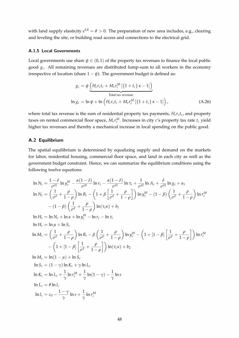
with land supply elasticity LSε = θ > 0. The preparation of new area includes, e.g., clearingand leveling the site, or building road access and connections to the electrical grid.

A.1.5 Local Governments

Local governments use share ψ ∈ (0, 1) of the property tax revenues to finance the local publicgood gc. All remaining revenues are distributed lump-sum to all workers in the economyirrespective of location (share 1− ψ). The government budget is defined as:( )

gc = ψ Hcrctc + McrM [{1 + tc}c κ − 1]︸︷︷︸( Total tax revenue )ln g M

c = ln ψ + ln Hcrctc + Mcrc [{1 + tc} κ − 1] , (A.26)

where total tax revenue is the sum of residential property tax payments, Hcrctc, and propertytaxes on rented commercial floor space, McrM

c . Increases in city c’s property tax rate tc yieldhigher tax revenues and thereby a mechanical increase in local spending on the public good.

A.2 Equilibrium

The spatial equilibrium is determined by equalizing supply and demand on the marketsfor labor, residential housing, commercial floor space, and land in each city as well as thegovernment budget constraint. Hence, we can summarize the equilibrium conditions using thefollowing twelve equations:

1− δ W α(1− δ) α(1− δ) 1 δln Nc = ln y − r −c ln c ln τc + ln Ac + ln gc + a1(σH σH σH σH σH) ( [ ]) ( )

1 ρ 1 ρ 1 ρln N ln B 1 ln yW M

c = + c − + β + − −F 1 F 1 c (1 β) + ln rσ − ρ σ − ρ σF 1 c− ρ( )

1 ρ− (1− β) + ln(τσF 1 cκ) + b1− ρ

ln Hc = ln N Wc + ln α + ln y −c ln rc − ln τc

ln Hc = ln µ + ln Sc( ) ( ) ( [ ])1 ρ 1 ρ ρ

ln Mc = + ln B W 1 Mc − β + ln y − −F 1 c 1 + [1 β] + ln r

σ − ρ σF 1− ρ σF 1 c− ρ( [ ])1 ρ− 1 + [1− β] + ln(τ

σF 1 cκ) + b2− ρ

ln Mc = ln(1− µ) + ln Sc

ln Sc = (1− γ) ln Kc + γ ln Lc

1ln K M 1 1

c = ln Lc + ln rc + ln(1− γ)− ln sγ γ γ

ln Lc = θ ln lc

1− γ 1ln lc = c0 − ln s + ln rM

cγ γ

48

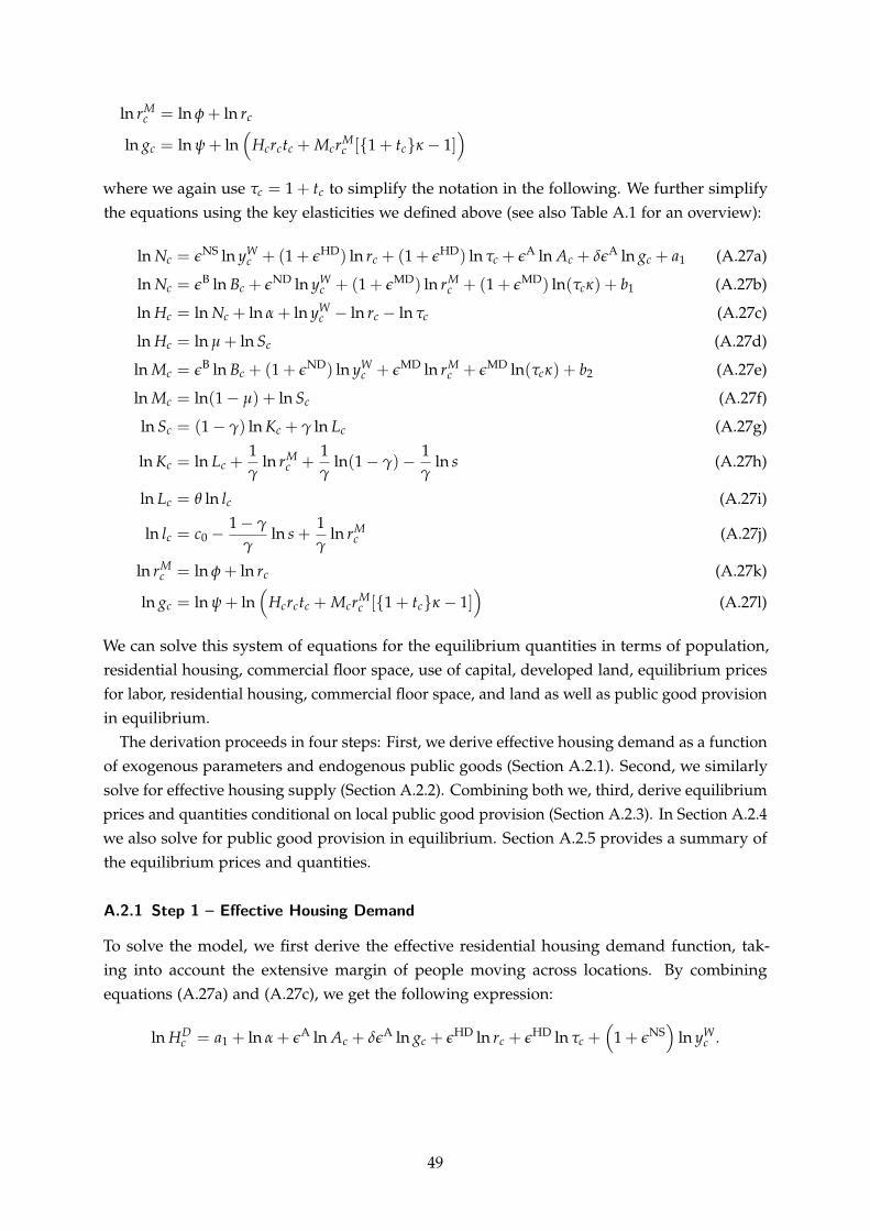
ln rMc = ln φ + ln rc( )

ln gc = ln ψ ln Hcrctc + McrM+ c [{1 + tc}κ − 1]

where we again use τc = 1 + tc to simplify the notation in the following. We further simplifythe equations using the key elasticities we defined above (see also Table A.1 for an overview):

ln N NSc = ε ln yW HD HD A A

c + (1 + ε ) ln rc + (1 + ε ) ln τc + ε ln Ac + δε ln gc + a1 (A.27a)

ln N B ln B ND ln yW 1 MD ln rM 1 MDc = ε c + ε c + ( + ε ) c + ( + ε ) ln(τcκ) + b1 (A.27b)

ln Hc = ln N Wc + ln α + ln y −c ln rc − ln τc (A.27c)

ln Hc = ln µ + ln Sc (A.27d)

ln M Bc = ε ln B ND

c + (1 + ε ) ln yW MDc + ε ln rM MD

c + ε ln(τcκ) + b2 (A.27e)

ln Mc = ln(1− µ) + ln Sc (A.27f)

ln Sc = (1− γ) ln Kc + γ ln Lc (A.27g)1

ln Kc = ln Lc + ln rM 1 1c + ln(1− γ)− ln s (A.27h)

γ γ γ

ln Lc = θ ln lc (A.27i)1− γ 1

ln l c ln s ln rMc = 0 − + c (A.27j)

γ γ

ln rMc = ln φ + ln rc (A.27k)( )

ln gc = ln ψ + ln Hcrctc + M Mcr {c [ 1 + tc}κ − 1] (A.27l)

We can solve this system of equations for the equilibrium quantities in terms of population,residential housing, commercial floor space, use of capital, developed land, equilibrium pricesfor labor, residential housing, commercial floor space, and land as well as public good provisionin equilibrium.

The derivation proceeds in four steps: First, we derive effective housing demand as a functionof exogenous parameters and endogenous public goods (Section A.2.1). Second, we similarlysolve for effective housing supply (Section A.2.2). Combining both we, third, derive equilibriumprices and quantities conditional on local public good provision (Section A.2.3). In Section A.2.4we also solve for public good provision in equilibrium. Section A.2.5 provides a summary ofthe equilibrium prices and quantities.

A.2.1 Step 1 – Effective Housing Demand

To solve the model, we first derive the effective residential housing demand function, tak-ing into account the extensive margin of people moving across locations. By combiningequations (A.27a) and (A.27c), we get the following expression: ( )

ln HDc = a1 + ln Aα + ε ln A A

c + δε ln g HD HD NS Wc + ε ln rc + ε ln τc + 1 + ε ln yc .

49

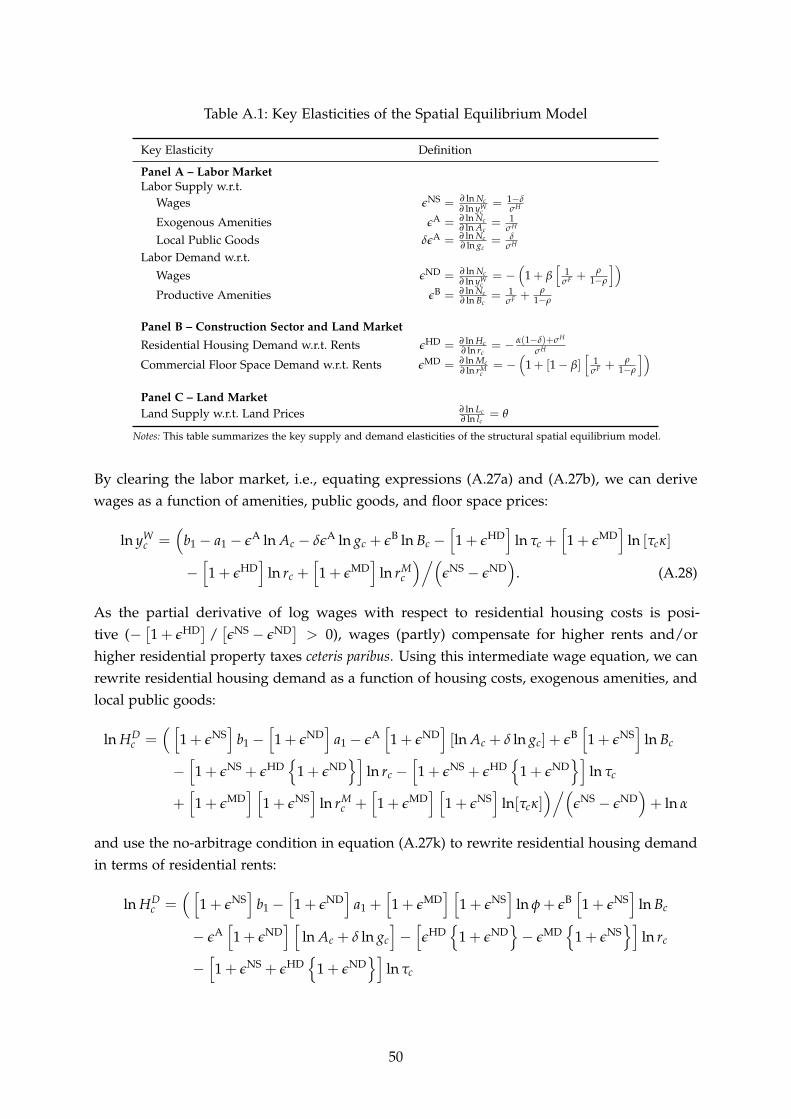
Table A.1: Key Elasticities of the Spatial Equilibrium Model

Key Elasticity Definition

Panel A – Labor MarketLabor Supply w.r.t.

Wages εNS = ∂ ln Nc∂ ln yW

c= 1−δ

σH

Exogenous Amenities εA = ∂ ln Nc∂ ln Ac

= 1σH

Local Public Goods δεA = ∂ ln Nc∂ ln gc

= δσH

Labor Demand w.r.t.Wages εND = ∂ ln Nc

∂ ln yWc= −

(1 + β

[1

σF +ρ

1−ρ

])Productive Amenities εB = ∂ ln Nc

∂ ln Bc= 1

σF +ρ

1−ρ

Panel B – Construction Sector and Land Market

Residential Housing Demand w.r.t. Rents εHD = ∂ ln Hc∂ ln rc

= − α(1−δ)+σH

σH

Commercial Floor Space Demand w.r.t. Rents εMD = ∂ ln Mc∂ ln rM

c= −

(1 + [1− β]

[1

σF +ρ

1−ρ

])Panel C – Land MarketLand Supply w.r.t. Land Prices ∂ ln Lc

∂ ln lc= θ

Notes: This table summarizes the key supply and demand elasticities of the structural spatial equilibrium model.

By clearing the labor market, i.e., equating expressions (A.27a) and (A.27b), we can derivewages as a function of amenities, public goods, and floor space prices:( [ ] [ ]

ln yW b A= − a1 − ε ln A Ac − ε ln g B

c c + ε ln B HD MD1 δ c − 1 + ε ln τc + 1 + ε ln [τcκ][ ] [ ] )/( )− 1 HD MD M NS ND+ ε ln rc + 1 + ε ln rc ε − ε . (A.28)

As the partial derivative of log wages with respect to residential housing costs is posi-[ ] [ ]tive ( 1 HD / NS ND− + ε ε − ε > 0), wages (partly) compensate for higher rents and/orhigher residential property taxes ceteris paribus. Using this intermediate wage equation, we canrewrite residential housing demand as a function of housing costs, exogenous amenities, andlocal public goods:( [ ] [ ] [ ] [ ]

ln HDc = 1 NS ND A ND B NS+ ε b1 − 1 + ε a1 − ε 1 + ε [ln Ac + δ ln gc] + ε 1 + ε ln Bc[ { }] [ { }]

1 NS HD+ 1 ND NS HD ND− ε + ε + ε ln rc − 1 + ε + ε 1 + ε ln τc[ ] [ ] [ ] [ ] )/( )MD+ 1 + ε 1 NS+ ε ln rM

c + 1 MD+ ε 1 NS NS ND+ ε ln[τcκ] ε − ε + ln α

and use the no-arbitrage condition in equation (A.27k) to rewrite residential housing demandin terms of residential rents:( [ ] [ ] [ ] [ ] [ ]

ln HD 1 NS b 1 ND NS+ 1 MD−c = + ε 1 + ε a + 1 NSε + ε ln B1 φ + ε 1 + ε ln Bc[ ] [ ] [ { } { }]

A− 1 ND+ ε Ac + δ ln g HDc − ε 1 ND MD NSε ln + ε − ε 1 + ε ln rc[ { }]

− 1 NS HD+ ε + ε 1 ND+ ε ln τc

50

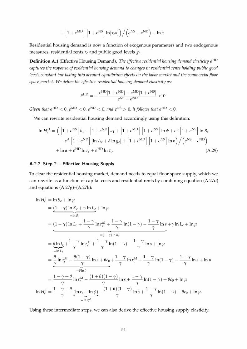
[ ] [ ] )/( )MD NS NS ND+ 1 + ε 1 + ε ln[τcκ] ε − ε + ln α.

Residential housing demand is now a function of exogenous parameters and two endogenousmeasures, residential rents rc and public good levels gc.

Definition A.1 (Effective Housing Demand). The effective residential housing demand elasticity ε̃HD

captures the response of residential housing demand to changes in residential rents holding public goodlevels constant but taking into account equilibrium effects on the labor market and the commercial floorspace market. We define the effective residential housing demand elasticity as:

HDHD ε [1 ND MD NS+ ε ]− ε [1 + ε ]

ε̃ = − < 0.εNS − εND

Given that HD MD ND NS HDε < 0, ε < 0, ε < 0, and ε > 0, it follows that ε < 0.

We can rewrite residential housing demand accordingly using this definition:( [ ] [ ] [ ] [ ] [ ]ln HD 1 NS MD NS

c b ND B= + ε 1 − 1 + ε a1 + 1 ε 1 + ε ln NS+ φ + ε 1 + ε ln Bc[ ] [ ] [ ] )/( )A ND NS− ε 1 + ε ln A + ln g MD NS ND[ c δ c] + 1 + ε 1 + ε ln κ ε − ε

+ ln α + ε̃HD ln rc + ε̃HD ln τc. (A.29)

A.2.2 Step 2 – Effective Housing Supply

To clear the residential housing market, demand needs to equal floor space supply, which wecan rewrite as a function of capital costs and residential rents by combining equation (A.27d)and equations (A.27g)–(A.27k):

ln HSc = ln Sc + ln µ

= (1− γ) ln Kc + γ ln L︸︷︷︸c + ln µ

=ln Sc

1− γ M 1− γ 1− γ= (1− γ) ln Lc + ln rc + ln(1− γ)− ln s+γ ln Lc + ln µ

γ γ γ︸︷︷︸=(1−γ) ln Kc

1− γ − −ln l ln rM 1 γ 1 γ

= θ c + ln(1 )−c + − γ ln s + ln︸︷︷︸ µγ γ γ

=ln Lc

θ M θ(1− γ) 1− γ γ= ln r − ln s + θc0 + rM 1− 1− γ

ln + ln(1− −c c γ) ln s + ln µγ γ γ γ γ︸︷︷︸

=θ ln lc

1− γ + θ M (1 + θ)(1− γ) 1− γ= ln r −c ln s + ln(1− γ) + θc0 + ln µ

γ γ γ

1− γln HS + θ (1 + θ)(1− γ) 1− γ

c = (ln rc + ln φ)− ln s + ln(1− γ) + θc + ln µ.γ ︸︷︷︸ 0

γ γM=ln rc

Using these intermediate steps, we can also derive the effective housing supply elasticity.

51

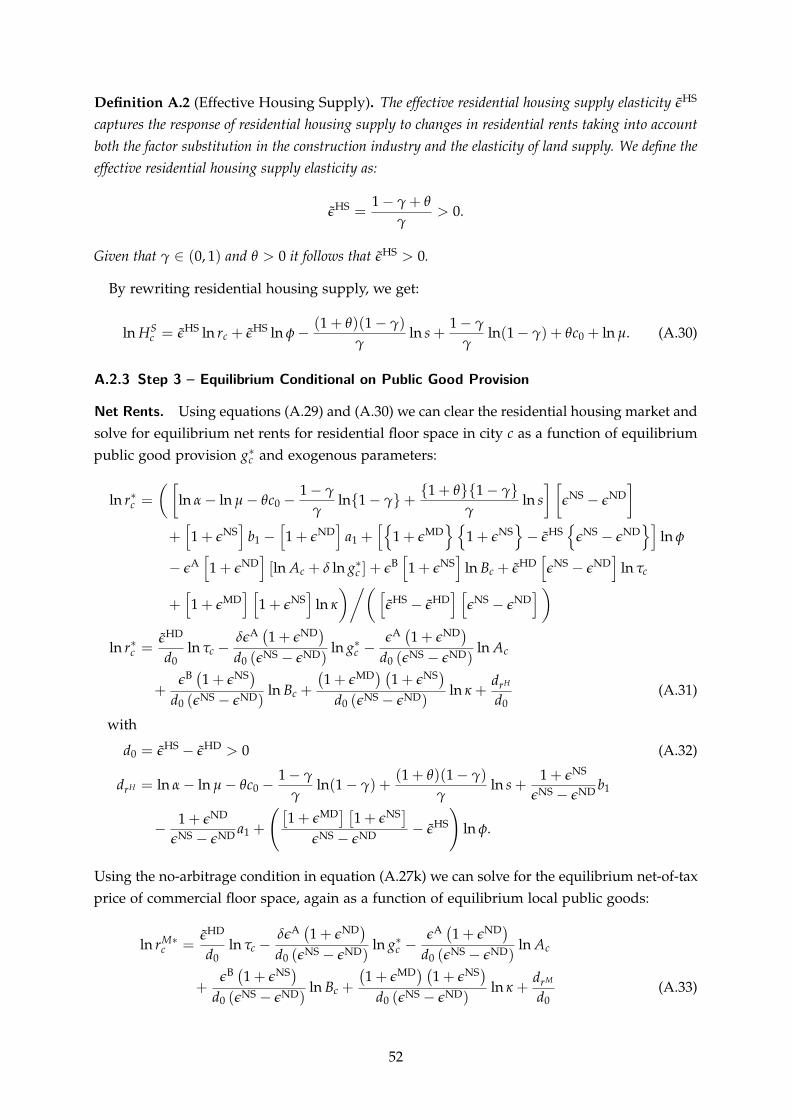
Definition A.2 (Effective Housing Supply). The effective residential housing supply elasticity ε̃HS

captures the response of residential housing supply to changes in residential rents taking into accountboth the factor substitution in the construction industry and the elasticity of land supply. We define theeffective residential housing supply elasticity as:

ε̃HS 1− γ + θ= > 0.

γ

Given that HSγ ∈ (0, 1) and θ > 0 it follows that ε̃ > 0.

By rewriting residential housing supply, we get:

ln HS HS HS (1 + θ)(1− γ) 1− γ− −c = ε̃ ln rc + ε̃ ln φ ln s + ln(1 γ) + θc0 + ln µ. (A.30)γ γ

A.2.3 Step 3 – Equilibrium Conditional on Public Good Provision

Net Rents. Using equations (A.29) and (A.30) we can clear the residential housing market andsolve for equilibrium net rents for residential floor space in city c as a function of equilibriumpublic good provision g∗c and exogenous parameters:( [ ] [ ]

∗ 1− γ {1 + θ}{1− γ}ln r ln NS ND= α−c ln µ− θc0 − ln{1− γ}+ ln s ε − ε

γ γ[ ] [ ] [{ }{ } { }]1 NS+ + ε b1 − 1 ND a NS

1 + 1 MD+ ε 1 + ε − ε̃HS NS ND+ ε ε − ε ln φ[ ] [ ] [ ]A ND B NS HD NS ND− ε 1 + ε [ln A + δ ln g∗c c ] + ε 1 + ε ln Bc + ε̃ ε − ε ln τc[ ] [ ] )/( [ ] [ ] )

MD+ 1 + ε 1 NS+ ε ln κ ε̃HS − ε̃HD NS NDε − ε( ) ( )˜HD A ND A

∗ ε δε 1 + ε 1 NDε + εln rc = ln τc − ln

εNS − εND g∗ −d c ln A

0 d0 ( ) d c0 (εNS − εND)( ) ( ) ( )B 1 NS MD NSε + ε 1 + ε 1 + ε d

ln r+ lnH

κ + (A.31)d NS Bc +ND NS ND0 (ε − ε ) d0 (ε − ε ) d0

with

d HD0 ε̃HS= − ε̃ > 0 (A.32)

1 NS− γ (1 + θ)(1− γ) 1 + εd H = ln α− ln µ− θc0 −r ln(1− γ) + ln s +

γ γ εNS − εND b1([ ] [ ] )1 ND MD NS+ ε 1 + ε 1 + ε

+ − ε̃HS− a1 ln φ.εNS − εND εNS − εND

Using the no-arbitrage condition in equation (A.27k) we can solve for the equilibrium net-of-taxprice of commercial floor space, again as a function of equilibrium local public goods:( ) ( )

ln rM∗ ε̃HD A Aδε 1 ND+ ε ε 1 ND+ εc = ln τc − ln lnNS0 (εNS − εND g∗ −

d0 d c A) d c

0 (ε − εND)( ) ( ) ( )Bε 1 NS MD NS+ ε 1 + ε 1 + ε d+ ln B rM

c + ln κ + (A.33)d (εNS − εND) d0 (εNS − εND0 ) d0

52

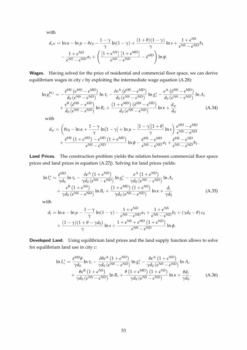
with

1− γ (1 + θ)(1 NS− γ) 1 + εd M = ln α− ln µ− −r θc0 ln(1− γ) + ln s + 1

γ γ εNS b− εND([ ] [ ] )1 ND+ ε 1 NS+ ε 1 MD+ ε

− a HD1 + − ε̃ ln φ.

εNS − εND εNS − εND

Wages. Having solved for the price of residential and commercial floor space, we can deriveequilibrium wages in city c by exploiting the intermediate wage equation (A.28):( ) ( ) ( )

˜HS HD MD A HS MD A MD−∗ ε ε ε δε ε̃ HS− ε ∗ ε ε̃ − εln yW

c = − ln τ lnd c − − ln

(εNS − εND) d c(εNS A

εND gc0 0 − ) d0 (εNS − εND)( ) ( ) ( )Bε ε̃HS HD− ε 1 MD+ ε ε̃HS HD− ε d

ln w+ c + ln κ + (A.34)

d (εNS B− εND) d (εNS − εND0 0 ) d0

with ( )1 MD− γ [1− ][1 HDγ + θ] ε − ε

dw = θc0 − ln α + ln[1− γ] + ln µ− ln sγ γ εNS − εND( ) ( )

˜HS MDε 1 HD HD+ ε − ε 1 + HS HDε ε̃ MD− ε ε̃HS − ε+ ln φ− a1 + b1.

εNS − εND εNS − εND εNS − εND

Land Prices. The construction problem yields the relation between commercial floor spaceprices and land prices in equation (A.27j). Solving for land prices yields:( ) ( )

HDε̃ A ND A+ εln ∗ δε 1 1 NDε + ε

lc = ln τc − lnd c

γ NS ND g∗ −d c ln

γ NS ND A0 ( 0 (ε − ε ) γd (ε − ε )) ( ) ( 0 )Bε 1 NS MD NS+ ε 1 + ε 1 + ε d

ln B ln l+γd c + κ + (A.35)

εNS − εND0 ( ) γd NS ND0 (ε − ε ) γd0

with

1− γ 1 ND NS+ ε 1 + εdl = ln α− ln µ− ln(1− γ)− a1 + b1 + (γd0 − θ) c0

γ εNS − εND εNS − εND( )1 1 d 1 NS HD ND( − γ)( + θ − γ 0) + ε + ε 1 + ε

+ ln s + ln φ.γ εNS − εND

Developed Land. Using equilibrium land prices and the land supply function allows to solvefor equilibrium land use in city c: ( ) ( )A

∗ ˜HD NDε θ θε 1 ND Aδ + ε εL = ln τc − ln g∗

θ 1 + εln −c γd γd ( NS − εND c ln c

ε ) γd (εNS ND A0 0 0 − ε )( ) ( ) ( )B NS MD NSθε 1 + ε θ 1 + ε 1 + ε θd

ln B ln l+ c + κ + . (A.36)γd0 (εNS − εND) γd NS0 (ε − εND) γd0

53

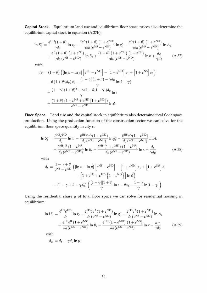
Capital Stock. Equilibrium land use and equilibrium floor space prices also determine theequilibrium capital stock in equation (A.27h):( ) ( )ND

∗ ε̃HD(1 A A ND+ θ) δε (1 + θ) 1 + ε ε (1 + θ) 1 + εln Kc = ln τc − ln g∗ −

d ND c lnγd γ (εNS A

0 0 − ε ) γd c0 (εNS − εND)( ) ( ) ( )Bε (1 + θ) 1 NS+ ε (1 + θ) 1 MD NS+ ε 1 + ε d

+ lnNS ND B ln Kc + κ + (A.37)

γd0 (ε − ε ) γd0 (εNS − εND) γd0

with ( [ ] [ ] [ ] )d 1 ln ln NS ND ND NS

K = ( + θ) [ α− µ] ε − ε − 1 + ε a1 + 1 + ε b1

(1− γ)(1 + θ)− γd0− θ (1 + θγd0) c0 − ln(1− γ)γ

2(1− γ)(1 + θ) − γ(1 + θ[1− γ])d0+ ln s

γ( [ ])(1 + θ) 1 NS HDε + ε 1 ND+ + ε

+ ln φ.εNS − εND

Floor Space. Land use and the capital stock in equilibrium also determine total floor spaceproduction. Using the production function of the construction sector we can solve for theequilibrium floor space quantity in city c:

HS HD HS A ND HS A ND∗ ε̃ ε̃ ε̃ δε (1 + ε ) ε̃ ε (1 + ε )

ln S = ln τc − ln g∗ −c d0 d0 (εNS − εND c ln) d NS ND Ac( ) ( ) ( 0 (ε − ε ))

ε̃HS B NS HS MDε 1 NS+ ε ε̃ 1 + ε 1 + ε d+ ln

d0 (εNS − εND Bc + ln Sκ + (A.38)

) d0 (εNS − εND) γd0

with ( [ ] [ ] [ ]1− γ + θdS = [ln α− ln NS NDµ] ε − ε − 1 ND+ ε

εNS ND a1 + 1 NS+ ε b1− ε [ { }] )1 NS HD 1 ND+ + ε + ε + ε ln φ( )

[1− γ][1 + θ] 1− γ+ (1− γ + θ − γd0) ln s− θc0 − ln[1− γ] .

γ γ

Using the residential share µ of total floor space we can solve for residential housing inequilibrium:

˜HS ˜HD ˜HS A NDε 1 HS Aε ε δε ( + ε ) ε̃ ε (1 ND+ ε )ln H∗c = ln τc − lnNS ND g∗ − A

d0 d c ln(ε − ε ) d c

(εNS − εND)( )0 ( ) ( 0 )˜HS B 1 NS ˜HS MD NSε ε + ε ε 1 + ε 1 + ε d

+ ln B + ln Hκ + (A.39)

d cND0 (εNS − ε ) d0 (εNS − εND) γd0

with

dH = dS + γd0 ln µ.

54

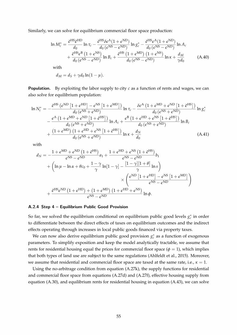
Similarly, we can solve for equilibrium commercial floor space production:

˜HS ˜HD ˜HS A 1 ND HS+ ˜ A∗ ε ε ε (1 NDε δε ( ε ) ∗ ε + ε )

ln M − −c = ln τ lnd εNS g

d c c ln Ac0 0 ( − εND) d NS ND( ) ( ) ( 0 (ε − ε ))

ε̃HS Bε 1 NS HSε ε̃ 1 MD+ + ε 1 NS+ ε d+ ln B M

c + ln κ + (A.40)d (εNS − εND) d (εNS − εND0 0 ) γd0

with

dM = dS + γd0 ln(1− µ).

Population. By exploiting the labor supply to city c as a function of rents and wages, we canalso solve for equilibrium population:( [ ] [ ]) ( [ ])

˜HS ND 1 HD NS 1 MD A MD ND HSε ε + −∗ ε ε + ε δε 1 + ε + ε 1 + ε̃ln N = − ∗

c ln τd c − ln

(εNS + εND) d0 (εNS cεND g0 + )( [ ]) ( [ ])Aε 1 MD ND HS B HD NS HS+ ε + ε 1 + ε̃ ε 1 + ε + ε 1 + ε̃

− lnd c + ln c

(εNS + εND A NS0 d0 (ε + εND B) )( ) ( [ ])

1 MD HD NS HS+ ε 1 + ε + ε 1 + ε̃ dN+ ln κ + (A.41)d (εNS + εND0 ) d0

with ( ) ( )1 MD ND HS HD NS HS+ ε + ε 1 + ε̃ 1 + ε + ε 1 + ε̃

dN = −εNS a1 + b1( − εND εNS − εND )

1− γ [1− γ][1 + θ]+ ln µ− ln α + θc0 + ln[1− γ]− ln s

γ γ( [ ] [ ])ND MDε 1 HD NS+ ε − ε 1 + ε×

εNS − εND( ) ( ) ( )ε̃HS NDε 1 HD+ ε + 1 MD+ 1 HD NSε + ε + ε

+ ln φ.εNS − εND

A.2.4 Step 4 – Equilibrium Public Good Provision

So far, we solved the equilibrium conditional on equilibrium public good levels g∗c in orderto differentiate between the direct effects of taxes on equilibrium outcomes and the indirecteffects operating through increases in local public goods financed via property taxes.

We can now also derive equilibrium public good provision g∗c as a function of exogenousparameters. To simplify exposition and keep the model analytically tractable, we assume thatrents for residential housing equal the prices for commercial floor space (φ = 1), which impliesthat both types of land use are subject to the same regulations (Ahlfeldt et al., 2015). Moreover,we assume that residential and commercial floor space are taxed at the same rate, i.e., κ = 1.

Using the no-arbitrage condition from equation (A.27k), the supply functions for residentialand commercial floor space from equations (A.27d) and (A.27f), effective housing supply fromequation (A.30), and equilibrium rents for residential housing in equation (A.43), we can solve

55

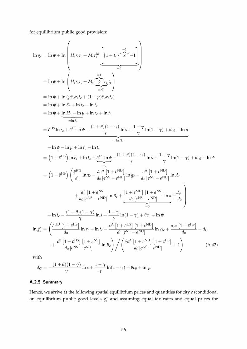
for equilibrium public good provision: = ︷︸︸1 ︷ ln gc = ln Mψ + lnH crctc + Mcr { }c 1 + tc κ −1 ︸︷︷︸ =tc

︷=︸︸1︷ = ln ψ + lnHcrctc + Mc φ r︸︷︷︸c tc

=rMc

= ln ψ + ln (µScrctc + (1− µ)Scrctc)

= ln ψ + ln Sc + ln rc + ln tc

= ln ψ + ln Hc − ln µ+ ln r︸︷︷︸ c + ln tc

=ln Sc

1−HS HS (1 + θ)( γ) 1− γ= ε̃ ln rc + ε̃ ln φ− ln s + ln(1− γ) + θc0 + ln µ

γ γ︸︷︷︸=ln Hc

+ ln ψ− ln µ + ln rc + ln tc( )HS HS (1 + θ)(1− γ) 1− γ

= 1 + ε̃ ln rc + ln tc + ε̃ ln φ− ln s + ln(1− γ) + θc ln︸︷︷︸ 0 + ψγ γ( =0[ ] [ ]( ) ˜HD A NDε δε 1 A+ ε ε

= 1 HS 1 ND+ ε+ ε̃ ln τ − ln g − ln A

d c0 d c

0 [εNS − εND] d c0 [εNS − εND] [ ] [ ] [ ]B MDε 1 NS + ε 1 NS+ ε 1 + ε d H

+ lnd0 [ε − εND Bc + ln rκ +NS ] d NS ND ︸ 0 [ε − ε ] d︷︷︸ 0

=0

(1 + θ)(1− γ) 1− γ+ ln tc − ln s + ln(1− γ) + θc0 + ln ψ

γ γ( [ ] [ ] [ ] [ ]˜HD 1 ˜HS A HS ND

∗ ε + ε ε 1 + ε̃ 1 + ε drH 1 + ε̃HSln g = ln τc + ln tc −c ln +

d c0 [εNS − εND A + d

d0 ] d G0[ ] [ ] )/( [ ] [ ] )

Bε 1 + ˜HS NDε 1 NS A HS+ ε δε 1 + ε 1 + ε̃+ ln 1

d c[εNS − εND B + (A.42)

] d [εNS − εND0 0 ]

with

(1 + θ)(1− γ) 1− γdG = − ln s + ln(1− γ) + θc0 + ln ψ.

γ γ

A.2.5 Summary

Hence, we arrive at the following spatial equilibrium prices and quantities for city c (conditionalon equilibrium public good levels g∗c and assuming equal tax rates and equal prices for

56

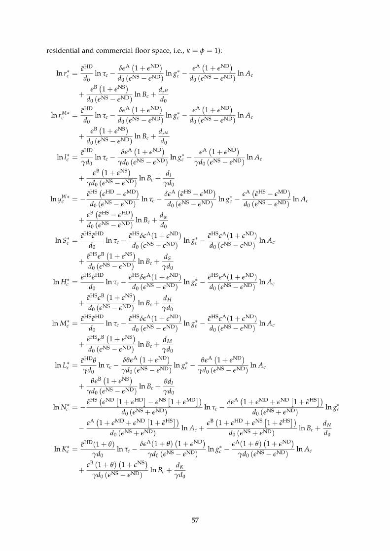
residential and commercial floor space, i.e., κ = φ = 1):( ) ( )ND A∗ ε̃HD A NDδε 1 + ε

r = ln ∗ ε 1 + εln c τc − ln g −c ln

d NS A0 d c

0 (ε − εND) d0 (εNS − εND)( )Bε 1 NS+ ε d+ ln B rH

+d c

0 (εNS − εND) d( ) 0 ( )A A ND∗ ε̃HD NDδε 1 + ε ε 1 + ε

ln rM ln τc −c = lnd d NS ND g∗ −c ln

0 0 (ε ε ) d c− 0 εNS − εND A( )( )B NSε 1 + ε d

+ lnd0 (εNS − εND B rM

c +) d( )0 ( )

ln l∗ε̃HD A 1 ND Aδ + ε ∗ ε 1 NDε + ε

− −c = ln τ lnεNS − εND g

d c c lnγ γd c

( ) γd (εNS − εND A0 0 0 )( )Bε 1 NS+ ε dl+ ln

γd0 (εNS − ND Bc +ε ) γd( ) 0 ( ) ( )

˜HS HD MD A HS MDε − ε δε ε −ln yW ˜HS MD A−∗ ε ε

= − ln τ − ln g∗ε ε̃ ε

c d c −NS ND d NS ND c lnNS0 (ε − ε ) 0 (ε − ε ) d0 (ε − εND Ac)( )Bε ε̃HS HD− ε dw

+ lnd0 (εNS Bc +− εND) d0

˜HS ˜HD ˜HS A ND∗ ε ε ε δε (1 HS A+ ε ) ε̃ ε (1 ND+ ε )

ln S = ln τc −c lnNS ND g∗ −d0 d c ln

0 (ε − ε ) d (εNS − εND Ac0 )( )

˜HS B 1 NSε ε + ε d+ ln

d0 (ε − εND B Sc +NS ) γd0

∗ ε̃HS ˜HD Aε ε̃HSδε (1 ND HS A+ ε ) ε̃ ε (1 ND+ ε )ln Hc = ln τ −

d c − ln g∗d c ln Ac

0 0 (εNS − εND) d0 (εNS − εND)( )˜HS Bε ε 1 NS+ ε d

+ ln B H+d c

0 (εNS − εND) γd0A

∗ ε̃HSε̃HD ε̃HSδε (1 ND HS A ND+ ε ) ε̃ ε (1 + ε )ln Mc = ln τ − ln ∗

εND g −d c c ln

0 d0 (εNS − ) d0 (εNS Ac− εND)( )ε̃HS Bε 1 NS+ ε d

+ ln M

d c +(εNS ND B

0 − ε ) γd( )0 ( )A ND∗ ε̃HD A NDθ δθε 1 + ε= ln τ

d c ln g∗θε 1 + ε

ln L − −c d c ln Ad c

γ εND0 γ (εNS − ) γ (εNS − εND)( )0 0Bθε 1 NS+ ε θdl+ ln +

γd c(εNS − εND B

0 ) γd( [ ] [ 0 ]) ( [ ])HS ND HD NS MD A MD ND HS∗ ε̃ ε 1 + ε − ε 1 + ε δε 1 + ε + ε 1 + ε̃

ln N −c = ln τc − lnNS ND NS ND g∗d0 (ε + ε ) d c

0 (ε + ε )( [ ]) ( [ ])A MD ND HSε 1 HS B HD NS+ ε + ε 1 + ε̃ ε 1 + ε + ε 1 + ε̃ d− ln A ln B Nc +d d c +NS0 (εNS + εND) 0 (ε + εND) d( ) ( ) 0

HD A ND A ND∗ ε̃ (1 + θ) δε (1 + θ) 1 + ε ∗ ε (1 + θ) 1 + ε

ln Kc = ln τ gγd c − ln −c ln A

0 γd c0 (εNS − εND) γd NS ND( ) 0 (ε − ε )

Bε (1 + θ) 1 NS+ ε d+ ln B K+

γd c0 (εNS − εND) γd0

57

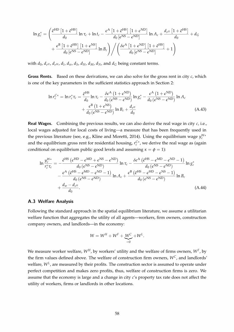
( [ ] [ ] [ ] [ ]∗ ε̃HD 1 ND+ ε̃HS A HSε 1 + ε̃ 1 + ε d 1 + ε̃HS

ln g c + ln −c = ln τ tc ln A rH

c + +d d [εNS − εND d

0 0 ] d G0[ ] [ ] )/( [ ] [ ] )

B HS NS A ND HSε 1 + ε̃ 1 + ε δε 1 + ε 1 + ε̃+ ln B + 1

d cεNS − εND0 [ ] d0 [εNS − εND]

with d0, drH , drM , dl , dw, dS, dH, dM, dN , and dG being constant terms.

Gross Rents. Based on these derivations, we can also solve for the gross rent in city c, whichis one of the key parameters in the sufficient statistics approach in Section 2:( ) ( )

HS∗ ε̃ A ND A ND

∗ δε + ε ε + εln rC 1

= ln r = ln τ − ln −c c τ g∗1

c ln Ad c

0 d0 (εNS ND c− ε ) d c0 (εNS − εND)( )Bε 1 NS+ ε drH

+ lnd NS − εND Bc + (A.43)

0 (ε ) d0

Real Wages. Combining the previous results, we can also derive the real wage in city c, i.e.,local wages adjusted for local costs of living—a measure that has been frequently used inthe previous literature (see, e.g., Kline and Moretti, 2014). Using the equilibrium wage yW∗

c

and the equilibrium gross rent for residential housing, rC∗c , we derive the real wage as (again

conditional on equilibrium public good levels and assuming κ = φ = 1):( ) ( )yW∗ ˜HS HD MD NS ND A HS MD NDε ε − ε + ε − ε δε ε −c ˜ ε − ε − 1

ln = − ln τ − ∗r∗c τ d c ln

0 (εNS − εND gc ) d NS ND c( ) ( 0 (ε − ε ))Aε ε̃HS MD ND B HS HD NS− ε − ε − 1 ε ε̃ − ε − ε − 1− ln Ac + ln

d (εNS − εND0 ) d0 (εNS − εND Bc)

dw − drH+ . (A.44)

d0

A.3 Welfare Analysis

Following the standard approach in the spatial equilibrium literature, we assume a utilitarianwelfare function that aggregates the utility of all agents—workers, firm owners, constructioncompany owners, and landlords—in the economy:

W WH WF C= + + W WL︸︷︷︸+ .=0

We measure worker welfare, WH, by workers’ utility and the welfare of firms owners, WF, bythe firm values defined above. The welfare of construction firm owners, WC, and landlords’welfare, WL, are measured by their profits. The construction sector is assumed to operate underperfect competition and makes zero profits, thus, welfare of construction firms is zero. Weassume that the economy is large and a change in city c’s property tax rate does not affect theutility of workers, firms or landlords in other locations.

58

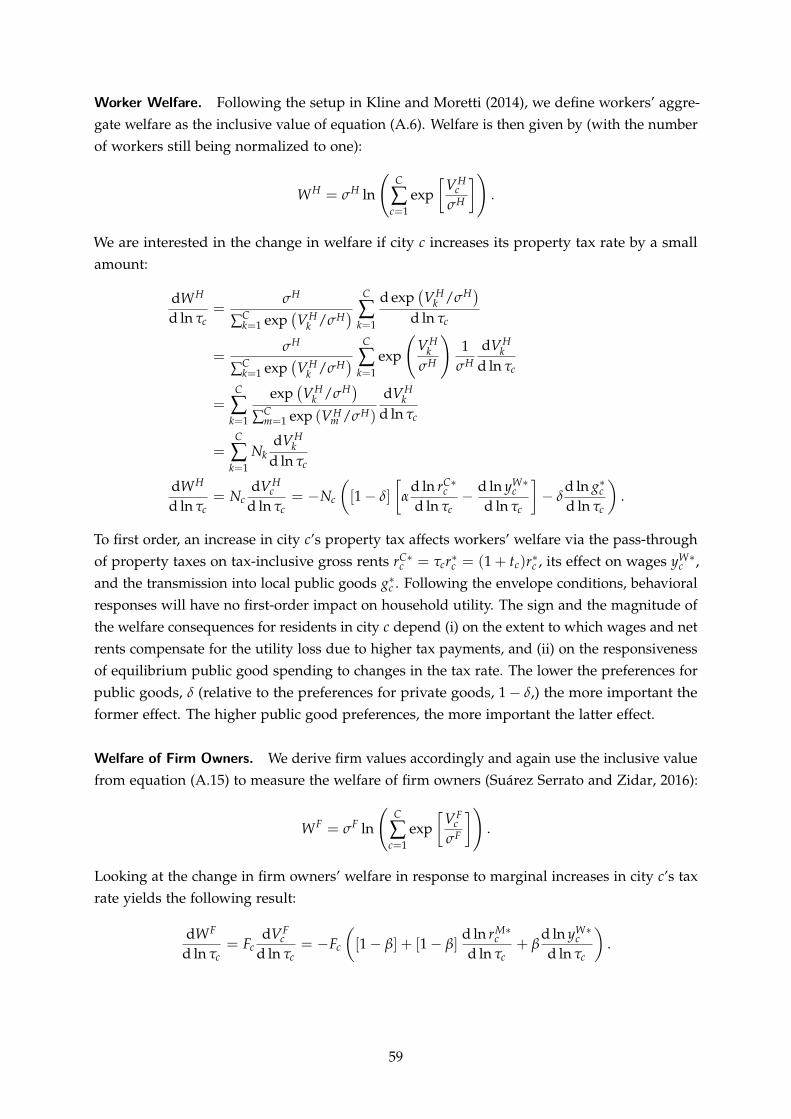
Worker Welfare. Following the setup in Kline and Moretti (2014), we define workers’ aggre-gate welfare as the inclusive value of equation (A.6). Welfare is then given by (with the numberof workers still being normalized to one): (

C [ ])HWH H V

= σ ln ∑ exp c .σH

c=1

We are interested in the change in welfare if city c increases its property tax rate by a smallamount: ( )

dWH H Cσ d exp VH Hσ( ) ∑ k /=

d ln τc ∑Ck=1 exp VH

k /σHk= d ln τ1 c( )

H Cσ VHk 1 dVH

= ( )Ck VH ∑ exp k

∑ 1 exp k /σH σH σH d ln τc= k( =1)C exp VH

= ∑ k / Hσ dVHk

∑C exp (VH Hk=1 m=1 m /σ ) d ln τc

C dVH= ∑ N k

k=

d ln τk 1 c ( [dWH C∗ )

dVH W∗ ] ∗N c d ln r d ln y d ln g

= c = −N 1 c c c−d ln τc d ln c [ − δ] α − δ .

τc d ln τc d ln τc d ln τc

To first order, an increase in city c’s property tax affects workers’ welfare via the pass-throughof property taxes on tax-inclusive gross rents rC∗

c = τcr∗c = (1 + t ∗c)rc , its effect on wages yW∗

c ,and the transmission into local public goods g∗c . Following the envelope conditions, behavioralresponses will have no first-order impact on household utility. The sign and the magnitude ofthe welfare consequences for residents in city c depend (i) on the extent to which wages and netrents compensate for the utility loss due to higher tax payments, and (ii) on the responsivenessof equilibrium public good spending to changes in the tax rate. The lower the preferences forpublic goods, δ (relative to the preferences for private goods, 1− δ,) the more important theformer effect. The higher public good preferences, the more important the latter effect.

Welfare of Firm Owners. We derive firm values accordingly and again use the inclusive valuefrom equation (A.15) to measure the welfare of firm owners (Suárez Serrato and Zidar, 2016):(

C [ ])FWF F V

σ ∑ exp c= ln .σF

c=1

Looking at the change in firm owners’ welfare in response to marginal increases in city c’s taxrate yields the following result: ( )

dWF dVF d ln rM∗c c d ln yW∗

= Fc = −F [1− β] + [1 c− β] + β .d ln τc d ln c

τc d ln τc d ln τc

59

A change in the property tax rate thus operates via (i) the impact on local wages yW∗c , and

(ii) the impact on the gross price of commercial floor space κ(1 + tc)rM∗c = κτcrM∗

c . The changein the welfare of firm owners thus depends on the share of the tax burden that can be passedon to landlords in terms of lower net prices for commercial floor space and the share that canbe shifted to workers via lower wages. Both effects are weighted according to their importancein the production function governed by the Cobb-Douglas parameter β.

Welfare of Construction Company Owners. The welfare of firm owners in the constructionindustry is given by their profits based on equation (A.23):

C C ( )WC ∑ ΠC ∑ rM= c = ∗

c S∗ −c sK∗ −c l∗c L∗c = 0.c=1 c=1

Property tax increases yield lower sales in the construction industry because workers and firmsdemand less floor space S∗ and every unit is sold at a lower price rM∗

c c . Construction firms reactby decreasing their demand for land, L∗c , and capital, K∗c , and thus the price of land, l∗c , willdecrease as well. With some algebra, one can show that WC evaluates to zero in equilibriumand construction firms still make zero profits irrespective of the tax as long as we assumeprice-taking behavior and constant returns to scale (see, e.g., Thorsnes, 1997, Epple et al., 2010,Combes et al., 2017).

Welfare of Land Owners. Since construction companies operate in a perfectly competitivemarket, landlord welfare will be determined by the impact on land owners. We denote landowners’ profits by producer surplus as in Kline and Moretti (2014), i.e., the area between landprices and the inverse land supply function defined in equation (A.25). We normalize thisnumber with the size of the nationwide land market denoted by Λ: ︷=l∗

L∗︸︸c︷

C ∫ c( ) ( ) 1

L 1 1∗ 1 C L∗1 1+ C L∗ L θ

W c θ 1 θ ∗ c c= lΛ ∑ − ∗ ∗ − ∗ ∗ −

c u θ du = ∑ lc Lc =1 ∑ lc Lc + θc=1 Λ c=1 1 + Λ 1 10 θ c= ∗

L 1 C lc L∗W =

Λ ∑ c .c=1 1 + θ

Tax increases in city c reduce the welfare of land owners according to the following expression:( )dWL 1 d ∗

= l∗L∗c

d ln τc 1 c + L∗dlc

+ θ) d ln c( Λ τ( c d ln τc )1 ∗d exp [ln L∗

= l c ] exp [ln l∗c ](1 c + L∗

dc+ θ)Λ d ln τc d ln τ( c )

1 ∗d exp [ln L∗c ] d ln L∗ ∗c ] d ln l

= l c d exp [ln l ∗c + L∗ c

c(1 + θ)Λ d ln L∗c d ln τ d ln ∗c lc d ln τ( ) c

1 d ln L∗ d ln l∗= l∗ ∗ c

(1 + θ)Λ c L + L∗ln c l∗ c

c d cτc d ln τc

60

( )l∗ ∗c L ∗

c d ln L∗c d ln lc= +(1 + θ)Λ d ln τc d ln τc

dWL l∗ ∗ ∗ ∗ ∗ ∗c Lc d ln rc lc Lc d ln lc d ln l

= = = Λ c ,d ln τc γΛ d ln τc Λ d ln c

τc d ln τc

where Λc denotes the share of local land sales l∗c L∗c relative to the nationwide land market Λ.The stronger the impact of property taxes on land prices and the more severe the reduction inland demand due to higher taxes, the bigger the welfare loss for land owners. As their welfareis decreasing in the land supply elasticity (see denominator), landlords will only bear partof the tax burden as long as the supply of land ready for construction is not perfectly elastic.Otherwise landlords make zero profits and won’t bear any tax burden.

Summary. After deriving the welfare impact of property tax increases for all four groups ofagents, we summarize the welfare consequences in the following Proposition A.1:

Proposition A.1 (Welfare Effects in the Structural Model). Let WH, WF, WC, and WL denote thewelfare of workers, firm owners, constructors, and land owners in the spatial equilibrium, respectively.The welfare changes of a marginal increase in city c’s property tax rate tc are determined by:

(i) the elasticities of equilibrium rents, land prices, and wages with respect to the property tax rate,

(ii) the responsiveness of the local public good provision in equilibrium with respect to the tax,

(iii) three exogenous model parameters, namely the housing share in consumption, α, the labor share inthe tradable good production, β, and the preferences for local public goods, δ.

This result is based on the four welfare predictions (each evaluated for a single household):( [ ] )dWH d ln rC∗ d ln

= − [1 c d ln yW∗ ∗c gc− δ] α − − δ (A.45)

d ln τc d ln τc d ln τc d ln τ( c

dWF d ln rM∗ )c d ln yW∗

c= − [1− β] + [1− β] + β (A.46)d ln τc d ln τc d ln τc

dWC= 0 (A.47)

d ln τc

dWL d ln l∗c= . (A.48)d ln τc d ln τc

The analysis shows that workers’ marginal welfare loss from tax hikes decreases in thepreference for the local public good, δ. Hence, the stronger the preferences for public goodsand the stronger the transmission of taxes into public good spending, the smaller the welfareloss as workers are compensated for rising costs of living. Proposition A.1 implies that the rent,land price, wage, and public good elasticities with respect to the property tax are sufficientto infer the welfare effects of the tax in a local labor market model (given the housing sharein consumption, the labor share in production, and the preferences for public goods). In thefollowing, we discuss the comparative statics behind these elasticities.

61

A.4 Comparing Welfare Predictions

In this section we compare the welfare predictions that arise from the sufficient statisticsapproach in Proposition 1 to those from the structural representation of the spatial equilibriummodel derived in Proposition A.1. To illustrate differences and similarities between theseresults, we elaborate on the welfare effects separately for each group of agents putting theequations from both propositions side-by-side.

Workers. We start the discussion by comparing the impact of small property tax increases onhousehold utility in both approaches. The first of the following two equations illustrates the re-sults for workers’ welfare from Proposition A.1, the second equation restates the correspondingresult from the sufficient statistics approach:( [ ] )

dWH d ln rC∗ W= − [1 c d ln y ∗

c d ln g∗c− δ] α − − δ (A.49a)d ln τc d ln τ( c d ln τc d ln τ[ ] ) c

v v drC∂ ∂ ∗∆ i i v

W i= − h∗ c dy∗i ∂ dg∗ci − −

∂y i , (A.49b)∂y dtc dt g dt︸︷︷c︸ ∂ c

Wdy ∗= i

dtc

where we multiply the latter equation by the marginal utility from income for better compara-bility across equations.

Both results lead to the same prediction regarding the impact on household utility, consistingof three components. First, household utility decreases in the pass-through of taxes intotax-inclusive gross rents (d ln rC∗

c /d ln τc in the structural model, drC∗c /dtc in the sufficient

statistics approach). This effect is scaled by the importance of housing expenditures in overallconsumption (via the housing expenditure share α in the structural model and the size ofthe dwelling h∗i in the sufficient statistics approach) and the preferences for private goodconsumption (denoted by 1− δ in the structural model and ∂vi/∂y in the sufficient statisticsapproach).

Second, household utility increases in the responsiveness of local wages to property taxincreases (d ln yW∗

c /d ln τc in the structural model, dy∗i /dtc in the sufficient statistics approach),again weighted by households’ marginal utility from income. In the structural model, weassumed that renter households only receive income from wage earnings, excluding otherincome channels by assumption.

Third, household utility increases when additional tax revenues are used for higher publicgood provision (d ln g∗c /d ln τc in the structural model, dg∗c /dtc in the sufficient statisticsapproach). In contrast to rents and wages, this effect is weighted by households’ preferencesfor public goods (denoted by δ in the structural model and ∂vi/∂g in the sufficient statisticsapproach).

62

Firm Owners. When comparing the implications on household utility for firm owners in bothapproaches, we arrive at the following two results:( )

dWF d ln rM∗c d ln yW∗

c= − [1− β] + [1− β] + β (A.50a)d ln τc d ln τc d ln τ( ) c[ ]

v v drC∂ i ∂ ∗ ∗ ∗∆W i i

i − h∗ c dyi ∂v dgc= − −i , (A.50b)∂y ∂y dtc dt︸︷c g dt︸︷︷︸︷︸ ∂︸︷︷ c︸

=0 Fdy ∗ =i 0= dtc

where we again multiply the result from Proposition 1 with the marginal utility from incomefor better comparability. Since the structural approach relied on the assumption that firmowners are absent from the city and thus not affected by rent changes or additional publicgood provision, utility changes in equation (A.50a) are solely determined by the impact onfirm profits. Translated to the sufficient statistics prediction, this closes down the first andthe third term on the right-hand side of equation (A.50b) by assumption. Only the impact onhousehold income—reflected in the second term on the right-hand side (dy∗i /dtc)—remains inthe equation, reflecting the change in business profits just as in the structural model.

Landlords. Finally, we compare the impact of property tax increases on landlords’ utility:

dWL d ln l∗c= (A.51a)d ln τc d ln τ( c [ )

∂v C∗i ∂vi c dy∗

]∗dr i ∂vi dg∗

∆Wi = − h c− −∂y ∂y i . (A.51b)

dt︸︷︷ c dt︸︸︷︷c︸ ∂g dt︸︷︷ c︸=0 Ldy ∗ =0

= idtc

In the structural model, we equalized landlord utility with consumer surplus on the landmarket, which decreases in proportion to decreases in the land price for small tax changes.As for firm owners, we followed the standard assumption in the spatial equilibrium literatureand assumed landlords to live abroad and thus be unaffected by changes other than thosereflecting income from the housing market. When applying this assumption to the sufficientstatistics approach, equation (A.51b) simplifies to the impact of property taxes on landlordincome, dyL∗

i /dtc.

Summary. The welfare predictions for the three groups of agents yield very similar resultsregarding the impact of small property tax increases on household utility. This similarityreflects the virtue of sufficient statistics approaches: they allow to abstract from deep structuralmodeling assumptions while still offering clear-cut results on the welfare effects of policychanges.

63

A.5 Comparative Statics

Using the equilibrium outcomes derived in Section A.2 we can take a closer look at thecomparative statics in the model. In Section A.5.1, we first analyze the effects of tax increaseson the key determinants for welfare effects laid out in the previous section. In a second step, wederive comparative statics of other equilibrium prices in Section A.5.2. Finally, in Section A.5.3we discuss comparative statics for equilibrium quantities.

A.5.1 Key Determinants for Welfare Effects

As stated in Proposition A.1 on the welfare effects in our structural equilibrium model, we areparticularly interested in four elasticities: the elasticity of gross rents with respect to propertytax changes, the elasticity of local wages with respect to property tax changes, the elasticityof land prices with respect to property tax changes, and the elasticity of local public goodprovision with respect to property tax changes. In the following, we discuss the comparativestatics for each of these four elasticities.

Local Public Goods. We start by studying the impact of property tax increases on local publicgoods, which is given by the following formula:

d ln g∗ c (tc, r∗ ∗

c, g {c τc}c [τ ]) ∂ ln g∗ ∗c ∂ ln t ∗ ∂ ln r ∗ ∗

c ∂ ln gc c ∂ ln rc d ln gc = +lnτ ln ln r∗

+ c ln t ln g d ln ︸∂ ︷︷ c ln ∗︸︸∂ ︷︷τ︸c ∂ ∂ ∂ τ︸︷︷ c︸︸︷︷τc︸︸︷︷ c︸ c

>0 >0 >0 <0( <)0/ ( )d ln g∗ (1 + tc) /tc ˜HD 1 + ε̃HSε εc ˜HS HD− ε̃

= + . (A.52)d ln τ A ND HS A ND HS

c δε (1+ε )(1+ε̃ ) δε (1+ε )(1+ε̃ )( ˜HS HD NS + +ε −ε̃ )(ε − ND 1

ε ) ( −ε̃HD)( NSε − ND 1ε̃HS ε )

This effect on equilibrium public good provision in city c can thus be decomposed in (i) apositive mechanical effect through higher revenues from taxing the existing housing stock atcurrent prices, and (ii) a countervailing behavioral effect on the tax base reflecting that highertaxes decrease prices and quantities traded on both floor space markets.

Just as in the standard Laffer curve argument, the higher the property tax rate tc, the moreimportant the second, behavioral channel distorting the tax base relative to the mechanicalrevenue effect. The total effect of tax increases on public good spending will be positive as longas the tax rate is sufficiently small:

d ln g∗ HS HDc ε̃ − ε̃> 0 ⇔ t <

d ln c − .τc ε̃HS (1 + ε̃HD)

In the following, we turn to the elasticities of gross rents, wages, and land prices with respectto property tax increases making use of this intermediate result to disentangle the differentdriving forces underlying the model.

64

Gross Rents. The effect of property tax increases on equilibrium tax-inclusive gross rents forresidential and commercial floor space in city c is given by the following formula:

d ln rC∗ (τ , g∗ [τ ]) d ln τ r∗ ∗c c c c c c (τc, gc [τc]) d ln crMτ ∗ ∗

c (τc, gc [τc])= =

d ln τc d ln τc d ln τc

∂ ln rC∗ ∂ ln rC∗ ∗c c d ln gc= +

∂ ln τc ∂ ln g∗c d ln τc( ) ε̃HD(1 ε̃HS+ ) 1HS A tε̃ δε 1 ND+ ε HS HD + + c

ε̃ −ε̃ t= − c . (A.53)ε̃HS − ε̃HD︸︷︷︸ (ε̃HS − ε̃HD) (εNS − εND) A ND HSδε (1+ε )(1+ε̃ )︸︷︷︸ + 1︸( HSε̃ −ε̃HD)( NSε − NDε )

>0 >0 ︷︷︸Q0

The impact of tax increases on consumer price rents (d ln rC∗c /d ln τc) can be decomposed into

two effects: (i) a direct effect reflecting the pass-through of tax increases in consumer pricerents that depends on the relative elasticities of (effective) housing supply and housing demandas in the standard textbook incidence model, and (ii) an indirect effect operating throughthe transmission of tax revenue into local public goods and the capitalization of public goodprovision in local prices. Figure A.1 illustrates these two effects. Panel A shows the partial,direct effect reflecting the standard tax incidence mechanism. The more mobile households areand the more elastic housing demand, the lower (higher) will be the direct pass-through oftax increases in consumer (producer) price rents. Panel B depicts the indirect effect and showshow the analysis changes when higher taxes lead to additional local public good provision,which is capitalized in rents and increases local cost-of-living. The indirect effect countervailsthe decrease in housing demand triggered by the tax increase—thereby raising consumer pricerents even further and alleviating the reduction in producer price rents. This latter effect willbe positive as long as public good spending increases in the tax rate.

Wages. Third, the effect of property tax increases on equilibrium wages is given by:

d ln yW∗c (τc, g∗c [τc]) ∂ ln yW∗

c ∂ ln yW∗c d ln g∗c= +

d ln τc ∂ ln τ ∗c ∂ ln gc d ln τc( ) ( ) HD(1 HSε̃ +ε̃ )˜HS HD MD A HS MD 1+tε ε − ε δε ε̃ − ε HS HD + c

˜ ˜ t= − − ε −ε c . (A.54)d (εNS − εND) d (εNS − εND) Aδε (1+ NDε )(1+ ˜HS︷︷︸︸ 0 ε )︸ 0 ︷︷︸ HD NS ND +︸( HS 1

ε̃ −ε̃ )(ε︷︷−ε ) ︸Q0 <0

Q0

The total effect of property tax increases on equilibrium wages in city c can be decomposedin (i) a direct effect that is potentially compensating for higher costs of living due to the taxincrease, and (ii) an indirect effect operating through higher local public good provision. Botheffects may potentially be smaller or larger than zero, the sign being theoretically undeterminedin both cases.

Tax increases trigger two opposing effects for profit maximizing firms in the city. On theone hand, higher property tax payments raise the factor price of commercial floor space and

65

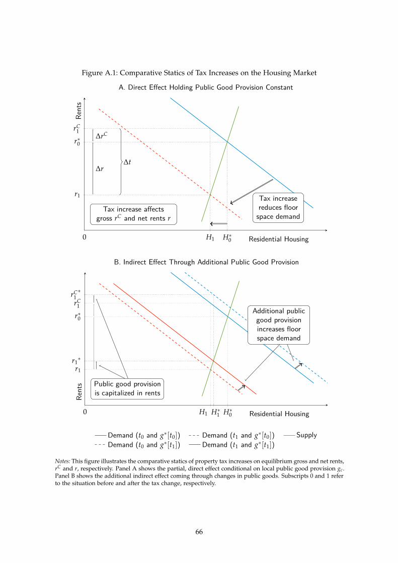
Figure A.1: Comparative Statics of Tax Increases on the Housing Market

0 H∗0H1

r∗0

r1

rC1

Tax increasereduces floorspace demand

∆rC

∆r∆t

Tax increase affectsgross rC and net rents r

Residential Housing

Rents

A. Direct Effect Holding Public Good Provision Constant

0 H1 H∗1 H∗0

r1

r1∗

r∗0

rC1

rC1∗

Public good provisionis capitalized in rents

Additional publicgood provisionincreases floorspace demand

Residential Housing

Rents

B. Indirect Effect Through Additional Public Good Provision

Demand (t0 and g∗[t0]) Demand (t1 and g∗[t0]) SupplyDemand (t0 and g∗[t1]) Demand (t1 and g∗[t1])

Notes: This figure illustrates the comparative statics of property tax increases on equilibrium gross and net rents,rC and r, respectively. Panel A shows the partial, direct effect conditional on local public good provision gc.Panel B shows the additional indirect effect coming through changes in public goods. Subscripts 0 and 1 referto the situation before and after the tax change, respectively.

66

firms thus try to re-optimize by using less floor space relative to labor. On the other hand,property taxes make it more costly for workers to live in city c and residents demand higherwages to compensate for increased costs of living. Without compensating wage increases,inframarginal workers will move to other places. The sign and the magnitude of the two directeffects of tax increases on wages are determined by the relative strength of the residential andthe commercial floor space demand elasticity, HDε and MDε , respectively.

The indirect effect again operates through the capitalization of public goods into wages anddepends on the extent to which tax increases yield additional public good spending at the locallevel. As long as higher taxes raise the level of public good provision, the indirect channel willlead to lower wages, since workers are compensated via additional amenities.

Figure A.2 illustrates both the direct and the indirect effect for the impact of tax increaseson wage earnings (d ln yW∗/d ln τc). Tax increases lead to rising consumer price rents, whichreduces the attractiveness of the city for workers; their labor supply to the city decreases (seePanel A). Taxes also increase the factor price of commercial floor space and reduce firms’ floorspace demand, which lowers the marginal product of labor and thus decreases labor demand.Panel A illustrates the case where workers are more responsive and wages increase in responseto the tax. The indirect effect through additional public good spending operates in the oppositedirection and makes the city more attractive for both workers and firms (see Panel B).

Land Prices. Finally, we derive the effect of property tax increases on equilibrium land prices:

d ln l∗c (τc, g∗c [τc]) ∂ ln l∗c ∂ ln l∗c d ln g∗c= +d ln τc ∂ ln τc ∂ ln g∗c d ln τc ( ) HDε̃ (1 HS+ε̃ ) 1HD A 1 ND +t

HS HD + cε̃ δε + ε ˜− ε̃ t= −ε c .γ (ε̃HS − ε̃HD) γ (ε̃HS − ε̃HD) (εNS − εND) Aδ )(1+ ˜HSε (1+ NDε ε )︸︷︷︸︸︷︷︸ (ε̃HS−ε̃HD)( NS ND + 1

ε ε )<0 >0 ︸︷︷− ︸

Q0

(A.55)

The total effect of property tax increases on equilibrium land prices in city c (d ln l∗c /d ln τc) canagain be decomposed in (i) a direct, negative effect that reflects lower construction activity andreduced land use in the construction sector due to the tax increase, and (ii) an indirect effectoperating through higher local public good provision, where the sign is again theoreticallyundetermined. This indirect effect depends on the impact of public goods on land prices(second term in the last equation) and the degree to which tax increases raise the public goodprovision (last term in the equation). This latter effect will be positive as long as public goodspending increases in the tax rate.

The reasoning behind the negative direct effect is that less land is needed for constructionif population levels, floor space demand, and the housing stock decrease. As a result, landprices decrease as well to balance supply and demand, and to reach a new equilibrium on themarket for land ready for development. This direct effect is again potentially diminished byan indirect effect operating through increases in local public goods, which would make city c

67

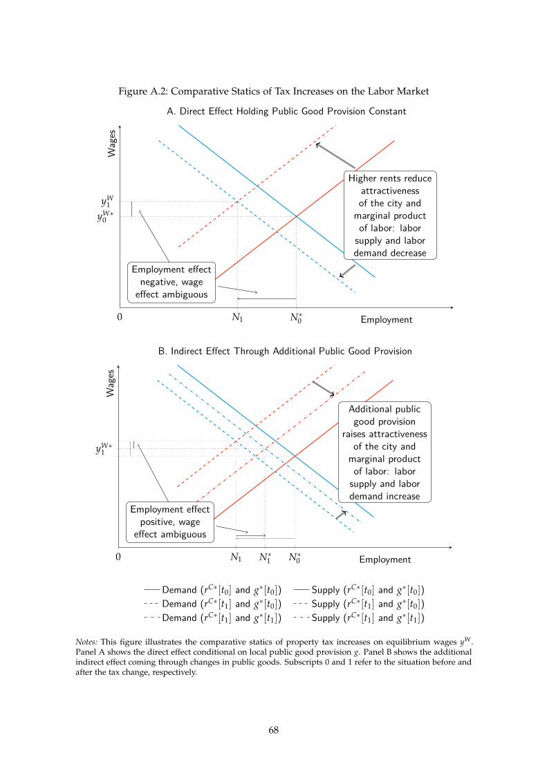
Figure A.2: Comparative Statics of Tax Increases on the Labor Market

0 N1 N∗0

yW∗0

yW1

Employment effectnegative, wageeffect ambiguous

Higher rents reduceattractivenessof the city andmarginal productof labor: laborsupply and labordemand decrease

Employment

Wages

A. Direct Effect Holding Public Good Provision Constant

0 N1 N∗1 N∗0

yW∗1

Employment effectpositive, wage

effect ambiguous

Additional publicgood provision

raises attractivenessof the city andmarginal productof labor: laborsupply and labordemand increase

Employment

Wages

B. Indirect Effect Through Additional Public Good Provision

Demand (rC∗[t0] and g∗[t0]) Supply (rC∗[t0] and g∗[t0])Demand (rC∗[t1] and g∗[t0]) Supply (rC∗[t1] and g∗[t0])Demand (rC∗[t1] and g∗[t1]) Supply (rC∗[t1] and g∗[t1])

Notes: This figure illustrates the comparative statics of property tax increases on equilibrium wages yW .Panel A shows the direct effect conditional on local public good provision g. Panel B shows the additionalindirect effect coming through changes in public goods. Subscripts 0 and 1 refer to the situation before andafter the tax change, respectively.

68

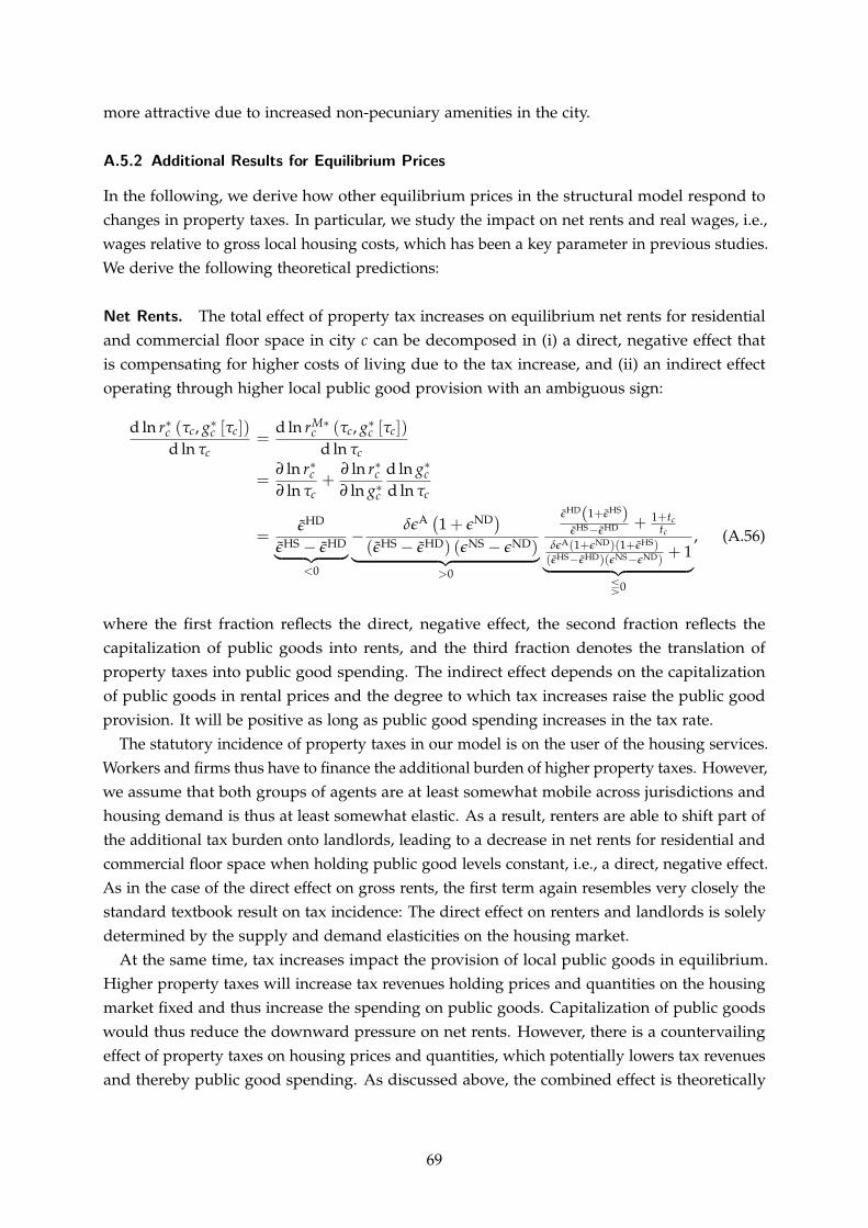
more attractive due to increased non-pecuniary amenities in the city.

A.5.2 Additional Results for Equilibrium Prices

In the following, we derive how other equilibrium prices in the structural model respond tochanges in property taxes. In particular, we study the impact on net rents and real wages, i.e.,wages relative to gross local housing costs, which has been a key parameter in previous studies.We derive the following theoretical predictions:

Net Rents. The total effect of property tax increases on equilibrium net rents for residentialand commercial floor space in city c can be decomposed in (i) a direct, negative effect thatis compensating for higher costs of living due to the tax increase, and (ii) an indirect effectoperating through higher local public good provision with an ambiguous sign:

d ln r∗c (τ ∗ M∗ ∗c, gc [τc]) d ln rc (τc, gc [τc])

=d ln τc d ln τc

∂ ln r∗c ∂ ln r∗c d ln g∗c= +∂ ln τc ∂ ln g∗c d ln τc ( ) ˜HDε (1 HS+ε̃ )A 1HD +t˜ δε 1 ND+ ε cε ˜HS

= ε ˜HD + t− −ε c , (A.56)˜HS︸ε − HD︷︷ ε̃ ︸ (ε̃HS − ε̃HD) (εNS − εND) A ND HSδε (1+ε )(1+ε̃ )︸︷︷︸ + 1︸( HSε̃ − ˜HD NSε )( NDε ε )

< >0 ︷︷−0 ︸Q0

where the first fraction reflects the direct, negative effect, the second fraction reflects thecapitalization of public goods into rents, and the third fraction denotes the translation ofproperty taxes into public good spending. The indirect effect depends on the capitalizationof public goods in rental prices and the degree to which tax increases raise the public goodprovision. It will be positive as long as public good spending increases in the tax rate.

The statutory incidence of property taxes in our model is on the user of the housing services.Workers and firms thus have to finance the additional burden of higher property taxes. However,we assume that both groups of agents are at least somewhat mobile across jurisdictions andhousing demand is thus at least somewhat elastic. As a result, renters are able to shift part ofthe additional tax burden onto landlords, leading to a decrease in net rents for residential andcommercial floor space when holding public good levels constant, i.e., a direct, negative effect.As in the case of the direct effect on gross rents, the first term again resembles very closely thestandard textbook result on tax incidence: The direct effect on renters and landlords is solelydetermined by the supply and demand elasticities on the housing market.

At the same time, tax increases impact the provision of local public goods in equilibrium.Higher property taxes will increase tax revenues holding prices and quantities on the housingmarket fixed and thus increase the spending on public goods. Capitalization of public goodswould thus reduce the downward pressure on net rents. However, there is a countervailingeffect of property taxes on housing prices and quantities, which potentially lowers tax revenuesand thereby public good spending. As discussed above, the combined effect is theoretically

69

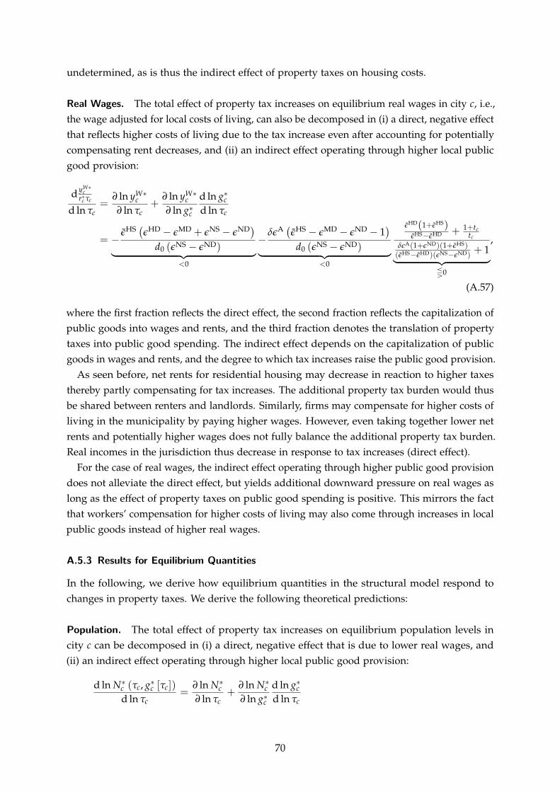
undetermined, as is thus the indirect effect of property taxes on housing costs.

Real Wages. The total effect of property tax increases on equilibrium real wages in city c, i.e.,the wage adjusted for local costs of living, can also be decomposed in (i) a direct, negative effectthat reflects higher costs of living due to the tax increase even after accounting for potentiallycompensating rent decreases, and (ii) an indirect effect operating through higher local publicgood provision:

d yW∗c

r∗c τc ∂ ln yW∗c ∂ ln yW∗

c d ln g∗c= +d ln τc ∂ ln τc ∂ ln g∗c d ln τc( ) ( ) ˜HD 1+ ˜HSε ( ε )HS HD NS NDε̃ MD A HS MD ND 1+t

ε − ε + ε − ε δε ε̃ − ε − ε − 1 ε̃HS + c−ε̃HD t= − − c

d (εNS − εND) d (εNS − εND) A(1+ ND HS ,0 0 δε ε )(1+ε̃ )︸︷︷︸︸︷︷︸ HS +︸(ε̃ − HDε̃ )( NSε − ND 1

ε )<0 <0 ︷︷︸

Q0

(A.57)

where the first fraction reflects the direct effect, the second fraction reflects the capitalization ofpublic goods into wages and rents, and the third fraction denotes the translation of propertytaxes into public good spending. The indirect effect depends on the capitalization of publicgoods in wages and rents, and the degree to which tax increases raise the public good provision.

As seen before, net rents for residential housing may decrease in reaction to higher taxesthereby partly compensating for tax increases. The additional property tax burden would thusbe shared between renters and landlords. Similarly, firms may compensate for higher costs ofliving in the municipality by paying higher wages. However, even taking together lower netrents and potentially higher wages does not fully balance the additional property tax burden.Real incomes in the jurisdiction thus decrease in response to tax increases (direct effect).

For the case of real wages, the indirect effect operating through higher public good provisiondoes not alleviate the direct effect, but yields additional downward pressure on real wages aslong as the effect of property taxes on public good spending is positive. This mirrors the factthat workers’ compensation for higher costs of living may also come through increases in localpublic goods instead of higher real wages.

A.5.3 Results for Equilibrium Quantities

In the following, we derive how equilibrium quantities in the structural model respond tochanges in property taxes. We derive the following theoretical predictions:

Population. The total effect of property tax increases on equilibrium population levels incity c can be decomposed in (i) a direct, negative effect that is due to lower real wages, and(ii) an indirect effect operating through higher local public good provision:

d ln N∗c (τc, g∗c [τ ∗ ∗ ∗c]) ∂ ln Nc ∂ ln Nc d ln gc= +

d ln τc ∂ ln τ ∂ ln g∗c c d ln τc

70

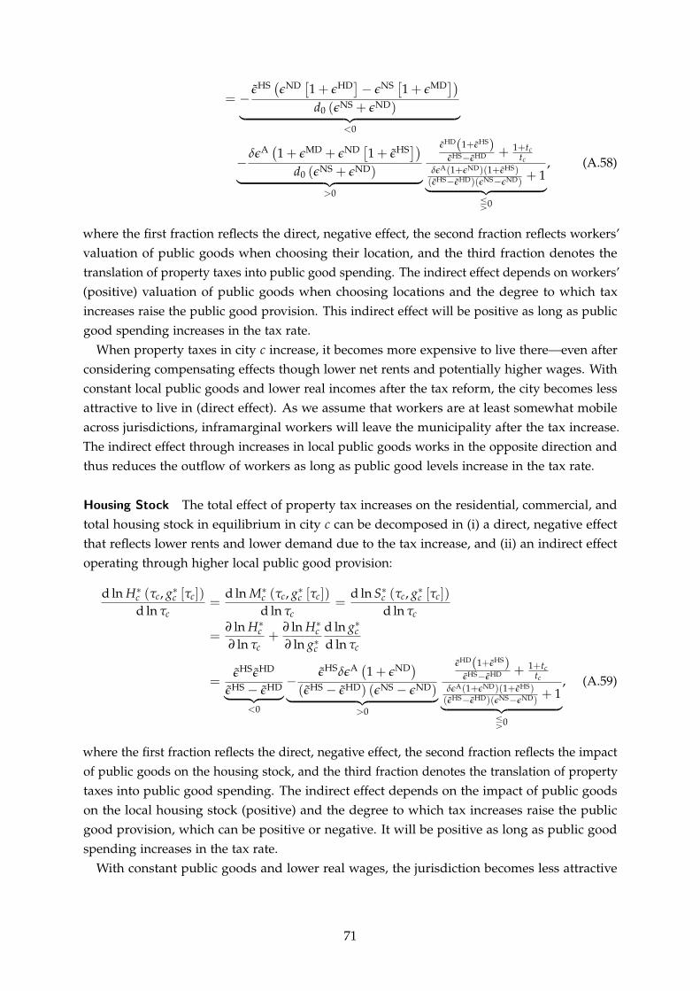
( [ ] [ ])ε̃HS ND HDε 1 NS+ ε − ε 1 MD+ ε

= −d0 (εNS + εND)︸︷︷︸

<0( [ ]) ε̃HD(1+ε̃HS)A NDδε 1 MD HS 1+t+ ε + ε 1 + ε̃ c

˜HS t− ε −ε̃HD +c , (A.58)

d (εNS + εND) Aδε (1+ NDε )(1+ ˜HS︸ 0 ε )︷︷︸ (ε̃HS−ε̃HD + 1︸ )( NS NDε︷︷−ε )>0 ︸

Q0

where the first fraction reflects the direct, negative effect, the second fraction reflects workers’valuation of public goods when choosing their location, and the third fraction denotes thetranslation of property taxes into public good spending. The indirect effect depends on workers’(positive) valuation of public goods when choosing locations and the degree to which taxincreases raise the public good provision. This indirect effect will be positive as long as publicgood spending increases in the tax rate.

When property taxes in city c increase, it becomes more expensive to live there—even afterconsidering compensating effects though lower net rents and potentially higher wages. Withconstant local public goods and lower real incomes after the tax reform, the city becomes lessattractive to live in (direct effect). As we assume that workers are at least somewhat mobileacross jurisdictions, inframarginal workers will leave the municipality after the tax increase.The indirect effect through increases in local public goods works in the opposite direction andthus reduces the outflow of workers as long as public good levels increase in the tax rate.

Housing Stock The total effect of property tax increases on the residential, commercial, andtotal housing stock in equilibrium in city c can be decomposed in (i) a direct, negative effectthat reflects lower rents and lower demand due to the tax increase, and (ii) an indirect effectoperating through higher local public good provision:

d ln H∗c (τc, g∗c [τc]) d ln M∗c (τc, g∗c [τc]) d ln S∗ (τ , g∗c c c [τc])= =

d ln τc d ln τc d ln τc∂ ln H∗c ∂ ln H∗c d ln g∗c= +∂ ln τc ∂ ln g∗c d ln τc ( ) ε̃HD(1 HS+ε̃ )˜HS HD HS A NDε ε̃ ε̃

1+tδε 1 + ε + c

HS− HDε̃ ε̃ t= − c , (A.59)ε̃HS ˜︸ − εHD HS ˜︸ (ε̃︷︷ − εHD) (εNS − εND) Aδε (1+ NDε )(1+ε̃HS)︸︷︷︸ HS HD NS ND +

ε − 1( ˜ −ε̃ )(ε ε )

<0 >0 ︸︷︷︸Q0

where the first fraction reflects the direct, negative effect, the second fraction reflects the impactof public goods on the housing stock, and the third fraction denotes the translation of propertytaxes into public good spending. The indirect effect depends on the impact of public goodson the local housing stock (positive) and the degree to which tax increases raise the publicgood provision, which can be positive or negative. It will be positive as long as public goodspending increases in the tax rate.

With constant public goods and lower real wages, the jurisdiction becomes less attractive

71

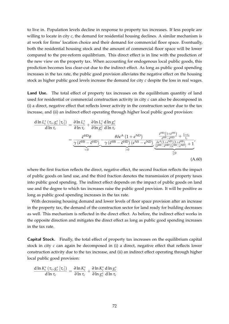
to live in. Population levels decline in response to property tax increases. If less people arewilling to locate in city c, the demand for residential housing declines. A similar mechanism isat work for firms’ location choice and their demand for commercial floor space. Eventually,both the residential housing stock and the amount of commercial floor space will be lowercompared to the pre-reform equilibrium. This direct effect is in line with the prediction ofthe new view on the property tax. When accounting for endogenous local public goods, thisprediction becomes less clear-cut due to the indirect effect. As long as public good spendingincreases in the tax rate, the public good provision alleviates the negative effect on the housingstock as higher public good levels increase the demand for city c despite the loss in real wages.

Land Use. The total effect of property tax increases on the equilibrium quantity of landused for residential or commercial construction activity in city c can also be decomposed in(i) a direct, negative effect that reflects lower activity in the construction sector due to the taxincrease, and (ii) an indirect effect operating through higher local public good provision:

d ln L∗c (τc, g∗c [τc]) ∂ ln L∗ L∗ ∗c ∂ ln c d ln gc= +

d ln τ ∂ ln τ ∂ ln g∗c c c d ln τc ( ) HD HSε̃ (1+ε̃ )ε̃HD A NDθ 1 1+t

θδε + ε c˜HS− ˜HD +

= − ε ε tc

γ (ε̃HS − ε̃HD) γ (ε̃HS − ε̃HD) (εNS − εND) A( ND ,ε )(1+ HSδε 1+ ε̃ )︸︷︷︸︸︷︷︸ + 1︸(ε̃HS− ˜HD)( NSε︷ − NDε ︷ ε )

<0 >0 ︸Q0

(A.60)

where the first fraction reflects the direct, negative effect, the second fraction reflects the impactof public goods on land use, and the third fraction denotes the transmission of property taxesinto public good spending. The indirect effect depends on the impact of public goods on landuse and the degree to which tax increases raise the public good provision. It will be positive aslong as public good spending increases in the tax rate.

With decreasing housing demand and lower levels of floor space provision after an increasein the property tax, the demand of the construction sector for land ready for building decreasesas well. This mechanism is reflected in the direct effect. As before, the indirect effect works inthe opposite direction and mitigates the direct effect as long as public good spending increasesin the tax rate.

Capital Stock. Finally, the total effect of property tax increases on the equilibrium capitalstock in city c can again be decomposed in (i) a direct, negative effect that reflects lowerconstruction activity due to the tax increase, and (ii) an indirect effect operating through higherlocal public good provision:

d ln K∗c (τc, g∗c [τc]) ∂ ln K∗c ∂ ln K∗c d ln g∗c= +d ln τ ∗c ∂ ln τc ∂ ln gc d ln τc

72

( ) ˜HD(1 HSε +ε̃ )ε̃HD(1 A ND 1+t

+ θ) δε 1 + ε (1 + θ) + c˜HS HD

= − ε −ε̃ tc ,γ (ε̃HS − ε̃HD) γ (ε̃HS − ε̃HD) (εNS − εND) Aδε (1+ NDε )(1+ε̃HS)︸︷︷︸︸︷︷︸ ( HS HD NS ND + 1︸ ε̃ −ε̃ )(ε −ε )

<0 >0 ︷︷︸Q0

(A.61)

where the first fraction reflects the direct, negative effect, the second fraction reflects theimpact of public goods on the equilibrium capital stock, and the third fraction denotes thetranslation of property taxes into public good spending, where the sign of the latter term isagain theoretically undetermined. The indirect effect depends on the impact of public goodson the capital stock and the degree to which tax increases raise the public good provision. Itwill be positive as long as public good spending increases in the tax rate.

Lower population levels, lower housing demand, and a smaller housing stock reduce theneed for additional construction. Analogous to the demand for developed land, the capitaldemand of the construction sector declines, too. Again, this is in line with the capital taxview and reflects the direct effect holding public good provision constant. The indirect effectoperates through the impact of public goods on the capital stock and will alleviate the directnegative effect as long as tax increases yield additional tax revenues that are spent on increasesin local public good provision.

73

B Data Appendix

Table B.1: Definition of Variables and Data Sources

Variable Years Source

Business Tax Rates 2001–2018 Annual reports on the business tax scaling factors of German municipalities arepublished by the Statistical Offices (publication Hebesätze der Realsteuern). Wecalculate the local business tax rate as the product of local business tax scalingfactors and a federal tax rate of 5% (before 2008) and 3.5% (since 2008).

Business Profits 2008–2015 Annual statistics on total business profits in a municipality are provided by theFederal Statistical Office and the Statistical Offices of the Länder (publicationRealsteuervergleich). We calculate business profits as total business tax revenuesdivided by the local business tax rate.

Housing Prices 2008–2015 We calculate municipality-year averages in per square meter consumer and pro-ducer price rents (Bruttowarmmiete and Kaltmiete, respectively) as well as offeredsales prices per square meter (Kaufpreise) based on the dataset RWI-GEO-RED v3provided by the research data center FDZ Ruhr. This dataset includes all real-estate advertisements published on the platform ImmobilienScout24 (Boelmannand Schaffner, 2019). We combine four scientific use files which are differenti-ated by ad types: houses offered for rent (DOI: 10.7807/immo:red:hm:suf:v3,apartments offered for rent (DOI: 10.7807/immo:red:wm:suf:v3), houses offeredfor sale (DOI: 10.7807/immo:red:hk:suf:v3), and apartments offered for sale(DOI: 10.7807/immo:red:wk:suf:v3).We only include apartments with a living space between 40 and 100 squaremeters and houses with a living space of 100 to 200 square meters (roughlythe 10th and 90th percentiles for both dwelling types). We drop propertieswith unrealistic prices per square meter (net rents below three or above 20 EURper square meter, sales prices below 200 or above 8,000 EUR per square meter,roughly corresponding to the bottom and top 0.5 percent) and unrealisticreported ancillary cost to net rent ratio (below 4% or above 30% for houses,below 10% or above 40% for apartments). We further exclude rental ads (offeredsales) that are posted more than six (twelve) months.

Housing StockOwnership

2011 Census data on the ownership of the local housing stock is provided by the Fed-eral Statistical Office. We classify municipalities as having either (i) more publiclandlords or (ii) more private landlords. The first category includes municipali-ties with a “typical” ownership mix of as well as those municipalities with arather large public or non-profit housing ownership share of at least 10% (clas-sifications: Kommune oder kommunales Wohnungsunternehmen, Bund oder Land, orOrganisation ohne Erwerbszweck). The second category consists of municipalitieswith a commercial share of at least 10% (classifications: PrivatwirtschaftlichesWohnungsunternehmen or Anderes privatwirtschaftliches Unternehmen) or an ex-tremely large private owner share above 95% (classifications: Privatperson/-en,Gemeinschaft von Wohnungseigentümern/-innen, or Wohnungsgenossenschaft).

continued

74

http://doi.org/10.7807/immo:red:hm:suf:v3

http://doi.org/10.7807/immo:red:wm:suf:v3

http://doi.org/10.7807/immo:red:hk:suf:v3

http://doi.org/10.7807/immo:red:wk:suf:v3

Table B.1 continued

Variable Years Source

Land Use 2007 Data on land use in German municipalities is provided in the database StatistikLokal by the Federal Statistical Office and the Statistical Offices of the Länder.We construct two measures of housing supply constraints based on this data.First, we classify municipalities according to the share of undevelopable land(wetlands, water bodies, mining areas, and wasteland) over the total surfaceof the municipality. Second, we calculate the share of already developedland (residential, commercial, industrial land use as well as streets) over thepotentially developable area in a municipality.

Local GDP 2008–2015(counties)

Data on the gross domestic product per capita in German counties is providedby the Working Group Regional Accounts (Volkswirtschaftliche Gesamtrechnungder Länder, Revision 2014).

Population 2008–2015 Annual data on municipal population are provided by the Federal StatisticalOffice and the Statistical Offices of the Länder (Gemeindeverzeichnis). We adjustpopulation levels before 2011 using the Census shock to smoothen breaks inmunicipal time series due to different reporting methods.

Property Tax Rates 2001–2018 Annual reports on the property tax scaling factors of German municipalities arepublished by the Statistical Offices (publication Hebesätze der Realsteuern). Wecalculate the local property tax rate as the product of local property tax scalingfactors and an average federal tax rate of 0.32%.

Revenues 2008–2015 Data on municipal revenues are provided by the Federal Statistical Office andthe Statistical Offices of the Länder in the online database Regionalstatistik. Prop-erty tax revenues come from the publication Realsteuervergleich. Revenues arebased on quarterly financial statements of German municipalities (VierteljährlicheKassenergebnisse) using accrual accounting (Doppelte Buchführung, Doppik).

Spending 2009–2015 Data on municipal expenditures are provided by the Federal Statistical Of-fice and the Statistical Offices of the Länder (Koordinierung länderübergreifendeDatenanfrage). Expenditures are based on annual financial statements of Ger-man municipalities (Jahresrechnungsstatistik) using accrual accounting (DoppelteBuchführung, Doppik).

Standard TaxRates

2001–2018(states)

We collect state-level standard scaling factors (known as Fiktive Hebesätze, Nivel-lierungshebesätze, or Durchschnittshebesätze) for the local property tax from statelaws on fiscal equalization schemes and publications of the Statistical Officesof the Länder. We calculate standard tax rates by multiplying these state-widescaling factors with the average federal tax rate of 0.32%.

Unemployment 2008–2015 Annual statistics on the number of unemployed individuals in each Germanmunicipality are provided in the publication Arbeitsmarkt in Zahlen – Arbeits-marktstatistik / Arbeitslose nach Gemeinden by the Federal Employment Agency(Bundesagentur für Arbeit).

Wages 2008–2015 The Institute for Employment Research (IAB) provided us with annual dataon municipality-level average daily wages of all employees subject to socialsecurity.

Notes: This table summarizes the definition of variables used in our empirical analysis and provides details on the data sources.See Table B.2 for descriptive statistics.

75

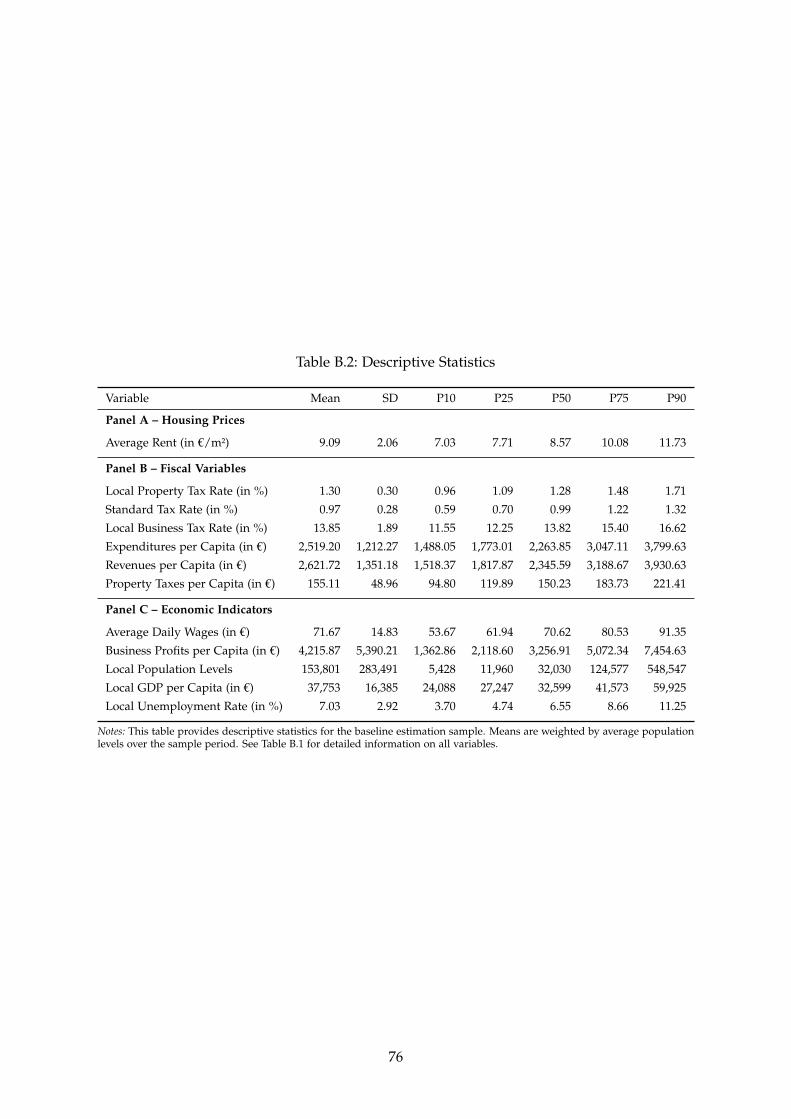
Table B.2: Descriptive Statistics

Variable Mean SD P10 P25 P50 P75 P90

Panel A – Housing Prices

Average Rent (in €/m²) 9.09 2.06 7.03 7.71 8.57 10.08 11.73

Panel B – Fiscal Variables

Local Property Tax Rate (in %) 1.30 0.30 0.96 1.09 1.28 1.48 1.71

Standard Tax Rate (in %) 0.97 0.28 0.59 0.70 0.99 1.22 1.32

Local Business Tax Rate (in %) 13.85 1.89 11.55 12.25 13.82 15.40 16.62

Expenditures per Capita (in €) 2,519.20 1,212.27 1,488.05 1,773.01 2,263.85 3,047.11 3,799.63

Revenues per Capita (in €) 2,621.72 1,351.18 1,518.37 1,817.87 2,345.59 3,188.67 3,930.63

Property Taxes per Capita (in €) 155.11 48.96 94.80 119.89 150.23 183.73 221.41

Panel C – Economic Indicators

Average Daily Wages (in €) 71.67 14.83 53.67 61.94 70.62 80.53 91.35

Business Profits per Capita (in €) 4,215.87 5,390.21 1,362.86 2,118.60 3,256.91 5,072.34 7,454.63

Local Population Levels 153,801 283,491 5,428 11,960 32,030 124,577 548,547

Local GDP per Capita (in €) 37,753 16,385 24,088 27,247 32,599 41,573 59,925

Local Unemployment Rate (in %) 7.03 2.92 3.70 4.74 6.55 8.66 11.25

Notes: This table provides descriptive statistics for the baseline estimation sample. Means are weighted by average populationlevels over the sample period. See Table B.1 for detailed information on all variables.

76

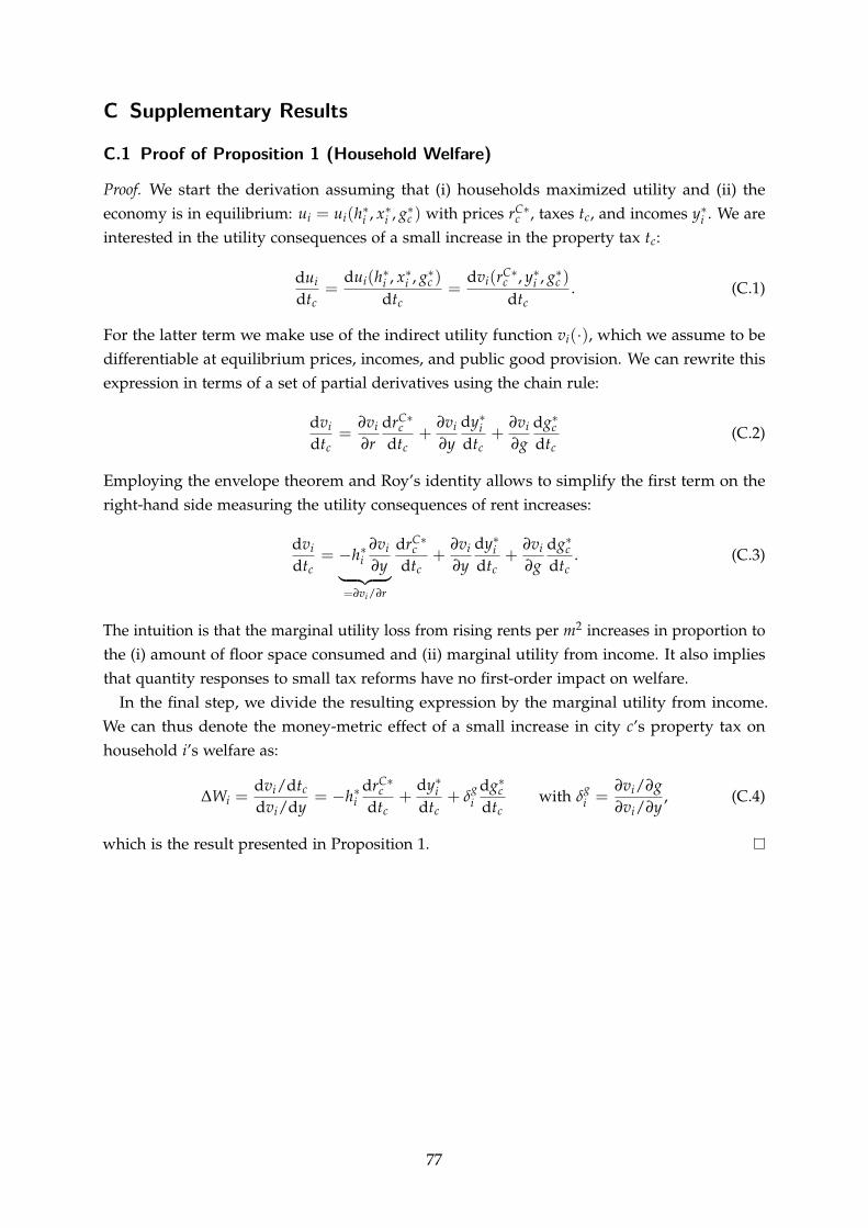
C Supplementary Results

C.1 Proof of Proposition 1 (Household Welfare)

Proof. We start the derivation assuming that (i) households maximized utility and (ii) theeconomy is in equilibrium: u = u (h∗, x∗ ∗

i i i i , gc ) with prices rC∗c , taxes t ∗

c, and incomes yi . We areinterested in the utility consequences of a small increase in the property tax tc:

dui du x∗i(h∗i , i , g∗c ) dv ∗i(rC∗

c , yi , g∗c )= = . (C.1)dtc dtc dtc

For the latter term we make use of the indirect utility function vi(·), which we assume to bedifferentiable at equilibrium prices, incomes, and public good provision. We can rewrite thisexpression in terms of a set of partial derivatives using the chain rule:

dvi ∂vi drC∗c ∂v d ∂ dg∗i y∗i vi c= + + (C.2)

dtc ∂r dtc ∂y dtc ∂g dtc

Employing the envelope theorem and Roy’s identity allows to simplify the first term on theright-hand side measuring the utility consequences of rent increases:

dv ∗i ∗ ∂vi drC∗

c ∂vi dyi ∂vi dg∗h c= − i + + . (C.3)

dtc ∂y dtc ∂y dtc ∂g dt︸︷︷︸ c

=∂vi/∂r

The intuition is that the marginal utility loss from rising rents per m2 increases in proportion tothe (i) amount of floor space consumed and (ii) marginal utility from income. It also impliesthat quantity responses to small tax reforms have no first-order impact on welfare.

In the final step, we divide the resulting expression by the marginal utility from income.We can thus denote the money-metric effect of a small increase in city c’s property tax onhousehold i’s welfare as:

dv C∗∆W i/dtc dr ∗ ∗

h∗ c dyi g dgc g ∂vi/∂gi = = − i + + δ with δ = , (C.4)

dvi/dy dtc dt ic dt i

c ∂vi/∂y

which is the result presented in Proposition 1.

77

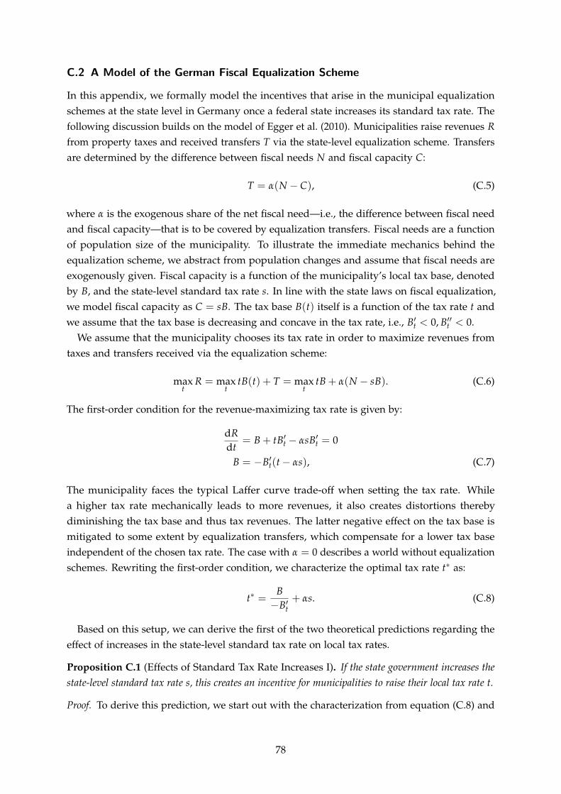
C.2 A Model of the German Fiscal Equalization Scheme

In this appendix, we formally model the incentives that arise in the municipal equalizationschemes at the state level in Germany once a federal state increases its standard tax rate. Thefollowing discussion builds on the model of Egger et al. (2010). Municipalities raise revenues Rfrom property taxes and received transfers T via the state-level equalization scheme. Transfersare determined by the difference between fiscal needs N and fiscal capacity C:

T = α(N − C), (C.5)

where α is the exogenous share of the net fiscal need—i.e., the difference between fiscal needand fiscal capacity—that is to be covered by equalization transfers. Fiscal needs are a functionof population size of the municipality. To illustrate the immediate mechanics behind theequalization scheme, we abstract from population changes and assume that fiscal needs areexogenously given. Fiscal capacity is a function of the municipality’s local tax base, denotedby B, and the state-level standard tax rate s. In line with the state laws on fiscal equalization,we model fiscal capacity as C = sB. The tax base B(t) itself is a function of the tax rate t andwe assume that the tax base is decreasing and concave in the tax rate, i.e., B′t < 0, B′′t < 0.

We assume that the municipality chooses its tax rate in order to maximize revenues fromtaxes and transfers received via the equalization scheme:

max R = max tB(t) + T = max tB + α(N − sB). (C.6)t t t

The first-order condition for the revenue-maximizing tax rate is given by:

dR= B + tB′ −t αsB′

dt t = 0

B = −B′t(t− αs), (C.7)

The municipality faces the typical Laffer curve trade-off when setting the tax rate. Whilea higher tax rate mechanically leads to more revenues, it also creates distortions therebydiminishing the tax base and thus tax revenues. The latter negative effect on the tax base ismitigated to some extent by equalization transfers, which compensate for a lower tax baseindependent of the chosen tax rate. The case with α = 0 describes a world without equalizationschemes. Rewriting the first-order condition, we characterize the optimal tax rate t∗ as:

t∗B

= +−B′αs. (C.8)

t

Based on this setup, we can derive the first of the two theoretical predictions regarding theeffect of increases in the state-level standard tax rate on local tax rates.

Proposition C.1 (Effects of Standard Tax Rate Increases I). If the state government increases thestate-level standard tax rate s, this creates an incentive for municipalities to raise their local tax rate t.

Proof. To derive this prediction, we start out with the characterization from equation (C.8) and

78

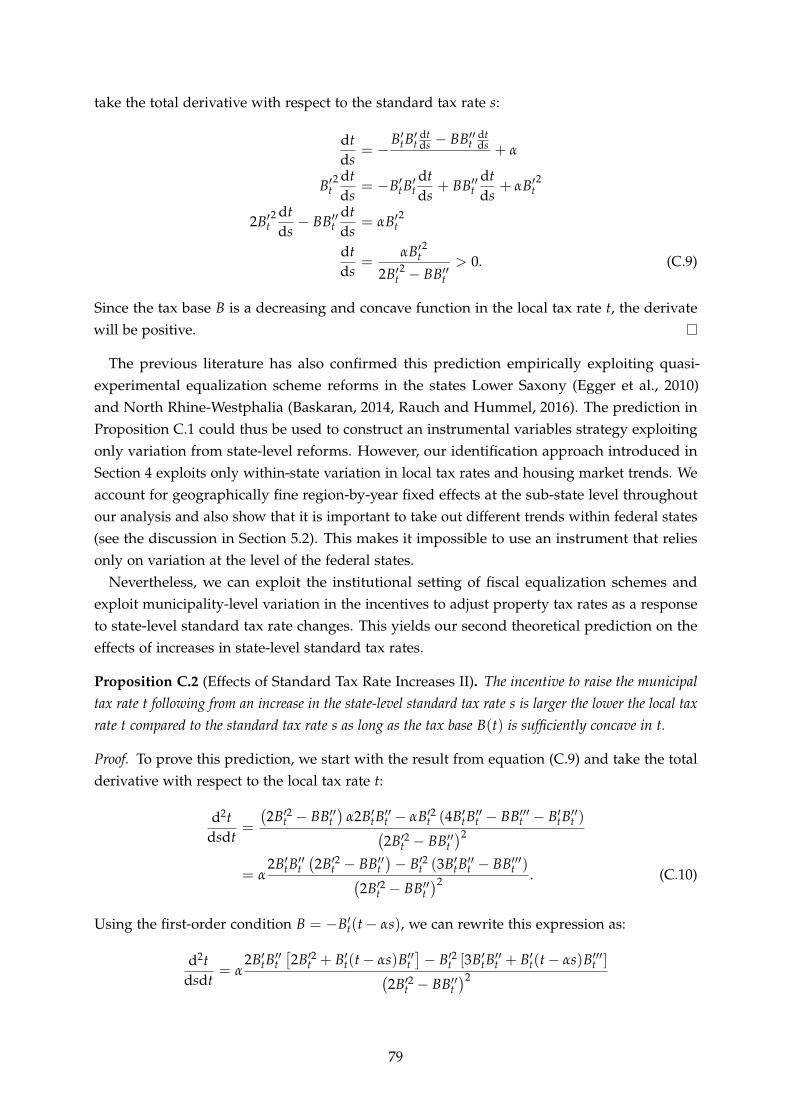
take the total derivative with respect to the standard tax rate s:

dt B′tB′ dt −t ds BB′′ dt

t ds= − + αds

′2 dtBt = −B′

ds tB′ dtt + BB′′

dtds t + αB′2

ds t

2B′2dt −t BB′′

dt ′2ds t = αB

ds t

dt αB′2t= > 0. (C.9)ds 2B′2 −t BB′′t

Since the tax base B is a decreasing and concave function in the local tax rate t, the derivatewill be positive.

The previous literature has also confirmed this prediction empirically exploiting quasi-experimental equalization scheme reforms in the states Lower Saxony (Egger et al., 2010)and North Rhine-Westphalia (Baskaran, 2014, Rauch and Hummel, 2016). The prediction inProposition C.1 could thus be used to construct an instrumental variables strategy exploitingonly variation from state-level reforms. However, our identification approach introduced inSection 4 exploits only within-state variation in local tax rates and housing market trends. Weaccount for geographically fine region-by-year fixed effects at the sub-state level throughoutour analysis and also show that it is important to take out different trends within federal states(see the discussion in Section 5.2). This makes it impossible to use an instrument that reliesonly on variation at the level of the federal states.

Nevertheless, we can exploit the institutional setting of fiscal equalization schemes andexploit municipality-level variation in the incentives to adjust property tax rates as a responseto state-level standard tax rate changes. This yields our second theoretical prediction on theeffects of increases in state-level standard tax rates.

Proposition C.2 (Effects of Standard Tax Rate Increases II). The incentive to raise the municipaltax rate t following from an increase in the state-level standard tax rate s is larger the lower the local taxrate t compared to the standard tax rate s as long as the tax base B(t) is sufficiently concave in t.

Proof. To prove this prediction, we start with the result from equation (C.9) and take the totalderivative with respect to the local tax rate t:( )

d2t 2B′2 −t BB′′ α2B′B′′ B′2− α (4B′B′′ − BB′′′ − ′t t t t t t t BtB

′′t )= ( )dsdt 2B′2 −t BB′′ 2( ) t

2B′B′′ 2B′2 ′2− BB′′ − B (3B′B′′ − ′t t t t t t t BB ′′t )

= α ( ) . (C.10)2B′2 2− B ′

t B′t

Using the first-order condition B = −B′(t−t αs), we can rewrite this expression as:[ ]d2t 2B′ ′tB

′ t−t 2B′2t + B′t( αs)B′′ 2− ′′′( t B′ −t [3B′) tB′′t + B′t(t αs)Bt ]

= αdsdt 22B′2 −t BB′′t

79

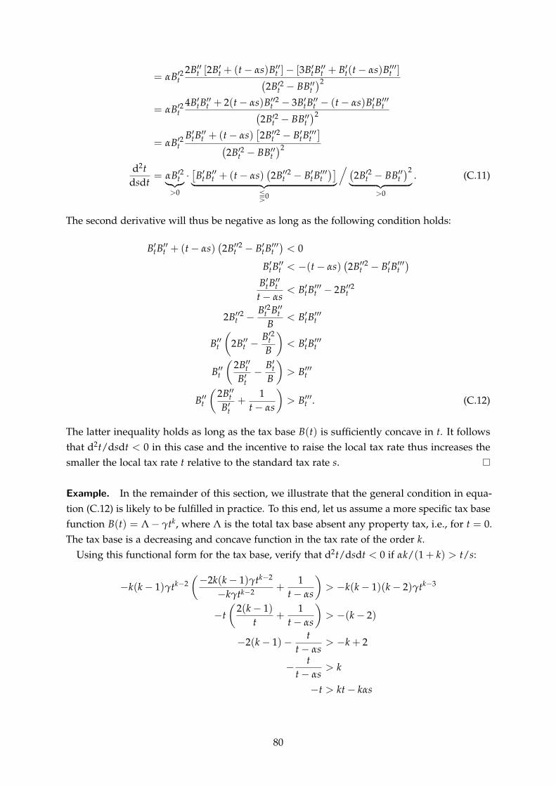
2B′′ [2B′ + (t− αs)B′′]− [3B′B′′ + B′(t− αs)B′′′B′2 t t ( t t ) t t t ]

= α t2B′2 −t BB′′ 2

t

4B′B′′ 2 2+ (t− αs)B′′ − 3B′B′′ − (t− αs)B′B′′′t= B tα ′2 t t t t tt ( )22B′2 −t BB′′[ t ]

B′B′′′2 t t + (t− αs) 2B′′2 −B ( t B′) tB

′′′t= α t

2B′2 2−t BB′′td2t [ /

= αB′2 · B′B′′( 2−t (t− αs) 2B′′2t + ′

t BtB′′′)] ( )

t t 2B′2 − BB′′ . (C.11)dsdt ︸︷︷︸︸︷︷︸︸ t ︷︷ t ︸

>0 S0 >0

The second derivative will thus be negative as long as the following condition holds:

B′)

B′′( 2+ (t− ′

t B −t αs) 2 ′′ ′t BtB

′′t < 0

B′(

B′′ < −(t− αs) 2B′′2 − B′B′′′)

t t t t t

B′tB′′t B′B′′′ 2B′′2< −

t t− αs t t

′2B′′2

B′2t B ′t− < B′B′′′t B t t(B′′t 2B′′

B′)2

t−t < B′B tB

′′′t(

B′′2B′′ ′)

t Bt−t ′ > B′′′Bt B t(

B′′2B′′

)t 1 ′

t B′+ > B′′t . (C.12)−t t αs

The latter inequality holds as long as the tax base B(t) is sufficiently concave in t. It followsthat d2t/dsdt < 0 in this case and the incentive to raise the local tax rate thus increases thesmaller the local tax rate t relative to the standard tax rate s.

Example. In the remainder of this section, we illustrate that the general condition in equa-tion (C.12) is likely to be fulfilled in practice. To this end, let us assume a more specific tax basefunction B(t k) = Λ− γt , where Λ is the total tax base absent any property tax, i.e., for t = 0.The tax base is a decreasing and concave function in the tax rate of the order k.

Using this functional form for the tax base, verify that d2t/dsdt < 0 if αk/(1 + k) > t/s:( )k− −2 2k(k 2− 1 tk)γ − 1

k k 1 t k k 1 k 2 tk 3− ( − )γ + > − ( − )( − )γ −−kγtk−2 t− αs( )

2(k− 1) 1−t + > −(k− 2)t t− αs

t−2(k− 1)− > −k + 2t− αs

t− > kt− αs−t > kt− kαs

80

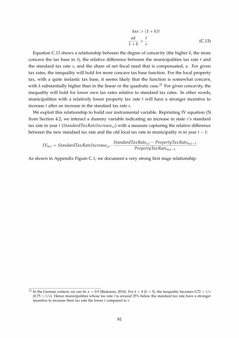
kαs > (1 + k)tαk t

> . (C.13)1 + k s

Equation C.13 shows a relationship between the degree of concavity (the higher k, the moreconcave the tax base in t), the relative difference between the municipalities tax rate t andthe standard tax rate s, and the share of net fiscal need that is compensated, α. For giventax rates, the inequality will hold for more concave tax base function. For the local propertytax, with a quite inelastic tax base, it seems likely that the function is somewhat concave,with k substantially higher than in the linear or the quadratic case.21 For given concavity, theinequality will hold for lower own tax rates relative to standard tax rates. In other words,municipalities with a relatively lower property tax rate t will have a stronger incentive toincrease t after an increase in the standard tax rate s.

We exploit this relationship to build our instrumental variable. Reprinting IV equation (5)from Section 4.2, we interact a dummy variable indicating an increase in state s’s standardtax rate in year t (StandardTaxRateIncreases,t) with a measure capturing the relative differencebetween the new standard tax rate and the old local tax rate in municipality m in year t− 1:

StandardTaxRates,t − PropertyTaxRateIVm,t = StandardTaxRateIncrease m,t−1

s,t · PropertyTaxRatem,t−1

As shown in Appendix Figure C.1, we document a very strong first stage relationship.

21 In the German context, we can fix α = 0.9 (Baskaran, 2014). For k = 4 (k = 5), the inequality becomes 0.72 > t/s(0.75 > t/s). Hence municipalities whose tax rate t is around 25% below the standard tax rate have a strongerincentive to increase their tax rate the lower t compared to s.

81

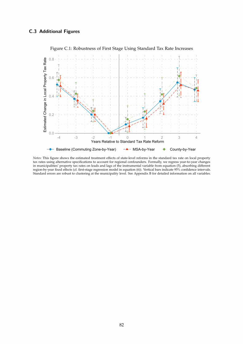
C.3 Additional Figures

Figure C.1: Robustness of First Stage Using Standard Tax Rate Increases

0.0

0.2

0.4

0.6

0.8

Estim

ated

Cha

nge

in L

ocal

Pro

perty

Tax

Rat

e

-4 -3 -2 -1 0 1 2 3 4Years Relative to Standard Tax Rate Reform

Baseline (Commuting Zone-by-Year) MSA-by-Year County-by-Year

Notes: This figure shows the estimated treatment effects of state-level reforms in the standard tax rate on local propertytax rates using alternative specifications to account for regional confounders. Formally, we regress year-to-year changesin municipalities’ property tax rates on leads and lags of the instrumental variable from equation (5), absorbing differentregion-by-year fixed effects (cf. first-stage regression model in equation (6)). Vertical bars indicate 95% confidence intervals.Standard errors are robust to clustering at the municipality level. See Appendix B for detailed information on all variables.

82

Figure C.2: Effect of Property Taxes on Net Rents

-0.04

-0.02

0.00

0.02

0.04

Estim

ated

Effe

ct R

elat

ive

to P

re-R

efor

m Y

ear


Notes: This figure illustrates the estimated treatment effect of a one percentage point increase in the property tax rate on netrents (in logs) relative to the pre-reform year. The underlying econometric model is described in equations (3) and (4). Thespecification also accounts for leads and lags in the local business tax rate and CZ-by-year fixed effects. Observations areweighted by average population levels over the sample period. Vertical bars indicate 95% confidence intervals. Standarderrors are robust to clustering at the municipality level. See Appendix B for detailed information on all variables.

Figure C.3: Effect of Property Taxes on Offered Sales Prices

-0.10

-0.05

0.00

0.05

0.10

Estim

ated

Effe

ct R

elat

ive

to P

re-R

efor

m Y

ear


Notes: This figure illustrates the estimated treatment effect of a one percentage point increase in the property tax rate onoffered sales prices (in logs) relative to the pre-reform year. The underlying econometric model is described in equations (3)and (4). The specification also accounts for leads and lags in the local business tax rate and CZ-by-year fixed effects.Observations are weighted by average population levels over the sample period. Vertical bars indicate 95% confidenceintervals. Standard errors are robust to clustering at the municipality level. See Appendix B for detailed information on allvariables.

83

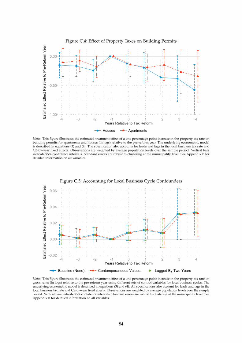
Figure C.4: Effect of Property Taxes on Building Permits

-1.00

-0.50

0.00

Estim

ated

Effe

ct R

elat

ive

to P

re-R

efor

m Y

ear


Houses Apartments

Notes: This figure illustrates the estimated treatment effect of a one percentage point increase in the property tax rate onbuilding permits for apartments and houses (in logs) relative to the pre-reform year. The underlying econometric modelis described in equations (3) and (4). The specification also accounts for leads and lags in the local business tax rate andCZ-by-year fixed effects. Observations are weighted by average population levels over the sample period. Vertical barsindicate 95% confidence intervals. Standard errors are robust to clustering at the municipality level. See Appendix B fordetailed information on all variables.

Figure C.5: Accounting for Local Business Cycle Confounders

-0.02

0.00

0.02

0.04

0.06

Estim

ated

Effe

ct R

elat

ive

to P

re-R

efor

m Y

ear


Baseline (None) Contemporaneous Values Lagged By Two Years

Notes: This figure illustrates the estimated treatment effect of a one percentage point increase in the property tax rate ongross rents (in logs) relative to the pre-reform year using different sets of control variables for local business cycles. Theunderlying econometric model is described in equations (3) and (4). All specifications also account for leads and lags in thelocal business tax rate and CZ-by-year fixed effects. Observations are weighted by average population levels over the sampleperiod. Vertical bars indicate 95% confidence intervals. Standard errors are robust to clustering at the municipality level. SeeAppendix B for detailed information on all variables.

84

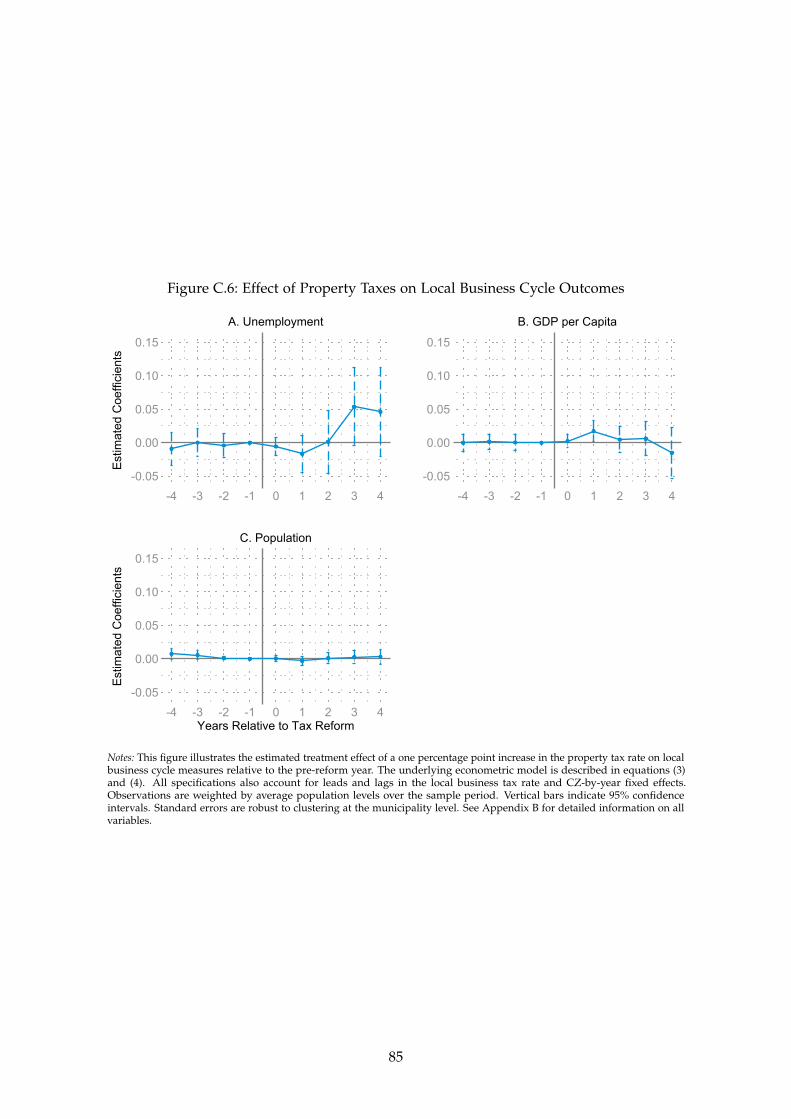
Figure C.6: Effect of Property Taxes on Local Business Cycle Outcomes

-0.05

0.00

0.05

0.10

0.15

Estim

ated

Coe

ffici

ents

-4 -3 -2 -1 0 1 2 3 4

A. Unemployment

-0.05

0.00

0.05

0.10

0.15

-4 -3 -2 -1 0 1 2 3 4

B. GDP per Capita

-0.05

0.00

0.05

0.10

0.15

Estim

ated

Coe

ffici

ents


C. Population

Notes: This figure illustrates the estimated treatment effect of a one percentage point increase in the property tax rate on localbusiness cycle measures relative to the pre-reform year. The underlying econometric model is described in equations (3)and (4). All specifications also account for leads and lags in the local business tax rate and CZ-by-year fixed effects.Observations are weighted by average population levels over the sample period. Vertical bars indicate 95% confidenceintervals. Standard errors are robust to clustering at the municipality level. See Appendix B for detailed information on allvariables.

85

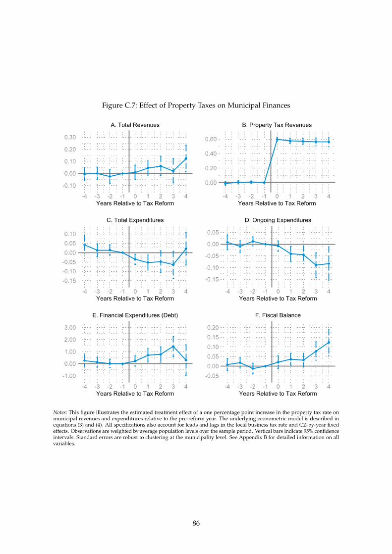
Figure C.7: Effect of Property Taxes on Municipal Finances

-0.10

0.00

0.10

0.20

0.30


A. Total Revenues

0.00

0.20

0.40

0.60


B. Property Tax Revenues

-0.15-0.10-0.050.000.050.10


C. Total Expenditures

-0.15

-0.10

-0.05

0.00

0.05


D. Ongoing Expenditures

-1.00

0.00

1.00

2.00

3.00


E. Financial Expenditures (Debt)

-0.050.000.050.100.150.20


F. Fiscal Balance

Notes: This figure illustrates the estimated treatment effect of a one percentage point increase in the property tax rate onmunicipal revenues and expenditures relative to the pre-reform year. The underlying econometric model is described inequations (3) and (4). All specifications also account for leads and lags in the local business tax rate and CZ-by-year fixedeffects. Observations are weighted by average population levels over the sample period. Vertical bars indicate 95% confidenceintervals. Standard errors are robust to clustering at the municipality level. See Appendix B for detailed information on allvariables.

86

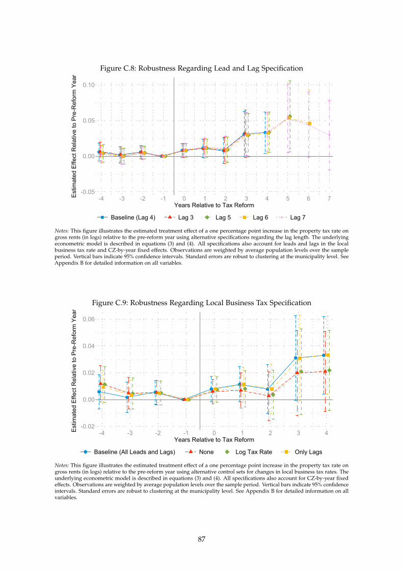
Figure C.8: Robustness Regarding Lead and Lag Specification

-0.05

0.00

0.05

0.10

Estim

ated

Effe

ct R

elat

ive

to P

re-R

efor

m Y

ear

-4 -3 -2 -1 0 1 2 3 4 5 6 7Years Relative to Tax Reform

Baseline (Lag 4) Lag 3 Lag 5 Lag 6 Lag 7

Notes: This figure illustrates the estimated treatment effect of a one percentage point increase in the property tax rate ongross rents (in logs) relative to the pre-reform year using alternative specifications regarding the lag length. The underlyingeconometric model is described in equations (3) and (4). All specifications also account for leads and lags in the localbusiness tax rate and CZ-by-year fixed effects. Observations are weighted by average population levels over the sampleperiod. Vertical bars indicate 95% confidence intervals. Standard errors are robust to clustering at the municipality level. SeeAppendix B for detailed information on all variables.

Figure C.9: Robustness Regarding Local Business Tax Specification

-0.02

0.00

0.02

0.04

0.06

Estim

ated

Effe

ct R

elat

ive

to P

re-R

efor

m Y

ear


Baseline (All Leads and Lags) None Log Tax Rate Only Lags

Notes: This figure illustrates the estimated treatment effect of a one percentage point increase in the property tax rate ongross rents (in logs) relative to the pre-reform year using alternative control sets for changes in local business tax rates. Theunderlying econometric model is described in equations (3) and (4). All specifications also account for CZ-by-year fixedeffects. Observations are weighted by average population levels over the sample period. Vertical bars indicate 95% confidenceintervals. Standard errors are robust to clustering at the municipality level. See Appendix B for detailed information on allvariables.

87

Figure C.10: Robustness Regarding Estimation Model Specification

0.00

0.05

0.10Es

timat

ed E

ffect

Rel

ativ

e to

Pre

-Ref

orm

Yea

r


Baseline (First Differences) Fixed Effects Model

Notes: This figure illustrates the estimated treatment effect of a one percentage point increase in the property tax rate ongross rents (in logs) relative to the pre-reform year comparing first differences results and estimates from a model withmunicipality fixed effects. The underlying econometric model is described in equations (3) and (4). All specifications alsoaccount for leads and lags in the local business tax rate and CZ-by-year fixed effects. Observations are weighted by averagepopulation levels over the sample period. Vertical bars indicate 95% confidence intervals. Standard errors are robust toclustering at the municipality level. See Appendix B for detailed information on all variables.

Figure C.11: Robustness Regarding Sample Composition

-0.02

0.00

0.02

0.04

0.06

Estim

ated

Effe

ct R

elat

ive

to P

re-R

efor

m Y

ear


Baseline (≥ 15 Ads) ≥ 1 Ad ≥ 5 Ads ≥ 25 Ads ≥ 50 Ads

Notes: This figure illustrates the estimated treatment effect of a one percentage point increase in the property tax rate ongross rents (in logs) relative to the pre-reform year using different requirements regarding the minimum number of ads permunicipality-year observation. The underlying econometric model is described in equations (3) and (4). All specificationsalso account for leads and lags in the local business tax rate and CZ-by-year fixed effects. Observations are weighted byaverage population levels over the sample period. Vertical bars indicate 95% confidence intervals. Standard errors are robustto clustering at the municipality level. See Appendix B for detailed information on all variables.

88

Figure C.12: Robustness Regarding Weighting Procedure

-0.02

0.00

0.02

0.04

0.06

0.08

Estim

ated

Effe

ct R

elat

ive

to P

re-R

efor

m Y

ear


Baseline (Avg. Population) None Current Popul. Number of Ads

Notes: This figure illustrates the estimated treatment effect of a one percentage point increase in the property tax rate ongross rents (in logs) relative to the pre-reform year using different weighting procedures. The underlying econometric modelis described in equations (3) and (4). All specifications also account for leads and lags in the local business tax rate andCZ-by-year fixed effects. Observations are weighted by average population levels over the sample period. Vertical barsindicate 95% confidence intervals. Standard errors are robust to clustering at the municipality level. See Appendix B fordetailed information on all variables.

Figure C.13: Robustness Regarding Geographical Coverage

-0.02

0.00

0.02

0.04

0.06

Estim

ated

Effe

ct R

elat

ive

to P

re-R

efor

m Y

ear


Baseline (West Germany) All Germany (Including East)

Notes: This figure illustrates the estimated treatment effect of a one percentage point increase in the property tax rateon gross rents (in logs) relative to the pre-reform year for West Germany only and all Germany including the East. Theunderlying econometric model is described in equations (3) and (4). All specifications also account for leads and lags in thelocal business tax rate and CZ-by-year fixed effects. Observations are weighted by average population levels over the sampleperiod. Vertical bars indicate 95% confidence intervals. Standard errors are robust to clustering at the municipality level. SeeAppendix B for detailed information on all variables.

89

Figure C.14: Reduced-Form Effects on Other Welfare-Relevant Outcomes

-0.02

-0.01

0.00

0.01

0.02

0.03

Estim

ated

Coe

ffici

ents


A. Wages

-0.40

-0.20

0.00

0.20

0.40

-4 -3 -2 -1 0 1 2 3 4

Years Relative to Tax Reform

B. Business Income

Notes: This figure illustrates the estimated treatment effect of a one percentage point increase in the property tax rateon average municipal wages and business incomes relative to the pre-reform year. The underlying econometric modelis described in equations (3) and (4). All specifications also account for leads and lags in the local business tax rate andCZ-by-year fixed effects. Observations are weighted by average population levels over the sample period. Vertical barsindicate 95% confidence intervals. Standard errors are robust to clustering at the municipality level. See Appendix B fordetailed information on all variables.

Figure C.15: Property Tax Increases and Absolute Utility Changes

-200

-180

-160

-140

-120

-100

Mon

ey-M

etric

Util

ity L

oss

(in E

uro

per Y

ear)


Notes: This figure illustrates the money-metric utility consequences of a one percentage point increase in the local propertytax over the distribution of household consumption (in euro per year). We simulate money-metric utility changes aspresented in equation (7) and Table 1 for each household in the German Income and Expenditure Survey (EVS, 2013). Thedepicted curves are based on average changes within percentiles of the consumption distribution across households usingsampling weights and the OECD-modified equivalence scale. See Appendix B for detailed information on all variables.

90

Figure C.16: Property Tax Increases and Household Utility – Inference

-4.0

-2.0

0.0

2.0

4.0

Rel

ativ

e U

tility

Los

s (in

%)


Full Model (Baseline) 90/95% CI

A. Full Model

-4.0

-2.0

0.0

2.0

4.0


Partial Model 90/95% CI

B. Partial Model

Notes: This figure illustrates the relative utility consequences of a one percentage point increase in the local property tax overthe household consumption distribution (in percent) showing 90% and 95% confidence intervals. Panel A shows the resultsfor the full model including housing market and general equilibrium responses. Panel B illustrates the welfare effects ofhousing market responses only. We calculate relative utility losses as money-metric utility changes in euro per year dividedby total household consumption. We simulate money-metric utility changes as presented in equation (7) and Table 1 for eachhousehold in the German Income and Expenditure Survey (EVS, 2013). The depicted curves are based on average changeswithin percentiles of the consumption distribution across households using sampling weights and the OECD-modifiedequivalence scale. Confidence intervals are based on 1,000 bootstrap replications of the respective simulation. In eachbootstrap run, we sample independently from the EVS survey and the coefficient distributions of medium-run estimates.See Appendix B for detailed information on all variables.

91

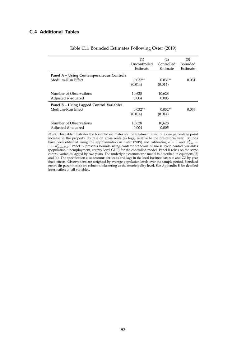
C.4 Additional Tables

Table C.1: Bounded Estimates Following Oster (2019)

(1) (2) (3)Uncontrolled Controlled Bounded

Estimate Estimate Estimate

Panel A – Using Contemporaneous ControlsMedium-Run Effect 0.032** 0.031** 0.031

(0.014) (0.014)

Number of Observations 10,628 10,628Adjusted R-squared 0.004 0.005

Panel B – Using Lagged Control VariablesMedium-Run Effect 0.032** 0.032** 0.033

(0.014) (0.014)

Number of Observations 10,628 10,628Adjusted R-squared 0.004 0.005

Notes: This table illustrates the bounded estimates for the treatment effect of a one percentage pointincrease in the property tax rate on gross rents (in logs) relative to the pre-reform year. Boundshave been obtained using the approximation in Oster (2019) and calibrating δ = 1 and R2

max =1.3 · R2

controlled. Panel A presents bounds using contemporaneous business cycle control variables(population, unemployment, county-level GDP) for the controlled model. Panel B relies on the samecontrol variables lagged by two years. The underlying econometric model is described in equations (3)and (4). The specification also accounts for leads and lags in the local business tax rate and CZ-by-yearfixed effects. Observations are weighted by average population levels over the sample period. Standarderrors (in parentheses) are robust to clustering at the municipality level. See Appendix B for detailedinformation on all variables.

92

C.5 Sensitivity of Simulated Welfare Effects

In this section we test the robustness of our simulation result to various modeling assumptions.Appendix Figure C.17 illustrates the results, always contrasting the baseline model from themain text (in blue) to an alternative simulation (in red).

In Panel A we test whether our method to calculate the additional tax burden for houseowners and landlords drives our findings. Our baseline simulation relies on imputed rents (forowner-occupied housing) and the average property tax-to-rent ratio (for landlords) in order topredict additional tax payments, which may potentially underestimate the actual tax bill. Wecompare this prediction to an alternative simulation where we use the reported property taxbase instead to calculate the increase in tax payments resulting from a one percentage pointincrease in the property tax. Results turn out to be quite similar for both implementations.The latter method yields somewhat lower utility losses for households in the upper half of thedistribution and thus if anything a more regressive pattern compared to the baseline.

In Panel B we check whether results are sensitive to the assignment to different percentiles. Inthe baseline we group households based on private consumption expenditures. An alternativeway to calculate population percentiles is to use total household income on the horizontal axisand also scale relative utility losses using income instead of consumption. We find very similareffects of around −1.1 percent relative utility loss at the bottom of the income distribution, butlower relative utility losses for households above the first decile. Overall, grouping and scalingover household income yields a more regressive pattern with approximately zero losses at thetop of the distribution. The intuition behind this pattern is that total income is more unequallydistributed across households compared to consumption expenditures.

Next we assess the impact of our tax simulation in Panel C. In the baseline simulation, weimpute marginal tax rates based on the statutory schedules in the personal income tax system,social security contributions, and transfer withdrawal (assuming a marginal rate of 80%). Sincethe EVS survey includes little information on the tax unit, these statutory rates may be at oddswith the actual rates. Alternatively we calculate average income tax rates and average rates forsocial security contributions within population percentiles and use these imputed average taxwedges to transform gross income effects into net income changes.22 Results are rather similaracross the distribution with somewhat lower relative utility losses for medium incomes andvery similar results at both ends of the consumption distribution.

In Panel D we further assess whether results are different for West Germany compared to allGerman states. Our baseline estimate on the pass-through of taxes into gross rents and also thebaseline simulation are based on West Germany only. In Appendix Figure C.13 we showedthat pass-through results are very similar when including East Germany as well. Similarly, wefind that simulation results are very stable whether we simulate household utility changes forWest Germany only or for East and West Germany combined using all 42,792 households fromthe EVS survey.

{22 We impute the following sets of tax rates: I 1 T I }100

τp = |H | ∑ ii∈Hp

for the pure income tax wedge (applying top Yi p{ =1

landlord and business incomes), and W 1 T I S }100τ = ∑ i T

+ ip |H | i∈Hp Yi yW for the tax wedge on wage earnings.

p i p=1

93

Finally, we turn to the importance of local public goods (bottom row of Appendix Figure C.17).In the baseline simulation we used a revealed preferences approach to calibrate individuals’preferences for public vs. private goods based on the observed ratio of local governmentexpenditures relative to local GDP, δ = 0.073 (resulting in g

δ =i 0.079). In Panel E of AppendixFigure C.17, we replicate this simulation while assuming a higher valuation of public goods,namely the baseline estimate δ = 0.16 from Fajgelbaum et al. (2019). In Panel F, we furtherincrease the calibrated valuation for public goods using their upper bound estimate of δ = 0.23from Fajgelbaum et al. (2019). In line with the negative semi-elasticity of municipal expenditureswith respect to the property tax rate shown in Appendix Figure C.7, we find that the utilitylosses increase the higher the relative valuation for public vs. private goods. This effect ismost pronounced for households at the lower end of the distribution and less relevant forhigh-consumption households, enforcing the regressive nature of the property tax.

94

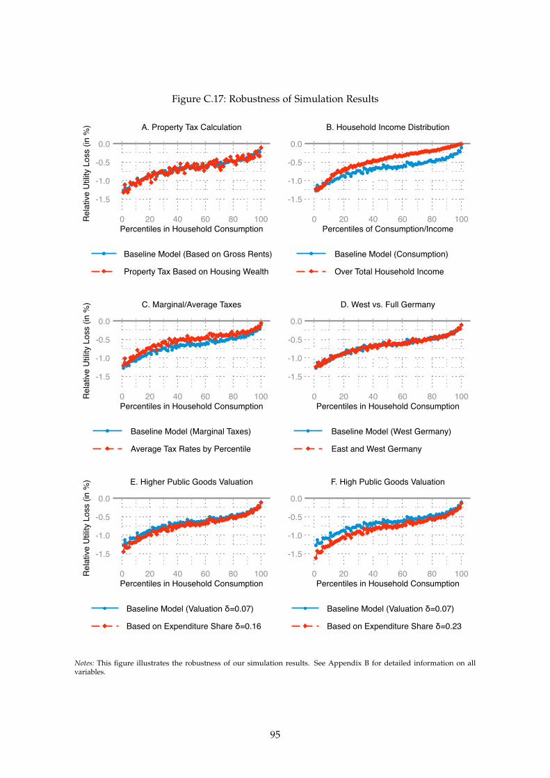
Figure C.17: Robustness of Simulation Results

-1.5

-1.0

-0.5

0.0

Rela

tive

Utilit

y Lo

ss (i

n %

)


Baseline Model (Based on Gross Rents)

Property Tax Based on Housing Wealth

A. Property Tax Calculation

-1.5

-1.0

-0.5

0.0

0 20 40 60 80 100Percentiles of Consumption/Income

Baseline Model (Consumption)

Over Total Household Income

B. Household Income Distribution

-1.5

-1.0

-0.5

0.0

Rela

tive

Utilit

y Lo

ss (i

n %

)


Baseline Model (Marginal Taxes)

Average Tax Rates by Percentile

C. Marginal/Average Taxes

-1.5

-1.0

-0.5

0.0


Baseline Model (West Germany)

East and West Germany

D. West vs. Full Germany

-1.5

-1.0

-0.5

0.0

Rela

tive

Utilit

y Lo

ss (i

n %

)


Baseline Model (Valuation δ=0.07)

Based on Expenditure Share δ=0.16

E. Higher Public Goods Valuation

-1.5

-1.0

-0.5

0.0


Baseline Model (Valuation δ=0.07)

Based on Expenditure Share δ=0.23

F. High Public Goods Valuation

Notes: This figure illustrates the robustness of our simulation results. See Appendix B for detailed information on allvariables.

95

Documents

Max Löffler, Sebastian Siegloch