Metal Foam Effective Transport Properties

14

Metal Foam Effective Transport Properties

Jean-Michel Hugo1,2, Emmanuel Brun3 and Frédéric Topin1 1IUSTI Laboratory CNRS UMR 6595, Université de Provence,

2MOTA S.A. Cooling System, Z.I. les Paluds, 3European Synchrotron Radiation Facility,

France

1. Introduction

Solid foams are a relatively new class of multifunctional materials that present attractive

thermal, mechanical, electrical and acoustic properties. Moreover, they also promote

mixing and have excellent specific mechanical properties. They are widely quoted to

present a random topology, high open porosity, low relative density and high thermal

conductivity of the cell edges, large accessible surface area per unit volume (Ashby et al.,

2000). Usually, geometric properties such as high tortuosity and high specific surface are

proposed to explain their properties, although fluid tortuosity is close to 1 and specific

surface is usually smaller than 10000m²/m3. They are nowadays proposed for their use in

numerous applications such as compact heat exchangers, reformers, biphasic cooling

systems and spreaders. They are also used in high-power batteries for lightweight

cordless electronics, and catalytic field application such as fuel cells systems (Catillon et

al., 2004; Dukhan et al., 2005; Mahjoob & Vafai, 2008; Tadrist et al., 2004). In this chapter,

we expose experimental and numerical tools to determine effective transport properties of

metal foam for mono-and-biphasic flow.

2. Representative volume element

Definitions of a continuous medium equivalent to the real porous structure, as well as the

definition of the applicability level of the macroscopic model, constitutes a tricky problem

that has long been debated (Auriault, 1991; Baveye & Sposito, 1984; Marle, 1982; Quintard &

Whitaker, 1991) among others. The forms of the used phenomenological laws have been

obtained from correlations resulting from experiments and not from physical laws. The

valuable expressions are much diversified and the choice for one or the other is only

justified when compared with specific experiments. We thus consider, classically, that the

foam could be assimilated to a homogeneous equivalent medium (Dullien, 1992). Thus, each

measured quantities will not describe the foam sample itself, but rather a homogeneous

media which has the same properties. There is yet no theoretical evidence to justify this

assumption. Thus, we only consider that this condition is satisfied when the considered

phenomenon occurs on a sufficient distance. Determination of a Rve is thus evaluation of

the relevant distance for the considered observation.

www.intechopen.com

Evaporation, Condensation and Heat Transfer

280

2.1 Rve determination procedure A definition of the Rve was proposed by (Drugan & Willis, 1996) : ‘‘It is the smallest material volume element of the composite for which the usual spatially constant (overall modulus) macroscopic constitutive representation is a sufficiently accurate model to represent mean constitutive response’’. We propose to qualitatively identify Rve associated to both geometrical and physical macroscopic properties using a pragmatic statistical approach (Kanit et al., 2003). The property considered is calculated for a large number of fixed-size boxes (n=100 to 1000) randomly located in the sample. We obtain a distribution of mean values for a given size of box. We then studied the influence of the box size on the standard deviation of these distributions. The size of the Rve is defined as the volume for which the distribution of the mean values present a standard deviation below a given threshold. We could also define the size of the Rve as the volume for which the maximum difference is below a given threshold; it would be a much robust criteria since Standard statistics could hide a Maximum Difference (MD) far greater than standard deviation (Std Dev). In our case both quantities vary similarly and thus Std. Dev threshold is sufficient. For all studied quantities, the standard deviation decrease roughly exponentially with the box size. For a Std Dev of 10 % we observe that maximum differences (MD) between two realizations could exceed 25%. At 5% Std Dev, MD stay around 15%. This value is indeed rather important but the available samples do not permit to be more precise. To compare the different foams, the size of the box was normalized by the pore diameter. Moreover the standard deviation and the maximum difference are normalized with the mean value of the property studied for the considered foam.

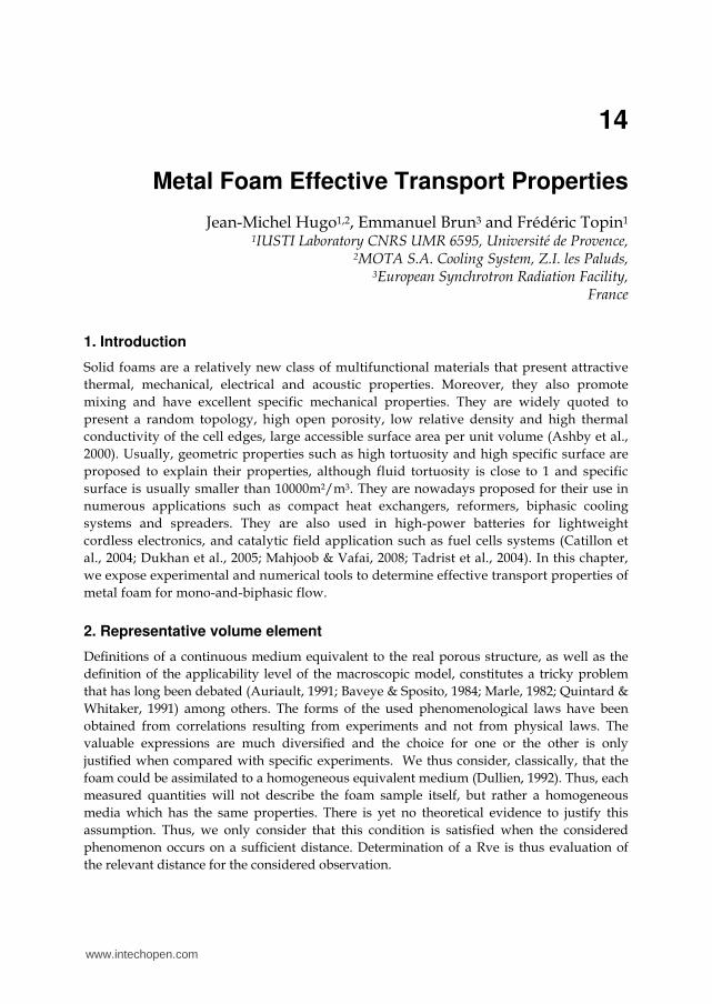
2.2 Geometrical Rve Porosity and specific surface are estimated from the 3D density images obtained with X-ray tomography. Porosity is trivially obtained by counting the voxels of the different phase. The "Marching Cubes" algorithm uses the 3D density images to obtain the mesh of solid surface (Lorensen & Cline, 1987). The mesh data triangles are ordered so that each triangle is included into a unique cubic mesh composing the 3D sample. Once the mesh has been generated for the sample, it is then easy to calculate a specific surface area within a small volume taken in the sample: the cubes composing the volume are retrieved and the surface area of the triangles contained in these cubes is summed. Figure 1 shows the influence of the box size on standard deviation and on the maximum difference of both porosity (a) and specific surface (b) area distribution. For porosity we can define a unique Rve for these samples. We observe similar standard deviation variations for several manufacturers. According our 5% criteria the Rve of porosity is a cube of 0.7 pore diameter side. Similar behavior in standard deviation variation is observed for the Rve of specific surface. A single size of Rve can be defined for all these samples: similar standard deviation variations are also observed for the foams from different manufacturers. According to our 5% criteria, the Rve for specific surface is a cube roughly 3 dp in side length. The absence of differences between foams from different manufacturer can be explained by the fact that the manufacturing processes are roughly similar (replication of polymer foam) and lead to the same solid volume fraction (porosity around 90 % is a manufacturer goal). Plateau law gives globally struts shape but local variations in the cells organization induce different shapes of struts inter-connection and strut cross section (roughly curved triangle).

www.intechopen.com


281

These perturbations may be due to several effects (gravity, drainage, deposition, casting…) during manufacturing process. This gives insight on the fact that specific surface Rve size is far greater than porosity one, but further investigation needed to clarify this point.

Fig. 1. Geometrical REV determination. (a) porosity. (b) specific surface. Hollow symbol: Std. dev.; Filled ones: max. difference.

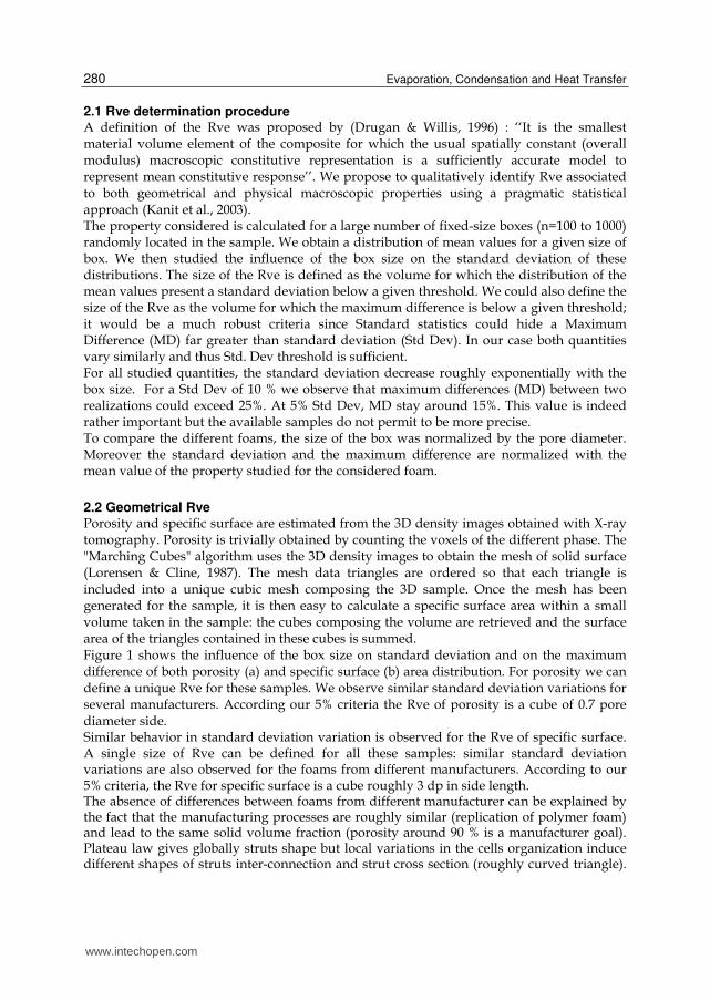
2.3 Physical Rve Concerning velocity, the method for obtaining Rve is the same as for geometrical properties. But determining the local averaged pressure gradient from the pressure field is more difficult (Barrere, 1990; Renard et al., 2001). Even if local pressure gradient are not fully perpendicular to main flow direction (Figure 2), this effect is small and we consider that macroscopic pressure is constant on planes perpendicular to the main flow direction (established flow in an isotropic medium). Thus, we calculate mean pressure on planes perpendicular to the main flow direction at several locations, and we estimate the slope of the mean pressure variation by linear regression. We have chosen the coefficient of determination R2 of the linear regression as a pertinent parameter and we keep our 5% criteria to establish the Rve size. We made these calculations for different sizes of a randomly located box in the medium and we studied the influence of the box volume on the coefficient of determination R2 of the linear regression.

Fig. 2. Physical RVE determination. (a) velocity. Hollow symbols: standard deviation; Filled one: Maximum error. (b) Hollow symbol: pressure gradient; filled ones: regression coefficient. Calculations using either Finite Volume or Lattice Botzmann approach.

www.intechopen.com


282

Figure 2.a shows the influence of the box size on standard deviation and on the maximum

difference of mean velocity. To establish Rve for the mean velocity value, we used the

velocity field obtained from the computations (§3.3). No clear influence of the Reynolds

number on RVE size can be identified for both methods on the studied range. We observe

that for simulation, a box of 3 dp side seems to be sufficient to define the mean velocity for

these Reynolds numbers.

Figure 2.b presents the estimation of the pressure gradient by a linear regression and its

coefficient of determination R2, for different volumes and different Reynolds numbers.

The estimate of the pressure gradient is quite constant for a box 3 pore diameters in size and

the associated coefficient of regression R2 is good (> 0.99). As a result, 3 pore diameters are

sufficient to establish pressure drop Rve.

3. Single-phase flow

3.1 Flow law It is well known that flows at very low flow rates through a porous medium are governed by Darcy’s law (Darcy, 1856).

dP μ

- = udz K

(1)

Where dP/dz is the pressure gradient along the main flow z-direction, µ the dynamic

viscosity, u is Darcy’s or the seepage velocity and K (m²) is the permeability (or Darcy’s

permeability) of the medium.

For homogeneous porous media, a nonlinear relationship between the pressure drop and

the flow rate characterize “high-velocity” flows. At high Reynolds number (strong inertia

regime), the empirical Forchheimer equation is used to account for the deviation from

Darcy’s law (incompressible fluid) (Eq.2) or extended to compressible fluid and expressed as

a function of mass flow rate (Eq.3).

2dP(z) μ- = u +┚ρu

dz K

⎛ ⎞⎜ ⎟⎝ ⎠ (2)

2dρ(z)P(z) μ- = η+┚η

dz K

⎛ ⎞⎜ ⎟⎝ ⎠ (3)

Where ρ (kg.m-3) is the fluid density, η (kg.m-2.s-1) the mass flow rate and β (m−1) the inertia

factor or the non-Darcy flow coefficient. In this formulation the Brinkman correction is

neglected. That means that the pressure drop is considered as the sum of two terms: viscous

(u, Darcy law) and inertia (u2) terms.

Several authors have shown that the onset of the non-linear behavior (that is sometime

called the weak inertia regime) may be described by a cubic law (Firdaous et al., 1997; Mei &

Auriault, 1993; Wodie & Levy, 1991):

2

3dP μ ρ- = u + u

dz K μγ ⋅ (4)

www.intechopen.com


283

Where γ is a dimensionless parameter for the non-linear term. Comparing equations (4) and

(2) shows up that ( )┛ρ┚ u = uμ

could be described as a velocity dependant inertial

coefficient. This expression is proposed to describe flow in porous media at intermediate Reynolds number (typically 10<Re<10000). This equation was obtained by numerical simulations in a two-dimensional periodic porous medium, and by using the homogenization technique for an isotropic homogeneous 3D porous medium. In spite of the numerous attempts to clarify the physical reasons for the non-linear behavior described above, neither Forchheimer equation (2) nor the weak inertia equation (4) have received any physical justification (Fourar et al., 2004). The pressure gradient across the foam is thus a function of system geometry (porosity, pore and ligament size...), as well as physical properties of the fluid phase (viscosity, density). On the other hand, for all three formulations of pressure gradient through the porous media, K, β and γ are intrinsic characteristic of the solid matrix alone and are, thus, independent of the fluid nature.

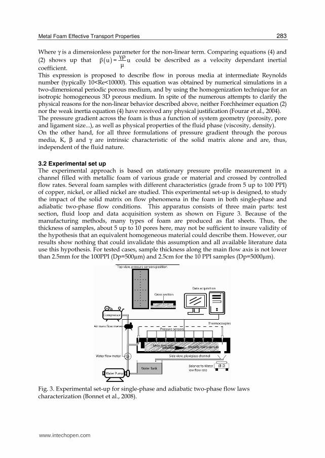
3.2 Experimental set up The experimental approach is based on stationary pressure profile measurement in a channel filled with metallic foam of various grade or material and crossed by controlled flow rates. Several foam samples with different characteristics (grade from 5 up to 100 PPI) of copper, nickel, or allied nickel are studied. This experimental set-up is designed, to study the impact of the solid matrix on flow phenomena in the foam in both single-phase and adiabatic two-phase flow conditions. This apparatus consists of three main parts: test section, fluid loop and data acquisition system as shown on Figure 3. Because of the manufacturing methods, many types of foam are produced as flat sheets. Thus, the thickness of samples, about 5 up to 10 pores here, may not be sufficient to insure validity of the hypothesis that an equivalent homogeneous material could describe them. However, our results show nothing that could invalidate this assumption and all available literature data use this hypothesis. For tested cases, sample thickness along the main flow axis is not lower than 2.5mm for the 100PPI (Dp=500µm) and 2.5cm for the 10 PPI samples (Dp=5000µm).

Fig. 3. Experimental set-up for single-phase and adiabatic two-phase flow laws characterization (Bonnet et al., 2008).

www.intechopen.com


284

The test section (250 mm length, 50 mm wide and adjustable height) is instrumented with 12 pressure sensors (Sensym®, sensitivity 2.6 µV per Pa) placed every centimetre along the main flow axis. Additional pressure sensors are placed along 3 lines perpendicular to the flow direction to assess the one-dimensional nature of the flow. Foam samples (whose lengths vary from 130 up to 200 mm) are placed in the central part of the channel in order to keep a tranquilization zone upstream and downstream of the sample. Test section is placed horizontally in order to avoid uncertainties due to hydrostatic effects (Madani et al., 2007). The liquid fluid loop is constituted by a storage tank (50 l capacity) and a variable velocity gear pump which can give a constant flow rate in the range of 0–10-4 m3 s -1 independently of pump downstream conditions. Constant air flow (range 0-4 10-3 Nm3 s-1) is obtained by using a compressor and a pressure regulation valve. The test section is connected, downstream, to a separator which is installed for the two-phase flow experiments. The liquid flows by gravity down the storage tank while the air is simply released to atmosphere. A weighted tank could be inserted in the liquid loop to assess the mass flow rate. Liquid flow rate is monitored (upstream of the test section) using two turbine flow meters (Mac-Millan®) for optimal accuracy over the full range of experiments. The first one works in the range of 3.33 10-5 - 8.10-5 m3s-1 and the other one in the range 1.6 10-6- 3.33 10-5 m3s-1. The weighting device arranged in downstream of the test section has a sensitivity of about 1 g and a capacity of 3 l. Air flow is monitored upstream of the test section using three mass- flow meters (Aalborg®) respective operating range: 0-50, 0-100 and 0-250 Nl/min. An accuracy of about 0.1 % overall flow rate range is thus obtained. Pressures, temperature and inlet flow rate of both fluid (air and water) are continuously monitored. The same experimental procedure is used for all tests. Before each series of measurement, the foam sample was flooded a long time ensuring initial wetting (water) or drying (air), and established flow. The fluid is then, maintained on circulation for about half an hour after system has reached a stationary regime. Hydrodynamic (null flow) profile is checked before experiment in order to eliminate all offset between pressure sensors. For each measurement, an averaging procedure (averaging time 1minute, data acquisition 500 Hz) is used to reduce measurement noise, after checking stationary behavior of pressure and flow rate signal. Accuracy of pressure measurement is better than 5 Pa (Madani et al., 2007).

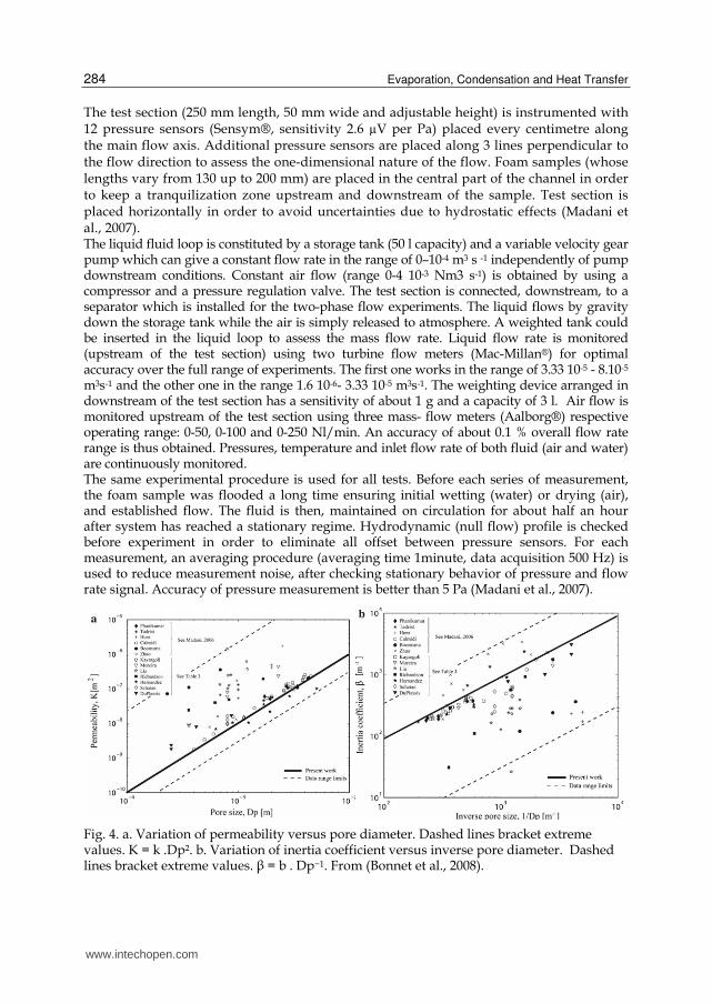
Fig. 4. a. Variation of permeability versus pore diameter. Dashed lines bracket extreme values. K = k .Dp². b. Variation of inertia coefficient versus inverse pore diameter. Dashed lines bracket extreme values. ┚ = b . Dp−1. From (Bonnet et al., 2008).

www.intechopen.com


285

After each measurement series, the flow is stopped and the hydrostatic pressure profile is measured anew and compared to the previous hydrostatic one. In this way we could ensure that pressure sensors bias has not changed with the time. Gravity and capillarity driven flow through cell edges during the manufacture of metallic foams induce material property gradients (tortuosity, cell size…) and cells themselves are not spherical (Brun et al., 2009). Slight anisotropy of geometrical parameters is observed for ours sample. Nevertheless at this stage of the study we neglect these effects. Measurement of full permeability and inertial coefficient tensor is, yet, difficult and the precision of our set-up in the studied configuration doesn’t allow measurement of transverse pressure gradient with an accuracy compatible with the objectives of this work (Renard et al., 2001).

3.3 Numerical simulation Foam meshes have been obtained by reconstruction of tomographic images. We imaged cylindrical samples of 40 mm diameter and 15 mm thickness. High-resolution microtomography acquisition was performed on the ID19 beam line of the ESRF. Sample size was maximized while respecting the data-volume constraint and X-ray image resolution. We thus acquired a large number of cells while efficiently detecting struts (E. Brun et al., 2009). We have measured several useful morphological parameters such as specific surface, porosity, pore diameter distribution and cells orientations from 3D images analysis using iMorph (Brun et al., 2009; Brun et al., 2008). The sample size (15 mm in all directions) is sufficient (i.e. greater than Rve) to define macroscopic parameters. The computational domain is divided in three parts: Inlet zone, test section and outlet zone to avoid bias product by back conduction and fluid recirculation. Volume mesh (~1 million cells with a mean size of about 0.2 mm and a minimal one of 0.05 mm) is generated from actual solid surface using StarCCM4+ mesher. It is composed from core polyhedral meshes in both solid and fluid phases with additional prism layers mesh in fluid phase in the vicinity of solid surfaces. Boundary conditions are: imposed temperature on one lateral wall and adiabatic on the others. Inlet temperature and pressure are imposed. Other walls are symmetry planes.

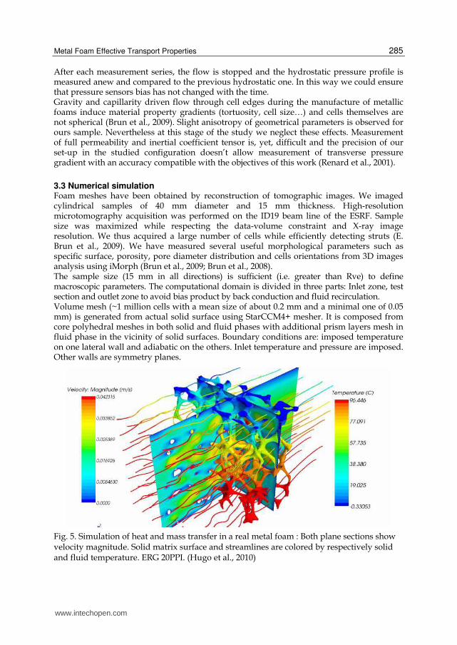
Fig. 5. Simulation of heat and mass transfer in a real metal foam : Both plane sections show velocity magnitude. Solid matrix surface and streamlines are colored by respectively solid and fluid temperature. ERG 20PPI. (Hugo et al., 2010)

www.intechopen.com


286

The Navier-Stokes equations and energy balance equation are solved using a finite volume

method (StarCCM+). These equations are solved at the pore scale and give access to velocity

and pressure fields in the fluid phase and temperature in both, solid and fluid phases. Local

heat fluxes across the solid matrix surface are also determined. Numerical simulations are

performed for a wide Reynolds number range (10-2 – 104). On Figure 5 the two plane

sections show velocity magnitude. Important velocity gradient could be observed locally

while a constant averaged value is obtained in a cross section normal to principal fluid flow

direction. Solid surface is colored with its temperature. A sharp gradient exists near the

cooled wall while near the other side; fluid and solid temperature are roughly identical. This

indicates that solid matrix allows heat conduction to take place between the heated wall and

the fluid core like a classical fin. Finally, we can observe that the fluid flow is not very

tortuous but struts lead to a local deformation of the thermal boundary layer. This indicates

that boundary layers will not develop near wall channel. Also, some eddies could be located

in the wake of struts. These phenomena govern heat transfer enhancement and pressure

drop increase.

To establish parameters K and β numerically, simulations must be performed for several

values of Reynolds. K and β are then computed by fitting pressure gradient versus

superficial velocity data with the Forchheimer model. Results are then compared to those

obtained experimentally. (Kim et al., 2001; Tadrist et al., 2004) give experimental data for

pressure losses in similar metal foam (ERG) for liquid and gas flows (Table 1 and Figure 6).

For clarity, data are shown by a friction factor, defined by (5), versus the Reynolds number.

2

2

ΔP Dp 2Dpf = = + 2┚Dp

L K.Re0.5ρU (5)

At macroscopic scale, mean velocities are indeed representative of global fluid behavior. Nevertheless, according to Reynolds number values, velocity gradients and preferential paths may appear. For Reynolds near unity, velocity field is very homogeneous, and struts wakes are very small (Similar to Stokes regimes around cylinders). For higher Reynolds, large eddies and recirculations are observed in the struts wakes. The flow may become un-stationary and wake interactions between struts may appear. A strut in the wake of the previous will exhibit poor heat performance. Preferential high velocity path will cause rather important pressure gradient. Some high velocity vectors exist just upstream of struts. This is a typical 3D effect, the flow get around the struts in the third dimension. Global heat exchange limitation and strong inertia effects intensity at high Reynolds can be explained by these phenomena. On the other hand, low tortuosity of pore space associated to the relatively small specific surface of the solid matrix could not explain heat transfer performance and inertia effect intensity. On Figure 6, experimental data from (Tadrist et al., 2004) for two pores diameters (3 and 4.5mm) are compared to numerical results with a good agreement. For all pore diameters, friction factor is described by a unique curve. Equation (2) associated to these results demonstrates that both permeability and inertia coefficient evolve with the pore diameter only for these structurally similar foam samples. For a given Reynolds, to conserve a constant friction factor, permeability should be proportional to the squared pore diameter

and β to the inverse of the pore diameter as (Bonnet et al., 2008) has shown experimentally on several metal foams. Virtual Samples (VS) were created to verify this behaviour (Table1).

www.intechopen.com


287

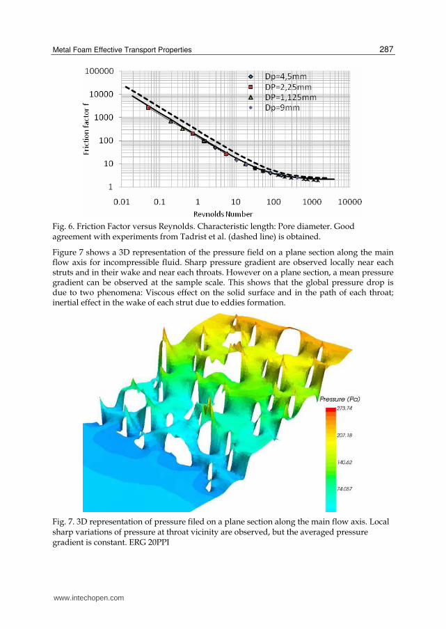
Fig. 6. Friction Factor versus Reynolds. Characteristic length: Pore diameter. Good agreement with experiments from Tadrist et al. (dashed line) is obtained.

Figure 7 shows a 3D representation of the pressure field on a plane section along the main flow axis for incompressible fluid. Sharp pressure gradient are observed locally near each struts and in their wake and near each throats. However on a plane section, a mean pressure gradient can be observed at the sample scale. This shows that the global pressure drop is due to two phenomena: Viscous effect on the solid surface and in the path of each throat; inertial effect in the wake of each strut due to eddies formation.

Fig. 7. 3D representation of pressure filed on a plane section along the main flow axis. Local sharp variations of pressure at throat vicinity are observed, but the averaged pressure gradient is constant. ERG 20PPI

www.intechopen.com


288

Sample Pore

diameter

Strut

Diameter Porosity

Specific

surface Permeability

Inertia

coefficient

Dp [µm] ds [µm] ε Sp

[m2/m3] K [m2] ┚ [m-1]

Ni 100 500 1.38E-09 1686

Ni10 4429 409 0.92 680 7.63E-08 248

NC 4753 400 0.9 5600 2.01E-09 2175

NC 3743 569 88 0.87 5303 2.11E-09 1329

NC 2733 831 120 0.91 3614 4.79E-09 1088

NC 1723 1840 255 0.88 1658 1.14E-08 446

NC 1116 2452 337 0.89 1295 3.62E-08 364

Cu 40 1500 224 0.95 2000 7.20E-08 1107

Cu 10 4055 152 0.94 758 8.95E-08 180

ERG10 4449 366 0.86 668 1.30E-06 111

ERG20 3720 232 0.89 791 2.97E-07 266

ERG40 2380 189 0.9 1120 6.60E-08 389

Kelvin Cell 14200 1775 0.87 250 2.00E-06 350

CTIF stoch. 4200 * 0.75 800 6.83E-08 2100

VS 5 14880 928 0.89 198 4.80E-06 53

VS 10 7440 464 0.89 396 1.30E-06 111

VS 40 1860 116 0.89 1582 7.48E-08 612

VS 80 930 58 0.89 3164 1.89E-08 1208

Table 1. Summary of various metal foam sample morphological and flow law properties.

Greyed values: Pore scale direct numerical simulation. *Stochastic CTIF foam is not

composed of a struts network (Dairon & Gaillard, 2009). VS samples are Virtual Samples

created by homothetic transform of ERG 20PPI.

The friction factor versus Reynolds curve exhibits two behaviors separated by a transition

zone. For Reynolds smaller than 50, viscous effects are predominant. Pressure drop

increases linearly with the velocity. For high Reynolds (greater than 2000) inertia effects

dominate the flow behavior. The pressure drop increases as the square of velocity. For

Reynolds between 50 and 2000, there is a transition zone where, both, viscous and inertial

effects govern pressure losses. Overall Friction law is well described by the Forchheimer

model. Inertia coefficients and permeability obtained from numerical simulations are

summarized in Table 1. and compared to experimental data. Foam pore diameters in

(Tadrist et al., 2004) study have been determined latter by (Brun, 2009). (Kim et al., 2001)

only gives foam grade; pore diameter are not exactly determined. However, flow law

parameters for 40PPI foam given in both experimental studies are quite close. This

indicates that the grade is clearly not relevant as pore size estimator. Moreover, both

numerical and experimental data lead to the same dependence of β in function of K.

Several authors have proposed to use squareroot of K as pore size estimator but K is

usually difficult to measure accurately. This is particularly true in case of high pore size

foam (> 5 mm).

www.intechopen.com


289

3.4 Heat transfer Direct experimental measurement of volume heat transfer coefficient is not easy for fluid

flow crossing metal foam. Generally authors propose global heat transfer coefficient of a

channel filled by a porous media (Kim et al., 2001). There are few works dealing with local

heat transfer coefficient between fluid and solid phase (Serret, Stamboul, & Topin, 2007).

However wall heat transfer coefficient is an averaging on different transport and diffusion

properties on a known channel or heat exchanger geometry and can thus be used only in

these cases.

In the following section, we propose different analytical and numerical models to rely this

coefficient and experimental or simulation data. Models can be used to determine heat

transfer coefficient from data or to predict heat exchanger performance from the knowledge

of thermal properties. Heat transfer law is also determined from direct numerical simulation

performed on the real foam geometry (Hugo et al., 2010).

Experimental set up described above is modified to perform heat transfer measurement.

Thermocouples are added to measure local temperature along the main flow axis. Fluid

flow can be heated before the channel or heat flux can be imposed on the channel wall. Two

protocols are studied:

• In the first case, the metal foam is heated by hot air flow and then cooled by air at

ambient temperature. Transient outlet temperature signal is used with .a 0D analytical

model to evaluate heat transfer coefficient.

• In the second case, fluid flow at ambient temperature is imposed at the inlet. Heat flux

is imposed on the channel wall. Temperature at the outlet is measured at steady state. A

2D two temperature model (non local thermal equilibrium (Moyne, 1997)) allows one

determining numerically the heat transfer coefficient.

3.4.1 0D analytical model

Metal foam is considered as thermally thin body and its temperature is considered as

homogeneous and equals to Tm. Air flow temperature Ta is imposed at the channel inlet.

( ) ( ) ( )mp vol m f

solid

T1 C h T T 0

t

∂− ε ⋅ ρ ⋅ ⋅ + ⋅ − =

∂ (6)

in out exf in .

p

fluid

T T PT T

22 m C

+= = + ⎛ ⎞

⋅ ⋅⎜ ⎟⎝ ⎠ (7)

Where ε (−) is the porosity, ρ(kg/m3) the metal density, Cp (J/kg/K) the metal heat capacity,

η (kg/s) is air mass flow rate and hvol (W/m3/K) the volume heat transfer coefficient.

Fluid temperature profile is considered as linear through the channel. A mean air

temperature Tf is defined by (8).

( ) ( ) ( ) mex vol m f p

solid

TP h V T T 1 V C

t

∂= ⋅ ⋅ − = − − ε ⋅ ⋅ ρ ⋅ ⋅

∂ (8)

Previous equations lead to the following differential equation on foam temperature:

www.intechopen.com


290

( ) ( ) ( )mp vol m in.solid

p

fluid

V T1 C 1 h T T 0

t2 m C

⎛ ⎞⎜ ⎟∂⎜ ⎟

− ε ⋅ ρ ⋅ ⋅ − ⋅ ⋅ + ⋅ − =⎜ ⎟ ∂⎛ ⎞⎜ ⎟⋅ ⋅⎜ ⎟⎜ ⎟⎝ ⎠⎝ ⎠ (9)

mt

T A.Exp B⎛ ⎞

= − +⎜ ⎟τ⎝ ⎠ (10)

The solution (10) of this equation shows that foam temperature and, thus outlet temperature

is decreasing exponentially with the same characteristic time τ. For a constant inlet temperature, the measurement of the outlet temperature in function of the time (Figure 8) allows one determining the heat transfer coefficient with relation (12).

Fig. 8. Experimental fluid temperature temporal decrease along the main flow axis during sample cooling. An exponential decrease is observed. Aluminium foam (porosity 75%)

( ) ( )p .solid

p

fluidvol

V1 C 1

2 m C

h

⎛ ⎞⎜ ⎟⎜ ⎟− ε ⋅ ρ ⋅ − ⋅⎜ ⎟⎛ ⎞⎜ ⎟⋅ ⋅⎜ ⎟⎜ ⎟⎝ ⎠⎝ ⎠=

τ (11)

The main limit of this method is the limited range of usable sample thickness. The foam sample must be large enough to establish fluid boundary layers and be representative volume (RVE) and small enough to respect the thermal thin body hypothesis. However, as most foams are produced as flat sheets, this point is not critical for many applications.

3.4.2 Numerical model In the case of geometry that doesn’t allow using the 0D model, a 2D numerical method based on a non equilibrium model between solid and fluid phase could be used. Equations (13) and (14) describe this model:

www.intechopen.com


291

( ) ( ) ( )eff

ff

f fp p m f

f f

Tk

T U T xC C h T T

t x x

∂⎛ ⎞∂ ⋅⎜ ⎟∂ ∂ ⋅ ∂⎝ ⎠ε ⋅ ρ ⋅ ⋅ + ρ ⋅ ⋅ = + ⋅ −

∂ ∂ ∂ (12)

( ) ( ) ( )eff

ss

sp s f

s

Tk

T x1 C h T T

t x

∂⎛ ⎞∂ ⋅⎜ ⎟∂ ∂⎝ ⎠− ε ⋅ ρ ⋅ ⋅ = + ⋅ −

∂ ∂ (13)

Fluid velocity considered here is the macroscopic one and is considered constant in the channel and the previous equations system is solved by a 2D finite volume method. We present, in this case, results obtained for the second experimental set up configuration (state measurement, heated wall). The knowledge of effective thermal conductivity for both phase and dispersion of the fluid phase is needed to use this model. As the thermal dispersion in the fluid phase is often not precisely known (Delgado, 2007), the stagnant fluid phase effective conductivity is used in present work. Dispersion phenomena is thus impacting the heat transfer coefficient value.

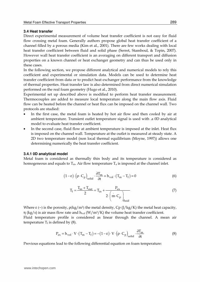
3.4.3 Local results In order to gain a better interpretation of global heat transfer performance, a local Nusselt and also heat transfer coefficient along the fluid flow are deduced from the simulation by dividing the test zone in numerous thin boxes perpendicular to the main flow axis. In each box, mean temperatures of both fluid and solid phases as well as exchanged heat flux are determined.

Fig. 9. Local (diamonds) and integrated (dashed line) Nusselt number along the main flow axis. Characteristic length: Strut diameter. ERG 20PPI

Figure 9 shows local and integrated Nusselt number variations along the main flow axis. Nusselt number decreases slightly along the flow direction and its averaging reaches a quasi-constant value after 3 pores diameters. But its behavior differs from the empty channel case. No clear entrance zone is observed. High amplitude oscillations around the global decreasing trend with a one-pore period are observed. Local Nusselt maxima and a

www.intechopen.com


292

minima are located at every half pore diameter. Cells present a staggered arrangement and Nusselt increases in the vicinity of throats. The cell arrangement along the main flow axis limits global thermal and flow boundary layers formation. (Madani et al., 2005) have experimentally shown similar results. For application purpose, pore size should be chosen according to the (empty) channel boundary layer characteristic length. Like a fin, foam efficiently contributes to heat transfer only on relatively short distance from

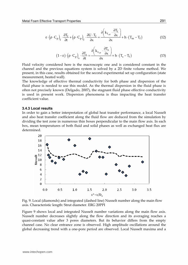
the heated wall. This active length is defined as the distance where fluid and solid phases

reach the same temperature (difference less than 5%).

On Figure 10, one could see that active length is close to 1.5Dp. Above this distance from the

heated wall, heat flux is close to zero. We determine the local heat flux exchanged between

fluid and solid phases. Below y*=y/Dp=0.5, heat flux are very high. The heat flux decreases

roughly exponentially above 1 pore diameter.

Fig. 10. Solid-fluid heat flux at foam surface, temperature of both fluid and solid phase versus the distance from the heated wall. x*=1.62. ERG 20PPI

3.4.4 Macroscopic results Usually, heat transfer coefficient is presented as Nusselt number versus Reynolds number calculated with pore diameter as characteristic length. The following values are obtained for Kelvin Cell foam :

n 1/3Nu Re Pr= α ⋅ (14)

Where Pr is the fluid Prandtl number. Values of α are generally between 0.3 and 1.5 and values of n between 0.3 and 0.7 (Kim et al., 2001; Lu, Stone, & Ashby, 1998; Serret et al., 2007). Numerical and experimental results are in good agreement at low Reynolds number. Uncertainties on temperature and specific surface measurement can lead to a global error of about 15% on the volume heat transfer coefficient for 0D model. For 2D model, Finite volume method solver, mesh and effective thermal conductivity can lead to an error of about 20%. For high Reynolds, results are differing. RANS model (k-epsilon) on the direct numerical simulation may not be adapted to turbulent flow through metal foam.

www.intechopen.com


293

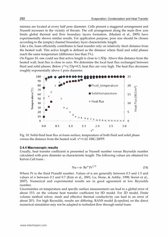
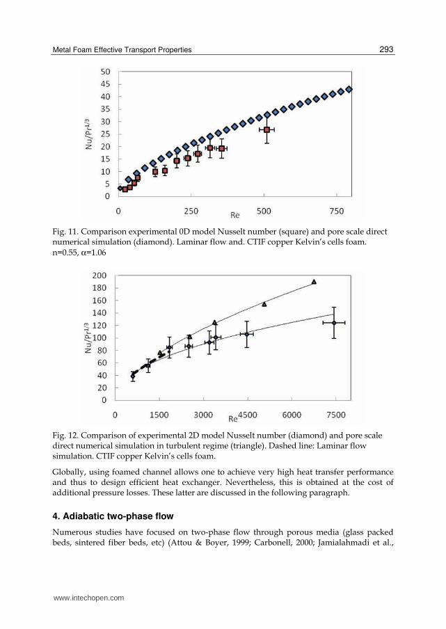
Fig. 11. Comparison experimental 0D model Nusselt number (square) and pore scale direct numerical simulation (diamond). Laminar flow and. CTIF copper Kelvin’s cells foam.

n=0.55, α=1.06

Fig. 12. Comparison of experimental 2D model Nusselt number (diamond) and pore scale direct numerical simulation in turbulent regime (triangle). Dashed line: Laminar flow simulation. CTIF copper Kelvin’s cells foam.

Globally, using foamed channel allows one to achieve very high heat transfer performance and thus to design efficient heat exchanger. Nevertheless, this is obtained at the cost of additional pressure losses. These latter are discussed in the following paragraph.

4. Adiabatic two-phase flow

Numerous studies have focused on two-phase flow through porous media (glass packed beds, sintered fiber beds, etc) (Attou & Boyer, 1999; Carbonell, 2000; Jamialahmadi et al.,

www.intechopen.com


294

2005). This type of flow is frequently encountered in many fields, such as petroleum engineering, nuclear safety, etc. Many questions remain to be answered in order to fully understand the physical mechanisms that are involved when two fluids flow concurrently through porous media. The correlations that make it possible to predict two-phase flow laws can be used only for the experimental conditions in which they have been established (strong influence of the porous geometry, sensitivity to configuration, etc).

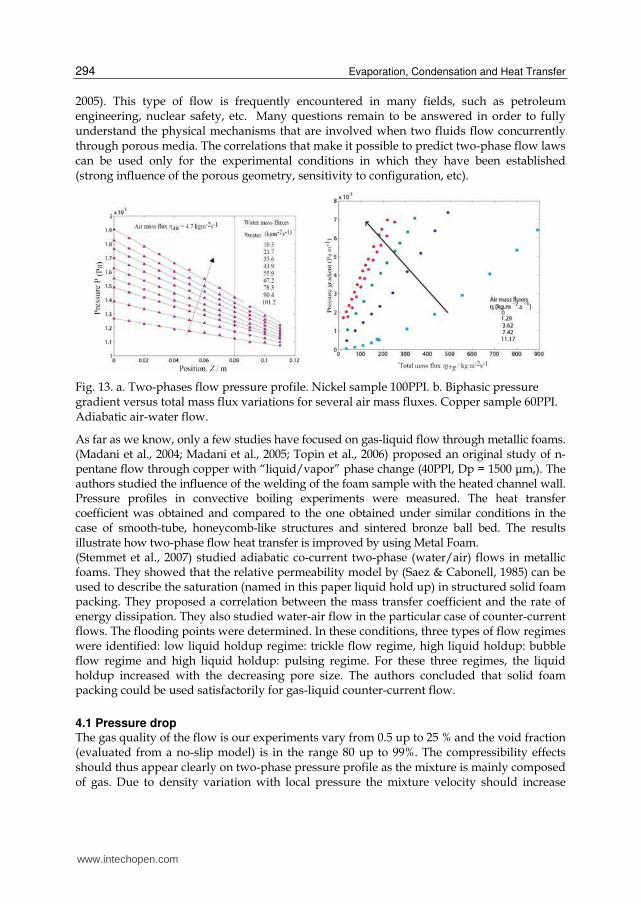
Fig. 13. a. Two-phases flow pressure profile. Nickel sample 100PPI. b. Biphasic pressure gradient versus total mass flux variations for several air mass fluxes. Copper sample 60PPI. Adiabatic air-water flow.

As far as we know, only a few studies have focused on gas-liquid flow through metallic foams. (Madani et al., 2004; Madani et al., 2005; Topin et al., 2006) proposed an original study of n-pentane flow through copper with “liquid/vapor” phase change (40PPI, Dp = 1500 μm,). The authors studied the influence of the welding of the foam sample with the heated channel wall. Pressure profiles in convective boiling experiments were measured. The heat transfer coefficient was obtained and compared to the one obtained under similar conditions in the case of smooth-tube, honeycomb-like structures and sintered bronze ball bed. The results illustrate how two-phase flow heat transfer is improved by using Metal Foam. (Stemmet et al., 2007) studied adiabatic co-current two-phase (water/air) flows in metallic foams. They showed that the relative permeability model by (Saez & Cabonell, 1985) can be used to describe the saturation (named in this paper liquid hold up) in structured solid foam packing. They proposed a correlation between the mass transfer coefficient and the rate of energy dissipation. They also studied water-air flow in the particular case of counter-current flows. The flooding points were determined. In these conditions, three types of flow regimes were identified: low liquid holdup regime: trickle flow regime, high liquid holdup: bubble flow regime and high liquid holdup: pulsing regime. For these three regimes, the liquid holdup increased with the decreasing pore size. The authors concluded that solid foam packing could be used satisfactorily for gas-liquid counter-current flow.

4.1 Pressure drop The gas quality of the flow is our experiments vary from 0.5 up to 25 % and the void fraction (evaluated from a no-slip model) is in the range 80 up to 99%. The compressibility effects should thus appear clearly on two-phase pressure profile as the mixture is mainly composed of gas. Due to density variation with local pressure the mixture velocity should increase

www.intechopen.com


295

from inlet to outlet producing an increasing pressure gradient. But, as experimental results are correctly modeled by linear approximation, it should exist an antagonist effect (void fraction variation probably) that mask this behavior (Figure 13). Figure 13 illustrates the influence of air flow rate on biphasic pressure gradient. For a given total mass flux the pressure loss is proportional to air flow rate. In other words, pressure gradient is proportional to flow quality. The curvature of these curves is inversely proportional to the quality of the flow. This indicates that viscous effects depend more strongly on quality than inertial one.

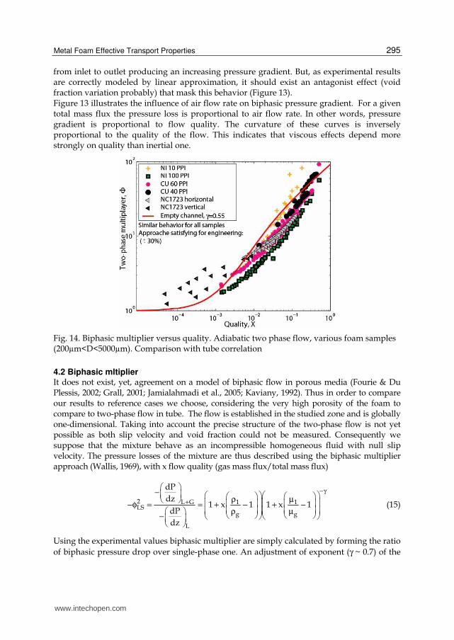
Fig. 14. Biphasic multiplier versus quality. Adiabatic two phase flow, various foam samples (200µm<D<5000µm). Comparison with tube correlation

4.2 Biphasic mltiplier It does not exist, yet, agreement on a model of biphasic flow in porous media (Fourie & Du Plessis, 2002; Grall, 2001; Jamialahmadi et al., 2005; Kaviany, 1992). Thus in order to compare our results to reference cases we choose, considering the very high porosity of the foam to compare to two-phase flow in tube. The flow is established in the studied zone and is globally one-dimensional. Taking into account the precise structure of the two-phase flow is not yet possible as both slip velocity and void fraction could not be measured. Consequently we suppose that the mixture behave as an incompressible homogeneous fluid with null slip velocity. The pressure losses of the mixture are thus described using the biphasic multiplier approach (Wallis, 1969), with x flow quality (gas mass flux/total mass flux)

2 L G 1 1LS

g g

L

dP

dz1 x 1 1 x 1

dP

dz

−γ

+

⎛ ⎞−⎜ ⎟ ⎛ ⎞⎛ ⎞⎛ ⎞ ⎛ ⎞ρ µ⎝ ⎠ ⎜ ⎟⎜ ⎟⎜ ⎟ ⎜ ⎟−φ = = + − + −⎜ ⎟ ⎜ ⎟⎜ ⎟⎜ ⎟ρ µ⎛ ⎞ ⎝ ⎠ ⎝ ⎠− ⎝ ⎠⎝ ⎠⎜ ⎟⎝ ⎠

(15)

Using the experimental values biphasic multiplier are simply calculated by forming the ratio

of biphasic pressure drop over single-phase one. An adjustment of exponent (γ ~ 0.7) of the

www.intechopen.com


296

viscosity term appearing in the biphasic multiplier expression allows modeling all experimental data with reasonable agreement. Figure 14 present the comparison of

experimental results with the correlation proposed by Mac Adams (γ = -0.25) for laminar flow in tubes (Wallis, 1969). All experimental data are roughly located on a unique curve similar to the literature correlation. Nevertheless a slight influence of pore size is visible on this figure. When pore size increase the biphasic multiplier seems to be closer to the value obtained for tube. But more experimental data are needed to interpret this effect. This approach has been applied with reasonable agreement in convective boiling case, using biphasic multiplier given by Mac Adam correlation (Madani et al., 2004).

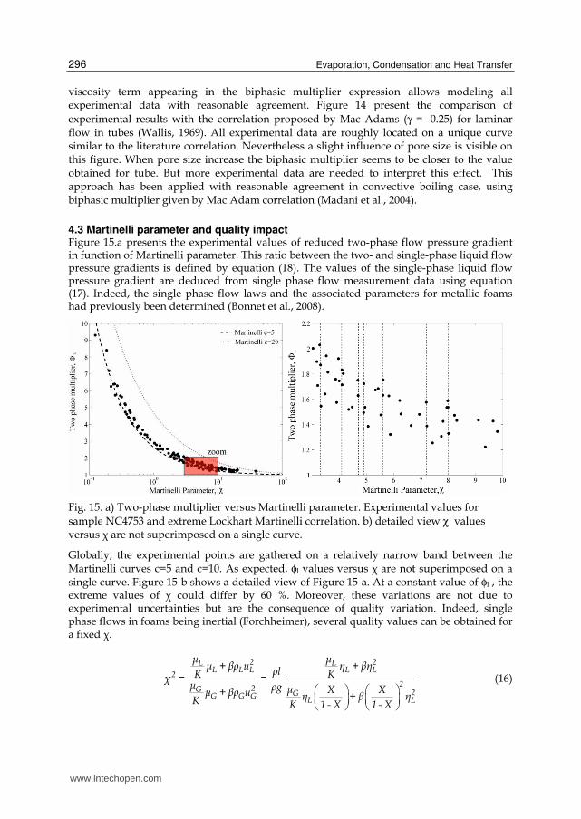
4.3 Martinelli parameter and quality impact Figure 15.a presents the experimental values of reduced two-phase flow pressure gradient in function of Martinelli parameter. This ratio between the two- and single-phase liquid flow pressure gradients is defined by equation (18). The values of the single-phase liquid flow pressure gradient are deduced from single phase flow measurement data using equation (17). Indeed, the single phase flow laws and the associated parameters for metallic foams had previously been determined (Bonnet et al., 2008).

Fig. 15. a) Two-phase multiplier versus Martinelli parameter. Experimental values for

sample NC4753 and extreme Lockhart Martinelli correlation. b) detailed view χ values versus χ are not superimposed on a single curve.

Globally, the experimental points are gathered on a relatively narrow band between the Martinelli curves c=5 and c=10. As expected, φl values versus χ are not superimposed on a single curve. Figure 15-b shows a detailed view of Figure 15-a. At a constant value of φl , the extreme values of χ could differ by 60 %. Moreover, these variations are not due to experimental uncertainties but are the consequence of quality variation. Indeed, single phase flows in foams being inertial (Forchheimer), several quality values can be obtained for a fixed χ.

⎛ ⎞ ⎛ ⎞⎜ ⎟ ⎜ ⎟⎝ ⎠ ⎝ ⎠

2 2L LL L L L L

22

2G 2GG G GL L

μ μμ + βρ u η + βηρlK Kχ = =μ ρg μ X Xμ + βρ u η + β ηK K 1 - X 1 - X

(16)

www.intechopen.com


297

The values of φl range from 1 to 10 when χ ranges from 0.1 up to 100. For a given χ, the experiment shows that values systematically increase with quality (Figure 16). In terms of pressure gradient, the deviation between the model predictions and experimental results is always smaller than 25 %.Thus these approaches are suitable for design or engineering purposes. Let us notice that for a sheer Darcy flow, the relationship between quality X and Martinelli

parameter χ is bijective. Unfortunately, at constant χ, the experimental data available did not

allow us to determine any analytical expression correlating φL with quality. As a result, the

use of any function of χ alone would only give an approximation of two-phase pressure gradient.

Fig. 16. Two-phase multiplier versus Martinelli parameter for sample pore sizes in the range 400-2000 µm. Experimental values and comparison with two literature correlations. No clear difference between samples is observed.

5. Convective boiling

5.1 Experimental set-up The boiling mechanisms in copper foam and the evaluation of the impact of the solid matrix on flow and heat transfer phenomena were experimentally studied. It consisted of 2 rectangular channel (10x50x100 (resp.200) mm) that contained a 40 PPI grade copper foam. The smallest one is welded to the wall, as the other is just inserted in the channel A liquid (i.e., n-pentane, low toxicity, low boiling point: 36 °C at atmospheric pressure, low phase-change enthalpy) flowed through the porous media vertically from the bottom to the top (Figure 17). The channel was instrumented with 40 thermocouples and 15 pressure sensors (Madani et al., 2004; Madani et al., 2005). Before each experiment, we apply repeated Boiling-cooling sequences in order to eliminate non-condensable substances, and then flow is imposed at the desired flow rate (0- 80 kg m-2 s-1). After stationary regime is reached, heating power (range 0 – 25 Wcm-2) is applied. All data are continuously monitored. When stationary regime is reached temperature and pressure profiles are recorded as well as flow rate, heating power…

www.intechopen.com


298

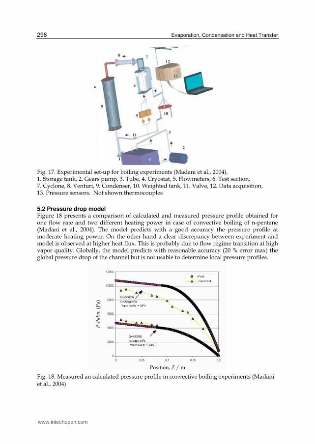
Fig. 17. Experimental set-up for boiling experiments (Madani et al., 2004). 1. Storage tank, 2. Gears pump, 3. Tube, 4. Cryostat, 5. Flowmeters, 6. Test section, 7. Cyclone, 8. Venturi, 9. Condenser, 10. Weighted tank, 11. Valve, 12. Data acquisition, 13. Pressure sensors. Not shown thermocouples

5.2 Pressure drop model Figure 18 presents a comparison of calculated and measured pressure profile obtained for one flow rate and two different heating power in case of convective boiling of n-pentane (Madani et al., 2004). The model predicts with a good accuracy the pressure profile at moderate heating power. On the other hand a clear discrepancy between experiment and model is observed at higher heat flux. This is probably due to flow regime transition at high vapor quality. Globally, the model predicts with reasonable accuracy (20 % error max) the global pressure drop of the channel but is not usable to determine local pressure profiles.

Fig. 18. Measured an calculated pressure profile in convective boiling experiments (Madani et al., 2004)

P-P

atm

, (P

a)

Position, Z / m

www.intechopen.com


299

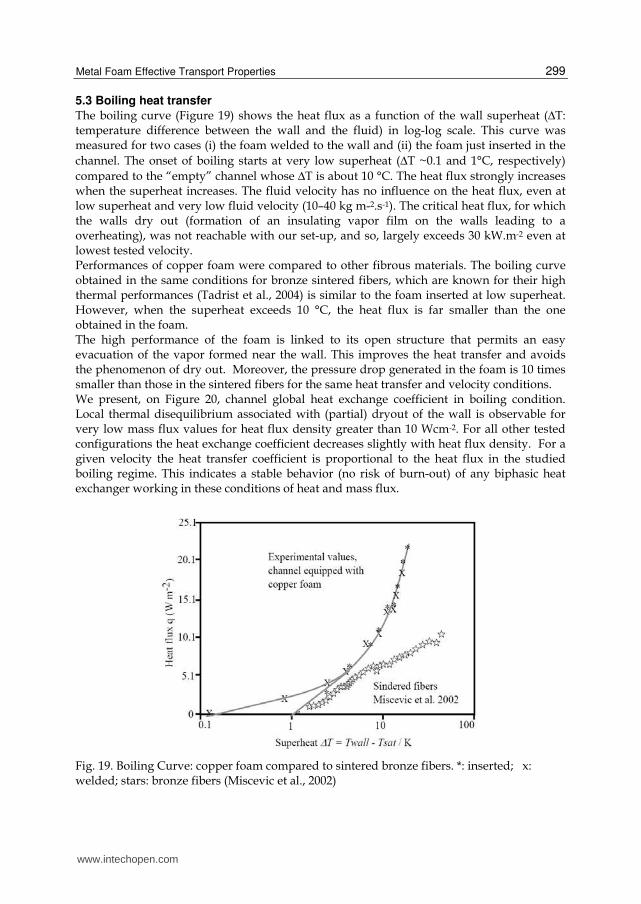
5.3 Boiling heat transfer

The boiling curve (Figure 19) shows the heat flux as a function of the wall superheat (ΔT: temperature difference between the wall and the fluid) in log-log scale. This curve was measured for two cases (i) the foam welded to the wall and (ii) the foam just inserted in the

channel. The onset of boiling starts at very low superheat (ΔT ~0.1 and 1°C, respectively)

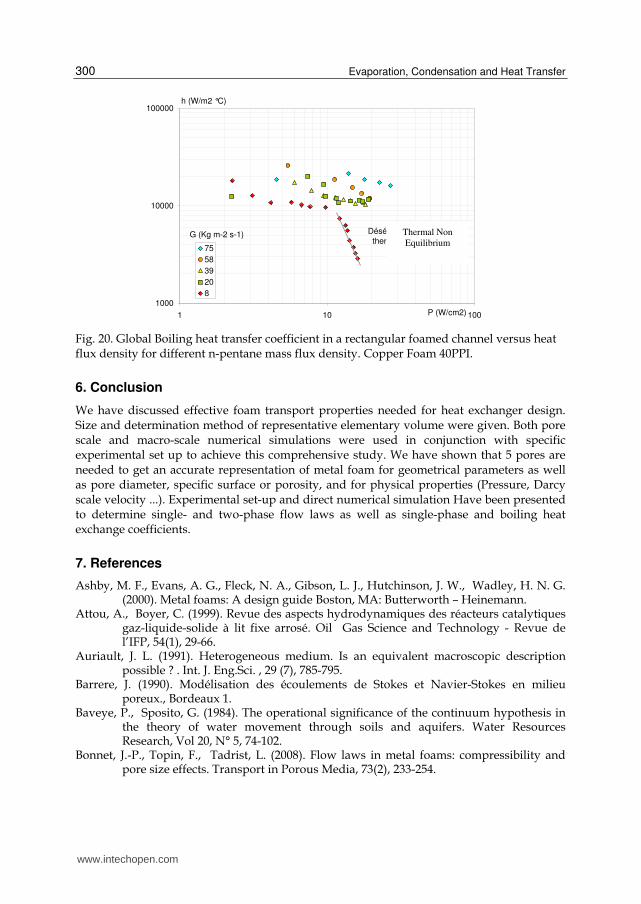
compared to the “empty” channel whose ΔT is about 10 °C. The heat flux strongly increases when the superheat increases. The fluid velocity has no influence on the heat flux, even at low superheat and very low fluid velocity (10–40 kg m-2.s-1). The critical heat flux, for which the walls dry out (formation of an insulating vapor film on the walls leading to a overheating), was not reachable with our set-up, and so, largely exceeds 30 kW.m-2 even at lowest tested velocity. Performances of copper foam were compared to other fibrous materials. The boiling curve obtained in the same conditions for bronze sintered fibers, which are known for their high thermal performances (Tadrist et al., 2004) is similar to the foam inserted at low superheat. However, when the superheat exceeds 10 °C, the heat flux is far smaller than the one obtained in the foam. The high performance of the foam is linked to its open structure that permits an easy evacuation of the vapor formed near the wall. This improves the heat transfer and avoids the phenomenon of dry out. Moreover, the pressure drop generated in the foam is 10 times smaller than those in the sintered fibers for the same heat transfer and velocity conditions. We present, on Figure 20, channel global heat exchange coefficient in boiling condition. Local thermal disequilibrium associated with (partial) dryout of the wall is observable for very low mass flux values for heat flux density greater than 10 Wcm-2. For all other tested configurations the heat exchange coefficient decreases slightly with heat flux density. For a given velocity the heat transfer coefficient is proportional to the heat flux in the studied boiling regime. This indicates a stable behavior (no risk of burn-out) of any biphasic heat exchanger working in these conditions of heat and mass flux.

Fig. 19. Boiling Curve: copper foam compared to sintered bronze fibers. *: inserted; x: welded; stars: bronze fibers (Miscevic et al., 2002)

www.intechopen.com


300

1000

10000

100000

1 10 100

75

58

39

20

8

G (Kg m-2 s-1)

P (W/cm2)

h (W/m2 °C)

Déséquilibre

thermique

Fig. 20. Global Boiling heat transfer coefficient in a rectangular foamed channel versus heat flux density for different n-pentane mass flux density. Copper Foam 40PPI.

6. Conclusion

We have discussed effective foam transport properties needed for heat exchanger design. Size and determination method of representative elementary volume were given. Both pore scale and macro-scale numerical simulations were used in conjunction with specific experimental set up to achieve this comprehensive study. We have shown that 5 pores are needed to get an accurate representation of metal foam for geometrical parameters as well as pore diameter, specific surface or porosity, and for physical properties (Pressure, Darcy scale velocity ...). Experimental set-up and direct numerical simulation Have been presented to determine single- and two-phase flow laws as well as single-phase and boiling heat exchange coefficients.

7. References

Ashby, M. F., Evans, A. G., Fleck, N. A., Gibson, L. J., Hutchinson, J. W., Wadley, H. N. G. (2000). Metal foams: A design guide Boston, MA: Butterworth – Heinemann.

Attou, A., Boyer, C. (1999). Revue des aspects hydrodynamiques des réacteurs catalytiques gaz-liquide-solide à lit fixe arrosé. Oil Gas Science and Technology - Revue de l’IFP, 54(1), 29-66.

Auriault, J. L. (1991). Heterogeneous medium. Is an equivalent macroscopic description possible ? . Int. J. Eng.Sci. , 29 (7), 785-795.

Barrere, J. (1990). Modélisation des écoulements de Stokes et Navier-Stokes en milieu poreux., Bordeaux 1.

Baveye, P., Sposito, G. (1984). The operational significance of the continuum hypothesis in the theory of water movement through soils and aquifers. Water Resources Research, Vol 20, N° 5, 74-102.

Bonnet, J.-P., Topin, F., Tadrist, L. (2008). Flow laws in metal foams: compressibility and pore size effects. Transport in Porous Media, 73(2), 233-254.

Thermal Non

Equilibrium

www.intechopen.com


301

Brun, E. (2009). De l’imagerie 3d des structures à l’étude des mécanismes de transport en milieux cellulaires. Ph.D. Université de Provence.

Brun, E., Vicente, J., Topin, F., Occelli, R. (2008). IMorph : A 3D morphological tool to fully analyse all kind of cellular materials Paper presented at the Cellmet'08, Dresden, Allemagne.

Brun, E., Vicente, J., Topin, F., Occelli, R., Clifton, M. (2009). Microstructure and transport properties of cellular materials: representative volume element. Adv. Mat. Eng., 21 (10) , 805-810 .

Carbonell, R. G. (2000). Multiphase Flow Models in Packed Beds. Oil Gas Science and Technology – Rev. IFP 55(4), 417-425.

Catillon, S., Louis, C., Topin, F., Vicente, J., Rouget, R. (2004). Influence of Cellular Structure in catalytic reactors for H2 Production: Application to Improvement of Methanol Steam Reformer by the Addition of a Copper Foam. Paper presented at the 2nd France-Deutchland Fuel Cells Conference, Belfort, France.

Dairon, J., Gaillard, Y. (2009). Casting parts with CTIF foams. Paper presented at the MetFoam'09, Brastislava.

Darcy, H. P. G. (1856). Exposition et application des principes à suivre et des formules à employer dans les questions de distribution d'eau. Les fontaines publiques de la ville de Dijon. Paris: Victor Delmont.

Delgado, J. M. P. Q. (2007). Longitudinal and Transverse Dispersion in Porous Media. Chemical Engineering Research and Design, 85(9), 1245-1252.

Drugan, W. J., Willis, J. R. (1996). A micromechanics based nonlocal constitutive equation and estimates of representative volume element size for elastic composites. J. Mech. Phys. Solids., 44, 497–524.

Dukhan, N., Quinones-Ramos, P., Cruz-Ruiz, E., Velez-Reyes, M., E., Scott. (2005). One-dimensional heat transfer analysis in open-cell 10-ppi metal foam. International Journal of Heat and Mass Transfer, 48, 5112–5120.

Dullien, F. A. L. (1992). Porous media. Fluid transport and pore structure: Academic Press. Firdaous, M., Guermond, J. L., Le Quere, P. (1997). Nonlinear corrections to Darcy’s law at

low Reynolds numbers. J Fluid Mech 343:331–50. Fourar, M., Radilla, G., Lenormand, R., Moyne, C. (2004). On the non-linear behavior of a

laminar single-phase flow through two and three-dimensional porous media. Advances in Water Resources 27, 669-677.

Fourie, J. G., Du Plessis, J. P. (2002). Pressure drop modelling in cellular metallic foams. Chemical Engineering Science, 57(14), 2781-2789.

Grall, V. (2001). Etude experimentale d'ecoulements diphasiques liquide-gaz en mini canaux et en milieu poreux modèle. INP Toulouse.

Hugo, J.-M., Topin, F., Brun, E., Vicente, J. (2010). Conjugate Heat and Mass Transfer in Metal Foams: A Numerical Study for Heat Exchangers Design. Diffusion in Solids and Liquids V, Defect and Diffusion Forum, 297-301

Hugo, J.-M., Topin, F., Tadrist, L., Brun, E. (2010). From pore scale numerical simulation of conjugate heat transfer in cellular material to effectives transport properties of real structures. Paper presented at the IHTC 14, Washington.

Jamialahmadi, M., Muller-Steinhagen , H., Izadpanah, M. R. (2005). Pressure drop, gas hold-up and heat transfer during single and two-phase flow through porous media. International Journal of Heat and Fluid Flow 26, 156-172.

Kanit, T., Galliet, S. F. I., Mounoury, V., Jeulin, D. (2003). Determination of the size of the representative volume element for random composites: statistical and numerical approach. International Journal of Solids and Structures, 40(13-14), 3647-3679.

www.intechopen.com


302

Kaviany, M. (1992). Principles of heat transfer in porous media: Springer-Verlag. Kim, S. Y., Kang, B. H., Kim, J.-H. (2001). Forced convection from aluminum foam materials

in an asymmetrically heated channel. IJHMT, 44(7), 1451-1454. Lorensen, W. E., Cline, H. E. (1987). Marching Cubes: A High Resolution 3D Surface

Construction Algorithm. Computer Graphics, 21(3), 163-169. Lu, T. J., Stone, H. A., Ashby, M. F. (1998). Heat transfer in open- cell metal foams. Acta

Materialia, 46(10), 3619-3635. Madani, B., Topin, F., Tadrist, L. (2004). Ebullition convective dans les mousses métalliques :

Analyse expérimentale des effets de contact matrice solide -paroi. Paper presented at the Congrès de la SFT 04, Giens, France.

Madani, B., Topin, F., Tadrist, L., Bouhadef, K. (2005). Mesure du coefficient de transfert de chaleur local paroi-fluide dans un canal à mousse métallique en écoulement liquide et en ébullition. Paper presented at the 12ième JITH, Tanger, Maroc.

Madani, B., Topin, F., Tadrist, L., Rigollet, F. (2007). Flow laws in metallic foams: experimental determination of inertial and viscous contribution. Jounal of Porous Media, 10(1), 51-70.

Mahjoob, S., Vafai, K. (2008). A synthesis of fluid and thermal transport models for metal foam heat exchangers. International Journal of Heat and Mass Transfer, 51, 3701–3711.

Marle, C. (1982). On macroscopic equation governing multiphase flow with diffusion and chemical reactions in porous media. Int. J. Eng. Sci, 20(5), 643-662.

Mei, C., Auriault, J. L. (1993). The effect of weak inertia on flow through a porous medium. J. Fluid Mech., 222, 647-663.

Miscevic, M., Topin, F., Tadrist, L. (2002). Convective boiling phenomena in a sintered fibrous channel:Study of thermal non-equilibrium behavior Journal of Porous Media, 5(4), 229-239.

Moyne, C. (1997). Two-equation model for a diffusive process in porous media using the volume averaging method with an unsteady-state closure. Advances in Water Resources, 29(2-3), 63-76.

Quintard, M., Whitaker, S. (1991). Transport Process in ordered and disordered porous media. Paper presented at the 1991 ICHMT International Seminar on heat and mass transfer in porous media.

Renard, P., Genty, A., Stauffer, F. (2001). Laboratory détermination of the full permeability tensor. Journal of geophysical research, 106(B11), 26443-26452.

Saez, A. E., Cabonell, R. G. (1985). Hydrodynamic parameters for gas - liquid cocurrent flow in packed beds,. AIChE J, 31, 52 - 62.

Serret, D., Stamboul, T., Topin, F. (2007). Transferts dans les mousses métalliques :Mesure du coefficient d’échange de chaleur entre phases Paper presented at the Congrès de la SFT, SFT 07, Ille des Embiez.

Stemmet, C. P., van der Schaaf, J., Kuster, B. F. M., Schouten, J. C. (2007). Gas–liquid mass transfer and axial dispersion in solid foam packings. Chemical Engineering Science, 62, 5444 - 5450.

Tadrist, L., Miscevic, M., Rahli, O., Topin, F. (2004). About the Use of Fibrous Materials in Compact Heat Exchangers. Experimental Thermal and Fluid Science, 28, 193 – 199.

Topin, F., Bonnet, J.-P., Madani, B., Tadrist, L. (2006). Experimental Analysis of Multiphase Flow in Metallic foam: Flow Laws, Heat Transfer and Convective Boiling. Advanced material Engineering, 8(9), 890-899.

Wallis, G. (1969). One-Dimensional Two-Phase Flow New-York, NY: Mc graw Hill. Wodie, J. C., Levy, T. (1991). Correction non linéaire de la loi de Darcy. C. R. Acad. Sci.,

312(II), 157-161.

www.intechopen.com

Evaporation, Condensation and Heat transferEdited by Dr. Amimul Ahsan

ISBN 978-953-307-583-9Hard cover, 582 pagesPublisher InTechPublished online 12, September, 2011Published in print edition September, 2011

InTech EuropeUniversity Campus STeP Ri Slavka Krautzeka 83/A 51000 Rijeka, Croatia Phone: +385 (51) 770 447 Fax: +385 (51) 686 166www.intechopen.com

InTech ChinaUnit 405, Office Block, Hotel Equatorial Shanghai No.65, Yan An Road (West), Shanghai, 200040, China

Phone: +86-21-62489820 Fax: +86-21-62489821

The theoretical analysis and modeling of heat and mass transfer rates produced in evaporation andcondensation processes are significant issues in a design of wide range of industrial processes and devices.This book includes 25 advanced and revised contributions, and it covers mainly (1) evaporation and boiling,(2) condensation and cooling, (3) heat transfer and exchanger, and (4) fluid and flow. The readers of this bookwill appreciate the current issues of modeling on evaporation, water vapor condensation, heat transfer andexchanger, and on fluid flow in different aspects. The approaches would be applicable in various industrialpurposes as well. The advanced idea and information described here will be fruitful for the readers to find asustainable solution in an industrialized society.

How to referenceIn order to correctly reference this scholarly work, feel free to copy and paste the following:

Jean-Michel Hugo, Emmanuel Brun and Fre ́de ́ric Topin (2011). Metal Foam Effective Transport Properties,Evaporation, Condensation and Heat transfer, Dr. Amimul Ahsan (Ed.), ISBN: 978-953-307-583-9, InTech,Available from: http://www.intechopen.com/books/evaporation-condensation-and-heat-transfer/metal-foam-effective-transport-properties

© 2011 The Author(s). Licensee IntechOpen. This chapter is distributedunder the terms of the Creative Commons Attribution-NonCommercial-ShareAlike-3.0 License, which permits use, distribution and reproduction fornon-commercial purposes, provided the original is properly cited andderivative works building on this content are distributed under the samelicense.

https://creativecommons.org/licenses/by-nc-sa/3.0/

Documents

Metal Foam Effective Transport Properties