SAP Buffers Purpose

Each SAP instance (application server) has its own buffers. These buffers are also known as client caches because they are implemented on the client, that is, the application server. SAP buffers occupy memory areas that are local to the work process, and in individual shared memory segments that can be accessed by all work processes. These memory areas are executed for the application server.

Some of the shared memory segments in an SAP System are grouped into one shared memory segment known as a pool. This is done to meet the operating system limits on the number of shared memory allocations per process. In most operating systems, you can allocate as many shared memory segments as required. The limits depend on the kernel configuration. The AIX operating system, for example, allows 10 shared memory segments per process.

SAP buffers store frequently-used data, and make this data available to the local application server instance. This helps to reduce the number of database accesses, the load on the database server (it does not need to be accessed repeatedly to obtain the same information), and network traffic. As a result, system performance is considerably improved.

The data that is buffered includes ABAP programs and screens, ABAP Dictionary data, and company-specific data. Typically these remain unchanged during system operation.

You can change, or tune, the sizes of buffers to optimize performance for a particular hardware configuration. There are several ways to tune buffers. As there are many constraints to consider when change the buffer size, several difficulties may arise.

You can use table buffering to fine-tune applications, that is, some or all of the contents of infrequently changed tables can be held in local buffers.

SAP Buffers

Program Buffer This buffer occupies a whole shared memory segment.

Generic Buffer

Screen BufferThese buffers are held in a shared memory pool. All work processes can access this pool.

Roll Area Local work process buffers. Only one work process can access these buffers at a time.

 

Monitoring in the CCMS PurposeThe CCMS provides a range of monitors for monitoring the SAP environments and its components. These monitors are indispensable for understanding and evaluating the behavior of the SAP processing environment. In the case of poor performance values, the monitors provide you with the information required to fine tune your SAP system and therefore to ensure that your SAP installation is running efficiently.

Implementation ConsiderationsFor central monitoring, that is, for the monitoring of a system landscape from one system, you must perform various configuration steps yourself. These are outlined in Configuring the Monitoring Architecture.

FeaturesThe CCMS analysis monitors provide functions for

        Checking the system status and the operating modes        Detecting and correcting potential problems as quickly as possible        An early diagnosis of potential problems, such as resource problems in a host or database system, which could

affect the SAP system        The analysis and fine tuning of the SAP system and its environment (host and database system) to optimize

the throughput of the SAP system

The previous monitoring and alert system in the CCMS was replaced by the monitoring architecture. The new monitoring architecture provides all of the functions that previously existed as well as new, more reliable alerts and more complex, more powerful functions.

UseYou can either use the following monitors independently or execute them as analysis methods in the alert monitor:

        Global Work Process Overview

        Workload Monitor

        Global Workload Monitor

        Operating System Monitor

        Operating System Collector        SAP Buffer        Database Monitor

 

Global Work Process Overview Purpose

You can quickly investigate the potential cause of a system performance problem by checking the work process load. You can use the global work process overview to:

Monitor the work process load on all active instances across the system Identify locks in the database (lock waits).

Using the Global Work Process Overview screen, you can see at a glance:

The status of each application server The reason why it is not running Whether it has been restarted The CPU and request run time The user who has logged on and the client that they logged on to The report that is running

 

See also:

 Selecting Work Processes

Displaying Detailed Work Process Information

Selecting Work Processes 

Procedure Call CCMS Control/monitoring Work process overview. Alternatively, call Transaction SM66. Choose the Select process pushbutton.

Select the work processes and statuses that you want to display more information on. You can also display information on specific programs and users.

Type

Choose the work process type.

Status

You can select the work process statuses you are interested in.

Runtime selection

Use this option to select long-running work processes.

Application selection

Use this option to select requests for specific R/3 transactions.

Reporting

Use this option to select specific ABAP/4 programs.

User selection

You can investigate the potential specific causes of a problem. If you suspect that a particular user is blocking work processes, enter the name of the program or user, then choose Continue to filter the information.

 

Displaying Detailed Work Process Information 

Procedure Choose CCMS Control/monitoring Work process overview. Alternatively, call Transaction SM66. Position the cursor on the instance and choose Choose. You can terminate the program that is currently

running and debug it.

For background processes, additional information is available for the background job that is currently running. You can only display this information, if you are logged onto the instance where the job is running, or if you choose Settings and deselect Display only abbreviated information, avoid RFC. In any case, the job must still be running.

 

Workload Monitor Purpose

The workload monitor (transaction ST03N) is intended for use by EarlyWatch and GoingLive teams. The workload monitor was reworked as part of the EnjoySAP initiative, so that the Workload Overview is now simpler and more intuitive.

You use the workload monitor to analyze statistical data from the SAP kernel. When analyzing the performance of a system, you should normally start by analyzing the workload overview. For example, you can display the totals for all instances and the compare the performances of individual instances over specific periods of time. You can quickly determine the source of possible performance problems using the large number of analysis views and the determined data.

You can use the workload monitor to display the:

Number of configured instances for each SAP R/3 System Number of users working on the different instances Distribution of response times Distribution of workload by transaction steps, transactions, packages, subapplications, and applications Transactions with the highest response time and database time Memory usage for each transaction or each user per dialog step Workload through RFC, listed by transactions, function modules and destinations

Number and volume of spool requests Statistics about response time distributeion, with or without the GUI time Optional: Table accesses Workload and transactions used listed by users, payroll number, and client Workload generated by requests from external systems

For all of this data:

You can display the data for a particular instance (not only the one to which your logged on) or optionally totalled for all instances.

Depending on your user mode, you can choose the time period for which you want to display the data between day, week and month (or determine the length of time yourself using the Last Minutes’ Load function).

For most analysis views, you can display all or only certain task types.

Integration

The workload monitor completely replaces the old ST03 transaction.

Features

The workload monitor has an interface that is divided into two parts. Use the tree structures on the left of the screen to make the following settings:

Select the user mode Select the time period for which you want to display the workload Select various functions and analysis views (which data you want to display).

The system then displays the result on the right of the screen in a standardized ALV Grid Control. With it, you can :

Adjust the Layout of the Data Output Find the information you want using sort and filter functions Save user-specific views Display statistics graphically

Operating the Workload Monitor UseThe Workload Monitor is a one-screen transaction that has as few additional menus as possible. This makes operation significantly easier and more intuitive.

IntegrationTransaction ST03N of the Workload Monitor has replaced the old transaction ST03.

Features

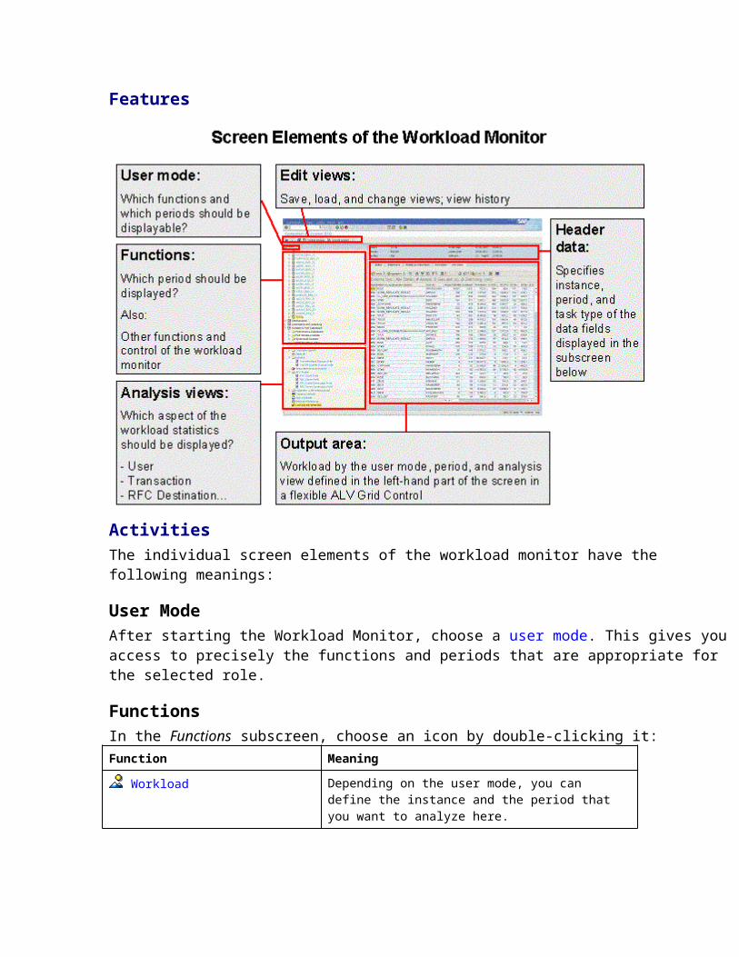
ActivitiesThe individual screen elements of the workload monitor have the following meanings:

User ModeAfter starting the Workload Monitor, choose a user mode. This gives you access to precisely the functions and periods that are appropriate for the selected role.

FunctionsIn the Functions subscreen, choose an icon by double-clicking it:Function Meaning

Workload Depending on the user mode, you can define the instance and the period that you want to analyze here.

Detailed Analysis These functions read the workload directly from the statistics files of the individual instances.

Business Transaction Analysis

You can perform a very precise analysis of individual transactions here, down to the level of individual steps.

Last Minutes’ Load You can use this function to analyze the workload data that has not yet been written to the performance database MONI.

Load History and Distribution

Load History

Instance Comparison

Users per Instance

With these functions, you cannot display the workload for a particular instance and a particular period (as in the other workload monitor functions), but rather compare the workload of different instances or periods.Display the most important data together therefore allows a direct comparison of the instances.

BW Workload Statistics of the BW Workload Monitor (only if there is a Business Warehouse in the system)

Collector & Performance Database Among other things, you can use this function to define which values the statistics collector collects, how often, and how long they are to be retained in the performance database in what time resolution.

Analysis ViewsAn analysis view displays a particular aspect of the workload. In the Analysis View subscreen, choose the view that you want to analyze by double-clicking it.

Only those analysis views are displayed:

         That are active in the selected user mode          For which data exists

Output AreaThe output area uses an ALV Grid Control, with which you can greatly tailor the selected view to your requirements. For most load parameters, the workload monitor displays more data fields than are required for your analysis. You therefore have a considerable amount of help available in the output area to find the information relevant for you:

        The data of most analysis views is grouped in the results area by tab pages for different topic areas.        To obtain an overview of which data fields exist for an analysis view, choose the All Data tab page.

        Using the standard functions of the ALV Grid Control, you can

        Show and hide columns         Sort rows by the contents of a column         Set and delete filters         Perform summations         Export tables as a file type of your choice         Display tables as graphics         Save sort orders, filters, and selected columns as your layout

Editing ViewsChoose one of the following buttons in the Edit Views screen area:Button Meaning

Save View Saves the current view as your initial screen for the workload monitor (see also Saving User-Specific Views)

Previous View or  Next View Moves one view forward or back in the view history

Full Screen: Show/Hide Tree Shows or hides the Functions and Analysis Views subscreens on the left of the screen

Global Workload Monitor PurposeThe Global Workload Monitor (transaction ST03G) display statistical records for entire landscapes and therefore allows you to analyze statistics data for both SAP R/3 and non-SAP R/3 systems. You can use this data to analyze the workload of the monitored components in great detail. The monitor is organized as a one-screen transaction so that its operation is very intuitive, and so that you can query all desired data with only a few mouse clicks.While statistics records for an SAP R/3 system can only trace actions that are processed by SAP R/3 components, you can use Distributed Statistics Records (DSRs) to trace actions that are processed across the non-SAP R/3 components J2EE Engine, ITS, and BC. This also works across component boundaries. Components that write statistics records send data from the statistics record with their communication with other components (their “passport”), meaning that the originator of an action or a data flow of a business process can be traced even beyond component boundaries.The DSRs are first stored locally on the relevant component and are transferred to a monitoring system hourly by CCMS agents, where the aggregated statistical data is stored in a performance database and regularly reorganized.

Integration        The operation of the global workload monitor is largely similar to the operation of the SAP R/3 workload

monitor (transaction ST03N), which displays statistical data for the local ABAP system. The Global Workload Monitor actually uses functions of the SAP R/3 Workload Monitor when you analyze the workload of SAP R/3 Systems.

        The Global Workload Monitor displays statistical data aggregated by the collector. You can display raw statistical data (individual records) from SAP R/3 and non-SAP R/3 Systems from complex system landscapes using the functional trace (transaction STATTRACE). The functional trace offers a finer resolution. You can use the functional trace to trace actions that belong to a business process across system boundaries.

The differences between the functional trace and the Global Workload Monitor are explained in the section Difference Between the Functional Trace and the Global Workload Monitor.

FeaturesYou can perform the following analyses, among others, in the Global Workload Monitor:

        How is the workload distributed among the individual service types? (For more information about service types, see Displaying the Workload Overview.)

        What is the workload of individual actions?        How is the workload distributed over the individual hours of the day?        Which action steps have the longest response and wait time?        What workload data is created when calling external components?        What is the workload of individual users and which actions has a user performed?        What workload is created in a component on the basis of actions of external components?        What is the response time distribution for individual service types (required, for example, for Service Level

Agreements)?        What is the availability of the statistical data for the individual components?

The following applies to all of these analyses:

        You can choose the period for which you want to display data between day, week, and month, or specify the Last Minutes’ Load as you require.

        You can display data for any component or optionally totaled for all components of a type.

See also:Operating the Global Workload MonitorConfiguring/Self-Monitoring of the Global Workload MonitorWorkload Collector Monitor 

Operating System Monitor Purpose

An SAP instance runs within an operating system. The operating system provides the instance with the following resources:

Virtual memory Physical memory CPU File system management Physical disk Network

Bottlenecks in these areas can significantly affect the performance of the SAP system. You can monitor these resources using the CCMS operating system monitor.

The operating system monitor helps you locate the cause of a performance problem. If the source of the problem is in the operating system, you can analyze it further and resolve it using external tools or other external means.

Performance indicators are:

Average load of and utilization of the CPU Memory utilization Paging in and out of data to and from the memory (replaced by pool data in the OS/400 operating system

monitor) Disk utilization information LAN activity Operating system configuration parameters

See Also:

Calling the Operating System Monitor

Operating System Monitor Data: CPU

Operating System Monitor Data: Memory Management

Operating System Monitor Data: File System and LAN

Calling the Operating System Monitor Use

You can use the operating system monitor to monitor the system resources that the operating system provides. The collector SAPOSCOL collects these resources. You can call the monitor for the server on which you are currently logged on, or for another service.

You can also monitor operating system data using the CCMS monitor Operating System (transaction RZ20). However, the data displayed there is, in principle, only complete if the monitored servers belong to SAP systems. This restriction does not apply to the operating system monitor.

Prerequisites

SAPOSCOL must be running so that the data is available.

Procedure

To call the individual functions shown in the table, choose CCMS Control/Monitoring Performance Menu Operating System.

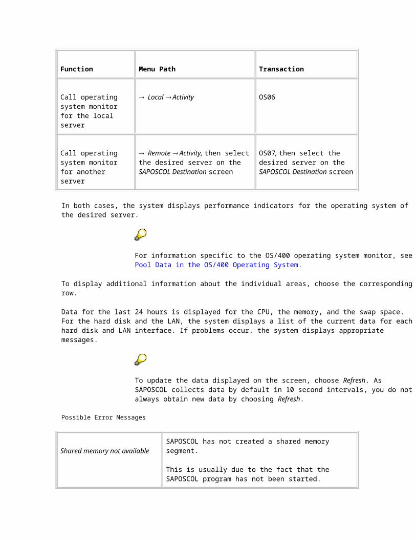
Function Menu Path Transaction

Call operating system monitor for the local server

Local Activity OS06

Call operating system monitor for another server

Remote Activity, then select the desired server on the SAPOSCOL Destination screen

OS07, then select the desired server on the SAPOSCOL Destination screen

In both cases, the system displays performance indicators for the operating system of the desired server.

For information specific to the OS/400 operating system monitor, see Pool Data in the OS/400 Operating System.

To display additional information about the individual areas, choose the corresponding row.

Data for the last 24 hours is displayed for the CPU, the memory, and the swap space. For the hard disk and the LAN, the system displays a list of the current data for each hard disk and LAN interface. If problems occur, the system displays appropriate messages.

To update the data displayed on the screen, choose Refresh. As SAPOSCOL collects data by default in 10 second intervals, you do not always obtain new data by choosing Refresh.

Possible Error Messages

Shared memory not availableSAPOSCOL has not created a shared memory segment.

This is usually due to the fact that the SAPOSCOL program has not been started.

Collector not running SAPOSCOL was started and created a shared memory segment, but was later terminated.

For more information about this topic, see Error Analysis: Operating System Collector.

Operating System Monitor Data: CPU Definition

The following data about CPU usage is displayed for every CPU, broken down as percentages by:

Users System Times in which the CPU had no task to perform or was waiting for an input/output (idle)

Many factors could lead to an excessively high CPU utilization, and you should therefore perform a detailed analysis. If the problem was caused by too many active processes in the host system, you could, for example, transfer CPU-intensive programs to times when there is a lower system workload, or to other host systems. You could also increase the number of CPUs or upgrade the CPU(s).

When calculating the hourly value for the last 24 hours, these values are averaged over all CPUs of a host.

Other Values Collected

Number of CPUs Interrupts per second/hour System calls per second/hour Context switches per second/hour Average number of waiting processes for the last minute, last five minutes and the last 15 minutes

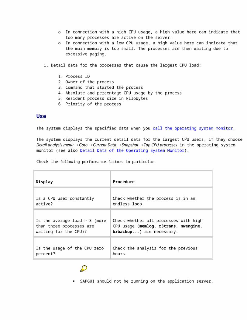
This is the number of processes for each CPU that are in a wait queue before they are assigned to a free CPU. As long as the average remains at one process for each available CPU, the CPU resources are sufficient. As of an average of around three processes for each available CPU, there is a bottleneck at the CPU resources.

o In connection with a high CPU usage, a high value here can indicate that too many processes are active on the server.

o In connection with a low CPU usage, a high value here can indicate that the main memory is too small. The processes are then waiting due to excessive paging.

1. Detail data for the processes that cause the largest CPU load:

1. Process ID 2. Owner of the process 3. Command that started the process 4. Absolute and percentage CPU usage by the process 5. Resident process size in kilobytes 6. Priority of the process

Use

The system displays the specified data when you call the operating system monitor.

The system displays the current detail data for the largest CPU users, if they choose Detail analysis menu Goto Current Data Snapshot Top CPU processes in the operating system monitor (see also Detail Data of the Operating System Monitor).

Check the following performance factors in particular:

Display Procedure

Is a CPU user constantly active? Check whether the process is in an endless loop.

Is the average load > 3 (more than three processes are waiting for the CPU)?

Check whether all processes with high CPU usage (memlog, r3trans, nwengine, brbackup...) are necessary.

Is the usage of the CPU zero percent? Check the analysis for the previous hours.

SAPGUI should not be running on the application server. You can also display SAP work processes with high CPU usage with the SAP process

overview. The SAP process overview displays the ABAP program that is using the CPU.

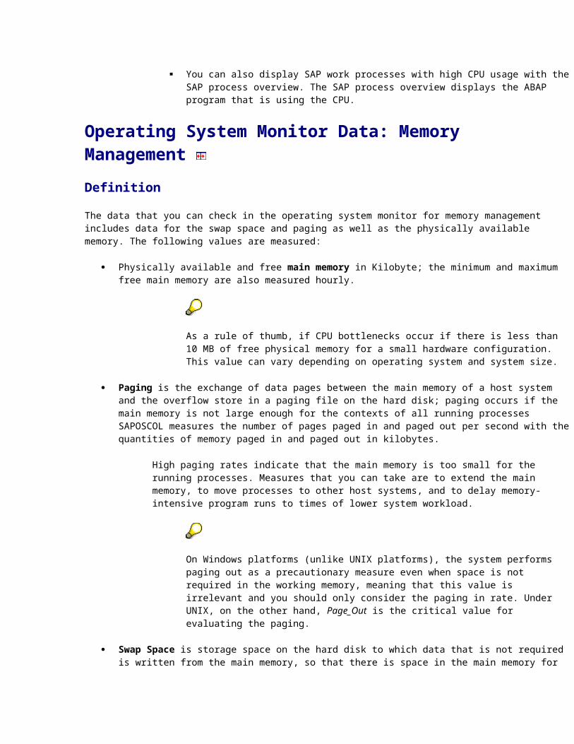
Operating System Monitor Data: Memory Management Definition

The data that you can check in the operating system monitor for memory management includes data for the swap space and paging as well as the physically available memory. The following values are measured:

Physically available and free main memory in Kilobyte; the minimum and maximum free main memory are also measured hourly.

As a rule of thumb, if CPU bottlenecks occur if there is less than 10 MB of free physical memory for a small hardware configuration. This value can vary depending on operating system and system size.

Paging is the exchange of data pages between the main memory of a host system and the overflow store in a paging file on the hard disk; paging occurs if the main memory is not large enough for the contexts of all running processes SAPOSCOL measures the number of pages paged in and paged out per second with the quantities of memory paged in and paged out in kilobytes.

High paging rates indicate that the main memory is too small for the running processes. Measures that you can take are to extend the main memory, to move processes to other host systems, and to delay memory-intensive program runs to times of lower system workload.

On Windows platforms (unlike UNIX platforms), the system performs paging out as a precautionary measure even when space is not required in the working memory, meaning that this value is irrelevant and you should only consider the paging in rate. Under UNIX, on the other hand, Page_Out is the critical value for evaluating the paging.

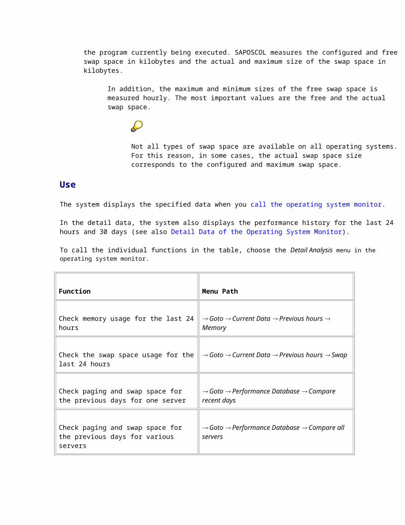
Swap Space is storage space on the hard disk to which data that is not required is written from the main memory, so that there is space in the main memory for the program currently being executed. SAPOSCOL measures the configured and free swap space in kilobytes and the actual and maximum size of the swap space in kilobytes.

In addition, the maximum and minimum sizes of the free swap space is measured hourly. The most important values are the free and the actual swap space.

Not all types of swap space are available on all operating systems. For this reason, in some cases, the actual swap space size corresponds to the configured and maximum swap space.

Use

The system displays the specified data when you call the operating system monitor.

In the detail data, the system also displays the performance history for the last 24 hours and 30 days (see also Detail Data of the Operating System Monitor).

To call the individual functions in the table, choose the Detail Analysis menu in the operating system monitor.

Function Menu Path

Check memory usage for the last 24 hours Goto Current Data Previous hours Memory

Check the swap space usage for the last 24 hours

Goto Current Data Previous hours Swap

Check paging and swap space for the previous days for one server

Goto Performance Database Compare recent days

Check paging and swap space for the previous days for various servers

Goto Performance Database Compare all servers

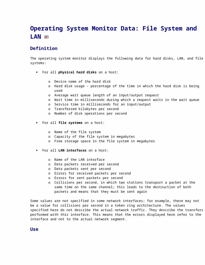
Operating System Monitor Data: File System and LAN Definition

The operating system monitor displays the following data for hard disks, LAN, and file systems:

For all physical hard disks on a host:

o Device name of the hard disk o Hard disk usage – percentage of the time in which the hard disk is being used o Average wait queue length of an input/output request o Wait time in milliseconds during which a request waits in the wait queue o Service time in milliseconds for an input/output o Transferred kilobytes per second o Number of disk operations per second

For all file systems on a host:

o Name of the file system o Capacity of the file system in megabytes o Free storage space in the file system in megabytes

For all LAN interfaces on a host:

o Name of the LAN interface o Data packets received per second o Data packets sent per second o Errors for received packets per second o Errors for sent packets per second o Collisions per second, in which two stations transport a packet at the same time on the same

channel; this leads to the destruction of both packets and means that they must be sent again

Some values are not specified in some network interfaces; for example, there may not be a value for collisions per second in a token ring architecture. The values specified here do not describe the actual network traffic. They describe the transfers performed with this interface. This means that the errors displayed here refer to the interface and not to the actual network segment.

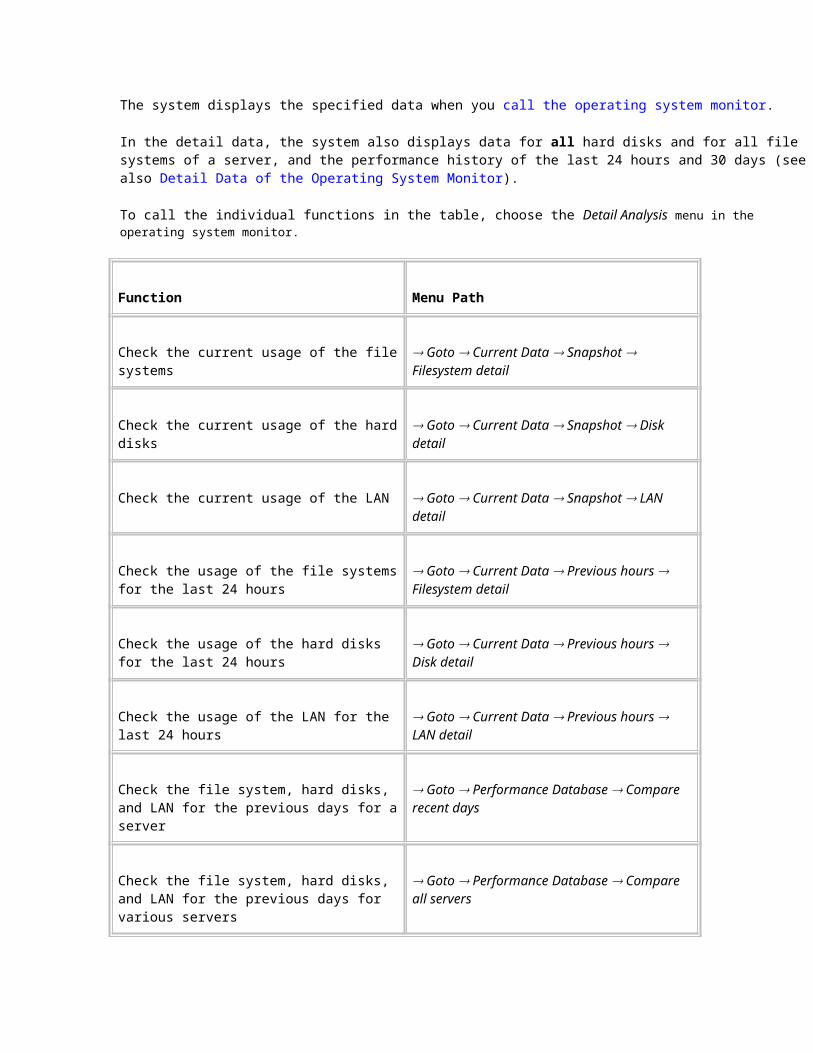
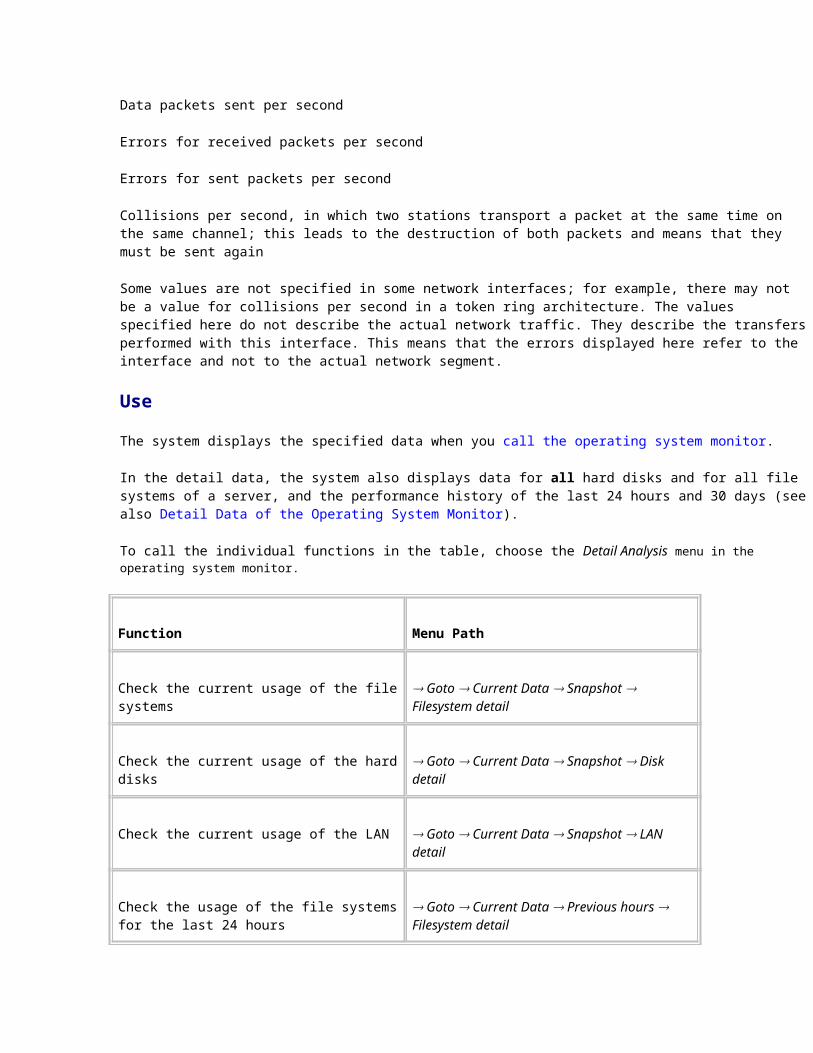
Use

The system displays the specified data when you call the operating system monitor.

In the detail data, the system also displays data for all hard disks and for all file systems of a server, and the performance history of the last 24 hours and 30 days (see also Detail Data of the Operating System Monitor).

To call the individual functions in the table, choose the Detail Analysis menu in the operating system monitor.

Function Menu Path

Check the current usage of the file systems Goto Current Data Snapshot Filesystem detail

Check the current usage of the hard disks Goto Current Data Snapshot Disk detail

Check the current usage of the LAN Goto Current Data Snapshot LAN detail

Check the usage of the file systems for the last 24 hours

Goto Current Data Previous hours Filesystem detail

Check the usage of the hard disks for the last 24 hours

Goto Current Data Previous hours Disk detail

Check the usage of the LAN for the last 24 hours

Goto Current Data Previous hours LAN detail

Check the file system, hard disks, and LAN for the previous days for a server

Goto Performance Database Compare recent days

Check the file system, hard disks, and LAN for the previous days for various servers

Goto Performance Database Compare all servers

See also:

Operating System Monitor Data: CPU

Operating System Monitor Data: Memory Management

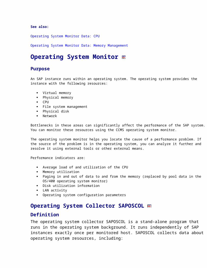
Operating System Monitor Purpose

An SAP instance runs within an operating system. The operating system provides the instance with the following resources:

Virtual memory Physical memory CPU File system management Physical disk Network

Bottlenecks in these areas can significantly affect the performance of the SAP system. You can monitor these resources using the CCMS operating system monitor.

The operating system monitor helps you locate the cause of a performance problem. If the source of the problem is in the operating system, you can analyze it further and resolve it using external tools or other external means.

Performance indicators are:

Average load of and utilization of the CPU Memory utilization Paging in and out of data to and from the memory (replaced by pool data in the OS/400 operating system

monitor) Disk utilization information LAN activity Operating system configuration parameters

Operating System Collector SAPOSCOL DefinitionThe operating system collector SAPOSCOL is a stand-alone program that runs in the operating system background. It runs independently of SAP instances exactly once per monitored host. SAPOSCOL collects data about operating system resources, including:

        Usage of virtual and physical memory        CPU utilization        Utilization of physical disks and file systems        Resource usage of running processes

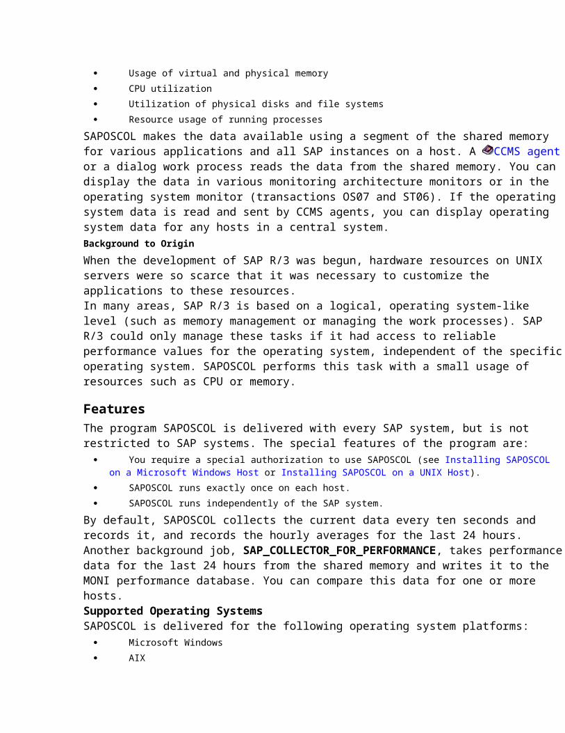
SAPOSCOL makes the data available using a segment of the shared memory for various applications and all SAP instances on a host. A CCMS agent or a dialog work process reads the data from the shared memory. You can display the data in various monitoring architecture monitors or in the operating system monitor (transactions OS07 and ST06). If the operating system data is read and sent by CCMS agents, you can display operating system data for any hosts in a central system. Background to OriginWhen the development of SAP R/3 was begun, hardware resources on UNIX servers were so scarce that it was necessary to customize the applications to these resources.In many areas, SAP R/3 is based on a logical, operating system-like level (such as memory management or managing the work processes). SAP R/3 could only manage these tasks if it had access to reliable performance values for the operating system, independent of the specific operating system. SAPOSCOL performs this task with a small usage of resources such as CPU or memory.

FeaturesThe program SAPOSCOL is delivered with every SAP system, but is not restricted to SAP systems. The special features of the program are:

        You require a special authorization to use SAPOSCOL (see Installing SAPOSCOL on a Microsoft Windows Host or Installing SAPOSCOL on a UNIX Host).

        SAPOSCOL runs exactly once on each host.        SAPOSCOL runs independently of the SAP system.

By default, SAPOSCOL collects the current data every ten seconds and records it, and records the hourly averages for the last 24 hours.Another background job, SAP_COLLECTOR_FOR_PERFORMANCE, takes performance data for the last 24 hours from the shared memory and writes it to the MONI performance database. You can compare this data for one or more hosts.Supported Operating SystemsSAPOSCOL is delivered for the following operating system platforms:

        Microsoft Windows        AIX        SUN/SOLARIS        HP-UX        LINUX        OS/390        OS/400        SNI

        ALPHAOSF

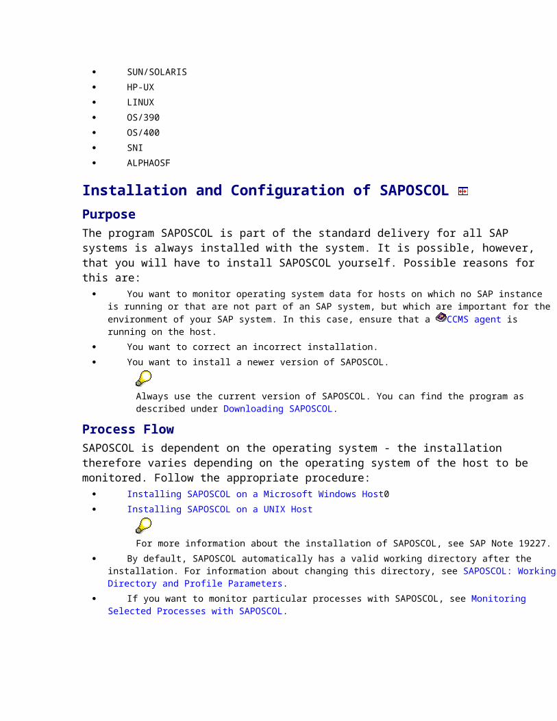
Installation and Configuration of SAPOSCOL PurposeThe program SAPOSCOL is part of the standard delivery for all SAP systems is always installed with the system. It is possible, however, that you will have to install SAPOSCOL yourself. Possible reasons for this are:

        You want to monitor operating system data for hosts on which no SAP instance is running or that are not part of an SAP system, but which are important for the environment of your SAP system. In this case, ensure that a

CCMS agent is running on the host.        You want to correct an incorrect installation.        You want to install a newer version of SAPOSCOL.

Always use the current version of SAPOSCOL. You can find the program as described under Downloading SAPOSCOL.

Process FlowSAPOSCOL is dependent on the operating system - the installation therefore varies depending on the operating system of the host to be monitored. Follow the appropriate procedure:

        Installing SAPOSCOL on a Microsoft Windows Host0        Installing SAPOSCOL on a UNIX Host

For more information about the installation of SAPOSCOL, see SAP Note 19227.        By default, SAPOSCOL automatically has a valid working directory after the installation. For information about

changing this directory, see SAPOSCOL: Working Directory and Profile Parameters.        If you want to monitor particular processes with SAPOSCOL, see Monitoring Selected Processes with

SAPOSCOL.

Control the Operating System Collector SAPOSCOL Purpose

After you have installed and started the operating system collector SAPOSCOL, it automatically begins to collect operating system data for its local host and to store this data in the shared memory.

SAPOSCOL provides various settings that you can use to improve its performance, to customize the quantity of collected data to your requirements, and to help you find the causes of errors.

Process Flow

The following sections contain the most important information about controlling SAPOSCOL

Control SAPOSCOL from the SAP System 

Use

You can control and monitor SAPOSCOL within the SAP system using the operating system monitor (transactions ST06 and OS07). You can use the following commands to do this:

Start and stop SAPOSCOL (to start and stop SAPOSCOL on a remote host, see Control SAPOSCOL on Remote Hosts).

Display dev_coll, the log file of SAPOSCOL Display the current status of SAPOSCOL Set and delete the detailed selection (see SAPOSCOL Log Files).

Control SAPOSCOL from the Operating System Use

You can also control SAPOSCOL directly from the operating system input prompt.

SAPOSCOL must be running for you to be able to use the following commands. Start the operating system collector with the command saposcol –l.

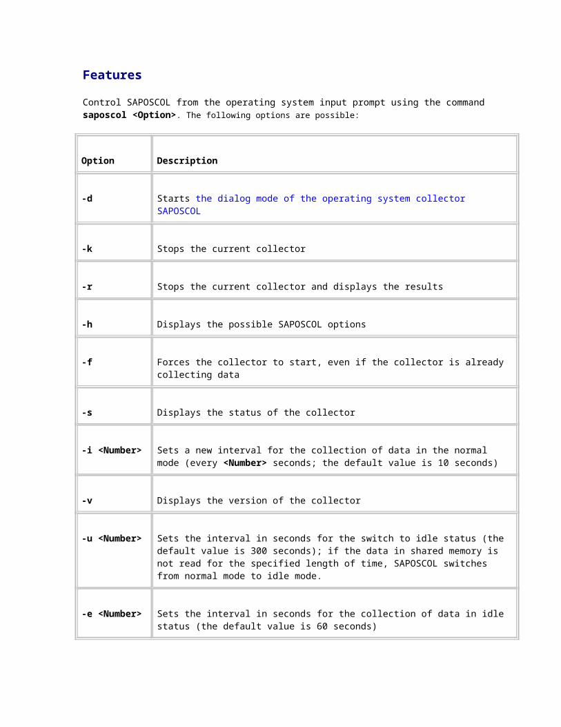
Features

Control SAPOSCOL from the operating system input prompt using the command saposcol <Option>. The following options are possible:

Option Description

-d Starts the dialog mode of the operating system collector SAPOSCOL

-k Stops the current collector

-r Stops the current collector and displays the results

-h Displays the possible SAPOSCOL options

-f Forces the collector to start, even if the collector is already collecting data

-s Displays the status of the collector

-i <Number> Sets a new interval for the collection of data in the normal mode (every <Number> seconds; the default value is 10 seconds)

-v Displays the version of the collector

-u <Number> Sets the interval in seconds for the switch to idle status (the default value is 300 seconds); if the data in shared memory is not read for the specified length of time, SAPOSCOL switches from normal mode to idle mode.

-e <Number> Sets the interval in seconds for the collection of data in idle status (the default value is 60 seconds)

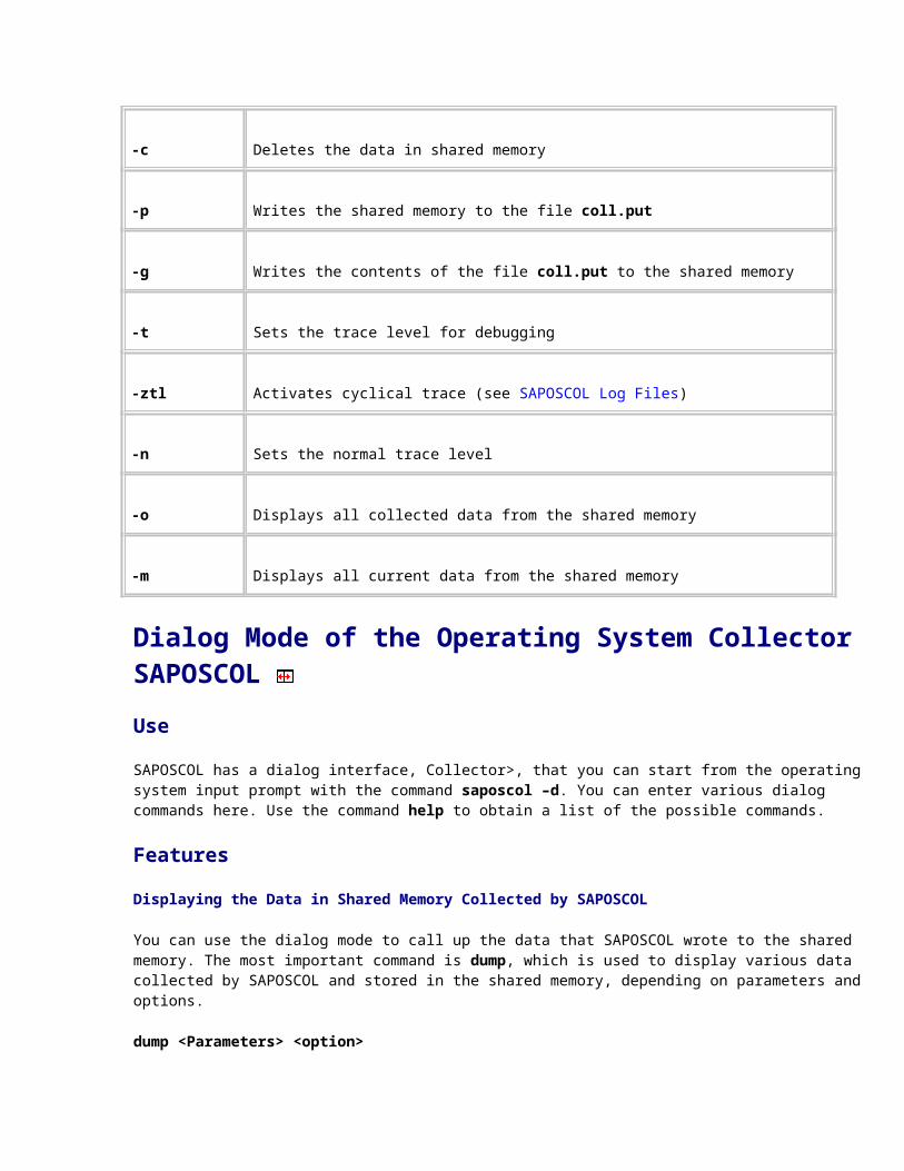
-c Deletes the data in shared memory

-p Writes the shared memory to the file coll.put

-g Writes the contents of the file coll.put to the shared memory

-t Sets the trace level for debugging

-ztl Activates cyclical trace (see SAPOSCOL Log Files)

-n Sets the normal trace level

-o Displays all collected data from the shared memory

-m Displays all current data from the shared memory

Dialog Mode of the Operating System Collector SAPOSCOL Use

SAPOSCOL has a dialog interface, Collector>, that you can start from the operating system input prompt with the command saposcol –d. You can enter various dialog commands here. Use the command help to obtain a list of the possible commands.

Features

Displaying the Data in Shared Memory Collected by SAPOSCOL

You can use the dialog mode to call up the data that SAPOSCOL wrote to the shared memory. The most important command is dump, which is used to display various data collected by SAPOSCOL and stored in the shared memory, depending on parameters and options.

dump <Parameters> <option>

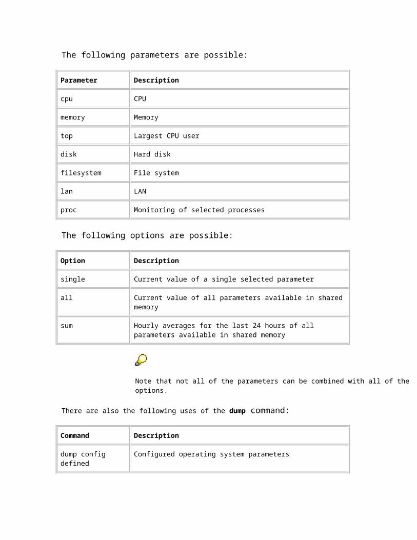
The following parameters are possible:

Parameter Description

cpu CPU

memory Memory

top Largest CPU user

disk Hard disk

filesystem File system

lan LAN

proc Monitoring of selected processes

The following options are possible:

Option Description

single Current value of a single selected parameter

all Current value of all parameters available in shared memory

sum Hourly averages for the last 24 hours of all parameters available in shared memory

Note that not all of the parameters can be combined with all of the options.

There are also the following uses of the dump command:

Command Description

dump configdefined

Configured operating system parameters

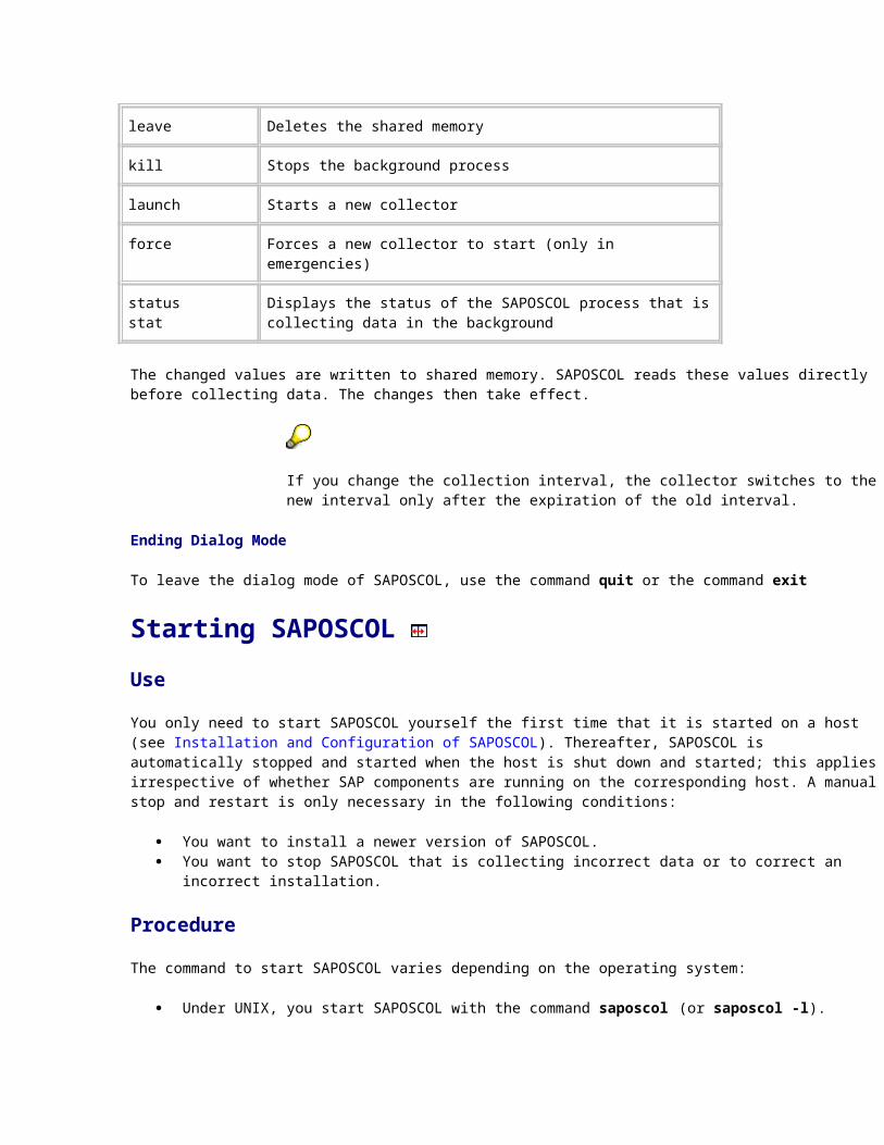
dump config used Currently used operating system parameters

dump hour Displays a list of the last 24 hours; each of the 24 entries has the format hour: <0-23> of day <Number>, where <Number> specifies whether SAPOSCOL has consistent data for that hour:0: No data available1: current hour2: inconsistent data<date (JJJJMMTT)>: Data available

To display the memory-related operating system data in the shared memory, enter the following command at the Collector> command line:

dump memory all

The following information is displayed:

Collector> dump memory allPages paged in / sec         1Pages paged out / sec        0KB    paged in / sec         4KB    paged out / sec        0freemem [KB]             13312physmem [KB]             65536swap configured  [KB]    76348swap total size  [KB]    76348swap free inside [KB]    72556

Controlling SAPOSCOL in Dialog Mode

You can control SAPOSCOL in dialog mode using the following commands at the Collector> input prompt:

Command Description

detailson Sets the details flag

detailsoff Cancels the details flag

interval <n> Changes the collection interval to <n> seconds (Default = 10)

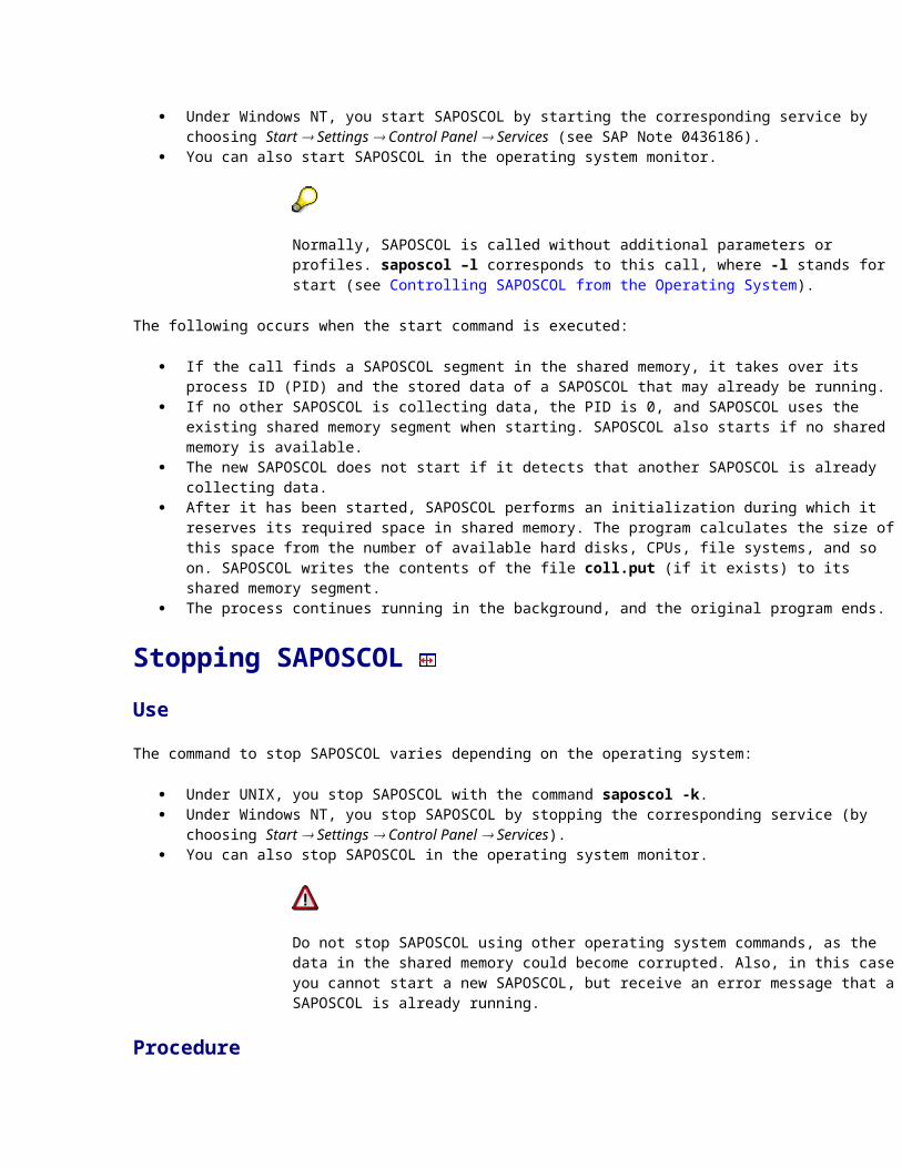
leave Deletes the shared memory

kill Stops the background process

launch Starts a new collector

force Forces a new collector to start (only in emergencies)

statusstat

Displays the status of the SAPOSCOL process that is collecting data in the background

The changed values are written to shared memory. SAPOSCOL reads these values directly before collecting data. The changes then take effect.

If you change the collection interval, the collector switches to the new interval only after the expiration of the old interval.

Ending Dialog Mode

To leave the dialog mode of SAPOSCOL, use the command quit or the command exit

Starting SAPOSCOL Use

You only need to start SAPOSCOL yourself the first time that it is started on a host (see Installation and Configuration of SAPOSCOL). Thereafter, SAPOSCOL is automatically stopped and started when the host is shut down and started; this applies irrespective of whether SAP components are running on the corresponding host. A manual stop and restart is only necessary in the following conditions:

You want to install a newer version of SAPOSCOL. You want to stop SAPOSCOL that is collecting incorrect data or to correct an incorrect installation.

Procedure

The command to start SAPOSCOL varies depending on the operating system:

Under UNIX, you start SAPOSCOL with the command saposcol (or saposcol -l). Under Windows NT, you start SAPOSCOL by starting the corresponding service by choosing Start Settings

Control Panel Services (see SAP Note 0436186). You can also start SAPOSCOL in the operating system monitor.

Normally, SAPOSCOL is called without additional parameters or profiles. saposcol –l corresponds to this call, where -l stands for start (see Controlling SAPOSCOL from the Operating System).

The following occurs when the start command is executed:

If the call finds a SAPOSCOL segment in the shared memory, it takes over its process ID (PID) and the stored data of a SAPOSCOL that may already be running.

If no other SAPOSCOL is collecting data, the PID is 0, and SAPOSCOL uses the existing shared memory segment when starting. SAPOSCOL also starts if no shared memory is available.

The new SAPOSCOL does not start if it detects that another SAPOSCOL is already collecting data. After it has been started, SAPOSCOL performs an initialization during which it reserves its required space in

shared memory. The program calculates the size of this space from the number of available hard disks, CPUs, file systems, and so on. SAPOSCOL writes the contents of the file coll.put (if it exists) to its shared memory segment.

The process continues running in the background, and the original program ends.

Stopping SAPOSCOL Use

The command to stop SAPOSCOL varies depending on the operating system:

Under UNIX, you stop SAPOSCOL with the command saposcol -k. Under Windows NT, you stop SAPOSCOL by stopping the corresponding service (by choosing Start

Settings Control Panel Services). You can also stop SAPOSCOL in the operating system monitor.

Do not stop SAPOSCOL using other operating system commands, as the data in the shared memory could become corrupted. Also, in this case you cannot start a new SAPOSCOL, but receive an error message that a SAPOSCOL is already running.

Procedure

The command to stop SAPOSCOL first starts a new SAPOSCOL that stops the active SAPOSCOL after a second. The following occurs:

The new SAPOSCOL connects to the shared memory. Using the shared memory, it determines the process ID (PID) of the SAPOSCOL that is collecting data. If the new SAPOSCOL finds a valid PID, it sets a flag in shared memory. When the old SAPOSCOL finds this

flag, it resets the flag and deletes the PID from shared memory. If this is not complete within 20 seconds, the new SAPOSCOL stops the old SAPOSCOL.

How long a shared memory segment exists depends on the operating system. On a UNIX operating system, it is stored until SAPOSCOL deletes it. On Windows NT, the shared memory is deleted by the operating system if no process is connected with it.

The old SAPOSCOL writes the data in shared memory to the file coll.put in the SAPOSCOL working directory. The program then ends.

When the host is restarted, the file coll.put is imported so that the combined data is available in the shared memory. If, for example, SAPOSCOL is stopped at 12:03 and is restarted at 14:49, the data until 12:00 is still available for the SAP system. To avoid confusion, invalid data for the time from 12:00 until 14:00 is not displayed in the overview of the last hours in the operating system monitor.

Delete the file coll.put, if you stop SAPOSCOL in the context of error analysis, as the program imports the (possibly erroneous) measured values from the file to the shared memory segment if it is restarted.

Reducing the CPU Load Caused by SAPOSCOL Use

SAPOSCOL can use a high proportion of operating system resources, as it periodically collects data from the operating system. Which data requires the most resources during collection depends on the operating system. You have the following options to minimize the CPU usage of SAPOSCOL:

Procedure

Delete the Detail Selection

You can control the collection of data by SAPOSCOL by having certain data, the collection of which has a particularly high influence on the performance, collected less frequently. Which data belongs to this group depends on the operating system of the monitored host:

By default, detail selection is set (Details required pushbutton in the operating system monitor; command detailson in dialog mode). To remove detail selection, choose Details Off in the operating system monitor, or enter the command detailsoff in the dialog mode. This setting applies universally.

Use the Idle Mode of SAPOSCOL

If the data is not read from the shared memory during a period of five minutes, SAPOSCOL switches from normal mode to idle mode. In this mode, the collector collects data every minute instead of every ten seconds. This is sufficient for a well-founded hourly average value. If a process reads data from the shared memory during idle mode, SAPOSCOL switches back to normal mode.

Operating System Monitor Data: CPU Definition

The following data about CPU usage is displayed for every CPU, broken down as percentages by:

Users

System Times in which the CPU had no task to perform or was waiting for an input/output (idle)

Many factors could lead to an excessively high CPU utilization, and you should therefore perform a detailed analysis. If the problem was caused by too many active processes in the host system, you could, for example, transfer CPU-intensive programs to times when there is a lower system workload, or to other host systems. You could also increase the number of CPUs or upgrade the CPU(s).

When calculating the hourly value for the last 24 hours, these values are averaged over all CPUs of a host.

Other Values Collected

Number of CPUs Interrupts per second/hour System calls per second/hour Context switches per second/hour Average number of waiting processes for the last minute, last five minutes and the last 15 minutes

This is the number of processes for each CPU that are in a wait queue before they are assigned to a free CPU. As long as the average remains at one process for each available CPU, the CPU resources are sufficient. As of an average of around three processes for each available CPU, there is a bottleneck at the CPU resources.

o In connection with a high CPU usage, a high value here can indicate that too many processes are active on the server.

o In connection with a low CPU usage, a high value here can indicate that the main memory is too small. The processes are then waiting due to excessive paging.

Detail data for the processes that cause the largest CPU load:

o Process ID o Owner of the process o Command that started the process o Absolute and percentage CPU usage by the process o Resident process size in kilobytes o Priority of the process

Use

The system displays the specified data when you call the operating system monitor.

The system displays the current detail data for the largest CPU users, if they choose Detail analysis menu Goto Current Data Snapshot Top CPU processes in the operating system monitor (see also Detail Data of the Operating System Monitor).

Check the following performance factors in particular:

Display Procedure

Is a CPU user constantly active? Check whether the process is in an endless loop.

Is the average load > 3 (more than three processes are waiting for the CPU)?

Check whether all processes with high CPU usage (memlog, r3trans, nwengine, brbackup...) are necessary.

Is the usage of the CPU zero percent? Check the analysis for the previous hours.

SAPGUI should not be running on the application server. You can also display SAP work processes with high CPU usage with the SAP process

overview. The SAP process overview displays the ABAP program that is using the CPU.

Operating System Monitor Data: Memory Management Definition

The data that you can check in the operating system monitor for memory management includes data for the swap space and paging as well as the physically available memory. The following values are measured:

Physically available and free main memory in Kilobyte; the minimum and maximum free main memory are also measured hourly.

As a rule of thumb, if CPU bottlenecks occur if there is less than 10 MB of free physical memory for a small hardware configuration. This value can vary depending on operating system and system size.

Paging is the exchange of data pages between the main memory of a host system and the overflow store in a paging file on the hard disk; paging occurs if the main memory is not large enough for the contexts of all running processes SAPOSCOL measures the number of pages paged in and paged out per second with the quantities of memory paged in and paged out in kilobytes.

High paging rates indicate that the main memory is too small for the running processes. Measures that you can take are to extend the main memory, to move processes to other host systems, and to delay memory-intensive program runs to times of lower system workload.

On Windows platforms (unlike UNIX platforms), the system performs paging out as a precautionary measure even when space is not required in the working memory, meaning that this value is irrelevant and you should only consider the paging in rate. Under UNIX, on the other hand, Page_Out is the critical value for evaluating the paging.

Swap Space is storage space on the hard disk to which data that is not required is written from the main memory, so that there is space in the main memory for the program currently being executed. SAPOSCOL measures the configured and free swap space in kilobytes and the actual and maximum size of the swap space in kilobytes.

In addition, the maximum and minimum sizes of the free swap space is measured hourly. The most important values are the free and the actual swap space.

Not all types of swap space are available on all operating systems. For this reason, in some cases, the actual swap space size corresponds to the configured and maximum swap space.

Use

The system displays the specified data when you call the operating system monitor.

In the detail data, the system also displays the performance history for the last 24 hours and 30 days (see also Detail Data of the Operating System Monitor).

To call the individual functions in the table, choose the Detail Analysis menu in the operating system monitor.

Function Menu Path

Check memory usage for the last 24 hours Goto Current Data Previous hours Memory

Check the swap space usage for the last 24 hours

Goto Current Data Previous hours Swap

Check paging and swap space for the previous days for one server

Goto Performance Database Compare recent days

Check paging and swap space for the previous days for various servers

Goto Performance Database Compare all servers

Operating System Monitor Data: File System and LAN 

Definition

The operating system monitor displays the following data for hard disks, LAN, and file systems:

For all physical hard disks on a host:

o Device name of the hard disk o Hard disk usage – percentage of the time in which the hard disk is being used o Average wait queue length of an input/output request o Wait time in milliseconds during which a request waits in the wait queue o Service time in milliseconds for an input/output o Transferred kilobytes per second o Number of disk operations per second

For all file systems on a host:

o Name of the file system o Capacity of the file system in megabytes o Free storage space in the file system in megabytes

For all LAN interfaces on a host:

o Name of the LAN interface o Data packets received per second o Data packets sent per second o Errors for received packets per second o Errors for sent packets per second o Collisions per second, in which two stations transport a packet at the same time on the same

channel; this leads to the destruction of both packets and means that they must be sent again

Some values are not specified in some network interfaces; for example, there may not be a value for collisions per second in a token ring architecture. The values specified here do not describe the actual network traffic. They describe the transfers performed with this interface. This means that the errors displayed here refer to the interface and not to the actual network segment.

Use

The system displays the specified data when you call the operating system monitor.

In the detail data, the system also displays data for all hard disks and for all file systems of a server, and the performance history of the last 24 hours and 30 days (see also Detail Data of the Operating System Monitor).

To call the individual functions in the table, choose the Detail Analysis menu in the operating system monitor.

Function Menu Path

Check the current usage of the file systems Goto Current Data Snapshot

Filesystem detail

Check the current usage of the hard disks Goto Current Data Snapshot Disk detail

Check the current usage of the LAN Goto Current Data Snapshot LAN detail

Check the usage of the file systems for the last 24 hours

Goto Current Data Previous hours Filesystem detail

Check the usage of the hard disks for the last 24 hours

Goto Current Data Previous hours Disk detail

Check the usage of the LAN for the last 24 hours

Goto Current Data Previous hours LAN detail

Check the file system, hard disks, and LAN for the previous days for a server

Goto Performance Database Compare recent days

Check the file system, hard disks, and LAN for the previous days for various servers

Goto Performance Database Compare all servers

SAPOSCOL: Error Analysis Purpose

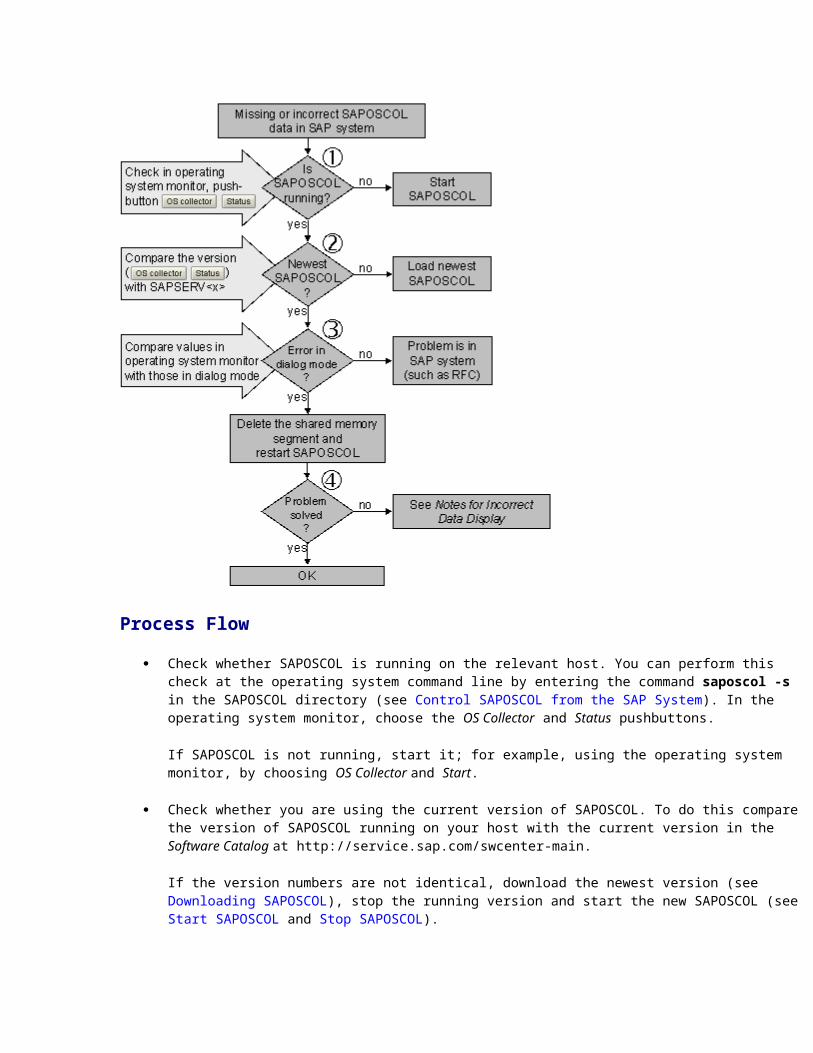
If incorrect, incomplete, or no values at all about the operating system are displayed in the operating system monitor or in the Alert Monitor of an SAP systems, we recommend the following procedure:

Process Flow

Check whether SAPOSCOL is running on the relevant host. You can perform this check at the operating system command line by entering the command saposcol -s in the SAPOSCOL directory (see Control SAPOSCOL from the SAP System). In the operating system monitor, choose the OS Collector and Status pushbuttons.

If SAPOSCOL is not running, start it; for example, using the operating system monitor, by choosing OS Collector and Start.

Check whether you are using the current version of SAPOSCOL. To do this compare the version of SAPOSCOL running on your host with the current version in the Software Catalog at http://service.sap.com/swcenter-main.

If the version numbers are not identical, download the newest version (see Downloading SAPOSCOL), stop the running version and start the new SAPOSCOL (see Start SAPOSCOL and Stop SAPOSCOL).

Compare the values displayed in the operating system monitor and in the Dialog Mode of the SAPOSCOL Operating System Collector.

If the values are identical and the incorrect values are therefore already present in the shared memory segment of SAPOSCOL, the SAP system is not the cause of the problem. In this case, restart SAPOSCOL and delete the shared memory segment after stopping SAPOSCOL.

If the problems persist after a restart, you can find notes for correcting the errors, some of which are platform-dependent under Notes for Incorrect Data Display

Operating System Monitor Data: CPU Definition

The following data about CPU usage is displayed for every CPU, broken down as percentages by:

Users System Times in which the CPU had no task to perform or was waiting for an input/output (idle)

Many factors could lead to an excessively high CPU utilization, and you should therefore perform a detailed analysis. If the problem was caused by too many active processes in the host system, you could, for example, transfer CPU-intensive programs to times when there is a lower system workload, or to other host systems. You could also increase the number of CPUs or upgrade the CPU(s).

When calculating the hourly value for the last 24 hours, these values are averaged over all CPUs of a host.

Other Values Collected

Number of CPUs Interrupts per second/hour System calls per second/hour Context switches per second/hour Average number of waiting processes for the last minute, last five minutes and the last 15 minutes

This is the number of processes for each CPU that are in a wait queue before they are assigned to a free CPU. As long as the average remains at one process for each available CPU, the CPU resources are sufficient. As of an average of around three processes for each available CPU, there is a bottleneck at the CPU resources.

o In connection with a high CPU usage, a high value here can indicate that too many processes are active on the server.

o In connection with a low CPU usage, a high value here can indicate that the main memory is too small. The processes are then waiting due to excessive paging.

Detail data for the processes that cause the largest CPU load:

1. Process ID 2. Owner of the process 3. Command that started the process 4. Absolute and percentage CPU usage by the process

5. Resident process size in kilobytes 6. Priority of the process

Use

The system displays the specified data when you call the operating system monitor.

The system displays the current detail data for the largest CPU users, if they choose Detail analysis menu Goto Current Data Snapshot Top CPU processes in the operating system monitor (see also Detail Data of the Operating System Monitor).

Check the following performance factors in particular:

Display Procedure

Is a CPU user constantly active? Check whether the process is in an endless loop.

Is the average load > 3 (more than three processes are waiting for the CPU)?

Check whether all processes with high CPU usage (memlog, r3trans, nwengine, brbackup...) are necessary.

Is the usage of the CPU zero percent? Check the analysis for the previous hours.

1. SAPGUI should not be running on the application server. 2. You can also display SAP work processes with high CPU usage with the SAP process

overview. The SAP process overview displays the ABAP program that is using the CPU.

Operating System Monitor Data: Memory Management Definition

The data that you can check in the operating system monitor for memory management includes data for the swap space and paging as well as the physically available memory. The following values are measured:

Physically available and free main memory in Kilobyte; the minimum and maximum free main memory are also measured hourly.

As a rule of thumb, if CPU bottlenecks occur if there is less than 10 MB of free physical memory for a small hardware configuration. This value can vary depending on operating system and system size.

Paging is the exchange of data pages between the main memory of a host system and the overflow store in a paging file on the hard disk; paging occurs if the main memory is not large enough for the contexts of all running processes SAPOSCOL measures the number of pages paged in and paged out per second with the quantities of memory paged in and paged out in kilobytes.

High paging rates indicate that the main memory is too small for the running processes. Measures that you can take are to extend the main memory, to move processes to other host systems, and to delay memory-intensive program runs to times of lower system workload.

On Windows platforms (unlike UNIX platforms), the system performs paging out as a precautionary measure even when space is not required in the working memory, meaning that this value is irrelevant and you should only consider the paging in rate. Under UNIX, on the other hand, Page_Out is the critical value for evaluating the paging.

Swap Space is storage space on the hard disk to which data that is not required is written from the main memory, so that there is space in the main memory for the program currently being executed. SAPOSCOL measures the configured and free swap space in kilobytes and the actual and maximum size of the swap space in kilobytes.

In addition, the maximum and minimum sizes of the free swap space is measured hourly. The most important values are the free and the actual swap space.

Not all types of swap space are available on all operating systems. For this reason, in some cases, the actual swap space size corresponds to the configured and maximum swap space.

Use

The system displays the specified data when you call the operating system monitor.

In the detail data, the system also displays the performance history for the last 24 hours and 30 days (see also Detail Data of the Operating System Monitor).

To call the individual functions in the table, choose the Detail Analysis menu in the operating system monitor.

Function Menu Path

Check memory usage for the last 24 hours Goto Current Data Previous hours Memory

Check the swap space usage for the last 24 hours

Goto Current Data Previous hours Swap

Check paging and swap space for the previous days for one server

Goto Performance Database Compare recent days

Check paging and swap space for the previous days for various servers

Goto Performance Database Compare all servers

Operating System Monitor Data: File System and LAN Definition

The operating system monitor displays the following data for hard disks, LAN, and file systems:

1. For all physical hard disks on a host:

Device name of the hard disk

Hard disk usage – percentage of the time in which the hard disk is being used

Average wait queue length of an input/output request

Wait time in milliseconds during which a request waits in the wait queue

Service time in milliseconds for an input/output

Transferred kilobytes per second

Number of disk operations per second

For all file systems on a host:

Name of the file system

Capacity of the file system in megabytes

Free storage space in the file system in megabytes

For all LAN interfaces on a host:

Name of the LAN interface

Data packets received per second

Data packets sent per second

Errors for received packets per second

Errors for sent packets per second

Collisions per second, in which two stations transport a packet at the same time on the same channel; this leads to the destruction of both packets and means that they must be sent again

Some values are not specified in some network interfaces; for example, there may not be a value for collisions per second in a token ring architecture. The values specified here do not describe the actual network traffic. They describe the transfers performed with this interface. This means that the errors displayed here refer to the interface and not to the actual network segment.

Use

The system displays the specified data when you call the operating system monitor.

In the detail data, the system also displays data for all hard disks and for all file systems of a server, and the performance history of the last 24 hours and 30 days (see also Detail Data of the Operating System Monitor).

To call the individual functions in the table, choose the Detail Analysis menu in the operating system monitor.

Function Menu Path

Check the current usage of the file systems Goto Current Data Snapshot Filesystem detail

Check the current usage of the hard disks Goto Current Data Snapshot Disk detail

Check the current usage of the LAN Goto Current Data Snapshot LAN detail

Check the usage of the file systems for the last 24 hours

Goto Current Data Previous hours Filesystem detail

Check the usage of the hard disks for the last 24 hours

Goto Current Data Previous hours Disk detail

Check the usage of the LAN for the last 24 hours

Goto Current Data Previous hours LAN detail

Check the file system, hard disks, and LAN for the previous days for a server

Goto Performance Database Compare recent days

Check the file system, hard disks, and LAN for the previous days for various servers

Goto Performance Database Compare all servers

Buffer Components Definition

An SAP buffer consists of the following parts:

Mode tableThe mode table resides in shared memory and tells you which pool contains which shared memory areas. The mode table is part of the common information on the shared memory areas that are accessed by the work processes.

For example, SAP Key 1 with Mode = 0, instructs the OS kernel to extract this buffer from the default pool and to allocate a unique shared memory segment.

SAP Key 10 with Mode = pool size instructs the OS kernel to store the buffer specifically in pool 10.

SAP Key 11 with Mode = -10 means that the buffer is located in pool 10.

SAP Global Management Table

A shared memory area that is allocated by the dispatcher during system startup.

When semaphore protection is on, the SAP Global Management Table is addressed exclusively by SAP Shared Memory Management. This is a central agent that is found in each work process and that sets up a shared memory area for the local application server or instance.

The SAP Shared Memory Management issues a call to the operating system (OS) when it creates a shared memory area. As a result, the SAP key is assigned to an OS key. The OS returns a unique identifier (handle) for the shared memory area, with which the SAP Shared Memory Management addresses the shared memory area that was created by the OS. All work processes in the SAP System can access the SAP Global Management Table. The handle can be accessed by all work processes.

Address TableEvery work process contains this table.

Assigns virtual addresses to the physical addresses of the shared memory areas.

Shared Memory Objects

These include the buffers, for example.

HeaderContains information on the shared memory area (also called memory segment).

If a write error occurs outside the segment area, then the uniformity of the header is destroyed. The control function of the SAP Management of Shared Memory checks the consistency of the headers.

IDIdentifies the memory area.

The ID is assigned when a SAP Shared Memory Management user requests the memory area.

Storage ClassThe memory class.

Examples of memory classes: permanent (local), shared, roll, paging and short.

Subdivision A mark for the requested area that can be referred to later when you release the memory area.

Size include header Buffer size including the header.

Alignment Alignment of memory areas in accordance with hardware constraints.

 

See also:

Buffer Synchronization

Buffer Types

Buffer Synchronization The fact that each application server has its own buffers could result in data inconsistency across the various application servers (instances). To prevent data inconsistency, the SAP System uses periodical buffer synchronization, which is sometimes called buffer refresh.

Every modifying action on buffered data, which could also be buffered by other application servers, produces synchronization telegrams that are written to a central DB table (DDLOG). Every application server periodically reads the telegrams written since the last synchronization, and checks its buffers for data to be refreshed.

Buffer synchronization can be controlled by changing the following parameters in the instance profile:

rdisp/bufrefmode = sendon | sendoff, exeauto | exeoff rdisp/bufreftime = (in seconds, time between two synchronization)

During the period between two refreshes, an application server may read data from its buffers while they are being modified by another application server. For this reason, no important volatile customer data should be buffered in the SAP buffers.

Examples of buffered data:

Table TSTC (SAP transaction codes)

Table T100 (error messages)

ABAP executables

Screens

Buffer synchronization is required only for distributed SAP Systems when more than one application server (instance) is used. If your SAP System utilizes only one application server (instance), buffer synchronization is not needed. When the application server is restarted, all buffers are erased and dynamically reconstructed.

Before you use tp (SAP transport program) to import objects into a central instance (that is, only one instance in the whole SAP System), you should set the following parameter:

rdisp/bufrefmode = sendoff, exeauto

If you set the paramter to ‘ exeoff ’, the central instance does not read the DDLOG table. This means that any changes to repository objects in the database (that is written to using tp ) are not updated in the SAP repository buffers. This may mean that the system displays syntax error messages for the ABAP programs that are affected.

The ABAP processor can detect whether a version of the ABAP program imported via tp is new, and reloads the program buffer. The SAP repository buffers still contain the old repository objects.

Repository Buffers (Nametab Buffers) Definition

The name table (nametab) contains the table and field definitions that are activated in the SAP System. An entry is made in the Repository buffer when a mass activator or a user (using the ABAP Dictionary, Transaction SE11) requests to activate a table. The corresponding name table is then generated from the information that is managed in the Repository.

The Repository buffer is mainly known as the nametab buffer (NTAB), but it is also known as the ABAP Dictionary buffer.

The description of a table in the Repository is distributed among several tables (for field definition, data element definition and domain definition). This information is summarized in the name table. The name table is saved in the following database tables:

DDNTT (table definitions)

DDNTF (field descriptions)

The Repository buffer consists of four buffers in shared memory, one for each of the following:

Table definitions TTAB buffer Table DDNTT

Field descriptions FTAB buffer Table DDNTF

Initial record layouts IREC buffer Contains the record layout initialized depending on the field type

Short Nametab SNTAB buffer A short summary of TTAB and FTAB buffers

The Short nametab and Initial record layouts are not saved in the database. Instead, they are derived from the contents of tables DDNTT and DDNTF.

When access to a table is requested, the database access agent embedded in each work process first reads the Short nametab buffer for information about the table. If the information is insufficient (for example, the SELECT statement uses a non-primary key) it accesses the Table definitions buffer and then the Field descriptions buffer. By reading the Repository buffers, the database access agent knows whether the table is buffered or not. Using this information, it accesses the table buffers (partial buffer or generic buffer) or the database.

The IREC buffer is read:

When a REFRESH command is executed in an ABAP program

At an INSERT command, when a record is created in the buffers before the data is inserted and the fields are initialized with the values found in IREC buffer

You can set the buffers mentioned above by editing the parameters in the instance profile.

See also:

 

Typical Parameter Settings for SAP Buffers Repository Buffer (Nametab Buffer)The following table provides an overview of the capacity of the repository buffer. This capacity is allocated using the corresponding profile parameters. It also specifies the number of the associated key:Buffer Number of Entries in the

Management AreaUser Data[in Kilobytes]

Key

Table definition (TTAB)

rsdb/ntab/entrycount Non-Unicode: rsdb/ntab/entrycount´ 188 / 1024Unicode: rsdb/ntab/entrycount´ 292 / 1024

42

Field description (FTAB)

rsdb/ntab/entrycount rsdb/ntab/ftabsize 43

Short nametab (SNTAB)

rsdb/ntab/entrycount / 4 rsdb/ntab/sntabsize 45

Initial record (IRBD)

rsdb/ntab/entrycount / 4 rsdb/ntab/irbdsize 44

The size of an entry in the management area is – depending on the hardware platform used – around 50 bytes.

All of the listed buffers are in memory pool 40. The size of the shared memory pool is therefore controlled by the parameter ipc/shm_psize_40. For more information, see Repository Buffer

Table Buffers

Generic key (resident) buffer (TABL)The number of directory entries (one for every resident table or each generic area) is defined with zcsa/db_max_buftab. The size of the data area in bytes is defined by zcsa/table_buffer_area. You can use ipc/shm_psize_19 to control the positioning of the buffer. The parameter is usually set to –10 (Pool 10). The parameter zcsa/exchange_mode should not be changed. Keep the default value Off.

Single key (partial) buffer (TABLP)The number of directory entries (one for each table) is defined with rtbb/max_tables. The size of the data area in KB is defined by rtbb/buffer_length. You can use the parameter ipc/shm_psize_33 to control the positioning of the buffer. It is normally set to 0, that is, the buffer is not in a pool. The parameter rtbb/frame_length defines the length of a frame in KB and should always be set to the default value of 4. For more information, see Table Buffers.

Program BufferYou can only define the size of the program buffer with one parameter: abap/buffersize. The size is defined in KB. The number of directory entries is calculated from this parameter. You can control the placing of the buffer with ipc/shm_psize_06. This parameter is normally set to 0, that is, the buffer is not in a pool. For more information, see Program Buffers.

SAP GUI Buffers

Screen buffer (PRES)You can define the size of the directory, that is, the maximum number of screens (dynpros) using zcsa/bufdir_entries. The total size of the buffer in KB is defined by zcsa/presentation_buffer_area. The storage area for the directory is included here. Control the placement of the GUI buffers using parameter ipc/shm_psize_14. This parameter is usually set to-10, which means that it is in pool 10.

CUA bufferThe parameter rsdb/cua/buffersize defines the total size of the buffer in KB. The number of directory entries is calculated as total size / 2KB. You can control the placing of the buffer with ipc/shm_psize_47. This parameter is normally set to -40, that is, the buffer is in pool 40. For more information, see SAPgui Buffers.

Roll and Paging BuffersThe parameters rdisp/ROLL_SHM and rdisp/PG_SHM are used to allocate the roll and paging buffer in 8KB blocks. This buffer is normally placed outside a pool. To place the buffer inside a pool, set the parameters ipc/shm_psize_08 and ipc/shm_psize_09. For more information, see Roll and Paging Buffers

SAP Calendar BufferYou can define the size of the calendar buffer in bytes in profile parameter zcsa/calendar_area. For more information, see SAP Calendar Buffer See also:SAP Note 103747 on the SAP Service Marketplace

Special Aspects of Tuning Definition

Only transparent tables and pooled tables can be buffered. You should buffer tables that

Only have read-only accesses

Have not been modified.

Other tables should only be buffered if the write accesses occur very infrequently and the tables do not contain customer data. In the case of tables that are modified frequently, the additional processing required could cancel out any performance gains achieved by buffering.

Buffering types

Full (residential) buffering

Either the whole table or none of the table is stored in the buffer. This type of buffering is recommended (as a rule of thumb) for the following tables:

Tables up to 30KB in size, and accessed frequently, but all accesses are read accesses.

Larger tables where large numbers of records are frequently accessed. However, if the application program is able to formulate an extremely selective WHERE condition for these multiple accesses using a database index, it may be advisable to dispense with buffering. In this case, pooled tables should be converted to transparent tables.

Tables where frequent attempts are made to access data not contained in the table, resulting in a "No record found" message. With full buffering all records of a table are contained in the buffer, which means a faster response to indicate whether or not the table contains a record for a specific key can be displayed.

Tables which are small and are subjected to large number of read accesses, but are rarely written to.

Generic buffering

When you access a record from the table, other records whose generic key fields correspond to this record are also loaded into the buffer. This type of buffering is recommended (as a rule of thumb) for the following tables:

Client-dependent, fully buffered tables are automatically buffered generically (even if full buffering was selected in the table’s settings). The client field is the generic key.

Language-dependent tables.

Single-record buffering (partial buffering)

Only records in a table, which is being accessed, are loaded into the buffer. This type of buffering is recommended (as a rule of thumb) for the following tables:

Large tables where few records are accessed. The amount of records accessed should be between 100KB and 200KB.

The partial buffer also contains negative information. That is, if a record is accessed which does not exist in the database table, an empty record is stored in the buffer and a flagbyte is set to indicate the record does not exist.

Working with Call Statistics Use

You can use the buffer monitor to help you decide which buffers to tune.

Procedure

2. To display the call statistics, from the initial screen, choose Administration System administration Monitor Performance Setup/Buffers Buffers Detail analysis menu Call statistics. On the next screen, make a selection and choose Enter.

3. Sort the display according to the data records called. Position the cursor on an entry in the column Calls (under DB activity) and choose Sort.

Result

The Changes column indicates which tables are being changed most frequently. You can generally consider buffering tables with many read accesses but with fewer than 100 changes per day.

The system displays the number of changes made since the system was started. By checking the dates at the top of the screen, you can determine the number of days that have elapsed since system startup.

Therefore: Changes per day = Total changes Total number of days in the selected time period

You should also consider the table type. Only buffer tables of type TRANSP or Pool are important here. Ignore those that are of type System as these tables should not be changed.

 

Working with Call Statistics Use

You can use the buffer monitor to help you decide which buffers to tune.

Procedure

2. To display the call statistics, from the initial screen, choose Administration System administration Monitor Performance Setup/Buffers Buffers Detail analysis menu Call statistics. On the next screen, make a selection and choose Enter.

3. Sort the display according to the data records called. Position the cursor on an entry in the column Calls (under DB activity) and choose Sort.

Result

The Changes column indicates which tables are being changed most frequently. You can generally consider buffering tables with many read accesses but with fewer than 100 changes per day.

The system displays the number of changes made since the system was started. By checking the dates at the top of the screen, you can determine the number of days that have elapsed since system startup.

Therefore: Changes per day = Total changes Total number of days in the selected time period

You should also consider the table type. Only buffer tables of type TRANSP or Pool are important here. Ignore those that are of type System as these tables should not be changed.

 

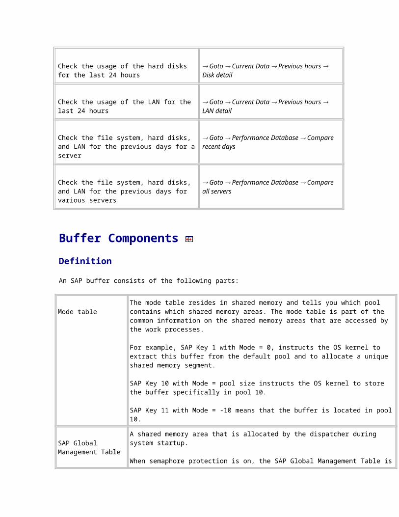
Reasons for Poor Buffer Quality Definition

Poor buffer quality may be caused by any of the following:

Transports

Every time you transport new developed source into the system that is running the tp , you invalidate all entries in the program buffer and clear all other buffers (command $SYNC ). Unlike the other buffers, the program buffer does not start empty, but is filled with invalid programs. It is very important to execute as few transports as possible and to collect data for collective transports.

Buffer resets

Setting up a buffer requires a large number of database and network accesses, and places a considerable load on the system. Therefore, only reset the buffers if inconsistencies occurred between the buffer and the database. This might happen, for example, if you update a buffered table with native SQL, that is, the database table is updated directly by bypassing the buffer. To reset the table buffers, enter $TAB in the command field. Use the command $SYNC to reset all the SAP buffers on the application server. These commands only affect the buffers of the application server on which the commands are entered. The buffers of the other application servers in the network are not affected.

Using the commands $TAB and $SYNC places an extremely large load on the system. In large systems, it could take up to one hour (depending on the access profile) for the buffer load to return to its original state. System performance is greatly impeded during this time.

Offline backups, SAP System reboots

Both of these actions require the SAP System to be shut down, and then started up again. All buffers of all servers are reset. Again, this takes a considerable amount of time.

Program development

Software development should not be done in a productive system, as development systems require a very large program buffer.

High Buffer Quality Definition

The following describes how the buffer quality of the SAP buffers should be in a SAP System with good performance.

Repository buffers (nametab buffers)

The qualities of the Repository buffers can reach 99.9% in a system that has been running for a few days. If the buffer quality is less than 95%, you should investigate the situation further.

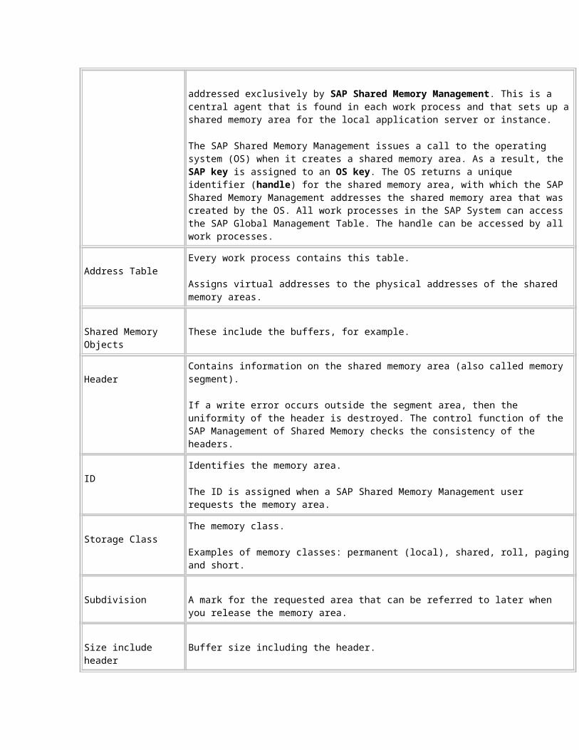
Check the:

Available freespace

Available directories Object swaps Buffer history.

Program buffer

The program buffer contains the generated ABAP programs (load).

 

Critical effects on the program buffer

Transports

Every time a new source is transported into the system using the R3trans program, all entries in the program buffer are invalidated, and all other buffers are cleared (equivalent to the $SYNC command). Unlike the other buffers, the program buffer is not empty after transport, but is filled with invalid programs.

Therefore, it is better to execute as few transports as possible and to collect data to do several transports at once. For more information, see Program Buffer.

Presentation and calendar buffers

The quality should also be above 95%. Also check available freespace and the freespace history. For more information, see SAPgui Buffers and SAP Calendar Buffer.

Table buffers

As mentioned above, the quality of the single key buffer increases very slowly from system startup. Therefore, bad quality (< 90%) should only be of concern if there is no freespace left in the buffer.

The quality of the generic key buffer should be greater than 95% and can be up to 99%. For more information, see Table Buffers

See also:

 

Roll and Paging Buffers, Extended Memory Definition

The roll and paging buffers are the preferred working area of the roll and paging areas for an instance (application server). The remaining area is located on disk as roll and paging files. The user context is stored in the extended

memory and the roll area (when the job is "rolled out" of a work process). The paging area stores special data for the ABAP processor, while the extended memory stores a large portion of the internal tables of a program.

You set the roll and paging buffers, as well as the extended memory using the parameters in the instance profile.

Buffer Types Definition

There are seven main groups of buffers found in the shared memory. For more information on each buffer type, see :

 

Repository Buffers

Table Buffers

Program Buffer

SAPgui Buffers

Roll and Paging Buffers

SAP Calendar Buffer

SAP Cursor Cache

Repository Buffers (Nametab Buffers) Definition

The name table (nametab) contains the table and field definitions that are activated in the SAP System. An entry is made in the Repository buffer when a mass activator or a user (using the ABAP Dictionary, Transaction SE11) requests to activate a table. The corresponding name table is then generated from the information that is managed in the Repository.

The Repository buffer is mainly known as the nametab buffer (NTAB), but it is also known as the ABAP Dictionary buffer.

The description of a table in the Repository is distributed among several tables (for field definition, data element definition and domain definition). This information is summarized in the name table. The name table is saved in the following database tables:

DDNTT (table definitions)

DDNTF (field descriptions)

The Repository buffer consists of four buffers in shared memory, one for each of the following:

Table definitions TTAB buffer Table DDNTT

Field descriptions FTAB buffer Table DDNTF

Initial record layouts IREC buffer Contains the record layout initialized depending on the field type

Short Nametab SNTAB buffer A short summary of TTAB and FTAB buffers

The Short nametab and Initial record layouts are not saved in the database. Instead, they are derived from the contents of tables DDNTT and DDNTF.

When access to a table is requested, the database access agent embedded in each work process first reads the Short nametab buffer for information about the table. If the information is insufficient (for example, the SELECT statement uses a non-primary key) it accesses the Table definitions buffer and then the Field descriptions buffer. By reading the Repository buffers, the database access agent knows whether the table is buffered or not. Using this information, it accesses the table buffers (partial buffer or generic buffer) or the database.

The IREC buffer is read:

When a REFRESH command is executed in an ABAP program

At an INSERT command, when a record is created in the buffers before the data is inserted and the fields are initialized with the values found in IREC buffer

You can set the buffers mentioned above by editing the parameters in the instance profile.

See also:

Table Buffers Definition

There are two kinds of table buffers:

Partial table buffers

Generic table buffers

Use

The table below displays these table buffers and their functions.

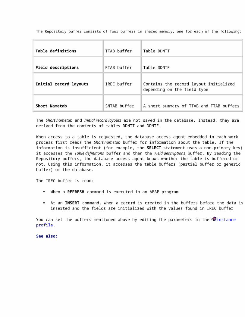
Buffer Also known as Function

Partial table buffer TABLPpartial buffersingle record table buffersingle key buffer

Stores single table entries, that is, one record with its field values.

Generic table buffer TABLgeneric bufferresident-table buffer100% buffergeneric key buffer

Stores a range of table entries, that is, a range of records with their field values.The generic table buffer can also store all the entries (records) in a table. This is known as resident (or full) buffering.

Whether a table is partially buffered, generically buffered, or fully buffered depends on its attribute settings. You can change the buffer attributes of a table using Transaction SE13. For more information, see Typical Parameter Settings for SAP Buffers.

See also:

Program Buffers Definition

The following table displays the program buffer and its functions.

Buffer Also known as Function

Program buffer SAP executable bufferABAP bufferPXA (Program Execution Area)

Stores the compiled executable versions of ABAP programs (loads).The contents of this buffer are stored in tables D010L (ABAP loads), D010T (texts) and D010Y (symbol table).

The program buffer has a hash structure and supports LRU (Least Recently Used) displacement.

You can reconfigure the program buffer by adjusting its instance profile parameters

SAPgui Buffers 

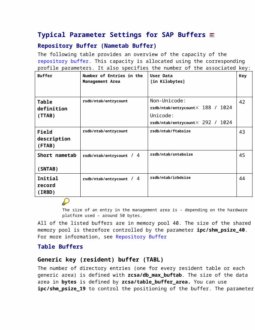
Definition

There are two kinds of SAPgui buffers:

Presentation buffers

Menu buffers

The following table shows the SAPgui buffers and their functions:

Buffer Also known as Function

Presentation buffer Screen bufferDynpro buffer

Stores the generated screens (DYNPRO loads).The presentation buffer is adjusted by changing its instance profile parameters.

Menu buffer CUA buffer Stores objects from the SAPgui.For example, menus, pushbutton definitions. These objects are from tables D345T (CUA texts) and D342L (CUA loads). The buffer has directory structure and supports LRU displacement.The menu buffer is adjusted by amending its instance profile parameters.

SAP Calendar Buffer Definition

The SAP calendar buffer stores all defined factory and public holiday calendars.

Calendars are stored in the database tables TFACS and THOCS.

The buffer has a directory structure. This means that if the shared memory is configured too small, only the required data is loaded; there is no LRU displacement of the contents of the buffer.

You can change the calendar buffer by editing the parameter in the instance profile.

SAP Cursor Cache Definition

The SAP cursor cache helps to improve system performance by reducing the number of parsing of SQL statements; it is database-dependent. The SAP cursor cache is only slightly different for Oracle, Informix and SAP DB. It is totally different for AS/400 and MS SQL Server.

There are two types of cursor caches:

Statement ID cache

Statement cache

Changing the SAP cursor cache parameter value in the default profile will affect other areas as well. You are therefore advised not to tune it without the recommendation of a qualified SAP expert.

Statement IDs and the Statement Analyzer

The source of each SQL statement in the SAP System (ABAP, DYNP, the C modules of the database interface) assigns an ID to its Open SQL / Native SQL etc. statement. The statement ID includes:

Module name (report name)

Statement number (line number)

Timestamp (time of ABAP generation)

The statement ID provides an easy way to recognize statements. There may be different statement IDs for one statement (for example, different ABAP programs doing the same SELECT ). The Statement Analyzer eliminates such duplicities. When it receives an SQL statement (in control block form), this database interface module checks if the statement is simple (for example, SELECT * FROM T100 WHERE... =... AND... =... ), or complex (for example, SELECT * FROM T100 WHERE... <... AND... >... ). If the statement ID is simple, the Statement Analyzer assigns a ‘normalized’ statement ID.

The analyzer is called by the RSQL or Open SQL interface. If it is able to assign a normalized ID, the original ID (if existing) is replaced.

The Buffer Monitor Purpose

With the CCMS buffer monitor you can analyze the state of the SAP buffers and evaluate their quality. You can use this information to determine the areas in which you should change buffer sizes to improve performance.

The buffer monitor gives you the following information for a selected server:

Quality of the most important buffers

Sizes of the most important buffers

Call statistics (database activity)

Memory usage

Semaphore usage

Table calls

Usage and configuration of the roll file

Usage and configuration of the paging file Usage of extended and heap memory

Buffer resets

Number of objects in the buffers

See also:

 

Buffer Monitor and Tune Summary

Checking Memory Usage

Displaying Table Buffers

Buffer Quality: Overview

Buffer Monitor and Tune Summary To call the buffer monitor:

From the initial R/3 screen, choose Tools Administration Monitor Performance Setup/Buffers Buffers (or call Transaction ST02 )

The buffer monitor displays information about buffer and memory usage and load for the instance where the user is logged on. Statistics are compiled from the time the server is started.

The Tune Summary screen is divided into four parts:

Buffer SAP memory Cursor cache Call statistics

Buffers

The first column of the tune summary shows the names of the buffers:

The four R/3 Repository buffers

The program, CUA, screen, and calendar buffers

The table buffers

See also:

 

Repository Buffers (Nametab Buffers)

Hit Ratios

The hit ratios are displayed in percent.

The following diagram illustrates what is meant by hit ratios. A hit is when a object (such as a table, screen or program) in the buffer(1) is accessed. If the object has to be read from the database(2), the buffer access fails.

 

Buffer hit ratio = Buffer object reads / logical requests

 

Buffer Quality

Buffer Quality = saved database calls / (database calls + saved database calls)

The database interface can translate one logical request into several database calls.

Buffer Quality: Overview

 

Allocated Size

The allocated size is measured in KB. It is different from the available buffer size because part of the space is used for buffer management.

 

Freespace

Freespace is important for analyzing the buffer size. The space remaining in the buffer is displayed in KB and as a percentage of the available buffer size.

 

Number of Directories

Even if there is freespace in the buffer, objects may not always be loaded into the buffer because there are no more free directories. The buffer monitor displays the number of directories available for the buffer, and the number and percentage free. The buffer directories point to the location of the objects stored in the buffer.

 

Swapping

When a buffer has insufficient freespace or free directories, it has to swap objects out of the buffer in order to load a new object. The column Swap shows how many objects have been swapped out since system startup.

 

Database Accesses

When an object cannot be read from the buffer, the database has to be accessed. The number of database accesses is displayed in the last column on this screen.

If a critical situation occurs in a buffer, the data for that buffer (freespace/object swaps) is displayed in red.

 

SAP memory

The following information is displayed:

The amount of space currently used in percent and in KB The maximum value (max. use) since system startup The amount of space used in shared memory and on the disk.

See also:

Roll and Paging Buffers

 

For more information:

For details about an individual memory area, select a line.

The Detailed Analysis windows (Extended Memory and Heap Memory) include functions for information about:

Quotas

Memory allocation (sequence, size)

Ext. mem. blocks

Extended memory user

Current parameters

The instance profile settings for memory management

History

Memory usage over the course of several days.

 

SAP cursor cache

The R/3 System has a cursor cache that stores cursors for SELECT statements to avoid time consuming PREPARE processing.

This cache has a fixed size and cannot be changed.

SAP Cursor Cache

Call statistics

The Tune Summary screen displays the access statistics for all data either residing in the SAP pool buffers or the database.

The following table describes the information of the tune summary.

Table: Tune Summary

Screen Information

First column Contains the different kinds of statements that can be used to access a table.( SELECT SINGLE , SELECT , INSERT , UPDATE , DELETE ).

Last line Shows the total - or in the case of the hit ratios, the average - data of the call statistics.

Next column Shows the hit rates for the SELECT statements for buffered tables. A hit rate for the other statements ( UPDATE , INSERT and DELETE ) is not displayed because these statements always have to be passed to the database.

ABAP Processor Displays the number of logical requests to the buffered tables, and how many of them failed.

The subsequent columns display:

The average database call time

The number of affected rows.

Table access failures are not the same as buffer access failures. The SQL statements SELECT SINGLE, INSERT, DELETE, and UPDATE can fail if the specified data record does not exist. A buffer access can "fail", if the table has not yet been loaded into the buffer.

Some logical requests cannot be satisfied by buffer access and require that the database be accessed.

 

Buffer history

Analyze the buffer history to find the correct buffer sizes.

 

To display the buffer history:

From the initial R/3 screen, choose Tools Administration Monitor Performance Setup/Buffers Buffers Goto Performance database This server history

The data displayed is similar to the columns in the Tune Summary.

The sizes of the buffers may be appropriate for the current system situation, but may have been too small for recent days. If so, you should resize the buffers even if the sizes are appropriate for the current situation.

 

Checking Memory Usage Use

Before you change the size of a buffer, you should determine how much memory the buffer is currently allocated. This is important because the memory that is allocated to buffers should not significantly exceed the size of the physical memory, otherwise operating system swapping will occur.

Most server memory resources are used by the:

Operating system (usually around 30 MB)

Database system (See the database documentation)

SAP System

Procedure

To check the memory usage, from the initial screen, choose Administration System administration Monitor Performance Setup/Buffers Buffers Goto Current local data Additional functions Storage.

You should allocate as much memory as possible to ensure that good buffer quality.

It is usually more effective to allocate memory to the SAP buffers than to the database buffers. However, once the buffers are optimized (that is, no more object swaps occur), it does not make sense to increase buffer size further, since this will not improve performance.

How Much Operating System Paging is Acceptable? Definition

How much operating system paging is acceptable depends largely on the database server and the application servers.

On the database server, the I/O activity to the disks is normally quite high due to accesses to the database. Additional operating system paging should therefore be avoided to prevent an additional bottleneck. On the application server, disk accesses are usually less frequent. Therefore, operating system paging using a large buffer can be more efficient than a buffer which is too small which would lead to multiple database accesses and increased network traffic.

Directory Space and Data Space Definition

For most buffers you can adjust the number of directory entries and the size of the user data area separately. SAP recommends that you increase both components, since an increase in one component may lead to a bottleneck in the other.

Displaying Table Buffers Procedure

2. From the SAP initial screen, choose Administration System administration Monitor Performance Setup/Buffers Buffers Goto Current local data Table buffers Single record or Generic key.

You should only buffer tables that you change infrequently. You specify whether or not a table should be buffered in Transaction SE13.

Changes to buffered information must be updated in the buffers of other application servers that are sharing that information. These updates can adversely affect performance. The more servers that need updating, the more expensive the update process.

If all operations are performed on a central server, you can deactivate the buffer update messaging service.

There are two profile parameters that control the behavior of synchronization for the application server:

Parameter name Recommended value

rdisp/bufrefmode sendoff, exeoff (central system)

rdisp/bufrefmode sendon, exeauto (client/server)

rdisp/bufreftime 60

Displaying Parameter Settings for the Current Instance

You define current parameters in the SAP instance profile. Restart the instance to activate any changes. To display the parameter settings:

2. From the SAP initial screen, choose Administration System administration Monitor Performance Setup/Buffers Buffers Goto Profile parameters Current.

 

Tuning SAP Buffers Definiton

It is beneficial to keep as much data buffered as possible. This helps avoid repetitive database accesses, for example from the network and Interprocess Communication (IPC), and maximize system performance.

Reduced performance is caused by

Buffers set too small.

The required data cannot be stored in the buffers. Instead, objects have to be swapped out of the buffers. This causes expensive database accesses.

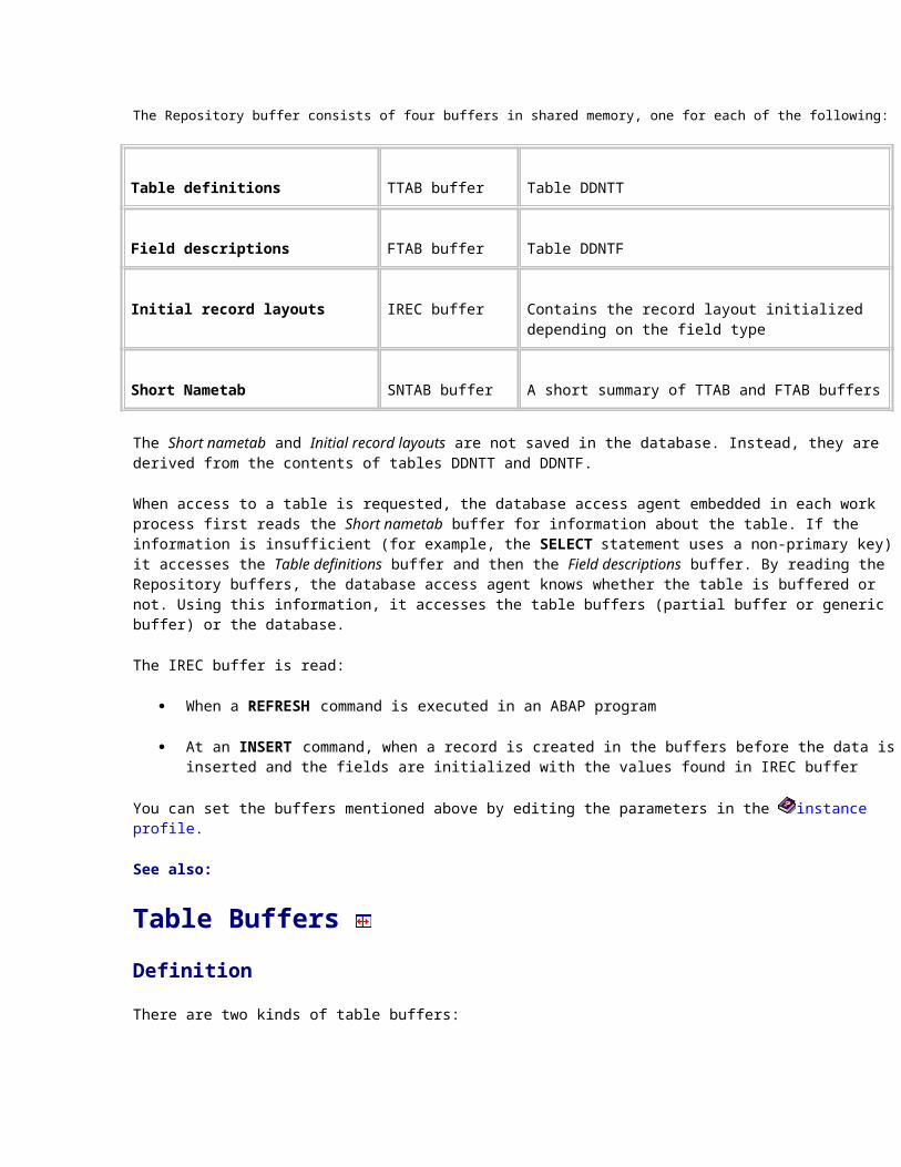
Buffers set too large

Memory is wasted. Paging may occur if too much memory is taken from the operating system and allocated to the SAP buffers and database.

You should check regularly whether the buffer size is suited to your system requirements. Since buffers are crucial for the performance of the SAP System, all buffers (except the SAP cursor cache) should be adjusted to their optimal value.

The optimum size for each buffer depends largely on the specific configuration of the server, that is, the applications, the number of users working in each module, and so on. Therefore, it is difficult to specify values suitable for all configurations. The most important criterion for the correct buffer size is the buffer quality.

You should not adjust buffers in cases where poor buffer quality is due to special circumstances, for example, object swaps in the program buffer in a system with a high level of development activity.

Buffer Tuning Checklist

If there is insufficient memory to set the appropriate buffer sizes, you should consider adding physical memory. However, since this could take some time, you may have to decide which buffers are most important and should be adjusted first using the existing memory.

As a guideline, the most important buffers are those that:

Are responsible for good dialog performance Are used most frequently Require relatively few memory resources

These criteria give you the following priority list:

2. Repository buffers (nametab buffers) 3. Table buffers 4. Program buffers 5. Roll and page file buffers 6. SAPgui buffers

See also:

 

Adjusting Pool Sizes Use

Many of the SAP buffers are contained in shared memory pools. When the sizes of these buffers are changed, it is necessary to adjust the size of the corresponding pool as well.

The CCMS profile maintenance tool makes these adjustments automatically.

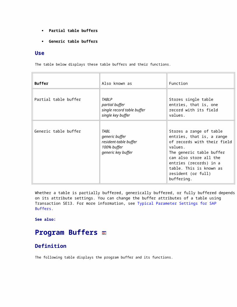
Procedure

To display information about the shared memory segments and the pools, from the initial screen, choose Tools Administration Monitor Performance Setup/Buffers Buffers Goto Current local data Additional functions Storage Shared memory detail.

You can change the pools and the shared memory segments with parameter ipc/shm_psize_<two-digit shared-memory id> .

You can change both the size and the location of the shared memory segment. The shared memory regions with the keys 10, 20, and 40 are used as shared memory pools by the SAP System. The size of these pools is determined by the values of the system profile parameters ipc/shm_psize_10 , _20 , and _40 .

ipc/shm_psize_10 =12000000

This parameter sets the size of shared memory pool 10 to 12,000,000 bytes. The shared memory pools must be large enough to hold the shared memory regions that belong to them. If you change the size of a region that belongs a pool, you must also change the size of the pool. You must also change the size of a pool if you add a new shared memory region to it.

For all other keys, this parameter can be used to define the position of the shared memory region. In this case the shared memory parameters have the following format:

ipc/shm_psize_nn = value

where nn is the SAP shared memory key and value is the attribute of the shared memory region.

Shared memory parameters

The SAP System uses the default disposition (in pool or directly allocated) of the shared memory region.

Table: Assignment of pools to keys

Object key Pool

11 – 19 10

21 – 29 20 (not used currently)

41 - 49 40

All other objects are not located in a pool, as specified by the default settings.

 

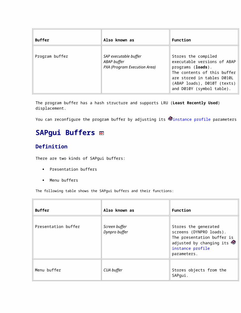
A shared memory parameter ipc/shm_psize_nn can have the following values:

The value 0The shared memory region is removed from its standard pool (if any) and is allocated directly by the operating system.

ipc/shm_psize_19 =0 removes the 100%-resident table buffer from its default pool 10. If your host operating system does not limit the number of shared memory allocations, you can remove shared memory regions from pools. Removing a region from a pool simplifies the maintenance of the system profile because you no longer need to adjust the size of a pool when you adjust the size of a region. If a region does belong to a pool, you must change the pool size in accordance with changes that you make to the shared memory regions in the pool.

A negative valueThe shared memory region is assigned to the shared memory pool whose shared memory key is the same as the value.

ipc/shm_psize_33 =-10 adds the partial table buffer to shared memory pool 10.

Shared memory parameters other than those for keys 10, 20, and 40 should not have values greater than 0. Otherwise, the SAP System treats the shared memory region as a pool.

The default settings for the shared memory parameters will not be automatically found in the profile. They will only appear if they have been inserted manually, either to confirm or to change the default setting.

CCMS/System Monitoring OSS s 

 

 Note Number Description

0000589 R3 Instance Cannot Be Started000112 Trace Information

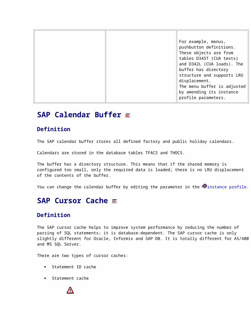
0001916 Logging Table Changes In R30002033 Startup Fails000666 Origins Of Profile Parameters001942 How Does R3trans Work ?0021636 RAM Extension Which Changes To Profile0028893 Changing The Password Of The User SAPR30033772 Correct Config Of DrWatson0035388 Problems With NT Scheduler0037626 SAP Tool R3Chop0040457 Inst s TCPIP Win NT0053211 NT Appear To Hang SAP Service Problems007684 Problems With TCPIP009984 Security R3 on NT0102390 Use Of NT Perfromance Monitor0103747 Performance Parameter Recommendation0110368 New CCMS Monitoring Infrastructure0113440 Logon Load Balancing Default Logon Group0117907 Memory Allocation Display In SM04 and ST020118093 Concepts Of Defining Logon Load Balancing0127773 Several Enqueue WP0131030 Performance Problem In 45B0137478 Installing Dialog Instace Gateway 4.6x0139418 Logging User Actions0144978 System Not Installed Properly0147568 PXANOFREESPACE015374 Performance Analysis CheckList0155402 Analysis Of Hanging Situations016187 Config Alert Values016223 roll area problem0162266 NT Inst R3trans0165485 R3 Server Security Under NT0181867 Hang Situation With SPO WorkProcess0182067 Ext Mem Limited To 8GB0203924 Performance Problems 46022099 Max No Of Term Reached

026317 Setting Up Logon Load Balancing028392 R3 systems on NT Servers030258 DrWatson Error In R3033973 Semaphore034998 Check OS Level If R3 Is Running038052 System Panic Due To Low Space039412 How Many WP To Config044649 Error During Startsap051789 Poor User Distribution In Logon061626 ThreshHold Values067231 PXA_NO_FREE_SPACE068896 R3trans Performance Problems And Cluster079435 Automatic Reset From PRIV Session082655 Instance Not Config Properly085254 Inst Dailog Instance088416 Zero Admin Mem Management For 40A NT097461 CCMS Enhancements0110172 Transaction With Large Storage Requirements0110529 NT Perf Monitor0178448 Sys Config Monitor Tree0217507 problems Starting R3 Instance