Motion Reconstruction of Vortex-Induced Vibration of Long

Motion Reconstruction of Vortex-Induced

Vibration of Long Flexible Riser from

Experimental and Field Test Data

Ming Li

Ma

ste

r of

Scie

nce T

he

sis

Motion Reconstruction of Vortex-

Induced Vibration of Long Flexible

Riser from Experimental and Field

Test Data

MASTER OF SCIENCE THESIS

For the degree of Master of Science in Offshore and Dredging

Engineering at Delft University of Technology

Ming Li

July 22, 2016

Faculty of Mechanical, Maritime and Materials Engineering • Delft University of

Technology

The work in this thesis was supported by Delft University of Technology

Copyright ○c Delft University of Technology

All rights reserved.

DELFT UNIVERSITY OF TECHNOLOGY

DEPARTMENT OF

OFFSHORE AND ENGINEERING

The undersigned hereby certify that they have read and recommend to the Faculty of

Mechanical, Maritime and Materials Engineering of acceptance of a thesis entitled

MOTION RECONSTRUCTION OF VORTEX-INDUCED VIBRATION OF LONG

FLEXIBLE RISER FROM EXPERIMENTAL AND FIELD TEST DATA

By

MING LI

in partial fulfillment of the requirements for the degree of

MASTER OF SCIENCE

OFFSHORE AND DREDGING ENGINEERING

Dated: July 22, 2016

Chairman of Graduation Committee: Prof. Dr. A. V. Metrikine

University Supervisor: Dr. Y. Qu

University Supervisor: Dr. F. Pisano

University Supervisor: Dr. D. Fallais

Abstract

Vortex-induced vibration (VIV) of long flexible cylindrical structures enduring ocean

currents is ubiquitous in the offshore industry. Though significant effort has gone into

understanding this complicated fluid-structure interaction problem, major challenges

remain in modelling and predicting the response of such structures. The work presented

in this thesis applies the modal approach to do reconstruction of the riser VIV motion

from experimental data at first and then performs some analyses to the riser VIV

response based on the reconstructed result.

In the first part of the thesis, the modal approach is classified into frequency domain

method and time domain method according to the types of the measurement data. Two

systematic frameworks to do motion reconstruction are built for these two methods.

Besides, two factors probably leading to the reconstruction error are proposed. One is

using the strain measurement to identify the low modes VIV motion and the other one is

unreasonable choice of participating modes.

In the second part of the thesis, the riser VIV motion in ExxonMobil VIV test is

reconstructed using the frequency domain method and that in the second Gulf Stream

VIV test is reconstructed using the time domain method. In the reconstruction process,

several problems are needed to be solved, such as the choice of time window, filtering

data and the choice of participating modes. And the accuracy of the reconstructed result

is verified using the extraction method. Finally, two examples are given to demonstrate

the reconstruction errors induced by the above two facors.

In the final part of the thesis, some key parameters are extracted out to show the

effects of external conditions, e.g. current profile, current speed and strake coverage, on

the VIV displacement magnitude and response frequency of the riser. Besides, three

methods are provided to identify the travelling wave in the riser VIV response.

Acknowledgement

I owe the successful completion of this thesis to several people involved in the

whole process.

At first, I would like to express my sincere gratefulness to Yang Qu, my university

daily supervisor. His feedback provided me with the guidance that I needed to study.

Also, I am grateful for our cooperation during the whole period of the graduation study

and the fact that he was always available for questions and discussion.

Moreover, I would like to thank the chairman of my graduation committee, Professor

Andrei Metrikine, for his guidance and remarks during this graduation study. His valuable

advice and especially his to-the-point questions helped me to understand the physics of

this problem deeply.

Finally, I would like to thank my friends and family for their encouragement, patience

and mental support.

Contents

1

Contents

List of Figures ............................................................................................................... 6

List of Tables ............................................................................................................... 12

Nomenclature .............................................................................................................. 14

1 Introduction ............................................................................................................. 16

1.1 Background ........................................................................................................ 16

1.2 Vortex-Induced Vibration .................................................................................... 17

1.2.1 Vortex-shedding ....................................................................................... 17

1.2.2 Lock in ...................................................................................................... 18

1.2.3 Influencing parameters ............................................................................. 19

1.3 Studies on VIV of riser ........................................................................................ 21

1.3.1 Experimental studies ................................................................................ 22

1.3.2 Semi-Empirical VIV Response Computational Tools ................................ 23

1.3.3 Numerical Simulation ................................................................................ 24

1.4 Research objectives............................................................................................ 24

1.5 Thesis outline...................................................................................................... 25

2 Approach to riser VIV response reconstruction ................................................... 26

2.1 Problem statement .............................................................................................. 26

2.2 Reconstruction approach .................................................................................... 27

2.2.1 Modal approach ........................................................................................ 27

2.2.2 Theoretical basis for modal approach ....................................................... 28

2.2.3 Limitations of modal approach .................................................................. 28

Contents

2

2.3 Modal approach description ................................................................................ 29

2.3.1 Frequency domain method ....................................................................... 30

2.3.2 Time domain method ................................................................................ 33

2.4 Identifiably and error analysis ............................................................................. 34

2.4.1 Identifiably analysis .................................................................................. 34

2.4.2 Error analysis of noise on strain measurement ......................................... 35

2.4.3 Error analysis of unreasonable choice of participating modes .................. 36

3 The ExxonMobil and second Gulf Stream VIV tests ............................................. 38

3.1 Introduction ......................................................................................................... 38

3.2 ExxonMobil VIV test ............................................................................................ 38

3.2.1 Background .............................................................................................. 38

3.2.2 Riser model .............................................................................................. 39

3.2.3 Test rig ..................................................................................................... 40

3.2.4 Instrumentation and data acquisition ........................................................ 41

3.3 The second Gulf Stream VIV test ........................................................................ 44

3.3.1 Background .............................................................................................. 44

3.3.2 Experiment set-up .................................................................................... 44

3.3.3 Pipe model ............................................................................................... 45

3.3.4 Measurement system ............................................................................... 47

4 Riser VIV response reconstruction of ExxonMobil VIV test ................................. 50

4.1 Choice of response reconstruction approach ...................................................... 50

4.2 Response reconstruction steps ........................................................................... 50

4.2.1 Choice of time window .............................................................................. 50

4.2.2 Preparation of data matrix b .................................................................... 51

4.2.3 Preparation of system matrix A ............................................................... 55

4.2.4 Obtaining the modal weights matrix w ..................................................... 59

4.2.5 Results ..................................................................................................... 60

Contents

3

4.3 Verification of the accuracy of reconstructed results ........................................... 63

4.4 Example of error from noise on strain measurement ........................................... 65

4.5 Results summary ................................................................................................ 67

4.5.1 Bare riser response .................................................................................. 67

4.5.2 50% straked riser response ...................................................................... 69

4.5.3 Fully straked riser response ...................................................................... 71

5 Analyses to reconstructed VIV responses in ExxonMobil VIV test ..................... 74

5.1 Riser VIV modal decomposition .......................................................................... 74

5.1.1 Response modes and response frequencies ............................................ 74

5.1.2 Numerical method .................................................................................... 75

5.1.3 Application to ExxonMobil VIV test and discussion ................................... 76

5.2 Travelling waves in riser VIV response ............................................................... 79

5.2.1 Uniform flow ............................................................................................. 79

5.2.2 Linearly sheared flow ................................................................................ 80

5.3 Key parameters analyses ................................................................................... 80

5.3.1 Bare riser .................................................................................................. 81

5.3.2 50% straked riser ..................................................................................... 86

5.3.3 Fully straked riser ..................................................................................... 90

5.3.4 Conclusions .............................................................................................. 94

6 Riser VIV response reconstruction of the second Gulf Stream VIV test ............. 96

6.1 Characteristics of the second Gulf Stream VIV test ............................................. 96

6.1.1 Characteristics of tested pipe ................................................................... 96

6.1.2 Characteristics of measured data ............................................................. 98

6.2 Data preprocessing ........................................................................................... 100

6.2.1 Unwrapping data .................................................................................... 100

6.2.2 Choice of time window ............................................................................ 102

6.2.3 Bandpass filter data ................................................................................ 103

Contents

4

6.2.4 Decompose filtered data ......................................................................... 104

6.3 Preparation of data matrix C ........................................................................... 106

6.4 Preparation of system matrix ....................................................................... 106

6.5 Reconstructed result ......................................................................................... 108

6.6 Verification of the accuracy of reconstructed result ........................................... 108

6.7 Examples of error from choice of participating modes ....................................... 110

6.8 Peak response mode ........................................................................................ 112

6.9 Travelling wave in riser VIV response ............................................................... 114

7 Conclusions ........................................................................................................... 116

7.1 Summary of contributions from each chapter .................................................... 116

7.1.1 Riser VIV response reconstruction method ............................................. 116

7.1.2 Description of two objective VIV tests ..................................................... 117

7.1.3 Response reconstruction using experimental data ................................. 117

7.1.4 Analyses to the reconstructed VIV response .......................................... 118

7.2 Recommendations for future research .............................................................. 119

Bibliography .............................................................................................................. 120

A Fairing and strake configurations ....................................................................... 124

B Chosen parameters for bare riser cases in ExxonMobil VIV test ...................... 126

C Power spectral density (PSD) of reconstructed displacement signals ............. 128

D Rotation angles ..................................................................................................... 134

List of Figures

6

List of Figures

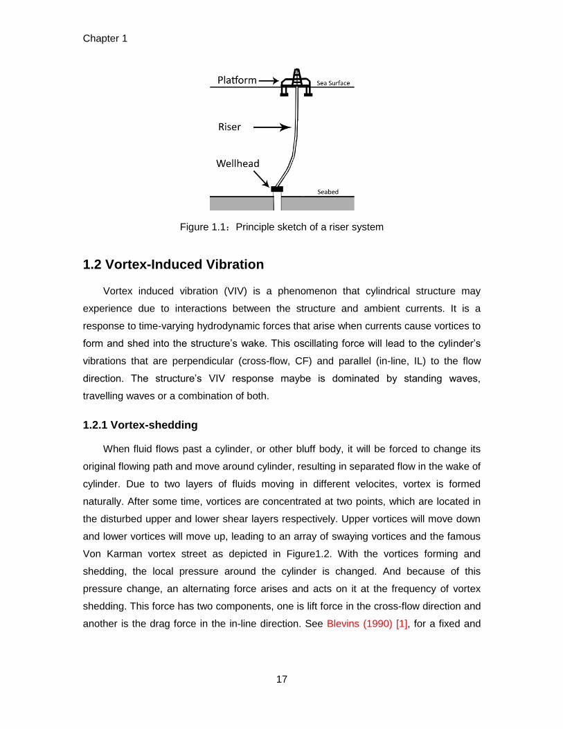
Figure 1.1：Principle sketch of a riser system ............................................................... 17

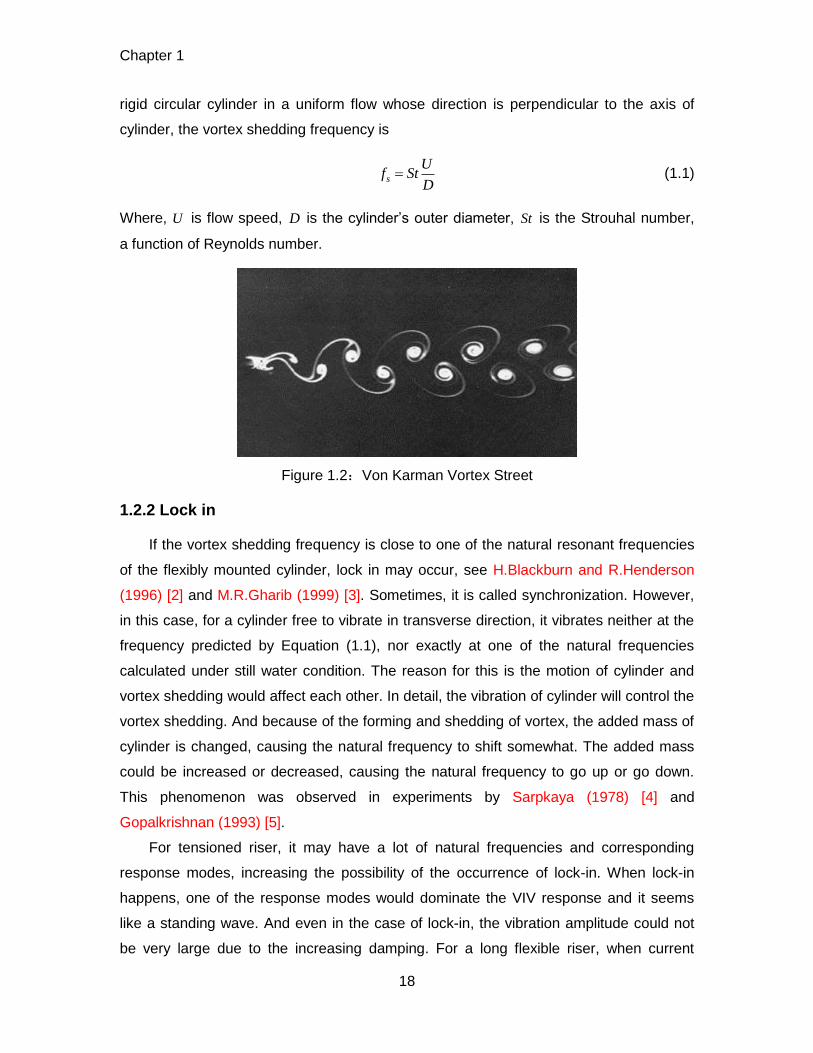
Figure 1.2：Von Karman Vortex Street ......................................................................... 18

Figure 1.3: The relationship of Strouhal number and Reynolds number ....................... 20

Figure 1.4: The variation of added mass coefficient with reduced velocity and different

normalised vibration amplitude values......................................................... 21

Figure 2.1: Flow chart of frequency domain method for riser VIV response reconstruction

.................................................................................................................... 32

Figure 2.2: Flow chart of time domain method for riser VIV response reconstruction ..... 34

Figure 2.3: The first three mode-shapes of displacement and curvature........................ 35

Figure 3.1: Photography of helical strakes installed on the riser model ......................... 40

Figure 3.2: Sketch of rotating test rig used for ExxonMobil VIV test ............................... 41

Figure 3.3: Accelerometers and strain gauges mounted on riser model ........................ 42

Figure 3.4: Strain gauge and accelerometer placement on the riser model ................... 42

Figure 3.5: Overview sketch of instrument placement ................................................... 43

Figure 3.6：Experiment set-up for the second Gulf Stream VIV test ............................. 45

Figure 3.7: Photographs of : (a) Triple helical strake (b) Fairing .................................... 46

Figure 3.8：Cross-section of the Pipe from the Gulf Stream Test ................................. 48

Figure 3.9: Side View of the Pipe from the Gulf Stream Test ......................................... 48

Figure 4.1: The variation of current speed with time for test 1113.................................. 51

Figure 4.2: The derived cross-flow displacement amplitute spectrum of the point where

sensor Acc_CF16 locates for case 1113 ..................................................... 53

List of Figures

7

Figure 4.3: The derived in-line displacement amplitute spectrum of the point where

sensor Acc_IL16 locates for case 1113 ....................................................... 53

Figure 4.4: The derived cross-flow displacement amplitute spectrum of the point where

sensor Acc_CF08 locates for case 1217 ..................................................... 54

Figure 4.5: The derived in-line displacement amplitute spectrum of the point where

sensor Acc_IL08 locates for case 1217 ....................................................... 54

Figure 4.6: The natural frequencies of riser in still water under constant tension of 700N

as a function of mode number ..................................................................... 56

Figure 4.7: Error of estimates of modal weights assuming uncorrelated noise of unit

variance on all curvature measurements ..................................................... 58

Figure 4.8: Normalized RMS modal weights for case 1113 ........................................... 59

Figure 4.9: Normalized RMS modal weights for case 1217 ........................................... 60

Figure 4.10: The comparison of the RMS of the original (at accelerometer locations) and

reconstructed CF displacements for case 1113 ........................................... 61

Figure 4.11: The comparison of the RMS of the original (at accelerometerlocations) and

reconstructed IL displacements for case 1113 ............................................ 61


reconstructed CF displacements for case 1217 ........................................... 62


reconstructed IL displacements for case 1217 ............................................ 62

Figure 4.14: The comparison of reconstructed and measured RMS CF displacements at

the position where the target accelerometer locates for case 1113 ............. 63

Figure 4.15: The comparison of reconstructed and measured RMS IL displacements at


Figure 4.16: The comparison of reconstructed and measured RMS CF displacements at


Figure 4.17: The comparison of reconstructed and measured RMS IL displacements at


Figure 4.18: The comparison of the RMS of the reconstructed IL displacements from

modified system matrix and original system matrix for case 1217 ............... 66

Figure 4.19: The comparison of modified and original normalized RMS modal weights for

in-line VIV response in case 1217 ............................................................... 66

Figure 4.20: The RMS of riser CF displacements for bare riser and uniform flow cases 67

Figure 4.21: The RMS of riser IL displacements for bare riser and uniform flow cases .. 68

List of Figures

8

Figure 4.22: The RMS of riser CF displacements for bare riser and sheared flow cases

.................................................................................................................... 68

Figure 4.23: The RMS of riser IL displacements for bare riser and sheared flow cases . 69

Figure 4.24: The RMS of riser CF displacements for 50% straked riser and uniform flow

cases .......................................................................................................... 69

Figure 4.25: The RMS of riser IL displacements for 50% straked riser and uniform flow

cases .......................................................................................................... 70

Figure 4.26: The RMS of riser CF displacements for 50% straked riser and sheared flow

cases .......................................................................................................... 70

Figure 4.27: The RMS of riser IL displacements for 50% straked riser and sheared flow

cases .......................................................................................................... 71

Figure 4.28: The RMS of riser CF displacements for fully straked riser and uniform flow

cases .......................................................................................................... 71

Figure 4.29: The RMS of riser IL displacements for fully straked riser and uniform flow

cases .......................................................................................................... 72

Figure 4.30: The RMS of riser CF displacements for fully straked riser and sheared flow

cases .......................................................................................................... 72

Figure 4.31: The RMS of riser IL displacements for fully straked riser and sheared flow

cases .......................................................................................................... 73

Figure 5.1: The peak response modal magnitude for the dominate cross-flow peak

response frequency (9.86 Hz) in test 1113 .................................................. 77

Figure 5.2: The peak response modal phase angle for the dominate cross-flow peak




Figure 5.4: The peak response modal phase angle for the dominate cross-flow peak


Figure 5.5: The contour plot of a two-second-long reconstructed CF displacement time

series for test 1113. ..................................................................................... 79


series for test 1217. ..................................................................................... 80

Figure 5.7: The spatial mean RMS CF and IL displacements for bare riser and uniform

flow cases ................................................................................................... 82

List of Figures

9

Figure 5.8: The spatial mean RMS CF and IL displacements for bare riser and sheared

flow cases ................................................................................................... 82

Figure 5.9: Dominant frequencies for bare riser and uniform flow cases........................ 83

Figure 5.10: Dominant frequencies for bare riser and sheared flow cases ..................... 84

Figure 5.11: Dominant mode with respect to displacement for bare riser and uniform flow

cases .......................................................................................................... 85

Figure 5.12: Dominant mode with respect to displacement for bare riser and sheared

flow cases ................................................................................................... 85

Figure 5.13: The spatial mean RMS CF and IL displacements for 50% straked riser and

uniform flow cases ...................................................................................... 86

Figure 5.14: The spatial mean RMS CF and IL displacements for 50% straked riser and

sheared flow cases ..................................................................................... 87

Figure 5.15: Dominant frequencies for 50% straked riser and uniform flow cases ......... 88

Figure 5.16: Dominant frequencies for 50% straked riser and sheared flow cases ........ 89

Figure 5.17: Dominant mode with respect to displacement for 50% straked riser and


Figure 5.18: Dominant mode with respect to displacement for 50% straked riser and


Figure 5.19: The spatial mean RMS CF and IL displacements for fully straked riser and


Figure 5.20: The spatial mean RMS CF and IL displacements for fully straked riser and


Figure 5.21: Dominant frequencies for fully straked riser and uniform flow cases .......... 92

Figure 5.22: Dominant frequencies for fully straked riser and sheared flow case ........... 93

Figure 5.23：Dominant mode with respect to displacement for fully straked riser and


Figure 5.24: Dominant mode with respect to displacement for fully straked riser and


Figure 6.1: Bottom end (railroad wheel) depth below the free surface of the water versus

top end angle of inclination with vertical for all cases .................................. 97

Figure 6.2: The natural frequencies of the pipe in still water under constant tension of

810 lb as a function of mode number .......................................................... 98

Figure 6.3: (a) the deflected shape of the pipe (b) normal incidence current profile ....... 99

List of Figures

10

Figure 6.4: RMS bending strain for case 20061023203818. Data from all the four

quadrants has been shown ....................................................................... 100

Figure 6.5: The RMS of cross-flow bending strains for case 20061023203818 ........... 102

Figure 6.6: Time-frequency plot of the cross-flow bending strain signal at the sensor

location with the largest RMS cross-flow bending strain in case

20061023203818 ...................................................................................... 103

Figure 6.7: The RMS of filtered cross-flow bending strains for case 20061023203818 104

Figure 6.8: Normalized PSD of the first nine POD subprocesses ................................ 106

Figure 6.9: The discrete mode-shape of the first POD mode ....................................... 107

Figure 6.10： The RMS of the reconstructed VIV displacement of the riser in cross-flow

direction for case 20061023203818 .......................................................... 108

Figure 6.11: The comparison of reconstructed and measured RMS CF bending strains at

the position where the target strain sensor locates .................................... 109

Figure 6.12: The RMS of the reconstructed VIV displacement of the riser in cross-flow

direction for the participating modes of 12-20 ........................................... 110


direction for the participating modes of 44-52 ............................................ 111


direction for the participating modes of 1-58 .............................................. 112

Figure 6.15: Peak response modal magnitude of riser cross-flow VIV response at 3.45Hz

.................................................................................................................. 113

Figure 6.16: Peak response modal phase angle of riser cross-flow VIV response at

3.45Hz ...................................................................................................... 113

Figure 6.17: The contour plot of a five-second-long reconstructed CF displacement time

series. The arrows trace the propogation of a crest in space and time. ..... 114

Figure A.1: Strake Configurations ................................................................................ 124

Figure A.2: Fairing and strake transitions from the 40% coverage cases with transition

.................................................................................................................. 125

Figure A.3: Fairing Configurations ............................................................................... 125

Figure C.1: PSD of CF displacements for the bare riser and uniform flow cases ......... 128

Figure C.2: PSD of IL displacements for the bare riser and uniform flow cases ........... 128

Figure C.3: PSD of CF displacements for the bare riser and sheared flow cases ........ 129

List of Figures

11

Figure C.4: PSD of IL displacements for the bare riser and sheared flow cases .......... 129

Figure C.5: PSD of CF displacements for 50% straked riser and uniform flow cases .. 130

Figure C.6: PSD of IL displacements for 50% straked riser and uniform flow cases .... 130

Figure C.7: PSD of CF displacements for 50% straked riser and sheared flow cases . 131

Figure C.8: PSD of IL displacements for 50% straked riser and sheared flow cases ... 131

Figure C.9: PSD of CF displacements for fully straked riser and uniform flow cases ... 131

Figure C.10: PSD of IL displacements for fully straked riser and uniform flow cases ... 132

Figure C.11: PSD of CF displacements for fully straked riser and sheared flow cases 132

Figure C.12: PSD of IL displacements for fully straked riser and sheared flow case .... 132

Figure D.1: Illustration of determining rotation angles of Q1-Q3 plane to cross-flow

direction at all the sensor locations by identifying maxima in the PSD of

cross-flow bending strains around 1X frequency (3.45 HZ) ....................... 136

List of Tables

12

List of Tables

Table 3.1: ExxonMobil VIV test: Riser model properties ................................................ 39

Table 3.2: Other employed transducers in ExxonMobil VIV test .................................... 43

Table 3.3: The second Gulf Stream experiment: Pipe properties .................................. 45

Table 3.4: Strake Properties .......................................................................................... 46

Table 3.5: Fairing Properties ......................................................................................... 47

Table 4.1: The natural frequencies of riser in still water under constant tension of 700N

.................................................................................................................... 57

Table B.1: The chosen parameters for bare riser and uniform flow cases ................... 126

Table B.2: The chosen parameters for bare riser and sheared flow cases .................. 127

List of Tables

13

Nomenclature

14

Nomenclature

VIV Vortex-Induced Vibration

sf Vortex shedding frequency

Re Reynolds number

St Strouhal number

rV Reduced velocity

rm Mass ratio

aC Added mass coefficient

am Added mass per unit length

,A System Matrix

ˆ,b c Data Matrix

n Mode-shapes of displacement

n Mode-shapes of curvature

nw Modal weights

Bending strain

a Acceleration

Curvature

Curvature measurement noise

D Outer diameter of riser model

R Outer radius of riser model

L Length of riser model

E Young’s Modulus

Nomenclature

15

I Moment of Inertia

CF Cross-flow

IL In-line

RMS Root Mean Square

RMSy RMS of reconstructed displacemet in cross-flow direction

RMSx RMS of reconstructed displacemet in in-line direction

RMSw RMS of modal weights

domf Dominant response frequency

x Differential strain from quadrants 1 and 3

y Differential strain from quadrants 2 and 4

CF Cross-flow bending strain

POD Proper Orthogonal Decomposition

n POD mode-shapes

nu Scalar subprocesses

Chapter 1

16

Chapter 1

1 Introduction

1.1 Background

The offshore industry is a huge industry and it is very important from economical

perspective. Therefore, any unexpected stoppages about the offore platform’s

production would be quite expensive. What’s more, oil spill will cause a great pollution to

ocean environment, as happened in the Gulf of Mexico. Thus, it is very important to

ensure the offshore platform’s smooth and safe production. In the offshore industry, the

riser, which connects the platform to the well at the sea bed, see Figure 1, is one of the

most critical components. It is used for both drilling and oil transportation. And the

phenomenon of current-induced vortex-induced vibration (VIV) with regard to marine

riser is widely observed and it will cause costly and environmentally unfriendly fatigue

failure. In recent years, many offshore projects are done in deep water areas like Gulf of

Mexico and West Africa. As the water depth increases, the fatigue damage related to

wave and vessel motion may keep roughly constant or diminish. However, current can

act over the whole water depth, tending to cause more severe fatigue damage to marine

riser. In addition, in such deep water depth, long flexible risers are increasingly required.

And the VIV response of long flexible rier is more complicated than short rigid riser, thus,

it is quite important to predict the VIV response of this kind of riser.

Chapter 1

17

Figure 1.1：Principle sketch of a riser system

1.2 Vortex-Induced Vibration

Vortex induced vibration (VIV) is a phenomenon that cylindrical structure may

experience due to interactions between the structure and ambient currents. It is a

response to time-varying hydrodynamic forces that arise when currents cause vortices to

form and shed into the structure’s wake. This oscillating force will lead to the cylinder’s

vibrations that are perpendicular (cross-flow, CF) and parallel (in-line, IL) to the flow

direction. The structure’s VIV response maybe is dominated by standing waves,

travelling waves or a combination of both.

1.2.1 Vortex-shedding

When fluid flows past a cylinder, or other bluff body, it will be forced to change its

original flowing path and move around cylinder, resulting in separated flow in the wake of

cylinder. Due to two layers of fluids moving in different velocites, vortex is formed

naturally. After some time, vortices are concentrated at two points, which are located in

the disturbed upper and lower shear layers respectively. Upper vortices will move down

and lower vortices will move up, leading to an array of swaying vortices and the famous

Von Karman vortex street as depicted in Figure1.2. With the vortices forming and

shedding, the local pressure around the cylinder is changed. And because of this

pressure change, an alternating force arises and acts on it at the frequency of vortex

shedding. This force has two components, one is lift force in the cross-flow direction and

another is the drag force in the in-line direction. See Blevins (1990) [1], for a fixed and

Chapter 1

18

rigid circular cylinder in a uniform flow whose direction is perpendicular to the axis of

cylinder, the vortex shedding frequency is

s

Uf St

D (1.1)

Where, U is flow speed, D is the cylinder’s outer diameter, St is the Strouhal number,

a function of Reynolds number.

Figure 1.2：Von Karman Vortex Street

1.2.2 Lock in

If the vortex shedding frequency is close to one of the natural resonant frequencies

of the flexibly mounted cylinder, lock in may occur, see H.Blackburn and R.Henderson

(1996) [2] and M.R.Gharib (1999) [3]. Sometimes, it is called synchronization. However,

in this case, for a cylinder free to vibrate in transverse direction, it vibrates neither at the

frequency predicted by Equation (1.1), nor exactly at one of the natural frequencies

calculated under still water condition. The reason for this is the motion of cylinder and

vortex shedding would affect each other. In detail, the vibration of cylinder will control the

vortex shedding. And because of the forming and shedding of vortex, the added mass of

cylinder is changed, causing the natural frequency to shift somewhat. The added mass

could be increased or decreased, causing the natural frequency to go up or go down.

This phenomenon was observed in experiments by Sarpkaya (1978) [4] and

Gopalkrishnan (1993) [5].

For tensioned riser, it may have a lot of natural frequencies and corresponding

response modes, increasing the possibility of the occurrence of lock-in. When lock-in

happens, one of the response modes would dominate the VIV response and it seems

like a standing wave. And even in the case of lock-in, the vibration amplitude could not

be very large due to the increasing damping. For a long flexible riser, when current

Chapter 1

19

speed varys considerably along its length, there would be a multitude of vortex shedding

frequencies. As a consequence, several modes can be candidates for lock-in vibration.

What’s more, the variation of added mass would probably make the natural frequencies

of riser to be different from those calculated under still water condition. This would make

us hard to find the participating mode exactly just according the oscillating frequency.

From model tests with a taut cable in sheared flow, Lie et al., (1997) [6] find that a

second-mode lock-in vibration changed to a third-mode lock-in in a short time while the

VIV frequency kept unchanged.

1.2.3 Influencing parameters

Reynolds number, Re , is a dimensionless number which is the ratio of inertial

forces to viscous forces. It is used to classify the flow patterns. Laminar flow occurs at

low Reynolds numbers (<2300) and turbulent flow occurs at high Reynolds numbers

(>4000). The definition of Reynolds number is given by:

ReUD UD

(1.2)

Where, U is the mean fluid velocity, D is the diameter of the cylinder, is the density

of the fluid, is the dynamic viscosity of the fluid, and is the kinematic viscosity of the

fluid.

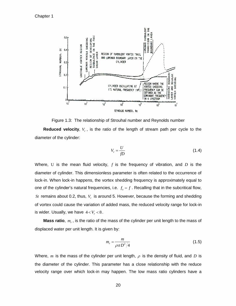
Strouhal number, St , is a dimensionless number describing oscillating flow

mechanisms. It is given by

sf DSt

U (1.3)

Where, sf is the vortex-shedding frequency (also referred to as the Strouhal frequency),

D is the diameter of the cylinder, and U is the mean flow velocity. Strouhal number is

the function of Reynolds number and their relationship can be seen in Figure 1.3 from

Lienhard (1996) [7]. In the subcritical regime, the value of St remains at about 0.2. In the

critical regime, the variation range of Strouhal number is relatively large and its

maximum value could be 0.4. In the supercritical regime, the Strouhal number is about

0.27.

Chapter 1

20

Figure 1.3: The relationship of Strouhal number and Reynolds number

Reduced velocity, rV , is the ratio of the length of stream path per cycle to the

diameter of the cylinder:

r

UV

fD (1.4)

Where, U is the mean fluid velocity, f is the frequency of vibration, and D is the

diameter of cylinder. This dimensionless parameter is often related to the occurrence of

lock-in. When lock-in happens, the vortex shedding frequency is approximately equal to

one of the cylinder’s natural frequencies, i.e. sf f . Recalling that in the subcritical flow,

St remains about 0.2, thus, rV is around 5. However, because the forming and shedding

of vortex could cause the variation of added mass, the reduced velocity range for lock-in

is wider. Usually, we have 4 8rV .

Mass ratio, rm , is the ratio of the mass of the cylinder per unit length to the mass of

displaced water per unit length. It is given by:

2 4

r

mm

D (1.5)

Where, m is the mass of the cylinder per unit length, is the density of fluid, and D is

the diameter of the cylinder. This parameter has a close relationship with the reduce

velocity range over which lock-in may happen. The low mass ratio cylinders have a

Chapter 1

21

much wider lock-in range than the high mass ratio cylinders. It is because the influence

of added mass variation is more critical for low mass ratio cylinders.

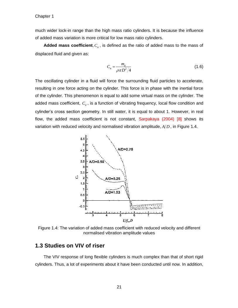
Added mass coefficient, aC , is defined as the ratio of added mass to the mass of

displaced fluid and given as:

2 4

aa

mC

D (1.6)

The oscillating cylinder in a fluid will force the surrounding fluid particles to accelerate,

resulting in one force acting on the cylinder. This force is in phase with the inertial force

of the cylinder. This phenomenon is equal to add some virtual mass on the cylinder. The

added mass coefficient, aC , is a function of vibrating frequency, local flow condition and

cylinder’s cross section geometry. In still water, it is equal to about 1. However, in real

flow, the added mass coefficient is not constant, Sarpakaya (2004) [8] shows its

variation with reduced velocity and normalised vibration amplitude, A D , in Figure 1.4.

Figure 1.4: The variation of added mass coefficient with reduced velocity and different normalised vibration amplitude values

1.3 Studies on VIV of riser

The VIV response of long flexible cylinders is much complex than that of short rigid

cylinders. Thus, a lot of experiments about it have been conducted until now. In addition,

Chapter 1

22

some semi-empirical computational programmes and the numerical method are

constructed to predict its VIV response.

1.3.1 Experimental studies

Over the past decades, several VIV experiments using long flexible risers were

performed. The measured data can be used as benchmark information to update

database and improve VIV calculating models.

Some VIV experiments were conducted in laboratory. In June 2003, Exxonmobil

performed VIV testing on a long flexible riser at the Norwegian Marine Technology

Research Institute (Marintek), see Frank et al., (2004) [9]. The used riser was made of

brass with a length of 9.63m and an outer diameter of 20m. This testing was conducted

on both bare riser and straked risers with four percentages of spatial coverage. Uniform

flow and linearly sheared flow were simulated. Bending strains and accelerations were

measured in both CF and IL directions.

In late 2003, the Norwegian Deepwater Programme (NDP) also performed a VIV

testing at Marintek (H.Braaten and H.Lie, 2004) [10]. During experiment, a long model

riser with a length of 38m and diameter of 27mm was towed horizontally by their

Trondheim Ocean Basin facility. Uniform flow and linearly sheared flow were also

simulated in this experiment. And bending strains and accelerations were measured in

both CF and IL directions. This testing was conducted with bare riser and straked risers.

These straked risers have two different geometries and some different percentages of

strake coverage.

In addition, some VIV tests using long flexible cylinder were performed under field

conditions. In 1997, at Hanøytangen outside Bergen, Norway, the Hanøytangen testing

was conducted (Huse et al., 1998) [11]. The length of tested riser was 90m and the

diameter was 30mm. The riser was furnitured with 29 bending strain sensors at every

3m in both CF and IL directions. A well defined lineared flow was simulated.

In 2004, at Lake Seneca, New York, the Lake Seneca VIV testing was conducted at

the Naval Underwater Warfare Center (NUWC) Test Facility (Vandiver et al., 2005) [12].

The tested risers have two different lengths, 61.26m and 122.23m, and a diameter of

3.33m. It was tensioned by a railroad suspended at the bottom of riser and towed by

boat at velocities ranging from 0.3m/s to 1.1m/s. The response was measured by evenly

spaced triaxial accelerometers. Both bare riser and riser with a triple helical strake were

tested.

Chapter 1

23

In 2006, the second Gulf Stream experiement was performed by the research group

of Prof. Kim Vandiver in Gulf Stream off the coast of Miami (Vandiver et al., 2006) [13]. It

is the same to the Lake Seneca experiment that a fiberglass pipe was tensioned by a

railroad at the bottom and towed by a boat. The length of tested pipe was 153.77m and

the diameter was 3.58cm. But the difference is that the Gulf-stream is the fastest ocean

current in the world. While sailing the boat in different directions relative to the ocean

current’s direction, many current profiles along the pipe were produced, which are

recorded by Acoustic Doppler Current Profilers (ADCP). The pipe had four quadrants

and each quadrant was furnitured with two optical fibers containing 70 bending strain

gauges in total at every 7ft. In addition to bare pipes, pipes of helical strakes or fairings

with different spatial coverages were also tested.

The objectives of these VIV tests were: (1) to improve the understanding of the

characteristics of the VIV of long flexible riser, such as the high harmonics and travelling

wave; (2) to evaluate the associated fatigue damage caused by VIV; (3) to assess the

effectiveness of the strakes or fairings in mitigating VIV.

1.3.2 Semi-Empirical VIV Response Computational Tools

Based on experimental results and theoretical studies, several semi-empirical

computer models have been constructed to predict the VIV response of marine risers,

such as SHEAR7 (Vandiver and Lee, 2005) [14], VIVA (Triantafyllou et al., 1999) [15],

VIVANA (MARINTEK, 2001) [16], and ViComo (Moe et al., 2001) [17]. These models,

aimed at solving engineering problems, have some intrinsic limitations, which would

produce errors in predicting VIV response. First, these models are based on strip theory

and finite element method. That is to say the hydrodynamics (lift, drag, damping and

added mass) are estimated just according to the local vibration and flow conditions, not

considering the effect of flow and vortex shedding along the riser axis. Second, the

database used by these models is originated from the laboratory experiments with

limited Reynolds number. The realistic marine risers may experience high Reynolds

number and turbulent flow in sea. Third, these models do not include IL response. It is

probably due to the underestimation of the importantance of IL vibration for fatigue

damage.

Chapter 1

24

1.3.3 Numerical Simulation

The alternative approach to semi-empirical model is computational fluid dynamics

(CFD), see Etienne et al, 2001 [18] and Willden and Graham, 2001 [19]. CFD is based

on the basic hydrodynamic theory, such as conservation of mass, conservation of

momentum and conservation of energy. In general, it includes three stages. The first

stage is the pre-processor which includes defining fluid properties, physical model, grid

size, time step and boundary condition. The second stage is solver. In this stage, the

CFD problem is solved by numerical methods, such as finite difference method (FDM),

finite element method (FEM) and finite volume method (FVM). The last stage is post-

processor. In this stage, the solution can be analysed and visualized. With the rapid

progress of computational techniques and capabilities, VIV response could be predicted

more accurately in the future.

1.4 Research objectives

The research objectives of this thesis mainly include the following three parts:

1) Figuring out a new approach for reconstructing the VIV response of long flexible

riser from the VIV test data or searching an existed reconstruction approach and

doing some improvement with it. Once the reconstruction approach is determined,

there are many things to be analyzed, e.g. the advantages and shortcomings of this

approach, the specific steps of using this approach to reconstruct the riser VIV

response, and the accuracy verification of reconstructed result.

2) Analyzing the characteristics of the riser VIV response based on the reconstructed

result. After finishing the reconstruction, the specific features of the riser VIV

response under a certain external condition can be known by extracting some key

parameters, e.g. response frequency, VIV displacement magnitude, travelling wave

direction and speed, and power-in region. These characteristics will improve our

understanding about the riser VIV response and give some supports to the

theoretical research about it.

3) The reconstructed result can provide benchmark information for calibration and

validation of semi-empirical tools that predict riser response.

Chapter 1

25

1.5 Thesis outline

This thesis is structured as follows:

Chapter 1 presents a brief introduction about vortex-induced vibration and summary

on the studies on it in the past.

Chapter 2 describes the issue that will be addressed in the thesis and presents two

approaches, i.e. modal approach and Fourier series approach, to reconstruct the riser

VIV response. After comparing the advantages and shortcomings of these two

approaches, the modal approach is chosen. And the modal approach can be classified

as frequency domain method and time domain method. In addition, the errors induced

by the noise on strain signal and chosen participating modes are analyzed.

Chapter 3 gives an introduction of ExxonMobil experimental VIV test and the

second Gulf Stream field VIV test, which includes experiment set-up, tested riser model

and measurement system.

Chapter 4 performs the riser VIV response reconstruction with regard to the

ExxonMobil VIV test. The systematic and detailed reconstruction steps are presented.

In addition, the error analysis and accuracy verification are done.

Chapter 5 analyzes the riser VIV responses in ExxonMobil VIV test. Some key

characteristics about riser VIV response, e.g. response frequency, VIV displacement

magnitude and travelling wave, can be extracted from the reconstructed results in

previous chapter. By analyzing those extracted features, the influences of external

conditions, e.g. current speed, current profiler and covered strake or fairing, on the riser

VIV response could be found.

Chapter 6 performs the riser VIV response reconstruction in terms of the second

Gulf Stream VIV test. Because of the long length of the tested pipe and complicated

current condition, the riser VIV response in this test is very complex and irregular. Thus,

the Proper Orthogonal Decomposition (POD) method is used to decompose the

measured data and extract the energetic and relatively regular riser VIV resposne. POD

can also aid the identification of the participating modes. This technique is very useful in

reconstructing the riser VIV response in VIV field test.

Chapter 7 summarizes the principle contributions of each chapter and provides

some recommendations for the future research about this subject.

Chapter 2

26

Chapter 2

2 Approach to riser VIV response

reconstruction

2.1 Problem statement

As we all know, vortex-induced vibration is a very complex interaction problem of

fluid and structure. In order to understand it deeply, the riser VIV motion is needed to be

obtained. One approach to achieve it is that when riser properties and flow condition are

known, we can use the knowledge of hydrodynamics to estimate the vortex-induced

forces, and then use the knowledge of structural dynamics to calculate the vortex-

induced motion. Another approach is that we can obtain it from the sensor measurement

data of VIV experiement. These sensor measurements have the following characteristics:

1) High temporal sampling rate: Each sensor measures the signal with high sampling in

time. It is because the VIV of riser often involves high harmoic and frequency motion.

2) Limited number of sensors: In general, only a limited number of sensors are put on

the selected positions of the riser. It is because the employment of a large number of

sensors will increase the experiment cost largely considering that the riser in field

VIV test is often very long. What’s more, if two sensors are located too closely, they

would mutually influence the quality of their measurement. Usually, the sensors are

often evenly placed. However, they probably become unevenly spaced because of

the failure of some sensors during test.

3) Indirect measurement of displacement: At present, it is not feasible to measure the

riser displacement directly. The typical employed sensors in VIV experiments now

are accelerometer for measuring acceleration, and strain gauge for measuring

bending strain.

Chapter 2

27

Therefore, I need to use these indirect measurements of riser displacement from the

limited number of sensors on the riser to reconstruct the riser VIV motion, i.e. to obtain

the VIV motion at all the points along its span.

2.2 Reconstruction approach

A spatial continuous function along the length of the riser is the prerequisite for riser

VIV response reconstruction. After reading some related literatures, the modal approach

had been applied mostly to solve the reconstruction issue from different signals, e.g.

Kaasen et al. (2000) [20], who used rotation-rates and accelerations as input signals,

and Trim et al. (2005) [21], who adopted the strain and acceleration signals, and Lie and

kaasen (2006) [22], who used only the strain signals.

2.2.1 Modal approach

All of the above researchers thought that the displaced shape of the riser could be

composed as a series of its free vibration modes, at any instant in time. Thus, for

example, the VIV displacement in cross-flow direction can be expressed as:

1

( , ) ( ) , 0,n n

n

y z t w t z z L

(2.1)

Under different fluid conditions, the response frequencies along the riser’s span are

different and so the participating modes become different. In order to avoid the error

result from the participation of spurious higher or lower modes, the way of choosing the

participating modes from 1 to maximum number M, i.e. the number of measurements, is

not accepted. Assuming the participating modes are n1 to nN, Equation (2.1) can be

recasted as:

1

( , ) ( ) , 0,Nn

n n

n n

y z t w t z z L

(2.2)

Where, t is the time, z denotes the vertical position along the riser with origin at the top

end, L is the length of the riser, ( )nw t are the modal weights, n z are the eigenmodes

or mode-shapes, and n is the order of mode.

Assuming that there are M measurements in a VIV test, then a linear system with M

equations and N (N=nN-n1+1) unknowns can be established using the relationships

between VIV displacement and measurements, e.g. bending strain and acceleration.

Chapter 2

28

After solving this linear system, the modal weights at any instance of time are obtained

and then the riser VIV response reconstruction is finished.

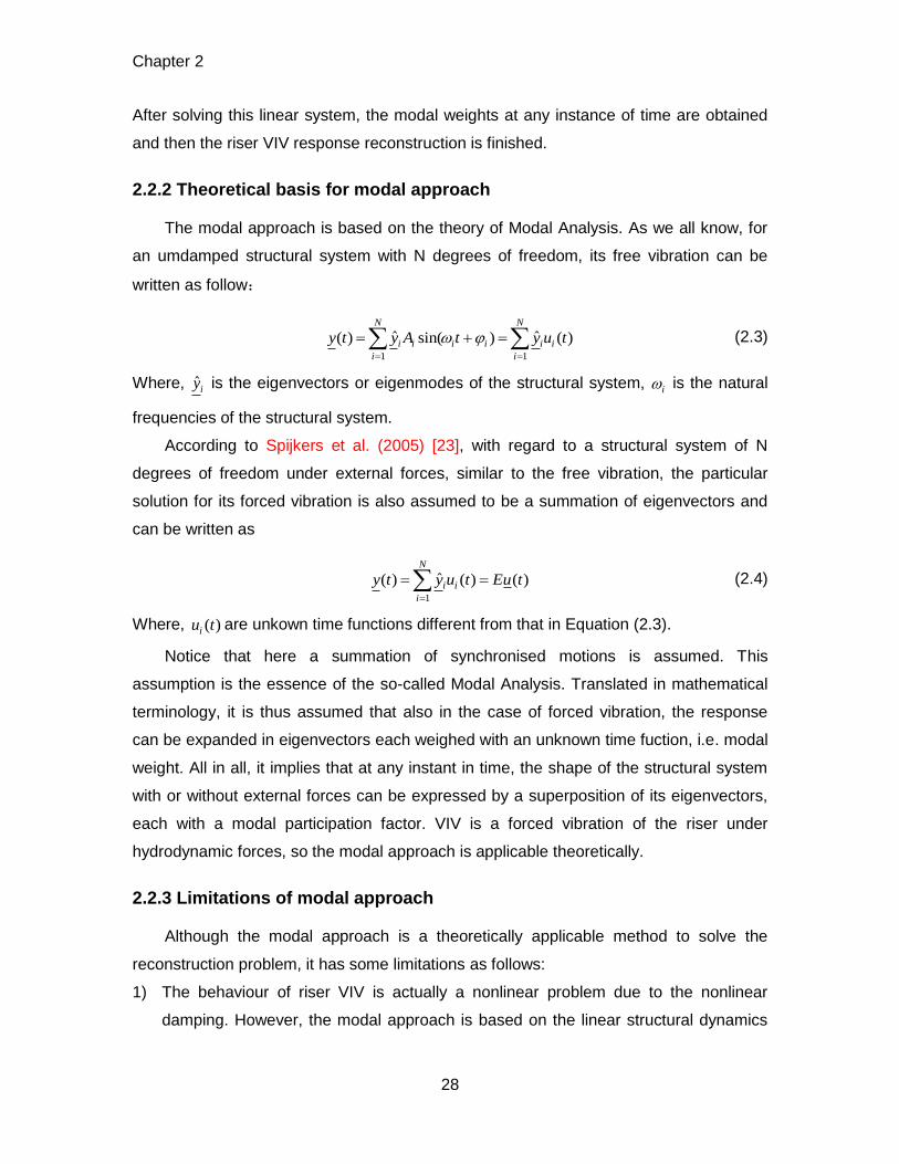
2.2.2 Theoretical basis for modal approach

The modal approach is based on the theory of Modal Analysis. As we all know, for

an umdamped structural system with N degrees of freedom, its free vibration can be

written as follow：

1 1

ˆ ˆ( ) sin( ) ( )N N

i i i i i i

i i

y t y A t y u t

(2.3)

Where, îy is the eigenvectors or eigenmodes of the structural system, i is the natural

frequencies of the structural system.

According to Spijkers et al. (2005) [23], with regard to a structural system of N

degrees of freedom under external forces, similar to the free vibration, the particular

solution for its forced vibration is also assumed to be a summation of eigenvectors and

can be written as

1

ˆ( ) ( ) ( )N

i i

i

y t y u t Eu t

(2.4)

Where, ( )iu t are unkown time functions different from that in Equation (2.3).

Notice that here a summation of synchronised motions is assumed. This

assumption is the essence of the so-called Modal Analysis. Translated in mathematical

terminology, it is thus assumed that also in the case of forced vibration, the response

can be expanded in eigenvectors each weighed with an unknown time fuction, i.e. modal

weight. All in all, it implies that at any instant in time, the shape of the structural system

with or without external forces can be expressed by a superposition of its eigenvectors,

each with a modal participation factor. VIV is a forced vibration of the riser under

hydrodynamic forces, so the modal approach is applicable theoretically.

2.2.3 Limitations of modal approach

Although the modal approach is a theoretically applicable method to solve the

reconstruction problem, it has some limitations as follows:

1) The behaviour of riser VIV is actually a nonlinear problem due to the nonlinear

damping. However, the modal approach is based on the linear structural dynamics

Chapter 2

29

techniques and the mode superposition principle. Using a linear approach to slove a

nonlinear issue, the error is unavoidable.

2) Usually, the riser in VIV test is identical to a tensioned beam with the pinned-pinned

boundary condition. Thus, in the later parts solving the reconstruction problem, the

mode-shapes of the riser’s VIV displacement are approximated with sinusoids, i.e.

sinn z n z L . Actually, only when the riser is without damping and has uniform

mass distribution along its span, its mode-shapes can be absolutely sinusoidal.

However, the riser in VIV test is often with damping, thus, the actual mode-shapes

are complex. Besides, since the added mass and damping will change in time and

space with frequency and amplitude of vibration, the true mode-shapes for the riser

in VIV test are not constant and then very hard to find out. Finally, some

experimental conditions will also impose some influences on the eigenmodes of the

riser. For example, in the ExxonMobil VIV test introduced in chapter 3, the upper

end of the riser was connected to a spring system and would sag due to current

drag. And in the second Gulf Stream VIV test described in chapter 3, the utilized

riser was deflected in a degree due to the current drag force during the test.

3) Even though the sinusoidal mode-shapes are very close to the actual mode-shapes

of the tested riser, the perfectly correct participating modes are still quite hard to find

out. It is mainly due to the following two reasons. On one hand, in this thesis, the

choice of participating modes is based on simply calculated natural frequencies of

the riser in still water and the spectral analyses of measurements. However, due to

time-varying tension, and temporal and spatial variation of added mass, the natural

frequencies of the tested riser are not constant and are always changing.

Consequently, the simply calculated natural frequencies are not always correct. On

the other hand, sometimes, the riser VIV response contains a lot of frequencies and

is dominated by the travelling wave, especially under sheared flow condition, which

will make it quite difficult to identify the absolutely correct participating modes. So

the only thing I can do is to make sure that the main participating modes will be

definitely included and reconstruction error will be reduced as small as possible.

2.3 Modal approach description

The modal approach can be classified into frequency domain method or time

domain method and using which method depends on the types of provided

Chapter 2

30

measurements. When attainable signals are both acceleration and strain, the frequency

domain method is preferred because acceleration involves the second time derivative of

displacement and the time function ( )n t in Equation (2.2) is unknown. If only strain

signal is provided, the time domain method can be adopted to solve the VIV response

reconstruction issue. These two methods will be introduced in detail below.

2.3.1 Frequency domain method

The detailed procedures of using the frequency domain method to solve the VIV

response reconstruction issue are described below.

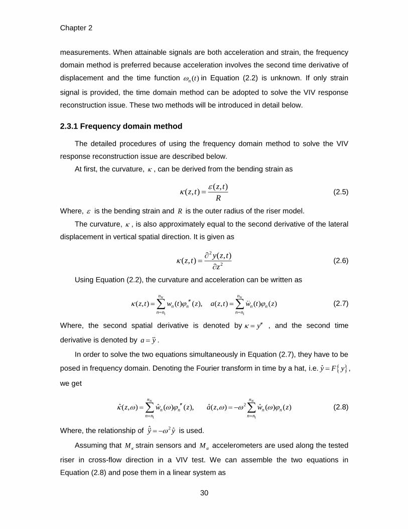
At first, the curvature, , can be derived from the bending strain as

( , )

( , )z t

z tR

(2.5)

Where, is the bending strain and R is the outer radius of the riser model.

The curvature, , is also approximately equal to the second derivative of the lateral

displacement in vertical spatial direction. It is given as

2

2

( , )( , )

y z tz t

z

(2.6)

Using Equation (2.2), the curvature and acceleration can be written as

1 1

( , ) ( ) ( ), ( , ) ( ) ( )N Nn n

n n n n

n n n n

z t w t z a z t w t z

(2.7)

Where, the second spatial derivative is denoted by y , and the second time

derivative is denoted by a y .

In order to solve the two equations simultaneously in Equation (2.7), they have to be

posed in frequency domain. Denoting the Fourier transform in time by a hat, i.e. y F y ,

we get

1 1

2ˆ ˆ ˆ ˆ( , ) ( ) ( ), ( , ) ( ) ( )N Nn n

n n n n

n n n n

z w z a z w z

(2.8)

Where, the relationship of 2ˆ ˆy y is used.

Assuming that M strain sensors and aM accelerometers are used along the tested

riser in cross-flow direction in a VIV test. We can assemble the two equations in

Equation (2.8) and pose them in a linear system as

Chapter 2

31

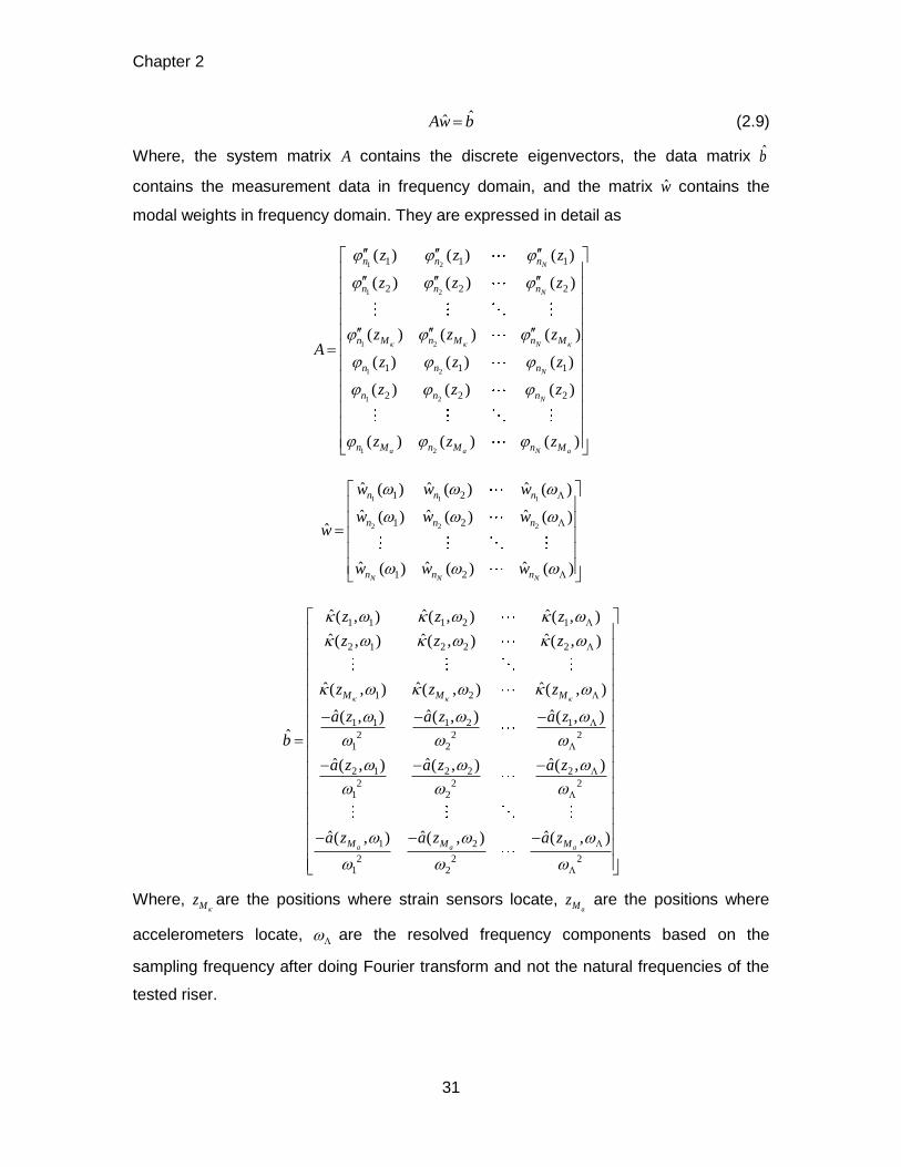
ˆÂw b (2.9)

Where, the system matrix A contains the discrete eigenvectors, the data matrix b

contains the measurement data in frequency domain, and the matrix w contains the

modal weights in frequency domain. They are expressed in detail as

1 2

1 2

1 2

1 2

1 2

1 2

1 1 1

2 2 2

1 1 1

2 2 2

( ) ( ) ( )

( ) ( ) ( )

( ) ( ) ( )

( ) ( ) ( )

( ) ( ) ( )

( ) ( ) ( )

N

N

N

N

N

a a N a

n n n

n n n

n M n M n M

n n n

n n n

n M n M n M

z z z

z z z

z z zA

z z z

z z z

z z z

1 1 1

2 2 2

1 2

1 2

1 2

ˆ ˆ ˆ( ) ( ) ( )

ˆ ˆ ˆ( ) ( ) ( )ˆ

ˆ ˆ ˆ( ) ( ) ( )N N N

n n n

n n n

n n n

w w w

w w ww

w w w

1 1 1 2 1

2 1 2 2 2

1 2

1 1 1 2 1

2 2 21 2

2 1 2 2 2

2 2 21 2

1

21

ˆ ˆ ˆ( , ) ( , ) ( , )

ˆ ˆ ˆ( , ) ( , ) ( , )

ˆ ˆ ˆ( , ) ( , ) ( , )

ˆ ˆ ˆ( , ) ( , ) ( , )

ˆ

ˆ ˆ ˆ( , ) ( , ) ( , )

ˆ ˆ( , ) ( ,a a

M M M

M M

z z z

z z z

z z z

a z a z a z

b

a z a z a z

a z a z

2

2 22

ˆ) ( , )aMa z

Where, Mzare the positions where strain sensors locate,

aMz are the positions where

accelerometers locate, are the resolved frequency components based on the

sampling frequency after doing Fourier transform and not the natural frequencies of the

tested riser.

Chapter 2

32

Assemble

Compute Fourier transform

Given data:

Reconstruction in

frequency domain

Compute inverse

Fourier transform

Obtain displacement

at any location

It can be seen from Equation (2.9) that we have ( )aM M M M equations with

1 1NN N n n unknowns. In order to avoid an under-determined system, we require

that N M . If the number of selected modes is equal to the number of measurements

( N M ), the system of equations has a single and unique solution as

1 ˆw A b (2.10)

If fewer than M modes participate in the riser VIV response, the system can be

sloved using the least square method. The solution becomes

1 ˆ ˆˆ ( ) ( ) ( ) ( )T Tw A A A b Hb (2.11)

Once the modal weights in frequency domain is obtained, we can do inverse Fourier

transform with it to achieve the modal weights in time domain, i.e. 1 ˆ( ) ( )w t F w .

Finally, the VIV displacement at all the points along the length of the riser, at any

instant of time, can be obtained using Equation (2.2). This method can be applied to

cross-flow and in-line VIV response reconstructions separately and it should be noted

that the number of selected modes and which modes may be quite different for them.

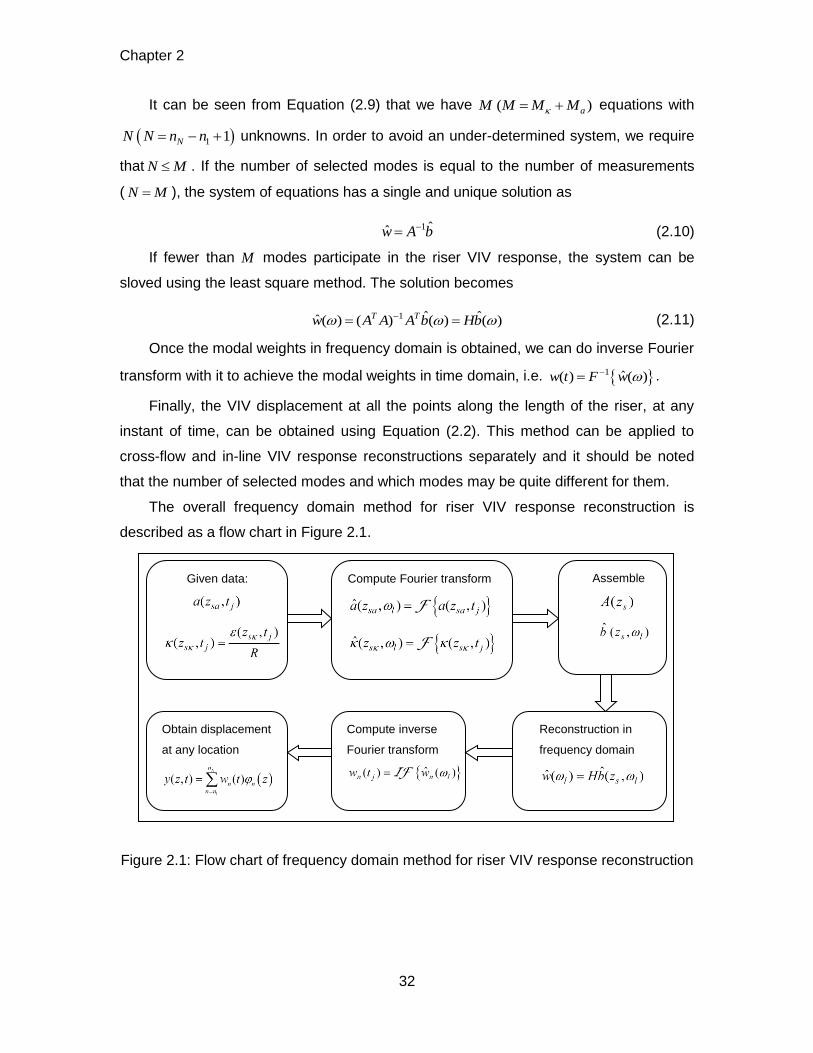
The overall frequency domain method for riser VIV response reconstruction is

described as a flow chart in Figure 2.1.

Figure 2.1: Flow chart of frequency domain method for riser VIV response reconstruction

Chapter 2

33

2.3.2 Time domain method

In the case that only strain data is provided, the time domain method can be used to

slove the problem of riser VIV response reconstruction. The difference of this method

from the frequency domain method is that we do not perform Fourier transform with

Equation (2.7). The reconstruction issue can be just posed in time domain using the first

equation in Equation (2.7). Recasting this equation as

1 1

( , ) ( ) ( ) ( ) ( )N Nn n

n n n n

n n n n

z t w t z w t z

(2.12)

Where, ( )n z are the mode-shapes of riser curvature.

Assembling the above equation in each sampling time, a linear system in time

domain will be established as

( ) ( )w t c t (2.13)

Where, the system matrix, , comprises the mode-shapes of riser curvature, the data

matrix, c , is formed from the measured strains, and the matrix, w , contains the modal

weights in time domain. They are expressed in detail as

1 2

1 2

1 2

1 1 1

2 2 2

( ) ( ) ( )

( ) ( ) ( )

( ) ( ) ( )

N

N

N

n n n

n n n

n M n M n M

z z z

z z z

z z z

1 1 1

2 2 2

1 2

1 2

1 2

( ) ( ) ( )

( ) ( ) ( )

( ) ( ) ( )N N N

n n n n

n n n n

n n n n

w t w t w t

w t w t w tw

w t w t w t

1 1 1 2 1

2 1 2 2 2

1 2

( , ) ( , ) ( , )

( , ) ( , ) ( , )

( , ) ( , ) ( , )

n

n

M M M n

z t z t z t

z t z t z tc

z t z t z t

Similarly, as long as 1 1NN N n n is smaller than M , this system can be

sloved in a least-squares sense as

1( ) ( ) ( )T Tw t c t (2.14)

Chapter 2

34

Given data:

Assemble:

Reconstruction in

time domain:

Obtain displacement

at any location:

After obtaining the modal weights vector at any instant of time, Equation (2.2) can

be used again to achieve the VIV displacements of all the points on the riser, at any

instant of time.

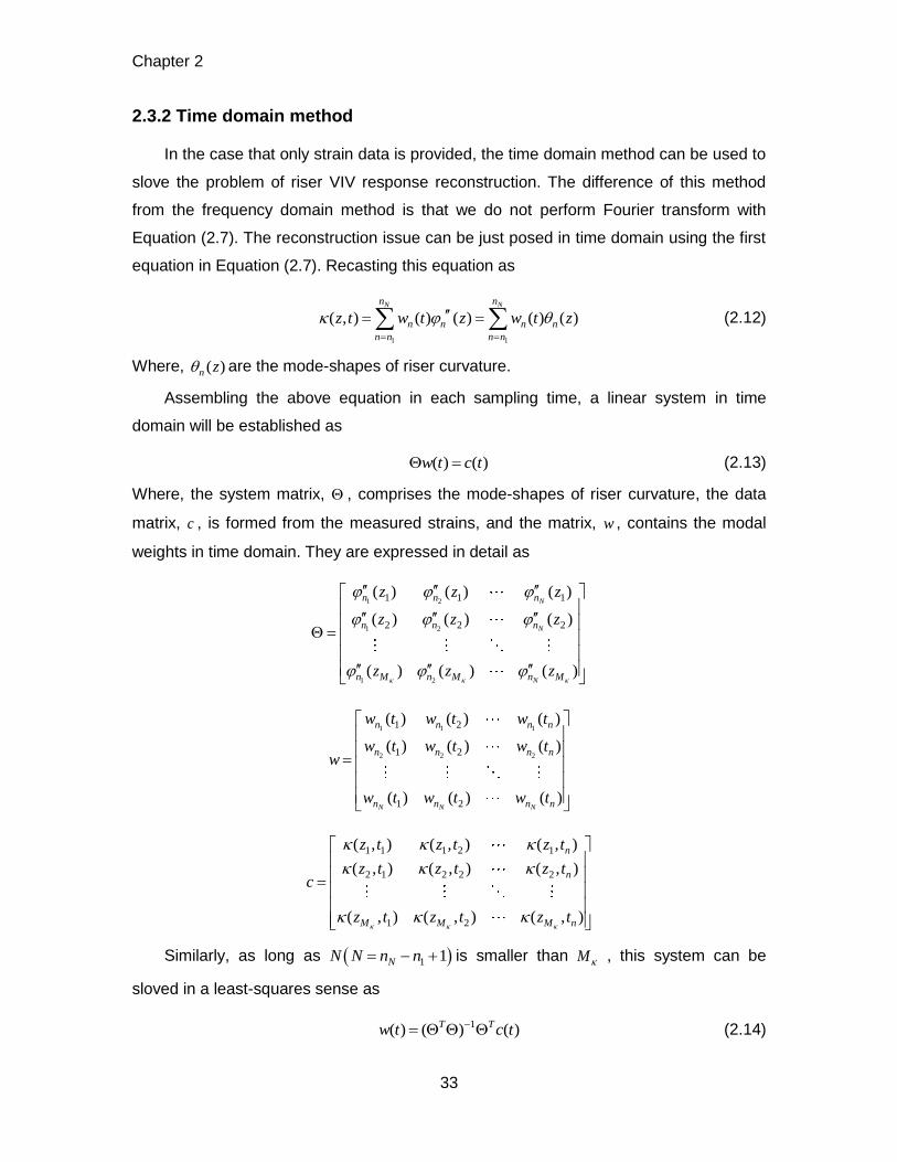
The overall time domain method for riser VIV response reconstruction is described

as a flow chart in Figure 2.2

Figure 2.2: Flow chart of time domain method for riser VIV response reconstruction

2.4 Identifiably and error analysis

2.4.1 Identifiably analysis

As mentioned previously, the mode-shapes of VIV displacement are approximated

with sinusoids, i.e.

( ) sinn

nz z

L

(2.15)

Then the mode-shapes of riser curvature become sinusoidal too and it can be

written as

2( ) ( ) ( ) sin( )n n

n nz z

L L

(2.16)

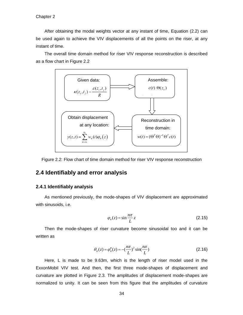
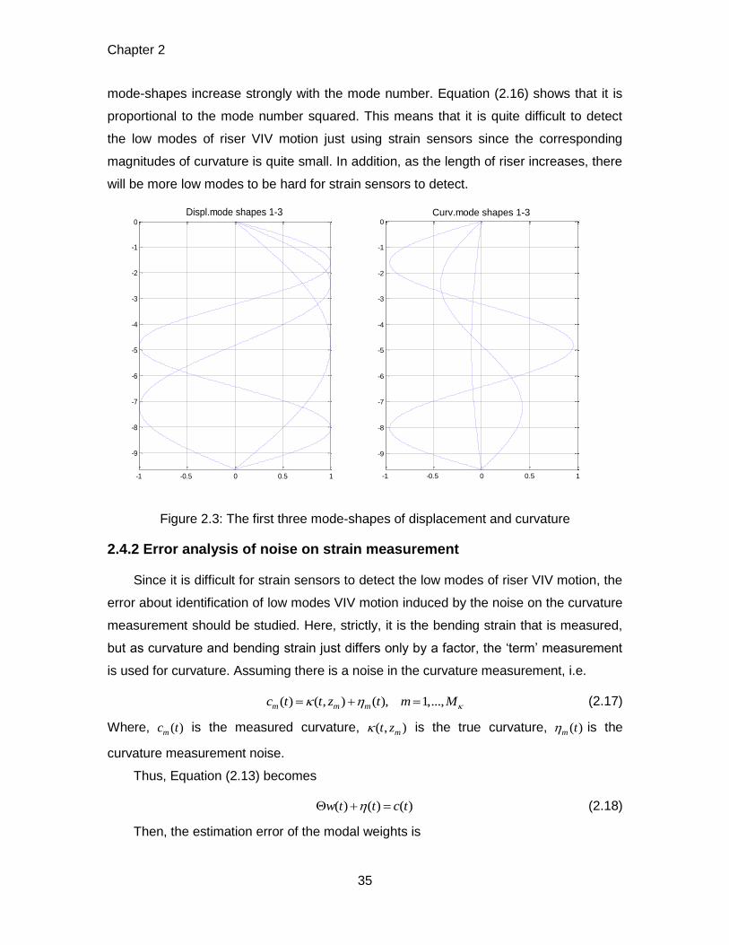
Here, L is made to be 9.63m, which is the length of riser model used in the

ExxonMobil VIV test. And then, the first three mode-shapes of displacement and

curvature are plotted in Figure 2.3. The amplitudes of displacement mode-shapes are

normalized to unity. It can be seen from this figure that the amplitudes of curvature

Chapter 2

35

mode-shapes increase strongly with the mode number. Equation (2.16) shows that it is

proportional to the mode number squared. This means that it is quite difficult to detect

the low modes of riser VIV motion just using strain sensors since the corresponding

magnitudes of curvature is quite small. In addition, as the length of riser increases, there

will be more low modes to be hard for strain sensors to detect.

Figure 2.3: The first three mode-shapes of displacement and curvature

2.4.2 Error analysis of noise on strain measurement

Since it is difficult for strain sensors to detect the low modes of riser VIV motion, the

error about identification of low modes VIV motion induced by the noise on the curvature

measurement should be studied. Here, strictly, it is the bending strain that is measured,

but as curvature and bending strain just differs only by a factor, the ‘term’ measurement

is used for curvature. Assuming there is a noise in the curvature measurement, i.e.

( ) ( , ) ( ), 1,...,m m mc t t z t m M (2.17)

Where, ( )mc t is the measured curvature, ( , )mt z is the true curvature, ( )m t is the

curvature measurement noise.

Thus, Equation (2.13) becomes

( ) ( ) ( )w t t c t (2.18)

Then, the estimation error of the modal weights is

-1 -0.5 0 0.5 1

-9

-8

-7

-6

-5

-4

-3

-2

-1

0

Displ.mode shapes 1-3

-1 -0.5 0 0.5 1

-9

-8

-7

-6

-5

-4

-3

-2

-1

0

Curv.mode shapes 1-3

Chapter 2

36

1( ) ( ) ( )T Te t t (2.19)

Assuming the components of ( )t to be uncorrelated with equal variance 2 , then

the covariance matrix E of the estimation error becomes

1 1 1 2( ) [( ) }] ( )T T T T T T T TE ee E (2.20)

Here, E means the statistical expectation. The diagonal elements of matrix are the

variances of the estimation errors of the modal weights:

1 2 3

2 2 2, , ,... ( )e e e diag (2.21)

2 2( )nn eE w t (2.22)

With regard to the reconstruction error induced by using curvature measurement to

identify the low modes riser VIV motion, an example will be given in chapter 4 to

demonstrate it.

2.4.3 Error analysis of unreasonable choice of participating modes

When using the modal approach to reconstruct riser VIV motion, one of the

important steps is to choose the participating modes. The reconstructed result depends

largely on how many and which modes to be included. If the participating modes are

decided from 1 to the maximum accepted mode number, i.e. the number of points on the

riser with sensor, sometimes the reconstruction error will arise due to the participation of

spurious higher or lower modes. That is to say, in the case that the natural frequencies

corresponding to low modes are quite lower than reasonable Strouhal frequency or the

natural frequencies of high modes are far higher than it, these lower or higher modes are

not supposed to enter into the system matrix.

In terms of the reconstruction error induced by the unreasonable way of choosing

participating modes, an example will be given in chapter 6 to demonstrate it.

Chapter 2

37

Chapter 3

38

Chapter 3

3 The ExxonMobil and second Gulf

Stream VIV tests

3.1 Introduction

In the past few decades, a lot of VIV tests using long flexible riser had been

conducted in both the well controlled laboratory and hard controlled field, and they are

briefly introduced in chapter 1. According to the title of my graduation project, one

experimental VIV test and one field VIV test are needed to be picked. The VIV test data

are the prerequisite for doing riser VIV response reconstruction and only the complete

and clear test data for ExxonMobil and the second Gulf Stream VIV tests could be

obtained in Vortex Induced Vibration Data Repository (MIT, 2007) [24]. Besides, after

searching and browsing relevant papers on the internet, it is very lucky that riser VIV

response reconstruction with regard to these two tests have not been done so far.

Therefore, these two tests are selected as my targets.

3.2 ExxonMobil VIV test

The detailed information of ExxonMobil VIV test can be found from the test report by

Tognarelli and Lie, 2003 [25].

3.2.1 Background

In June 2003, ExxonMobil performed vortex-induced vibration (VIV) testing on a

long flexible riser model in the 10m-deep towing tank at the Norwegian Marine

Technology Research Institute (MARINTEK) in Trondheim, Norway.

Chapter 3

39

The riser model, with or without suppression devices, was tested both vertically and

in inclined positions in a rotating rig in order to obtain uniform and linearly varying

sheared current. The riser model was heavily instrumented to obtain signals of bending

strain and lateral acceleration in both cross-flow and in-line directions.

3.2.2 Riser model

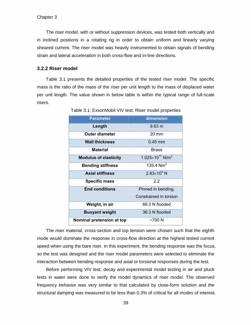
Table 3.1 presents the detailed properties of the tested riser model. The specific

mass is the ratio of the mass of the riser per unit length to the mass of displaced water

per unit length. The value shown in below table is within the typical range of full-scale

risers.

Table 3.1: ExxonMobil VIV test: Riser model properties

Parameter dimension

Length 9.63 m

Outer diameter 20 mm

Wall thickness 0.45 mm

Material Brass

Modulus of elasticity 1.0251011

N/m2

Bending stiffness 135.4 Nm2

Axial stiffness 2.83106 N

Specific mass 2.2

End conditions Pinned in bending,

Constrained in torsion

Weight, in air 66.0 N flooded

Buoyant weight 36.3 N flooded

Nominal pretension at top ~700 N

The riser material, cross-section and top tension were chosen such that the eighth

mode would dominate the response in cross-flow direction at the highest tested current

speed when using the bare riser. In this experiment, the bending response was the focus,

so the test was designed and the riser model parameters were selected to eliminate the

interaction between bending response and axial or torsional responses during the test.

Before performing VIV test, decay and experimental model testing in air and pluck

tests in water were done to verify the model dynamics of riser model. The observed

frequency behavior was very similar to that calculated by close-form solution and the

structural damping was measured to be less than 0.3% of critical for all modes of interest.

Chapter 3

40

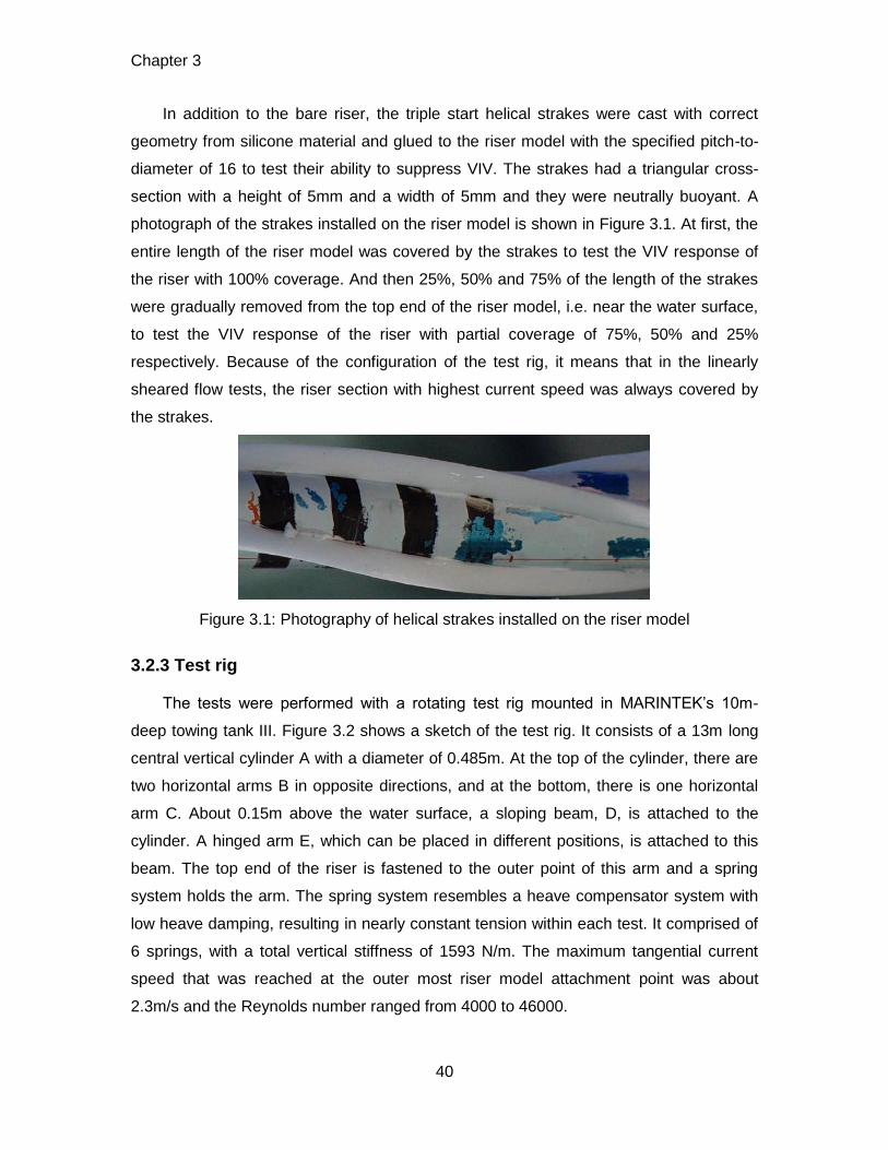
In addition to the bare riser, the triple start helical strakes were cast with correct

geometry from silicone material and glued to the riser model with the specified pitch-to-

diameter of 16 to test their ability to suppress VIV. The strakes had a triangular cross-

section with a height of 5mm and a width of 5mm and they were neutrally buoyant. A

photograph of the strakes installed on the riser model is shown in Figure 3.1. At first, the

entire length of the riser model was covered by the strakes to test the VIV response of

the riser with 100% coverage. And then 25%, 50% and 75% of the length of the strakes

were gradually removed from the top end of the riser model, i.e. near the water surface,

to test the VIV response of the riser with partial coverage of 75%, 50% and 25%

respectively. Because of the configuration of the test rig, it means that in the linearly

sheared flow tests, the riser section with highest current speed was always covered by

the strakes.

Figure 3.1: Photography of helical strakes installed on the riser model

3.2.3 Test rig

The tests were performed with a rotating test rig mounted in MARINTEK’s 10m-

deep towing tank III. Figure 3.2 shows a sketch of the test rig. It consists of a 13m long

central vertical cylinder A with a diameter of 0.485m. At the top of the cylinder, there are

two horizontal arms B in opposite directions, and at the bottom, there is one horizontal

arm C. About 0.15m above the water surface, a sloping beam, D, is attached to the

cylinder. A hinged arm E, which can be placed in different positions, is attached to this

beam. The top end of the riser is fastened to the outer point of this arm and a spring

system holds the arm. The spring system resembles a heave compensator system with

low heave damping, resulting in nearly constant tension within each test. It comprised of

6 springs, with a total vertical stiffness of 1593 N/m. The maximum tangential current

speed that was reached at the outer most riser model attachment point was about

2.3m/s and the Reynolds number ranged from 4000 to 46000.

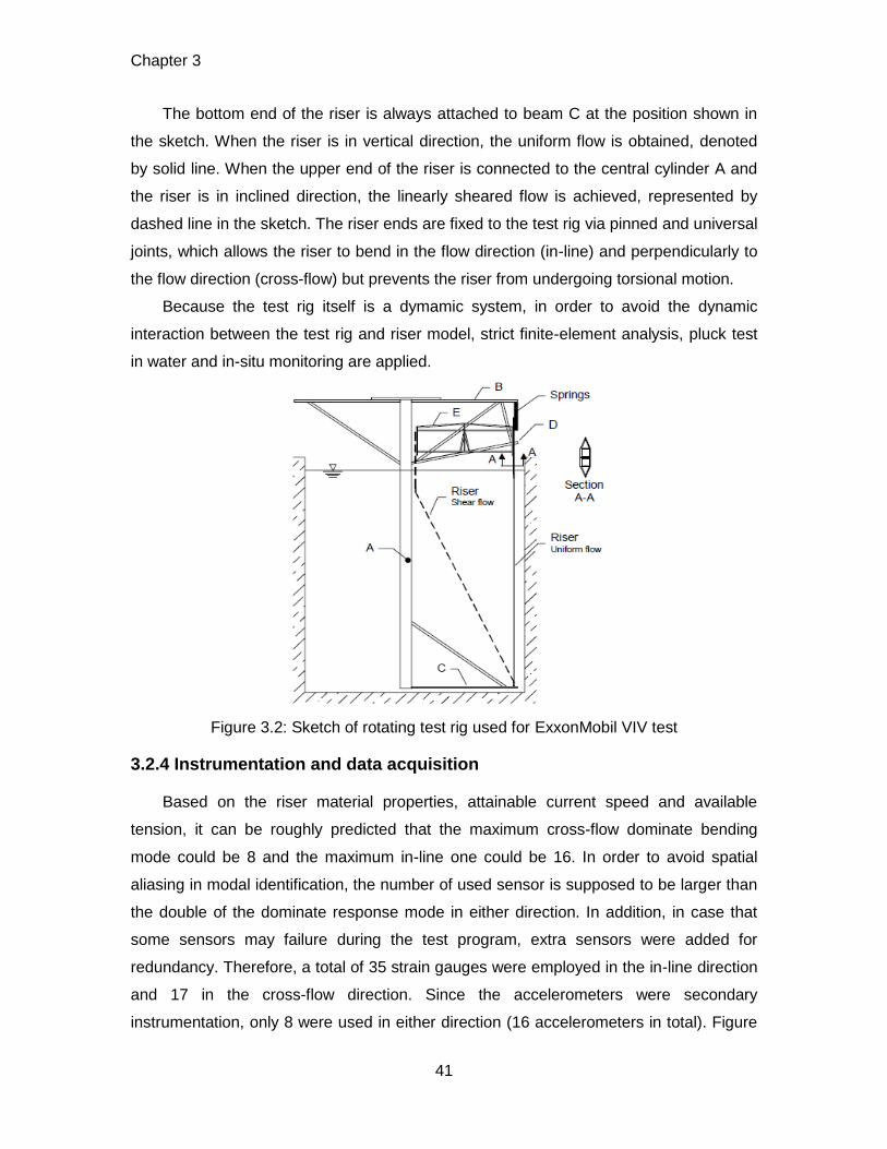
Chapter 3

41

The bottom end of the riser is always attached to beam C at the position shown in

the sketch. When the riser is in vertical direction, the uniform flow is obtained, denoted

by solid line. When the upper end of the riser is connected to the central cylinder A and

the riser is in inclined direction, the linearly sheared flow is achieved, represented by

dashed line in the sketch. The riser ends are fixed to the test rig via pinned and universal

joints, which allows the riser to bend in the flow direction (in-line) and perpendicularly to

the flow direction (cross-flow) but prevents the riser from undergoing torsional motion.

Because the test rig itself is a dymamic system, in order to avoid the dynamic

interaction between the test rig and riser model, strict finite-element analysis, pluck test

in water and in-situ monitoring are applied.

Figure 3.2: Sketch of rotating test rig used for ExxonMobil VIV test

3.2.4 Instrumentation and data acquisition

Based on the riser material properties, attainable current speed and available

tension, it can be roughly predicted that the maximum cross-flow dominate bending

mode could be 8 and the maximum in-line one could be 16. In order to avoid spatial

aliasing in modal identification, the number of used sensor is supposed to be larger than

the double of the dominate response mode in either direction. In addition, in case that

some sensors may failure during the test program, extra sensors were added for

redundancy. Therefore, a total of 35 strain gauges were employed in the in-line direction

and 17 in the cross-flow direction. Since the accelerometers were secondary

instrumentation, only 8 were used in either direction (16 accelerometers in total). Figure

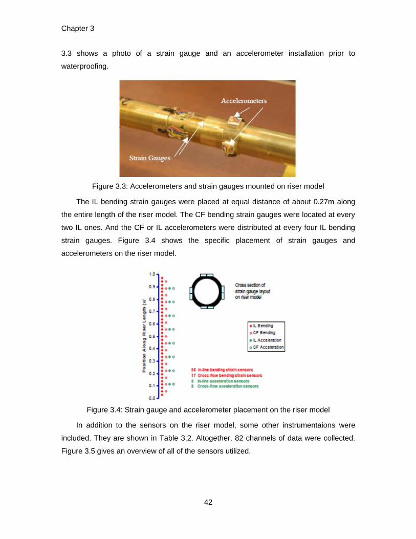
Chapter 3

42

3.3 shows a photo of a strain gauge and an accelerometer installation prior to

waterproofing.

Figure 3.3: Accelerometers and strain gauges mounted on riser model

The IL bending strain gauges were placed at equal distance of about 0.27m along

the entire length of the riser model. The CF bending strain gauges were located at every

two IL ones. And the CF or IL accelerometers were distributed at every four IL bending

strain gauges. Figure 3.4 shows the specific placement of strain gauges and

accelerometers on the riser model.

Figure 3.4: Strain gauge and accelerometer placement on the riser model

In addition to the sensors on the riser model, some other instrumentaions were

included. They are shown in Table 3.2. Altogether, 82 channels of data were collected.

Figure 3.5 gives an overview of all of the sensors utilized.

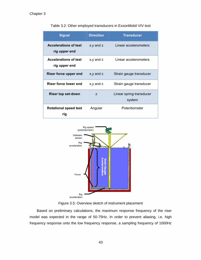
Chapter 3

43

Table 3.2: Other employed transducers in ExxonMobil VIV test

Signal Direction Transducer

Accelerations of test

rig upper end

x,y and z Linear accelerometers

Accelerations of test

rig upper end

x,y and z Linear accelerometers

Riser force upper end x,y and z Strain gauge transducer

Riser force lower end x,y and z Strain gauge transducer

Riser top set-down z Linear spring-transducer

system

Rotational speed test

rig

Angular Potentiometer

Figure 3.5: Overview sketch of instrument placement

Based on preliminary calculations, the maximum response frequency of the riser

model was expected in the range of 50-75Hz. In order to prevent aliasing, i.e. high

frequency response onto the low frequency response, a sampling frequency of 1000Hz

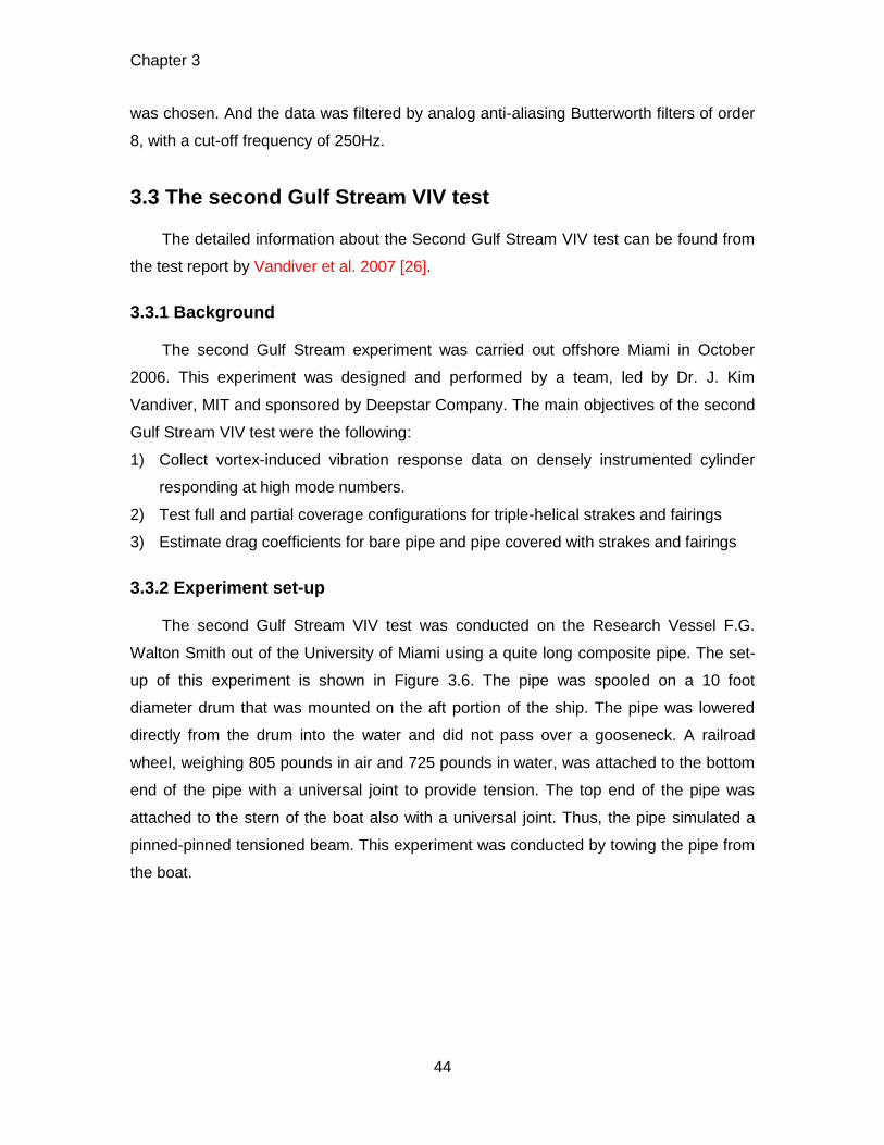
Chapter 3

44

was chosen. And the data was filtered by analog anti-aliasing Butterworth filters of order

8, with a cut-off frequency of 250Hz.

3.3 The second Gulf Stream VIV test

The detailed information about the Second Gulf Stream VIV test can be found from

the test report by Vandiver et al. 2007 [26].

3.3.1 Background

The second Gulf Stream experiment was carried out offshore Miami in October

2006. This experiment was designed and performed by a team, led by Dr. J. Kim

Vandiver, MIT and sponsored by Deepstar Company. The main objectives of the second

Gulf Stream VIV test were the following:

1) Collect vortex-induced vibration response data on densely instrumented cylinder

responding at high mode numbers.

2) Test full and partial coverage configurations for triple-helical strakes and fairings

3) Estimate drag coefficients for bare pipe and pipe covered with strakes and fairings

3.3.2 Experiment set-up

The second Gulf Stream VIV test was conducted on the Research Vessel F.G.

Walton Smith out of the University of Miami using a quite long composite pipe. The set-

up of this experiment is shown in Figure 3.6. The pipe was spooled on a 10 foot

diameter drum that was mounted on the aft portion of the ship. The pipe was lowered

directly from the drum into the water and did not pass over a gooseneck. A railroad

wheel, weighing 805 pounds in air and 725 pounds in water, was attached to the bottom

end of the pipe with a universal joint to provide tension. The top end of the pipe was

attached to the stern of the boat also with a universal joint. Thus, the pipe simulated a

pinned-pinned tensioned beam. This experiment was conducted by towing the pipe from

the boat.

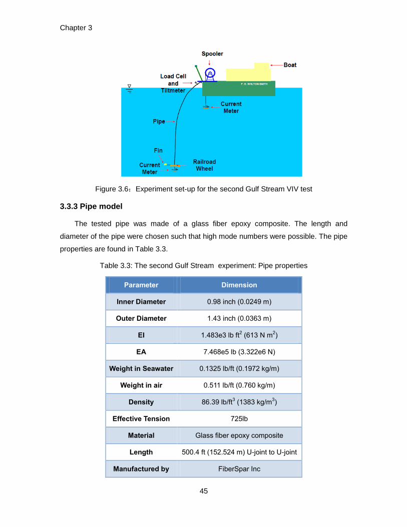
Chapter 3

45

Figure 3.6：Experiment set-up for the second Gulf Stream VIV test

3.3.3 Pipe model

The tested pipe was made of a glass fiber epoxy composite. The length and

diameter of the pipe were chosen such that high mode numbers were possible. The pipe

properties are found in Table 3.3.

Table 3.3: The second Gulf Stream experiment: Pipe properties

Parameter Dimension

Inner Diameter 0.98 inch (0.0249 m)

Outer Diameter 1.43 inch (0.0363 m)

EI 1.483e3 lb ft2 (613 N m

2)

EA 7.468e5 lb (3.322e6 N)

Weight in Seawater 0.1325 lb/ft (0.1972 kg/m)

Weight in air 0.511 lb/ft (0.760 kg/m)

Density 86.39 lb/ft3 (1383 kg/m

3)

Effective Tension 725lb

Material Glass fiber epoxy composite

Length 500.4 ft (152.524 m) U-joint to U-joint

Manufactured by FiberSpar Inc

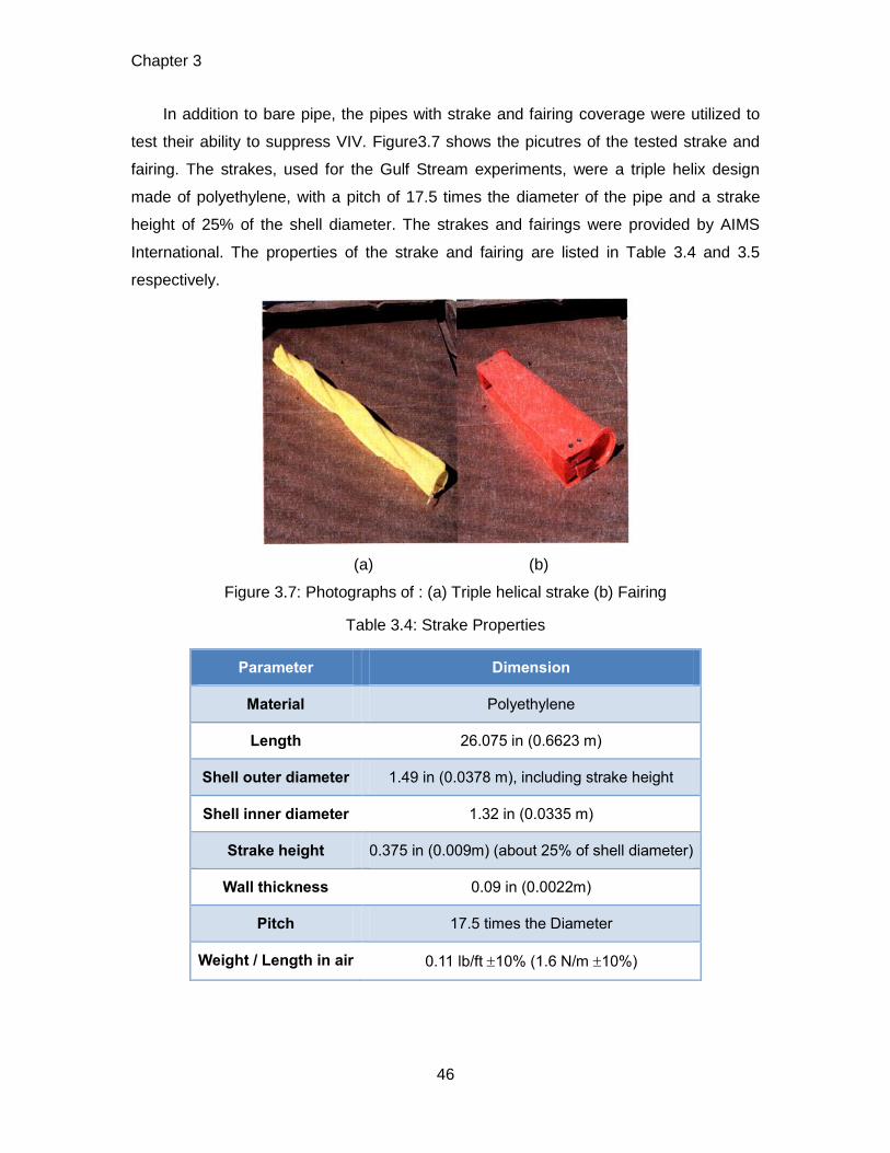
Chapter 3

46

In addition to bare pipe, the pipes with strake and fairing coverage were utilized to

test their ability to suppress VIV. Figure3.7 shows the picutres of the tested strake and

fairing. The strakes, used for the Gulf Stream experiments, were a triple helix design

made of polyethylene, with a pitch of 17.5 times the diameter of the pipe and a strake

height of 25% of the shell diameter. The strakes and fairings were provided by AIMS

International. The properties of the strake and fairing are listed in Table 3.4 and 3.5

respectively.

(a) (b)

Figure 3.7: Photographs of : (a) Triple helical strake (b) Fairing

Table 3.4: Strake Properties

Parameter Dimension

Material Polyethylene

Length 26.075 in (0.6623 m)

Shell outer diameter 1.49 in (0.0378 m), including strake height

Shell inner diameter 1.32 in (0.0335 m)

Strake height 0.375 in (0.009m) (about 25% of shell diameter)

Wall thickness 0.09 in (0.0022m)

Pitch 17.5 times the Diameter

Weight / Length in air 0.11 lb/ft 10% (1.6 N/m 10%)

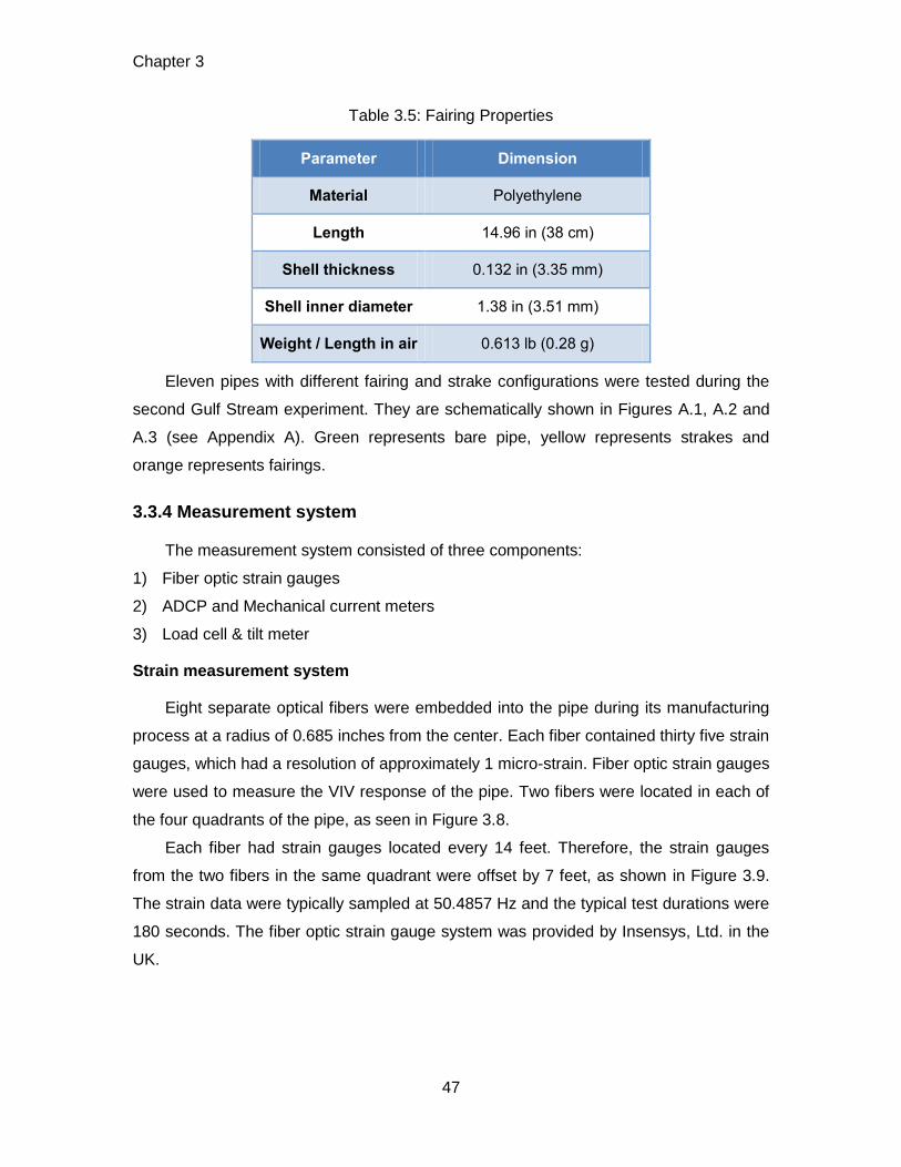
Chapter 3

47

Table 3.5: Fairing Properties

Parameter Dimension

Material Polyethylene

Length 14.96 in (38 cm)

Shell thickness 0.132 in (3.35 mm)

Shell inner diameter 1.38 in (3.51 mm)

Weight / Length in air 0.613 lb (0.28 g)

Eleven pipes with different fairing and strake configurations were tested during the

second Gulf Stream experiment. They are schematically shown in Figures A.1, A.2 and

A.3 (see Appendix A). Green represents bare pipe, yellow represents strakes and

orange represents fairings.

3.3.4 Measurement system

The measurement system consisted of three components:

1) Fiber optic strain gauges

2) ADCP and Mechanical current meters

3) Load cell & tilt meter

Strain measurement system

Eight separate optical fibers were embedded into the pipe during its manufacturing

process at a radius of 0.685 inches from the center. Each fiber contained thirty five strain

gauges, which had a resolution of approximately 1 micro-strain. Fiber optic strain gauges

were used to measure the VIV response of the pipe. Two fibers were located in each of

the four quadrants of the pipe, as seen in Figure 3.8.

Each fiber had strain gauges located every 14 feet. Therefore, the strain gauges

from the two fibers in the same quadrant were offset by 7 feet, as shown in Figure 3.9.

The strain data were typically sampled at 50.4857 Hz and the typical test durations were

180 seconds. The fiber optic strain gauge system was provided by Insensys, Ltd. in the

UK.

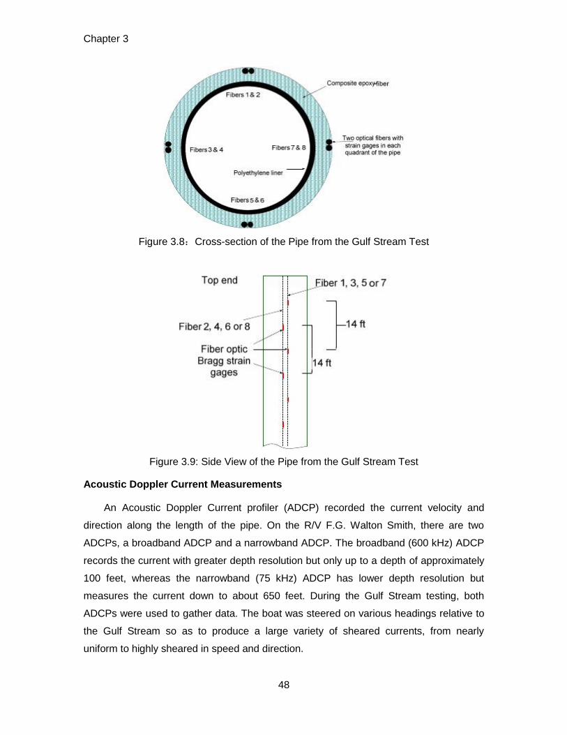
Chapter 3

48

Figure 3.8：Cross-section of the Pipe from the Gulf Stream Test

Figure 3.9: Side View of the Pipe from the Gulf Stream Test

Acoustic Doppler Current Measurements

An Acoustic Doppler Current profiler (ADCP) recorded the current velocity and

direction along the length of the pipe. On the R/V F.G. Walton Smith, there are two

ADCPs, a broadband ADCP and a narrowband ADCP. The broadband (600 kHz) ADCP

records the current with greater depth resolution but only up to a depth of approximately

100 feet, whereas the narrowband (75 kHz) ADCP has lower depth resolution but

measures the current down to about 650 feet. During the Gulf Stream testing, both

ADCPs were used to gather data. The boat was steered on various headings relative to

the Gulf Stream so as to produce a large variety of sheared currents, from nearly

uniform to highly sheared in speed and direction.

Chapter 3

49

Mechanical current meters were also used at the surface and approximately 5 feet

below the railroad wheel. These mechanical current meters were used to verify the

ADCP and, in most cases, showed a good match to the ADCP measured current values.

Load cell and tilt meter

In addition, a tilt meter was used to measure the inclination at the top of the pipe

and a load cell was used to measure the tension at the top of the pipe, as seen in Figure

3.6.

Chapter 4

50

Chapter 4

4 Riser VIV response reconstruction

of ExxonMobil VIV test

4.1 Choice of response reconstruction approach

As said in chapter 3, both acceleration and bending strain are measured in

ExxonMobil VIV test, thus, the frequency method introduced in chapter 2 is preferred.

Trim et al. (2005) [21] also said adding acceleration signals will yield a better result.

4.2 Response reconstruction steps

Before performing riser VIV response reconstruction of ExxonMobil VIV test, we

need to obtain this test’s measurement data. It can be got in Vortex Induced Vibration

Data Repository (MIT, 2007) [24].

4.2.1 Choice of time window

In ExxonMobil VIV test, every single test is conducted as the following steps:

1) Instrumentation verification and zero setting on all channels

2) Start-up of rotating rig and rotation speed starts to increase

3) Rotating rig accelerates to a specified rotation speed which corresponds to a desired

current speed

4) Rotation speed keeps almost constant for a period

5) Rotating rig starts to decrease

In order to find the principles of riser VIV under a specific current condition exactly,

we need to choose a period during which this external current condition is steady and

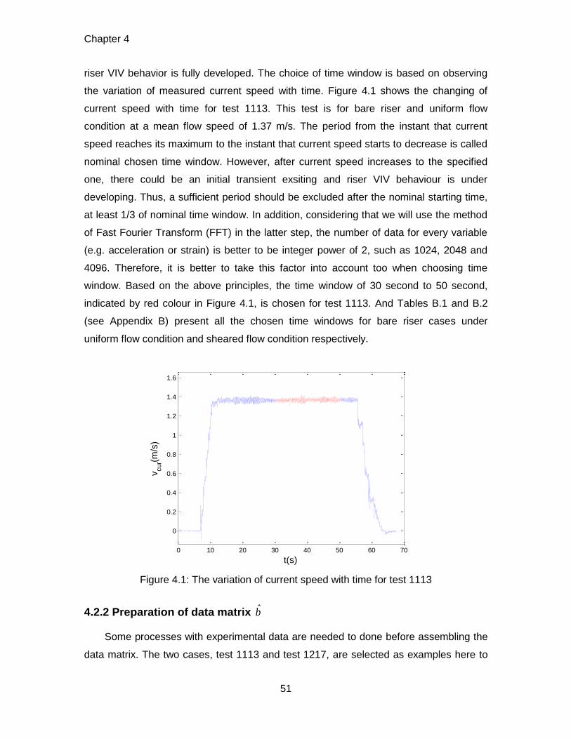
Chapter 4

51

riser VIV behavior is fully developed. The choice of time window is based on observing

the variation of measured current speed with time. Figure 4.1 shows the changing of

current speed with time for test 1113. This test is for bare riser and uniform flow

condition at a mean flow speed of 1.37 m/s. The period from the instant that current

speed reaches its maximum to the instant that current speed starts to decrease is called

nominal chosen time window. However, after current speed increases to the specified

one, there could be an initial transient exsiting and riser VIV behaviour is under

developing. Thus, a sufficient period should be excluded after the nominal starting time,

at least 1/3 of nominal time window. In addition, considering that we will use the method

of Fast Fourier Transform (FFT) in the latter step, the number of data for every variable

(e.g. acceleration or strain) is better to be integer power of 2, such as 1024, 2048 and

4096. Therefore, it is better to take this factor into account too when choosing time

window. Based on the above principles, the time window of 30 second to 50 second,

indicated by red colour in Figure 4.1, is chosen for test 1113. And Tables B.1 and B.2

(see Appendix B) present all the chosen time windows for bare riser cases under

uniform flow condition and sheared flow condition respectively.

Figure 4.1: The variation of current speed with time for test 1113

4.2.2 Preparation of data matrix b

Some processes with experimental data are needed to done before assembling the

data matrix. The two cases, test 1113 and test 1217, are selected as examples here to

0 10 20 30 40 50 60 70

0

0.2

0.4

0.6

0.8

1

1.2

1.4

1.6

t(s)

vcur(m

/s)

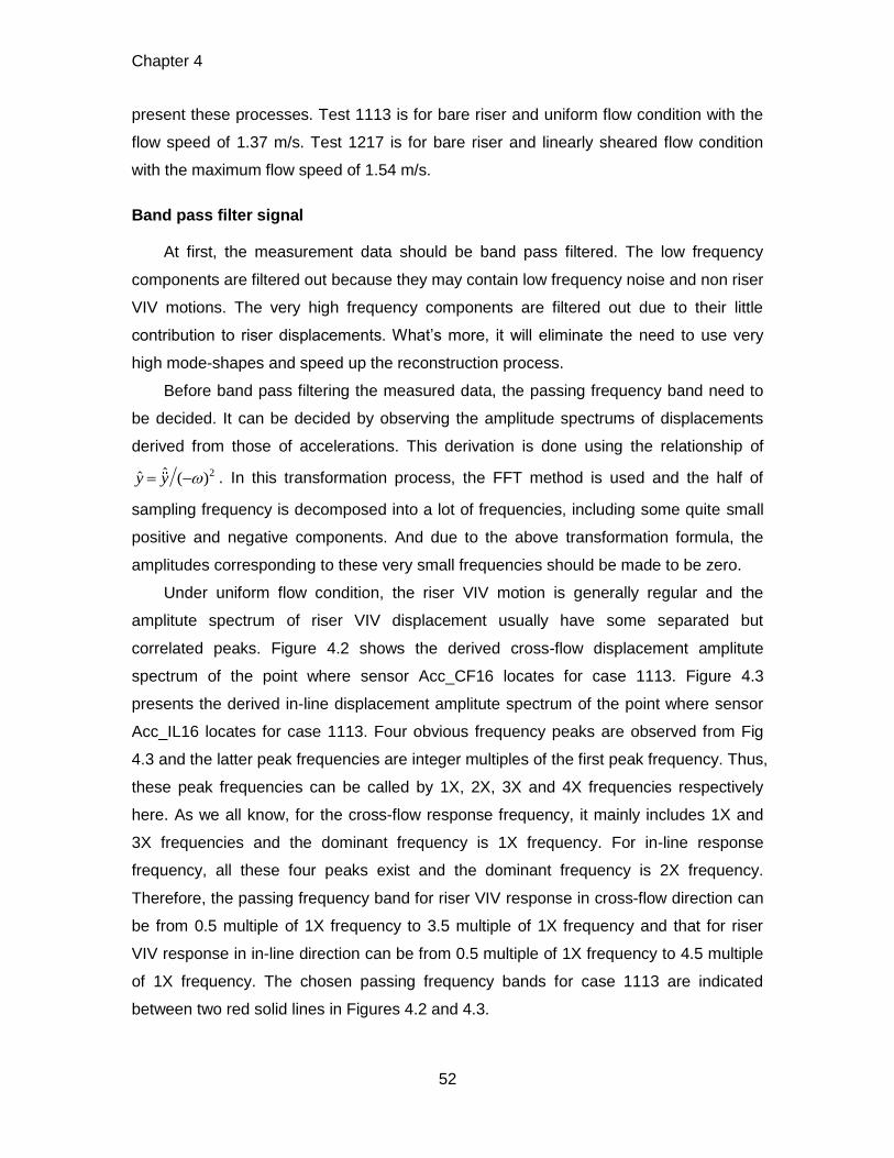
Chapter 4

52

present these processes. Test 1113 is for bare riser and uniform flow condition with the

flow speed of 1.37 m/s. Test 1217 is for bare riser and linearly sheared flow condition

with the maximum flow speed of 1.54 m/s.

Band pass filter signal

At first, the measurement data should be band pass filtered. The low frequency

components are filtered out because they may contain low frequency noise and non riser

VIV motions. The very high frequency components are filtered out due to their little

contribution to riser displacements. What’s more, it will eliminate the need to use very

high mode-shapes and speed up the reconstruction process.

Before band pass filtering the measured data, the passing frequency band need to

be decided. It can be decided by observing the amplitude spectrums of displacements

derived from those of accelerations. This derivation is done using the relationship of

2ˆˆ ( )y y . In this transformation process, the FFT method is used and the half of

sampling frequency is decomposed into a lot of frequencies, including some quite small

positive and negative components. And due to the above transformation formula, the

amplitudes corresponding to these very small frequencies should be made to be zero.

Under uniform flow condition, the riser VIV motion is generally regular and the

amplitute spectrum of riser VIV displacement usually have some separated but

correlated peaks. Figure 4.2 shows the derived cross-flow displacement amplitute

spectrum of the point where sensor Acc_CF16 locates for case 1113. Figure 4.3

presents the derived in-line displacement amplitute spectrum of the point where sensor

Acc_IL16 locates for case 1113. Four obvious frequency peaks are observed from Fig

4.3 and the latter peak frequencies are integer multiples of the first peak frequency. Thus,

these peak frequencies can be called by 1X, 2X, 3X and 4X frequencies respectively

here. As we all know, for the cross-flow response frequency, it mainly includes 1X and

3X frequencies and the dominant frequency is 1X frequency. For in-line response

frequency, all these four peaks exist and the dominant frequency is 2X frequency.

Therefore, the passing frequency band for riser VIV response in cross-flow direction can

be from 0.5 multiple of 1X frequency to 3.5 multiple of 1X frequency and that for riser

VIV response in in-line direction can be from 0.5 multiple of 1X frequency to 4.5 multiple

of 1X frequency. The chosen passing frequency bands for case 1113 are indicated

between two red solid lines in Figures 4.2 and 4.3.

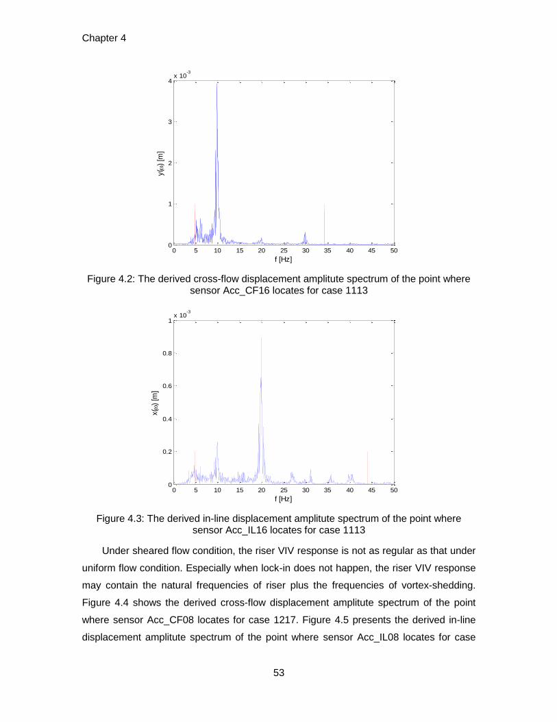
Chapter 4

53

Figure 4.2: The derived cross-flow displacement amplitute spectrum of the point where sensor Acc_CF16 locates for case 1113

Figure 4.3: The derived in-line displacement amplitute spectrum of the point where sensor Acc_IL16 locates for case 1113

Under sheared flow condition, the riser VIV response is not as regular as that under

uniform flow condition. Especially when lock-in does not happen, the riser VIV response

may contain the natural frequencies of riser plus the frequencies of vortex-shedding.

Figure 4.4 shows the derived cross-flow displacement amplitute spectrum of the point

where sensor Acc_CF08 locates for case 1217. Figure 4.5 presents the derived in-line

displacement amplitute spectrum of the point where sensor Acc_IL08 locates for case

0 5 10 15 20 25 30 35 40 45 500

1

2

3

4x 10

-3

f [Hz]

y(

) [m

]

0 5 10 15 20 25 30 35 40 45 500

0.2

0.4

0.6

0.8

1x 10

-3

f [Hz]

x(

) [m

]

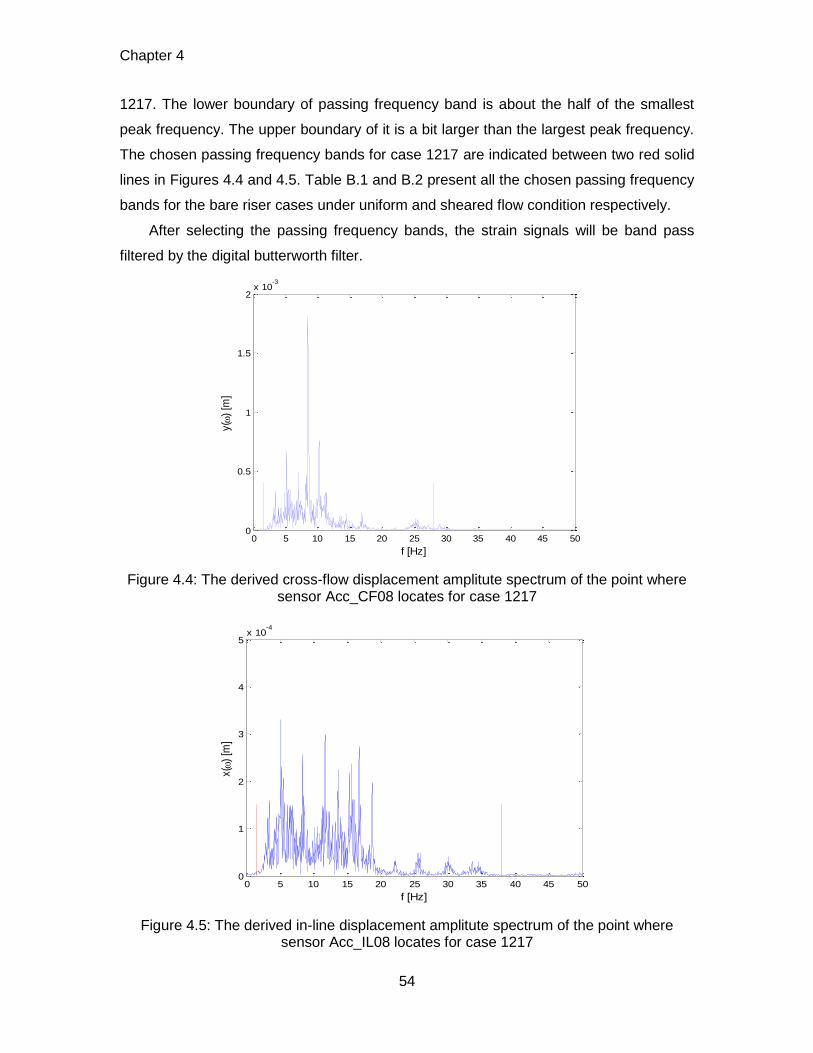
Chapter 4

54

1217. The lower boundary of passing frequency band is about the half of the smallest

peak frequency. The upper boundary of it is a bit larger than the largest peak frequency.

The chosen passing frequency bands for case 1217 are indicated between two red solid

lines in Figures 4.4 and 4.5. Table B.1 and B.2 present all the chosen passing frequency

bands for the bare riser cases under uniform and sheared flow condition respectively.

After selecting the passing frequency bands, the strain signals will be band pass

filtered by the digital butterworth filter.

Figure 4.4: The derived cross-flow displacement amplitute spectrum of the point where sensor Acc_CF08 locates for case 1217

Figure 4.5: The derived in-line displacement amplitute spectrum of the point where sensor Acc_IL08 locates for case 1217

0 5 10 15 20 25 30 35 40 45 500

0.5

1

1.5

2x 10

-3

f [Hz]

y(

) [m

]

0 5 10 15 20 25 30 35 40 45 500

1

2

3

4

5x 10

-4

f [Hz]

x(

) [m

]

Chapter 4

55

Assemble data matrix b

Performing Fourier transform with the filtered strain signals and dividing the

submatrix by the riser outer radius R , it can be entered into the data matrix b . And

the derived submatrix y can be just put into the data matrix b .

4.2.3 Preparation of system matrix A

This section mainly includes two parts. One part is the choice of participating modes.

The other one is modifying the system matrix.

Choice of participating modes

Before selecting the participating modes, the natural frequencies of the riser in still

water need to be calculated at first. The riser in this experiment is like an axially

tensioned beam. Its governing equation of motion can be expressed as

2 4 2

2 2 2( ) 0a

w w wm m EI T

t z z

(4.1)

Where, m is riser mass per unit length, am is added mass per unit length, w is the

transverse displacement, E is the Young modulus, I is the moment of inertia of the

riser, T is the tension in the riser, z is vertical coordinate along the riser.

Because the boundary condition of the riser is pinned-pinned, the mode-shapes of

riser VIV displacement are sinusoidal and the transverse displacement can be given as

( , ) sin( )sin(2 )n

n zw z t A f t

L

(4.2)

Where, n is the mode number, L is the length of the riser, nf is natural frequency.

Substituting Equation (4.2) into Equation (4.1), the natural frequencies of the riser

can be obtained as

4 21

2 ( ) ( )n

a a

EI n T nf

m m L m m L

(4.3)

It can be observed from Equation (4.3) that the natural frequency of the tensioned

beam can be expressed by the natural frequency of non tensioned beam and that of

tensioned string without stiffness. Because

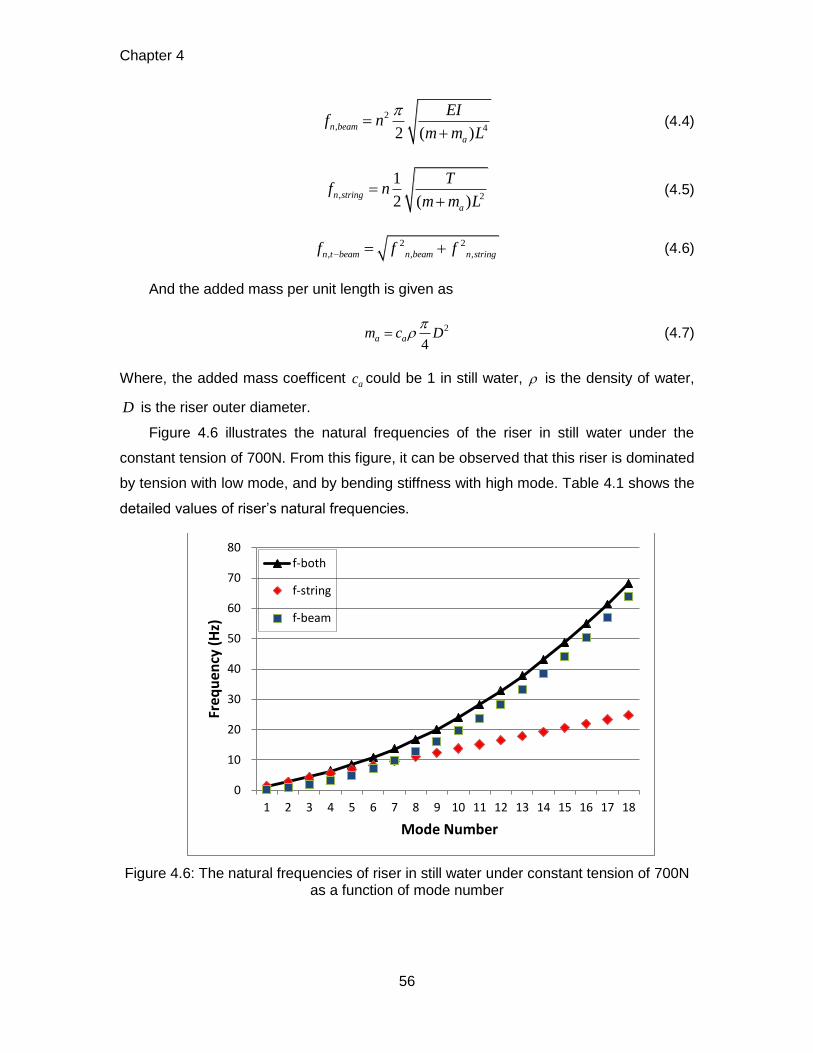
Chapter 4

56

2

, 42 ( )n beam

a

EIf n

m m L

(4.4)

, 2

1

2 ( )n string

a

Tf n

m m L

(4.5)

2 2

, , ,n t beam n beam n stringf f f (4.6)

And the added mass per unit length is given as

2

4a am c D

(4.7)

Where, the added mass coefficent ac could be 1 in still water, is the density of water,

D is the riser outer diameter.

Figure 4.6 illustrates the natural frequencies of the riser in still water under the

constant tension of 700N. From this figure, it can be observed that this riser is dominated

by tension with low mode, and by bending stiffness with high mode. Table 4.1 shows the

detailed values of riser’s natural frequencies.

Figure 4.6: The natural frequencies of riser in still water under constant tension of 700N as a function of mode number

0

10

20

30

40

50

60

70

80

1 2 3 4 5 6 7 8 9 10 11 12 13 14 15 16 17 18

Freq

uen

cy (

Hz)

Mode Number

f-both

f-string

f-beam

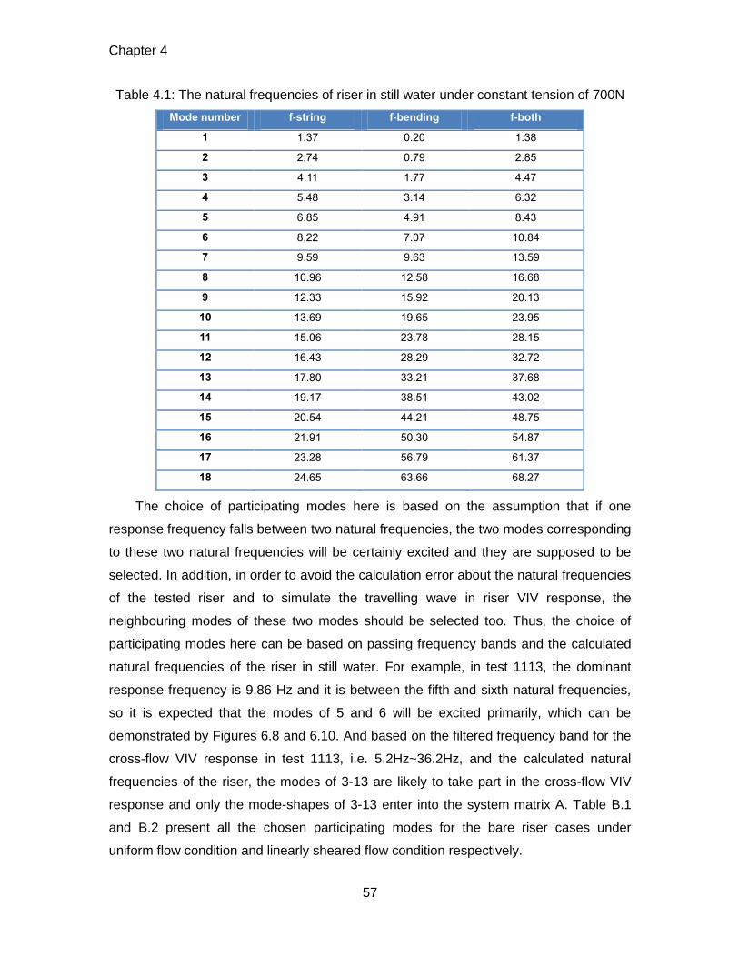
Chapter 4

57

Table 4.1: The natural frequencies of riser in still water under constant tension of 700N

Mode number f-string f-bending f-both

1 1.37 0.20 1.38

2 2.74 0.79 2.85

3 4.11 1.77 4.47

4 5.48 3.14 6.32

5 6.85 4.91 8.43

6 8.22 7.07 10.84

7 9.59 9.63 13.59

8 10.96 12.58 16.68

9 12.33 15.92 20.13

10 13.69 19.65 23.95

11 15.06 23.78 28.15

12 16.43 28.29 32.72

13 17.80 33.21 37.68

14 19.17 38.51 43.02

15 20.54 44.21 48.75

16 21.91 50.30 54.87

17 23.28 56.79 61.37

18 24.65 63.66 68.27

The choice of participating modes here is based on the assumption that if one

response frequency falls between two natural frequencies, the two modes corresponding

to these two natural frequencies will be certainly excited and they are supposed to be

selected. In addition, in order to avoid the calculation error about the natural frequencies

of the tested riser and to simulate the travelling wave in riser VIV response, the

neighbouring modes of these two modes should be selected too. Thus, the choice of

participating modes here can be based on passing frequency bands and the calculated

natural frequencies of the riser in still water. For example, in test 1113, the dominant

response frequency is 9.86 Hz and it is between the fifth and sixth natural frequencies,

so it is expected that the modes of 5 and 6 will be excited primarily, which can be

demonstrated by Figures 6.8 and 6.10. And based on the filtered frequency band for the

cross-flow VIV response in test 1113, i.e. 5.2Hz~36.2Hz, and the calculated natural

frequencies of the riser, the modes of 3-13 are likely to take part in the cross-flow VIV

response and only the mode-shapes of 3-13 enter into the system matrix A. Table B.1

and B.2 present all the chosen participating modes for the bare riser cases under

uniform flow condition and linearly sheared flow condition respectively.

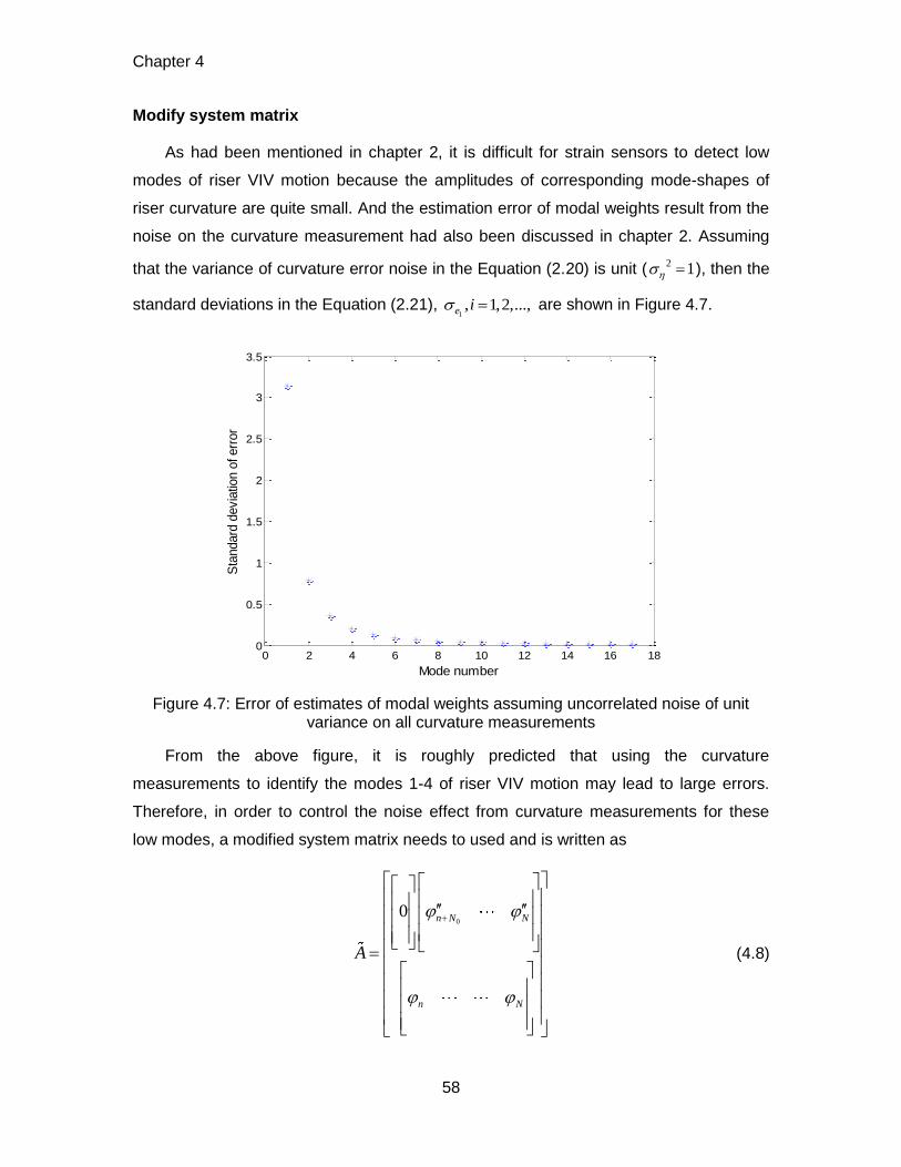
Chapter 4

58

Modify system matrix

As had been mentioned in chapter 2, it is difficult for strain sensors to detect low

modes of riser VIV motion because the amplitudes of corresponding mode-shapes of

riser curvature are quite small. And the estimation error of modal weights result from the

noise on the curvature measurement had also been discussed in chapter 2. Assuming

that the variance of curvature error noise in the Equation (2.20) is unit ( 2 1 ), then the

standard deviations in the Equation (2.21), 1, 1,2,...,e i are shown in Figure 4.7.

Figure 4.7: Error of estimates of modal weights assuming uncorrelated noise of unit variance on all curvature measurements

From the above figure, it is roughly predicted that using the curvature

measurements to identify the modes 1-4 of riser VIV motion may lead to large errors.

Therefore, in order to control the noise effect from curvature measurements for these

low modes, a modified system matrix needs to used and is written as

00 n N N

n N

A

(4.8)

0 2 4 6 8 10 12 14 16 180

0.5

1

1.5

2

2.5

3

3.5

Mode number

Sta

ndard

devia

tion o

f err

or

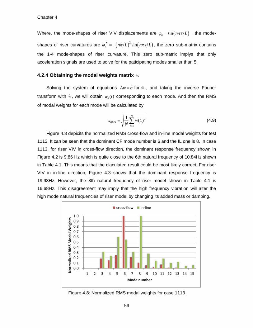
Chapter 4

59

Where, the mode-shapes of riser VIV displacements are sinn n z L , the mode-

shapes of riser curvatures are 2sinn n L n z L , the zero sub-matrix contains

the 1-4 mode-shapes of riser curvature. This zero sub-matrix implys that only

acceleration signals are used to solve for the paticipating modes smaller than 5.

4.2.4 Obtaining the modal weights matrix w

Solving the system of equations ˆÂw b for w , and taking the inverse Fourier

transform with w , we will obtain ( )nw t corresponding to each mode. And then the RMS

of modal weights for each mode will be calculated by

2

1

1( )

N

RMS i

i

w w tN

(4.9)

Figure 4.8 depicits the normalized RMS cross-flow and in-line modal weights for test

1113. It can be seen that the dominant CF mode number is 6 and the IL one is 8. In case

1113, for riser VIV in cross-flow direction, the dominant response frequency shown in

Figure 4.2 is 9.86 Hz which is quite close to the 6th natural frequency of 10.84Hz shown

in Table 4.1. This means that the claculated result could be most likely correct. For riser

VIV in in-line direction, Figure 4.3 shows that the dominant response frequency is

19.93Hz. However, the 8th natural frequency of riser model shown in Table 4.1 is

16.68Hz. This disagreement may imply that the high frequency vibration will alter the

high mode natural frequencies of riser model by changing its added mass or damping.

Figure 4.8: Normalized RMS modal weights for case 1113

0.0

0.1

0.2

0.3

0.4

0.5

0.6

0.7

0.8

0.9

1.0

1 2 3 4 5 6 7 8 9 10 11 12 13 14 15No

rmal

ize

d R

MS

Mo

dal

We

igh

ts

Mode number

cross-flow in-line

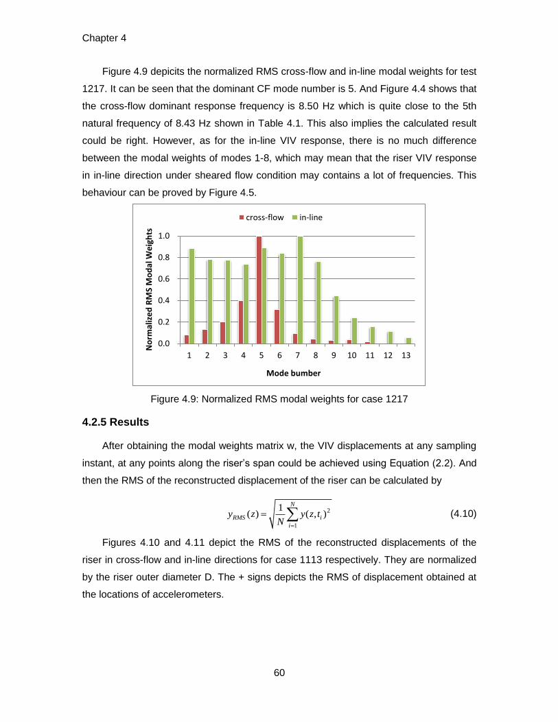
Chapter 4

60

Figure 4.9 depicits the normalized RMS cross-flow and in-line modal weights for test

1217. It can be seen that the dominant CF mode number is 5. And Figure 4.4 shows that

the cross-flow dominant response frequency is 8.50 Hz which is quite close to the 5th

natural frequency of 8.43 Hz shown in Table 4.1. This also implies the calculated result

could be right. However, as for the in-line VIV response, there is no much difference

between the modal weights of modes 1-8, which may mean that the riser VIV response

in in-line direction under sheared flow condition may contains a lot of frequencies. This

behaviour can be proved by Figure 4.5.

Figure 4.9: Normalized RMS modal weights for case 1217

4.2.5 Results

After obtaining the modal weights matrix w, the VIV displacements at any sampling

instant, at any points along the riser’s span could be achieved using Equation (2.2). And

then the RMS of the reconstructed displacement of the riser can be calculated by

2

1

1( ) ( , )

N

RMS i

i

y z y z tN

(4.10)

Figures 4.10 and 4.11 depict the RMS of the reconstructed displacements of the

riser in cross-flow and in-line directions for case 1113 respectively. They are normalized

by the riser outer diameter D. The + signs depicts the RMS of displacement obtained at

the locations of accelerometers.

0.0

0.2

0.4

0.6

0.8

1.0

1 2 3 4 5 6 7 8 9 10 11 12 13

No

rmal

ize

d R

MS

Mo

dal

We

igh

ts

Mode bumber

cross-flow in-line

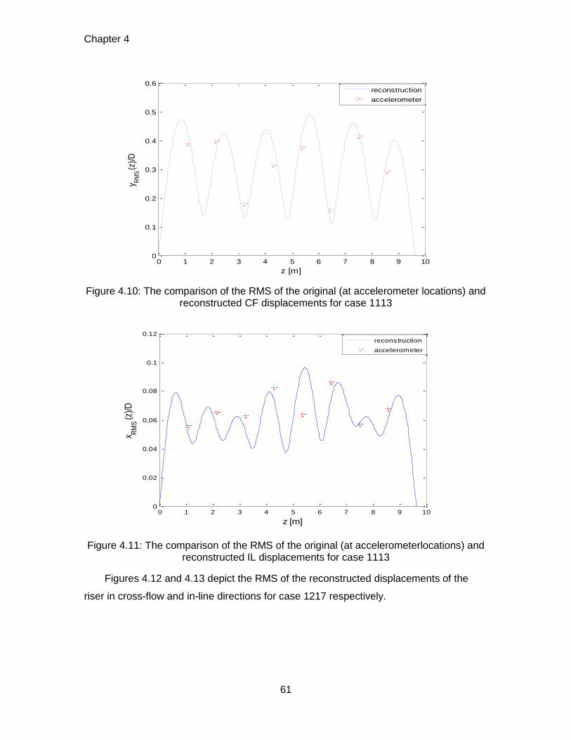
Chapter 4

61

Figure 4.10: The comparison of the RMS of the original (at accelerometer locations) and reconstructed CF displacements for case 1113

Figure 4.11: The comparison of the RMS of the original (at accelerometerlocations) and reconstructed IL displacements for case 1113

Figures 4.12 and 4.13 depict the RMS of the reconstructed displacements of the

riser in cross-flow and in-line directions for case 1217 respectively.

0 1 2 3 4 5 6 7 8 9 100

0.1

0.2

0.3

0.4

0.5

0.6

z [m]

y RM

S (z)

/D

reconstruction

accelerometer

0 1 2 3 4 5 6 7 8 9 100

0.02

0.04

0.06

0.08

0.1

0.12

z [m]

x RM

S (z

)/D

reconstruction

accelerometer

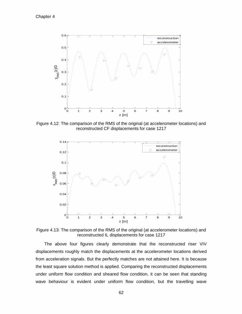
Chapter 4

62

Figure 4.12: The comparison of the RMS of the original (at accelerometer locations) and reconstructed CF displacements for case 1217

Figure 4.13: The comparison of the RMS of the original (at accelerometer locations) and reconstructed IL displacements for case 1217

The above four figures clearly demonstrate that the reconstructed riser VIV

displacements roughly match the displacements at the accelerometer locations derived

from acceleration signals. But the perfectly matches are not attained here. It is because

the least square solution method is applied. Comparing the reconstructed displacements

under uniform flow condition and sheared flow condition, it can be seen that standing

wave behaviour is evident under uniform flow condition, but the travelling wave

0 1 2 3 4 5 6 7 8 9 100

0.1

0.2

0.3

0.4

0.5

0.6

z [m]

y RM

S (z)

/D

reconstruction

accelerometer

0 1 2 3 4 5 6 7 8 9 100

0.02

0.04

0.06

0.08

0.1

0.12

0.14

z [m]

x RM

S (z)

/D

reconstruction

accelerometer

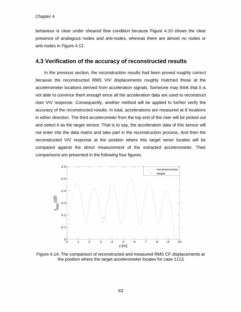
Chapter 4

63

behaviour is clear under sheared flow condition because Figure 4.10 shows the clear

presence of analogous nodes and anti-nodes, whereas there are almost no nodes or

anti-nodes in Figure 4.12.

4.3 Verification of the accuracy of reconstructed results

In the previous section, the reconstruction results had been proved roughly correct

because the reconstructed RMS VIV displacements roughly matched those at the

accelerometer locations derived from acceleration signals. Someone may think that it is

not able to convince them enough since all the acceleration data are used to reconstruct

riser VIV response. Consequently, another method will be applied to further verify the

accuracy of the reconstructed results. In total, accelerations are measured at 8 locations

in either direction. The third accelerometer from the top end of the riser will be picked out

and select it as the target sensor. That is to say, the acceleration data of this sensor will

not enter into the data matrix and take part in the reconstruction process. And then the

reconstructed VIV response at the position where this target senor locates will be

compared against the direct measurement of the extracted accelerometer. Their

comparisons are presented in the following four figures.

Figure 4.14: The comparison of reconstructed and measured RMS CF displacements at the position where the target accelerometer locates for case 1113

0 1 2 3 4 5 6 7 8 9 100

0.1

0.2

0.3

0.4

0.5

0.6

z [m]

y RM

S (z

)/D

reconstruction

target

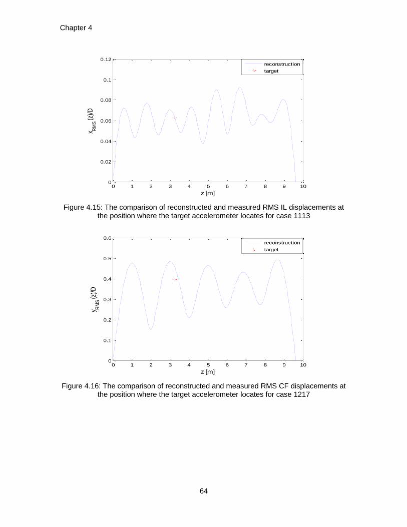
Chapter 4

64

Figure 4.15: The comparison of reconstructed and measured RMS IL displacements at the position where the target accelerometer locates for case 1113

Figure 4.16: The comparison of reconstructed and measured RMS CF displacements at the position where the target accelerometer locates for case 1217

0 1 2 3 4 5 6 7 8 9 100

0.02

0.04

0.06

0.08

0.1

0.12

z [m]

x RM

S (z

)/D

reconstruction

target

0 1 2 3 4 5 6 7 8 9 100

0.1

0.2

0.3

0.4

0.5

0.6

z [m]

y RM

S (z

)/D

reconstruction

target

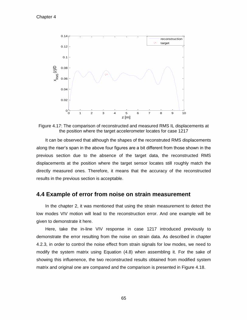
Chapter 4

65

Figure 4.17: The comparison of reconstructed and measured RMS IL displacements at the position where the target accelerometer locates for case 1217

It can be observed that although the shapes of the reconstruted RMS displacements

along the riser’s span in the above four figures are a bit different from those shown in the

previous section due to the absence of the target data, the reconstructed RMS

displacements at the position where the target sensor locates still roughly match the

directly measured ones. Therefore, it means that the accuracy of the reconstructed

results in the previous section is acceptable.

4.4 Example of error from noise on strain measurement

In the chapter 2, it was mentioned that using the strain measurement to detect the

low modes VIV motion will lead to the reconstruction error. And one example will be

given to demonstrate it here.

Here, take the in-line VIV response in case 1217 introduced previously to

demonstrate the error resulting from the noise on strain data. As described in chapter

4.2.3, in order to control the noise effect from strain signals for low modes, we need to

modify the system matrix using Equation (4.8) when assembling it. For the sake of

showing this influenence, the two reconstructed results obtained from modified system

matrix and original one are compared and the comparison is presented in Figure 4.18.

0 1 2 3 4 5 6 7 8 9 100

0.02

0.04

0.06

0.08

0.1

0.12

0.14

z [m]

x RM

S (z

)/D

reconstruction

target

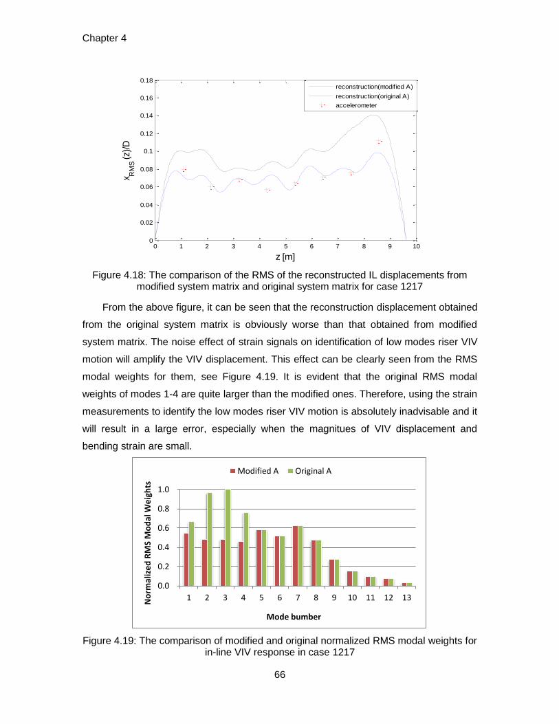
Chapter 4

66

Figure 4.18: The comparison of the RMS of the reconstructed IL displacements from modified system matrix and original system matrix for case 1217

From the above figure, it can be seen that the reconstruction displacement obtained

from the original system matrix is obviously worse than that obtained from modified

system matrix. The noise effect of strain signals on identification of low modes riser VIV

motion will amplify the VIV displacement. This effect can be clearly seen from the RMS

modal weights for them, see Figure 4.19. It is evident that the original RMS modal

weights of modes 1-4 are quite larger than the modified ones. Therefore, using the strain

measurements to identify the low modes riser VIV motion is absolutely inadvisable and it

will result in a large error, especially when the magnitues of VIV displacement and

bending strain are small.

Figure 4.19: The comparison of modified and original normalized RMS modal weights for in-line VIV response in case 1217

0 1 2 3 4 5 6 7 8 9 100

0.02

0.04

0.06

0.08

0.1

0.12

0.14

0.16

0.18

z [m]

x RM

S (

z)/

D

reconstruction(modif ied A)

reconstruction(original A)

accelerometer

0.0

0.2

0.4

0.6

0.8

1.0

1 2 3 4 5 6 7 8 9 10 11 12 13No

rmal

ize

d R

MS

Mo

dal

We

igh

ts

Mode bumber

Modified A Original A

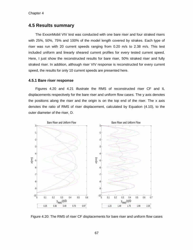
Chapter 4

67

4.5 Results summary

The ExxonMobil VIV test was conducted with one bare riser and four straked risers

with 25%, 50%, 75% and 100% of the model length covered by strakes. Each type of

riser was run with 20 current speeds ranging from 0.20 m/s to 2.38 m/s. This test

included uniform and linearly sheared current profiles for every tested current speed.

Here, I just show the reconstructed results for bare riser, 50% straked riser and fully

straked riser. In addition, although riser VIV response is reconstructed for every current

speed, the results for only 10 current speeds are presented here.

4.5.1 Bare riser response

Figures 4.20 and 4.21 illustrate the RMS of reconstructed riser CF and IL

displacements respectively for the bare riser and uniform flow cases. The y axis denotes

the positions along the riser and the origin is on the top end of the riser. The x axis

denotes the ratio of RMS of riser displacement, calculated by Equation (4.10), to the

outer diameter of the riser, D.

Figure 4.20: The RMS of riser CF displacements for bare riser and uniform flow cases

0 0.1 0.2 0.3 0.4 0.5 0.6-10

-9

-8

-7

-6

-5

-4

-3

-2

-1

0

yRMS

(z)/D

z[m

]

Bare Riser and Uniform Flow

0.25 0.36 0.49 0.70 0.97

0 0.1 0.2 0.3 0.4 0.5 0.6 0.7-10

-9

-8

-7

-6

-5

-4

-3

-2

-1

0

yRMS

(z)/D

z[m

]


1.23 1.49 1.75 1.99 2.25

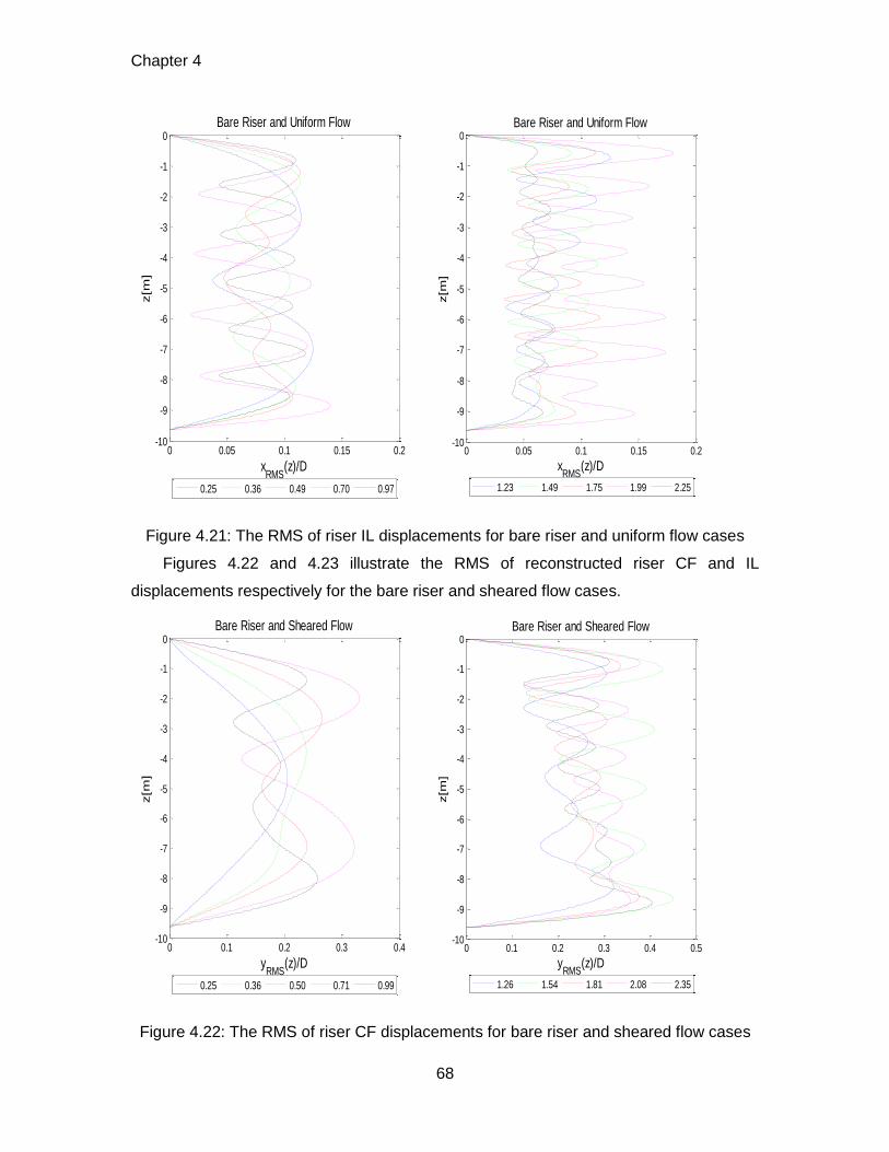
Chapter 4

68

Figure 4.21: The RMS of riser IL displacements for bare riser and uniform flow cases


displacements respectively for the bare riser and sheared flow cases.

Figure 4.22: The RMS of riser CF displacements for bare riser and sheared flow cases

0 0.05 0.1 0.15 0.2-10

-9

-8

-7

-6

-5

-4

-3

-2

-1

0

xRMS

(z)/D

z[m

]


0.25 0.36 0.49 0.70 0.97

0 0.05 0.1 0.15 0.2-10

-9

-8

-7

-6

-5

-4

-3

-2

-1

0

xRMS

(z)/D

z[m

]


1.23 1.49 1.75 1.99 2.25

0 0.1 0.2 0.3 0.4-10

-9

-8

-7

-6

-5

-4

-3

-2

-1

0

yRMS

(z)/D

z[m

]

Bare Riser and Sheared Flow

0.25 0.36 0.50 0.71 0.99

0 0.1 0.2 0.3 0.4 0.5-10

-9

-8

-7

-6

-5

-4

-3

-2

-1

0

yRMS

(z)/D

z[m

]


1.26 1.54 1.81 2.08 2.35

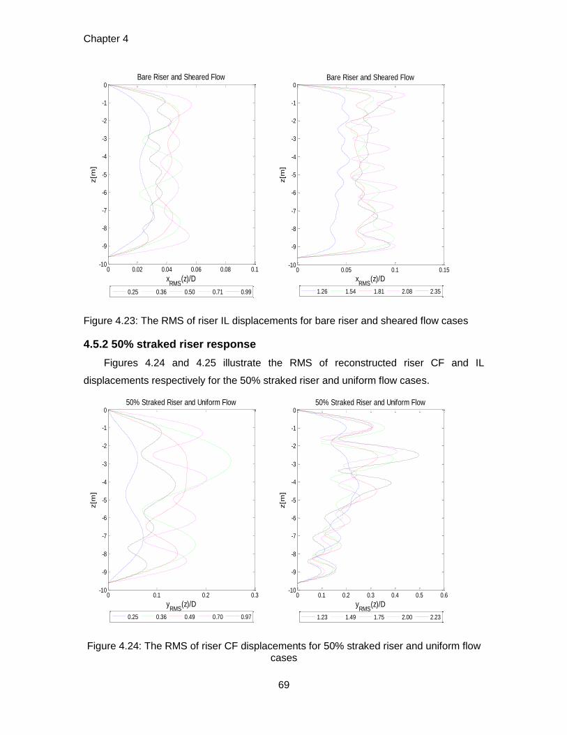
Chapter 4

69

Figure 4.23: The RMS of riser IL displacements for bare riser and sheared flow cases

4.5.2 50% straked riser response


displacements respectively for the 50% straked riser and uniform flow cases.

Figure 4.24: The RMS of riser CF displacements for 50% straked riser and uniform flow cases

0 0.02 0.04 0.06 0.08 0.1-10

-9

-8

-7

-6

-5

-4

-3

-2

-1

0

xRMS

(z)/D

z[m

]


0.25 0.36 0.50 0.71 0.99

0 0.05 0.1 0.15-10

-9

-8

-7

-6

-5

-4

-3

-2

-1

0

xRMS

(z)/Dz[m

]


1.26 1.54 1.81 2.08 2.35

0 0.1 0.2 0.3-10

-9

-8

-7

-6

-5

-4

-3

-2

-1

0

yRMS

(z)/D

z[m

]

50% Straked Riser and Uniform Flow

0.25 0.36 0.49 0.70 0.97

0 0.1 0.2 0.3 0.4 0.5 0.6-10

-9

-8

-7

-6

-5

-4

-3

-2

-1

0

yRMS

(z)/D

z[m

]


1.23 1.49 1.75 2.00 2.23

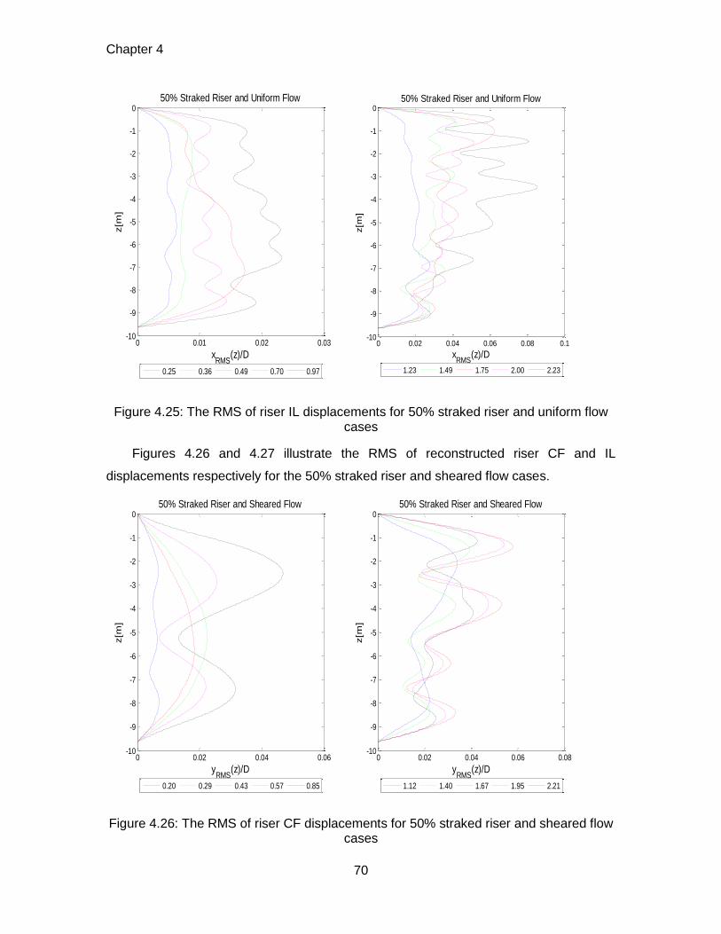
Chapter 4

70

Figure 4.25: The RMS of riser IL displacements for 50% straked riser and uniform flow cases


displacements respectively for the 50% straked riser and sheared flow cases.

Figure 4.26: The RMS of riser CF displacements for 50% straked riser and sheared flow cases

0 0.01 0.02 0.03-10

-9

-8

-7

-6

-5

-4

-3

-2

-1

0

xRMS

(z)/D

z[m

]


0.25 0.36 0.49 0.70 0.97

0 0.02 0.04 0.06 0.08 0.1-10

-9

-8

-7

-6

-5

-4

-3

-2

-1

0

xRMS

(z)/Dz[m

]


1.23 1.49 1.75 2.00 2.23

0 0.02 0.04 0.06-10

-9

-8

-7

-6

-5

-4

-3

-2

-1

0

yRMS

(z)/D

z[m

]

50% Straked Riser and Sheared Flow

0.20 0.29 0.43 0.57 0.85

0 0.02 0.04 0.06 0.08-10

-9

-8

-7

-6

-5

-4

-3

-2

-1

0

yRMS

(z)/D

z[m

]


1.12 1.40 1.67 1.95 2.21

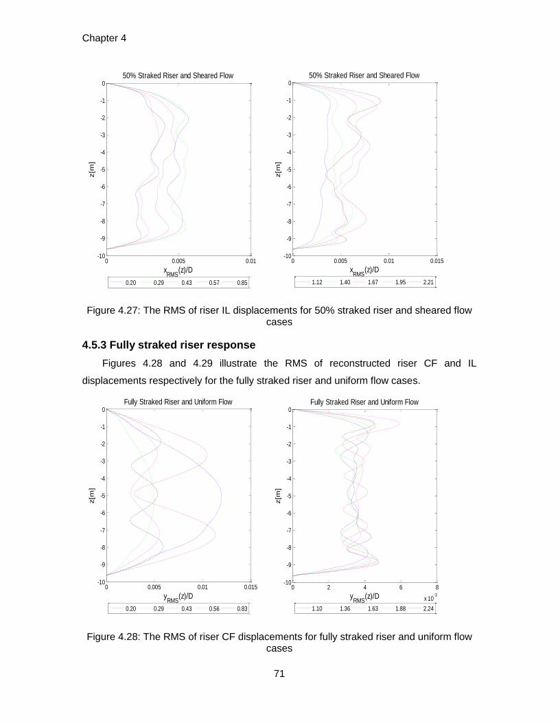
Chapter 4

71

Figure 4.27: The RMS of riser IL displacements for 50% straked riser and sheared flow cases

4.5.3 Fully straked riser response


displacements respectively for the fully straked riser and uniform flow cases.

Figure 4.28: The RMS of riser CF displacements for fully straked riser and uniform flow cases

0 0.005 0.01-10

-9

-8

-7

-6

-5

-4

-3

-2

-1

0

xRMS

(z)/D

z[m

]


0.20 0.29 0.43 0.57 0.85

0 0.005 0.01 0.015-10

-9

-8

-7

-6

-5

-4

-3

-2

-1

0

xRMS

(z)/Dz[m

]


1.12 1.40 1.67 1.95 2.21

0 0.005 0.01 0.015-10

-9

-8

-7

-6

-5

-4

-3

-2

-1

0

yRMS

(z)/D

z[m

]

Fully Straked Riser and Uniform Flow

0.20 0.29 0.43 0.56 0.83

0 2 4 6 8

x 10-3

-10

-9

-8

-7

-6

-5

-4

-3

-2

-1

0

yRMS

(z)/D

z[m

]


1.10 1.36 1.63 1.88 2.24

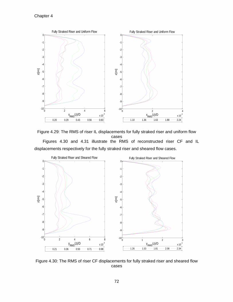
Chapter 4

72

Figure 4.29: The RMS of riser IL displacements for fully straked riser and uniform flow cases


displacements respectively for the fully straked riser and sheared flow cases.

Figure 4.30: The RMS of riser CF displacements for fully straked riser and sheared flow cases

0 2 4 6

x 10-3

-10

-9

-8

-7

-6

-5

-4

-3

-2

-1

0

xRMS

(z)/D

z[m

]


0.20 0.29 0.43 0.56 0.83

0 2 4

x 10-3

-10

-9

-8

-7

-6

-5

-4

-3

-2

-1

0

xRMS

(z)/Dz[m

]


1.10 1.36 1.63 1.88 2.24

0 2 4 6 8

x 10-3

-10

-9

-8

-7

-6

-5

-4

-3

-2

-1

0

yRMS

(z)/D

z[m

]

Fully Straked Riser and Sheared Flow

0.21 0.36 0.50 0.71 0.98

0 1 2 3

x 10-3

-10

-9

-8

-7

-6

-5

-4

-3

-2

-1

0

yRMS

(z)/D

z[m

]


1.26 1.53 1.81 2.08 2.34

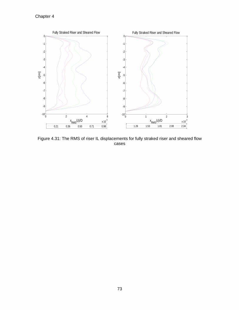
Chapter 4

73

Figure 4.31: The RMS of riser IL displacements for fully straked riser and sheared flow cases

0 2 4 6

x 10-3

-10

-9

-8

-7

-6

-5

-4

-3

-2

-1

0

xRMS

(z)/D

z[m

]


0.21 0.36 0.50 0.71 0.98

0 1 2 3

x 10-3

-10

-9

-8

-7

-6

-5

-4

-3

-2

-1

0

xRMS

(z)/Dz[m

]


1.26 1.53 1.81 2.08 2.34

Chapter 5

74

Chapter 5

5 Analyses to reconstructed VIV

responses in ExxonMobil VIV test

5.1 Riser VIV modal decomposition

In the chapter 4, the method of superposing the riser’s free vibration modes was

used to reconstruct the riser’s VIV responses in the ExxonMobil experiment. However,

the response modes corresponding to the riser’s specific response frequencies are not

known and they are most likely not the free vibration modes of the riser. Thus, in order to

eliminate the misunderstanding about the free vibration mode and response mode, these

specific response modes are needed to be extracted. In simple terms, the free vibration

mode refers to the riser’s natural frequency and the response mode refers to the riser’s

specific response frequency. And based on the obtained spatially and temporally dense

riser displacement signals after the response reconstruction, the extraction of response

mode becomes feasible.

5.1.1 Response modes and response frequencies

Before extracting the response mode, it needs to be defined at first. The response

mode denotes the special (complex) spatial function that describes the response of the

riser at a specific frequency (response frequency). The bivariate and dense signals of

riser VIV displacements in space and time can be expressed by its two dimensional

Fourier transforms as:

21 1

1( , ) ( , )

2

l jm r

Mi tik z

r j m l

m l

y z t k e e

(5.1)

Recasting Equation (5.1) as:

Chapter 5

75

1

( , ) ( ) l ji t

r j l r

l

y z t Y z e

(5.2)

Where, ( )l rY z are the 1,2,...l complex response modes corresponding to the

response frequencies l , and are given as:

21

1( ) ( , )

2

m r

Mik z

l r m l

m

Y z k e

(5.3)

Peak response modes: With regard to the riser VIV response having one single

peak frequency or a few separate peak frequencies, the response modes corresponding

to these peak response frequencies, which are denoted by n , can be extracted. These

extracted response modes are called peak response modes and are denoted by n rY z .

Thus, n is a subset of l and n rY z is a subset of l rY z . As a consequence, the

response of the riser could be approximated using the peak response modes as:

1

( , ) n j

Ni t

r j n r

n

y z t Y z e

(5.4)

5.1.2 Numerical method

Based on the definition of response modes given in chapter 5.1.1, a numerical

method to extract these response modes from the reconstruction data is found. The

Fourier expansion of the time series of VIV displacements at any given locations rz can

be written as:

1

ˆ( , ) Re ( , ) l ji t

r j r l

l

y z t y z e

(5.5)

Where, ˆ( , )r ly z is a complex quantity, representing the thl Fourier coefficient

corresponding to the frequency l from the signal at position rz . The response mode at

frequency l , denoted by ( )l rY z , can be obtained by extracting the Fourier coefficients at

each point along the entire riser corresponding to the frequency l as:

ˆ( ) ( , )l r r lY z y z (5.6)

The modal magnitude | ( ) |l rY z corresponding to the response mode ( )l rY z is

obtained as:

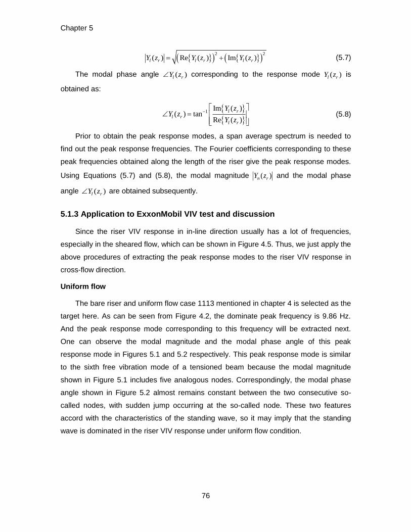
Chapter 5

76

2 2

( ) Re ( ) Im ( )l r l r l rY z Y z Y z (5.7)

The modal phase angle ( )l rY z corresponding to the response mode ( )l rY z is

obtained as:

1

Im ( )( ) tan

Re ( )

l r

l r

l r

Y zY z

Y z

(5.8)

Prior to obtain the peak response modes, a span average spectrum is needed to

find out the peak response frequencies. The Fourier coefficients corresponding to these

peak frequencies obtained along the length of the riser give the peak response modes.

Using Equations (5.7) and (5.8), the modal magnitude ( )n rY z and the modal phase

angle ( )l rY z are obtained subsequently.

5.1.3 Application to ExxonMobil VIV test and discussion

Since the riser VIV response in in-line direction usually has a lot of frequencies,

especially in the sheared flow, which can be shown in Figure 4.5. Thus, we just apply the

above procedures of extracting the peak response modes to the riser VIV response in

cross-flow direction.

Uniform flow

The bare riser and uniform flow case 1113 mentioned in chapter 4 is selected as the

target here. As can be seen from Figure 4.2, the dominate peak frequency is 9.86 Hz.

And the peak response mode corresponding to this frequency will be extracted next.

One can observe the modal magnitude and the modal phase angle of this peak

response mode in Figures 5.1 and 5.2 respectively. This peak response mode is similar

to the sixth free vibration mode of a tensioned beam because the modal magnitude

shown in Figure 5.1 includes five analogous nodes. Correspondingly, the modal phase

angle shown in Figure 5.2 almost remains constant between the two consecutive so-

called nodes, with sudden jump occurring at the so-called node. These two features

accord with the characteristics of the standing wave, so it may imply that the standing

wave is dominated in the riser VIV response under uniform flow condition.

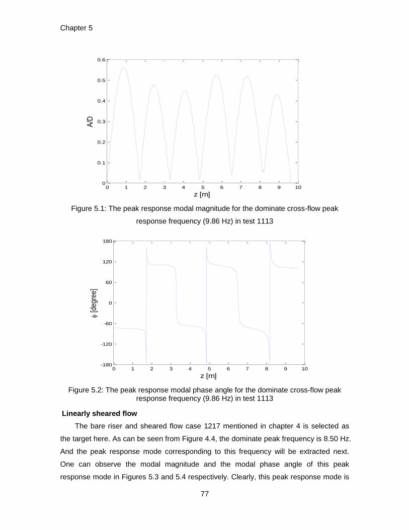
Chapter 5

77


response frequency (9.86 Hz) in test 1113

Figure 5.2: The peak response modal phase angle for the dominate cross-flow peak response frequency (9.86 Hz) in test 1113

Linearly sheared flow

The bare riser and sheared flow case 1217 mentioned in chapter 4 is selected as

the target here. As can be seen from Figure 4.4, the dominate peak frequency is 8.50 Hz.

And the peak response mode corresponding to this frequency will be extracted next.

One can observe the modal magnitude and the modal phase angle of this peak

response mode in Figures 5.3 and 5.4 respectively. Clearly, this peak response mode is

0 1 2 3 4 5 6 7 8 9 100

0.1

0.2

0.3

0.4

0.5

0.6

z [m]

A/D

0 1 2 3 4 5 6 7 8 9 10-180

-120

-60

0

60

120

180

z [m]

[d

egre

e]

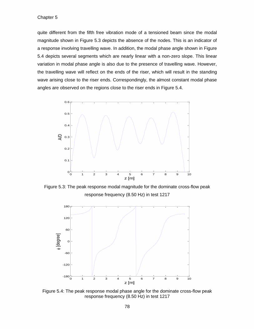
Chapter 5

78

quite different from the fifth free vibration mode of a tensioned beam since the modal

magnitude shown in Figure 5.3 depicts the absence of the nodes. This is an indicator of

a response involving travelling wave. In addition, the modal phase angle shown in Figure

5.4 depicts several segments which are nearly linear with a non-zero slope. This linear

variation in modal phase angle is also due to the presence of travelling wave. However,

the travelling wave will reflect on the ends of the riser, which will result in the standing

wave arising close to the riser ends. Correspondingly, the almost constant modal phase

angles are observed on the regions close to the riser ends in Figure 5.4.


response frequency (8.50 Hz) in test 1217

Figure 5.4: The peak response modal phase angle for the dominate cross-flow peak response frequency (8.50 Hz) in test 1217

0 1 2 3 4 5 6 7 8 9 100

0.1

0.2

0.3

0.4

0.5

0.6

z [m]

A/D

0 1 2 3 4 5 6 7 8 9 10-180

-120

-60

0

60

120

180

z [m]

[d

egre

e]

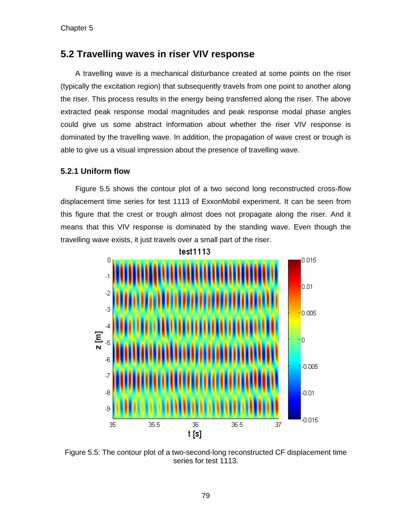
Chapter 5

79

5.2 Travelling waves in riser VIV response

A travelling wave is a mechanical disturbance created at some points on the riser

(typically the excitation region) that subsequently travels from one point to another along

the riser. This process results in the energy being transferred along the riser. The above

extracted peak response modal magnitudes and peak response modal phase angles

could give us some abstract information about whether the riser VIV response is

dominated by the travelling wave. In addition, the propagation of wave crest or trough is

able to give us a visual impression about the presence of travelling wave.

5.2.1 Uniform flow

Figure 5.5 shows the contour plot of a two second long reconstructed cross-flow

displacement time series for test 1113 of ExxonMobil experiment. It can be seen from

this figure that the crest or trough almost does not propagate along the riser. And it

means that this VIV response is dominated by the standing wave. Even though the

travelling wave exists, it just travels over a small part of the riser.

Figure 5.5: The contour plot of a two-second-long reconstructed CF displacement time series for test 1113.

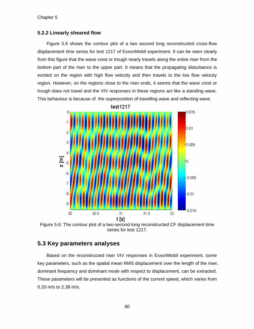
Chapter 5

80

5.2.2 Linearly sheared flow

Figure 5.6 shows the contour plot of a two second long reconstructed cross-flow

displacement time series for test 1217 of ExxonMobil experiment. It can be seen clearly

from this figure that the wave crest or trough nearly travels along the entire riser from the

bottom part of the riser to the upper part. It means that the propagating disturbance is

excited on the region with high flow velocity and then travels to the low flow velocity

region. However, on the regions close to the riser ends, it seems that the wave crest or

trough does not travel and the VIV responses in these regions act like a standing wave.

This behaviour is because of the superposition of travelling wave and reflecting wave.


series for test 1217.

5.3 Key parameters analyses

Based on the reconstructed riser VIV responses in ExxonMobil experiment, some

key parameters, such as the spatial mean RMS displacement over the length of the riser,

dominant frequency and dominant mode with respect to displacement, can be extracted.

These parameters will be presented as functions of the current speed, which varies from

0.20 m/s to 2.38 m/s.

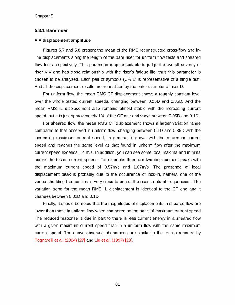
Chapter 5

81

5.3.1 Bare riser

VIV displacement amplitude

Figures 5.7 and 5.8 present the mean of the RMS reconstructed cross-flow and in-

line displacements along the length of the bare riser for uniform flow tests and sheared

flow tests respectively. This parameter is quite suitable to judge the overall severity of

riser VIV and has close relationship with the riser’s fatigue life, thus this parameter is

chosen to be analyzed. Each pair of symbols (CF/IL) is representative of a single test.

And all the displacement results are normalized by the outer diameter of riser D.

For uniform flow, the mean RMS CF displacement shows a roughly constant level

over the whole tested current speeds, changing between 0.25D and 0.35D. And the

mean RMS IL displacement also remains almost stable with the increasing current

speed, but it is just approximately 1/4 of the CF one and varys between 0.05D and 0.1D.

For sheared flow, the mean RMS CF displacement shows a larger variation range

compared to that observed in uniform flow, changing between 0.1D and 0.35D with the

increasing maximum current speed. In general, it grows with the maximum current

speed and reaches the same level as that found in uniform flow after the maximum

current speed exceeds 1.4 m/s. In addition, you can see some local maxima and minima

across the tested current speeds. For example, there are two displacement peaks with

the maximum current speed of 0.57m/s and 1.67m/s. The presence of local

displacement peak is probably due to the occurrence of lock-in, namely, one of the

vortex shedding frequencies is very close to one of the riser’s natural frequencies. The

variation trend for the mean RMS IL displacement is identical to the CF one and it

changes between 0.02D and 0.1D.

Finally, it should be noted that the magnitudes of displacements in sheared flow are

lower than those in uniform flow when compared on the basis of maximum current speed.

The reduced response is due in part to there is less current energy in a sheared flow

with a given maximum current speed than in a uniform flow with the same maximum

current speed. The above observed phenomena are similar to the results reported by

Tognarelli et al. (2004) [27] and Lie et al. (1997) [28].

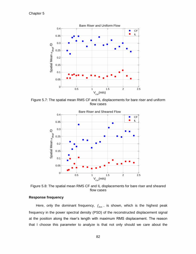
Chapter 5

82

Figure 5.7: The spatial mean RMS CF and IL displacements for bare riser and uniform flow cases

Figure 5.8: The spatial mean RMS CF and IL displacements for bare riser and sheared flow cases

Response frequency

Here, only the dominant frequency, domf , is shown, which is the highest peak

frequency in the power spectral density (PSD) of the reconstructed displacement signal

at the position along the riser’s length with maximum RMS displacement. The reason

that I choose this parameter to analyze is that not only should we care about the

0.5 1 1.5 2 2.50

0.05

0.1

0.15

0.2

0.25

0.3

0.35

0.4

Vcur

(m/s)

Spatial M

ean

dis

pl /

D


CF

IL

0.5 1 1.5 2 2.50

0.05

0.1

0.15

0.2

0.25

0.3

0.35

0.4

Vcur

(m/s)

Spatial M

ean

dis

pl /

D


CF

IL

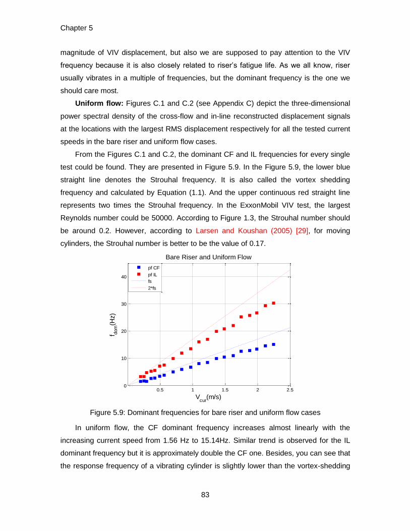
Chapter 5

83

magnitude of VIV displacement, but also we are supposed to pay attention to the VIV

frequency because it is also closely related to riser’s fatigue life. As we all know, riser

usually vibrates in a multiple of frequencies, but the dominant frequency is the one we

should care most.

Uniform flow: Figures C.1 and C.2 (see Appendix C) depict the three-dimensional

power spectral density of the cross-flow and in-line reconstructed displacement signals

at the locations with the largest RMS displacement respectively for all the tested current

speeds in the bare riser and uniform flow cases.

From the Figures C.1 and C.2, the dominant CF and IL frequencies for every single

test could be found. They are presented in Figure 5.9. In the Figure 5.9, the lower blue

straight line denotes the Strouhal frequency. It is also called the vortex shedding

frequency and calculated by Equation (1.1). And the upper continuous red straight line

represents two times the Strouhal frequency. In the ExxonMobil VIV test, the largest

Reynolds number could be 50000. According to Figure 1.3, the Strouhal number should

be around 0.2. However, according to Larsen and Koushan (2005) [29], for moving

cylinders, the Strouhal number is better to be the value of 0.17.

Figure 5.9: Dominant frequencies for bare riser and uniform flow cases

In uniform flow, the CF dominant frequency increases almost linearly with the

increasing current speed from 1.56 Hz to 15.14Hz. Similar trend is observed for the IL

dominant frequency but it is approximately double the CF one. Besides, you can see that

the response frequency of a vibrating cylinder is slightly lower than the vortex-shedding

0.5 1 1.5 2 2.50

10

20

30

40

Vcur

(m/s)

f dom

(Hz)


pf CF

pf IL

fs

2*fs

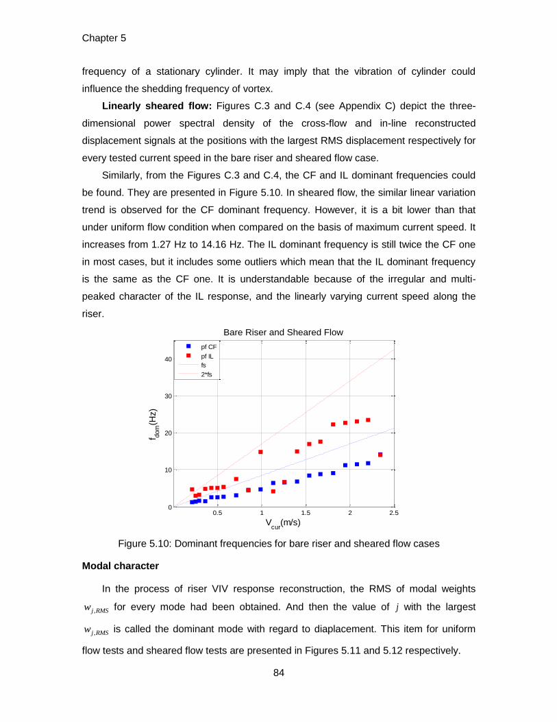
Chapter 5

84

frequency of a stationary cylinder. It may imply that the vibration of cylinder could

influence the shedding frequency of vortex.

Linearly sheared flow: Figures C.3 and C.4 (see Appendix C) depict the three-

dimensional power spectral density of the cross-flow and in-line reconstructed

displacement signals at the positions with the largest RMS displacement respectively for

every tested current speed in the bare riser and sheared flow case.

Similarly, from the Figures C.3 and C.4, the CF and IL dominant frequencies could

be found. They are presented in Figure 5.10. In sheared flow, the similar linear variation

trend is observed for the CF dominant frequency. However, it is a bit lower than that

under uniform flow condition when compared on the basis of maximum current speed. It

increases from 1.27 Hz to 14.16 Hz. The IL dominant frequency is still twice the CF one

in most cases, but it includes some outliers which mean that the IL dominant frequency

is the same as the CF one. It is understandable because of the irregular and multi-

peaked character of the IL response, and the linearly varying current speed along the

riser.

Figure 5.10: Dominant frequencies for bare riser and sheared flow cases

Modal character

In the process of riser VIV response reconstruction, the RMS of modal weights

,j RMSw for every mode had been obtained. And then the value of j with the largest

,j RMSw is called the dominant mode with regard to diaplacement. This item for uniform

flow tests and sheared flow tests are presented in Figures 5.11 and 5.12 respectively.

0.5 1 1.5 2 2.50

10

20

30

40

Vcur

(m/s)

f dom

(Hz)


pf CF

pf IL

fs

2*fs

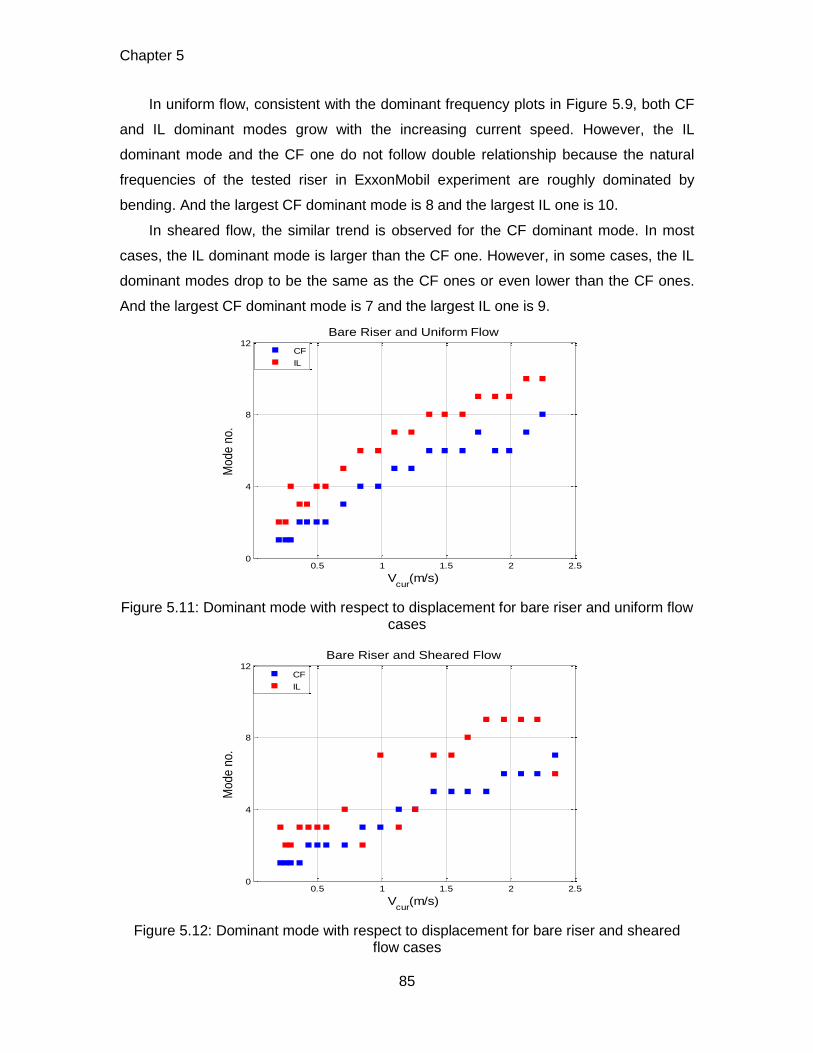
Chapter 5

85

In uniform flow, consistent with the dominant frequency plots in Figure 5.9, both CF

and IL dominant modes grow with the increasing current speed. However, the IL

dominant mode and the CF one do not follow double relationship because the natural

frequencies of the tested riser in ExxonMobil experiment are roughly dominated by

bending. And the largest CF dominant mode is 8 and the largest IL one is 10.

In sheared flow, the similar trend is observed for the CF dominant mode. In most

cases, the IL dominant mode is larger than the CF one. However, in some cases, the IL

dominant modes drop to be the same as the CF ones or even lower than the CF ones.

And the largest CF dominant mode is 7 and the largest IL one is 9.

Figure 5.11: Dominant mode with respect to displacement for bare riser and uniform flow cases

Figure 5.12: Dominant mode with respect to displacement for bare riser and sheared flow cases

0.5 1 1.5 2 2.50

4

8

12

Vcur

(m/s)

Mode n

o.


CF

IL

0.5 1 1.5 2 2.50

4

8

12

Vcur

(m/s)

Mode n

o.


CF

IL

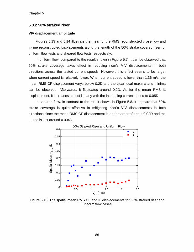
Chapter 5

86

5.3.2 50% straked riser


Figures 5.13 and 5.14 illustrate the mean of the RMS reconstructed cross-flow and

in-line reconstructed displacements along the length of the 50% strake covered riser for

uniform flow tests and sheared flow tests respectively.

In uniform flow, compared to the result shown in Figure 5.7, it can be observed that

50% strake coverage takes effect in reducing riser’s VIV displacements in both

directions across the tested current speeds. However, this effect seems to be larger

when current speed is relatively lower. When current speed is lower than 1.36 m/s, the

mean RMS CF displacement varys below 0.2D and the clear local maxima and minima

can be observed. Afterwards, it fluctuates around 0.2D. As for the mean RMS IL

displacement, it increases almost linearly with the increasing current speed to 0.05D.

In sheared flow, in contrast to the result shown in Figure 5.8, it appears that 50%

strake coverage is quite effective in mitigating riser’s VIV displacements in both

directions since the mean RMS CF displacement is on the order of about 0.02D and the

IL one is just around 0.004D.

Figure 5.13: The spatial mean RMS CF and IL displacements for 50% straked riser and uniform flow cases

0.5 1 1.5 2 2.50

0.05

0.1

0.15

0.2

0.25

0.3

0.35

0.4

Vcur

(m/s)

Spatial M

ean

dis

pl /

D


CF

IL

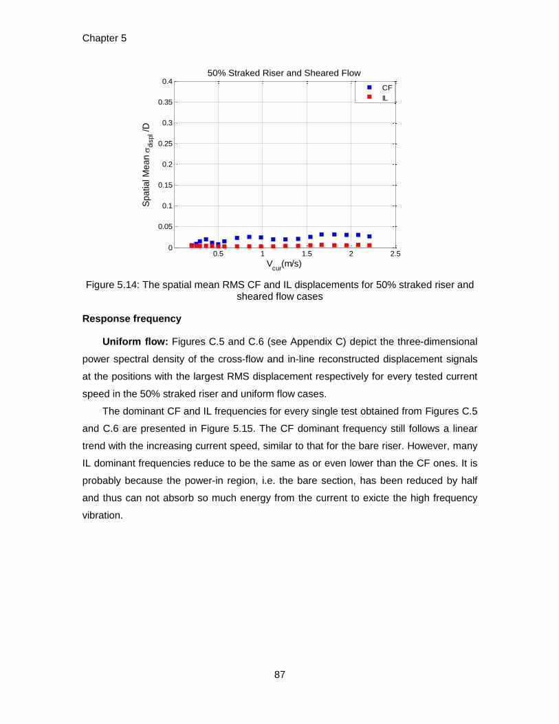
Chapter 5

87

Figure 5.14: The spatial mean RMS CF and IL displacements for 50% straked riser and sheared flow cases

Response frequency

Uniform flow: Figures C.5 and C.6 (see Appendix C) depict the three-dimensional

power spectral density of the cross-flow and in-line reconstructed displacement signals

at the positions with the largest RMS displacement respectively for every tested current

speed in the 50% straked riser and uniform flow cases.

The dominant CF and IL frequencies for every single test obtained from Figures C.5

and C.6 are presented in Figure 5.15. The CF dominant frequency still follows a linear

trend with the increasing current speed, similar to that for the bare riser. However, many

IL dominant frequencies reduce to be the same as or even lower than the CF ones. It is

probably because the power-in region, i.e. the bare section, has been reduced by half

and thus can not absorb so much energy from the current to exicte the high frequency

vibration.

0.5 1 1.5 2 2.50

0.05

0.1

0.15

0.2

0.25

0.3

0.35

0.4

Vcur

(m/s)

Spatial M

ean

dis

pl /

D


CF

IL

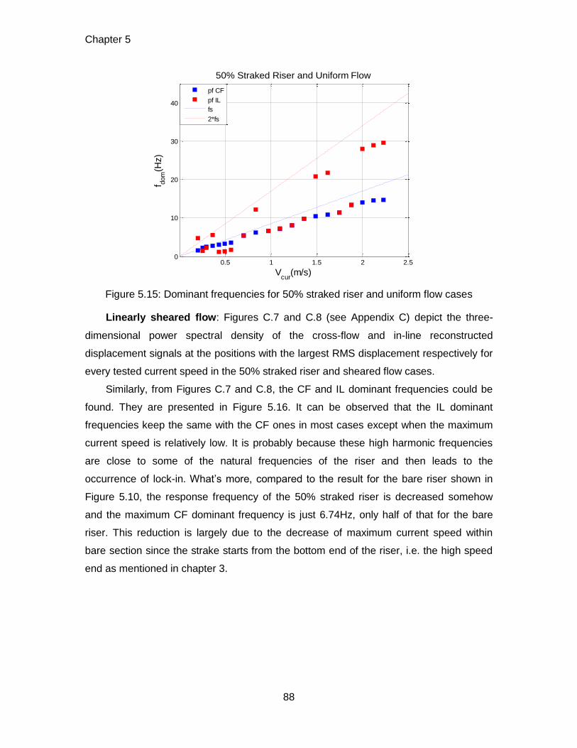
Chapter 5

88

Figure 5.15: Dominant frequencies for 50% straked riser and uniform flow cases

Linearly sheared flow: Figures C.7 and C.8 (see Appendix C) depict the three-

dimensional power spectral density of the cross-flow and in-line reconstructed

displacement signals at the positions with the largest RMS displacement respectively for

every tested current speed in the 50% straked riser and sheared flow cases.

Similarly, from Figures C.7 and C.8, the CF and IL dominant frequencies could be

found. They are presented in Figure 5.16. It can be observed that the IL dominant

frequencies keep the same with the CF ones in most cases except when the maximum

current speed is relatively low. It is probably because these high harmonic frequencies

are close to some of the natural frequencies of the riser and then leads to the

occurrence of lock-in. What’s more, compared to the result for the bare riser shown in

Figure 5.10, the response frequency of the 50% straked riser is decreased somehow

and the maximum CF dominant frequency is just 6.74Hz, only half of that for the bare

riser. This reduction is largely due to the decrease of maximum current speed within

bare section since the strake starts from the bottom end of the riser, i.e. the high speed

end as mentioned in chapter 3.

0.5 1 1.5 2 2.50

10

20

30

40

Vcur

(m/s)

f dom

(Hz)


pf CF

pf IL

fs

2*fs

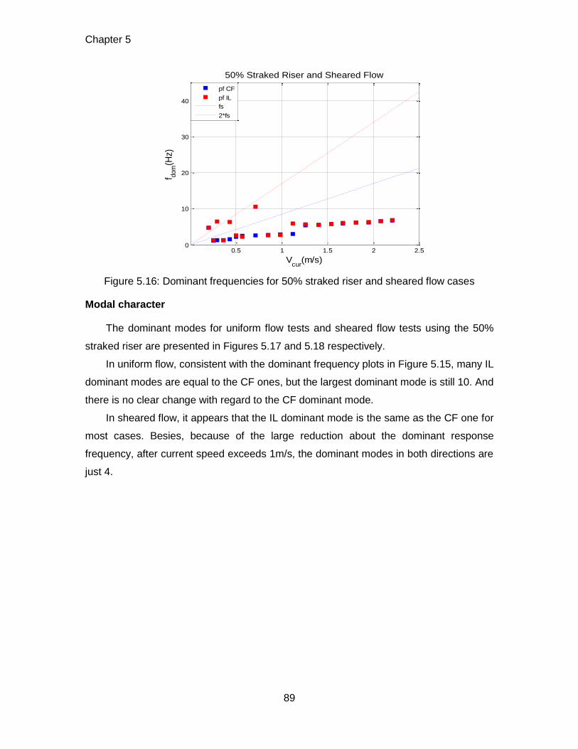
Chapter 5

89

Figure 5.16: Dominant frequencies for 50% straked riser and sheared flow cases

Modal character

The dominant modes for uniform flow tests and sheared flow tests using the 50%

straked riser are presented in Figures 5.17 and 5.18 respectively.

In uniform flow, consistent with the dominant frequency plots in Figure 5.15, many IL

dominant modes are equal to the CF ones, but the largest dominant mode is still 10. And

there is no clear change with regard to the CF dominant mode.

In sheared flow, it appears that the IL dominant mode is the same as the CF one for

most cases. Besies, because of the large reduction about the dominant response

frequency, after current speed exceeds 1m/s, the dominant modes in both directions are

just 4.

0.5 1 1.5 2 2.50

10

20

30

40

Vcur

(m/s)

f dom

(Hz)


pf CF

pf IL

fs

2*fs

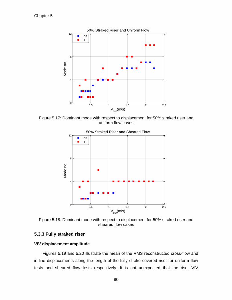
Chapter 5

90

Figure 5.17: Dominant mode with respect to displacement for 50% straked riser and uniform flow cases

Figure 5.18: Dominant mode with respect to displacement for 50% straked riser and sheared flow cases

5.3.3 Fully straked riser


Figures 5.19 and 5.20 illustrate the mean of the RMS reconstructed cross-flow and

in-line displacements along the length of the fully strake covered riser for uniform flow

tests and sheared flow tests respectively. It is not unexpected that the riser VIV

0.5 1 1.5 2 2.50

4

8

12

Vcur

(m/s)

Mode n

o.


CF

IL

0.5 1 1.5 2 2.50

4

8

12

Vcur

(m/s)

Mode n

o.


CF

IL

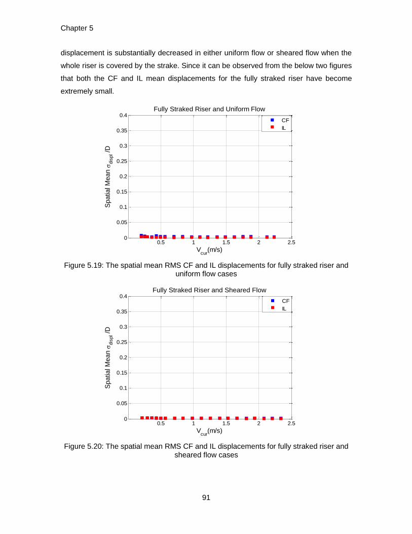
Chapter 5

91

displacement is substantially decreased in either uniform flow or sheared flow when the

whole riser is covered by the strake. Since it can be observed from the below two figures

that both the CF and IL mean displacements for the fully straked riser have become

extremely small.

Figure 5.19: The spatial mean RMS CF and IL displacements for fully straked riser and uniform flow cases

Figure 5.20: The spatial mean RMS CF and IL displacements for fully straked riser and sheared flow cases

0.5 1 1.5 2 2.50

0.05

0.1

0.15

0.2

0.25

0.3

0.35

0.4

Vcur

(m/s)

Spatial M

ean

dis

pl /

DFully Straked Riser and Uniform Flow

CF

IL

0.5 1 1.5 2 2.50

0.05

0.1

0.15

0.2

0.25

0.3

0.35

0.4

Vcur

(m/s)

Spatial M

ean

dis

pl /

D


CF

IL

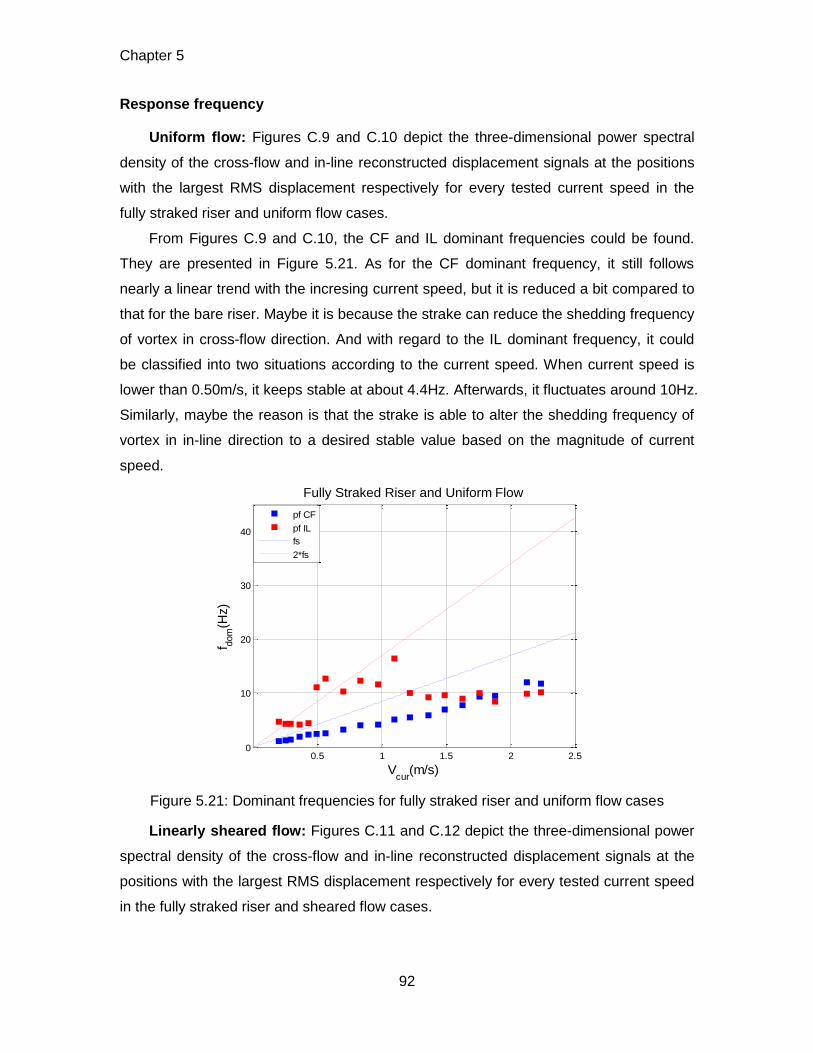
Chapter 5

92

Response frequency

Uniform flow: Figures C.9 and C.10 depict the three-dimensional power spectral

density of the cross-flow and in-line reconstructed displacement signals at the positions

with the largest RMS displacement respectively for every tested current speed in the

fully straked riser and uniform flow cases.

From Figures C.9 and C.10, the CF and IL dominant frequencies could be found.

They are presented in Figure 5.21. As for the CF dominant frequency, it still follows

nearly a linear trend with the incresing current speed, but it is reduced a bit compared to

that for the bare riser. Maybe it is because the strake can reduce the shedding frequency

of vortex in cross-flow direction. And with regard to the IL dominant frequency, it could

be classified into two situations according to the current speed. When current speed is

lower than 0.50m/s, it keeps stable at about 4.4Hz. Afterwards, it fluctuates around 10Hz.

Similarly, maybe the reason is that the strake is able to alter the shedding frequency of

vortex in in-line direction to a desired stable value based on the magnitude of current

speed.

Figure 5.21: Dominant frequencies for fully straked riser and uniform flow cases

Linearly sheared flow: Figures C.11 and C.12 depict the three-dimensional power

spectral density of the cross-flow and in-line reconstructed displacement signals at the

positions with the largest RMS displacement respectively for every tested current speed

in the fully straked riser and sheared flow cases.

0.5 1 1.5 2 2.50

10

20

30

40

Vcur

(m/s)

f dom

(Hz)


pf CF

pf IL

fs

2*fs

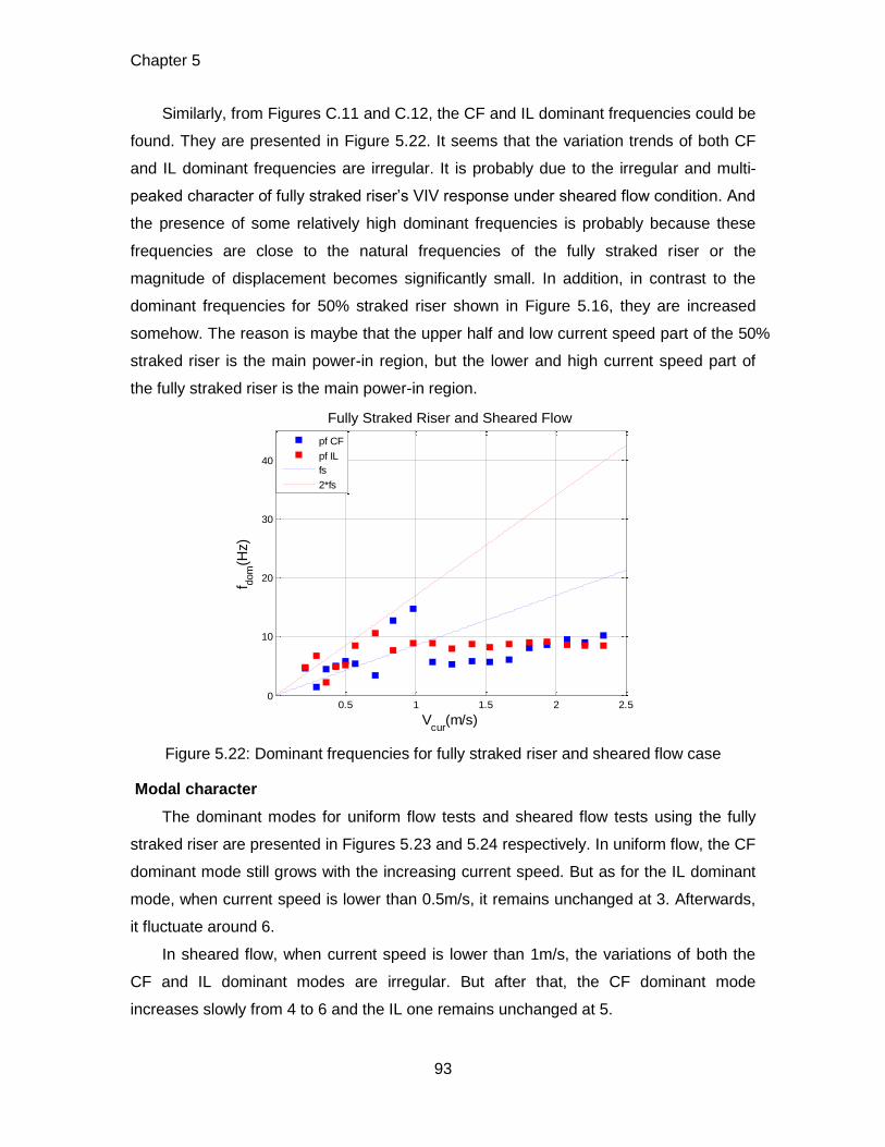
Chapter 5

93

Similarly, from Figures C.11 and C.12, the CF and IL dominant frequencies could be

found. They are presented in Figure 5.22. It seems that the variation trends of both CF

and IL dominant frequencies are irregular. It is probably due to the irregular and multi-

peaked character of fully straked riser’s VIV response under sheared flow condition. And

the presence of some relatively high dominant frequencies is probably because these

frequencies are close to the natural frequencies of the fully straked riser or the

magnitude of displacement becomes significantly small. In addition, in contrast to the

dominant frequencies for 50% straked riser shown in Figure 5.16, they are increased

somehow. The reason is maybe that the upper half and low current speed part of the 50%

straked riser is the main power-in region, but the lower and high current speed part of

the fully straked riser is the main power-in region.

Figure 5.22: Dominant frequencies for fully straked riser and sheared flow case

Modal character

The dominant modes for uniform flow tests and sheared flow tests using the fully

straked riser are presented in Figures 5.23 and 5.24 respectively. In uniform flow, the CF

dominant mode still grows with the increasing current speed. But as for the IL dominant

mode, when current speed is lower than 0.5m/s, it remains unchanged at 3. Afterwards,

it fluctuate around 6.

In sheared flow, when current speed is lower than 1m/s, the variations of both the

CF and IL dominant modes are irregular. But after that, the CF dominant mode

increases slowly from 4 to 6 and the IL one remains unchanged at 5.

0.5 1 1.5 2 2.50

10

20

30

40

Vcur

(m/s)

f dom

(Hz)


pf CF

pf IL

fs

2*fs

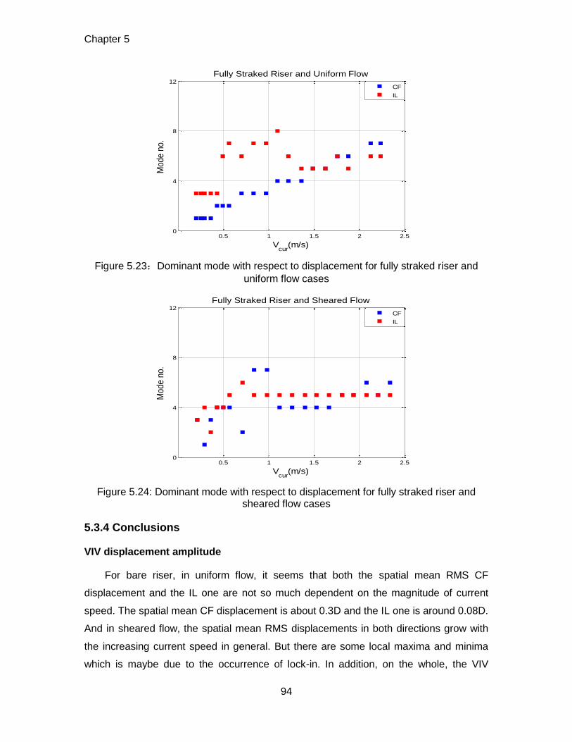
Chapter 5

94

Figure 5.23：Dominant mode with respect to displacement for fully straked riser and

uniform flow cases

Figure 5.24: Dominant mode with respect to displacement for fully straked riser and sheared flow cases

5.3.4 Conclusions


For bare riser, in uniform flow, it seems that both the spatial mean RMS CF

displacement and the IL one are not so much dependent on the magnitude of current

speed. The spatial mean CF displacement is about 0.3D and the IL one is around 0.08D.

And in sheared flow, the spatial mean RMS displacements in both directions grow with

the increasing current speed in general. But there are some local maxima and minima

which is maybe due to the occurrence of lock-in. In addition, on the whole, the VIV

0.5 1 1.5 2 2.50

4

8

12

Vcur

(m/s)

Mode n

o.


CF

IL

0.5 1 1.5 2 2.50

4

8

12

Vcur

(m/s)

Mode n

o.


CF

IL

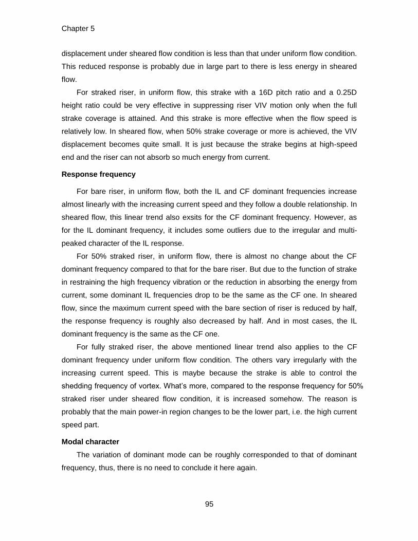
Chapter 5

95

displacement under sheared flow condition is less than that under uniform flow condition.

This reduced response is probably due in large part to there is less energy in sheared

flow.

For straked riser, in uniform flow, this strake with a 16D pitch ratio and a 0.25D

height ratio could be very effective in suppressing riser VIV motion only when the full

strake coverage is attained. And this strake is more effective when the flow speed is

relatively low. In sheared flow, when 50% strake coverage or more is achieved, the VIV

displacement becomes quite small. It is just because the strake begins at high-speed

end and the riser can not absorb so much energy from current.

Response frequency

For bare riser, in uniform flow, both the IL and CF dominant frequencies increase

almost linearly with the increasing current speed and they follow a double relationship. In

sheared flow, this linear trend also exsits for the CF dominant frequency. However, as

for the IL dominant frequency, it includes some outliers due to the irregular and multi-

peaked character of the IL response.

For 50% straked riser, in uniform flow, there is almost no change about the CF

dominant frequency compared to that for the bare riser. But due to the function of strake

in restraining the high frequency vibration or the reduction in absorbing the energy from

current, some dominant IL frequencies drop to be the same as the CF one. In sheared

flow, since the maximum current speed with the bare section of riser is reduced by half,

the response frequency is roughly also decreased by half. And in most cases, the IL

dominant frequency is the same as the CF one.

For fully straked riser, the above mentioned linear trend also applies to the CF

dominant frequency under uniform flow condition. The others vary irregularly with the

increasing current speed. This is maybe because the strake is able to control the

shedding frequency of vortex. What’s more, compared to the response frequency for 50%

straked riser under sheared flow condition, it is increased somehow. The reason is

probably that the main power-in region changes to be the lower part, i.e. the high current

speed part.

Modal character

The variation of dominant mode can be roughly corresponded to that of dominant

frequency, thus, there is no need to conclude it here again.

Chapter 6

96

Chapter 6

6 Riser VIV response reconstruction

of the second Gulf Stream VIV test

6.1 Characteristics of the second Gulf Stream VIV test

6.1.1 Characteristics of tested pipe

The tested pipe in the second Gulf Stream VIV test is quite different from that used

in the ExxonMobil VIV test. One is that this pipe was not straight and was deflected

during the test. Another is that the natural frequency of this pipe is absolutely dominated

by tension and this pipe may undergo very high mode number VIV motion.

Deflected shape

When the test did not start, the pipe hung vertically and remained straight. And

when the pipe was towed by the boat, the current drag force on the pipe would cause

the pipe to deflect, which would then cause the railroad wheel on the bottom end of the

pipe to move aft and lift. In this experiment, a depth gauge was attached to the bottom

railroad wheel to aid in finding the deflected shape of the pipe. Figure 6.1 shows the

depth of railroad wheel, as measured by the depth gauge, versus the top angle,

measured by the tilt meter on the top of the pipe. Since the top inclination angle is

another measurement of the deflection of the pipe, the depth and the top tilt angle

should be related. Using a second order polynomial to fit all the data from the bare pipe

tests, Equation (6.1) was found:

20.0417( ) 0.3274( ) 494.18Depth tilt tilt (6.1)

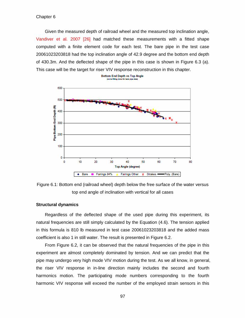
Chapter 6

97

Given the measured depth of railroad wheel and the measured top inclination angle,

Vandiver et al. 2007 [26] had matched these measurements with a fitted shape

computed with a finite element code for each test. The bare pipe in the test case

20061023203818 had the top inclination angle of 42.9 degree and the bottom end depth

of 430.3m. And the deflected shape of the pipe in this case is shown in Figure 6.3 (a).

This case will be the target for riser VIV response reconstruction in this chapter.

Figure 6.1: Bottom end (railroad wheel) depth below the free surface of the water versus

top end angle of inclination with vertical for all cases

Structural dynamics

Regardless of the deflected shape of the used pipe during this experiment, its

natural frequencies are still simply calculated by the Equation (4.6). The tension applied

in this formula is 810 lb measured in test case 20061023203818 and the added mass

coefficient is also 1 in still water. The result is presented in Figure 6.2.

From Figure 6.2, it can be observed that the natural frequencies of the pipe in this

experiment are almost completely dominated by tension. And we can predict that the

pipe may undergo very high mode VIV motion during the test. As we all know, in general,

the riser VIV response in in-line direction mainly includes the second and fourth

harmonics motion. The participating mode numbers corresponding to the fourth

harmonic VIV response will exceed the number of the employed strain sensors in this

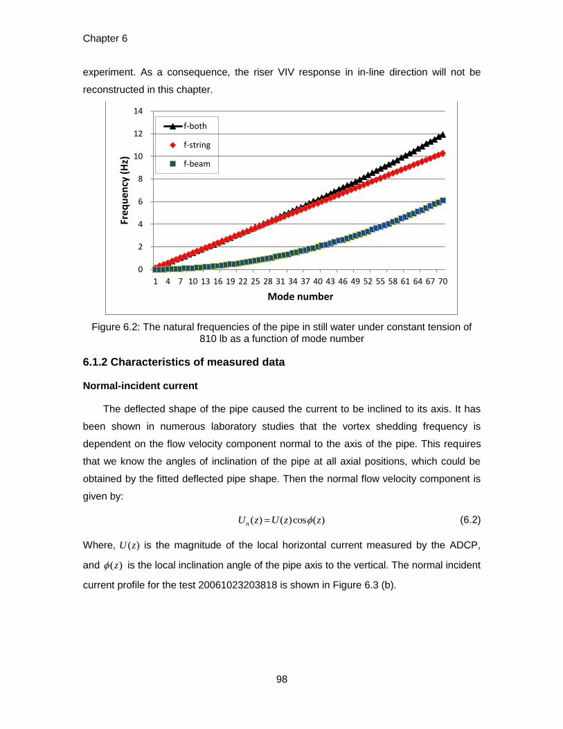
Chapter 6

98

experiment. As a consequence, the riser VIV response in in-line direction will not be

reconstructed in this chapter.

Figure 6.2: The natural frequencies of the pipe in still water under constant tension of 810 lb as a function of mode number

6.1.2 Characteristics of measured data

Normal-incident current

The deflected shape of the pipe caused the current to be inclined to its axis. It has

been shown in numerous laboratory studies that the vortex shedding frequency is

dependent on the flow velocity component normal to the axis of the pipe. This requires

that we know the angles of inclination of the pipe at all axial positions, which could be

obtained by the fitted deflected pipe shape. Then the normal flow velocity component is

given by:

( ) ( )cos ( )nU z U z z (6.2)

Where, ( )U z is the magnitude of the local horizontal current measured by the ADCP,

and ( )z is the local inclination angle of the pipe axis to the vertical. The normal incident

current profile for the test 20061023203818 is shown in Figure 6.3 (b).

0

2

4

6

8

10

12

14

1 4 7 10 13 16 19 22 25 28 31 34 37 40 43 46 49 52 55 58 61 64 67 70

Freq

uen

cy (

Hz)

Mode number

f-both

f-string

f-beam

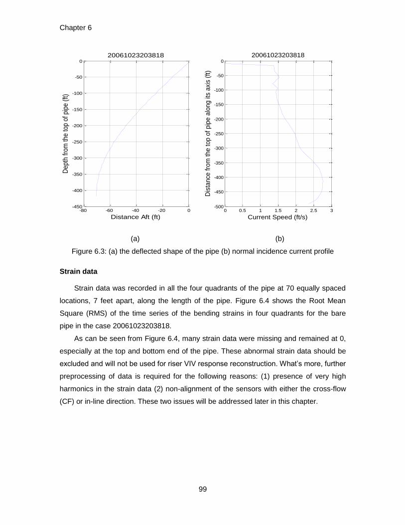
Chapter 6

99

(a) (b)

Figure 6.3: (a) the deflected shape of the pipe (b) normal incidence current profile

Strain data

Strain data was recorded in all the four quadrants of the pipe at 70 equally spaced

locations, 7 feet apart, along the length of the pipe. Figure 6.4 shows the Root Mean

Square (RMS) of the time series of the bending strains in four quadrants for the bare

pipe in the case 20061023203818.

As can be seen from Figure 6.4, many strain data were missing and remained at 0,

especially at the top and bottom end of the pipe. These abnormal strain data should be

excluded and will not be used for riser VIV response reconstruction. What’s more, further

preprocessing of data is required for the following reasons: (1) presence of very high

harmonics in the strain data (2) non-alignment of the sensors with either the cross-flow

(CF) or in-line direction. These two issues will be addressed later in this chapter.

-80 -60 -40 -20 0-450

-400

-350

-300

-250

-200

-150

-100

-50

0D

epth

from

the

top

of p

ipe

(ft)

Distance Aft (ft)

20061023203818

0 0.5 1 1.5 2 2.5 3-500

-450

-400

-350

-300

-250

-200

-150

-100

-50

0

Dis

tance

fro

m the t

op o

f pip

e a

long it

s axi

s (f

t)

Current Speed (ft/s)

20061023203818

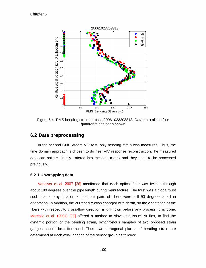
Chapter 6

100

Figure 6.4: RMS bending strain for case 20061023203818. Data from all the four quadrants has been shown

6.2 Data preprocessing

In the second Gulf Stream VIV test, only bending strain was measured. Thus, the

time domain approach is chosen to do riser VIV response reconstruction.The measured

data can not be directly entered into the data matrix and they need to be processed

previously.

6.2.1 Unwrapping data

Vandiver et al. 2007 [26] mentioned that each optical fiber was twisted through

about 180 degrees over the pipe length during manufacture. The twist was a global twist

such that at any location z, the four pairs of fibers were still 90 degrees apart in

orientation. In addition, the current direction changed with depth, so the orientation of the

fibers with respect to cross-flow direction is unknown before any processing is done.

Marcollo et al. (2007) [30] offered a method to slove this issue. At first, to find the

dynamic portion of the bending strain, synchronous samples of two opposed strain

gauges should be differenced. Thus, two orthogonal planes of bending strain are

determined at each axial location of the sensor group as follows:

0 50 100 150 200 2500

0.1

0.2

0.3

0.4

0.5

0.6

0.7

0.8

0.9

1

Re

lativ

e a

xia

l po

siti

on

(z/L

, 0

at b

otto

m e

nd

RMS Bending Strain ()

20061023203818

Q1

Q2

Q3

Q4

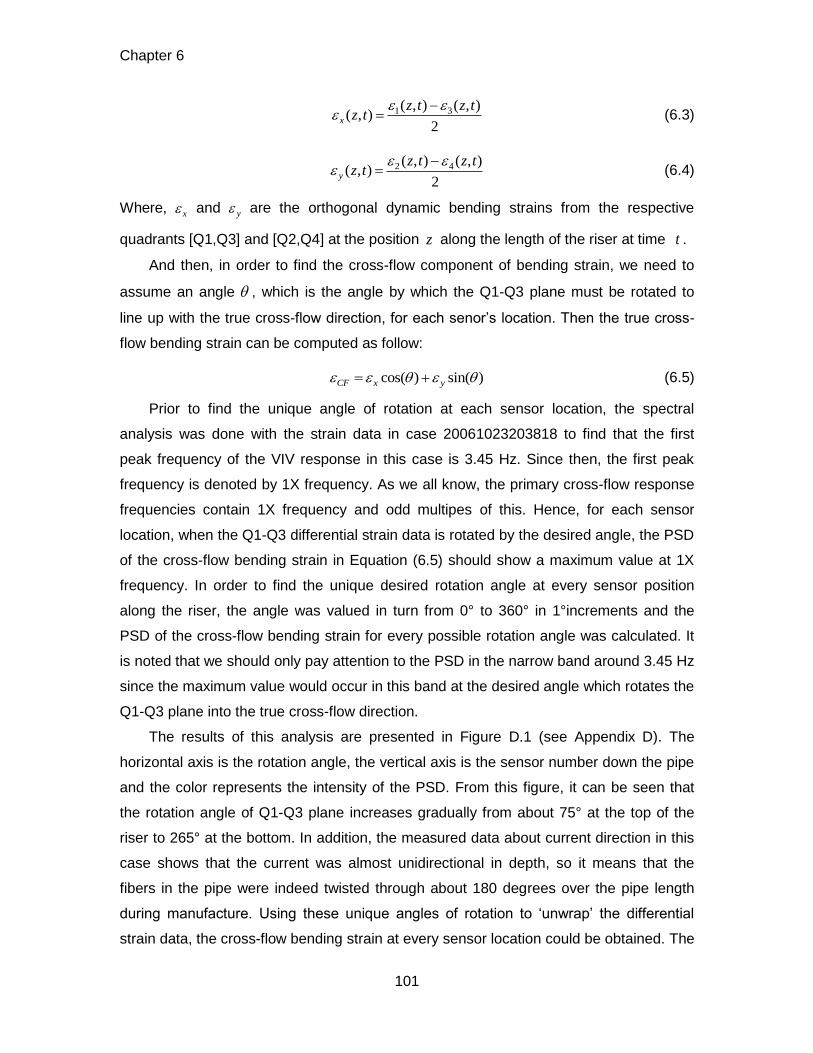
Chapter 6

101

1 3( , ) ( , )( , )

2x

z t z tz t

(6.3)

2 4( , ) ( , )( , )

2y

z t z tz t

(6.4)

Where, x and y are the orthogonal dynamic bending strains from the respective

quadrants [Q1,Q3] and [Q2,Q4] at the position z along the length of the riser at time t .

And then, in order to find the cross-flow component of bending strain, we need to

assume an angle , which is the angle by which the Q1-Q3 plane must be rotated to

line up with the true cross-flow direction, for each senor’s location. Then the true cross-

flow bending strain can be computed as follow:

cos( ) sin( )CF x y (6.5)

Prior to find the unique angle of rotation at each sensor location, the spectral

analysis was done with the strain data in case 20061023203818 to find that the first

peak frequency of the VIV response in this case is 3.45 Hz. Since then, the first peak

frequency is denoted by 1X frequency. As we all know, the primary cross-flow response

frequencies contain 1X frequency and odd multipes of this. Hence, for each sensor

location, when the Q1-Q3 differential strain data is rotated by the desired angle, the PSD

of the cross-flow bending strain in Equation (6.5) should show a maximum value at 1X

frequency. In order to find the unique desired rotation angle at every sensor position

along the riser, the angle was valued in turn from 0° to 360° in 1°increments and the

PSD of the cross-flow bending strain for every possible rotation angle was calculated. It

is noted that we should only pay attention to the PSD in the narrow band around 3.45 Hz

since the maximum value would occur in this band at the desired angle which rotates the

Q1-Q3 plane into the true cross-flow direction.

The results of this analysis are presented in Figure D.1 (see Appendix D). The

horizontal axis is the rotation angle, the vertical axis is the sensor number down the pipe

and the color represents the intensity of the PSD. From this figure, it can be seen that

the rotation angle of Q1-Q3 plane increases gradually from about 75° at the top of the

riser to 265° at the bottom. In addition, the measured data about current direction in this

case shows that the current was almost unidirectional in depth, so it means that the

fibers in the pipe were indeed twisted through about 180 degrees over the pipe length

during manufacture. Using these unique angles of rotation to ‘unwrap’ the differential

strain data, the cross-flow bending strain at every sensor location could be obtained. The

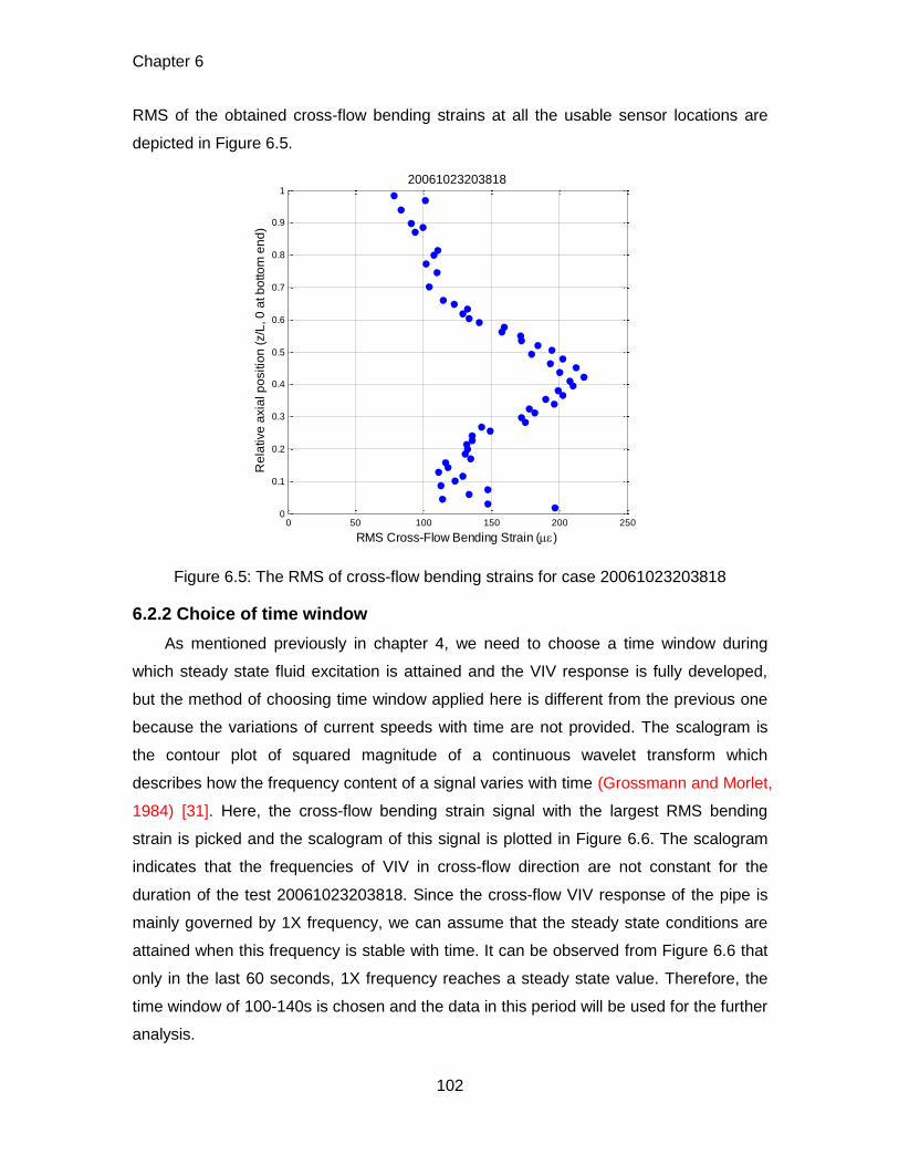
Chapter 6

102

RMS of the obtained cross-flow bending strains at all the usable sensor locations are

depicted in Figure 6.5.

Figure 6.5: The RMS of cross-flow bending strains for case 20061023203818

6.2.2 Choice of time window

As mentioned previously in chapter 4, we need to choose a time window during

which steady state fluid excitation is attained and the VIV response is fully developed,

but the method of choosing time window applied here is different from the previous one

because the variations of current speeds with time are not provided. The scalogram is

the contour plot of squared magnitude of a continuous wavelet transform which

describes how the frequency content of a signal varies with time (Grossmann and Morlet,

1984) [31]. Here, the cross-flow bending strain signal with the largest RMS bending

strain is picked and the scalogram of this signal is plotted in Figure 6.6. The scalogram

indicates that the frequencies of VIV in cross-flow direction are not constant for the

duration of the test 20061023203818. Since the cross-flow VIV response of the pipe is

mainly governed by 1X frequency, we can assume that the steady state conditions are

attained when this frequency is stable with time. It can be observed from Figure 6.6 that

only in the last 60 seconds, 1X frequency reaches a steady state value. Therefore, the

time window of 100-140s is chosen and the data in this period will be used for the further

analysis.

0 50 100 150 200 2500

0.1

0.2

0.3

0.4

0.5

0.6

0.7

0.8

0.9

1

Re

lative

axia

l p

ositio

n (

z/L

, 0

at b

otto

m e

nd

)

RMS Cross-Flow Bending Strain ()

20061023203818

Chapter 6

103

Figure 6.6: Time-frequency plot of the cross-flow bending strain signal at the sensor location with the largest RMS cross-flow bending strain in case 20061023203818

6.2.3 Bandpass filter data

As can be seen from Figure 6.6, the CF VIV response in test case 20061023203818

contains very high harmonics motion. And due to both the limitation of the number of the

usable sensors and the very high mode VIV response in this case, the CF bending strain

data should be band pass filtered to clear the very high harmonics VIV response. As we

all know, the primary CF VIV response frequencies contain 1X frequency and odd

multipes of this. However, based on the theory of Spatial Nyquist’s Criterion (Mukundan,

2008) [32], the number of usable sensors in this test case, i.e. fifty-eight, is not enough

to reconstruct the third and fifth harmonic responses since the associated participating

modes are larger than sixty. Thus, the passing frequency bands are chosen to be 0.5

times to 1.5 times 1X frequency, i.e. 1.73 Hz-5.18 Hz. It means that only the first

harmonic VIV response will be considered in the response reconstruction. And it should

be noted that even though the third and fifth harmonic responses contribute little to the

magnitude of VIV displacement, but may contribute much to the bending strain and

fatigue life. The RMS of the filtered cross-flow bending strains at all the usable sensor

locations are depicted in Figure 6.7.

Time(s)

Fre

qu

en

cy(H

z)

Scalogram

0 20 40 60 80 100 120 140 160

5

10

15

20

25

0

0.5

1

1.5

2

2.5

3

3.5

4

4.5

5x 10

-4

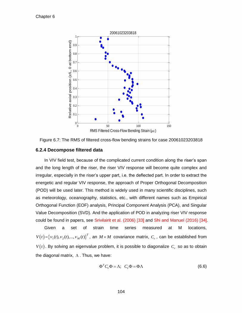
Chapter 6

104

Figure 6.7: The RMS of filtered cross-flow bending strains for case 20061023203818

6.2.4 Decompose filtered data

In VIV field test, because of the complicated current condition along the riser’s span

and the long length of the riser, the riser VIV response will become quite complex and

irregular, especially in the riser’s upper part, i.e. the deflected part. In order to extract the

energetic and regular VIV response, the approach of Proper Orthogonal Decomposition

(POD) will be used later. This method is widely used in many scientific disciplines, such

as meteorology, oceanography, statistics, etc., with different names such as Empirical

Orthogonal Function (EOF) analysis, Principal Component Analysis (PCA), and Singular

Value Decomposition (SVD). And the application of POD in analyzing riser VIV response

could be found in papers, see Srivilairit et al. (2006) [33] and Shi and Manuel (2016) [34].

Given a set of strain time series measured at M locations,

1 2( ), ( ),..., ( )T

MV t t t t , an M M covariance matrix, C , can be established from

V t . By solving an eigenvalue problem, it is possible to diagonalize C so as to obtain

the diagonal matrix, . Thus, we have:

;TC C (6.6)

0 50 100 1500

0.1

0.2

0.3

0.4

0.5

0.6

0.7

0.8

0.9

1

Re

lative

axia

l p

ositio

n (

z/L

, 0

at b

otto

m e

nd

)

RMS Filtered Cross-Flow Bending Strain ()

20061023203818

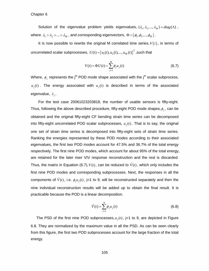
Chapter 6

105

Solution of the eigenvalue problem yields eigenvalues, 1 2{ , ,..., } { }M diag ,

where 1 2 ... M , and corresponding eigenvectors, 1 2, ,..., M .

It is now possible to rewrite the original M correlated time series, V t , in terms of

uncorrelated scalar subprocesses, 1 2( ) ( ), ( ),..., ( )T

MU t u t u t u t ,such that

1

( ) ( ) ( )M

j j

j

V t U t u t

(6.7)

Where, j represents the jth POD mode shape associated with the jth scalar subprocess,

( )ju t . The energy associated with ( )ju t is described in terms of the associated

eigenvalue, j .

For the test case 20061023203818, the number of usable sensors is fifty-eight.

Thus, following the above described procedure, fifty-eight POD mode shapes, j , can be

obtained and the original fifty-eight CF bending strain time series can be decomposed

into fifty-eight uncorrelated POD scalar subprocesses, ( )ju t . That is to say, the original

one set of strain time series is decomposed into fifty-eight sets of strain time series.

Ranking the energies represented by these POD modes according to their associated

eigenvalues, the first two POD modes account for 47.5% and 36.7% of the total energy

respectively. The first nine POD modes, which account for about 95% of the total energy,

are retained for the later riser VIV response reconstruction and the rest is discarded.

Thus, the matrix in Equation (6.7), ( )V t , can be reduced to ˆ( )V t , which only includes the

first nine POD modes and corresponding subprocesses. Next, the responses in all the

components of ˆ( )V t , i.e. ( )j ju t , j=1 to 9, will be reconstructed separately and then the

nine individual reconstruction results will be added up to obtain the final result. It is

practicable because the POD is a linear decomposition.

9

1

ˆ( ) ( )j j

j

V t u t

(6.8)

The PSD of the first nine POD subprocesses, ( )ju t , j=1 to 9, are depicted in Figure

6.8. They are normalized by the maximum value in all the PSD. As can be seen clearly

from this figure, the first two POD subprocesses account for the large fraction of the total

energy.

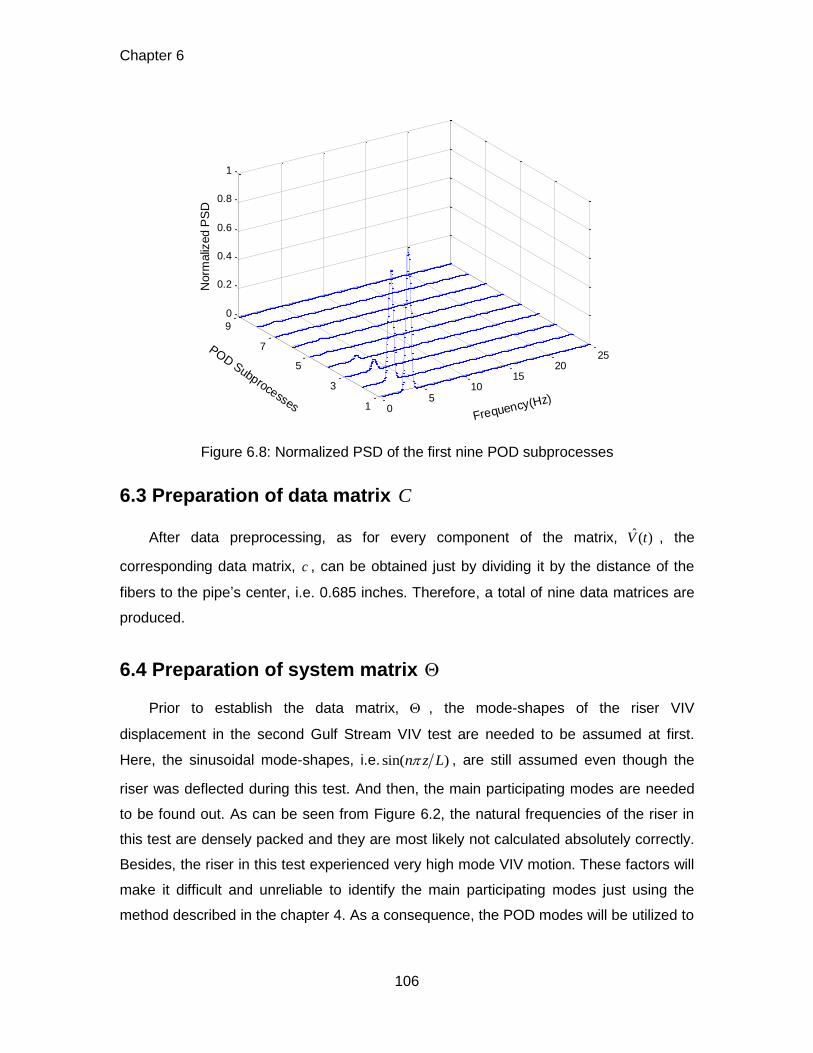
Chapter 6

106

Figure 6.8: Normalized PSD of the first nine POD subprocesses

6.3 Preparation of data matrix C

After data preprocessing, as for every component of the matrix, ˆ( )V t , the

corresponding data matrix, c , can be obtained just by dividing it by the distance of the

fibers to the pipe’s center, i.e. 0.685 inches. Therefore, a total of nine data matrices are

produced.

6.4 Preparation of system matrix

Prior to establish the data matrix, , the mode-shapes of the riser VIV

displacement in the second Gulf Stream VIV test are needed to be assumed at first.

Here, the sinusoidal mode-shapes, i.e. sin( )n z L , are still assumed even though the

riser was deflected during this test. And then, the main participating modes are needed

to be found out. As can be seen from Figure 6.2, the natural frequencies of the riser in

this test are densely packed and they are most likely not calculated absolutely correctly.

Besides, the riser in this test experienced very high mode VIV motion. These factors will

make it difficult and unreliable to identify the main participating modes just using the

method described in the chapter 4. As a consequence, the POD modes will be utilized to

05

1015

2025

1

3

5

7

9

0

0.2

0.4

0.6

0.8

1

Frequency(Hz)

POD Subprocesses

Norm

aliz

ed P

SD

Chapter 6

107

aid in identifying the main participating modes (Kleiven, 2002) [35]. The first POD mode

is plotted in Figure 6.9. The ‘o’ signs represent sensor locations.

Figure 6.9: The discrete mode-shape of the first POD mode

According to the number of the crests in Figure 6.9, it can be determined that the

primary participating mode associated with the first harmonic VIV response is about 27.

And I use the frequency method to make a judgement again. The 1X frequency, 3.45 Hz,

is not very close to the calculated natural frequency corresponding to the 27rd

eigenmode of the riser, 4.06 Hz. This disagreement means that the previously calculated

natural frequencies are a bit wrong. And due to the presence of travelling wave in the

VIV response in this test, the neighbouring modes around 27 should be included too and

the participating modes of 23-31 are chosen to reconstruct the first harmonic VIV

response finally.

After determining the participating modes for the first harmonic VIV response, the

system matrix, , in Equation (2.13) can be assembled. Finally, there is one point

needed to be noticed, which is that not too much participating modes are applied here,

and there are three purposes for this action. This first one is to prevent the occurrence of

spatial aliasing, i.e. the mode-shapes can partly act as substitutes for one another. If

spatial aliasing happens, the reconstruction result will be quite abnormal and large due

to the singularity of the system matrix. The second one is to prevent the reconstruction

-0.3 -0.2 -0.1 0 0.1 0.2 0.30

0.1

0.2

0.3

0.4

0.5

0.6

0.7

0.8

0.9

1

Re

lative

axia

l p

ositio

n (

z/L

, 0

at b

otto

m e

nd

)

First POD Mode

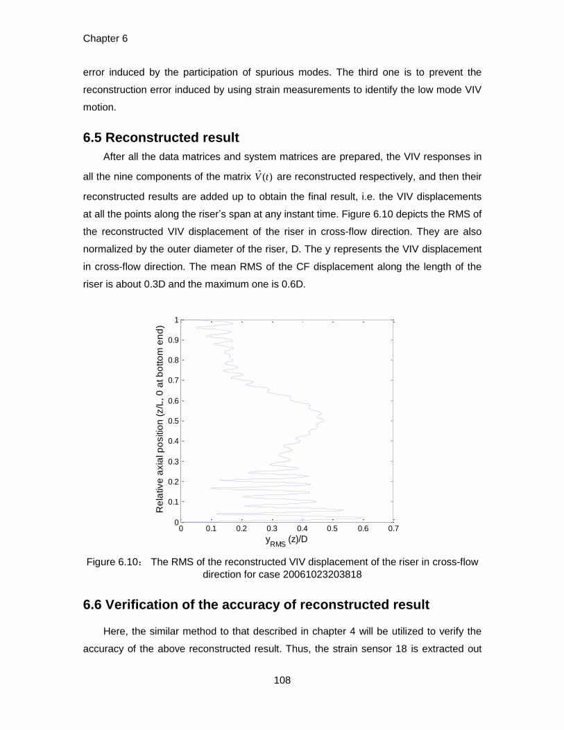
Chapter 6

108

error induced by the participation of spurious modes. The third one is to prevent the

reconstruction error induced by using strain measurements to identify the low mode VIV

motion.

6.5 Reconstructed result

After all the data matrices and system matrices are prepared, the VIV responses in

all the nine components of the matrix ˆ( )V t are reconstructed respectively, and then their

reconstructed results are added up to obtain the final result, i.e. the VIV displacements

at all the points along the riser’s span at any instant time. Figure 6.10 depicts the RMS of

the reconstructed VIV displacement of the riser in cross-flow direction. They are also

normalized by the outer diameter of the riser, D. The y represents the VIV displacement

in cross-flow direction. The mean RMS of the CF displacement along the length of the

riser is about 0.3D and the maximum one is 0.6D.

Figure 6.10： The RMS of the reconstructed VIV displacement of the riser in cross-flow

direction for case 20061023203818

6.6 Verification of the accuracy of reconstructed result

Here, the similar method to that described in chapter 4 will be utilized to verify the

accuracy of the above reconstructed result. Thus, the strain sensor 18 is extracted out

0 0.1 0.2 0.3 0.4 0.5 0.6 0.70

0.1

0.2

0.3

0.4

0.5

0.6

0.7

0.8

0.9

1

Re

lative

axia

l p

ositio

n (

z/L

, 0

at b

otto

m e

nd

)

yRMS

(z)/D

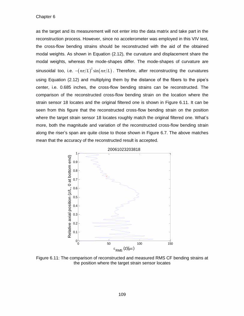
Chapter 6

109

as the target and its measurement will not enter into the data matrix and take part in the

reconstruction process. However, since no accelerometer was employed in this VIV test,

the cross-flow bending strains should be reconstructed with the aid of the obtained

modal weights. As shown in Equation (2.12), the curvature and displacement share the

modal weights, whereas the mode-shapes differ. The mode-shapes of curvature are

sinusoidal too, i.e. 2sinn L n L . Therefore, after reconstructing the curvatures

using Equation (2.12) and multiplying them by the distance of the fibers to the pipe’s

center, i.e. 0.685 inches, the cross-flow bending strains can be reconstructed. The

comparison of the reconstructed cross-flow bending strain on the location where the

strain sensor 18 locates and the original filtered one is shown in Figure 6.11. It can be

seen from this figure that the reconstructed cross-flow bending strain on the position

where the target strain sensor 18 locates roughly match the original filtered one. What’s

more, both the magnitude and variation of the reconstructed cross-flow bending strain

along the riser’s span are quite close to those shown in Figure 6.7. The above matches

mean that the accuracy of the reconstructed result is accepted.

Figure 6.11: The comparison of reconstructed and measured RMS CF bending strains at the position where the target strain sensor locates

0 50 100 1500

0.1

0.2

0.3

0.4

0.5

0.6

0.7

0.8

0.9

1

Re

lative

axia

l p

ositio

n (

z/L

, 0

at b

otto

m e

nd

)

RMS

(z)()

20061023203818

Chapter 6

110

6.7 Examples of error from choice of participating modes

In the chapter 2, it was mentioned that unreasonable choice of participating modes

would lead to the reconstruction error. Next, some examples will be given to

demonstrate it. In this test case, the modes of 23-31 were chosen previously to

reconstruct the first harmonic VIV response. Now, the participating modes are altered to

12-20 or 44-52 and the reconstruction results for these two choices are presented in

Figures 6.12 and 6.13. The former result is obviously wrong since the magnitude of the

VIV displacement in the region close to the riser top end could not be so large. The latter

one is also clearly not correct because the magnitude of the spatial mean RMS of the

cross-flow VIV displacement is around 0.35D generally. The intrinsic reason is that the

natural frequencies corresponding to the modes of 12-20 are quite lower than 1X

frequency and the natural frequencies corresponding to the modes of 44-52 are quite

higher than 1X frequency, so these two choices of participating modes are unreasonable.

Figure 6.12: The RMS of the reconstructed VIV displacement of the riser in cross-flow direction for the participating modes of 12-20

0 0.1 0.2 0.3 0.4 0.5 0.6 0.70

0.1

0.2

0.3

0.4

0.5

0.6

0.7

0.8

0.9

1

Re

lative

axia

l p

ositio

n (

z/L

, 0

at b

otto

m e

nd

)

yRMS

(z)/D

participating modes:12-20

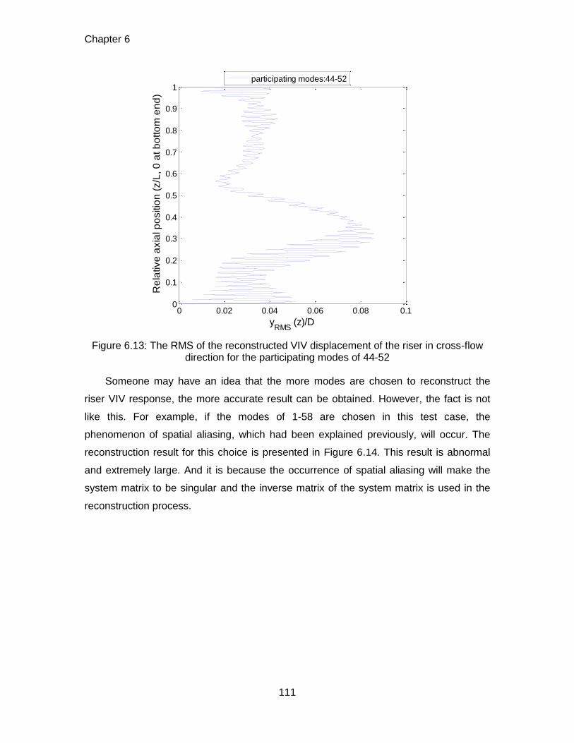
Chapter 6

111


Someone may have an idea that the more modes are chosen to reconstruct the

riser VIV response, the more accurate result can be obtained. However, the fact is not

like this. For example, if the modes of 1-58 are chosen in this test case, the

phenomenon of spatial aliasing, which had been explained previously, will occur. The

reconstruction result for this choice is presented in Figure 6.14. This result is abnormal

and extremely large. And it is because the occurrence of spatial aliasing will make the

system matrix to be singular and the inverse matrix of the system matrix is used in the

reconstruction process.

0 0.02 0.04 0.06 0.08 0.10

0.1

0.2

0.3

0.4

0.5

0.6

0.7

0.8

0.9

1

Re

lative

axia

l p

ositio

n (

z/L

, 0

at b

otto

m e

nd

)

yRMS

(z)/D


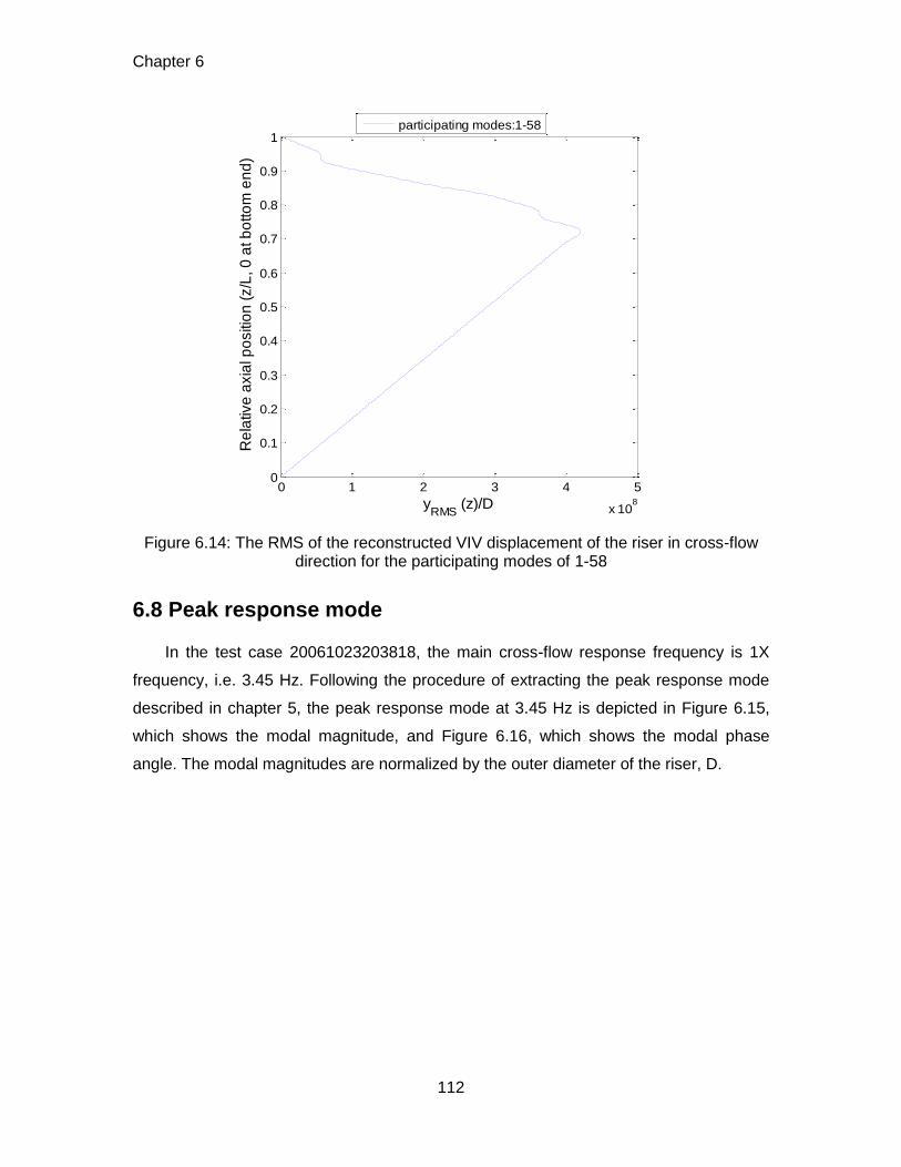
Chapter 6

112


6.8 Peak response mode

In the test case 20061023203818, the main cross-flow response frequency is 1X

frequency, i.e. 3.45 Hz. Following the procedure of extracting the peak response mode

described in chapter 5, the peak response mode at 3.45 Hz is depicted in Figure 6.15,

which shows the modal magnitude, and Figure 6.16, which shows the modal phase

angle. The modal magnitudes are normalized by the outer diameter of the riser, D.

0 1 2 3 4 5

x 108

0

0.1

0.2

0.3

0.4

0.5

0.6

0.7

0.8

0.9

1

Re

lativ

e a

xia

l po

siti

on

(z/L

, 0

at b

otto

m e

nd

)

yRMS

(z)/D


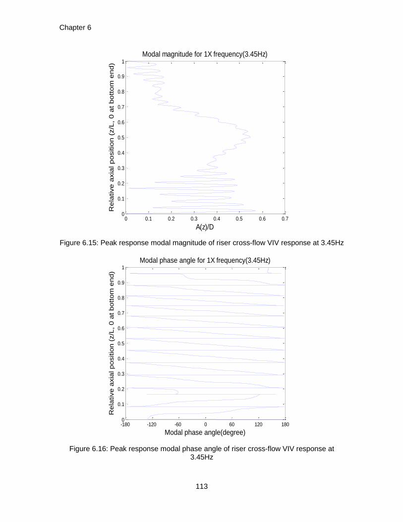
Chapter 6

113

Figure 6.15: Peak response modal magnitude of riser cross-flow VIV response at 3.45Hz

Figure 6.16: Peak response modal phase angle of riser cross-flow VIV response at 3.45Hz

0 0.1 0.2 0.3 0.4 0.5 0.6 0.70

0.1

0.2

0.3

0.4

0.5

0.6

0.7

0.8

0.9

1

Rela

tive a

xia

l positio

n (

z/L

, 0 a

t bottom

end)

A(z)/D

Modal magnitude for 1X frequency(3.45Hz)

-180 -120 -60 0 60 120 1800

0.1

0.2

0.3

0.4

0.5

0.6

0.7

0.8

0.9

1

Rela

tive a

xia

l positio

n (

z/L

, 0 a

t bottom

end)

Modal phase angle(degree)

Modal phase angle for 1X frequency(3.45Hz)

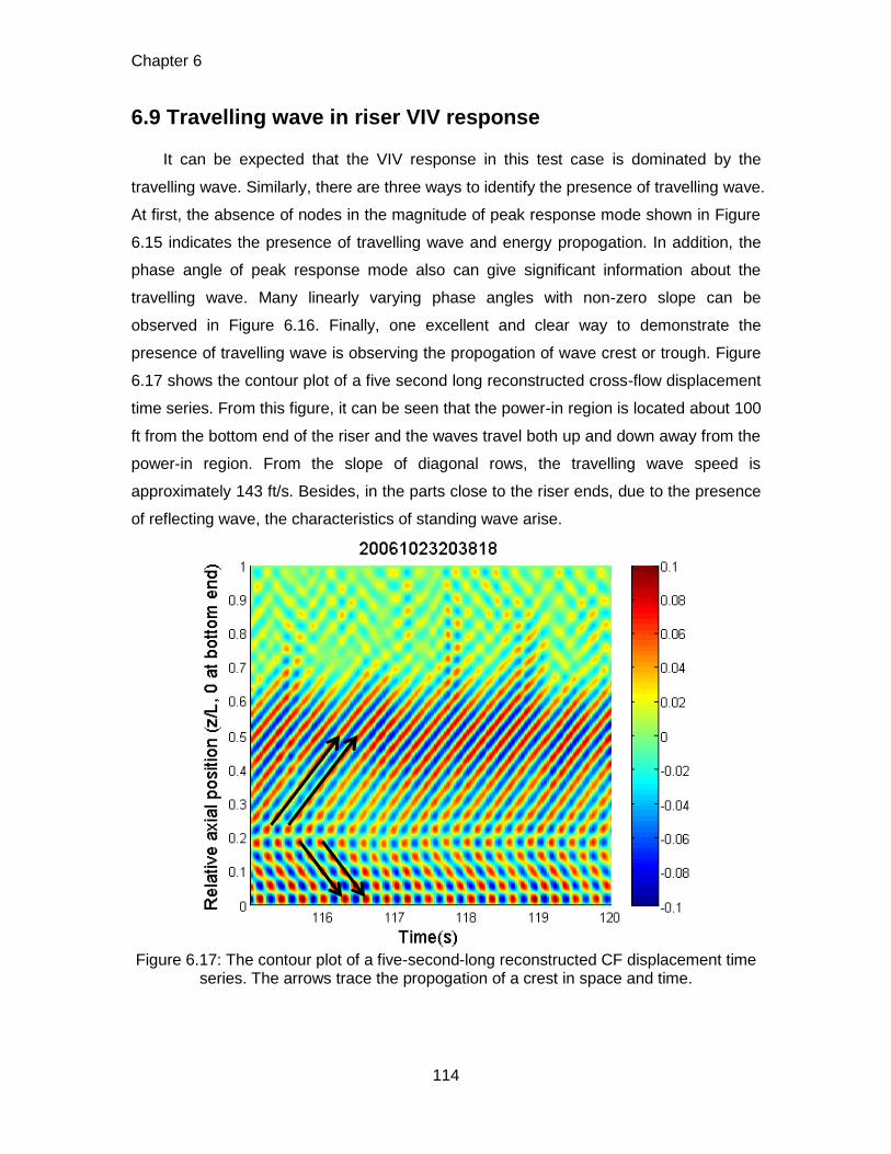
Chapter 6

114

6.9 Travelling wave in riser VIV response

It can be expected that the VIV response in this test case is dominated by the

travelling wave. Similarly, there are three ways to identify the presence of travelling wave.

At first, the absence of nodes in the magnitude of peak response mode shown in Figure

6.15 indicates the presence of travelling wave and energy propogation. In addition, the

phase angle of peak response mode also can give significant information about the

travelling wave. Many linearly varying phase angles with non-zero slope can be

observed in Figure 6.16. Finally, one excellent and clear way to demonstrate the

presence of travelling wave is observing the propogation of wave crest or trough. Figure

6.17 shows the contour plot of a five second long reconstructed cross-flow displacement

time series. From this figure, it can be seen that the power-in region is located about 100

ft from the bottom end of the riser and the waves travel both up and down away from the

power-in region. From the slope of diagonal rows, the travelling wave speed is

approximately 143 ft/s. Besides, in the parts close to the riser ends, due to the presence

of reflecting wave, the characteristics of standing wave arise.

Figure 6.17: The contour plot of a five-second-long reconstructed CF displacement time

series. The arrows trace the propogation of a crest in space and time.

Chapter 6

115

Chapter 7

116

Chapter 7

7 Conclusions

7.1 Summary of contributions from each chapter

The work presented in this thesis can be subdivided into four major parts. In the first

part of the thesis, the modal approach is chosen to do riser VIV response reconstruction.

In the second part of the thesis, the descriptions of ExxonMobil experimental and the

second Gulf Stream field VIV tests are done. In the third part of the thesis, the riser VIV

responses in these two tests are reconstructed using the modal approach. In the final

part of the theis, some analyses with regard to the riser VIV responses in tests are done

based on the reconstructed results.

7.1.1 Riser VIV response reconstruction method

In the chapter 2 of this thesis, the algorithms using the modal approach to

reconstruct the response of a riser from experimental data are developed. The specific

contributions of this chapter are as follows:

Theoretical basis and limitations of modal approach: The modal approach is

based on the theory of Modal Analysis. There are three limitations of the modal

approach. The first one is that the modal approach is a linear method, whereas the VIV

is a nonlinear problem. The second one is that the true mode-shapes of the riser’s VIV

displacement are not constant and very hard to find out. The sinusoidal mode-shape is

just an approximation. The final one is that the chosen participating modes can not be

perfectly correct.

Classification of modal approach: The modal approach can be classified into the

frequency domain method and time domain method. Choosing which method depends

on the types of provided measurements.

Chapter 7

117

Development of a systematic algorithm for riser VIV response reconstruction:

Two algorithms using the frequency domain method and time domain method

respectively are developed.

Response reconstruction error analysis: Two sources of error during response

reconstruction are identified. One is using strain measurement to identify the low modes

riser VIV motion. Another is unreasonable choice of participating modes.

7.1.2 Description of two objective VIV tests

In the chapter 3 of this thesis, the ExxonMobil experimental VIV test and the second

Gulf Stream field VIV test are described in detail. The description is focused on three

parts, i.e. experiment set-up, properties of riser model, and measurement system.

7.1.3 Response reconstruction using experimental data

In the chapter 4 of this thesis, the riser VIV responses in ExxonMobil experimental

VIV test are reconstructed from strain and acceleration signals using the frequency

domain method. In the chapter 6 of this thesis, one riser VIV response in the second

Gulf Stream field VIV test is reconstructed from only the strain signals using the time

domain method. The specific contributions of these two chapters are as follows:

Preparation of data matrix: In this section, the choice of time window is quite

important. In the chapter 4, the latter part of the period with almost constant current

velocity, i.e. the period during which the VIV behaviour is fully developed, is chosen. In

the chapter 6, the scalogram (time-frequency representation) is used to extract a

statistically region of a signal. In addition, in order to clear the harmful and unnecessary

frequency components of the data, it is band pass filtered using the butterworth digital

filter. Finally, in the chapter 6, due to the complex and nonuniform VIV response along

the length of the riser in field VIV test, the approach of Proper Orthogonal Decomposition

(POD) is used to decompose the experimental data and to extract the energetic and

regular components.

Preparation of system matrix: In this section, the most important part is the

choice of participating modes, which is based on the assumption that if one response

frequency falls between two natural frequencies, the two modes corresponding to these

two natural frequencies and their neighbouring modes will be excited. In the chapter 4,

the choice of participating modes is based on the simply calculated natural frequencies

of the riser in still water and spectral analysis of the experimental data. In the chapter 6,

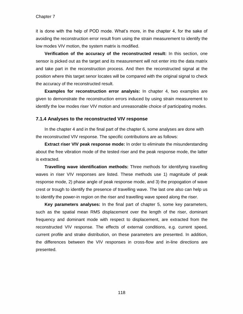
Chapter 7

118

it is done with the help of POD mode. What’s more, in the chapter 4, for the sake of

avoiding the reconstruction error result from using the strain measurement to identify the

low modes VIV motion, the system matrix is modified.

Verification of the accuracy of the reconstructed result: In this section, one

sensor is picked out as the target and its measurement will not enter into the data matrix

and take part in the reconstruction process. And then the reconstructed signal at the

position where this target senor locates will be compared with the original signal to check

the accuracy of the reconstructed result.

Examples for reconstruction error analysis: In chapter 4, two examples are

given to demonstrate the reconstruction errors induced by using strain measurement to

identify the low modes riser VIV motion and unreasonable choice of participating modes.

7.1.4 Analyses to the reconstructed VIV response

In the chapter 4 and in the final part of the chapter 6, some analyses are done with

the reconstructed VIV response. The specific contributions are as follows:

Extract riser VIV peak response mode: In order to eliminate the misunderstanding

about the free vibration mode of the tested riser and the peak response mode, the latter

is extracted.

Travelling wave identification methods: Three methods for identifying travelling

waves in riser VIV responses are listed. These methods use 1) magnitude of peak

response mode, 2) phase angle of peak response mode, and 3) the propogation of wave

crest or trough to identify the presence of travelling wave. The last one also can help us

to identify the power-in region on the riser and travelling wave speed along the riser.

Key parameters analyses: In the final part of chapter 5, some key parameters,

such as the spatial mean RMS displacement over the length of the riser, dominant

frequency and dominant mode with respect to displacement, are extracted from the

reconstructed VIV response. The effects of external conditions, e.g. current speed,

current profile and strake distribution, on these parameters are presented. In addition,

the differences between the VIV responses in cross-flow and in-line directions are

presented.

Chapter 7

119

7.2 Recommendations for future research

Although the riser VIV response can be reconstructed using the modal approach

and some analyses are done about VIV characteristics, there are some

recommendations with regard to the future research of this subject.

Improvement of the modal approach or new reconstruction approach: As

mentioned in the chapter 2 of this thesis, the modal approach has some limitations. The

sinusoidal mode-shapes used in this thesis are just approximations. Thus, a finite

element model can be built to find the more closed mode-shapes of the tested riser and

its natural frequencies. Alternatively, the method of superposing the peak response

modes, which can be obtained by means of prediction programs like VIVA, to

reconstruct riser VIV response.

Verification of the accuracy of the reconstructed result: If the benchmark data

are given, the verification of the accuracy of the reconstructed result will be more reliable.

Besides, the choice of participating modes will become more accurate and so the

response reconstruction error analysis will become more precise.

Analysis to the riser VIV response: Some important coefficients, such as the lift

force coefficient and drag force coefficient can be extracted base on the reconstructed

VIV response. And the VIV fatigue life along the length of the riser can be calculated

from the reconstructed bending strains. These results will provide benchmark

information for the VIV prediction program.

Bibliography

120

Bibliography

[1] Blevins, R.D., 1990. Flow-Induced Vibration, second edition. Van Nostrand Reinhold, New York.

[2] H.Blackburn and R.Henderson. Lock-in behaviour in simulated vortex-induced vibration. Experimental Thermal and Fluid Science, Volume 12, Issue 2, February 1996, Pages 184-189.

[3] M.R.Gharib. Vortex-Induced Vibration, Absence of Lock-in and Fluid Force Deduction. Phd Thesis, California Institute of Technology, Source DAI-B 62/04, p.1922, Oct 2001,182 pages,1999.

[4] Sarpkaya, T., 1978, Fluid forces on oscillating cylinders. Journal of The Waterway, Port, Costal and Ocean Division 104, 275-290.

[5] Gopalkrishman, R., 1993, Vortex-induced Forces on Oscillating Bluff Cylinders, Ph.D. Thesis, MIT, Cambridge, MA,USA.

[6] Lie, H., Larsen, C.M., Vandiver, J.K., 1997. Vortex induced vibrations of long marine riser; model test in a rotating rig. 16th International Conference on Offshore Mechanics and Arctic Engineering, Yokohama, Japan.

[7] Lienhard, I.H, 1996. Synopsis of lift, drag and vortex frequency data for rigid circular cylinders. Washington State University, college of Engineering, Research Division Bulletin 300.

[8] T.Sarkaya. A Critical Review of the Intrinsic Nature of Vortex-Induced Vibrations. Journal of Fluids and Structures, 19:389-447,2004.

[9] W.R. Frank, M.A. Tognarelli, S.T. Slocum, R.B. Campbell, and S. Balasubramanian. Flow-Induced Vibration of a Long, Flexible, Straked Cylinder in Uniform and Linearly Sheared Currents. In Proceedings of the Offshore Technology Conference, Paper no. 16340, Houston, USA, 2004.

[10] H.Braaten and H.Lie. NDP Riser High Mode VIV Tests. Main Report No. 512394.00.01. Norwegian Marine Technology Research Institute, 2004.

[11] E.Huse, G.Kleiven, and F.G. Nielsen. Large Scale Model Testing of Deep Sea Risers. In Proceedings of the Offshore Technology Conference, Paper no. 8701, Houston, USA, 1998.

[12] J.K. Vandiver, H. Marcollo, S. Fantone, V. Jaiswal, V. Jhingran, and S. Swithenbank. DeepStar 7402Miami 2004 riser report. Deepstar-7402-Miami testing, Massachusetts Institute of Technology, Cambridge, MA, USA, 2005.

Bibliography

121

[13] J.K. Vandiver, S.Swithenbank, V,Jaiswal, and V.Jhingran. Fatigue damage from high mode number vortex-induced vibration. In Proceedings of the 25th International Conference on Offshore Mechanics and Arctic Engineering (OMAE), Hamburg, Germany, June 2006.

[14] J.K. Vandiver and L.Lee. SHEAR7 V4.4 Program Theoretical Manual. Massachusetts Institute of Technology, Cambridge, MA, 2005

[15] Triantafyllou, M.S, Triantafyllou, G.S., Tein, D., Ambrose, B.D., 1999. Pragmatic riser VIV analysis. In: Proceedings from the Offshore Technology Conference, OTC 10931, Houston, USA.

[16] MARINTEK, 2001, VIVANA-Theory Manual. MARINTEK Report MTF00-023, MARINTEK, Trondheim, Norway.

[17] Moe, G., Arntsen, Ø.A., Hoen, C., 2001. VIV analysis of risers by complex modes. In: Proceedings from the International Symposium on Offshore and Polar Engineering, IL-38.

[18] Etienne, S., Biolley, F., Fontaine, E., Le Cunff, C., Heurtier,J.M., 2001. Numerical simulations of vortex-induced vibrations of slender flexible offshore structures. In: Proceedings of the 11th International Offshore and Polar Engineering Conference, Stavanger, Norway, pp. 419-425.

[19] Willden, R.H.J., Graham, J.M.R., 2001. Numerical prediction of VIV on long flexible circular cylinders. Journal of Fluids and Structures 15, 659-669.

[20] Kaasen, K.E., Lie, H., Solaas, F., Vandiver, J.K., 2000. Norwegian Deepwater Programme: Analysis of vortex-induced vibrations of marine risers based on full-scale measurements. OTC 11997, Offshore Technology Conference, Houston, Texas, USA.

[21] Trim, A.D., Braaten, H., Lie, H., Tognarelli, M.A., 2005. Experimental investigation of vortex-induced vibration of long marine risers. Journal of Fluids and Structures 21, 335-361.

[22] Lie, H., Kaasen, K.E., 2006. Modal analysis of measurements from a large-scale VIV model test of a riser in linearly sheared flow. Journal of Fluids and Structures 22, 557-575..

[23] J.M.J. Spijkers, A.W.C.M. Vrouwenvelder, E.C. Klaver, 2005. Structural Dynamics. Delft University of Technology, Pages 35-38.

[24] Vortex-Induced Vibration Data Repository (VIVDR). Site hosted by Center for Ocean Engineering, Massachusetts Institute of Technology, Cambridge, MA, USA, 2007, http://web.mit.edu/towtank/www/vivdr/datasets.html.

[25] M.A.Tognarelli and H.Lie. VIV Suppression Tests on High L/D Flexible Cylinders. Main Report No. 512382.00.01. Norwegian Marine Technology Research Institute, 2003.

[26] Vandiver J.K., Swithenbank S.B., Jaiswal V. and Jhingran V., 2007. DeepStar 8402: Gulf Stream Experiment October 2006, Document No.DSVIII CTR 8402, Massachusetts Institute of Technology.

[27] Tognarelli, M.A., Slocum, S.T., Frank, W.R., Campbell, R.B. 2004. VIV response of a long flexible cylinder in uniform and linearly sheared currents, OTC 16338, Offshore Technology Conference, Houston, Texas, USA.

http://web.mit.edu/towtank/www/vivdr/datasets.html

Bibliography

122

[28] Lie, H., Larsen, C.M., Vandiver, J.K., 1997. Vortex induced vibrations of long marine risers; model test in a ratating rig. OMAE Conference, Vol. 1-B, Yokohama,Japan, pp.241-252.

[29] Larsen, C.M., Koushan, K., 2005. Empirical model for the analysis of vortex induced vibrations of free spanning pipelines. EURODYN Conference, Paris, France.

[30] Marcollo, H., Chaurasia, H. and Vandiver, J.K., Phenomenon Observed in VIV Bare Riser Field Tests, Proceedings of the 26th International Conference on Offshore Mechanics and Arctic Engineering, 2007, OMAE2007-29562.

[31] A. Grossmann, J. Morlet. Decomposition of hardy functions into square integrable wavelets of constant shape. SIAM.J.MATH.ANAL, Vol.15, No.4, July 1984.

[32] Mukundan H., 2008. Vortex-induced vibration of marine risers: motion and force reconstruction from field and experimental data. Ph. D. Thesis, Massachusetts Institute of Technology, Cambridge, MA, USA.

[33] Srivilairit, T., Manuel, L., and Saranyasoontorn, K., 2006. On the use of empirical orthogonal decomposition of field data to study deepwater current profiles for risers. In Proceedings of the 16th International Offshore and Polar Engineering Conference (ISOPE-2006), San Francisco, California, May 2006.

[34] Shi, C., and Manuel, L., 2016. An empirical procedure for fatigue damage estimation in instrumented risers. In Proceedings of the 35th International Conference on Ocean, Offshore and Arctic Engineering (OMAE2016-54623), Busan, Korea, June 2016.

[35] Kleiven, G., 2002. Identifying VIV vibration modes by use of the empirical orthogonal functions technique. In Proceedings of 21st International Conference on Offshore Mechanics and Arctic Engineering (OMAE2002), Oslo, Norway, June 2002.

Bibliography

123

Appendix A

124

Appendix A

Fairing and strake configurations

40% all at 25% on 50% 50% 62% 84%

bottom end both ends Center Staggered Staggered Staggered

Figure A.1: Strake Configurations

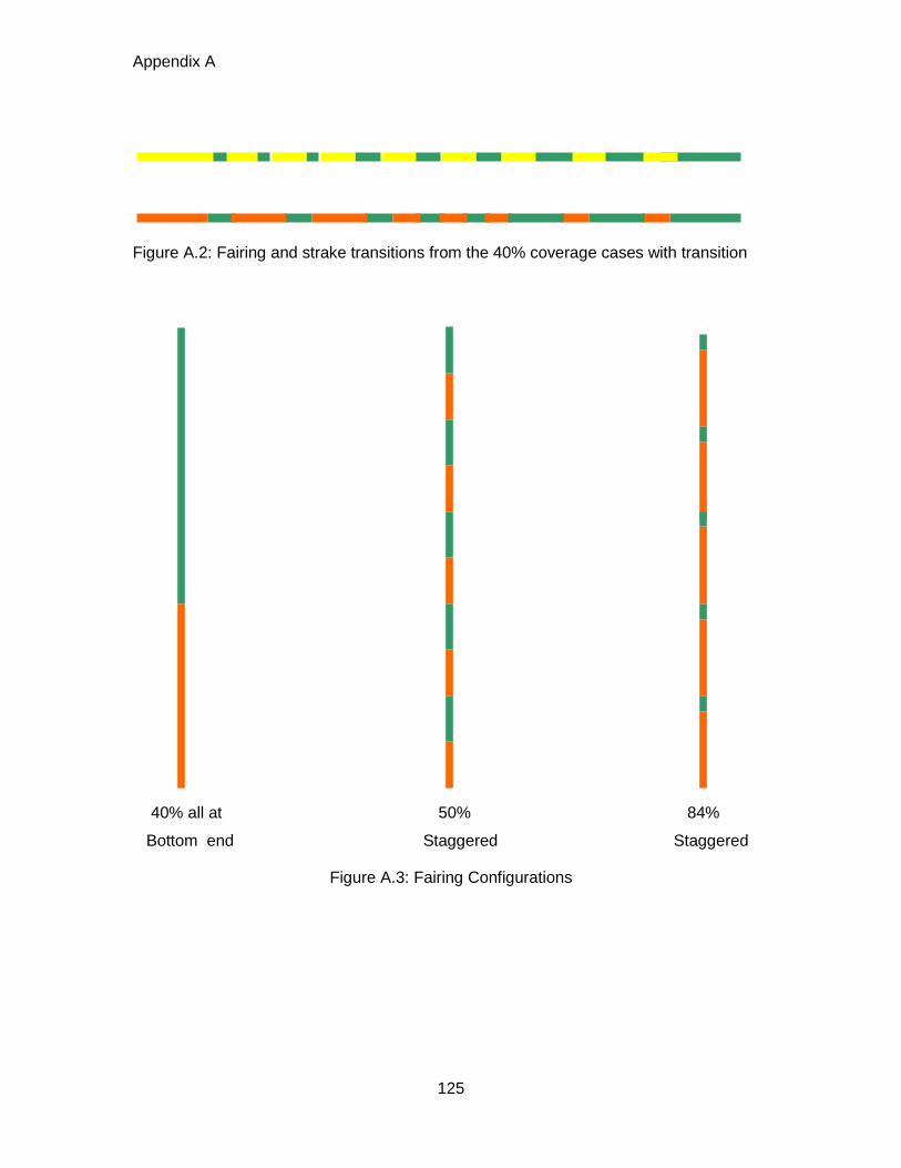
Appendix A

125

Figure A.2: Fairing and strake transitions from the 40% coverage cases with transition

40% all at 50% 84%

Bottom end Staggered Staggered

Figure A.3: Fairing Configurations

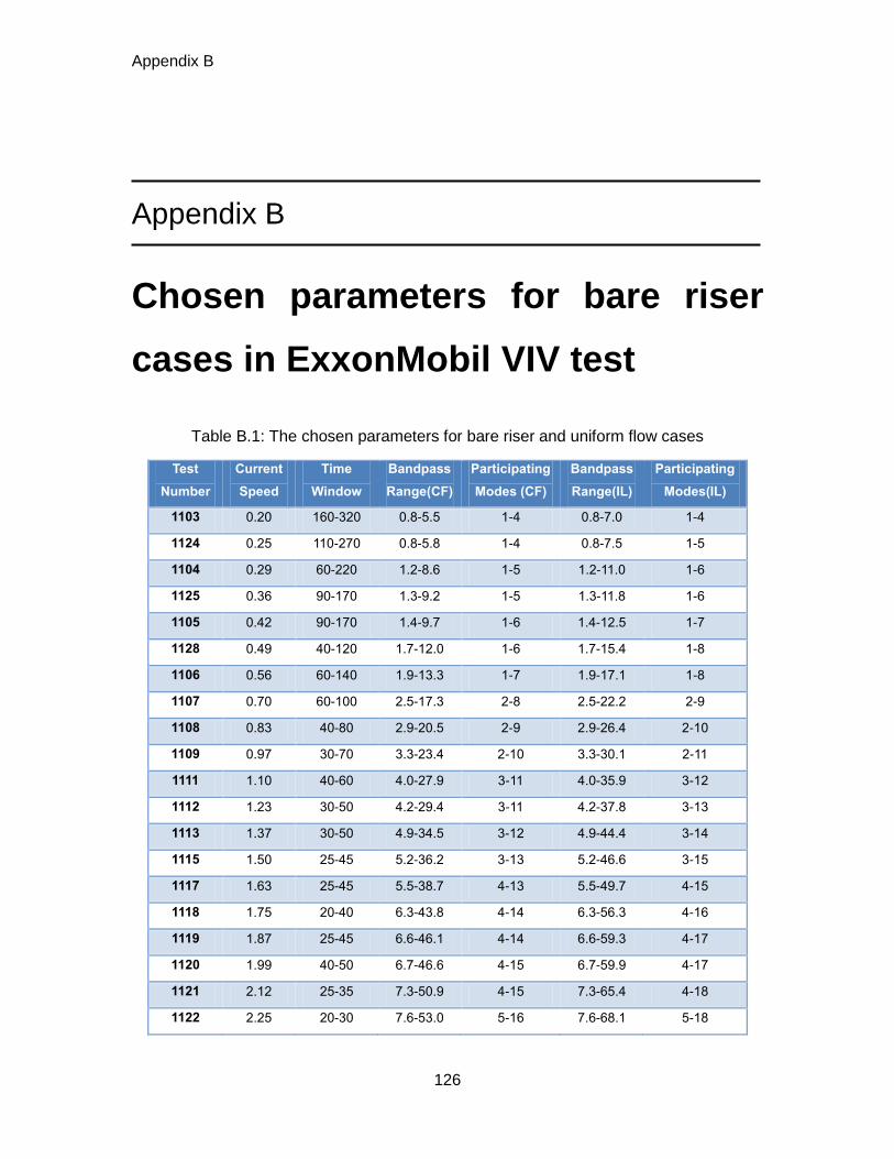
Appendix B

126

Appendix B

Chosen parameters for bare riser

cases in ExxonMobil VIV test

Table B.1: The chosen parameters for bare riser and uniform flow cases

Test

Number

Current

Speed

Time

Window

Bandpass

Range(CF)

Participating

Modes (CF)

Bandpass

Range(IL)

Participating

Modes(IL)

1103 0.20 160-320 0.8-5.5 1-4 0.8-7.0 1-4

1124 0.25 110-270 0.8-5.8 1-4 0.8-7.5 1-5

1104 0.29 60-220 1.2-8.6 1-5 1.2-11.0 1-6

1125 0.36 90-170 1.3-9.2 1-5 1.3-11.8 1-6

1105 0.42 90-170 1.4-9.7 1-6 1.4-12.5 1-7

1128 0.49 40-120 1.7-12.0 1-6 1.7-15.4 1-8

1106 0.56 60-140 1.9-13.3 1-7 1.9-17.1 1-8

1107 0.70 60-100 2.5-17.3 2-8 2.5-22.2 2-9

1108 0.83 40-80 2.9-20.5 2-9 2.9-26.4 2-10

1109 0.97 30-70 3.3-23.4 2-10 3.3-30.1 2-11

1111 1.10 40-60 4.0-27.9 3-11 4.0-35.9 3-12

1112 1.23 30-50 4.2-29.4 3-11 4.2-37.8 3-13

1113 1.37 30-50 4.9-34.5 3-12 4.9-44.4 3-14

1115 1.50 25-45 5.2-36.2 3-13 5.2-46.6 3-15

1117 1.63 25-45 5.5-38.7 4-13 5.5-49.7 4-15

1118 1.75 20-40 6.3-43.8 4-14 6.3-56.3 4-16

1119 1.87 25-45 6.6-46.1 4-14 6.6-59.3 4-17

1120 1.99 40-50 6.7-46.6 4-15 6.7-59.9 4-17

1121 2.12 25-35 7.3-50.9 4-15 7.3-65.4 4-18

1122 2.25 20-30 7.6-53.0 5-16 7.6-68.1 5-18

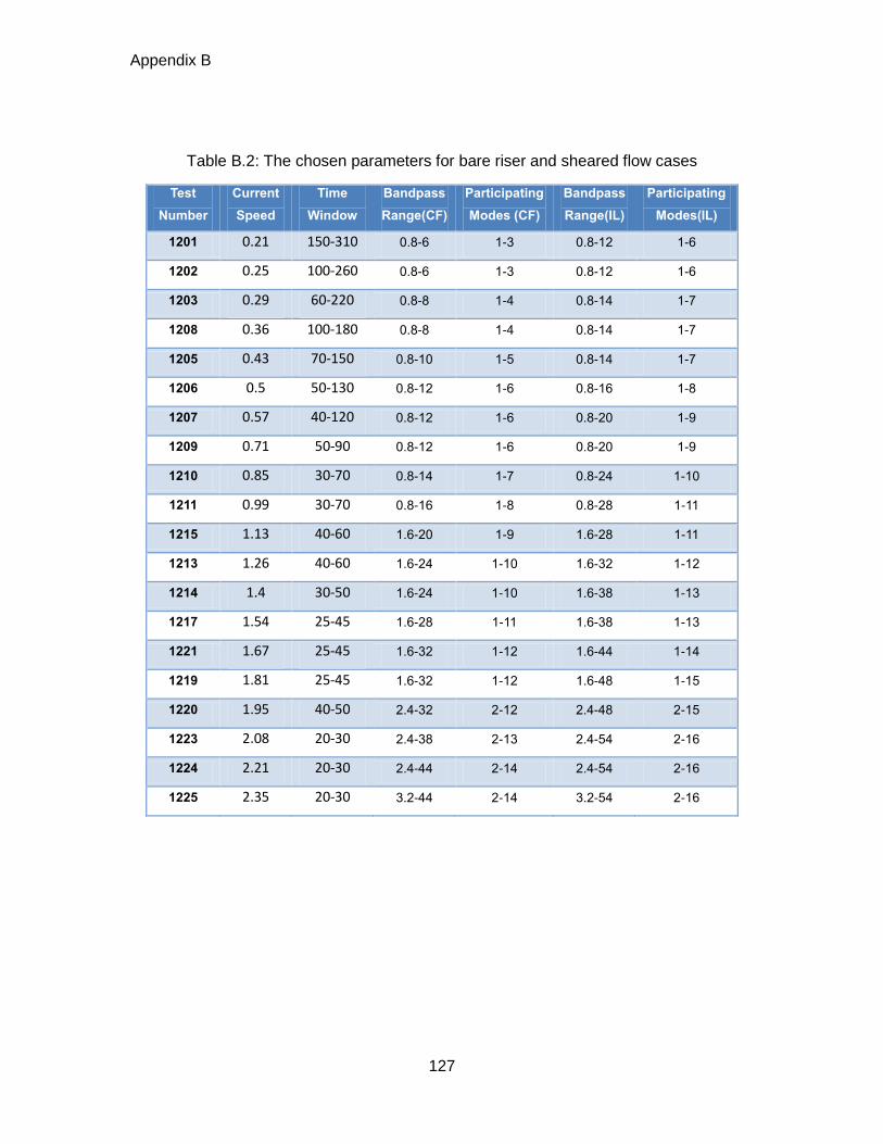
Appendix B

127

Table B.2: The chosen parameters for bare riser and sheared flow cases

Test

Number

Current

Speed

Time

Window

Bandpass

Range(CF)

Participating

Modes (CF)

Bandpass

Range(IL)

Participating

Modes(IL)

1201 0.21 150-310 0.8-6 1-3 0.8-12 1-6

1202 0.25 100-260 0.8-6 1-3 0.8-12 1-6

1203 0.29 60-220 0.8-8 1-4 0.8-14 1-7

1208 0.36 100-180 0.8-8 1-4 0.8-14 1-7

1205 0.43 70-150 0.8-10 1-5 0.8-14 1-7

1206 0.5 50-130 0.8-12 1-6 0.8-16 1-8

1207 0.57 40-120 0.8-12 1-6 0.8-20 1-9

1209 0.71 50-90 0.8-12 1-6 0.8-20 1-9

1210 0.85 30-70 0.8-14 1-7 0.8-24 1-10

1211 0.99 30-70 0.8-16 1-8 0.8-28 1-11

1215 1.13 40-60 1.6-20 1-9 1.6-28 1-11

1213 1.26 40-60 1.6-24 1-10 1.6-32 1-12

1214 1.4 30-50 1.6-24 1-10 1.6-38 1-13

1217 1.54 25-45 1.6-28 1-11 1.6-38 1-13

1221 1.67 25-45 1.6-32 1-12 1.6-44 1-14

1219 1.81 25-45 1.6-32 1-12 1.6-48 1-15

1220 1.95 40-50 2.4-32 2-12 2.4-48 2-15

1223 2.08 20-30 2.4-38 2-13 2.4-54 2-16

1224 2.21 20-30 2.4-44 2-14 2.4-54 2-16

1225 2.35 20-30 3.2-44 2-14 3.2-54 2-16

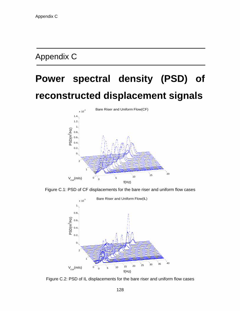
Appendix C

128

Appendix C

Power spectral density (PSD) of

reconstructed displacement signals

Figure C.1: PSD of CF displacements for the bare riser and uniform flow cases

Figure C.2: PSD of IL displacements for the bare riser and uniform flow cases

05

1015

20

0

1

2

0

0.2

0.4

0.6

0.8

1

1.2

1.4

x 10-4

f(Hz)

Bare Riser and Uniform Flow(CF)

Vcur

(m/s)

PS

D(m

2/H

z)

0 5 10 15 20 25 30 35 40

0

1

2

0

0.2

0.4

0.6

0.8

1

x 10-5

f(Hz)

Bare Riser and Uniform Flow(IL)

Vcur

(m/s)

PS

D(m

2/H

z)

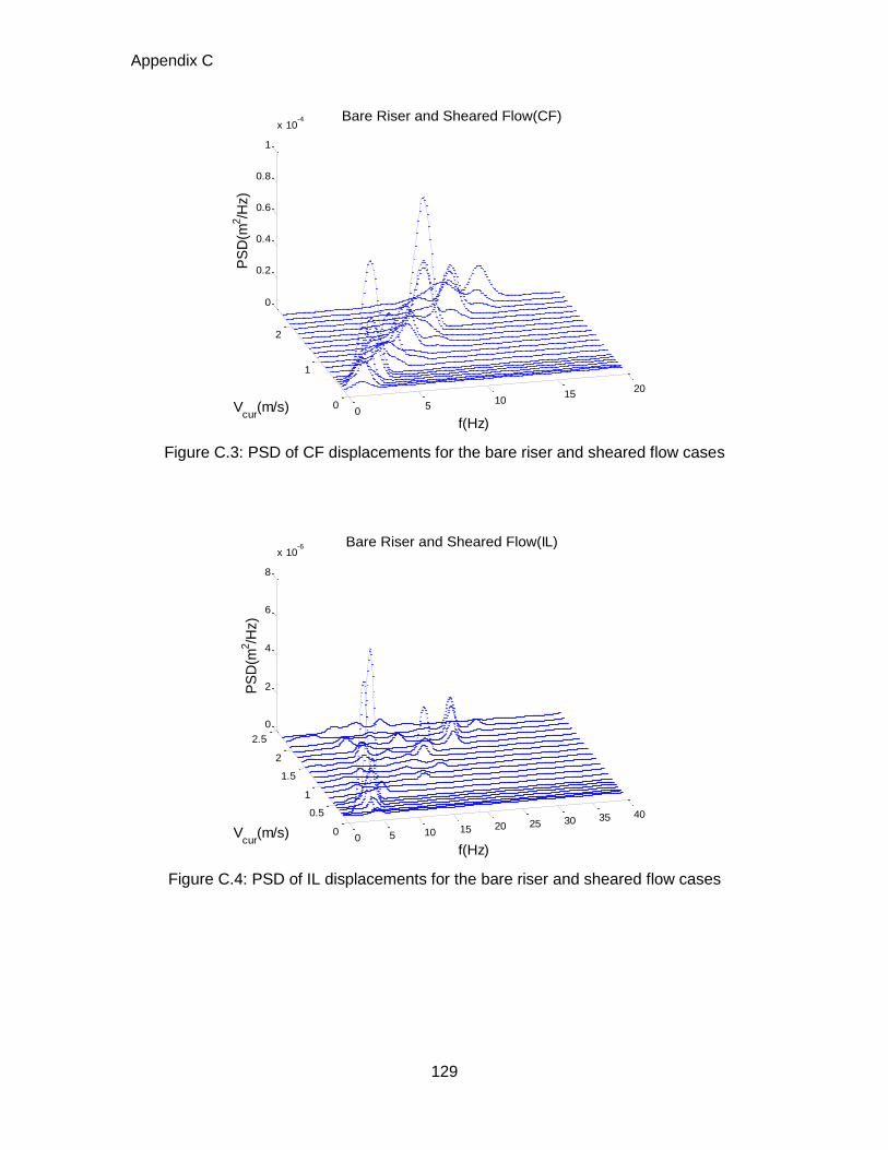
Appendix C

129

Figure C.3: PSD of CF displacements for the bare riser and sheared flow cases

Figure C.4: PSD of IL displacements for the bare riser and sheared flow cases

05

1015

20

0

1

2

0

0.2

0.4

0.6

0.8

1

x 10-4

f(Hz)

Bare Riser and Sheared Flow(CF)

Vcur

(m/s)

PS

D(m

2/H

z)

0 5 10 15 20 25 30 35 40

0

0.5

1

1.5

2

2.5

0

2

4

6

8

x 10-6

f(Hz)

Bare Riser and Sheared Flow(IL)

Vcur

(m/s)

PS

D(m

2/H

z)

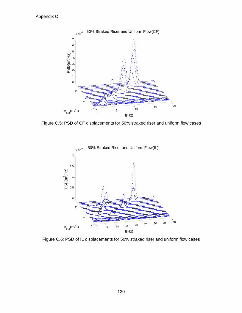
Appendix C

130

Figure C.5: PSD of CF displacements for 50% straked riser and uniform flow cases

Figure C.6: PSD of IL displacements for 50% straked riser and uniform flow cases

05

1015

20

0

1

2

0

1

2

3

4

5

6

7

x 10-5

f(Hz)

50% Straked Riser and Uniform Flow(CF)

Vcur

(m/s)

PS

D(m

2/H

z)

0 5 10 15 20 25 30 35 40

0

1

2

0

0.5

1

1.5

2

x 10-6

f(Hz)

50% Straked Riser and Uniform Flow(IL)

Vcur

(m/s)

PS

D(m

2/H

z)

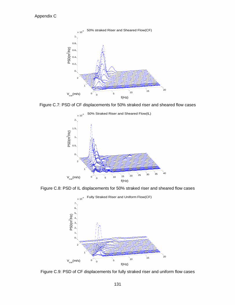
Appendix C

131

Figure C.7: PSD of CF displacements for 50% straked riser and sheared flow cases

Figure C.8: PSD of IL displacements for 50% straked riser and sheared flow cases

Figure C.9: PSD of CF displacements for fully straked riser and uniform flow cases

05

1015

20

0

1

2

0

0.2

0.4

0.6

0.8

1

x 10-6

f(Hz)

50% straked Riser and Sheared Flow(CF)

Vcur

(m/s)

PS

D(m

2/H

z)

0 5 10 15 20 25 30 35 40

0

1

2

0

0.5

1

1.5

2

x 10-8

f(Hz)

50% Straked Riser and Sheared Flow(IL)

Vcur

(m/s)

PS

D(m

2/H

z)

05

1015

20

0

1

2

0

1

2

3

4

5

6

7

x 10-8

f(Hz)

Fully Straked Riser and Uniform Flow(CF)

Vcur

(m/s)

PS

D(m

2/H

z)

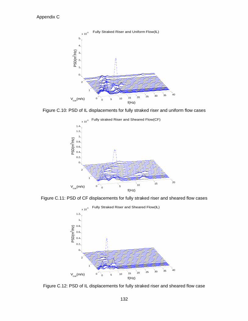
Appendix C

132

Figure C.10: PSD of IL displacements for fully straked riser and uniform flow cases

Figure C.11: PSD of CF displacements for fully straked riser and sheared flow cases

Figure C.12: PSD of IL displacements for fully straked riser and sheared flow case

0 5 10 15 20 25 30 35 40

0

1

2

0

1

2

3

4

5

x 10-9

f(Hz)

Fully Straked Riser and Uniform Flow(IL)

Vcur

(m/s)

PS

D(m

2/H

z)

05

1015

20

0

1

2

0

0.2

0.4

0.6

0.8

1

1.2

1.4

x 10-8

f(Hz)

Fully straked Riser and Sheared Flow(CF)

Vcur

(m/s)

PS

D(m

2/H

z)

0 5 10 15 20 25 30 35 40

0

1

2

0

0.2

0.4

0.6

0.8

1

1.2

x 10-8

f(Hz)

Fully Straked Riser and Sheared Flow(IL)

Vcur

(m/s)

PS

D(m

2/H

z)

Appendix C

133

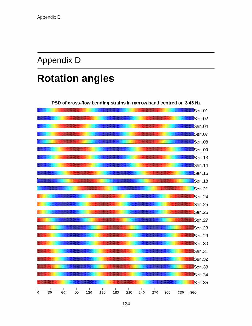
Appendix D

134

Appendix D

Rotation angles

PSD of cross-flow bending strains in narrow band centred on 3.45 Hz

Sen.01

Sen.02

Sen.04

Sen.07

Sen.08

Sen.09

Sen.13

Sen.14

Sen.16

Sen.18

Sen.21

Sen.24

Sen.25

Sen.26

Sen.27

Sen.28

Sen.29

Sen.30

Sen.31

Sen.32

Sen.33

Sen.34

Sen.35

0 30 60 90 120 150 180 210 240 270 300 330 360

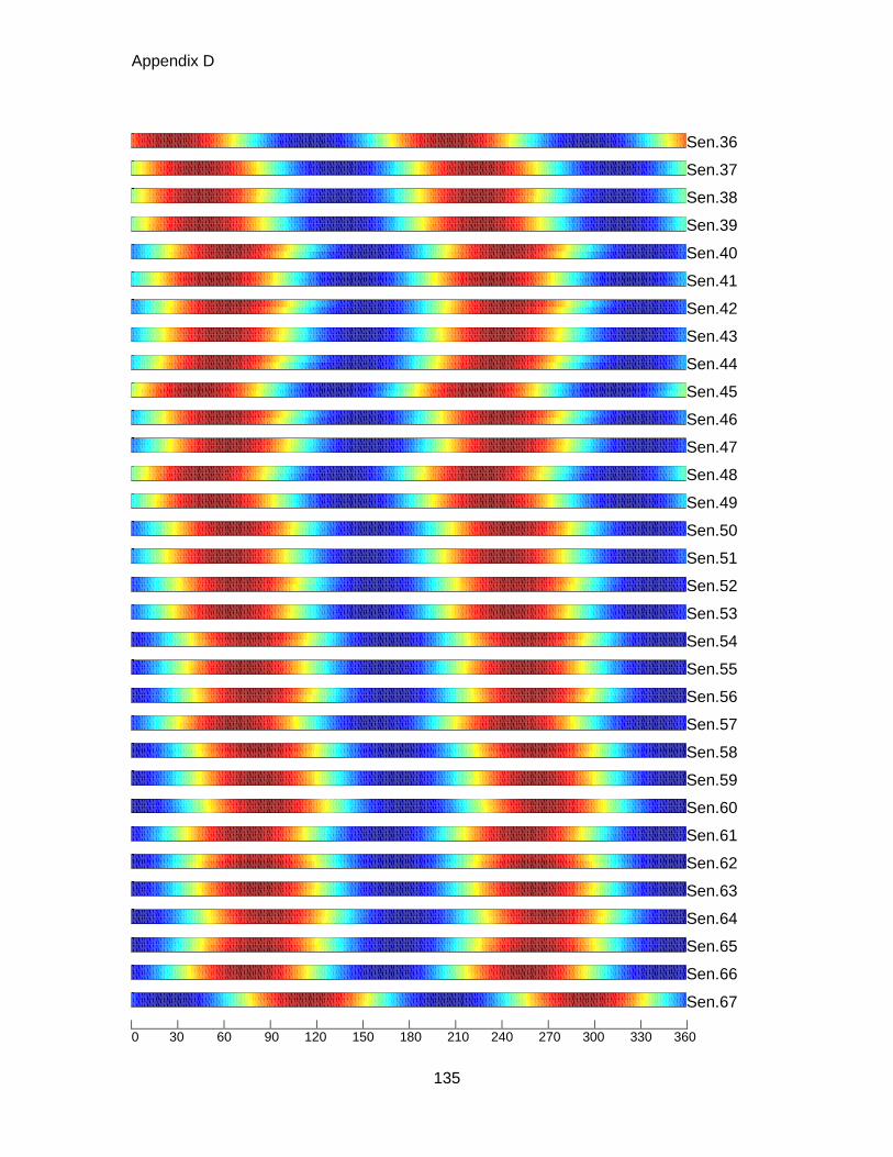
Appendix D

135

Sen.36

Sen.37

Sen.38

Sen.39

Sen.40

Sen.41

Sen.42

Sen.43

Sen.44

Sen.45

Sen.46

Sen.47

Sen.48

Sen.49

Sen.50

Sen.51

Sen.52

Sen.53

Sen.54

Sen.55

Sen.56

Sen.57

Sen.58

Sen.59

Sen.60

Sen.61

Sen.62

Sen.63

Sen.64

Sen.65

Sen.66

Sen.67

0 30 60 90 120 150 180 210 240 270 300 330 360

Appendix D

136

Sen.68

Sen.69

Sen.70

0 30 60 90 120 150 180 210 240 270 300 330 360

Rotation angle

Figure D.1: Illustration of determining rotation angles of Q1-Q3 plane to cross-flow direction at all the sensor locations by identifying maxima in the PSD of cross-flow

bending strains around 1X frequency (3.45 HZ)

0 50 100 150 200 250 300 350

Documents

Motion Reconstruction of Vortex-Induced Vibration of Long