Ann. Inst. Statist. Math. Vol. 57, No. 4, 617-635 (2005) Q2005 The Institute of Statistical Mathematics

NONLINEAR REGRESSION MODELING USING REGULARIZED LOCAL LIKELIHOOD METHOD

YOSHISUKE NONAKA* AND SADANORI KONISHI

Graduate School of Mathematics, Kyushu University, 6-10-1 Hakozaki, Higashi-Ku, Fukuoka 812-8581, Japan, e-mail: konishi@math.kyushu-u.ac.jp

(Received December 16, 2003; revised August 6, 2004)

Abs t r a c t . We introduce a nonlinear regression modeling strategy, using a regular- ized local likelihood method. The local likelihood method is effective for analyzing data with complex structure. It might be, however, pointed out that the stability of the local likelihood estimator is not necessarily guaranteed in the case that the struc- ture of system is quite complex. In order to overcome this difficulty, we propose a regularized local likelihood method with a polynomial function which unites local like- lihood and regularization. A crucial issue in constructing nonlinear regression models is the choice of a smoothing parameter, the degree of polynomial and a regularization parameter. In order to evaluate models estimated by the regularized local likelihood method, we derive a model selection criterion from an information-theoretic point of view. Real data analysis and Monte Carlo experiments are conducted to examine the performance of our modeling strategy.

Key words and phrases: Information criteria, local maximum likelihood estimates, model selection, generalized linear models, regularization.

1. Introduction

Local likelihood est imation has received considerable a t ten t ion as a useful technique for analyzing da ta with complex s t ruc ture (Tibshirani and Hastie (1987), Hjort and Jones (1996), Copas and Eguchi (1998), nguchi and Copas (1998), Loader (1999), nguchi and Kim (2001), Eguchi et al. (2003), and so on).

A local likelihood function is cons t ructed based on first considering a paramet r ic model for the unknown t rue model. It is defined as a locally weighted log-likelihood with weights determined by a kernel function and a bandwidth. When a large bandwid th is chosen, the es t imator is close to the max imum likelihood es t imator and tends to have a large bias. On the other hand, when a small bandwid th is chosen, the es t imator depends much on the da ta points and tends to have a large variance. In the local modeling, bandwidth plays an impor tan t role for controling the trade-off between bias and variance of the est imator (Wand and Jones (1995), Simonoff (1996)).

Issues still remain in construct ing nonlinear regression models based on the local likelihood from a finite and noisy set of data. First, the stabil i ty of local likelihood esti- mators is not guaranteed in the case tha t the s t ructure of the system is quite complex.

*Now at Biostatistics Center, Kurume University, 67 Asahi-Machi, Kurume, Fukuoka 830-0011, Japan, e-maih nonaka_yoshisuke@kurume-u.ac.jp.

617

618 YOSHISUKE NONAKA AND SADANORI KONISHI

In order to overcome this issue, we introduce a regularized local likelihood function with regularization parameter that controls the local likelihood function and the complex- ity of a nonlinear regression model. Second, the local likelihood procedure requires the choice of a bandwidth, the degree of the polynomial and also a regularization parameter. In order to choose these adjusted parameters, we derive model selection and evaluation criteria. These criteria are derived under model misspecification both for distributional and structural assumptions, which is usually the case in practice. Our modeling strategy can be easily applied to analyze multi-dimensional continuous data, and clear improve- ments are obtained for the use of the regularization parameter in the regularized local likelihood functions.

This article is organized as follows. In Section 2 we describe the proposed regular- ized local likelihood method in the context of generalized linear models and present an information criterion for evaluating the estimated models. In Section 3 we describe the multivariate regularized local likelihood method. Section 4 includes some applications to real data sets and numerical results, in which we use the regularized local likelihood method with Gaussian and logistic models. Some concluding remarks are given in Sec- tion 5.

2. Regularized local likelihood method

Local likelihood method has both parametric and nonparametric theoretical aspects. Eguchi and Kim (2001) bridged a gap between these theories for the local likelihood method. In this paper we call regression models based on the local likelihood method "nonlinear" regression models, since a modeling strategy is used for a curve fitting and a surface fitting. We consider a nonlinear modeling strategy based on the regularized local likelihood method in the context of generalized linear models (Nelder and Wedderburn (1972), McCullagh and Nelder (1989), Green and Silverman (1994), Fan et al. (1995)). We first introduce the regularized local likelihood method in the case of univariate ex- planatory variables.

2.1 Model Suppose we have n independent observations {(Yi, xi); i = 1, 2 , . . . , n}, where yi are

random response variables and xi are univariate explanatory variables. It is assumed that the responses Yi are generated from an unknown true distribution G(y I x) with density 9(y [ x). Generally, a regression model consists of a random component which specifies the distribution of the response Y and systematic component which presents the structure of the conditional expectation re(x) = ElY I x].

It is assumed that Y has a distribution in the exponential family, taking the form

(2.1) / O(x)y -- b(O(x) ) f (Y I x) = exp + c(y, r

L J

where b(-) and c(., .) are known functions. Here, function 0(.) is called the canonical parameter and function r is called the dispersion parameter. We assume that the log-likelihood ~--]~i~x log f(yi I x~) satisfies the Bartlett (1954) identities. The mean and variance of Y can be derived easily from the well known relations

(2.2) re(x) = E[Y I x] = b'(O(x)), Var[Y [ x] = ~b(x)b"(O(x)),

R E G U L A R I Z E D LOCAL LIKELIHOOD M E T H O D 619

where b'(.) and b"(.) are differential of first and second order respectively. In usual generalized linear models, the unknown regression function m(x) is modeled linearly via the known link function/(-):

(2.3) l(rn(x)) =/30 +/31x.

The function l links the regression function to a linear space of the covariates. If l ---- (5') -1, then I is called the canonical link function since in the case l(m(x)) is the canonical parameter in the exponential family (2.1). Expressions (2.2) and (2.3) characterize the generalized linear models.

In some situations, the use of the linear relationship (2.3) has a problem. Trial and error are required in order to search for a reasonable parametric link function. So we use the technique with local polynomial. The aim of the local modeling approach is searching for a model that describes the data well.

Here, we focus on estimating 0(x) since estimating m(x) is equivalent to estimating O(x) = (b')-l(m(x)). Assume that the function O(x) is at least p-times differentiable at a point x0. Then O(x) can be approximated locally by a polynomial of degree p for x in a neighbourhood of x0

(2.4) O(x) ,~ O(xo) + o(~)(xo)(x - xo) + . . . + o(p) (xo) (x - x o F / p !

= ~(x0)r~(x; x0), where ~j (x0) = 0(J)(Xo)/j! (j = 0, 1 , . . . , p ) , ~(x0) = (~0(x0), Zl (x0),...,/3p(X0)) T and x(x; Xo) = (1, x - xo,. �9 �9 (x - xo)P) T. Then the data {Yl, Y2,.-., Yn} are summarized by a model from a class of probability densities

(2.5) f(v~ I x~; ~(xo), r = exp { ~(x~ x(xi; x~ - b(cl(x~ x(xi; x~ + c(yi, r ) } ,

where r is the dispersion parameter at Xo.

2.2 Estimation The unknown parameters j3(Xo) and r in (2.5) may be estimated by maximizing

the local log-likelihood function. However, when fitting a nonlinear model to data with complex structure, the local likelihood method does not yield satisfactory results. Instead of maximizing this function, we propose choosing the parameters 13(x0) and r to maximize the regularized local log-likehood function:

(2.6) RL(Ct(Xo),r h,A) n

---- ~ Wh ( Xi ; xo ) log f (Yi I xi ; /3( Xo ), r -- n)~t3( xo ) T K ~( Xo ) /2 i = l

_ ~ ~(z0)~x(x~; xoly~-_~(~(xol~x(x~; xol) } - ~ wh(x~; x0) [ r + c(v~, r

i=l - n/~(xo)TKCl(xo)/2.

The first term in the right side of the equation (2.6) is a usual local log-likelihood function, where Wh(X; Xo) is a weight function and we use the Gaussian kernel:

(2 .7 ) Wh(X;Xo)=(27rh2) -1/2exp { ( x - x ~ 2h 2 , x E ( -oc , oo).

620 YOSHISUKE NONAKA AND SADANORI KONISHI

h is a bandwidth which controls the smoothness of estimated curve. The second term in the right side of the equation (2.6) is a regularization term. Typical forms for the (p + 1) • (p + 1) matrix K are given in the following forms

(2.8) P I : K = 0p T ' ' D k Dk 0p Ip

where Ip is a p-dimensional identity matrix, 0p is a p-dimensional zero vector and Dk is a (p - k) x p matrix tha t represents the difference operator given by

O k = ( (-1)~ ... (--1)kkCk 0 . . . . . . 0 ) 0 (-1)~ ... (--1)kkCk 0 - 0 �9 . . . " . . " ) " � 9 " . "

0 . . . . . . 0 (-1)%Co ... (-1)kkC~

with nCk = n! / {k ! (n - k)!}. The A is a regularization parameter which controls the local log-likelihood and the complexity of the estimated model.

The estimator ~(Xo) is obtained as a solution of ORL(/S(Xo), r p, h, A)/0/3 = 0. This equation is generally nonlinear in /3(xo), so we optimize /3(xo) by the iterative algorithm. After the estimator /~)(xo) is obtained, the estimator ~(xo) is given as a solution of ORL(~(Xo), r p, h, A)/0r = 0. Replacing the unknown parameter/3(Xo) and ~b(Xo) by ~(xo) and ~(Xo) respectively and noting that parameter 0(xi) in the exponential family (2.1) is directly given by O(xi) -=/3(xi)Tx(x~; zi) =/3o(x~), we obtain the estimated model as follows

2.2.1 Gaussian model We consider the following model:

(2.10) Yi = m(x~) + si, ~i ~ N(O, a2(xi)) (i = 1 , . . . , n),

where m(.) is an unknown smooth function. Then taking b(O(xi)) = O(xi)a/2, r = o2(zo),

- 2 { Y~ ] / l l o g { 2 ~ ( x o ) } c(y~, ~ ( x o ) ) - Y~ 1 1 2r 2 log{27r~b(Xo)} = - 2 a--~o) J -

and l(m(x~) ) = m(x~) = b' (O(xi) ) = O(x~) = 13(xo)T x(xi; XO) in the exponential family of densities (2.5), we have a nonlinear regression model with Gaussian noise which can be expressed as

(2.11) fN(Yi [ xi;/3(xo),a2(Xo)) = {2wa2(Xo)}- l /2exp [ {Yi-- /3(xo)Tx(xi;Xo)} 2] 2~2(x0)

A (p + 1)-dimensional parameter/3(Xo) and an error variance a2(xo) in equation (2.11) are estimated by the maximization of the regularized local log-likelihood function (2.6).

REGULARIZED LOCAL LIKELIHOOD METHOD 621

T he n the est imators of /3(x0) and a2(x0) are explicitly given by

(2.12) /3(xo) = ( x T w x + n C K ) - I X T W y ,

&2(Xo) = {y - X~(Xo) } T W {y -- X ~ ( x o ) } / t r (W) ,

where X -- ( x ( x l ; x0) , . . �9 X(Xn; Xo) ) T, W = diag{wh(xi; x0)}, y = (Yl, Y2, . . . , Yn) T and = Aa 2 is another expression of the regularization parameter . Replacing the unknown

parameters /3(x0) and a2(Xo) in (2.1t) by their sample es t imators /3 (x i ) and 6Z(xi), we obta in the statist ical model

[ - (2.13) fN(Yi I Xi; ~(Xi), (12(Xi)) = {27re2(xi)} -1/2 exp {Yi - ~ ( x i ) } 2

2~r2(xi)

The local polynomial ridge regression proposed by Seifert and Gasser (1996, 2000) may be considerd as a special case of our regularized local likelihood method. Moreover when A -- 0, the es t imator /3(x0) in (2.12) is equivalent to the local polynomial es t imator (Stone (1977), Cleveland (1979), Fan and Gijbel (1996), Loader (1999)).

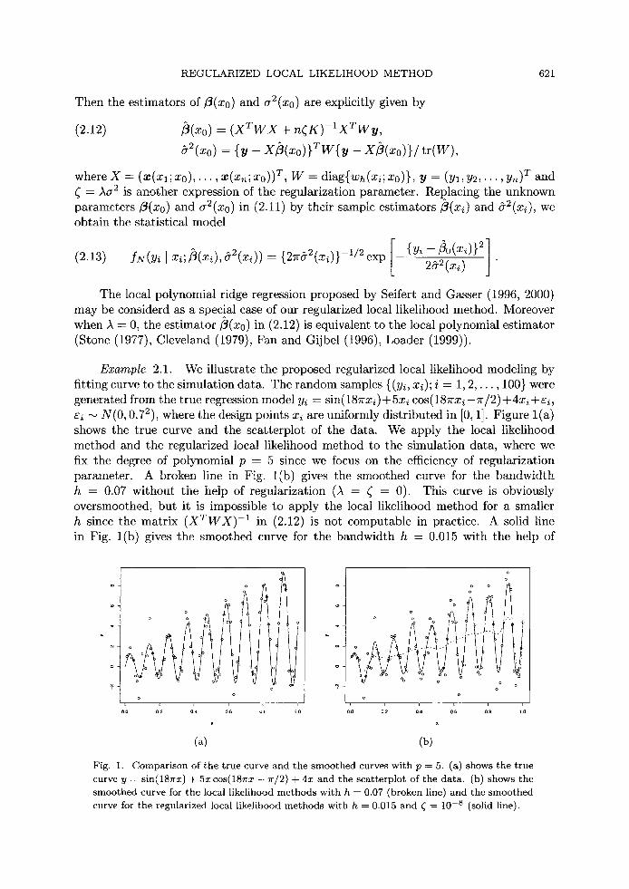
Example 2.1. We illustrate the proposed regularized local likelihood modeling by fitting curve to the simulation data. The random samples {(y~, xi); i = 1, 2 , . . . , 100} were generated from the t rue regression model y~ = sin(187rxi)+5x~ cos(187rxi-~r/2) +4x~ +s~, si ~ N(0, 0.72), where the design points xi are uniformly dis t r ibuted in [0, 1]. Figure l (a) shows the t rue curve and the scat terplot of the data. We apply the local likelihood method and the regularized local likelihood method to the simulation data, where we fix the degree of polynomial p -- 5 since we focus on the efficiency of regularizat ion parameter . A broken line in Fig. l (b) gives the smoothed curve for the bandwid th h = 0.07 wi thout the help of regularizat ion (A = r = 0). This curve is obviously oversmoothed, but it is impossible to apply the local likelihood me thod for a smaller h since the mat r ix ( x T w x ) -1 in (2.12) is not computable in practice. A solid line in Fig. l (b) gives the smoothed curve for the bandwidth h = 0.015 with the help of

0.0 0 2 0 4 o.6

x

~ o

o o

o

o

I I I I [ [ i

$ ~3 0 0 0 2 0 . 4 0 . 6 O e 1 0

X

(a) (b)

Fig. 1. Comparison of the true curve and the smoothed curves with p = 5. (a) shows the true curve y : sin(18~rx) + 5xcos(18~rx - 7r/2) + 4x and the scatterplot of the data. (b) shows the smoothed curve for the local likelihood methods with h ---- 0.07 (broken line) and the smoothed curve for the regularized local likelihood methods with h -- 0.015 and ~ = 10 -s (solid line).

622 YOSHISUKE NONAKA AND SADANORI KONISHI

regularization, where we use the regularization parameter ~ = 10 -s . This curve gives a good representation of the underlying function over the region [0, 1]. We observe that by appropriate choice of h and ~, our nonlinear regression modeling strategy can capture the true structure generating the data for large p.

2.2.2 Logistic model Let Yl, Y2,.. . , Yn be independent sequences of binary random variables taking values

of 0 or 1 with conditional probabilities Pr(yi = 1 [ xi) -- 7r(xi) and Pr(yi = 0 [ xi) = 1 -7c(xi), where xi are univariate explanatory variables. Taking O(xi) = log[Tr(xi)/{1 - 7r(xi)}], b(O(xi)) = log[1 + exp{0(x~)}], r = 1, c(y~,r = 0 and l(m(xi)) = log[m(xi)/{1 - m(xi)}] = O(xi) = j3(xo)Tx(xi; Xo) in (2.5), we have a nonlinear logistic regression model as follows

(2.14) fL(Y I f (XO)) = XO) {1 - 7r(xi; XO)} 1-y' ,

where

(2.15) exp{13(xo)T x(xi; XO)}

7r(xi; Xo) = 1 + exp{~(xo)Tx(xi; xo)}"

The unknown parameter vector/3(x0) is estimated by maximizing the regularized local log-likelihood (2.6), where the matrix K is given by P2 in equation (2.8). Then we can obtain the estimated model as follows

(2.16) fL(Yi I xi,~(xi)) = #(xi;xi)Ui{1 - ~ ( x i ; x i ) } 1 - y i (i = 1,.. . ,n),

where ~r (xi; xi) = exp {~0 (xi) } /[1 + exp{r (xi) }1 is the estimated conditional probability. Nonlinear regression models based on the regularized local likelihood method depend

on a bandwidth h, the degree of polynomial p and a regularization parameter A. In the next subsection we derive a model evaluation criterion for nonlinear regression models estimated by the regularized local likelihood method.

2.3 Model selection Suppose that we observe a realization of a random variable with distribution as

defined in Subsection 2.1. We recall that the statistical model f (y [ x, ~(x), ~(x)) defined in (2.9) is constructed within the generalized linear model framework. We want to assess the closeness of f (y I x, ~(x), ~(x)) to the true model g(y I x) from a predictive point of view.

Konishi and Kitagawa (1996) proposed a model selection criterion as an estimator of the Kullback-Leibler information between the true model and the estimated model. As shown in the Appendix, we can obtain an information criterion to evaluate the es- timated model f(Yi [ xi, ~(zi), r in (2.9) with (p + 2)-dimensional parameter esti- mator 0(x) = (~(x) T, ~(x)) T. The information criterion based on the regularized local likelihood method with the exponential family is given by

(2.17) GICh p')' = -2 ~ ~ [3~ - i=1 ( ~-~,e.x~ + c(yi, ~(xi)) }

2 '~ + - tr{- (xd-lQ(xd}, n

i=1

R E G U L A R I Z E D L O C A L L I K E L I H O O D M E T H O D 623

where we use the following notations:

(2.18)

Q(x) - 1 n~(x)

-A(2)X/~(x) - AK~(x) ITAX pTA(1)T

AO)p - ~(x) )~K3(x) l~p ] ~ ( x ) v ~ w p j '

R(x) - 1 x T w F x + n~(x))~K AO)ln/~b(x) 1 n~b(x) 1TAO)T/~b(X) - -r '

.J

A (k) = X T W A k, A = diag{yi - b'(~(x)Tx(xi; x))},

F = diag{b"(~(x)Tx(xi; x))},

P = ( P l , P 2 , . . . , P n ) T, q -- (q l ,q2 , - . . , q~)T ,

In = (1, 1 , . . . , 1) T (n x 1),

~ ( x ) ~ ( x ~ ; x)y~ - b ( ~ ( x ) ~ x ( ~ ; ~)) Oc(y,, r P~ = ~(x)~ + 0 r

r

We select a bandwid th h, the degree of polynomial p and a regularization parameter A which minimize the information criterion (2.17). 2.3.1 Gaussian model

Using the equations (2.17) and (2.18), we can obtain the information criterion for the es t imated Gaussian model fg(Yi ]x~; ~(xi), 52(x/)) in (2.13) as follows;

(2.19) GICh,p,~ = ~ llog{2~5-2(x{)} -/3o(zi)} 2 ] + ,=1 L ~2(x,) j

2 n + - E t r{R(x~)-~Q(xi)} ,

n i=1

1 Q(x)- n~4(x)

[ A(~)X _ )~b2(x)Kh(x)ITAX , ~(3) 1A(1)-I ] X | I_.~__ITA(3)T __ l lTA(1) T 1 T 4 1 t r (W) J '

k 25"2(x) *n`~N 2 * n ' ' N 4a4(x) l n A N w ] ' n -- ~

R(x) - 1 [ x T W X + na2(x) AK - - 1 A ( 1 ) I 5 2 ( x ) ~'N ~n ]

n52(x) | __j_l .1TAO)T 1 t r (W) ' L ~:(~) ~ ~N 2a:(~)

where A ~ ) = xTWAkN and AN = diag{yi - ~(x) Tx(xi; x)}. 2.3.2 Logistic model

In the case of the es t imated logistic model fL(Yi ]xi,/3(x~)) in (2.16), we can obtain the information criterion as follows;

(2.20) GICh,p,~ -- - - 2 E l o g f L ( y i I~ ,3(x~) ) + - tr(R(x~)-lQ(~)}, n

i=1 i=1 n

1 E { y i _ ~(x / ;x )} ~)(x) = i = 1

~x O%(y~, r ~(~) q~ - ~ / { 3 ( x ) T x ( x ~ ; x)y~ - b (3(x)~x(x~; x))} + ~ - ~ �9

624 YOSHISUKE NONAKA AND SADANORI KONISHI

• [w~(z~; x){y~ - ~(x~; x)}~(~; x) - ~K3(x)]~(z,; x) ~, n

~(x) = _ 1 ~ [ w ~ ( ~ ; x)~(~; ~){1 - ~(x~; x)}~(x~; x)x(~; ~)~ - ~K], n i= l

where #(xi; x) = exp{~(x)T x(xi; x)}/[1 + exp{~(x)T x(xi; X)}].

3. Multivariate regularized local likelihood method

In this section, we describe the regularized local likelihood method for the case of d explanatory variables.

3.1 Model and estimation Suppose we have n independent observations {(y~, x~);i = 1, 2 , . . . , n}, where y~

are ramdom response variables and xi = (X~l, x i2 , . . . , Xid) T are d-dimensional explana- tory variable vectors. It is assumed that the conditional distribution of Y, given x = (Xl, x2 , . . . , Xd) T, belongs to the exponential family which is given by replacing x with x in (2.1). The parameters 0(.) and r are related to the conditional mean and condi- tional variance similarly to the single covariate case.

Assume that the function O(x) is differentiable at a point x0. Then O(x) can be approximated locally by a polynomial of degree 1:

O0(x0), f l , (3.1) O(x) ~ O(xo) + ~ x T LX -- Xo) = (xo)Tx*(x; XO),

where/3*(x0) = (~(~(x0), ~ ( X o ) , . . . , ~ ( X 0 ) ) T, /~(~(X0) = 0(~g0), /~;(X0) ---- 00(XO)/(~Xj (j = 1, 2 , . . . , d) and x*(x; Xo) = (1, (x - xo)T) T. More generally, approximation (3.1) can be expanded to the higher order term (see Ruppert and Wand (1994)). But we use approximation (3.1) in order not to increase the number of unknown parameters.

Then the data {Yl, Y2, �9 �9 �9 Yn} were summarized by a model from a class of probabil- ity densities f(Yi ] xi; ft*(~0), r which are expressed by (2.5). We propose choosing unknown parameters/3"(~o) and r to maximize the regularized local log-likehood function

(3.2) RL(I~* (Xo), r H, A)

---~WH(Xi;XO){ ~*(x~176176176 i=1 ~D (-~-0)

+ c(~, r J

- nAfl*(xo)TKf~*(xo)/2.

The weight function WH(ggi; X0) is the Gaussian product kernel:

Kd(H-I (x - Xo)) d ( (3.3) WH(X;Xo) = idet(H)] , Kd(U) = (27r) -d/2 H exp ~,--lu2"~

j=1 2 ] '

where a matrix H is a p x p nonsingular bandwidth matrix. We use H = hid, where Id is a d-dimensional identity matrix and h is a bandwidth. The regularization term is

R E G U L A R I Z E D LOCAL LIKELIHOOD M E T H O D 625

given by equation:

(3.4) 0 0F] 0d IdJ

where 0g is a d-dimensional zero vector. The estimators ~* (x0) and r are obtained by the iterative algorithm. Replacing

the unknown parameters f~* (x0) and r by ~* (x0) and ~(x0) respectively and noting that the parameter 0(xi) in the exponential family f(Yi I xi;/Y*(x0), r is directly given by 0(xi) = fF(xi)Tx*(xi; xi) ----/3~(xi), we obtain the estimated model:

(3.5) f(Y~ l X~'~*(x~)'~(x~)) = exp { ~)(x~)y~- b(~(x~)) -t-c(Y~' ~(x~)) I

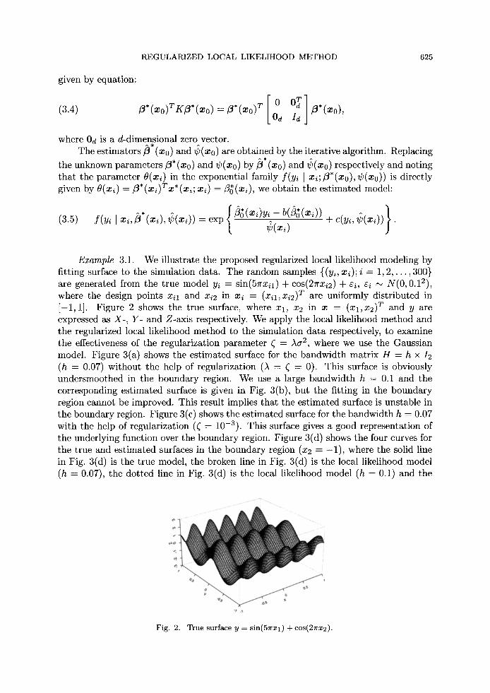
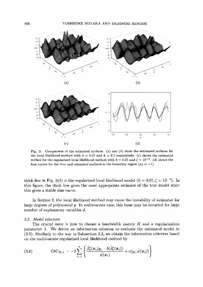
Example 3.1. We illustrate the proposed regularized local likelihood modeling by fitting surface to the simulation data. The random samples {(y~, x~); i = 1, 2 , . . . , 300} are generated from the true model Yi = sin(5~rXil) + cos(27rxi2) + ei, ei ~ N(0, 0.12), where the design points Xil and xi2 in xi = (xil,xi2) T are uniformly distributed in [-1, 1]. Figure 2 shows the true surface, where Xl, x2 in x = (xl,x2) T and y are expressed as X-, Y- and Z-axis respectively. We apply the local likelihood method and the regularized local likelihood method to the simulation data respectively, to examine the effectiveness of the regularization parameter r -- /~6r 2, where we use the Gaussian model. Figure 3(a) shows the estimated surface for the bandwidth matrix H = h • (h -- 0.07) without the help of regularization ()~ = r = 0). This surface is obviously undersmoothed in the boundary region. We use a large bandwidth h = 0.1 and the corresponding estimated surface is given in Fig. 3(b), but the fitting in the boundary region cannot be improved. This result implies that the estimated surface is unstable in the boundary region. Figure 3(c) shows the estimated surface for the bandwidth h -- 0.07 with the help of regularization (r = 10-3). This surface gives a good representation of the underlying function over the boundary region. Figure 3(d) shows the four curves for the true and estimated surfaces in the boundary region (x2 -- -1) , where the solid line in Fig. 3(d) is the true model, the broken line in Fig. 3(d) is the local likelihood model (h = 0.07), the dotted line in Fig. 3(d) is the local likelihood model (h -- 0.1) and the

ca

vao

o,

o,

Fig. 2. True surface y = sin(57rXl) + cos(27rx2).

626 YOSHISUKE N O N A K A A N D SADANORI KONISHI

(a) (b)

P,

Z ~

/ -

I ~ I 4 I

-10 4}5 O0 0.5 1.0

X1

(c) (d)

Fig. 3. Comparison of the estimated surfaces. (a) and (b) show the est imated surfaces for the local likelihood method with h ---- 0.07 and h ---- 0.1 respectively. (c) shows the est imated surface for the regularized local likelihood method with h ---- 0.07 and ~ = 10 - 3 . (d) shows the four curves for the true and estimated surfaces in the boundary region (x2 = - 1 ) .

thick line in Fig. 3(d) is the regularized local likelihood model (h -- 0.07, ~ = 10-3). In this figure, the thick line gives the most appropriate estimate of the true model since this gives a stable sine curve.

In Section 2, the local likelihood method may cause the instability of estimator for large degrees of polynomial p. In multivariate case, this issue may be occurred for large number of explanatory variables d.

3.2 Model selection The crucial issue is how to choose a bandwidth matrix H and a regularization

parameter ~. We derive an information criterion to evaluate the estimated model in (3.5). Similarly to the way in Subsection 2.3, we obtain the information criterion based on the multivariate regularized local likelihood method by n{ } (3.6) cIc.,

i = 1

REGULARIZED LOCAL LIKELIHOOD METHOD 627

where

1 -

+ ~ E tr{R(x,)-l(~(x,)}, i=1

pTA(')T ~(~)pTWp " / '

] n~)(x) 1TA(1)T/(~(X) - -~(x)qTWln '

A (k) = x T W A k, X = ( X * ( X i ; X ) , . . . , ~ * ( X n ; X ) ) T , W --- diag{wu(xi;x)).

The notations A, F, p and q are given by (2.18), where we use ~*(x)Tx*(xi; X) and ~(x) instead of ~(x)Tx(xi; x) and ~(x) respectively. We select a bandwidth matrix H and a regularization parameter A which mininize the information criterion (3.6).

We give the information criteria in the case of Gaussian and logistic models. 3.2.1 Gaussian model

We use the Gaussian regression model fN(Yi [ xi; ~*(xi) , &2(xi)) in (2.13), where

the estimators ~*(Xo) and 52(Xo) are given by

(3.7) ~*(x0) = (X T W X + n~Q)-lX T Wy,

52(x0) = {y - X~*(xo)} T W{y - X~* (xo)}/ tr( W).

Then we obtain the information criterion for the estimated Gaussian model as follows;

(3.8) GICH,;~ = s [log{2~-~2(xi)}+ { Y i - ~ ( x i ) } 2 1 2 n i = 1 ~ ' ~ J + --n Ei=l tr(R(xi)-lO(wi)}' 1

O(x)- n54(x) [~T(x)A(2N)X--)~52(z)Kf~(X) ITANX ~ 1 A(3)1 - -1A(1)" I N n 2 " ' N ~n

X 1 ~T a(3)T 1 ~T a(1)T 1 1 T A 4 1 t r ( W ) ' ~ ' n ' ~ N -- -~J 'n~N ~ n N w l n -- "~

1 [ x T W X + n o 2 ( x ) A K 1__ .4(1)1 1

where A~ ) = X T WAkN and AN = diag{yi - ~*(x)Tx*(xi; X)}. 3.2.2 Logistic model

In the case of logistic model, we can obtain the information criterion as follows

Tt ^$ 2 Tt

(3.9) GICH,,X ---- --2 ElOgfL(yi I ~ , ~ (~)) + - E tr{R(xi)-l(~(xi)}, n

i =1 i=1 n I Z{Y~- *(~'; ~)} Q(~) =

i=1

• [~.(~; ~){y~ - ~(~; ~)}~*(~; ~) - ~K3*(~)]~*(~; ~)~, n

R(~) = _1 E[~ . (~ , ; ~)~(~,; ~){1 - ~(~; ~)}~*(~,; ~)~*(~; ~)T - ~K], n

i = l

628 YOSHISUKE NONAKA AND SADANORI KONISHI

for the estimator ~* (x) which maximizes the regularized local likelihood function (3.2),

where ~(xi; x) = exp{~*(x)Tx*(xi; X)}/[1 + exp{~*(x)Tx*(Xi; ~)}] and fL(Yi ] xi, f3*(xi)) : #(xi; xi)Y'{1 -- ~(X,; xi)} 1-y'.

4. Real examples and numerical results

In this section we use a real data example and Monte Carlo simulations to investigate the performance of the regularized local likelihood modeling.

4.1 Summer rainfall data We apply the proposed modeling procedure to the rainfall data in Kagoshima. In

general, investigators in national meteorological observatories observe the sky at fixed times. For example, when they observe the clouds, they look out over the sky and observe the rate of the clouds which is called "cloud amount". They classify the weather condition as "Blue Sky" or "Cloudy". However, a weather condition such as "Rain" does not relate to cloud amount directly. Therefore, we investigate the relationship between cloud amount and "Rain" using our nonlinear modeling procedure.

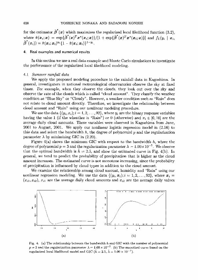
We use the data {(Yi, xi); i = 1, 2 , . . . , 92}, where Yi are the binary response variables having the value 1 (if the wheather is "Rain") or 0 (otherwise) and x~ E [0, 10] are the average daily cloud amounts. These variables were observed in Kagoshima from June, 2001 to August, 2001. We apply our nonlinear logistic regression model in (2.16) to this data and select the bandwidth h, the degree of polynomial p and the regularization parameter A by minimizing GIC in (2.20).

Figure 4(a) shows the minimum GIC with respect to the bandwidth h, where the degree of polynomial p -- 3 and the regularization parameter A -- 1.00 • 10 -7. We observe that the optimal bandwidth is h - 2.5, and show the estimated curve in Fig. 4(b). In general, we tend to predict the probability of precipitation that is higher as the cloud amount increases. The estimated curve is not monotone increasing, since the probability of precipitation is influenced by cloud types in addition to the cloud amount.

We examine the relationship among cloud amount, humidity and "Rain" using our nonlinear regression modeling. We use the data {(Yi, xi); i : 1, 2 , . . . , 92}, where xi -- (x~l, xi2), xil are the average daily cloud amounts and xi2 are the average daily values

~.O 25 h 30 3~ 40

J

o o o o o o ~ o o o ~ o o o o o ~ ~ 0 ~ o

2 4 e 8 lO

(~) (b)

Fig. 4. (a) The relationship between the bandwidth h and GIC with the number of polynomial p ---- 3 and the regularization parameter A = 1.00 • 10 -7 . (b) The smoothed curve based on the regularized local likelihood model and GIC (~t = 2.5, ~ = 1.00 • 10-7).

REGULARIZED LOCAL LIKELIHOOD M E T H O D 629

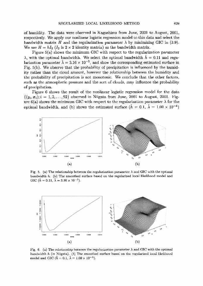
of humidity. The data were observed in Kagoshima from June, 2001 to August, 2001, respectively. We apply our nonlinear logistic regression model to this data and select the bandwidth matrix H and the regularization parameter A by minimizing GIC in (3.9). We use H = hi2 (12 is 2 x 2 identity matrix) as the bandwidth matrix.

Figure 5(a) shows the minimum GIC with respect to the regularization parameter A, with the optimal bandwidth. We select the optimal bandwidth h = 0.11 and regu- larization parameter A = 3.16 x 10 -5, and show the corresponding estimated surface in Fig. 5(b). We observe that the probability of precipitation is influenced by the humid- ity rather than the cloud amount, however the relationship between the humidity and the probability of precipitation is not monotonic. We conclude that the other factors, such as the atmospheric pressure and the sort of clouds, may influence the probability of precipitation.

Figure 6 shows the result of the nonlinear logistic regression model for the data {(y~, x~);i = 1, 2 , . . . , 9 2 } observed in Niigata from June, 2001 to August, 2001. Fig- ure 6(a) shows the minimum GIC with respect to the regularization parameter A for the optimal bandwidth, and (b) shows the estimated surface (h = 0.1, A = 1.00 x 10 -4)

2 O.QGO0 O00G~ 00004 0.00~6 OOCOe 0(]010

(a) (b)

Fig. 5. (a) The relationship between the regularization parameter A and GIC with the optimal bandwidth h. (b) The smoothed surface based on the regularized local likelihood model and GIC (h = 0.11, s = 3.16 x 10-5) .

-

O.C~O0 0 .00~ 00004 0(:006 Q(X~6 OD010

Q~

(a) (b)

Fig. 6. (a) The relationship between the regularization parameter A and GIC with the optimal bandwidth h (in Niigata). (b) The smoothed surface based on the regularized local likelihood model and GIC (h = 0.1, A ---- 1.00 x 10-4) .

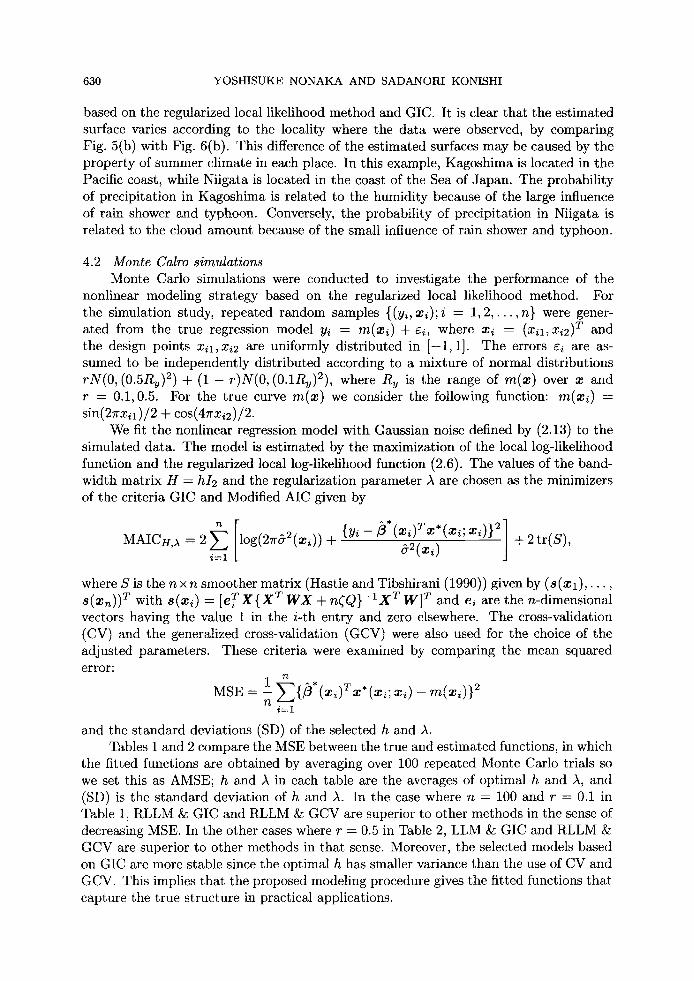
630 Y O S H I S U K E N O N A K A A N D S A D A N O R I K O N I S H I

based on the regularized local likelihood method and GIC. It is clear that the estimated surface varies according to the locality where the data were observed, by comparing Fig. 5(b) with Fig. 6(b). This difference of the estimated surfaces may be caused by the property of summer climate in each place. In this example, Kagoshima is located in the Pacific coast, while Niigata is located in the coast of the Sea of Japan. The probability of precipitation in Kagoshima is related to the humidity because of the large influence of rain shower and typhoon. Conversely, the probability of precipitation in Niigata is related to the cloud amount because of the small influence of rain shower and typhoon.

4.2 Monte Calro simulations Monte Carlo simulations were conducted to investigate the performance of the

nonlinear modeling strategy based on the regularized local likelihood method. For the simulation study, repeated random samples {(Yi, xi);i -- 1, 2 , . . . , n } were gener- ated from the true regression model Yi = m(x~) + e~, where xi -- (X~l, x~2) T and the design points xil,xi2 are uniformly distributed in [-1, 1]. The errors 6i are as- sumed to be independently distributed according to a mixture of normal distributions rN(O, (0.5Ry) 2) + (1 - r)N(0, (0.1Ry)2), where Ry is the range of re(x) over x and r = 0.1, 0.5. For the true curve re(x) we consider the following function: m(x~) = sin(27rx,1)/2 + cos(47rx~2)/2.

We fit the nonlinear regression model with Gaussian noise defined by (2.13) to the simulated data. The model is estimated by the maximization of the local log-likelihood function and the regularized local log-likelihood function (2.6). The values of the band- width matrix H -- hi2 and the regularization parameter ~ are chosen as the minimizers of the criteria GIC and Modified AIC given by

2 ~i=1 [ l~ + {Yi - ~*(xi)Tx*(Xi;~U(X~) xi)}2- + 2 tr(S), MAICH,~

where S is the n• smoother matrix (Hastie and Tibshirani (1990)) given by ( s ( x l ) , . . . , s(xn)) T with s(xi) = [ e T X { X T W X + n~Q}- IX T W]T and ei are the n-dimensional vectors having the value 1 in the i-th entry and zero elsewhere. The cross-validation (CV) and the generalized cross-validation (GCV) were also used for the choice of the adjusted parameters. These criteria were examined by comparing the mean squared error:

n

MSE = 1 V ~ i ~ . l x ~Tx.(X i----1

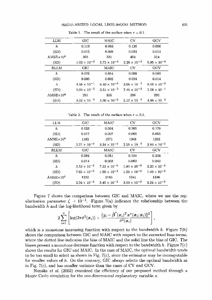
and the standard deviations (SD) of the selected h and A. Tables 1 and 2 compare the MSE between the true and estimated functions, in which

the fitted functions are obtained by averaging over 100 repeated Monte Carlo trials so we set this as AMSE; h and )~ in each table are the averages of optimal h and )~, and (SD) is the standard deviation of h and A. In the case where n = 100 and r = 0.1 in Table 1, RLLM & GIC and RLLM &: GCV are superior to other methods in the sense of decreasing MSE. In the other cases where r = 0.5 in Table 2, LLM ~z GIC and RLLM GCV are superior to other methods in that sense. Moreover, the selected models based on GIC are more stable since the optimal h has smaller variance than the use of CV and GCV. This implies that the proposed modeling procedure gives the fitted functions that capture the true structure in practical applications.

R E G U L A R I Z E D L O C A L L I K E L I H O O D M E T H O D

Table 1. The resul t of t he surface when r = 0.1.

631

LLM G I C M A I C C V G C V

h 0.119 0.063 0.126 0.096

(SD) 0.015 0.008 0.034 0.014

A M S E • 104 395 331 454 314

(SD) 1.03 • 10 - 2 5.72 • 10 - 3 2.28 • 10 - 2 5.95 • 10 -3

RLLM G I C M A I C C V G C V

h 0.076 0.054 0.088 0.080

(SD) 0.009 0.002 0.024 0.014

A 4.58 x 10 - 1 8.40 x 10 - 3 3.66 • 10 - 2 8.56 • 10 - 2

(SD) 5.05 • 10 - 2 2.51 x 10 - 2 7.46 x 10 - 2 1.08 x 10 -1

A M S E x 104 291 355 299 292

(SD) 4.02 • 10 - 3 5.36 x 10 - 3 5.57 x 10 - 3 4.98 x 10 -3

Table 2. The resul t of t he surface when r = 0.5.

LLM G I C M A I C C V G C V

h 0.123 0.064 0.205 0.170

(SD) 0.017 0.007 0.065 0.055

A M S E • 104 1183 1971 1348 1283

(SD) 2.21 • 10 - 2 3.34 • 10 - 2 2.51 • 10 - 2 2.84 • 10 -2

R L L M GIC M A I C CV G C V

h 0.084 0.051 0.154 0.134

(SD) 0.014 0.002 0.062 0.042

A 3.53 • 10 - 2 7.22 x 10 - 5 1.89 x 10 - 2 2.20 • 10 - 2

(SD) 7.65 x 10 - 3 1.50 x 10 - 4 1.59 • 10 - 2 1.49 x 10 - 2

A M S E x 104 1232 2185 1241 1186

(SD) 2.34 • 10 - 2 3.45 x 10 - 2 3.03 x 10 - 2 3.24 x 10 -2

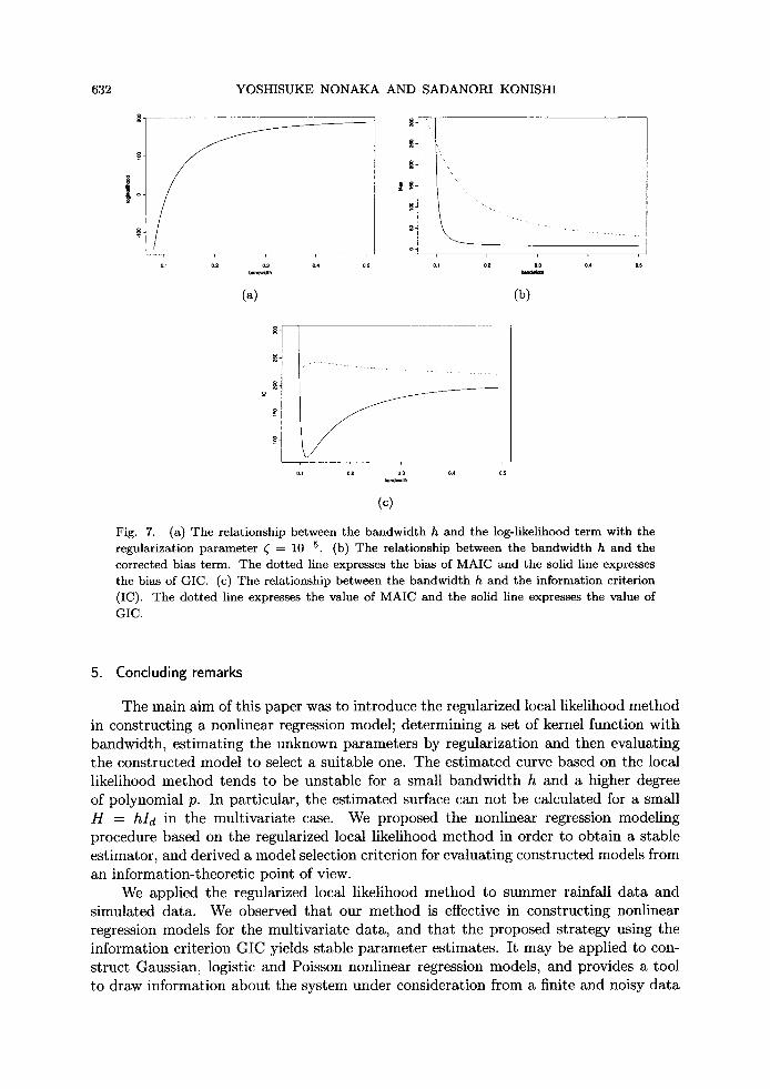
Figure 7 shows the comparison between GIC and MAIC, where we use the reg- ularization parameter ~ = 10 -5. Figure 7(a) indicates the relationship between the bandwidth h and the log-likelihood term given by

i=1 (~2 ( ~ i ) '

which is a monotone increasing function with respect to the bandwidth h. Figure 7(b) shows the comparison between GIC and MAIC with respect to the corrected bias terms, where the dotted line indicates the bias of MAIC and the solid line the bias of GIC. The biases present a monotone decrease function with respect to the bandwidth h. Figure 7(c) shows the results for GIC and MAIC. In the case of MAIC, the optimal bandwidth tends to be too small to select as shown in Fig. 7(c), since the estimator may be incomputable for smaller values of h. On the contrary, GIC always selects the optimal bandwidth as in Fig. 7(c), and has smaller variance than the cases of CV and GCV.

Nonaka et al. (2003) examined the efficiency of our proposed method through a Monte Carlo simulation for the one-dimensional explanatory variable x.

632 YOSHISUKE N O N A K A AND SADANORI KONISHI

1 ~o-

0.2 03

(a)

~4

o ~

O.2 0.3

(b)

Y

J 0.1 02 03 0.4 O~

(c)

Fig. 7. (a) The re la t ionship between the b a n d w i d t h h and the log-likelihood t e rm wi th the regularizat ion pa rame te r ~ --= 10 -5 . (b) The relat ionship be tween the bandwid th h and the corrected bias term. The dot ted line expresses the bias of MAIC and the solid line expresses the bias of GIC. (c) The relat ionship between the bandwid th h and the informat ion cri terion (IC). The do t t ed line expresses the value of MAIC and the solid line expresses the value of GIC.

5. Concluding remarks

The main aim of this paper was to introduce the regularized local likelihood method in constructing a nonlinear regression model; determining a set of kernel function with bandwidth, estimating the unknown parameters by regularization and then evaluating the constructed model to select a suitable one. The estimated curve based on the local likelihood method tends to be unstable for a small bandwidth h and a higher degree of polynomial p. In particular, the estimated surface can not be calculated for a small H = hid in the multivariate case. We proposed the nonlinear regression modeling procedure based on the regularized local likelihood method in order to obtain a stable estimator, and derived a model selection criterion for evaluating constructed models from an information-theoretic point of view.

We applied the regularized local likelihood method to summer rainfall data and simulated data. We observed that our method is effective in constructing nonlinear regression models for the multivariate data, and that the proposed strategy using the information criterion GIC yields stable parameter estimates. It may be applied to con- struct Gaussian, logistic and Poisson nonlinear regression models, and provides a tool to draw information about the system under consideration from a finite and noisy data

R E G U L A R I Z E D L O C A L L I K E L I H O O D M E T H O D 633

set. We would recommend implementing nonlinear regression modeling based on the regularized local likelihood method, using the information criterion GIC.

Acknowledgements

The authors would like to thank the referees and the Editor for their helpful com- ments and suggestions.

Appendix: Derivation of the information criterion

We derive an information criterion to evaluate models estimated by the regularized local likelihood method.

Suppose that zl, z2 , . . . , zn are future observations for the response variable Y drawn from g(y [ x). Let f (z [ X;O(X)) = [L~=I f(z~ [ xi;~(xi),r and g(z I X) -- I-L~=I g(z~ [ x~). An information criterion may be derived as an estimator of the Kullback- Leibler information (Kullback and Leibler (1951))

(A.1) KL{g, f} = EG(zix)[logg(z I X)] - Ea(zpx)[logf(z ] X; 0(X))]

conditional on 0(X) = (/3(X) T, ~(X)) T. The first term in the right-hand side of equation (A.1) is constant over all models

and only the second term

(A.2) Ea(z,x)[logf(z I X;O(Xo))] = f logf(z I x;O(xo))dG(z Ix),

is relevant. Hence, instead of minimizing the Kullback-Leibler information (A.1), we maximize the expected log-likelihood (A.2) that depends on the unknown true distribu- tion G(z I X). An estimate of the expected log-likelihood is the log-likelihood

(A.3) ~ log f(Yi ] xi; 0(x0)), i=1

obtained by replacing the unknown distribution G(z ] X) by the empirical distribution. Then the bias of the log-likelihood in estimating the expected log-likelihood is given by

b (a ) = Ea(ulX)[log f (y I X; b(x0)) - EG(z,x)[log f ( z I X; b(x0))]].

Konishi and Kitagawa (1996) considered an asymptotic bias for a statistical model with functional estimators and gave the bias by a function of the empirical influence function of estimators and the score function of a specified parametric model. It may be seen that the regularized local likelihood estimator 0(x0) = (~(Xo) T, ~/)(XO)) T c a n be expressed as 0(x0) = T(G) for the functional T(.) defined by

(A.4) f ~---o{Wh(X;xo)logf(z I x;O(xo))- ;~f~(xo)TKf~(xo)/2} T(C)dG(z)=0,

where G and G are respectively the joint distribution of (x, y) and the empirical distribu- tion function based on the observed data. Replacing G in (A.4) by Ge -- (1-E)G+eS(v,x)

6 3 4 Y O S H I S U K E N O N A K A A N D S A D A N O R I K O N I S H I

with 5(u,~ ) being a point of mass at (y, x) and differentiating with respect to ~ yield the

influence function of the regularized estimator O(xo) = T(G) in the form

(A.5) T(I)(z l x;C)

= R(G)-lO{Wh(X; xo)log f ( z I x; O(xo)) - Aj3(xo)TK~(xo)/2} T(G) ~

where

OOO0 T dG(z),

with a(z [ x; O(xo)) = Wh(X; Xo) log f(z I X; O(xo)) -- A~(xo)TKj3(Xo)/2. It follows from Theorem 2.1 in Konishi and Kitagawa (1996) (see also Konishi

(1999)) that the bias is asymptotically given by D(G) = tr{R(G)-IQ(G)} + o(1/n), where

Q ( G ) : f { OA(zlx;O(x~ 0logf(zlx;O(xo))}ooT T(G)dG(z).

By replacing the unknown distribution G by the empirical distribution G, we have an information criterion

~b

(A.7) GICh,p,:~(xo) = - 2 E l o g f(yi I xi; O(x0)) + 2 t r{R(G)-IQ(G)}. i=1

where

Q(~) = 1 ~ { OA(yi I xi;O(xo))Ologf(yi I xi;O(xo))

n i=1 [ O000T

It might be noticed here that the information criterion based on the local method has two problems: the information criterion GICh,p,),(Xo) in (A.7) depends on the point x0, and this method assesses the closeness of f(y I x; 0(x0)) to the model g(Y I x) for a fixed point x0. In order to assess the closeness of f(y I x; O(x)) to the model 9(Y ] x), we modify the information criterion (A.7) in the following:

n n

(A.8) GICh,pA = - 2 Z l o g f ( y i I xi;O(xi)) + 2 E tr{[~(xi)-lQ'(xi)}' n i -~ l i = 1

where we replace Q(G) and R(G) with Q(x0) and -~(x0), respectively. For the problem of choosing among different models, we select the model for which the value of the information criterion GICh,pA is smallest.

Irizarry (2001) proposed the use of a weighted version of the Kullback-Leibler in- formation and derived the model selection criterion WAIC. That assesses the closeness of f(y [ x; t~(x0)) to the model g(y [ x) for a fixed point x0.

REGULARIZED LOCAL LIKELIHOOD METHOD 635

REFERENCES

Bartlett, M. S. (1954). A note on some multiplying factors for various X approximations, Journal of the Royal Statistical Society, Series, B, 16, 296-298.

Cleveland, W. S. (1979). Robust locally weighted regression and smoothing scatterplots, Journal of the American Statistical Association, 74, 829-836.

Copas, B. J. and Eguchi, S. (1998). Sensitivity approximations for selectivity bias in observational data analysis, Research Memo., No. 660, The Institute of Statistical Mathematics, Tokyo.

Eguchi, S. and Copas, J. (1998). A class of local likelihood methods and near-parametric asymptotics, Journal of the Royal Statistical Society, Series, B, 60, 709-724.

Eguchi, S. and Kim, T. Y. (2001). Local likelihood method and theory for a bridge of parametric and nonparametric regression, Research Memo., No. 806, The Institute of Statistical Mathematics, Tokyo.

Eguchi, S., Kim, T. Y. and Park, B. U. (2003). Local likelihood method: A bridge over parametric and nonparametric regression, Journal of Nonparametric Statistics, 15, 665-683.

Fan, J. and Gijbels, I. (1996). Local Polynomial Modelling and Its Applications, Chapman & Hall, London.

Fan, J., Heckman, N. E. and Wand, M. P. (1995). Local polynomial kernel regression for generalized linear models and quasi-likelihood functions, Journal of the American Statistical Association, 90, I41-150.

Green, P. J. and Silverman, B. W. (1994). Nonparametric Regression and Generalized Linear Models, Chapman 8z Hall, London.

Hastie, T. and Tibshirani, R. (1990). Generalized Additive Models, Chapman L: Hall, London. Hjort, N. L. and Jones, M. L. (1996). Locally parametric nonpararaetric density estimation, Annals of

Statistics, 24, 1667-1678. Irizarry, R. A. (2001). Information and posterior probability criteria for model selection in local likeli-

hood estimation, Journal of the American Statistical Association, 96, 303~16. Konishi, S. (1999). Statistical mode] evaluation and information criteria, Multivariate Analysis, Design

of Experiments and Survey Sampling (ed. S. Ghosh), 369-399, Marcel Dekker, New York. Konishi, S. and Kitagawa, G. (1996). Generalised information criteria in model selection, Biometrika,

83, 875-890. Kullback, S. and Leibler, R. A. (1951). On information and sufficiency, Annals of Mathematical Statis-

tics, 22, 79-86. Loader, C. R. (1999). Local Regression and Likelihood, Springer, New York. McCullagh, P. and Nelder, J. A. (1989). Generalized Linear Models, Chapman L: Hall, London. Nelder, J. A. and Wedderburn, R. W. M. (1972). Generalized linear models, Journal of the Royal

Statistical Society, Series, A, 135, 370-384. Nonaka, Y., Ando, T. and Konisbi, S. (2003). Nonlinear regression modeling using regularized local

likelihood (in Japanese), Journal o] the Japanese Society of Computational Statistics, 16, 43-57. Ruppert, D. and Vv'and, M. P. (1994). Multivariate locally weighted least squares regression, Annals of

Statistics, 22, 1346-1370. Seifert, B. and Gasser, T. (1996). Variance properties of local polynomials and ensuing modifications,

Statistical Theory and Computational Aspects of Smoothing (eds. W. Hs and M. G. Schimek), 50-127, Physica, Heidelberg.

Seifert, B. and Gasser, T. (2000). Data adaptive ridging in local polynomial regression, Journal of the Computational and Graphical Statistics, 9, 338-360.

Simonoff, J. S. (1996). Smoothing Methods in Statistics, Springer, New York. Stone, C. J. (1977). Consistent nonparametric regression (with discussion), Annals of Statistics, 5,

595 645. Tibshirani, R. J. and Hastie, T. J. (1987). Local likelihood estimation, Journal of the American Statis-

tical Association, 82, 559-567. Wand, M. P. and Jones, M. C. (1995). Kernel Smoothing, Chapman L: Hall, London.