Oil Spill Candidate Detection from SAR Imagery Using a Thresholding-GuidedStochastic Fully-Connected Conditional Random Field Model

Linlin Xu, M. Javad Shafiee, Alexander Wong, Fan Li, Lei Wang, David ClausiDepartment of Systems Design Engineering, University of Waterloo

{l44xu, mjshafiee, a28wong, f33li, lei.wang, dclausi}@uwaterloo.ca

Abstract

The detection of marine oil spill candidate from synthet-ic aperture radar (SAR) images is largely hampered by SARspeckle noise and the complex marine environment. In thispaper, we develop a thresholding-guided stochastic fully-connected conditional random field (TGSFCRF) model forinferring the binary label from SAR imagery. First, an in-tensity thresholding approach is used to estimate the initiallabels of oil spill candidates and the background. Second,a Gaussian mixture model (GMM) is trained using all thepixels based on the initial labels. Last, based on the G-MM model, a graph-cut optimization approach is used forinferring the final labels. By using a threholding-guidedapproach, TGSFCRF can exploit the statistical character-istics of the two classes for better label inference. More-over, by using a stochastic clique approach, TGSFCRF effi-ciently addresses the global-scale spatial correlation effect,and thereby can better resist the influence of SAR specklenoise and background heterogeneity. Experimental resultson RADARSAT-1 ScanSAR imagery demonstrate that TGS-FCRF can accurately delineate oil spill candidates withoutcommitting too much false alarms.

1. Introduction

Spaceborne synthetic aperture radar (SAR), due to itsability to cover large areas irrespective of weather condi-tion or sun-light illumination, provides a powerful tool forthe detection of marine oil spill, which is usually causedby ships or drilling platforms, and greatly endanger themarine ecosystem. Efficient identification of potential oilspills from SAR imagery is crucial for supporting quick re-sponse to oil pollution and the cleanup efforts. The first useof SAR image for oil spill monitoring was by Elachi [1],who investigated the feasibility of Seasat imagery for oilspill detection. After the launch of the second generationof satellite SAR sensors in the 1990s, such as ENVISAT,ERS-2, and RADARSAT-1, SAR images became extensive-

ly used for oil spill detection [2–8]. The third generationof SAR sensors were launched in the past five years, suchas Canadian RADARSAT-2, Italian Cosmo-Skymed, Ger-man TerraSAR-X and Japanese ALOS. These sensors arecharacterized by multi-polarization options, higher spatialresolution and shorter revisit time, therefore, provide bettercapability for oil spill detection [9, 10].

Today, almost all of the operational marine monitoringprograms depend on trained human analysts to determineoil spill candidates, by visual interpretation, based on theirexperiences and prior knowledge [11]. However, dealingwith a large amount of SAR images of vast marine re-gions is costly and time-consuming. As such, automaticmethods for oil spill detection have been a very active re-search topic in remote sensing community. In the last twodecades, efforts have been made by several organization-s towards the development of semi-automated or fully au-tomated systems for oil spill detection based on SAR im-agery. Examples include the semi-automated systems suchas Ocean Monitoring Workstation (OMW) at CIS [2], Alas-ka SAR Demonstration (AKDEMO) system [12], the Euro-pean Commission Joint Research Centre (JRC) system [13],the Norwegian Defense Research Establishment (NDRE)system [14], and a fully-automated Kongsberg Satellite Ser-vices (KSAT)s oil spill detection system at Norway [15].

Oil spills appear as dark-spots on SAR imagery. How-ever, other natural or man-made phenomena (e.g., organicfilm and low wind area), called look-alikes, also appear asdark-formations on SAR ocean images [16]. It is difficult todiscriminate oil spills from look-alikes solely based on SARintensity values. Ancillary features regarding dark-spots(e.g., texture, geometric shape, contrast with surroundingareas and contextual information) has to be extracted to fur-ther classify oil spills from look-alikes [17]. As a result, anoil spill identification system typically requires three stages:(i) oil spill candidate detection, (ii) feature extraction, and(iii) classification [18]. The first step aims to detect fromSAR imagery all dark-spots that are potential oil spills. Thisstep is very important for the system, because once oil spill-s are omitted in this step, they will never be detected in the

4321

following steps. Moreover, the false detections in the firststep will increase the computational burden and classifica-tion difficulty of the subsequent steps.

This paper therefore focuses on developing effective oilspill candidate detection algorithm. Several approacheshave been proposed for oil spill candidate detection. Thecommonly used approaches are based on intensity thresh-olding. Many global thresholds have been proposed: Nir-chio et al. set the threshold as the normalized radar crosssection (NRCS) minus standard deviation of the SAR im-age [19]; Fiscella et al. used half of the averaged NRCS [7].Although the global thresholding methods have high com-putational efficiency, they sometimes fail to detect weak oilspill candidate because the global thresholds do not alwaysaccount for the local variation. By selecting the thresholdlocally, adaptive thresholding methods tend to be able todelineate oil spill candidates more accurately. Solberg et al.set the threshold to be k dB below the mean value estimat-ed in a moving window [4, 15, 20]. In order to resist theinfluence of speckle noise, Shu et al. proposed a threshold-ing method that takes advantage of spatial density informa-tion [21]. Another approach exploits the edge informationon SAR image for oil spill detection. Chen et al. proposedthe use of both Difference of Gaussian (DoG) and Laplaceof Gaussian (LoG) to detect the boundary of oil spills [22].As a band pass filter, the wavelet method was used for thedelineation of oil spill areas [23–25]. Other more sophisti-cated oil spill candidate detection methods have been pro-posed, such as the neural network based approach [26] andthe marked point process based approach [27].

The effectiveness of an oil spill candidate detection sys-tem depends highly on its capability to deal with the diffi-culties caused by the complex marine environment and theSAR speckle noise. First, the class separability between theoil spill candidate and the background is usually very low,due to the variation caused by SAR speckle noise and thelow intensity contrast between oil spill candidate and thebackground. In order to increase the class separability, thespatial contextual information in SAR image has to be ex-ploit to resist the influence of speckle noise and to highlightthe difference between the target and the background. Al-though oil spill candidates are weak signals, they tend topresent significant patterns when being examined on largespatial scale. Consequently, the model accounting for large-scale spatial correlation effect is more suitable for oil spillcandidate detection. Nevertheless, modeling large-scale s-patial correlation effect usually cause very high computa-tional cost. A spatial model that addresses large-scale spa-tial correlation effect in a efficient and adaptive manner istherefore required. Second, performing oil spill detection ina totally unsupervised manner is not appropriate, becauseoil spill candidate are weak signals that usually constitutelimited number of pixels comparing with the background.

Considering the heterogeneity of the background, a unsu-pervised segmentation approach tends to split the big classof background into two small classes, leading to failure inoil spill candidate detection. As such, a guided-approachthat learns what the two classes (i.e., oil spill candidate classand the background class) look like in a guided manner isdesirable.

The paper therefore presents a thresholding-guided s-tochastic fully-connected conditional random field (TGS-FCRF) algorithm for oil spill candidate detection. Compar-ing with ordinary conditional random field (CRF) that on-ly considers the correlation effect in a small neighborhood,the fully-connected CRF (FCRF) addresses the correlationeffect in the global image scale. However, FCRF usually re-quires huge computational cost. The TGSFCRF model canmaintain the advantage of FCRF, but reduce its computa-tional cost by using a stochastic clique approach, where theconnectivity of a node with all the other nodes in the graphis determined in a stochastic manner [28]. Considering oilspill candidates are usually weak signals and can be easilymisclassified under a totally unsupervised circumstance, weadopt a thresholding-guided approach to regulate the learn-ing process. The experiments on RADARSAT-1 SAR im-agery indicate that the proposed algorithm can accuratelydelineate oil spill candidate comparing with other methods.

The rest of the paper is organized as below. Section 2 de-scribes the TGSFCRF model and its implementation. Sec-tion 3 presents the experiments results on RADARSAT-1SAR images. Section 4 concludes the study.

2. Methodology

In this section, we start with a introduction to TGSFCRFframework in the context of SAR oil spill candidate detec-tion, followed by the detailed illustration of key componentsin TGSFCRF.

2.1. TGSFCRF Framework

TGSFCRF is a fully-connected random field model,where threholding approach is used as a guide to learn mod-el parameters, and the stochastic clique is used to determinethe connectivity among nodes in a fully-connected graph.

Let xi and yi denote respectively the intensity observa-tion and the class label of a site in the SAR image latticeI contains |I| = N sites. The SAR image is expressed asX = {xi|i ∈ I} and the labels corresponding to this ob-servation as Y = {yi|i ∈ I}. Oil spill candidate detectionaims to infer Y given X by maximizing the following con-ditional probability distribution:

4322

P (Y |X) = (1)1

Z(X)exp

(−∑i

ψu(yi, X)−∑

(i,j)∈C

ψp(yi, yj , X))

where Z(X) is the partition function, ψu and ψp are theunary potential and the pairwise potential respectively andC encodes the set of clique structure in the random field.The clique structure C in (1) determines the connectivityamong nodes in the neighborhood. Since the underlyinggraph is assumed to be fully-connected, the neighborhoodof node i denoted by Ni, has the following expression:

Ni = {j|j = 1 : N, j 6= i} (2)

Figure 1. The flowchart of TGSFCRF.

As shown by Fig. 1, in TGSFCRF, an intensity thresh-olding approach is first conducted to estimate the initial es-timation of binary labels, based on which, a Gaussian mix-ture model (GMM) involving the oil spill candidate classand the background class are learned. Based on GMM anda stochastic clique structure, a graph-cut approach is usedto optimize the objective function of TGSFCRF, leading tothe final estimation of the class labels.

In the following sections, we illustrate some key compo-nents in TGSFCRF algorithm, as well as the optimizationscheme.

2.2. Intensity Thresholding

The initial class label of the pixel at the ith site isachieved by performing an intensity thresholding approach,according to the following rule:

y0i =

{1 if xi > thrd0 otherwise. (3)

where thrd = mean(X) − ω · std(X) with ω usually be-ing 1. Since different images tend to have different mean

and standard deviation values, using thrd can adapt to theindividual histogram characteristics.

2.3. GMM Learning

The initial class labels Y 0 will be used to estimate theunknown parameters in the unary potential, which is for-mulated as below:

ψu(yi, X) = −log(p(yi|xi)

)(4)

where p(yi|ii) is the posterior probability of yi given xibased on a GMM. The parameters in GMM are estimatedby the maximum likelihood (ML) approach.

2.4. Stochastic Clique

To take the advantage of large-range spatial informa-tion with feasible computational complexity, we adapt thestochastic clique approach in [28] for modeling the spatialcorrelation effect in SAR image.

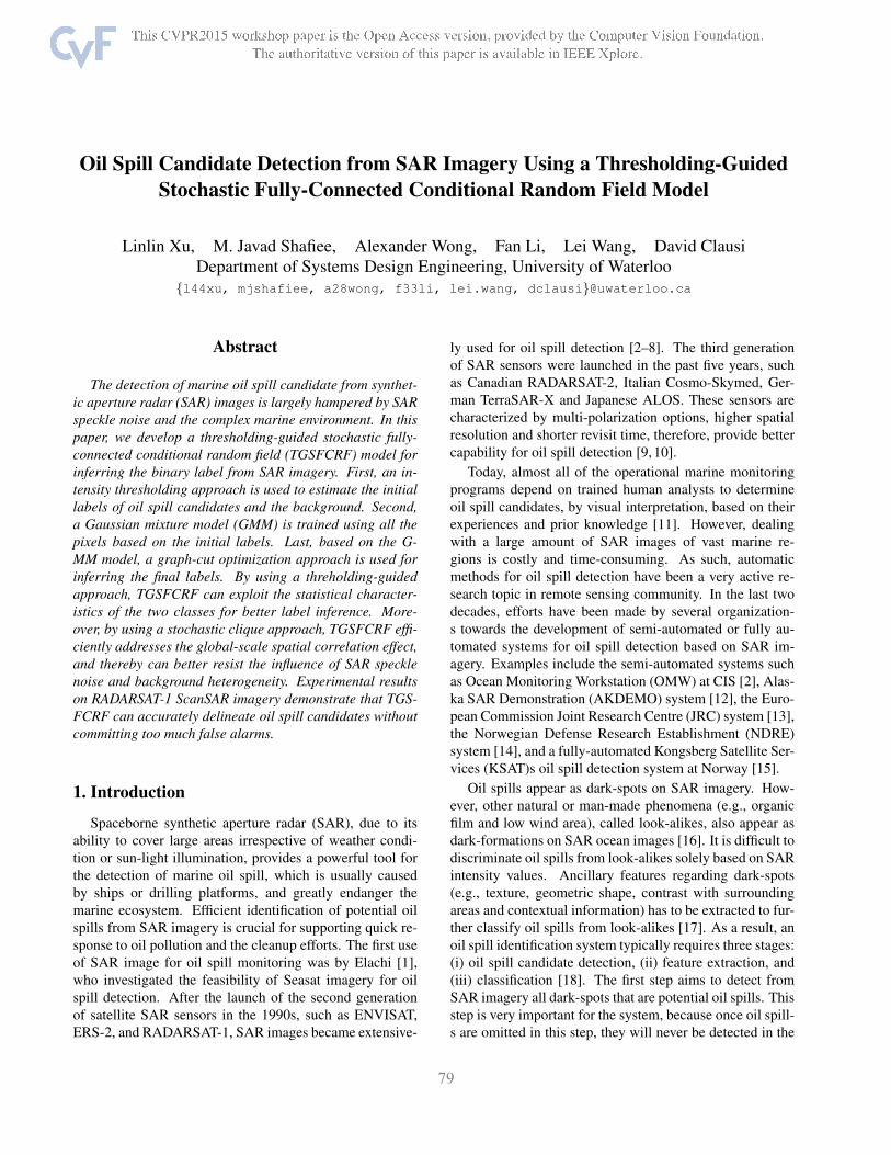
Fig. 2 displays some examples of SAR oil spill candidateimages. As demonstrated in Fig. 2(a), the oil spill candidatecan have elongated structures, which implies long range s-patial correlation effect. Fig. 2(b) and Fig. 2(c), however,indicate that oil spill candidate sometimes has a big densestructure. Therefore, modeling oil spill candidates by fixedclique structure is challenging due to the variation in thedirection and scale of spatial correlation effect. Howev-er, determining the clique structure in a data-driven man-ner might be more appropriate. Consequently, TGSFCRF,where stochastic clique approach is used to sample the rel-evant clique connectivities from a fully-connected randomfield, can capture the useful spatial contextual informationfor enhancing the detectability of oil spill candidate.

The widely used pairwise clique structure is adoptedhere. The clique structure C is a combination of individualstochastic clique structures {C(i)} associated with differentnodes in the random field:

C ={C(i)} (5)C(i) ={(i, j)|j ∈ Ni, 1{i,j} = 1} (6)

where 1{i,j} = 1 is a clique indicator function determiningwhether two nodes i and j can construct a clique or not,according to a stochastic measure:

1{i,j} =

{1 if γ · PijQij > ϕ0 otherwise. (7)

where Pij is the data similarity likelihood between pixel xiand xj , Qij is the probabilistic spatial closeness measure-ment from xi to xj in image space, γ determines the sparsityof the graph, and ϕ is a random value in the range of [0, 1]generated from a uniform distribution.

4323

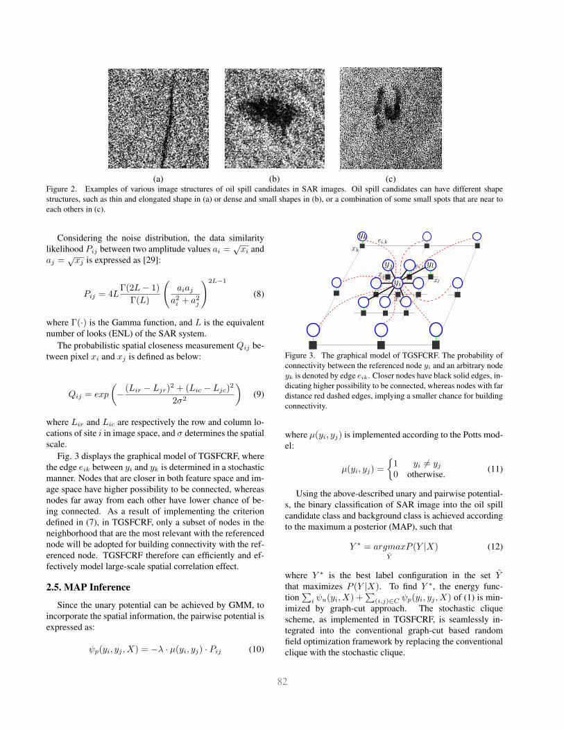
(a) (b) (c)Figure 2. Examples of various image structures of oil spill candidates in SAR images. Oil spill candidates can have different shapestructures, such as thin and elongated shape in (a) or dense and small shapes in (b), or a combination of some small spots that are near toeach others in (c).

Considering the noise distribution, the data similaritylikelihood Pij between two amplitude values ai =

√xi and

aj =√xj is expressed as [29]:

Pij = 4LΓ(2L− 1)

Γ(L)

(aiaj

a2i + a2j

)2L−1

(8)

where Γ(·) is the Gamma function, and L is the equivalentnumber of looks (ENL) of the SAR system.

The probabilistic spatial closeness measurement Qij be-tween pixel xi and xj is defined as below:

Qij = exp

(− (Lir − Ljr)2 + (Lic − Ljc)

2

2σ2

)(9)

where Lir and Lic are respectively the row and column lo-cations of site i in image space, and σ determines the spatialscale.

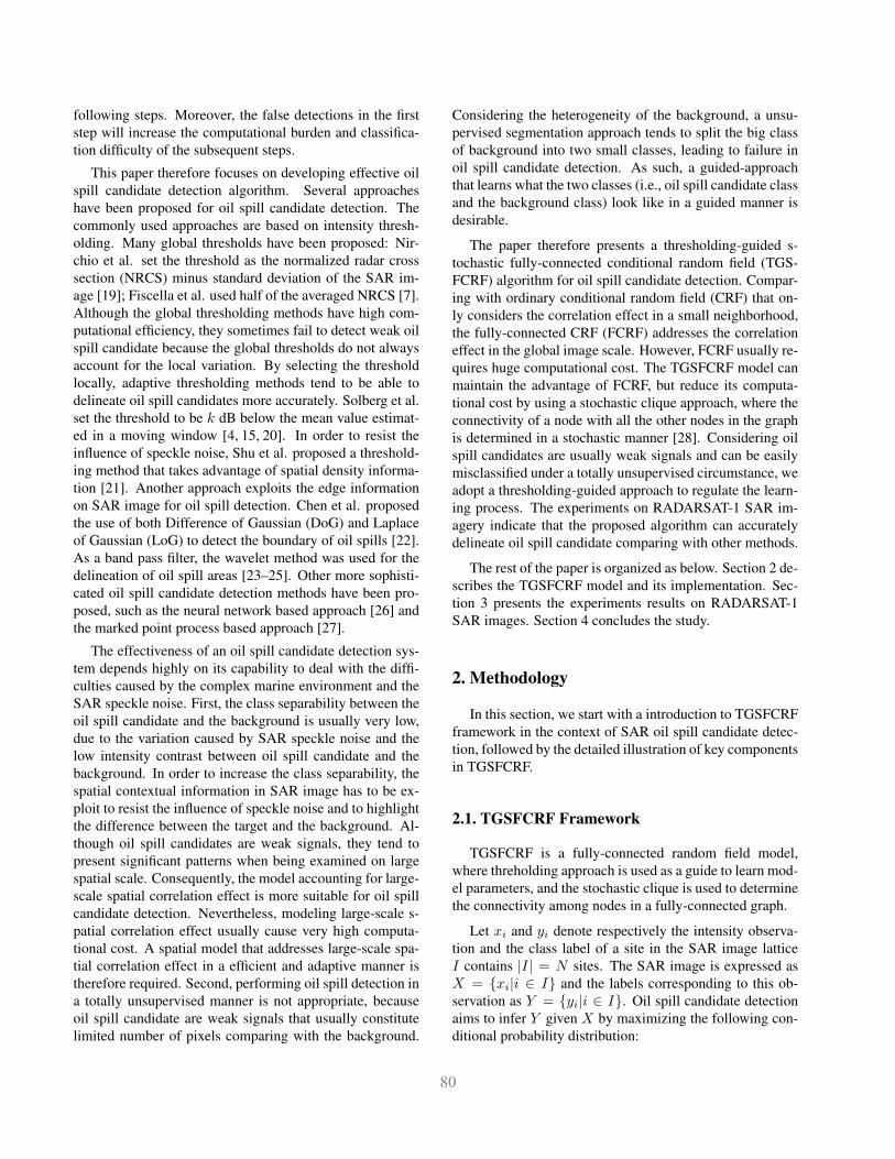
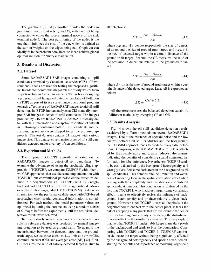
Fig. 3 displays the graphical model of TGSFCRF, wherethe edge eik between yi and yk is determined in a stochasticmanner. Nodes that are closer in both feature space and im-age space have higher possibility to be connected, whereasnodes far away from each other have lower chance of be-ing connected. As a result of implementing the criteriondefined in (7), in TGSFCRF, only a subset of nodes in theneighborhood that are the most relevant with the referencednode will be adopted for building connectivity with the ref-erenced node. TGSFCRF therefore can efficiently and ef-fectively model large-scale spatial correlation effect.

2.5. MAP Inference

Since the unary potential can be achieved by GMM, toincorporate the spatial information, the pairwise potential isexpressed as:

ψp(yi, yj , X) = −λ · µ(yi, yj) · Pij (10)

Figure 3. The graphical model of TGSFCRF. The probability ofconnectivity between the referenced node yi and an arbitrary nodeyk is denoted by edge eik. Closer nodes have black solid edges, in-dicating higher possibility to be connected, whereas nodes with fardistance red dashed edges, implying a smaller chance for buildingconnectivity.

where µ(yi, yj) is implemented according to the Potts mod-el:

µ(yi, yj) =

{1 yi 6= yj0 otherwise. (11)

Using the above-described unary and pairwise potential-s, the binary classification of SAR image into the oil spillcandidate class and background class is achieved accordingto the maximum a posterior (MAP), such that

Y ∗ = argmaxY

P (Y |X) (12)

where Y ∗ is the best label configuration in the set Ythat maximizes P (Y |X). To find Y ∗, the energy func-tion

∑i ψu(yi, X) +

∑(i,j)∈C ψp(yi, yj , X) of (1) is min-

imized by graph-cut approach. The stochastic cliquescheme, as implemented in TGSFCRF, is seamlessly in-tegrated into the conventional graph-cut based randomfield optimization framework by replacing the conventionalclique with the stochastic clique.

4324

The graph-cut [30, 31] algorithm divides the nodes ingraph into two disjoint sets Ys and Yt, with each set beingconnected to either the source terminal node s or the sinkterminal node t. The best partitioning of the nodes is theone that minimizes the cost of the cut, which is defined asthe sum of weights on the edges being cut. Graph-cut canideally fit in the problem here, because it can achieve globaloptimal solution for binary classification.

3. Results and Discussion3.1. Dataset

Some RADARSAT-1 SAR images containing oil spillcandidates provided by Canadian ice service (CIS) of Envi-ronment Canada are used for testing the proposed algorith-m. In order to monitor the illegal release of oily wastes fromships traveling in Canadian waters, CIS has been designinga program called Integrated Satellite Tracking of Pollution(ISTOP) as part of its ice surveillance operational programtowards effective use of RADARSAT images to aid oil spilldetection. In ISTOP, human analysts at CIS manually inter-pret SAR images to detect oil spill candidates. The imagesprovided by CIS are RADARSAT-1 ScanSAR intensity da-ta, with HH polarization and a spatial resolution of 50×50m. Sub-images containing both oil spill candidate and thesurrounding sea area were clipped to test the proposed ap-proach. The test dataset contains 21 images with variousimage size. This dataset covers major types of oil spill can-didates detected under a variety of sea conditions.

3.2. Experimental Methods

The proposed TGSFCRF algorithm is tested on theRADARSAT-1 images to detect oil spill candidates. Toexamine the advantage of using the stochastic clique ap-proach in TGSFCRF, we compare TGSFCRF with other t-wo CRF approaches that use the same implementation withTGSFCRF but conventional pairwise clique structure de-fined in a neighborhood, i.e., TGCRF3 with 3×3 neigh-borhood and TGCRF11 with 11×11 neighborhood. More-over, the threholding-guided GMM (TGGMM) model is al-so used to show the performance difference with CRF-basedapproaches when spatial contextual information is not ad-dressed. For each method, the model parameter values areoptimized by tuning the parameters using a random subsetof 5 images before the experiments until the best visual de-tection results were achieved.

To quantitatively assess the accuracy of the detection re-sults, a reference dataset was produced by manual image-interpretation to be used as ground-truth. To quantify theinconsistency between the detected target and the ground-truth target, we use three statistics, i.e., omission error (CE),commission error (OE), and averaged error (AE) [32]. First,CE measures the ratio of falsely-detected target relative to

all detections:

CE =AE −AEinR

AE(13)

where AE and AR denote respectively the size of detect-ed target and the size of ground-truth target, and AEinR isthe size of detected target within a certain distance of theground-truth target. Second, the OE measures the ratio ofthe omission in detections relative to the ground-truth tar-get.

OE =AR −ARinE

AR(14)

where ARinE is the size of ground-truth target within a cer-tain distance of the detected target. Last, AE is expressed asbelow:

AE =CE +OE

2(15)

AE therefore measures the balanced detection capabilityof different methods by averaging CE and OE.

3.3. Results Analysis

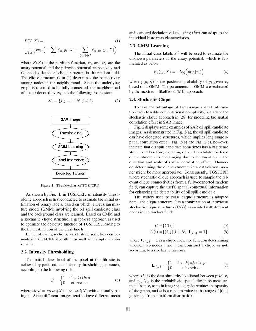
Fig. 4 shows the oil spill candidate detection result-s achieved by different methods on several RADARSAT-1Images. Due to the existence of speckle noise and the lowcontrast between oil spill candidates and the background,the TGGMM approach tends to produce many false detec-tions. Comparing with TGGMM, TGCRF3 is less affect-ed by the speckle noise and greatly reduces false alarms,indicating the benefits of considering spatial contextual in-formation for label inference. Nevertheless, TGCRF3 tendsto be easily disturbed by the background heterogeneity, andwrongly classified some dark areas in the background as oilspill candidates. This demonstrate the limitation and weak-ness of modeling local-scale spatial correlation effect whendealing with the complexity and unstationaries of SAR oilspill candidate images. This conclusion is reinforced by thefact that TGCRF11, which address larger-range correlationeffect, is able to effectively resists the influence of back-ground heterogeneity and produce relatively clean back-ground. However, since TGCRF11 uses all the pixels in theneighborhood to connect with the center pixel, it faces therisk of accepting many pixels that are irrelevant to the centerpixel for building connectivity, considering the disturbanceof noise effect on the similarity measures. This may explainthat fact that TGCRF11 undesirably keeps many dark pixelsin the background and tends to blur the boundaries. Com-paring with TGCRF3 and TGCRF11, TGSFCRF can bet-ter delineate the target without being significantly affectedby the background heterogeneity and speckle noise, demon-strating the benefits and importance of modeling large-scale

4325

spatial correlation effect by determining the clique structurein a stochastic data-driven manner.

Table 1 shows the statistics of the numerical measuresachieved by different methods on the 21 RADARSAT-1SAR images. The statistics are basically consistent withthe visual detection results. Overall, TGSFCRF achieveslower mean OE values, and much lower mean CE and AEvalues than TGCRF3 and TGCRF11, indicating a good bal-ance between the ability to detect the target and the abilityto resist the influence of the disturbance caused backgroundheterogeneity. According to mean AE value, the secondbest method is TGCRF11, which achieves lower mean CEvalue, but slightly higher OE than TGCRF3. All CRF-basedapproach produce lower mean AE value than TGGMM ap-proach, which stably achieve very high OE and CE valueson the test images. Moreover, since the standard deviationof a statistic implies the degree of fluctuation of statisticvalues over different test images, the fact that TGGMMachieves the lowest Std. values on all statistics indicatesthat TGGMM performs consistently worse than the othermethods over all test images.

4. ConclusionsIn this paper, we presented a TGSFCRF algorithm for

the purpose of oil spill candidate detection. Comparing theCRF and FCRF, TGSFCRF is more capable of modelinglarge-scale spatial correlation effect by the use of stochasticclique approach, and thereby is more tailored to the char-acteristics of SAR oil spill candidates. In order to reducethe uncertainties caused by the background heterogeneityand the unbalanced class distribution, TGSFCRF adopts athreholding-guided approach to aid the learning of modelparameters. This characteristic also allows TGSFCRF to besolved by a graph-cut approach to achieve global optimalin a binary labeling problem. The experiments conduct-ed on many RADARSAT-1 ScanSAR images demonstratethat TGSFCRF can better delineate oil spill candidate, with-out being significantly affected by background and fore-ground heterogeneities. One limitation of TGSFCRF maybe caused by the use of suboptimal intensity thresholds. InTGSFCRF, the threshold is set to be the mean intensity val-ue minus one standard deviation of the image. However,this parameter setting may be biased, depending on variousfactors such as the proportion of the target relative to thebackground, the degree of background heterogeneity andSAR speckle noise. Therefore, TGSFCRF can probably en-hanced by better determination of the threshold that takesinto consideration the statistical distributions of the classes.Moreover, considering that the intensity similarity amongindividual pixels cannot reflect the textual characteristics,the stochastic clique approach in TGSFCRF can possiblybe improved by adopting patch similarities that address lo-cal textual patterns.

5. AcknowledgementsThis work is partly funded by the Natural Sciences and

Engineering Research Council of Canada (NSERC) and theCanadian Space Agency (CSA). This research was under-taken, in part, thanks to funding from the Canada ResearchChairs program.

References[1] C. Elachi, “Spaceborne imaging radar: geologic and oceano-

graphic applications,” Science, vol. 209, no. 4461, pp. 1073–1082, 1980.

[2] M. D. Henschel, R. Olsen, P. Hoyt, and P. W. Vachon,“The ocean monitoring workstation: experience gainedwith RADARSAT,” Geomatics in the ERA of RADARSAT(GER97), 1997.

[3] A. H. S. Solberg and E. Volden, “Incorporation of priorknowledge in automatic classification of oil spills in ER-S SAR images,” in Geoscience and Remote Sensing, 1997.IGARSS’97. Remote Sensing-A Scientific Vision for Sustain-able Development., 1997 IEEE International, vol. 1. IEEE,1997, pp. 157–159.

[4] A. S. Solberg, G. Storvik, R. Solberg, and E. Volden, “Au-tomatic detection of oil spills in ERS SAR images,” Geo-science and Remote Sensing, IEEE Transactions on, vol. 37,no. 4, pp. 1916–1924, 1999.

[5] H. Espedal, “Satellite SAR oil spill detection using wind his-tory information,” International Journal of Remote Sensing,vol. 20, no. 1, pp. 49–65, 1999.

[6] H. Espedal and O. Johannessen, “Cover: Detection of oilspills near offshore installations using synthetic apertureradar (sar),” 2000.

[7] B. Fiscella, A. Giancaspro, F. Nirchio, P. Pavese, andP. Trivero, “Oil spill detection using marine SAR images,”International Journal of Remote Sensing, vol. 21, no. 18, pp.3561–3566, 2000.

[8] F. Del Frate, A. Petrocchi, J. Lichtenegger, and G. Calabresi,“Neural networks for oil spill detection using ERS-SAR da-ta,” Geoscience and Remote Sensing, IEEE Transactions on,vol. 38, no. 5, pp. 2282–2287, 2000.

[9] A. Gambardella, M. Migliaccio, and G. De Grandi, “Waveletpolarimetric SAR signature analysis of sea oil spills andlook-alike features,” in Geoscience and Remote Sens-ing Symposium, 2007. IGARSS 2007. IEEE International.IEEE, 2007, pp. 983–986.

[10] V. V. Malinovsky, S. Sandven, A. S. Mironov, and A. E. Ko-rinenko, “Identification of oil spills based on ratio of alter-nating polarization images from ENVISAT,” in Geoscienceand Remote Sensing Symposium, 2007. IGARSS 2007. IEEEInternational. IEEE, 2007, pp. 1326–1329.

[11] Z. Ou, D. Abreu et al., “Integrated satellite tracking of pollu-tion: a new operational program,” in 2007 IEEE Internation-al Geoscience and Remote Sensing Symposium, 2007, pp.967–970.

4326

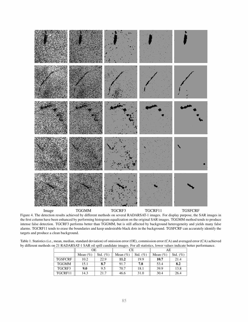
Image TGGMM TGCRF3 TGCRF11 TGSFCRFFigure 4. The detection results achieved by different methods on several RADARSAT-1 images. For display purpose, the SAR images inthe first column have been enhanced by performing histogram equalization on the original SAR images. TGGMM method tends to produceintense false detection. TGCRF3 performs better than TGGMM, but is still affected by background heterogeneity and yields many falsealarms. TGCRF11 tends to erase the boundaries and keep undesirable black dots in the background. TGSFCRF can accurately identify thetargets and produce a clean background.

Table 1. Statistics (i.e., mean, median, standard deviation) of omission error (OE), commission error (CA) and averaged error (CA) achievedby different methods on 21 RADARSAT-1 SAR oil spill candidate images. For all statistics, lower values indicate better performance.

OE CE AEMean (%) Std. (%) Mean (%) Std. (%) Mean (%) Std. (%)

TGSFCRF 10.2 22.9 11.2 19.9 10.7 21.4TGGMM 15.1 8.7 91.7 7.8 53.4 8.2TGCRF3 9.0 9.5 70.7 18.1 39.9 13.8

TGCRF11 14.3 21.7 46.6 31.0 30.4 26.4

4327

[12] W. G. Pichel and P. Clemente-Colon, “NOAA CoastWatchSAR applications and demonstration,” Johns Hopkins APLtechnical digest, vol. 21, no. 1, pp. 49–57, 2000.

[13] G. Ferraro, A. Bernardini, M. David, S. Meyer-Roux,O. Muellenhoff, M. Perkovic, D. Tarchi, and K. Topouzelis,“Towards an operational use of space imagery for oil pollu-tion monitoring in the Mediterranean basin: A demonstrationin the Adriatic sea,” Marine Pollution Bulletin, vol. 54, no. 4,pp. 403–422, 2007.

[14] K. Eldhuset, “An automatic ship and ship wake detectionsystem for spaceborne SAR images in coastal regions,” Geo-science and Remote Sensing, IEEE Transactions on, vol. 34,no. 4, pp. 1010–1019, 1996.

[15] A. H. S. Solberg, C. Brekke, and P. Ove Husoy, “Oil spilldetection in Radarsat and Envisat SAR images,” Geoscienceand Remote Sensing, IEEE Transactions on, vol. 45, no. 3,pp. 746–755, 2007.

[16] P. Clemente-Colon and X.-H. Yan, “Low-backscatter oceanfeatures in synthetic aperture radar imagery,” Johns HopkinsAPL Technical Digest, vol. 21, no. 1, pp. 116–121, 2000.

[17] K. N. Topouzelis, “Oil spill detection by sar images: darkformation detection, feature extraction and classification al-gorithms,” Sensors, vol. 8, no. 10, pp. 6642–6659, 2008.

[18] C. Brekke and A. H. Solberg, “Oil spill detection by satel-lite remote sensing,” Remote sensing of environment, vol. 95,no. 1, pp. 1–13, 2005.

[19] F. Nirchio, M. Sorgente, A. Giancaspro, W. Biamino,E. Parisato, R. Ravera, and P. Trivero, “Automatic detectionof oil spills from sar images,” International Journal of Re-mote Sensing, vol. 26, no. 6, pp. 1157–1174, 2005.

[20] A. H. Solberg, S. T. Dokken, and R. Solberg, “Automaticdetection of oil spills in Envisat, Radarsat and ERS SAR im-ages,” in Geoscience and Remote Sensing Symposium, 2003.IGARSS’03. Proceedings. 2003 IEEE International, vol. 4.IEEE, 2003, pp. 2747–2749.

[21] Y. Shu, J. Li, H. Yousif, and G. Gomes, “Dark-spot detectionfrom SAR intensity imagery with spatial density threshold-ing for oil-spill monitoring,” Remote Sensing of Environmen-t, vol. 114, no. 9, pp. 2026–2035, 2010.

[22] C. Chen, K. Chen, L. Chang, and A. Chen, “The use of satel-lite imagery for monitoring coastal environment in taiwan,”in Geoscience and Remote Sensing, 1997. IGARSS’97. Re-mote Sensing-A Scientific Vision for Sustainable Develop-ment., 1997 IEEE International, vol. 3. IEEE, 1997, pp.1424–1426.

[23] A. K. Liu, C. Y. Peng, and S.-S. Chang, “Wavelet analysisof satellite images for coastal watch,” Oceanic Engineering,IEEE Journal of, vol. 22, no. 1, pp. 9–17, 1997.

[24] S. Wu and A. Liu, “Towards an automated ocean feature de-tection, extraction and classification scheme for SAR im-agery,” International Journal of Remote Sensing, vol. 24,no. 5, pp. 935–951, 2003.

[25] S. Derrode and G. Mercier, “Unsupervised multiscale oil s-lick segmentation from sar images using a vector HMC mod-el,” Pattern Recognition, vol. 40, no. 3, pp. 1135–1147, 2007.

[26] K. Topouzelis, V. Karathanassi, P. Pavlakis, and D. Rokos,“Detection and discrimination between oil spills and look-alike phenomena through neural networks,” ISPRS Journalof Photogrammetry and Remote Sensing, vol. 62, no. 4, pp.264–270, 2007.

[27] Y. Li and J. Li, “Oil spill detection from SAR intensity im-agery using a marked point process,” Remote Sensing of En-vironment, vol. 114, no. 7, pp. 1590–1601, 2010.

[28] M. Shafiee, A. Wong, P. Siva, and P. Fieguth, “Efficientbayesian inference using fully connected conditional randomfields with stochastic cliques,” in International Conferenceon Image Processing (ICIP). IEEE, 2014, pp. 1–5.

[29] C.-A. Deledalle, L. Denis, and F. Tupin, “Iterative weight-ed maximum likelihood denoising with probabilistic patch-based weights,” Image Processing, IEEE Transactions on,vol. 18, no. 12, pp. 2661–2672, 2009.

[30] L. Ford and D. Fulkerson, Flows in networks. PrincetonPrinceton University Press, 1962, vol. 1962.

[31] P. Kohli and P. Torr, “Dynamic graph cuts for efficient infer-ence in markov random fields,” IEEE Transactions on Pat-tern Analysis and Machine Intelligence,, vol. 29, no. 12, pp.2079–2088, 2007.

[32] C. Wiedemann, C. Heipke, H. Mayer, and O. Jamet, “Empir-ical evaluation of automatically extracted road axes,” Empiri-cal Evaluation Techniques in Computer Vision, pp. 172–187,1998.

4328