On the Economic Geography of InternationalMigration

Caglar Ozden ∗ Christopher Parsons †

January 13, 2014

Abstract

We exploit the bilateral and skill dimensions from recent data sets of internationalmigration to test for the existence of Zipf’s and Gibrat’s Laws in the context ofaggregate and high-skilled international immigration and emigration using graphical,parametric and non-parametric analysis. The top tails of the distributions ofaggregate and high-skilled immigrants and emigrants adhere to a Pareto distributionwith an exponent of unity i.e. Zipf’s Law holds. We find some evidence in favourof Gibrat’s Law holding for immigration stocks, i.e. that the growth in stocks isindependent of their initial values and stronger evidence that immigration densitiesare diverging over time. Conversely, emigrant stocks are converging in the sense thatcountries with smaller emigrant stocks are growing faster than their larger sovereigncounterparts. These findings are consistent with relatively few destinations, withlow birth rates, continuing to attract the vast majority of emigrants whom facelower migration costs from evermore origin countries, whose birth rates are higher.We also document within immigration stocks, immigrant densities and emigrantdensities and to a lesser extent within emigrant stocks, convergence in the high skillcomposition, consistent with an increasing global supply of high-skilled workers andthe imposition of selective immigration policies.

JEL classification: F22, J61

Keywords: Zipf’s Law, Gibrat’s Law, International Migration

∗Development Economics Research Group, World Bank, Washington. E-mail cozden@worldbank.org†Department of International Development, University of Oxford, Queen Elizabeth House, 3 Mansfield

Road, Oxford OX1 3TB, United Kingdom. E-mail: christopher.parsons@qeh.ox.ac.uk.We are grateful to Ferdinand Rauch for useful and timely comments and would like to extend our

gratitude to Simone Bertoli and Frederic Docquier for their combined encouragement for writing thispaper.

1 Introduction

In urban economics, Zipf’s Law and Gibrat’s Law occupy a special place in explaining

the relationships between cities in terms of their relative sizes and growth rates. In this

paper, we link the literature on international migration to urban economics, especially

the literature on population growth and distributions. More specifically, we draw upon

two of the most recent advances in the development of bilateral migration data, Ozden

et al. (2011) and Artuc et al. (2013), to examine the existence of Gibrat’s and Zipf’s Laws

for immigrant and emigrant levels and densities in aggregate levels as well as examining

high-skilled migration patterns.

Zipf’s law for cities states that the city size distribution within a country can be

approximated by a power law distribution. More specifically, if we were to rank the

cities in terms of their sizes, the nth largest city is 1/n of the size of the largest city.

Another way to state this regularity is running a regression with ln(city size rank) as

the dependent variable and ln(city size) as the main explanatory variable. The coefficient

typically is equal to around 1 with a high level of precision, especially when larger cities

are considered.

Gibrat’s law, on the other hand, is about growth rates and was initially noted for the

French firms Gibrat (1931). When applied to cities, it states that growth processes have

a common mean and are independent of initial sizes. The seminal paper of Gabaix (1999)

establishes that, when cities grow according to Gibrat’s law, then, in steady state, their

size distribution will follow a pareto distribution with a power exponent of 1. This, as

well as numerous results from across the urban economics literature, which also show that

Zipf’s Law holds, provides some evidence against the existence of Gibrat’s Law, which

instead predicts that the resulting distribution is log-normal. Eeckhout (2004) manages

to accommodate both ‘laws’ by showing that Pareto distribution best fits the observed

pattern if upper tail of the distribution of city sizes is considered. Conversely, a log-normal

distribution provides the best fit if the entire distribution were to be considered. These

patterns are observed across the world and are discussed in great detail in many other

places (such as Gabaix and Ioannides (2004).

2

The natural question then is to ask what mechanisms exist that might link Gibrat’s

and Zipf’s laws. This question is especially important when divergent rates of population

growth across locations are the norm. Among the causes that would lead to differing

growth rates are climate, natural disasters and resource endowments. There are numerous

examples of cities that disappear from history or boom after a discovery of a natural

resource for example. People however, have the ability to move from one location to

another, especially as some locations become overcrowded and resources are restrained

due to higher natural growth rates. Under these circumstances, the convergence of growth

rates via migration would naturally take place within a larger geographic area (such as a

country) without internal barriers to population mobility.

There had been few studies that take the analysis outside of national boundaries since

the theoretical models used to explain Zipf’s and Gibrat’s laws are not truly applicable

when the unit of observation is a sovereign country. Governments exercise considerable

power over their international (as opposed to internal) borders and can dictate who can

enter and, to a certain extent, exit the country. The most prominent study is Rose

(2005) who tests these theories using countries as the relevant geographical entities. He

concludes that the ‘hypothesis of no effect of size on growth usually cannot be rejected.’1

When testing the Zipf’s law for countries, Rose (2005) shows that it also strongly holds

in the upper tail of the distribution of country sizes, as is the case with city sizes. The

only study that links Gibrat’s and Zipf’s laws to international immigration is the work by

Clemente et al. (2011) who uses aggregate immigration numbers and densities. They test

for the existence of Zipf’s Law specifically in the context of immigrant levels and densities

and find for the top 50 countries that Zipf’s Law holds only for immigrant levels.

In this paper, we draw upon two recent bilateral migration databases, Ozden et al.

(2011) and Artuc et al. (2013). These yield two advantages. Firstly, global bilateral

migration data allow us to calculate country level emigrant stocks, as opposed to simply

1Offering a critique of Rose (2005), Gonzlez-Val and Sanso-Navarro (2010) apply more up-to-dateempirical strategies to test the application of Gibrat’s Law to countries and find mixed results, someevidence in favour of population growth being independent of initial country size but conclude on thewhole that the results from across their range of empirical strategies that some evidence of convergenceis found.

3

immigrant stocks. Secondly, the latter database, which reports bilateral migration stocks

by education levels, allows us to further delineate between patterns of migrants with low

and high education levels.

Zipf’s law implies a concentrated distribution of the total population among a few

large cities. We observe similar patterns in immigration patterns but the converse over

time in emigration patterns. In 2000, the top ten receiving countries accounted for no

less than 57% of the world migrant stock, which is approximately equivalent to the

total emigrant stocks of the top 25 emigration countries in the same decade. In 1960,

the equivalent figure for the top ten receiving nations was 54%, which is equivalent to

less than the total emigrant stock of the top 9 sending countries in 1960. A similar

concentration is observed for individual corridors. In 2000, of all bilateral corridors (over

40,000 in total) comprised fewer than 50 migrants each. Together, they accounted for

only 0.1 percent of total migrant stock. On the other hand, in the same year, just 505

corridors accounted for over 80 percent of the global migrant stock of over 160 million

people.

Whether the sum of these bilateral trends holds across countries is the subject of our

paper. We delve deeper into the observed patterns of international migration over the

period 1960-2000, by examining the existence of Zipf’s and Gibrat’s Laws, two empirical

regularities that are ubiquitous in the urban economics literature. We therefore adopt

an alternative perspective in analyzing to what extent the underlying trends in global

migration patterns are converging or diverging.

The results in the paper are both interesting and encouraging. In regards to Zipf’s

law, we find that it holds very strongly in the upper tail of the distribution with the Pareto

coefficient very close to unity for both immigration and emigration for all time periods.

The results are less precise for high skilled migration but we cannot reject the coefficient

being unity. When the whole sample is included, we find a log-normal distribution in

terms of immigrant sizes which are very similar to the results found for cities and countries

in the literature. With respect to Gibrat’s law, our results are somewhat less uniform. We

find evidence of convergence with the growth rates being linked negatively to initial levels

4

for both aggregate and high-skilled immigration and emigration levels and densities. In

our non-parametric analysis, we find some evidence in favour of Gibrat’s Law holding for

immigration stocks, i.e. that the growth in stocks is independent of their initial values

and stronger evidence that immigration densities are diverging over time. Conversely,

emigrant stocks are converging in the sense that countries with smaller emigrant stocks

are growing faster than their larger sovereign counterparts. These are all surprising

regularities given that government policies and other physical and cultural barriers impose

strong restrictions on international migration patterns.

The following Section offers a brief overview of the bilateral data sets that we use

in the paper. Section 3 introduces an analysis of Zipf’s Law while in Section 4 we

analyse the extent to which the underlying distributions of our variables of interest

approximate to log-normal distributions. Section 5 presents an examination of Gibrat’s

Law in international migration patterns, before we finally conclude.

2 Basics of Migration Data

This section aims to outline the broad patterns observed in the global migration databases.

Ozden et al. (2011) show that while the global migrant stock increased from 92 million

to 165 million between 1960 and 2000,2 immigrants as a share of the world population

actually decreased from 3.05 percent to 2.71 percent during the same period. Ozden

et al. (2011) provide bilateral migrant stocks for 226 origins and destinations globally at

decennial intervals between 1960 and 2000, which correspond to the last five completed

census rounds. While South-South migration dominates the global stock, mainly due

to the millions of migrants created during the partition of India and the collapse of

the Soviet Union, the most significant trend between 1960 and 2000 has been the surge

in South-North migration. Over the period, two-thirds of the total growth in migration

stocks was due to migrant flows to Western Europe and the United States from developing

countries. Other notable patterns were the emergence of the oil-rich Persian Gulf countries

2The data from the 2010 census round is currently being collated since these data are typicallypublished with a significant lag.

5

as key destinations, greater intra-Africa migration flows and migration to the “migrant-friendly”

countries of the New World, namely, Australia, New Zealand, and Canada.

The analysis of international migration patterns faces many challenges and these

studies aim to overcome them in various ways. For example, no census round has ever

been completed in the sense that all countries have participated. Even when censuses are

conducted, not all countries are willing to make the data publicly available. International

borders have changed over time, most notably following the dissolution of the Soviet

Union and Yugoslavia. Various countries adhere to different methodologies, national

standards and classifications when conducting their censuses and recording the results.

Ozden et al. (2011) strive to present as full and as harmonious a matrix of aggregate

bilateral migration stocks over the period, breaking down the numbers in accordance

with the international borders currently in existence. migrant stock, respectively.

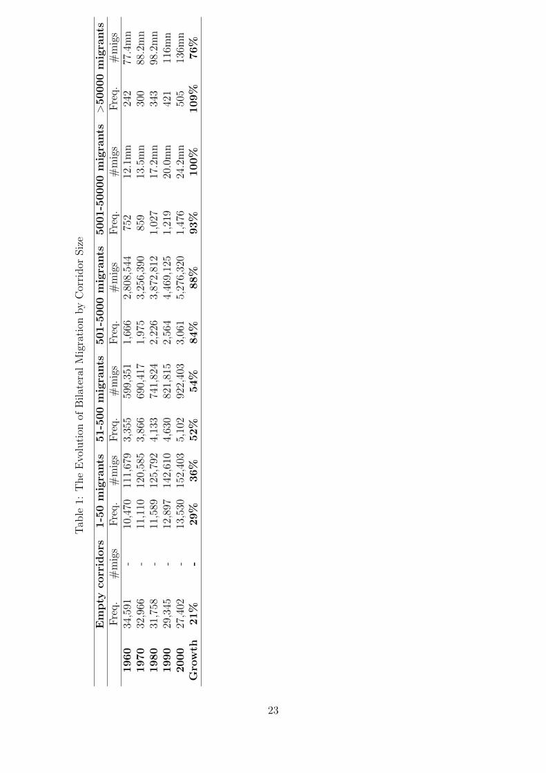
Table 1 presents summary statistics of the frequency and the total numbers of migrants

comprising bilateral migrant corridors of various sizes (zero corridors, 1-50 migrants,

51-500 migrants, 501-5,000 migrants, 5,001-50,000 migrants and corridors containing more

than 50,000 migrants) over the period 1960-2000. Several stark patterns are evident. Over

time, the number of empty bilateral migrant corridors has fallen substantially as the globe

has become more interconnected through international migration. While smaller corridors

are far more common, these comprise far fewer international migrants as when compared

to larger corridors. As discussed earlier, around half of all bilateral corridors (over 40

thousand) are basically empty and have less than fifty migrants in each. These micro

corridors account around 0.1 percent of global migrant stocks.

The basic numbers suggest an agglomeration of human capital in the upper tail of the

distribution as shown in Figure 1. This pattern might be indicative of Zipf’s Law holding;

and concurrently a diversification in terms of the increasing numbers of origins from which

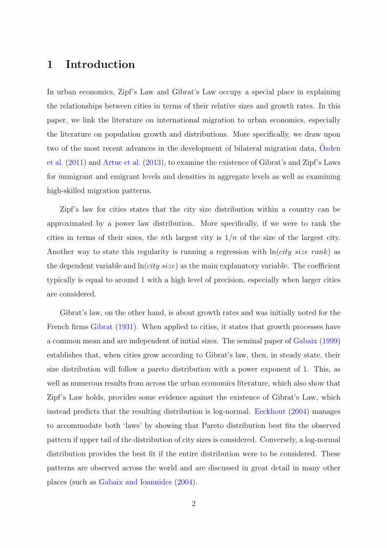
these migrants hail. Figure 2 plots the growth in bilateral migration corridors over the

period 1960 and 2000 against their initial values, a graphical examination of whether

Gibrat’s Law holds or not. The two lines correspond to lines of best fits should zero

values be included or excluded. Should they be included, by adding one to the log, the

6

figure suggests that Gibrat’s Law holds. If they were to be excluded, signs of convergence

across the entire distribution of bilateral migration corridors are evident.

3 Zipf’s Law in International Migration

We begin our analysis with an examination of the existence of Zipf’s Law, the so-called

rank-size rule, which can be viewed as an empirical regularity that describes the (upper

tail) of the population distribution of the geographical entity under investigation. This

distribution may result from a growth process that may or may not be governed by

Gibrat’s law. 3 Typically the existence of Zipf’s Law is analysed graphically and using

regression techniques.4 Both approaches first rank the (population) size variable of

interest S, from highest to lowest (S1 > S2 > S3 > ... SN). Then the natural logarithm

of the rank variable is analysed with respect to the natural logarithm of the (population)

size variable.

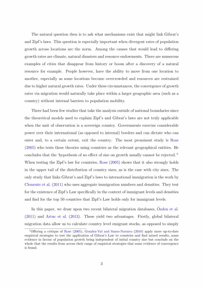
The top two panels in Figure 3 show the graphical scatter plots of the natural

logarithms of the rank of total immigrant and emigrant levels for the 50 countries in

the top tail of the various distributions contained in Ozden et al. (2011). Although we

plot these only for the year 2000, these graphs are representative of other decades as well.

The bottom two panels instead draw on the data from Artuc et al. (2013). These data

instead refer to high-skilled migrants, defined as having completed at least one year of

tertiary education. Clear linear trends are evident, but the line imposed demonstrates

that some deviations from Zipf’s Law clearly exist in the data. For a more robust analysis

we turn to simple regression analysis, following the norms in the literature. Zipf’s Law

can be expressed as:

P (Size > S) = αS(−β) (1)

3Some of the prominent paper in the literature explore the theoretical linkages. Examples areDuranton (2007) Gabaix (1999) and Eeckhout (2004).

4We do not report estimates using the Hill estimator since Gabaix and Ioannides (2004) argue thatin finite samples the properties of this estimator are ‘worrisome’.

7

where α is a constant and β = 1 if Zipf’s law holds. For the basis of our regression analysis

we denote m to be the stock of immigrants or emigrants, expressed either in levels or in

terms of densities, high-skilled or otherwise. Next, r is the rank of m, when ordered from

highest to lowest. Equation (1) expressed in logarithmic form can be written as:

log r = α + β logm+ ε (2)

where ε is an error term and β is the Pareto exponent, which equals unity if Zipf’s Law

holds. Equation (2) is typically estimated using OLS, which leads to strongly biased

results in small samples (Gabaix and Ibragimov, 2007). These authors propose a simple

and efficient remedy to overcome these biases, namely to subtract one-half from the rank.

The regression to be estimated therefore becomes:

log (r − 0.5) = α + β logm+ ε (3)

Despite this adjustment, the standard error of β is not equal to that obtained from

OLS, but instead can be approximated as β√

2n

(Gabaix and Ioannides (2004), Gabaix

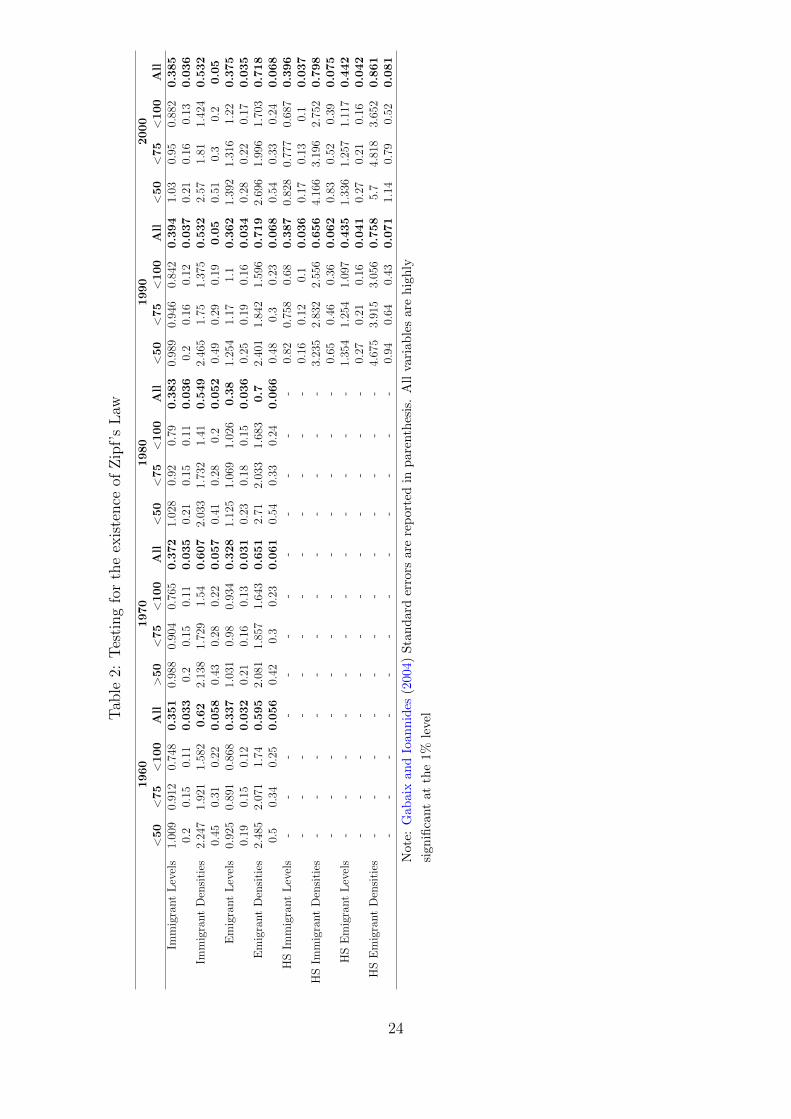
and Ibragimov (2007)). Table 2 presents the regression results from across our various

specifications together with with corrected standard errors for each decade from 1960 to

2000.

Beginning with the total migrant measures, the Pareto coefficient is remarkably close

to unity (at 1.03 for 2000) for the 50 largest countries in the upper tail of the size

distribution, although Zipf’s Law is resolutely rejected across the entire distribution where

the coefficient is 0.385 for 2000. This is consistent with the results presented in Eeckhout

(2004) which argues that the Pareto distribution best describes the upper tail but a

log-normal distribution provides a better fit over the entire distribution. The estimates

of the Zipf coefficient have remained fairly stable over time for both immigrant and

emigrant levels. In contrast, the estimates on immigrant densities have risen in the upper

tail of the distribution, demonstrating some convergence across these countries, but have

fallen across the entire distribution, i.e. providing evidence of divergence. The estimates

8

on emigrant densities however show some signs of convergence between 1960 and 2000.

Turning to the High Skill migration numbers in the bottom eight rows of Table 2,

although the point estimates on the Zipf coefficient are substantively different from unity,

they are nevertheless within the confidence intervals. Both immigrant and emigrant levels

are similar in both 1990 and 2000 and if anything exhibit marginal convergence. Turning

to high skilled immigrant and emigrant densities, both have increased significantly across

the entire distribution, which again is indicative of a process of convergence across the

globe.

4 An examination of log-normality

The previous section showed that we cannot reject the existence of Zipf’s Law in the

upper tails of the distributions of total and high skilled immigrants and emigrants in

levels. On the other hand, if we were to consider the entire distribution, we easily reject

Zipf’s Law. With these results in hand, we next empirically test whether or not the

underlying distributions of our variables approximate to log normal. If this is the case, it

might be the case that Gibrat’s law holds i.e. that these distributions could have resulted

from an independent growth process.

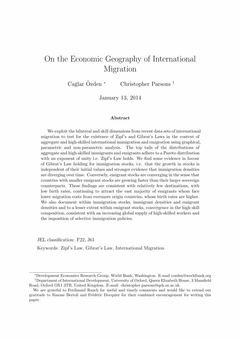
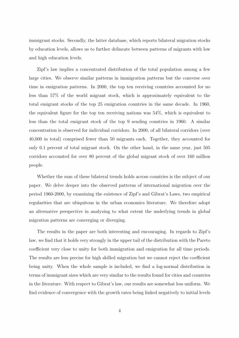
Figures 1 and 4, show the (Epanechnikov) kernel density plots, in 1960 and 2000

for total emigrant levels and densities and total immigrant levels and densities and then

similarly in 1990 and 2000 for the highly skilled. We implement a series of Kolmogorov-Smirnov

equality-of-distributions tests where the null hypothesis is that the relevant variable is

distributed log-normally. Table 3 presents the corrected p-values from the Kolmogorov-Smirnov

tests for each migration variable in 1960 and 2000 and in 1990 and 2000 for the highly

skilled. In just over half of the total cases, we fail to reject the null hypothesis of (log)

normality. Cases where we can reject the null are highlighted in bold. Both immigrant

levels and densities are log-normally distributed as was the case in Clemente et al. (2011).5

Since if Gibrat’s Law were to hold, the resulting distributions of the relevant variables

5 Note that the scale of our density figures differ from Clemente et al. (2011) since we calculate ourdensity measure differently and we further omit refugees, i.e. forced migrants from our analysis.

9

will be log-normal, we proceed by examining whether Gibrat’s Law holds for our various

measures of international migration.

5 Gibrat’s Law in International Migration

As opposed to the static analysis presented when discussing Zipf’s Law, an examination of

Gibrat’s Law with growth rates requires a dynamic analysis of global migration movements.

Gibrat (1931) postulated that “The Law of proportionate effect will therefore imply

that the logarithms will be distributed following the (normal distribution)” (as quoted

in Eeckhout (2004)). In other words, should the growth of geographical entities be

independent of their size, their growth will subsequently result in a log-normal distribution.

Of course, this does not mean that a log-normal distribution implies that Gibrat’s Law

necessarily holds. Both immigration and emigration are determined by government

policies and limited to the extent by which individuals are willing and able to move.

Internal mobility, on the other hand, is far less restricted and is typically thought to lead to

Zipf’s and Gibrat’s laws. Thus, it is difficult to argue that some natural underlying law of

nature would determine the underlying growth and distribution processes of populations

over national boundaries and across the globe.

We estimate parametric and non-parametric kernel regressions to test for the existence

of Gibrat’s Law. These regress the size of migrant populations (or in our case densities)

on their growth.6 In logarithmic form, parametric regressions take the following form:

logmit − logmit−1 = γ + δ logmit + µit (4)

where γ is a constant and µ is a stochastic error term, such that if δ = 0 then Gibrat’s

Law holds. Following the analysis of Eaton and Eckstein (1997), we distinguish between

the aforementioned case of (i) parallel growth, when δ = 0, i.e. when growth does not

depend on initial size, (ii) convergent growth, when δ < 0 when smaller initial populations

6While Panel Unit Root tests have been suggested as appropriate in the literature, it is not feasibleto conduct such an analysis in the current work due to the frequency of our data (decennial) and thelow number of observations in our underlying data (five points in time or four growth rates).

10

grow faster than their larger counterparts so that there is long-run convergence to the

median value and (iii) divergent growth when β > 1, meaning that growth is a positive

monotonic function of initial size. Evidence of either convergent or divergent growth can

therefore be taken as evidence against the existence of Gibrat’s Law.

Table 4 presents the results from this first round of analysis, where Equation (4)

is estimated with OLS with robust standard errors, due to typical heteroskedasticity of

these types of results Gonzlez-Val and Sanso-Navarro (2010). Although Gibrat’s Law is

fundamentally a long run concept, we estimate Equation (4) across each decade for each

of our different measures of immigration and emigration.

The simplest and most intuitive way to test for the existence of Gibrat’s Law is

by plotting geographical entities’ growth on their initial values, which for the sake of

brevity are not included here but are available on request. Such an analysis is strongly

reflected in the results in Table 4.7 Across all decades and across all measures, the

parametric regression results are negative and statistically significant or else statistically

insignificant. These results are indicative of convergence over time or indeed of Gibrat’s

Law holding. Fundamentally however, Gibrat’s Law is a long-run concept and it might

therefore be more appropriate to have more faith in the final column of results from over

the period 1960-2000. In each case the results are strongly negative and statistically

significant, providing some evidence of convergence in immigrant and emigrant levels and

densities over time.

Our OLS estimates yield total or aggregate effects of initial size on subsequent growth,

while conversely non-parametric estimates facilitate an analysis of the effects of initial

size across the entire distribution. We follow Eeckhout (2004) for our non-parametric

analysis of Gibrat’s Law and adopt the following specification:

gi = m(Si) + εi (5)

where gi is the decadal growth of one of our migration measures normalised between two

7We do not report the R2 from these regressions although these are very low for our decadal regressionsand substantially higher for those regressions run over forty years.

11

consecutive periods by subtracting the mean growth and dividing through by the standard

deviation. Maintaining our notation from earlier, mi is the corresponding logarithm of

the relevant migration measure. Since such estimators are sensitive to atypical values,

we follow Clemente et al. (2011) and drop the bottom 5% of observations. Figures 5 and

6 plot the results from these regressions and we would expect these values to be flat and

concentrated around zero if Gibrat’s Law were to hold.

In keeping with the findings of Clemente et al. (2011), we find, at least across most

of the distribution of the stock of immigrants, that Gibrat’s Law holds. The major

exceptions are those countries in the lower end of the distribution, which tend to grow

faster than the other countries in the distribution. We find much stronger evidence of the

divergence in immigrant densities across the globe. The underlying distributions for both

of these variables are log-normal however, demonstrating that log-normality can result,

despite Gibrat’s Law not holding. Emigrant stocks exhibit strong signs of convergence

with smaller emigrant stocks growing far more strongly than larger emigrant stocks. The

results from the kernel regression for emigrant densities are far mixed however, no doubt

in part reflecting the role played by Small Island Developing States (see for example de la

Croix et al. (2013).

All of the kernel regression plots pertaining to the highly skilled, reflect patterns of

convergence since they slope down from left to right. Our estimates for emigrant levels

are never statistically different from zero, providing some evidence that Gibrat’s Law

holds in this context, although the confidence intervals are very wide. The same is true

for the middle and the very upper tail of the distribution of immigrants in levels. These

findings are consistent with the fact that a relatively small number of destinations with

low birth rates, continue to attract a growing number of emigrants from origin countries

where birth rates are higher. In this respect our conclusions are consistent with Clemente

et al. (2011), only we provide further evidence as to the other side of the migration coin.

The convergence in emigration levels are indicative of destination countries drawing on

a greater number of origin countries to meet their human capital needs. Arguably the

mechanics of this process have be lubricated by falling global migration costs.

12

The composition of high skilled immigrant and emigrant levels and densities exhibit

signs of convergence, albeit to differing degrees. These patterns are consistent with the

onset of the global competition for international talent, an increasing global supply of

high-skilled workers across all origins, limited supplies per origin as well as the imposition

of selective immigration policies by an increasing number of destination countries.

6 Conclusion

Gibrat’s and Zipf’s laws are among the most studied and well established phenomenon in

various contexts including linguistics, firm sizes and urban agglomorations. The linkages

between population growth and the distribution across geographic space are key to all

economic analysis since economic activity cannot be analyzed in isolation from location.

Thus, it is important to study and identify the underlying processes that determine the

growth rates of populations over time and their allocation across various locations. Even

though Zipf’s and Gibrat’s laws have been extensively analyzed in the literature, there

are fewer studies on the role of population movements and there are even fewer studies

that focus on mobility across national boundaries. It is therefore natural to search for a

relationship between such population laws and migration patterns.

New data sets on bilateral migration stocks enable us to carry out these analysis.

Ozden et al. (2011) reports bilateral stocks for all migrants for each decade between 1960

and 2000 for 226 countries. Similarly, Artuc et al. (2013) analyzes migrant stocks by

education categories for 1990 and 2000. The current analysis demonstrates interesting

patterns. In terms of comparison to Zipf’s law, we see that the migration patterns are very

similar to what is observed with respect to cities. In the upper end of the distribution,

Zipf’s law holds since the Pareto coefficient is very close to unity. On the other hand, when

the whole distribution is included, we often fail to reject the log-normality assumption,

especially in the case of immigration. High-skilled levels satisfy (although less well) to

Zipf’s Law but more often fail to adhere to log-normality.

While the tests regarding Zipf’s law and the size distribution analysis are static, the

13

tests on the Gibrat’s law and the growth rates require dynamic analysis. The results in

this area are also promising. We find evidence of convergence in the relatively simpler

parametric analysis. In the case of non-parametric regressions, we find some evidence

in favour of Gibrat’s Law holding for immigration stocks, i.e. that the growth in stocks

is independent of their initial values and stronger evidence that immigration densities

are diverging over time. Conversely, emigrant stocks are converging in the sense that

countries with smaller emigrant stocks are growing faster than their larger sovereign

counterparts.

Our goal in this paper is to extend the insights from the urban economics literature

to international migration. Zipf’s and Gibrat’s laws provide natural avenues to do so

since they are linked via population movements. We find various support for these laws

in international migration which is surprising given the policies and many other barriers

that limit international migration patterns.

14

References

Artuc, E., F. Docquier, C. Ozden, and C. Parsons (2013): “A Global Assessment

of Human Capital Mobility: the Role of non-OECD Destinations,” IMI Working Paper

WP-75-2013, University of Oxford, International Migration Institute.

Clemente, J., R. Gonzlez-Val, and I. Olloqui (2011): “Zipfs and Gibrats laws

for migrations,” The Annals of Regional Science, 47, 235–248.

de la Croix, D., F. Docquier, and M. Schiff (2013): “Brain Drain and Economic

Performance in Small Island Developing States,” in The Socio-Economic Impact of

Migration flows. Effects on Trade, Remittances, Output, and the Labour Markets, ed.

by G. P. Andres Artal-Tur and F. Requena-Silvente, Springer, chap. 6.

Duranton, G. (2007): “Urban Evolutions: The Fast, the Slow, and the Still,” American

Economic Review, 97, 197–221.

Eaton, J. and Z. Eckstein (1997): “Cities and growth: Theory and evidence from

France and Japan,” Regional Science and Urban Economics, 27, 443–474.

Eeckhout, J. (2004): “Gibrat’s Law for (All) Cities,” American Economic Review, 94,

1429–1451.

Gabaix, X. (1999): “Zipf’s Law for Cities: An Explanation,” The Quarterly Journal of

Economics, 114, 739–767.

Gabaix, X. and R. Ibragimov (2007): “Rank-1/2: A Simple Way to Improve the

OLS Estimation of Tail Exponents,” NBER Technical Working Papers 0342, National

Bureau of Economic Research, Inc.

Gabaix, X. and Y. M. Ioannides (2004): “The evolution of city size distributions,” in

Handbook of Regional and Urban Economics, ed. by J. V. Henderson and J. F. Thisse,

Elsevier, vol. 4 of Handbook of Regional and Urban Economics, chap. 53, 2341–2378.

Gibrat, R. (1931): Les inegalites economiques: applications: aux inegalites des richesses

15

... aux statistiques des familles, etc. d’une loi nouvelle, la loi de l’effet proportionnel,

Librairie du Recueil Sirey.

Gonzlez-Val, R. and M. Sanso-Navarro (2010): “Gibrats law for countries,”

Journal of Population Economics, 23, 1371–1389.

Ozden, C., C. R. Parsons, M. Schiff, and T. L. Walmsley (2011): “Where on

Earth is Everybody? The Evolution of Global Bilateral Migration 1960-2000,” The

World Bank Economic Review.

Rose, A. K. (2005): “Cities and Countries,” NBER Working Papers 11762, National

Bureau of Economic Research, Inc.

16

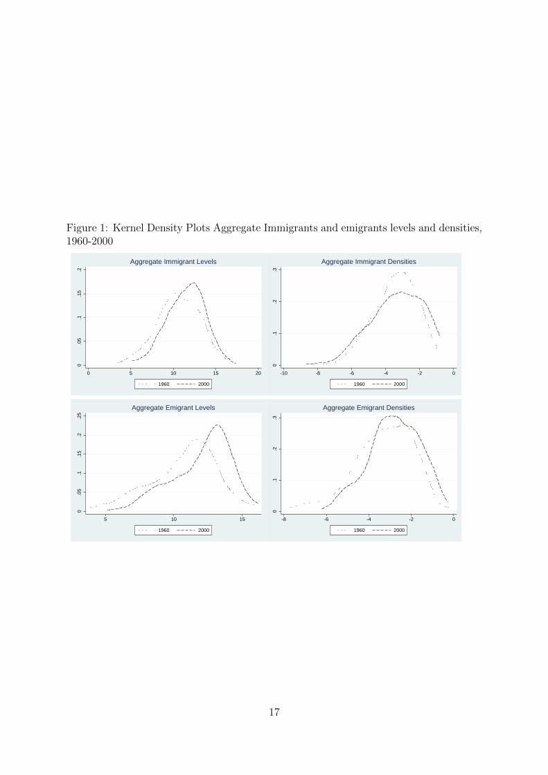
Figure 1: Kernel Density Plots Aggregate Immigrants and emigrants levels and densities,1960-2000

0.0

5.1

.15

.2

0 5 10 15 20

1960 2000

Aggregate Immigrant Levels

0.1

.2.3

-10 -8 -6 -4 -2 0

1960 2000

Aggregate Immigrant Densities

0.0

5.1

.15

.2.2

5

5 10 15

1960 2000

Aggregate Emigrant Levels

0.1

.2.3

-8 -6 -4 -2 0

1960 2000

Aggregate Emigrant Densities

17

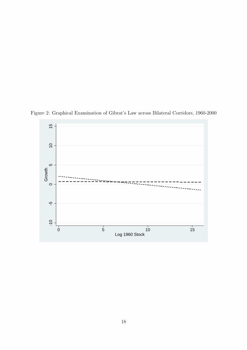
Figure 2: Graphical Examination of Gibrat’s Law across Bilateral Corridors, 1960-2000

-10

-50

510

15G

row

th

0 5 10 15Log 1960 Stock

18

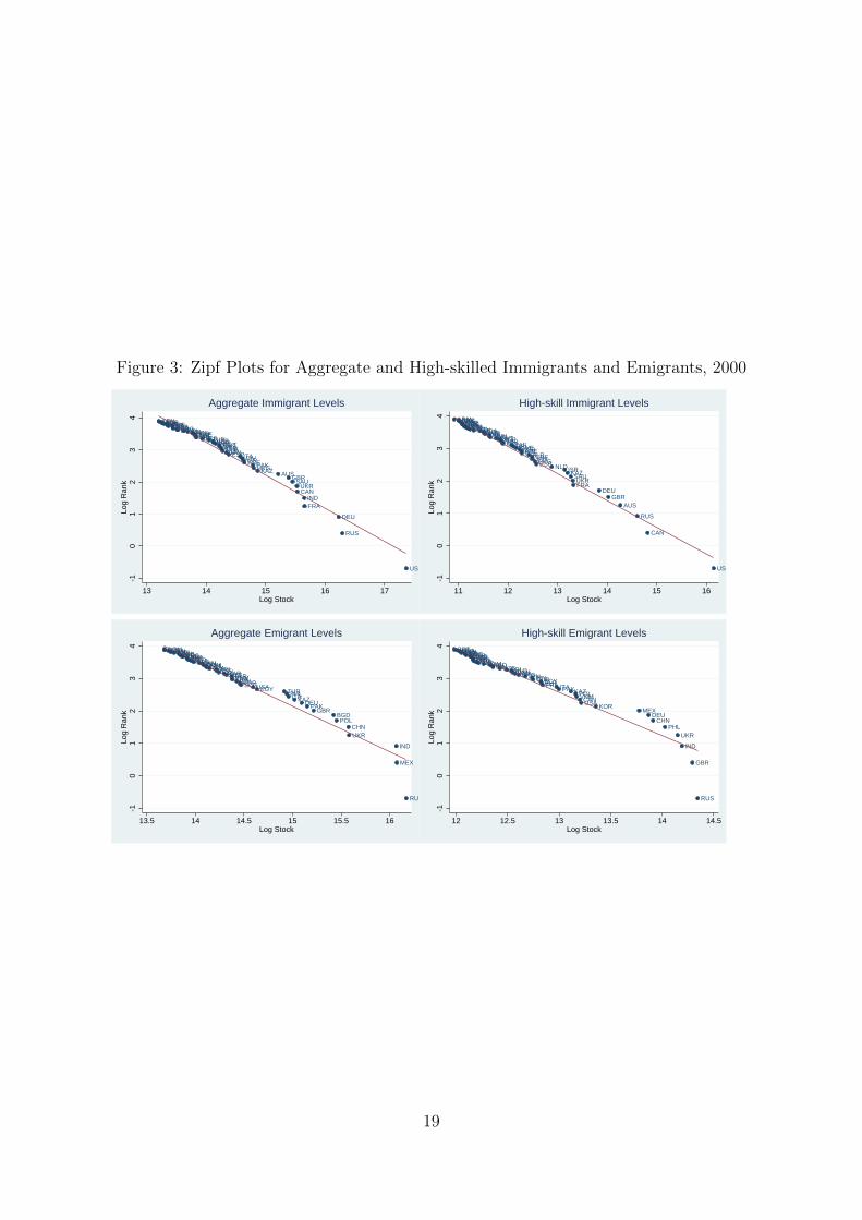
Figure 3: Zipf Plots for Aggregate and High-skilled Immigrants and Emigrants, 2000

USA

IND

PAK

RUS

DEU

UKR

FRA

CAN

ARG

POL

KAZ AUSGBR

HKG

BRA

ISR

BLRTURZAFAUT

CIVCHEJPN

BGDUZBSGP

VENPSE

THA

ITANLD

BELNPL

NZLSWE

ESP

KORNGA

KWT

SAU

BFAHRVKEN

MYS

GRC IRN

LBYOMNPRT

ARE

-10

12

34

Log

Ran

k

13 14 15 16 17Log Stock

Aggregate Immigrant Levels

USA

CAN

AUSGBR

RUS

DEU

SAUFRAUKR

IND

NLDKAZ

NZLCHE

ISR

UZB

JPNHKGESP

POLESTLVA

SWEZAFARE

BELITAKWT

PHLBRAGRCHRV

TUR

MEXPSE

PAK

OMNNOR

MDAJORIRL

TJK

SGPAUT

SYR

YUG

ARM

BLR

TWN

ARG

-10

12

34

Log

Ran

k

11 12 13 14 15 16Log Stock

High-skill Immigrant Levels

IND

PAK

RUS

UKR

POLCHN

ITA

GBRDEU

BLR

ESP

KAZ

FRA

CZE

CAN

USA

GRC

PRTDZA

KOR

MARPRI

MEX

ROM

SCG

IRL

BFAAZE

IDN

TUR

VNM

MYSBIH

JAMIRQ

UZBCOL

EGY

IRN

PHL

PSEJOR

BRACUB

AFGALB

GEOSLVDOM

BGD

-10

12

34

Log

Ran

k

13.5 14 14.5 15 15.5 16Log Stock

Aggregate Emigrant Levels

GBR

DEU

RUS

IND

PHLCHN

CAN

UKR

USAMEX

POL

KOR

ITA

JPNCUBFRA

BGD

EGYIRNNLD

VNMPAK

BLRHKGTWN

IRLJAM

IDN

GRC

COLTURROM

LBNBIH

MYSMARYUG

KAZ

NZLESP

UZB

PERPRT

ZAFGEO

IRQNGABRAHTI

AZE

-10

12

34

Log

Ran

k

12 12.5 13 13.5 14 14.5Log Stock

High-skill Emigrant Levels

19

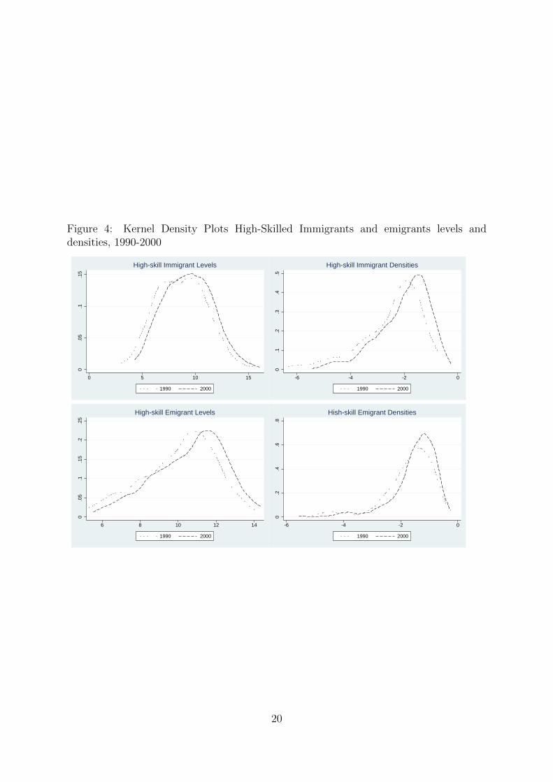
Figure 4: Kernel Density Plots High-Skilled Immigrants and emigrants levels anddensities, 1990-2000

0.0

5.1

.15

0 5 10 15

1990 2000

High-skill Immigrant Levels

0.1

.2.3

.4.5

-6 -4 -2 0

1990 2000

High-skill Immigrant Densities

0.0

5.1

.15

.2.2

5

6 8 10 12 14

1990 2000

High-skill Emigrant Levels

0.2

.4.6

.8

-6 -4 -2 0

1990 2000

Hish-skill Emigrant Densities

20

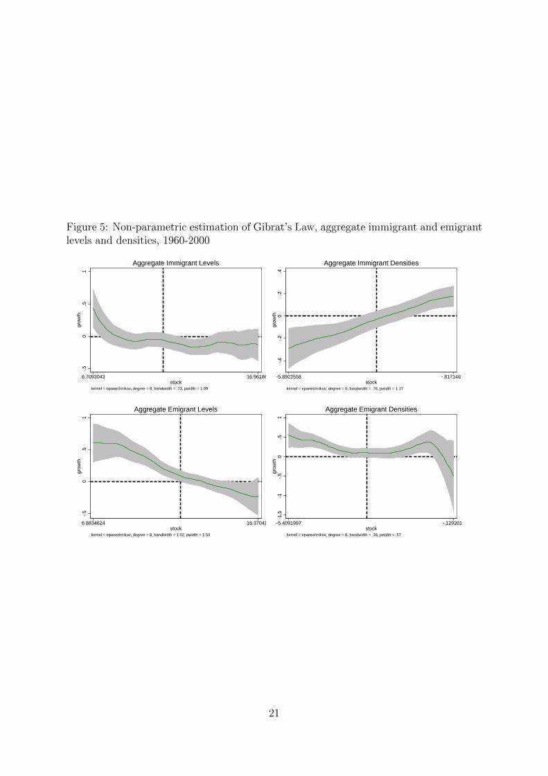
Figure 5: Non-parametric estimation of Gibrat’s Law, aggregate immigrant and emigrantlevels and densities, 1960-2000

-.5

0.5

1gr

owth

6.7093043 16.961861stock

kernel = epanechnikov, degree = 0, bandwidth = .73, pwidth = 1.09

Aggregate Immigrant Levels

-.4

-.2

0.2

.4gr

owth

-5.8922558 -.81714618stock

kernel = epanechnikov, degree = 0, bandwidth = .78, pwidth = 1.17

Aggregate Immigrant Densities

-.5

0.5

1gr

owth

6.8834624 16.370417stock

kernel = epanechnikov, degree = 0, bandwidth = 1.02, pwidth = 1.53

Aggregate Emigrant Levels

-1.5

-1-.

50

.51

grow

th

-5.4091997 -.1292019stock

kernel = epanechnikov, degree = 0, bandwidth = .38, pwidth = .57

Aggregate Emigrant Densities

21

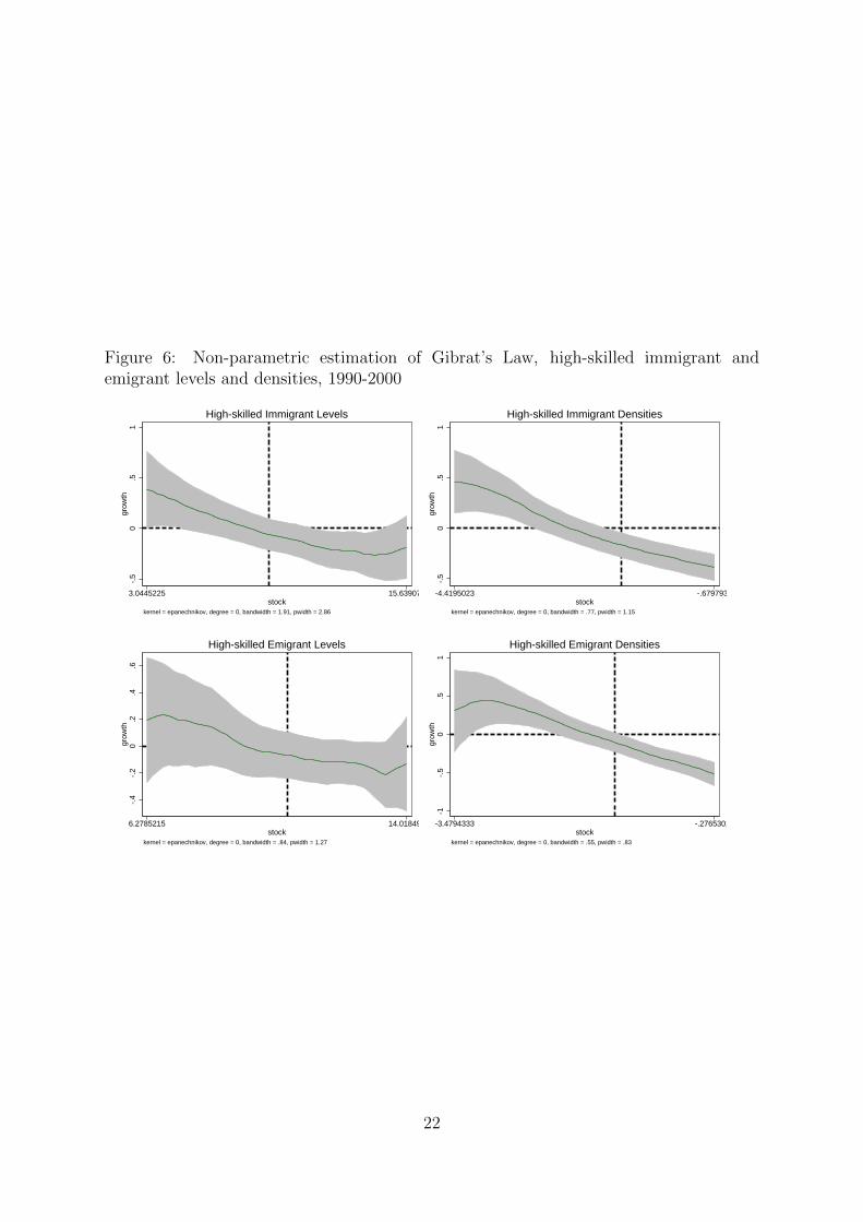
Figure 6: Non-parametric estimation of Gibrat’s Law, high-skilled immigrant andemigrant levels and densities, 1990-2000

-.5

0.5

1gr

owth

3.0445225 15.639072stock

kernel = epanechnikov, degree = 0, bandwidth = 1.91, pwidth = 2.86

High-skilled Immigrant Levels

-.5

0.5

1gr

owth

-4.4195023 -.6797933stock

kernel = epanechnikov, degree = 0, bandwidth = .77, pwidth = 1.15

High-skilled Immigrant Densities

-.4

-.2

0.2

.4.6

grow

th

6.2785215 14.018495stock

kernel = epanechnikov, degree = 0, bandwidth = .84, pwidth = 1.27

High-skilled Emigrant Levels

-1-.

50

.51

grow

th

-3.4794333 -.27653015stock

kernel = epanechnikov, degree = 0, bandwidth = .55, pwidth = .83

High-skilled Emigrant Densities

22

Tab

le1:

The

Evo

luti

onof

Bilat

eral

Mig

rati

onby

Cor

ridor

Siz

e

Empty

corridors

1-50migra

nts

51-500migra

nts

501-5000migra

nts

5001-50000migra

nts

>50000migra

nts

Fre

q.

#m

igs

Fre

q.

#m

igs

Fre

q.

#m

igs

Fre

q.

#m

igs

Fre

q.

#m

igs

Fre

q.

#m

igs

1960

34,5

91-

10,4

7011

1,67

93,

355

599,

351

1,66

62,

808,

544

752

12.1

mn

242

77.4

mn

1970

32,9

66-

11,1

1012

0,58

53,

866

690,

417

1,97

53,

256,

390

859

13.5

mn

300

88.2

mn

1980

31,7

58-

11,5

8912

5,79

24,

133

741,

824

2,22

63,

872,

812

1,02

717

.2m

n34

398

.2m

n1990

29,3

45-

12,8

9714

2,61

04,

630

821,

815

2,56

44,

469,

125

1,21

920

.0m

n42

111

6mn

2000

27,4

02-

13,5

3015

2,40

35,

102

922,

403

3,06

15,

276,

320

1,47

624

.2m

n50

513

6mn

Growth

21%

-29%

36%

52%

54%

84%

88%

93%

100%

109%

76%

23

Tab

le2:

Tes

ting

for

the

exis

tence

ofZ

ipf’

sL

aw

1960

1970

1980

1990

2000

<50

<75

<100

All

>50

<75

<100

All

<50

<75

<100

All

<50

<75

<100

All

<50

<75

<100

All

Imm

igra

nt

Lev

els

1.00

90.

912

0.74

80.351

0.98

80.

904

0.76

50.372

1.02

80.

920.

790.383

0.98

90.

946

0.84

20.394

1.03

0.95

0.88

20.385

0.2

0.15

0.11

0.033

0.2

0.15

0.11

0.035

0.21

0.15

0.11

0.036

0.2

0.16

0.12

0.037

0.21

0.16

0.13

0.036

Imm

igra

nt

Den

siti

es2.

247

1.92

11.

582

0.62

2.13

81.

729

1.54

0.607

2.03

31.

732

1.41

0.549

2.46

51.

751.

375

0.532

2.57

1.81

1.42

40.532

0.45

0.31

0.22

0.058

0.43

0.28

0.22

0.057

0.41

0.28

0.2

0.052

0.49

0.29

0.19

0.05

0.51

0.3

0.2

0.05

Em

igra

nt

Lev

els

0.92

50.

891

0.86

80.337

1.03

10.

980.

934

0.328

1.12

51.

069

1.02

60.38

1.25

41.

171.

10.362

1.39

21.

316

1.22

0.375

0.19

0.15

0.12

0.032

0.21

0.16

0.13

0.031

0.23

0.18

0.15

0.036

0.25

0.19

0.16

0.034

0.28

0.22

0.17

0.035

Em

igra

nt

Den

siti

es2.

485

2.07

11.

740.595

2.08

11.

857

1.64

30.651

2.71

2.03

31.

683

0.7

2.40

11.

842

1.59

60.719

2.69

61.

996

1.70

30.718

0.5

0.34

0.25

0.056

0.42

0.3

0.23

0.061

0.54

0.33

0.24

0.066

0.48

0.3

0.23

0.068

0.54

0.33

0.24

0.068

HS

Imm

igra

nt

Lev

els

--

--

--

--

--

--

0.82

0.75

80.

680.387

0.82

80.

777

0.68

70.396

--

--

--

--

--

--

0.16

0.12

0.1

0.036

0.17

0.13

0.1

0.037

HS

Imm

igra

nt

Den

siti

es-

--

--

--

--

--

-3.

235

2.83

22.

556

0.656

4.16

63.

196

2.75

20.798

--

--

--

--

--

--

0.65

0.46

0.36

0.062

0.83

0.52

0.39

0.075

HS

Em

igra

nt

Lev

els

--

--

--

--

--

--

1.35

41.

254

1.09

70.435

1.33

61.

257

1.11

70.442

--

--

--

--

--

--

0.27

0.21

0.16

0.041

0.27

0.21

0.16

0.042

HS

Em

igra

nt

Den

siti

es-

--

--

--

--

--

-4.

675

3.91

53.

056

0.758

5.7

4.81

83.

652

0.861

--

--

--

--

--

--

0.94

0.64

0.43

0.071

1.14

0.79

0.52

0.081

Not

e:G

abai

xan

dIo

ann

ides

(2004)

Sta

nd

ard

erro

rsare

rep

ort

edin

pare

nth

esis

.A

llva

riab

les

are

hig

hly

sign

ifica

nt

atth

e1%

leve

l

24

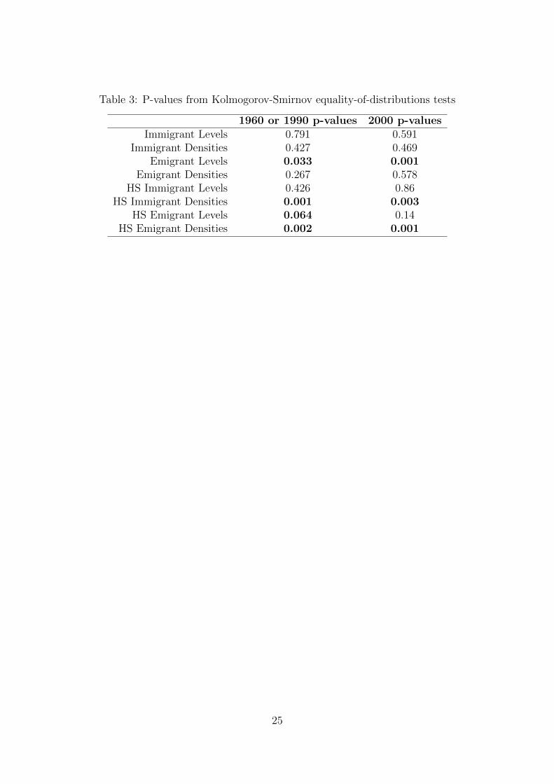
Table 3: P-values from Kolmogorov-Smirnov equality-of-distributions tests

1960 or 1990 p-values 2000 p-valuesImmigrant Levels 0.791 0.591

Immigrant Densities 0.427 0.469Emigrant Levels 0.033 0.001

Emigrant Densities 0.267 0.578HS Immigrant Levels 0.426 0.86

HS Immigrant Densities 0.001 0.003HS Emigrant Levels 0.064 0.14

HS Emigrant Densities 0.002 0.001

25

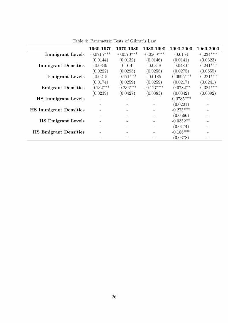
Table 4: Parametric Tests of Gibrat’s Law

1960-1970 1970-1980 1980-1990 1990-2000 1960-2000Immigrant Levels -0.0715*** -0.0570*** -0.0569*** -0.0154 -0.234***

(0.0144) (0.0132) (0.0146) (0.0141) (0.0323)Immigrant Densities -0.0349 0.014 -0.0318 -0.0480* -0.241***

(0.0222) (0.0295) (0.0258) (0.0275) (0.0555)Emigrant Levels -0.0215 -0.171*** -0.0185 -0.0695*** -0.221***

(0.0174) (0.0259) (0.0259) (0.0217) (0.0241)Emigrant Densities -0.132*** -0.236*** -0.127*** -0.0782** -0.384***

(0.0239) (0.0427) (0.0383) (0.0342) (0.0392)HS Immigrant Levels - - - -0.0735*** -

- - - (0.0201) -HS Immigrant Densities - - - -0.275*** -

- - - (0.0566) -HS Emigrant Levels - - - -0.0352** -

- - - (0.0174) -HS Emigrant Densities - - - -0.186*** -

- - - (0.0378) -

26