RVCQ3D Rotor Viscous Code Quasi-3-D

User’s Manual and Documentation Version 406, May 2011

Dr. Rodrick V. Chima

NASA Glenn Research Center, MS 5-12 21000 Brookpark Road

Cleveland, Ohio 44135 USA

phone: 216-433-5919 email: chima@nasa.gov

web: http://www.grc.nasa.gov/WWW/5810/rvc download: http://sr.grc.nasa.gov

Abstract

RVCQ3D (Rotor Viscous Code Quasi-3-D) is a rapid computer code for analysis of inviscid or viscous blade-to-

blade flows in turbomachinery. It accounts for the quasi-three-dimensional effects of rotation, radius change, and

stream surface heght variation. The code has been used at NASA Glenn and in U.S. industries and universities for a

wide variety of problems including analysis of turbopump blades for the Space Shuttle main engine, analysis of

roughness effects on fan blades, and the design of supersonic fan blades. The code runs quickly on most computers.

This report serves as the user’s manual and documentation for the RVCQ3D code. The code and some aspects of the

numerical method are described. Steps for code installation and execution are given. The grid, input, and output

variables are described in detail.

Introduction

RVCQ3D is a rapid computer code for analysis of quasi-three-dimensional viscous flows in turbomachinery.

RVCQ3D is applicable to most types of turbomachinery including compressors and turbines with axial, radial, or

mixed flows. The code solves the thin-layer Navier-Stokes equations on a blade-to-blade surface of revolution using

central or upwind finite-difference techniques. Three turbulence models are available – the Baldwin-Lomax model,

the Cebeci-Smith model, and Wilcox’s 2006 k- model. RVCQ3D is written completely in Fortran and runs quickly

on a Linux workstation. RVCQ3D will run on a PC or Mac, but the user will have to make the appropriate

conversions. Solution files are compatible with most CFD flow visualization packages.

The code uses an explicit multistage Runge-Kutta solution scheme to march the solution in time from an initial

guess to a steady-state solution. A spatially-varying time step and implicit residual smoothing are used to accelerate

convergence. Preconditioning can be used to accelerate convergence for low speed flows.

C-type grids are used to give good resolution of blade leading edges and wakes. Grid input is in standard

PLOT3D xyz-file format, so any C-grid generator can be used. However, the GRAPE code developed by Reece

Sorenson at NASA Ames Research Center [1] has been modified for turbomachinery by the author, and works

directly with RVCQ3D. GRAPE is distributed by the NASA Glenn Research Center Software Repository,

http://sr.grc.nasa.gov.

Namelist input data is supplied to RVCQ3D as text file. Typical solutions take 2000-3000 iterations to converge

and require a few minutes on a fast PC, depending on grid size and flow characteristics. Printed output consists of a

residual history, spanwise profiles of blade-to-blade averaged quantities at the grid inlet and exit, and streamwise

profiles of various quantities on the blade surfaces. No graphical output is provided, but the solution files can be

read directly and plotted using the public domain CFD visualization codes PLOT3D, or the commercial codes

FieldView, and Tecplot.

This documentation briefly describes how the RVCQ3D code works. Instructions for dimensioning, compiling,

and running RVCQ3D are given for Linux workstations. The namelist input variables are described in detail.

Finally, the structure of the output file is described.

2

Four test cases are included: a flat plate boundary layer, a subsonic turbine stator, an annular compressor

cascade, and a centrifugal impeller, (see Test Cases, page 16). A separate Fortran program plate.f is included for

generating the flat plate grid. Grids for the turbomachinery test cases must be generated with the GRAPE code that

is distributed separately. The test cases cover most of the input options available in the code. Comparisons to

experimental data, when available, are included in separate Excel files.

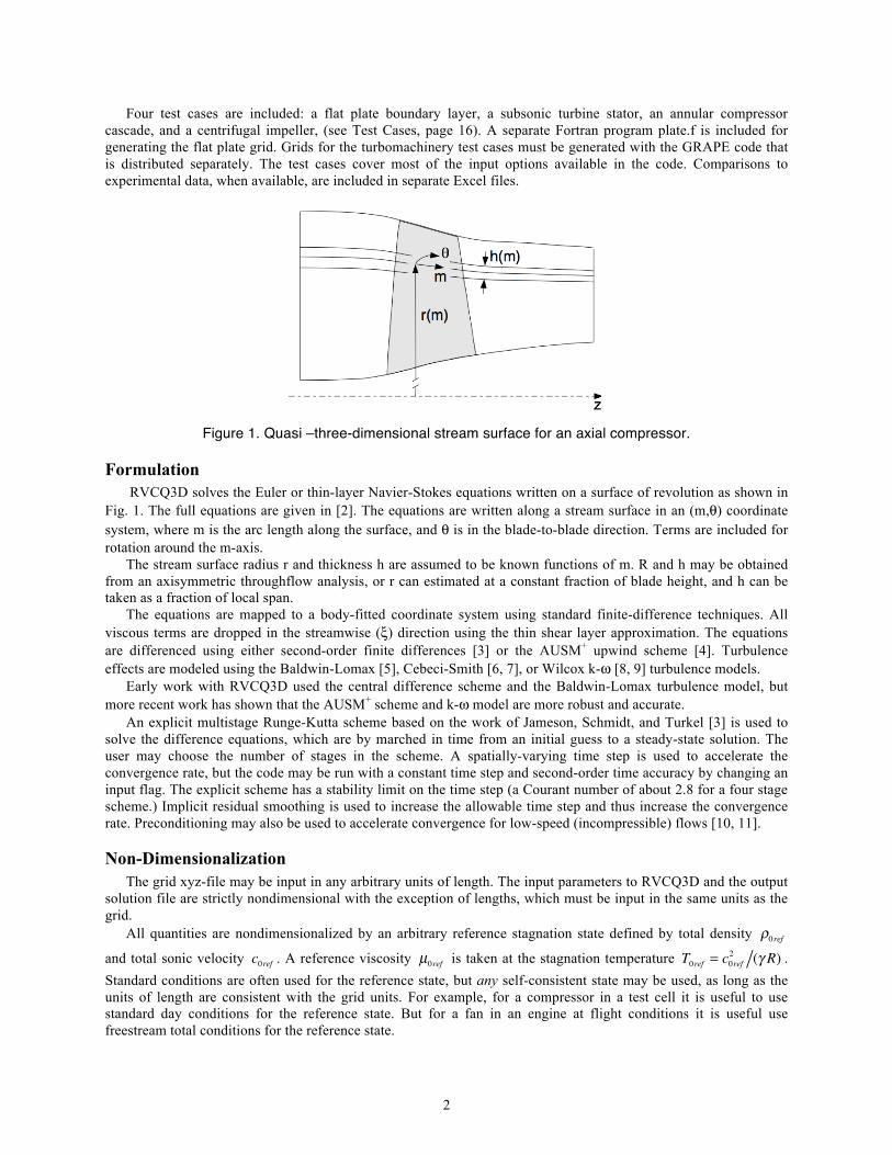
Figure 1. Quasi –three-dimensional stream surface for an axial compressor.

Formulation

RVCQ3D solves the Euler or thin-layer Navier-Stokes equations written on a surface of revolution as shown in

Fig. 1. The full equations are given in [2]. The equations are written along a stream surface in an (m, ) coordinate

system, where m is the arc length along the surface, and is in the blade-to-blade direction. Terms are included for

rotation around the m-axis.

The stream surface radius r and thickness h are assumed to be known functions of m. R and h may be obtained

from an axisymmetric throughflow analysis, or r can estimated at a constant fraction of blade height, and h can be

taken as a fraction of local span.

The equations are mapped to a body-fitted coordinate system using standard finite-difference techniques. All

viscous terms are dropped in the streamwise ( ) direction using the thin shear layer approximation. The equations

are differenced using either second-order finite differences [3] or the AUSM+ upwind scheme [4]. Turbulence

effects are modeled using the Baldwin-Lomax [5], Cebeci-Smith [6, 7], or Wilcox k- [8, 9] turbulence models.

Early work with RVCQ3D used the central difference scheme and the Baldwin-Lomax turbulence model, but

more recent work has shown that the AUSM+ scheme and k- model are more robust and accurate.

An explicit multistage Runge-Kutta scheme based on the work of Jameson, Schmidt, and Turkel [3] is used to

solve the difference equations, which are by marched in time from an initial guess to a steady-state solution. The

user may choose the number of stages in the scheme. A spatially-varying time step is used to accelerate the

convergence rate, but the code may be run with a constant time step and second-order time accuracy by changing an

input flag. The explicit scheme has a stability limit on the time step (a Courant number of about 2.8 for a four stage

scheme.) Implicit residual smoothing is used to increase the allowable time step and thus increase the convergence

rate. Preconditioning may also be used to accelerate convergence for low-speed (incompressible) flows [10, 11].

Non-Dimensionalization

The grid xyz-file may be input in any arbitrary units of length. The input parameters to RVCQ3D and the output

solution file are strictly nondimensional with the exception of lengths, which must be input in the same units as the

grid.

All quantities are nondimensionalized by an arbitrary reference stagnation state defined by total density 0ref

and total sonic velocity c0ref . A reference viscosity μ0ref is taken at the stagnation temperature T0ref = c0ref2 ( R) .

Standard conditions are often used for the reference state, but any self-consistent state may be used, as long as the

units of length are consistent with the grid units. For example, for a compressor in a test cell it is useful to use

standard day conditions for the reference state. But for a fan in an engine at flight conditions it is useful use

freestream total conditions for the reference state.

3

For input and output, pressures and temperatures are nondimensionalized by P0ref and T0ref . Within the code,

pressures are usually nondimensionalized by 0ref c0ref2

= P0ref .

Four input parameters must be properly nondimensionalized: renr, om, prat, and tw (See RVCQ3D Input pp.

10.)

Numerical Method

Multistage Runge-Kutta Scheme

Jameson, Schmidt, and Turkel developed multistage schemes [3] as a simplification of classical Runge-Kutta

integration schemes for ODE’s. The simplification reduces the required storage, but also reduces the time-accuracy

of the schemes, usually to second order. The following discussion of these schemes should give some guidance in

choosing parameters for running the code.

The kth-stage of an n-stage scheme may be written as:

qk = q0 k t RIk+ RV

0( )

where q is an array of five conservation variables (see Solution Q-File, pp. 21), k is current the stage, q0 is the

previous time step, k are the multistage coefficients discussed below, t is the time step, RIk

is the inviscid part

of the residual, and RVk is the viscous part of the residual plus the artificial dissipation, if applicable. Note that RI

k is

evaluated at every stage k, but RVk

is only evaluated at the initial stage for computational efficiency.

n 1

2

3

4

5

*

2 1.2 1. .95

3 .6 .6 1. 1.5

4 .25 .3333 .5 1. 2.8

5 .25 .1667 .375 .5 1. 3.6

Table 1. Runge-Kutta parameters and maximum Courant number for n-stage schemes.

The maximum stable Courant number * for an n-stage scheme can be shown to be * n 1 . The actual

stability limit depends on the choice of k . For consistency n must equal 1. For second-order time accuracy n 1

must equal 1/2. The values of k used in the code and the theoretical maximum Courant number * are set by a

data statement in subroutine setup and are given in table 1.

The number of stages is set with the variable nstg. Nstg = 4 is recommended, although Jameson et al. tend to

favor 5 stages. The 2-stage scheme (nstg = 2) is very robust and often works when everything else fails.

A spatially-varying t is used to accelerate the convergence of the code. Setting ivdt = 1 sets the Courant

number to a constant (input variable cfl) everywhere on the grid, and recalculates it every icrnt iterations. This

option is strongly recommended. Set icrnt to a moderate number, e.g. 10, so that the time step is recalculated

occasionally. The time step is recalculated when the code is restarted and may cause jumps in the residual if icrnt is

too big.

Implicit residual smoothing (described later) may be used to increase the maximum Courant number by a factor

of two to three, thereby increasing the convergence rate as well.

Central Difference Scheme and Artificial Viscosity

The central-difference scheme is selected by setting icdup = 1 (the default.) It is the fastest of the three

differencing schemes used in RVCQ3D, it gives moderately smeared shocks, and it may show velocity overshoots at

the edge of boundary layers. It is recommended when quick answers are desired.

Second-order central differences require an artificial viscosity term to prevent odd-even decoupling. A fourth-

difference artificial viscosity term is used for this purpose. This term is third-order accurate in space and thus does

4

not affect the formal second-order accuracy of the scheme. The input variable avisc4 scales the fourth-difference

artificial viscosity, and should be set between 0.25 and 2.0 A good starting value is 1.0. If the solution is wiggly,

increase avisc4 by 0.25. If it is smooth, try reducing avisc4 by 0.25. Larger values of avisc4 may improve

convergence somewhat, but the magnitude of avisc4 has little effect on predicted losses or efficiency.

The code also uses a second-difference artificial viscosity term for shock capturing. The term is multiplied by a

second difference of the pressure that is designed to detect shocks. Note that the second-difference artificial

viscosity is first-order in space, so that the solution reduces to first-order accurate near shocks. Two other switches

developed by Jameson, et al. [3] are used to reduce overshoots around shocks. The input variable avisc2 scales the

second difference artificial viscosity. Avisc2 can be set to 0.0 for purely subsonic flows, and is usually set to 1.0 for

flows with shocks. If shocks are wiggly, increase avisc2 by 0.5. If they are smeared out, try decreasing avisc2 by

0.5. Shocks will be smeared over a few cells regardless of the value of avisc2. The magnitude of avisc2 also has

little effect on predicted loss or efficiency.

Eigenvalue scaling described in [12] is used to scale the artificial viscosity terms in each grid direction. This

greatly improves the robustness of the code. The artificial viscosity is also reduced linearly by the grid index near

walls to reduce its effect on the physical viscous terms. Input variable jedge is the index where the linear reduction

begins.

For computational efficiency the artificial viscosity is usually calculated only at the first stage of the Runge-

Kutta scheme. This works well for most problems, but for difficult problems the robustness of the scheme can be

improved by updating the artificial viscosity more often. This is done by setting ndis = 2. For nstg = 2 or 3 this has

no effect. For nstg = 4 the artificial viscosity is calculated at stages 1 and 2. For nstg = 5 the artificial viscosity is

calculated at stages 1, 3, and 5. The physical viscous terms are calculated at the same time as the artificial viscosity.

Thus, setting ndis = 2 increases the CPU time per stage significantly, but it is so reliable that it is usually the

preferred scheme.

AUSM+ Upwind Scheme

The Advection Upstream Splitting Method (AUSM+) upwind scheme is selected by setting icdup = 1. It is the

least dissipative but slowest of the three differencing schemes used in RVCQ3D. It is recommended for most

problems.

The AUSM+ family of upwind schemes was developed by Meng-Sing Liou and others [4, 13]. The AUSM

+

scheme defines a cell interface Mach number based on characteristic speeds from neighboring cells. The interface

Mach number is used to determine the upwind extrapolation for the convective part of the inviscid fluxes. A separate

splitting is used for the pressure terms. The van Albada limiter is used to estimate interface fluxes with second-order

accuracy.

The speed of sound at the cell interface is multiplied by a function that effectively scales the numerical

dissipation with the local flow speed, giving appropriate amounts of dissipation for all flow speeds. The scaling

function is based on an average interface Mach number that must be limited by a cutoff Mach number Mref. In

RVCQ3D this is set by input variables ausmk and refm, where

ausmk = 0.5 1.0

refm = min(Mmax,1.0)

and Mmax is the maximum Mach number expected in the flow. Ausmk and refm are the only input variables that

affect the AUSM+

scheme.

H-CUSP Upwind Scheme

The Convective Upwind Split Pressure (CUSP) upwind scheme is selected by setting icdup = 2. It gives the

sharpest shocks but is the most dissipative of three differencing schemes used in RVCQ3D. It is second in execution

speed. It is only recommended for occasional problems where the AUSM+ scheme will not converge.

CUSP schemes were described by Tatsumi, Martinelli, and Jameson in [14, 15]. The H-CUSP scheme uses the

stagnation enthalpy h as the conservation variable in the energy equation. The scheme was developed as a flux-split

scheme similar to AUSM+, but it is implemented as a limited dissipative flux added to a central-difference scheme.

Jameson’s SLIP limiter is used to produce a second-order non-oscillatory scheme. For computational efficiency the

dissipative fluxes are updated less often than the central-difference fluxes. The implementation in RVCQ3D is

described in [4].

5

Like the AUSM+ scheme, the H-CUSP scheme requires a cutoff Mach number, set by by input variables hcuspk

and refm, where

hcuspk = 0.05 0.20

refm = min(Mmax,1.0)

and Mmax is the maximum Mach number expected in the flow. Hcuspk, refm, and ndis are the only input variables

that affect the H-CUSP scheme.

Implicit Residual Smoothing

Implicit residual smoothing is selected by setting irs = 1. It was introduced by Lerat in France and popularized

by Jameson in the U.S. as a means of increasing the stability limit and convergence rate of explicit schemes. The

idea is simple: run the multistage scheme at a high, unstable Courant number, but maintain stability by smoothing

the residual occasionally using an implicit filter. The scheme can be written as follows:

1( ) 1( )R = R

Here and are constant smoothing coefficients in the body-fitted coordinate directions and shown in

figure 2. Here is a second-difference operator, R is the smoothed residual, and R is the unsmoothed residual.

It can be shown that implicit residual smoothing does not change the solution if the scheme converges. Linear

stability theory shows that the scheme can be made unconditionally stable if i are big enough, but also shows that

the effects of artificial viscosity are diminished as the Courant number is increased. In practice the best strategy is to

double or triple the Courant number of the unsmoothed scheme. If the residual is smoothed after every stage, the

theoretical 1-D values of i needed for stability are given by:

i

1

4 *

2

1

where * is the Courant limit of the unsmoothed scheme (given in table 1), and is the larger operating

Courant number. For example, to run a four-stage scheme at a Courant number = 5.6 , the smoothing coefficient

should be:

i

1

4

5.6

2.8

2

1 = 0.75

Three variables, eps, epi, and epj are input to RVCQ3D. Eps is the overall smoothing coefficient. The 1-D limit

for given above usually works well, but can be increased up to 2.5 if the code blows up, and can be decreased

slightly to improve convergence if the code is stable. Values of are scaled within the code at each grid point by

multiplying eps by the same Eigenvalue scaling coefficients used for the artificial dissipation. This has proven to be

quite robust. Epi and epj can be used to scale eps in the i- and j-directions, but they are usually left at their default

values of 1.0.

Implicit residual smoothing involves a scalar tridiagonal inversion for each variable along each grid line in each

direction. It adds about 20 percent to the CPU time when applied after each stage. Smoothing can be done after

every other stage to reduce CPU time (about 7 percent) by setting irs = 2, but eps must be increased (approximately

doubled.) This option is rarely used.

6

Recommended Numerical Parameters

nstg ndis cfl eps Comments

2 1 2.5 1.35–1.60 very robust, fast per stage

4 2 5.6 0.75–1.00 good overall scheme

5 2 7.0 1.25–1.50 slow per stage, fast convergence

Table 2 Recommended numerical parameters for three Runge–Kutta schemes.

Table 2 lists recommended parameters for three numerical schemes, in order of the author’s preference. For all

schemes use irs = 1. For the central-difference scheme use avisc2 = 1.0 and avisc4 = 0.5.

Preconditioning

Preconditioning is selected by setting ipc = 1. It is used to improve convergence for low speed (incompressible)

flows.

Density-based codes like RVCQ3D solve the continuity equation by driving the density residual to zero. For low

speed (nearly incompressible) flows the density residual is naturally near zero, and the schemes fail to converge.

Preconditioning, described in references [10, 11] improves the convergence rate in two ways. First, it replaces the q-

variables q = [ , u, v, e ] with variables that are better behaved at low speeds W = [ p, u, v, h ] , where p is

the pressure and h is the total enthalpy. Second, it multiplies the equations by a matrix designed to equalize the wave

speeds of each equation. The preconditioning matrix has the local flow velocity in the denominator and must be

limited when the velocity becomes small. The preconditioning operator is designed so that it has no effect on the

steady-state solution.

Preconditioning works extremely well for the Euler equations and less well for the Navier-Stokes equations. It

will allow solutions for very low Mach number flows to converge when they would not converge otherwise.

Turbulence Models

The turbulence model is selected using input variable ilt (Inviscid, Laminar, Turbulent,) see &nam5 - Viscous

Parameters, pp. 13.

Three turbulence models are available in RVCQ3D, the algebraic Baldwin-Lomax and Cebeci-Smith models,

and Wilcox’s 2006 two-equation k- models. All three models include transition models and surface roughness

effects.

Baldwin-Lomax and Cebeci-Smith Turbulence Models

The Baldwin-Lomax model is selected by setting input variable ilt = 2. The model is implemented as described

in the original reference [5], except that two constants have been changed to CCP = 1.216 and CKleb = 0.646 . The

length scale for the Baldwin-Lomax model is correlated to the maximum of a function f = y D , where y is the

distance from the wall, is the magnitude of the vorticity, and D is the Van Driest damping function. In some

cases that maximum is not well behaved, so RVCQ3D limits the search to the grid line at j-index jedge away from

the body. Input variable jedge should be chosen slightly larger than the largest extent of the boundary layer.

Solutions are usually insensitive to values of jedge if it is big enough, but may under predict viscous effects if it is

too small.

The Cebeci-Smith model is selected by setting input variable ilt = 3. The model is implemented like the

Baldwin- Lomax model except that the length scale is found by integrating

f dy = *

0ue

as described in [7]. Here the upper bound of the integral is usually found automatically since f 0 as y .

However, cases with free-stream vorticity can have a non-zero f outside the boundary layer, so input variable jedge

7

is used to bound the integral in RVCQ3D. The Cebeci-Smith model is very reliable for turbine heat transfer

problems, but is not recommended for transonic compressors that may produce free-stream vorticity behind the bow

shock.

Transition is predicted in both models at the location where μturb μlam > cmutm , where cmutm is an input

variable usually set to 14, as recommended in [5]. The model is crude but often works surprisingly well for moderate

Reynolds numbers and low free-stream turbulence.

Roughness effects are included in both models using the Cebeci-Chang roughness model [6]. The model

modifies the turbulent length scale based on the equivalent sand-grain roughness height in turbulent wall units h+ .

The roughness height is input using variable hrough, and h+ is calculated internally. If hrough = 0.0 a model for a

hydraulically smooth surface is used.

Wilcox k- Turbulence Model

The k- model is selected by setting input variable ilt = 4 or 5. The model is described in [8], and implemented

as described in [9] using a first-order upwind ADI scheme. Two versions of the model are included, a baseline

model (ilt = 4) and a low Reynolds number model (ilt = 5). The baseline model gives a fully turbulent solution that

is valid all the way to the wall, unlike k- models. The low Reynolds number model includes transition effects.

Wilcox’s 2006 model includes a cross diffusion term that reduces dependence on freestream values of , and a

shear stress limiter that reduces the turbulent viscosity when production of turbulent kinetic energy exceeds

destruction. The shear stress limiter has been shown to improve results for shock-separated flows. The stress limiter

is selected by setting isst = 1.

Three input parameters affect the k- model, the surface roughness hrough as described above, the free-stream

turbulence level tintens (typically 0.0 to 0.05), and the free-stream turbulent viscosity tmuinf = μturb μlam( ) ,

typically 0.1. Solutions are generally insensitive to tmuinf, except for the location of transition.

Previous versions of RVCQ3D used a turbulent length scale tlength instead of tmuinf. Tlength was awkward to

use but has been retained in the code for backward compatibility.

8

Unzipping, Compiling, and Running RVCQ3D RVCQ3D is supplied as a zipped file. It will unzip into a directory with the same name as the file. This

documentation should be in the main directory. There are subdirectories for source code and test cases. On a Linux

system: unzip rvcq3d_406.zip

Compiling RVCQ3D

Go to the src directory and edit the Makefile. Compiler commands are set for the Intel Linux compiler, FC = ifort –fast

Change the commands as necessary for your compiler. Full optimization usually works well. Near the bottom of the

Makefile there may be a line that moves the executable to a bin directory. Keep or remove this line as desired. mv rvcq3d ~/bin

Save the file and exit.

Most arrays are allocated dynamically, but a few work arrays have fixed maximum dimensions. Edit modules.f90

and modify the maximum dimensions if desired. Default values for most input variables are also set here. parameter (idm=385, jdm=95)

Run make. Move the executable to a directory in your path.

Clean up object and executable files if desired by running make clean

Standard Input, Output, and Binary Files

An input file for RVCQ3D is read from Fortran unit 5 (standard input.) Printed output from RVCQ3D is written

to Fortran unit 6 (standard output.) Binary files linked to Fortran units 1 - 3 and 7 - 8 may be used by RVCQ3D,

depending on input options. The units are used as follows:

fort.1 input grid file, required. See Grid XYZ-File, pp. 21.

fort.2 input solution file, read if iresti = 1. See Solution Q-File, pp. 21.

fort.3 output solution file, written if iresto = 1. See Solution Q-File, pp. 21.

fort.7 input k- turbulence file, read if iresti = 1 and ilt 4. See Solution k- File, pp. 21.

fort.8 output k- turbulence file, written if iresto = 1 and ilt 4. See Solution k- File, pp. 21.

All files are written and read as unformatted binary files. They are not explicitly opened in the code.

Running RVCQ3D

Files are usually linked to Fortran units before running RVCQ3D,

ln xyz.file fort.1

ln input.q.file fort.2

ln output.q.file fort.3

ln input.kw.file fort.7

ln output.kw.file fort.8

then RVCQ3D is run as a standard Linux process: rvcq3d < input_file > output_file &

Shell Script

Rather than linking files manually, Linux c-shell scripts are included for running each case. Briefly, the scripts

do the following:

Sets prefixes pin and pout for input and output files. Input files will be named pin.q and pin.kw. Output files will

be named pout.out, pout.q, and pout.kw. You may want to include the iteration count in the prefixes. If you use the

same prefix for both, the output files will overwrite the input files at completion.

set pin= … #set input prefix here

9

set pout= … #set output prefix here

Links the input and output files to the appropriate Fortran unit numbers. You will have to edit the link for the

grid (xyz) file. ln grid.xyz fort.1 #set grid file here ln $qin fort.2 #restart q input etc.

Links the k- turbulence model files.

set kw=1 #set to zero if not running the k-w model … endif Cats (concatenates) the namelist data below until the line labeled EOIN to a file called input. Change your

RVCQ3D input here. cat > input << EOIN ‘Title goes here’ &nl1 m=169 … &end

…

EOIN

Runs RVCQ3D in the background and uses tail to follow the output. You can kill the tail command with

<control> c. rvcq3d <input > $out & tail -f $out

10

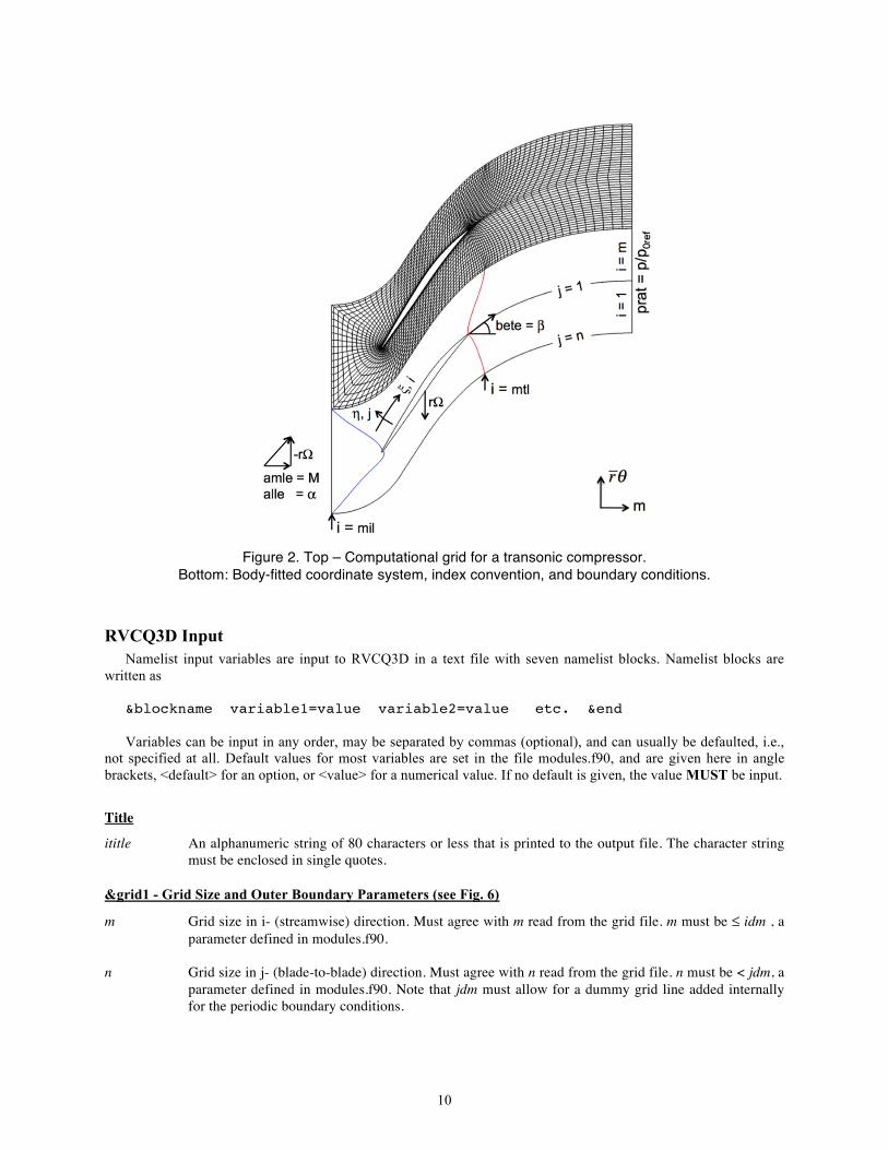
Figure 2. Top – Computational grid for a transonic compressor. Bottom: Body-fitted coordinate system, index convention, and boundary conditions.

RVCQ3D Input

Namelist input variables are input to RVCQ3D in a text file with seven namelist blocks. Namelist blocks are

written as

&blockname variable1=value variable2=value etc. &end

Variables can be input in any order, may be separated by commas (optional), and can usually be defaulted, i.e.,

not specified at all. Default values for most variables are set in the file modules.f90, and are given here in angle

brackets, <default> for an option, or <value> for a numerical value. If no default is given, the value MUST be input.

Title

ititle An alphanumeric string of 80 characters or less that is printed to the output file. The character string must be enclosed in single quotes.

&grid1 - Grid Size and Outer Boundary Parameters (see Fig. 6)

m Grid size in i- (streamwise) direction. Must agree with m read from the grid file. m must be idm , a parameter defined in modules.f90.

n Grid size in j- (blade-to-blade) direction. Must agree with n read from the grid file. n must be < jdm, a

parameter defined in modules.f90. Note that jdm must allow for a dummy grid line added internally for the periodic boundary conditions.

11

mtl i-index of lower trailing-edge point on a C-grid. Mtl is printed at the end of the GRAPE output. Mtl can be 1 for a blade that extends to the exit of the grid.

mil i-index of the last periodic point on the outer boundary. Also acts as the lower point on the inlet

boundary. Mil is printed at the end of the GRAPE output. ich Cascade / flat plate or duct analysis flag. = 0 Cascade analysis on a C-grid. Trailing edge at mtl, inlet at mil. <default>. = 1 or 2 Flat plate or duct analysis on an H-grid. Symmetry boundary conditions are applied on the

lower and upper walls, then overwritten with actual wall boundary conditions from i = mtl to i = mtr. = 1 Wall boundary conditions on the lower wall only. Can be used for a flat plate test case for testing

turbulence models. Leading edge at mtl, set mil = m. = 2 Wall boundary conditions on both walls. Can be used to analyze simple duct flows. Set mtl = 1,

mil = m.

&nam2 - Algorithm Parameters

icdup Flag for setting the differencing scheme for the inviscid fluxes = 0 Central differences with artificial viscosity = 1 AUSM+ upwind scheme = 2 H-CUSP upwind scheme nstg Number of stages for the Runge-Kutta scheme, usually 4, but can be 2-5. <4> ndis Number of evaluations of the artificial and physical dissipation terms during the Runge-Kutta scheme.

(See Central Difference Scheme and Artificial Viscosity on pp. 3.) Can be 1 <default> or 2. If ndis = 2 the dissipative terms are evaluated as follows: nstg = 2 or 3 after stage 1 only (same as ndis = 1) nstg = 4 after stages 1 and 2 nstg = 5 after stages 1, 3, and 5. avisc2 Second-order artificial dissipation coefficient. Typically 0.0 - 2.0. Use 0.0 for purely subsonic flow or

1.0 for flows with shocks. <1.0>. avisc4 Fourth-order artificial dissipation coefficient. Typically 0.25 - 1.5. Start at 1.0 and reduce avisc4 to

0.5 if possible. <0.5>. irs Implicit residual smoothing flag. Usually = 1. (See Implicit Residual Smoothing on pp. 5.) = 0 No residual smoothing = 1 Implicit smoothing after every Runge-Kutta stage <default>. = 2 Implicit smoothing after every other stage. eps must be increased (roughly x 2) for this option to

work. eps Overall implicit smoothing coefficient based on the 1-D stability limit. (See Implicit Residual

Smoothing on pp. 5.) RVCQ3D will calculate the 1-D limit if eps is defaulted. epi, epj Implicit smoothing coefficient multipliers for the i- and j-directions. Rarely used. <1>. ivdt Variable time step flag. = 0 Spatially constant time step. = 1 Spatially variable time step. <default, highly recommended>. cfl Courant number, typically 5.6 (see Multistage Runge-Kutta Scheme on pp. 3.) If ivtstp = 0, cfl is the

maximum Courant number for the grid, usually located where the grid spacing is smallest. If ivtstp = 1, the Courant number will equal cfl everywhere. <5.6>

12

ipc Preconditioning flag, (see Preconditioning on pp. 6.) Should give a substantial speedup for low Mach numbers < 0.3.

= 0 No preconditioning. <default> = 1 Merkel, Choi, Turkel scheme. = 2 Weiss and Smith scheme, very similar to the Merkel, et al. scheme. refm Reference relative Mach number used for preconditioning and the AUSM+ and H-CUSP schemes. For

preconditioning, refm should be the lesser of 1.0 or the largest relative Mach number expected in the flow. Convergence is mildly sensitive to refm and pck, so try to keep these values as small as possible. For high speed flows set refm = 0.7, and use ausmk and hcuspk to scale the reference Mach number for the AUSM+ and H-CUSP schemes. <amle>

pck Refm multiplier for preconditioning (Turkel’s parameter k). Typically 0.1 – 0.3, but larger values may

be necessary for stability. <0.15> ausmk Refm multiplier for the AUSM+ scheme. Typically 0.5 – 1.0. <1.0> hcuspk Refm multiplier for the H-CUSP scheme. Typically 0.05 – 0.20. <0.1>

&nam3 - Boundary Condition & Code Control

itmax Number of iterations, typically 1000 - 2000, but more may be needed for a converged solution. iresti Flag for reading the input restart files. Restart files are in PLOT3D format in the relative frame. = 1 Read restart q file from fort.2 and k- file from fort.7 else No action taken. <default> iresto Flag for writing the output restart file. = 1 Write restart q file to fort.3 and k- file to fort.8. <default> else No action taken. newkw Flag for running the k- model with a fixed flow solution, usually from an algebraic model. = 0 No action taken. <default> else Run the k-w model itmax iterations and write the k- file. ibcin Old inlet boundary condition flag, now used to set ibcinu and ibcinv, or to set supersonic inflow. <default uses ibcinu and ibcinv> = 1 ibcinu = 1, ibcinv = 1 = 2 Supersonic inflow - all quantities are fixed at the inlet. = 3 ibcinu = 1, ibcinv = 2 ibcinu Inlet boundary condition flag for meridional velocity component vm .

= 1 Riemann invariant extrapolated from the interior to get vm . <default>

= 2 Total velocity V extrapolated from the interior to get vm . Often works best for low-speed flows.

ibcinv Inlet boundary condition flag for tangential velocity component v .

= 1 v is specified using amle and alle. <default>

= 2 v vm = tan( ) is specified. is found by extrapolating alle to the upstream boundary. May not

be well-posed for transonic compressors where the inflow angle may be set by unique incidence. ibcex Exit boundary condition flag. Three conservation variables are extrapolated to the exit. Ibcex

determines how the exit pressure p is determined. = 1 The exit pressure is held constant at prat. Good for subsonic outflow. <default>

13

= 2 Supersonic outflow. p is extrapolated to the boundary. = 3 The average exit pressure is held constant at prat, but p can vary blade-to-blade. Based on

characteristic boundary conditions developed by Giles. Good for transonic turbines with shocks leaving the trailing edge.

ires Iteration increment for writing residuals in the output file. If the solution blows up, set ires = 1 to print

the size and location of the maximum residual at each iteration. <10> icrnt Iteration increment for updating the time step. If icrnt is too big, the residual history may be

discontinuous when t is recalculated. <10>. ixrm Flag for additional output of blade coordinates and radius. = 0 No output <default>. = 1 x, y, and r are printed in the output file. mioe Residual history output flag. = 1 Print rmax and min

. Good for fans.

= 2 Print rmax and mout. Good for choked turbines.

= 3 Print rmax and merror. Good measure of overall accuracy. <default>

= 4 Print minand mout

.

&nam4 - Flow Parameters

Initial conditions are input in terms of the blade leading edge and trailing edge velocity triangles. Absolute Mach

number amle and flow angle alle are input at the leading edge, and relative flow angle bete is input at the trailing

edge. An analytic solution of the 1-D continuity equation is used to determine the conditions at the boundaries of the

grid.

Inlet boundary conditions are set using the initial conditions described above. Variables ibcinu and ibcinv

determine which of these conditions are held fixed with the solution. Inlet total pressure and total temperature can be

input using p0in and t0in described below.

The exit boundary condition is usually held at a constant static pressure ratio prat. Variable ibcex determines

how prat is specified.

p0in P0in / P0ref at the inlet. Can be used to simulate a blade row in a multistage environment.

t0in T0in /T0ref at the inlet. Can be used to simulate a blade row in a multistage environment. <1.0>

prat Pexit / P0ref used for the exit boundary condition. < Default calculated from the initial conditions>.

amle Absolute Mach number at the leading edge. Used for initial conditions. Note that the inlet Mach

number will change with the solution for subsonic inflow. alle Absolute flow angle at the leading edge in degrees. <Default = 0.0 for axial inflow.> bete Relative flow angle at the trailing edge in degrees. Can be estimated by measuring the grid angle at

the trailing edge. Only used for initial conditions. <0.0> g Ratio of specific heats. < = 1.4 for air>.

&nam5 - Viscous Parameters

ilt Inviscid, Laminar, or Turbulent analysis and turbulence model options. = 0 Inviscid Euler solution. The remaining viscous parameters are not used if ilt = 0. = 1 Laminar. Viscous terms are calculated but the turbulent viscosity is zero.

14

= 2 Turbulent using the Baldwin-Lomax turbulence model [5, 7]. <default> = 3 Turbulent using the Cebeci-Smith turbulence model [6, 7]. This model works well for turbine heat

transfer but may over predict losses for transonic compressors. = 4 Fully turbulent using the baseline Wilcox k- turbulence model [8, 9]. = 5 Turbulent with transition using the low Reynolds number Wilcox k- turbulence model [8, 9]. itur The turbulence model is updated every itur iterations. <5> itur = 2 is recommended for the k- model itur = 5 is recommended for the Baldwin-Lomax and Cebeci-Smith models. jedge The last j-index searched for the blade turbulent length scale. For the Baldwin-Lomax model (ilt = 2),

jedge should be a grid line slightly bigger than the largest expected blade boundary layer. For the Cebeci-Smith turbulence model (ilt = 3), jedge should be a grid line slightly bigger than half the largest expected blade boundary layer. Not used for the k- model. <10>

NOTE: Jedge is also used to reduce the artificial viscosity in viscous layers if icdup = 1. The artificial

viscosity is multiplied by a linear function of j-index that goes from 1/jedge at the wall to 1 at j = jedge. This improves viscous loss predictions. Jedge is set to 1 internally for inviscid flow.

renr Reynolds number per unit length based on reference conditions, renr = 0ref c0ref / μ0ref . Must have

units of [1/grid units]. Generally much larger that a conventional free stream Reynolds number. For example, for standard conditions and a grid with units of [ft],

0ref = 0.07657 lbm/ft3

c0ref = 1116.7 ft/sec

μ0ref = 3.717 10-7lbf sec/ft2 =1.197 10-5lbm /(ft sec)

renr = 0.07657 1116.7 /1.197 10-5

= 7.143 106 /ft

prnr Prandtl number. <0.7 for air> tw Normalized wall temperature, Twall /T0ref .

= 0 Adiabatic wall boundary conditions are used. = 1 Twall = T0ref .

else Twall = tw T0ref .

vispwr Exponent for laminar viscosity power law. < 0.667 for air> cmutm Value of μturb / μlaminar

at which transition occurs. Baldwin and Lomax recommend 14. Increase to

move transition downstream or vice-versa. The flow is fully turbulent if cmutm = 0. <14>. dblh Inlet boundary layer thickness on the lower (hub) wall of an H-grid (ich = 1 or 2). <0.0> dblt Inlet boundary layer thickness on the upper (tip) wall of an H-grid (ich = 2). <0.0>

&nam6 - Blade Row Data

omega Normalized blade row rotational speed, / c0ref ,where is the wheel speed in radians per second.

Omega has dimensions of [1/grid units]. Omega is positive in the positive -direction, and tends to be negative for most GRC geometries. <0>.

15

nblade Number of blades, nblade 1. <1> = 1 Linear cascade with radius = 1 and stream surface thickness = 1. > 1 Annular cascade with pitch = 2 r / nblade .

NOTE: Since grids are generated independently using the GRAPE code, it is possible that the pitch

determined from the grid will not match the pitch determined from nblade. In that case RVCQ3D rescales the -coordinates of the grid to give the correct pitch, and prints a warning in the output file.

nmn Number of stream surface input points, 1 nmn 100 . <1> 2 Stream surface input is read after &nam7 as described below. else Linear cascade with radius = 1 and stream surface thickness = 1. No stream surface data is read.

&nam7 –k- model parameters

hrough Surface roughness height in grid units. Usually hrough = 0 is used to model a hydraulically smooth surface. To model a rough surface like a turbine blade set hrough = equivalent sand grain roughness height, or 2 – 4 times the RMS roughness height. If the first grid point off the wall is at y+ = 2 , then

hrough must be > 2.5 ywall to have much effect.

= 0. Hydraulically smooth surface. > 0. Roughness effects are modeled using the Cebeci-Chang model or Wilcox’s roughness boundary

condition for . tintens Freestream turbulence intensity as a decimal fraction. Determines the inlet value of k for the k-

model. Can be set very small, but a value of zero will give a laminar solution. <default = 0.01, i.e., one percent>

tmuinf μturb μlam( ) Normalized inlet turbulent viscosity. Used to set the inlet value for . Typically 0.1 or

less. Very small values can cause an abrupt decay of very close to the inlet boundary. <0.1> tlength Old input variable used to determine the inlet value of . Retained for backwards compatibility.

Tmuinf is used instead if tlength is omitted. <default> Turbulent length scale in grid units. Typically 0.03 boundary layer height, or 0.001 pitch. isst Flag for the stress limiter in Wilcox’s 2006 k- model. Limits the turbulent viscosity when production

of turbulent kinetic energy exceeds destruction. Works well for shock separated flows. = 0 No stress limiter, <default>. else Stress limiter is used.

Stream Surface Input

The stream surface coordinates m, r(m), and h(m) (see Fig. 5.) are input as three arrays of length nmn 100 . m

and r must be in the same units as the grid coordinates. r and h are spline fit to the grid as functions of m, so m must

increase monotonically, and r and h should be smooth. Points are extrapolated if m does not span the m-coordinates

of the grid.

r and h have first-order effects on the flow solution and should be picked carefully. Stream tubes coordinates can

be calculated using an axisymmetric throughflow code like Ted Katsanis’ MERIDL code (the unusual variable

names below were borrowed from MERIDL), or Jim Crouse’s compressor design code. For a first guess h can be

taken as the local blade span, and r can be taken as the radius at a certain fraction of that span.

srsp m-coordinates where r and h are specified. Must increase monotonically. rmsp r-coordinates of the stream-surface at points srsp. The magnitude of rmsp enters directly into the flow

equations in terms like rd , so the actual values are important.

16

besp Stream-surface thickness h at points srsp. The magnitude of h is unimportant – only dh / (hdm) affects the solution, so h is usually normalized to 1.0 at the inlet and scaled from there. The magnitude of besp does affect the printed mass flow, so for linear cascades where the distance between the sidewalls is well defined it may be desirable to leave h not normalized.

The coordinates are read using three unformatted read statements, e.g.:

read(5,*)(srsp(i),i=1,nmn) read(5,*)(rmsp(i),i=1,nmn) read(5,*)(besp(i),i=1,nmn)

RVCQ3D Output

Printed output from RVCQ3D is written to Fortran unit 6 (standard output.) The output is divided into several

sections. The output may be separated using an editor and plotted using Excel or any x-y plotting package that can

read tabular data. The output includes the following information:

• The input variables are echoed back for reference, and any warnings about the input are written.

• A table of -averaged flow variables at the inlet and exit is written. Both absolute and relative quantities are given.

An energy-averaging scheme is used that gives a local, rather than mixed-out average. These variables are either

based on the initial guess or on the restart file, depending on how the code is started.

• The convergence history gives maximum and RMS residuals of density, mass flow error, and exit flow properties

P0exit and T0exit versus iteration.

• Blade surface distributions of the following quantities are written:

m m-coordinate mbar arc length from the leading edge. Subroutine oblade.f has other options for mbar commented out. rho / 0ref

ps p / P0ref

ts T /T0ref

M_isen Isentropic Mach number y+ Grid spacing at the wall in turbulent wall units. Should < 2 – 3 at most grid points for accurate

prediction of losses and heat transfer. 1000*Cf Skin friction coefficient

Cf = μV

n wall

1

2 inVin2

1000*St Stanton number

St = kT

n wallinVinCp Tin Twall( )

tmu_max Maximum values of μturb / μlamalong each i grid line. Can be used to identify transition. For the

Baldwin-Lomax and Cebeci-Smith models transition occurs where tmu_max jumps abruptly from 0 to > cmutm. For the k- model transition occurs more gradually but should be obvious as a rapid growth of tmu_max.

• The table of -averaged flow variables at the inlet and exit is repeated for the final solution.

Test Cases

Flat Plate Boundary Layer

17

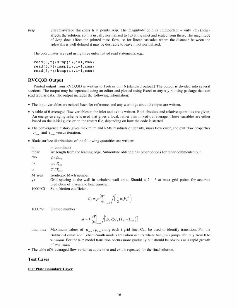
Figure 3. Mach contours for a flat plate boundary layer.

A flat plate boundary layer test case is included to test viscous terms and turbulence models in RVCQ3D. Mach

contours for the case are shown in Figure 3. A separate Fortran code plate.f is included for generating the flat plate

grid. Input variables are hard-coded and described by comments at the top of the code. The RVCQ3D solution uses

the central-difference scheme and k- turbulence model with transition. The Excel spreadsheet plate.xlsx compares

calculated skin friction to laminar and turbulent power law correlations.

To generate the grid and run RVCQ3D: compile plate.f a.out mv fort.1 plate.xyz plate.csh

Goldman Turbine Vane

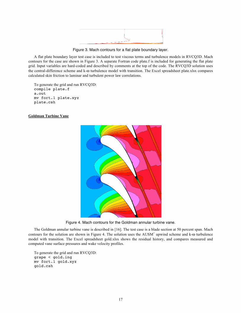
Figure 4. Mach contours for the Goldman annular turbine vane.

The Goldman annular turbine vane is described in [16]. The test case is a blade section at 50 percent span. Mach

contours for the solution are shown in Figure 4. The solution uses the AUSM+ upwind scheme and k- turbulence

model with transition. The Excel spreadsheet gold.xlsx shows the residual history, and compares measured and

computed vane surface pressures and wake velocity profiles.

To generate the grid and run RVCQ3D: grape < gold.ing mv fort.1 gold.xyz gold.csh

18

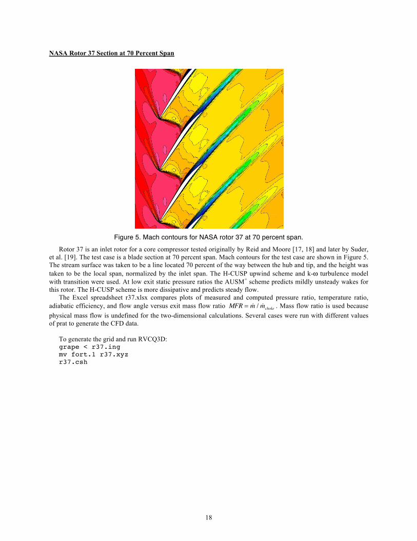
NASA Rotor 37 Section at 70 Percent Span

Figure 5. Mach contours for NASA rotor 37 at 70 percent span.

Rotor 37 is an inlet rotor for a core compressor tested originally by Reid and Moore [17, 18] and later by Suder,

et al. [19]. The test case is a blade section at 70 percent span. Mach contours for the test case are shown in Figure 5.

The stream surface was taken to be a line located 70 percent of the way between the hub and tip, and the height was

taken to be the local span, normalized by the inlet span. The H-CUSP upwind scheme and k- turbulence model

with transition were used. At low exit static pressure ratios the AUSM+ scheme predicts mildly unsteady wakes for

this rotor. The H-CUSP scheme is more dissipative and predicts steady flow.

The Excel spreadsheet r37.xlsx compares plots of measured and computed pressure ratio, temperature ratio,

adiabatic efficiency, and flow angle versus exit mass flow ratio MFR = m / mchoke . Mass flow ratio is used because

physical mass flow is undefined for the two-dimensional calculations. Several cases were run with different values

of prat to generate the CFD data.

To generate the grid and run RVCQ3D: grape < r37.ing mv fort.1 r37.xyz r37.csh

19

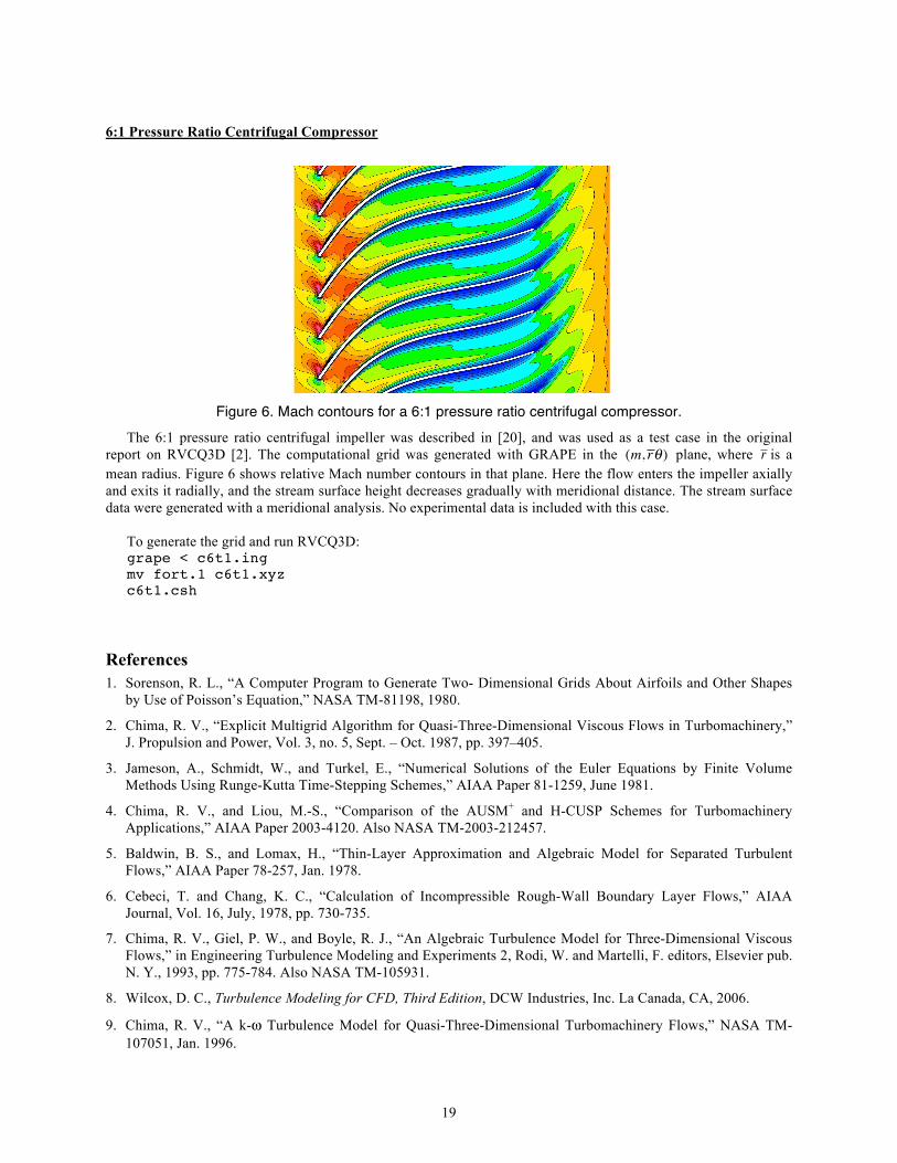
6:1 Pressure Ratio Centrifugal Compressor

Figure 6. Mach contours for a 6:1 pressure ratio centrifugal compressor.

The 6:1 pressure ratio centrifugal impeller was described in [20], and was used as a test case in the original

report on RVCQ3D [2]. The computational grid was generated with GRAPE in the (m, r ) plane, where r is a

mean radius. Figure 6 shows relative Mach number contours in that plane. Here the flow enters the impeller axially

and exits it radially, and the stream surface height decreases gradually with meridional distance. The stream surface

data were generated with a meridional analysis. No experimental data is included with this case.

To generate the grid and run RVCQ3D: grape < c6t1.ing mv fort.1 c6t1.xyz c6t1.csh

References

1. Sorenson, R. L., “A Computer Program to Generate Two- Dimensional Grids About Airfoils and Other Shapes

by Use of Poisson’s Equation,” NASA TM-81198, 1980.

2. Chima, R. V., “Explicit Multigrid Algorithm for Quasi-Three-Dimensional Viscous Flows in Turbomachinery,”

J. Propulsion and Power, Vol. 3, no. 5, Sept. – Oct. 1987, pp. 397–405.

3. Jameson, A., Schmidt, W., and Turkel, E., “Numerical Solutions of the Euler Equations by Finite Volume

Methods Using Runge-Kutta Time-Stepping Schemes,” AIAA Paper 81-1259, June 1981.

4. Chima, R. V., and Liou, M.-S., “Comparison of the AUSM+ and H-CUSP Schemes for Turbomachinery

Applications,” AIAA Paper 2003-4120. Also NASA TM-2003-212457.

5. Baldwin, B. S., and Lomax, H., “Thin-Layer Approximation and Algebraic Model for Separated Turbulent

Flows,” AIAA Paper 78-257, Jan. 1978.

6. Cebeci, T. and Chang, K. C., “Calculation of Incompressible Rough-Wall Boundary Layer Flows,” AIAA

Journal, Vol. 16, July, 1978, pp. 730-735.

7. Chima, R. V., Giel, P. W., and Boyle, R. J., “An Algebraic Turbulence Model for Three-Dimensional Viscous

Flows,” in Engineering Turbulence Modeling and Experiments 2, Rodi, W. and Martelli, F. editors, Elsevier pub.

N. Y., 1993, pp. 775-784. Also NASA TM-105931.

8. Wilcox, D. C., Turbulence Modeling for CFD, Third Edition, DCW Industries, Inc. La Canada, CA, 2006.

9. Chima, R. V., “A k- Turbulence Model for Quasi-Three-Dimensional Turbomachinery Flows,” NASA TM-

107051, Jan. 1996.

20

10. Turkel, E., “A Review of Preconditioning Methods for Fluid Dynamics,” Applied Numerical Mathematics, Vol.

12, 1993, pp. 257-284.

11. Tweedt, D. L., Chima, R. V., and Turkel, E., “Preconditioning for Numerical Simulation of Low Mach Number

Three-Dimensional Viscous Turbomachinery Flows,” AIAA Paper 97-1828, June 1997. Also NASA TM-

113120.

12. Chima, R. V., “Viscous Three-Dimensional Calculations of Transonic Fan Performance,” in CFD Techniques for

Propulsion Applications, AGARD Conference Proceedings, No. CP-510, AGARD, Neuilly-Sur-Seine, France,

Feb. 1992, pp. 21-1 to 21-19. Also NASA TM-103800.

13. Liou, M.-S., and Steffen Jr. C. J., “A New Flux Splitting Scheme,” J. Computational Physics, Vol. 107, No. 1,

July 1993, pp 23-29.

14. Tatsumi, S., Martinelli, L., and Jameson, A., “Design, Implementation, and Validation of Flux Limited Schemes

for the Solution of the Compressible Navier-Stokes Equations,” AIAA Paper 94-0647, Jan. 1994.

15. Tatsumi, S., Martinelli, L., and Jameson, A., “A New High Resolution Scheme for Compressible Viscous Flow

with Shocks,” AIAA Paper 95-0466, Jan. 1995.

16. Goldman, L. J., and McLallin, K. L. "Cold-Air Annular Cascade Investigation of Aerodynamic Performance of

Core-Engine-Cooled Turbine Vanes. I: Solid Vane Performance and Facility Description," NASA TMX-3224,

1975.

17. Reid, L. and Moore, R. D., "Design and Overall Performance of Four Highly-Loaded, High Speed Inlet Stages

for an Advanced, High Pressure Ratio Core Compressor," NASA TP=1337, 1978.

18. Reid, L. and Moore, R. D., "Experimental Study of Low Aspect Ratio Compressor Blading," ASME Paper 80-

GT-6, Mar. 1980.

19. Suder, K. L. and Celestina, M. L., "Experimental and Computational Investigation of the Tip Clearance Flow in

a Transonic Axial Compressor Rotor," NASA TM-106711, 1994.

20. Klassen, H. A., Wood, J. R., and Schumann, L. F., “ Experimental Performance of a 16.10 Centimeter-Tip-

Diameter Sweptback Centrifugal Compressor Designed for a 6:1 Pressure Ratio,” NASA TM x-3552, 1977.

21

Appendix - File Descriptions

Grid XYZ-File

Grids are stored using standard PLOT3D xyz-file structure. Grids can be read with the following Fortran code:

! read grid coordinates read(1)m,n read(1)((x(i,j),i=1,m),j=1,n)), & ((y(i,j),i=1,m),j=1,n))

Solution Q-File

Solution files are stored in standard PLOT3D q-file structure in the rotating frame of reference. The variables are

q = [ , u, v , e ]

e = CvT +1

2u2 + v 2( )

Solution files can be read with the following Fortran code:

! read q-file read(2)m,n read(2)emir,abir,renr,time read(2)(((qq(k,i,j),i=1,m),j=1,n),k=1,4) ! additional geometry data and residual history read(2)mtl,mil,ires,nres,nmn,g,omega,yscl read(2)((resd(nr,l),nr=1,nres),l=1,5 ! further data for Dan Tweedt’s post-processing codes read(2)((qq(k,i,n),i=1,m),k=1,4) read(2)cfl,dtmin,idum,idum read(2)(srsp(l),l=1,nmn) read(2)(rmsp(l),l=1,nmn) read(2)(besp(l),l=1,nmn)

Solution k- File

The k- files are also stored in standard PLOT3D q-file structure for convenience. The variables are:

wk = [ k, , μturb , Returb ]

K- files can be read with the following Fortran code

read(7)m,n read(7)emir,abir,renr,float(iter) read(7)((wk(1,i,j),i=1,m),j=1,n), & ((wk(2,i,j),i=1,m),j=1,n), & ((tmu( i,j),i=1,m),j=1,n), & ((re( i,j),i=1,m),j=1,n)