Embed Size (px)
Citation preview

Western Australian School of Mines
Selection Criteria For
Loading and Hauling Equipment - Open Pit Mining Applications
Volume 1
Raymond J Hardy
This Thesis is presented for the Degree
Of Doctor of Philosophy
Of Curtin University of Technology
July 2007

i
DECLARATION
This thesis does not contain material previously accepted for the award of any other
degree or diploma in any university. To the best of my knowledge and belief, where
this thesis contains material previously published by any other person, due
acknowledgement has been made.
………………………..
R J Hardy 9 July 2007
THESIS PRESENTATION
Scope of the research, breadth of topics and resulting extensive documentation
required presentation of the thesis in two volumes.
Volume 1 Selection Criteria Issues, Productivity and Analysis – Chapters 1 to
3 included in Volume 1; and
Volume 2 Selection Process, Costs, Conclusions and Recommendations –
Chapters 4 to 7 - plus References, Appendices and Supplementary
Information – included in Volume 2.
ii
ABSTRACT
Methods for estimating productivity and costs, and dependent equipment selection
process, have needed to be increasingly reliable. Estimated productivity and costs
must be as accurate as possible in reflecting actual productivity and costs
experienced by mining operations to accommodate the long-term trend for
diminishing commodity prices,
For loading and hauling equipment operating in open pit mines, some of the
interrelated estimating criteria have been investigated for better understanding; and,
consequently, more reliable estimates of production and costs, also more effective
equipment selection process.
Analysis recognizes many of the interrelated criteria as random variables that can
most effectively be reviewed, analyzed and compared in terms of statistical
mathematical parameters.
Emphasized throughout is the need for management of the cyclical loading and
hauling system using conventional shovels/excavators/loaders and mining trucks to
sustain an acceptable “rhythm” for best practice productivity and most-competitive
unit-production costs.
Outcomes of the research include an understanding that variability of attributes needs
to be contained within acceptable limits. Attributes investigated include truck
payloads, bucket loads, loader cycle time, truck loading time and truck cycle time.
Selection of “ultra-class” mining trucks (≥ 290 -tonne payload) and suitable loading
equipment is for specialist mining applications only. Where local operating
environment and cost factors favourably supplement diminishing cost-benefits of
truck scale, ultra-class trucks may be justified. Bigger is not always better – only
where bigger can be shown to be better by reasons in addition to the modest cost
benefits of ultra-class equipment.
Truck over-loading may, to a moderate degree, increase productivity, but only at
increased unit cost. From a unit-cost perspective it is better to under-load than over-
load mining trucks.
Where unit production cost is more important than absolute productivity, under-
trucking is favoured compared with over-trucking loading equipment.
iii
Bunching of mining trucks manifests as a queuing effect – a loss of effective truck
hours. To offset the queuing effect, required productivity needs to be adjusted to
anticipate “bunching inefficiency”. The “basic number of trucks” delivered by
deterministic estimating must provide for bunching inefficiency before application of
simulation applications or stochastic analysis is used to determine the necessary
number of trucks in the fleet.
In difficult digging conditions it is more important to retain truck operating rhythm
than to focus on achieving target payload by indiscriminately adding loader passes.
Where trucks are waiting to load, operational tempo should be restored by sacrificing
one or more passes. Trucks should preferably be loaded by not more than the
nominal (modal) number plus one pass.
The research has:
• Identified and investigated attributes that affect the dispersion of truck
payloads, bucket loads, bucket-cycle time, loading time and truck-cycle time.
• The outcomes of the research indicate a need to correlate drilling and blasting
quality control and truck payload dispersion. Further research can be
expected to determine the interrelationship between accuracy of drilling and
blasting attributes including accuracy of hole location and direction.
• Preliminary investigations indicate a relationship between drill-and-blast
attributes through blasting quality control to bucket design, dimensions and
shape; also discharge characteristics that affect bucket cycle time that needs
further research.

iv
ACKNOWLEDGEMENT
“No man is an Island, entire of itself.” from Devotions by John Donne
Soon after setting out on the research journey recorded in this thesis the words of
John Donne, above, were brought home with undeniable impact. In addition to the
knowledge acquired during a working lifetime in the mining industry, civil
construction and associated vocations the author still depended on many others to
safely and satisfactorily reach journey’s end. Generous support and contribution of
many friends, associates and casual acquaintances in industry and academia that have
assisted along the way are acknowledged with sincere thanks and great appreciation.
Every reasonable effort has been made to correctly acknowledge the owners of
copyright material. The author would be pleased to hear from any copyright owner
incorrectly, or not, acknowledged.
Support and assistance of the following are especially acknowledged:
Associate Professor Dr Emmanuel Chanda of the WA School of Mines (WASM)
Mining Department, for his continued encouragement, guidance and supervision;
also at WASM, Dr Peter Lilley (formerly Director of WASM, now with CSIRO,
Perth), Mahinda Kuruppu and Clive Workman-Davies assisted from time to time.
Western Premier Coal Limited, Collie, WA – within the Wesfarmers Limited group
of companies - provided funding for WASM research projects that partially
supported the research work described by the thesis. That support is gratefully
acknowledged.
At WesTrac, Caterpillar dealer located in South Guildford Western Australia
(franchised some 80 years as the first Cat dealer outside USA, more recently
expanding into New South Wales and China), personnel that have assisted with
information and operating data are too numerous to individually acknowledge. To
WesTrac staff in general my sincere thanks.
Individual acknowledgements must be afforded Jim Walker, CEO, for opening the
door to the huge knowledge base acquired by WesTrac and possessed by its South
Guildford staff; Fred Haynes for his interest, support and supply of weighing data in
the early stages; Tony Power who kept the author in touch with technical advances
and developments in the mining industry; Adrian Clement who gave his time
v
generously, provided access to VIMS and Minestar data to support the research, also
for demonstrating the exciting benefits and promise of these real-time data access
systems and Peter Perich for showing the way to market equipment prices and
comments on written down values of mining equipment. More recently Quentin
Landre has supplied Caterpillar equipment specification material; also providing
information to enable any WASM student to access specifications and performance
data vital to their understanding of mobile mining equipment.
Particularly I am indebted to WesTrac for access to FPC simulation software and
other mining equipment applications over the years; also for a lifetime supply of
Performance Handbooks and related specification material.
To David Rea of Caterpillar, many thanks for the insight afforded the author on
VIMS and related matters; also to Caterpillar Global Mining generally for access to
technical material made available at recent Miners’ Forum’s in Western Australia.
Other OEM - dealership contacts also contributed including: from Minepro, P & H
dealer, Noel Skilbeck and staff; from Komatsu, Alan Costa; from Liebherr, Henning
Kloeverkorn, Merv. Laing and Duncan Hooper; from Terex Mining – O & K, Craig
Watson and Andy McElroy; from Hitachi, Eric Green – to all many thanks and best
wishes to those contacts who have moved on in their career paths.
Tony Cutler of OTRACO provided comprehensive information on large earthmover
tyres, especially for ultra-class trucks; also Hans Weber of Michelin provided
technical information on tyre application and management for large mining trucks.
To the many other personal and commercial contacts in and associated with the
mining industry that have steadily increased the volume of knowledge and
understanding available to the author, knowledge that was tapped to progress the
research, the author extends heartfelt thanks and appreciation.
Last but not least the author acknowledges the contribution of his partner in life,
Heide, who supported the research with an interesting mixture of tolerance and
vigorous encouragement including many exhortations to “get on with it” – when the
author was experiencing adequate strength of spirit but an inhibiting weakness of
flesh.
Raymond J Hardy, July 2007.
vi
VOLUME 1
TABLE OF CONTENTS DECLARATION i THESIS PRESENTATION i ABSTRACT ii ACKNOWLEDGEMENT iv TABLE OF CONTENTS, VOLUME 1 & VOLUME 2 vi LIST OF TABLES xii LIST OF FIGURES xvi
SELECTION CRITERIA – PRODUCTIVITY AND ANALYSIS
CHAPTER 1 1 INTRODUCTION
1.1 RESEARCH CONCEPTION 1 1.2 RESEARCH OBJECTIVES 2 1.3 HISTORICAL BACKGROUND 4
1.3.1 Research Formulation 4 1.3.2 Mining Commodity Prices – The Ultimate Cost Driver 6 1.3.3 Recent Surface Mining History 7 1.3.4 Demand for Increasing Scale 10 1.3.5 Evolutionary Trends 11
CHAPTER 2 13 RESEARCH METHODOLOGY
2.1 RESEARCH BACKGROUND 13 2.1.1 Uncertain and Imprecise Estimating Practices 13 2.1.2 Questionable Standards and Measures 16 2.1.3 Cost Benefits From Up-scaling and "The Law of Diminishing Returns" 19 2.1.4 Changing Technology 23
2.2 RESEARCH PHILOSOPHY 23 2.2.1 Research Techniques and Reality 23 2.2.2 Personal Rules and Understandings 25 2.2.3 Units 26
2.3 METHODOLOGY AND LIMITATIONS 26 2.3.1 Research Procedures 26 2.3.2 Statistics 27
2.4 SIGNIFICANCE OF RESEARCH 29 2.5 FACILITIES AND RESOURCES 30 2.6 ETHICAL ISSUES 31
vii
CHAPTER 3 32 LOAD AND HAUL PERFORMANCE
3.1 PROJECT PRODUCTION SCALE 32 3.1.1 Introduction 32 3.1.2 Capacity Hierarchy 33
3.2 LOADING EQUIPMENT 36 3.2.1 Selection Process 36 3.2.2 Cyclic vs. Continuous Excavation 36 3.2.3 Loading Equipment Options 37 3.2.4 Intrinsic Loader Performance 40 3.2.5 Single or Double Side Loading 47 3.2.6 Loader Passes and Truck Exchange Time 49 3.2.7 Bucket Factor 52 3.2.8 Bucket Loads 60 3.2.9 Bucket Cycle Time 86 3.2.10 Bucket Dumping 123
3.3 MINING TRUCKS 128 3.3.1 Selection Process 128 3.3.2 Cyclic versus Continuous Haulage 129 3.3.3 Truck Types and Application 130 3.3.4 Intrinsic Truck Performance 132 3.3.5 Body Selection and Truck Payload 137 3.3.6 Truck Payload Measuring Initiatives 153 3.3.7 Truck Payload Centre of Gravity (CG) 174 3.3.8 Tyres 209 3.3.9 Bucket Passes and Payloads 216 3.3.10 Truck Performance and Productivity 230 3.3.11 Haul Roads and Site Severity 253
3.4 EQUIPMENT SELECTION AND MAINTENANCE 257 3.4.1 Introduction and Research Limits 257 3.4.2 Selection Criteria Related to Maintenance 257 3.4.3 Benchmarks and Key Performance Indicators 268 3.4.4 Maintain-And-Repair-Contracts 269 3.4.5 Equipment Sales Agreements 272
3.5 FLEET MATCHING, BUNCHING, QUEUING 272 3.5.1 Introduction 272 3.5.2 Preliminary Fleet Numbers 274 3.5.3 Fleet Matching - Overtrucking, & Undertrucking 293 3.5.4 Bunching - Contributing Factors and Treatment 295
3.6 TIME MANAGEMENT - DEFINITIONS 305 3.6.1 Introduction 305 3.6.2 Definitions 305 3.6.3 Dispatch Systems 307
viii
VOLUME 2
TABLE OF CONTENTS
DECLARATION i THESIS PRESENTATION i ABSTRACT ii ACKNOWLEDGEMENT iv TABLE OF CONTENTS, VOLUME 1 & VOLUME 2 vi LIST OF TABLES xii LIST OF FIGURES xvi
SELECTION PROCESS, COSTS, CONCLUSIONS AND RECOMMENDATIONS
CHAPTER 4 311 EQUIPMENT SELECTION
4.1 SELECTION IMPLEMENTATION 311 4.1.1 Introduction 311 4.1.2 Key Considerations 317 4.1.3 Selection Process 320 4.1.4 Selection Strategy 324 4.1.5 Loading and Hauling Equipment Options 330
4.2 LARGER MINING EQUIPMENT 339 4.2.1 Introduction 339 4.2.2 Diminishing Cost Benefit 340 4.2.3 Is Bigger Better? 343 4.2.4 Future Mining Equipment Improvements 346 4.2.5 Hypothetical 500 Tonne Payload Truck 349 4.2.6 Trolley Assist 353 4.2.7 Dispatch Systems & Autonomous Load & Haul Equipment 354
CHAPTER 5 356 LOAD AND HAUL COSTS
5.1 BASIS OF COST ANALYSES AND DISCUSSION 356 5.1.1 Costs - A Snapshot In Time 356 5.1.2 Relative Importance of Cost Estimates 356 5.1.3 Basis of Cost Indices 357
5.2 COST INDICES AND PROPORTIONS OF HAUL AND TOTAL MINING COSTS 359
5.2.1 Fixed and Variable Costs 359 5.2.2 Capital Redemption 360 5.2.3 Capital Recovery Risk 361 5.2.4 Operating Cost Indices 365 5.2.5 Fuel Consumption and Cost Indices 366
5.3 COSTS - TRUCK OVERLOADING AND PAYLOAD DISTRIBUTION EFFECTS 368
5.3.1 Introduction 368

ix
5.3.2 Component Life and Payload Relationship 369 5.3.3 Haul Cost Indices for Payload Distribution Range 370 5.3.4 Truck Overloading, Component Life and Haul Cost 372 5.3.5 Interpretation and Comments 374 5.3.6 Payload Dispersion, Component Life and Haul Cost Index 376 5.3.7 Interpretation and Comments 379
5.4 COSTS AND BUCKET-PASS SACRIFICE 379 5.4.1 Introduction 379 5.4.2 Comparative Cost Indices 380 5.4.3 Cost Criteria for Sacrificing Bucket Loads 382 5.4.4 Interpretation and Comments 383
5.5 COSTS AND OVERTRUCKING AND UNDERTRUCKING; ALSO BUNCHING 385
5.5.1 Introduction - Defining the Problems 385 5.5.2 Productivity Cost Indices and Relationships 386 5.5.3 Previous Research - Extended Analysis 388 5.5.4 Outcomes, Interpretation and Comment 396 5.5.5 Over-trucking, Under trucking - Productivity and Costs 399 5.5.6 Bunching - Productivity and Costs 405
CHAPTER 6 411 SUPPLEMENTARY ACTIVITIES
6.1 ADDITIONAL INTER-ACTIVES 411 6.1.1 Planning and Equipment Selection 411 6.1.2 Drilling and Blasting 412 6.1.3 Dumps and Stockpiles 415 6.1.4 Mixed Fleets 419 6.1.5 Dispatch Systems and Remote Control 420 6.1.6 Autonomous Haulage Systems 422
CHAPTER 7 425 SUMMARY OF RESEARCH
7.1 CRITERIA INVESTIGATED 425 7.2 SUMMARY OF OUTCOMES 426
7.2.1 In the Beginning ---- 426 7.2.2 Research Framework and Preliminaries 426 7.2.3 Performance 417 7.2.4 Equipment Selection 430 7.2.5. Costs – Relative Indices and Comparisons 431
CHAPTER 8 432 CONCLUSIONS AND RECOMMENDATIONS FOR FURTHER RESEARCH 432
8.1 CONCLUSIONS 432 8.1.1 Compliance with Objectives 432 8.1.2 Conclusions 432
8.2 RECOMMENDATIONS FOR FURTHER RESEARCH
REFERENCES 437

x
APPENDICES APPENDED TABLES
Table Number
Table Title Volume 2 Page
Title Page – Table Numbering System 442 2.1 Typical Mining Operations - KPI 443 & 444 3.5 Bucket Load Data Observed 16 February 2004 - 700 tonne
Hydraulic Shovel Loading 220 tonne Trucks 445
3.8 Bucket Load Data Observed, 16 - February 2004 - 190 tonne Wheel Loader loading 220 tonne Trucks
446
3.13 Bucket Load Summary - April 2004190 tonne Wheel Loader loading 220 tonne Trucks
447
3.28 Summary of Measures of Central Tendency and Dispersion 448 3.29 Summary of Measures of Central Tendency and Dispersion 449 3.30 All Truck Loading Times - Filter Level 3 One-Second &
Five Second Frequency Distribution 450
3.32 Gamma Distribution Parameters 451 3.35 Comparison of Operating Weights of Caterpillar Mining
Trucks 452
3.36 Voids Ratio, Loose Density and Body Volume Issues 453 & 454 3.37 Truck Payload CV vs. Voids Ratio CV 455 & 456 3.38 Voids Ratio and Potential Truck Overloading 457 & 458 3.57 Productivity Criteria For Sacrificing Bucket Loads 459 3.59 Shovel Cycle Time Calculator 460 to 463 3.70 Probability That Exactly N Units Will Be Available 464 3.71 Probability That At Least N Units Will Be Available 465 3.75 Time Definitions Adopted By A Typical Dispatch System 466 5.10 Cost Criteria For Sacrificing Bucket Loads 467 5.11
A, B & C Theoretical Truck Numbers for Range of Selected Truck Numbers (Integer) & for Range of Cost Ratios - R - Loading Equipment,/Truck Costs
468 to 470
MATHEMATICAL PRINCIPLES AND NOTES 471 Table of Contents 472 MPN 1 Introduction 473 MPN 2 Research and Relevant Statistical Mathematics 473 MPN 3 Basic Statistical Theory 476 MPN 4 Gamma Distribution Parameters 481 MPN 5 “Mode” – A Suitable Measure of Central Tendency for Cycle Times 482 MPN 6 Skewness of Distributions of Bucket Cycle & Truck Loading Times 487 MPN 7 Parameters for Gamma Distributions 489 MPN 8 Payload Distribution and Individual Wheel Loads 490 MPN 9 Bucket Passes and Payloads 499
DISTRIBUTION TESTING 501
Table of Contents…………………………………………………………… 502 KS 1 Introduction…………………………………………………………… 503 KS 2 Distributions and Tests………………………………………………... 503 KS 3 Kolmogorov - Smirnov Non-parametric Tests……………………….. 506 KS 4 Probability Plots……………………………………………………… 514 KS 5 Quantile–Quantile Plots……………………………………………… 514 KS 6 Summary of K – S Test results, Pplots, Qplots and Interpretation….. 516

xi
Figure 3.2 and Table 3.7…………………………………………………… 521 Figure 3.2A and Table 3.10………………………………………………... 524 Figure 3.3 and Table 3.12………………………………………………….. 526 Figure 3.4 and Table 3.12………………………………………………….. 528 Figure 3.5 and Table 3.12………………………………………………….. 530 Figure 3.6 and Table 3.14………………………………………………….. 534 Figure 3.7 and Table 3.15………………………………………………….. 536 Figure 3.8 and Table 3.16………………………………………………….. 538 Figure 3.9 and Table 3.17………………………………………………….. 540 Figure 3.12 and Table 3.20………………………………………………… 542 Figure 3.18 and Table 3.24………………………………………………… 545 Figure 3.19 and Table 3.24………………………………………………… 548 Figure 3.24 and Table 3.25………………………………………………… 552 Figure 3.25 and Table 3.25………………………………………………… 555 Table 3.53………………………………………………………………….. 557
TABLES AND FILES ON CD (INSIDE BACK COVER)
SELECTED TABLESS Listed below are “Selected Tables” that readers may find of practical use or may serve as a foundation for further research. For convenience they are provided on a CD inside the back cover of Volume 2.
Table Number Table Title Page Number For Hard Copy
3.4 Loader Efficiency - ηLE% - and Number of Truck-Loading Passes
Vol. 1, p 50
3.57 Productivity Criteria for Sacrificing Bucket Loads
Vol. 2, p 459
3.59 Cycle Time Calculator, 4 Parts Vol. 2, pp 460 - 463
3.70 and 3.71 Probability Tables Vol. 2, pp 464, 465
5.10 Cost Criteria for Sacrificing Bucket Loads Vol. 2, p 467
SUPPLEMENTARY INFORMATION Three papers published during the tenure of the research have been referred to in the text. Copies of files are on the CD inside the back cover of Volume 2.
Hardy#1, Raymond J, (2003) Four-Pass Loading, Must Have Or Myth? Fifth Large Open Pit Mining Conference, 2003, Kalgoorlie, Western Australia, The Australasian Institute of Mining and Metallurgy.
Hardy#2, Raymond J, (2003) Outsource or Owner Operate, Twelfth International Symposium on Mine Planning and Equipment Selection, Kalgoorlie, Western Australia, Australasian Institute of Mining and Metallurgy.
Hardy#3, Raymond J, (2005) Outsource versus Owner Operate, IIR Contract Mining Conference, 2005, Perth, Western Australia. (An update of a previous paper included in references as Hardy#2, 2003).

xii
LIST OF TABLES Table
Number Table Description Volume 1
Page Volume 2
Page 2.1 Typical Mining Operation KPI –2 pages 429 & 430
2.2 Analysis of Affects of Excavator/Truck Matching On Load and Haul Costs (Gregory, 2003)
19
3.1 Correction Factors For Rope Shovel Cycle Times (Harnischfeger, 2003)
44
3.2 Non-Optimum Digging Depth Correction Factor for Rope Shovel Cycle Time (Atkinson T, 1992)
44
3.3 Loader Productivity Bench marks (Tasman, 1997) 46 3.4 Loader Efficiency - ηLE% - and Number of Truck-
Loading Passes 50
3.5 Bucket Load Data Observed 16 February 2004, 700 tonne Hydraulic Shovel Loading 220 tonne Trucks
445
3.6 700 tonne Hydraulic Shovel Loading 220 tonne Trucks
64
3.7 Statistical Analysis of Bucket Load Data 16 February 2004, 700 tonne Hydraulic Shovel Loading 220 tonne Trucks
65
3.8 Bucket Load Data Observed, 16 February 2004, 190 tonne Wheel Loader loading 220 tonne Trucks
446
3.9 Bucket Load Summary - 16 February 2004, 190 tonne Wheel Loader loading 220 tonne Trucks
65
3.10 Statistical Analysis of Bucket Load Data - 16 February 2004, 190 tonne Wheel Loader loading 220 tonne Trucks
66
3.11 Table Bucket Load Summary - April 2004 – 700 tonne Hydraulic Shovel Loading 220 tonne Trucks.
68 & 69
3.12 Statistical Analysis of Bucket Load Data - April 2004, 700 tonne Hydraulic Shovel Loading 220 tonne Trucks
70
3.13 Bucket Load Summary - April 2004, 190 tonne Wheel Loader loading 220 tonne Trucks
447
3.14 Statistical Analysis of Bucket Load Data - April 2004, 190 tonne Wheel Loader loading 220 tonne Trucks
72
3.15 Summary - Statistical Analysis of All Bucket Load Data, 700 tonne Hydraulic Shovel Loading 220 tonne Trucks
77
3.16 Selected 4 Pass Bucket Load Data, 700 tonne Hydraulic Shovel Loading 220 tonne Trucks
78
3.17 Selected 5 Pass Bucket Load Data, 700 tonne Hydraulic Shovel Loading 220 tonne Trucks
79
3.18 Summary Of Bucket Load Data Recorded February & April 2004
81
3.19 Summary of (Bucket and Truck Loading Time) Data Residuals at Each Filter Stage
89
3.20 Raw Data Bucket-Pass Analysis 93 3.21 Mean Cycle Times for Each (Bucket) Pass 95

xiii
Table Number
Table Description Volume 1 Page
Volume 2 Page
3.22 Mean Cycle Times & Coefficients of Variation for Range of Loading Passes – Filter Level 2
10o
3.23 Average Range, Mode Median and Mean Values of Loading Time for a Range of Loading Passes
102
3.24 Summary of Descriptive Statistics - Filter Level 2 103 3.25 Summary of Descriptive Statistics - Filter Level 3 105 3.26 Mean Cycle Times & Coefficients of Variation for
Range of Loading Passes - Filter Level 3 106
3.27 Average Range, Mode Median and Mean Values of Loading Time for a Range of Loading Passes
107
3.28 Summary of Measures of Central Tendency and Dispersion
448
3.29 Summary of Measures of Central Tendency and Dispersion (amended as per text)
449
3.30 All Truck Loading Times - Filter Level 3 - One-Second & Five Second Frequency Distribution
450
3.31 Summary of Coefficients of Variation Based On Mean and Mode
116
3.32 Gamma Distribution Parameters 451 3.33 Coefficient of Variation Index v. Number of
Bucket Passes - Truck Payloads and Truck Loading Times
122
3.34 Truck Payload v. GMW Ratios 131 3.35 Comparison of Operating Weights of Caterpillar
Mining Trucks Caterpillar Performance Handbook 35, October 2004
452
3.36 Voids Ratio, Loose Density and Body Volume Issues
453 & 454
3.37 Truck Payload CV v. Voids Ratio CV 455 & 456 3.38 Voids Ratio and Potential Truck Overloading 457 & 458 3.39 Typical Mining Truck Axle Load Distributions 176 3.40 Standard Specifications for Caterpillar 793C
Mining Trucks 177
3.41 Variation of Axle Load Distributions For Superimposed Payload Displacement
180
3.42 Variation In Wheel Loads For Payload Centre of Gravity Displacement
181
3.43 Direct Tyre Load Increase For Offset of Rear Axle Loads Braking Torque Virtual Load & Distributed Axle Loads
187
3.44 GMW Distribution and Wheel Loads With Increased Grade – Upgrade Loaded
191
3.45 GMW Distribution and Wheel Loads With Increased Grade – Downgrade Loaded
192
3.46 Weighing v. VIMS Comparisons 197 3.47 Payload Data for Comparison of VIMS Reweigh
(Second Range) and Static (Loading) 202
3.48 Tyre Life Indices (Cutler#2, 2004) 210 3.49 Tyre Costs as a Proportion of Hauling Costs 211 3.50 Affect of Gradient On Tyre Wear (Michelin
Presentation) 213
3.51 Comparative Tyre Life v. Road Gradient (Michelin technical presentation)
214
xiv
Table Number
Table Description Volume 1 Page
Volume 2 Page
3.52 Failure Modes for Tyres - Caterpillar Forward Mining Seminar 2001
214
3.53 Case Study 1 - Comparative Descriptive Statistics for Payloads and Passes
218
3.54 Case Studies 2 & 3 - Comparative Descriptive Statistics for Payloads and Passes
219
3.55 Distribution of Bucket passes/Truck Payload 222 3.56 Comparative Measures of Loading Practice
Quality 229
3.57 Productivity Criteria For Sacrificing Bucket Loads 459 3.58 Truck Working Face Widths Metres 232 3.59 Shovel Cycle Time Calculator - 4 Parts 460 to 463 3.60 Loading Times and Truck Trip Times 238 3.61 Coefficients of Variation – Truck Trip & Loading
Times 238
3.62 Conceptual Deep-pit Haul Road Course Details - for FPC Analysis
240
3.63 FPC Results - Comparison Across the Range of Caterpillar Mining Trucks - Deep-pit Application
243 & 244
3.64 Comparative Performance Indices for Payload Range +/- 20% - For Three Courses
249
3.65 Comparative Productivity Indices for Payload Range +/- 20% - For Three Courses
250
3.66 Mechanical Availability v. Maintenance Benchmarks
266
3.67 Benchmarks for World Class Operations (Caterpillar Global Mining)
269
3.68 Cost Items As % of Total Mining Costs (Kirk, 2000)
271
3.69 Load and Haul Equipment, Preliminary Selection Planning
280
3.70 Probability That Exactly N Units Will Be Available
464
3.71 Probability That At Least N Units Will Be Available
465
3.72 Probabilistic Determination of Fleet Units For a Range of - MA x U where Basic Fleet Units for Productivity = 15
287
3.73 Summary of Multiple Shovel Cases 292 3.74 Truck Variable Performance Factors 301 3.75 Time Definitions Adopted By A Typical Dispatch
System 466
3.76 Time Definitions & Breakdowns – Empirical Data 308 4.1 Potential Impacts of Non-optimum Truck
Selection 325
4.2 Truck Specification Comparison 331 4.3 Loading Equipment Specification Comparison 336 4.4 Fuel Consumption of Caterpillar Mining Trucks 342 4.5 Estimated Engine Life In Terms of Fuel Burn &
Fuel Burn Rates for Mining Trucks 343
4.6 Productivity and Cost Indices v. Payload/GMW Ratio
347

xv
4.7 Comparative Indices - Caterpillar Mining Trucks
Plus Hypothetical 500 Tonne Payload Truck 350
5.1 Haulage Cost Proportions 358 5.2 Cost Indices - Mining Trucks 366 5.3 Cost Indices – Loading Equipment 366 5.4 Fuel Consumption/Cost Indices 367 5.5 Haul Cost Indices For Payload Distribution Range 371 5.6 Haul Cost Index Trends - Variable Dispersion
Range and Mean Overloading 373
5.7 Accumulated Cost Indices for Variable Truck Payload
374
5.8 Component Life/Cost and Haul Cost Indices v. Payload Dispersion
377
5.9 Haul Cost Index for Payload Proportion Sacrificed 381 5.10 Cost Criteria For Sacrificing Bucket Loads 467 5.11
A to C
Theoretical Truck Numbers for Range of Selected Truck Numbers (Integer) & for Range of Cost Ratios - R - Loading Equipment,/Truck Costs
468 to 470
5.12 Summary of Theoretical Truck Numbers for Selected Actual Trucks n and Related Values of Cost Index PS/CT
393
5.13 Maximum Theoretical Number of Trucks for Specific Truck Number (Integer) Selection
394
5.14 Summary of Theoretical Truck Numbers for Range of Cost Ratio - R
395
5.15 Production and Cost Indices – R = 1 & 3, t = 5 401 5.16 Production and Cost Indices – R = 1 & 3, t = 7 402 5.17 Bunching-Effect Parameters for Mining Trucks 409

xvi
LIST OF FIGURES Figure
Number Figure Description Volume 1
Page 1.1 Commodity Prices: Long Term Trend 7
2.1 Haul Cost Index vs. Truck Size (Gregory, 2002) 20
2.2 Total Open Pit Mining Costs By Activity (Gregory, 2002) 22
3.1 Loading Equipment - Comparative Features and Applications 40
3.2 Bucket Loads February 2004 (Except First Loads), 700 tonne Hydraulic Shovel - 34 CM Bucket, Loading 220 tonne Trucks - 35 records
66
3.2A Bucket Loads February 2004 (Except First Loads) , 190 tonne Wheel Loader - 16 CM Bucket, Loading 220 tonne Trucks - 43 Records
67
3.3 Bucket Loads April 2004 (Except First Loads), 700 tonne Hydraulic Shovel - 34 CM Bucket, Loading 220 tonne Trucks - 237 Records
70
3.4 Truck Payloads April 2004, 700 tonne Hydraulic Shovel & 34 CM Bucket, Loading 220 tonne Trucks - 73 Records
71
3.5 Bucket Passes per Truck Load April 2004, 700 Tonne Shovels and 34 CM Buckets, Loading 220 Tonne Trucks - 73 Records
71
3.6 Bucket Loads April 2004, 190 tonne Wheel Loader - 16 CM Bucket, Loading 220 tonne Trucks - 59 Records
72
3.7
Summary of Bucket Loads, 700 tonne Hydraulic Shovel & 34 CM Bucket - 272 Records
77
3.8 Summary of Bucket Loads, 700 tonne Hydraulic Shovel & 34 CM Bucket - 140 Records, FOUR PASS LOADS ONLY
78
3.9 Summary of Bucket Loads, 700 tonne Hydraulic Shovel & 34 CM Bucket - 115 Records, FIVE PASS LOADS ONLY
79
3.10 Summary - Coefficients of Variation for Selected Bucket Load & Payload Data Sets
82
3.11 CV of Truck Payloads v. Number of Passes 83 3.12 Bucket Passes Per Truck Load 428 Records - Raw Data for
Comparable Operations 94
3.13 Mean Bucket Cycle Times -For Each Pass 550 Tonne Hydraulic Shovel Loading 220 Tonne Trucks - Level 2 Filtered Except as Indicated
96
3.14 Mean Bucket & Truck Loading Cycle Times Filter Level 2, Cases Indicated By Legend
100
3.15 Coefficients of Variation for Range of Passes - Filter Level 2 Cases Indicated By Legend
100
3.16 Average Range, Mode, Median and Mean Values of Loading Times Level 2 Filtered
102
3.17 INDICES _ Average Range, Mode, Median and Mean Values of Loading Times, Level 2 Filtered
102
3.18 Bucket Cycle Times - Less First Cycle, Filter Level 2, 1725 Bucket Cycles
104
3.19 Loading Time Distribution - Filter Level 2, 368 Truck Loading Times
104
3.2.9.9 Mean Bucket Cycle Times - Filter Level 3 (Filtered - 60/45) - Cases Indicated By Legend
106
xvii
Figure Number
Figure Description Volume 1 Page
3.21 Coefficients of Variation for Range of Passes – Filter Level 3 - Cases Indicated By Legend
106
3.22 Average Range, Mode, Median and Mean Values of Loading Times - Filter Level 3
107
3.23 INDICES _ Average Range, Mode, Median and Mean Values of Loading Times - Filter Level 3 (Filtered - 60/45)
108
3.24 Bucket Cycle Times Excluding First Pass Filter Level 3 to Max 45 Seconds - 882 Bucket Cycles
111
3.25 Loading Time Distribution - Filter Level 3 - 188 Truck Loading Times
112
3.26 Summary - Coefficients of Variation Based On Mean and Mode
116
3.27 Coefficient of Variation Index v. Number of Bucket Passes - Applies to Truck Payloads and Truck Loading Times
123
3.28 Mining Truck Types (Hays, 1990, p672) 130 3.29 Mechanical v. AC v. DC Drive Efficiencies - (Caterpillar
Australia) 135
3.30 Liner Options – Rock Box (Caterpillar Mining Forum, 2003)
139
3.31 Liner Options – Grid Liners (Caterpillar Mining Forum, 2003)
139
3.32 Liner Options – Skeletal Mechanically Attached Wear Plate System (MAWPS) (Caterpillar Mining Forum, 2003)
140
3.33 Liner Options – MAWPS Installed & Operational (Caterpillar Mining Forum, 2003)
140
3.34 SAE 2:1 Volume v. Conical Volume (Caterpillar Australia)
144
3.35 Illustration of Realistic Slopes -Based on Angle of Repose (Caterpillar Australia)
144
3.36 Typical MSD Design 793C - General Arrangement 147
3.37 Typical MSD Design 793C – Plate Arrangement 148
3.38 Loose Density v. Voids Ratio CVVR 161 3.39 Loose Density v. Voids Ratio CVVR -
Hypothetical Reducing CVVR as Mean VR Decreases 162
3.40 Truck Payload CVPL v. Voids Ratio CVVR 164 3.41 Theoretical Truck Payload Maxima v. Voids Ratio CVVR -
Selected Constant Body Capacity 167
3.42 Theoretical Potential Overload At Selected Voids Ratios v. Voids Ratio CVVR
167
3.43 Load Centre Marker for MSD Bodies - (Cat 793C Mining Truck as example)
177
3.44 Relationship Between Superimposed Payload Displacement and GMW Distribution to Wheels - Variation of Axle Load Distribution
180
3.45 Relationship Between Superimposed Payload Displacement and GMW Distribution to Individual Wheels
181
3.46 Axle Group Arrangement (Cat 793D as example) 184 3.47 Direct Tyre Load Increase For "Offset" of Rear Axle Loading
& Virtual Payload Increment From Braking Torque 188
3.48 Wheel Load Variation v. Gradient - Upgrade Loaded - Adopting Cat 793C Mining Truck As Example
193
xviii
Figure Number
Figure Description Volume 1 Page
3.49 Wheel Load Variation v. Gradient - Down Grade Loaded - Adopting Cat 793C Mining Truck As Example
193
3.50 Rimpull – GMW (Caterpillar PHB 35, 2004 p9.41) 194
3.51 Comparison of Payloads - Unfiltered - VIMS Reweigh (Second Range) & Static (Loading) - 73 Records
203
3.52 Comparison of Payloads - Filtered +/- 5% - VIMS Reweigh (Second Range) & Static (Loading) - 62 Records
204
3.53 Tyre Wear Rate and Tyre Load (Michelin Presentation) 213 3.54 220 Tonne Truck Payloads - Down Loaded August 2003,
2632 Records - Payloads after filtering out 2 pass loads 221
3.55 Case 1 - Truck Payloads - CV v. Passes 221 3.56 Coefficients of Variation of Truck Trip & Loading Times -
225 tonne trucks loaded by 700 tonne hydraulic shovels 239
3.57 Safe Speed vs. Favourable Grade for Off-Highway Trucks - Caterpillar FPC 3.05B Manual, Appendix B
242
3.58 Operator Efficiency - Caterpillar FPC 3.05B Manual, Appendix B
242
3.59 Average Speed - Travel Only 245 3.60 Fuel per Tonne-km - Three Courses 246 3.61 Potential Production - Tonne-km per Payload Tonne 247 3.62 Performance & Productivity Indices v. Payload Range +/-
20% - Course 1 250
3.63 Performance & Productivity Indices v. Payload Range +/- 20% - Course 2
251
3.64 Performance & Productivity Index v. Payload Range +/- 20% - Course 3
251
3.65 Mechanical Availability v. MTBS at Various MTTR 267 3.66 Mechanical Availability v. MTTR at Various MTBS 267 3.67 Conceptual Cumulative Production Plan And
Matching Equipment Productivity 281
3.68 “The Perfect Match Point” (Gove, 1994) 293 3.69 Mismatch Efficiency v. Fleet Match (Gove, 1994) 294 3.70 Bunching Efficiency v. Fleet Match (Gove, 1994) 297 3.71 Loader Mismatch & Bunching v. Fleet Match (Gove, 1994) 298 3.72 Hauler Mismatch & Bunching v. Fleet Match (Gove, 1994) 298 3.73 Interpretation of Definitions 306 4.1 Generic Mining Development Outline 320 4.2 Truck Selection Process 321 4.3 Loading Unit Selection Process 322 4.4 Potential Impact of Non-optimum Truck Selection 325 4.5 Relative Load and Haul Costs as Loading Equipment Scale
Increases for a Range of Truck Payloads (Gregory#2, 2003) 327
4.6 Mining Trucks - Comparison of Flywheel kW vs. GMW, Payload vs. GMW & kW vs. Payload
331
4.7 Trucks - Payload vs. GMW Ratio 332 4.8 Loading Equipment - Comparison of Flywheel kW and
Operating Weight Per Bucket Cubic Metre 336
4.9 Hauling Cost Trend With Truck Scale 344 4.10 Productivity and Cost Indices v. Payload/GMW Ratio 346 4.11 Comparative Indices - Caterpillar Mining Trucks Plus
Hypothetical 500 Tonne Truck 349

xix
Figure Number
Figure Description Volume 1 Page
4.12 Cat Mining Trucks Selection Criteria - Comparative Indices Plus Hypothetical 500 Tonne Truck
350
5.1 Haulage Cost Proportions - (Gregory B, 2002) 355 5.2 Haulage Cost Proportions - Adjusted for Fuel 35 to 55
cents/litre 356
5.3 Haulage Cost Proportions Further Adjusted for +50% Tyre Cost
356
5.4 Capital Recovery Risk 360 5.5 Mining Equipment Maintenance Cost - (Hardy #2, 2003) 361 5.6 Fuel/Component Cost Index Comparisons - Payloads 80% to
120% 365
5.7 Approved Generic target Rating - Caterpillar Inc. 10/10/20 Policy, April 2002
367
5.8 Component Life vs. Payload - Caterpillar Inc.10/10/20 Policy, April 2002
367
5.9 Component Life, Cost and Haul Cost Indices v. Payload Distribution
369
5.10 Haul Cost Index - Variable Mean Overloading 371 5.11 Accumulated Haul Cost Indices v. Mean Payload 372 5.12 Dispersion Haul Cost Index vs. Variable Payload Dispersion
Range 375
5.13 Range of Theoretical Number of Trucks for which a Specific Number of Trucks Provides Lowest Production Cost Match, Cost Ratio, Loading Equipment/Truck – R = 1
388
5.14 Theoretical Number of Trucks 389 5.15 Truck Number n (Integer) Selection for Range of Cost Ratios
for Specific Range of Theoretical Number of Trucks t 391
5.16 Effect on Range of Theoretical Number of Trucks for Specific Selected Truck numbers as Loading Equipment Cost/Truck Cost Varies from 1 to 3
393
5.17 Production and Unit Cost Indices - R = 1 & 3 for t = 5 399 5.18 Production and Unit Cost Indices - R = 1 & 3 for t = 7 400 5.19 Total Trip Time TT - Distribution
& Waiting Time TW By Difference 404
1
CHAPTER 1
INTRODUCTION
1.1 RESEARCH CONCEPTION
Traditional mobile equipment selection methods, load-and-haul cost estimating
techniques and productivity forecasting have more often been artistic than scientific
based on observations and experience of the author. Historically, empirical
performance data for loading and hauling has been analyzed deterministically using
expected or typical values. More recently application of information technology
systems for control and recording performance of mining operations in real time has
produced a wealth of reliable data. Availability of reliable operational data facilitates
immediate management response to inefficiencies and provides instant remedies for
productivity misadventure. Deterministic calculations based on empirical data
adopting expected (“mean”) values as inputs, tempered with intuition and refined
with experienced insight have historically yielded estimates of productivity and
operating costs that largely provided satisfactory management guidance. But all too
often such analyses have proved to be remote from actual achievable results. Too
often outcomes have not met expectancy based on traditional estimating and
forecasting methods. Occasionally, performance realisation is consistent with
expectancy; but it later becomes obvious that errors in data and/or logic have been
compensated by fortuitous conservative calculations – a product of experience.
Scale of open pit mining operations has increased realizing unit cost benefits to
accommodate a competitive market driven by steadily decreasing real-terms prices of
mineral commodities. Accordingly mobile equipment capacities have been increased
to provide mining operators with the ability to respond. Increasing scale of mining
equipment, especially loading equipment and mining trucks, has been accompanied
by unit cost benefits, especially for haulage, that diminish with increasing equipment
scale. Diminishing unit-cost outcomes demand increasingly precise analysis and
estimating techniques. Models adopted for analysis need to accurately represent
actual operating situations. Stochastic techniques are replacing deterministic
methods. More recently, dynamic-simulation computer applications are being
increasingly adopted resulting in improved reliability in forecasting, production
strategy development, mine planning and cost estimation.
2
Although modeling, productivity forecasting and cost estimating have advanced
many traditional methods and simplistic techniques still being applied need to be
upgraded. Improved analysis alternatives need to be identified or developed and
made available for practitioners. These conclusions have been material in justifying
need for research of Selection Criteria for Load and Haul Equipment for Open Pit
Mining.
1.2 RESEARCH OBJECTIVES
The following research objectives were identified:
1. Broadly review open pit mining economics, productivity and unit mining
costs, to establish relative contributions of individual productivity/cost
components.
2. Identify significant productivity and cost drivers in loading and hauling
operations in open cut mining, reviewing existing standards; or in default, to
suggest suitable performance criteria.
3. Determine issues that influence productivity and unit cost estimates, which
traditionally have been provided for by some form of efficiency factor,
contingency allowance or the like in lieu of realistic analysis.
4. Prioritize the individual issues, research previous work by others and, if
warranted, analyze the various problems working towards solutions, or to at
least suggest paths to understanding of each issue.
5. Develop new techniques for improved equipment selection practices, endorse
existing, or recommend some basic rules for operating the largest open pit
mining equipment as well as offering management protocols and techniques
for improved productivity and cost benefit.
6. Examine mining truck and loading equipment inter-actives in order to review
the current philosophic trend in the open pit mining industry that “biggest
isn’t always best”. Further, to consider why industry practitioners often opt
for a small number of larger loading machines when an increased number of
smaller loading machines of equivalent total bucket displacement will likely
provide more efficient loading, greater operating flexibility and hauling
3
operations with improved “rhythm” - given that mine planning can make
available increased working positions.
7. Review modeling research on “bunching” (the cause of queuing effects) of
mining trucks and resulting effect in terms of operating efficiency,
productivity and unit load and haul costs.
8. Continue on from initial research for a paper Four Pass Loading – Must Have
Or Myth presented at the 5th Large Open Pit Conference, Kalgoorlie Western
Australia, November 2003 – copy provided in Supplementary Information on
the CD pocketed inside back cover of Volume 2 - (Hardy#1, 2003); and to
further research truck payload distributions, relate bucket load distributions to
payload distributions, analyzing haulage cost imposts for widely disperse
payload distributions; and to examine implications for large mining trucks.
9. Analyze productivity, unit costs and efficiency of large mining trucks,
including the trend for diminishing returns with increasing scale; and discuss
directions for future development including limitations to current generic
configurations and problems with extrapolating current designs.
10. Interpret the results of all reviews and investigation to determine criteria for
reliable equipment selection, productivity and cost estimation criteria to
improve management of load and haul operations and realize planned project
outcomes.
11. Summarize the research results and generally provide improved
understanding of the fundamentals of productivity, unit costs and equipment
selection criteria for open pit mining applications.
The first stage in equipment procurement is to adopt-and-modify, or develop, a
reliable process that includes investigation, estimation of quantities and required
productivity, identification of complying equipment, and matching loading to hauling
capacity to satisfy a pre-determined production programme. These procurement
activities are the focus and objective of the research leading to interpretations and
conclusions in this thesis – to provide criteria and protocols to enable:
• Pre-emption of selection of inadequate equipment or provision of excessive,
redundant capacity.
4
• Determination of principles for conduct of a reliable procurement process to
avoid undesirable outcomes.
• Assignment of accountability for definitive due diligence and investigation.
• Realization of best-practice load-and-haul productivity and cost outcomes.
1.3 HISTORICAL BACKGROUND
1.3.1 Research Formulation
The historical evolution of surface mining practices using specially designed load
and haul equipment is recent when compared with development of mining methods
in general. Technological advances and market demands for goods have driven an
ever-increasing need for mineral commodities. Late in the 19th and early in the 20th
century the burgeoning demand for energy minerals and base metals by the maturing
industrial revolution provided the stimulus for mining operations of increasing scale.
Mineral resources identified to meet demand for bulk commodities have trended
away from the rare small-rich native-metal occurrences and narrow seams of high-
quality solid fuels to lower grade/quality, more extensive deposits favouring surface
access rather than traditional underground vein-mining methods.
In the context of this thesis open pit mining is a separate evolutionary development
of surface mining, distinct from strip mining for coal and quarrying for basic
construction materials. It has evolved rapidly from mid-twentieth century with more
dramatic advances over the most recent 30 years. Compared with the low evolution
of underground mining, the historically pre-eminent mining method, technological
advance of open pit mining methods has been spectacular. Some of the methods
using open pit load-and-haul equipment have been retrospectively adapted to
underground mining operations in the thrust for increased productivity and lower
mining costs.
In the light of modern technological advances, review of some time-honored open pit
mining practices and procedures and equipment applications has posed unanswered
questions. A desire to provide answers to these questions has been the focus of
research recorded in this thesis.
5
Obvious issues, subjects of debate and divided opinion throughout a significant
period of recent industrial experience, stand out as ready-made research topics. These
include:
• Optimum number of passes of loading equipment to load mining trucks for
each open pit mining operation.
• Management practices to realize the expected cost benefits from increased
scale of open pit operations and equipment.
• Determination of how the distribution of payloads in trucks affects open pit
mining economics.
• Understanding of loading performance drivers for optimization of loading
efficiency and lowest-possible loading costs.
• How to implement control of truck payloads to an acceptable distribution
range with confidence to deliver optimum mining economics and safe
operations.
• Economic comparison of under -trucking or over-trucking: Is under-trucking
of loading equipment by rounding down theoretical truck numbers to a digital
number, more economic than rounding up to over-truck or even perfectly
match intrinsic performance of trucks with loading equipment?
• Economic comparison of over-shoveling i.e., under-trucking: Is it more
economic to over-shovel, i.e., under-truck, with trucks at maximum
productivity; or to over-truck with shovel at maximum productivity? and the
relationship of these operating states to bunching and queuing in general.
• Efficiency of shovel and truck matching: Is it more effective in terms of
productivity and load-and-haul costs to have, say;
Two large shovels loading trucks in four passes;
Or three smaller shovels to load the same trucks in six passes?
Given that shovels are adequately serviced by trucks at all times and provided that
mine planning can accommodate the additional working face(s):
Is it more economical to fill trucks to target payload capacity even if
6
more bucket passes are required?
Or should a pass or passes, and payload, be sacrificed to maintain
operational “rhythm”; and
Circumstances that determine the adoption of either option?
These obvious questions and other production and cost issues not so obvious in
planning, estimating and operating open pit mines, were prioritized to practically
limit the scope of the research.
It was realized that thorough investigation of load-and-haul production and costs
would determine a scope for the current research that includes all previously
identified unanswered questions.
From literature research, retrospective review of case studies and consulting projects
accumulated over approximately ten years, a number of what are believed to be the
more significant key productivity and cost drivers have been identified, examined,
analysed and interpreted. For these research topics, economic implications have been
determined, decision-making criteria identified and practices recommended to
achieve optimum economics of load-and-haul operations over a range of open pit-
mining situations.
To limit the research to a practical scope load-and-haul operations in deep open pits
have been the main focus of the research. Scope and directions taken by the research
have been significantly influenced by involvement in and experience gained from the
evolution of open pit mining in Western Australia.
Although influenced by Western Australian open pit mining history and practices, it
is reasonable to expect the generic nature of analysis throughout, together with
interpretations and conclusions of the research, will apply equally for open pit
operations of similar nature elsewhere.
1.3.2 Mining Commodity Prices – The Ultimate Cost Driver
Real-terms prices of mining commodities have been steadily diminishing. Figure 1.1
demonstrates this trend for 150 years to 1995. This trend, driven by marketing
competition, is believed to be continuing, albeit at reduced differential rate.
Competitive reduction of mining costs has driven the downward trend whilst
sustaining profit margins, albeit also diminishing, at levels that justify investment in
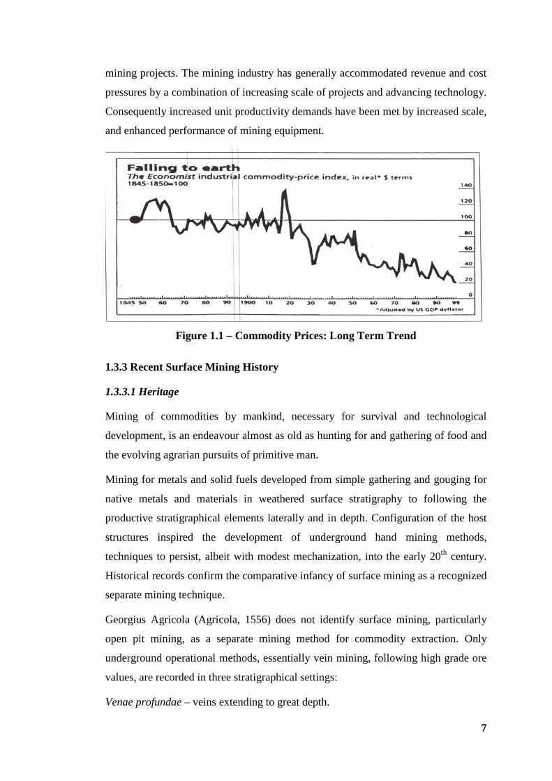
7
mining projects. The mining industry has generally accommodated revenue and cost
pressures by a combination of increasing scale of projects and advancing technology.
Consequently increased unit productivity demands have been met by increased scale,
and enhanced performance of mining equipment.
Figure 1.1 – Commodity Prices: Long Term Trend
1.3.3 Recent Surface Mining History
1.3.3.1 Heritage
Mining of commodities by mankind, necessary for survival and technological
development, is an endeavour almost as old as hunting for and gathering of food and
the evolving agrarian pursuits of primitive man.
Mining for metals and solid fuels developed from simple gathering and gouging for
native metals and materials in weathered surface stratigraphy to following the
productive stratigraphical elements laterally and in depth. Configuration of the host
structures inspired the development of underground hand mining methods,
techniques to persist, albeit with modest mechanization, into the early 20th century.
Historical records confirm the comparative infancy of surface mining as a recognized
separate mining technique.
Georgius Agricola (Agricola, 1556) does not identify surface mining, particularly
open pit mining, as a separate mining method for commodity extraction. Only
underground operational methods, essentially vein mining, following high grade ore
values, are recorded in three stratigraphical settings:
Venae profundae – veins extending to great depth.
8
Venae diletatae – veins thickened or lensed out.
Venae cumulatae – combined smaller veins relatively close together – a series of
conformable stringers.
James McClelland (McClelland, 1941) describes a number of iron ore and base metal
surface mining operations utilizing power shovels on rails loading into rail cars.
Introduction of road transport with 20-ton petrol-engined trucks and the resulting
increased flexibility is noted. Steeper access ramps at 8% - 10% are identified as
advantageous. By 1938, off-highway mining trucks had been introduced to the
Mesabi Range iron ore mines, Minnesota, USA, both in the typical 2 – 4 wheel
configuration of modern day trucks and tractor-trailer ore carriers. Track-mounted
power shovels have been developed contemporaneously with evolution of the
modern mining truck.
1.3.3.2 Western Australia
In early 20th century Western Australia, open pit mining (then termed “open cut”
mining) typically utilized glory-hole recovery of ore mined by underhand benching
of surface crown pillars as oxidized (weathered) ore sources to supplement
underground gold operations. In the early 1970’s gold miners benefited from a rising
gold price, due mainly to IMF deregulation of the gold price of US$35 per ounce
Troy and allowing the gold price to float on an open market. Open pit gold mining
commenced at a greenfields deposit at Telfer in the Little Sandy Desert of the East
Pilbara. From the mid 1970’s through the 1980’s open pit mining on the Golden Mile
at Kalgoorlie, extracted surface pillars in the weathered zone above underground
workings that previously could not economically or safely be mined by underground
methods. In the past twenty-five years, resurgence of gold mining based on open pit
mining methods was facilitated by lower-cost carbon-in-leach and carbon-in-pulp
treatment of weathered (oxidized) ores. Exploitation of lower grade weathered ore
remaining after underground operations, plus some greenfields low-grade
developments, burgeoned and then waned. More recently the gold mining industry
has consolidated to a small number of larger open pit gold mines still operating.
Current open pit gold operations mine both weathered and primary (sulphide) ores
requiring concentrating followed by pyrometallurgical or biological calcining prior to
leaching and gold recovery.
9
Early coal production at Collie, Western Australia for power generation and
locomotive fuel was mainly from underground mines using room-and-pillar mining
methods, supplemented by small-scale open pits using conventional rope shovels and
highway trucks or, at least in one instance, small track-mounted dragline where
seams outcropped. When the Hebe underground mine flooded in the 1950’s
(fortunately without loss of life), the Muja open pit was commenced using
conventional rope shovels and trucks on the same coal measures containing eight
seams with the Hebe as the basement seam. After initial box-cutting with motor
scrapers to remove tertiary sediments above the coal measures, open pit mining
commenced on the basement Hebe seam with the bonus of picking up seven thinner
seams higher in the coal measures that were uneconomic to mine by underground
methods. Open pit mining of the Muja coal measures and other seam groups within
the Collie Basin, which larger mining equipment can extract economically, is
continuing.
Lifting of the embargo on exporting of iron ore from Australia in the early 1960’s
initiated the world-class open pit iron ore mines of the Pilbara region of Western
Australia with large infrastructure requirements of ports, railways, towns and
services that currently retain a significant market share of world iron ore production.
Open pit mining techniques developed on the Mesabi Ranges, USA, were imported
to Western Australia. Electric rope shovels and largest available mining trucks were
introduced with the iron-ore industry keeping abreast of technology by upgrading as
larger trucks and loading units became available.
1.3.3.3 Evolution of Open Pit Mining Equipment
Since the 1940’s, there has been constant development of rope shovels with
introduction of hydraulic excavators, both backhoes and shovels, initially developed
in Europe in the 1960’s. The earliest large mining hydraulic shovels and backhoes
were introduced to Australia at Weipa, North Queensland about 1974, soon followed
at Collie in 1976, when a third generation of 85-ton trucks replaced 40-ton mining
trucks that had replaced smaller mining trucks introduced soon after the Muja open
pit commenced operations. Currently Collie coal mines use 240-ton mining trucks
and electric-powered rope shovels to load them. Equipment upscaling at Collie in the
1970’s was triggered by a practical fourfold increase in the price of oil. Return to
coal-fired electric power generation became an economic necessity in Western
10
Australia. “Mothballed” coal-fired thermal power stations were restored as base load
generation with oil-powered generation plant relegated to peak load service.
Similar parallel history of open pit mining development to that described above for
Western Australia has been experienced both nationally and internationally.
Development of strip coal mines in Queensland and NSW involving dragline
stripping and significant load-and-haul pre-strip operations have been spectacular.
Emergence of Japan as booming heavy-industry economy post WW II created
unprecedented demand for coal and iron ore that was met by Pilbara iron ore and
Bowen Basin coking coal.
1.3.4 Demand for Increasing Scale
A generation ago open pit mines using truck haulage were developed using
equipment sourced from the construction industry. The worldwide upsurge in large
infrastructure projects following World War II provided incentive for mobile
equipment manufacturers to develop off-highway trucks and equipment to load them.
There was also a demand for other earthmoving equipment including motor scrapers,
graders, track and wheel dozers and support equipment for the major civil earthworks
projects undertaken at that time. Typical developments included the Tennessee
Valley Authority and Interstate Highway initiatives in USA, Snowy Mountain
Hydroelectric Authority in Australia and the rebuilding of European war-affected
infrastructure.
Currently original equipment manufacturers (OEM’S’s) market mining trucks and
loading shovels specifically designed for open pit mining applications. Open pit
mining operators have a choice of mining trucks with either mechanical drive or
electric drive, both DC and AC, to 360 tons (330 tonnes) or more. These trucks can
be matched to rope shovels to 1400 tonnes operating mass, bucket capacity 56 cubic
metres, i.e., some 100 tonnes per bucket pass; or hydraulic excavators/shovels to
1,000 tonnes operating mass, bucket capacity 47 cubic metres, i.e., some 85 tonnes.
Extrapolation of designs to even larger equipment, particularly trucks, is currently an
active discussion topic throughout the mining and equipment supply industries.
There will be need in the future for innovative designs that depart from the currently
available mining truck configuration and physical form to achieve significant
measurable improvements in performance and operating incremental cost benefits.
11
Scaling up mining trucks and matching loading equipment for economic and
strategic reasons, has been a pervasive feature of open pit mining operations
internationally and for all commodities. Market demand has been met by response
from OEM’s with “ultra”-class - +300tonne - mining trucks and matching loading
equipment, including ubiquitous rope shovels and hydraulic excavators, of ever-
increasing scale and capacity. But an unfortunate side effect of increasing equipment
scale has been diminishing incremental cost-reduction benefits.
1.3.5 Evolutionary Trends
Recent history has been a story of ever-increasing scale of open pit mining
production equipment with rapid obsolescence. Upgrades by OEM’S have been
frequent with major re-works of mechanical mining trucks, more fuel-efficient
engines, low profile tyres with longer life potential, mine-specific design bodies that
provide for lower tare and higher payload. A recent major development has been
provision of AC electric wheel motors with improved torque-speed curve
characteristics approaching the power transmission efficiency of mechanical drives.
The improved efficiency of AC wheel motors compared with dated DC technology
can be expected to increase interest in trolley assist systems. As the current cost of
diesel fuel is at levels exceeding historical costs in countries that embraced trolley
assist because they were penalized by unnaturally high oil prices, e.g., South Africa
when sanctioned for their apartheid policy.
Mining trucks have been increasing in scale to realize the benefits of reduced unit
cost of production. Accordingly, there has been demand for loading equipment that
can three or four-pass load larger trucks to yield cost savings through both expected
lower unit loading costs from larger equipment and haulage cost benefit from
reduced truck-loading times.
OEM’s generally offer a nominal 240 ton payload mining truck. They are now
offering “ultra-class” trucks up to 360 - 400 ton payload with mechanical and AC
electrical drivelines. Early “ultra-class” mining trucks used DC wheel motors. When
first available AC wheel motors were supplied with “ultra-class” trucks with DC
motors as an option. Currently DC motors tend to phase out at 240 ton trucks with
OEM’S retroactively providing AC alternatives to DC systems down through the
range of large mining trucks.
12
Loading equipment for four-pass loading of “ultra”-class trucks, must have effective
bucket capacity of 90 to 100 tons. Allowing for practical bucket fill factors, bucket
capacities must be in the range of 95 to 105 tonnes metric.
An increase in the number of passes to load a truck, say to 5, 6 or 7 will obviously
tend to increase loading and total truck cycle times, reduce productivity and increase
unit cost due to extra loading time and truck haulage time. However, a number of
latent and indirect productivity/cost offsets tend to significantly compensate cost of
increased number of passes. These latent and indirect cost offsets are identified and
quantified in relative terms in Chapter 5.
The technology for autonomous truck haulage systems exists. Remote load-and-haul
units are currently working in underground mines. Autonomous haulage systems are
being tested for feasibility and operationally tested in open pit mines. Such systems
can be expected to become commercial and available in the near future.
13
CHAPTER 2
RESEARCH METHODOLOGY
2.1 RESEARCH BACKGROUND
2.1.1 Uncertain and Imprecise Estimating Practices
Experience with production planning, equipment selection and cost estimation for
feasibility studies, mining contracts and in-house budgets has revealed accuracy
limitations of estimates and selections based on determinative processes. To reduce
the risk of significant production shortfalls, and to cover the gap between
determinative estimation and reality, contingency allowances, or “fudge” factors, are
applied.
Traditionally contingency allowances have covered for omissions of Pareto-style
practices for compiling production and economic profiles of prospects to decide
whether to embrace for development or reject a possible project. Contingency
allowances are not only a treatment for risk of omission in estimating. These
corrective adjustments also cover for latent conditions, and possibly for lazy or
inadequate due diligence in the early investigative stages of feasibility studies
through to the procurement process as a prospect progresses to development.
In essence, contingency allowances in traditional estimating are expected to cover for
any lack of fit or inadequacy of the conceptual model in representing actual
operations and suitability of that model as a basis for productivity determination and
cost estimation.
Increasing cost pressures have demanded ever-increasing precision in estimating
techniques to accommodate falling commodity prices in real terms - Section 1.3.2.
Traditional estimating techniques, based on simple-system models using
deterministic processes manipulating discrete data are being supplemented by more
sophisticated analysis of complex models applying stochastic processes and
simulation techniques.
The more modern approaches to estimating forecasting and budgeting using system
simulations have introduced new terminology (Banks, 1996). Such as:
14
• System – defined by Banks below – for example open pit mine production
operations;
• Entities – mobile equipment: loaders, trucks and support equipment;
• Attributes – speed, capacity, breakdown rate;
• Activities – loading, hauling, turn and spot, turn and dump, waiting (queuing);
• Events – complete loading, breakdown; and
• State Variables – available, operating, standby, down.
“A system is defined as a group of objects that are joined together in
some regular interaction or interdependence towards accomplishment of
some purpose.” (Banks, 1996)
Systems can be discrete or continuous. Generally open pit mining operations can be
considered as discrete systems. Some activities within a discrete system can be
continuous, e.g., conveyor transport of materials mined with continuous-mining
methods or conversion of a discrete loading activity to a continuous sub-system
through a surge hopper and conveyor feeder. This research reviews open pit mining
systems using shovels loading mining trucks that are taken to be discrete, and
analyses and interprets activities that affect mining productivity and unit costs.
Traditional production scheduling and cost estimations are based on conceptual
operations models that are simplified to a degree that is comfortable for the
estimator. Variables are considered as discrete; variability is dealt with by using
mean, or occasionally, modal values. Traditional calculation processes are
deterministic, using expected (mean) values of empirical data. Most component
inputs for analysis of the nature and significance of attributes are randomly variable
distributions best analyzed stochastically.
This research examines some of the more important productivity and cost drivers by
analyzing operational data recorded by real-time monitoring facilities that track
activities of mining entities, i.e., shovels, trucks and supporting equipment. The
benefits of data collection and presentation by dynamically programmed dispatch
facilities are manifest.
Research described herein is a natural progression from limited accuracy outcomes
by applying traditional simple models and deterministic processes for mining
15
equipment selection both in terms of type and numbers. Estimates produced,
forecasts created and budgets compiled for productivity and mining costs by
deterministic process occasionally deliver inadequate results, even when modified by
practical factors to make the analysis fit experience-based anticipated outcomes, i.e.,
empirical evidence. Research has enabled investigation of reasons for actual
outcomes falling short of predictions in open pit mining operations.
Production and cost estimating, and operating standards, based on estimated average
performance may not deliver expectancies. For example:
• Mining-truck payload dispersion over a wide range has become more
important as mining trucks have increased in size. Compared with under-
loaded trucks, life of driveline components, including tyres, tends to reduce,
and braking distance increases, for over-loaded trucks. Increased payload
dispersion, and consequent truck cycle-time variability, increases bunching
effects.
• Selection of trucks and loading equipment on the basis of estimated average
performance without probabilistic consideration of combined, binomially
distributed availability and utilization of truck and loading equipment fleets
tends to underestimate fleet numbers.
• Tendency to adhere to time-honoured standards, such as, three or four pass
loading without investigation of all a-productive flow-on effects to
interrelated operational functions.
• Truck-bunching effects near the “match” point, where loading and hauling
capacities are practically equal, can cause loading equipment to be idle for
short periods. Simply over trucking to ensure that loading production is
maximized also determines collective productivity; but trucking efficiency is
reduced, hauling ucosts increase and overall mining ucosts increase. Over
trucking treatments include the tendency to always round up parts of trucks or
loading equipment when analyzing production and costs – generally without
considering the potential cost-reduction benefit of under trucking, or “over-
shoveling”, to maximize truck efficiency for any required productivity.
• Lack of appreciation of the diminishing cost benefits with increasing scale of
loading and hauling equipment, a result of ignoring details of necessary
16
changes in support equipment, facilities, and management systems –
especially the need for increasingly-precise management of time.
2.1.2 Questionable Standards and Measures
Adequately productive mining operations must also be efficient, and must sustain
competitive commodity costs. It is important to differentiate between absolute
production, i.e., the total tonnes or bank cubic metres (BCM) loaded and hauled, and
productivity, i.e., the rate of production, usually, per unit of time, per unit of
capacity, per unit of expense, per machine or per man-hour, and the like. Focus on
absolute production alone rather than a balanced consideration of efficiency,
productivity and cost is often an impediment to best management practices and
equipment selection for open pit mining.
Key Performance Indicators (KPI) adopted by mining operations for management
control are almost invariably productivity oriented. There appears to be confidence
that optimum economic costs are a natural consequence of maximum productivity.
This not necessarily so and some circumspection is justified. It is often necessary, to
consider productivity and operating costs independently. Certainly increased
productivity may significantly reduce estimated or budget costs. But depending on
the circumstances and how productivity is increased, “abcosts” (= absolute costs, i.e.,
empirical costs – actually experienced and realised after the event; not relative to any
unit basis such as time, production units and the like.) may stay the same or increase,
albeit moderately; and “ucosts” (= unit costs, i.e., abcosts per unit of time,
production, and the like.) may vary from significant decrease to significant increase.
In these potentially confusing situations it is understandable that fallacious
conclusions can result. It is easy to understand how technical investigators and
observers can fall for the “post hoc ergo propter hoc” fallacy – “after this therefore
because of this”. Paul Samuelson (Samuelson, 1958) explains this fallacy with the
examples: “The difficulty of analyzing causes when controlled experimentation is
impossible is well illustrated by the confusion of the savage medicine man who thinks
that a both witchcraft and a little arsenic are necessary to kill his enemy, or that only
after he has put on his green robe in spring will the trees do the same.” It is
important to extend any individual analysis of either productivity or costs to
consideration of interrelated factors and how bottom-line economics are likely to be
affected.
17
In support of this perception of over-focus on productivity, typical KPI (from a
recent mining contract) are listed in Table 2.1 appended in Volume 2. The emphasis
on production and productivity of the KPI’s in Table 2.1 is obvious with only one
exception in this typical list where a ucost is set as a performance standard. Certainly
productivity influences costs, but not exclusively nor necessarily predictably.
Certainly planned production will be achieved by realizing budgeted productivity,
but there is no certainty that budgeted or lowest costs will result.
The value of daily production tallies as a measure of efficiency has long been
recognized as questionable. Fivaz, Cutland and Balchin (Fivaz, 1973) in discussing
open pit fleet control, noted that: “The initial problem to be tackled was to seek an
answer to the question: How good are the operations on shift?” The measure
traditionally used was production tally. This figure however has great shortcomings
as a yardstick for operating efficiency….” Although absolute production has been
recognized as a questionable standard for measuring operating efficiency,
managements often persist with focusing primarily on production, with only
secondary attention to operating efficiency, when addressing equipment selection or
monitoring open pit operations.
In more recent times, application of sophisticated dispatch systems utilizing real-time
analysis of loading and hauling operations by computers has provided a programmed
automatic response in allocating hauling units to optimize performance of loading
resources. These systems, based on global positioning (GPS) of mobile equipment,
are adopted by open pit mine operators to realise the promise of significantly
improved truck utilisation in open pit operations with complex multi-loading position
options. However, is the efficiency improvement as significant as the market
promotional material would have us believe? Perhaps some credit should be afforded
the one or more human minds that monitor dispatch systems and over-ride them
when practical commonsense so indicates? Effect of degree of complexity of
operations must be considered. Digital dispatch systems are obviously more
beneficial for large mining operations with several mining groups, say three or more,
with more than 20 mining trucks operating. Only moderate or even small benefit can
be expected from application of dynamically-programmed dispatch systems to
smaller mining operations with 20 or less trucks. In such cases manual dispatch
systems alone can provide a substantial improvement and dynamically-programmed
18
digital-computer facilities may only provide small additional improvement? One
important advantage of digital dispatch systems is the detailed and comprehensive
data collected that can provide useful reports for operations management.
Operational data can be delivered in real time, for rapid remedial management
response to unacceptable load-and-haul equipment dispositions.
The de facto standard of three or four pass loading of mining trucks also warrants
investigation. It should be noted that shovel/excavator-truck match to theoretically
yield four passes can, in practical truck loading, yield a distribution with values from
two to seven passes or more depending on the characteristics of the material being
loaded and truck loading practices. This issue is expanded and reviewed in some
detail in Chapter 3.
A recent broad industry review of load and haul operations indicated that the
“average benchmark for mining truck loading is five passes” (Gregory, 2003). In his
paper “Excavator Selection”, Bruce Gregory indicates that only small cost penalty
results from varying from the indicated optimum modal value over a range of four to
six passes as illustrated by Table 2.2 (Gregory, 2003).
Other issues in relation to truck payload distribution dealt with in Chapter 5 indicate
that, in appropriate best load-and-haul costs may be realized by loading with modal
values of five or six passes in preference to the quasi-industry standard of four
passes.
Natural learning curves for introduction of new mining equipment to a site require
time. Estimated performance and cost estimates using deterministic processes based
on theoretical performance criteria are rarely achieved early in the life of new
equipment, or substantially upgraded models. This trend seems to be more
pronounced as scale of mining trucks increase; also for loading equipment to load
them.
Acquiring recently developed large open pit mining equipment with little application
history is a risk to be considered. This is especially true if retaining current operating
status of the mining operation is imperative. In the early stages of detailed planning
activity and at mining commencement, operations may suffer substantial inefficiency
from the additional management and technical workload of shepherding largely
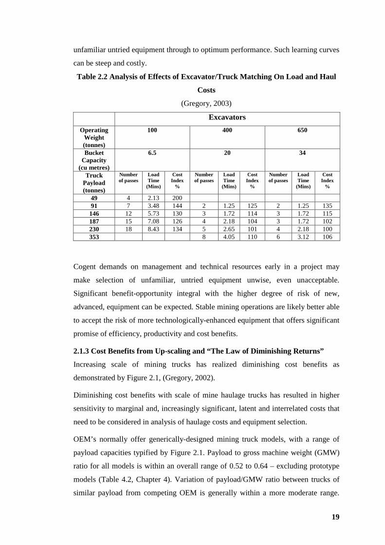
19
unfamiliar untried equipment through to optimum performance. Such learning curves
can be steep and costly.
Table 2.2 Analysis of Effects of Excavator/Truck Matching On Load and Haul
Costs
(Gregory, 2003)
Excavators Operating
Weight (tonnes)
100 400 650
Bucket Capacity
(cu metres)
6.5 20 34
Truck Payload (tonnes)
Number of passes
Load Time
(Mins)
Cost Index
%
Number of passes
Load Time
(Mins)
Cost Index
%
Number of passes
Load Time
(Mins)
Cost Index
%
49 4 2.13 200 91 7 3.48 144 2 1.25 125 2 1.25 135
146 12 5.73 130 3 1.72 114 3 1.72 115 187 15 7.08 126 4 2.18 104 3 1.72 102 230 18 8.43 134 5 2.65 101 4 2.18 100 353 8 4.05 110 6 3.12 106
Cogent demands on management and technical resources early in a project may
make selection of unfamiliar, untried equipment unwise, even unacceptable.
Significant benefit-opportunity integral with the higher degree of risk of new,
advanced, equipment can be expected. Stable mining operations are likely better able
to accept the risk of more technologically-enhanced equipment that offers significant
promise of efficiency, productivity and cost benefits.
2.1.3 Cost Benefits from Up-scaling and “The Law of Diminishing Returns”
Increasing scale of mining trucks has realized diminishing cost benefits as
demonstrated by Figure 2.1, (Gregory, 2002).
Diminishing cost benefits with scale of mine haulage trucks has resulted in higher
sensitivity to marginal and, increasingly significant, latent and interrelated costs that
need to be considered in analysis of haulage costs and equipment selection.
OEM’s normally offer generically-designed mining truck models, with a range of
payload capacities typified by Figure 2.1. Payload to gross machine weight (GMW)
ratio for all models is within an overall range of 0.52 to 0.64 – excluding prototype
models (Table 4.2, Chapter 4). Variation of payload/GMW ratio between trucks of
similar payload from competing OEM is generally within a more moderate range.
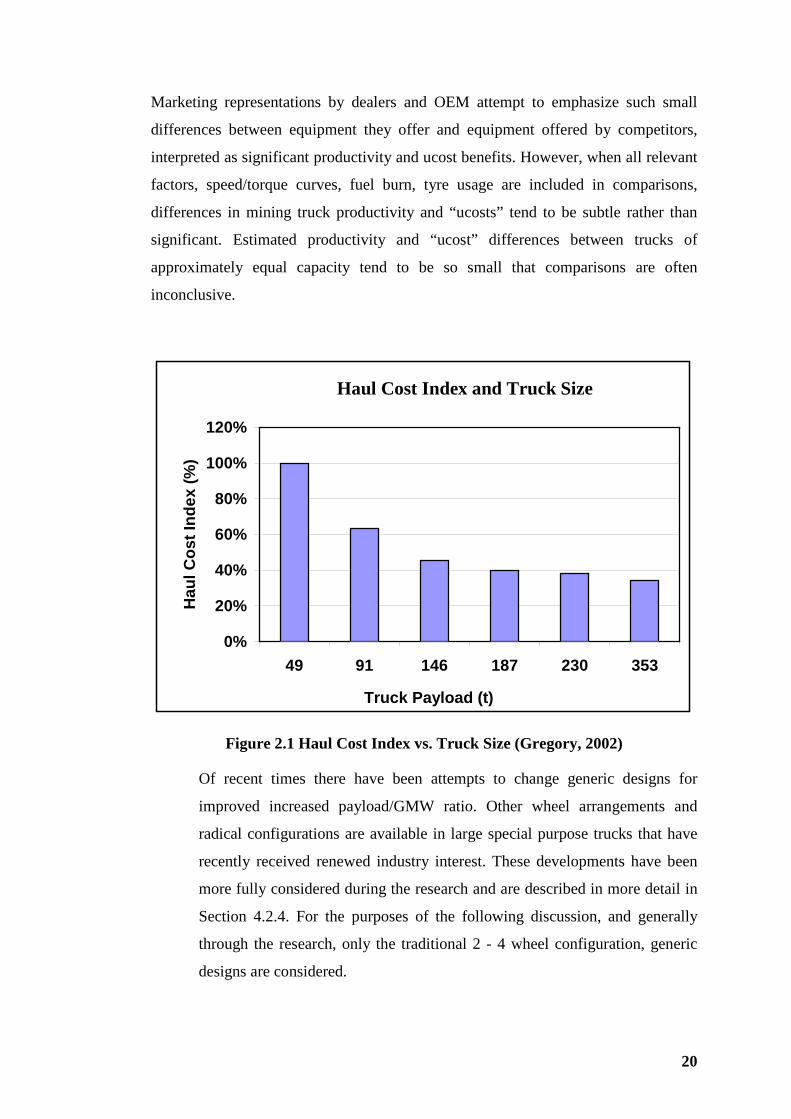
20
Marketing representations by dealers and OEM attempt to emphasize such small
differences between equipment they offer and equipment offered by competitors,
interpreted as significant productivity and ucost benefits. However, when all relevant
factors, speed/torque curves, fuel burn, tyre usage are included in comparisons,
differences in mining truck productivity and “ucosts” tend to be subtle rather than
significant. Estimated productivity and “ucost” differences between trucks of
approximately equal capacity tend to be so small that comparisons are often
inconclusive.
0%
20%
40%
60%
80%
100%
120%
49 91 146 187 230 353
Truck Payload (t)
Hau
l Cos
t Ind
ex (%
)
Figure 2.1 Haul Cost Index vs. Truck Size (Gregory, 2002)
Of recent times there have been attempts to change generic designs for
improved increased payload/GMW ratio. Other wheel arrangements and
radical configurations are available in large special purpose trucks that have
recently received renewed industry interest. These developments have been
more fully considered during the research and are described in more detail in
Section 4.2.4. For the purposes of the following discussion, and generally
through the research, only the traditional 2 - 4 wheel configuration, generic
designs are considered.
Haul Cost Index and Truck Size
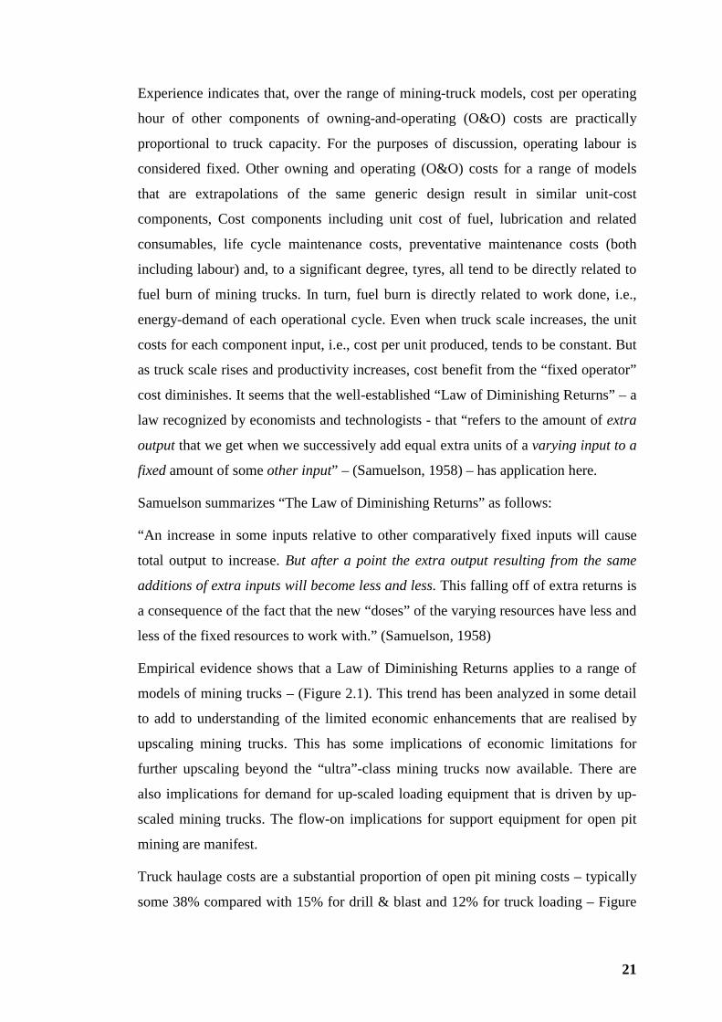
21
Experience indicates that, over the range of mining-truck models, cost per operating
hour of other components of owning-and-operating (O&O) costs are practically
proportional to truck capacity. For the purposes of discussion, operating labour is
considered fixed. Other owning and operating (O&O) costs for a range of models
that are extrapolations of the same generic design result in similar unit-cost
components, Cost components including unit cost of fuel, lubrication and related
consumables, life cycle maintenance costs, preventative maintenance costs (both
including labour) and, to a significant degree, tyres, all tend to be directly related to
fuel burn of mining trucks. In turn, fuel burn is directly related to work done, i.e.,
energy-demand of each operational cycle. Even when truck scale increases, the unit
costs for each component input, i.e., cost per unit produced, tends to be constant. But
as truck scale rises and productivity increases, cost benefit from the “fixed operator”
cost diminishes. It seems that the well-established “Law of Diminishing Returns” – a
law recognized by economists and technologists - that “refers to the amount of extra
output that we get when we successively add equal extra units of a varying input to a
fixed amount of some other input” – (Samuelson, 1958) – has application here.
Samuelson summarizes “The Law of Diminishing Returns” as follows:
“An increase in some inputs relative to other comparatively fixed inputs will cause
total output to increase. But after a point the extra output resulting from the same
additions of extra inputs will become less and less. This falling off of extra returns is
a consequence of the fact that the new “doses” of the varying resources have less and
less of the fixed resources to work with.” (Samuelson, 1958)
Empirical evidence shows that a Law of Diminishing Returns applies to a range of
models of mining trucks – (Figure 2.1). This trend has been analyzed in some detail
to add to understanding of the limited economic enhancements that are realised by
upscaling mining trucks. This has some implications of economic limitations for
further upscaling beyond the “ultra”-class mining trucks now available. There are
also implications for demand for up-scaled loading equipment that is driven by up-
scaled mining trucks. The flow-on implications for support equipment for open pit
mining are manifest.
Truck haulage costs are a substantial proportion of open pit mining costs – typically
some 38% compared with 15% for drill & blast and 12% for truck loading – Figure
22
2.2 (Gregory, 2002). The cost breakdown shown in Figure 2.2 is a typical
expectation for an accumulation of cost estimates for feasibility studies.
Drilling5%
Blasting10%
Loading12%
Hauling38%
AncillaryEquipment
17%
Management & Supervision
6%
Other12%
Typical Open Pit Mining Cost Breakdown
Figure 2.2 – Typical Open Pit Mining Costs by Activity (Gregory, 2002)
As pits deepen, haul distances extend and cycle times increase. Truck-haulage
proportions of total open pit mining costs increase. It can be assumed from Figure
2.2 that mean values of combined load and haul costs typically contribute about half
of total open pit mining costs. Further loading costs contribute about a quarter of
total load-and-haul costs. When load-and-haul cost tends to increase as a proportion
of total cost, haulage costs will contribute the majority (more than 75%) of the
increase. Understanding the productivity and cost interrelationships between loading
and truck haulage is critical for valid analysis of best economics for truck haulage or
combined load-and-haul.
The above discussion and illustration demonstrates the relative importance of truck
haulage costs compared with total mining costs. Although loading costs do not rank
significantly higher than other costs, such as drilling and blasting or ancillary
equipment, the interrelationship between loading and hauling demands that, in
practice, analysis of either of these elemental activities requires consideration of the
23
operational contribution, constraints, limitations, and costs of the interrelated
function.
2.1.4 Improving Technology and Analytical Practices
Equipment selection for a “greenfields” mining operation, or for replacement
equipment to sustain or improve project economics as conditions and planning
change, requires that the larger the equipment the more precise must be the
assessment, selection and estimating processes with commensurately increasing
technical and management effort.
It is counter-beneficial for mining equipment to provide improved technology and
capability that may be hindered by traditional, over-simplified selection process and
practices often overly focused on production, do not include adequate due diligence,
and, consequently, disappoint and fail to deliver the economic promise that initially
justified the investment.
Research described in this thesis addresses current techniques and practices,
considers what is available with current technology, and looks forward to what might
be possible in the future.
2.2 RESEARCH PHILOSOPHY
2.2.1 Research Techniques and Reality
The broad process for the research described herein, adopted the policy that
individual issues, productivity and cost drivers would be considered in terms of
singular attributes whilst, conceptually at least, keeping all interrelated attributes
constant. The successive activities of a mining operation are interdependent. The best
unit cost per tonne of ore treated or per unit of commodity produced is not
necessarily realised by minimizing the operating cost of each individual activity
(Atkinson, 1992).
The artificiality of considering processes and mechanics of singular attributes whilst
keeping interfacing attributes constant was considered. Parallels were identified in
research strategies adopted within scientific fields. The writings of David Suzuki, a
Professor of Genetics at the University of British Columbia, are relevant. In his book
(Suzuki, 1990) Suzuki describes the scientific process for acquiring knowledge to
control the environmental world in which we all live as follows:
24
“Science’s Jigsaw Puzzle
Science provides a unique way of describing the world around us. Its basic
methodology is to focus on one aspect of nature, isolating it from all else, controlling
everything impinging on it and measuring everything that happens. Science has
enabled us to look at nature and gain insights, but ones that are fragmented into bits
and pieces.
The apparent success of science in acquiring knowledge necessary to control the
world is based on the assumption that if nature is reduced to its most basic parts, a
comprehensive explanation will eventually be obtained by simply fitting the
components back together like pieces in a giant jigsaw puzzle.
Twentieth century scientists discovered that this hope simply does not hold up in the
real world. They found that we cannot know anything with absolute certainty even at
the most elementary level of subatomic particles. This is because the behaviour of
those particles can be described only statistically, not with certainty. Physicists have
also learned that the very act of observing nature changes it, because in order to see
it we have to control it; thus we can never know nature as it really is.
Perhaps the most shocking discovery was that when we reduce nature to its most
basic components, the description we obtain is of little value in predicting the
properties of those elements when they are combined.”
There are obvious parallels to the above observations in mining engineering research.
Many of the disciplined management processes used, including quality assurance,
continuous improvement programmes and formal risk management processes,
involve reducing operating systems and cost compilations to the most basic
elemental attributes. Analysis techniques consider basic attributes in isolation and
manipulate values assigned to each attribute for improved control including
efficiency, productivity, cost benefit, reduction to acceptable risk residuals and the
like. The points made by David Suzuki are interpreted in mining-engineering-
research equivalents as follows:
• Generally mining-engineering research adopts a basic methodology of
considering relevant individual attributes of systems in isolation.
25
• Insights can be gained from analysis of behaviour facilitated by
fragmentation into suitable individual attributes conceptually amenable to
consideration in isolation.
• The aim is for a comprehensive understanding of a system by collectively
considering all attributes together by means of the individual insights gained
in isolation.
• Any comprehensive understanding so obtained is subject to a degree of
uncertainty; and so must be adopted and applied with a degree of caution.
• Degree of uncertainty is a normal consequence of the nature of the individual
attributes where variability characteristics can only be described
stochastically.
• Any conclusions drawn from consideration of individual attributes must be
applied with caution in forecasting behaviour of the combined system.
2.2.2 Personal Rules and Understandings
The following personal rules have been applied during the research:
• All standards and time-honoured rules may be subjected to scrutiny in the
light of advancing technology, availability of empirical data, availability of
updated analysis methods and consequent improved understanding.
• Results from analysis of an individual attribute or component, when
combined with interrelated attributes within a system, must be re-considered
for combinatorial effects.
• The benefit of hindsight in the form of outcomes from research performed by
predecessors is a great legacy and advantage to be used with appropriate
humility, due acknowledgement and great respect.
• In undertaking research, there must be realization that others may have
previously or recently traversed the same investigative paths. Somewhere in
the world others may be currently pursuing similar lines of thought and be
advancing knowledge in a similar area of research. In such circumstances it is
assumed that duplication of research effort is not wasted; it may well add to
the work of others, lead to even better understanding and to discovery of
original concepts.
26
The final results described in this thesis are made available to all others currently
working, or who may in the future work in a related field or extension of the research
described herein. Future researchers finding these results of value, carry best wishes
for success in achieving their objectives.
2.2.3 Units
Metric units have been adopted throughout the research. Other units have been
introduced when required but are defined at the first usage.
Hours are solar hours based on 24 hours per day for 365 (366 days per year for leap
years is ignored as being of small effect) as the calendar dictates. “Calendar time” is
a generic term for the solar-time system.
2.3 METHODOLOGY AND LIMITATIONS
2.3.1 Research Procedures
The general approach to research of selection criteria for load-and-haul equipment
for open pit mining was essentially analytical, drawing on:
• Initial conception based on personal experience and field observations to
investigate and achieve a better understanding of the systems, drivers,
operational problems and outcomes; and
• Empirical evidence collected during the research to test the hypotheses and
theories developed by analysis.
Methodology adopted for the research and consequent limitations to scope of the
research includes:
• Discussion of initial outline with general objectives with supervisors.
• Literature research.
• Review of personal work history for relevant experiences.
• Identification of issues needing resolution based on experience, peer
discussions and literature research and developing strategies to realize
solutions.
• Collection of empirical data related to efficiency, productivity and cost
performance of load and haul activities.
27
• Development of hypotheses based on actual observations, analysis and
interpretation of results; and interpretations of references or data acquired
during the research.
• Work on hypothetical case studies using empirical data from operations and
productivity and cost analysis to test hypotheses.
• Interpret results and record outcomes.
• Write a thesis in compliance with guidelines of Curtin University of
Technology for submission to supervisors that fulfills the objectives of the
approved research outline with a view to ultimate acceptance.
• Research has been limited to examination of significant issues, events,
activities and attributes identified during the initial broad review of open pit
mining economics.
• The research set out to develop and present each hypothesis, generally prove
or disprove validity, to interpret the results in terms of recommended
practices and procedures for realizing benefit in efficiency, productivity and
operating costs.
2.3.2 Statistics
Collection and analysis of actual data from operating open pit mines has been
required. Analysis of that data has yielded descriptive statistics that provide a reliable
means of modelling open pit mining production activities for accurate prediction and
forecasting of productivity and cost performance.
All empirical data for bucket loads and bucket cycle times have been accepted as
continuous random variables. Data for bucket passes is, of course, discrete. Statistical
mathematical purists may consider that accepting such data analyzed herein as
“random” to be, at least, questionable. That the subsequent analysis assuming
variables to be continuous and random; and that any subsequent modelling of
distributions appears to yield reasonable consistent and expected results is considered
sufficient justification for any assumptions made. Due consideration has been given
to the “After this therefore because of this.” fallacy when making assumptions.
Analytical procedures generally follow a series of simple activities:
28
• Data was collected from operations included truck payloads, bucket loads,
number of bucket passes per payload, loading equipment cycle times, truck
loading times, incremental components of hauling operations time and total
hauling cycle time.
• Empirical data was generally assumed to be random and continuous; and
could be so modelled, with the exception of bucket passes per truck payload.
Bucket passes can be modelled by a Poisson, specifically an Erlang, discrete
distribution.
• Comparative dispersion of data distributions for load-and-haul attributes and
the probability of occurrence (or non-occurrence)of events, was a principal
analytical focus.
• Some confidence interval limits for selected variables were found to be set by
design or safety protocols, such as, Caterpillar’s “10:10:20 Policy” described
and considered in some detail in Chapters 3 and 5.
• Analytical process involved examining data for obvious spurious records and
applying appropriate filtering. Any filtering applied to eliminate spurious data
has generally been small; and is considered to have not materially influenced
the conclusions drawn from developed statistics. But any substantial filtering
to deliberately select subsets of data for analytical purposes that are
considered material in effect is identified and discussed in detail.
• Development of descriptive statistics for measures of central tendency,
measures of dispersion to adequately describe each individual distribution
studied, plotting histograms and superimposing a suitable distribution model,
also testing for skewness.
• Initial model fitting was qualitative with selected verifications using the
Kolmogorov-Smirnov (K-S) test for examples of each type of data including
truck payloads, bucket loads, bucket cycle times, truck loading times and
truck cycle times. Summary information and sample outputs of Kolmogorov-
Smirnov tests from the research and supplementary Probability and Quantile
plots are included in a separate section entitled “Distribution Testing” in
Volume 2, Appendices.
29
• Interpretations, implications and inferences that can logically be drawn from
the statistical results are described and summarized at appropriate locations
throughout the text, generally summarized in Chapter 6 and Chapter 7.
Mathematical background required to implement research analysis is documented in
a separate section entitled, Mathematical Principles – Notes, included in Volume 2,
Appendices, pp 457 – 486.
2.4 SIGNIFICANCE OF RESEARCH
Research topics within the total body of work where significant advances have been
made include:
• Mining-truck payload analysis and interpretations, based on several data sets
downloaded from several unidentified open pit mining operations made
available by equipment dealers and reported in this thesis with permission of
mining property owners that:
Provide improved understanding of payload distribution statistics.
Provide an insight into the relationship between bucket passes and
payload dispersion.
• Bucket load analysis using raw data downloaded by Caterpillar’s Minestar
communications system from the vital information management system
(VIMS) for each mining truck incorporating on-board load sensing and a
reporting system.
• Testing and verifying hypotheses based on truck payload and average bucket
load relationships - possibly a first published analysis of such data and
systems to test such theories.
• Research outcomes have delivered an initial understanding of the difficulties
in reducing dispersion of truck payloads. The most effective control methods
appear to result from ensuring adequate fragmentation and consistency of
condition of material to be loaded and hauled, and/or loading with more
passes of reduced quantity.
30
• Development of greater understanding of limitations to cost benefits from
upscaling mining trucks that will assist with equipment selection and
operating practices in open pit mines.
• Expanding on, and advancing previous research, on the comparative cost
benefits over a range of bucket passes to load mining trucks. De facto
industry standards of three/four pass loading have been questioned (Hardy #1,
2003) further investigated and, subsequently, comparative cost benefits
quantified identifying and allowing for a number of latent costs that are most
often ignored in traditional load-and-haul cost estimations.
• Potential questionable reliability of predictions and forecasts due to general
adoption of traditional deterministic analysis has been investigated. The
necessity for a more realistic stochastic analysis for determining behaviour of
many variable attributes in loading and hauling systems is a significant
research outcome.
2.5 FACILITIES AND RESOURCES
All research work has been undertaken solely by the author. Experience gained
during more than thirty-five years of mining technical support, mining contracting,
mine management and mining consulting practice has provided a valuable
foundation for the research. A significant resource supporting the research is the
author’s relevant experiences together with a substantial personal reference library
including technical reports, notebooks and diaries. The many case studies
accumulated have provided a substantial basis for the research. A well-equipped
home office, supplemented by occasional visits to the WA School of Mines,
Kalgoorlie has provided facilities in which the research was implemented.
The Robinson Library within Curtin University of Technology, industry and journal
websites have provided relevant reference material.
Research supervisors, colleagues, industry peers and contacts, OEM and dealer
representatives have been most supportive and generous with information, data and
pertinent references. Where used in the research process, such material assistance has
been duly acknowledged.
31
2.6 ETHICAL ISSUES
The nature of the research, industrial orientation and sources of information do not
necessitate any significant ethical considerations.
No person, persons or organisation have been identified or quoted without
permission, especially personal communications, or the material has been published
and is available for public information. All such material used in the research has
been duly acknowledged.
To the best of the author’s knowledge, there have not been any ethical transgressions
either in process of the research or recorded in this thesis.
32
CHAPTER 3
LOAD AND HAUL PERFORMANCE
3.1 PROJECT PRODUCTION SCALE
3.1.1 Introduction
A number of open-pit project scale parameters have to be identified and/or
determined prior to selecting loading and hauling equipment to deliver required
productivity most economically. Equipment selection should preferably provide
some flexibility to cover risks such as latent production timing demands. The degree
of flexibility provided as a risk treatment to cover short term demands to upscale; or
downscale, operations is a matter for assessment depending on the risk profile of
each individual project.
An early and essential task is to determine the initial scale of operations. Production
programmes and mining rates used for initial planning need to be confirmed by
proving feasibility including project economics, marketing, environmental and socio-
economic acceptability and general practicality and community acceptance prior to
committing to development. Many factors influence the production scale of a project
including:
• Mineral resources and economically determined ore reserves available for
mining.
• The commodity to be produced – whether it is nationally and/or globally,
strategic, whether it is high unit value such as precious metals or gemstones
or low unit value such as bulk commodities including salt, basic construction
materials, iron ore, oil sands, steaming and coking coal.
• Marketing issues including local, national or international demand,
commodity production the market will bear and long term marketing strategy
for project production.
• Availability of the necessary service resources such as power and water and
the necessary generating, capturing and reticulation infrastructure, human and
equipment resources that can be tapped for the benefit of the project; and, if
33
not existing or available, a practical situation exists for establishment of the
project resource requirements.
• Environmental and sociological constraints that may dictate capping
productivity of a development project even to the extent of rendering it
uneconomic.
• Intrinsic capacity of some infrastructure items such as railways, pipelines,
conveyors and ports that have a minimum capacity for viability; and that
predetermine a minimum production level to be tested against other potential
constraining factors.
Factors identified above are some of the preliminary considerations that may well
yield a determination, at least for planning purposes, of a suitable production scale
for the project. In the absence of such project-specific criteria, it is necessary to
consider previous industry experience either personal, advice from peers, or recorded
by authors that have proposed standard formulae for the purpose. Lawrence Smith
provides some “rules of thumb” divided broadly into two groups – (1) related to
physical characteristics and (2) related to economic characteristics.
For current purposes the discussion will be confined to “Taylor’s Law - for
underground and open pit mines except for a few structurally controlled situations”:
t/d = 0.014(Reserves)0.75
t/d = tonnes per day of ore produced. For open pit operations t/d must be increased
by the waste/ore ratio and the total production rate so derived. Taylor’s Law has been
recorded here “for reference only” and for when all else fails. It “should be used with
caution” (Smith L D, 1990).
3.1.2 Capacity Hierarchy
Experience indicates that each facility in a mining and ore treatment process tends, as
the project develops and settles down to a mature production operation, to have a
redundancy that progressively reduces in degree through the process. Managements
seem to provide a degree of over-capacity relative to the next-in-line downstream
activity in a project process hierarchy. Ernest Bohnet supports this with “For any
analysis (of mining method or equipment selection) it is better to have the first unit in
the chain of production with greater capacity than the downstream unit.” (Bohnet,
34
1990). In-built redundancy appears to be particularly so when a process stage
consists a single production unit. Immediately following discrete production
facilities; and sometimes before, surge capacity is usually built into the system such
as primary crushed ore stockpiles to facilitate continuous supply to downstream
process activities.
In the mining operational context, drilling equipment generally has significant
overcapacity as does hardware and facilities for preparation of and delivery of
blasting agents. Mining capacity generally exceeds the ore production schedule.
Capacity of loading equipment generally tends to exceed total mining production
requirements; that is exceeding intrinsic capacity of the truck fleet. Evidence to
support this observation is seen in bench marking studies as discussed in 3.2.4. There
occasionally appears to be a tendency to over truck production schedule
requirements; but in mature open pit operations truck redundancy seems less likely
than excess capacity of loading equipment. Crusher capacity is often some 50%
redundant compared with milling capacity, particularly where there is only a single
primary crusher. In such cases there is always a substantial crushed ore stockpile to
sustain mill feed for crusher downtime.
• It is most cost effective to deliver ore as mined and hauled directly to the
crusher; but ore supply from the pit does not always match and may exceed
crusher capacity from time to time. Many operations stockpile all or at least
part of mined ore and reclaim it for transport to the crusher cross blending in
the process. The cost of re-handling all ore to be crushed is often justified by,
and offset by improved concentrator recovery. Cross blending metalliferous
ores requiring concentrating delivers a more uniform head grade to the
concentrator with resulting enhanced recovery. Ore stockpiling to facilitate
cross-blending generally provides a bonus of flexibility where ore exposure
in the pit is intermittent and vice versa. The ore re-handle equipment fleet
usually has a significant redundancy compared with the operating profile of
the crusher. Additional capacity in the re-handle fleet adds a further bonus of
flexibility to mining operations.
The general tendency for provision of excess mining equipment capacity has at least
two benefits:
35
1. There is inherent flexibility that can provide rapid response to production
schedule increases, at least to an initial degree. If the loading equipment
capacity is available it is more convenient and generally an easier task to add
some hire trucks and auxiliary support for short term cover until the
production crisis passes or until permanent haulage equipment and auxiliary
support can be procured. Particularly, in the larger shovel range, hire or used
equipment is not as readily available as trucks and support equipment.
2. Experience has shown that continuous improvement campaigns for cost
benefits are most beneficially progressed by increasing utilisation of existing
equipment capacity. Working operating equipment more hours in any given
period is most beneficial. The next most beneficial improvement opportunity
is to provide operating and maintenance labour to make operational any
equipment fleet redundancy. This last practice manifestly reduces operational
flexibility and increases operational risk. But, the immediate cost benefits and
rewards of the resulting business opportunity may be attractive so making the
increased risk acceptable. Depending on economic forecasts investing in
equipment redundancy as a risk treatment may be justified by the benefits of
future production flexibility.
In summary, mining operations have a tendency to be initially supplied with; or to
acquire over time, equipment with substantial excess capacity. Justification for this
over-capacity is believed to be a manifestation of intuitive or formal risk treatment
by mine developers and mine managers. Formal risk analysis is a burgeoning
technique that is a natural outcome of the needs of the mining industry to work
smarter to accommodate the cost pressures resulting from the long-term real-terms
prices for mined commodities as described in Section 2.3.2. Identifying, assessing
and treating of mining operational risk is the formal process that likely justifies
current mining equipment over capacity. But the industry has a long history of such
overcapacity provisions that can only be explained as the intuitive response to the
lessons of experience.
In the research described by this thesis the philosophy of carrying mining equipment
overcapacity is not endorsed unless there are valid analytical reasons, technical
and/or risk assessment, to over truck or over shovel.
36
3.2 LOADING EQUIPMENT
3.2.1 Selection Process
Surface mining operations (including open pit mining) require the application of
many interdependent activities including ground preparation (ripping and pushing,
drilling and blasting), excavation and loading, transport, waste disposal, ore sizing,
attritioning and treatment and commodity recovery, packaging and transport
(Atkinson, 1992).
This thesis is confined to open pit mines and to load and haul and closely related
activities. Because of the interdependence between all activities in a mineral-
commodity business endeavour, it is potentially misleading to focus on one
individual activity or small partition of activities, refer to Section 2.5.1. Throughout
the analysis that follows in this thesis, any results from isolated considerations have
been viewed with caution. Such results have been considered, and, where possible
have been tested, in combination with all inter-relatives; and, where necessary,
modified to reflect these considerations and testing.
Elevated risk from equipment selection in isolation cannot be overstressed. Any
process to select excavating and loading equipment must include due consideration
of the mining trucks to be loaded. Similarly any selection process to select mining
trucks must include due consideration of excavating and loading equipment to load
them. In these circumstances it is fitting to consider which should be selected first -
loaders or trucks? Traditionally there has been a tendency for selection of excavation
and loading equipment to satisfy a production requirement and trucks are then
selected to service the transport requirements. This is despite the well-recognized
component cost criteria where transport is two to five times the cost of excavation
and loading in open pit mines. Reliable processes for determining loading equipment
and truck types, size and numbers consider loading equipment and trucks in isolation
for convenience but in combination at the first opportunity in the process. This is
revisited in Section 3.3.
3.2.2 Cyclic vs. Continuous Excavation
There are many options for materials handling systems and mining equipment to
conduct open pit mining operations. The general materials handling system will be
determined by the commodity, downstream treatment of the commodity such as
37
direct use for power generation, feedstock for iron and steel, secondary and tertiary
treatment to a high value additive for special manufacturing economies or extraction
and recovery of precious metals or gem stones used in high-value industries or as a
medium of financial exchange. Generally mining systems can be classified as
Continuous or Cyclic (Atkinson, 1992).
• Continuous excavation systems used in open pit mining include bucket wheel
and bucket chain excavators or dredges applied in brown coal mining for
power generation typified by many European examples; also Yallourn and
Morwell in Victoria – essentially large-volume open-pit mining operations.
• Cyclic excavation systems include shovels, draglines, wheel loaders and
scrapers with ripping dozers that are specifically or severally applicable for a
large range of operational scales, commodities and open pit mining
configurations.
Continuous excavation systems are generally matched to continuous transport
systems including belt conveyors, pipelines and, historically, aerial ropeways: but
there could be applications where continuous excavation could be matched to cyclic
transport, mining trucks, where the material mined suits continuous excavation but
operational life or production rate cannot justify investment in continuous transport.
Cyclic excavator systems can be matched to continuous transport systems
particularly for large-scale long-life deep open pits where waste and ore transported
on conveyors (generally after crushing to conveyable size) is the best economic
solution. Most often, cyclic excavation systems are matched to cyclic transport
systems, typically conventional loading equipment loading mining trucks. This cyclic
excavation-transport combination is the focus of this thesis.
3.2.3 Loading Equipment Options
Rope shovels (sometimes termed cable shovels) have a long development history.
Initially on rails, steam-powered rope shovels gave way to on-board diesel powered
shovels on caterpillar tracks. As scale of shovels increased, larger electric DC motor
drives were developed powered by AC/DC motor/generator sets controlled by Ward-
Leonard systems with reticulated power delivered by trailing cable at standard
frequencies (Hertz – Hz) and voltages now available to 13,800v AC.
38
Prior to the development of draglines for stripping overburden from coal seams, large
stripping shovels were developed to side cast overburden. Recent developments in
large mining shovels have focused on more efficient AC motor drives and electronic
control systems.
Development of wheel loaders, from their introduction in the late 1930’s, has
continued for some fifty years with ever-larger machines currently offered from a
number of original equipment manufacturers. Typically cycle times of large wheel
loaders are some 150% or more compared with cycle times for an equivalent shovel
or excavator. Mechanical drive loaders to 210 tonnes and 50 tonne bucket load have
recently been surpassed by an electric-wheel loader at 245 tones operating weight
and 72 tonnes bucket load. Cycle time improvements have also been an added
benefit of recent large wheel loader development.
Large wheel loaders are often favoured as support loading equipment because of
mobility advantage. They can more readily relocate to cover for unplanned downtime
of a rope shovel, hydraulic shovel or excavator or to clean up small quantities of
batter trimmings and like activities Where mobility, in-pit blending, multi-material
selectivity or self-sufficiency for pit-floor housekeeping are major issues, particularly
in shallow open-pit operations such as lateritic ores, bauxite mining and similar,
wheel loaders may be applied as prime loading equipment. Final clean up to prepare
faces for blasting are also an advantage as the loader can work up to within a few
minutes of a time deadline for clearing a mining locality for a blast. More recently
developed or upgraded large wheel loaders have the advantage of faster digging
cycles that more closely approach a rope or hydraulic shovel.
Hydraulic excavators, initially in backhoe configuration and later as shovels, have
provided an alternative for loading mining trucks. Initially a product developed in
Europe for the construction industry, where boom and stick reach were important,
hydraulic excavators; and subsequently shovels, have developed specifically for
mining operations. Features of the excavator evolution include, the so-called “mass
excavation” configuration - larger buckets for enhanced production capacity -
necessitating shorter booms and sticks for excavators, short booms and arms for
shovels. First appearing in Australia in the early 1970’s with 4 – 5 CM buckets, 80 –
90 tonne operating weight, hydraulic loading equipment solutions have evolved to
39
the current availability of 47 CM (85tonnes) bucket shovels with operating weight of
some 1,000 tonnes.
A notable feature of hydraulic face shovels is the ability to pivot the bucket,
changing the angle of attack of bucket teeth, at any point within the operating
envelope to enable crowding into or breaking out of the face. Some hydraulic shovels
have mechanisms to enhance this feature. Not available on rope shovels, this feature,
allows for removal of material in the face from the top down, an obvious advantage
for hydraulic shovels that facilitates selective mining and prevention of face
overhang (Files, 1990).
John Wiebmer (Wiebmer, 1994) observed: “No two mines are the same. Each
requires a unique system of people, machines and processes to meet production
requirements profitably. Miners today, as never before, have a wide array of choices
in loading tools to meet operational needs. Cable (rope) shovels, hydraulic shovels
and excavators and wheel loaders … different horses for different courses.” The
breadth and depth of choice imposes a need for due diligence in determining the
complete characteristics of the service required and careful analysis of the options to
satisfy those needs.
Early considerations should consider the special features, advantages and
disadvantages of each type of loading equipment in comparison with the unique
conditions and characteristics of the proposed mining operation. Some of the initial
considerations are listed in Figure 3.1, with a suggested ranking for each type of
equipment.
In the early stages of an open pit mining development the question will arise: “What
type of loading equipment will be most applicable and deliver best economics?” This
question will be addressed in more detail in a following section. The answer can only
be delivered by a duly diligent analysis of the specific mining application each of
which are, at least in detail, unique.
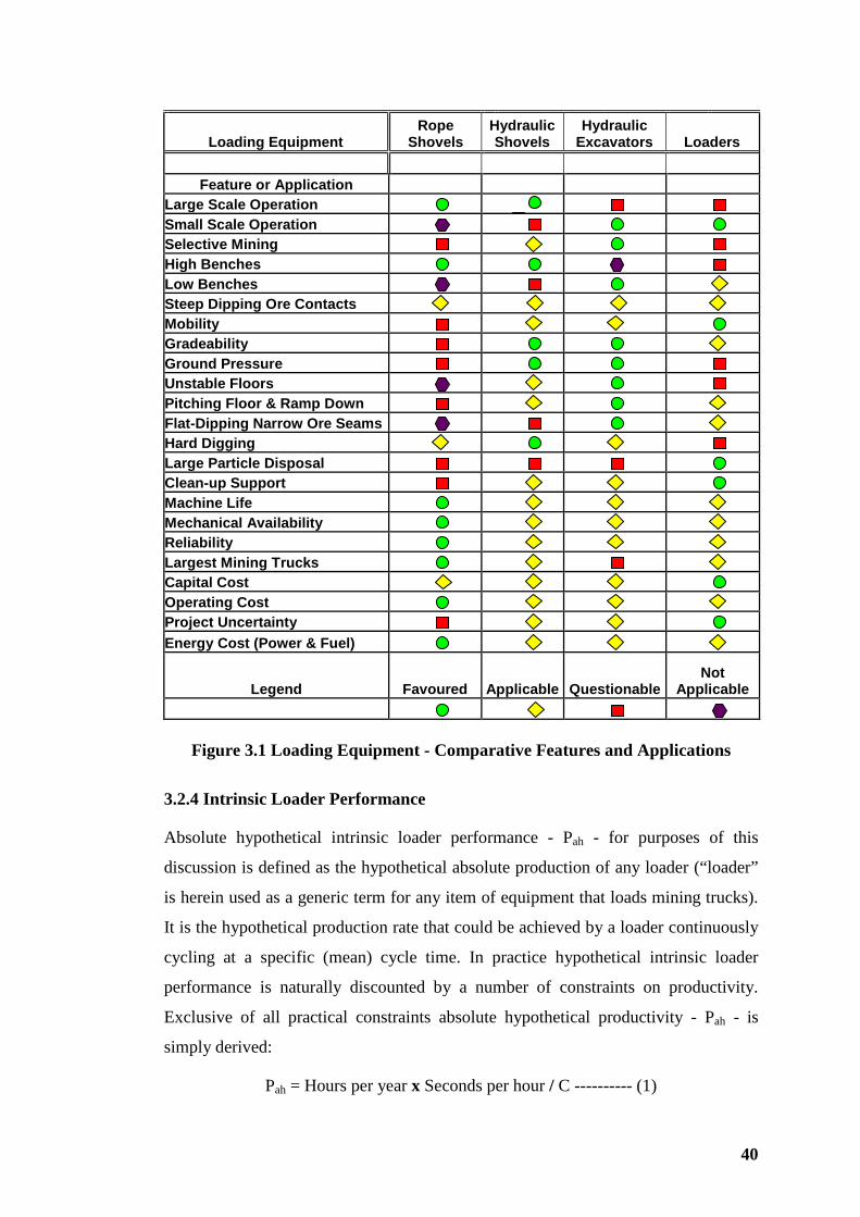
40
Figure 3.1 Loading Equipment - Comparative Features and Applications
3.2.4 Intrinsic Loader Performance
Absolute hypothetical intrinsic loader performance - Pah - for purposes of this
discussion is defined as the hypothetical absolute production of any loader (“loader”
is herein used as a generic term for any item of equipment that loads mining trucks).
It is the hypothetical production rate that could be achieved by a loader continuously
cycling at a specific (mean) cycle time. In practice hypothetical intrinsic loader
performance is naturally discounted by a number of constraints on productivity.
Exclusive of all practical constraints absolute hypothetical productivity - Pah - is
simply derived:
Pah = Hours per year x Seconds per hour / C ---------- (1)
Loading Equipment Rope
Shovels Hydraulic Shovels
Hydraulic Excavators Loaders
Feature or Application
Large Scale Operation Small Scale Operation Selective Mining High Benches Low Benches Steep Dipping Ore Contacts Mobility Gradeability Ground Pressure Unstable Floors Pitching Floor & Ramp Down Flat-Dipping Narrow Ore Seams Hard Digging Large Particle Disposal Clean-up Support Machine Life Mechanical Availability Reliability Largest Mining Trucks Capital Cost Operating Cost Project Uncertainty Energy Cost (Power & Fuel)
Legend Favoured Applicable Questionable Not
Applicable
41
Equation (1) yields loose cubic metres (LCM) per cubic metre of bucket capacity.
C is the estimated mean loader cycle time in seconds.
Pah is equivalent to the displaced volume of a loader with a 1 CM bucket cycling
continuously. It will be noted that the equation also yields hypothetical maximum
loading cycles per year.
Productivity
The following discussion is based on a description of dragline productivity factors
and calculations that are directly applicable to truck loading equipment (Humphrey,
1990).
To arrive at a practical productivity for loading equipment the following limiting
factors must be applied to Pah. Some of the factors have distinct categorical variations
critical for loading equipment productivity calculations.
Time Factors – summarized in more detail in 3.6:
• Calendar Hours Hc – solar hours in any given period of observation, e.g., year
or day based on solar time – 24 hours per day for 365 (or 366 days per leap
year) generally termed “hours” in this thesis.
• Scheduled Hours Hs – the annual hours the loader is expected to operate at
expected productivity – 8,760 (8,784 for a leap year is generally ignored for
convenience) less allowances for public holidays, any planned interruptions
to operations and daily hours when work is not scheduled.
• Available Hours A – the part of scheduled hours when the loader is
mechanically and electrically ready to operate – those scheduled hours when
the equipment is under the operational control of open-pit production
management and not out of service for maintenance.
• Utilized Hours or Operating Hours U – the part of the available hours that the
loader is actually operating at expected productivity – excludes extraneous
lost time due to unplanned interruptions to operation of specific items, groups
or all mining equipment and any inefficiency due to logistical
mismanagement or inadequate operator response.
Material Factors – see Section 3.2.7 for more detailed discussion:
42
• In situ Density (as determined by laboratory density determination from
samples termed Apparent Rock Density – ARD) – tonnes per BCM - an
inherent property of the material to be mined that varies with the geological
setting; but also may vary within any discrete stratigraphic horizon – a
typically low-dispersion random variable.
• Swell Factor Sw – a variable dependent on the inherent structural and
geotechnical properties; and the mechanisms and degree of disturbance of the
material to be mined measured as the ratio of the volume of a specific weight
of material after disturbance by blasting, ripping and pushing, loading into
trucks or dumped at material disposal points – crusher, ore stockpile or waste
dump and the in situ volume. That is:
- Swell Factor = LCM/BCM = (1 + Swell) --------------(2)
LCM =loose cubic metres
BCM = Bank – in situ – cubic metres
Equipment Factors – more detailed discussion is continued in Sections 3.2.7 and
3.2.8:
• Rated Bucket Capacity Bc – generally reported as struck by rope shovel
manufacturers and 2:1 heaped by hydraulic shovel and excavator
manufacturers with capacity determined in compliance with an industry
standard, i.e., SAE J67.
• Loader cycle time in seconds Tc, or cycles per unit of time as convenient, that
includes due allowance for non-optimum digging depth varying angles of
swing – a random variable that is dependent on the condition of material to be
loaded, physical characteristics of the loading operation, mechanical and
electrical/hydraulic performance of the loader, efficiency of the operator and
any extraneous interference that may impinge on the loading operation.
• Bucket Fill Factor Ff – a variable that typically, for full bucket loads, can be
expected to have low dispersion (coefficient of variation of 0.1 or less)
considered volumetrically so visual control and measurement is possible and
can be effective - generally defined volumetrically as the ratio or percentage
43
of actual volume in the bucket compared with a standard rated bucket
capacity that vary for loader types – see next point.
• Bucket Factor Bf (Ff / Sw BCM or ARD . Ff / Sw tonnes) – a random variable
that combines the effects of in situ density, swell and volumetric fill factor –
enables analytical connection of loader performance with in situ volume and
computations in terms of mass – generally expressed as a dimensionless
factor that can be interpreted in terms of volume or mass depending on the
context – a convenient cover-all device.
The above factors can be applied to obtain a preliminary productivity estimate Pe –
BCM/hr - as follows:
For draglines; also applies to loaders delivering to surge accommodation and
continuous transport systems (Humphrey, 1990):
Pe = (3600/Tc) x (Hs/year) x A x U x (Bc/Sw) x Ff BCM/hr ---------- (3)
For loading shovels (after Atkinson, 1992 and substituting symbols):
Pe = Bc x (3600/Tc) x SF x A x U x Bf x PF BCM/hr or tonnes/hr ---------(4)
Tc is the average loading cycle time - in equation (4). OEM and equipment dealers
generally provide average cycle times for loading equipment items. Empirical values
are tabulated for a range of digging conditions. Typically four levels of digging
difficulty are specified in empirical terms viz., Easy, Medium, Hard and Very Hard
(Harnischfeger, 2003). Cycle times generally tend to increase with scale of
equipment and difficulty of filling the bucket. Both large rope shovels and hydraulic
shovels cycle in the range 25 to 45 seconds depending on operating conditions.
Actual observed cycle time data is discussed in more detail in Sections 3.2.9 and
3.3.10.
Obviously, if cycle times are manifestly increased by digging difficulty, the rewards
from improvement will justify significant effort and investment in improving
operating conditions by attention to drilling and blasting, particularly pattern
accuracy, hole alignment, consistent depth of hole, sub-drill depth, stemming length
and stemming quality, detonation sequence and delay; also by increasing drilling per
unit volume and powder factor to some cost-justifiable degree. The ultimate benefit
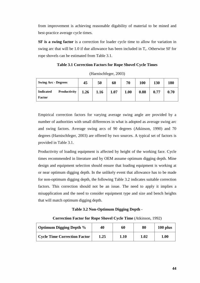
44
from improvement is achieving reasonable digability of material to be mined and
best-practice average cycle times.
SF is a swing factor is a correction for loader cycle time to allow for variation in
swing arc that will be 1.0 if due allowance has been included in Tc. Otherwise SF for
rope shovels can be estimated from Table 3.1.
Table 3.1 Correction Factors for Rope Shovel Cycle Times
(Harnischfeger, 2003)
Swing Arc - Degrees 45 50 60 70 100 130 180
Indicated Productivity
Factor 1.26 1.16 1.07 1.00 0.88 0.77 0.70
Empirical correction factors for varying average swing angle are provided by a
number of authorities with small differences in what is adopted as average swing arc
and swing factors. Average swing arcs of 90 degrees (Atkinson, 1990) and 70
degrees (Harnischfeger, 2003) are offered by two sources. A typical set of factors is
provided in Table 3.1.
Productivity of loading equipment is affected by height of the working face. Cycle
times recommended in literature and by OEM assume optimum digging depth. Mine
design and equipment selection should ensure that loading equipment is working at
or near optimum digging depth. In the unlikely event that allowance has to be made
for non-optimum digging depth, the following Table 3.2 indicates suitable correction
factors. This correction should not be an issue. The need to apply it implies a
misapplication and the need to consider equipment type and size and bench heights
that will match optimum digging depth.
Table 3.2 Non-Optimum Digging Depth -
Correction Factor for Rope Shovel Cycle Time (Atkinson, 1992)
Optimum Digging Depth % 40 60 80 100 plus
Cycle Time Correction Factor 1.25 1.10 1.02 1.00
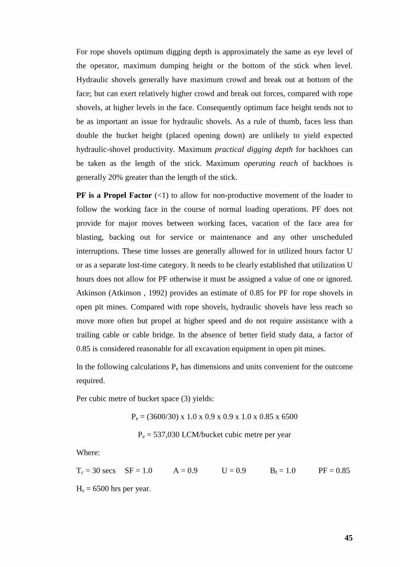
45
For rope shovels optimum digging depth is approximately the same as eye level of
the operator, maximum dumping height or the bottom of the stick when level.
Hydraulic shovels generally have maximum crowd and break out at bottom of the
face; but can exert relatively higher crowd and break out forces, compared with rope
shovels, at higher levels in the face. Consequently optimum face height tends not to
be as important an issue for hydraulic shovels. As a rule of thumb, faces less than
double the bucket height (placed opening down) are unlikely to yield expected
hydraulic-shovel productivity. Maximum practical digging depth for backhoes can
be taken as the length of the stick. Maximum operating reach of backhoes is
generally 20% greater than the length of the stick.
PF is a Propel Factor (<1) to allow for non-productive movement of the loader to
follow the working face in the course of normal loading operations. PF does not
provide for major moves between working faces, vacation of the face area for
blasting, backing out for service or maintenance and any other unscheduled
interruptions. These time losses are generally allowed for in utilized hours factor U
or as a separate lost-time category. It needs to be clearly established that utilization U
hours does not allow for PF otherwise it must be assigned a value of one or ignored.
Atkinson (Atkinson , 1992) provides an estimate of 0.85 for PF for rope shovels in
open pit mines. Compared with rope shovels, hydraulic shovels have less reach so
move more often but propel at higher speed and do not require assistance with a
trailing cable or cable bridge. In the absence of better field study data, a factor of
0.85 is considered reasonable for all excavation equipment in open pit mines.
In the following calculations Pe has dimensions and units convenient for the outcome
required.
Per cubic metre of bucket space (3) yields:
Pe = (3600/30) x 1.0 x 0.9 x 0.9 x 1.0 x 0.85 x 6500
Pe = 537,030 LCM/bucket cubic metre per year
Where:
Tc = 30 secs SF = 1.0 A = 0.9 U = 0.9 Bf = 1.0 PF = 0.85
Hs = 6500 hrs per year.
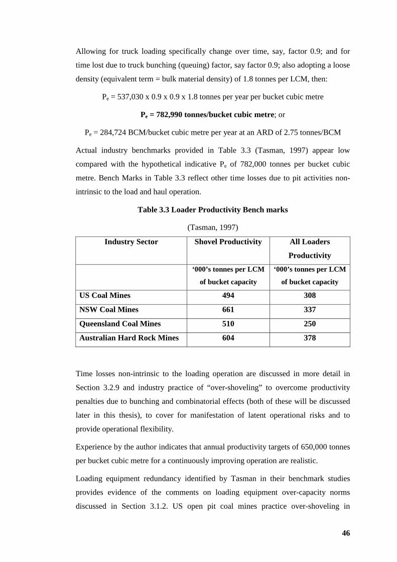
46
Allowing for truck loading specifically change over time, say, factor 0.9; and for
time lost due to truck bunching (queuing) factor, say factor 0.9; also adopting a loose
density (equivalent term = bulk material density) of 1.8 tonnes per LCM, then:
Pe = 537,030 x 0.9 x 0.9 x 1.8 tonnes per year per bucket cubic metre
Pe = 782,990 tonnes/bucket cubic metre; or
Pe = 284,724 BCM/bucket cubic metre per year at an ARD of 2.75 tonnes/BCM
Actual industry benchmarks provided in Table 3.3 (Tasman, 1997) appear low
compared with the hypothetical indicative Pe of 782,000 tonnes per bucket cubic
metre. Bench Marks in Table 3.3 reflect other time losses due to pit activities non-
intrinsic to the load and haul operation.
Table 3.3 Loader Productivity Bench marks
(Tasman, 1997)
Industry Sector Shovel Productivity All Loaders
Productivity
‘000’s tonnes per LCM
of bucket capacity
‘000’s tonnes per LCM
of bucket capacity
US Coal Mines 494 308
NSW Coal Mines 661 337
Queensland Coal Mines 510 250
Australian Hard Rock Mines 604 378
Time losses non-intrinsic to the loading operation are discussed in more detail in
Section 3.2.9 and industry practice of “over-shoveling” to overcome productivity
penalties due to bunching and combinatorial effects (both of these will be discussed
later in this thesis), to cover for manifestation of latent operational risks and to
provide operational flexibility.
Experience by the author indicates that annual productivity targets of 650,000 tonnes
per bucket cubic metre for a continuously improving operation are realistic.
Loading equipment redundancy identified by Tasman in their benchmark studies
provides evidence of the comments on loading equipment over-capacity norms
discussed in Section 3.1.2. US open pit coal mines practice over-shoveling in
47
contrast to over trucking generally practiced by Australian open pit coal mines; and,
generally, US coal mines were more efficient and lower cost than either NSW or
Queensland coal mines (Tasman, 1997)
As a preliminary step in excavation equipment selection expected excavator
productivity can be estimated from equation (4) by addressing each of the factors and
assigning a value suitable for the mining project under consideration. An alternative
approach is to adopt productivity per bucket cubic metre of, say, 600,000 tonnes and
so determine the bucket cubic metres required. Consideration of the number of
working locations then determines the bucket size for each of the chosen number of
shovels. This naturally leads to an indication of the size, or sizes, of mining truck that
should be considered for truck selection.
3.2.5 Single or Double Side Loading
The industry standard for truck loading is single-side loading with the truck to the
left of the loader when addressing the face.
The operator’s station or cab is situated to the right of the boom on rope shovels so
the operator has a good view of the face on the return swing from a conventional
single-side truck loading arrangement and can select the next digging point. On the
loaded swing the stick is practically horizontal and generally above the operator’s
line of sight facilitating spotting of the bucket over the truck. Hydraulic shovels,
generally physically smaller than rope shovels of equivalent performance,
traditionally have the cab on the left hand side to facilitate bucket spotting. On the
return swing the boom lowers and the arm folds back to draw the bucket back to the
toe of the face. At this stage the operator can see over the arm and bucket to spot the
digging position. Operators of excavators configured as backhoes have generally
better visibility conditions compared with hydraulic shovels as the excavation
envelope is well below the cab. In larger hydraulic shovels, cabs are sometimes
mounted on the right side of the boom. The high cab and relatively short bucket arm
provide reasonable visibility of the face to select digging positions.
Wheel loaders have centrally located cabs generally mounted on the rear module
behind the articulation hitch to improve the ride for the operator and provide a safer
position when working under high faces There are historical examples of a large
loaders where the cab was offset to the right side as with rope shovels; also another
48
example where the cab was mounted on the front module in an attempt to improve
vision and a more conventional driving feel when articulating. Both these cab
configurations for wheel loaders have been discontinued.
Truck loading time is lost when trucks exchange for loading. After the last bucket
load is placed on a truck the loader returns to the face to pick up the first bucket load
and then swings (or trams in the case of a wheel loader) to spot the incoming truck.
Truck “turn-and-spot” time is typically some 45 seconds but can vary depending on
manoeuvering safety practice and available bench space. As the truck “turn-and-
spot” time generally exceeds loader cycle time, the nett time between “turn-and-
spot” and loader cycling, i.e., “truck exchange time”, is waiting time for the loader –
optimally in the order of 10 seconds. In the previous section it was shown that some
500,000 cycles per year are practical with a loader. So, for optimal “truck exchange
time” and, depending on the number of passes for truck loading, annualized change
over waiting time for the loader is in the order of 350 hours for 4-pass loading and
230 hours for 6-pass loading. The implications of this loading inefficiency will be
addressed in more detail in Section 3.2.6.
To eliminate, or at least reduce the changeover loader waiting time; and where
operating conditions permit, double-side loading may be adopted. In this method the
next truck in line spots on the other side of the shovel ready to be loaded.
The larger dumping radius of rope shovels compared with hydraulic shovels provides
more margin for error for an operator positioning a truck without benefit of bucket
spotting by the loader operator.
Double-side loading is not always possible, particularly as working-face length
reduces. Opportunity for double-side loading with the larger range of shovels reduces
to some 50% or less where working faces reduce to 150 metres or less in width. It
may be unsafe or practically impossible for trucks to be spotted on both sides of the
loader where materials are piled against pit walls, at bench edges or in narrow
working locations.
Best applications for double-side loading are bulk-mining operations such as open pit
coalmines where shovel-and-truck operations chop down ahead of a dragline
operation. Pre-stripping benches in strip coalmines can have extended face lengths
measured in kilometers. Iron ore and other large base metal operations, where mining
49
of long faces is the norm; and only minimal selectivity is required, are suited to
double-side loading.
In practice, first bucket loads inclusive of truck exchange time are often used by
loader operators as opportunity for some face housekeeping that, even with double
side loading, is necessary so there is occasionally some loading delay. Although
promising significant efficiency improvement double-side loading tends to deliver
only modest time benefits for those exceptional open pit mining operations where
rope shovels are working on long working faces for extended and continuous
periods.
3.2.6 Loader Passes and Truck Exchange Time
In Section 3.2.4 time losses for propelling to follow the face, truck exchange time
and bunching (queuing) were identified as required provisions in the process of
estimating loader productivity.
Time lost in propelling is more fully considered in Section 3.2.9 along with
extraordinary time losses such as handling large particles and for bench cleanup
(except for self-sufficient wheel loaders).
Bunching warrants, and is given substantial consideration, in separate Section 3.4.
Truck exchange time reduces loading efficiency to a degree dependent on:
• Truck “turn-and-spot” time;
• Cycle time for the first bucket load; and
• Number of bucket passes to load a truck.
It is generally concluded that increasing the number of passes reduces truck haulage
productivity. The logic is that additional passes increases truck cycle time so
reducing productivity. This conclusion is not necessarily based on complete
consideration of all factors involved. It will be considered in more detail in Section
3.3.
Paradoxically, increasing the number of passes increases loading efficiency as shown
in Table 3.4. It is apparent that there is a trade-off between efficiency of trucks and
loading equipment serving them. Figure 2.2, shows the relative importance of truck
haulage costs as a proportion of total mining costs. The importance of considering
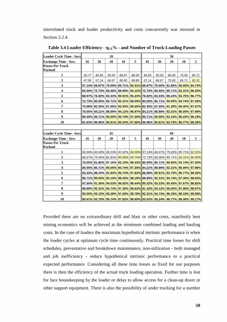
50
interrelated truck and loader productivity and costs concurrently was stressed in
Section 3.2.4.
Table 3.4 Loader Efficiency - ηLE% - and Number of Truck-Loading Passes
Loader Cycle Time - Secs 20 30 Exchange Time - Secs 45 30 20 10 5 45 30 20 10 5 Passes Per Truck Payload
1 30.77 40.00 50.00 66.67 80.00 40.00 50.00 60.00 75.00 85.71
2 47.06 57.14 66.67 80.00 88.89 57.14 66.67 75.00 85.71 92.31
3 57.14% 66.67% 75.00% 85.71% 92.31% 66.67% 75.00% 81.82% 90.00% 94.74% 4 64.00% 72.73% 80.00% 88.89% 94.12% 72.73% 80.00% 85.71% 92.31% 96.00% 5 68.97% 76.92% 83.33% 90.91% 95.24% 76.92% 83.33% 88.24% 93.75% 96.77% 6 72.73% 80.00% 85.71% 92.31% 96.00% 80.00% 85.71% 90.00% 94.74% 97.30% 7 75.68% 82.35% 87.50% 93.33% 96.55% 82.35% 87.50% 91.30% 95.45% 97.67% 8 78.05% 84.21% 88.89% 94.12% 96.97% 84.21% 88.89% 92.31% 96.00% 97.96% 9 80.00% 85.71% 90.00% 94.74% 97.30% 85.71% 90.00% 93.10% 96.43% 98.18%
10 81.63% 86.96% 90.91% 95.24% 97.56% 86.96% 90.91% 93.75% 96.77% 98.36%
Loader Cycle Time - Secs 45 60 Exchange Time - Secs 45 30 20 10 5 45 30 20 10 5 Passes Per Truck Payload
1 50.00% 60.00% 69.23% 81.82% 90.00% 57.14% 66.67% 75.00% 85.71% 92.31%
2 66.67% 75.00% 81.82% 90.00% 94.74% 72.73% 80.00% 85.71% 92.31% 96.00%
3 75.00% 81.82% 87.10% 93.10% 96.43% 80.00% 85.71% 90.00% 94.74% 97.30% 4 80.00% 85.71% 90.00% 94.74% 97.30% 84.21% 88.89% 92.31% 96.00% 97.96% 5 83.33% 88.24% 91.84% 95.74% 97.83% 86.96% 90.91% 93.75% 96.77% 98.36% 6 85.71% 90.00% 93.10% 96.43% 98.18% 88.89% 92.31% 94.74% 97.30% 98.63% 7 87.50% 91.30% 94.03% 96.92% 98.44% 90.32% 93.33% 95.45% 97.67% 98.82% 8 88.89% 92.31% 94.74% 97.30% 98.63% 91.43% 94.12% 96.00% 97.96% 98.97% 9 90.00% 93.10% 95.29% 97.59% 98.78% 92.31% 94.74% 96.43% 98.18% 99.08%
10 90.91% 93.75% 95.74% 97.83% 98.90% 93.02% 95.24% 96.77% 98.36% 99.17%
Provided there are no extraordinary drill and blast or other costs, manifestly best
mining economics will be achieved at the minimum combined loading and hauling
costs. In the case of loaders the maximum hypothetical intrinsic performance is when
the loader cycles at optimum cycle time continuously. Practical time losses for shift
schedules, preventative and breakdown maintenance, non-utilization - both managed
and job inefficiency - reduce hypothetical intrinsic performance to a practical
expected performance. Considering all these time losses as fixed for our purposes
there is then the efficiency of the actual truck loading operation. Further time is lost
for face housekeeping by the loader or delay to allow access for a clean-up dozer or
other support equipment. There is also the possibility of under trucking for a number
51
of reasons; or truck performance variance causing bunching resulting in loader
waiting time. For purposes of this current discussion let us also consider these and
any other lost times as fixed and otherwise accounted for.
Time will be lost for truck change over – the focus of this discussion. Typically
change over for large mining trucks is in the order of, say, 45 secs of truck time
(OEM typically recommend 0.7 mins – 42 secs - as an average time). Hays advises
that “Spot time for large rear dump trucks usually is between 0.40 to 0.70 minutes.
Spot time for tractor-trailer units may range from 0.15 to 1.00 minutes, depending on
the method and need for backing.” (Hays, 1990). Truck exchange time tends to
increase with truck size. Since 1990 mining trucks of 218 tonnes with more recent
development up to 340 tonnes have been available from the major OEM and their
dealers. Turn and spot times for these larger to ultra large trucks is considered
typically higher in the range 45 to 50 seconds.
During truck “turn-and-spot” time the loader is typically filling the first bucket load.
Depending on the safety protocol practiced, the loader will lose the nett exchange
time - between a maximum of the “turn-and-spot” time and the difference between
“turn-and-spot” time and loader cycle time. That is from 45 seconds to – for single
side loading - approaching a notional minimum of 10 seconds (time taken whilst the
truck is reversing to “spot”) to zero for double side loading. The loading exchange
efficiency ηLE will vary in accordance with:
ηLE =
Double-sided loading will tend to minimize nett exchange time. Double-sided
loading will not necessarily totally eliminate this lost time particularly if the loader
Number of passes to load truck x cycle time Number of passes x cycle time plus nett exchange time (45 seconds to approach zero).
In Table 3.4 four loading times have been selected corresponding to the practical
range expected for the types of loading equipment considered in this thesis. The
chosen range also generally covers cycle-time confidence interval for a shovel with a
mean cycle time of 30 seconds and an assumed coefficient of variation (CV) = σ/μ of
0.25. For each of the four loader cycle times a range of five nett exchange time losses
ranging from 45 down to 5 seconds has been analysed. A truck exchange time of 45
seconds has been adopted for this example.
52
has to swing through an additional arc from last to first bucket. Also, double-sided
loading is not always possible due to physical work area limitations.
It will be noted from Table 3.4 that, for any nett exchange time, the higher the
number of passes the more efficient is the realisation of expected loading
performance. Even for small nett exchange time losses, there is measurable loss of
loading efficiency as the number of loading passes decreases.
What does this mean in practice? Three and four pass loading is not necessarily most
efficient in terms of intrinsic productivity and unit cost for loading of mining trucks.
Also, it may be better in terms of loading-cost benefit for several reasons, including
those indicated; and others to be discussed later in this thesis (including truck
coverage and loader availability) to have three loaders, say of 37 tonnes actual per
pass loading 220 tonne trucks in 6 passes than two loaders of 55 tonnes actual per
pass loading 220 tonne trucks in 4 passes. This assumes that it is possible to plan for
at least three working faces at all times. In fact, at similar cycle times gross actual
mine production may well be greater with the three smaller loaders. Of course the
bottom line mining costs will reflect the additional costs of hauling for the additional
truck cycle time as passes increase; and, manifestly the nett effect of marginally
higher unit costs for smaller loading equipment that tends to be offset by the higher
operating efficiency, ηLE, experienced by the smaller loaders. But the only costs
really affected by additional stationary time in a truck cycle time are fixed owning
costs, small costs for engine idling and directly related maintenance, labour for
operating and other relevant overheads non-intrinsic to trucks. Discussions later in
this thesis will show these to be small.
3.2.7 Bucket Factor
As discussed in Section 3.2.4 Bucket Factor is a combination of in situ density, swell
and bucket fill factors. It can be expressed in several ways including, as a ratio, as a
percentage, as BCM per bucket load or, most convenient to measure as tonnes per
bucket load. Combining all of the individual randomly variable properties into a
single Bucket Factor is a common, convenient practice.
Traditionally loading productivity calculations have been based on volume as a direct
consequence of the normal three-dimensional geometrical process in developing
optimum (economic) open pit designs. Consequently all the productivity-modifying
53
factors have traditionally been expressed in volumetric terms - ratios or percentages
based on volumetric quotients. Typically productivity of loading equipment is
estimated as BCM per unit of time as a basis for production scheduling and loading
equipment comparisons.
Loader equipment selection can be based on volumetric calculations up to a point.
But eventually there has to be a conversion to weight calculations to ensure
compliance with rated suspended load for rope shovels, rated bucket plus load weight
for hydraulic shovels and backhoes and allowable bucket payload weight in wheel
loaders for stability considerations when tramming and articulating. OEM apply
design limits for component life and operational criteria such as stability, steering
and braking – all of which are gross machine weight (GMW) and payload sensitive.
As discussed in Section 3.3, productivity of mining trucks is a function of GMW.
To determine mining product quantities and facilitate metallurgical control and
management of ore treatment process, ore volumes must be converted to tonnes by
applying an estimated In situ density provided by a suitable number of ARD
determinations for each ore and waste material type.
It is important to note that, in the process of using volumetric calculations in
estimates for the purposes of feasibility determination or budget compilation, an
error in the determined ARD compared with the actual in situ density as realised
through the mining and product recovery processes will have effect equivalent to an
error of similar magnitude in ore reserve grade, mill head grade or product recovery;
also effect equivalent to a reduction in product price of similar proportion. The
importance of determining, as accurately as possible, a suite of ARD data that can be
used as a reliable basis for estimating in situ ore density is obvious. The availability
of further ARD data that effectively represent the in situ density of waste materials to
reliably determine productivity and operating costs is also obvious. As evidenced in
some detail in discussions on in situ density to follow, fortuitously in situ density
(ARD) is a low-dispersion variable so adequately representative samples for in situ
density can be relatively small in number of observations (Harr, 1977).
Intrinsic performance of trucks is dependent on gross machine weight (GMW) that
includes the randomly variable payload weight when loaded. So for purposes of truck
selection and all relevant calculations a reliable estimate of the in situ density and
54
load factor (inverse of swell factor) of all materials to be mined and transported by
trucks must be determined (Cat PHB, 2004).
Three variable properties influence bucket factor:
1. In situ density of material in place before free-digging or conditioning by
blasting or other fragmentation method estimated from samples subjected to
laboratory determinations to provide “apparent rock density” (ARD) values
that can be processed to provide mean ARD for mining-performance
estimating purposes and, just as importantly to provide density statistics for
resource assessment and ore reserve definition. In situ density, measured as
ARD, is a natural material characteristic that can only be observed and
utilized in volumetric or weight estimating processes.
Average in situ density generally increases with depth through horizons of
transported rock detritus through transition zones to the so-called oxidation
cut-off horizon and into practically homogeneous fresh rock basements; i.e.,
inversely with the degree of weathering; except that surface lateritic
development can produce higher density capping with in situ density
approaching but lower than fresh rock density. There can be some sub-lateral
variation of in situ density in fresh rock zones due to litho-logical and
mineralogy changes and different geological history of individual
stratigraphic elements.
Within any homogeneous horizon of fresh or slightly altered rock in situ
density will vary dependent on the mineralogical compositional changes from
point to point.
Milton Harr has reported on variability of solid rock density investigations by
others (Harr, 1977). Work by Stomatapoulas and Kitzias (1973), where 991
tests of a variety of soils types from many countries over some ten years
yielded the following results for rock solids:
• Mean – μ 2.68
• Standard Deviation – σ 0.06
• Coefficient of Variation - CV 2.2%
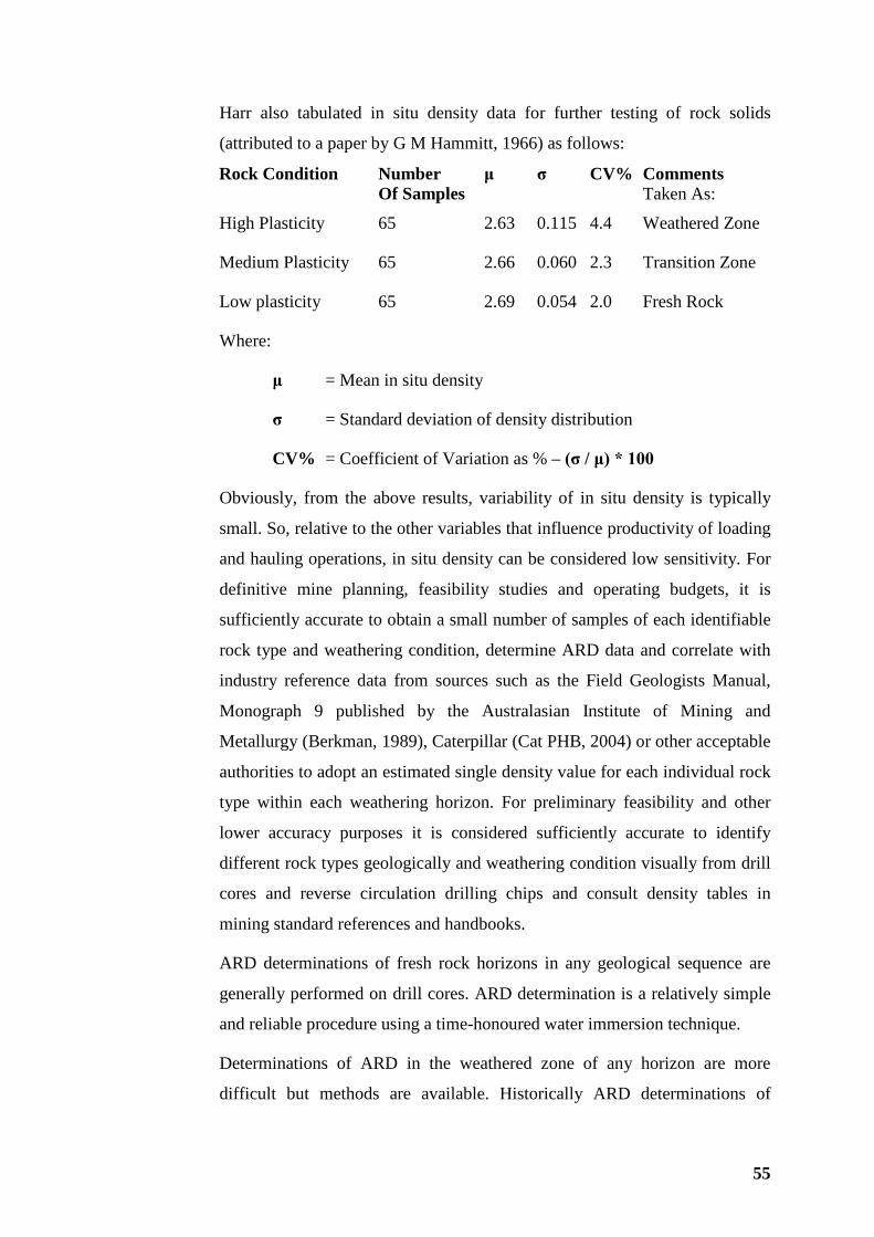
55
Harr also tabulated in situ density data for further testing of rock solids
(attributed to a paper by G M Hammitt, 1966) as follows:
Rock Condition Number μ σ CV% Comments Of Samples Taken As:
High Plasticity 65 2.63 0.115 4.4 Weathered Zone
Medium Plasticity 65 2.66 0.060 2.3 Transition Zone
Low plasticity 65 2.69 0.054 2.0 Fresh Rock
Where:
μ = Mean in situ density
σ = Standard deviation of density distribution
CV% = Coefficient of Variation as % – (σ / μ) * 100
Obviously, from the above results, variability of in situ density is typically
small. So, relative to the other variables that influence productivity of loading
and hauling operations, in situ density can be considered low sensitivity. For
definitive mine planning, feasibility studies and operating budgets, it is
sufficiently accurate to obtain a small number of samples of each identifiable
rock type and weathering condition, determine ARD data and correlate with
industry reference data from sources such as the Field Geologists Manual,
Monograph 9 published by the Australasian Institute of Mining and
Metallurgy (Berkman, 1989), Caterpillar (Cat PHB, 2004) or other acceptable
authorities to adopt an estimated single density value for each individual rock
type within each weathering horizon. For preliminary feasibility and other
lower accuracy purposes it is considered sufficiently accurate to identify
different rock types geologically and weathering condition visually from drill
cores and reverse circulation drilling chips and consult density tables in
mining standard references and handbooks.
ARD determinations of fresh rock horizons in any geological sequence are
generally performed on drill cores. ARD determination is a relatively simple
and reliable procedure using a time-honoured water immersion technique.
Determinations of ARD in the weathered zone of any horizon are more
difficult but methods are available. Historically ARD determinations of
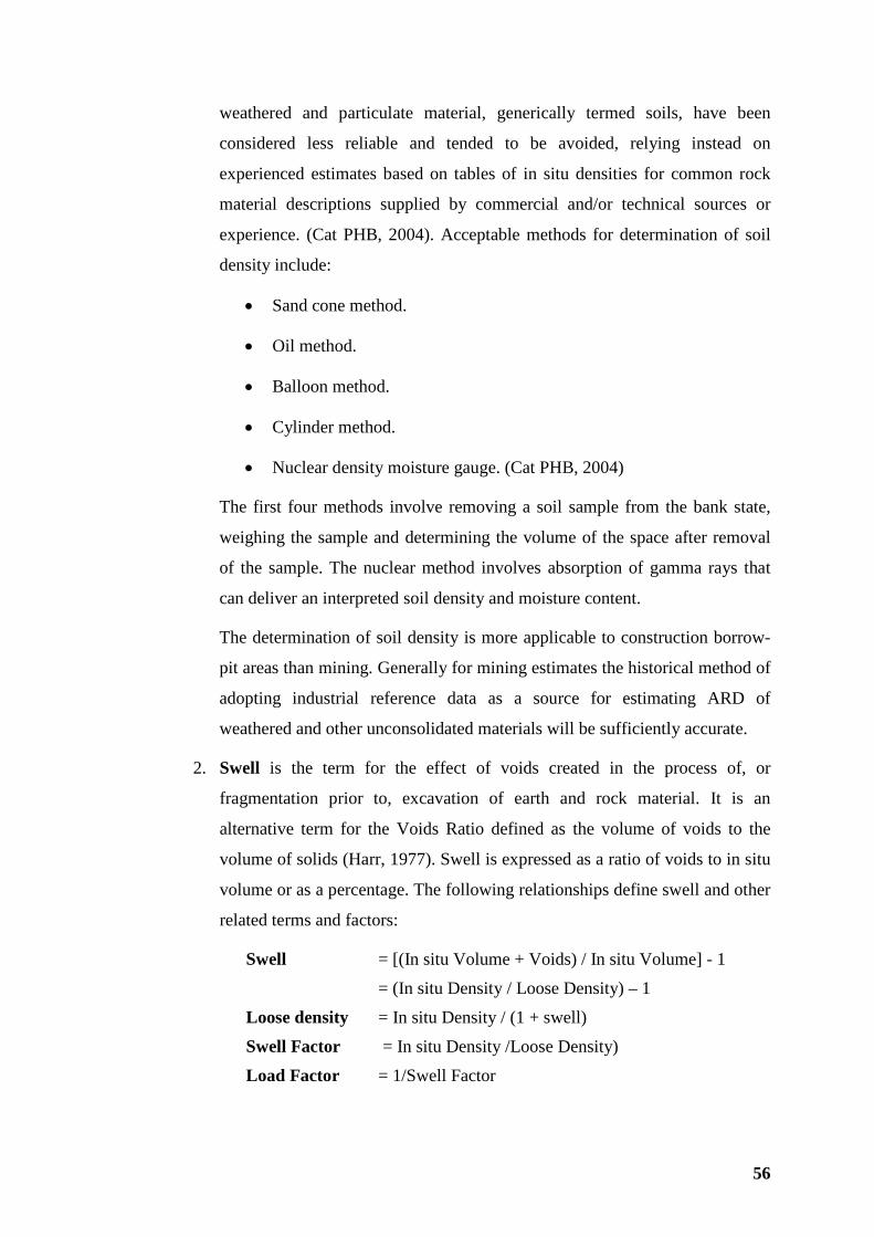
56
weathered and particulate material, generically termed soils, have been
considered less reliable and tended to be avoided, relying instead on
experienced estimates based on tables of in situ densities for common rock
material descriptions supplied by commercial and/or technical sources or
experience. (Cat PHB, 2004). Acceptable methods for determination of soil
density include:
• Sand cone method.
• Oil method.
• Balloon method.
• Cylinder method.
• Nuclear density moisture gauge. (Cat PHB, 2004)
The first four methods involve removing a soil sample from the bank state,
weighing the sample and determining the volume of the space after removal
of the sample. The nuclear method involves absorption of gamma rays that
can deliver an interpreted soil density and moisture content.
The determination of soil density is more applicable to construction borrow-
pit areas than mining. Generally for mining estimates the historical method of
adopting industrial reference data as a source for estimating ARD of
weathered and other unconsolidated materials will be sufficiently accurate.
2. Swell is the term for the effect of voids created in the process of, or
fragmentation prior to, excavation of earth and rock material. It is an
alternative term for the Voids Ratio defined as the volume of voids to the
volume of solids (Harr, 1977). Swell is expressed as a ratio of voids to in situ
volume or as a percentage. The following relationships define swell and other
related terms and factors:
Swell = [(In situ Volume + Voids) / In situ Volume] - 1
= (In situ Density / Loose Density) – 1
Loose density = In situ Density / (1 + swell)
Swell Factor = In situ Density /Loose Density)
Load Factor = 1/Swell Factor
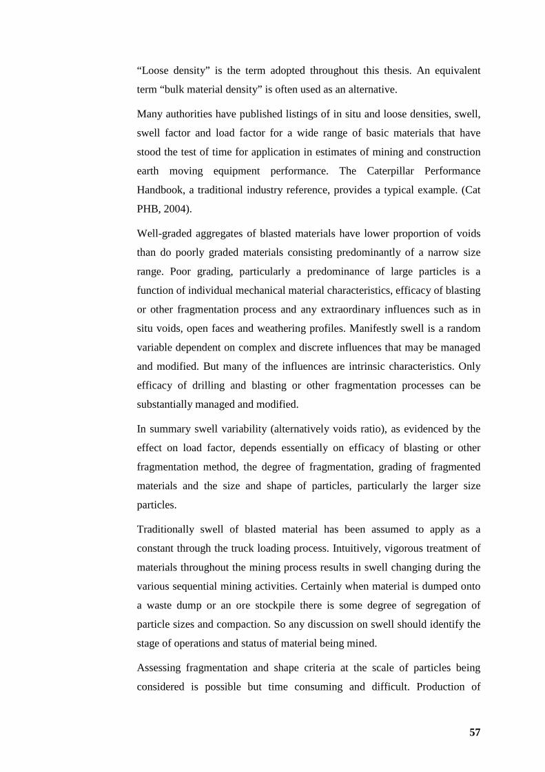
57
“Loose density” is the term adopted throughout this thesis. An equivalent
term “bulk material density” is often used as an alternative.
Many authorities have published listings of in situ and loose densities, swell,
swell factor and load factor for a wide range of basic materials that have
stood the test of time for application in estimates of mining and construction
earth moving equipment performance. The Caterpillar Performance
Handbook, a traditional industry reference, provides a typical example. (Cat
PHB, 2004).
Well-graded aggregates of blasted materials have lower proportion of voids
than do poorly graded materials consisting predominantly of a narrow size
range. Poor grading, particularly a predominance of large particles is a
function of individual mechanical material characteristics, efficacy of blasting
or other fragmentation process and any extraordinary influences such as in
situ voids, open faces and weathering profiles. Manifestly swell is a random
variable dependent on complex and discrete influences that may be managed
and modified. But many of the influences are intrinsic characteristics. Only
efficacy of drilling and blasting or other fragmentation processes can be
substantially managed and modified.
In summary swell variability (alternatively voids ratio), as evidenced by the
effect on load factor, depends essentially on efficacy of blasting or other
fragmentation method, the degree of fragmentation, grading of fragmented
materials and the size and shape of particles, particularly the larger size
particles.
Traditionally swell of blasted material has been assumed to apply as a
constant through the truck loading process. Intuitively, vigorous treatment of
materials throughout the mining process results in swell changing during the
various sequential mining activities. Certainly when material is dumped onto
a waste dump or an ore stockpile there is some degree of segregation of
particle sizes and compaction. So any discussion on swell should identify the
stage of operations and status of material being mined.
Assessing fragmentation and shape criteria at the scale of particles being
considered is possible but time consuming and difficult. Production of
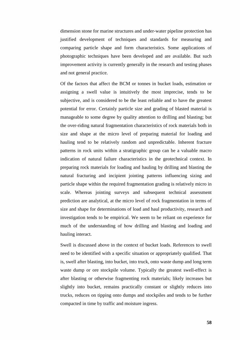
58
dimension stone for marine structures and under-water pipeline protection has
justified development of techniques and standards for measuring and
comparing particle shape and form characteristics. Some applications of
photographic techniques have been developed and are available. But such
improvement activity is currently generally in the research and testing phases
and not general practice.
Of the factors that affect the BCM or tonnes in bucket loads, estimation or
assigning a swell value is intuitively the most imprecise, tends to be
subjective, and is considered to be the least reliable and to have the greatest
potential for error. Certainly particle size and grading of blasted material is
manageable to some degree by quality attention to drilling and blasting; but
the over-riding natural fragmentation characteristics of rock materials both in
size and shape at the micro level of preparing material for loading and
hauling tend to be relatively random and unpredictable. Inherent fracture
patterns in rock units within a stratigraphic group can be a valuable macro
indication of natural failure characteristics in the geotechnical context. In
preparing rock materials for loading and hauling by drilling and blasting the
natural fracturing and incipient jointing patterns influencing sizing and
particle shape within the required fragmentation grading is relatively micro in
scale. Whereas jointing surveys and subsequent technical assessment
prediction are analytical, at the micro level of rock fragmentation in terms of
size and shape for determinations of load and haul productivity, research and
investigation tends to be empirical. We seem to be reliant on experience for
much of the understanding of how drilling and blasting and loading and
hauling interact.
Swell is discussed above in the context of bucket loads. References to swell
need to be identified with a specific situation or appropriately qualified. That
is, swell after blasting, into bucket, into truck, onto waste dump and long term
waste dump or ore stockpile volume. Typically the greatest swell-effect is
after blasting or otherwise fragmenting rock materials; likely increases but
slightly into bucket, remains practically constant or slightly reduces into
trucks, reduces on tipping onto dumps and stockpiles and tends to be further
compacted in time by traffic and moisture ingress.
59
From the above discussion it is concluded that single value estimates for
swell, or predictions of how swell varies statistically, are questionably
reliable and should be treated with caution.
3. Bucket Fill is a variable, generally volumetric, measure of the efficiency of
loading operations. Bucket capacity is designed to a standard as discussed in
Section 3.2.4. Operators endeavour to lift full bucket loads for each pass
except where, by judgment of volumetric appearance of truck loading, or by
feed-back from truck payload sensing systems, truck overloading is likely.
Buckets are designed so that, when filled, excess initially spills over the teeth
or cutting lip and finally over the ends of the bucket and, by design, never
over the back of the bucket for obvious safety reasons. Backhoes dig below
the bench but similar bucket design criteria are used. One common problem
with backhoes in hard rock materials is damage to the underside of the stick
from over filled buckets – particularly where bucket fill is achieved low in the
face, when boom and stick are extended reaching for the load and the full
bucket tucks up under the backhoe stick. Bucket fill for all loader types is
significantly influenced by the stacking characteristics of the material that
increase voids within the bucket, i.e., the variability of swell – or voids ratio.
Obviously material that breaks into large slabs and elongated particles will
tend to increase voids within blasted material, a phenomenon that will persist,
possibly with some variation, into the loader bucket. The degree of increase
or decrease in swell within the loader bucket is considered to be dependent on
the relationship between maximum particle dimensions, internal bucket
dimensions and bucket shape.
Bucket fill is also, to a large degree, dependent on the skill and application of
the operator. Generally the first bucket load is a full load as the operator takes
advantage of the truck exchange time for face house keeping, including
setting up a heaped full first-load for the next truck. Intermediate loads are
also as full as possible; but the operator is sustaining best possible cycle times
with the last load sometimes a partial load to top up the truck. These first and
last-load biases must be considered in any statistical analysis of bucket load
data.
60
Bucket fill factor is a random continuous variable that is not strictly
independent due to the degree of bias that operators can exercise. But for
large sample of bucket loads and related truck loads the application of bias
tends to be random and continuous. In effect small samples of bucket loads
that coalesce as truck payloads have representative records in separate sub
samples of first loads, intermediate and last loads that exhibit differing
descriptive statistics. It is possible to analyze such data and draw valid
conclusions from the trends so determined.
3.2.8 Bucket Loads
Preliminaries
Bucket loads of material prepared by drilling and blasting or ripping and pushing by
dozer for loading into mining trucks are basic fundamental quantities for open pit
production. Research of the volumetric and mass movement characteristics of load
and haul operations involves statistical analysis of relatively large samples of bucket
loads that are transported as small samples - truck payloads.
Where load and haul activities involve different loading equipment and materials
significantly different in physical characteristics or preparation by way of
fragmentation for loading, each identifiable set of conditions must be viewed as
separate sub-samples of bucket loads and related truck payloads.
The actual load in each bucket pass in the process of loading mining trucks is
determined by the several factors discussed in Section 3.2.7. These factors are
considered to be significantly interactive. The underlying fragmentation
characteristics that determine swell likely influence the ability of operators to achieve
consistently high bucket fills and may also inhibit digability by effecting penetration
of the face when crowding to achieve bucket load. Generally factors influencing
bucket load variability are random, difficult to both predict and to control.
In the process of loading trucks the underlying variability of individual bucket loads
will determine the variability of truck payloads.
Practical experience indicates that the following fundamentals need to be kept in
view:
61
1. In situ density is a natural given. Variability down through the weathering
profile or across the stratigraphic members associated with any potentially
economic mineral occurrence is pre-determined and only requires acceptably
accurate measuring procedures.
2. Loading equipment operators will use their best efforts to fill the bucket on
every occasion, except when visual assessment or truck-payload sensing
facilities indicate a partial bucket load is required. Experienced operators are
consistently good at loading trucks. It is optimistic to attempt control of
payload dispersion through application of a subjective loading technique.
The relationship between payload dispersion and material preparation for
loading is discussed in Section 3.3.6. If material to be loaded is well prepared
payload dispersion is unlikely to be excessive. Influence of loader operator
skill on truck payloads is revisited in Section 3.3.5 and Section 3.3.8.
3. Any excessive payload is a direct result of the last bucket load (or loads in the
absence of a payload indication facility) placed on a truck.
4. Potential for over loading trucks is dependent on the proportion of a truck
payload that each bucket load represents. That is, truck payload dispersion
has an inverse relationship to the number of bucket passes to load each truck.
Statistical analysis shows that the relationship between bucket and payload
data is consistent with Sample Theory and the Central Limit Theorem (MPN
3, Mathematical Principles – Notes, Volume 2, Appendices}; and also
confirms the intuitive concept that the lower the number of passes the more
disperse will be the distribution of resulting truck payloads..
It is most important to be able to predetermine the variability of truck payloads to:
• Comply with design standards for steering and braking safety that set
limitations on gross machine weight (GMW) for mining trucks –
conveniently interpreted in terms of payload limitations by considering the
truck tare as generally constant; but with due allowance for debris, carry-
back and added mass due to body repairs;
• Comply with target truck-payload limitations particularly to accommodate
overloading and so avoid latent accelerated wear-and-tear of driveline
62
componentry due to increased fuel burn; also suspension components due to
excessive working stress levels;
• To limit the dispersion of payload distribution within reasonable limits so
reduce variability of truck performance due to variation in GMW that in turn
will ameliorate inefficiency due to bunching of trucks.
• To consistently achieve expected tyre life – tyres being considered the final
driveline and suspension component for mining trucks.
So truck payloads should be retained within a specific confidence interval. A suitable
key performance indicator (KPI) for purposes of analysis and control is the
descriptive statistic Coefficient of Variation (CV = Standard deviation/Arithmetic
Mean). The necessary CV limitation on truck payloads for the several operating
standards is exactly similar to the CV limitation on the distribution of average bucket
loads in each payload for a constant number of bucket passes per payload.
Truck payloads are small samples of the sub sample of bucket loads for an
identifiable mining operational phase. Each small sample consists of the number of
bucket passes per truck payload. Consequently the descriptive statistics of truck
payloads are related to all bucket loads in the sub-sample.
Relevant practical truck payload issues are covered in additional detail in Section 3.3
and supporting descriptive statistical mathematics are provided in Mathematical
Principles – Notes, MPN 1 to MPN 3, appended in Volume 2.
Previous research on truck payload dispersion and number of loading passes
identified a need to obtain actual bucket load data to confirm the hypotheses
developed using statistical mathematical relationships (Hardy#1, 2003).
Direct collection of bucket load data from wheel loaders has been in process of
development over many years and has been of particular interest for load-and-carry
operations in stockpile reclaiming. In open pit mining applications the ultimate
objective is to be able to predict and control truck payloads. Consequently
application of wheel loader weighing systems in mining applications is not as
favoured as truck payload sensing systems. Currently an alliance between an OEM
and a research organization is testing a bucket weighing system for rope shovels. The
system is reported to be close to commercial release.
63
Ready collection of bucket load data has not been practically possible until recent
refinements of on-board load sensing systems has facilitated collection of truck-
payload building data. Cumulative truck payload is recorded after each bucket pass.
OEM and their dealers offer information products, specifically onboard sensing and
information management that integrated with mining information systems have the
facility to provide constant productivity information from trucks, loaders and other
earthmoving equipment. Amongst other things, these information systems can record
and make available, in real time, payload increase for each bucket load. Onboard
data processing and recording downloads to local data servers that can be accessed,
given security authorization, by telephone connection anywhere in the world. Recent
broadband transmission facilities have further enhanced speed and reliability of data
transfer.
Caterpillar, supplier of the VIMS/TPMS (Vital Information Management
System/Truck Payload Management System, hereinafter referred to generically as
VIMS) used to collect bucket load and truck payload data for this research, states
accuracy of VIMS as 95% of loads +/-5%. It is believed that this is typically
representative of the current accuracy-status of on-board truck payload sensing
systems offered by all OEM of mining trucks. Although limited in precision these
systems do provide data sufficiently accurate and useful for comparisons and to
develop understanding of the underlying relationships between the various loading
factors that influence truck performance. A more detailed discussion on accuracy
limitations of truck payload measuring using available technology is provided by
earlier research on four-pass loading (Hardy, 2003). A copy of the relevant paper is
provided in Supplementary Information appended.
Further discussion on reasons for inaccuracy of VIMS and equivalent systems is
provided in Section 3.3.7.
To facilitate the research, access was obtained to data and information from a 220
tonne truck fleet as described below.
Bucket load data observations were conducted in two phases:
1. Real time observations using Caterpillar’s Minestar software to access
VIMS truck payload data were recorded in real time over two sessions
each of several hours duration. This provided valuable insight into the
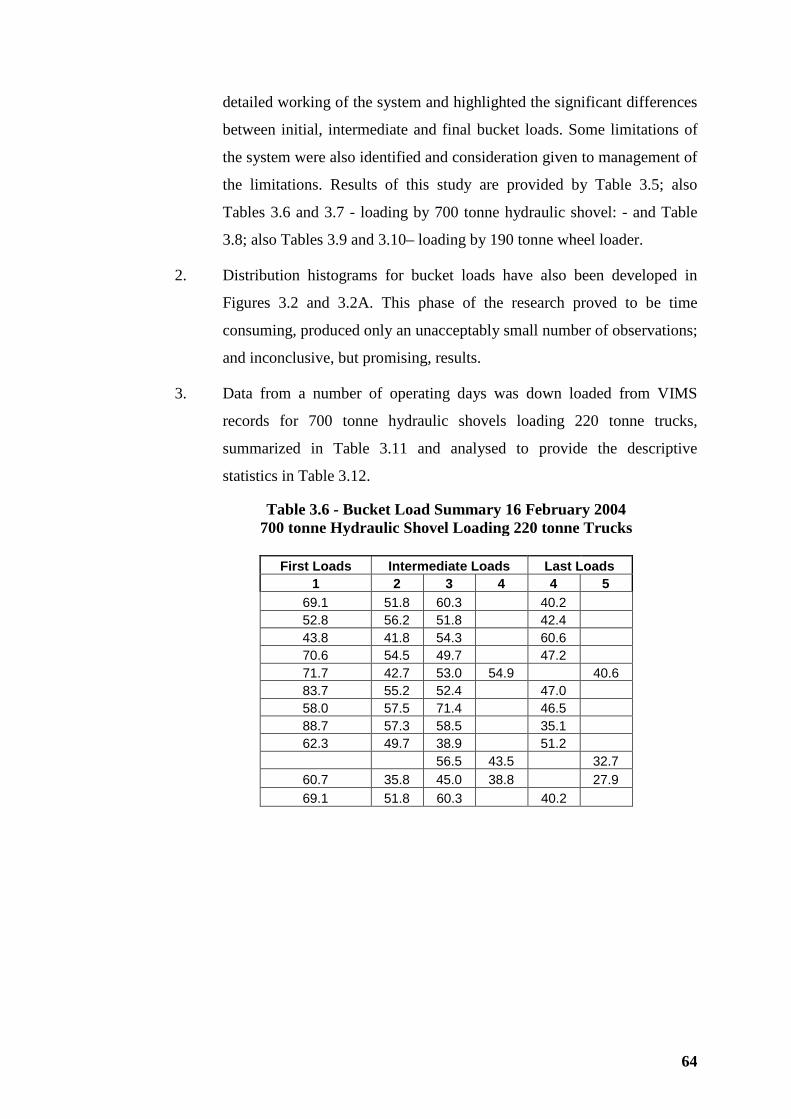
64
detailed working of the system and highlighted the significant differences
between initial, intermediate and final bucket loads. Some limitations of
the system were also identified and consideration given to management of
the limitations. Results of this study are provided by Table 3.5; also
Tables 3.6 and 3.7 - loading by 700 tonne hydraulic shovel: - and Table
3.8; also Tables 3.9 and 3.10– loading by 190 tonne wheel loader.
2. Distribution histograms for bucket loads have also been developed in
Figures 3.2 and 3.2A. This phase of the research proved to be time
consuming, produced only an unacceptably small number of observations;
and inconclusive, but promising, results.
3. Data from a number of operating days was down loaded from VIMS
records for 700 tonne hydraulic shovels loading 220 tonne trucks,
summarized in Table 3.11 and analysed to provide the descriptive
statistics in Table 3.12.
Table 3.6 - Bucket Load Summary 16 February 2004 700 tonne Hydraulic Shovel Loading 220 tonne Trucks
First Loads Intermediate Loads Last Loads
1 2 3 4 4 5 69.1 51.8 60.3 40.2 52.8 56.2 51.8 42.4 43.8 41.8 54.3 60.6 70.6 54.5 49.7 47.2 71.7 42.7 53.0 54.9 40.6 83.7 55.2 52.4 47.0 58.0 57.5 71.4 46.5 88.7 57.3 58.5 35.1 62.3 49.7 38.9 51.2
56.5 43.5 32.7 60.7 35.8 45.0 38.8 27.9 69.1 51.8 60.3 40.2
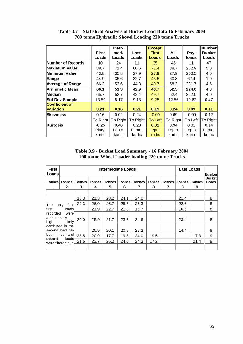
65
Table 3.7 – Statistical Analysis of Bucket Load Data 16 February 2004 700 tonne Hydraulic Shovel Loading 220 tonne Trucks
First
Loads
Inter- med.
Loads Last
Loads
Except First
Loads All
Loads Pay-loads
Number Bucket Loads
Number of Records 10 24 11 35 45 11 47 Maximum Value 88.7 71.4 60.6 71.4 88.7 262.9 5.0 Minimum Value 43.8 35.8 27.9 27.9 27.9 200.5 4.0 Range 44.9 35.6 32.7 43.5 60.8 62.4 1.0 Average of Range 66.3 53.6 44.3 49.7 58.3 231.7 4.5 Arithmetic Mean 66.1 51.3 42.9 48.7 52.5 224.0 4.3 Median 65.7 52.7 42.4 49.7 52.4 222.0 4.0 Std Dev Sample 13.59 8.17 9.13 9.25 12.56 19.62 0.47 Coefficient of Variation 0.21 0.16 0.21 0.19 0.24 0.09 0.11 Skewness 0.16 0.02 0.24 -0.09 0.69 -0.09 0.12 To Right To Right To Right To Left To Right To Left To Right Kurtosis -0.25 0.40 0.28 0.01 0.94 0.01 0.14
Platy-kurtic
Lepto-kurtic
Lepto-kurtic
Lepto-kurtic
Lepto-kurtic
Lepto-kurtic
Lepto-kurtic
Table 3.9 - Bucket Load Summary - 16 February 2004 190 tonne Wheel Loader loading 220 tonne Trucks
First
Loads Intermediate Loads
Last Loads
Number Bucket Loads Tonnes Tonnes Tonnes Tonnes Tonnes Tonnes Tonnes Tonnes Tonnes Tonnes Tonnes
1 2 3 4 5 6 7 8 7 8 9
The only four first loads recorded were anomalously high – likely combined in the second load. So both first and second loads were filtered out.
18.3 21.3 28.2 24.1 24.0 21.4 8 29.3 26.0 26.7 25.7 26.3 22.6 8
21.9 22.7 21.8 16.7 16.5 8
20.0 25.9 21.7 23.3 24.6 23.4 8
20.9 20.1 20.9 25.2 14.4 8 23.5 20.9 17.7 19.8 24.0 19.5 17.3 9 21.6 23.7 26.0 24.0 24.3 17.2 21.4 9
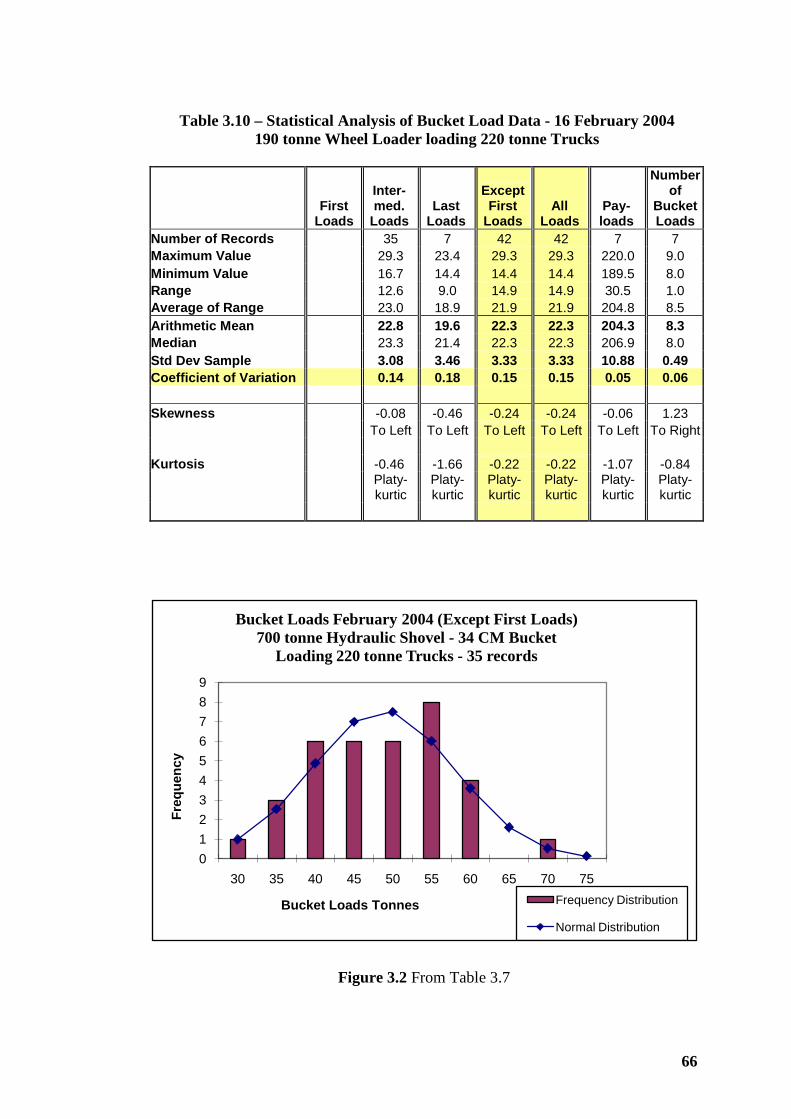
66
Table 3.10 – Statistical Analysis of Bucket Load Data - 16 February 2004 190 tonne Wheel Loader loading 220 tonne Trucks
First
Loads
Inter- med.
Loads Last
Loads
Except First
Loads All
Loads Pay- loads
Number of
Bucket Loads
Number of Records 35 7 42 42 7 7 Maximum Value 29.3 23.4 29.3 29.3 220.0 9.0 Minimum Value 16.7 14.4 14.4 14.4 189.5 8.0 Range 12.6 9.0 14.9 14.9 30.5 1.0 Average of Range 23.0 18.9 21.9 21.9 204.8 8.5 Arithmetic Mean 22.8 19.6 22.3 22.3 204.3 8.3 Median 23.3 21.4 22.3 22.3 206.9 8.0 Std Dev Sample 3.08 3.46 3.33 3.33 10.88 0.49 Coefficient of Variation 0.14 0.18 0.15 0.15 0.05 0.06 Skewness -0.08 -0.46 -0.24 -0.24 -0.06 1.23 To Left To Left To Left To Left To Left To Right Kurtosis -0.46 -1.66 -0.22 -0.22 -1.07 -0.84
Platy-kurtic
Platy-kurtic
Platy-kurtic
Platy-kurtic
Platy-kurtic
Platy-kurtic
Figure 3.2 From Table 3.7
0123456789
30 35 40 45 50 55 60 65 70 75
Freq
uenc
y
Bucket Loads Tonnes
Bucket Loads February 2004 (Except First Loads)700 tonne Hydraulic Shovel - 34 CM Bucket
Loading 220 tonne Trucks - 35 records
Frequency Distribution
Normal Distribution
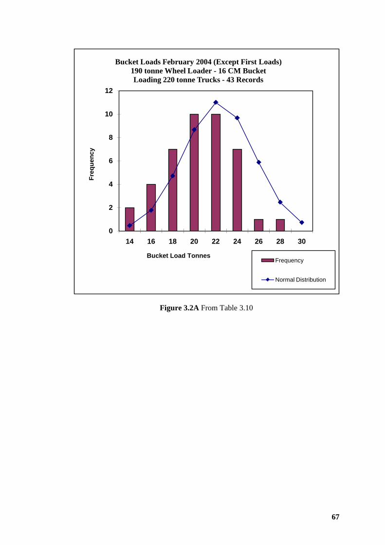
67
Figure 3.2A From Table 3.10
0
2
4
6
8
10
12
14 16 18 20 22 24 26 28 30
Freq
uenc
y
Bucket Load Tonnes
Bucket Loads February 2004 (Except First Loads) 190 tonne Wheel Loader - 16 CM BucketLoading 220 tonne Trucks - 43 Records
Frequency
Normal Distribution
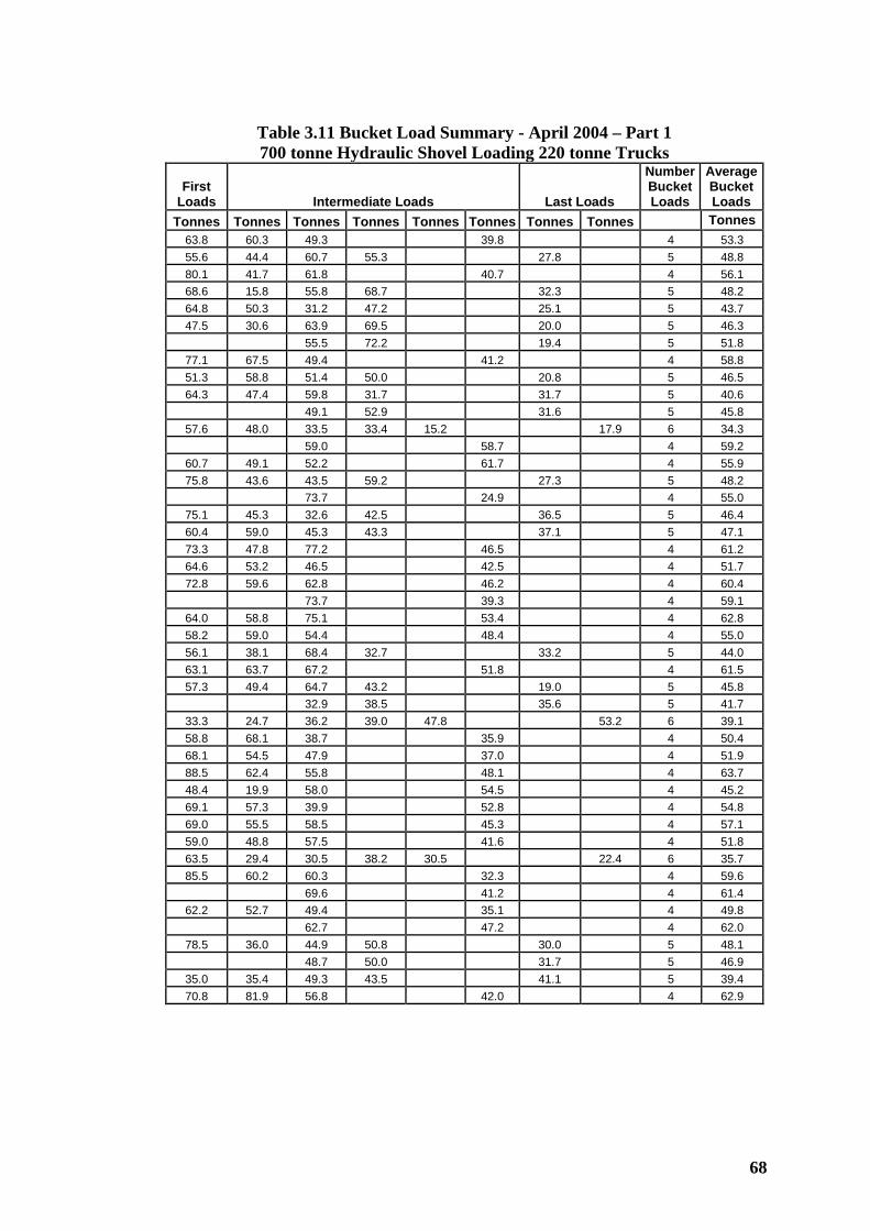
68
Table 3.11 Bucket Load Summary - April 2004 – Part 1 700 tonne Hydraulic Shovel Loading 220 tonne Trucks
First Loads Intermediate Loads Last Loads
Number Bucket Loads
Average Bucket Loads
Tonnes Tonnes Tonnes Tonnes Tonnes Tonnes Tonnes Tonnes Tonnes 63.8 60.3 49.3 39.8 4 53.3 55.6 44.4 60.7 55.3 27.8 5 48.8 80.1 41.7 61.8 40.7 4 56.1 68.6 15.8 55.8 68.7 32.3 5 48.2 64.8 50.3 31.2 47.2 25.1 5 43.7 47.5 30.6 63.9 69.5 20.0 5 46.3
55.5 72.2 19.4 5 51.8 77.1 67.5 49.4 41.2 4 58.8 51.3 58.8 51.4 50.0 20.8 5 46.5 64.3 47.4 59.8 31.7 31.7 5 40.6
49.1 52.9 31.6 5 45.8 57.6 48.0 33.5 33.4 15.2 17.9 6 34.3
59.0 58.7 4 59.2 60.7 49.1 52.2 61.7 4 55.9 75.8 43.6 43.5 59.2 27.3 5 48.2
73.7 24.9 4 55.0 75.1 45.3 32.6 42.5 36.5 5 46.4 60.4 59.0 45.3 43.3 37.1 5 47.1 73.3 47.8 77.2 46.5 4 61.2 64.6 53.2 46.5 42.5 4 51.7 72.8 59.6 62.8 46.2 4 60.4
73.7 39.3 4 59.1 64.0 58.8 75.1 53.4 4 62.8 58.2 59.0 54.4 48.4 4 55.0 56.1 38.1 68.4 32.7 33.2 5 44.0 63.1 63.7 67.2 51.8 4 61.5 57.3 49.4 64.7 43.2 19.0 5 45.8
32.9 38.5 35.6 5 41.7 33.3 24.7 36.2 39.0 47.8 53.2 6 39.1 58.8 68.1 38.7 35.9 4 50.4 68.1 54.5 47.9 37.0 4 51.9 88.5 62.4 55.8 48.1 4 63.7 48.4 19.9 58.0 54.5 4 45.2 69.1 57.3 39.9 52.8 4 54.8 69.0 55.5 58.5 45.3 4 57.1 59.0 48.8 57.5 41.6 4 51.8 63.5 29.4 30.5 38.2 30.5 22.4 6 35.7 85.5 60.2 60.3 32.3 4 59.6
69.6 41.2 4 61.4 62.2 52.7 49.4 35.1 4 49.8
62.7 47.2 4 62.0 78.5 36.0 44.9 50.8 30.0 5 48.1
48.7 50.0 31.7 5 46.9 35.0 35.4 49.3 43.5 41.1 5 39.4 70.8 81.9 56.8 42.0 4 62.9
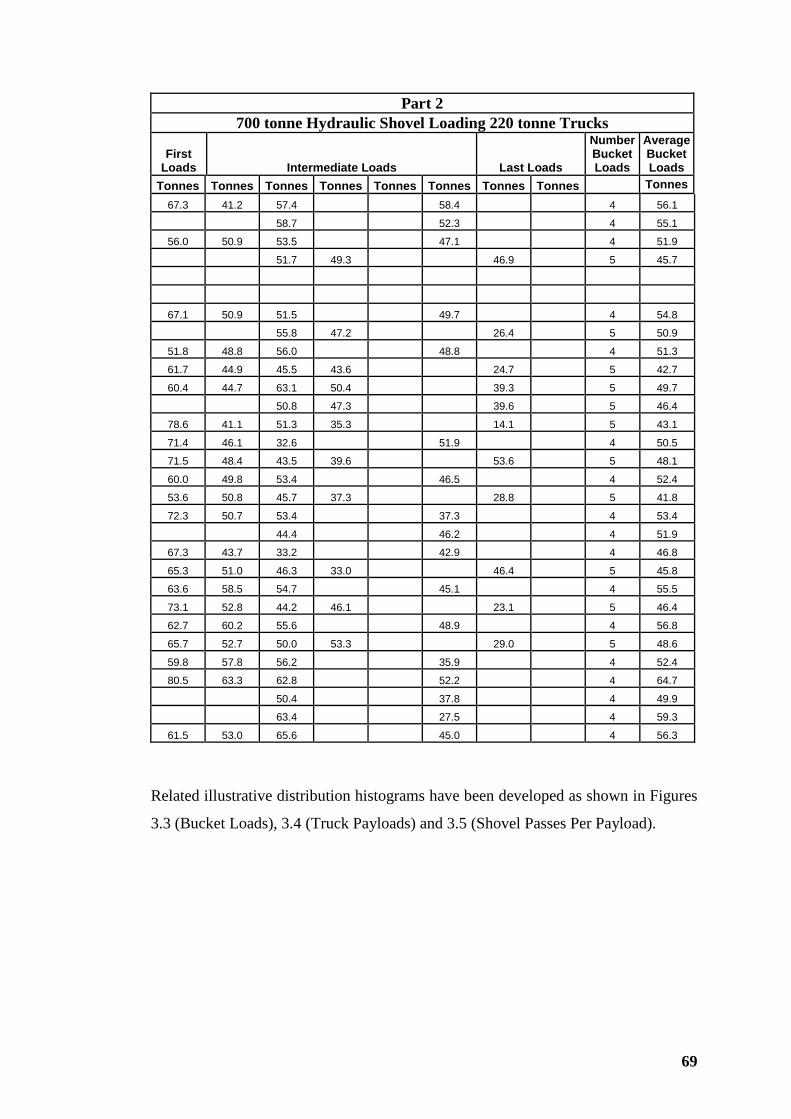
69
Part 2 700 tonne Hydraulic Shovel Loading 220 tonne Trucks
First Loads Intermediate Loads Last Loads
Number Bucket Loads
Average Bucket Loads
Tonnes Tonnes Tonnes Tonnes Tonnes Tonnes Tonnes Tonnes Tonnes 67.3 41.2 57.4 58.4 4 56.1
58.7 52.3 4 55.1
56.0 50.9 53.5 47.1 4 51.9
51.7 49.3 46.9 5 45.7
67.1 50.9 51.5 49.7 4 54.8
55.8 47.2 26.4 5 50.9
51.8 48.8 56.0 48.8 4 51.3
61.7 44.9 45.5 43.6 24.7 5 42.7
60.4 44.7 63.1 50.4 39.3 5 49.7
50.8 47.3 39.6 5 46.4
78.6 41.1 51.3 35.3 14.1 5 43.1
71.4 46.1 32.6 51.9 4 50.5
71.5 48.4 43.5 39.6 53.6 5 48.1
60.0 49.8 53.4 46.5 4 52.4
53.6 50.8 45.7 37.3 28.8 5 41.8
72.3 50.7 53.4 37.3 4 53.4
44.4 46.2 4 51.9
67.3 43.7 33.2 42.9 4 46.8
65.3 51.0 46.3 33.0 46.4 5 45.8
63.6 58.5 54.7 45.1 4 55.5
73.1 52.8 44.2 46.1 23.1 5 46.4
62.7 60.2 55.6 48.9 4 56.8
65.7 52.7 50.0 53.3 29.0 5 48.6
59.8 57.8 56.2 35.9 4 52.4
80.5 63.3 62.8 52.2 4 64.7
50.4 37.8 4 49.9
63.4 27.5 4 59.3
61.5 53.0 65.6 45.0 4 56.3
Related illustrative distribution histograms have been developed as shown in Figures
3.3 (Bucket Loads), 3.4 (Truck Payloads) and 3.5 (Shovel Passes Per Payload).
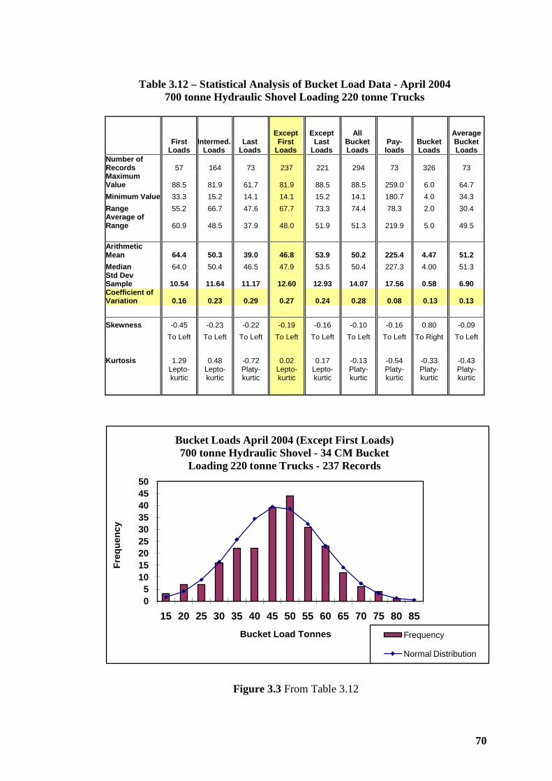
70
Table 3.12 – Statistical Analysis of Bucket Load Data - April 2004 700 tonne Hydraulic Shovel Loading 220 tonne Trucks
First
Loads Intermed.
Loads Last
Loads
Except First
Loads
Except Last
Loads
All Bucket Loads
Pay-loads
Bucket Loads
Average Bucket Loads
Number of Records 57 164 73 237 221 294 73 326 73 Maximum Value 88.5 81.9 61.7 81.9 88.5 88.5 259.0 6.0 64.7 Minimum Value 33.3 15.2 14.1 14.1 15.2 14.1 180.7 4.0 34.3 Range 55.2 66.7 47.6 67.7 73.3 74.4 78.3 2.0 30.4 Average of Range 60.9 48.5 37.9 48.0 51.9 51.3 219.9 5.0 49.5 Arithmetic Mean 64.4 50.3 39.0 46.8 53.9 50.2 225.4 4.47 51.2 Median 64.0 50.4 46.5 47.9 53.5 50.4 227.3 4.00 51.3 Std Dev Sample 10.54 11.64 11.17 12.60 12.93 14.07 17.56 0.58 6.90 Coefficient of Variation 0.16 0.23 0.29 0.27 0.24 0.28 0.08 0.13 0.13 Skewness -0.45 -0.23 -0.22 -0.19 -0.16 -0.10 -0.16 0.80 -0.09 To Left To Left To Left To Left To Left To Left To Left To Right To Left Kurtosis 1.29 0.48 -0.72 0.02 0.17 -0.13 -0.54 -0.33 -0.43
Lepto-kurtic
Lepto-kurtic
Platy-kurtic
Lepto-kurtic
Lepto-kurtic
Platy-kurtic
Platy-kurtic
Platy-kurtic
Platy-kurtic
Figure 3.3 From Table 3.12
05
101520253035404550
15 20 25 30 35 40 45 50 55 60 65 70 75 80 85
Freq
uenc
y
Bucket Load Tonnes
Bucket Loads April 2004 (Except First Loads)700 tonne Hydraulic Shovel - 34 CM Bucket
Loading 220 tonne Trucks - 237 Records
Frequency
Normal Distribution
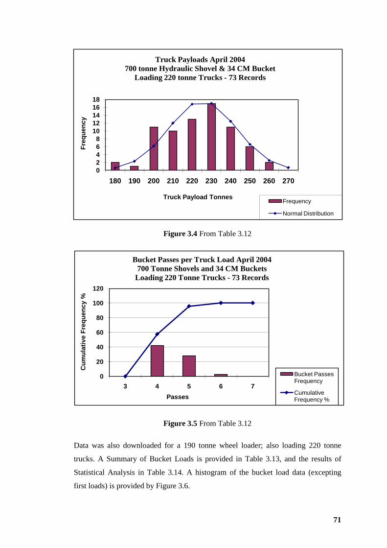
71
Figure 3.4 From Table 3.12
Figure 3.5 From Table 3.12
Data was also downloaded for a 190 tonne wheel loader; also loading 220 tonne
trucks. A Summary of Bucket Loads is provided in Table 3.13, and the results of
Statistical Analysis in Table 3.14. A histogram of the bucket load data (excepting
first loads) is provided by Figure 3.6.
02468
1012141618
180 190 200 210 220 230 240 250 260 270
Freq
uenc
y
Truck Payload Tonnes
Truck Payloads April 2004700 tonne Hydraulic Shovel & 34 CM Bucket
Loading 220 tonne Trucks - 73 Records
Frequency
Normal Distribution
0
20
40
60
80
100
120
3 4 5 6 7
Cum
ulat
ive
Freq
uenc
y %
Passes
Bucket Passes per Truck Load April 2004700 Tonne Shovels and 34 CM Buckets
Loading 220 Tonne Trucks - 73 Records
Bucket Passes Frequency
Cumulative Frequency %

72
Figure 3.6 From Table 3.14
0
5
10
15
20
25
12 15 18 21 24 27 30 33 36 39
Freq
uenc
y
Bucket Load Tonnes
Bucket Loads April 2004190 tonne Wheel Loader - 16 CM BucketLoading 220 tonne Trucks - 59 Records
Bucket Load Frequency
Normal Distribution
Table 3.14 – Statistical Analysis of Bucket Load Data - April 2004 190 tonne Wheel Loader loading 220 tonne Trucks
First
Loads Intermed.
Loads Last
Loads
Except First
Loads
Except Last
Loads All Loads Truck
Payloads
Number Bucket Passes
Average Bucket Loads
Number of Records 4 51 8 59 55 63 8 8 8 Maximum Value 49.9 37.1 28.4 37.1 49.9 49.9 239.5 12.0 28.5 Minimum Value 33.8 12.6 13.5 12.6 12.6 12.6 194.4 7.0 20.0 Range 16.1 24.5 14.9 24.5 37.3 37.3 45.1 5.0 8.5 Average of Range 41.8 24.9 20.9 24.9 31.3 31.3 217.0 9.5 24.2 Arithmetic Mean 40.84 23.41 19.19 22.84 24.68 23.98 213.08 8.88 24.41 Median 39.8 22.5 19.0 22.3 22.8 22.5 213.6 9.0 23.9 Std Dev Sample 6.82 4.37 4.78 4.62 6.41 6.46 13.47 1.55 2.67 Coefficient of Variation 0.167 0.187 0.249 0.202 0.260 0.269 0.063 0.175 0.109 Skewness 0.79 0.60 0.91 0.44 1.66 1.52 0.73 0.88 0.16 To Right To Right To Right To Right To Right To Right To Right To Right To Right Kurtosis 0.88 2.03 0.85 1.33 4.25 3.99 1.82 2.18 0.49
Lepto-kurtic
Lepto-kurtic
Lepto-kurtic
Lepto-kurtic
Lepto-kurtic
Lepto-kurtic
Lepto-kurtic
Lepto-kurtic
Lepto-kurtic
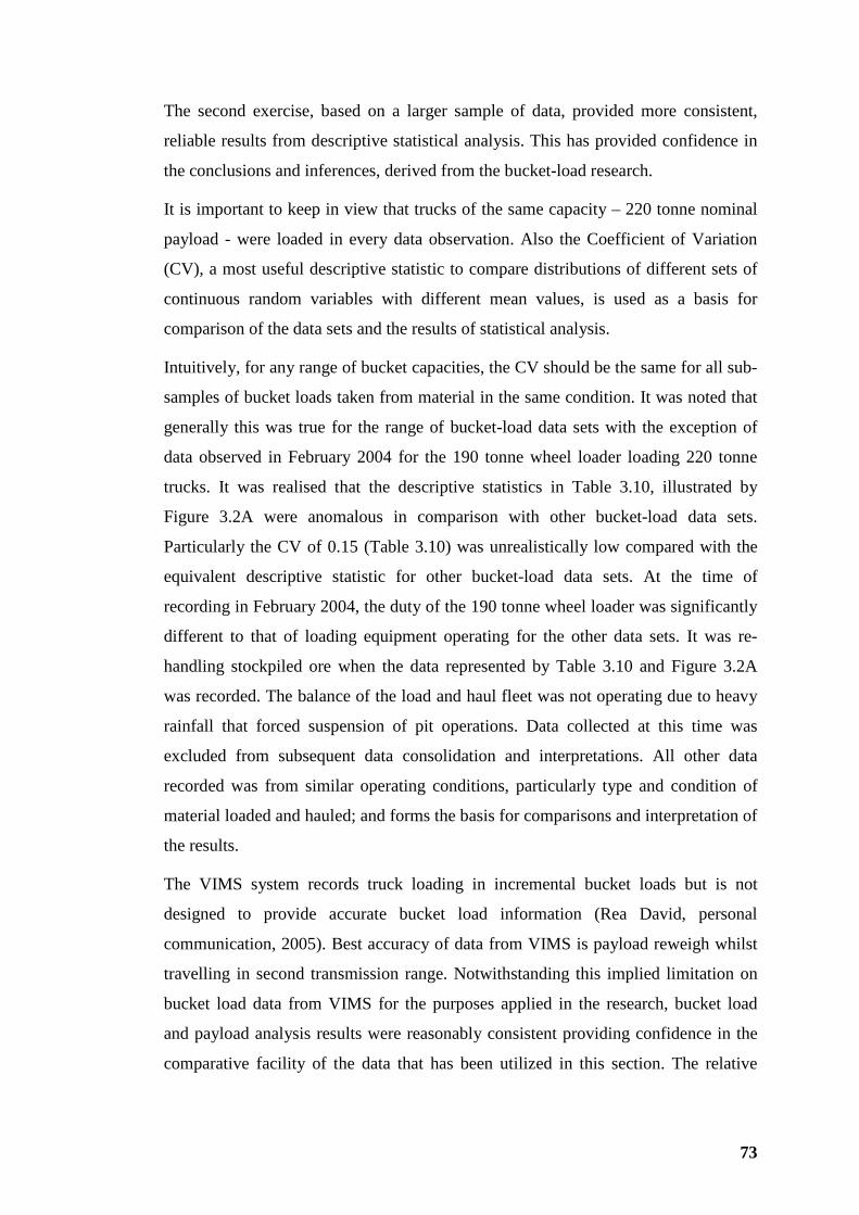
73
The second exercise, based on a larger sample of data, provided more consistent,
reliable results from descriptive statistical analysis. This has provided confidence in
the conclusions and inferences, derived from the bucket-load research.
It is important to keep in view that trucks of the same capacity – 220 tonne nominal
payload - were loaded in every data observation. Also the Coefficient of Variation
(CV), a most useful descriptive statistic to compare distributions of different sets of
continuous random variables with different mean values, is used as a basis for
comparison of the data sets and the results of statistical analysis.
Intuitively, for any range of bucket capacities, the CV should be the same for all sub-
samples of bucket loads taken from material in the same condition. It was noted that
generally this was true for the range of bucket-load data sets with the exception of
data observed in February 2004 for the 190 tonne wheel loader loading 220 tonne
trucks. It was realised that the descriptive statistics in Table 3.10, illustrated by
Figure 3.2A were anomalous in comparison with other bucket-load data sets.
Particularly the CV of 0.15 (Table 3.10) was unrealistically low compared with the
equivalent descriptive statistic for other bucket-load data sets. At the time of
recording in February 2004, the duty of the 190 tonne wheel loader was significantly
different to that of loading equipment operating for the other data sets. It was re-
handling stockpiled ore when the data represented by Table 3.10 and Figure 3.2A
was recorded. The balance of the load and haul fleet was not operating due to heavy
rainfall that forced suspension of pit operations. Data collected at this time was
excluded from subsequent data consolidation and interpretations. All other data
recorded was from similar operating conditions, particularly type and condition of
material loaded and hauled; and forms the basis for comparisons and interpretation of
the results.
The VIMS system records truck loading in incremental bucket loads but is not
designed to provide accurate bucket load information (Rea David, personal
communication, 2005). Best accuracy of data from VIMS is payload reweigh whilst
travelling in second transmission range. Notwithstanding this implied limitation on
bucket load data from VIMS for the purposes applied in the research, bucket load
and payload analysis results were reasonably consistent providing confidence in the
comparative facility of the data that has been utilized in this section. The relative
74
accuracy of VIMS data in various situations is covered in more detail in Section
3.3.7.
Bucket Load Data Characteristics
It was noted that, for all truck-loading records, first loads were anomalously high.
This is considered to be the result of a combination of influences including:
1. Loading-equipment operators utilize truck exchange time to ensure that the
first bucket load is full – in excess of 100% bucket factor where possible. The
first bucket load may be partially re-handled (utilizing part of the truck-
changeover time) to ensure that the best possible bucket load is achieved.
2. The way in which the load sensing and recording system that provided
bucket-load data described below accounts for truck tare.
3. Placement of the first bucket load, or any bucket load, displaced from the
designed centre of gravity (CG) position of the truck payload. The load
sensing system within Caterpillar’s VIMS is sensitive to location of the CG
of truck payloads within the truck body. This is discussed in more detail in
Sections 3.3.5 and 3.3.7. Essentially, if the payload CG is forward of the
design position:
• Load on front wheels is increased and rear wheels decreased – with
implications for reduced tyre life on front wheels.
• The payload sensing system reports lower than actual payload i.e., the
value that would be derived from weighing all four truck wheels and
deducting pre-weighed truck tare.
• Conversely, and importantly in the case of first bucket loads, rearward
displacement behind design payload CG position of total or partial
payload will be sensed by the VIMS system as lower than actual
incremental or total payload in the truck body.
Notwithstanding the potential for errors in incremental and total truck payload data
due to displacement of payload CG from the designed location, The data collected
and subsequent analysis is valuable in providing insight and understanding of the
bucket load: truck-payload relationship discussed in some detail below in this
section.
75
The truck payload system is calibrated initially by manually setting a truck tare
weight from sensed loads. The system can of automatically calibrate, but only within
a limited range around the initial tare weight. Each time the configuration of the
truck is changed, e.g. exchange of a ride strut, manual recalibration should be
implemented. The reliability of the system to auto-calibrate is dependent on
equipment operators and maintainers observing anomalous first loads and effecting a
recalibration. So, in the absence of current correct calibration or if there is a
mechanical fault in the suspension group, the payload weighing first sensed after the
first bucket pass can include any error in the preset tare weight, any debris attached
to the truck frame and any carry-back material in the truck body.
Caterpillar recommends an allowance of 4% of the frame weight fully-equipped
ready-to-operate, equivalent to some 1.2% of GMW – amounting to some 5 tonnes
for a 220 tonne truck. An on-site weighing study of 220 tonne trucks (Maloney,
2002) measured total “debris” and “carry back”. More than 100 trucks were weighed
before and after washing down and clearing “carry back” from body. Results yielded
average “carry back in the tray ” of 4.2 tonnes with a maximum value near 8 tonnes,
equivalent to 2% of GMW. Experience indicates that the combined weight of
“debris” and “carry back” varies from zero to more than 10 tonnes depending on
truck scale and site conditions. In all performance and productivity calculations for
mining trucks contribution to GMW by “debris” and “carry back” requires
consideration in terms of site and operational specifics. This is further considered in
Section 3.3.
Caterpillar has recently amended the VIMS payload measuring software to provide
for application of a load factor derived from weighbridge data. This facilitates
accommodation by VIMS of body exchange to third party designs or a MSD body
(described in some detail in Section 3.3.5) by correcting for errors due to fore or aft
displacement of CG of truck payload.
Means of recorded last bucket loads are comparatively lower than the sample mean
believed to be due to operators using the last load to top-up truck loads.
Filtering of Data
As explained above, initial review of bucket load data revealed obvious anomalously
high values for first bucket loads. These anomalies and any related second bucket
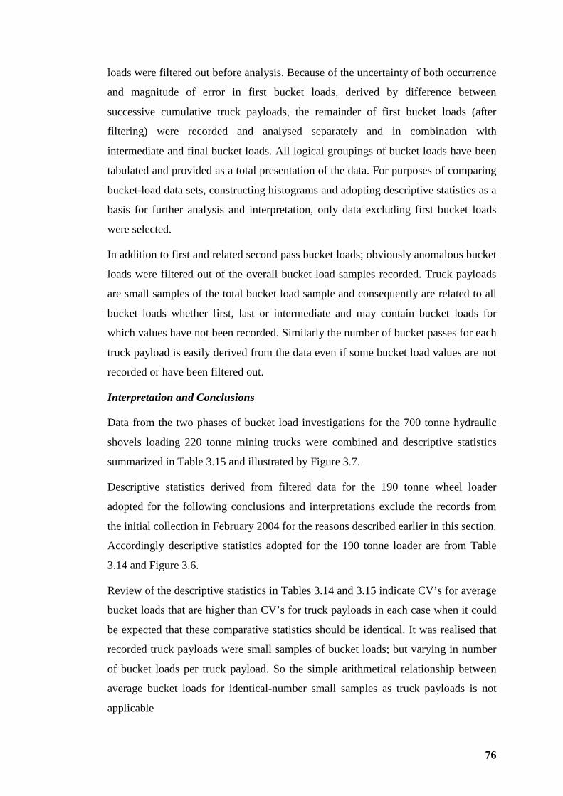
76
loads were filtered out before analysis. Because of the uncertainty of both occurrence
and magnitude of error in first bucket loads, derived by difference between
successive cumulative truck payloads, the remainder of first bucket loads (after
filtering) were recorded and analysed separately and in combination with
intermediate and final bucket loads. All logical groupings of bucket loads have been
tabulated and provided as a total presentation of the data. For purposes of comparing
bucket-load data sets, constructing histograms and adopting descriptive statistics as a
basis for further analysis and interpretation, only data excluding first bucket loads
were selected.
In addition to first and related second pass bucket loads; obviously anomalous bucket
loads were filtered out of the overall bucket load samples recorded. Truck payloads
are small samples of the total bucket load sample and consequently are related to all
bucket loads whether first, last or intermediate and may contain bucket loads for
which values have not been recorded. Similarly the number of bucket passes for each
truck payload is easily derived from the data even if some bucket load values are not
recorded or have been filtered out.
Interpretation and Conclusions
Data from the two phases of bucket load investigations for the 700 tonne hydraulic
shovels loading 220 tonne mining trucks were combined and descriptive statistics
summarized in Table 3.15 and illustrated by Figure 3.7.
Descriptive statistics derived from filtered data for the 190 tonne wheel loader
adopted for the following conclusions and interpretations exclude the records from
the initial collection in February 2004 for the reasons described earlier in this section.
Accordingly descriptive statistics adopted for the 190 tonne loader are from Table
3.14 and Figure 3.6.
Review of the descriptive statistics in Tables 3.14 and 3.15 indicate CV’s for average
bucket loads that are higher than CV’s for truck payloads in each case when it could
be expected that these comparative statistics should be identical. It was realised that
recorded truck payloads were small samples of bucket loads; but varying in number
of bucket loads per truck payload. So the simple arithmetical relationship between
average bucket loads for identical-number small samples as truck payloads is not
applicable
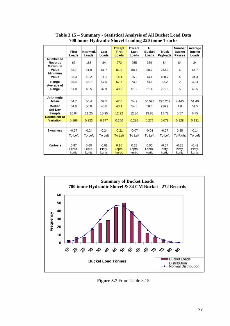
77
Table 3.15 – Summary - Statistical Analysis of All Bucket Load Data
700 tonne Hydraulic Shovel Loading 220 tonne Trucks
Figure 3.7 From Table 3.15
0
10
20
30
40
50
60
Freq
uenc
y
Bucket Load Tonnes
Summary of Bucket Loads700 tonne Hydraulic Shovel & 34 CM Bucket - 272 Records
Bucket Loads DistributionNormal Distribution
First
Loads Intermed.
Loads Last
Loads
Except First
Loads
Except Last
Loads
All Bucket Loads
Truck Payloads
Number Bucket Passes
Average Bucket Loads
Number of Records 67 188 84 272 255 339 84 84 84
Maximum Value 88.7 81.9 61.7 81.9 88.7 88.7 262.9 6 64.7
Minimum Value 33.3 15.2 14.1 14.1 15.2 14.1 180.7 4 34.3 Range 55.4 66.7 47.6 67.7 73.5 74.6 82.2 2 30.4
Average of Range 61.0 48.5 37.9 48.0 51.9 51.4 221.8 5 49.5
Arithmetic
Mean 64.7 50.4 39.5 47.0 54.2 50.523 225.202 4.440 51.40 Median 64.0 50.8 40.6 48.1 54.3 50.8 226.2 4.0 51.5 Std Dev Sample 10.94 11.25 10.95 12.22 12.80 13.88 17.72 0.57 6.75
Coefficient of Variation 0.169 0.223 0.277 0.260 0.236 0.275 0.079 0.128 0.131
Skewness -0.27 -0.24 -0.24 -0.21 -0.07 -0.04 -0.07 0.85 -0.14
To Left To Left To Left To Left To Left To Left To Left To Right To Left
Kurtosis 0.87 0.60 -0.61 0.10 0.28 0.00 -0.57 -0.28 -0.42
Lepto-kurtic
Lepto-kurtic
Platy-kurtic
Lepto-kurtic
Lepto-kurtic
Lepto-kurtic
Platy-kurtic
Platy-kurtic
Platy-kurtic
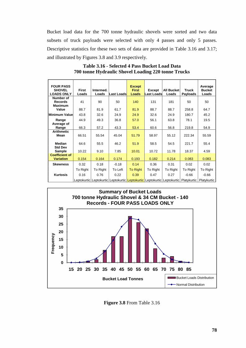
78
Bucket load data for the 700 tonne hydraulic shovels were sorted and two data
subsets of truck payloads were selected with only 4 passes and only 5 passes.
Descriptive statistics for these two sets of data are provided in Table 3.16 and 3.17;
and illustrated by Figures 3.8 and 3.9 respectively.
Table 3.16 - Selected 4 Pass Bucket Load Data 700 tonne Hydraulic Shovel Loading 220 tonne Trucks
Figure 3.8 From Table 3.16
0
5
10
15
20
25
30
35
15 20 25 30 35 40 45 50 55 60 65 70 75 80 85
Freq
uenc
y
Bucket Load Tonnes
Summary of Bucket Loads700 tonne Hydraulic Shovel & 34 CM Bucket - 140
Records - FOUR PASS LOADS ONLY
Bucket Loads Distribution
Normal Distribution
FOUR PASS SHOVEL
LOADS ONLY First
Loads Intermed.
Loads Last Loads
Except First
Loads Except
Last Loads All Bucket
Loads Truck
Payloads
Average Bucket Loads
Number of Records 41 90 50 140 131 181 50 50
Maximum Value 88.7 81.9 61.7 81.9 88.7 88.7 258.8 64.7
Minimum Value 43.8 32.6 24.9 24.9 32.6 24.9 180.7 45.2 Range 44.9 49.3 36.8 57.0 56.1 63.8 78.1 19.5
Average of Range 66.3 57.2 43.3 53.4 60.6 56.8 219.8 54.9
Arithmetic Mean 66.51 55.54 45.04 51.79 58.97 55.12 222.34 55.59
Median 64.6 55.5 46.2 51.9 58.5 54.5 221.7 55.4 Std Dev Sample 10.22 9.10 7.85 10.01 10.72 11.78 18.37 4.59
Coefficient of Variation 0.154 0.164 0.174 0.193 0.182 0.214 0.083 0.083
Skewness 0.32 0.18 -0.18 0.14 0.36 0.31 0.02 0.02 To Right To Right To Left To Right To Right To Right To Right To Right
Kurtosis 0.16 0.76 0.22 0.39 0.47 0.27 -0.66 -0.66 Leptokurtic Leptokurtic Leptokurtic Leptokurtic Leptokurtic Leptokurtic Platykurtic Platykurtic
79
Table 3.17 Selected 5 Pass Bucket Load Data 700 tonne Hydraulic Shovel Loading 220 tonne Trucks
Figure 3.9 From Table 3.17
Distributions of bucket loads and truck payloads were examined qualitatively by
constructing histograms with superimposed model distribution curves as shown by
Figures 3.2 through 3.9 excepting Figure 3.5 for number of bucket passes. The
0
5
10
15
20
25
30
15 20 25 30 35 40 45 50 55 60 65 70 75 80 85
Freq
uenc
y
Bucket Load Tonnes
Summary of Bucket Loads700 tonne Hydraulic Shovel & 34 CM Bucket - 115
Records - FIVE PASS LOADS ONLY
Bucket Loads Distribution
Normal Distribution
First
Loads Intermed.
Loads Last Loads
Except First
Loads Except
Last Loads All Bucket
Loads Truck
Payloads
Average Bucket Loads
Number of Records 23 84 31 115 107 138 31 31
Maximum Value 78.6 72.2 53.6 72.2 78.6 78.6 262.9 52.6
Minimum Value 35.0 30.6 14.1 14.1 30.6 14.1 197.0 39.4 Range 43.6 41.6 39.5 58.1 48.0 64.5 65.9 13.2
Average of Range 56.8 51.4 33.9 43.2 54.6 46.4 230.0 46.0
Arithmetic
Mean 63.15 48.03 31.40 43.54 51.28 46.81 230.50 46.10 Median 64.3 47.4 31.6 44.7 50.0 46.6 232.0 46.4 Std Dev Sample 10.66 9.25 8.99 11.77 11.38 13.69 15.99 3.20
Coefficient of Variation 0.169 0.193 0.286 0.270 0.222 0.292 0.069 0.069
Skewness -0.67 0.35 0.41 -0.06 0.40 0.11 -0.14 -0.14
To Left To Right To Right To Left To Right To Right To Left To Left
Kurtosis 0.73 0.11 0.12 -0.15 -0.30 -0.30 -0.22 -0.22 Leptokurtic Leptokurtic Leptokurtic Platy-kurtic Platykurtic Platykurtic Platykurtic Platykurtic
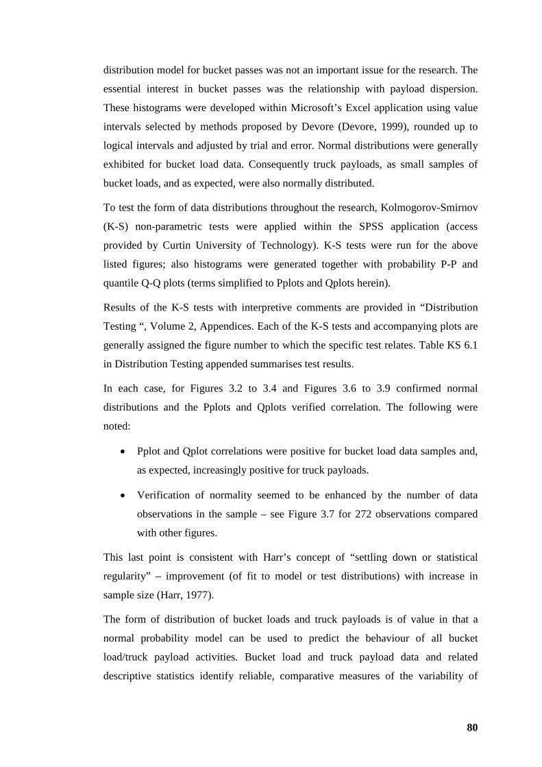
80
distribution model for bucket passes was not an important issue for the research. The
essential interest in bucket passes was the relationship with payload dispersion.
These histograms were developed within Microsoft’s Excel application using value
intervals selected by methods proposed by Devore (Devore, 1999), rounded up to
logical intervals and adjusted by trial and error. Normal distributions were generally
exhibited for bucket load data. Consequently truck payloads, as small samples of
bucket loads, and as expected, were also normally distributed.
To test the form of data distributions throughout the research, Kolmogorov-Smirnov
(K-S) non-parametric tests were applied within the SPSS application (access
provided by Curtin University of Technology). K-S tests were run for the above
listed figures; also histograms were generated together with probability P-P and
quantile Q-Q plots (terms simplified to Pplots and Qplots herein).
Results of the K-S tests with interpretive comments are provided in “Distribution
Testing “, Volume 2, Appendices. Each of the K-S tests and accompanying plots are
generally assigned the figure number to which the specific test relates. Table KS 6.1
in Distribution Testing appended summarises test results.
In each case, for Figures 3.2 to 3.4 and Figures 3.6 to 3.9 confirmed normal
distributions and the Pplots and Qplots verified correlation. The following were
noted:
• Pplot and Qplot correlations were positive for bucket load data samples and,
as expected, increasingly positive for truck payloads.
• Verification of normality seemed to be enhanced by the number of data
observations in the sample – see Figure 3.7 for 272 observations compared
with other figures.
This last point is consistent with Harr’s concept of “settling down or statistical
regularity” – improvement (of fit to model or test distributions) with increase in
sample size (Harr, 1977).
The form of distribution of bucket loads and truck payloads is of value in that a
normal probability model can be used to predict the behaviour of all bucket
load/truck payload activities. Bucket load and truck payload data and related
descriptive statistics identify reliable, comparative measures of the variability of
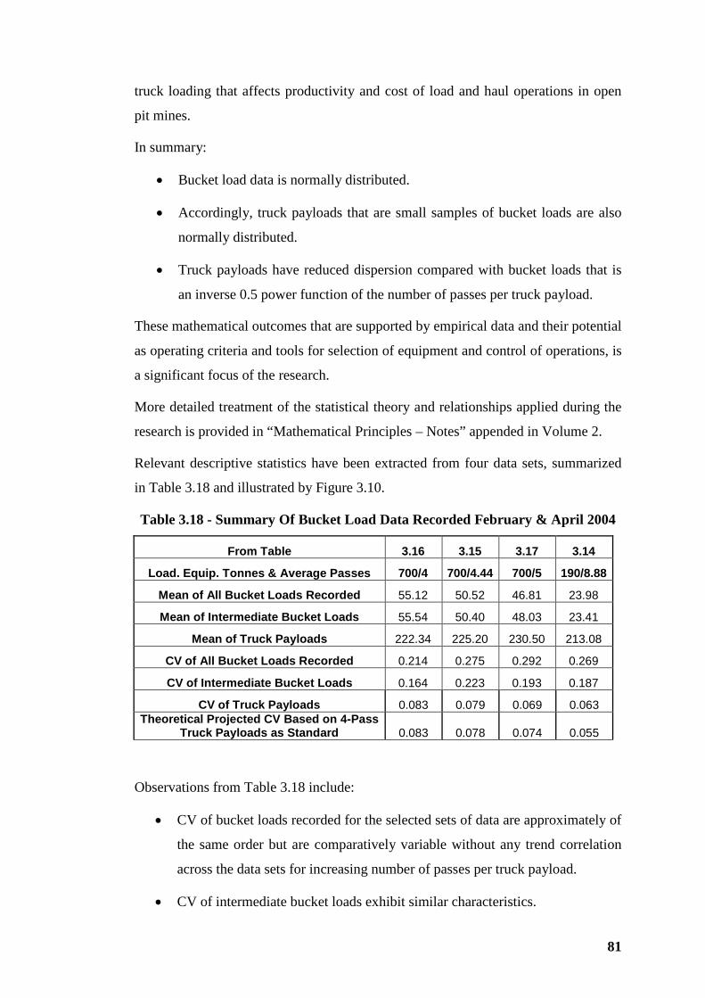
81
truck loading that affects productivity and cost of load and haul operations in open
pit mines.
In summary:
• Bucket load data is normally distributed.
• Accordingly, truck payloads that are small samples of bucket loads are also
normally distributed.
• Truck payloads have reduced dispersion compared with bucket loads that is
an inverse 0.5 power function of the number of passes per truck payload.
These mathematical outcomes that are supported by empirical data and their potential
as operating criteria and tools for selection of equipment and control of operations, is
a significant focus of the research.
More detailed treatment of the statistical theory and relationships applied during the
research is provided in “Mathematical Principles – Notes” appended in Volume 2.
Relevant descriptive statistics have been extracted from four data sets, summarized
in Table 3.18 and illustrated by Figure 3.10.
Table 3.18 - Summary Of Bucket Load Data Recorded February & April 2004
From Table 3.16 3.15 3.17 3.14
Load. Equip. Tonnes & Average Passes 700/4 700/4.44 700/5 190/8.88
Mean of All Bucket Loads Recorded 55.12 50.52 46.81 23.98
Mean of Intermediate Bucket Loads 55.54 50.40 48.03 23.41
Mean of Truck Payloads 222.34 225.20 230.50 213.08
CV of All Bucket Loads Recorded 0.214 0.275 0.292 0.269
CV of Intermediate Bucket Loads 0.164 0.223 0.193 0.187
CV of Truck Payloads 0.083 0.079 0.069 0.063 Theoretical Projected CV Based on 4-Pass
Truck Payloads as Standard 0.083 0.078 0.074 0.055
Observations from Table 3.18 include:
• CV of bucket loads recorded for the selected sets of data are approximately of
the same order but are comparatively variable without any trend correlation
across the data sets for increasing number of passes per truck payload.
• CV of intermediate bucket loads exhibit similar characteristics.
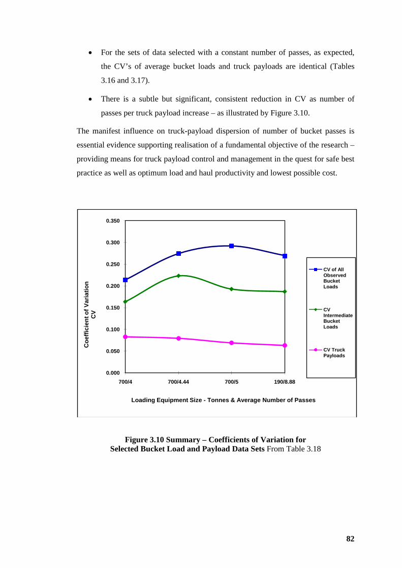
82
• For the sets of data selected with a constant number of passes, as expected,
the CV’s of average bucket loads and truck payloads are identical (Tables
3.16 and 3.17).
• There is a subtle but significant, consistent reduction in CV as number of
passes per truck payload increase – as illustrated by Figure 3.10.
The manifest influence on truck-payload dispersion of number of bucket passes is
essential evidence supporting realisation of a fundamental objective of the research –
providing means for truck payload control and management in the quest for safe best
practice as well as optimum load and haul productivity and lowest possible cost.
Figure 3.10 Summary – Coefficients of Variation for Selected Bucket Load and Payload Data Sets From Table 3.18
0.000
0.050
0.100
0.150
0.200
0.250
0.300
0.350
700/4 700/4.44 700/5 190/8.88
Coe
ffici
ent o
f Var
iatio
n C
V
Loading Equipment Size - Tonnes & Average Number of Passes
CV of All Observed Bucket Loads
CV Intermediate Bucket Loads
CV Truck Payloads
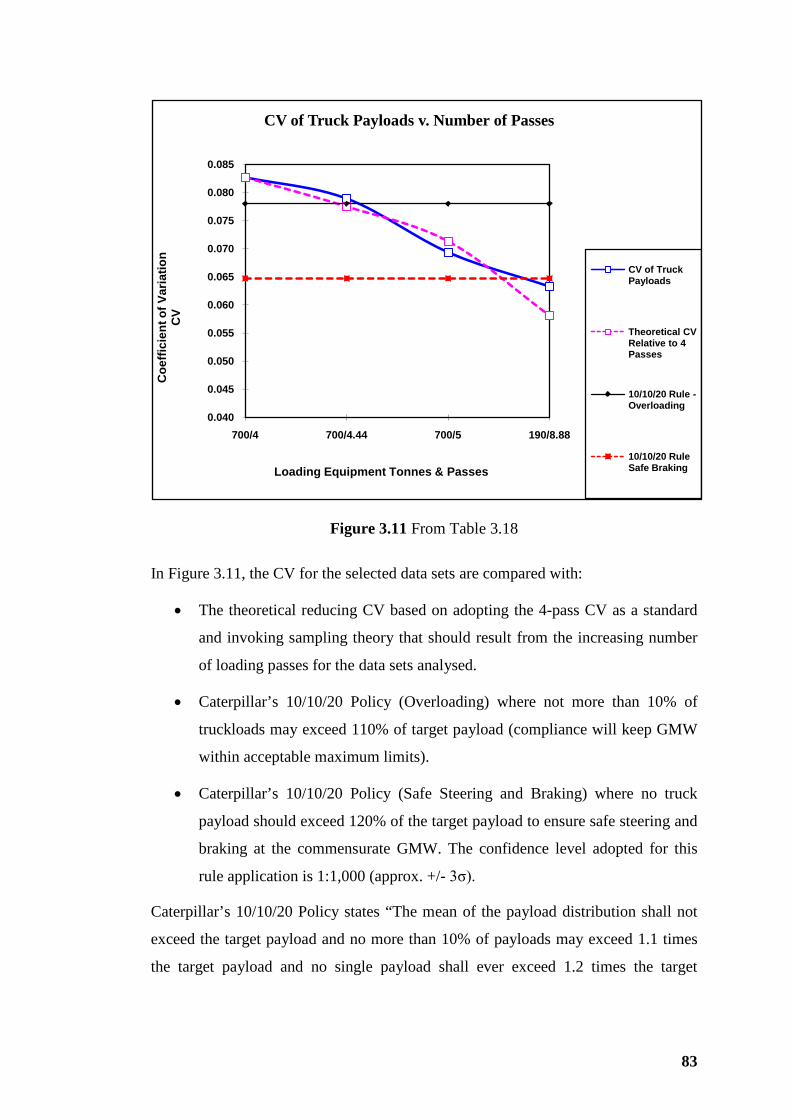
83
Figure 3.11 From Table 3.18
In Figure 3.11, the CV for the selected data sets are compared with:
• The theoretical reducing CV based on adopting the 4-pass CV as a standard
and invoking sampling theory that should result from the increasing number
of loading passes for the data sets analysed.
• Caterpillar’s 10/10/20 Policy (Overloading) where not more than 10% of
truckloads may exceed 110% of target payload (compliance will keep GMW
within acceptable maximum limits).
• Caterpillar’s 10/10/20 Policy (Safe Steering and Braking) where no truck
payload should exceed 120% of the target payload to ensure safe steering and
braking at the commensurate GMW. The confidence level adopted for this
rule application is 1:1,000 (approx. +/- 3σ).
Caterpillar’s 10/10/20 Policy states “The mean of the payload distribution shall not
exceed the target payload and no more than 10% of payloads may exceed 1.1 times
the target payload and no single payload shall ever exceed 1.2 times the target
0.040
0.045
0.050
0.055
0.060
0.065
0.070
0.075
0.080
0.085
700/4 700/4.44 700/5 190/8.88
Coe
ffici
ent o
f Var
iatio
n
CV
Loading Equipment Tonnes & Passes
CV of Truck Payloads v. Number of Passes
CV of Truck Payloads
Theoretical CV Relative to 4 Passes
10/10/20 Rule -Overloading
10/10/20 Rule Safe Braking
84
payload.” The meaning and derivation of “target payload” and operating implications
are dealt with in some detail in Sections 3.3.5 and 3.3.9.
The implications and conclusions of the above comparisons are also expanded in
some detail in Sections 3.3.5, 3.3.6, 3.3.7 and 3.3.9.
Comments
Descriptive statistics for four-pass loading in Table 3.16 reveal:
• Relatively even mean values for subsets of first, intermediate, last and all
bucket loads that are also reflected by the CV in each case.
• Compared with CV’s of other data sets the four-pass CV’s are generally
lower as illustrated by Figure 3.10.
• As illustrated by Figure 3.11, notwithstanding the lower bucket-load CV’s the
CV for four-pass truck payloads is the highest value at 0.083 compared with
data sets for higher numbers of passes.
Review of Table 3.17 for five pass loading indicates:
• A relatively high mean truck payload of 230.50 tonnes.
• Relatively low mean value for last bucket loads.
• A consequently higher than expected CV for the data set of all bucket loads –
as illustrated by Figure 3.10.
• Notwithstanding the high CV for all bucket loads the five-pass truck payload
CV reduced to 0.069 – a natural consequence of the increased number of
bucket loads compared with lower-pass data sets. This natural phenomenon
can be explained by statistical mathematics, including sample theory
summarized from a number of references in MPN 3, Mathematical Principles
– Notes appended in Volume 2.
Review of Table 3.14 for the 190 tonne wheel loader, averaging 8.88 passes per truck
payload, shows:
• A relatively high CV for all bucket loads – illustrated by Figure 3.10
• A low CV for truck payloads of 0.063 – also shown by Figures 3.10 and 3.11.
85
• But, as illustrated by Figure 3.11, the reasonable correlation, based on sample
theory, between actual recorded data and theoretical projection of CV for
truck payloads from data sets recorded from the 700 tonne hydraulic shovel –
– is not sustained for the 190 tonne loader statistics.
In this last case it is not clear why the correlation between actual and theoretical
CV’s across the range of data sets does not persist through to an average of 8.88
passes per truck payload by the 190 tonne wheel loader. Review of descriptive
statistics in Table 3.14 for 190 tonne wheel loader data confirms that the
mathematical relationship between standard deviations and CV for bucket loads and
for truck payloads exhibits reasonable correlation.
Features of the statistics include:
• The mean of last bucket loads was relatively low.
• The outlying low values substantially reduced the truck payload mean but not
significantly affecting the bucket load dispersion – resulting in elevating the
CV for all bucket loads to 0.269 as shown in Table 3.14.
• In turn CV of truck payloads might be expected to be elevated. But, as noted
in the comments on 4-pass loading, and as illustrated by Figure 3.10, reduced
bucket load CV does not appear to significantly influence CV of truck
payloads; so, conversely, high CV of bucket loads in this case do not
necessarily significantly influence CV of truck payloads averaging 8.88
passes.
• The small sub-sample of data records, 63 bucket loads, 71 passes; and, likely
most significantly, 8 truck payloads in this data set may be insufficient to
provided sufficiently accurate and reliable descriptive statistics.
• Although actual to theoretical CV correlation was not sustained, the
downward trend with increasing number of loading passes continued – as
confirmed by Table 3.18 and illustrated by Figure 3.11.
Comparison of statistical results with the 10/10/20 Policy, promoted by Caterpillar
Inc through Caterpillar Global Mining, Peoria, Illinois, USA, in Figure 3.11 indicate
that:
86
• Compliance with the “10/10” part of the Policy, applying to truck
overloading, is facilitated as CV of truck payloads decreases – an inter-active
result of specifically, the increasing number of truck-loading passes; also,
ensuring consistent digability (voids ratio, fragmentation and size
distribution) of material being loaded.
• Compliance with the more stringent “20” part of the Policy (as shown by
Figure 3.11) relating to safe steering and braking is also facilitated, albeit at
lower CV, for similar reasons.
• Compliance with the “20” part of the Policy – no truck to exceed 120% of the
target payload – appears to automatically ensure compliance with the “10/10”
part of the Policy for truck overloading.
The issues generally identified in the above comments are revisited in more detail in
Section 3.3.6.
87
3.2.9 Bucket Cycle Time
Preliminaries
Bucket-cycle and truck-loading times substantially determine productivity of all
loading equipment. Bucket cycle time data are:
• In practice generally rounded up or down to unit-second intervals for
recording purposes.
• Selected in small samples accumulating to truck loading time.
Condition of the material to be loaded, physical operating conditions and efficiency
of loading equipment operators substantially influence bucket cycle times. Influence
of operators and material condition tend to be random in effect. As small
accumulations of continuously random bucket cycle time so truck loading times are
continuously random with collected data similarly rounded up to unit-second
intervals of time.
All of these variables are “continuous and random” since any of the outcomes within
the total distribution of outcomes is possible to be observed individually or as a
sample for any event.
Absolute productivity of cyclical truck-loading equipment is a function of the total
number of bucket cycles in any chosen period of time. Also, absolute productivity of
cyclical haulage equipment such as mining trucks is, to a significant degree, a
function of the time taken to load each truck that, in turn, is a function of the bucket
cycle time, the number of bucket passes per load and, as described in Section 3.3.9,
to a degree, dependent on the payload per bucket cycle.
Consideration of the above, along with the influence of number of passes of bucket
loads on the dispersion of truck payload distributions introduced in Section 3.2.8,
initiated the thought that a similar concept applies to loading cycle times. That is:
• Bucket cycle times, as small samples, constitute truck-loading time.
• Sample Theory and the Central Limit Theorem (summarily described in
Mathematical Principles – Notes, MPN 1 to MPN 3, appended), seen to apply
to data from bucket loads and resulting truck payloads, likely are also
88
relevant to bucket cycle times and truck loading times, albeit to a differing
degree.
• Increasing passes to load a truck likely tend to reduce the variability of the
truck loading time (albeit longer by the additional passes) that will
consequently provide more consistency and "rhythm" to hauling operations.
• The concept of “rhythm” as a desirable operational state developed in this
section and Section 3.4, is an incentive to seek further evidence to support the
hypothesis advanced in earlier sections that pursuit of the expected
productivity and cost benefits of 4 or even 3 pass loading is not all positive
due, in the case of cycle times, to increased bunching (queuing) inefficiency.
Any expected benefits of short truck loading times will be, to some degree,
offset by the increase in bunching inefficiency - the question is - how much?
This question is addressed in Section 3.4.
Data and Filtering
Table 3.19 summarizes a sample of bucket-cycle-time data acquired from an open pit
mining operation where 550 tonne hydraulic shovels with 34 cubic metre buckets
load 220 tonne mining trucks. It was noted that the truck exchange time was included
in the first bucket cycle time. This complication required that analyses consider two
sub-samples of the data, i.e., first bucket cycles and bucket cycles exclusive of the
first. Truck loading times calculated from the data necessarily included the first pass
cycle time. The effect of the extended-time first cycles including truck exchange time
as high-end outliers in the bucket cycle time distribution also required consideration.
Truck exchange time in the context of truck loading time is that part of the fixed
“turn-and-spot” time for a truck nett of the continuously variable first bucket cycle
time that occurs concurrently as the truck is maneuvering into position for loading. It
was indicated that “turn-and-spot” time, also a continuous random variable, generally
exceeds the time for the first bucket cycle. Truck exchange time is a continuous
random variable, being the difference between the two continuous random variables
of “turn-and-spot” time and nett cycle time for the first bucket load.
A hypothetical case is worth considering where “turn-and-spot” time is generally
constant in operation; but variable only to the extent of the intrinsic performance of a
89
mining truck in specific operating conditions. Any changes in the hypothetical
constant (intrinsic) “turn-and-spot” time:
• Will adjust the truck exchange time by a like amount.
• In turn the mean loading time will be adjusted by a similar time interval.
• The variation and standard deviation of truck loading time distribution will
not be affected as the constant adjustment does not affect the dispersion of the
distribution.
So, if the truck-exchange time is reduced by a practically constant value the mean
truck loading time will be so reduced but with no effect on the measures of
dispersion of the truck loading time distribution. (Devore, 1999). Deterministic
calculations of truck loading time and total haul cycle times; and subsequent
deterministic productivity estimates rely on this mathematical proposition.
The relationship between loading equipment performance efficiency and number of
passes per truck payload was introduced in Section 3.2.6 and demonstrated by Table
3.4. Particularly the significant affect of truck exchange time was demonstrated. In
the context of mining truck performance, “turn-and-spot” time is the fixed time
dedicated to locating the truck ready for loading. In the context of loading equipment
performance, this truck-cycle time increment, nett of the time taken to first bucket
cycle time to the point of readiness to dump into the truck, is, the “truck exchange”
time. The effect of this idle time is reflected in loading equipment productivity.
The raw bucket cycle time data was reviewed and three levels of filtering
successively applied to deliver:
1. Filter Level 1 – nett of obviously non-comparable, erroneous or anomalous
records.
2. Filter Level 2 – nett of the bulk of time anomalies due to causes non-intrinsic
to the capability of the loading equipment, operator efficiency or loading
equipment operating techniques – facilitated by deleting complete truck
loading time records containing an anomalous bucket cycle time.
3. Filter Level 3 – where complete truck loading time records containing first
cycle times greater than 60 seconds and/or subsequent cycle times greater
than 45 seconds were deleted to provide “smoother” loading time data and an
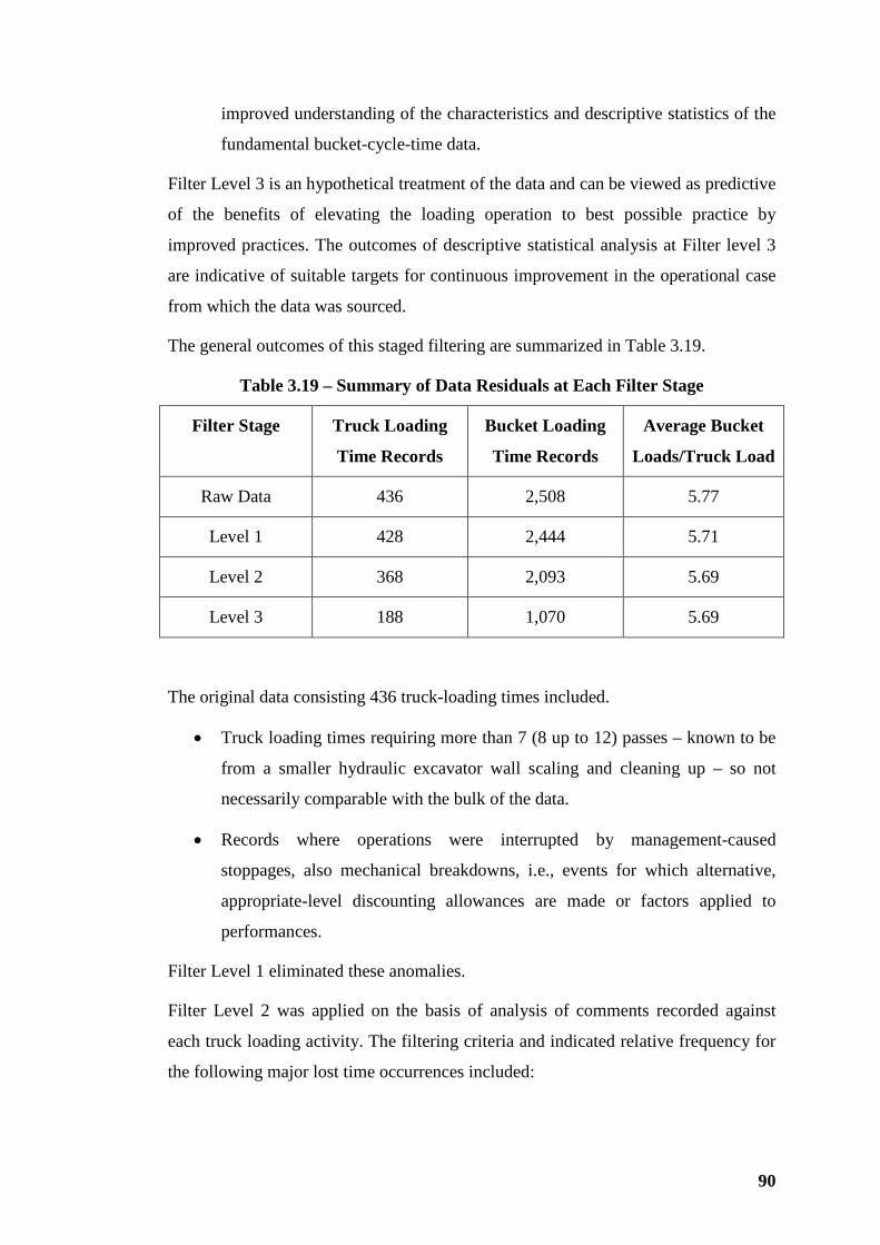
90
improved understanding of the characteristics and descriptive statistics of the
fundamental bucket-cycle-time data.
Filter Level 3 is an hypothetical treatment of the data and can be viewed as predictive
of the benefits of elevating the loading operation to best possible practice by
improved practices. The outcomes of descriptive statistical analysis at Filter level 3
are indicative of suitable targets for continuous improvement in the operational case
from which the data was sourced.
The general outcomes of this staged filtering are summarized in Table 3.19.
Table 3.19 – Summary of Data Residuals at Each Filter Stage
Filter Stage Truck Loading
Time Records
Bucket Loading
Time Records
Average Bucket
Loads/Truck Load
Raw Data 436 2,508 5.77
Level 1 428 2,444 5.71
Level 2 368 2,093 5.69
Level 3 188 1,070 5.69
The original data consisting 436 truck-loading times included.
• Truck loading times requiring more than 7 (8 up to 12) passes – known to be
from a smaller hydraulic excavator wall scaling and cleaning up – so not
necessarily comparable with the bulk of the data.
• Records where operations were interrupted by management-caused
stoppages, also mechanical breakdowns, i.e., events for which alternative,
appropriate-level discounting allowances are made or factors applied to
performances.
Filter Level 1 eliminated these anomalies.
Filter Level 2 was applied on the basis of analysis of comments recorded against
each truck loading activity. The filtering criteria and indicated relative frequency for
the following major lost time occurrences included:
91
• Clean up by shovel or waiting on support equipment to effect house keeping
at the working face – 32%.
• Waiting on trucks – 30%.
• Re-locating from the working area to a new digging location on the same face
or relocating to an entirely new face – 28%.
• Some 4% of the time-loss incidents were for shovel manoeuvering - but not
leaving the working face.
• A further 4% of time loss occurrences were caused by trucks bogging in the
bench with the shovel required to manoeuvre behind the truck and lift/push
the truck out of the boggy area.
• The balance of lost-time incidents included isolated occurrences of face
scaling to avoid truck damage from collapses, dealing with face collapses,
large particles in the face, bridging in the bucket and water truck intrusions.
The above-listed time-loss incidents are due to causes independent of the capability
of loading equipment, the operator or method of operation. Accordingly, it is logical
to separate such occurrences from cycle time estimation or selection, to assess and
allow for the impact on load and haul productivity of such time losses independently.
There are three significant reasons for separate treatment of such time losses:
1. For operational monitoring and control, transparency of time contingency or
separate discount factoring provides understanding of the nature and
magnitude of allowances.
2. Such extraordinary time losses are an indication of the degree of inefficacy of
pit development plans and operating deployment strategies, adverse influence
from interrelated activities such as drilling and blasting and the physical and
geotechnical characteristics of each individual ore deposit and its host
stratigraphy.
3. Any allowances for these time losses are, of necessity based more on
experience and operational expectation, i.e., “crystal-ball gazing” and
unrelated to intrinsic capability of the loading equipment, the operators and
operating techniques.
92
Some causes of minor time losses including operator changeovers and minor
stoppages for mechanical inspection are closely interrelated with performance of the
equipment and/or operator inefficiency/maintenance support and rightly should be
included in time categories such as equipment management efficiency and
maintenance downtime. For the research analysis these minor time losses were
considered inconsequently small and were ignored.
The data was collected from a base metal open-pit mine where ultramafic rock types
are chemically altered to chloritic schists and talcose horizons in the weathered zone.
There is a relatively deep weathering profile with:
• Shallow tertiary-lateritic capping over an incompetent highly weathered zone
that, in some areas is free-digging massive leached-out clays; over
• A transition zone containing some massive clay inliers with a mixture of
highly-weathered to fresh rock risers and floaters including some chemically-
altered ore lenses; where, generally, drilling and blasting quality and
consistency is difficult to achieve; over
• A fresh ultramafic rock zone where the bulk of ore suitable for froth-flotation
concentration is mined; also where drilling and blasting quality is more
consistent.
At the time of data recording, load and haul operations were in the transition zone
where occasionally areas of incompetent clays are exposed on benches – so some
bogging of trucks was experienced.
Data records that were obviously affected by operating conditions characteristic of
the transition zone were filtered out on the basis that separate allowances would be
made for resulting time losses.
It is not represented that the extraordinary time losses listed; and accepted as a basis
for filtering the data from Level 1 to Level 2 to minimize their effect; are in any way
typical of open pit mining operations. There would certainly be some similar time-
loss occurrences in other open pit mining operations. But it is generally accepted that
in considering individual mining properties there are “No Two The Same”. This was
an observation of A. A. C. (Bert) Mason adopted as the title of his autobiographical
history of forty years of evaluating and developing Australian mining properties
(Mason, 1994).
93
But it is represented, and analysis shows, that the data collected provides an insight
into the stochastic relationship between bucket cycle times, truck loading times and
the effect of number of passes on variability of truck loading time.
Filtering to Level 3 was based on descriptive statistics resulting from Level 2 as
follows:
• For bucket cycles other than first cycles, by assigning a maximum value of 45
seconds that, on the basis of experience, is consistent with a mean of 28 to 30
seconds; and
• Assigning a maximum of 60 seconds to first bucket-loads to allow for a
reasonable, inclusive truck-exchange time of 15 seconds included in truck
loading time.
Comments on criteria for Filter Level 3:
1. First passes – observed minimum of 33 seconds – expected reasonable mean
value assumed at 45 seconds – so set maximum at 60 seconds for an
approximate 27 second range.
2. Passes after the first – initial minimum observed at 9 seconds so filtered out
at Filter Level 2 to a minimum of 15 seconds – assumed an expected
reasonable mean time for passes nett of truck exchange time of approximately
30 seconds – so set maximum at 45 seconds for an approximate 30 second
range.
That the distribution for all bucket passes exhibits a negative (to left) skew, Table
3.25 (left hand column, albeit relatively small skewness) indicates that the
centralizing effect of Filter Level 3, although only a hypothetical case, is slightly
over-enthusiastic. Table 3.27 and Figures 3.22 and 3.23 illustrate that the mode,
median and mean are practically coincident. (Tables 3.25 and 3.27, Figures 3.22 and
3.23 are included in this section)
The assumptions for filtering and the outcomes are further revisited in more detail in
the interpretation of descriptive statistics.
Statistical Analysis and Results
The overall objective of the analysis was to:
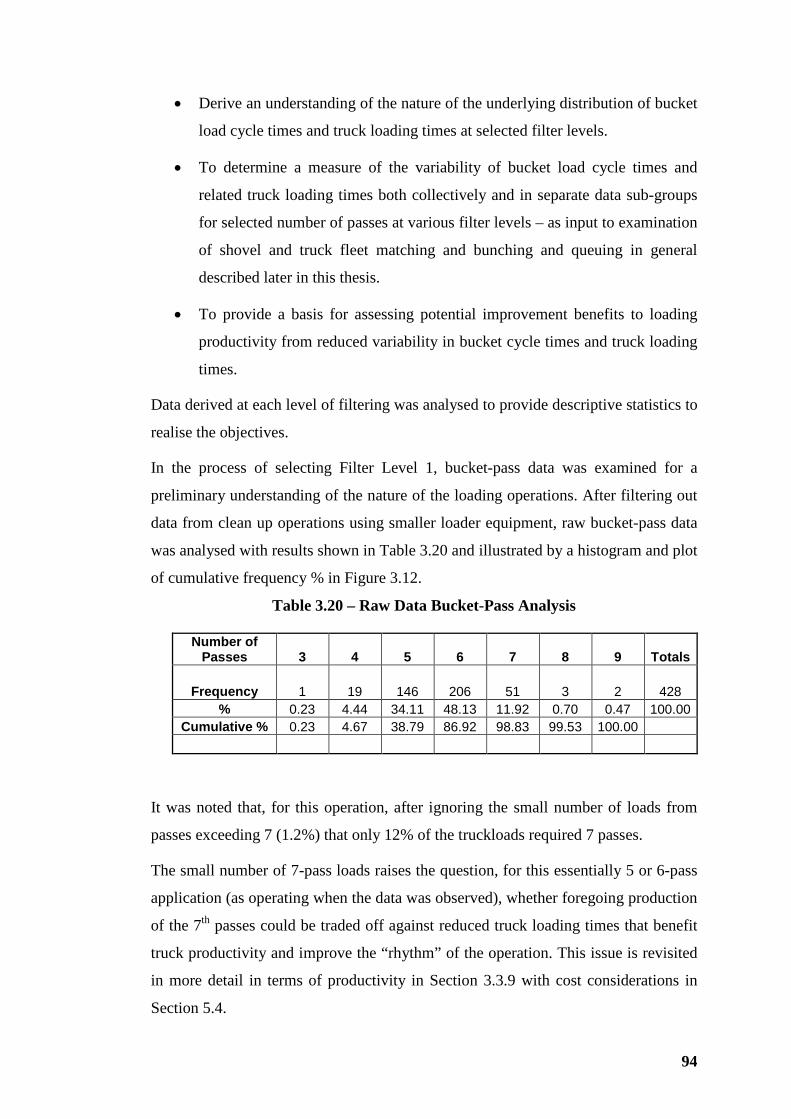
94
• Derive an understanding of the nature of the underlying distribution of bucket
load cycle times and truck loading times at selected filter levels.
• To determine a measure of the variability of bucket load cycle times and
related truck loading times both collectively and in separate data sub-groups
for selected number of passes at various filter levels – as input to examination
of shovel and truck fleet matching and bunching and queuing in general
described later in this thesis.
• To provide a basis for assessing potential improvement benefits to loading
productivity from reduced variability in bucket cycle times and truck loading
times.
Data derived at each level of filtering was analysed to provide descriptive statistics to
realise the objectives.
In the process of selecting Filter Level 1, bucket-pass data was examined for a
preliminary understanding of the nature of the loading operations. After filtering out
data from clean up operations using smaller loader equipment, raw bucket-pass data
was analysed with results shown in Table 3.20 and illustrated by a histogram and plot
of cumulative frequency % in Figure 3.12.
Table 3.20 – Raw Data Bucket-Pass Analysis
Number of Passes 3 4 5 6 7 8 9 Totals
Frequency 1 19 146 206 51 3 2 428 % 0.23 4.44 34.11 48.13 11.92 0.70 0.47 100.00
Cumulative % 0.23 4.67 38.79 86.92 98.83 99.53 100.00
It was noted that, for this operation, after ignoring the small number of loads from
passes exceeding 7 (1.2%) that only 12% of the truckloads required 7 passes.
The small number of 7-pass loads raises the question, for this essentially 5 or 6-pass
application (as operating when the data was observed), whether foregoing production
of the 7th passes could be traded off against reduced truck loading times that benefit
truck productivity and improve the “rhythm” of the operation. This issue is revisited
in more detail in terms of productivity in Section 3.3.9 with cost considerations in
Section 5.4.
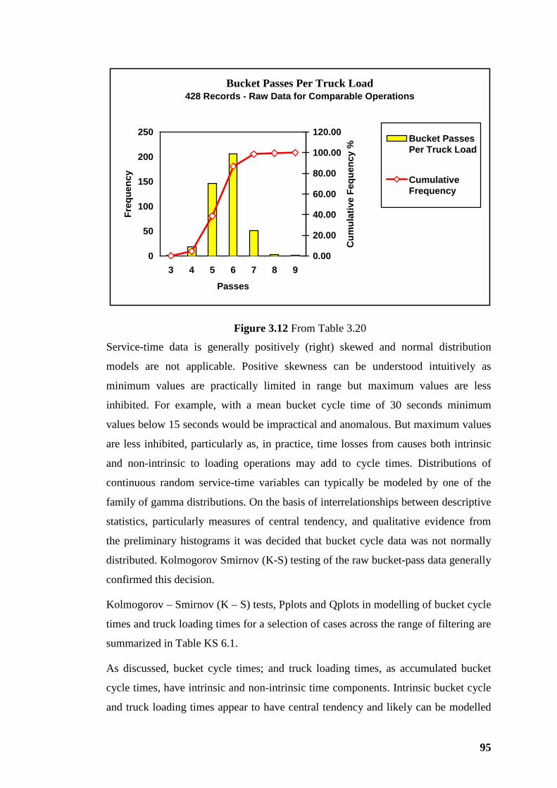
95
Bucket Passes Per Truck Load428 Records - Raw Data for Comparable Operations
0
50
100
150
200
250
3 4 5 6 7 8 9
Passes
Freq
uenc
y
0.00
20.00
40.00
60.00
80.00
100.00
120.00
Cum
ulat
ive
Fequ
ency
%
Bucket PassesPer Truck Load
CumulativeFrequency
Figure 3.12 From Table 3.20
Service-time data is generally positively (right) skewed and normal distribution
models are not applicable. Positive skewness can be understood intuitively as
minimum values are practically limited in range but maximum values are less
inhibited. For example, with a mean bucket cycle time of 30 seconds minimum
values below 15 seconds would be impractical and anomalous. But maximum values
are less inhibited, particularly as, in practice, time losses from causes both intrinsic
and non-intrinsic to loading operations may add to cycle times. Distributions of
continuous random service-time variables can typically be modeled by one of the
family of gamma distributions. On the basis of interrelationships between descriptive
statistics, particularly measures of central tendency, and qualitative evidence from
the preliminary histograms it was decided that bucket cycle data was not normally
distributed. Kolmogorov Smirnov (K-S) testing of the raw bucket-pass data generally
confirmed this decision.
Kolmogorov – Smirnov (K – S) tests, Pplots and Qplots in modelling of bucket cycle
times and truck loading times for a selection of cases across the range of filtering are
summarized in Table KS 6.1.
As discussed, bucket cycle times; and truck loading times, as accumulated bucket
cycle times, have intrinsic and non-intrinsic time components. Intrinsic bucket cycle
and truck loading times appear to have central tendency and likely can be modelled
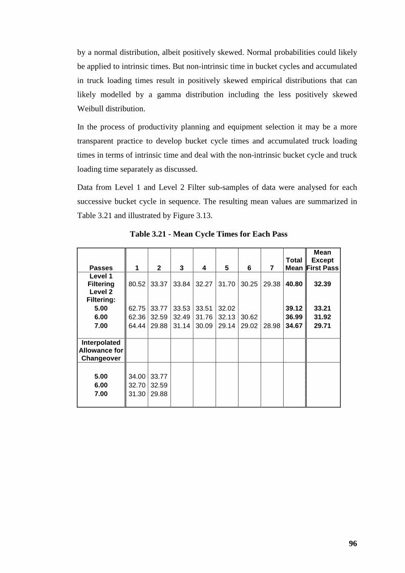
96
by a normal distribution, albeit positively skewed. Normal probabilities could likely
be applied to intrinsic times. But non-intrinsic time in bucket cycles and accumulated
in truck loading times result in positively skewed empirical distributions that can
likely modelled by a gamma distribution including the less positively skewed
Weibull distribution.
In the process of productivity planning and equipment selection it may be a more
transparent practice to develop bucket cycle times and accumulated truck loading
times in terms of intrinsic time and deal with the non-intrinsic bucket cycle and truck
loading time separately as discussed.
Data from Level 1 and Level 2 Filter sub-samples of data were analysed for each
successive bucket cycle in sequence. The resulting mean values are summarized in
Table 3.21 and illustrated by Figure 3.13.
Table 3.21 - Mean Cycle Times for Each Pass
Passes 1 2 3 4 5 6 7 Total Mean
Mean Except
First Pass Level 1 Filtering 80.52 33.37 33.84 32.27 31.70 30.25 29.38 40.80 32.39 Level 2
Filtering: 5.00 62.75 33.77 33.53 33.51 32.02 39.12 33.21 6.00 62.36 32.59 32.49 31.76 32.13 30.62 36.99 31.92 7.00 64.44 29.88 31.14 30.09 29.14 29.02 28.98 34.67 29.71
Interpolated
Allowance for Changeover
5.00 34.00 33.77 6.00 32.70 32.59 7.00 31.30 29.88
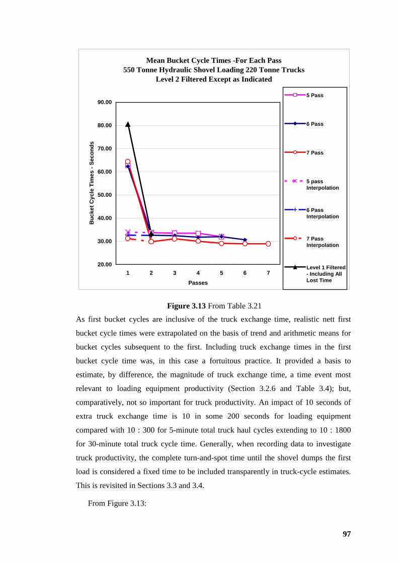
97
Mean Bucket Cycle Times -For Each Pass550 Tonne Hydraulic Shovel Loading 220 Tonne Trucks
Level 2 Filtered Except as Indicated
20.00
30.00
40.00
50.00
60.00
70.00
80.00
90.00
1 2 3 4 5 6 7Passes
Buc
ket C
ycle
Tim
es -
Seco
nds
5 Pass
6 Pass
7 Pass
5 passInterpolation
6 PassInterpolation
7 PassInterpolation
Level 1 Filtered- Including AllLost Time
Figure 3.13 From Table 3.21
As first bucket cycles are inclusive of the truck exchange time, realistic nett first
bucket cycle times were extrapolated on the basis of trend and arithmetic means for
bucket cycles subsequent to the first. Including truck exchange times in the first
bucket cycle time was, in this case a fortuitous practice. It provided a basis to
estimate, by difference, the magnitude of truck exchange time, a time event most
relevant to loading equipment productivity (Section 3.2.6 and Table 3.4); but,
comparatively, not so important for truck productivity. An impact of 10 seconds of
extra truck exchange time is 10 in some 200 seconds for loading equipment
compared with 10 : 300 for 5-minute total truck haul cycles extending to 10 : 1800
for 30-minute total truck cycle time. Generally, when recording data to investigate
truck productivity, the complete turn-and-spot time until the shovel dumps the first
load is considered a fixed time to be included transparently in truck-cycle estimates.
This is revisited in Sections 3.3 and 3.4.
From Figure 3.13:
98
1. Mean cycle time for each successive pass - for Pass 2 and above - shows a
subtle downward trend.
2. First passes from Filter Level 1, before deletion of time losses non-intrinsic to
equipment and operator performance, have been included in Figure 3.13 and
indicate a mean of 80.5 seconds compared with some 62 to 64 seconds at
Filter level 2 – so providing an indicated average of some 18 seconds (for this
operation at the time data was recorded) due to those events that justified
exclusion by filtering to Filter Level 2; also
3. First passes from Filter Level 2 show means of 62.7 to 64.4 seconds
compared to extrapolated first cycle times estimated from means and trend of
subsequent passes of 31.3 to 34 seconds, so indicating truck exchange times
of 28.7 to 33.1 seconds in addition to the estimated first bucket cycle time. In
terms of industry standards the indicated truck exchange time range is
excessive – this issue is discussed in more detail below.
Interpretations of the observations include:
1. The subtle reducing trend of bucket cycle times is interpreted as evidence of
the effect of the face-working technique where, for single side loading, the
load from the furthest swing position is taken first to take advantage of the
truck exchange time; and each successive bucket load is taken working
towards the truck. For double-side loading the technique is often reversed. In
this case, as the shovel has to swing through 180 degrees, the first bucket load
is effectively 90 degrees swing wherever it is taken. To maintain an even-
reach digging face, operators double-side loading generally take the first
bucket load from the centre or from a proud section of the face or to facilitate
bringing down an incipient overhang. The second bucket is generally from
the toe of the face closest to the truck working away from the truck for
successive bucket loads. These techniques are generally considered to deliver
the best truck loading productivity. In practice variable digability can
influence operators to focus on easier bucket-filling zones in the face. Best-
practice operators avoid this temptation using the easier digging sections as
later or last bucket loads to realise a truck load within the ideal designed
number of passes. Collapse of overhangs is an all-too-often occurrence that is
99
a potential hazard for equipment and operators. Best-practice operators deal
with overhangs at the incipient stage; and resist the temptation to burrow into
the face where easy digging is presented. Best-practice operating is all about
rhythm. An operator failing to persevere with a face-working plan best suited
to the operation is counter-rhythmic. Technique-induced inefficiencies need
to be investigated to determine if the cause is operator inattention, where the
remedy is obvious; or there are underlying operating and material-preparation
conditions that are frustrating the best intentions of the operators.
2. Time loss of 18 seconds for events non-intrinsic to the equipment and the
operator – identified herein as “pit housekeeping” - represent an 8% time
impost in mean truck loading time at Filter Level 1. As indicated, the data
was recorded when operating conditions were relatively difficult. Physical
working space is known to have been limited at the time. Material preparation
by way of drilling and blasting was not realizing optimum results because of
variable material competency across the stratigraphy being mined.
Accordingly the indicated discount factor for the “pit housekeeping” of 92%
is considered abnormally high. In practical loading operations there will
always be some extraordinary time losses for the several reasons listed and
other minor causes. It is considered that, for best practice, an achievable
factor would be 98% with an absolutely, and unacceptable, low value of 90%.
Traditionally estimations and operating budgets include this pit housekeeping
inefficiency in a job management efficiency factor that includes non-
utilization of available equipment. With the benefit of being able to identify
and quantify such events, pit-housekeeping inefficiency should be separately
identified and treated to facilitate management and control.
3. A mean truck exchange time of some 31 seconds included in the first bucket
load data at Filter Level 2 is unacceptably high. As indicated, working space
in the deep open pit where the data was recorded tends to be limited.
Standardized safe and quick turn-and-spot techniques for exchanging trucks
have to be modified because of limited span of working-face between pit
walls. Turn-and-spot times were discussed in Section 3.2.6 and the effect on
loading equipment efficiency illustrated by Table 3.4. For the 220 tonne
mining trucks being discussed an average turn and spot time of 45 seconds is
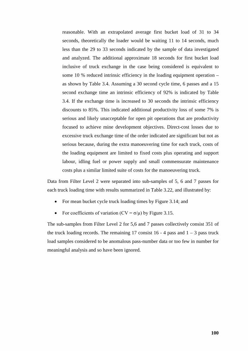
100
reasonable. With an extrapolated average first bucket load of 31 to 34
seconds, theoretically the loader would be waiting 11 to 14 seconds, much
less than the 29 to 33 seconds indicated by the sample of data investigated
and analyzed. The additional approximate 18 seconds for first bucket load
inclusive of truck exchange in the case being considered is equivalent to
some 10 % reduced intrinsic efficiency in the loading equipment operation –
as shown by Table 3.4. Assuming a 30 second cycle time, 6 passes and a 15
second exchange time an intrinsic efficiency of 92% is indicated by Table
3.4. If the exchange time is increased to 30 seconds the intrinsic efficiency
discounts to 85%. This indicated additional productivity loss of some 7% is
serious and likely unacceptable for open pit operations that are productivity
focused to achieve mine development objectives. Direct-cost losses due to
excessive truck exchange time of the order indicated are significant but not as
serious because, during the extra manoeuvering time for each truck, costs of
the loading equipment are limited to fixed costs plus operating and support
labour, idling fuel or power supply and small commensurate maintenance
costs plus a similar limited suite of costs for the manoeuvering truck.
Data from Filter Level 2 were separated into sub-samples of 5, 6 and 7 passes for
each truck loading time with results summarized in Table 3.22, and illustrated by:
• For mean bucket cycle truck loading times by Figure 3.14; and
• For coefficients of variation (CV = σ/μ) by Figure 3.15.
The sub-samples from Filter Level 2 for 5,6 and 7 passes collectively consist 351 of
the truck loading records. The remaining 17 consist 16 - 4 pass and 1 – 3 pass truck
load samples considered to be anomalous pass-number data or too few in number for
meaningful analysis and so have been ignored.
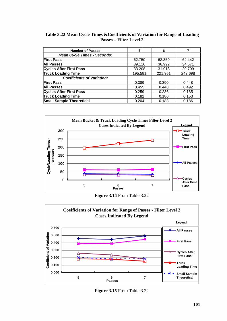
101
Mean Bucket & Truck Loading Cycle Times Filter Level 2Cases Indicated By Legend
0
50
100
150
200
250
300
5 6 7Passes
Cyc
le/L
oadi
ng T
imes
- Se
cond
s
TruckLoadingTime
First Pass
All Passes
CyclesAfter FirstPass
Legend
Figure 3.14 From Table 3.22
Coefficients of Variation for Range of Passes - Filter Level 2Cases Indicated By Legend
0.000
0.100
0.200
0.300
0.400
0.500
0.600
5 6 7Passes
Coe
ffici
ent o
f Var
iatio
n
All Passes
First Pass
Cycles AfterFirst Pass
TruckLoading Time
Small SampleTheoretical
Legend
Figure 3.15 From Table 3.22
Table 3.22 Mean Cycle Times &Coefficients of Variation for Range of Loading Passes – Filter Level 2
Number of Passes 5 6 7
Mean Cycle Times - Seconds: First Pass 62.750 62.359 64.442 All Passes 39.116 36.992 34.671 Cycles After First Pass 33.208 31.918 29.709 Truck Loading Time 195.581 221.951 242.698
Coefficients of Variation: First Pass 0.389 0.390 0.448 All Passes 0.455 0.448 0.492 Cycles After First Pass 0.259 0.236 0.185 Truck Loading Time 0.182 0.180 0.153 Small Sample Theoretical 0.204 0.183 0.186
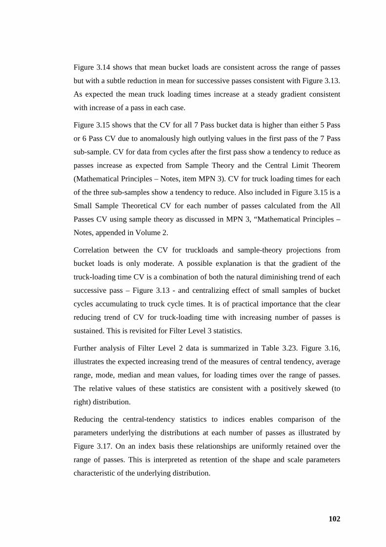
102
Figure 3.14 shows that mean bucket loads are consistent across the range of passes
but with a subtle reduction in mean for successive passes consistent with Figure 3.13.
As expected the mean truck loading times increase at a steady gradient consistent
with increase of a pass in each case.
Figure 3.15 shows that the CV for all 7 Pass bucket data is higher than either 5 Pass
or 6 Pass CV due to anomalously high outlying values in the first pass of the 7 Pass
sub-sample. CV for data from cycles after the first pass show a tendency to reduce as
passes increase as expected from Sample Theory and the Central Limit Theorem
(Mathematical Principles – Notes, item MPN 3). CV for truck loading times for each
of the three sub-samples show a tendency to reduce. Also included in Figure 3.15 is a
Small Sample Theoretical CV for each number of passes calculated from the All
Passes CV using sample theory as discussed in MPN 3, “Mathematical Principles –
Notes, appended in Volume 2.
Correlation between the CV for truckloads and sample-theory projections from
bucket loads is only moderate. A possible explanation is that the gradient of the
truck-loading time CV is a combination of both the natural diminishing trend of each
successive pass – Figure 3.13 - and centralizing effect of small samples of bucket
cycles accumulating to truck cycle times. It is of practical importance that the clear
reducing trend of CV for truck-loading time with increasing number of passes is
sustained. This is revisited for Filter Level 3 statistics.
Further analysis of Filter Level 2 data is summarized in Table 3.23. Figure 3.16,
illustrates the expected increasing trend of the measures of central tendency, average
range, mode, median and mean values, for loading times over the range of passes.
The relative values of these statistics are consistent with a positively skewed (to
right) distribution.
Reducing the central-tendency statistics to indices enables comparison of the
parameters underlying the distributions at each number of passes as illustrated by
Figure 3.17. On an index basis these relationships are uniformly retained over the
range of passes. This is interpreted as retention of the shape and scale parameters
characteristic of the underlying distribution.
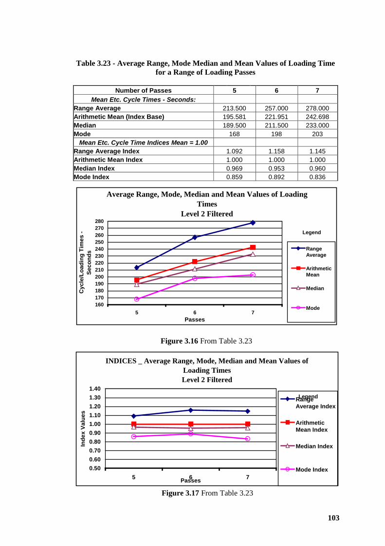
103
Table 3.23 - Average Range, Mode Median and Mean Values of Loading Time for a Range of Loading Passes
Number of Passes 5 6 7
Mean Etc. Cycle Times - Seconds: Range Average 213.500 257.000 278.000 Arithmetic Mean (Index Base) 195.581 221.951 242.698 Median 189.500 211.500 233.000 Mode 168 198 203
Mean Etc. Cycle Time Indices Mean = 1.00 Range Average Index 1.092 1.158 1.145 Arithmetic Mean Index 1.000 1.000 1.000 Median Index 0.969 0.953 0.960 Mode Index 0.859 0.892 0.836
Average Range, Mode, Median and Mean Values of Loading Times
Level 2 Filtered
160170180190200210220230240250260270280
5 6 7Passes
Cyc
le/L
oadi
ng T
imes
- Se
cond
s RangeAverage
ArithmeticMean
Median
Mode
Legend
Figure 3.16 From Table 3.23
INDICES _ Average Range, Mode, Median and Mean Values of Loading TimesLevel 2 Filtered
0.500.600.700.800.901.001.101.201.301.40
5 6 7Passes
Inde
x Va
lues
RangeAverage Index
ArithmeticMean Index
Median Index
Mode Index
Legend
Figure 3.17 From Table 3.23
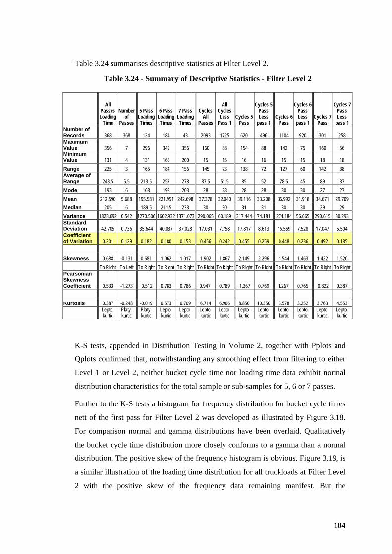
104
Table 3.24 summarises descriptive statistics at Filter Level 2.
Table 3.24 - Summary of Descriptive Statistics - Filter Level 2
All Passes Loading
Time
Number of
Passes
5 Pass Loading Times
6 Pass Loading Times
7 Pass Loading Times
Cycles All
Passes
All Cycles Less
Pass 1 Cycles 5
Pass
Cycles 5 Pass Less
pass 1 Cycles 6
Pass
Cycles 6 Pass Less
pass 1 Cycles 7
Pass
Cycles 7 Pass Less
pass 1 Number of Records 368 368 124 184 43 2093 1725 620 496 1104 920 301 258 Maximum Value 356 7 296 349 356 160 88 154 88 142 75 160 56 Minimum Value 131 4 131 165 200 15 15 16 16 15 15 18 18 Range 225 3 165 184 156 145 73 138 72 127 60 142 38 Average of Range 243.5 5.5 213.5 257 278 87.5 51.5 85 52 78.5 45 89 37 Mode 193 6 168 198 203 28 28 28 28 30 30 27 27 Mean 212.590 5.688 195.581 221.951 242.698 37.378 32.040 39.116 33.208 36.992 31.918 34.671 29.709 Median 205 6 189.5 211.5 233 30 30 31 31 30 30 29 29 Variance 1823.692 0.542 1270.506 1602.932 1371.073 290.065 60.189 317.444 74.181 274.184 56.665 290.615 30.293 Standard Deviation 42.705 0.736 35.644 40.037 37.028 17.031 7.758 17.817 8.613 16.559 7.528 17.047 5.504 Coefficient of Variation 0.201 0.129 0.182 0.180 0.153 0.456 0.242 0.455 0.259 0.448 0.236 0.492 0.185 Skewness 0.688 -0.131 0.681 1.062 1.017 1.902 1.867 2.149 2.296 1.544 1.463 1.422 1.520 To Right To Left To Right To Right To Right To Right To Right To Right To Right To Right To Right To Right To Right Pearsonian Skewness Coefficient 0.533 -1.273 0.512 0.783 0.786 0.947 0.789 1.367 0.769 1.267 0.765 0.822 0.387 Kurtosis 0.387 -0.248 -0.019 0.573 0.709 6.714 6.906 8.850 10.350 3.578 3.252 3.763 4.553
Lepto-kurtic
Platy-kurtic
Platy-kurtic
Lepto-kurtic
Lepto-kurtic
Lepto-kurtic
Lepto-kurtic
Lepto-kurtic
Lepto-kurtic
Lepto-kurtic
Lepto-kurtic
Lepto-kurtic
Lepto-kurtic
K-S tests, appended in Distribution Testing in Volume 2, together with Pplots and
Qplots confirmed that, notwithstanding any smoothing effect from filtering to either
Level 1 or Level 2, neither bucket cycle time nor loading time data exhibit normal
distribution characteristics for the total sample or sub-samples for 5, 6 or 7 passes.
Further to the K-S tests a histogram for frequency distribution for bucket cycle times
nett of the first pass for Filter Level 2 was developed as illustrated by Figure 3.18.
For comparison normal and gamma distributions have been overlaid. Qualitatively
the bucket cycle time distribution more closely conforms to a gamma than a normal
distribution. The positive skew of the frequency histogram is obvious. Figure 3.19, is
a similar illustration of the loading time distribution for all truckloads at Filter Level
2 with the positive skew of the frequency data remaining manifest. But the
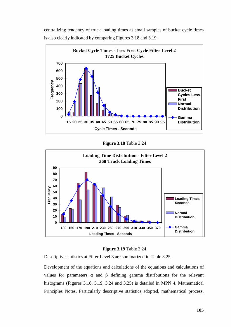
105
centralizing tendency of truck loading times as small samples of bucket cycle times
is also clearly indicated by comparing Figures 3.18 and 3.19.
Bucket Cycle Times - Less First Cycle Filter Level 21725 Bucket Cycles
0
100
200
300
400
500
600
700
15 20 25 30 35 40 45 50 55 60 65 70 75 80 85 90 95
Cycle Times - Seconds
Freq
uenc
y
BucketCycles LessFirstNormalDistribution
GammaDistribution
Figure 3.18 Table 3.24
Loading Time Distribution - Filter Level 2368 Truck Loading Times
0
10
20
30
40
50
60
70
80
90
130 150 170 190 210 230 250 270 290 310 330 350 370Loading Times - Seconds
Freq
uenc
y
Loading Times -Seconds
NormalDistribution
GammaDistribution
Figure 3.19 Table 3.24
Descriptive statistics at Filter Level 3 are summarized in Table 3.25.
Development of the equations and calculations of the equations and calculations of
values for parameters α and β defining gamma distributions for the relevant
histograms (Figures 3.18, 3.19, 3.24 and 3.25) is detailed in MPN 4, Mathematical
Principles Notes. Particularly descriptive statistics adopted, mathematical process,
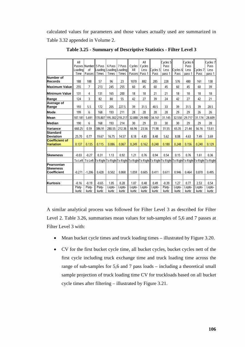
106
calculated values for parameters and those values actually used are summarized in
Table 3.32 appended in Volume 2.
Table 3.25 - Summary of Descriptive Statistics - Filter Level 3
All Passes Loading
Time
Number of
Passes
5 Pass Loading Times
6 Pass Loading Times
7 Pass Loading Times
Cycles All
Passes
All Cycles Less
Pass 1 Cycles 5
Pass
Cycles 5 Pass Less
pass 1 Cycles 6
Pass
Cycles 6 Pass Less
pass 1 Cycles 7
Pass
Cycles 7 Pass Less
pass 1 Number of Records 188 188 57 96 23 1070 882 285 228 576 480 161 138 Maximum Value 255 7 213 245 255 60 45 60 45 60 45 60 39
Minimum Value 131 4 131 165 200 18 18 21 21 18 18 18 18 Range 124 3 82 80 55 42 27 39 24 42 27 42 21 Average of Range 193 5.5 172 205 227.5 39 31.5 40.5 33 39 31.5 39 28.5 Mode 199 6 168 193 211 28 28 28 28 29 29 26 26 Mean 187.181 5.691 170.807 195.302 218.217 32.888 29.980 34.161 31.145 32.550 29.717 31.174 28.609 Median 190 6 168 193 214 30 29 33 30 30 29 29 28 Variance 660.25 0.59 386.91 280.55 212.36 66.96 23.56 71.98 31.55 65.35 21.44 56.16 13.61 Standard Deviation 25.70 0.77 19.67 16.75 14.57 8.18 4.85 8.48 5.62 8.08 4.63 7.49 3.69 Coefficient of Variation 0.137 0.135 0.115 0.086 0.067 0.249 0.162 0.248 0.180 0.248 0.156 0.240 0.129 Skewness -0.03 -0.27 0.31 1.13 0.92 1.21 0.76 0.94 0.54 0.15 0.76 1.61 0.36 To Left To Left To Right To Right To Right To Right To Right To Right To Right To Right To Right To Right To Right Pearsonian Skewness Coefficient -0.271 -1.206 0.428 0.502 0.868 1.059 0.605 0.411 0.611 0.946 0.464 0.870 0.495 Kurtosis -0.16 -0.19 -0.65 1.05 0.28 1.07 0.48 0.49 -0.39 1.27 0.77 2.53 0.54
Platy-kurtic
Platy-kurtic
Platy-kurtic
Lepto-kurtic
Lepto-kurtic
Lepto-kurtic
Lepto-kurtic
Lepto-kurtic
Platy-kurtic
Lepto-kurtic
Lepto-kurtic
Lepto-kurtic
Lepto-kurtic
A similar analytical process was followed for Filter Level 3 as described for Filter
Level 2. Table 3.26, summarises mean values for sub-samples of 5,6 and 7 passes at
Filter Level 3 with:
• Mean bucket cycle times and truck loading times – illustrated by Figure 3.20.
• CV for the first bucket cycle time, all bucket cycles, bucket cycles nett of the
first cycle including truck exchange time and truck loading time across the
range of sub-samples for 5,6 and 7 pass loads – including a theoretical small
sample projection of truck loading time CV for truckloads based on all bucket
cycle times after filtering – illustrated by Figure 3.21.
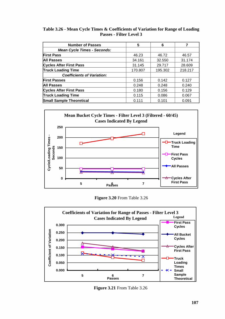
107
Table 3.26 - Mean Cycle Times & Coefficients of Variation for Range of Loading Passes - Filter Level 3
Number of Passes 5 6 7
Mean Cycle Times - Seconds: First Pass 46.23 46.72 46.57 All Passes 34.161 32.550 31.174 Cycles After First Pass 31.145 29.717 28.609 Truck Loading Time 170.807 195.302 218.217
Coefficients of Variation: First Passes 0.156 0.142 0.127 All Passes 0.248 0.248 0.240 Cycles After First Pass 0.180 0.156 0.129 Truck Loading Time 0.115 0.086 0.067 Small Sample Theoretical 0.111 0.101 0.091
Mean Bucket Cycle Times - Filter Level 3 (Filtered - 60/45)Cases Indicated By Legend
0
50
100
150
200
250
5 6 7Passes
Cyc
le/L
oadi
ng T
imes
- Se
cond
s
Truck LoadingTime
First PassCycles
All Passes
Cycles AfterFirst Pass
Legend
Figure 3.20 From Table 3.26
Coefficients of Variation for Range of Passes - Filter Level 3Cases Indicated By Legend
0.000
0.050
0.100
0.150
0.200
0.250
0.300
5 6 7Passes
Coe
ffici
ent o
f Var
iatio
n
First PassCycles
All BucketCycles
Cycles AfterFirst Pass
TruckLoadingTimesSmallSampleTheoretical
Legend
Figure 3.21 From Table 3.26
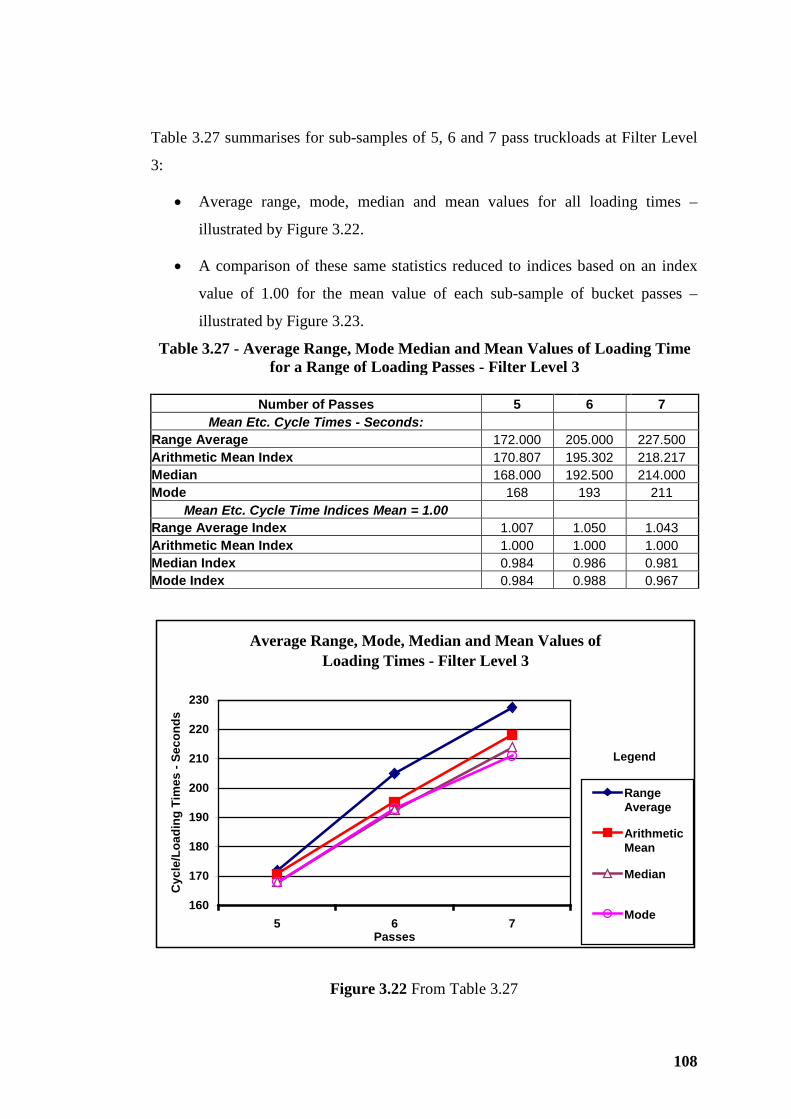
108
Table 3.27 summarises for sub-samples of 5, 6 and 7 pass truckloads at Filter Level
3:
• Average range, mode, median and mean values for all loading times –
illustrated by Figure 3.22.
• A comparison of these same statistics reduced to indices based on an index
value of 1.00 for the mean value of each sub-sample of bucket passes –
illustrated by Figure 3.23.
Table 3.27 - Average Range, Mode Median and Mean Values of Loading Time for a Range of Loading Passes - Filter Level 3
Number of Passes 5 6 7
Mean Etc. Cycle Times - Seconds: Range Average 172.000 205.000 227.500 Arithmetic Mean Index 170.807 195.302 218.217 Median 168.000 192.500 214.000 Mode 168 193 211
Mean Etc. Cycle Time Indices Mean = 1.00 Range Average Index 1.007 1.050 1.043 Arithmetic Mean Index 1.000 1.000 1.000 Median Index 0.984 0.986 0.981 Mode Index 0.984 0.988 0.967
Average Range, Mode, Median and Mean Values of Loading Times - Filter Level 3
160
170
180
190
200
210
220
230
5 6 7Passes
Cyc
le/L
oadi
ng T
imes
- Se
cond
s
RangeAverage
ArithmeticMean
Median
Mode
Legend
Figure 3.22 From Table 3.27
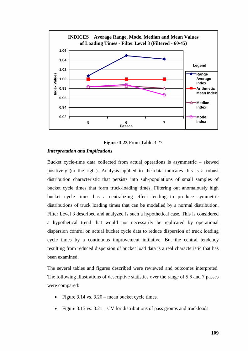
109
INDICES _ Average Range, Mode, Median and Mean Values of Loading Times - Filter Level 3 (Filtered - 60/45)
0.92
0.94
0.96
0.98
1.00
1.02
1.04
1.06
5 6 7Passes
Inde
x Va
lues Range
AverageIndexArithmeticMean Index
MedianIndex
ModeIndex
Legend
Figure 3.23 From Table 3.27
Interpretation and Implications
Bucket cycle-time data collected from actual operations is asymmetric – skewed
positively (to the right). Analysis applied to the data indicates this is a robust
distribution characteristic that persists into sub-populations of small samples of
bucket cycle times that form truck-loading times. Filtering out anomalously high
bucket cycle times has a centralizing effect tending to produce symmetric
distributions of truck loading times that can be modelled by a normal distribution.
Filter Level 3 described and analyzed is such a hypothetical case. This is considered
a hypothetical trend that would not necessarily be replicated by operational
dispersion control on actual bucket cycle data to reduce dispersion of truck loading
cycle times by a continuous improvement initiative. But the central tendency
resulting from reduced dispersion of bucket load data is a real characteristic that has
been examined.
The several tables and figures described were reviewed and outcomes interpreted.
The following illustrations of descriptive statistics over the range of 5,6 and 7 passes
were compared:
• Figure 3.14 vs. 3.20 – mean bucket cycle times.
• Figure 3.15 vs. 3.21 – CV for distributions of pass groups and truckloads.
110
• Figure 3.16 vs. 3.22 – measures of central tendency for truck loading times.
• Figure 3.17 v. 3.23 – measures of central tendency reduced to relative
indices.
The following trends and outcomes were noted:
1. Means of bucket cycle times, whatever the grouping, are generally consistent
over the sub-sample range of 5,6 and 7 passes at all levels of filtering –
Figures 3.14 and 3.20.
2. Filtering at Level 2 to eliminate time events non-intrinsic to the truck loading
operation, by deleting non-complying complete truck loading records,
reduced the mean of first passes by 16 to 18 seconds – Table 3.21. This is a
measure of the effect of events non-intrinsic to truck loading operations for
the operation and operating circumstances – equivalent to 7% to 8% of the
actual mean loading time at Filter Level 1. This is considered towards the
upper end of the range of the affect of “pit-house-keeping” activities on mean
truck loading time. An appropriate range is considered to be best at 98% to a
low performance of 90%.
The outcome is that loading performance calculated from intrinsic equipment
capability must provide for some “pit house keeping” duties – a factor in the
range of 98% to 90% is suggested. This practical allowance should be
separate and transparent. The actual effect is measurable and manageable.
3. First pass bucket cycle times at Filter Level 2 are reasonably uniform over the
range of 5 to 7 passes. At Filter Level 3, with elimination of outlying high
values, CV for first-pass bucket cycle times exhibit a reducing trend over the
5 to 7 pass range – Figure 3.21. This trend is believed to be anomalous, a by-
product of the hypothetical filtering and reduced sample size; and is not
considered as having any relevant significance.
4. Compared with Filter Level 2, filtering to Level 3 hypothetically reduced the
mean for first pass bucket cycle times by some 15 seconds across the range of
5,6 and 7 pass sub-samples – Tables 3.22 and 3.26.
5. Filtering to level 3 also hypothetically reduced the mean for all bucket cycle
times by a moderate 5 to 3.5 seconds over the 5 to 7 pass range of sub-
111
samples reflecting the combined averaging of the first pass adjustment over
increasing passes for each sub-sample and the small general filtering
reduction for all bucket cycle times subsequent to the first.
6. Means of truck loading times at both Filter Levels 2 and 3 reconcile with
mean bucket times so confirming the arithmetic of the analysis.
7. Review of standard deviations, by applying sample theory as described in
MPN 1 to MPN3, Mathematical Principles – Notes, over the range of bucket
passes at both Filter Levels 2 and 3 – Tables 3.24 and 3.25 - indicate only fair
correlation with standard deviations for truck loading times (see Figures 3.15
and 3.21).
8. At Filter Level 2 expected reducing trend of CV of loading times with
increased number of passes is evident in Figure 3.15; and, more convincingly,
evident in Figure 3.21 at Filter Level 3. Particularly at Filter Level 3, the
gradient of the CV trend for truck loading times is steeper than for both
passes after the first and for the small sample theoretical projection. A
weighted combination of trend gradients for these two CV statistics correlates
closely with the CV trend for truck loading times – likely as a result of the
centralizing effect of the filtering process. So, as dispersion control is effected
on bucket cycle times (by means discussed below), it appears that the small-
sample down-trending of CV for truck loading times with increasing numbers
of passes per load should become more effective. This down trending CV-
effect should be reflected by reduced bunching inefficiency and improved
load-and-haul “rhythm”.
9. It is generally concluded that increasing passes per truck load and so
increasing loading time has real benefit in reducing dispersion of distribution
of truck-loading times. But increasing passes is at the expense of increased
truck loading times. The resulting reduced hauling productivity will, to some
degree, be offset by the reduced variability in loading times that reflect in
reduced bunching (queuing) inefficiency and so assist operators to retain
“rhythm” in loading and hauling operations.
10. Filter Level 3 has not only centralized the distribution of truck loading times
as illustrated by Figures 3.22 and 3.23 but has created bi or multi-modal
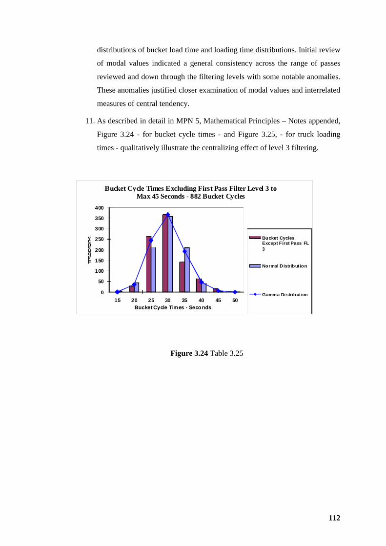
112
distributions of bucket load time and loading time distributions. Initial review
of modal values indicated a general consistency across the range of passes
reviewed and down through the filtering levels with some notable anomalies.
These anomalies justified closer examination of modal values and interrelated
measures of central tendency.
11. As described in detail in MPN 5, Mathematical Principles – Notes appended,
Figure 3.24 - for bucket cycle times - and Figure 3.25, - for truck loading
times - qualitatively illustrate the centralizing effect of level 3 filtering.
0
50
100
150
200
250
300
350
400
15 20 25 30 35 40 45 50
Frequency
Bucket Cycle Times - Seconds
Bucket Cycle Times Excluding First Pass Filter Level 3 to Max 45 Seconds - 882 Bucket Cycles
Bucket Cycles Except First Pass FL 3
Normal D istribution
Gamma Di stribution
Figure 3.24 Table 3.25
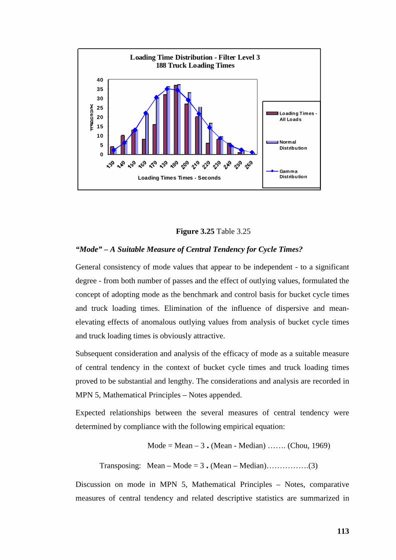
113
0
5
10
15
20
25
30
35
40
Frequency
Loading Times Times - Seconds
Loading Time Distribution - Filter Level 3188 Truck Loading Times
Loading Times -All Loads
Normal Distribution
Gamma Distribution
Figure 3.25 Table 3.25
“Mode” – A Suitable Measure of Central Tendency for Cycle Times?
General consistency of mode values that appear to be independent - to a significant
degree - from both number of passes and the effect of outlying values, formulated the
concept of adopting mode as the benchmark and control basis for bucket cycle times
and truck loading times. Elimination of the influence of dispersive and mean-
elevating effects of anomalous outlying values from analysis of bucket cycle times
and truck loading times is obviously attractive.
Subsequent consideration and analysis of the efficacy of mode as a suitable measure
of central tendency in the context of bucket cycle times and truck loading times
proved to be substantial and lengthy. The considerations and analysis are recorded in
MPN 5, Mathematical Principles – Notes appended.
Expected relationships between the several measures of central tendency were
determined by compliance with the following empirical equation:
Mode = Mean – 3 . (Mean - Median) ……. (Chou, 1969)
Transposing: Mean – Mode = 3 . (Mean – Median)…………….(3)
Discussion on mode in MPN 5, Mathematical Principles – Notes, comparative
measures of central tendency and related descriptive statistics are summarized in
114
Table 3.28, Volume 2, Appendices. Mode values considered anomalous by
comparison over the range of sub-samples were subsequently reviewed and amended
to include alternative mode values and related statistics as shown in Table 3.29,
Volume 2, Appendices.
The alternative values generally comply with the hierarchical order of measures of
central tendency, i.e., mean > median > mode; also, values in Table 3.29 generally
correlate with the empirical ratio (mean - median) : (mean – mode) = 1 : 3.
Alternative, amended, values of mode for truck loading times included in Table 3.29
are from analysis shown in Table 3.30, Volume 2, Appendices. The complete
discussion, analysis, interpretation, implications and subsequent inferences are
provided in MPN 5 in Mathematical Principles – Notes appended in Volume 2.
Small samples of truck loading times may exhibit multi-modal characteristics.
Where data demonstrates multi-modal characteristics of the distribution at any
chosen frequency interval, increasing the interval of frequency – in this case from
one second to five, ten and twenty seconds successively tends to interpolate a
primary mode frequency range containing the unit frequency range modal value, as
shown by Table 3.30.
On the basis of above discussion, and analysis described in MPN 5, Mathematical
Principles – Notes it is concluded that, subject to some manageable limitations, mode
is a reliable and, as will be shown, useful central tendency measure for bucket cycle
and truck-loading times.
Skewness of Distributions of Bucket Cycle & Truck Loading Times
The validity of mode as a measure for bucket cycle time and truck loading time has
been discussed. The natural positive skew of bucket cycle time and loading time
distributions has also been discussed. Qualitatively from the several histograms
included in Illustrations the positive skew is moderate to mild for truck loading times
and generally high for bucket cycle times. (For more detail on the following
discussion refer to MPN 6 and MPN 7, Mathematical Principles – Notes, appended
in Volume 2). As shown by Table 3.32, Volume 2, Appendices, parameters α and β
were derived for modelling gamma distributions for comparison with actual
frequency distributions - using the proposition μ = α . β and σ2 = α . β2 (Devore,
1999). Both α and β proved to be relatively high numbers in order to generate a
115
skewed distribution model tending away from the asymmetric towards a symmetric,
normal distribution - particularly as the level of filtering increased. This tendency has
already been discussed in empirical terms.
Mode is not generally considered a reliable measure of central tendency for highly
skewed distributions because the mode is located too close to one of the extreme
values to be representative of the distribution (Chou, 1969). But modelling
experience as described supports the conclusion that truck-loading time distributions
are not highly skewed.
A derivation of criteria for assessing degree of skewness was developed from
Pearson’s coefficients for skewness (Chou, 1999) as described in MPN 6,
Mathematical Principles – Notes, appended. Measures of skewness were examined to
test the hypothesis of using any of the several coefficients of skewness as a measure
for control and improvement of bucket cycle and truck loading times.
As described in MPN 6, Mathematical Principles – Notes, appended, examination -
as limited by the data sample available - of coefficient of skewness as an
improvement or control measure was not absolutely conclusive; but the hypothesis
that measures of skewness have potential to support or substitute for comparing the
measures of central tendency is considered worthy of further research.
Forecasts - Management and Control
For samples of > 500 bucket cycle times and for samples of > 100 truck loading
times, the evidence confirms stability of mode for measuring central tendency. This
evidence promotes the concept of mode – the most frequently expected cycle or
loading time - as a measure of minimum target or benchmark for estimating and
forecasting bucket cycle times and truck loading times; also as a basis for directly
related operational management and control.
Notwithstanding the analytical indications that bucket cycle times are highly skewed,
as dispersion is reduced (by control of practices and techniques) centralizing
tendency will tend to reduce skewness of bucket cycle times to moderate or even
mild levels. This is evidenced by the descriptive statistics at Filter Level 3.
Consequently mode is proposed as a potentially valid, reliable measure of central
tendency in the case of bucket cycle times and truck loading times in the context of
continuously improving management and control.
116
In addition mode can provide a target or bench mark for bucket cycle and truck
loading times against which observed mean values can be compared. The difference
between mean and mode values is a measure of the potential improvement except
that achieving equal mean and mode values is a hypothetical, perfect outcome where
distributions of bucket cycle and truck-loading times are symmetrical. This is
considered a theoretical, impractical and non-achievable outcome that, modestly
discounted, could be useful as a target for continuous improvement. Where the
means of collecting bucket cycle and truck loading times exist, mean and mode
values can be adopted as key performance indicators (KPI) and compared as a
performance quotient (PQBCT for bucket cycle times or PQLT for truck loading times,
generically referred to as PQT) with a practical target of:
Mode / Mean = PQT = 0.95, say (or other standard chosen)
The comparative standard corresponds to a CVmean ≈ 0.16 for bucket cycle times; and
CVmean ≈ 0.10 for truck loading times consistent with a typical operation with 4 to 7
pass loading and mean passes of some 5.5. For other operations with less or more
bucket passes PQT = 0.95 would likely still be valid but corresponding CVmean and
CVmode values would change. The target statistics are consistent with an ideal
operation where well-controlled dispersion of bucket cycle times and a focus on
achieving best practice load-and-haul performance results in acceptable operating
“rhythm”.
For any of the sub-sample sets (constant bucket passes) of data from any sample of
bucket cycle and truck loading times, the mean tends to diminish as management and
control improvements reduce impact of outlying values on the distribution. In
contrast it has been shown that mode is almost constant and so potentially more
reliable and useful. So a modal coefficient of variation can be conveniently adopted
as a dimensionless measure for comparing dispersion of distributions of bucket cycle
time and truck loading times with differing numbers of passes.
That is: CVmean = σ / Mean
CVmode = σ / Mode
Both mean and mode coefficients of variation are compared in Table 3.31 in and
Figure 3.26.
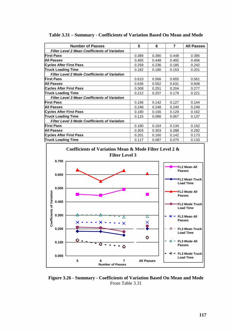
117
Table 3.31 – Summary - Coefficients of Variation Based On Mean and Mode
Number of Passes 5 6 7 All Passes Filter Level 2 Mean Coefficients of Variation
First Pass 0.389 0.390 0.448 0.395 All Passes 0.455 0.448 0.492 0.456 Cycles After First Pass 0.259 0.236 0.185 0.242 Truck Loading Time 0.182 0.180 0.153 0.201
Filter Level 2 Mode Coefficients of Variation First Pass 0.610 0.566 0.655 0.561 All Passes 0.636 0.552 0.631 0.608 Cycles After First Pass 0.308 0.251 0.204 0.277 Truck Loading Time 0.212 0.207 0.179 0.221
Filter Level 3 Mean Coefficients of Variation First Pass 0.156 0.142 0.127 0.144 All Passes 0.248 0.248 0.240 0.249 Cycles After First Pass 0.180 0.156 0.129 0.162 Truck Loading Time 0.115 0.086 0.067 0.137
Filter Level 3 Mode Coefficients of Variation First Pass 0.180 0.154 0.134 0.152 All Passes 0.303 0.303 0.288 0.292 Cycles After First Pass 0.201 0.160 0.142 0.173 Truck Loading Time 0.117 0.087 0.070 0.133
Coefficients of Variation Mean & Mode Filter Level 2 & Filter Level 3
0.000
0.100
0.200
0.300
0.400
0.500
0.600
0.700
5 6 7 All PassesNumber of Passes
Coe
ffici
ents
of V
aria
tion
FL2 Mean AllPasses
FL2 Mean TruckLoad Time
FL2 Mode AllPasses
FL2 Mode TruckLoad Time
FL3 Mean AllPasses
FL3 Mean TruckLoad Time
FL3 Mode AllPasses
FL3 Mode TruckLoad Time
Figure 3.26 - Summary - Coefficients of Variation Based On Mean and Mode From Table 3.31
118
From Table 3.31 and Figure 3.26:
For Bucket Cycle Times – 5, 6 and 7 passes:
At Filter Level 2: Range:
CVmode 0.55 to 0.64
CVmean 0.46 to 0.49
At Filter Level 3: Range:
CVmode 0.29 to 0.30
CVmean 0.24 to 0.25
Comparative “All Pass” values for bucket cycle times fall within the indicated range.
For Truck Loading Times – 5, 6 and 7 passes:
At Filter Level 2: Range:
CVmode 0.21 to 0.18
CVmean 0.18 to 0.15
At Filter Level 3: Range:
CVmode 0.12 to 0.07
CVmean 0.12 to 0.07
Comparative “All Pass” values for truck loading times are generally significantly
higher than for the sub-samples of 5, 6 and 7 passes. There are two reasons for this
apparent anomaly:
1. “All-Pass” truck-loading-time data having a range of values (measure of
dispersion) that cover the total, cumulative, range of the 5, 6 and 7 pass sub-
samples of truck loading times. The increased cumulative dispersion of the
“All Pass” data indicated by overall range is reflected in the other measures
of dispersion, particularly standard deviation σ. Increased σ results in
increased CVmode and CVmean - so the higher CV values for truck loading
times for “All Passes” in Table 3.31 and Figure 3.26.
119
2. “All-Pass” bucket cycle and truck-loading-time data includes some 4-Pass
sets and one 3-Pass set of bucket cycle time data that, typically, have similar
standard deviation to 5, 6 and 7 pass sub-samples but tend to lower the mean
value of truck loading times – so elevating the CV of “All-Pass” truck
loading time.
It will also be noted that, as discussed:
• At hypothetical Filter Level 3 the CVmean and CVmode values for truck loading
times are practically the same.
• The reduction in both CVmean and CVmode for truck loading times as number
of passes increase is clearly indicated at both Filter Level 2 and Filter Level
3.
In conclusion, Table 3.31 and Figure 3.26 demonstrate that, to the extent that mode is
a stable and valid KPI for central tendency of distributions of bucket-cycle and truck-
loading times, a CV derivative of mode is also a valid alternative for measuring
comparative dispersion if coefficient of variation is the comparative descriptive
statistic of choice.
Conclusions
Basic elements of bucket cycle time consist:
• Select and line up digging target in face (in final braking stage of return
swing), address the face, fill bucket, break out and commence to swing.
• Swing loaded to dumping spot.
• Dump bucket load.
• Return swing.
These basic components are further addressed in Sections 3.3.11 and 4.1.4.
The following conclusions are drawn from analysis and discussion in this section and
related supporting information in Mathematical Principles – Notes, Tables and
Figures appended.
1. Raw bucket cycle and truck loading data records include time utilizations and
losses in addition to the basic elements described that impact directly on
bucket cycle times. Activities non-intrinsic to the loading operation may
inflate bucket cycle and truck loading times. These time components have
been discussed. On the basis of limited operating data available and
120
knowledge of the actual operating conditions, a discount factor in the range
0.92 to 0.98 is indicated as justified.
2. Time is utilized for necessary activities that enable operations to progress
including face housekeeping necessarily performed by loading equipment,
maneuvering in a limited operating area, dealing with oversize particles in the
face and following the face as excavation progresses. This category of time is
treated by a propel factor in Section 3.2.4 – recommended at 0.85 by
Atkinson (Atkinson T, 1992). In the absence of empirical determination of a
suitable average or allowance range, factor application is the alternative
option. This time utilization category needs to be transparently assessed,
allowed for and, if possible, separately recorded in operations to enable
examination of nett purely-intrinsic bucket cycle time and truck loading time
data for control and management.
3. Truck Exchange Time is the difference between “turn-and-spot” time for
mining trucks and time taken for the first bucket cycle from last dump and
truck dispatch to the position of “dump-ready” spotting position for the
operator of the next truck to be loaded. The general issues and magnitude of
truck exchange time have been discussed in some detail in Section 3.2.6 –
specifically the influence on intrinsic productive efficiency of loading
equipment. It is paradoxical that the smaller the number of passes taken to
load a mining truck the lower the intrinsic loading efficiency; but the higher
the intrinsic hauling efficiency.
4. On the evidence of the data sample available (2,508 bucket cycle times and
436 truck loading times) bucket cycle times are highly positively skewed.
This is consistent with experienced, intuitive expectations. Bucket cycle time
data is expected to be truncated at a minimum of some 15 seconds with mean
values nett of all non-intrinsic time losses and inefficiencies generally in the
range 20 to 45 seconds depending on the type, size of loading equipment and
operating conditions; but with maximum values that can include high outliers
resulting in exaggerated positive skewness.
5. Compared with bucket cycle times, truck-loading times, as expected, exhibit
central tendency. Degree of skewness and dispersion is generally lower.
Accordingly CV values for truck loading times are likely in the range 0.2 or
121
less with reducing CV values as the number of passes increases; but,
naturally, increased mean truck loading time.
6. Reduced dispersion of truck loading times tends to reduce the degree of
bunching inefficiency – as discussed in Section 3.4. Reducing dispersion of
truck loading times is a desirable management initiative in the interests of
improved “rhythm”, increased productivity and cost benefit improvements.
7. Analysis of actual bucket cycle and truck loading time data provides
empirical evidence that reduction of dispersion of bucket cycle times will
have a centralizing effect on the distribution of truck loading times; i.e., an
effective reduction in the dispersion of truck loading times and improved
“rhythm”.
8. Mean truck loading times decrease with reduced number of bucket passes,
theoretically increasing the productivity of hauling; but, as expected, the CV
for truck loading times increases implying that short truck-loading times will
tend to exhibit increased dispersion that manifests as increased bunching
inefficiency and less “rhythm” – discussed in Section 3.4.
9. As operational improvements are effected to substantially eliminate time
utilisation and time losses non-intrinsic to the loading operation, consequent
dispersion reduction of bucket cycle time distributions will be reflected in
significant reduced dispersion of truck loading times – in addition to any
dispersion reduction from increased number of bucket passes.
10. Reducing truck loading time dispersion to realise benefits by way of reduced
bunching and improved hauling “rhythm” can be achieved by any of the
following individually or combination:
• Ensuring that the material to be loaded is in condition suitable to realise
optimum (best practically possible) bucket filling times within each
bucket cycle time – this benefit is complementary to the significant
benefit realised by higher bucket fill factors, reduced bucket load
dispersion, flowing on to improved control of truck payload dispersion
and containing truck payloads within an acceptable confidence interval.
• Identifying and treating any extraordinary time utilization and losses non-
intrinsic to loading operations (suggested to reduce intrinsic loading time
to 92% to 98% for the individual operation where data analysed in this
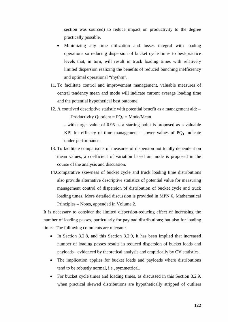
122
section was sourced) to reduce impact on productivity to the degree
practically possible.
• Minimizing any time utilization and losses integral with loading
operations so reducing dispersion of bucket cycle times to best-practice
levels that, in turn, will result in truck loading times with relatively
limited dispersion realizing the benefits of reduced bunching inefficiency
and optimal operational “rhythm”.
11. To facilitate control and improvement management, valuable measures of
central tendency mean and mode will indicate current average loading time
and the potential hypothetical best outcome.
12. A contrived descriptive statistic with potential benefit as a management aid: –
Productivity Quotient = PQT = Mode/Mean
- with target value of 0.95 as a starting point is proposed as a valuable
KPI for efficacy of time management – lower values of PQT indicate
under-performance.
13. To facilitate comparisons of measures of dispersion not totally dependent on
mean values, a coefficient of variation based on mode is proposed in the
course of the analysis and discussion.
14.Comparative skewness of bucket cycle and truck loading time distributions
also provide alternative descriptive statistics of potential value for measuring
management control of dispersion of distribution of bucket cycle and truck
loading times. More detailed discussion is provided in MPN 6, Mathematical
Principles – Notes, appended in Volume 2.
It is necessary to consider the limited dispersion-reducing effect of increasing the
number of loading passes, particularly for payload distributions; but also for loading
times. The following comments are relevant:
• In Section 3.2.8, and this Section 3.2.9, it has been implied that increased
number of loading passes results in reduced dispersion of bucket loads and
payloads - evidenced by theoretical analysis and empirically by CV statistics.
• The implication applies for bucket loads and payloads where distributions
tend to be robustly normal, i.e., symmetrical.
• For bucket cycle times and loading times, as discussed in this Section 3.2.9,
when practical skewed distributions are hypothetically stripped of outliers
123
non-intrinsic to actual loading equipment cycling, the resulting hypothetical
distributions exhibit centralizing tendencies to which reduced dispersion –
lower CV – applies; and increased number of passes does have a beneficial
effect by reducing dispersion, but at the expense of increased loading time.
• Between the practical limits of three passes and eight passes, increasing the
number of bucket passes tends to have reducing dispersion-reduction benefit.
• Table 3.33 provides the relative effect on CV of increasing passes by
assigning an index of 1.00 to the CV for a single pass with increased number
of passes aligning with reducing CV index. The percentage change for each
digital addition to number of passes is also provided in Table 3.33.
• Figure 3.27 illustrates trends of the data in Table 3.33 – particularly the
diminishing benefit of CV reduction as number of passes increase.
• The gradient of the curves in Figure 3.27 are steepest for the range three to
eight passes. For nine passes or more the trends tend to be asymptotic – i.e.,
increased number of passes above eight delivers substantially diminished
returns in dispersion reduction.
• So practical benefit in CV reduction, indicative of distribution dispersion
reduction, is limited to the range three to eight passes with the greatest
potential benefits realised from 3 to 4 (87%), 4 to 5 (89%), 3 to 5 (77%) and 4
to 6 (82%).
Table 3.33 - Coefficient of Variation Index v. Number of Bucket Passes Truck Payloads and Truck Loading Times
Number
of Passes 1 2 3 4 5 6 7 8 9 10 11 12
CV Index 1.000 0.707 0.577 0.500 0.447 0.408 0.378 0.354 0.333 0.316 0.302 0.289 Change
% 0% 70.7% 81.6% 86.6% 89.4% 91.3% 92.6% 93.5% 94.3% 94.9% 95.3% 95.7%
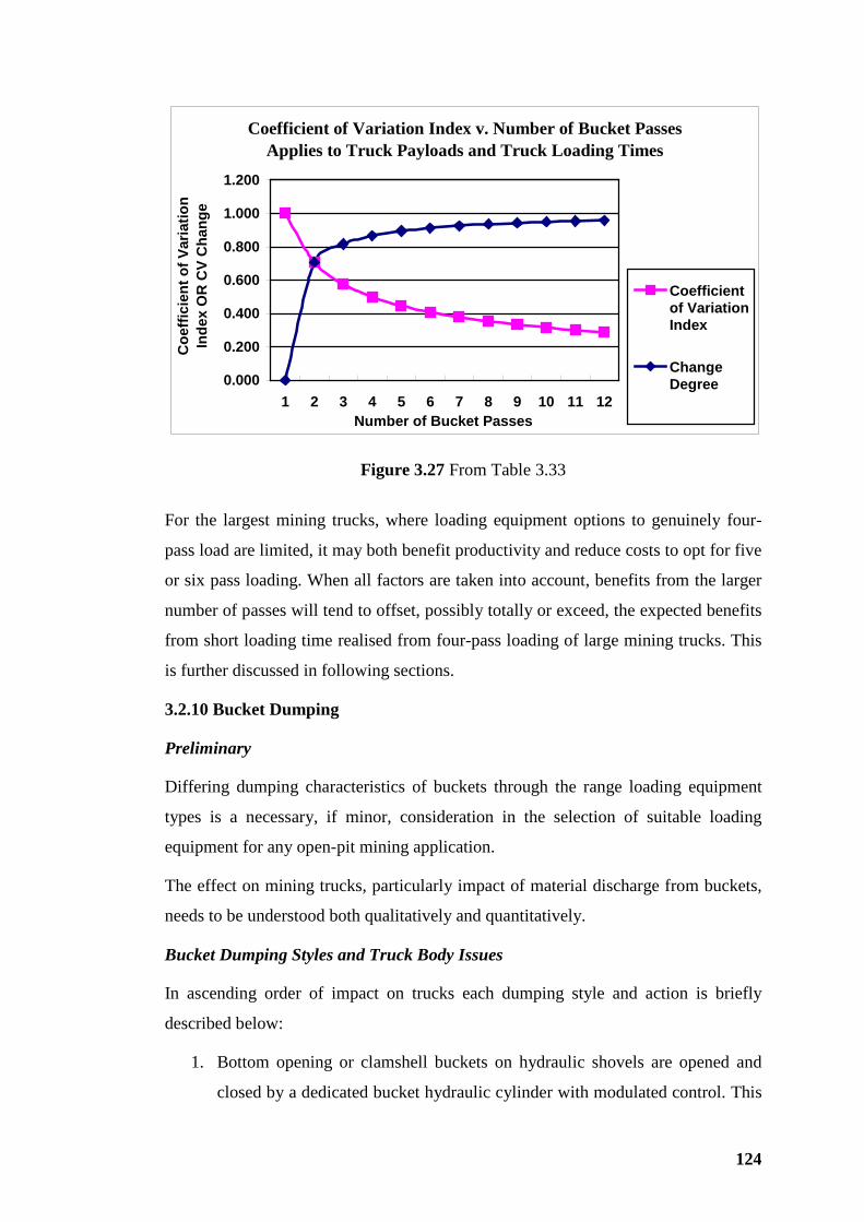
124
Coefficient of Variation Index v. Number of Bucket PassesApplies to Truck Payloads and Truck Loading Times
0.000
0.200
0.400
0.600
0.800
1.000
1.200
1 2 3 4 5 6 7 8 9 10 11 12Number of Bucket Passes
Coe
ffici
ent o
f Var
iatio
n In
dex
OR
CV
Cha
nge
Coefficientof VariationIndex
ChangeDegree
Figure 3.27 From Table 3.33
For the largest mining trucks, where loading equipment options to genuinely four-
pass load are limited, it may both benefit productivity and reduce costs to opt for five
or six pass loading. When all factors are taken into account, benefits from the larger
number of passes will tend to offset, possibly totally or exceed, the expected benefits
from short loading time realised from four-pass loading of large mining trucks. This
is further discussed in following sections.
3.2.10 Bucket Dumping
Preliminary
Differing dumping characteristics of buckets through the range loading equipment
types is a necessary, if minor, consideration in the selection of suitable loading
equipment for any open-pit mining application.
The effect on mining trucks, particularly impact of material discharge from buckets,
needs to be understood both qualitatively and quantitatively.
Bucket Dumping Styles and Truck Body Issues
In ascending order of impact on trucks each dumping style and action is briefly
described below:
1. Bottom opening or clamshell buckets on hydraulic shovels are opened and
closed by a dedicated bucket hydraulic cylinder with modulated control. This
125
arrangement enables dumping with low clearance between bucket and truck,
controlled discharge; and if necessary partial load dumping. Clamshell
buckets on hydraulic shovels can also be rotated forwards with bucket tilt
cylinder(s) to dump a large particle so avoiding any possibility of the particle
bridging and jamming in the bucket – altogether the most versatile bucket
style and facility over the range of loading equipment.
2. Hydraulic excavators, with buckets of cutting-edge width decreasing through
the range mass excavation (mining applications), normal and trenching, dig
with a backhoe action. The excavator works from the top of the face and the
bucket tilt cylinders rotate the bucket away from the face to break out when
bucket is full. When filled the crown of the load is under the stick. With
excessively high bucket fills in hard rock the load can damage the underside
of the stick. When discharging, the bucket tilt cylinder(s) provides
modulation control. Dumping height can be at low clearance – sufficient for
bucket teeth to clear the truck floor or payload when the bucket is reverse
rotating in an “un-curling-like” action. Impact on trucks can be controlled and
comparatively “soft” - similar to clamshell buckets.
3. Front-end wheel-loader (FEWL) buckets have significantly larger capacity
than a hydraulic or rope shovel of equal operating weight. Dimensions of
FEWL buckets reflect the special purpose shape. Typically bucket width :
height and bucket width : depth ratios are large. The bucket must have
sufficient width to protect the front tyres when the loader is crowding the face
to fill the bucket. Generally available dumping height is more limited with
FEWL than with shovels and excavators. Wheel loader operators tram
forward with the bucket at dumping height with the bucket held in the carry
position until the hinge pins (bottom bucket hook up and centre of rotation for
bucket dumping) clear the side rail of the truck. The FEWL is braked to
stationery before front tyres collide with the truck. Simultaneously the bucket
is rotated forward by the bucket cylinder(s) to dump the load. Bucket
cylinder(s) provide modulation during dumping to control discharge rate to
minimize impact on the truck – particularly the first load is controlled to
establish a protective layer on the floor of the truck body. Later bucket loads
are dumped with more speed. The last pass is carefully placed over the load
126
centre of gravity on the truck body if provided and, in default, over the
bottom trunnion of the body lift cylinder as a guide. FEWL operators do have
some facility to centralize each bucket load on the centerline of the truck
body by crowding forward using the bucket as a bulldozer to move material
across the truck. Best-practice operators develop a technique of flicking the
tailings of each bucket load off bucket floor and cutting edge and point
adaptors using the fast, but modulated, bucket cylinder control. This
technique minimizes carry-back in the bucket.
4. Rope shovel buckets have digging-geometry limitations in that the bucket
pitch relative to the stick is adjustable only with pitch braces - short
turnbuckle struts - between bucket and stick. But the pitch braces can only be
adjusted when the shovel is not operating. Unlike hydraulic shovels,
excavators and FEWL, digging geometry of rope shovel buckets cannot be
adjusted on the fly whilst operating. Activating the latch securing the
trapdoor bottom of rope shovel buckets dumps total bucket loads. The load
discharges under gravity pushing the trapdoor clear. Snubbers on the hinges
control swing of the trapdoor. Snubbers are travel dampers (traditionally)
using Beleville spring washers, elastomer pads or hydraulics that positively
damp and limit trapdoor swing to avoid damage by impact between the
bucket trapdoor and the truck body. The dumping system of rope shovels
precludes any modulation or control of bucket dumping. It should be noted
that the pitch angle of the bucket generally prevents free fall of the total
bucket load into the truck body. Typically bucket loads slide down the angled
front face of the bucket so reducing velocity of discharge.
Generally:
• Rope shovels are time-proven well established technology with only
moderate evolutionary change and improvement to bucket design and
appointments. Setting up rope shovel geometry for optimum digging is an art
producing a configuration that is fixed until loading operations are suspended
to make adjustments.
• Hydraulic shovels and mass excavators have the advantage of higher
versatility compared with rope shovels. Partial discharge is possible but rarely
127
practiced. Operators appear to prefer taking a reduced bucket load to top up a
truck payload. Adjustments to digging geometry of hydraulic loading
equipment can be; and as a facet of digging technique are, made at any time
without interrupting loading operations. If necessary, top up of truck payload
by less than a full bucket load can only be effected by taking a partial last
bucket load.
• FEWL bucket technology is well established with evolutionary improvements
limited to bucket cross-section profile to facilitate bucket filling and detailed
design for reduced wear, improved reliability and extended bucket life.
Partial discharge is convenient if necessary. Adjustments to digging geometry
are convenient at any time and part of normal operating technique. FEWL
buckets can serve as a bulldozer for face and dump housekeeping with the
penalty of accelerated underside wear of cutting edge, points and adaptors
and sacrificial wear plates on the underside of the bucket.
The apparent advantage of hydraulic loading equipment compared with rope shovels
in this limited comparison must be considered along with all other comparative
characteristics and more importantly:
• Optimum choice for the operation.
• Productivity.
• Owning and Operating unit cost of production.
The two volumetric standards for bucket capacity are:
• Struck – essentially water line volume taking a line through the back wall top
edge to the base of the bucket points (teeth) - adopted by rope shovel OEM.
• SAE 2:1 Heaped – in addition to the volume to the water line a pyramidal
topping projected with slopes of 2 horizontal to 1 vertical is superimposed -
adopted by OEM offering hydraulic shovels, excavators or FEWL.
Bucket capacity of rope shovels is conservative in comparison with other loading
equipment standards. This is a consideration in pre- selection investigation of loading
equipment. But a more important consideration, for the loading equipment options
under consideration, is the bucket load factor and the actual bucket load per pass,
both volumetrically and in terms of weight that will determine the target mean
128
number of passes to meet the target truck payload (mean) and to match the
volumetric capacity of the truck body.
Truck Body Capacity
Of the several standards for volumetric capacity of mining truck bodies the most
commonly used is the SAE 2:1 rating. The truck body is assumed completely filled
to the side rails with a 1:1 projected slope from the rear discharge edge to side-rail
height. A pyramidal super-load above the body side rails is projected at a slope of 2
horizontal : 1 vertical. Although comparative this protocol is not realised in practice
as some parts of the load, particularly the four corners within the body and above the
side rails, adopt a naturally-reposed, conical shape. Also the sharp pyramidal apex is,
in practice, an artificial concept.
There has been substantial recent attention to this issue. Third party truck-body
design-and-suppliers market on the basis of designs for truck-body volume capacity
that are more realistic than the SAE 2 : 1 standard. This issue is revisited in more
detail in Section 3.3.5.
129
3.3 MINING TRUCKS
3.3.1 Selection Process
The introductory discussion on loading equipment in Section 3.2.1 is equally
applicable to selection of mining trucks for a specific application and production
plan.
The issue of priority of selection – loading equipment or transport equipment – was
briefly introduced in Section 3.2.1. The concept of capacity hierarchy was also
introduced and discussed in Section 3.2.1. It was noted that capacity of loading
equipment generally tends to exceed total mining production requirements; also
tends to exceed the intrinsic capacity of the truck fleet. Evidence of “over-shoveling”
from bench marking studies was discussed in Section 3.2.4. This implied loading
inefficiency is complemented by a benchmark truck utilisation in Australian
metalliferous mines of 50%. That is 50% of annual total hours of 8,760 (Tasman,
1997) with even lower benchmark utilizations in Australian open pit coalmines.
It is believed these benchmark utilizations are ultra-conservative outcomes of open
pit mines mostly producing feedstock for steel mills and power generation. These
comparatively low utilizations are believed to be a symptom of mature producers on
long-term contracts requiring high reliability of supply and with commodity prices
largely cost-driven rather than subject to robust market-place competition. Security
of supply and consistency of product specification are both important factors, the
influence of which tends to shape mining equipment asset management and
operations management strategy in these specific sectors of the mining industry that
constitute a large proportion of open pit mining commercial activity in Australia.
Open pit mines producing precious metals and stones; also high-value base metal
producers, where an open international competitive market largely controls prices
(albeit clouded to some degree by the affect of forward sales and futures trading),
necessarily adopt different equipment inventory strategies. In a highly competitive,
commercial environment, investment in mining equipment, particularly loading and
hauling equipment, tends to be more closely tailored to firm productivity and cost
budgets to realise competitive cost of production – below the median and preferably
in the lower quartile of production costs. This cost-competitive environment can be
expected to yield best-practice outcomes. These commercial characteristics are the
130
backdrop and basis for considerations to follow with overall truck utilisation
assumed to be in the range 65% to 75%.
The risk accepted by selecting loading equipment in isolation was discussed in
Section 3.2.1. A similar risk is attached to selecting mining trucks without
simultaneous consideration of matching loading equipment. Because haulage in open
pit mines contributes a relatively large proportion of total mining costs, 3 to 4 times
the unit cost of loading, it is logical that equipment selection should focus on the
mining-truck options to meet production programmes and then to select loading
equipment from available options to suit the trucks. This is the general policy
recommended and adopted for the purposes of the research described in this thesis.
But mining trucks and loading equipment are so interrelated by cross effects on
mining productivity and costs that some early consideration needs to be given to
suitable loading equipment, - type, size and indicative numbers in concert with
determining type, size and indicative numbers of mining trucks. This will ensure that
when mining truck selection is finalized that loading equipment selection is
essentially confirmatory, without the necessity for major scale and specification
changes.
Truck selection should be the principle focus but with all necessary consideration of
interrelated loading equipment selection issues; and, to a lesser degree, support
equipment, i.e., pit house keeping mobile equipment including dozers. Graders water
trucks and specialised road construction equipment.
3.3.2 Cyclic versus Continuous Haulage
As indicated in Section 3.2.2, cyclic, conventional loading equipment serviced by
cyclic mining trucks – specifically conventional rear-dump, off-highway trucks are
the focus of this thesis. This type of haulage unit is very flexible and imposes fewer
constraints on open pit mine design compared with alternative truck types described
in the following section.
3.3.3 Truck Types and Application
Mining Truck Types
Off-highway trucks can be conveniently classified as three types:
1. Conventional rear-dump.
2. Tractor-trailer - bottom or side dump.
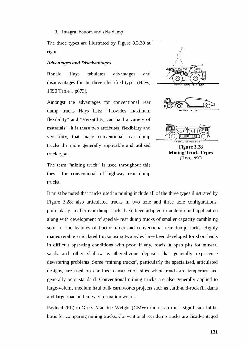
131
3. Integral bottom and side dump.
The three types are illustrated by Figure 3.3.28 at
right.
Advantages and Disadvantages
Ronald Hays tabulates advantages and
disadvantages for the three identified types (Hays,
1990 Table 1 p673).
Amongst the advantages for conventional rear
dump trucks Hays lists: “Provides maximum
flexibility” and “Versatility, can haul a variety of
materials”. It is these two attributes, flexibility and
versatility, that make conventional rear dump
trucks the more generally applicable and utilised
truck type.
The term “mining truck” is used throughout this
thesis for conventional off-highway rear dump
trucks.
It must be noted that trucks used in mining include all of the three types illustrated by
Figure 3.28; also articulated trucks in two axle and three axle configurations,
particularly smaller rear dump trucks have been adapted to underground application
along with development of special- rear dump trucks of smaller capacity combining
some of the features of tractor-trailer and conventional rear dump trucks. Highly
maneuverable articulated trucks using two axles have been developed for short hauls
in difficult operating conditions with poor, if any, roads in open pits for mineral
sands and other shallow weathered-zone deposits that generally experience
dewatering problems. Some “mining trucks”, particularly the specialised, articulated
designs, are used on confined construction sites where roads are temporary and
generally poor standard. Conventional mining trucks are also generally applied to
large-volume medium haul bulk earthworks projects such as earth-and-rock fill dams
and large road and railway formation works.
Payload (PL)-to-Gross Machine Weight (GMW) ratio is a most significant initial
basis for comparing mining trucks. Conventional rear dump trucks are disadvantaged
Figure 3.28 Mining Truck Types
(Hays, 1990)
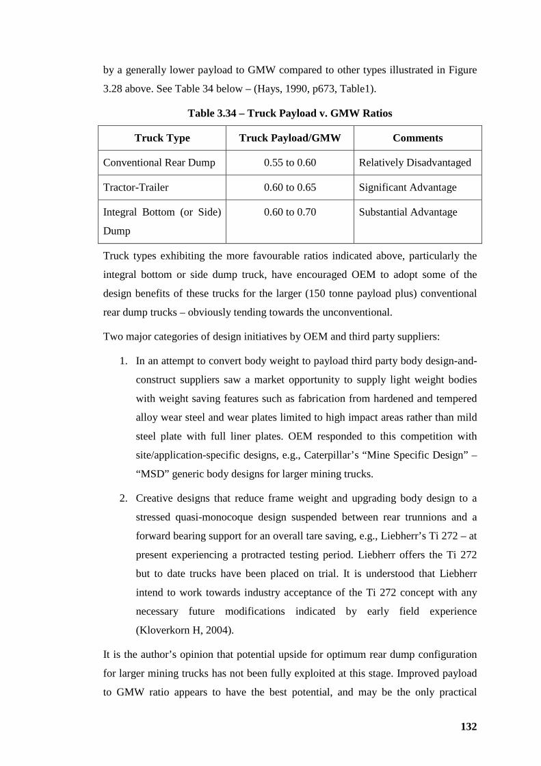
132
by a generally lower payload to GMW compared to other types illustrated in Figure
3.28 above. See Table 34 below – (Hays, 1990, p673, Table1).
Table 3.34 – Truck Payload v. GMW Ratios
Truck Type Truck Payload/GMW Comments
Conventional Rear Dump 0.55 to 0.60 Relatively Disadvantaged
Tractor-Trailer 0.60 to 0.65 Significant Advantage
Integral Bottom (or Side)
Dump
0.60 to 0.70 Substantial Advantage
Truck types exhibiting the more favourable ratios indicated above, particularly the
integral bottom or side dump truck, have encouraged OEM to adopt some of the
design benefits of these trucks for the larger (150 tonne payload plus) conventional
rear dump trucks – obviously tending towards the unconventional.
Two major categories of design initiatives by OEM and third party suppliers:
1. In an attempt to convert body weight to payload third party body design-and-
construct suppliers saw a market opportunity to supply light weight bodies
with weight saving features such as fabrication from hardened and tempered
alloy wear steel and wear plates limited to high impact areas rather than mild
steel plate with full liner plates. OEM responded to this competition with
site/application-specific designs, e.g., Caterpillar’s “Mine Specific Design” –
“MSD” generic body designs for larger mining trucks.
2. Creative designs that reduce frame weight and upgrading body design to a
stressed quasi-monocoque design suspended between rear trunnions and a
forward bearing support for an overall tare saving, e.g., Liebherr’s Ti 272 – at
present experiencing a protracted testing period. Liebherr offers the Ti 272
but to date trucks have been placed on trial. It is understood that Liebherr
intend to work towards industry acceptance of the Ti 272 concept with any
necessary future modifications indicated by early field experience
(Kloverkorn H, 2004).
It is the author’s opinion that potential upside for optimum rear dump configuration
for larger mining trucks has not been fully exploited at this stage. Improved payload
to GMW ratio appears to have the best potential, and may be the only practical
133
potential, for improved productivity and unit owning and operating costs for large
mining trucks It could be reasonably expected that all OEM are pursuing all potential
improvements in payload to GMW ratio for improving the current, and developing
the next generation of large mining trucks.
Conventional rear dump trucks generally have a higher power-to-weight ratio than
other truck types. Together with loaded GMW distribution of 33% on the steering
wheels and 67% on the dual driving wheels, high power-to-weight realizes better
gradeability for deep pit operations.
Larger conventional rear dump trucks generally have higher average wheel loadings
that are more demanding on tyres leading to speed-haul distance limitations
compared with other types of trucks. Wheel loadings and tyre performance for the
various truck types will be considered in more detail in 3.3.7 below.
3.3.4 Intrinsic Truck Performance
Performance of all off-highway trucks, including mining trucks of the conventional
rear-dump type, is a function of the following:
Componentry – An Historical Review
Drive Line Components – typical simplified lists:
Mechanical Trucks: Engine, torque converter, transmission, differential and final
drives.
Electric Drive Trucks: Engine, alternator, converter, DC wheel motors with integral
reduction gear train and mechanical final drives; alternatively, from converter,
inverter, AC drive motors with integral reduction gear train and mechanical final
drives.
Historically OEM shared many of the above components.
OEM commonly engineered trucks around available components from three major
engine suppliers, two major torque converter/transmission third party suppliers, and
three electrical driveline component suppliers.
More recently two OEM have emerged from the industry rationalization as suppliers
of the full range of mechanical drive developing their own engines, transmissions
134
and complete drivelines. Obviously some of the componentry is outsourced but
supply is to purchasers’ specification and standards and, often, designs.
The field of OEM manufacturing electric-drive trucks has been rationalized from
four majors and as many second tier manufacturers to four enjoying significant
market share. OEM continue to supply large mining trucks with designs engineered
around electric-drive components from three major third-party suppliers. Engines are
sourced from two major suppliers and offered to customers to make a choice
With substantial commonality in designs, specification and even componentry,
differences in intrinsic performance of mining trucks offered by any OEM tend to be
more subtle than substantial.
Early development of off-highway trucks was essentially an extrapolation of
configurations and designs of conventional highway vehicles. Engine, clutch,
transmission and driveline to the rear wheels was typical in the earliest off-highway
trucks. Power-shift transmissions (first seen in early Ford Model T vehicles some
100 years ago) and hydraulic torque converters were to follow with the next advance
to automatic-shift transmissions.
Development of mechanical drive mining trucks stalled at 50 tonne capacity in the
1950’s encouraging the adoption of DC electric traction drives from railway
locomotives to increase truck capacity successively through 65, 75, 85 100, 120 to
150 and ultimately 200 tons (of 2,000 lbs). Mechanical drive trucks eventually
caught up increasing in capacity through 85, 100 to another plateau at 120 ton trucks
due to non-availability of transmissions rated at 900kW or more. Over the most
recent 20 years OEM have developed and offer trucks up to 360 tons with a choice of
mechanical or AC electric drive with DC drive losing favour for the larger capacity
mining trucks.
The efficiency advantage from engine flywheel to road of mechanical drives
compared with DC electrics has encouraged development of AC wheel motors that
closely compete with mechanical drive efficiency for the largest mining trucks. The
new AC systems have subsequently been retroactively developed down to 120-ton
trucks.
Steering and braking performance must comply with recognized international
standards from SAE, ISO or standards endorsed in the country where trucks will
135
operate. All OEM can be expected to ensure that steering and braking systems have
substantial excess performance above the minimum standard to ensure compliance
after some moderate deterioration consistent with reasonable wear and tear before
mandatory maintenance and to allow for varying operator efficiency. But steering
and braking systems are still cost-driven designs (to a low degree of acceptable
residual risk) that can be expected:
• To have comparable rather than significantly different performance over the
full range of truck capacities and for all OEM.
• To have warranty limited to a maximum GMW or payload – Caterpillar’s
policy is a maximum over-target payload of 120% (some 11% of GMW).
Similar design-and-supply philosophy generally applies through all componentry for
large mining trucks.
Engines for large mining trucks have traversed several phases of development. All
engines for mining trucks use Diesel’s cycle with relatively recent historical trading
off of extended torque curves in favour of engine speed – “over-square” engines.
Even more recently there has been a reversal of this trend with increasing engine
stroke delivering the advantage of lower BMEP (brake-mean-effective-pressure),
longer engine life and, importantly at current prices, improved fuel economy.
The study of engines for large mining trucks, the design issues, future opportunities
including lubricant disposal through supplementation of fuel is a substantial research
subject in its own right.
Debate continues between operators, OEM and suppliers of large mining trucks on
the relative merits of mechanical compared with electric-wheel, particularly AC,
drive.
Mechanical drive componentry modifies the conventional umbrella-shaped speed-
torque curve of diesel engines to a flatter torque curve in saw-tooth form by changing
transmission ratios so providing an extended torque range many times the range of
the useful torque range of engines.
DC drives have been disadvantaged in that the speed-torque curve with its
spectacular low speed rise to peak torque tends to fall away quickly so limiting truck
acceleration to a short initial period.
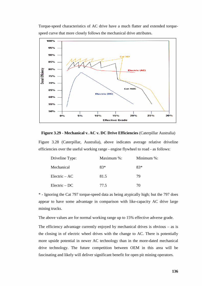
136
Torque-speed characteristics of AC drive have a much flatter and extended torque-
speed curve that more closely follows the mechanical drive attributes.
Figure 3.29 - Mechanical v. AC v. DC Drive Efficiencies (Caterpillar Australia)
Figure 3.28 (Caterpillar, Australia), above indicates average relative driveline
efficiencies over the useful working range - engine flywheel to road - as follows:
Driveline Type: Maximum %: Minimum %:
Mechanical 83* 83*
Electric – AC 81.5 79
Electric – DC 77.5 70
* - Ignoring the Cat 797 torque-speed data as being atypically high; but the 797 does
appear to have some advantage in comparison with like-capacity AC drive large
mining trucks.
The above values are for normal working range up to 15% effective adverse grade.
The efficiency advantage currently enjoyed by mechanical drives is obvious – as is
the closing in of electric wheel drives with the change to AC. There is potentially
more upside potential in newer AC technology than in the more-dated mechanical
drive technology. The future competition between OEM in this area will be
fascinating and likely will deliver significant benefit for open pit mining operators.
137
Fuel burn rates are directly related to the above-indicated efficiencies for trucks of
equal GMW. So fuel economy has been the principal focus in comparing alternative
truck drive systems. Recent fuel price increases seem to be persistent and likely to
have long-term effect making the comparison focus even more acute.
Characteristics of drive system options:
Mechanical Drive: Driving response and travelling characteristics closest to on-
highway vehicle, fuel-efficient, very mature technology development, with
comparatively less potential for improvements. Starting torque modulation control is
an advantage on wet or soft benches.
AC Drive: Driving response has specific characteristics, starting torque can be very
high so heavy foot = wheel spin with increased risk of tyre cutting on wet benches,
electric resistance braking response is different requiring different skill in
application, close to mechanical drive fuel efficiency, improved electrical efficiency
compared with DC, more recent technology with significant improvement potential.
DC Drive: As the forerunner, exhibits driving characteristics similar to AC drives.
Dated technology that is disadvantaged in terms of efficiency, performance and cost
effectiveness compared with mechanical and AC drives. DC appears to be phasing
out in favour of AC drives, introduced for the largest mining trucks and in process of
retroactively replacing DC drive systems.
Which drive system is best? There is no clear favoured system. The decision to opt
for either mechanical or AC drive may rest on the comfort the owner/operator has
with electric drive technology, physical conditions in the open pit including haul road
profile, wet and soft running conditions in loading areas with potential for tyre
damage and road construction and maintenance standards.
In the broad view, differences, although measurable in intrinsic performance terms,
in the ultimate productivity and cost differences tend to be subtle. Selection needs to
focus on greater differences such as product support, how the selected truck fits into
local skills demography, pit geometry and environmental issues. High top speed is of
little use if the opportunity to use it is limited or denied by operating circumstances
or other limitations such as tyres, overheating in high ambient temperature.
138
3.3.5 Body Selection and Truck Payload
Body Development and Experiments
Evolution of body designs has created a classifiable range that is described by
Ronald Hays (Hays, 1990, p675) as follows:
“Rear dump bodies are available in several basic styles with the following most
common:
Transverse V-shaped, flat bottom floor;
Transverse V-shaped, longitudinal V-shaped floor;
Horizontal, flat bottom floor;
Horizontal, longitudinal V-shaped floor.”
“Transverse V-shaped” describes the side profile of the truck body – alternatively
termed “wedge” design - currently the industry standard profile. Current body
designs are tending to favour flat bottom floors – particularly favoured by special
weight-saving designs, such as Caterpillar’s MSD (Mine Specific Design) body
options, offered for larger mining trucks.
Since 1990 evolution of mining trucks has marched on with several notable advances
to enhance performance and contain costs:
• Initiatives in modular design to facilitate maintenance described in more
detail in Section 3.3.8 below.
• Reduction of tare, or “nett machine weight” (NMW), as it is more often
termed in the industry, to realise increased payload for a constant GMW. As
indicated above, recent body design philosophy, initiated by third party body
suppliers and counter-response by OEM, aims to reduce tare in favour of
increased truck payload. So OEM and distributors occasionally have to
supply with, or ready for, a third party designed and supplied body.
• Gravitating to wedge shaped bodies with flat floors as an emerging design
standard relatively simple to fabricate and refurbish.
• “Duck tails” – Hays’ “upward sloped tail chute” (Hays, 1990, p675) are in the
past. Current practice for load retention is to rely on forward slope of the flat
floor supplemented by liners in the form of rock-box grillages that retain fine
139
material so protecting the body floor in the high-wear area. Protection options
for high wear areas inside bodies including the “duck tail” are illustrated by
Figures 3.30 to 3.33,
• There has been some interest in “limited-life” bodies where cost of early
replacement is traded off against reduced on site repairs and increased
payload. A brief initiative by OEM and third party body suppliers to produce
Ultra Light Weight (ULW) bodies was rewarded with only limited success.
This concept of bodies designed for regular total replacement has contracted
to applications with relatively low-impact and low-wear materials – where
sufficient body life is realised to justify total replacement cost
• ULW bodies for large mining trucks have been tested in iron ore, oil/tar sands
and coal overburden applications with little success. Applications for
lightweight, highly fragmented and low-abrasion materials have enjoyed
some success. Hard-rock, moderate-to-severe, applications have moved on to
more robust designs. There is significant local (Western Australia) history of
ULW trials with some successes; but also substantial failures – particularly in
more severe hardrock applications. At present the “limited-life” philosophy
does not appears to have significant or increasing following. It is not clear if
the apparent lack of interest is due to misapplication, resistance to change
within maintenance management or “great-idea-poor-design-and-execution”
syndrome or a combination of these. But there is manifest ground swell of
mood for change/reversion to more robust designs.
• Bodies fabricated from aluminum alloy; also rubber-lined with cable-
suspended rubber floors have also been field tested, particularly where
loading noise from steel bodies is perceived as a problem. These experiments
enjoyed only limited success being confined to operations where material
hauled is low impact, usually for long hauls and where cost of roads to
highway (unsealed) standards (to reduce site-severity vibration effects on
light weight bodies) can be justified.
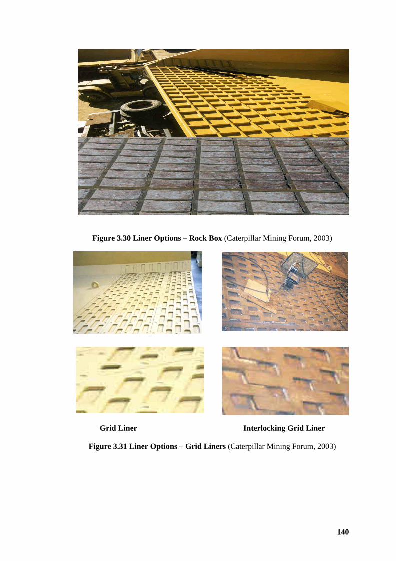
140
Figure 3.30 Liner Options – Rock Box (Caterpillar Mining Forum, 2003)
Grid Liner Interlocking Grid Liner
Figure 3.31 Liner Options – Grid Liners (Caterpillar Mining Forum, 2003)
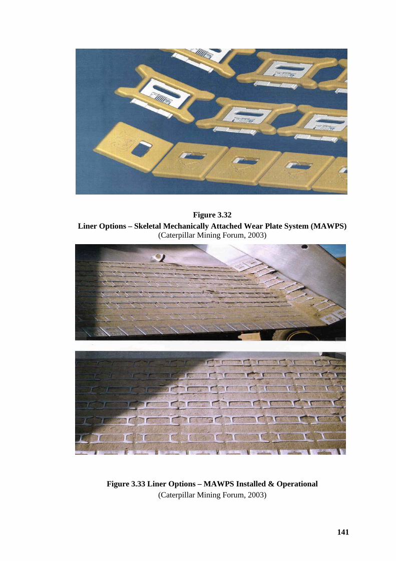
141
Figure 3.32 Liner Options – Skeletal Mechanically Attached Wear Plate System (MAWPS)
(Caterpillar Mining Forum, 2003)
Figure 3.33 Liner Options – MAWPS Installed & Operational (Caterpillar Mining Forum, 2003)
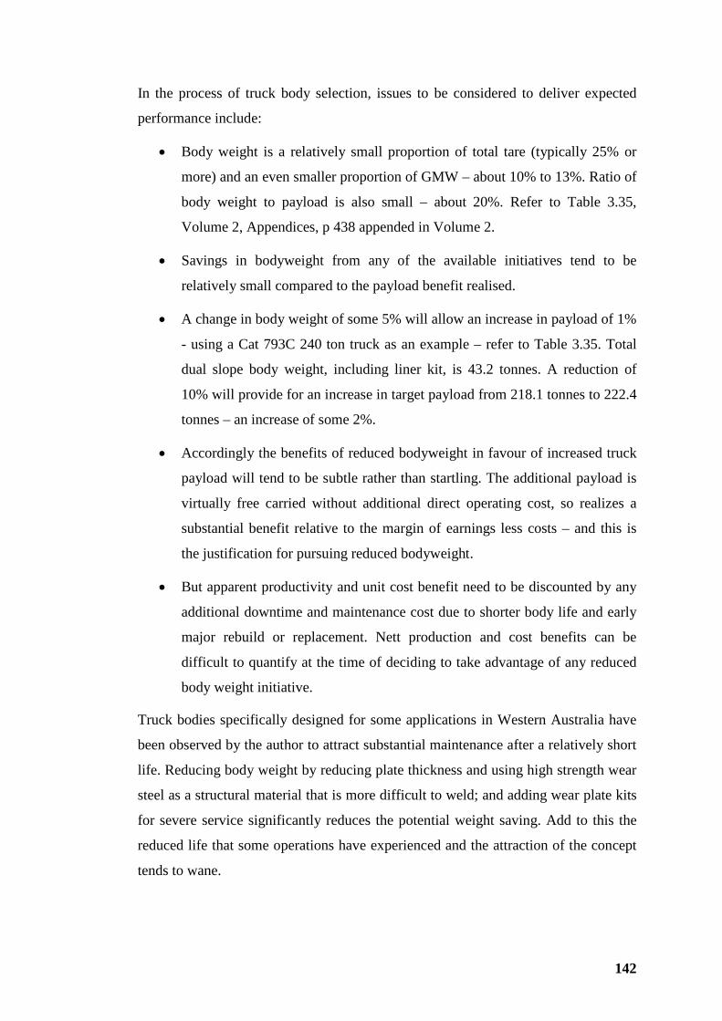
142
In the process of truck body selection, issues to be considered to deliver expected
performance include:
• Body weight is a relatively small proportion of total tare (typically 25% or
more) and an even smaller proportion of GMW – about 10% to 13%. Ratio of
body weight to payload is also small – about 20%. Refer to Table 3.35,
Volume 2, Appendices, p 438 appended in Volume 2.
• Savings in bodyweight from any of the available initiatives tend to be
relatively small compared to the payload benefit realised.
• A change in body weight of some 5% will allow an increase in payload of 1%
- using a Cat 793C 240 ton truck as an example – refer to Table 3.35. Total
dual slope body weight, including liner kit, is 43.2 tonnes. A reduction of
10% will provide for an increase in target payload from 218.1 tonnes to 222.4
tonnes – an increase of some 2%.
• Accordingly the benefits of reduced bodyweight in favour of increased truck
payload will tend to be subtle rather than startling. The additional payload is
virtually free carried without additional direct operating cost, so realizes a
substantial benefit relative to the margin of earnings less costs – and this is
the justification for pursuing reduced bodyweight.
• But apparent productivity and unit cost benefit need to be discounted by any
additional downtime and maintenance cost due to shorter body life and early
major rebuild or replacement. Nett production and cost benefits can be
difficult to quantify at the time of deciding to take advantage of any reduced
body weight initiative.
Truck bodies specifically designed for some applications in Western Australia have
been observed by the author to attract substantial maintenance after a relatively short
life. Reducing body weight by reducing plate thickness and using high strength wear
steel as a structural material that is more difficult to weld; and adding wear plate kits
for severe service significantly reduces the potential weight saving. Add to this the
reduced life that some operations have experienced and the attraction of the concept
tends to wane.
143
In the end result, enhancing payload by reducing truck tare through reduced body
weight is likely cost advantageous providing that all maintenance risks are identified,
assessed and, as necessary, treated before finalizing the financial justification to
proceed.
Body Volume Capacity and Standards
Volumetric capacity of truck bodies has traditionally been based on SAE standards;
both struck and heaped 2:1 capacities (Hays, 1990)
OEM specifications for mining trucks generally provide both struck and heaped 2:1
volumes; but, at least, the heaped 2:1 capacity will be provided. The pyramidal
projection and sharp peak of this standard model for truck body capacity is artificial
and is not realised in practice and can only be considered as an indicative guide. A
particular impractical perception is that the rear free face of struck volume is
projected back from the discharge edge at 1:1 – an obviously optimistic, impractical
model of angle of repose of most mined materials in a truck. The heaped 2:1 model is
essentially a pyramidal shaped projection superimposed on the struck volume.
Experience shows that the general angle of repose of most materials mined is steeper
than 2:1; but certainly not as steep as 1:1. Actual corners of truck payloads are not
sharp but tend to be conical sectors with a rounded truncation of the peak.
Ronald Hays advises: “Experience indicates that actual capacities are about 105% to
130% of SAE (standard) struck volumes with higher percentages valid for largest
trucks with wide bodies and top (side rail) extensions.” (Hays, 1990).
Table 3.35, appended in Volume 2, provides a list of Caterpillar mining trucks
showing that ratio of OEM-specified 2:1 heaped volume to struck volume varies
from 127% to 143% with modal ratios in order of 133%. High values in this range of
trucks are for a 90 tonne payload truck that has a relatively wide body compared with
both wheelbase and body target length. Low values are for the largest truck currently
available with a relatively short target length and close-to-square body target. Mining
trucks from other OEM can be expected to exhibit similar relationships between
struck and heaped 2:1 rated capacity; also for the other specification items in Table
3.35.
The actual volume accommodated by a truck body does not conform to the
hypothetical solid geometrical configuration of SAE heaped 2:1. Natural angle of
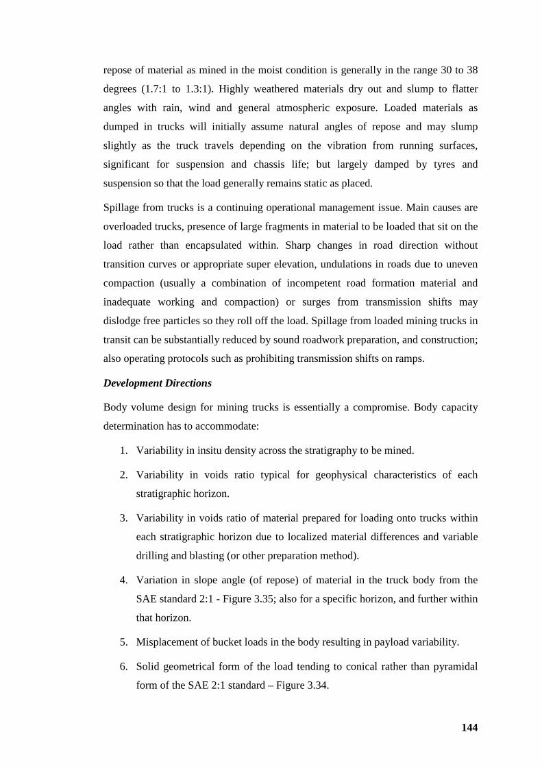
144
repose of material as mined in the moist condition is generally in the range 30 to 38
degrees (1.7:1 to 1.3:1). Highly weathered materials dry out and slump to flatter
angles with rain, wind and general atmospheric exposure. Loaded materials as
dumped in trucks will initially assume natural angles of repose and may slump
slightly as the truck travels depending on the vibration from running surfaces,
significant for suspension and chassis life; but largely damped by tyres and
suspension so that the load generally remains static as placed.
Spillage from trucks is a continuing operational management issue. Main causes are
overloaded trucks, presence of large fragments in material to be loaded that sit on the
load rather than encapsulated within. Sharp changes in road direction without
transition curves or appropriate super elevation, undulations in roads due to uneven
compaction (usually a combination of incompetent road formation material and
inadequate working and compaction) or surges from transmission shifts may
dislodge free particles so they roll off the load. Spillage from loaded mining trucks in
transit can be substantially reduced by sound roadwork preparation, and construction;
also operating protocols such as prohibiting transmission shifts on ramps.
Development Directions
Body volume design for mining trucks is essentially a compromise. Body capacity
determination has to accommodate:
1. Variability in insitu density across the stratigraphy to be mined.
2. Variability in voids ratio typical for geophysical characteristics of each
stratigraphic horizon.
3. Variability in voids ratio of material prepared for loading onto trucks within
each stratigraphic horizon due to localized material differences and variable
drilling and blasting (or other preparation method).
4. Variation in slope angle (of repose) of material in the truck body from the
SAE standard 2:1 - Figure 3.35; also for a specific horizon, and further within
that horizon.
5. Misplacement of bucket loads in the body resulting in payload variability.
6. Solid geometrical form of the load tending to conical rather than pyramidal
form of the SAE 2:1 standard – Figure 3.34.
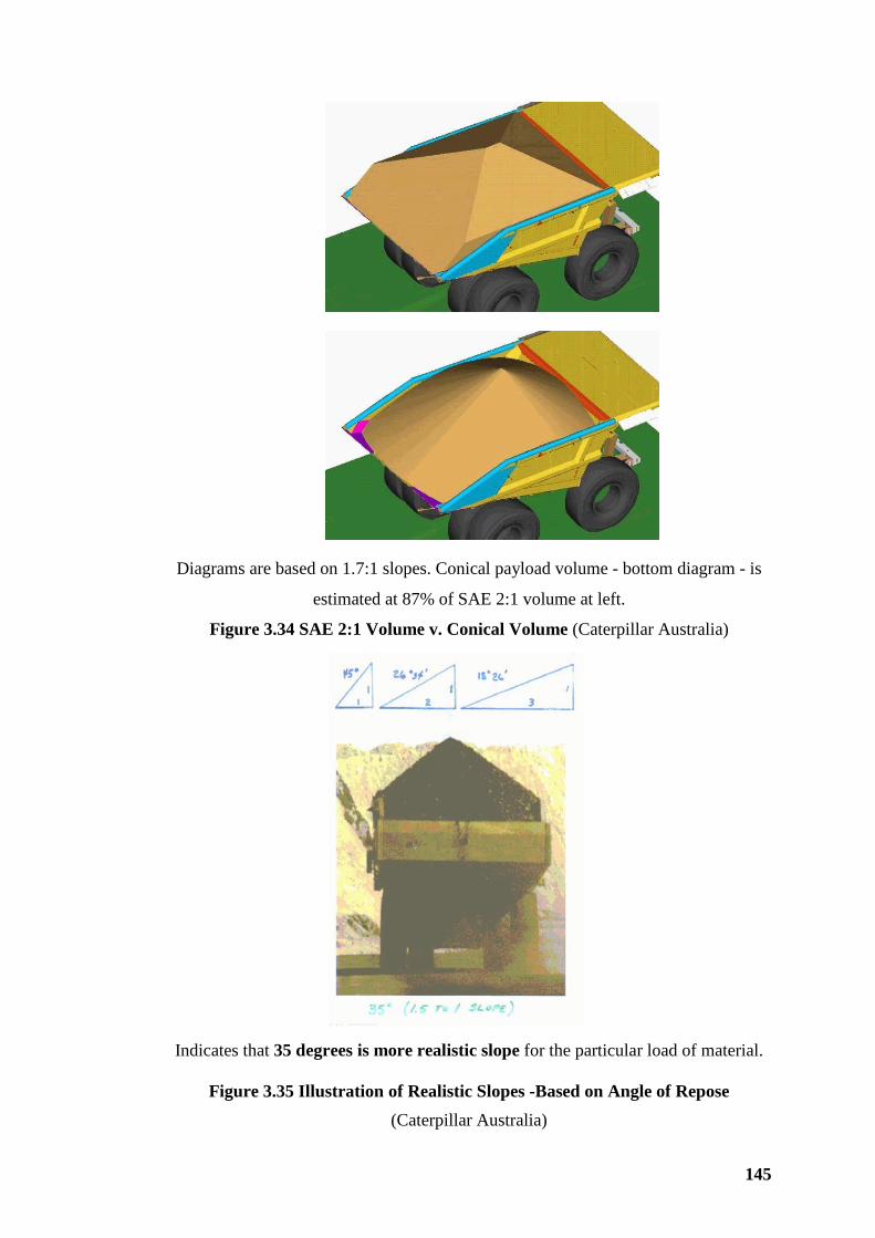
145
Diagrams are based on 1.7:1 slopes. Conical payload volume - bottom diagram - is
estimated at 87% of SAE 2:1 volume at left.
Figure 3.34 SAE 2:1 Volume v. Conical Volume (Caterpillar Australia)
Indicates that 35 degrees is more realistic slope for the particular load of material.
Figure 3.35 Illustration of Realistic Slopes -Based on Angle of Repose (Caterpillar Australia)
146
Determination of body capacity of mining trucks is based on:
• Insitu density provided by the purchaser/future operator (from a number of
apparent rock density determinations).
The following are best performed cooperatively between purchaser and supplier:
• Adoption of a load factor that is a convenient ratio of loose to insitu density
that, in application, accommodates all of the factors such as swell, voids ratio,
and their variability (Caterpillar, PHB 35).
• A factor allowing for the expected variation in slope angle and solid
geometrical form of the payload relative to SAE 2:1 rating – 87% is one
estimate – Figure 3.34.
• Mining truck OEM and third party body suppliers are designing bodies using
capacity criteria modelled on actual observations of load form. In detail the
form of the load model is considered to be conical above the side rail so
causing voids at front and rear corners rather than pyramidal as assumed by
the SAE heaped 2:1 standard. There is some compensation for the corner
voids with adoption of angles of repose steeper than 2:1. Figure 3.34 and
Figure 3.35 above, from Caterpillar, illustrate the concept of conical load
profile and slopes steeper than 2:1 – 1.7:1 in the concept of Figure 3.34.
Although truck specifications from all OEM include the SAE 2:1 capacity, for axle-
load distribution specifications; and for body design, more realistic load profiles have
been adopted. Particularly for the recently developed Cat MSDII body; and
equivalents from other OEM and third party body suppliers, initiatives have been
based on more realistic load modelling.
Bodies for larger trucks now tend to be designed for the mining conditions to be
experienced. Caterpillar’s MSD bodies are an example. The type of material to be
transported, fresh rock, transition or highly weathered, including abrasion potential
are assessed and bodies designed to the specification including expected
material density. Bodies so designed are fabricated from hardened and tempered
weldable alloy steel. Liner kits are limited to light impact inserts across the front
147
bulkhead and body floor with wear protection at discharge – rock boxes or one of a
number of grid liners on offer as illustrated by Figures 3.30 to 3.33.
Reference to Table 3.35, appended Volume 2, indicates that body weight for
Caterpillar trucks (including liners) only constitutes 8% to 14% of GMW – and 15%
to 20% of truck payload. So a reduction of 10% of bodyweight will realize 1.5% to
2.5% addition to payload.
A typical Caterpillar MSD design for a 793C mining truck (nominal 240 tons) is
illustrated by Figures 3.3.5.7A and B appended. It will be noted that:
• Compared with the flat floor body weight in Table 3.35, the 793C MSD body
realizes weight saving of 8 tonnes i.e. some 20% of body weight, allowing
some 3.5% increase in target payload.
• Heaped 2:1 volume rating has increased from 147.7 to 175.8 cubic metres to
accommodate relatively low density material at 1.6 tonnes per loose cubic
metre.
• Corner fillets (standard for Caterpillar MSD bodies) provided in the particular
design and application are intended to inhibit saturated sandstone and
mudstone sediments from the partings between multiple coal seams
compacting in reentrant corners as “carryback”: (the corner fillets also
function structurally to stiffen the corners and avoid high stress
concentrations at 90 degree reentrant corners).
• The comparatively light liner plates of 450 Brinell Hardness Number (BHN)
weldable steel on the rear floor and sides plus floor impact plates are
supplementary wear treatment on a body generally designed to be wear
resistant, being fabricated from weldable 400 BHN hardened and tempered
alloy steel plate.
• The typical MSD cutaways at the rear of body sides are shown in detail in
Figures 3.3.5.7A and 3.3.5.7B. This saves weight of unnecessary body side
extensions and discourages overfilling the body to spill over the discharge
edge with the risk of further spillage whilst hauling.
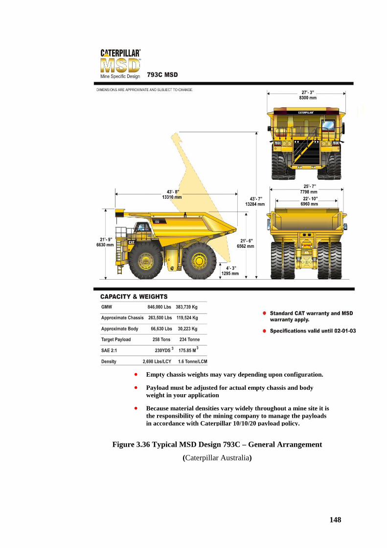
148
Figure 3.36 Typical MSD Design 793C – General Arrangement
(Caterpillar Australia)
• Empty chassis weights may vary depending upon configuration.
• Payload must be adjusted for actual empty chassis and body weight in your application
• Because material densities vary widely throughout a mine site it is the responsibility of the mining company to manage the payloads in accordance with Caterpillar 10/10/20 payload policy.
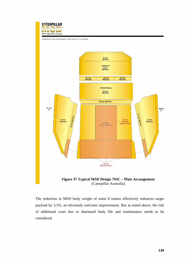
149
The reduction in MSD body weight of some 8 tonnes effectively enhances target
payload by 3.5%, an obviously welcome improvement. But as noted above, the risk
of additional costs due to shortened body life and maintenance needs to be
considered.
Figure 37 Typical MSD Design 793C – Plate Arrangement (Caterpillar Australia)
150
The example described is for moderate to light duty, accommodating low impact
materials that are abrasive having high silica content. The reduction of 20%
illustrated can be considered as a typical practical limit.
An improvement in the second generation of development in MSD II bodies is a
flare-out from front to rear to reduce wear on body sides and bottom corners. For a
nominal 220 tonne truck the taper is some 300 mm front to rear. Technically this
increases the operating width of the truck; but the overall increase is small – some
150 mm – compared with the nominal specified width of 7.41 metres.
An important consideration in hauling efficiency is carryback of material in the body
generally compacted into reentrant corners where sides meet the floor - more
importantly in the front corners. Corners fillets can be seen in Figures 3.36 and 3.37
as a treatment to reduce carryback. Early designs of truck bodies included rolled or
pressed plate circular quadrant fillets to all body corners. This detail seems to have
been abandoned in the interests of construction simplicity and cost. The 450 BHN
hardened and tempered plates are likely not amenable to pressing or rolling. But it
would possible to make up corner quadrants in mild steel plate and provide wear-
resistant liner-plate protection.
Truck Bodies For A Range of Material Density
Open pit developers and mining operators often have to cope with hauling of
materials with a range of density. Some typical examples are discussed below.
A. An open pit coal mine of moderate scale where a laterite capping overlays
tertiary sediments – transported granite detritals – that overlay sub-
bituminous coal measures with sandstone-mudstone partings. Typical density
profile is:
Insitu ARD – tonnes/bank cubic metre
Laterite Capping Estimated 2.4 - small quantity
Tertiary Sediments 2.0
Shale Partings 1.8
Coal 1.34
B. A deep open pit gold mine with shallow, transported, lateritic gravelly clays
ranging in depth from zero to as deep as 30 metres across the pit width
overlaying a weathered zone down to 60 metres depth (ranging from 2 metres
151
to 60 metres or more) with a sharp oxidation cutoff, typical of the Achaean
greenstone stratigraphy of the Eastern Goldfields of WA. Typical density
profile:
Insitu ARD – tonnes/bank cubic metre
Gravel Clays 1.8 (author’s estimate)
Weathered Zone 2.4 (author’s estimate)
Fresh Rock Zone 2.8
C. A deep base metal open pit with laterite cover down to some 3 metres over
leached out clay weathered zone as deep as 30 metres, followed by a
transition zone of some 20 to 30 metres exhibiting the complete range of
incompetent clay to fresh rock to an oxidation cutoff above fresh rock.
Typical insitu density profile is:
Insitu ARD – tonnes/bank cubic metre
Laterite 2.4
Weathered Zone 2.2
Transition Zone 2.4
Fresh Rock Zone 2.6
Example A:
Rope shovels load a mixed fleet of mining trucks currently in process of rolling over
to a 220 tonne mechanical drive fleet. Coal is hauled in the same trucks used for
overburden and interburden, i.e., partings between the seams. Body size is selected
for overburden and interburden. Full-volume payloads of coal under-load the trucks.
The coal-haul distance from pit exit to crusher is some 5 km of fast, flat road. So the
lightly loaded trucks reduce the TKPH (tonnes-kilometres-per-hour) demand on
tyres. The operator opts for the flexibility of this arrangement in preference to a
dedicated fleet of smaller mining trucks with bodies sized for coal.
It is understood that new mining trucks are sized for the sandstone/mudstone partings
that are of similar loose density to the tertiary sands.
Example B:
Current open pit depth is more than 300 metres with an ultimate depth exceeding 500
metres. As the pit deepens, the proportion of tertiary detritals and weathered zone
becomes less as the pit walls are pushed back.
152
In this example truck bodies are selected for the estimated loose density derived from
estimated swell (voids ratio) and an insitu density of 2.88. Any inefficiency due to
transporting lighter materials that are relatively small quantities is absorbed in
mining costs – assumed to be a studied compromise.
It should be noted that historically detritals and weathered zone were a more
significant proportion of total production. This was a period when the current open
pit was worked as several individual relatively shallow open pits along a strike of
several kilometres. As the pits have coalesced into one large pit, the proportion of
lower-density material has reduced significantly.
Example C:
Current pit depth is some 200 metres with a final design depth of some 400 metres. A
compromise similar to Example B above has been made in this case.
In this particular case the open pit was commenced with a substantial pre-strip of
weathered and transition zones to the base of transition and into the fresh rock zone
hosting the ore targets to expose and commence mining of first ore. As the open pit
has developed, the proportions of lower density weathered and transition materials
have diminished – as with Example B. For this operation truck body capacity has
been selected for the fresh rock zone with a density of 2.6 tonnes per BCM and a
loose density assessed as 1.7 tonnes per LCM.
In each of the above cases truck body capacity is essentially a compromise. The
options are:
1. Select bodies to carry optimum truck payload with the material of expected
lowest loose density and control potential truck overload by monitoring
indicated truck payload with a load measuring system such as Caterpillar’s
VIMS or equivalent with indicator light or digital readout – and, in default,
by limiting the number of bucket loads in each payload.
2. Select bodies to accommodate optimum truck payload of material density
corresponding to the maximum quantity in the suite of differing density
materials to be hauled. For higher density materials truck payloads can be
controlled as described in option 1 above. For lower density materials, any
inefficiency caused by under loading trucks is a compromise to be accepted
and absorbed; but there is always the option to fit side rail extensions
153
(“hungry boards”) temporarily or permanently provided the quantity of lower
density material justifies the cost of body-capacity enhancement.
Each case of multiple material densities needs to be considered on its merits; and
comparative unit costs compiled for loading and hauling in each case. As with many
cost comparisons in the process of equipment selection; or operating open pit mines,
particularly unit cost differences tend to be subtle. But for this particular case, the
difference between comparative costs can be considered a valid basis for decision if
those costs are prepared diligently and with the necessary precision to suit any
comparison that may be made.
It should be noted that truck fleet additions and replacements are an opportunity to
re-visit truck-body capacity and body design in general. This is a typical due-
diligence opportunity that should not be overlooked in the process of acquiring new
haulage equipment.
As a last point:
It is manifestly important to ensure that truck-body capacity should be comfortably
sufficient to accommodate optimum mean truck payload. It is a far more comfortable
management priority to control mean truck payloads down to target payload than to
suffer the inefficiency and cost of under loaded trucks with the fallback remedy of
adding extensions (“hungry boards”) to body side rails to increase truck body
capacity.
Interpretation and Comments
Recent efforts by OEM and third party body designer-suppliers to increase payloads
and so improve payload : GMW ratio by refined body designs have been successful
but necessarily limited in effect. Selecting body designs resulting from these
initiatives necessarily has to be justified on the basis of productivity and cost
analysis. Any initiatives by OEM and third-party suppliers to improve body designs,
reduce body weights and improve payloads are obviously potentially beneficial in
terms of productivity. But the outcomes can be expected to the useful rather than
spectacular. Although possibly of moderate rather than spectacular value,
Caterpillar’s MSD truck bodies or equivalents from other OEM are likely justifiable,
even attractive to open pit mining operators, on the basis that small contributions
154
accumulate to significant improvement – a fundamental continuous improvement
philosophy.
Compared with refined body design, there is greater potential for productivity and
cost improvements by moving on from the time-honoured 2-4 wheel mining truck
configuration with payload : GMW ratios in the range 0.55 to 0.60. Recent industrial
advances in this direction were briefly discussed in Section 3.3.3. It can be expected
that initiatives will surface in the future to substantially improve payload : GMW
ratio for mining trucks by creative designs and non-traditional configurations.
3.3.6 Truck Payload Measuring Initiatives
Preliminary Discussion – History and Current Status
Discussion in Section 3.3.5 on body selection design describes questionably practical
body capacity specification standards and recent efforts to develop bodies with
capacity based on more realistic volumetric models.
Payload weight measuring developments have been a continuing focus of OEM, tyre
suppliers and equipment operators. Intrinsic truck performance is a function of
GMW (tare plus payload weight) and NMW - tare weight alone. Early payload
measuring consisted recording a relatively small sample of payloads effected by
weighing trucks unloaded (tare/NMW) and loaded (GMW). Mining trucks were
(and, for calibration purposes, still are) weighed wheel-by-wheel using a
transportable platform weighbridge temporarily installed at road level. Payload is
derived by difference between GMW and NMW.
Payload control has historically relied on operators sustaining consistent, repeatable
volumetric loading practice visually with occasional weighbridge verification of
payload actually achieved.
On-board Payload Measuring
More recent payload measuring developments utilise sensing of differences in
suspension cylinder pressures for loaded and unloaded trucks to determine NMW
and GMW. Initially systems were prone to significant error due to derivations based
on single, static readings of suspension pressures from stationary trucks. Caterpillar’s
Truck Payload Measuring System (TPMS) is an example still offered; but in much
155
improved form, for smaller trucks where the complete VIMS system is not justified.
Similar systems are offered by all truck OEM.
More recent improvements include Caterpillar encapsulating TPMS within the VIMS
system. Still based on sensing suspension cylinder pressures, the updated system
samples a number of pressure readings and derives mean values to improve accuracy.
Static readings are taken of incremental payload additions by bucket load after the
truck becomes stationary. Readings and resulting payload calculations are subject to
errors as described in Section 3.2.8 and as further discussed in Section 3.3.7.
On departure fully loaded, VIMS senses when the truck shifts to second range on the
level pit floor, samples suspension cylinder pressures and derives mean GMW.
Payload is determined by difference using a pre-calibrated NMW. Limited self-
calibration facility and other calibration issues were described in Section 3.2.8.
Caterpillar claims accuracy of +/- 5% for 95% of loads measured. Systems provided
by other OEM can be expected to provide similar facilities with equivalent accuracy.
Partial payload measuring facility and convenient data transfer capability were both
described in Section 3.2.8.
Historical payload measurement efforts have not considered measurement of loose
volume of each payload. Influence of material fragmentation on loose density and
consequent effect of variability on loading equipment performance were introduced
in Sections 3.2.4 and 3.2.8. Actual bank volume per truck payload can be derived
from open pit volume surveys and truckload numbers from production records.
Volumetric Measurement of Payloads
Transcale, in collaboration with CSIRO, have developed a system, Trayscan, to
measure truck payload volume on the fly. The system consists of two scanning lasers
mounted on a boom extending from the platform of a scissors-lift vehicle that can be
moved around the site and set up alongside a haul road. As trucks pass under the
lasers a 3D profile is built up from processed data.
The output provides:
• Volume of truck payload by difference and estimates of body utilisation.
• Load distribution, enabling determination of CG of the payload.
• Angle of repose of materials in trucks.
156
• Fragmentation can be characterized from texture of the 3D surface and
calibrated with other particle size measuring systems to reconcile with
drilling and blasting practice. (Valmadre A, Pers. Comm., 2005)
Transcale have also developed a mining truck weighbridge system with capacity up
to 700 tonnes (equivalent to 400 tonnes of payload). Using Trayscan and Transcale
facilities in combination will facilitate determination of loose density of payload in
the truck. Currently accuracy of field weighbridges is understood by the author to be
in the order of +/- 1% or less.
Accuracy of Trayscan indicated in promotional material to be from field tests is
+1.4% of published calculated struck volume. A test of Trayscan-determined actual,
fully-loaded average volume indicated 1.6% above published struck volume and only
–0.4% less than published heaped 2:1 capacity for the 91 cubic metre bodies of the
nominal 160 tonne mining trucks measured (Valmadre A, Pers. Comm., 2005).
This last volume comparison is interesting in that OEM and third party body
manufacturers promote the concept that the 2:1 heaped standard is artificial and not
representative of the actual form and volume of a full body payload. From the results
claimed by Trayscan it seems that, notwithstanding the conservative 2:1 slopes
assumed by the heaped SAE 2:1 standard, the actual steeper slopes in the range 1.7:1
to 1.5:1 tend to compensate for the actual proportion of the payload over struck being
conical rather than the pyramidal shape assumed by the standard. There is room for
further research of this issue.
Efficiency of loading operators in filling trucks also needs to be considered.
Loose Density –Discussion
Estimation of loose density in material piles or trucks has generally been based on
the ratio of BCM : truck payload volume of standard 2:1 heaped capacity – selected
load factor multiplied by insitu density and adjusted on the basis of experience.
Loose densities so derived are of questionable accuracy but, historically, have been
accepted as reasonably comparative.
Mean value for loose density, with reasonable degree of accuracy, can only be
measured indirectly. Volumes are much more convenient to measure using surveying
techniques that have become sophisticated and very responsive so operators
generally measure production and report in volume units. As shown below, loose
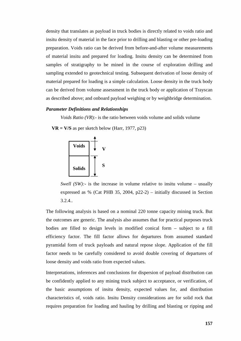
157
density that translates as payload in truck bodies is directly related to voids ratio and
insitu density of material in the face prior to drilling and blasting or other pre-loading
preparation. Voids ratio can be derived from before-and-after volume measurements
of material insitu and prepared for loading. Insitu density can be determined from
samples of stratigraphy to be mined in the course of exploration drilling and
sampling extended to geotechnical testing. Subsequent derivation of loose density of
material prepared for loading is a simple calculation. Loose density in the truck body
can be derived from volume assessment in the truck body or application of Trayscan
as described above; and onboard payload weighing or by weighbridge determination.
Parameter Definitions and Relationships
Voids Ratio (VR):- is the ratio between voids volume and solids volume
VR = V/S as per sketch below (Harr, 1977, p23)
Swell (SW):- is the increase in volume relative to insitu volume – usually
expressed as % (Cat PHB 35, 2004, p22-2) – initially discussed in Section
3.2.4..
The following analysis is based on a nominal 220 tonne capacity mining truck. But
the outcomes are generic. The analysis also assumes that for practical purposes truck
bodies are filled to design levels in modified conical form – subject to a fill
efficiency factor. The fill factor allows for departures from assumed standard
pyramidal form of truck payloads and natural repose slope. Application of the fill
factor needs to be carefully considered to avoid double covering of departures of
loose density and voids ratio from expected values.
Interpretations, inferences and conclusions for dispersion of payload distribution can
be confidently applied to any mining truck subject to acceptance, or verification, of
the basic assumptions of insitu density, expected values for, and distribution
characteristics of, voids ratio. Insitu Density considerations are for solid rock that
requires preparation for loading and hauling by drilling and blasting or ripping and
Voids
Solids
V
S
158
pushing. Variability of Insitu Density of solid rock is generally small with CV in the
range 2% to 4% (Harr, 1977). Lower values in the CV range are applicable for higher
density primary and metamorphosed rock types generally unaffected by weathering.
For the purposes of the following analysis mean values have been adopted for insitu
density. Variability of insitu density and affect on the analytical outcomes has been
taken as small and ignored.
1 Mean Load Factor (LFMEAN) is the ratio between mean loose and mean insitu
density (Cat PHB 35, 2004, p22-2).
LFMEAN = 100%/(100% + SW%)
LFMEAN is a convenient parameter for estimating purposes. It is derived from
mean voids ratio as shown in Item 3 below.
The range of load factors assumed for analysis ranges for granite is 0.61 (Cat PHB
35, 2004) increasing through 0.67 to 0.75 as efficacy of fragmentation and volume
increase by drill and blast or other means falls away from optimum.
2 Mean Loose Density (LDMEAN) = Insitu Density (ID) x LF.
LDMEAN = LF x ID
ID ≡ Specific Gravity (SG) for practical purposes of the current analysis – see
Item 4 below.
3 Mean Voids Ratio – deduced from Load Factor as follows:
SW ≡ VR in same units – proportional or %.
LF = 1/(1 + SW) (Caterpillar PHB 35, 2004)
= 1/(1 + VRMEAN) the fundamental determination of Load Factor.
VRMEAN = (1/LF) - 1
4 Voids Ratio Coefficient of Variation (CVVR) – assumed range based on:
159
Insitu Density (ID ≡ Specific Gravity [SG] for practical purposes) of low
plasticity (primary or metamorphosed fresh rock) rocks has a CV in order of 0.02
(Harr, 1977, p369)
Review of CVVR determined for a selection of particulate materials by others
(Table 10-1, Harr, 1977, p369) and intuitive understanding for hard rock prepared
for hauling that a practical CVVR range is 0.05 to 0.15 with hypothetical CVVR
values, 0.0 and 0.20, added to extend the trend.
5 Distribution of Voids Ratio assumed to be normal. Where expected (mean)
value of the VR distribution is 1, CVVR = σ. Z for the model normal probability
distribution = 3.08 for a one-tailed probability of 0.999. That is, any empirical VR
≤ (1 + 3.08CVVR). That is:
VRMAX = (1 + 3.08CVVR) x VRMEAN
Devore provides probabilities for given Z values (Devore J, 1999, Table A3 inside
cover)
6 Normal distribution symmetry is assumed to apply. Accordingly, for a one-
tailed probability of 0.999 any empirical VR ≥ (1 - 3.08CVVR). That is:
VRMIN = (1 – 3.08CVVR) x VRMEAN
7 Estimated Maximum Loose Density (LDMAX) derived from VRMIN, and Insitu
Density (ID):
LDMAX = ID x (1/(1 + VRMIN))
8 Expected Value (mean) of Loose Density LDMEAN for Selected Load Factor
LDMEAN = LF x ID Repeat of (2) above.
160
9 Estimated Minimum Loose Density (LD) derived from VRMAX, and Insitu
Density (ID):
LDMIN = ID x (1/(1 + VRMAX))
10 Theoretical Body Capacity (BCT) At Selected Fill Efficiency – derived from:
Selected Target Payload (PLMEAN)
Selected Fill Efficiency ≤ 1 (ηF)
Expected (Mean) Loose Density LDMEAN
BCT = PLMEAN/(LDMEAN x ηF)
11 Estimated SAE 2:1 Body Capacity (BCSAE) – At Selected Body Factor:
Selected Body Form Factor (BFF) to revert from conical solid load and realistic
repose slope to pyramidal SAE form and 2:1 slopes BFF ≥ 1
BCSAE = BCT x BFF
12 Theoretical Payload (Maximum) at Minimum of Voids Ratio Range – For
Target Body Capacity at Selected Load Factor, Insitu Density and Selected Fill
Factor – For the Range of Voids Ratio CV.
PLMAX = BCT x LDMAX x ηF
13 Mean Payload at Mean Voids Ratio – For Target Body Capacity at Selected
Load Factor, Insitu Density, and Selected Fill Factor – For the Range of Voids
Ratio CV.
PLMEAN = BCT x LDMEAN x ηF
161
14 Theoretical Payload (Minimum) at Maximum of Voids Ratio Range– For
Target Body Capacity at Selected Load Factor, Insitu Density and Selected Fill
Factor – For the Range of Voids Ratio CV.
PLMIN = BCT x LDMIN x ηF
15 Maximum Loose Density Proportion of Mean %
A percentage index applicable to any mining truck subject to analysis and
premises stated above.
LDMAX% = LDMAX x 100/LDMEAN
As body capacity is a designed constant, the above equation is equivalent to the
ratio of payload maximum to payload mean expressed as %.
16 Theoretical % Overload (OLT) at Voids Ratio Minimum – At Selected Fill
Factor
OLT% = (PLMAX x 100/ PLMEAN) -100
17 Minimum Loose Density Proportion of Mean %
A percentage index applicable to any mining truck subject to analysis and
premises stated above.
LDMIN% = LDMIN x 100/LDMEAN
18 Derived Truck Payload Coefficient of Variation (CVPL) is, within the
constraints of this analysis, directly related to variability of Loose Density of
material in the truck body. Assuming a probability of 0.999 and the Z statistic =
3.08 – as described in Item 5 – a reasonable approximation for the truck payload
CVPL can be derived as follows:
CVPL = (PLMAX – PLMEAN)/(PLMEAN x 3.08)
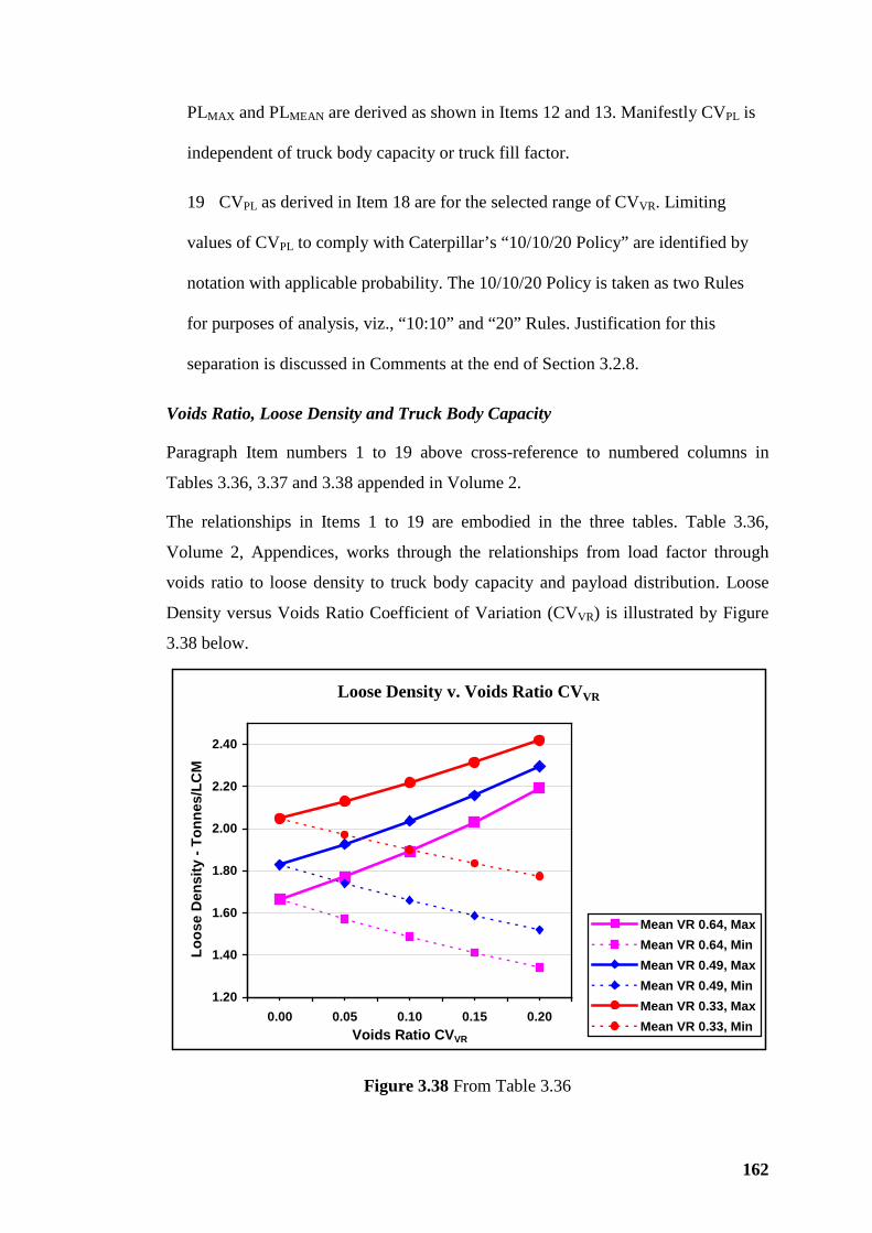
162
PLMAX and PLMEAN are derived as shown in Items 12 and 13. Manifestly CVPL is
independent of truck body capacity or truck fill factor.
19 CVPL as derived in Item 18 are for the selected range of CVVR. Limiting
values of CVPL to comply with Caterpillar’s “10/10/20 Policy” are identified by
notation with applicable probability. The 10/10/20 Policy is taken as two Rules
for purposes of analysis, viz., “10:10” and “20” Rules. Justification for this
separation is discussed in Comments at the end of Section 3.2.8.
Voids Ratio, Loose Density and Truck Body Capacity
Paragraph Item numbers 1 to 19 above cross-reference to numbered columns in
Tables 3.36, 3.37 and 3.38 appended in Volume 2.
The relationships in Items 1 to 19 are embodied in the three tables. Table 3.36,
Volume 2, Appendices, works through the relationships from load factor through
voids ratio to loose density to truck body capacity and payload distribution. Loose
Density versus Voids Ratio Coefficient of Variation (CVVR) is illustrated by Figure
3.38 below.
Loose Density v. Voids Ratio CVVR
1.20
1.40
1.60
1.80
2.00
2.20
2.40
0.00 0.05 0.10 0.15 0.20Voids Ratio CVVR
Loos
e D
ensi
ty -
Tonn
es/L
CM
Mean VR 0.64, MaxMean VR 0.64, MinMean VR 0.49, MaxMean VR 0.49, MinMean VR 0.33, MaxMean VR 0.33, Min
Figure 3.38 From Table 3.36
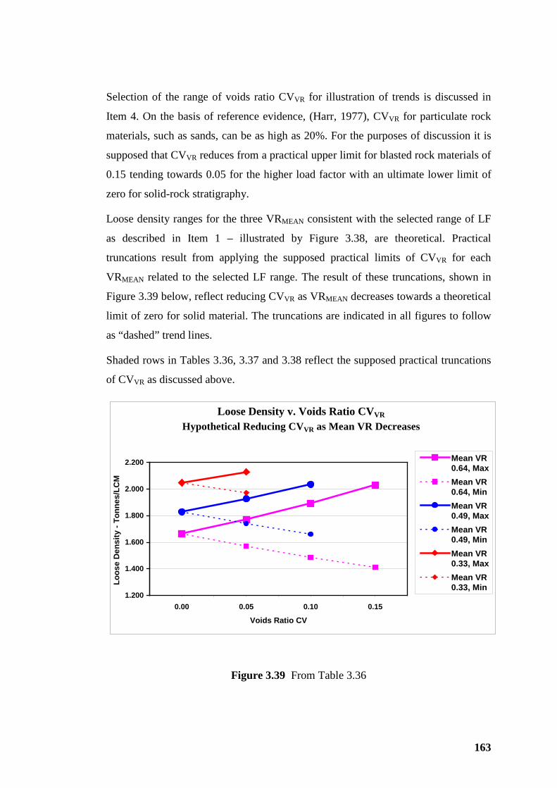
163
Selection of the range of voids ratio CVVR for illustration of trends is discussed in
Item 4. On the basis of reference evidence, (Harr, 1977), CVVR for particulate rock
materials, such as sands, can be as high as 20%. For the purposes of discussion it is
supposed that CVVR reduces from a practical upper limit for blasted rock materials of
0.15 tending towards 0.05 for the higher load factor with an ultimate lower limit of
zero for solid-rock stratigraphy.
Loose density ranges for the three VRMEAN consistent with the selected range of LF
as described in Item 1 – illustrated by Figure 3.38, are theoretical. Practical
truncations result from applying the supposed practical limits of CVVR for each
VRMEAN related to the selected LF range. The result of these truncations, shown in
Figure 3.39 below, reflect reducing CVVR as VRMEAN decreases towards a theoretical
limit of zero for solid material. The truncations are indicated in all figures to follow
as “dashed” trend lines.
Shaded rows in Tables 3.36, 3.37 and 3.38 reflect the supposed practical truncations
of CVVR as discussed above.
Loose Density v. Voids Ratio CVVR
Hypothetical Reducing CVVR as Mean VR Decreases
1.200
1.400
1.600
1.800
2.000
2.200
0.00 0.05 0.10 0.15
Voids Ratio CV
Loos
e D
ensi
ty -
Tonn
es/L
CM
Mean VR0.64, MaxMean VR0.64, MinMean VR0.49, MaxMean VR0.49, MinMean VR0.33, MaxMean VR0.33, Min
Figure 3.39 From Table 3.36
164
Figure 3.39 implies that, as efficacy of drill and blast preparation of material reduces,
mean voids ratio will decrease and loose density will increase. The range of
applicable CVVR, in accordance with the relevant supposition above, is also expected
to decrease so limiting the loose density range.
Table 3.36, appended in Volume 2, and Figure 3.39, previous page, show that:
• For higher VRMEAN the wider practical range of CVVR results in relatively
wide variation in LD.
• The wide variation in LD flows on as a substantial variation in truck payload.
• As VRMEAN increases, LF (applicable to either bank volume or tonnes)
naturally decreases – truck payload tends to decrease so justifying an
increase in truck body capacity – as shown in Tables 3.36 and 3.37.
• Increasing trend in load factor/loose density resulting from reduced VRMEAN
might be seen as a convenient remedy for the undesirable tendency of
increased VRMEAN to reduce truck payload as indicated; but, as discussed
below, decreased VRMEAN has significant negative effect on loading
productivity.
• Experience evidences that reduced VRMEAN results in reduced digability; so
loading equipment will experience slow and inefficient bucket filling and
consequent reduced productivity.
Digability is discussed in context with VR and productivity in some detail below.
Payload CV v. Voids Ratio CV
Table 3.37, Volume 2, Appendices is an extract from Table 3.36 to facilitate Figure
3.40. Overlaid on Figure 3.40 and figures to follow are practical limits to each of the
variables compared with CVVR for compliance with Caterpillar’s “10:10:20 Policy”.
For convenience of the analysis the “10/10/20 Policy” is considered as two separate
protocols. Each of these protocols – “10:10 Rule” and “20 Rule” – have different
functions. The “10:10 Rule” relates to adverse outcomes for component life and
operating cost resulting from breach of overload tolerance. The “20 Rule” relates to
absolute loading limit for preservation of steering and braking safety. The two
“Rules” also relate to different levels of truck payload coefficient of variation
(CVPL), viz.,
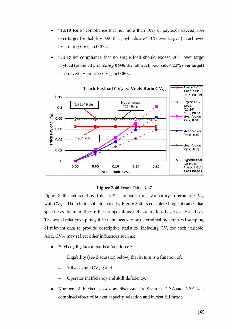
165
• “10:10 Rule” compliance that not more than 10% of payloads exceed 10%
over target (probability 0.90 that payloads are ≤ 10% over target ) is achieved
by limiting CVPL to 0.078.
• “20 Rule” compliance that no single load should exceed 20% over target
payload (assumed probability 0.999 that all truck payloads ≤ 20% over target)
is achieved by limiting CVPL to 0.065.
Truck Payload CVPL v. Voids Ratio CVVR
0
0.02
0.04
0.06
0.08
0.1
0.12
0.00 0.05 0.10 0.15 0.20Voids Ratio CVVR
Truc
k Pa
yloa
d C
V PL
Payload CV0.065, "20"Rule, P0.999
Payload CV0.078,"10:10"Rule, P0.90Mean VoidsRatio 0.64
Mean VoidsRatio 0.49
Mean VoidsRatio 0.33
Hypothetical"25 Rule"Payload CV0.081 P0.999
Figure 3.40 From Table 3.37
Figure 3.40, facilitated by Table 3.37, compares truck variability in terms of CVPL
with CVVR. The relationship depicted by Figure 3.40 is considered typical rather than
specific as the trend lines reflect suppositions and assumptions basic to the analysis.
The actual relationship may differ and needs to be determined by empirical sampling
of relevant data to provide descriptive statistics, including CV, for each variable.
Also, CVPL may reflect other influences such as:
• Bucket (fill) factor that is a function of:
Digability (see discussion below) that in turn is a function of:
VRMEAN and CVVR; and
Operator inefficiency and skill deficiency.
• Number of bucket passes as discussed in Sections 3.2.8.and 3.2.9 – a
combined effect of bucket capacity selection and bucket fill factor.
"20" Rule
"10:10" Rule Hypothetical "25" Rule
166
From Figure 3.40, theoretically, as VRMEAN decreases, LDMEAN increases. As a result
of the supposed truncation limits, CVVR reduces. As a further result CVPL reduces
significantly so that, in the circumstances, compliance with the 10/10/20 Policy
appears to be a non-issue. But, as a reality check, the above discussion on digability
and VRMEAN should be noted.
At optimally high VRMEAN, where digability is acceptable, the inference of Figure
3.40 is that CVVR increases. In turn CVPL increases so compliance with the “10/10/20
Policy” does become an issue. From Figure 3.40, and subject to all underlying
assumptions and suppositions, it appears that, for VRMEAN 0.64, compliance with the
“10:10 Rule” only becomes a problem when CVVR ≥ 0.16; but non-compliance with
the “20 Rule” will be likely for CVVR ≥. 0.14.
The hypothetical concept of a “25 Rule” is also introduced as an overlay on Figure
3.40. The “25 Rule” must remain hypothetical until such time as the mining truck
market and OEM can justify consideration of, and, if necessary, design for, higher
standards of steering and braking capability.
Clearly the “25 Rule” is a hypothetical concept of the author only based on the
mathematical relationships of payload distributions. It has no connection with the
Caterpillar 10:10:20 Policy described herein. Neither has it been discussed with
Caterpillar or any other OEM. The 10:10:20 Policy addresses for Caterpillar trucks
maintaining steering and brake certification to SAE and ISO standards and British
Columbia Codes. Understood by the author to be the first of its kind, the “Policy” has
served, and continues to serve, the industry well in maintaining safe load and haul
operations.
OEM other than Caterpillar can be expected to adopt the same design standards for
equipment manufacture; and, therefore, should require similar limits for payload and
GMW.
The hypothetical “25 Rule” – where, with a probability of 0.999, no single payload
should be greater than 25% overload - corresponds to a CVPL of 0.081. In such case
the “10:10 Rule” and “25 Rule” would be reasonably consistent standards of limiting
CVPL. Given a “25 Rule” the “10:10 Rule” would control the CVPL upper limit to
0.078. In such circumstances compliance with the “10:10 Rule”, at the chosen
confidence level of 1:1,000, would ensure compliance with the “25 Rule”. This is in
167
contrast with the current situation where compliance with the “20 Rule” at CVPL ≤
0.065 ensures compliance with the “10:10 Rule”.
Compliance with the “10:10 Rule” is generally tested by compiling truck payloads,
i.e., empirical data from VIMS, or an equivalent, and/or truck weighing. Payloads >
110% of target payload are counted and expressed as % of total payloads. Collecting
empirical truck payload data as an accumulative running sample size of, say, 1,000
payloads and deriving descriptive statistics to test CVPL ≤ 0.078 can achieve the
same result.
From Tables 3.36.and 3.37, each of the three selected VRMEAN (as a derivative of
LFMEAN) the calculations yielded a specific body capacity. This is a somewhat
artificial concept. It will also be noted that calculations from VRMEAN through to
LDMEAN are independent of body capacity. So Figures 3.38 and 3.39 are valid for any
designed body capacity.
Comparison of CVPL and CVVR in Figure 3.40 is also independent of body capacity
and truck filling efficiency factors as noted in Item 18.
Voids Ratio CV v. Maximum Truck Payload
To facilitate Figures 3.41 and 3.4, Table 3.38, Volume 2, Appendices, was compiled
by modifying Tables 3.36 and 3.37 both appended in Volume 2, to a common truck
body capacity based on the highest VRMEAN in the range adopted for analysis. Basing
analysis on maximum truck payloads and potential truck overload on a common
truck body capacity provides more realistic comparative results.
Figure 3.41 relates PLMAX to CVVR over the selected VRMEAN range. This
relationship is a simple extension of the CVPL v. CVVR relationship of Figure 3.40. In
earlier Section 3.2.8 the connection between truck payload and CVPL was discussed
in some detail.
It will be noted that:
• The equivalent potential limit of excess over target payload, the “10:10
Rule”, is overlaid as part of the “Rules suite”; but has no significant relevance
in the context of Figure 3.41.
• The “20 Rule” and hypothetical “25 Rule” are superimposed to indicate
absolute compliance limits.
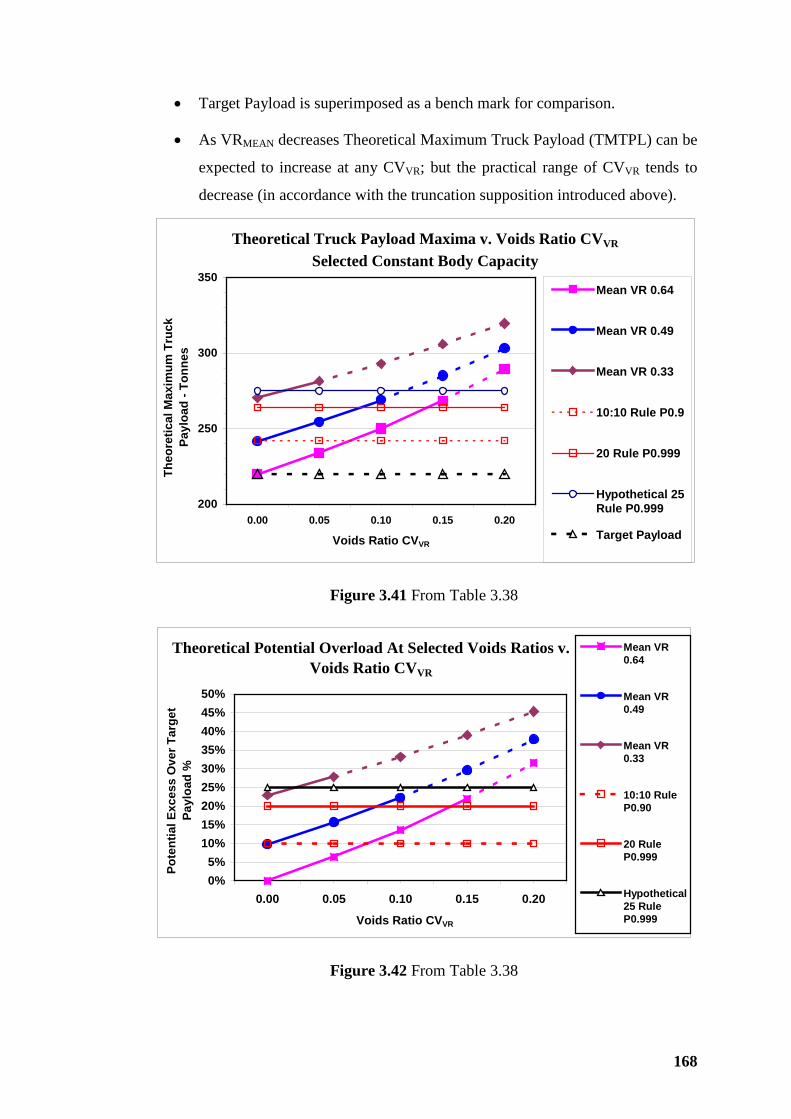
168
• Target Payload is superimposed as a bench mark for comparison.
• As VRMEAN decreases Theoretical Maximum Truck Payload (TMTPL) can be
expected to increase at any CVVR; but the practical range of CVVR tends to
decrease (in accordance with the truncation supposition introduced above).
Theoretical Truck Payload Maxima v. Voids Ratio CVVR
Selected Constant Body Capacity
200
250
300
350
0.00 0.05 0.10 0.15 0.20
Voids Ratio CVVR
Theo
retic
al M
axim
um T
ruck
Pa
yloa
d - T
onne
s
Mean VR 0.64
Mean VR 0.49
Mean VR 0.33
10:10 Rule P0.9
20 Rule P0.999
Hypothetical 25Rule P0.999
Target Payload
Figure 3.41 From Table 3.38
Theoretical Potential Overload At Selected Voids Ratios v. Voids Ratio CVVR
0%5%
10%15%20%25%30%35%40%45%50%
0.00 0.05 0.10 0.15 0.20
Voids Ratio CVVR
Pote
ntia
l Exc
ess
Ove
r Tar
get
Payl
oad
%
Mean VR0.64
Mean VR0.49
Mean VR0.33
10:10 RuleP0.90
20 RuleP0.999
Hypothetical25 RuleP0.999
Figure 3.42 From Table 3.38

169
As shown by Figure 3.41 the TMTPL below the practical truncations of CVVR are
within reach of compliance with the “20 Rule” (and would generally comply with the
hypothetical “25 Rule”); but compliance with the “10:10 Rule” tends to become
more difficult, if not impossible.
The conclusion implies that, for any given truck body capacity, the potential to
overload increases with reducing VR – as expected intuitively. Fortunately offsetting
this to a partial, if not total, effect is the expected reduction in CVVR as VRMEAN
decreases. Compliance with the “20 Rule” is likely possible with some operational
fine-tuning such as:
1. Curing the underlying cause by improving fragmentation – particle size,
grading and shape – in preparing material for loading.
Or, if inhibited by adverse insitu material conditions, the cure is prohibitively costly
or unacceptable operationally:
2. Treating the symptoms by controlling truck payloads with a system such as
VIMS or equivalent that, if, on reweigh, a truck payload is indicated in excess
of 20% overload, triggers an override system such as Caterpillar’s MAX
Payload Speed Manager. When Reweigh identifies a payload in excess of
120% of target this system within VIMS automatically restricts the
transmission to second range and the engine to 1,750 RPM. Speed of large
mining trucks on flat roads with typical in-pit rolling resistance is limited to
some 14 kph. With engine power so limited climbing ramps in deep pits, if at
all possible, will be limited to first range converter drive. So, practically, the
unacceptably high payload has to be dumped at the face or elsewhere within
the open pit.
Obviously the first of the above treatments is preferred if conditions and economics
are not prohibitive. Disturbance to the “rhythm of operations by interfering with
hauling routine, a side effect of the second treatment, generally reduces efficiency
and affects productivity so is to be avoided. But cost considerations or adverse
operating conditions may compel adoption of the second treatment.
Figure 3.42, previous page, comparing Potential % Payload In Excess of Target and
CVVR is essentially an alternative expression of Figure 3.41 with Potential %
Overload replacing Theoretical Maximum Truck Payload. This illustration clearly
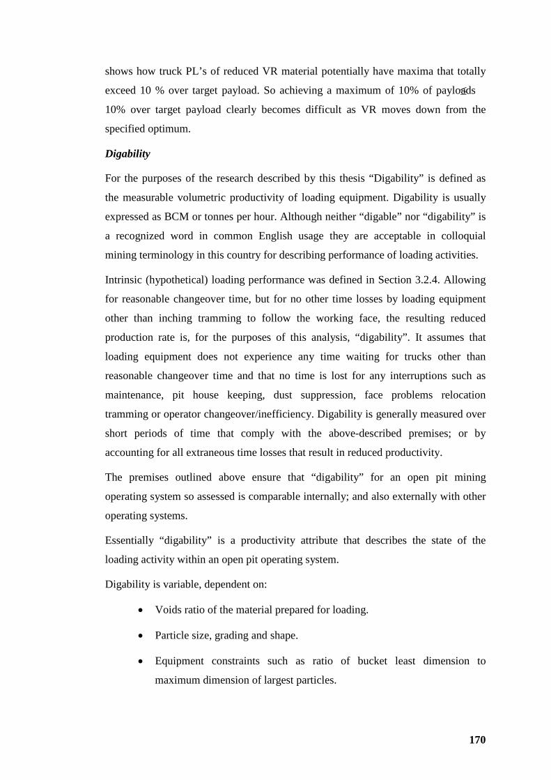
170
shows how truck PL’s of reduced VR material potentially have maxima that totally
exceed 10 % over target payload. So achieving a maximum of 10% of payloads ≤
10% over target payload clearly becomes difficult as VR moves down from the
specified optimum.
Digability
For the purposes of the research described by this thesis “Digability” is defined as
the measurable volumetric productivity of loading equipment. Digability is usually
expressed as BCM or tonnes per hour. Although neither “digable” nor “digability” is
a recognized word in common English usage they are acceptable in colloquial
mining terminology in this country for describing performance of loading activities.
Intrinsic (hypothetical) loading performance was defined in Section 3.2.4. Allowing
for reasonable changeover time, but for no other time losses by loading equipment
other than inching tramming to follow the working face, the resulting reduced
production rate is, for the purposes of this analysis, “digability”. It assumes that
loading equipment does not experience any time waiting for trucks other than
reasonable changeover time and that no time is lost for any interruptions such as
maintenance, pit house keeping, dust suppression, face problems relocation
tramming or operator changeover/inefficiency. Digability is generally measured over
short periods of time that comply with the above-described premises; or by
accounting for all extraneous time losses that result in reduced productivity.
The premises outlined above ensure that “digability” for an open pit mining
operating system so assessed is comparable internally; and also externally with other
operating systems.
Essentially “digability” is a productivity attribute that describes the state of the
loading activity within an open pit operating system.
Digability is variable, dependent on:
• Voids ratio of the material prepared for loading.
• Particle size, grading and shape.
• Equipment constraints such as ratio of bucket least dimension to
maximum dimension of largest particles.
171
Interpretation and Conclusions
Control and management measuring tools for load and haul productivity, such as
described above (VIMS, TPMS and equivalents and Trayscan), facilitate after-the-
event accounting for payload volumetric and weight efficiency; and any consequent
management action is necessarily reactive rather than proactive.
Effective process for procurement of mining trucks is based on reliable design
criteria including specifying body style and capacity to accommodate the volume of
loose material that will realise the target mean payload weight. It is necessary to have
confidence that, by filling truck bodies to a consistent volumetric level and shape
mean target payloads by weight, constrained within a mandatory distribution range,
will be achieved consistently and reliably.
Onboard payload measuring is a useful management aid that can provide some
guidance for monitoring control of actual payload within a reasonable tolerance or
target payload protocol such as Caterpillar’s 10/10/20 Policy. Verification of payload
volume as provided by systems such as Trayscan is also a desirable management aid.
But neither of these essentially monitoring systems impose any absolute constraint
on the actual payload placed in the truck body. A correctly sized body and
predictable, repeatable loose density of material to be hauled will enable competent
operators to produce distributions of truck payloads that are confined within
acceptable dispersion limits.
Equipment selection and procurement processes and related focus of the research
described in this thesis were outlined in Section 2.2.
Fundamental to achieving these objectives is the necessity to have available reliable
methods of estimating loose density of materials to be loaded. The current state of
knowledge of loose density determination is based on empirical observations of swell
– increase in insitu volume in preparing the material for loading and hauling –
interpreted as load factor criteria and listed in industrial references such as Cat PHB,
2004 as described above.
The adoption of such reference material is reasonable for general, deterministic,
estimating purposes. In the absence of actual operating evidence, criteria selected
from references that are empirically based is the best available. But, for an on-going
open pit operation, a more scientific and duly diligent approach is possible.
172
Empirical data is available to determine design criteria. Such criteria include loose
density treated stochastically for final, definitive body capacity determination and
design detail in larger mining trucks, the performance and operating costs of which
are so sensitive to any payloading inefficiency. This stochastic-based analysis and
highlighting of the relationship between variability of VR of material prepared for
loading onto mining trucks; and the consequent, variability in truck payloads
provides useful guidelines.
The value of a more reliable determination of loose density of materials is manifest.
Loading bucket and truck body capacities are dependent on a reliable estimate of
loose density in the truck body. Voids Ratio (VR) expresses the relationship between
loose volume and insitu volume. VRMEAN provides a measurable parameter that can
be related to Digability (D), i.e., loading performance; also providing a relationship
through fragmentation to drilling and blasting design parameters. Insitu density is a
variable but with small variability as described in Section 3.2.7. As loose density is
directly related to VR so the significant variability of VR will be reflected by loose
density variability. Payloads are directly dependent on loose density of material in a
truck body with practically fixed volume. So variability of VR will be reflected by
variability of truck payloads.
As VR variability is an outcome of drill and blast efficacy so truck payload
variability is dependent on drill and blast (or other pre-loading process)
fragmentation and particle grading outcomes.
Section 3.2.7 described how bucket factors are dependent on insitu density, swell
(voids ratio) and operator efficiency. Truck filling efficiency will therefore have
similar dependencies. Insitu density variability is relatively small. On the basis of
experience it is hypothesized that operator skills are predictably high so variability
due to operator inefficiency will tend to be relatively small. This leaves swell, i.e.,
VR variability as the dominant contributor to truck payload variability.
The principal driver of truck payload dispersion is voids ratio dispersion that is, in
turn, directly related to drill and blast efficacy.
Fundamental to selection of loading equipment and mining trucks, more specifically
loading equipment bucket and truck body capacities, is VR of material to be loaded
and hauled. So this measurable parameter, VR, should be tied to selected equipment
173
as a KPI for operators to be able to compare with empirical data from actual
operations.
The interrelationship between digability and drilling and blasting is further discussed
in Section 6.1.2. Load and haul productivity and cost relationships are further
considered in Section 5.3.
The analysis above examined the relationship between CVPL and CVVR and PLMEAN
and VRMEAN. Taking a broader view it must be recognized that CVPL and PLMEAN
are, as described above, also affected by:
• Variability in insitu density, fortunately small as evidenced above, that
manifests cumulatively in CVVR.
• Bucket fill factor that is a function of digability (including VRMEAN and CVVR
parameters), and small-effect operator skill and efficiency.
• Number of bucket passes per truck payload (also interrelated with bucket fill
factor, digability and operator skill and efficiency) – the effects of which
were discussed in some detail in 3.2.8 and 3.2.9 above.
In 3.5 below productivity effects of bunching and queuing are discussed.
Consistency, i.e., low dispersion, of truck payloads and loading times is a
prerequisite for achieving an acceptable standard of “rhythm” that always
characterizes optimum productivity and acceptable operating cost outcomes.
Finally, achieving optimum high VR is essential to preempt problems with digability,
bucket filling, truck target payload and compliance with safety and design-permitted
protocols for truck operations.
For consistency it is also important to limit VR variability, indicated by CVVR. The
outcome from achieving expected values of VRMEAN and CVVR will be forecast
productivity and operating costs accompanied by acceptable operating “rhythm”.
VRMEAN and CVVR have been shown, by analysis, to be most useful predictive
indicators of the state of the load and haul system and to be a principal attribute for
predicting productivity outcomes from load and haul activities. VR values for each
blast can be reasonably and simply derived from in-pit surveys. VRMEAN and CVVR
are convenient parameters derived directly from VR data samples.
174
In-truck payload measurement systems, volume or weight, are essentially monitoring
facilities, most useful as indicators of productivity and performance activities. Such
systems do not solve problems – they only identify that a problem exists and indicate
magnitude of the problem.
Ubiquitous management systems such as Caterpillar’s TPMS embedded in VIMS;
and similar systems from other OEM, integrated with supplementary control systems
are now familiar facilities for monitoring truck payload weights and providing
management information. Recent technological developments, such as Trayscan, for
measuring in-truck volume indicate efficacy of volumetric truck payload. When
combined with payload weight sensing, loose density in the truck body is simply
calculated – so VRMEAN in the truck body can be derived. Further, VRMEAN in truck
bodies can be correlated with VRMEAN in the face. As a means of realizing these
performance criteria, payload measuring systems, weight or volume, provide
valuable accounting information on operating performance.
The starting point for ensuring efficacy and expected outcomes in loading and
hauling activities is quality-assured drilling and blasting practices. Drilling and
blasting outcomes are directly related to performance and efficiency of downstream
load and haul activities. A convenient and fundamental control parameter through the
activity process from blast design to load and haul productivity, and acceptable unit
costs, is Voids Ratio and its variability parameters.
As a final thought on compliance with Caterpillars 10/10/20 Policy:
• It is shown above that compliance with the “10/10” rule is likely with a
payload CV of ≤ 0.078.
• Compliance with the “20” rule is likely at the more stringent CV of ≤ 0.065.
It is concluded that, for compliance with the “20” rule, CV ≤ 0.065, implying that not
more than 10% of payloads should exceed something less than 110% of mean target
payload or vice versa. The options for “20” rule compliance appear to be:
• Not more than 6.2% of payloads should exceed 110% of mean target; or
• Not more than 10% of payloads should exceed 108.3% of target mean.
In practice compliance with the “10/10” rule as an operating protocol and rejecting
+120% payloads is likely necessarily practical, particularly for Caterpillar trucks.
175
3.3.7 Truck Payload Centre of Gravity (CG)
This section examines distribution of GMW, NMW (tare) and payload to truck
axles and wheels of naturally occurring, but abnormal, operating conditions during
hauling operations, Particularly consideration is given to axle load distribution on
ramps and the effect of rear wheels running up the toe of the face, generally
referred to as “chocking” of truck wheels. The effect of moving the payload CG on
distribution of wheel loads is examined; and payload measuring using suspension
cylinder (ride strut) pressure differentials, and expected accuracy of this technique,
is also considered.
The general thrust of investigation in this section is to develop some understanding
of the magnitude of load-transferring effects between axles due to payload
misplacement; effect of ramps and virtual load increases or decreases due to
braking of stationary trucks. Variability of tyre loads, particularly overload, is
significant operationally, particularly as truck size increases.
The GMW of a mining truck, determined on level ground with the truck stationary
and brakes off, or at constant velocity consists:
• Suspended weight that includes the chassis, body driveline components:
For mechanical drive trucks - forward of the main drive shaft (that can
oscillate via two constant velocity {universal} couplings).
For electric drive trucks – all electrical components except the wheel
motors.
• All services, onboard storage of fuel, lubricants, hydraulic fluids, coolant
and payload.
• Unsuspended weight that includes the pistons and lower sections of the ride
struts, rear wheel group including any driveline componentry attached to it
(mechanical transmissions or electric wheel motors and final drive reduction
gearing) and the wheels and tyres.
The following significant issues need to be considered:
176
• Variation of GMW distribution to front and rear axles – particularly tyre
loads in excess of designed expectancy on which forecasts of tyre
performance and operating costs are based.
• Operational circumstances that generate excessive loads on truck structural
componentry including chassis, suspension, A-frame trunnion, four bar
linkage or other arrangements that transfer driving and braking forces
through the mechanical systems of the truck with the potential to reduce
component life and increase maintenance costs.
• How accuracy of on-board load-sensing management systems based on ride
strut pressure variations might be reduced by variation of CG location due
to abnormal off-design payload configurations; also
• Operational circumstances that result in inaccuracy and unreliability of
payload management systems.
Limited consideration is also given to results of loading off the fore and aft
centerline of trucks.
Parts A to F in this section consider three basic problems:
1. Consideration of axle and wheel loads as payload is hypothetically
misplaced in truck bodies under theoretical conditions where simple statics
can validly analyze the force systems applying and provide understanding as
discussed in Parts A to D and the complementary analysis in MPN 8, Parts
A to D in Mathematical Principles – Notes.
2. Considerations of situations where braking and drive torque are necessarily
applied and further complicate mechanical analysis as shown in Parts E and
F and the related detailed analysis in Parts E and F in MPN 8, Mathematical
Principles – Notes.
3. As a natural extension of load distribution considerations, to review
accuracy of load measuring systems based on ride strut pressure sensing in
practical applications.
The following generally summarises analysis provided in detail in MPN 8,
Mathematical Principles – Notes appended in Volume 2.
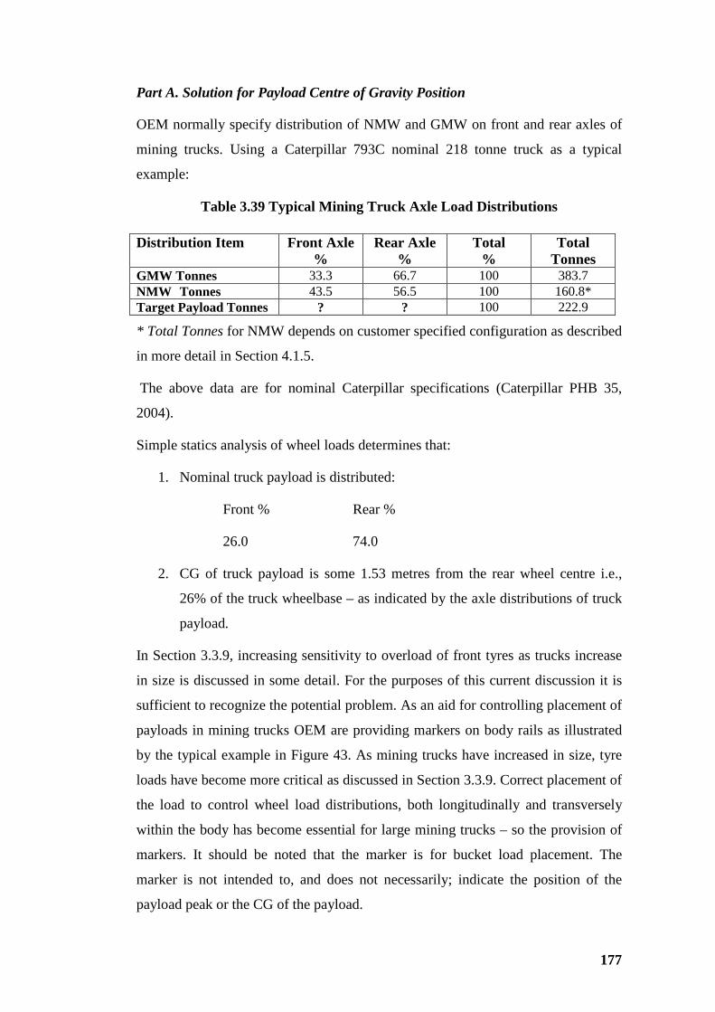
177
Part A. Solution for Payload Centre of Gravity Position
OEM normally specify distribution of NMW and GMW on front and rear axles of
mining trucks. Using a Caterpillar 793C nominal 218 tonne truck as a typical
example:
Table 3.39 Typical Mining Truck Axle Load Distributions
* Total Tonnes for NMW depends on customer specified configuration as described
in more detail in Section 4.1.5.
The above data are for nominal Caterpillar specifications (Caterpillar PHB 35,
2004).
Simple statics analysis of wheel loads determines that:
1. Nominal truck payload is distributed:
Front % Rear %
26.0 74.0
2. CG of truck payload is some 1.53 metres from the rear wheel centre i.e.,
26% of the truck wheelbase – as indicated by the axle distributions of truck
payload.
In Section 3.3.9, increasing sensitivity to overload of front tyres as trucks increase
in size is discussed in some detail. For the purposes of this current discussion it is
sufficient to recognize the potential problem. As an aid for controlling placement of
payloads in mining trucks OEM are providing markers on body rails as illustrated
by the typical example in Figure 43. As mining trucks have increased in size, tyre
loads have become more critical as discussed in Section 3.3.9. Correct placement of
the load to control wheel load distributions, both longitudinally and transversely
within the body has become essential for large mining trucks – so the provision of
markers. It should be noted that the marker is for bucket load placement. The
marker is not intended to, and does not necessarily; indicate the position of the
payload peak or the CG of the payload.
Distribution Item Front Axle %
Rear Axle %
Total %
Total Tonnes
GMW Tonnes 33.3 66.7 100 383.7 NMW Tonnes 43.5 56.5 100 160.8* Target Payload Tonnes ? ? 100 222.9
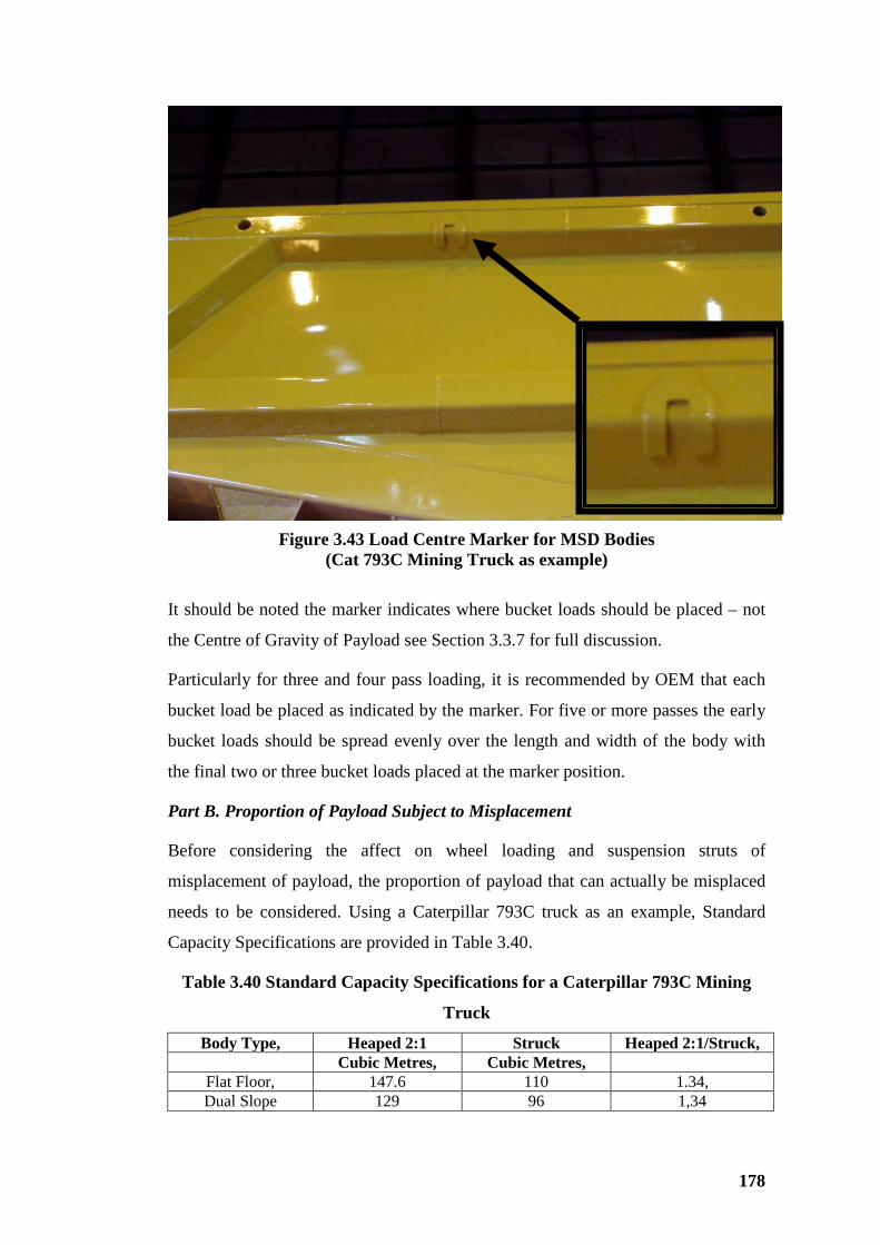
178
Figure 3.43 Load Centre Marker for MSD Bodies (Cat 793C Mining Truck as example)
It should be noted the marker indicates where bucket loads should be placed – not
the Centre of Gravity of Payload see Section 3.3.7 for full discussion.
Particularly for three and four pass loading, it is recommended by OEM that each
bucket load be placed as indicated by the marker. For five or more passes the early
bucket loads should be spread evenly over the length and width of the body with
the final two or three bucket loads placed at the marker position.
Part B. Proportion of Payload Subject to Misplacement
Before considering the affect on wheel loading and suspension struts of
misplacement of payload, the proportion of payload that can actually be misplaced
needs to be considered. Using a Caterpillar 793C truck as an example, Standard
Capacity Specifications are provided in Table 3.40.
Table 3.40 Standard Capacity Specifications for a Caterpillar 793C Mining
Truck
Body Type, Heaped 2:1 Struck Heaped 2:1/Struck, Cubic Metres, Cubic Metres,
Flat Floor, 147.6 110 1.34, Dual Slope 129 96 1,34
179
For the purposes of the following discussion it will be assumed that some 34% of
the struck volume is superimposed above the side rails of the body (equivalent to
0.34/1.34 = 25.4% of total payload).
The form and shape of the payload proportion superimposed above the struck
volume has been discussed in Section 3.3.5. Current industry direction is to assume
a conical form with slopes steeper than 2:1 – in the order of 1.7:1 – although slopes
as steep as 1.5:1 are observed in actual practice. For the following discussion,
payload slope of 1.5:1 has been adopted.
As shown in MPN 8, Part B, Mathematical Principles – Notes, amending the shape
of the superimposed load from a pyramidal to a conical form and changing the
slope from 2:1 to 1.5:1 indicatively increases the proportion of superimposed
load relative to struck volume to 0.40.
So the ratio of superimposed volume to total payload = 0.40/1.40 = 28.6%
Providing for a small freeboard allowance below the side rails ≈ 30%
It is hypothesized that the struck proportion of the payload is practically confined,
so the CG of the contained portion, the struck volume, remains practically fixed.
The “superimposed” load is assumed to have an essentially symmetrical form with
a centre of mass at the sectional centroid in all dimensions. This proportion of the
payload is considered to be misplaced to varying degrees to determine effects on
the suspension and wheel loads. That is, only the superimposed load can be
misplaced from the designed position.
For the nominal payload of 222.9 tonnes:
Proportion of payload fixed in position = 0.7 . 222.9 = 156.0tonnes
Proportion of payload that can be misplaced = 0.3 . 222.9 = 66.9tonnes
For convenience of calculations it is assumed that the CG locations for the
superimposed load and the contained load (struck volume) and the combined
payload are all on the same vertical alignment. Considering the wedge shape of the
body in elevation, the natural repose slope at rear and steeper containment at the
front of the body the base target for the superimposed load is approximately square.
There is no certainty that the component and combined CG do align. But the actual
180
misalignments will be small and are considered to not invalidate general outcomes
of calculations and interpretations.
It should also be noted that, for the hypothetical cases considered, the superimposed
load only is misplaced forwards. Theoretically the rear slope could move forward,
also leaving a void at the rear of the contained (struck) volume and potentially
under-loading the truck. No provision has been made for this rear slope void and
potential under-loading for two reasons:
1. It is considered that the effect on the distribution calculations would be
small.
2. A void on the rear slope will be obvious to the loading equipment operator;
and skilled operators will place bucket loads to remedy any such obvious
voids.
Part C. Relationship Between Misplacement and Distribution of Superimposed
Payload To Wheels
Five cases were considered:
• A hypothetical case where the superimposed payload proportion only moves
0.5 metres to the rear to increase rear suspension and wheel loads –
questionable practically as the open and uncontained rear slope has little
accommodation for rearward misplacement of the superimposed load before
spillage occurs.
• Generally practical cases of misplacement of the superimposed proportion
of payload forward by 0.5, 1.0, 1.5 and 2.0 metres; of these 1.5 and 2.0
metres, are also likely impractical because the payload would manifestly
spill across the canopy and be obvious to the operator and supervision.
By apportioning the components of GMW - in accordance with relationships of
simple statics – distribution of GMW on front and rear wheels is derived. Results
are relative to the design CG position that realizes a distribution of 33.3% to front
and 66.7% to rear wheels when the truck is on a horizontal surface.
Table 3.41 summarises the spreadsheet analysis for axle load proportions for a
range of payload displacements in MPN 8, Part C, Mathematical Principles –
Notes. Figure 3.44 illustrates the results of analysis.
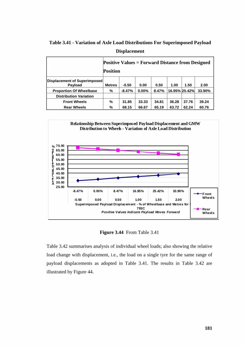
181
Table 3.41 - Variation of Axle Load Distributions For Superimposed Payload
Displacement
Positive Values = Forward Distance from Designed
Position
Displacement of Superimposed Payload Metres -0.50 0.00 0.50 1.00 1.50 2.00
Proportion Of Wheelbase % -8.47% 0.00% 8.47% 16.95% 25.42% 33.90% Distribution Variation
Front Wheels % 31.85 33.33 34.81 36.28 37.76 39.24 Rear Wheels % 68.15 66.67 65.19 63.72 62.24 60.76
25.0030.0035.0040.0045.0050.0055.0060.0065.0070.00
-8.47% 0.00% 8.47% 16.95% 25.42% 33.90%
-0.50 0.00 0.50 1.00 1.50 2.00
Axle Load Distribution %
Superimposed Payload Displacement - % of Wheelbase and Metres for Caterpil lar 793C
Positive Values Indicate Payload Moves Forward
Relationship Between Superimposed Payload Displacement and GMW Distribution to Wheels - Variation of Axle Load Distribution
Front Wheels
Rear Wheels
Figure 3.44 From Table 3.41
Table 3.42 summarises analysis of individual wheel loads; also showing the relative
load change with displacement, i.e., the load on a single tyre for the same range of
payload displacements as adopted in Table 3.41. The results in Table 3.42 are
illustrated by Figure 44.
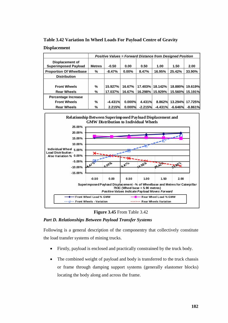
182
Table 3.42 Variation In Wheel Loads For Payload Centre of Gravity
Displacement
Positive Values = Forward Distance from Designed Position
Displacement of Superimposed Payload Metres -0.50 0.00 0.50 1.00 1.50 2.00
Proportion Of Wheelbase % -8.47% 0.00% 8.47% 16.95% 25.42% 33.90% Distribution
Front Wheels % 15.927% 16.67% 17.403% 18.142% 18.880% 19.619% Rear Wheels % 17.037% 16.67% 16.298% 15.929% 15.560% 15.191%
Percentage Increase Front Wheels % -4.431% 0.000% 4.431% 8.862% 13.294% 17.725% Rear Wheels % 2.215% 0.000% -2.215% -4.431% -6.646% -8.861%
-15.00%
-10.00%
-5.00%
0.00%
5.00%
10.00%
15.00%
20.00%
25.00%
-0.50 0.00 0.50 1.00 1.50 2.00
Individual Wheel Load Distr ibution -Also Variation %
Superimposed Payload Displacement - % of Wheelbase and Metres for Caterpillar 793C (Wheel base = 5.90 metres)
Positive Values Indicate Payload Moves Forward
Relationship Between Superimposed Payload Displacement and GMW Distribution to Individual Wheels
Front Wheel Load % GMW Rear Wheel Load % GMWFront Wheels - Variation Rear Wheels Variation
Figure 3.45 From Table 3.42
Part D. Relationships Between Payload Transfer Systems
Following is a general description of the componentry that collectively constitute
the load transfer systems of mining trucks.
• Firstly, payload is enclosed and practically constrained by the truck body.
• The combined weight of payload and body is transferred to the truck chassis
or frame through damping support systems (generally elastomer blocks)
locating the body along and across the frame.
183
• Tipping trunnion pins are not designed to be under load except during body
tipping – any load on trunnion pins with the body down is due to collapse of
the damped body elastomer support system or misalignment/warping of
body structure.
• The chassis and all load components above it are supported by the
suspension system generally consisting of inert gas over oil suspension
cylinders commonly termed “ride struts” or simply “struts”.
• Oil in suspension cylinders acts as a gas seal and oil seal lubricant – oil
seals are generally a group of elastomer o-rings with the outside ring
designed to act as a wiper seal to prevent build up of contaminated oil on
the cylinder shaft and consequent contamination of contained oil.
• Other suspension mediums, including stacked elastomer blocks acting as
compression elements, have also been used with only limited success – such
alternatives have not carried forward into current designs for large mining
trucks.
• Generally front ride struts have longer travel than the rear struts; but across
the range of large mining trucks available there are exceptions where front
and rear struts have practically equal travel and at least one truck where
rear-strut travel exceeds travel for front struts.
• Rear struts carry some double the load of a front strut; so rear struts are
necessarily stiffer, i.e., have a higher spring rate (load over travel) than front
struts.
• Front ride struts are generally in line with the front wheel centres for all
mining trucks – in some designs, particularly Caterpillar and Komatsu, the
front suspension cylinder acts as the steering king post with a stub axle
mounted onto the strut shaft; other designs have trailing links positioning
integral stub axles or double wishbone configurations supporting a separate
king post/stub axle assembly, similar to light highway vehicles. These
alternative front suspension systems that position the front axle have
suspension struts mounted between front wheel support componentry and
the chassis frame with universal pin and bush mountings designed to
accommodate loads only in line with the strut.
184
• Rear struts are mounted between chassis frame and rear axle group either
behind the centerline of the rear axle and wheels or directly above the rear
axle/wheel group on the axle centerline. Mountings are generally universal
so that, for practical purposes, struts only experience in-line loads.
• Where the rear ride struts are mounted behind the rear axle centre, a
secondary support system consisting of an A frame or four-bar linkage
transfers suspension torque to the chassis as horizontal or vertical forces –
this secondary support system also acts as thrust or draw bar componentry
that accommodates drive and braking torque and transmits rimpull reaction
to the truck chassis to drive the truck forward or in reverse.
• There is no commonality of suspension system designs amongst the five
major OEM supplying mining trucks (Caterpillar, Komatsu, Liebherr, Terex
and Hitachi) with each vendor marketing the claimed special benefits of
each system – all of which are functional; and all of which exhibit only
small variations in geometrical displacement as a natural consequence of
limited suspension movement under operational conditions.
The following descriptions and analysis apply generally to the Caterpillar range of
mining trucks – adopting the Cat 793C nominal 240 ton (218 tonne) truck as a
model for analysis. Similar analysis, differing only in detail could be applied to any
mining truck from any OEM.
Special features of the generic Caterpillar truck configuration include:
• Mechanical drive system for the complete range of mining trucks available
at time of writing this thesis – a situation that may change in the future.
• Torque converter and lock up componentry close mounted to the engine
flywheel housing and transmission close mounted to the rear wheel
assembly connected by a relatively short drive shaft including constant
velocity joints allowing independent rear axle group movement.
• An A-frame provides rear axle location with the forward trunnion (a ball
joint) allowing universal movement of the rear axle group – a common
feature of the range of Caterpillar mining trucks up to the Cat 793C nominal
218 tonne truck – that has been changed to a 4-bar linkage for the top-of-
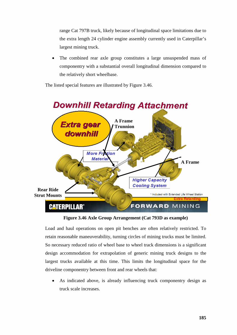
185
range Cat 797B truck, likely because of longitudinal space limitations due to
the extra length 24 cylinder engine assembly currently used in Caterpillar’s
largest mining truck.
• The combined rear axle group constitutes a large unsuspended mass of
componentry with a substantial overall longitudinal dimension compared to
the relatively short wheelbase.
The listed special features are illustrated by Figure 3.46.
Figure 3.46 Axle Group Arrangement (Cat 793D as example)
Load and haul operations on open pit benches are often relatively restricted. To
retain reasonable maneuverability, turning circles of mining trucks must be limited.
So necessary reduced ratio of wheel base to wheel track dimensions is a significant
design accommodation for extrapolation of generic mining truck designs to the
largest trucks available at this time. This limits the longitudinal space for the
driveline componentry between front and rear wheels that:
• As indicated above, is already influencing truck componentry design as
truck scale increases.
A Frame
Rear Ride Strut Mounts
A Frame Trunnion
186
• Is a constraint on extrapolation of current configurations to even larger
mining trucks than are offered by OEM at this time.
Analysis in terms of simple statics of the load transference systems, using a Cat
793C truck as a model, are provided in a series of equations in MPN 8, Part D,
Mathematical Principles – Notes. These theoretical, simple statics relationships
provide a basis for general understanding but are dependent on some assumptions
that are not necessarily absolutely true in practice. These assumptions include:
• Trucks are on level ground and remain horizontal during loading.
• Trucks are stationary and remain so without application of brake or drive
torques unless specifically stated otherwise.
• Geometrical relationship between the various load transfer systems is
retained both intrinsically and in space.
• All external forces applied to ride struts are represented without loss (due to
friction) by the pressure differentials in the ride struts.
• There are no transverse force components that reduce the force applied to
ride struts.
The above list is not represented as exhaustive. In practice the load transfer systems
and load sensing facilities of large mining trucks cannot be exactly modelled by
simple theoretical concepts. The geometry of the suspension and load transfer
systems does not remain constant. Small, but significant, changes to strut alignment
due to difference in front and rear strut travel under incrementally changing load,
appear to play a significant role in determining accuracy of load measuring systems
based on suspension pressure differentials. Also, friction in ride strut seals affects
response to discrete load variations – with reduced degree of friction effect where
strut loads are varied dynamically, i.e., when the truck is travelling.
Part E. Rear Wheels On Toe of Face Or Otherwise Chocking Wheels
Effects on rear wheel load and suspension resulting from chocking the wheels
whilst spotting the truck for loading are analyzed in MPN 8, Part E, Mathematical
Principles – Notes appended in Volume 2. Practical causes of wheel chocking
include reversing a pair of rear wheels onto the toe of the face, or wheels contacting
debris – tailings - from loading operations and the like.
187
A general practical case where only one rear group of dual wheels is chocked is
adopted for analysis. It is possible for a single rear wheel to experience chocking
effects. But the analysis is based on each wheel of a dual pair sharing forces from
chocking effects equally. Specific outcomes of the case of chocking a single wheel
are generally discussed below. The equations developed in MPN 8, Part E,
Mathematical Principles - Notes will generally be valid for the static forces
applying in the hypothesized circumstances.
Incipient dynamic forces, resulting from braking torque to restrain the chocked
truck in position, are distributed through the chassis to manifest as forces on ride
struts that are, in turn, distributed to front and rear axles. Even if one rear dual
wheel group or single wheel only is chocked, ride struts for a specific axle, front or
rear, will generally share any virtual increase in suspended load equally across the
truck – i.e., incremental virtual load on left and right side struts should be
practically equal.
Diagrams illustrate both static and incipient dynamic sets of loads and relevant
equations are provided in the table in Part E, (MPN 8, Mathematical Principles –
Notes:
1. Static loads on a rear wheel group of a pair of dual wheels due to the load
offsetting effect of chocking are resolved vertically and horizontally only
affecting tyre and wheel loads.
2. Incipient dynamic loading resulting from braking torque to retain the truck
in position (equilibrium) is resolved into components that affect ride-strut
loads.
Using a Cat 793C with 40.00 R57 tyres as a model, Table 3.43 indicates:
• Static load increase in tyre-support reaction on a wheel group of a pair of
wheels/tyres for a range of offsets caused by chocking.
• That, if chocking affects a single wheel and tyre, the increase in individual
wheel/tyre load could be double the static load increase indicated by Table
3.43
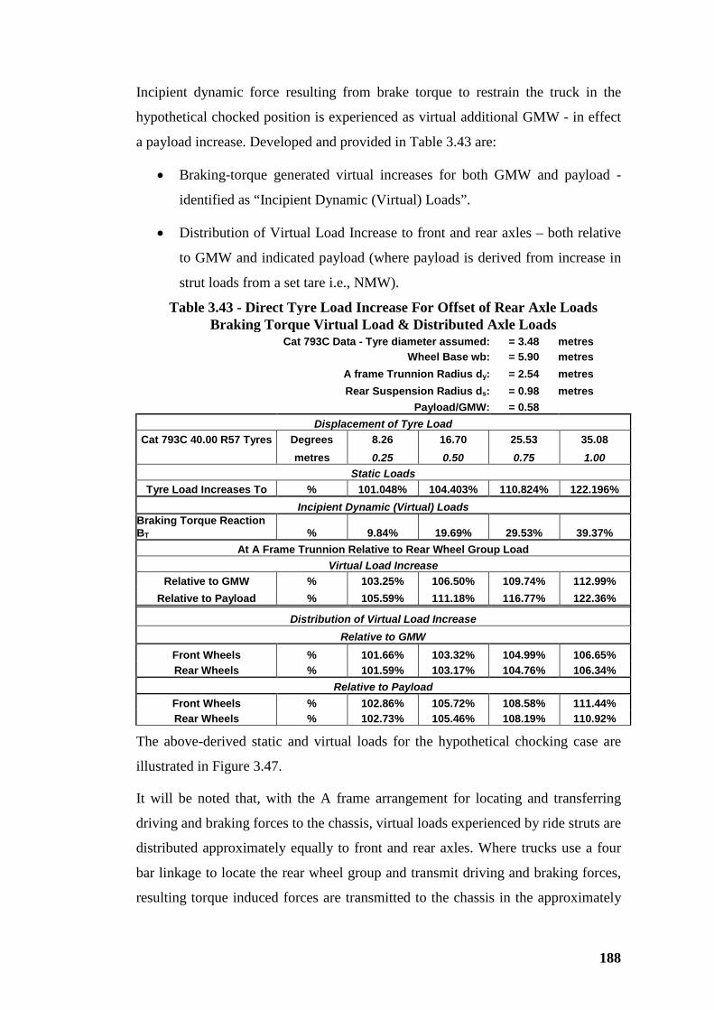
188
Incipient dynamic force resulting from brake torque to restrain the truck in the
hypothetical chocked position is experienced as virtual additional GMW - in effect
a payload increase. Developed and provided in Table 3.43 are:
• Braking-torque generated virtual increases for both GMW and payload -
identified as “Incipient Dynamic (Virtual) Loads”.
• Distribution of Virtual Load Increase to front and rear axles – both relative
to GMW and indicated payload (where payload is derived from increase in
strut loads from a set tare i.e., NMW).
Table 3.43 - Direct Tyre Load Increase For Offset of Rear Axle Loads Braking Torque Virtual Load & Distributed Axle Loads
Cat 793C Data - Tyre diameter assumed: = 3.48 metres Wheel Base wb: = 5.90 metres A frame Trunnion Radius dy: = 2.54 metres Rear Suspension Radius ds: = 0.98 metres Payload/GMW: = 0.58
Displacement of Tyre Load Cat 793C 40.00 R57 Tyres Degrees 8.26 16.70 25.53 35.08
metres 0.25 0.50 0.75 1.00 Static Loads
Tyre Load Increases To % 101.048% 104.403% 110.824% 122.196% Incipient Dynamic (Virtual) Loads
Braking Torque Reaction BT % 9.84% 19.69% 29.53% 39.37%
At A Frame Trunnion Relative to Rear Wheel Group Load Virtual Load Increase
Relative to GMW % 103.25% 106.50% 109.74% 112.99% Relative to Payload % 105.59% 111.18% 116.77% 122.36%
Distribution of Virtual Load Increase Relative to GMW
Front Wheels % 101.66% 103.32% 104.99% 106.65% Rear Wheels % 101.59% 103.17% 104.76% 106.34%
Relative to Payload Front Wheels % 102.86% 105.72% 108.58% 111.44% Rear Wheels % 102.73% 105.46% 108.19% 110.92%
The above-derived static and virtual loads for the hypothetical chocking case are
illustrated in Figure 3.47.
It will be noted that, with the A frame arrangement for locating and transferring
driving and braking forces to the chassis, virtual loads experienced by ride struts are
distributed approximately equally to front and rear axles. Where trucks use a four
bar linkage to locate the rear wheel group and transmit driving and braking forces,
resulting torque induced forces are transmitted to the chassis in the approximately
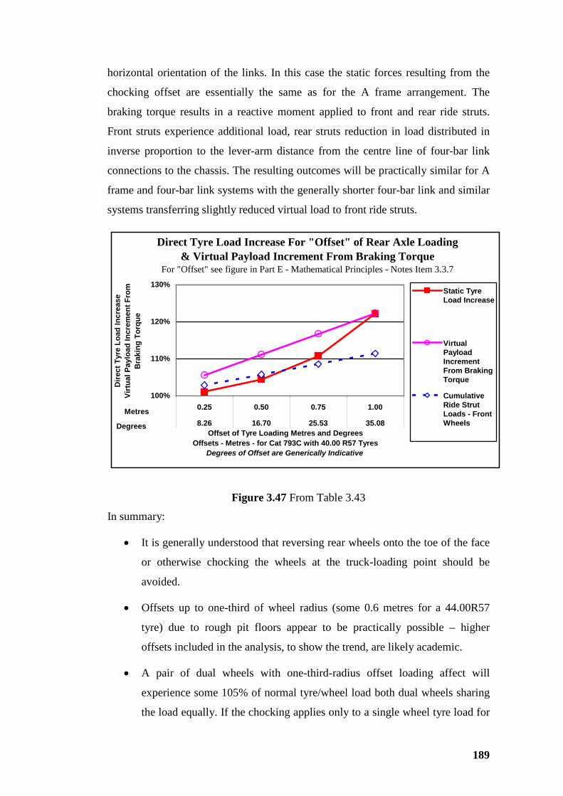
189
horizontal orientation of the links. In this case the static forces resulting from the
chocking offset are essentially the same as for the A frame arrangement. The
braking torque results in a reactive moment applied to front and rear ride struts.
Front struts experience additional load, rear struts reduction in load distributed in
inverse proportion to the lever-arm distance from the centre line of four-bar link
connections to the chassis. The resulting outcomes will be practically similar for A
frame and four-bar link systems with the generally shorter four-bar link and similar
systems transferring slightly reduced virtual load to front ride struts.
Direct Tyre Load Increase For "Offset" of Rear Axle Loading& Virtual Payload Increment From Braking Torque
For "Offset" see figure in Part E - Mathematical Principles - Notes Item 3.3.7
100%
110%
120%
130%
0.25 0.50 0.75 1.00
8.26 16.70 25.53 35.08Offset of Tyre Loading Metres and Degrees
Offsets - Metres - for Cat 793C with 40.00 R57 TyresDegrees of Offset are Generically Indicative
Dire
ct T
yre
Load
Incr
ease
Virt
ual P
aylo
ad In
crem
ent F
rom
B
raki
ng T
orqu
e
Static TyreLoad Increase
VirtualPayloadIncrementFrom BrakingTorque
CumulativeRide StrutLoads - FrontWheels
Metres
Degrees
Figure 3.47 From Table 3.43
In summary:
• It is generally understood that reversing rear wheels onto the toe of the face
or otherwise chocking the wheels at the truck-loading point should be
avoided.
• Offsets up to one-third of wheel radius (some 0.6 metres for a 44.00R57
tyre) due to rough pit floors appear to be practically possible – higher
offsets included in the analysis, to show the trend, are likely academic.
• A pair of dual wheels with one-third-radius offset loading affect will
experience some 105% of normal tyre/wheel load both dual wheels sharing
the load equally. If the chocking applies only to a single wheel tyre load for

190
that wheel could theoretically increase to more than double, some 210% of
normal tyre and wheel load.
• Braking torque to restrain the truck in the chocked position induces loads on
the chassis that manifest as virtual additional higher GMW and
consequently increased payload as sensed by suspension components.
• Payload measuring facilities such as Caterpillar’s VIMS will tend to record
high when a rear wheel is chocked, the truck tends to roll forward, and
brakes are used to maintain the truck in position; and vice versa if the truck
tends to roll backwards.
• The various tables and illustrations referred to provide an indication of the
potential degree of over-assessment of payload by using suspension sensing
for chocked-wheel situations.
• When brakes are released and the truck is on a level surface load-suspension
measurement facilities can be expected to return to normal.
• Since trucks are usually loaded with the brakes on (generally rear wheel
parking brakes only) and driveline in neutral or off-power, the load sensing
system will potentially over-record for forward movement tendency or
under-record for rearward movement tendency.
• To avoid these potential sensing errors, VIMS reweighs the truck in forward
motion in second transmission range by sampling ride strut pressures a
number of times, deriving a mean value, deducting pre-determined NMW
and recording the nett result as payload. Other OEM are understood to adopt
similar techniques.
• It will be noted that the chocking induced static forces affect tyre and wheel
loads and incipient dynamic, virtual, forces affect suspension loads
independently.
Part F. Load Distribution on Ramps
In MPN 8, Part F Load Distribution On Ramps, Mathematical Principles – Notes
appended in Volume 2, analysis indicates how axle-load distribution varies with
ramp grade.
191
The analysis is based on hauling upgrade. Downgrade hauling can be considered
using the same analytical arguments with appropriate adjustments to applicable
geometrical configuration of the truck and loading system.
Essentially:
• Upgrade hauling transfers axle loads that reflect distributed GMW
(including payload) from front to rear wheels.
• The degree of transfer increases with ramp grade and height of the CG of
the loaded truck above the wheel centres.
Focus of this part F is limited to the order of magnitude of axle-load transfer in
terms of the two variables – ramp grade and CG height.
MPN 8, Part F Load Distribution On Ramps, Mathematical Principles – Notes
appended in Volume 2, provides details of the analysis. Calculations of axle-load
distribution for ranges of effective ramp grades and CG height are summarized in
Tables 3.44 – Upgrade and 3.45 – Downgrade, next two pages. The results in these
tables are illustrated by Figures 3.48 - Upgrade and 3.49 – Downgrade. Comparing
these two figures it is obvious that increase in front wheel loading downgrade is
significantly greater than for rear wheels upgrade, e.g.;
At 10% Ramp Grade, CG height = 4.0 metres (assumed) – indicated wheel load
variations:
Front Wheels: Rear Wheels
Upgrade -30% +14%
Downgrade +40% -20%
The significance of the above outcomes for expected tyre performance/life on
downgrade-loaded hauling is manifest.
The discussion is limited to static loading only.
For upgrade hauling, driving torque applied at the wheels tends to further reduce
load on the front wheels and increase load on the rear wheels. For downgrade-
loaded hauling, braking torque has the opposite effect loading up front wheels and
relieving load on rear wheels.
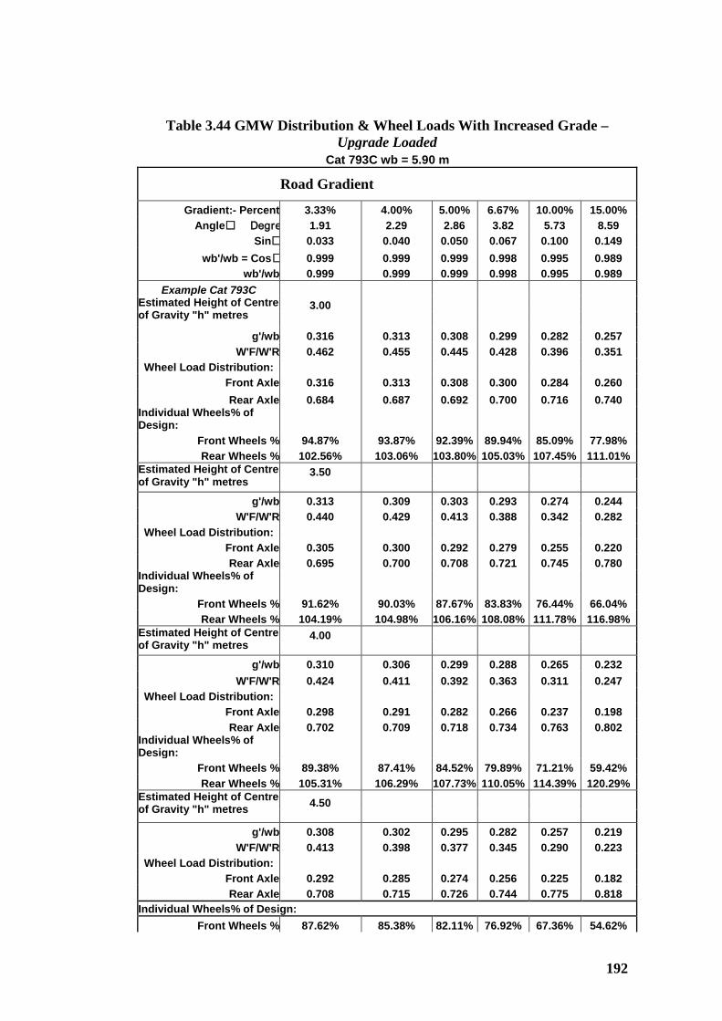
192
Table 3.44 GMW Distribution & Wheel Loads With Increased Grade – Upgrade Loaded
Cat 793C wb = 5.90 m
Road Gradient
Gradient:- Percent 3.33% 4.00% 5.00% 6.67% 10.00% 15.00% Angle Degre 1.91 2.29 2.86 3.82 5.73 8.59
Sin 0.033 0.040 0.050 0.067 0.100 0.149 wb'/wb = Cos 0.999 0.999 0.999 0.998 0.995 0.989
wb'/wb 0.999 0.999 0.999 0.998 0.995 0.989 Example Cat 793C
Estimated Height of Centre of Gravity "h" metres
3.00
g'/wb 0.316 0.313 0.308 0.299 0.282 0.257 W'F/W'R 0.462 0.455 0.445 0.428 0.396 0.351
Wheel Load Distribution: Front Axle 0.316 0.313 0.308 0.300 0.284 0.260 Rear Axle 0.684 0.687 0.692 0.700 0.716 0.740
Individual Wheels% of Design:
Front Wheels % 94.87% 93.87% 92.39% 89.94% 85.09% 77.98% Rear Wheels % 102.56% 103.06% 103.80% 105.03% 107.45% 111.01%
Estimated Height of Centre of Gravity "h" metres
3.50
g'/wb 0.313 0.309 0.303 0.293 0.274 0.244 W'F/W'R 0.440 0.429 0.413 0.388 0.342 0.282
Wheel Load Distribution: Front Axle 0.305 0.300 0.292 0.279 0.255 0.220 Rear Axle 0.695 0.700 0.708 0.721 0.745 0.780
Individual Wheels% of Design:
Front Wheels % 91.62% 90.03% 87.67% 83.83% 76.44% 66.04% Rear Wheels % 104.19% 104.98% 106.16% 108.08% 111.78% 116.98%
Estimated Height of Centre of Gravity "h" metres
4.00
g'/wb 0.310 0.306 0.299 0.288 0.265 0.232 W'F/W'R 0.424 0.411 0.392 0.363 0.311 0.247
Wheel Load Distribution: Front Axle 0.298 0.291 0.282 0.266 0.237 0.198 Rear Axle 0.702 0.709 0.718 0.734 0.763 0.802
Individual Wheels% of Design:
Front Wheels % 89.38% 87.41% 84.52% 79.89% 71.21% 59.42% Rear Wheels % 105.31% 106.29% 107.73% 110.05% 114.39% 120.29%
Estimated Height of Centre of Gravity "h" metres 4.50
g'/wb 0.308 0.302 0.295 0.282 0.257 0.219
W'F/W'R 0.413 0.398 0.377 0.345 0.290 0.223 Wheel Load Distribution:
Front Axle 0.292 0.285 0.274 0.256 0.225 0.182 Rear Axle 0.708 0.715 0.726 0.744 0.775 0.818
Individual Wheels% of Design: Front Wheels % 87.62% 85.38% 82.11% 76.92% 67.36% 54.62%
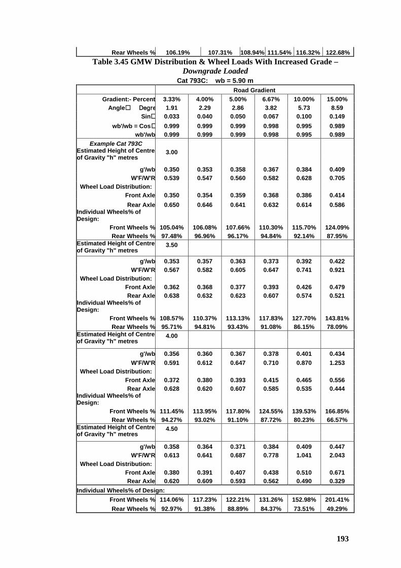
193
Rear Wheels % 106.19% 107.31% 108.94% 111.54% 116.32% 122.68% Table 3.45 GMW Distribution & Wheel Loads With Increased Grade –
Downgrade Loaded Cat 793C: wb = 5.90 m
Road Gradient Gradient:- Percent 3.33% 4.00% 5.00% 6.67% 10.00% 15.00%
Angle Degre 1.91 2.29 2.86 3.82 5.73 8.59 Sin 0.033 0.040 0.050 0.067 0.100 0.149
wb'/wb = Cos 0.999 0.999 0.999 0.998 0.995 0.989 wb'/wb 0.999 0.999 0.999 0.998 0.995 0.989
Example Cat 793C Estimated Height of Centre of Gravity "h" metres
3.00
g'/wb 0.350 0.353 0.358 0.367 0.384 0.409 W'F/W'R 0.539 0.547 0.560 0.582 0.628 0.705
Wheel Load Distribution: Front Axle 0.350 0.354 0.359 0.368 0.386 0.414 Rear Axle 0.650 0.646 0.641 0.632 0.614 0.586
Individual Wheels% of Design:
Front Wheels % 105.04% 106.08% 107.66% 110.30% 115.70% 124.09% Rear Wheels % 97.48% 96.96% 96.17% 94.84% 92.14% 87.95%
Estimated Height of Centre of Gravity "h" metres
3.50
g'/wb 0.353 0.357 0.363 0.373 0.392 0.422 W'F/W'R 0.567 0.582 0.605 0.647 0.741 0.921
Wheel Load Distribution: Front Axle 0.362 0.368 0.377 0.393 0.426 0.479 Rear Axle 0.638 0.632 0.623 0.607 0.574 0.521
Individual Wheels% of Design:
Front Wheels % 108.57% 110.37% 113.13% 117.83% 127.70% 143.81% Rear Wheels % 95.71% 94.81% 93.43% 91.08% 86.15% 78.09%
Estimated Height of Centre of Gravity "h" metres
4.00
g'/wb 0.356 0.360 0.367 0.378 0.401 0.434 W'F/W'R 0.591 0.612 0.647 0.710 0.870 1.253
Wheel Load Distribution: Front Axle 0.372 0.380 0.393 0.415 0.465 0.556 Rear Axle 0.628 0.620 0.607 0.585 0.535 0.444
Individual Wheels% of Design:
Front Wheels % 111.45% 113.95% 117.80% 124.55% 139.53% 166.85% Rear Wheels % 94.27% 93.02% 91.10% 87.72% 80.23% 66.57%
Estimated Height of Centre of Gravity "h" metres
4.50
g'/wb 0.358 0.364 0.371 0.384 0.409 0.447 W'F/W'R 0.613 0.641 0.687 0.778 1.041 2.043
Wheel Load Distribution: Front Axle 0.380 0.391 0.407 0.438 0.510 0.671 Rear Axle 0.620 0.609 0.593 0.562 0.490 0.329
Individual Wheels% of Design: Front Wheels % 114.06% 117.23% 122.21% 131.26% 152.98% 201.41% Rear Wheels % 92.97% 91.38% 88.89% 84.37% 73.51% 49.29%
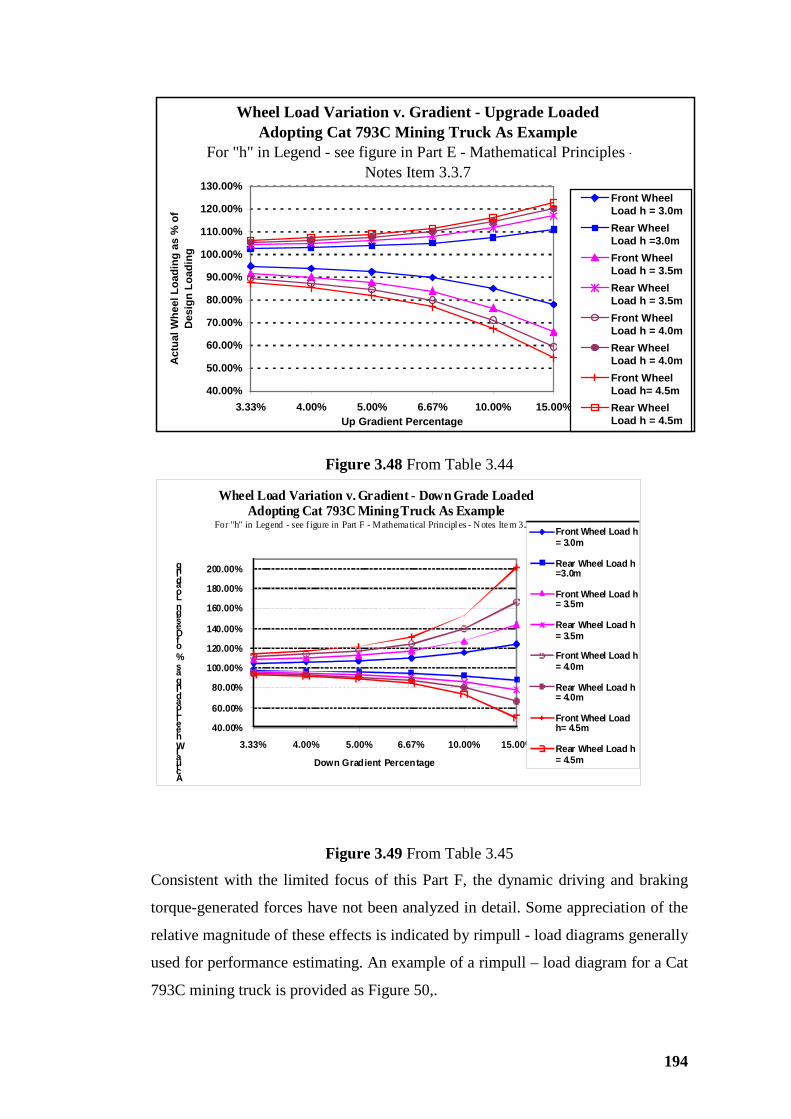
194
Wheel Load Variation v. Gradient - Upgrade LoadedAdopting Cat 793C Mining Truck As Example
For "h" in Legend - see figure in Part E - Mathematical Principles - Notes Item 3.3.7
40.00%
50.00%
60.00%
70.00%
80.00%
90.00%
100.00%
110.00%
120.00%
130.00%
3.33% 4.00% 5.00% 6.67% 10.00% 15.00%Up Gradient Percentage
Act
ual W
heel
Loa
ding
as
% o
f D
esig
n Lo
adin
gFront WheelLoad h = 3.0mRear WheelLoad h =3.0mFront WheelLoad h = 3.5mRear WheelLoad h = 3.5mFront WheelLoad h = 4.0mRear WheelLoad h = 4.0mFront WheelLoad h= 4.5mRear WheelLoad h = 4.5m
Figure 3.48 From Table 3.44
40.00%
60.00%
80.00%
100.00%
120.00%
140.00%
160.00%
180.00%
200.00%
3.33% 4.00% 5.00% 6.67% 10.00% 15.00%
Actual Wheel Loading as % of Design Loading
Down Gradient Percentage
Wheel Load Variation v. Gradient - Down Grade LoadedAdopting Cat 793C Mining Truck As Example
For "h" in Legend - see f igure in Part F - Mathema tical Principl es - N otes Ite m 3.3.7Front Wheel Load h = 3.0m
Rear Wheel Load h =3.0m
Front Wheel Load h = 3.5m
Rear Wheel Load h = 3.5m
Front Wheel Load h = 4.0m
Rear Wheel Load h = 4.0m
Front Wheel Load h= 4.5m
Rear Wheel Load h = 4.5m
Figure 3.49 From Table 3.45
Consistent with the limited focus of this Part F, the dynamic driving and braking
torque-generated forces have not been analyzed in detail. Some appreciation of the
relative magnitude of these effects is indicated by rimpull - load diagrams generally
used for performance estimating. An example of a rimpull – load diagram for a Cat
793C mining truck is provided as Figure 50,.
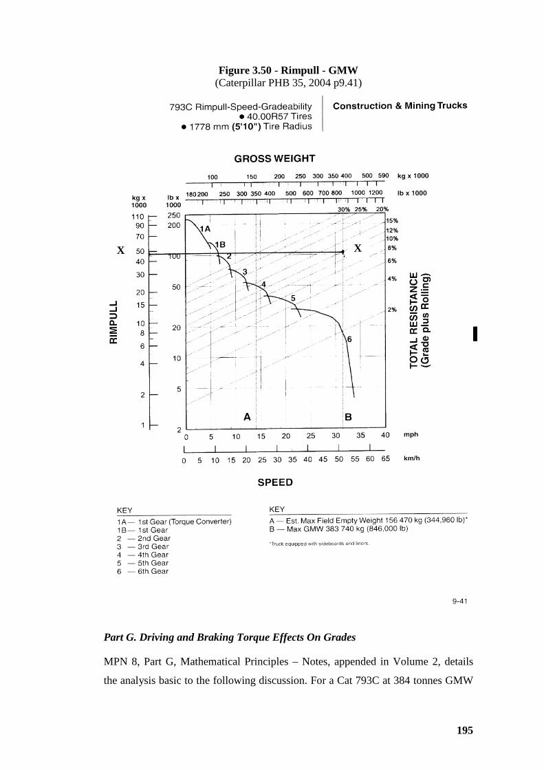
195
Figure 3.50 - Rimpull - GMW (Caterpillar PHB 35, 2004 p9.41)
Part G. Driving and Braking Torque Effects On Grades
MPN 8, Part G, Mathematical Principles – Notes, appended in Volume 2, details
the analysis basic to the following discussion. For a Cat 793C at 384 tonnes GMW
X X
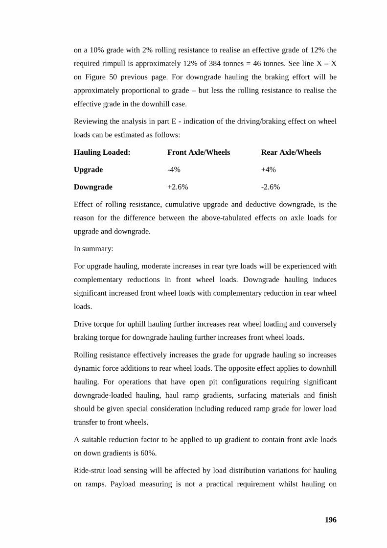
196
on a 10% grade with 2% rolling resistance to realise an effective grade of 12% the
required rimpull is approximately 12% of 384 tonnes = 46 tonnes. See line X – X
on Figure 50 previous page. For downgrade hauling the braking effort will be
approximately proportional to grade – but less the rolling resistance to realise the
effective grade in the downhill case.
Reviewing the analysis in part E - indication of the driving/braking effect on wheel
loads can be estimated as follows:
Hauling Loaded: Front Axle/Wheels Rear Axle/Wheels
Upgrade -4% +4%
Downgrade +2.6% -2.6%
Effect of rolling resistance, cumulative upgrade and deductive downgrade, is the
reason for the difference between the above-tabulated effects on axle loads for
upgrade and downgrade.
In summary:
For upgrade hauling, moderate increases in rear tyre loads will be experienced with
complementary reductions in front wheel loads. Downgrade hauling induces
significant increased front wheel loads with complementary reduction in rear wheel
loads.
Drive torque for uphill hauling further increases rear wheel loading and conversely
braking torque for downgrade hauling further increases front wheel loads.
Rolling resistance effectively increases the grade for upgrade hauling so increases
dynamic force additions to rear wheel loads. The opposite effect applies to downhill
hauling. For operations that have open pit configurations requiring significant
downgrade-loaded hauling, haul ramp gradients, surfacing materials and finish
should be given special consideration including reduced ramp grade for lower load
transfer to front wheels.
A suitable reduction factor to be applied to up gradient to contain front axle loads
on down gradients is 60%.
Ride-strut load sensing will be affected by load distribution variations for hauling
on ramps. Payload measuring is not a practical requirement whilst hauling on
197
ramps. But if ride strut sensing is used to measure payload, particularly to indicate
when target payload has been achieved during ramping-down operations, special
consideration will need to be given to output from Caterpillar’s VIMS and similar
systems supplied by other OEM. Generally static loads measured by ride struts on a
10% ramp should be in the order of 99.5% of measurements with the truck in
normal level configuration. The effect of the incipient dynamic loads due to brake
torque will complicate load measuring. Accuracy of strut-pressure sensing for load
measuring is discussed in more detail below.
Payload Measuring Accuracy and Related Issues - Discussion
There is evidence that VIMS and equivalent load sensing systems from other OEM
are affected by misplacement of payload in the body. Payload values indicated by
VIMS or equivalents are not always consistent with scale weighings. VIMS et al
are sensitive to both payload CG shifts and overloading. Analysis in Part D
examined basic physical relationships between loads imposed on ride struts and
mechanical systems that transfer loads from ride struts to axles and individual
wheels. Intuitively ride strut pressure variations should provide a means of
collectively measuring preloads and incremental payloads. This is the fundamental
principle utilised for load measuring by VIMS et al. Analysis using simple statics
verifies that, specifically for payload placed in the body, collective load increase on
all ride struts determined from pressure variance must correspond to the total
payload added to the body. Theoretically the total of strut load increases is
independent of CG misplacement of payload in the body. But, as indicated in Part
D there is a number of practical reasons why the simple theoretical model is
inadequate in this case. There is substantial evidence that payload measurements
using VIMS are sensitive to CG misplacement and overloading of trucks. It is likely
that similar effects on accuracy of payload measuring systems supplied by other
OEM will be experienced, albeit of differing effect depending on detail of
suspension systems utilised.
Characteristics of payload measuring systems using suspension cylinder pressure
sensing are discussed in terms of advice on Caterpillar’s VIMS facility provided by
David Rea from Caterpillar Global Mining (Rea D, personal communication,
2005).
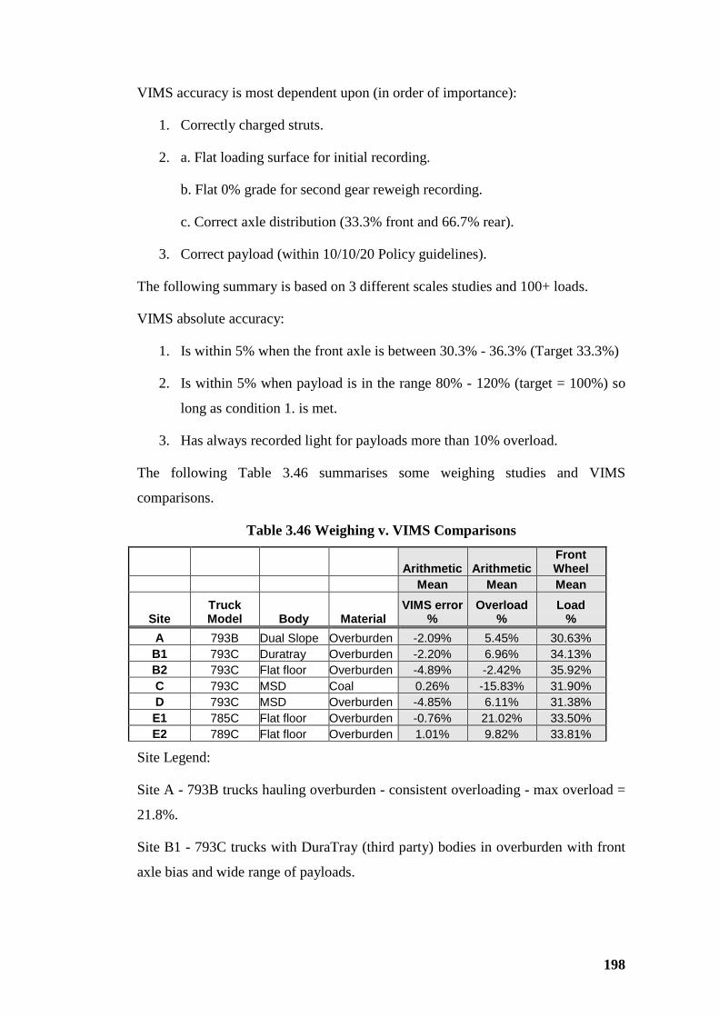
198
VIMS accuracy is most dependent upon (in order of importance):
1. Correctly charged struts.
2. a. Flat loading surface for initial recording.
b. Flat 0% grade for second gear reweigh recording.
c. Correct axle distribution (33.3% front and 66.7% rear).
3. Correct payload (within 10/10/20 Policy guidelines).
The following summary is based on 3 different scales studies and 100+ loads.
VIMS absolute accuracy:
1. Is within 5% when the front axle is between 30.3% - 36.3% (Target 33.3%)
2. Is within 5% when payload is in the range 80% - 120% (target = 100%) so
long as condition 1. is met.
3. Has always recorded light for payloads more than 10% overload.
The following Table 3.46 summarises some weighing studies and VIMS
comparisons.
Table 3.46 Weighing v. VIMS Comparisons
Arithmetic Arithmetic Front Wheel
Mean Mean Mean
Site Truck Model Body Material
VIMS error %
Overload %
Load %
A 793B Dual Slope Overburden -2.09% 5.45% 30.63% B1 793C Duratray Overburden -2.20% 6.96% 34.13% B2 793C Flat floor Overburden -4.89% -2.42% 35.92% C 793C MSD Coal 0.26% -15.83% 31.90% D 793C MSD Overburden -4.85% 6.11% 31.38% E1 785C Flat floor Overburden -0.76% 21.02% 33.50% E2 789C Flat floor Overburden 1.01% 9.82% 33.81%
Site Legend:
Site A - 793B trucks hauling overburden - consistent overloading - max overload =
21.8%.
Site B1 - 793C trucks with DuraTray (third party) bodies in overburden with front
axle bias and wide range of payloads.
199
Site B2 - 793C trucks with flat floor bodies in overburden with front axle bias and
wide range of payloads.
Site C - 793C trucks with MSD bodies hauling coal with rear axle bias and
consistent under loading - max under load = -26.7%.
Site D - 793C trucks with MSD bodies hauling overburden at a strip coal mine.
Site E1 - 785C trucks with flat floor bodies hauling overburden and gold ore.
Site E2 - 789C with flat floor bodies hauling overburden and gold ore.
Parts E and F indicate that, except where trucks are unnaturally restrained by severe
wheel chocking and on ramp grades that loaded GMW will generally be distributed
in the ranges of 33.3% front and 66.7% rear +/- 10%. This accommodates the
VIMS front-axle distribution-criteria of range 30.3% to 36.3%.
Summarizing the empirical evidence – for actual payload in the range 80% to 120%
of target payload: and provided the front axle distribution is in the range 30.3% to
36.3%, VIMS accuracy is in the range +/-5% for 95% of payloads.
The following reasons for VIMS payload accuracy varying between +/-5% are
hypothesized:
• Response of suspension struts is affected by friction between seals and
cylinder bore – (particularly noticeable when ride struts are new - Power A,
pers. commun. 2005).
• When a truck is subjected to wheel chocking or on ramps, transverse loads
will be developed across ride struts, particularly front struts that serve as
steering king posts, increasing load on strut seals tending to reduce response
of suspension cylinders to in-line loads.
• Front struts generally have greater travel than rear ride struts – so changing
strut geometry; and, prospectively, application of transverse load
components across struts.
• Rear ride struts generally are mounted to minimise effect of any transverse
load components – described in more detail.
200
• It is hypothesized that front ride struts are subjected to relatively greater
transverse force components – particularly where the strut acts as the
steering king post.
Rear ride struts, and front ride struts of trailing link and double wishbone front
suspension systems are commonly mounted using a double bush arrangement
consisting a pin through a parallel-bore grease-lubricated bush with an outer
spherical surface that matches up to two spherical half bushes, also grease
lubricated, pressed with an interference fit into the mounting eye at each end of the
strut. The end journals of the strut mounting pins are located and fixed within
sacrificial bushes pressed into the mounting clevises with keeper plates to retain the
pin in place longitudinally and prevent pin rotation. The above description is only
one arrangement. Other designs may change in detail but the functional intention, to
allow universal movement, will be similar.
The nett effect of the above-described mounting arrangement is to minimise
transfer of transverse forces in any direction to rear ride struts or front struts with
similar mounting details. Efficacy of the universal mounting system is dependent
on:
• Efficiency of lubrication.
• Wear condition of the lubricated bushes that have a discrete life and
occasionally will experience metal-to-metal contact.
• Auto-lubrication of all grease bearings is practically universal for large
mining trucks; but grease systems do break down in part or totally from
time to time.
• Bushes do wear and grease ways can be blocked or reduced in cross-section
by wear.
Any or all of the above can contribute to spurious transverse load forces being
transferred to ride struts.
Whatever causes contribute to variability in payload measuring by VIMS (or its
equivalents), it has been empirically shown that, compared with scale weighing of
mining trucks VIMS payload measuring can exhibit differences in the range +/-5%
201
in association with front-axle loading bias and/or overloading consequently
resulting in lower-than scale-measured payloads being recorded by VIMS.
In addition to the causes identified, VIMS payload measuring is likely significantly
affected by variability in loose density of material being loaded onto trucks and the
consequent variable disposition of load in truck bodies. During the loading process,
VIMS may indicate that payload is under target and the body is practically filled
(due to lower-than-expected loose density). If loading continues additional
“superimposed” load (see Part B) to make up target payload must be placed
forward in the body so tending to bias load distribution to the front axle. In such
circumstances empirical evidence indicates VIMS tends to record lower than actual
payload. One reason for these hypothetical circumstances could be body capacity
inadequate to accommodate target payload at loose density of material being
hauled.
Selection of body type and capacity must, with high probability, accommodate the
expected loose density range of material being hauled. There are several issues to
be considered:
• If a range of material types - and loose densities, each with its unique
distribution parameters - must be hauled, what determinative value of loose
density should be used to design body capacity?
• What are the relative proportions of different material types – to determine
whether to set body capacity to accommodate loose density for all material
types (and with general excess body capacity for all but one specific type)
or to accept under loading for relatively small proportions of one or more
types of material?
• What distribution parameters apply to loose density of specific materials to
be hauled to enable determination of a loose density value that will, with,
say, 95% probability, ensure that body capacity is sufficient to
accommodate target payload for each truckload.
• If VIMS indicates loading should be truncated before the truck body is filled
volumetrically, potentially there may be load distribution bias either to front
or rear depending on placement of the partial volumetric load within the
body. There is obvious opportunity to overload trucks that will be avoided
202
by guidance from VIMS and high standards of loading equipment operating
techniques.
Rear axle bias of loaded trucks is generally of less impact on individual wheel and
tyre loads as indicated by Table 3.42, further illustrated by Figure 3.48 - upgrade
hauling; and Figure 3.49- downgrade hauling. Much steeper curve gradients are
manifest for front axle load increase as downgrade increases in Figure 3.49
compared with increase in rear axle loads, as upgrade increases, in Figure 3.48.
In the final analysis suspension-based load measuring systems such as
TPMS/VIMS are the best payload monitoring option currently available. Compared
with currently available volumetric payload measuring systems VIMS and
equivalents have the following advantages:
• VIMS et al are onboard systems that can output to warning lights or digital
displays externally on the truck, alternatively accessed on monitors by
equipment operators, truck or loading, and any interested personnel in real
time, both on site and at any location of choice serviced by modern
communication mediums.
• Each truck is independently serviced by a facility non-intrusive to truck
operation (does not dictate truck route or position at any time). Load
recording is an adjunct to; and, apart from sharing data with other
equipment management facilities, is independent of all other vital
information recording systems and operational functions.
• Provides at-the-loading-point payload measuring facilitating payload control
– available in real time to loading equipment operators and other interested
parties.
Recent initiatives in volumetric sensing of payload volume in truck bodies, such as
Trayscan (described in Section 3.3.6.), are located remote from the loading point on
a haul road from pit to waste dump or ore processing. In large operations with
multiple pit exits and several concurrently active haul roads multiple monitoring
facilities (that can be mobile) will be required. As with suspension sensing load
measuring, these types of systems do not interfere with the intrinsic productivity of
trucks. Also, volumetric payload measuring is independent of the NMW and how
that may change during hauling operations due to carryback and debris
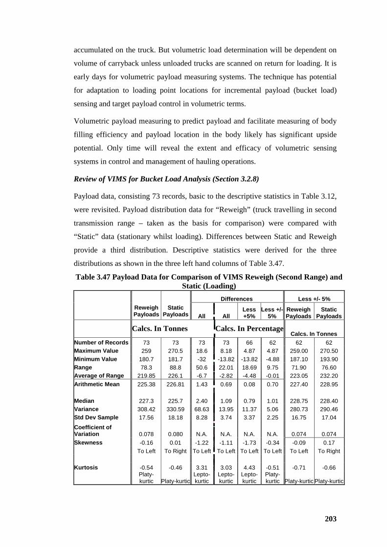
203
accumulated on the truck. But volumetric load determination will be dependent on
volume of carryback unless unloaded trucks are scanned on return for loading. It is
early days for volumetric payload measuring systems. The technique has potential
for adaptation to loading point locations for incremental payload (bucket load)
sensing and target payload control in volumetric terms.
Volumetric payload measuring to predict payload and facilitate measuring of body
filling efficiency and payload location in the body likely has significant upside
potential. Only time will reveal the extent and efficacy of volumetric sensing
systems in control and management of hauling operations.
Review of VIMS for Bucket Load Analysis (Section 3.2.8)
Payload data, consisting 73 records, basic to the descriptive statistics in Table 3.12,
were revisited. Payload distribution data for “Reweigh” (truck travelling in second
transmission range – taken as the basis for comparison) were compared with
“Static” data (stationary whilst loading). Differences between Static and Reweigh
provide a third distribution. Descriptive statistics were derived for the three
distributions as shown in the three left hand columns of Table 3.47.
Table 3.47 Payload Data for Comparison of VIMS Reweigh (Second Range) and Static (Loading)
Reweigh Payloads
Static Payloads
Differences Less +/- 5%
All All Less +5%
Less +/- 5%
Reweigh Payloads
Static Payloads
Calcs. In Tonnes Calcs. In Percentage
Calcs. In Tonnes Number of Records 73 73 73 73 66 62 62 62 Maximum Value 259 270.5 18.6 8.18 4.87 4.87 259.00 270.50 Minimum Value 180.7 181.7 -32 -13.82 -13.82 -4.88 187.10 193.90 Range 78.3 88.8 50.6 22.01 18.69 9.75 71.90 76.60 Average of Range 219.85 226.1 -6.7 -2.82 -4.48 -0.01 223.05 232.20 Arithmetic Mean 225.38 226.81 1.43 0.69 0.08 0.70 227.40 228.95 Median 227.3 225.7 2.40 1.09 0.79 1.01 228.75 228.40 Variance 308.42 330.59 68.63 13.95 11.37 5.06 280.73 290.46 Std Dev Sample 17.56 18.18 8.28 3.74 3.37 2.25 16.75 17.04
Coefficient of Variation 0.078 0.080 N.A. N.A. N.A. N.A. 0.074 0.074 Skewness -0.16 0.01 -1.22 -1.11 -1.73 -0.34 -0.09 0.17 To Left To Right To Left To Left To Left To Left To Left To Right Kurtosis -0.54 -0.46 3.31 3.03 4.43 -0.51 -0.71 -0.66
Platy-kurtic Platy-kurtic
Lepto-kurtic
Lepto-kurtic
Lepto-kurtic
Platy-kurtic Platy-kurtic Platy-kurtic
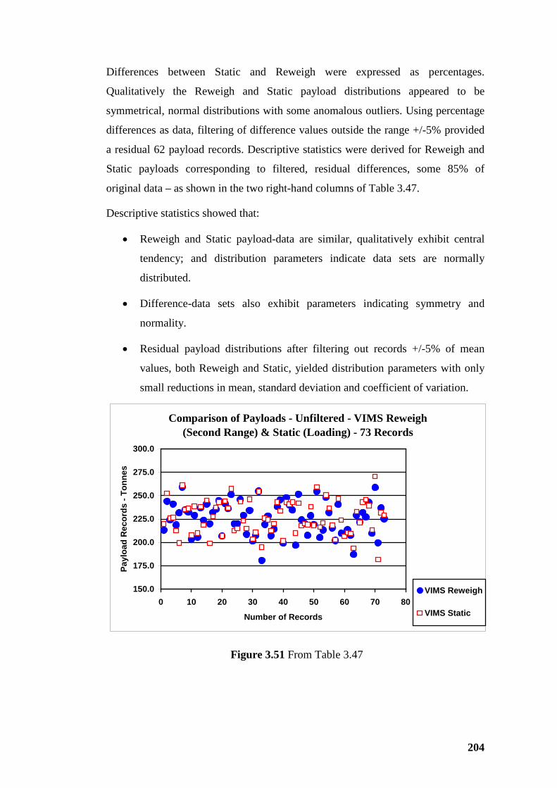
204
Differences between Static and Reweigh were expressed as percentages.
Qualitatively the Reweigh and Static payload distributions appeared to be
symmetrical, normal distributions with some anomalous outliers. Using percentage
differences as data, filtering of difference values outside the range +/-5% provided
a residual 62 payload records. Descriptive statistics were derived for Reweigh and
Static payloads corresponding to filtered, residual differences, some 85% of
original data – as shown in the two right-hand columns of Table 3.47.
Descriptive statistics showed that:
• Reweigh and Static payload-data are similar, qualitatively exhibit central
tendency; and distribution parameters indicate data sets are normally
distributed.
• Difference-data sets also exhibit parameters indicating symmetry and
normality.
• Residual payload distributions after filtering out records +/-5% of mean
values, both Reweigh and Static, yielded distribution parameters with only
small reductions in mean, standard deviation and coefficient of variation.
Comparison of Payloads - Unfiltered - VIMS Reweigh (Second Range) & Static (Loading) - 73 Records
150.0
175.0
200.0
225.0
250.0
275.0
300.0
0 10 20 30 40 50 60 70 80
Number of Records
Payl
oad
Rec
ords
- To
nnes
VIMS Reweigh
VIMS Static
Figure 3.51 From Table 3.47
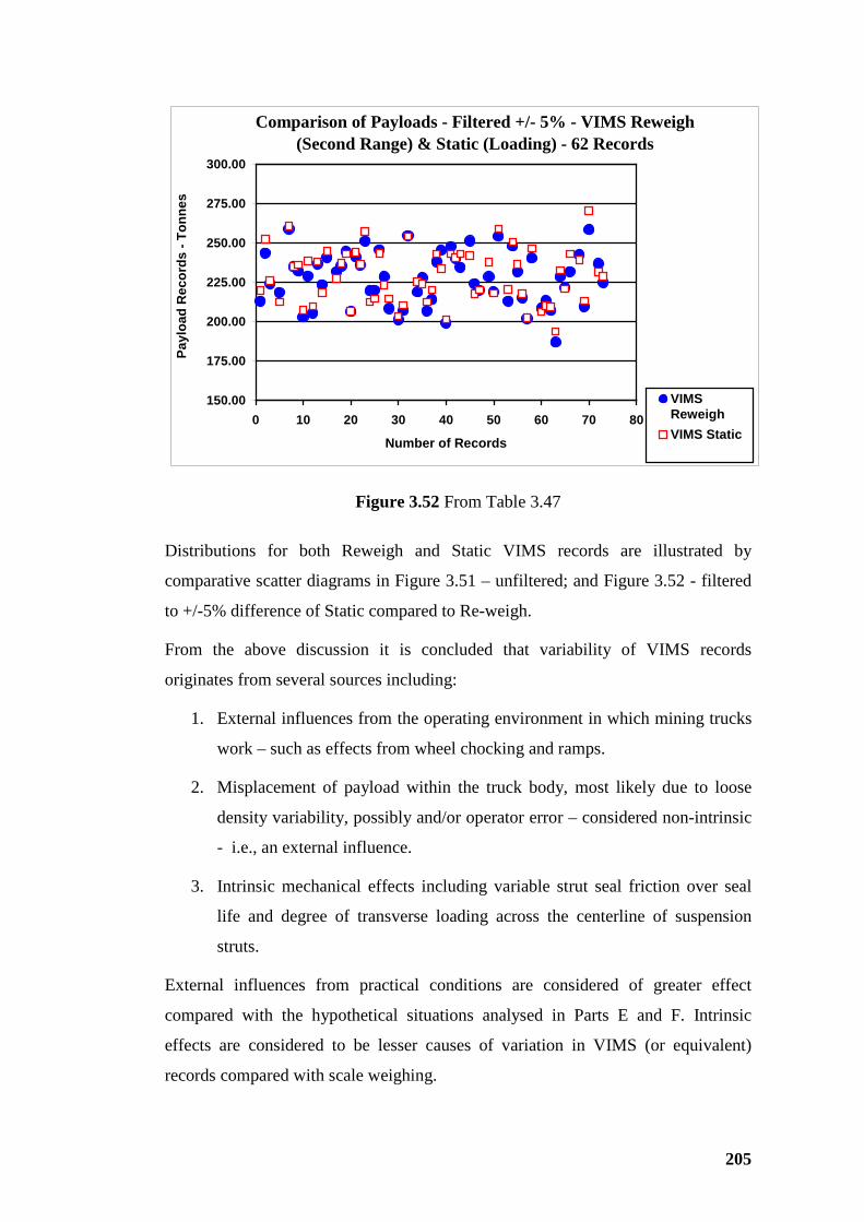
205
150.00
175.00
200.00
225.00
250.00
275.00
300.00
0 10 20 30 40 50 60 70 80
Number of Records
Payl
oad
Rec
ords
- To
nnes
VIMSReweighVIMS Static
Comparison of Payloads - Filtered +/- 5% - VIMS Reweigh (Second Range) & Static (Loading) - 62 Records
Figure 3.52 From Table 3.47
Distributions for both Reweigh and Static VIMS records are illustrated by
comparative scatter diagrams in Figure 3.51 – unfiltered; and Figure 3.52 - filtered
to +/-5% difference of Static compared to Re-weigh.
From the above discussion it is concluded that variability of VIMS records
originates from several sources including:
1. External influences from the operating environment in which mining trucks
work – such as effects from wheel chocking and ramps.
2. Misplacement of payload within the truck body, most likely due to loose
density variability, possibly and/or operator error – considered non-intrinsic
- i.e., an external influence.
3. Intrinsic mechanical effects including variable strut seal friction over seal
life and degree of transverse loading across the centerline of suspension
struts.
External influences from practical conditions are considered of greater effect
compared with the hypothetical situations analysed in Parts E and F. Intrinsic
effects are considered to be lesser causes of variation in VIMS (or equivalent)
records compared with scale weighing.
206
In the final analysis, payload/GMW-measuring systems using suspension cylinder
sensing deliver:
• Variable but acceptable accuracy at the loading point – variable to differing
degrees depending on external affects not the least of which is variability of
material loose density.
• More reliable and repeatable payload/GMW measurement by reweighing
using a small sample of strut pressure recordings in second range of
mechanical drive transmissions, or equivalent conditions for an electric
wheel-motor mining truck.
• Typically VIMS and equivalents provide payload/GMW measurements that
are generally repeatable and reliable within a reasonably limited range and
with high probability.
• Accuracy of VIMS reweighing relative to scale weighing is claimed, with
support of empirical evidence, to be +/-5% for 95% of truckloads measured.
Accuracy of VIMS Reweigh may be higher than claimed if the following are
considered:
• Extreme inaccuracy values are for abnormal cases – where payload is
misplaced or overloaded or other influences affect accuracy.
• Understood inaccuracy ranging to +/- 1% for in-ground scales is cumulative
with any inaccuracy of VIMS.
• Recent and on-going technical improvements as keen competition for
market share of large mining truck sales encourages OEM to provide
customer ever-improved truck management systems.
A technologically advanced well-maintained on-board weighing system should
generally deliver +/-2% accuracy (Power A, 2005, pers. commun.). Consideration
of this advice is supportive particularly where trucks are loaded as per design and
truck payloads are in compliance with the applicable control standard such as
Caterpillar’s “10/10/20 Policy”.
For the single case of 73 records analysed as described, static payload measurement
at the loading point compared with reweighing of the moving truck included
207
individual payload variations in the range +8% to –14%. But as described and
illustrated, descriptive statistics for the two distributions, static and re-weigh, were
comparable. Particularly mean values were little different varying only by some
0.6%. This is interpreted as, at least initial, evidence that using VIMS for payload
monitoring during loading will likely result in mean reweigh payloads that meet
chosen control criteria - such as Caterpillar’s 10/10/20 Policy. This of course, is
with the proviso that the various factors influencing payload variability such as
material condition, loose density variability and operational techniques are within
design and best practice limits.
In Section 3.2.8 bucket loads included in small samples that make up truck
payloads were downloaded from static loading data. Each bucket load recorded for
each small sample of bucket loads accumulating to a truck payload was
proportionally modified to convert static data to equivalent reweigh data. Based on
the evidence of comparable descriptive statistics for static and reweigh data
distributions; and considering that bucket load data were treated as a selection of
distributions that were analysed and compared in terms of descriptive statistics, in
hindsight it is concluded that proportional correction of static bucket loads to
reweigh-based data was likely unnecessary. It is believed that analyzing bucket
loads based on static data, as recorded, would have provided similar outcomes
leading to identical interpretations and conclusions.
Descriptive statistics in Tables 3.15, 3.16, and 3.17 compare distributions of truck
payloads, bucket loads, selected bucket load groups (first, last and intermediate)
and sub-groups of four and five-pass bucket load/truck payload data. Measures of
expected values (means), dispersion (standard deviation) and comparative
variability (coefficient of variation) are generally consistent and reconcilable in
terms of mathematical relationships.
It is concluded that the consistency and comparability of descriptive statistics of
static and reweigh data is empirical evidence that data remotely downloaded from
VIMS using Caterpillar’s Minestar system, subsequent analysis discussed in
Section 3.2.8 has resulted in generally valid interpretations and conclusions.
208
Interpretation, Conclusions and Comments
Earliest considerations in this Section 3.3.7 on “Truck Payload Centre of Gravity
(CG) exposed a wide field of relevant issues. Each issue considered seemed to
raise more questions than were answered. Consequently the issues expanded out to
include consideration of:
• Body loading efficacy and implications of payload CG misplacement in
distribution of NMW and truck payload as axle loads.
• Load transference between truck axles due to practical but abnormal
operations including rear wheel chocking and uphill or downhill hauling.
• Leveraging affects from incipient or actual dynamic situations that are
registered by truck suspension as additional “virtual load” – outcomes of
analysis of these first three considerations are provided above or in
Mathematical Principles - Notes appended in Volume 2.
• Review of intrinsic accuracy of payload measuring systems using
suspension-cylinder pressure sensing.
• Review of reasons for output variability from such payload measuring
systems.
• Brief comparative comments on volumetric payload measuring systems
currently on offer and in process of development.
• Review of validity of using static and reweigh payload data in terms of
individual bucket loads to examine the relationship between number of
passes, bucket load anomalies and truck payload dispersion.
• Acknowledgement of the continual presence and significant influence of
loose density variability in control and management of payload dispersion –
a presence that grew in impact and importance in the course of the research.
Truck Selection and Productivity
Relevant issues in truck selection arising from this section 3.3.7 include:
• In the process of procurement, through contact with dealers and OEM
supplying mining trucks, performance information and management

209
systems will be offered – a typical example is Caterpillar’s VIMS and its
many integral and adjunct options.
• Integral with, or separable from, the total vital information system, on-board
payload measuring using suspension cylinder pressure sensing will
generally be offered.
• Due diligence in investigative stages of the procurement process must
deliver an understanding of the benefits of payload measuring and what it
promises for monitoring and management control of hauling operations.
• Body type and design for specific service – and, most importantly, adequate
truck body capacity - that will avoid the too-often-seen “ducktail extension”
and “side extensions” as untidy remedies. These afterthought, remedial
extensions should not be confused with the addition of colloquially-termed
“hungry boards” when owners, particularly civil construction and mining
contactors, have deliberately sought to overload smaller construction trucks
on typically short hauls.
• Particularly there needs to be an understanding of accuracy claims and what
payload measuring systems can be expected to deliver.
• Implications in terms of management commitment to processing the wealth
of data from payload measuring and related systems and compile it into
acutely focused and user-friendly reports for the benefit of managing load
and haul operations.
Effective use of systems acquired to monitor and manage hauling operations should
be a natural progression from selection in the process of mining truck procurement.
Specific issues include:
• Securing comprehensive records that are interpreted and compiled in user-
friendly reports; and developing techniques to maximize productivity and
equipment performance benefits from the systems.
• Accommodating within operational and maintenance management plans
best practice for utilisation and maintenance of equipment, also for
management and information systems, applying the same standards and
importance as granted to critical operating componentry of the equipment.
210
As mining trucks increase in size and capacity there is ever increasing demand for
sophistication and attention to operational control and management – particularly of
payload dispersion, body designs, placement of payload in truck bodies, avoidance
of unacceptable operational severity and misadventure. To satisfy this demand
onboard information systems, VIMS and equivalents, are essential adjunct
componentry for large mining trucks to realise the expected benefits from increased
unit capital investment. It is not so much a matter of justifying adoption of onboard
information, management and control systems for large mining trucks but justifying
any decision not to adopt them.
3.3.8 Tyres
Pneumatic tyres fitted to mobile earthmoving equipment are generally treated as a
consumable for purposes of cost estimating and budgeting. Tyre costs are normally
expressed as unit cost per operating hour of the equipment or per unit of production
– normally per tonne, but optionally per BCM. Unit cost of tyres is not directly
comparable between operations and is essentially a local performance measure
where productivity is measured in BCM.
But, in effect, tyres are an essential driveline component for equipment running on
them. Compared with other driveline componentry tyres have a relatively short life.
Tyre life for mining trucks is generally in the range 2,000 to 6,000 hour; or, say,
40,000 to 120,000 kilometres – with tyre life for larger mining trucks at the lower
end of the range.
Tyre life, Costs and Truck Scale
As truck size increases tyre life tends to reduce as shown in Table 3.48; and tyre
costs tend to increase as a proportion of total hauling unit costs. It will be noted that
Tyre Life Index for larger mining trucks has substantial upside potential. This is
consistent with industry history. As larger trucks have been developed and
marketed, tyre manufacturers have responded with larger tyres designed for the
increased service. Tyre development tends to be delayed compared with other
product improvements for mining trucks. It involves substantial field-testing and
experience. Onsite management of larger tyres by operators also needs to be more
diligent. To provide a basis for improving tyre life, road surfaces, general running
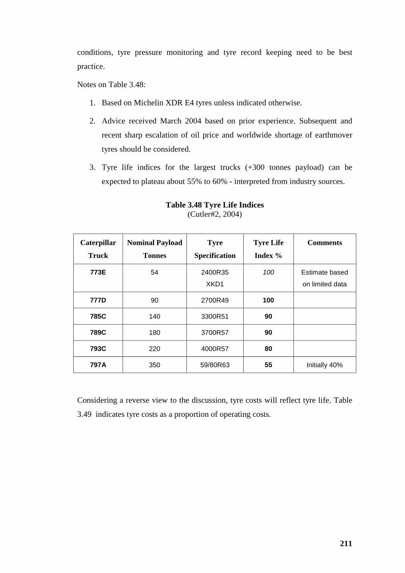
211
conditions, tyre pressure monitoring and tyre record keeping need to be best
practice.
Notes on Table 3.48:
1. Based on Michelin XDR E4 tyres unless indicated otherwise.
2. Advice received March 2004 based on prior experience. Subsequent and
recent sharp escalation of oil price and worldwide shortage of earthmover
tyres should be considered.
3. Tyre life indices for the largest trucks (+300 tonnes payload) can be
expected to plateau about 55% to 60% - interpreted from industry sources.
Table 3.48 Tyre Life Indices
(Cutler#2, 2004)
Considering a reverse view to the discussion, tyre costs will reflect tyre life. Table
3.49 indicates tyre costs as a proportion of operating costs.
Caterpillar
Truck
Nominal Payload
Tonnes
Tyre
Specification
Tyre Life
Index %
Comments
773E 54 2400R35
XKD1
100 Estimate based
on limited data
777D 90 2700R49 100
785C 140 3300R51 90
789C 180 3700R57 90
793C 220 4000R57 80
797A 350 59/80R63 55 Initially 40%
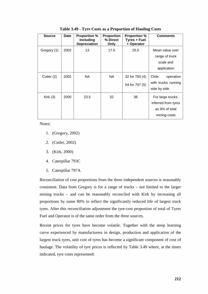
212
Table 3.49 - Tyre Costs as a Proportion of Hauling Costs Source Date Proportion %
Including Depreciation
Proportion % Direct
Only
Proportion % Tyres + Fuel + Operator
Comments
Gregory (1) 2002 13 17.5 25.5 Mean value over
range of truck
scale and
application
Cutler (2) 2002 NA NA 32 for 793 (4)
54 for 797 (5)
Chile operation
with trucks running
side by side
Kirk (3) 2000 23.5 32 38 For large trucks.
Inferred from tyres
as 9% of total
mining costs
Notes:
1. (Gregory, 2002)
2. (Cutler, 2002)
3. (Kirk, 2000)
4. Caterpillar 793C
5. Caterpillar 797A
Reconciliation of cost proportions from the three independent sources is reasonably
consistent. Data from Gregory is for a range of trucks – not limited to the larger
mining trucks – and can be reasonably reconciled with Kirk by increasing all
proportions by some 80% to reflect the significantly reduced life of largest truck
tyres. After this reconciliation adjustment the tyre-cost proportion of total of Tyres
Fuel and Operator is of the same order from the three sources.
Recent prices for tyres have become volatile. Together with the steep learning
curve experienced by manufacturers in design, production and application of the
largest truck tyres, unit cost of tyres has become a significant component of cost of
haulage. The volatility of tyre prices is reflected by Table 3.49 where, at the times
indicated, tyre costs represented:
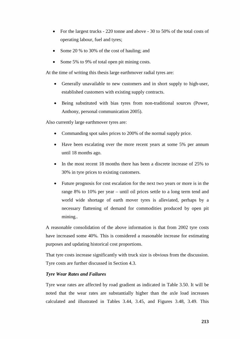
213
• For the largest trucks - 220 tonne and above - 30 to 50% of the total costs of
operating labour, fuel and tyres;
• Some 20 % to 30% of the cost of hauling; and
• Some 5% to 9% of total open pit mining costs.
At the time of writing this thesis large earthmover radial tyres are:
• Generally unavailable to new customers and in short supply to high-user,
established customers with existing supply contracts.
• Being substituted with bias tyres from non-traditional sources (Power,
Anthony, personal communication 2005).
Also currently large earthmover tyres are:
• Commanding spot sales prices to 200% of the normal supply price.
• Have been escalating over the more recent years at some 5% per annum
until 18 months ago.
• In the most recent 18 months there has been a discrete increase of 25% to
30% in tyre prices to existing customers.
• Future prognosis for cost escalation for the next two years or more is in the
range 8% to 10% per year – until oil prices settle to a long term tend and
world wide shortage of earth mover tyres is alleviated, perhaps by a
necessary flattening of demand for commodities produced by open pit
mining..
A reasonable consolidation of the above information is that from 2002 tyre costs
have increased some 40%. This is considered a reasonable increase for estimating
purposes and updating historical cost proportions.
That tyre costs increase significantly with truck size is obvious from the discussion.
Tyre costs are further discussed in Section 4.3.
Tyre Wear Rates and Failures
Tyre wear rates are affected by road gradient as indicated in Table 3.50. It will be
noted that the wear rates are substantially higher than the axle load increases
calculated and illustrated in Tables 3.44, 3.45, and Figures 3.48, 3.49. This
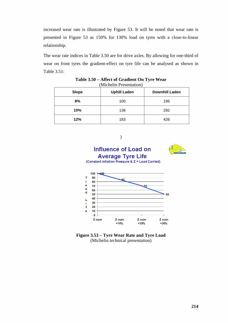
214
increased wear rate is illustrated by Figure 53. It will be noted that wear rate is
presented in Figure 53 as 150% for 130% load on tyres with a close-to-linear
relationship.
The wear rate indices in Table 3.50 are for drive axles. By allowing for one-third of
wear on front tyres the gradient-effect on tyre life can be analysed as shown in
Table 3.51:
Table 3.50 – Affect of Gradient On Tyre Wear (Michelin Presentation)
Slope Uphill Laden Downhill Laden
8% 100 195
10% 136 292
12% 183 426
)
Figure 3.53 – Tyre Wear Rate and Tyre Load
(Michelin technical presentation)
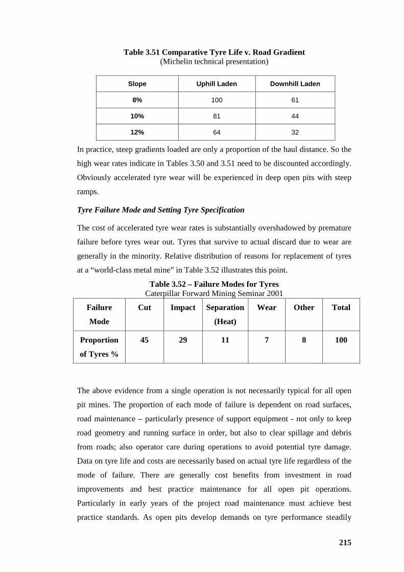
215
Table 3.51 Comparative Tyre Life v. Road Gradient (Michelin technical presentation)
Slope Uphill Laden Downhill Laden
8% 100 61
10% 81 44
12% 64 32
In practice, steep gradients loaded are only a proportion of the haul distance. So the
high wear rates indicate in Tables 3.50 and 3.51 need to be discounted accordingly.
Obviously accelerated tyre wear will be experienced in deep open pits with steep
ramps.
Tyre Failure Mode and Setting Tyre Specification
The cost of accelerated tyre wear rates is substantially overshadowed by premature
failure before tyres wear out. Tyres that survive to actual discard due to wear are
generally in the minority. Relative distribution of reasons for replacement of tyres
at a “world-class metal mine” in Table 3.52 illustrates this point.
Table 3.52 – Failure Modes for Tyres Caterpillar Forward Mining Seminar 2001
Failure
Mode
Cut Impact Separation
(Heat)
Wear Other Total
Proportion
of Tyres %
45 29 11 7 8 100
The above evidence from a single operation is not necessarily typical for all open
pit mines. The proportion of each mode of failure is dependent on road surfaces,
road maintenance – particularly presence of support equipment - not only to keep
road geometry and running surface in order, but also to clear spillage and debris
from roads; also operator care during operations to avoid potential tyre damage.
Data on tyre life and costs are necessarily based on actual tyre life regardless of the
mode of failure. There are generally cost benefits from investment in road
improvements and best practice maintenance for all open pit operations.
Particularly in early years of the project road maintenance must achieve best
practice standards. As open pits develop demands on tyre performance steadily
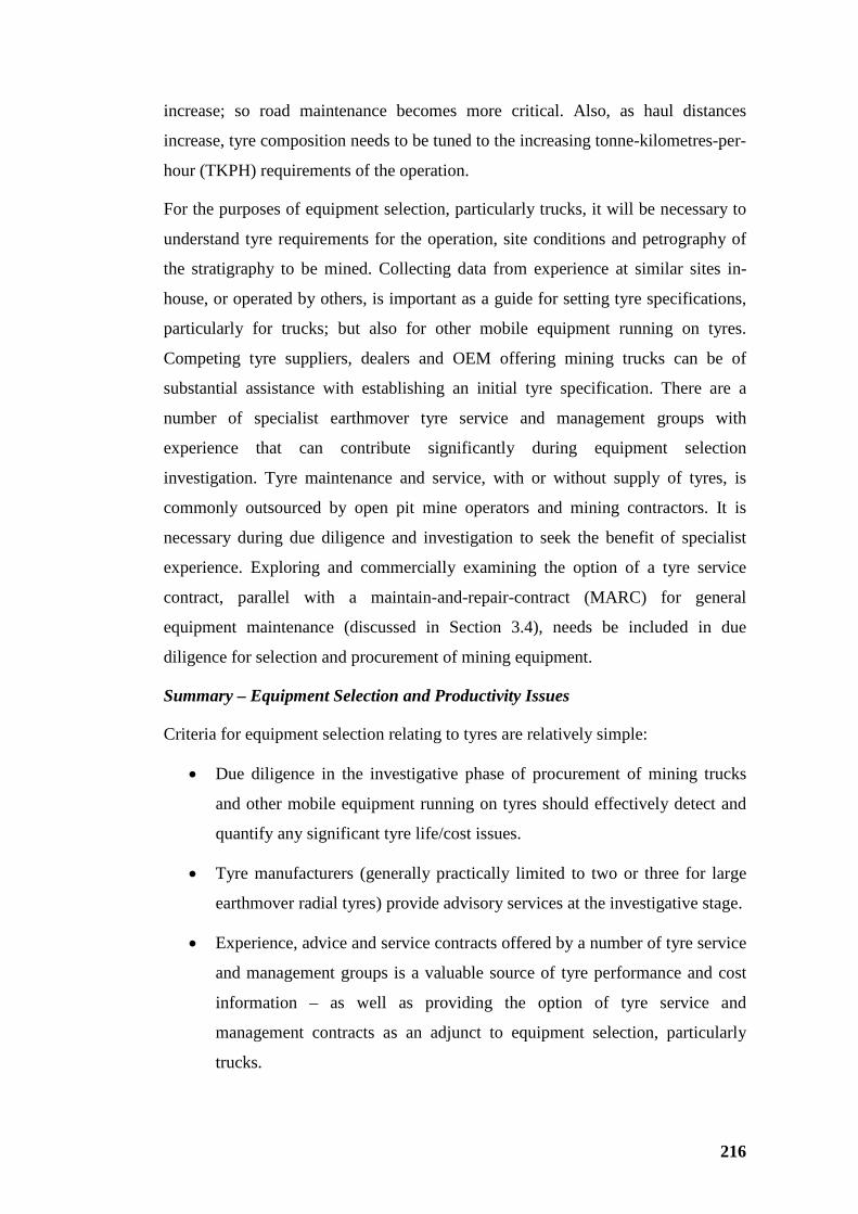
216
increase; so road maintenance becomes more critical. Also, as haul distances
increase, tyre composition needs to be tuned to the increasing tonne-kilometres-per-
hour (TKPH) requirements of the operation.
For the purposes of equipment selection, particularly trucks, it will be necessary to
understand tyre requirements for the operation, site conditions and petrography of
the stratigraphy to be mined. Collecting data from experience at similar sites in-
house, or operated by others, is important as a guide for setting tyre specifications,
particularly for trucks; but also for other mobile equipment running on tyres.
Competing tyre suppliers, dealers and OEM offering mining trucks can be of
substantial assistance with establishing an initial tyre specification. There are a
number of specialist earthmover tyre service and management groups with
experience that can contribute significantly during equipment selection
investigation. Tyre maintenance and service, with or without supply of tyres, is
commonly outsourced by open pit mine operators and mining contractors. It is
necessary during due diligence and investigation to seek the benefit of specialist
experience. Exploring and commercially examining the option of a tyre service
contract, parallel with a maintain-and-repair-contract (MARC) for general
equipment maintenance (discussed in Section 3.4), needs be included in due
diligence for selection and procurement of mining equipment.
Summary – Equipment Selection and Productivity Issues
Criteria for equipment selection relating to tyres are relatively simple:
• Due diligence in the investigative phase of procurement of mining trucks
and other mobile equipment running on tyres should effectively detect and
quantify any significant tyre life/cost issues.
• Tyre manufacturers (generally practically limited to two or three for large
earthmover radial tyres) provide advisory services at the investigative stage.
• Experience, advice and service contracts offered by a number of tyre service
and management groups is a valuable source of tyre performance and cost
information – as well as providing the option of tyre service and
management contracts as an adjunct to equipment selection, particularly
trucks.
217
• It is essential to determine the nature of the tyre rating recommended by the
suppliers to relate to the road construction specifications in relation to road
geometry and running surface finish.
• The larger the scale of mining trucks, the more demanding will be the
standards of haul road construction, surface finish and ongoing
maintenance.
• Impact of tyres on performance and cost increases with the scale of trucks
and increased haul distance – for the largest trucks operational performance
limitations controlled by tyres - may be most significant factors in
determining productivity and cost criteria for determination of project
economics.
Failure to align tyre specification with service and adopted road standards will
prevent realisation of expected tyre costs.
Accelerated tyre wear due to open pit designs with steep ramps, albeit an economic
necessity, will also mean more downtime for tyre replacement so reduced
productivity – a relatively moderate, but important issue in terms of load-and-haul
productivity and cost.
Truck-performance effects due to tyre wear are further addressed in Section 3.3.11.
3.3.9 Bucket Passes and Payloads
Introduction
Analysis of bucket loads and resulting payloads in Section 3.2.8 arrived at
significant conclusions including:
• As expected bucket loads tend to be normally distributed with truck
payloads exhibiting greater central tendency.
• Means of first bucket loads are manifestly higher and means of last bucket
loads generally lower than means of the population for bucket loads.
• Coefficient of variation (CV) of bucket loads or truck payloads is a
convenient statistic to compare sub-populations from a range of loading
operations.
218
• Caterpillar’s 10/10/20 Policy was related to the truck payload CV statistic as
a comparative compliance criterion.
Further analysis in Section 3.3.6 introduced “digability” as the measure of loading
productivity. The significant relationship between variability of voids ratio of
material to be loaded and hauled and truck payload variability was developed
analytically. The most important direct relationship between drilling and blasting
outcomes, in terms of fragmentation and size/shape grading and efficacy of
subsequent load and haul activities was discussed and emphasized.
In this Section 3.3.9 a number of load and haul operations are analysed and
compared using a suite of descriptive statistics to show that the hypotheses and
theories developed in the initial phases of the research are consistent with operating
experience.
Discussions in this section extend to consideration of the number of passes and
implications for:
• Truck payload consistency
• Loading time consistency
• Variability of truck loading time and truck trip times.
The benefit from achieving acceptable operating “rhythm” in load and haul
operations is discussed with the ultimate objective of cyclical loading and hauling
operations simulating a continuous transport system as closely as possible.
Protocols for load and haul practice with the ultimate objective of achieving
acceptable “rhythm are recommended.
In the process of selecting load and haul equipment, the protocols recommended in
the discussion to follow are prerequisites for ensuring realization of productivity
expectations.
Load and Haul Case Studies - Statistics
Load and haul data from three open-pit mining operations were analyzed,
specifically:
Case 1 2,632 records from an open pit gold mine using nominal 225 tonne
trucks
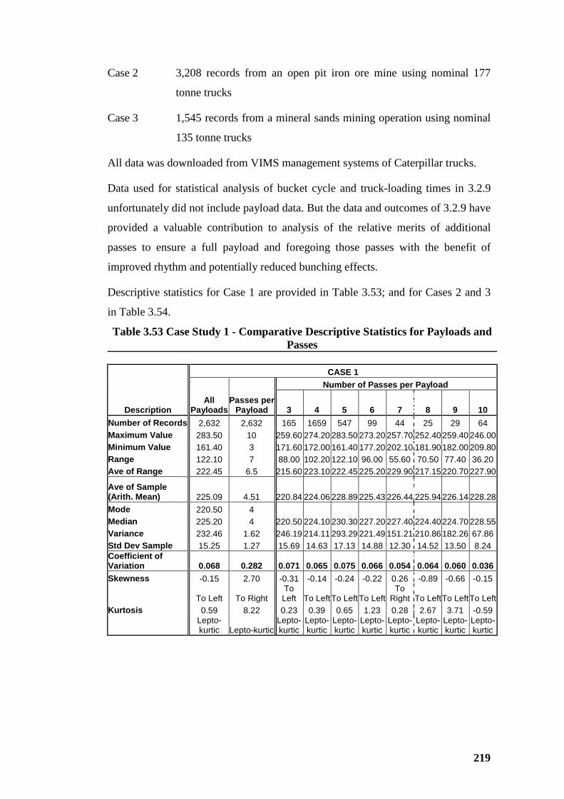
219
Case 2 3,208 records from an open pit iron ore mine using nominal 177
tonne trucks
Case 3 1,545 records from a mineral sands mining operation using nominal
135 tonne trucks
All data was downloaded from VIMS management systems of Caterpillar trucks.
Data used for statistical analysis of bucket cycle and truck-loading times in 3.2.9
unfortunately did not include payload data. But the data and outcomes of 3.2.9 have
provided a valuable contribution to analysis of the relative merits of additional
passes to ensure a full payload and foregoing those passes with the benefit of
improved rhythm and potentially reduced bunching effects.
Descriptive statistics for Case 1 are provided in Table 3.53; and for Cases 2 and 3
in Table 3.54.
Table 3.53 Case Study 1 - Comparative Descriptive Statistics for Payloads and Passes
CASE 1
All Payloads
Passes per Payload
Number of Passes per Payload
Description 3 4 5 6 7 8 9 10 Number of Records 2,632 2,632 165 1659 547 99 44 25 29 64 Maximum Value 283.50 10 259.60 274.20 283.50 273.20 257.70 252.40 259.40 246.00 Minimum Value 161.40 3 171.60 172.00 161.40 177.20 202.10 181.90 182.00 209.80 Range 122.10 7 88.00 102.20 122.10 96.00 55.60 70.50 77.40 36.20 Ave of Range 222.45 6.5 215.60 223.10 222.45 225.20 229.90 217.15 220.70 227.90
Ave of Sample (Arith. Mean) 225.09 4.51 220.84 224.06 228.89 225.43 226.44 225.94 226.14 228.28 Mode 220.50 4 Median 225.20 4 220.50 224.10 230.30 227.20 227.40 224.40 224.70 228.55 Variance 232.46 1.62 246.19 214.11 293.29 221.49 151.21 210.86 182.26 67.86 Std Dev Sample 15.25 1.27 15.69 14.63 17.13 14.88 12.30 14.52 13.50 8.24 Coefficient of Variation 0.068 0.282 0.071 0.065 0.075 0.066 0.054 0.064 0.060 0.036 Skewness -0.15 2.70 -0.31 -0.14 -0.24 -0.22 0.26 -0.89 -0.66 -0.15
To Left To Right To Left To Left To Left To Left
To Right To Left To Left To Left
Kurtosis 0.59 8.22 0.23 0.39 0.65 1.23 0.28 2.67 3.71 -0.59
Lepto-kurtic Lepto-kurtic
Lepto-kurtic
Lepto-kurtic
Lepto-kurtic
Lepto-kurtic
Lepto-kurtic
Lepto-kurtic
Lepto-kurtic
Lepto-kurtic
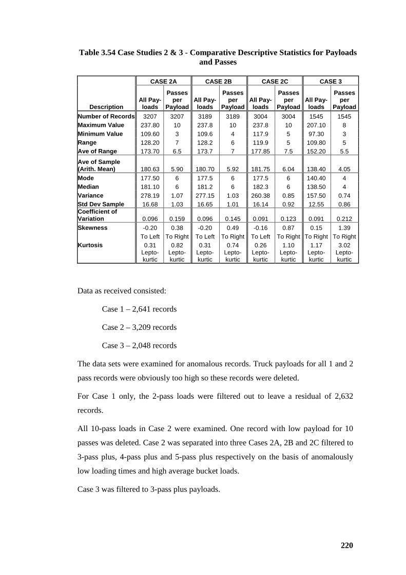
220
Table 3.54 Case Studies 2 & 3 - Comparative Descriptive Statistics for Payloads and Passes
CASE 2A CASE 2B CASE 2C CASE 3
Description
All Pay-loads
Passes per
Payload
All Pay-loads
Passes per
Payload
All Pay-loads
Passes per
Payload
All Pay-loads
Passes per
Payload Number of Records 3207 3207 3189 3189 3004 3004 1545 1545 Maximum Value 237.80 10 237.8 10 237.8 10 207.10 8 Minimum Value 109.60 3 109.6 4 117.9 5 97.30 3 Range 128.20 7 128.2 6 119.9 5 109.80 5 Ave of Range 173.70 6.5 173.7 7 177.85 7.5 152.20 5.5
Ave of Sample (Arith. Mean) 180.63 5.90 180.70 5.92 181.75 6.04 138.40 4.05 Mode 177.50 6 177.5 6 177.5 6 140.40 4 Median 181.10 6 181.2 6 182.3 6 138.50 4 Variance 278.19 1.07 277.15 1.03 260.38 0.85 157.50 0.74 Std Dev Sample 16.68 1.03 16.65 1.01 16.14 0.92 12.55 0.86 Coefficient of Variation 0.096 0.159 0.096 0.145 0.091 0.123 0.091 0.212 Skewness -0.20 0.38 -0.20 0.49 -0.16 0.87 0.15 1.39 To Left To Right To Left To Right To Left To Right To Right To Right Kurtosis 0.31 0.82 0.31 0.74 0.26 1.10 1.17 3.02
Lepto-kurtic
Lepto-kurtic
Lepto-kurtic
Lepto-kurtic
Lepto-kurtic
Lepto-kurtic
Lepto-kurtic
Lepto-kurtic
Data as received consisted:
Case 1 – 2,641 records
Case 2 – 3,209 records
Case 3 – 2,048 records
The data sets were examined for anomalous records. Truck payloads for all 1 and 2
pass records were obviously too high so these records were deleted.
For Case 1 only, the 2-pass loads were filtered out to leave a residual of 2,632
records.
All 10-pass loads in Case 2 were examined. One record with low payload for 10
passes was deleted. Case 2 was separated into three Cases 2A, 2B and 2C filtered to
3-pass plus, 4-pass plus and 5-pass plus respectively on the basis of anomalously
low loading times and high average bucket loads.
Case 3 was filtered to 3-pass plus payloads.
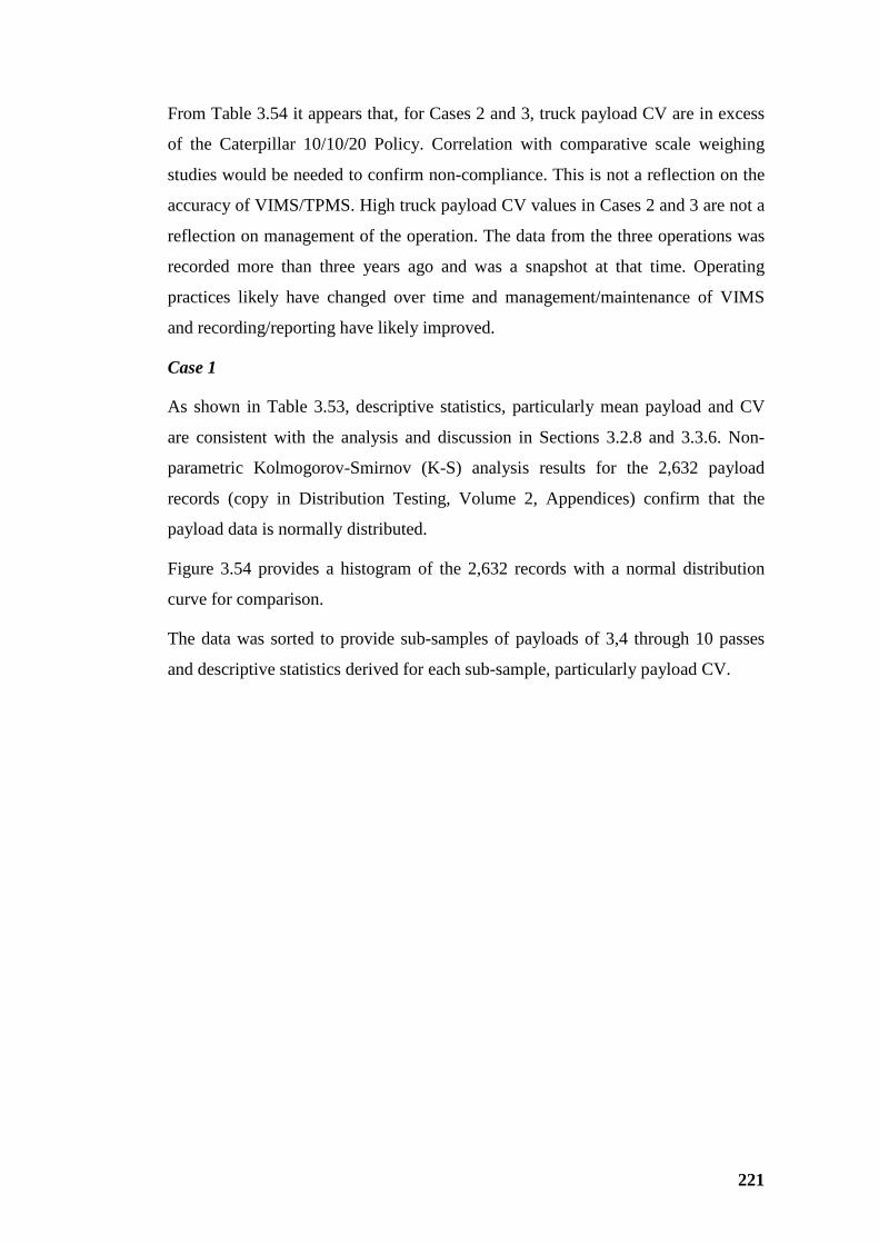
221
From Table 3.54 it appears that, for Cases 2 and 3, truck payload CV are in excess
of the Caterpillar 10/10/20 Policy. Correlation with comparative scale weighing
studies would be needed to confirm non-compliance. This is not a reflection on the
accuracy of VIMS/TPMS. High truck payload CV values in Cases 2 and 3 are not a
reflection on management of the operation. The data from the three operations was
recorded more than three years ago and was a snapshot at that time. Operating
practices likely have changed over time and management/maintenance of VIMS
and recording/reporting have likely improved.
Case 1
As shown in Table 3.53, descriptive statistics, particularly mean payload and CV
are consistent with the analysis and discussion in Sections 3.2.8 and 3.3.6. Non-
parametric Kolmogorov-Smirnov (K-S) analysis results for the 2,632 payload
records (copy in Distribution Testing, Volume 2, Appendices) confirm that the
payload data is normally distributed.
Figure 3.54 provides a histogram of the 2,632 records with a normal distribution
curve for comparison.
The data was sorted to provide sub-samples of payloads of 3,4 through 10 passes
and descriptive statistics derived for each sub-sample, particularly payload CV.
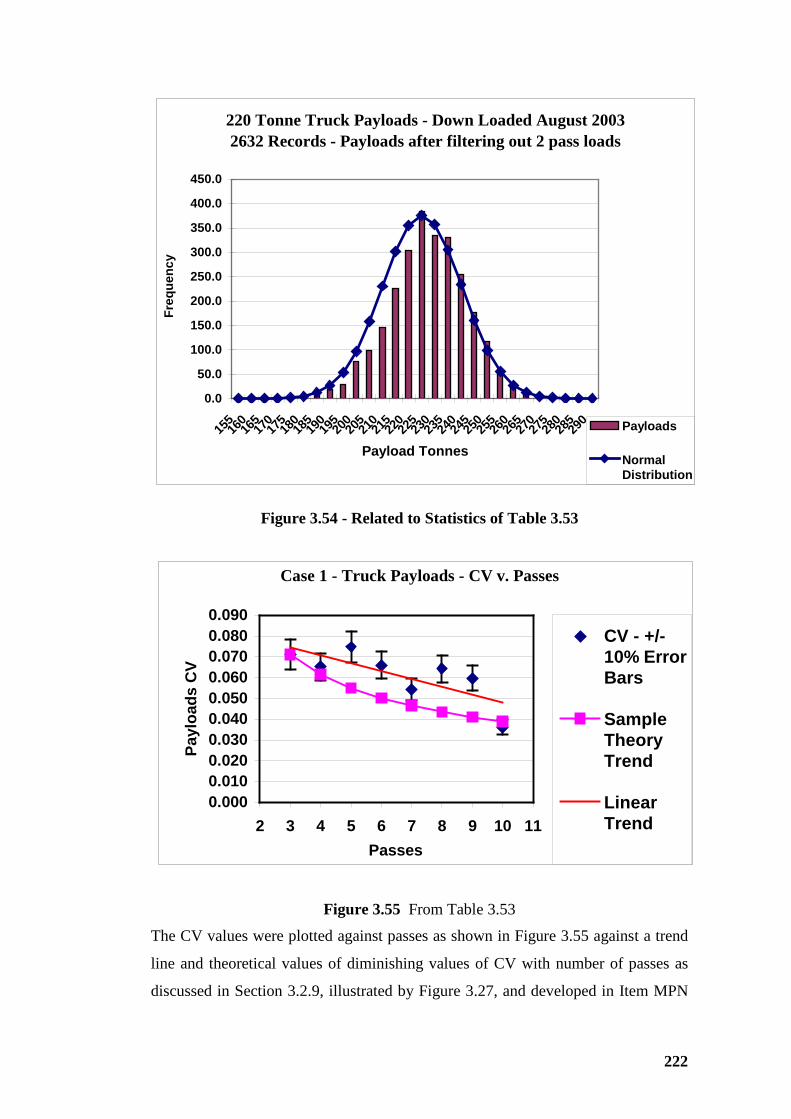
222
220 Tonne Truck Payloads - Down Loaded August 20032632 Records - Payloads after filtering out 2 pass loads
0.0
50.0
100.0
150.0
200.0
250.0
300.0
350.0
400.0
450.0
15516
016
517
017
518
018
519
019
520
020
521
021
522
022
523
023
524
024
525
025
526
026
527
027
528
028
529
0
Payload Tonnes
Freq
uenc
y
Payloads
NormalDistribution
Figure 3.54 - Related to Statistics of Table 3.53
Case 1 - Truck Payloads - CV v. Passes
0.0000.0100.0200.0300.0400.0500.0600.0700.0800.090
2 3 4 5 6 7 8 9 10 11Passes
Payl
oads
CV
CV - +/-10% ErrorBars
SampleTheoryTrend
LinearTrend
Figure 3.55 From Table 3.53
The CV values were plotted against passes as shown in Figure 3.55 against a trend
line and theoretical values of diminishing values of CV with number of passes as
discussed in Section 3.2.9, illustrated by Figure 3.27, and developed in Item MPN
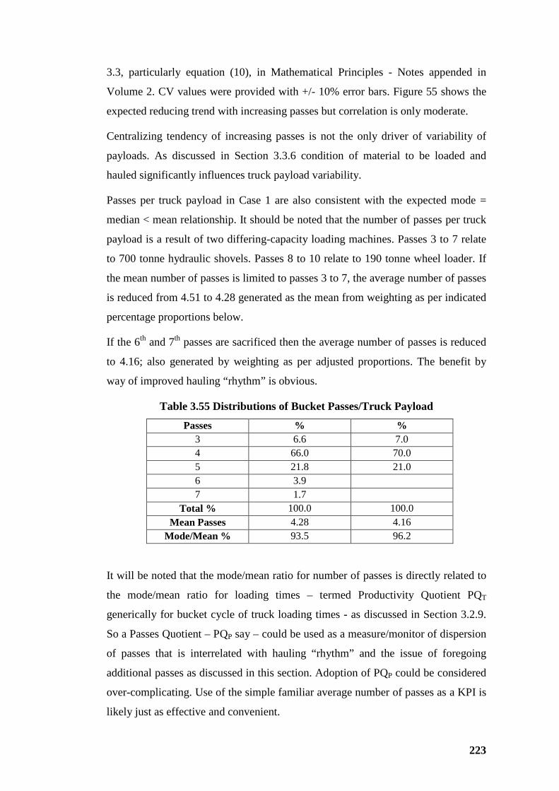
223
3.3, particularly equation (10), in Mathematical Principles - Notes appended in
Volume 2. CV values were provided with +/- 10% error bars. Figure 55 shows the
expected reducing trend with increasing passes but correlation is only moderate.
Centralizing tendency of increasing passes is not the only driver of variability of
payloads. As discussed in Section 3.3.6 condition of material to be loaded and
hauled significantly influences truck payload variability.
Passes per truck payload in Case 1 are also consistent with the expected mode =
median < mean relationship. It should be noted that the number of passes per truck
payload is a result of two differing-capacity loading machines. Passes 3 to 7 relate
to 700 tonne hydraulic shovels. Passes 8 to 10 relate to 190 tonne wheel loader. If
the mean number of passes is limited to passes 3 to 7, the average number of passes
is reduced from 4.51 to 4.28 generated as the mean from weighting as per indicated
percentage proportions below.
If the 6th and 7th passes are sacrificed then the average number of passes is reduced
to 4.16; also generated by weighting as per adjusted proportions. The benefit by
way of improved hauling “rhythm” is obvious.
Table 3.55 Distributions of Bucket Passes/Truck Payload
Passes % % 3 6.6 7.0 4 66.0 70.0 5 21.8 21.0 6 3.9 7 1.7
Total % 100.0 100.0 Mean Passes 4.28 4.16
Mode/Mean % 93.5 96.2
It will be noted that the mode/mean ratio for number of passes is directly related to
the mode/mean ratio for loading times – termed Productivity Quotient PQT
generically for bucket cycle of truck loading times - as discussed in Section 3.2.9.
So a Passes Quotient – PQP say – could be used as a measure/monitor of dispersion
of passes that is interrelated with hauling “rhythm” and the issue of foregoing
additional passes as discussed in this section. Adoption of PQP could be considered
over-complicating. Use of the simple familiar average number of passes as a KPI is
likely just as effective and convenient.
224
Simply – if the actual mean number of passes is less than or equal to the selected
notional mean number of passes for loading a truck built into the loading and
hauling equipment selection criteria, say, 105% of the modal value, then likely
there is no need to look further. It the mean number of passes is greater than the
planned mean number of passes i.e., say, >105% of modal value - then records need
to be examined for additional passes that may be sacrificed cost-beneficially to
realize the expected standard of operational “rhythm” inherent in the selection
criteria.
Productivity and cost implications of foregoing additional passes for marginal top
up of truck payloads are discussed.
Productivity and Sacrificing Passes
To justify an additional pass or passes, production lost by sacrificing one or more
additional passes with the result of an incompletely filled truck body must be more
than the truck production gained by reducing delay to all trucks in the hauling fleet.
The above statement can be expressed as:
PLX > PLL (A)
PLX = Payloads proportion gained - by foregoing additional pass(s)
PLL = Payload proportion lost.
Simplified equation (A) is developed in detail in MPN 9 in Mathematical Principles
– Notes, appended in Volume 2. The analysis in this section is in terms of
production alone without consideration of productivity v. payload variability or cost
implications. Cost analysis related to bucket-pass sacrifice is provided in Section
5.4.
Productivity relationship with variable payload of mining trucks is analysed and
interpreted in Section 3.3.10. The further steps to connect driveline component life
and fuel burn with payload variability and to analyse cost implications are dealt
with in Section 5.3. Table 3.57 is intended to provide guidance by indicating, in
terms of production, when an extra bucket load should be sacrificed to benefit
overall productivity and “rhythm” of load and haul operations.
Bucket pass sacrifice tends to become more justifiable as:
225
• Pass to be sacrificed trends downwards, i.e., sacrificing the 8th pass for 6-
pass mode loading is more justifiable than the 7th for 5-pass mode that is, in
turn more justifiable than the 6th pass for 4-pass mode loading.
• Bucket cycle time TBC increases.
• The number of trucks time-benefiting from bucket-pass sacrifice increase.
• The truck trip time TT decreases.
Sacrificing more than one bucket load, if practical, could also be justified provided
the truck payloads proportion gained is favourable when compared with production
proportion of payloads lost by sacrifice.
Validity of Bucket Load Sacrifice Criteria
In terms of production alone, the above justification criteria:
1. Will be valid when loading equipment appears to be over trucked – a
common case where maximum shovel productivity is the focus with
acceptance of the resulting haulage cost premium – the “maximum-
production-with-mining cost-penalty” case.
2. Will likely be valid generally when loading equipment and trucks appear to
be exactly matched based on mean values for operating criteria – the
hypothetical case that rarely if ever happens, and when it does the
experience is fleeting; also the maximum bunching case, where variability
in truck loading and trip time components has maximum effect and
bunching productivity loss is a maximum.
3. Generally invalid where loading equipment appears to be nearly always
waiting for trucks – an additional bucket load or loads will reduce
shovel/loader waiting time – could add productivity at marginal load and
haul cost without affecting other trucks and shovels in the combined fleets;
but also, theoretically, could cause a subsequent delay of all trucks in a
future bunching occurrence. This so-called “undertrucking” – the author
prefers “over-shoveling” (OS) - is likely the lowest cost option with trucks
working at maximum efficiency and loading equipment underutilised.
The expressions “appear(s) to be” used in the three cases are deliberately
precautionary. As discussed in more detail in Section 5.4, any operating group of
226
loading and hauling equipment may instantaneously appear to be any one of the
three cases. But mean parameters of sampling observations of the production group
may be consistently specifically one of the three cases.
Case 3. – the OS case - is the practical operating circumstance that is most complex
and likely more appropriately should be modelled and subjected to simulation to
determine outcomes.
The above analysis and criteria are relatively rudimentary and limited to production
considerations alone. They are considered of sufficient accuracy for initial
estimating and for setting of standards for equipment selection; but always if
matching of trucks and loading equipment and the alternatives of over-trucking or
over-shoveling are concurrently considered.
Bucket sacrifice justification in terms of haul costs is revisited in Section 5.4
together with further discussion on criteria for application.
The above-developed criteria have interrelationship with bunching/queuing effects.
Sacrificing additional bucket loads to fill a truck body when localized low bucket-
fill factors are experienced will tend to reduce productivity discounting due to
bunching/queuing.
In Section 3.2.9 bucket cycle times and truck loading times were analysed in some
detail for an operation where the bucket fill factor, on the evidence of VIMS data,
at that time, was a relatively low 0.65. Some 13% of bucket passes were 7th pass or
more. Allowing for a reduced bucket load of some 75% of the mean of bucket
loads, there was potentially justification for truncating loading operations at 6
passes.
Table 3.17 indicates that last loads are substantially reduced compared with mean
of all bucket loads and mean of intermediate bucket loads (excluding first and last
passes). Adoption of a discount factor on last bucket loads for the analysis to follow
is considered reasonable – 0.75 is indicated as an acceptable default discount factor.
Practitioners and researchers can reproduce Table 3.57, appended in Volume 2,
from item MPN 9 in Mathematical Principles – Notes, also appended in Volume 2.
For convenience a copy of the spreadsheet file including Table 3.57 is on the CD in
the pocket inside the back cover of this thesis document.
227
Reduced Payload and Productivity
Hanby, in Part 3 of his three-part paper, has analyzed the affects on productivity
and unit haulage cost as a result of reducing truck payload (Hanby, 1991).
Relationships between truck mass and dynamic performance parameters - velocity,
acceleration, time and distance - were developed. Hanby chose the quotient -
travelling time/percentage payload - to represent haulage cost per unit volume or
mass as convenient so assuming a linear relationship with unit hauling for both
truck trip time and payload. Hanby’s choice of haulage cost parameter is valid only
within the limitations of his analysis.
The assumptions and limitations adopted by Hanby included:
• Individual comparative range of cases each of specific total resistance.
• A single mining truck hauling constant distance at that specific resistance;
≈.to one-way haul over a single haul course segment.
• Over a range of payloads from 30% to 170%
• Calculation of time for the selected distance.
• Derived haulage unit cost indicator as the quotient - time / % payload.
Hauling unit costs can be considered a linear function of truck trip time – but only
when compared for limited hypothetical cases where all truck payloads are mean,
where all trucks have exactly the same GMW : NMW ratio; and performance and
haul distance is the same for all cases – limitations that generally apply to Hanby’s
analysis.
But unit haul costs for variable payload are measurably non-linear. Caterpillar has
observed that driveline component life decreases more, and non-linearly, for
overloads than increased life is realised for under loading. The author has analysed
and discussed cost implications of this non-linear payload - maintenance cost
relationship in previous research (Hardy#1, 2003). This non-linear relationship is
further analyzed and discussed in more detail in Sections 3.3.10 and 5.3. Unit cost
for haulage per unit of distance in practical truck cycles varies with one-way haul
distance; but the effect would be small except for the “fixed” time events with
practically fixed cost that is a smaller proportion of total unit costs as one-way
hauls increase. So unit cost of haulage per unit time varies as one-way hauls vary,
228
but not linearly, due to changing proportion of so-called “fixed” time included in
truck trip time – a factor excluded by limitations of Hanby’s analysis.
Notwithstanding the above comments on Hanby’s cost-indicator quotient and the
assumption of linear cost – time; and cost – payload relationships, the outcomes of
Hanby’s research, limited as discussed, provides valuable insight that:
• Up to a total resistance of 24% it appears to be financially disadvantageous
to operate a mining truck with generally reduced payload – as total
resistance in practical situations is unlikely to approach 24% by a
substantial margin, this outcome applies generally in practice.
• Most importantly, generally overloading trucks is likely to be counter-
productive, not realise any significant cost benefit, and ultimately could be
unsafe (Hanby, 1991).
The outcomes of Hanby’s research provide a foundation and opportunity to further
investigate the increased complexity of actual load and haul operations.
In this section the interrelationship between numbers of trucks being serviced by
loading equipment has been analysed in terms of sacrificing relatively small
portions of truck payload to gain additional truck payloads. It is hypothesized there
are circumstances where extending the number of bucket passes to realise full
payloads is not cost beneficial. Analysis and interpretation in this section has tested
the hypothesis and has established that, for favourable operating circumstances,
sacrifice of additional bucket passes will be justified – particularly where loading
equipment is over trucked. This hypothesis is further discussed in Section 5.4 in
terms of comparative costs. Certainly planning prior to equipment selection needs
to include definition of the loading and hauling operating circumstances prior to
setting service requirements of loading equipment and mining trucks.
Interpretation and Summary
This section has examined case studies of substantial truck payload data samples
from operations using differing size of mining trucks, loading equipment to load
and haul and different materials. The analysis and concepts developed in Sections
3.2.8 and 3.3.6 have been generally verified by the case studies.
229
Sacrificing extra passes to top up trucks to full loads to realize the benefit of
improved productivity load and haul “rhythm” was also analyzed. A case was made
to sacrifice additional bucket loads in favourable circumstances including:
• Where the truck fleet appears to be operated with loading equipment over
trucked or close to “matched” – there may be a case where the truck fleet
appears to be over-shoveled (= under trucked) but this circumstance needs
to be modelled for simulation with appropriate recognition of stochastic
parameters.
• Where production lost by pass sacrifice is compensated by increased
productivity of the truck fleet by time saving.
Analysis of the sacrifice productivity trade-off has been summarized in a relatively
simple formula that has been interpreted in a selection table – Table 3.57 -
appended in Volume 2 – to provide a decision facility.
The importance of modal values of bucket passes became obvious in the course of
analysis. A concept of a Productivity Quotient PQP, consisting passes mode/mean is
discussed above similar to the concept of PQT to monitor bucket cycle or truck-
loading times as discussed in Section 3.2.9. The alternative to the concept of PQP,
i.e., establishing the relationship of mean of actual passes to planned mean of
passes, is likely as convenient and effective.
Estimators building up productivity data for the purposes of testing feasibility, with
flow on to criteria for equipment selection; also for compiling operating budgets
must be aware that when four, five or more passes are adopted as a deterministic
design parameter they are really selecting the modal value. Chou provides: “The
‘mode’ is often the concept in most people’s minds when they speak of ‘averages’.”
(Chou, 1969).
There must always be realization that, by selecting, say, four-pass loading that
actual truck loading times will reflect more than 4 x mean bucket cycle time.
Suggested values of mean number of passes for “best practice” and “less than best
practice”, i.e., a\measures of loading time quality, are shown in Table 3.56.
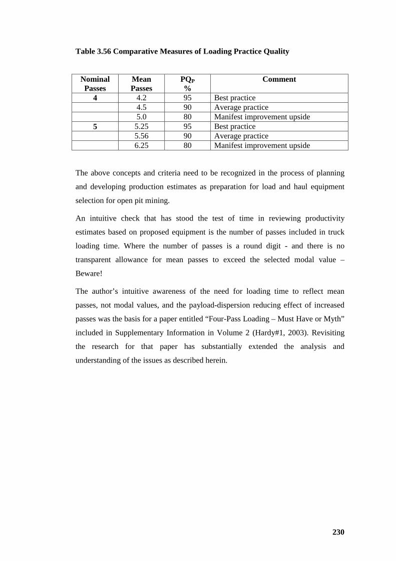
230
Table 3.56 Comparative Measures of Loading Practice Quality
Nominal Passes
Mean Passes
PQP %
Comment
4 4.2 95 Best practice 4.5 90 Average practice 5.0 80 Manifest improvement upside 5 5.25 95 Best practice 5.56 90 Average practice 6.25 80 Manifest improvement upside
The above concepts and criteria need to be recognized in the process of planning
and developing production estimates as preparation for load and haul equipment
selection for open pit mining.
An intuitive check that has stood the test of time in reviewing productivity
estimates based on proposed equipment is the number of passes included in truck
loading time. Where the number of passes is a round digit - and there is no
transparent allowance for mean passes to exceed the selected modal value –
Beware!
The author’s intuitive awareness of the need for loading time to reflect mean
passes, not modal values, and the payload-dispersion reducing effect of increased
passes was the basis for a paper entitled “Four-Pass Loading – Must Have or Myth”
included in Supplementary Information in Volume 2 (Hardy#1, 2003). Revisiting
the research for that paper has substantially extended the analysis and
understanding of the issues as described herein.
231
3.3.10 Truck Performance and Productivity
Introduction
This section of the research moves on to analyze truck trip times in terms of four
time components in two general categories:
Fixed:
1. Manoeuvre-and-spot (TS) for loading
2. Manoeuvre-and-dump (TD)
Variable:
3. Loading (TL)
4. Travel (TV)
Accumulation of the four components is commonly termed “truck cycle time”; but is
termed herein as “truck trip time” TT.
In preparing for equipment selection, productivity estimates are dependent on truck
trip time TT.
Although traditionally designated as “fixed” both TS and TD are, in reality, alike with
all time components, variable –– intrinsically, a function of equipment capability;
and non-intrinsically due to extraneous events that cause extraordinary time losses.
Variability of loading time was analyzed and discussed in Section 3.2.9. Travel time
variability is analyzed below.
The four components and truck trip time are discussed in turn.
1. Manoeuvre and Spot Time - TS
Mean TS times for large mining trucks are suggested as:
• “Usually between 0.4 to 0.7 minutes” (Hays, 1990)
• “Typically between 0.6 to 0.8 minutes” (Caterpillar#1, 2004)
The more recent publication and commercial responsibility attached thereto are
likely significant. The author’s experience is that TS time of 0.75 minutes – intrinsic
time only – for large trucks to 220 tonne nominal payload is a reasonable typical
value.
In Section 3.2.9 TS-time is conveniently analyzed in two parts:
232
1. The major proportion of TS time from departure of the previously loaded
truck and the waiting truck is clear to manoeuvre through the turn and reverse
until the shovel is in the spot position ready to dump – the time coincident
with the shovel cycle time through to position ready to spot and dump; and
2. The minor residual of TS time until the spot position is reached and the shovel
dumps - the nett exchange time experience by the shovel whilst waiting for
the truck to spot.
The division of TS time is only relevant for analysis of truck loading time and effect
on productivity of loading equipment.
Obviously TS time for trucks is substantially coincident with the first bucket cycle
time. It can be extended by any extraordinary time loss by the shovel during the first
bucket cycle as discussed in Section 3.2.9.
Typical nett truck exchange time (intrinsic only) from loading equipment ready to
dump and the truck spotting is 12 to 15 seconds. Ramani has used 0.2 minutes for the
“incremental exchange time” (Ramani, 1990)
As TS times are a relatively small proportion of truck trip time, certainly ≤ 10%, and
typically in the range 4% down to 1.5%, errors in estimating this time component are
of small effect. Adoption of 0.7 or 0.75 minutes will be generally acceptable –
always provided that any extraordinary time losses are dealt with separately and
transparently.
The above discussion assumes reasonable working face width, manoeuvering area
and competent bench surface material. Incompetent floors and resulting high rolling
resistance, potential for bogging of trucks, limited working face and restricted work
area and interference from support equipment attending to “housekeeping” activities
can significantly elevate TS times, possibly by as much as 100% in worst possible
combinations of unfavourable conditions.
Table 3.58, provides a recommended range of working widths for a range of trucks
with indicated nominal payloads, at various operating-comfort levels, based on
consideration of dimensions of trucks and appropriate loading equipment.
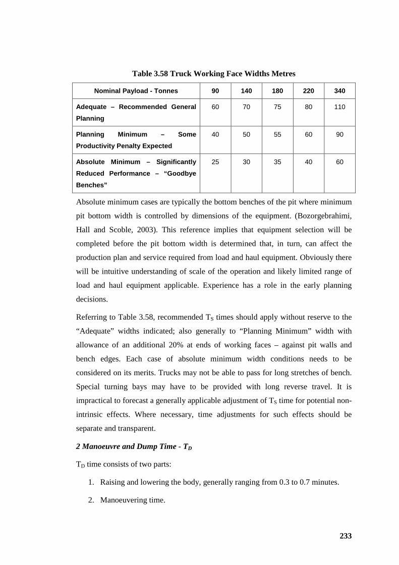
233
Table 3.58 Truck Working Face Widths Metres
Nominal Payload - Tonnes 90 140 180 220 340
Adequate – Recommended General
Planning 60 70 75 80 110
Planning Minimum – Some Productivity Penalty Expected
40 50 55 60 90
Absolute Minimum – Significantly
Reduced Performance – “Goodbye
Benches”
25 30 35 40 60
Absolute minimum cases are typically the bottom benches of the pit where minimum
pit bottom width is controlled by dimensions of the equipment. (Bozorgebrahimi,
Hall and Scoble, 2003). This reference implies that equipment selection will be
completed before the pit bottom width is determined that, in turn, can affect the
production plan and service required from load and haul equipment. Obviously there
will be intuitive understanding of scale of the operation and likely limited range of
load and haul equipment applicable. Experience has a role in the early planning
decisions.
Referring to Table 3.58, recommended TS times should apply without reserve to the
“Adequate” widths indicated; also generally to “Planning Minimum” width with
allowance of an additional 20% at ends of working faces – against pit walls and
bench edges. Each case of absolute minimum width conditions needs to be
considered on its merits. Trucks may not be able to pass for long stretches of bench.
Special turning bays may have to be provided with long reverse travel. It is
impractical to forecast a generally applicable adjustment of TS time for potential non-
intrinsic effects. Where necessary, time adjustments for such effects should be
separate and transparent.
2 Manoeuvre and Dump Time - TD
TD time consists of two parts:
1. Raising and lowering the body, generally ranging from 0.3 to 0.7 minutes.
2. Manoeuvering time.
234
Combined typical TD times for rear dumps are 1.0 minute and for bottom dumps are
0.5 minute (Hays, 1990). A typical range of TD times for rear dumping mining trucks
is 1.0 to 1.2 minutes (Caterpillar#1, 2004).
Soft running conditions and poor dumping point housekeeping (dangerous dump
edges and inadequate safety windrows etc.), or queuing at crushers and/or stockpile
areas add to TD times. These inhibiting factors should be preferably be eliminated;
but in default should be treated by applying separate, transparent contingency time
allowances.
3 Truck Loading Time - TL
Discussed at some length in Section 3.2.9, in summary, loading time is:
• From the loading equipment perspective, an accumulation of a limited
number of bucket-cycle times and nett truck exchange time – TC as applied in
Section 3.2.4.
• From the truck perspective, an accumulation of delivery of the first pass
immediately on spot – normally 3 to 5 seconds provided in estimates – and
the second through to the final bucket pass to realise a full truck body load,
determined by the operator visually, and/or assisted by onboard payload
weighing, with dispatch signaled by the loading equipment operator –
designated TL herein.
Results of statistical analysis of loading times TC in Section 3.2.9 relevant to this
section can be briefly summarized:
• Filtered to intrinsic loading time levels, distributions of TC exhibit central
tendency that, with the addition of extraordinary time losses in practical
application, becomes increasingly positive (right) skewed with increasing
mean values and CV.
• From the analysis in Section 3.2.9, the CV range for TC are in the order of
0.10 to 0.15 when filtered to exclude non-intrinsic, extraordinary time losses;
and increasing to the order of 0.15 up to 0.20 retrogressing through the
adopted filtering levels back to raw data.
235
The difference between TC and TL has been explained above. It is the author’s
opinion that these two loading times should exhibit similar variability as the basic
time components, bucket cycle times, are generally represented similarly.
Loading time variability suggested by others include Elbrond who has used CV of
0.30 for both loading time TL and truck travel time TT (truck trip time herein) –
(Elbrond, 1990, p743).
Typical loading times can estimated by:
TC = n . TBC + TEX (1) Loading equipment
TL = TF + (n-1) x TBC (2) Trucks
TBC = Bucket cycle time
TEX = Nett truck exchange time ≡ shovel wait time to spot truck.
n = Number of bucket passes
TF = Time for dumping first bucket load
It will be noted that the ratio:
n x TBC / (n x TBC + TEX)
is equivalent to the pass-dependent loading efficiency developed and discussed in
Section 3.2.6 and illustrated by Table 3.4.
Estimation of Bucket Cycle Times
Table 3.59 – Parts 1 to 4, Volume 2, Appendices, summarize a bucket cycle time
calculation method. Estimated bucket cycle times TBC are built up from incremental
time components including:
• Dump bucket load - TF
• Return rotation of loading equipment (or manoeuvre of wheel loader)
• Pause to position bucket and address digging face
• Fill bucket
• Rotate loaded to bucket dump position
Nett truck exchange time, TEX, may be included in the first bucket load by some
estimators and data collection systems – as with data analysed in Section 3.2.9. For
236
the purposes of this analysis of bucket cycle time, nett truck exchange time is
considered a separate time event.
Table 3.59 is a prototype forecast facility for TBC based on general industrial practice
and experience of the author. Although empirical to a large degree, the inputs
adopted need to be confirmed for specific applications against time and motion data
for each of the time elements to prove validity of assumptions and calculation criteria
adopted. The table is limited to electric rope shovels and hydraulic shovels, but
covers a substantial selection of the range of capacity offered by OEM. The four-part
TBC selection Table 3.59 is not a finished product; but it is a useful start, covering a
substantial range of loading equipment. It presents an opportunity for future
researchers to refine, extend as necessary and confirm empirically.
Assumptions basic to compiling Table 3.59 Parts 1 to 4 include:
• TEX - is not included and must be separately estimated – see discussion
below.
• TF – for all shovels is set at 3 seconds – average for and applicable for all
loads including the first – allows for “feeling” loads into the truck body to
avoid damage and spillage – wheel loaders should be provided with more
time to dump by extending TF to 5 seconds.
• Return rotation unloaded – assessed from revolving speed of shovel
superstructure from OEM specifications. Allowance is made for acceleration
and deceleration correlated with industry standards where available estimates
providing for a range of swing angles. Slewing acceleration and braking
characteristics were discussed with OEM and dealer representatives and
adjusted as necessary consistent with the author’s experience.
• Pause and position the bucket to address the face of material to be loaded -
allowing a mean 3 seconds for any necessary position correction or extra
back swing of the stick to position for pickup of large particles tailed off the
slumping face and so clear the face in front of the shovel.
• Fill bucket - provision for four levels of digging difficulty – based
substantially on experience and with due consideration of standard industry
references including:
237
Caterpillar Performance Hand Book (Caterpillar#1, 2004)
SME Mining Engineers Handbook (Atkinson, 1990) recommends values
for bucket filling times that have been modified to reflect more recent
improvements in digging performance – particularly upgraded
specification of electric rope shovels, hydraulic powered shovels and
excavators.
Table 3.59 Parts 1 to 4, appended in Volume 2, were developed as a Microsoft Excel
spreadsheet. A copy of the file is included on a CD in a pocket inside the back cover
of this thesis.
Practical Loading Time Distributions
Loading time data is generally available from load and haul data from dispatch
management systems. Time components that make up truck loading time, in the
context discussed above, are assumed to have specific instantaneous beginning and
end points that may be, to some degree, automatically triggered by events sensed at
truck or shovel. But sometimes beginning and end points in time are triggered by
proximity observation using GST facilities in dispatch systems. Such observations
are not discrete events so there may be some inaccuracy, albeit modest, in loading
time data. One such definition of time events for a dispatch system describes loading
time as follows:
“When a haul truck hauling empty goes within a 50m radius and first stops it
automatically goes into wait at Shovel unless it is waiting behind other trucks, then it
will go into queuing at shovel. If the shovel at this time is not loading another truck it
will automatically go into face preparation.
If the shovel finishes loading a truck and there is not another truck already in wait at
shovel then the shovel is placed in Shovel waiting (i.e. waiting for a truck to arrive).
When the haul truck goes within 25m of the shovel and stops the truck and shovel
will automatically go into loading time. As soon as the truck heads off and hits a
nominal speed (to allow for minor repositioning under the shovel - when it hits
second gear) it will automatically go to hauling full. The shovel will then revert back
to face preparation before being triggered back into load by the arrival of the next
truck.
238
The entire haul cycle
• The truck has to stop to change a time category - so event triggers are
practically discrete.
is the time from dump to load to dump. This is the entire time
from the time the truck dumps until it dumps its next load.” (Cutts, 2005).
It should be noted that, for the practical case above:
• The 25m-proximity trigger will generally be when the truck has completed its
180o turn and stopped. - the time taken to reverse, say, 25 metres will be in
the order of 10 to 15 seconds, approximately corresponding to the nett truck
exchange time as discussed in this section, also in Sections 3.2.6 and 3.2.9.
• Loading time data from the system as configured will be comparative for that
site.
• Data from dispatch systems and traditional time and motion field studies are
reconcilable – when in doubt, system data can be compared with field
observations – or conveniently with video recording reconciled to the
relevant real time period.
Table 3.60, provides descriptive statistics for a sample of 2,630 loading times
(recorded in accordance with the definition) and a further sample of 51 truck trip
times extracted from the 2,630 records with the selected, same one-way haul distance
with equal loaded and return hauls. Yield of suitable trip time data was limited due to
the imposed dispatching prescription. A busy dynamically programmed dispatch
system sends trucks to differing load and dump points over differing routes.
Table 3.61, is an extract from Table 3.60 demonstrating:
• For loading times - TL - filtering of outliers increases central tendency with
CV converging on 0.20.
• For truck trip times – TT – filtering outliers shows a tendency for CV in the
range 0.20 to 0.10.
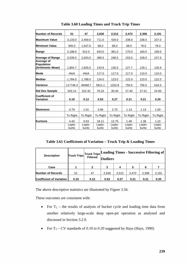
239
Table 3.60 Loading Times and Truck Trip Times
Number of Records 51 47 2,630 2,512 2,472 2,308 2,191
Maximum Value 3,133.0 2,459.0 711.0 429.0 238.0 238.0 237.0
Minimum Value 945.0 1,547.0 68.0 68.0 68.0 78.0 78.0
Range 2,188.0 912.0 643.0 361.0 170.0 160.0 159.0
Average of Range 2,039.0 2,003.0 389.5 248.5 153.0 158.0 157.5 Average of Population (Arithmetic Mean) 1,804.7 1,826.0 143.9 130.5 127.7 129.1 126.9
Mode #N/A #N/A 117.0 117.0 117.0 110.0 110.0
Median 1,784.0 1,788.0 124.0 123.0 122.0 123.0 122.0
Variance 117746.3 49468.7 5811.1 1252.8 750.5 756.5 616.5
Std Dev Sample 343.14 222.42 76.23 35.40 27.40 27.51 24.83
Coefficient of Variation 0.19 0.12 0.53 0.27 0.21 0.21 0.20
Skewness 0.79 1.01 3.96 2.70 1.13 1.13 1.00
To Right To Right To Right To Right To Right To Right To Right
Kurtosis 4.43 0.53 18.11 12.75 1.49 1.38 1.22
Lepto-kurtic
Lepto-kurtic
Lepto-kurtic
Lepto-kurtic
Lepto-kurtic
Lepto-kurtic
Lepto-kurtic
Table 3.61 Coefficients of Variation – Truck Trip & Loading Times
Description Truck Trips Truck Trips Filtered
Loading Times - Successive Filtering of
Outliers
Case 1 2 3 4 5 6 7
Number of Records 51 47 2,630 2,512 2,472 2,308 2,191
Coefficient of Variation 0.19 0.12 0.53 0.27 0.21 0.21 0.20
The above descriptive statistics are illustrated by Figure 3.56.
These outcomes are consistent with:
• For TL – the results of analysis of bucket cycle and loading time data from
another relatively large-scale deep open-pit operation as analysed and
discussed in Section 3.2.9.
• For TT – CV standards of 0.10 to 0.20 suggested by Hays (Hays, 1990)
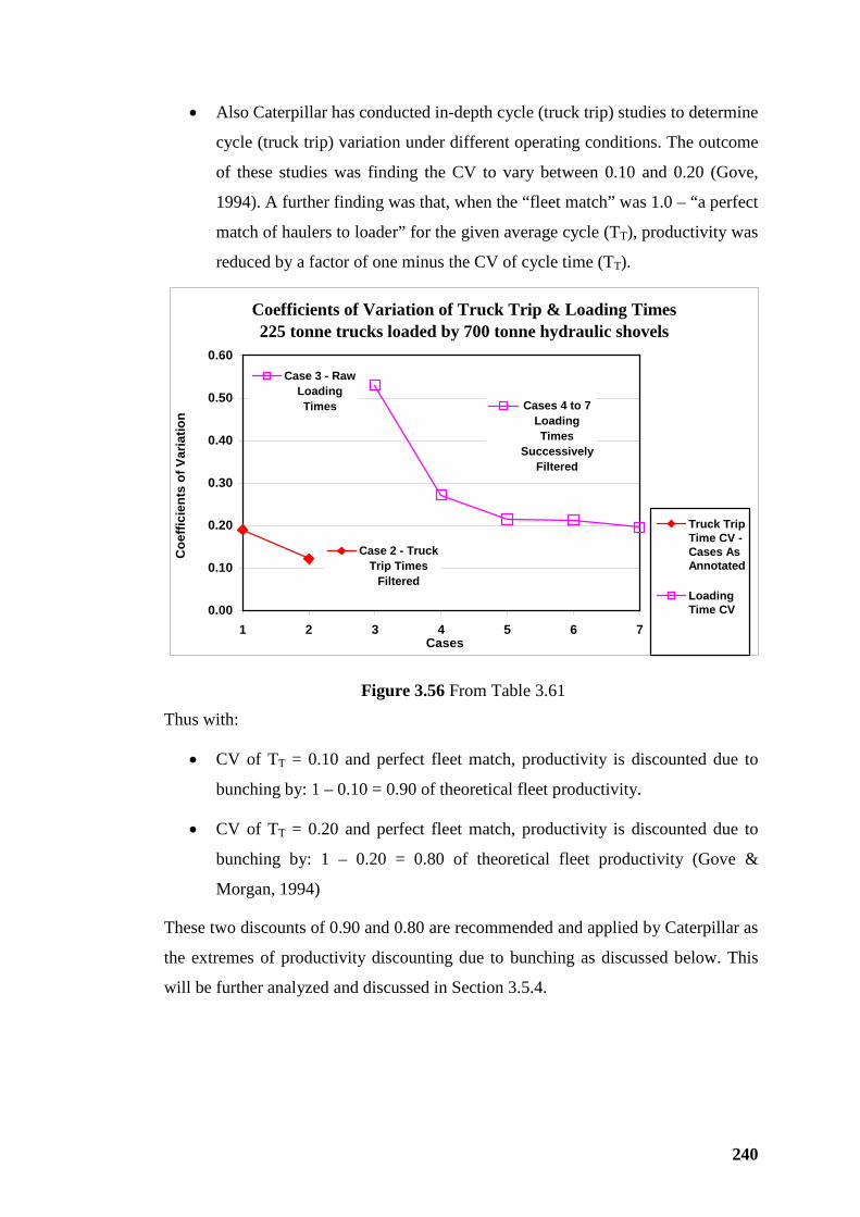
240
• Also Caterpillar has conducted in-depth cycle (truck trip) studies to determine
cycle (truck trip) variation under different operating conditions. The outcome
of these studies was finding the CV to vary between 0.10 and 0.20 (Gove,
1994). A further finding was that, when the “fleet match” was 1.0 – “a perfect
match of haulers to loader” for the given average cycle (TT), productivity was
reduced by a factor of one minus the CV of cycle time (TT).
Coefficients of Variation of Truck Trip & Loading Times225 tonne trucks loaded by 700 tonne hydraulic shovels
Case 2 - Truck Trip Times
Filtered
Case 3 - Raw Loading Times Cases 4 to 7
Loading Times
Successively Filtered
0.00
0.10
0.20
0.30
0.40
0.50
0.60
1 2 3 4 5 6 7Cases
Coe
ffici
ents
of V
aria
tion
Truck TripTime CV -Cases AsAnnotated
LoadingTime CV
Figure 3.56 From Table 3.61
Thus with:
• CV of TT = 0.10 and perfect fleet match, productivity is discounted due to
bunching by: 1 – 0.10 = 0.90 of theoretical fleet productivity.
• CV of TT = 0.20 and perfect fleet match, productivity is discounted due to
bunching by: 1 – 0.20 = 0.80 of theoretical fleet productivity (Gove &
Morgan, 1994)
These two discounts of 0.90 and 0.80 are recommended and applied by Caterpillar as
the extremes of productivity discounting due to bunching as discussed below. This
will be further analyzed and discussed in Section 3.5.4.
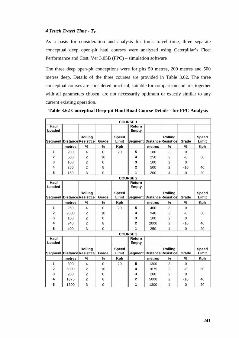
241
4 Truck Travel Time - TV
As a basis for consideration and analysis for truck travel time, three separate
conceptual deep open-pit haul courses were analyzed using Caterpillar’s Fleet
Performance and Cost, Ver 3.05B (FPC) – simulation software
The three deep open-pit conceptions were for pits 50 metres, 200 metres and 500
metres deep. Details of the three courses are provided in Table 3.62. The three
conceptual courses are considered practical, suitable for comparison and are, together
with all parameters chosen, are not necessarily optimum or exactly similar to any
current existing operation.
Table 3.62 Conceptual Deep-pit Haul Road Course Details - for FPC Analysis
COURSE 1 Haul
Loaded Return Empty
Segment Distance Rolling
Resist’ce Grade Speed Limit Segment Distance
Rolling Resist’ce Grade
Speed Limit
metres % % Kph metres % % Kph 1 200 4 0 20 5 180 3 0 2 500 2 10 4 250 2 -8 50 3 100 2 0 3 100 2 0 4 250 2 8 2 500 2 -10 40 5 180 3 0 1 200 4 0 20
COURSE 2 Haul
Loaded Return Empty
Segment Distance Rolling
Resist’ce Grade Speed Limit Segment Distance
Rolling Resist’ce Grade
Speed Limit
metres % % Kph metres % % Kph 1 250 4 0 20 5 400 3 0 2 2000 2 10 4 940 2 -8 50 3 100 2 0 3 100 2 0 4 940 2 8 2 2000 2 -10 40 5 400 3 0 1 250 4 0 20
COURSE 3 Haul
Loaded Return Empty
Segment Distance Rolling
Resist’ce Grade Speed Limit Segment Distance
Rolling Resist’ce Grade
Speed Limit
metres % % Kph metres % % Kph 1 300 4 0 20 5 1300 3 0 2 5000 2 10 4 1875 2 -8 50 3 200 2 0 3 200 2 0 4 1875 2 8 2 5000 2 -10 40 5 1300 3 0 1 1300 4 0 20
242
Haul road construction and operating conditions were assumed generally in
accordance with best-practice standards as described in references including:
• Walter Kaufman and James Ault - (Kaufman & Ault, 1977)
• Caterpillar PHB 35, 2004, p27-1 – (Caterpillar#1, 2004)
• Caterpillar FPC 3.05B, 2004, pp106, 107 – (Caterpillar#2, 2004)
• Ronald Hays – (Hays, 1990, p677)
It will be noted that:
• Grade of the in-pit ramp was set at 10% with grade of the dump ramp at 8% -
all other course segments were assumed horizontal.
• Rolling resistance was chosen consistent with correctly constructed haul
roads using acceptable materials – haul roads that are well maintained.
• Speed limits were set at 20 kph in-pit loaded, 50 kph down dump ramp and
40 kph down in-pit ramp on return – based on the author’s experience for in-
pit bench travel and from consideration of Caterpillar recommendations
(Caterpillar#2, 2004) – see Figure 3.57.
• Operator Efficiency was applied by FPC in accordance with a job-studies
based relationship between operator efficiency and one-way haul distance as
default that can be over-ridden if desired – the analysis accepted default
(Caterpillar#2,2004) – see Figure 3.58.
The FPC simulations were compiled for a range of six mining trucks from nominal
54 to 349 tonnes payload. Table 3.63, summarises the FPC results. Manoeuvre and
dump times - TD - adopted over the truck range are shown in the table.
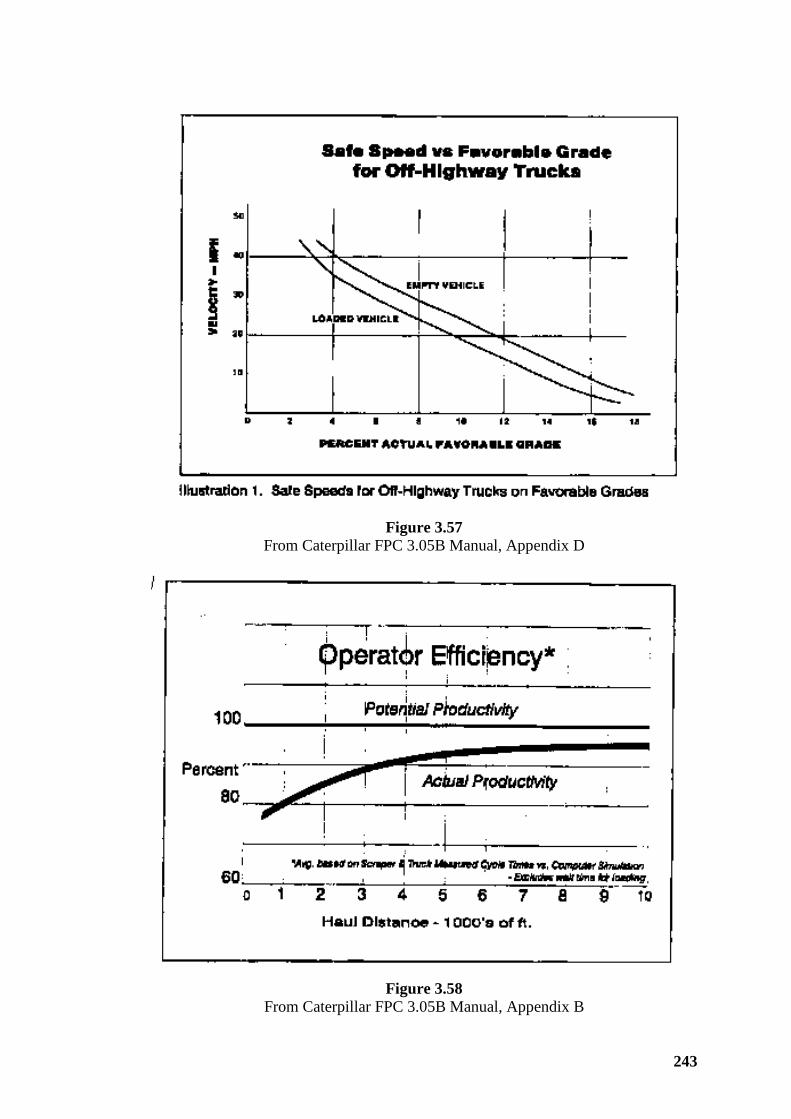
243
Figure 3.57
From Caterpillar FPC 3.05B Manual, Appendix D
Figure 3.58
From Caterpillar FPC 3.05B Manual, Appendix B
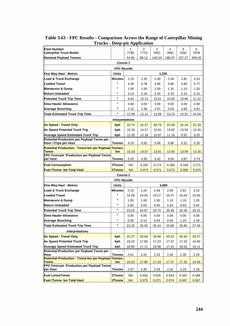
244
Table 3.63 - FPC Results - Comparison Across the Range of Caterpillar Mining Trucks - Deep-pit Application
Fleet Number 1 2 3 4 5 6 Caterpillar Truck Model 773E 777D 785C 789C 793C 797B Nominal Payload Tonnes 53.90 88.12 140.24 180.07 227.27 349.02
Course 1
FPC Results One Way Haul - Metres Units 1,230 Load & Truck Exchange Minutes 2.15 2.20 2.49 2.49 2.81 3.10 Loaded Travel " 4.35 4.78 4.96 4.86 4.80 4.77 Manœuvre & Dump " 1.00 1.00 1.00 1.10 1.10 1.20 Return Unloaded " 2.14 2.16 2.16 2.15 2.15 2.15 Potential Truck Trip Time " 9.63 10.13 10.61 10.60 10.86 11.22 Slow Hauler Allowance " 0.00 0.00 0.00 0.00 0.00 0.00 Average Bunching " 2.31 1.99 2.97 2.63 4.65 4.82 Total Estimated Truck Trip Time " 11.95 12.12 13.58 13.23 15.51 16.04
Interpretations Av Speed - Travel Only kph 22.74 21.27 20.73 21.06 21.24 21.33 Av Speed Potential Truck Trip kph 15.33 14.57 13.91 13.92 13.59 13.16
Average Speed Estimated Truck Trip kph 12.35 12.18 10.87 11.16 9.52 9.20 Potential Production per Payload Tonne per Hour =Trips per Hour Tonnes 6.23 5.92 5.66 5.66 5.52 5.35 Potential Production - Tonne-km per Payload Tonne
Tonnes-km 15.33 14.57 13.91 13.92 13.59 13.16
FPC Forecast Production per Payload Tonne per Hour Tonnes 5.02 4.95 4.42 4.54 3.87 3.74
Fuel Consumption l/Tonne NA 0.182 0.174 0.180 0.169 0.171 Fuel /Tonne- km Total Haul l/Tonne NA 0.074 0.071 0.073 0.069 0.070
Course 2 FPC Results
One Way Haul - Metres Units 3,690 Load & Truck Exchange Minutes 2.15 2.20 2.49 2.49 2.81 3.10 Loaded Travel " 14.28 16.03 16.57 16.27 16.03 15.93 Manœuvre & Dump " 1.00 1.00 1.00 1.10 1.10 1.20 Return Unloaded " 5.60 5.63 5.64 5.63 5.63 5.92 Potential Truck Trip Time " 23.03 24.87 25.70 25.49 25.56 26.15 Slow Hauler Allowance " 0.00 0.00 0.00 0.00 0.00 0.00 Average Bunching " 0.30 0.13 0.54 0.40 1.24 1.34 Total Estimated Truck Trip Time " 23.33 25.00 26.24 25.89 26.80 27.49
Interpretations Av Speed - Travel Only kph 22.27 20.44 19.94 20.22 20.44 20.27 Av Speed Potential Truck Trip kph 19.23 17.80 17.23 17.37 17.32 16.93 Average Speed Estimated Truck Trip kph 18.98 17.71 16.88 17.10 16.52 16.11 Potential Production per Payload Tonne per Hour Tonnes 2.61 2.41 2.33 2.35 2.35 2.29 Potential Production - Tonne-km per Payload Tonne
Tonnes-km 19.23 17.80 17.23 17.37 17.32 16.93
FPC Forecast Production per Payload Tonne per Hour Tonnes 2.57 2.40 2.29 2.32 2.24 2.18
Fuel Litres/Tonne l/Tonne NA 0.554 0.525 0.543 0.497 0.498 Fuel /Tonne- km Total Haul l/Tonne NA 0.075 0.071 0.074 0.067 0.067
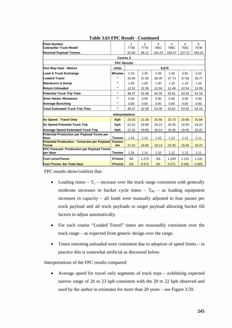
245
Table 3.63 FPC Result - Continued
Fleet Number 1 2 3 4 5 6 Caterpillar Truck Model 773E 777D 785C 789C 793C 797B Nominal Payload Tonnes 53.90 88.12 140.24 180.07 227.27 349.02
Course 3 FPC Results
One Way Haul - Metres Units 8,675 Load & Truck Exchange Minutes 2.15 2.20 2.49 2.49 2.81 3.10 Loaded Travel " 32.90 37.00 38.39 37.73 37.05 36.77 Manœuvre & Dump " 1.00 1.00 1.00 1.10 1.10 1.20 Return Unloaded " 12.31 12.38 12.50 12.49 12.54 13.09 Potential Truck Trip Time " 48.37 52.58 54.39 53.81 53.52 54.16 Slow Hauler Allowance " 0.00 0.00 0.00 0.00 0.00 0.00 Average Bunching " 0.00 0.00 0.00 0.00 0.00 0.00 Total Estimated Truck Trip Time " 48.37 52.58 54.39 53.81 53.52 54.16
Interpretations Av Speed - Travel Only Kph 23.03 21.08 20.46 20.73 20.99 20.88 Av Speed Potential Truck Trip Kph 21.52 19.80 19.14 19.35 19.45 19.22 Average Speed Estimated Truck Trip Kph 21.52 19.80 19.14 19.35 19.45 19.22 Potential Production per Payload Tonne per Hour Tonnes 1.24 1.14 1.10 1.12 1.12 1.11 Potential Production - Tonne-km per Payload Tonne
Tonnes-km 21.52 19.80 19.14 19.35 19.45 19.22
FPC Forecast Production per Payload Tonne per Hour Tonnes 1.24 1.14 1.10 1.12 1.12 1.11
Fuel Litres/Tonne l/Tonne NA 1.270 NA 1.239 1.131 1.131
Fuel /Tonne- km Total Haul l/Tonne NA 0.073 NA 0.071 0.065 0.065
FPC results show/confirm that:
• Loading times – TL – increase over the truck range consistent with generally
moderate increases in bucket cycle times – TBC - as loading equipment
increases in capacity – all loads were manually adjusted to four passes per
truck payload and all truck payloads to target payload allowing bucket fill
factors to adjust automatically.
• For each course “Loaded Travel” times are reasonably consistent over the
truck range – as expected from generic design over the range.
• Times returning unloaded were consistent due to adoption of speed limits – in
practice this is somewhat artificial as discussed below.
Interpretations of the FPC results compared:
• Average speed for travel only segments of truck trips – exhibiting expected
narrow range of 20 to 23 kph consistent with the 20 to 22 kph observed and
used by the author in estimates for more than 20 years – see Figure 3.59.
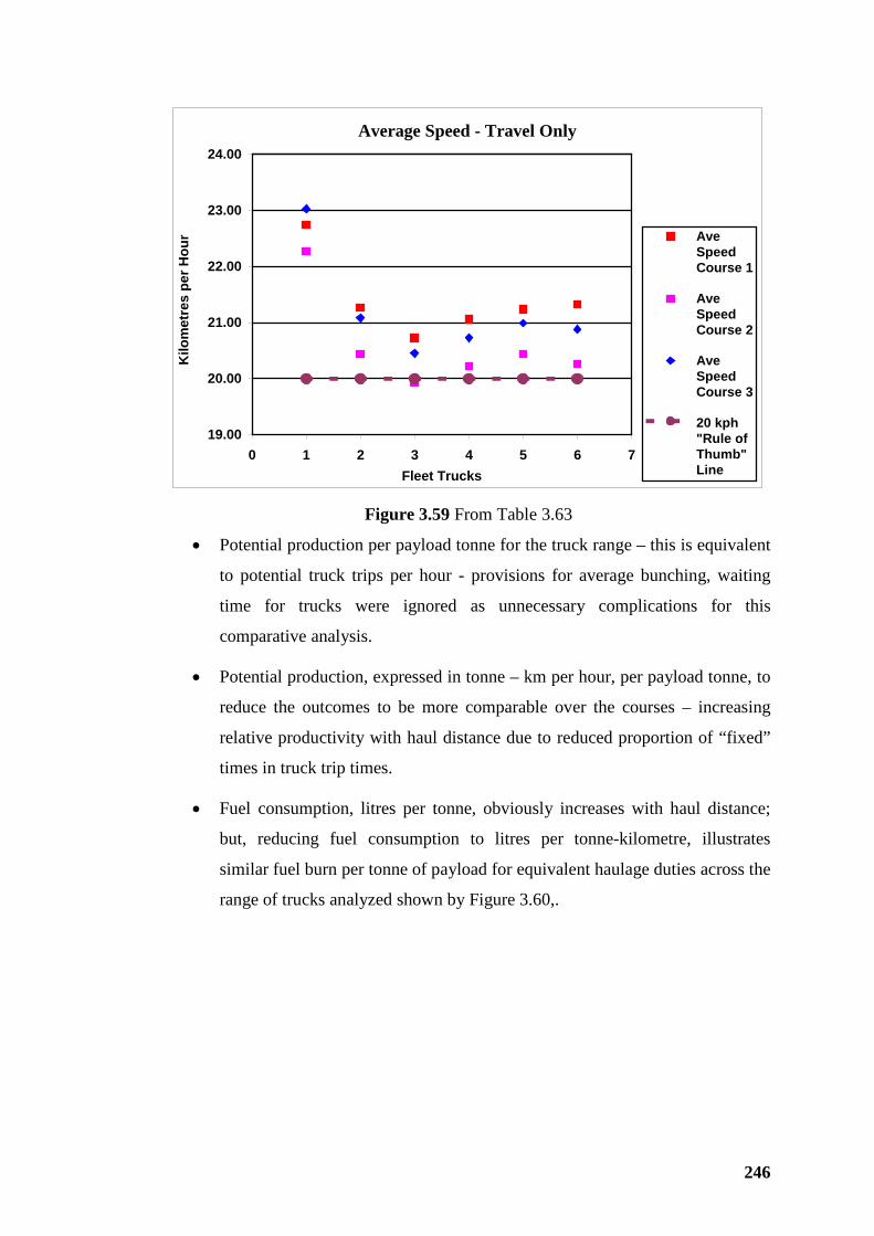
246
Average Speed - Travel Only
19.00
20.00
21.00
22.00
23.00
24.00
0 1 2 3 4 5 6 7Fleet Trucks
Kilo
met
res
per H
our Ave
SpeedCourse 1
AveSpeedCourse 2
AveSpeedCourse 3
20 kph"Rule ofThumb"Line
Figure 3.59 From Table 3.63
• Potential production per payload tonne for the truck range – this is equivalent
to potential truck trips per hour - provisions for average bunching, waiting
time for trucks were ignored as unnecessary complications for this
comparative analysis.
• Potential production, expressed in tonne – km per hour, per payload tonne, to
reduce the outcomes to be more comparable over the courses – increasing
relative productivity with haul distance due to reduced proportion of “fixed”
times in truck trip times.
• Fuel consumption, litres per tonne, obviously increases with haul distance;
but, reducing fuel consumption to litres per tonne-kilometre, illustrates
similar fuel burn per tonne of payload for equivalent haulage duties across the
range of trucks analyzed shown by Figure 3.60,.
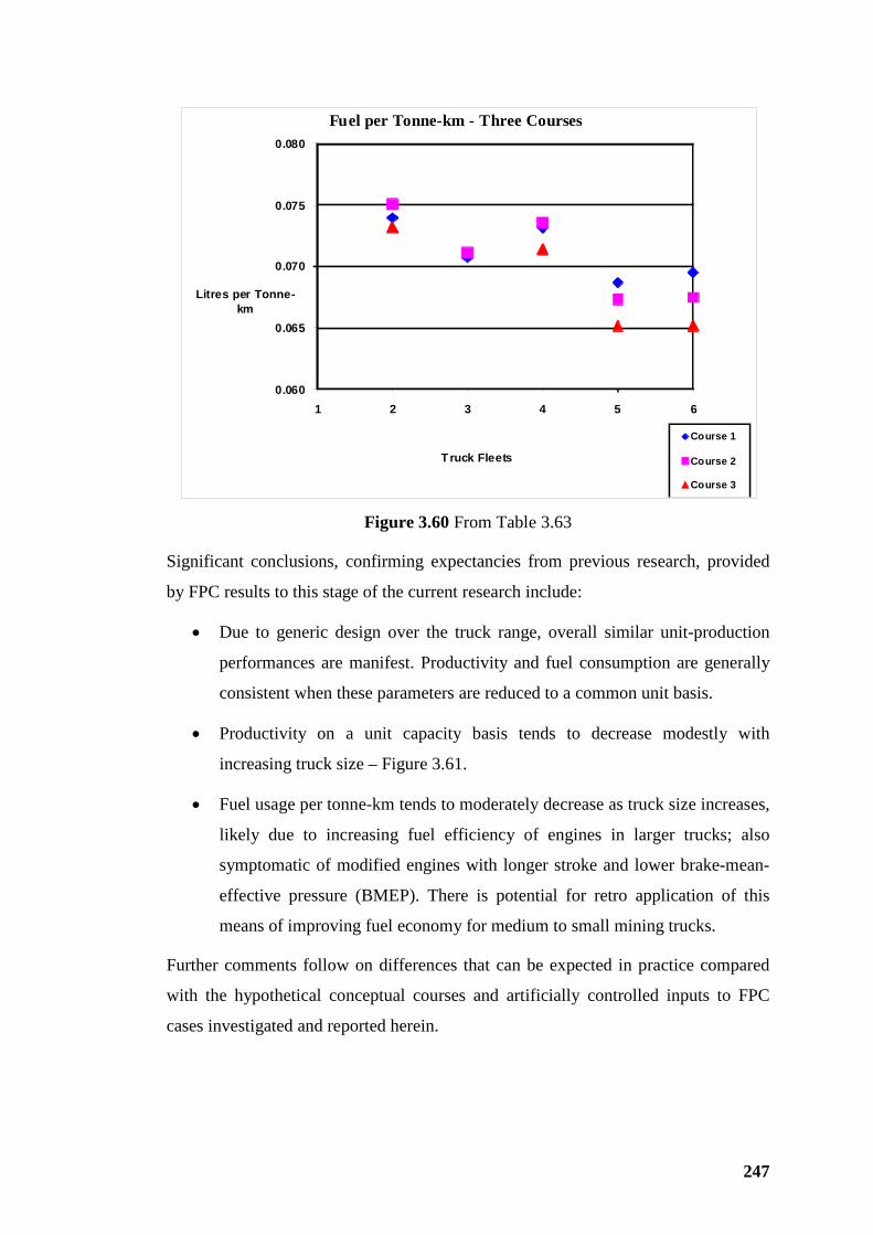
247
0.060
0.065
0.070
0.075
0.080
1 2 3 4 5 6
Litres per Tonne-km
Truck Fleets
Fuel per Tonne-km - Three Courses
Course 1
Course 2
Course 3
Figure 3.60 From Table 3.63
Significant conclusions, confirming expectancies from previous research, provided
by FPC results to this stage of the current research include:
• Due to generic design over the truck range, overall similar unit-production
performances are manifest. Productivity and fuel consumption are generally
consistent when these parameters are reduced to a common unit basis.
• Productivity on a unit capacity basis tends to decrease modestly with
increasing truck size – Figure 3.61.
• Fuel usage per tonne-km tends to moderately decrease as truck size increases,
likely due to increasing fuel efficiency of engines in larger trucks; also
symptomatic of modified engines with longer stroke and lower brake-mean-
effective pressure (BMEP). There is potential for retro application of this
means of improving fuel economy for medium to small mining trucks.
Further comments follow on differences that can be expected in practice compared
with the hypothetical conceptual courses and artificially controlled inputs to FPC
cases investigated and reported herein.
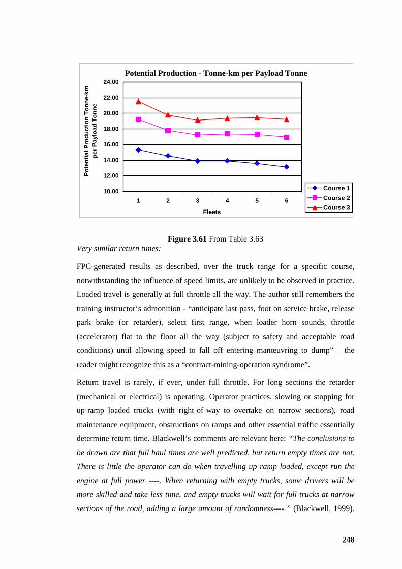
248
Potential Production - Tonne-km per Payload Tonne
10.00
12.00
14.00
16.00
18.00
20.00
22.00
24.00
1 2 3 4 5 6
Fleets
Pote
ntia
l Pro
duct
ion
Tonn
e-km
pe
r Pay
load
Ton
ne
Course 1Course 2Course 3
Figure 3.61 From Table 3.63 Very similar return times:
FPC-generated results as described, over the truck range for a specific course,
notwithstanding the influence of speed limits, are unlikely to be observed in practice.
Loaded travel is generally at full throttle all the way. The author still remembers the
training instructor’s admonition - “anticipate last pass, foot on service brake, release
park brake (or retarder), select first range, when loader horn sounds, throttle
(accelerator) flat to the floor all the way (subject to safety and acceptable road
conditions) until allowing speed to fall off entering manœuvring to dump” – the
reader might recognize this as a “contract-mining-operation syndrome”.
Return travel is rarely, if ever, under full throttle. For long sections the retarder
(mechanical or electrical) is operating. Operator practices, slowing or stopping for
up-ramp loaded trucks (with right-of-way to overtake on narrow sections), road
maintenance equipment, obstructions on ramps and other essential traffic essentially
determine return time. Blackwell’s comments are relevant here: “The conclusions to
be drawn are that full haul times are well predicted, but return empty times are not.
There is little the operator can do when travelling up ramp loaded, except run the
engine at full power ----. When returning with empty trucks, some drivers will be
more skilled and take less time, and empty trucks will wait for full trucks at narrow
sections of the road, adding a large amount of randomness----.” (Blackwell, 1999).
249
Considering speed alone, down-ramp is obviously more risky than up-ramp
operation. Road surfaces that are over-watered or wet from rain always encourage a
prudent reduction in down-ramp speed.
Contingency allowances for increased return time are dependent on the specific
operation, competence of road surfacing materials and efficacy of road maintenance.
It is not practical to set specific guidelines. As a broad guide the optimum return time
to loaded travel time ratio will be in the range 35% to 45 %. But in special cases
return time proportion may exceed 50%. Longer than expected return times require
investigation and adoption of suitable allowances. The author has observed one
open-pit coal mine in a high rainfall region where, for a number of reasons, including
wet, incompetent road surfacing materials, return time for a relatively short haul
exceeded loaded travel time.
Practical Loading Time Adjustments
Considerations include:
• Truck exchange time – discussed in Section 3.2.9..
• Additional loading time for part or the whole of a bucket pass – TBC or part
thereof – as discussed in Section 3.3.9.
It will be noted that the total of loading time TL plus manoeuvre and dump time TD
range indicated in Table 3.63, is 3.15 to 4.3 minutes. Passes were limited to 4. For an
initial conservative fixed time in truck trip time TT it is recommended that an
additional 0.4 minutes providing a practical range of 3.4 to 4.5 minutes. For initial
deterministic analysis of trucks, before loading equipment options have been
identified, a fixed time of 4 minutes is a reasonable provision.
Payload Variability and Truck Travel Times
To analyze cost penalties from overloading large mining trucks; also for examination
of the affect of payload dispersion on operating costs, a matrix of cases was analyzed
using Caterpillar’s FPC as follows:
• Course 1, 2 and 3 and the range of six mining trucks used in the analysis were
retained.
• Nine cases of truck-payload variation in 5% payload increments through the
range +/-20% were created for each course within FPC by, for convenience,
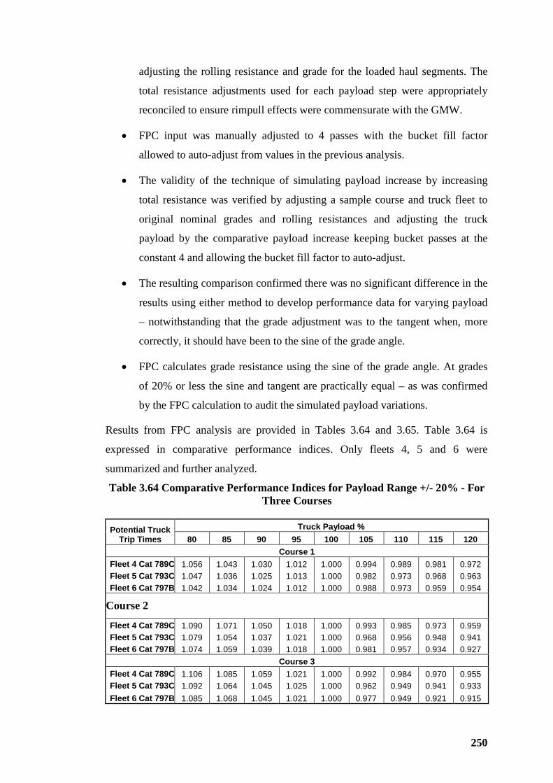
250
adjusting the rolling resistance and grade for the loaded haul segments. The
total resistance adjustments used for each payload step were appropriately
reconciled to ensure rimpull effects were commensurate with the GMW.
• FPC input was manually adjusted to 4 passes with the bucket fill factor
allowed to auto-adjust from values in the previous analysis.
• The validity of the technique of simulating payload increase by increasing
total resistance was verified by adjusting a sample course and truck fleet to
original nominal grades and rolling resistances and adjusting the truck
payload by the comparative payload increase keeping bucket passes at the
constant 4 and allowing the bucket fill factor to auto-adjust.
• The resulting comparison confirmed there was no significant difference in the
results using either method to develop performance data for varying payload
– notwithstanding that the grade adjustment was to the tangent when, more
correctly, it should have been to the sine of the grade angle.
• FPC calculates grade resistance using the sine of the grade angle. At grades
of 20% or less the sine and tangent are practically equal – as was confirmed
by the FPC calculation to audit the simulated payload variations.
Results from FPC analysis are provided in Tables 3.64 and 3.65. Table 3.64 is
expressed in comparative performance indices. Only fleets 4, 5 and 6 were
summarized and further analyzed.
Table 3.64 Comparative Performance Indices for Payload Range +/- 20% - For Three Courses
Potential Truck Trip Times
Truck Payload % 80 85 90 95 100 105 110 115 120
Course 1 Fleet 4 Cat 789C 1.056 1.043 1.030 1.012 1.000 0.994 0.989 0.981 0.972 Fleet 5 Cat 793C 1.047 1.036 1.025 1.013 1.000 0.982 0.973 0.968 0.963 Fleet 6 Cat 797B 1.042 1.034 1.024 1.012 1.000 0.988 0.973 0.959 0.954
Course 2
Fleet 4 Cat 789C 1.090 1.071 1.050 1.018 1.000 0.993 0.985 0.973 0.959 Fleet 5 Cat 793C 1.079 1.054 1.037 1.021 1.000 0.968 0.956 0.948 0.941 Fleet 6 Cat 797B 1.074 1.059 1.039 1.018 1.000 0.981 0.957 0.934 0.927
Course 3 Fleet 4 Cat 789C 1.106 1.085 1.059 1.021 1.000 0.992 0.984 0.970 0.955 Fleet 5 Cat 793C 1.092 1.064 1.045 1.025 1.000 0.962 0.949 0.941 0.933 Fleet 6 Cat 797B 1.085 1.068 1.045 1.021 1.000 0.977 0.949 0.921 0.915
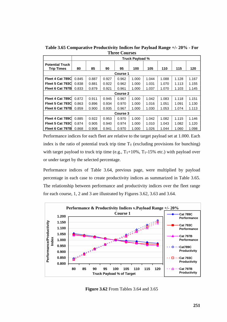
251
Table 3.65 Comparative Productivity Indices for Payload Range +/- 20% - For Three Courses
Truck Payload %
Potential Truck Trip Times 80 85 90 95 100 105 110 115 120
Course 1 Fleet 4 Cat 789C 0.845 0.887 0.927 0.962 1.000 1.044 1.088 1.128 1.167 Fleet 5 Cat 793C 0.838 0.881 0.922 0.962 1.000 1.031 1.070 1.113 1.155 Fleet 6 Cat 797B 0.833 0.879 0.921 0.961 1.000 1.037 1.070 1.103 1.145
Course 2 Fleet 4 Cat 789C 0.872 0.911 0.945 0.967 1.000 1.042 1.083 1.118 1.151 Fleet 5 Cat 793C 0.863 0.896 0.934 0.970 1.000 1.016 1.051 1.091 1.130 Fleet 6 Cat 797B 0.859 0.900 0.935 0.967 1.000 1.030 1.053 1.074 1.113
Course 3 Fleet 4 Cat 789C 0.885 0.922 0.953 0.970 1.000 1.042 1.082 1.115 1.146 Fleet 5 Cat 793C 0.874 0.905 0.940 0.974 1.000 1.010 1.043 1.082 1.120 Fleet 6 Cat 797B 0.868 0.908 0.941 0.970 1.000 1.026 1.044 1.060 1.098
Performance indices for each fleet are relative to the target payload set at 1.000. Each
index is the ratio of potential truck trip time TT (excluding provisions for bunching)
with target payload to truck trip time (e.g., TT+10%, TT-15% etc.) with payload over
or under target by the selected percentage.
Performance indices of Table 3.64, previous page, were multiplied by payload
percentage in each case to create productivity indices as summarized in Table 3.65.
The relationship between performance and productivity indices over the fleet range
for each course, 1, 2 and 3 are illustrated by Figures 3.62, 3.63 and 3.64.
Performance & Productivity Indices v.Payload Range +/- 20%Course 1
0.8000.8500.9000.9501.0001.0501.1001.1501.200
80 85 90 95 100 105 110 115 120Truck Payload % of Target
Perf
orm
ance
/Pro
duct
ivity
In
dex
Cat 789CPerformance
Cat 793CPerformance
Cat 797BPerformance
Cat789CProductivity
Cat 793CProductivity
Cat 797BProductivity
Figure 3.62 From Tables 3.64 and 3.65
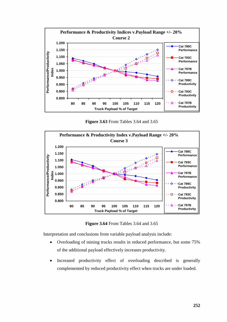
252
Performance & Productivity Indices v.Payload Range +/- 20%Course 2
0.800
0.850
0.900
0.950
1.000
1.050
1.100
1.150
1.200
80 85 90 95 100 105 110 115 120Truck Payload % of Target
Perf
orm
ance
/Pro
duct
ivity
In
dex
Cat 789CPerformance
Cat 793CPerformance
Cat 797BPerformance
Cat 789CProductivity
Cat 793CProductivity
Cat 797BProductivity
Figure 3.63 From Tables 3.64 and 3.65
Performance & Productivity Index v.Payload Range +/- 20%Course 3
0.800
0.850
0.900
0.950
1.000
1.050
1.100
1.150
1.200
80 85 90 95 100 105 110 115 120Truck Payload % of Target
Perf
orm
ance
/Pro
duct
ivity
In
dex
Cat 789CPerformance
Cat 793CPerformance
Cat 797BPerformance
Cat 789CProductivity
Cat 793CProductivity
Cat 797BProductivity
Figure 3.64 From Tables 3.64 and 3.65
Interpretation and conclusions from variable payload analysis include:
• Overloading of mining trucks results in reduced performance, but some 75%
of the additional payload effectively increases productivity.
• Increased productivity effect of overloading described is generally
complemented by reduced productivity effect when trucks are under loaded.
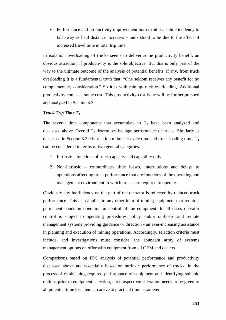
253
• Performance and productivity improvement both exhibit a subtle tendency to
fall away as haul distance increases – understood to be due to the affect of
increased travel time in total trip time.
In isolation, overloading of trucks seems to deliver some productivity benefit, an
obvious attraction, if productivity is the sole objective. But this is only part of the
way to the ultimate outcome of the analysis of potential benefits, if any, from truck
overloading It is a fundamental truth that: “One seldom receives any benefit for no
complementary consideration.” So it is with mining-truck overloading. Additional
productivity comes at some cost. This productivity-cost issue will be further pursued
and analyzed in Section 4.3.
Truck Trip Time TT
The several time components that accumulate to TT have been analyzed and
discussed above. Overall TT determines haulage performance of trucks. Similarly as
discussed in Section 3.2.9 in relation to bucket cycle time and truck-loading time, TT
can be considered in terms of two general categories:
1. Intrinsic – functions of truck capacity and capability only.
2. Non-intrinsic – extraordinary time losses, interruptions and delays to
operations affecting truck performance that are functions of the operating and
management environment in which trucks are required to operate.
Obviously any inefficiency on the part of the operator is reflected by reduced truck
performance. This also applies to any other item of mining equipment that requires
permanent hands-on operation in control of the equipment. In all cases operator
control is subject to operating procedures policy and/or on-board and remote
management systems providing guidance or direction - an ever-increasing assistance
in planning and execution of mining operations. Accordingly, selection criteria must
include, and investigations must consider, the abundant array of systems
management options on offer with equipment from all OEM and dealers.
Comparisons based on FPC analysis of potential performance and productivity
discussed above are essentially based on intrinsic performance of trucks. In the
process of establishing required performance of equipment and identifying suitable
options prior to equipment selection, circumspect consideration needs to be given to
all potential time loss items to arrive at practical time parameters.
254
Any and all non-intrinsic time-loss provisions need to be transparent and justified by
duly diligent investigation of local, national and international mining operations.
Operational experience, either in-house or imported, provides models for guidance
on non-intrinsic time-loss items.
3.3.11 Haul Roads and Site Severity
For mining equipment selection, particularly trucks, it is sufficient to specify that
investigation and analysis is based on specific standards for road construction and
maintenance that can be set in terms of measurable criteria. Performance and
productivity implications of non-conformance with adopted standards need to be
quantified and costed. All stakeholders need to be involved in the adoption of
standards for pit configuration, particularly for haul road geometry standards,
construction materials and formation profile dimensions and details. The final road
specifications and other details need to be commercial in the context of project
feasibility studies or justification for investment expenditure. At the time of
investigating equipment selection, pit design details, particularly haul road
construction and mining truck option interrelationships, should be developed
concurrent with selection preliminaries and identification of initial options.
Only a brief introductory treatment of haul roads and site severity implications was
addressed by the research.
Haul-road layout and design, formation shape, structural profile and running surface
quality have become more important as size of mining trucks has increased. Trucks
in the 90 tonne to 135 tonne range have, historically, proved more tolerant of less-
than-optimum road construction and surface finish standards.
For optimum performance mining trucks require:
• Safe road width for the number of traffic lanes, single lane roads to have bays
strategically placed for passing and with adequate allowance for safety
windrows and drainage with allowance under high walls to accommodate
small debris particles that may fall from the face.
• Sound road formation from competent sub-grade materials designed for truck
wheel loads and suitable surfacing for safe operations under all weather
conditions.
255
• Road layout designs that, for truck options under consideration, comply with
standards for bend radius, maximum speed ≥ maximum speed of the truck,
appropriate super-elevation for the maximum speed and widening at bends to
accommodate the wider radial cover whilst trucks negotiate bends.
• Standard transition curves into and out of bends; also vertical transition
curves where vertical profile of haul roads changes direction – particularly
where the loaded truck runs off the bench onto the access ramp.
• Quality maintenance of road surfaces to retain cross-section and running
surface in design condition; and expedient clearance of spillage to ensure
expected truck trip time TT and realization of expected life for tyres and rims,
suspension componentry and all structural elements of the truck frame and
superstructure.
All of the above truck performance prerequisites are operational rather than planning
and equipment procurement process. But truck selection is performance based and
made on the basis of an expectancy of consistent acceptable working conditions.
These conditions must be specified, understood and a commitment of all
stakeholders for final truck-selection decisions to meet requirements.
Road Construction, Criteria and Standards
Road layout and construction criteria for the full range of mining trucks are available
from the following standard and references:
• Kaufman W W and Ault J C, (1977) Design of Surface Mine Haul Roads,
Information Circular 8758, US Department of the Interior, Bureau of Mines,
Washington DC USA. (Kaufman & Ault, 1977)
• Feddock J E, (2002) Haul Roads, Mining Reference Handbook, Ed. Lowrie R
L, Society for Mining Metallurgy and Exploration Inc., Littleton CO, USA
(Feddock, 2002)
• Caterpillar (2004) Performance Handbook Edition 35, Caterpillar Inc.,
Peoria. Illinois USA, for curve radii, speed and super-elevation,
(Caterpillar#1, 2004)
Kaufman and Ault visited some 300 mines in USA and Canada and based analysis
on available specific standards to produce a de facto general standard for all
256
significant aspects of haul road alignment, road width, braking, construction,
materials, all road safety and operating accoutrements, special safety provisions and
maintenance.
Feddock has summarized Kaufman and Ault’s recommendations and Caterpillar
have provided curve, speed and road super elevation options based on Kaufman and
Ault.
Braking standards for large mining trucks appears to be subject to interpretation. The
Society of Automotive Engineers, SAE 166, has set minimum values for vehicle in
various GMW classes. For vehicles > 400,000 lbs GMW (> 181.5 tonnes ≡ 100
tonnes payload) the maximum stopping distance from 20 mph allowed = 175 feet
(53.4 metres) on dry flat concrete. Kaufman and Ault report on empirical testing of
mining trucks where brake fade effects were tested. A safe braking distance of 61
metres was suggested by the research and recommended by Walter Kaufman and
James Ault. They comment that “most” mining trucks exceed (sic meet the
requirements of) that limitation” (Kaufman & Ault, 1977). If braking distance for
loaded down-ramp operations is an issue it should be raised with dealers and OEM
early in the selection process.
As commented above, road layout configuration, construction and maintenance are
essentially operational issues, Any problems or issues with roads in terms of the
several factors discussed need to be resolved as prerequisites to proceeding with
equipment selection. It needs to be born in mind that the larger the truck or loading
equipment the more vulnerable to potential problems with accommodating marginal,
close-to-unacceptable, operational limits.
The research has not dealt with the matters discussed above in any detail. This
section is intended to provide some starting points for readers who have need to
pursue specific haul road topics in depth.
Monitoring Site Severity
Mining trucks exhibit increasing sensitivity to site severity of operations, particularly
roads as truck capacity increases. To ensure expected life of suspension and
structural componentry, operators of large mining trucks generally accept as
necessary site severity monitoring systems that can report in real time and/or
accumulate data and down load periodic reports.
257
In the larger truck range all OEM and dealers provide site severity sensing and
reporting systems. Caterpillar, pioneers in the technique, provides a typical system.
The VIMS management system records suspension strut pressure transients that are
caused by dynamic suspension loads. Pressure transients registered and damped by
nitrogen over oil suspension mediums register short-time duration variations
transmitted from the road surface through the tyres and suspension. Amplitude of the
pressure transients is a measure of quality of the road surface. Initially an electronic
control module adjunct to VIMS and software that measured and reported racking
and pitching was marketed as Application Severity Analysis (ASA). More recently,
in the process of development of the add-on hardware, software and output reports,
the system is currently offered as Road Analysis Control (RAC). A significant
improvement in RAC is the Fatigue Equivalent Load Analysis (FELA) that stores
and compares actual racking and pitching measurement with intended design values
for life cycle of components affected by haul road induced stresses – tyres, rims,
suspension componentry and super-structure. RAC provides for real-time warnings
at increasingly serious levels to operators as well as periodic management reports.
Remote interrogation of the system is also provided for supervisory monitoring of
operation of the truck.
In the process of mining truck selection, OEM and dealers will offer monitoring
systems such as Caterpillar’s RAC, as add-ons to VIMS and similar management
systems. For large mining trucks such systems are of invaluable assistance to monitor
haul-road maintenance and general truck operating conditions to provide a
management facility for realization of:
• Expected travel times and truck productivity.
• Operating “rhythm” in haulage operations.
• Expected life of componentry including suspension, truck frame and
superstructure.
• Expected life of tyres and rims.
258
3.4 EQUIPMENT SELECTION AND MAINTENANCE
3.4.1 Introduction and Research Limits
This section substantially extends criteria for equipment selection to include
maintenance issues. Consideration must also be given to operational maintenance
issues; but only` to the extent that selection decisions have significant impact on
operational maintenance facilities and general long-term maintenance efficacy.
Loading and hauling equipment must be maintained mechanically and/or electrically
to a predetermined standard - including tyres for trucks - to achieve expected
performance. While loading and hauling equipment is being maintained it is
generally not able to produce. Only the largest shovels and draglines used in strip
mining permit limited maintenance activity whilst in operation. Productive time, nett
of the time necessarily lost for maintenance, must obviously be maximized for best
production practice. Criteria for equipment selection need to include acceptable
availability of productive time. Most importantly, load and haul equipment needs to
be reliable and have predictable mechanical performance.
Both selection and operation of loading and hauling equipment are dependent on
cogent maintenance-related issues that demand duly diligent investigation of:
• Relative merits of optional equipment considered in the process of selection.
• Detailed criteria for specific operational factors in the form of benchmarks
(BM) and key performance indicators (KPI).
Consideration of equipment maintenance in the selection process widens the field of
investigation to require a multi-disciplinary effort. From a focus on performance and
productivity investigation extends to basic reliability and convenience of
maintenance. High maintenance reliability and efficiency results in optimum
operating time for acceptable productivity to realise required total production.
3.4.2 Selection Criteria Related to Maintenance
Industry Experience
As discussed in Section 4.1.1 an essential early stage in the equipment selection and
procurement process is investigation of experience of current (in-house and
externally) and previous owners of the equipment options being considered.
Sources of current owners of equipment under consideration include:
259
• OEM and dealers who can be expected to be keen to facilitate site visits to
demonstrate equipment offered – it is part of the choreography of mining
equipment marketing - so enjoy.
• Service industry consultants and organizations keen to be involved in
development or expansion projects early in the planning stage.
• Experienced colleagues both internal and external to the mining entity that is
investigating equipment procurement – a benefit of (and justification for)
industry “net-working” by mining professionals.
• Consumable suppliers, including tyres and ground engaging tools and third-
party offsite maintenance service providers.
• Personal knowledge of all stakeholders interfacing with the load-and-haul
equipment procurement process.
Maintenance experience of other owners of mining equipment under consideration
for procurement is valuable evidence in the equipment selection process.
It is important to determine from all owners and industry contacts having experience
with some or all of the equipment options under selection consideration if, with the
benefit of hindsight, the same procurement decisions would be made; and, if not,
why not?
Preparation of lists of discussion topics is a necessary prerequisite for best returns
from due diligence examination of equipment options. Following are some general
topics that should be included in preparation for investigation.
Maintainability
The coined term “maintainability” refers to the convenience of effecting all
necessary maintenance activities. Assessment of maintainability requires
involvement of personnel with specific expertise, preferably internal, who will be
taking delivery of equipment on site and have the responsibility for establishing
facilities and managing operational maintenance on site.
A suitable checklist of items to investigate maintainability and other essential
features of mobile equipment includes:
Generally:
260
• Expected life of major driveline (including wheel groups, tyres and rims),
suspension and structural components such as bodies and buckets; also
travelling componentry, tracks, track drives and support frames.
• Initiatives in modular designs to facilitate component-exchange with the
benefit of reduced maintenance response times.
• Improved component designs to extend life – modular designs with focus on
component exchange that facilitate rationalization of in-house or supplier
component inventory - favouring component inventory over spare parts on
site; or off-site on call, so optimizing maintenance resource commitment and
minimizing maintenance costs – ties into product support discussions below.
Detailed:
• Operator station appointments, operator-friendly controls and comfort to
minimise fatigue.
• Review onboard fire suppression installations in the engine compartment and
mounting position for luggable fire extinguishers on equipment.
• Identify and inspect actual installation of lubrication services such as fast
fuelling facilities, auto-lube grease systems, centralized lubricant top-up
points, waste oil extraction,.
• Access around and particularly over driveline componentry.
• Position of all breather locations, access for cleaning and any owner
initiatives by way of in-field modifications to extend breather lines to a
“clean-air” location.
• Any maintenance problems experienced by other owners, remedies applied
and, particularly, any outstanding problems.
• In terms of maintainability, would each owner repeat order specific
replacement component items; and, if not, why not?
Preparation of comprehensive checklists to facilitate due diligence is of paramount
importance. Any residual blanks in check lists following site visits need to be
followed up before finalizing the equipment selection investigation.
261
Discovery of more faults in, say, one truck option compared with others, on its own,
is not necessarily a sufficient reason for discounting or excluding that particular
option. The complete picture has to be considered including:
• Remedies applied, promptness of vendors, efficacy of remedies.
• How the faults remedied or otherwise were discovered – if disclosed by the
OEM or dealer accompanied by advice that improvement has/is being
actioned should be given significant credit.
• Market share of the specific model of equipment is also a good guide.
Beware the faultless equipment item. It is the author’s experience that a faultless
machine or one with few faults is not necessarily a credit to the specific equipment
item but is often a commentary on the inefficacy of the investigator’s due diligence.
Larger mining organizations can benefit from establishing internal generic
configurations and standards for mining equipment for all options offered for the
basic OEM/dealer specification. A general specification including mounting
positions and details for add-ons such as fire extinguishers and buyer-requested
modifications can be established. Future equipment selection projects can benefit
from the established owner-approved specifications and detail drawings. Future
purchases can then be specified by exceptions necessary for the specific application,
updating as necessary for current models. In the absence of such owner standards, it
is possible for different sites within a large mining group to have different
configurations of the same equipment for no good reason, a manifestly unsatisfactory
and potentially costly position.
Product Support
Achieving expected availability of mobile equipment is dependent on support by
OEM and dealers by way of:
• Spare components and parts for components.
• Offsite overhauls and test facilities for quality assurance of rebuilds.
• Training of servicing personnel, operating demonstrators and trainers and
specific training of special tooling and equipment management systems.
262
• Interface with the OEM on warranty issues and unforeseen equipment
application problems.
• Performance guarantees, generally offered by dealers with OEM sanction.
• Availability of maintain-and-repair-contracts, MARC, to reduce the
maintenance-related operational risk for owners; also to divest the owner of
responsibility for insurance spares as discussed below.
Adequate product support is a most important prerequisite to realising expected
productivity of mobile equipment.
Special working conditions could possibly favour a normally relatively minor
attribute of a particular equipment model to the exclusion of other options. Such
circumstances may be possible and could be promoted by focused marketing. But the
author has not experienced such circumstances. It is the author’s opinion and
experience that, when independently analysed, generally the differences between
mobile equipment models of approximately equivalent capability and performance
offered by the field of OEM tend to be subtle in terms of productivity and unit cost of
production.
In any objective analysis (say, using weighted matrix methods) considering purchase
price, estimated operating costs, forecast productivity, product support and other
factors the analyst considers relevant, product support should, and normally does,
receive high priority and weight.
In the author’s opinion, product support should be the paramount factor in any
procurement process aiming to arrive at a decision to purchase an item of
mobile equipment.
Product support:
• Should be included as a group of topics during site visits.
• Needs to be thoroughly probed in discussions with OEM and dealers.
• Particularly availability of service exchange of major driveline components,
engines, torque-converter/transmissions, differential groups, alternators,
inverter groups, wheel motors, management system componentry should be
determined and included in selection considerations.
263
The larger and more specialised an item of production equipment becomes the more
insurance spares will need to be carried by an owner/operator. For example It may be
that an owner may well have a spare slewing ring assembly for a large shovel but
rely on a supplier for service exchange truck engines. Investigation of insurance-
spares policy of other mining equipment operators (including rationale for policy) is
an essential due diligence activity in the process of equipment selection.
Essentially assurance of product support is a risk treatment to cover likelihood and
consequences of excessive equipment downtime due to inadequate supply of backup
components and parts; also to ensure that specialist maintenance and operating skills
are applied to realise expected equipment performance.
Large operations, say, more than 15 large mining trucks (135 tonne plus payload)
should consider carrying their own insurance spares (unless the policy is to carry a
spare truck or trucks) included in the initial delivery programme. Insurance spares (or
spare truck[s]) are an alternative to service exchange that has the advantage of the
owner being in control of the componentry. There is an element of competition for
service exchange components in the hands of dealers or maintenance-service third
parties where a number of customers have to be satisfied.
Owning insurance spares also has the advantage that the condition of the replacement
components is consistent with the residual value of each mining equipment item in
the asset schedule. Also, increasing number of trucks in the fleet reduces unit-cost
write off for insurance componentry inventory. Investment in insurance spares for
trucks is relatively easy to justify.
It should be noted that, for every 3 large trucks, approximately one engine
replacement per year would be required. As fleets increase over 20 trucks towards 30
trucks or more, one the spare engine will be cycled 7 to 10 times. As change outs are
not evenly spaced, more than one spare component may be justified. Simulation
techniques are obviously applicable to the problem of component inventory for large
truck fleets.
Generally smaller numbers of loading equipment items tend to limit the degree of
insurance spares that can be justified. Particularly for diesel-powered shovels spare
engines are difficult to justify for 1 to 2 engine changes per year on average for 3 to 4
shovel operation. The author’s experience with a logistically difficult operation
264
(Telfer, Western Australia) was best productivity and economics were realised by
carrying spare components as a complete loading equipment item. The operation was
“over-shoveled”. Trucks controlled the total productivity and operated with
minimum bunching. This operational circumstance will be further addressed in 3.5
and Section 4.3.
A medium-sized development of a “greenfields” mining project with 1 or 2 loading
equipment items and 8 to 12 medium sized mining trucks may have difficulty in
financing the up-front cost of insurance spares. Dealer credit can likely be negotiated
as a condition of equipment purchase to supply insurance componentry with payment
deferred, say, one year. The alternative is to ensure that service exchange is available
and rely on it; a factor that may become significant in the selection process.
Obviously the operational risk is increased but may be acceptable to a new mining
house with limitations on development capital funding.
So there are several options for equipment support by way of insurance spares. Duly
diligent investigation of the options needs to be conducted by the future owner’s
equipment selection personnel or third party expert investigators to reduce risk of
unavailability of replacement componentry to an acceptable residual. Selection of
load and haul equipment needs to address product support – particularly supply of
insurance spares. If supplied as part of a fleet package there may be some purchasing
advantage or financial/tax benefit from including insurance spares in the deal.
Mechanical Availability – MTBF and MTTR
Productivity of mining equipment is essentially dependent on the equipment being in
good order and available for work. Given equipment is available for work it is then a
responsibility of production management to utilise available equipment productively.
In the context of production management, there are two distinct time categories that
exclude productive work:
1. That time, commonly termed “downtime” when equipment is disabled or in
the hands of maintenance staff and consequently not available for work.
2. That time when equipment is available but is not required by production
management to work.
265
Item 2 - non-operating - time has been expressed as a percentage historically termed
“Job Management Efficiency” that is generated as a quotient of utilised time and
available time.
JME % = Utilised time x 100 Time available for work Traditionally provision for non-utilisation and JME has been facilitated by the “50
(or 45) Minute Hour”. In estimating practice, available hours were discounted to 50
(or 45) minutes – equivalent to applying a JME of 83.3% (or 75%).
Item 1 time can be expressed as a percentage termed “Mechanical Availability” that
is generated as a quotient as follows:
MA % = Time available for work + Downtime Combining these two time bench marks as a product:
Utilisation % =
Time available for work x 100
For the avoidance of doubt it is sound practice to make the availability decision
dependent on function. If in the hands and under control of the maintenance function,
equipment is not available. If in the hands and under control of production
management, equipment is available.
Utilised time x 100 Time available for work + Downtime
The “50 (or 45) minute hour” and JME are traditional terms and concepts with
reducing current use. Availability of onboard recording of equipment activities
enables classification of time components to be as specific as necessary with current
practices, providing for detailed time analysis within maintenance activities; also
time available for production and reporting systems. Utilisation and related time
issues are further discussed in Sections 3.5 and 3.6.
MA is a time-honoured benchmark for industries using mobile or static equipment
that requires periodic maintenance either planned or unplanned. Unfortunately, as a
KPI or benchmark, MA is more applicable locally, within rather than between
operations where the definitions of “downtime” and “time available for work” are
understood so providing consistency of comparison.
It will be noted that “time available for work + downtime” can be interpreted as the
total calendar time in any specific period such as a day, week, month or year. In such
cases MA is more comparable between mining operations. But there is still wide
ranging interpretations of the definition of “time available for work”.
266
Terminology, definitions and concepts in the following discussion generally follow
relevant product support materials from Caterpillar. But interpretations and any
errors are the responsibility of the author.
In the context of maintenance functions MA is considered differently - characterized
by the more recent concepts of Mean Time To Repair (MTTR) and Mean Time
Between Failures (MTBF), Downtime (MTBD) or Stoppages (MTBS).
Early practice adopted “Failures”. Recognition of “Failures”, as not a strictly correct
description of non-availability resulted in substitution of “Downtime”. In turn,
“Downtime” does not allow for subtle interpretation of necessary, routine, planned
maintenance, at least in some part, to be inherently unavoidable maintenance time
with downtime reserved to break downs and major componentry replacement or
repair. So the gravitation to “Stoppages” as a more strictly correct and acceptable
term for time dedicated to maintenance activity. MTBS is used by Caterpillar Global
Mining and was adopted throughout this thesis.
“Reliability” is the prime measure of maintenance efficacy. Expressed as Mean
Time Between Stoppages (MTBS), reliability is arguably the single most significant
impact upon mechanical availability; and therefore upon productivity.
MTBS is a direct measure of reliability derived by the following equation:
MTBS = Operated Hours / Number Of Downtime Incidents
In the above equation the term “incidents” means machine stoppages or shutdowns.
Operational stoppages (or shutdowns) at shift change, lunch, or fueling (including
top ups) or equipment testing are not counted. Maintenance or mechanically related
stoppages – including scheduled lube service during preventative, planned
maintenance; but not daily servicing or oil level checks - are counted.
Efficiency, in the mechanical maintenance context, is a measure of turnaround time
or efficient use of downtime in getting a machine back into service. Mean Time To
Repair (MTTR), as a benchmark, is the most significant direct measure of repair
and/or maintenance efficiency.
MTTR is derived from the following equation:
MTTR = Downtime Hours / Number Of Downtime Incidents
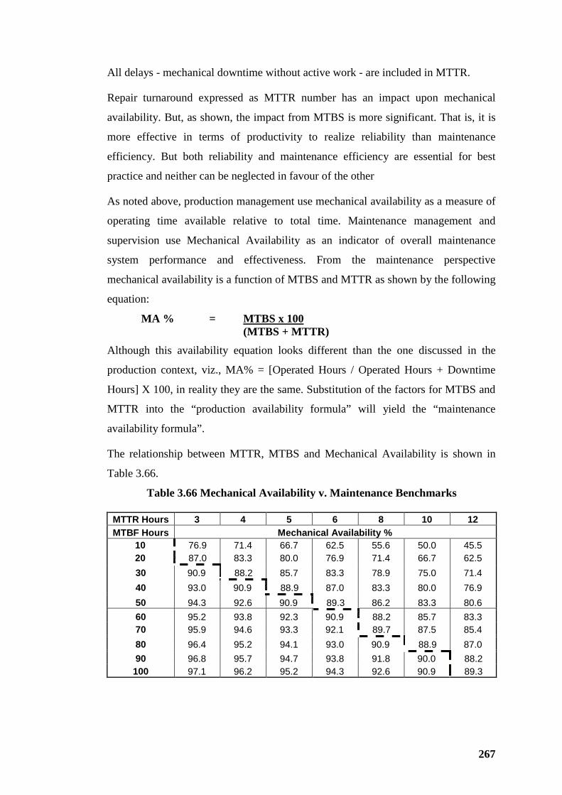
267
All delays - mechanical downtime without active work - are included in MTTR.
Repair turnaround expressed as MTTR number has an impact upon mechanical
availability. But, as shown, the impact from MTBS is more significant. That is, it is
more effective in terms of productivity to realize reliability than maintenance
efficiency. But both reliability and maintenance efficiency are essential for best
practice and neither can be neglected in favour of the other
As noted above, production management use mechanical availability as a measure of
operating time available relative to total time. Maintenance management and
supervision use Mechanical Availability as an indicator of overall maintenance
system performance and effectiveness. From the maintenance perspective
mechanical availability is a function of MTBS and MTTR as shown by the following
equation:
MA % =
Table 3.66 Mechanical Availability v. Maintenance Benchmarks
MTBS x 100 (MTBS + MTTR)
Although this availability equation looks different than the one discussed in the
production context, viz., MA% = [Operated Hours / Operated Hours + Downtime
Hours] X 100, in reality they are the same. Substitution of the factors for MTBS and
MTTR into the “production availability formula” will yield the “maintenance
availability formula”.
The relationship between MTTR, MTBS and Mechanical Availability is shown in
Table 3.66.
MTTR Hours 3 4 5 6 8 10 12 MTBF Hours Mechanical Availability %
10 76.9 71.4 66.7 62.5 55.6 50.0 45.5 20 87.0 83.3 80.0 76.9 71.4 66.7 62.5 30 90.9 88.2 85.7 83.3 78.9 75.0 71.4 40 93.0 90.9 88.9 87.0 83.3 80.0 76.9 50 94.3 92.6 90.9 89.3 86.2 83.3 80.6 60 95.2 93.8 92.3 90.9 88.2 85.7 83.3 70 95.9 94.6 93.3 92.1 89.7 87.5 85.4 80 96.4 95.2 94.1 93.0 90.9 88.9 87.0 90 96.8 95.7 94.7 93.8 91.8 90.0 88.2 100 97.1 96.2 95.2 94.3 92.6 90.9 89.3
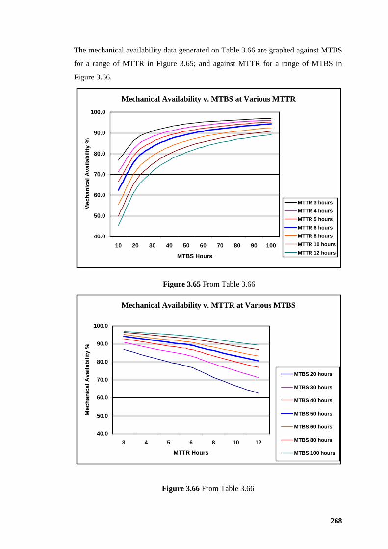
268
The mechanical availability data generated on Table 3.66 are graphed against MTBS
for a range of MTTR in Figure 3.65; and against MTTR for a range of MTBS in
Figure 3.66.
Mechanical Availability v. MTBS at Various MTTR
40.0
50.0
60.0
70.0
80.0
90.0
100.0
10 20 30 40 50 60 70 80 90 100
MTBS Hours
Mec
hani
cal A
vaila
bilit
y %
MTTR 3 hoursMTTR 4 hoursMTTR 5 hoursMTTR 6 hoursMTTR 8 hoursMTTR 10 hoursMTTR 12 hours
Figure 3.65 From Table 3.66
Mechanical Availability v. MTTR at Various MTBS
40.0
50.0
60.0
70.0
80.0
90.0
100.0
3 4 5 6 8 10 12
MTTR Hours
Mec
hani
cal A
vaila
bilit
y %
MTBS 20 hours
MTBS 30 hours
MTBS 40 hours
MTBS 50 hours
MTBS 60 hours
MTBS 80 hours
MTBS 100 hours
Figure 3.66 From Table 3.66
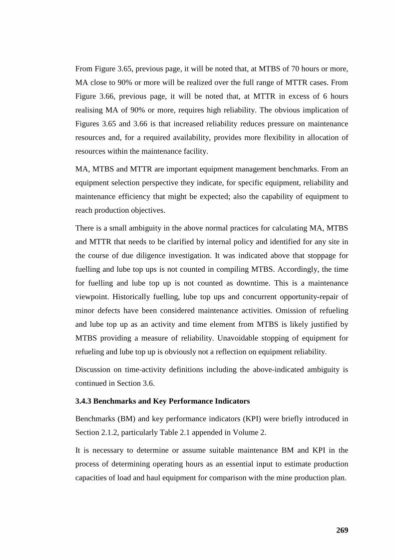
269
From Figure 3.65, previous page, it will be noted that, at MTBS of 70 hours or more,
MA close to 90% or more will be realized over the full range of MTTR cases. From
Figure 3.66, previous page, it will be noted that, at MTTR in excess of 6 hours
realising MA of 90% or more, requires high reliability. The obvious implication of
Figures 3.65 and 3.66 is that increased reliability reduces pressure on maintenance
resources and, for a required availability, provides more flexibility in allocation of
resources within the maintenance facility.
MA, MTBS and MTTR are important equipment management benchmarks. From an
equipment selection perspective they indicate, for specific equipment, reliability and
maintenance efficiency that might be expected; also the capability of equipment to
reach production objectives.
There is a small ambiguity in the above normal practices for calculating MA, MTBS
and MTTR that needs to be clarified by internal policy and identified for any site in
the course of due diligence investigation. It was indicated above that stoppage for
fuelling and lube top ups is not counted in compiling MTBS. Accordingly, the time
for fuelling and lube top up is not counted as downtime. This is a maintenance
viewpoint. Historically fuelling, lube top ups and concurrent opportunity-repair of
minor defects have been considered maintenance activities. Omission of refueling
and lube top up as an activity and time element from MTBS is likely justified by
MTBS providing a measure of reliability. Unavoidable stopping of equipment for
refueling and lube top up is obviously not a reflection on equipment reliability.
Discussion on time-activity definitions including the above-indicated ambiguity is
continued in Section 3.6.
3.4.3 Benchmarks and Key Performance Indicators
Benchmarks (BM) and key performance indicators (KPI) were briefly introduced in
Section 2.1.2, particularly Table 2.1 appended in Volume 2.
It is necessary to determine or assume suitable maintenance BM and KPI in the
process of determining operating hours as an essential input to estimate production
capacities of load and haul equipment for comparison with the mine production plan.
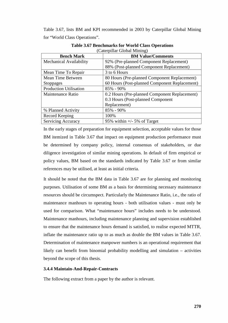
270
Table 3.67, lists BM and KPI recommended in 2003 by Caterpillar Global Mining
for “World Class Operations”.
Table 3.67 Benchmarks for World Class Operations (Caterpillar Global Mining)
Bench Mark BM Value/Comments Mechanical Availability 92% (Pre-planned Component Replacement)
88% (Post-planned Component Replacement) Mean Time To Repair 3 to 6 Hours Mean Time Between Stoppages
80 Hours (Pre-planned Component Replacement) 60 Hours (Post-planned Component Replacement)
Production Utilisation 85% - 90% Maintenance Ratio 0.2 Hours (Pre-planned Component Replacement)
0.3 Hours (Post-planned Component Replacement)
% Planned Activity 85% - 90% Record Keeping 100% Servicing Accuracy 95% within +/- 5% of Target
In the early stages of preparation for equipment selection, acceptable values for those
BM itemized in Table 3.67 that impact on equipment production performance must
be determined by company policy, internal consensus of stakeholders, or due
diligence investigation of similar mining operations. In default of firm empirical or
policy values, BM based on the standards indicated by Table 3.67 or from similar
references may be utilised, at least as initial criteria.
It should be noted that the BM data in Table 3.67 are for planning and monitoring
purposes. Utilisation of some BM as a basis for determining necessary maintenance
resources should be circumspect. Particularly the Maintenance Ratio, i.e., the ratio of
maintenance manhours to operating hours - both utilisation values - must only be
used for comparison. What “maintenance hours” includes needs to be understood.
Maintenance manhours, including maintenance planning and supervision established
to ensure that the maintenance hours demand is satisfied, to realise expected MTTR,
inflate the maintenance ratio up to as much as double the BM values in Table 3.67.
Determination of maintenance manpower numbers is an operational requirement that
likely can benefit from binomial probability modelling and simulation – activities
beyond the scope of this thesis.
3.4.4 Maintain-And-Repair-Contracts
The following extract from a paper by the author is relevant.
271
“Throughout the history of contract open-pit mining, mobile equipment dealers have
been offering an extension of the traditional business of sales (new and used), parts,
offsite component/machine overhauls and training to include contract, onsite, total
service of mobile plant. Until more recently the style of equipment design, labour
costs and overheads, (and, particularly, reasonable availability of skilled maintenance
labour) made it difficult for equipment dealers to compete with in-house routine
servicing and maintenance of mobile equipment. This situation has changed.
Currently both earthmoving contractors and owners are executing contracts with
equipment dealers for a total onsite service – a maintain-and-repair-contract
(MARC)” (Hardy #3, 2005).
The business cycle that favoured inclusion of supply, maintain and repair of mobile
equipment and the many other peripheral supply or service opportunities in contracts
offered to earth moving contractors has moved on to a phase where owners are
considering alternative options. Mining contractors have traditionally managed the
logistics of establishing equipment, maintenance facilities, a suitably skilled
workforce and outsourced:
• Supply of equipment and finance;
• Major component rebuilds and equipment spares;
• Subcontracted tyre fitting and management service;
• Supply of tyres and accessories;
• Supply of fuel, lubricants and cleaning fluids;
• Down-the-hole service of explosives and supply of accessories;
• Supply of all other consumables;
• Sometimes blast hole drilling; and,
• Pit dewatering when included in their work.
In recent times there has been a tendency for owners to take over and in-house
manage many of the supply and service functions historically included in mining
contract works. Of interest is the degree of actual hands-on management control that
owner miners are currently choosing to retain. Table 3.68- provided by Linton Kirk
(Kirk, 2000), shows that recent conversions to owner mining have retained hands-on
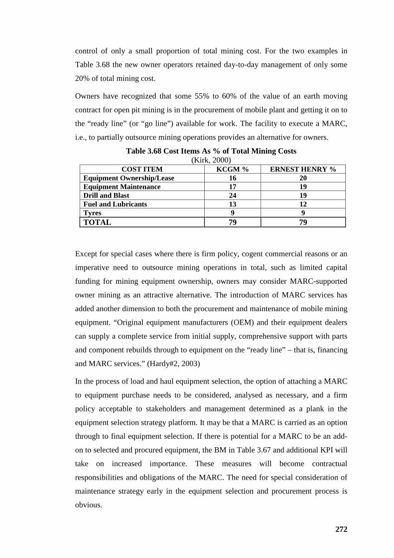
272
control of only a small proportion of total mining cost. For the two examples in
Table 3.68 the new owner operators retained day-to-day management of only some
20% of total mining cost.
Owners have recognized that some 55% to 60% of the value of an earth moving
contract for open pit mining is in the procurement of mobile plant and getting it on to
the “ready line” (or “go line”) available for work. The facility to execute a MARC,
i.e., to partially outsource mining operations provides an alternative for owners.
Table 3.68 Cost Items As % of Total Mining Costs (Kirk, 2000)
COST ITEM KCGM % ERNEST HENRY % Equipment Ownership/Lease 16 20 Equipment Maintenance 17 19 Drill and Blast 24 19 Fuel and Lubricants 13 12 Tyres 9 9 TOTAL 79 79
Except for special cases where there is firm policy, cogent commercial reasons or an
imperative need to outsource mining operations in total, such as limited capital
funding for mining equipment ownership, owners may consider MARC-supported
owner mining as an attractive alternative. The introduction of MARC services has
added another dimension to both the procurement and maintenance of mobile mining
equipment. “Original equipment manufacturers (OEM) and their equipment dealers
can supply a complete service from initial supply, comprehensive support with parts
and component rebuilds through to equipment on the “ready line” – that is, financing
and MARC services.” (Hardy#2, 2003)
In the process of load and haul equipment selection, the option of attaching a MARC
to equipment purchase needs to be considered, analysed as necessary, and a firm
policy acceptable to stakeholders and management determined as a plank in the
equipment selection strategy platform. It may be that a MARC is carried as an option
through to final equipment selection. If there is potential for a MARC to be an add-
on to selected and procured equipment, the BM in Table 3.67 and additional KPI will
take on increased importance. These measures will become contractual
responsibilities and obligations of the MARC. The need for special consideration of
maintenance strategy early in the equipment selection and procurement process is
obvious.
273
3.4.5 Equipment Sales Agreements
Warranties, performance guarantees and formal agreements are necessary protective
instruments for purchasers of mining equipment. It is important during the due
diligence phase of equipment selection to establish reasonable expectancies that are
neither optimistic nor too protective of operating performance in the future. In the
earliest selection stages discussions may be initiated on warranty, particularly
extensions, performance guarantees for new, relatively untried equipment models
under consideration. At some stage, particularly if MARC is an option, formal
agreement(s) may need to be prepared. Facilities for such specialised document
preparation need to be arranged with the greatest possible lead-time to avoid
unnecessary delays when the procurement process is nearing conclusion.
3.5 FLEET MATCHING, BUNCHING, QUEUING
3.5.1 Introduction
In the process of equipment selection it is necessary to utilise effective procedures
and practices to arrive at a robust estimate of the necessary number of trucks in a
fleet to satisfy the planned production programme. Procedures and practices adopted
need to ensure that sufficient trucks are productive for sufficient time to fulfill
production requirements.
Of necessity the number of loading equipment items and capacity are complementary
considerations to resolve interactive effects with trucks that determine productivity
of the combined fleet. Such interactives include number of bucket passes, bucket
cycle times and other time components affecting truck loading time.
The discussion also extends to consideration of probabilistic analysis of truck
availability for single and multiple loading equipment cases as a more effective
alternative in comparison with traditional, deterministic practices.
A-productive Factors – Discounting Productivity
Productivity of loading and hauling equipment is reduced from theoretical to actual
experienced performance by a number of a-productive factors. In Section 3.4 a-
productive factors of mechanical availability and utilisation were discussed. This
discussion is extended to further a-productive factors related to fleet matching and
variability of truck loading and trip times – generally termed “bunching”.
274
Such a-productive factors can be considered intrinsic to loading and/or loading
equipment where there are direct performance differences attributable to equipment
or the normal operation of that equipment. In contrast a-productive effects can be
considered non-intrinsic where there are extraneous effects not related to the
capability of the equipment or the direct operation of it.
Examples of intrinsic effects are variabilities of engine power, power transmission of
other driveline componentry, tyre outside diameter due to wear, NMW, quantities of
debris on frames and carry back in truck bodies (and buckets particularly for wheel
loaders); and operator efficiency that has been empirically been shown to be a
function of haul distance, see Section 3.3.10 and Figure 3.58. Generally intrinsic a-
productive effects are causes of “bunching” as described in literature and used in
common operational terminology.
Non-intrinsic a-productive effects are the result of extraneous activity, sometimes
related, but often unrelated, to load and haul equipment characteristics and
capability. Examples include traffic and stationary obstructions on roads, road re-
construction or construction of road extensions, general pit housekeeping, specific
housekeeping at the working face, large particles in the face, road and trafficable area
watering, providing access for other functions such as blasting agent and accessory
transport, latent ground conditions that interrupt operations, re-routing one or more
trucks from a specific duty cycle, assigning too many trucks – overtrucking - and any
casual un-scheduled stoppages of loading equipment or trucks.
Terminology
The terms “bunching” and “queuing” are commonly used with overlapping meanings
and sometimes for the same condition in load and haul systems. Particularly
Caterpillar in the FPC Handbook (Caterpillar#2, 2004); and Dan Gove and Bill
Morgan use the term “bunching” only in analysis and discussion that is focussed on
optimizing truck and loader matching (Gove & Morgan, 1994). Elbrond describes, as
an alternative to simulation, development of a deterministic process for calculating
waiting time for trucks where a queue exists at the loader in terms of “queuing
theory” (Elbrond, 1990). Ramani provides solutions to fleet matching using
deterministic, (including “average delay” as a time element), statistical (probabilistic)
275
and simulation methods without referring to either “bunching” or “queuing”
(Ramani, 1990).
Christina Burt and co-authors (Burt et al, 2005), in an extended abstract, provide the
following definitions:
“Bunching Theory: Bunching models capture the tendency of moving objects to
bunch together when moving in a line. This is generally due to some of the objects
being operated or moving more efficiently than others.
Queuing Theory: Queuing theory is the study of waiting times, lengths, and other
properties of queues.”
The focus of this part of the research and thesis is on a-productive effects of
“bunching” phenomena and what drives them. Wait time and other queuing issues
are incidental to the analysis and interpretations. “Bunching” has been adopted
herein as a generic term to cover the physical affect of any delay to trucks and
loading equipment that causes loss of production.
Analysis Methods
Initial calculations of fleet estimates and matching are generally deterministic using
expected (mean) values. Consideration of affects of a-productive factors that are
independent random variables, such as mechanical non-availability, requires
application of probabilistic techniques to realise acceptable results for fleet matching.
It is necessary to realize an acceptable treatment of the a-productive effect of
interaction between independent, randomly variable time-performance characteristics
of loading equipment and trucks that manifests as “bunching”. This can be achieved
by application of empirical deterministic relationships or introduction of simulation
techniques utilizing probabilistic techniques modelling empirical operational data.
This section generally follows the indicated analysis process including deterministic
application of empirically based criteria to quantify “bunching” effects.
3.5.2 Preliminary Fleet Numbers
Preliminaries
The following preliminary analysis assumes that all variables are expected (mean)
values. Any practical application of the relationships and equations is necessarily
276
deterministic. Using the symbols as defined in Sections 3.3.9 and 3.3.10, truck-
loading time can be expressed in terms of bucket cycle times as:
• From loading equipment perspective – TC = TEX + n . TBC
• From truck perspective – TL = TF + (n-1) . TBC
n = number of bucket cycles.
Truck trip time can be considered in terms of components:
• TT = TV + TD + TS + TL
• TV = TVL + TVE - subscripts “VL” and “VE” indicate “loaded” and “empty”
respectively.
In the process of load-and-haul equipment selection the “which comes first?”
question must be resolved. Many practitioners and authors indicate that loading
equipment selection is resolved, at least generally, before proceeding to truck
selection. It is the author’s opinion that loading equipment selection considerations
should only proceed to the limited extent necessary to allow progress of truck
selection. When truck selection has been resolved to an acceptable conclusion, then
selection of loading equipment can be concluded. Of course, concluding loading
equipment selection should, prudently, be followed by an audit of truck selection
criteria and process to ensure that the fleet configuration is optimum.
Some estimating formulae offered by other authors include (symbols for variables
substituted to be consistent with usage herein; also units assumed consistent with
context of equations):
Truck loading time - TL:
TL = PL/Pe (1)
PL = truck payload
Pe = shovel productivity
TL = PL . TBC/Bcap (2)
TBC = bucket cycle time
Bcap = bucket capacity utilised (after application of fill factor)
277
Travel Time – TV, Haul Distance – DH, Relationships:
Subscript “L” = “loaded”
Subscript “E” = “empty”
TVL = DHL/SAVL
TVE = DHE/SAVE
TV = (DHL + DHE)/SAV (3)
TV = travel time
DHL = haul distance loaded
DHE = haul distance empty
SAV = average speed
From Table 3.63 - SAV ≈ 21 kph
TV minutes = DH metres x 60/21,000
= 0.00286 x DH (4)
Consider a loader has loaded a single truck that is en route to dump and return.
Assuming for the purposes of analysis that all variables are expected (mean) values;
also assuming that the “return” time is substantially larger than the manoeuvre and
spot plus loading time - then the loader experiences waiting time – WL - as follows:
WL = (TV +TD) – (TS +TL)
Generalized for N trucks in the fleet (N is always an integer) – and a single loading
unit – mean loader waiting time W is derived from:
W = (TV +TD) – (N-1)(TS +TL) (5)
If the loader does not experience waiting time W = 0. Simple algebraic manipulation
yields:
N = TT/(TS + TL) (6)
If W ≠ 0; but 0 < W < (TS +TL) then:
W = (TV +TD + TS + TL) – N . (TS +TL)
N + W/(TS +TL) = TT/(TS + TL) where 0 < W/(TS +TL) < 1.0
278
[N]* = [TT/(TS + TL)]* (7)
[N]* = number of trucks after rounding (up or down)
[TT/(TS + TL)]* = signifies rounding up or down to an integer.
The above equations (1) to (7), for a single truck loading group are offered by, or
derived from, a number of references particularly, Ramani (Ramani, 1990) and
Fourie and Dohm (Fourie, 1992).
Initial Fleet Estimates and Matching to Loading Equipment
Estimating truck fleet requirements to match a single loading unit to satisfy a planned
production programme is an iterative process. Initial estimates, to be used as a basis
for analysis to accommodate a-productive factors discussed, can be developed by
several methods including:
1. Application of equation (7) where the total truck trip and truck loading times,
TT and TL are known or can be estimated with reasonable accuracy;
2. In the absence of TT and TL the following method for deep open pits can be
applied.
The depth of pit is multiplied by the access ramp grade expressed as a
percentage; and, to estimate one-way haul distance, apply one-way haul
distance factor KD - for pits to 100 metres KD = 2, for pits to 200 metres KD =
1.8 and for pits to 500 metres KD = 1.6.
To establish an estimated total haul double the distance.
Take 0.3% to derive total travel minutes.
Add fixed times 0.75 + 1.0 +3.0 minutes for manoeuvre and spot, (fixed
times can be modified if desired but reasonable changes will be only of small
effect in the outcome) manoeuvre and dump and loading time to arrive at
estimated truck trip time.
Initial Estimate of Number of Trucks - Nie - for a single loading unit:
Nie = (0.003 x DHie x KD x 2 + TS + TL + TD)/(TS + TL) (8)
The following examples illustrate the method:
Example 1: 50m deep pit, 10% access ramp KD = 2.
279
Nie = (50 x 10 x 2 x 2 x 0.003 +4.75)/3.75
= 10.75/3.75
= 2.87 trucks
Example 2: 200m deep pit, 10% access ramp KD = 1.8.
Nie = (200 x 10 x 1.8 x 2 x 0.003 +4.75)/3.75
= 26.35/3.75
= 7.03 trucks
Example 3: 500m deep pit, 10% access ramp KD = 1.6.
Nie = (500 x 10 x 1.6 x 2 x 0.003 +4.75)/3.75
= 52.75/3.75
= 14.07 trucks
It will be noted that the estimating technique using equation (8) is a simple extension
of equations (1) to (7). Reference to Table 3.63, shows the second of the estimating
methods (in the absence of TT and TL) is reasonably consistent with truck trip times
as generated by Caterpillar’s FPC and sufficiently accurate for initial estimates.
It must be emphasized that the above-recommended “rule-of-thumb” estimating
method is confined to deep open pits for a single, or each, loading unit. Preliminary
estimation methods for open pits with configurations and geometry differing from
pits normally described as “deep” can be developed similarly.
Initial estimates are not an essential step in the equipment selection process; but, in
the absence of intuitive insight and experience, may be necessary to narrow down the
options for suitable trucks and loading equipment to match to required productivity.
Indicative truck numbers established from equation (8) need to be checked against
truck numbers from equation (7) when TT and TL are ultimately known.
Basic Truck Fleet Numbers
The following discussion is in context with deep open pit mining. Other open pit
configurations can be similarly treated with appropriate adjustments to process.
Assuming:
• Possession of a production plan;
280
• Indicated necessary productivity; and
• Some preliminary thoughts on the range of applicable trucks:
It is necessary to set up some typical haul road profiles through the depth of the pit to
provide a range of cases for fleet selection and matching determinations.
The following description is more a mine planning activity than equipment selection.
There is interactive overlap where discrimination between planning and equipment
selection is practically difficult.
Sufficient typical haul profiles need to be analysed to provide a suite of estimated
performance data for comprehensive truck fleet and loading equipment analysis.
Suggested bench levels for typical haul road profiles:
• Say two benches down (more or less as necessary) to cover the vertical zone
through clearing, topsoil and subsoil harvesting for rehabilitation purposes.
Through the upper weathered zone where lateritic-cemented horizons may be
harvested for road building/surfacing materials; and where highly weathered
zones may be “free digging” – where some of barren pit overburden may be
mined by scrapers as an option to loading and truck haulage.
• At elevations where there are substantial changes in the weathering profile
from weathered to transition to fresh rock – where there will be significant
changes in bank and loose density and voids ratio of material to be hauled
and necessary fragmentation methods must change radically, e.g.,
introduction of drilling and blasting.
• At one-third of the depth – approximately 50% of pit volume remains to be
mined.
• At half the depth – approximately 25% of pit volume remains to be mined.
• At planned pit bottom.
For the suite of haul road profiles, develop for the pre-selected range of alternative
trucks, truck trip times, loading times and other time components necessary for
deterministic estimating of basic fleet numbers. It is common practice to use
commercially developed software such as Caterpillar’s FPC (see Section 3.3.10) or
Runge Mining’s Talsim. It should be noted that both of these software packages tend
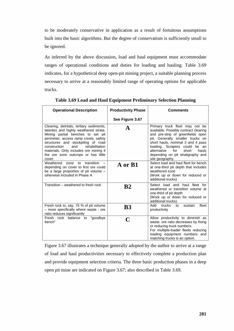
281
to be moderately conservative in application as a result of fortuitous assumptions
built into the basic algorithms. But the degree of conservatism is sufficiently small to
be ignored.
As inferred by the above discussion, load and haul equipment must accommodate
ranges of operational conditions and duties for loading and hauling. Table 3.69
indicates, for a hypothetical deep open-pit mining project, a suitable planning process
necessary to arrive at a reasonably limited range of operating options for applicable
trucks.
Table 3.69 Load and Haul Equipment Preliminary Selection Planning
Operational Description Productivity Phase
See Figure 3.67
Comments
Clearing, detritals, tertiary sediments, laterites and highly weathered strata. Mining partial benches to set pit perimeter, access ramp crests, safety structures and stockpiling of road construction and rehabilitation materials. Only includes ore mining if the ore zone outcrops or has little cover.
A Primary truck fleet may not be available. Possibly contract clearing and pre-strip of greenfields open pit. Generally smaller trucks on short hauls, nominal 3 and 4 pass loading. Scrapers could be an alternative for short hauls depending on pit stratigraphy and site geography.
Weathered zone to transition – depending on cover to first ore could be a large proportion of pit volume – otherwise included in Phase A
A or B1 Select load and haul fleet for bench at one-third pit depth that includes weathered zone (Work up or down for reduced or additional trucks)
Transition – weathered to fresh rock B2 Select load and haul fleet for weathered or transition volume at one-third of pit depth (Work up or down for reduced or additional trucks)
Fresh rock to, say, 75 % of pit volume – more specifically where waste : ore ratio reduces significantly
B3 Add trucks to sustain fleet productivity
Fresh rock balance to “goodbye bench” C Allow productivity to diminish as
waste: ore ratio decreases by fixing or reducing truck numbers. For multiple-loader fleets reducing loading equipment numbers and matching trucks is an option.
Figure 3.67 illustrates a technique generally adopted by the author to arrive at a range
of load and haul productivities necessary to effectively complete a production plan
and provide equipment selection criteria. The three basic production phases in a deep
open pit mine are indicated on Figure 3.67; also described in Table 3.69.
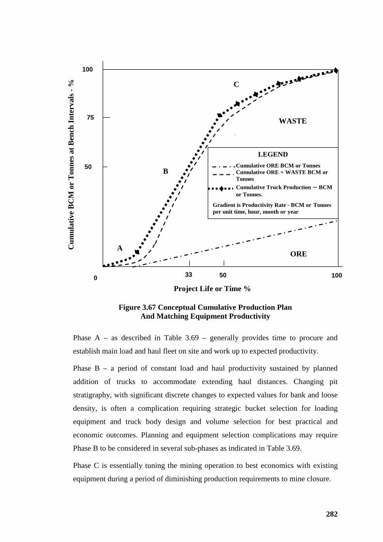
282
Figure 3.67 Conceptual Cumulative Production Plan And Matching Equipment Productivity
Phase A – as described in Table 3.69 – generally provides time to procure and
establish main load and haul fleet on site and work up to expected productivity.
Phase B – a period of constant load and haul productivity sustained by planned
addition of trucks to accommodate extending haul distances. Changing pit
stratigraphy, with significant discrete changes to expected values for bank and loose
density, is often a complication requiring strategic bucket selection for loading
equipment and truck body design and volume selection for best practical and
economic outcomes. Planning and equipment selection complications may require
Phase B to be considered in several sub-phases as indicated in Table 3.69.
Phase C is essentially tuning the mining operation to best economics with existing
equipment during a period of diminishing production requirements to mine closure.
100
100
50
75
33
50
A
B
C
ORE
WASTE
0
LEGEND Cumulative ORE BCM or Tonnes Cumulative ORE + WASTE BCM or Tonnes Cumulative Truck Production – BCM or Tonnes.
Gradient is Productivity Rate - BCM or Tonnes per unit time, hour, month or year
Project Life or Time %
Cum
ulat
ive
BC
M o
r T
onne
s at B
ench
Inte
rval
s - %
283
It is obvious that load and haul equipment should primarily be selected to satisfy the
necessary mining duties for the largest proportion of production volume that can be
identified with discretely similar mining properties – preferably at constant
productivity. The ultimate mining goal is to produce a stream of run-of-mine ore, or
more generally mineral product that satisfies the needs of downstream sizing,
processing and transport with ever-increasing concentration through to final mining
commodity production. Generally, proceeding downstream from the mining
operation, processing functions receive feed-rates, with reducing dispersion, trending
towards the central limit, i.e., mean feed rate. Accordingly load and haul equipment
selected for deep open pit mines, in fact for all mines, must satisfy the specific needs
of downstream facilities including practically constant production rate of mineral
product.
Mine planning activities will yield a suite of productivity requirements for mining
yields at differing horizons through the depth of the open pit. Each discrete
productivity requirement needs to be satisfied by a number of trucks. Each truck has
a productivity of:
VT tonnes or BCM per hour = PL . 60/TT (9)
VT = Productivity per truck tonnes per hour (TPH) or BCM per hour
(BCM/H)
PL = truck payload in tonnes of BCM
TT = Truck trip time – minutes
Phase Productivity VPH TPH or BCM/H is an outcome of planning activities
described above.
Basic number of trucks – NB:
NB = VPH/VT (10)
Equipment matching to a productivity requirement determined by planning is
generally an iterative process. As will be seen below, probabilistic analysis of truck
and loading equipment availability tends to discount expected production
performance based on deterministic analysis. Accordingly, intuitive, experienced
consideration of planning-derived productivity requirements may be prudently
increased by a contingency allowance. That is, VPH should include any necessary
284
allowances to ensure that the basic number of trucks provides for all a-productive
effects other than those that are covered by subsequent probabilistic analysis. It
should be noted that, in default of providing contingencies to satisfy intuitive and
experienced expectations, the same outcome will be achieved by iterative process.
By application of the above, or techniques of similar effect, basic load and haul fleet
numbers are derived, specifically trucks. It should be noted that, for this truck fleet
estimation, TT is based on notional or first-estimate loading equipment
characteristics. Number of loading equipment items can be estimated using equation
(7) to determine the number of trucks that can be loaded by a single loading unit.
Estimates of basic truck numbers are substantially independent of loading equipment
options at this stage of the selection process. Particularly the resulting truck numbers
are independent of the number of loading units.
Treatment of A-productive Factors
Having established the basic fleet numbers from equation (10), a number of a-
productive effects need to be considered including the following five factors:
1. Mechanical non-availability to accommodate maintenance of equipment,
specifically trucks.
2. Non-utilisation due to inefficient management of available equipment.
3. Operator inefficiency as discussed in Section 3.3.10 and illustrated by Figure
3.58.
4. Loading and hauling equipment mismatch, i.e., insufficient trucks so that
loading equipment productivity is reduced below expectancy by having to
wait for trucks; or excess trucks so that unit truck productivity reduces below
expectancy by trucks having to wait to be loaded.
5. Reduced load and haul performance due to “bunching” caused by
individually variable truck trip times and loading equipment bucket cycle
time. That is, variable intrinsic performance of individual equipment items as
discussed below - affecting both truck and loading equipment performance
that results in the hypothetical “rhythmical” cyclical load and haul system
deteriorating to a “bunched” system. There is a tendency for the time lost by
individual equipment items to interfere with following items. Unless there is
285
provision and policy provides for trucks to pass, all units in the cyclical
system will tend to gravitate to the performance of the slowest truck.
Discussing each of the five factors in terms of treatment:
Mechanical non-availability:
Maintenance activities effectively isolate trucks from productive operations.
Assuming scheduled work hours are a practical maximum, replacing trucks sterilized
by maintenance by adding to the fleet is the appropriate treatment. Mechanical
availability is an independent random variable.
Non-utilisation:
Non-utilisation of load and haul equipment is also an independent random variable.
In a greenfields project and where all production and maintenance planning is based
on deterministic analysis then equipment utilisation can be viewed as a parallel to
mechanical availability. For a brownfields extension of existing operations or
equipment replacement selection process, care needs to taken to ensure that
estimated productivity requirements do not already partly or totally compensate for
non-utilisation. Adding trucks to compensate for non-utilisation assumes that a
similarly inefficient operational model is retained for all trucks. That is, the
operational circumstances and practices that result in non-utilisation are the same for
every truck, say; but they may differ between types of equipment. So loading
equipment can experience differing utilisation characteristics to trucks and other
equipment categories.
Operator inefficiency:
There is empirical evidence that operator inefficiency is haul distance dependent with
efficiency increasing with haul distance. Figure 3.58 indicates that, ignoring one-way
hauls of less than 1,000 metres, expected operator efficiency is some 90% for short
hauls increasing to 97% for longest hauls. The effect of operator inefficiency is to
generally and modestly detune equipment performance. Operator inefficiency is an
independent, random variable and accordingly could be treated stochastically. The
nature of operator inefficiency is an outcome of the interaction between the operator
and the equipment unit through the medium of the truck control system. Maximum
performance is a result of best possible response. As skilled as operators may be,
there will tend to be some small lapses in time response that manifest as operator
286
inefficiency. It is the author’s opinion that corrections for operator inefficiency
should be made where the time lapses manifest, i.e., to truck trip time or loading
equipment cycle or loading time. For the purposes of discussion and analysis herein
it is assumed that allowance for operator inefficiency is made to truck trip times and
loading times, i.e., as a contingency allowance included in target productivity used to
determine basic truck numbers.
Fleet matching:
Fleet matching is generally treated deterministically in terms of expected (mean)
performance values for both loading equipment and trucks. The perfect match point
is hypothetical. It is where truck trip and loading times have an exact integer
relationship: where there is no waiting time experienced by loading equipment
between truck arrivals; also returning trucks do not experience waiting time before
loading. Generally, the theoretical truck fleet match will not be an exact integer.
There is practical necessity to round up to overtruck or down to undertruck. These
issues are discussed in more detail below.
Bunching:
Productivity effects of “Bunching” are complex and vary substantially through the
range from significantly overtrucked to undertrucked – or “over-shoveled”.
Discussion in Sections 3.5.3, 3.5.4 and 3.5.5 describe the implications of the various
possible operating circumstances, resulting “bunching” effect and productivity
implications.
Treatment of basic truck numbers based on productivity requirements to arrive at a
fleet number that will compensate for maintenance non-availability; also to allow for
non-utilisation has been traditionally deterministic. A mechanical availability of, say,
90% and an independent utilisation of, say, 90% results in a combined factor of 81%.
As noted care needs to be taken to ensure that non-utilisation and perhaps mechanical
non-availability is not double counted when using empirical data in cases such as
“brownfields”: development or replacement.
NFD = NB/(MA . U) (11)
MA = mechanical availability as defined in Section 3.4.
U = utilisation as discussed in Section 3.4 and in this Section 3.5
287
NFD = deterministic fleet number.
Example: If a basic truck fleet of 15 trucks (NB) is required to meet the required
productivity, application of equation (11) estimates fleet number as:
NFD = 15/0.81 = 18.52 – say 19 trucks where MA = 0.9 and U = 0.9.
In practice this would be found to be an insufficient truck fleet to cover for MA and
U at the assumed values. Equation (11) assumes that MA, also U or the combination
of them are constant values consistent with empirical outcomes when, in fact, both
MA, U and their combination are independent random variables that can be modelled
by a binomial distribution. A probabilistic treatment provides more adequately for
random service outages for maintenance and to allow for non-utilisation. References
that support probabilistic treatment of truck number determination and truck hours
analysis including (Bohnet, 1992, p1535), (Hays, 1990, p684), and (Ramani, 1990,
p727).
The binomial probability function can be expressed as
Px;N =NCx . px . qN-x (A)
Px;N = Probability of exactly x experiences from a population of N
possibilities
NCx = Combinations of N experiences taken x at a time
px = Probability of a single experience
qN-x =Probability of a single non-experience.
Background and development of equation (A) can be found in standard mathematical
references. (Chou, 1969), or (Devore, 1999). The above symbols are generally
consistent with the referenced texts.
Ramani’s notation is generally adopted for the following discussion. Rewriting
equation (A) accordingly:
Pn = NCn . (Pa)n . (Pna)N-n (12)
Pn = probability that exactly n units are available
NCn = combination of N units taken n at a time (n ≤ N)
Pa = probability that a single unit is available
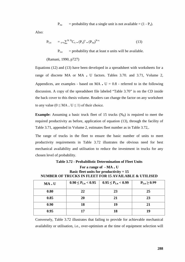
288
Pna = probability that a single unit is not available = (1 - Pa).
Also:
PLn = x=n∑N NCx . (Pa)x . (Pna)N-x (13)
PLn = probability that at least n units will be available.
(Ramani, 1990, p727)
Equations (12) and (13) have been developed in a spreadsheet with worksheets for a
range of discrete MA or MA . U factors. Tables 3.70. and 3.71, Volume 2,
Appendices, are examples - based on MA . U = 0.8 - referred to in the following
discussion. A copy of the spreadsheet file labeled “Table 3.70” is on the CD inside
the back cover to this thesis volume. Readers can change the factor on any worksheet
to any value (0 ≤ MA . U ≤ 1) of their choice.
Example: Assuming a basic truck fleet of 15 trucks (NB) is required to meet the
required productivity as before, application of equation (13), through the facility of
Table 3.71, appended in Volume 2, estimates fleet number as in Table 3.72,.
The range of trucks in the fleet to ensure the basic number of units to meet
productivity requirements in Table 3.72 illustrates the obvious need for best
mechanical availability and utilisation to reduce the investment in trucks for any
chosen level of probability.
Table 3.72 - Probabilistic Determination of Fleet Units For a range of - MA . U
Basic fleet units for productivity = 15 NUMBER OF TRUCKS IN FLEET FOR 15 AVAILABLE & UTILISED
MA . U 0.90 ≤ PLn < 0.95 0.95 ≤ PLn < 0.99 PLn ≥ 0.99
0.80 22 23 25
0.85 20 21 23
0.90 18 19 21
0.95 17 18 19
Conversely, Table 3.72 illustrates that failing to provide for achievable mechanical
availability or utilisation, i.e., over-optimism at the time of equipment selection will
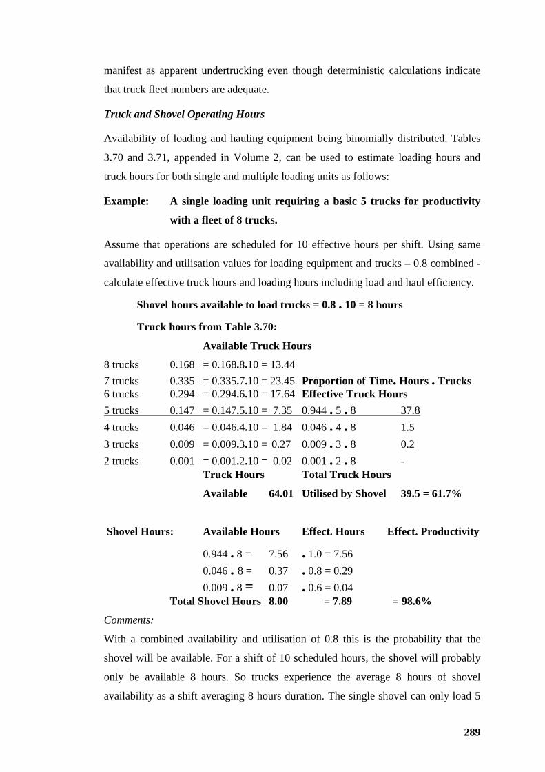
289
manifest as apparent undertrucking even though deterministic calculations indicate
that truck fleet numbers are adequate.
Truck and Shovel Operating Hours
Availability of loading and hauling equipment being binomially distributed, Tables
3.70 and 3.71, appended in Volume 2, can be used to estimate loading hours and
truck hours for both single and multiple loading units as follows:
Example: A single loading unit requiring a basic 5 trucks for productivity
with a fleet of 8 trucks.
Assume that operations are scheduled for 10 effective hours per shift. Using same
availability and utilisation values for loading equipment and trucks – 0.8 combined -
calculate effective truck hours and loading hours including load and haul efficiency.
Shovel hours available to load trucks = 0.8 . 10 = 8 hours
Truck hours from Table 3.70:
Available Truck Hours
8 trucks 0.168 = 0.168.8.10 = 13.44 7 trucks 0.335 = 0.335.7.10 = 23.45 Proportion of Time. Hours . Trucks 6 trucks 0.294 = 0.294.6.10 = 17.64 Effective Truck Hours
Comments:
5 trucks 0.147 = 0.147.5.10 = 7.35 0.944 . 5 . 8 37.8 4 trucks 0.046 = 0.046.4.10 = 1.84 0.046 . 4 . 8 1.5 3 trucks 0.009 = 0.009.3.10 = 0.27 0.009 . 3 . 8 0.2 2 trucks 0.001 = 0.001.2.10 = 0.02 0.001 . 2 . 8 - Truck Hours Total Truck Hours
Available 64.01 Utilised by Shovel 39.5 = 61.7%
Shovel Hours: Available Hours Effect. Hours Effect. Productivity
0.944 . 8 = 7.56 . 1.0 = 7.56 0.046 . 8 = 0.37 . 0.8 = 0.29 0.009 . 8 = 0.07 . 0.6 = 0.04 Total Shovel Hours 8.00 = 7.89 = 98.6%
With a combined availability and utilisation of 0.8 this is the probability that the
shovel will be available. For a shift of 10 scheduled hours, the shovel will probably
only be available 8 hours. So trucks experience the average 8 hours of shovel
availability as a shift averaging 8 hours duration. The single shovel can only load 5
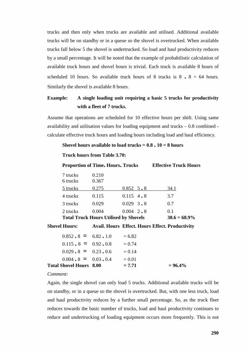
290
trucks and then only when trucks are available and utilised. Additional available
trucks will be on standby or in a queue so the shovel is overtrucked. When available
trucks fall below 5 the shovel is undertrucked. So load and haul productivity reduces
by a small percentage. It will be noted that the example of probabilistic calculation of
available truck hours and shovel hours is trivial. Each truck is available 8 hours of
scheduled 10 hours. So available truck hours of 8 trucks is 8 . 8 = 64 hours.
Similarly the shovel is available 8 hours.
Example: A single loading unit requiring a basic 5 trucks for productivity
with a fleet of 7 trucks.
Assume that operations are scheduled for 10 effective hours per shift. Using same
availability and utilisation values for loading equipment and trucks – 0.8 combined -
calculate effective truck hours and loading hours including load and haul efficiency.
Shovel hours available to load trucks = 0.8 . 10 = 8 hours
Truck hours from Table 3.70:
Proportion of Time. Hours. Trucks Effective Truck Hours
7 trucks 0.210 6 trucks 0.367
Comment:
5 trucks 0.275 0.852 5 . 8 34.1 4 trucks 0.115 0.115 4 . 8 3.7
3 trucks 0.029 0.029 3 . 8 0.7 2 trucks 0.004 0.004 2 . 8 0.1 Total Truck Hours Utilised by Shovels 38.6 = 68.9%
Shovel Hours: Avail. Hours Effect. Hours Effect. Productivity
0.852 . 8 = 6.82 . 1.0 = 6.82 0.115 . 8 = 0.92 . 0.8 = 0.74 0.029 . 8 = 0.23 . 0.6 = 0.14 0.004 . 8 = 0.03 . 0.4 = 0.01 Total Shovel Hours 8.00 = 7.71 = 96.4%
Again, the single shovel can only load 5 trucks. Additional available trucks will be
on standby, or in a queue so the shovel is overtrucked. But, with one less truck, load
and haul productivity reduces by a further small percentage. So, as the truck fleet
reduces towards the basic number of trucks, load and haul productivity continues to
reduce and undertrucking of loading equipment occurs more frequently. This is not
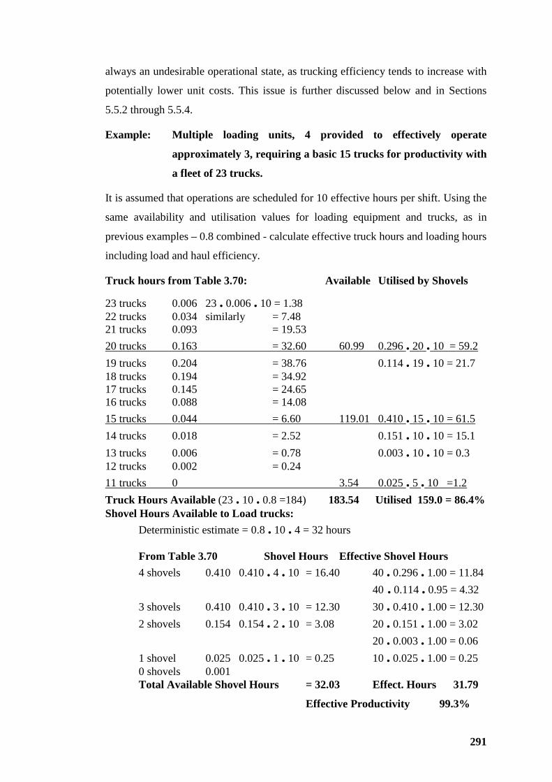
291
always an undesirable operational state, as trucking efficiency tends to increase with
potentially lower unit costs. This issue is further discussed below and in Sections
5.5.2 through 5.5.4.
Example: Multiple loading units, 4 provided to effectively operate
approximately 3, requiring a basic 15 trucks for productivity with
a fleet of 23 trucks.
It is assumed that operations are scheduled for 10 effective hours per shift. Using the
same availability and utilisation values for loading equipment and trucks, as in
previous examples – 0.8 combined - calculate effective truck hours and loading hours
including load and haul efficiency.
Truck hours from Table 3.70: Available Utilised by Shovels
23 trucks 0.006 23 . 0.006 . 10 = 1.38 22 trucks 0.034 similarly = 7.48 21 trucks 0.093 = 19.53 20 trucks 0.163 = 32.60 60.99 0.296 . 20 . 10 = 59.2 19 trucks 0.204 = 38.76 0.114 . 19 . 10 = 21.7 18 trucks 0.194 = 34.92 17 trucks 0.145 = 24.65 16 trucks 0.088 = 14.08 15 trucks 0.044 = 6.60 119.01 0.410 . 15 . 10 = 61.5 14 trucks 0.018 = 2.52 0.151 . 10 . 10 = 15.1 13 trucks 0.006 = 0.78 0.003 . 10 . 10 = 0.3 12 trucks 0.002 = 0.24 11 trucks 0 3.54 0.025 . 5 .
Effective Productivity 99.3%
10 =1.2 Truck Hours Available (23 . 10 . 0.8 =184) 183.54 Utilised 159.0 = 86.4% Shovel Hours Available to Load trucks:
Deterministic estimate = 0.8 . 10 . 4 = 32 hours
From Table 3.70 Shovel Hours Effective Shovel Hours 4 shovels 0.410 0.410 . 4 . 10 = 16.40 40 . 0.296 . 1.00 = 11.84
40 . 0.114 . 0.95 = 4.32 3 shovels 0.410 0.410 . 3 . 10 = 12.30 30 . 0.410 . 1.00 = 12.30 2 shovels 0.154 0.154 . 2 . 10 = 3.08 20 . 0.151 . 1.00 = 3.02 20 . 0.003 . 1.00 = 0.06 1 shovel 0.025 0.025 . 1 . 10 = 0.25 10 . 0.025 . 1.00 = 0.25 0 shovels 0.001 Total Available Shovel Hours = 32.03 Effect. Hours 31.79
292
Comment:
With a number of loading units there is potential for truck loading at any time within
a scheduled shift. Total effective shovel hours using Table 3.70, appended in Volume
2, indicates that there are probably 3.2 shovels available as expected from
deterministic calculation of mechanical availability and utilisation. Total utilised
truck hours indicate an average of nearly 5 trucks at the shovel as expected. The
calculations indicate that occasionally the shovels are undertrucked. For some 30%
of the time 4 shovels are available, they will probably be limited to 19 trucks. As
shovels go out of service operating shovels, as expected, are probably overtrucked.
It will be noted that, for all examples, productive truck hours are less than available
truck hours due to independence and randomness of loading and hauling operations.
Consideration was given to improving productive hours relative to available hours.
Two methods are hypothesized as follows:
1. Reduce the number of trucks so running undertrucked with eventually no
waiting time for trucks so improved hauling efficiency but at the cost of
loading productivity.
2. Increasing the number of loading items selected at a reduced size and bucket
capacity to load in an extra pass or more, modestly increase the truck trip
time TT significantly increase truck loading time TL but increasing the
probability of an exact number of loading equipment items being available to
load trucks.
The first option only appeals where efficiency of truck operations is highest and unit
costs are likely lowest, where the productivity reduction due to reduced loading
efficiency is strategically acceptable. The second option only appeals where planning
can accommodate the additional loading unit or units; where the increased unit cost
of loading with smaller units is acceptably offset by the improved trucking efficiency
and consequent reduced hauling unit cost. The selected configuration of loading
items and trucks needs to be tailored to the specific mining operation and the
necessary load and haul duties to be provided by the equipment fleet.
Two further recasts of the example for multiple loading items, with all assumed
parameters the same, were calculated based on 3 shovels and 5 shovels. Appropriate
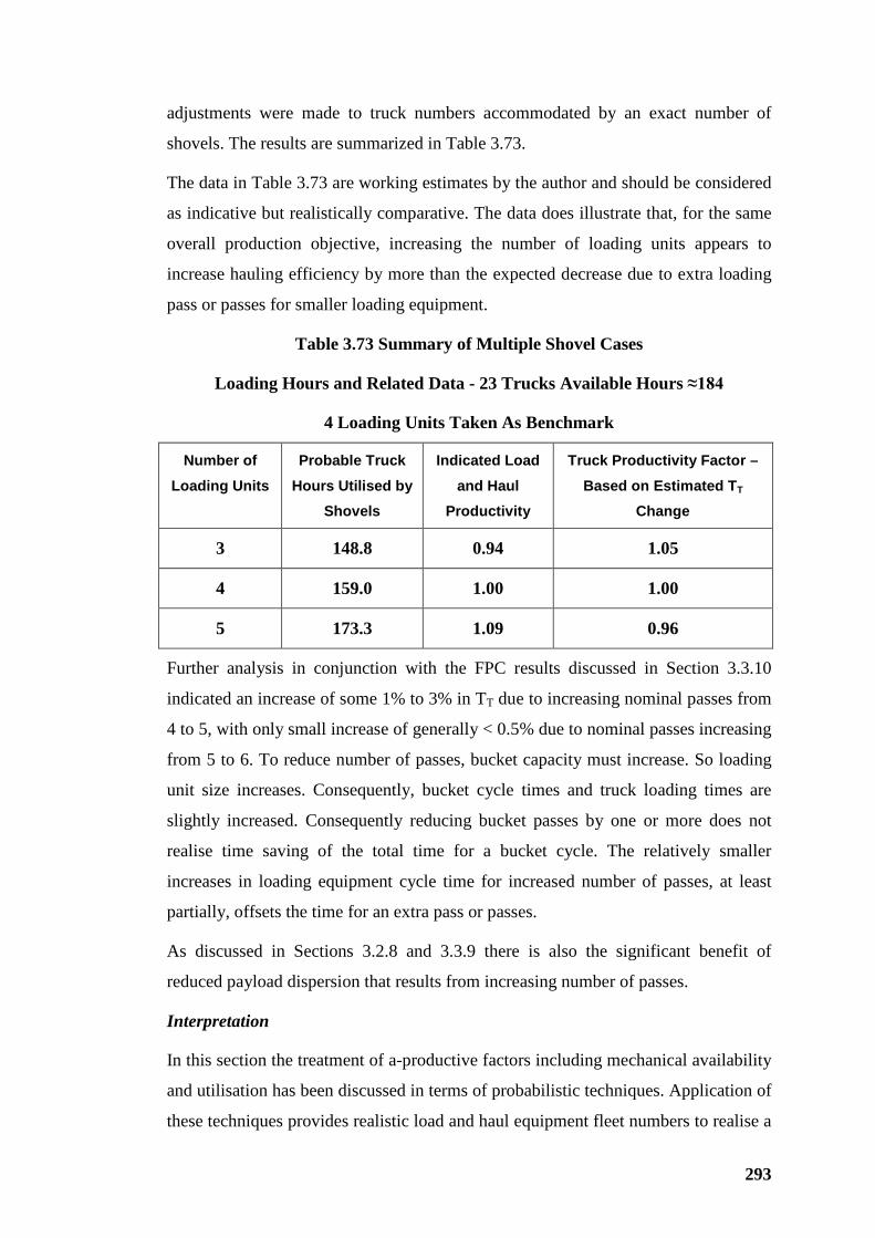
293
adjustments were made to truck numbers accommodated by an exact number of
shovels. The results are summarized in Table 3.73.
The data in Table 3.73 are working estimates by the author and should be considered
as indicative but realistically comparative. The data does illustrate that, for the same
overall production objective, increasing the number of loading units appears to
increase hauling efficiency by more than the expected decrease due to extra loading
pass or passes for smaller loading equipment.
Table 3.73 Summary of Multiple Shovel Cases
Loading Hours and Related Data - 23 Trucks Available Hours ≈184
4 Loading Units Taken As Benchmark
Number of
Loading Units
Probable Truck
Hours Utilised by Shovels
Indicated Load
and Haul Productivity
Truck Productivity Factor –
Based on Estimated TT Change
3 148.8 0.94 1.05
4 159.0 1.00 1.00
5 173.3 1.09 0.96
Further analysis in conjunction with the FPC results discussed in Section 3.3.10
indicated an increase of some 1% to 3% in TT due to increasing nominal passes from
4 to 5, with only small increase of generally < 0.5% due to nominal passes increasing
from 5 to 6. To reduce number of passes, bucket capacity must increase. So loading
unit size increases. Consequently, bucket cycle times and truck loading times are
slightly increased. Consequently reducing bucket passes by one or more does not
realise time saving of the total time for a bucket cycle. The relatively smaller
increases in loading equipment cycle time for increased number of passes, at least
partially, offsets the time for an extra pass or passes.
As discussed in Sections 3.2.8 and 3.3.9 there is also the significant benefit of
reduced payload dispersion that results from increasing number of passes.
Interpretation
In this section the treatment of a-productive factors including mechanical availability
and utilisation has been discussed in terms of probabilistic techniques. Application of
these techniques provides realistic load and haul equipment fleet numbers to realise a
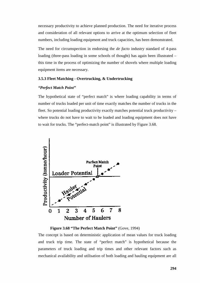
294
necessary productivity to achieve planned production. The need for iterative process
and consideration of all relevant options to arrive at the optimum selection of fleet
numbers, including loading equipment and truck capacities, has been demonstrated.
The need for circumspection in endorsing the de facto industry standard of 4-pass
loading (three-pass loading in some schools of thought) has again been illustrated –
this time in the process of optimizing the number of shovels where multiple loading
equipment items are necessary.
3.5.3 Fleet Matching - Overtrucking, & Undertrucking
“Perfect Match Point”
The hypothetical state of “perfect match” is where loading capability in terms of
number of trucks loaded per unit of time exactly matches the number of trucks in the
fleet. So potential loading productivity exactly matches potential truck productivity –
where trucks do not have to wait to be loaded and loading equipment does not have
to wait for trucks. The “perfect-match point” is illustrated by Figure 3.68.
Figure 3.68 “The Perfect Match Point” (Gove, 1994)
The concept is based on deterministic application of mean values for truck loading
and truck trip time. The state of “perfect match” is hypothetical because the
parameters of truck loading and trip times and other relevant factors such as
mechanical availability and utilisation of both loading and hauling equipment are all
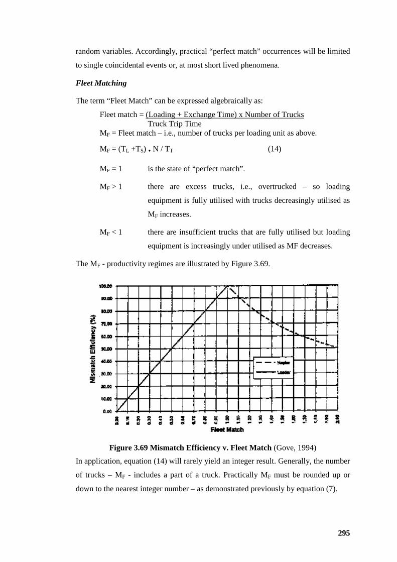
295
random variables. Accordingly, practical “perfect match” occurrences will be limited
to single coincidental events or, at most short lived phenomena.
Fleet Matching
The term “Fleet Match” can be expressed algebraically as:
Fleet match = (Loading + Exchange Time) x Number of Trucks Truck Trip Time
MF = Fleet match – i.e., number of trucks per loading unit as above.
MF = (TL +TS) . N / TT (14)
MF = 1 is the state of “perfect match”.
MF > 1 there are excess trucks, i.e., overtrucked – so loading
equipment is fully utilised with trucks decreasingly utilised as
MF increases.
MF < 1 there are insufficient trucks that are fully utilised but loading
equipment is increasingly under utilised as MF decreases.
The MF - productivity regimes are illustrated by Figure 3.69.
Figure 3.69 Mismatch Efficiency v. Fleet Match (Gove, 1994)
In application, equation (14) will rarely yield an integer result. Generally, the number
of trucks – MF - includes a part of a truck. Practically MF must be rounded up or
down to the nearest integer number – as demonstrated previously by equation (7).
296
Mismatch Treatment Options
Opinions amongst equipment-selection practitioners are mixed on the appropriate
protocol for rounding of truck fleet match. The author has observed a traditional
tendency of estimators to always round up. This is a conservative practice from a
production perspective, but does not necessarily realise best unit costs.
Fourie and Dohm provide a “rule of thumb” that parts of trucks in the range:– > 0 ≤
0.29 should be rounded down and parts of trucks in the range:- ≥ 0.30 < 1.00 should
be rounded up. (Fourie, 1992). This arbitrary treatment may be adequate for
preliminary estimates. But, as shown in 5.5.3, rounding to nearest integer number of
trucks is a joint productivity-cost issue. Generally rounding down sacrifices loading
equipment productivity for lowest unit cost of production. This is discussed in terms
of cost effects in some detail in Sections 5.5.3 and 5.5.4.
It is the author’s experience that, where production targets are firm, not to be
exceeded, best load and haul operating rhythm, and optimum operating costs, are
achieved by opting to round down to a modest undertrucking state. Where production
must be maximized; and the potential cost penalty is justified by downstream
processing cost benefits and marketing opportunities, then overtrucking will likely be
the adopted option. From time to time, there will be changing economic and
operating circumstances where either undertrucking or overtrucking loading
equipment is the favoured operating state.
3.5.4 Bunching - Contributing Factors and Treatment
Nature of Bunching
The fifth of the a-productive factors identified in Section 3.5.2 is “bunching”. In
effect bunching is a result of general detuning of load and haul fleet performance –
equivalent to an increase in truck trip time TT. Alternatively, greater-than-expected
waiting time WL can be experienced by loading equipment if sufficiently
undertrucked to ameliorate bunching. Particularly higher than expected bunching a-
productivity can result from a closer-than-expected approach to exact fleet match
between loading equipment and trucks.
Some authors have treated “fleet matching” and “bunching” concurrently or in close
succession with the inference of interrelationship or firm connection. As discussed
below, there is empirical evidence consistent with intuitive reasoning that the degree
297
of bunching effect increases to a maximum at the “perfect match point” This implies
that bunching can be treated by fleet mismatching. In fact, the two issues are quite
separate in cause and effect. Fleet matching can be expressed mathematically in
terms of mean values of operating parameters and treated deterministically using
equation (14) or other related linear relationships that include cost considerations –
as shown in Sections 5.5.3 and 5.5.4. A mismatch can be simply treated by adding or
subtracting trucks. Productivity reduction due to bunching cannot be remedied by
adding trucks. Productivity necessary to realise planned production must provide
sufficiently for any bunching a-productivity that the load-and-haul fleet configuration
attracts. So, it is necessary to establish a policy of fleet matching configuration to
anticipate bunching effects likely to be experienced when load and haul equipment
has been identified and fleet numbers established probabilistically as shown in
Section 3.5.2.
In the following discussion, “Bunching” is described as an outcome of variability in
operating parameters. Distribution modelling of the bunching phenomenon, or
developing other mathematical process as a basis for analysis, is difficult; and
difficulty increases with complexity of the operation.
Bunching manifests as a productivity inefficiency resulting from a-rhythmic loading
and hauling operations that result in increased load and haul costs.
If operating sufficiently overtrucked, “bunching” results only in a general detune of
truck fleet performance – similar to an increase in TT. Trucking costs tend to increase
moderately without change in productivity. If overtrucking is limited with number of
trucks close to the “perfect match point”, loading equipment will tend to experience
increased waiting time due to bunching, so loss of productivity.
If undertrucked, loading equipment will be under-utilised manifesting as waiting
time that accommodates part or all of the truck trip time extension due to bunching
causes and effects. In the undertrucked state, loading equipment will experience a-
productivity due to mismatch but will also experience reduced bunching a-
productivity than would be experienced at the “match point”. An extreme case can be
hypothesized where undertrucking effect offsets bunching effect. In the significantly
overtrucked state, loading equipment will not experience a-productivity due to
mismatch. But increasing overtrucking will increase expected waiting time for trucks
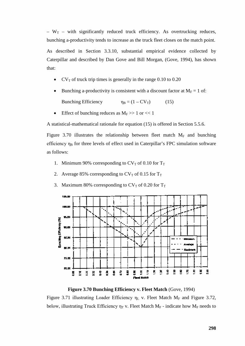
298
– WT – with significantly reduced truck efficiency. As overtrucking reduces,
bunching a-productivity tends to increase as the truck fleet closes on the match point.
As described in Section 3.3.10, substantial empirical evidence collected by
Caterpillar and described by Dan Gove and Bill Morgan, (Gove, 1994), has shown
that:
• CVT of truck trip times is generally in the range 0.10 to 0.20
• Bunching a-productivity is consistent with a discount factor at MF = 1 of:
Bunching Efficiency ηB = (1 – CVT) (15)
• Effect of bunching reduces as MF >> 1 or << 1
A statistical-mathematical rationale for equation (15) is offered in Section 5.5.6.
Figure 3.70 illustrates the relationship between fleet match MF and bunching
efficiency ηB for three levels of effect used in Caterpillar’s FPC simulation software
as follows:
1. Minimum 90% corresponding to CVT of 0.10 for TT
2. Average 85% corresponding to CVT of 0.15 for TT
3. Maximum 80% corresponding to CVT of 0.20 for TT
Figure 3.70 Bunching Efficiency v. Fleet Match (Gove, 1994)
Figure 3.71 illustrating Loader Efficiency ηL v. Fleet Match MF and Figure 3.72,
below, illustrating Truck Efficiency ηT v. Fleet Match MF - indicate how MF needs to
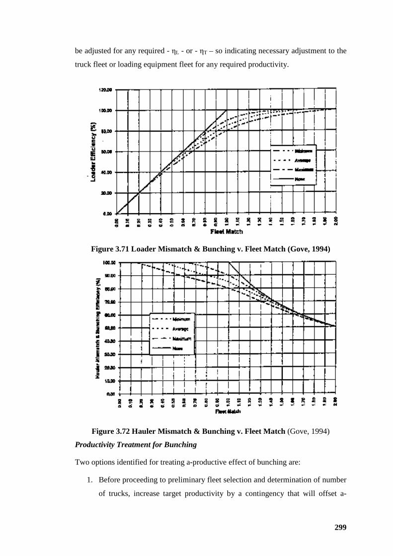
299
be adjusted for any required - ηL - or - ηT – so indicating necessary adjustment to the
truck fleet or loading equipment fleet for any required productivity.
Figure 3.71 Loader Mismatch & Bunching v. Fleet Match (Gove, 1994)
Figure 3.72 Hauler Mismatch & Bunching v. Fleet Match (Gove, 1994)
Productivity Treatment for Bunching
Two options identified for treating a-productive effect of bunching are:
1. Before proceeding to preliminary fleet selection and determination of number
of trucks, increase target productivity by a contingency that will offset a-
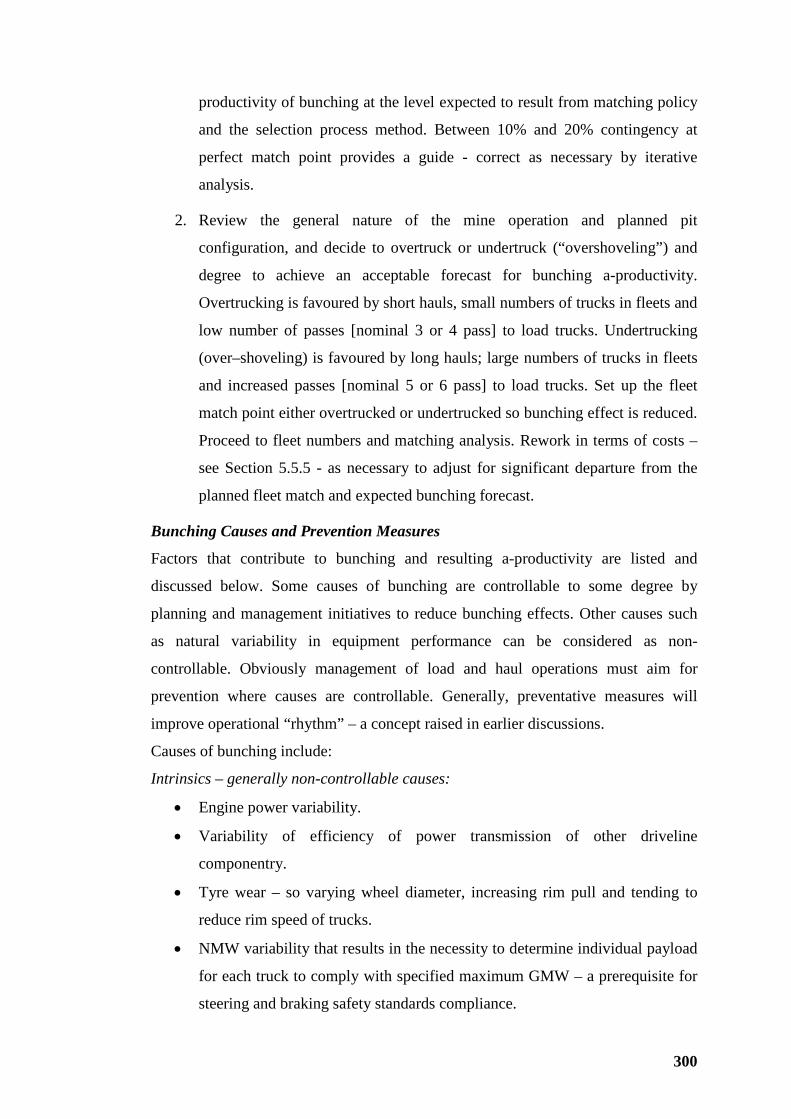
300
productivity of bunching at the level expected to result from matching policy
and the selection process method. Between 10% and 20% contingency at
perfect match point provides a guide - correct as necessary by iterative
analysis.
2. Review the general nature of the mine operation and planned pit
configuration, and decide to overtruck or undertruck (“overshoveling”) and
degree to achieve an acceptable forecast for bunching a-productivity.
Overtrucking is favoured by short hauls, small numbers of trucks in fleets and
low number of passes [nominal 3 or 4 pass] to load trucks. Undertrucking
(over–shoveling) is favoured by long hauls; large numbers of trucks in fleets
and increased passes [nominal 5 or 6 pass] to load trucks. Set up the fleet
match point either overtrucked or undertrucked so bunching effect is reduced.
Proceed to fleet numbers and matching analysis. Rework in terms of costs –
see Section 5.5.5 - as necessary to adjust for significant departure from the
planned fleet match and expected bunching forecast.
Bunching Causes and Prevention Measures
Factors that contribute to bunching and resulting a-productivity are listed and
discussed below. Some causes of bunching are controllable to some degree by
planning and management initiatives to reduce bunching effects. Other causes such
as natural variability in equipment performance can be considered as non-
controllable. Obviously management of load and haul operations must aim for
prevention where causes are controllable. Generally, preventative measures will
improve operational “rhythm” – a concept raised in earlier discussions.
Causes of bunching include:
Intrinsics – generally non-controllable causes:
• Engine power variability.
• Variability of efficiency of power transmission of other driveline
componentry.
• Tyre wear – so varying wheel diameter, increasing rim pull and tending to
reduce rim speed of trucks.
• NMW variability that results in the necessity to determine individual payload
for each truck to comply with specified maximum GMW – a prerequisite for
steering and braking safety standards compliance.
301
• Debris adhering to truck chassis and structure.
• Carry-back in the truck body.
• Variable operator skill and efficiency – a result of varying natural skills,
training levels together with effects of changing operating conditions
including weather and staff turnover.
Non-intrinsics – generally controllable to some degree:
• Variability in surfaces of roads and manoeuvering areas.
• Changing competency of materials exposed by mining as a foundation for
mine haul roads.
• Availability of road surfacing materials in required quantity and of acceptable
quality.
• Other mining activities that interrupt or interfere with loading and hauling
operations.
• Errors and omissions by supervision, management, oversights in pit
development strategy, mine planning and scheduling.
• Non-optimum maintenance reliability and efficiency (bench marks for which
are provided in Section 3.4 – specifically Table 3.67).
The above list is representative rather than exhaustive. Degree of effect on bunching
by listed causes, and consequent a-productivity is wide ranging. The end effect
observed empirically is an accumulation that does not always allow identification of
specific causes to enable application of management remedies. The above items are
discussed in more detail below.
Discussion On Some Variability Factors
Caterpillar claims that new and dealer-repaired or remanufactured engines will
dynamometer-test to +/-3% of designed flywheel power. Data provided by WesTrac,
Caterpillar’s dealership in Western Australia, has been analysed. Descriptive
statistics are provided in Table 3.74. CV of this small sample of off-site rebuilds only
is 1.35% inferring a range of +/-3.7% - consistent with relatively low dispersion. The
statistics are expressed both in terms of dynamometer tests in kW; also in indices
based on specified engine power of 1300 kW. New engines ex factory and
remanufactured engines can be expected to exhibit reduced variability – within the
claimed range indicated

302
.
Table 3.74 Truck Variable Performance Factors Engine Power kW Truck NMW kW Indices Mean Minima
Number of Records 32 32 24 24 Maximum Value 2388 1.038 166.13 164.30 Minimum Value 2221 0.966 157.65 155.70
Range 167 0.073 8.47 8.60 Range % 7.25 7.248 5.23 5.40
Average of Range 2304.50 1.002 161.89 160.00
Average of Population (Arithmetic Mean) 2304.13 1.002 161.91 159.31 Median 2303.50 1.002 161.86 159.60
Variance 963.73 0.000 4.83 4.54 Std Dev Sample 31.04 0.0135 2.20 2.13
Coefficient of Variation 0.0135 0.0135 0.0136 0.0134
Skewness 0.03 0.03 0.14 0.10 To Right To Right To Right To Right
Kurtosis 1.82 1.82 -0.51 -0.15 Leptokurtic Leptokurtic Platykurtic Platykurtic
NMW variability is illustrated by descriptive statistics of a small sample of data
(provided by WesTrac) in Table 3.74. NMW of nominal 220-tonne payload trucks
were weighed at three separate times. Descriptive statistics of means of NMW
determinations for each truck in the fleet are shown in Table 3.74. The relatively low
but significant variability of the small sample of NMW shown by CV of 1.4% and a
range of 5.2% in Table 3.74 is some half the variability indicated by advice from
Hays that NMW can vary +/-5%, (Hays, 1990, p675). Trucks operating in deep pits
spend more than some 70% (as much as 75% - Table 3.63) of travel time fully
loaded. So performance for that segment of a truck trip is subject to GMW. As NMW
is in the order of 40% to 50% of GMW, effect of variability on measured NMW
relative to GMW is proportionally reduced. The effect of variability of truck payload
measured relative to GMW is similarly proportionally reduced. Joint distribution
theory also indicates that expected values are simply cumulative but variance is an
exponential function as follows:
EGMW = ENMW + EPL (16)
EGMW = Expected (mean) value of GMW.
ENMW = Expected (mean) value of NMW.
303
EPL = Expected (mean) value of PL.
σGMW2 = σNMW
2 + σPL2 (17)
σGMW = √(σNMW2 + σPL
2) (17A)
σGMW = standard deviation of GMW
σNMW = standard deviation of NMW
σPL = standard deviation of PL
Equations (16), (17) and (17A) are valid for random variables. Equations (17) and
(17A) are valid only for independent variables. (Chou, 1969, p178). NMW and PL
are generally treated as independent random variables in the research.
Measuring relative variability in terms of CV, equation 17A shows that the relative
variability - CV, of GMW will generally be significantly lower than the variability,
i.e., CV’s of either NMW or PL:
σGMW > σNMW; also σGMW > σPL
CV is a quotient of σ/mean of variable, always < 1. When comparing CV statistics
with values < 1:
CVGMW < CVNMW; also CVGMW < CVPL
The cited relationships have application, utilized in Section 5.5.6, for the similar
relationship that generally exists between truck trip times as an accumulation of
components including loading time, dumping time, turn and spot, queuing time; and,
importantly, waiting time.
The interpretation of the above discussion is that NMW variability is measurable and
significant when standing alone. But the productivity effect of NMW variability is
relatively reduced when combined with payload variability. But the effect does
potentially influence truck payload capacity and measured payload variability in
actual operations, albeit to relatively small degree. Efforts to reduce NMW
variability are beneficial and considered to be generally justified.
Tyre-wear induces truck-performance variability due to decreased wheel radius and
consequent increased rimpull. There is a complementary small reduction in top speed
that can be assessed from tyre dimensions.
304
Standard tread depth of tyres for larger mining trucks is designated E4 – an
indication of the wear potential of tyres. The ratio of E4 tread depth to tyre diameter
is in the order of 6% for large mining truck tyres, so maximum possible diameter
reduction from wear is limited to some 6%. Only a small proportion of tyres on large
mining trucks wear out - tread worn away to a bald, slick tyre surface. Premature
failure due to separation, sidewall cutting or rock penetration preempts tread wearing
out for in the order of 90% of tyres at sites where operational conditions are severe
(author’s experience).
For the purposes of discussion, it can be assumed that average tread wear to failure is
50%. This corresponds to an average wheel radius decrease, and rimpull increase, of
some 3%. So, up-ramp speed for deep pits will tend to decrease slightly. But this is
dependent on the rimpull/speed curve for the particular truck and how it negotiates
the ramp profile. All other segments of a truck haul that are not at full power will not
be affected by tread wear. Average TT time variations due to tyre wear in deep pits
can be expected to range +/- 1% to 1.5% from mean tyre diameters. Accordingly a-
productive effect due to tyre wear can be considered relatively small.
In Section 3.3.4 and, particularly, Figure 3.29, it was indicated that power
transmission loss from engine flywheel to wheels is some 17% for mechanical drive
trucks to 26% for DC electric wheel trucks with losses for AC electric-wheel trucks
in the order of 20% approaching mechanical drives. These are nominal average
power-loss percentages. The shape of the torque – speed curve for alternative drive
systems is also a difference significant in the operational application of mining
trucks. The practically flat torque curve of mechanical drive trucks has advantages in
deep pit operations.
There is also significant variability in the transmission systems of mining trucks. The
author’s best estimate based on experience with dynamometer tests of mechanical
transmissions and efficiency tests of electric motors, generators and alternators
would be a variability range similar to engine variability, i.e., +/- 3% to 5% over
component life.
It can be concluded from the discussion (albeit limited to a small number of factors)
that the several factors contributing to bunching effects tend to be individually small.
But collectively the factors accumulate to a significant a-productive bunching effect.
305
Consequently, controllable factors, the non-intrinsics and those intrinsics that can be
managed to advantage, need to be identified and the necessary controls established
and implemented. Prevention of bunching effects is an unrealistic expectancy. But
minimization of bunching is a realistic ambition by addressing influencing factors
and working towards reasonable operational “rhythm”.
In the process of equipment selection, when setting up operating criteria including
productivity required to realise the mine production plan, some concept of bunching
effect to be accommodated must be developed. The a-productive effect of bunching
can be assessed; but this is dependent on the degree of control to be exercised over
the causes of bunching effects that must be specified, justified as realistic and
effectively established.
Bunching Comments
A-productive effects from bunching manifest as inefficiencies in load and haul
performance. The nature and degree of reduced productivity is a complex outcome
dependent on variability in performance of the equipment items that make up a load
and haul fleet. There is empirical evidence of the degree of bunching effect that can
be applied to discount productivity to provide realistic production results. Literature
research for mathematical analytical solutions was unsuccessful. A typical comment
in references (paraphrased): “It is difficult to obtain wait times for loading equipment
and trucks as a function of the number of loading items and trucks” - (Ramani,
1990).
It is also difficult to model bunching effects stochastically. These difficulties have
been addressed by using empirical data as the basis for simulation of truck waiting
time and bunching effects as an alternative solution.
The criteria (illustrated by Figure 3.70) for bunching inefficiency, over a range of
fleet match values, are based on Caterpillar’s research as presented by Gove and
Morgan. These criteria are in general industry use for estimating bunching effects. If
the option to adopt a specific selection of these criteria is exercised, they are
embedded in results from FPC simulation applications that are generally accepted by
the mining industry. So, it is concluded that bunching criteria, based on empirical
observations and described above, are adequate for adoption by estimators and
306
engineers for purposes of establishing production and productivity in the process of
load and haul equipment selection for open pit mining.
Notwithstanding the perceived practical adequacy of the empirical-based approach
discussed, Section 5.5.6 offers a rationale in statistical-mathematical terms for
equation (15) as a basis for discussing cost effects of bunching.
3.6 TIME MANAGEMENT – DEFINITIONS
3.6.1 Introduction
Before commencing selection of equipment of suitable capacity, and in adequate
numbers, to satisfy a mining production objective, all of the necessary inputs need to
be assembled. Realistic production estimates and other operating parameters, and an
understanding and setting up of a sound basis drawn from prior effective mine
planning are essential prerequisites for effective equipment selection. The process
and various inputs are more fully discussed in Section 4.1.1 to follow.
Setting up a defined Time Management System is an imperative management
initiative to enable determination of time components relevant to productivity
determinations. An essential input to establishing required equipment performance is
a realistic estimation (particularly for a “greenfields” project) or determination from
historical data, in-house or industry-wide, of the number of productive hours per
year, that can be adopted as a robust basis for required productivity determinations.
3.6.2 Definitions
For the purposes of discussion a simplified time management system and inferred
time definitions is provided by Figure 3.73. The following definitions are illustrated
by Figure 3.73:
Potential Working Hours = Calendar Time = 24 hours everyday of the year – taken
as 8,760 hours.
Mechanical Availability (MA): = Available Time
Calendar Time
= Calendar time – Downtime
Calendar time
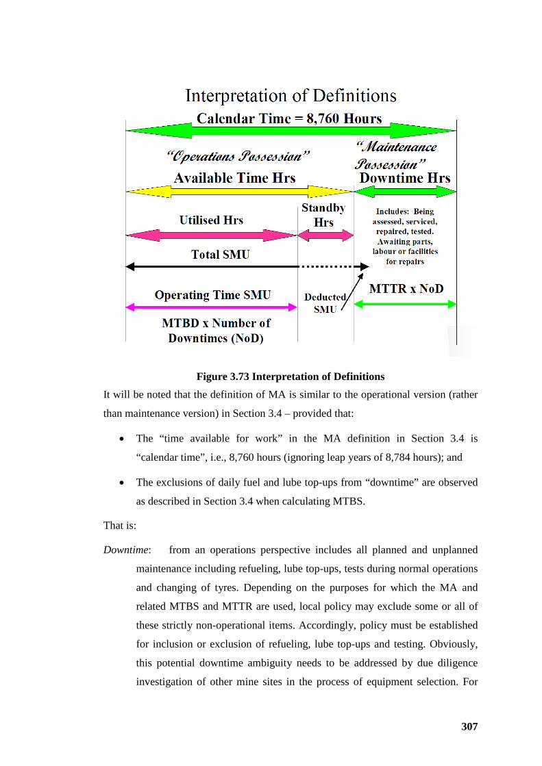
307
Figure 3.73 Interpretation of Definitions
It will be noted that the definition of MA is similar to the operational version (rather
than maintenance version) in Section 3.4 – provided that:
• The “time available for work” in the MA definition in Section 3.4 is
“calendar time”, i.e., 8,760 hours (ignoring leap years of 8,784 hours); and
• The exclusions of daily fuel and lube top-ups from “downtime” are observed
as described in Section 3.4 when calculating MTBS.
That is:
Downtime: from an operations perspective includes all planned and unplanned
maintenance including refueling, lube top-ups, tests during normal operations
and changing of tyres. Depending on the purposes for which the MA and
related MTBS and MTTR are used, local policy may exclude some or all of
these strictly non-operational items. Accordingly, policy must be established
for inclusion or exclusion of refueling, lube top-ups and testing. Obviously,
this potential downtime ambiguity needs to be addressed by due diligence
investigation of other mine sites in the process of equipment selection. For
308
the avoidance of doubt, the author places the boundary of downtime
according to whichever function has “possession” of the equipment,
maintenance or operations – as illustrated by Figure 3.73.
Available: simply – if equipment is not down it is operational.
Utilised Time: (Use of Availability) alternatively termed Operating Time: =
Proportion of time actually used in operations
Standby Time: non-utilised available time.
Reliability – MTBD }These three items, referred to in Figure 3.73
Maintainability – MTTR }previous page, were described and discussed
Number of Downtimes (NoD) }in Section 3.4.
Service Meter Units – SMU The record in SMU of equipment operating
time as the time the engine is running (for equipment powered by internal
combustion engine) or by power metering of electric powered equipment.
SMU–determined operating time as recorded by on-board information management
systems (such as Caterpillar’s VIMS or equivalent) is always greater than operating
time measured by equipment activity from dispatch systems or operator time keeping
records. Specifically for trucks, that the engine is running is not necessarily evidence
that the truck is engaged in productive operations. The author is aware of a deep
open pit operation using 225 tonne trucks where, for an annual average, effective
operating hours were 92% of the SMU recorded for the same annual period.
The provided description of Time Definitions should be considered as introductory
only.
3.6.3 Dispatch Systems
As the demand increases for more management control to realise productivity and
cost expectancies for equipment of increasing scale the need for accurate, accessible
data of ever-increasing detail becomes more cogent.
Table 3.75, Volume 2, Appendices, provides time definitions from a typical dispatch
facility. The detail of time allocation is substantially increased from that used to
compile Figure 3.73. Increased discrimination by defining more detailed time
components provides accurate time bases for a large number of key performance
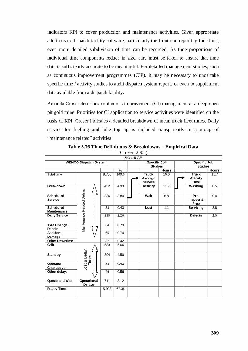
309
indicators KPI to cover production and maintenance activities. Given appropriate
additions to dispatch facility software, particularly the front-end reporting functions,
even more detailed subdivision of time can be recorded. As time proportions of
individual time components reduce in size, care must be taken to ensure that time
data is sufficiently accurate to be meaningful. For detailed management studies, such
as continuous improvement programmes (CIP), it may be necessary to undertake
specific time / activity studies to audit dispatch system reports or even to supplement
data available from a dispatch facility.
Amanda Croser describes continuous improvement (CI) management at a deep open
pit gold mine. Priorities for CI application to service activities were identified on the
basis of KPI. Croser indicates a detailed breakdown of mean truck fleet times. Daily
service for fuelling and lube top up is included transparently in a group of
“maintenance related” activities.
Table 3.76 Time Definitions & Breakdowns – Empirical Data (Croser, 2004)
SOURCE WENCO Dispatch System Specific Job
Studies Specific Job
Studies % Hours Hours
Total time 8,760 100.00
Truck Average Service
19.6 Truck Activity
Time
11.7
Breakdown 432 4.93 Activity 11.7 Washing 0.5
Scheduled Service
336 3.84 Wait 6.8 Pre-inspect &
Prep
0.4
Scheduled Maintenance
38 0.43 Lost 1.1 Servicing 8.8
Daily Service 110 1.26 Defects 2.0
Tyre Change / Repair
64 0.73
Accident Damage
65 0.74
Other Downtime 37 0.42 Crib 583 6.66
Standby 394 4.50
Operator Changeover
38 0.43
Other delays 49 0.56
Queue and Wait Operational Delays
711 8.12
Ready Time 5,903 67.38
Mai
nten
ance
Rel
ated
Del
ays
Lost
& D
elay
Ti
mes
310
Table 3.76 illustrates Croser’s technique of “drilling down” through time analysis
levels to isolate specific detailed time components to assess potential for production /
cost improvement and so assignment of priorities (Croser, 2004).
Clearly the degree of detail described by Amanda Croser is not necessary for
establishing the basis of load and haul equipment selection. It is considered sufficient
to estimate or establish from existing empirical data realistic average time
assignments in annual hours for:
• Rostered (scheduled) time.
• Available time.
• Utilised time.
• Direct operating time.
This last item is useful if instantaneous digging rates are a productivity estimating
parameter. If equipment productivity rates are recorded or estimated over a period of
a shift or longer period then for production estimating it may be more appropriate to
use utilised time as the basis for production estimating.
Obviously, care needs to be taken to understand current definitions of time
components and reporting / estimating practice during due diligence investigation
both internally and at any external mining operation.
Western Australian School of Mines
Selection Criteria For
Loading and Hauling Equipment - Open Pit Mining Applications
Volume 2
Raymond J Hardy
This Thesis is presented for the Degree
Of Doctor of Philosophy
Of Curtin University of Technology
July 2007
i
DECLARATION
This thesis does not contain material previously accepted for the award of any other
degree or diploma in any university. To the best of my knowledge and belief, where
this thesis contains material previously published by any other person, due
acknowledgement has been made.
………………………..
R J Hardy 9 July 2007
THESIS PRESENTATION
Scope of the research, breadth of topics and resulting extensive documentation
required presentation of the thesis in two volumes.
Volume 1 Selection Criteria Issues, Productivity and Analysis – Chapters 1 to
3 included in Volume 1; and
Volume 2 Selection Process, Costs, Conclusions and Recommendations –
Chapters 4 to 7 - plus References, Appendices and Supplementary
Information – included in Volume 2.

ii
ABSTRACT
Methods for estimating productivity and costs, and dependent equipment selection
process, have needed to be increasingly reliable. Estimated productivity and costs
must be as accurate as possible in reflecting actual productivity and costs
experienced by mining operations to accommodate the long-term trend for
diminishing commodity prices,
For loading and hauling equipment operating in open pit mines, some of the
interrelated estimating criteria have been investigated for better understanding; and,
consequently, more reliable estimates of production and costs, also more effective
equipment selection process.
Analysis recognizes many of the interrelated criteria as random variables that can
most effectively be reviewed, analyzed and compared in terms of statistical
mathematical parameters.
Emphasized throughout is the need for management of the cyclical loading and
hauling system using conventional shovels/excavators/loaders and mining trucks to
sustain an acceptable “rhythm” for best practice productivity and most-competitive
unit-production costs.
Outcomes of the research include an understanding that variability of attributes needs
to be contained within acceptable limits. Attributes investigated include truck
payloads, bucket loads, loader cycle time, truck loading time and truck cycle time.
Selection of “ultra-class” mining trucks (≥ 290 -tonne payload) and suitable loading
equipment is for specialist mining applications only. Where local operating
environment and cost factors favourably supplement diminishing cost-benefits of
truck scale, ultra-class trucks may be justified. Bigger is not always better – only
where bigger can be shown to be better by reasons in addition to the modest cost
benefits of ultra-class equipment.
Truck over-loading may, to a moderate degree, increase productivity, but only at
increased unit cost. From a unit-cost perspective it is better to under-load than over-
load mining trucks.
Where unit production cost is more important than absolute productivity, under-
trucking is favoured compared with over-trucking loading equipment.

iii
Bunching of mining trucks manifests as a queuing effect – a loss of effective truck
hours. To offset the queuing effect, required productivity needs to be adjusted to
anticipate “bunching inefficiency”. The “basic number of trucks” delivered by
deterministic estimating must provide for bunching inefficiency before application of
simulation applications or stochastic analysis is used to determine the necessary
number of trucks in the fleet.
In difficult digging conditions it is more important to retain truck operating rhythm
than to focus on achieving target payload by indiscriminately adding loader passes.
Where trucks are waiting to load, operational tempo should be restored by sacrificing
one or more passes. Trucks should preferably be loaded by not more than the
nominal (modal) number plus one pass.
The research has:
• Identified and investigated attributes that affect the dispersion of truck
payloads, bucket loads, bucket-cycle time, loading time and truck-cycle time.
• The outcomes of the research indicate a need to correlate drilling and blasting
quality control and truck payload dispersion. Further research can be
expected to determine the interrelationship between accuracy of drilling and
blasting attributes including accuracy of hole location and direction.
• Preliminary investigations indicate a relationship between drill-and-blast
attributes through blasting quality control to bucket design, dimensions and
shape; also discharge characteristics that affect bucket cycle time that needs
further research.

iv
ACKNOWLEDGEMENT
“No man is an Island, entire of itself.” from Devotions by John Donne
Soon after setting out on the research journey recorded in this thesis the words of
John Donne, above, were brought home with undeniable impact. In addition to the
knowledge acquired during a working lifetime in the mining industry, civil
construction and associated vocations the author still depended on many others to
safely and satisfactorily reach journey’s end. Generous support and contribution of
many friends, associates and casual acquaintances in industry and academia that have
assisted along the way are acknowledged with sincere thanks and great appreciation.
Every reasonable effort has been made to correctly acknowledge the owners of
copyright material. The author would be pleased to hear from any copyright owner
incorrectly, or not, acknowledged.
Support and assistance of the following are especially acknowledged:
Associate Professor Dr Emmanuel Chanda of the WA School of Mines (WASM)
Mining Department, for his continued encouragement, guidance and supervision;
also at WASM, Dr Peter Lilley (formerly Director of WASM, now with CSIRO,
Perth), Mahinda Kuruppu and Clive Workman-Davies assisted from time to time.
Western Premier Coal Limited, Collie, WA – within the Wesfarmers Limited group
of companies - provided funding for WASM research projects that partially
supported the research work described by the thesis. That support is gratefully
acknowledged.
At WesTrac, Caterpillar dealer located in South Guildford Western Australia
(franchised some 80 years as the first Cat dealer outside USA, more recently
expanding into New South Wales and China), personnel that have assisted with
information and operating data are too numerous to individually acknowledge. To
WesTrac staff in general my sincere thanks.
Individual acknowledgements must be afforded Jim Walker, CEO, for opening the
door to the huge knowledge base acquired by WesTrac and possessed by its South
Guildford staff; Fred Haynes for his interest, support and supply of weighing data in
the early stages; Tony Power who kept the author in touch with technical advances
and developments in the mining industry; Adrian Clement who gave his time

v
generously, provided access to VIMS and Minestar data to support the research, also
for demonstrating the exciting benefits and promise of these real-time data access
systems and Peter Perich for showing the way to market equipment prices and
comments on written down values of mining equipment. More recently Quentin
Landre has supplied Caterpillar equipment specification material; also providing
information to enable any WASM student to access specifications and performance
data vital to their understanding of mobile mining equipment.
Particularly I am indebted to WesTrac for access to FPC simulation software and
other mining equipment applications over the years; also for a lifetime supply of
Performance Handbooks and related specification material.
To David Rea of Caterpillar, many thanks for the insight afforded the author on
VIMS and related matters; also to Caterpillar Global Mining generally for access to
technical material made available at recent Miners’ Forum’s in Western Australia.
Other OEM - dealership contacts also contributed including: from Minepro, P & H
dealer, Noel Skilbeck and staff; from Komatsu, Alan Costa; from Liebherr, Henning
Kloeverkorn, Merv. Laing and Duncan Hooper; from Terex Mining – O & K, Craig
Watson and Andy McElroy; from Hitachi, Eric Green – to all many thanks and best
wishes to those contacts who have moved on in their career paths.
Tony Cutler of OTRACO provided comprehensive information on large earthmover
tyres, especially for ultra-class trucks; also Hans Weber of Michelin provided
technical information on tyre application and management for large mining trucks.
To the many other personal and commercial contacts in and associated with the
mining industry that have steadily increased the volume of knowledge and
understanding available to the author, knowledge that was tapped to progress the
research, the author extends heartfelt thanks and appreciation.
Last but not least the author acknowledges the contribution of his partner in life,
Heide, who supported the research with an interesting mixture of tolerance and
vigorous encouragement including many exhortations to “get on with it” – when the
author was experiencing adequate strength of spirit but an inhibiting weakness of
flesh.
Raymond J Hardy, July 2007.

vi
VOLUME 1
TABLE OF CONTENTS DECLARATION i THESIS PRESENTATION i ABSTRACT ii ACKNOWLEDGEMENT iv TABLE OF CONTENTS, VOLUME 1 & VOLUME 2 vi LIST OF TABLES xii LIST OF FIGURES xvi
SELECTION CRITERIA – PRODUCTIVITY AND ANALYSIS
CHAPTER 1 1 INTRODUCTION
1.1 RESEARCH CONCEPTION 1 1.2 RESEARCH OBJECTIVES 2 1.3 HISTORICAL BACKGROUND 4
1.3.1 Research Formulation 4 1.3.2 Mining Commodity Prices – The Ultimate Cost Driver 6 1.3.3 Recent Surface Mining History 7 1.3.4 Demand for Increasing Scale 10 1.3.5 Evolutionary Trends 11
CHAPTER 2 13 RESEARCH METHODOLOGY
2.1 RESEARCH BACKGROUND 13 2.1.1 Uncertain and Imprecise Estimating Practices 13 2.1.2 Questionable Standards and Measures 16 2.1.3 Cost Benefits From Up-scaling and "The Law of Diminishing Returns" 19 2.1.4 Changing Technology 23
2.2 RESEARCH PHILOSOPHY 23 2.2.1 Research Techniques and Reality 23 2.2.2 Personal Rules and Understandings 25 2.2.3 Units 26
2.3 METHODOLOGY AND LIMITATIONS 26 2.3.1 Research Procedures 26 2.3.2 Statistics 27
2.4 SIGNIFICANCE OF RESEARCH 29 2.5 FACILITIES AND RESOURCES 30 2.6 ETHICAL ISSUES 31

vii
CHAPTER 3 32 LOAD AND HAUL PERFORMANCE
3.1 PROJECT PRODUCTION SCALE 32 3.1.1 Introduction 32 3.1.2 Capacity Hierarchy 33
3.2 LOADING EQUIPMENT 36 3.2.1 Selection Process 36 3.2.2 Cyclic vs. Continuous Excavation 36 3.2.3 Loading Equipment Options 37 3.2.4 Intrinsic Loader Performance 40 3.2.5 Single or Double Side Loading 47 3.2.6 Loader Passes and Truck Exchange Time 49 3.2.7 Bucket Factor 52 3.2.8 Bucket Loads 60 3.2.9 Bucket Cycle Time 86 3.2.10 Bucket Dumping 123
3.3 MINING TRUCKS 128 3.3.1 Selection Process 128 3.3.2 Cyclic versus Continuous Haulage 129 3.3.3 Truck Types and Application 130 3.3.4 Intrinsic Truck Performance 132 3.3.5 Body Selection and Truck Payload 137 3.3.6 Truck Payload Measuring Initiatives 153 3.3.7 Truck Payload Centre of Gravity (CG) 174 3.3.8 Tyres 209 3.3.9 Bucket Passes and Payloads 216 3.3.10 Truck Performance and Productivity 230 3.3.11 Haul Roads and Site Severity 253
3.4 EQUIPMENT SELECTION AND MAINTENANCE 257 3.4.1 Introduction and Research Limits 257 3.4.2 Selection Criteria Related to Maintenance 257 3.4.3 Benchmarks and Key Performance Indicators 268 3.4.4 Maintain-And-Repair-Contracts 269 3.4.5 Equipment Sales Agreements 272
3.5 FLEET MATCHING, BUNCHING, QUEUING 272 3.5.1 Introduction 272 3.5.2 Preliminary Fleet Numbers 274 3.5.3 Fleet Matching - Overtrucking, & Undertrucking 293 3.5.4 Bunching - Contributing Factors and Treatment 295
3.6 TIME MANAGEMENT - DEFINITIONS 305 3.6.1 Introduction 305 3.6.2 Definitions 305 3.6.3 Dispatch Systems 307

viii
VOLUME 2
TABLE OF CONTENTS
DECLARATION i THESIS PRESENTATION i ABSTRACT ii ACKNOWLEDGEMENT iv TABLE OF CONTENTS, VOLUME 1 & VOLUME 2 vi LIST OF TABLES xii LIST OF FIGURES xvi
SELECTION PROCESS, COSTS, CONCLUSIONS AND RECOMMENDATIONS
CHAPTER 4 311 EQUIPMENT SELECTION
4.1 SELECTION IMPLEMENTATION 311 4.1.1 Introduction 311 4.1.2 Key Considerations 317 4.1.3 Selection Process 320 4.1.4 Selection Strategy 324 4.1.5 Loading and Hauling Equipment Options 330
4.2 LARGER MINING EQUIPMENT 339 4.2.1 Introduction 339 4.2.2 Diminishing Cost Benefit 340 4.2.3 Is Bigger Better? 343 4.2.4 Future Mining Equipment Improvements 346 4.2.5 Hypothetical 500 Tonne Payload Truck 349 4.2.6 Trolley Assist 353 4.2.7 Dispatch Systems & Autonomous Load & Haul Equipment 354
CHAPTER 5 356 LOAD AND HAUL COSTS
5.1 BASIS OF COST ANALYSES AND DISCUSSION 356 5.1.1 Costs - A Snapshot In Time 356 5.1.2 Relative Importance of Cost Estimates 356 5.1.3 Basis of Cost Indices 357
5.2 COST INDICES AND PROPORTIONS OF HAUL AND TOTAL MINING COSTS 359
5.2.1 Fixed and Variable Costs 359 5.2.2 Capital Redemption 360 5.2.3 Capital Recovery Risk 361 5.2.4 Operating Cost Indices 365 5.2.5 Fuel Consumption and Cost Indices 366
5.3 COSTS - TRUCK OVERLOADING AND PAYLOAD DISTRIBUTION EFFECTS 368
5.3.1 Introduction 368
ix
5.3.2 Component Life and Payload Relationship 369 5.3.3 Haul Cost Indices for Payload Distribution Range 370 5.3.4 Truck Overloading, Component Life and Haul Cost 372 5.3.5 Interpretation and Comments 374 5.3.6 Payload Dispersion, Component Life and Haul Cost Index 376 5.3.7 Interpretation and Comments 379
5.4 COSTS AND BUCKET-PASS SACRIFICE 379 5.4.1 Introduction 379 5.4.2 Comparative Cost Indices 380 5.4.3 Cost Criteria for Sacrificing Bucket Loads 382 5.4.4 Interpretation and Comments 383
5.5 COSTS AND OVERTRUCKING AND UNDERTRUCKING; ALSO BUNCHING 385
5.5.1 Introduction - Defining the Problems 385 5.5.2 Productivity Cost Indices and Relationships 386 5.5.3 Previous Research - Extended Analysis 388 5.5.4 Outcomes, Interpretation and Comment 396 5.5.5 Over-trucking, Under trucking - Productivity and Costs 399 5.5.6 Bunching - Productivity and Costs 405
CHAPTER 6 411 SUPPLEMENTARY ACTIVITIES
6.1 ADDITIONAL INTER-ACTIVES 411 6.1.1 Planning and Equipment Selection 411 6.1.2 Drilling and Blasting 412 6.1.3 Dumps and Stockpiles 415 6.1.4 Mixed Fleets 419 6.1.5 Dispatch Systems and Remote Control 420 6.1.6 Autonomous Haulage Systems 422
CHAPTER 7 425 SUMMARY OF RESEARCH
7.1 CRITERIA INVESTIGATED 425 7.2 SUMMARY OF OUTCOMES 426
7.2.1 In the Beginning ---- 426 7.2.2 Research Framework and Preliminaries 426 7.2.3 Performance 417 7.2.4 Equipment Selection 430 7.2.5. Costs – Relative Indices and Comparisons 431
CHAPTER 8 432 CONCLUSIONS AND RECOMMENDATIONS FOR FURTHER RESEARCH 432
8.1 CONCLUSIONS 432 8.1.1 Compliance with Objectives 432 8.1.2 Conclusions 432
8.2 RECOMMENDATIONS FOR FURTHER RESEARCH
REFERENCES 437
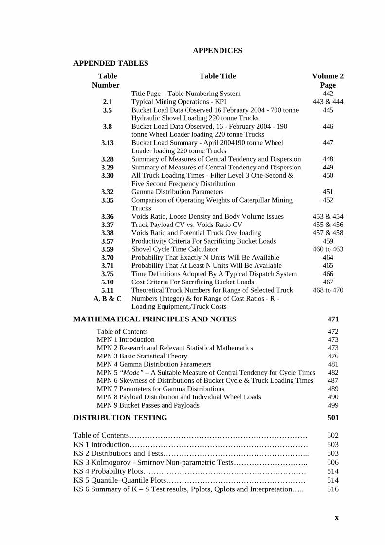
x
APPENDICES APPENDED TABLES
Table Number
Table Title Volume 2 Page
Title Page – Table Numbering System 442 2.1 Typical Mining Operations - KPI 443 & 444 3.5 Bucket Load Data Observed 16 February 2004 - 700 tonne
Hydraulic Shovel Loading 220 tonne Trucks 445
3.8 Bucket Load Data Observed, 16 - February 2004 - 190 tonne Wheel Loader loading 220 tonne Trucks
446
3.13 Bucket Load Summary - April 2004190 tonne Wheel Loader loading 220 tonne Trucks
447
3.28 Summary of Measures of Central Tendency and Dispersion 448 3.29 Summary of Measures of Central Tendency and Dispersion 449 3.30 All Truck Loading Times - Filter Level 3 One-Second &
Five Second Frequency Distribution 450
3.32 Gamma Distribution Parameters 451 3.35 Comparison of Operating Weights of Caterpillar Mining
Trucks 452
3.36 Voids Ratio, Loose Density and Body Volume Issues 453 & 454 3.37 Truck Payload CV vs. Voids Ratio CV 455 & 456 3.38 Voids Ratio and Potential Truck Overloading 457 & 458 3.57 Productivity Criteria For Sacrificing Bucket Loads 459 3.59 Shovel Cycle Time Calculator 460 to 463 3.70 Probability That Exactly N Units Will Be Available 464 3.71 Probability That At Least N Units Will Be Available 465 3.75 Time Definitions Adopted By A Typical Dispatch System 466 5.10 Cost Criteria For Sacrificing Bucket Loads 467 5.11
A, B & C Theoretical Truck Numbers for Range of Selected Truck Numbers (Integer) & for Range of Cost Ratios - R - Loading Equipment,/Truck Costs
468 to 470
MATHEMATICAL PRINCIPLES AND NOTES 471 Table of Contents 472 MPN 1 Introduction 473 MPN 2 Research and Relevant Statistical Mathematics 473 MPN 3 Basic Statistical Theory 476 MPN 4 Gamma Distribution Parameters 481 MPN 5 “Mode” – A Suitable Measure of Central Tendency for Cycle Times 482 MPN 6 Skewness of Distributions of Bucket Cycle & Truck Loading Times 487 MPN 7 Parameters for Gamma Distributions 489 MPN 8 Payload Distribution and Individual Wheel Loads 490 MPN 9 Bucket Passes and Payloads 499
DISTRIBUTION TESTING 501
Table of Contents…………………………………………………………… 502 KS 1 Introduction…………………………………………………………… 503 KS 2 Distributions and Tests………………………………………………... 503 KS 3 Kolmogorov - Smirnov Non-parametric Tests……………………….. 506 KS 4 Probability Plots……………………………………………………… 514 KS 5 Quantile–Quantile Plots……………………………………………… 514 KS 6 Summary of K – S Test results, Pplots, Qplots and Interpretation….. 516
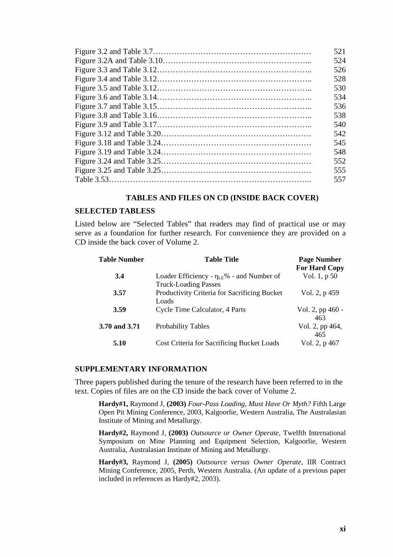
xi
Figure 3.2 and Table 3.7…………………………………………………… 521 Figure 3.2A and Table 3.10………………………………………………... 524 Figure 3.3 and Table 3.12………………………………………………….. 526 Figure 3.4 and Table 3.12………………………………………………….. 528 Figure 3.5 and Table 3.12………………………………………………….. 530 Figure 3.6 and Table 3.14………………………………………………….. 534 Figure 3.7 and Table 3.15………………………………………………….. 536 Figure 3.8 and Table 3.16………………………………………………….. 538 Figure 3.9 and Table 3.17………………………………………………….. 540 Figure 3.12 and Table 3.20………………………………………………… 542 Figure 3.18 and Table 3.24………………………………………………… 545 Figure 3.19 and Table 3.24………………………………………………… 548 Figure 3.24 and Table 3.25………………………………………………… 552 Figure 3.25 and Table 3.25………………………………………………… 555 Table 3.53………………………………………………………………….. 557
TABLES AND FILES ON CD (INSIDE BACK COVER)
SELECTED TABLESS Listed below are “Selected Tables” that readers may find of practical use or may serve as a foundation for further research. For convenience they are provided on a CD inside the back cover of Volume 2.
Table Number Table Title Page Number For Hard Copy
3.4 Loader Efficiency - ηLE% - and Number of Truck-Loading Passes
Vol. 1, p 50
3.57 Productivity Criteria for Sacrificing Bucket Loads
Vol. 2, p 459
3.59 Cycle Time Calculator, 4 Parts Vol. 2, pp 460 - 463
3.70 and 3.71 Probability Tables Vol. 2, pp 464, 465
5.10 Cost Criteria for Sacrificing Bucket Loads Vol. 2, p 467
SUPPLEMENTARY INFORMATION Three papers published during the tenure of the research have been referred to in the text. Copies of files are on the CD inside the back cover of Volume 2.
Hardy#1, Raymond J, (2003) Four-Pass Loading, Must Have Or Myth? Fifth Large Open Pit Mining Conference, 2003, Kalgoorlie, Western Australia, The Australasian Institute of Mining and Metallurgy.
Hardy#2, Raymond J, (2003) Outsource or Owner Operate, Twelfth International Symposium on Mine Planning and Equipment Selection, Kalgoorlie, Western Australia, Australasian Institute of Mining and Metallurgy.
Hardy#3, Raymond J, (2005) Outsource versus Owner Operate, IIR Contract Mining Conference, 2005, Perth, Western Australia. (An update of a previous paper included in references as Hardy#2, 2003).
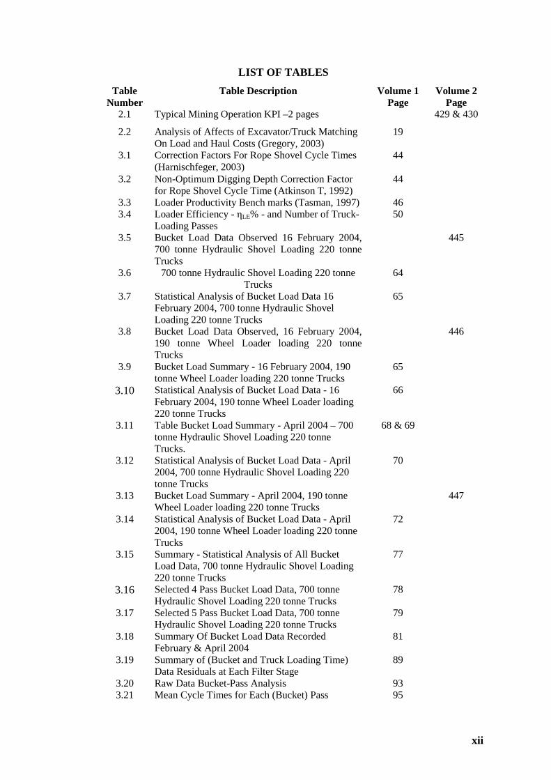
xii
LIST OF TABLES Table
Number Table Description Volume 1
Page Volume 2
Page 2.1 Typical Mining Operation KPI –2 pages 429 & 430
2.2 Analysis of Affects of Excavator/Truck Matching On Load and Haul Costs (Gregory, 2003)
19
3.1 Correction Factors For Rope Shovel Cycle Times (Harnischfeger, 2003)
44
3.2 Non-Optimum Digging Depth Correction Factor for Rope Shovel Cycle Time (Atkinson T, 1992)
44
3.3 Loader Productivity Bench marks (Tasman, 1997) 46 3.4 Loader Efficiency - ηLE% - and Number of Truck-
Loading Passes 50
3.5 Bucket Load Data Observed 16 February 2004, 700 tonne Hydraulic Shovel Loading 220 tonne Trucks
445
3.6 700 tonne Hydraulic Shovel Loading 220 tonne Trucks
64
3.7 Statistical Analysis of Bucket Load Data 16 February 2004, 700 tonne Hydraulic Shovel Loading 220 tonne Trucks
65
3.8 Bucket Load Data Observed, 16 February 2004, 190 tonne Wheel Loader loading 220 tonne Trucks
446
3.9 Bucket Load Summary - 16 February 2004, 190 tonne Wheel Loader loading 220 tonne Trucks
65
3.10 Statistical Analysis of Bucket Load Data - 16 February 2004, 190 tonne Wheel Loader loading 220 tonne Trucks
66
3.11 Table Bucket Load Summary - April 2004 – 700 tonne Hydraulic Shovel Loading 220 tonne Trucks.
68 & 69
3.12 Statistical Analysis of Bucket Load Data - April 2004, 700 tonne Hydraulic Shovel Loading 220 tonne Trucks
70
3.13 Bucket Load Summary - April 2004, 190 tonne Wheel Loader loading 220 tonne Trucks
447
3.14 Statistical Analysis of Bucket Load Data - April 2004, 190 tonne Wheel Loader loading 220 tonne Trucks
72
3.15 Summary - Statistical Analysis of All Bucket Load Data, 700 tonne Hydraulic Shovel Loading 220 tonne Trucks
77
3.16 Selected 4 Pass Bucket Load Data, 700 tonne Hydraulic Shovel Loading 220 tonne Trucks
78
3.17 Selected 5 Pass Bucket Load Data, 700 tonne Hydraulic Shovel Loading 220 tonne Trucks
79
3.18 Summary Of Bucket Load Data Recorded February & April 2004
81
3.19 Summary of (Bucket and Truck Loading Time) Data Residuals at Each Filter Stage
89
3.20 Raw Data Bucket-Pass Analysis 93 3.21 Mean Cycle Times for Each (Bucket) Pass 95
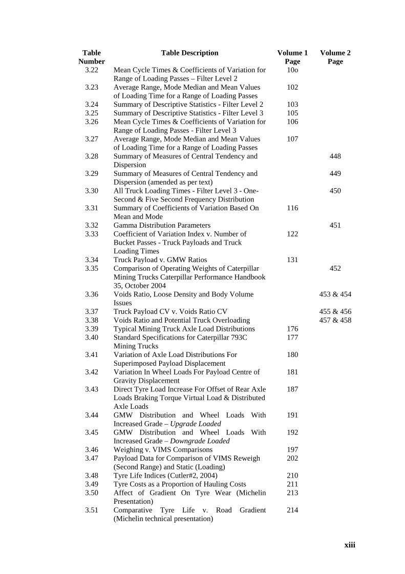
xiii
Table Number
Table Description Volume 1 Page
Volume 2 Page
3.22 Mean Cycle Times & Coefficients of Variation for Range of Loading Passes – Filter Level 2
10o
3.23 Average Range, Mode Median and Mean Values of Loading Time for a Range of Loading Passes
102
3.24 Summary of Descriptive Statistics - Filter Level 2 103 3.25 Summary of Descriptive Statistics - Filter Level 3 105 3.26 Mean Cycle Times & Coefficients of Variation for
Range of Loading Passes - Filter Level 3 106
3.27 Average Range, Mode Median and Mean Values of Loading Time for a Range of Loading Passes
107
3.28 Summary of Measures of Central Tendency and Dispersion
448
3.29 Summary of Measures of Central Tendency and Dispersion (amended as per text)
449
3.30 All Truck Loading Times - Filter Level 3 - One-Second & Five Second Frequency Distribution
450
3.31 Summary of Coefficients of Variation Based On Mean and Mode
116
3.32 Gamma Distribution Parameters 451 3.33 Coefficient of Variation Index v. Number of
Bucket Passes - Truck Payloads and Truck Loading Times
122
3.34 Truck Payload v. GMW Ratios 131 3.35 Comparison of Operating Weights of Caterpillar
Mining Trucks Caterpillar Performance Handbook 35, October 2004
452
3.36 Voids Ratio, Loose Density and Body Volume Issues
453 & 454
3.37 Truck Payload CV v. Voids Ratio CV 455 & 456 3.38 Voids Ratio and Potential Truck Overloading 457 & 458 3.39 Typical Mining Truck Axle Load Distributions 176 3.40 Standard Specifications for Caterpillar 793C
Mining Trucks 177
3.41 Variation of Axle Load Distributions For Superimposed Payload Displacement
180
3.42 Variation In Wheel Loads For Payload Centre of Gravity Displacement
181
3.43 Direct Tyre Load Increase For Offset of Rear Axle Loads Braking Torque Virtual Load & Distributed Axle Loads
187
3.44 GMW Distribution and Wheel Loads With Increased Grade – Upgrade Loaded
191
3.45 GMW Distribution and Wheel Loads With Increased Grade – Downgrade Loaded
192
3.46 Weighing v. VIMS Comparisons 197 3.47 Payload Data for Comparison of VIMS Reweigh
(Second Range) and Static (Loading) 202
3.48 Tyre Life Indices (Cutler#2, 2004) 210 3.49 Tyre Costs as a Proportion of Hauling Costs 211 3.50 Affect of Gradient On Tyre Wear (Michelin
Presentation) 213
3.51 Comparative Tyre Life v. Road Gradient (Michelin technical presentation)
214

xiv
Table Number
Table Description Volume 1 Page
Volume 2 Page
3.52 Failure Modes for Tyres - Caterpillar Forward Mining Seminar 2001
214
3.53 Case Study 1 - Comparative Descriptive Statistics for Payloads and Passes
218
3.54 Case Studies 2 & 3 - Comparative Descriptive Statistics for Payloads and Passes
219
3.55 Distribution of Bucket passes/Truck Payload 222 3.56 Comparative Measures of Loading Practice
Quality 229
3.57 Productivity Criteria For Sacrificing Bucket Loads 459 3.58 Truck Working Face Widths Metres 232 3.59 Shovel Cycle Time Calculator - 4 Parts 460 to 463 3.60 Loading Times and Truck Trip Times 238 3.61 Coefficients of Variation – Truck Trip & Loading
Times 238
3.62 Conceptual Deep-pit Haul Road Course Details - for FPC Analysis
240
3.63 FPC Results - Comparison Across the Range of Caterpillar Mining Trucks - Deep-pit Application
243 & 244
3.64 Comparative Performance Indices for Payload Range +/- 20% - For Three Courses
249
3.65 Comparative Productivity Indices for Payload Range +/- 20% - For Three Courses
250
3.66 Mechanical Availability v. Maintenance Benchmarks
266
3.67 Benchmarks for World Class Operations (Caterpillar Global Mining)
269
3.68 Cost Items As % of Total Mining Costs (Kirk, 2000)
271
3.69 Load and Haul Equipment, Preliminary Selection Planning
280
3.70 Probability That Exactly N Units Will Be Available
464
3.71 Probability That At Least N Units Will Be Available
465
3.72 Probabilistic Determination of Fleet Units For a Range of - MA x U where Basic Fleet Units for Productivity = 15
287
3.73 Summary of Multiple Shovel Cases 292 3.74 Truck Variable Performance Factors 301 3.75 Time Definitions Adopted By A Typical Dispatch
System 466
3.76 Time Definitions & Breakdowns – Empirical Data 308 4.1 Potential Impacts of Non-optimum Truck
Selection 325
4.2 Truck Specification Comparison 331 4.3 Loading Equipment Specification Comparison 336 4.4 Fuel Consumption of Caterpillar Mining Trucks 342 4.5 Estimated Engine Life In Terms of Fuel Burn &
Fuel Burn Rates for Mining Trucks 343
4.6 Productivity and Cost Indices v. Payload/GMW Ratio
347
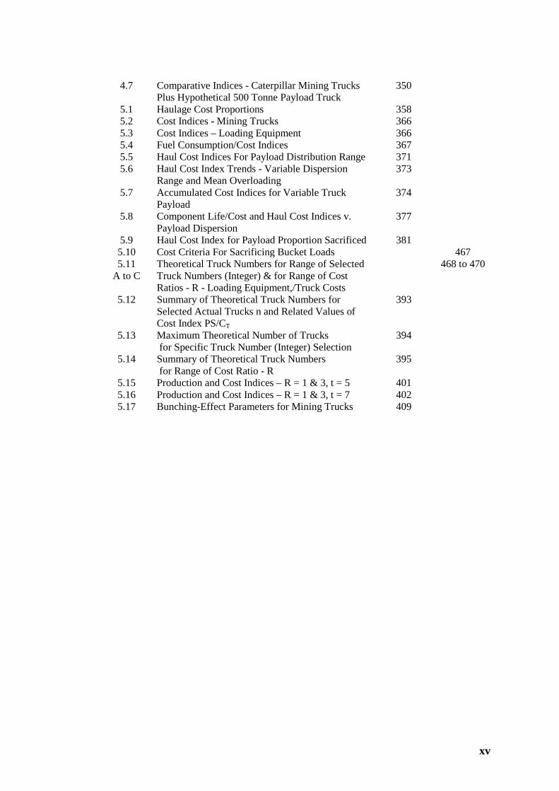
xv
4.7 Comparative Indices - Caterpillar Mining Trucks
Plus Hypothetical 500 Tonne Payload Truck 350
5.1 Haulage Cost Proportions 358 5.2 Cost Indices - Mining Trucks 366 5.3 Cost Indices – Loading Equipment 366 5.4 Fuel Consumption/Cost Indices 367 5.5 Haul Cost Indices For Payload Distribution Range 371 5.6 Haul Cost Index Trends - Variable Dispersion
Range and Mean Overloading 373
5.7 Accumulated Cost Indices for Variable Truck Payload
374
5.8 Component Life/Cost and Haul Cost Indices v. Payload Dispersion
377
5.9 Haul Cost Index for Payload Proportion Sacrificed 381 5.10 Cost Criteria For Sacrificing Bucket Loads 467 5.11
A to C
Theoretical Truck Numbers for Range of Selected Truck Numbers (Integer) & for Range of Cost Ratios - R - Loading Equipment,/Truck Costs
468 to 470
5.12 Summary of Theoretical Truck Numbers for Selected Actual Trucks n and Related Values of Cost Index PS/CT
393
5.13 Maximum Theoretical Number of Trucks for Specific Truck Number (Integer) Selection
394
5.14 Summary of Theoretical Truck Numbers for Range of Cost Ratio - R
395
5.15 Production and Cost Indices – R = 1 & 3, t = 5 401 5.16 Production and Cost Indices – R = 1 & 3, t = 7 402 5.17 Bunching-Effect Parameters for Mining Trucks 409
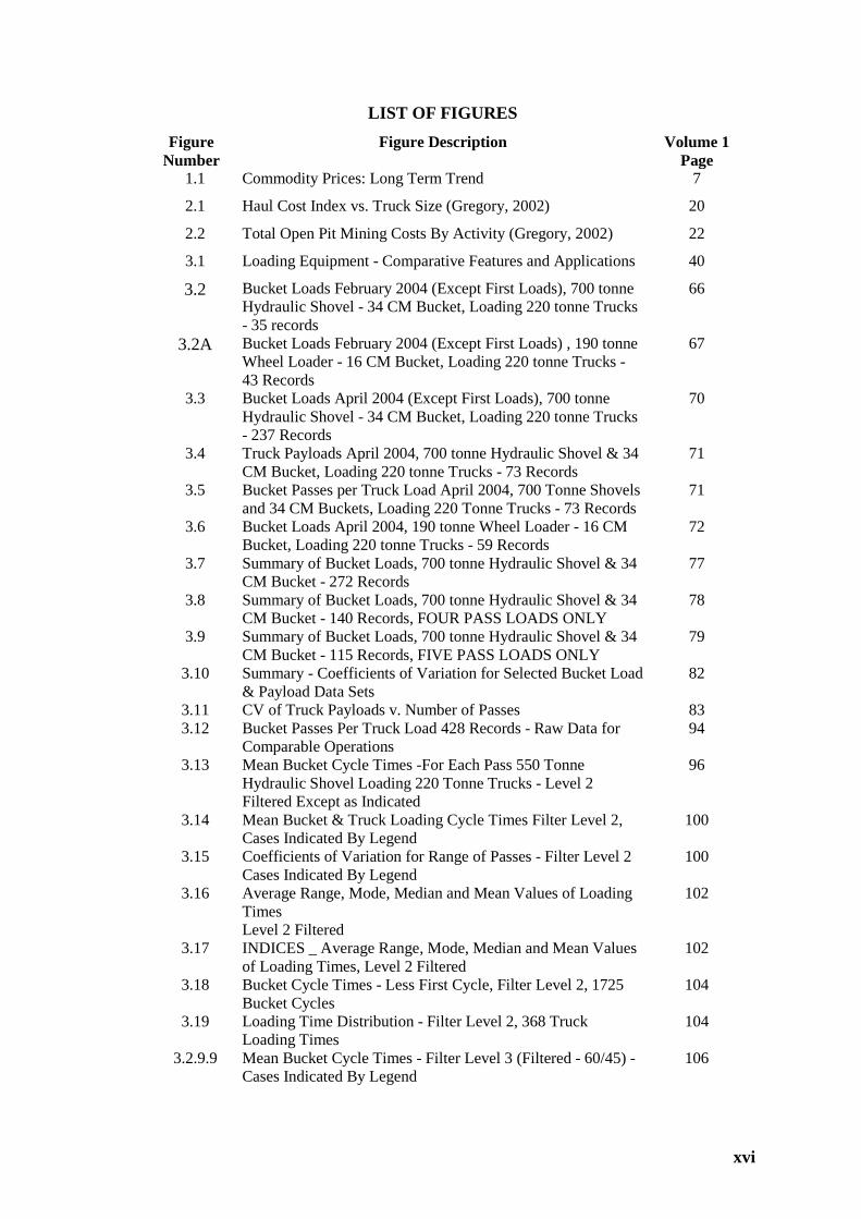
xvi
LIST OF FIGURES Figure
Number Figure Description Volume 1
Page 1.1 Commodity Prices: Long Term Trend 7
2.1 Haul Cost Index vs. Truck Size (Gregory, 2002) 20
2.2 Total Open Pit Mining Costs By Activity (Gregory, 2002) 22
3.1 Loading Equipment - Comparative Features and Applications 40
3.2 Bucket Loads February 2004 (Except First Loads), 700 tonne Hydraulic Shovel - 34 CM Bucket, Loading 220 tonne Trucks - 35 records
66
3.2A Bucket Loads February 2004 (Except First Loads) , 190 tonne Wheel Loader - 16 CM Bucket, Loading 220 tonne Trucks - 43 Records
67
3.3 Bucket Loads April 2004 (Except First Loads), 700 tonne Hydraulic Shovel - 34 CM Bucket, Loading 220 tonne Trucks - 237 Records
70
3.4 Truck Payloads April 2004, 700 tonne Hydraulic Shovel & 34 CM Bucket, Loading 220 tonne Trucks - 73 Records
71
3.5 Bucket Passes per Truck Load April 2004, 700 Tonne Shovels and 34 CM Buckets, Loading 220 Tonne Trucks - 73 Records
71
3.6 Bucket Loads April 2004, 190 tonne Wheel Loader - 16 CM Bucket, Loading 220 tonne Trucks - 59 Records
72
3.7
Summary of Bucket Loads, 700 tonne Hydraulic Shovel & 34 CM Bucket - 272 Records
77
3.8 Summary of Bucket Loads, 700 tonne Hydraulic Shovel & 34 CM Bucket - 140 Records, FOUR PASS LOADS ONLY
78
3.9 Summary of Bucket Loads, 700 tonne Hydraulic Shovel & 34 CM Bucket - 115 Records, FIVE PASS LOADS ONLY
79
3.10 Summary - Coefficients of Variation for Selected Bucket Load & Payload Data Sets
82
3.11 CV of Truck Payloads v. Number of Passes 83 3.12 Bucket Passes Per Truck Load 428 Records - Raw Data for
Comparable Operations 94
3.13 Mean Bucket Cycle Times -For Each Pass 550 Tonne Hydraulic Shovel Loading 220 Tonne Trucks - Level 2 Filtered Except as Indicated
96
3.14 Mean Bucket & Truck Loading Cycle Times Filter Level 2, Cases Indicated By Legend
100
3.15 Coefficients of Variation for Range of Passes - Filter Level 2 Cases Indicated By Legend
100
3.16 Average Range, Mode, Median and Mean Values of Loading Times Level 2 Filtered
102
3.17 INDICES _ Average Range, Mode, Median and Mean Values of Loading Times, Level 2 Filtered
102
3.18 Bucket Cycle Times - Less First Cycle, Filter Level 2, 1725 Bucket Cycles
104
3.19 Loading Time Distribution - Filter Level 2, 368 Truck Loading Times
104
3.2.9.9 Mean Bucket Cycle Times - Filter Level 3 (Filtered - 60/45) - Cases Indicated By Legend
106

xvii
Figure Number
Figure Description Volume 1 Page
3.21 Coefficients of Variation for Range of Passes – Filter Level 3 - Cases Indicated By Legend
106
3.22 Average Range, Mode, Median and Mean Values of Loading Times - Filter Level 3
107
3.23 INDICES _ Average Range, Mode, Median and Mean Values of Loading Times - Filter Level 3 (Filtered - 60/45)
108
3.24 Bucket Cycle Times Excluding First Pass Filter Level 3 to Max 45 Seconds - 882 Bucket Cycles
111
3.25 Loading Time Distribution - Filter Level 3 - 188 Truck Loading Times
112
3.26 Summary - Coefficients of Variation Based On Mean and Mode
116
3.27 Coefficient of Variation Index v. Number of Bucket Passes - Applies to Truck Payloads and Truck Loading Times
123
3.28 Mining Truck Types (Hays, 1990, p672) 130 3.29 Mechanical v. AC v. DC Drive Efficiencies - (Caterpillar
Australia) 135
3.30 Liner Options – Rock Box (Caterpillar Mining Forum, 2003)
139
3.31 Liner Options – Grid Liners (Caterpillar Mining Forum, 2003)
139
3.32 Liner Options – Skeletal Mechanically Attached Wear Plate System (MAWPS) (Caterpillar Mining Forum, 2003)
140
3.33 Liner Options – MAWPS Installed & Operational (Caterpillar Mining Forum, 2003)
140
3.34 SAE 2:1 Volume v. Conical Volume (Caterpillar Australia)
144
3.35 Illustration of Realistic Slopes -Based on Angle of Repose (Caterpillar Australia)
144
3.36 Typical MSD Design 793C - General Arrangement 147
3.37 Typical MSD Design 793C – Plate Arrangement 148
3.38 Loose Density v. Voids Ratio CVVR 161 3.39 Loose Density v. Voids Ratio CVVR -
Hypothetical Reducing CVVR as Mean VR Decreases 162
3.40 Truck Payload CVPL v. Voids Ratio CVVR 164 3.41 Theoretical Truck Payload Maxima v. Voids Ratio CVVR -
Selected Constant Body Capacity 167
3.42 Theoretical Potential Overload At Selected Voids Ratios v. Voids Ratio CVVR
167
3.43 Load Centre Marker for MSD Bodies - (Cat 793C Mining Truck as example)
177
3.44 Relationship Between Superimposed Payload Displacement and GMW Distribution to Wheels - Variation of Axle Load Distribution
180
3.45 Relationship Between Superimposed Payload Displacement and GMW Distribution to Individual Wheels
181
3.46 Axle Group Arrangement (Cat 793D as example) 184 3.47 Direct Tyre Load Increase For "Offset" of Rear Axle Loading
& Virtual Payload Increment From Braking Torque 188
3.48 Wheel Load Variation v. Gradient - Upgrade Loaded - Adopting Cat 793C Mining Truck As Example
193

xviii
Figure Number
Figure Description Volume 1 Page
3.49 Wheel Load Variation v. Gradient - Down Grade Loaded - Adopting Cat 793C Mining Truck As Example
193
3.50 Rimpull – GMW (Caterpillar PHB 35, 2004 p9.41) 194
3.51 Comparison of Payloads - Unfiltered - VIMS Reweigh (Second Range) & Static (Loading) - 73 Records
203
3.52 Comparison of Payloads - Filtered +/- 5% - VIMS Reweigh (Second Range) & Static (Loading) - 62 Records
204
3.53 Tyre Wear Rate and Tyre Load (Michelin Presentation) 213 3.54 220 Tonne Truck Payloads - Down Loaded August 2003,
2632 Records - Payloads after filtering out 2 pass loads 221
3.55 Case 1 - Truck Payloads - CV v. Passes 221 3.56 Coefficients of Variation of Truck Trip & Loading Times -
225 tonne trucks loaded by 700 tonne hydraulic shovels 239
3.57 Safe Speed vs. Favourable Grade for Off-Highway Trucks - Caterpillar FPC 3.05B Manual, Appendix B
242
3.58 Operator Efficiency - Caterpillar FPC 3.05B Manual, Appendix B
242
3.59 Average Speed - Travel Only 245 3.60 Fuel per Tonne-km - Three Courses 246 3.61 Potential Production - Tonne-km per Payload Tonne 247 3.62 Performance & Productivity Indices v. Payload Range +/-
20% - Course 1 250
3.63 Performance & Productivity Indices v. Payload Range +/- 20% - Course 2
251
3.64 Performance & Productivity Index v. Payload Range +/- 20% - Course 3
251
3.65 Mechanical Availability v. MTBS at Various MTTR 267 3.66 Mechanical Availability v. MTTR at Various MTBS 267 3.67 Conceptual Cumulative Production Plan And
Matching Equipment Productivity 281
3.68 “The Perfect Match Point” (Gove, 1994) 293 3.69 Mismatch Efficiency v. Fleet Match (Gove, 1994) 294 3.70 Bunching Efficiency v. Fleet Match (Gove, 1994) 297 3.71 Loader Mismatch & Bunching v. Fleet Match (Gove, 1994) 298 3.72 Hauler Mismatch & Bunching v. Fleet Match (Gove, 1994) 298 3.73 Interpretation of Definitions 306 4.1 Generic Mining Development Outline 320 4.2 Truck Selection Process 321 4.3 Loading Unit Selection Process 322 4.4 Potential Impact of Non-optimum Truck Selection 325 4.5 Relative Load and Haul Costs as Loading Equipment Scale
Increases for a Range of Truck Payloads (Gregory#2, 2003) 327
4.6 Mining Trucks - Comparison of Flywheel kW vs. GMW, Payload vs. GMW & kW vs. Payload
331
4.7 Trucks - Payload vs. GMW Ratio 332 4.8 Loading Equipment - Comparison of Flywheel kW and
Operating Weight Per Bucket Cubic Metre 336
4.9 Hauling Cost Trend With Truck Scale 344 4.10 Productivity and Cost Indices v. Payload/GMW Ratio 346 4.11 Comparative Indices - Caterpillar Mining Trucks Plus
Hypothetical 500 Tonne Truck 349
xix
Figure Number
Figure Description Volume 1 Page
4.12 Cat Mining Trucks Selection Criteria - Comparative Indices Plus Hypothetical 500 Tonne Truck
350
5.1 Haulage Cost Proportions - (Gregory B, 2002) 355 5.2 Haulage Cost Proportions - Adjusted for Fuel 35 to 55
cents/litre 356
5.3 Haulage Cost Proportions Further Adjusted for +50% Tyre Cost
356
5.4 Capital Recovery Risk 360 5.5 Mining Equipment Maintenance Cost - (Hardy #2, 2003) 361 5.6 Fuel/Component Cost Index Comparisons - Payloads 80% to
120% 365
5.7 Approved Generic target Rating - Caterpillar Inc. 10/10/20 Policy, April 2002
367
5.8 Component Life vs. Payload - Caterpillar Inc.10/10/20 Policy, April 2002
367
5.9 Component Life, Cost and Haul Cost Indices v. Payload Distribution
369
5.10 Haul Cost Index - Variable Mean Overloading 371 5.11 Accumulated Haul Cost Indices v. Mean Payload 372 5.12 Dispersion Haul Cost Index vs. Variable Payload Dispersion
Range 375
5.13 Range of Theoretical Number of Trucks for which a Specific Number of Trucks Provides Lowest Production Cost Match, Cost Ratio, Loading Equipment/Truck – R = 1
388
5.14 Theoretical Number of Trucks 389 5.15 Truck Number n (Integer) Selection for Range of Cost Ratios
for Specific Range of Theoretical Number of Trucks t 391
5.16 Effect on Range of Theoretical Number of Trucks for Specific Selected Truck numbers as Loading Equipment Cost/Truck Cost Varies from 1 to 3
393
5.17 Production and Unit Cost Indices - R = 1 & 3 for t = 5 399 5.18 Production and Unit Cost Indices - R = 1 & 3 for t = 7 400 5.19 Total Trip Time TT - Distribution
& Waiting Time TW By Difference 404
311
CHAPTER 4
EQUIPMENT SELECTION
4.1 SELECTION IMPLEMENTATION
4.1.1.1 Preamble
Chapter 4 describes review processes and activities based on selection criteria that
facilitate equipment selection decisions. Except for additions to existing fleets (where
uniformity of fleets is productivity and cost beneficial) mining equipment selection is
generally comparative. A favoured option is determined in terms of the criteria
examined in Chapter 3.
Research moved on to address preliminaries and final analysis culminating in
equipment procurement. Final selection processes generally commence with
compilations of comparative equipment specifications that, for each functional type
of mining equipment have high probability of achieving required productivity
performance and realization of planned production.
4.1.1.2 Specification Fundamentals
A “specification” provides a description of the service or product - the resource
inputs and methods applied. Other parts of procurement documentation, including
formally tendered contracts, providing information on administration, financial,
commercial and legal matters are generally labelled “terms and conditions”.
Writing and compiling a specification requires the most comprehensive input from
stakeholders within a procuring organisation. It is the outcome of all prerequisite
planning; also production and operational investigation within the overall
procurement process.
Specifications can be of several types each with a separate technique for specifying
any individual equipment item, including:
1. Functional – usually with attached general performance undertaking or
guarantee.
4.1.1 Introduction
312
2. Performance – defined performance in quantity, quality and time.
3. Technical – detailed to the degree of non-ambiguity on the basic materials,
physical form and quality of each individual item in the group of individual
parts that make up an equipment unit.
4. Reference – to standard specification documentation - a secondary stage of
Type 3. - with possibly addition of some part of techniques of Type 1. and/or
Type 2.
Examples of specification techniques for specifying a mousetrap:
• Functional: - to attract, using cheese bait, and kill mice instantaneously.
• Performance: - to be baited with cheese and safely hand set to kill mice
instantaneously with a minimum life of 500 operations.
• Technical: - A pinus radiata timber base with dimensions “x - y - z”,
powered by a coil spring of “g” gauge steel wire preloaded to “k” kilos and
with an operating time of “t” milliseconds etc.
Advantages of “performance” and “functional” specifications, individually or
combined:
• Reduced time and effort to prepare.
• Avoids bias for/against one method or type of product/service.
• Encourages more innovative and economical responses.
• Allow bidders to offer alternative, low-cost solutions.
• Provides results-based responses.
• Relieves procurer of responsibility for product design.
Prerequisites for an effective specification:
• Developed from clear objectives that are the result of thorough investigation
and due diligence.
• Express needs clearly, concisely and unambiguously.
• Not containing unnecessary details.
• Logically constructed to enable analysis by others.
313
• Maximize use of standards of construction, performance and acceptance
criteria.
• State principle criteria for evaluation of quotations or tenders, supply and
operational performance; and final acceptance.
• Special needs of each unique mining project.
• Non-discriminatory against any supplier/contractor.
• Provides opportunity for alternative or innovative quotations that satisfy
project needs.
Compiling and writing a specification requires efficient due diligence and will
generally be re-drafted many times to satisfy stakeholders.
A refined Specification is achieved by:
• Multi-stage tendering process – this is the normal situation where equipment
selection process involves multiple and repetitive dialogue between suppliers
and purchasers of mining equipment.
• Painstaking, repetitive editing and re-drafting.
• Realization that contract risk of an inadequate specification is generally high
to extreme with unacceptable likelihood and consequences.
The above discussion on specifications was compiled with reference to “Contract
Management in Australia” by John James (James, 1995).
4.1.1.3 Equipment Specifications
A reliable specification leaves no “hanging” questions. If for any sentence any of the
simple questions Why? When? Where? What? and How? are valid, then the
specification must be amended to satisfactorily answer the question(s).
Most mining equipment procurement involves a “Type 4.” specification, as well as
some combination of “Types 1 to 3”. Suppliers (OEM and dealers) compile standard
specification documentation, inclusive of a small list of separately priced optional
items. Each optional item offered can be accepted or rejected by the purchaser.
Optional on-board equipment operational and management systems are generally
separately specified and priced. Suppliers will generally accommodate specific needs
of purchasers for equipment specification and terms and conditions of tendering.
314
Any amended or additional specifications required by the purchaser can be
negotiated with the dealer/OEM. The responsibility for any consequent modifications
depends on the nature of each modification or additional equipment. For example
supplying and location of portable fire extinguishers would certainly be a dealer
responsibility. But supply and installation detail of fire suppression equipment in an
engine compartment, can be expected to benefit from, and require OEM involvement
to preserve warranty and any performance guarantees.
On arriving at a final specification satisfactory to the purchaser and acceptable to the
dealer and OEM:
• Final pricing can be negotiated or tendered to the purchaser.
• Terms of payment can be determined.
• Delivery arrangements can be finalized.
Unqualified acceptance of quotation or tender by the buyer sets the terms of contract
as negotiated and agreed. It is the mutual responsibility of the supplier (OEM/dealer)
and purchaser to meet their individual obligations to satisfactorily conclude the
supply contract.
4.1.1.4 Performance Guarantees
Provided the agreed specification does not preclude or conflict with a specified
performance guarantee it can be expected to be enforceable and provide the
protection, and risk amelioration the purchaser expects. It is the author’s experience
that if “performance guarantees are too good to be true” they usually are.
Enforceability of unrealistic performance guarantees goes hand-in-hand with
protracted dispute; and management distraction results from the dispute resolution
process.
Purchasers should be duly diligent and make their own reasonable assessment of
performance of equipment. During the process of equipment selection this
assessment needs to be audited against internal experience, performance at other
sites; and with circumspect consideration of performance information provided
during the course of marketing activities of dealers and OEM.
It will be realised that OEM design and build mining equipment to suit a broad, but
necessarily limited, range of ambient conditions. Optional configurations are often
315
available to extend compatibility of equipment to extreme limits of ambient
conditions. But departure from anticipated ambient operating conditions should be
treated as an exception for application of performance guarantees when caused by:
• Latent conditions that could not be reasonably foreseen by the purchaser or
supplier.
• Omissions, misinterpretation of information or insufficient prior collection of
operating-conditions data.
It is the author’s opinion that performance guarantees:
• Are no substitute for meticulous due diligence by the potential purchaser in
the process of mining equipment selection and procurement.
• Serve the purpose of indicating good faith of the supplier in specification of,
and expected performance from, individual equipment items – but always if
actual ambient, physical operating conditions, operational functions and
demands and management controls are within the ambit anticipated in
establishing guaranteed performance.
4.1.1.5 Load and Haul Equipment Options
There is an overwhelming range of options on offer when selecting mining
equipment. For loading and hauling equipment there are some six suppliers
providing loading equipment options and some five suppliers of large mining trucks.
In discussing the need for, and justifying the application of simulation methods for
estimating truck requirements for large open pits, Garston Blackwell (Blackwell,
1999) raises the need for a “realistic approach”. Blackwell, in supporting the need for
a realistic approach, advises: “Unfortunately there are many factors governing the
tonnage hauled by open pit truck fleets that cannot be treated simply, and doing so
will usually result in an operation that cannot meet production objectives.” This
implies support for, application of, probabilistic techniques for estimating “realistic”
truck numbers as described in Section 3.5.
Blackwell further advises: “Assumptions made in calculating vehicle performance
are optimistic.” - for the following reasons:
• Empty trucks are always heavier than when manufactured because of mud
and debris stuck to the truck body.
316
• Extra steel is added to bodies to reinforce (rapid) wearing surfaces and
damage points.
• Engines, and to a lesser extent, transmissions do not always operate at rated
capacity.
• Diesel fuel quality varies (and ambient operating temperature affects fuel
burn).
• (Pay) loads carried are variable.
• Road conditions are variable and single lane traffic may be experienced over
some in-pit haul segments.
Blackwell describes a case study where “the slowest vehicle (truck) travelling up-
ramp loaded (was observed) at half the speed of the fastest truck”. As startling as
Blackwell’s advice sounds, it is consistent with general observations. The “slowest-
fastest” spread highlighted is a range of some +/- 33% of the mean speed assuming a
symmetrical distribution. Discounting this effect on truck trip time TT consistent with
FPC output in Table 3.63, for medium to long hauls, realizes an indicated range for
corresponding change of TT ranging +/- 20% – 22%. This indicates a CV for TT in
the order of 7%.
As discussed in Section 3.3.10, Dan Gove and Bill Morgan (Gove, 1994) describe
empirical evidence of CV for TT in the range 0.10 to 0.20. This is consistent with the
observed CV of truck trip time TT distributions of 0.19 unfiltered to 0.12 filtered
(only for anomalous values, not for non-intrinsic delays) for the case study discussed
in Section 3.3.10 and shown in Table 3.60. Data from both Caterpillar and in Table
3.60 are empirical. Data from Table 3.63 is generated by Caterpillar’s FPC
application and not subject to non-intrinsic time losses and delays. The results are not
necessarily comparable. But considering the accumulative effect of non-intrinsic
delays on the FPC data would likely significantly reduce the difference. Certainly the
research analysis appears to be consistent with Blackwell’s observations for loaded
trucks ascending ramps (Blackwell, 1999).
Selection of loading equipment also needs a realistic approach when applying
productivity criteria. The open pit mining industry appears to have been sensitive to
this need. As described in Section 3.2, bench marking of shovel performance

317
indicates a tendency for the industry to respond to the many reducing factors and
criteria by acceptance and a tendency to over-shovel resulting in loading equipment
benchmarks of some half of intrinsic performance.
The range of options for trucks and loading equipment and comparative intrinsic
performance criteria are further discussed in Section 4.1.5.
4.1.2.1 All Mining Equipment
The following key considerations need to be addressed in commencing to implement
mining equipment selection:
Locality and General Operating Conditions
• Location of proposed or existing operation and logistical scenario.
• Political situation and politico-risk profile.
• Meteorological environment for operations.
• Socio-economic and human resources circumstances.
• Environmental conditions.
• Special safety and health conditions.
• General risk profile of existing or future mining operations, especially
hauling operations.
Project Characteristics
• Mining plan, production programme and productivity required.
• Blending requirements and any special delivery requirements for materials
such as ore at a crushing facility.
• Special features of the mine plan including loaded down-ramp hauls, steep
ramps, long hauls, road surfacing details, separate ore and waste fleets (mixed
truck and loading equipment fleets) and trolley assist.
• Industrial background including working hours, rosters, statutory or agreed
restrictions, existing industrial culture, quality and quantity of labour and
special training requirements related thereto – for operations, maintenance
4.1.2 Key Considerations
318
and interrelated mining functions including work practices of contractors on
site.
• Corporate policy interrelated with the hauling operation.
4,1,2,2 Considerations - Trucks
• Reliability of each truck option under consideration.
• Reliability of product support by suppliers.
• Available delivery compared with project requirements and any flexibility in
those requirements.
• Tyre operating conditions relative to tyres available.
• Productivity issues including truck body type, capacity and (if any) liner-kit
details requiring attention.
• Handling wet materials, highly abrasive and physically demanding materials
including cherts and other siliceous materials.
• Truck performance expectancy based on simulation using deterministic data
and calculation methods such as FPC (Caterpillar) and Talsim (Runge
Mining) – comprehensive analysis of enough cases to cover the range of
expected performances required.
• Determination of truck numbers including matching trucks to loading
equipment.
The above lists are a composite from work by Bruce Gregory (Gregory#1, 2002),
(Gregory#2, 2003) and the author’s experience in mining development projects.
4.1.2.3 Considerations - Loading Equipment
Project Characteristics
Key considerations to be addressed to implement selection of mining loading
equipment include:
• Geology of the stratigraphy hosting the ore and geometry of the ore deposits.
• Selectivity requirements.
• Production and productivity requirements for the various materials to be
mined.
319
• Mining plan, production programme and productivity profile required.
• Handling wet materials, highly abrasive and physically demanding materials
including cherts and other siliceous materials.
• Bench heights – including limitations to control dilution/ore loss for flat-
dipping ore deposits.
• Corporate policy interrelated with the hauling operation.
Loading Equipment - Considerations
• Reliability of each loading option under consideration.
• Reliability of product support by suppliers.
• Available delivery compared with project requirements and any flexibility in
those requirements.
• Productivity issues including bucket design, capacity and details of ground
engaging tools requiring attention.
• Loader performance expectancy based on deterministic data and calculation
methods – analysis of enough cases to cover the range of expected
performances required.
• Determination of loading equipment numbers including matching with trucks.
• Expected digging characteristics of materials to be mined and all relevant
parameters such as fragmentation and voids ratio.
• Minimum mining width.
• Loading equipment mobility requirements.
• Favoured loading equipment option or options including shovel or backhoe,
electric or diesel-hydraulic and required dumping height to suit favoured
trucks.
The above list is a composite from work by Bruce Gregory (Gregory#2, 2003) and
the author’s experience.
320
4.1.3.1 Timing of Equipment Selection
When does mining equipment selection need to be addressed in the total
development process? This question might well surface when the first indicatively
economic drill intersections cause both internal excitement for, and external interest
in, an exploration project.
From the earliest testing of economic feasibility, costs need to be estimated to enable
determination of resource delineation and ore definition criteria such as cut-off
grade; also to establish design criteria for optimal pit-design software. Initially costs
for such activities are more often adapted from existing operations or previous
feasibility studies by suitably adjusting for characteristics and conditions of the
project; also for cost variation with time. For preliminary feasibility study purposes,
costs so adapted are sufficiently accurate. Expected estimation accuracy at this early
development stage is +/-30% or more.
Results from such preliminary studies are the basis for a decision to “mothball” the
project (and wait for more favourable marketing environment), to abandon the
prospect or to sell. Alternatively, preliminary study results may be sufficiently
encouraging, providing opportunity to promote the project. Action taken may include
increasing the area of interest, step-out and/or in-fill drilling; and more detailed,
technical input through a further study iteration expected to produce more reliable
feasibility study results.
At this second stage, where cost estimates need to be more refined, initial mining
equipment selection, along with all other significantly increased metallurgical,
marketing, environmental and engineering inputs needs to be implemented.
Figure 4.1 indicates the project stages where mining equipment selection is an
activity in ever-increasing degrees of refinement through to awarding supply
contracts or placing orders.
Technical facilitation of mining equipment selection is a linear process through
deterministic and probabilistic calculation stages as implied in Section 3.5 above.
4.1.3 Selection Process
321
Typical simplified equipment selection process outlines are provided by Figure 4.2,
for trucks and Figure 4.3, for loading equipment. These process outlines were
prepared for an actual shovel and truck selection project. It will be noted that the
simplified flow charts served as report forms and include cost estimations and
comparisons – a management requirement when the form was designed.
In Section 3.4.2, product support by equipment suppliers was identified as the most
important issue in mining equipment selection. Comparative cost differences tend to
be subtle and consequently are often not clearly conclusive. So cost comparisons
tend to be more confirmatory than a robust aid for decision. Obviously, costs are
needed for budget purposes and for compiling of total mining costs. To reduce
repetitive work, and for economy of technical resource utilization, cost estimations
should be left as late as possible in the equipment selection process. This does not
mean that all options are carried forward. The selection process through application
of selection criteria and due diligence investigation of all interrelated issues should
eliminate many of the options as unsuitable for the planned production programme
and operational characteristics.
The initial five activities in both Figure 4.2, and Figure 4.3, for either truck or
loading unit selection, can be generally described as “due diligence”. This
investigative stage was referred to, and its importance emphasized, initially in
relation to “maintainability” in Section 3.4.2 and subsequently through Section 3.4
and in Section 4.1.2.
4.1.4.1 Effects of Non-optimum Selection – Trucks
Bruce Gregory compared the cost-impact due to non-optimum truck selection for a
number of issues relative to a small degree of performance effect. His work was
based on 2002 prices (Gregory#1, 2002). Table 4.1 updates Gregory’s comparison to
reflect recent increases in the price of fuel and tyres. Degrees of performance effect
were amended and an indicated impact of poor product support by suppliers was
quantified. The results in Table 4.1 are illustrated by Figure 4.4.
4.1.4 Selection Strategy
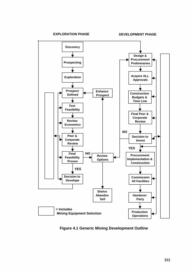
322
Discovery
Production Operations
Review Options
Handover Party
Design & Procurement Preliminaries
Prospect Defined
Test Feasibility
Prospecting
Exploration
Review Economics
Final Feasibility
Proven
Acquire ALL Approvals
CommissionAll Facilities
Construction Budgets & Time Line
Decision to Develope
Peer & Corporate
Review
Final Peer & Corporate
Review
Decision to Invest
Procurement Implementation &
Construction
Shelve Abandon
Sell
Enhance Prospect
NO
YES
Figure 4.1 Generic Mining Development Outline
YES
NO
EXPLORATION PHASE DEVELOPMENT PHASE
= Includes Mining Equipment Selection
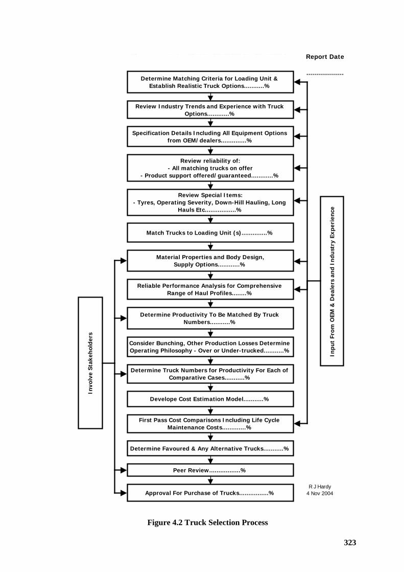
323
Determine Matching Criteria for Loading Unit & Establish Realistic Truck Options...........%
Review Industry Trends and Experience with Truck Options............%
Specification Details Including All Equipment Options from OEM/dealers..............%
Review reliability of:- All matching trucks on offer
- Product support offered/guaranteed............%
Review Special Items:- Tyres, Operating Severity, Down-Hill Hauling, Long
Hauls Etc.................%
Match Trucks to Loading Unit (s)..............%
Material Properties and Body Design,Supply Options............%
Reliable Performance Analysis for Comprehensive Range of Haul Profiles........%
Figure 4.1.3.2 - TRUCK SELECTION PROCESS
Determine Productivity To Be Matched By Truck Numbers...........%
Develope Cost Estimation Model...........%
Consider Bunching, Other Production Losses Determine Operating Philosophy - Over or Under-trucked...........%
First Pass Cost Comparisons Including Life Cycle Maintenance Costs.............%
Determine Truck Numbers for Productivity For Each of Comparative Cases...........%
Approval For Purchase of Trucks................%
Peer Review.................%
Determine Favoured & Any Alternative Trucks...........%
Invo
lve
Stak
ehol
ders
Inpu
t Fr
om O
EM &
Dea
lers
and
Ind
ustr
y Ex
peri
ence
R J Hardy4 Nov 2004
Report Date
...................
Figure 4.2 Truck Selection Process
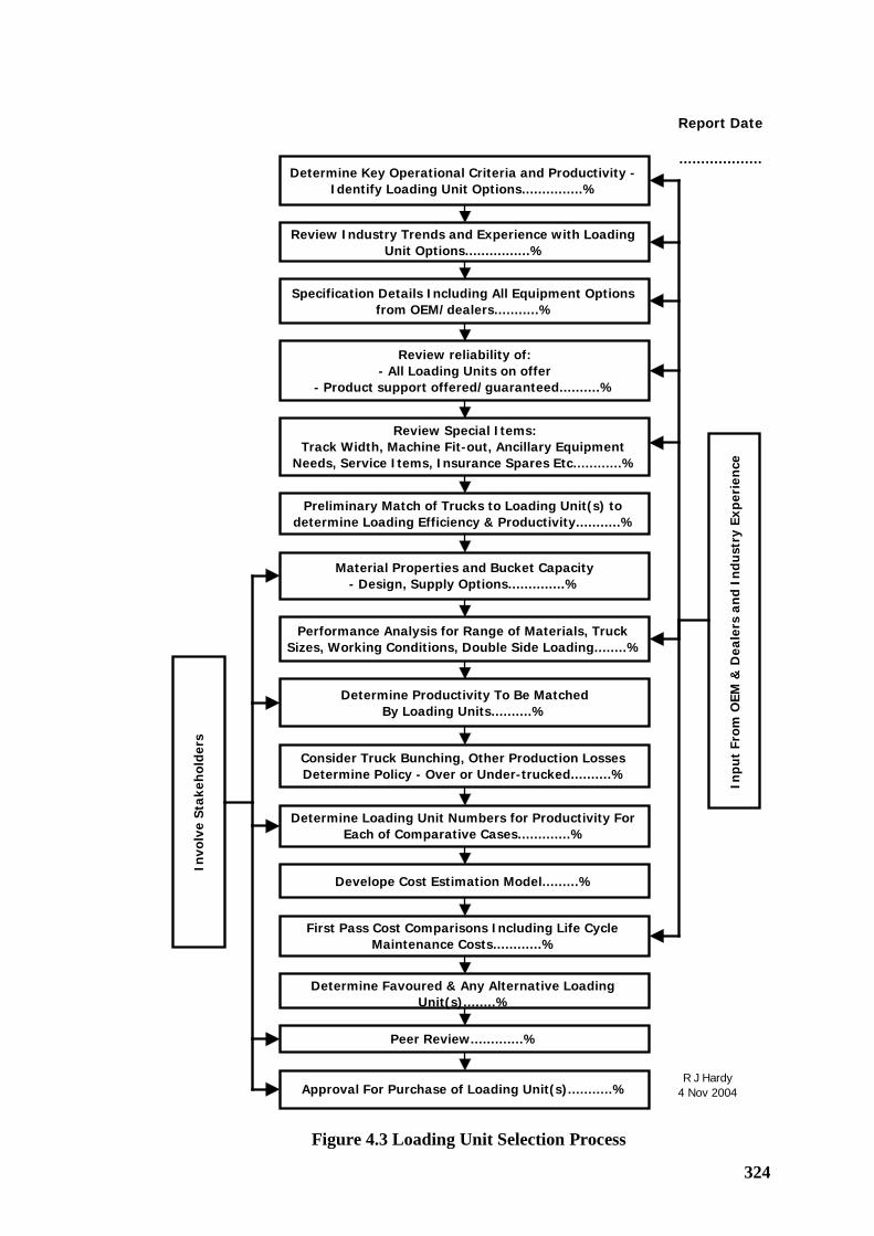
324
Determine Key Operational Criteria and Productivity - Identify Loading Unit Options...............%
Review Industry Trends and Experience with Loading Unit Options................%
Specification Details Including All Equipment Options from OEM/dealers...........%
Review reliability of:- All Loading Units on offer
- Product support offered/guaranteed..........%
Review Special Items:Track Width, Machine Fit-out, Ancillary Equipment
Needs, Service Items, Insurance Spares Etc............%
Preliminary Match of Trucks to Loading Unit(s) to determine Loading Efficiency & Productivity...........%
Material Properties and Bucket Capacity- Design, Supply Options..............%
Performance Analysis for Range of Materials, Truck Sizes, Working Conditions, Double Side Loading........%
Figure 4.1.3.3 - LOADING UNIT SELECTION PROCESS
Determine Productivity To Be MatchedBy Loading Units..........%
Develope Cost Estimation Model.........%
Consider Truck Bunching, Other Production Losses Determine Policy - Over or Under-trucked..........%
First Pass Cost Comparisons Including Life Cycle Maintenance Costs............%
Determine Loading Unit Numbers for Productivity For Each of Comparative Cases.............%
Approval For Purchase of Loading Unit(s)...........%
Peer Review.............%
Determine Favoured & Any Alternative Loading Unit(s)........%
Invo
lve
Stak
ehol
ders
Inpu
t Fr
om O
EM &
Dea
lers
and
Ind
ustr
y Ex
peri
ence
R J Hardy4 Nov 2004
Report Date
...................
Figure 4.3 Loading Unit Selection Process
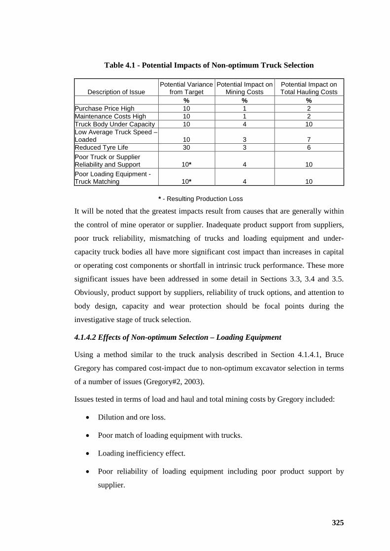
325
Table 4.1 - Potential Impacts of Non-optimum Truck Selection
Description of Issue Potential Variance
from Target Potential Impact on
Mining Costs Potential Impact on Total Hauling Costs
% % % Purchase Price High 10 1 2 Maintenance Costs High 10 1 2 Truck Body Under Capacity 10 4 10 Low Average Truck Speed – Loaded 10 3 7 Reduced Tyre Life 30 3 6 Poor Truck or Supplier Reliability and Support 10* 4 10 Poor Loading Equipment - Truck Matching 10* 4 10 * - Resulting Production Loss
It will be noted that the greatest impacts result from causes that are generally within
the control of mine operator or supplier. Inadequate product support from suppliers,
poor truck reliability, mismatching of trucks and loading equipment and under-
capacity truck bodies all have more significant cost impact than increases in capital
or operating cost components or shortfall in intrinsic truck performance. These more
significant issues have been addressed in some detail in Sections 3.3, 3.4 and 3.5.
Obviously, product support by suppliers, reliability of truck options, and attention to
body design, capacity and wear protection should be focal points during the
investigative stage of truck selection.
4.1.4.2 Effects of Non-optimum Selection – Loading Equipment
Using a method similar to the truck analysis described in Section 4.1.4.1, Bruce
Gregory has compared cost-impact due to non-optimum excavator selection in terms
of a number of issues (Gregory#2, 2003).
Issues tested in terms of load and haul and total mining costs by Gregory included:
• Dilution and ore loss.
• Poor match of loading equipment with trucks.
• Loading inefficiency effect.
• Poor reliability of loading equipment including poor product support by
supplier.
326
• Effect on load and haul costs due to non-optimum loading equipment
capacity.
The above list was consolidated to four factors analyzed for effect on load and haul
costs, total mining costs and ultimately profitability, viz.:
1. Dilution
2. Poor reliability (both equipment intrinsically and product support).
3. Match with trucks (non-optimum).
4. Inefficiency (inclusive of all causes).
Analysis in terms of profitability reduction ranked the factors in the order shown.
The above four factors, especially dilution and equipment reliability, should
obviously be the focus for the investigative stage of loading-equipment selection.
4.1.4.3 Loading Equipment Capacity and Load and Haul Costs
In the course of analyzing effect of non-optimum outcomes from testing loading
equipment Bruce Gregory provides valuable insight into the relationship between
loading equipment size for each truck payload capacity measured in terms of load
and haul costs (Gregory#2. 2003).
Figure 4.5 is reproduced from Gregory’s paper. Ordinate values are load and haul
cost indices with lowest cost calculated during analysis set at 100%.
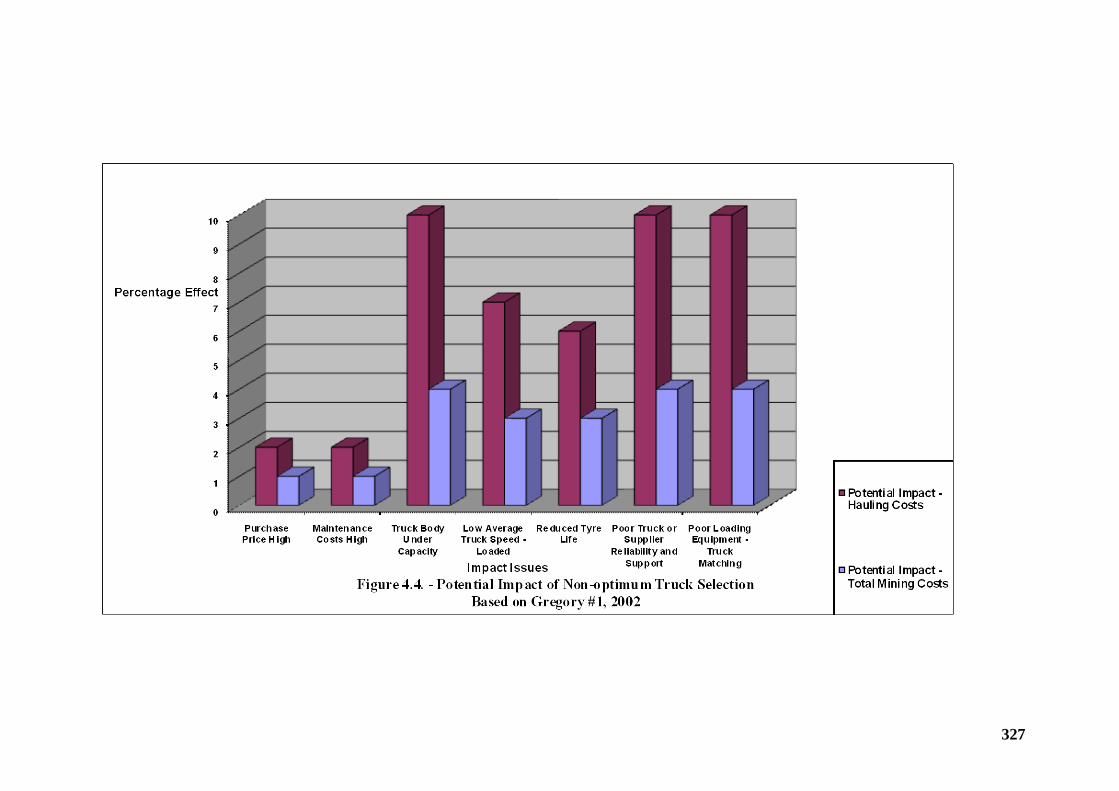
327

328
From analysis and Figure 4.5 Gregory concluded that:
• Truck size is a significantly greater load-and-haul cost driver than loading
equipment size.
• Lowest estimated load and haul costs were for the largest mining equipment
analyzed.
• For a selected truck size, the largest loading equipment did not always result
in the lowest load and haul index. Gregory explains this as mainly due to
bucket – truck body matching.
• For any selected truck size, load and haul costs varied over a narrow range of
5% for different loading equipment sizes.
Further interesting interpretations of the results illustrated in Figure 4.5 include:
• As shown by Figure 2.2, (cost proportions updated to current prices in
Section 5.1.3 –Table 5.1 and Figures 5.1 to 5.3) hauling cost is typically in
the order of three times the cost of loading within total mining costs for a
deep open pit. It is obvious that load and haul costs are not as sensitive to
loading equipment size alternatives when compared over a range of trucks.
• Alternative loading equipment for any specific truck size will require
different loading times involving different numbers of bucket passes. From
Figure 4.5 load and haul costs are not particularly sensitive to changing size
of loading equipment. This implies that load and haul costs are not
particularly sensitive to number of bucket passes. This further supports the
hypotheses in Sections 3.2.8 and 3.3.9 that increasing the number of bucket
passes to realise the benefit of reducing the dispersion of truck payload
distributions could be cost beneficial overall.
• The range of load and haul indices in Figure 4.5, for each truck size over the
loading equipment options analyzed is small - some +/-2.5% for the smallest
truck reducing to some +/-1.5% for the largest truck. Converting the
comparison to total mining cost indices approximately halves these ranges –
Figure 2.2 illustrates. If the comparison is considered in terms of total project
costs or profitability, changing loading equipment size (measured by
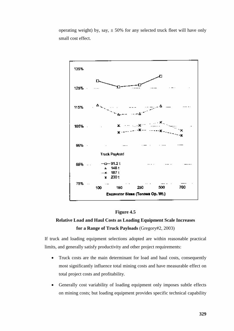
329
operating weight) by, say, ± 50% for any selected truck fleet will have only
small cost effect.
Figure 4.5
Relative Load and Haul Costs as Loading Equipment Scale Increases
for a Range of Truck Payloads (Gregory#2, 2003)
If truck and loading equipment selections adopted are within reasonable practical
limits, and generally satisfy productivity and other project requirements:
• Truck costs are the main determinant for load and haul costs, consequently
most significantly influence total mining costs and have measurable effect on
total project costs and profitability.
• Generally cost variability of loading equipment only imposes subtle effects
on mining costs; but loading equipment provides specific technical capability
330
to, firstly ensure that trucks function as intended. Secondly loading
equipment must accommodate all of the constraints to ensure that ore is
extracted with minimum loss/dilution, in accordance with the mine plan and
detailed pit plans based on stratigraphy of the ore and adequate geotechnical
constraints to ensure safe operations.
• The comparative results illustrated by Figure 4.5 imply that, provided loading
equipment satisfies requirements for selective mining and the condition and
digging characteristics of material being loaded, an error of, say, one step in
model range in selecting loading equipment size is, by a significant margin,
not as significant as selecting a truck with non-optimum payload capacity.
• Finally, a decision for replacement of trucks with up-scaled truck models to
benefit from reduced unit costs may not necessarily further significantly
benefit from replacing loading equipment with up-scaled units.
Truck and loading equipment selection processes always need to apply detailed
attention to the duties of each open pit mining operation.
4.1.5.1 Mining Trucks
A sample of mining trucks offered by the principal truck manufacturers is analyzed
in Table 4.2.
Figure 4.6 illustrates the comparative criteria that indicate relative performance of
trucks, viz.,
• Engine power in kilowatts at the flywheel (i.e., nett of all engine auxiliaries,
radiator fan, alternator, air service and air conditioning compressors) versus
GMW – kW/tonne.
• Payload tonnes versus GMW tonnes.
• Engine power in kilowatts at the flywheel versus payload tonnes.
Where manufacturers offer a range of engines the highest specification configuration
was chosen in compiling Table 4.2. Largest tyre options, if any, were also chosen.
4.1.5 Loading and Hauling Equipment Options
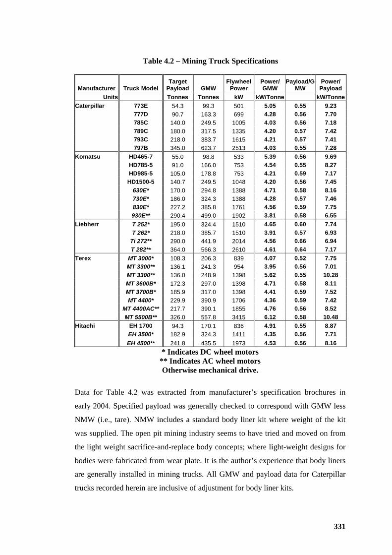
331
Table 4.2 – Mining Truck Specifications
Manufacturer Truck Model Target
Payload GMW Flywheel
Power Power/ GMW
Payload/GMW
Power/ Payload
Units Tonnes Tonnes kW kW/Tonne kW/Tonne Caterpillar 773E 54.3 99.3 501 5.05 0.55 9.23 777D 90.7 163.3 699 4.28 0.56 7.70 785C 140.0 249.5 1005 4.03 0.56 7.18 789C 180.0 317.5 1335 4.20 0.57 7.42 793C 218.0 383.7 1615 4.21 0.57 7.41 797B 345.0 623.7 2513 4.03 0.55 7.28 Komatsu HD465-7 55.0 98.8 533 5.39 0.56 9.69 HD785-5 91.0 166.0 753 4.54 0.55 8.27 HD985-5 105.0 178.8 753 4.21 0.59 7.17 HD1500-5 140.7 249.5 1048 4.20 0.56 7.45 630E* 170.0 294.8 1388 4.71 0.58 8.16 730E* 186.0 324.3 1388 4.28 0.57 7.46 830E* 227.2 385.8 1761 4.56 0.59 7.75 930E** 290.4 499.0 1902 3.81 0.58 6.55 Liebherr T 252* 195.0 324.4 1510 4.65 0.60 7.74 T 262* 218.0 385.7 1510 3.91 0.57 6.93 Ti 272** 290.0 441.9 2014 4.56 0.66 6.94 T 282** 364.0 566.3 2610 4.61 0.64 7.17 Terex MT 3000* 108.3 206.3 839 4.07 0.52 7.75 MT 3300** 136.1 241.3 954 3.95 0.56 7.01 MT 3300** 136.0 248.9 1398 5.62 0.55 10.28 MT 3600B* 172.3 297.0 1398 4.71 0.58 8.11 MT 3700B* 185.9 317.0 1398 4.41 0.59 7.52 MT 4400* 229.9 390.9 1706 4.36 0.59 7.42 MT 4400AC** 217.7 390.1 1855 4.76 0.56 8.52 MT 5500B** 326.0 557.8 3415 6.12 0.58 10.48 Hitachi EH 1700 94.3 170.1 836 4.91 0.55 8.87 EH 3500* 182.9 324.3 1411 4.35 0.56 7.71 EH 4500** 241.8 435.5 1973 4.53 0.56 8.16
* Indicates DC wheel motors ** Indicates AC wheel motors Otherwise mechanical drive.
Data for Table 4.2 was extracted from manufacturer’s specification brochures in
early 2004. Specified payload was generally checked to correspond with GMW less
NMW (i.e., tare). NMW includes a standard body liner kit where weight of the kit
was supplied. The open pit mining industry seems to have tried and moved on from
the light weight sacrifice-and-replace body concepts; where light-weight designs for
bodies were fabricated from wear plate. It is the author’s experience that body liners
are generally installed in mining trucks. All GMW and payload data for Caterpillar
trucks recorded herein are inclusive of adjustment for body liner kits.
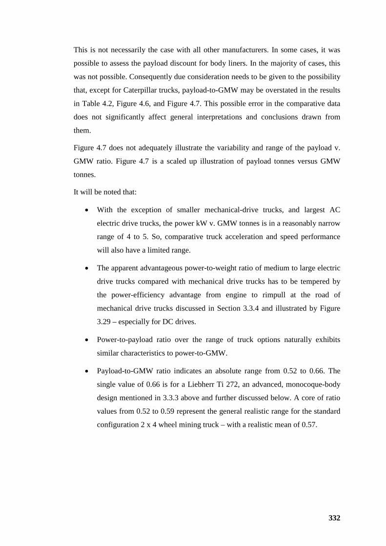
332
This is not necessarily the case with all other manufacturers. In some cases, it was
possible to assess the payload discount for body liners. In the majority of cases, this
was not possible. Consequently due consideration needs to be given to the possibility
that, except for Caterpillar trucks, payload-to-GMW may be overstated in the results
in Table 4.2, Figure 4.6, and Figure 4.7. This possible error in the comparative data
does not significantly affect general interpretations and conclusions drawn from
them.
Figure 4.7 does not adequately illustrate the variability and range of the payload v.
GMW ratio. Figure 4.7 is a scaled up illustration of payload tonnes versus GMW
tonnes.
It will be noted that:
• With the exception of smaller mechanical-drive trucks, and largest AC
electric drive trucks, the power kW v. GMW tonnes is in a reasonably narrow
range of 4 to 5. So, comparative truck acceleration and speed performance
will also have a limited range.
• The apparent advantageous power-to-weight ratio of medium to large electric
drive trucks compared with mechanical drive trucks has to be tempered by
the power-efficiency advantage from engine to rimpull at the road of
mechanical drive trucks discussed in Section 3.3.4 and illustrated by Figure
3.29 – especially for DC drives.
• Power-to-payload ratio over the range of truck options naturally exhibits
similar characteristics to power-to-GMW.
• Payload-to-GMW ratio indicates an absolute range from 0.52 to 0.66. The
single value of 0.66 is for a Liebherr Ti 272, an advanced, monocoque-body
design mentioned in 3.3.3 above and further discussed below. A core of ratio
values from 0.52 to 0.59 represent the general realistic range for the standard
configuration 2 x 4 wheel mining truck – with a realistic mean of 0.57.
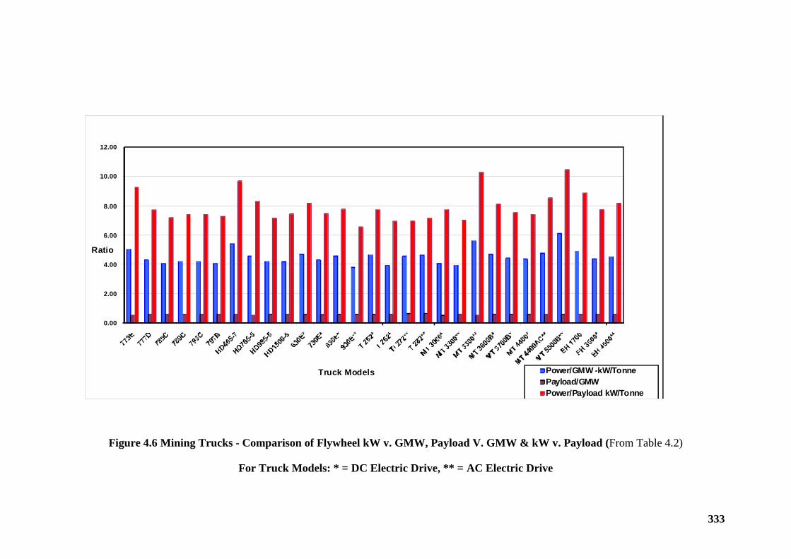
333
0.00
2.00
4.00
6.00
8.00
10.00
12.00
Ratio
Truck Models Power/GMW -kW/TonnePayload/GMWPower/Payload kW/Tonne
Figure 4.6 Mining Trucks - Comparison of Flywheel kW v. GMW, Payload V. GMW & kW v. Payload (From Table 4.2)
For Truck Models: * = DC Electric Drive, ** = AC Electric Drive
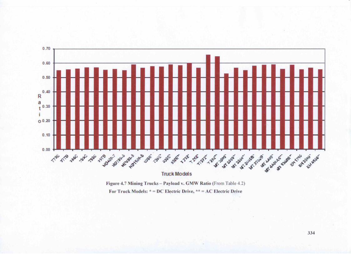
335
Adding power to a mining truck increases rimpull thus increasing acceleration and
speed. But addition of power comes at a cost including:
• Measurable additional fuel burn and associated lube service costs.
• Potential tyre life reduction due to additional torque to produce the rimpull –
the largest truck tyres exhibit tendency to shoulder separations associated
with wall deformation resulting from acceleration torque and transverse
distortion due to thrust loads at corners that are more critical as trucks
increase in size (Cutler, 2002).
• A small increase in NMW in the order of 1 to 2 tonnes.
• Also, increased speed is accompanied by higher impact stresses through
suspension and frame.
If existing truck designs cannot accommodate all resulting increased dynamic
stresses, there may be need for structural upgrading and suspension up-rating,
causing increased GMW.
Experience indicates that apparent significant increased capability in any one
operating function tends to be offset, at least partially, by a decrease in performance
and/or marginally increased cost. Apparent beneficial features of truck options
revealed by due diligence and detailed investigation are generally partly or totally
offset by compensating side effects that will be discovered by penetrating research.
In summary, due diligence and investigation of truck options are an absolute
necessity for reliable equipment selection. Investigation must be exhaustive with the
realisation that, for every apparent attractive feature of a specific truck, there will
likely be offsetting features that necessarily need to be discovered.
4.1.5.2 Loading Equipment
A sample of electric rope shovels and hydraulic shovels offered by principal
manufacturers are listed in Table 4.3. Figure 4.8 illustrates comparative criteria
indicating relative performance of shovels, viz.,
• Operating weight (GMW) tonnes versus rated bucket cubic metres. Rated
bucket cubic metres are struck for electric rope shovels and SAE heaped 2:1
for hydraulic shovels and excavators.
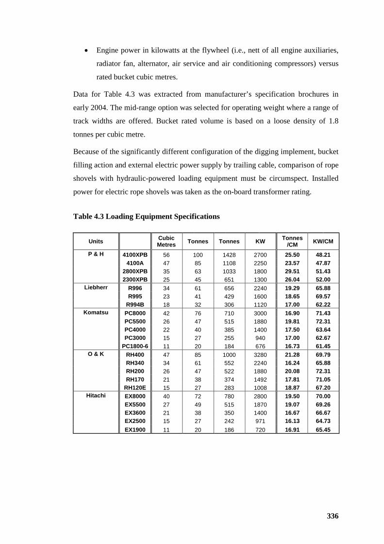
336
• Engine power in kilowatts at the flywheel (i.e., nett of all engine auxiliaries,
radiator fan, alternator, air service and air conditioning compressors) versus
rated bucket cubic metres.
Data for Table 4.3 was extracted from manufacturer’s specification brochures in
early 2004. The mid-range option was selected for operating weight where a range of
track widths are offered. Bucket rated volume is based on a loose density of 1.8
tonnes per cubic metre.
Because of the significantly different configuration of the digging implement, bucket
filling action and external electric power supply by trailing cable, comparison of rope
shovels with hydraulic-powered loading equipment must be circumspect. Installed
power for electric rope shovels was taken as the on-board transformer rating.
Table 4.3 Loading Equipment Specifications
Units Cubic Metres Tonnes Tonnes KW Tonnes
/CM KW/CM
P & H 4100XPB 56 100 1428 2700 25.50 48.21 4100A 47 85 1108 2250 23.57 47.87 2800XPB 35 63 1033 1800 29.51 51.43 2300XPB 25 45 651 1300 26.04 52.00
Liebherr R996 34 61 656 2240 19.29 65.88 R995 23 41 429 1600 18.65 69.57 R994B 18 32 306 1120 17.00 62.22
Komatsu PC8000 42 76 710 3000 16.90 71.43 PC5500 26 47 515 1880 19.81 72.31 PC4000 22 40 385 1400 17.50 63.64 PC3000 15 27 255 940 17.00 62.67 PC1800-6 11 20 184 676 16.73 61.45
O & K RH400 47 85 1000 3280 21.28 69.79 RH340 34 61 552 2240 16.24 65.88 RH200 26 47 522 1880 20.08 72.31 RH170 21 38 374 1492 17.81 71.05 RH120E 15 27 283 1008 18.87 67.20
Hitachi EX8000 40 72 780 2800 19.50 70.00 EX5500 27 49 515 1870 19.07 69.26 EX3600 21 38 350 1400 16.67 66.67 EX2500 15 27 242 971 16.13 64.73 EX1900 11 20 186 720 16.91 65.45
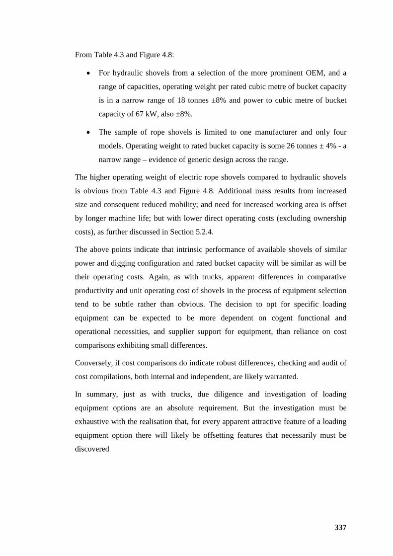
337
From Table 4.3 and Figure 4.8:
• For hydraulic shovels from a selection of the more prominent OEM, and a
range of capacities, operating weight per rated cubic metre of bucket capacity
is in a narrow range of 18 tonnes ±8% and power to cubic metre of bucket
capacity of 67 kW, also ±8%.
• The sample of rope shovels is limited to one manufacturer and only four
models. Operating weight to rated bucket capacity is some 26 tonnes ± 4% - a
narrow range – evidence of generic design across the range.
The higher operating weight of electric rope shovels compared to hydraulic shovels
is obvious from Table 4.3 and Figure 4.8. Additional mass results from increased
size and consequent reduced mobility; and need for increased working area is offset
by longer machine life; but with lower direct operating costs (excluding ownership
costs), as further discussed in Section 5.2.4.
The above points indicate that intrinsic performance of available shovels of similar
power and digging configuration and rated bucket capacity will be similar as will be
their operating costs. Again, as with trucks, apparent differences in comparative
productivity and unit operating cost of shovels in the process of equipment selection
tend to be subtle rather than obvious. The decision to opt for specific loading
equipment can be expected to be more dependent on cogent functional and
operational necessities, and supplier support for equipment, than reliance on cost
comparisons exhibiting small differences.
Conversely, if cost comparisons do indicate robust differences, checking and audit of
cost compilations, both internal and independent, are likely warranted.
In summary, just as with trucks, due diligence and investigation of loading
equipment options are an absolute requirement. But the investigation must be
exhaustive with the realisation that, for every apparent attractive feature of a loading
equipment option there will likely be offsetting features that necessarily must be
discovered
338
0.00
10.00
20.00
30.00
40.00
50.00
60.00
70.00
80.00
90.00
100.00
Shovel Model
Operating Weight Tonnes Per Bucket CM
Flywheel kW Per Bucket C M
4100??? = P & HR??? = LiebherrPC???? = KomatsuRH??? = O & KEX???? = Hitachi
Electric Rope Shovels Hydraulic Shovels & Backhoes
Figure 4.8 Loading Equipment - Comparison of Flywheel kW and Operating Weight
Per Bucket Cubic Metre (From Table 4.3)
Ope
ratin
g W
eigh
t per
Buc
ket C
M
kW p
er B
ucke
t CM
339
Wheel Loaders
Large wheel loaders still enjoy a small market share for loading large mining trucks.
Examples of wheel loaders with mechanical drive and hydraulic-powered loading
implements are available to 205 tonnes operating mass and nominal 36 tonnes bucket
capacity with the market favourite at 190 tonnes operating weight and nominal 34
tonnes bucket capacity. High lift configurations for loading large mining trucks are
some 1% heavier and nominal bucket capacity is reduced by some 5%. Electric
wheel loaders with hydraulic powered loading implements are available to 245
tonnes with bucket capacity of 72 tonnes.
Wheel loaders have mobility, advantageous in multi-pit operations, to clean up small
quantities, to finish up to a face allowing less mobile shovels, including electric rope
shovels, to move to a new digging location avoiding delays in clearing an area for
blasting. There are applications of large wheel loaders as the prime loading
equipment in waste stripping and bulk mining operations. But, application of loaders
for bulk of production is generally rare compared with rope shovels, hydraulic
shovels and excavators.
For the purposes of research, analysis was confined to shovels.
4.2 LARGER MINING EQUIPMENT
Diminishing prices for commodities, with the subsequent need to increase operating
scale, and the demand for larger mining equipment to realize decreased costs, was
discussed in Section 2.3.2.
Consequently the focus of the open pit mining industry has been on larger equipment
with the objective of reducing unit-mining costs. More recently, the thrust for ever-
increasing scale of mining equipment has been tempered by the realization that cost
benefits of increasing scale tend to diminish as evidenced in technical literature.
“There are indications that some difficulties have accompanied the introduction of
larger equipment into mines such as complexity, dilution, lost production and
reduction of flexibility.” (Bozorgebrahimi, 2003).
4.2.1 Introduction
340
Benefits by way of reduced unit cost per tonne mined from larger equipment are
uncertain. There is suggestion that “the size of haul trucks and excavators has
reached a feasibility threshold where the economies of scale have peaked” –
attributed to the RAND Institute (Bozorgebrahimi, 2003).
Significant issues arising from increasing loading and hauling equipment scale are
discussed and analyzed in Sections 4.2.2 to 4.2.5.
The reducing cost-driven development of “ultra-class” (UC) mining trucks - 290
tonnes and higher payloads - was discussed in Section 2.1.3 and illustrated by Figure
2.1. Causes for diminishing haulage unit-cost-benefits with increasing truck size can
be reasoned from discussions and comparative data tabulated and illustrated in
Section 4.1.5. Similar ratios for power v. GMW, power v. payload; and payload v.
GMW over the range of mining trucks, including UC trucks, from different OEM,
illustrated by Figures 4.6, and 4.7, are a basis for understanding that performance of
conventional mining trucks per tonne of payload tends to be practically uniform.
Cost drivers for operating mining trucks can be conveniently categorized as:
1. Owning costs, including capital amortization, insurance and interest cost of
capital.
2. Fuel
3. Lubricants and filters.
4. Maintenance, including component rebuilds and labour to remove, repair and
replace.
5. Service labour for fuelling, daily top ups, inspections, field checks and
opportune minor repairs, supervision and management.
6. Tyres – replacement and management, including labour.
7. Operating labour.
Other authors and sources may use more detailed categories than the seven listed
above. But for the purposes of the research the above seven categories are convenient
and sufficient.
4.2.2 Diminishing Cost Benefit
341
4.2.2.1 Fuel Consumption per Payload Tonne per Kilometre Constancy
Fuel consumption per tonne of payload, per kilometre of one-way haul, is practically
independent of truck size and haul distance for open pits of comparative geometrical
configuration. Fuel consumption per tonne - km over a range of truck payload
capacities and haul distances is shown in Table 3.63, and illustrated by Figure 3.60.
The standard measure for fuel consumption of diesel engines is Brake Specific Fuel
Consumption (BSF) expressed as litres-per-kW or grams-per-kW of fuel, with air at
250 standard temperature, 99 kPa pressure, diesel fuel with specific gravity 0.84 and
viscosity compliant with API (American Petroleum Institute) standard gravity of 35.
This is a hypothetical test condition where engines are dynamometer tested
specifically for BSFC. In practical application, fuel is at a fuel tank temperature that
is a derivative of ambient operating temperature and bypass fuel temperature
returning to the tank. Resulting fuel temperature as delivered to the fuel pump tends
to build up to an equilibrium level significantly higher than ambient temperature. At
these higher temperatures, volume of fuel consumed for equivalent power is higher
than the standard BSFC. Tuning the engine for rated performance becomes more
difficult as operating temperature increases. Volumetric fuel consumption increases
with operating ambient temperatures. OEM’s offer a fuel-cooling option to reduce
volumetric consumption for large mining trucks operating in high ambient
conditions,
The term BSFC is historical rather than indicative of current practice in assessing
power rating of engines. Early testing of fuel consumption of engines involved
applying a friction brake to the engine output shaft, often on the periphery of the
flywheel, running the engine at constant measured speed, measuring brake torque,
deriving brake horsepower (BHP) and measuring fuel consumption – so BSFC.
Currently BSFC is derived during dynamometer testing of engine power output.
Engines being tested drive a hydraulic device that measures engine torque providing
similar facility as the historical “brake”.
Table 4.4 lists typical practical fuel consumptions in litres per kW for Caterpillar
mining trucks inclusive of all practical operating allowances. These data are
indicative only. Mining trucks from other manufacturers can be expected to exhibit
similar specific fuel consumption performance. BSFC data in Table 4.4 show the
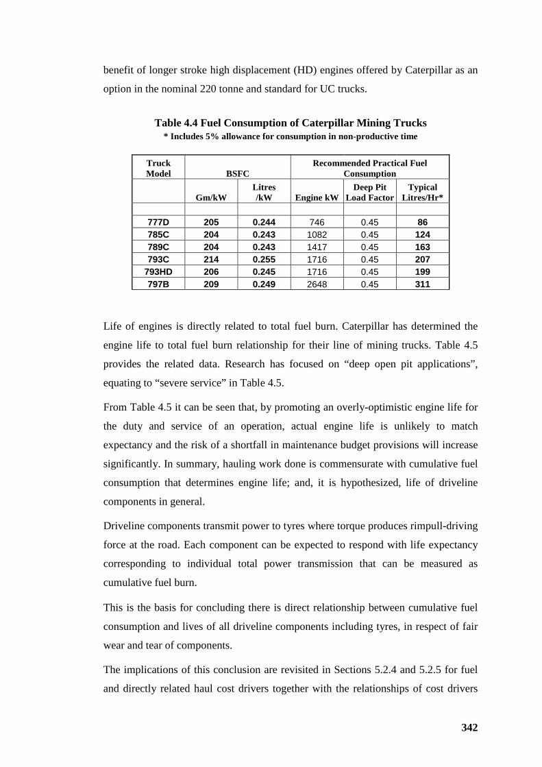
342
benefit of longer stroke high displacement (HD) engines offered by Caterpillar as an
option in the nominal 220 tonne and standard for UC trucks.
Table 4.4 Fuel Consumption of Caterpillar Mining Trucks
* Includes 5% allowance for consumption in non-productive time
Truck Model BSFC
Recommended Practical Fuel Consumption
Gm/kW Litres /kW Engine kW
Deep Pit Load Factor
Typical Litres/Hr*
777D 205 0.244 746 0.45 86 785C 204 0.243 1082 0.45 124 789C 204 0.243 1417 0.45 163 793C 214 0.255 1716 0.45 207
793HD 206 0.245 1716 0.45 199 797B 209 0.249 2648 0.45 311
Life of engines is directly related to total fuel burn. Caterpillar has determined the
engine life to total fuel burn relationship for their line of mining trucks. Table 4.5
provides the related data. Research has focused on “deep open pit applications”,
equating to “severe service” in Table 4.5.
From Table 4.5 it can be seen that, by promoting an overly-optimistic engine life for
the duty and service of an operation, actual engine life is unlikely to match
expectancy and the risk of a shortfall in maintenance budget provisions will increase
significantly. In summary, hauling work done is commensurate with cumulative fuel
consumption that determines engine life; and, it is hypothesized, life of driveline
components in general.
Driveline components transmit power to tyres where torque produces rimpull-driving
force at the road. Each component can be expected to respond with life expectancy
corresponding to individual total power transmission that can be measured as
cumulative fuel burn.
This is the basis for concluding there is direct relationship between cumulative fuel
consumption and lives of all driveline components including tyres, in respect of fair
wear and tear of components.
The implications of this conclusion are revisited in Sections 5.2.4 and 5.2.5 for fuel
and directly related haul cost drivers together with the relationships of cost drivers
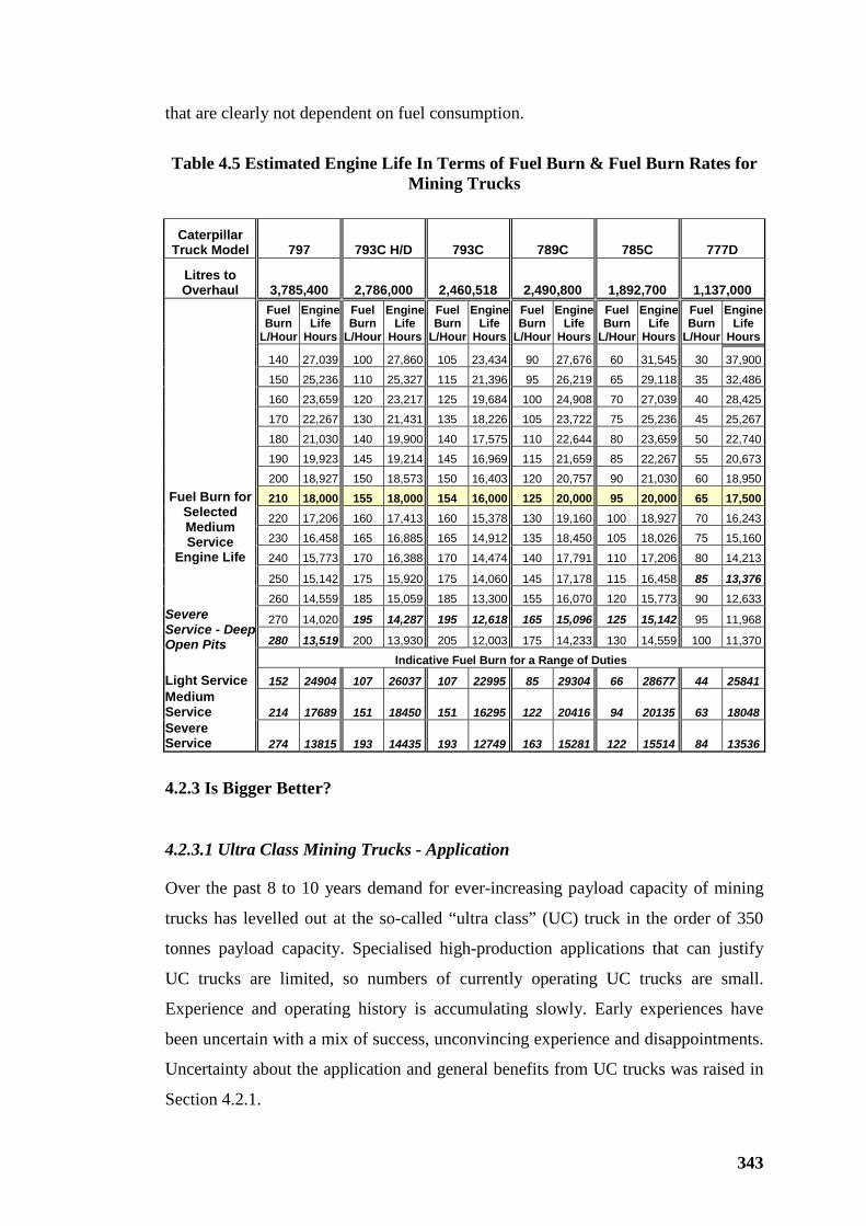
343
that are clearly not dependent on fuel consumption.
Table 4.5 Estimated Engine Life In Terms of Fuel Burn & Fuel Burn Rates for
Mining Trucks
Caterpillar Truck Model 797 793C H/D 793C 789C 785C 777D
Litres to Overhaul 3,785,400 2,786,000 2,460,518 2,490,800 1,892,700 1,137,000
Fuel Burn
L/Hour
Engine Life
Hours
Fuel Burn
L/Hour
Engine Life
Hours
Fuel Burn
L/Hour
Engine Life
Hours
Fuel Burn
L/Hour
Engine Life
Hours
Fuel Burn
L/Hour
Engine Life
Hours
Fuel Burn
L/Hour
Engine Life
Hours
140 27,039 100 27,860 105 23,434 90 27,676 60 31,545 30 37,900
150 25,236 110 25,327 115 21,396 95 26,219 65 29,118 35 32,486
160 23,659 120 23,217 125 19,684 100 24,908 70 27,039 40 28,425
170 22,267 130 21,431 135 18,226 105 23,722 75 25,236 45 25,267
180 21,030 140 19,900 140 17,575 110 22,644 80 23,659 50 22,740
190 19,923 145 19,214 145 16,969 115 21,659 85 22,267 55 20,673
200 18,927 150 18,573 150 16,403 120 20,757 90 21,030 60 18,950 Fuel Burn for
Selected Medium Service
Engine Life
210 18,000 155 18,000 154 16,000 125 20,000 95 20,000 65 17,500 220 17,206 160 17,413 160 15,378 130 19,160 100 18,927 70 16,243
230 16,458 165 16,885 165 14,912 135 18,450 105 18,026 75 15,160
240 15,773 170 16,388 170 14,474 140 17,791 110 17,206 80 14,213
250 15,142 175 15,920 175 14,060 145 17,178 115 16,458 85 13,376 260 14,559 185 15,059 185 13,300 155 16,070 120 15,773 90 12,633 Severe Service - Deep Open Pits
270 14,020 195 14,287 195 12,618 165 15,096 125 15,142 95 11,968
280 13,519 200 13,930 205 12,003 175 14,233 130 14,559 100 11,370
Indicative Fuel Burn for a Range of Duties
Light Service 152 24904 107 26037 107 22995 85 29304 66 28677 44 25841 Medium Service 214 17689 151 18450 151 16295 122 20416 94 20135 63 18048 Severe Service 274 13815 193 14435 193 12749 163 15281 122 15514 84 13536
4.2.3.1 Ultra Class Mining Trucks - Application
Over the past 8 to 10 years demand for ever-increasing payload capacity of mining
trucks has levelled out at the so-called “ultra class” (UC) truck in the order of 350
tonnes payload capacity. Specialised high-production applications that can justify
UC trucks are limited, so numbers of currently operating UC trucks are small.
Experience and operating history is accumulating slowly. Early experiences have
been uncertain with a mix of success, unconvincing experience and disappointments.
Uncertainty about the application and general benefits from UC trucks was raised in
Section 4.2.1.
4.2.3 Is Bigger Better?
344
UC trucks were first offered in the late 1990’s. Demand for UC trucks has increased
in the past five years with recent operating experience leading to uncertainty and the
question: “Is bigger better?” Articles in mining commercial literature, such as World
Mining Equipment, September 2002 issue, featuring a number of reports of UC truck
purchases and applications, have addressed this question in journalistic terms rather
than technically analytical treatments.
Bristol Voss (2001) reporting on a seminar at Alberta University, Canada quoted
Gerry Krause of Syncrude (tar sands mining in Canada) when he commented on
some common concerns with UC trucks. Krause was reported as follows: “Is going
from a fleet of eight small trucks to four large trucks the same as going from a fleet
of 120 small trucks to 60 large trucks?” Further points attributed to Krause included:
• Out-of-service trucks have significantly more a-productive effect on small
fleets.
• Larger trucks require wider haul roads with a total mining volume penalty in
deep open pits.
• Strip coalmines might find large trucks economic where a kimberlite pipe
diamond mine (≡ “deep open pit”) may not.
• Capitalization of the whole system of supporting facilities that must be
compatible with larger trucks becomes more significant.
• Road construction and maintenance equipment must be upgraded for larger
trucks.
• Tyre performance for UC trucks has been disappointing with the learning
curve of operators and suppliers still trending upwards.
• Impacts on mine planning for UC trucks that need larger manœuvring areas.
(Voss, 2001)
General conclusions on UC trucks in summary:
• UC trucks are only acceptably effective for specialised, high-volume
operations – deep open pits are unlikely to justify the adoption of UC trucks
at this stage of development.
345
• UC trucks are not a panacea for reducing mine-haulage costs in any but a
small number of specialised, large scale operating conditions.
• Replacing a fleet of smaller trucks with equivalent payload capacity of fewer
UC trucks is unlikely to improve total production or reduce unit-operating
costs – any cost benefit will be realized from reduced investment in
infrastructure and associated ongoing costs.
• Mixed fleets of UC and smaller trucks are unlikely to deliver any significant
unit cost benefit. It is more likely that the mix of performances will inhibit
“rhythm” of hauling operations and excessive bunching inefficiency is likely
an unacceptable risk.
In short: “greenfields”, large-scale bulk mining operations without extended steep
grades suit UC mining trucks. Otherwise, trucks in the nominal 220 tonne range are
likely a reasonable practical limit to be exceeded only with due caution for the truck
options currently available.
Significant issues for up-sizing mining trucks were also discussed by the author in a
paper published in 2003. (Hardy#2, 2003). Engineering effort must address
accommodation of larger mining trucks within detailed pit plans by increasing ramp
dimensions and upgrading haul-road construction specifications to accommodate
increased GMW. Also, servicing facilities, tooling and equipment require an
exponential improvement as trucks approach UC specifications. The general effect of
the management accommodations for increasing truck scale is illustrated by Figure
4.9, an amended version of Figure 2.1, referred to in Section 4.2.2.
The additional trend lines indicate possible outcomes from mine planning
accommodations of larger trucks and a further accommodation for infrastructure
upsizing. The tendency for the additional “accommodation” costs for UC mining
trucks is diagrammatically indicated by the upward trends and the uncertainty of the
relative haul costs of UC trucks by the query – “?”.
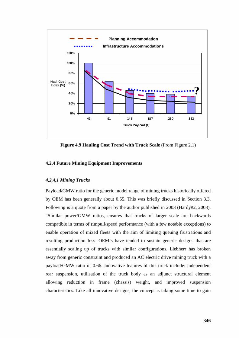
346
0%
20%
40%
60%
80%
100%
120%
49 91 146 187 230 353
Haul Cost Index (%)
Truck Payload (t)
Figure 4.9 Hauling Cost Trend with Truck Scale (From Figure 2.1)
4,2,4,1 Mining Trucks
Payload/GMW ratio for the generic model range of mining trucks historically offered
by OEM has been generally about 0.55. This was briefly discussed in Section 3.3.
Following is a quote from a paper by the author published in 2003 (Hardy#2, 2003).
“Similar power/GMW ratios, ensures that trucks of larger scale are backwards
compatible in terms of rimpull/speed performance (with a few notable exceptions) to
enable operation of mixed fleets with the aim of limiting queuing frustrations and
resulting production loss. OEM’s have tended to sustain generic designs that are
essentially scaling up of trucks with similar configurations. Liebherr has broken
away from generic constraint and produced an AC electric drive mining truck with a
payload/GMW ratio of 0.66. Innovative features of this truck include: independent
rear suspension, utilisation of the truck body as an adjunct structural element
allowing reduction in frame (chassis) weight, and improved suspension
characteristics. Like all innovative designs, the concept is taking some time to gain
4.2.4 Future Mining Equipment Improvements
?
Planning Accommodation
Infrastructure Accommodations
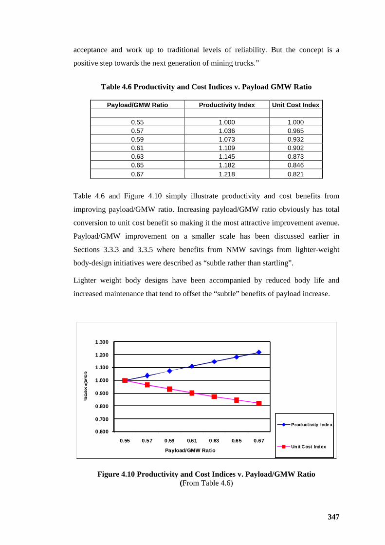
347
acceptance and work up to traditional levels of reliability. But the concept is a
positive step towards the next generation of mining trucks.”
Table 4.6 Productivity and Cost Indices v. Payload GMW Ratio
Payload/GMW Ratio Productivity Index Unit Cost Index
0.55 1.000 1.000 0.57 1.036 0.965 0.59 1.073 0.932 0.61 1.109 0.902 0.63 1.145 0.873 0.65 1.182 0.846 0.67 1.218 0.821
Table 4.6 and Figure 4.10 simply illustrate productivity and cost benefits from
improving payload/GMW ratio. Increasing payload/GMW ratio obviously has total
conversion to unit cost benefit so making it the most attractive improvement avenue.
Payload/GMW improvement on a smaller scale has been discussed earlier in
Sections 3.3.3 and 3.3.5 where benefits from NMW savings from lighter-weight
body-design initiatives were described as “subtle rather than startling”.
Lighter weight body designs have been accompanied by reduced body life and
increased maintenance that tend to offset the “subtle” benefits of payload increase.
0.600
0.700
0.800
0.900
1.000
1.100
1.200
1.300
0.55 0.57 0.59 0.61 0.63 0.65 0.67
Index Value
Payload/GMW Ratio
Productivity Inde x
Unit Cost Index
Figure 4.10 Productivity and Cost Indices v. Payload/GMW Ratio (From Table 4.6)
348
Other potential improvements, such as increasing power for enhanced up-ramp
speed, are subject to offsetting costs for fuel or power (trolley assist systems);
increased driveline component weight so increased GMW, albeit small, and
accelerated maintenance. Improvements involving increased operating speeds tend to
have a flow-on, accelerated maintenance cost through the entire vehicle including
frame and suspension. All of these offsetting limitations to improvement initiatives
for increased productivity increase the attraction of direct improvement by
significant design changes to mining truck configuration such as Liebherr’s Ti272
described in Section 3.3.3.
Mining equipment of the future will be expected to continue to accommodate ever-
reducing commodity prices - Figure 1.1 - and the consequent need for mining costs,
including haulage, to reduce and sustain acceptable profit margins.
The author’s opinion has not changed in respect of the potential for mining truck
improvement to deliver reduced haulage costs since first writing and publishing in
2003. OEM’s and the mining-truck supplier networks will continue to seek improved
performance aiming for reduced unit cost. Every little cost-saving contribution is
obviously beneficial. But mining truck development is at the stage where the more
radical design options, departures from generic design limitations, are more likely to
realize significant productivity and cost benefits.
4.2.4.2 Loading Equipment
Future focus for improved productivity and loading costs over the range of types and
bucket capacities of loading equipment is not as clearly defined as for mining trucks.
The ubiquitous electric rope shovel and its forerunner the steam shovel, initially
loading rail wagons in open pit mines, have a much longer history than mining
trucks. For applications such as strip coal mining, open pit iron ore mining and
similar bulk mining applications, where working areas are large, shovel relocations
infrequent and large bucket capacity is attractive, electric rope shovels continue to
enjoy market share. Improvements in rope shovels tend to be modest refinements and
adoption of enhanced electric power and control technology as it develops.
More recently developed hydraulic excavators and mining shovels are in a
continuous improvement phase with larger bucket capacities being offered to close
349
the capacity gap to the larger electric rope shovels. Diesel-powered hydraulic
systems are becoming more efficient so reducing fuel consumption.
The most attractive option for low capital and operating cost improvements is likely
reducing bucket cycle time, especially swing times with bucket loaded and empty.
These events are dependent on the cumulative installed power of slewing electric or
hydraulic motors that is only a proportion of the total power available at bucket
breakout in the digging segment of the bucket cycle. There are examples where both
electric and hydraulic shovel upgrades have included additional slewing
motor/transmission groups to retain bucket cycle time for larger bucket capacity that
in turn attracts structural/mechanical upgrade resulting in a heavier digging
implement group. It is a small design step to further enhance slewing power realizing
faster cycle time within practical limits. Operator comfort at faster slewing speeds
may become an issue. One solution could be for the operator’s cab to travel opposite
to the slew slowly over a small tangential distance to reduce effective slewing
acceleration and G force on the operator. Higher braking duty could be facilitated by
power regeneration, electrically or inert-gas-over-hydraulic accumulation. The
electrical and hydraulic engineering technology is available for increased slewing
acceleration and rotating speed.
During reading and collection of thoughts and ideas that have been expanded in the
research described herein, constancy and predictability of existing generic mining
truck designs became obvious. This initiated the idea that the profile of a 500 tonne
payload truck could be predicted by extrapolating characteristic criteria for mining
trucks.
The generic nature of current truck designs offered by OEM is shown to be
consistent and predictable by the following analysis.
Table 4.7 shows how equipment characteristics vary over the payload range of
Caterpillar mining trucks.
4.2.5 Hypothetical 500 Tonne Payload Truck
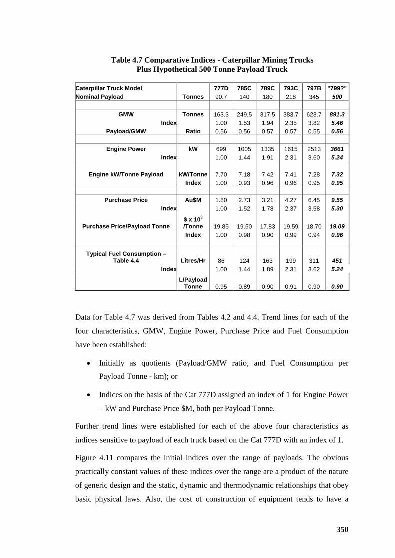
350
Table 4.7 Comparative Indices - Caterpillar Mining Trucks
Plus Hypothetical 500 Tonne Payload Truck Caterpillar Truck Model 777D 785C 789C 793C 797B "799?" Nominal Payload Tonnes 90.7 140 180 218 345 500
GMW Tonnes 163.3 249.5 317.5 383.7 623.7 891.3 Index 1.00 1.53 1.94 2.35 3.82 5.46
Payload/GMW Ratio 0.56 0.56 0.57 0.57 0.55 0.56
Engine Power kW 699 1005 1335 1615 2513 3661 Index 1.00 1.44 1.91 2.31 3.60 5.24
Engine kW/Tonne Payload kW/Tonne 7.70 7.18 7.42 7.41 7.28 7.32 Index 1.00 0.93 0.96 0.96 0.95 0.95
Purchase Price Au$M 1.80 2.73 3.21 4.27 6.45 9.55 Index 1.00 1.52 1.78 2.37 3.58 5.30
Purchase Price/Payload Tonne $ x 103
/Tonne 19.85 19.50 17.83 19.59 18.70 19.09 Index 1.00 0.98 0.90 0.99 0.94 0.96
Typical Fuel Consumption – Table 4.4 Litres/Hr 86 124 163 199 311 451
Index 1.00 1.44 1.89 2.31 3.62 5.24
L/Payload
Tonne 0.95 0.89 0.90 0.91 0.90 0.90
Data for Table 4.7 was derived from Tables 4.2 and 4.4. Trend lines for each of the
four characteristics, GMW, Engine Power, Purchase Price and Fuel Consumption
have been established:
• Initially as quotients (Payload/GMW ratio, and Fuel Consumption per
Payload Tonne - km); or
• Indices on the basis of the Cat 777D assigned an index of 1 for Engine Power
– kW and Purchase Price $M, both per Payload Tonne.
Further trend lines were established for each of the above four characteristics as
indices sensitive to payload of each truck based on the Cat 777D with an index of 1.
Figure 4.11 compares the initial indices over the range of payloads. The obvious
practically constant values of these indices over the range are a product of the nature
of generic design and the static, dynamic and thermodynamic relationships that obey
basic physical laws. Also, the cost of construction of equipment tends to have a
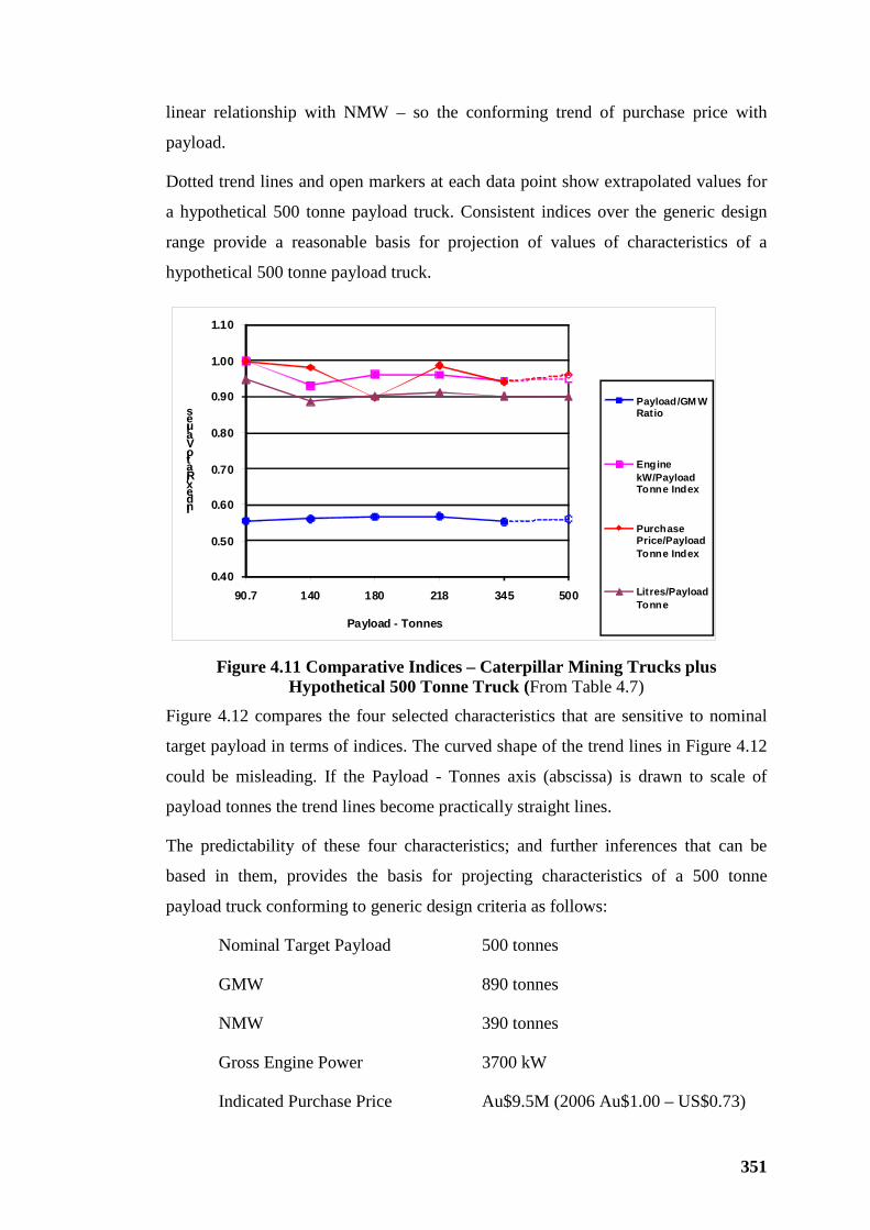
351
linear relationship with NMW – so the conforming trend of purchase price with
payload.
Dotted trend lines and open markers at each data point show extrapolated values for
a hypothetical 500 tonne payload truck. Consistent indices over the generic design
range provide a reasonable basis for projection of values of characteristics of a
hypothetical 500 tonne payload truck.
0.40
0.50
0.60
0.70
0.80
0.90
1.00
1.10
90.7 140 180 218 345 500
Index/Ratio Values
Payload - Tonnes
Payload/GM W Ratio
Engine kW/Payload Tonne Index
Purchase Price/Payload Tonne Index
Litres/Payload Tonne
Figure 4.11 Comparative Indices – Caterpillar Mining Trucks plus
Hypothetical 500 Tonne Truck (From Table 4.7)
Figure 4.12 compares the four selected characteristics that are sensitive to nominal
target payload in terms of indices. The curved shape of the trend lines in Figure 4.12
could be misleading. If the Payload - Tonnes axis (abscissa) is drawn to scale of
payload tonnes the trend lines become practically straight lines.
The predictability of these four characteristics; and further inferences that can be
based in them, provides the basis for projecting characteristics of a 500 tonne
payload truck conforming to generic design criteria as follows:
Nominal Target Payload 500 tonnes
GMW 890 tonnes
NMW 390 tonnes
Gross Engine Power 3700 kW
Indicated Purchase Price Au$9.5M (2006 Au$1.00 – US$0.73)
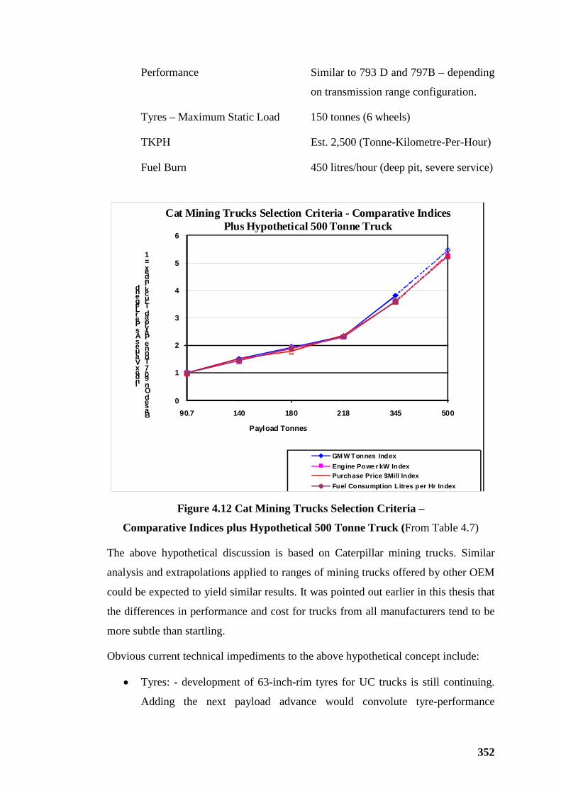
352
Performance Similar to 793 D and 797B – depending
on transmission range configuration.
Tyres – Maximum Static Load 150 tonnes (6 wheels)
TKPH Est. 2,500 (Tonne-Kilometre-Per-Hour)
Fuel Burn 450 litres/hour (deep pit, severe service)
0
1
2
3
4
5
6
90.7 140 180 218 345 500
Index Values As Per Legend
Based On 90.7 Tonne Payload Truck Index = 1
Payload Tonnes
Cat Mining Trucks Selection Criteria - Comparative Indices Plus Hypothetical 500 Tonne Truck
GM W Tonnes IndexEngine Powe r kW IndexPurchase Price $Mill IndexFuel Consumption Litres per Hr Index
Figure 4.12 Cat Mining Trucks Selection Criteria –
Comparative Indices plus Hypothetical 500 Tonne Truck (From Table 4.7)
The above hypothetical discussion is based on Caterpillar mining trucks. Similar
analysis and extrapolations applied to ranges of mining trucks offered by other OEM
could be expected to yield similar results. It was pointed out earlier in this thesis that
the differences in performance and cost for trucks from all manufacturers tend to be
more subtle than startling.
Obvious current technical impediments to the above hypothetical concept include:
• Tyres: - development of 63-inch-rim tyres for UC trucks is still continuing.
Adding the next payload advance would convolute tyre-performance
353
development and supply problems that currently are still being resolved.
Using 8 wheels with castor steering (existing technology) and possibly four-
wheel drive (AC electric drive) could be an option.
• Limited availability of high-speed – 1800 RPM – engines for mobile plant in
the required power range.
• Non-availability of mechanical transmissions; but AC traction systems from
electric powered railways could likely meet the power specification and be
adapted – similar to historical development of DC electric wheel motors for
mining trucks.
• Extrapolation of structural and mechanical designs would likely be
challenging – just as it has been for OEM in developing large through to UC
trucks – especially for drive wheel groups and truck bodies – to retain
generically similar performance and acceptable productivity.
From an applied research viewpoint the above discussion and predictions for a 500
tonne payload truck work are hypothetical - really “crystal-ball gazing”. But the
comparative tabulation and illustrations do reinforce, for trucks, that variable cost
components for hauling and loading equipment, when compared in terms of unit
costs, i.e., independent of truck payload or bucket load can be expected to be
predictable and practically constant.
Historically justification of adoption of trolley-assist mining-haulage systems needed
a significant gap between reconciled costs of diesel fuel and mains electric power for
haulage. Two recent events have closed the gap:
1. Development of more efficient AC power wheel motors in large and UC
mining trucks with retro-application to smaller capacity mining trucks.
2. Practically doubling of nett-of-tax diesel fuel price to large consumers over a
period of some four years to 2006, a continuing escalating trend.
4.2.6 Trolley Assist
354
Recent feasibility studies for deep open pits of medium to large production scale
have indicated that trolley-assist haulage is potentially cost beneficial.
It seems likely that future improvements to AC electric wheel drive systems have
potential to favour trolley assist, not only for enhanced up-ramp performance in deep
open pits, but also to reduce consumption of expensive diesel fuel.
Historically, inclusion of trolley-assist of DC drive trucks as an option in feasibility
studies for deep open pits generally revealed unacceptable risk in operation due to
rejects (overloaded trucks). A third lane on deep-pit ramps was required for rejected
loaded trucks travelling at lower speed. Cost of extra pit volume, together with
capitalization and on-going costs of the electrical reticulation system and trolley
equipment onboard trucks, at that time more-than-offset the apparent cost benefits
from increased productivity of trucks. Recent developments, including improved
power curve for AC drives, anecdotal evidence of improved reliability, improved
understanding of the need for controlled payload dispersion – to reduce over loading
and rejects - have elevated trolley assist to “potentially cost-beneficial”.
In the economic climate prevailing in the Australian mineral industry, trolley assist
has potential to extend mine life and recovered ore or product reserves for deep open
pits of the future. Certainly trolley assist should be an option carried forward in
feasibility studies until eliminated by economic and/or practical considerations.
4.2.7.1 Dispatch System Investment
Investigation of benefits from a site-specific dynamically-programmed dispatch
system (DS) should be integral with load-and-haul equipment selection. Benefits
from DS for moderate to large scale open pit mines generally justify investment.
Cost-benefit from efficient operation of truck haulage is an imperative as scale of
operations and equipment increases – Section 4.2.2. Initially located within sight of
open pit operations, DS have relocated to increasingly remote locations. Current
practice includes off-site locations in cities, in corporate offices or special purpose
facilities, centralizing dispatch control of a number of mines. It is technically
possible for dispatch staff to work from home linked by video and teleconferencing
to a DS; and to all relevant management links.
4.2.7 Dispatch Systems and Autonomous Load and Haul Equipment
355
4.2.7.2 Autonomous Mining Equipment
Remote dispatch control of load and haul equipment already exists. Underground
mining applications have adopted remote control by operators of mobile equipment
as a safety initiative. Development from remote control of equipment to autonomous
load and haul applications has been rapid with planning studies currently in progress
for completely autonomic systems of mining trucks, loading and support equipment.
Recent developments and trials of autonomous load-and-haul equipment, particularly
trucks are obviously socio-industrially and politically sensitive. Details of proposed
autonomous open pit systems were not available to the author. With performance and
cost information generally limited to hearsay at time of completion of the thesis, this
topic has not been researched. Further comments are provided in Section 6.1.6 and
8.2.
356
CHAPTER 5
LOAD AND HAUL COSTS
5.1 Basis of Cost Analyses and Discussion
5.1.1 Costs - A Snapshot In Time
Load and haul costs are the outcome of market-driven cost of goods and services that
are time-variable inputs to the cumulative cost of operating mining equipment. Cost
of operating loading equipment and mining trucks is time dependent. Unit load-and-
haul-cost outcomes are “a snapshot in time”. Cost of equipment items per operating
hour is dependent on both variable cost of goods and services and the, variable
operating duty of the mining equipment. For mining trucks and matching loading
equipment, operating duty is a function of open pit (or generally mine) geometry,
geographic location, meteorological operating environment and other factors
including industrial, human resources and socio-economic environments all of which
vary with time to some degree. Analysis of productivity and costs in this Chapter 5
are in terms of indices to facilitate comparisons, the time-dependence of which are
minimized.
5.1.2 Relative Importance of Cost Estimates
Experience with developing estimating costs for feasibility studies over the wide
range of precision and confidence levels; also for operating budget purposes,
provides understanding of the difficulty of comparing estimated costs for different
mining operations. Some degree of reconciliation is possible but the ultimate test for
mining operations is not on unit costs of operational functions or activities but how
the operation stacks up in the commodity market place. It is somewhat redundant to
compare estimated costs in detail for a project where the indicated total production
cost of a commodity falls in the lower quartile of producers worldwide. If the
feasibility study does not support development, there must be other impediments
such as poor business address with substantial sovereign risk or funding difficulties.
Drilling down to equipment selection criteria and focusing on cost comparisons, it is
the author’s experience that:
• Comparison of operating costs between mining operations involves complex
reconciliation with an outcome that always carries significant residual risk
357
unless the purpose and use that costs are transported between projects is
tolerant of substantial error between the estimates utilized and the ultimate
feasibility estimates or actual costs experienced.
• Differences in estimated or actual operating costs between items of loading or
hauling equipment with reasonably comparable performance, all other cost
influences being small, tend to be subtle rather than startling – as indicated
earlier in the thesis. It is conclusion that, for realization of expected
productivity and operating costs, non-pecuniary attributes such as reliability
and product support from suppliers need to be afforded substantial weight.
The above understandings lead to the conclusion that comparisons of cost estimates
for equipment selection purposes should be treated circumspectly, given limited
weight and should not be the sole basis for decisions. The obvious limitations of cost
estimates lead to the further conclusion that analysis is most conveniently served by
expressing and comparing costs in terms of comparative indices that are less time
dependent.
5.1.3 Basis of Cost Indices
For the purposes of discussions herein load and haul costs will be assumed to be
typically 50% of total mining costs as shown in Figure 2.2. Bruce Gregory
established the cost proportions in Figure 2.2 in 2002 (Gregory, 2002). Recently
there has been substantial volatility in fuel and tyre prices with significant increases.
Fuel-driven cost increases flow on to all manufactured goods, especially tyres. A
recent worldwide shortage of large earthmover tyres, which industry sources advise
is expected to last for several years, has elevated prices. Haul cost proportions
developed by Bruce Gregory (Gregory, 2002) have been adopted as a suitable basis
to factor up for comparative analysis.
All analysis to follow is in terms of cost indices. In order for the indices developed
and adopted for analysis to be reasonably indicative of current costs, Gregory’s 2002
haul cost proportions have been adjusted. Table 5.1 lists the original data and
compares original and adjusted proportions. Figures 5.1, 5.2, and 5.3, illustrate
successive adjustments to haul-cost proportions for increased cost of fuel and tyres.
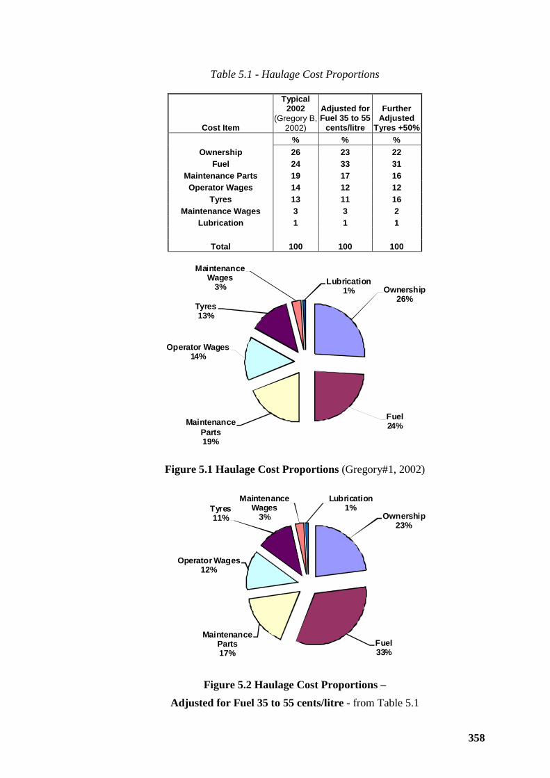
358
Ownership26%
Fuel24%Maintenance
Parts19%
Operator Wages14%
Tyres13%
Maintenance Wages
3% Lubrication1%
Figure 5.1 Haulage Cost Proportions (Gregory#1, 2002)
Ownership23%
Fuel33%
Maintenance Parts17%
Operator Wages12%
Tyres11%
Maintenance Wages
3%
Lubrication1%
Figure 5.2 Haulage Cost Proportions –
Adjusted for Fuel 35 to 55 cents/litre - from Table 5.1
Table 5.1 - Haulage Cost Proportions
Cost Item
Typical 2002
(Gregory B, 2002)
Adjusted for Fuel 35 to 55
cents/litre
Further Adjusted
Tyres +50% % % %
Ownership 26 23 22 Fuel 24 33 31
Maintenance Parts 19 17 16 Operator Wages 14 12 12
Tyres 13 11 16 Maintenance Wages 3 3 2
Lubrication 1 1 1
Total 100 100 100
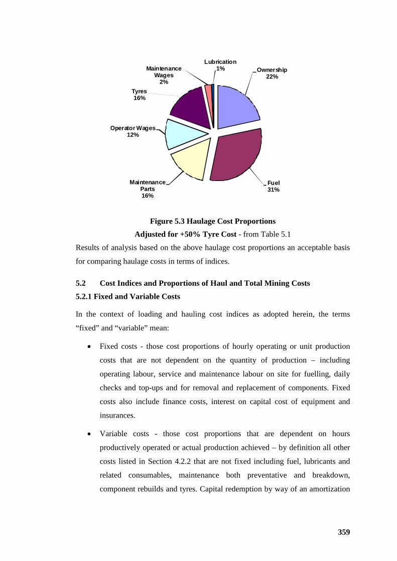
359
Ownership22%
Fuel31%
Maintenance Parts16%
Operator Wages12%
Tyres16%
Maintenance Wages
2%
Lubrication1%
Figure 5.3 Haulage Cost Proportions
Adjusted for +50% Tyre Cost - from Table 5.1
Results of analysis based on the above haulage cost proportions an acceptable basis
for comparing haulage costs in terms of indices.
5.2 Cost Indices and Proportions of Haul and Total Mining Costs
5.2.1 Fixed and Variable Costs
In the context of loading and hauling cost indices as adopted herein, the terms
“fixed” and “variable” mean:
• Fixed costs - those cost proportions of hourly operating or unit production
costs that are not dependent on the quantity of production – including
operating labour, service and maintenance labour on site for fuelling, daily
checks and top-ups and for removal and replacement of components. Fixed
costs also include finance costs, interest on capital cost of equipment and
insurances.
• Variable costs - those cost proportions that are dependent on hours
productively operated or actual production achieved – by definition all other
costs listed in Section 4.2.2 that are not fixed including fuel, lubricants and
related consumables, maintenance both preventative and breakdown,
component rebuilds and tyres. Capital redemption by way of an amortization
360
charge is considered as a variable cost for the purpose of comparing load-
and-haul costs.
The view taken herein of capital recovery costs for mining equipment is that capital
is redeemed as a charge per hour operated or per tonne produced as the case may be.
Recovery is over the assumed life of the equipment item with due allowance for
residual value, if any. Due deduction is made from the capital cost for consumable
items that are generally delivered with new equipment such as tyres on trucks and
ground engaging tools (GET) on shovels.
5.2.2 Capital Redemption
There is a gray area with deductions from capital costs for tyres on new trucks and
GET on shovels to established initial value for write-off. The line between
capitalized equipment cost and consumable cost is arbitrary. A clinical definition of
what constitutes capital value of an item of equipment could be based on whether the
component subject of a capital reduction has less life than assumed for capital
amortization – write-off – of the equipment item. For engines, transmissions, other
driveline componentry, lightweight truck bodies, shovel buckets, power transmission
componentry, hydraulic system components and electrical componentry that all have
a life-to-component-replacement, which is expensed at the time of replacement, there
could be a case for commensurate deductions for these components from initial book
value.
In short, and hypothetically, for the purposes of write-off, trucks and loading
equipment might be virtually stripped down to the frame. Basic componentry
expected to survive the full write-off period (conceptual equipment life) would be
depreciated according to tax statutes. All other components could be expensed over
expected individual component life, i.e., recovered by cost-provision accounting or
directly expensed as consumables. The effect would be accelerated write-off and
increased operating margin retention in the first one or two production years of a
project. A side benefit would be a closer correlation between market value (MV) and
written down value (WDV) – avoiding the potential need to bring a WDV loss to
account at equipment disposal.
Valid tax treatment of equipment write-off and acceptable accounting practice has
not been considered in the above discussion. Obviously, the direction of any further
361
research in respect of capital recovery requires consideration of legality and
corporate benefit of any accelerated (or deferred) asset write-off that might result.
5.2.3 Capital Recovery Risk
The following notes are from a paper published by the author in 2005 updating an
earlier paper on outsourcing or owner operating of mining operations (Hardy#3,
2005).
Owner operators and contract miners treat ownership cost of mining equipment
differently. A contractor writes off straight line, over an estimated life in hours, the
purchase price of equipment less residual value (and less any consumable deductions
such as tyres) based on expected market value (if any) at end of write-off period.
Theoretically, the point is reached where the written down value (WDV) equals the
residual value (RD), which in turn (hopefully) is not more than market value (MV).
For all mobile equipment, throughout its life MV is accepted as less than straight-line
WDV by a margin ranging from small to, say, 30% of original purchase value.
Caterpillar equipment appears to enjoy favourable resale value so a tendency for
reduced WDV – MV margins over machine life. Readily saleable equipment such as
off-highway trucks, graders, small loaders and excavators and sundry small mobile
plant generally realize minimum sale or trade-in value in the order of 15 %. Other
items including large excavators and loaders tend to realize lower values, (Perich,
2003).
So there is a risk for mine operators that, before reaching expected life, there could
be a gap between WDV and MV. Usually offsetting this risk to a significant degree
for mining contractors is the benefit of provision for component replacement and
associated maintenance and repair that accumulates because of an average hourly
maintenance cost for equipment items built into the scheduled prices. Provision
accounting has a two-fold benefit. It is a source of accumulated funds to be drawn
down when required for major planned maintenance, such as component
rebuild/replacement. Although not so intended, a provision account may also offset
any gap between MV and WDV in the event of premature disposal.
Owners generally write off at the allowable rate for tax purposes; and account for
depreciation accordingly. This avoids any accumulation (or over drawing) in the tax
equalization account that has to be brought to account as a profit (or loss) at some
362
future time. Tax write-off allowable for equipment has recently been amended to the
lesser of the life of the project or the term listed below:
Write offs under current tax rules: (available by search for TR 2000/18 C4 on the
Australian Tax Office website).
Equipment Description: Life: Years
Dozers 9
Electric Rope Shovels 25
Graders 10
Hydraulic Excavators 10
Lighting Plant 10
Off-highway Trucks 10
Scrapers 7
Wheel Loaders 8
In continuous mining operations (nominally 24 hours per day every day) main
production equipment accumulates between 5,000 to 6,500 productive operating
hours and up to 7,200 service meter units (SMU) per year, with larger equipment
generally reporting at the higher end of the range. Except for large electric shovels,
and to lesser degree hydraulic shovels, contractors will rarely estimate write-off life
of any item of even large equipment at more than 50,000 hours. This corresponds to
a maximum life of some eight years. Owner miners tend to write off at lower rates
than a contractor. Any difference between WDV and MV at time of sale or trade can
be carried forward by owners as a loss for tax purposes. But the net-of-tax loss to the
equipment owner will report in the year it occurs. Therefore there is potential for
owner miners to be reporting lower cash costs, and lower total costs with the
certainty that, at some future time, any accumulated depreciation cost loss will be
brought to account by a discrete loss and consequent reduction to future profit.
Figure 5.4 generally illustrates the analysis of capital-recovery risk. A reduced rate
of capital recovery is indicated in Figure 5.4 for owners to reflect the different
treatment of depreciation cost of assets. Owner miners will likely have a greater gap
between WDV and MV over much of the life of each item of equipment.
Owner miners must take the risk of any gap between MV and WDV in the event of a
premature shutdown of mining operations. In the balance, such risk for an owner (in
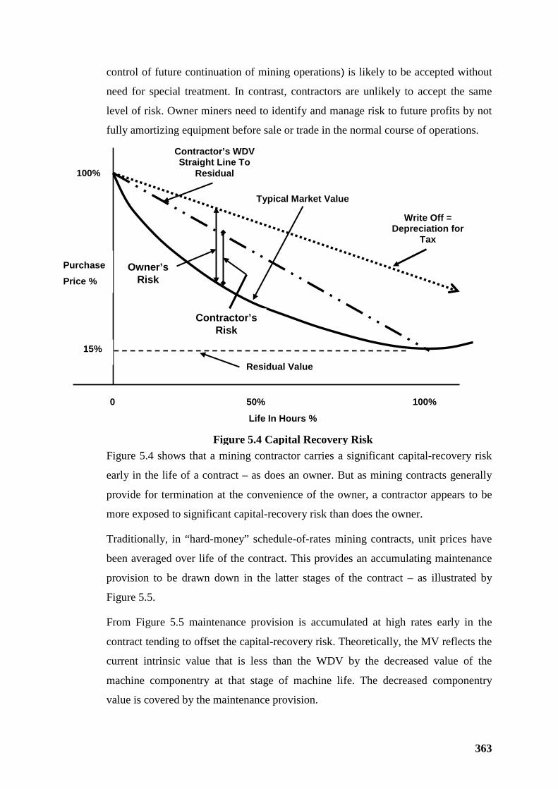
363
control of future continuation of mining operations) is likely to be accepted without
need for special treatment. In contrast, contractors are unlikely to accept the same
level of risk. Owner miners need to identify and manage risk to future profits by not
fully amortizing equipment before sale or trade in the normal course of operations.
Figure 5.4 shows that a mining contractor carries a significant capital-recovery risk
early in the life of a contract – as does an owner. But as mining contracts generally
provide for termination at the convenience of the owner, a contractor appears to be
more exposed to significant capital-recovery risk than does the owner.
Traditionally, in “hard-money” schedule-of-rates mining contracts, unit prices have
been averaged over life of the contract. This provides an accumulating maintenance
provision to be drawn down in the latter stages of the contract – as illustrated by
Figure 5.5.
From Figure 5.5 maintenance provision is accumulated at high rates early in the
contract tending to offset the capital-recovery risk. Theoretically, the MV reflects the
current intrinsic value that is less than the WDV by the decreased value of the
machine componentry at that stage of machine life. The decreased componentry
value is covered by the maintenance provision.
0 50% 100%
Life In Hours %
100%
15%
Purchase Price %
Contractor’s WDV Straight Line To
Residual
Residual Value
Typical Market Value
Write Off = Depreciation for
Tax
Owner’s Risk
Contractor’s Risk
Figure 5.4 Capital Recovery Risk
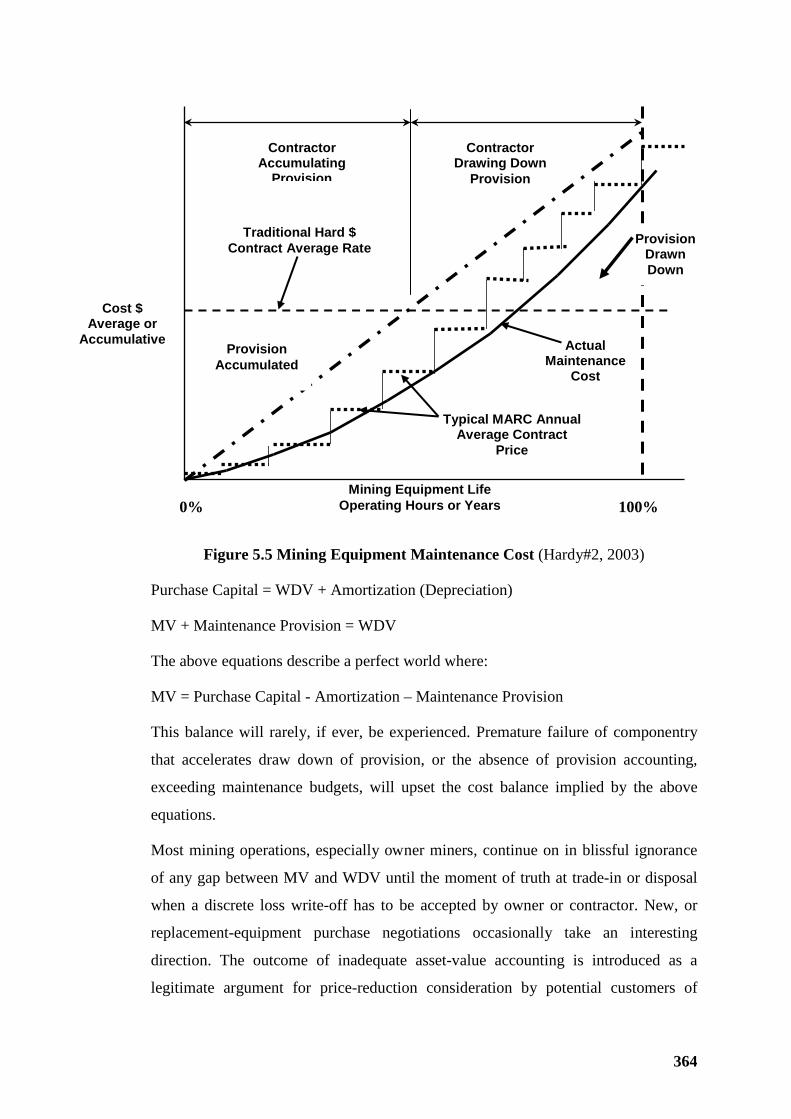
364
Figure 5.5 Mining Equipment Maintenance Cost (Hardy#2, 2003)
Purchase Capital = WDV + Amortization (Depreciation)
MV + Maintenance Provision = WDV
The above equations describe a perfect world where:
MV = Purchase Capital - Amortization – Maintenance Provision
This balance will rarely, if ever, be experienced. Premature failure of componentry
that accelerates draw down of provision, or the absence of provision accounting,
exceeding maintenance budgets, will upset the cost balance implied by the above
equations.
Most mining operations, especially owner miners, continue on in blissful ignorance
of any gap between MV and WDV until the moment of truth at trade-in or disposal
when a discrete loss write-off has to be accepted by owner or contractor. New, or
replacement-equipment purchase negotiations occasionally take an interesting
direction. The outcome of inadequate asset-value accounting is introduced as a
legitimate argument for price-reduction consideration by potential customers of
Mining Equipment Life Operating Hours or Years 0% 100%
Cost $ Average or
Accumulative
Contractor Accumulating
Provision
Contractor Drawing Down
Provision
Actual Maintenance
Cost
Typical MARC Annual Average Contract
Price
Provision Accumulated
Provision Drawn Down
Traditional Hard $ Contract Average Rate
365
OEM and dealers. Any gap between WDV and MV tends to be tabled by owners or
contractors during purchase negotiations. It is great credit to the parties involved in
new equipment deals that such invalid arguments are generally absorbed with
aplomb; eventually compromise is reached and a deal is done to the mutual
satisfaction of the parties.
Figure 5.5 illustrates that, any style of contract where remuneration terms reflect
actual maintenance costs incurred rather than average (including provision) costs,
effectively denies a mining contractor the de facto cover for capital-recovery risk in
the event of premature determination of the contract. Where a contractor establishes
maintenance provisions internally, it is generally viewed as a debt to an equipment
item. From this viewpoint, it is artificial to consider the same funding as cover for
capital recovery risk. But at the time of contract determination and equipment
disposal the MV will tend to reflect “as-is, where-is” value and any provision is then
available to cover the WDV - MV gap. If the contractor transfers the equipment to
alternative work, the provision covers future maintenance liability as intended. If,
through the remuneration process, a mining contractor does not receive maintenance
provision compensation then the capital-recovery exposure at contract termination-
of-convenience is a significant risk, likely more so than for an owner.
Nomination of a maintenance sub-contractor, novation or voluntary execution of a
MARC maintenance facility by a mining contractor has similar effect. MARC
maintenance facilities generally average prices annually with costs of component
rebuilds being included in cost estimates at pre-determined (sometimes warranted)
times. In effect, MARC pricing compiled cumulatively tends to parallel actual
cumulative costs. Figure 5.5 depicts cumulative trends. The step representation for a
MARC contract cost is a mix of constant annual charges with annual adjustments to
restore the cumulative MARC cost. In actual practice, practically constant monthly
payment for MARC services in each year should, more correctly, be depicted to
accumulate as a sequence of inclined trend lines.
5.2.4 Operating Cost Indices
Cost indices for haul operating states of production, waiting, standby without
operator and for extra operating time (improved efficiency within scheduled shift
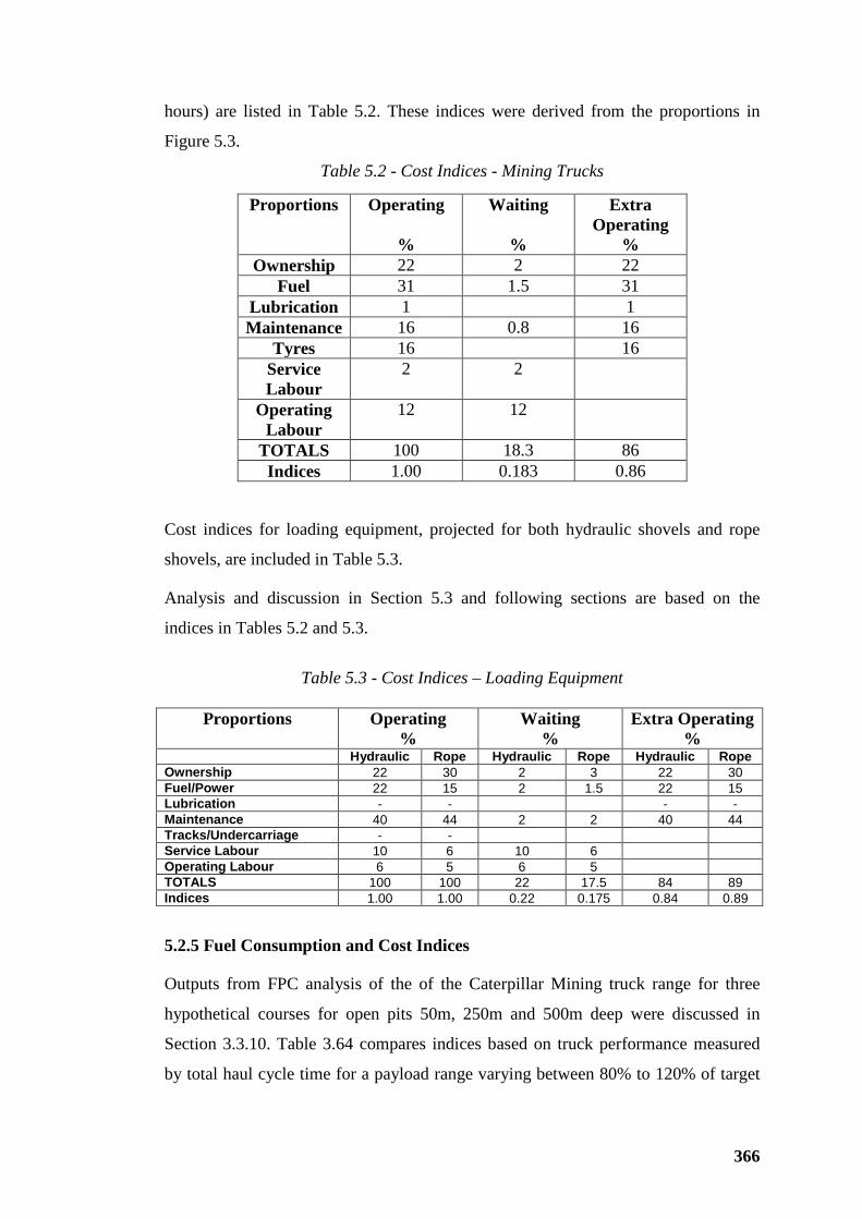
366
hours) are listed in Table 5.2. These indices were derived from the proportions in
Figure 5.3.
Table 5.2 - Cost Indices - Mining Trucks
Cost indices for loading equipment, projected for both hydraulic shovels and rope
shovels, are included in Table 5.3.
Analysis and discussion in Section 5.3 and following sections are based on the
indices in Tables 5.2 and 5.3.
Table 5.3 - Cost Indices – Loading Equipment
Proportions Operating
% Waiting
% Extra Operating
% Hydraulic Rope Hydraulic Rope Hydraulic Rope Ownership 22 30 2 3 22 30 Fuel/Power 22 15 2 1.5 22 15 Lubrication - - - - Maintenance 40 44 2 2 40 44 Tracks/Undercarriage - - Service Labour 10 6 10 6 Operating Labour 6 5 6 5 TOTALS 100 100 22 17.5 84 89 Indices 1.00 1.00 0.22 0.175 0.84 0.89
5.2.5 Fuel Consumption and Cost Indices
Outputs from FPC analysis of the of the Caterpillar Mining truck range for three
hypothetical courses for open pits 50m, 250m and 500m deep were discussed in
Section 3.3.10. Table 3.64 compares indices based on truck performance measured
by total haul cycle time for a payload range varying between 80% to 120% of target
Proportions Operating
%
Waiting
%
Extra Operating
% Ownership 22 2 22
Fuel 31 1.5 31 Lubrication 1 1 Maintenance 16 0.8 16
Tyres 16 16 Service Labour
2 2
Operating Labour
12 12
TOTALS 100 18.3 86 Indices 1.00 0.183 0.86
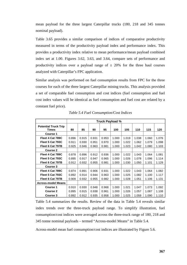
367
mean payload for the three largest Caterpillar trucks (180, 218 and 345 tonnes
nominal payload).
Table 3.65 provides a similar comparison of indices of comparative productivity
measured in terms of the productivity payload index and performance index. This
provides a productivity index relative to mean performance/mean payload combined
index set at 1.00. Figures 3.62, 3.63, and 3.64, compare sets of performance and
productivity indices over a payload range of ± 20% for the three haul courses
analyzed with Caterpillar’s FPC application.
Similar analysis was performed on fuel consumption results from FPC for the three
courses for each of the three largest Caterpillar mining trucks. This analysis provided
a set of comparable fuel consumption and cost indices (fuel consumption and fuel
cost index values will be identical as fuel consumption and fuel cost are related by a
constant fuel price).
Table 5.4 Fuel Consumption/Cost Indices
Truck Payload % Potential Truck Trip
Times 80 85 90 95 100 105 110 115 120 Course 1
Fleet 4 Cat 789C 0.896 0.915 0.931 0.953 1.000 1.019 1.038 1.060 1.076 Fleet 5 Cat 793C 0.911 0.930 0.951 0.970 1.000 1.022 1.062 1.079 1.098 Fleet 6 Cat 797B 0.925 0.946 0.963 0.981 1.000 1.023 1.042 1.080 1.103
Course 2 Fleet 4 Cat 789C 0.878 0.896 0.912 0.936 1.000 1.022 1.043 1.064 1.081 Fleet 5 Cat 793C 0.895 0.917 0.947 0.965 1.000 1.026 1.078 1.096 1.114 Fleet 6 Cat 797B 0.912 0.932 0.955 0.981 1.000 1.030 1.050 1.101 1.129
Course 3 Fleet 4 Cat 789C 0.874 0.891 0.906 0.931 1.000 1.022 1.043 1.064 1.082 Fleet 5 Cat 793C 0.892 0.914 0.944 0.963 1.000 1.025 1.082 1.100 1.117 Fleet 6 Cat 797B 0.909 0.932 0.955 0.982 1.000 1.028 1.051 1.106 1.131
Across-model Means Course 1 0.910 0.930 0.948 0.968 1.000 1.021 1.047 1.073 1.092 Course 2 0.895 0.915 0.938 0.961 1.000 1.026 1.057 1.087 1.108 Course 3 0.892 0.912 0.935 0.958 1.000 1.025 1.059 1.090 1.110
Table 5.4 summarizes the results. Review of the data in Table 5.4 reveals similar
index trends over the three-truck payload range. To simplify illustration, fuel
consumption/cost indices were averaged across the three-truck range of 180, 218 and
345 tonne nominal payloads – termed “Across-model Means” in Table 5.4.
Across-model mean fuel consumption/cost indices are illustrated by Figure 5.6.
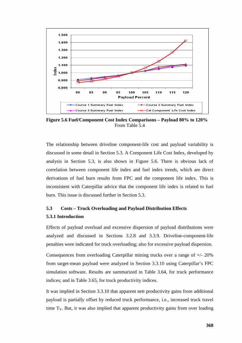
368
Figure 5.6 Fuel/Component Cost Index Comparisons – Payload 80% to 120%
From Table 5.4
The relationship between driveline component-life cost and payload variability is
discussed in some detail in Section 5.3. A Component Life Cost Index, developed by
analysis in Section 5.3, is also shown in Figure 5.6. There is obvious lack of
correlation between component life index and fuel index trends, which are direct
derivations of fuel burn results from FPC and the component life index. This is
inconsistent with Caterpillar advice that the component life index is related to fuel
burn. This issue is discussed further in Section 5.3.
5.3 Costs – Truck Overloading and Payload Distribution Effects
5.3.1 Introduction
Effects of payload overload and excessive dispersion of payload distributions were
analyzed and discussed in Sections 3.2.8 and 3.3.9. Driveline-component-life
penalties were indicated for truck overloading; also for excessive payload dispersion.
Consequences from overloading Caterpillar mining trucks over a range of +/- 20%
from target-mean payload were analyzed in Section 3.3.10 using Caterpillar’s FPC
simulation software. Results are summarized in Table 3.64, for truck performance
indices; and in Table 3.65, for truck productivity indices.
It was implied in Section 3.3.10 that apparent nett productivity gains from additional
payload is partially offset by reduced truck performance, i.e., increased truck travel
time TV. But, it was also implied that apparent productivity gains from over loading
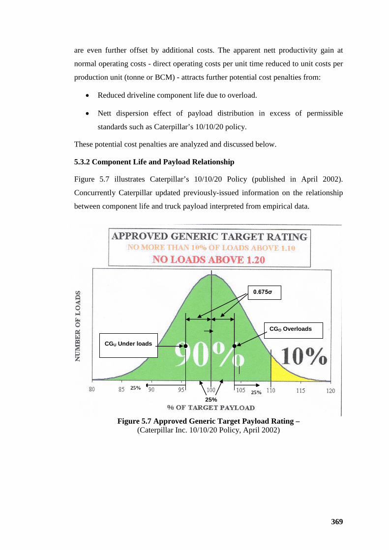
369
are even further offset by additional costs. The apparent nett productivity gain at
normal operating costs - direct operating costs per unit time reduced to unit costs per
production unit (tonne or BCM) - attracts further potential cost penalties from:
• Reduced driveline component life due to overload.
• Nett dispersion effect of payload distribution in excess of permissible
standards such as Caterpillar’s 10/10/20 policy.
These potential cost penalties are analyzed and discussed below.
5.3.2 Component Life and Payload Relationship
Figure 5.7 illustrates Caterpillar’s 10/10/20 Policy (published in April 2002).
Concurrently Caterpillar updated previously-issued information on the relationship
between component life and truck payload interpreted from empirical data.
Figure 5.7 Approved Generic Target Payload Rating –
(Caterpillar Inc. 10/10/20 Policy, April 2002)
CGU Under loads
CGO Overloads
0.675σ
25%
25% 25%
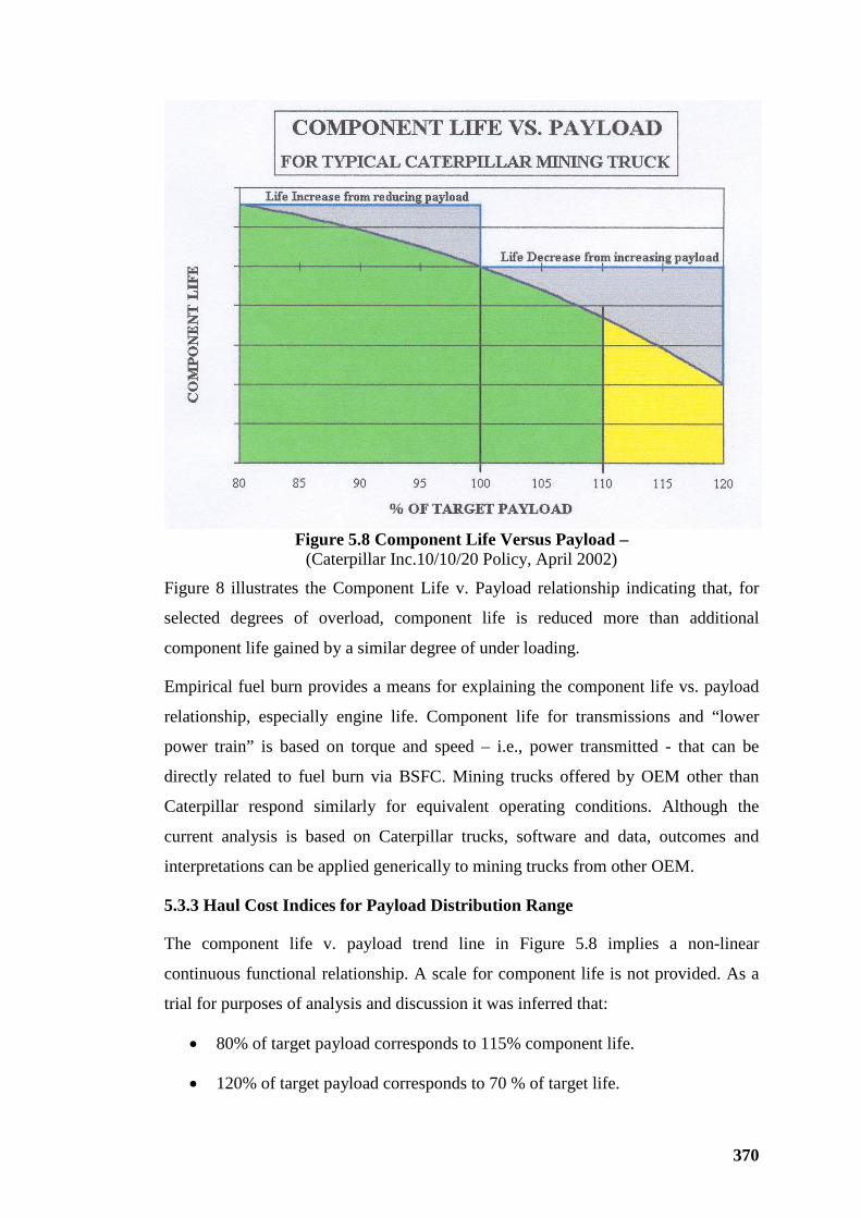
370
Figure 5.8 Component Life Versus Payload –
(Caterpillar Inc.10/10/20 Policy, April 2002)
Figure 8 illustrates the Component Life v. Payload relationship indicating that, for
selected degrees of overload, component life is reduced more than additional
component life gained by a similar degree of under loading.
Empirical fuel burn provides a means for explaining the component life vs. payload
relationship, especially engine life. Component life for transmissions and “lower
power train” is based on torque and speed – i.e., power transmitted - that can be
directly related to fuel burn via BSFC. Mining trucks offered by OEM other than
Caterpillar respond similarly for equivalent operating conditions. Although the
current analysis is based on Caterpillar trucks, software and data, outcomes and
interpretations can be applied generically to mining trucks from other OEM.
5.3.3 Haul Cost Indices for Payload Distribution Range
The component life v. payload trend line in Figure 5.8 implies a non-linear
continuous functional relationship. A scale for component life is not provided. As a
trial for purposes of analysis and discussion it was inferred that:
• 80% of target payload corresponds to 115% component life.
• 120% of target payload corresponds to 70 % of target life.
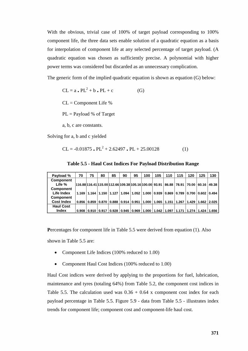
371
With the obvious, trivial case of 100% of target payload corresponding to 100%
component life, the three data sets enable solution of a quadratic equation as a basis
for interpolation of component life at any selected percentage of target payload. (A
quadratic equation was chosen as sufficiently precise. A polynomial with higher
power terms was considered but discarded as an unnecessary complication.
The generic form of the implied quadratic equation is shown as equation (G) below:
CL = a . PL2 + b . PL + c (G)
CL = Component Life %
PL = Payload % of Target
a, b, c are constants.
Solving for a, b and c yielded
CL = -0.01875 . PL2 + 2.62497 . PL + 25.00128 (1)
Percentages for component life in Table 5.5 were derived from equation (1). Also
shown in Table 5.5 are:
• Component Life Indices (100% reduced to 1.00)
• Component Haul Cost Indices (100% reduced to 1.00)
Haul Cost indices were derived by applying to the proportions for fuel, lubrication,
maintenance and tyres (totaling 64%) from Table 5.2, the component cost indices in
Table 5.5. The calculation used was 0.36 + 0.64 x component cost index for each
payload percentage in Table 5.5. Figure 5.9 - data from Table 5.5 - illustrates index
trends for component life; component cost and component-life haul cost.
Table 5.5 - Haul Cost Indices For Payload Distribution Range
Payload % 70 75 80 85 90 95 100 105 110 115 120 125 130 Component
Life % 116.88 116.41 115.00 112.66 109.38 105.16 100.00 93.91 86.88 78.91 70.00 60.16 49.38 Component Life Index 1.169 1.164 1.150 1.127 1.094 1.052 1.000 0.939 0.869 0.789 0.700 0.602 0.494
Component Cost Index 0.856 0.859 0.870 0.888 0.914 0.951 1.000 1.065 1.151 1.267 1.429 1.662 2.025 Haul Cost
Index 0.908 0.910 0.917 0.928 0.945 0.969 1.000 1.042 1.097 1.171 1.274 1.424 1.656
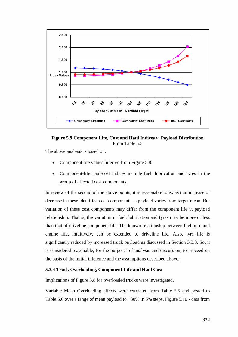
372
0.000
0.500
1.000
1.500
2.000
2.500
Index Values
Payload % of Mean - Nominal Target
Component Life Index Component Cost Index Haul Cost Index
Figure 5.9 Component Life, Cost and Haul Indices v. Payload Distribution
From Table 5.5
The above analysis is based on:
• Component life values inferred from Figure 5.8.
• Component-life haul-cost indices include fuel, lubrication and tyres in the
group of affected cost components.
In review of the second of the above points, it is reasonable to expect an increase or
decrease in these identified cost components as payload varies from target mean. But
variation of these cost components may differ from the component life v. payload
relationship. That is, the variation in fuel, lubrication and tyres may be more or less
than that of driveline component life. The known relationship between fuel burn and
engine life, intuitively, can be extended to driveline life. Also, tyre life is
significantly reduced by increased truck payload as discussed in Section 3.3.8. So, it
is considered reasonable, for the purposes of analysis and discussion, to proceed on
the basis of the initial inference and the assumptions described above.
5.3.4 Truck Overloading, Component Life and Haul Cost
Implications of Figure 5.8 for overloaded trucks were investigated.
Variable Mean Overloading effects were extracted from Table 5.5 and posted to
Table 5.6 over a range of mean payload to +30% in 5% steps. Figure 5.10 - data from
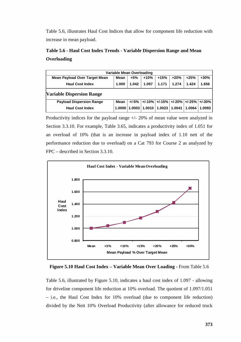
373
Table 5.6, illustrates Haul Cost Indices that allow for component life reduction with
increase in mean payload.
Table 5.6 - Haul Cost Index Trends - Variable Dispersion Range and Mean
Overloading
Variable Mean Overloading
Mean Payload Over Target Mean Mean +5% +10% +15% +20% +25% +30%
Haul Cost Index 1.000 1.042 1.097 1.171 1.274 1.424 1.656
Variable Dispersion Range Payload Dispersion Range Mean +/-5% +/-10% +/-15% +/-20% +/-25% +/-30%
Haul Cost Index 1.0000 1.0003 1.0010 1.0023 1.0041 1.0064 1.0093
Productivity indices for the payload range +/- 20% of mean value were analyzed in
Section 3.3.10. For example, Table 3.65, indicates a productivity index of 1.051 for
an overload of 10% (that is an increase in payload index of 1.10 nett of the
performance reduction due to overload) on a Cat 793 for Course 2 as analyzed by
FPC – described in Section 3.3.10.
0.800
1.000
1.200
1.400
1.600
1.800
Mean +5% +10% +15% +20% +25% +30%
Mean Payload % Over Target Mean
Haul Cost Index - Variable Mean Overloading
Haul Cost Index
Figure 5.10 Haul Cost Index – Variable Mean Over Loading - From Table 5.6
Table 5.6, illustrated by Figure 5.10, indicates a haul cost index of 1.097 - allowing
for driveline component life reduction at 10% overload. The quotient of 1.097/1.051
– i.e., the Haul Cost Index for 10% overload (due to component life reduction)
divided by the Nett 10% Overload Productivity (after allowance for reduced truck
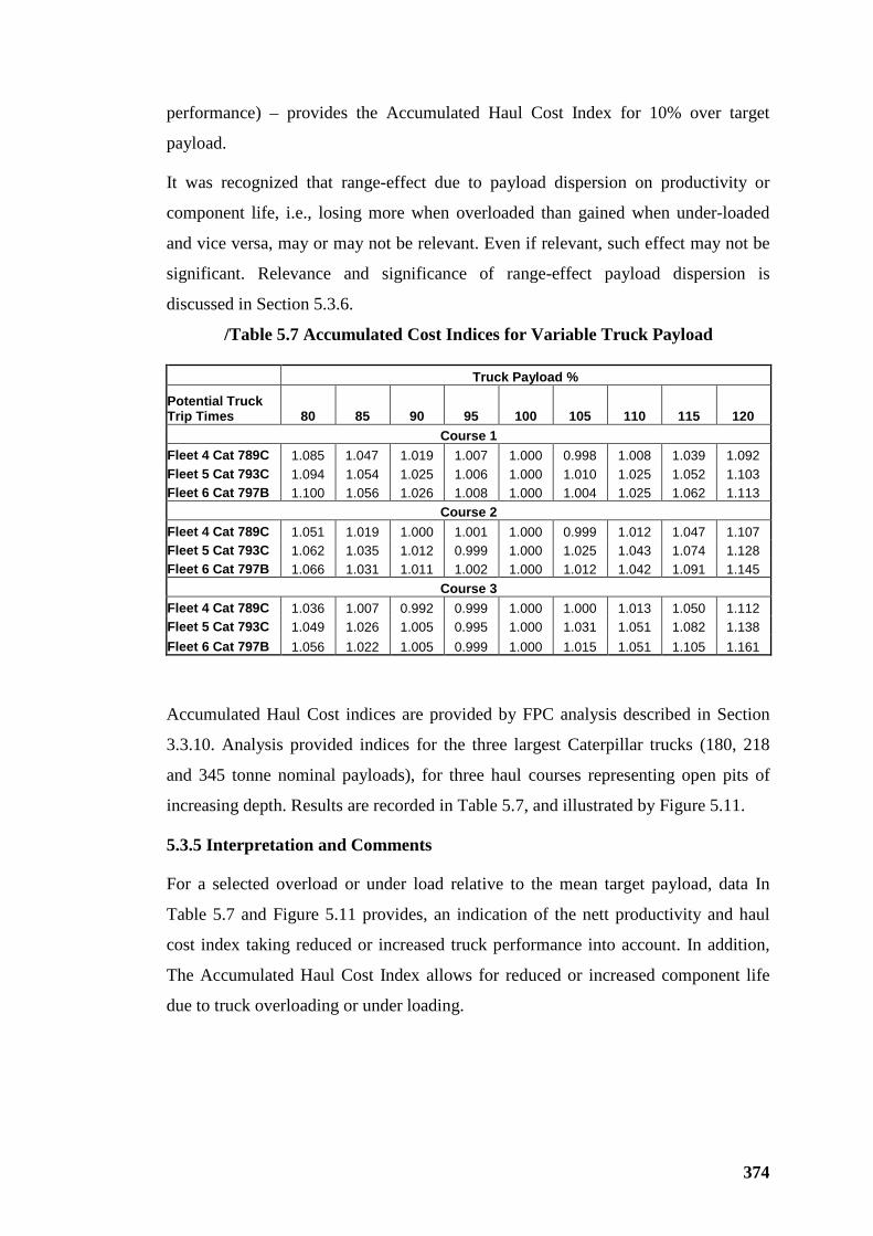
374
performance) – provides the Accumulated Haul Cost Index for 10% over target
payload.
It was recognized that range-effect due to payload dispersion on productivity or
component life, i.e., losing more when overloaded than gained when under-loaded
and vice versa, may or may not be relevant. Even if relevant, such effect may not be
significant. Relevance and significance of range-effect payload dispersion is
discussed in Section 5.3.6.
/Table 5.7 Accumulated Cost Indices for Variable Truck Payload
Truck Payload %
Potential Truck Trip Times 80 85 90 95 100 105 110 115 120
Course 1 Fleet 4 Cat 789C 1.085 1.047 1.019 1.007 1.000 0.998 1.008 1.039 1.092 Fleet 5 Cat 793C 1.094 1.054 1.025 1.006 1.000 1.010 1.025 1.052 1.103 Fleet 6 Cat 797B 1.100 1.056 1.026 1.008 1.000 1.004 1.025 1.062 1.113
Course 2 Fleet 4 Cat 789C 1.051 1.019 1.000 1.001 1.000 0.999 1.012 1.047 1.107 Fleet 5 Cat 793C 1.062 1.035 1.012 0.999 1.000 1.025 1.043 1.074 1.128 Fleet 6 Cat 797B 1.066 1.031 1.011 1.002 1.000 1.012 1.042 1.091 1.145
Course 3 Fleet 4 Cat 789C 1.036 1.007 0.992 0.999 1.000 1.000 1.013 1.050 1.112 Fleet 5 Cat 793C 1.049 1.026 1.005 0.995 1.000 1.031 1.051 1.082 1.138 Fleet 6 Cat 797B 1.056 1.022 1.005 0.999 1.000 1.015 1.051 1.105 1.161
Accumulated Haul Cost indices are provided by FPC analysis described in Section
3.3.10. Analysis provided indices for the three largest Caterpillar trucks (180, 218
and 345 tonne nominal payloads), for three haul courses representing open pits of
increasing depth. Results are recorded in Table 5.7, and illustrated by Figure 5.11.
5.3.5 Interpretation and Comments
For a selected overload or under load relative to the mean target payload, data In
Table 5.7 and Figure 5.11 provides, an indication of the nett productivity and haul
cost index taking reduced or increased truck performance into account. In addition,
The Accumulated Haul Cost Index allows for reduced or increased component life
due to truck overloading or under loading.
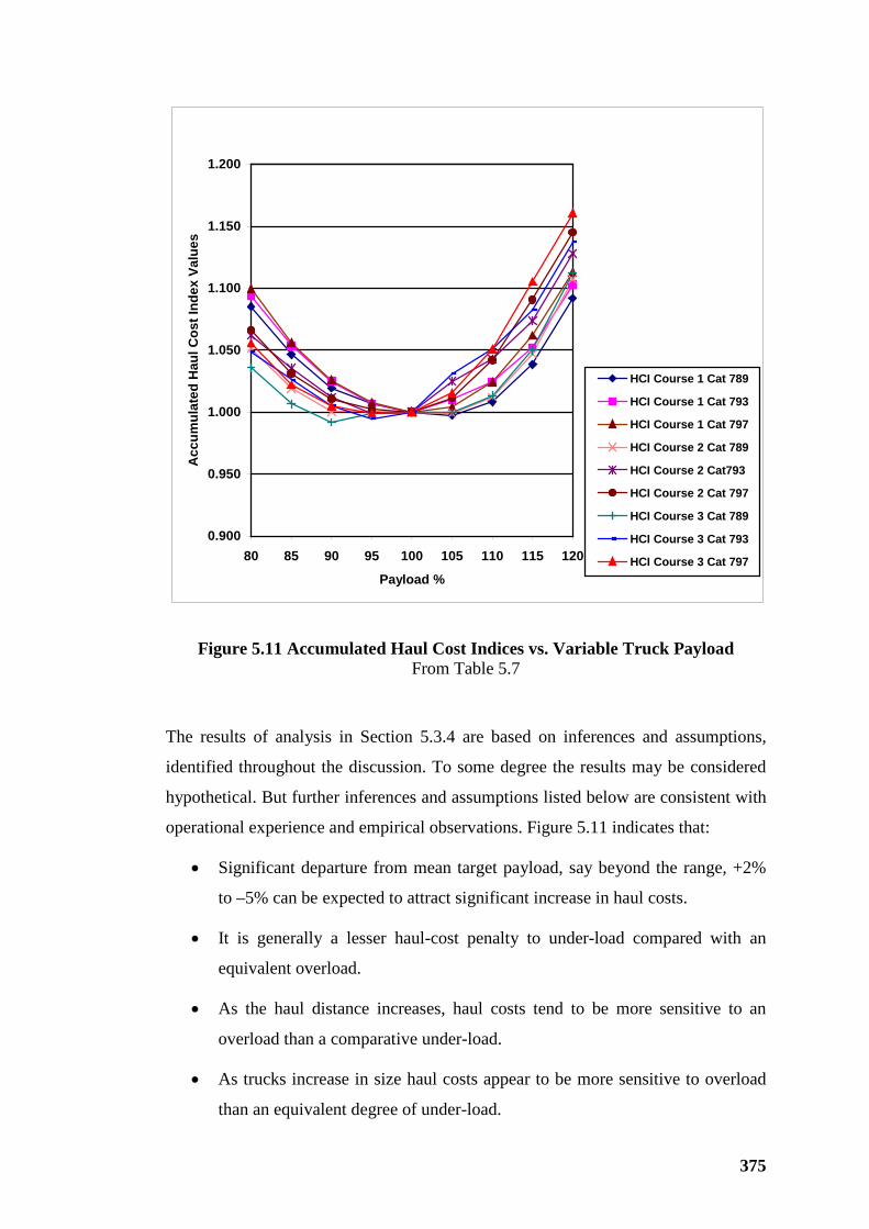
375
Accumulated Haul Cost Indices v. Mean Payload
0.900
0.950
1.000
1.050
1.100
1.150
1.200
80 85 90 95 100 105 110 115 120
Payload %
Acc
umul
ated
Hau
l Cos
t Ind
ex V
alue
s
HCI Course 1 Cat 789
HCI Course 1 Cat 793
HCI Course 1 Cat 797
HCI Course 2 Cat 789
HCI Course 2 Cat793
HCI Course 2 Cat 797
HCI Course 3 Cat 789
HCI Course 3 Cat 793
HCI Course 3 Cat 797
Figure 5.11 Accumulated Haul Cost Indices vs. Variable Truck Payload From Table 5.7
The results of analysis in Section 5.3.4 are based on inferences and assumptions,
identified throughout the discussion. To some degree the results may be considered
hypothetical. But further inferences and assumptions listed below are consistent with
operational experience and empirical observations. Figure 5.11 indicates that:
• Significant departure from mean target payload, say beyond the range, +2%
to –5% can be expected to attract significant increase in haul costs.
• It is generally a lesser haul-cost penalty to under-load compared with an
equivalent overload.
• As the haul distance increases, haul costs tend to be more sensitive to an
overload than a comparative under-load.
• As trucks increase in size haul costs appear to be more sensitive to overload
than an equivalent degree of under-load.
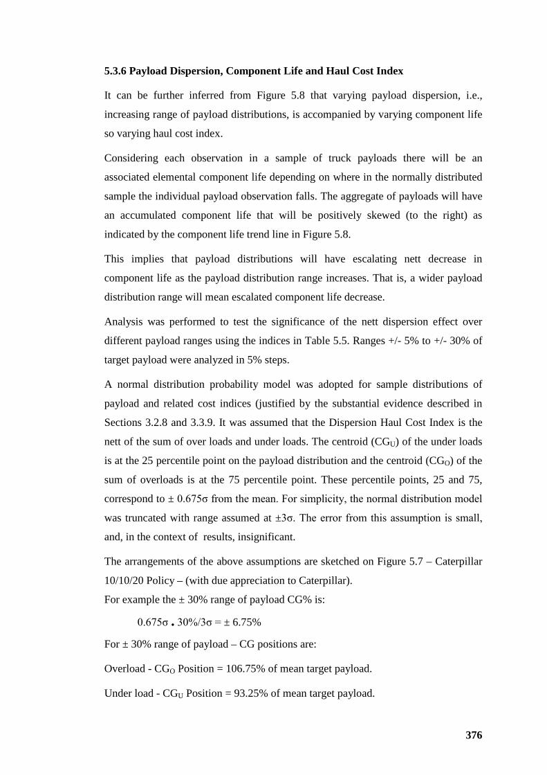
376
5.3.6 Payload Dispersion, Component Life and Haul Cost Index
It can be further inferred from Figure 5.8 that varying payload dispersion, i.e.,
increasing range of payload distributions, is accompanied by varying component life
so varying haul cost index.
Considering each observation in a sample of truck payloads there will be an
associated elemental component life depending on where in the normally distributed
sample the individual payload observation falls. The aggregate of payloads will have
an accumulated component life that will be positively skewed (to the right) as
indicated by the component life trend line in Figure 5.8.
This implies that payload distributions will have escalating nett decrease in
component life as the payload distribution range increases. That is, a wider payload
distribution range will mean escalated component life decrease.
Analysis was performed to test the significance of the nett dispersion effect over
different payload ranges using the indices in Table 5.5. Ranges +/- 5% to +/- 30% of
target payload were analyzed in 5% steps.
A normal distribution probability model was adopted for sample distributions of
payload and related cost indices (justified by the substantial evidence described in
Sections 3.2.8 and 3.3.9. It was assumed that the Dispersion Haul Cost Index is the
nett of the sum of over loads and under loads. The centroid (CGU) of the under loads
is at the 25 percentile point on the payload distribution and the centroid (CGO) of the
sum of overloads is at the 75 percentile point. These percentile points, 25 and 75,
correspond to ± 0.675σ from the mean. For simplicity, the normal distribution model
was truncated with range assumed at ±3σ. The error from this assumption is small,
and, in the context of results, insignificant.
The arrangements of the above assumptions are sketched on Figure 5.7 – Caterpillar
10/10/20 Policy – (with due appreciation to Caterpillar).
For example the ± 30% range of payload CG% is:
0.675σ . 30%/3σ = ± 6.75%
For ± 30% range of payload – CG positions are:
Overload - CGO Position = 106.75% of mean target payload.
Under load - CGU Position = 93.25% of mean target payload.
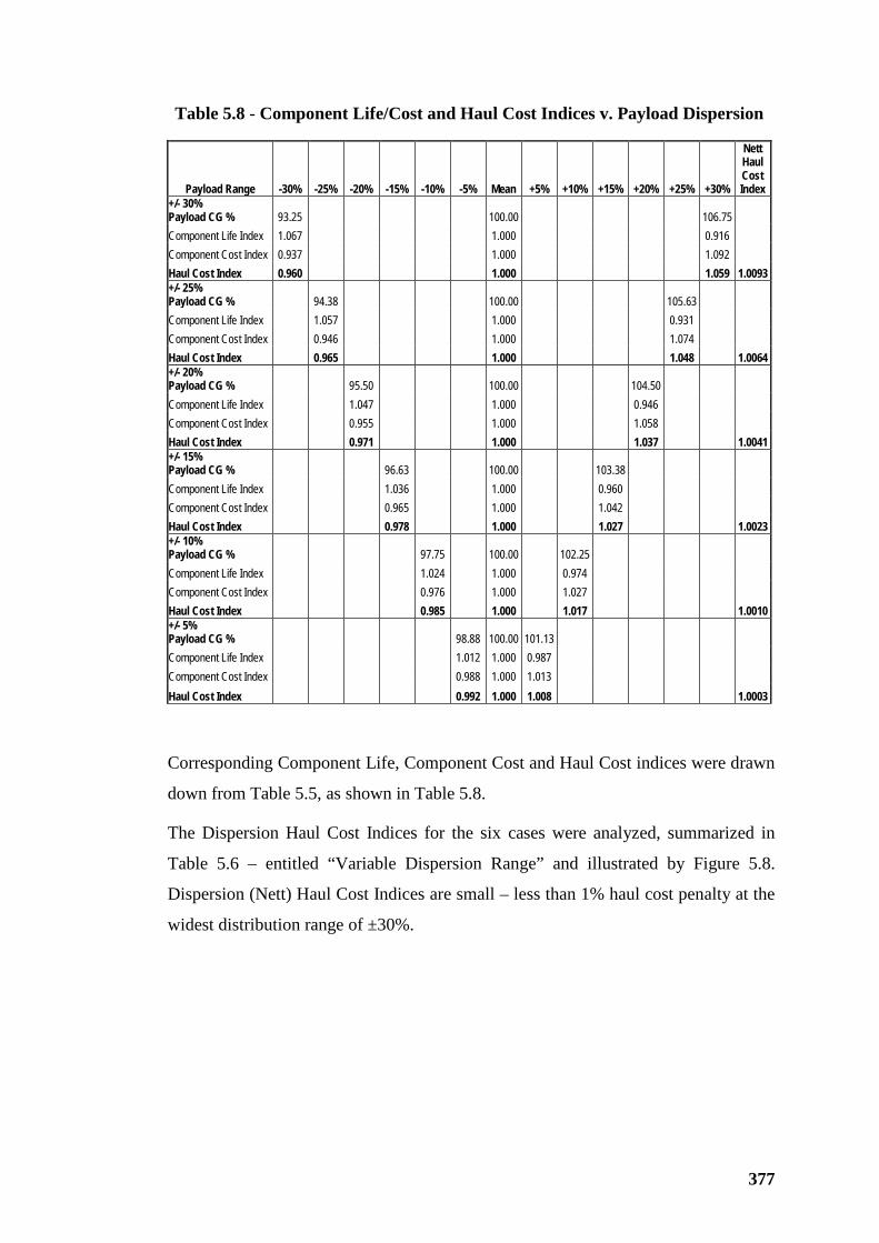
377
Table 5.8 - Component Life/Cost and Haul Cost Indices v. Payload Dispersion
Payload Range -30% -25% -20% -15% -10% -5% Mean +5% +10% +15% +20% +25% +30%
Nett Haul Cost Index
+/- 30% Payload CG % 93.25 100.00 106.75 Component Life Index 1.067 1.000 0.916 Component Cost Index 0.937 1.000 1.092 Haul Cost Index 0.960 1.000 1.059 1.0093 +/- 25% Payload CG % 94.38 100.00 105.63 Component Life Index 1.057 1.000 0.931 Component Cost Index 0.946 1.000 1.074 Haul Cost Index 0.965 1.000 1.048 1.0064 +/- 20% Payload CG % 95.50 100.00 104.50 Component Life Index 1.047 1.000 0.946 Component Cost Index 0.955 1.000 1.058 Haul Cost Index 0.971 1.000 1.037 1.0041 +/- 15% Payload CG % 96.63 100.00 103.38 Component Life Index 1.036 1.000 0.960 Component Cost Index 0.965 1.000 1.042 Haul Cost Index 0.978 1.000 1.027 1.0023 +/- 10% Payload CG % 97.75 100.00 102.25 Component Life Index 1.024 1.000 0.974 Component Cost Index 0.976 1.000 1.027 Haul Cost Index 0.985 1.000 1.017 1.0010 +/- 5% Payload CG % 98.88 100.00 101.13 Component Life Index 1.012 1.000 0.987 Component Cost Index 0.988 1.000 1.013 Haul Cost Index 0.992 1.000 1.008 1.0003
Corresponding Component Life, Component Cost and Haul Cost indices were drawn
down from Table 5.5, as shown in Table 5.8.
The Dispersion Haul Cost Indices for the six cases were analyzed, summarized in
Table 5.6 – entitled “Variable Dispersion Range” and illustrated by Figure 5.8.
Dispersion (Nett) Haul Cost Indices are small – less than 1% haul cost penalty at the
widest distribution range of ±30%.
378
0.9940
0.9960
0.9980
1.0000
1.0020
1.0040
1.0060
1.0080
1.0100
1.0120
Mean +/-5% +/-10% +/-15% +/-20% +/-25% +/-30%
Haul Cost Index Values
Payload Dispersion Range
Nett Haul Cost Index - Variable Payload Dispersion Range
Ne tt Haul Cost Index
Figure 5.12 Dispersion (Nett) Haul Cost Index vs. Variable Payload Dispersion
Range - From Table 5.6
5.3.7 Interpretation and Comments
On the basis of previous analysis of empirical evidence (truck payload data),
deterministic simulation (FPC) and assumptions identified through the process,
analysis in this section indicates that the effect of payload dispersion variability on
driveline component life is small but relevant. Certainly, the effect on driveline
life/cost is much smaller than the effect on productivity/cost of equivalent variation
from target payload. This implies that the dispersion of payload distribution is not a
significant issue if the upper range limit does not exceed the safety limit for truck
operating, specifically braking. Considering sensitivity to the assumed scale for
component life trend line in Figure 5.8, if assumed component life indices at extreme
+/- 20% payload limits, used for solving the quadratic continuous function were
doubled, Dispersion Haul Cost Indices would still be small; and, in the context of the
analysis, can be considered as not significant.
There is still benefit from reducing upper limit of the payload distribution range
below the quasi standard of +20% for compliance with the “20” element of
Caterpillar’s 10/10/20 policy. The more centralized the payload sample becomes, i.e.,
narrower the payload distribution range the less variable will be truck performance,
379
i.e., the more consistent will be truck travel times TV and consequently truck trip
times TT. Hauling “rhythm” will improve tending to reduce bunching affect and
increase truck-hauling efficiency.
These issues are further discussed in Section 5.5 below.
5.4 Costs and Bucket-Pass Sacrifice
5.4.1 Introduction
Productivity implications and circumstances justifying sacrifice of bucket loads to
improve load and haul “rhythm” were analyzed and discussed in Section 3.3.9.
Analysis in Section 3.3.9, compiled as Table 3.57 appended in Volume 2, is limited
to productivity only. This section analyzes and determines appropriate cost indices
applied comparatively to test validity of bucket load sacrifice in terms of costs.
Also analysis in Section 3.3.9 and this section ignores any reduced efficiency of
loading equipment due to increased truck exchanges. That is, loading equipment is
virtually over trucked at any bucket sacrifice event. For a bucket cycle time of 30
seconds and truck exchange time of 20 seconds the theoretical percentage decrease in
productive loading time (from Table 3.4):
• 5 pass to 4 pass is 88.24% to 85.71% = -2.5%.
• 6 pass to 5 pass is 90.0% to 88.24 % = -1.8%
• 7 pass to 6 pass is 91.3% to 90% = -1.3%
• 8 pass to 7 pass is 92.31% to 91.3% = -1.0%
So, generally bucket load sacrifice will be accompanied by 1.0% to 1.8% theoretical
reduction in loading efficiency over the practical range of sacrificed passes 8th to 7th
through to 6th to 5th passes. This reduction in total productivity (loading equipment
controls total productivity when over trucked – Figures 3.68 and 3.71) is small and,
for purposes of analysis and discussion, is ignored.
5.4.2 Comparative Cost Indices
An applicable Haul Cost Index (HCI) for additional payload proportions realized by
all trucks, i.e., PLX in Table 3.57 appended in Volume 2, can be derived from Table
5.2.
380
In the absence of bucket load sacrifice, waiting trucks have an estimated cost index
per unit of time of 0.183 (Figure 5.2). Obviously if, by bucket load sacrifice, waiting
time is converted to productive time, then additional production incurs an HCI of
0.817. This factor can be applied to PLX to arrive at a comparative incremental haul
cost HCX for the additional payload proportion realized.
Haul cost increment, HCLOSS, due to payload lost by sacrificing one or more bucket
loads (PLLOSS) is a function of:
• Payload proportion sacrificed.
• HCI of the proportion sacrificed.
Payload proportion sacrificed can be determined from the ratio of the sacrificed
bucket load to truck payload. In the compilation of Table 3.57 appended in Volume
2, this proportion was conveniently calculated for sacrifice of the 7th pass as follows:
PLLOSS =0.75/6.75* = 0.111
The origin of denominator 6.75* is:
• 6 normal bucket fill passes rated at 1.00 (not necessarily bucket fill factor
1.00) – plus
• 1 final top-up pass factored at 0.75 of a normal bucket fill as per discussion in
Section 3.3.9.
It could be argued that the first-pass bucket load is generally higher than the mean of
subsequent intermediate loads (excluding the last bucket load) as discussed in
Section 3.2.8 and illustrated by Tables 3.7 and Table 3.12 (appended) where it is
indicated that mean of first bucket loads is in the order of 130% of mean intermediate
bucket loads.
It is intuitively believed that some one-third, i.e., 10% of the apparent increased
bucket load is accumulated debris on the truck frame and carry-back in the truck
body that should be registered as NMW by recalibration of the payload measuring
facility on the mining trucks studied as discussed in Section 3.2.8. This implies that
first bucket loads could be in the order of some 20% in excess of mean intermediate
bucket loads.
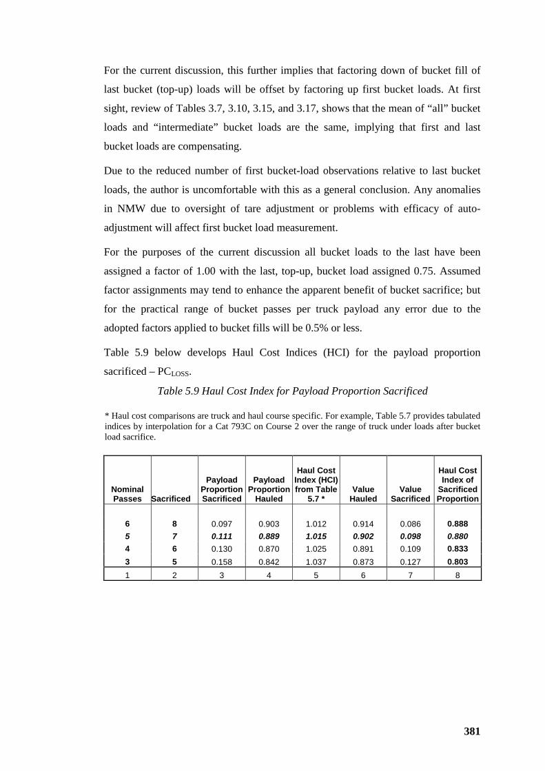
381
For the current discussion, this further implies that factoring down of bucket fill of
last bucket (top-up) loads will be offset by factoring up first bucket loads. At first
sight, review of Tables 3.7, 3.10, 3.15, and 3.17, shows that the mean of “all” bucket
loads and “intermediate” bucket loads are the same, implying that first and last
bucket loads are compensating.
Due to the reduced number of first bucket-load observations relative to last bucket
loads, the author is uncomfortable with this as a general conclusion. Any anomalies
in NMW due to oversight of tare adjustment or problems with efficacy of auto-
adjustment will affect first bucket load measurement.
For the purposes of the current discussion all bucket loads to the last have been
assigned a factor of 1.00 with the last, top-up, bucket load assigned 0.75. Assumed
factor assignments may tend to enhance the apparent benefit of bucket sacrifice; but
for the practical range of bucket passes per truck payload any error due to the
adopted factors applied to bucket fills will be 0.5% or less.
Table 5.9 below develops Haul Cost Indices (HCI) for the payload proportion
sacrificed – PCLOSS.
Table 5.9 Haul Cost Index for Payload Proportion Sacrificed * Haul cost comparisons are truck and haul course specific. For example, Table 5.7 provides tabulated indices by interpolation for a Cat 793C on Course 2 over the range of truck under loads after bucket load sacrifice.
Nominal Passes
Sacrificed
Payload Proportion Sacrificed
Payload Proportion
Hauled
Haul Cost Index (HCI) from Table
5.7 * Value
Hauled Value
Sacrificed
Haul Cost Index of
Sacrificed Proportion
6 8 0.097 0.903 1.012 0.914 0.086 0.888 5 7 0.111 0.889 1.015 0.902 0.098 0.880 4 6 0.130 0.870 1.025 0.891 0.109 0.833 3 5 0.158 0.842 1.037 0.873 0.127 0.803 1 2 3 4 5 6 7 8
382
Referring to Table 5.9:
• Column 1 – shows the nominal number of passes – i.e., the “modal” value.
• Column 2 – indicates pass sacrifice.
• Column 3 – indicates payload proportion sacrificed calculated by: PLLOSS = 0.75/(Pass sacrificed – 1 + 0.75)
Example: PLLOSS = 0.75/(7 – 1 + 0.75) = 0.111 as in Table 5.4.2.1
• Column 4 – indicates balance of payload hauled. That is: Payload nett of PLLOSS.
In Table 5.9 Payload factor = 1.0
• Column 5 – lists HCI derived from analysis over a range of payloads either side of the mean shown in Table 5.7.
• Column 6 – shows: Value Hauled = Payload proportion hauled x HCI.
• Column 7 – shows: Value Sacrificed = 1 – Value Hauled
• Column 8 – shows:
HCI of Sacrificed Portion = Value Sacrificed/ Payload Proportion Sacrificed
5.4.3 Cost Criteria for Sacrificing Bucket Loads
Table 5.10, appended in Volume 2, is an extension of Table 3.57, also appended in
Volume 2. The HCI for the pass sacrificed is applied to PLLOSS – the proportion of
truck payload sacrificed by a bucket load or loads sacrificed. A copy of the file is
provided on the CD inside the back cover of this thesis to complement the file for
Table 3.57.
As discussed in Section 5.4.2, the HCI to be applied to PLX – the additional payload
proportion realized by bucket load sacrifice is derived from Table 5.2 by the
difference between operating HCI 1.00 and waiting time HCI of 0.183, i.e., 0.817.
The comparative data is shown in Table 5.10, appended in Volume 2. Within that
table shading and lines delineate significant zones, each with status as follows:
• The shaded zone indicates values for Haul Cost Benefit – HCX – that do not
exceed Haul Cost Sacrifice – HCLOSS; so bucket pass sacrifice is not
beneficial for the selected case of nominal 5-pass loading and sacrificing the
7th pass.
383
• The heavy full line identifies the boundary of the Number of Trucks v. Truck
Trip Time array where bucket pass sacrifice changes from “unfavorable” to
“favorable”. The heavy dashed line indicates the boundary where bucket pass
sacrifice passes from “unfavorable” to “favorable”, if the total haul cost is
charged to waiting time when the truck is technically operating, but waiting
to be loaded.
This latter instance is conservative in reducing the zone favorable for bucket load
sacrifice. It could apply where accounting treatment of amortization is expensed as
an operating cost or cost provision. Traditional cost estimating for mining contract
scheduled rates necessarily includes capital recovery for all equipment supplied in
the rates for contract work (unless it is priced transparently as a periodic, such as
monthly, fee).
It is the author’s opinion that including total amortization cost in waiting time costs
is invalid for analyzing bucket-pass sacrifice benefits. But the error by inclusion is
intuitively considered to be small in the context of the comparative cost test.
As discussed in Section 5.3.2, driveline componentry life and costs are related to fuel
burn. There is a logical case to cost the entire capital write-off over fuel burn for the
life of the mining truck.
As an example: If a Cat 793C mining truck uses 2.7 million litres of fuel over an
engine life before overhaul – enduring some 14,000 operating SMU (engine hours) in
the process – then we could allow, say, 5 x engine lives (70,000 SMU) as the life of
the mining-truck frame and all componentry not replaced or rebuilt earlier in the
truck life. The life of a Cat 793C mining truck would then be 13.5 million litres of
fuel. This begs the question: Is this a reasonable life assessment? Assuming it is
reasonable for purposes of discussion, it can be concluded that including full write
off of capital cost per SMU whilst a truck is waiting to be loaded would be
unreasonable as fuel used by an idling engine is some 5% of the mean operating fuel
consumption. This supports the above discussion and the position taken in compiling
Table 5.10, appended in Volume 2.
5.4.4 Interpretation and Comments
Generally there is justification to sacrifice any bucket pass exceeding the sum of
nominal passes (modal value) plus one additional pass provided that:
384
• There is a truck waiting to be loaded or in position to exchange immediately
on departure of the loaded truck.
• The difference in comparative outcomes between the productivity test of
Table 3.57 and the cost test of Table 5.10, both appended in Volume 2, is
generally small. Compared with the haul-cost test the productivity test
excludes only a small number of additional cases because the applicable HCI
for PLLOSS is only slightly higher than the HCI applicable to PLX.
• The higher the HCI for PLX (and vice versa – lower the HCI for PLLOSS) the
more robust will be the justification for bucket-pass sacrifice.
• If the proportion of operating labour in the HCI applicable to PLX (see Table
5.2.) is reduced by increasing truck payload scale, HCX will tend to increase
- favoring bucket-pass sacrifice.
• As fuel and tyre cost proportions increase (by general cost escalation and
sharp rises due to international supply limitations) HCX will tend to increase
– again favoring bucket-pass sacrifice.
Variability of travel time TV for mining trucks means that, (for best practice truck
haulage with CVTV ≤ 0.10), unless truck match is 50% over or under exact match
some degree of bunching will occur – refer to Figure 3.70. Regardless of the
theoretical status of loading equipment/truck match within the +/- 50% limits,
loading equipment experiences over trucking, under trucking and, logically,
occasionally an exact match.
Bucket-pass sacrifice is likely favored where there are trucks waiting to be loaded or
where a returning truck can seamlessly complete the truck exchange with a loaded
truck. In these circumstances, application of a protocol limiting bucket passes will be
productivity positive and cost beneficial. In the absence of trucks waiting it is
commonsense for loading equipment operators to continue loading trucks to the
target (mean) payload using volumetric judgment or onboard payload sensing output
as a guide.
385
5.5 Costs and Over trucking, Under trucking; also Bunching
5.5.1 Introduction – Defining the Problems
Relative merits of over trucking and under trucking were discussed in terms of
productivity in Section 3.5.3.
The three states, over trucked, exactly matched and under trucked were considered as
follows:
• Over trucked, where productivity is at maximum loading equipment
performance.
• Under trucked, where productivity is at a proportion of the maximum loading
equipment performance consistent with the actual number of trucks relative
to the theoretical number of trucks at the match point.
• The hypothetical exactly matched case where actual trucks correspond to
theoretical trucks – obviously only possible where the theoretical number of
trucks is an integer.
The matched case can be considered trivial because it is rarely, if ever, going to
occur. It is that point where discrete functions expressing the relationship between
selection parameters for either over trucking or under trucking intersect. At that point
the theoretical number of trucks, calculated by methods described in Section 3.5.2
and Section 3.5.3, coincides with an integer number.
Relevance to Equipment Selection
Since the “matched” case can be considered trivial, there are two practical options:
1. To operate overtrucked; or
2. To operate undertrucked – or “over-shoveled” as indicated in Section 3.5.3.
When over trucked, loading equipment controls productivity that coincides with the
practical performance of that loading equipment – but with a cost penalty for under-
utilized trucks.
When loading equipment is under trucked effective trucks are fully utilized; but
loading equipment is under-utilized to the extent that the actual number is less than
the theoretical number of trucks – at a cost penalty due to inefficiency of loading
equipment.
386
Practical operational choices are to:
• Operate over trucked at full loading equipment productivity with a cost
penalty for under-utilized trucks; or
• Operate under trucked at reduced loading equipment productivity with an
attendant cost penalty due to loading inefficiency.
The above choices beg the question – Which option is the most economic?
Intuitively the cost penalty for loading equipment inefficiency will be less than the
cost penalty for overtrucking. Relativity of hauling cost some three times loading
cost is indicated by Figure 2.2, supporting under trucking as a best-economics policy.
But reduced loading-equipment productivity when under trucked could have cost
implications for downstream treatment and subsequent activities. Opting to under
truck is not a simple matter for intuitive decision.
Estimation of number of trucks, initially based on relativity of loading time to truck
travel time, amended by probabilistic analysis is discussed in Section 3.5.2. The
estimated match is rarely an exact integer number of trucks. When the theoretical
number of trucks is not an exact integer we have the option of rounding up or down.
Experience indicates that mining productivity and cost estimators have a
conservatively-driven penchant to round up. This preference will tend to over-truck
with cost penalty due to truck waiting time. Rounding down under trucks, but inflicts
a cost penalty due to loading inefficiency. Guidance for the appropriate rounding
decision is needed. This is the focus of Section 5.5.2.
5.5.2 Productivity, Cost Indices and Relationships
5.5.2.1 Hanby’s Solution – A Review
In Part 1 of a three-part paper I R Hanby addressed the problem of “shovel and truck
matching to obtain whole numbers” of trucks (Hanby, 1991, Part 1). The basic
criterion for the “simple solution” developed by Hanby is “minimum cost per unit of
volume moved”. Hanby’s objective was to provide a method of determining the
solution of an integer (selection) number of trucks for any theoretical number of
trucks determined by traditional estimating methods to provide lowest load and haul
costs.
387
In review, Hanby’s deterministic method is, to a degree, simplistic in that the unit
cost of owning and operating loading equipment and trucks is assumed constant for
all states of operation whether equipment is performing its assigned function (loading
or hauling) or waiting for trucks (loading equipment) or waiting to be loaded
(trucks). Hanby assumed a single loading equipment item and that all trucks were
alike and that truck-travel and loading times (and consequently loading times, if any)
are mean values with all trucks of identical specification and performance.
Hanby’s analysis was based on the theoretical number of trucks t for a match to be
calculated deterministically by his equivalent to equation (7) from 3.5.2, viz.,
t = (tL + tT)/tL - using Hanby’s notation and time definitions.
Generally equivalent to (using notation and definitions herein):
t = TT/(TL + TS) ≡ t = (TL + TV + TS + TD)/(TL + TS)
The above equation produces continuous values of t that are generally non-integer.
Benefits of probabilistic analysis in determining the theoretical truck match number
before rounding to an integer number were described in Section 3.5.2. Theoretical
matched number of trucks is discussed in Section 3.5.3.
Hanby’s analysis is applicable for the theoretical number of trucks regardless of the
method of determination. Relevant simplifications fundamental to Hanby’s analysis
are reviewed in detail in Section 5.5.3.
5.5.2.2 Costs and Outputs
Notation used below in this section; also in Section 5.5.3 below, is based on Hanby
with modification necessary to suit notation, particularly subscripts, throughout the
research and analysis described in this thesis.
Hanby showed that the ratio of total load and haul cost to truck cost is a function of
the ratio of loading equipment cost to truck cost, the actual integer number of trucks
selected and the theoretical number of trucks required for haulage service.
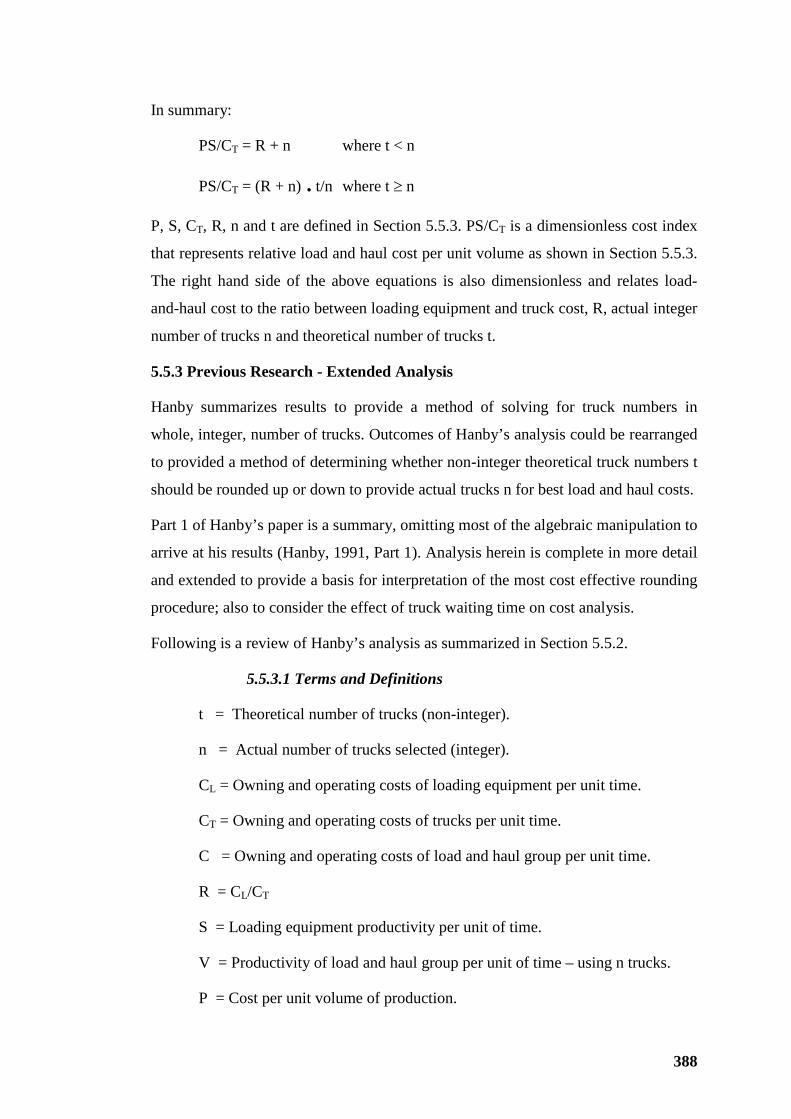
388
In summary:
PS/CT = R + n where t < n
PS/CT = (R + n) . t/n where t ≥ n
P, S, CT, R, n and t are defined in Section 5.5.3. PS/CT is a dimensionless cost index
that represents relative load and haul cost per unit volume as shown in Section 5.5.3.
The right hand side of the above equations is also dimensionless and relates load-
and-haul cost to the ratio between loading equipment and truck cost, R, actual integer
number of trucks n and theoretical number of trucks t.
5.5.3 Previous Research - Extended Analysis
Hanby summarizes results to provide a method of solving for truck numbers in
whole, integer, number of trucks. Outcomes of Hanby’s analysis could be rearranged
to provided a method of determining whether non-integer theoretical truck numbers t
should be rounded up or down to provide actual trucks n for best load and haul costs.
Part 1 of Hanby’s paper is a summary, omitting most of the algebraic manipulation to
arrive at his results (Hanby, 1991, Part 1). Analysis herein is complete in more detail
and extended to provide a basis for interpretation of the most cost effective rounding
procedure; also to consider the effect of truck waiting time on cost analysis.
Following is a review of Hanby’s analysis as summarized in Section 5.5.2.
5.5.3.1 Terms and Definitions
t = Theoretical number of trucks (non-integer).
n = Actual number of trucks selected (integer).
CL = Owning and operating costs of loading equipment per unit time.
CT = Owning and operating costs of trucks per unit time.
C = Owning and operating costs of load and haul group per unit time.
R = CL/CT
S = Loading equipment productivity per unit of time.
V = Productivity of load and haul group per unit of time – using n trucks.
P = Cost per unit volume of production.
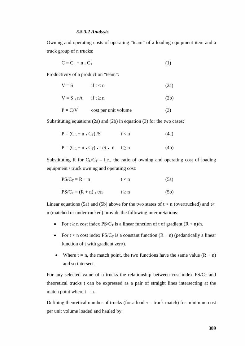
389
5.5.3.2 Analysis
Owning and operating costs of operating “team” of a loading equipment item and a
truck group of n trucks:
C = CL + n . CT (1)
Productivity of a production “team”:
V = S if t < n (2a)
V = S . n/t if t ≥ n (2b)
P = C/V cost per unit volume (3)
Substituting equations (2a) and (2b) in equation (3) for the two cases;
P = (CL + n . CT) /S t < n (4a)
P = (CL + n . CT) . t /S . n t ≥ n (4b)
Substituting R for CL/CT – i.e., the ratio of owning and operating cost of loading
equipment / truck owning and operating cost:
PS/CT = R + n t < n (5a)
PS/CT = (R + n) . t/n t ≥ n (5b)
Linear equations (5a) and (5b) above for the two states of t < n (overtrucked) and t ≥
n (matched or undertrucked) provide the following interpretations:
• For t ≥ n cost index PS/CT is a linear function of t of gradient (R + n)/n.
• For t < n cost index PS/CT is a constant function (R + n) (pedantically a linear
function of t with gradient zero).
• Where t = n, the match point, the two functions have the same value (R + n)
and so intersect.
For any selected value of n trucks the relationship between cost index PS/CT and
theoretical trucks t can be expressed as a pair of straight lines intersecting at the
match point where t = n.
Defining theoretical number of trucks (for a loader – truck match) for minimum cost
per unit volume loaded and hauled by:
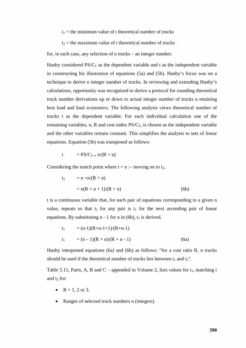
390
t1 = the minimum value of t theoretical number of trucks
t2 = the maximum value of t theoretical number of trucks
for, in each case, any selection of n trucks – an integer number.
Hanby considered PS/CT as the dependent variable and t as the independent variable
in constructing his illustration of equations (5a) and (5b). Hanby’s focus was on a
technique to derive n integer number of trucks. In reviewing and extending Hanby’s
calculations, opportunity was recognized to derive a protocol for rounding theoretical
truck number derivations up or down to actual integer number of trucks n retaining
best load and haul economics. The following analysis views theoretical number of
trucks t as the dependent variable. For each individual calculation one of the
remaining variables, n, R and cost index PS/CT, is chosen as the independent variable
and the other variables remain constant. This simplifies the analysis to sets of linear
equations. Equation (5b) was transposed as follows:
t = PS/CT . n/(R + n)
Considering the match point where t = n :– moving on to t2,
t2 = n +n/(R + n)
= n(R + n + 1)/(R + n) (6b)
t is a continuous variable that, for each pair of equations corresponding to a given n
value, repeats so that t2 for any pair is t1 for the next ascending pair of linear
equations. By substituting n - 1 for n in (6b), t1 is derived.
t1 = (n-1)(R+n-1+1)/(R+n-1)
t1 = (n – 1)(R + n)/(R + n - 1) (6a)
Hanby interpreted equations (6a) and (6b) as follows: “for a cost ratio R, n trucks
should be used if the theoretical number of trucks lies between t1 and t2”.
Table 5.11, Parts, A, B and C – appended in Volume 2, lists values for t1, matching t
and t2 for:
• R = 1, 2 or 3.
• Ranges of selected truck numbers n (integers).
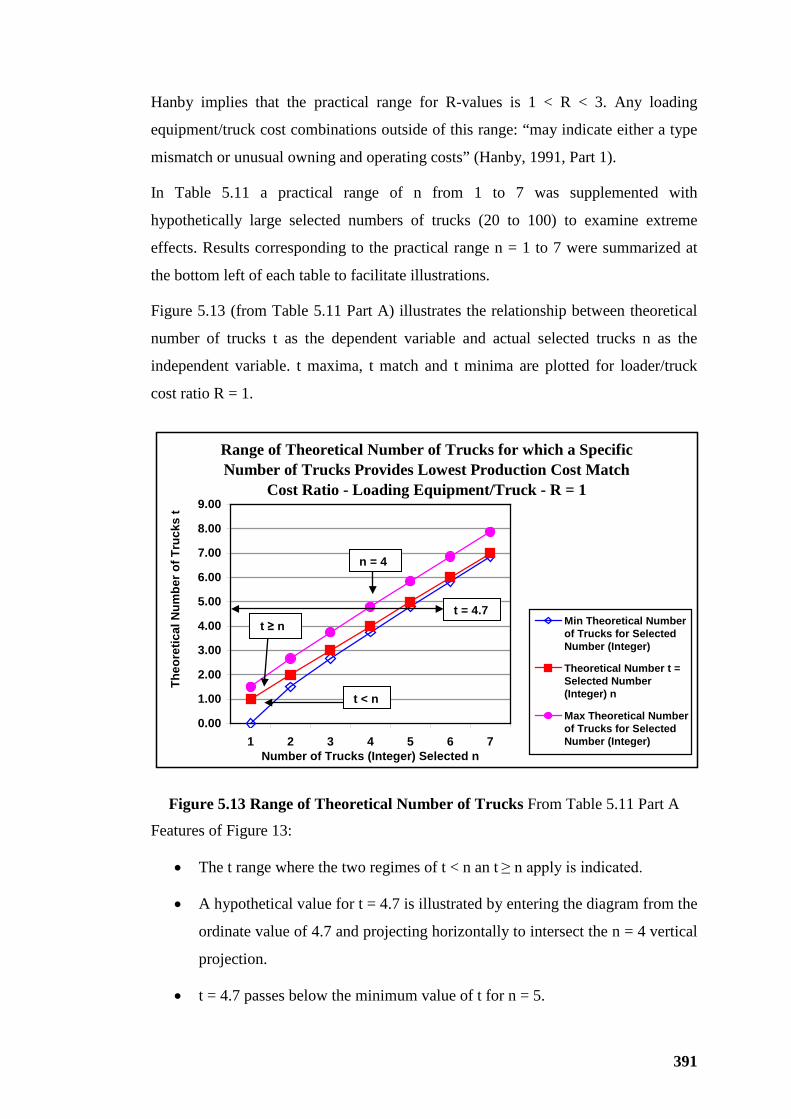
391
Hanby implies that the practical range for R-values is 1 < R < 3. Any loading
equipment/truck cost combinations outside of this range: “may indicate either a type
mismatch or unusual owning and operating costs” (Hanby, 1991, Part 1).
In Table 5.11 a practical range of n from 1 to 7 was supplemented with
hypothetically large selected numbers of trucks (20 to 100) to examine extreme
effects. Results corresponding to the practical range n = 1 to 7 were summarized at
the bottom left of each table to facilitate illustrations.
Figure 5.13 (from Table 5.11 Part A) illustrates the relationship between theoretical
number of trucks t as the dependent variable and actual selected trucks n as the
independent variable. t maxima, t match and t minima are plotted for loader/truck
cost ratio R = 1.
Range of Theoretical Number of Trucks for which a Specific Number of Trucks Provides Lowest Production Cost Match
Cost Ratio - Loading Equipment/Truck - R = 1
0.00
1.00
2.00
3.00
4.00
5.00
6.00
7.00
8.00
9.00
1 2 3 4 5 6 7Number of Trucks (Integer) Selected n
Theo
retic
al N
umbe
r of T
ruck
s t
Min Theoretical Numberof Trucks for SelectedNumber (Integer)
Theoretical Number t =Selected Number(Integer) n
Max Theoretical Numberof Trucks for SelectedNumber (Integer)
Figure 5.13 Range of Theoretical Number of Trucks From Table 5.11 Part A
Features of Figure 13:
• The t range where the two regimes of t < n an t ≥ n apply is indicated.
• A hypothetical value for t = 4.7 is illustrated by entering the diagram from the
ordinate value of 4.7 and projecting horizontally to intersect the n = 4 vertical
projection.
• t = 4.7 passes below the minimum value of t for n = 5.
t ≥ n
t < n
t = 4.7
n = 4
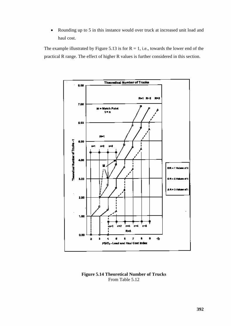
392
• Rounding up to 5 in this instance would over truck at increased unit load and
haul cost.
The example illustrated by Figure 5.13 is for R = 1, i.e., towards the lower end of the
practical R range. The effect of higher R values is further considered in this section.
Figure 5.14 Theoretical Number of Trucks
From Table 5.12
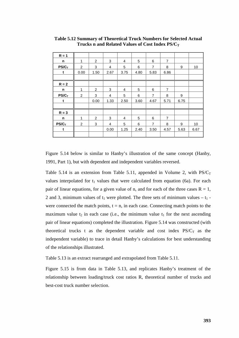
393
Figure 5.14 below is similar to Hanby’s illustration of the same concept (Hanby,
1991, Part 1), but with dependent and independent variables reversed.
Table 5.14 is an extension from Table 5.11, appended in Volume 2, with PS/CT
values interpolated for t1 values that were calculated from equation (6a). For each
pair of linear equations, for a given value of n, and for each of the three cases R = 1,
2 and 3, minimum values of t1 were plotted. The three sets of minimum values – t1 -
were connected the match points, t = n, in each case. Connecting match points to the
maximum value t2 in each case (i.e., the minimum value t1 for the next ascending
pair of linear equations) completed the illustration. Figure 5.14 was constructed (with
theoretical trucks t as the dependent variable and cost index PS/CT as the
independent variable) to trace in detail Hanby’s calculations for best understanding
of the relationships illustrated.
Table 5.13 is an extract rearranged and extrapolated from Table 5.11.
Figure 5.15 is from data in Table 5.13, and replicates Hanby’s treatment of the
relationship between loading/truck cost ratios R, theoretical number of trucks and
best-cost truck number selection.
Table 5.12 Summary of Theoretical Truck Numbers for Selected Actual Trucks n and Related Values of Cost Index PS/CT
R = 1
n 1 2 3 4 5 6 7 PS/CT 2 3 4 5 6 7 8 9 10
t 0.00 1.50 2.67 3.75 4.80 5.83 6.86
R = 2 n 1 2 3 4 5 6 7
PS/CT 2 3 4 5 6 7 8 9 t 0.00 1.33 2.50 3.60 4.67 5.71 6.75
R = 3 n 1 2 3 4 5 6 7
PS/CT 2 3 4 5 6 7 8 9 10 t 0.00 1.25 2.40 3.50 4.57 5.63 6.67
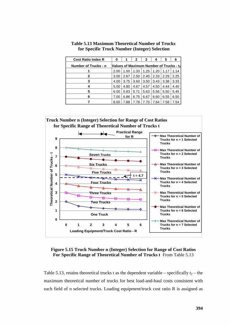
394
Truck Number n (Integer) Selection for Range of Cost Ratios for Specific Range of Theoretical Number of Trucks t
0
1
2
3
4
5
6
7
8
9
0 1 2 3 4 5 6
Loading Equipment/Truck Cost Ratio - R
Theo
retic
al N
umbe
r of T
ruck
s - t
Max Theoretical Number ofTrucks for n = 1 SelectedTrucks
Max Theoretical Number ofTrucks for n = 2 SelectedTrucks
Max Theoretical Number ofTrucks for n = 3 SelectedTrucks
Max Theoretical Number ofTrucks for n = 4 SelectedTrucks
Max Theoretical Number ofTrucks for n = 5 SelectedTrucks
Max Theoretical Number ofTrucks for n = 6 SelectedTrucks
Max Theoretical Number ofTrucks for n = 7 SelectedTrucks
One Truck
Two Trucks
Three Trucks
Four Trucks
Five Trucks
Six Trucks
Seven Trucks
Practical Rangefor R
Figure 5.15 Truck Number n (Integer) Selection for Range of Cost Ratios For Specific Range of Theoretical Number of Trucks t From Table 5.13
Table 5.13, retains theoretical trucks t as the dependent variable – specifically t2 – the
maximum theoretical number of trucks for best load-and-haul costs consistent with
each field of n selected trucks. Loading equipment/truck cost ratio R is assigned as
Table 5.13 Maximum Theoretical Number of Trucks for Specific Truck Number (Integer) Selection
Cost Ratio Index R 0 1 2 3 4 5 6
Number of Trucks - n Values of Maximum Number of Trucks - t2 1 2.00 1.50 1.33 1.25 1.20 1.17 1.14 2 3.00 2.67 2.50 2.40 2.33 2.29 2.25 3 4.00 3.75 3.60 3.50 3.43 3.38 3.33 4 5.00 4.80 4.67 4.57 4.50 4.44 4.40 5 6.00 5.83 5.71 5.63 5.56 5.50 5.45 6 7.00 6.86 6.75 6.67 6.60 6.55 6.50 7 8.00 7.88 7.78 7.70 7.64 7.58 7.54
t = 4.7
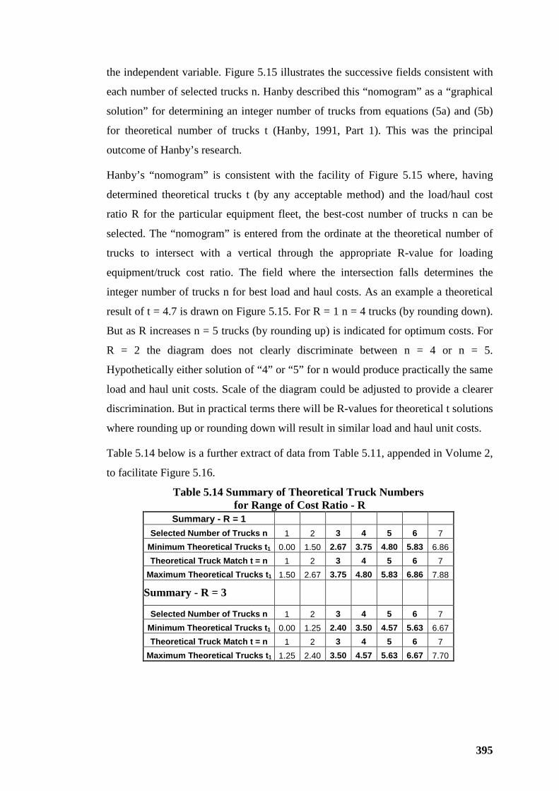
395
the independent variable. Figure 5.15 illustrates the successive fields consistent with
each number of selected trucks n. Hanby described this “nomogram” as a “graphical
solution” for determining an integer number of trucks from equations (5a) and (5b)
for theoretical number of trucks t (Hanby, 1991, Part 1). This was the principal
outcome of Hanby’s research.
Hanby’s “nomogram” is consistent with the facility of Figure 5.15 where, having
determined theoretical trucks t (by any acceptable method) and the load/haul cost
ratio R for the particular equipment fleet, the best-cost number of trucks n can be
selected. The “nomogram” is entered from the ordinate at the theoretical number of
trucks to intersect with a vertical through the appropriate R-value for loading
equipment/truck cost ratio. The field where the intersection falls determines the
integer number of trucks n for best load and haul costs. As an example a theoretical
result of t = 4.7 is drawn on Figure 5.15. For R = 1 n = 4 trucks (by rounding down).
But as R increases n = 5 trucks (by rounding up) is indicated for optimum costs. For
R = 2 the diagram does not clearly discriminate between n = 4 or n = 5.
Hypothetically either solution of “4” or “5” for n would produce practically the same
load and haul unit costs. Scale of the diagram could be adjusted to provide a clearer
discrimination. But in practical terms there will be R-values for theoretical t solutions
where rounding up or rounding down will result in similar load and haul unit costs.
Table 5.14 below is a further extract of data from Table 5.11, appended in Volume 2,
to facilitate Figure 5.16.
Table 5.14 Summary of Theoretical Truck Numbers for Range of Cost Ratio - R
Summary - R = 1 Selected Number of Trucks n 1 2 3 4 5 6 7
Minimum Theoretical Trucks t1 0.00 1.50 2.67 3.75 4.80 5.83 6.86 Theoretical Truck Match t = n 1 2 3 4 5 6 7
Maximum Theoretical Trucks t1 1.50 2.67 3.75 4.80 5.83 6.86 7.88
Summary - R = 3
Selected Number of Trucks n 1 2 3 4 5 6 7 Minimum Theoretical Trucks t1 0.00 1.25 2.40 3.50 4.57 5.63 6.67 Theoretical Truck Match t = n 1 2 3 4 5 6 7
Maximum Theoretical Trucks t1 1.25 2.40 3.50 4.57 5.63 6.67 7.70
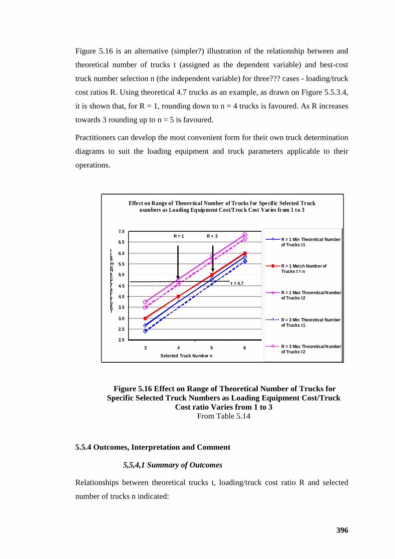
396
Figure 5.16 is an alternative (simpler?) illustration of the relationship between and
theoretical number of trucks t (assigned as the dependent variable) and best-cost
truck number selection n (the independent variable) for three??? cases - loading/truck
cost ratios R. Using theoretical 4.7 trucks as an example, as drawn on Figure 5.5.3.4,
it is shown that, for R = 1, rounding down to n = 4 trucks is favoured. As R increases
towards 3 rounding up to n = 5 is favoured.
Practitioners can develop the most convenient form for their own truck determination
diagrams to suit the loading equipment and truck parameters applicable to their
operations.
2. 0
2. 5
3. 0
3. 5
4. 0
4. 5
5. 0
5. 5
6. 0
6. 5
7. 0
3 4 5 6
Theoretical Truck Number t
Selected Truck Number n
Effect on Range of Theoretical Number of Trucks for Specif ic Selected Truck numbers as Loading Equipment Cost/Truck Cost Varies from 1 to 3
R = 1 Min Theoretical Number of Trucks t1
R = 1 Match Number of Trucks t = n
R = 1 Max Theoretical Number of Trucks t2
R = 3 Min Theoretical Number of Trucks t1
R = 3 Max Theoretical Number of Trucks t2
t = 4.7
R = 1 R = 3
Figure 5.16 Effect on Range of Theoretical Number of Trucks for Specific Selected Truck Numbers as Loading Equipment Cost/Truck
Cost ratio Varies from 1 to 3 From Table 5.14
5.5.4 Outcomes, Interpretation and Comment
5,5,4,1 Summary of Outcomes
Relationships between theoretical trucks t, loading/truck cost ratio R and selected
number of trucks n indicated:
397
• For practical ranges of selection parameters, rounding down of determined t
values to selected n trucks is generally more favoured than rounding up –
consistent with the support for under trucking to provide best costs for
loading and hauling as discussed in Section 3.5.3.
• As truck numbers increase, minimum theoretical number of trucks t1 tends to
be asymptotic to the matching number of trucks, i.e., the corresponding
selected actual number of trucks n – therefore, for increasing number of
trucks, rounding down tends to be more favourable.
• As loading-equipment/truck cost ratio increases, rounding up from the
theoretical number t to selected integer number n tends to be more
favourable.
• Where loading equipment cost is high (R → 3 or more), the addition of an
extra truck has less impact on load and haul unit costs and rounding up tends
to be more favourable.
The relationship between nominal numbers of passes per truck payload, one-way
haul distance and interrelated loading equipment and truck operating parameters has
been discussed in a number of contexts. In general it can be predicted that:
• For short hauls, where three or four-pass loading is favoured, then cost ratio
R will tend towards the upper limits of the practical range (R → 3 say).
Selected trucks n will tend to be theoretical trucks t +/- 0.5 - difference does
not clearly indicate favoured rounding direction.
• For long hauls, where five or six-pass loading is acceptable, R values will
tend to be in the lower end of the range, R < 2 say; number of trucks will be
in the upper range – say 5 plus – then selected number of trucks n will tend
to be theoretical trucks t + 0.25/-0.75 – rounding direction will be more
obvious.
Pursuing three and four-pass loading, in certain circumstances, has been shown to
have some disadvantages, including payload distribution dispersion and lower
intrinsic loading equipment efficiency. Analysis in this Section 5.5.4.1 produces
loading and hauling performance indices with higher R-values that result in rounding
errors tending to over truck or under truck to a degree reflected by cost penalties
398
measurably higher than alternative fleet arrangements. That is – more passes, more
trucks and lower loading equipment/truck cost ratio R can be measurably cost
beneficial.
5.5.4.2 Limitations of Hanby’s Analysis
Hanby’s analysis assumes that owning and operating cost of loading equipment and
trucks is constant for each hour of operating time, adding an element of conservative
bias. As developed by traditional methods, owning and operating cost per hour or
SMU (service meter unit) are, to some degree, empirically based; so tend to be
average costs per unit of elapsed time. Generally owning and operating costs spread
annualized cost over estimated productive operating time. Equipment costs are either
estimated averages for any state of operating (working or waiting) or zero when non-
operating. Traditional practices tend to estimate conservatively high unit production
costs that, to a substantial degree, tend to offset errors and omissions.
During operations there are periods when loading equipment and trucks are operating
but not productive. These differing operational phases were discussed in terms of
time definitions in some detail in Section 3.6.3 and illustrated by Table 3.75
appended in Volume 2.
In load and haul operations both loading equipment and trucks experience times
when equipment is operational but not productive, i.e., waiting. This raises the issue
of accuracy implications of the simple assumption of only two cost phases,
productive and non-operational, the basis of Hanby’s analysis. Justification for
adding another phase of waiting time when equipment is ready for work but not
productive is warranted.
Intuitively the two-phase cost simplification is considered not to reflect adversely on
Hanby’s results and conclusions. Analysis in Section 5.5.5, in addition to considering
waiting-time cost-effects in some detail, also provides confirmation that the
outcomes of Hanby’s analysis in terms of integer truck numbers are generally valid.
But when considering comparisons in terms of absolute cost indices analysis based
on more realistic time phases (three-phase cost analysis) will provide more accurate
assessment of costs
399
5.5.5 Overtrucking, Undertrucking - Productivity and Costs
The general problems of overtrucking, undertrucking, fleet matching and bunching
were discussed in terms of productivity in Section 3.5.3 and Section 3.5.4. It should
be noted that productivity and related cost analysis are generally in terms of mean or
average values for variables. The following analysis is similarly limited.
This section will address resultant cost effects due to productivity influences of
overtrucking, undertrucking and bunching.
5.5.5.1 Effect of Waiting Time on Load and Haul Costs
The analysis in Section 5.5.3 is used as a framework to develop equations equivalent
to (4a), (4b), (5a) and (5b); but for three phases of costs, operating waiting and non-
operating compared with the simple two phases adopted by Hanby and for the
analysis in Section 5.5.3 and discussions in Section 5.5.4.
Starting from the same premise - owning and operating costs of operating “team” of
a loading equipment item and a truck group of n trucks:
C = CL + n . CT (1’)
Let: cL = owning and operating cost of waiting loading equipment.
cT = owning and operating cost of waiting trucks.
And: r = cL/cT c.f. R = CL/CT
Let: k = proportion of productive operating time of trucks, so
1 – k = proportion of waiting time of trucks; and
p = proportion of productive operating time of loading equipment, so
1 – p = proportion of waiting time of loading equipment.
Repeating the analysis in Section 5.5.3 - we arrived at:
PS/CT = R + n t < n (5a)
PS/CT = (R + n) . t/n t ≥ n (5b)
If equations (5a) and (5b) are developed allowing for waiting time by modifying (4a)
and (4b):
P = (CL + k . n . CT) /S +(1 - k) . n . cT/S t < n (4a’)
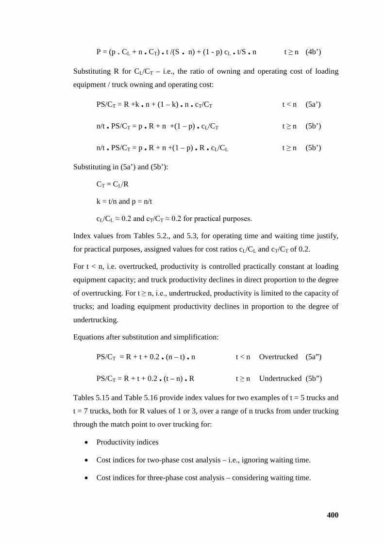
400
P = (p . CL + n . CT) . t /(S . n) + (1 - p) cL . t/S . n t ≥ n (4b’)
Substituting R for CL/CT – i.e., the ratio of owning and operating cost of loading
equipment / truck owning and operating cost:
PS/CT = R +k . n + (1 – k) . n . cT/CT t < n (5a’)
n/t . PS/CT = p . R + n +(1 – p) . cL/CT t ≥ n (5b’)
n/t . PS/CT = p . R + n +(1 – p) . R . cL/CL t ≥ n (5b’)
Substituting in (5a’) and (5b’):
CT = CL/R
k = t/n and p = n/t
cL/CL ≈ 0.2 and cT/CT ≈ 0.2 for practical purposes.
Index values from Tables 5.2., and 5.3, for operating time and waiting time justify,
for practical purposes, assigned values for cost ratios cL/CL and cT/CT of 0.2.
For t < n, i.e. overtrucked, productivity is controlled practically constant at loading
equipment capacity; and truck productivity declines in direct proportion to the degree
of overtrucking. For t ≥ n, i.e., undertrucked, productivity is limited to the capacity of
trucks; and loading equipment productivity declines in proportion to the degree of
undertrucking.
Equations after substitution and simplification:
PS/CT = R + t + 0.2 . (n – t) . n t < n Overtrucked (5a”)
PS/CT = R + t + 0.2 . (t – n) . R t ≥ n Undertrucked (5b”)
Tables 5.15 and Table 5.16 provide index values for two examples of t = 5 trucks and
t = 7 trucks, both for R values of 1 or 3, over a range of n trucks from under trucking
through the match point to over trucking for:
• Productivity indices
• Cost indices for two-phase cost analysis – i.e., ignoring waiting time.
• Cost indices for three-phase cost analysis – considering waiting time.
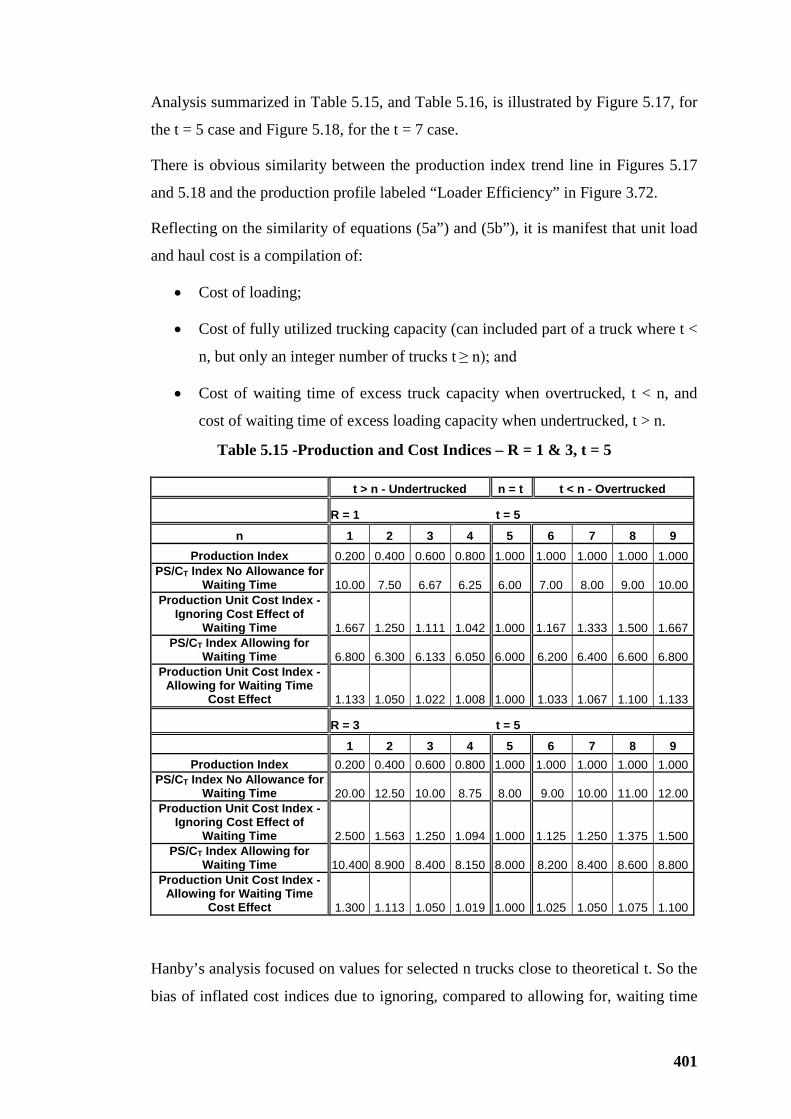
401
Analysis summarized in Table 5.15, and Table 5.16, is illustrated by Figure 5.17, for
the t = 5 case and Figure 5.18, for the t = 7 case.
There is obvious similarity between the production index trend line in Figures 5.17
and 5.18 and the production profile labeled “Loader Efficiency” in Figure 3.72.
Reflecting on the similarity of equations (5a”) and (5b”), it is manifest that unit load
and haul cost is a compilation of:
• Cost of loading;
• Cost of fully utilized trucking capacity (can included part of a truck where t <
n, but only an integer number of trucks t ≥ n); and
• Cost of waiting time of excess truck capacity when overtrucked, t < n, and
cost of waiting time of excess loading capacity when undertrucked, t > n.
Table 5.15 -Production and Cost Indices – R = 1 & 3, t = 5 t > n - Undertrucked n = t t < n - Overtrucked
R = 1 t = 5
n 1 2 3 4 5 6 7 8 9 Production Index 0.200 0.400 0.600 0.800 1.000 1.000 1.000 1.000 1.000
PS/CT Index No Allowance for Waiting Time 10.00 7.50 6.67 6.25 6.00 7.00 8.00 9.00 10.00
Production Unit Cost Index - Ignoring Cost Effect of
Waiting Time 1.667 1.250 1.111 1.042 1.000 1.167 1.333 1.500 1.667 PS/CT Index Allowing for
Waiting Time 6.800 6.300 6.133 6.050 6.000 6.200 6.400 6.600 6.800 Production Unit Cost Index -
Allowing for Waiting Time Cost Effect 1.133 1.050 1.022 1.008 1.000 1.033 1.067 1.100 1.133
R = 3 t = 5
1 2 3 4 5 6 7 8 9 Production Index 0.200 0.400 0.600 0.800 1.000 1.000 1.000 1.000 1.000
PS/CT Index No Allowance for Waiting Time 20.00 12.50 10.00 8.75 8.00 9.00 10.00 11.00 12.00
Production Unit Cost Index - Ignoring Cost Effect of
Waiting Time 2.500 1.563 1.250 1.094 1.000 1.125 1.250 1.375 1.500 PS/CT Index Allowing for
Waiting Time 10.400 8.900 8.400 8.150 8.000 8.200 8.400 8.600 8.800 Production Unit Cost Index -
Allowing for Waiting Time Cost Effect 1.300 1.113 1.050 1.019 1.000 1.025 1.050 1.075 1.100
Hanby’s analysis focused on values for selected n trucks close to theoretical t. So the
bias of inflated cost indices due to ignoring, compared to allowing for, waiting time
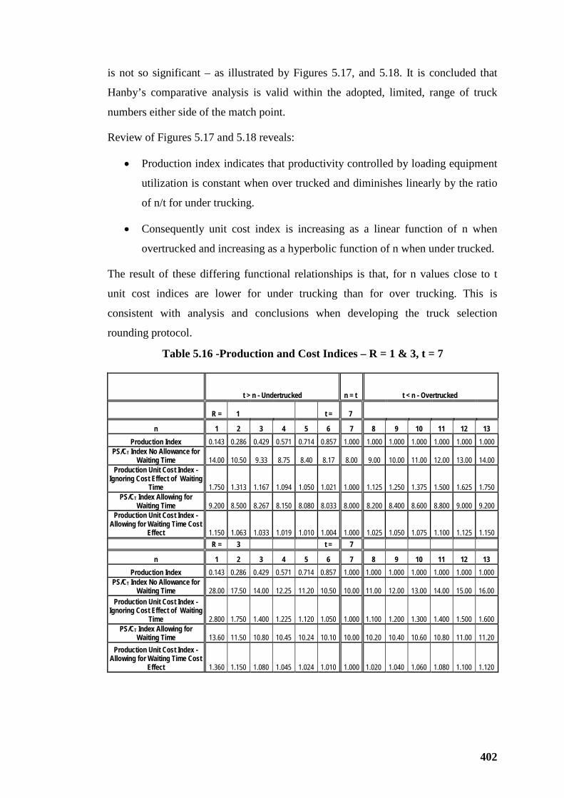
402
is not so significant – as illustrated by Figures 5.17, and 5.18. It is concluded that
Hanby’s comparative analysis is valid within the adopted, limited, range of truck
numbers either side of the match point.
Review of Figures 5.17 and 5.18 reveals:
• Production index indicates that productivity controlled by loading equipment
utilization is constant when over trucked and diminishes linearly by the ratio
of n/t for under trucking.
• Consequently unit cost index is increasing as a linear function of n when
overtrucked and increasing as a hyperbolic function of n when under trucked.
The result of these differing functional relationships is that, for n values close to t
unit cost indices are lower for under trucking than for over trucking. This is
consistent with analysis and conclusions when developing the truck selection
rounding protocol.
Table 5.16 -Production and Cost Indices – R = 1 & 3, t = 7
t > n - Undertrucked n = t t < n - Overtrucked
R = 1 t = 7
n 1 2 3 4 5 6 7 8 9 10 11 12 13 Production Index 0.143 0.286 0.429 0.571 0.714 0.857 1.000 1.000 1.000 1.000 1.000 1.000 1.000
PS/CT Index No Allowance for Waiting Time 14.00 10.50 9.33 8.75 8.40 8.17 8.00 9.00 10.00 11.00 12.00 13.00 14.00
Production Unit Cost Index - Ignoring Cost Effect of Waiting
Time 1.750 1.313 1.167 1.094 1.050 1.021 1.000 1.125 1.250 1.375 1.500 1.625 1.750 PS/CT Index Allowing for
Waiting Time 9.200 8.500 8.267 8.150 8.080 8.033 8.000 8.200 8.400 8.600 8.800 9.000 9.200 Production Unit Cost Index -
Allowing for Waiting Time Cost Effect 1.150 1.063 1.033 1.019 1.010 1.004 1.000 1.025 1.050 1.075 1.100 1.125 1.150
R = 3 t = 7
n 1 2 3 4 5 6 7 8 9 10 11 12 13 Production Index 0.143 0.286 0.429 0.571 0.714 0.857 1.000 1.000 1.000 1.000 1.000 1.000 1.000
PS/CT Index No Allowance for Waiting Time 28.00 17.50 14.00 12.25 11.20 10.50 10.00 11.00 12.00 13.00 14.00 15.00 16.00
Production Unit Cost Index - Ignoring Cost Effect of Waiting
Time 2.800 1.750 1.400 1.225 1.120 1.050 1.000 1.100 1.200 1.300 1.400 1.500 1.600 PS/CT Index Allowing for
Waiting Time 13.60 11.50 10.80 10.45 10.24 10.10 10.00 10.20 10.40 10.60 10.80 11.00 11.20 Production Unit Cost Index -
Allowing for Waiting Time Cost Effect 1.360 1.150 1.080 1.045 1.024 1.010 1.000 1.020 1.040 1.060 1.080 1.100 1.120
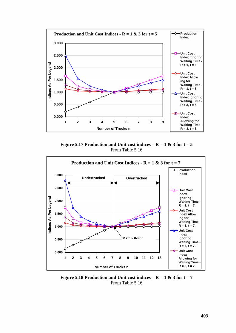
403
Production and Unit Cost Indices - R = 1 & 3 for t = 5
0.000
0.500
1.000
1.500
2.000
2.500
3.000
1 2 3 4 5 6 7 8 9
Number of Trucks n
Indi
ces
As
Per L
egen
d
ProductionIndex
Unit CostIndex IgnoringWaiting Time -R = 1, t = 5.
Unit CostIndex Allowing forWaiting Time -R = 1, t = 5.Unit CostIndex IgnoringWaiting Time -R = 3, t = 5.
Unit CostIndexAllowing forWaiting Time -R = 3, t = 5.
Figure 5.17 Production and Unit cost indices – R = 1 & 3 for t = 5 From Table 5.16
Production and Unit Cost Indices - R = 1 & 3 for t = 7
0.000
0.500
1.000
1.500
2.000
2.500
3.000
1 2 3 4 5 6 7 8 9 10 11 12 13
Number of Trucks n
Indi
ces
As
Per L
egen
d
ProductionIndex
Unit CostIndexIgnoringWaiting Time -R = 1, t = 7.Unit CostIndex Allowing forWaiting Time -R = 1, t = 7.Unit CostIndexIgnoringWaiting Time -R = 3, t = 7.Unit CostIndexAllowing forWaiting Time -R = 3, t = 7.
Undertrucked Overtrucked
Match Point
Figure 5.18 Production and Unit cost indices – R = 1 & 3 for t = 7
From Table 5.16
404
When under trucked, the unit cost of loading in the three-phase-cost case, where
allowance is made for cost of waiting time for loading equipment, is the same as for
fully utilized loading capacity at the match point or when over trucked. Reduced
utilization of loading equipment is offset by reduced production in proportion to
number of trucks selected, which is less than theoretical trucks required for a match.
So the loading component of load and haul unit cost is practically constant.
A similar situation applies to hauling unit cost of fully-utilized selected trucks n
when hauling unit cost for the consequent reduced production is the same as the
hauling unit cost of theoretical trucks t at the match point.
When over trucked, excess truck capacity is waiting and adds a commensurate
hauling unit cost. When under trucked, excess loading capacity is waiting and
similarly adds a commensurate loading unit cost.
Cost amelioration effect of considering waiting time is clearly demonstrated by
Tables 5.15, and 5.16; also Figures 5.17, and 5.18. The inflated cost bias of analysis
that ignores reduced cost for waiting time is more obvious as n values increase or
decrease from the match point.
Observations and conclusions from review of Tables 5.15 and 5.16; and Figures 5.17
and 5.18 include:
• Under trucking to any degree consistently increases load and haul unit costs
less than does the same degree of over trucking – so favouring under trucking
where the production programme can tolerate the small reduction.
• As expected, for increasing numbers of theoretical trucks, each additional
over match; or omitted truck under match, has less load-and-haul-cost impact
– compare Tables 5.15 and 5.16.
• As over trucking or under trucking increases, the “B” case (t = 7) indicates
similar bias gradients as does the “A” case (t = 5) – refer Tables 5.15 and
5.16; but index gradients for the “B” case (t = 7) are significantly flatter than
for the “A” case (t = 5) – consistent with the point immediately above.
• Subject to the discussion on Owning and Operating Costs below, actual over
trucking or under trucking is less cost penalizing than simplified analysis
405
based on simple two-phase cost analysis, ignoring waiting time effects, would
lead us to believe.
In the end result – over trucking or under trucking imposes cost penalties much less
than those indicated by two-phase cost analysis as adopted by Hanby; also by the
analysis herein in Section 5.5.3.
Simply, adding trucks that are not utilized only adds the cost of labour plus some 5%
of productive-operating fuel consumption and lubricants and a similar proportion of
driveline maintenance, investment amortization, and no tyre costs.
Similarly, under trucking underutilizes loading equipment. Productive time of
loading equipment, during which unit loading costs are generally constant, is
reduced. The balance, loading-equipment waiting time, imposes a cost similar in
compilation to waiting trucks. That is, cost of labour plus some small proportion; say
in the order of 5%, of energy/fuel consumption and lubricants, a similar proportion of
maintenance and investment amortization; and no ground engaging tools, running
gear, bucket repairs or digging implement structural/mechanical maintenance cost.
5.5.5.2 Owning and Operating Cost – Discussion
The above analysis adopts basic assumptions for the derivation of owning and
operating (O & O) costs for mining equipment items per unit of time (solar hour or
SMU). It is assumed that O & O costs are based on productive operating hours. That
is after all deductions for downtime and for non-productive time whether or not
deemed necessary for productive operations; and further, after allowance for job
management efficiency factors or deductions. This procedure allows for cost analysis
to separately and transparently account for waiting time, however caused, which
clearly indicates reduced O & O costs.
Table 3.75, appended in Volume 2, details time definitions that provide an
understanding of the implications of differing O & O costs for available equipment
that is not directly operating, i.e., on the job but not directly productive.
5.5.6 Bunching - Productivity and Costs
The efficiency-reducing effect of bunching was discussed generally in Section 3.5.4.
406
5.5.6.1 Derivation of ηB = (1 – CVT)
As discussed in Section 3.5.4, as reported by Caterpillar, empirical evidence
indicates that if:
CVT = 0.15 ηB = (1 – 0.15) = 0.85 or generally:
ηB = (1 – CVT) (15 - see Section 3.5.4)
Where:
CVT = Coefficient of variation of truck cycle time (total trip time TT herein).
ηB = Bunching efficiency.
As discussed in Section 3.5.4, and based on empirical evidence, Caterpillar have
recommended a practical range of bunching efficiencies from a high of 0.90, through
medium of 0.85 to a low of 0.80.
Bunching is a significant cause of TW, i.e., a small proportion of truck total trip time
TT. Variability, i.e., CVT – for total trip time TT, will always be less than CVW for
truck (or loading equipment) waiting time TW. Parallel logic is applied here as for
reasoning discussed in Section 3.5.4 for truck payload and NMW as proportions of
GMW, in Section 3.2.8 for bucket loads and truck payloads; and in Section 3.2.9 for
bucket cycle times as a proportion of truck loading time.
Bunching is a physical manifestation of variability of performance of the entity under
review. Queuing effects, measured by waiting time TW and number of trucks in the
queue are caused by bunching. Causes of bunching were discussed in some detail in
Section 3.5.4. Waiting time TW is mainly due to variability of total truck trip time TT.
That TT is a combination of several time identities discussed above – specifically TT
= TL + TV + TD +TS – is irrelevant for purposes of the current discussion. For
convenience the following rationale adopts total trip time TT as a basis. Outcomes are
consistent with empirical-based equation (15) above, bunching-effect discussion in
Section 3.5.4 and in this section. Adopted data following is also consistent with
analysis and references identified in Section 3.3.10.
It is an important distinction that truck waiting time, i.e., hauling time lost directly
related to bunching, can be generally classified as intrinsic. That is time losses from
inherent variability of the several components that combine to determine equipment
performance as discussed in Section 3.5.4.
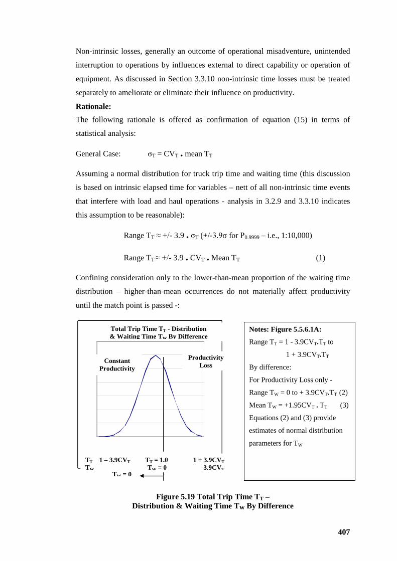
407
Non-intrinsic losses, generally an outcome of operational misadventure, unintended
interruption to operations by influences external to direct capability or operation of
equipment. As discussed in Section 3.3.10 non-intrinsic time losses must be treated
separately to ameliorate or eliminate their influence on productivity.
Rationale: The following rationale is offered as confirmation of equation (15) in terms of
statistical analysis:
General Case: σT = CVT . mean TT
Assuming a normal distribution for truck trip time and waiting time (this discussion
is based on intrinsic elapsed time for variables – nett of all non-intrinsic time events
that interfere with load and haul operations - analysis in 3.2.9 and 3.3.10 indicates
this assumption to be reasonable):
Range TT ≈ +/- 3.9 . σT (+/-3.9σ for P0.9999 – i.e., 1:10,000)
Range TT ≈ +/- 3.9 . CVT . Mean TT (1)
Confining consideration only to the lower-than-mean proportion of the waiting time
distribution – higher-than-mean occurrences do not materially affect productivity
until the match point is passed -:
Figure 5.19 Total Trip Time TT –
Distribution & Waiting Time TW By Difference
Total Trip Time TT - Distribution & Waiting Time TW By Difference
Constant Productivity
Productivity Loss
TT 1 – 3.9CVT TT = 1.0 1 + 3.9CVT TW TW = 0 3.9CVT
Notes: Figure 5.5.6.1A:
Range TT = 1 - 3.9CVT.TT to
1 + 3.9CVT.TT
By difference:
For Productivity Loss only -
Range TW = 0 to + 3.9CVT.TT (2)
Mean TW = +1.95CVT . TT (3)
Equations (2) and (3) provide
estimates of normal distribution
parameters for TW
TW = 0
408
Waiting time TW is a random variable dependent mainly on travel time randomly
variable travel time TV. As loading time and other components are small compared
with TV their variability may be ignored, i.e., these elemental times can be
considered constant (expected) values.
For fleet arrangements where loading equipment is theoretically under trucked or
over trucked by less than a unit truck. Some of the time bunching may reduce
conditions to loading equipment being undertrucked so productivity reduces. For the
balance of the time over trucked conditions will prevail. But this only results in
additional waiting time for trucks only and no material change to productivity.
Because total trip times exhibit central tendency, it is reasonable to assume that
waiting time data will be symmetrical. It is reasonable to assume that for practically
half of the time, there is a tendency for loss of productivity; and for the other half of
the time, constant productivity.
The rationale is illustrated by Figure 5.19 and related notes.
From equation (3) – for some 50% of operating time:
Mean TW = 1.95CVT . TT
Apparent ηB = (TT – TW)/TT
= (TT – 1.95CVT.TT)/TT
= (1 – 1.95CVT)
This is valid if all waiting events can affect production – consistent with the high end
of the range evidenced empirically. But a-productive effect of waiting time only
affects some 50% of waiting time events.
Mean ηB = [1 +(1 – 1.95CVT)]/2
= (2 - 1.95CVT)/2
ηB ≈ 1 - CVT practically corresponds to empirical equation (15).
The above rationale is considered to analytically support empirically based bunching
efficiency variability recommended by Caterpillar and generally adopted by industry.
It should be noted that the above relationship between bunching efficiency and
distribution parameters of truck trip time TT is independent of the origin of data, i.e.,
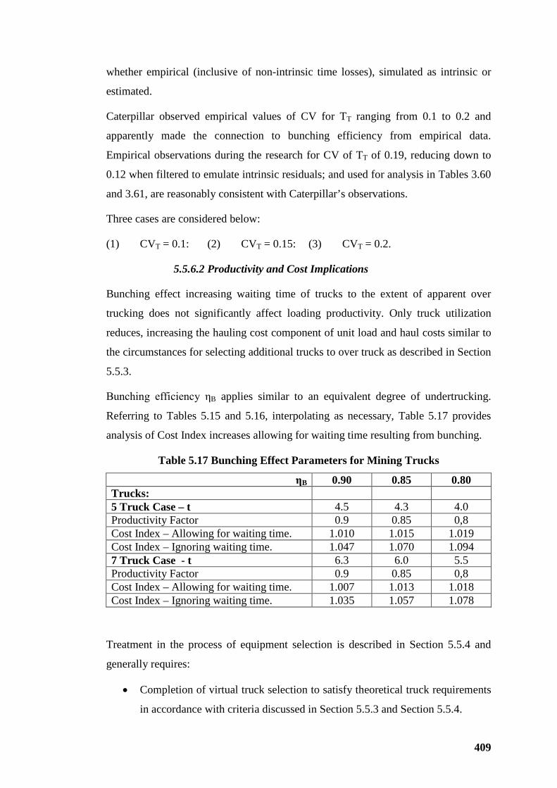
409
whether empirical (inclusive of non-intrinsic time losses), simulated as intrinsic or
estimated.
Caterpillar observed empirical values of CV for TT ranging from 0.1 to 0.2 and
apparently made the connection to bunching efficiency from empirical data.
Empirical observations during the research for CV of TT of 0.19, reducing down to
0.12 when filtered to emulate intrinsic residuals; and used for analysis in Tables 3.60
and 3.61, are reasonably consistent with Caterpillar’s observations.
Three cases are considered below:
(1) CVT = 0.1: (2) CVT = 0.15: (3) CVT = 0.2.
5.5.6.2 Productivity and Cost Implications
Bunching effect increasing waiting time of trucks to the extent of apparent over
trucking does not significantly affect loading productivity. Only truck utilization
reduces, increasing the hauling cost component of unit load and haul costs similar to
the circumstances for selecting additional trucks to over truck as described in Section
5.5.3.
Bunching efficiency ηB applies similar to an equivalent degree of undertrucking.
Referring to Tables 5.15 and 5.16, interpolating as necessary, Table 5.17 provides
analysis of Cost Index increases allowing for waiting time resulting from bunching.
Table 5.17 Bunching Effect Parameters for Mining Trucks
ηB 0.90 0.85 0.80 Trucks: 5 Truck Case – t 4.5 4.3 4.0 Productivity Factor 0.9 0.85 0,8 Cost Index – Allowing for waiting time. 1.010 1.015 1.019 Cost Index – Ignoring waiting time. 1.047 1.070 1.094 7 Truck Case - t 6.3 6.0 5.5 Productivity Factor 0.9 0.85 0,8 Cost Index – Allowing for waiting time. 1.007 1.013 1.018 Cost Index – Ignoring waiting time. 1.035 1.057 1.078
Treatment in the process of equipment selection is described in Section 5.5.4 and
generally requires:
• Completion of virtual truck selection to satisfy theoretical truck requirements
in accordance with criteria discussed in Section 5.5.3 and Section 5.5.4.
410
• Consideration of operating conditions, load and haul equipment, operating
configurations as planned and haulage conditions.
• Other considerations as discussed in Section 3.5.4 or Section 5.5.4.
In addition bunching productivity and cost effects need to be analyzed in accordance
with the above discussion in this Section 5.5.6 to fine-tune the fleet for acceptable
productivity at optimum cost. The nett result of bunching considerations is generally
an increase in the basic number of trucks as delivered by initial estimates.
Caterpillar’s FPC and similar load and haul simulation software apply bunching
treatment integral with the simulation applications.
411
CHAPTER 6
SUPPLEMENTARY ACTIVITIES
6.1 ADDITIONAL INTER-ACTIVES
This section briefly reviews additional inter-actives that overlap, or interface with,
the activities reviewed and analyzed in Chapters 3, 4 and 5. These supplementary
topics include recently emerging and developing activities that promise to
significantly influence future development of load and haul practices in open pit
mining.
The general approach of the research has been for improvement of understanding of
the basic selection criteria for load-and-haul equipment. These additional topics have
not been thoroughly investigated for this thesis. They have been identified in Chapter
4; related productivity and cost effects have been discussed in Chapter 5; are further
discussed in the context of application in this section; and finally considered in
Chapters 7 and 8 in the context of conclusions and recommendations for future
research.
During research of criteria for selection of mining equipment each topic was
analyzed to a degree of understanding, where that topic could be considered to have
met research objectives. In common with research in general, as research proceeds,
other inter-active, and supplementary topics emerge of sufficient relevance to
encourage consideration of inclusion in the research. Because of scope limitations,
determined by time and sheer bulk of research undertaken, some topics, investigation
of which appeared to be warranted, were excluded to provide priority for those topics
researched as described in this thesis.
Some of the more cogent complementary topics have been identified and briefly
discussed in Chapters 3 to 5. Additional topics, previously bypassed, are included in
the following discussion, at least to a preliminary degree sufficient to recognize their
importance as inter-active to the topics covered in more detail by the research.
This Chapter 6 reviews and briefly discusses those topics that, although interrelated
to primary activities researched, have not been investigated in detail.
412
6.1.1 Planning and Equipment Selection
In the broad activities of promoting a mineral prospect to an economic development
project, there is a succession of iterative processes that can generally be described as
project planning. The many disciplines applied to bring a development project to
reality each need to make important planning contributions. Integral with general
planning activities, including resource interpretation and delineation and ore reserve
definition, a number of activities, generally termed Mine Planning, must proceed.
Mine Planning not only involves consideration of exploitation methods but must also
consider operating scale. This leads to mining equipment selection.
Equipment selection, at least of principal items of loading and hauling equipment, is
considered early in mine planning. The interdependency of mine planning and
equipment selection is such that neither can be completely finalized without
complete resolution of the other – so requiring iterative process. Equipment selection
is carried forward integral with an ever-refining process through the many planning
iterations that yield finalized cost-optimized production schedules and mine plans,
estimation of costs, economic evaluation and feasibility testing.
Along the way changing, but continuously refining criteria for equipment selection
must be gathered, both internally from project planning and externally by due
diligence, to identify options available and characteristics of those options to form a
basis for decision.
The following four sections discuss, albeit briefly, some of the more cogent,
supplementary topics that interface with or overlap the research described in this
thesis.
6.1.2 Drilling and Blasting
Section 3.3.6 describes the analytical trail from truck payload dispersion to the drill-
and-blast quality control. The implication that control of truck payload dispersion
may most effectively be realized by best-practice drilling and blasting is an obvious
conclusion needing verification empirically. The promise for payload dispersion
control justifies the general review and comments in this Section 6.1.2.
Drilling and blasting parameters can be considered in two groups:
413
1. Blasting agent, explosives – specific quantities measured as “powder factor”,
generally kilogrammes/bank cubic metre; blasting accessory specifications
and characteristics, hole charging details including stemming – and cost per
unit volume or tonne.
2. Blast design, bench height, hole diameter and drilling pattern dimensions and
parameters that determine the distribution of blasting agent or explosive
through the material volume that is to be fragmented by blasting; also the
detonation sequence that determines material displacement, seismic vibration
and noise level of blasts.
Within these two groups activities and attributes related to quality control of blasted
material are of greatest interest for these discussions. Except for unconsolidated
highly-weathered materials – generally materials that can be extracted by so-called
“free digging” - such as detritals and tertiary sediments including wind or water
deposited sands and gravels, bank material, i.e. insitu material, generally needs
fragmentation in preparation for loading. Materials to be loaded from the sub-
weathered zones, i.e., particularly “fresh” or “transition” horizons, need to be drilled
and blasted. Variabilities of truck payloads, loading equipment-digging performance,
especially bucket fill factor; and consequently the number of passes are all
influenced by quality of fragmentation of material measured by maximum particle
size, size grading and voids ratio.
For cyclic loading there is a cost tradeoff where the total cost of fragmentation, plus
cost of loading and hauling is a minimum.
The relationship between variabilities of truck payload and voids ratio of material,
fragmented (generally by drilling and blasting) in preparation for loading, was
investigated and discussed in Section 3.3.6. Experience indicates that, where
fragmentation produces smaller mean particle size and more consistent size grading
of fragmented material, expected or enhanced digability is achieved. The relationship
between particle size and fragment grading and drilling and blasting design
parameters has been established. Therefore, it is hypothesized that a relationship
between fragmentation quality, specifically controlled voids ratio variability, and
truck payload variability, loading and hauling productivity and costs can be defined
in mathematical terms and substantiated empirically.
414
Considering two operating scenarios:
1. Small drilling patterns, small diameter holes with adequate powder factor
(kg/BCM of insitu material) will produce reduced particle sizes, i.e., high
fragmentation. But this could be at prohibitively high cost that, when added
to cost of loading and hauling (as productive and load-and-haul cost effective
as this may be) will be uneconomically high.
2. Conversely, given that bench height is adequate, large dimension patterns
with large holes at the same powder factor may cost less to provide the blast
holes, reduce cost of blasting accessories so reduce drill-and-blast costs; but
at the sacrifice of digability – decreased loading productivity, low bucket
factors, increased passes, increased payload dispersion and overall reduced
load and haul productivity and higher costs. Time losses, inconsistent loading
times and truck cycle times will exacerbate bunching/queuing and erode
operational “rhythm”. Since load-and-haul costs are three or more times drill-
and-blast costs, evidenced by Figure 2.2, the total of drill-and-blast costs and
load-and-haul costs could tend to be potentially uneconomic.
Between these two extremes there will be an optimum operating position where the
total cost of drill-and-blast and load-and-haul is a minimum. Comparing the
continuum of positions in terms of cost, using mean voids ratio and/or coefficient of
variation of voids ratio as characteristic parameters will produce a typical “bathtub”
curve. At the “nadir” of costs vs. mean voids ratio all underlying parameters
throughout the drill-and-blast and load-and-haul system will combine to produce
optimum (not necessarily maximum) productivity and minimum cost.
6.1.2.1 Bench Height – General Comments
For mining of some materials bench height can be predetermined by natural features.
Examples are coal seam width, flat dipping deposits such as sedimentary horizons
including mineral and tar/oil sands. Ore dilution considerations may determine bench
height in metalliferous open pit mines.
For successful, quality drill and blast results drilling patterns, drillhole diameter and
bench height and other drill and blast parameters must satisfy the principles of blast
design. A desire to increase drillhole diameter and pattern size drives the need to
increase bench height. Drill holes must be deep enough to provide adequate
415
stemming height and efficient fragmentation. But, as drillhole diameter reduces,
bench height does not necessarily need to reduce. An interesting example is basic
materials quarrying where high benches with small diameter holes and small-
dimension patterns are general practice for producing blasted hard rock to be crushed
and sized for aggregates. For these special design criteria reduced crushing and
screening costs offset increased cost of drilling and blasting.
Where continuous improvement programmes (CIP) investigate all cost components,
the author’s experience indicates that drill and blast costs tend to be an easy target.
Although drilling and blasting contributes only some 15% of total mining costs
(Figure 2.2), significant savings can be realized by increasing bench height, drillhole
diameter and pattern dimensions, with little if any change in powder factor.
There has been a trend for increased bench heights and drillhole diameters, with
appropriate adjustment of other blast design parameters, for drilling and blasting
practices in metalliferous mining. It is not clear that any resulting load-and-haul
productivity reduction or increased dilution effects have been fully accounted for
when assessing the apparent drill and blast savings. This is a classic case of
considering an activity in isolation with apparent attractive outcomes that are not
realized when all interactives are effective – as discussed in Section 2.2.1.
6.1.3 Dumps and Stockpiles
Selection of trucks both for capacity and supplier is determined by the service
required in terms of productivity and costs. One-way haul routes throughout the life
of the mine, at least the tenure of any selected mining method, need to be
determined; and productivity/cost implications identified and quantified. Production
schedules that identify destinations and target quantities per unit time are required.
As described, during the research deterministic simulation of hauling operations
provided data to progress loading and hauling equipment selection. An obvious
prerequisite is the location, dimensions and limitations on placement of both product
and waste material produced. This requires design of dumps and stockpiles
complementary to open pit design.
Continuously improving computer techniques have been developed for cost-
optimized pit designs. In contrast dumps and stockpiles have traditionally been
designed to fill available spaces within tenements, sometimes with height limitations,
416
using simple manually applied geometrical procedures. More recently fundamental
cost-element techniques applied to pit optimization have emerged in computer
applications for dump design.
The research did not undertake any major treatment of stockpile and waste dump
investigation, analysis or design. Some practical issues are identified with comments
on this reasonably important subject that, in the author’s opinion, has historically
tended to become a secondary planning consideration, often neglected, which can
ultimately impose an embarrassing production and cost penalty.
The following checklist with comments provides preliminary considerations for
planning stockpiles and dumps:
• Tenement boundary location by independent land survey should be available
supplying sufficient boundary markers to set out site works including
clearings, topsoil stripping and stockpiling, tailings dams, dumps and
stockpiles, explosives storage all buildings and constructions, and processing
facilities, sources of basic civil construction materials, mine water
evaporation ponds; and garbage/sewerage disposal.
• Half-metre (or closer) surface contour plans of mining tenements, at least the
areas with potential for occupation, to identify drainage courses and
catchments, to plan diversion of drainage channels, flood protection bunds
and dams as appropriate; and to provide a base digital terrain model for
determination of volumes of dumps and tailings dams.
• Sterilization drilling and geological interpretation of all areas that could
possibly be inundated by stockpiles, dumps and tailings, or occupied by mine
infrastructure.
• Determine general details of dump design, including height limitations,
finished batter profiles for long term stability, surface drainage control
facilities, rehabilitation - including re-vegetation details consistent with
permit conditions on tenements, requirements or recommendations of
statutory authorities and general best practice for dump/stockpile
construction.
417
• Determination of setback from the open pit rim of waste dump or stockpile of
materials for future processing, civil works and rehabilitation; allowances to
include for safety bund wall, potential long term subsidence – particularly in
weathered/transition zone – in compliance with statutory requirements and as
more conservatively amended by competent geotechnical assessment; and to
allow for potential pit deepening when resources, excluded from current pit
designs as uneconomic, can be upgraded to proven ore reserves; also
sufficient additional setback to allow for re-profiling as-dumped waste batters
to conform to a long-term stable angle of repose as required or recommended
by statutory authorities.
• Design dump access ramp(s) to provide optimum haulage costs after mining
trucks reach the surface crest of in-pit access ramps including, generous ramp
width, allowance for drains and spillage storage, straight ramps where
possible and, where necessary for high speed truck return, bends to have large
radius and adequate camber(?); and, where possible, a single constant
gradient from toe of the dump access ramp to crest at the top of the dump.
• Design dump-access ramps to crest at the centroid of dump surfaces. If
dumps are elongated, to match a long-narrow open pit form, then multiple
dump access ramps should be provided to match multiple open pit access
ramps in the early stages of open pit development to divide waste dumps into
sections with dimensions to minimize surface haul distances. Where, in the
mature period of pit development (say below mid-design depth so that some
60% or more of total material has been mined), where access may be limited
to one ramp then dump management should provided space to accommodate
the residual pit volume delivered from the final access ramp at minimum
haulage cost.
• Dump construction needs to be scheduled so that, as dumps extend laterally,
additional lifts are implemented as soon as practicable to provide haul-
distance options for tuning of trip time TT to available trucks.
Further comments on practices on top of waste dumps:
• Crests of access ramps should preferably be located near the geometrical
centroid of the dump surface for minimum on-dump haulage. Average on-
418
dump distances hauled are then to centroidal positions - of sectors for
circular-form dumps with average on-dump haul 0.71 times dump radius and
of triangles for square or rectangular form dumps with average on-dump haul
0.67 times the rectangular distance to the dump crest. So, practically, on-
dump haul distances can be averaged as 70% of average distance to the
dump edge from the access ramp crest.
• On-dump roads should fan out from the access-ramp crest built on a
formation above dump surfaces to provide for cross fall and road drainage;
also roads should be to best construction standards commencing from
compaction of the dump surface (loaded trucks are convenient compactors),
a selected-compacted formation, preferably with crushed rock sheeting to
provide an all-weather hauling surface of profile quality suitable for high
speed return hauls.
• Temporary extensions to tipping points of roads from termini of long-term
on-dump roads should be kept as short as practicable.
• As soon as possible after commencement of mining it is good practice to
mark out dumping limits with rows of truckloads dumped at ground level to
serve as more permanent markers than survey pegs and similar temporary
markers. These marker loads also act as “toe checkers” tending to stabilize
slopes where material tends to flow to a flatter-than-expected angle of
repose; also “toe checkers” catch most large particles that become free on
dump batters tending to build up rolling inertia.
• Before each lift, preferably progressively as dump surface develops, it is
good practice to loose dump loads on the dump surface. This provides
convenient and safe dumping, especially at night. The next lift is then
dumped over the loose dumped “moonscape”. There is a secondary benefit
of reducing the wind fetch on dump surfaces, encouraging turbulent rather
than laminar flow and reducing dust generation.
• It is beneficial to finish final dump surfaces with loose dumped loads to
reduce dust generation and contain precipitation until dumps can be
rehabilitated and finished with topsoil and seeding to promote vegetation.
419
• A comprehensive rehabilitation/vegetation protocol needs to be developed
complying with any statutory requirements. Such a protocol will generally be
a prerequisite to acquiring tenure of the property and/or permission to
develop. Implementation of rehabilitation provisions should commence as
soon as dumps are part completed as per plan with due conservative
consideration of risk of an extension to mining and waste disposal.
The described practices are important for acceptable hauling conditions and best-
practice mine management. Optimum truck cycle time is interrelated with ore
stockpile and waste dump configuration. Inadequate attention to the detailed design
of load-and-haul payload destinations has negative effect on mining productivity and
costs. Engineering and management of dumps and stockpiles is a stand-alone activity
for investigation/research, project planning and mine development.
6.1.4 Mixed Fleets
Many load and haul operations in open pit mines have mixed loading equipment and
mining truck fleets. This may be by design where ex-mine production consists
differing materials such as coal, partings and superincumbent overburden; or by
discrete increases or decreases to operating production scale. Destinations and one-
way hauls can be different for mining product for processing and superincumbent
waste material. So there can be valid operating reasons for mixed fleets. It should be
noted that OEM produce mining trucks with generic performance characteristics to
reduce the affects of mixed fleets with differing performance attributes. But there is
always small, but significant differences in the performance of equipment of
differing scale and between similar capacity equipment produced by different OEM.
Voluntarily acquiring mixed fleets to load and haul material of similar physical
nature over similar round-trip hauls will generally be disadvantageous by reducing
productivity and increasing costs. Where there is choice, avoiding mixed fleets is the
best commercial decision.
As discussed in Chapter 3 loading and hauling with mining trucks is a cyclic rather
than continuous production system. The cyclic nature with tendency to variability of
equipment performance and productivity introduces a-productive effects.
Differing performance of loading equipment and trucks is increased by:
• Mismatch between loading-equipment bucket capacity and truck payload.
420
• Discrete time step variability in truck loading tending to increase queuing
effect.
• Potential differing speeds of trucks so that normal TT variability and
bunching inefficiency are increased by additional time loss.
• Increased inventory of maintenance parts and exchange components
(insurance spares).
• Maintenance facilities may have to be expanded to suit largest equipment –
with some facilities limited in utility; also single or limited occupancy
facilities such as wash-down pads, routine service bays and tyre bays need to
be for the largest equipment.
• Adverse operator and maintenance attitudes to individual equipment items
perceived as less operator/mechanic friendly.
Higher capacity equipment tends to be inhibited by lower performance loading
equipment and trucks with a tendency towards the lowest common denominator, at
least lower than expectancy based on average performance over the mixed fleet.
6.1.5 Dispatch Systems and Remote Control
In the early 1990’s dynamic programming (DP) of complex production systems
enabled development of computer applications for operational control of open pit
mining. Currently larger open pit mining operations with multiple load and haul
fleets generally utilize a “dispatch system” (DS) applying DP algorithms in
sophisticated information technology and communications systems.
DS applying DP can only be as effective as the comprehensiveness of the algorithm
in representing specific DP and degree to which logic of the underlying DP emulates
the actual system. From some observations of DS in action with dispatch attendants
overriding the DS when they consider it necessary, it seems to the author there is a
strong possibility that DP and DS are not always superior to the human mind –
especially the consolidated power of several human minds all seeking to sustain
“rhythm” of loading and hauling operations by minimizing waiting time and
variability of TT and its parts, TL, TV, TD and TS (as defined in 3.3.10).
It seems possible that the benefits of dispatch systems can be enhanced by some old-
fashioned rhythmical practice, especially a bucket-load-sacrifice protocol as
421
discussed in Sections 3.3.9 and 5.4.3 and hauler operators in each fleet keeping
aware of passing points and whether they are ahead or behind time in the circuit,
identifying the slowest truck, advising supervision and replacing a slow truck for
maintenance attention if a spare truck is available. There must be a economic limit
where the delay of a slow truck becomes unacceptable. A simple answer could be
where the proportional delay of total trip time is equal to the inverse of the number of
trucks attending an item of loading equipment. In this circumstance effective truck
time lost is equivalent to an effective truck. These were all practices utilized on sites
managed by the author in the 1970’s before PC, DP and DS were available. Two-
way radios were often a luxury in those times. Load-and-haul “rhythm” was often in
evidence, especially on night shifts where strategic planning and pit “housekeeping”
during the day set up the pit for minimum queuing delay of loading and hauling
equipment.
Unless DP is heuristic, with some facility for recall of experience, application of a
fixed logical process reflecting DP may be applied by a DS to a fault - requiring
constant human monitoring and, occasionally, intervention as necessary.
The above comment is not intended as a criticism of DP and DS applications. A DS
can only be as effective as the underlying DP emulates the operating system. But
current state-of-the-art DS is a most welcome acquisition for open pit management.
Dispatch systems are amongst the most valuable recent developments in open pit
mining management, with the bonus of facility to collect and analyze data and
provide directions - all in real time. They also provide performance data in real time
and can record almost any selected performance indicators to aid management
oversight; and to measure performance against plans and projections. A DS is a
necessary foundation for development of autonomous mining systems. Control of
autonomous trucks can adapt current DS technology, retaining all of the initial
benefits described in Section 4.2.7, and facilitating autonomous hauling operations.
Future development of DS will parallel development of autonomous systems.
Currently development of remote control of DS off mine sites offers flexibility and
convenience for specialist labour to manage logistics of mining operations from city
locations. All mines within convenient geographic boundaries could be controlled
from a specific-purpose facility. The savings of accommodation capital and/or fly-in-
fly out transport costs are manifest.
422
6.1.6 Autonomous Haulage Systems
“Autonomy” implies complete freedom to function of the system’s own freewill, i.e.,
without human intervention. But, in these early stages, development of fully-
autonomous systems with complete freedom of solely self-determined operation
seems ambitious. At least, in the initial stages, constant human monitoring and
intervention seems to be a practical expectancy. As refinement of autonomous
systems with time encourages increasing confidence by operators and clients, degree
of autonomy and remoteness of controlling facilities can be expected to increase.
This is the promise of the future of DS and autonomous load-and-haul, even
complete mining systems. But it would be pure speculation to predict a time scale for
application of completely autonomous mining systems with only small management
intervention.
Some practical parallels provide interesting insight. Plans to automate the railway
systems of the Pilbara iron-ore province in the north-west of Western Australia have
been only modestly publicized. Predictable negative industrial reaction, and virtually
silent political response, is an indication that, even though the technology has been
demonstrated to be reliable and safe; and is readily available, implementation will be
steady rather than startling.
Another parallel is the potential for air transport to graduate to autonomous systems.
Developed for military pilotless aircraft, technology for safe autonomous control of
the world’s airliners is readily available; but there are few passengers who would fly
in them.
Recent development and trials of autonomous load and haul equipment, especially
trucks, to the best of the author’s knowledge, have not been publicly reported. With
performance and cost information generally limited to hearsay, this topic has not
been researched for this thesis. It is understood that economics of early trials were
obscured by the early-developmental cost of the truck add-ons and that early control
applications required remote operator attendance in a purpose built facility on site.
As the cost of truck control units reduces, when control centres are set up in lower-
cost environments remote from mine sites, with more reliability and increased
confidence in the systems autonomous haulage systems appear to be a natural
423
progression for development of open mining technology. Certainly this is a cogent
opportunity for future research.
It is understood that economics of prototype trials were obscured by the early-
developmental cost of the truck add-ons; and that early control applications required
remote operator attendance in a purpose built facility on site. As the cost of truck
control units reduces, when control centres are set up in lower-cost environments
remote from mine sites, with more reliability and increased confidence in the
systems, autonomous haulage systems appear to be a natural evolution for
development of open mining technology.
It is interesting to reflect on the interrelationship between equipment selection
criteria and characteristics of autonomous haulage systems. In Sections 4.2.2, 4.2.3
and 4.2.4 the diminishing unit cost-benefits of trucks of increasing scale was
reviewed. The cause of diminished unit cost-benefit was identified as off-setting
costs mainly for increased access-ramp volume and increased scale of maintenance
accommodation.
Operating labour, considered as a “fixed” cost, unitized over truck payload
contributes to reducing unit-haul costs as truck scale increases. Section 4.2.5
indicates the practically uniform unit cost of fuel and uniformity of other unit-cost
components that are directly proportional to fuel burn. This implies an underlying
practically constant unit cost over the payload range for many of the haul-cost
components. In contrast operating labour, in the order of 12 % of unit haulage cost
(Section 5.1.3), provides a diminishing-unit-cost effect as truck payload increases.
Diminishing unit cost of operating labour is a significant contribution to the
perceived unit-cost benefit of up-scaling to larger mining trucks.
It is interesting to consider the impact on unit costs by substantially removing
operating labour cost for an autonomous haulage system. Removing the majority of
labour cost will tend to have a retrogressive effect on justification of larger payload
and ultra class (UC) mining trucks. Additional flexibility may be available to
consider selection of trucks with a wide range payload without significant cost
penalty. This leads to a further possibility that truck selection will be driven by
comparison of other factors related to most convenient fleet number logistics.
The potential commercial impact on UC truck options is manifest.
424
A further benefit from autonomous haulage could be the potential for rhythmical
smoothing of truck cycle times i.e., virtual elimination of bunching and resulting
queuing effects. Autonomous haul systems need to control separation between trucks
for safe operations. It seems a small advance to control separation between trucks to
minimize (practically eliminate?) bunching with flow-on benefit of reduced fuel and
other consumable costs.
It seems only another small step for an autonomous control system to identify a slow
truck, compare system productivity with or without the offending truck, register
whether or not a replacement is on the “Go” line and make a decision to either leave
the offender in the fleet or deliver it to the workshop complete with complaint
diagnostics in real time on the remedial work required – all without human
intervention.
Certainly autonomous mining systems are a cogent and most interesting field for
future research.
425
CHAPTER 7
SUMMARY OF RESEARCH
7.1 CRITERIA INVESTIGATED
Productivity and cost criteria investigated as described in Chapters 3, 4 and 5
include:
• Truck payload distributions and implications for component life, safe
operations and compliance with limitations on operation of mining trucks.
• Bucket cycle time, number of passes, consequent truck loading time
including intrinsic efficiency and operating “rhythm” benefits in total truck
trip times by limiting non-intrinsic time losses.
• Accuracy and reliability of methods of measuring truck payloads.
• Perceived focus on productivity with optimum unit-cost realization an
apparent secondary objective.
• Truck payload variability that is seen as largely dependent on condition of
material to be loaded, with loading techniques and number of loading passes
having lesser influence.
• The de facto standards of three or four-pass loading is questioned, analyzed
and discussed in terms of real productivity/cost benefit.
• Importance of reliability, specifically equipment support and maintenance to
achieve expected performance.
• Operating environment, particularly roads and general site severity issues
that reduce haulage performance.
• Probabilistic determination of truck fleet numbers and related issues.
• Consideration of indirect cost of infrastructure and additional mining cost to
accommodate larger mining equipment.
• Loading equipment and truck mismatch; also truck-bunching effects
interpreted in terms of production and unit production costs.
426
7.2 SUMMARY OF OUTCOMES
The following summary covers the outcomes of analysis and discussion of Chapters
1 through 5 and related tables, illustrations and supplementary information.
7.2.1 In the Beginning ----
This summary of outcomes is generalized and not comprehensive in detail of
analysis results and outcome lists. More detailed outcomes are provided within each
topic throughout the thesis where readers can view summaries of topics researched in
context with the analysis, discussion and interpretation that precedes them.
Research undertaken was encouraged by historical mining background and
experiences as discussed in Chapter 1. The significant influence of mining
commodity prices, reducing in real terms over the past 150 years (Figure 1.1),
diminishing operating cost margins and consequent demand for increased operating
scale, in turn, requiring increased equipment scale have been fundamental cost-
reduction drivers. With the potential for future, further cost pressures, the question
needs to be answered - how to improve measuring, consequent planning and
selection of operating systems and appropriate equipment to meet the ever-increasing
precision required?
7.2.2 Research Framework and Preliminaries
Chapter 2 covers necessary matters of compliance, sets limits for the research and
generally describes techniques, procedures, standards and methodology of the
research.
Some indication of the philosophical approach to research by the author is provided
for readers to gain understanding of personal views, investigation, analysis and
interpretation.
7.2.3 Performance
Traditionally production and cost estimates have been deterministic, applying linear
equations to mean/average values of variable performance parameters. Ever
improving refined estimating techniques are needed to accommodate increasing cost
pressures (Figure 1.1). Techniques delivering more reliable, realistic productivity and
427
cost estimates require an understanding of effect of variability of analysis outcomes
measured by distribution parameters including range and coefficient of variation
(standard deviation/mean). Much of the research recorded in Chapter 3 involves
statistical analysis and stochastic techniques. Suitable models for sample
distributions of empirical data for bucket loads, truck payloads, bucket cycle times,
truck loading times and truck trip times have been identified. Development of
operating criteria provides a reliable basis for performance estimating and equipment
selection. Probabilistic methods are a necessity for reliable estimation of truck fleet
numbers.
The described techniques have been used for analysis during research with outcomes
generally discussed, interpreted in some detail and clarified by tabulations and
illustrations.
That the research has depended on statistical analytical methods is not meant to
imply that deterministic methods are flawed or outdated. Initial productivity and
estimates and equipment selection will generally be deterministic with adoption of
statistical mathematical techniques when the degree of precision demands fine
tuning.
Research of the many equipment selection criteria generally started from a
deterministic basis; but naturally led to the more refined techniques of statistical
analysis for greater understanding of the nature of the performance factors
investigated. The outcomes of the research have hopefully provided starting points
for readers to take the equipment selection process, mining productivity and cost
estimation to higher levels of refinement and reliability.
7.2.3.1 Loading Equipment
Early topics in Chapter 3 cover loading equipment selection criteria and performance
characteristics of loading equipment options for loading mining trucks. Critical
operating practices and characteristics have been covered in some detail. Especially
the intrinsic variability of loading equipment efficiency relative to number of passes
and truck changeover time has been analyzed. Bucket load/truck payload
interrelated variability and significance of number of passes, bucket cycle time and
truck loading time relative variability have been investigated in detail. The important
understanding of central tendency of intrinsic bucket cycle time, skewing effect of
428
non-intrinsic high outliers and consequent positive skewing of bucket cycle and truck
loading time distributions is also described in some detail.
The relationship between variability of truck payloads measured by coefficient of
variation (CV) and number of bucket passes was explored; also implications of truck
payload CV for compliance with Caterpillar’s 10/10/20 Policy for control of truck
payloads.
Implications for truck performance of payload and loading time variability have been
briefly discussed.
7.2.3.2 Mining Trucks
The research moved on to mining trucks where initial considerations emphasized the
relatively greater importance of unit cost of trucks compared with loading
equipment. Truck types and applications were discussed.
Factors affecting intrinsic performance of mining trucks were reviewed with body
capacity selection discussed in some detail.
An important outcome of the research is the recognition of a relationship between
variability of voids ratio of material to be loaded and hauled and variability of truck
payloads; and the logical extension that quality control of drilling and blasting has
significant effect on truck payload dispersion.
The research moved on to influence on wheel loads of trucks of movement of truck
payload centre of gravity within the truck body; also wheel chocking and gradient
wheel-load effects. Implications for on-board payload sensing from suspension
pressures, as well as tyre life, are discussed.
Tyres were investigated in terms of life and costs over a range of mining trucks from
nominal 53 tonne through to ultra class 350 tonne payload trucks. Analysis identified
tyre costs to be of increasing importance as truck scale increases, due to the need for
in-service improvements to tyres over significant time periods. Tyre design and
manufacture for large and ultra-class trucks is tuned to specific service for a
particular mine site.
Bucket passes and truck payloads were further investigated – especially the
perceived benefit of sacrificing passes under appropriate circumstances to improve
429
operating “rhythm”. This desirable state of cyclic transport most closely approaches
and realizes some of the benefits, at least in part, of continuous operations.
Truck performance and productivity were researched in terms of truck trip times
separated into intrinsic, reasonably predictable variability of inherent truck
performance; and less predictable, non-intrinsic time elements introduced by the
nature of the operations. Non-intrinsic time elements are generally casual delays and
interruptions to hauling operations that are estimated by empirical evidence of
experience in-house or at similar operations.
Managing intrinsic time loss requires control and continuation of consistent
equipment performance. Managing non-intrinsic time loss requires action to remedy
undesirable operational activities, operating misadventure, unexpected delays from
latent conditions; also from poor operating practices.
The necessity for and importance of sustaining correctly designed and maintained
haul roads to achieve best possible truck-operating “rhythm” was emphasized.
Maintenance issues related to mining equipment selection were examined. The
importance of equipment reliability that is substantially a benefit from selecting
equipment with sound, adequate product support from dealers and OEM was
emphasized. Reliability is seen as most important, likely more so than difference in
purchase price and direct owning and operating costs. Differences in direct purchase
costs, owning and operating costs and overall performance between different models
of equipment of similar performance offered by individual OEM/suppliers tend to be
subtle rather than significant.
Deciding necessary truck fleet numbers to satisfy a total production plan was initially
analyzed deterministically. The limitations of deterministic analysis were
demonstrated. Probabilistic techniques for deciding truck fleet numbers; also the
effect of changing numbers of loading units were explored, summarized and
interpreted and the more reliable results illustrated.
Fleet matching of trucks (with loading equipment), over trucking and under trucking
were considered in terms of performance effect. Causes of bunching, and remedial
measures were also reviewed and discussed.
Time categorization for load and haul operations was reviewed with time elements
defined and discussed.
430
7.2.4 Equipment Selection
In Chapter 4 key considerations for loading equipment and mining truck selection
were identified and discussed. Process and strategy was reviewed. Loading and
hauling equipment options have been discussed in some detail, illustrating the
relatively small performance differences of similar equipment from competitive
manufacturers.
Diminishing cost benefit with increasing scale has been reviewed. The question: “Is
Bigger Better?” has been discussed in context with diminishing unit cost benefits as
truck scale increases; also in terms of differing operational conditions.
Direction and focus of future improvements in loading and hauling equipment were
also reviewed. Robust generic design criteria for mining trucks consistent over the
full range of nominal truck capacities have been demonstrated. Consistency of truck
design criteria has been used to extrapolate selected criteria for a hypothetical
nominal 500 tonne capacity mining truck with relevant theoretical specification.
Historically application of Trolley Assist systems in Australia has not been justifiable
due to:
• Comparatively low price of diesel fuel in Australia.
• Relatively lower power efficiency of DC wheel motors compared with diesel
powered mining trucks.
• Questionable reliability of overhead conductor systems due to overload
rejection (mainly caused by over loading of trucks) with need for extra access
ramp width; and
• Applications limited to mines where power supply infrastructure on access
ramps has many years of permanence to facilitate cost amortization.
Recent changes in the relevant cost factors, including development of AC wheel
motors with improved efficiency; also substantially-increased diesel fuel prices have
closed the economic gap. Trolley Assist can no longer be summarily dismissed for
open pit mine haulage in Australia. In the current economic context it is certainly an
option that needs to be included in consideration of feasibility of projects with deep-
open-pit hauls.
431
7.2.5 Costs – Relative Indices and Comparisons
Absolute costs, estimates or actual expenses, are a “snapshot in time”. Equipment
operating costs, in money terms, are only valid for limited time due to volatile cost
elements of fuel, lubricants and tyres. Recently shortages of skilled labour have
caused wage escalation making labour costs less predictable. All analysis for the
research has been in terms of cost indices to make cost analysis generic and
applicable for longer time periods. Cost apportioning is generally based on empirical
evidence. Obviously the relativity of cost indices changes with time. But it is
convenient to update indices by factoring changes as effected for the research. Cost
indices so derived are considered sufficiently accurate for the comparative purposes
applied in the research.
Derivation of cost indices has been explained, including adjustments for recent
substantially-increased fuel and tyre costs.
Capital costs and recovery (amortization) have been discussed in the context of
owner mining; also in terms mining contract pricing where service contractors need
to recover depreciation (conventionally accounted for by owners as a non-cash cost)
through contract remuneration.
The concept of fuel consumption as a basis for estimating equipment life has been
reviewed.
Cost effects of overloading trucks and payload dispersion are analyzed, interpreted
and implications discussed. Also, cost effect of truck payload dispersion on truck
driveline components including tyres is analyzed, interpreted and summarized in
terms of cost significance.
Bucket-pass sacrifice, discussed in terms of productivity earlier in the research, is
analyzed in cost-effect terms to supplement productivity analysis.
Finally, over trucking, under trucking and bunching are analyzed in some detail to
provided a basis for definitive cost estimation that affords due recognition of these
factors in terms of productivity and costs.
432
CHAPTER 8
CONCLUSIONS
AND
RECOMMENDATIONS FOR FURTHER RESEARCH
8.1 CONCLUSIONS
8.1.1 Compliance with Objectives
In final review:
• Outcomes of the research generally satisfy Research Objectives stated in
Section 1.2.
• Research methodology, including techniques, procedures and limitations
generally complies with commitments outlined in Chapter 2.
• In common with most human endeavour, open pit mining, specifically load
and haul operations, is a complex of interrelationships that influence
interfacing and overlapping activities.
• Therefore boundaries adopted during the research are artificial and
determined by the author; not necessarily a logical boundary or limit where
the conditions change to a degree justifying topic isolation.
• Load and haul operations are a continuum of interrelated activities. No sooner
has consideration, analysis or interpretation of a topic reached a logical
conclusion than another topic emerges with as cogent and demanding
justification for research as topics initially investigated.
It is left to readers to determine the value of the research for their own purposes. For
the author it has consolidated observation and study of mining operations over a
working lifetime with more recent focus on open pit mining operations.
8.1.2 Conclusions
Section 7.2.1 indicates that detailed outcomes of the research follow individual
sections. The following conclusions are a summary of selected research results.
433
Outcomes of the research include the understanding that, for all selection criteria that
are variables, variability needs to be contained within acceptable intrinsic and
controlled non-intrinsic limits. That includes payload, loader cycle time, loading
time, truck cycle time. As variability truck payload increases truck performance
reduces and costs for fuel, mechanical maintenance, tyres and all other consumables
increase. Generally productivity decreases and operating cost increases with increase
in variability of selection criteria.
For best operational production and cost performance of mining trucks, based on
analysis of a sample >1,000 loads, truck payloads need to be kept in a distribution
range with a mean value close to target payload , say in the range +/- 3%; and a
coefficient of variation (CV) ≤ 6.5% (complies with Caterpillars “20” criterion of
their 10/10/20 Policy). For best loading efficiency and truck loading time, non-
intrinsic time delays (not directly related; but often operationally unavoidable time
attributes) must be managed to a minimum where a tendency for symmetry of the
loading time distribution begins to emerge.
Within a truck payload range of +/- 10% lower unit costs are realized from under-
loading compared with over-loading. For the same truck payload range productivity
gain or loss is similar, +/- some 5%.
A well defined equipment selection process, inclusive of all stakeholders, is an
absolute necessity for satisfactory downstream productivity and cost performance.
Selection of “ultra-class” mining trucks (≥ 290 -tonne payload) and suitable loading
equipment is for special mining applications only. Where favourable local operating
environment and cost factors supplement diminishing cost-benefits of truck scale,
ultra-class trucks may be justified. Replacing a fleet of large mining trucks (150 to
220 tonnes payload) with ultra-class trucks is unlikely to deliver any reliable
productivity or cost improvements except for exceptionally large-scale bulk-product
mining operations in environments where establishment and infrastructure costs are
most significant.
Bigger is not always better – only where bigger can be shown to be better by reasons
in addition to the only-modest unit-cost benefits of ultra-class equipment.
434
Truck over-loading may, to a moderate degree, increase productivity, but only at
increased unit cost. From a unit-cost perspective it is better to under-load than over-
load mining trucks.
Where unit production cost is more important than absolute productivity, under
trucking is favoured compared with over trucking loading equipment.
The nett effect of bunching of mining trucks is a queuing effect of loss of effective
truck hours. To offset the queuing effect, basic productivity required needs to be
adjusted to anticipate “bunching inefficiency” i.e., queuing effect. The “basic number
of trucks” delivered by deterministic estimating will, therefore, provide for bunching
inefficiency before application of simulation applications or stochastic analysis is
used to determine the necessary number of trucks in the fleet.
In difficult digging conditions it is more important to retain truck operating rhythm
than to focus on achieving target payload by indiscriminately adding loader passes.
Where trucks are waiting to load, operational tempo should be restored by sacrificing
one or more passes. Obviously it should not need commenting that, with trucks
constantly queuing, there is always the trivial option to stand a truck down. Trucks
generally should be loaded by not more than the nominal (modal) number plus one
pass. When there are no trucks waiting or about to form a queue, then filling the
trucks to target payload provides best-production and lowest-cost benefits.
Experienced operators adopt these operating practices intuitively.
It has been generally concluded that where criteria for the selection of load and haul
equipment for open pit mining are variables then it is necessary to:
1. Understand the inter-relatives and drivers that determine intrinsic
performance of an item of equipment; and to manage the influence of those
inter-relatives for best-practice variability control. That is, to change the
drivers of the inter-relatives, and accept the fundamental effect of drivers of
intrinsic attributes.
2. Identify and quantify non-intrinsic attributes that reduce performance and to
manage to minimize or eliminate where possible to reduce to a minimum
extraneous losses and inefficiencies.
3. Understand the difference between what can be changed and what needs to be
accepted as a natural consequence.
435
8.2 RECOMMENDATIONS FOR FURTHER RESEARCH
The outcomes of the work raise the prospect of further research. There are likely
many avenues worthy of investigation including:
1. Correlation of drilling and blasting design parameters through condition of
blasted material, particularly voids ratio, through to truck payload dispersion
– that would provide a basis by measuring voids ratio to predict load and haul
productivity and so indicate mining cost for each blasted block. This could be
expected to yield a process for optimizing drill and blast designs and provide
indication, both qualitatively and quantitatively, prior to load and haul of
blasts where reduced quality of fragmentation will result in reduced load and
haul productivity.
2. To further extend the research of the recognized link between truck payload
variability and voids ratio variability in order to develop the relationship
between error magnitudes of drill hole patterns and hole alignment and
Coefficient of Variation for Voids Ratio - consequently to predict the
necessary error limits for drill hole parameters to acceptably limit truck
payload dispersion..
3. Correlation of drilling and blasting design parameters through particle size
distribution to particle stacking in loading equipment buckets, relationship
between particle size and form and bucket dimensions and shape, to bucket
fill factors, bucket designs and capacity, productivity and related cost
implications. This could be expected to enable practical setting of drill and
blast design parameters for available buckets; or alternatively indicate
necessary bucket dimensions to accommodate expected fragmentation.
4. Effect of autonomous equipment including remote control and operating
management of open pit mines on productivity, mining costs and total
product unit cost; and most suitable payload capacity of trucks for
autonomous operation.
5. To determine relationships between cost parameters and so indicate where
Trolley Assist is favoured or unfavourable. Recent global escalation of oil
prices to a higher plateau will strengthen the case for trolley assist of electric-
drive mining trucks. Improved efficiency of AC power systems has also
436
contributed. Thorough research of the production and cost drivers of trolley-
assisted haulage systems for comprehensive understanding is required. It
should be possible to create a generically-applicable analytical programme
that tests economic feasibility of Trolley Assist given values of fuel price,
local electric power charges and other relevant inputs.
6. Certainly there are many opportunities throughout the open pit mining
industry for gathering empirical evidence to confirm, or disprove, the analysis
and hypotheses developed from the research described in this thesis.
7. Comments on some potential benefits and influences on criteria for
equipment selection from adoption of autonomous load and haul systems are
provided in Section 6.1.6. Certainly evolution of DS applications and recent
elevation to development of autonomous load and haul systems is a most
fertile field for future research. It could be expected that, as individual scopes
are determined for research of autonomous systems, other research avenues
will manifest. The overall prospects for valuable research and potential for
rewards in the form of increased productivity and reduced unit mining costs
are cogent incentives that are unlikely to be ignored.
To those future researchers who wish to continue:
• To investigate any of the above prospective research opportunities or any
other avenues that arise from them.
• Investigation for confirmation of the research outcomes herein, for critical
review, or to generally advance understanding of open pit mining economics.
• To increase the understanding of load and hauls operations in open pit
mining, or mining in general:
my sincere best wishes.
Raymond J Hardy
September 2007.
437
REFERENCES
Agricola, Georgius (1556). De Re Metallica, 1912 English Translation by Hoover
Herbert C and Hoover Lou, printed Dover 1950: reprinted by The Mining Magazine,
Edgar Rickard, London.
Atkinson#1, Thomas, (1992), Selection and Sizing of Excavating Equipment, SME
Mining Engineering Handbook, Two Vols. Ed., H. L. Hartman, Littleton, Colorado
USA, Society for Mining Metallurgy, and Exploration, Inc. Vol. 2 pp1311 to 1333.
Atkinson#2, Thomas, (1992), Future Concepts in Surface Mining, SME Mining
Engineering Handbook, Two Vols. Ed., H. L. Hartman, Littleton, Colorado USA,
Society for Mining Metallurgy, and Exploration, Inc. Vol. 2 pp1355 to 1357.
Atkinson#3, Thomas, (1992), Design and Layout of Haul Roads, SME Mining
Engineering Handbook, Two Vols. Ed., H. L. Hartman, Littleton, Colorado USA,
Society for Mining Metallurgy, and Exploration, Inc. Vol. 2 pp1334 to 1342.
Banks J, Carson J S II and Nelson B L (1996), Discrete Event System Simulation 2nd
Edit., Upper Saddle River, New Jersey, Prentice Hall.
Berkman D A (1989), Monograph 9 Field Geologists Manual 3rd Edit,, The
Australasian Institute of Mining and Metallurgy.
Blackwell G H (1999), Estimation of large open pit haulage truck requirements,
CIM Bulletin, Vol. 92 Issue 1028, pp143-148.
Bohnet Ernest, (1992), Method Advantages and Disadvantages, SME Mining
Engineering Handbook, Two Vols. Ed. H. L. Hartman, Littleton, Colorado USA,
Society of Mining, Metallurgy and Exploration, Inc. Vol. 2 pp1533 - 1537.
Bozorgebrahimi A E, Hall. R A and Scoble M. (2003), Economies and Scale in
Surface Mining Equipment - Dimensions and Impact Analysis, Twelfth International
Symposium on Mine Planning and Equipment Selection, Kalgoorlie, Western
Australia, Australasian Institute of Mining and Metallurgy.
Caterpillar#1 (2004), Caterpillar Performance Handbook Edition 35, Caterpillar
Inc, Peoria, Illinois, USA.
Caterpillar#2 (2004), Fleet Performance and Cost Ver. 3.05B – Manual, Caterpillar
Inc, Peoria, Illinois, USA.
438
Chou Ya-lun, (1969). Statistical Analysis, New York, Holt, Rinehart and Winston.
Burt Christina, Caccetta L, Hill S and Welgama P (2005). Models for Mining
Equipment Selection, Mathematics Department, Bentley, Curtin University of
Technology, Western Australia (draft of paper in preparation).
Croser, Amanda, (2004), Continuous Improvement at a Large Open Pit Operation,.
The AusIMM New Leaders Conference, Ballarat, Victoria, Australia, The
Australasian Institute of Mining and Metallurgy.
Cutler Tony, (2002), Ultra-class Truck Tire Operation and Management, World
Mining Equipment Haulage Conference, 2002, Tucson, Arizona, USA.
Cutler Tony, (2004), Tyre Life Indices, Personal Communication, Otraco, Perth,
Western Australia.
Cutts Terry, (2005). Wenco System Definitions, Personal Communication,
Kalgoorlie Central Gold Mine, Kalgoorlie, Western Australia.
Devore Jay L, (1999), Probability and Statistics for Engineering and the Sciences,
5th Edit. California Polytechnic State University, Duxbury.
Elbrond J. (1990), Haulage System Analysis: Queuing Theory, Surface Mining, Ed.
B A Kennedy, Littleton CO USA, Society for Mining, Metallurgy and Exploration
Inc., pp743 to 748.
Feddock J E (2002), Haul Roads, Mining Reference Handbook, Ed. R L Lowrie,
Littleton CO USA, Society for Mining, Metallurgy and Exploration Inc. pp197 to
204.
Filas F J (2002), Excavation, Loading and Material Transport, Mining Reference
Handbook, Ed. R L Lowrie, Littleton CO USA, Society for Mining, Metallurgy and
Exploration Inc. pp215-241.
Files T I (1990), Hydraulic Excavators, Surface Mining, Ed. B A Kennedy, Littleton
CO USA, Society for Mining, Metallurgy, and Exploration, Inc., pp634 to 638.
Fivaz N, Cutland J R and Balchin C J (1973), Allocation and control of the truck
fleet at Nchanga open-pit, Zambia, Institute of Mining and Metallurgy.
439
Fourie G A F and Dohm Jnr G C (1992), Open Pit Planning and Design, SME
Mining Engineering Handbook, Two Vols., Ed. H L Hartman, Littleton CO USA,
Society for Mining, Metallurgy, and Exploration, Inc. Vol. 2 pp1283 - 1292.
Gove Dan G and Morgan Bill. (1994), Optimizing Truck - Loader Matching, Miners
Forum 94 - Infinite Possibilities, (by invitation), Perth Western Australia, Caterpillar
Inc. Peoria IL USA.
Gregory#1 Bruce S (2002), Truck Selection, Driving Down Operating Costs
Conference, Kalgoorlie, Western Australia, Australian Journal of Mining.
Gregory#2 Bruce S (2003), Excavator Selection, Twelfth International Symposium
on Mine Planning and Equipment Selection, Kalgoorlie, Western Australia, The
Australasian Institute of Mining and Metallurgy.
Gupta Ritu (2004). Recommendation of Kolmogorov - Smirnov test for distribution
modeling, Personal Communication, Mathematics Department, Curtin University of
Technology, Bentley, Western Australia.
Hanby I R (1991, Part 1), Enhancement of dump truck operating efficiency: Part 1
– method of shovel and truck matching to obtain whole numbers, Transactions of the
Institute of Mining and Metallurgy (Section A: Mining industry) Vol. 100 (January -
April 1991).
Hanby I R (1991, Part 3), Enhancement of dump truck operating efficiency: Part 3 -
effect of reduced payload, Transactions of the Institute of Mining and Metallurgy
(Section A: Mining industry) Vol. 100 (January - April 1991).
Hardy#1 Raymond J (2003), Four-Pass Loading, Must Have Or Myth? Fifth Large
Open Pit Mining Conference, 2003, Kalgoorlie, Western Australia, The Australasian
Institute of Mining and Metallurgy.
Hardy#2 Raymond J (2003), Outsource or Owner Operate, Twelfth International
Symposium on Mine Planning and Equipment Selection, 2003, Kalgoorlie, Western
Australia, Australasian Institute of Mining and Metallurgy.
Hardy#3 Raymond J (2005), Outsource versus Owner Operate, IIR Contract Mining
Conference 2005, Perth, Western Australia. An update of the previous paper,
Hardy#2, 2003.
440
Harnischfeger (2003), Peak Performance Practices, Milwaukee, Wisconsin USA, P
& H Mining Equipment, Brochure.
Harr Milton E (1977), Mechanics of Particulate Media - A Probabilistic Approach,
West Lafayette, Indiana, USA, McGraw Hill International Book Company.
Hays Ronald M. (1990), Trucks, Surface Mining, Ed. B A Kennedy, Littleton CO
USA, Society for Mining, Metallurgy and Exploration, Inc., pp672-691.
Humphrey James D (1990), Walking Draglines, Surface Mining, Ed. B A Kennedy,
Littleton, CO. USA, Society for Mining, Metallurgy, and Exploration, Inc. pp638 to
652.
James John F. (1995), Contract Management in Australia, Harper Educational
(Australia) Pty. Ltd. Ch. 6 pp91 to 100.
Kaufman Walter K. and Ault James C. (1977), Design of Surface Mine Haul Roads
- A Manual, United States Department of the Interior, Bureau of Mines, Information
Circular 8758.
Kirk L J (2000), Owner versus contract mining, Paper delivered at a conference in
Athens, November 2000.
Kloverkorn Henning (2004), Comments on Liebherr TI 272, Personal
Communication, Perth, Western Australia.
Maloney Chad F (2002), A Comparative Analysis and Optimization of the Haulage
Fleet at the KCGM Fimiston Pit Operations, Thesis for Bachelor of Mining
Engineering, WA School of Mines, Kalgoorlie, Western Australia, Curtin University
of Technology pp55 & 56.
Mason A A C (Bert) (1994), No Two The Same, The AusIMM Publication Series
3/94, The Australasian Institute of Mining and Metallurgy.
McClelland James F (1941), Prospecting, Development and Exploitation of Mineral
Deposits, Mining Engineers' Handbook, Two Vols. Robert Peele and Church J A,
New York, John Wiley & Sons, Vol. 1 pp10-430 to 10-472.
Perich Peter N (2003), Used Equipment Prices, Personal Communication, WesTrac,
Caterpillar dealer, South Guildford Western Australia.
441
Power Anthony (2005), VIMS Payload Response with New Ride Struts, Personal
Communication, WesTrac, Caterpillar dealer, South Guildford, Western Australia.
Ramani R V (1990), Haulage Systems Simulation Analysis, Surface Mining, Ed. B
A Kennedy, Littleton CO USA, Society for Mining Metallurgy and Exploration
pp724-742.
Rea David (2005), VIMS Accuracy Summary, Personal Communication, Caterpillar
Inc. Peoria ILL USA.
Samuelson Paul A (1958), Economics, 4th Edit. New York, McGraw-Hill.
Sargent F R (1990), Mining and Quarry Shovels, Surface Mining, Ed. B A Kennedy,
Littleton CO USA, Society for Mining Metallurgy and Exploration Inc. pp626-638.
Smith L D (1997), A critical examination of the methods and factors affecting the
selection of an optimum production rate, CIM Bulletin, Vol. 90 Issue 1007, pp48-54.
Spiegel Murray R (1961), Theory and Problems of Statistics, Schaum’s Outline
Series, New York, McGraw-Hill.
Suzuki David (1990), Inventing the Future, Sydney, New South Wales, Allen &
Unwin.
Tasman (1997), Bench Marking the Productivity of Australia's Black Coal Industry,
Tasman Asia Pacific Pty Ltd, Lyneham Australian Capital Territory. pp i to xv and 1
to 85.
Tasman (1997), The Scope for Productivity Improvement in Australia's Open Cut
Black Coal Industry, Tasman Asia Pacific Pty Ltd, Lyneham Australian Capital
Territory, pp i to xv and 1 to 85.
Voss B (2001), Is Bigger Better? World Mining Equipment, Issue November 2001.
Wiebmer John (1994), Different Horses for Different Courses -Choosing the right
loading tool for your operation, Miners Forum 94 Conference, Las Vegas USA,
Society for Mining, Metallurgy, and Exploration Inc.
442
VOLUME 2
APPENDED TABLES A comprehensive List of Tables and location of first reference in the text is provided in pp xii
to xv following the Table of Contents
Tabulations are in chronological order as they are referred to in the text.
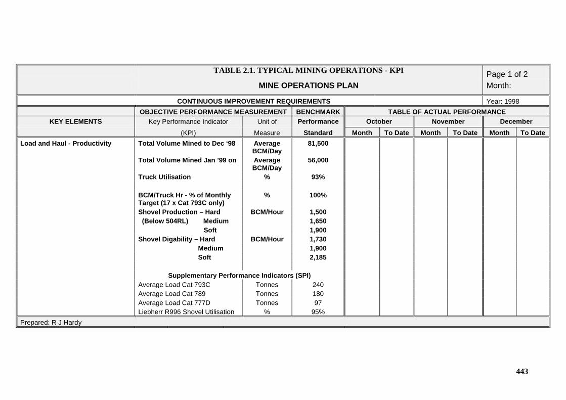
443
TABLE 2.1. TYPICAL MINING OPERATIONS - KPI Page 1 of 2 MINE OPERATIONS PLAN Month:
CONTINUOUS IMPROVEMENT REQUIREMENTS Year: 1998 OBJECTIVE PERFORMANCE MEASUREMENT BENCHMARK TABLE OF ACTUAL PERFORMANCE
KEY ELEMENTS Key Performance Indicator Unit of Performance October November December (KPI) Measure Standard Month To Date Month To Date Month To Date
Load and Haul - Productivity Total Volume Mined to Dec ‘98 Average BCM/Day
81,500
Total Volume Mined Jan ’99 on Average BCM/Day
56,000
Truck Utilisation % 93% BCM/Truck Hr - % of Monthly
Target (17 x Cat 793C only) % 100%
Shovel Production – Hard BCM/Hour 1,500 (Below 504RL) Medium 1,650 Soft 1,900
Shovel Digability – Hard BCM/Hour 1,730 Medium 1,900 Soft 2,185 Supplementary Performance Indicators (SPI) Average Load Cat 793C Tonnes 240 Average Load Cat 789 Tonnes 180
Average Load Cat 777D Tonnes 97 Liebherr R996 Shovel Utilisation % 95%
Prepared: R J Hardy
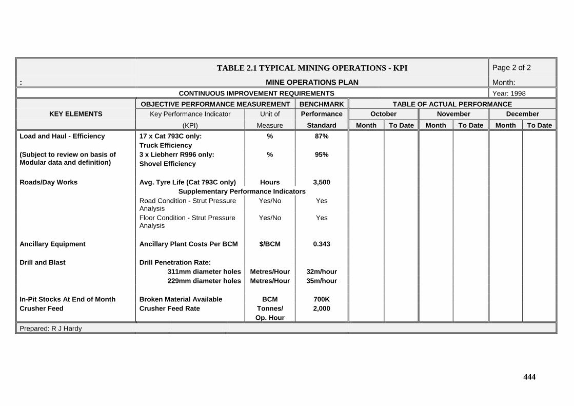
444
TABLE 2.1 TYPICAL MINING OPERATIONS - KPI Page 2 of 2
: MINE OPERATIONS PLAN Month: CONTINUOUS IMPROVEMENT REQUIREMENTS Year: 1998 OBJECTIVE PERFORMANCE MEASUREMENT BENCHMARK TABLE OF ACTUAL PERFORMANCE
KEY ELEMENTS Key Performance Indicator Unit of Performance October November December (KPI) Measure Standard Month To Date Month To Date Month To Date
Load and Haul - Efficiency 17 x Cat 793C only: Truck Efficiency
% 87%
(Subject to review on basis of Modular data and definition)
3 x Liebherr R996 only: Shovel Efficiency
% 95%
Roads/Day Works Avg. Tyre Life (Cat 793C only) Hours 3,500 Supplementary Performance Indicators Road Condition - Strut Pressure
Analysis Yes/No Yes
Floor Condition - Strut Pressure Analysis
Yes/No Yes
Ancillary Equipment Ancillary Plant Costs Per BCM $/BCM 0.343 Drill and Blast Drill Penetration Rate: 311mm diameter holes Metres/Hour 32m/hour 229mm diameter holes Metres/Hour 35m/hour In-Pit Stocks At End of Month Broken Material Available BCM 700K Crusher Feed Crusher Feed Rate Tonnes/
Op. Hour 2,000
Prepared: R J Hardy
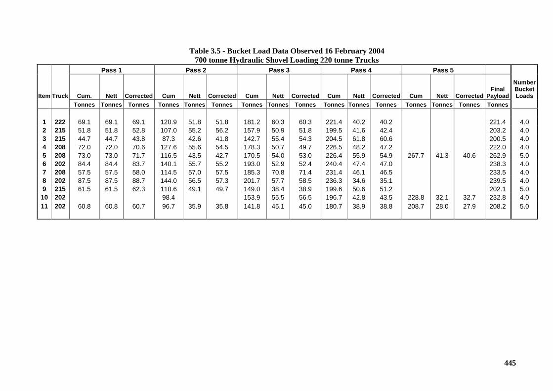
445
Table 3.5 - Bucket Load Data Observed 16 February 2004 700 tonne Hydraulic Shovel Loading 220 tonne Trucks
Pass 1 Pass 2 Pass 3 Pass 4 Pass 5
Item Truck Cum. Nett Corrected Cum Nett Corrected Cum Nett Corrected Cum Nett Corrected Cum Nett Corrected Final
Payload
Number Bucket Loads
Tonnes Tonnes Tonnes Tonnes Tonnes Tonnes Tonnes Tonnes Tonnes Tonnes Tonnes Tonnes Tonnes Tonnes Tonnes Tonnes
1 222 69.1 69.1 69.1 120.9 51.8 51.8 181.2 60.3 60.3 221.4 40.2 40.2 221.4 4.0 2 215 51.8 51.8 52.8 107.0 55.2 56.2 157.9 50.9 51.8 199.5 41.6 42.4 203.2 4.0 3 215 44.7 44.7 43.8 87.3 42.6 41.8 142.7 55.4 54.3 204.5 61.8 60.6 200.5 4.0 4 208 72.0 72.0 70.6 127.6 55.6 54.5 178.3 50.7 49.7 226.5 48.2 47.2 222.0 4.0 5 208 73.0 73.0 71.7 116.5 43.5 42.7 170.5 54.0 53.0 226.4 55.9 54.9 267.7 41.3 40.6 262.9 5.0 6 202 84.4 84.4 83.7 140.1 55.7 55.2 193.0 52.9 52.4 240.4 47.4 47.0 238.3 4.0 7 208 57.5 57.5 58.0 114.5 57.0 57.5 185.3 70.8 71.4 231.4 46.1 46.5 233.5 4.0 8 202 87.5 87.5 88.7 144.0 56.5 57.3 201.7 57.7 58.5 236.3 34.6 35.1 239.5 4.0 9 215 61.5 61.5 62.3 110.6 49.1 49.7 149.0 38.4 38.9 199.6 50.6 51.2 202.1 5.0 10 202 98.4 153.9 55.5 56.5 196.7 42.8 43.5 228.8 32.1 32.7 232.8 4.0 11 202 60.8 60.8 60.7 96.7 35.9 35.8 141.8 45.1 45.0 180.7 38.9 38.8 208.7 28.0 27.9 208.2 5.0
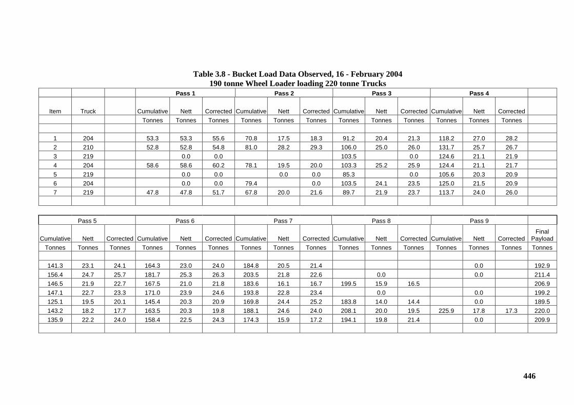
446
Table 3.8 - Bucket Load Data Observed, 16 - February 2004 190 tonne Wheel Loader loading 220 tonne Trucks
Pass 1 Pass 2 Pass 3 Pass 4
Item Truck Cumulative Nett Corrected Cumulative Nett Corrected Cumulative Nett Corrected Cumulative Nett Corrected Tonnes Tonnes Tonnes Tonnes Tonnes Tonnes Tonnes Tonnes Tonnes Tonnes Tonnes Tonnes
1 204 53.3 53.3 55.6 70.8 17.5 18.3 91.2 20.4 21.3 118.2 27.0 28.2 2 210 52.8 52.8 54.8 81.0 28.2 29.3 106.0 25.0 26.0 131.7 25.7 26.7 3 219 0.0 0.0 103.5 0.0 124.6 21.1 21.9 4 204 58.6 58.6 60.2 78.1 19.5 20.0 103.3 25.2 25.9 124.4 21.1 21.7 5 219 0.0 0.0 0.0 0.0 85.3 0.0 105.6 20.3 20.9 6 204 0.0 0.0 79.4 0.0 103.5 24.1 23.5 125.0 21.5 20.9 7 219 47.8 47.8 51.7 67.8 20.0 21.6 89.7 21.9 23.7 113.7 24.0 26.0
Pass 5 Pass 6 Pass 7 Pass 8 Pass 9
Cumulative Nett Corrected Cumulative Nett Corrected Cumulative Nett Corrected Cumulative Nett Corrected Cumulative Nett Corrected Final
Payload Tonnes Tonnes Tonnes Tonnes Tonnes Tonnes Tonnes Tonnes Tonnes Tonnes Tonnes Tonnes Tonnes Tonnes Tonnes Tonnes
141.3 23.1 24.1 164.3 23.0 24.0 184.8 20.5 21.4 0.0 192.9 156.4 24.7 25.7 181.7 25.3 26.3 203.5 21.8 22.6 0.0 0.0 211.4 146.5 21.9 22.7 167.5 21.0 21.8 183.6 16.1 16.7 199.5 15.9 16.5 206.9 147.1 22.7 23.3 171.0 23.9 24.6 193.8 22.8 23.4 0.0 0.0 199.2 125.1 19.5 20.1 145.4 20.3 20.9 169.8 24.4 25.2 183.8 14.0 14.4 0.0 189.5 143.2 18.2 17.7 163.5 20.3 19.8 188.1 24.6 24.0 208.1 20.0 19.5 225.9 17.8 17.3 220.0 135.9 22.2 24.0 158.4 22.5 24.3 174.3 15.9 17.2 194.1 19.8 21.4 0.0 209.9
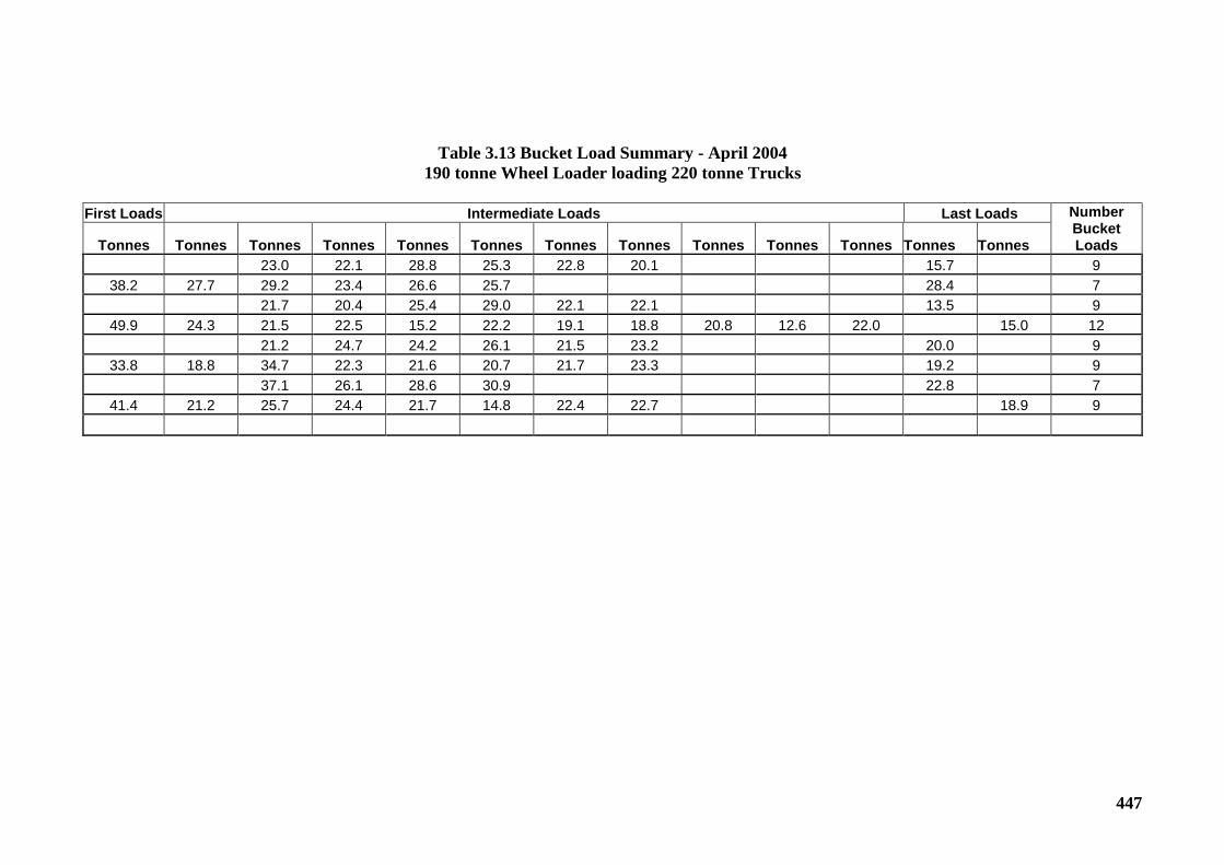
447
Table 3.13 Bucket Load Summary - April 2004 190 tonne Wheel Loader loading 220 tonne Trucks
First Loads Intermediate Loads Last Loads Number
Bucket Loads Tonnes Tonnes Tonnes Tonnes Tonnes Tonnes Tonnes Tonnes Tonnes Tonnes Tonnes Tonnes Tonnes
23.0 22.1 28.8 25.3 22.8 20.1 15.7 9 38.2 27.7 29.2 23.4 26.6 25.7 28.4 7
21.7 20.4 25.4 29.0 22.1 22.1 13.5 9 49.9 24.3 21.5 22.5 15.2 22.2 19.1 18.8 20.8 12.6 22.0 15.0 12
21.2 24.7 24.2 26.1 21.5 23.2 20.0 9 33.8 18.8 34.7 22.3 21.6 20.7 21.7 23.3 19.2 9
37.1 26.1 28.6 30.9 22.8 7 41.4 21.2 25.7 24.4 21.7 14.8 22.4 22.7 18.9 9
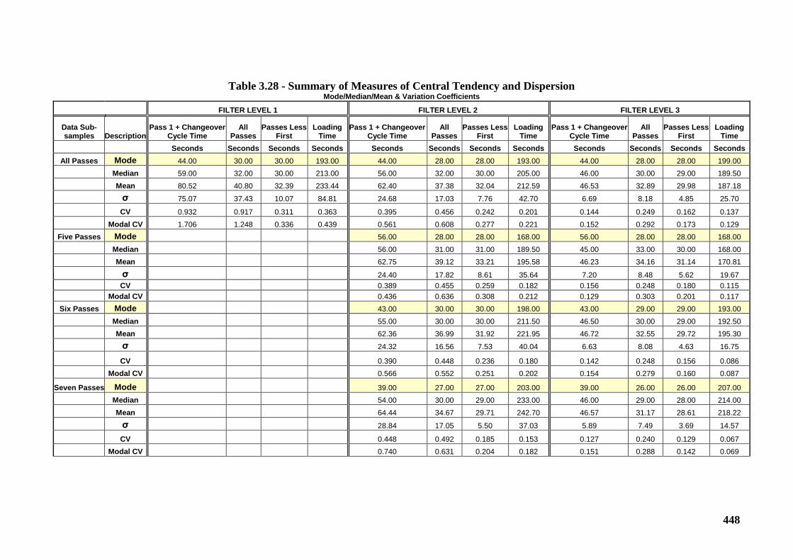
448
Table 3.28 - Summary of Measures of Central Tendency and Dispersion
Mode/Median/Mean & Variation Coefficients
FILTER LEVEL 1 FILTER LEVEL 2 FILTER LEVEL 3
Data Sub-samples Description
Pass 1 + Changeover Cycle Time
All Passes
Passes Less First
Loading Time
Pass 1 + Changeover Cycle Time
All Passes
Passes Less First
Loading Time
Pass 1 + Changeover Cycle Time
All Passes
Passes Less First
Loading Time
Seconds Seconds Seconds Seconds Seconds Seconds Seconds Seconds Seconds Seconds Seconds Seconds All Passes Mode 44.00 30.00 30.00 193.00 44.00 28.00 28.00 193.00 44.00 28.00 28.00 199.00
Median 59.00 32.00 30.00 213.00 56.00 32.00 30.00 205.00 46.00 30.00 29.00 189.50 Mean 80.52 40.80 32.39 233.44 62.40 37.38 32.04 212.59 46.53 32.89 29.98 187.18
σ 75.07 37.43 10.07 84.81 24.68 17.03 7.76 42.70 6.69 8.18 4.85 25.70
CV 0.932 0.917 0.311 0.363 0.395 0.456 0.242 0.201 0.144 0.249 0.162 0.137 Modal CV 1.706 1.248 0.336 0.439 0.561 0.608 0.277 0.221 0.152 0.292 0.173 0.129 Five Passes Mode 56.00 28.00 28.00 168.00 56.00 28.00 28.00 168.00
Median 56.00 31.00 31.00 189.50 45.00 33.00 30.00 168.00 Mean 62.75 39.12 33.21 195.58 46.23 34.16 31.14 170.81
σ 24.40 17.82 8.61 35.64 7.20 8.48 5.62 19.67 CV 0.389 0.455 0.259 0.182 0.156 0.248 0.180 0.115 Modal CV 0.436 0.636 0.308 0.212 0.129 0.303 0.201 0.117
Six Passes Mode 43.00 30.00 30.00 198.00 43.00 29.00 29.00 193.00 Median 55.00 30.00 30.00 211.50 46.50 30.00 29.00 192.50 Mean 62.36 36.99 31.92 221.95 46.72 32.55 29.72 195.30
σ 24.32 16.56 7.53 40.04 6.63 8.08 4.63 16.75
CV 0.390 0.448 0.236 0.180 0.142 0.248 0.156 0.086 Modal CV 0.566 0.552 0.251 0.202 0.154 0.279 0.160 0.087
Seven Passes Mode 39.00 27.00 27.00 203.00 39.00 26.00 26.00 207.00 Median 54.00 30.00 29.00 233.00 46.00 29.00 28.00 214.00 Mean 64.44 34.67 29.71 242.70 46.57 31.17 28.61 218.22
σ 28.84 17.05 5.50 37.03 5.89 7.49 3.69 14.57
CV 0.448 0.492 0.185 0.153 0.127 0.240 0.129 0.067 Modal CV 0.740 0.631 0.204 0.182 0.151 0.288 0.142 0.069
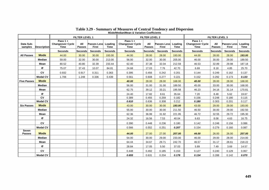
449
Table 3.29 - Summary of Measures of Central Tendency and Dispersion
Mode/Median/Mean & Variation Coefficients
FILTER LEVEL 1 FILTER LEVEL 2 FILTER LEVEL 3
Data Sub-samples Description
Pass 1 + Changeover Cycle
Time All
Passes Passes Less
First Loading
Time
Pass 1 + Changeover Cycle
Time All
Passes Passes Less
First Loading
Time
Pass 1 + Changeover Cycle
Time All
Passes Passes Less
First Loading
Time Seconds Seconds Seconds Seconds Seconds Seconds Seconds Seconds Seconds Seconds Seconds Seconds
All Passes Mode 44.00 30.00 30.00 193.00 44.00 28.00 28.00 193.00 44.00 28.00 28.00 193.00 Median 59.00 32.00 30.00 213.00 56.00 32.00 30.00 205.00 46.00 30.00 29.00 189.50 Mean 80.52 40.80 32.39 233.44 62.40 37.38 32.04 212.59 46.53 32.89 29.98 187.18
σ 75.07 37.43 10.07 84.81 24.68 17.03 7.76 42.70 6.69 8.18 4.85 25.70
CV 0.932 0.917 0.311 0.363 0.395 0.456 0.242 0.201 0.144 0.249 0.162 0.137 Modal CV 1.706 1.248 0.336 0.439 0.561 0.608 0.277 0.221 0.152 0.292 0.173 0.133 Five Passes Mode 40.00 28.00 28.00 168.00 40.00 28.00 28.00 168.00
Median 56.00 31.00 31.00 189.50 45.00 33.00 30.00 168.00 Mean 62.75 39.12 33.21 195.58 46.23 34.16 31.14 170.81
σ 24.40 17.82 8.61 35.64 7.20 8.48 5.62 19.67 CV 0.389 0.455 0.259 0.182 0.156 0.248 0.180 0.115 Modal CV 0.610 0.636 0.308 0.212 0.180 0.303 0.201 0.117
Six Passes Mode 43.00 30.00 30.00 193.00 43.00 29.00 29.00 193.00 Median 55.00 30.00 30.00 211.50 46.50 30.00 29.00 192.50 Mean 62.36 36.99 31.92 221.95 46.72 32.55 29.72 195.30
σ 24.32 16.56 7.53 40.04 6.63 8.08 4.63 16.75
CV 0.390 0.448 0.236 0.180 0.142 0.248 0.156 0.086 Modal CV 0.566 0.552 0.251 0.207 0.154 0.279 0.160 0.087
Seven Passes Mode 44.00 27.00 27.00 207.00 44.00 26.00 26.00 207.00
Median 54.00 30.00 29.00 233.00 46.00 29.00 28.00 214.00 Mean 64.44 34.67 29.71 242.70 46.57 31.17 28.61 218.22
σ 28.84 17.05 5.50 37.03 5.89 7.49 3.69 14.57
CV 0.448 0.492 0.185 0.153 0.127 0.240 0.129 0.067 Modal CV 0.655 0.631 0.204 0.178 0.134 0.288 0.142 0.070
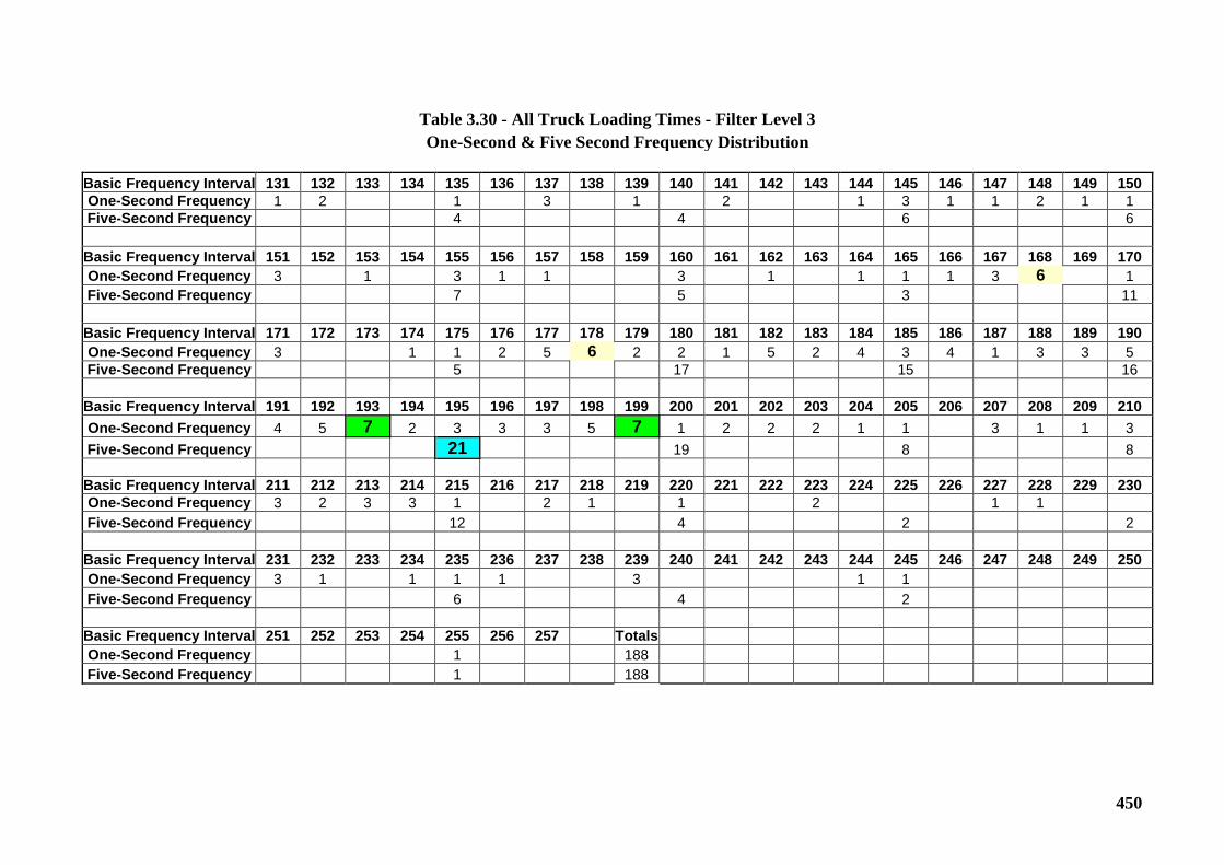
450
Table 3.30 - All Truck Loading Times - Filter Level 3 One-Second & Five Second Frequency Distribution
Basic Frequency Interval 131 132 133 134 135 136 137 138 139 140 141 142 143 144 145 146 147 148 149 150 One-Second Frequency 1 2 1 3 1 2 1 3 1 1 2 1 1 Five-Second Frequency 4 4 6 6 Basic Frequency Interval 151 152 153 154 155 156 157 158 159 160 161 162 163 164 165 166 167 168 169 170 One-Second Frequency 3 1 3 1 1 3 1 1 1 1 3 6 1 Five-Second Frequency 7 5 3 11 Basic Frequency Interval 171 172 173 174 175 176 177 178 179 180 181 182 183 184 185 186 187 188 189 190 One-Second Frequency 3 1 1 2 5 6 2 2 1 5 2 4 3 4 1 3 3 5 Five-Second Frequency 5 17 15 16 Basic Frequency Interval 191 192 193 194 195 196 197 198 199 200 201 202 203 204 205 206 207 208 209 210 One-Second Frequency 4 5 7 2 3 3 3 5 7 1 2 2 2 1 1 3 1 1 3 Five-Second Frequency 21 19 8 8 Basic Frequency Interval 211 212 213 214 215 216 217 218 219 220 221 222 223 224 225 226 227 228 229 230 One-Second Frequency 3 2 3 3 1 2 1 1 2 1 1 Five-Second Frequency 12 4 2 2 Basic Frequency Interval 231 232 233 234 235 236 237 238 239 240 241 242 243 244 245 246 247 248 249 250 One-Second Frequency 3 1 1 1 1 3 1 1 Five-Second Frequency 6 4 2 Basic Frequency Interval 251 252 253 254 255 256 257 Totals One-Second Frequency 1 188 Five-Second Frequency 1 188
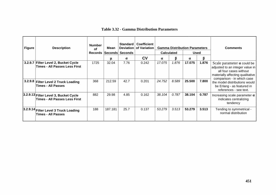
451
Table 3.32 - Gamma Distribution Parameters
Figure Description Number
of Records
Mean Standard Deviation
Coefficient of Variation Gamma Distribution Parameters Comments
Seconds Seconds Calculated Used
μ σ CV α β α β 3.2.9.7 Filter Level 2, Bucket Cycle
Times - All Passes Less First 1725 32.04 7.76 0.242 17.075 1.876 17.075 1.876 Scale parameter α could be
adjusted to an integer value in all four cases without
materially affecting qualitative comparison - in which case
the model distributions would be Erlang - as featured in
references - see text.
3.2.9.8 Filter Level 2 Truck Loading
Times - All Passes 368 212.59 42.7 0.201 24.752 8.589 25.500 7.800
3.2.9.13 Filter Level 3, Bucket Cycle
Times - All Passes Less First 882 29.98 4.85 0.162 38.104 0.787 38.104 0.787 Increasing scale parameter α
indicates centralizing tendency
3.2.9.14 Filter Level 3 Truck Loading Times - All Passes
188 187.181 25.7 0.137 53.279 3.513 53.279 3.513 Tending to symmetrical - normal distribution
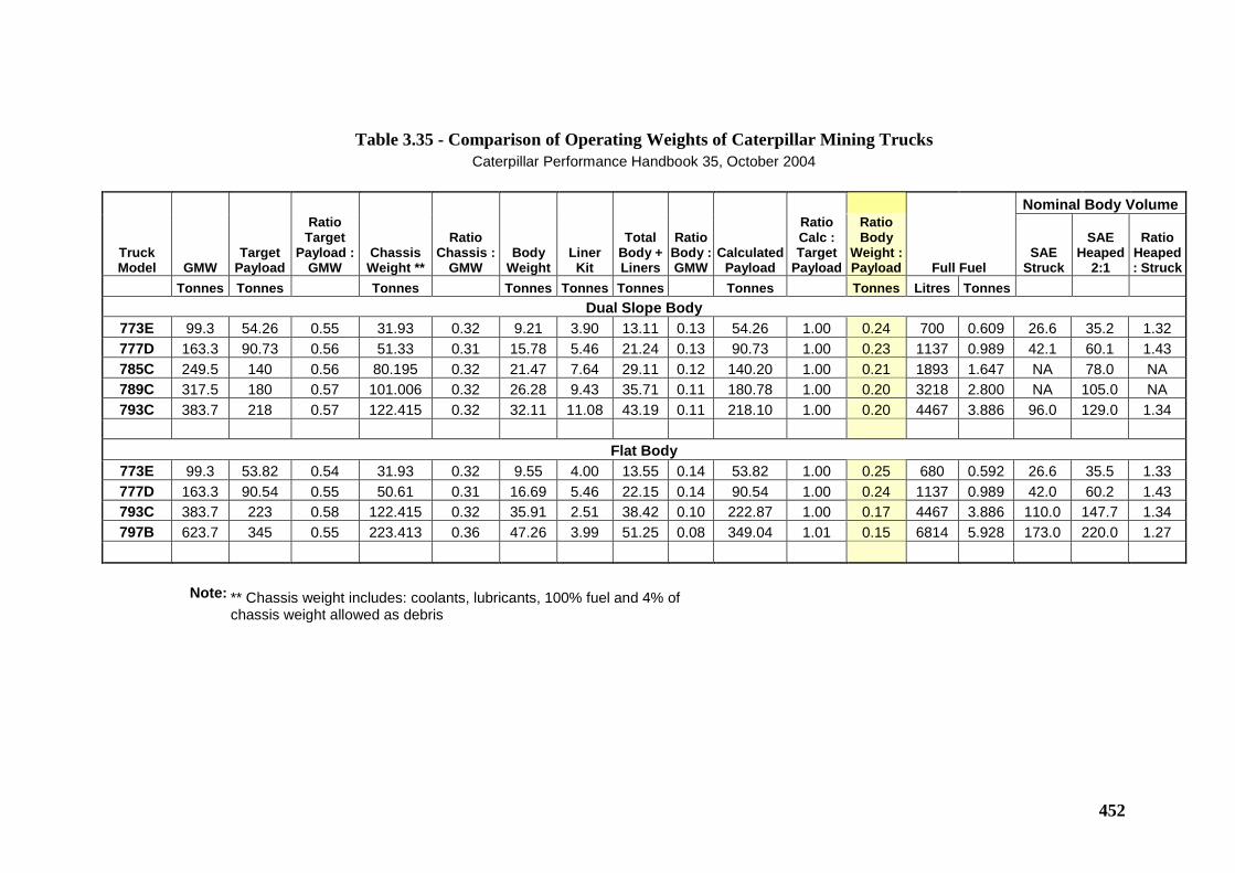
452
Table 3.35 - Comparison of Operating Weights of Caterpillar Mining Trucks Caterpillar Performance Handbook 35, October 2004
Nominal Body Volume
Truck Model GMW
Target Payload
Ratio Target
Payload : GMW
Chassis Weight **
Ratio Chassis :
GMW Body
Weight Liner
Kit
Total Body + Liners
Ratio Body : GMW
Calculated Payload
Ratio Calc : Target
Payload
Ratio Body
Weight : Payload Full Fuel
SAE Struck
SAE Heaped
2:1
Ratio Heaped : Struck
Tonnes Tonnes Tonnes Tonnes Tonnes Tonnes Tonnes Tonnes Litres Tonnes Dual Slope Body
773E 99.3 54.26 0.55 31.93 0.32 9.21 3.90 13.11 0.13 54.26 1.00 0.24 700 0.609 26.6 35.2 1.32 777D 163.3 90.73 0.56 51.33 0.31 15.78 5.46 21.24 0.13 90.73 1.00 0.23 1137 0.989 42.1 60.1 1.43 785C 249.5 140 0.56 80.195 0.32 21.47 7.64 29.11 0.12 140.20 1.00 0.21 1893 1.647 NA 78.0 NA 789C 317.5 180 0.57 101.006 0.32 26.28 9.43 35.71 0.11 180.78 1.00 0.20 3218 2.800 NA 105.0 NA 793C 383.7 218 0.57 122.415 0.32 32.11 11.08 43.19 0.11 218.10 1.00 0.20 4467 3.886 96.0 129.0 1.34
Flat Body
773E 99.3 53.82 0.54 31.93 0.32 9.55 4.00 13.55 0.14 53.82 1.00 0.25 680 0.592 26.6 35.5 1.33 777D 163.3 90.54 0.55 50.61 0.31 16.69 5.46 22.15 0.14 90.54 1.00 0.24 1137 0.989 42.0 60.2 1.43 793C 383.7 223 0.58 122.415 0.32 35.91 2.51 38.42 0.10 222.87 1.00 0.17 4467 3.886 110.0 147.7 1.34 797B 623.7 345 0.55 223.413 0.36 47.26 3.99 51.25 0.08 349.04 1.01 0.15 6814 5.928 173.0 220.0 1.27
Note: ** Chassis weight includes: coolants, lubricants, 100% fuel and 4% of
chassis weight allowed as debris
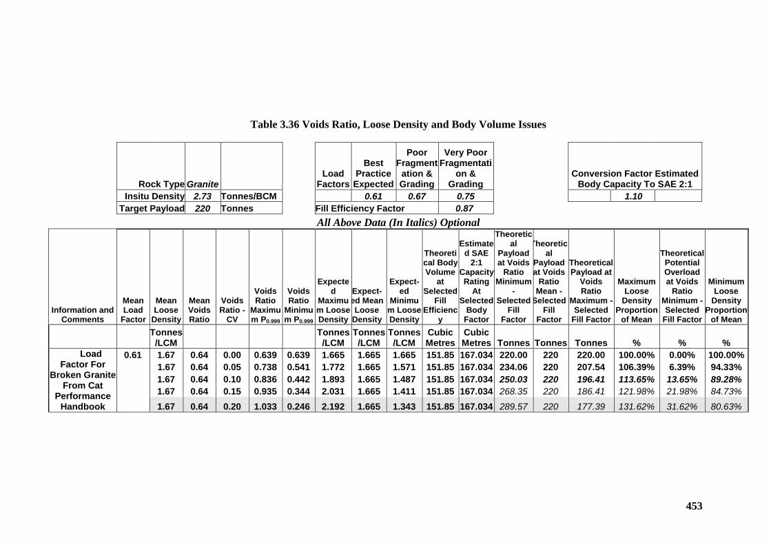
453
Table 3.36 Voids Ratio, Loose Density and Body Volume Issues
Rock Type Granite Load
Factors
Best Practice
Expected
Poor Fragment
ation & Grading
Very Poor Fragmentati
on & Grading
Conversion Factor Estimated Body Capacity To SAE 2:1
Insitu Density 2.73 Tonnes/BCM 0.61 0.67 0.75 1.10 Target Payload 220 Tonnes Fill Efficiency Factor 0.87
All Above Data (In Italics) Optional
Information and Comments
Mean Load
Factor
Mean Loose
Density
Mean Voids Ratio
Voids Ratio -
CV
Voids Ratio
Maximum P0.999
Voids Ratio
Minimum P0.999
Expected
Maximum Loose Density
Expect-ed Mean Loose
Density
Expect-ed
Minimum Loose Density
Theoretical Body Volume
at Selected
Fill Efficienc
y
Estimated SAE
2:1 Capacity Rating
At Selected
Body Factor
Theoretical
Payload at Voids
Ratio Minimum
- Selected
Fill Factor
Theoretical
Payload at Voids
Ratio Mean -
Selected Fill
Factor
Theoretical Payload at
Voids Ratio
Maximum - Selected
Fill Factor
Maximum Loose
Density Proportion
of Mean
Theoretical Potential Overload at Voids
Ratio Minimum - Selected
Fill Factor
Minimum Loose
Density Proportion
of Mean
Tonnes /LCM
Tonnes /LCM
Tonnes /LCM
Tonnes /LCM
Cubic Metres
Cubic Metres Tonnes Tonnes Tonnes % % %
Load Factor For
Broken Granite From Cat
Performance Handbook
0.61 1.67 0.64 0.00 0.639 0.639 1.665 1.665 1.665 151.85 167.034 220.00 220 220.00 100.00% 0.00% 100.00% 1.67 0.64 0.05 0.738 0.541 1.772 1.665 1.571 151.85 167.034 234.06 220 207.54 106.39% 6.39% 94.33%
1.67 0.64 0.10 0.836 0.442 1.893 1.665 1.487 151.85 167.034 250.03 220 196.41 113.65% 13.65% 89.28% 1.67 0.64 0.15 0.935 0.344 2.031 1.665 1.411 151.85 167.034 268.35 220 186.41 121.98% 21.98% 84.73%
1.67 0.64 0.20 1.033 0.246 2.192 1.665 1.343 151.85 167.034 289.57 220 177.39 131.62% 31.62% 80.63%
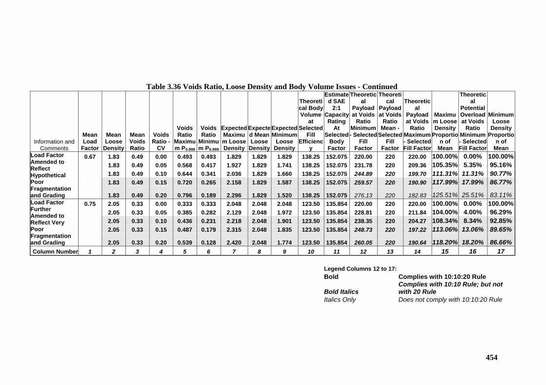
454
Table 3.36 Voids Ratio, Loose Density and Body Volume Issues - Continued
Information and Comments
Mean Load
Factor
Mean Loose
Density
Mean Voids Ratio
Voids Ratio -
CV
Voids Ratio
Maximum P0.999
Voids Ratio
Minimum P0.999
Expected Maximum Loose Density
Expected Mean Loose
Density
Expected Minimum
Loose Density
Theoretical Body Volume
at Selected
Fill Efficienc
y
Estimated SAE
2:1 Capacity Rating
At Selected
Body Factor
Theoretical
Payload at Voids
Ratio Minimum - Selected
Fill Factor
Theoretical
Payload at Voids
Ratio Mean -
Selected Fill
Factor
Theoretical
Payload at Voids
Ratio Maximum - Selected Fill Factor
Maximum Loose Density
Proportion of
Mean
Theoretical
Potential Overload at Voids
Ratio Minimum - Selected Fill Factor
Minimum Loose
Density Proportio
n of Mean
Load Factor Amended to Reflect Hypothetical Poor Fragmentation and Grading
0.67 1.83 0.49 0.00 0.493 0.493 1.829 1.829 1.829 138.25 152.075 220.00 220 220.00 100.00% 0.00% 100.00% 1.83 0.49 0.05 0.568 0.417 1.927 1.829 1.741 138.25 152.075 231.78 220 209.36 105.35% 5.35% 95.16%
1.83 0.49 0.10 0.644 0.341 2.036 1.829 1.660 138.25 152.075 244.89 220 199.70 111.31% 11.31% 90.77% 1.83 0.49 0.15 0.720 0.265 2.158 1.829 1.587 138.25 152.075 259.57 220 190.90 117.99% 17.99% 86.77%
1.83 0.49 0.20 0.796 0.189 2.296 1.829 1.520 138.25 152.075 276.13 220 182.83 125.51% 25.51% 83.11% Load Factor Further Amended to Reflect Very Poor Fragmentation and Grading
0.75 2.05 0.33 0.00 0.333 0.333 2.048 2.048 2.048 123.50 135.854 220.00 220 220.00 100.00% 0.00% 100.00% 2.05 0.33 0.05 0.385 0.282 2.129 2.048 1.972 123.50 135.854 228.81 220 211.84 104.00% 4.00% 96.29% 2.05 0.33 0.10 0.436 0.231 2.218 2.048 1.901 123.50 135.854 238.35 220 204.27 108.34% 8.34% 92.85% 2.05 0.33 0.15 0.487 0.179 2.315 2.048 1.835 123.50 135.854 248.73 220 197.22 113.06% 13.06% 89.65%
2.05 0.33 0.20 0.539 0.128 2.420 2.048 1.774 123.50 135.854 260.05 220 190.64 118.20% 18.20% 86.66% Column Number 1 2 3 4 5 6 7 8 9 10 11 12 13 14 15 16 17
Legend Columns 12 to 17: Bold Complies with 10:10:20 Rule
Bold Italics Complies with 10:10 Rule; but not with 20 Rule
Italics Only Does not comply with 10:10:20 Rule
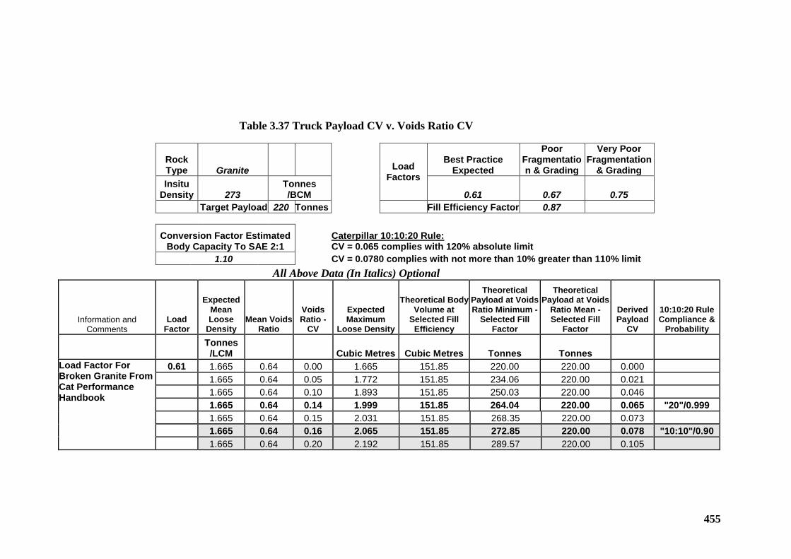
455
Table 3.37 Truck Payload CV v. Voids Ratio CV
Rock Type Granite Load
Factors
Best Practice Expected
Poor Fragmentation & Grading
Very Poor Fragmentation
& Grading
Insitu
Density 273 Tonnes /BCM 0.61 0.67 0.75
Target Payload 220 Tonnes Fill Efficiency Factor 0.87
Conversion Factor Estimated
Body Capacity To SAE 2:1 Caterpillar 10:10:20 Rule:
CV = 0.065 complies with 120% absolute limit 1.10 CV = 0.0780 complies with not more than 10% greater than 110% limit
All Above Data (In Italics) Optional
Information and
Comments Load
Factor
Expected Mean Loose
Density Mean Voids
Ratio
Voids Ratio -
CV
Expected Maximum
Loose Density
Theoretical Body Volume at
Selected Fill Efficiency
Theoretical Payload at Voids Ratio Minimum -
Selected Fill Factor
Theoretical Payload at Voids
Ratio Mean - Selected Fill
Factor
Derived Payload
CV
10:10:20 Rule Compliance &
Probability
Tonnes /LCM Cubic Metres Cubic Metres Tonnes Tonnes
Load Factor For Broken Granite From Cat Performance Handbook
0.61 1.665 0.64 0.00 1.665 151.85 220.00 220.00 0.000 1.665 0.64 0.05 1.772 151.85 234.06 220.00 0.021 1.665 0.64 0.10 1.893 151.85 250.03 220.00 0.046 1.665 0.64 0.14 1.999 151.85 264.04 220.00 0.065 "20"/0.999 1.665 0.64 0.15 2.031 151.85 268.35 220.00 0.073 1.665 0.64 0.16 2.065 151.85 272.85 220.00 0.078 "10:10"/0.90 1.665 0.64 0.20 2.192 151.85 289.57 220.00 0.105
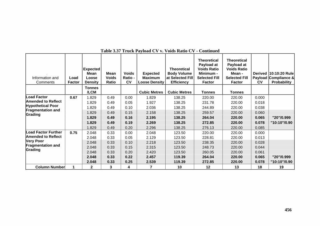
456
Table 3.37 Truck Payload CV v. Voids Ratio CV - Continued
Information and Comments
Load Factor
Expected Mean Loose
Density
Mean Voids Ratio
Voids Ratio -
CV
Expected Maximum
Loose Density
Theoretical Body Volume
at Selected Fill Efficiency
Theoretical Payload at Voids Ratio Minimum -
Selected Fill Factor
Theoretical Payload at Voids Ratio
Mean - Selected Fill
Factor
Derived Payload
CV
10:10:20 Rule Compliance &
Probability
Tonnes /LCM Cubic Metres Cubic Metres Tonnes Tonnes
Load Factor Amended to Reflect Hypothetical Poor Fragmentation and Grading
0.67 1.829 0.49 0.00 1.829 138.25 220.00 220.00 0.000 1.829 0.49 0.05 1.927 138.25 231.78 220.00 0.018 1.829 0.49 0.10 2.036 138.25 244.89 220.00 0.038 1.829 0.49 0.15 2.158 138.25 259.57 220.00 0.060 1.829 0.49 0.16 2.195 138.25 264.04 220.00 0.065 "20"/0.999 1.829 0.49 0.19 2.269 138.25 272.85 220.00 0.078 "10:10"/0.90 1.829 0.49 0.20 2.296 138.25 276.13 220.00 0.085
Load Factor Further Amended to Reflect Very Poor Fragmentation and Grading
0.75 2.048 0.33 0.00 2.048 123.50 220.00 220.00 0.000 2.048 0.33 0.05 2.129 123.50 228.81 220.00 0.013 2.048 0.33 0.10 2.218 123.50 238.35 220.00 0.028 2.048 0.33 0.15 2.315 123.50 248.73 220.00 0.044 2.048 0.33 0.20 2.420 123.50 260.05 220.00 0.061
2.048 0.33 0.22 2.457 119.39 264.04 220.00 0.065 "20"/0.999 2.048 0.33 0.25 2.539 119.39 272.85 220.00 0.078 "10:10"/0.90
Column Number 1 2 3 4 7 10 12 13 18 19
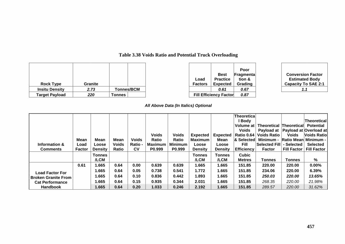
457
Table 3.38 Voids Ratio and Potential Truck Overloading
Rock Type Granite Load
Factors
Best Practice
Expected
Poor Fragmenta
tion & Grading
Conversion Factor Estimated Body
Capacity To SAE 2:1 Insitu Density 2.73 Tonnes/BCM 0.61 0.67 1.1
Target Payload 220 Tonnes Fill Efficiency Factor 0.87
All Above Data (In Italics) Optional
Information & Comments
Mean Load
Factor
Mean Loose
Density
Mean Voids Ratio
Voids Ratio -
CV
Voids Ratio
Maximum P0.999
Voids Ratio
Minimum P0.999
Expected Maximum
Loose Density
Expected Mean Loose
Density
Theoretical Body
Volume at Voids
Ratio 0.64 & Selected
Fill Efficiency
Theoretical Payload at Voids Ratio Minimum -
Selected Fill Factor
Theoretical Payload at
Voids Ratio Mean - Selected Fill Factor
Theoretical Potential
Overload at Voids Ratio Minimum - Selected
Fill Factor
Tonnes /LCM
Tonnes /LCM
Tonnes /LCM
Cubic Metres Tonnes Tonnes %
Load Factor For Broken Granite From
Cat Performance Handbook
0.61 1.665 0.64 0.00 0.639 0.639 1.665 1.665 151.85 220.00 220.00 0.00% 1.665 0.64 0.05 0.738 0.541 1.772 1.665 151.85 234.06 220.00 6.39% 1.665 0.64 0.10 0.836 0.442 1.893 1.665 151.85 250.03 220.00 13.65% 1.665 0.64 0.15 0.935 0.344 2.031 1.665 151.85 268.35 220.00 21.98% 1.665 0.64 0.20 1.033 0.246 2.192 1.665 151.85 289.57 220.00 31.62%
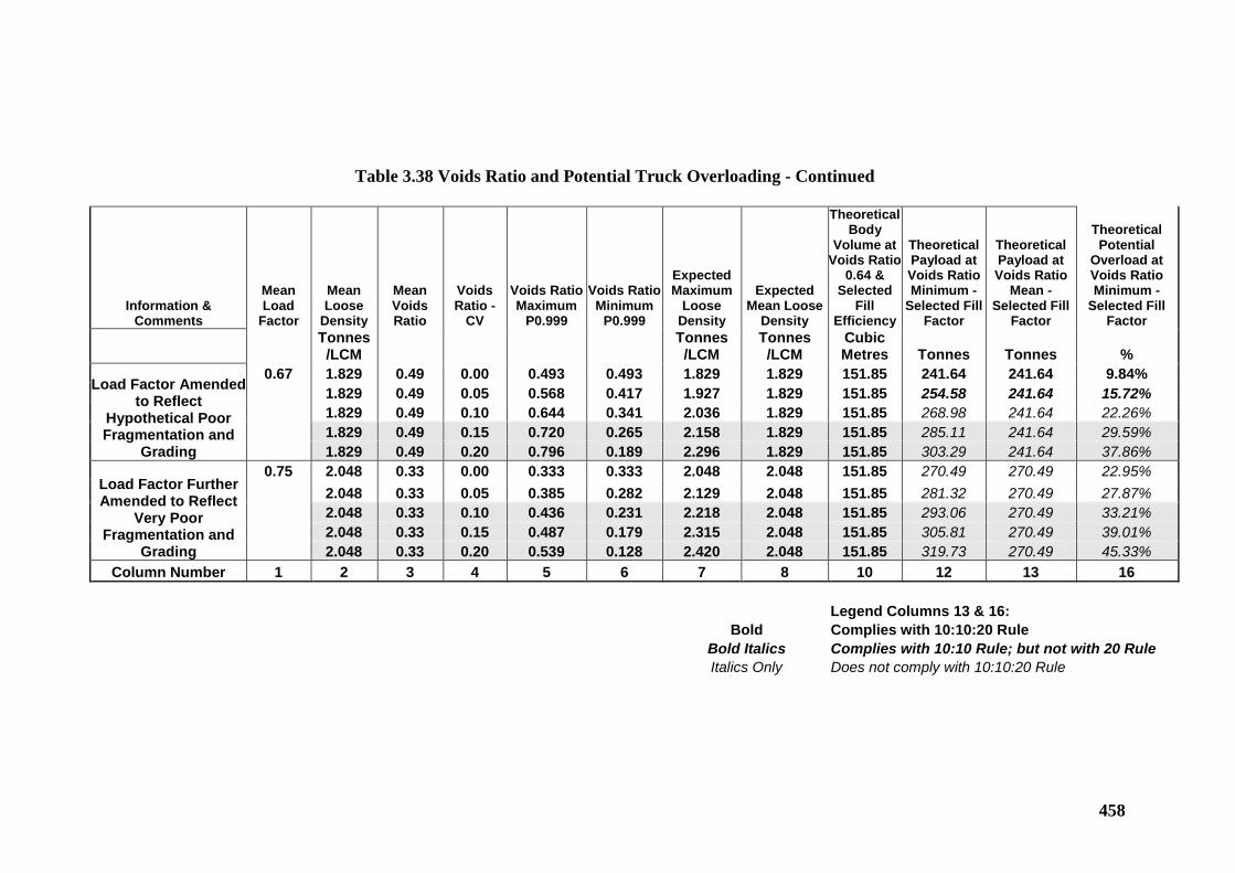
458
Table 3.38 Voids Ratio and Potential Truck Overloading - Continued
Information & Comments
Mean Load
Factor
Mean Loose
Density
Mean Voids Ratio
Voids Ratio -
CV
Voids Ratio Maximum
P0.999
Voids Ratio Minimum
P0.999
Expected Maximum
Loose Density
Expected Mean Loose
Density
Theoretical Body
Volume at Voids Ratio
0.64 & Selected
Fill Efficiency
Theoretical Payload at Voids Ratio Minimum -
Selected Fill Factor
Theoretical Payload at Voids Ratio
Mean - Selected Fill
Factor
Theoretical Potential
Overload at Voids Ratio Minimum -
Selected Fill Factor
Tonnes /LCM
Tonnes /LCM
Tonnes /LCM
Cubic Metres Tonnes Tonnes %
Load Factor Amended to Reflect
Hypothetical Poor Fragmentation and
Grading
0.67 1.829 0.49 0.00 0.493 0.493 1.829 1.829 151.85 241.64 241.64 9.84% 1.829 0.49 0.05 0.568 0.417 1.927 1.829 151.85 254.58 241.64 15.72% 1.829 0.49 0.10 0.644 0.341 2.036 1.829 151.85 268.98 241.64 22.26% 1.829 0.49 0.15 0.720 0.265 2.158 1.829 151.85 285.11 241.64 29.59% 1.829 0.49 0.20 0.796 0.189 2.296 1.829 151.85 303.29 241.64 37.86%
Load Factor Further Amended to Reflect
Very Poor Fragmentation and
Grading
0.75 2.048 0.33 0.00 0.333 0.333 2.048 2.048 151.85 270.49 270.49 22.95% 2.048 0.33 0.05 0.385 0.282 2.129 2.048 151.85 281.32 270.49 27.87% 2.048 0.33 0.10 0.436 0.231 2.218 2.048 151.85 293.06 270.49 33.21% 2.048 0.33 0.15 0.487 0.179 2.315 2.048 151.85 305.81 270.49 39.01% 2.048 0.33 0.20 0.539 0.128 2.420 2.048 151.85 319.73 270.49 45.33%
Column Number 1 2 3 4 5 6 7 8 10 12 13 16 Legend Columns 13 & 16: Bold Complies with 10:10:20 Rule Bold Italics Complies with 10:10 Rule; but not with 20 Rule Italics Only Does not comply with 10:10:20 Rule
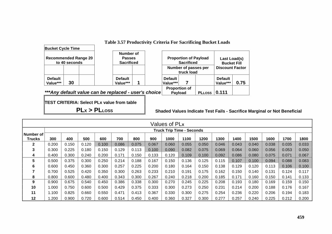
459
Table 3.57 Productivity Criteria For Sacrificing Bucket Loads Bucket Cycle Time
Recommended Range 20
to 40 seconds
Number of Passes
Sacrificed Proportion of Payload
Sacrificed Last Load(s) Bucket Fill
Discount Factor
Number of passes per
truck load
Default Value*** 30
Default Value*** 1
Default Value*** 7
Default Value*** 0.75
***Any default value can be replaced - user's choice Proportion of
Payload PLLOSS 0.111
TEST CRITERIA: Select PLx value from table
PLX > PLLOSS Shaded Values Indicate Test Fails - Sacrifice Marginal or Not Beneficial
Values of PLX Number of
Trucks
Truck Trip Time - Seconds
300 400 500 600 700 800 900 1000 1100 1200 1300 1400 1500 1600 1700 1800 2 0.200 0.150 0.120 0.100 0.086 0.075 0.067 0.060 0.055 0.050 0.046 0.043 0.040 0.038 0.035 0.033 3 0.300 0.225 0.180 0.150 0.129 0.113 0.100 0.090 0.082 0.075 0.069 0.064 0.060 0.056 0.053 0.050 4 0.400 0.300 0.240 0.200 0.171 0.150 0.133 0.120 0.109 0.100 0.092 0.086 0.080 0.075 0.071 0.067 5 0.500 0.375 0.300 0.250 0.214 0.188 0.167 0.150 0.136 0.125 0.115 0.107 0.100 0.094 0.088 0.083 6 0.600 0.450 0.360 0.300 0.257 0.225 0.200 0.180 0.164 0.150 0.138 0.129 0.120 0.113 0.106 0.100 7 0.700 0.525 0.420 0.350 0.300 0.263 0.233 0.210 0.191 0.175 0.162 0.150 0.140 0.131 0.124 0.117 8 0.800 0.600 0.480 0.400 0.343 0.300 0.267 0.240 0.218 0.200 0.185 0.171 0.160 0.150 0.141 0.133 9 0.900 0.675 0.540 0.450 0.386 0.338 0.300 0.270 0.245 0.225 0.208 0.193 0.180 0.169 0.159 0.150
10 1.000 0.750 0.600 0.500 0.429 0.375 0.333 0.300 0.273 0.250 0.231 0.214 0.200 0.188 0.176 0.167 11 1.100 0.825 0.660 0.550 0.471 0.413 0.367 0.330 0.300 0.275 0.254 0.236 0.220 0.206 0.194 0.183 12 1.200 0.900 0.720 0.600 0.514 0.450 0.400 0.360 0.327 0.300 0.277 0.257 0.240 0.225 0.212 0.200
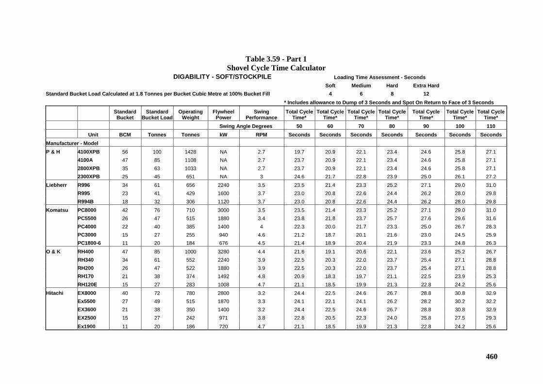
460
Table 3.59 - Part 1
Shovel Cycle Time Calculator DIGABILITY - SOFT/STOCKPILE Loading Time Assessment - Seconds Soft Medium Hard Extra Hard Standard Bucket Load Calculated at 1.8 Tonnes per Bucket Cubic Metre at 100% Bucket Fill 4 6 8 12 * Includes allowance to Dump of 3 Seconds and Spot On Return to Face of 3 Seconds
Standard Bucket
Standard Bucket Load
Operating Weight
Flywheel Power
Swing Performance
Total Cycle Time*
Total Cycle Time*
Total Cycle Time*
Total Cycle Time*
Total Cycle Time*
Total Cycle Time*
Total Cycle Time*
Swing Angle Degrees 50 60 70 80 90 100 110 Unit BCM Tonnes Tonnes kW RPM Seconds Seconds Seconds Seconds Seconds Seconds Seconds
Manufacturer - Model P & H 4100XPB 56 100 1428 NA 2.7 19.7 20.9 22.1 23.4 24.6 25.8 27.1 4100A 47 85 1108 NA 2.7 23.7 20.9 22.1 23.4 24.6 25.8 27.1 2800XPB 35 63 1033 NA 2.7 23.7 20.9 22.1 23.4 24.6 25.8 27.1 2300XPB 25 45 651 NA 3 24.6 21.7 22.8 23.9 25.0 26.1 27.2 Liebherr R996 34 61 656 2240 3.5 23.5 21.4 23.3 25.2 27.1 29.0 31.0 R995 23 41 429 1600 3.7 23.0 20.8 22.6 24.4 26.2 28.0 29.8 R994B 18 32 306 1120 3.7 23.0 20.8 22.6 24.4 26.2 28.0 29.8 Komatsu PC8000 42 76 710 3000 3.5 23.5 21.4 23.3 25.2 27.1 29.0 31.0 PC5500 26 47 515 1880 3.4 23.8 21.8 23.7 25.7 27.6 29.6 31.6 PC4000 22 40 385 1400 4 22.3 20.0 21.7 23.3 25.0 26.7 28.3 PC3000 15 27 255 940 4.6 21.2 18.7 20.1 21.6 23.0 24.5 25.9 PC1800-6 11 20 184 676 4.5 21.4 18.9 20.4 21.9 23.3 24.8 26.3 O & K RH400 47 85 1000 3280 4.4 21.6 19.1 20.6 22.1 23.6 25.2 26.7 RH340 34 61 552 2240 3.9 22.5 20.3 22.0 23.7 25.4 27.1 28.8 RH200 26 47 522 1880 3.9 22.5 20.3 22.0 23.7 25.4 27.1 28.8 RH170 21 38 374 1492 4.8 20.9 18.3 19.7 21.1 22.5 23.9 25.3 RH120E 15 27 283 1008 4.7 21.1 18.5 19.9 21.3 22.8 24.2 25.6 Hitachi EX8000 40 72 780 2800 3.2 24.4 22.5 24.6 26.7 28.8 30.8 32.9 Ex5500 27 49 515 1870 3.3 24.1 22.1 24.1 26.2 28.2 30.2 32.2 EX3600 21 38 350 1400 3.2 24.4 22.5 24.6 26.7 28.8 30.8 32.9 EX2500 15 27 242 971 3.8 22.8 20.5 22.3 24.0 25.8 27.5 29.3 Ex1900 11 20 186 720 4.7 21.1 18.5 19.9 21.3 22.8 24.2 25.6
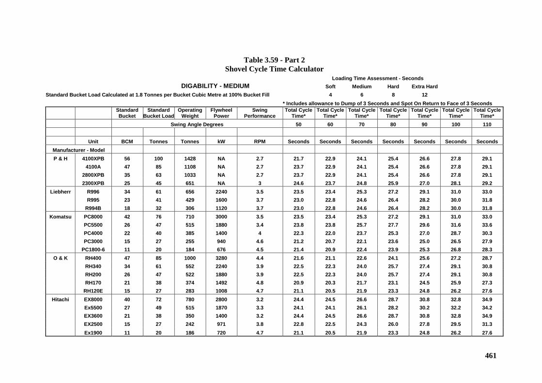
461
Table 3.59 - Part 2
Shovel Cycle Time Calculator Loading Time Assessment - Seconds DIGABILITY - MEDIUM Soft Medium Hard Extra Hard Standard Bucket Load Calculated at 1.8 Tonnes per Bucket Cubic Metre at 100% Bucket Fill 4 6 8 12 * Includes allowance to Dump of 3 Seconds and Spot On Return to Face of 3 Seconds
Standard Bucket
Standard Bucket Load
Operating Weight
Flywheel Power
Swing Performance
Total Cycle Time*
Total Cycle Time*
Total Cycle Time*
Total Cycle Time*
Total Cycle Time*
Total Cycle Time*
Total Cycle Time*
Swing Angle Degrees 50 60 70 80 90 100 110 Unit BCM Tonnes Tonnes kW RPM Seconds Seconds Seconds Seconds Seconds Seconds Seconds
Manufacturer - Model P & H 4100XPB 56 100 1428 NA 2.7 21.7 22.9 24.1 25.4 26.6 27.8 29.1
4100A 47 85 1108 NA 2.7 23.7 22.9 24.1 25.4 26.6 27.8 29.1 2800XPB 35 63 1033 NA 2.7 23.7 22.9 24.1 25.4 26.6 27.8 29.1 2300XPB 25 45 651 NA 3 24.6 23.7 24.8 25.9 27.0 28.1 29.2
Liebherr R996 34 61 656 2240 3.5 23.5 23.4 25.3 27.2 29.1 31.0 33.0 R995 23 41 429 1600 3.7 23.0 22.8 24.6 26.4 28.2 30.0 31.8 R994B 18 32 306 1120 3.7 23.0 22.8 24.6 26.4 28.2 30.0 31.8
Komatsu PC8000 42 76 710 3000 3.5 23.5 23.4 25.3 27.2 29.1 31.0 33.0 PC5500 26 47 515 1880 3.4 23.8 23.8 25.7 27.7 29.6 31.6 33.6 PC4000 22 40 385 1400 4 22.3 22.0 23.7 25.3 27.0 28.7 30.3 PC3000 15 27 255 940 4.6 21.2 20.7 22.1 23.6 25.0 26.5 27.9 PC1800-6 11 20 184 676 4.5 21.4 20.9 22.4 23.9 25.3 26.8 28.3
O & K RH400 47 85 1000 3280 4.4 21.6 21.1 22.6 24.1 25.6 27.2 28.7 RH340 34 61 552 2240 3.9 22.5 22.3 24.0 25.7 27.4 29.1 30.8 RH200 26 47 522 1880 3.9 22.5 22.3 24.0 25.7 27.4 29.1 30.8 RH170 21 38 374 1492 4.8 20.9 20.3 21.7 23.1 24.5 25.9 27.3 RH120E 15 27 283 1008 4.7 21.1 20.5 21.9 23.3 24.8 26.2 27.6
Hitachi EX8000 40 72 780 2800 3.2 24.4 24.5 26.6 28.7 30.8 32.8 34.9 Ex5500 27 49 515 1870 3.3 24.1 24.1 26.1 28.2 30.2 32.2 34.2 EX3600 21 38 350 1400 3.2 24.4 24.5 26.6 28.7 30.8 32.8 34.9 EX2500 15 27 242 971 3.8 22.8 22.5 24.3 26.0 27.8 29.5 31.3 Ex1900 11 20 186 720 4.7 21.1 20.5 21.9 23.3 24.8 26.2 27.6
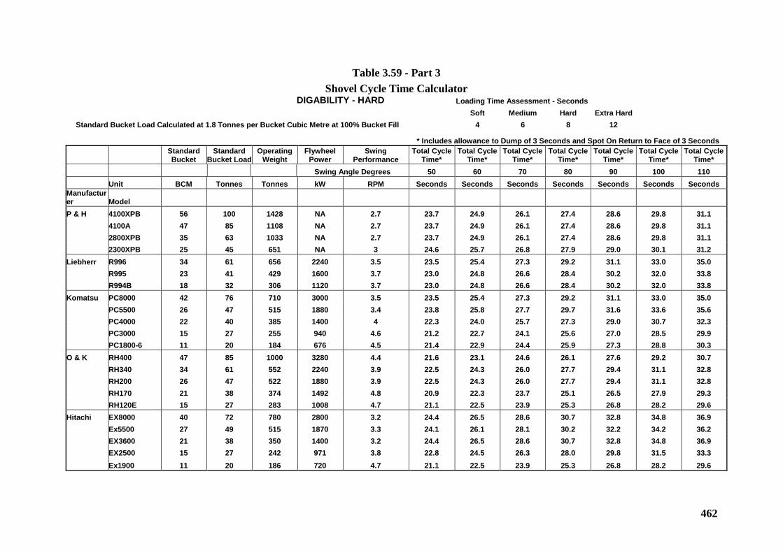
462
Table 3.59 - Part 3 Shovel Cycle Time Calculator
DIGABILITY - HARD Loading Time Assessment - Seconds Soft Medium Hard Extra Hard
Standard Bucket Load Calculated at 1.8 Tonnes per Bucket Cubic Metre at 100% Bucket Fill 4 6 8 12
* Includes allowance to Dump of 3 Seconds and Spot On Return to Face of 3 Seconds
Standard Bucket
Standard Bucket Load
Operating Weight
Flywheel Power
Swing Performance
Total Cycle Time*
Total Cycle Time*
Total Cycle Time*
Total Cycle Time*
Total Cycle Time*
Total Cycle Time*
Total Cycle Time*
Swing Angle Degrees 50 60 70 80 90 100 110 Unit BCM Tonnes Tonnes kW RPM Seconds Seconds Seconds Seconds Seconds Seconds Seconds Manufacturer Model P & H 4100XPB 56 100 1428 NA 2.7 23.7 24.9 26.1 27.4 28.6 29.8 31.1 4100A 47 85 1108 NA 2.7 23.7 24.9 26.1 27.4 28.6 29.8 31.1 2800XPB 35 63 1033 NA 2.7 23.7 24.9 26.1 27.4 28.6 29.8 31.1 2300XPB 25 45 651 NA 3 24.6 25.7 26.8 27.9 29.0 30.1 31.2 Liebherr R996 34 61 656 2240 3.5 23.5 25.4 27.3 29.2 31.1 33.0 35.0 R995 23 41 429 1600 3.7 23.0 24.8 26.6 28.4 30.2 32.0 33.8 R994B 18 32 306 1120 3.7 23.0 24.8 26.6 28.4 30.2 32.0 33.8 Komatsu PC8000 42 76 710 3000 3.5 23.5 25.4 27.3 29.2 31.1 33.0 35.0 PC5500 26 47 515 1880 3.4 23.8 25.8 27.7 29.7 31.6 33.6 35.6 PC4000 22 40 385 1400 4 22.3 24.0 25.7 27.3 29.0 30.7 32.3 PC3000 15 27 255 940 4.6 21.2 22.7 24.1 25.6 27.0 28.5 29.9 PC1800-6 11 20 184 676 4.5 21.4 22.9 24.4 25.9 27.3 28.8 30.3 O & K RH400 47 85 1000 3280 4.4 21.6 23.1 24.6 26.1 27.6 29.2 30.7 RH340 34 61 552 2240 3.9 22.5 24.3 26.0 27.7 29.4 31.1 32.8 RH200 26 47 522 1880 3.9 22.5 24.3 26.0 27.7 29.4 31.1 32.8 RH170 21 38 374 1492 4.8 20.9 22.3 23.7 25.1 26.5 27.9 29.3 RH120E 15 27 283 1008 4.7 21.1 22.5 23.9 25.3 26.8 28.2 29.6 Hitachi EX8000 40 72 780 2800 3.2 24.4 26.5 28.6 30.7 32.8 34.8 36.9 Ex5500 27 49 515 1870 3.3 24.1 26.1 28.1 30.2 32.2 34.2 36.2 EX3600 21 38 350 1400 3.2 24.4 26.5 28.6 30.7 32.8 34.8 36.9 EX2500 15 27 242 971 3.8 22.8 24.5 26.3 28.0 29.8 31.5 33.3 Ex1900 11 20 186 720 4.7 21.1 22.5 23.9 25.3 26.8 28.2 29.6
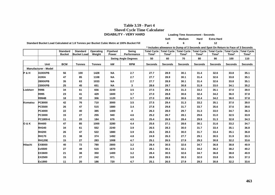
463
Table 3.59 - Part 4 Shovel Cycle Time Calculator
DIGABILITY - VERY HARD Loading Time Assessment - Seconds Soft Medium Hard Extra Hard
Standard Bucket Load Calculated at 1.8 Tonnes per Bucket Cubic Metre at 100% Bucket Fill 4 6 8 12 * Includes allowance to Dump of 3 Seconds and Spot On Return to Face of 3 Seconds
Standard Bucket
Standard Bucket Load
Operating Weight
Flywheel Power
Swing Performance
Total Cycle Time*
Total Cycle Time*
Total Cycle Time*
Total Cycle Time*
Total Cycle Time*
Total Cycle Time*
Total Cycle Time*
Swing Angle Degrees 50 60 70 80 90 100 110
Unit BCM Tonnes Tonnes kW RPM Seconds Seconds Seconds Seconds Seconds Seconds Seconds Manufacturer - Model
P & H 4100XPB 56 100 1428 NA 2.7 27.7 28.9 30.1 31.4 32.6 33.8 35.1 4100A 47 85 1108 NA 2.7 27.7 28.9 30.1 31.4 32.6 33.8 35.1 2800XPB 35 63 1033 NA 2.7 27.7 28.9 30.1 31.4 32.6 33.8 35.1 2300XPB 25 45 651 NA 3 28.6 29.7 30.8 31.9 33.0 34.1 35.2 Liebherr R996 34 61 656 2240 3.5 27.5 29.4 31.3 33.2 35.1 37.0 39.0 R995 23 41 429 1600 3.7 27.0 28.8 30.6 32.4 34.2 36.0 37.8 R994B 18 32 306 1120 3.7 27.0 28.8 30.6 32.4 34.2 36.0 37.8 Komatsu PC8000 42 76 710 3000 3.5 27.5 29.4 31.3 33.2 35.1 37.0 39.0 PC5500 26 47 515 1880 3.4 27.8 29.8 31.7 33.7 35.6 37.6 39.6 PC4000 22 40 385 1400 4 26.3 28.0 29.7 31.3 33.0 34.7 36.3 PC3000 15 27 255 940 4.6 25.2 26.7 28.1 29.6 31.0 32.5 33.9 PC1800-6 11 20 184 676 4.5 25.4 26.9 28.4 29.9 31.3 32.8 34.3 O & K RH400 47 85 1000 3280 4.4 25.6 27.1 28.6 30.1 31.6 33.2 34.7 RH340 34 61 552 2240 3.9 26.5 28.3 30.0 31.7 33.4 35.1 36.8 RH200 26 47 522 1880 3.9 26.5 28.3 30.0 31.7 33.4 35.1 36.8 RH170 21 38 374 1492 4.8 24.9 26.3 27.7 29.1 30.5 31.9 33.3 RH120E 15 27 283 1008 4.7 25.1 26.5 27.9 29.3 30.8 32.2 33.6 Hitachi EX8000 40 72 780 2800 3.2 28.4 30.5 32.6 34.7 36.8 38.8 40.9 Ex5500 27 49 515 1870 3.3 28.1 30.1 32.1 34.2 36.2 38.2 40.2 EX3600 21 38 350 1400 3.2 28.4 30.5 32.6 34.7 36.8 38.8 40.9 EX2500 15 27 242 971 3.8 26.8 28.5 30.3 32.0 33.8 35.5 37.3 Ex1900 11 20 186 720 4.7 25.1 26.5 27.9 29.3 30.8 32.2 33.6
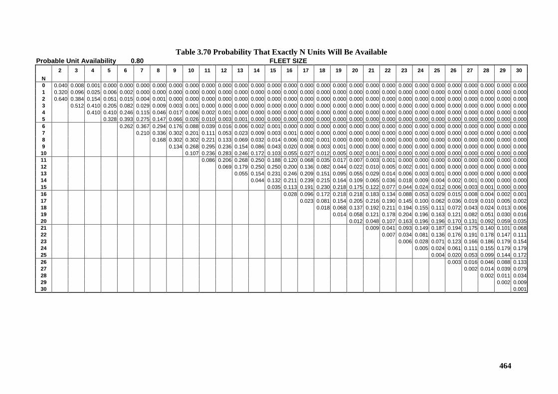
464
Table 3.70 Probability That Exactly N Units Will Be Available Probable Unit Availability 0.80 FLEET SIZE
2 3 4 5 6 7 8 9 10 11 12 13 14 15 16 17 18 19 20 21 22 23 24 25 26 27 28 29 30 N 0 0.040 0.008 0.001 0.000 0.000 0.000 0.000 0.000 0.000 0.000 0.000 0.000 0.000 0.000 0.000 0.000 0.000 0.000 0.000 0.000 0.000 0.000 0.000 0.000 0.000 0.000 0.000 0.000 0.000 1 0.320 0.096 0.025 0.006 0.002 0.000 0.000 0.000 0.000 0.000 0.000 0.000 0.000 0.000 0.000 0.000 0.000 0.000 0.000 0.000 0.000 0.000 0.000 0.000 0.000 0.000 0.000 0.000 0.000 2 0.640 0.384 0.154 0.051 0.015 0.004 0.001 0.000 0.000 0.000 0.000 0.000 0.000 0.000 0.000 0.000 0.000 0.000 0.000 0.000 0.000 0.000 0.000 0.000 0.000 0.000 0.000 0.000 0.000 3 0.512 0.410 0.205 0.082 0.029 0.009 0.003 0.001 0.000 0.000 0.000 0.000 0.000 0.000 0.000 0.000 0.000 0.000 0.000 0.000 0.000 0.000 0.000 0.000 0.000 0.000 0.000 0.000 4 0.410 0.410 0.246 0.115 0.046 0.017 0.006 0.002 0.001 0.000 0.000 0.000 0.000 0.000 0.000 0.000 0.000 0.000 0.000 0.000 0.000 0.000 0.000 0.000 0.000 0.000 0.000 5 0.328 0.393 0.275 0.147 0.066 0.026 0.010 0.003 0.001 0.000 0.000 0.000 0.000 0.000 0.000 0.000 0.000 0.000 0.000 0.000 0.000 0.000 0.000 0.000 0.000 0.000 6 0.262 0.367 0.294 0.176 0.088 0.039 0.016 0.006 0.002 0.001 0.000 0.000 0.000 0.000 0.000 0.000 0.000 0.000 0.000 0.000 0.000 0.000 0.000 0.000 0.000 7 0.210 0.336 0.302 0.201 0.111 0.053 0.023 0.009 0.003 0.001 0.000 0.000 0.000 0.000 0.000 0.000 0.000 0.000 0.000 0.000 0.000 0.000 0.000 0.000 8 0.168 0.302 0.302 0.221 0.133 0.069 0.032 0.014 0.006 0.002 0.001 0.000 0.000 0.000 0.000 0.000 0.000 0.000 0.000 0.000 0.000 0.000 0.000 9 0.134 0.268 0.295 0.236 0.154 0.086 0.043 0.020 0.008 0.003 0.001 0.000 0.000 0.000 0.000 0.000 0.000 0.000 0.000 0.000 0.000 0.000 10 0.107 0.236 0.283 0.246 0.172 0.103 0.055 0.027 0.012 0.005 0.002 0.001 0.000 0.000 0.000 0.000 0.000 0.000 0.000 0.000 0.000 11 0.086 0.206 0.268 0.250 0.188 0.120 0.068 0.035 0.017 0.007 0.003 0.001 0.000 0.000 0.000 0.000 0.000 0.000 0.000 0.000 12 0.069 0.179 0.250 0.250 0.200 0.136 0.082 0.044 0.022 0.010 0.005 0.002 0.001 0.000 0.000 0.000 0.000 0.000 0.000 13 0.055 0.154 0.231 0.246 0.209 0.151 0.095 0.055 0.029 0.014 0.006 0.003 0.001 0.000 0.000 0.000 0.000 0.000 14 0.044 0.132 0.211 0.239 0.215 0.164 0.109 0.065 0.036 0.018 0.009 0.004 0.002 0.001 0.000 0.000 0.000 15 0.035 0.113 0.191 0.230 0.218 0.175 0.122 0.077 0.044 0.024 0.012 0.006 0.003 0.001 0.000 0.000 16 0.028 0.096 0.172 0.218 0.218 0.183 0.134 0.088 0.053 0.029 0.015 0.008 0.004 0.002 0.001 17 0.023 0.081 0.154 0.205 0.216 0.190 0.145 0.100 0.062 0.036 0.019 0.010 0.005 0.002 18 0.018 0.068 0.137 0.192 0.211 0.194 0.155 0.111 0.072 0.043 0.024 0.013 0.006 19 0.014 0.058 0.121 0.178 0.204 0.196 0.163 0.121 0.082 0.051 0.030 0.016 20 0.012 0.048 0.107 0.163 0.196 0.196 0.170 0.131 0.092 0.059 0.035 21 0.009 0.041 0.093 0.149 0.187 0.194 0.175 0.140 0.101 0.068 22 0.007 0.034 0.081 0.136 0.176 0.191 0.178 0.147 0.111 23 0.006 0.028 0.071 0.123 0.166 0.186 0.179 0.154 24 0.005 0.024 0.061 0.111 0.155 0.179 0.179 25 0.004 0.020 0.053 0.099 0.144 0.172 26 0.003 0.016 0.046 0.088 0.133 27 0.002 0.014 0.039 0.079 28 0.002 0.011 0.034 29 0.002 0.009 30 0.001
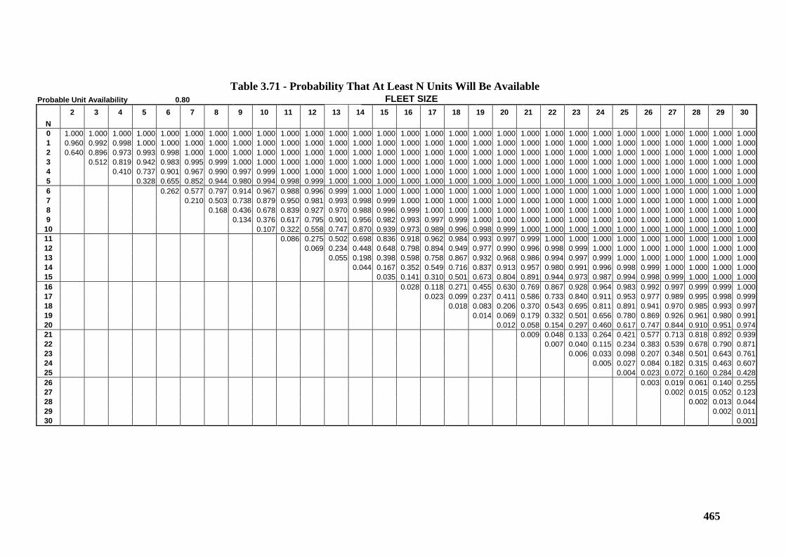
465
Table 3.71 - Probability That At Least N Units Will Be Available
Probable Unit Availability 0.80 FLEET SIZE 2 3 4 5 6 7 8 9 10 11 12 13 14 15 16 17 18 19 20 21 22 23 24 25 26 27 28 29 30 N 0 1.000 1.000 1.000 1.000 1.000 1.000 1.000 1.000 1.000 1.000 1.000 1.000 1.000 1.000 1.000 1.000 1.000 1.000 1.000 1.000 1.000 1.000 1.000 1.000 1.000 1.000 1.000 1.000 1.000 1 0.960 0.992 0.998 1.000 1.000 1.000 1.000 1.000 1.000 1.000 1.000 1.000 1.000 1.000 1.000 1.000 1.000 1.000 1.000 1.000 1.000 1.000 1.000 1.000 1.000 1.000 1.000 1.000 1.000 2 0.640 0.896 0.973 0.993 0.998 1.000 1.000 1.000 1.000 1.000 1.000 1.000 1.000 1.000 1.000 1.000 1.000 1.000 1.000 1.000 1.000 1.000 1.000 1.000 1.000 1.000 1.000 1.000 1.000 3 0.512 0.819 0.942 0.983 0.995 0.999 1.000 1.000 1.000 1.000 1.000 1.000 1.000 1.000 1.000 1.000 1.000 1.000 1.000 1.000 1.000 1.000 1.000 1.000 1.000 1.000 1.000 1.000 4 0.410 0.737 0.901 0.967 0.990 0.997 0.999 1.000 1.000 1.000 1.000 1.000 1.000 1.000 1.000 1.000 1.000 1.000 1.000 1.000 1.000 1.000 1.000 1.000 1.000 1.000 1.000 5 0.328 0.655 0.852 0.944 0.980 0.994 0.998 0.999 1.000 1.000 1.000 1.000 1.000 1.000 1.000 1.000 1.000 1.000 1.000 1.000 1.000 1.000 1.000 1.000 1.000 1.000 6 0.262 0.577 0.797 0.914 0.967 0.988 0.996 0.999 1.000 1.000 1.000 1.000 1.000 1.000 1.000 1.000 1.000 1.000 1.000 1.000 1.000 1.000 1.000 1.000 1.000 7 0.210 0.503 0.738 0.879 0.950 0.981 0.993 0.998 0.999 1.000 1.000 1.000 1.000 1.000 1.000 1.000 1.000 1.000 1.000 1.000 1.000 1.000 1.000 1.000 8 0.168 0.436 0.678 0.839 0.927 0.970 0.988 0.996 0.999 1.000 1.000 1.000 1.000 1.000 1.000 1.000 1.000 1.000 1.000 1.000 1.000 1.000 1.000 9 0.134 0.376 0.617 0.795 0.901 0.956 0.982 0.993 0.997 0.999 1.000 1.000 1.000 1.000 1.000 1.000 1.000 1.000 1.000 1.000 1.000 1.000
10 0.107 0.322 0.558 0.747 0.870 0.939 0.973 0.989 0.996 0.998 0.999 1.000 1.000 1.000 1.000 1.000 1.000 1.000 1.000 1.000 1.000 11 0.086 0.275 0.502 0.698 0.836 0.918 0.962 0.984 0.993 0.997 0.999 1.000 1.000 1.000 1.000 1.000 1.000 1.000 1.000 1.000 12 0.069 0.234 0.448 0.648 0.798 0.894 0.949 0.977 0.990 0.996 0.998 0.999 1.000 1.000 1.000 1.000 1.000 1.000 1.000 13 0.055 0.198 0.398 0.598 0.758 0.867 0.932 0.968 0.986 0.994 0.997 0.999 1.000 1.000 1.000 1.000 1.000 1.000 14 0.044 0.167 0.352 0.549 0.716 0.837 0.913 0.957 0.980 0.991 0.996 0.998 0.999 1.000 1.000 1.000 1.000 15 0.035 0.141 0.310 0.501 0.673 0.804 0.891 0.944 0.973 0.987 0.994 0.998 0.999 1.000 1.000 1.000 16 0.028 0.118 0.271 0.455 0.630 0.769 0.867 0.928 0.964 0.983 0.992 0.997 0.999 0.999 1.000 17 0.023 0.099 0.237 0.411 0.586 0.733 0.840 0.911 0.953 0.977 0.989 0.995 0.998 0.999 18 0.018 0.083 0.206 0.370 0.543 0.695 0.811 0.891 0.941 0.970 0.985 0.993 0.997 19 0.014 0.069 0.179 0.332 0.501 0.656 0.780 0.869 0.926 0.961 0.980 0.991 20 0.012 0.058 0.154 0.297 0.460 0.617 0.747 0.844 0.910 0.951 0.974 21 0.009 0.048 0.133 0.264 0.421 0.577 0.713 0.818 0.892 0.939 22 0.007 0.040 0.115 0.234 0.383 0.539 0.678 0.790 0.871 23 0.006 0.033 0.098 0.207 0.348 0.501 0.643 0.761 24 0.005 0.027 0.084 0.182 0.315 0.463 0.607 25 0.004 0.023 0.072 0.160 0.284 0.428 26 0.003 0.019 0.061 0.140 0.255 27 0.002 0.015 0.052 0.123 28 0.002 0.013 0.044 29 0.002 0.011 30 0.001
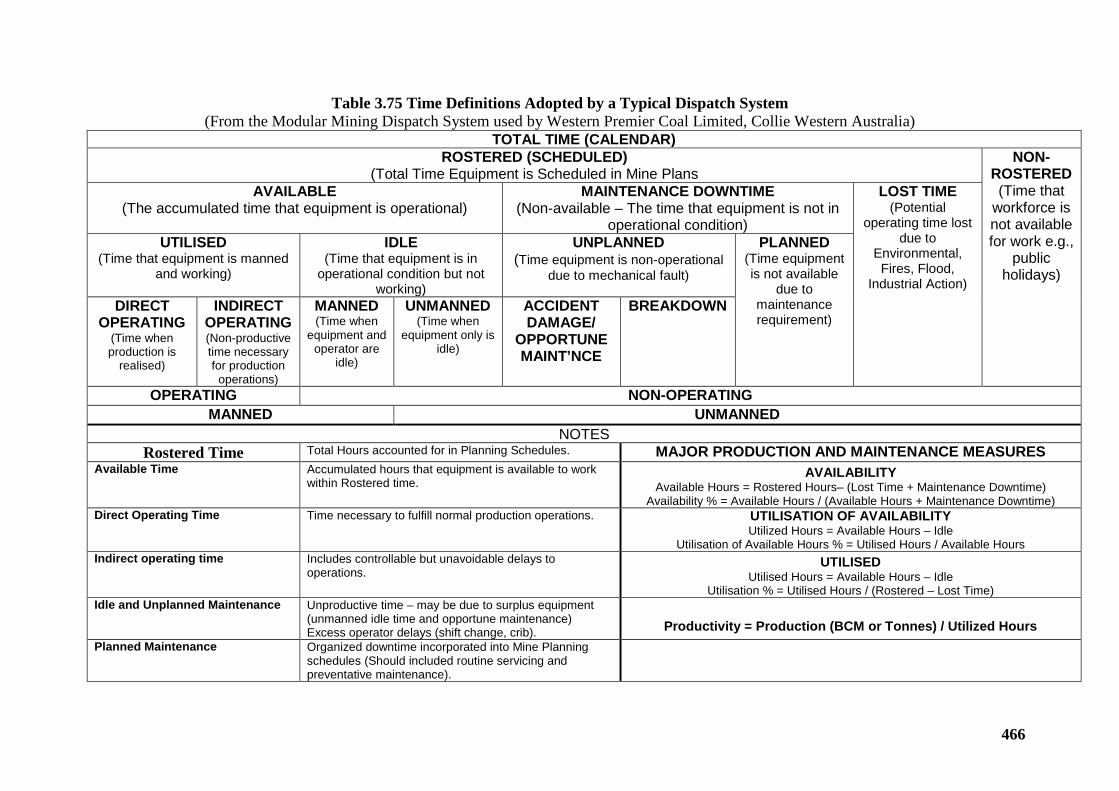
466
Table 3.75 Time Definitions Adopted by a Typical Dispatch System (From the Modular Mining Dispatch System used by Western Premier Coal Limited, Collie Western Australia)
TOTAL TIME (CALENDAR) ROSTERED (SCHEDULED)
(Total Time Equipment is Scheduled in Mine Plans NON-
ROSTERED (Time that
workforce is not available for work e.g.,
public holidays)
AVAILABLE (The accumulated time that equipment is operational)
MAINTENANCE DOWNTIME (Non-available – The time that equipment is not in
operational condition)
LOST TIME (Potential
operating time lost due to
Environmental, Fires, Flood,
Industrial Action)
UTILISED (Time that equipment is manned
and working)
IDLE (Time that equipment is in
operational condition but not working)
UNPLANNED (Time equipment is non-operational
due to mechanical fault)
PLANNED (Time equipment is not available
due to maintenance requirement)
DIRECT OPERATING
(Time when production is
realised)
INDIRECT OPERATING (Non-productive time necessary for production
operations)
MANNED (Time when
equipment and operator are
idle)
UNMANNED (Time when
equipment only is idle)
ACCIDENT DAMAGE/
OPPORTUNE MAINT’NCE
BREAKDOWN
OPERATING NON-OPERATING MANNED UNMANNED
NOTES Rostered Time Total Hours accounted for in Planning Schedules. MAJOR PRODUCTION AND MAINTENANCE MEASURES
Available Time Accumulated hours that equipment is available to work within Rostered time.
AVAILABILITY Available Hours = Rostered Hours– (Lost Time + Maintenance Downtime)
Availability % = Available Hours / (Available Hours + Maintenance Downtime) Direct Operating Time Time necessary to fulfill normal production operations. UTILISATION OF AVAILABILITY
Utilized Hours = Available Hours – Idle Utilisation of Available Hours % = Utilised Hours / Available Hours
Indirect operating time Includes controllable but unavoidable delays to operations.
UTILISED Utilised Hours = Available Hours – Idle
Utilisation % = Utilised Hours / (Rostered – Lost Time) Idle and Unplanned Maintenance Unproductive time – may be due to surplus equipment
(unmanned idle time and opportune maintenance) Excess operator delays (shift change, crib).
Productivity = Production (BCM or Tonnes) / Utilized Hours
Planned Maintenance Organized downtime incorporated into Mine Planning schedules (Should included routine servicing and preventative maintenance).
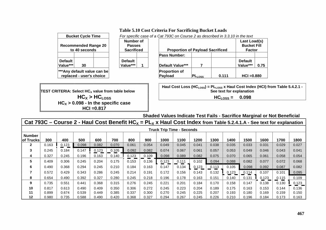
467
Table 5.10 Cost Criteria For Sacrificing Bucket Loads Bucket Cycle Time For specific case of a Cat 793C on Course 2 as described in 3.3.10 in the text
Recommended Range 20
to 40 seconds
Number of Passes
Sacrificed Proportion of Payload Sacrificed
Last Load(s) Bucket Fill
Factor Pass Number:
Default Value*** 30
Default Value*** 1 Default Value*** 7
Default Value*** 0.75
***Any default value can be
replaced - user's choice Proportion of Payload PLLOSS 0.111
HCI =0.880
TEST CRITERIA: Select HCX value from table below Haul Cost Loss (HCLOSS) = PLLOSS x Haul Cost Index (HCI) from Table 5.4.2.1 -
See text for explanation HCX > HCLOSS HCLOSS = 0.098
HCX > 0.098 - In the specific case
HCI =0.817
Shaded Values Indicate Test Fails - Sacrifice Marginal or Not Beneficial Cat 793C – Course 2 - Haul Cost Benefit HCX = PLX x Haul Cost Index from Table 5.2.4.1.A - See text for explanation
Truck Trip Time - Seconds Number
of Trucks 300 400 500 600 700 800 900 1000 1100 1200 1300 1400 1500 1600 1700 1800 2 0.163 0.123 0.098 0.082 0.070 0.061 0.054 0.049 0.045 0.041 0.038 0.035 0.033 0.031 0.029 0.027 3 0.245 0.184 0.147 0.123 0.105 0.092 0.082 0.074 0.067 0.061 0.057 0.053 0.049 0.046 0.043 0.041 4 0.327 0.245 0.196 0.163 0.140 0.123 0.109 0.098 0.089 0.082 0.075 0.070 0.065 0.061 0.058 0.054 5 0.409 0.306 0.245 0.204 0.175 0.153 0.136 0.123 0.111 0.102 0.094 0.088 0.082 0.077 0.072 0.068 6 0.490 0.368 0.294 0.245 0.210 0.184 0.163 0.147 0.134 0.123 0.113 0.105 0.098 0.092 0.087 0.082 7 0.572 0.429 0.343 0.286 0.245 0.214 0.191 0.172 0.156 0.143 0.132 0.123 0.114 0.107 0.101 0.095 8 0.654 0.490 0.392 0.327 0.280 0.245 0.218 0.196 0.178 0.163 0.151 0.140 0.131 0.123 0.115 0.109 9 0.735 0.551 0.441 0.368 0.315 0.276 0.245 0.221 0.201 0.184 0.170 0.158 0.147 0.138 0.130 0.123 10 0.817 0.613 0.490 0.409 0.350 0.306 0.272 0.245 0.223 0.204 0.189 0.175 0.163 0.153 0.144 0.136 11 0.899 0.674 0.539 0.449 0.385 0.337 0.300 0.270 0.245 0.225 0.207 0.193 0.180 0.169 0.159 0.150 12 0.980 0.735 0.588 0.490 0.420 0.368 0.327 0.294 0.267 0.245 0.226 0.210 0.196 0.184 0.173 0.163
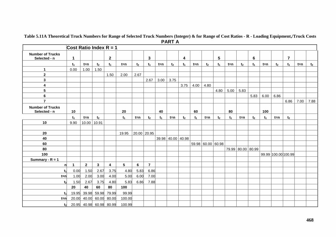
468
Table 5.11A Theoretical Truck Numbers for Range of Selected Truck Numbers (Integer) & for Range of Cost Ratios - R - Loading Equipment,/Truck Costs
PART A Cost Ratio Index R = 1
Number of Trucks Selected - n 1 2 3 4 5 6 7
t1 t=n t2 t1 t=n t2 t1 t=n t2 t1 t=n t2 t1 t=n t2 t1 t=n t2 t1 t=n t2 1 0.00 1.00 1.50 2 1.50 2.00 2.67 3 2.67 3.00 3.75 4 3.75 4.00 4.80 5 4.80 5.00 5.83 6 5.83 6.00 6.86 7 6.86 7.00 7.88
Number of Trucks Selected - n 10 20 40 60 80 100
t1 t=n t2 t1 t=n t2 t1 t=n t2 t1 t=n t2 t1 t=n t2 t1 t=n t2 10 9.90 10.00 10.91
20 19.95 20.00 20.95 40 39.98 40.00 40.98 60 59.98 60.00 60.98 80 79.99 80.00 80.99
100 99.99 100.00 100.99 Summary - R = 1
n 1 2 3 4 5 6 7 t1 0.00 1.50 2.67 3.75 4.80 5.83 6.86
t=n 1.00 2.00 3.00 4.00 5.00 6.00 7.00 t2 1.50 2.67 3.75 4.80 5.83 6.86 7.88
20 40 60 80 100 t1 19.95 39.98 59.98 79.99 99.99
t=n 20.00 40.00 60.00 80.00 100.00
t2 20.95 40.98 60.98 80.99 100.99
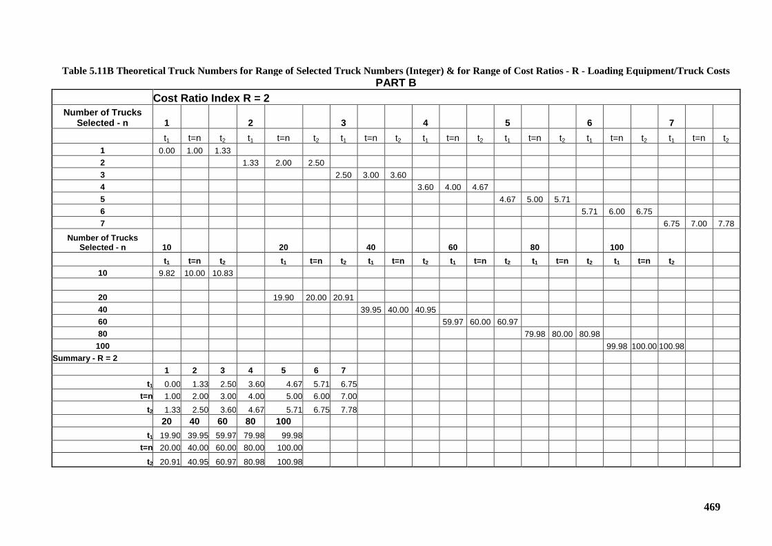
469
Table 5.11B Theoretical Truck Numbers for Range of Selected Truck Numbers (Integer) & for Range of Cost Ratios - R - Loading Equipment/Truck Costs PART B
Cost Ratio Index R = 2 Number of Trucks
Selected - n 1 2 3 4 5 6 7 t1 t=n t2 t1 t=n t2 t1 t=n t2 t1 t=n t2 t1 t=n t2 t1 t=n t2 t1 t=n t2
1 0.00 1.00 1.33 2 1.33 2.00 2.50 3 2.50 3.00 3.60 4 3.60 4.00 4.67 5 4.67 5.00 5.71 6 5.71 6.00 6.75 7 6.75 7.00 7.78
Number of Trucks Selected - n 10 20 40 60 80 100
t1 t=n t2 t1 t=n t2 t1 t=n t2 t1 t=n t2 t1 t=n t2 t1 t=n t2 10 9.82 10.00 10.83
20 19.90 20.00 20.91 40 39.95 40.00 40.95 60 59.97 60.00 60.97 80 79.98 80.00 80.98
100 99.98 100.00 100.98 Summary - R = 2 1 2 3 4 5 6 7
t1 0.00 1.33 2.50 3.60 4.67 5.71 6.75 t=n 1.00 2.00 3.00 4.00 5.00 6.00 7.00
t2 1.33 2.50 3.60 4.67 5.71 6.75 7.78 20 40 60 80 100
t1 19.90 39.95 59.97 79.98 99.98 t=n 20.00 40.00 60.00 80.00 100.00
t2 20.91 40.95 60.97 80.98 100.98

470
Table 5.11C Theoretical Truck Numbers for Range of Selected Truck Numbers (Integer) & for Range of Cost Ratios - R - Loading Equipment/Truck Costs PART C
Cost Ratio Index R = 3 Number of Trucks
Selected - n 1 2 3 4 5 6 7 t1 t=n t2 t1 t=n t2 t1 t=n t2 t1 t=n t2 t1 t=n t2 t1 t=n t2 t1 t=n t2
1 0.00 1.00 1.25 2 1.25 2.00 2.40 3 2.40 3.00 3.50 4 3.50 4.00 4.57 5 4.57 5.00 5.63 6 5.63 6.00 6.67 7 6.67 7.00 7.70
Number of Trucks Selected - n 10 20 40 60 80 100 t1 t=n t2 t1 t=n t2 t1 t=n t2 t1 t=n t2 t1 t=n t2 t1 t=n t2
10 9.75 10.00 10.77
20 19.86 20.00 20.87 40 39.93 40.00 40.93 60 59.95 60.00 60.95 80 79.96 80.00 80.96
100 99.97 100.00 100.97 Summary - R = 3 1 2 3 4 5 6 7
t1 0.00 1.25 2.40 3.50 4.57 5.63 6.67 t=n 1.00 2.00 3.00 4.00 5.00 6.00 7.00
t2 1.25 2.40 3.50 4.57 5.63 6.67 7.70 20 40 60 80 100
t1 19.86 39.93 59.95 79.96 99.97 t=n 20.00 40.00 60.00 80.00 100.00
t2 20.87 40.93 60.95 80.96 100.97

471
MATHEMATICAL PRINCIPLES - NOTES
Includes Table of Contents
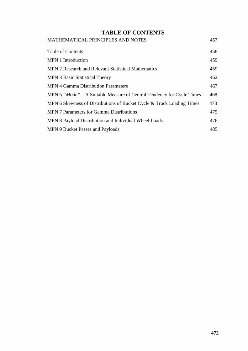
472
TABLE OF CONTENTS MATHEMATICAL PRINCIPLES AND NOTES 457 Table of Contents 458
MPN 1 Introduction 459
MPN 2 Research and Relevant Statistical Mathematics 459
MPN 3 Basic Statistical Theory 462
MPN 4 Gamma Distribution Parameters 467
MPN 5 “Mode” – A Suitable Measure of Central Tendency for Cycle Times 468
MPN 6 Skewness of Distributions of Bucket Cycle & Truck Loading Times 473
MPN 7 Parameters for Gamma Distributions 475
MPN 8 Payload Distribution and Individual Wheel Loads 476
MPN 9 Bucket Passes and Payloads 485
473
MPN 1 Introduction Statistical theory and methods have been studied, described and applied to the
limited degree necessary to facilitate analysis, interpretation and conclusive
outcomes of the research. Proof of the propositions adopted for research purposes has
been left for the reader to pursue in the many excellent texts on the subject some of
which have been acknowledged and listed in References in the thesis, specifically
referred to in the thesis and within these notes.
The mathematical principles visited in the research are not presented as an
exhaustive or comprehensive treatment – only as a means to facilitate the research
outcomes and assist the reader.
MPN 2 Research and Relevant Statistical Mathematics Definitive understanding of productivity and performance criteria for loading and
hauling equipment is an essential basis for selecting equipment items from available
options. Initial comparisons are generally made in terms of expected values,
arithmetic means, adopted for deterministic methods to estimate productivity and
performance.
Previous experience with investigation of productivity in open pit mining operations,
and how to effect improvement, has led to an understanding that deterministic
analysis based on expected values is inadequate for the level of understanding
necessary to manage and improve operational performance. A stochastic approach to
analysis of data and interpretation of the results in terms of operational criteria and
protocols is required. Preliminary investigation of load and haul operations by the
author in terms of performance and efficiency commenced some years ago. Recent
outcomes from feasibility and improvement studies were sufficiently interesting and
encouraging to formalize a research project that has ultimately coalesced as the
subject of this thesis. Research described in the thesis includes investigation of the
bucket load – truck payload relationship, bucket cycle times and truck loading time,
influence of number of bucket passes on productivity and efficiency of load and haul
operations and related issues. Early investigations recognized the need to adopt
descriptive statistics to identify, test and adopt probability distributions used to
model observed empirical distributions.
474
The need for sufficient understanding of the behaviour of mining operational events
observed as empirical data distributions ultimately led to frequency analysis using
convenient, appropriate frequency intervals and construction of histograms to be
compared with continuous model/test distributions. Many of the empirical data
distributions rearranged as frequency distributions observed in loading and hauling
functions exhibit symmetry and central tendency that indicate observed data is, in
many cases, normally distributed.
Sample theory has proved most useful in understanding the relationship between
number of bucket passes and dispersion of truck payload distributions; also between
bucket cycle times and truck loading times.
Application of Small (Exact) Sample Theory has not been necessary as:
• Generally empirical distributions of bucket loads and truck payloads can be
modelled by normal distributions – refer Section 3.2.8.
• Empirical distributions of bucket cycle times and loading times are
substantially positively skewed exhibiting significant high values and
affected by anomalous outliers (likely a separate random variable
distribution) that are non-intrinsic to actual loading operations refer Section
3.2.9.
Analysis of this latter case was facilitated by:
• Testing with gamma distributions that, on realising qualitative acceptance
exhibited significantly high shape and scale parameters indicating underlying
central tendency of empirical data, i.e., a tendency to skewed normal
distributions.
• Objective filtering with regard to origins of anomalous outliers – aiming to
separate from the basic intrinsic loading function data affected by activities
non-intrinsic to the basic loading operation.
As shown in Section 3.2.9 in the thesis, manifest in the relevant tables and illustrated
by associated figures, filtering outcomes can expose incipient central tendency and a
drift towards symmetry.
Truck payloads can be viewed as small samples of bucket loads and truck loading
time as small samples of bucket cycle times.
475
Because of normality of bucket loads and, as a consequence normally distributed
truck payloads, application of small (exact) sample theory was unnecessary.
Highly skewed bucket cycle times and truck loading times might have been
advantageously analysed using Student’s (Gosset’s) “t” distribution as a model to
compare empirical data sets and suitable test models in terms of the “t” statistic.
Proceeding to this level of comparative analysis was considered unnecessary as
acceptable results and understanding sufficient for the purposes of the research was
achieved by filtering. Operating on the data without filtering would have been tacit
acceptance that anomalous outliers in bucket cycle time and loading time
distributions are intrinsic to the basic loading function when experienced
understanding of anomalous time outliers recognizes such acceptance as
unreasonable.
When reviewing Student’s “t” distribution for applicability it was noted that,
compared with a normal distribution, the family of “t” distributions:
• Have a platykurtic trend as sample numbers decrease.
• Tails extend along the “t” value axis as sample number (N) decreases
indicative of increase distribution dispersion.
So, consistent with intuitive understanding and empirical observations, dispersion of
truck loading times drawn from a population of bucket cycle times will tend to
increase as the number of bucket passes to load trucks decrease. The result will be
increased variability in truck loading times as bucket-cycle time increases. This is
confirmed by the analysis and interpretation in Section 3.2.9.
Identification of applicable test distributions to compare with empirical data from
production operations was, initially, essentially qualitative using histograms and
assumed continuous test distribution models – supported by evidence such as
relatively small standard deviation as demonstrated comparatively between empirical
data and assumed continuous distribution models by coefficients of variation (CV).
A more reliable confirmation of applicability of test distribution forms was
considered necessary. From the many test procedures available the non-parametric
Kolmogorov – Smirnov (KS) test was chosen for the following reasons:
476
• Recommendation by Ritu Gupta, a statistical mathematician at Curtin
University of Technology, Bentley campus (Gupta, 2004).
• Readily available within SPSS software application – licence extended by
Curtin University.
• User friendliness.
• Convenience of application.
• Necessity for only a general understanding of statistical mathematics
underlying the distribution test procedure.
Further details of the procedure and outcomes of the KS test are provided in a
separate section in the Appendix entitled: “Distribution Testing – Kolmogorov –
Smirnov Test”.
MPN3 Basic Statistical Theory References consulted as theoretical basis for analysis and interpretation of
distribution data in the course of the research include:
• Devore, Jay L, Probability and Statistics for Engineering and the Sciences,
Duxbury (Devore, 1999)
• Chou, Ya-lun, Statistical Analysis for Business and Economic Applications,
Holt, Rinehart and Winston (Chou, 1969)
• Spiegel, Murray R, Theory and Problems of Statistics, Schaum’s Outline
Series, McGraw-Hill (Spiegel, 1961)
The following theory is used as the basis for analysis in Section 3.2.8 and Section
3.2.9 in the thesis text.
The introductory statistical theory below is an edited extract from a paper by the
author entitled Four Pass Loading – Must have or Myth (Hardy#1, 2003). A
complete copy of the paper is available in Supplementary Information as a file on the
CD accompanying this thesis – inside the back cover. The research described in the
thesis required a more complete and extensive review of statistical theory as
described below.
477
MPN 3.1 Application of Sample Theory to Bucket and Truck Payloads
Considering the general relationship between truck payloads and bucket loads; and
assuming that normal distribution models apply to all actual recorded data, then:
μs = μp/N ----------------------------------------(1A)
σs = σp/N -----------------------------------------(1B)
Where:
μs = Mean of sample mean of bucket loads
μp = Mean of truck payloads
σs = Standard Deviation of the small sample mean of bucket loads, i.e. the
mean of bucket loads in a truck payload.
σp = Standard deviation of truck payloads
N = is the number of bucket loads (small sample) in a truck payload
The above is a naive arithmetical relationship used in the research only for checking
calculations and as a scale reference.
MPN 3.2 Sampling Distribution of Sample Means
Sample theory provides that, for samples (N) from a large sample (Np), (where
Np>N), the standard deviation of sample means:
σs = [σ/√N][√{(Np – N)/(Np – 1)}] -------------(2)
where:
σ = Standard Deviation of bucket loads in the total bucket-load population
i.e. all the bucket loads in all truck payloads.
Np = number of bucket loads in the total bucket-load sample (a large
number)
The expression [√{(Np – N)/(Np – 1)}] is a finite population correction factor (FPCF)
that allows for:
• Finite populations sampled without replacement.
• Samples that are relatively large, say greater than 5% of the population.
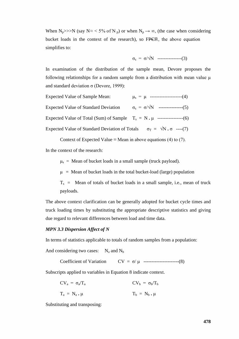
478
When Np>>>N (say N ≈ < 5% of N p) or when Np → ∞, (the case when considering
bucket loads in the context of the research), so FPCF → 1, the above equation
simplifies to:
σs = σ/√N ---------------(3)
In examination of the distribution of the sample mean, Devore proposes the
following relationships for a random sample from a distribution with mean value μ
and standard deviation σ (Devore, 1999):
Expected Value of Sample Mean: μs = μ --------------------(4)
Expected Value of Standard Deviation σs = σ/√N ---------------(5)
Expected Value of Total (Sum) of Sample Ts = N . μ ----------------(6)
Expected Value of Standard Deviation of Totals σT = √N . σ ----(7)
Context of Expected Value ≡ Mean in above equations (4) to (7).
In the context of the research:
μs = Mean of bucket loads in a small sample (truck payload).
μ = Mean of bucket loads in the total bucket-load (large) population
Ts = Mean of totals of bucket loads in a small sample, i.e., mean of truck
payloads.
The above context clarification can be generally adopted for bucket cycle times and
truck loading times by substituting the appropriate descriptive statistics and giving
due regard to relevant differences between load and time data.
MPN 3.3 Dispersion Affect of N
In terms of statistics applicable to totals of random samples from a population:
And considering two cases: Na and Nb
Coefficient of Variation CV = σ/ μ ----------------------(8)
Subscripts applied to variables in Equation 8 indicate context.
CVa = σa/Ta CVb = σb/Tb
Ta = Na . μ Tb = Nb . μ
Substituting and transposing:
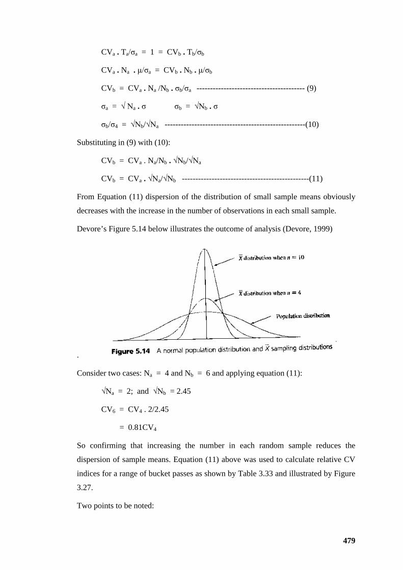
479
CVa . Ta/σa = 1 = CVb . Tb/σb
CVa . Na . μ/σa = CVb . Nb . μ/σb
CVb = CVa . Na /Nb . σb/σa ---------------------------------------- (9)
σa = √ Na . σ σb = √Nb . σ
σb/σ4 = √Nb/√Na ----------------------------------------------------(10)
Substituting in (9) with (10):
CVb = CVa . Na/Nb . √Nb/√Na
CVb = CVa . √Na/√Nb -----------------------------------------------(11)
From Equation (11) dispersion of the distribution of small sample means obviously
decreases with the increase in the number of observations in each small sample.
Devore’s Figure 5.14 below illustrates the outcome of analysis (Devore, 1999)
.
Consider two cases: Na = 4 and Nb = 6 and applying equation (11):
√Na = 2; and √Nb = 2.45
CV6 = CV4 . 2/2.45
= 0.81CV4
So confirming that increasing the number in each random sample reduces the
dispersion of sample means. Equation (11) above was used to calculate relative CV
indices for a range of bucket passes as shown by Table 3.33 and illustrated by Figure
3.27.
Two points to be noted:
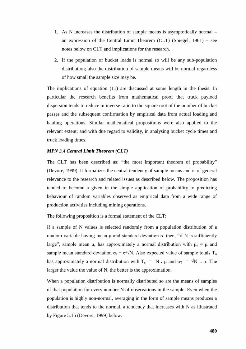
480
1. As N increases the distribution of sample means is asymptotically normal –
an expression of the Central Limit Theorem (CLT) (Spiegel, 1961) – see
notes below on CLT and implications for the research.
2. If the population of bucket loads is normal so will be any sub-population
distribution; also the distribution of sample means will be normal regardless
of how small the sample size may be.
The implications of equation (11) are discussed at some length in the thesis. In
particular the research benefits from mathematical proof that truck payload
dispersion tends to reduce in inverse ratio to the square root of the number of bucket
passes and the subsequent confirmation by empirical data from actual loading and
hauling operations. Similar mathematical propositions were also applied to the
relevant extent; and with due regard to validity, in analysing bucket cycle times and
truck loading times.
MPN 3.4 Central Limit Theorem (CLT)
The CLT has been described as: “the most important theorem of probability”
(Devore, 1999). It formalizes the central tendency of sample means and is of general
relevance to the research and related issues as described below. The proposition has
tended to become a given in the simple application of probability to predicting
behaviour of random variables observed as empirical data from a wide range of
production activities including mining operations.
The following proposition is a formal statement of the CLT:
If a sample of N values is selected randomly from a population distribution of a
random variable having mean μ and standard deviation σ, then, “if N is sufficiently
large”, sample mean μs has approximately a normal distribution with μs = μ and
sample mean standard deviation σs = σ/√N. Also expected value of sample totals To
has approximately a normal distribution with Ts = N . μ and σT = √N . σ. The
larger the value the value of N, the better is the approximation.
When a population distribution is normally distributed so are the means of samples
of that population for every number N of observations in the sample. Even when the
population is highly non-normal, averaging in the form of sample means produces a
distribution that tends to the normal, a tendency that increases with N as illustrated
by Figure 5.15 (Devore, 1999) below.
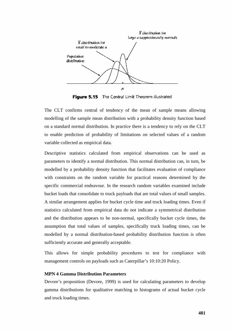
481
The CLT confirms central of tendency of the mean of sample means allowing
modelling of the sample mean distribution with a probability density function based
on a standard normal distribution. In practice there is a tendency to rely on the CLT
to enable prediction of probability of limitations on selected values of a random
variable collected as empirical data.
Descriptive statistics calculated from empirical observations can be used as
parameters to identify a normal distribution. This normal distribution can, in turn, be
modelled by a probability density function that facilitates evaluation of compliance
with constraints on the random variable for practical reasons determined by the
specific commercial endeavour. In the research random variables examined include
bucket loads that consolidate to truck payloads that are total values of small samples.
A similar arrangement applies for bucket cycle time and truck loading times. Even if
statistics calculated from empirical data do not indicate a symmetrical distribution
and the distribution appears to be non-normal, specifically bucket cycle times, the
assumption that total values of samples, specifically truck loading times, can be
modelled by a normal distribution-based probability distribution function is often
sufficiently accurate and generally acceptable.
This allows for simple probability procedures to test for compliance with
management controls on payloads such as Caterpillar’s 10:10:20 Policy.
MPN 4 Gamma Distribution Parameters Devore’s proposition (Devore, 1999) is used for calculating parameters to develop
gamma distributions for qualitative matching to histograms of actual bucket cycle
and truck loading times.
482
Expected value: E(X) = μ = α . β -----------------------------(1)
Variation: V(X) = σ2 = α . β2 so σ = √α . β --(2)
Transposing and using CV = σ / μ
α = 1 / CV2 -----------------------------------(3)
β = μ . CV2 -----------------------------------(4)
μ = mean
σ2 = variance
σ = standard deviation
CV = Coefficient of variation
α =. Gamma distribution scale parameter
β = Gamma distribution shape parameter
Parameter values, calculated using the above equations, and summarized in Table
3.32, were used to develope the gamma distribution frequency curves for qualitative
comparison in Figures 3.18, 3.19, 3.24 and 3.25.
MPN 5 “Mode” – A Suitable Measure of Central Tendency for Cycle Times Comparing measures of central tendency at both Filter Level 2 (refer to thesis text
for clarification) – Figures 3.16 and 3.17, - and Filter Level 3 (refer to thesis text for
clarification) – Figures 3.22 and 3.23, over the 5-pass to 7-pass range indicated that:
• At Filter Level 2, as expected for positively skewed distributions, the general
relationship between central tendency measures of average range > mean >
median > mode are generally in compliance with the empirical equation:
Mode = Mean – 3 . (Mean-Median) ……. (Chou, 1969)
Transposing: Mean – Mode = 3 . (Mean – Median)…………….(3)
Equation (3) was applied to test consistency of measures of central tendency.
• At Filter Level 3, as expected, the effect of filtering has centralized the
residual data but, generally, each measure of central tendency retains its
hierarchical position. The small overlap in Figure 3.23, where the mode falls
483
inside the median value for the 6-pass sub-sample of truck loading times, is
believed to be due to the effect of hypothetical filtering smoothing data to a bi
or multi-modal state.
• Modal values for continuous random distributions are a “simple and useful
concept” (Chou, 1969) but of doubtful reliability, but may be positively
influenced by:
Sample size.
Rounding method to whole numbers.
Frequency interval. (Chou, 1969)
Most of these reliability impediments are removed “in whole or part when
data is arranged in a frequency distribution” and the mode is determined from
“the frequency distribution of the same data” (Chou, 1969). These are the
circumstances for treatment of data samples and mode determination herein.
• Intuitively mode should not be significantly affected by filtering. Filter Level
1, Filter Level 2 and Filter Level 3, for the reasons described earlier in this
section, all aimed to remove outlying values that will not affect modal values.
So constant modal values were expected across filtering levels. Non-
compliance with this expectancy triggered investigation and determination of
the reasons.
• Table 3.28, summarises all of the measures of central tendency and dispersion
at each of the levels of filtering. It is noted that:
For bucket cycle times, mode values are generally consistent through the
filter levels and only exhibit small variability through the range of all
passes and 5, 6 and 7 passes.
Mode values for first passes including exchange time, a relatively
smaller data set, are consistent through the filter levels for all passes but
the sub-samples of 5, 6 and 7 passes indicate a tendency for unreliability.
Truck loading times, also a smaller data set, exhibited some anomalous
mode values through the range of filter levels.
484
Expected values, means, of bucket cycle times, first passes including
exchange time and bucket cycle times all exhibit sensitivity to filtering
level, i.e., to outlying values that filtering aims to remove. This leads to
the conclusion that mean values are not a reliable measure of central
tendency for predicting expected values of bucket cycle times and truck
loading times. The mean as an applicable measure of central tendency in
all cases suffers from its sensitivity to outlying high or low values
(Devore, 1999).
In the case of bucket cycle and truck loading times, comparison of mean
and mode provides a measure of the effect of time lost to events or
activities that are non-intrinsic to, or symptoms of inefficiency of,
loading operations.
• It is noted that, at Filter Level 3, for all loading times, the mode of 199
seconds appears anomalously high. Data for all truck loading times was
tabulated as a frequency distribution in one-second and five-second intervals
as shown in Table 3.30. At one-second frequency intervals two modes of 7
records manifest at 193 and 199 seconds. Two sub-modes of 6 records
manifest at 168 and 178 seconds. This raises the possibility that for larger
samples of data with tendency to statistical regularity (Harr, 1977) a single
mode could manifest at 168, 178, 193, or 199 or perhaps (but unlikely) at
some other value. In such circumstances there is no logical basis for selecting
one modal value in preference to another. (Chou 1969,). Accumulating to
five-second frequency intervals a single mode (21 records) manifests at the
191 –195 second interval. As mode is the most frequent value observed it
adopts the designation of the frequency interval – in this case, say, mid value
192.5. It is concluded that a larger sample of data would more likely have
promoted 193 seconds as the mode at one-second frequency intervals. This
modal value was adopted as an alternative. These observations at
hypothetical Filter Level 3 collectively evidence that modal values can be
unstable and so unreliable for relatively small data samples.
• The inconsistent mode value for all truck loading times at Filter Level 3
outlined above, as a result of selection of a single mode in a multi-mode
distribution by the Excel spreadsheet statistical MODE function, triggered
485
further comprehensive review of modal values for bucket cycle time and
truck loading time similar to the analysis for all truck loading times at Filter
Level 3 shown in Table 3.30.
• Intuitively modal values will become less reliable as the data sample numbers
decrease with multi-modal distributions resulting. Multiple appearances of
observations in the same frequency interval of a continuous random
distribution decrease towards 0 as sample size reduces. So modal values of
bucket cycle times for all passes or passes less the first appear to be
comparatively more reliable than any sub-group of the total data sample such
as first passes including truck exchange time and truck loading time
particularly when the total data sample is sub-grouped into 5, 6 and 7 passes.
For example at Filter Level 3 there is a total of 1,070 bucket cycle times, 188
first pass and truck loading times, 57, 5-pass loads, 96, 6-pass loads and only
23, 7-pass loads.
• Analysis of modal values for truck loading times at Filter level 3 indicated an
alternative mode of 193 seconds for all truckloads; and at 7 passes three mode
values were identified at 207, 211, and 231 seconds. The computed mode of
207 seconds was retained. Review at 5 and 6 passes confirmed the computed
modes for truck loading times.
• Analysis of first passes including exchange time at Filter Level 3, confirmed
computed modes at all passes and 6 passes (where three modes at 42, 43 and
44 were identified), but indicated alternatives of 40 seconds at 5 passes and
44 seconds at 7 passes.
• Truck loading times at Filter Level 2 were analysed for multiple modes
confirming computed modes for all passes and 5 passes and indicating an
alternatives of 193 seconds at 6 passes for the computed 198 seconds. At 7
passes multiple modes of 203, 207,211, 220, 231, 244, 283 and 304 seconds
manifested – a result of the small sub-sample number of observations.
Widening frequency intervals to 5 seconds and 10 seconds still produced
multiple modes. For the purposes of the analysis an alternative of 207
seconds at 7 passes was adopted.
486
• Analysis of first passes including exchange time at Filter Level 2, confirmed
computed modes at all passes and 6 passes, but indicated alternatives of 40
seconds at 5 passes and 44 seconds at 7 passes.
• Generally for examination of multi-modal frequency distributions, frequency
interval was increased from one to five, to ten and to twenty seconds as a
basis for interpolating mode (Chou, 1969).
• Anomalous modal values in Table 3.28 were replaced with alternative values
as shown in Table 3.29. It will be noted that the alternative values generally
comply with the hierarchical order of measures of central tendency, i.e., mean
> median > mode and correlation with the empirical ratio (mean-median) :
(mean – mode) = 1 : 3.
Review of Tables 3.28 and 3.29 indicates the apparent stability of mode through the
filter levels for all bucket cycle times and cycle times nett of the first pass. Modal
values are generally minimum values of comparable measures of central tendency in
compliance with the hierarchical order for positively skewed distributions of mean >
median > mode. There is a notable exception at Filter Level 3 for all loading times
where the hypothetical level of filtering has overly modified the data to create a
negatively (to left) skewed distribution for all truck loading times – an artificial and
impractical distribution outcome.
Figure 3.24, for bucket cycle times, qualitatively illustrates the centralizing effect of
Filter Level 3. The histogram of empirical bucket cycle time data compared with
normal and gamma distribution models is positively skewed (to the right), albeit
modestly. Distribution of truck loading data at Filter Level 3 is qualitatively
illustrated by Figure 3.25 - also compared with normal and gamma distribution
models. In the case of truck loading times at Filter level 3 the distribution is modestly
negatively skewed (to the left)
Figure 3.25 qualitatively indicates that the hypothetical distribution is approximately
symmetrical and likely can be modelled by a normal distribution. This is verified by
Kolmogorov-Smirnov (K-S) non-parametric testing (see K-S output cross referenced
to Figure 3.25:- in Distribution Testing – Kolmogorov–Smirnov Testing in this
Volume). This outcome is considered purely hypothetical and considered of little
practical importance because of the artificially high level of filtering. It is most
487
unlikely that a distribution of empirical data from the most efficient operation where
there is insignificant extraneous time losses in loading operations would be
negatively skewed.
MPN 6 Skewness of Distributions of Bucket Cycle & Truck Loading Times The validity of mode as a measure for bucket cycle time and truck loading time has
been discussed in Section 3.2.9 in the thesis text and in MPN 5 above. The natural
positive skew of bucket cycle time and loading time distributions has also been
discussed. Qualitatively from the several histograms included in Illustrations the
positive skew is moderate to subtle for truck loading times and generally more
pronounced for bucket cycle times.
Criteria for assessing skewness as high, moderate or mild were derived using
Pearson’s First Coefficient of Skewness (Chou, 1969).
Skp = (Mean – Mode) / σ ……………..(4)
Skp = Pearson’s First Coefficient of Skewness
As Mode is only an approximation and, in general, is the least stable of the central
tendency measures, a median-based coefficient, Pearson’s Second Coefficient of
Skewness, may be substituted (particularly applicable for moderately skewed
distributions).
Skp = 3 . (Mean – Median) / σ ……………..(5)
Equation (5) above results from substituting for Mode in equation (4) with:
Mode = Mean – 3(Mean – Median) – see MPN 5 above.
For symmetric, normal, distributions:
Mean = Median = Mode so
Skp = 0
Skp range = +/- 3 theoretically. But practically Skp range rarely exceeds +/- 1
(Chou, 1969)
It should be noted that skewness coefficients developed in Tables 3.24 and 3.25, and
in other tables throughout this thesis are developed from data samples by the
Microsoft Excel application. Excel uses a version of skewness measure based on the
488
third moment of each data point from the mean divided by the standard deviation to
produce a dimensionless skewness coefficient.
Included in Tables 3.24 are Pearson Second Coefficients of Skewness (PSC) based
on Median values that are generally lower than skewness measures from the Excel
version.
Based on Chou’s practical range limits of +/- 1 for Skp as described above, the
following criteria were adopted for PSC:
High Skewness >0.6
Moderate Skewness =/<0.6>0.3
Mild Skewness =/<0.3
It will be noted that Skp values at Filter level 2 from Table 3.24:
• For Truck Loading Times:
All Passes and the 5 Pass sub-sample are indicated in the moderate range; and
6 pass and 7 pass sub-sample are indicated to be towards the lower margin of
the high range.
• For Bucket Cycle Times:
Generally all sub samples of data are in the high range.
At Filter Level 3, Skp values from Table 3.25:
• For Truck Loading Times:
All Passes, 5 Pass and 6 Pass sub- samples are in the moderate to mild range
and the 7 Pass sub-sample is at the lower margin of the high range.
• For Bucket Cycle Times:
There is a general tendency for reduction from the high skewness range to the
moderate range as passes increase.
In conclusion (refer Tables 3.24 and 3.25):
• Degree of skewness is a measure of distribution asymmetry. A tendency
towards distribution symmetry will be accompanied by a reduction in the
degree of skewness.
489
• Following on from the concept of Mode as a performance and control criteria
for bucket cycle ant truck loading times, and the discussion on reliability of
mode values the concept of skewness as an alternative improvement measure
was considered.
• Expected reduction of skewness from Filter Level 2 to Filter Level 3 was
positive for truck loading times based on all bucket cycle time data; but for
sub-samples at selected pass numbers the tendency for reduction was positive
but with negative anomalies.
• Similar results were noted for the Skewness measure used by Microsoft
Excel.
• In view of the anomalies and the limited statistical evidence it can only be
hypothesized, at this stage, that coefficients of skewness have potential to
provided a measure of improvement and control.
• More evidence is required from more tests with larger data samples to firm up
and elevate the hypothesis to a practical protocol.
MPN 7 Parameters for Gamma Distributions As stated in Section 3.2.9, parameters α and β - derived for modelling gamma
distributions for comparison with actual frequency distributions, using the
proposition μ = αβ and σ2 = αβ2 (Devore, 1999) - were both relatively high numbers.
This is consistent with generation of a distribution model tending away from the
asymmetric towards a symmetric, normal distribution; particularly as the level of
filtering increased. This tendency has already been discussed in empirical terms
above.
Table 3.32 summarises the α and β values derived and used for gamma distribution
models applied in relevant histograms shown in Figures 3.18, 3.19, 3.24 and 3.25.
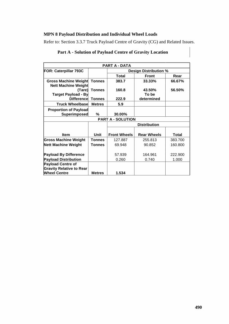
490
MPN 8 Payload Distribution and Individual Wheel Loads Refer to: Section 3.3.7 Truck Payload Centre of Gravity (CG) and Related Issues.
Part A - Solution of Payload Centre of Gravity Location
PART A - DATA
FOR: Caterpillar 793C Design Distribution % Total Front Rear
Gross Machine Weight Tonnes 383.7 33.33% 66.67% Nett Machine Weight
(Tare) Tonnes 160.8 43.50% 56.50% Target Payload - By
Difference Tonnes 222.9 To be
determined Truck Wheelbase Metres 5.9
Proportion of Payload Superimposed % 30.00%
PART A - SOLUTION Distribution
Item Unit Front Wheels Rear Wheels Total Gross Machine Weight Tonnes 127.887 255.813 383.700 Nett Machine Weight Tonnes 69.948 90.852 160.800 Payload By Difference 57.939 164.961 222.900 Payload Distribution 0.260 0.740 1.000 Payload Centre of Gravity Relative to Rear Wheel Centre Metres 1.534
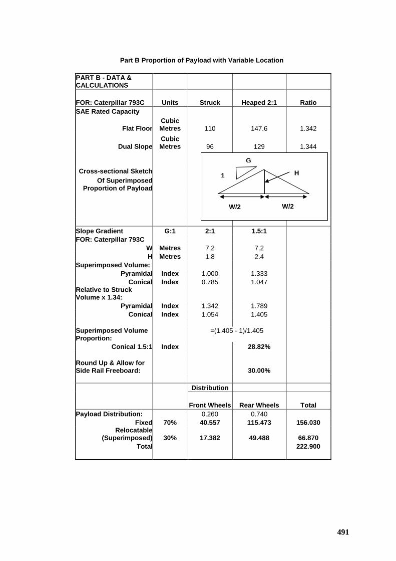
491
Part B Proportion of Payload with Variable Location
PART B - DATA & CALCULATIONS
FOR: Caterpillar 793C Units Struck Heaped 2:1 Ratio SAE Rated Capacity
Flat Floor Cubic Metres 110 147.6 1.342
Dual Slope Cubic Metres 96 129 1.344
Cross-sectional Sketch
Of Superimposed Proportion of Payload
Slope Gradient G:1 2:1 1.5:1 FOR: Caterpillar 793C
W Metres 7.2 7.2 H Metres 1.8 2.4
Superimposed Volume: Pyramidal Index 1.000 1.333
Conical Index 0.785 1.047 Relative to Struck Volume x 1.34:
Pyramidal Index 1.342 1.789 Conical Index 1.054 1.405
Superimposed Volume Proportion:
=(1.405 - 1)/1.405
Conical 1.5:1 Index 28.82%
Round Up & Allow for Side Rail Freeboard: 30.00% Distribution
Front Wheels Rear Wheels Total Payload Distribution: 0.260 0.740
Fixed 70% 40.557 115.473 156.030 Relocatable
(Superimposed) 30% 17.382 49.488 66.870 Total 222.900
H
W/2 W/2
1
G
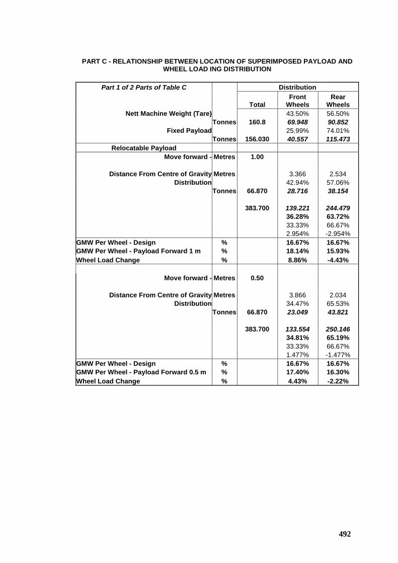
492
PART C - RELATIONSHIP BETWEEN LOCATION OF SUPERIMPOSED PAYLOAD AND
WHEEL LOAD ING DISTRIBUTION
Part 1 of 2 Parts of Table C Distribution
Total Front
Wheels Rear
Wheels Nett Machine Weight (Tare) 43.50% 56.50%
Tonnes 160.8 69.948 90.852 Fixed Payload 25.99% 74.01%
Tonnes 156.030 40.557 115.473 Relocatable Payload
Move forward - Metres 1.00
Distance From Centre of Gravity Metres 3.366 2.534 Distribution 42.94% 57.06%
Tonnes 66.870 28.716 38.154 383.700 139.221 244.479 36.28% 63.72% 33.33% 66.67% 2.954% -2.954% GMW Per Wheel - Design % 16.67% 16.67% GMW Per Wheel - Payload Forward 1 m % 18.14% 15.93% Wheel Load Change % 8.86% -4.43%
Move forward - Metres 0.50
Distance From Centre of Gravity Metres 3.866 2.034 Distribution 34.47% 65.53%
Tonnes 66.870 23.049 43.821 383.700 133.554 250.146 34.81% 65.19% 33.33% 66.67% 1.477% -1.477% GMW Per Wheel - Design % 16.67% 16.67% GMW Per Wheel - Payload Forward 0.5 m % 17.40% 16.30% Wheel Load Change % 4.43% -2.22%
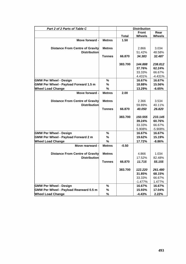
493
Part 2 of 2 Parts of Table C Distribution
Total Front
Wheels Rear
Wheels Move forward - Metres 1.50
Distance From Centre of Gravity Metres 2.866 3.034
Distribution 51.42% 48.58% Tonnes 66.870 34.383 32.487 383.700 144.888 238.812 37.76% 62.24% 33.33% 66.67% 4.431% -4.431% GMW Per Wheel - Design % 16.67% 16.67% GMW Per Wheel - Payload Forward 1.5 m % 18.88% 15.56% Wheel Load Change % 13.29% -6.65%
Move forward - Metres 2.00
Distance From Centre of Gravity Metres 2.366 3.534 Distribution 59.89% 40.11%
Tonnes 66.870 40.050 26.820 383.700 150.555 233.145 39.24% 60.76% 33.33% 66.67% 5.908% -5.908% GMW Per Wheel - Design % 16.67% 16.67% GMW Per Wheel - Payload Forward 2 m % 19.62% 15.19% Wheel Load Change % 17.72% -8.86%
Move rearward - Metres -0.50
Distance From Centre of Gravity Metres 4.866 1.034 Distribution 17.52% 82.48%
Tonnes 66.870 11.715 55.155 383.700 122.220 261.480 31.85% 68.15% 33.33% 66.67% -1.477% 1.477% GMW Per Wheel - Design % 16.67% 16.67% GMW Per Wheel - Payload Rearward 0.5 m % 15.93% 17.04% Wheel Load Change % -4.43% 2.22%
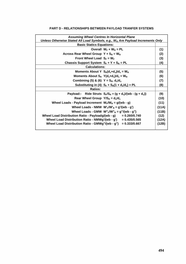
494
PART D - RELATIONSHIPS BETWEEN PAYLOAD TRANFER SYSTEMS
Assuming Wheel Centres In Horizontal Plane
Unless Otherwise Stated All Load Symbols, e.g., WR, Are Payload Increments Only Basic Statics Equations:
Overall WF + WR = PL (1) Across Rear Wheel Group Y + SR = WR (2)
Front Wheel Load SF = WF (3) Chassis Support System SF + Y + SR = PL (4)
Calculations: Moments About Y SR(dy+ds)/dy = WR (5)
Moments About SR Y(dy+ds)/ds = WR (6) Combining (5) & (6) Y = SR. ds/dy (7)
Substituting in (4) SF + SR(1 + ds/dy) = PL (8) Ratios:
Payload:- Ride Struts SF/SR = (g + ds)/{wb - (g + ds)} (9) Rear Wheel Group Y/SR = ds/dy (10)
Wheel Loads - Payload Increment WF/WR = g/(wb - g) (11) Wheel Loads - NMW W'F/W'R = g'/(wb - g') (11A) Wheel Loads - GMW W"F/W"R = g"/(wb - g") (11B)
Wheel Load Distribution Ratio - Payload g/(wb - g) = 0.260/0.740 (12) Wheel Load Distribution Ratio - NMW g'/(wb - g') = 0.435/0.565 (12A) Wheel Load Distribution Ratio - GMW g"/(wb - g") = 0.333/0.667 (12B)
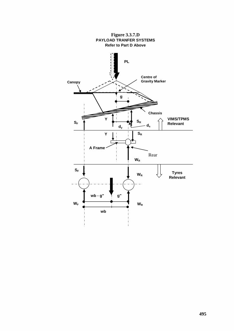
495
Figure 3.3.7.D PAYLOAD TRANFER SYSTEMS
Refer to Part D Above
SR SF Y
SR Y
WR
WR
WR
SF
WF
PL
Chassis
Canopy Centre of Gravity Marker
A Frame Rear
wb
dy ds
g
VIMS/TPMS Relevant
Tyres Relevant
g" wb - g"
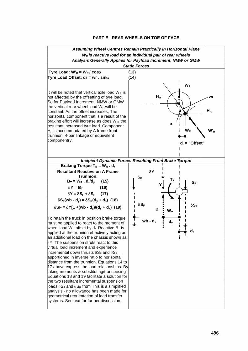
496
PART E - REAR WHEELS ON TOE OF FACE
Assuming Wheel Centres Remain Practically In Horizontal Plane
WR is reactive load for an individual pair of rear wheels Analysis Generally Applies for Payload Increment, NMW or GMW
Static Forces Tyre Load: W'R = WR / cosα (13) Tyre Load Offset: dr = wr . sinα (14)
It will be noted that vertical axle load WR is not affected by the offsetting of tyre load. So for Payload Increment, NMW or GMW the vertical rear wheel load WR will be constant. As the offset increases, The horizontal component that is a result of the braking effort will increase as does W'R the resultant increased tyre load. Component HR is accommodated by A frame front trunnion, 4-bar linkage or equivalent componentry.
Incipient Dynamic Forces Resulting From Brake Torque Braking Torque TB = WR . dr
Resultant Reactive on A Frame Trunnion:
BT = WR . dr/dy (15) δY = BT (16) δY = δSF + δSR (17)
δSF(wb - dy) = δSR(dy + ds) (18) δSF = δY[1 +(wb - dy)/(dy + ds) (19)
To retain the truck in position brake torque must be applied to react to the moment of wheel load WR offset by dr. Reactive BT is applied at the trunnion effectively acting as an additional load on the chassis shown as δY. The suspension struts react to this virtual load increment and experience incremental down thrusts δSF and δSR apportioned in inverse ratio to horizontal distance from the trunnion. Equations 14 to 17 above express the load relationships. By taking moments & substituting/transposing Equations 18 and 19 facilitate a solution for the two resultant incremental suspension loads δSF and δSR from This is a simplified analysis - no allowance has been made for geometrical reorientation of load transfer systems. See text for further discussion.
WR
WR
HR
HR
W'R
wr
dr = "Offset"
α
SR Y
WR
TB
δSF
SF
B
δSR
δY
dy
ds
wb - dy
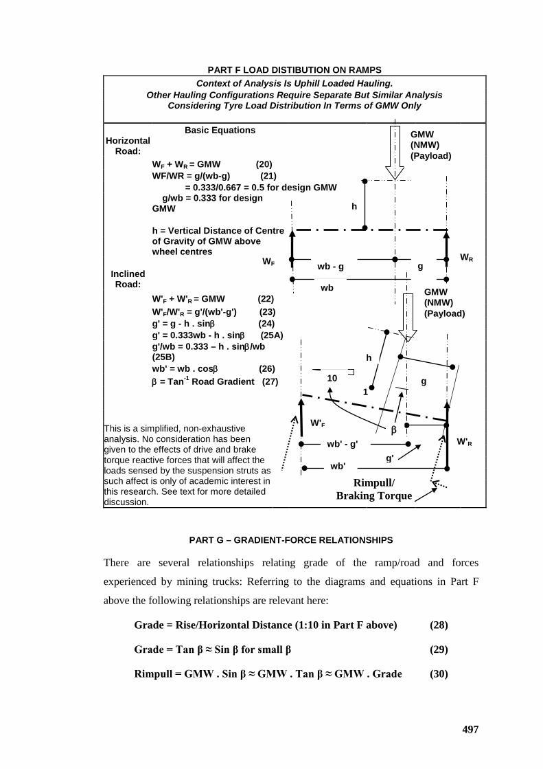
497
PART F LOAD DISTIBUTION ON RAMPS Context of Analysis Is Uphill Loaded Hauling.
Other Hauling Configurations Require Separate But Similar Analysis Considering Tyre Load Distribution In Terms of GMW Only
Basic Equations Horizontal
Road: WF + WR = GMW (20) WF/WR = g/(wb-g) (21) = 0.333/0.667 = 0.5 for design GMW
g/wb = 0.333 for design GMW
h = Vertical Distance of Centre
of Gravity of GMW above wheel centres
Inclined Road:
W'F + W'R = GMW (22) W'F/W'R = g'/(wb'-g') (23) g' = g - h . sinβ (24) g' = 0.333wb - h . sinβ (25A)
g'/wb = 0.333 – h . sinβ/wb (25B)
wb' = wb . cosβ (26) β = Tan-1 Road Gradient (27)
This is a simplified, non-exhaustive analysis. No consideration has been given to the effects of drive and brake torque reactive forces that will affect the loads sensed by the suspension struts as such affect is only of academic interest in this research. See text for more detailed discussion.
PART G – GRADIENT-FORCE RELATIONSHIPS
There are several relationships relating grade of the ramp/road and forces
experienced by mining trucks: Referring to the diagrams and equations in Part F
above the following relationships are relevant here:
Grade = Rise/Horizontal Distance (1:10 in Part F above) (28)
Grade = Tan β ≈ Sin β for small β (29)
Rimpull = GMW . Sin β ≈ GMW . Tan β ≈ GMW . Grade (30)
1 10
h
wb - g
wb
g
g
h
GMW (NMW) (Payload)
GMW (NMW) (Payload)
WF WR
wb' g'
wb' - g'
W'F
W'R β
Rimpull/ Braking Torque
498
For a practical maximum “effective grade” (‘effective grade” interpreted below) of,
say, 18% (15% +3% rolling resistance), necessarily of limited distance:
Equation (30) above: Rimpull ≈ 0.18 . GMW
Above is overstated by: Tan β /Sin β = 0.18/0.1771 = 1.016
That is +1.6% - conservative - error.
It should be noted that rimpull is sensitive to “Effective Grade” (including rolling
resistance) – sometimes termed “Total Resistance” (Caterpillar PHB 35, 2004)
Ramps and roads with lesser grades will have reduced errors. For practical purposes,
estimating rimpull by applying grade to GMW is reasonable.
It should be noted that ride struts rotate in space by the same angle as the grade of the
ramp or road. Accordingly the ride struts will measure a component of the vertical
loads normally carried, viz.,
Strut load on ramp = normal strut load. Cos β (31)
For 15% Grade: Ride Strut Loads = Normal loads . 0.989
That is an effective reduction of 1.1%.
Load measuring using ride strut pressures is not relevant on ramps so the above has
little, if any, practical utility.
“Effective Grade ≡Total Resistance”: In addition to the resistance or propulsive
effects of road surface grade there are other elements of resistance that can
conveniently be combined with geometrical grade as “effective grade”. There is an
inherent resistance to rolling of pneumatic tyres on a perfectly flat non-yielding
surface that depends on the internal tyre structure and tyre pressure. Tyre rolling
resistance for mining trucks is in the order of 1.0% to 2.5 % of GMW depending on
the number of wheels and tyre construction. With fabric-reinforced, bias-ply tyres
practically history, having been essentially replaced by steel-reinforced radial-ply
tyres, the current practical range is generally 1.0% to 1.5% for conventional six-
wheel mining trucks (Caterpillar PHB 35. 2004).
499
MPN 9. Bucket Passes and Payloads
Refer to Section 3.3.9 Bucket Passes and Payloads - Productivity and Sacrificing
Passes.
Assuming there is always a truck waiting to be loaded, bucket loads in excess of
planned passes effectively delays all subsequent trucks by a cycle time for each
additional pass.
On each occasion, sacrificing a bucket pass or passes saves time as follows:
TTS = TB . nS . NT (1)
TTS = Trucking time saved – seconds
TB = Bucket cycle time - seconds
nS = Number of passes sacrificed, equivalent to number of occasions
NT = Number of trucks affected
Extra payload proportion represented by time saved per occasion:
PLX = TB . nS . NT / TT (1A)
PLX = Extra payload(s)
TT = Truck trip time – seconds.
Payload proportion lost by sacrificing a bucket pass:
PLL = 1 . FF / MP for one pass sacrifice (2)
PLL = nS . FF / MP generally (2A)
PLL = Payload proportion lost by sacrificing a bucket pass.
FF = Fill discount factor for the sacrificed bucket pass or mean over passes
sacrificed.
MP = Mean number of passes for target payload
In terms of productivity, the test for sacrifice of a bucket pass is:
PLX ≥ PLL (3)
The above equations 1A, 2A and relationship 3 are the basis for Table 3.57. The
above analysis and Table 3.57 are limited to a single pass sacrifice. Multiple pass
sacrifice is a relatively minor complication. Equations (1) and (1A) can be applied
generally for sacrificed passes. Equation (2) is modified to (2A) to be generally
applicable and FF is then the mean bucket fill over the passes sacrificed. The
500
spreadsheet containing Table 3.57 can accommodate multiple passes by an optional
selection for number of passes. This can be verified by review of the copy of the file
on the CD inside the back cover of the thesis.
It should be noted that the above analysis is in terms of productivity alone. Relevant
cost implications have been considered and analyzed in Section 5.4.3, to this stage of
analysis.
501
DISTRIBUTION TESTING
KOLMOGOROV – SMIRNOV NON-PARAMETRIC TESTING
P-P PLOTS
Q-Q PLOTS
Includes Table of Contents
502
TABLE OF CONTENTS - DISTRIBUTION TESTING Table of Contents…………………………………………………………… 502
KS 1 Introduction…………………………………………………………… 503
KS 2 Distributions and Tests………………………………………………... 503
KS 3 Kolmogorov - Smirnov Non-parametric Tests……………………….. 506
KS 4 Probability Plots……………………………………………………… 514
KS 5 Quantile–Quantile Plots……………………………………………… 514
KS 6 Summary of K – S Test results, Pplots, Qplots and Interpretation….. 516
Figure 3.2 and Table 3.7…………………………………………………… 521
Figure 3.2A and Table 3.10………………………………………………... 524
Figure 3.3 and Table 3.12………………………………………………….. 526
Figure 3.4 and Table 3.12………………………………………………….. 528
Figure 3.5 and Table 3.12………………………………………………….. 530
Figure 3.6 and Table 3.14………………………………………………….. 534
Figure 3.7 and Table 3.15………………………………………………….. 536
Figure 3.8 and Table 3.16………………………………………………….. 538
Figure 3.9 and Table 3.17………………………………………………….. 540
Figure 3.12 and Table 3.20………………………………………………… 542
Figure 3.18 and Table 3.24………………………………………………… 545
Figure 3.19 and Table 3.24………………………………………………… 548
Figure 3.24 and Table 3.25………………………………………………… 552
Figure 3.25 and Table 3.25………………………………………………… 555
Table 3.53………………………………………………………………….. 557
503
KOLMOGOROV – SMIRNOV (K-S) NON-PARAMETRIC DISTRIBUTION TESTING
KS 1 INTRODUCTION
Historical and current production and cost records; also current industry-wide
experience are a source of data to be used as a basis, generally for inference and
specifically, for pre-selection analysis during all levels of feasibility from
preliminary to final. The value of historical and current data records continues
through procurement investigation and due diligence activity to arrive at a decision
to issue orders or execute supply contracts for initiating or continuing commercial
mining operations.
These notes are provided as support for the general investigative process used in the
course of the research and described by this thesis. Some inferences drawn and
hypotheses on behaviour of some critical productivity and cost criteria based on
statistical analysis are validated by observation of events, i.e. empirical data, from
actual mining operations.
KS 2 DISTRIBUTIONS AND TESTS
Events recorded as empirical data from open-pit mining activities are most often
continuous (e.g., bucket loads and truck payloads; bucket cycles and truck loading
time, truck travel time including variable dump time) or discrete (e.g., bucket passes
per truck load, truck loads per unit of time). The noted sources of data are random
variables.
In the broadest sense investigation and analysis, especially in the process of
establishing the services required from a load and haul fleet for an open-pit mining
operation, can be viewed generically as a simulation process. “A simulation is the
imitation of the operation of a real-world process or system over time. Whether done
by hand or on a computer, simulation involves the generation of an artificial history
of a system, and the observation of that artificial history to draw inferences
concerning the operating characteristics of the real system.”(Banks J, 1996)
The behaviour of a system is studied:
• By developing a simulation model – usually in the form of assumption(s)
regarding operation of the system.
504
• Assumption(s) are expressed in mathematical, logical, symbolic relationships
between the objects of interest.
• Once developed and validated a model can be utilised to examine any “what-
if” queries about the real-world system.
• Simulation models can be used both for analysis of existing systems and for
design, prediction of performance of new systems. (Banks J, 1996, p3)
Utilisation of simulation models varies from the simplest application of mathematical
processes to the highly complex where mathematical analysis is difficult if not
possible. Techniques applied range from:
• Traditional simple methods of hand-worked estimating using deterministic
methods through;
• Linear programming, multiple regression and complex; but well-developed,
relatively complex, mathematical methods to;
• Imitation of the behaviour of the system using numerical, computer-based
simulation.
Recent common usage of the term “simulation” has tended to confine it to the more
complex numerical computer-facilitated analytical processes. But, in the broadest
sense, all estimating processes infer adoption of a model that, when analysed, is
predictable and provides repeatable outcomes. But all of these processes are
estimating and any model chosen to represent a real system is an estimate of the form
and characteristics of the real system.
All analysis from the simplest deterministic to the complex simulation requires input
of relevant operating criteria and general understanding of the interrelationship
between component functions that make up the system. Investigation of some of the
applicable criteria and understanding of interrelationships was a primary objective of
the research.
As described herein the approach was to examine data from actual operations,
whether from continuous or discrete variables, to estimate a range of descriptive
statistics including:
505
• Maximum and minimum values - from which the range and mean of the
range were derived – as first indicative measures of dispersion and symmetry.
• Arithmetic Mean – as the principle measure of central tendency.
• Median and Mode – as secondary measures of central tendency; and with the
mean as joint indicators of symmetry.
• Variance – produced but not utilised.
• Standard Deviation – as an important measure of dispersion.
• Coefficient of Variation derived from Standard Deviation / Mean –an
important dimensionless measure of dispersion allowing comparison of actual
data dispersion with other similar operating activities.
• Skewness and Kurtosis - as measures of central tendency and distribution
“shape”.
Descriptive statistics of principal interest in the research are shown in bold.
The listed descriptive statistics provided impressions of symmetry, degree of
dispersion and skewness inferring, in many cases, a suitable model distribution. For
example:
• Tendency to symmetry, low dispersion and low skewness inferred a Normal
Distribution – particularly for bucket loads and truck payloads.
• Long positive tails, i.e., high positively skewness and high dispersion with
mean>median>mode in the ratio of 1:2 inferred a Gamma Distribution –
particularly for bucket cycle times and truck loading times especially where
empirical data is unfiltered.
When continuously variable data from a real system is available, the process of
selecting a model distribution to approximate the real system consists:
• Organize data in a frequency distribution with equal-width frequency
intervals selected .as described in Section 3.2.8 in the thesis.
• Construct a histogram from frequency distribution data iteratively
adjusting frequency intervals to smooth up the shape.
506
• From the histogram shape infer a comparative test distribution and
overlay a continuous test distribution curve over the histogram.
The purpose of preparing a histogram is to infer a known probability distribution
function (pdf) of probability mass function (pmf) (Banks J, 1996)
This qualitative identification process is severally illustrated in cases identified in
List of Figures by any of Figures 3.2 through 9 and Figure 3.where ? Indicates any
integer 2 to 9, .
Valuable references for background to the following discussion to follow and for
definition of terms include Chou Y, 1969, p45 for explanation of terms, “relative
distribution”, “relative frequency distribution” and “absolute frequency distribution”;
p59 & 60 for Probability as the limiting value of Relative Frequency; p123 “relative
frequency is the objective or empirical definition of probability”; p160 & 161 for
basics including random variables, events and probability function; and Devore J,
1999, p60 “Limiting Relative Frequency ≡ Probability”.
KS 3 KOLMOGOROV – SMIRNOV NON-PARAMETRIC TESTS
Preamble
Where empirical data distributions were highly skewed, and for the general
avoidance of doubt, applicability of selected test distributions was verified with the
non-parametric Kolmogorov – Smirnov (K - S) test.
Reasons for selection of the K - S test were listed in MPN 2 in Mathematical
Principle – Notes.
Essentially the K - S test is a “goodness-of-fit” test that enables repeatable testing of
distributions of differing event scale. As adopted in SPSS the K – S test measures the
degree of agreement between the distribution of a sample of empirically generated
data and a theoretical distribution. Data from the empirical distribution is presented
as a cumulative distribution function (cdf) of relative frequencies and compared with
a cdf of relative frequencies (essentially a probability density function) for the test
distribution. The test distribution is chosen intuitively or qualitatively on the basis of
descriptive statistics and frequency histograms for the empirical data.
507
K-S Test Process
The process generally consists:
• Reducing empirical data to relative frequency of each individual observation
and standardizing so that the sum of all empirical frequencies = 1.
• Arranging the empirical frequency observations in ascending order and
compiling a cdf.
• Overlaying the cdf of the test distribution in similar relative frequency form.
• Calculate differences between the frequency distributions and determining
the maximum absolute difference (maximum value ignoring sign), i.e., |D|.
• Multiply the maximum absolute frequency difference, |D|, by √N, where N is
the number of empirical observations, to determine K - S “Z” - the test
statistic. (Multiplying by √N adjusts the sample measure of variation σS to the
population value σ = 1 in the standardized form of the test distribution).
• At the calculated ZC value a P-value = αC, is compared with a critical value
that corresponds to the selected significance (of “goodness-of-fit”) level, α –
generally one of 0.1, 0.05 and 0.01 – the SPSS K - S application is based on a
critical αC compared with a selected significance level of 0.05.
• α is the “rejection area” – containing all of the K – S Z values where the null
hypothesis H0 is rejected.
The K – S test adopts the null hypothesis - H0 - that there is no significant difference
between the empirical sample distribution and the test distribution.
Discussion and Interpretation
If a K - S test yields a ZC statistic < critical Zα and a corresponding Asymptotic
Significance (AS – discussed below) ≥ 0.05, i.e., the critical value of α - the specified
level of significance - then H0 will be accepted. Alternatively a ZC statistic > critical
Zα and a corresponding AS < 0.05, then H0 will be rejected.
α = P-value; the area in the upper tail of a pdf and is the error
probability for a Type I Error, i.e., that the null hypothesis is rejected when it is true.
For more detail on “Tests of Hypotheses” and error “Types” refer to Devore J, 1999
pp310 to 314.
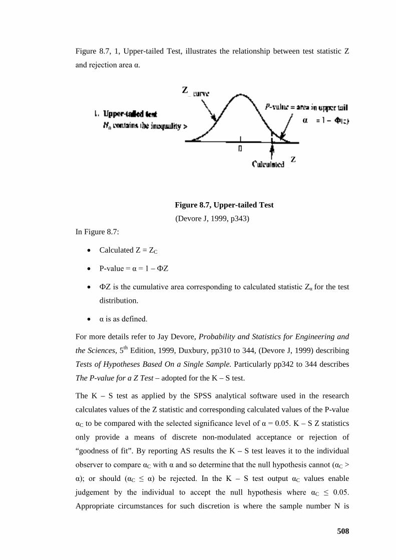
508
Figure 8.7, 1, Upper-tailed Test, illustrates the relationship between test statistic Z
and rejection area α.
Figure 8.7, Upper-tailed Test
(Devore J, 1999, p343)
In Figure 8.7:
• Calculated Z = ZC
• P-value = α = 1 – ФZ
• ФZ is the cumulative area corresponding to calculated statistic Zα for the test
distribution.
• α is as defined.
For more details refer to Jay Devore, Probability and Statistics for Engineering and
the Sciences, 5th Edition, 1999, Duxbury, pp310 to 344, (Devore J, 1999) describing
Tests of Hypotheses Based On a Single Sample. Particularly pp342 to 344 describes
The P-value for a Z Test – adopted for the K – S test.
The K – S test as applied by the SPSS analytical software used in the research
calculates values of the Z statistic and corresponding calculated values of the P-value
αC to be compared with the selected significance level of α = 0.05. K – S Z statistics
only provide a means of discrete non-modulated acceptance or rejection of
“goodness of fit”. By reporting AS results the K – S test leaves it to the individual
observer to compare αC with α and so determine that the null hypothesis cannot (αC >
α); or should (αC ≤ α) be rejected. In the K – S test output αC values enable
judgement by the individual to accept the null hypothesis where αC ≤ 0.05.
Appropriate circumstances for such discretion is where the sample number N is
α
Z
Z
509
large. Reporting AS results allows application of discretion in terms of “practical
significance” assessment to temper or override “statistical significance” when N is
large (Devore J, 1999, p348). This discussion item is of academic interest only in the
context of the research as the results of K – S tests were generally robustly in favour
of acceptance of the null hypothesis or, alternatively, to reject it.
The K – S test as applied by SPSS reports calculated values of the Z statistic and the
corresponding α value termed Asymptotic Significance (AS) in the report table.
Comparing the calculated αC value with the selected significance value of 0.05
facilitates the test.
Critical Z values drawn on by SPSS appear to correspond to the values in Table A8
from Banks J, Carson JS, and Nelson BL, Discrete Event Simulation 2nd Edit, 1996,
Prentice-Hall, p539 except that the K – S Z values are extended by the √N multiplier
as described. A copy of Table A8 is shown herein.
Table KS 3.1 includes extended K – S critical Z values for the three levels of selected
reject area, α, significance in Table A8. Figure KS 3.1 illustrates the trend towards
limiting values as critical Z values approach limits of:
AS Critical Value α Limiting Critical Z Value (N > 35)
0.10 1.22
0.05 1.36 adopted for K – S test
0.01 1.63
The trend lines at the three levels of significance are generally smooth from N = 10
to 25. For N > 25 the more erratic Z values are believed to be due to rounding up
critical values in Banks’ Table A8 to the second decimal place. For a practical range
of sample numbers critical Z values can be approximated as constants:
N Range Critical AS 0.10 0.05 0.01
10 to 20 1.17 1.30 1.56
20 to 35 1.20 1.34 1.60
>35 As above 1.22 1.36 1.63
Small differences between the cumulative relative frequency distribution of a sample
of N observations and the test distribution, in like configuration, report as small K –
S Z values that in turn correspond to calculated αC values higher than selected

510
significance value of α = 0.05 indicating that H0 cannot be rejected, i.e., should be
accepted. This validates the selected test distribution family.
In the K – S results table produced by SPSS a value of Asymptotic Significance (AS)
is shown. This is the value of reject area α corresponding to the calculated Z for the
test. So:
Calculated AS ≥ Selected significance value 0.05
Corresponds to:
Calculated ZC < Critical Zα
In both cases the null hypothesis H0 cannot be rejected. Obviously, for AS < 0.05 →
0 the rejection area is diminishing. Continues under illustration on page K – S 10
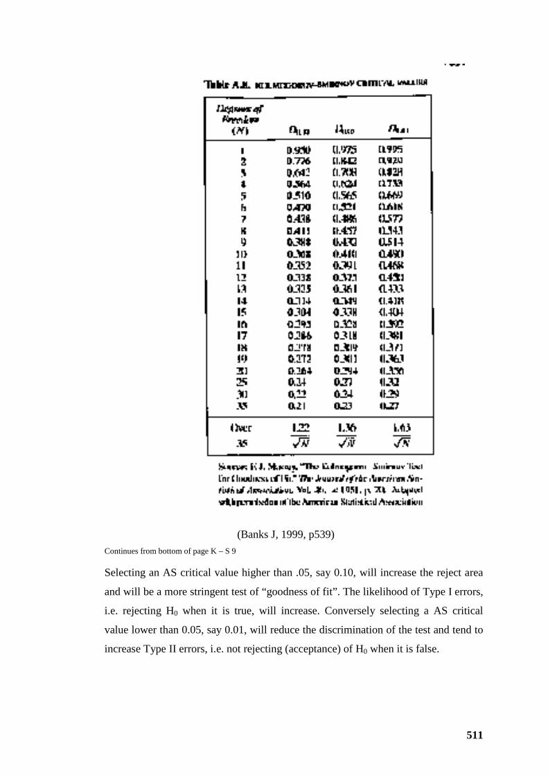
511
(Banks J, 1999, p539)
Continues from bottom of page K – S 9
Selecting an AS critical value higher than .05, say 0.10, will increase the reject area
and will be a more stringent test of “goodness of fit”. The likelihood of Type I errors,
i.e. rejecting H0 when it is true, will increase. Conversely selecting a AS critical
value lower than 0.05, say 0.01, will reduce the discrimination of the test and tend to
increase Type II errors, i.e. not rejecting (acceptance) of H0 when it is false.

512
K – S Test Outcomes
A sample of K – S tests performed during analysis of bucket loads and truck
payloads in Section 3.2.8 and bucket cycle times and truck loading times in Section
3.2.9 follow this discussion. Each K – S test is cross-referenced to the corresponding
Table and Figure in Sections 3.2.8, 3.2.9 or other appropriate sections of the thesis
text where K - S tests have been applied.
The results of the sample of K – S tests have been summarized in Table KS 6.1.
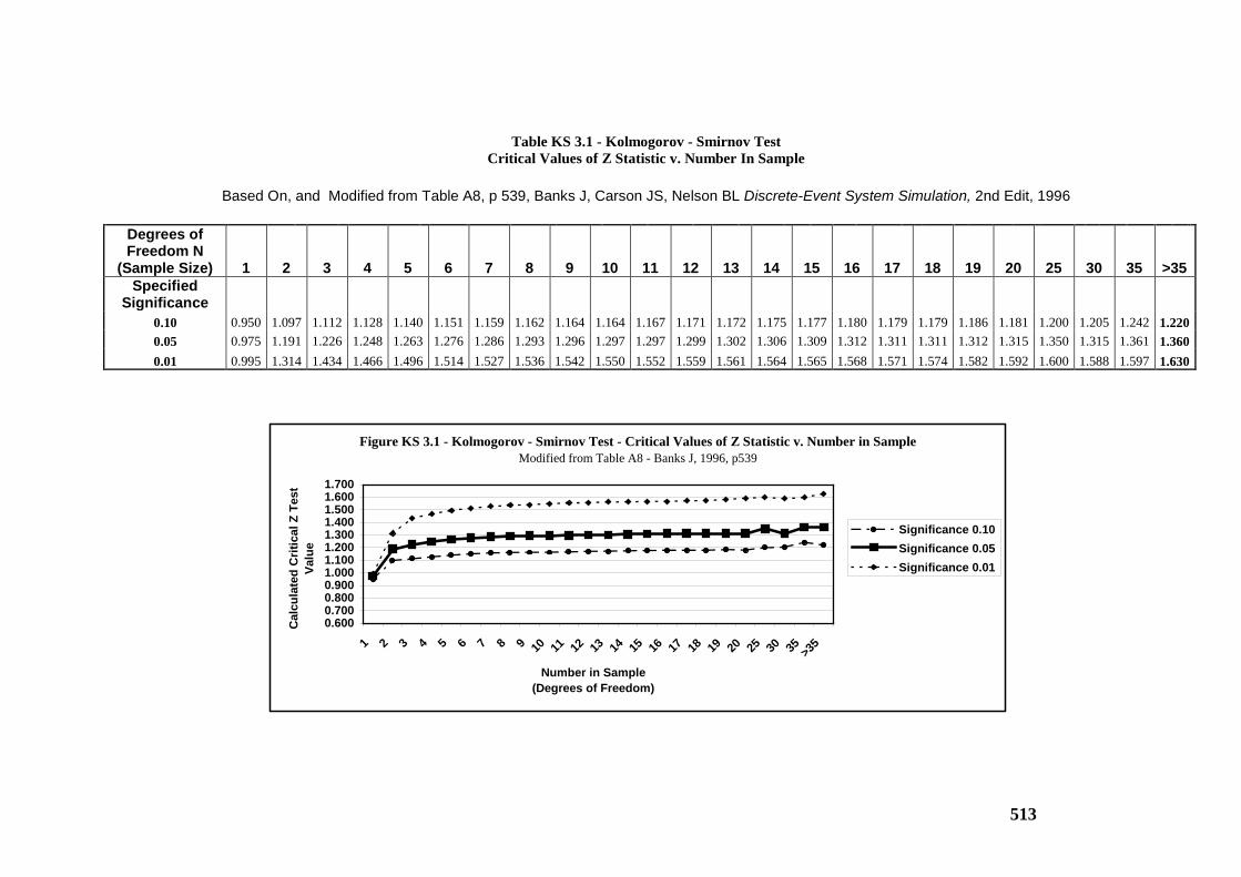
513
Figure KS 3.1 - Kolmogorov - Smirnov Test - Critical Values of Z Statistic v. Number in Sample Modified from Table A8 - Banks J, 1996, p539
0.6000.7000.8000.9001.0001.1001.2001.3001.4001.5001.6001.700
1 2 3 4 5 6 7 8 9 10 11 12 13 14 15 16 17 18 19 20 25 30 35 >35
Number in Sample(Degrees of Freedom)
Cal
cula
ted
Crit
ical
Z T
est
Valu
e
Significance 0.10Significance 0.05Significance 0.01
Table KS 3.1 - Kolmogorov - Smirnov Test Critical Values of Z Statistic v. Number In Sample
Based On, and Modified from Table A8, p 539, Banks J, Carson JS, Nelson BL Discrete-Event System Simulation, 2nd Edit, 1996
Degrees of Freedom N
(Sample Size) 1 2 3 4 5 6 7 8 9 10 11 12 13 14 15 16 17 18 19 20 25 30 35 >35 Specified
Significance 0.10 0.950 1.097 1.112 1.128 1.140 1.151 1.159 1.162 1.164 1.164 1.167 1.171 1.172 1.175 1.177 1.180 1.179 1.179 1.186 1.181 1.200 1.205 1.242 1.220 0.05 0.975 1.191 1.226 1.248 1.263 1.276 1.286 1.293 1.296 1.297 1.297 1.299 1.302 1.306 1.309 1.312 1.311 1.311 1.312 1.315 1.350 1.315 1.361 1.360 0.01 0.995 1.314 1.434 1.466 1.496 1.514 1.527 1.536 1.542 1.550 1.552 1.559 1.561 1.564 1.565 1.568 1.571 1.574 1.582 1.592 1.600 1.588 1.597 1.630
514
KS 4 PROBABILITY PLOTS
An effective and convenient method of testing an assumed family of distributions
against a distribution of empirical sample data is by comparing probability plots
(Devore J, 1999, p186).
The SPSS application package provides, in addition to the K – S test procedure, a
facility for comparative Probability Plots – termed P-P Plots in SPSS but simplified
to Pplots herein- where pairs of relative frequency values, empirical sample and
selected test distribution, are compared graphically.
Pplots produced by SPSS in conjunction with the K – S tests are constructed
generally as follows:
• Empirical sample data is sorted in order from the smallest to highest values.
• Arrange the data in cumulative frequency intervals that practically consist a
cumulative probability distribution – the “observed cumulative probability”.
• Plot the “expected cumulative probability” for the test distribution based on
similar cumulative frequency intervals against the “observed cumulative
probability”.
• If the Pplot generally falls on a straight line with gradient 1 (45o) then the
assumed test distribution is plausible.
• Deviations from the 45o straight line, at extreme values, notwithstanding
good correlation for central values, indicate that the test distribution is not an
acceptable choice.
Convenient availability in the SPSS application of Pplots promoted inclusion with
each K – S test as additional evidence of acceptance or non-acceptance of the test
distribution. It should be noted that a decision based on a Pplot whether to accept or
reject a hypothesized distribution model is subjective.
KS 5 QUANTILE-QUANTILE PLOTS
Histograms from empirical data and their qualitative fit to a continuous density
function – a test distribution – may be difficult to compare. This is particularly so for
a small number of events, N; and if the frequency intervals adopted for the frequency
515
distribution of empirical data to draft the histogram are not optimum. Histograms of
a small number of events in an even smaller number of frequency intervals are often
ragged and difficult to compare.
Banks (Banks J, 1996, p365) provides details of the underlying theory for Quantile-
Quantile Plots (Q-Q Plots as produced by SPSS and simplified to Qplots herein). For
the purposes of application of Qplots as a supplement to K – S tests it is considered
sufficient to understand that:
• An empirical cumulative distribution function can be compared with a
member of a family of distributions – the test distribution – in cdf form.
• A Quantile (Q) is a statistic that can conveniently be viewed as a special
frequency value.
• A cumulative Q plot of the empirical data that will be approximately a
straight line can be compared with a Q plot of the test distribution.
• A Q plot of the test distribution will also be a straight line.
• Comparing the two Q plots will yield an approximately straight line with a
gradient of 1 (45o).
• Deviation, usually in a systematic manner, from the 45o straight line indicates
the assumed test distribution is inappropriate.
As with Pplots, convenient availability in the SPSS application of Qplots encouraged
and facilitated inclusion with each K – S test as additional evidence of acceptance or
non-acceptance of the test distribution.
It should be noted that Qplots are based on a similar comparison of empirical data
with a distribution model as the K – S test. But the Qplot has some similarities with
Pplots. So in some respects the inclusion of Qplots in the context of the research
could be considered academic. Notwithstanding this reservation Qplots have been
reported for completeness and for readers who favour the Qplot as a test procedure.
It should be noted that, as with Pplots a decision based on Qplots whether to accept
or reject a hypothesized distribution model is also subjective.
516
KS 6 SUMMARY OF K – S TEST RESULTS, PPLOTS AND QPLOTS AND
INTERPRETATION
Summary of Results
Table KS 6.1, summarises the results of K – S Tests, Pplots and Qplots with
comments on individual test comparisons.
Interpretation
Bucket Loads and Truck Payloads
It is clearly shown by the results in Table KS 6.1 and in the K - S test results
following this section - Figures 3.2 to 3.4 and 3.6 to 3.9 - that bucket loads and truck
payloads are generally normally distributed. Truck payload control criteria (such as
Caterpillar’s 10:10:20 rule) in terms of statistics can be drawn from the normal
probability model. This is discussed in some detail in Section 3.2.8 in the thesis.
Bucket Cycle Time and Truck Loading Time
Modelling of bucket cycle times and truck loading times is differing problem as
illustrated by the results in Table KS 6.1 for Figures 3.2.9.1, 3.2.9.7, 3.2.9.8,
3.2.9.13, 3.2.9.14. As discussed in 3.2.9 in the thesis, bucket cycle times and truck
loading times, as accumulated bucket cycle times, have intrinsic and non-intrinsic
time components. Intrinsic bucket cycle and truck loading times appear to have
central tendency and likely can be modelled by a normal distribution, albeit
positively skewed. Normal probabilities could likely be applied to intrinsic times.
But non-intrinsic time in bucket cycles and accumulated in truck loading times result
in positively skewed empirical distributions that can likely modelled by a gamma
distribution including the less positively skewed Weibull distribution.
In the process of productivity planning and equipment selection it may be a more
transparent practice to develop bucket cycle times and accumulated truck loading
times in terms of intrinsic time and deal with the non-intrinsic bucket cycle and truck
loading time separately as discussed in 3.2.9.in the thesis.
Bucket Passes Per Truck Payload
As shown by the results in Table Ks 6.1 for Figures 3.5 and 3.12, modelling of
bucket passes per truckload is a further separate complication.
517
Hypothetically, the range of distribution models that can be emulated by a random
empirical sample of passes per truckload can, in practice, vary from a discrete single
constant value (by operational protocol) to a quasi symmetrical normal distribution
for a large number (N) of passes.
The results in Table KS 6.1 for Figures 3.5 and 3.12 indicate the range of
possibilities, at least to some degree.
The K – S test for Figure 3.5 – for a range of passes 4 to 6, a limited range of 3
values – provides no lead to an acceptable distribution model. Pplots for Normal,
(encouraging, but doubtful acceptance) through Lognormal, Gamma to Weibull
(reasonable acceptance as a model) indicates improving “goodness of fit”.
The K – S test for Figure 3.12 - for a range of passes 3 to 9, an extended range of 7
values – did not support acceptance of the normal model. Pplots indicated a Normal
distribution as reasonably acceptable with Gamma improving and Weibull as best
“goodness of fit”. But the indication by Pplot that the Normal model is “reasonably
acceptable” indicates the trend to central tendency of the increased range of number
of passes.
The implication of passes per truckload for truck payload dispersion has been
discussed at some length in Section 3.2.8 in the thesis.
In terms of truck loading time the implications of numbers of passes is discussed
further and in more detail in Sections 3.2.11 and 4.1.4.
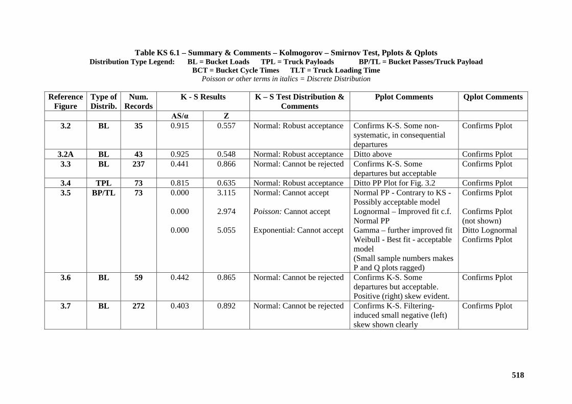
518
Table KS 6.1 – Summary & Comments – Kolmogorov – Smirnov Test, Pplots & Qplots Distribution Type Legend: BL = Bucket Loads TPL = Truck Payloads BP/TL = Bucket Passes/Truck Payload
BCT = Bucket Cycle Times TLT = Truck Loading Time Poisson or other terms in italics = Discrete Distribution
Reference
Figure Type of Distrib.
Num. Records
K - S Results K – S Test Distribution & Comments
Pplot Comments Qplot Comments
AS/α Z 3.2 BL 35 0.915 0.557 Normal: Robust acceptance Confirms K-S. Some non-
systematic, in consequential departures
Confirms Pplot
3.2A BL 43 0.925 0.548 Normal: Robust acceptance Ditto above Confirms Pplot 3.3 BL 237 0.441 0.866 Normal: Cannot be rejected Confirms K-S. Some
departures but acceptable Confirms Pplot
3.4 TPL 73 0.815 0.635 Normal: Robust acceptance Ditto PP Plot for Fig. 3.2 Confirms Pplot 3.5 BP/TL 73 0.000
0.000
0.000
3.115
2.974
5.055
Normal: Cannot accept Poisson: Cannot accept Exponential: Cannot accept
Normal PP - Contrary to KS - Possibly acceptable model Lognormal – Improved fit c.f. Normal PP Gamma – further improved fit Weibull - Best fit - acceptable model (Small sample numbers makes P and Q plots ragged)
Confirms Pplot Confirms Pplot (not shown) Ditto Lognormal Confirms Pplot
3.6 BL 59 0.442 0.865 Normal: Cannot be rejected Confirms K-S. Some departures but acceptable. Positive (right) skew evident.
Confirms Pplot
3.7 BL 272 0.403 0.892 Normal: Cannot be rejected Confirms K-S. Filtering-induced small negative (left) skew shown clearly
Confirms Pplot
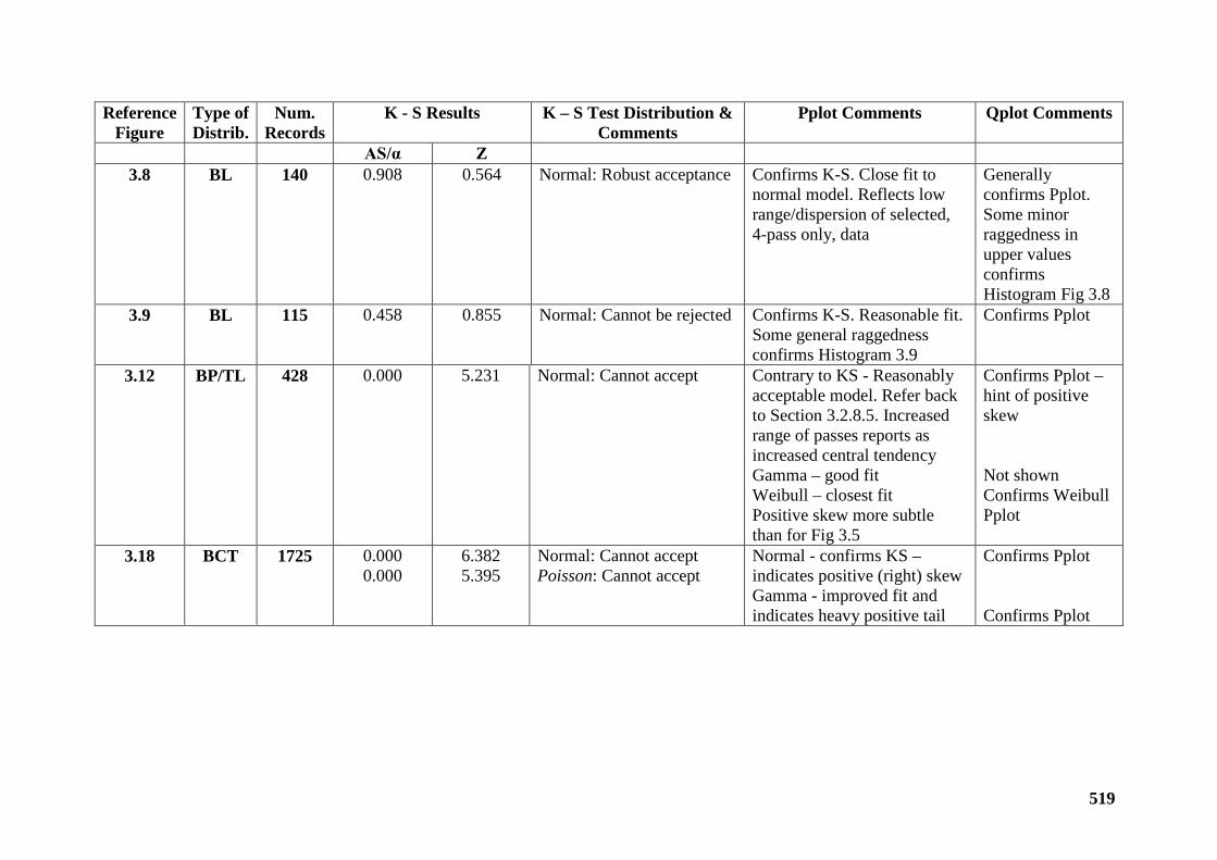
519
Reference Figure
Type of Distrib.
Num. Records
K - S Results K – S Test Distribution & Comments
Pplot Comments Qplot Comments
AS/α Z 3.8 BL 140 0.908 0.564 Normal: Robust acceptance Confirms K-S. Close fit to
normal model. Reflects low range/dispersion of selected, 4-pass only, data
Generally confirms Pplot. Some minor raggedness in upper values confirms Histogram Fig 3.8
3.9 BL 115 0.458 0.855 Normal: Cannot be rejected Confirms K-S. Reasonable fit. Some general raggedness confirms Histogram 3.9
Confirms Pplot
3.12 BP/TL 428 0.000 5.231 Normal: Cannot accept Contrary to KS - Reasonably acceptable model. Refer back to Section 3.2.8.5. Increased range of passes reports as increased central tendency Gamma – good fit Weibull – closest fit Positive skew more subtle than for Fig 3.5
Confirms Pplot – hint of positive skew Not shown Confirms Weibull Pplot
3.18 BCT 1725 0.000 0.000
6.382 5.395
Normal: Cannot accept Poisson: Cannot accept
Normal - confirms KS – indicates positive (right) skew Gamma - improved fit and indicates heavy positive tail
Confirms Pplot Confirms Pplot
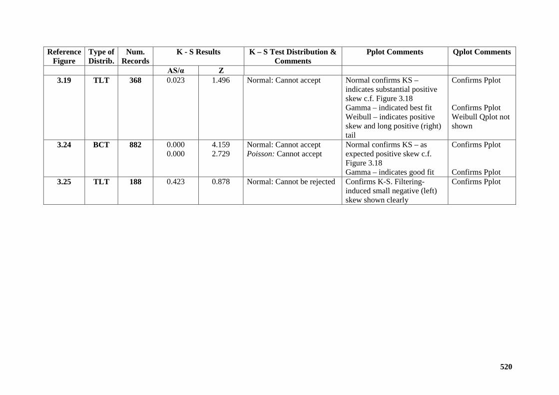
520
Reference Figure
Type of Distrib.
Num. Records
K - S Results K – S Test Distribution & Comments
Pplot Comments Qplot Comments
AS/α Z 3.19 TLT 368 0.023 1.496 Normal: Cannot accept Normal confirms KS –
indicates substantial positive skew c.f. Figure 3.18 Gamma – indicated best fit Weibull – indicates positive skew and long positive (right) tail
Confirms Pplot Confirms Pplot Weibull Qplot not shown
3.24 BCT 882 0.000 0.000
4.159 2.729
Normal: Cannot accept Poisson: Cannot accept
Normal confirms KS – as expected positive skew c.f. Figure 3.18 Gamma – indicates good fit
Confirms Pplot Confirms Pplot
3.25 TLT 188 0.423 0.878 Normal: Cannot be rejected Confirms K-S. Filtering-induced small negative (left) skew shown clearly
Confirms Pplot
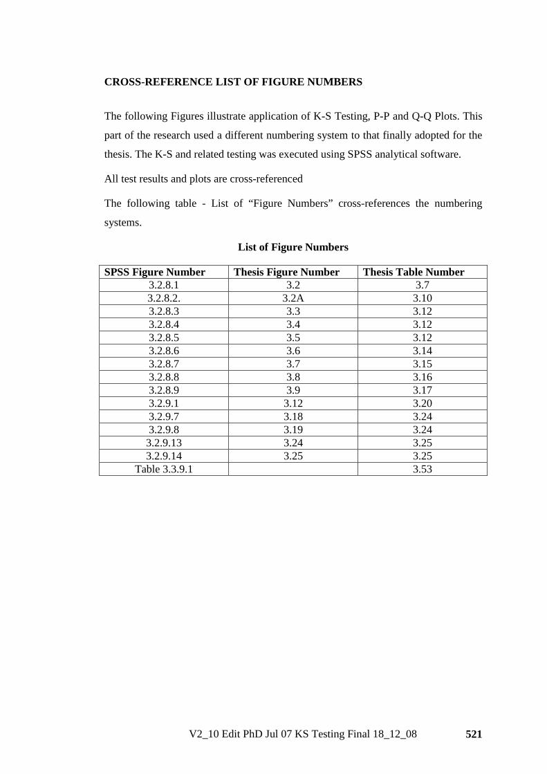
V2_10 Edit PhD Jul 07 KS Testing Final 18_12_08 521
CROSS-REFERENCE LIST OF FIGURE NUMBERS
The following Figures illustrate application of K-S Testing, P-P and Q-Q Plots. This
part of the research used a different numbering system to that finally adopted for the
thesis. The K-S and related testing was executed using SPSS analytical software.
All test results and plots are cross-referenced
The following table - List of “Figure Numbers” cross-references the numbering
systems.
List of Figure Numbers
SPSS Figure Number Thesis Figure Number Thesis Table Number 3.2.8.1 3.2 3.7 3.2.8.2. 3.2A 3.10 3.2.8.3 3.3 3.12 3.2.8.4 3.4 3.12 3.2.8.5 3.5 3.12 3.2.8.6 3.6 3.14 3.2.8.7 3.7 3.15 3.2.8.8 3.8 3.16 3.2.8.9 3.9 3.17 3.2.9.1 3.12 3.20 3.2.9.7 3.18 3.24 3.2.9.8 3.19 3.24 3.2.9.13 3.24 3.25 3.2.9.14 3.25 3.25
Table 3.3.9.1 3.53
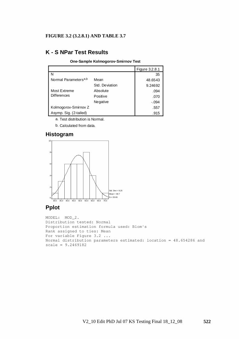
V2_10 Edit PhD Jul 07 KS Testing Final 18_12_08 522
FIGURE 3.2 (3.2.8.1) AND TABLE 3.7
K - S NPar Test Results
One-Sample Kolmogorov-Smirnov Test
3548.65439.24692
.094
.070-.094.557.915
NMeanStd. Deviation
Normal Parametersa,b
AbsolutePositiveNegative
Most ExtremeDifferences
Kolmogorov-Smirnov ZAsymp. Sig. (2-tailed)
Figure 3.2.8.1
Test distribution is Normal.a.
Calculated from data.b.
Histogram
70.065.060.055.050.045.040.035.030.0
10
8
6
4
2
0
Std. Dev = 9.25
Mean = 48.7
N = 35.00
Pplot MODEL: MOD_2. Distribution tested: Normal Proportion estimation formula used: Blom's Rank assigned to ties: Mean For variable Figure 3.2 ... Normal distribution parameters estimated: location = 48.654286 and scale = 9.2469182
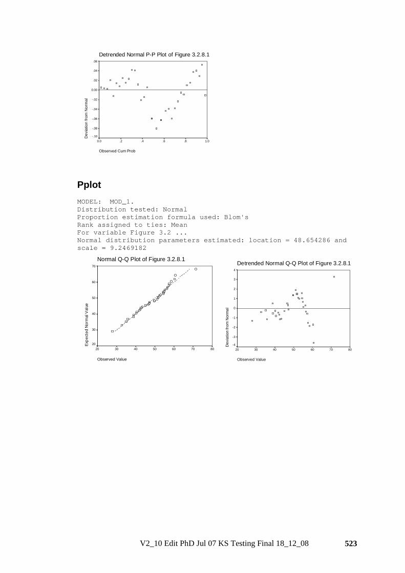
V2_10 Edit PhD Jul 07 KS Testing Final 18_12_08 523
Detrended Normal P-P Plot of Figure 3.2.8.1
Observed Cum Prob
1.0.8.6.4.20.0
Dev
iatio
n fro
m N
orm
al
.06
.04
.02
0.00
-.02
-.04
-.06
-.08
-.10
Pplot MODEL: MOD_1. Distribution tested: Normal Proportion estimation formula used: Blom's Rank assigned to ties: Mean For variable Figure 3.2 ... Normal distribution parameters estimated: location = 48.654286 and scale = 9.2469182
Normal Q-Q Plot of Figure 3.2.8.1
Observed Value
80706050403020
Expe
cted
Nor
mal
Val
ue
70
60
50
40
30
20
Detrended Normal Q-Q Plot of Figure 3.2.8.1
Observed Value
80706050403020
Dev
iatio
n fro
m N
orm
al
4
3
2
1
0
-1
-2
-3
-4

V2_10 Edit PhD Jul 07 KS Testing Final 18_12_08 524
FIGURE 3.2A (3.2.8.2) AND TABLE 3.10
K - S NPar Test Results
One-Sample Kolmogorov-Smirnov Test
4322.26513.29552
.084
.057-.084.548.925
NMeanStd. Deviation
Normal Parametersa,b
AbsolutePositiveNegative
Most ExtremeDifferences
Kolmogorov-Smirnov ZAsymp. Sig. (2-tailed)
Figure 3.2.8.2
Test distribution is Normal.a.
Calculated from data.b.
Histogram
29.028.0
27.026.0
25.024.0
23.022.0
21.020.0
19.018.0
17.016.0
15.014.0
8
6
4
2
0
Std. Dev = 3.30
Mean = 22.3
N = 43.00
Pplot MODEL: MOD_1. Distribution tested: Normal Proportion estimation formula used: Blom's Rank assigned to ties: Mean For variable Figure 3.2A ... Normal distribution parameters estimated: location = 22.265116 and scale = 3.2955153
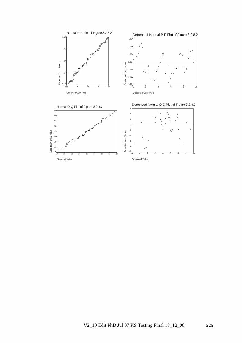
V2_10 Edit PhD Jul 07 KS Testing Final 18_12_08 525
Normal P-P Plot of Figure 3.2.8.2
Observed Cum Prob
1.00.75.50.250.00
Exp
ecte
d C
um P
rob
1.00
.75
.50
.25
0.00
Detrended Normal P-P Plot of Figure 3.2.8.2
Observed Cum Prob
1.0.8.6.4.20.0
Dev
iatio
n fro
m N
orm
al
.06
.04
.02
0.00
-.02
-.04
-.06
Normal Q-Q Plot of Figure 3.2.8.2
Observed Value
302826242220181614
Expe
cted
Nor
mal
Val
ue
30
28
26
24
22
20
18
16
14
Detrended Normal Q-Q Plot of Figure 3.2.8.2
Observed Value
302826242220181614
Dev
iatio
n fro
m N
orm
al
.6
.4
.2
.0
-.2
-.4
-.6
-.8
-1.0
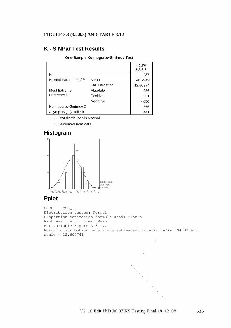
V2_10 Edit PhD Jul 07 KS Testing Final 18_12_08 526
FIGURE 3.3 (3.2.8.3) AND TABLE 3.12
K - S NPar Test Results
One-Sample Kolmogorov-Smirnov Test
23746.7949
12.60374.056.031
-.056.866.441
NMeanStd. Deviation
Normal Parametersa,b
AbsolutePositiveNegative
Most ExtremeDifferences
Kolmogorov-Smirnov ZAsymp. Sig. (2-tailed)
Figure3.2.8.3
Test distribution is Normal.a.
Calculated from data.b.
Histogram
80.075.0
70.065.0
60.055.0
50.045.0
40.035.0
30.025.0
20.015.0
30
20
10
0
Std. Dev = 12.60 Mean = 46.8
N = 237.00
Pplot MODEL: MOD_1. Distribution tested: Normal Proportion estimation formula used: Blom's Rank assigned to ties: Mean For variable Figure 3.3 ... Normal distribution parameters estimated: location = 46.794937 and scale = 12.603741
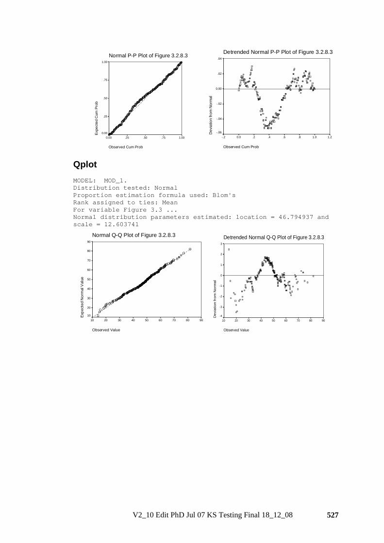
V2_10 Edit PhD Jul 07 KS Testing Final 18_12_08 527
Normal P-P Plot of Figure 3.2.8.3
Observed Cum Prob
1.00.75.50.250.00
Expe
cted
Cum
Pro
b
1.00
.75
.50
.25
0.00
Detrended Normal P-P Plot of Figure 3.2.8.3
Observed Cum Prob
1.21.0.8.6.4.20.0-.2
Dev
iatio
n fro
m N
orm
al
.04
.02
0.00
-.02
-.04
-.06
Qplot MODEL: MOD_1. Distribution tested: Normal Proportion estimation formula used: Blom's Rank assigned to ties: Mean For variable Figure 3.3 ... Normal distribution parameters estimated: location = 46.794937 and scale = 12.603741
Normal Q-Q Plot of Figure 3.2.8.3
Observed Value
908070605040302010
Expe
cted
Nor
mal
Val
ue
90
80
70
60
50
40
30
20
10
Detrended Normal Q-Q Plot of Figure 3.2.8.3
Observed Value
908070605040302010
Dev
iatio
n fr
om N
orm
al
3
2
1
0
-1
-2
-3
-4
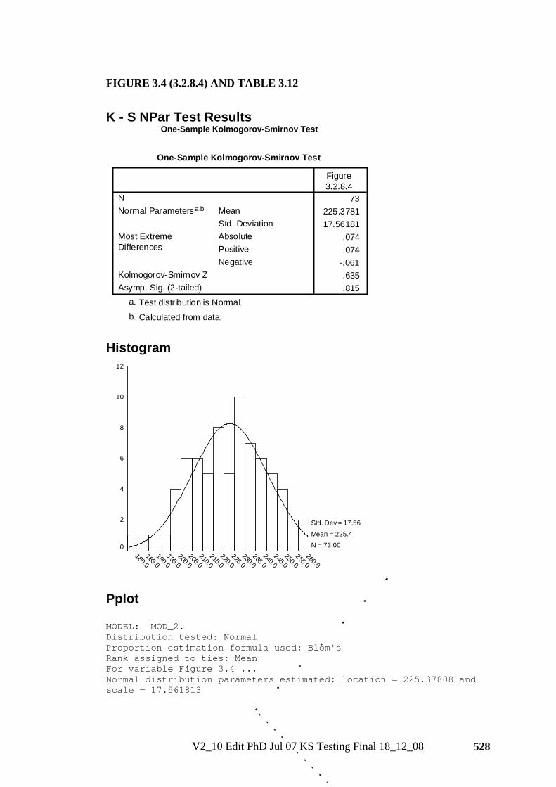
V2_10 Edit PhD Jul 07 KS Testing Final 18_12_08 528
FIGURE 3.4 (3.2.8.4) AND TABLE 3.12
K - S NPar Test Results One-Sample Kolmogorov-Smirnov Test
One-Sample Kolmogorov-Smirnov Test
73225.378117.56181
.074
.074-.061.635.815
NMeanStd. Deviation
Normal Parametersa,b
AbsolutePositiveNegative
Most ExtremeDifferences
Kolmogorov-Smirnov ZAsymp. Sig. (2-tailed)
Figure3.2.8.4
Test distribution is Normal.a.
Calculated from data.b.
Histogram
260.0255.0
250.0245.0
240.0235.0
230.0225.0
220.0215.0
210.0205.0
200.0195.0
190.0185.0
180.0
12
10
8
6
4
2
0
Std. Dev = 17.56
Mean = 225.4
N = 73.00
Pplot MODEL: MOD_2. Distribution tested: Normal Proportion estimation formula used: Blom's Rank assigned to ties: Mean For variable Figure 3.4 ... Normal distribution parameters estimated: location = 225.37808 and scale = 17.561813
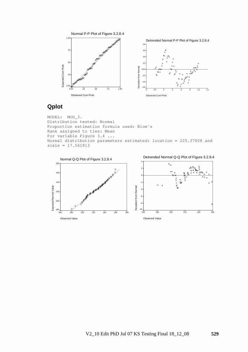
V2_10 Edit PhD Jul 07 KS Testing Final 18_12_08 529
Normal P-P Plot of Figure 3.2.8.4
Observed Cum Prob
1.00.75.50.250.00
Expe
cted
Cum
Pro
b
1.00
.75
.50
.25
0.00
Detrended Normal P-P Plot of Figure 3.2.8.4
Observed Cum Prob
1.21.0.8.6.4.20.0-.2
Dev
iatio
n fro
m N
orm
al
.08
.06
.04
.02
0.00
-.02
-.04
-.06
Qplot MODEL: MOD_3. Distribution tested: Normal Proportion estimation formula used: Blom's Rank assigned to ties: Mean For variable Figure 3.4 ... Normal distribution parameters estimated: location = 225.37808 and scale = 17.561813
Normal Q-Q Plot of Figure 3.2.8.4
Observed Value
280260240220200180160
Expe
cted
Nor
mal
Val
ue
280
260
240
220
200
180
Detrended Normal Q-Q Plot of Figure 3.2.8.4
Observed Value
260240220200180160
Dev
iatio
n fro
m N
orm
al
4
2
0
-2
-4
-6
-8
-10
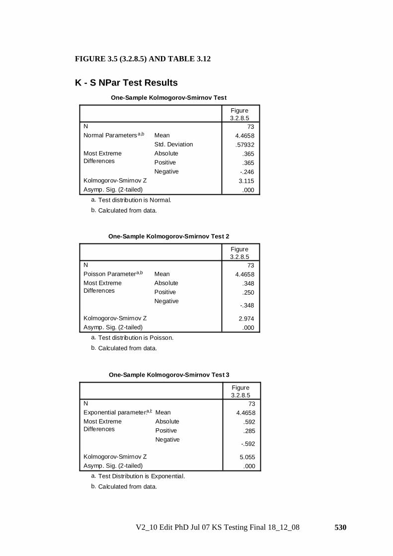
V2_10 Edit PhD Jul 07 KS Testing Final 18_12_08 530
FIGURE 3.5 (3.2.8.5) AND TABLE 3.12
K - S NPar Test Results
One-Sample Kolmogorov-Smirnov Test
734.4658.57932
.365
.365-.2463.115
.000
NMeanStd. Deviation
Normal Parametersa,b
AbsolutePositiveNegative
Most ExtremeDifferences
Kolmogorov-Smirnov ZAsymp. Sig. (2-tailed)
Figure3.2.8.5
Test distribution is Normal.a.
Calculated from data.b.
One-Sample Kolmogorov-Smirnov Test 2
734.4658
.348
.250
-.348
2.974.000
NMeanPoisson Parametera,b
AbsolutePositiveNegative
Most ExtremeDifferences
Kolmogorov-Smirnov ZAsymp. Sig. (2-tailed)
Figure3.2.8.5
Test distribution is Poisson.a.
Calculated from data.b.
One-Sample Kolmogorov-Smirnov Test 3
734.4658
.592
.285
-.592
5.055.000
NMeanExponential parameter.a,b
AbsolutePositiveNegative
Most ExtremeDifferences
Kolmogorov-Smirnov ZAsymp. Sig. (2-tailed)
Figure3.2.8.5
Test Distribution is Exponential.a.
Calculated from data.b.
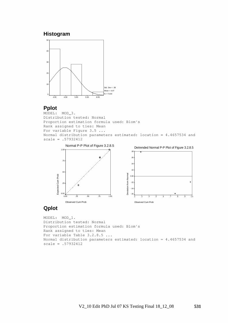
V2_10 Edit PhD Jul 07 KS Testing Final 18_12_08 531
Histogram
6.005.505.004.504.00
50
40
30
20
10
0
Std. Dev = .58
Mean = 4.47
N = 73.00
Pplot MODEL: MOD_3. Distribution tested: Normal Proportion estimation formula used: Blom's Rank assigned to ties: Mean For variable Figure 3.5 ... Normal distribution parameters estimated: location = 4.4657534 and scale = .57932412
Normal P-P Plot of Figure 3.2.8.5
Observed Cum Prob
1.00.75.50.250.00
Expe
cted
Cum
Pro
b
1.00
.75
.50
.25
0.00
Detrended Normal P-P Plot of Figure 3.2.8.5
Observed Cum Prob
1.0.9.8.7.6.5.4.3.2
Dev
iatio
n fr
om N
orm
al
.08
.06
.04
.02
0.00
-.02
-.04
-.06
Qplot MODEL: MOD_1. Distribution tested: Normal Proportion estimation formula used: Blom's Rank assigned to ties: Mean For variable Table 3.2.8.5 ... Normal distribution parameters estimated: location = 4.4657534 and scale = .57932412
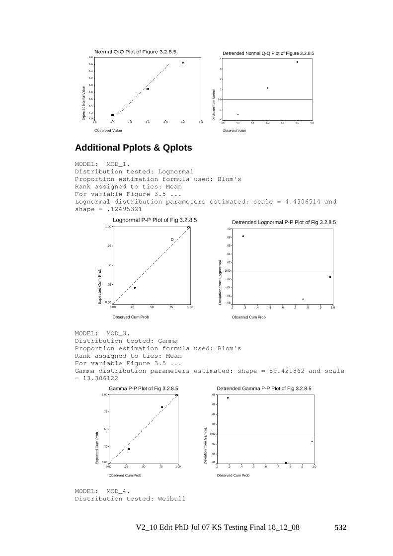
V2_10 Edit PhD Jul 07 KS Testing Final 18_12_08 532
Normal Q-Q Plot of Figure 3.2.8.5
Observed Value
6.56.05.55.04.54.03.5
Expe
cted N
orm
al Va
lue
5.8
5.6
5.4
5.2
5.0
4.8
4.6
4.4
4.2
4.0
Detrended Normal Q-Q Plot of Figure 3.2.8.5
Observed Value
6.56.05.55.04.54.03.5
Dev
iatio
n fro
m N
orm
al
.4
.3
.2
.1
0.0
-.1
-.2
Additional Pplots & Qplots MODEL: MOD_1. Distribution tested: Lognormal Proportion estimation formula used: Blom's Rank assigned to ties: Mean For variable Figure 3.5 ... Lognormal distribution parameters estimated: scale = 4.4306514 and shape = .12495321
Lognormal P-P Plot of Fig 3.2.8.5
Observed Cum Prob
1.00.75.50.250.00
Expe
cted
Cum
Pro
b
1.00
.75
.50
.25
0.00
Detrended Lognormal P-P Plot of Fig 3.2.8.5
Observed Cum Prob
1.0.9.8.7.6.5.4.3.2
Dev
iatio
n fr
om L
ogno
rmal
.10
.08
.06
.04
.02
0.00
-.02
-.04
-.06
-.08
MODEL: MOD_3. Distribution tested: Gamma Proportion estimation formula used: Blom's Rank assigned to ties: Mean For variable Figure 3.5 ... Gamma distribution parameters estimated: shape = 59.421862 and scale = 13.306122
Gamma P-P Plot of Fig 3.2.8.5
Observed Cum Prob
1.00.75.50.250.00
Expe
cted
Cum
Pro
b
1.00
.75
.50
.25
0.00
Detrended Gamma P-P Plot of Fig 3.2.8.5
Observed Cum Prob
1.0.9.8.7.6.5.4.3.2
Dev
iatio
n fro
m G
amm
a
.08
.06
.04
.02
0.00
-.02
-.04
-.06
MODEL: MOD_4. Distribution tested: Weibull
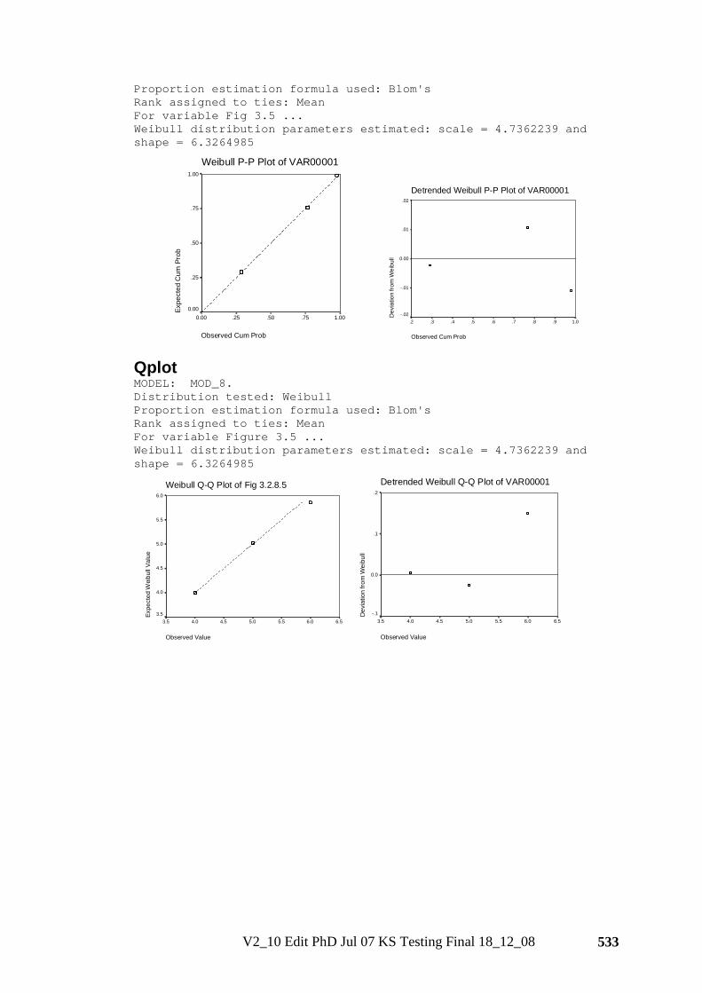
V2_10 Edit PhD Jul 07 KS Testing Final 18_12_08 533
Proportion estimation formula used: Blom's Rank assigned to ties: Mean For variable Fig 3.5 ... Weibull distribution parameters estimated: scale = 4.7362239 and shape = 6.3264985
Weibull P-P Plot of VAR00001
Observed Cum Prob
1.00.75.50.250.00
Expe
cted
Cum
Pro
b1.00
.75
.50
.25
0.00
Detrended Weibull P-P Plot of VAR00001
Observed Cum Prob
1.0.9.8.7.6.5.4.3.2
Dev
iatio
n fro
m W
eibu
ll
.02
.01
0.00
-.01
-.02
Qplot MODEL: MOD_8. Distribution tested: Weibull Proportion estimation formula used: Blom's Rank assigned to ties: Mean For variable Figure 3.5 ... Weibull distribution parameters estimated: scale = 4.7362239 and shape = 6.3264985
Weibull Q-Q Plot of Fig 3.2.8.5
Observed Value
6.56.05.55.04.54.03.5
Expe
cted
Wei
bull
Valu
e
6.0
5.5
5.0
4.5
4.0
3.5
Detrended Weibull Q-Q Plot of VAR00001
Observed Value
6.56.05.55.04.54.03.5
Dev
iatio
n fro
m W
eibu
ll
.2
.1
0.0
-.1
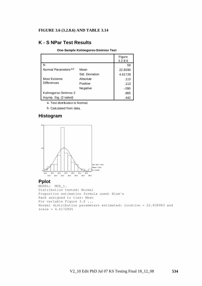
V2_10 Edit PhD Jul 07 KS Testing Final 18_12_08 534
FIGURE 3.6 (3.2.8.6) AND TABLE 3.14
K - S NPar Test Results
One-Sample Kolmogorov-Smirnov Test
5922.83904.61728
.113
.113-.090.865.442
NMeanStd. Deviation
Normal Parametersa,b
AbsolutePositiveNegative
Most ExtremeDifferences
Kolmogorov-Smirnov ZAsymp. Sig. (2-tailed)
Figure3.2.8.6
Test distribution is Normal.a.
Calculated from data.b.
Histogram
38.036.0
34.032.0
30.028.0
26.024.0
22.020.0
18.016.0
14.012.0
20
10
0
Std. Dev = 4.62
Mean = 22.8
N = 59.00
Pplot MODEL: MOD_1. Distribution tested: Normal Proportion estimation formula used: Blom's Rank assigned to ties: Mean For variable Figure 3.6 ... Normal distribution parameters estimated: location = 22.838983 and scale = 4.6172845
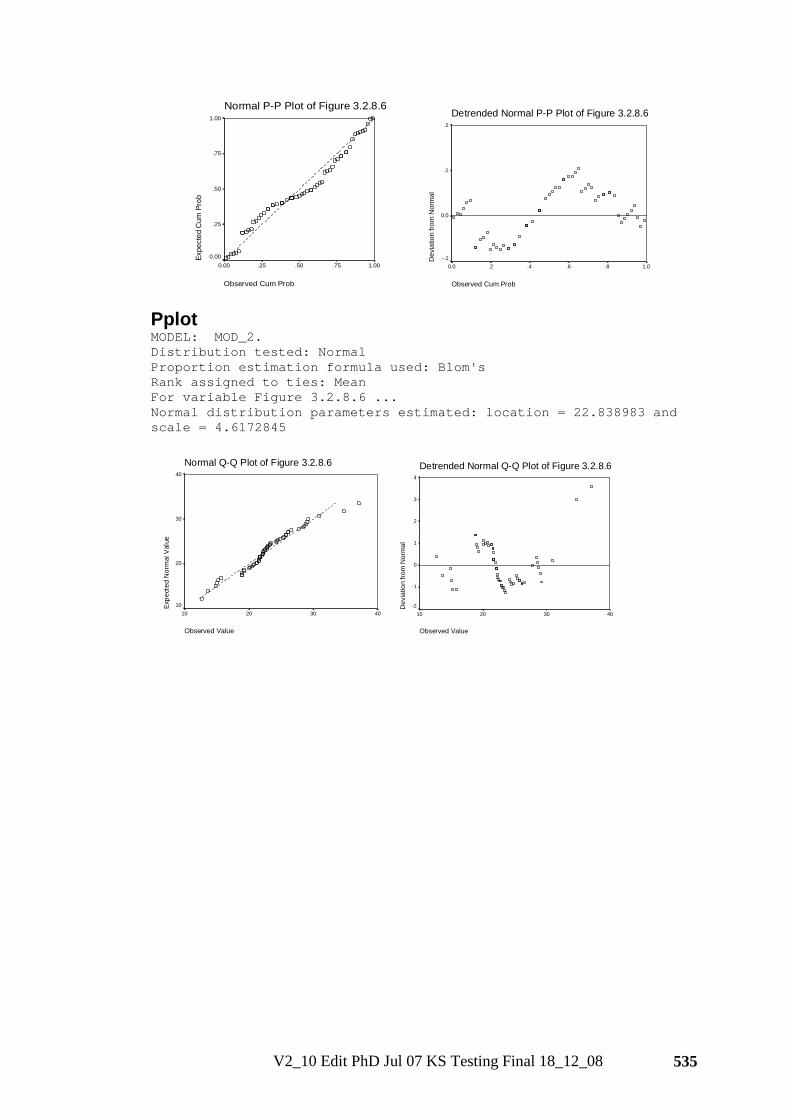
V2_10 Edit PhD Jul 07 KS Testing Final 18_12_08 535
Normal P-P Plot of Figure 3.2.8.6
Observed Cum Prob
1.00.75.50.250.00
Expe
cted
Cum
Pro
b
1.00
.75
.50
.25
0.00
Detrended Normal P-P Plot of Figure 3.2.8.6
Observed Cum Prob
1.0.8.6.4.20.0
Dev
iatio
n fro
m N
orm
al
.2
.1
0.0
-.1
Pplot MODEL: MOD_2. Distribution tested: Normal Proportion estimation formula used: Blom's Rank assigned to ties: Mean For variable Figure 3.2.8.6 ... Normal distribution parameters estimated: location = 22.838983 and scale = 4.6172845
Normal Q-Q Plot of Figure 3.2.8.6
Observed Value
40302010
Expe
cted
Nor
mal
Val
ue
40
30
20
10
Detrended Normal Q-Q Plot of Figure 3.2.8.6
Observed Value
40302010
Dev
iatio
n fro
m N
orm
al
4
3
2
1
0
-1
-2
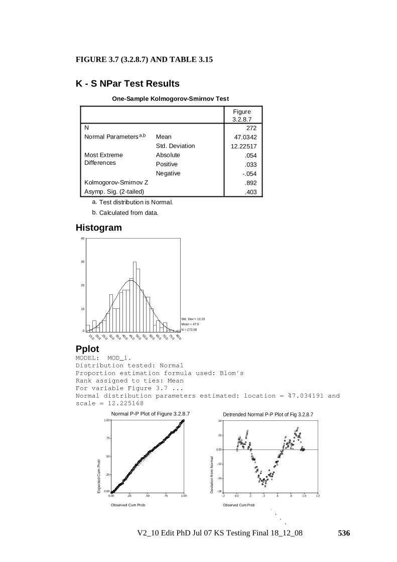
V2_10 Edit PhD Jul 07 KS Testing Final 18_12_08 536
FIGURE 3.7 (3.2.8.7) AND TABLE 3.15
K - S NPar Test Results
One-Sample Kolmogorov-Smirnov Test
27247.0342
12.22517.054.033
-.054.892.403
NMeanStd. Deviation
Normal Parametersa,b
AbsolutePositiveNegative
Most ExtremeDifferences
Kolmogorov-Smirnov ZAsymp. Sig. (2-tailed)
Figure3.2.8.7
Test distribution is Normal.a.
Calculated from data.b.
Histogram
80.075.0
70.065.0
60.055.0
50.045.0
40.035.0
30.025.0
20.015.0
40
30
20
10
0
Std. Dev = 12.23 Mean = 47.0
N = 272.00
Pplot MODEL: MOD_1. Distribution tested: Normal Proportion estimation formula used: Blom's Rank assigned to ties: Mean For variable Figure 3.7 ... Normal distribution parameters estimated: location = 47.034191 and scale = 12.225168
Normal P-P Plot of Figure 3.2.8.7
Observed Cum Prob
1.00.75.50.250.00
Expe
cted
Cum
Pro
b
1.00
.75
.50
.25
0.00
Detrended Normal P-P Plot of Fig 3.2.8.7
Observed Cum Prob
1.21.0.8.6.4.20.0-.2
Dev
iatio
n fr
om N
orm
al
.04
.02
0.00
-.02
-.04
-.06
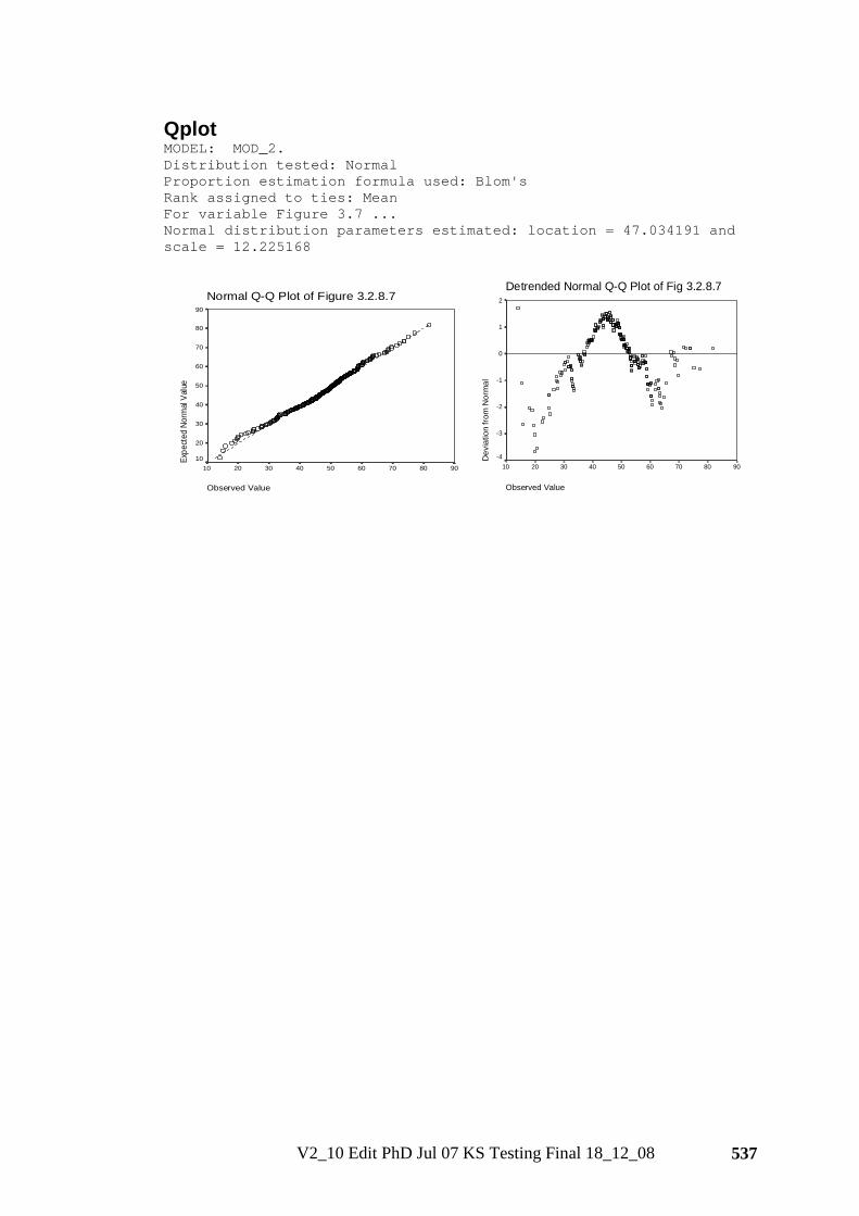
V2_10 Edit PhD Jul 07 KS Testing Final 18_12_08 537
Qplot MODEL: MOD_2. Distribution tested: Normal Proportion estimation formula used: Blom's Rank assigned to ties: Mean For variable Figure 3.7 ... Normal distribution parameters estimated: location = 47.034191 and scale = 12.225168
Normal Q-Q Plot of Figure 3.2.8.7
Observed Value
908070605040302010
Expe
cted
Nor
mal
Valu
e
90
80
70
60
50
40
30
20
10
Detrended Normal Q-Q Plot of Fig 3.2.8.7
Observed Value
908070605040302010
Dev
iatio
n fro
m N
orm
al
2
1
0
-1
-2
-3
-4
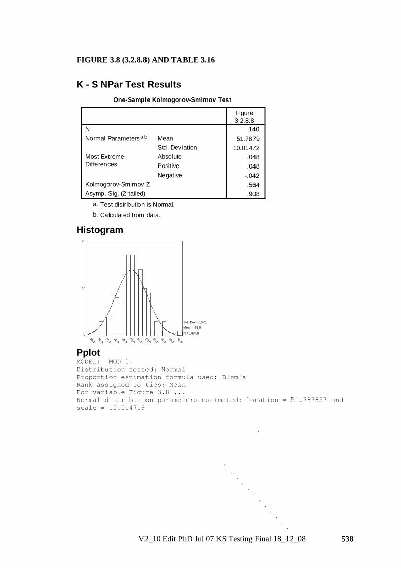
V2_10 Edit PhD Jul 07 KS Testing Final 18_12_08 538
FIGURE 3.8 (3.2.8.8) AND TABLE 3.16
K - S NPar Test Results
One-Sample Kolmogorov-Smirnov Test
14051.7879
10.01472.048.048
-.042.564.908
NMeanStd. Deviation
Normal Parametersa,b
AbsolutePositiveNegative
Most ExtremeDifferences
Kolmogorov-Smirnov ZAsymp. Sig. (2-tailed)
Figure3.2.8.8
Test distribution is Normal.a.
Calculated from data.b.
Histogram
80.075.0
70.065.0
60.055.0
50.045.0
40.035.0
30.025.0
20
10
0
Std. Dev = 10.01 Mean = 51.8
N = 140.00
Pplot MODEL: MOD_1. Distribution tested: Normal Proportion estimation formula used: Blom's Rank assigned to ties: Mean For variable Figure 3.8 ... Normal distribution parameters estimated: location = 51.787857 and scale = 10.014719
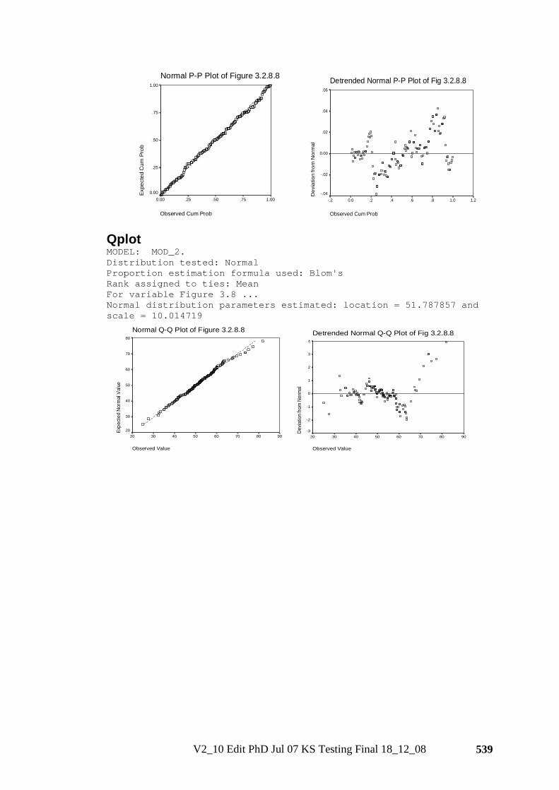
V2_10 Edit PhD Jul 07 KS Testing Final 18_12_08 539
Normal P-P Plot of Figure 3.2.8.8
Observed Cum Prob
1.00.75.50.250.00
Expe
cted
Cum
Pro
b
1.00
.75
.50
.25
0.00
Detrended Normal P-P Plot of Fig 3.2.8.8
Observed Cum Prob
1.21.0.8.6.4.20.0-.2
Dev
iatio
n fr
om N
orm
al
.06
.04
.02
0.00
-.02
-.04
Qplot MODEL: MOD_2. Distribution tested: Normal Proportion estimation formula used: Blom's Rank assigned to ties: Mean For variable Figure 3.8 ... Normal distribution parameters estimated: location = 51.787857 and scale = 10.014719
Normal Q-Q Plot of Figure 3.2.8.8
Observed Value
9080706050403020
Expe
cted
Nor
mal
Valu
e
80
70
60
50
40
30
20
Detrended Normal Q-Q Plot of Fig 3.2.8.8
Observed Value
9080706050403020
Devia
tion
from
Nor
mal
4
3
2
1
0
-1
-2
-3
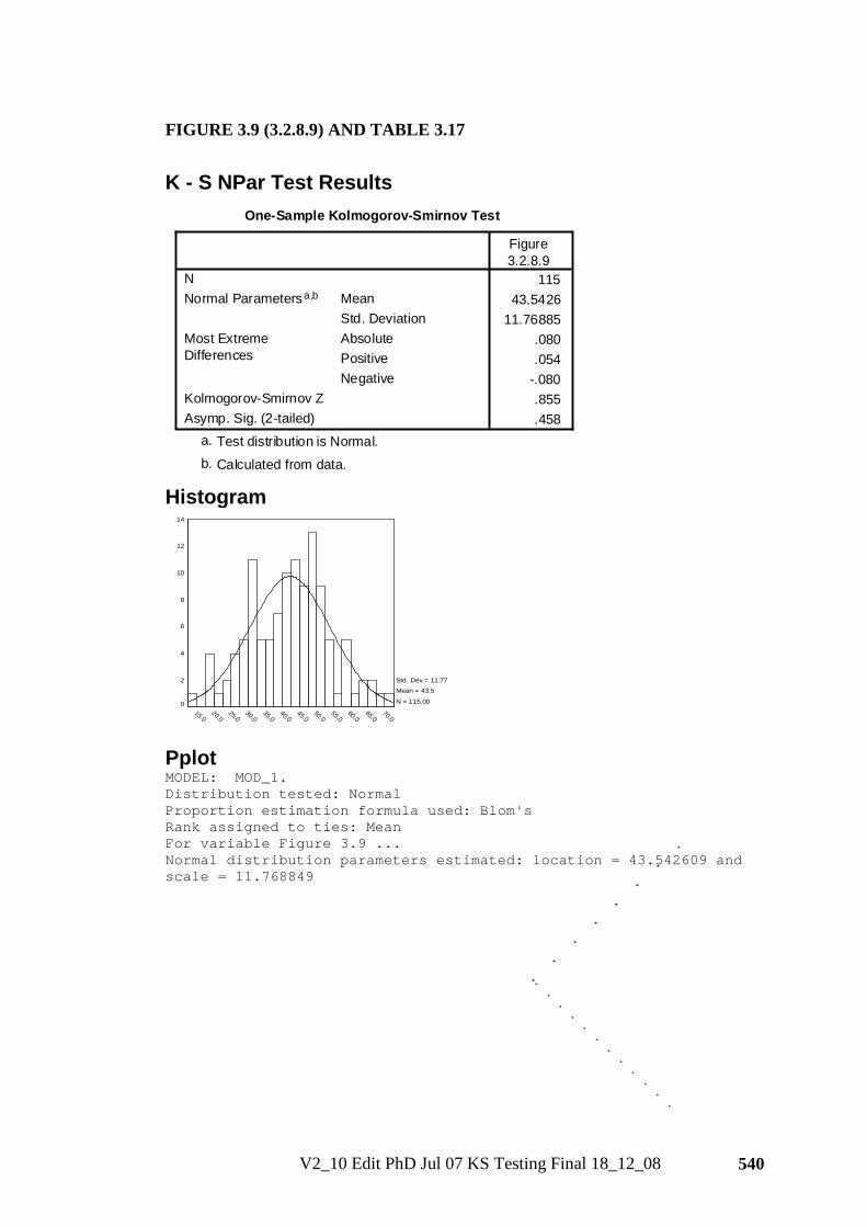
V2_10 Edit PhD Jul 07 KS Testing Final 18_12_08 540
FIGURE 3.9 (3.2.8.9) AND TABLE 3.17
K - S NPar Test Results
One-Sample Kolmogorov-Smirnov Test
11543.5426
11.76885.080.054
-.080.855.458
NMeanStd. Deviation
Normal Parametersa,b
AbsolutePositiveNegative
Most ExtremeDifferences
Kolmogorov-Smirnov ZAsymp. Sig. (2-tailed)
Figure3.2.8.9
Test distribution is Normal.a.
Calculated from data.b.
Histogram
70.065.0
60.055.0
50.045.0
40.035.0
30.025.0
20.015.0
14
12
10
8
6
4
2
0
Std. Dev = 11.77 Mean = 43.5
N = 115.00
Pplot MODEL: MOD_1. Distribution tested: Normal Proportion estimation formula used: Blom's Rank assigned to ties: Mean For variable Figure 3.9 ... Normal distribution parameters estimated: location = 43.542609 and scale = 11.768849

V2_10 Edit PhD Jul 07 KS Testing Final 18_12_08 541
Normal P-P Plot of Figure 3.2.8.9
Observed Cum Prob
1.00.75.50.250.00
Expe
cted
Cum
Pro
b
1.00
.75
.50
.25
0.00
Detrended Normal P-P Plot of Fig 3.2.8.9
Observed Cum Prob
1.21.0.8.6.4.20.0-.2
Dev
iatio
n fr
om N
orm
al
.06
.04
.02
0.00
-.02
-.04
-.06
-.08
Qplot MODEL: MOD_2. Distribution tested: Normal Proportion estimation formula used: Blom's Rank assigned to ties: Mean For variable Figure 3.9... Normal distribution parameters estimated: location = 43.542609 and scale = 11.768849
Normal Q-Q Plot of Figure 3.2.8.9
Observed Value
8070605040302010
Expe
cted
Nor
mal
Valu
e
80
70
60
50
40
30
20
10
Detrended Normal Q-Q Plot of Fig 3.2.8.9
Observed Value
8070605040302010
Devia
tion
from
Nor
mal
4
3
2
1
0
-1
-2
-3
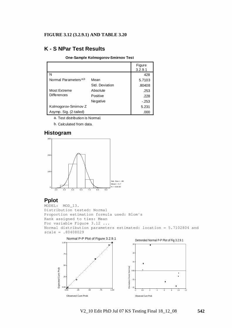
V2_10 Edit PhD Jul 07 KS Testing Final 18_12_08 542
FIGURE 3.12 (3.2.9.1) AND TABLE 3.20
K - S NPar Test Results
One-Sample Kolmogorov-Smirnov Test
4285.7103.80408
.253
.228-.2535.231
.000
NMeanStd. Deviation
Normal Parametersa,b
AbsolutePositiveNegative
Most ExtremeDifferences
Kolmogorov-Smirnov ZAsymp. Sig. (2-tailed)
Figure3.2.9.1
Test distribution is Normal.a.
Calculated from data.b.
Histogram
9.08.07.06.05.04.03.0
300
200
100
0
Std. Dev = .80
Mean = 5.7
N = 428.00
Pplot MODEL: MOD_13. Distribution tested: Normal Proportion estimation formula used: Blom's Rank assigned to ties: Mean For variable Figure 3.12 ... Normal distribution parameters estimated: location = 5.7102804 and scale = .80408029
Normal P-P Plot of Figure 3.2.9.1
Observed Cum Prob
1.00.75.50.250.00
Expe
cted
Cum
Pro
b
1.00
.75
.50
.25
0.00
Detrended Normal P-P Plot of Fig 3.2.9.1
Observed Cum Prob
1.21.0.8.6.4.20.0-.2
De
via
tion
fro
m N
orm
al
.03
.02
.01
0.00
-.01
-.02
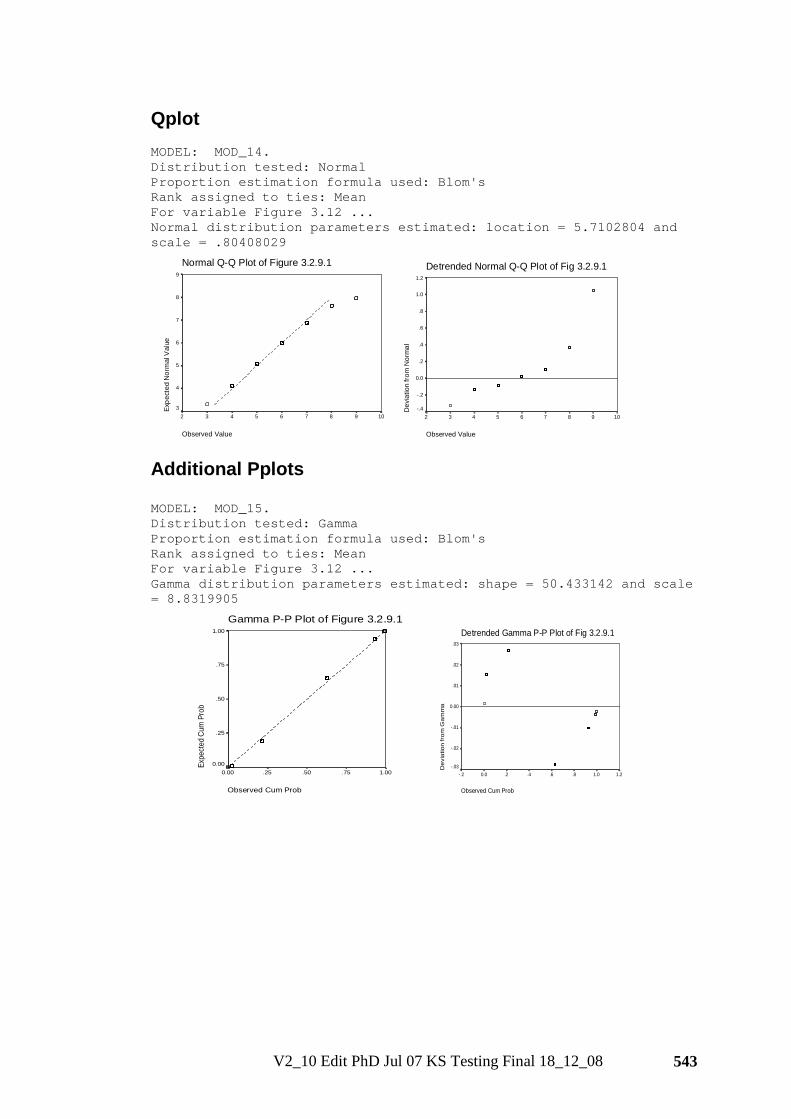
V2_10 Edit PhD Jul 07 KS Testing Final 18_12_08 543
Qplot MODEL: MOD_14. Distribution tested: Normal Proportion estimation formula used: Blom's Rank assigned to ties: Mean For variable Figure 3.12 ... Normal distribution parameters estimated: location = 5.7102804 and scale = .80408029
Normal Q-Q Plot of Figure 3.2.9.1
Observed Value
1098765432
Expe
cted
Nor
mal
Val
ue
9
8
7
6
5
4
3
Detrended Normal Q-Q Plot of Fig 3.2.9.1
Observed Value
1098765432
Dev
iatio
n fro
m N
orm
al
1.2
1.0
.8
.6
.4
.2
0.0
-.2
-.4
Additional Pplots MODEL: MOD_15. Distribution tested: Gamma Proportion estimation formula used: Blom's Rank assigned to ties: Mean For variable Figure 3.12 ... Gamma distribution parameters estimated: shape = 50.433142 and scale = 8.8319905
Gamma P-P Plot of Figure 3.2.9.1
Observed Cum Prob
1.00.75.50.250.00
Expe
cted
Cum
Pro
b
1.00
.75
.50
.25
0.00
Detrended Gamma P-P Plot of Fig 3.2.9.1
Observed Cum Prob
1.21.0.8.6.4.20.0-.2
Dev
iatio
n fr
om G
amm
a
.03
.02
.01
0.00
-.01
-.02
-.03

V2_10 Edit PhD Jul 07 KS Testing Final 18_12_08 544
MODEL: MOD_16. Distribution tested: Weibull Proportion estimation formula used: Blom's Rank assigned to ties: Mean For variable Figure 3.12 ... Weibull distribution parameters estimated: scale = 6.05427 and shape = 7.7076501
Weibull P-P Plot of Figure 3.2.9.1
Observed Cum Prob
1.00.75.50.250.00
Expe
cted
Cum
Pro
b
1.00
.75
.50
.25
0.00
Detrended Weibull P-P Plot of Fig 3.2.9.1
Observed Cum Prob
1.21.0.8.6.4.20.0-.2
Devia
tion
from
Wei
bull
.03
.02
.01
0.00
-.01
-.02
-.03
Additional Qplot MODEL: MOD_17. Distribution tested: Weibull Proportion estimation formula used: Blom's Rank assigned to ties: Mean For variable Figure 3.12 ... Weibull distribution parameters estimated: scale = 6.05427 and shape = 7.7076501
Weibull Q-Q Plot of Figure 3.2.9.1
Observed Value
1098765432
Expe
cted
Weib
ull V
alue
8
7
6
5
4
3
2
Detrended Weibull Q-Q Plot of Fig 3.2.9.1
Observed Value
1098765432
Dev
iatio
n fro
m W
eibu
ll
1.4
1.2
1.0
.8
.6
.4
.2
0.0
-.2
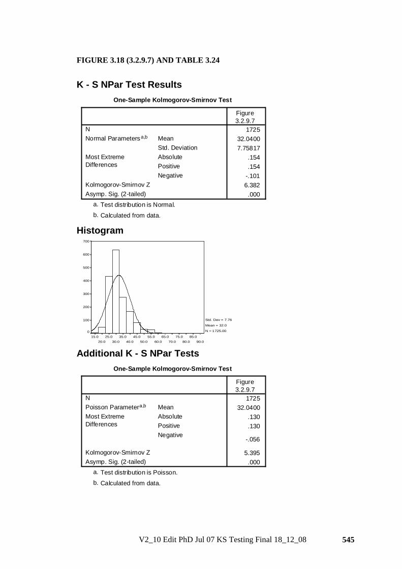
V2_10 Edit PhD Jul 07 KS Testing Final 18_12_08 545
FIGURE 3.18 (3.2.9.7) AND TABLE 3.24
K - S NPar Test Results
One-Sample Kolmogorov-Smirnov Test
172532.04007.75817
.154
.154-.1016.382
.000
NMeanStd. Deviation
Normal Parametersa,b
AbsolutePositiveNegative
Most ExtremeDifferences
Kolmogorov-Smirnov ZAsymp. Sig. (2-tailed)
Figure3.2.9.7
Test distribution is Normal.a.
Calculated from data.b.
Histogram
90.085.0
80.075.0
70.065.0
60.055.0
50.045.0
40.035.0
30.025.0
20.015.0
700
600
500
400
300
200
100
0
Std. Dev = 7.76
Mean = 32.0
N = 1725.00
Additional K - S NPar Tests
One-Sample Kolmogorov-Smirnov Test
172532.0400
.130
.130
-.056
5.395.000
NMeanPoisson Parametera,b
AbsolutePositiveNegative
Most ExtremeDifferences
Kolmogorov-Smirnov ZAsymp. Sig. (2-tailed)
Figure3.2.9.7
Test distribution is Poisson.a.
Calculated from data.b.
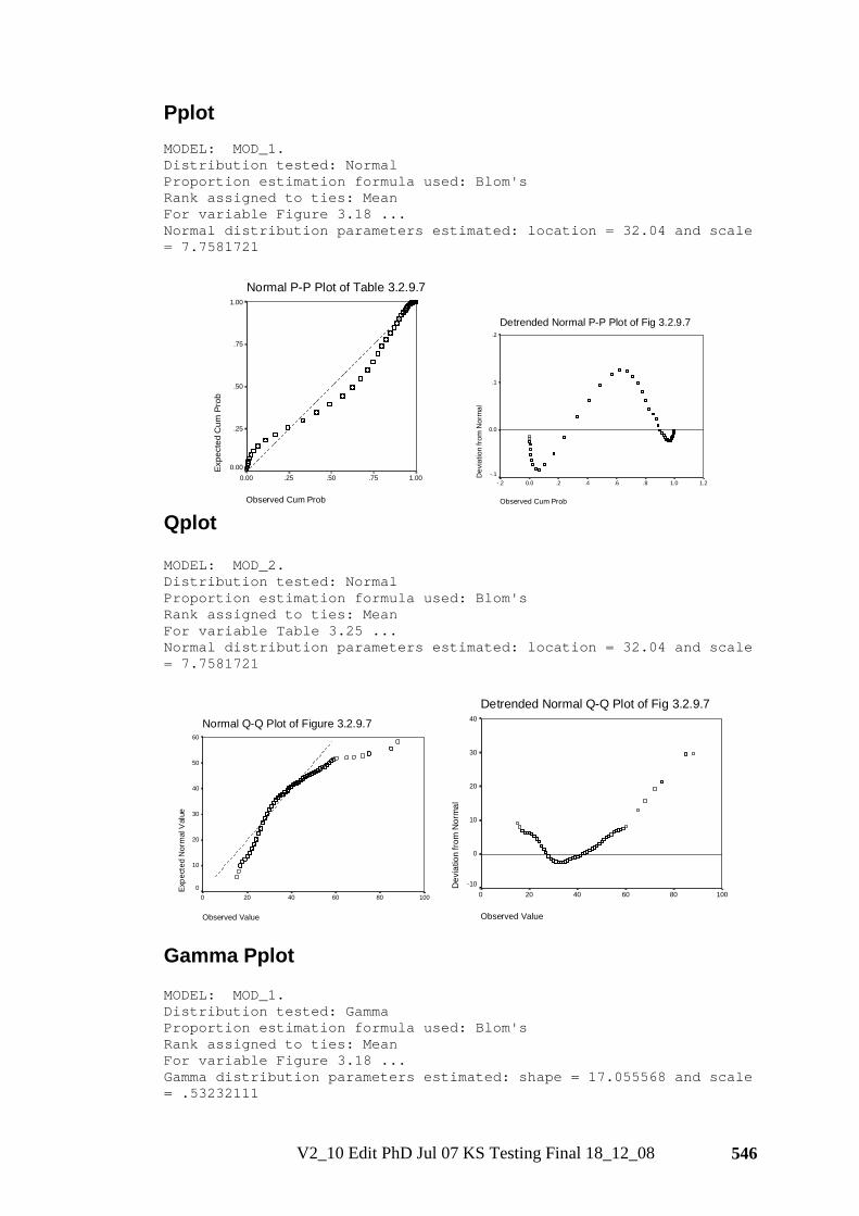
V2_10 Edit PhD Jul 07 KS Testing Final 18_12_08 546
Pplot MODEL: MOD_1. Distribution tested: Normal Proportion estimation formula used: Blom's Rank assigned to ties: Mean For variable Figure 3.18 ... Normal distribution parameters estimated: location = 32.04 and scale = 7.7581721
Normal P-P Plot of Table 3.2.9.7
Observed Cum Prob
1.00.75.50.250.00
Expe
cted
Cum
Pro
b
1.00
.75
.50
.25
0.00
Detrended Normal P-P Plot of Fig 3.2.9.7
Observed Cum Prob
1.21.0.8.6.4.20.0-.2D
evia
tion
from
Nor
mal
.2
.1
0.0
-.1
Qplot MODEL: MOD_2. Distribution tested: Normal Proportion estimation formula used: Blom's Rank assigned to ties: Mean For variable Table 3.25 ... Normal distribution parameters estimated: location = 32.04 and scale = 7.7581721
Normal Q-Q Plot of Figure 3.2.9.7
Observed Value
100806040200
Expe
cted
Nor
mal
Val
ue
60
50
40
30
20
10
0
Detrended Normal Q-Q Plot of Fig 3.2.9.7
Observed Value
100806040200
Dev
iatio
n fro
m N
orm
al
40
30
20
10
0
-10
Gamma Pplot MODEL: MOD_1. Distribution tested: Gamma Proportion estimation formula used: Blom's Rank assigned to ties: Mean For variable Figure 3.18 ... Gamma distribution parameters estimated: shape = 17.055568 and scale = .53232111
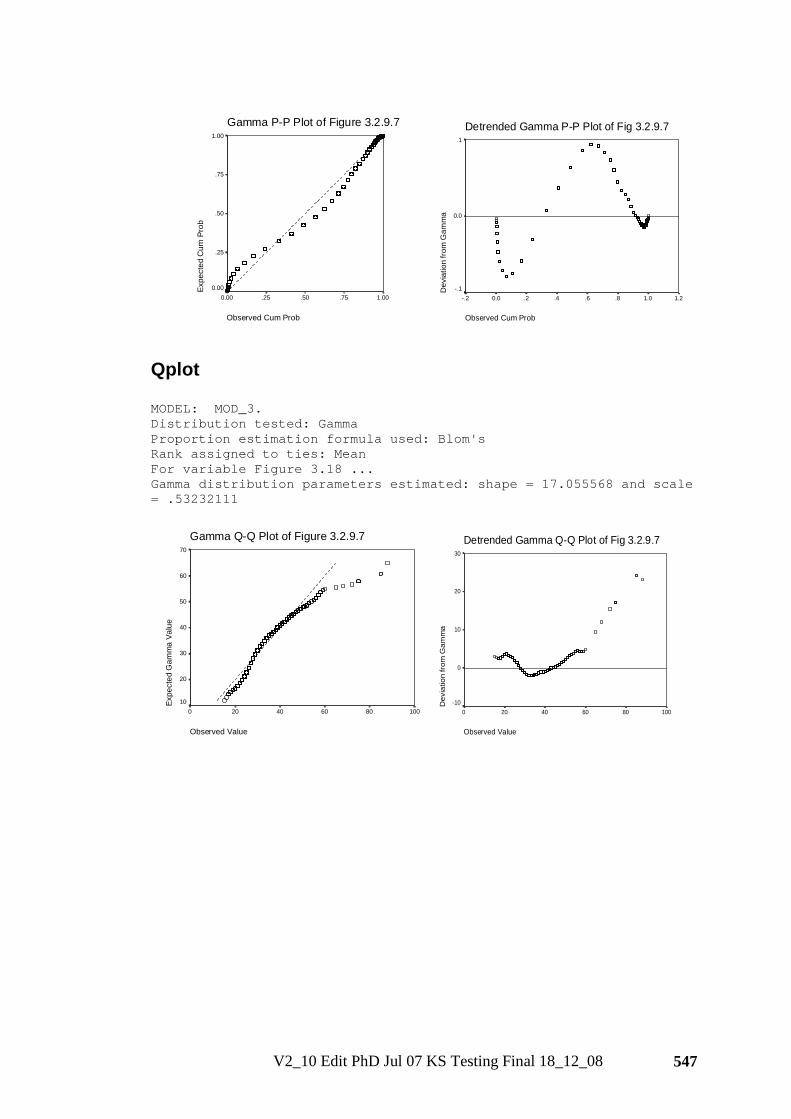
V2_10 Edit PhD Jul 07 KS Testing Final 18_12_08 547
Gamma P-P Plot of Figure 3.2.9.7
Observed Cum Prob
1.00.75.50.250.00
Expe
cted
Cum
Pro
b
1.00
.75
.50
.25
0.00
Detrended Gamma P-P Plot of Fig 3.2.9.7
Observed Cum Prob
1.21.0.8.6.4.20.0-.2
Dev
iatio
n fro
m G
amm
a
.1
0.0
-.1
Qplot MODEL: MOD_3. Distribution tested: Gamma Proportion estimation formula used: Blom's Rank assigned to ties: Mean For variable Figure 3.18 ... Gamma distribution parameters estimated: shape = 17.055568 and scale = .53232111
Gamma Q-Q Plot of Figure 3.2.9.7
Observed Value
100806040200
Expe
cted
Gam
ma
Valu
e
70
60
50
40
30
20
10
Detrended Gamma Q-Q Plot of Fig 3.2.9.7
Observed Value
100806040200
Dev
iatio
n fr
om G
amm
a
30
20
10
0
-10
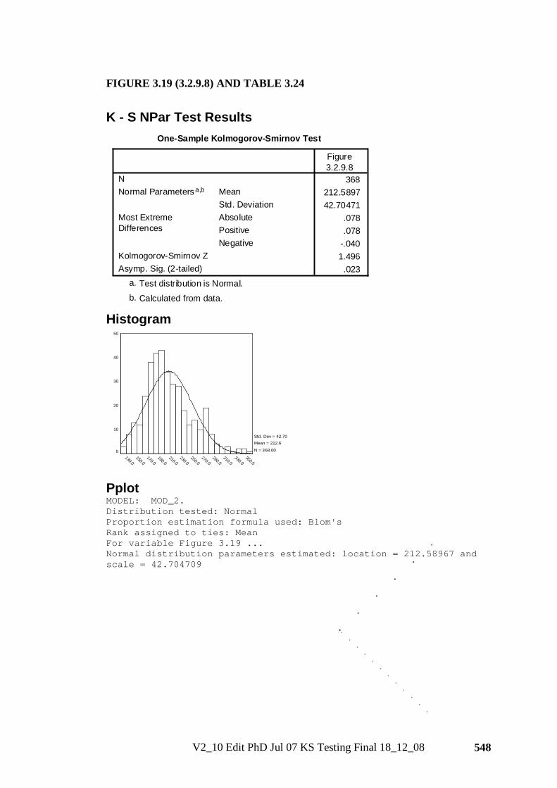
V2_10 Edit PhD Jul 07 KS Testing Final 18_12_08 548
FIGURE 3.19 (3.2.9.8) AND TABLE 3.24
K - S NPar Test Results
One-Sample Kolmogorov-Smirnov Test
368212.589742.70471
.078
.078-.0401.496
.023
NMeanStd. Deviation
Normal Parametersa,b
AbsolutePositiveNegative
Most ExtremeDifferences
Kolmogorov-Smirnov ZAsymp. Sig. (2-tailed)
Figure3.2.9.8
Test distribution is Normal.a.
Calculated from data.b.
Histogram
350.0330.0
310.0290.0
270.0250.0
230.0210.0
190.0170.0
150.0130.0
50
40
30
20
10
0
Std. Dev = 42.70 Mean = 212.6
N = 368.00
Pplot MODEL: MOD_2. Distribution tested: Normal Proportion estimation formula used: Blom's Rank assigned to ties: Mean For variable Figure 3.19 ... Normal distribution parameters estimated: location = 212.58967 and scale = 42.704709
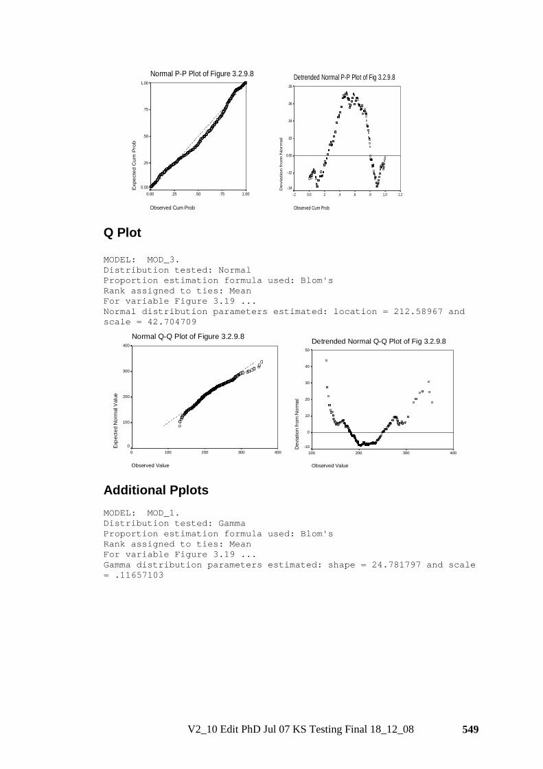
V2_10 Edit PhD Jul 07 KS Testing Final 18_12_08 549
Normal P-P Plot of Figure 3.2.9.8
Observed Cum Prob
1.00.75.50.250.00
Exp
ecte
d C
um P
rob
1.00
.75
.50
.25
0.00
Detrended Normal P-P Plot of Fig 3.2.9.8
Observed Cum Prob
1.21.0.8.6.4.20.0-.2
De
via
tio
n f
rom
No
rma
l
.08
.06
.04
.02
0.00
-.02
-.04
Q Plot MODEL: MOD_3. Distribution tested: Normal Proportion estimation formula used: Blom's Rank assigned to ties: Mean For variable Figure 3.19 ... Normal distribution parameters estimated: location = 212.58967 and scale = 42.704709
Normal Q-Q Plot of Figure 3.2.9.8
Observed Value
4003002001000
Expe
cted
Nor
mal
Val
ue
400
300
200
100
0
Detrended Normal Q-Q Plot of Fig 3.2.9.8
Observed Value
400300200100
Dev
iatio
n fro
m N
orm
al
50
40
30
20
10
0
-10
Additional Pplots MODEL: MOD_1. Distribution tested: Gamma Proportion estimation formula used: Blom's Rank assigned to ties: Mean For variable Figure 3.19 ... Gamma distribution parameters estimated: shape = 24.781797 and scale = .11657103
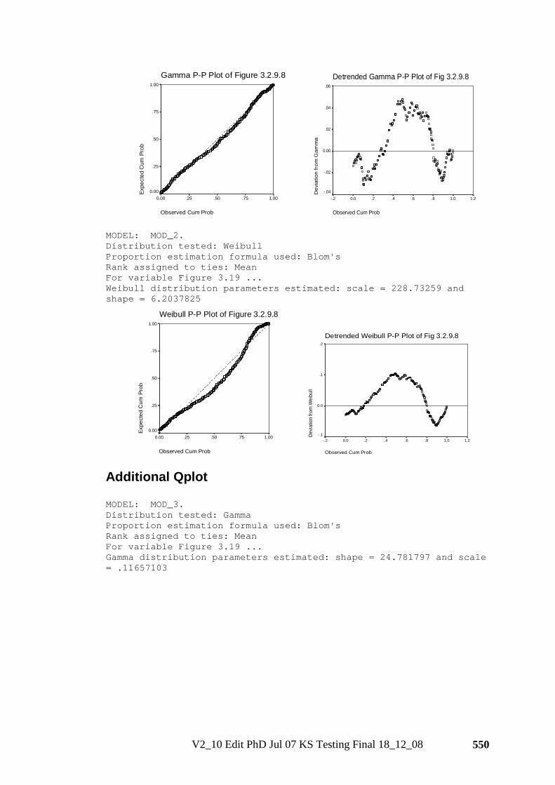
V2_10 Edit PhD Jul 07 KS Testing Final 18_12_08 550
Gamma P-P Plot of Figure 3.2.9.8
Observed Cum Prob
1.00.75.50.250.00
Expe
cted
Cum
Pro
b
1.00
.75
.50
.25
0.00
Detrended Gamma P-P Plot of Fig 3.2.9.8
Observed Cum Prob
1.21.0.8.6.4.20.0-.2
Dev
iatio
n fr
om G
amm
a
.06
.04
.02
0.00
-.02
-.04
MODEL: MOD_2. Distribution tested: Weibull Proportion estimation formula used: Blom's Rank assigned to ties: Mean For variable Figure 3.19 ... Weibull distribution parameters estimated: scale = 228.73259 and shape = 6.2037825
Weibull P-P Plot of Figure 3.2.9.8
Observed Cum Prob
1.00.75.50.250.00
Expe
cted
Cum
Pro
b
1.00
.75
.50
.25
0.00
Detrended Weibull P-P Plot of Fig 3.2.9.8
Observed Cum Prob
1.21.0.8.6.4.20.0-.2
Dev
iatio
n fro
m W
eibu
ll
.2
.1
0.0
-.1
Additional Qplot MODEL: MOD_3. Distribution tested: Gamma Proportion estimation formula used: Blom's Rank assigned to ties: Mean For variable Figure 3.19 ... Gamma distribution parameters estimated: shape = 24.781797 and scale = .11657103
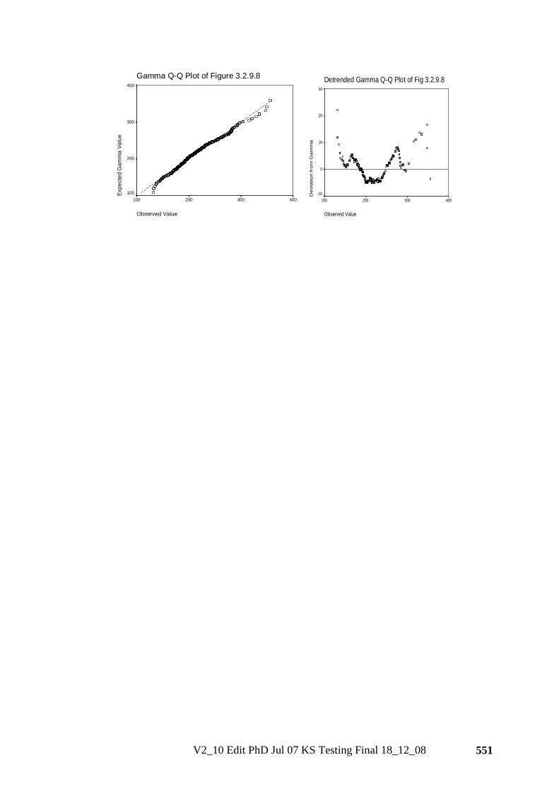
V2_10 Edit PhD Jul 07 KS Testing Final 18_12_08 551
Gamma Q-Q Plot of Figure 3.2.9.8
Observed Value
400300200100
Expe
cted
Gam
ma
Valu
e
400
300
200
100
Detrended Gamma Q-Q Plot of Fig 3.2.9.8
Observed Value
400300200100
De
via
tion
fro
m G
am
ma
30
20
10
0
-10
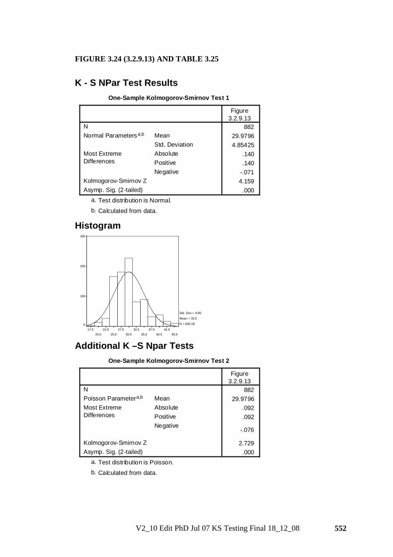
V2_10 Edit PhD Jul 07 KS Testing Final 18_12_08 552
FIGURE 3.24 (3.2.9.13) AND TABLE 3.25
K - S NPar Test Results
One-Sample Kolmogorov-Smirnov Test 1
88229.97964.85425
.140
.140-.0714.159
.000
NMeanStd. Deviation
Normal Parametersa,b
AbsolutePositiveNegative
Most ExtremeDifferences
Kolmogorov-Smirnov ZAsymp. Sig. (2-tailed)
Figure3.2.9.13
Test distribution is Normal.a.
Calculated from data.b.
Histogram
45.042.5
40.037.5
35.032.5
30.027.5
25.022.5
20.017.5
300
200
100
0
Std. Dev = 4.85
Mean = 30.0
N = 882.00
Additional K –S Npar Tests
One-Sample Kolmogorov-Smirnov Test 2
88229.9796
.092
.092
-.076
2.729.000
NMeanPoisson Parametera,b
AbsolutePositiveNegative
Most ExtremeDifferences
Kolmogorov-Smirnov ZAsymp. Sig. (2-tailed)
Figure3.2.9.13
Test distribution is Poisson.a.
Calculated from data.b.
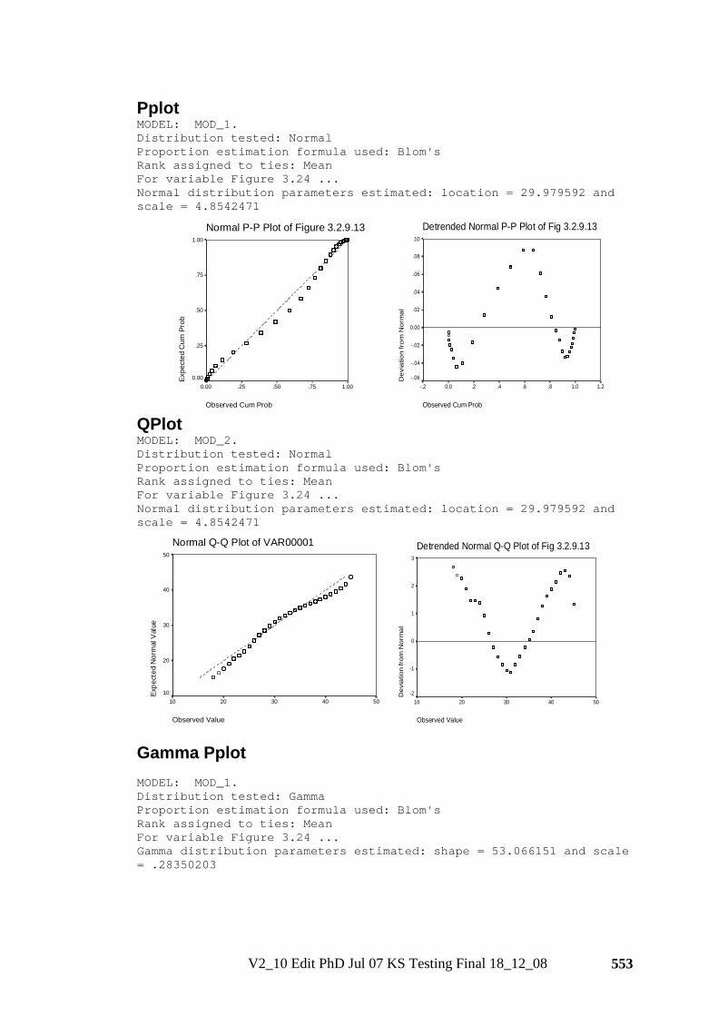
V2_10 Edit PhD Jul 07 KS Testing Final 18_12_08 553
Pplot MODEL: MOD_1. Distribution tested: Normal Proportion estimation formula used: Blom's Rank assigned to ties: Mean For variable Figure 3.24 ... Normal distribution parameters estimated: location = 29.979592 and scale = 4.8542471
Normal P-P Plot of Figure 3.2.9.13
Observed Cum Prob
1.00.75.50.250.00
Expe
cted
Cum
Pro
b
1.00
.75
.50
.25
0.00
Detrended Normal P-P Plot of Fig 3.2.9.13
Observed Cum Prob
1.21.0.8.6.4.20.0-.2
Dev
iatio
n fr
om N
orm
al
.10
.08
.06
.04
.02
0.00
-.02
-.04
-.06
QPlot MODEL: MOD_2. Distribution tested: Normal Proportion estimation formula used: Blom's Rank assigned to ties: Mean For variable Figure 3.24 ... Normal distribution parameters estimated: location = 29.979592 and scale = 4.8542471
Normal Q-Q Plot of VAR00001
Observed Value
5040302010
Expe
cted
Nor
mal
Val
ue
50
40
30
20
10
Detrended Normal Q-Q Plot of Fig 3.2.9.13
Observed Value
5040302010
Dev
iatio
n fr
om N
orm
al
3
2
1
0
-1
-2
Gamma Pplot MODEL: MOD_1. Distribution tested: Gamma Proportion estimation formula used: Blom's Rank assigned to ties: Mean For variable Figure 3.24 ... Gamma distribution parameters estimated: shape = 53.066151 and scale = .28350203
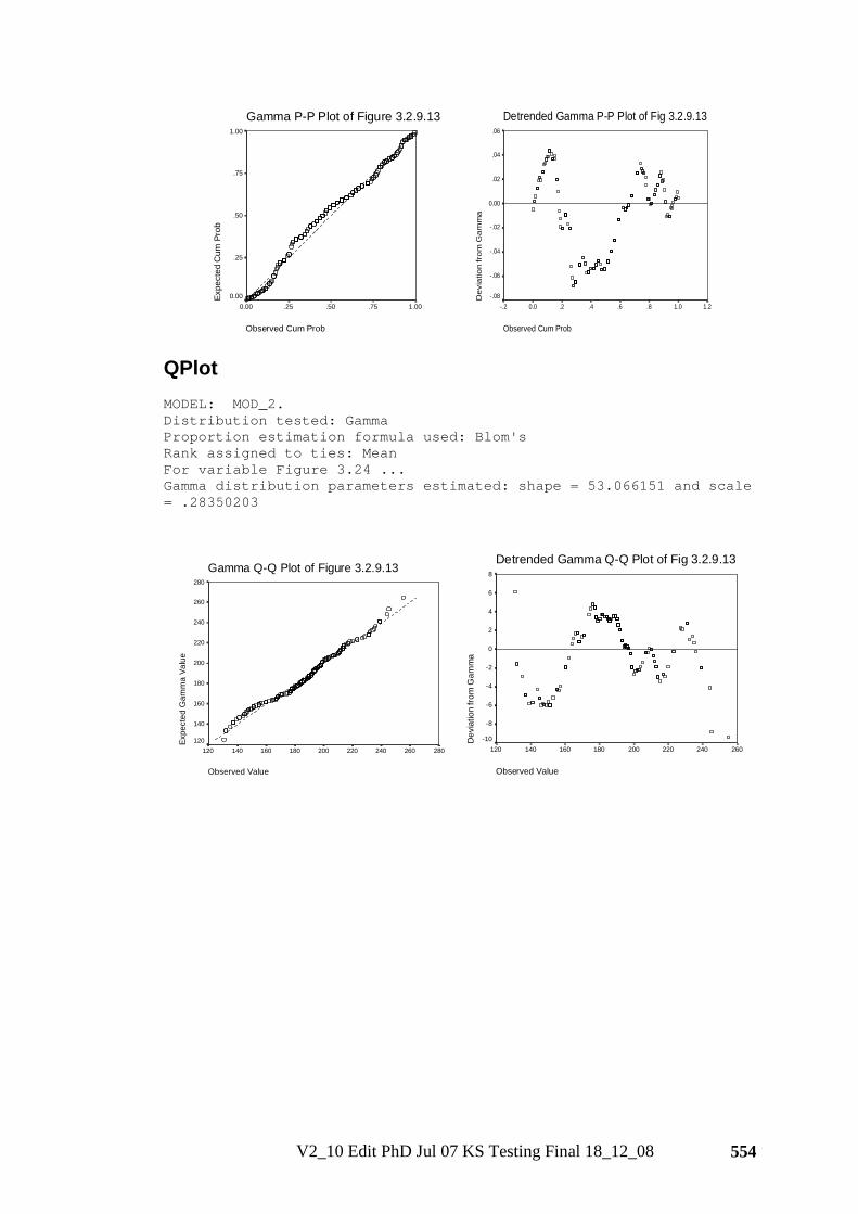
V2_10 Edit PhD Jul 07 KS Testing Final 18_12_08 554
Gamma P-P Plot of Figure 3.2.9.13
Observed Cum Prob
1.00.75.50.250.00
Expe
cted
Cum
Pro
b
1.00
.75
.50
.25
0.00
Detrended Gamma P-P Plot of Fig 3.2.9.13
Observed Cum Prob
1.21.0.8.6.4.20.0-.2
De
via
tion
fro
m G
am
ma
.06
.04
.02
0.00
-.02
-.04
-.06
-.08
QPlot MODEL: MOD_2. Distribution tested: Gamma Proportion estimation formula used: Blom's Rank assigned to ties: Mean For variable Figure 3.24 ... Gamma distribution parameters estimated: shape = 53.066151 and scale = .28350203
Gamma Q-Q Plot of Figure 3.2.9.13
Observed Value
280260240220200180160140120
Expe
cted
Gam
ma
Valu
e
280
260
240
220
200
180
160
140
120
Detrended Gamma Q-Q Plot of Fig 3.2.9.13
Observed Value
260240220200180160140120
Dev
iatio
n fro
m G
amm
a
8
6
4
2
0
-2
-4
-6
-8
-10
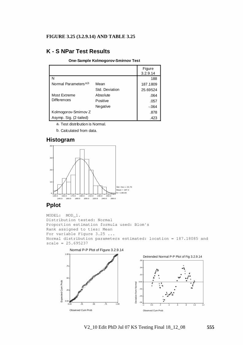
V2_10 Edit PhD Jul 07 KS Testing Final 18_12_08 555
FIGURE 3.25 (3.2.9.14) AND TABLE 3.25
K - S NPar Test Results
One-Sample Kolmogorov-Smirnov Test
188187.180925.69524
.064
.057-.064.878.423
NMeanStd. Deviation
Normal Parametersa,b
AbsolutePositiveNegative
Most ExtremeDifferences
Kolmogorov-Smirnov ZAsymp. Sig. (2-tailed)
Figure3.2.9.14
Test distribution is Normal.a.
Calculated from data.b.
Histogram
260.0250.0
240.0230.0
220.0210.0
200.0190.0
180.0170.0
160.0150.0
140.0130.0
40
30
20
10
0
Std. Dev = 25.70
Mean = 187.2
N = 188.00
Pplot MODEL: MOD_1. Distribution tested: Normal Proportion estimation formula used: Blom's Rank assigned to ties: Mean For variable Figure 3.25 ... Normal distribution parameters estimated: location = 187.18085 and scale = 25.695237
Normal P-P Plot of Figure 3.2.9.14
Observed Cum Prob
1.00.75.50.250.00
Expe
cted
Cum
Pro
b
1.00
.75
.50
.25
0.00
Detrended Normal P-P Plot of Fig 3.2.9.14
Observed Cum Prob
1.21.0.8.6.4.20.0-.2
Dev
iatio
n fro
m N
orm
al
.06
.04
.02
0.00
-.02
-.04
-.06
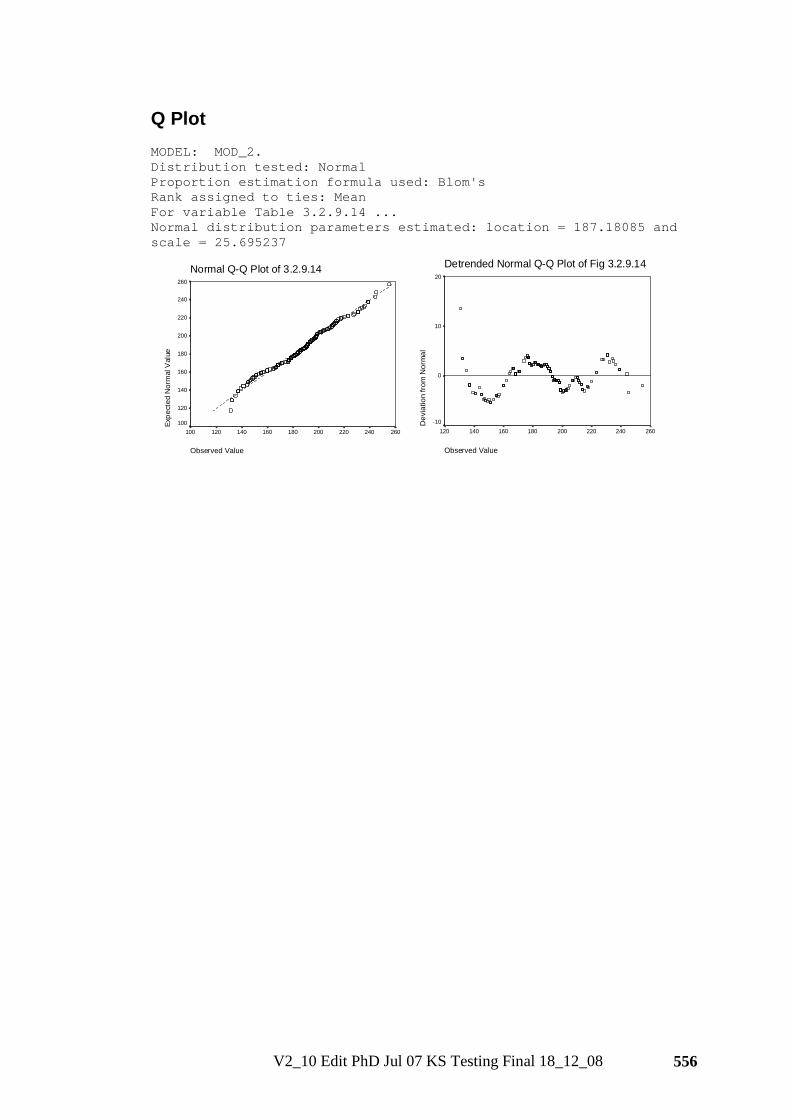
V2_10 Edit PhD Jul 07 KS Testing Final 18_12_08 556
Q Plot MODEL: MOD_2. Distribution tested: Normal Proportion estimation formula used: Blom's Rank assigned to ties: Mean For variable Table 3.2.9.14 ... Normal distribution parameters estimated: location = 187.18085 and scale = 25.695237
Normal Q-Q Plot of 3.2.9.14
Observed Value
260240220200180160140120100
Expe
cted
Nor
mal
Val
ue
260
240
220
200
180
160
140
120
100
Detrended Normal Q-Q Plot of Fig 3.2.9.14
Observed Value
260240220200180160140120D
evia
tion
from
Nor
mal
20
10
0
-10
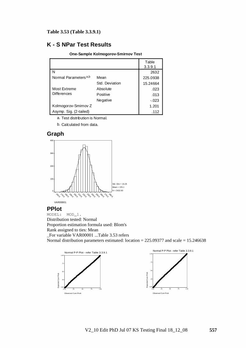
V2_10 Edit PhD Jul 07 KS Testing Final 18_12_08 557
Table 3.53 (Table 3.3.9.1) K - S NPar Test Results
One-Sample Kolmogorov-Smirnov Test
2632225.093815.24664
.023
.013-.0231.201
.112
NMeanStd. Deviation
Normal Parametersa,b
AbsolutePositiveNegative
Most ExtremeDifferences
Kolmogorov-Smirnov ZAsymp. Sig. (2-tailed)
Table3.3.9.1
Test distribution is Normal.a.
Calculated from data.b.
Graph
VAR00001
280.0270.0
260.0250.0
240.0230.0
220.0210.0
200.0190.0
180.0170.0
160.0
400
300
200
100
0
Std. Dev = 15.25 Mean = 225.1
N = 2632.00
PPlot MODEL: MOD_1. Distribution tested: Normal Proportion estimation formula used: Blom's Rank assigned to ties: Mean _For variable VAR00001 ...Table 3.53 refers Normal distribution parameters estimated: location = 225.09377 and scale = 15.246638
Normal P-P Plot - refer Table 3.3.9.1
Observed Cum Prob
1.00.75.50.250.00
Expe
cted
Cum
Pro
b
1.00
.75
.50
.25
0.00
Normal P-P Plot - refer Table 3.3.9.1
Observed Cum Prob
1.00.75.50.250.00
Expe
cted
Cum
Pro
b
1.00
.75
.50
.25
0.00
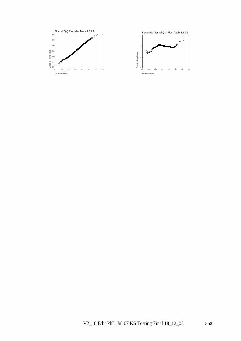
V2_10 Edit PhD Jul 07 KS Testing Final 18_12_08 558
Normal Q-Q Plot refer Table 3.3.9.1
Observed Value
300280260240220200180160
Expe
cted
Nor
mal
Val
ue
280
260
240
220
200
180
160
Detrended Normal Q-Q Plot - Table 3.3.9.1
Observed Value
300280260240220200180160
Dev
iatio
n fro
m N
orm
al
10
0
-10
-20