Embed Size (px)
Citation preview
High Low
tropopause
z
x
ziz
Adapted from Meteorology for Scientists and Engineers, A TechnicalCompanion Book to C. Donald Ahrens' Meteorology Today, 2nd Ed., byStull, p. 69. Copyright 2000. Reprinted with permission of Brooks/
Cole, a division of Thomson Learning: www.thomsonrights.com.Fax 800-730-2215.
Stormy Weather
406 The Atmospheric Boundary Layer
Anabatic and katabatic flows are examples ofa broader class of diurnally varying thermallydriven circulations, which also include land and seabreezes described in the next subsection.Horizontal temperature gradients caused by differ-ential solar heating or longwave cooling cause hori-zontal pressure gradients, as described by thehypsometric equation and the thermal wind effect.For example, over sloping terrain during the after-noon, a pressure gradient forms normal to theslope, as illustrated in Fig. 9.32. This pressure-gradient force induces an upslope (anabatic) flowduring daytime, while the increased density ofthe air just above the surface at night induces adownslope (katabatic) flow.
Fig. 9.29 The two dominant mechanisms for boundary-layer air to pass the capping inversion and enter the freeatmosphere. [Courtesy of Roland B. Stull.]
Tropopausez
x
y
Venting bythunderstorms
Ventingby fronts
frontal inversion
warm aircoldair
BL
frontalzone
zi
clouds
zi
BL
clouds
tropopause
Hei
ght,
z
Fig. 9.30 Vertical cross section illustrating the destruction ofthe capping inversion zi and venting of boundary layer (BL) airnear frontal zones, and subsequent reestablishment of the cap-ping inversion under the frontal inversion after cold frontal pas-sage. [Adapted from Meteorology for Scientists and Engineers, ATechnical Companion Book to C. Donald Ahrens’ MeteorologyToday, 2nd Ed., by Stull, p. 69. Copyright 2000. Reprinted withpermission of Brooks/Cole, a division of Thomon Learning:www.thomsonrights.com. Fax 800-730-2215.]
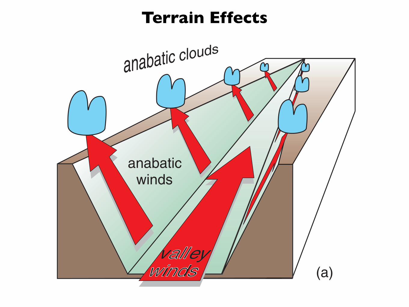
vallalleywindswinds
anabaticwinds
(a)
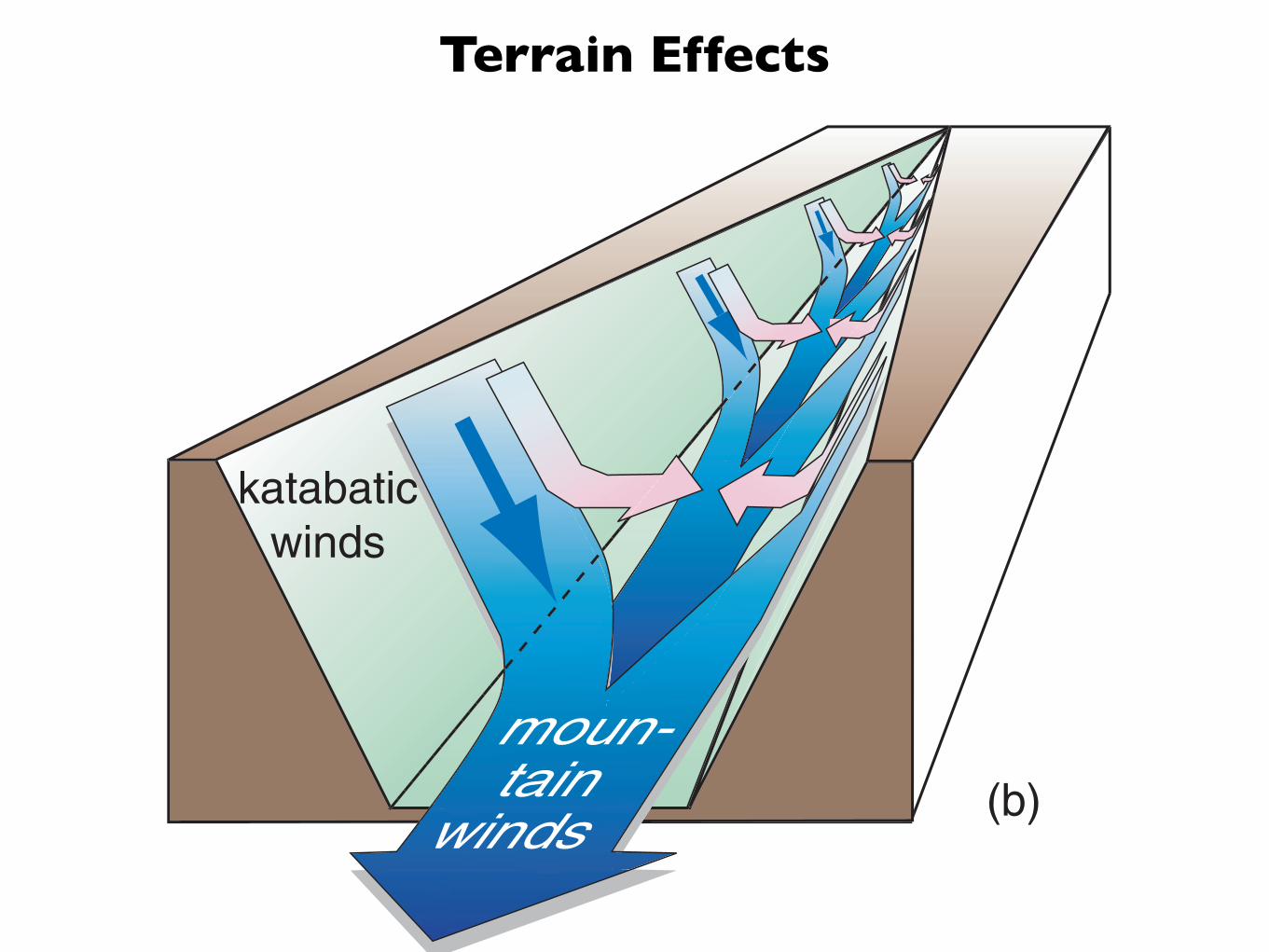
moun-tain
winds
katabaticwinds
(b)
Fig. 9.31 (a) Daytime conditions of anabatic (warm upslope)winds along the valley walls, and associated valley winds alongthe valley floor. (b) Nighttime conditions of katabatic (colddownslope) winds along the valley walls, and associated moun-tain winds draining down the valley floor streambed. [Adaptedfrom R. B. Stull, An Introduction to Boundary Layer Meteorology,Kluwer, Academic Publishers, Dordrecht, The Netherlands, 1988,Fig. 14.5, p. 592, Copyright 1988 Kluwer Academic Publishers,with kind permission of Springer Science and Business Media.]
top of boundary layer
High Low
subsidence
updr
afts
divergence convergence
tropopause
z
x
zi
deepclouds
Fig. 9.28 Vertical slice through an idealized atmosphereshowing variations in the boundary layer depth zi in cyclonic(low pressure) and anticyclonic (high pressure) weather condi-tions. [Adapted from Meteorology for Scientists and Engineers, ATechnical Companion Book to C. Donald Ahrens’ MeteorologyToday, 2nd Ed., by Stull, p. 69. Copyright 2000. Reprinted withpermission of Brooks/Cole, a division of Thomon Learning:www.thomsonrights.com. Fax 800-730-2215.]
P732951-Ch09.qxd 9/12/05 7:48 PM Page 406
Stormy Weather
n
warm aircoldair
BL
frontalzone
zi
clouds
zi
BL
clouds
tropopause
Hei
ght,
z
Adapted from Meteorology for Scientists and Engineers, ATechnical Companion Book to C. Donald Ahrens' MeteorologyToday, 2nd Ed., by Stull, p. 69. Copyright 2000. Reprinted
with permission of Brooks/Cole, a division of ThomsonLearning: www.thomsonrights.com. Fax 800-730-2215.
Stormy Weather
The Atmospheric Boundary Layer
• Turbulence (9.1)
• The Surface Energy Balance (9.2)
• Vertical Structure (9.3)
• Evolution (9.4)
• Special Effects (9.5)
• The Boundary Layer in Context (9.6)
Diurnal Mountain Winds
Meteorology 3000Mountain Weather and Climate
Spring 2005
C. David Whiteman
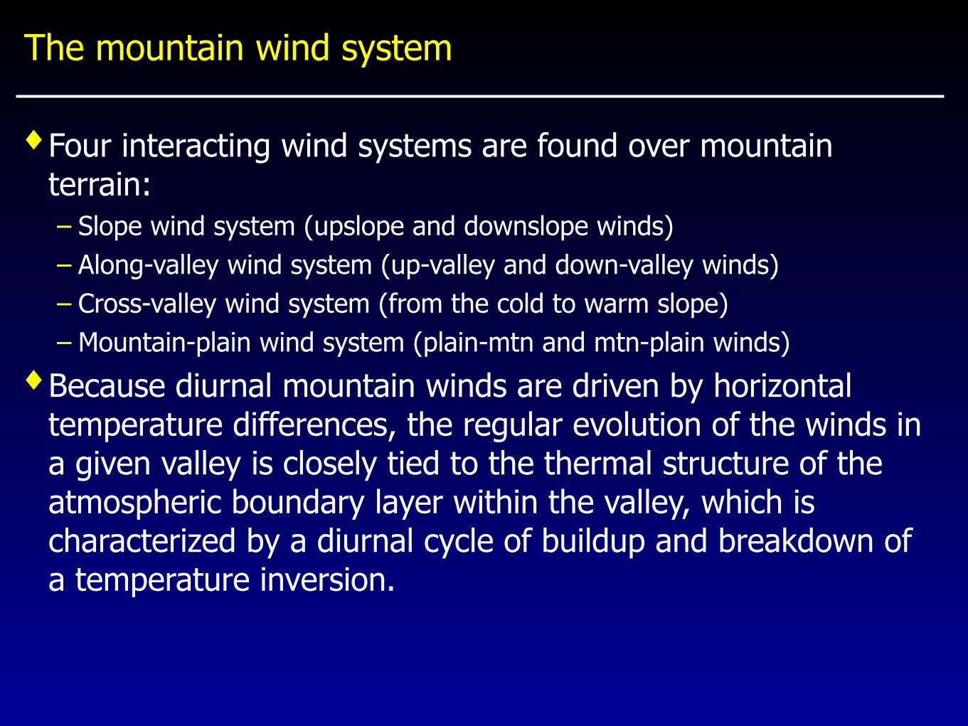
The mountain wind system
♦Four interacting wind systems are found over mountain terrain:– Slope wind system (upslope and downslope winds)– Along-valley wind system (up-valley and down-valley winds)– Cross-valley wind system (from the cold to warm slope)– Mountain-plain wind system (plain-mtn and mtn-plain winds)
♦Because diurnal mountain winds are driven by horizontal temperature differences, the regular evolution of the winds in a given valley is closely tied to the thermal structure of the atmospheric boundary layer within the valley, which is characterized by a diurnal cycle of buildup and breakdown of a temperature inversion.
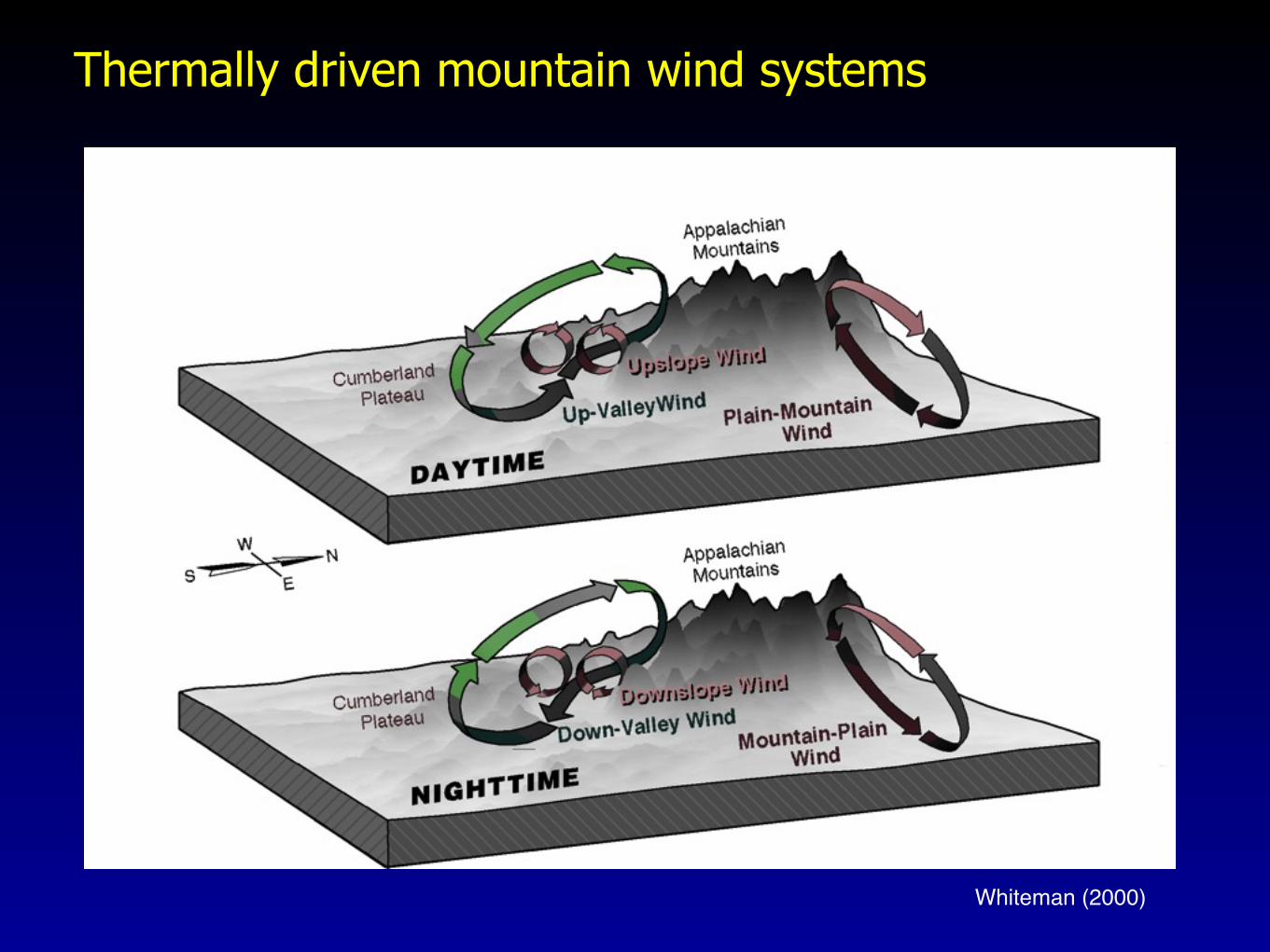
Thermally driven mountain wind systems
Whiteman (2000)
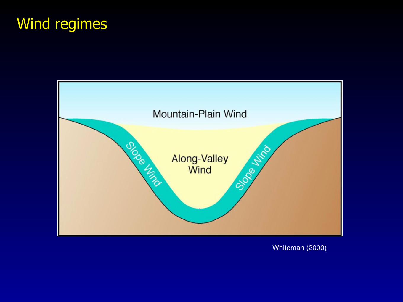
Wind regimes
Whiteman (2000)
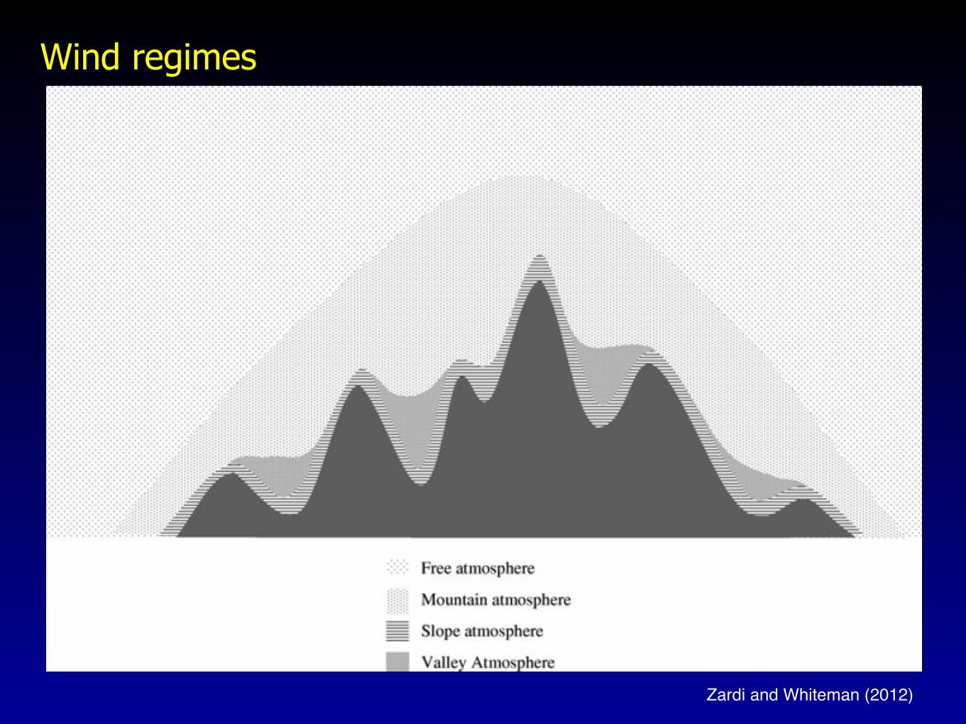
Wind regimes2 Diurnal Mountain Wind Systems 37
Fig. 2.1 Diagram of the structure of the atmosphere above a mountain ridge (Adapted from Ekhart1948, © Societe Meteorologique de France. Used with permission)
winds undergo a reversal to the daytime winds flowing up the terrain. The eveningtransition phase completes the cycle as the inversion rebuilds and the winds onceagain reverse to the nighttime direction.
Diurnal mountain winds are a key feature of the climatology of mountainousregions (Whiteman 1990, 2000; Sturman et al. 1999). In fact, they are so consistentthat they often appear prominently in long-term climatic averages (Martınez et al.2008). They are particularly prevalent in anticyclonic synoptic weather conditionswhere background winds are weak and skies are clear, allowing maximum incomingsolar radiation during daytime and maximum outgoing longwave emission fromthe ground during nighttime. Diurnal wind systems are usually better developed insummer than in winter, because of the stronger day-night heating contrasts. Thelocal wind field patterns and their timing are usually quite similar from day to dayunder anticyclonic weather conditions (see, e.g., Guardans and Palomino 1995). Thecharacteristic diurnal reversal of the slope, valley, and mountain-plain wind systemsis also seen under partly cloudy or wind-disturbed conditions, though it is sometimesweakened by the reduced energy input or modified by winds aloft.
The speed, depth, duration and onset times of diurnal wind systems vary fromplace to place, depending on many factors including terrain characteristics, groundcover, soil moisture, exposure to insolation, local shading and surface energy budget(Zangl 2004). Many of these factors have a strong seasonal dependence. Indeed, theamplitude of horizontal pressure gradients driving valley winds displays appreciableseasonal variations (see e.g. Cogliati and Mazzeo 2005).
Zardi and Whiteman (2012)
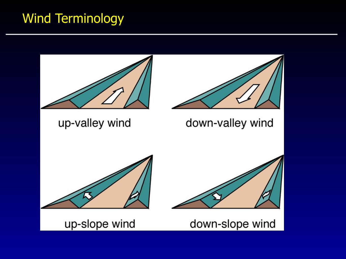
Wind Terminology
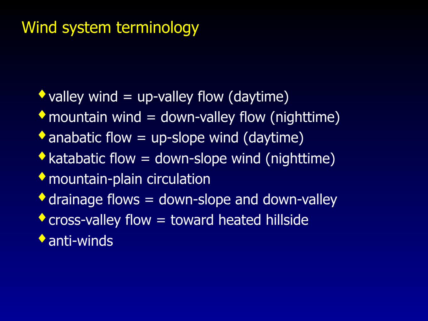
Wind system terminology
♦valley wind = up-valley flow (daytime)♦mountain wind = down-valley flow (nighttime)♦anabatic flow = up-slope wind (daytime)♦katabatic flow = down-slope wind (nighttime)♦mountain-plain circulation♦drainage flows = down-slope and down-valley♦cross-valley flow = toward heated hillside♦anti-winds
Terrain Effects
vallalleywindswinds
anabaticwinds
(a)
moun-tain
winds
katabaticwinds
(b)
Adapted from R. B. Stull, An Introduction to BoundaryLayer Meteorology, Kluwer, Academic Publishers, Dordrecht,The Netherlands, 1988, Fig. 14.5, p. 592, Copyright 1988
Kluwer Academic Publishers, with kind permission ofSpringer Science and Business Media.
Terrain Effectsvallalley
windswinds
anabaticwinds
(a)
moun-tain
winds
katabaticwinds
(b)
Adapted from R. B. Stull, An Introduction to BoundaryLayer Meteorology, Kluwer, Academic Publishers, Dordrecht,The Netherlands, 1988, Fig. 14.5, p. 592, Copyright 1988
Kluwer Academic Publishers, with kind permission ofSpringer Science and Business Media.
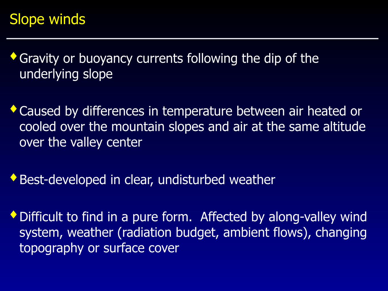
Slope winds
♦Gravity or buoyancy currents following the dip of the underlying slope
♦Caused by differences in temperature between air heated or cooled over the mountain slopes and air at the same altitude over the valley center
♦Best-developed in clear, undisturbed weather
♦Difficult to find in a pure form. Affected by along-valley wind system, weather (radiation budget, ambient flows), changing topography or surface cover
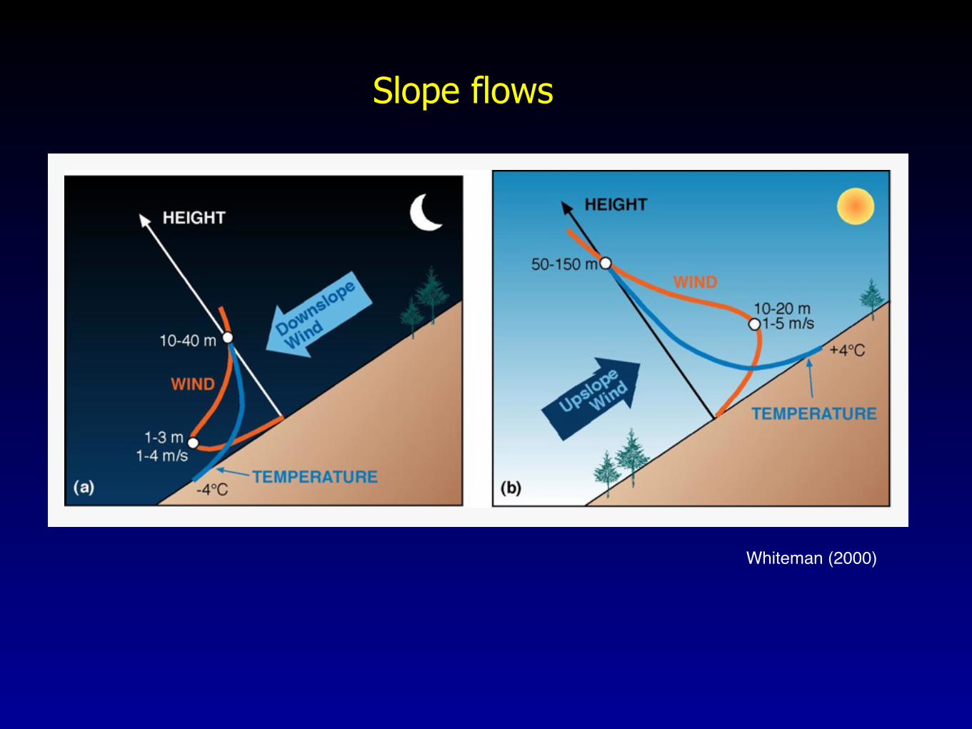
Slope flows
Whiteman (2000)
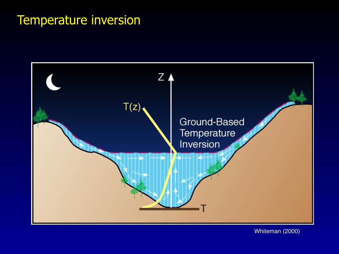
Temperature inversion
Whiteman (2000)
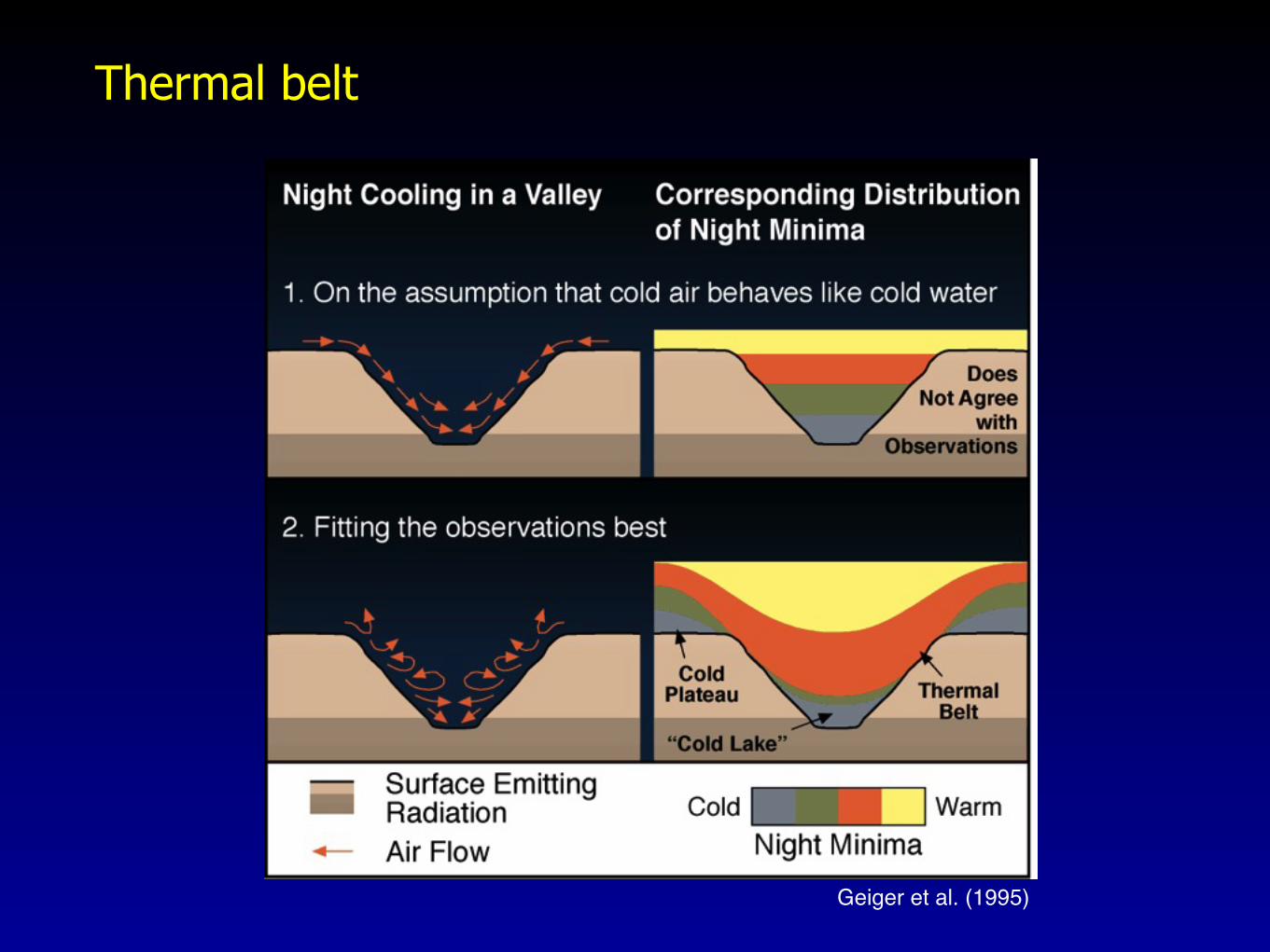
Thermal belt
Geiger et al. (1995)
Valley Winds
♦Air currents trying to equalize horizontal pressure gradients built up hydrostatically between valley and plain
♦Caused by the stronger heating and cooling of the valley atmosphere as compared to the adjacent plain
♦Best-developed in clear undisturbed weather
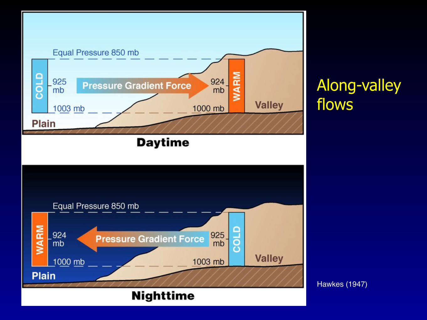
Along-valley flows
Hawkes (1947)
Along-valley flows
Zardi and Whiteman (2012)
64 D. Zardi and C.D. Whiteman
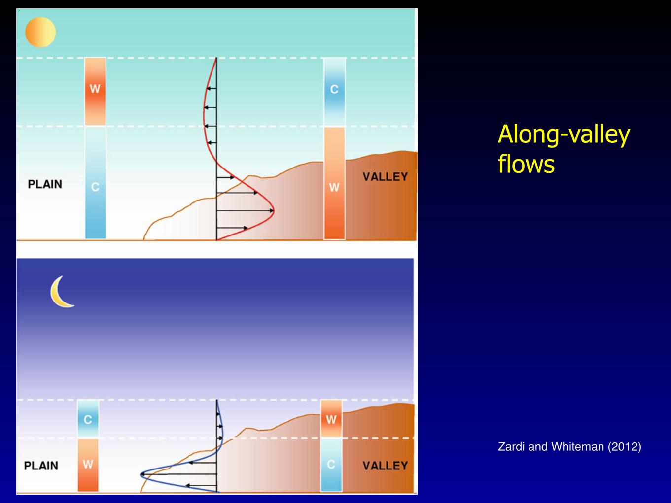
Fig. 2.8 Idealized picture of the development of daytime up-valley winds (upper panel) andnighttime down-valley winds (lower panel) in a valley-plain system with a horizontal floor. The redand blue curves are vertical profiles of the horizontal valley wind component at a location close tothe valley inlet. Two columns of air are shown – one over the valley floor and one above the plain.Red and blue sections of the columns indicate layers where potential temperature is relatively warm(W) or cold (C). The free atmosphere is assumed to be unperturbed by the daily cycle at the topsof the columns (Adapted from Whiteman 2000)
2006). Figure 2.9, for example, compares modeled temperature profiles within avalley and over the adjacent plain to illustrate the reversing temperature gradientswith height that drive the elevated return circulations (from Rampanelli et al. 2004).Investigations by Buettner and Thyer (1966) in valleys that radiate out from theisolated volcano of Mt. Rainier, Washington (USA), found that the upper branchesof the valley circulations there could even be observed within the terrain-confined
Along-valley flows
Zardi and Whiteman (2012)
68 D. Zardi and C.D. Whiteman
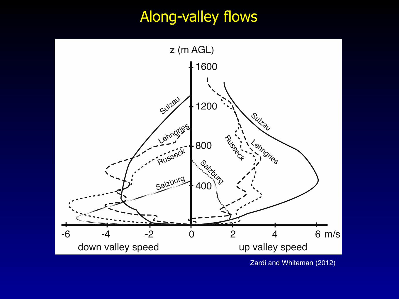
Fig. 2.10 Average up- and down-valley wind profiles from four valleys using all daytime andnighttime data from the locations indicated (Ekhart 1944) (© E. Schweizerbart Science Publisherswww.borntraeger.cramer.de. Used with permission)
model simulations have also shown a divergence of along-valley mass flux inthe daytime up-valley flows for the Inn Valley (Vergeiner 1983; Freytag 1988;Zangl 2004), the Kali Gandaki Valley (Egger et al. 2000; Zangl et al. 2001) andin the Wipp Valley (Rucker et al. 2008). This along-valley mass flux divergenceis somewhat counterintuitive, since one might expect an up-valley flow in themain valley to dissipate with up-valley distance as the flows turn up the slopesand tributaries. Various mechanisms have been invoked to explain the mass fluxdivergence, including compensating subsidence over the main valley, transition tosupercritical flow in the widening part of a valley (possibly favored by gravity wavesproduced by protruding ridges), and intra-valley change in the horizontal pressuregradient induced by differential heating rates.
In different valleys (Fig. 2.10), the vertical structure, strength and duration ofup- and down-valley flows differ, depending on climatic and/or local factors (Ekhart1948; Loffler-Mang et al. 1997). One cannot assume that valleys with strong up-valley flows will also have strong down-valley flows. In the Kali Gandaki valleyof Nepal, the daytime up-valley winds are much stronger than the nocturnal down-valley winds (Egger et al. 2000, 2002). In California’s San Joaquin Valley, the up-valley flows can persist all night (Zhong et al. 2004). In other cases, such as inChile’s Elqui Valley, nocturnal down-valley winds are not observed at all (Kalthoffet al. 2002), while down-valley winds may persist all day in snow-covered valleys(Whiteman 1990).
Down-valley winds are often enhanced where valleys issue onto the adjacentplains or into wider valleys. Drainage flows in the valley decrease in depth,
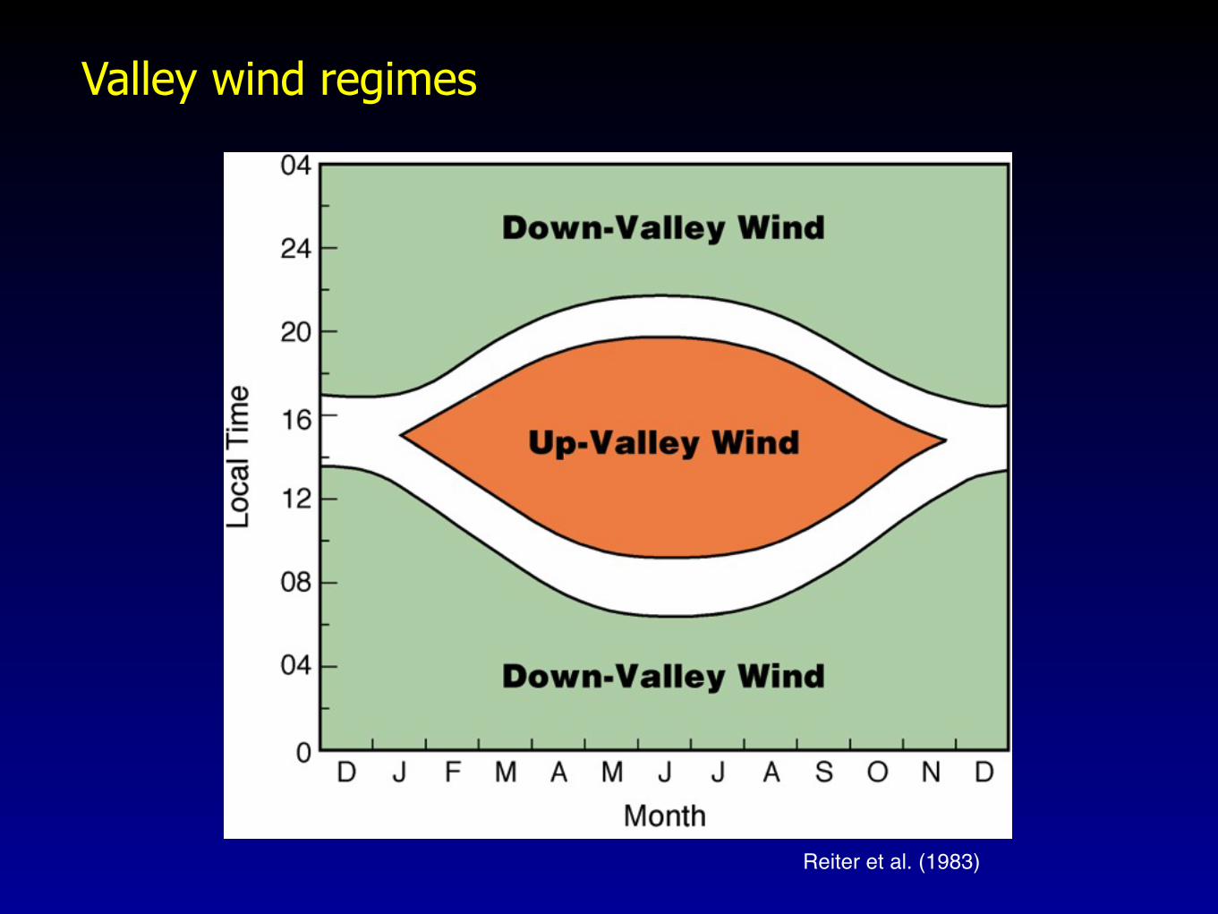
Valley wind regimes
Reiter et al. (1983)
Terrain Effects
!"#$%&' ()* !"# $%&'()* + &',- ./
!"#$%&'()!(*+, -$.('#/0 1&.$#/ !"#$%'()!(*+, %.,!!2., /.*3',#&! '#
4$2#&*'#$2! .,/'$#! *., $-&,# *&&,#3,3 5" * #245,. $- 3'!&'#()
&'6, %7,#$4,#* $# !4*++,. !(*+,!8 '#(+23'#/ !"# $%&'( 91,(&'$# :0;<8)*+&,"%& $"-.( *#3 /.&,%0+/"1 0/*+'(8 +$(*+ *((,+,.*&'$#! $- &7, ='#3$6,. 4$2#&*'# (.,!&!8 2/*03%&! $- +$=)*+&'&23, ='#3!8 +,,)!'3, >0"-%,4?('.(2+*&'$#!8 1*,*1 0/*+'(8 2"&&.1 0/*+'(8 $"3. ,+12+/.&0.8 5"1)"&-*1,.6 (,1..,(8 3$=#!+$%, ='#3 !&$.4!8 *#3 74'1"+/%0 8+)#( 9@'/0A0BB<0 C6,# +$= 7'++! (*# ,D,.& * !2.%.'!'#/+" !&.$#/ '#!2,#(, $#(+$23 %*&&,.#! 9@'/0 A0B;< *#3 %.,('%'&*&'$# *4$2#&!0
!"#$%& '())( E,.&'(*+ (.$!!)!,(&'$# !F,&(7,! $- !$4, $- &7, %7,#$4,#* $5)
!,.6,3 '# 4$2#&*'#! 32.'#/ ='#3" ($#3'&'$#!0 GH3*%&,3 -.$4 I0J0 1&2++8 9&:&,1*'+0,%*& ,* ;*+&'"14 <"4.1 =.,.*1*/*!48 K+2=,.8 L$.3.,(7&8 MA::8 NNN %%0O
8 Wind Flow Models COST 710 WG 4
2.3 Single hill
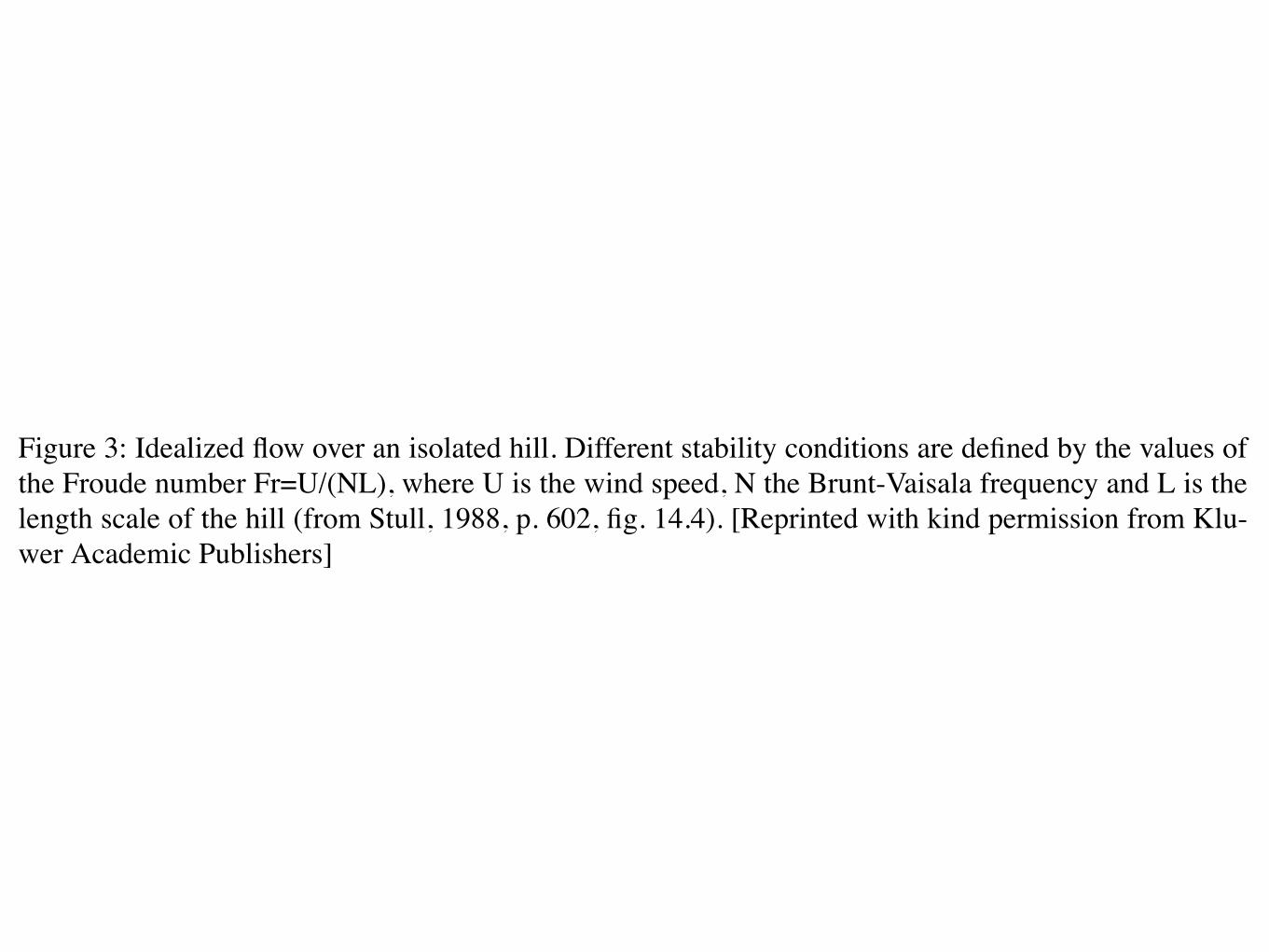
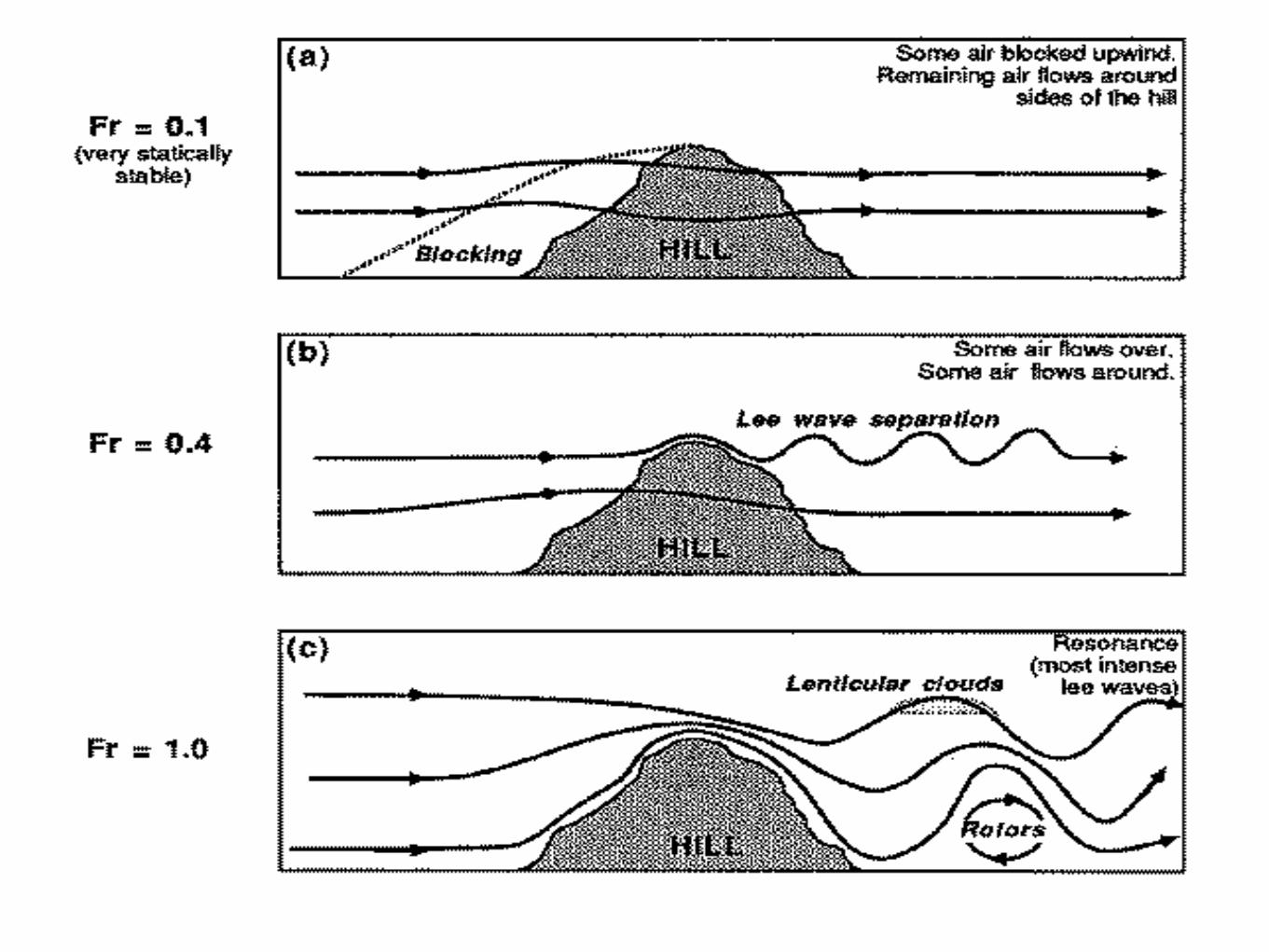
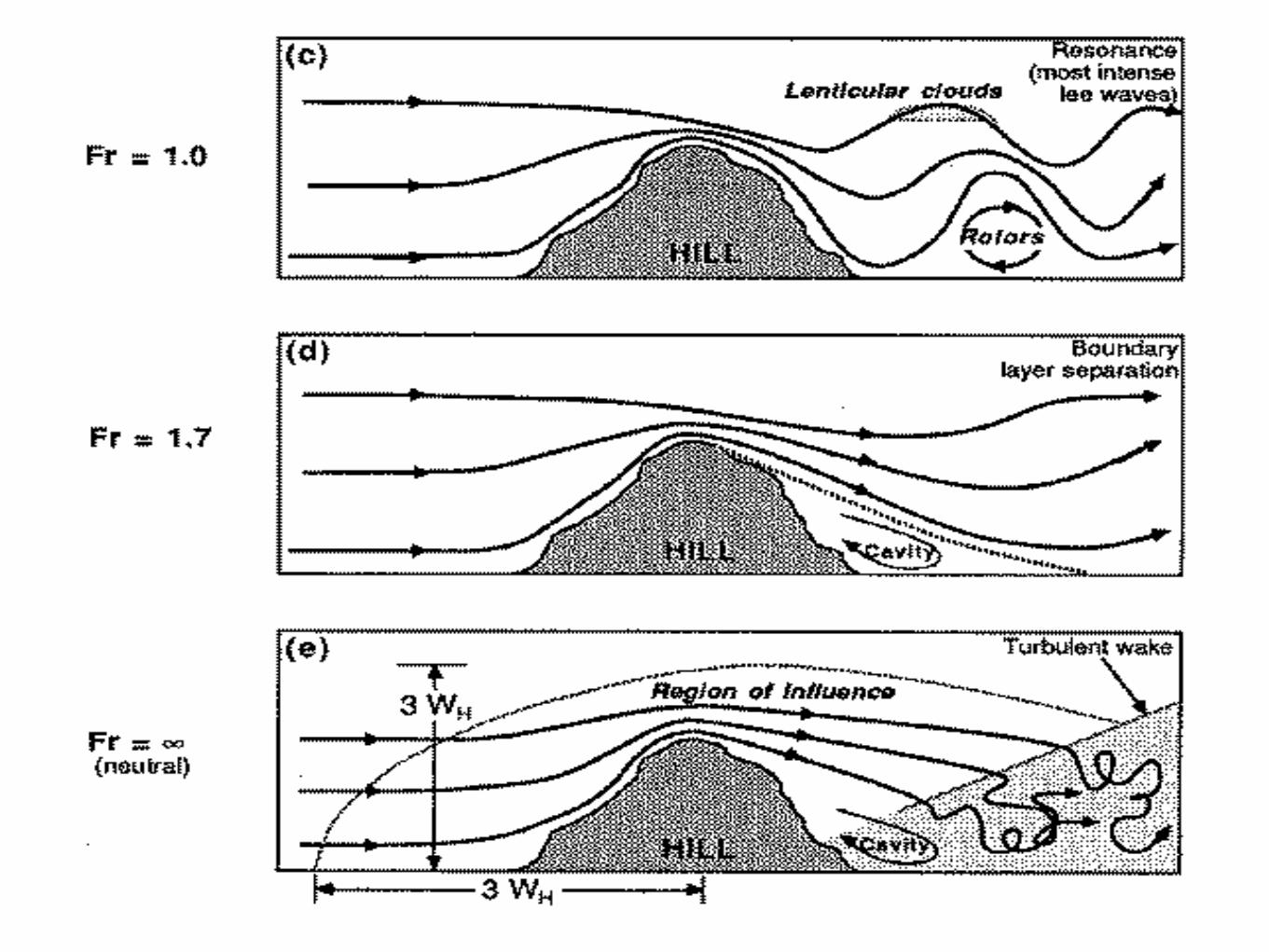
The atmospheric flow over a hill of moderate slope is a complex terrain flow case that has beenthe object of many theoretical and experimental studies during the last 20 years. Experimentalstudies have been performed both in real atmosphere and laboratories (e.g: Khurshudyan et al.,1981; Finnigan et al., 1990; Baskaran et al., 1987, 1991; Mickle et al., 1988; Frank et al., 1993;Walmsley and Taylor, 1996). Jackson and Hunt (1975) and Hunt et al., (1988a, 1988b)represent the most influential theoretical works relating to flow over low hills, in neutral andstable conditions, where the equations of motion can be linearized. The variations induced onturbulent quantities have been investigated in depth by Zeman and Jensen (1987). Thesestudies allowed a satisfactory knowledge to be reached of the modification induced by a singletopographic obstacle, on both mean and turbulent atmospheric variables, in neutral and stableconditions.
Figure 3: Idealized flow over an isolated hill. Different stability conditions are defined by the values ofthe Froude number Fr=U/(NL), where U is the wind speed, N the Brunt-Vaisala frequency and L is thelength scale of the hill (from Stull, 1988, p. 602, fig. 14.4). [Reprinted with kind permission from Klu-wer Academic Publishers]
8 Wind Flow Models COST 710 WG 4
2.3 Single hill
The atmospheric flow over a hill of moderate slope is a complex terrain flow case that has beenthe object of many theoretical and experimental studies during the last 20 years. Experimentalstudies have been performed both in real atmosphere and laboratories (e.g: Khurshudyan et al.,1981; Finnigan et al., 1990; Baskaran et al., 1987, 1991; Mickle et al., 1988; Frank et al., 1993;Walmsley and Taylor, 1996). Jackson and Hunt (1975) and Hunt et al., (1988a, 1988b)represent the most influential theoretical works relating to flow over low hills, in neutral andstable conditions, where the equations of motion can be linearized. The variations induced onturbulent quantities have been investigated in depth by Zeman and Jensen (1987). Thesestudies allowed a satisfactory knowledge to be reached of the modification induced by a singletopographic obstacle, on both mean and turbulent atmospheric variables, in neutral and stableconditions.
Figure 3: Idealized flow over an isolated hill. Different stability conditions are defined by the values ofthe Froude number Fr=U/(NL), where U is the wind speed, N the Brunt-Vaisala frequency and L is thelength scale of the hill (from Stull, 1988, p. 602, fig. 14.4). [Reprinted with kind permission from Klu-wer Academic Publishers]
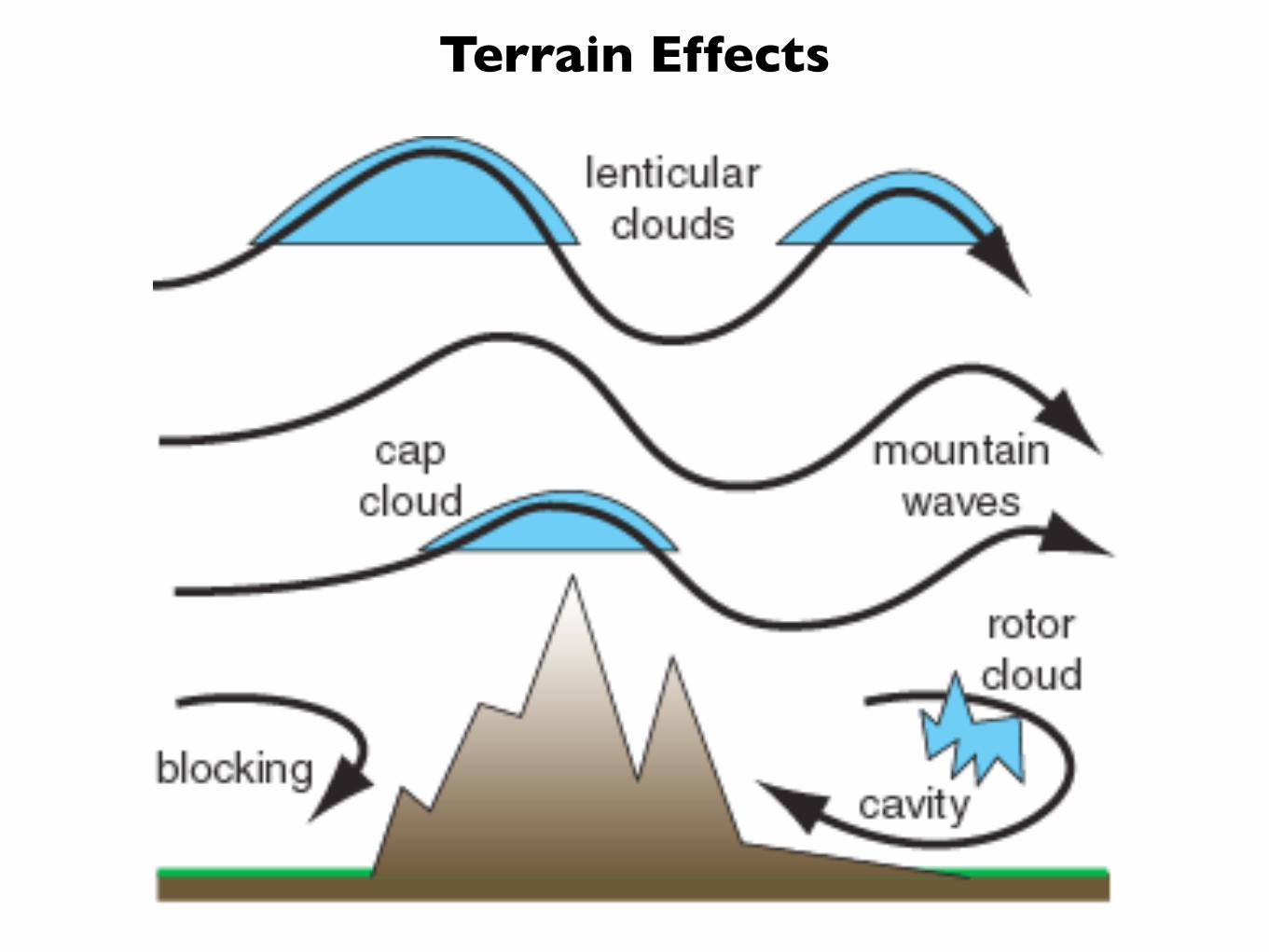
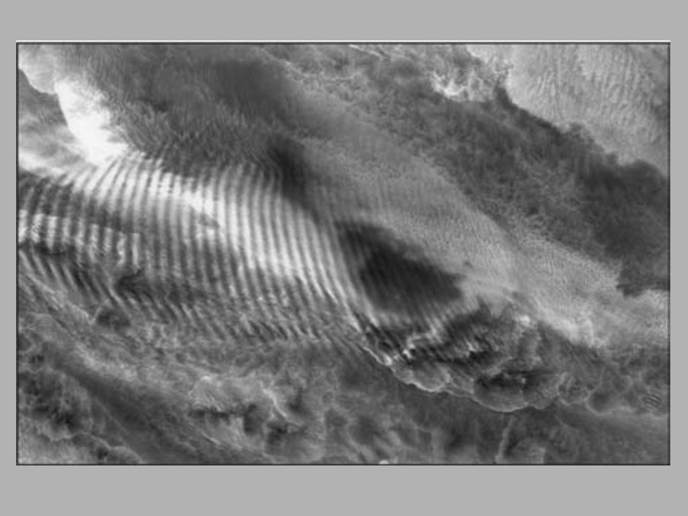
328 MOUNTAIN WAVES AND DOWNSLOPE WINDSTORMS
lenticular clouds
roll clouds
lee wave region
cap cloud
rotor
Figure 12.1 Trapped waves and associated clouds in the lee of a mountain ridge. (Adapted from an image provided bythe Cooperative Program for Operational Meteorology, Education, and Training [COMET].)
The solution for w for each mode is determinedby the Taylor-Goldstein equation (6.36), which can bewritten as
d2w
dz2+
!N2
u2 ! 1
u
d2u
dz2! k2
"w = d2w
dz2+
#!2 ! k2$ w = 0,
(12.2)
where ! =%
N2
u2 ! 1u
d2udz2 is the Scorer parameter. As in
Chapter 6, we obtain fundamentally different solutionsdepending on whether the term in parentheses is positiveor negative (i.e., depending on whether !2 > k2). We shalllook at solutions for several simplified environments.
12.1.1 Series of ridges with constantzonal wind and static stability
In our first simplified scenario, we consider a series ofridges separated by a distance Lx that defines a particularwavenumber k = 2"/Lx of the terrain. We assume that theenvironmental wind is zonal with a constant speed, u0,and the static stability is constant such that N is constant.Under these conditions, !2 ! k2 reduces to N2/u2
0 ! k2 andis constant, so the solution to (12.1), using (12.2), can beexpressed
w" = Aei(kx+mz) + Bei(kx!mz), (12.3)

90 Atmospheric Thermodynamics
mountainous terrain, as shown in the top photographin Fig. 3.14 or by an intense local disturbance, asshown in the bottom photograph. The following exer-cise illustrates how buoyancy oscillations can beexcited by flow over a mountain range.
Exercise 3.13 A layer of unsaturated air flows overmountainous terrain in which the ridges are 10 kmapart in the direction of the flow. The lapse rate is 5 °Ckm!1 and the temperature is 20 °C. For what value ofthe wind speed U will the period of the orographic(i.e., terrain-induced) forcing match the period of abuoyancy oscillation?
Solution: For the period " of the orographic forcingto match the period of the buoyancy oscillation, it isrequired that
where L is the spacing between the ridges. Hence,from this last expression and (3.75),
or, in SI units,
!
Layers of air with negative lapse rates (i.e., tempera-tures increasing with height) are called inversions. Itis clear from the aforementioned discussion thatthese layers are marked by very strong static stabil-ity. A low-level inversion can act as a “lid” that trapspollution-laden air beneath it (Fig. 3.15). The layeredstructure of the stratosphere derives from the factthat it represents an inversion in the vertical temper-ature profile.
If # $ #d (Fig. 3.12b), a parcel of unsaturated airdisplaced upward from O will arrive at A with a tem-perature greater than that of its environment.Therefore, it will be less dense than the ambient air
! 20 m s!1
U %104
2& "9.8
293 #(9.8 ! 5.0) ' 10!3$%1/2
U %LN2&
%L2&
"!T
(#d ! #)%1/2
" %LU
%2&
N
Fig. 3.14 Gravity waves, as revealed by cloud patterns.The upper photograph, based on NOAA GOES 8 visiblesatellite imagery, shows a wave pattern in west to east(right to left) airflow over the north–south-oriented moun-tain ranges of the Appalachians in the northeastern UnitedStates. The waves are transverse to the flow and their hori-zontal wavelength is &20 km. The atmospheric wave pat-tern is more regular and widespread than the undulationsin the terrain. The bottom photograph, based on imageryfrom NASA’s multiangle imaging spectro-radiometer(MISR), shows an even more regular wave pattern in a thinlayer of clouds over the Indian Ocean.
Fig. 3.15 Looking down onto widespread haze over south-ern Africa during the biomass-burning season. The haze isconfined below a temperature inversion. Above the inversion,the air is remarkably clean and the visibility is excellent.(Photo: P. V. Hobbs.)
P732951-Ch03.qxd 9/12/05 7:41 PM Page 90
Terrain Effects
!"#$%&' ()* !"# $%&'()* + &',- ./
!"#$%&'()!(*+, -$.('#/0 1&.$#/ !"#$%'()!(*+, %.,!!2., /.*3',#&! '#
4$2#&*'#$2! .,/'$#! *., $-&,# *&&,#3,3 5" * #245,. $- 3'!&'#()
&'6, %7,#$4,#* $# !4*++,. !(*+,!8 '#(+23'#/ !"# $%&'( 91,(&'$# :0;<8)*+&,"%& $"-.( *#3 /.&,%0+/"1 0/*+'(8 +$(*+ *((,+,.*&'$#! $- &7, ='#3$6,. 4$2#&*'# (.,!&!8 2/*03%&! $- +$=)*+&'&23, ='#3!8 +,,)!'3, >0"-%,4?('.(2+*&'$#!8 1*,*1 0/*+'(8 2"&&.1 0/*+'(8 $"3. ,+12+/.&0.8 5"1)"&-*1,.6 (,1..,(8 3$=#!+$%, ='#3 !&$.4!8 *#3 74'1"+/%0 8+)#( 9@'/0A0BB<0 C6,# +$= 7'++! (*# ,D,.& * !2.%.'!'#/+" !&.$#/ '#!2,#(, $#(+$23 %*&&,.#! 9@'/0 A0B;< *#3 %.,('%'&*&'$# *4$2#&!0
!"#$%& '())( E,.&'(*+ (.$!!)!,(&'$# !F,&(7,! $- !$4, $- &7, %7,#$4,#* $5)
!,.6,3 '# 4$2#&*'#! 32.'#/ ='#3" ($#3'&'$#!0 GH3*%&,3 -.$4 I0J0 1&2++8 9&:&,1*'+0,%*& ,* ;*+&'"14 <"4.1 =.,.*1*/*!48 K+2=,.8 L$.3.,(7&8 MA::8 NNN %%0O
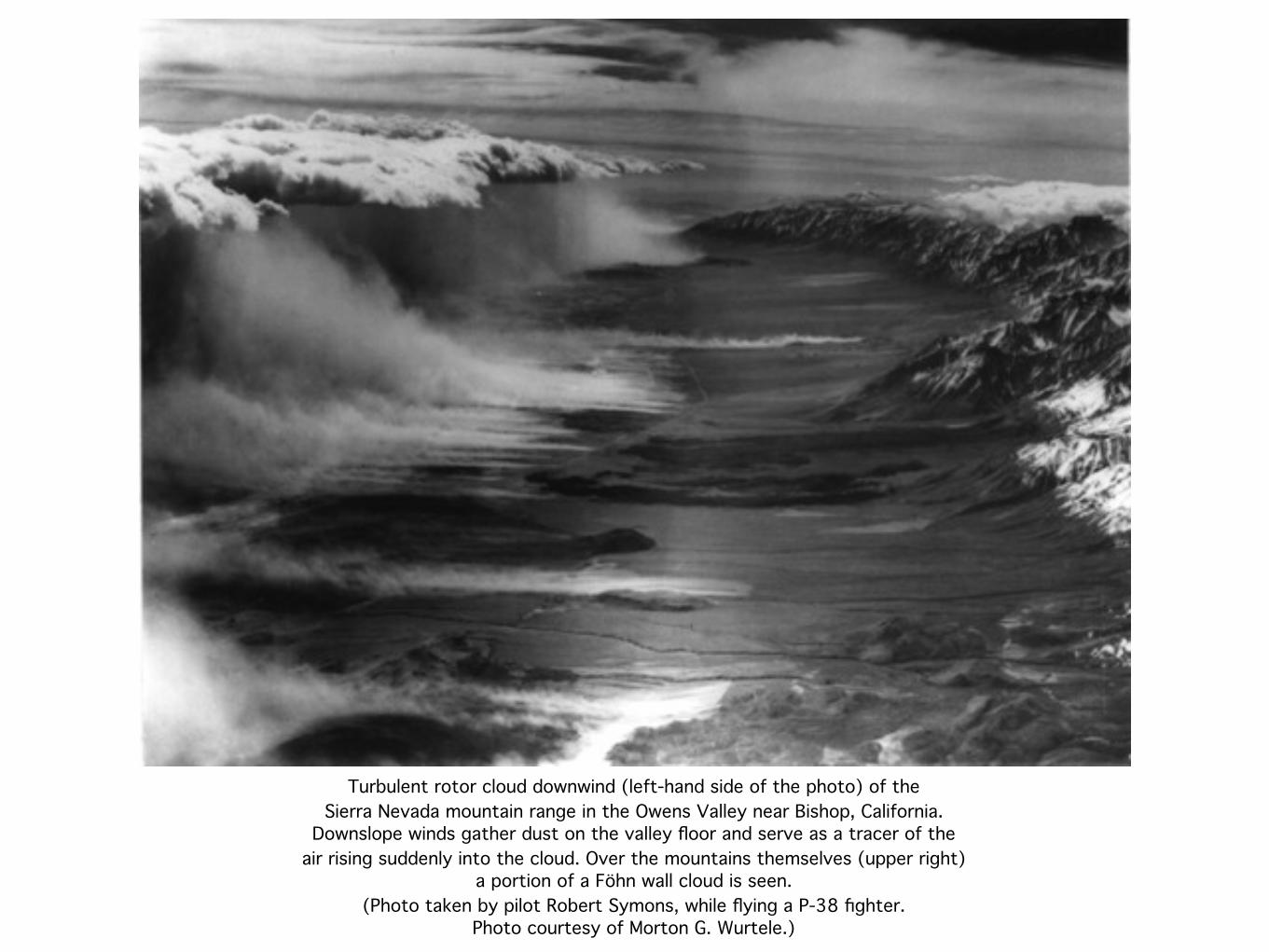
Turbulent rotor cloud downwind (left-hand side of the photo) of the Sierra Nevada mountain range in the Owens Valley near Bishop, California.
Downslope winds gather dust on the valley floor and serve as a tracer of the air rising suddenly into the cloud. Over the mountains themselves (upper right)
a portion of a Föhn wall cloud is seen. (Photo taken by pilot Robert Symons, while flying a P-38 fighter.
Photo courtesy of Morton G. Wurtele.)
DOWNSLOPE WINDSTORMS 339
streamline. This provides an important boundary conditionfor the solution of (12.27), allowing one to predict !c, thedisplacement of the dividing streamline. The solutions aregiven by a family of curves for !c versus ht, with a differentcurve for each upstream height of the dividing stream-line (normalized using the vertical wavelength). Behavioranalogous to hydraulics is possible when the undisturbedheight of the dividing streamline is between (1/4 + n)"z
and (3/4 + n)"z. For these optimal values of H0, and asufficiently high mountain, the dividing streamline willdescend on both the windward and leeward sides of themountain in a manner resembling that of shallow waterflow that transitions from supercritical to subcritical whenpassing over the mountain. Accompanying this descent isa significant increase in wind speed.
The phenomenon of wave amplification due to wavebreaking was originally interpreted as a form of resonance
due to reflection of wave energy at the level of the overturnedlayer.9 As stated previously, the layer in which breakingoccurs is presumed to have a low Richardson number andoften reversed flow such that a critical level is generatedby the breaking (this has been referred to in the literatureas a self-induced critical level; because the phase speed formountain waves is zero, the cross-mountain component ofthe flow is zero in a critical level). As discussed in Section6.4, linear waves encountering a critical level can experienceover-reflection when the Richardson number is less thanone-quarter. The over-reflected waves will interfere withthe incident waves, with resonance possible only for criticallevel heights of 1
4 , 34 , 5
4 , . . . vertical wavelengths above theground. This is a valid mechanism for wave amplification,but some simulations suggest that the critical level heights
9 See Clark and Peltier (1984) and Peltier and Clark (1983).
0
1
2
3
4
5
6
7
8
z (k
m)
x (km) x (km)
0
1
2
3
4
5
6
7
8
z (k
m)
–40 –20 0 20 40 60 –40 –20 0 20 40 60
(a) (b)
(c) (d)
350
320
290
320
290
350
290
320
350
350
320
290
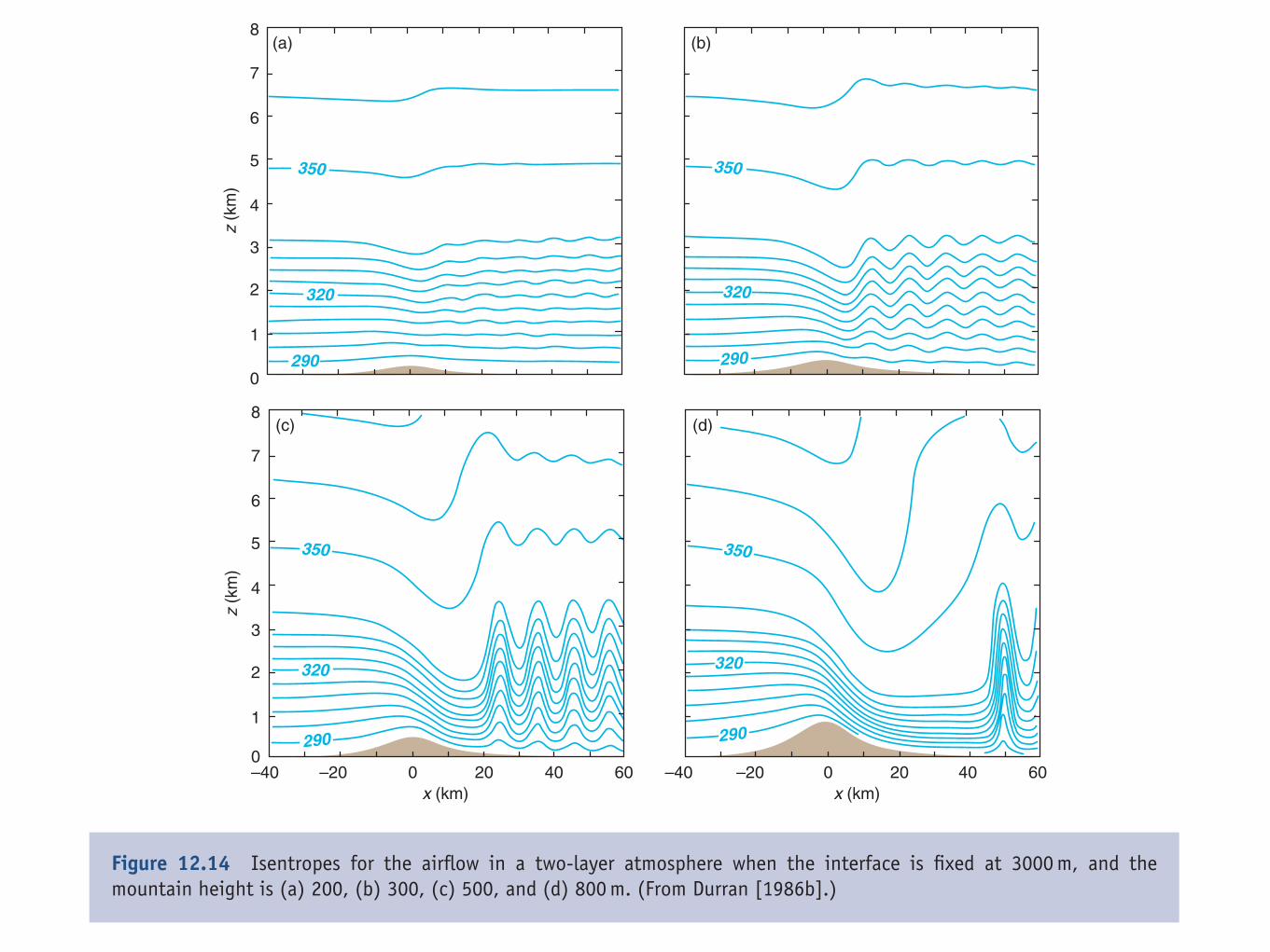
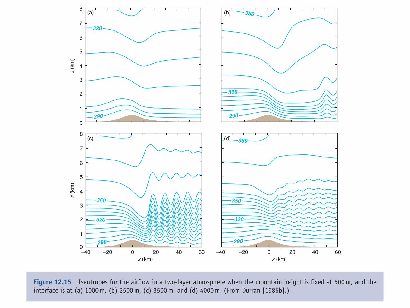
Figure 12.14 Isentropes for the airflow in a two-layer atmosphere when the interface is fixed at 3000 m, and themountain height is (a) 200, (b) 300, (c) 500, and (d) 800 m. (From Durran [1986b].)
340 MOUNTAIN WAVES AND DOWNSLOPE WINDSTORMS
leading to significant wave amplification are better matchedwith those predicted by the hydraulic jump analog thanwith those predicted by the wave-resonance theory.10 Thewave-resonance theory depends on the existence of high-amplitude waves such that wave breaking occurs. At thatpoint, it may be that the nonlinear effects, which areincluded in the hydraulic jump analog, are essential. Similarzonal wind amplification will occur if the mean wind profilecontains a critical level.
In the final observed situation, that of a layer withstrong static stability below a layer with lesser stability,the displacement of the interface will influence the pres-sure gradient, although not as directly as this displacementdoes when the interface represents a true density, ratherthan stability, discontinuity. An analytic expression can be
10 See Durran and Klemp (1987).
developed for the contribution to the total perturbationpressure owing to the displacement of the interface, andsimulations suggest that as the flow becomes more non-linear [for example, as the mountain height is increased(Figure 12.14)] this contribution to the pressure gradienton the lee side becomes dominant, suggesting the flow isthen governed by the hydraulic analog.11
When the flow is in a regime analogous to shallow-watertheory, we expect the depth of the stable layer, analogousto the depth of the shallow water fluid, to play a large rolein determining the flow properties. Indeed, simulationssuggest that varying the depth of the stable layer has aninfluence similar to varying the fluid depth in the two-layer model for shallow-water theory (Figure 12.15). As thestable layer depth increases, the isentropes transition from
11 See Durran (1986b).
0
1
2
3
4
5
6
7
8
z (k
m)
x (km) x (km)
0
1
2
3
4
5
6
7
8
z (k
m)
–40 –20 0 20 40 60 –40 –20 0 20 40 60
(a) (b)
(c) (d)
320
290 290
320
350
380
350
320
290
350
320
290
Figure 12.15 Isentropes for the airflow in a two-layer atmosphere when the mountain height is fixed at 500 m, and theinterface is at (a) 1000 m, (b) 2500 m, (c) 3500 m, and (d) 4000 m. (From Durran [1986b].)
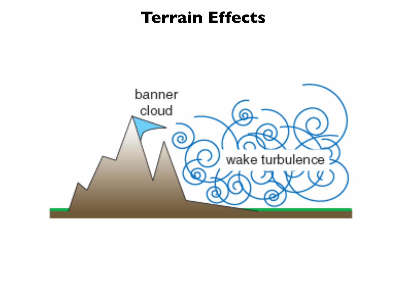
Terrain Effects
!"#$%&' ()* !"# $%&'()* + &',- ./
!"#$%&'()!(*+, -$.('#/0 1&.$#/ !"#$%'()!(*+, %.,!!2., /.*3',#&! '#
4$2#&*'#$2! .,/'$#! *., $-&,# *&&,#3,3 5" * #245,. $- 3'!&'#()
&'6, %7,#$4,#* $# !4*++,. !(*+,!8 '#(+23'#/ !"# $%&'( 91,(&'$# :0;<8)*+&,"%& $"-.( *#3 /.&,%0+/"1 0/*+'(8 +$(*+ *((,+,.*&'$#! $- &7, ='#3$6,. 4$2#&*'# (.,!&!8 2/*03%&! $- +$=)*+&'&23, ='#3!8 +,,)!'3, >0"-%,4?('.(2+*&'$#!8 1*,*1 0/*+'(8 2"&&.1 0/*+'(8 $"3. ,+12+/.&0.8 5"1)"&-*1,.6 (,1..,(8 3$=#!+$%, ='#3 !&$.4!8 *#3 74'1"+/%0 8+)#( 9@'/0A0BB<0 C6,# +$= 7'++! (*# ,D,.& * !2.%.'!'#/+" !&.$#/ '#!2,#(, $#(+$23 %*&&,.#! 9@'/0 A0B;< *#3 %.,('%'&*&'$# *4$2#&!0
!"#$%& '())( E,.&'(*+ (.$!!)!,(&'$# !F,&(7,! $- !$4, $- &7, %7,#$4,#* $5)
!,.6,3 '# 4$2#&*'#! 32.'#/ ='#3" ($#3'&'$#!0 GH3*%&,3 -.$4 I0J0 1&2++8 9&:&,1*'+0,%*& ,* ;*+&'"14 <"4.1 =.,.*1*/*!48 K+2=,.8 L$.3.,(7&8 MA::8 NNN %%0O
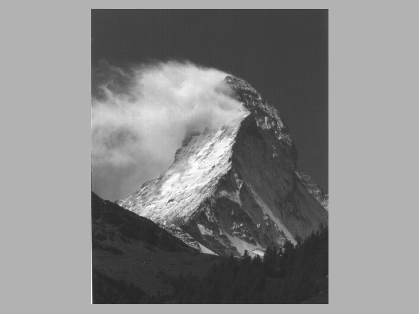
Terrain Effects
Terrain Effects
6 Wind Flow Models COST 710 WG 4
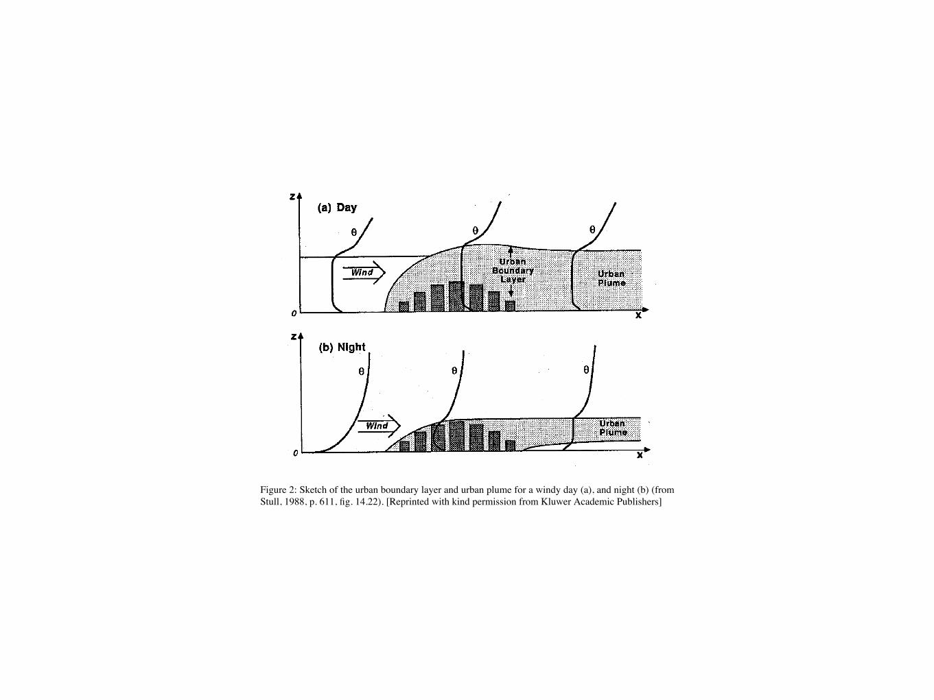
The urban heat island (UHI) is a phenomena caused by the larger warming of the air above theurban area with respect to the countryside. As discussed by Oke (1987) various causes can beconsidered responsible for the heat island existence, and their relative role depend on the sea-son, the geographic location and the city characteristics. Among others, the increase of surfaceheat flux caused by the urban surface properties and the anthropogenic heat flux caused byhuman activities can be cited. In fair and near calm conditions the UHI generates a circulationthat is characterized by the rise of warm air above the city and the convergence of surfacewinds from the countryside to the centre of the UHI. The vertical development of the UHI cir-culation is conditioned by the atmospheric stability. In non-stagnating weather conditions theUHI and the urban canopy modify the boundary layer characteristics giving rise to the UrbanBoundary Layer (Fig. 2) and to a plume that is transported downwind outside of the city.
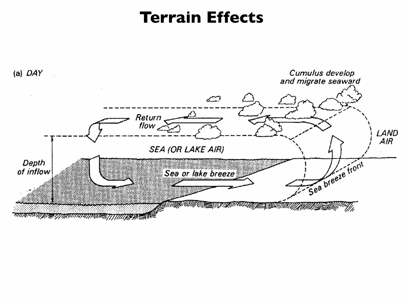
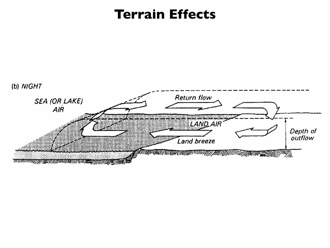
Figure 1: Land and sea breeze circulations across a shoreline by day (a) and at night (b), during anticy-clonic weather (from Oke, 1987, p. 168, fig. 5.6). [Reprinted with permission from Methuen & Co. Ltd]
The development of the UHI has been observed even in rather small towns with 10-20thousand inhabitants. Similar effects can be observed around large industrial complexescharacterized by high energy consumption.These atmospheric circulations can be considered nearly-closed and characterized by periodicreverse of flow direction. Pollutant dispersed in such conditions can be trapped by the flowrecirculating inside the area touched by the phenomena. These conditions can be responsiblefor high concentration episodes. Frequently pollutants emitted near coastal areas are simulta-neously subjected to recirculation and to fast chemical reactions. Recirculation of pollutants in
Terrain Effects
6 Wind Flow Models COST 710 WG 4
The urban heat island (UHI) is a phenomena caused by the larger warming of the air above theurban area with respect to the countryside. As discussed by Oke (1987) various causes can beconsidered responsible for the heat island existence, and their relative role depend on the sea-son, the geographic location and the city characteristics. Among others, the increase of surfaceheat flux caused by the urban surface properties and the anthropogenic heat flux caused byhuman activities can be cited. In fair and near calm conditions the UHI generates a circulationthat is characterized by the rise of warm air above the city and the convergence of surfacewinds from the countryside to the centre of the UHI. The vertical development of the UHI cir-culation is conditioned by the atmospheric stability. In non-stagnating weather conditions theUHI and the urban canopy modify the boundary layer characteristics giving rise to the UrbanBoundary Layer (Fig. 2) and to a plume that is transported downwind outside of the city.
Figure 1: Land and sea breeze circulations across a shoreline by day (a) and at night (b), during anticy-clonic weather (from Oke, 1987, p. 168, fig. 5.6). [Reprinted with permission from Methuen & Co. Ltd]
The development of the UHI has been observed even in rather small towns with 10-20thousand inhabitants. Similar effects can be observed around large industrial complexescharacterized by high energy consumption.These atmospheric circulations can be considered nearly-closed and characterized by periodicreverse of flow direction. Pollutant dispersed in such conditions can be trapped by the flowrecirculating inside the area touched by the phenomena. These conditions can be responsiblefor high concentration episodes. Frequently pollutants emitted near coastal areas are simulta-neously subjected to recirculation and to fast chemical reactions. Recirculation of pollutants in
Terrain Effects
410 The Atmospheric Boundary Layer
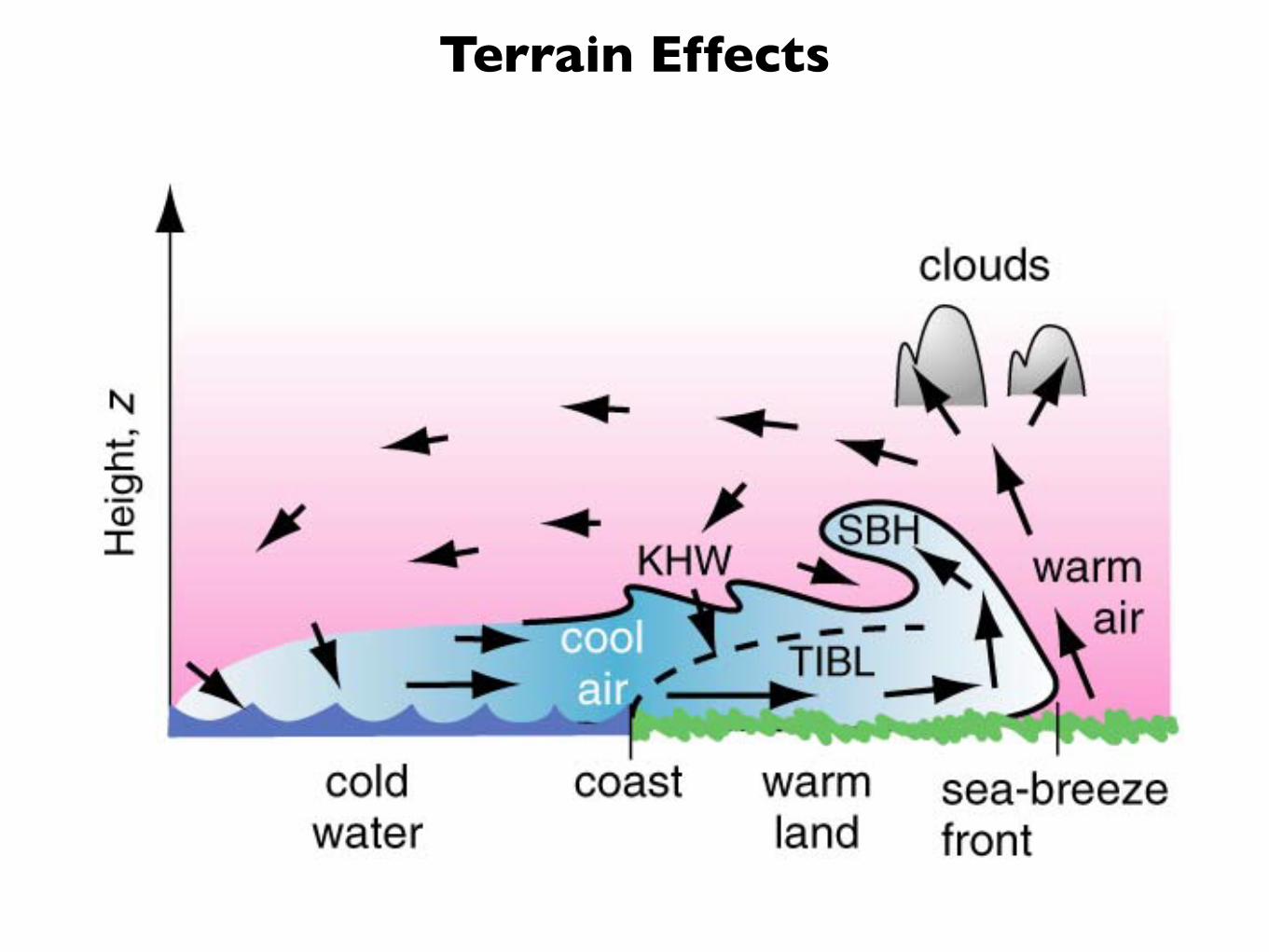
between local flows that distort the sea breeze and cre-ate regions of enhanced convergence and divergence.The sea breeze can also interact with boundary-layerconvection, horizontal roll vortices, and urban heatislands, causing complex dispersion of pollutants emit-ted near the shore. If the onshore synoptic-scalegeostrophic wind is too strong, a TIBL developsinstead of a sea-breeze circulation.
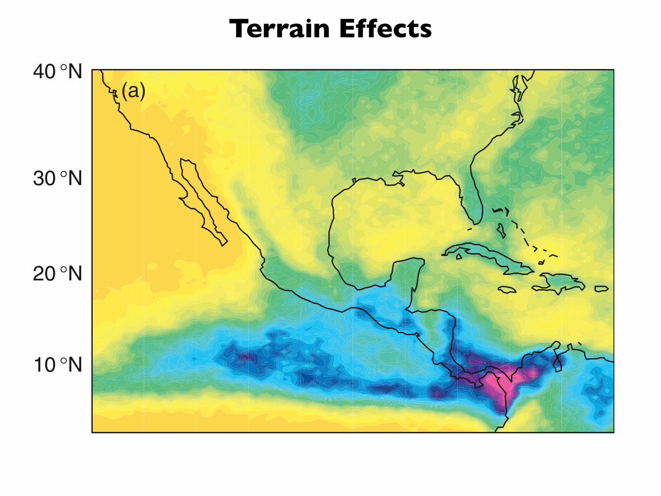
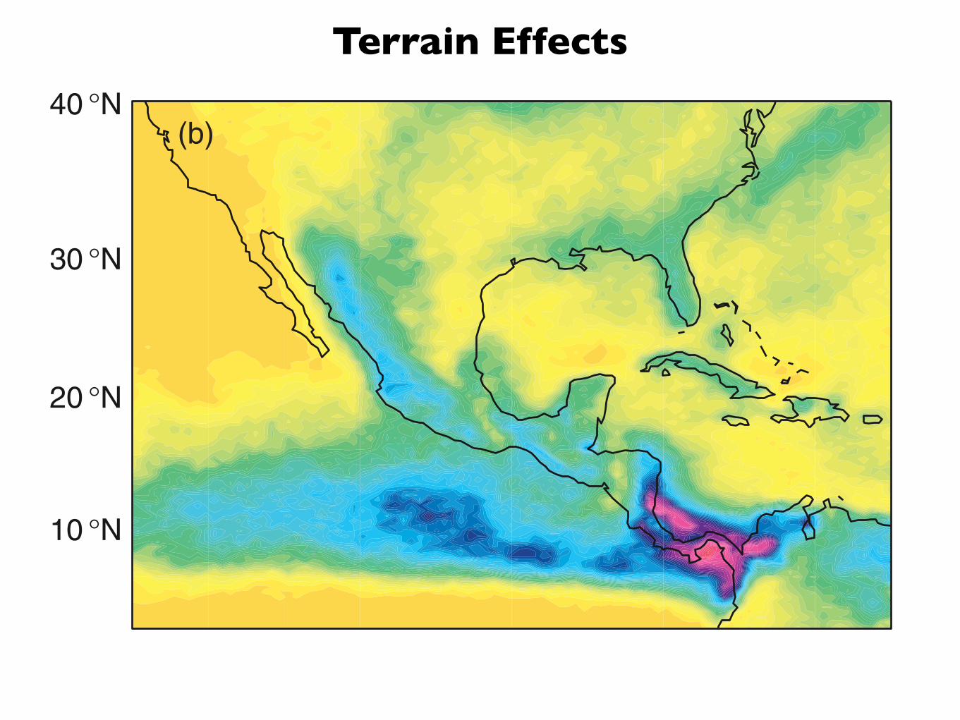
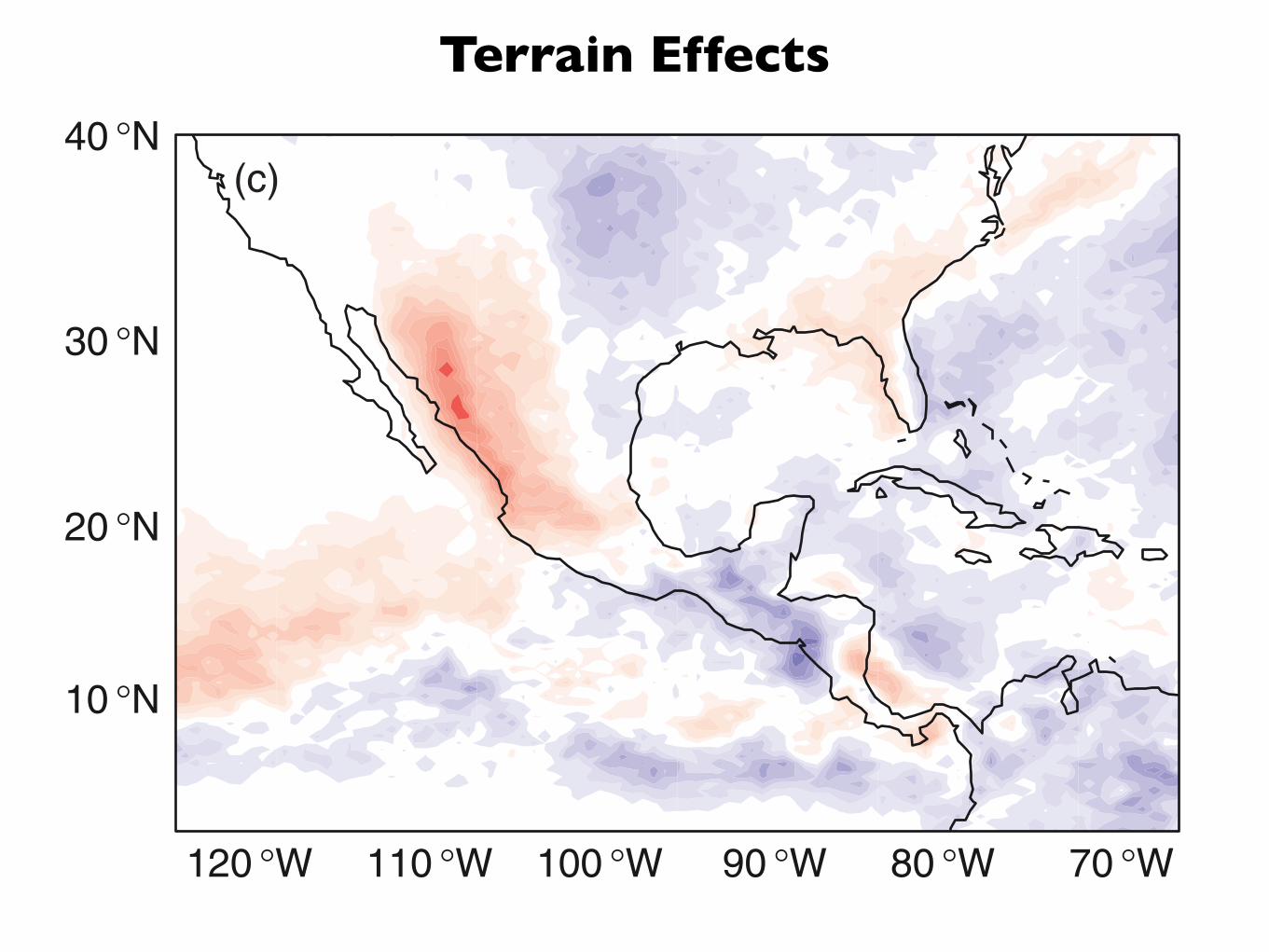
In regions such as the west coast of the Americas,where major mountain ranges lie within a few hundredkilometers of the coast, sea breezes and terrain effectsappear in combination. Figure 9.36 shows an exampleof how low-level convergence associated with theboundary-layer wind field influences the diurnal cyclein deep convection and rainfall over Central America.Elevated land areas along the crest of the SierrasMadre mountain range experience convection duringthe afternoon when the sea breeze and upslope flowconspire to produce low-level convergence. In contrast,the offshore waters experience convection most fre-quently during the early morning hours, in response tothe convergence associated with the land breeze, aug-mented by katabatic winds from the nearby mountains.Morning convection is particularly strong in the Gulfof Panama because of its concave coastline. The preva-lence of afternoon convection, driven by the the seabreeze circulation, is also clearly evident over thesoutheastern United States.
9.5.3 Forest Canopy Effects
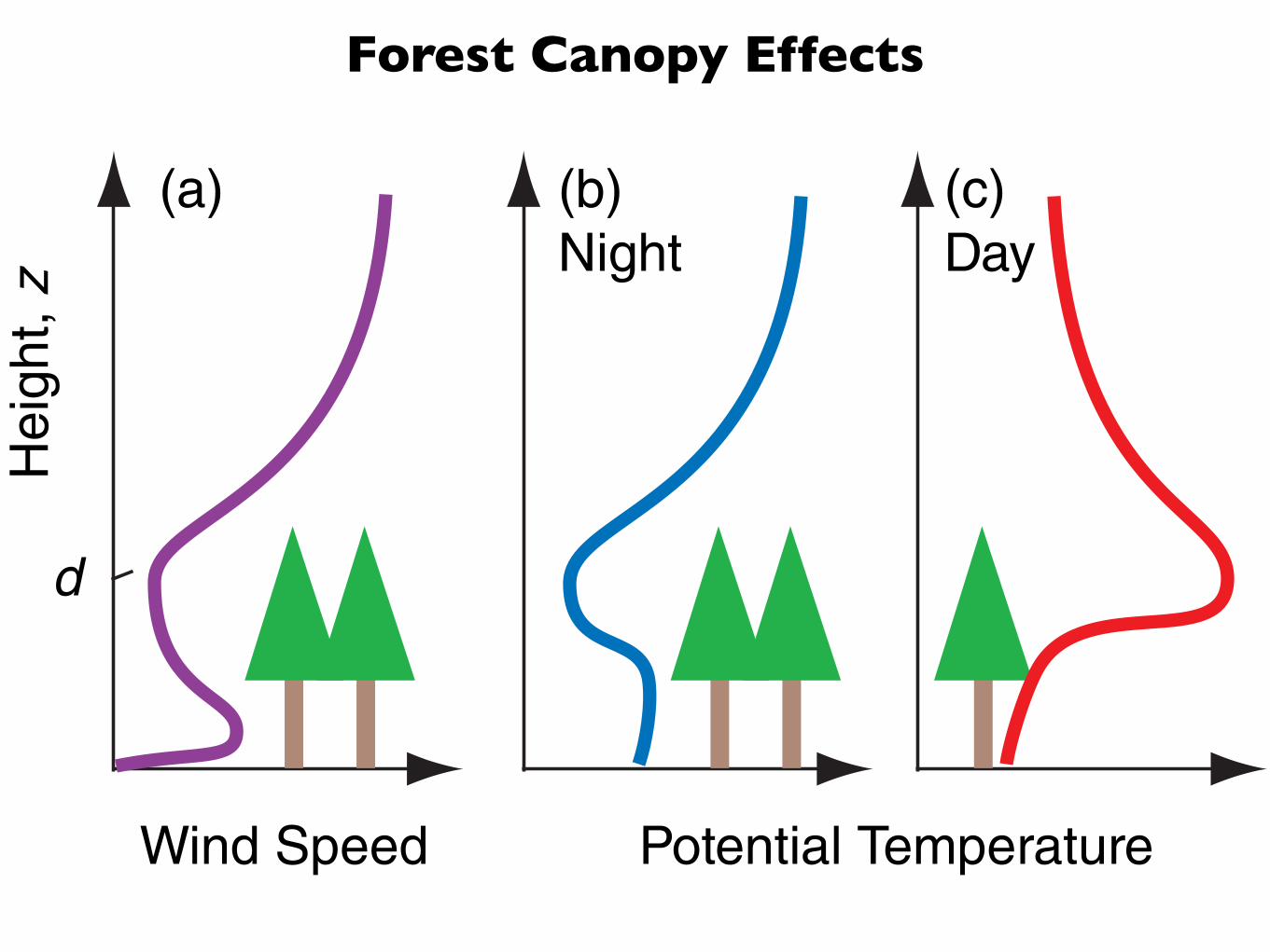
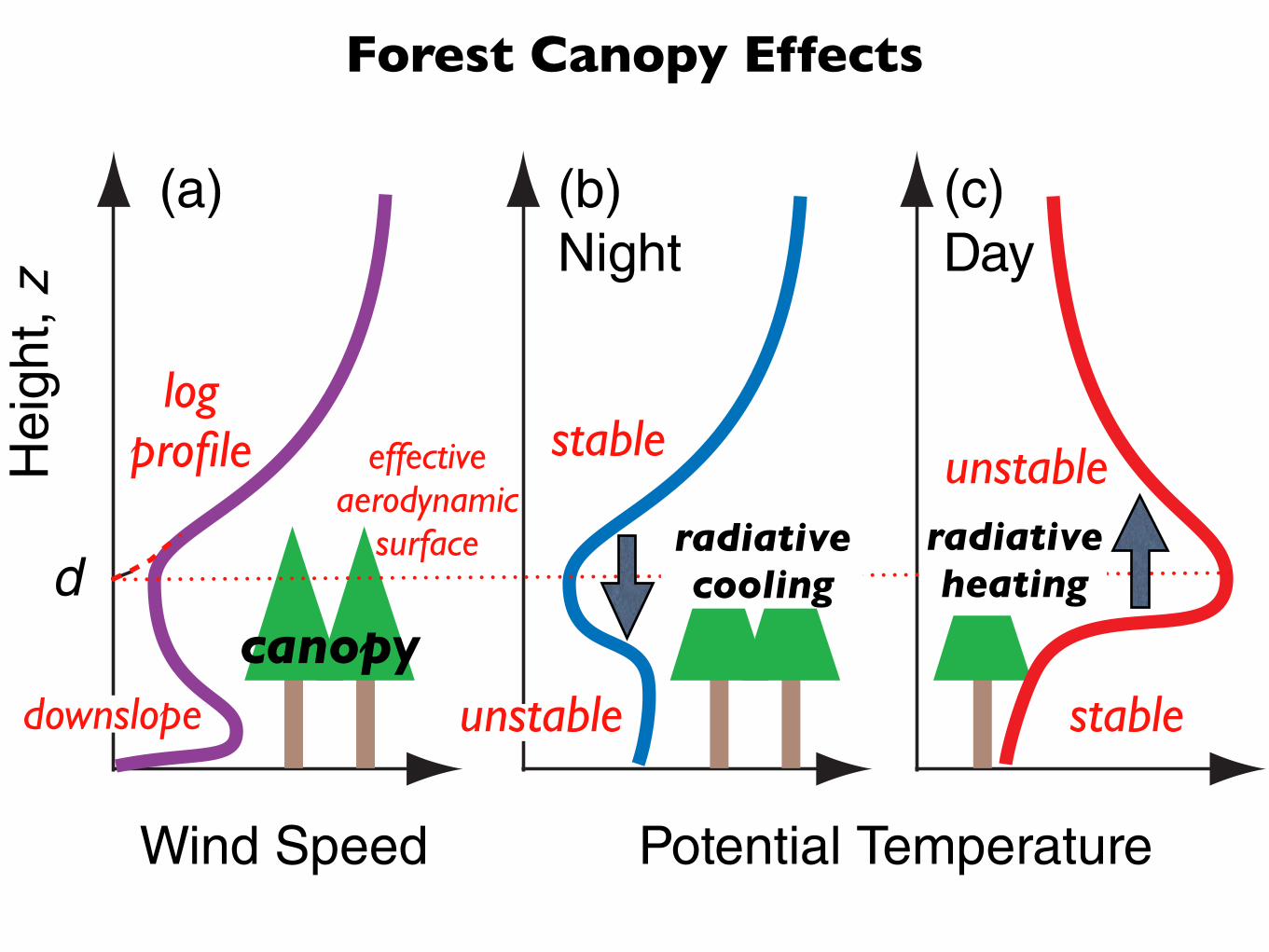
The drag associated with forest canopies (i.e., theleafy top part of the trees) is so strong that the flowabove the canopy often becomes partially separatedfrom the flow below, in the trunk space. In the regionabove the canopy in the surface layer, the flowexhibits the typical logarithmic wind profile but withthe effective aerodynamic surface displaced upwardto near the canopy top (Fig. 9.37a). In the trunkspace the air often has a relative maximum of windspeed between the ground and the canopy, and oftenthese subcanopy winds flow mostly downslope bothday and night if the canopy is dense.
The static stability below the canopy is often oppo-site to that above the canopy. For example, duringclear nights, strong longwave cooling of the canopywill cause a statically stable boundary layer to formabove the canopy (Fig. 9.37b). However, some ofthe cold air from the canopy sinks as upside-downthermals, creating a convective mixed layer in thetrunk space at night that gets cooler as the night pro-
gresses. During daytime, a superadiabatic surfacelayer with warm convective thermals forms abovethe canopy, while in the trunk space the air iswarmed from the canopy above and becomes stati-cally stable (Fig. 9.37c). These peculiar configurationsof static stability are successfully captured with thenonlocal method of determining static stability.
70 °W
10 °N
20 °N
30 °N
40 °N
10 °N
20 °N
30 °N
40 °N
10 °N
20 °N
30 °N
40 °N
120 °W 110 °W 100 °W 90 °W 80 °W
(a)
(b)
(c)
Fig. 9.36 Frequency of deep convection as indicated byclouds with tops colder than !38 °C at two different timesof day during July at around (a) 5 AM local time and (b) 5 PM
local time. Panel (c) shows the difference (a)–(b). Color scalefor (a) and (b) analogous to that in Fig. 1.25; in (c) red shad-ing indicates heavier precipitation at 5 PM. [Courtesy of U.S.CLIVAR Pan American Implementation Panel and KenHoward, NOAA-NSSL.]
P732951-Ch09.qxd 9/12/05 7:48 PM Page 410
Terrain Effects
410 The Atmospheric Boundary Layer
between local flows that distort the sea breeze and cre-ate regions of enhanced convergence and divergence.The sea breeze can also interact with boundary-layerconvection, horizontal roll vortices, and urban heatislands, causing complex dispersion of pollutants emit-ted near the shore. If the onshore synoptic-scalegeostrophic wind is too strong, a TIBL developsinstead of a sea-breeze circulation.
In regions such as the west coast of the Americas,where major mountain ranges lie within a few hundredkilometers of the coast, sea breezes and terrain effectsappear in combination. Figure 9.36 shows an exampleof how low-level convergence associated with theboundary-layer wind field influences the diurnal cyclein deep convection and rainfall over Central America.Elevated land areas along the crest of the SierrasMadre mountain range experience convection duringthe afternoon when the sea breeze and upslope flowconspire to produce low-level convergence. In contrast,the offshore waters experience convection most fre-quently during the early morning hours, in response tothe convergence associated with the land breeze, aug-mented by katabatic winds from the nearby mountains.Morning convection is particularly strong in the Gulfof Panama because of its concave coastline. The preva-lence of afternoon convection, driven by the the seabreeze circulation, is also clearly evident over thesoutheastern United States.
9.5.3 Forest Canopy Effects
The drag associated with forest canopies (i.e., theleafy top part of the trees) is so strong that the flowabove the canopy often becomes partially separatedfrom the flow below, in the trunk space. In the regionabove the canopy in the surface layer, the flowexhibits the typical logarithmic wind profile but withthe effective aerodynamic surface displaced upwardto near the canopy top (Fig. 9.37a). In the trunkspace the air often has a relative maximum of windspeed between the ground and the canopy, and oftenthese subcanopy winds flow mostly downslope bothday and night if the canopy is dense.
The static stability below the canopy is often oppo-site to that above the canopy. For example, duringclear nights, strong longwave cooling of the canopywill cause a statically stable boundary layer to formabove the canopy (Fig. 9.37b). However, some ofthe cold air from the canopy sinks as upside-downthermals, creating a convective mixed layer in thetrunk space at night that gets cooler as the night pro-
gresses. During daytime, a superadiabatic surfacelayer with warm convective thermals forms abovethe canopy, while in the trunk space the air iswarmed from the canopy above and becomes stati-cally stable (Fig. 9.37c). These peculiar configurationsof static stability are successfully captured with thenonlocal method of determining static stability.
70 °W
10 °N
20 °N
30 °N
40 °N
10 °N
20 °N
30 °N
40 °N
10 °N
20 °N
30 °N
40 °N
120 °W 110 °W 100 °W 90 °W 80 °W
(a)
(b)
(c)
Fig. 9.36 Frequency of deep convection as indicated byclouds with tops colder than !38 °C at two different timesof day during July at around (a) 5 AM local time and (b) 5 PM
local time. Panel (c) shows the difference (a)–(b). Color scalefor (a) and (b) analogous to that in Fig. 1.25; in (c) red shad-ing indicates heavier precipitation at 5 PM. [Courtesy of U.S.CLIVAR Pan American Implementation Panel and KenHoward, NOAA-NSSL.]
P732951-Ch09.qxd 9/12/05 7:48 PM Page 410
Forest Canopy Effects
9.6 The Boundary Layer in Context 411
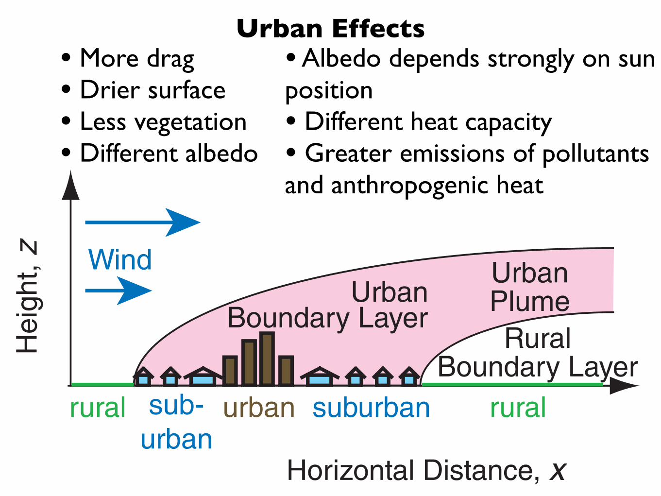
9.5.4 Urban Effects
Large cities differ from the surrounding rural areasby virtue of having larger buildings that exert astronger drag on the wind; less ground moisture andvegetation, resulting in reduced evaporation; differ-ent albedo characteristics that are strongly depend-ent on the relationship between sun position andalignment of the urban street canyons; different heatcapacity; and greater emissions of pollutants andanthropogenic heat production. All of these effectsusually cause the city center to be warmer than thesurroundings—a phenomenon called the urban heatisland (Fig. 9.38a).
When a light synoptic-scale wind is blowing, theexcess warmth and increased pollutants extenddownwind as a city-scale urban plume (Fig. 9.38b). Insome of these urban plumes the length of the grow-ing season (days between last frost in spring and firstfrost in fall) in the rural areas adjacent to the city hasbeen observed to increase by 15 days compared tothe surrounding regions.
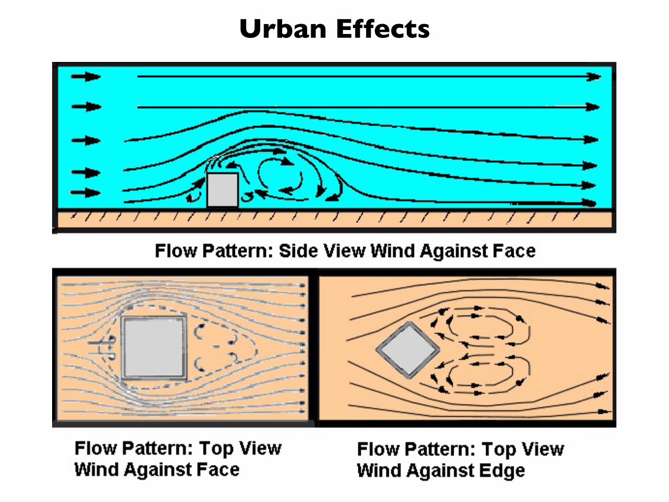
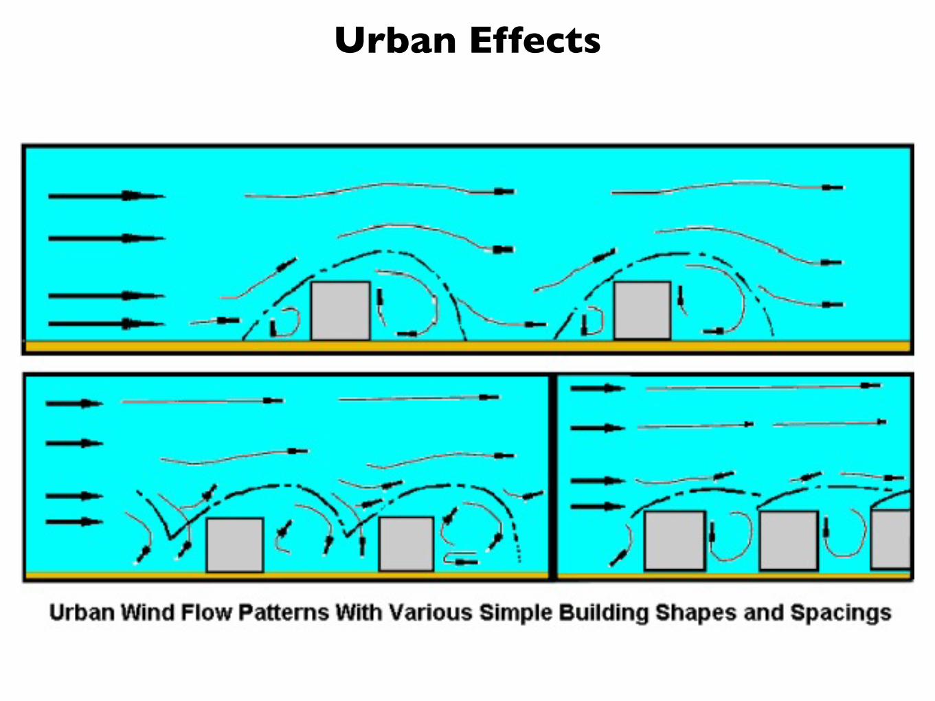
Within individual street canyons between strongbuildings, winds can be funneled and accelerated.Also, as fast winds from aloft hit tall buildings, thewinds are deflected downward to increase windspeeds near the base of these skyscrapers. Behindindividual buildings is often a “cavity” of circulationwith surface wind direction opposite to the strongerwinds aloft, which can cause unanticipated transportof pollutants from the street level up to open win-dows. In lighter wind conditions, the increased rough-ness length associated with tall buildings can reducethe wind speed on average over the whole city, allow-ing pollutant concentrations to build to high levels.
The largest cities generate and store so much heatthat they can create convective mixed layers overthem both day and night during fair-weather condi-tions. This urban heat source is often associated withenhanced thermals and updrafts over the city, withweak return-circulation downdrafts over the adjacentcountryside. One detrimental effect is that pollutantsare continually recirculated into the city. Also, theenhanced convection over a city can cause measurableincreases in convective clouds and thunderstorm rain.
9.6 The Boundary Layerin ContextBoundary-layer meteorology is still a relativelyyoung field of study with many unsolved problems.The basic equations of thermodynamics and dynam-ics have resisted analytical solution for centuries. TheReynolds-averaging approach resorts to statisticalaverages of the effects of turbulence in an attempt tocircumvent the intrinsic lack of predictability in thedeterministic solutions of the eddies themselves. Theturbulence closure problem has not been solved, andthe chaotic nature of turbulence poses major chal-lenges. Many of the useful empirical relationships,
Hei
ght,
z
d
Wind Speed Potential Temperature
(a) (b)Night
(c)Day
Fig. 9.37 (a) Wind speed in a forest canopy. (b) Potentialtemperature profile on a clear night with light winds. The leveld represents the displacement distance of the effective surfacefor the logarithmic wind profile in the surface layer above thetop of the canopy. (c) Same as (b), but on a sunny day.[Courtesy of Roland B. Stull.]
Fig. 9.38 (a) Urban heat island effect, with warmer air tem-peratures over and downwind of a city. Air temperature excessin the city core can be 2 to 12 °C warmer than the airupstream over rural areas. The grid of lines represents roads.(b) Vertical cross section through a city. The urban plumeincludes excess heat as well as increased pollution. [Adaptedfrom T. R. Oke, Boundary Layer Climates, 2nd Ed., Routledge,New York (1987).]
North
Wind
24°C22°C
T = 20°C
26°C
(a)
Horizontal Distance, x
Wind
Hei
ght,
z
urban suburbansub-urban
ruralrural
UrbanBoundary Layer
UrbanPlumeRural
Boundary Layer
(b)
P732951-Ch09.qxd 9/12/05 7:48 PM Page 411
Forest Canopy Effects
9.6 The Boundary Layer in Context 411
9.5.4 Urban Effects
Large cities differ from the surrounding rural areasby virtue of having larger buildings that exert astronger drag on the wind; less ground moisture andvegetation, resulting in reduced evaporation; differ-ent albedo characteristics that are strongly depend-ent on the relationship between sun position andalignment of the urban street canyons; different heatcapacity; and greater emissions of pollutants andanthropogenic heat production. All of these effectsusually cause the city center to be warmer than thesurroundings—a phenomenon called the urban heatisland (Fig. 9.38a).
When a light synoptic-scale wind is blowing, theexcess warmth and increased pollutants extenddownwind as a city-scale urban plume (Fig. 9.38b). Insome of these urban plumes the length of the grow-ing season (days between last frost in spring and firstfrost in fall) in the rural areas adjacent to the city hasbeen observed to increase by 15 days compared tothe surrounding regions.
Within individual street canyons between strongbuildings, winds can be funneled and accelerated.Also, as fast winds from aloft hit tall buildings, thewinds are deflected downward to increase windspeeds near the base of these skyscrapers. Behindindividual buildings is often a “cavity” of circulationwith surface wind direction opposite to the strongerwinds aloft, which can cause unanticipated transportof pollutants from the street level up to open win-dows. In lighter wind conditions, the increased rough-ness length associated with tall buildings can reducethe wind speed on average over the whole city, allow-ing pollutant concentrations to build to high levels.
The largest cities generate and store so much heatthat they can create convective mixed layers overthem both day and night during fair-weather condi-tions. This urban heat source is often associated withenhanced thermals and updrafts over the city, withweak return-circulation downdrafts over the adjacentcountryside. One detrimental effect is that pollutantsare continually recirculated into the city. Also, theenhanced convection over a city can cause measurableincreases in convective clouds and thunderstorm rain.
9.6 The Boundary Layerin ContextBoundary-layer meteorology is still a relativelyyoung field of study with many unsolved problems.The basic equations of thermodynamics and dynam-ics have resisted analytical solution for centuries. TheReynolds-averaging approach resorts to statisticalaverages of the effects of turbulence in an attempt tocircumvent the intrinsic lack of predictability in thedeterministic solutions of the eddies themselves. Theturbulence closure problem has not been solved, andthe chaotic nature of turbulence poses major chal-lenges. Many of the useful empirical relationships,
Hei
ght,
z
d
Wind Speed Potential Temperature
(a) (b)Night
(c)Day
Fig. 9.37 (a) Wind speed in a forest canopy. (b) Potentialtemperature profile on a clear night with light winds. The leveld represents the displacement distance of the effective surfacefor the logarithmic wind profile in the surface layer above thetop of the canopy. (c) Same as (b), but on a sunny day.[Courtesy of Roland B. Stull.]
Fig. 9.38 (a) Urban heat island effect, with warmer air tem-peratures over and downwind of a city. Air temperature excessin the city core can be 2 to 12 °C warmer than the airupstream over rural areas. The grid of lines represents roads.(b) Vertical cross section through a city. The urban plumeincludes excess heat as well as increased pollution. [Adaptedfrom T. R. Oke, Boundary Layer Climates, 2nd Ed., Routledge,New York (1987).]
North
Wind
24°C22°C
T = 20°C
26°C
(a)
Horizontal Distance, x
Wind
Hei
ght,
z
urban suburbansub-urban
ruralrural
UrbanBoundary Layer
UrbanPlumeRural
Boundary Layer
(b)
P732951-Ch09.qxd 9/12/05 7:48 PM Page 411
canopy
log profile effective
aerodynamic surface
downslope
stable
stable
unstable
unstable
radiative cooling
radiative heating
Urban Effects
9.6 The Boundary Layer in Context 411
9.5.4 Urban Effects
Large cities differ from the surrounding rural areasby virtue of having larger buildings that exert astronger drag on the wind; less ground moisture andvegetation, resulting in reduced evaporation; differ-ent albedo characteristics that are strongly depend-ent on the relationship between sun position andalignment of the urban street canyons; different heatcapacity; and greater emissions of pollutants andanthropogenic heat production. All of these effectsusually cause the city center to be warmer than thesurroundings—a phenomenon called the urban heatisland (Fig. 9.38a).
When a light synoptic-scale wind is blowing, theexcess warmth and increased pollutants extenddownwind as a city-scale urban plume (Fig. 9.38b). Insome of these urban plumes the length of the grow-ing season (days between last frost in spring and firstfrost in fall) in the rural areas adjacent to the city hasbeen observed to increase by 15 days compared tothe surrounding regions.
Within individual street canyons between strongbuildings, winds can be funneled and accelerated.Also, as fast winds from aloft hit tall buildings, thewinds are deflected downward to increase windspeeds near the base of these skyscrapers. Behindindividual buildings is often a “cavity” of circulationwith surface wind direction opposite to the strongerwinds aloft, which can cause unanticipated transportof pollutants from the street level up to open win-dows. In lighter wind conditions, the increased rough-ness length associated with tall buildings can reducethe wind speed on average over the whole city, allow-ing pollutant concentrations to build to high levels.
The largest cities generate and store so much heatthat they can create convective mixed layers overthem both day and night during fair-weather condi-tions. This urban heat source is often associated withenhanced thermals and updrafts over the city, withweak return-circulation downdrafts over the adjacentcountryside. One detrimental effect is that pollutantsare continually recirculated into the city. Also, theenhanced convection over a city can cause measurableincreases in convective clouds and thunderstorm rain.
9.6 The Boundary Layerin ContextBoundary-layer meteorology is still a relativelyyoung field of study with many unsolved problems.The basic equations of thermodynamics and dynam-ics have resisted analytical solution for centuries. TheReynolds-averaging approach resorts to statisticalaverages of the effects of turbulence in an attempt tocircumvent the intrinsic lack of predictability in thedeterministic solutions of the eddies themselves. Theturbulence closure problem has not been solved, andthe chaotic nature of turbulence poses major chal-lenges. Many of the useful empirical relationships,
Hei
ght,
z
d
Wind Speed Potential Temperature
(a) (b)Night
(c)Day
Fig. 9.37 (a) Wind speed in a forest canopy. (b) Potentialtemperature profile on a clear night with light winds. The leveld represents the displacement distance of the effective surfacefor the logarithmic wind profile in the surface layer above thetop of the canopy. (c) Same as (b), but on a sunny day.[Courtesy of Roland B. Stull.]
Fig. 9.38 (a) Urban heat island effect, with warmer air tem-peratures over and downwind of a city. Air temperature excessin the city core can be 2 to 12 °C warmer than the airupstream over rural areas. The grid of lines represents roads.(b) Vertical cross section through a city. The urban plumeincludes excess heat as well as increased pollution. [Adaptedfrom T. R. Oke, Boundary Layer Climates, 2nd Ed., Routledge,New York (1987).]
North
Wind
24°C22°C
T = 20°C
26°C
(a)
Horizontal Distance, x
Wind
Hei
ght,
z
urban suburbansub-urban
ruralrural
UrbanBoundary Layer
UrbanPlumeRural
Boundary Layer
(b)
P732951-Ch09.qxd 9/12/05 7:48 PM Page 411
• More drag• Drier surface• Less vegetation• Different albedo
• Albedo depends strongly on sun position• Different heat capacity• Greater emissions of pollutants and anthropogenic heat
COST 710 WG 4 Wind Flow Models 7
land/sea breezes can occur in two ways. Polluted air may follow a recirculatory trajectory bybeing advected landward in the sea breeze, be lifted by rising air at the sea breeze front andreturn seaward in the upper return flow. These processes were documented along the EastCoast of Spain (Millan et al., 1992) and Vancouver (Steyn et al., 1995). Horizontal recircula-tion occurs when polluted air is carried landward by sea breeze during daylight hours, and sea-ward by the land breeze, at night. In both mechanisms, pollutants emitted at ground level canbe trapped aloft when the flow at the surface is decoupled from upper winds, creating a reser-voir layer of aged polluted air mass, as observed by Millan et al. (1996), and McKendry et al.,(1996).The processes of fumigation of aged reservoir layer or effluents emitted above the inter-nal boundary layer were also studied (Portelli, 1982; McRae et al., 1981; Millan, et al., 1984).A pollutant plume released from an elevated source emitting into the stable layer dispersesvery little as it moves downwind. When it reaches the downwind point where the mixing layerextends upwards to the plume height, the material in the plume mixes rapidly downwards tocause fumigation. This fumigation process can occur also when the polluted air mass aloft isintersected by the growing convective layer (Millan, et al. 1996). To be able to evaluate suchdispersion conditions, a correct description (modelling) of the 3-D flow characteristics and itstime evolution is of fundamental importance due to the features of non-homogeneity and non-stationarity of the flow.
Figure 2: Sketch of the urban boundary layer and urban plume for a windy day (a), and night (b) (fromStull, 1988, p. 611, fig. 14.22). [Reprinted with kind permission from Kluwer Academic Publishers]
The flows described above are classical examples for meso-scale dispersion problems (20-200km), but are also important at smaller dispersion scale.
Urban Effects
Urban Effects
Urban Effects
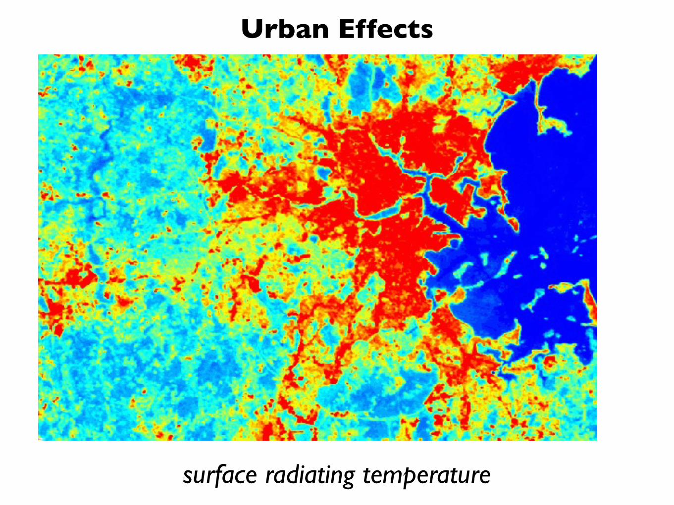
surface radiating temperature
Urban Effects
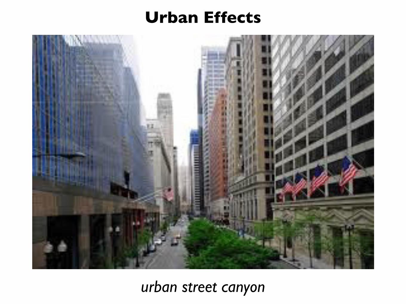
urban street canyon
Urban Effects
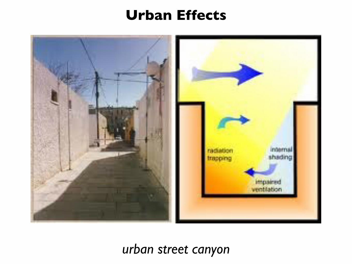
urban street canyon
Urban Effects
Urban Effects

Wind Engineering
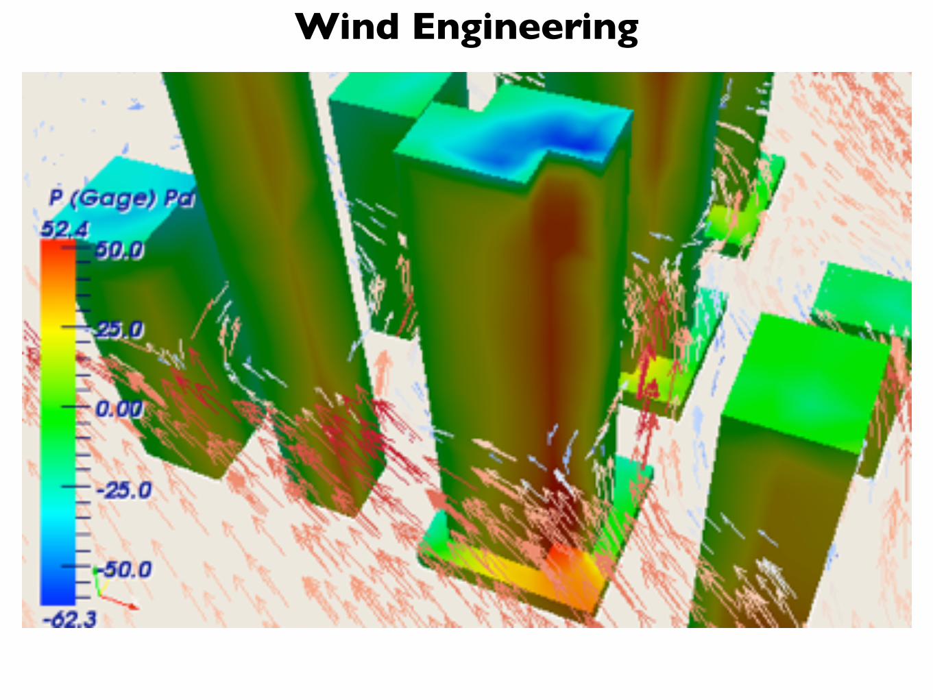
Wind Engineering
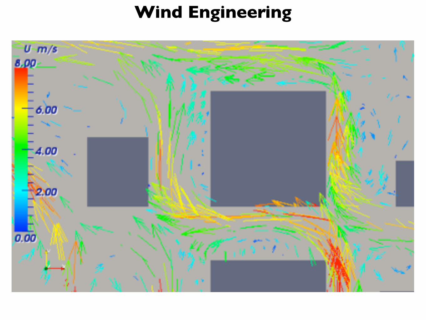
Wind Engineering
Wind Engineering

Wind Engineering
Alan G. Davenport, with a model of New York City in 1980.
DUST STORMS IN THEEASTERN GREAT BASIN
Maura HahnenbergerUniversity of Utah
Department of Atmospheric [email protected]
http://hahnenberger.weebly.comTwitter: @Maura_Science
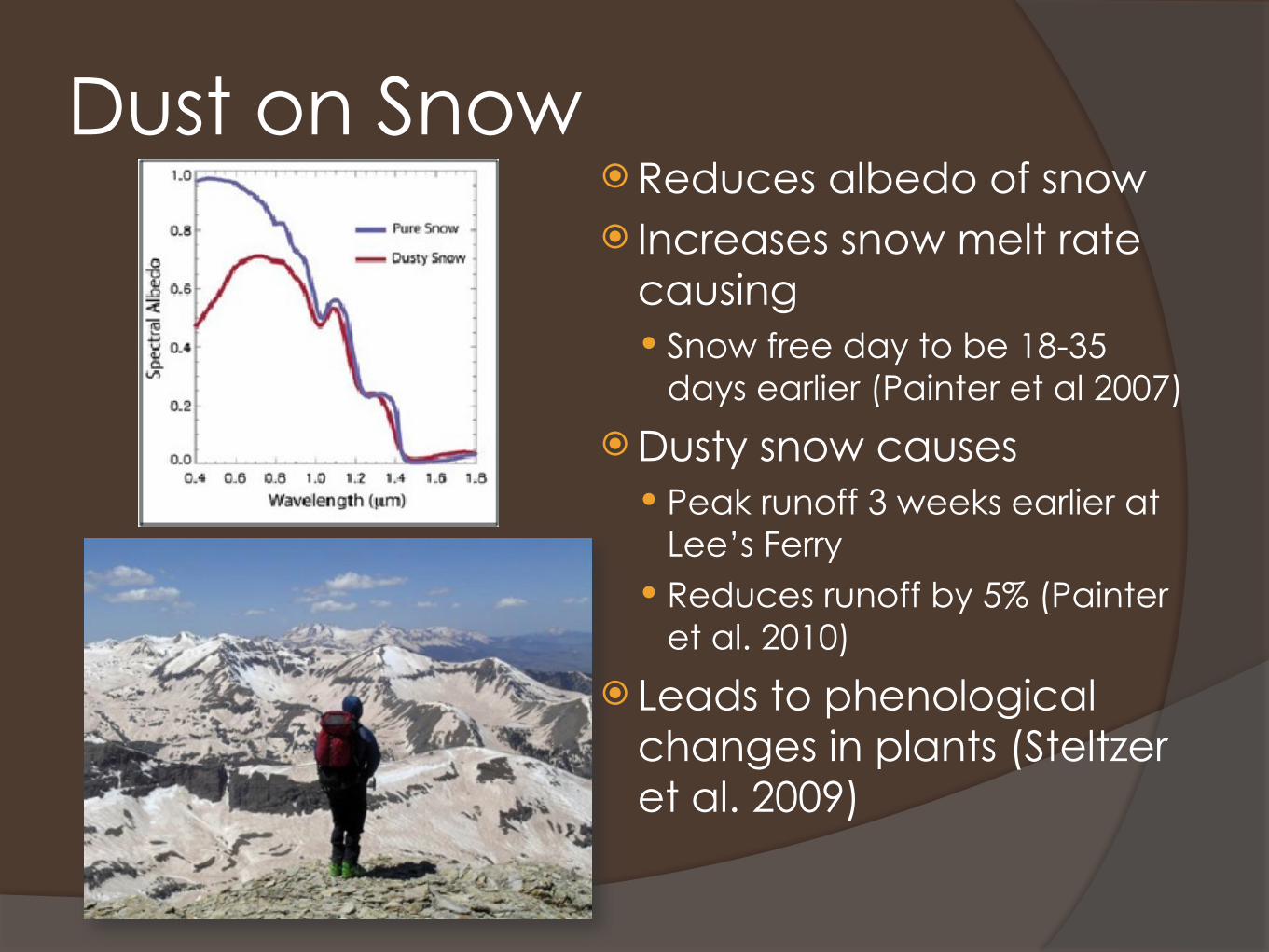
Dust on Snow Reduces albedo of snow Increases snow melt rate
causing Snow free day to be 18-35
days earlier (Painter et al 2007)
Dusty snow causes Peak runoff 3 weeks earlier at
Lee’s Ferry Reduces runoff by 5% (Painter
et al. 2010)
Leads to phenological changes in plants (Steltzer et al. 2009)
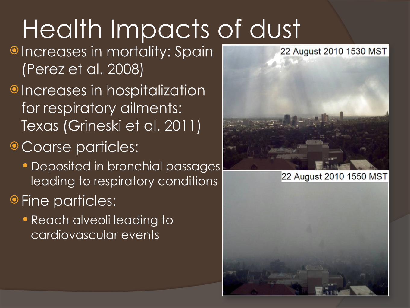
Health Impacts of dust Increases in mortality: Spain
(Perez et al. 2008) Increases in hospitalization
for respiratory ailments: Texas (Grineski et al. 2011)
Coarse particles: Deposited in bronchial passages
leading to respiratory conditions
Fine particles: Reach alveoli leading to
cardiovascular events
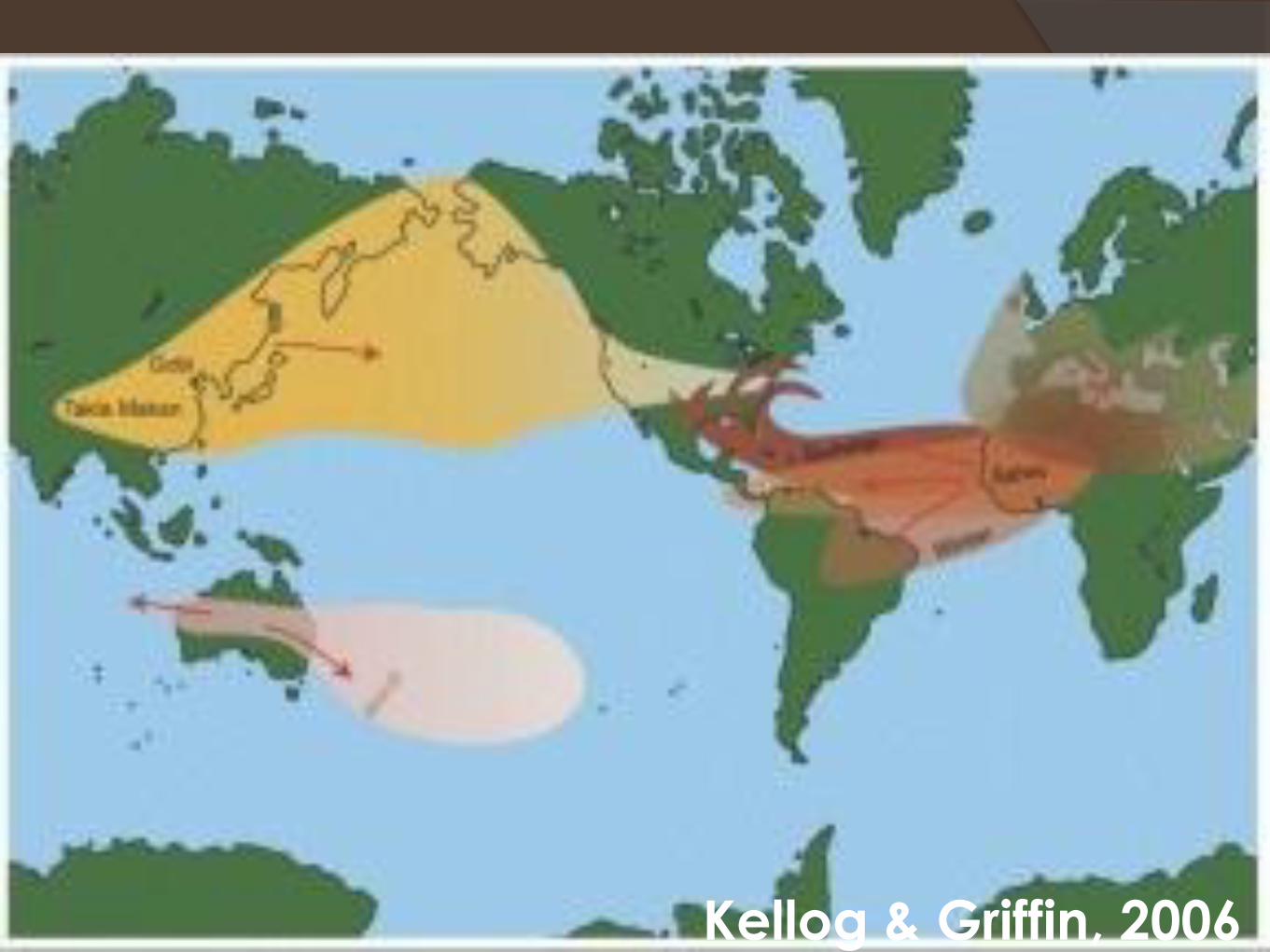
Kellog & Griffin, 2006
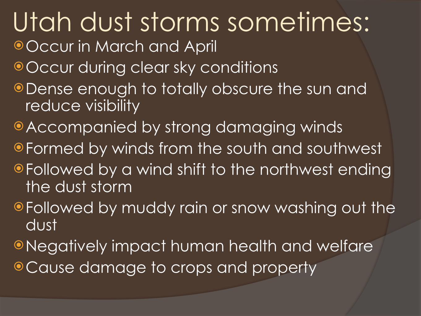
Utah dust storms sometimes:Occur in March and AprilOccur during clear sky conditionsDense enough to totally obscure the sun and
reduce visibilityAccompanied by strong damaging windsFormed by winds from the south and southwestFollowed by a wind shift to the northwest ending
the dust stormFollowed by muddy rain or snow washing out the
dustNegatively impact human health and welfareCause damage to crops and property
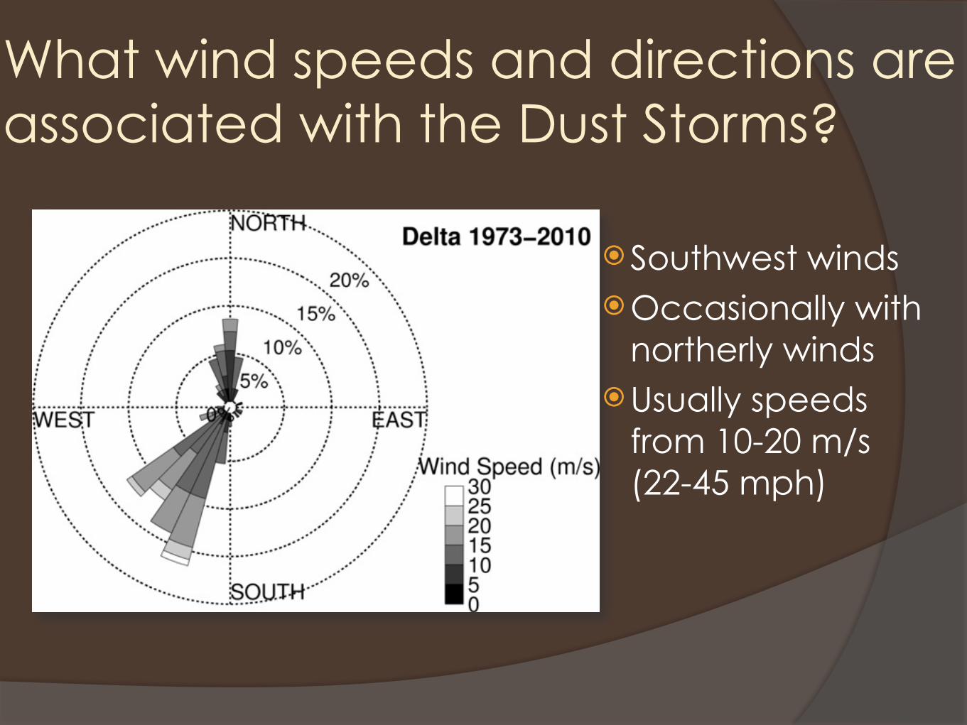
What wind speeds and directions are associated with the Dust Storms?
Southwest windsOccasionally with
northerly windsUsually speeds
from 10-20 m/s (22-45 mph)
L
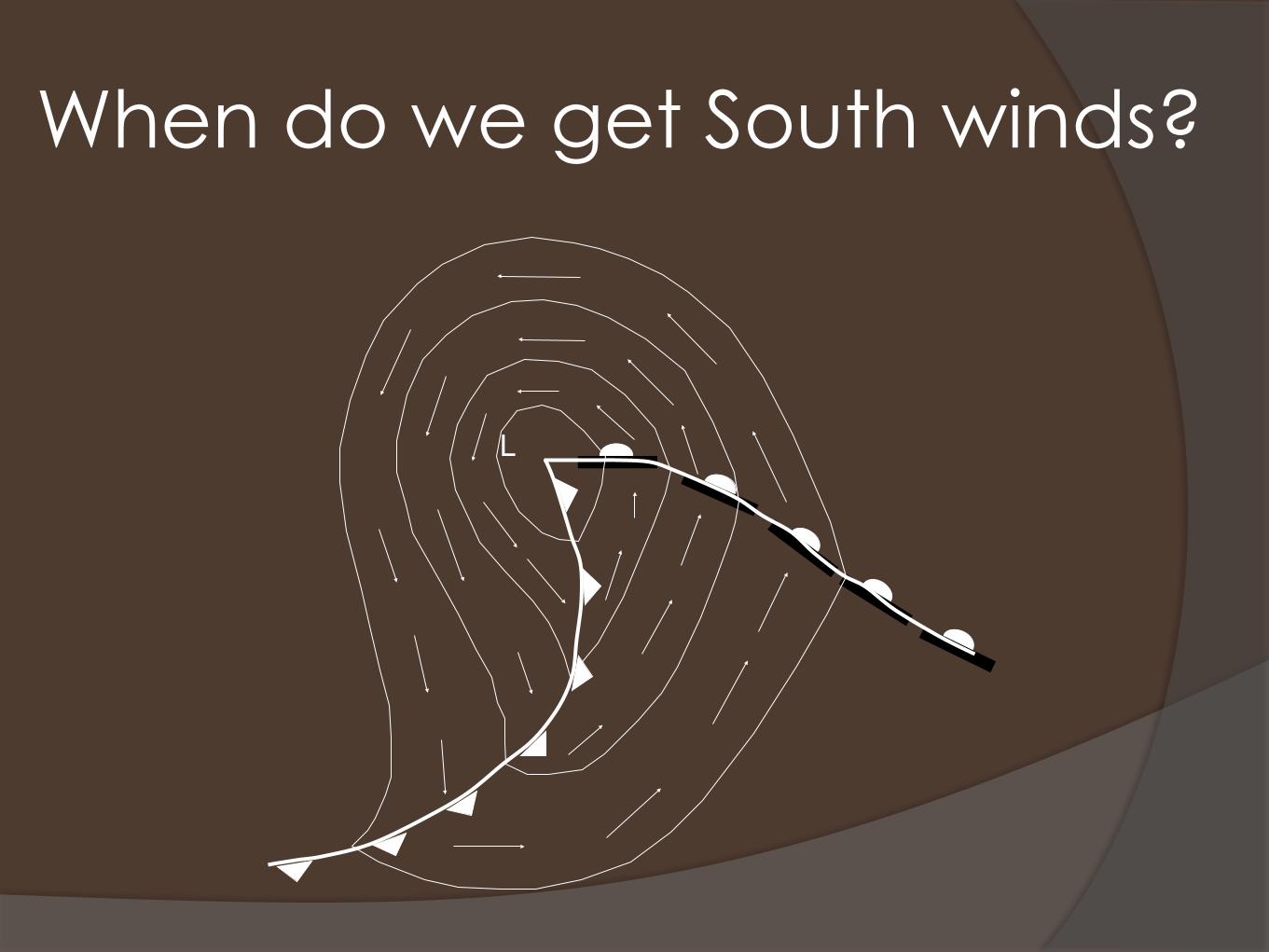
When do we get South winds?
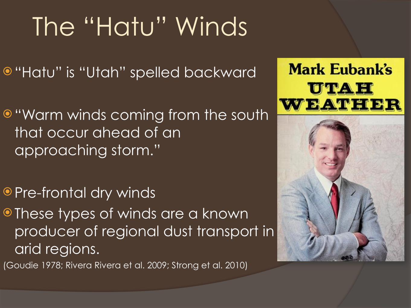
The “Hatu” Winds
“Hatu” is “Utah” spelled backward
“Warm winds coming from the south that occur ahead of an approaching storm.”
Pre-frontal dry windsThese types of winds are a known
producer of regional dust transport in arid regions.
(Goudie 1978; Rivera Rivera et al. 2009; Strong et al. 2010)
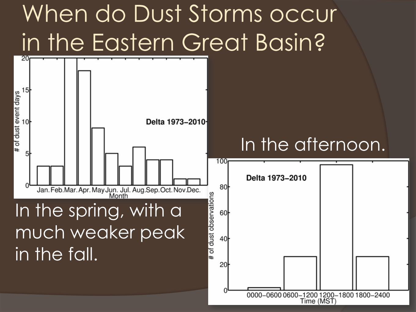
When do Dust Storms occurin the Eastern Great Basin?
In the spring, with a much weaker peak in the fall.
In the afternoon.
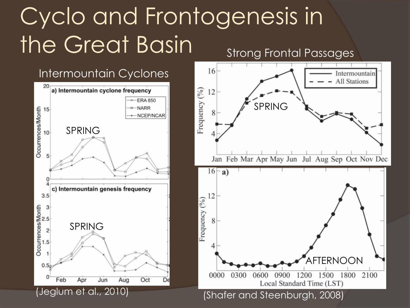
Cyclo and Frontogenesis in the Great Basin
(Shafer and Steenburgh, 2008)(Jeglum et al., 2010)
SPRING
SPRING
SPRING
AFTERNOON
Intermountain Cyclones
Strong Frontal Passages
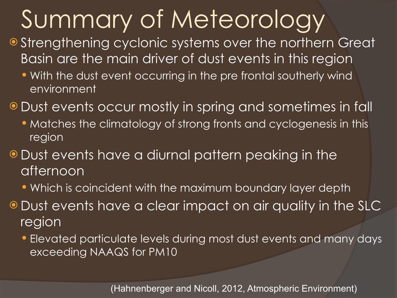
Summary of Meteorology Strengthening cyclonic systems over the northern Great
Basin are the main driver of dust events in this region With the dust event occurring in the pre frontal southerly wind
environment
Dust events occur mostly in spring and sometimes in fall Matches the climatology of strong fronts and cyclogenesis in this
region
Dust events have a diurnal pattern peaking in the afternoon Which is coincident with the maximum boundary layer depth
Dust events have a clear impact on air quality in the SLC region Elevated particulate levels during most dust events and many days
exceeding NAAQS for PM10
(Hahnenberger and Nicoll, 2012, Atmospheric Environment)

Summary of Source AreasMost dust plumes originate from:
Dry Lake Beds (Playas) Disturbed areas
Anthropogenic influence on most sourcesDrought helps drive dust production
Human activities can directly alter dust production…Must take landscape, soils, and climate into account
(Hahnenberger and Nicoll, submitted, Geomorphology)