General rights Copyright and moral rights for the publications made accessible in the public portal are retained by the authors and/or other copyright owners and it is a condition of accessing publications that users recognise and abide by the legal requirements associated with these rights.

Users may download and print one copy of any publication from the public portal for the purpose of private study or research.

You may not further distribute the material or use it for any profit-making activity or commercial gain

You may freely distribute the URL identifying the publication in the public portal If you believe that this document breaches copyright please contact us providing details, and we will remove access to the work immediately and investigate your claim.

Downloaded from orbit.dtu.dk on: Dec 02, 2021

The 3D X-ray diffraction microscope and its application to the study of recrystallizationkinetics

Lauridsen, Erik Mejdal

Publication date:2001

Document VersionPublisher's PDF, also known as Version of record

Link back to DTU Orbit

Citation (APA):Lauridsen, E. M. (2001). The 3D X-ray diffraction microscope and its application to the study of recrystallizationkinetics. Risø National Laboratory. Denmark. Forskningscenter Risoe. Risoe-R No. 1266(EN)

Risø-R-1266(EN)

The 3D X-Ray Diffraction Microscope and its Application to the Study of Recrystallization Kinetics Erik Mejdal Lauridsen

RO isø National Laboratory, Roskilde

ctober 2001

Contents

Preface 3

1 Introduction 5

2 The 3D X-Ray Diffraction Microscope 7 2.1 Experimental set-up 8

2.1.1 The x-ray optics 8 2.1.2 The diffractometer 10 2.1.3 The third dimension 11

2.1.3.1 Tracking principle 11 2.1.3.2 Conical slit 12 2.1.3.3 Focusing analyzer 13

2.2 The GRAINDEX program 15 2.2.1 Coordinate transformations 16 2.2.2 Image analysis 17 2.2.3 Ray tracing 18 2.2.4 Indexing 18 2.2.5 Grain boundary mapping 20

2.2.5.1 Back projection of outlines 21 2.2.5.2 Back projection of intensities 22

2.2.6 GRAINDEX examples 23 2.2.6.1 Grain mapping of Aluminium 24 2.2.6.2 Wetting in Al/Ga system 25 2.2.6.3 Grain rotation 25

2.3 Discussion and outlook 27

3 Recrystallization Kinetics and the 3DXRD Microscope 29 3.1 Experimental 30

3.1.1 Set-up 30 3.1.2 What is measured 33 3.1.3 Orientation determination 34 3.1.4 Experimental considerations 37

3.2 Data analysis 38 3.2.1 Image processing 38 3.2.2 Data transformation 39 3.2.3 Peak identification 40 3.2.4 Integrated intensities 41 3.2.5 Grain volumes 42

4 Recrystallization Kinetics of Commercial Purity Aluminium 45 4.1 Introduction to the sample 45 4.2 Initial sample characterization 46

4.2.1 Optical Microscopy results 46 4.2.2 Electron back scattering results 47 4.2.3 EBSD result 47

4.2.3.1 Growth behaviour 47 4.2.3.2 Microstructure evolution 49 4.2.3.3 Recrystallized volume fractions 49 4.2.3.4 Final grain sizes 50

4.3 3DXRD results 51

Risø-R-1266(EN) 1

4.3.1 Experimental 51 4.3.2 ODF measurements 53 4.3.3 Individual growth curves 56

4.3.3.1 Nucleation 56 4.3.3.2 Growth 56

4.3.4 Overall recrystallization process 57 4.3.4.1 Nucleation times 57 4.3.4.2 Grain sizes 58 4.3.4.3 Growth rates 59

4.3.5 Orientation dependencies 62 4.3.5.1 Individual growth curves 62 4.3.5.2 Nucleation times 63 4.3.5.3 Grain sizes 64 4.3.5.4 Growth rates 66 4.3.5.5 Impingement 67

4.4 Discussion and outlook 68

5 Conclusion 73 5.1 The tracking technique and GRAINDEX software 73 5.2 In-situ measurements of growth kinetics 74 5.3 Recrystallization kinetics of commercially pure aluminium 75

Reference List 79

Appendix A: Published Papers 87

2 Risø-R-1266(EN)

Preface This thesis is submitted in partial fulfillment of the requirement for obtaining the Ph.D. degree at the University of Copenhagen. The research described was carried out in the Materials Research Department at Risø National Laboratory, under the supervision of Jens Als-Nielsen, University of Copenhagen and Hen-ning Friis Poulsen and Dorte Juul Jensen, Materials Research Department, Risø National Laboratory.

During the spring 2000 I spent three months as a visiting Ph.D. student in the Department of Physics at the Carnegie Mellon University, Pittsburgh. I am thankful to Anthony (Tony) D. Rollet for introducing me to the field of grain growth, and to Robert (Bob) M. Suter for a stimulating collaboration regarding the tracking software. Special thanks goes to Bob, Cindy and their family for making me and my family feel at home during our stay in Pittsburgh.

I am very grateful for the involvement and encouragement of my Risø supervi-sors Henning Friis Poulsen and Dorte Juul Jensen. They have always showed a sincere interest in my work and have contributed with many helpful comments and suggestions during the project.

During the years I have benefited from various scientific discussions with the members of the SKAL group, and their help are gratefully acknowledged. As well as Preben Olesen and Palle Nielsen are acknowledged for general techni-cal assistance, often on a last minute basis.

A large part of my Ph.D. study has been carried out at the Materials Science beamline ID11 at the European Synchrotron Radiation Facility and I would like to thank the staff at the beamline for their willingness to help during critical moments. A special thanks goes to Ulrich Lienert.

Finally I would like to use this opportunity to thank my wife, Pia; without you this would not have been possible.

Risø-R-1266(EN) 3

4 Risø-R-1266(EN)

1 Introduction Controlling the properties of metallic materials, such as for example strength and formability, is of key importance for a wide range of industrial applications. The properties of the material can be altered by thermo-mechanical processing typically consisting of various deformation and annealing processes. During deformation point defects and dislocations are introduced in the material result-ing in a transformation from an ensemble of defect-free grains (Fig. 1.1a) to a deformation microstructure (Fig. 1.1b). The details of the deformation structure depend on the material and on the deformation parameters. By a subsequent annealing new almost defect-free nuclei appear in the deformed microstructure (Fig. 1.1c). Driven by the stored energy associated with the dislocations in the deformed state the new nuclei grow and invariably replace the deformed micro-structure (Fig. 1.1d). The process of nucleation and growth of these new nuclei is referred to as recrystallization. Hence, to fully control the macroscopic prop-erties of the material, a detailed understanding of the fundamental mechanisms of deformation and annealing is required.

[1pnscdthwthflsistcantywst

peminodst

R

Fig. 1.1. Illustration of the microstructure evolution following deforma-tion and annealing. Courtesy Dorte Juul Jensen.

From the very early metallurgical studies, dating more than 150 years back ], and up till today, the level of understanding of these mechanisms has de-

ended on the capabilities of the characterization techniques available. Tech-iques such as optical microscopy, transmission electron microscopy (TEM), anning electron microscopy (SEM), laboratory x-ray diffraction and neutron

iffraction are currently some of the most frequently used tools for the study of ermo-mechanical processes. Common for all the microscopy techniques, as ell as laboratory x-ray diffraction, is that they are surface probes. This implies at they are restricted to either in-situ studies of the surface, which will be in-uenced by surface effects such as strain relaxation, pinning, and atypical diffu-on, or to experiments based on sectioning of the sample and thereby limited to atic investigations. Out of the five techniques mentioned above the only one pable of true bulk measurements is neutron diffraction. The resolution of a

eutron diffraction experiments is, however, in the millimetre range whereas pical grain sizes are in the micrometer range. Hence, neutron diffraction is ell suited for studies of average bulk behaviour but fails when it comes to the udy of individual grains. To further the understanding of the mechanisms of deformation and annealing

rocesses we need to be able to see what is happening to the individual grains bedded deep inside the sample. And not only do we need to be able to look

side the sample, we also need to be able to do it while the deformation process r annealing process is taking place. A need is therefore identified for a non-estructive technique that provides three-dimensional information of the micro-ructure in the bulk of the sample. The resolution of the technique should be

isø-R-1266(EN) 5

comparable with typical grains sizes, hence, in the order of micrometers. Fur-thermore the technique must enable analysis over an ensemble of 10-1000 grains for significant overall conclusions to be drawn. Likewise, the data acqui-sition speed must be sufficient to perform in-situ processing studies.

By the development of the novel 3-Dimensional X-Ray Diffraction (3DXRD) microscope [2,3], a new characterization tool that fulfils the above requirements has become available. The 3DXRD microscope is the result of a joint collabora-tion between Risø National Laboratory and the European Synchrotron Radiation Facility (ESRF) and is situated at the Materials Science beamline at the ESRF, Grenoble.

During the three years as a Ph.D. student I have had the privilege of participating in the construction, commissioning and employment of the new and promising tool for the materials science society, namely the 3DXRD micro-scope. Short time after I was started as a Ph.D. student in the summer of 1998 the construction of the microscope was initiated, and in December 1998 the first test experiment was performed using the new 3DXRD microscope. This test experiment involved the annealing of commercial purity aluminium, and al-lowed for the first time a detailed study of the individual grains during anneal-ing [A3]. The results of this first test experiment will be presented later in the thesis. During the spring of 1999 the 3DXRD microscope was commissioned, and in August 1999 it was made available to external users.

Working with an advanced experimental facility like the 3DXRD microscope is very much a team “sport”. Typically 4-5 days of beamtime are assigned to an experiment and involves 4-6 persons. The fact that currently only 5 Risø people, including my self, have the necessary experience to run the 3DXRD micro-scope, implies that these 5 persons participates in practically every aspect re-garding the microscope. There are, however, two specific areas where I have been the main responsible; the first relates to the automatic processing of the vast amounts of data produced by the 3DXRD microscope and has resulted in the development of the GRAINDEX program [A1,A2], whereas the second in-volves the development and application of a technique for in-situ studies of re-crystallization kinetics [A3,A4]. These two topics constitute the main part of the thesis.

The thesis work has resulted in 11 publications which are reprinted in appen-dix A and refereed to as paper A1-A11. The main part of the thesis is based on the papers A1-A4.

6 Risø-R-1266(EN)

2 The 3D X-Ray Diffraction Micro-scope

Until recently, neutron diffraction has been the only true bulk characterization technique available. However, with the construction of third generation high energy synchrotron facilities like the European Synchrotron Radiation Facility (ESRF) in Grenoble, France, this is no longer the case. High energy x-rays (40-100 keV), as opposed to standard laboratory x-rays, interact only weakly with matter. This results in penetration depths of minimum 1 mm in typical metals and up to 4 cm in aluminium (see Fig. 2.1) enabling measurements of true bulk behaviour. The high penetration power combined with the high flux available at third generation synchrotrons (see Fig. 2.2) provide the foundation for detailed three-dimensional structural characterization of bulk material.

Fig. 2.1. Penetration depths in various metals for high energy x-rays. The penetration depth is defined as the thickness at which there is 10% trans-mission of the x-rays. Courtesy Henning Friis Poulsen.

The enormous potential of these unique properties was first realized in 1995 by a group of scientists at the Materials Research Department, Risø National Laboratory [2,4], and during a materials science workshop at the ESRF in 1997 is was decided to build a dedicated experimental station at the ESRF materials science beamline ID11 in a joint collaboration between Risø National Labora-tory and the ESRF [5]. The instrument, referred to as the 3D X-Ray Diffraction (3DXRD) microscope, is dedicated characterization of local structural proper-ties within thick specimens, especially in in-situ studies of deformation and an-nealing processes in metals and ceramics. The construction of the 3DXRD mi-croscope began in the fall of 1998, and after a commissioning period during the spring of 1999, it was made available to external users in August 1999.

The aim of the present chapter is to give an overall description of the princi-ples of the 3DXRD microscope. As such it includes topics, which are direct re-sults of my thesis work, as well as topics that I have been involve with but which are not directly related to my thesis work. My main focus has been on the so-called tracking technique, and especially on the development of a soft-ware program termed GRAINDEX used for automatic data processing of the vast amount of data produced by the microscope [A1]. The algorithms behind the GRAINDEX program will be explained, and to show the usefulness of the program a number of examples of use will be given.

Risø-R-1266(EN) 7

Fig. 2.2. Evolution of the brilliance (photons/s/mm2/mrad2/0.1%BW) from the early x-ray tubes to today’s third generation synchrotron sources. Courtesy ESRF.

2.1 Experimental set-up Many fundamental quantities of polycrystallinond phase particles, cracks etc., have dimeHence, the experimental set-up for the 3DXRspatial resolution in the micrometer range – intrivial task, and has only been possible by tcombined with high mechanical stability of thment of novel techniques for defining the third

2.1.1 The x-ray optics One of the key features of the 3DXRD microshigh energy x-ray optics. Optics for microfoyears for conventional low energy x-rays andtron beamlines and laboratory x-ray sources thnately direct application of these standard optirays is not possible. Thus, new optical compocally for use with high energy x-rays [7,8]. Twused for focusing at the 3DXRD microscope: cut Laue crystals and elliptically bent multilathe focussing of the beam the optical componetors resulting in an energy bandwidth of 0.1-10.5 mrad [7,9]. Several combinations of the oline focusing using a single Laue crystal, ii) poof a Laue crystal and a multilayer (see Fig. 2.combination of two multilayers (Kirkpatric-Bafocal sizes are currently 1.2 µm and 5 × 5 µmfocusing, respectively [9]. Which of the set-upoint focusing depends on the specific eLaue/multilayer solution is relatively easy toenergy bandwidth and beam divergence by chbeam [8]. The multilayer/multilayer solutionflux and should be chosen if flux is of primemultilayer/multilayer set-up

8

e materials, such as grains, sec-nsions on the micrometer scale.

D microscope should provide a all 3 dimensions. This is by far a he use of advanced x-ray optics e diffractometer and the develop- dimension.

cope is the use of microfocusing cusing have existed for several

are being used at many synchro-roughout the world [6]. Unfortu-cal components to high energy x-nents had to be designed specifi-o types of optical components are cylindrically bent asymmetrically yers [7,9]. Apart from providing nts also function as monochroma-% and a divergence of less than

ptical components can be used, i) int focusing using a combination

3), or iii) point focussing using a ez geometry [10]). The achieved 2 for the line focusing and point ps ii) and iii) that is chosen for xperimental requirements. The

focus and allows for tuning the anging the height of the incoming does however provide a higher importance. The focusing of the

is however

Risø-R-1266(EN)

sourcefocuspq

source

p

q

p 50 m, q 1.5 m

Fig. 2.4. Illustration of the principles of the focusing optics. Top. The cylindrically bent Laue crystal focus the beam in the vertical direction and monochromize the white beam. The band width of the mono-chromized beam depends on the height of the incoming beam 32. Bottom: the elliptically bent multilayers can both be used for horizontal and vertical focusing of the beam. The thickness of the mul-tilayer is varied continuously from one end to the other to compensate for the difference in the angle of incidence. p and q refers to the source distance and focal distance, respectively. Courtesy Ulrich Lienert.

Fig. 2.3. Contents of the optics box of the 3DXRD microscope. The incoming white (polychromatic) x-ray beam enters the optics box from the right. It is monochromized and vertically focused by the bent Laue crystal. The remains of the white beam are absorbed by the beam-stop. The monochromatic vertically focused beam continues to the bent multilayer, which provides the horizontal focusing. Courtesy Ulrich Lienert.

multilayer300 mm

bent Si-Laue crystal

Risø-R-1266(EN) 9

somewhat more complicated and does not allow for changing of the energy bandwidth and beam divergence. The obtained focal spot sizes are mainly lim-ited by shape errors of the optical elements and further progress is expected. The optical elements are designed for use with a specific x-ray energy and at present two sets are available at the 3DXRD microscope, one set for 50 keV and one set for 80 keV. An illustration of the optical elements are shown in Fig, 2.4. The use of high energy microfocusing optics is essential for the 3DXRD micro-scope as they provide several orders of magnitude more flux compared with the use of perfect flat monochromators and narrow apertures [7]. By using focusing optics the flux in the focal point is typically 1011-1012 photons/sec.

2.1.2 The diffractometer The 3DXRD microscope is a heavy-duty horizontal two-axis diffractometer and is designed to hold 200 kg with an absolute accuracy of a few microns. It con-sists basically of two parts; a sample tower and a 2θ-arm carrying the detec-tor(s) (see Fig. 2.5). The sample tower and the 2θ-arm are mounted on two separate granite blocks and connected by a weak link in order to reduce the ef-fect of mechanical vibrations. The 2θ-arm was made long (2.5m) to allow for a high angular resolution in 2θ. Thanks to the low scattering angles at high ener-gies, experiments can in general be performed without the need for Eulerian cradles or equivalents and the associated sphere-of-confusion problems. Instead an x-y-z-ω sample stage is used, with an air-borne ω rotation stage for maxi-

Fig. 2.5. A photo of the 3DXRD microscope installed at the materials sci-ence beamline at the ESRF. The white box in the back of the picture, marked (a) is the optics box, cf. Fig. 2.3. The sample tower is indicated by (b) and a two-dimensional detector is positioned on the 2θ-arm (c). The yellow and red line indicates the direct beam and a diffracted beam, re-spectively. Courtesy Søren Fæster Nielsen.

10 Risø-R-1266(EN)

mum accuracy. Several 2D detectors are available including tapered charge coupled devices (CCDs), CCDs coupled to image intensifiers, on-line image plate scanners and a high resolution CCD. The high resolution CCD is designed to be semi-transparent and as such it can be used simultaneously in combination with, for example, a large field of view CCD. Sample auxiliaries include 2 fur-naces and a 25 kN Instron tensile machine for in-situ measurements. All move-ments are motorized, and all motors, detectors, and auxiliaries are controlled via SPEC, the ESRF controlling software [11]. A complete library of SPEC macros has been developed especially for the 3DXRD microscope and provides fully automatic data acquisition as well as alignment procedures.

2.1.3 The third dimension As shown above the use of high energy focusing optics provides micrometer size resolution in two dimensions. However, in order to be able to perform three-dimensional structural characterization the third dimension also has to be defined. Four different methods have been developed for such depth-resolved studies: x-ray tracing with line- [A1,A2] or point focus, conical slits [12] and focusing analyzer optics [13]. In all cases the diffracted beam is transmitted through the sample and the illuminated area is determined by focusing. A sum-mary of advantages and limitations of the four different techniques are given in table 2.1 at the end of the section.

2.1.3.1 Tracking principle

The first method for defining the third dimension, termed tracking, was inspired by the methods used in high-energy particle physics. The principle is an exten-sion of the classical rotation method: a monochromatic beam of high energy x-rays, focused in one dimension, impinges on the sample and the directions of the diffracted beams are traced by translation of 2D detectors. The tracking method is designed for fast and non-destructive characterization of the-

Fig. 2.6. Sketch of the tracking principle. Spots arising from the same re-flection at different sample-detector distances are identified. Linear fits through these are extrapolated to give the position of the grain within the illuminated layer in the sample. The angles (2θ,η,ω) are defined as well as the laboratory coordinate system . From [A1]. ( lll z,y,x )

sample

ω

2 dimensionaldetector

beam

beamstop

2θω

LL

0

1

2

η

η1

2

L3

2θ

1

2

z

ly

lx

lz

Risø-R-1266(EN) 11

individual grains inside crystalline bulk materials (powders or polycrystals). It allows for the position, volume and orientation of hundreds of grains to be de-termined simultaneously. The details of the tracking principle are described in Lauridsen et al. [A1] but for the continuity of the chapter parts of the paper are included in the following. “The experimental geometry is sketched in Fig. 2.6. The sample is mounted on an ω rotation stage. A beam of monochromatic high energy x-rays is focused in one direction in order to define a layer in the sample, which is perpendicular to the ω rotation axis. Some of the grains intersected by this layer will give rise to diffracted beams, which are transmitted through the sample to be observed as spots by a flat two-dimensional detector. The detector is aligned perpendicular to the incident beam. In addition, an optional slit is pla-ced before the sample.

The tracking algorithm works as follows: images are acquired at a number of rotation axis-to-detector distances, L1 to LN (Typically N = 3). Equivalent spots, generated by the same reflection, are identified and a best fit is determined to a line through the center-of-mass (CMS) positions of these spots. This determines the scattered wavevector which is specified in terms of the scattering angle, 2θ, and the azimuthal angle, η. Extrapolating the fitted line to its intersection with the incident beam determines the CMS position of the illuminated section of the grain of origin, specified by (xl, yl). For definitions of zero points and positive directions, see Fig. 2.6.

To obtain information from all grains in one layer, the x-ray tracing is re-peated at a number of ω settings in steps of ∆ω. During each exposure the sam-ple is oscillated by ±∆ω/2. Typically, an ω-range of 25o – 40o provides a suffi-cient number of Bragg peaks from each grain. If the ω range is expanded to 180o, all reflections are illuminated with the exception of those lying in two small “blind” spots on the unit sphere (centered on the ω–axis) with a total spherical area of 4π(1 – cos(θ)), where θ is the Bragg angle. For high energy x-rays with wavelength, λ, much less than the lattice constant, this area is negligi-ble for low order reflections. This observation justifies the use of a sample stage with only one rotation.

Finally, for a complete mapping, the procedure is repeated for a set of layers by translating the sample in z. In this way a 6-dimensional space, consisting of the (x, y, z, ω, 2θ, η) coordinates for the various reflections is probed with es-sentially a two-dimensional scan over ω and z.

As a variation of the tracking method one could consider the monochromatic beam being restricted in two directions – either by focusing or by slits. This is an option if the overlap between spots arising from the grains in the full layer is too severe. For each ω-setting the beam then defines a stripe through the sam-ple. Upon rotation only grains close to the rotation axis will remain fully illumi-nated. The majority of the spots therefore need to be discarded from the analy-sis, and a full mapping requires additional scanning with translations x and y on top of the rotation table.” from [A1].

Examples of use of the tracking technique will be given later in this chapter.

2.1.3.2 Conical slit

The tracking technique provides a fast way of obtaining three-dimensional in-formation. It is, however, restricted to crystalline materials and does not apply to deformed materials. The solution for depth-resolved studies of deformed ma-terials is the use of conical slits.

12 Risø-R-1266(EN)

The conical slit set-up is an extension of traditional cross-beam techniques. Traditional cross-beam techniques are based on insertion of pinholes in both the incoming and diffracted beams, and thereby defining a local volume. The use of pinholes does, however, only allow measurements of a narrow range of orienta-tions given by the solid angle defined by the pinhole, leading to very slow data-acquisitions rates. To circumvent this problem a new technique using conical slits has been implemented at the 3DXRD microscope [12]. The idea is to use a slit with conical openings along the diffracted Debye-Scherrer cones (see Fig. 2.7). The slit openings are aligned such that they all point to the same point in the sample. The gauge volume is then defined by the intersection of the narrow

incoming beam and the extension of the conical slit openings (see bottom part of Fig. 2.7). By this method complete information on texture and strain field can be obtained simultaneously from a local gauge volume inside the sample, sim-ply by rotating around the ω-axis.

Fig. 2.7. Top: Illustration of the conical slit principle used at the 3DXRD microscope. Bottom: The gauge volume (shaded grey) is de-fined by the intersection of the incoming beam and the openings of the conical slit. From [A5].

2.1.3.3 Focusing analyzer

The third method for obtaining depth resolved information involve the use of focusing optics on both the incident beam and the exit (diffracted) beam. An illustration of the principle is shown in Fig. The method has not yet been im-plemented at the 3DXRD microscope, but preliminary tests experiments have shown very promising results [13].

Risø-R-1266(EN) 13

Fig. 2.8. Illustration of the focusing analyser principle. A focusing multi-layer is positioned behind the sample and focus the diffracted beams onto the detector.

Table 2.1. Characteristics for identification of individual nuclei/grains of the four techniques for 3D beam definitions. Depending on the type of beam definition, data from for example several x,y position inside the sample may be achieved simultaneously. This is marked by * in the table. The parameters x,y,h and r refer to sample position along incident beam, sample position perpendicular to incident beam, azimuthal angle along Debye-Scherrer cone as recorded on the detector and (hkl) reflex, respec-tively. (reproduced from [A5], with the focal sizes updated to reflect cur-rent status).

Type Spatial Resolu-tion (mm)

Limitation Simultaneous Data Acquisi-

tion

Recording time for

one sample layer

Comments

x y η r X-ray tracing (line fo-

cus)

)2sin(

52.1x

θ⋅⋅

Detector resolution,

mosaic spread

* * * * 1 min Fast, re-quires sub-

stantial soft-ware analy-

sis, only relevant for undeformed or weakly deformed materials.

X-ray tracing (point focus)

)2sin(

555

θ⋅⋅

Detector resolution,

mosaic spread

* * * 1 hour As above, but can be used for

more heavily deformed materials.

Conical slit )2tan(

2555

θ⋅⋅

Manufactur-ing

* * 12 hours Easy data analysis, but

relatively poor spatial resolution.

Focusing optics

1055 ⋅⋅ Aberrations in optics

(*) - Good spatial resolution, but slow.

14 Risø-R-1266(EN)

2.2 The GRAINDEX program One of the main advantages of the 3DXRD microscope is that the data acquisi-tion is so fast that it allows for in-situ studies. This does, however, also result in a vast amount of data, typically several giga bytes (Gb) per hour. Hence, devel-opment of software for automatic data processing is vital for a successful and efficient operation of the 3DXRD microscope.

A software program, termed GRAINDEX [A1], has been developed for the processing of data taken using the tracking technique describe above. The pro-gram is written as an add-on to the commercial image analysis software Image Pro Plus [15]. The data acquisition at the 3DXRD microscope is controlled via Image Pro Plus, and by writing GRAINDEX as an add-on it has immediate ac-cess to the acquired images as well as all image processing tools available in Image Pro Plus. To allow for a high degree of flexibility the GRAINDEX pro-gram is written using a modular structure as illustrated by the outline of the program shown in Fig 2.9. As with the tracking technique, the details of the algorithms used in the GRAINDEX software are described in Lauridsen et al. 2001 [A1], but is included in this chapter to give a coherent description of the capabilities of the 3DXRD microscope. The overall algorithm of the GRAINDEX program is the following: “Initially, all grains are associated with the same a priori known space group and lattice parameters, representing, for example, a stoichiometric and strain-free reference material. The ray tracing provides a list of reflections characterized by their center-of-mass origin and integrated intensity. The reflections are sorted with respect to their grain of ori-gin by the central indexing algorithm. Next, the positions, volumes and crystal-lographic orientations of the grains can be fitted.

Once the grains are indexed, single crystal refinements may be applied. Alter-natively, the relevant part of the data may be reinvestigated for a stress analysis. Depending on grain size, it may also be possible to produce a 3D map of grain boundaries” from [A1]. In the following the different parts of the GRAINDEX program will be explained in further detail. The potential of the program is illus-trated by a number of examples in the end of the section.

Fig. 2.9. A flow chart for the track-ing method using the GRAINDEX algorithmGRAINDEX gen-erates a list of grains with associ-ated positions and orienta-tions as well as sets of in-dexed reflections with associated in-tegrated intensities. The output may be used for crystallo-graphic refine-ments of the grains or - with a reanaly-sis of the raw data

.

Risø-R-1266(EN) 15

- for determining the average strain tensors. Furthermore, for coarse-grained materials the grain boundaries can be mapped in three dimen-sions [A1].

2.2.1 Coordinate transformations Before focusing on the individual modules of the GRAINDEX program it is useful to define the coordinate systems in use and the transformations relating them. “The algebra for associating scattering observations with reciprocal space is well described for single crystals by Busing & Levy [16]. The polycrystal case differs by the need for one extra coordinate system since the sample and grains are different objects. For reference purposes we go through the equations, following the single crystal formalism of Busing and Levy [16] as close as pos-sible (our sign convention for ω, however, is opposite to theirs). Four Cartesian coordinate systems are introduced: the laboratory system, the ω-axis system, the sample system, and the Cartesian grain system.

We describe the coordinate transformations for an arbitrary scattering vector, G. The laboratory system ( is defined in Fig 2.6. It has pointing along the incoming beam, transverse to it in the horizontal plane and positive upwards, parallel to the ω rotation axis. In this system, vectors are given the subscript l: G

)

)ωωω ˆˆˆ

)

s

)

lll z,y,x

lylx

lz

l. The ω-system is rigidly attached to the ω turntable of the 3DXRD microscope. For ω = 0, the ω and laboratory systems are the same. Hence, the scattering vector transforms as

( z,y,x

Gl = Ω Gω with

Eq. 2-1

−=

1000)ωcos()ωsin(0)ωsin()ωcos(

Ω

The sample system is fixed with respect to the sample, e.g. defined

by deformation axes (RD, TD, ND). The orientation of the sample on the ω turntable is given by the S matrix: G

( sss z,y,x

ω = S Gs. S must be provided by the user, and is typically used to swap axes, to simplify the data analysis.

The crystallographic orientation of a grain with respect to the sample is given by the U matrix: G = U Gc, where index c refers to the Cartesian grain system

. This is fixed with respect to the reciprocal lattice (a*, b*, c*) in the grain. We use the convention that is parallel to a*, is in the plane of a* and b*, and is perpendicular to that plane. Let G be represented in the recip-rocal lattice system by the Miller indices G

( ccc z,y,x

cx cy

czhkl = (h, k, l). The correspondence

between the Cartesian grain system and reciprocal space is then given by the B matrix: Gc = B Ghkl, with

Eq. 2-2

)αsin()αcos(

)

ββ−γ

βγ=

)sin(c00)sin(c)sin(b0

cos(c)cos(ba

**

****

*****

B

and

)βsin()αsin(

)αcos()γcos()βcos()cos( **

*** −=α Eq. 2-3

16 Risø-R-1266(EN)

Here (a,b,c,α,β,γ) and (a*,b*,c*,α∗ ,β∗ ,γ∗ ) symbolize the lattice parameters in di-rect and reciprocal space, respectively.

The orientation matrix U can be parameterized in numerous ways, well known from texture analysis. As default we use the ( )21,, ϕϕφ Euler angle notation [17]:

)(cos)(sin)φ(cos)(sin)φ(sin

)(sin)φ(cos)(cos)φ(cos)cos(φ)sin(φ)φ(sin)(cos)φ(sin)cos(φ)cos(φ)φ(sin)(sin)φ(sin)(cos)φ(cos)sin(φ)sin(φ)φ(cos)(cos)φ(sin)sin(φ)cos(φ)cos(φ

22

121212121

121212121

333231

232221

131211

φφφφ−φ+−φ+

φφ−−φ−

=

UUUUUUUUU

Eq. 2-4

Equations and diagrams with reference to pole figures and the high energy x-

ray set-up can be found in Mishin et al. [A8] . Next, we deduce the basic diffractometer equations. In order for a given scat-

tering vector G to give rise to a diffraction spot it must fulfill Bragg’s law,

λθπ= /)sin(4G . Eq. 2-5

From the geometry in Fig 2.6 we have

ηθηθ−

−θ

λπ=

)cos()2sin()sin()2sin(

1)2cos(2Gl Eq. 2-6

The coordinate transforms introduced above lead to

Eq. 2-7 hkll GG ΩSUB=

“ from [A1]. This is the basic diffractometer equation relating a scattering vector Gl in the laboratory coordinate system to a scattering vector Ghkl in the crystal laboratory system.

Having established the coordinate transformations used with the 3DXRD mi-croscope, we will now focus on the individual parts of the GRAINDEX pro-gram (cf. Fig. 2.9).

2.2.2 Image analysis The first step in the data analysis is to locate the diffraction spots on the images. “Initially all images are scanned for bright objects that satisfy certain criteria on area, connectivity and maximum intensity. These criteria depend on experimen-tal conditions, and generally have to be found by trial-and-error. Additional cri-teria may apply, such as the location of an object in the image. Objects meeting the criteria are defined as spots. Spots are associated with a CMS pixel position, an ω position – the middle of the ∆ω interval – and an integrated intensity.

Depending on mosaic spread, the same reflections may give rise to spots ap-pearing at several consecutive ω settings. GRAINDEX identifies such groups as

Risø-R-1266(EN) 17

single spots, adds integrated intensities and assigns pixel positions and ω posi-tions based on weighted averages.” from [A1].

2.2.3 Ray tracing “Next, valid spots in images acquired at different detector distances are grouped into a reflection, and a linear fit (orthogonal regression) is performed. Three criteria are applied to discriminate against erroneous groupings, typically caused by spot overlap. First, tolerances are set on the χ2 of the fit and the variation in integrated intensity within corresponding spots. Second, the fitted 2θ value is compared to calculated ones. If the observed value matches, within a tolerance, one of the calculated values, the reflection is put in a list with others of that hkl-family; otherwise it is disregarded. If the observed 2θ could be associated with more than one hkl, list entries corresponding to each hkl-family are created. The erroneous reflections are sorted out later. Third, the fitted CMS origin obtained by extrapolation of the fitted line to the incident beam plane should be positioned within the illuminated region of the sample.

The integrated intensity of the reflection is taken to be that of the outermost L setting. For comparison between reflections it is multiplied by polarization and Lorentz factors. With our conventions the Lorentz factor is

)ηsin()θ2sin(1)η,θ2(Lor =

Note that spots appearing near η = 0o and η = 180o have to be discarded as the Lorentz factor is diverging at this point and parts of the mosaic spread may be situated in the inaccessible areas on the unit sphere near the rotation axis. Also such spots will tend to appear at several consecutive ω-settings, adding to noise in the summed intensity. In practice this restriction is handled by defining cer-tain η-ranges to be void.” from [A1].

2.2.4 Indexing The list of reflections found by the ray tracing is then sent to the indexing mod-ule. “The indexing is, however, not a straight forward process due partly to the overlap between spots, partly to the magnitude of them. Three criteria may be applied to sort reflections according to grain: the position (xω, yω), the crystal-lography, and the integral intensities (area of grain section). Among these, the latter is considered the least robust. One reason is the issue of the “grains at the boundary”. In many cases, samples will have a plate- or rod-like geometry with dimensions too large for the incident beam to illuminate an entire section. Hence, there will be a number of grains which will be partly illuminated and which will tend to rotate in and out of the illuminated area. The spots arising from these pieces of grains will still be assigned correct orientations and x-ray tracing will the place the CM of the pieces within the area of the full grains. In contrast, the intensities will be reduced. In the limit of the grain dimensions be-ing much larger than the accuracy with which the x-ray tracing defines the CM positions, it is possible to rely primarily on the position criterion.

In the limit of the grains being much smaller than the error on the CM posi-tion, indexing must rely on the crystallographic criteria. Let us therefore con-sider the case of equal sized grains, all placed at the origin. At first, it seems relevant to compute the angles between all pairs of observed reflections and compare these to a list of allowed angles, dictated by the space-group symme-try. Grains are then defined by groups of reflections, where all pairs mutually fulfill the angle criterion.” from [A1]. This approach was implemented in the

18 Risø-R-1266(EN)

early versions of the GRAINDEX program, and gave satisfactory results for coarse-grained materials with 20-50 grains in the illuminated layer. (see section 2.2.6.1 for an example). However as n reflections give rise to 2n possible groups, the speed of analysis becomes prohibitive for large n.

To circumvent this a new approach for handling large numbers of reflections has been developed. The idea is to probe the space group symmetry directly, leading to an algorithm for which the speed is almost independent of n*. “By rearranging Eq. 2-7 as

Eq. 2-8 hkls GG BU=

the measurements of Gs and crystallographic properties (B, Ghkl) are separated. Note that the number, n, of measured reflections (Gs)i increases with the num-ber of grains whereas the number M0 of theoretical reflections (BGhkl)j is con-stant.

The underlying principle of the algorithm is to scan through all orientations and for each orientation U count the number, Mexp, of (hkl)’s for which there is at least one observation Gs that matches UBGhkl. Grains are defined by com-pleteness and uniqueness criteria. The former requires Mexp ≥ (1-α) M0, where the tolerance α is rather small. The latter requires the set of matching (hkl)’s not to be a sub-set of the set of matching (hkl)’s for another U setting. Naturally, scanning through all orientations in a strict mathematical sense is not possible. However, by incrementing the three Euler angles defining U by finite steps and allowing a corresponding mismatch between the left and right-hand sides of Eq.2-8., the number of orientations to test becomes finite.

To sample Euler space homogeneously we use the metric [18]

21221 )sin(8

1),,( ϕϕφφπ

=ϕϕφ ddddU Eq. 2-9

Furthermore the crystal symmetry of each grain implies that only a subset of the full [0,π] x [0,2π] x [0,2π] Euler space needs to be sampled. As an example, 1/24 of the volume is sufficient for cubic symmetry and this yields a corre-sponding increase in speed of the algorithm. For a discussion of the symmetries in Euler space see e.g. Randle and Engler, 2000 [19].

To allow an effective search for the (Gs)i’s, initially these are placed in look-up tables, one for each hkl family. In these the unit vectors Gs/ Gs are repre-sented by spherical coordinates (ψ1,ψ2). For a given UBGhkl an area around the theoretical (ψ1,ψ2)0 is searched and the matching observations found (if any). The size of the search area reflects the measuring errors and the step size in the scan over Euler space.

For a given step in Euler space the calculated Ghkl's are grouped according to: A. Reflections that have no matching observations B. Reflections that have one matching observation C. Reflections that have two or more matching observations. Provided the number of A type reflections is small enough to fulfil the com-pleteness criteria, a linear least squares fit is made to the orientation of the grain based on the Gs vectors associated with group B. To linearize Eq. 2-8 in φ, ϕ1, and ϕ2 we expand to first order around the nominal step position in Euler space.

* The development and implementation of this new indexing approach was done by my college

Søren Schmidt.

Risø-R-1266(EN) 19

Hence, for a given step and corresponding U( 02

01

0 ,, ϕϕφ ) 0 = U we have

( )02

01

0 ,, ϕϕφ

( ) ( ) ( ) 20

21

0

1

00 ϕ∆ϕ

+ϕ∆ϕ

+φ∆φ

+= mnmnmnmnmn UUUUUUUUδδ

δδ

δδ

Eq. 2-10

For step sizes of a few degrees in φ, ϕ1, and ϕ2 this is an excellent approxima-tion. The fit is weighted with respect to the estimated experimental errors in ω and η

( )( )

∑ η∆ω∆σ

ϕ∆ϕ∆φ∆−=χ

ji, 2ij

2ijhkl21js2

),(

)G(),,()G( BU Eq. 2-11

Here index i runs over the spatial coordinates: i=1,2,3 while j enumerates the members of group B. σ2

ij is the error on Gs vector number j in the point U0, cal-culated by error-propagation using Eqs. 2-1 and 2-6.

This approach - trusting the group B reflections - has one pitfall. Assume a re-flection from the grain to be found is lacking, e.g. due to overlap, but one stray reflection is positioned within the same search area in (ψ1,ψ2). Then the stray reflection will be assigned as a group B reflection. This reflection is likely to move the least-squares fit minimum substantially as it contributes with a large weight. To discard such "outliers" the fit is performed in iterative steps using a re-weighting scheme. Alternative methods for producing a more robust fit with less or no weight on outliers can be found in the book by Press and co-workers [20].

The final result of the fit to the group B reflections is used to choose among observations in group C. For a given (hkl), the Gs observation that is closest and within ∆ω and n⋅ ∆η of the expected position is chosen (if any).

Returning to the general case of grains of various sizes, which on average are comparable to the error in the CM positions, GRAINDEX uses a modification of the Euler scan procedure just outlined. Once an orientation is found fulfilling the completeness criterion, the associated B and C type reflections are sorted by CM position and/or integrated intensity as well.

Having indexed the grains, optimized positions and volumes can be found from the set of associated reflections. GRAINDEX determines the position as a weighted average of the (xω, yω) coordinates. The volume is defined by conven-tional single-crystal refinement. The necessary intensity normalization can be obtained e.g. by summing all the reflections from all the grains in the layer of interest – that is by acquiring data through a complete ω sweep from –90° to 90°. “ from [A1].

2.2.5 Grain boundary mapping One extension available for the GRAINDEX program is the mapping of grain boundaries for coarse-grained materials with limited mosaic spread. This is the topic of paper [A2] by Poulsen et al. and parts of this section is quotations from that paper. “For a “perfect” grain with no orientation spread and an ideal in-strument there will be a one-to-one correspondence between the shape of the illuminated cross-section of a grain and the shape of any associated diffraction spot. Hence, the position of the grain boundary can be determined by back-projecting the periphery of the diffraction spot along the line established by the x-ray tracing. Introducing a local co-ordinate system (ydet, zdet) around the CMS

20 Risø-R-1266(EN)

of the spot and analogously a system (∆x, ∆y) around the CMS of the grain sec-tion the projection becomes

ydet = ∆y and zdet = ∆x tan(2θ)cos(η). Eq. 2-12

For high energy x-rays with small Bragg angles, the projection is seen to be

very anisotropic. Typically a square grain section is projected into a rectangular diffraction spot with an aspect ratio of 10:1. Furthermore for η = 90° and η = 270° the projection collapses into a line. Hence, diffraction spots appearing within a certain η range around these numbers cannot be part of the analysis.

In metallurgy and ceramics research grains are seldom truly perfect. More-over, instrumental resolution is an issue. Hence, the intensity distribution of a spot on the detector, Idet(ydet, zdet), can be seen as the idealised response of a “perfect” grain, I0, convoluted with the instrumental resolution function, Res, and the orientation spread of the reflection, Q. Res can be determined with a high degree of accuracy – its main components are the detector response func-tion and the smearing caused by the oscillation in ω during acquisition. In con-trast Q varies from reflection to reflection and is a priori unknown. (However, provided the detector is sufficiently close to the sample, there is no noticeable spread in 2θ.)

The existence of an orientation spread within each grain also implies that some of the reflections will be associated with several diffraction spots appear-ing in images acquired at neighbouring ω settings. As the ω axis is a fixpoint for the rotation, this effect is pronounced for reflections appearing near the axis - that is for spots with η ≈ 0° and η ≈180°.

To handle these complications it seems relevant to use space-filling algo-rithms based on either intensity conservation constraints or fits to the local ori-entation function (Monte Carlo simulations) and work along these routes are in progress. “ from [A2]. The present work has, however, been concentrated on two simpler and more direct methods for mapping the grain boundaries. The first method is based on determining the outlines of the diffraction spots and back projecting the outlines into the sample plane. The second method is con-ceptually similar to the first method, but in this case the intensities of the dif-fraction spots is back projected into the sample plane before the outlines are produced.

2.2.5.1 Back projection of outlines

The back projection of outlines can be seen as a fast procedure for obtaining a coarse map of the grain boundaries. This coarse map may be refined later in the analysis by more advanced algorithms. Two ways of determining the outlines of the diffraction spots have been tested. “In the first, the outline of a given spot was determined by an intensity threshold, fixed at a certain percentage of the maximum pixel intensity within the spot. In the second, the outline was defined by the points of steepest descent. The image processing program Image Pro used by GRAINDEX provides routines to find the outline of any object by ei-ther method. It was found that the steepest descent method was is the more ro-bust.

For a given reflection, the back projected outline can be associated with two types of errors. The first is related to the uncertainty in the CMS projection. The second reflects the anisotropy in the projection, cf. Eq. 2-12. Based on these errors, the resulting grain boundary can be determined from a fit to the back projected outlines of all the reflections associated with the grain. Alternatively, the grain boundary is determined as the back projected outline of the reflection

Risø-R-1266(EN) 21

which have superior projection properties. That is, the one associated with a minimum orientation spread and with the most favourable angular setting - the largest projection factor tan(2θ)cos(η), cf. Eq. 2-12.

The problem of a reflection breaking up into several spots is solved by merg-ing the back projected outlines of the individual parts as shown in Fig. 2.11.” from [A2]. This procedure works reasonable well when the mosaic spread has the form of a slowly varying gradient inside the grain. However, the procedure of combining outlines from the same reflection will most likely fail if the mo-saic spread fluctuates throughout the grain.

ω = −2°

ω = 0°

ω = +2°

Fig. 2.11. Example of projection of outlines in the case of grain break-up. For this particular reflection the diffracted intensity is distributed over 3 images, acquired at ω = -2°,0°, and 2°. Left: identical sections of the im-ages acquired at the 3 ω-settings. Right: the back-projection of the out-lines of the four spots into the sample plane (white lines). These are su-perposed on an EBSD image of the same section of the sample surface (colours and black lines). The white scale bar at the bottom is 100 µm [A2].

2.2.5.2 Back projection of intensities

This second method was developed especially for combining intensities of the same reflection from images taken at different ω settings. Doing this has the advantage of improving the ω resolution. Due to the different ω settings one cannot just add the images, determine an overall outline and project that onto the sample plane. Instead the intensities of the individual images have to be pro-jected back onto the sample plane before they can be added. The basic algo-rithm of the method consists of the following steps:

1. The intensity pattern of an observed spot is mapped onto the

sample plane. Associated with this intensity is a center of mass position of this intensity and a scattering vector obtained by GRAINDEX.

2. If, at the next ω setting, a spot is seen which, within the toler-

ances, has the same center of mass position and scattering vector, then the new intensity is added to that previous observed.

22 Risø-R-1266(EN)

3. When no new spots, matching the previous ones, are observed, the reflection is considered complete. The back projected inten-sity pattern is written to an image file and the grain outline is de-termined.

Fig. 2.12. Example of projection of intensities. For comparison the same reflection as in Fig. X is used. Left: the pro-jected intensities of the individual spots are pro-jected onto the sample plane and added. Also shown is the correspond-ing outline (red line). Right: the outline is su-perimposed on the EBSD image of the same sec-tion of the sample sur-face (colours and black lines).

An example of the back projected intensities is shown in Fig. 2.12. For com-parison the same reflection shown in Fig. 2.11 have been used. The left part of Fig. 2.12 shows the added intensities in the sample plane and the corresponding outline. In the right part of Fig. 2.12 the outline has been superimposed on the EBSD pattern of the same sample surface. Comparing the outline with the com-bination of the individual outlines shown in Fig. 2.11, we see that the overall grain shape is almost identical. The second method described here is, however, much more computationally expensive and should therefore only be used in cases where the simpler and much faster projection of outlines is insufficient.

Both methods described here suffer from the lack of being space-filling in na-

ture. Hence, additional algorithms have to be developed for providing the space-filling. They are, however, both conceptually simple and as such provide a very efficient tool for the mapping of grain boundaries in coarse-grained materials with limited mosaic spread.

As shown in Fig. 2.9 other examples of extensions to the GRAINDEX program include single-crystal refinement and strain analysis. A description of these ex-tensions is however beyond the scope of the present thesis and the reader is re-ferred to the paper by Poulsen et al. [A2].

2.2.6 GRAINDEX examples The GRAINDEX program has proven to be an indispensable tool, not only for tracking experiments, but for almost every experiment performed at the 3DXRD microscope. To illustrate the versatility of the GRAINDEX program a few examples will be shown in the following. Common for all the examples shown is the dependency on the GRAINDEX program for the data analysis.

Risø-R-1266(EN) 23

2.2.6.1 Grain mapping of Aluminium

The first tracking experiment performed at the 3DXRD microscope was done in October 1999 on a coarse-grained 99.996% pure aluminium polycrystal [A2]. The main purpose of the experiment was to verify the tracking principle. Before bringing the sample to the synchrotron, the sample surface was characterized using EBSD [21]. In this way the local orientations on the surface were sampled in a 20×20 µm2 grid. In total some 50 grains were identified.

Fig. 2.13. Diffraction patterns from the aluminium polycrystal at sample-detector distances of 7.6 mm (left), 10.3 mm (middle) and 12.9 mm (right), respectively. The rectangular spots near the center of the images are artifacts caused by the tails of the incident beam. The horizontal length of the rectangular spots is 0.8 mm. [A2].

At the 3DXRD microscope the sample was aligned with the same sample sur-face parallel to the beam. Using a 800×5 µm2 line focus a layer located 10 µm below the sample surface was mapped out as described in sec. 2.1.3.1. The tracking was done using a high-resolution 2-dimensional detector, which con-sists of a powder scintillator screen coupled by focusing optics to a CCD. The resulting pixel size of the detector is 4.3 µm, but the point-spread-function is substantially larger, with a FWHM of 16 µm. Using 1 second exposures, 22 equidistant ω-settings, with ∆ω = 2°, and three distances the entire layer was mapped in less than 4 minutes. An example of the acquired images is shown in Fig. 2.13. Notice how the reflections move outwards as the distance is increased.

Fig. 2.14. Validation of the tracking technique. Colours and black out-lines mark the grains and grain boundaries on the surface of the alumin-ium polycrystal as determined by electron microscopy (EBSD). Superim-posed, as white lines are the grain boundaries resulting from the syn-chrotron experiment. The scale bar in the bottom is 400 µm. [A2].

Using the method of back projection of outlines a map of the grain boundaries was produced. The resulting grain boundary map is shown in Fig. 2.14 super-imposed on the EBSD map. Clearly a full 3-dimensional mapping could be ob-tained simply by translating the sample along the z-direction. The misfit be-tween the tracking and the EBSD boundaries was found by linear intercept to be

24 Risø-R-1266(EN)

26 µm in average with a maximum of 40 µm. These numbers should be com-pared with the 16 µm point-spread-function of the detector, the 20 µm step-size in the EBSD data and the 10 µm difference in z. The grain orientations deter-mined by the tracking technique and EBSD were reproduced within 1°. In com-parison the tracking procedure produced grain orientations with an accuracy of better than ±0.1°, as determined by the scatter between reflections from the same grain [A2]. The difference between the techniques is therefore mainly thought to be due to misalignment errors.

2.2.6.2 Wetting in Al/Ga system

The second example does also involve tracking – in this case three-dimensional mapping is performed. The purpose of the experiment was to study the influ-ence of the grain misorientation on the wetting behaviour of the individual grain boundaries [A7]. Initially the three-dimensional grain structure and the orienta-tions of the individual grains in an aluminium polycrystal were determined us-ing the tracking technique at the 3DXRD microscope. Subsequently the alumin-ium sample was exposed to liquid gallium and the wetting of the grain bounda-ries was followed in-situ using synchrotron radiation x-ray microtomography. X-ray microtomography has a spatial resolution which is superior to the spatial resolution currently available with the 3DXRD microscope, it is, however, in-capable of measuring grain orientations. Hence, by combining these two com-plementary techniques detailed spatial information, as well as information on orientations is obtained, allowing a detailed study of grain boundary wetting in this very complex system.

Fig. 2.15. Two sections 100 µm apart through the cylindrical Al. The two sections are reconstructed tomographically in (a) and (d) where the grey lines correspond to the position of the Ga. The white superimposed lines in (b) and (e) correspond to the grain boundaries determined with the tracking technique. (c) and (f) are schematic illustrations of the grain boundaries determined by both techniques (full lines) and only by the tracking technique (dotted lines). The calculated misorientations between neighbouring grains are written on the boundaries. From [A7].

2.2.6.4 Grain rotation

The last example is included to illustrate how the GRAINDEX program can be used for other purposes than mapping of grain boundaries. The purpose of the experiment was to measure grain rotations in-situ during deformation of an

Risø-R-1266(EN) 25

99.996% pure aluminium polycrystals [22]. The aluminium polycrystal was de-formed in tension using the stress rig available at the 3DXRD microscope. Measurements of the diffracted spots were made for strains of 0, 2, 4, 5, 7, 9, and 11%. An example of the raw images is shown in Fig. 2.16. During the de-formation the orientation of the individual grains will change leading to a change in the ω- and η positions of the diffracted spots. This is illustrated in the bottom part of Fig 2.16 where one diffraction spot from one of the measured grains is shown for two different strain levels.

Fig. 2.16. Example of raw data for ω = 1° and 0% strain (top) The circle marks the (220) Debye-Scherrer ring, and the box identifies a spot related to grain 1. The enlarged areas (bottom) show the movement of this spot on the ring, by com-parison with a corre-sponding image at ω = -5° and 11% strain. From [22].

Fig. 2.17. The dynamics of four embedded alu-minium grains during tensile deformation. Ex-perimental data (open circles) are shown as in-verse pole figures, which represent the position of the tensile axis in the re-ciprocal space of the grains. Strain levels were 0, 2, 4, 5, 7, 9 and 11%. The data is compared to A) a full-constraints Tay-lor model and B) a Sachs model. From [22].

The role of the GRAINDEX program for this experiment was twofold. Prior

to the deformation the ray tracing part of GRAINDEX was used to identify grains located in the center of the sample. This was done to ensure that the se-lected grains remains inside the illuminated gauge volume during rotations.

26 Risø-R-1266(EN)

Among the grains located in the center of the sample four grains having orienta-tions of particularly interest was chosen for further investigation by use of the indexing part of the GRAINDEX program. For each strain level the reflections from the four grains of interest were sorted out from a background arising from all other grains and the orientations of the four grains were calculated using GRAINDEX. The resulting rotation paths for the four grains is shown in Fig. 2.17 by use of inverse pole figures [19]. The top part of Fig. 2.17 shows the comparison of the experimental data with the texture model suggested by Tay-lor [23] and the bottom part shows the comparison to the texture model sug-gested by Sachs [24]. Apart from the three examples shown here another example of the application of the GRAINDEX program within the field of recrystallization kinetics will be given in chapter 3.

2.3 Discussion and outlook The 3DXRD microscope presented in this chapter has shown that dedicated ex-perimental stations utilizing focused high energy synchrotron x-ray radiation can provide new detailed insight to many fundamental mechanisms of materials science. The three examples shown demonstrate that new experimental evidence is obtainable, which could never have been achieved using conventional charac-terization techniques. This is further demonstrated by the results presented in the remaining of the thesis. It is my belief that this new detailed information will lead to a deeper understanding of the basic mechanisms within a broad range of materials science.

One has, through, to remember that large advanced experimental facilities like the 3DXRD microscope, only can be realized by putting a significant effort into development and perfecting of novel techniques and instrumentation. As such the 3DXRD microscope presented here has only become a reality due to hard work and great team spirit by the people involved with the 3DXRD microscope.

The ultimate goal is to provide an experimental technique which has superior properties and a high level of flexibility, and which at the same time is as user friendly, as for instance, the automated EBSD technique [21].

To reach this goal the 3DXRD microscope is continuously updated. On the instrumentation side several initiatives has been taken. One example relates to improvement of the focusing. The two-dimensional focusing is currently limited by the slope errors of the multilayer substrate. However, new advances in pol-ishing and deposition techniques points in the direction of improved multilayers and thereby better focusing. Another example is the construction of a “2nd gen-eration” high resolution 2-dimensional detector. It is based on the same princi-ples as the “1st generation” used for the tracking example described in section 2.2.6.1, but should provide a spatial resolution of 1 µm. With this level of spa-tial resolution a new series of experiments becomes possible. One example is the study of grain boundary migration during grain growth. Such studies, requir-ing precise measurements of the boundary curvature [25], have so far been re-stricted to surface studies [26]. Another aspect of the 3DXRD microscope cur-rently being improved is related to the acquisition speed. At present scanning the sample using the ω-turntable is done in steps while oscillating around each position. Significant improvements of the acquisition speed can be obtained if images are acquired continuously while moving the sample. This involves fast readout detectors and detailed logging of the positions the images are taken. The outcome of this is e.g. faster mapping of grain boundaries enabling detailed in-

Risø-R-1266(EN) 27

situ mapping of large volumes and in general it will lead to more efficient use of the valuable synchrotron beam time.

As illustrated with the GRAINDEX program, the usability of the of the 3DXRD microscope is closely related to the development of automatic software routines for data analysis. Also on this front, new initiatives have been started. Short term projects involve improvements of the existing GRAINDEX pro-gram. These are especially concentrated on the image analysis part using ad-vanced image processing techniques [eg. blob splitting [27]]. More long term projects are software algorithms which are not limited by mosaic spread and which are space-filling in nature. The outcome of this will be orientation maps, similar to those obtained by EBSD, but in this case it will be in three dimen-sions.

Finally new initiatives to improve the user friendliness has also been started. These include automatic alignment procedures and the possibility of using sev-eral of the methods available at the 3DXRD microscope simultaneously. An example of the latter could be the following. Initially a three-dimensional map-ping of the sample is performed using the tracking technique. This involve the use of a high resolution detector and a line focus. Based on the grain boundary map produced by on-line analysis using the GRAINDEX program a few local volumes of interest are identified. The microstructural evolution of these local volumes can then be studied in-situ by zooming in on the local volumes using e.g. the conical slit and a point focus. During the experiment one can then swap back and forth between these two methods to get an overall view as well as very local information. At the present such an experiment is not possible as swapping between two experimental set-ups takes approximately one day and requires dismounting and reassembly of the set-up. The development of such automatic instrument control will certainly result in an increased usability and flexibility of the 3DXRD microscope.

28 Risø-R-1266(EN)

3 Recrystallization Kinetics and the 3DXRD Microscope

Traditionally recrystallization kinetics has been studied using stereology [28]. Two methods have been used for these studies. The oldest method involves measuring the largest grain diameter on a plane of polish on each specimen in a series of partially recrystallized specimens annealed isothermally at different annealing times [29]. This method can, however, only be applied during the early stages of recrystallization where impingement between neighbouring grains has not occurred. The second method, suggested by Cahn and Hagel [30], involves the measurements of a globally averaged interface migration rate based on the two stereological parameters VV, the volume fraction recrystallized, and SV, the free surface area per unit volume. Using the EBSD technique for the Cahn-Hagel measurements provides information on the orientation dependen-cies of the recrystallization kinetics [31]. Both methods are, however, static in nature and as such they can on provide average information on the recrystalliza-tion kinetics.

Apart from these two static methods a number of more advanced in-situ tech-niques have been applied to the study of recrystallization kinetics. In-situ an-nealing in a high voltage transmission electron microscope (HVTEM) [32] or in a scanning electron microscope (SEM) [33] allows for detailed studies of nu-cleation and growth kinetics. They are, however, both surface probes and inter-pretation of bulk behaviour based on the results obtained using these surface techniques should be conducted with great care. Neutron diffraction, however does probe the bulk of the material and as such it is capable of in-situ measure-ments of the recrystallization kinetics in the bulk of the material. However, due to the poor resolution of neutron diffraction, it can only measure the average recrystallization kinetics. Only in a few special cases were the grain sizes are big enough (mm size) it is possible to study the growth of a limited number of grains [34]. Also synchrotron radiation has been applied to the study of recrys-tallization kinetics. Wroblewski et al. [35] have used a new imaging technique to the study of recrystallization in copper and obtain growth curves of the indi-vidual surface grain. The technique is, however, surface limited and as such in principle not different than the in-situ annealing in the HVEM or SEM. High energy synchrotron radiation has the penetration power necessary for true bulk studies. This has been used for in-situ studies of the evolution of the average grain sizes in a nanocrystaline steel sample by means of line broadening analy-sis [36].

As seen above there exist a number of different techniques for the study of re-crystallization kinetics. They do, however, all suffer from one or more of the following limitations

• The presence of free surfaces will enviably affect the recrystallization

kinetics due to strain relaxation, pinning, and atypical diffusion. • Only average properties can be measured. • Only a limited number of grains can be studied preventing studies of

for example grain orientation effects.

Risø-R-1266(EN) 29

Hence, the currently available techniques are not capable of giving a full characterization of the microstructural changes taking place in the interior of the material during recrystallization.

By the development of the 3DXRD microscope [2,3] at the European Syn-chrotron Radiation Facility (ESRF) a new tool for studies of recrystallization kinetics has become available. As describe in the previous chapter the unique properties of the 3DXRD microscope has already provided new valuable infor-mation on a wide range of phenomena in materials science. The present chapter will focus on the application of the 3DXRD microscope within the field of re-crystallization kinetics. The use of focused monochromatic high-energy x-rays (E ≥ 40keV) yields a unique combination of high penetration power (millime-tres to centimetres), high intensity and a spatial resolution comparable to the size of a typically nuclei [37]. Based on these unique properties a new tech-nique, which for the first time allows in-situ measurements of the growth behav-iour of individual bulk nuclei/grains, has been developed and implemented at the 3DXRD microscope [A3]. The topics of the present chapter will be a de-tailed description of the experimental aspects of this new technique followed by a description of the processing steps involved with the data analysis. At the end of the chapter the advantages and limitations of the technique will be discussed as well as future improvements and extensions to the technique.

3.1 Experimental The basic idea behind the technique is to measure the diffracted intensity of a number of individual grains during annealing. Exploiting the fact that the dif-fracted intensity can be directly related to the volume of the diffracting nu-cleus/grain we obtain a complete measure of the recrystallization kinetics of the individual nuclei from the moment they nucleate till they reach their final grain size.

3.1.1 Set-up The set-up used for the technique is shown in Fig. 3.1. It is basically a simple version of the tracking set-up discussed in chapter 2. The main differences are; a) a square beam profile is used instead of a line profile, b) only one detector distance is used and c) the detector used has a large field of view compared to the high resolution detector used in a typical tracking experiment. The five main components of the set-up are; 1) focusing x-ray optics. 2) a slit positioned in front of the sample, 3) a sample stage, 4) an x-ray transparent furnace and 5) a two-dimensional detector.

2 dimensionaldetector

beamstop

2Θ

Focal Point

Bent Laue crystal Slit

sample

ω xy z

Furnace

ωη

y

Bent multilayer

Fig. 3.1. Experimental set-up for studies of recrystallization kinetics at the 3DXRD microscope [A3].

30 Risø-R-1266(EN)

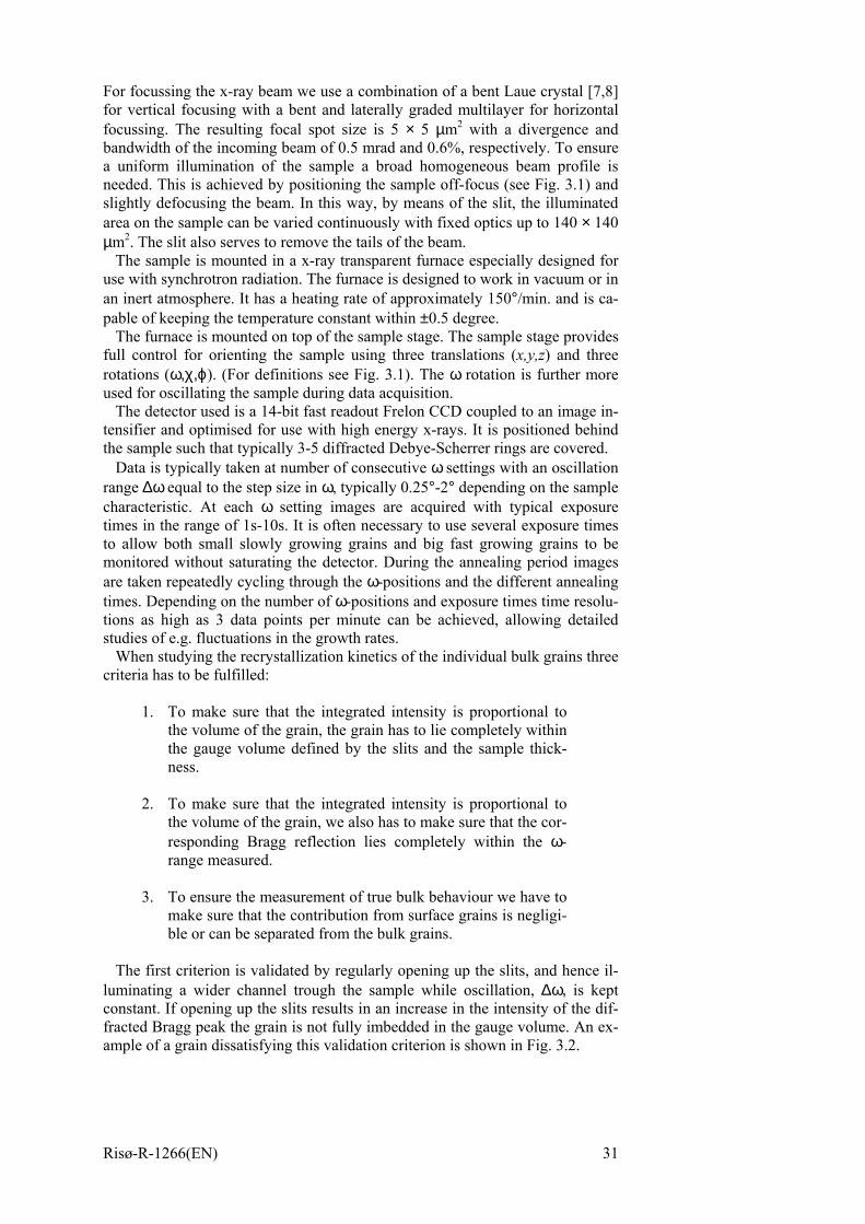
For focussing the x-ray beam we use a combination of a bent Laue crystal [7,8] for vertical focusing with a bent and laterally graded multilayer for horizontal focussing. The resulting focal spot size is 5 × 5 µm2 with a divergence and bandwidth of the incoming beam of 0.5 mrad and 0.6%, respectively. To ensure a uniform illumination of the sample a broad homogeneous beam profile is needed. This is achieved by positioning the sample off-focus (see Fig. 3.1) and slightly defocusing the beam. In this way, by means of the slit, the illuminated area on the sample can be varied continuously with fixed optics up to 140 × 140 µm2. The slit also serves to remove the tails of the beam.

The sample is mounted in a x-ray transparent furnace especially designed for use with synchrotron radiation. The furnace is designed to work in vacuum or in an inert atmosphere. It has a heating rate of approximately 150°/min. and is ca-pable of keeping the temperature constant within ±0.5 degree.

The furnace is mounted on top of the sample stage. The sample stage provides full control for orienting the sample using three translations (x,y,z) and three rotations (ω,χ,ϕ). (For definitions see Fig. 3.1). The ω rotation is further more used for oscillating the sample during data acquisition.

The detector used is a 14-bit fast readout Frelon CCD coupled to an image in-tensifier and optimised for use with high energy x-rays. It is positioned behind the sample such that typically 3-5 diffracted Debye-Scherrer rings are covered.

Data is typically taken at number of consecutive ω settings with an oscillation range ∆ω equal to the step size in ω, typically 0.25°-2° depending on the sample characteristic. At each ω setting images are acquired with typical exposure times in the range of 1s-10s. It is often necessary to use several exposure times to allow both small slowly growing grains and big fast growing grains to be monitored without saturating the detector. During the annealing period images are taken repeatedly cycling through the ω-positions and the different annealing times. Depending on the number of ω-positions and exposure times time resolu-tions as high as 3 data points per minute can be achieved, allowing detailed studies of e.g. fluctuations in the growth rates.

When studying the recrystallization kinetics of the individual bulk grains three criteria has to be fulfilled:

1. To make sure that the integrated intensity is proportional to

the volume of the grain, the grain has to lie completely within the gauge volume defined by the slits and the sample thick-ness.

2. To make sure that the integrated intensity is proportional to

the volume of the grain, we also has to make sure that the cor-responding Bragg reflection lies completely within the ω-range measured.

3. To ensure the measurement of true bulk behaviour we have to

make sure that the contribution from surface grains is negligi-ble or can be separated from the bulk grains.

The first criterion is validated by regularly opening up the slits, and hence il-

luminating a wider channel trough the sample while oscillation, ∆ω, is kept constant. If opening up the slits results in an increase in the intensity of the dif-fracted Bragg peak the grain is not fully imbedded in the gauge volume. An ex-ample of a grain dissatisfying this validation criterion is shown in Fig. 3.2.

Risø-R-1266(EN) 31

Fig. 3.2. Illustration of the first validation criterion. The measured growth curve reveals that the grain is nucleated inside the illuminated channel but eventually grow outside the channel as indicated by the in-crease in intensity at the validation points.

The second criterion is validated by the use of consecutive omega settings. The first and last ω-setting is only used for validation purposes, hence a mini-mum of three consecutive ω-settings are required. The integration of a Bragg reflection is only valid if there is no intensity of the Bragg reflection left at these two outermost validation settings.

The last criterion can be approached in two different ways. The first is a sta-tistically approach, where it is ensured that the fraction of surface grains is neg-ligible compared to that of bulk grains. This can be done by varying the ratio between the beam size and the sample thickness. The second approach is a more direct discrimination between surface grains and bulk grains. As illustrated in Fig. 3.3 the position of the diffracted beam on the detector depends on the posi-tion of the grain in the sample. Hence, by comparing the position of a Bragg peak with the envelope of the positions of a large number of peaks of roughly the same orientation it is possible to determine whether the diffracting grain is located at the surface or within the bulk of the sample.

2D-detector

Diffracted beams

Sample

Incident beam

Fig. 3.3. Illustration of the determination of surface grains based on the radial position of the measured diffraction spots. Comparing the radial distance of a grain with the enveloped of the radial distances of a large number of grains with similar orientation may idicate whether it is a sur-face grain or not.

32 Risø-R-1266(EN)

3.1.2 What is measured Typical examples of raw data is shown in Fig. 3.4. To the left is shown the ini-tial data before start of annealing. The image shows the diffracted Debye-Scherrer rings from the deformed microstructure. For deformations of medium to high strains the microstructure typically brakes up in a large number of small domains [38] giving rise to a diffraction signal that resample that of a powder sample. It is, however, clear that the intensity of this “powder-like” Debye-Scherrer ring is not constant along the ring, but varies slowly as a function of the azimuthal angle η. This is due to the fact that the crystal orientations of these small domains, constituting the deformed state, are not randomly oriented, but have a distribution of preferred orientation, a so-called texture. The different rings visible in Fig. 3.4 corresponds to the different lattice planes fulfilling the Bragg condition (see Eq. 2-5) and are labelled with the corresponding Miller indices of the lattice planes. The innermost very broad ring is due to scattering from the glass of the furnace and should be ignored. The image to the right of Fig. 3.4 shows the diffracted signal from the same gauge volume after annealing for 162 minutes at 270oC. The “powder-like” signal from the deformed micro-structure is now almost entirely replaced by discrete diffraction spots from the individual recrystallized grains.

Fig. 3.4. Example of raw data showing the Debye-Scherrer rings from the deformation texture and the appearing Bragg peaks from the individual grains. A) At time t = 0 minutes, and B) at time t =162 minutes.

Fig. 3.5 shows a small part of the acquired images including a segment of the 111 Debye-Scherrer ring. In Fig. 3.5a, before the onset of annealing, we see a tail of the broad background from the deformed microstructure, in the following referred to as the texture background. After annealing for 5 minutes at 270oC (Fig. 3.5b) two small peaks, labelled A and B, have appeared on top of the tex-ture background. After another 10 minutes of annealing a third peak, labelled C, has appeared (Fig. 3.5c). And after further annealing we see that peak C has ended up being much larger than peak A and B, and that peak B has almost stopped its growth. Notice also that the signal from the deformed microstructure decreases as the overall recrystallized volume fraction increases. From this se-quence of images, it is evident that by acquiring a series of images during the annealing the nucleation and growth kinetics of the individual grains can be fol-lowed in great detail.

Risø-R-1266(EN) 33

Fig. 3.5. Images of the measured intensity distribution on the detector showing the evolution of the texture background and the individual Bragg peaks as a function of time.

Texture background

Peak A Peak B

Peak B Peak A

Peak C Peak C

Peak A

Peak B

a) b)

c) d)

3.1.3 Orientation determination The 3DXRD method reveals not only the growth kinetics of the individual grains, but at the same time information on the crystal orientation of the grains is provided. Two approaches exist on how to obtain information about the crys-tallographic orientation of the grains. The first approach is based on a single reflection from a grain. The main advantage of this approach is that it is fast and does not require any additional measurements. It does, however, only provide partial information on the orientation of the grain. The other approach is based on several reflections from the same grain. Using this approach full information is obtained about the orientation of the grain. The drawbacks of this approach is that it does require some additional measurements and also some additional data processing. In the following the two approaches for orientation determination will be explained in more detail.

Partial orientation information

34 Risø-R-1266(EN)

)

By a stereographic projection of the scattering vectors onto the (RD,TD)-plane of the sample, there is a one-to-one correlation between the coordinates of a diffraction peak ( θηω 2,, and the ( )βα, -coordinate in the corresponding pole figure. The trace in the pole figure that is measured depend on the orientation of the sample. This is illustrated in Fig. 3.6, where the trace of the Debye-Scherrer ring is shown in pole figure coordinates for two different orientations of the

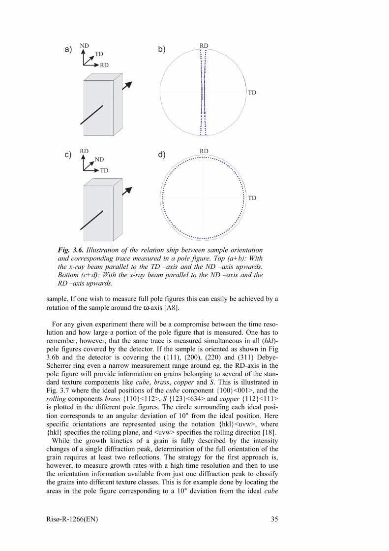
samprotat

FatBR

Fo

lutioremepole 3.6b Schepole dard Fig. rollinis plotion specihkl Whchangrainhowethe othe gareas

Risø

TD

ND

ND RD

RD

TD

TD

RD

RD

TD

a)

c) d)

b)

ig. 3.6. Illustration of the relation ship between sample orientation nd corresponding trace measured in a pole figure. Top (a+b): With he x-ray beam parallel to the TD –axis and the ND –axis upwards. ottom (c+d): With the x-ray beam parallel to the ND –axis and the D –axis upwards.

le. If one wish to measure full pole figures this can easily be achieved by a ion of the sample around the ω-axis [A8].

r any given experiment there will be a compromise between the time reso-n and how large a portion of the pole figure that is measured. One has to mber, however, that the same trace is measured simultaneous in all (hkl)-figures covered by the detector. If the sample is oriented as shown in Fig and the detector is covering the (111), (200), (220) and (311) Debye-

rrer ring even a narrow measurement range around eg. the RD-axis in the figure will provide information on grains belonging to several of the stan-texture components like cube, brass, copper and S. This is illustrated in

3.7 where the ideal positions of the cube component 100<001>, and the g components brass 110<112>, S 123<634> and copper 112<111> tted in the different pole figures. The circle surrounding each ideal posi-

corresponds to an angular deviation of 10° from the ideal position. Here fic orientations are represented using the notation hkl<uvw>, where specifies the rolling plane, and <uvw> specifies the rolling direction [18]. ile the growth kinetics of a grain is fully described by the intensity

ges of a single diffraction peak, determination of the full orientation of the requires at least two reflections. The strategy for the first approach is, ver, to measure growth rates with a high time resolution and then to use rientation information available from just one diffraction peak to classify rains into different texture classes. This is for example done by locating the in the pole figure corresponding to a 10° deviation from the ideal cube

-R-1266(EN) 35

orientation (see Fig. 3.7). For each diffraction peak on the detector, the corre-sponding pole figure coordinates are calculated and if they fall within 10° from the ideal cube component it is classified as “near” cube orientation. If the dif-fraction peak falls within a 10° deviation from several ideal texture components it is assign to the one with the smallest deviation.

111 pole figure

RD

TD

RD

TD

RD

TD

RD

TD

200 pole figure

RD

TD

RD

TD

RD

TD

RD

TD

220 pole figure

RD

TD

RD

TD

RD

TD

RD

TD

311 pole figure

RD

TD

RD

TD

RD

TD

RD

TD

Cube Brass Copper S

Fig. 3.7. Illustration of the influence of multiplicity on the overlap of regions surrounding the ideal standard texture components. The standard components shown are: Cube, ♦ Brass, • Copper and ∗ S. The lines surrounding the standard components corresponds to a 10° deviation. a) 200 pole figure and b) 220 pole figure.

This simple procedure for orientation analysis implies some limitations. This is best seen by comparing the 200 and the 311 pole figures shown in Fig. 3.7. For the 200 pole figure, having the lowest multiplicity, the degree of overlap between the different texture components are negligible. However, for pole figures with higher multiplicity, like the 311 pole figure, the degree of overlap becomes much more severe and determination of the orientation be-comes more ambiguous.

Full orientation information

It is possible to overcome the problem of overlapping texture components as described above using the second approach based on several reflections. The development of the GRAINDEX software (see chapter 2) has opened the possi-bility of determining the full orientation of individual grains within a polycrys-talline material. Hence, combining the use of the GRAINDEX software with the technique for recrystallization kinetics describe above, a complete description covering both growth kinetics and crystallographic orientation of the individual grains can be obtained. In order for the GRAINDEX algorithm to work one

36 Risø-R-1266(EN)

would need to scan a broad ω range to ensure that a sufficient number of dif-fraction peaks from each grain are measured. This can either be done during the entire annealing period, resulting in a somewhat coarser time resolution, or, if it can be assumed that grains do not disappear during the annealing, such a scan can be done at the end of the annealing and thereby not affecting the time reso-lution. An example of the latter approach is shown in Fig. 3.8. These data is from an experiment on an commercial purity aluminium alloy (AA3104) that has been hot deformed at 325°C to a strain of ~2.3 and then annealed at the 3DXRD microscope at 340°C∗ . The growth kinetics of the grains were meas-ured using a narrow ω-range around ω = 0°. At the end of annealing a much broader scan was performed (ω = -45° to 45°) to be used with the GRAINDEX program. The GRAINDEX analysis resulted in a list of the indexed grains with their full orientation and the peaks belonging to each grain. Using this informa-tion the growth kinetics data were re-examined and the growth curves based on three different reflections from the same grain were found. As can been seen in Fig. 3.8 the growth curves of the individual reflections all show the same behav-iour as expected. This clearly proof that the GRAINDEX program is capable of indexing of individual grains imbedded within a polycrystalline material.

-50 0 50 100 150 200 2500

0.5

1

1.5

2

2.5

3

3.5

4

4.5x 104

Orientation of grain:

(φ1,Φ,φ2) = (156°,67°,42°)

based on a fit to 13 reflections

Annealing time [min]

Grain volume [ µ

m3 ]

(111) reflection(02-2) reflection(13-1) reflection

Fig. 3.8. Example of combining the recrystallization kinetics technique and the GRAINDEX program. Shown is the measured growth kinetics of three individual reflections from the same grain. As expected the three growth curves all show the same behaviour. Using the GRAINDEX pro-gram the orientation of the grain is be found, in the given case based on a fit to 13 reflections.

3.1.4 Experimental considerations The outcome of this type of recrytsallization kinetics experiment, depend en-tirely on the proper choice of experimental parameters. It is therefore very im-

∗ The experiment was done in collaboration with Alcan International and RWTH Aachen.

Risø-R-1266(EN) 37

port to analyse the basic properties of the sample material, such as final grain sizes and mocaisity, before the real annealing experiment can begin. The ex-perimental parameters which needs to be considered are:

• The x-ray energy. At the present the 3DXRD are set up to use two different energies, 50 keV and 80 keV. For typical materials an x-ray energy of 50 keV provides sufficient penetration power (see Fig. 2.1), however, some materials may require the use of 80 keV x-rays.

• The size of the x-ray beam. The size of the x-ray beam has to be lar-ger than the final grain size to fully illuminate the grains. In practice a beam size of at least 3 times the final grain size is desirable. There is however an upper limit of how large beam sizes that can be achieved while keeping the beam profile homogenous. One also has to remember that increasing the beam size will enviably decrease the flux.

• The oscillation range ∆ω. It is important that the oscillation range is larger than the mosaicity of the sample to get the entire integrated in-tensity. However, the larger the oscillation range is, the bigger the chance for peak overlap. Using a too large oscillation range also lowers the ratio of the Bragg peak intensity compared to the texture background.

• The number of omega settings. The number of omega settings de-termines how large a portion of pole figure space is covered (see sec 3.1.3). Choosing the omega range is a compromise between the frac-tion of orientation space that needs to be covered and the desired time resolution. The larger an omega range the coarser time resolu-tion.

• The exposure times. Typically several exposure times are needed. On the one side relatively long exposure are needed to obtain good counting statistics of the small slowly growing nuclei/grains, and on the other side short exposure time are needed to avoid saturation of the detector for the large fast growing grains. Again a compromise has to be made between the number of exposure times and the de-sired time resolution.

3.2 Data analysis As in the case of the tracking concept described in chapter 2, this technique also produces a vast number of data, typically of the order of 1000 images for one annealing experiment. For handling these huge amounts of data we have devel-oped a software package that enables fast processing of the data. In the follow-ing the processing steps from raw images to individual growth curves of the grains is described.

3.2.1 Image processing When working with x-ray radiation using two-dimensional detectors like CCD’s there is a number of pre-processing steps that needs to be considered before the actual data analysis can be done. These pre-processing steps are summarized in the following:

• Correction for electronic noise. The electronic noise associated with the

CCD has two contributions: a constant read-out noise independent of the exposure time, and a so-called dark current proportional to the ex-

38 Risø-R-1266(EN)

posure time. To correct for it images are acquired without any x-ray beam. By subtracting these images from the raw images the contribu-tion from the electronic noise is removed from the images.

• Non-uniformity of sensitivity response of the detector (Flat field correc-tion). Owing to geometry, and artifacts of manufacture, the sensitivity of different areas of the detector may vary. This can be calibrated by uniform exposure of the detector [39] but is by far a trivial task. For the present study, it is assumed that the non-uniformity of the sensitivity re-sponse of the detector is negligible. That this assumption is indeed rea-sonable is supported by the fact that the three growth curves from the same grain shown in Fig. 3.8 fall on top of each other.

• Correction for spatial distortion. Spatial distortion of the detector can be an important effect and when not corrected can prevent successful inte-gration of the data. This is especially important for the GRAINDEX analysis. Mapping of the spatial distortion of the detector can be done using a known spacing calibration grid to measure the distortion at a number of discrete points. Once the mapping is done it can be used to correct the images.

• Normalization to synchrotron beam current. Due to energy losses of the electron bunch orbiting the storage ring the intensity of the emitted x-ray beam is slowly decreasing with time. This decrease in intensity is not negligible compared to the duration of a typical recrystallization ex-periment, therefore the beam current of the storage ring is constantly monitored and the background subtracted intensities is subsequently normalized.

• Polarization effects. X-ray diffraction depend on the polarization of the incident x-ray beam. However, for high energy x-rays the effect of po-larization is negligible and it was therefore ignored in the current study.

3.2.2 Data transformation The most efficient way of working with these huge amounts of data is to trans-form the images into azimuthal projections of the intensity distribution of the individual Debye-Scherrer rings. An example of such intensity profiles is shown in Fig. 3.9. The Bragg peaks from the individual grains are clearly identified as sharp peaks on top of a much broader texture background from the remaining deformed matrix. This projection is done either after the experiment by the pro-gram Fit2D [40] especially developed for processing of x-ray data or online dur-ing the experiment using the so-called software frontend [41] developed for use at the 3DXRD microscope. This procedure has a number of advantages that will become clear later in this section. The most obvious advantage is the reduction of data in terms of bytes. One image is typically 2-3 Mb in size which is then transformed into 4-6 text files containing the intensity projections with a total size of a few kb. So instead of working with a dataset of several Gb only a few Mb has to be processed.

Risø-R-1266(EN) 39

3ThBshmpecatocoaninnuvastthHthdiopfuhothbethpr

40

50 100 150 200 250 300 350

200

400

600

800

1000

1200

η angle [°]

Inte

nsity

[arb

.uni

t]

Fig. 3.9 Example of azimuthal projection of the intensity along a De-bye-Scherrer ring at the late stage of recrystallization. The new recrys-tallized grains are clearly seen as sharp peaks on top of the broad tex-ture background.

.2.3 Peak identification e first problem encountered when analyzing the data, was to identify the

ragg peaks from the individual grains. If we look at the azimuthal projection own in Fig. 3.10 we see that the peak profiles of the recrystallized grains are uch sharper than the broad texture background. Hence, the positions of the aks can be found simply using the derivatives of the intensity. This is typi-lly done on data taken at a late stage in the recrystallization process in order have nice strong peaks from the recrystallized grains. One should however mpare the result of the identification routine at such a late stage with that of earlier stage to verify if grains are disappearing or not. Not all peaks present the azimuthal projections can be used. As mentioned in sec. 3.1.1 there is a mber of criteria that a Bragg reflection has to fulfill in order to be considered lid. In order to simply the data analysis the criterion 2) in sec. 3.1.1 is further

rengthened. Not only does the Bragg reflection has to lie completely with in e ω-range measured, it has to lie within the ω-range of a single oscillation. ence it is not allowed to have tails in any of the neighboring ω-settings. Fur-ermore it has to be well separated from neighboring Bragg peaks along the η-rection as well as in the ω-direction. As a part of the software package devel-ed for the data analysis, is a program that automatically identifies peaks that lfill these criteria. Due to the complex nature of the intensity profiles it is wever recommended to confirm the result of identification routine before fur-er data analysis. Whether or not a grain fulfill criterion nr. 1 in sec.3.1.1 will come evident when validation points (see sec. 3.1.1) is plotted together with e normal data points. An example is shown in Fig. 3.1. Depending on the ap-oached chosen for fulfilling criterion nr. 3 in sec. 3.1.1 some additional analy-

Risø-R-1266(EN)

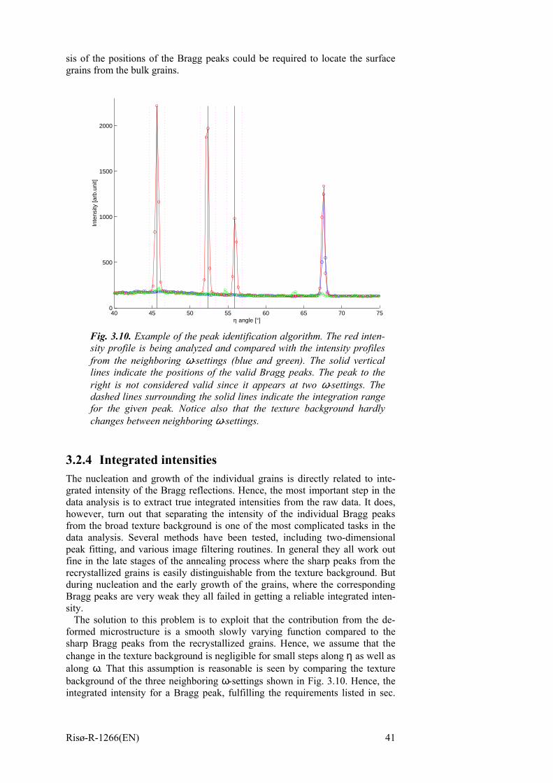
sis of the positions of the Bragg peaks could be required to locate the surface grains from the bulk grains.

40 45 50 55 60 65 70 750

500

1000

1500

2000

η angle [°]

Inte

nsity

[arb

.uni

t]

Fig. 3.10. Example of the peak identification algorithm. The red inten-sity profile is being analyzed and compared with the intensity profiles from the neighboring ω-settings (blue and green). The solid vertical lines indicate the positions of the valid Bragg peaks. The peak to the right is not considered valid since it appears at two ω-settings. The dashed lines surrounding the solid lines indicate the integration range for the given peak. Notice also that the texture background hardly changes between neighboring ω-settings.

3.2.4 Integrated intensities The nucleation and growth of the individual grains is directly related to inte-grated intensity of the Bragg reflections. Hence, the most important step in the data analysis is to extract true integrated intensities from the raw data. It does, however, turn out that separating the intensity of the individual Bragg peaks from the broad texture background is one of the most complicated tasks in the data analysis. Several methods have been tested, including two-dimensional peak fitting, and various image filtering routines. In general they all work out fine in the late stages of the annealing process where the sharp peaks from the recrystallized grains is easily distinguishable from the texture background. But during nucleation and the early growth of the grains, where the corresponding Bragg peaks are very weak they all failed in getting a reliable integrated inten-sity.

The solution to this problem is to exploit that the contribution from the de-formed microstructure is a smooth slowly varying function compared to the sharp Bragg peaks from the recrystallized grains. Hence, we assume that the change in the texture background is negligible for small steps along η as well as along ω. That this assumption is reasonable is seen by comparing the texture background of the three neighboring ω-settings shown in Fig. 3.10. Hence, the integrated intensity for a Bragg peak, fulfilling the requirements listed in sec.

Risø-R-1266(EN) 41

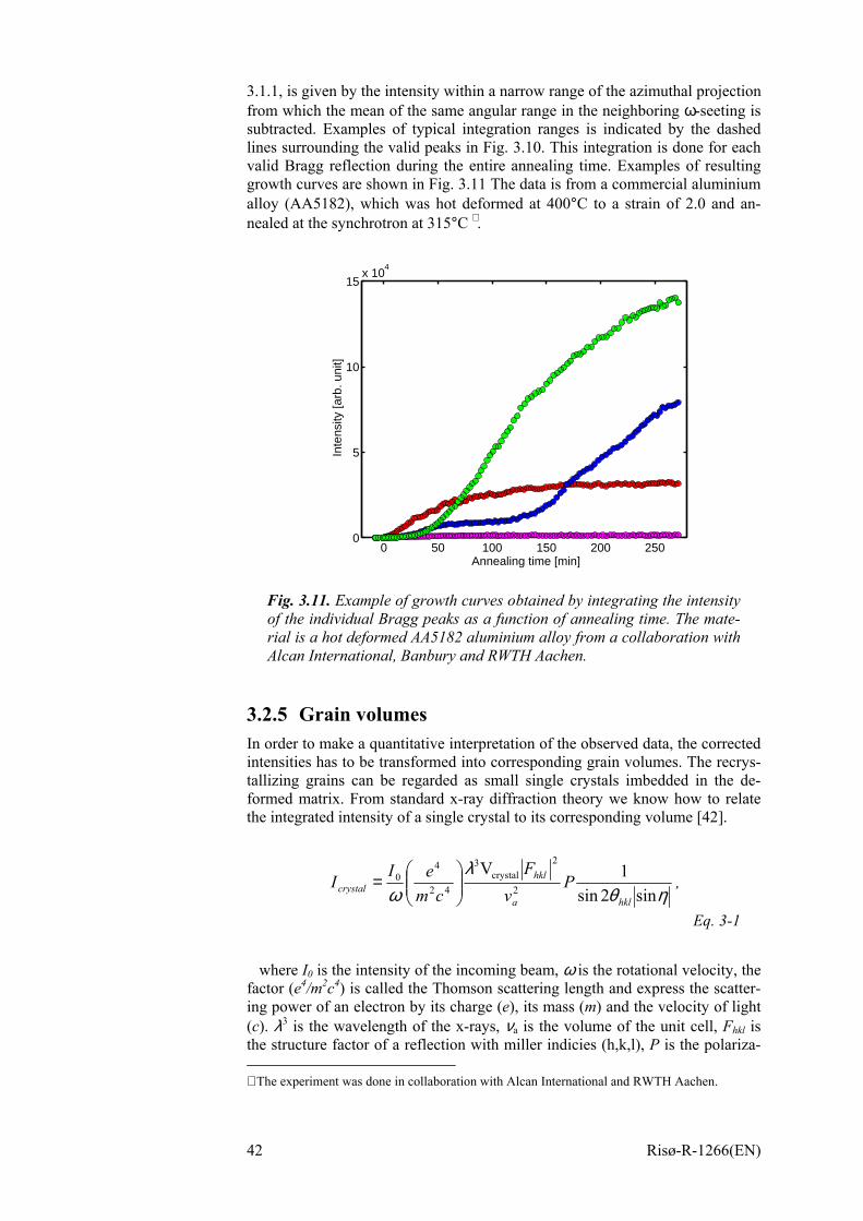
3.1.1, is given by the intensity within a narrow range of the azimuthal projection from which the mean of the same angular range in the neighboring ω-seeting is subtracted. Examples of typical integration ranges is indicated by the dashed lines surrounding the valid peaks in Fig. 3.10. This integration is done for each valid Bragg reflection during the entire annealing time. Examples of resulting growth curves are shown in Fig. 3.11 The data is from a commercial aluminium alloy (AA5182), which was hot deformed at 400°C to a strain of 2.0 and an-nealed at the synchrotron at 315°C ∗ .

Annealing time [min]

Inte

nsity

[arb

. uni

t]

0 50 100 150 200 250

0

5

10

15x 10

4

Fig. 3.11. Example of growth curves obtained by integrating the intensity of the individual Bragg peaks as a function of annealing time. The mate-rial is a hot deformed AA5182 aluminium alloy from a collaboration with Alcan International, Banbury and RWTH Aachen.

3.2.5 Grain volumes In order to make a quantitative interpretation of the observed data, the corrected intensities has to be transformed into corresponding grain volumes. The recrys-tallizing grains can be regarded as small single crystals imbedded in the de-formed matrix. From standard x-ray diffraction theory we know how to relate the integrated intensity of a single crystal to its corresponding volume [42].

ηθ

λω sin2sin

1V2

2crystal

3

42

40

hkla

hklcrystal P

vF

cmeII

= ,

Eq. 3-1

where I0 is the intensity of the incoming beam, ω is the rotational velocity, the

factor (e4/m2c4) is called the Thomson scattering length and express the scatter-ing power of an electron by its charge (e), its mass (m) and the velocity of light (c). λ3 is the wavelength of the x-rays, νa is the volume of the unit cell, Fhkl is the structure factor of a reflection with miller indicies (h,k,l), P is the polariza- ∗ The experiment was done in collaboration with Alcan International and RWTH Aachen.

42 Risø-R-1266(EN)

tion factor (see above), 1/(sin2θhkl |sinη|) is the Lorentz factor (cf.sec. 2.2.3) and Vcrystal is the volume of the single crystal.

Hence, by measuring the intensity of the incoming beam and the diffracted in-tensity of a single grain we can calculate the corresponding grain volume. It is, however, not possible to measure the intensity of the incoming beam without affecting it, and at the same time it will involve further complexity of the ex-perimental set-up. We find that using the data itself for intensity normalization is a much more convenient and also more reliable way of extracting the grain volumes. The approach is the following. Recalling that the microstructure of a deformed metal consists of very small regions of similar orientations [38]. These small regions can be regarded as a “powder” with a preferred orientation, i.e. the deformation texture. From stan-dard x-ray theory we know the expression for the diffracted intensity of a pow-der with a random orientation distribution

tPv

Fmcm

eIIHKLa

HKLpowder θ

λsin4

1V2

2sample

3

42

4

0

= Eq. 3-2

where m is the multiplicity of the HKL reflection and Vsample is the gauge vol-ume. This expression is easily modified to take the orientation distribution of the “powder-like” sample into account.

( ) tPv

Fmcm

eISIHKLa

HKLHKLtexture θ

⋅∂ω∂ηηω= ∫ ∫

ω∆

ω∆− sin41V

, 2

2sample

3

42

4

0

2/

2/

2

0

λπ

Eq. 3-3

Here the factor SHKL(ω,η) is the probability distribution of the HKL pole figure. The integration is over the trace measured in the pole figure (see sec. 3.1.3). An expression for the grain volume can now be obtained by taking the ratio of the two equations Eq 3-1 and Eq 3-3.

( )hklhkl

HKL

HKL

hklHKL

texture

crystal

fm

ft

SII

ηθθ

⋅ω

⋅∂ω∂ηηω=

−ω∆

ω∆−∫ ∫ sin2sin

sin4V

V1, 2sample

2crystal

12/

2/

2

0

π

Eq. 3-4

We then get the following expression the grain volume Vcrystal :

( ) crystalI

hklf

hklConsttextureIcrystalI

HKL

hkl

hklf

HKLfmtS

hklhkl

HKL 2

sin2sin

sin4

sin2sin

2

2sampleV

,crystalV 2/

2/

2

0

η⋅=

θ

ηθ⋅ω⋅∂ω∂ηηω= ∫ ∫

ω∆

ω∆−

θπ

Eq. 3-5

If spherical grain shapes are assumed we can transforme this volume into an equivalent sphere radius

Risø-R-1266(EN) 43

3 crystalcrystal 4

V3R

π= Eq. 3-6

3.3 Discussion and outlook In spite of the very simple set-up of the presented technique the potential scien-tific outcome is exceptional. For the first time growth kinetics of individual bulk grains can be studied in-situ. Furthermore the technique provides the possibility of investigating orientation dependencies of the growth kinetics.

The technique has been developed for studies of recrystallization kinetics in metals and as such it has already been used for several studies [A3,A4]. The prospect of the technique for investigation the effect of processing parameters on the fundamental properties of metallic materials has already attracted the attention from industry, and the results from experiments conducted in collabo-ration with Alcan International, Banburry and RWTH Aachen is currently being processed. The technique is not restricted to studies of recrystallization kinetics, but can equally well be applied to other scientific areas, like for example phase transformations, and first experiments relating to the phase transformation in steels as a function of temperature or straining have been conducted [43].

The main limitations of the technique is due to peak overlap caused by very high number of grains in the gauge volume or by highly textured samples, which may lead to biasing of the data analysis. Two solutions to this limitation exists. One is to reduced the investigated gauge volume by e.g. a conical slit and thereby reduce the number of reflecting grains. This will ease the analysis at the expense of poorer statistics. The other solution is based on a finer ω sampling. Using a smaller oscillation range, ∆ω, corresponding to a finer sampling in ori-entation space, will ease the separation of Bragg reflections from grains having almost similar orientations. The finer ω sampling will, however, lead to a lower time resolution and/or poorer statistics. With the ongoing development of a con-tinuous acquisition routine based on fast readout detectors, compared to the cur-rently used stepwise acquisition routine, it is, however, most likely that a finer ω sampling may be possible without compromising the statistics and time reso-lution.

The focus of this chapter have been on measuring growth kinetics, but the technique might also be used for measurements of nucleation densities and nu-cleation rates. This can be done in a similar way as describe for determining the full orientation of a grain (sec. 3.1.3) by using the GRAINDEX program.

44 Risø-R-1266(EN)

4 Recrystallization Kinetics of Commercial Purity Aluminium

The material chosen for the investigations of real in-situ growth kinetics of in-dividual bulk grains using the technique described in the previous chapter was a commercial purity aluminium alloy of type AA1050 cold rolled to 90% reduc-tion in thickness. The main reason for choosing this material is that it has al-ready been characterised in detail by electron microscopy and neutron diffrac-tion [44] and a model has been developed to simulate the recrystallization proc-ess [45]. In addition the AA1050 alloy is a commercially used material and as such it is of interest not only to the material science society but also for industry [46].

One of the classical problems in the field of recrystallization kinetics is the understanding of the appearance of the so-called cube texture following anneal-ing of medium to high stacking fault energy fcc materials like for example alu-minium and copper. The volume fraction of cube grains is typically found to be dominating in materials of high purity and/or high deformation, whereas it tends to be less dominating in particle containing materials and/or medium deforma-tions. For the chosen AA1050 commercial aluminium alloy the resulting recrys-tallization texture will thus be a compromise between a tendency to randomise the texture due to the presence of large FeAl3 particles, and a tendency to pro-mote the formation of a cube texture due to the 90% reduction in thickness by cold-rolling.

Earlier studies on the same AA1050 alloy by Vandermeer & Juul Jensen have shown that for high annealing temperatures (T=280°C) the emergence of the cube texture component can be ascribed to a growth advantage of the cube grains compared to grains of other orientation [44,47], whereas for lower an-nealing temperatures (T=245°C-265°C) no such clear growth advantage could be detected [48].

The aim of the present investigation of the AA1050 alloy is to use the tech-nique described in the previous chapter to study the growth behaviour of a large number of individual grains. The annealing temperature was in this case chosen as T=270°C to supplement the earlier studies. The study of the individual grains, compared to the average behaviour studied by conventional techniques, is expected to give new types of information about the recrystallization kinetics of the AA1050 alloy. In light of the special interest in the cube texture discussed above, orientation dependencies of the recrystallization kinetics will also be ex-amined with particular focus on the cube texture component.

4.1 Introduction to the sample The AA1050 aluminium alloy was prepared for a Brite-Euram project spon-sored by the European Union. The purpose of the project was to develop new and improved materials for use in the aluminium industry and was a collabora-tion between several universities, national laboratories and industrial compa-nies. The special properties of this AA1050 alloy were obtained by a very com-plex processing as described by Vandermeer and Juul Jensen [48]: “The alumin-ium alloy AA1050 was continuously cast at Hydro Aluminium, Sunndalsøra, Norway. The composition of the alloy is listed in table 4.1. After scalping, the

Risø-R-1266(EN) 45

cast ingot was subjected to a pre-processing heat treatment at 600°C for 24 hours. Further processing to a plate product at Alcan International, Banbury, England, consisted of an additional heat treatment with an 8 hour hold at 600°C, a slow cooling to 500°C at a cooling rate of 7°C per hour, a 6 hour hold at 500°C and finally cooling to 400°C at 50°C per hour followed by hot rolling at 400°C to a reduction of 75%. Subsequently the hot rolled plate was given a final recrystallization anneal for 1 hour at 450°C. This complex processing procedure was designed to produce a plate with a relatively uniform distribution of 1.7 µm average diameter precipitates, a relatively weak initial texture and a recrystal-lized grain size of 50-100 µm.”.

Table 4.1. Composition of the AA1050 alloy (wt.%) from [48].

Al Fe Mg Mn Si Cu Ca Na Ti B 99.46 0.3384 0.0011 0.0026 0.1538 0.0019 0.0002 0.0005 0.0066 0.0021 For the present investigation this starting material was cold rolled to a thick-

ness reduction of 90%. From the cold rolled plate several samples were cut hav-ing dimensions of 8 mm along the rolling direction (RD), 1 mm along the trans-verse direction (TD), and 3 mm along the normal direction (ND). In addition a few samples having dimensions of 8 mm along RD, 3 mm along TD, and 1 mm along ND were also cut.

4.2 Initial sample characterization Before investigating the recrystallization kinetics using the 3DXRD microscope as described in the previous chapter, the sample material was carefully charac-terized in order to plan the details of the experiment. To do this several of the cold rolled samples were annealed at 270°C for various periods and examined using both optical microscopy and electron microscopy.

4.2.1 Optical Microscopy results The first step in the initial sample characterization was to look at the samples using optical microscopy. Using the optical microscope an overview of the mi-crostructure after different periods of annealing is easily obtained. Some exam-ples are given in Fig. 4.1 showing the as-deformed, and almost recrystallized microstructure, respectively.

Fig. 4.1. Optical micrographs showing the as-deformed microstructure (left) and the almost recrystallized microstructure (right) of the AA1050 aluminium alloy. A colour filter has been used to enhance the details of the microstructure.

46 Risø-R-1266(EN)

4.2.2 Electron back scattering results Following the optical microscopy examination, the samples were studied using electron microscopy for a more detailed examination. Fig. 4.2 shows an electron back scattering image of the RD/ND plane. The precipitate particles are seen as bright spots and appear to be aligned along the rolling direction.

Fig. 4.2. Back scatter images taken by the scanning electron microscope. Left: The RD-ND plane of the AA1050 alloy annealed for 2000s. At this point the material is only partly recrystallized. Right: RD-ND plane of the AA1050 alloy annealed for 10000s corresponding to approx. 90% re-crystallization. The particles are seen as bight spots in the images and appear to be aligned in the rolling (horizontal) direction. The images are taken with a magnification of 1000x, and the white scale bar at the bot-tom of the images corresponds to 10 µm.

4.2.3 EBSD result The three most important sample parameters for the study of recrystallization kinetics at the 3DXRD microscope are 1) the duration of the entire recrystalliza-tion process, 2) the final grain sizes and 3) the mosaic spread of the recrystal-lized grains. The easiest way of obtaining this kind of information is to use the electron back scattering diffraction technique (EBSD) [49].

4.2.3.1 Growth behaviour

First the growth behaviour of the samples was examined to look for any an-isotropic growth. Earlier studies of the same material cold rolled 90% and an-

Fig. 4.3. EBSD ori-entation map of the RD-ND plane of the AA1050 alloy an-nealed at 270°C for 800 seconds. The nu-clei appear to be equiaxed. The thin dark lines corre-spond to a 1° misori-entation and the thick black lines corre-spond to 15° misori-entations.

Risø-R-1266(EN) 47

nealed at 280°C have found a slight growth advantage in the rolling direction, resulting in an aspect ratio of the grain diameter (RD/ND) of 1.4 [44]. To test these findings two samples, cut to expose the RD-ND and RD-TD plane, re-spectively, were annealed for 800s at 270°C and examined by EBSD. An exam-ple of the measured orientation maps is shown in Fig. 4.3. No notably differ-ences in the aspect ratios of the grains were observed and spherical growth is assumed in the further data analysis. Based on the EBSD maps the mosaic spread of the recrystallized grains was found to be less than 0.5°, which is the angular resolution of the EBSD technique. It was later found, by using the 3DXRD microscope, that the mosaic spread of the recrystallized grains were actually less than 0.05°.

Fig. 4.4. Microstructure evolution of the AA1050 aluminium alloy as studied by the EBSD. The orienta-tion maps are measured on the RD-ND planes and correspond to an-nealing times of a) 2000s, b) 4000s, c) 8000s and d) 10800s. Thin lines correspond to misorientations of more than 1° and thick lines to misorientations of more than 15°. The colour scheme used is arbitrar-ily and differs from image to image. Notice the different scale bars of the images.

48 Risø-R-1266(EN)

4.2.3.2 Microstructure evolution

To supplement the data from the optical microscope (Fig. 4.1) the microstruc-ture evolution was studied as a function of annealing time by EBSD. This was done by preparing a number of samples annealed for different periods. Two dif-ferent furnaces were used for these heat treatments; a standard laboratory oil bath and the synchrotron furnace. The use of different furnaces was done in or-der to check the absolute temperature readings of the synchrotron furnace. In-spections of orientation maps from samples annealed for the same period of time, but using the different furnaces, did not reveal any notable differences. Based on this it was concluded that the absolute temperature readings of the synchrotron were correct. The transformation from a deformed microstructure to a nearly full recrystallized microstructure is illustrated in Fig. 4.4 by some of the measured orientation maps.

4.2.3.3 Recrystallized volume fractions

The recrystallized volume fractions were extracted from the EBSD map accord-ing to the method suggested by Krieger Lassen and Juul Jensen [50]. By speci-fying a maximum misorientation angle (0.75°) allowed inside a grain and a minimum “safe” grain size (10 µm2) chosen such that grains above this size are certain to be new recrystallized grains, an EBSD pattern quality threshold for recrystallized regions was determined based on the measured data. The data was then re-examined using the misorientation angle, a minimum grain size (4 µm2) and the pattern quality threshold to identify the recrystallized grains. The result of such an analysis is shown in Fig. 4.5 where the volume fraction recrystallized (VV) is plotted as a function of annealing time.

10

210

310

410

50

0.1

0.2

0.3

0.4

0.5

0.6

0.7

0.8

0.9

1

annealing time [sec.]

Fra

ctio

n re

crys

t. (V

V )

Oil bathSynch. furnace

102

103

104

105

10−2

10−1

100

101

102

annealing time [sec.]

−ln

(1−V

V )

Oil bathSynch. furnace

Fig. 4.5. Evolution of the volume fraction recrystallized (VV) as a function of an-nealing time. To the left is plotted the measured values of VV vs. time and to the right an Avrami plot [51,52] of the same data is shown. Circles represent data obtained using the oil bath, while squares represent data obtained using the syn-chrotron furnace. The solid black line is a fit of the Avrami equation (Eq. 4-1) to all of the data. The cyan dash-dotted line and the blue dotted line are fit of the Avrami equation to the initial and final stages, respectively.

The VV vs. annealing time relationship is usually described by the Avrami equation

Risø-R-1266(EN) 49

Eq. 4-1 ( kV BtV −−= exp1 )

where t is the annealing time and B and k are constants describing the recrystal-lization kinetics. The exponent k is normally referred to as the Avrami expo-nent. The solid black line plotted in Fig. 4.5 is a fit of the Avrami equation (Eq. 4-1) to the data. In the right part of Fig. 4.5 the same data is plotted in a form that is normally referred to as an Avrami plot [51,52] or a Johnson plot [53]. The Avrami exponent k is then given by the slope of a straight line. From the plots shown in Fig. 4.5 it is evident that the simple Avrami equation cannot de-scribe the entire evolution of the volume fraction recrystallized. This finding is not exceptional, deviations from the Avrami equation are frequently reported in the literature, e.g. [54]. However in most cases the Avrami plot of the VV vs. t behaviour has a downward convex form, with the data deviating from the straight-line behaviour at the later annealing times. The more upward concave form found in this study, has only been reported once before in the literature by Vandermeer and Juul Jensen [48]. They have previously made studies on ex-actly the same material annealed at temperatures ranging from 245°C to 280°C, and have found a similar behaviour using linear intercept measurements with the EBSD. Following their data analysis, the current data was described using two sets of Avrami constants. The first set was found by fitting the Avrami equation to the first four data points, and the second set was found by fitting the Avrami equation to the last six data points. The obtained Avrami constants are listed in table 4.1.

Table 4.2. Avrami constants obtained by fitting the Avrami equation to the data in Fig.4.5.

B k Entire data set 3.4⋅10-7 1.67 First part (t ≤ 4000s) 9.8⋅10-3 0.40 Last part (t ≥ 4000s) 3.1⋅10-8 1.94

The investigation of the volume fractions recrystallized shows that using an

annealing temperature of 270°C results in a fully recrystallized sample after ap-proximately 3-4 hours. This appears to be a reasonable time scale for an in-situ synchrotron experiment.

4.2.3.4 Final grain sizes

Having established the mosaic spread of the grains and the duration time for full recrystallization, the last parameter needed for an investigation of the recrystal-lization kinetics using the 3DXRD microscope is an estimate of the final grain sizes of the recrystallized grains. This information was obtained from a large EBSD orientation map of the RD-ND plane of a fully recrystallized sample, which has been annealed for 76 hours at 270°C (see Fig. 4.6.). Using a mini-mum grain size of 1 pixel (5x5 µm2) and a minimum misorientation angle of 0.75° the mean grain area of a plane of polish is found to 204.8 µm2. Assuming spherical grain shapes this gives an estimated mean grain diameter of

50 Risø-R-1266(EN)

m 6.20m 8.204area2diameter 2 µ=µ⋅ππ

8=π

⋅⋅π4= Eq. 4-2

where the bar refers to mean values and the stereological factor (4/π) converts the measured mean 2-dimensional diameter into an estimated mean 3-dimensional diameter [28].

Fig. 4.6. Large orientation map used for grain size determination. The thick black lines indicate a misorientation angle of more than 15 degrees.

4.3 3DXRD results Two experimental investigations of the recrystallization kinetics of the AA1050 alloy using the 3DXRD microscope has been carried out. The first experiment was done in December 1998, while the 3DXRD microscope was still under con-struction. For the first time detailed information on the nucleation and growth kinetics of individual bulk grains was followed in-situ [A3]. Unfortunately, the majority of the measured data had to be discarded due to instability problems of the instrument at this early stage. Only a few grains were found to be valid, but the details of these few grains provided completely new insight to the mecha-nisms of the recrystallization process in the AA1050 alloy [A3]. A new experi-ment aimed at examining the orientation dependence of the recrystallization kinetics was subsequently planned. This second experiment was carried out in February 2001 and resulted in 244 valid grains [A4].

In this section data from both experiments will be presented, looking both at the information provided by the individual growth curves and by a statistical description of the overall recrystallization parameters. Finally the orientation dependency on the recrystallization kinetics will be investigated, with particular focus on the cube orientation [A4].

4.3.1 Experimental The set-up used in the experiments was similar to that described in section 3.1*. The experimental parameters for the two experiments are listed in table 4.3. For

Risø-R-1266(EN) 51

* For the December 1998 experiment the validation routines and data analysis were slightly dif-

ferent than what is described in chapter 3. See [lauridsen] for details.

the December 1998 experiment only one sample was investigated, whereas in the February 2001 experiment in total four samples were investigated.

Table 4.3. Parameters used for the experimental investigations of the re-crystallization kinetics of the AA1050 using the 3DXRD microscope tech-nique described in chapter 3.

Experimetal parameters used at the 3DXRD microscope

December 1998 experiment X-ray energy 50 keV Normal gauge volume 70 µm × 70 µm × 1000 µm Validation gauge volume 100 µm × 100 µm × 1000 µm Annealing temperature 270°C Measured Debye-Scherrer rings 111,200,220,311and

222 Sample A1 Sample orientation (x,y,z) TD,RD,ND Omega positions 0° Oscillation range 0.2° Exposure times 0.5s and 10s / 0.1s and 0.5s Total annealing time 162 min.

February 2001 experiment X-ray energy 50 keV Normal gauge volume 100 µm × 100 µm × 1000 µm Validation gauge volume 140 µm × 140 µm × 1000 µm Annealing temperature 270°C Measured Debye-Scherrer rings 111,200,220 and 311 Sample B1 Sample orientation (x,y,z) TD,ND,RD Omega positions -1.0°,-0.5°,0.0°,0.5°, and 1.0° Oscillation range 0.5° Exposure times 1s, 4s, and 10s Total annealing time 220 minutes Sample B2 Sample orientation (x,y,z) TD,ND,RD Omega positions -0.5°,0.0°, and 0.5° Oscillation range 0.5° Exposure times 1s, 4s, and 10s Total annealing time 178 minutes Sample B3 Sample orientation (x,y,z) TD,ND,RD Omega positions -0.5°,-0.25°,0.0°,0.25°, and 0.5° Oscillation range 0.25° Exposure times 1s, 2s, and 5s Total annealing time 178 minutes

52 Risø-R-1266(EN)

Sample B4 Sample orientation (x,y,z) TD,ND,RD Omega positions -0.5°,0.0°, and 0.5° Oscillation range 0.5° Exposure times 2s Total annealing time 34 minutes

For the February 2001 experiment aluminium absorbers of various thickness

had to be inserted into the direct beam in order to avoid saturation of the detec-tor. The measured background corrected images were subsequently scaled ac-cording to the amount of absorber.

As mentioned above one of the main tasks for the February 2001 experiment was to look for orientation dependencies of the growth behaviour, especially with regard to the cube orientation 100<001>. Based on an examination of the positions of the cube component in the 111, 200, 220 and 311 pole figures it was decided to focus on a small region around the RD-axis in the pole figure. As seen in Fig. 3.6 this corresponds to mounting the samples with the TD-direction along the x-axis (parallel to the x-ray beam), the ND-direction along the y-axis and the RD-direction along the z-axis. Comparing the trace in the pole figure (see Fig. 3.6) with the positions of the poles of the cube compo-nent (see Fig. 3.7), it is seen that 2 out of 3 poles in the 200 pole figure and 2 out of 6 poles in the 220 pole figure are covered with this set-up. In addition also grains belonging to the three rolling components (Br 110<112>, S 123<634> and Cu 112<111>), as well as other (“random”) orientations, could be detected on all of the four measured Debye-Scherrer rings.

As seen in table 4.3, the experimental parameters were varied slightly from sample to sample. This was done to allow for studies of different aspects of the recrystallization process. Samples B1 and B3 were studied using a relatively high number of omega positions resulting in a large number of grains at the ex-pense of a lower time resolution. A large number of grains are essential for a statistical analysis of the growth kinetics. Whereas the main purpose for sample B4 was to make a detailed study of the initial stages of the recrystallization process. Therefore in this case only one effective ω-setting was used (two posi-tions are used for validation) and only one exposure time, which lead to a time resolution as high as two data points per minute.

Based on the estimated grain size (see section 4.2.3.4) the dimensions of the gauge volume were chosen such that the fraction of surface grains was negligi-ble (approximately 6%).

The February 2001 experiment was performed before the indexing part of the GRAINDEX program (see section 2.2.4) was fully developed. It was therefore decided to use the orientation information available from just one diffraction peak as explained in section 3.1.3. Using this approach the data was grouped into three different texture groups; cube orientations, rolling orientations, de-fined by Br, S and Cu, and other orientations.

4.3.2 ODF measurements For each sample full pole figures where measured before the onset of annealing and again at the end of the annealing period using a gauge volume of 140 µm × 140 µm × 1000 µm. From the measured pole figures corresponding orientation distribution functions (ODFs), showing the distribution of orientations in Euler space, were calculated [55]. An example of the measured ODFs before and after recrystallization is shown in Fig. 4.7 for sample B2. Due to the cubic crystal

Risø-R-1266(EN) 53

symmetry and the orthorhombic sample symmetry only a subset of Euler space is needed, namely φ1 ∈ [0°-90°], Φ ∈ [0°-90°], and φ2 ∈ [0°-90°] [17]. Before the annealing the sample possess a typical rolling texture (upper part of Fig. 4.7) with main components being the Br 110<112>, S 123<634> and Cu 112<111> [56]. After annealing the texture of the sample is substantially al-tered. Some rolling texture still remains, but in addition a cube texture 100<001> has emerged. The calculated volume fractions of the different tex-ture components derived from the ODFs are listed in table 4.3. The procedure used for calculation of the volume fractions is described in [57].

Table 4.4. Estimated volume fraction based on the ODFs in Fig. 4.7. A 15° deviation from the ideal texture components has been used to define the texture classes.

Before annealing After annealing Br 110<112> 17.6 % 9.7 % S [58]<634> 39.5 % 21.5 % Cu 112<111> 14.0 % 8.7 % Rolling total 71.1 % 39.9 % Cube 100<001> 0.9 % 4.9 % Other 28.0 % 55.2 %

54 Risø-R-1266(EN)

φ1

Φ

φ2:0−>90

Contour lines: 1,2,3.. etc. x random. Min: 0.0, Max: 12.8

φ1

Φ

φ2:0−>90

Contour lines: 1,2,3.. etc. x random. Min: 0.0, Max: 6.9

Fig. 4.7. Calculated orientation distributions (ODFs) for the B2 sample based on the full 111, 220, and 220 pole figures measured at the 3DXRD microscope. Top: Initial rolling texture before annealing. Bot-tom: Recrystallization texture after annealing. Notice the appearance of the cube texture component located in the corners of the φ2 = 0° and φ2 = 90° sections after annealing.

Risø-R-1266(EN) 55

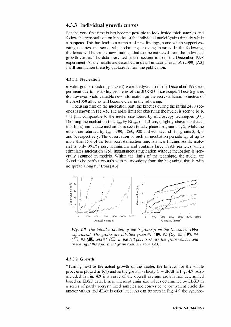
4.3.3 Individual growth curves For the very first time is has become possible to look inside thick samples and follow the recrystallization kinetics of the individual nuclei/grains directly while it happens. This has lead to a number of new findings, some which support ex-isting theories and some, which challenge existing theories. In the following, the focus will be on the new findings that can be extracted from the individual growth curves. The data presented in this section is from the December 1998 experiment. As the results are described in detail in Lauridsen et al. (2000) [A3] I will summarize these by quotations from the publication.

4.3.3.1 Nucleation

6 valid grains (randomly picked) were analysed from the December 1998 ex-periment due to instability problems of the 3DXRD microscope. These 6 grains do, however, yield valuable new information on the recrystallization kinetics of the AA1050 alloy as will become clear in the following.

“Focusing first on the nucleation part, the kinetics during the initial 2400 sec-onds is shown in Fig 4.8. The noise limit for observing the nuclei is seen to be R ≈ 1 µm, comparable to the nuclei size found by microscopy techniques [37]. Defining the nucleation time tnuc by R(tnuc ) = 1.3 µm, (slightly above our detec-tion limit) immediate nucleation is seen to take place for grain # 1, 2, while the others are retarded by tnuc = 300, 1860, 900 and 600 seconds for grains 3, 4, 5 and 6, respectively. The observation of such an incubation periode tnuc of up to more than 15% of the total recrystallization time is a new finding. As the mate-rial is only 99.5% pure aluminium and contains large FeAl3 particles which stimulates nucleation [25], instantaneous nucleation without incubation is gen-erally assumed in models. Within the limits of the technique, the nuclei are found to be perfect crystals with no mosaicity from the beginning, that is with no spread along η.” from [A3].

Annealing time [s]

0 400 800 1200 1600 2000 2400

Gra

in v

olum

e (µ

m3)

0

10

20

30

40

50

Annealing time (s)

0 400 800 1200 1600 2000 2400

Gra

in r

adiu

s (µ

m)

0

2

4

6

Fig. 4.8. The initial evolution of the 6 grains from the December 1998 experiment. The grains are labelled grain #1 ( ), #2 ( ), #3 ( ), #4 ( ), #5 ( ), and #6 ( ). In the left part is shown the grain volume and in the right the equivalent grain radius. From [A3].

4.3.3.2 Growth

“Turning next to the actual growth of the nuclei, the kinetics for the whole process is plotted as R(t) and as the growth velocity G = dR/dt in Fig. 4.9. Also included in Fig. 4.9 is a curve of the overall average growth rate determined based on EBSD data. Linear intercept grain size values determined by EBSD in a series of partly recrystallized samples are converted to equivalent circle di-ameter values and dR/dt is calculated. As can be seen in Fig. 4.9 the synchro-

56 Risø-R-1266(EN)

tron results and the EBSD results are of the same order of magnitude. That the two sets of results do not agree perfectly may be ascribed to variations in growth rate from nucleus to nucleus, which relate both to the orientation of the nucleus and to the local surroundings which change in space as well as in time as the nucleus grows. Furthermore, from the figure it is clear that there are large fluctuations in growth rates both within and between the 6 different synchrotron curves. Notice in particular the growth velocity of nucleus #5, which at its maximum is 0.0061 mm/second, 1 order of magnitude above the average. In interpreting the curves in Fig. 4.9, it is essential to remember that the synchro-tron data represent the movement of the total (free plus impinged) surface area. This is particularly important at longer annealing times where the impingement between nuclei is significant. Fig. 4.9 shows that even, for t < 2000 seconds – where VV ≤ 0.15 , there are large fluctuations from nucleus to nucleus and as a function of time.

Another interesting feature is the abrupt disappearance of nucleus # 4 around t = 6000 when it has reached a size of R ≅ 2.5 µm. (The scatter in the data for t > 6000 reflects the background noise for the short acquisition time –by direct in-spection of the images no trace of the grain is found.) Optical microscopy re-vealed that annealing of a sample at 270°C for a very extended period of time (t > 120h) does not lead to significant grain growth. The disappearance of nucleus #4 is therefore believed to be a local discrete grain growth phenomenon and not a consequence of standard “macroscopic” grain growth.” from [A3].

Annealing time (s)102 103

dR/d

t (µ m

/s)

10-4

10-3

10-2

Annealing time (s)0 2000 4000 6000 8000 10000

Gra

in r

adiu

s (µ

m)

0

2

4

6

8

10

12

14

A B

Fig. 4.9. The full evolution of the 6 grains from the December 1998 ex-periment: grain #1 ( ), #2 ( ), #3 ( ), #4 ( ), #5 ( ), and #6 ( ). Left is shown the equivalent sphere radius Rgrain and right – for the first 2400 seconds - Ggrain = dRgrain /dt. The data were smoothed before differ-entiation. Also shown are EBSD results (straight line) for the average growth velocity for all grains. From [A3].

4.3.4 Overall recrystallization process To obtain sufficient data for a investigation of the overall recrystallization proc-ess of the AA1050 alloy a second experiment was performed in February 2001 [A4]. From this experiment 244 grains were analysed allowing for a statistical analysis of the parameters describing the overall recrystallization process.

4.3.4.1 Nucleation times

Due to the difficulties of measuring nucleation rates using standard characteri-zation techniques [59], all existing recrystallization models are based on as-sumptions about the nucleation kinetics [51-53,60,61]. Typically site-saturation, meaning that all nuclei are pre-existing and start growing at t=0, or constant

Risø-R-1266(EN) 57

nucleation rates are assumed. As noted above, site-saturation is normally as-sumed for aluminium alloys containing large particles like the AA1050 alloy.

The 3DXRD microscope provides an experimental tool for determining the real nucleation rate without the necessity of underlying assumptions. Using the same approach as described in sec. 4.3.3.1 the nucleation times were determined for all 244 analysed grains. The result is shown in Fig. 4.10. From the distribu-tion of nucleation times it is clear that the majority of the nuclei nucleate within the very early stage of the recrystallization as would have been assumed for the AA1050 alloy [62]. There are, however, a number of nuclei with nucleation times as large as up to 75 minutes, corresponding to VV ≈ 0.35 (cf. Fig 4.5). Hence, the data shows that the nucleation mechanism of the AA1050 alloy is not as simple as the site-saturation mechanism normally assumed for this type of alloy [25]. Based on such distributions the nucleation rate as a function of time can easily be derived.

Nucleation time [min]

Number of grains: 244

Fre

quen

cy [%

]

0 10 20 30 40 50 60 70 80

0

5

10

15

20

25

30

35

40

45

50

Fig. 4.10. The 3DXRD allows for the first time direct measurements of the nucleation rate as a function of time. Shown here is the distribution of nucleation times measured for the AA1050 alloy. The nucleation time is determined as the time when the radius of the nucleus is 1.3 µm. The dis-tribution shows that the nucleation mechanism of the AA1050 alloy is not as simple as the site-saturation mechanism normally assumed for this type of alloy [25].

4.3.4.2 Grain sizes

Another important parameter describing the recrystallization process is the final recrystallized grain sizes. Distributions of grain sizes are normally derived from inspections of planar sections resulting in a 2-dimensional grain size (area) dis-tribution. Based on this 2-dimensional distribution, an estimated 3-dimensional grain size (volume) distribution can derived using various assumptions regard-ing grain size and grain shape [28]. Real 3-dimensional grain size (volume) dis-tributions have so far only been obtainable by serial sectioning of the sample. This procedure is, however, very labour intensive and will eventually transform the sample into a pile of dust. With the 3DXRD microscope 3-dimensional grain size (volume) distributions can de derived non-destructively from the measured growth curves of the individual grains. Using Eq. 3-5 the measured intensities at a given annealing time can be transformed into a corresponding grain volume distribution. Assuming spherical growth this measured grain vol-

58 Risø-R-1266(EN)

ume distribution can be transformed into an equivalent grain diameter distribu-tion. In Fig. 4.11 such an equivalent grain diameter distribution is shown after 175 minutes annealing. At this stage the AA1050 alloy is approximately 90% recrystallized (cf. Fig. 4.5). The mean equivalent grain diameter at this stage is found to be 17 µm. Keeping in mind that the value of 17 mm is for 90% recrys-tallized, we can compare this with the value of 20.6 µm measured on a 100% recrystallized sample by converting the measured average grain area measured on a plane of polish into an estimated average 3-dimensional grain size. Taken into account fact that the latter value is obtained indirectly using a number of assumptions [28] and that the orientation map used for the determination of the average 2-dimensional grain size had a grid size of 5 µm (cf. Fig. 4.6) prevent-ing smaller grain areas to be detected, the obtained value if 17 µm seems rea-sonable.

Mean grain size: 17 µm

Number of grains: 197

Final grain diameter [µm]

Fre

quen

cy [%

]

0 5 10 15 20 25 30 35 40 45 50

0

5

10

15

20

25

Fig. 4.11. 3-dimensional grain size distribution of the AA1050 alloy after annealing for 175 minutes at 270°C (≈ 90% recrystallized). The meas-ured grain volumes have been transformed into equivalent sphere diame-ters. The reason that this distribution is based on 197 grains, and not 244 as in Fig. 4.10, is simply that only 3 out of the 4 measured samples were annealed for more than 180 minutes (cf. table 4.3)

Unlike static measurement techniques such as standard microscopy tech-niques, which are only capable of taking a snapshot of the microstructure, the 3DXRD microscope also provides information on the evolution of the grain size distribution. An example of this showing the evolution of the mean grain size as a function of annealing time will be given in sec 4.3.5.4.

4.3.4.3 Growth rates

Apart from the nucleation rate, discussed above, modelling of recrystallization kinetics also includes the growth rate(s) of the nuclei [51-53,60,61]. These are typically measured by linear intercept methods on a series of partly recrystal-lized samples using the EBSD as described in [45] resulting in an overall aver-age growth rate. That the use of overall average growth rates is a gross over-simplification of the actual growth process is clearly demonstrated by the growth curves shown in Fig. 4.9 revealing a wide variation in the growth behav-iour between the individual grains as well as for the individual grains them-selves.

Risø-R-1266(EN) 59

From the individual growth curves measured by the 3DXRD microscope the growth rates of the individual grains can be determined. This results in a distribution of growth rates compared to the overall average growth rate determined by the linear intercept method. The procedure used to obtain the growth rate from the individual growth curves is illustrated in Fig. 4.12. The growth rate of a grain after a given time (t) of growth is determined by first transforming the grain volumes into equivalent grain radii assuming spherical growth. Then the gradient of the radius curve is determined by a linear fit to the neighbourhood of R(tnuc+ t), where tnuc is the nucleation time determined as de-scribed in sec 4.3.3.1.

0 500 1000 1500 2000

0

0.5

1

1.5

2

2.5

3

Annealing time [sec.]

Gra

in r

adiu

s [µ

m]

0 500 1000 1500 20000

20

40

60

80

100

120

140

Annealing time [sec.]

Gra

in v

olum

e [µ

m3 ]

tnuc

t

tnuc

+ t

Fig. 4.12. Illustration of the procedure used for determination of growth rates from the individual growth curves. To the left is shown an example of the volume growth of an individual grain, and to the right the equiva-lent sphere radius is shown. The growth rate of a grain after having grown for a time, t, is given by the gradient to the radius curve at the time t + tnuc, where tnuc is the nucleation time as described in section 4.3.3.1. The gradient is determined by a linear fit to the neighbourhood of R(t + tnuc).

Using this procedure the growth rates of the grains can be determined at time

during the annealing. An example of the evolution of the determined growth rate distribution is shown in Fig. 4.13 for t = 600s, 1200s, 2400s and 9000s cor-responding to the sample being approximately 10%, 15%, 20% and 70% recrys-tallized, respectively. A number of conclusions can be made by examining the data shown in Fig. 4.13. First of all it is evident that there exist a distribution of growth rates, all grains do not grow with the same speed. This is not so surpris-ing considering the heterogeneity of the deformed matrix, but has so far been impossible to measure with conventional techniques. What is also seen is that the shape of the growth rate distribution changes as a function of annealing time. In the beginning the distribution of growth rates is very broad, but as times goes it sharpens and its maximum moves towards low growth rates. The main mechanism responsible for this behaviour is impingement between the grains. As mentioned in section 4.3.3.2 one has to remember that the used tech-nique does not provide any information on the spatial distribution of the nuclei. Thus, no information is available on when the grains start to impinge with one another. This means that the measured growth rate is the mean value for the en-tire grain boundary, impinged as well as un-impinged. As a consequence the measured growth rate of an individual grain will start to decrease when the grain begin to impinge with the neighbouring grains. Another mechanism, which might contribute to the observed shift in the growth rate distribution, is

60 Risø-R-1266(EN)

changes in the driving force for the grain boundary migration. This is for in-stance the case if concurrent recovery takes place during the annealing. During recovery annihilation and rearrangement of the dislocations in the deformed matrix occurs and thereby lowers the driving force for the grain boundary mi-gration.

Real “free to grow” growth rates can, however, be extracted from the earliest stages of the annealing under the assumption that the degree of impingement is small and can be neglected. Hence, the distribution shown in Fig. 4.13a may be taken as the real “free to grow” growth rate distribution.

The procedure used for obtaining growth rate distributions outlined above as-sumes that the growth rate (dR/dt) is independent of the grain size. To a first approach this may be a reasonable assumption for the migration of high angle boundaries during recrystallization. There are on the other hand examples of annealing processes where this is not the case, like for example in secondary recrystallization (also known as grain growth) where the growth rate is given by dR/dt ∝ 1/R [25]. To test the assumption used for the growth rate determination the cross-correlation [20] between the derived growth rates and the correspond-ing grain sizes was investigated. The result of the analysis revealed that there is a small, but not negligible, correlation between the derived growth rates and the corresponding grain sizes. This small correlation is, however, not sufficient to account for the observed distribution of growth rates. Hence, the measured growth rate distribution is not only a grain size effect, but reflect the unique growth behaviour of the individual grains.

A)

Growth rate [µm/s]

Fre

quen

cy [%

]

0.000 0.002 0.004 0.0060

10

20

30B)

Growth rate [µm/s]

Fre

quen

cy [%

]

0.000 0.002 0.004 0.0060

10

20

30

40C)

Growth rate [µm/s]

Fre

quen

cy [%

]

0.000 0.002 0.004 0.0060

20

40

60

80D)

Growth rate [µm/s]

Fre

quen

cy [%

]

0.000 0.002 0.004 0.0060

5

10

15

20

25

Fig. 4.13. Distributions of growth rates measured by the 3DXRD micro-scope. Shown are the growth rate distribution after A) 600s, B) 1200s, C) 2400s and D) 9000s minutes of growth corresponding to approximately 10%, 15%, 20% and 70% recrystallization. The change in the growth rate distribution as a function annealing time is mainly due to increasing impingement between the grains. Due to the limited degree of impinge-ment in the initial stages of the recrystallization process, the distribution shown in A) may be taken as the real “free to grow” growth rate distribution.

Risø-R-1266(EN) 61

4.3.5 Orientation dependencies Up on till now we have looked at the recrystallization kinetics of all the grains regardless of the orientation of the individual grains. It has, however, long been recognized that the recrystallization kinetics may to a large extent be orientation dependent, either in case of oriented nucleation or in the case of oriented growth [63]. Previous investigations of the same AA1050 alloy annealed at 280°C, done by Vandermeer and Juul Jensen using EBSD, has found that grains having cube orientation on average grow approximately 1.5 times faster than other ori-entations [47]. A more recent study of the AA1050 alloy by the same authors using lower annealing temperatures do not show a growth advantage for the cube grains [48]. Why this discrepancy between high and low annealing tem-peratures is observed is still not well understood. With the aim of contributing to a better understanding of the orientation de-pendence on the recrystallization kinetics of the AA1050 alloy, the results pre-sented above are re-examined using the orientation information of the individual grains (see sec. 3.1.3). The number of grains belonging to the three chosen tex-ture groups is listed in table 4.5.

Table 4.5. Result of orientation analysis of the 244 grains analysed. A 10° deviation were allowed from the ideal positions of the standard com-ponents

Texture group Number of grains Cube orientation 14 Rolling orientations (Br, S, and Cu)

124

Other orientations 106 Total 244

4.3.5.1 Individual growth curves

In section 4.3.3.2 it was found that there is a large variation in the growth curves of the individual grains. One way to explain this would be if all grains belong-ing to the same texture component shows the same growth behaviour. The ob-served variation in growth behaviour could then be ascribed to the presence of different texture components. To test whether this is the case the measured growth curves of all the observed cube grains (14 grains) were plotted together in Fig. 4.14. The plot clearly shows that even within the same texture compo-nent substantial variations in the recrystallization kinetics are present. This demonstrates that the growth kinetics of the individual grains is not simply given by their orientation and stresses the importance of understanding the in-fluence of the heterogeneity of the deformed microstructure on the growth ki-netics of the individual grains [A4].

62 Risø-R-1266(EN)

0 50 100 150 2000

0.5

1

1.5

2

2.5

3

3.5x 10

4

Gra

in v

olum

e [µ

m3 ]

Annealing time [min.] Fig. 4.14. Growth curves of all the 14 observed cube grains. From the plot it is clearly seen that even within the same texture component a large variation in growth behaviour is observed. Hence, the growth behaviour of the individual grains is substantially influenced by the their local sur-roundings. The length of the growth curves differs from grains to grains is due to the different annealing times of the four samples and that fact that some of the grains eventually grow outside the gauge volume or saturates the detector.

4.3.5.2 Nucleation times

In section 4.3.4.1 it was found that the majority of the nuclei nucleated in the very early stages of the recrystallization process. There were, however, a num-ber of grains with considerable longer nucleation times. This begs the question “Do these “late” grains belong to any specific texture group?”. To answer this question the data from Fig. 4.10 where grouped according to the orientation of the grains. The result is shown in Fig. 4.15. No clear conclusion can be drawn from the data in Figure 4.15. We see that “late” grains are found both among the rolling orientations and the other orientations. Whether the absence of “late” grains among the cube orientations is due to limited statistics, or whether it is due to a special nucleation mechanism can not be concluded based on the pre-sent data.

Risø-R-1266(EN) 63

0 20 40 60 800

10

20

30

40

50

Nucleation time [min]F

requ

ency

[%]

Cube orientation

0 20 40 60 800

10

20

30

40

50

Nucleation time [min]

Fre

quen

cy [%

]

Rolling orientations

0 20 40 60 800

10

20

30

40

50

Nucleation time [min]F

requ

ency

[%]

Other orientations

thddmsabandAbspboth

4

Tcricspmsatiro

6

Fig. 4.15. Investigation of orien-tation dependency on the nuclea-tion times. The data from Fig.4.10 has been group into threetexture groups; cube, rolling andother. No notably difference isseen in the nucleation behaviourof the different texture groups.The frequency shown on the y-axis is the total number of grains,hence the sum of the three distri-bution gives the distributionshown in Fig. 4.10.

To check the consistency of the conclusions made by a visual inspection of e data shown in Fig. 4.15. a Kolmogorov-Smirnov test [20] was applied to the

ata. The Kolmogorov-Smirnov test can be used to check whether two sets of ata are drawn from the same distribution. The starting hypothesis of the Kol-ogorov-Smirnov test is that the two compared data sets are drawn from the me distribution. The test then returns the probability of the starting hypothesis

eing true, where values close to one mean the datasets most like are similar d values close to zero mean that there is very little probability for the two

atasets being similar. Using this test on the nucleation data obtained for the A1050 alloy showed that there is no significant difference in the three distri-utions shown in Fig. 4.15, confirming what was concluded from the visual in-ection. This is further supported by the mean values of the three distributions

eing 7 minutes for the cube grains, and 9 minutes for the rolling grains and ther grains. The slightly lower value for the cube grains is most likely due to e poor statistic.

.3.5.3 Grain sizes

he measurement of grain sizes is a very direct way of characterizing the mi-ostructure. Unfortunately the details of the underlying recrystallization kinet-s cannot be derived from grain size measurements only. Depending on the atial distribution of nucleation sites, the nucleation rate and the growth rates, aterials with quite different recrystallization kinetics might end up with the me grain size distribution. Nonetheless, the recrystallized grain size distribu-

on, and the associated texture distribution, is of major importance for the mac-scopic properties of the material [64].

4 Risø-R-1266(EN)

In section 4.3.2 investigation of the final recrystallization texture showed that it was dominated by the cube texture and the rolling texture. To check if this finding has anything to do with the final grain sizes the orientation dependence of the grain size was investigated. The result of the investigation is shown in Fig. 4.16. It is immediately seen that there is a significant spread in the final grain size within each texture group reflecting the observed large variations in growth behaviour. In addition to this there is also a significant difference in the shape of the final grain size distribution between the different texture groups. This observation is also supported by the result of a Kolmogorov-Smirnov analysis.

Final grain diameter [µm]

Fre

quen

cy [%

]

Cube orientation

0 10 20 30 40 500

5

10

15

20

25

Final grain diameter [µm]

Fre

quen

cy [%

]

Rolling orientations

0 10 20 30 40 500

5

10

15

20

25

Final grain diameter [µm]

Fre

quen

cy [%

]

Other orientations

0 10 20 30 40 500

5

10

15

20

25

Fig. 4.16. Investiga-tion of orientation de-pendency of the final grain sizes. A clear difference is observed between rolling grains and other grains.

Earlier studies of this AA1050 alloy [44] annealed at 280°C have found that

the average final cube grain size is 1.4 times larger than that of other grains, and 1.7 times larger than rolling grains. To compare the present data with these findings, the mean grain size versus annealing time is plotted in Fig. 4.17 for all of the grains, as well as the individual texture groups. From the figure it is seen also in this case that the average cube grain size does end up being bigger than other grains by a factor of 1.3 in nice agreement with the previous study. On the other hand, the average rolling grain size does end up being similar to that of the cube grains in disagreement with the previous result. It should be noted that the two studies were performed at two different annealing temperatures.

Risø-R-1266(EN) 65

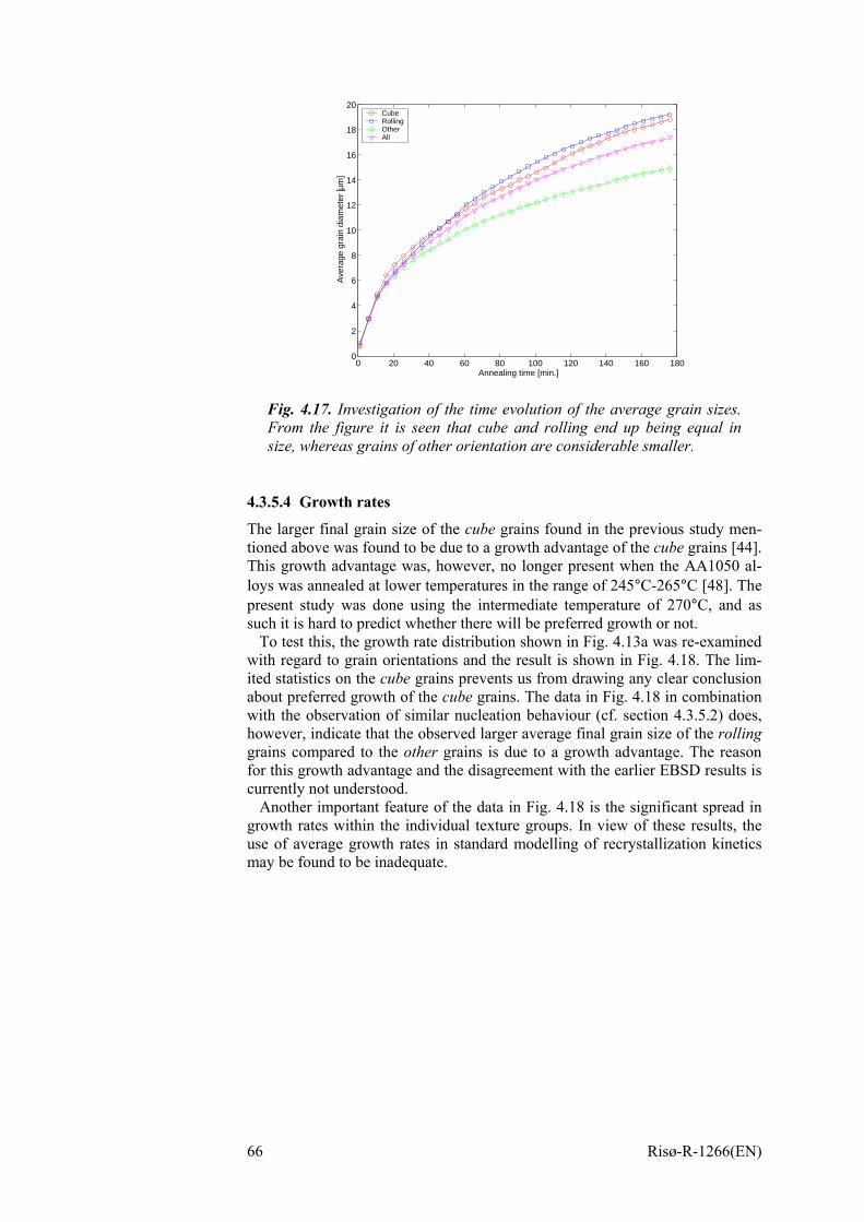
0 20 40 60 80 100 120 140 160 1800

2

4

6

8

10

12

14

16

18

20

Annealing time [min.]

Ave

rage

gra

in d

iam

eter

[µm

]

CubeRollingOtherAll

Fig. 4.17. Investigation of the time evolution of the average grain sizes. From the figure it is seen that cube and rolling end up being equal in size, whereas grains of other orientation are considerable smaller.

4.3.5.4 Growth rates

The larger final grain size of the cube grains found in the previous study men-tioned above was found to be due to a growth advantage of the cube grains [44]. This growth advantage was, however, no longer present when the AA1050 al-loys was annealed at lower temperatures in the range of 245°C-265°C [48]. The present study was done using the intermediate temperature of 270°C, and as such it is hard to predict whether there will be preferred growth or not.

To test this, the growth rate distribution shown in Fig. 4.13a was re-examined with regard to grain orientations and the result is shown in Fig. 4.18. The lim-ited statistics on the cube grains prevents us from drawing any clear conclusion about preferred growth of the cube grains. The data in Fig. 4.18 in combination with the observation of similar nucleation behaviour (cf. section 4.3.5.2) does, however, indicate that the observed larger average final grain size of the rolling grains compared to the other grains is due to a growth advantage. The reason for this growth advantage and the disagreement with the earlier EBSD results is currently not understood.

Another important feature of the data in Fig. 4.18 is the significant spread in growth rates within the individual texture groups. In view of these results, the use of average growth rates in standard modelling of recrystallization kinetics may be found to be inadequate.

66 Risø-R-1266(EN)

0.000 0.002 0.004 0.0060

5

10

15

20

25

Growth rate [µm/s]

Fre

quen

cy [%

]

Cube orientation

0.000 0.002 0.004 0.0060

5

10

15

20

25

Growth rate [µm/s]

Fre

quen

cy [%

]

Rolling orientations

0.000 0.002 0.004 0.0060

5

10

15

20

25

Growth rate [µm/s]

Fre

quen

cy [%

]

Other orientations

4.3.5.

As mtweenbehavgrowting thdiffergroupdifferevolugroupgrowtto decof the

Risø-

Fig. 4.18. Investigation of pre-ferred growth. The measured growth rates after 600s of growth (see Fig. 4.13A) is grouped according to grain orientation. The average growth rates are: 1.57⋅10-3 µm/s for cube grains, 1.67⋅10-

3 µm/s for rolling grains and 1.26⋅10-3 µm/s for other grains. The shapes of the distributions for the rolling grains and other grains are clearly different as is also confirmed by the Kolmo-gorov-Smirnov analysis.

5 Impingement

entioned above the present technique does not allow the impingement be- grains to be measured directly. Some information on the impingement iour can, however, be obtained indirectly by looking at the evolution of h rate distribution. Assuming that any concurrent recovery going on dur-e annealing will happen uniformly throughout the sample, any observed ences in the decrease of the average growth rate of the different texture s may be ascribed to differences in the impingement conditions, hence, to ences in the spatial distribution of the nuclei. In Fig. 4.19 is plotted the tion of the average measured growth rate of the three different texture s as a function of time of growth. Apart from the absolute values of the h rates, the average growth rate of the different texture components seems rease in a similar way. This may be interpreted as the spatial distribution nuclei belonging to the three different texture groups being similar.

R-1266(EN) 67

0 50 100 1500.2

0.4

0.6

0.8

1

1.2

1.4

1.6

1.8x 10

−3

Annealing time [min.]

Mea

n gr

owth

rat

e [µ

m/s

]

allcuberollingother

Fig. 4.19. Evolution of the measured mean growth rate for all of the grains, as well as for the 3 texture groups; cube, rolling and other. Apart from the differences in the absolute values, the decrease in the mean growth rate for the 3 texture groups seems to be similar, indicating simi-lar impingement conditions.

4.4 Discussion and outlook The 3DXRD microscope results presented in this chapter have shown that new detailed information on the recrystallization kinetics of the individual grains can be obtained. Information that could never have been achieved using conven-tional characterization techniques.

For the AA1050 commercial aluminium alloy investigated this has lead to a number of new findings:

• Observation of grains having significantly retarded nucleation. For particle containing alloys, like the AA1050 alloy, particle stimulated nucleation (PSN) is believed to be the primary nucleation mechanism [25]. Particle stimulated nucleation is normally associated with site saturation, hence, the observation of grains having significantly re-tarded nucleation may indicate the presence of a secondary nucleation mechanism.

• Fluctuation of growth rates within grains. The observation of substan-tial fluctuations in the growth rate of the individual grains (Fig 4.9) point towards the necessity of understanding the influence of the de-tails of the deformed microstructure on the growth the individual nu-clei. One explanation for the observed fluctuations could be the effect of orientation pinning as suggested by Juul Jensen [65]. In this case the fluctuations in the growth rate is thought to be due to the continu-ously changing orientation relationship between the growing grain boundary and the surrounding deformed matrix. When the grain boundary meets orientations similar to its own the mobility of the grain boundary decreases (low angle boundary) and when the grain boundary meets orientations different from its own the mobility in-creases (high angle boundary) [25].

68 Risø-R-1266(EN)

• Fluctuation of growth rates between individual grains. Also between the individual grains significant fluctuations in the growth rates are observed. As a first attempt this may be explained by the enhanced mobility of specific texture components [66], however, a detailed study of the orientation dependence shows that even within the indi-vidual texture components large variations in the growth behaviour is observed (see e.g. Fig 4.14 and Fig 4.15). This may be explained by a combination of the different impingement conditions for the different nuclei and the details of the specific deformed matrix surrounding the individual nuclei. At 90% reduction in thickness, the deformed matrix is heavily subdivided into small µm-sized volume elements of differ-ent crystallographic orientations [67]. As both the driving force for recrystallization and the mobility of the recrystallization front may depend on these crystallographic orientations, it seems not surprising that large fluctuations in growth rate are observed between the indi-vidual nuclei.

• Observation of similar nucleation behaviour for all three texture groups; cube, rolling and other. Investigations of the orientation de-pendence of the nucleation behaviour did not reveal any differences due to grain orientation. Information of this kind is not obtainable with any other technique.

• Observed growth advantage of grains having cube and rolling orienta-tions. Investigations of the initial growth rates reveals that cube grains or rolling grains have an average growth advantage of 1.3- and 1.4 times that of other grains, respectively. That cube grains may have growth advantage compared to other (random) orientation has been reported several times before in the literature. This has also been found in a previous study of the AA1050 alloy using an annealing temperature of 280°C [44,47]. The observation that rolling grains also have a growth advantage compared to other grains has not been re-ported earlier and disagrees with the earlier study [44,47]. Many of the rolling grains were found on the 311 Debye-Scherrer ring, which has a high degree of overlap between the different texture components. To test whether the observed growth advantage of the rolling grains were due to the ambiguousness of the orientation as-signment of the 311 reflections, the analysis was repeated exclud-ing these reflections. The remaining rolling grains were, however, still found to have an average growth advantage compared to the other grains. A more plausible explanation may be that rolling grains, unlike cube and other, are nucleating on top of the strong signal from the rolling components of the deformed microstructure. As such it may be more difficult to observe the small rolling grain, and therefore there may be a tendency only to measure the largest rolling grains. This would lead to a measured higher growth rate and grain size. Thus, more tests are necessary to determine whether this observation is real or whether it is an artifact caused by the data processing.

• Evolution of grain size distribution. The presented 3DXRD technique allows for the first time the evolution of the grain size distribution of the same ensemble of grains to be followed in-situ. For the AA1050 alloy this have been used to follow the mean grain size of individual texture groups as a function of annealing time. It is found that grains having cube or rolling orientations end up being significantly larger than grains having other orientations. This may be attributed to the observed growth advantage mentioned above.

Risø-R-1266(EN) 69

In the following I will try to summarize the results regarding the overall re-

crystallization kinetics of the AA1050 obtained in this study. The investigation of the measured orientation distribution functions (ODFs) showed that the vol-ume fraction of the cube orientation changed from virtually nothing to approxi-mately 5% after annealing at 270°C. The other dominating texture components after recrystallization were the rolling texture components already present in the as-deformed sample. The following investigation of the measured growth curves of the individual grains showed that the domination of the cube and roll-ing textures found in the ODFs might be related to the observed larger mean grain sizes seen for these two texture groups. A larger mean grain size can be obtained by one of the following three mechanisms or a combination of these; 1) early nucleation, 2) higher growth rate, or 3) more favourable impingement conditions. From Fig. 4.15 it was found that the nucleation behaviour for the three texture groups were very similar. Hence, mechanism 1) cannot explained the observed size advantage of the cube grains and rolling grains. The investiga-tion of the initial growth rate (believed to be the “true” growth rate) revealed that both cube grains and rolling grains on average have a higher growth rate than other grains. Hence, mechanism 2) might explain the observed size advan-tage. Finally investigations of the evolution of the average growth rates as a function of time indicate that the impingement conditions are the same for the three texture groups, and as such mechanism 3) does not seem to contribute to the observed size advantage of the cube grains and rolling grains. Hence, the preferential growth is found to be the main mechanism responsible for the ob-servation of a average size advantage of the cube grains and the rolling grains in 90% cold-rolled AA1050 commercial purity aluminium when annealed at 270°C.

Fig. 4.20. Motivated by the measured growth rate distribution for the AA1050 aluminium alloy the JMAK formalism were reinvestigated and it is shown the implementation of a growth grate distribution into the framework of the JMAK formalism has a drastic impact on the avrami plot. There is a striking resemblance between the derived plot and the measured data shown in Fig. 4.5.

Another interesting observation derived from the present study relate to the modelling of recrystallization kinetics [A11]. Existing models for recrystalliza-tion kinetics, where most of them have their genesis in the models of Kolmo-gorov, Johnson and Mehl and Avrami (KJMA) [51-53,60], are typically assum-ing one overall average nucleation rate and one overall average growth rate, or alternatively one average nucleation rate and one average growth rate for each texture components [68]. The results from the 3DXRD microscope do, how-

70 Risø-R-1266(EN)

ever, show that all the grains of the AA1050 alloy have their own kinetics, and no two grains are alike. Hence, the only way to thoroughly describe the overall recrystallization kinetics is by distributions of nucleation rates and growth rates. This was already realized by Gordon and Vandermeer [69] in 1959 but the in-ability to measure such distributions at that time kept them from pursuing this idea. With the results for the AA1050 alloy presented here renewed motivation for formulating recrystallization models based on distributions both of nuclea-tion and growth rates now exists. A first attempt of incorporating a distribution of growth rates into the KJMA formalism is described in [A11]. Based on an examination of the data on the AA1050 alloy a mathematical description of the growth rate distribution is chosen and incorporated into the KJMA framework with drastic consequences for the Avrami plot as shown in Fig. 4.20. The intro-duction of growth rate distributions into the KJMA theory results in a deviation from the classical linear appearance in the Avrami plot towards a more upward concave form. The form of the curve shown in Fig. 4.20 has some resemblance with the VV vs. time plot for the AA1050 alloy shown in Fig. 4.5 and one might speculate that the distribution of growth rates somehow has a profound effect on the recrystallization kinetics of this material.

Risø-R-1266(EN) 71

72 Risø-R-1266(EN)

5 Conclusion The thesis work has concentrated on the development of a novel 3D X-Ray Dif-fraction (3DXRD) microscope and its applications to the studies of recrystalli-zation. The 3DXRD microscope is dedicated to 3D structural characterization of thick samples utilizing focused high energy synchrotron radiation (40-100keV). The instrument is located at the Materials Science beamline at the European Synchrotron Radiation Facility (ESRF), Grenoble, and is the result of a joint collaboration between Risø National Laboratory and the ESRF.

The three main topics of the thesis have been: 1) the implementation of a so-called tracking technique for 3D characterization using the 3DXRD microscope and the development of a software program, GRAINDEX, for automatic proc-essing of the vast amount of data produced by the tracking technique, 2) the development of a technique capable of measuring the growth kinetics of a large number of individual grains by using the 3DXRD microscope, and 3) the appli-cation of this technique to the study of recrystallization kinetics of a commercial purity aluminium alloy. As such, the work has involved instrument develop-ment, software development and the application of these to studies of materials science. In the following a summation of the thesis, including previous discus-sions, will be made and the most important conclusions will be drawn.

5.1 The tracking technique and GRAINDEX soft-ware

Several techniques have been developed for 3D characterization of bulk sam-ples using the 3DXRD microscope these are based on: ray-tracing [A1,A2], conical slits [12], and focusing optics [13]. The present thesis work has primar-ily been concerned with the ray-tracing technique, referred to as tracking. The tracking technique provides a fast and non-destructive tool for 3D characteriza-tion of polycrystalline materials with no or limited mosaic spread [A5]. The high acquisition speed of the tracking technique and the use of 2D detectors do, however, result in vast amounts of data impracticable for manual data analysis. Thus, to facilitate the data analysis, an automated data processing software pro-gram, termed GRAINDEX, has been developed. Based on ray-tracing of the measured diffraction spots, GRAINDEX is able to identify and index the reflec-tions belonging to the individual grains of a polycrystalline material. The com-bination of the tracking technique and the GRAINDEX software allows for the position, volume and orientation of hundreds of grains to be determined simul-taneously. The obtained information can then be used for further analysis of e.g. single crystal refinement or stress analysis [A2]. For coarse-grained materials the outcome of the GRAINDEX program may be used for construction of 3D maps of grain boundaries and two approaches for obtaining the grain boundary outlines by back-projection of either the periphery or intensity of the diffraction spots have been developed [A2].

Three examples have been presented to illustrate the potential of the tracking concept. The first example, involving grain boundary mapping of a coarse-grained aluminium alloy demonstrates the capability of producing 3D maps of the grain structure. Due to the high speed of the tracking technique, such 3D maps could be used for in-situ studies of for example grain growth [70]. The

Risø-R-1266(EN) 73

second example, involving wetting in Al/Ga systems, illustrates a second use of the tracking concept, namely the initial characterization using the 3DXRD mi-croscope combined with a subsequent investigation by a complementary tech-nique, which in the present case was x-ray microtomography. In the last exam-ple, involving grain rotations in aluminium, two different applications of the GRAINDEX program were used in the same experiment. Initially the ray-tracing part is used to locate grains of specific interest, and subsequently the indexing part is used to follow the grain rotation of these selected grains.

In conclusion it has been shown that the tracking technique, in combination with the GRAINDEX software, is a unique tool for 3D investigations of various phenomena in materials science, either as an independent technique or in com-bination with complementary techniques.

5.2 In-situ measurements of growth kinetics In addition to the general tracking technique described above, a second tech-nique focusing especially on in-situ measurements of growth kinetics has been presented. Contrary to the tracking technique describe above, this technique does not provide any spatial information, but is optimised to the study of growth kinetics of a large number of individual bulk grains with a very high time reso-lution (several data point per minute). The basic idea of the technique is very simple and based on monitoring the diffracted intensity of a large number of individual grains during annealing. Exploiting the fact that the diffracted inten-sity can be directly related to the volume of the diffracting grains, a complete measure of the growth kinetics of the individual grains, from the moment they nucleate till they reach their final grain size, can be obtained. Two approaches for correlating the observed growth kinetics with the orientation of the grain has been devised. The first approach is based on the position of a single measured Bragg reflection in the corresponding pole figure. By comparing the position of the reflection in the pole figure with the position of standard texture compo-nents, the grain can be assigned to a specific texture class, e.g. cube or rolling [A4]. The second approach consists of combining the technique of measuring growth kinetics with the GRAINDEX software. Hence, initially the growth ki-netics, based on a single reflection, is monitored with a high time resolution us-ing the current technique. From time to time a broad ω-scan in performed re-sulting in the measurement of several reflections from each grain, alternatively this could be done at the end of the experiment. Based on the broad ω-scan the GRAINDEX is used to determine the full orientation of each of the individual grains. Hence, by combining the two techniques full information regarding the growth kinetics as well as the orientation is obtained.

As in the case of the tracking technique, the full potential of the technique for measuring growth kinetics has first become accessible, by the development of a software package for automatic identification of valid reflections and extraction of the corresponding measured growth curves and orientation information.

The technique was developed for studies of recrystallization kinetics in metals and as such it has already been used for several studies [A3,A4]. The prospect of the technique for investigation the effect of processing parameters on the fundamental properties of metallic materials has already attracted the attention from industry, and the results from experiments conducted in collaboration with Alcan International, Banburry and RWTH Aachen is currently being processed. The technique is not restricted to studies of recrystallization kinetics, but can equally well be applied to other scientific areas, like for example phase trans-

74 Risø-R-1266(EN)

formations, and first experiments relating to the phase transformation in steels as a function of temperature or straining have been conducted [43].

The main limitations of the technique is due to peak overlap caused by very high number of grains in the gauge volume or by highly textured samples, which may lead to biasing of the data analysis. Two solutions to this limitation have been suggested. One is to reduced the investigated gauge volume by e.g. a conical slit and thereby reduce the number of reflecting grains. This will ease the analysis at the expense of poorer statistics. The other suggestion is based on a finer ω sampling. Using a smaller oscillation range, ∆ω, corresponding to a finer sampling in orientation space, will ease the separation of Bragg reflections from grains having almost similar orientations. The finer ω sampling will, how-ever, lead to a lower time resolution and/or poorer statistics. With the ongoing development of a continuous acquisition routine based on fast readout detectors, compared to the currently used stepwise acquisition routine, it is, however, most likely that a finer ω sampling may be possible without compromising the statis-tics and time resolution.

5.3 Recrystallization kinetics of commercial purity aluminium

The recrystallization kinetics of a commercial purity aluminium alloy (AA1050) cold rolled to 90% thickness reduction and annealed at 270°C has been studied using the technique describe above. Face centred cubic materials of medium to high stacking fault energy, like the AA1050 aluminium alloy, are know to de-velop a more or less pronounced cube texture during annealing [63]. In spite of many years of intensive studies [71] the mechanisms responsible for the emer-gence of the cube texture in these kind of alloys is still not understood [72]. Ear-lier investigations of the same AA1050 aluminium alloy using neutron diffrac-tion has shown that annealing at 280°C leads to a change in the volume fraction of “cube grains” from virtually zero in the as-deformed sample to approxi-mately 10% in the fully recrystallized sample [44]. This has been correlated to an average growth advantage of grains belonging to the cube texture component as compared to grains of “random” orientation determined by linear intercept measurements with the electron back scatter diffraction (EBSD) technique [73]. A later study by the same authors, on the same alloy but using lower annealing temperatures (245°C-265°C) did, however, not reveal any growth advantages for the cube grains. The aim of the present investigation was to achieve new information on the recrystallization kinetics of the AA1050 aluminium alloy to further the understanding of the underlying recrystallization mechanisms.

Two experiments were conducted using the 3DXRD microscope and in total 5 samples were investigated. The first experiment allowed for the first time in-situ observations of the recrystallization kinetics of the individual bulk nu-clei/grains. The growth curves of 6 randomly picked grains were measured re-vealing new details regarding the nucleation and growth behaviour of the AA1050 aluminium alloy, that could never have been obtained by conventional techniques. The aim of the second experiment was to investigate the orientation dependence of the recrystallization kinetics, and in total 244 growth curves were measured. The investigation of the growth curves from the two experiments have resulted in a number of new findings regarding the recrystallization kinet-ics of the AA1050 aluminium alloy, where the main observations will be sum-marized in the following.

By investigations of orientation distribution functions (ODFs) based on meas-urements of complete pole figures before and after annealing the volume frac-

Risø-R-1266(EN) 75

tion of cube grains were found to increase from 0.9% to 4.9% during the anneal-ing. This increase may be attributed to either a higher fraction of nuclei having cube orientations than nuclei of random orientations, normally referred to as oriented nucleation [63], or to a higher average growth rate of cube grains com-pared to grains having random orientations, normally referred to as oriented growth [63], or to a combination of both. The employed technique did not allow for investigations of oriented nucleation and as such the following discussion will be concentrated on the question of oriented growth as well as on the overall recrystallization process.

The first observation made by examining the measured growth curves is that every grain has its own kinetic, not two growth curves are alike. This observa-tion has a striking contrast to the general assumption used in modelling of re-crystallization kinetics that each grain may be represented in the mathematical formulations as an “average” grain [53] .

The noise limit for observing the new nuclei was found to be at a equivalent sphere radius (R) approximately 1 µm, comparable to the nuclei size found by microscopy techniques [37]. A distribution of the measured nucleation times revealed that the majority of the nuclei were form in the initial stages of the re-crystallization process (VV < 0.1). There are, however, a number of nuclei (ap-proximately 10%) which nucleate at considerable later stages (up to VV ≈ 0.35). For a particle containing alloy like the AA1050 aluminium alloy, particle stimu-lated nucleation (PSN) is believed to be the primary nucleation mechanism [74]. Particle stimulated nucleation is normally assumed to give rise to site-saturation [48], but the present data indicates that this may not always be the case.

The employed technique does not provide any spatial information on the dis-tribution of the nuclei, hence the impingement conditions for the individual grains are unknown. It may, however, seem reasonable to assume that the growth curves at the early stages of recrystallization, where it may be assumed that impingement can be neglected, reflects the real “free to grow” behaviour. The growth rates derived at these early stages reveals that there is a significant variation in the growth rate of the individual grains as well as between the grains. Investigations of the orientation dependence of the growth rates shows that these variations in growth rates are also found within grains belonging to the same texture component [A4] and stresses the importance of understanding the influence of the in-homogeneity of the deformed microstructure on the growth kinetics of the individual grains.

By comparing the measured growth curves as a function of time, an evolution of the real 3D grain size distribution can be obtained, which is not possible by any other technique. Comparing the average final grain of the three texture groups: cube, rolling, and other, shows that both the cube and rolling grains on averaged are found to be 1.3 times larger than grains having other orientations. A possible explanation for this observed size advantage could either be due to differences in nucleation behaviour, impingement behaviour or growth behav-iour. Investigations of the nucleation behaviour of the three different texture groups did not reveal any notably differences. Nor did the indirectly estimated impingement behaviour based on observations of the decrease in the average impingement influenced growth rate. The investigation of the early growth rates did, however, reveal significantly differences between the three texture groups. The average growth rates of the cube and rolling grains were found to be 1.2 and 1.3 times the average growth rate of grains having other orientations, re-spectively. Thus, based on the present investigation the observation of a larger average grain of the cube and rolling grains is found to be due to a growth ad-vantage (preferred growth [75]).

The absolute values of the determined average initial growth rates of the three texture groups all fall nicely between the values of the Cahn-Hagel growth rates

76 Risø-R-1266(EN)

obtained for T=265°C and T=280°C by Vandermeer and Juul Jensen [48]. Also the observation that the average growth rate for cube grains is 1.2 times the av-erage growth rate of other grains, is consistent with the observation by Vander-meer and Juul Jensen. They find an average growth advantage of cube grains of 1.5 at T=280°C [47], whereas no growth advantage was observed at T=265°C [48]. Also the ratio of 1.3 between the average final recrystallized grain size of the cube grains and other grains in the current study is in nice agreement with the value of 1.4 found by Juul Jensen (1995) [44].

The observed growth and size advantage for the rolling grains is however a new finding, and is in disagreement with the observations of Vandermeer and Juul Jensen [44,47] done at T=280°C. No previous observations of growth or size advantages of rolling grains in similar alloys have been reported. It is my belief that the observed growth and size advantage of the rolling grains found in the present study is the result of a biased data analysis. A possible explanation for such a bias could be the presence of a dominating rolling texture in the ini-tial as-deformed sample. As a consequence new grains belonging to the cube or other texture groups will appear on the Debye-Scherrer ring in regions where the diffracted signal from the deformed microstructure is weak, whereas grains belonging to the rolling texture will form on top of the strong signal from the rolling components of the deformed microstructure. Hence, when identifying valid reflections the small rolling grains may have a tendency to “disappear” in the signal from the deformed microstructure, and thereby only large rolling grains are detected as valid grains leading to an overestimated average growth rate and final grain size. Such biasing can be avoided by reducing the diffracted signal from the deformed microstructure using either a conical slit or a finer oscillation range as explained in section 3.3.

Another interesting observation derived from the present study relate to the modelling of recrystallization kinetics [A11]. Existing models for recrystalliza-tion kinetics, where most of them have their genesis in the models of Kolmo-gorov, Johnson and Mehl and Avrami (KJMA) [51-53,60], are typically assum-ing one overall average nucleation rate and one overall average growth rate, or alternatively one average nucleation rate and one average growth rate for each texture components [75]. The results from the 3DXRD microscope does, how-ever, show that the only way to thoroughly describe the overall recrystallization kinetics is by distributions of nucleation rates and growth rates. This was al-ready realized by Gordon and Vandermeer in 1959 [69] but the inability of measuring such distributions at that time kept them from pursuing this idea. With the results for the AA1050 alloy presented here renewed motivation for formulating recrystallization models based on distributions of nucleation rates and growth rates now exists. A result of a first attempt of incorporating a distri-bution of growth rates into the KJMA formalism has been presented [A11]. Based on an examination of the data on the AA1050 alloy a mathematical de-scription of the growth rate distribution is chosen and incorporated into the KJMA formulism with drastically consequences for the Avrami plot. The intro-duction of growth rate distributions into the KJMA theory results in a deviation from the classical linear appearance in the Avrami plot towards a more upward concave form. A form which has some resemblance with the VV vs. time plot for the AA1050 alloy found in the present study by EBSD measurements, and which is also found by Vandermeer and Juul Jensen for annealing temperatures in the range of 245°C-280°C [48]. Motivated by this resemblance one might speculate that the distribution of growth rates somehow has a profound effect on the recrystallization kinetics of this material.

Risø-R-1266(EN) 77

78 Risø-R-1266(EN)

Reference List [1]. R.A. Vandermeer (2001). Advances in the Study of Recrystallization

Kinetics. Proceedings of the First Joint International Conference on Recrystallization and Grain Growth 2 (Eds.G. Gottstein and D. A. Molodov) . pp 645-657.

[2]. H.F. Poulsen, S. Garbe, T. Lorentzen, D. Juul Jensen, F.W. Poulsen, N.H. Andersen, T. Frello, R. Feidenhansl and H. Graafsma (1997). Ap-plications of high-energy synchrotron radiation for structural studies of polycrystalline materials, Journal of Synchrotron Radiation 4, 147-154.

[3]. D. Juul Jensen and H.F. Poulsen (2000). Recrystallization in 3D. Re-crystallization - Fundamental Aspects and Relations to Deformation Microstructure (Eds.N. Hansen et al.) Roskilde, Denmark: Risø Na-tional Laboratory). pp 103-124.

[4]. H.F. Poulsen and D. Juul Jensen (1995). Synchrotron Radiation Diffrac-tion: A Novel Tool for Recrystallization Studies in Bulk Micrometer^3 Sized Local Areas. Microstructural and Crystallographic Aspects of Recrystallization (Eds.N. Hansen et al.) Roskilde, Denmark: Risø Na-tional Laboratory). pp 503-508.

[5]. Å. Kvick and H.F. Poulsen (1997). Local Characterization of Materials by Synchrotron Radiation. Workshop Proceedings. Internal ESRF Pub-lication No. ESRF97KV10T .

[6]. B.W. Batterman and D.H. Bilderback (1991). X-Ray Monochromators and Mirrors in Handbook on Synchrotron Radiation. (Elsevier Science Publishers B.V). pp 105-153.

[7]. U. Lienert, C. Schulze, V. Honkimaki, T. Tschentscher, S. Garbe, O. Hignette, A. Horsewell, M Lingham, H.F. Poulsen, N.B. Thomsen and E. Ziegler (1998). Focusing optics for high-energy X-ray diffraction, Journal of Synchrotron Radiation 5, 226-231.

[8]. C. Schulze, U. Lienert, M. Hanfland, M. Lorenzen and F. Zontone (1998). Microfocusing of hard x-rays with cylindrically bent crystal monochromators, Journal of Synchrotron Radiation 5, 77-81.

[9]. U. Lienert, H.F. Poulsen, R.V. Martins and Å. Kvick (2000). A high energy microscope for local strain measurements within bulk materials, Proceedings of the Fifth European Conference on Residual Stresses 347-3, 95-100.

[10]. P. Kirkpatrick and A.V. Baez (1948). Formation of Optical Images by X-Rays, Journal of the Optical Society of America 38, 766-774.

[11]. Certified Scientific Software. http://www.certif.com. [12]. S.F. Nielsen, A. Wolf, H.F. Poulsen, M. Ohler, U. Lienert and R.A

Owen (2000). A conical slit for three-dimensional XRD mapping, Journal of Synchrotron Radiation 7, 103-109.

[13]. U. Lienert, H.F. Poulsen, V. Honkimaki, C. Schulze and O. Hignette (1999). A focusing multilayer analyser for local diffraction studies, Journal of Synchrotron Radiation 6, 979-984.

[14]. E.M. Lauridsen, S. Schmidt, R.M. Suter and H.F. Poulsen. Tracking: a Method for Structural Characterization of Grains in Powders or Poly-crystals. To appear in Journal of Applied Crystallography.

[15]. Media Cybernetics. http://www.mediacy.com. [16]. W.R. Busing and H.A. Levy (1967). Acta Cryst. 22, 457-464.

Risø-R-1266(EN) 79

[17]. H.J. Bunge (1982). Texture Analysis in Materials Science. (Butter-worths, London).

[18]. L. Hansen, J. Pospiech, and K. Lücke (1978). Tables of Texture Analy-sis of Cubic Crystals. (Springer-Verlag, Berlin).

[19]. V. Randle and O. Engler (2000). Introduction to Texture Analysis, Macrotexture, Microtexture and Orientation Mapping. (Gordon and Breach Publishing Group).

[20]. W.H. Press and others (1992). Numerical Recipes in FORTRAN. (Cambridge University Press).

[21]. N.C. Krieger Lassen (1992). Automatic Crystal Orientation Determina-tion From EBSPs, Micron and Microscopia Acta 191-192.

[22]. L. Margulies, G. Winther and H.F. Poulsen (2001). In situ measurement of grain rotation during deformation of polycrystals, Science 291, 2392-2394.

[23]. G.I. Taylor (1938). J. Inst. Met. 62, 307. [24]. G. Sachs (1928). Z. Ver. Dtsch. Ing. 72-22, 734. [25]. F.J. Humphreys and M. Hatherly (1995). Recrystallization and Related

Annealing Phenomena. (Pergamon Press). [26]. B.L. Adams, S. Ta'asan, D. Kinderlehrer, I. Livshits, D.E. Mason,

C.T.Wu, W.W. Mullins, G.S. Rohrer, A.D. Rollett, and D.M. Saylor, (1999). Extracting grain boundary and surface energy from measure-ment of triple junction geometry, Interface Science 7, 321-338.

[27]. D.S. Bright (1995). MacLispix – A Special-Purpose Public Domain Image-Analysis Program for the MacIntosh, Microbeam Analysis 4, 151-163.

[28]. R.T. Dehoff and F.N. Rhines (1968). Quantitative Microscopy. (McGraw-Hill Book Co, New York).

[29]. W.A. Anderson and R.F. Mehl (1945). Recrystallization of Aluminium in Term of Rate of Nucleation and Rate of Growth, Trans AIME 161, 140-172.

[30]. J.W. Cahn and W.C. Hagel (1962). Theory of the Pearlite Reaction in Decomposition of Austenite by Diffusional Processes (Interscience Publ., NY) pp 131-196.

[31]. R.A. Vandermeer and D. Juul Jensen (1994). On the extimation of Cahn-Hagel interface migration rates, Scripta Metallurgica Et Materi-alia 30, 1575-1580.

[32]. B. Bay and N. Hansen (1984). Recrystallization in Commercially Pure Aluminum, Metallurgical Transactions A 15A, 287-297.

[33]. F.J. Humphreys and M. Ferry (1996). Combined in-situ annealing and EBSD of deformed aluminium alloys, Aluminium Alloys: Their Physi-cal and Mechanical Properties, Pts 1-3 217, 529-534 .

[34]. V. Branger, M.H. Mathon, T. Baudin and R. Penelle (2000). "In-situ" neutron diffraction study of the cube crystallographic texture develop-ment in Fe53%-Ni alloy during recrystallization, Scripta Materialia 43, 325-330.

[35]. T. Wroblewski, O. Clauss, H.A. Crostack, A. Ertel, F. Fandrich, C. Genzel, K. Hradil, W. Ternes and E. Woldt (1999). A new diffractome-ter for materials science and imaging at HASYLAB beamline G3, Nu-clear Instruments & Methods in Physics Research Section A- Accelera-tors Spectrometers Detectors and Associated Equipment 428, 570-582.

[36]. H. Natter, M. Schmelzer, M.S. Loffler, C.E. Krill, A. Fitch and R. Hem-pelmann (2000). Grain-growth kinetics of nanocrystalline iron studied in situ by synchrotron real-time X-ray diffraction, Journal of Physical Chemistry B 104, 2467-2476.

80 Risø-R-1266(EN)

[37]. B. Bay and N. Hansen (1979). Initial Stages of Recrystallization in Aluminum of Commercial Purity, Metallurgical Transactions A 10A, 279-288.

[38]. D.A. Hughes (2000). Deformation Microstructures and Selected Exam-ples of Their Recrystallization. Recrystallization - Fundamental Aspects and Relations to Deformation Microstructure (Eds.N. Hansen et al.) Roskilde, Denmark: Risø National Laboratory). pp 49-70.

[39]. D.J. Thomas (1990). Calibrating an Area-Detector Diffractometer: Inte-gral Response, Proc. R. Soc. Lond. A428, 181-214.

[40]. A.P. Hammersley, S.O. Svensson, M. Hanfland, A.N. Fitch and D. Hausermann (1996). Two-dimensional detector software: From real de-tector to idealised image or two-theta scan, High Pressure Research 14, 235-248.

[41]. 3DXRD software frontend developed by S. Schmidt (2001). [42]. B.E.Warren (1990). X-Ray Diffraction. (Dover Publications, Inc., New

York). [43]. E. Offerman and S. Kruijver, private communication [44]. D. Juul Jensen (1995). Growth-Rates And Misorientation Relationships

Between Growing Nuclei Grains And The Surrounding Deformed Ma-trix During Recrystallization, Acta Metallurgica Et Materialia 43, 4117-4129.

[45]. R.A. Vandermeer and D. Juul Jensen (1994). Modeling Microstructural Evolution Of Multiple Texture Components During Recrystallization, Acta Metallurgica Et Materialia 42, 2427-2436.

[46]. D. Samputh, W.S. Miller, R. Van der broeck, and P. De Smet (1996). Microstructural Reactions Occurring During Homogenisation of AA1050 Alloy, Materials Science Forum 217-222, 747-752.

[47]. R.A. Vandermeer and D. Juul Jensen (1998). The migration of high an-gle grain boundaries during recrystallization, Interface Science 6, 95-104.

[48]. R.A.Vandermeer and D. Juul Jensen (2001). Microstructural path and temperature dependence of recrystallization in commercial aluminum, Acta Materialia 49, 2083-2094.

[49]. N.C. Krieger Lassen, D. Juul Jensen, and K. Conradsen (1992). Image Processing Procedures for Analysis of Electron Back Scattering Pat-terns, Scanning Microscopy 6, 115-121.

[50]. N.C. Krieger Lassen and D. Juul Jensen (1999).Automatic Recognition of Recrystallized Grains in Partly Recrystallized Samples From Crystal Orientation Maps. Proceedings of the Twelfth International Conference on Textures of Materials (ICOTOM-12) (Ed.J.A.Szpunar) Montreal, Canada. pp 854-859.

[51]. M. Avrami (1939). Kinetics of Phase Change I. General Theory, J. Chem. Phys. 7, 1103-1112.

[52]. M. Avrami (1940). Kinetics of Phase Change II. Transformation-Time Relations for Random Distribution of Nuclei, J. Chem. Phys. 8, 212-224.

[53]. W.A. Johnson and R.F. Mehl (1939). Reaction Kinetics in Processes of Nucleation and Growth, Trans AIME 135, 416-458.

[54]. B. Hutchinson, S. Jonsson, and L. Ryde (1989). On The Kinetics Of Recrystallization In Cold-Worked Metals, Scripta Metallurgica 23, 671-676.

[55]. K. Pawlik and J. Pospiech (1987). in Theoretical Methods of Texture Analysis p 127.

Risø-R-1266(EN) 81

[56]. H. Mecking (1985). Textures in Metals in Preferred Orientation in De-formed Metals and Rocks: An Introduction to Modern Texture Analysis (Academic Press, Inc., London) pp 267-306.

[57]. D. Juul Jensen and M.T. Lyttle (1999).Reproducibility of Experimental Texture Measurement. Proceedings of the Twelfth International Con-ference on Textures of Materials (ICOTOM-12) (Ed.J.A.Szpunar) Montreal, Canada. pp 46-51.

[58]. R.K. Bolingbroke, T. Furu, D. Juul Jensen and K. VernonParry (1996). Annealing behaviour of dilute aluminium alloys following hot deforma-tion, Materials Science and Technology 12, 897-903.

[59]. D. Juul Jensen (2001).Experimental Measurements of Nucleation and Growth Rates. Proceedings of the First Joint International Conference on Recrystallization and Grain Growth vol. 1 (Eds. G. Gottstein and D. A. Molodov) . pp 73-86.

[60]. A.N. Kolmogorov (1937). On the Statistical Theory of Metal Crystalli-zation, Izv. Akad. Nauk. USSR-Ser. Matemat. 1, 355-359.

[61]. R.A. Vandermeer, R.A. Masumura and B.B. Rath. (1991). Microstruc-tural Paths Of Shape-Preserved Nucleation And Growth Transforma-tions, Acta Metallurgica Et Materialia 39, 383-389.

[62]. R.A. Vandermeer and D. Juul Jensen (1995). Quantifying Recrystalliza-tion Nucleation And Growth-Kinetics Of Cold-Worked Copper By Mi-crostructural Analysis, Metallurgical and Materials Transactions A-Physical Metallurgy and Materials Science 26, 2227-2235.

[63]. R.D. Doherty, L.C. Chen and I. Samajdar (1998). Cube recrystallization texture - experimental results and modeling, Materials Science and En-gineering A-Structural Materials Properties Microstructure and Proc-essing 257, 18-36.

[64]. J.R Hirsch,.W.B. Hutchinson and K. Lücke (1991). Effect Of Initial Grain-Size And Shape On Textures In Sheet Steel, Textures and Micro-structures 14, 691-696.

[65]. D. Juul Jensen and K. Mehnert (1998).Orientation Pinning During Growth. Grain Growyh in Polycrystalline Materials III (Eds.H.Weiland et al.) : The Minerals, Metals & Materials Society). pp 251-262.

[66]. G. Ibe and K. Lücke (1968). Arch. Eisenhüttenwesen 39(9), 693 [67]. N. Hansen and D. Juul Jensen (1999). Development of microstructure

in FCC metals during cold work, Philosophical Transactions of the Royal Society of London Series A-Mathematical Physical and Engineer-ing Sciences 357, 1447-1469.

[68]. D. Juul Jensen (1992). Modeling Of Microstructure Development Dur-ing Recrystallization , Scripta Metallurgica Et Materialia 27, 1551-1556.

[69]. R.A. Vandermeer and P. Gordon (1959). Edge-Nucleated, Growth Con-trolled Recrystallization Aluminium, Trans. Metall. Soc. AIME 215, 577-588.

[70]. E.M. Lauridsen and R.M. Suter. Unpublished work. [71]. R.D. Doherty, D.A. Hughes, F.J. Humphreys, J.J. Jonas, D. Juul Jensen,

M.E. Kassner, W.E. King, T.R. McNelley, H.J. McQueen and A.D. Rollett (1997). Current issues in recrystallization: a review, Materials Science and Engineering A-Structural Materials Properties Microstruc-ture and Processing 238, 219-274.

[72]. R.D. Doherty, G. Gottstein, J. Hirsch, W.B. Hutchinson, K. Lücke, E. Nes, And P.J. Wilbrandt (1988).Report of Panel on Recrystallization Textures: Mechanisms and Experiments. ICOTOM 8 (Eds.J.S. Kallend and G. Gottstein) The Metallurgical Society AIME, Warrendale, PA. pp 563-572.

82 Risø-R-1266(EN)

[73]. R.A. Vandermeer and D. Juul Jensen (1996). Quantification of Micro-structural Evolution and Texture Development During Recrystalliza-tion, Textures and Microstructures 26-27, 263-279.

[74]. F.J. Humphreys (1977). Acta Metall. 25, 1323 [75]. D. Juul Jensen (1997). Simulation of recrystallization microstructures

and textures: Effects of preferential growth, Metallurgical and Materi-als Transactions A-Physical Metallurgy and Materials Science 28, 15-25.

Risø-R-1266(EN) 83

84 Risø-R-1266(EN)

Risø-R-1266(EN) 85

86 Risø-R-1266(EN)

Appendix A: Published Papers

Paper A1: E.M. Lauridsen, S. Schmidt, R.M. Suter and H.F. Poulsen (2001). Tracking: a Method for Structural Characterization of Grains in Powders or Polycrystals. J. Appl. Cryst. In Press.

Paper A2: H.F. Poulsen, S.F. Nielsen, E.M. Lauridsen, S. Schmidt, R.M.

Suter, U. Lienert, L. Margulies, T. Lorentzen and D. Juul Jen-sen (2001). Three-Dimensional Maps of Grain Boundaries and the Stress-State of Individual Grains. J. Appl. Cryst. In Press.

Paper A3: E.M. Lauridsen, D. Juul Jensen, U. Lienert and H.F. Poulsen

(2000). Kinetics of Individual Grains During Recrystallization. Scripta Mater., 43, 561-566.

Paper A5: D. Juul Jensen, Å. Kvick, E.M. Lauridsen, U. Lienert, L. Mar-

gulies, S.F. Nielsen and H.F. Poulsen (2000). Plastic Deforma-tion and Recrystallization Studied by the 3D X-Ray Micro-scope. Mat. Res. Soc. Symp. Proc., 590, 227-240.

Paper A6: S.F. Nielsen, E.M. Lauridsen, D. Juul Jensen and H.F.

Poulsen (2000). A Three-Dimensional X-Ray Diffraction Mi-croscope for Deformation Studies of Polycrystals. Proceedings of ICSMA12, Asilomar, California. In press.

Paper A7: S.F. Nielsen, W. Ludwig, D. Bellet, E.M. Lauridsen, H.F.

Poulsen and D. Juul Jensen (2000). Three Dimensional Map-ping of Grain Boundaries. Proceedings of the 21th Interna-tional symposium on materials science: Recrystallization - fundamental aspects and relations to deformation micro-structure. Risø National Laboratory. Edited by N. Hansen et al. (Risø, Roskilde, Denmark, 2000), p. 473-478.

Paper A8: O.V. Mishin, E.M. Lauridsen, N.C. Krieger-Lassen, G. Brück-

ner, T. Tschentscher, B. Bay, D. Juul Jensen and H.F. Poulsen (2000). Application of High-Energy Synchrotron Radiation for Texture Studies. J. Appl. Cryst., 33, 364-371.

Paper A9: O.V. Mishin, E.M. Lauridsen, N.C. Krieger-Lassen, H.F. Poul-

sen, D. Juul Jensen, G. Brückner and B. Bay (1999). Compari-son of Experimental Techniques for Characterization of Through-Thickness Texture Variations. Proceedings of the Twelfth International Conference on Textures of Materials ( ICOTOM12), Edited by J.A. Szpunar. (NRC Research Press, Ottawa), 1, 174-179.

Paper A10: H.F. Poulsen, D. Juul Jensen, T. Tschentscher, L. Wcislak,

E.M. Lauridsen, L. Margulies and S. Schmidt (2001). Quantifi-cation of Minor Texture Components by Hard X-Rays. Tex-tures and Microstructures, In Press.

Risø-R-1266(EN) 87

Paper A11: D. Juul Jensen, E.M. Lauridsen and R.A. Vandermeer (2002). In-Situ Determination of Grain Boundary Migration During Recrystallization. To appear in TMS Annual Meeting 2002, Se-attle.

88 Risø-R-1266(EN)

Risø-R-1266(EN) 89

90 Risø-R-1266(EN)