The Conditional Distribution of Goodness-of-Fit Statistics for Discrete Data

The Conditional Distribution of Goodness-of-Fit Statistics for Discrete DataAuthor(s): Peter McCullaghSource: Journal of the American Statistical Association, Vol. 81, No. 393 (Mar., 1986), pp. 104-107Published by: American Statistical AssociationStable URL: http://www.jstor.org/stable/2287974 .

Accessed: 14/06/2014 00:47

Your use of the JSTOR archive indicates your acceptance of the Terms & Conditions of Use, available at .http://www.jstor.org/page/info/about/policies/terms.jsp

.JSTOR is a not-for-profit service that helps scholars, researchers, and students discover, use, and build upon a wide range ofcontent in a trusted digital archive. We use information technology and tools to increase productivity and facilitate new formsof scholarship. For more information about JSTOR, please contact [email protected].

.

American Statistical Association is collaborating with JSTOR to digitize, preserve and extend access to Journalof the American Statistical Association.

http://www.jstor.org

This content downloaded from 185.2.32.28 on Sat, 14 Jun 2014 00:47:18 AMAll use subject to JSTOR Terms and Conditions

http://www.jstor.org/action/showPublisher?publisherCode=astata

http://www.jstor.org/stable/2287974?origin=JSTOR-pdf

http://www.jstor.org/page/info/about/policies/terms.jsp


The Conditional Distribution of Goodness-of-Fit

Statistics for Discrete Data

PETER McCULLAGH*

I consider the distribution of Pearson's statistic and of the likelihood-ratio goodness-of-fit statistic for discrete data in the important case where the data are extensive but sparse. It is argued that the appropriate reference distribution is conditional on the sufficient statistic for the unknown regression parameters, ,B. The first three conditional asymptotic cumulants are derived by Edgeworth expansion, and these are used for the computation of tail probabilities. The principal advantage of the limit considered here, as opposed to the more usual x2 limit, is that the cell counts need not be large.

KEY WORDS: Conditional inference; Cumulants; Edgeworth approximation; Log-linear model; Linear logistic model; Sparse data.

1. INTRODUCTION

The object of this article is to derive, either exactly or approximately, the conditional distributions of certain commonly used goodness-of-fit statistics for discrete data in the important case where the data are sparse. For arbitrary log-linear or linear logistic models, exact specification of the conditional distribution is usually not feasible. For that reason, I concentrate on asymptotic approximations appropriate in the limit n -+ oo, as opposed to the more usual limit ,i X-+ oo (n fixed), where p1i = E(Yi) is the mean of the ith observation and i = 1, . . . , n. In the context of contingency tables, n is the number of cells and ,i is the mean count for cell i.

A number of authors have discussed the possibility of using normal rather than x2 approximations when the degrees of freedom are large (e.g., Morris 1975, Koehler and Lamtz 1980, and Fienberg 1979). Although I do use normal and Edgeworth approximations, the main emphasis in this article is different in two important respects. First, I consider specifically the case in which there are unknown parameters to be estimated. Second, I argue that it is the conditional distribution of the statistic and not its marginal distribution that is relevant for assessing goodness of fit. Both of these are typically asymptotically normal but, as shown in Section 4, the difference between the two can be very large indeed. If there are no unknown parameters, the conditioning statistic disappears and we are left with the marginal distribution.

Out of the many possible goodness-of-fit statistics, I concentrate on the two most commonly used in applications- namely, the deviance

D = > {2Y1log(Yi/Ai) - 2(Yi_ -A i)} (1)

and Pearson's statistic

p = > (yi - A,)2 A (2)

* Peter McCullagh is Professor, Department of Statistics, University of Chi- cago, Chicago, IL 60637.

In all calculations, I take Y to be a vector of length n, i to be an unknown parameter vector of lengthp, and ,u to be a function of i$ specified by the model, either log-linear or linear logistic as appropriate. The appropriate conditioning variable to remove distributional dependence on i$ is the sufficient statistic for i$. More generally, if the sufficient statistic is not complete, it would be appropriate to condition on $, the maximum likelihood estimate of Pi

When there are no unknown parameters, or where the appropriate conditional distribution has a simple form, simulation can be used to determine the approximate null distributions of P and D. A number of authors have in fact made extensive Monte Carlo investigations of the marginal distributions of P and D for sparse data. When unknown parameters are present, however, it is usually not easy to simulate from the conditional distribution; unconditional simulation, on the other hand, is not relevant for significance testing and can give misleading an- swers, as shown in Section 3. The objective of this article is to give an approximate analytical solution, thereby avoiding the need for conditional simulation.

Section 2 is devoted to log-linear models for Poisson responses, and in Section 3 I consider binomial responses. Binary data are considered in Section 4.

It should be emphasized at the outset that I do not necessarily recommend either (1) or (2) as useful statistics for detecting lack of fit when the data are sparse. Indeed, it will be seen that D, in particular, often has very little diagnostic power and, in the case of binary data, D has no diagnostic power whatsoever. In this respect, the conclusions of this article contradict Cochran (1952, sec. 14), who suspected that in small samples, the likelihood-ratio test would be more powerful than Pearson's test.

The emphasis in this article is not on the details of regularity conditions but on obtaining usable results under reasonable assumptions when the data are extensive but sparse. By this I mean that the number of independent observations or "cells" is large but that, typically, each cell contributes only a small amount of information to the total. More precisely, I assume that p is fixed as n -X oo and that the maximum likelihood estimate of P is consistent; that is, i$ = i$ + Op(n 1/2). For log-linear and linear logistic models, these conditions imply, in essence, that var(Y1) must be bounded away from zero as n -+ oo.

2. LOG-LINEAR MODELS

Suppose now that the components of Y are independent Pois- son random variables with mean E(Y1) = pi. Writing 1i = log pi, the log-linear model becomes

'1 = Xl}, (3)

? 1986 American Statistical Association Journal of the American Statistical Association

March 1986, Vol. 81, No. 393, Theory and Methods

104



McCullagh: Conditional Distribution of Goodness-of-Fit Statistics 105

where q is a n x 1 vector and X is a full-rank model matrix of known constants. The sufficient statistic S = X`Y, of di- mension p, is complete, and the maximum likelihood estimate satisfies XTI = S, where q = X, and pi, = exp(i1).

I consider first the conditional distribution of D given S. Now, D may be decomposed in much the same way as a sum of squares, into the two quantities

D = 2 E {Yilog(YiJ,i) - (Yi -i)l

- 2 , {HAlog(/Ai1i) - (Ai i - )}

= E d(Yi; pi) - E d( Ai; pi).

Under (3), the second term above is Op(l) and conditionally constant: its unconditional distribution is x2 + Op(n 1). Thus we require the conditional distribution of d(Yi; pi) given S, at least approximately, for large n. By the central limit theorem, the joint distribution of I d(Yi; pii) and S is (p + 1)-variate normal, the covariance matrix of S being XVX, where V = diag{u 1, . .A in}. Writing di = d(Yi; Hi), Kli) = E(di), K4) = var(di), and Kli? = cov(di, Yi) = dK'i)ldqi, the unconditional mean and variance of z di may be written as Kl) and K), both involving sums over the components of the mean vector IL. The covariance of E di and S, expressed as a column vector, is XTKil, where Kil is a vector of length n with elements Kli?.

To first order, it follows that, conditionally on S, E di is asymptotically normal with conditional mean

K| ) + k1TlX(X'VX)'(S - XTu) + 0(1) = K|) + 0(1) (4)

and conditional variance

K2)- kf 1TX(XWVX)'lXTk1l1 + O(n11) . (5)

Thus the standardized statistic

{D - Rl)IK)- 41lX(X"VX)-1XTkC11}112 (6)

is conditionally N(O, 1) + 0p(n 1/2) under HO, large values being taken as evidence against HO.

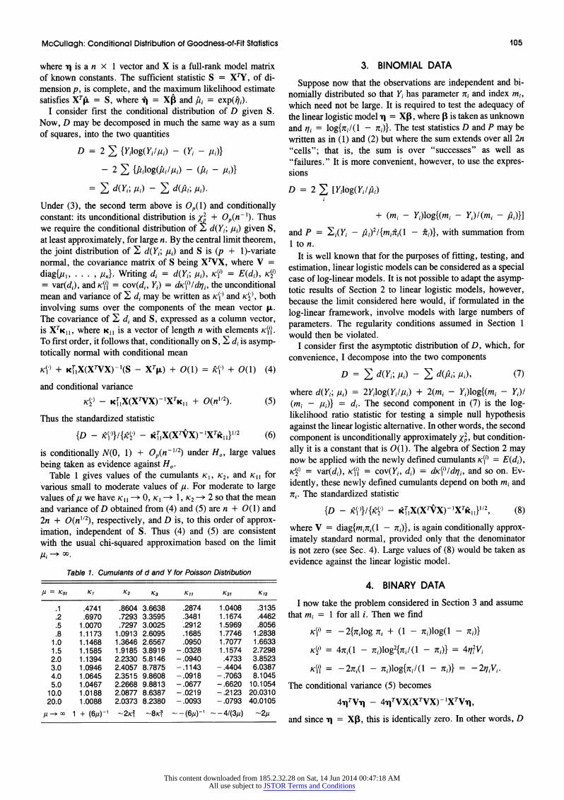
Table 1 gives values of the cumulants K1, K2, and K11 for various small to moderate values ofpu. For moderate to large

values ofutwe havecKum 0O, K1 1, K2 2 sothatthe mean and variance of D obtained from (4) and (5) are n + 0(1) and 2n + 0(n112), respectively, and D is, to this order of approximation, independent of S. Thus (4) and (5) are consistent with the usual chi-squared approximation based on the limit

Table 1. Cumulants of d and V for Poisson Distribution

U = K01 K 1 K2 K3 K11 K21 K 12

.1 .4741 .8604 3.6638 .2874 1 .0408 .3135

.2 .6970 .7293 3.3595 .3481 1.1674 .4462

.5 1.0070 .7297 3.0025 .2912 1.5969 .8056

.8 1.1173 1.0913 2.6095 .1685 1.7746 1.2838 1 .0 1 .1468 1 .3646 2.6567 .0950 1 .7077 1 .6633 1.5 1.1585 1 .9185 3.8919 - .0328 1.1574 2.7298 2.0 1 .1394 2.2330 5.8146 - .0940 .4733 3.8523 3.0 1.0946 2.4057 8.7875 - .1143 - .4404 6.0387 4.0 1 .0645 2.351 5 9.8608 - .0918 - .7063 8.1045 5.0 1 .0467 2.2668 9.8813 - .0677 - .6620 10.1054

10.0 1.0188 2.0877 8.6387 - .0219 - .2123 20.0310 20.0 1.0088 2.0373 8.2380 - .0093 -.0793 40.0105

8 X>o 1 + (6i)1 ' -2K2 -8K3 --(6i)1 ' -4I(38i) -28i

3. BINOMIAL DATA

Suppose now that the observations are independent and bi- nomially distributed so that Yi has parameter 7ri and index mi, which need not be large. It is required to test the adequacy of the linear logistic model q = X,, where , is taken as unknown and qi = log{7ri/(1 - 7ri)}. The test statistics D and P may be written as in (1) and (2) but where the sum extends over all 2n "cells"; that is, the sum is over "successes" as well as "failures." It is more convenient, however, to use the expres- sions

D = 2 > [Yilog(YIfiAi)

+ (mi - Yi)log{(mi - Yi)-(Mi _

Ai)j]

and P = 7 - ,2)2I{mi1(l - ft)}, with summation from 1 ton.

It is well known that for the purposes of fitting, testing, and estimation, linear logistic models can be considered as a special case of log-linear models. It is not possible to adapt the asymptotic results of Section 2 to linear logistic models, however, because the limit considered here would, if formulated in the log-linear framework, involve models with large numbers of parameters. The regularity conditions assumed in Section 1 would then be violated.

I consider first the asymptotic distribution of D, which, for convenience, I decompose into the two components

D = E d(Yi; pi) - E d( Ai; pi), (7)

where d(Yi; pi) = 2Yjlog(YIpju) + 2(mi - Yj)log{(mi - Yj)l (mi - pi)} = di. The second component in (7) is the log- likelihood ratio statistic for testing a simple null hypothesis against the linear logistic alternative. In other words, the second component is unconditionally approximately 4p, but conditionally it is a constant that is 0(1). The algebra of Section 2 may now be applied with the newly defined cumulants Kli) = E(dj), K2) = var(di), KV) = cov(Yi, di) = dKi')Idij, and so on. Ev- idently, these newly defined cumulants depend on both mi and 7ti. The standardized statistic

{D - K - KIcX(XTVX KXTk11}112, (8)

where V = diag{mizi( - 7ri)}, is again conditionally approximately standard normal, provided only that the denominator is not zero (see Sec. 4). Large values of (8) would be taken as evidence against the linear logistic model.

4. BINARY DATA

I now take the problem considered in Section 3 and assume that mi = 1 for all i. Then we find

K|i) = - 2{1zilog 1r, + (1 - 7ri)log(1 - 7ri)}

K') = 4( 1 - 7ri)log2{i / (1 - 7rg)} =74i V

K|i? = -27r1i( - 7rj)log{7rj/(1 - 7ri)} = - 2iVi.

The conditional variance (5) becomes

4n TVnq - 4n TVX(XTVX)'XTVnq,

and since vj = X,f, this is identically zero. In other words, D



106 Journal of the American Statistical Association, March 1986

is conditionally degenerate at the point -2 1 {f'ilog 7it + (1 - f1)log(1 - fj)} and contains no information regarding lack of fit of the linear logistic model (Williams 1983). A similar result applies as an approximation in the case of log-linear models if all of the means are small and the constant vector, 1, lies in the column space of X.

The preceding result shows that the total deviance is a function of the sufficient statistic and is therefore uninformative regarding lack of fit. The same is true of certain subtotals of the deviance in certain circumstances. Consider, for example, the statistic T = Ei cidi. A straightforward calculation shows that if the vector with elements ciqi lies in the column space of X, then T is conditionally degenerate; that is, T is a function of the sufficient statistic. For example, if X is the incidence matrix for a one-way layout with k blocks, the k subtotals of D, one for each block, are all conditionally degenerate.

Note that if we were to use the unconditional asymptotic distribution of D, this would be based on D - N(KI ), 4qTVq), where both of the asymptotic moments are functions of the unknown ,B. If we substitute ,B for , and use N(kl , 4iTvj) as an approximate reference distribution, we have identically that D - K, giving a tail probability of i independently of the data.

5. PEARSON'S STATISTIC

Using the summation convention, Pearson's statistic may be written as

P = (Yi - pi)(Yj - p0v,

where V` = diag{V-'(ji)} is the inverse covariance matrix of Y. A simple rearrangement leads to

P = (Yi - ji)(Yj - p)Vi)

- 2( - H)(Yj - /i)vij - (aii - pi)(/2j - fj)vii

The leading term is O(n) + Op(n"'2); the second term is Op(l) in view of the likelihood equations XT(Y - A) = 0; the third term is Op(l) marginally and 0(1) conditionally. Now write

vij = Vij + Vijk(tk - 1k) + 0(n'1)

- Vj + Vijkai(Y, - pi) + O(n1),

where Vijk = dVijldlk is zero unless i = j = k and A = {aj} = X(XWX) - 1XT is a symmetric n X n matrix. Thus, putting Zi = Yi - pi, we have

P = Z1ZjV'i + Viiala ZiZjZk + OpM().

Using the results of McCullagh (1984), we find the unconditional moments of P to be

E(P) = n + 0(1) (9)

and

var(P) = 2 m )

+ CT(V' - A)C + 0(nl2), (10)

where C1 is the ratio of the third to the second cumulant of Y1. The limit m, X+o in (10) gives the variance for the Poisson

case. A similar calculation for the covariance of Sj and P gives cov(Sj, P) = 0(1) rather than 0(n) as was the case for the likelihood-ratio statistic. In other words, to first order in n, P and S are independent, the conditional variance being obtained by inserting consistent estimates in (10).

In the case of single samples and one-way layouts, we have CT(V-1 - A)C = 0 so that var(P) = 2 1 (mi - 1)/mi. For Poisson observations this takes the value 2n, whereas for binary data, var(P) = 0 as might be expected. The quantity 2 E (mi - )/Imi is the leading term in the exact expression for var(P) derived by Haldane (1939). The error term is in fact 0(1) rather than 0(n '2).

More precise calculations, correct conditionally to second order, were given by McCullagh (1985) for arbitrary linear exponential-family models. Moreover, a simple algorithm was given for computing the first three conditional cumulants, and this can be applied routinely regardless of the complexity of the model matrix.

6. SECOND-ORDER CALCULATIONS

To improve on the first-order normal-theory approximations to the distributions of D and P, it is necessary to compute the conditional mean up to and including terms that are 0(1) and the conditional variance up to and including terms that are 0(n 12). A second-order correction involving the conditional skewness is applied using Edgeworth expansion. The formulas necessary for computing conditional cumulants were given by McCullagh (1984, sec. 6.1). Only the final result of such calculations is given here.

After rather lengthy calculations involving expansion of ,B - ,B up to the quadratic term in S - XTpu, the conditional expectation of D after linear and quadratic regression on S may be shown to be

E(D I S) = _

- 1TXTf X(XtX)l1 + 0(n') (11)

where ? = diag{K|I - KjKU31/Kg}. In the case of the Poisson distribution, K3= = = pi and the remaining cumulants are given in Table 1. For large ,i we have K|I - K- 2Vi so that the 0(1) correction in (11) tends to p, as is to be expected on the basis of the x2 approximation. The conditional variance ofD is var(D I S) = K- _KIX(XVX)'XTk11 + e + 0(n1), where e is a rather complicated expression involving X and the fourth-order cumulants K22, K13, and K4, as well as lower-order cumulants. In the simplest case, where the observations con- stitute a simple random sample, we find that

2x = (K22 - 2yK13 + y2K04)/V

+ (K 2 + K21K03 - 4yK12K03 + 2y2K2 )/V2,

where y = KII/V and, in general e 2p as ,u -m oo. For small degrees of freedom it is often advantageous to use the crude approximation

var(D | S) - (1 - pln){ik) - KljX(XVX)'XTIc11}, (12)

which has an error that is 0(1) as n -+oo. For fixed n, the error in (12) is 0(jc'l) as,~u -* o, and in this limit (11) and (12) both agree with the x2 approximation.



McCullagh: Conditional Distribution of Goodness-of-Fit Statistics 107

The conditional skewness of D may be written as

- 3A1 X(XTVX) -X A

+ 3kf1X(XTVX) - I(XTK X)(XTVX) T 'XTk1

YrYs YX XiXi13 + 0(1), (13)

where K21 is a vector of length n, K12 = diag{KV}, and the summation convention has been employed in the final term with i = 1, .. ., n and r, s, t = 1, ... , p. The vector y is given by (XWVX)- XTKI Iand Kg3 =E(Yi - pi)3. In applications in which the degrees of freedom are few, it is best to multiply (13) by the factor (1 - p/n), but this correction, though helpful, does not remove the 0(1) error term in (13).

The approximate significance level can now be obtained via the standardized statistic

Z = {D - E(D I S)}I{var(D I S)1'

using the Edgeworth expansion,

Pr(Z > z I S) = 1 - ?(z)

+ /(Z)(z2 - l)p3/6 + 0(n'1), (14)

where p3 is the standardized conditional skewness of Z obtained from (12) and (13), the latter formula with the correction factor 1 - pln.

7. A SIMPLE EXAMPLE

I consider a particularly simple example with independent and identically distributed Poisson observations with n = 3, p = 1. Such a small value of n is unfavorable for the limits considered here. The exact and approximate first three conditional cumulants of D are given in Table 2 for y = 1, 2, 5. These are to be compared with the cumulants of x2, which are 2, 4, 16. Bearing in mind that errors in the higher-order cumulants have a progressively decreasing effect on probability calculations, the approximations (11), (12), and (13) are sur- prisingly good. In the cases y = 1 and y = 2, D has support on 3 and 7 points, respectively. Thus no continuous approximation is likely to be adequate in these cases. For y = 5, D is supported on 27 points and the Edgeworth approximation seems to be preferable to the X2 approximation, at least in the region of most interest. In this particular case the limiting normal distribution for D is the same as that given by Morris (1975), because the conditional distribution, given y, is multinomial.

Table 2. Exact and Approximate Conditional Cumulants of D

Kl K2 K3

S Approx. Exact Approx. Exact Approx. Exact

= 1 2.66 2.58 2.71 3.29 4.43 3.35 y= 2 2.43 2.38 4.46 5.26 11.81 15.26

= 5 2.12 2.11 4.53 4.61 19.72 20.79 2

X2 2.0 4.0 16.0

Routine computation of the conditional cumulants (1 1), (12), and (13) is feasible for log-linear models. For linear logistic models, on the other hand, the computations are excessively heavy because the required cumulants depend both on the binomial probability and on the binomial index. The correspond- ing computations for Pearson's statistic given in Section 4 (and with greater accuracy in McCullagh 1985) are simpler, and routine computation is quite feasible. The results of a small- scale simulation study were reported by McCullagh (1985) for binary data with n = 50, p = 3, giving very sparse data. These simulation results confirm (9) and (10) but demonstrate the inadequacy of the normal approximation. The Edgeworth approximation with skewness correction gives better results, and I would expect the same to be true for the deviance statistic.

[Received February 1984. Revised July 1985.]

REFERENCES

Cochran, W. G. (1952), "The x2 Test of Goodness of Fit," Annals of Math- ematical Statistics, 23, 315-345.

Fienberg, S. E. (1979), "The Use of Chi-squared Statistics for Categorical Data Problems," Journal of the Royal Statistical Society, Ser. B, 41, 54- 64.

Haldane, J. B. S. (1939), "The Mean and Variance of x2 When Used as a Test of Homogeneity When Expectations Are Small," Biometrika, 31, 346-355.

Koehler, K. J., and Larntz, K. (1980), "An Empirical Investigation of Good- ness-of-Fit Statistics for Sparse Multinomials," Journal of the American Statistical Association, 75, 336-344.

McCullagh, P. (1984), "Tensor Notation and Cumulants of Polynomials," Biometrika, 71, 461-476.

(1985), "On the Asymptotic Distribution of Pearson's Statistic in Linear Exponential-Family Models," International Statistical Review, 53, 61-67.

Morris, C. L. (1975), "Central Limit Theorem for Multinomial Sums," The Annals of Statistics, 3, 165-188.

Williams, D. A. (1983), "The Use of the Deviance to Test the Goodness of Fit of a Logistic-Linear Model to Binary Data," GLIM Newsletter, 6, 60- 63.



Documents

The Conditional Distribution of Goodness-of-Fit Statistics for Discrete Data