THE USE OF SYNCHROPHASORS IN ANALYSING VOLTAGE

STABILITY AND DETECTING VOLTAGE COLLAPSE

Daniel James Gill

Murdoch University

©2016

Daniel Gill

ALL RIGHTS RESERVED

i

Abstract

Voltage stability is an incredibly important concept in power systems engineering. Voltages can

become unstable due to numerous reasons, but the most common reason is when the power

generation and load gap is too large. In the worst case scenario, voltage instability can cause voltage

collapse. Voltage collapse refers to the shutdown of a power system due to its inability to maintain

adequate bus voltage levels. When the event of voltage collapse begins in a power system, circuit

protection systems can become unstable and inoperable.

With the increasing complexity of the world’s power transmission networks, it is becoming more and

more difficult to analyse and maintain power system stability. This report looks at how four voltage

stability analysis methods, namely, the Voltage Change Index (VCI), the Voltage Collapse Proximity

Indicator (VCPI), Continuation Power Flow (CPF) and the New Voltage Stability Index (NVSI), can be

used in conjunction with synchrophasor measurements to analyse voltage stability and detect

voltage collapse.

Results show that the NVSI is the best analysis method as it can detect the voltage collapse point as

well as give a good indication of the voltage stability of a system. The VCPI can predict voltage

collapse under specific scenarios, but it does not effectively show how close the system is to voltage

collapse at a given operating point. The VCI was determined to not be useful in detecting voltage

collapse, but it does, however, provide a useful bus ranking system that lists each load bus from

‘strongest’ to ‘weakest’ which in turn provides an indication of relative bus voltage stability levels.

The CPF method was found to not work well with synchrophasor measurements.

ii

Acknowledgements

I would like to express my utmost gratitude to the Murdoch University Engineering Faculty who have

provided me the knowledge and pathway to accomplish my dream of becoming an Electrical Power

Engineer. In particular, I would like to thank my Thesis supervisor Dr. Gregory Crebbin.

Additionally, I would like to thank all my family and friends for moulding me into the person I am

today.

iii

Table of Contents

List of Tables ------------------------------------------------------------------------------------------- vi

List of Figures ------------------------------------------------------------------------------------------ vii

1.0 Introduction --------------------------------------------------------------------------------------- Page 1

1.1 Thesis Introduction ------------------------------------------------------------------------- Page 1

1.2 Thesis Objective ----------------------------------------------------------------------------- Page 1

1.3 Thesis Organisation ------------------------------------------------------------------------- Page 1

2.0 Review of Phasors, Synchrophasors & PMU’s -------------------------------------------- Page 3

2.1 Phasor Overview ----------------------------------------------------------------------------- Page 3

2.2 Synchrophasor and PMU Overview ----------------------------------------------------- Page 3

3.0 Stability Review ---------------------------------------------------------------------------------- Page 5

3.1 Power System Stability --------------------------------------------------------------------- Page 5

3.2 Rotor Angle Stability ------------------------------------------------------------------------ Page 6

3.3 Frequency Stability -------------------------------------------------------------------------- Page 6

3.4 Voltage Stability ------------------------------------------------------------------------------ Page 6

3.5 Voltage Collapse Overview ---------------------------------------------------------------- Page 8

3.6 Real Voltage Collapse Incidents ---------------------------------------------------------- Page 8

4.0 Discussion and Methods of Voltage Stability Analysis ---------------------------------- Page 10

4.1 Voltage Stability Analysis Introduction ------------------------------------------------- Page 10

4.2 Definition of Dynamic and Static Analysis --------------------------------------------- Page 10

4.3 Voltage Stability Indices ------------------------------------------------------------------- Page 11

4.4 PV and QV Curves --------------------------------------------------------------------------- Page 11

4.5 L-Index Sensitivity Methods -------------------------------------------------------------- Page 14

4.6 Modal Analysis Using the Reduced Jacobian Matrix -------------------------------- Page 15

4.7 The Voltage Stability Index (VSI) --------------------------------------------------------- Page 17

4.8 The Voltage Collapse Proximity Indicator (VCPI) ------------------------------------- Page 18

iv

4.9 Relative Voltage Change Method / Voltage Change Index (VCI) ---------------------- Page 19

4.10 Continuation Power Flow (CPF) -------------------------------------------------------------- Page 20

4.11 New Voltage Stability Index (NVSI) ---------------------------------------------------------- Page 21

5.0 Research Methodology ------------------------------------------------------------------------------- Page 22

5.1 Research Methodology Introduction --------------------------------------------------------- Page 22

5.2 MATPOWER Overview ---------------------------------------------------------------------------- Page 22

5.3 Test System ------------------------------------------------------------------------------------------ Page 24

5.4 Research Methodology Overview -------------------------------------------------------------- Page 27

5.5 Methodology for Computing VCI’s ------------------------------------------------------------- Page 28

5.6 Methodology for Continuation Power Flow Analysis ------------------------------------- Page 28

5.7 Methodology for Computing VCPI’s ----------------------------------------------------------- Page 28

5.8 Methodology for Computing NVSI’s ----------------------------------------------------------- Page 29

6.0 Results and Discussion --------------------------------------------------------------------------------- Page 30

6.1 Voltage Change Index Analysis Results -------------------------------------------------------- Page 30

6.2 Continuation Power Flow Analysis Results --------------------------------------------------- Page 32

6.3 Voltage Collapse Proximity Indicator Analysis Results ------------------------------------- Page 34

6.4 New Voltage Stability Indicator Results ------------------------------------------------------- Page 38

6.5 Comparison of Bus Rankings --------------------------------------------------------------------- Page 40

6.6 Further Discussion of Results -------------------------------------------------------------------- Page 41

7.0 Conclusion and Recommendations ---------------------------------------------------------------- Page 42

7.1 Conclusion ------------------------------------------------------------------------------------------- Page 42

7.2 Recommendations --------------------------------------------------------------------------------- Page 43

8.0 Works Cited ---------------------------------------------------------------------------------------------- Page 44

Appendices ---------------------------------------------------------------------------------------------------- Page 47

Appendix A - Phasor Data from Voltage Change Index Analysis ----------------------------- Page 47

Appendix B - Phasor Data from Voltage Collapse Proximity Indicator Analysis ---------- Page 51

v

Appendix C - MATLAB Code to Run the Continuation Power Flow Solver on Bus b for the IEEE 14-

Bus Case at Base Operating Condition ------------------------------------------------------ Page 66

Appendix D - MATLAB Code to Run the Continuation Power Flow Solver on Bus b for the IEEE 14-

Bus Case at Base Operating Condition with Line k Removed -------------------------- Page 66

Appendix E - MATLAB Code to Run a Newton Power Flow on the IEEE 14-Bus Case with Adjusted

Load Factor ----------------------------------------------------------------------------------------- Page 67

Appendix F - MATLAB Code to Run a Newton Power Flow on the IEEE 14-Bus Case with Adjusted

Reactive Load Factor ----------------------------------------------------------------------------- Page 67

Appendix G - MATLAB Code to Run a Newton Power Flow on the IEEE 14-Bus Case with Adjusted

Load Factor and Line k Removed -------------------------------------------------------------- Page 68

Appendix H - IEEE 14 Bus Case MATLAB M-File -------------------------------------------- Page 68

vi

List of Tables

Table 1: Critical Load Factors for Different Operating Conditions -------------------------------- Page 30

Table 2: Load Bus VCI’s for Different Operating Conditions ---------------------------------------- Page 30

Table 3: Load Bus VCI Rankings for Different Conditions -------------------------------------------- Page 31

Table 4: Load Bus VCI’s with Increasing Load Factor ------------------------------------------------- Page 31

Table 5: Voltage Collapse Point Data from CPF (Base Case) ---------------------------------------- Page 32

Table 6: Voltage Collapse Point Data from CPF (Line 4 Removed) -------------------------------- Page 32

Table 7: Voltage Collapse Point Data from CPF (Line 11 Removed) ------------------------------- Page 33

Table 8: Voltage Collapse Point Data from CPF (Line 17 Removed) ------------------------------- Page 33

Table 9: CPF Load Bus Rankings for Different Operating Conditions ------------------------------ Page 34

Table 10: Load Bus VCPI’s with Increasing Load Factor ----------------------------------------------- Page 35

Table 11: Load Bus VCPI Rankings for Different Load Factors -------------------------------------- Page 35

Table 12: Load Bus VCPI’s with Increasing Reactive Load Factor ---------------------------------- Page 36

Table 13: Load Bus VCPI Rankings for Different Reactive Load Factors -------------------------- Page 36

Table 14: Comparison of Pre and Post-Contingency Load Bus VCPI’s at

CLC (Line 4 Removed) ----------------------------------------------------------------------------------------- Page 37

Table 15: Load Bus VCPI Rankings for Pre and Post-Contingency Operating

Conditions at CLC (Line 4 Removed) ----------------------------------------------------------------------- Page 37

Table 16: Branch NVSI values with Increasing Load Factor ------------------------------------------- Page 38

Table 17: Branch NVSI Rankings for Increasing Load Factors ---------------------------------------- Page 39

vii

List of Figures

Figure 1: Reference Wave Produced by PMU ----------------------------------------------------- Page 3

Figure 2: Local Wave Measured by PMU ----------------------------------------------------------- Page 4

Figure 3: Typical PV Curve ------------------------------------------------------------------------------ Page 12

Figure 4: Typical QV Curve ------------------------------------------------------------------------------ Page 13

Figure 5: Equivalent 2 Bus System --------------------------------------------------------------------- Page 17

Figure 6: IEEE 14-Bus System Single Line Diagram ------------------------------------------------- Page 24

Figure 7: IEEE 14-Bus System Summary -------------------------------------------------------------- Pages 25-26

1

1.0 Introduction

1.1 Thesis Introduction

The worldwide energy demand is increasing. This is mostly due to industrialisation, globalisation,

and the economical bloom of upcoming markets like China and India. Over the next three decades,

world energy consumption is projected to increase by 56 percent. [1] To combat energy demand

growth, the integration of renewable energy and the promotion of distributed energy resources are

being looked at as possible solutions. On top of this, renewable power generation is predicted to

grow immensely as greenhouse gas emission regulations are implemented in numerous places

around the world. [2] As a result of the aforementioned points, power systems are beginning to

become more and more complex and stressed. [3] As a further result, it will become more difficult to

maintain stability in these more complex transmission networks.

Methods for measuring real-time voltage stability are currently being developed to be used in the

more complicated power transmission networks of the future. Synchrophasor measurement devices

[4] known as phasor measurement units (PMU’s) are a promising new endeavour which allow for the

real-time analysis of electrical power systems. These devices measure power system variables which

are time-synchronised to within a millisecond. [5] The use of PMU’s allows for the creation of large

scale protection schemes which are commonly referred to as “wide area measurement and

protection systems”. In the future, these devices are going to be used in conjunction with traditional

power system protection methods and will be instrumental in the protection and control of the

world’s increasingly complicated power transmission networks.

1.2 Thesis Objective

The objective of this thesis is to investigate the use of synchrophasors in analysing voltage stability

and detecting voltage collapse. To carry out the investigation, synchrophasor data will be retrieved

from a power system using MATPOWER. [6] The synchrophasor data will then be computed into

voltage stability indices in an attempt to give an indication of the voltage stability level of each load

bus in the power system as well as their proximity to voltage collapse. The synchrophasor data will

also be used to determine where system voltage collapse occurs. These results will be analysed and

conclusions will be drawn on their effectiveness.

The network being simulated is the IEEE 14-bus network. [7] It is assumed that voltage collapse

occurs, and thus, the network is deemed unstable, when the MATPOWER power flow algorithm does

not converge to a solution.

1.3 Thesis Organisation

This Thesis is organised into 7 main chapters. Chapter 1 (this chapter) is an introduction to the Thesis

which goes over the objective of the Thesis itself. Chapter 2 is a review of phasors, synchrophasors

and PMUs. Chapter 3 is a review of system stability. This chapter will discuss voltage stability, rotor

angle stability, frequency stability, voltage collapse, and a few real life voltage collapse incidents.

2

Chapter 4 is a discussion of methods of voltage stability analysis. This chapter goes over many

different voltage stability analysis methods and talks about their advantages and disadvantages.

Chapter 5 goes over the research methodology used in the simulations. Chapter 6 discusses the

results of the simulations. Chapter 7 is the conclusion to the Thesis which sums up its key findings.

3

2.0 Review of Phasors, Synchrophasors & PMU’s

2.1 Phasor Overview

A phasor is a complex number that represents a sinusoidal function that has a time-invariant

amplitude, angular frequency and initial phase.

A sinusoidal waveform is expressed by Equation 1 below;

𝑦(𝑡) = 𝐴𝑐𝑜𝑠(2𝜋𝑓𝑡 + 𝜃) = 𝐴𝑐𝑜𝑠(𝜔𝑡 + 𝜃)

Euler’s formula states that sinusoids can be represented as the sum of two complex functions;

𝐴𝑐𝑜𝑠(𝜔𝑡 + 𝜃) = 𝐴 ∗𝑒𝑖(𝜔𝑡+𝜃)+𝑒−𝑖(𝜔𝑡+𝜃)

2

Euler’s formula also states that sinusoids can be represented by the real part of one of the function;

𝐴𝑐𝑜𝑠(𝜔𝑡 + 𝜃) = 𝑅𝑒{𝐴 ∗ 𝑒𝑖(𝜔𝑡+𝜃)} = 𝑅𝑒{𝐴𝑒𝑖𝜃 ∗ 𝑒𝑖𝜔𝑡}

This can be represented in angle notation as

𝐴∠𝜃

Equations 3 and 4 are analytical representations of Equation 2. The term A represents the magnitude

of the sinusoidal wave, whilst the term 𝜃 represents the initial phase of the sinusoidal wave.

2.2 Synchrophasor and PMU Overview

The term synchrophasor is short for “synchronised phasor measurement”. Synchrophasor devices

allow for the real-time analysis of electrical power systems. Power system protection and control is

in turn improved as a result of the implementation of these devices.

At a fundamental level;

“Synchrophasors provide a means for comparing a phasor to an absolute time reference.” [8]

A device known as a phasor measurement unit (PMU) is what actually creates a synchrophasor. The

way a PMU works is outlined as follows;

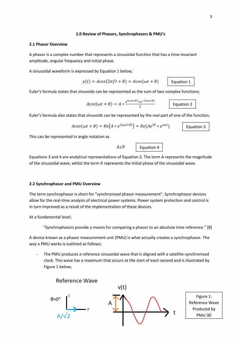
- The PMU produces a reference sinusoidal wave that is aligned with a satellite-synchronised

clock. This wave has a maximum that occurs at the start of each second and is illustrated by

Figure 1 below;

Equation 1

Equation 2

Equation 3

Equation 4

Figure 1:

Reference Wave

Produced by

PMU [8]

4

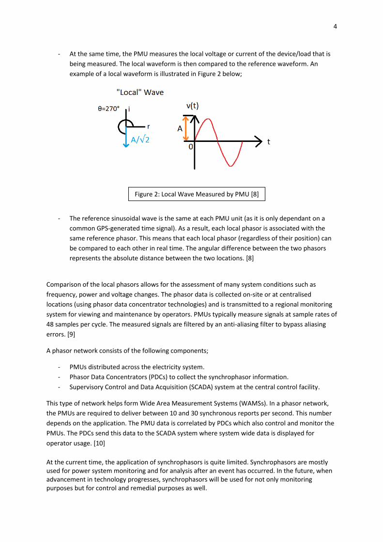
- At the same time, the PMU measures the local voltage or current of the device/load that is

being measured. The local waveform is then compared to the reference waveform. An

example of a local waveform is illustrated in Figure 2 below;

- The reference sinusoidal wave is the same at each PMU unit (as it is only dependant on a

common GPS-generated time signal). As a result, each local phasor is associated with the

same reference phasor. This means that each local phasor (regardless of their position) can

be compared to each other in real time. The angular difference between the two phasors

represents the absolute distance between the two locations. [8]

Comparison of the local phasors allows for the assessment of many system conditions such as

frequency, power and voltage changes. The phasor data is collected on-site or at centralised

locations (using phasor data concentrator technologies) and is transmitted to a regional monitoring

system for viewing and maintenance by operators. PMUs typically measure signals at sample rates of

48 samples per cycle. The measured signals are filtered by an anti-aliasing filter to bypass aliasing

errors. [9]

A phasor network consists of the following components;

- PMUs distributed across the electricity system.

- Phasor Data Concentrators (PDCs) to collect the synchrophasor information.

- Supervisory Control and Data Acquisition (SCADA) system at the central control facility.

This type of network helps form Wide Area Measurement Systems (WAMSs). In a phasor network,

the PMUs are required to deliver between 10 and 30 synchronous reports per second. This number

depends on the application. The PMU data is correlated by PDCs which also control and monitor the

PMUs. The PDCs send this data to the SCADA system where system wide data is displayed for

operator usage. [10]

At the current time, the application of synchrophasors is quite limited. Synchrophasors are mostly used for power system monitoring and for analysis after an event has occurred. In the future, when advancement in technology progresses, synchrophasors will be used for not only monitoring purposes but for control and remedial purposes as well.

Figure 2: Local Wave Measured by PMU [8]

5

3.0 Stability Review

3.1 Power System Stability

Since as early as the 1920s, power system stability has been viewed as an important problem for

secure system operation. [11] This importance is reinforced by the number of major blackouts

caused by power system instability over time.

Due to the evolution of power systems and the increasing growth and complexity of transmission

networks, there have emerged many different types of system instability. The three main types of

system instability, that is, those of which that provide the greatest concern to system stability, are

voltage stability, frequency stability and rotor angle stability. [12] The purpose of this section of the

Thesis is to review and clarify the different types of system stability so they can be understood

better.

The definition of power system stability is stated as follows: “Power system stability is the ability of

an electric power system, for a given initial operating condition, to regain a state of operating

equilibrium after being subjected to a physical disturbance, with most system variables bounded so

that practically the entire system remains intact.” [12]

Although the above definition is referring to the stability of a power system as a whole, the stability

of other components, such as a generator or group of generators is often of importance as well. For

example, the stability of a remote generator could become lost without the loss of the stability of

the main power system. [12] The same can be said about a load or group of loads.

Power systems exhibit a wide range of disturbances. In fact, disturbances to a power system may range from very small to significantly large. A small disturbance includes a load change in a power system, whilst a large disturbance may be a short circuit at a critical part of a power system. After being subjected to a disturbance, the stability of a power system depends on its initial operating condition and the nature of the disturbance itself. [12]

Prior to a disturbance, a power system is said to be operating in an equilibrium state. After a disturbance occurs but the system still remains stable, the power system will enter a new equilibrium state. A power system’s stability is governed by an equilibrium set. [12] This equilibrium set is a region that governs if a system will still remain stable or not after a disturbance is introduced due to the change in equilibrium state.

6

3.2 Rotor Angle Stability

The definition of rotor angle stability is as follows; “The ability of synchronous machines of an

interconnected power system to remain in synchronism after being subjected to a disturbance”. [12]

When a disturbance is introduced into a transmission network, generators can experience an

increase in angular motion. This causes these generators to become unsynchronised with other

generators in the system. When a generator is operating at steady-state, that is, when it is rotating

at a constant angular velocity, there exists an equilibrium between its input mechanical torque and

output electromagnetic torque. An introduced disturbance can throw out this equilibrium and this

causes the generator’s rotor to accelerate or deaccelerate. The ability of a generator to keep in

synchronisation with the other generators in a system after a disturbance refers to how well the

generator maintains the balance between its mechanical and electromagnetic torques.

As a synchronous machine’s rotor angle changes, its power output changes. The extent of this is determined by the machine’s power-angle relationship. Let us imagine that after a disturbance is introduced to a power system, one of the system’s generators speeds up, so that it is, in that instant, running faster than another generator. The faster generator will now have an angular position that is further ahead than the slower generator’s angular position. There is now an angular difference between the two generators. This angular difference causes a load shift from the slower machine to the faster machine. The extent of the load switch is governed by the faster generator’s power-angle relationship. In turn, the load shift then tends to decrease the angular separation between the generators. This is not always the case, though. If the disturbance causes the generators to have an angular difference that is beyond a certain limit, instability will result. This is because the system cannot absorb the energy corresponding to the rotor speed differences. [12]

3.3 Frequency Stability

Frequency stability is the ability of a power system to maintain steady frequency following a severe system upset resulting in a significant imbalance between generation and load. A transmission network’s frequency stability is determined by how well the system can restore the balance between generation and load. Frequency swings that can trip electrical devices such as relays are a type of frequency instability.

Large disturbances to a transmission network are the biggest causes of frequency instability. Conditions associated with frequency instability include inadequate system responses, poor control and protection equipment coordination and insufficient generation reserve. [12]

3.4 Voltage Stability

Voltage stability is “the ability of a power system to maintain steady voltages at all buses in the

system after being subjected to a disturbance from a given initial operating condition”. [12] It is the

power system’s ability to maintain equilibrium between load supply and load demand. Types of

voltage instability include the rise or fall of bus voltages, load loss in specific areas, and transmission

line tripping. Voltage instability can also cause generators to lose synchronism, and the loss of

generator synchronism can also cause drops in network bus voltages.

7

The two biggest causes of voltage stability are load restoration and reactive power flow.

Let us imagine that after a disturbance is introduced to a transmission network, the power

consumed by the loads drops significantly. The load power can be restored by various means

including motor slip adjustment, distribution voltage regulators, tap-changing transformers and

thermostats. [12] Restoring the load power causes a large increase in reactive power consumption,

and this in turn causes voltage reduction.

Reactive power is a problem because of the fact that a large voltage drop occurs when active and

reactive power flows through inductive reactances in a transmission network. Reactive power flow

can increase due to certain types of disturbances on the transmission network. To keep up with this

demand, the generators must put out more power. Doing this will increase the magnitude of the

voltage drops across the transmission network as dictated by Ohm’s Law. When reactive power

demand is increased to a level where the power resources can no longer generate this level of

reactive power, voltage stability can no longer be provided and voltage collapse occurs.

Voltage stability can be classified into the following types:

- Large-disturbance voltage stability;

- Small-disturbance voltage stability.

These types of stability can be further classified as being either short-term or long-term.

Large-disturbance voltage stability refers to how well a transmission system can maintain steady

voltages after large system disturbances occur. Large-system disturbances include system faults, loss

of generation and circuit contingencies. [12] The characteristics of the system, as well as the control

and protection schemes present in the transmission network, determine large-disturbance voltage

stability.

Small-disturbance voltage stability refers to how well a transmission system can maintain steady

voltages after small system disturbances occur. Small-system disturbances include incremental

changes in system load. [12] Load characteristics and capability of continuous and discrete controls

influence small-disturbance voltage stability.

Short-term voltage stability involves “the dynamics of fast acting load components such as induction

motors, electronically controlled loads, and HVDC converters”. [12] This type of voltage stability

involves time periods that are in the order of seconds long. Long-term voltage stability involves

“slower acting equipment such as tap-changing transformers, thermostatically controlled loads, and

generator current limiters.” [12] This type of voltage stability involves time periods that are in the

order of minutes long. When long-term instability occurs, the elements involved will try to restabilise

the system. If these elements are driven to a point where they are running outside of their operating

limits, further instability will result.

8

3.5 Voltage Collapse Overview

The term voltage collapse refers to the shutdown of a power system due to the inability to maintain

adequate voltage levels. [13] When operation is normal, voltage levels are maintained at steady

levels. When a change in load demand occurs, reactive resources are adjusted to compensate for

this. When a large disturbance causes a decrease in voltage levels across the transmission network,

corrective action is in place to restore the voltage levels within a matter of minutes. Examples of

such corrective action include generator excitation systems, automatic or manual tapping of

transformers, and the switching of static compensation devices. [13]

When the transmission system is subjected to an extreme disturbance, these corrective actions may

temporarily restore voltage levels before they fall again to very low levels. As voltage continues to

fall to even lower levels, circuit protection systems begin to become unstable and inoperable. This is

due to the direct effect of the low voltages, or angular instability which can occur at low voltages. In

today’s transmission systems, protective devices observe these abnormal conditions and trigger

circuit breakers to open and de-energise the transmission system itself. This whole process can occur

in a matter of seconds to minutes. [13]

The following are factors that largely contribute to voltage instability/collapse: [13]

- Generation and load gap is too large

- Under-load tap changer action during low voltage conditions

- Unfavourable load characteristics

- Poor coordination between various control and protective systems

- Excessive use of shunt capacitor compensation

3.6 Real Voltage Collapse Incidents

Real voltage collapse incidents can help to give greater insight into the importance of voltage

stability and the reasons why it occurs.

In July of 1979, a BC Hydro power plant in Canada had a voltage collapse incident. This was caused

when a 100MW load was lost along a tie-line connection. This caused an increase in active power

transfer. As a result of this, voltages along the tie-line began to fall. The connected load then

decreased due to this fall of voltage. The tie-line transmission was increased even more due to the

fact that active power production was not reduced. After about one minute, the voltage in the

middle of the line had fallen to approximately 0.5pu. The tie-line was tripped due to overcurrent at

one end and due to a distance relay at the other. [14]

On August 4th 1982, numerous blackouts occurred in Belgium. [14] This collapse was due to

transmission capacity problems with the associated power plants. In this instance, only a few plants

were being used for generation due to the fact that there were only low loads in the area. As a

result, the plants were operating close to their operating limits. The generator tripped due to a lack

of reactive power and multiple generators were field current limited. Eventually, more generators

started tripping. As a result of this, voltage levels in the transmission network dropped drastically

and eventually the system was de-energised by its relays. Thus, voltage collapse had occurred.

9

On July 23 1987, a voltage collapse incident occurred in Tokyo. This day was characterised by

abnormally hot weather. After around midday, the load pick-up rate was approximately 1% per

minute. [14] To combat this increase in load, all available shunt capacitors were used in the system.

Eventually, voltage levels fell to approximately 0.75pu and as a result the transmission network was

de-energised by protective relays. The cause of the rapid load pick-up rate was thought to have been

due to unfavourable load characteristics of air conditioners. [14]

On August 28th 2003, a transformer was taken out of service because it contained a wrong Buchholz

alarm. Whilst the transformer was being taken out of service, an incorrect relay setting tripped an

adjacent cable section. This led to the power outage of a limited area. [15]

On September 28th 2003, a huge blackout occurred in Italy. This blackout was initiated by a line trip

in Switzerland. Unfortunately, the line could not be reconnected as the phase angle difference was

too large. Approximately 20 minutes later, a second line tripped. This caused a fast trip-sequence

that caused all lines interconnecting to Italy to overload. As a result of the trip sequence, the

frequency in Italy ramped down by 2.5Hz for 2.5 minutes. This caused the whole country to lose

power. [15]

10

4.0 Discussion and Methods of Voltage Stability Analysis

4.1 Voltage Stability Analysis Introduction

In general, the analysis of voltage stability in a transmission system should look at the following key

points: [16]

- How close is the system to voltage instability or collapse?

- When does the voltage instability occur?

- Where are the vulnerable spots of the system?

- What are the key contributing factors?

- What areas are involved?

Voltage instability is a dynamic phenomenon that can last from seconds to multiple minutes. It is

closely related to the maximum loadability of a transmission system. Because of this, developing

methods of determining maximum loadability has always been a strong area of interest, and it is

becoming an increasingly more important issue. The last few decades have seen the development of

numerous voltage stability analysis methods.

This chapter will review many different methods of voltage stability analysis and look at the benefits

and problems associated with them. Before doing that it will briefly outline the difference between

dynamic and static analysis.

4.2 Definition of Dynamic and Static Analysis

In recent years there has been a lot of industry attention given to finding and strengthening methods

of voltage stability analysis. Voltage stability analysis is now included as part of routine planning and

operation studies by many utilities. [17]

There are two main types of voltage stability analysis methods;

- Dynamic analysis

- Static analysis

Dynamic analysis uses time-domain simulations to solve nonlinear system differential/algebraic

equations. [17] This method is more accurate in replicating the time responses of the power system.

This method, however, does have its problems. It is very computationally expensive and time

consuming, and does not readily provide information regarding the sensitivity or degree of

instability. [17]

Static analysis only involves the solutions of algebraic equations. It is much more computationally

efficient. This method is the most ideal for studies where voltage stability limits need to be

determined. [17]

11

4.3 Voltage Stability Indices

Voltage stability indices (VSIs) provide a scalar measurement that shows how far a power system’s

operating point is from the voltage stability limit. These measurements are needed due to the fact

that voltage magnitudes, by themselves, are not useful in doing this. VSIs can thus be used to

indicate when a power system is approaching voltage collapse.

Numerous VSIs have been developed to determine power system voltage stability margins. [18]

There are some VSIs which are power flow analysis based. These include Jacobian matrix singular

values and load flow feasibility. These VSIs are generally not suitable for online use because of the

fact that they “depend on traditional state estimators which usually take minutes to update the

snapshot of the power systems”. [18] Other VSIs are based on phasor measurements. Different

types of VSIs will be discussed in this chapter.

Phasor measurement based VSIs only use voltage and current phasor measurements to evaluate and

monitor system stability. Some phasor measurement based VSI algorithms require an input of

Thevenin equivalent parameters in order to be computed, whereas some can just use the phasor

measurements directly.

4.4 PV and QV Curves

The relationships between transmitted power, receiving end voltage, and reactive power injection

are of large importance in power system analysis. PV and QV curves are traditional forms of

displaying these relationships. To create PV curves, analysis processes are used which involve using a

series of power flow solutions for increasing transfers of MW and the monitoring of system voltages

that result. [19] This analysis method is good for modelling increasing loads in a power transmission

system. This analysis requires specific buses to be selected for monitoring and PV curves are plotted

for each of these buses. [19]

12

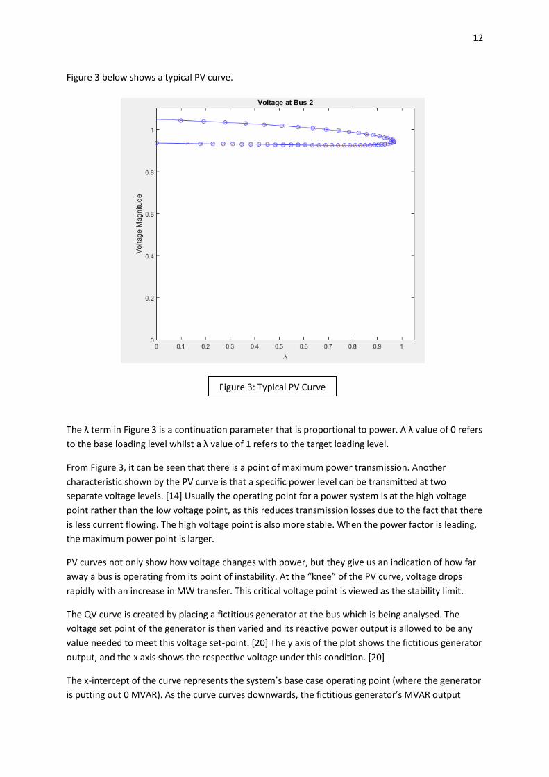
Figure 3 below shows a typical PV curve.

The λ term in Figure 3 is a continuation parameter that is proportional to power. A λ value of 0 refers

to the base loading level whilst a λ value of 1 refers to the target loading level.

From Figure 3, it can be seen that there is a point of maximum power transmission. Another

characteristic shown by the PV curve is that a specific power level can be transmitted at two

separate voltage levels. [14] Usually the operating point for a power system is at the high voltage

point rather than the low voltage point, as this reduces transmission losses due to the fact that there

is less current flowing. The high voltage point is also more stable. When the power factor is leading,

the maximum power point is larger.

PV curves not only show how voltage changes with power, but they give us an indication of how far

away a bus is operating from its point of instability. At the “knee” of the PV curve, voltage drops

rapidly with an increase in MW transfer. This critical voltage point is viewed as the stability limit.

The QV curve is created by placing a fictitious generator at the bus which is being analysed. The

voltage set point of the generator is then varied and its reactive power output is allowed to be any

value needed to meet this voltage set-point. [20] The y axis of the plot shows the fictitious generator

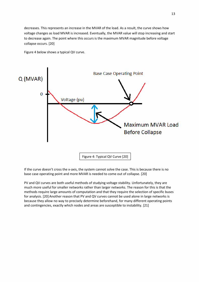
output, and the x axis shows the respective voltage under this condition. [20]

The x-intercept of the curve represents the system’s base case operating point (where the generator

is putting out 0 MVAR). As the curve curves downwards, the fictitious generator’s MVAR output

Figure 3: Typical PV Curve

13

decreases. This represents an increase in the MVAR of the load. As a result, the curve shows how

voltage changes as load MVAR is increased. Eventually, the MVAR value will stop increasing and start

to decrease again. The point where this occurs is the maximum MVAR magnitude before voltage

collapse occurs. [20]

Figure 4 below shows a typical QV curve.

If the curve doesn’t cross the x-axis, the system cannot solve the case. This is because there is no base case operating point and more MVAR is needed to come out of collapse. [20] PV and QV curves are both useful methods of studying voltage stability. Unfortunately, they are much more useful for smaller networks rather than larger networks. The reason for this is that the methods require large amounts of computation and that they require the selection of specific buses for analysis. [20] Another reason that PV and QV curves cannot be used alone in large networks is because they allow no way to precisely determine beforehand, for many different operating points and contingencies, exactly which nodes and areas are susceptible to instability. [21]

Figure 4: Typical QV Curve [20]

14

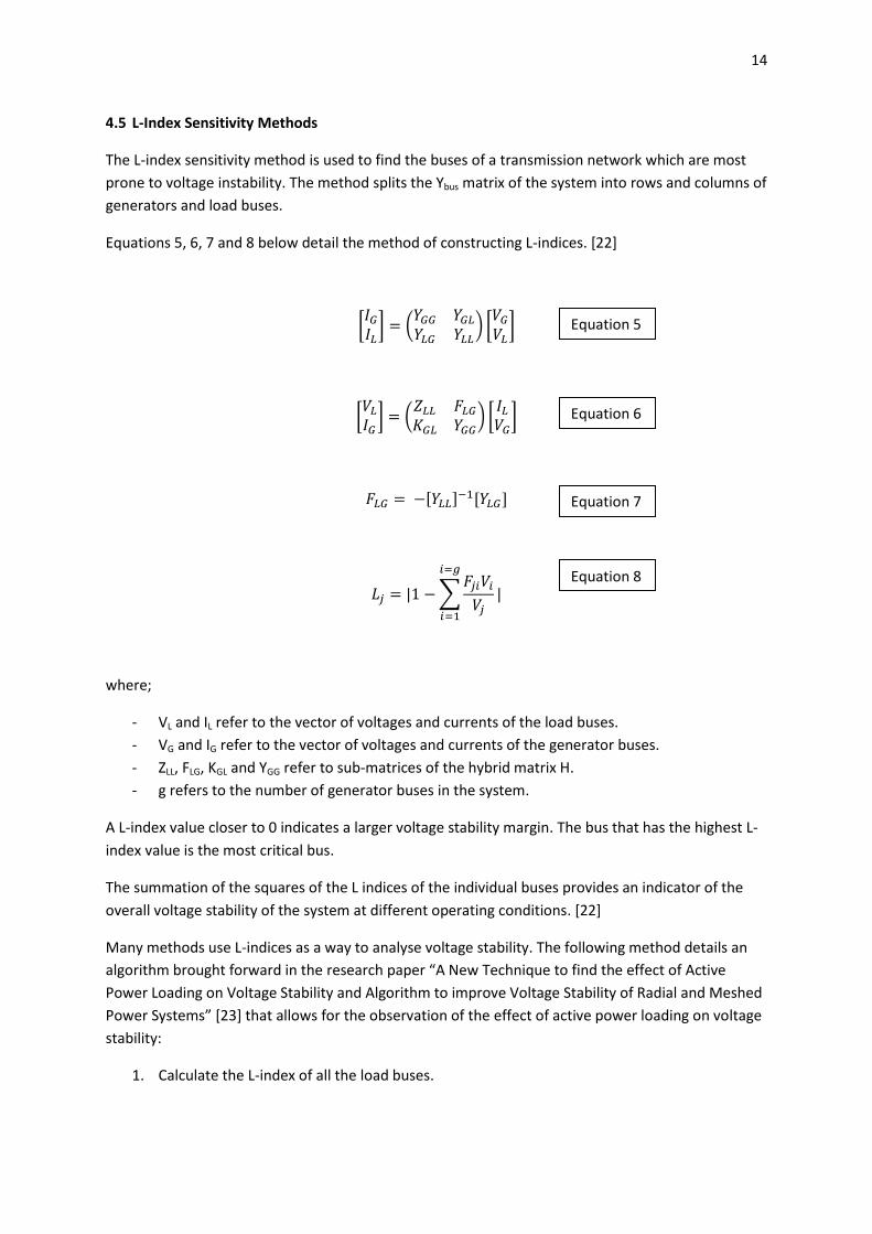
4.5 L-Index Sensitivity Methods

The L-index sensitivity method is used to find the buses of a transmission network which are most

prone to voltage instability. The method splits the Ybus matrix of the system into rows and columns of

generators and load buses.

Equations 5, 6, 7 and 8 below detail the method of constructing L-indices. [22]

[𝐼𝐺

𝐼𝐿] = (

𝑌𝐺𝐺 𝑌𝐺𝐿

𝑌𝐿𝐺 𝑌𝐿𝐿) [

𝑉𝐺

𝑉𝐿]

[𝑉𝐿

𝐼𝐺] = (

𝑍𝐿𝐿 𝐹𝐿𝐺

𝐾𝐺𝐿 𝑌𝐺𝐺) [

𝐼𝐿

𝑉𝐺]

𝐹𝐿𝐺 = −[𝑌𝐿𝐿]−1[𝑌𝐿𝐺]

𝐿𝑗 = |1 − ∑𝐹𝑗𝑖𝑉𝑖

𝑉𝑗

𝑖=𝑔

𝑖=1

|

where;

- VL and IL refer to the vector of voltages and currents of the load buses.

- VG and IG refer to the vector of voltages and currents of the generator buses.

- ZLL, FLG, KGL and YGG refer to sub-matrices of the hybrid matrix H.

- g refers to the number of generator buses in the system.

A L-index value closer to 0 indicates a larger voltage stability margin. The bus that has the highest L-

index value is the most critical bus.

The summation of the squares of the L indices of the individual buses provides an indicator of the

overall voltage stability of the system at different operating conditions. [22]

Many methods use L-indices as a way to analyse voltage stability. The following method details an

algorithm brought forward in the research paper “A New Technique to find the effect of Active

Power Loading on Voltage Stability and Algorithm to improve Voltage Stability of Radial and Meshed

Power Systems” [23] that allows for the observation of the effect of active power loading on voltage

stability:

1. Calculate the L-index of all the load buses.

Equation 5

Equation 6

Equation 7

Equation 8

15

2. Calculate the Active Power L-index Sensitivity Matrix. [22] The method for doing this is not

detailed in this report.

3. Choose a limit for the L-index and call it Llimit.

4. Find the buses which have an L-index that is more than Llimit and let these buses be [B2 B5 B7].

5. Find ΔLred. ΔLred is taken for the buses which are exceeding Llimit. ΔLred = [ΔL2 ΔL5 ΔL7].

6. Find the reduced Active Power L-index Sensitivity Matrix (Lrp). This matrix relates ΔLrp and

ΔPred where ΔPred = [P2 P5 P7].

7. ΔLred = ΔLrp* ΔPred.

8. Take ∑ΔPred as the objective function.

9. Perform optimisation, minimising objective function satisfying the constraints ΔLmin ≤ ΔL ≤

ΔLmax where:

ΔLmin = ΔLactual – ΔLlimit and ΔLmax = [1] - Lactual

10. The amount of reactive power to be reduced at each bus for increasing the voltage stability

is now shown.

This method has been applied to several Indian rural distribution networks which demonstrated

applicability of the proposed approach. [23] A disadvantage to this approach is that it is very

computationally intensive.

4.6 Modal Analysis Using the Reduced Jacobian Matrix

Modal analysis is an analysis technique that is used to determine the most vulnerable areas of a

power network in terms of voltage instability. It is used when selecting the best locations for

installing reactive compensation equipment as well as for determining the most effective actions to

take when voltage conditions need to be alleviated. [24] Modal analysis has the ability to predict

voltage collapse in transmission networks. [25]

Modal analysis in transmission networks involves the computation of the smallest Eigen values and

eigenvectors of the power system’s reduced Jacobian matrix [27] obtained from the load flow

solution [26]. [25] The computed Eigen values are associated with voltage and reactive power

variation and can be used to provide a relative measure of voltage stability. [25] The weakest nodes

and buses in the system can also be found by analysing the participation factor associated with these

Eigen values. [25]

The issue with modal analysis, however, is that its results are only valid for incremental changes; it

has a powerful ability to provide information on system trends but lacks the ability to estimate the

actual numerical values of system variables following changes. [24]

The research paper “Voltage Stability Evaluation Using Modal Analysis” by Telang and Khampariya

[21] outlines a method for evaluating voltage stability using modal analysis as quoted below:

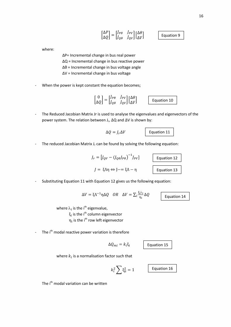
- The injected power in buses can be represented by using the following linear system model

(derived from Newton Raphson power flow);

16

[∆𝑃∆𝑄

] = [𝐽𝑃𝜃 𝐽𝑃𝑉

𝐽𝑄𝜃 𝐽𝑄𝑉] [

∆𝜃∆𝑉

]

where:

∆P= Incremental change in bus real power

∆Q = Incremental change in bus reactive power

∆θ = Incremental change in bus voltage angle

∆V = Incremental change in bus voltage

- When the power is kept constant the equation becomes;

[0

∆𝑄] = [

𝐽𝑃𝜃 𝐽𝑃𝑉

𝐽𝑄𝜃 𝐽𝑄𝑉] [

∆𝜃∆𝑉

]

- The Reduced Jacobian Matrix Jr is used to analyse the eigenvalues and eigenvectors of the

power system. The relation between Jr, ∆Q and ∆V is shown by:

∆𝑄 = 𝐽𝑟∆𝑉

- The reduced Jacobian Matrix Jr can be found by solving the following equation:

𝐽𝑟 = [𝐽𝑄𝑉 − (𝐽𝑄𝜃𝐽𝑃𝜃)−1

𝐽𝑃𝑉]

𝐽 = ξΛη ⇔ J−= ξΛ − η

- Substituting Equation 11 with Equation 12 gives us the following equation:

∆𝑉 = ξΛ−1η∆𝑄 𝑂𝑅 ∆𝑉 = ∑ξii

ηi𝑖 ∆𝑄

where i is the ith eigenvalue,

ξi is the ith column eigenvector

ηi is the ith row left eigenvector

- The ith modal reactive power variation is therefore

∆𝑄𝑚𝑖 = 𝑘𝑖ξi

where 𝑘𝑖 is a normalisation factor such that

𝑘𝑖2 ∑ ξji

2 = 1

The ith modal variation can be written

Equation 9

Equation 10

Equation 11

Equation 12

Equation 13

Equation 14

Equation 15

Equation 16

17

∆𝑉𝑚𝑖 =1

i∆𝑄𝑚𝑖

- The voltage stability can be defined by the mode of the eigenvalues. The minimum

eigenvalue in a power system is the global VSI value. A larger eigenvalue will give smaller

changes in the voltages when small disturbances happen. A system is stable when the

eigenvalue of Jr is positive. The limit is reached when one of the eigenvalues reach zero. If

one of the eigenvalues is negative the system is unstable. [21]

- The left and right eigenvectors corresponding to the critical modes in the system can provide

information concerning the mechanism of voltage stability. [21] The bus participation of the

bus can be defined as:

𝑃𝑘𝑖 = ξkiηki

- Bus participation factors show the voltage stability of nodes in the power system. Bus

participation factors are shown in a matrix form called the participation matrix. The row of

the matrix indicates the bus number and the matrix column indicates the system mode. The

bigger the value of the bus participation factor indicates the more affecting the bus is to the

power system. [21]

4.7 The Voltage Stability Index (VSI)

The Voltage Stability Index (VSI) is an index that is based on direct measurements (such as bus

voltages and sensitivity factors). It is a simpler approach which is currently being used in the industry

as a tool in voltage stability analysis. The VSI looked at here was introduced in the research paper

“Synchrophasor-Based Real-Time Voltage Stability Index” [18] by Yanfeng Gong and Noel Schulz of

Mississippi State University.

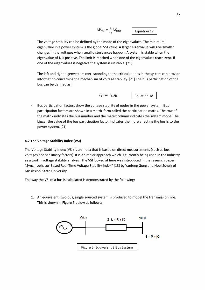
The way the VSI of a bus is calculated is demonstrated by the following:

1. An equivalent, two-bus, single sourced system is produced to model the transmission line.

This is shown in Figure 5 below as follows:

Equation 17

Equation 18

Figure 5: Equivalent 2 Bus System

18

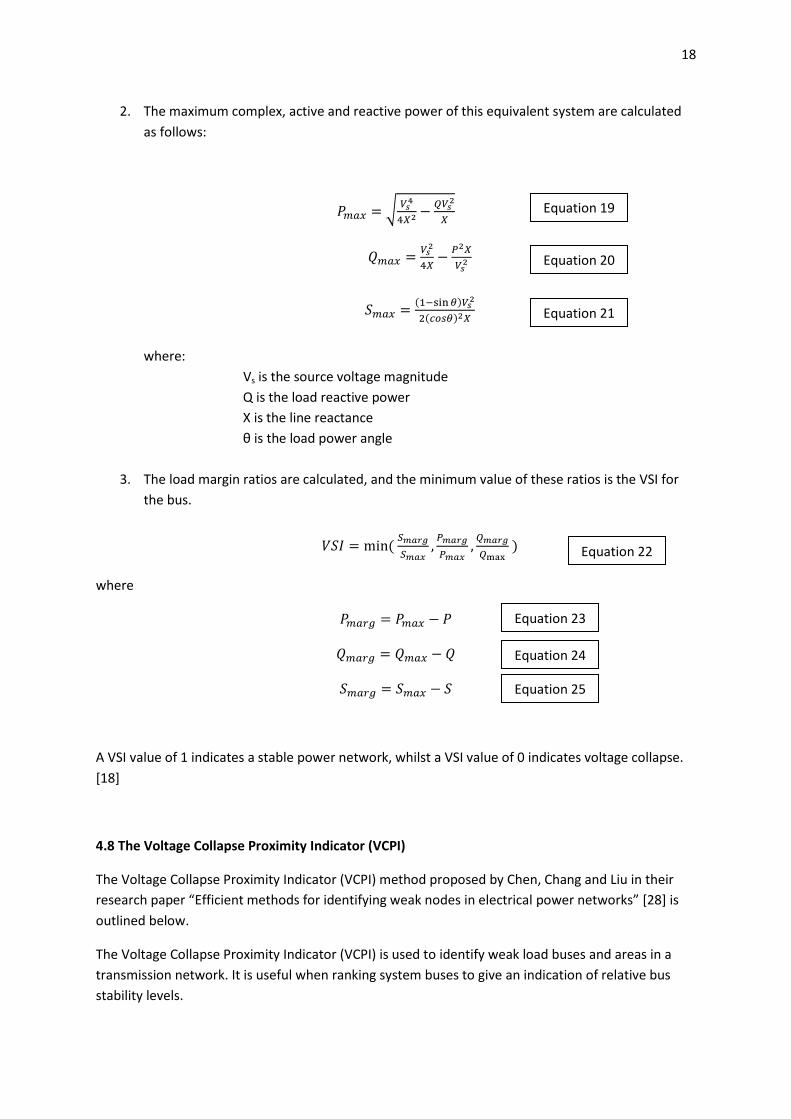
2. The maximum complex, active and reactive power of this equivalent system are calculated

as follows:

𝑃𝑚𝑎𝑥 = √ 𝑉𝑠4

4𝑋2 −𝑄𝑉𝑠

2

𝑋

𝑄𝑚𝑎𝑥 =𝑉𝑠

2

4𝑋−

𝑃2𝑋

𝑉𝑠2

𝑆𝑚𝑎𝑥 =(1−sin 𝜃)𝑉𝑠

2

2(𝑐𝑜𝑠𝜃)2𝑋

where:

Vs is the source voltage magnitude

Q is the load reactive power

X is the line reactance

θ is the load power angle

3. The load margin ratios are calculated, and the minimum value of these ratios is the VSI for

the bus.

𝑉𝑆𝐼 = min ( 𝑆𝑚𝑎𝑟𝑔

𝑆𝑚𝑎𝑥,

𝑃𝑚𝑎𝑟𝑔

𝑃𝑚𝑎𝑥,

𝑄𝑚𝑎𝑟𝑔

𝑄max )

where

𝑃𝑚𝑎𝑟𝑔 = 𝑃𝑚𝑎𝑥 − 𝑃

𝑄𝑚𝑎𝑟𝑔 = 𝑄𝑚𝑎𝑥 − 𝑄

𝑆𝑚𝑎𝑟𝑔 = 𝑆𝑚𝑎𝑥 − 𝑆

A VSI value of 1 indicates a stable power network, whilst a VSI value of 0 indicates voltage collapse.

[18]

4.8 The Voltage Collapse Proximity Indicator (VCPI)

The Voltage Collapse Proximity Indicator (VCPI) method proposed by Chen, Chang and Liu in their

research paper “Efficient methods for identifying weak nodes in electrical power networks” [28] is

outlined below.

The Voltage Collapse Proximity Indicator (VCPI) is used to identify weak load buses and areas in a

transmission network. It is useful when ranking system buses to give an indication of relative bus

stability levels.

Equation 19

Equation 20

Equation 21

Equation 22

Equation 23

Equation 24

Equation 25

19

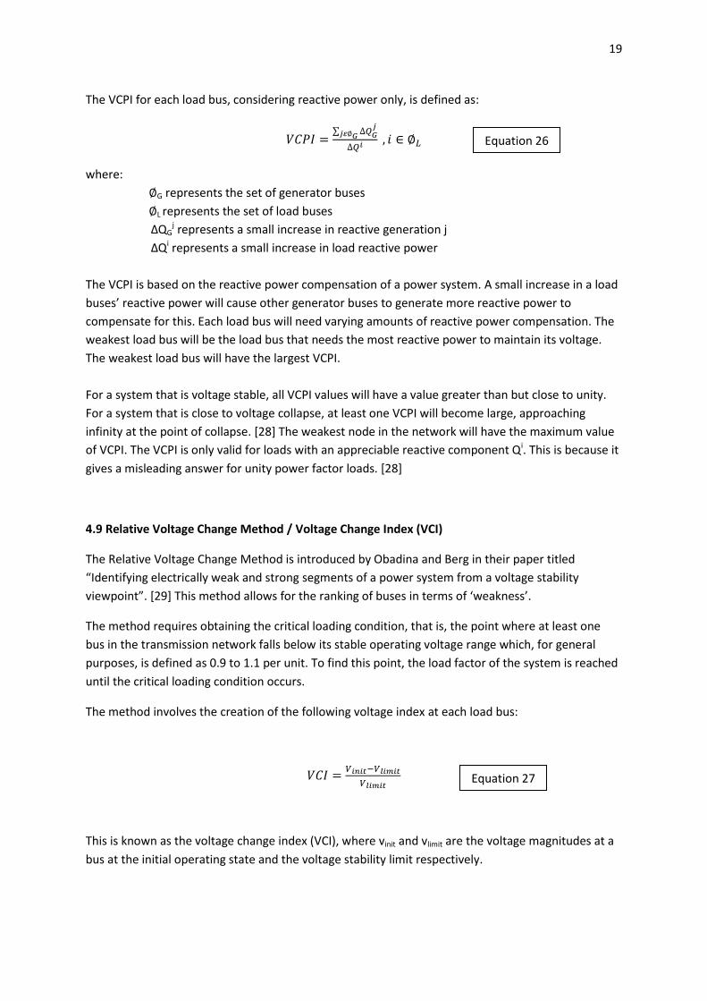
The VCPI for each load bus, considering reactive power only, is defined as:

𝑉𝐶𝑃𝐼 =∑ ∆𝑄𝐺

𝑗𝑗𝜀∅𝐺

∆𝑄𝑖 , 𝑖 ∈ ∅𝐿

where:

∅G represents the set of generator buses

∅L represents the set of load buses

∆QGj represents a small increase in reactive generation j

∆Qi represents a small increase in load reactive power

The VCPI is based on the reactive power compensation of a power system. A small increase in a load

buses’ reactive power will cause other generator buses to generate more reactive power to

compensate for this. Each load bus will need varying amounts of reactive power compensation. The

weakest load bus will be the load bus that needs the most reactive power to maintain its voltage.

The weakest load bus will have the largest VCPI.

For a system that is voltage stable, all VCPI values will have a value greater than but close to unity.

For a system that is close to voltage collapse, at least one VCPI will become large, approaching

infinity at the point of collapse. [28] The weakest node in the network will have the maximum value

of VCPI. The VCPI is only valid for loads with an appreciable reactive component Qi. This is because it

gives a misleading answer for unity power factor loads. [28]

4.9 Relative Voltage Change Method / Voltage Change Index (VCI)

The Relative Voltage Change Method is introduced by Obadina and Berg in their paper titled

“Identifying electrically weak and strong segments of a power system from a voltage stability

viewpoint”. [29] This method allows for the ranking of buses in terms of ‘weakness’.

The method requires obtaining the critical loading condition, that is, the point where at least one

bus in the transmission network falls below its stable operating voltage range which, for general

purposes, is defined as 0.9 to 1.1 per unit. To find this point, the load factor of the system is reached

until the critical loading condition occurs.

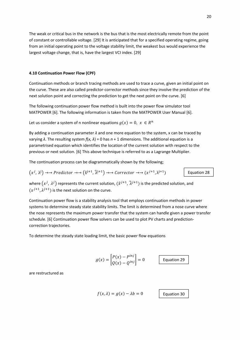
The method involves the creation of the following voltage index at each load bus:

𝑉𝐶𝐼 =𝑉𝑖𝑛𝑖𝑡−𝑉𝑙𝑖𝑚𝑖𝑡

𝑉𝑙𝑖𝑚𝑖𝑡

This is known as the voltage change index (VCI), where vinit and vlimit are the voltage magnitudes at a

bus at the initial operating state and the voltage stability limit respectively.

Equation 26

Equation 27

20

The weak or critical bus in the network is the bus that is the most electrically remote from the point

of constant or controllable voltage. [29] It is anticipated that for a specified operating regime, going

from an initial operating point to the voltage stability limit, the weakest bus would experience the

largest voltage change, that is, have the largest VCI index. [29]

4.10 Continuation Power Flow (CPF)

Continuation methods or branch tracing methods are used to trace a curve, given an initial point on

the curve. These are also called predictor-corrector methods since they involve the prediction of the

next solution point and correcting the prediction to get the next point on the curve. [6]

The following continuation power flow method is built into the power flow simulator tool

MATPOWER [6]. The following information is taken from the MATPOWER User Manual [6].

Let us consider a system of n nonlinear equations 𝑔(𝑥) = 0, 𝑥 ∈ 𝑅𝑛

By adding a continuation parameter λ and one more equation to the system, x can be traced by

varying λ. The resulting system f(x, λ) = 0 has n + 1 dimensions. The additional equation is a

parametrised equation which identifies the location of the current solution with respect to the

previous or next solution. [6] This above technique is referred to as a Lagrange Multiplier.

The continuation process can be diagrammatically shown by the following;

(𝑥𝑗, λj) →→ 𝑃𝑟𝑒𝑑𝑖𝑐𝑡𝑜𝑟 →→ (x̂j+1, λ̂j+1) →→ 𝐶𝑜𝑟𝑟𝑒𝑐𝑡𝑜𝑟 →→ (𝑥𝑗+1, λj+1)

where (𝑥𝑗 , 𝜆𝑗) represents the current solution, (𝑥𝑗+1, �̂�𝑗+1) is the predicted solution, and

(𝑥𝑗+1, 𝜆𝑗+1) is the next solution on the curve.

Continuation power flow is a stability analysis tool that employs continuation methods in power

systems to determine steady state stability limits. The limit is determined from a nose curve where

the nose represents the maximum power transfer that the system can handle given a power transfer

schedule. [6] Continuation power flow solvers can be used to plot PV charts and prediction-

correction trajectories.

To determine the steady state loading limit, the basic power flow equations

𝑔(𝑥) = [𝑃(𝑥) − 𝑃𝑖𝑛𝑗

𝑄(𝑥) − 𝑄𝑖𝑛𝑗] = 0

are restructured as

𝑓(𝑥, 𝜆) = 𝑔(𝑥) − 𝜆𝑏 = 0

Equation 29

Equation 30

Equation 28

21

where 𝑥 ≡ (θ, Vm) and b is a vector of power transfer given by

𝑏 = [𝑃𝑡𝑎𝑟𝑔𝑒𝑡

𝑖𝑛𝑗− 𝑃𝑏𝑎𝑠𝑒

𝑖𝑛𝑗

𝑄𝑡𝑎𝑟𝑔𝑒𝑡𝑖𝑛𝑗

− 𝑄𝑏𝑎𝑠𝑒𝑖𝑛𝑗

]

The effects of the variation of loading or generation can be investigated using the continuation

method by composing the b vector appropriately. [6]

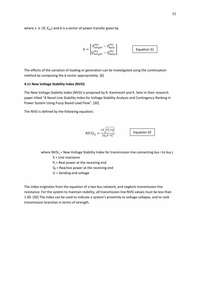
4.11 New Voltage Stability Index (NVSI)

The New Voltage Stability Index (NVSI) is proposed by R. Kanimozhi and K. Selvi in their research

paper titled “A Novel Line Stability Index for Voltage Stability Analysis and Contingency Ranking in

Power System Using Fuzzy Based Load Flow”. [30]

The NVSI is defined by the following equation;

𝑁𝑉𝑆𝐼𝑖𝑗 =2𝑋√𝑃𝑗

2+𝑄𝑗2

2𝑄𝑗𝑋−𝑉𝑖2

where NVSIij = New Voltage Stability Index for transmission line connecting bus i to bus j

X = Line reactance

Pj = Real power at the receiving end

Qj = Reactive power at the receiving end

Vi = Sending end voltage

The index originates from the equation of a two bus network, and neglects transmission line

resistance. For the system to maintain stability, all transmission line NVSI values must be less than

1.00. [30] The index can be used to indicate a system’s proximity to voltage collapse, and to rank

transmission branches in terms of strength.

Equation 31

Equation 32

22

5.0 Research Methodology

5.1 Research Methodology Introduction

The aim of the research carried out for this report was to investigate the use of synchrophasors in

analysing voltage stability and detecting voltage collapse.

The voltage stability analysis indices / methods chosen to incorporate into the simulations are listed

as follows:

- The Voltage Change Index (VCI)

- The Voltage Collapse Proximity Indicator (VCPI)

- Continuation Power Flow (CPF)

- The New Voltage Stability Index (NVSI)

The simulation software used in the research was MATPOWER [6], a stand-alone package of MATLAB

M-files which is used for solving power flow and optimal power flow problems. The tabulation

software used in my research was Microsoft Excel 2010.

This chapter will give a clear step-by-step procedure outlining the methodology of my simulations, as

well as give a discussion on MATPOWER.

5.2 MATPOWER Overview

This section gives a basic description of MATPOWER. Most information shown here is taken directly

from the MATPOWER User Manual.

MATPOWER is a third party stand-alone package of MATLAB M-files which is used for solving power

flow and optimal power flow (OPF) problems. It utilizes an extensible architecture that allows

the user to easily add new variables, constraints and costs to the standard OPF problem

formulation while preserving the structure needed to use pre-compiled solvers. [31] The software

design has the advantage of minimizing the coupling between variables, constraints and costs,

making it possible, for example, to add variables to an existing model without having to

explicitly modify existing constraints or costs to accommodate them. [31] Simply put, MATLAB is

used to provide high performance with code that is simple to modify and understand.

As mentioned before, MATPOWER’s primary functionality is to solve power flow and optimal power

flow problems. It does this via 3 steps:

- Preparing the input data defining all of the relevant system parameters [6]

- Invoking the function to run the simulation [6]

- Viewing and accessing the results that are printed to the screen and/or saved in output data

structures or files [6]

MATPOWER allows for the modification of real and reactive power demand. The following MATLAB

prompt is entered to load the IEEE 30-bus system, increase its real power demand at bus 2 to

30MW, and then run an AC optimal power flow with default options.

23

>> define_constants;

>> mpc = loadcase(‘case30’);

>> mpc.bus(2, PD) = 30;

>> runopf(mpc);

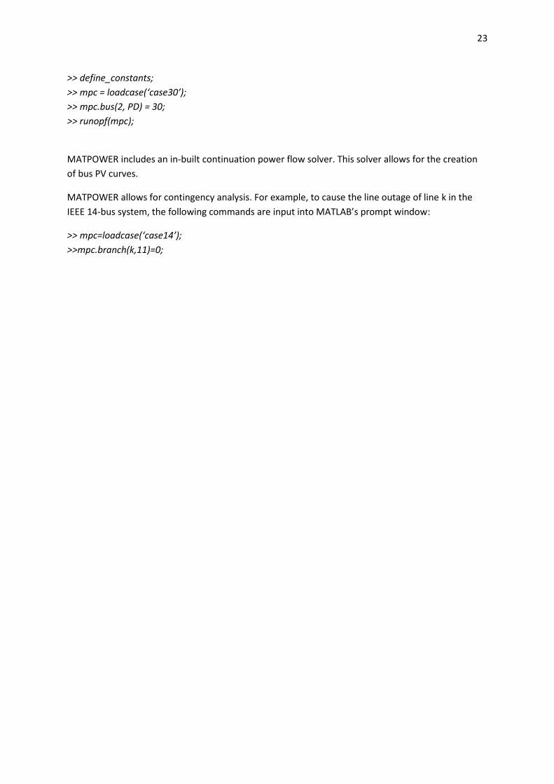
MATPOWER includes an in-built continuation power flow solver. This solver allows for the creation

of bus PV curves.

MATPOWER allows for contingency analysis. For example, to cause the line outage of line k in the

IEEE 14-bus system, the following commands are input into MATLAB’s prompt window:

>> mpc=loadcase(‘case14’);

>>mpc.branch(k,11)=0;

24

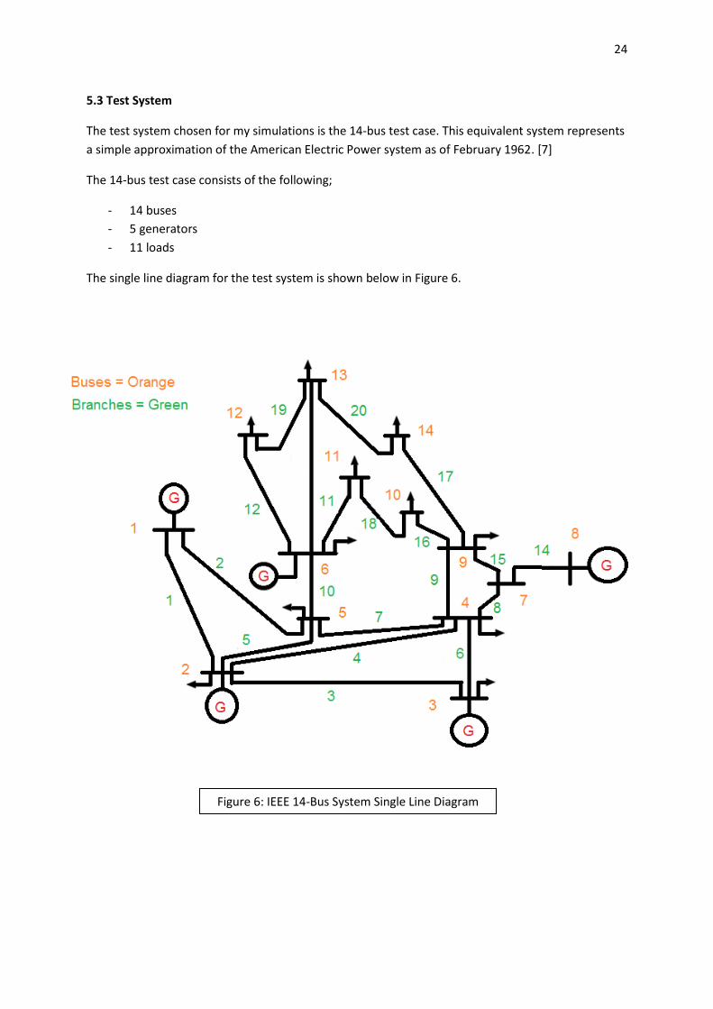
5.3 Test System

The test system chosen for my simulations is the 14-bus test case. This equivalent system represents

a simple approximation of the American Electric Power system as of February 1962. [7]

The 14-bus test case consists of the following;

- 14 buses

- 5 generators

- 11 loads

The single line diagram for the test system is shown below in Figure 6.

Figure 6: IEEE 14-Bus System Single Line Diagram

25

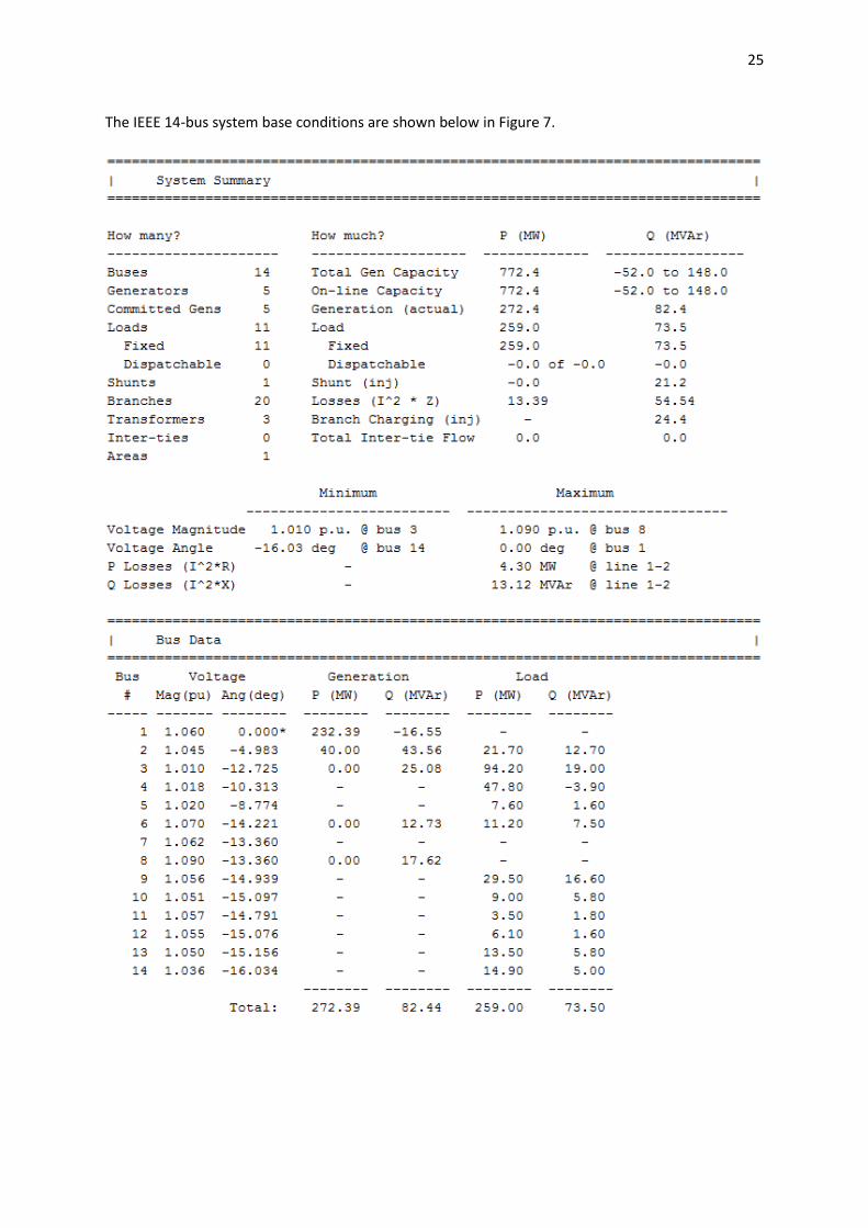
The IEEE 14-bus system base conditions are shown below in Figure 7.

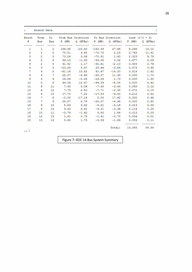
26

Figure 7: IEEE 14-Bus System Summary

27

5.4 Research Methodology Overview

As mentioned previously, the voltage stability analysis tools used in the research simulations are the

following:

- The Voltage Change Index (VCI)

- Continuation Power Flow (CPF)

- The Voltage Collapse Proximity Indicator (VCPI)

- The New Voltage Stability Index (NVSI)

All four of these analysis tools are based on phasor data. This means that all the data needed for the

relevant computations can be measured by PMUs. The phasor data required for each analysis

method are summarised below.

- Voltage Change Index: Load bus voltages at operating condition and load bus voltages at

critical loading condition.

- Continuation Power Flow: Load bus power values and load bus voltages.

- The Voltage Collapse Proximity Indicator: Load bus reactive power and generator reactive

power generation.

- The New Voltage Stability Index: Real power at receiving end bus, reactive power at

receiving end bus and sending end bus voltage.

Various operating scenarios are emulated in the simulations to represent the power transmission system operating under typical real life conditions. These operating scenarios are as follows:

1. System Net Load Factor Increase (Active and reactive power both scaled up by the same

magnitude)

The biggest and most common cause of voltage instability in a power transmission network

is the case where generation can no longer supply load demand. This situation can arise

when an unpredicted rise in load power demand occurs.

2. System Net Load Reactive Power Increase

As has been established earlier, there is a strong link between reactive power increase and

voltage. A higher reactive power demand results in higher system losses. This brings rise to

instability.

3. Contingency

The transmission lines in a power system vary in terms of resilience to power flow changes.

In some cases, after a line outage occurs, power is redirected to other lines in the network.

Some lines may be able to handle the increase in line loading, whilst others may be unable

to and in-turn also trip. The latter is common when a line trip occurs when the network is

experiencing high loading conditions. This can lead to abnormal operating conditions.

28

5.5 Methodology for Computing VCIs

The VCI for each load bus will be calculated under a variety of different system conditions. This is

done to show how the weakest bus in the network can change under different operating cases. The

operating cases being analysed are listed as follows:

- Base Case

- Line 4 Outage

- Line 11 Outage

- Line 17 Outage

Initially, the per-unit load bus voltages for each operating case are recorded. For every operating

case, the load factor of every load bus in the system will be equally increased in constant increments

to find each system’s critical loading condition. The critical loading condition occurs when at least

one load bus in the system has a per-unit voltage outside the range of 1.1 and 0.9. The per-unit load

bus voltages will be recorded at each critical loading condition. The VCI values will then be calculated

from the obtained data and the buses will be ranked from ‘strongest’ to ‘weakest’ for each operating

case.

5.6 Methodology for Continuation Power Flow Analysis

The in-built MATPOWER continuation power flow solver will be used to create a PV curve for each

load bus. The PV curve will show the effect that increasing the active power loading of the bus has

on the bus voltage. The PV curve will then be used to obtain the critical active power and voltage

values for each load bus (not including the loads at buses 1, 2, 3, 6, 7 and 8 as only pure load buses

can be considered).

The continuation power flow solver will then be used to gather the critical power and voltage data

for each load bus under the line 4 removed, line 11 removed and line 17 removed conditions.

5.7 Methodology for Computing VCPIs

Firstly, the voltage collapse point of the system needs to be found by increasing the system net load factor. The voltage collapse point for the system will be when MATPOWER’s Newton Raphson power flow method does not converge. The critical loading condition must also be determined by increasing the net load factor of the system (this has already been found from the VCI simulations). At the initial operating condition, the immediate post-voltage collapse operating condition, the critical loading operating condition, and incremented load factor operating conditions in between these, the following procedure must be followed:

- Run the load flow to obtain the reactive power generation for each generation bus in the

system.

29

- Increase the reactive power of just one load bus by 1 (this number is chosen for

simplification purposes) and run the load flow again to find the increase in reactive power

generation for each generation bus in the system. Do the same for every other load bus.

The collection of this phasor data means that the VCPI values of every load bus under each net load

factor condition can now be calculated.

The load bus VCPI values will then be determined for increasing load reactive power values only. This

means that the critical loading condition due to system net reactive load factor increase will need to

be found.

For contingency analysis, the following method was applied. Under initial operating conditions, line 4

will be removed from the system to replicate a line outage. The data required for computing the

VCPI for each load bus under the post-contingency condition will then be obtained using the method

as detailed above. The initial operating condition pre-contingency and post-contingency VCPI values

for the load buses can then be compared.

It is important to note that VCPI values for load buses 2, 3, and 6 are not computed as only pure load

buses can be considered for VCPI computation.

5.8 Methodology for Computing NVSIs

The NVSI of each transmission branch will be calculated for the system’s initial operating condition,

the system’s immediate post-voltage collapse condition, and the incremented load factor conditions

in between.

30

6.0 Results and Discussion

6.1 Voltage Change Index Analysis Results

The critical loading conditions for each operating condition are documented in Table 1 below.

Operating Condition

Critical Load Factor

Base Case 2.8

Line 4 Removed 2.5

Line 11 Removed 2.2

Line 17 Removed 2.0

The load bus VCI values for each operating condition are tabulated in Table 2 below.

Base Case

Line 4 Removed

Line 11 Removed

Line 17 Removed

Bus No. VCI VCI VCI VCI

1 0.0000 0.0000 0.0000 0.0000

2 0.0000 0.0000 0.0000 0.0000

3 0.0000 0.0000 0.0000 0.0000

4 0.0911 0.1103 0.0550 0.0366

5 0.0921 0.1122 0.0505 0.0376

6 0.0000 0.0000 0.0000 0.0000

7 0.0793 0.0787 0.0622 0.0320

8 0.0000 0.0000 0.0000 0.0000

9 0.1186 0.1123 0.1008 0.0483

10 0.1145 0.1057 0.1197 0.0476

11 0.0623 0.0572 0.1328 0.0271

12 0.0353 0.0303 0.0243 0.0214

13 0.0521 0.0448 0.0386 0.0348

14 0.1397 0.1230 0.1062 0.0992

Table 1: Critical Load Factors for Different Operating Conditions

Table 2: Load Bus VCIs for Different Operating Conditions

31

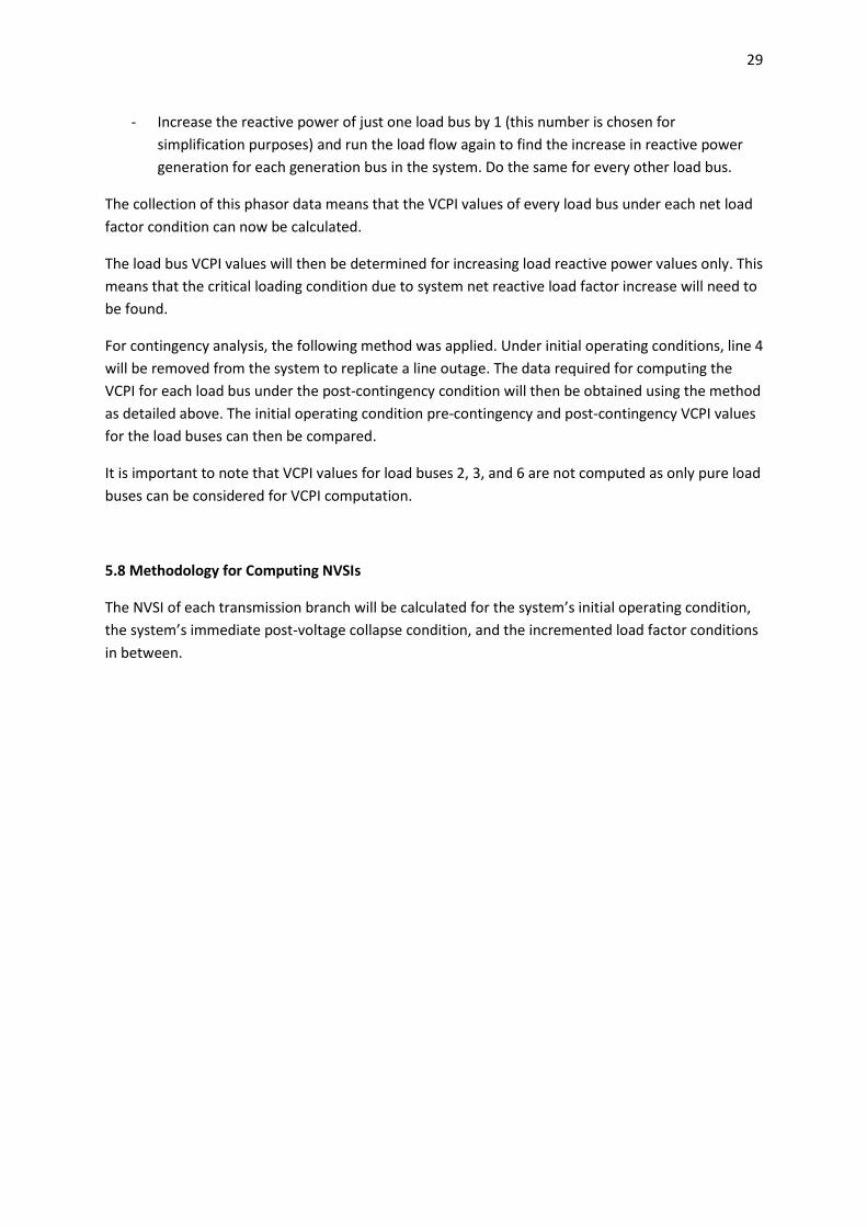
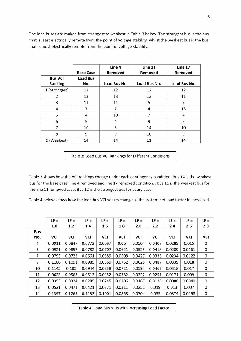
The load buses are ranked from strongest to weakest in Table 3 below. The strongest bus is the bus

that is least electrically remote from the point of voltage stability, whilst the weakest bus is the bus

that is most electrically remote from the point of voltage stability.

Base Case

Line 4 Removed

Line 11 Removed

Line 17 Removed

Bus VCI Ranking

Load Bus No. Load Bus No. Load Bus No. Load Bus No.

1 (Strongest) 12 12 12 12

2 13 13 13 11

3 11 11 5 7

4 7 7 4 13

5 4 10 7 4

6 5 4 9 5

7 10 5 14 10

8 9 9 10 9

9 (Weakest) 14 14 11 14

Table 3 shows how the VCI rankings change under each contingency condition. Bus 14 is the weakest

bus for the base case, line 4 removed and line 17 removed conditions. Bus 11 is the weakest bus for

the line 11 removed case. Bus 12 is the strongest bus for every case.

Table 4 below shows how the load bus VCI values change as the system net load factor in increased.

LF = 1.0

LF = 1.2

LF = 1.4

LF = 1.6

LF = 1.8

LF = 2.0

LF = 2.2

LF = 2.4

LF = 2.6

LF = 2.8

Bus No. VCI VCI VCI VCI VCI VCI VCI VCI VCI VCI

4 0.0911 0.0847 0.0772 0.0697 0.06 0.0504 0.0407 0.0289 0.015 0

5 0.0921 0.0857 0.0782 0.0707 0.0621 0.0525 0.0418 0.0289 0.0161 0

7 0.0793 0.0722 0.0661 0.0589 0.0508 0.0427 0.0335 0.0234 0.0122 0

9 0.1186 0.1091 0.0985 0.0869 0.0752 0.0625 0.0487 0.0339 0.018 0

10 0.1145 0.105 0.0944 0.0838 0.0721 0.0594 0.0467 0.0318 0.017 0

11 0.0623 0.0563 0.0513 0.0452 0.0382 0.0322 0.0251 0.0171 0.009 0

12 0.0353 0.0324 0.0285 0.0245 0.0206 0.0167 0.0128 0.0088 0.0049 0

13 0.0521 0.0471 0.0421 0.0371 0.0311 0.0251 0.019 0.013 0.007 0

14 0.1397 0.1265 0.1133 0.1001 0.0858 0.0704 0.055 0.0374 0.0198 0

Table 3: Load Bus VCI Rankings for Different Conditions

Table 4: Load Bus VCIs with Increasing Load Factor

32

Table 4 indeed shows that the load bus VCI values get smaller as the load factor is increased, but this

data is not useful as voltages phasors by themselves can provide this information. The VCI is thus

better used for determining the weak buses in a transmission network. The VCI can be useful when a

change in system operating conditions occurs (e.g. when a line becomes out of service). After a

change in system operating conditions occurs, voltage phasor data for the new operating condition

can be extracted. This extracted data can then be used so that the bus ranking can be updated to

show which buses are now the weakest.

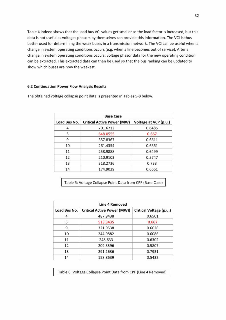
6.2 Continuation Power Flow Analysis Results

The obtained voltage collapse point data is presented in Tables 5-8 below.

Base Case

Load Bus No. Critical Active Power (MW) Voltage at VCP (p.u.)

4 701.6712 0.6485

5 648.0555 0.667

9 357.8367 0.6611

10 261.4354 0.6361

11 258.9888 0.6499

12 210.9103 0.5747

13 318.2736 0.733

14 174.9029 0.6661

Line 4 Removed

Load Bus No. Critical Active Power (MW)) Critical Voltage (p.u.)

4 487.9438 0.6501

5 513.3435 0.667

9 321.9538 0.6628

10 244.9882 0.6086

11 248.633 0.6302

12 209.3596 0.5807

13 291.1636 0.7931

14 158.8639 0.5432

Table 5: Voltage Collapse Point Data from CPF (Base Case)

Table 6: Voltage Collapse Point Data from CPF (Line 4 Removed)

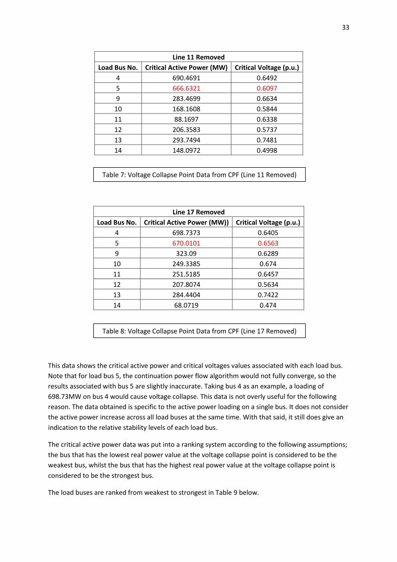
33

Line 11 Removed

Load Bus No. Critical Active Power (MW) Critical Voltage (p.u.)

4 690.4691 0.6492

5 666.6321 0.6097

9 283.4699 0.6634

10 168.1608 0.5844

11 88.1697 0.6338

12 206.3583 0.5737

13 293.7494 0.7481

14 148.0972 0.4998

Line 17 Removed

Load Bus No. Critical Active Power (MW)) Critical Voltage (p.u.)

4 698.7373 0.6405

5 670.0101 0.6563

9 323.09 0.6289

10 249.3385 0.674

11 251.5185 0.6457

12 207.8074 0.5634

13 284.4404 0.7422

14 68.0719 0.474

This data shows the critical active power and critical voltages values associated with each load bus.

Note that for load bus 5, the continuation power flow algorithm would not fully converge, so the

results associated with bus 5 are slightly inaccurate. Taking bus 4 as an example, a loading of

698.73MW on bus 4 would cause voltage collapse. This data is not overly useful for the following

reason. The data obtained is specific to the active power loading on a single bus. It does not consider

the active power increase across all load buses at the same time. With that said, it still does give an

indication to the relative stability levels of each load bus.

The critical active power data was put into a ranking system according to the following assumptions;

the bus that has the lowest real power value at the voltage collapse point is considered to be the

weakest bus, whilst the bus that has the highest real power value at the voltage collapse point is

considered to be the strongest bus.

The load buses are ranked from weakest to strongest in Table 9 below.

Table 7: Voltage Collapse Point Data from CPF (Line 11 Removed)

Table 8: Voltage Collapse Point Data from CPF (Line 17 Removed)

34

Base Case Line 4

Removed Line 11

Removed Line 17

Removed

Bus Ranking

Load Bus No. Load Bus No. Load Bus No. Load Bus No.

1 (Strongest) 5 5 4 4

2 4 4 5 5

3 9 9 13 9

4 13 13 9 13

5 10 11 12 11

6 11 10 10 10

7 12 12 14 12

8 (Weakest) 14 14 11 14

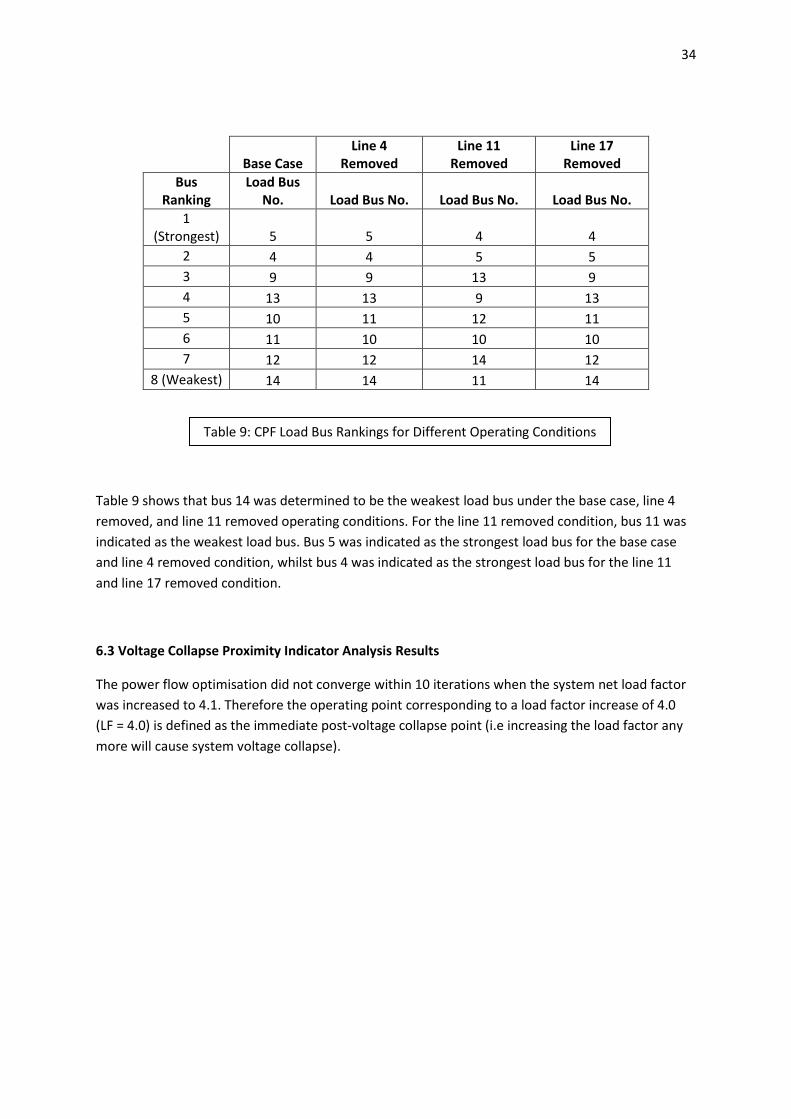
Table 9 shows that bus 14 was determined to be the weakest load bus under the base case, line 4

removed, and line 11 removed operating conditions. For the line 11 removed condition, bus 11 was

indicated as the weakest load bus. Bus 5 was indicated as the strongest load bus for the base case

and line 4 removed condition, whilst bus 4 was indicated as the strongest load bus for the line 11

and line 17 removed condition.

6.3 Voltage Collapse Proximity Indicator Analysis Results

The power flow optimisation did not converge within 10 iterations when the system net load factor

was increased to 4.1. Therefore the operating point corresponding to a load factor increase of 4.0

(LF = 4.0) is defined as the immediate post-voltage collapse point (i.e increasing the load factor any

more will cause system voltage collapse).

Table 9: CPF Load Bus Rankings for Different Operating Conditions

35

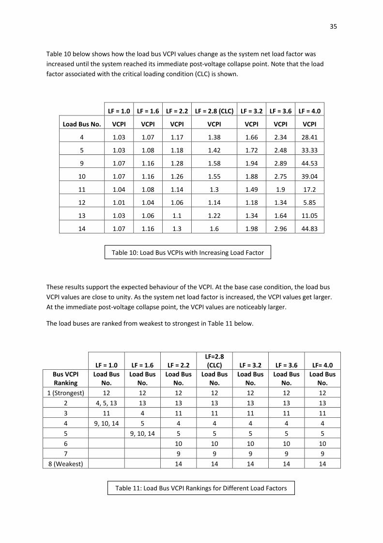
Table 10 below shows how the load bus VCPI values change as the system net load factor was

increased until the system reached its immediate post-voltage collapse point. Note that the load

factor associated with the critical loading condition (CLC) is shown.

LF = 1.0 LF = 1.6 LF = 2.2 LF = 2.8 (CLC) LF = 3.2 LF = 3.6 LF = 4.0

Load Bus No. VCPI VCPI VCPI VCPI VCPI VCPI VCPI

4 1.03 1.07 1.17 1.38 1.66 2.34 28.41

5 1.03 1.08 1.18 1.42 1.72 2.48 33.33

9 1.07 1.16 1.28 1.58 1.94 2.89 44.53

10 1.07 1.16 1.26 1.55 1.88 2.75 39.04

11 1.04 1.08 1.14 1.3 1.49 1.9 17.2

12 1.01 1.04 1.06 1.14 1.18 1.34 5.85

13 1.03 1.06 1.1 1.22 1.34 1.64 11.05

14 1.07 1.16 1.3 1.6 1.98 2.96 44.83

These results support the expected behaviour of the VCPI. At the base case condition, the load bus

VCPI values are close to unity. As the system net load factor is increased, the VCPI values get larger.

At the immediate post-voltage collapse point, the VCPI values are noticeably larger.

The load buses are ranked from weakest to strongest in Table 11 below.

LF = 1.0 LF = 1.6 LF = 2.2

LF=2.8 (CLC) LF = 3.2 LF = 3.6 LF= 4.0

Bus VCPI Ranking

Load Bus No.

Load Bus No.

Load Bus No.

Load Bus No.

Load Bus No.

Load Bus No.

Load Bus No.

1 (Strongest) 12 12 12 12 12 12 12

2 4, 5, 13 13 13 13 13 13 13

3 11 4 11 11 11 11 11

4 9, 10, 14 5 4 4 4 4 4

5 9, 10, 14 5 5 5 5 5

6 10 10 10 10 10

7 9 9 9 9 9

8 (Weakest) 14 14 14 14 14

Table 10: Load Bus VCPIs with Increasing Load Factor

Table 11: Load Bus VCPI Rankings for Different Load Factors

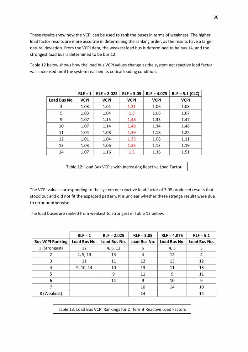
36

These results show how the VCPI can be used to rank the buses in terms of weakness. The higher

load factor results are more accurate in determining the ranking order, as the results have a larger

natural deviation. From the VCPI data, the weakest load bus is determined to be bus 14, and the

strongest load bus is determined to be bus 12.

Table 12 below shows how the load bus VCPI values change as the system net reactive load factor

was increased until the system reached its critical loading condition.

RLF = 1 RLF = 2.025 RLF = 3.05 RLF = 4.075 RLF = 5.1 (CLC)

Load Bus No. VCPI VCPI VCPI VCPI VCPI

4 1.03 1.04 1.31 1.06 1.08

5 1.03 1.04 1.3 1.06 1.07

9 1.07 1.15 1.48 1.33 1.47

10 1.07 1.14 1.49 1.34 1.48

11 1.04 1.08 1.39 1.18 1.25

12 1.01 1.04 1.33 1.08 1.11

13 1.03 1.06 1.35 1.13 1.19

14 1.07 1.16 1.5 1.36 1.51

The VCPI values corresponding to the system net reactive load factor of 3.05 produced results that

stood out and did not fit the expected pattern. It is unclear whether these strange results were due

to error or otherwise.

The load buses are ranked from weakest to strongest in Table 13 below.

RLF = 1 RLF = 2.025 RLF = 3.05 RLF = 4.075 RLF = 5.1

Bus VCPI Ranking Load Bus No. Load Bus No. Load Bus No. Load Bus No. Load Bus No.

1 (Strongest) 12 4, 5, 12 5 4, 5 5

2 4, 5, 13 13 4 12 4

3 11 11 12 13 12

4 9, 10, 14 10 13 11 13

5 9 11 9 11

6 14 9 10 9

7 10 14 10

8 (Weakest) 14 14

Table 12: Load Bus VCPIs with Increasing Reactive Load Factor

Table 13: Load Bus VCPI Rankings for Different Reactive Load Factors

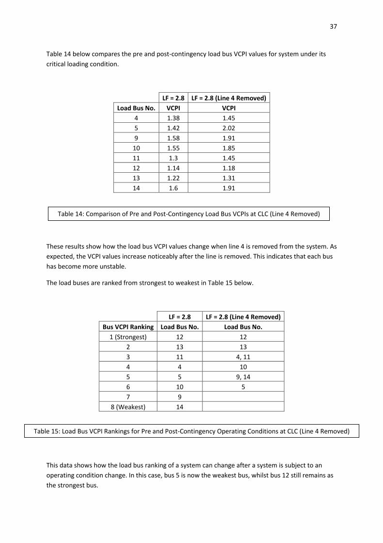
37

Table 14 below compares the pre and post-contingency load bus VCPI values for system under its

critical loading condition.

LF = 2.8 LF = 2.8 (Line 4 Removed)

Load Bus No. VCPI VCPI

4 1.38 1.45

5 1.42 2.02

9 1.58 1.91

10 1.55 1.85

11 1.3 1.45

12 1.14 1.18

13 1.22 1.31

14 1.6 1.91

These results show how the load bus VCPI values change when line 4 is removed from the system. As

expected, the VCPI values increase noticeably after the line is removed. This indicates that each bus

has become more unstable.

The load buses are ranked from strongest to weakest in Table 15 below.

LF = 2.8 LF = 2.8 (Line 4 Removed)

Bus VCPI Ranking Load Bus No. Load Bus No.

1 (Strongest) 12 12

2 13 13

3 11 4, 11

4 4 10

5 5 9, 14

6 10 5

7 9

8 (Weakest) 14

This data shows how the load bus ranking of a system can change after a system is subject to an

operating condition change. In this case, bus 5 is now the weakest bus, whilst bus 12 still remains as

the strongest bus.

Table 14: Comparison of Pre and Post-Contingency Load Bus VCPIs at CLC (Line 4 Removed)

Table 15: Load Bus VCPI Rankings for Pre and Post-Contingency Operating Conditions at CLC (Line 4 Removed)

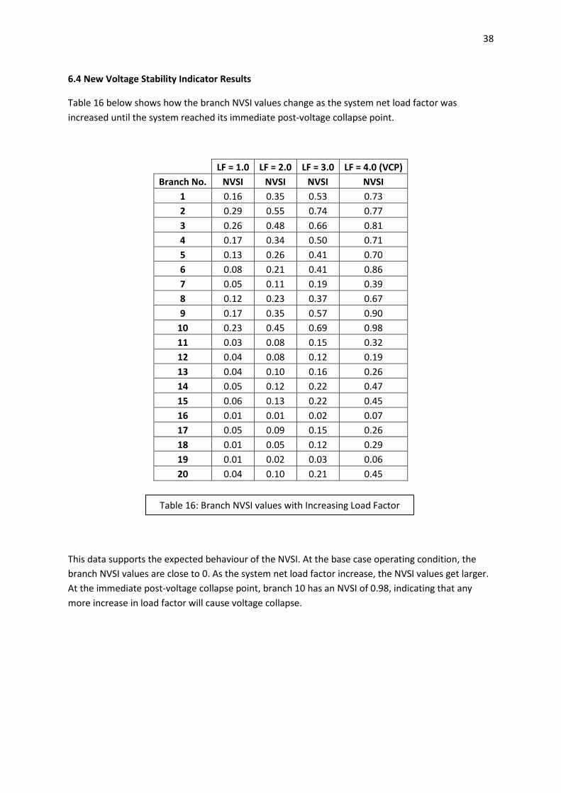
38

6.4 New Voltage Stability Indicator Results

Table 16 below shows how the branch NVSI values change as the system net load factor was

increased until the system reached its immediate post-voltage collapse point.

LF = 1.0 LF = 2.0 LF = 3.0 LF = 4.0 (VCP)

Branch No. NVSI NVSI NVSI NVSI

1 0.16 0.35 0.53 0.73

2 0.29 0.55 0.74 0.77

3 0.26 0.48 0.66 0.81

4 0.17 0.34 0.50 0.71

5 0.13 0.26 0.41 0.70

6 0.08 0.21 0.41 0.86

7 0.05 0.11 0.19 0.39

8 0.12 0.23 0.37 0.67

9 0.17 0.35 0.57 0.90

10 0.23 0.45 0.69 0.98

11 0.03 0.08 0.15 0.32

12 0.04 0.08 0.12 0.19

13 0.04 0.10 0.16 0.26

14 0.05 0.12 0.22 0.47

15 0.06 0.13 0.22 0.45

16 0.01 0.01 0.02 0.07

17 0.05 0.09 0.15 0.26

18 0.01 0.05 0.12 0.29

19 0.01 0.02 0.03 0.06

20 0.04 0.10 0.21 0.45

This data supports the expected behaviour of the NVSI. At the base case operating condition, the

branch NVSI values are close to 0. As the system net load factor increase, the NVSI values get larger.

At the immediate post-voltage collapse point, branch 10 has an NVSI of 0.98, indicating that any

more increase in load factor will cause voltage collapse.

Table 16: Branch NVSI values with Increasing Load Factor

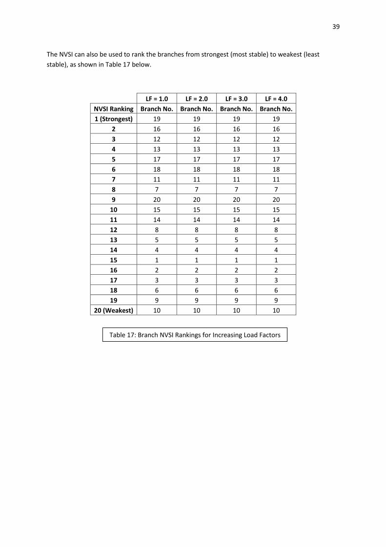
39

The NVSI can also be used to rank the branches from strongest (most stable) to weakest (least

stable), as shown in Table 17 below.

LF = 1.0 LF = 2.0 LF = 3.0 LF = 4.0

NVSI Ranking Branch No. Branch No. Branch No. Branch No.

1 (Strongest) 19 19 19 19

2 16 16 16 16

3 12 12 12 12

4 13 13 13 13

5 17 17 17 17

6 18 18 18 18

7 11 11 11 11

8 7 7 7 7

9 20 20 20 20

10 15 15 15 15

11 14 14 14 14

12 8 8 8 8

13 5 5 5 5

14 4 4 4 4

15 1 1 1 1

16 2 2 2 2

17 3 3 3 3

18 6 6 6 6

19 9 9 9 9

20 (Weakest) 10 10 10 10

Table 17: Branch NVSI Rankings for Increasing Load Factors

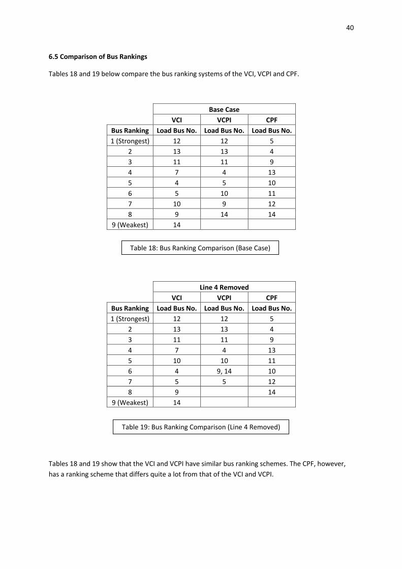
40

6.5 Comparison of Bus Rankings

Tables 18 and 19 below compare the bus ranking systems of the VCI, VCPI and CPF.

Base Case

VCI VCPI CPF

Bus Ranking Load Bus No. Load Bus No. Load Bus No.

1 (Strongest) 12 12 5

2 13 13 4

3 11 11 9

4 7 4 13

5 4 5 10

6 5 10 11

7 10 9 12

8 9 14 14

9 (Weakest) 14

Line 4 Removed

VCI VCPI CPF

Bus Ranking Load Bus No. Load Bus No. Load Bus No.

1 (Strongest) 12 12 5

2 13 13 4

3 11 11 9

4 7 4 13

5 10 10 11

6 4 9, 14 10

7 5 5 12

8 9 14

9 (Weakest) 14

Tables 18 and 19 show that the VCI and VCPI have similar bus ranking schemes. The CPF, however,

has a ranking scheme that differs quite a lot from that of the VCI and VCPI.

Table 18: Bus Ranking Comparison (Base Case)

Table 19: Bus Ranking Comparison (Line 4 Removed)

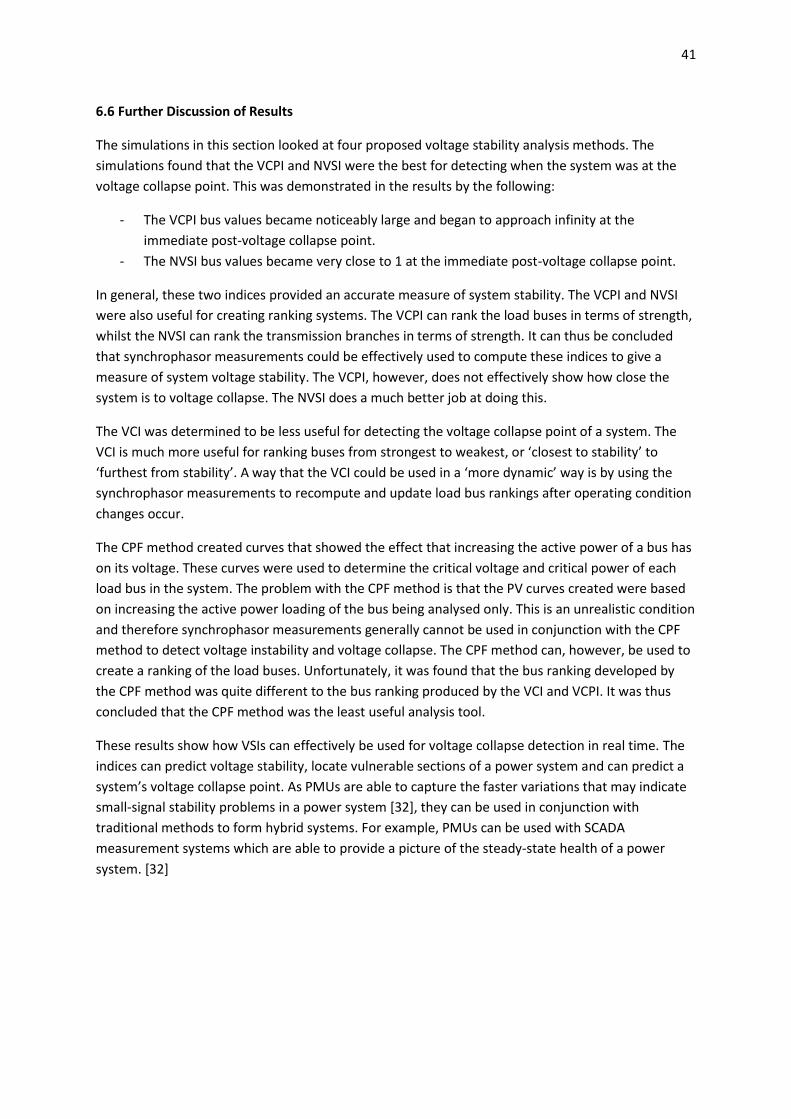
41

6.6 Further Discussion of Results

The simulations in this section looked at four proposed voltage stability analysis methods. The

simulations found that the VCPI and NVSI were the best for detecting when the system was at the

voltage collapse point. This was demonstrated in the results by the following:

- The VCPI bus values became noticeably large and began to approach infinity at the

immediate post-voltage collapse point.

- The NVSI bus values became very close to 1 at the immediate post-voltage collapse point.

In general, these two indices provided an accurate measure of system stability. The VCPI and NVSI

were also useful for creating ranking systems. The VCPI can rank the load buses in terms of strength,

whilst the NVSI can rank the transmission branches in terms of strength. It can thus be concluded

that synchrophasor measurements could be effectively used to compute these indices to give a

measure of system voltage stability. The VCPI, however, does not effectively show how close the

system is to voltage collapse. The NVSI does a much better job at doing this.

The VCI was determined to be less useful for detecting the voltage collapse point of a system. The

VCI is much more useful for ranking buses from strongest to weakest, or ‘closest to stability’ to

‘furthest from stability’. A way that the VCI could be used in a ‘more dynamic’ way is by using the

synchrophasor measurements to recompute and update load bus rankings after operating condition

changes occur.

The CPF method created curves that showed the effect that increasing the active power of a bus has

on its voltage. These curves were used to determine the critical voltage and critical power of each

load bus in the system. The problem with the CPF method is that the PV curves created were based

on increasing the active power loading of the bus being analysed only. This is an unrealistic condition

and therefore synchrophasor measurements generally cannot be used in conjunction with the CPF

method to detect voltage instability and voltage collapse. The CPF method can, however, be used to

create a ranking of the load buses. Unfortunately, it was found that the bus ranking developed by

the CPF method was quite different to the bus ranking produced by the VCI and VCPI. It was thus

concluded that the CPF method was the least useful analysis tool.

These results show how VSIs can effectively be used for voltage collapse detection in real time. The

indices can predict voltage stability, locate vulnerable sections of a power system and can predict a

system’s voltage collapse point. As PMUs are able to capture the faster variations that may indicate

small-signal stability problems in a power system [32], they can be used in conjunction with

traditional methods to form hybrid systems. For example, PMUs can be used with SCADA

measurement systems which are able to provide a picture of the steady-state health of a power

system. [32]

42

7.0 Conclusion and Recommendations

7.1 Conclusion

This thesis investigated the use of synchrophasors in analysing voltage stability and detecting voltage

collapse. The voltage stability analysis methods used in conjunction with the synchrophasor

measurements obtained from the simulations were the Voltage Change Index (VSI), the Voltage

Collapse Proximity Indicator (VCPI), Continuation Power Flow (CPF) and the New Voltage Stability

Index (NVSI). The simulations were done in MATPOWER and used the IEEE 14-bus system.

The VCI was determined to not be useful in detecting voltage collapse. It does, however, provide a

useful bus ranking system that lists each load bus from ‘strongest’ to ‘weakest’. The weakest bus

refers to the bus that experiences the largest voltage change when going from an initial operating

point to the critical loading condition. The VCI was determined to be useful for updating bus ranking

systems after changes in system operating condition occurs (e.g. when a line becomes out of

service).

The VCPI proved to be an effective indicator of voltage stability levels. It was, however, not so

effective at indicating proximity to voltage collapse. As the system net load factor was increased, the

VCPI tended to increase as well. The VCPI indicates that voltage collapse is about to occur when its

magnitude gets significantly larger and begins to approach infinity. The problem lies in the fact that

the index does not have a way of determining when this will start happening (unlike the NVSI where

the voltage collapse occurs when one of the branch indexes reaches the value of 1). Another issue

with the VCPI is that it requires the loads to have significant reactive power loading components.

Like the VCI, the VCPI could be used to create a bus ranking system. The bus ranking systems of the

VCI and VCPI were very similar.

The CPF method was the least useful method for analysing voltage stability and detecting voltage

collapse. The reason for this was because it is based on the usage of load bus PV curves which were

generated by increasing the active power loading of just one load until the power system reached

voltage collapse. As this is an unrealistic condition, it cannot adequately be used in dynamic analysis

and does not provide much useful data. The CPF method can provide a bus ranking system (by

ranking the critical powers of each load bus) but this ranking proved to deviate heavily from the

rankings created by the VCI and VCPI.

The NVSI proved to have the greatest capability in measuring voltage stability and detecting voltage

collapse. This is due to the fact that the index lies between 0 and 1, with 1 indicating system voltage

collapse. Simulations validated this, with some branch NVSI values becoming very close to 1 at the

immediate post-voltage collapse point. Because the NVSI has such clear margins, it cannot only be

used to gauge system stability, but it can also be used to determine a system’s proximity to voltage

collapse. The NVSI could also be used to rank the transmission branches in terms of stability.

43

7.2 Recommendations

This report investigated the use of various voltage stability analysis tools using a steady state

analysis approach. A recommendation for future synchrophasor studies would be to use a dynamic

analysis approach. This type of approach would allow for a more in-depth analysis into the time-

response of power systems and how voltage stability indices respond to system disturbances and

operating condition changes.

A natural extension of this research would be to investigate further into the use of the NVSI and VCPI

stability indices as these indices proved to be the most effective at monitoring bus voltage stability.

These indices could be investigated using a larger power network (perhaps a 30 or 40 bus system)

and a much larger array of operating conditions could be simulated in order to provide more in-

depth results.

Further extension of this research includes investigating methods of voltage stability correction and

how VSIs could be used in conjunction with these correction methods.

44

8.0 Works Cited

[1] International Energy Outlook 2013 (IEO2013), released by the U.S. Energy Information

Administration (EIA), 2013

[2] Bloomberg New Energy Finance, “New Energy Outlook 2015”, URL:

http://www.bloomberg.com/company/new-energy-outlook/

[3] M. Glavic Quanta Technology, USAD. Novosel ; E. Heredia ; D. Kosterev ; A. Salazar ; F. Habibi-

Ashrafi ; M. Donnelly “Real-Time Voltage Control Under Stressed Conditions”, IEEE Power and

Energy Magazine (Volume: 10, Issue: 4), pp. 43-55

[4] National Instruments NI 9244 Datasheet, URL: http://www.ni.com/datasheet/pdf/en/ds-527

[5] Eric Sagen, Kenneth Workman, Schweitzer Engineering Laboratories, Inc, “Methods of Time

Synchronization”, 63rd Annual Georgia Tech Protective Relaying Conference Atlanta, Georgia, April

22–24, 2009

[6] Ray D. Zimmerman, Carlos E. Murillo-Sanchez, “MATPOWER 5.1 User’s Manual”, March 20 2015,

URL: http://www.pserc.cornell.edu/matpower/manual.pdf

[7] Illinois Center for a Smarter Electric Grid (ICSEG), IEEE 14-bus system, URL:

http://icseg.iti.illinois.edu/ieee-14-bus-system, Date accessed: October 2015

[8] Roy Moxley, “Synchrophasors in the Real World”, Schweitzer Engineering Laboratories, Inc.,

2006, URL:

https://cdn.selinc.com/assets/Literature/Publications/Technical%20Papers/6194_Synchrophasors_R

M_20060118_Web.pdf?v=20160303-081549

[9] Electric Power Research Institute, “Phasor Measurement Unit (PMU) Implementation and

Applications”, EPRI, Palo Alto, CA: 2007. 1015511

[10] Waheed Ur Rahman, Muhammad Ali, Chaudhry A. Mehmood, Asadullah Khan, “Design and

Implementation for Wide Area Power System Monitoring and Protection using Phasor measuring

Units” Electrical Engineering Department, COMSATS Institute of Information Technology, April 2013

[11] C. P. Steinmetz, “Power control and stability of electric generating stations” AIEE Trans., vol.

XXXIX, Part II, July 1920, pp. 1215-1287

[12] IEEE/CIGRE Joint Task Force on Stability Terms and Definitions, “Definition and Classification of

Power System Stability”, IEEE Transactions on Power Systems (Volume: 19, Issue: 3) 2003

[13] Kumaraswamy, Jahnavi,W.V., Devaraju,T., Ramesh,P.,“An Optimal Power Flow (OPF) Method

with Improved Voltage Stability Analysis”, Proceedings of the World Congress on Engineering

London, U.K. Vol. II, July 4 -6, 2012

[14] Stefan Johansson, Fredrik Sjogren, “Voltage Collapse in Power Systems”, Chalmers University of

Technology 1995. URL: http://webfiles.portal.chalmers.se/et/Lic/Johansson%26SjogrenLic.pdf

45

[15] Günther Beck, Dusan Povh, Dietmar Retzmann, Erwin Teltsch, “Global Blackouts – Lessons

Learned”, Siemens, July 2011. URL: http://www.energy.siemens.com/mx/pool/hq/power-

transmission/HVDC/Global_Blackouts.pdf

[16] I Kumarswamy and P Ramanareddy. “Analysis of Voltage Stability Using L-Index Method”. 2011.

ECO Services International

[17] B. Gao, G.K. Morison, P. Kundur, “Towards the development of a systematic approach for

voltage stability assessment of large-scale power systems”, IEEE Transactions on Power Systems

(Volume: 11, Issue: 3), August 1996. pp. 1314-1324

[18] Yanfeng Gong, N. Schulz, N. Guzman, "Synchrophasor-Based Real-Time Voltage Stability Index",

2006 IEEE PES Power Systems Conference and Exposition, Oct. 29 2006-Nov. 1 2006, pp. 1029-1036

[19] PowerWorld Corporation, “Voltage Stability Using PV Curves”, URL:

http://www.powerworld.com/files/S06PVCurves.pdf, Access date: October 2015

[20] PowerWorld Corporation, “Voltage Stability Using QV Curves”, URL:

http://www.powerworld.com/files/S07QVCuvers.pdf, Access date: October 2015

[21] Bhawana Telang, Prabodh Khampariya, “Voltage Stability Evaluation Using Modal Analysis”,

International Journal of Scientific Research Engineering & Technology (IJSRET), ISSN 2278-0882

Volume 4, Issue 4, April 2015, pp. 1529-1542

[22] P. Kessel, Glavitsch, ”Estimating the Voltage Stability of a Power System”, IEEE Transaction

on Power Delivery, Vol PWRD-1, No 3, July 1986, pp. 346-354

[23] B. Mahipal, P. Venugopal Rao, T. Swetha, G. Babu Naik, Ch. Nareshkumar, “A New Technique to

find the effect of Active Power Loading on Voltage Stability and Algorithm to improve Voltage

Stability of Radial and Meshed Power Systems”, Journal of Information Engineering and Applications

ISSN 2224-5782 (print) ISSN 2225-0506 (online) Vol.3, No.5, 2013

[24] H.J.C.P. Pinto, N. Martins, X. Vieira F°, A. Bianco, P. Gomes, M. G. dos Santos, “Modal Analysis

for Voltage Stability: Application at Base Case and Point of Collapse”, Bulk Power System Voltage

Phenomena - III Voltage Stability, Security & Control Davos, Switzerland, 22-26 August 1994

[25] S Shirisha, P l v Prasanna and Siva Mallikarjuna N Rao. Article: “Evaluation of Modal Analysis for

Voltage Stability using Artificial Immune Systems”, International Journal of Computer Applications

46(9):6-10, May 2012

[26] J.L. Kirtley Jr., Massachusetts Institute of Technology, “Introduction to Load Flow”, URL:

http://ocw.mit.edu/courses/electrical-engineering-and-computer-science/6-061-introduction-to-

electric-power-systems-spring-2011/readings/MIT6_061S11_ch5.pdf

[27] Wolfram Alpha, Jacobian Matrices, URL: http://mathworld.wolfram.com/Jacobian.html

[28] Y.L. Chen, C.W. Chang, C.C. Liu, “Efficient methods for identifying weak nodes in electrical power

networks”, IEE Proceedings - Generation, Transmission and Distribution (Volume: 142, Issue: 3), May

1995, pp. 317-322

46

[29] O.O. Obadina, G.J. Berg, “Identifying electrically weak and strong segments of a power system

from a voltage stability viewpoint”, IEE Proceedings C - Generation, Transmission and Distribution

(Volume: 137, Issue: 3), 19 June 1989, pp. 205-212

[30] R. Kanimozhi, K. Selvi, “A Novel Line Stability Index for Voltage Stability Analysis and

Contingency Ranking in Power System Using Fuzzy Based Load Flow”, JEET, Vol. 8, No. 4, July 2013

[31] Ray D. Zimmerman, Carlos E. Murillo-Sanchez, “MATPOWER’s Extensible Optimal Power Flow

Architecture”, 2009 IEEE Power & Energy Society General Meeting, 26-30 July 2009, pp. 1-7

[32] R. Klump ; Lewis University & PowerWorld Corporation ; R. E. Wilson ; K. E. Martin, “Visualizing

Real-Time Security Threats Using Hybrid SCADA / PMU Measurement Displays”, Proceedings of the

38th Annual Hawaii International Conference on System Sciences, 03-06 Jan. 2005, pp. 55c

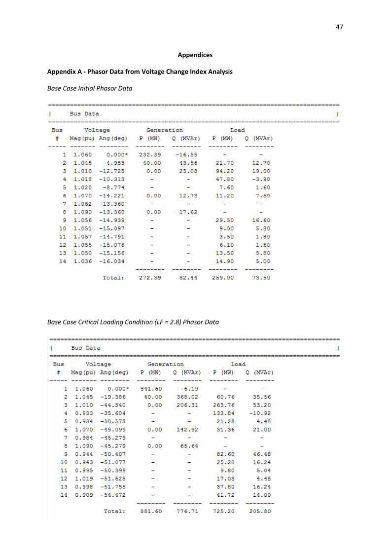
47

Appendices

Appendix A - Phasor Data from Voltage Change Index Analysis

Base Case Initial Phasor Data

Base Case Critical Loading Condition (LF = 2.8) Phasor Data

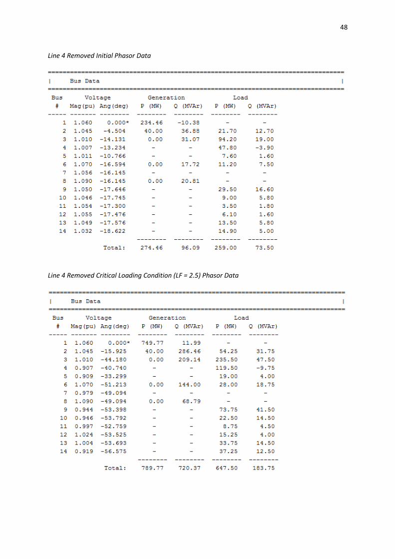
48

Line 4 Removed Initial Phasor Data

Line 4 Removed Critical Loading Condition (LF = 2.5) Phasor Data

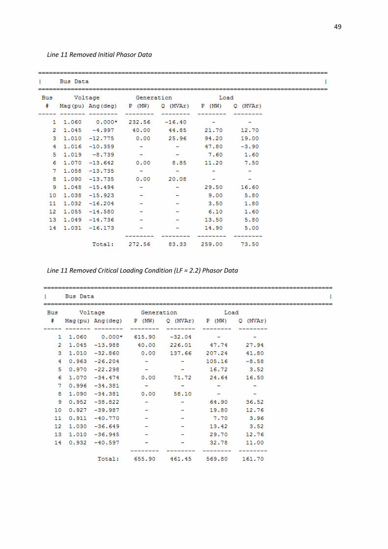
49

Line 11 Removed Initial Phasor Data

Line 11 Removed Critical Loading Condition (LF = 2.2) Phasor Data

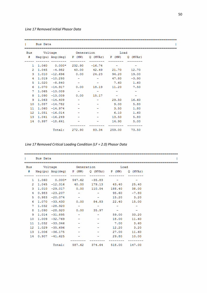
50

Line 17 Removed Initial Phasor Data

Line 17 Removed Critical Loading Condition (LF = 2.0) Phasor Data

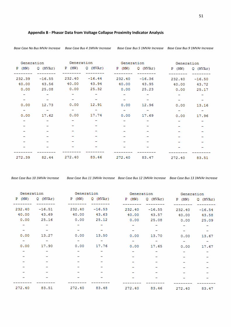
51

Appendix B - Phasor Data from Voltage Collapse Proximity Indicator Analysis

Base Case No Bus MVAr Increase Base Case Bus 4 1MVAr Increase Base Case Bus 5 1MVAr Increase Base Case Bus 9 1MVAr Increase

Base Case Bus 10 1MVAr Increase Base Case Bus 11 1MVAr Increase Base Case Bus 12 1MVAr Increase Base Case Bus 13 1MVAr Increase

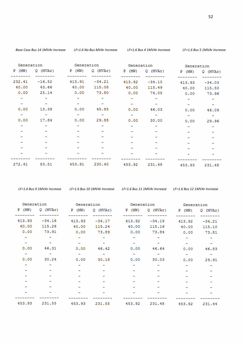
52

Base Case Bus 14 1MVAr Increase LF=1.6 No Bus MVAr Increase LF=1.6 Bus 4 1MVAr Increase LF=1.6 Bus 5 1MVAr Increase

LF=1.6 Bus 9 1MVAr Increase LF=1.6 Bus 10 1MVAr Increase LF=1.6 Bus 11 1MVAr Increase LF=1.6 Bus 12 1MVAr Increase

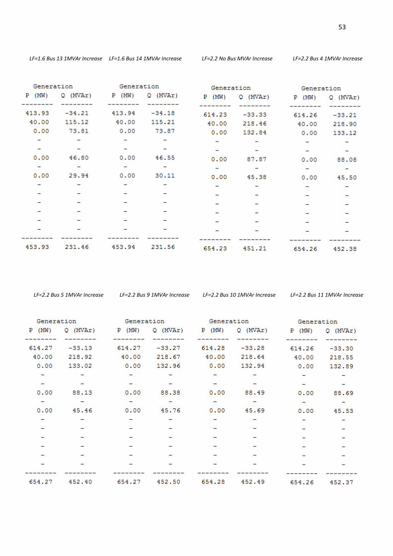
53

LF=1.6 Bus 13 1MVAr Increase LF=1.6 Bus 14 1MVAr Increase LF=2.2 No Bus MVAr Increase LF=2.2 Bus 4 1MVAr Increase

LF=2.2 Bus 5 1MVAr Increase LF=2.2 Bus 9 1MVAr Increase LF=2.2 Bus 10 1MVAr Increase LF=2.2 Bus 11 1MVAr Increase

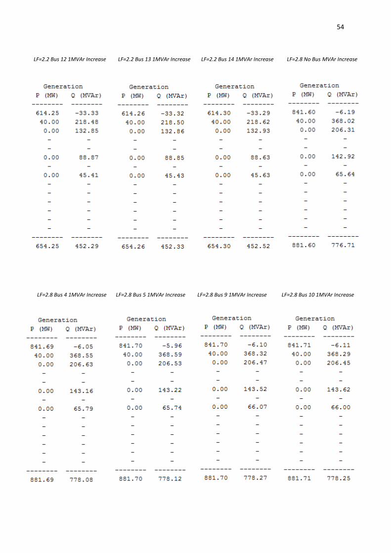
54

LF=2.2 Bus 12 1MVAr Increase LF=2.2 Bus 13 1MVAr Increase LF=2.2 Bus 14 1MVAr Increase LF=2.8 No Bus MVAr Increase

LF=2.8 Bus 4 1MVAr Increase LF=2.8 Bus 5 1MVAr Increase LF=2.8 Bus 9 1MVAr Increase LF=2.8 Bus 10 1MVAr Increase

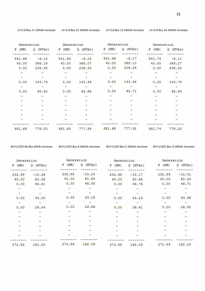
55

LF=2.8 Bus 11 1MVAr Increase LF=2.8 Bus 12 1MVAr Increase LF=2.8 Bus 13 1MVAr Increase LF=2.8 Bus 14 1MVAr Increase

RLF=2.025 No Bus MVAr Increase RLF=2.025 Bus 4 1MVAr Increase RLF=2.025 Bus 5 1MVAr Increase RLF=2.025 Bus 9 1MVAr Increase

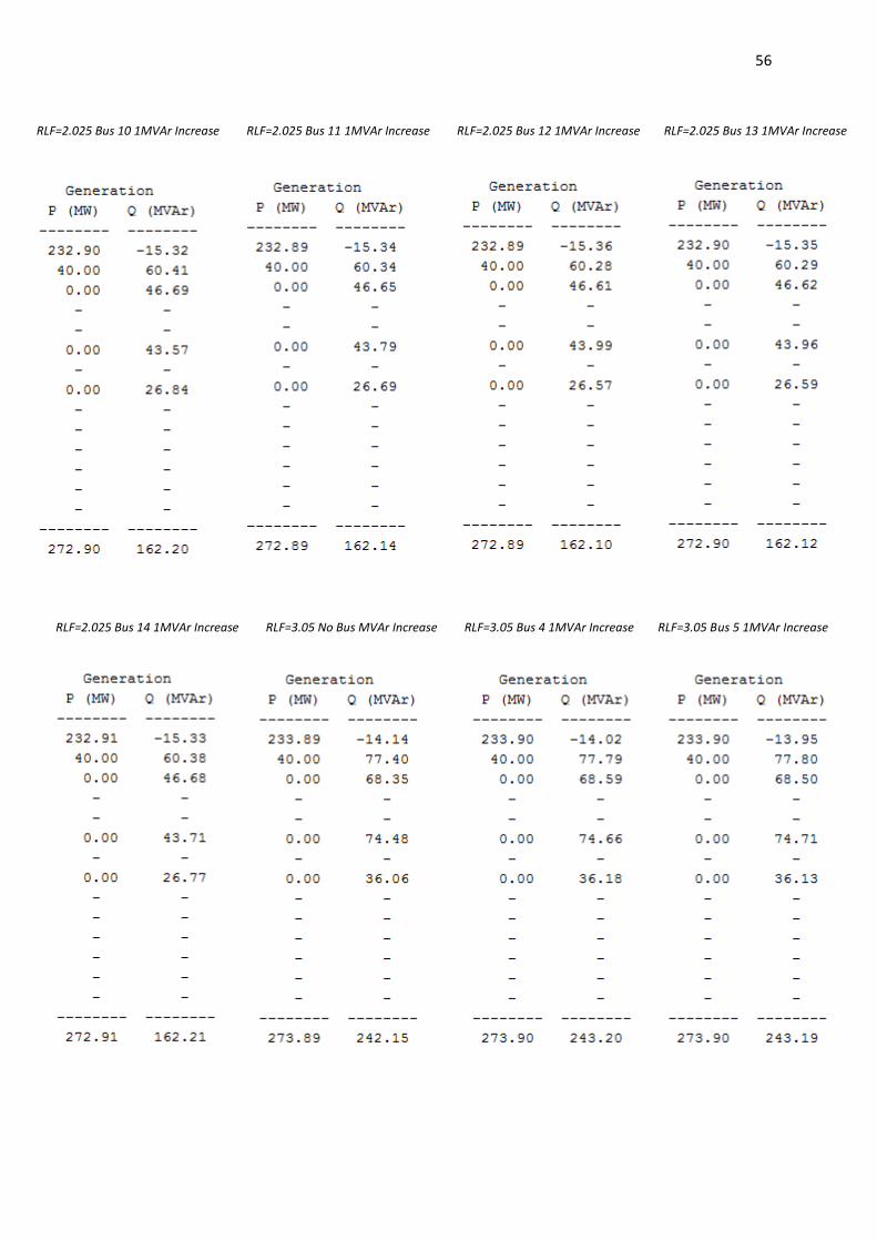
56

RLF=2.025 Bus 10 1MVAr Increase RLF=2.025 Bus 11 1MVAr Increase RLF=2.025 Bus 12 1MVAr Increase RLF=2.025 Bus 13 1MVAr Increase

RLF=2.025 Bus 14 1MVAr Increase RLF=3.05 No Bus MVAr Increase RLF=3.05 Bus 4 1MVAr Increase RLF=3.05 Bus 5 1MVAr Increase

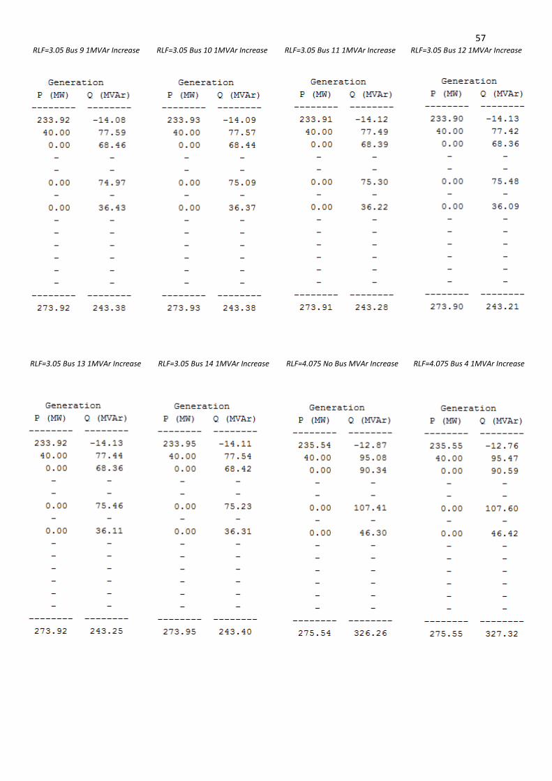
57

RLF=3.05 Bus 9 1MVAr Increase RLF=3.05 Bus 10 1MVAr Increase RLF=3.05 Bus 11 1MVAr Increase RLF=3.05 Bus 12 1MVAr Increase

RLF=3.05 Bus 13 1MVAr Increase RLF=3.05 Bus 14 1MVAr Increase RLF=4.075 No Bus MVAr Increase RLF=4.075 Bus 4 1MVAr Increase

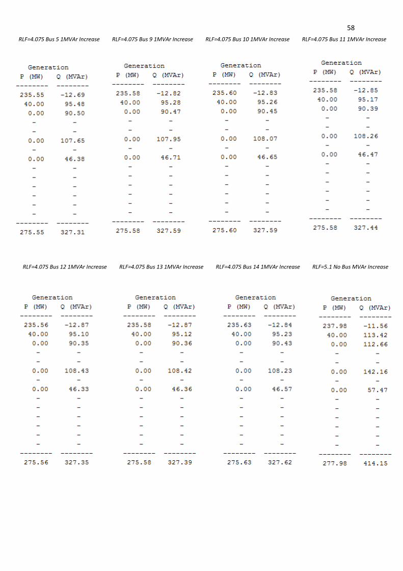
58

RLF=4.075 Bus 5 1MVAr Increase RLF=4.075 Bus 9 1MVAr Increase RLF=4.075 Bus 10 1MVAr Increase RLF=4.075 Bus 11 1MVAr Increase

RLF=4.075 Bus 12 1MVAr Increase RLF=4.075 Bus 13 1MVAr Increase RLF=4.075 Bus 14 1MVAr Increase RLF=5.1 No Bus MVAr Increase

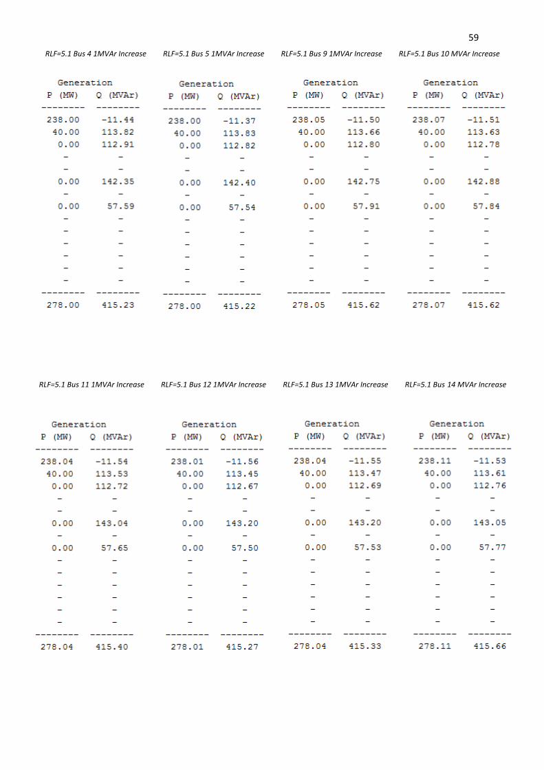
59

RLF=5.1 Bus 4 1MVAr Increase RLF=5.1 Bus 5 1MVAr Increase RLF=5.1 Bus 9 1MVAr Increase RLF=5.1 Bus 10 MVAr Increase

RLF=5.1 Bus 11 1MVAr Increase RLF=5.1 Bus 12 1MVAr Increase RLF=5.1 Bus 13 1MVAr Increase RLF=5.1 Bus 14 MVAr Increase

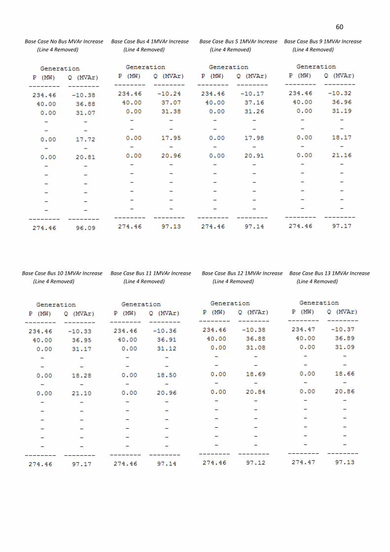
60

Base Case No Bus MVAr Increase Base Case Bus 4 1MVAr Increase Base Case Bus 5 1MVAr Increase Base Case Bus 9 1MVAr Increase

(Line 4 Removed) (Line 4 Removed) (Line 4 Removed) (Line 4 Removed)

Base Case Bus 10 1MVAr Increase Base Case Bus 11 1MVAr Increase Base Case Bus 12 1MVAr Increase Base Case Bus 13 1MVAr Increase

(Line 4 Removed) (Line 4 Removed) (Line 4 Removed) (Line 4 Removed)

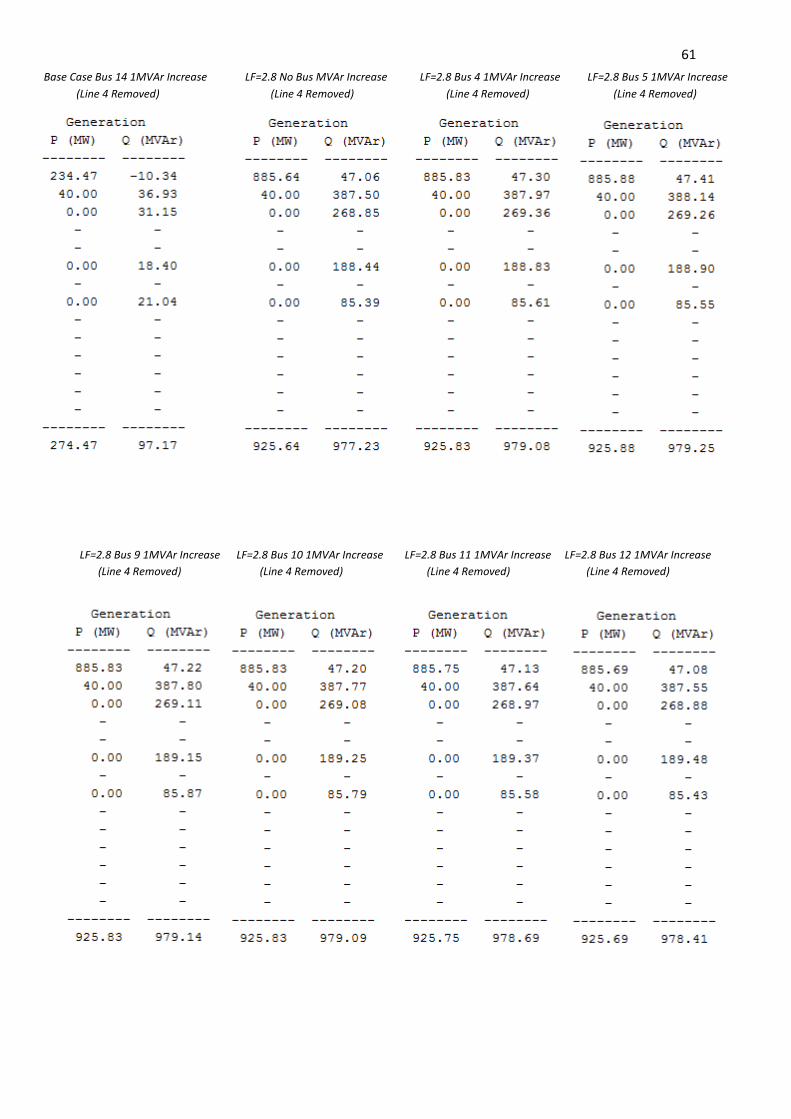
61

Base Case Bus 14 1MVAr Increase LF=2.8 No Bus MVAr Increase LF=2.8 Bus 4 1MVAr Increase LF=2.8 Bus 5 1MVAr Increase

(Line 4 Removed) (Line 4 Removed) (Line 4 Removed) (Line 4 Removed)

LF=2.8 Bus 9 1MVAr Increase LF=2.8 Bus 10 1MVAr Increase LF=2.8 Bus 11 1MVAr Increase LF=2.8 Bus 12 1MVAr Increase

(Line 4 Removed) (Line 4 Removed) (Line 4 Removed) (Line 4 Removed)

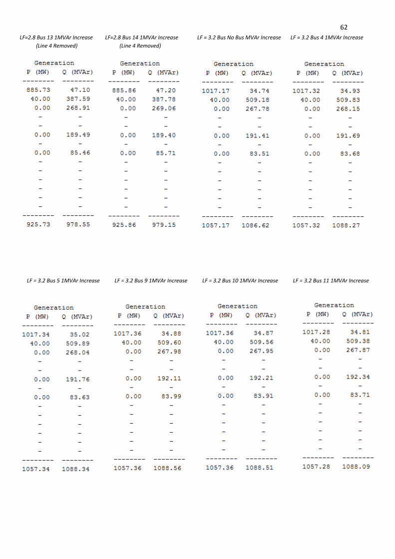
62

LF=2.8 Bus 13 1MVAr Increase LF=2.8 Bus 14 1MVAr Increase LF = 3.2 Bus No Bus MVAr Increase LF = 3.2 Bus 4 1MVAr Increase

(Line 4 Removed) (Line 4 Removed)

LF = 3.2 Bus 5 1MVAr Increase LF = 3.2 Bus 9 1MVAr Increase LF = 3.2 Bus 10 1MVAr Increase LF = 3.2 Bus 11 1MVAr Increase

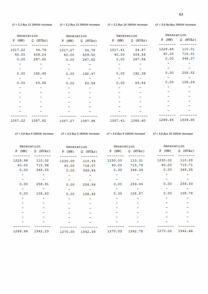
63

LF = 3.2 Bus 12 1MVAr Increase LF = 3.2 Bus 13 1MVAr Increase LF = 3.2 Bus 14 1MVAr Increase LF = 3.6 No Bus 1MVAr Increase

LF = 3.6 Bus 4 1MVAr Increase LF = 3.6 Bus 5 1MVAr Increase LF = 3.6 Bus 9 1MVAr Increase LF = 3.6 Bus 10 1MVAr Increase

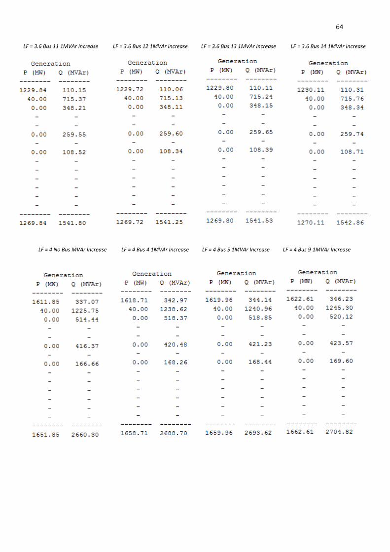
64

LF = 3.6 Bus 11 1MVAr Increase LF = 3.6 Bus 12 1MVAr Increase LF = 3.6 Bus 13 1MVAr Increase LF = 3.6 Bus 14 1MVAr Increase

LF = 4 No Bus MVAr Increase LF = 4 Bus 4 1MVAr Increase LF = 4 Bus 5 1MVAr Increase LF = 4 Bus 9 1MVAr Increase

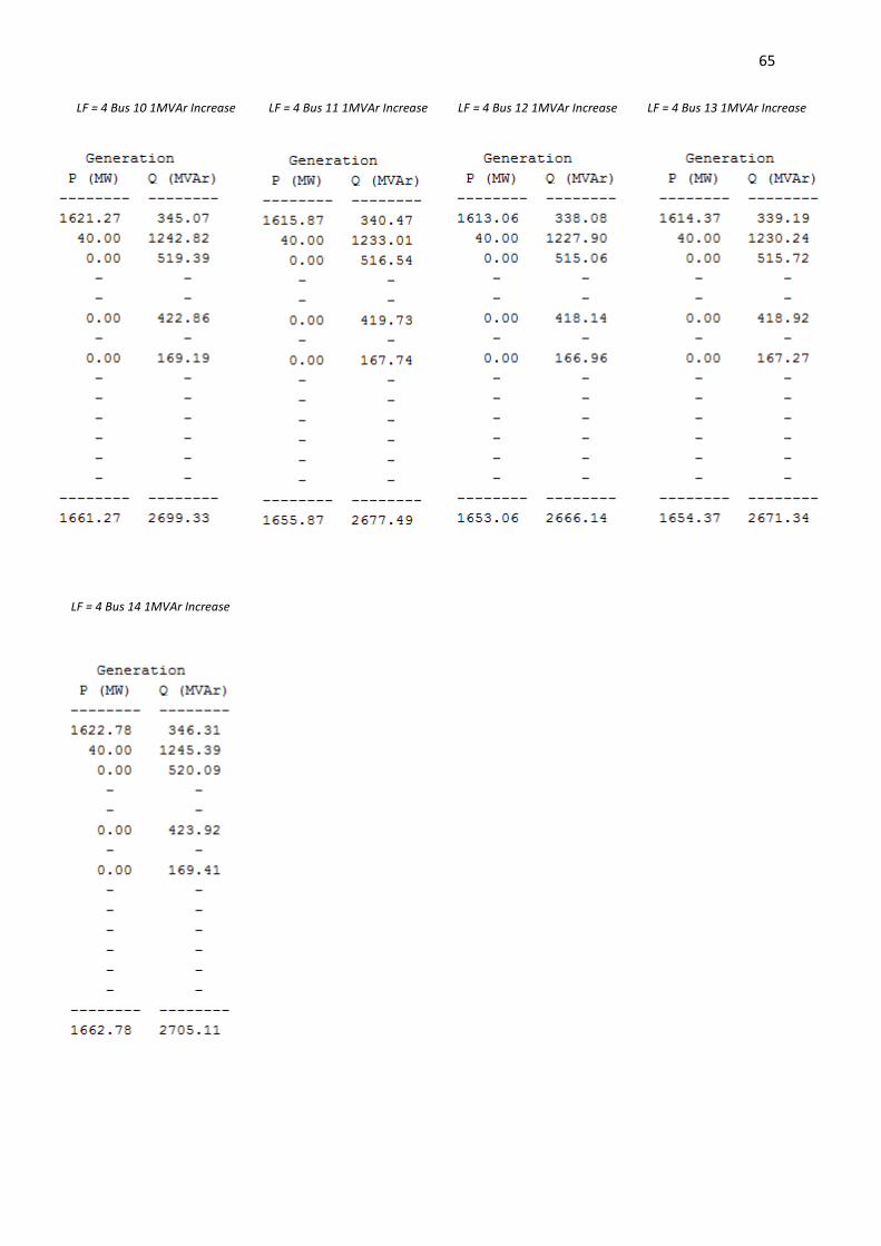
65

LF = 4 Bus 10 1MVAr Increase LF = 4 Bus 11 1MVAr Increase LF = 4 Bus 12 1MVAr Increase LF = 4 Bus 13 1MVAr Increase

LF = 4 Bus 14 1MVAr Increase

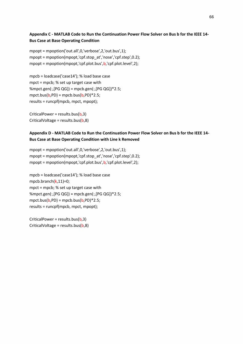
66

Appendix C - MATLAB Code to Run the Continuation Power Flow Solver on Bus b for the IEEE 14-

Bus Case at Base Operating Condition

mpopt = mpoption('out.all',0,'verbose',2,'out.bus',1);

mpopt = mpoption(mpopt,'cpf.stop_at','nose','cpf.step',0.2);

mpopt = mpoption(mpopt,'cpf.plot.bus',b,'cpf.plot.level',2);

mpcb = loadcase('case14'); % load base case

mpct = mpcb; % set up target case with

%mpct.gen(:,[PG QG]) = mpcb.gen(:,[PG QG])*2.5;

mpct.bus(b,PD) = mpcb.bus(b,PD)*2.5;

results = runcpf(mpcb, mpct, mpopt);

CriticalPower = results.bus(b,3)

CriticalVoltage = results.bus(b,8)

Appendix D - MATLAB Code to Run the Continuation Power Flow Solver on Bus b for the IEEE 14-

Bus Case at Base Operating Condition with Line k Removed

mpopt = mpoption('out.all',0,'verbose',2,'out.bus',1);

mpopt = mpoption(mpopt,'cpf.stop_at','nose','cpf.step',0.2);

mpopt = mpoption(mpopt,'cpf.plot.bus',b,'cpf.plot.level',2);

mpcb = loadcase('case14'); % load base case

mpcb.branch(k,11)=0;

mpct = mpcb; % set up target case with

%mpct.gen(:,[PG QG]) = mpcb.gen(:,[PG QG])*2.5;

mpct.bus(b,PD) = mpcb.bus(b,PD)*2.5;

results = runcpf(mpcb, mpct, mpopt);

CriticalPower = results.bus(b,3)

CriticalVoltage = results.bus(b,8)

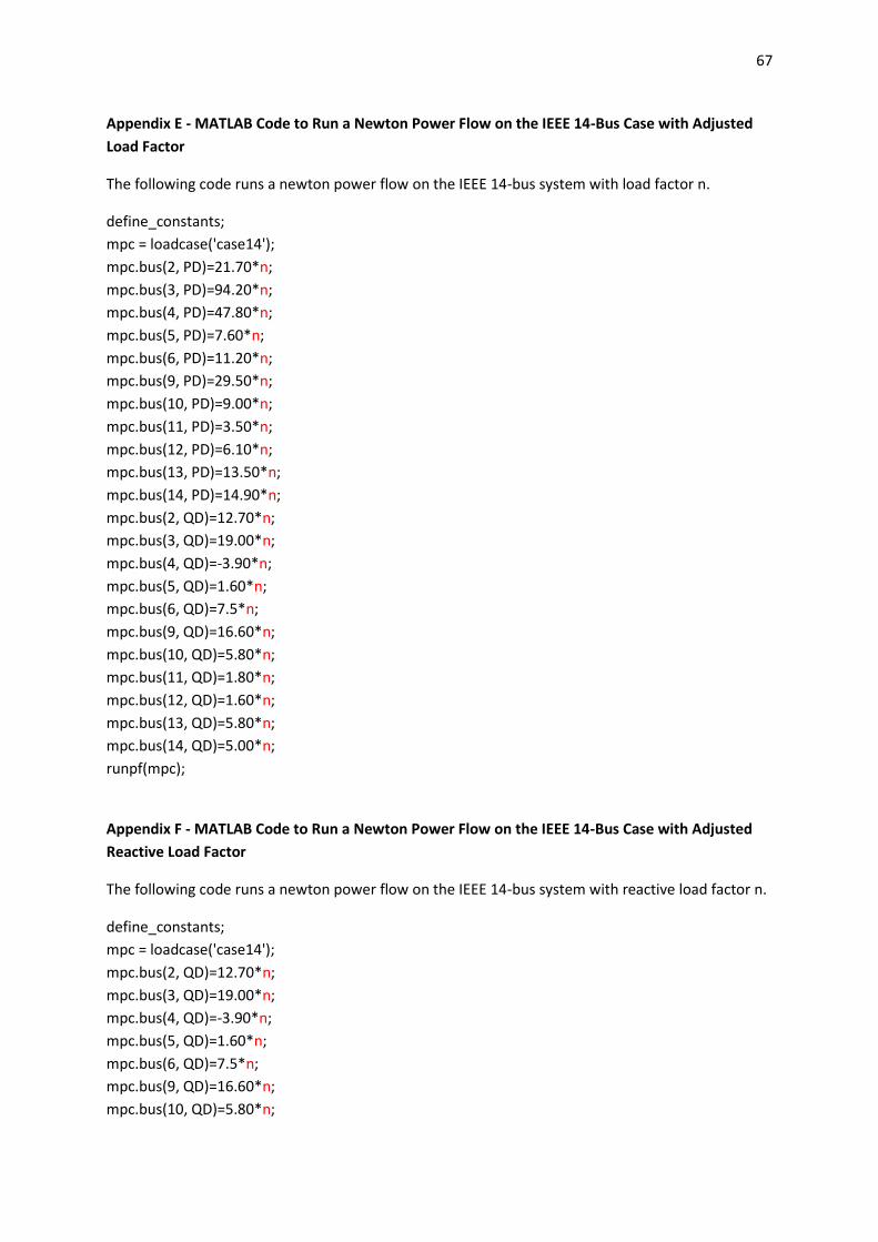
67

Appendix E - MATLAB Code to Run a Newton Power Flow on the IEEE 14-Bus Case with Adjusted

Load Factor

The following code runs a newton power flow on the IEEE 14-bus system with load factor n.

define_constants;

mpc = loadcase('case14');

mpc.bus(2, PD)=21.70*n;

mpc.bus(3, PD)=94.20*n;

mpc.bus(4, PD)=47.80*n;

mpc.bus(5, PD)=7.60*n;

mpc.bus(6, PD)=11.20*n;

mpc.bus(9, PD)=29.50*n;

mpc.bus(10, PD)=9.00*n;

mpc.bus(11, PD)=3.50*n;

mpc.bus(12, PD)=6.10*n;

mpc.bus(13, PD)=13.50*n;

mpc.bus(14, PD)=14.90*n;

mpc.bus(2, QD)=12.70*n;

mpc.bus(3, QD)=19.00*n;

mpc.bus(4, QD)=-3.90*n;

mpc.bus(5, QD)=1.60*n;

mpc.bus(6, QD)=7.5*n;

mpc.bus(9, QD)=16.60*n;

mpc.bus(10, QD)=5.80*n;

mpc.bus(11, QD)=1.80*n;

mpc.bus(12, QD)=1.60*n;

mpc.bus(13, QD)=5.80*n;

mpc.bus(14, QD)=5.00*n;

runpf(mpc);

Appendix F - MATLAB Code to Run a Newton Power Flow on the IEEE 14-Bus Case with Adjusted

Reactive Load Factor

The following code runs a newton power flow on the IEEE 14-bus system with reactive load factor n.

define_constants;

mpc = loadcase('case14');

mpc.bus(2, QD)=12.70*n;

mpc.bus(3, QD)=19.00*n;

mpc.bus(4, QD)=-3.90*n;

mpc.bus(5, QD)=1.60*n;

mpc.bus(6, QD)=7.5*n;

mpc.bus(9, QD)=16.60*n;

mpc.bus(10, QD)=5.80*n;

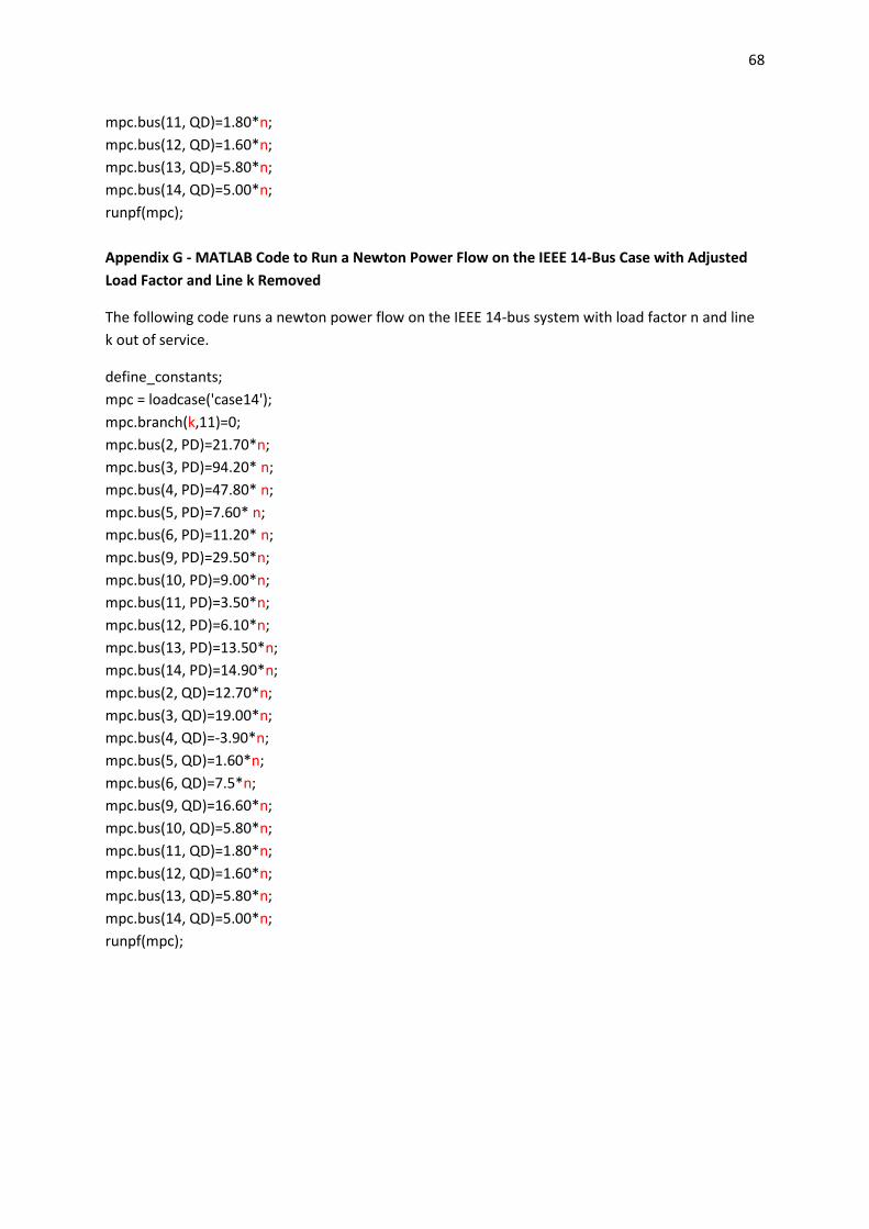
68

mpc.bus(11, QD)=1.80*n;

mpc.bus(12, QD)=1.60*n;

mpc.bus(13, QD)=5.80*n;

mpc.bus(14, QD)=5.00*n;

runpf(mpc);

Appendix G - MATLAB Code to Run a Newton Power Flow on the IEEE 14-Bus Case with Adjusted

Load Factor and Line k Removed

The following code runs a newton power flow on the IEEE 14-bus system with load factor n and line

k out of service.

define_constants;

mpc = loadcase('case14');

mpc.branch(k,11)=0;

mpc.bus(2, PD)=21.70*n;

mpc.bus(3, PD)=94.20* n;

mpc.bus(4, PD)=47.80* n;

mpc.bus(5, PD)=7.60* n;

mpc.bus(6, PD)=11.20* n;

mpc.bus(9, PD)=29.50*n;

mpc.bus(10, PD)=9.00*n;

mpc.bus(11, PD)=3.50*n;

mpc.bus(12, PD)=6.10*n;

mpc.bus(13, PD)=13.50*n;

mpc.bus(14, PD)=14.90*n;

mpc.bus(2, QD)=12.70*n;

mpc.bus(3, QD)=19.00*n;

mpc.bus(4, QD)=-3.90*n;

mpc.bus(5, QD)=1.60*n;

mpc.bus(6, QD)=7.5*n;

mpc.bus(9, QD)=16.60*n;

mpc.bus(10, QD)=5.80*n;

mpc.bus(11, QD)=1.80*n;

mpc.bus(12, QD)=1.60*n;

mpc.bus(13, QD)=5.80*n;

mpc.bus(14, QD)=5.00*n;

runpf(mpc);

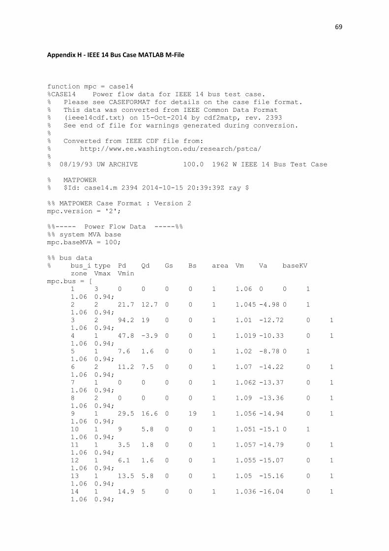
69

Appendix H - IEEE 14 Bus Case MATLAB M-File

function mpc = case14

%CASE14 Power flow data for IEEE 14 bus test case.

% Please see CASEFORMAT for details on the case file format.

% This data was converted from IEEE Common Data Format

% (ieee14cdf.txt) on 15-Oct-2014 by cdf2matp, rev. 2393

% See end of file for warnings generated during conversion.

%

% Converted from IEEE CDF file from:

% http://www.ee.washington.edu/research/pstca/

%

% 08/19/93 UW ARCHIVE 100.0 1962 W IEEE 14 Bus Test Case

% MATPOWER

% $Id: case14.m 2394 2014-10-15 20:39:39Z ray $

%% MATPOWER Case Format : Version 2

mpc.version = '2';

%%----- Power Flow Data -----%%

%% system MVA base

mpc.baseMVA = 100;

%% bus data

% bus_i type Pd Qd Gs Bs area Vm Va baseKV

zone Vmax Vmin

mpc.bus = [

1 3 0 0 0 0 1 1.06 0 0 1

1.06 0.94;

2 2 21.7 12.7 0 0 1 1.045 -4.98 0 1

1.06 0.94;

3 2 94.2 19 0 0 1 1.01 -12.72 0 1

1.06 0.94;

4 1 47.8 -3.9 0 0 1 1.019 -10.33 0 1

1.06 0.94;

5 1 7.6 1.6 0 0 1 1.02 -8.78 0 1

1.06 0.94;

6 2 11.2 7.5 0 0 1 1.07 -14.22 0 1

1.06 0.94;

7 1 0 0 0 0 1 1.062 -13.37 0 1

1.06 0.94;

8 2 0 0 0 0 1 1.09 -13.36 0 1

1.06 0.94;

9 1 29.5 16.6 0 19 1 1.056 -14.94 0 1

1.06 0.94;

10 1 9 5.8 0 0 1 1.051 -15.1 0 1

1.06 0.94;

11 1 3.5 1.8 0 0 1 1.057 -14.79 0 1

1.06 0.94;

12 1 6.1 1.6 0 0 1 1.055 -15.07 0 1

1.06 0.94;

13 1 13.5 5.8 0 0 1 1.05 -15.16 0 1

1.06 0.94;

14 1 14.9 5 0 0 1 1.036 -16.04 0 1

1.06 0.94;

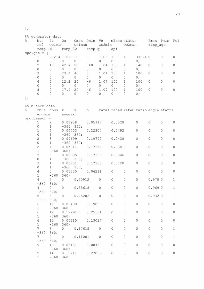
70

];

%% generator data

% bus Pg Qg Qmax Qmin Vg mBase status Pmax Pmin Pc1

Pc2 Qc1min Qc1max Qc2min Qc2max ramp_agc

ramp_10 ramp_30 ramp_q apf

mpc.gen = [

1 232.4 -16.9 10 0 1.06 100 1 332.4 0 0 0

0 0 0 0 0 0 0 0 0;

2 40 42.4 50 -40 1.045 100 1 140 0 0 0

0 0 0 0 0 0 0 0 0;

3 0 23.4 40 0 1.01 100 1 100 0 0 0

0 0 0 0 0 0 0 0 0;

6 0 12.2 24 -6 1.07 100 1 100 0 0 0

0 0 0 0 0 0 0 0 0;

8 0 17.4 24 -6 1.09 100 1 100 0 0 0

0 0 0 0 0 0 0 0 0;

];

%% branch data

% fbus tbus r x b rateA rateB rateC ratio angle status

angmin angmax

mpc.branch = [

1 2 0.01938 0.05917 0.0528 0 0 0 0

0 1 -360 360;

1 5 0.05403 0.22304 0.0492 0 0 0 0

0 1 -360 360;

2 3 0.04699 0.19797 0.0438 0 0 0 0

0 1 -360 360;

2 4 0.05811 0.17632 0.034 0 0 0 0 0

1 -360 360;

2 5 0.05695 0.17388 0.0346 0 0 0 0

0 1 -360 360;

3 4 0.06701 0.17103 0.0128 0 0 0 0

0 1 -360 360;

4 5 0.01335 0.04211 0 0 0 0 0 0

1 -360 360;

4 7 0 0.20912 0 0 0 0 0.978 0 1

-360 360;

4 9 0 0.55618 0 0 0 0 0.969 0 1

-360 360;

5 6 0 0.25202 0 0 0 0 0.932 0 1

-360 360;

6 11 0.09498 0.1989 0 0 0 0 0 0

1 -360 360;

6 12 0.12291 0.25581 0 0 0 0 0 0

1 -360 360;

6 13 0.06615 0.13027 0 0 0 0 0 0

1 -360 360;

7 8 0 0.17615 0 0 0 0 0 0 1

-360 360;

7 9 0 0.11001 0 0 0 0 0 0 1

-360 360;

9 10 0.03181 0.0845 0 0 0 0 0 0

1 -360 360;

9 14 0.12711 0.27038 0 0 0 0 0 0

1 -360 360;

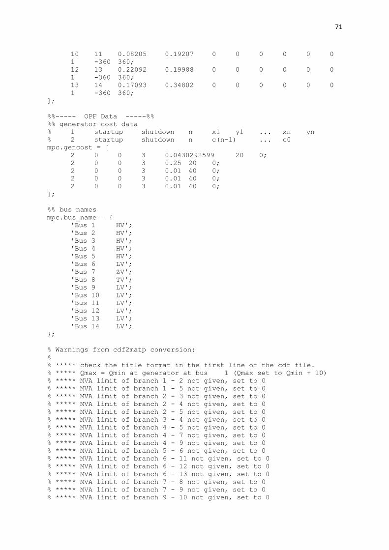
71

10 11 0.08205 0.19207 0 0 0 0 0 0

1 -360 360;

12 13 0.22092 0.19988 0 0 0 0 0 0

1 -360 360;

13 14 0.17093 0.34802 0 0 0 0 0 0

1 -360 360;

];

%%----- OPF Data -----%%

%% generator cost data

% 1 startup shutdown n x1 y1 ... xn yn

% 2 startup shutdown n c(n-1) ... c0

mpc.gencost = [

2 0 0 3 0.0430292599 20 0;

2 0 0 3 0.25 20 0;

2 0 0 3 0.01 40 0;

2 0 0 3 0.01 40 0;

2 0 0 3 0.01 40 0;

];

%% bus names

mpc.bus_name = {

'Bus 1 HV';

'Bus 2 HV';

'Bus 3 HV';

'Bus 4 HV';

'Bus 5 HV';

'Bus 6 LV';

'Bus 7 ZV';

'Bus 8 TV';

'Bus 9 LV';

'Bus 10 LV';

'Bus 11 LV';

'Bus 12 LV';

'Bus 13 LV';

'Bus 14 LV';

};

% Warnings from cdf2matp conversion:

%

% ***** check the title format in the first line of the cdf file.

% ***** Qmax = Qmin at generator at bus 1 (Qmax set to Qmin + 10)

% ***** MVA limit of branch 1 - 2 not given, set to 0

% ***** MVA limit of branch 1 - 5 not given, set to 0

% ***** MVA limit of branch 2 - 3 not given, set to 0

% ***** MVA limit of branch 2 - 4 not given, set to 0

% ***** MVA limit of branch 2 - 5 not given, set to 0

% ***** MVA limit of branch 3 - 4 not given, set to 0

% ***** MVA limit of branch 4 - 5 not given, set to 0

% ***** MVA limit of branch 4 - 7 not given, set to 0

% ***** MVA limit of branch 4 - 9 not given, set to 0

% ***** MVA limit of branch 5 - 6 not given, set to 0

% ***** MVA limit of branch 6 - 11 not given, set to 0

% ***** MVA limit of branch 6 - 12 not given, set to 0

% ***** MVA limit of branch 6 - 13 not given, set to 0

% ***** MVA limit of branch 7 - 8 not given, set to 0

% ***** MVA limit of branch 7 - 9 not given, set to 0

% ***** MVA limit of branch 9 - 10 not given, set to 0

72

% ***** MVA limit of branch 9 - 14 not given, set to 0

% ***** MVA limit of branch 10 - 11 not given, set to 0

% ***** MVA limit of branch 12 - 13 not given, set to 0

% ***** MVA limit of branch 13 - 14 not given, set to 0