Embed Size (px)
Citation preview

FINAL REPORT TONATIONAL COUNCIL FOR SOVIET AND EAST EUROPEAN RESEARC H
TITLE : The Regional Economy of the Soviet Union :An Economic Modeling Study
AUTHOR : Fyodor I . Kushnirsky
CONTRACTOR : Wharton Econometric Forecasting Associates
PRINCIPAL INVESTIGATOR : Fyodor I . Kushnirsky
COUNCIL CONTRACT NUMBER : 625-6
DATE : October 1, 198 4
The work leading to this report was supported in whole or i npart from funds provided by the National Council for Sovie tand East European Research .

EXECUTIVE SUMMAR Y
This report describes the construction of a multiregiona leconometric model of the Soviet Union . The model is composed o f91 blocks of equations : a macroeconomic block for the USSR as a whole ,macroeconomic blocks for each of the 15 union republics, and 75 sectora lblocks for each republic . The sectors identified in the model are :Industry, Agriculture and Forestry, Transportation and Communications ,Construction, and Trade and Other Productive Branches .
The aim of building the model is to analyze and forecast the primar yindicators of spatial developments in the Soviet economy . The model wa sdesigned so that the relationships among regional, industrial, an dnational indicators would be simple and follow a step-by-step procedur eof planning calculations . This required considering some methodologica lproblems related to particular features of the Soviet economy . Amongthese are the role of the components of the final demands, the treatmen tof variables as endogenous or exogenous, definition of saving ,interpretation of government spending, complications arising from th erole of the regional aspect, and effects of the constraints on mai ngroups of inputs .
Interdependence among the variables is determined in the model' sstructure by their connections with the macroeconomic block and by th efeedback from the macrolevel to all sectors of the economy . In eac hrepublic block of the model, thera is an input-output table indicatin gtechnological dependence of a sector on other sectors in and outside th erepublic . Distributional relationships with the union budget indicat efor a republic and its sectors the dependence on the development of al lother republics .
In order to develop a technique for solving the econometric system ,incorporating input-output tables so that the values of output and fina ldemand are mutually adjusted and justified, a special econometri caccelerator was combined with an input-output multiplier . Th epossibility of treating the components of final demand and gross outpu tas exogenous was presented by the inclusion of a mechanism to captur ethe feedback to gross outputs from the final demands, which are both th eresult of current productive activity and (as a source of investment) afactor of economic growth .
The information on which the model is based consists of time serie sfor sector, republic, and union indicators . These include observation sfor 1965-1980 that are either official data or estimates . In total ,there are 75 republic data files and a union data file . The followin gindicators form the republic files : gross value of output, net value o foutput, capital stock, investment, investment minus depreciation fo rreplacement, wages, profits, depreciation, depreciation for
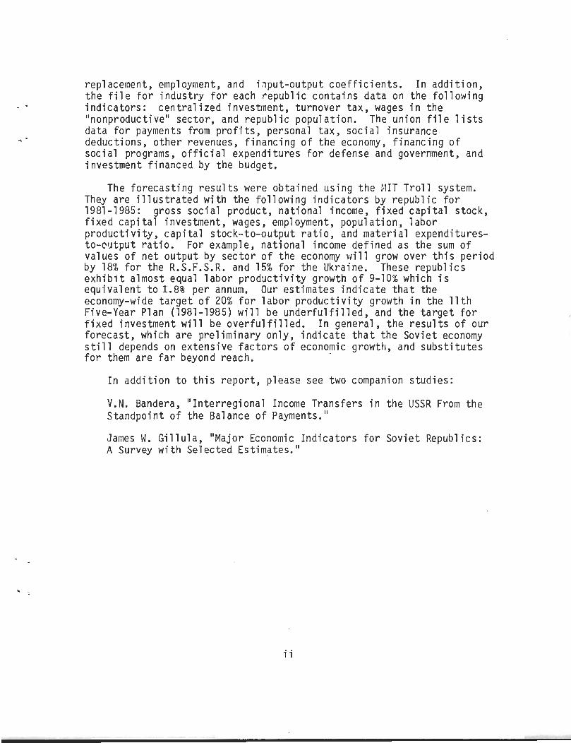
replacement, employment, and input-output coefficients . In addition ,the file for industry for each republic contains data on the followin gindicators : centralized investment, turnover tax, wages in th e" nonproductive " sector, and republic population . The union file list sdata for payments from profits, personal tax, social insuranc edeductions, other revenues, financing of the economy, financing o fsocial programs, official expenditures for defense and government, an dinvestment financed by the budget .
The forecasting results were obtained using the MIT Troll system .They are illustrated with the following indicators by republic fo r1981-1985 : gross social product, national income, fixed capital stock ,fixed capital investment, wages, employment, population, labo rproductivity, capital stock-to-output ratio, and materia
l expenditures-to-output ratio. For example, national income defined as the sum ofvalues of net output by sector of the economy will grow over this perio dby 18% for the R .S .F.S .R . and 15% for the Ukraine . These republic sexhibit almost equal labor productivity growth of 9-10% which i sequivalent to 1 .8% per annum . Our estimates indicate that th eeconomy-wide target of 20% for labor productivity growth in the 11t hFive-Year Plan (1981-1985) will be underfulfilled, and the target fo rfixed investment will be overfulfilled . In general, the results of ourforecast, which are preliminary only, indicate that the Soviet econom ystill depends on extensive factors of economic growth, and substitute sfor them are far beyond reach .
In addition to this report, please see two companion studies :
V .N . Bandera, " Interregional Income Transfers in the USSR From th eStandpoint of the Balance of Payments . "
James W . Gillula, " Major Economic Indicators for Soviet Republics :A Survey with Selected Estimates . "
ii

Table of Content s
Chapter
Page
1. Introduction 1
2. Particular Features of a Planned Economy and It sRegional Aspect 4
3. The Structure of the Model 9
4. Input-Output Tables Within the Econometric Model 1 9
5. The Data and Their Sources 28
6 . Illustration of the Forecasting Results 3 7
References 45
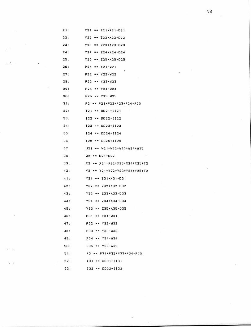
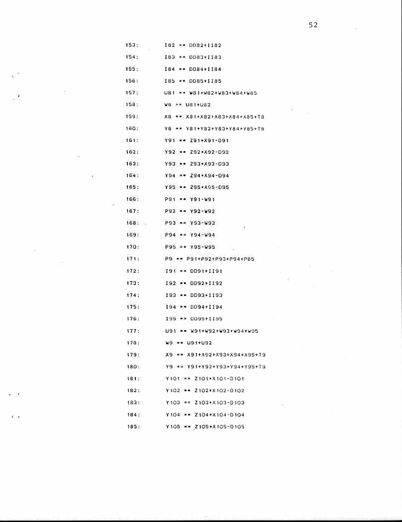
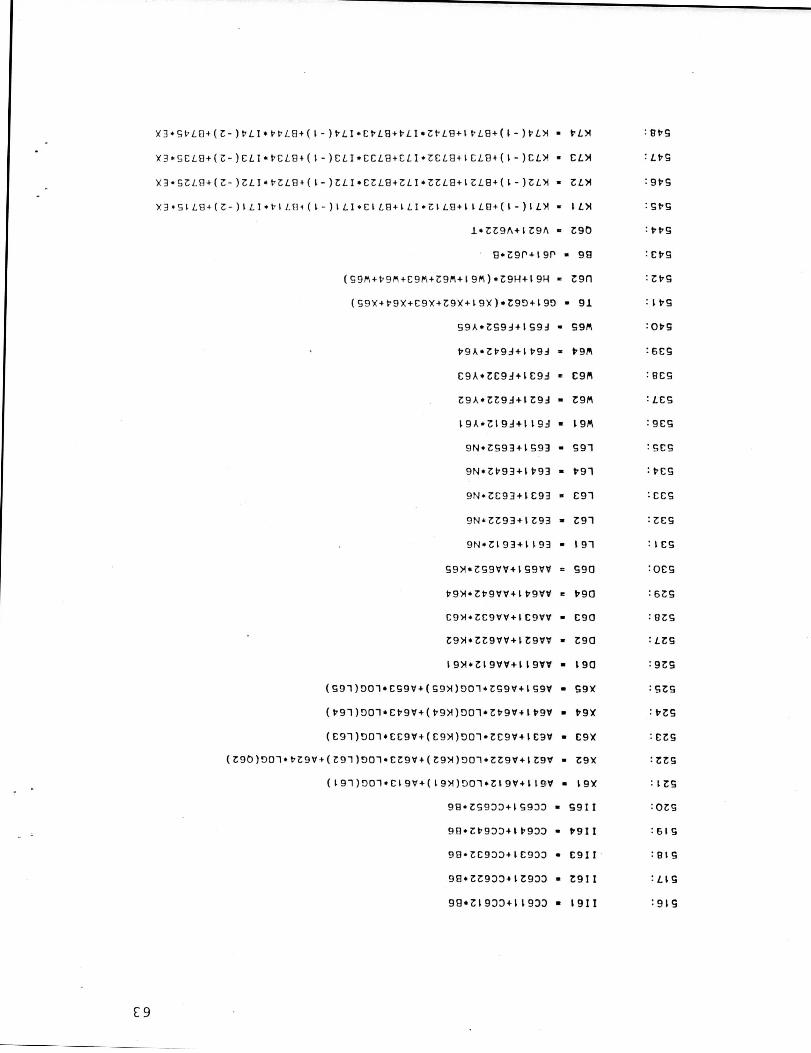
Appendix . The List of Equations 47
111

1
1 . INTRODUCTIO N
Regional analysis has always played an important role in Sovie t
economic planning . Relevant problems have become increasingly importan t
since the 1965 Economic Reform, which reintroduced the vertical branc h
principle of management . Resource distribution is centered in th e
all-union branch ministries that have gained sole control over material an d
financial allocations for industries with all-union and union-republi c
subordination of enterprises . Ministries in the Soviet Union receiv e
allocations directly from Gosplan, and the Council of Ministers oversee s
the distribution of the most important materials and equipment . Thi s
branch-line centralization has contributed to long-term deterioration o f
economic conditions in many provincial regions and, as a consequence ,
stimulated attempts to coordinate the branch and the territorial approache s
to plannning . Another factor responsible for this deterioration was th e
lack of coordination of growing inter-industrial dependence on loca l
sources of labor, water supply, sewage systems, transportation, roa d
construction, as well as land allocation and pollution problems .
Furthermore, future developments in the Soviet economy may draw th e
attention of analysts to the regional aspects of planning . Proposals t o
develop and increase the role of territorial structures have been prominen t
in recent discussions of economic reform .
Among the most important regional indicators are thos e
characterizing economic growth, investment, employment, productivity ,
population, standards of living, etc . Much effort has been devoted by
Western scholars to studying regional differences in Soviet economic

2
growth, productivity, investment, etc . The recent publication edited b y
Koropeckyj and Schroeder (1981) is an example of comprehensive analysis o f
the development of Soviet republics and economic regions . Among others ,
studies on republic input-output tables (see Gillula (1977)), Sovie t
regional modeling (see Bond (1980)), and republic economic development (se e
Koropeckyj, ed . (1977) and Bandera and Melnyk (1973)) could be mentioned) .
There is little need to stress the importance of the econometri c
modeling of Soviet regional developments . But particular features of th e
planned economy such as the regulation of almost all aspects of economi c
activity, the role of distributional mechanisms, and the clos e
relationships between regional economic units and the state budget an d
other macroindicators are factors that require special methods o f
analysis . Though the nature of the information available on the Sovie t
economy is an important consideration because of numerous gaps ,
discrepancies, and inconsistency in the data, statistical inference prove s
to be fruitful due to the close interdependence among the economi c
indicators . An example of successful Western studies of the Sovie t
national economy based on this approach is the WEFA Soviet econometri c
model, SOVMOD (see Green and Higgins (1977)) .
To some extent, the multiregional econometric model described i n
this report is an extension of the WEFA Soviet econometric model in th e
spatial dimension of the Soviet economy . But the model described here i s
primarily designed to be close to Soviet planning methodology itself i n
explaining direct and feedback connections among regional, industrial, an d
national indicators . The experience of the author in economic planning an d
econometric modeling in the Soviet Union is reflected in this study . For

example, this experience suggests that simple relationships among th e
indicators in a model following the step-by-step procedure of plannin g
calculations usually operate better than complicated explanatory
equations . While, for many reasons, the size of the model itself may no t
be too significant, the adequacy of economic information and the technique s
employed are very important issues .
The purpose of this report is to present the results of building a
multiregional econometric model of the Soviet Union . The fifteen Sovie t
republics, with five sectors of the economy represented in each, along wit h
the national macrolevel, are the block units and subdivisions of th e
model . At its present stage, the model incorporates some 900 equations ,
relationships, and conditions .
The contents of the report are divided into chapters illustratin g
the methodological problems of building the model, the structure of th e
model, and the problem of incorporating input-output tables, the data an d
their sources, and some applications . The results presented, especiall y
those concerning the structure and specification of the model, are
necessarily fragmentary . A full list of the model's equations is given i n
the appendix .

4
2 . PARTICULAR FEATURES OF A PLANNED ECONOMY AND ITS REGIONAL ASPEC T
Without presenting a complete description of a planned economy, w e
would like to make some comments on the specific character of such a n
economy which needs to be taken into account in macroeconomic modeling . To
some extent, there are similarities in the modeling of free-market an d
planned economies . In both cases, one deals with consumption, investment ,
production, technological constraints, prices, income distribution, etc .
On the other hand, the procedures that determine the outcome of forecast s
in each case are different, and not only in the interpretation of variable s
or political and ideological phraseology .
In a model of a free-market economy, components of final demand pla y
the determining role . For a planned economy, the situation is different .
Simplifying the matter, it could be said that not only does consumption no t
play a determining role, but it is doubtful that planners even know wha t
consumers would like to buy . More attention is paid to the demands o f
enterprises for raw materials, energy, and equipment distributed throug h
the system of material supply . Moreover, enterprises do not "buy" thes e
goods, and money is used in the supply system only for accounting . Ex-ante
market demand of the population in the sense of what people want to bu y
cannot be estimated from the data available . Instead, there is a differen t
sort of demand -- the so-called "satisfied demand" -- which is used i n
planning and statistics . It is determined by the level of output an d
priorities for the current period and, most important, by the patterns o f
outputs and inputs developed in the previous period . It is clear that thi s
ex-post demand is actually supply and, therefore, the computationa l
sequence should be the reverse of that for a free-market economy .
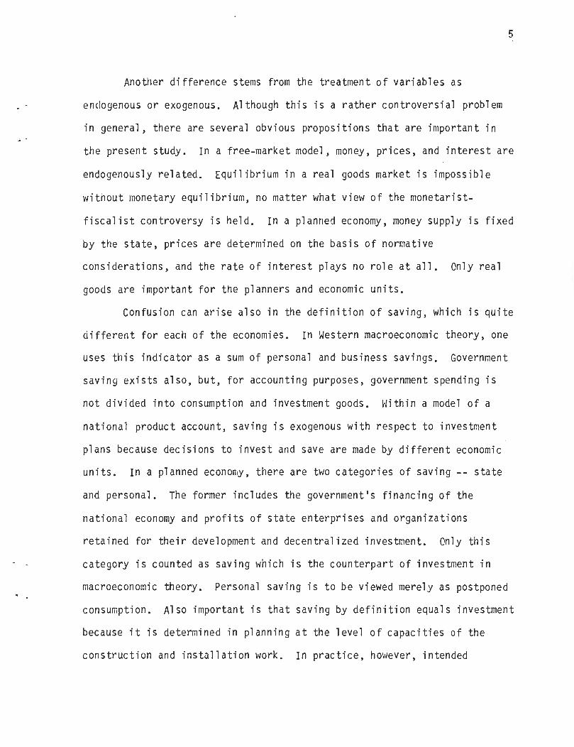
Another difference stems from the treatment of variables a s
endogenous or exogenous . Although this is a rather controversial proble m
in general, there are several obvious propositions that are important i n
the present study . In a free-market model, money, prices, and interest ar e
endogenously related . Equilibrium in a real goods market is impossibl e
without monetary equilibrium, no matter what view of the monetarist-
-fiscalist controversy is held . In a planned economy, money supply is fixe d
by the state, prices are determined on the basis of normativ e
considerations, and the rate of interest plays no role at all . Only rea l
goods are important for the planners and economic units .
Confusion can arise also in the definition of saving, which is quit e
different for each of the economies . In Western macroeconomic theory, on e
uses this indicator as a sum of personal and business savings . Governmen t
saving exists also, but, for accounting purposes, government spending i s
not divided into consumption and investment goods . Within a model of a
national product account, saving is exogenous with respect to investmen t
plans because decisions to invest and save are made by different economi c
units . In a planned economy, there are two categories of saving -- stat e
and personal . The former includes the government's financing of th e
national economy and profits of state enterprises and organization s
retained for their development and decentralized investment . Only thi s
category is counted as saving which is the counterpart of investment i n
macroeconomic theory . Personal saving is to be viewed merely as postpone d
consumption . Also important is that saving by definition equals investmen t
because it is determined in planning at the level of capacities of th e
construction and installation work . In practice, however, intended

6
investment is different from actual saving since the construction industr y
and industrial suppliers fail to meet their plan targets . Therefore, in a
planned economy, the macroproblem of equilibrium between investment an d
saving involves both macro- and microlevels of the decision-making process ,
with the implication of direct and feedback relationships between them ,
The interpretation of government spending is another potentia l
source of confusion . In a planned economy, government spending should no t
be separated from consumption and investment in national produc t
accounting . Consumption, investment, and net exports should be the onl y
items in the national product . Within consumption, personal and publi c
categories can be separated, the latter equal to government spending fo r
housing, municipal services, health, education, administration, defense ,
and other institutions of the "nonmaterial" sphere serving the population .
And within investment, almost all will be public .
For the regional aspect of the modeling of a planned economy ,
distinguishing several definitions of national income is important . Of th e
three kinds of national income -- produced, distributed, and utilized - -
the third is a crucial problem in regional planning . The first (produced )
is similar by definition to the net national product measured as the ne t
value added of enterprises producing material goods and services . Th e
second (distributed) is close to the national income defined as a sum o f
incomes of state enterprises, organizations, and employees . The third
(utilized) is similar to the final demands for goods and services, but i n
the sense defined above, i .e ., "satisfied demand ." For the Soviet Union a s
a whole, the differences among all three kinds of income are caused b y
losses, errors, and omissions . For Soviet republics, however, the level of

7
"satisfied demand" can vary, with an implication that utilized income i s
not equal to that produced . When income utilized in a republic is lowe r
than that produced, the republic's product is greater than actua l
consumption and capital accumulation (basically, the latter equals fixe d
investment plus increase in inventory) . This means that some part of th e
product is distributed elsewhere in the country without compensation to th e
republic . Therefore, republic investment does not necessarily depend full y
on the operation of its enterprises and saving may not be equal to th e
value of investment goods .
In regional planning, the meaning of variables is not as obvious a s
for the nation as a whole . In the Soviet Union, there are three categorie s
of enterprises and organizations -- union, union-republic, and republic - -
and, according to the present economic organization, only the last belong s
to the republic economy . But at the final stage of the development of a
detailed draft plan, indicators of the so-called comprehensive territoria l
plan are computed . They cover all enterprises and organizations in th e
republic, regardless of their category . In the regional units of th e
econometric model discussed below, indicators are defined in accordanc e
with the comprehensive territorial plan .
Such a breakdown of the economy, when some industries have direc t
vertical connections with the macrolevel and some interact with it onl y
through horizontal republic institutions, is reflected in the model wit h
two types of relationships . The first shows direct flows of payments ou t
of profits, social insurance deductions, and others from industries to th e
states budget . And the second involves the intermediate territorial leve l
for relevant indicators such as turnover tax, taxes on the population, etc .

8
To some extent, these relationships imitate a dual principle of managemen t
-- branch and territorial -- where the priority belongs to the former .
Informational flows of three stages of planning -- control figures ,
draft plan, and assignment of the targets to executors -- differ wit h
respect to direction, purpose, content, and the degree of aggregation . Th e
purpose of the first stage is to determine aggregate guidelines for al l
economic units with the use of some hypotheses, assumptions, and goals se t
up on the basis of the normative approach . The results of modeling ca n
explain the main technological relationships of this stage of planning a t
some level of formalization and aggregation .
There are some principles of computation at the first stage o f
planning mentioned above that must be taken into consideration in th e
modeling methodology . The procedure has an iterative character due to th e
fact that industrial variable s. starting the sequence of calculations depen d
on the output of the system as a whole . In other words, all economic unit s
of the system need information as to the limits of resources that can b e
allocated to them . The reason for this iterative organization o f
calculations is that the approximate output of the system is to be foun d
first . Only then can the resources resulting from it be distributed, an d
the technological sequence of calculations start . Further, the initia l
version of output is corrected, and, on the next iteration, changes ar e
made in the values of all indicators in the same order as on the firs t
iteration . In the model, this procedure is reflected in a set of feedback s
from the state budget variables, itemizing the financing of the nationa l
economy, to the indicators of industrial development .
Thus, to start calculations at the stage of control figures, initia l
constraints for major groups of resources -- labor, investment, and ra w
materials -- must be known . Ordering and distributing material inputs i n
physical terms is a perpetual process which starts before and ends afte r
the plan of production is confirmed . For this reason, constraints o n
material inputs are practically not taken into account at the contro l
figures stage, which causes numerous complications and corrections at othe r
stages . What industries and regional units have to know at this stage i s
their limits on labor force and investment . While constraints for th e
former are determined precisely enough at the republic level (with the use
of horizontal links), the latter is distribute strictly on the vertica l
principle . Only when ministries, departments, and republics acquir e
information on these limits, can they start compiling their plan targets .
This iterative process is interpreted in the model with simultaneou s
calculations of indicators at macro- and microlevels of the economy .
3 . THE STRUCTURE OF THE MODE L
The general structure of the model consists of 75 republic secto r
blocks, 15 republic blocks, and a macroeconomic block . The republic block s
are as follows :
1. Armeni a
2. Azerbaidzha n
3. Belorussi a
4. Estonia

1 0
5. Georgi a
6. Kazakhsta n
7.
Kirgizi a
8. Latvi a
9. Lithuani a
10. Moldavi a
11.
R .S .F .S .R .
12. Tadzhikista n
13. Turkmenista n
14. Ukrain e
15. Uzbekista n
In each of these republics there are five sector blocks identifie d
as follows :
1. Industry
2. Agriculture and Forestry
3. Transportation and Communication s
4. Constructio n
5. Trade and Other Productive Branche s
Interdependence among the variables is determined in the model b y
their connections with the macroeconomic block and by the feedback from th e
macrolevel to all sectors of the economy (see Figure 1) . In each republi c
block of the model, there is an input-output table indicating technologica l
dependence of a sector on other sectors in and outside the republic .
Distributional relationships with the union budget indicate for a republi c
and its sectors the dependence on the development of all other republics .

Figure 1
Structural Relationships among the Sector ,
Republic, and Macroeconomic Blocks

1 2
Figure 1 illustrates some of the relationships among the indicator s
of the sector, republic, and macroeconomic blocks . The notation o f
variables in Figure 1 is as follows :
X = gross value of output ;
Y = net value of output ;
K = capital stock ;
I = investment ;
W = wages ;
P = profits ;
D = depreciation ;
L = labor ;
N = population ;
T = turnover tax ;
R1 = total turnover tax;
R2 = payments from profits ;
R3 = taxes on population ;
R4 = social insurance deductions ;
R = budget revenue ;
E l = financing of the national economy ;
E2 = financing of social and cultural programs ;
E3 = expenditure for defense and government ;
B = investment component of budget .
Some of the main relationships among the indicators starting from
the macroeconomic block are treated below in more detail .
The first budget revenue item is the sum of turnover taxes paid b y
republics as territorial units of the economy and levied on consumer goods,

1 3
usually at the initial stage of their production . It is computed in tw o
sectors of the economy : industry, and trade and distribution . But indee d
all sectors participate in the production of consumer goods, eithe r
directly, e .g ., agriculture, or indirectly, e .g ., construction an d
transportation . For this reason, the aggregate republic turnover ta x
function is defined as depending on the output of all five "productive "
sectors of the economy* :
15
5R 1 = [ E
v
+ v ( E
X .j
] ,
i=1
iO
ii j=i
i j
where X ij = gross value of output in j th sector of i th republic . Th e
expression in brackets is turnover tax "produced" in i th republic, and i t
differs for each republic by the values of coefficients via an d
These coefficients are estimated from Soviet statistics and vary fro m
republic to republic depending on the structure of their outputs . A
republic with a higher share of consumer goods produced will have a
relatively greater estimate of vl . The composition of both estimates - -
vi0and vil --
reflects the trend in the change of turnover tax in th e
i th republic with respect to the growth of its output and indicates t o
what extent such a growth is favorable for consumer goods . For example ,
other things unchanged, the higher v i1 and lower v ia , the greater i s
the gradual shift to the production of consumer goods in the i th republic .
*Since we do not discuss statistical problems of estimation, th eresidual terms in all equations are omitted . Here and below, Greek letter sdenote estimated coefficients . In an equation for the USSR as a whole ,they have one subscript and, for a republic and republic sector of th eeconomy, two and three subscripts, respectively .

1 4
The second budget-revenue item, payments from profits, consisting o f
payments for capital stock, circulating capital, and the free residual ,
depends on the total value of profits earned by enterprises of all th e
republics :
2
1 5R
=po+p1( E P i ) ,
i=1
where P i = total amount of profit made by the enterprises located in th e
territory of i th republic, regardless of the level of thei r
subordination . Profits for all republics are calculated in advance, an d
then the function for payments from profits is defined .
Population-taxes and social insurance-deduction components of budge t
revenues are defined as functions of the total wage bill :
1 5R k = 1k + 1k (
W ), k = 3,4 ,0
i= 1
where W i = wages paid by the enterprises and organizations of the ith
republic calculated in each of the above two functions .
Taking into account the fifth budget-revenue item, the miscellaneou s
part of budget revenues, defined as a linear function of all other item s
totalled previously, yields the following equality for budget revenues :
5
k
R= E
R .k=1

1 5
All three components of expenditures (financing of the nationa l
economy, financing of social programs, and expenditures for defense an d
government) are modeled as functions of budget revenues :
Ek = Tk + Tk R, k = 1,2,3 .1
To maintain the feedback to industrial indicators, the investmen t
component (B) is isolated in the expenditures for the development of th e
national economy :
1B = a + 6 E .
0
1
At this stage, budget indicators are prepared for linking with th e
main regional indicators . From the standpoint of industrial units o f
republic models, budget expenditures are exogenous inputs, and, from th e
standpoint of the budget balance, industrial inputs are exogenous . But for
the closed model, both kinds of inputs are endogenous . Centralize d
investment is explained as flowing from the budget to the republic level o f
the economy :
B i
8 io + 6 B,
i = 1, . . .,15,

1 6
where B . = centralized investment at the republic level of the economy ,
so that the balancing equality is B =
B 1 . Each republic's portion o f
total centralized investment in the economy is arrived at through th e
variety of different coefficients6i0
andd il '
The industrial indicator of investment can be determined as a sum o f
three components -- centralized investment defined above, decentralize d
investment financed by enterprises with a statutory portion of profit s
retained for their productive and social development, and depreciatio n
payments to the degree foreseen for the replacement of worn-out capital :
I ij = nij 0 + nijlDij + nij2Pij + nij3Bi,
i = 1, . . .,15 ;
j = 1, . . .5 ,
where I ij , D i0 ,and P ij = total investment, depreciation payments, an d
profits, respectively, in the j th "productive" sector of the i th
republic . Coefficients differ for all republics and sectors conforming to
different values of investment as a regional sectoral variable .
Depreciation payments by sector of the economy are a function of existin g
capital stock :
D = a
+ a
Klj
ijO
ijl i j '
and profit is a residual :
i = 1, . . .,15 ;
j = 1, . . .,5 ,
Pij = Yij - Wij,
i = 1, . . .,15 ;
j = 1,
,5,

1 7
where Kij, Y .ij '. and
Wij=capital stock, net product, and wages ,
respectively, in the j th sector of the i th republic .
With the exception of agriculture, the production functions are
identified in the following form :
X
= a
Ka1J1 L a132 ,
i = 1, . . .,15 ;
j = 1,3,4,5 ,ij
ij0ij
i j
where Xij , Kij , and Lij = gross value of output, capital stock, and
employment, respectively, in the j th sector of the i th republic . I n
addition to the above factors, the agricultural production function (j=2 )
includes the total area sown in a republic . In total, for 15 republics an d
5 sectors of the economy, there are 75 production functions of the sam e
form but with different coefficients, as is the case for all other sectora l
republic variables .
In planning theory and practice, the average annual capital stock i s
computed on the basis of balance considerations taking into account capita l
stock in the preceding year, capital put into use and scrapped, an d
averaging coefficients transforming the last two items into a capital-yea r
measure . Capital put into use, in turn, depends on investment, so that th e
corresponding synthesized relationship between capital stock and investmen t
is :
K
= K
+ a
+a
I +s
I
+S
Iij
ij,t-1
ijO
ijl ij
ij2 i ,.~, t-1
ij3 ij,t-2,
i = 1, . . .,15 ;
j = 1, . . .,5
1 8
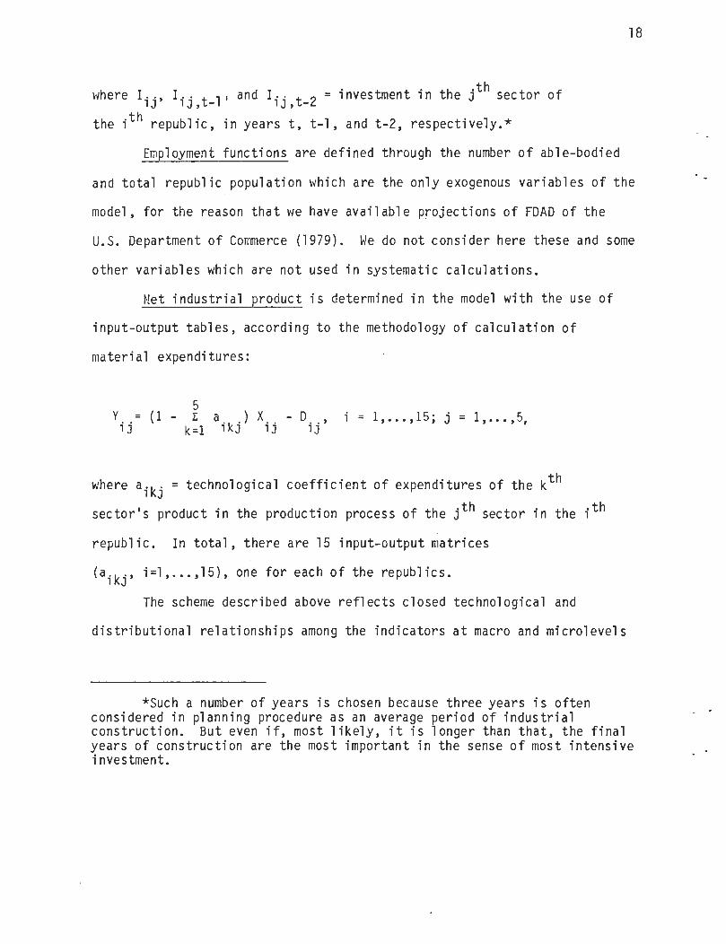
whereI ij' Iij,t-1'
and I ij,t-2 = investment in the j th sector o f
the i th republic, in years t, t-1, and t-2, respectively . *
Employment functions are defined through the number of able-bodie d
and total republic population which are the only exogenous variables of th e
model, for the reason that we have available projections of FDAD of th e
U .S . Department of Commerce (1979) . We do not consider here these and som e
other variables which are not used in systematic calculations .
Net industrial product is determined in the model with the use o f
input-output tables, according to the methodology of calculation o f
material expenditures :
5Y ij = (1 -
a ikj ) X . . - D . . ,,
i = 1, . . .,15 ; j = 1, . . .,5,k= 1
where a ikj = technological coefficient of expenditures of the k th
sector ' s product in the production process of the j th sector in the i th
republic . In total, there are 15 input-output matrice s
(a ikj , i=1, . . .,15), one for each of the republics .
The scheme described above reflects closed technological an d
distributional relationships among the indicators at macro and microlevel s
*Such a number of years is chosen because three years is ofte nconsidered in planning procedure as an average period of industria lconstruction . But even if, most likely, it is longer than that, the fina lyears of construction are the most important in the sense of most intensiv einvestment .

1 9
of the economy . These relationships are based on the double role of th e
net national product discussed in more detail in the author's publicatio n
with Emel'ianov (1974) . This indicator is the result of the curren t
productive activity and, at the same time, a factor influencing economi c
growth in the current and future cycles of production .
4 . INPUT-OUTPUT TABLES WITHIN THE ECONOMETRIC MODE L
Although, as alternative techniques, input-output and econometri c
models are usually developed in parallel both for free-market and planne d
economies, some writers have used input-output tables and their component s
in econometric research . The pioneering attempt was made by Fisher, Klein ,
and Shinkai (1965) who initially computed final demands series with
input-output relations and then applied regression techniques to explai n
them by relevant GNP components . Among the further attempts is a n
interesting idea developed by Green, Guill, Levine, and Miovic (1976) .
They included total material inputs as a third factor, along with labor an d
capital, in the estimated production functions of the SRI-WEFA Sovie t
Econometric Model, finding these inputs as column totals of th e
input-output flow matrix which is revised at each iteration .
Trying to circumvent the problem of scarcity of input-output data ,
some writers proceeded to use either "direct" methods such as RAS, o r
"indirect" econometric techniques of estimating their changes over time .
Thus, Preston (1975) used the econometric approach, developed by Hickman
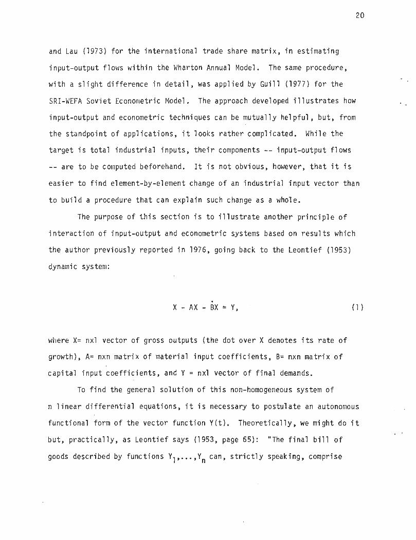
2 0
and Lau (1973) for the international trade share matrix, in estimatin g
input-output flows within the Wharton Annual Model . The same procedure ,
with a slight difference in detail, was applied by Guill (1977) for th e
SRI-WEFA Soviet Econometric Model . The approach developed illustrates ho w
input-output and econometric techniques can be mutually helpful, but, fro m
the standpoint of applications, it looks rather complicated . While the
target is total industrial inputs, their components -- input-output flow s
-- are to be computed beforehand . It is not obvious, however, that it i s
easier to find element-by-element change of an industrial input vector tha n
to build a procedure that can explain such change as a whole .
The purpose of this section is to illustrate another principle o f
interaction of input-output and econometric systems based on results whic h
the author previously reported in 1976, going back to the Leontief (1953 )
dynamic system :
X-AX-BX=Y,
(1 )
where X= nxl vector of gross outputs (the dot over X denotes its rate o f
growth), A= nxn matrix of material input coefficients, B= nxn matrix o f
capital input coefficients, and Y = nxl vector of final demands .
To find the general solution of this non-homogeneous system o f
n linear differential equations, it is necessary to postulate an autonomou s
functional form of the vector function Y(t) . Theoretically, we might do i t
but, practically, as Leontief says (1953, page 65) : "The final bill o f
goods described by functions Y l , . . .,Yn can, strictly speaking, comprise

2 1
any demand not derivable, i .e . not explainable, on the basis of th e
structural input-output relationships explicitly accounted for by the flow
and stock coefficients appearing on the left-hand side of the particula r
open system used . "
In order to develop the technique for solving system (1) so that
values of X and Y are mutually adjusted and justified, we will isolate th e
built-in differential accelerator, replacing it with a special econometri c
system, and retain the multiplier effect for the input-output system . A
more adequate description of the feedback to the gross outputs from th e
final demands, which is both the result of current productive activity an d
(as a source of investment) a factor of economic growth, will make i t
possible to treat the components of vector Y, along with X, as endogenous .
To illustrate the origin of the econometric accelerator in th e
model, we will use, besides X and Y, the following four nxl variables :
K = capital stock, I = investment, D = depreciation, K = employment ; an d
three scalar variables : Z = national income ; S = saving of state
enterprises and organizations ; N = population . The general specificatio n
of its equations can be written as the following simplified version of th e
model described above :
1.
Gross output
X it = Xi(Kit,Lit), i=l,. . ., n
2.
Capital stock
K it
Ki(Kit-l'Iit'Iit-1"')' i=l,. . ., n
3.
Investment
Iit = Ii(St,Dit), i=l,
. . .,n

2 2
4 . Depreciation D i
=
D i (K it ),
i=l, . . ., n
5 . Employment L it
=
L i (Nt ),
i=1, . . ., n
6 . Accumulation St = S(Z t )
n7 . National
income Z
=
E
(Y
-D
)t
i=1
it
i t
8 . Population (Nt
=
N(t) .
These are the equations for the jth sector of the economy for th e
ith republic which are used in computations for the system as a whole . Th e
structure of the model follows the distributional character of Sovie t
economic planning so that some policy indicators could play a direc t
regulator role for the republics and sectors of the economy . In a planned
economy, of course, any of the indicators may be used as a polic y
instrument, but in the planning process the three basic groups o f
indicators are labor, investment, and the supply of resources . At the
initial stage of planning ("control figures") outlining the main guideline s
for the development of the economy, the first two are most important, an d
they are included in the model .
The constraints for employment are determined precisely enough a t
the republic level, but the bulk of investment, i .e ., its centralized part ,
is distributed strictly on the vertical principle . That determines the
iterative character of planning at the "control figures " stage . To put i t
differently, the entire sequence of calculations depends on the output o f

2 3
the system as a whole which, in turn, is a function of the operations o f
al
its individual units .
In the above system, there are 5n+3 equations with 6n+3 variable s
(excluding t and lagged components), so that, at each step of calculation ,
we can find 5n+3 variables being given n arbitrary variables . Let them b e
the elements of vector Y ; then, being restricted to the linear form of th e
above expressions and eliminating the intermediate variables, we wil l
obtain the following system of equations in X, Y, and t :
0
1X t =
(t) + 2 i'Y t ,
(2 )
where k 0 (t)
(x0(t), .••,a0 (t)) ;x1
()J, . . .,X'); i = nxl unity vector .
Vector function 2. 0 (t) separates for each industry the influence o f
predetermined factors such as demographic changes, prehistory of curren t
growth, etc ., and has a cumulative effect on the gross outputs . Vector
l iQ
s comprised of constant terms and plays the role of marginal output ,
resulting from the change in final demand as a factor of economic growth .
If we combine system (2), which describe a matrix accelerator, wit h
the static form of system (1), which describes a matrix accelerator, w e
will obtain the expanded system of 2n equations with 2n unknown component s
of X and Y . Denoting the equilibrium solution by X and Y, the condition o f
equilibrium can be written :
0
- 1X t = z (t) + RYt = (I-A)
Yt ,
(3)

2 4
1
where R E t i', and A - (a
i,j=1, . . .,n) .1 3
System (3) performs endogenous calculations of final demands an d
gross outputs taking into account the structural parameters and accumulate d
potential of economic growth . The computing advantage of such a
description is in the dimension of the dynamic system which does not depen d
on the extension of the lagged variables and exogenous functions, i .e . ,
remains the same as in a static situation . All relevant complications are
absorbed by the vector £°(t) which is to be recalculated at the beginnin g
of each successive iteration .
Since [(I-A)-1-R]-1 = (I-A) [I-R(I-A)]-1, it follows fro m
system (3) that :
-1 £G
-1 £GXt = B
(t) and Yt = (I-A)B
(t) ,
where B = I - R(I-A) .
Components of vectors X t and Y t determined with expressions (4 )
provide the equilibrium solution of system (3) . The crucial property o f
matrix B is that the solution can be found with immediate formulas withou t
inverting it . The easiest way to show this is to substitute function (2 )
for Xt in the input-output equations summing them :
i'Y t = Yi ' (I-A)i0(t) ,
and expression (5) for i ' Yt in the econometric part of system (3) :
Xt = (I+G)20(t) and Yt = (I-A) (I+G)QG(t),
(4 )
(5 )
(6)
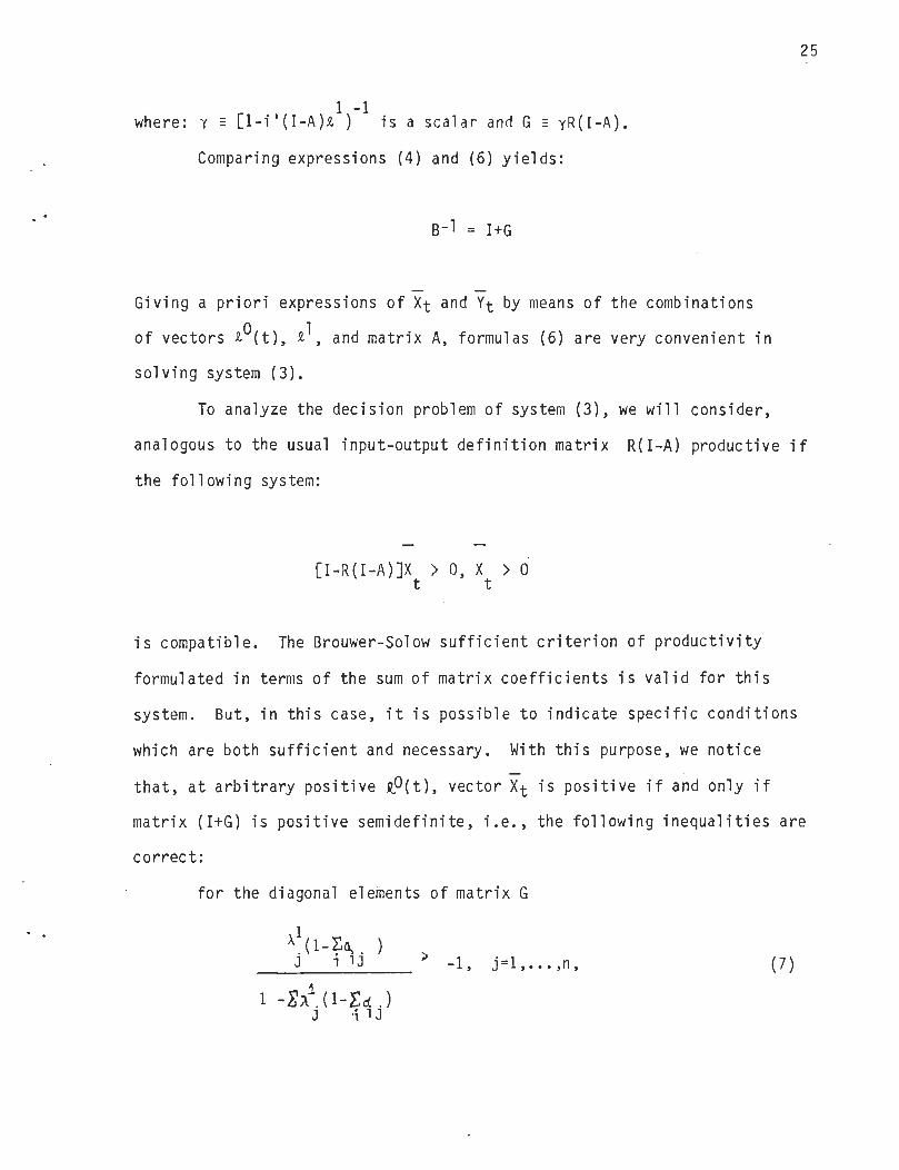
2 5
1 - 1where : ,'
[1-i'(I-A)z )
is a scalar and G
YR(I-A) .
Comparing expressions (4) and (6) yields :
Giving a priori expressions of Xt and Yt by means of the combination s
of vectors i°(t), Q 1 , and matrix A, formulas (6) are very convenient i n
solving system (3) .
To analyze the decision problem of system (3), we will consider ,
analogous to the usual input-output definition matrix R(I-A) productive i f
the following system :
[I-R(I-A)]Xt > 0, X t > 0
is compatible . The Brouwer-Solow sufficient criterion of productivity
formulated in terms of the sum of matrix coefficients is valid for thi s
system . But, in this case, it is possible to indicate specific condition s
which are both sufficient and necessary . With this purpose, we notic e
that, at arbitrary positive e(t), vector X t is positive if and only i f
matrix (I+G) is positive semidefinite, i .e ., the following inequalities ar e
correct :
for the diagonal elements of matrix G
a1 (1-Ear . )i 1 J -1,
j=1, . . .,n ,
1 -EA ( 1 -Ed . )J
. i 1 J
( 7 )

2 6
for the rest of its n(n-l) element s
al (1-Ea
)j
i ik a
0, j,k = 1, . . .,n ; j*k, ( 8 )
1 - Ea 1 1-Ea )J
-i 1 J
and for the row totals of matrix G
X 1 (n-EEa
)j
ki ik
>
-1, j=1, . . .,n .
1 - Ea l (1-Ea )J
j 1 J
Analyzing inequalities (7)-(9), it is possible to show that they ar e
equivalent to the following (n+l) conditions :
n (10 )E a < 1, j=1, . . .,n ,
i=1 1 J
(11 )E
A . (1 - a . . )
<1 ,j=1
3 i=1
1 3
which, therefore, are necessary and sufficient for the productivity o f
matrix R(I-A) .
Inequalities (10) are nothing more than a usual input-outpu t
requirement reflecting the fact that the cost of material inputs must no t
exceed the value of an entire product . The left-hand side of conditio n
(11), which is the trace of matrix R(I-A), can be viewed as the power o f
feedback from the results of the current productive activity to the gros s
outputs . Practically, it is by far less than unity because such feedbac k
is small relative to the effect of the accumulated potential of economi c
growth (vector RO (t) ) .
( 9 )

2 7
The feature of matrix R(I-A), which makes possible the above
results, is its special structure : each elemen t
A 1 (1-Ea ), j,k = 1, . . .,n,is a product of two numbers, the first of whic hj
i j k
is the same for all columns, and the second the same for all rows .
Therefore, all its principal minors but the first-order singular, the ran k
of the matrix is one, and so is the number of its non-zero characteristi c
roots . Finally, this single characteristic root is equal to the trace o f
matrix R(I-A) and, according to condition (11), less than unity . Thi s
property ensures the [R(I-A)] n ; 0 when n+ so that B-1 can be expande d
in a series :
E [R(I-A)] = I + R(I-A) + [R(I-A)] +n=0
and hence :
0X t = 2 (t) + R(I-A)Q O (t) + [R0-A)] 2 0 (t) + . . .
The illustrated principle of expansion of vector Xt differs from that for
a usual input-output multiplier which, of course, is also available in thi s
case . In the familiar version, only the vector of material inputs i s
expanded, and the vector of final demands is included as a whole . In th e
developed model, the part of industrial grow output which depends on th e
current productive activity is distributed in successive cycles of feedbac k
effects on economic growth . Moreover, analogous separate expansions are
possible both for the vectors of material inputs and final demands .

2 8
5 . THE DATA AND THEIR SOURCES
The time series for sector, republic, and union indicators includ e
observations for 1965-1980, which are either official data or estimates .
In total, there are seventy five republic data files, five for each o f
fifteen republics, and a union data file . The following indicators form
republic files : X ij = gross value of output ; Y ij = net value o f
output ; K ij = capital stock ; I ij = investment ; Il ij = investmen t
minus depreciation for replacement ; ldij = wages ; P ij = profits ;
Dij = depreciation ; DD . . = depreciation for replacement ;
L ij = employment ; Z . . = input-output coefficients, where i=1, . . .,15 an d
j=l, . . .,5 represent the j th sector of the i th republic . In addition ,
the file for industry for each republic contains the data on the followin g
indicators : B i = centralized investment ; Ti = turnover tax ;
U i2 = wages in the "nonproductive" sector ; N i = republic population .
The union file lists the data for the indicators as follows :
R2 = payments from profits ; R3 = personal tax ; R4 = social insuranc e
deductions ; R5 = other revenues ; E l = financing of the economy ;
E 2 = financing of social programs ; E3 = expenditures for defense an d
government ; B = investment financed by the budget .
The following is a more detailed description of the methodology use d
to derive the data and the sources of the data .
Gross Value of Output (x) (Million Rubles, 1973 prices )
Whenever available, the data were taken from the yearbooks of th e
corresponding republics . The following data were obtained by interpolation :

2 9
Armenian - "construction" and "transportation and communications "
(1966-1969, 1974), "trade and other" (1974), "republic total" (1967-1969) ;
Azerbaidzhan - "transportation and communications", "construction", "trade
and other" (1974, 1976-1978) ;
Belorussia - "agriculture" (1966-1967), "transportation an d
communications", "construction", "trade and other" (1966-1969, 1973) ;
Estonia - "transportation and communications", "construction", "trade an d
other" (1966-1967, 1972-1974) ;
Georgia - "transportation and communications", "construction", "trade an d
other" (1966-1969, 1974) ;
Kazakhstan - "agriculture" (1966-1967), "transportation and
communications", "trade and other" (1972-1974) ;
Kirgizia - "agriculture" (1966-1967), "transportation and communications" ,
"construction", "trade and other " (1966-1969, 1974) ;
Latvia and Moldavia - "transportation and communications", "construction" ,
"trade and other " (1966-1969) ;
Lithuania - "agriculture" (1966-1969) ;
R .S .F .S .R . and Uzbekistan - "agriculture" (1966-1967), "transportation an d
communications", "construction", "trade and other" (1966-1969) ;
Tadzhikistan - "agriculture" (1966-1967, 1979), "transportation an d
communications", "construction", trade and other " (1966-1969, 1971 ,
1973-1974) ;
Turkmenistan and Ukraine - "transportation and communications" ,
"construction", "trade and other" (1966-1969, 1971-1974) ; Turkmenia -
"agriculture" (1966-1967) .

3 0
The following data were obtained by extrapolation using the averag e
differences of the previous four years : (1) 1978-1980 for "construction" ,
"transportation and communications", "trade and other" in the followin g
republics : Belorussia, Georgia, Lithuania, Moldavia, Turkmenistan ; (2 )
1979-1980 for the same sectors in the following republics : Armenia ,
Estonia, Latvia, Tadzhikistan, Uzbekistan ; (3) 1980 for the same sectors i n
Azerbaidzhan ; (4) 1977-1980 for the same sectors in Kazakhstan ; (5 )
1976-1980 for the same sectors in Kirgizia ; (6) 1974-1980 for the sam e
sectors in R .S .F .S .R .
National Income (Y) (Million Rubles, 1973 prices )
All data (except those for 1975) are derived proportional to th e
gross value of output (GVO) for the following republics : Armenia ,
Belorussia, Estonia, Kazakhstan, Moldavia, R .S .F .S .R, Turkmenistan, an d
Tadzhikistan .
All data (except 1973) for Azerbaidzhan are taken proportional to
GVO . The following data are taken proportional to GVO (all sectors) :
Georgia (1966-1969, 1976-1980), Latvia (1966-1969, 1974-1980), Lithuani a
(1966-1969, 1974, 1979-1980), Kirgizia (1966-1969, 1971-1974, 1977-1980) ,
Ukraine (1966-1969, 1974), uzbekistan (1966-1969, 1979, 1980) .
Productive Capital Stock (K) (Million Rubles, 1973 prices )
The source for 1965-1977 data (all republics, all sectors) is "Fixe d
Capital in Soviet Republics in 1973 Prices", by Gillula (1981) . The

3 1
4 -
1979-1980 data (all sectors) were found by extrapolation using the averag e
increase of the previous three years for the following republics :
Azerbaidzhan, Estonia, Georgia, R .S .F .S .R, Ukraine, Uzbekistan .
The 1978-1980 data (all sectors) were found by extrapolation usin g
the average increase of the last three years for the following republics :
Tadzhikistan, Turkmenistan .
Capital Investment (I) (Million Rubles, 1973 prices )
The data for "trade and other" were found by taking 10% of the su m
of ("trade and other" and "non-productive sector") for all republic s
except : Georgia, Kazakhstan, Latvia, Lithuania .
For these republics, the 1965, 1970, and 1975 data are taken fro m
yearbooks and for the intermediate years are interpolated . The data fo r
"centralized investment" (1976-1980) are taken as a percentage of "tota l
investment" . The percentage used is approximately equal to the proportion s
of the previous years (all republics) .
The data for years 1965-1975 ("industry", "agriculture" ,
"transportation and communications", "construction", "total") are take n
from SOVMOD statistics for all republics .
The following data were found by extrapolation using the averag e
difference of four previous years : Armenia (1979-1980), Azerbaidzha n
(1980, except "agriculture"), Estonia (1980), Georgia (1980), Kazakhsta n
(1979-1980), Kirgizia (1980), Latvia (1980), Moldavia (1980), R .S .F .S .R .
(1980), Tadzhikistan (1979-1980), Turkmenia (1980), Uzbekistan (1980) .
3 2
The data for years 1976-1979(80) are taken from the yearbooks of th e
corresponding republics .
Labor (L) (1000 people )
The 1965-1975 data (all republics) were taken from SOVMOD for th e
following sectors : "industry", "agriculture", "nonproductive" .
The 1976-1980 data (all republics) for "industry" are taken a s
estimated by J . Gillula . The following data were found by extrapolatio n
based on the average differences over the last four years : Armeni a
(1979-1980, all sectors except "industry"), Azerbaidzhan (1980), Belorussi a
(1976-1980, all sectors except "industry"), Kazakhstan (1979-1980 : "tota l
employment", "trade and other", "transportation and communications" ,
"nonproductive"), Kirgizia (1980, all sectors), Lithuania (1979-1980 :
"nonproductive", total employment"), Moldavia (all sectors excep t
"industry"), R .S .F .S .R . (1980 : "transportation and communications", "trad e
and other", "nonproductive", "total employment"), Tadzhikistan ("trade an d
other", "transportation and communications", "nonproductive") .
The following data were found by interpolation : Belorussi a
(1966-1969, 1971-1974 : "transportation and communications", "trade an d
other"), R .S .F .S .R . (1976 : all sectors except "industry", "construction") ,
Ukraine (1966-1969, 1971-1974 : "transportation and communications", trad e
and other") .
The 1965-1969 data for Turkmenistan ("transportation an d
communications", "construction", "trade and other") were derived from tren d
regressions using the 1970-1975 data .
i

3 3
Wages (W) (Million Rubles, current prices )
The 1965-1975 data for all sectors except "nonproductive sector"
were found by multiplying : (average monthly wage x 12 x (employment) . Th e
data for "nonproductive sector" were found as the difference between th e
("total") and (sum of all other sectors) .
The 1976-1980 data were found with the use of trend regressions for
the following republics ; Armenia, Azerbaidzhan, Georgia, Kazakhstan (al l
sectors) .
The 1976 data for Belorussia were found by interpolation (al l
sectors) . The 1980 data for Estonia, Kirgizia, Latvia, R .S .F .S .R ,
Turkmenistan, Uzbekistan (all sectors) are based on the extrapolation o f
average increments in the previous four years .
The 1977-1980 data for Lithuania and Moldavia (all sectors) were
found with trend regressions . The 1979-1980 data for Tadzhikistan (al l
sectors) were found by extrapolation based on the average increase for th e
past three years .
Profits (P) (Millions Rubles, current prices )
The following data (all sectors) were found with the use of tren d
regressions : Armenia (1979-1980), Azerbaidzhan (1980), Belorussia (1980) ,
Estonia (1980), Georgia (1978, 1980), Kazakhstan (1965-1969, 1980) ,
Kirgizia (1965-1969, 1980), Latvia (1980), Lithuania (1979-1980), Moldavi a
(1979-1980), R .S .F.S .R . (1980), Tadzhikistan (1976-1980), Turkmenistan

3 4
(1980), Uzbekistan (1980) . All other data are taken from the correspondin g
yearbooks .
Depreciation, Total (D) and for Replacement (DD )
(Million Rubles, current prices )
The data (1965-1975 : all sectors) were based on the depreciation -
to - capital stock ratio from union totals for the following republics ;
Belorussia, Estonia, Kazakhstan . The 1976-1980 data for these republic s
were found with trend regressions .
The following data were interpolated :
Armenia (1966-1969 : all sectors) ;
Azerbaidzhan (1966-1969, 1971-1974 : depreciation for replacemen t
only, and "trade and other" from 1966 to 1969 and 1971 to 1972) ;
Kirgizia ("trade and other" from 1966 to 1969) ; Lithuani a
(1966-1969 : all sectors) ;
Moldavia (1973-1974 : all sectors and "trade and other" from 1971 t o
1974) ;
R .S .F .S .R . ("trade and other" from 1971 to 1974 and 1978 data fo r
all sectors) ;
Tadzhikistan (all sectors from 1966 to 1969) ;
Turkmenistan (all sectors from 1966-1969 and 1973 to 1974) ;
Ukraine ("trade and other" 1966-1969 ; 1975 data are based on a n
average increase in 1973 and 1974 for each sector) ;
Uzbekistan (all sectors :
1966-1969, 1971-1972, and 1976) .
The following data were obtained with the use of trend regressions :

3 5
Armenia ("trade and other" from 1979 to 1980) ;
Georgia (all sectors from 1970 to 1980) ;
Kirgizia (all sectors :
1965 to 1969 and 1975-1980, regressions ru n
on data from 1970 to 1974) ;
Lithuania (all sectors from 1965 to 1969, with the 1970-1978 dat a
used to obtain coefficients) ;
Moldavia ("trade and other" from 1979 to 1980) ;
Tadzhikistan (all sectors from 1974 to 1980, with the 1965-1973 dat a
used to obtain coefficients) ;
Ukraine (all sectors from 1965 to 1976 and 1978-1980) .
The following data were extrapolated using an average increase fo r
the last three years : 1979 and 1980 figures for all sectors except "trad e
and other" for the following republics ; Armenia, Latvia, and Lithuani a
(including "trade and other"), Moldavia, Turkmenistan (including "trade and
other" from 1978 to 1980) .
Figures for 1980 were extrapolated for the following republics ;
Azerbaidzhan, R .S .F.S .R ., Uzbekistan ("trade and other" were extrapolate d
for 1979) .
Turnover Tax (T) (Million Rubles, current prices )
The data for 1966 were derived from sources provided by the Foreig n
Demographic Analysis Division of U .S . Department of Commerce . The data fo r
years 1965, 1967-1975 were found by multiplying the 1966 data by "Rates o f
Growth of Gross Output" (Narkhoz) . Data for 1976-1980 were found by tren d
regressions run on 1965-1975 data .
3 6
Total Area Sown (Q) (Million hectares )
The data for republics were derived from Narkhoz SSSR, 1980 .
Difference Between Capital Investment and Depreciatio n
for Replacement (II) (Million Rubles )
The data (for all republics and all sectors) were found by
subtracting the values for Depreciation for Replacement (DD) from those fo r
Capital Investment (I) .
Budget Data (Million Rubles, current prices )
Centralized Investment(B) data for 1965-1975 were found as the sum
of two types of decentralized investment listed in the "Consolidated State
Budget for the Union as a whole and for the Republics" handbook :
decentralized capital investment and decentralized capital investment o f
organizations and enterprises . The data for Payment for Profits (R2 ) ,
Personal Tax (R3 ), Social Insurance Deductions (R 4 ), Other Revenue s
(R5 ), Financing the Economy (E l ), Financing of Cultural Measure s
(E2 ), Defense and Government (E 3 ) were taken directly from Narkho z
tables for all budget indicators .

3 7
6 . ILLUSTRATION OF THE FORECASTING RESULT S
Table 2 illustrates the projected growth of ten main macroindicator s
by republic for 1981-1985 calculated with the use of the model describe d
above . The indicators are as follows : gross social product X, nationa l
income produced Y, fixed capital stock K, fixed capital investment I, wage s
W, employment L, population N, labor productivity (nationa
l income-to-employment ratio) 1, capital stock-to-output ratio k, materia l
expenditures-to-output ratio m.
Gross Social Product . According to Soviet methodology, thi s
indicator is defined as the sum of gross values of output by sector of th e
economy . As one can see in Table 2, the republics with the highest shar e
in total GSP - the RSFSR and the Ukraine - are among those having th e
lowest rates of economic growth, with totals of 18 and 16 percen t
respectively . The Asian republics are among those with highest rates o f
growth : Kazakhstan and Kirgizia, along with Belorussia, will increase th e
value of their GSP by 29 percent in 1981-1985, while Turkmenistan wil l
increase its by 37 percent .
National Income . National income of republics is determined as the
sum of net values of output by sector of the economy . The target for th e
growth of national income in the 11th Five-Year Plan equals 18 percent, an d
so does the result suggested by our model . The fact that the model
estimates the same rate of growth for gross social product and nationa l
income leads to the conclusion that the target to reduce the share o f
material expenditures (intermediate product) in the total output, will not

Table 2 . Growth of the Main Macroindicators by Republic in 1981-198 5
Gros sSocia lProduc t
1
National
Income1'
Capita lStoc k
KInvestmen t
1
Labo r
L WagesWPopulation
NProductivity
1
Capital-to-
Outpu tRatio k
Materia lExpenditures -
to-Output
Ratio m
USSR 18 18 42 0
Armenia 20-1 0
Azerbaidzhan 23 - 5
Belorussia 29 30 23 20 9 _27_ 4 __ 18 -4 - 1
l9 22 17 3 16 1 16 + 4 - 1Estonia 1 7
Georgia 32 29 36 12 22 6 14 -4 +2
Kazakhstan 29 -1 +1
Kirgizia 29 16 -4 +1
Latvia 15 13 22 18 +6 +]
Lithuan a 24 21 32 22 +8 + 2
Moldavia 18 20+b
+1
R.S.F.S.R . 18 . 41 0
Tadzhikistan 22 15 +2 + 1
Turkmenistan 37 ®n 18 15 12 -9 4A
Ukraine 16 16 +4 1
Uzbekistan 25 21+5 1
3 9
be met, as it has not been in the past . It should be mentioned here tha t
the ambitious target of reducing consumption of rolled metals by 18-2 0
percent in the 11th Five-Year plan, along with energy and fuels, and t o
increase the share of net value added accordingly was set by the party an d
planning authorities . The authorities, of course, hardly believe this i s
realistic, but both planning discipline and the mobilizing effect o f
planning require imposing tough constraints and goals .
Professor Koropeckyj (1931) estimated gross national product pe r
capita by republic in 1970 . Estonia, Latvia, and the R .S .F .S .R . gained th e
first, second, and third places respectively . It is interesting that ,
according to our calculations, these republics will be leading in pe r
capita production of national income fifteen years hence, i .e ., in 1985 .
The three lagging republics -- Uzbekistan, Azerbaidzhan, and Turkmenista n
-- also turn out to be the same in both studies .
Fixed Capital Stock . The transition from extensive to intensiv e
economic growth declared by the Soviets for the 10th and 11th five-yea r
plans has to result in the gradual restructuring of the composition o f
fixed capital stock . The role of machinery and equipment in the investmen t
process has to grow at the expense of construction industry . This is th e
result of the investment process changing its emphasis from building new
capacities to reconstruction and modernization of existing ones .
Nevertheless, new capacities will probably grow at a speed greater tha n
that desired by Soviet authorities, which is an indication that obsolet e
equipment will still continue to be operated . In the 10th Five-Year Pla n
about 30 percent of the total product mix of machine-building ministries

40
had been manufactured for more than ten years . There is no indication tha t
this trend will be reversed and that the machine-building industry wil l
introduce more rapid technological change in the Soviet economy . Th e
results indicated in Table 2 show that the leading republics -- th e
R .S .F .S .R and the Ukraine -- will lag behind some of the others, with 2 0
and 21 percent increases in fixed capital stock respectively .
Fixed Capital Investment . According to the estimates in Table 2 ,
the variation of investment growth among republics is rather limited, from
15 percent for Tadzhikistan, the lowest, to 22 percent for Lithuania, th e
highest . Of course, high or low growth for these republics is not of muc h
importance by itself because it is measured relative to small absolut e
values, where insignificant fluctuations can result in significant rates o f
growth . Total, all-union, fixed investment growth equals 18 percen t
according to our calculations . This is in excess of the 11th Five-Yea r
Plan target of 11 percent growth . Investment is such a volatile indicato r
that the relevant equations should, of course, incorporate a judgmenta l
component reflecting the estimate of possible changes in the future
policies .
In this respect our results could contain an upward bias . On th e
other hand, it is not clear whether the planned target of 11 percent growth
is the estimate of potential capacities of industries manufacturin g
investment goods . It might follow as well from a desire to reduce capita l
investment flows sharply to force the ministries and enterprises to see k
alternative ways of increasing productivity . If this assumption is true ,
then the economy has the productive capacity to surpass the planned target

4 1
for investment growth . The actual increase of this indicator wa s
42 percent in the 9th Five-Year Plan (1971-1975) and 29 percent in the 10t h
Five-Year Plan (1976-1980) . Increasing prices of machinery and equipmen t
is another factor that will contribute to investment growth, although no t
in physical terms . This is not taken into account in the process o f
five-year planning which creates a downward bias in estimating output i n
money terms and an upward bias for output in physical terms .
Labor and Population . Population is an exogenous variable of our
model . The projections of the FDAD of the U .S . bureau of Census (1979 )
were employed with these purposes . They foresee the highest growth rate s
for Uzbekistan (16%), Tadzhikistan (16%), and Turkmenistan (15%) and lowes t
for Latvia (1%), Estonia (1%), and the Ukraine (2%) . The growth of tota l
population is forecasted at the level of 5 percent whereas, according t o
our calculations, total employment can increase by about 8 percent in th e
five-year period . The discrepancy indicates that some reserves of manpowe r
still exist in the Soviet economy . However, the question of how to engag e
these resources in material production is beyond the scope of a n
econometric study, and additional analysis will be needed . Table 2 show s
that the pattern of employment growth distribution reflects that o f
population, the result that could be expected .
Labor Productivity . The labor productivity indicator is defined i n
the Soviet economy as average product, i .e ., the output-to-labor ratio .
The 1979 Resolution of the Central Committee and Council of Minister s
brought an essential change in the measurement of this indicator .

4 1
for investment growth . The actual increase of this indicator wa s
42 percent in the 9th Five-Year Plan (1971-1975) and 29 percent in the 10t h
Five-Year Plan (1976-1980) . Increasing prices of machinery and equipmen t
is another factor that will contribute to investment growth, although no t
in physical terms . This is not taken into account in the process o f
five-year planning which creates a downward bias in estimating output i n
money terms and an upward bias for output in physical terms .
Labor and Population . Population is an exogenous variable of our
model . The projections of the FDAD of the U .S . bureau of Census (1979 )
were employed with these purposes . They foresee the highest growth rates
for Uzbekistan (16%), Tadzhikistan (16%), and Turkmenistan (15%) and lowes t
for Latvia (1%), Estonia (1%), and the Ukraine (2%) . The growth of total
population is forecasted at the level of 5 percent whereas, according t o
our calculations, total employment can increase by about 8 percent in th e
five-year period . The discrepancy indicates that some reserves of manpowe r
still exist in the Soviet economy . However, the question of how to engag e
these resources in material production is beyond the scope of an
econometric study, and additional analysis will be needed . Table 2 show s
that the pattern of employment growth distribution reflects that o f
population, the result that could be expected .
Labor Productivity . The labor productivity indicator is defined i n
the Soviet economy as average product, i .e ., the output-to-labor ratio .
The 1979 Resolution of the Central Committee and Council of Minister s
brought an essential change in the measurement of this indicator .

4 2
According to the Resolution, net value of output (chistaia produktsiia) ,
not grow value of output (valovaia produktsiia) as before, is to be use d
for these purposes . The reason for this was to avoid the double countin g
of material expenditures in the expression of productivity and to isolat e
the contribution of each enterprise on the basis of net value added pe r
employee . In many cases, however, the initial version is still bein g
employed .
It is easy to show that the create of productivity growth can b e
expressed as follows :
r
_ (r u -r1)/R ,
where r.n = rate of increase of productivity in current period ;
r u = rate of increase of the value of output ; rl = rate of increase o f
manpower in current period ; R 1 = growth ratio of manpower, i .e . ,
R 1 = 1 + r 1 .
Evidently, the higher the rate r u of increase of output, th e
higher the productivity growth measured by formula (12) . But the point i s
that the output is expressed in money terms and, therefore, depends o n
prices . The rate of its increase, if computed discretely at successiv e
periods of time, could be decomposed as follows :
ru = rx + rp + rxrp,
(12 )
(13 )
where r u = rate of increase of output in current period ; rx = rate of
4 3
increase of real output or output in physical terms for a monoproduc t
industry ; rp = rate of price increase measured usually by a price index .
Where the third term on the right-hand side of formula (13) is negligible ,
real economic growth is the difference between actual growth and that o f
prices .
Although only the real-growth component in formula (13) contribute s
to productivity growth, no distinction between the two components -- outpu t
growth in physical terms and that due to the price growth -- is made i n
formula (12) . Therefore, national economic plans account for bogu s
productivity growth if there are significant price increases . For example ,
the change of product mix leading to the growth of average prices mean s
productivity growth from the enterprise's standpoint . Not without reason
tie change of the product mix is one of the most important factors of th e
productivity growth accounted for at all levels of the economy .
Even with the above reservations, our calculations indicate very
modest productivity growth in the 1981-1985 five-year period . With total
all-union growth of labor productivity of 10 percent during this period ,
the republic data vary from 3 percent for Tadzhikistan to 18 percent fo r
Belorussia . The largest republics -- the RSFSR. and the Ukraine -- exhibi t
almost equal productivity growth of 9-10 percent which is equivalent toa
1 .8 percent growth rate per annum . These results demonstrate that the pla n
target calling for 20 percent productivity growth in the 11th Five-Yea r
Plan will not be met .
Capital-to-Output Ratio . This ratio changes insignificantly ove r
time, but much attention is paid to it in planning .
It is viewed as an

4 4
indication of success in reducing the costs of construction an d
installation work and newly-introduced equipment . It also characterize s
the productivity of machinery and equipment and the degree of waste o f
capacities . Therefore, according to the mobilizing effect of planning ,
this ratio should tend to decline . Our calculations produced mixe d
results . As one can see from Table 2, the capital-to-output ratio wil l
decrease for seven republics and increase for eight of them . Mos t
important is that this ratio will increase for both leading republics - -
the R .S .F .S .R . and the Ukraine -- and for the economy as a whole .
Material Expenditures-to-Output Ratio . From our calculations, i t
follows that this ratio will increase for ten republics, decline for thre e
republics, and will not change for two of them . Despite ever-growin g
material expenditures per ruble of output, two unprecedent programs -- fo r
saving metals and energy -- were declared in operation for the"1th
Five-Year Plan . The results of our calculations and the analysis of othe r
factors indicate that these programs will not be successful . The stric t
enforcement of the tough constraints on major material inputs imposed b y
these programs would lead to a further slump in Soviet economic growth . I n
spite of all the attempts to reverse events, the Soviet economy stil l
depends on extensive factors of economic growth, and substitutes for the m
are far beyond reach .

4 5
Reference s
Baldwin, G .S . Population Projections by Age and Sex : For the Republics an d
Major Economic Regions of the U .S .S .R ., 1970 to 2000 . Washington, D .C . :
U .S . Government Printing Office (1979) .
Bandera, V .N . and Z .L . Melnyk, eds . The Soviet Economy in Regiona l
Perspective .
New York : Praeger (1973) .
Bond, D .L .
" Regional Economic Modeling in the Soviet Union " , a Report to th e
National Council for Soviet and East European Research (1980) .
Emel'ianov, A.S . and F .I . Kushnirsky . Modelirovanie pokazatelei razvitii a
ekonomiki soiuznoi respubliki (Modeling the Indicators of Economic Growt h
of a Republic) . Moscow : Ekonomika (1974) .
Fisher, F .M ., L .R . Klein, and Y . Shinkai .
" Price and Output Aggregation i n
the Brookings Econometric Model ."
In J .S . Duesenberry, G . Fromm, L .R .
Klein, and E . Kuh, eds . The Brookings Quarterly Econometric Model of th e
United States . Chicago : Rand McNally (1965) .
Gillula, J .W .
" Input-Output Analysis", in I .S . Koropeckyj, ed .
The Ukrain e
within the U .S .S .R .
New York : Praeger (1977) .
Gillula, J .W .
"Fixed Capital in Soviet Republics in 1973 Prices: 1960 t o
1979", Working Paper . FDAD, U .S . Bureau of the Census (1981) .
Green, D .W ., G .D . Guill, H .S . Levine, and P . Miovic .
"An Evaluation of th e
Tenth Five-Year Plan Using the SRI-WEFA Econometric Model of the Sovie t
Union ."
In U .S . Congress, Joint Economic Committee, Soviet Economy in a
New Perspective . Washington, D .C . (1976) .
Green, D .W . and C .I . Higgins .
A Macroeconometric Model of the Soviet Union :
SOVMOD .
New York : Academic Press (1977) .
4 6
Guill, G .D . "Input-Output Within the Context of the SRI-WEFA Sovie t
Econometric Model ."
In V.G . Treml, ed . Studies in Soviet Input-Outpu t
Analysis .
New York : Praeger (1977) .
Hickman, B .G . and L .J . Lau .
"Elasticities of Substitution and Export Demands
in a World Trade Model ." European Economic Review 4 (1973) .
Koropeckyj, I .S ., ed .
The Ukraine within the U .S .S .R . An Economic Balanc e
Sheet .
New York : Praeger (1977) .
Koropeckyj, I .S ., and G.E . Schroeder, eds .
Economics of Soviet Regions .
New
York : Praeger (1981) .
Kushnirsky, F .I .
"O sposobe dopolneniia mezhotraslevogo balansa do zamknuto i
skhemy paschetov proizvodstva (Complement of the Input-Output Scheme to a
Closed Model for Production Calculations)" . Ekonomika i matematicheski e
metody 5 (1976) .
Leontief, W .W .
"Static and Dynamic Theory ."
In W .W . Leontief et al . Studies
in the Structure of the American Economy . New York : Oxford Universit y
Press (1953) .
Nikaido, H . Convex Structures and Economic Theory . New York : Academic Pres s
(1968) .
Preston, R .S . "The Wharton Long-Term Model : Input-Output Within the Context
of a Macro Forecasting Model ."
International Economic Review 16 (1975) .
Stone, R . and A. Brown .
"Behavioral and Technical Change in Economi c
Models " .
In E .A .G . Robinson, ed . Problems in Economic Development .
New
York : McMillan (1965j .