Towards an integrated approach to stochastic process-based modelling: with applications to animal behaviour and spatio-temporal spread

Glenn Marion1, David M. Walker2, Alex Cook3, David L. Swain4 and Mike R. Hutchings5. 1Biomathematics and Statistics Scotland, James Clerk Maxwell Building, The King’s Buildings, Mayfield Road, Edinburgh EH9 3JZ, UK. Email: glenn@bioss.ac.uk Tel : +44 (0)131 650 4898 Fax : +44 (0)131 650 4901 2Department of Applied Mathematics, Hong Kong Polytechnic University, Hung Hom, Kowloon, Hong Kong. Email: enwalker@eieserver.eie.polyu.edu.hk 3School of Mathematical and Computer Sciences, Heriot Watt University, Edinburgh EH14 4AS, UK. Email: a.r.cook@ma.hw.ac.uk 4CSIRO Livestock Industries, JM Rendel Laboratories, Ibis Avenue, North Rockhampton, QLD, 4701. Australia. Email: dave.swain@csiro.au

5Scottish Agricultural College, West Mains Road, Edinburgh EH9 3JG, UK. Email: mike.hutchings@sac.ac.uk

Abstract : Using example applications from our recent research we illustrate the development of an integrated approach to modelling biological processes based on stochastic modelling techniques. The goal of this programme of research is to provide a suite of mathematical and statistical methods to enable models to play a more central role in the development of scientific understanding of complex biological systems. The resulting framework should allow models to both inform, and be informed by data collection, and enable probabilistic risk assessments to reflect inherent variability and uncertainty in current knowledge of the system in question. We focus on discrete state-space Markov processes as they provide a general and flexible framework both to describe and infer the behaviour of a broad range of systems. Unfortunately the nonlinearities required to model many real world systems typically mean that such discrete state-space stochastic processes are intractable to analytic solution necessitating the use of simulation and analytic approximations. We show how to formulate stochastic process-based models within this framework and discuss the representation of spatial and temporal heterogeneity. Simple population models are developed and used to illustrate these concepts. We describe how to simulate from such models, and compare them with their deterministic counterparts. In addition, we discuss two methods, closure schemes and linearization about steady-states, which can be used to obtain analytic insights in to model behaviour. We outline how to conduct parameter estimation for such models when, as is typically the case for biological and agricultural systems, only partial observations are available. Having focussed on familiar population level models in introducing our integrated approach its wider applicability is illustrated by two contrasting applications from our recent research. The first example combines the development and analysis of an agent-based model describing grazing in heterogeneous environments, with parameter inference based on data generated using a transponder system in a behavioural experiment on diary cows. The second example makes use of large-scale data describing bio-geographical features of the landscape and the spatio-temporal spread of an alien plant to estimate the parameters of a stochastic model of dispersal and establishment.

1. Introduction A key difficulty faced in the study of biological and agricultural systems is their immense complexity. This fact makes even the observation, recording and cataloguing of biological phenomena a formidable task and such problems are compounded when one seeks to understand, predict and manipulate the dynamic processes underlying this observed complexity. Mathematical modelling currently plays an important role in developing scientific understanding of complex biological processes, and model-based risk assessments make it relevant to policy makers and resource managers. However, the gathering pace of data acquisition and consequent advances in knowledge require the continuing development of both mathematical methods, to cope with increasing complexity, and statistical methods, to fully integrate data and models. Ideally such methods should allow mathematical models to both inform, and be informed by data collection, and enable probabilistic risk assessments to reflect inherent variability and uncertainty in current knowledge of the system in question. In this chapter, using examples from our research, we illustrate the development of such an integrated approach to modelling biological processes based on stochastic modelling techniques. However, the picture is still somewhat incomplete and we discuss areas where further research effort is required to fully integrate model development and empirical effort. In the next few paragraphs we outline our approach, and in particular motivate our focus on stochastic models. We discuss: (i) the implementation simulation and analytic treatment of stochastic models; (ii) the incorporation of individual variability and spatio-temporal heterogeneity which are an inherent property of many biological systems; and (iii) statistically correct parameter inference and probabilistic model based risk assessment accounting for system variability, and uncertainty in models and parameters. Advances in both data collection, such as radio-tracking, contact-logging and Global Positioning Systems (GPS), and data collation, such as the development of Geographic Information Systems (GIS) and the creation of large-scale species atlases enable parameter inference across a widening range of applications. Despite increases in available computing power statistically correct inference is still a significant bottleneck for complex models. Moreover, a commonly encountered problem in modelling biological systems is the explosion of model complexity, leading to poorly understood behaviour and low predictive ability. Our approach therefore is to develop simple parsimonious stochastic process-based models which are more amenable to analysis and rigorous statistical treatment than complex mechanistic systems models. An important feature of many biological and agricultural systems is that of heterogeneity in both space and time, and between individuals. It has been shown that such variability can quantitatively and qualitatively change model behaviour, and should therefore be considered. A particularly powerful approach is to model heterogeneity by introducing a stochastic, or random, element into models. The model then predicts variation, in time and space or between individuals, in the outcomes of a particular event. This has the advantage of representing heterogeneity parsimoniously with relatively few parameters and without increasing the number of variables needed

to represent the state of the system. Rand and Wilson (1991) partition such stochastic effects for epidemics into two types (i) demographic fluctuations arising from the stochastic nature of contacts and infection events; and (ii) randomness in the environment and thereby in the parameters affecting the epidemic. This demographic and environmental stochasticity can produce model behaviour quite distinct from deterministic implementation (see for, example, Gurney and Middleton, 1996; Wilson and Hassell, 1997; Kokko and Ebenhard, 1996; Marion et al., 1998). As a first step the stochastic approach models heterogeneity at the population level and there is no need to model individuals explicitly. However, the representation of heterogeneity can be enhanced by combining such stochasticity with an explicit representation of space, and/or of individuals. In the simplest case individuals and locations are treated identically, but nonetheless variation will be observed when comparing across individuals or locations for a given model run. Such spatial and temporal heterogeneities have been shown to be critical in understanding epidemiological and ecological processes (for a selection of papers see e.g. Tilman and Karieva, 1997). In some circumstances it may be possible to partially attribute differences between locations or individuals to variations in some measurable factors or covariates, for example land-use category or animal status (lactating/non-lactating). In such cases the response will remain stochastic but the probability of different outcomes will depend on the covariates and thus vary between individuals or locations. For example, in studying the spread of an invasive plant Cook et al. (2006) define the suitability of local habitats in terms of land-use classes, temperature and altitude. A useful framework for developing stochastic process-based models is that of discrete state-space Markov processes (Cox and Miller, 1965). The theory provides a general and flexible framework both to describe and infer behaviour. It is a powerful tool for developing models and provides a framework to parameterize such models from data. Crucially this framework enables the discrete nature of populations to be modelled in contrast to models based on deterministic ordinary differential equations, or diffusion-like approximations such as stochastic differential equations (see below). The Markovian assumption is extremely widely used, for example being implicit in many ordinary differential equation models. However, in some cases a non-Markovian description of the system might be more parsimonious, but in principle any system can be expressed as a Markov process by a suitable expansion of the state-space. Unfortunately the nonlinearities required to model many real world systems typically mean that such discrete state-space stochastic processes are intractable to analytic solution (Isham, 1991; Bolker and Pacala 1997; Filipe and Gibson, 1998; Matis et al. 1998; Keeling, 2000a,b), however simulation is usually straightforward (Renshaw, 1991) unless the expected number of events is extremely large. The stochastic approach can also point the way towards better deterministic process models by accounting for variability and spatial heterogeneity using suitable limiting processes and approximations (Whittle, 1957; Isham, 1991; Bolker and Pacala, 1997; Matis et al., 1998; Keeling, 2000a,b; Holmes et al., 2004; Marion et al., 2005). Such approaches are typically based on so-called closure approximations which we discuss below, and they offer analytic insights into system behaviour in addition to a computationally efficient alternative to, and check on, stochastic simulation. A widely applicable alternative approximation procedure, based on expansion around the steady state (Bailey, 1963), re-casts the model in terms of linearised stochastic differential equations from which fluctuation characteristics may be obtained (Nisbet and Gurney, 1982; Marion et al., 2000).

An important aspect of model development is the handling of uncertainty and the integration with data, and these are key difficulties for process-based models. Statistical approaches are data driven, naturally incorporate uncertainty, and a large toolkit is available for parameter estimation and assessing model performance. On the other hand such methodology is poorly developed for process-based models.

Typically uncertainty can be broken down into uncertainty about the parameter values for specific models, and model uncertainty. If parameters are jointly estimated from data in a statistical fashion then the effect of the resulting parameter uncertainty can be accounted for in model output by repeatedly drawing parameter combinations from their joint distribution and running the model. If a distribution over a set of stochastic models can also be inferred then predictions can reflect the inherent variability of the system and uncertainty in both models (Draper, 1995) and parameter values. It is easy to see that a proper accounting of variability and uncertainty is crucial in any model-based risk assessment as it changes the nature of the advice given to resource managers or policy makers from unequivocal recommendation to probabilistic (e.g. a given course of action will result in the desired outcome with a certain probability). This distinction is especially important for phenomena, such as epidemics, which exhibit threshold behaviour.

Fitting stochastic dynamical models directly to observations allows parameter uncertainty to be treated more completely since the model itself defines the error distribution and implicitly accounts for correlations in the data. In contrast estimation based on least-squares, as often used for deterministic models, typically makes the additional assumptions that errors are uncorrelated and Gaussian. However, a full analytic treatment of parameter estimation for dynamical stochastic systems is rarely feasible since observations of biological processes from practical experiments or field studies typically record only a subset of the information that defines the evolution of the system. In such cases we must ``integrate out'' the missing information which typically leads to analytically intractable high dimensional integrals. Recent advances in computing power mean that sampling methods and in particular Markov chain Monte Carlo, or MCMC (Metropolis et al., 1953; Hastings, 1970; Gelfand and Smith, 1990; Smith and Roberts, 1993; Besag and Green, 1993), are flexible enough to be used to make inferences about missing data and unknown parameters by providing robust approximations to such difficult integrals. The methods are based on Gibbs sampling, Metropolis-Hastings algorithms and the methodological advance of reversible-jump MCMC which is specifically tailored to explore state spaces of varying dimension (Gelman et al., 1995; Gilks et al., 1996; Gamerman, 1997; Green, 1995). The need to sample from state spaces of varying dimension arises here because the observed data does not determine the numbers of all event types. Therefore sampling from the range of plausible reconstructions of the missing data implies sampling over different numbers of reconstructed events. It should be noted that this approach is limited to relatively small numbers of missing events although later we will show an example requiring the estimation of ~104 missing events. The joint estimation of parameters and missing data (also referred to as nuisance parameters) is typically conducted within the framework of Bayesian estimation (Lee, 2004) in which explicit quantification of uncertainty in model parameters (and indeed the missing data) is given by their posterior distributions with respect to the observed data and of course the model. A requirement, which should be mentioned, is the need

for the selection of subjective prior distribution of parameters in the Bayesian methodology. A potential advantage of this approach is that the shape of the prior can be chosen to quantify information gained from previous studies. In many cases however little prior information is available and the prior distribution is often chosen to be uniform, perhaps over some range of parameters determined from the literature. In either case prior influence, lessens with more information and large observation samples mean that posterior distributions are determined largely by the data. In addition the robustness of results to prior assumptions can be checked. The Bayesian approach coupled with MCMC techniques has been applied in recent years to infer the parameters of stochastic epidemic models (O’Neill and Roberts, 1999; Gibson and Renshaw, 2001a,b; Gibson and Renshaw 1998; Renshaw and Gibson 1998; Gibson, 1997). In principle the Bayesian approach can be extended to enable model uncertainty (amongst a defined set of models) to be accounted for. However, such methods are computationally expensive and this approach has been applied rarely (Gibson and Renshaw, 2001b). In the next section we show how to formulate stochastic process-based models and discuss how they may be used to represent spatial and temporal heterogeneity. A simple population model, the immigration-death process is developed and used to introduce discrete state-space Markov processes. Subsequently this model is extended to include a simple disease dynamic, and then used to illustrate how spatial heterogeneity can be handled within this stochastic framework. We describe how to simulate from such models, and compare them with their deterministic counterparts. In addition, we discuss two methods, closure schemes and linearization about steady-states, which can be used to obtain analytic insights in to model behaviour. This culminates in a description of a general discrete state-space Markov process, and in section 3 we outline how to conduct parameter estimation for such models when, as is typically the case for biological and agricultural systems, only partial observations are available. Having focussed on familiar population level models in introducing our integrated approach to stochastic modelling, section 4 illustrates its wider applicability by discussing two contrasting applications. Firstly we describe in some detail the formulation and analysis of a model of grazing behaviour, for which we infer parameter values from partial data gathered in a behavioural experiment on dairy cows. Finally, we consider the spread of an alien plant species across Britain, and describe the development of a model which incorporates the effect of spatial covariates on the suitability for colonisation. Bayesian estimation of parameters enables uncertainty in parameter values to be incorporated into model outputs predicting the risk of future colonisations. 2. Formulation and analysis of stochastic models In this section we illustrate the formulation and analysis of stochastic process-based models using a simple toy example. We start with perhaps the simplest non-spatial population model imaginable, namely the immigration-death process. Subsequently we introduce some non-linearity by modelling the spread of an infection in this population, and finally consider the impact of spatial heterogeneity on the system. We use this example to demonstrate how to formulate discrete state-space Markov processes, and contrast stochastic model behaviour with that of deterministic

counterparts. The solution of the linear immigration death model is discussed and the complications introduced by adding epidemiology used to illustrate the difficulties posed by the analysis of non-linear stochastic processes. The relative merits of several approximate approaches are discussed in this context. Finally we consider the effect of spatial heterogeneity and the utility of approximations to such complex stochastic processes. Model formulation and stochastic simulation for a simple example: To begin consider a population which is subject only to the twin effects of immigration at some constant rate ν, and death at per-capita rate µ. Then a standard deterministic continuous time model would describe the size of this population at time t by the positive real valued variable X(t) whose rate of change with time is given by the ordinary differential equation

)()( tXdt

tdX µν −= (1)

Where immigration balances mortality the population reaches the steady state where the rate of change dX(t)/dt=0. This steady state condition is equivalent to ν - µX(t) = 0 which is satisfied once the population size reaches µ/vX = . Demographic stochasticity Reformulating this model as a discrete state-space Markov process introduces fluctuations in immigrations and deaths, which represent demographic stochasticity that crudely accounts for individual variation. To do so the population size is now represented, more realistically as an integer valued stochastic process n(t) which increases by 1 when an immigration event occurs and decreases by 1 if a death event occurs. The occurrence of each event is governed by the rates defined above for the deterministic model as follows. The probability of an immigration event occurring during a sufficiently small time interval from t to t+δt, which is written as (t,t+δt), is proportional to the immigration rate ν and the length δt of the time interval ( ) tnnimmigratonP δν=+→ 1:

Similarly the probability that a death occurs in the short time interval (t,t+δt) given that the population is of size n(t) at time t, is proportional to the death rate µ n(t) ( ) ttnnndeathP δµ )(1: =−→

When the system is in state n(t) the time to the next event is exponentially distributed with the total event rate R(n; ν,µ) = ν+µ n(t) (see e.g. Renshaw, 1991; Cox and Miller, 1965). This means that the time to the next event can be generated by calculating τ = -ln(y)/R(n; ν,µ) where y~U(0,1) is a random number drawn uniformly between zero and 1 (Renshaw, 1991). Note that uniform random number generators are available as standard in many programming languages, numerical libraries and software applications. The time is then advanced to t+τ, and an immigration event occurs with probability ν/R(n; ν,µ) or else a death event occurs. To simulate this step draw a second random number y2~U(0,1), then an immigration event occurs if

y2≤ν/R(n; ν,µ) otherwise choose a death event. The population size is then adjusted according to the event type chosen (e.g. reduced by 1 for a death and increased by 1 for an immigration event) and the process can be simulated to arbitrary time in the future by iterating this procedure. For simple linear processes, such as immigration-death, simulation is not always required as analytic solutions can often be obtained (see below). The model underlying both the deterministic representation (1) and the stochastic formulation can be summarised in terms of the definition of the state-space and the specification of events and associated mean rates, as shown in Table 1. The stochastic model then follows from specifying that the event times are exponentially distributed, or equivalently that if rate Ri is associated with event i the probability of the occurrence of event i in a small time interval (t,t+δt) is given by Ri δt.

Change in state space Event description δn

Event Rate at time t

Immigration +1 ν Death -1 µ n(t)

Table 1: Definition of the linear Immigration-death process where the population size n(t) is governed by immigration at rate ν, and death at rate µ per-capita.

Environmental fluctuations Within this framework it is also relatively straightforward to account for temporal fluctuations in the environment by making the parameters of the model vary in time. The immigration rate ν(t) and per capita death rate µ(t) can be deterministic functions of time (e.g. sinusoidal reflecting diurnal or seasonal variation), stochastic processes representing random fluctuations or a combination of both. Although the exact simulation algorithm described earlier can be adapted for deterministically varying parameters, the easiest way to simulate the process is to adopt the following approximate algorithm. Firstly choose δt=min(1/ R(n;ν(t),µ(t)), δtmin) where δtmin is chosen so that changes in the time varying parameters can be ignored in the interval (t,t+δt), and update time to t+δt. Secondly, generate y~U(0,1) then if y<ν(t)δt choose an immigration event, else if y<ν(t)δt +µ(t)n(t)δt then a death occurs, otherwise no event occurs. Marion et al., (2000) explore the modelling of environmental fluctuations within stochastic population models. They suggest using some simple continuous valued stochastic processes to model random variation in rate parameters. In particular they consider transformations B(Z(t)) of the auto-correlated Gaussian mean-reverting Uhlenbeck-Ornstein process Z(t). Two transformations, B(Z)=Z2 and B(Z)=eZ, are employed to ensure that the rate parameters (e.g. ν(t)= B(Z(t))) remain non-negative. Z(t) can be generated by iterating the following difference equation

)()]([)()( tdBtttZZbtZttZ δσδδ +−+=+ where dB(0), dB( tδ ), dB(2 tδ ),…, dB(n tδ ),…, are uncorrelated Normal random variables with zero mean and unit variance. In equilibrium the mean and variance of

Z(t) are Z and b2/2σ respectively. A third characteristic of this noise process is its auto-correlation, or colour and this has an important effect in determining how the system responds to environmental perturbations. It is well known that the periodicity of deterministic perturbations strongly determines size of the resulting population fluctuations. For example, Roberts and Grenfell (1992) analyse the effect of seasonal fluctuations on the dynamics of a generic model of nematode infection in ruminants. Based on linearization around a steady state it can be shown that each system has a resonant frequency and any deterministic environmental perturbation at or near this will drive large fluctuations compared with environmental perturbations of a similar magnitude but of a different frequency. A similar effect is seen with stochastic perturbations where environmental noise with a colour (auto-correlation) close to the resonant frequency will produce relatively larger fluctuations. Analysis of stochastic models: Marion et al., (2000) solve the stochastic immigration-death process, showing for example that if the population size n(0)=0 then the population has a Poisson distribution with mean ( ) µνµ /1 te−− , which tends asymptotically to the deterministic steady state µν / . Indeed it is straightforward to show that in this linear model the expected population size E[n(t)] obeys the deterministic equation (1). To do so consider the expected change, at time t + tδ , in a population of size n(t) at time t

ttnttnttn δµνδδ )()1()1()()( −+++=+ , in which the right-most terms are the event probabilities multiplied by the change associated with each. Rearranging this expression one obtains

)()()( tnt

tnttn µνδδ

−=−+ .

Finally, taking the expectation at time t and taking the limit 0→tδ reveals that

)]([)]([ tnEdt

tndE µν −= ,

which is seen to be equivalent to the deterministic equation (1) on identifying X(t)= E[n(t)]. We will see later however that when the event rates are non-linear functions of the state variables (population size in this case) the deterministic model does not describe the evolution of the mean. Indeed if one replaces the linear death rate µn(t) in the preceding derivation with, say, µn2(t) we find that

)]([)]([ 2 tnEdt

tndE µν −= .

That is the evolution of the first-order moment E[n(t)] depends on the second-order moment E[n2(t)] which is related to the population variance (i.e., Var[n(t)] = E[n2(t)] - E[n(t)]2). It turns out that a similar equation can be obtained for the second-order moment, but that this depends on the third-order moment E[n3(t)], and in general the

evolution of the kth order moment E[nk(t)] depends on the (k+1)th order moment E[nk+1(t)]. This effect, which is indicative of a more general intractability of non-linear stochastic processes, is termed the problem of closure since any finite set of equations for the moments is not closed in the sense that it will depend on an additional variable not included in the set (e.g. in this case the (k+1)th order moment). The upshot of this is that any finite set of moment equations can’t be solved, even numerically. Similar problems arise with statistics other than the raw moments considered here, for example central moments or cumulants (Kendall, 1994). Moreover, other methods of solution become problematic when non-linearities are introduced into stochastic processes (see e.g. Renshaw, 1991) and in general it is not currently possible to obtain exact solutions for such systems. In such cases simulation remains the only generally applicable exact method for revealing model behaviour. One approach to the development of approximations to the discrete state-space Markov process is to add a stochastic term representing noise on to the deterministic equation (1). Stochastic calculus provides a formal framework for doing this, but a more intuitive approach is to consider the stochastic difference equation of the form

)(),),((),),(()(1

tBttXgttXftX ii

k

iδδµνδµνδ Σ

=

+= (2)

Where the functions f & g depend on state variable X(t) and the model parameters ν and µ, and δBi(0),δBi( tδ ),δBi(2 tδ ),…, δBi(n tδ ),…, are uncorrelated Normal random variables with zero mean and unit variance. In the limit 0→tδ , this can be expressed more formally as a stochastic differential equation (SDE, see e.g. Mao, 1997). The uncorrelated nature of the noise terms means that, to first order in tδ , the mean and variance of the update )(tXδ are given by

ttXftXE δµνδ ),),(()]([ = and ttXgtXE i

k

iδµνδ ),),(()]([ 2

1

2 Σ=

= .

The corresponding moments of the updates for the discrete-state-space Markov process model are ( ) ttntnE δµνδ )()]([ −= and ( ) ttntnE δµνδ )()]([ 2 += , which if there is a separate noise term for each event type suggests the following identities

)(),),(( tXtXf µνµν −= , νµν =),),((1 tXg and )(),),((2 tXtXg µµν = . Stochastic calculus gives mathematical meaning to the difference equation (2) in the limit 0→tδ , and provides tools for the analysis of the resulting SDE (Mao, 1997). However, as noted earlier it is straight-forward to simulate the process by iterating equation (2), and in some cases it is possible to show that this is a numerical solution which converges to the corresponding SDE as 0→tδ (Kloeden and Platen, 1992; Marion et al., 2002a). It should be noted that this system is simply a continuous approximation to the integer-valued Markov process. One particularly general approach to the analysis of the SDE system is to linearise around the fixed points of the deterministic dynamics (i.e. X where 0),),(( =µνtXf ). The fluctuation characteristics (expected values, variances and time-lagged correlations) around this

deterministic equilibrium can typically be obtained by spectral analysis (see e.g. Nisbet and Gurney, 1981; Marion et al., 2000). However, whilst this approach is quite general in its applicability, for example to demographic and environmental stochasticity, and can provide surprisingly accurate approximations to the discrete state-space Markovian system in equilibrium, it is not applicable to transient aspects of the process. Closure methods (Whittle, 1957; Isham, 1991; Bolker and Pacala 1997; Filipe and Gibson, 1998; Matis et al. 1998; Keeling, 2000a,b; Holmes et al., 2004; Marion et al., 2005) on the other-hand are applicable to both transient and equilibrium regimes, since they are based on equations describing the temporal evolution of quantities such as moments discussed above. As we saw above closure methods are not necessary for linear systems, but nonlinearity plays a central role in many biological systems and therefore such techniques are typically required for essentially all biologically plausible models. Moment-closure techniques are often based on the system of equations describing the evolution of moments up to some finite order k, which for non-linear models will depend on moments of order greater than k (in the case above the evolution of the kth order moments depended on the (k+1)th order moments). The system of equations is closed at order k, by making some assumption which enables moments of orders higher than k to be written in terms of moments of order less than or equal to k. This problem can be expressed in terms of raw moments )]([ tnE k as we have done here, or in terms of central moments ( )[ ]ktnEtnE )]([)( − , or so-called cumulants (the kth order cummulant is obtained by evaluating the kth derivative with respect to θ of [ ]( ))(ln tneE θ at θ=0). The first-order cummulant corresponds to the expected value and the second-order to the variance (Kendall, 1994). The lowest order closure schemes truncate the system of equations at k=1 which corresponds to ignoring fluctuations and therefore reproduce the deterministic version of the model discussed above. Some stochastic features can be retained by assuming that cumulants (Matis and Kife, 1996; Matis et al. 1998) or central moments (Bolker and Pacala, 1997) are zero above order k>1. For example cummulant truncation at second-order is equivalent to assuming a Normal distribution (Whittle, 1957). Moment-closure techniques are based on generalising this by making alternative distributional assumptions. Typically the parameters of the chosen distribution are determined from the set of moments up to order k, and higher-order moments can then be written in terms of these, thereby closing the system of equations. For example, Normal and (e.g. log) transformed Normal distributions are determined by first and second-order moments, and provide expressions for third- and higher-order moments. Typically standard distributions are used (e.g. binomial, Poisson, Normal, log-Normal etc.), but these may not always be suitable, for example when the coefficient of variation is large a Normal distribution can offer significant support to negative values which is an inappropriate description of population size. Krishnarajah et al. (2005) construct mixture distributions in a univariate setting in order to obtain better closure approximations in cases where standard distributions fail. A more realistic example: In order to illustrate the development of more realistic stochastic models consider extending our immigration-death model to include Susceptible-Infected disease

dynamics. The model must now account for the numbers of susceptible (nS) and infected (nI) individuals in the population. For simplicity assume only susceptible individuals are recruited into the population via immigration at rate ν, and that susceptible individuals become infected at rate βnSnI, and then remain so until death. Finally, assume that in addition to the population wide per-capita death rate µ there is also excess disease induced mortality at per-capita rate µI. The model is summarised in Table 2.

Change in state space Event description δnS δnI

Event Rate at time t

Immigration of susceptible +1 0 ν Infection of susceptible -1 +1 β nS(t) nI(t) Death of susceptible -1 0 µ nI(t) Death of infective 0 -1 (µ + µI )nI(t) Table 2: Susceptible-Infected disease dynamics with contact rate β, and demographic fluctuations induced by excess disease induced by background per-capita death rate µ, excess disease induced mortality at per-capita death rate µI, and immigration of susceptibles at rate ν.

As noted earlier once the state-space is defined and possible events and event rates chosen, it is straightforward to translate these into either a deterministic or a stochastic model. For consistency with previous notation, which emphasised that the deterministic model represents population size using continuous valued variables we will write the number of susceptibles as XS, and the number of infectives as XI. The rates of change of the susceptible and infected populations are then written as

ISSS XXX

dtdX

βµν −−= IIISI XXX

dtdX )( µµβ +−= (3)

The steady-state is given by simultaneously setting the rates of change dXS/dt and dXI/dt to be zero, and solving for XS and XI. Doing so reveals two steady-state solutions, the first corresponding to epidemic extinction

µν /0 =SX ; 00 =IX and the second to endemic disease

βµµ /)(1ISX += ;

βµµµµµνβ

)()(1

I

IIX

++−

=

At time t in the equivalent stochastic model the time to the next event is exponentially distributed with a rate equal to the sum of event rates R(n;ν, µ, µI, β) = ν+µ nS(t)+(µ+ µI) nI (t) + β nS(t)nI(t). And this event is an immigration, a susceptible death, an infective death or an infection with probabilities ν/ R(n;ν, µ, µI, β), µ nS(t)/R(n;ν, µ, µI, β), (µ+ µI) nI (t)/R(n;ν, µ, µI, β), and β nS(t)nI(t)/R(n;ν, µ, µI, β)

respectively. Thus simulation of this process is straightforward and proceeds as described earlier for the immigration-death model. Similarly, it is also possible to construct equations describing the evolution of the moments of this process as follows. Consider the expected number of susceptibles, at time t + tδ , in population with nS(t) susceptible and nI(t) infected individuals at time t

ttntnttnttnttn ISSSS δβδµνδδ )()()1()()1()1()()( −+−+++=+ . (4) As before the right-most terms are the event probabilities (i..e. the product of the event rate and tδ ) multiplied by the change associated with each. Finally rearranging this expression, taking the expectation at time t and taking the limit 0→tδ reveals that

)]()([)]([)]([

tntnEtnEdt

tndEISS

S βµν −−= .

And similarly consideration of the change in the size of the infected population leads to

)]([)()]()([)]([ tnEtntnEdt

tndESIIS

I µµβ +−= .

Note that these equations for the expectations (first-order moments) are not closed since they depend on the second-order term E[nS(t)nI(t)], and similarly the evolution equations for the second-order moments depend on third-order terms and so on. An important consequence of this lack of closure is that, unlike those in the linear-immigration-death model the expected value of the stochastic model need not coincide with the solution of the deterministic dynamics. Indeed in this case simulation of the stochastic model reveals that even when the deterministic dynamics give rise to the endemic steady-state the corresponding stochastic system is unstable and the disease outbreak dies out (see Marion et al. 2002b). Thus in this case it is extremely important to account for demographic fluctuations as they qualitatively change the behaviour of the model. Such stochastically induced instabilities are a common feature of a wide range of models in epidemiology and ecology. One of the most famous examples of this the instability of predator-prey interactions in which it is notoriously difficult to observe long-term persistence in non-spatial stochastic models or indeed in experimental systems (Renshaw, 1991). The standard solution is the introduction of spatial heterogeneities into the process, for example by allowing movement between discrete patches, which allows greater global persistence in the context of spatially asynchronous local extinctions and colonisations (Renshaw, 1991, Keeling, 2000a,b) To better understand the role of spatial heterogeneities consider its introduction into the simple SI model with immigration, death and disease induced mortality summarised in Table 2. Assume that there are now (nS)i susceptible and (nI)i infected individuals at patches i=1,…,N. The dynamics within each patch are simply those discussed above, but now the patches are linked by the random movement of infected

individuals between patches. Thus the rate of emigration of infectives from patch i is (nI)iλ, whilst their immigration rate into patch i is Nn iI

Ni /)(1=∑λ . This model can be

simulated by extending the algorithm described previously (also see below for a generic simulation algorithm). It is also possible to derive equations for the moments of the numbers of susceptibles and infectives at each site, (nS)i and (nI)i. However, it is both more convenient, and instructive to analyse the system in terms of spatial

averages ( )iIiS

N

innf

Nf )(,)(1

1=∑>=< . By writing down equations for each patch

analogous to (4), summing over all the sites, and dividing by N it is relatively straightforward to show that the first-order moments of the average numbers of

susceptibles and infectives across all the sites, iS

N

iS n

Nn )(1

1=∑>=< and

iI

N

iI n

Nn )(1

1=∑>=< respectively, obey the following equations,

])([)(])()([])([

])()([])([])([

><+−><=><

><−><−=><

tnEtntnEdt

tndE

tntnEtnEdt

tndE

IIISI

ISSS

µµβ

βµν

(5)

Note that these equations are not closed in terms of spatial moments, as the evolution of (the expectation of) >< )(tnS and >< )(tnI depend on the (expectation of the) second-order spatial average >< )()( tntn SI . Therefore, to make progress we employ closure schemes. The simplest of which is to ignore the spatial covariance, ))(),(( tntnCov IS , between numbers of infectives and susceptibles, and, since ))(),(()()()()( tntnCovtntntntn ISISIS +>><>=<< . This recovers the non-spatial deterministic model, note that λ only enters equations (5) via the second order-terms. Furthermore it suggests that, for a sufficiently large number of patches the deterministic model might be accurate in the limit of large λ as the resultantly high mixing rate would break-down any spatial correlations. Marion et al. (2002b) analyse a closely related model applied to auto-catalytic reactions. They derive moment equations analogous to (5), for the second-order spatial statistics >< )()( tntn IS

, >< )(2 tnS , and >< )(2 tnI showing that these depend on the third-order spatial moments >< )()(2 tntn IS and >< )()( 2 tntn IS . It is possible to deduce a number of results for the model considered here from the approximate analysis conducted by Marion et al. (2002b) who, in order to close this system of moment equations, employ a log-normal approximation which enables third-order spatial moments to be written as a function of the second-order spatial moments. The approximation is completed by assuming that the spatial domain is infinite and that correlations between spatial averages can therefore be ignored, for example that ])([])([])()([ ><><=>><< tnEtnEtntnE ISIS . By solving for the steady-state solution of the resulting approximation one obtains the fixed point

0))(),((0])([])([])([

/])([])([])([22

22

==><−><=><

=><−><=><

tntnCovtnEtnEtnE

tnEtnEtnE

IS

III

SSS µν

(6)

This shows disease extinction with the susceptible population governed by a Poisson distribution with mean ν/µ corresponding to the immigration-death process discussed earlier. In the limit of fast mixing, λ→∞, a second steady-state of the log-normal approximation can be identified to be

0))(),(()(

)(])([])([])([

/)(])([])([])([

22

22

=++−

=><−><=><

+=><−><=><

tntnCov

tnEtnEtnE

tnEtnEtnE

IS

I

IIII

IIIS

βµµµµµνβ

βµµ

(7)

corresponding to a Poisson-like distribution about the endemic steady-state of the deterministic model. Thus when the system size is large and mixing is strong the deterministic model is a good approximation to the spatial stochastic dynamics. However, Figure 1 shows that the stochastic and spatial system can have markedly different behaviour from the deterministic system. For small mixing rate λ the disease does not persist and steady-state (6) of the log-normal approximation is an accurate description of the spatial stochastic process. As λ increases the disease becomes persistent and the log-normal approximation captures this behaviour qualitatively become increasingly accurate as the mixing rate increases. For very fast mixing the expected value of the stochastic dynamics corresponds to the deterministic system, and the endemic steady-state of the log-normal approximation (7) provides an accurate representation of the first- and second-order spatial moments.

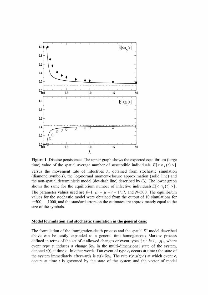
Figure 1 Disease persistence. The upper graph shows the expected equilibrium (large time) value of the spatial average number of susceptible individuals ])([ >< tnE S versus the movement rate of infectives λ, obtained from stochastic simulation (diamond symbols), the log-normal moment-closure approximation (solid line) and the non-spatial deterministic model (dot-dash line) described by (3). The lower graph shows the same for the equilibrium number of infective individuals ])([ >< tnE I . The parameter values used are β=1, µI = µ =ν = 1/17, and N=500. The equilibrium values for the stochastic model were obtained from the output of 10 simulations for t=500,…,1000, and the standard errors on the estimates are approximately equal to the size of the symbols. Model formulation and stochastic simulation in the general case: The formulation of the immigration-death process and the spatial SI model described above can be easily expanded to a general time-homogeneous Markov process defined in terms of the set of q allowed changes or event types {ei : i=1,...,q}, where event type ei induces a change δsei in the multi-dimensional state of the system, denoted s(t) at time t. In other words if an event of type ei occurs at time t the state of the system immediately afterwards is s(t)+δsei. The rate r(ei,s(t);a) at which event ei occurs at time t is governed by the state of the system and the vector of model

parameters a. The total event rate at time t is R(s(t);a) = qi 1=Σ r(ei,s(t);a). As we saw

above for the immigration-death model these rates may also be used to define a deterministic or mean-field dynamics in terms of ordinary differential equations. The stochastic dynamics of the corresponding time-homogeneous Markov process are defined as follows: (i) the time τ to the next event (of any type) is drawn from an exponential distribution with rate R(s(t);a); and (ii) the event type which occurs at time t+τ is chosen to be type ei with probability r(ei,s(t);a)/ R(s(t);a) (Cox and Miller, 1965). Then to simulate a realisation of this stochastic process iterate the following procedure: (i) generated the time to the next event τ = -ln(y)/R(n; ν,µ) where y~U(0,1) ; (ii) draw a second random variate y2~U(0,1), and starting with k=1 choose event k and update state-space accordingly, if y2≥ k

i 1=Σ r(ei,s(t);a)/ R(s(t);a), else increase k to k=k+1 and repeat; and (iii) update time to t+τ. It is also relatively straightforward to account for temporal fluctuations in the environment by making the parameters of the model vary in time. In such cases the easiest way to simulate the process is to adopt the following approximate algorithm. Firstly choose δt=min(1/ R(s(t);a(t)), δtmin) and update time to t+δt. Note δtmin is chosen so that changes in the time varying parameters are negligible in the interval (t,t+δtmin). Secondly, choose event ei with probability r(ei,s(t);a(t))δt. To do this generate a random variable y~U(0,1), calculate y’= yδt . Then starting with k=1 choose event k if y’≥ k

i 1=Σ r(ei,s(t);a), else k=k+1. Repeat until k=q+1 unless an event is chosen, in which case update state-space appropriately. Repeat procedure for the next time step. Note that if y’≥ q

i 1=Σ r(ei,s(t);a) then the above algorithm will move on to next time step and no event occurs in the interval (t,t+δt). 3. Parameter estimation in stochastic models: a general formulation Here we consider how to infer parameters from incomplete data for a general time-homogeneous Markov process defined above (see also Walker et al., 2006). Recall that the total event rate at time t is R(s(t);a) = q

i 1=Σ r(ei,s(t);a) and the time τ to the next event (of any type) is drawn from an exponential distribution with rate R(s(t);a); and the event type which occurs at time t+τ is chosen to be type ei with probability r(ei,s(t);a)/ R(s(t);a). This definition leads to a stochastic updating rule such that, conditional on the state of the system being s(t) at time t the probability density that an event of type ei occurs before any other event type and does so at time t+τ is given by, ( ) ));(());(,()()()()( atsR

ie eatsertstytsststsfi

ττδτ −==+<≤+=+ (8) Suppose the timings and nature of all events (e.g. all births, deaths, immigrations and infections etc.) which occur in the interval [t0, tn] are observed and recorded. Then let tk be the time at which event k in the sequence occurs and denote its type by E(k) ∈ {ei : i=1,...,q}. Suppose there are n events, then given an initial state s(t0) the finite and

complete realization of the stochastic process, { }n

ktksS

0== can be generated from the

set of events ζ ={(E(k),tk):k=1,...,n}. The Likelihood of the complete data set, ζ, L(a,ζ) = P(ζ | a, s(t0)), is the probability of observing the complete sequence of events ζ given the parameters a and the initial configuration s(t0) and is given by

( ) ∏−

−−−

−−∝n

k

atsRttk

kkkeatskErtsaP1

));(()(10

11));(),(()(,|ζ . (9)

In general the final observation time T may not coincide with the occurrence of the final event at tn. In such cases the likelihood (9) should be multiplied by an additional term exp{-(T-tn)R(s(tn);a)}describing the probability that nothing happens between tn and T. Given (9) if complete data is available Likelihood methods (Edwards, 1992) can be used to estimate model parameters. The likelihood follows directly from the definition of the model via the stochastic update rule (8), and in general this is also true for non-Markovian stochastic processes, although the form of the likelihood will differ from that shown in (9). In the sequel we shall simply write the complete likelihood as P(ζ | a) dropping the explicit dependence on the initial condition s(t0) which may either be regarded as known and fixed or considered as an additional set of parameters to be estimated and thus incorporated into the vector a. Note that we have already suppressed the conditional dependence of the likelihood on the model since we will not formally compare different models. In the case of incomplete data we observe a set of events D (the data), but there are also those hidden events H we do not observe. The complete realisation is therefore characterised by the full set of events ζ = (D, H). We note that in this missing data context one could employ data augmentation within a likelihood framework, however here we focus on a Bayesian treatment of this problem. Applying Bayes' rule,

)()()|()|(

BPAPABPBAP = ,

to P(ζ | a) = P(D,H | a) we obtain the joint posterior distribution for the parameters a and the unobserved events H,

)()()|,()|,(

DPaPaHDPDHaP = (10)

in terms of the likelihood for complete observations (9), the parameter prior P(a) and the normalisation constant P(D). The prior distribution is typically chosen to reflect any knowledge about the parameters available before the data D were obtained. For example P(a) may be derived from previous analysis, or simply be a uniform distribution over some plausible range of parameter values as ascertained from appropriate literature. In the absence of such information the prior is usually chosen to be some convenient form, for example for the rate parameters considered here, an (unnormalised) flat prior on the positive real line or a gamma distribution. In addition it is common to assume independence between the priors for each of the N

components of the parameter vector, i.e. ( ) ∏ −=

N

k kaPaP1

)( . It is good practice to test the robustness of any analysis to prior specification. Bayesian inference (see e.g. Lee, 2004) is based on the posterior distribution (10) which for a given set of data is simply proportional to the likelihood and the prior. For example the distribution of parameters is given by

∫= HdHDHaPDaP )|,()|( (11)

which is just the joint posterior (10) marginalised over the hidden events. However, this integral is typically analytically intractable and the space of possible hidden events too large to allow evaluation by quadrature. Moreover, evaluation of the normalisation constant P(D) in (10) involves integrals of similar computational complexity. Fortunately, Markov chain Monte Carlo techniques, allow parameter samples to be drawn directly from the posterior P(a, H | D) without having to calculate the normalisation constant P(D). The Metropolis-Hastings algorithm and Gibbs sampling allow parameter samples to be drawn directly from the posterior, but since the number of unobserved events is in general unknown, in sampling over H, the Markov chain must explore spaces of varying dimension (corresponding to the numbers of events in a given realisation) requiring application of reversible jump MCMC (Green, 1995). The samples generated from the posterior P(a, H | D) using MCMC allow the calculation of essentially any statistic based on the parameters, and missing events. For example the marginal distribution of parameters described by (11) may be estimated by simply disregarding the sampled hidden events and forming a histogram of the sampled parameter values only. The marginal distribution of any single parameter (component of a) or the joint distribution of two or more may be obtained in a similar fashion. Such estimates improve as the number of samples generated from the Markov chain increases. Reversible-jump Metropolis-Hastings Algorithm In order to implement the procedure described above samples of parameters and missing events must be generated from the posterior (10). In order to do this we describe here two algorithms, the first samples hidden events H for fixed parameters a, and the second samples parameters for fixed H. Samples from the joint distribution are obtained by iteratively applying the first and then the second algorithm. To generate samples of the missing events from the posterior P(a, H | D) for a given set of parameters a we employ reversible jump MCMC (Green, 1995) based on the Metropolis-Hastings algorithm (Metropolis et al., 1953; Hastings, 1970). Start with a set of hidden events H0 which are consistent with the observations D. Let Hi denote the set of hidden events at the ith step and iterate the following procedure M times:

1. propose Hi H’ with probability q(Hi ,H’)

2. set Hi+1 = H’ with probability :( ) ( )( ) ( )⎭

⎬⎫

⎩⎨⎧

',|,,'|',

,1minHHqaHDPHHqaHDP

ii

i

3. else Hi+1 = Hi

Note that since in general the method only makes use of relative values of the posterior P(a, H | D) the acceptance probability in step 2 is straightforward to calculate as the ratio of likelihoods of complete events (10) multiplied by a ratio of proposal probabilities (as shown). The proposal probabilities allow the exploration of the space of possible hidden events. In theory q(,) can be any distribution, e.g., uniform, however selection of the proposal distribution determines how well the chain mixes, and thus convergence time (the number of samples that must be discarded as burn-in). A general approach that enables a full exploration of the space of possible events, although may not be optimal, is to allow the proposal of three basic changes to the current reconstructed realization; a birth step where a new event is added to the realization; a death step where an event is deleted from the realization; and a rearrange step which changes the time of an existing event in the realization. In order to draw parameter samples from the posterior we can apply a variant on the above algorithm in which we keep the reconstructed events H fixed. If we draw parameter samples from the proposal distribution q(a,a') then the acceptance probability becomes

( ) ( )( ) ( ) ⎭

⎬⎫

⎩⎨⎧

',)(|,,')'('|,,1minaaqaPaHDPaaqaPaHDP

From which it is noted that if the proposal distribution were proportional to the posterior q(a,a') ≈ q(a')∝ ( ) )'('|, aPaHDP , then the acceptance probability would be 1. This is the basis of Gibbs sampling which in principle this is more efficient that using the Metropolis-Hastings algorithm as no samples are rejected. Of course the key difficulty is in drawing from a distribution proportional to the posterior. To see how this can be applied in the present context, suppose that ai ≥ 0, then we can assign a Gamma prior distribution P(ai) ≈ Ga( α,β)∝ ia

i ea βα −−1 . If the rates of the time-homogeneous Markov process (described earlier) are linear in ai then, up to a constant of proportionality independent of ai , the likelihood can be written

),,('),,('),|,( iii aHDaaHDiii eaaaHDP −− −

− ∝ βα where in general α' and β' depend on the data, the missing events and the other parameters a-i. It follows that since the prior is a gamma distribution then so is the posterior

)','()(),|,(),,|( ββαα ++== −− GaaPaaHDPaHDaP iiiii It is therefore possible to sample values directly from this distribution. Moreover this is relatively efficient compared with the Metropolis-Hastings algorithm, since α' and β' are certainly no more computationally demanding to calculate than the likelihood itself. To draw a set of samples {(ai,Hi):i=1,…N} from the joint posterior P(a, H | D ) we must choose {(a0,H0) consistent with the data D and then iterate the following:

A. For fixed parameters ai propose M changes to the hidden events using the reversible jump Metropolis-Hastings algorithm described in steps 1-3 above. This generates Hi+1

B. Draw the next set of parameter samples ai+1 using Gibbs sampling from

the univariate conditional posterior distributions. This combined Metropolis-Hastings/Gibbs procedure implements a Markov chain (indexed by i) which asymptotically as i → ∞ generates samples from the distribution P(a, H| D ) (Metropolis et al., 1953; Hastings, 1970; Green, 1995). In other words if we run the chain for long enough (the burn-in period) it will settle down to an equilibrium in which each sample generated (post burn-in) is draw from the posterior distribution. In practice the key problem is deciding on the burn-in period, that is, how many samples to discard before it is safe to assume that the Markov chain has converged to the desired distribution. There are a number of convergence diagnostics available (Gilks et al., 1996) but none guarantee convergence in general, and by far the most common approach is visual inspection of the chain output. This is the method we rely on and we monitor time series of the parameter samples obtained by the chain after an initial burn-in (determined post-hoc by visual inspection of the output). The Markov chain tends to mix more efficiently if, for each Gibbs sample of the parameters we typically perform many iterations M > 1of the Metropolis-Hastings sampling of the missing events. 4. Applications The examples used to illustrate the formulation and analysis of stochastic models in Section 2 focused on population level models with applications in ecology and epidemiology. Whilst there are many such applications of time-homogeneous Markov processes, these stochastic methods are remarkably flexible and can be employed across a wide spectrum of application. To illustrate this we now describe two contrasting applications drawn from our recent research. The first example combines the development and analysis of an agent-based model describing grazing in heterogeneous environments, with parameter inference based on data generated using contact logging in a behavioural experiment on diary cows. The second example makes use of large-scale data describing bio-geographical features of the landscape and the spatio-temporal spread of an alien plant to estimate the parameters of a stochastic model of dispersal and establishment. 4.1 Modelling individual grazing behaviour Marion et al. (2005) develop a simple stochastic agent-based model describing the grazing behaviour of herbivores in a spatially heterogeneous environment. The model reflects the biology in that decisions to move to a new location are based on visual assessment of the sward height (or some other proxy for nutritional value) in a surrounding neighbourhood, whilst the decision to graze the current location are based on the residual sward height and olfactory assessment of local faecal contamination. The model divides space into N discrete patches with ci animals and sward height hi in each patch i=1,…,N, and assumes that the agents (animals) either graze the current patch at rate βci(hi -h0) or move to one of z neighbouring patches j at rate ν ci hj /z . In

addition, the sward growth in each patch, i=1,…,N, is assumed to be logistic γ hi(1- hi/ hmax). The model is summarised in Table 3.

Change in state space Event description δhi δci δcj

Event Rate at time t

Grass growth at patch i +1 0 0 γ hi(1- hi/ hmax) Animal bite at patch i -1 0 0 β ci (hi- h0) Movement of animal from patch i to a neighbouring patch j

0 -1 +1 zν ci hj

Table 3: Agent-based model of grazing behaviour defined in terms of the sward height hi and the number of animals ci at patch i=1,...,N. The sward grows logistically at rate γ hi(1- hi/ hmax), and the agents take bites from patch i at rate β ci (hi- h0) and move from patch i to j at rate νci hj/z.

As was shown above for the SI model with immigration and death it is possible to

construct equations describing the spatial averages ),(11

ii

N

ichf

Nf

=∑>=< of the state-

variables. For example, note that since there are no births and deaths the animal density >< )(tc is constant, and the equation describing the average sward height

)(1)(1

thN

th i

N

i=∑>=< is written

( )

)](),([)]([

])([])([])([])([])([

max

0max

2

thtcCovthVarh

hthEtcEh

thEthEdt

thdE

βγ

βγ

−−

−><><−⎟⎟⎠

⎞⎜⎜⎝

⎛ ><−><=

><

where the variance in sward height )]([ thVar = ])([ 2 >< thE - 2])([ >< thE measures the spatial heterogeneity and the covariances )](),([ thtcCov = ])()([ >< thtcE -

])([])([ ><>< thEtcE measures the strength of association between tall swards and the grazing animals. It is worth noting that this equation involves no approximation and that the first line represents the equivalent non-spatial deterministic model. The variance and covariance terms in the second line therefore measure the importance of stochastic and spatial effects in the system; if both terms are close to zero then these effects are negligible. Evolution equations for the second-order quantities )]([ tcVar ,

)]([ thVar and )](),([ thtcCov , depend on third-order spatial moments and also on correlations between nearest neighbours. Marion et al. (2005) show how to close these equations using a variant of the log-normal approximation discussed in Section 2. As before this becomes more exact as the movement rate increases in a similar manner to the previous example.

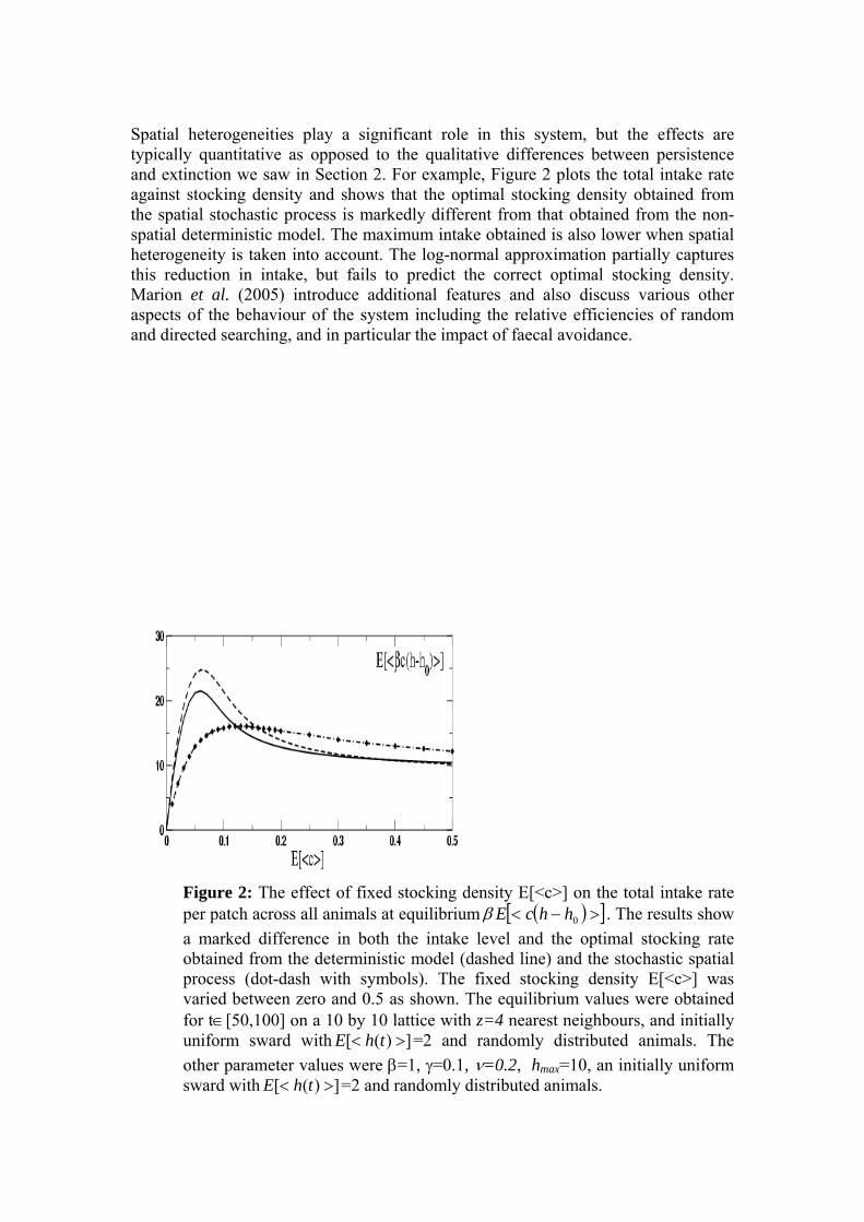
Spatial heterogeneities play a significant role in this system, but the effects are typically quantitative as opposed to the qualitative differences between persistence and extinction we saw in Section 2. For example, Figure 2 plots the total intake rate against stocking density and shows that the optimal stocking density obtained from the spatial stochastic process is markedly different from that obtained from the non-spatial deterministic model. The maximum intake obtained is also lower when spatial heterogeneity is taken into account. The log-normal approximation partially captures this reduction in intake, but fails to predict the correct optimal stocking density. Marion et al. (2005) introduce additional features and also discuss various other aspects of the behaviour of the system including the relative efficiencies of random and directed searching, and in particular the impact of faecal avoidance.

Figure 2: The effect of fixed stocking density E[<c>] on the total intake rate per patch across all animals at equilibrium ( )[ ]>−< 0hhcEβ . The results show a marked difference in both the intake level and the optimal stocking rate obtained from the deterministic model (dashed line) and the stochastic spatial process (dot-dash with symbols). The fixed stocking density E[<c>] was varied between zero and 0.5 as shown. The equilibrium values were obtained for t∈[50,100] on a 10 by 10 lattice with z=4 nearest neighbours, and initially uniform sward with ])([ >< thE =2 and randomly distributed animals. The other parameter values were β=1, γ=0.1, ν=0.2, hmax=10, an initially uniform sward with ])([ >< thE =2 and randomly distributed animals.

If the level of faecal contamination of patch i is described by the variable fi ≥ 0 avoidance behaviour can be accounted for by modifying the bite rate to be ( ) if

ii ehhc µβ −− 0 . Relative to the case of no avoidance the bite rate is progressively reduced as both the avoidance parameter µ ≥ 0 and the level of contamination increase. Friend et al. (2002) conducted an experiment at the Scottish Agricultural College (Dumfries, UK) to investigate avoidance behaviour in dairy cows. Prior to releasing animals into the outdoor experimental arena certain areas, amounting to approximately 5% of the total area of the paddock were artificially contaminated with faeces. The four animals released into the paddock were retro-fitted with faecal collection bags to prevent further contamination of the paddock during the experiment. Moreover, a data-logging system composed of transponders worn by the animals and aerials buried under the faecal contamination produced a record of every visit to the contaminated areas for each animal for the four day duration of the experiment. These data were supplemented by the daily measurement of the sward height in the contaminated zones and at a sample of points across the uncontaminated region. If sward growth is discounted it is possible to regard the data produced by this protocol as a partial history (see Section 3) of the stochastic model whose rates are defined in Table 3. The transponder data can be considered as direct observation of move events into the contaminated areas, although it should be noted that in some cases the transponder system logged multiple contacts in a short space of time and for the purpose of our analysis here these are regarded as a single visit, with the move event corresponding to the first contact. In addition the measured sward heights provide some information about bite events even though these are not recorded directly. In Section 3 the calculation of the likelihood was discussed in terms of events, but the sward height data are observations on the state-space of the system, rather than direct observations of events in the model. Nonetheless it is straight-forward to modify the event-based likelihood (9) described in Section 3 to account for such state-space observation by multiplying it with a noise model describing how state-space observations relate to the underlying state of the system. In this case assume that sward height measurements are subject to a Gaussian error with mean zero and standard deviation σ. Then if for a given event history the sward height of patch i at time t is hi(t) and the corresponding observation )(thobs is available, then the likelihood will gain the factor

( ) ( )( )⎟⎟⎠

⎞⎜⎜⎝

⎛ −−∝

σ2exp

2thth obsi .

Using this modification, the parameter inference techniques described in Section 3 have been applied to a variant of the with-avoidance foraging model described above. In particular, the paddock was divided into 20 patches of equal size one of which was considered to be the 5% contaminated area. The level of faecal contamination was described by fi = 1 in the contaminated patch and fi = 0 in the clean areas. Sward growth was ignored during the four day period of the experiment and for the movement the neighbourhood size was taken to be the entire paddock. In addition h0

was assumed zero and σ=1. The data provided all the move events into the

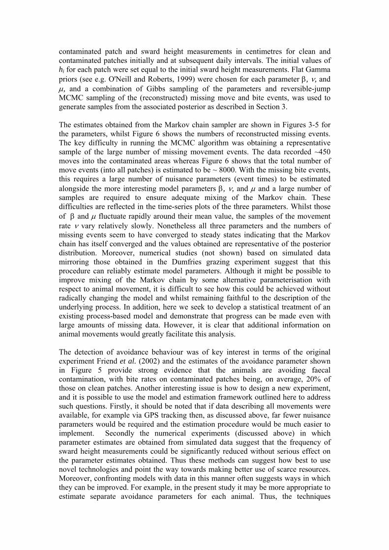
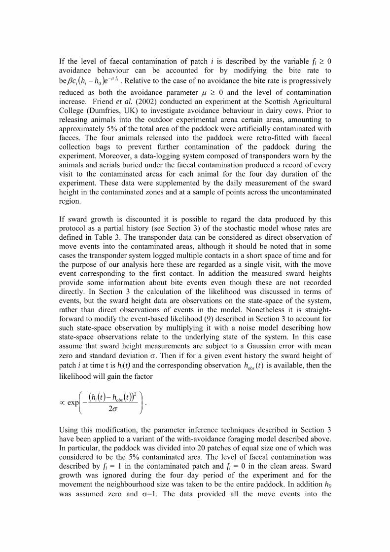
contaminated patch and sward height measurements in centimetres for clean and contaminated patches initially and at subsequent daily intervals. The initial values of hi for each patch were set equal to the initial sward height measurements. Flat Gamma priors (see e.g. O'Neill and Roberts, 1999) were chosen for each parameter β, ν, and µ, and a combination of Gibbs sampling of the parameters and reversible-jump MCMC sampling of the (reconstructed) missing move and bite events, was used to generate samples from the associated posterior as described in Section 3. The estimates obtained from the Markov chain sampler are shown in Figures 3-5 for the parameters, whilst Figure 6 shows the numbers of reconstructed missing events. The key difficulty in running the MCMC algorithm was obtaining a representative sample of the large number of missing movement events. The data recorded ~450 moves into the contaminated areas whereas Figure 6 shows that the total number of move events (into all patches) is estimated to be ~ 8000. With the missing bite events, this requires a large number of nuisance parameters (event times) to be estimated alongside the more interesting model parameters β, ν, and µ and a large number of samples are required to ensure adequate mixing of the Markov chain. These difficulties are reflected in the time-series plots of the three parameters. Whilst those of β and µ fluctuate rapidly around their mean value, the samples of the movement rate ν vary relatively slowly. Nonetheless all three parameters and the numbers of missing events seem to have converged to steady states indicating that the Markov chain has itself converged and the values obtained are representative of the posterior distribution. Moreover, numerical studies (not shown) based on simulated data mirroring those obtained in the Dumfries grazing experiment suggest that this procedure can reliably estimate model parameters. Although it might be possible to improve mixing of the Markov chain by some alternative parameterisation with respect to animal movement, it is difficult to see how this could be achieved without radically changing the model and whilst remaining faithful to the description of the underlying process. In addition, here we seek to develop a statistical treatment of an existing process-based model and demonstrate that progress can be made even with large amounts of missing data. However, it is clear that additional information on animal movements would greatly facilitate this analysis. The detection of avoidance behaviour was of key interest in terms of the original experiment Friend et al. (2002) and the estimates of the avoidance parameter shown in Figure 5 provide strong evidence that the animals are avoiding faecal contamination, with bite rates on contaminated patches being, on average, 20% of those on clean patches. Another interesting issue is how to design a new experiment, and it is possible to use the model and estimation framework outlined here to address such questions. Firstly, it should be noted that if data describing all movements were available, for example via GPS tracking then, as discussed above, far fewer nuisance parameters would be required and the estimation procedure would be much easier to implement. Secondly the numerical experiments (discussed above) in which parameter estimates are obtained from simulated data suggest that the frequency of sward height measurements could be significantly reduced without serious effect on the parameter estimates obtained. Thus these methods can suggest how best to use novel technologies and point the way towards making better use of scarce resources. Moreover, confronting models with data in this manner often suggests ways in which they can be improved. For example, in the present study it may be more appropriate to estimate separate avoidance parameters for each animal. Thus, the techniques

described here are potentially useful tools in linking empirical and theoretical developments more tightly.

Figure 3 Estimates of the movement rate ν obtained by applying the Bayesian inference scheme described in the text to data from the SAC grazing experiment. Top graph shows samples of ν generated from 1 million parameter samples the Markov chain after an initial burn-in of 500,000. Note, for every proposed change to the parameters 10 changes to the event history were proposed. Lower graph shows the histogram with 100 bins obtained from the post burn-in samples. The ν samples have mean 1.90 and standard deviation 0.07.

Figure 4 As above but for the bite rate β. The β samples have mean 0.06 and standard deviation 0.004.

Figure 5 As above but for the avoidance parameter µ. The µ samples have mean 1.59 and standard deviation 0.5.

Figure 6 The total number of move (upper graph) and bite (lower graph) events in the reconstructed event history obtained by applying the Bayesian inference scheme described in the text to data from the SAC grazing experiment. The graph shows total number of each event type generated for 1 million parameter samples of the Markov chain after an initial burn-in of 500,000. Note, for every proposed change to the parameters 10 changes to the event history were proposed.

4.2 Modelling the spread of an invasive species across a landscape Parameter estimation for fully spatio-temporal stochastic models is an area of ongoing development which forms a bridge between complex systems models and spatial statistical regression. As discussed in Section 3, the increasing capabilities of computational statistics in recent years, most notably the development of MCMC techniques (see Gilks et al., 1996, for a review), and their application to population processes such as epidemics (Gibson, 1997; Marion et al., 2003; Hohle et al., 2005; Gibson et al., 2006), means that it is now possible to fit ever more realistic models to observational data in a statistically rigorous fashion. Moreover, estimation in stochastic spatio-temporal models has the advantage over more traditional statistical techniques, such as logistic and autologistic regression (Collingham et al., 2000; Huffer and Wu, 1998; Beerling, 1993), of explicitly modelling change over time rather than assuming that the species' distribution (or other spatial pattern) has already reached equilibrium. However, one area in which the statistical treatment of spatio-temporal models is currently deficient is in its handling of covariate information. To date most applications have made little or no use of such data, largely focusing on estimating dispersal kernels and other key processes. On the other hand regressive techniques excel in their ability to estimate the effects of large numbers of covariates. Moreover, Hastings et al. (2005) suggest that the realistic incorporation of environmental spatial heterogeneity into models of spatio-temporal spread is a key challenge. Such issues are of practical significance to the spread of a disease or an alien species across a landscape. Non-indigenous species can cause substantial economical losses, and are recognised as one of the largest threats to native biodiversity and ecosystem functioning (Kolar and Lodge, 2001; Sala, 2001) and increasing globalisation has promoted the intentional and accidental spread of species through their natural dispersal barriers. Considerable research effort has therefore focused on this issue, and mathematical and statistical approaches have contributed to our understanding of the ecological processes underlying biological invasions (Kolar and Lodge, 2001). Cook et al. (2006) attempt to bridge the gap between complex systems models and spatial regressions by developing a time-homogeneous Markov process to model the spread of an invasive species across a landscape in terms of a contact process, describing both natural dispersal and human interventions such as transportation (deliberate and accidental), and the variations in bio-geographical features described a range of covariates such as habitat type and climate which cause spatial heterogeneity in local suitability for colonisation. This approach necessarily balances model parsimony, computational tractability and the desire for realism, for example by describing varied and complex transport processes by means of a single dispersal kernel. Within a Bayesian framework MCMC techniques are applied to estimate the parameters of this model from data describing the spread of the riparian weed Heracleum mantegazzianum (Giant Hogweed) in Britain in the 20th Century. A key advantage of the Bayesian approach is that model predictions can reflect both inherent variability and the estimated parameter uncertainty. In this case the risk of future

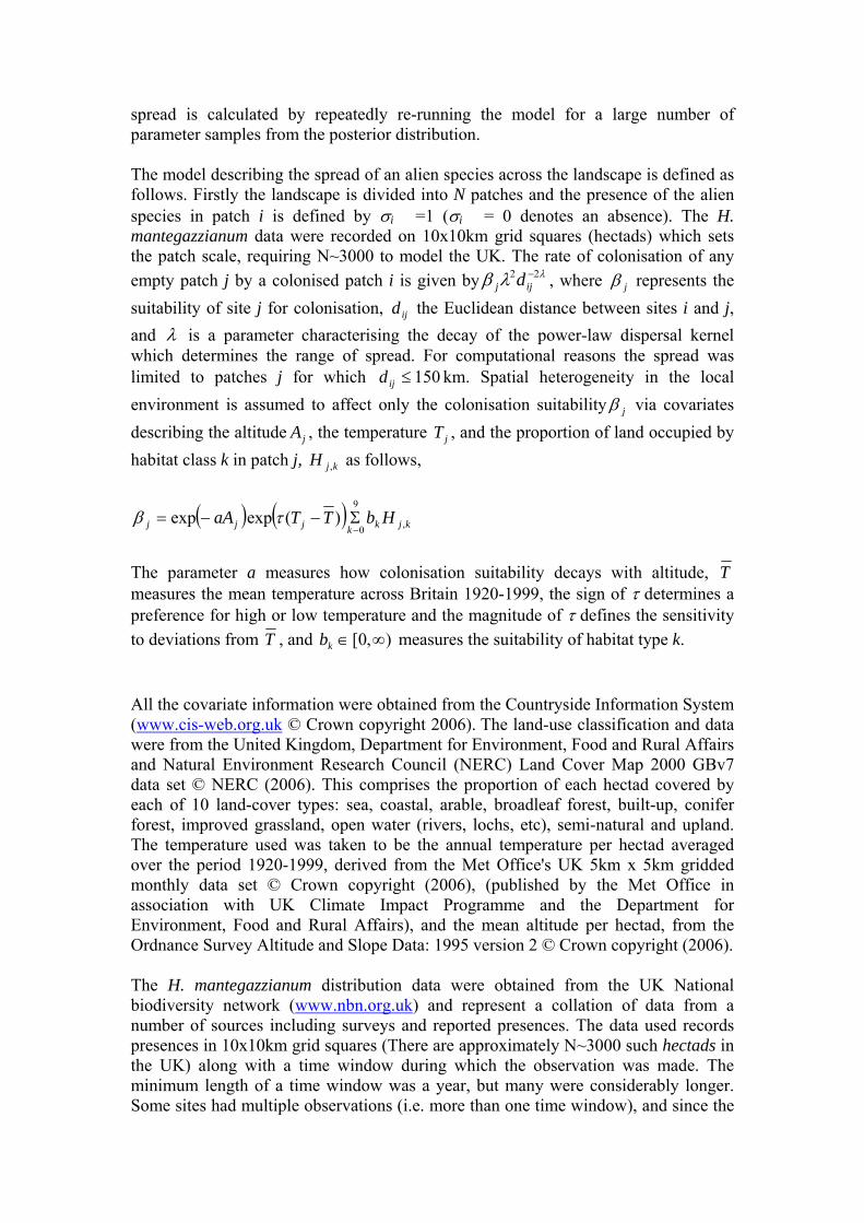
spread is calculated by repeatedly re-running the model for a large number of parameter samples from the posterior distribution. The model describing the spread of an alien species across the landscape is defined as follows. Firstly the landscape is divided into N patches and the presence of the alien species in patch i is defined by σi =1 (σi = 0 denotes an absence). The H. mantegazzianum data were recorded on 10x10km grid squares (hectads) which sets the patch scale, requiring N~3000 to model the UK. The rate of colonisation of any empty patch j by a colonised patch i is given by λλβ 22 −

ijj d , where jβ represents the suitability of site j for colonisation, ijd the Euclidean distance between sites i and j, and λ is a parameter characterising the decay of the power-law dispersal kernel which determines the range of spread. For computational reasons the spread was limited to patches j for which 150≤ijd km. Spatial heterogeneity in the local environment is assumed to affect only the colonisation suitability jβ via covariates describing the altitude jA , the temperature jT , and the proportion of land occupied by habitat class k in patch j, kjH , as follows,

( ) ( ) kjkkjjj HbTTaA ,

9

0)(expexp

−Σ−−= τβ

The parameter a measures how colonisation suitability decays with altitude, T measures the mean temperature across Britain 1920-1999, the sign of τ determines a preference for high or low temperature and the magnitude of τ defines the sensitivity to deviations from T , and ),0[ ∞∈kb measures the suitability of habitat type k. All the covariate information were obtained from the Countryside Information System (www.cis-web.org.uk © Crown copyright 2006). The land-use classification and data were from the United Kingdom, Department for Environment, Food and Rural Affairs and Natural Environment Research Council (NERC) Land Cover Map 2000 GBv7 data set © NERC (2006). This comprises the proportion of each hectad covered by each of 10 land-cover types: sea, coastal, arable, broadleaf forest, built-up, conifer forest, improved grassland, open water (rivers, lochs, etc), semi-natural and upland. The temperature used was taken to be the annual temperature per hectad averaged over the period 1920-1999, derived from the Met Office's UK 5km x 5km gridded monthly data set © Crown copyright (2006), (published by the Met Office in association with UK Climate Impact Programme and the Department for Environment, Food and Rural Affairs), and the mean altitude per hectad, from the Ordnance Survey Altitude and Slope Data: 1995 version 2 © Crown copyright (2006). The H. mantegazzianum distribution data were obtained from the UK National biodiversity network (www.nbn.org.uk) and represent a collation of data from a number of sources including surveys and reported presences. The data used records presences in 10x10km grid squares (There are approximately N~3000 such hectads in the UK) along with a time window during which the observation was made. The minimum length of a time window was a year, but many were considerably longer. Some sites had multiple observations (i.e. more than one time window), and since the

weed is extremely persistent we make the assumption that once a site is colonised it remains colonised forever; therefore, for the model considered here, subsequent observations provide no further information about the colonisation process. In this example we also make the simplifying assumption that the colonisation of a site occurs at the earliest end-point of all of the observation windows recorded at that site, since this is the first time we can be certain the plant has reached that site. In reality there is uncertainty in the colonisation time which could in principle be accounted for in the inference scheme described in Section 3, by specifying an observation model and treating colonisations as unobserved events. However, this may lead to problems of parameter identifiability and in any case will dramatically increase the computationally complexity of the problem. This is a reasonable compromise since the focus here the treatment of spatially explicit covariate information. Estimation of the model parameters under these assumptions reveals that the habitat with the highest posterior mean colonisability is broadleaf. This is in contrast to reports (Clapham et al., 1985; Tiley et al., 1996; Stace, 1997) that the weeds primary habitats include waste-lands, and rivers and canals which are included in the land-use classes built-up (estimated to be second most colonisable) and open-waters (fourth, just behind improved grasslands) respectively. There is evidence that hectads with a lower mean altitude are more suitable to H. mantegazzianum than higher areas. Interestingly, however, this is countervailed by the weed's preference for lower temperatures (evinced by posterior support for negative values of a). This is especially surprising since altitude is negatively correlated with temperature, and indeed we might have expected confounding of these two effects. Both results are, however, supported to some extent by the literature: Pysek et al. (1998) found that H. mantegazzianum was represented less in areas of the Czech Republic with warm winters than cold; Willis and Hulme (2002) found experimentally that survival and biomass were lower for H. mantegazzianum at high altitudes. We can also combine the effects of all covariates in the full model to evaluate which areas are more suitable for the weed. Figure 7 shows the posterior mean colonisability jβ for each hectad in Britain, with darker areas being more suited to the plant. There are considerable differences across sites, with the areas that have been colonised (most of England, the lowlands of Scotland) for the most part having high jβ . To evaluate where future colonisations are likely to occur 3000 simulations were performed, using parameter values sample from the posterior, for the time period 2000-2025 (the data extend to the end of 1999). Figure 7 maps the probability of sites being colonised by 2010, obtained by recording against time the proportion of simulations resulting in the colonisation of sites uncolonised at the start of 2000. The model predicts that upland areas are likely to remain uncolonised over this time scale. Cook et al. (2006) show that the exclusion of covariates describing local suitability not only produces biased estimates of the dispersal kernel, but also leads to the unlikely conclusion that upland areas will become colonised over this period. The inclusion of land-use and temperature covariates means that the model described here could be used to produce similar risk maps under future land use and climatic scenarios.

Figure 7 Risk maps for H. mantegazzianum. The left-hand map shows the posterior mean value of the potential colonisability Njj ,...1: =β of every hectad in Britain. The right-hand map shows hectads colonised by 1999 in red whilst the other colours indicate the probability of colonisation by 2010 as described in the text.

5. Conclusion In this chapter we have presented a range of tools which enable closer integration of model development and data collection for complex biological systems. The methods presented relate to dynamic stochastic process based models, and in particular we have focused on time-homogeneous Markov processes. The framework can account for spatio-temporal heterogeneities and individual variability which are often crucial in understanding the properties of biological systems. Unfortunately, the non-linear nature of such phenomena typically leads to models which are analytically intractable. However, a number of analytic approximations are available which help to verify simulation results and provide valuable insights into model behaviour. The applications considered revealed that such approximations often perform well in some parameter regions, but rather poorly in others. Therefore the development of improved approximations and analytic approaches to such models is an area of ongoing research. Computational statistical methods such as MCMC can be applied to infer model parameters even when observations are incomplete. Moreover, in a Bayesian framework this enables uncertainty in parameters, and in principle even in models, to be estimated. We described two applications in which parameter estimation was carried out using MCMC methods. In the first, incomplete

observations of animal behaviour were used to estimate the parameters of an agent-based model, and the framework used to improve the design of any future experiment. In the second, covariate effects on local establishment and parameters describing spatial spread were jointly estimated, and the resulting parameter uncertainty incorporated into projections of the future spread of an alien plant species across Britain. In practice such statistically correct parameter inference can be too computationally demanding to apply to complex models, or when there are too many missing observations. Therefore computationally efficient, and possibly in-exact, methods for parameter inference are required. Moreover, whilst there is a wide literature on model selection per se, model selection with respect to stochastic process-based models is poorly understood and further research is required. Nonetheless the applications discussed demonstrate that currently available methods are already useful tools in developing understanding of complex biological phenomena. References Bailey, N.T.J., (1963) The Elements of Stochastic Processes. John Wiley, New York. Beerling, D. J. (1993). The impact of temperature on the northern distribution limits of the introduced species fallopia japonica and impatiens glandulifera in north-west Europe. Journal of Biogeography 20, 45-53. Besag, J., Green, P. J., (1993) Spatial statistics and Bayesian computation. Journal of the Royal Statistical Society B 55, 25–37. Bolker, B., Pacala, S.W., (1997) Using moment equations to understand stochastically driven spatial pattern formation in ecological systems. Theoretical Population Biology 52, 179–197. Clapham, A. R., T. G. Tutin, and D. M. Moore (1985). Flora of the British Isles (3 ed.). Cambridge University Press. Collingham, Y. C., R. A. Wadsworth, B. Huntley, and P. E. Hulme (2000). Predicting the spatial distribution of non-indigenous riparian weeds: issues of spatial scale and extent. Journal of Applied Ecology 37 (Suppl. 1), 13-27. Cook, A., Marion, G., Butler, A. and Gibson, G. (2006) Bayesian inference for the spatio-temporal invasion of alien species. Bulletin of Mathematical Biology. Submitted. Cox, D. R., and Miller, H. D. (1965). The Theory of Stochastic Processes, Chapman and Hall, London. Draper, D. (1995) Assessment and propogation of model uncertainty (with discussion). Journal of the Royal Statistical. Society B, 57, 45-97. Edwards A. W. F. (1992) Likelihood, Johns Hopkins University Press, Baltimore.

Filipe, J.A.N., Gibson, G.J., (1998) Studying and approximating spatio-temporal models for epidemic spread and control. Philosophical Transactions of the Royal Society London B 353 (1378), 2153–2162. Friend, M.A., Swain, D.L., Mayes, R.W., & Hutchings, M.R. (2002) Combining an active transponder system with sprayed n-alkanes to monitor spatial and temporal grazing patterns of contaminated pastures. In Proceedings of the Xth European Intake Workshop, Iceland Gamerman, D., (1997) Markov Chain Monte Carlo. Chapman & Hall, London. Gelfand, A. E., Smith, A. F. M., (1990) Sampling-based approaches to calculating marginal densities. Journal of the American Statistical Association 9 85, 398–409. Gelman, A., Carlin, J. B., Stern, H. S., Rubin, D. B., (1995) Bayesian Data Analysis. Chapman & Hall, CRC. Gibson, G., C. Gilligan, J. Filipe, W. Otten, A. Cook, and G. Marion (2006). Bayesian estimation for percolation models of disease spread in plant communities. Statistics and Computing. In press Gibson, G. J., (1997) Markov chain Monte Carlo methods for fitting spatio-temporal stochastic models in plant epidemiology. Applied Statistics 46, 215–233. Gibson, G. J., Renshaw, E., (1998) Estimating parameters in stochastic compartmental models using Markov chain methods. IMA Journal of Mathematics Applied in Medicine & Biology 15,19–40. Gibson, G. J., Renshaw, E., (2001a) Inference for immigration-death processes with single and paired immigrants. Inverse Problems 17, 455–466. Gibson, G. J., Renshaw, E., (2001b) Likelihood estimation for stochastic compartmental models using Markov chain methods. Statistics and Computing 11, 347–358. Gilks, W. R., S. Richardson, and D. J. Spiegelhalter (1996). Introducing Markov chain Monte Carlo. In W. R. Gilks, S. Richardson, and D. J. Spiegelhalter (Eds.), Markov Chain Monte Carlo in Practice, pp. 1-19. Chapman & Hall, London. Green, P. J., (1995) Reversible jump Markov chain Monte Carlo computation and Bayesian model determination. Biometrika 82, 711–732. Gurney, W.S.C. and Middleton, A.J. (1996) Optimal resource allocation in a randomly varying environment, Functional Ecology 10, 602-612. Hastings, A., K. Cuddington, and K. F. e. a. Davies (2005). The spatial spread of invasions: new developments in theory and evidence. Ecology Letters 8, 91-101. Hastings, W. K., (1970) Monte Carlo sampling methods using Markov chains and their applications. Biometrika 57, 97–109.

Hohle, M., E. Jurgensen, and P. D. O'Neill (2005). Inference in disease transmission experiments by using stochastic epidemic models. Applied Statistics 54, 349-366. Holmes, P., Brown, E., Moehlis, J., Boyacz, R., Gao, J., Hu, P., Aston-Jones, G., Clayton, E., Rajkowski, J., Cohen, J. D., (2004) Optimal decisions: From neural spikes, through stochastic differential equations, to behaviour. In: Proceedings 2004 International Symposium on Nonlinear Theory and its Applications (NOLTA2004) Fukuoka, Japan, 15–18. Huffer, F. W. and H. Wu (1998). Markov chain Monte Carlo for autologistic regression models with application to the distribution of plant species. Biometrics 54, 509-524. Isham, V. (1991) Assessing the variability of stochastic epidemics. Mathematical Biosciences 107, 209-224. Keeling, M. J., (2000a) Metapopulation moments: coupling, stochasticity and persistence. Journal of Animal Ecology 69, 725–736. Keeling, M. J., (2000b) Multiplicative moments and measures of persistence in ecology. Journal of Theoretical Biology 205, 269–281. Kendall, M. G. (1994) Kendall’s Advanced Theory of Statistics - Distribution Theory: vol. 1 (A. Stuart and J. K. Ord, Eds.), Edward Arnold, London. Kloeden, P. E., and Platen, E. (1992) Numerical Solution of Stochastic Differential Equations, Springer-Verlag. Kokko, H., and Ebenhard, T. (1996) Measuring the strength of demographic stochasticity, Journal of Theoretical Biology 183, 169-178. Kolar, C. and Lodge, D. (2001) Progress in invasion biology: predicting invaders. Trends in Ecology and Evolution 16, 199-204. Krishnarajah, I., Cook, A., Marion, G. and Gibson, G. (2005) Novel Moment Closure Approximations in Stochastic Epidemics. Bulletin of Mathematical Biology 67, 855--873 Lee, P. M., (2004) Bayesian Statistics: an introduction. Arnold, London. Mao, X. (1997) Stochastic Differential Equations and Applications, Horwood. Marion, G., Mao, X. and Renshaw, E. (2002a) Convergence of the Euler scheme for a class of stochastic differential. International Mathematical Journal 1, 9-22. Marion, G., Mao, X., Renshaw, E. and Liu, J. (2002b) Spatial heterogeneity and the stability of reaction states in autocatalysis. Physical Review E 66, 051915.

Marion, G., Renshaw, E. and Gibson, G.J. (2000) Stochastic modelling of environmental variation for biological populations. Theoretical Population Biology 57, 197-217. Marion, G., Renshaw, E., and Gibson, G. (1998) Stochastic effects in a model of nematode infection in ruminants. IMA Journal of Mathematics Applied in Medicine and Biology, 15, 97-116. Marion, G., Swain, D. L., Hutchings, M. R., (2005) Understanding foraging behaviour in spatially heterogeneous environments. Journal of Theoretical Biology 232, 127–142. Matis, H.J., Kiffe, T.R., (1996) On approximating the moments of the equilibrium distribution of a stochastic logistic model. Biometrics 52, 980–991. Matis, J. H., Kiffe, T. R., and Parthasarathy P. R. (1998) On the cumulants of population size for the stochastic power law logistic model. Theoretical Population Biology 53, 16-29. Metropolis, M., Rosenbluth, A. W., Rosenbluth, M. N., Teller, A. H., Teller1 ,E., (1953) Equation of state calculations by fast computing machines. Journal of Chemical Physics 21, 1087–1092. Nisbet, R. M., and Gurney, W. S. C. (1982) Modelling Fluctuating Populations, Wiley, Chichester. O’Neill, P. D., Roberts, G. O., (1999) Bayesian inference for partially observed stochastic epidemics. Journal of the Royal Statistical Society A 162, 121–129. Pysek, P., M. Kopeck_y, V. Jarosk, and P. Kotkova (1998). The role of human density and climate in the spread of Heracleum mantegazzianum in the Central European landscape. Diversity and Distributions 4, 9-16. Rand, D.A., and Wilson, H.B. (1991) Chaotic stochasticity: a ubiquitous source of unpredictability in epidemics, Proceedings of the Royal Society of London B 246, 179-184. Renshaw, E. (1991) Modelling Biological Populations in Space and Time, Cambridge University Press, Cambridge. Renshaw, E., Gibson, G. J., (1998) Can Markov chain Monte Carlo be usefully applied to stochastic processes with hidden birth times? Inverse Problems 14, 1581–1606. Roberts, M. G., and Grenfell, B. T. (1992) The population dynamics of nematode infections of ruminants: the effect of seasonality in the free living stages, IMA Journal of Mathematics Applied in Medicine and Biology 9, 29-41. Sala, O. et. al.. (2001). Global biodiversity scenarios for the year 2100. Trends in Ecology and Evolution 287, 1770-1774.

Smith, A. F. M., Roberts, G. O., (1993) Bayesian computation via the Gibbs sampler and related Markov chain Monte Carlo methods. Journal of the Royal Statistical Society B 55, 3–23. Stace, C. (1997). New Flora of the British Isles. Cambridge University Press. Tiley, G. E. D., F. S. Dodd, and P. M. Wade (1996). Biological fauna of the British Isles: Heracleum mantegazzianum Sommier & Levier. Journal of Ecology 84, 297-319. Tilman, D. and Karieva, P. (1997) Spatial Ecology: the role of space in population dynamics and intraspecific interactions (Editors). Princeton University Press. Walker, D.M., Perez-Barberia, F.J. and Marion, G. (2006). Stochastic Modelling of Ecological Processes using Hybrid Gibbs Samplers. Ecological Modelling. In press. Whittle, P. (1957) On the use of the Normal approximation in the treatment of stochastic processes, Journal of the Royal Statistical Society B 19, 266-281. Willis, S. G. and P. E. Hulme (2002). Does temperature limit the invasion of impatiens glandulifera and heracleum mantegazzianum in the UK? Functional Ecology 16, 530-539. Wilson, H.B. and Hassell, M.P. (1997) Host-parasitoid spatial models: the interplay of demographic stochasticity and dynamics, Proceedings of the Royal Society of London B 264, 1189-1195.