Embed Size (px)
Citation preview
Transport Engineering [Transportation system analysis]
AAiT, Department of Civil and Environmental Engineering Page 1
CHAPTER 3
TRANSPORTATION SYSTEM ANALYSIS Topics covered under this chapter are:
3.1. Traffic engineering studies 3.1.1. Spot speed studies 3.1.2. Volume studies 3.1.3. Travel time and delay studies 3.1.4. Parking studies
3.2. Fundamental principles of traffic flow 3.2.1. Traffic flow elements 3.2.2. Flow-density relationships 3.2.3. Fundamental diagram of traffic flow 3.2.4. Mathematical relationships describing traffic flow 3.2.5. Shock waves in traffic streams 3.2.6. Gap and gap acceptance
3.3. Queuing Analysis 3.3.1. Queuing Patterns 3.3.2. Queuing models
3.1. Traffic Engineering Studies The availability of highway transportation has provided several advantages that contribute to a high standard of living. However, several problems related to the highway mode of transportation exist. These problems include highway-related accidents, parking difficulties, congestion, and delay. To reduce the negative impact of highways, it is necessary to adequately collect information that describes the extent of the problems and identifies their locations. Such information is usually collected by organizing and conducting traffic surveys and studies.
3.1.1. Spot speed studies Spot speed studies are conducted to estimate the distribution of speeds of vehicles in a stream of traffic at a particular location on a highway. A spot speed study is carried out by recording the speeds of a sample of vehicles at a specified location. Speed characteristics identified by such a study will be valid only for the traffic and environmental conditions that exist at the time of the study. Speed characteristics determined from a spot speed study may be used to Establish speed zones, Determine whether complaints about speeding are valid, Establish passing and no-passing zones, Design geometric alignment, Analyze accident data, Evaluate the effects of physical improvements, Determine the effects of speed enforcement programs and speed control measures, to determine speed trends and so forth. Locations for Spot Speed Studies The locations for spot speed studies depend on the anticipated use of the results. For example, it may be for basic data collection or speed trend analyses. Any location may be used for the solution of a specific traffic engineering problem. When spot speed studies are being conducted, it is important that unbiased data be obtained. This requires that drivers be unaware that such a study is being conducted. Equipment used should therefore be concealed from the driver, and observers conducting the study should be inconspicuous.
Transport Engineering [Transportation system analysis]
AAiT, Department of Civil and Environmental Engineering Page 2
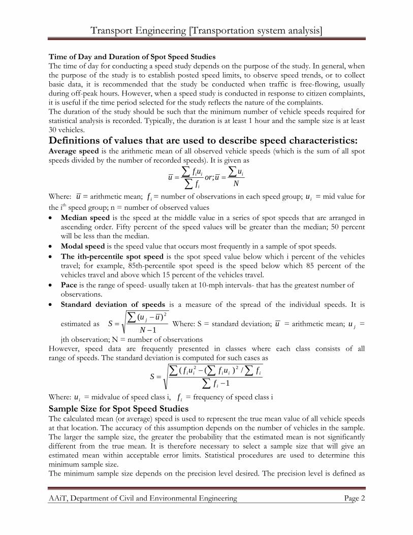
Time of Day and Duration of Spot Speed Studies The time of day for conducting a speed study depends on the purpose of the study. In general, when the purpose of the study is to establish posted speed limits, to observe speed trends, or to collect basic data, it is recommended that the study be conducted when traffic is free-flowing, usually during off-peak hours. However, when a speed study is conducted in response to citizen complaints, it is useful if the time period selected for the study reflects the nature of the complaints. The duration of the study should be such that the minimum number of vehicle speeds required for statistical analysis is recorded. Typically, the duration is at least 1 hour and the sample size is at least 30 vehicles. Definitions of values that are used to describe speed characteristics: Average speed is the arithmetic mean of all observed vehicle speeds (which is the sum of all spot speeds divided by the number of recorded speeds). It is given as
Nu
uorfuf
u i
i
ii ∑∑∑ == ;
Where: u = arithmetic mean; if = number of observations in each speed group; iu = mid value for the ith speed group; n = number of observed values • Median speed is the speed at the middle value in a series of spot speeds that are arranged in
ascending order. Fifty percent of the speed values will be greater than the median; 50 percent will be less than the median.
• Modal speed is the speed value that occurs most frequently in a sample of spot speeds. • The ith-percentile spot speed is the spot speed value below which i percent of the vehicles
travel; for example, 85th-percentile spot speed is the speed below which 85 percent of the vehicles travel and above which 15 percent of the vehicles travel.
• Pace is the range of speed- usually taken at 10-mph intervals- that has the greatest number of observations.
• Standard deviation of speeds is a measure of the spread of the individual speeds. It is
estimated as 1
)( 2
−
−= ∑
Nuu
S j
Where: S = standard deviation; u = arithmetic mean; ju =
jth observation; N = number of observations However, speed data are frequently presented in classes where each class consists of all range of speeds. The standard deviation is computed for such cases as
∑∑ ∑∑
−
−=
1/)(( 22
i
iiiii
ffufuf
S
Where: iu = midvalue of speed class i, if = frequency of speed class i Sample Size for Spot Speed Studies The calculated mean (or average) speed is used to represent the true mean value of all vehicle speeds at that location. The accuracy of this assumption depends on the number of vehicles in the sample. The larger the sample size, the greater the probability that the estimated mean is not significantly different from the true mean. It is therefore necessary to select a sample size that will give an estimated mean within acceptable error limits. Statistical procedures are used to determine this minimum sample size. The minimum sample size depends on the precision level desired. The precision level is defined as
Transport Engineering [Transportation system analysis]
AAiT, Department of Civil and Environmental Engineering Page 3
the degree of confidence that the sampling error of a produced estimate will fall within a desired fixed range. Thus, for a precision level of 90-10, there is a 90 percent probability (confidence level) that the error of an estimate will not be greater than 10 percent of its true value. The confidence level is commonly given in terms of the level of significance (α ), where α = (100 - confidence level). The commonly used confidence level for speed counts is 95 percent. The properties of the normal distribution have been used to develop an equation relating the sample size to the number of standard variations corresponding to a particular confidence level, the limits of tolerable error, and the standard deviation.
The formula is 2
=
dZN σ Where: N= minimum sample size; Z = number of standard deviations
corresponding to the required confidence level 1.96 for 95 percent confidence level; α = standard deviation (mph); d = limit of acceptable error in the speed estimate (mph). The standard deviation can be estimated from previous data, or a small sample size can first be used. Methods for Conducting Spot Speed Studies The methods used for conducting spot speed studies can generally be divided into two main categories: manual and automatic. Several automatic devices that can be used to obtain the instantaneous speeds of vehicles at a location on a highway are now available on the market. These automatic devices can be grouped into three main categories: (1) Those that use road detectors, (2) Those that use Doppler principle meters (radar type), and (3) Those that use the principles of electronics. Road Detectors Road detectors can be classified into two general categories: pneumatic road tubes and induction loops. These devices can be used to collect data on speeds at the same time as volume data are being collected. When road detectors are used to measure speed, they should be laid such that the probability of a passing vehicle closing the connection of the meter during a speed measurement is reduced to a minimum. This is achieved by separating the road detectors by a distance of 3 to 15 ft. The advantage of the detector meters is that human errors are considerably reduced. The disadvantages are that (1) these devices tend to be rather expensive, and (2) when pneumatic tubes are used, they are rather conspicuous and may, therefore, affect driver behavior, resulting in a distortion of the speed distribution. Doppler-Principle Meters Doppler meters work on the principle that when a signal is transmitted onto a moving vehicle, the change in frequency between the transmitted signal and the reflected signal is proportional to the speed of the moving vehicle. The difference between the frequency of the transmitted signal and that of the reflected signal is measured by the equipment, and then converted to speed in mph. In setting up the equipment, care must be taken to reduce the angle between the direction of the moving vehicle and the line joining the center of the transmitter and the vehicle. The value of the speed recorded depends on that angle. If the angle is not zero, an error related to the cosine of that angle is introduced, resulting in a lower speed than that which would have been recorded if the angle had been zero. However, this error is not very large, because the cosines of small angles are not much less than 1. The advantage of this method is that because pneumatic tubes are not used, if the equipment can be located at an inconspicuous position, the influence on driver behavior is considerably reduced. Electronic-Principle Detectors In this method, the presence of vehicles is detected through electronic means, and information on
Transport Engineering [Transportation system analysis]
AAiT, Department of Civil and Environmental Engineering Page 4
these vehicles is obtained, from which traffic characteristics such as speed, volume, queues, and headways are computed. The great advantage of this method over the use of road detectors is that it is not necessary to physically install loops or any other type of detector on the road. The most promising technology using electronics is video image processing, sometimes referred to as a machine-vision system. This system consists of an electronic camera overlooking a large section of the roadway and a microprocessor. The electronic camera receives the images from the road; the microprocessor determines the vehicle's presence or passage. This information is then used to determine the traffic characteristics in real time. One such system is the auto scope.
3.1.2. Volume studies Traffic volume studies are conducted to collect data on the number of vehicles and/or pedestrians that pass a point on a highway facility during a specified time period. This time period varies from as little as 15 min to as much as a year, depending on the anticipated use of the data. The data collected may also be put into subclasses which may include directional movement, occupancy rates, vehicle classification, and pedestrian age. Traffic volume studies are usually conducted when certain volume characteristics are needed, some of which are: 1. Average Annual Daily Traffic (AADT) is the average of 24-hr counts collected every day in
the year. AADTs are used in several traffic and transportation analyses for a. Estimation of highway user revenues b. Computation of accident rates in terms of accidents per 100 million vehicles per miles c. Establishment of traffic volume trends d. Evaluation of the economic feasibility of highway projects e. Development of freeway and major arterial street systems f. Development of improvement and maintenance programs 2. Average Daily Traffic (ADT) is the average of 24-hour counts collected over a number of days
greater than 1 but less than a year. ADTs may be used for Planning of highway activities, Measurement of current demand, Evaluation of existing traffic flow and so forth.
3. Peak Hour Volume (PHV) is the maximum number of vehicles that pass a point on a highway during a period of 60 consecutive minutes. The peak hour volumes PHVs are used for, Functional classification of highways, Design of the geometric characteristics of a highway, for example, number of lanes, intersection signalization, or channelization, For capacity analysis, Development of programs related to traffic operations, for example street systems or traffic routing and Development of parking regulations and etc.
4. Vehicle Classification (VC) records Volume with respect to the type of vehicles, for example, passenger cars, two-axle trucks, or three-axle trucks. VC is used in
a. Design of geometric characteristics, with particular reference to turning radii requirements, maximum grades, and lane widths, and so forth
b. Capacity analyses, with respect to passenger-car equivalents of trucks c. Adjustment of traffic counts obtained by machines d. Structural design of highway pavements, bridges, and so forth
5. Vehicle Miles of Travel (VMT) is a measure of travel along a section of road. It is the product of the traffic volume (that is, average weekday volume or ADT) and the length of roadway in miles to which the volume is applicable. VMTs are used mainly as a base for allocating resources for maintenance and improvement of highways.
Methods of Conducting Volume Counts Traffic volume counts are conducted using two basic methods: manual and automatic.
I. Manual Method Manual counting involves one or more persons recording observed vehicles using a counter. The
Transport Engineering [Transportation system analysis]
AAiT, Department of Civil and Environmental Engineering Page 5
main disadvantages of the manual count method are that (1) it is labor-intensive and can therefore be expensive, (2) it is subject to the limitations of human factors, and (3) it cannot be used for long periods of counting. II. Automatic Method
The automatic counting method involves the laying of surface detectors (such as pneumatic road tubes) or subsurface detectors (such as magnetic or electric contact devices) on the road. These detect the passing vehicle and transmit the information to a recorder, which is connected to the detector at the side of the road. Traffic Volume Data Presentation The data collected from traffic volume counts may be presented in one of several ways, depending on the type of count conducted and the primary use of the data. Some of the conventional data presentation techniques are:
• Traffic Flow Maps • Intersection Summary Sheets • Time-Based Distribution Charts • Summary Tables
Traffic Volume Characteristics A continuous count of traffic at a section of a road will show that traffic volume varies from hour to hour, from day to day, and from month to month. However, the regular observation of traffic volumes over the years has identified certain characteristics showing that although traffic volume at a section of a road varies from time to time this variation is repetitive and rhythmic. These characteristics of traffic volumes are taken in to consideration when traffic counts are being planned so that volumes collected at a particular time or place can be related to volumes collected at other times and places. Knowledge of these characteristics can also be used to estimate the accuracy of traffic counts. Sample Size and Adjustment of Periodic Counts The impracticality of collecting data continuously every day of the year at all counting stations makes it necessary to collect sample data from each class of highway and to estimate annual traffic volumes from periodic counts. This involves the determination of the minimum sample size (number of count stations) for a required level of accuracy and the determination of daily, monthly, and/or seasonal expansion factors for each class of highway. Determination of Number of Count Stations The minimum sample size depends on the precision level desired. The commonly used precision level for volume counts is 95-10. When the sample size is less than 30 and the selection of counting stations is random, a distribution known as the student's t distribution may be used to determine the sample size for each class of highway links. The student's t distribution is unbounded, with a mean of zero, and has a variance that depends on the scale parameter, commonly referred to as the degrees of freedom (ν ). The degrees of freedom (ν ) is a function of the sample size; ν = N -1 for the student's t distribution. The variance of the student's t distribution is ν /(ν - 2), which indicates that as ν approaches infinity, the variance approaches 1. Assuming that the sampling locations are randomly selected, the minimum sample number is given as
)/)()(/1(1)/(
2221,2/
2221,2/
dStNdSt
nN
N
−
−
+=
α
α
Where: n = minimum number of count locations required; t = value of the student's t distribution
Transport Engineering [Transportation system analysis]
AAiT, Department of Civil and Environmental Engineering Page 6
with (1 -α /2) confidence level (N - 1 degrees of freedom); N = total number of links (population) from which a sample is to be selected α = significance level; S = estimate of the spatial standard deviation of the link volumes; d= allowable range of error To use the above equation, estimates of the mean and standard deviation of the link volumes are required. These estimates can be obtained by taking volume counts at a few links or by using known values for other, similar highways. Adjustment of Periodic Counts Expansion factors, used to adjust periodic counts, are determined either from continuous count stations or from control count stations. Expansion Factors from Continuous Count Stations- Hourly, daily, and monthly expansion factors can be determined using data obtained at continuous count stations. Hourly expansion factors (HEFs) are determined by the formula
hourparticularforvolumeperiodhrforvolumetotalHEF
......
..24...... −=
These factors are used to expand counts of durations shorter than 24 hr to 24-hr volumes by multiplying the hourly volume for each hour during the count period by the HEF for that hour and finding the mean of these products. Daily expansion factors (DEFs) are computed as
dayparticularforvolumeaverageweektheforvolumetotalaverageDEF........
..........=
These factors are used to determine weekly volumes from counts of 24-hr duration multiplying the 24-hr volume by the DEF. Monthly expansion factors (MEFs) are computed as
monthparticularforADTAADTMEF
......=
The AADT for a given year may be obtained from the ADT for a given month multiplying this volume by the MEF.
3.1.3. Travel time and delay studies A travel time study determines the amount of time required to travel from one point to another on a given route. In conducting such a study, information may also be collected on the locations, durations, and causes of delays. When this is done, the study is known as a travel time and delay study. Data obtained from travel time and delay studies give a good indication of the level of service on the study section. These data also aid the traffic engineer in identifying problem locations, which may require special attention in order to improve the overall flow of traffic on the route. Applications of Travel Time and Delay Data The data obtained from travel time and delay studies may be used in any one of the following traffic engineering tasks:
• Determination of the efficiency of a route with respect to its ability to carry traffic • Identification of locations with relatively high delays and the causes for those delays • Performance of before-and-after studies to evaluate the effectiveness of traffic operation
improvements • Determination of relative efficiency of a route by developing sufficiency ratings or
congestion indices • Determination of travel times on specific links for use in trip assignment models • Compilation of travel time data that may be used in trend studies to evaluate the changes in
Transport Engineering [Transportation system analysis]
AAiT, Department of Civil and Environmental Engineering Page 7
efficiency and level of service with time • Performance of economic studies in the evaluation of traffic operation alternatives that
reduce travel time. Definition of Terms Related to Time and Delay Studies
1. Travel time is the time taken by a vehicle to traverse a given section of a highway 2. Running time is the time a vehicle is actually in motion while traversing a give section of a
highway. 3. Delay is the time lost by a vehicle due to causes beyond the control of the driver. 4. Operational delay is that part of the delay caused by the impedance of other traffic This
impedance can occur either as side friction, where the stream flow is interfered with by other traffic (for example, parking or un parking vehicles), or as internal friction, where the interference is within the traffic stream (for example, reduction in capacity of the highway).
5. Stopped-time delay is that part of the delay during which the vehicle is at rest 6. Fixed delay is that part of the delay caused by control devices such as traffic signals. This
delay occurs regardless of the traffic volume or the impedance that may exist. 7. Travel-time delay is the difference between the actual travel time and the time that will be
obtained by assuming that a vehicle traverses the study section at an average speed equal to that for an uncontested traffic flow on the section being studied.
Methods for Conducting Travel Time and Delay Studies Several methods have been used to conduct travel time and delay studies. These methods can be grouped into two general categories:
(1) Those using a test vehicle and (2) Those not requiring a test vehicle.
Methods Requiring a Test Vehicle This category involves three possible techniques:
• Floating-car, • Average-speed and • Moving-vehicle techniques. • Floating-Car Technique. In this method, the test car is driven by an observer along the
test section so that the test car "floats" with the traffic. The driver of the test vehicle attempts to pass as many vehicles as those that pass his test vehicle. The time taken to traverse the study section is recorded. This is repeated, and the average time is as the travel time. The minimum number of test runs can be determined using values of the T-distribution. The equation is
2.
=
dt
Nσα --- eq4.8
Where: N = sample size (minimum number of test runs), s = standard deviation (mph), d = limit of acceptable error in the speed estimate (mph), αt = value of the student's t distribution with (1 - a/2) confidence level and (N - 1) degrees of freedom, a = significance level The limit of acceptable error used depends on the purpose of the Study. The following limits are commonly used: Before-and-after studies: ±1.0 to ±3.0 mph Traffic operation, economic evaluations, and trend analyses: ±2.0 to ±4.0 Highway needs and transportation planning studies: ±3.0 to ±5.0 mph

Transport Engineering [Transportation system analysis]
AAiT, Department of Civil and Environmental Engineering Page 8
• Average-Speed Technique. This technique involves driving the test car along the length of the test section at a speed that, in the opinion of the driver, is the average speed of traffic stream. The time required to traverse the test section is noted. The test run is repeated for the minimum number of times, determined from Eq. 4.8, and the avenge time is recorded as the travel time.
• Moving-Vehicle Technique. In this technique, the observer makes a round trip on a test section like the one shown in Figure 4.15, where it is assumed that the road runs east-west. The observer starts collecting the relevant data at section X-X, drives the car eastward to section Y-Y, and then turns the vehicle around and drives westward to section X-X again. The following data are collected as the test vehicle makes the round trip: • The time it takes to travel from X-X to Y-Y (Te), in minutes • The time it takes to travel from Y-Y to X-X (Tw), in minutes • The number of vehicles traveling west in the opposite lane while the test car is traveling
east (Ne) • The number of vehicles that overtake the test car while it is traveling from Y-Y to X-X,
that is, traveling in the westbound direction (Ow) • The number of vehicles that the test car passes while it is traveling from Y-Y to X-X,
that is, traveling in the westbound direction (Pw) The volume (Vw) in the westbound direction can then be obtained from the expression
we
wwew TT
PONV
+−+
=60*)(
-----------4.9
Where, (Ne+ Ow - Pw) is the number of vehicles traveling westward that cross the line X-X during the time (Te-Tw). Note that when the test vehicle starts at X-X, traveling eastward, all vehicles traveling westward should get to XX before the test vehicle, except those that are passed by the test vehicle when it is traveling westward. Similarly, all vehicles that pass the test vehicle when it is traveling westward will get to X-X before the test vehicle. The test vehicle will also get to X-X before all vehicles it passes while traveling westward. These vehicles have, however, been counted as part of Ne or Ow and should therefore be subtracted from the sum of Ne and Ow to determine the number of westbound vehicles that cross X-X during the time the test vehicle travels from X-X to Y-Y and back to X-X. Similarly, the average travel time Tw in the westbound direction is obtained from
w
wwww
w
wwww
VPO
TT
VPOTT
)(*606060
−−=
−−=
----------4.10
If the test car is traveling at the average speed of all vehicles, it will most likely pass the same number of vehicles as the number of vehicles that overtake it. Since it is probable that the test car will not be traveling at the average speed, the second term of Eq. 4.10 corrects for the difference between the number of vehicles that overtake the test car and the number of vehicles that are overtaken by the test car. Methods Not Requiring a Test Vehicle This category includes the
• License-plate method and • The interview method
Transport Engineering [Transportation system analysis]
AAiT, Department of Civil and Environmental Engineering Page 9
• License-Plate Observations. The license-plate method requires that observers be posi-tioned at the beginning and end of the test section. Observers can also be positioned at other locations if elapsed times to those locations are required. Each observer records the last three or four digits of the license plate of each car that passes, together with the time at which the car passes. The reduction of the data is accomplished in the office by matching the times of arrival at the beginning and end of the test section for each license plate recorded. The difference between these times is the traveling time of each vehicle. The average of these is the average traveling time on the test section. It has been suggested that a sample size of 50 matched license plates will give reasonably accurate results.
• Interviews. The interviewing method is carried out by obtaining information from people who drive on the study site regarding their travel times, their experience of delays, and so forth. This method facilitates the collection of a large amount of data in a relatively short time. However, it requires the cooperation of the people contacted, since the result depends entirely on the information given by them.
3.1.4. Parking studies
Types of Parking Facilities Parking facilities can be divided into two main groups:
• On-street and • Off-street.
On-Street Parking Facilities These are also known as curb facilities. Parking bays are provided alongside the curb on one or both sides of the street. These bays can be unrestricted parking facilities if the duration of parking is unlimited and parking is free, or they can be restricted parking facilities if parking is limited to specific times of the day for a maximum duration. Parking at restricted facilities may or may not be free. Restricted facilities may also be provided for specific purposes, such as to provide handicapped parking or as bus stops or loading bays. Off-Street Parking Facilities These facilities may be privately or publicly owned; they include surface lots and garages. Self-parking garages require that drivers park their own automobiles; attendant-parking garages maintain personnel to park the automobiles. Definitions of Parking Terms 1. A space-hour is a unit of parking that defines the use of a single parking space for a period of 1
hr. 2. Parking volume is the total number of vehicles that park in a study area during a specific length
of time, usually a day. 3. Parking accumulation is the number of parked vehicles in a study area at any specified time.
These data can be plotted as a curve of parking accumulation against time, which shows the variation of the parking accumulation during the day.
4. The parking load is the area under the accumulation curve between two specific times. It is usually given as the number of space-hours used during the specified period of time.
5. Parking duration is the length of time a vehicle is parked at a parking bay. When the parking duration is given as an average, it gives an indication of how frequently a parking space becomes available.
6. Parking turnover is the rate of use of a parking space. It is obtained by dividing the parking volume for a specified period by the number of parking spaces.
Transport Engineering [Transportation system analysis]
AAiT, Department of Civil and Environmental Engineering Page 10
Methods of Parking Studies A comprehensive parking study usually involves
(1) Inventory of existing parking facilities, (2) Collection of data on parking accumulation, parking turnover, and parking duration, (3) Identification of parking generators, and (4) Collection of information on parking demand. (5) Information on related factors, such as financial, legal, and administrative matters, may also
be collected. Analysis of Parking Data Analysis of parking data includes summarizing, coding, and interpreting the data so that the relevant information required for decision-making can be obtained. The relevant information includes
• Number and duration for vehicles legally parked • Number and duration for vehicles illegally parked • Space-hours of demand for parking • Supply of parking facilities
The analysis required to obtain information on the first two items is straightforward; it usually involves simple arithmetical and statistical calculations. Data obtained from these items are then used to determine parking space-hours. The space-hours of demand for parking are obtained from the expression
∑=
=N
iiitnD
1)(
Where: D= space vehicle-hours demand for a specific period of time; N = number of classes of parking duration ranges; ti = mid parking duration of the ith class; ni= number of vehicles parked for the ith duration range The space-hours of supply are obtained from the expression
∑=
=N
iitfS
1)(
Where: S = practical number of space-hours of supply for a specific period of time; N = number of parking spaces available; ti = total length of time in hours when the ith space can be legally parked on during the specific period; f= efficiency factor The efficiency factor is used to correct for time lost in each turnover. It is determined on the basis of the best performance a parking facility is expected to produce. Efficiency factors should therefore be determined for different types of parking facilities for example, surface lots, curb parking, and garages. Efficiency factors for curb parking, during highest demand, vary from 78 percent to 96 percent; for surface lots and garages, from 75 percent to 92 percent. Average values of f are 90 percent for curb parking, 80 percent for garages, and 85 percent for surface lots.
3.2. Fundamental Principles of Traffic Flow
Traffic flow theory involves the development of mathematical relationships among the primary elements of a traffic stream: flow, density, and speed. These relationships help the traffic engineer in planning, designing, and evaluating the effectiveness of implementing traffic engineering measures on a highway system. Traffic flow theory is used in design to determine adequate lane lengths for storing left-turn vehicles on separate left-turn lanes, the average delay at intersections and freeway ramp merging areas, and changes in the level of freeway performance due to the installation of
Transport Engineering [Transportation system analysis]
AAiT, Department of Civil and Environmental Engineering Page 11
improved vehicular control devices on ramps. Another important application of traffic flow theory is simulation, where mathematical algorithms are used to study the complex interrelationships that exist among the elements of a traffic stream or network and to estimate the effect of changes in traffic flow on factors such as accidents, travel time, air pollution, and gasoline consumption.
3.2.1. Traffic flow elements Let us first define the elements of traffic flow before discussing the relationships among them. Before we do that, though, we will describe the time-space diagram, which serves as a useful device for defining the elements of traffic flow.
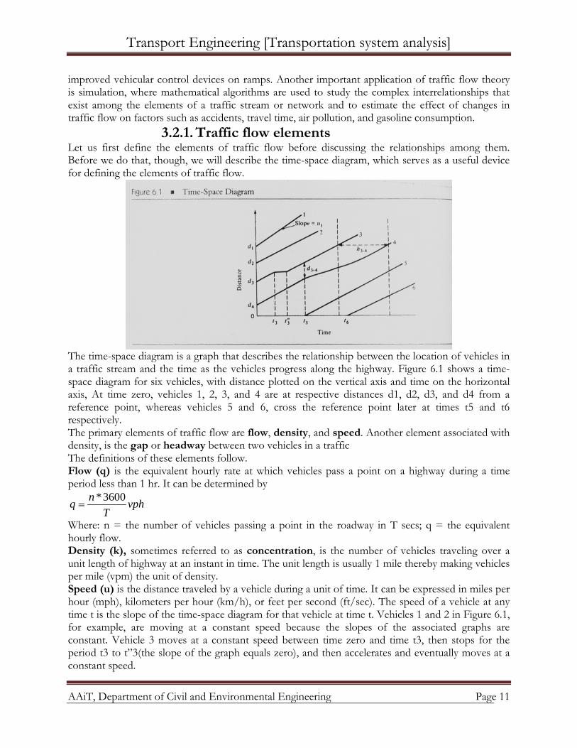
The time-space diagram is a graph that describes the relationship between the location of vehicles in a traffic stream and the time as the vehicles progress along the highway. Figure 6.1 shows a time-space diagram for six vehicles, with distance plotted on the vertical axis and time on the horizontal axis, At time zero, vehicles 1, 2, 3, and 4 are at respective distances d1, d2, d3, and d4 from a reference point, whereas vehicles 5 and 6, cross the reference point later at times t5 and t6 respectively. The primary elements of traffic flow are flow, density, and speed. Another element associated with density, is the gap or headway between two vehicles in a traffic The definitions of these elements follow. Flow (q) is the equivalent hourly rate at which vehicles pass a point on a highway during a time period less than 1 hr. It can be determined by
vphT
nq 3600*=
Where: n = the number of vehicles passing a point in the roadway in T secs; q = the equivalent hourly flow. Density (k), sometimes referred to as concentration, is the number of vehicles traveling over a unit length of highway at an instant in time. The unit length is usually 1 mile thereby making vehicles per mile (vpm) the unit of density. Speed (u) is the distance traveled by a vehicle during a unit of time. It can be expressed in miles per hour (mph), kilometers per hour (km/h), or feet per second (ft/sec). The speed of a vehicle at any time t is the slope of the time-space diagram for that vehicle at time t. Vehicles 1 and 2 in Figure 6.1, for example, are moving at a constant speed because the slopes of the associated graphs are constant. Vehicle 3 moves at a constant speed between time zero and time t3, then stops for the period t3 to t”3(the slope of the graph equals zero), and then accelerates and eventually moves at a constant speed.
Transport Engineering [Transportation system analysis]
AAiT, Department of Civil and Environmental Engineering Page 12
There are two types of mean speeds: time mean speed and space mean speed. Time mean speed ( tu ) is the arithmetic mean of the speeds of vehicles passing a point on a highway during an interval of time. The time mean speed is found by
∑=
=n
iit u
nu
1
1
Where: n =number of vehicles passing a point on the highway; ui = speed of the ith vehicle (ft/sec) Space mean speed ( su ) is the harmonic mean of the speeds of vehicles passing a point in a highway during an interval of time. It is obtained by dividing the total distance traveled by two or more vehicles on a section of highway by the total time required by these vehicles to travel that distance. This is the speed that is involved in flow-density relationships. The space mean speed is found by
∑∑==
== n
ii
n
ii
t
t
nL
u
nu
11)/1(
Where: su = space mean speed (ft/sec); n = number of vehicles; ti = the time it takes the ith vehicle to travel across a section of highway (see); Ui =speed of the ith vehicle (ft/sec); L = length of section of highway (ft) Time headway (h) is the difference between the time the front of a vehicle arrives at a point on the highway and the time the front of the next vehicle arrives at that same point. Time headway is usually expressed in seconds. For example, in the time-space diagram (Figure 6.1), the time headway between vehicles 3 and 4 at d1 is h3-4. Space headway (d) is the distance between the front of a vehicle and the front of the following vehicle. It is usually expressed in feet. The space headway between vehicles 3 and 4 at time t5 is d3-4 (see Figure 6.1).
3.2.2. Flow-density relationships The general equation relating flow, density, and space mean speed is given as
• Flow = (density) x (space mean speed) sukq *= --------------3.5 Each of the variables in Eq. 6.5 also depends on several other factors, including the characteristics of the roadway, the characteristics of the vehicle, the characteristics of the driver, and environmental factors such as the weather. Other relationships that exist among the traffic flow variables are given below.
• Space mean speed = (flow) x (space headway) dqus *= Where: d = (1/ k) = average space headway
• Density = (flow) x (travel time for unit distance) tqk *= Where: t is the average time for unit distance. Average space headway = (space mean speed) x (average time headway) hud s *= Average time headway = (average travel time for unit distance) x (average space headway) dth *=
Transport Engineering [Transportation system analysis]
AAiT, Department of Civil and Environmental Engineering Page 13
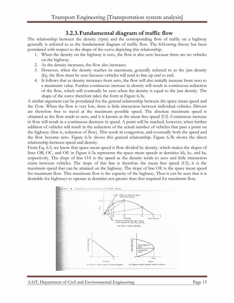
3.2.3. Fundamental diagram of traffic flow The relationship between the density (vpm) and the corresponding flow of traffic on a highway generally is referred to as the fundamental diagram of traffic flow. The fol1owing theory has been postulated with respect to the shape of the curve depicting this relationship.
1. When the density on the highway is zero, the flow is also zero because there are no vehicles on the highway.
2. As the density increases, the flow also increases. 3. However, when the density reaches its maximum, generally referred to as the jam density
(kj), the flow must be zero because vehicles will tend to line up end to end. 4. It follows that as density increases from zero, the flow will also initially increase from zero to
a maximum value. Further continuous increase in density will result in continuous reduction of the flow, which will eventually be zero when the density is equal to the jam density. The shape of the curve therefore takes the form in Figure 6.3a.
A similar argument can be postulated for the general relationship between the space mean speed and the f1ow. When the flow is very low, there is little interaction between individual vehicles. Drivers are therefore free to travel at the maximum possible speed. The absolute maximum speed is obtained as the flow tends to zero, and it is known as the mean free speed (Uf). Continuous increase in flow will result in a continuous decrease in speed. A point will be reached, however, when further addition of vehicles will result in the reduction of the actual number of vehicles that pass a point on the highway (that is, reduction of flow). This result in congestion, and eventually both the speed and the flow become zero. Figure 6.3c shows this general relationship. Figure 6.3b shows the direct relationship between speed and density. From Eq. 6.5, we know that space mean speed is flow divided by density, which makes the slopes of lines OB, OC, and OE in Figure 6.3a represents the space mean speeds at densities kb, kc, and ke, respectively. The slope of line OA is the speed as the density tends to zero and little interaction exists between vehicles. The slope of this line is therefore the mean free speed (Uf); it is the maximum speed that can be attained on the highway. The slope of line OE is the space mean speed for maximum flow. This maximum flow is the capacity of the highway. Thus it can be seen that it is desirable for highways to operate at densities not greater than that required for maximum flow.
Transport Engineering [Transportation system analysis]
AAiT, Department of Civil and Environmental Engineering Page 14
3.3.4. Mathematical relationships describing traffic flow Mathematical relationships describing traffic flow can be classified into two general Categories -macroscopic and microscopic- depending on the approach used in the development of these relationships. The macroscopic approach considers flow density relationships, whereas the microscopic approach considers spacing between and speed of individual vehicles. Macroscopic Approach The macroscopic approach considers traffic streams and develops algorithms that relate the flow to the density and space mean speeds. The two most commonly used macroscopic models are the Green shields and Greenberg models. Green shields Model. Green shields carried out one of the earliest recorded works, in which he studied the relationship between speed and density. He hypothesized that a linear relationship existed between speed and density, which he expressed as
kku
uuj
ffs *−= ------3.11
Corresponding relationships for flow and density and for flow and speed can be developed. Since kuq s= substituting suq / , for k in Eq. 3.11 gives
qku
uuuj
fsfs *.2 −= ------3.12
Also substituting kq / for su , in Eq. 6.11 gives
2*. kku
kuqj
ff −= -------3.13
Equations 6.12 and 6.13 indicate that if a linear relationship in the form of Eq. 6.11 is assumed for speed and density, then parabolic relationships are obtained between flow and density and between flow and speed. The shape of the curve shown in Figure 6.3a will therefore be a parabola. Also, Eqs. 6.12 and 6.13 can be used to determine the corresponding speed and the corresponding density for maximum flow. Consider Eq. 6.12.
qku
uuuj
fsfs *.2 −=
Differentiating q with respect to su we obtain
sj
ffs du
dqku
uu −=2
That is,
f
jsj
f
js
f
jf
s uk
ukuk
uuk
uud
dq 22 −=−=
For maximum flow,
0=sud
dq => f
jsj u
kuk 2= =>
2f
o
uu = -----3.14
Thus, the space mean speed uo, at which the volume is maximum, is equal to half the free mean speed. Consider Eg. 3.13.
Transport Engineering [Transportation system analysis]
AAiT, Department of Civil and Environmental Engineering Page 15
2*. kku
kuqj
ff −=
Differentiating q with respect to k, we obtain
j
ff k
uku
dkdq 2−=
For maximum flow,
0=dkdq =>
j
ff k
uku 2= =>
2j
o
kk = -----3.15
Thus, at the maximum flow, the density k. is half the jam density. The maximum flow for the Greenshields relationship can therefore be obtained from Eqs. 6.5, 6.14, and 6.15, as shown in Eq. 6.16.
4maxfjuk
q = ----------3.16
Greenberg Model. Several researchers have used the analogy of fluid flow to develop macroscopic relationships for traffic flow. One of the major contributions using the fluid-flow analogy was developed by Greenberg in the form
kk
cu js ln= -------3.17
kk
ckq jln= -------3.18
Differentiating q with respect to k, we obtain
ckk
cdkdq j −= ln
For maximum flow, 0=dkdq , 1ln =
kk j
Giving oj kk ln1ln += -----3.19
That is, 1ln =o
j
kk
and Substituting 1 for
o
j
kk
ln in eq 3.17 gives cuo =
Thus, the value of c is the speed at maximum flow. Model Application Use of these macroscopic models depends on whether they satisfy the boundary criteria of the fundamental diagram of traffic flow at the region that describes the traffic conditions. For example, the Green shields model satisfies the boundary conditions when the density k is approaching zero as well as when the density is approaching the jam density kj. The Greenshields model therefore can be used for light or dense traffic. The Greenberg model, on the other hand, satisfies the boundary conditions when the density is approaching the jam density, but it does not satisfy the boundary conditions when k is approaching zero. The Greenberg model is therefore useful only for dense traffic conditions. Calibration of Macroscopic Traffic Flow Models- The traffic models discussed thus far can be used to determine specific characteristics such as the speed and density at which maximum flow occurs and the jam density of a facility. This usually
Transport Engineering [Transportation system analysis]
AAiT, Department of Civil and Environmental Engineering Page 16
involves collecting appropriate data on the particular facility of interest and fitting the data points obtained to a suitable model. The most common method of approach is regression analysis. This is done by minimizing the squares of the differences between the observed and the expected values of a dependent variable. When the dependent variable is linearly related to the independent variable, the process is known as linear regression analysis, and when the relationship is with two or more independent variables, the process is known as multiple linear regression analysis. If a dependent variable y and an independent variable x are related by an estimated regression function, then
bxay += ------3.20 The constants a and b could be determined from
∑ ∑= =
−=−=n
i
n
iii xbyx
nby
na
1 1
1 ------------3.21
And
∑ ∑
∑∑∑
= =
===
−
−
=n
i
n
iii
n
ii
n
ii
n
iii
xn
x
yxn
yxb
1
2
1
2
111
1
1
----------3.22
Where: n = number of sets of observations; xi = ith observation for x; yi = ith observation for y A measure commonly used to determine the suitability of an estimated regression function is the coefficient of determination (or square of the estimated correlation coefficient) 2R , which is given by
∑
∑
=
=
−
−= n
ii
n
ii
yy
yYR
1
2
1
2
2
)(
)( ---------3.23
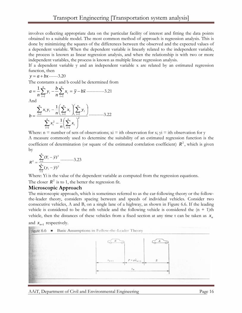
Where: Yi is the value of the dependent variable as computed from the regression equations. The closer 2R is to 1, the better the regression fit. Microscopic Approach The microscopic approach, which is sometimes referred to as the car-following theory or the follow-the-leader theory, considers spacing between and speeds of individual vehicles. Consider two consecutive vehicles, A and B, on a single lane of a highway, as shown in Figure 6.6. If the leading vehicle is considered to be the nth vehicle and the following vehicle is considered the (n + 1)th vehicle, then the distances of these vehicles from a fixed section at any time t can be taken as nx and 1+nx respectively.
Transport Engineering [Transportation system analysis]
AAiT, Department of Civil and Environmental Engineering Page 17
If the driver of vehicle B maintains an additional separation distance P above the separation distance at rest S such that P is proportional to the speed of vehicle B, then
1. += nxp ρ ---------3.25 Where: ρ = factor of proportionality with units of time; 1+nx = speed of the (n + l)th vehicle We can write
Sxxx nnn +=− ++ 11 . ρ -----3.26 Where S is the distance between front bumpers of vehicles at rest Differentiating Eq. 6.26 gives
)(111 ++ −= nnn xxx
ρ----3.27
Equation 6.27 is the basic equation of the microscopic models, and it describes the stimulus response of the models. Researchers have shown that a time lag exists for a driver to respond to any stimulus that is induced by the vehicle just ahead, and Eq. 6.27 can therefore be written as
)]()([)( 11 txtxTtx nnn ++ −=+ λ ------3.28 Where: T = time lag of response to the stimulus; λ = )/1( ρ (sometimes called the sensitivity) A general expression for λ is given in the form
lnn
mn
txtxTtx
a)]()([
)(
1
1
+
+
−+
=
λ --------3.29
The general expression for the microscopic models can then be written as
)]()([)]()([
)()( 1
1
11 txtx
txtxTtx
aTtx nnlnn
mn
n ++
++ −
−+
=+
-------3.30
Where a, l, and m are constants. The microscopic model (Eq. 6.30) can be used to determine the velocity, flow, and density of a traffic stream when the traffic stream is moving in a steady state. The direct analytical solution of either Eq. 6.28 or Eq. 6.30 is not easy. It can be shown, however, that the macroscopic models discussed earlier can all be obtained from Eq. 6.30. For example, if m = 0 and l = 1, the acceleration of the (n+ 1)th vehicle is given as
)]()([)()(
)(1
11 txtx
txtxaTtx
nn
nnn
+
++ −
−=+
Integrating the above expression, we find that the velocity of the (n + 1)th vehicle is CtxtxaTtx nnn ++−=+ ++ )]1()(ln[)( 11
Since we are considering the steady state condition,
CxxauutxTtx
nn
nn
+−===+
+ ]ln[)()(
1
Also,
=− +1nn xx Average space headway k1
=
Ck
au +=1ln
Using the boundary condition, 0=u When jkk =
Transport Engineering [Transportation system analysis]
AAiT, Department of Civil and Environmental Engineering Page 18
=
+
=
j
j
kaC
Ck
a
1ln
1ln0
Substituting for C in the equation for u, we obtain
=
−
=
kk
au
ka
kau
j
j
ln
1ln1ln
Which is the Greenberg model given in eq. 3.17. Similarly, if m s allowed to be 0 and l =2, we obtain the Greenshilds model.
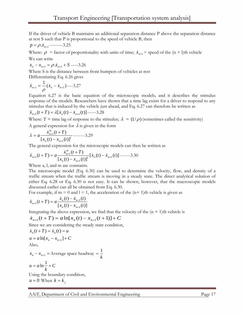
3.2.5. Shock waves in traffic streams The fundamental diagram of traffic flow for two adjacent sections of a highway with different capacities (maximum flows) is shown in Figure 6.7. This figure describes the phenomenon of backups and queuing on a highway due to a sudden reduction of the capacity of the highway (known as a bottle neck condition). The sudden reduction in capacity could be due to accidents, reduction in the number of lanes, restricted bridge sizes, work zones, a signal turning red, and so forth, creating a situation where the capacity on the highway suddenly changes from C1 to a lower value of C2, with a corresponding change in optimum density from a
ok to a value of bok .
When such a condition exists and the normal flow and density on the highway are relatively large,
Transport Engineering [Transportation system analysis]
AAiT, Department of Civil and Environmental Engineering Page 19
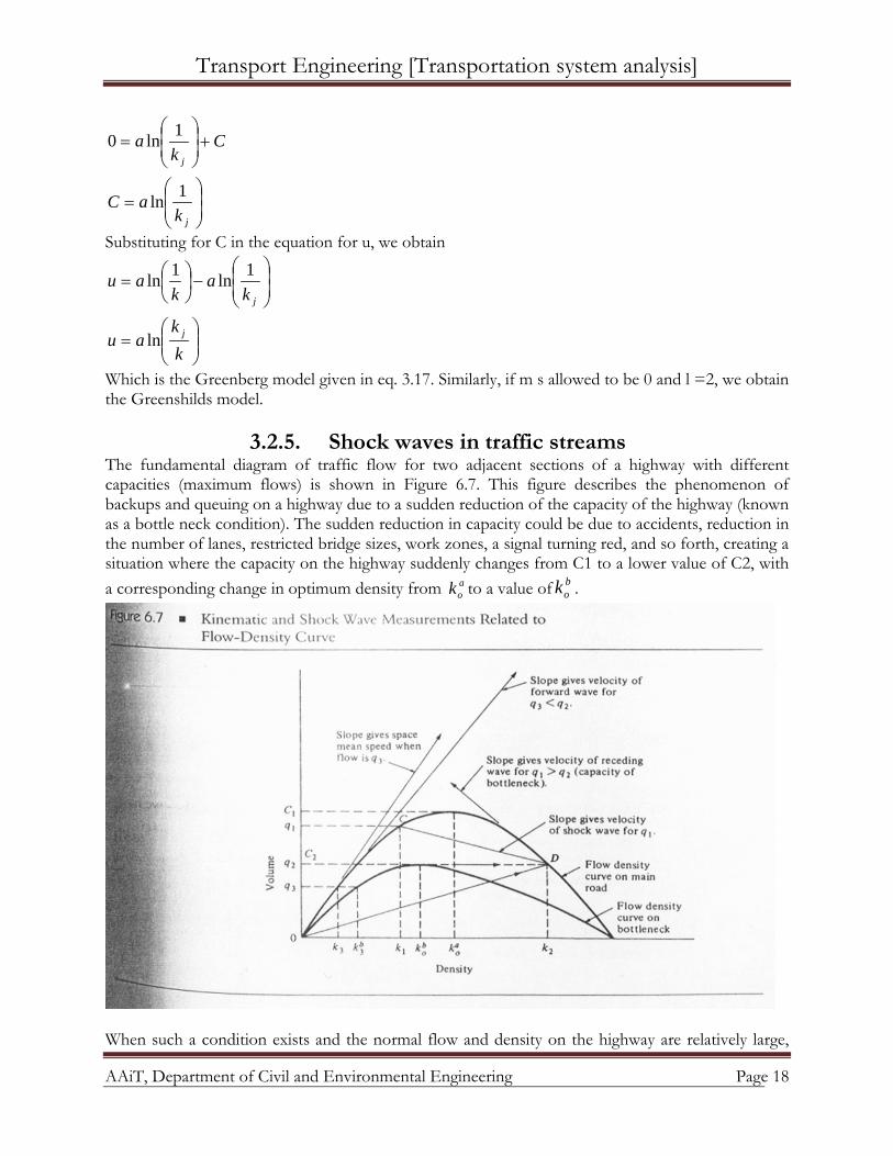
the speeds of the vehicles will have to be reduced while passing the bottleneck. The point at which the speed reduction takes place can be approximately noted by the turning on of the brake lights of the vehicles. An observer will see that this point moves upstream as traffic continues to approach the vicinity of the bottleneck, indicating an upstream movement of the point at which flow and density change. This phenomenon is usually referred to as a shockwave in the traffic stream. Let us consider two different densities of traffic, k1 and k 2, along a straight highway as shown in Figure 6.8, where k 1 > k 2. Let us also assume that these densities are separated by the line w, representing the shock wave moving at a speed Uw. If the line w moves in the direction of the arrow (that is, in the direction of the traffic flow), Uw is positive.
With U1 equal to the space mean speed of vehicles in the area with density kl (section P), the speed of the vehicle in this area relative to the line w is
)( 11 wr uuu −= The number of vehicles crossing line w from area P during a time period t is tkuN r 111 = Similarly, the speed of vehicles in the area with density k2 (section Q) relative to w is
)( 22 wr uuu −= And the number of vehicles crossing line w during a time period t is
tkuN r 222 = Since the net change is zero
21 NN = tkuutkuu ww 2211 )()( −=−
)( 121122 kkukuku w −=− -----6.31 If the flow rates in sections P and Q are ql and q2, respectively, then
111222 , kuqkuq == Substituting ql and q2 for k1u1 and k2u2 in Eg. 6.31 gives
)( 1212 kkuqq w −=− That is,
12
12
kkqquw −
−=
Which is also the slope of the line CD shown in Figure 6.7. This indicates that the velocity of the shock wave created by a sudden change of density from kl to k2 on a traffic stream is the slope of the chord joining the points associated with kl and k2 on the volume density curve for that traffic stream. Special Cases of Shock Wave Propagation The shock wave phenomenon can also be explained by considering a continuous change of flow and density in the traffic stream. If the change in flow and the change in density are very small, we can
Transport Engineering [Transportation system analysis]
AAiT, Department of Civil and Environmental Engineering Page 20
write qqq ∆=− 12 kkk ∆=− 12
The wave velocity can then be written as
dkdq
kquw =
∆∆
= -------3.33
Since sukq = , Substituting suk for q in eq 6.33 gives
dkukd
u sw
)(= -----3.34
dkud
kuu ssw −=
When such a continuous change of volume occurs in a vehicular flow, a phenomenon similar to that of fluid flow exists, in which the waves created in the traffic stream transport the continuous changes of flow and density. The speed of these waves is dq/dk and is given by Eq.6.34. We have already seen that as density increases, the space mean speed decreases (see Eq. 6.5), giving a negative value for du/dk. This shows that at any point on the fundamental diagram, the speed of the wave is theoretically less than the space mean speed of the traffic stream. Thus, the wave moves in the opposite direction relative to that of that of the traffic stream. The actual direction and speed of the wave will depend on the point at which we are on the curve (that is, the flow and density on the highway), and the resultant effect on the traffic downstream will depend on the capacity of the restricted area (bottleneck).
1. When both the flow and the density of the traffic stream are very low, that is, approaching zero, the flow is much lower than the capacity of the restricted area and there is very little interaction between the vehicles. The differential of su with respect to )/( dkudk s then tends to zero, and the wave velocity approximately equals the space mean speed. The wave therefore moves forward with respect to the road, and no backups result.
2. As the flow of the traffic stream increases to a value much higher than zero but still less than the capacity of the restricted area (say, q3 in Figure 6.7), the wave velocity is still less than the space mean speed of the traffic stream, and the wave moves forward relative to the road. This results in a reduction in speed and an increase in the density from k3 to k3b as vehicles enter the bottleneck but no backups occur.
3. When the volume on the highway is equal to the capacity of the restricted area (C2 in Figure 6.7), the speed of the wave is zero and the wave does not move. This result in a much slower speed and a greater increase in the density to b
ok as the vehicles enter the restricted area. Again, delay occurs but there are no backups.
4. However, when the flow on the highway is greater than the capacity of the restricted area, not only is the speed of the wave less than the space mean speed of the vehicle stream, but it moves backward relative to the road. As vehicles enter the restricted area, a complex queuing condition arises, resulting In an immediate increase in the density from k1to k2 in the upstream section of the road and a considerable decrease in speed. The movement of the wave toward the upstream section of the traffic stream creates a shock wave in the traffic stream, eventually resulting in backups, which gradually moves upstream of the traffic stream.
The expressions developed for the speed of the shock wave, Eqs. 3.32 and 3.34, can be applied to
Transport Engineering [Transportation system analysis]
AAiT, Department of Civil and Environmental Engineering Page 21
any of the specific models described earlier. For example, the Greenshields model can be written as
−=
j
ifsi k
kuu 1 ( )η−= 1fsi uu where
=
j
ii k
kη (normalized density)
If the Greenshields model fits the flow density relationship for a particular traffic stream, Eq.3.32 can be used to determine the speed of a shock wave as
( ) ( ) ( ) ( )
)](1[))(()()()(
)(1111
2112
121212
12
21
2212
12
112212
12
1122
12
11
22
ηη
ηηηη
−−=−
+−−−
==−
−−−
=
−
+−−=
−
−−−=
−
−−
−
=
fj
ff
j
ff
fffffjf
jf
w
ukk
kkkkku
kku
kk
kkku
kku
kkukukkku
kkukuk
kkkkuk
kkuk
u
The speed of a shock wave for the Green shields model is therefore given as )](1[ 21 ηη −−= fu ------3.36
Density Nearly Equal When there is only a small difference between kl and k2 (that is, 21 ηη ≈ ), (neglecting the small change in 1η )
]21[)](1[ 121 ηηη −=−−= ffw uuu
Stopping Waves Equation 6.36 can also be used to determine the velocity of the shock wave due to the change from green to red of a signal at an intersection approach if the Greenshields model is applicable. During the green phase, the normalized density is 1η .When the traffic signal changes to red, the traffic at the stop line of the approach comes to a halt, which results in a density equal to the jam density. The value of 2η is then equal to 1. The speed of the shock wave, which in this case is a stopping wave, can be obtained by
1
1 )]1(1[
η
η
fw
fw
uuuu−=
+−=-----6.37
Equation 6.37 indicates that in this case the shock wave travels upstream of the traffic with a velocity of 1ηfu . If the length of the red phase is t sec, then the length of the line of cars upstream at the stop line is tu f 1η .
Starting Waves At the instant when the signal again changes from red to green, 1η equals 1. Vehicles will then move forward at a speed of 2su , resulting in a density of 2η .The speed of the shock wave, which in this case is a starting wave, is obtained by
2
2 )]1(1[
η
η
fw
fw
uuuu−=
+−=-------6.38
Equation 6.35, ( )22 1 η−= fs uu , gives f
s
uu 2
2 1−=η
Transport Engineering [Transportation system analysis]
AAiT, Department of Civil and Environmental Engineering Page 22
The velocity of the shock wave is then obtained as 2sfw uuu +−=
Since the starting velocity 2su just after the signal changes to green is usually small, velocity of the starting shock wave approximately equals fu− .
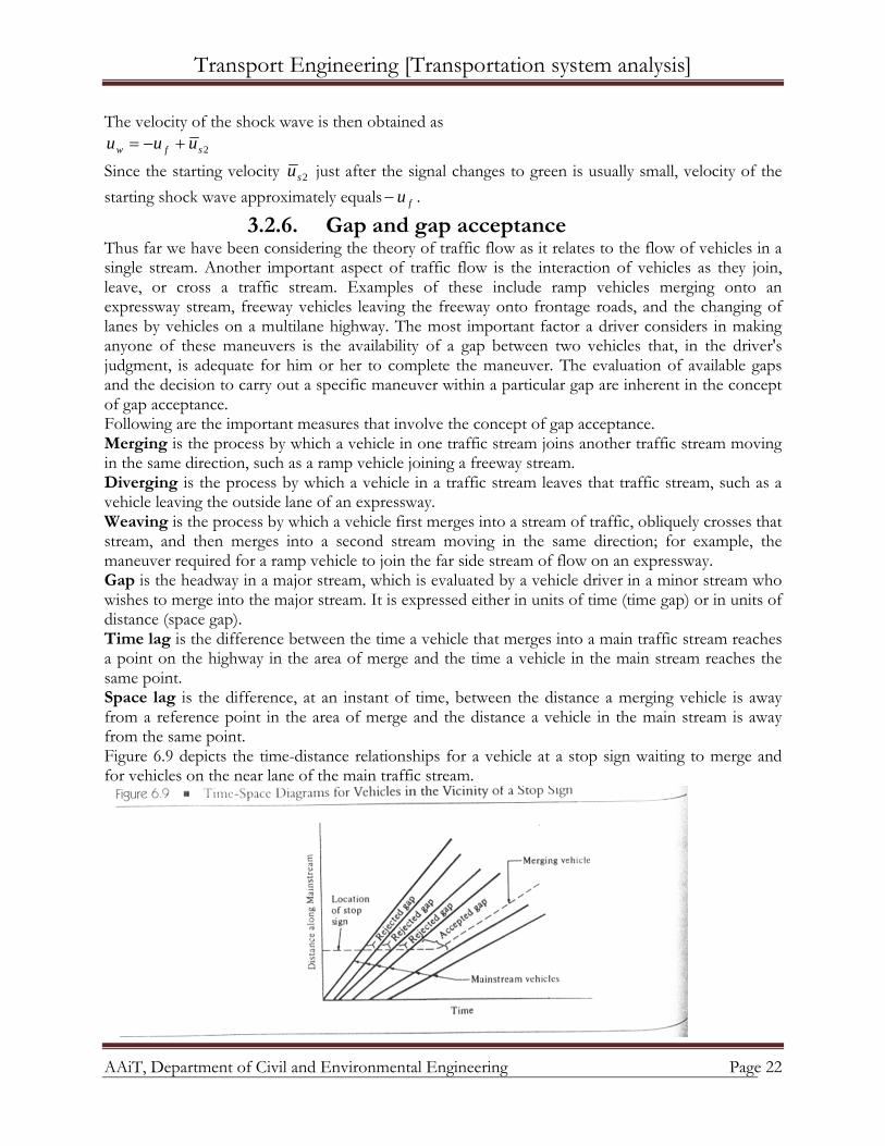
3.2.6. Gap and gap acceptance Thus far we have been considering the theory of traffic flow as it relates to the flow of vehicles in a single stream. Another important aspect of traffic flow is the interaction of vehicles as they join, leave, or cross a traffic stream. Examples of these include ramp vehicles merging onto an expressway stream, freeway vehicles leaving the freeway onto frontage roads, and the changing of lanes by vehicles on a multilane highway. The most important factor a driver considers in making anyone of these maneuvers is the availability of a gap between two vehicles that, in the driver's judgment, is adequate for him or her to complete the maneuver. The evaluation of available gaps and the decision to carry out a specific maneuver within a particular gap are inherent in the concept of gap acceptance. Following are the important measures that involve the concept of gap acceptance. Merging is the process by which a vehicle in one traffic stream joins another traffic stream moving in the same direction, such as a ramp vehicle joining a freeway stream. Diverging is the process by which a vehicle in a traffic stream leaves that traffic stream, such as a vehicle leaving the outside lane of an expressway. Weaving is the process by which a vehicle first merges into a stream of traffic, obliquely crosses that stream, and then merges into a second stream moving in the same direction; for example, the maneuver required for a ramp vehicle to join the far side stream of flow on an expressway. Gap is the headway in a major stream, which is evaluated by a vehicle driver in a minor stream who wishes to merge into the major stream. It is expressed either in units of time (time gap) or in units of distance (space gap). Time lag is the difference between the time a vehicle that merges into a main traffic stream reaches a point on the highway in the area of merge and the time a vehicle in the main stream reaches the same point. Space lag is the difference, at an instant of time, between the distance a merging vehicle is away from a reference point in the area of merge and the distance a vehicle in the main stream is away from the same point. Figure 6.9 depicts the time-distance relationships for a vehicle at a stop sign waiting to merge and for vehicles on the near lane of the main traffic stream.
Transport Engineering [Transportation system analysis]
AAiT, Department of Civil and Environmental Engineering Page 23
A driver who intends to merge must first evaluate the gaps that become available to determine which gap (if any) is large enough to accept the vehicle, in his or her opinion. In accepting that gap, the driver feels that he or she will be able to complete the merging maneuver and safely join the main stream within the length of the gap. This phenomenon generally is referred to as gap acceptance. It is of importance when engineers are considering the delay of vehicles on minor roads wishing to join a major-road traffic stream at un-signalized intersections, and also the delay of ramp vehicles wishing to join expressways. It can also be used in timing the release of vehicles at an on-ramp of an expressway, such that the probability of the released vehicle finding an acceptable gap in arriving at the freeway shoulder lane is maximum.
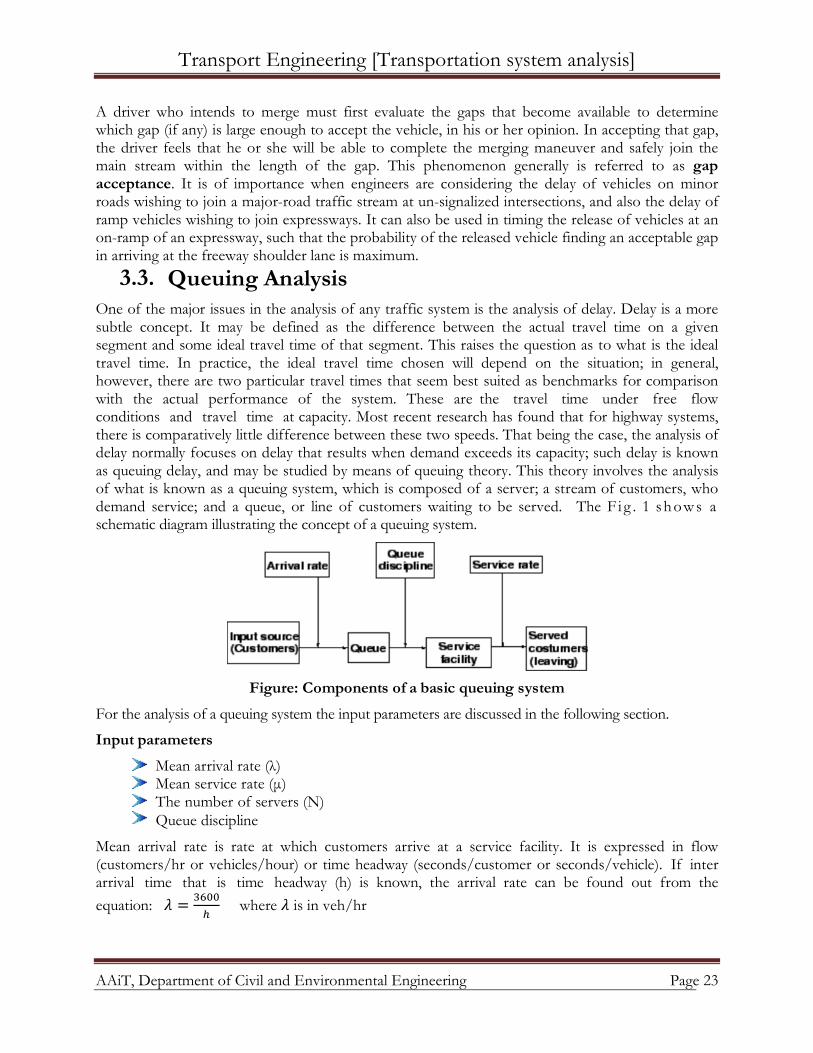
3.3. Queuing Analysis One of the major issues in the analysis of any traffic system is the analysis of delay. Delay is a more subtle concept. It may be defined as the difference between the actual travel time on a given segment and some ideal travel time of that segment. This raises the question as to what is the ideal travel time. In practice, the ideal travel time chosen will depend on the situation; in general, however, there are two particular travel times that seem best suited as benchmarks for comparison with the actual performance of the system. These are the travel time under free flow conditions and travel time at capacity. Most recent research has found that for highway systems, there is comparatively little difference between these two speeds. That being the case, the analysis of delay normally focuses on delay that results when demand exceeds its capacity; such delay is known as queuing delay, and may be studied by means of queuing theory. This theory involves the analysis of what is known as a queuing system, which is composed of a server; a stream of customers, who demand service; and a queue, or line of customers waiting to be served. The F i g . 1 shows a schematic diagram illustrating the concept of a queuing system.
Figure: Components of a basic queuing system
For the analysis of a queuing system the input parameters are discussed in the following section.
Input parameters
Mean arrival rate (λ) Mean service rate (μ) The number of servers (N) Queue discipline
Mean arrival rate is rate at which customers arrive at a service facility. It is expressed in flow (customers/hr or vehicles/hour) or time headway (seconds/customer or seconds/vehicle). If inter arrival time that is time headway (h) is known, the arrival rate can be found out from the equation: 𝜆 = 3600
ℎ where 𝜆 is in veh/hr
Transport Engineering [Transportation system analysis]
AAiT, Department of Civil and Environmental Engineering Page 24
Mean arrival rate can be specified as a deterministic distribution or probabilistic distribution and sometimes demand or input are substituted for arrival.
Mean service rate is the rate at which customers (vehicles depart from a transportation facility. It is expressed in flow (customers/hr or vehicles/hour) or time headway (seconds/customer or seconds/veh. If inter service time that is time headway (h) is known, the service rate can be found out from the equation: 𝜇 = 3600
ℎ where 𝜇 is in veh/hr
The number of servers that are being utilized should be specified and in the manner they work that is they work as parallel servers or series servers has to be specified.
Queue discipline is a parameter that explains how the customers arrive at a service facility. The various types of queue disciplines are
First in first out (FIFO) If the customers are served in the order of their arrival, then this is known as the first-come, first- served (FCFS) service discipline. Prepaid taxi queue at airports where a taxi is engaged on a first-come, first-served basis is an example of this discipline.
First in last out (FILO) Sometimes, the customers are serviced in the reverse order of their entry so that the ones who join the last are served first. For example, the people who join an elevator first are the last ones to leave it.
Served in random order (SIRO) under this rule customers are selected for service at random, irrespective of their arrivals in the service system. In this every customer in the queue is equally likely to be selected. The time of arrival of the customers is, therefore, of no relevance in such a case.
Priority scheduling under this rule customers are grouped in priority classes on the basis of some attributes such as service time or urgency or according to some identifiable characteristic, and FIFO rule is used within each class to provide service. Treatment of VIPs in preference to other patients in a hospitalis an example of priority service.
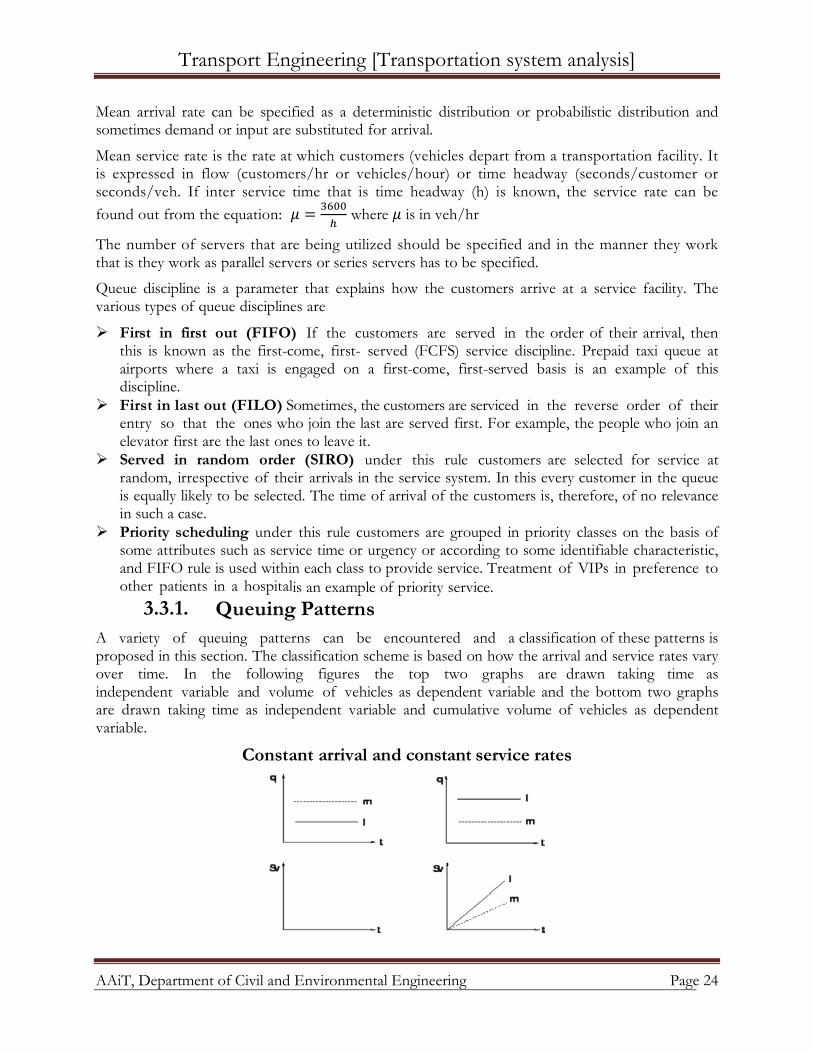
3.3.1. Queuing Patterns A variety of queuing patterns can be encountered and a classification of these patterns is proposed in this section. The classification scheme is based on how the arrival and service rates vary over time. In the following figures the top two graphs are drawn taking time as independent variable and volume of vehicles as dependent variable and the bottom two graphs are drawn taking time as independent variable and cumulative volume of vehicles as dependent variable.
Constant arrival and constant service rates
Transport Engineering [Transportation system analysis]
AAiT, Department of Civil and Environmental Engineering Page 25
Figure : Constant arrival and service rates ( l = arrival rate and m = service rate)
In the left hand part of the above Fig. arrival rate is less than service rate so no queuing is encountered and in the right hand part of the figure the arrival rate is higher than service rate, the queue has a never ending growth with a queue length equal to the product of time and the difference between the arrival and service rates.
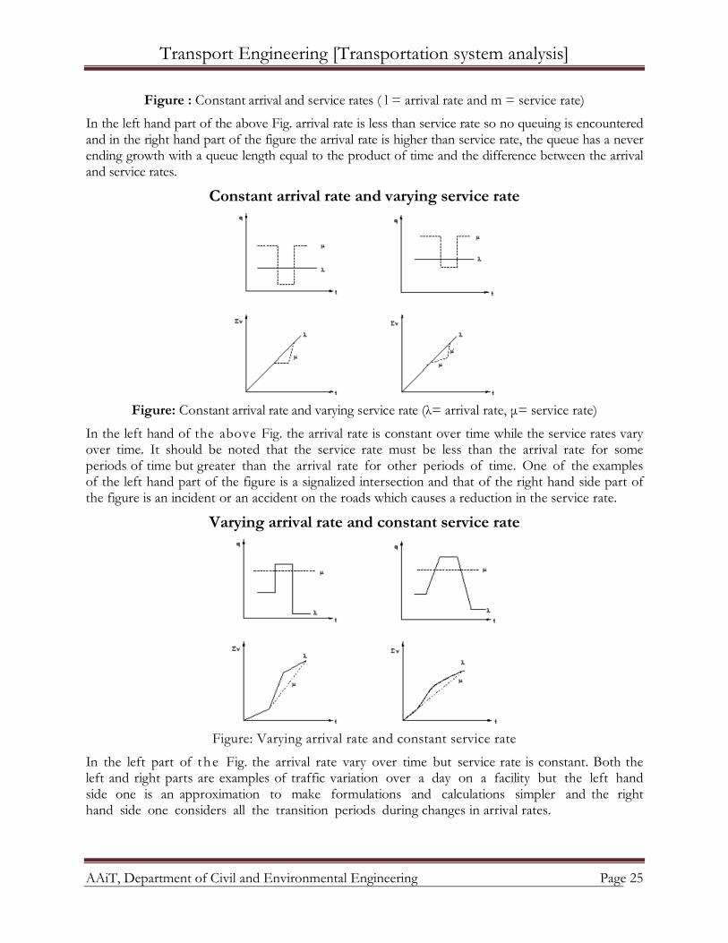
Constant arrival rate and varying service rate
Figure: Constant arrival rate and varying service rate (λ= arrival rate, μ= service rate)
In the left hand of the above Fig. the arrival rate is constant over time while the service rates vary over time. It should be noted that the service rate must be less than the arrival rate for some periods of time but greater than the arrival rate for other periods of time. One of the examples of the left hand part of the figure is a signalized intersection and that of the right hand side part of the figure is an incident or an accident on the roads which causes a reduction in the service rate.
Varying arrival rate and constant service rate
Figure: Varying arrival rate and constant service rate
In the left part of the Fig. the arrival rate vary over time but service rate is constant. Both the left and right parts are examples of traffic variation over a day on a facility but the left hand side one is an approximation to make formulations and calculations simpler and the right hand side one considers all the transition periods during changes in arrival rates.
Transport Engineering [Transportation system analysis]
AAiT, Department of Civil and Environmental Engineering Page 26
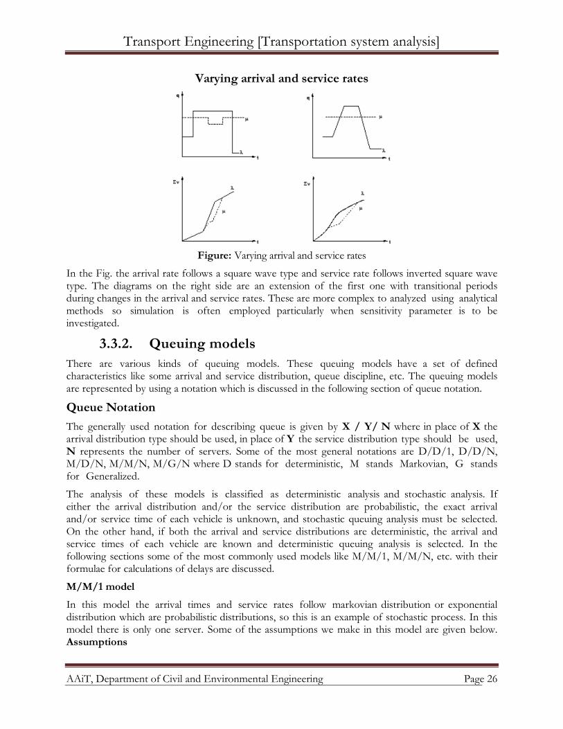
Varying arrival and service rates
Figure: Varying arrival and service rates
In the Fig. the arrival rate follows a square wave type and service rate follows inverted square wave type. The diagrams on the right side are an extension of the first one with transitional periods during changes in the arrival and service rates. These are more complex to analyzed using analytical methods so simulation is often employed particularly when sensitivity parameter is to be investigated.
3.3.2. Queuing models There are various kinds of queuing models. These queuing models have a set of defined characteristics like some arrival and service distribution, queue discipline, etc. The queuing models are represented by using a notation which is discussed in the following section of queue notation.
Queue Notation The generally used notation for describing queue is given by X / Y/ N where in place of X the arrival distribution type should be used, in place of Y the service distribution type should be used, N represents the number of servers. Some of the most general notations are D/D/1, D/D/N, M/D/N, M/M/N, M/G/N where D stands for deterministic, M stands Markovian, G stands for Generalized.
The analysis of these models is classified as deterministic analysis and stochastic analysis. If either the arrival distribution and/or the service distribution are probabilistic, the exact arrival and/or service time of each vehicle is unknown, and stochastic queuing analysis must be selected. On the other hand, if both the arrival and service distributions are deterministic, the arrival and service times of each vehicle are known and deterministic queuing analysis is selected. In the following sections some of the most commonly used models like M/M/1, M/M/N, etc. with their formulae for calculations of delays are discussed.
M/M/1 model
In this model the arrival times and service rates follow markovian distribution or exponential distribution which are probabilistic distributions, so this is an example of stochastic process. In this model there is only one server. Some of the assumptions we make in this model are given below. Assumptions
Transport Engineering [Transportation system analysis]
AAiT, Department of Civil and Environmental Engineering Page 27
1. Customers are assumed to be patient.
2. System is assumed to have unlimited capacity.
3. Users arrive from an unlimited source.
4. The queue discipline is assumed to be first in first out.
The various parameters that are to be evaluated in a queuing model and their formulae for this model are given below.
𝑈𝑡𝑖𝑙𝑖𝑧𝑎𝑡𝑖𝑜𝑛 𝑓𝑎𝑐𝑡𝑜𝑟 = 𝜌 =𝜆𝜇
The following formulae are valid only if arrival rate is less than service rate.
𝑓(𝑥) = 𝑃(𝑋 = 𝑥) = 𝑟𝑥(1 − 𝑥)
x = 0,1,2.....the number of customers at any instant. With this formula we can find out what percentage x number of customers are in the system. If x is taken as zero the formula yields the percentage of time the server is idle. The average number of customers at any time in the system
𝐸[𝑥] =𝑟
1 − 𝑟
The average number of customers in the queue at any time is
𝐸�𝐿𝑞� =𝑟2
1 − 𝑟
Expected time a customer spends in the system
𝐸[𝑇] =1
𝜇 − 𝜆
Expected time a customer spends in the queue
𝐸�𝑇𝑞� =𝜆
𝜇(𝜇 − 𝜆)
Numerical Example 1
The Vehicles arrive at a toll booth at an average rate of 300 per hour. Average waiting time at the toll booth is 10s per vehicle. If both arrivals and departures are exponentially distributed, what is the average number of vehicles in the system, average queue length, the average delay per vehicle, the average time a vehicle is in the system?
Solution
λ = 300 veh/hr 𝜇 = 3600ℎ
vehicles/hr
Utilization factor = traffic intensity = r = λµ
= 300360
= 0.833
The percent of time the toll booth will be idle = P (0) = P(X=0) =0.8330(1 − 0.833) =0.139(60𝑚𝑖𝑛) =8.34 min.
The average number of vehicles in the system = 𝐸[𝑥] = 𝑟1−𝑟
=4.98
Transport Engineering [Transportation system analysis]
AAiT, Department of Civil and Environmental Engineering Page 28
The average number of vehicles in the queue = 𝐸�𝐿𝑞� = 𝑟2
1−𝑟 = 4.01
The average a vehicle spend in the system = 𝐸[𝑇] = 1𝜇−𝜆
= 0.016 hr = 0.96 min = 57.6 sec
The average time a vehicle spends in the queue
𝐸�𝑇𝑞� =𝜆
𝜇(𝜇 − 𝜆)= 0.013ℎ𝑟 = 0.83𝑚𝑖𝑛 = 50𝑠𝑒𝑐
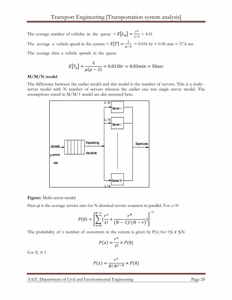
M/M/N model
The difference between the earlier model and this model is the number of servers. This is a multi -server model with N number of servers whereas the earlier one was single server model. The assumptions stated in M/M/1 model are also assumed here.
Figure: Multi-server model
Here 𝜇 is the average service rate for N identical service counters in parallel. For x=0
𝑃(0) = ��(𝑟𝑥
𝑥!+
𝑟𝑁
(𝑁 − 1)! (𝑁 − 𝑟))
𝑁−1
𝑥=0
�
−1
The probability of x number of customers in the system is given by P(x) for 1≤ 𝑥 ≤N
𝑃(𝑥) =𝑟𝑥
𝑥!× 𝑃(0)
For X > 1
𝑃(𝑥) =𝑟𝑥
𝑁!𝑁𝑥−𝑁 × 𝑃(0)
Transport Engineering [Transportation system analysis]
AAiT, Department of Civil and Environmental Engineering Page 29
The average number of customers in the system is
𝐸(𝑋) = 𝑟 + �𝑟𝑁+1
(𝑁 − 1)! (𝑁 − 𝑟)2� 𝑃(0)
The average queue length
𝐸(𝐿𝑞) = �𝑟𝑁+1
(𝑁 − 1)! (𝑁 − 𝑟)2� 𝑃(0)
The expected time in the system
𝐸[𝑇] =𝐸(𝑋)𝜆
The expected time in the queue
𝐸�𝑇𝑞� =𝐸(𝐿𝑞)𝜆
Numerical Example 2
Consider the earlier problem as a multi-server problem with two servers in parallel. Solution
λ =300 veh/hr 𝜇 = 360010
= 360 𝑣𝑒ℎ/ℎ𝑟
Utilization factor = traffic intensity = 𝑟 = 𝜆𝜇
= 300360
= 0.833
𝑃(0) = ��(𝑟𝑥
𝑥!+
𝑟𝑁
(𝑁 − 1)! (𝑁 − 𝑟))
𝑁−1
𝑥=0
�
−1
= 0.92(60) = 55.2𝑚𝑖𝑛
The average number of vehicles in the system 𝐸(𝑋) = 𝑟 + � 𝑟𝑁+1
(𝑁−1)!(𝑁−𝑟)2� 𝑃(0) = 1.22
The average number of vehicles in the queue = 𝐸(𝐿𝑞) = � 𝑟𝑁+1
(𝑁−1)!(𝑁−𝑟)2� 𝑃(0)= 0.387
The average time a vehicle spend in the system = 𝐸[𝑇] = 𝐸(𝑋)𝜆
= 0.004 hr = 14 sec
The ave rage t ime a vehic le spending in the queue 𝐸�𝑇𝑞� = 𝐸(𝐿𝑞)𝜆
= 0.00129hr = 4.64sec
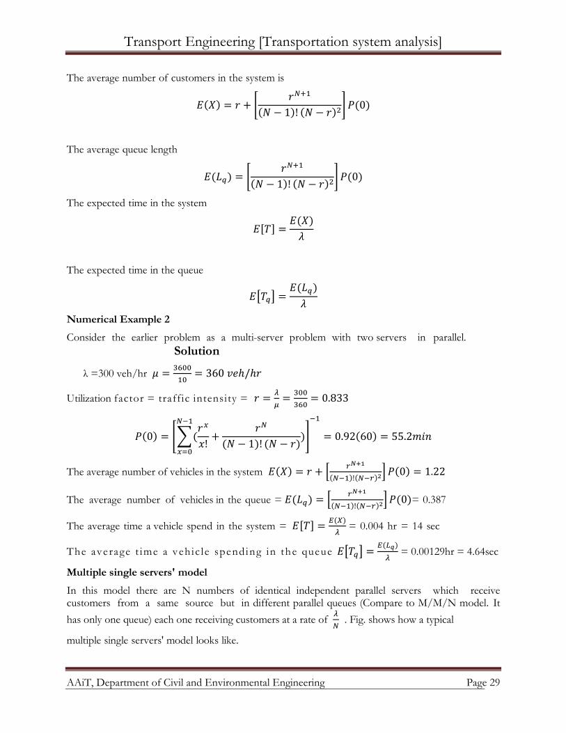
Multiple single servers' model
In this model there are N numbers of identical independent parallel servers which receive customers from a same source but in different parallel queues (Compare to M/M/N model. It has only one queue) each one receiving customers at a rate of 𝜆
𝑁 . Fig. shows how a typical
multiple single servers' model looks like.
Transport Engineering [Transportation system analysis]
AAiT, Department of Civil and Environmental Engineering Page 30
Figure: Multiple single servers
Numerical Example 3
Consider the problem 1 as a multiple single server's model with two servers which work independently with each one receiving half the arrival rate that is 150 veh/hr.
Solution
λ =150 veh/hr 𝜇 = 360010
= 360 𝑣𝑒ℎ/ℎ𝑟
Utilization factor = traffic intensity = 𝑟 = 𝜆𝜇
= 150360
= 0.416
The percent of time the toll booth will be idle P(X=0)
P (0) =(0.416)0(1 − 0.416) = 0.584(60𝑚𝑖𝑛) = 35.04 min
The average number of vehicles in the system = 𝐸[𝑥] = 𝑟1−𝑟
= 0.712
The average number of vehicles in the queue = 𝐸�𝐿𝑞� = 𝑟2
1−𝑟 = 0.296
The average a vehicle spend in the system = 𝐸[𝑇] = 1𝜇−𝜆
=0.0047 hr = 0.285 min = 17.14 sec
The average time a vehicle spends in the queue = 𝐸�𝑇𝑞� = 𝜆𝜇(𝜇−𝜆)
=0.0022hr =0.13 min = 8.05 sec
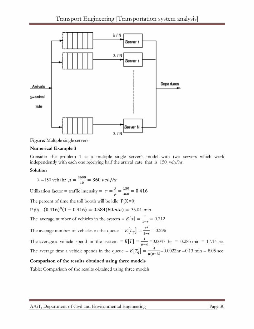
Comparison of the results obtained using three models
Table: Comparison of the results obtained using three models
Transport Engineering [Transportation system analysis]
AAiT, Department of Civil and Environmental Engineering Page 31
M/M/1 model
M/M/2 model
Multiple single sever model
Idle time of toll booths (minutes) 8.34 55.2 35.04
Number of vehicles in the system (unit) 4.98 1.22 0.712
Number of vehicles in the queue (unit) 4.01 0.387 0.296
Average waiting time in system (seconds) 57.6 14 17.14
Average waiting time in queue (seconds) 50 4.64 8.05
From the Table by providing 2 servers the queue length reduced from 4.01 to 0.387 and the average waiting time of the vehicles came down from 50 sec to 4.64 sec, but at the expense of having either one or both of the toll booths idle 92% of the time as compared to 13.9% of the time for the single-server situation. Thus there exists a trade-off between the customers' convenience and the cost of running the system.
D/D/N model
In this model the arrival and service rates are deterministic that is the arrival and service times of each vehicle are known. Assumptions
1. Customers are assumed to be patient.
2. System is assumed to have unlimited capacity.
3. Users arrive from an unlimited source.
4. The queue discipline is assumed to be first in first out.
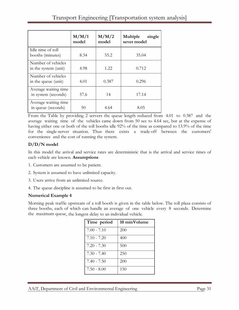
Numerical Example 4
Morning peak traffic upstream of a toll booth is given in the table below. The toll plaza consists of three booths, each of which can handle an average of one vehicle every 8 seconds. Determine the maximum queue, the longest delay to an individual vehicle.
Time period 10 minVolume
7.00 - 7.10 200
7.10 - 7.20 400
7.20 - 7.30 500
7.30 - 7.40 250
7.40 - 7.50 200
7.50 - 8.00 150
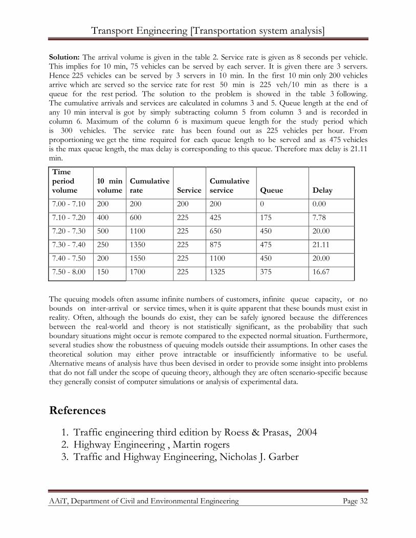
Transport Engineering [Transportation system analysis]
AAiT, Department of Civil and Environmental Engineering Page 32
Solution: The arrival volume is given in the table 2. Service rate is given as 8 seconds per vehicle. This implies for 10 min, 75 vehicles can be served by each server. It is given there are 3 servers. Hence 225 vehicles can be served by 3 servers in 10 min. In the first 10 min only 200 vehicles arrive which are served so the service rate for rest 50 min is 225 veh/10 min as there is a queue for the rest period. The solution to the problem is showed in the table 3 following. The cumulative arrivals and services are calculated in columns 3 and 5. Queue length at the end of any 10 min interval is got by simply subtracting column 5 from column 3 and is recorded in column 6. Maximum of the column 6 is maximum queue length for the study period which is 300 vehicles. The service rate has been found out as 225 vehicles per hour. From proportioning we get the time required for each queue length to be served and as 475 vehicles is the max queue length, the max delay is corresponding to this queue. Therefore max delay is 21.11 min.
Time period volume
10 min volume
Cumulative rate Service
Cumulative service Queue Delay
7.00 - 7.10 200 200 200 200 0 0.00
7.10 - 7.20 400 600 225 425 175 7.78
7.20 - 7.30 500 1100 225 650 450 20.00
7.30 - 7.40 250 1350 225 875 475 21.11
7.40 - 7.50 200 1550 225 1100 450 20.00
7.50 - 8.00 150 1700 225 1325 375 16.67
The queuing models often assume infinite numbers of customers, infinite queue capacity, or no bounds on inter-arrival or service times, when it is quite apparent that these bounds must exist in reality. Often, although the bounds do exist, they can be safely ignored because the differences between the real-world and theory is not statistically significant, as the probability that such boundary situations might occur is remote compared to the expected normal situation. Furthermore, several studies show the robustness of queuing models outside their assumptions. In other cases the theoretical solution may either prove intractable or insufficiently informative to be useful. Alternative means of analysis have thus been devised in order to provide some insight into problems that do not fall under the scope of queuing theory, although they are often scenario-specific because they generally consist of computer simulations or analysis of experimental data.
References
1. Traffic engineering third edition by Roess & Prasas, 2004 2. Highway Engineering , Martin rogers 3. Traffic and Highway Engineering, Nicholas J. Garber