Embed Size (px)
Citation preview
I
Use of Frequency Response
Analysis
to Detect
Transformer Winding
Movement
A report submitted to the school of Engineering and Information Technology,
Murdoch University in partial fulfilment of the requirement for
the degree of Bachelor of Engineering
Ibrahim Mohammed Ahmed
Thesis Final Report 2013
Supervisor: Dr Sujeewa Hettiwatte
Co-Supervisor: Dr Greg Crebbin

II
Declaration
Accept where indicated, this thesis project is my own work. The submission conforms to the
Murdoch University’s academic integrity commitments. I support a copy of my thesis when placed in
the University Library, being accessible for loans and photocopying subject in accordance to the
Copyright Act 1968.
Ibrahim M. Ahmed
22 of November 2013

III
Acknowledgements
All praise is due to the creator of the heaven and earth who has blessed with the opportunity to
study at a higher institution of learning like Murdoch University. I am full of admiration for Dr
Sujeewa Hettiwatte for his invaluable mentoring throughout my thesis project. I would also like to
express a gratitude to the Murdoch engineering academics for their excellent and active help during
my 4 years bachelor degree studies. Thank you to Dr Greg Crebbin for facilitating the opportunity to
start the journey in the first place.
I am grateful to my university colleagues for their support and encouragement. Special thanks to
Mohamoud Sagaale, Nisar Jaffrey and Clement Ayeni.
Finally, I am in debt to my mother for her overwhelming support and sincere advice. Also the
support from my family and friends has been immense during my university journey.

IV
To my beloved parents,
Zeinab and Mohammed

V
Contents Page
Contents Declaration .............................................................................................................................................. II
Acknowledgements ................................................................................................................................ III
Dedications ............................................................................................................................................ IV
Nomenclatures ..................................................................................................................................... VIII
Abbreviations ......................................................................................................................................... IX
List of Figures .......................................................................................................................................... X
List of Tables .......................................................................................................................................... XI
Abstract ................................................................................................................................................. XII
Chapter 1 ................................................................................................................................................. 1
1.1 Problem statement ....................................................................................................................... 1
1.2 Motivation ..................................................................................................................................... 1
1.3 Literature Review .......................................................................................................................... 2
1.4 Thesis Objectives ........................................................................................................................... 3
Chapter 2 ................................................................................................................................................. 4
2.1 Introduction .................................................................................................................................. 4
2.2 Frequency response analysis ........................................................................................................ 4
2.3 FRA measurement setup ............................................................................................................... 5
2.4 Description of 6.6kV transformer ................................................................................................. 6
2.5 Transformer core .......................................................................................................................... 7
2.6 Transformer material .................................................................................................................... 8
2.7 Types of windings .......................................................................................................................... 9
2.7.1 Layer type ............................................................................................................................... 9
2.7.2 Continuous disc type ............................................................................................................ 10
Chapter 3 ............................................................................................................................................... 11
Electrical Parameter Calculations ..................................................................................................... 11
3.1 Introduction ................................................................................................................................ 11
3.2 Series capacitance ....................................................................................................................... 12
3.3 Inductance................................................................................................................................... 14
3.4 Ground Capacitance .................................................................................................................... 15
Chapter 4 ............................................................................................................................................... 18

VI
Modelling a transformer winding ..................................................................................................... 18
4.1 Introduction ................................................................................................................................ 18
4.2 Different proposed models ......................................................................................................... 19
4.3 Lumped parameter model .......................................................................................................... 20
4.4 Measuring methodology ............................................................................................................. 22
4.4.1 SFRA Measurand .................................................................................................................. 22
4.5 Fault diagnosis using SFRA .......................................................................................................... 23
4.5.1 Types of analysis .................................................................................................................. 23
4.6 Frequency range ......................................................................................................................... 24
4.7 Frequency response analysis ...................................................................................................... 25
Chapter 5 ............................................................................................................................................... 26
Results ................................................................................................................................................... 26
5.1 Introduction ................................................................................................................................ 26
5.2 Case 1 .......................................................................................................................................... 27
5.3 Case 2 .......................................................................................................................................... 28
5.4 Case 3 .......................................................................................................................................... 29
5.5 Case 4 .......................................................................................................................................... 30
5.6 Case 5 .......................................................................................................................................... 31
5.7 Case 6 .......................................................................................................................................... 32
5.8 Discussion .................................................................................................................................... 33
Conclusion ............................................................................................................................................. 35
Recommendation for further work....................................................................................................... 36
The frequency at which core winding impact can be neglected ...................................................... 36
Model improvement ......................................................................................................................... 36
Software package for computation .................................................................................................. 36
Appendices ............................................................................................................................................ 37
Appendix A. Transformer data .......................................................................................................... 37
Appendix B. Series capacitance calculation ...................................................................................... 38
Turn to turn capacitance ............................................................................................................... 38
Disc to disc capacitance ................................................................................................................ 38
Series capacitance ......................................................................................................................... 39
Appendix C. Inductance Calculation ................................................................................................. 40
A general approach ....................................................................................................................... 40
Lyle’s method for rectangular cross-section coils used for thesis ................................................ 41

VII
Appendix D. Ground capacitance calculation ................................................................................... 42
Appendix E. Matlab code for case 1 ................................................................................................. 44
Appendix F. Matlab code for case 2 .................................................................................................. 45
Appendix G. Matlab code for case 3 ................................................................................................. 46
Appendix H. Matlab code for case 4 ................................................................................................. 47
Appendix I. Matlab code for case 5 .................................................................................................. 48
Appendix J. Matlab code for case 6 .................................................................................................. 49
Appendix K. simpowersystem Block diagrams inputs ...................................................................... 50
Primary circuit ............................................................................................................................... 50
Case 1 ................................................................................................................................................ 51
Case 2 ................................................................................................................................................ 52
Case 3 ................................................................................................................................................ 52
References ............................................................................................................................................ 53

VIII
Nomenclature
o Permittivity of free space
r Relative permittivity of inter-turn insulation
o Permeability of free space
*
p Relative permittivity of inter-disc insulation
*
pb Relative permittivity of inter-disc spacers
l Length of 2 discs
ir Inner radius
or Outer radius
Single sided insulation paper thickness of turns
Angle subtended by a key spacer at the centre
D Depth of inter-turn
sC Series capacitance
gC Ground capacitance
L Inductance
ttC Turn to Turn capacitance
ddC Disc to disc capacitance
S Width of spacers
mR Mean radius
h Turn height
w Turn width
NB Number of turns
A Cross-section area
R Reluctance

IX
Abbreviations
CB Bushing Capacitance
CTC Continuously transposed cable
FEM Finite element method
FRA Frequency response analysis
HV High voltage
LV Low voltage
MTL Multiple transmission line model
SFRA Sweep frequency response analysis

X
List of Figures
Figure 1: Experiment setup of the system .............................................................................................. 5
Figure 2: Front view of 6.6kV transformer .............................................................................................. 6
Figure 3: Core type of transformer ......................................................................................................... 7
Figure 4: Shell type of transformer ......................................................................................................... 7
Figure 5: layer type winding .................................................................................................................... 9
Figure 6: Continuous disc type winding ................................................................................................ 10
Figure 7: Disc pair of a continuous winding .......................................................................................... 12
Figure 8: Cdd configuration .................................................................................................................... 13
Figure 9: Lyle’s method for rectangular cross section coils .................................................................. 14
Figure 10: Representation of the LV and HV core ................................................................................ 15
Figure 11: LV and HV calculation configuration .................................................................................... 15
Figure 12: Portrayal of the spacers ....................................................................................................... 16
Figure 13: Equivalent electrical network .............................................................................................. 21
Figure 14: Effect of series capacitance using impedance measurement .............................................. 27
Figure 15: Effect of inductance using impedance measurement ......................................................... 28
Figure 16: Effect of ground capacitance using impedance measurement .......................................... 29
Figure 17: Effect of series capacitance using transfer function ............................................................ 30
Figure 18: Effect of increase in inductance on the primary circuit using transfer function ................. 31
Figure 19: Effect of ground capacitance on the primary circuit using transfer function ...................... 32

XI
List of Tables
Table 1: Calculated model parameter values ....................................................................................... 17
Table 2: list of SFRA measurement reporting ....................................................................................... 24
Table 3: Transformer parameter and fault type relationship ............................................................... 25
Table 4: Element by element fault simulation ...................................................................................... 26
Table 5: Effect of 20% increase in the various electrical parameter on the Frequency response
analysis magnitude and phase (relative to the fingerprint) ................................................................. 33

XII
Abstract
In this thesis, a study of continuous disc type 6.6kV transformer winding was utilised to investigate
winding deformation by means of frequency response analysis (FRA). The equivalent electrical circuit
is based on the lumped parameter model. Transformer elements include series capacitance, ground
capacitance and inductance. The calculation were based on 6.6kV transformer design specification
data sheet.
The values of the parameters were changed in order to simulate a likelihood of failure on the
windings, which would correspond to unique frequency range spectrum. The FRA simulation range
is from 10 kHz to 2 MHz. Then sensitivity analyses were performed to assess the accuracies of the
two types of measurand: transfer function (
) and trans impedance (
).
Matlab/simpowersystem software was used for simulation analysis and the bodeplot command was
implemented to graph the magnitude and phase of the equivalent circuit (healthy circuit) and circuit
with introduced fault. A linear frequency scale was utilised in order to compare the small differences
at certain frequency bands. This thesis presents FRA which includes sweep frequency response
analysis (SFRA), the measurement techniques and interpretation of SFRA measurement.
In this thesis, a simulation model of a continuous disc type 6.6kV transformer was utilised to study
frequency response analysis (FRA) which includes SFRA. The model was based on lumped
parameters using circuit elements of series capacitance, inductance and ground capacitance. Faults
were simulated through change in value of series capacitance, inductance and ground capacitance. .
It was found that an increase of 20% in inductance, which corresponds to disc deformation and local
breakdown faults etc. alters the FRA signature over the entire frequency range (10 Hz-2 MHz). On
the other hand a change in series capacitance and ground capacitance which correlates to disc
movement faults occurs only at frequencies above 400 kHz.

1
Chapter 1
1.1 Problem statement
Power transformers play a central role within the electrical transmission and distribution network. A
malfunctioning in the service can cause far reaching consequence. The economic costs of
maintenance and the loss of electrical power are some of the major concerns. The bulk of
transformers now in service were commissioned before 1970’s and as consequence the majority of
the population has surpassed their design life [1]. During a fault, the transformer experiences
mechanical forces which are enforced on the windings. If these forces surpass the capability of the
transformer, winding distortion can occur [2].
Although transformers are robust and can survive numerous short circuit faults without complete
failure, the impact of significant winding deformation reduces lifespan incrementally due to locally
amplified electromagnetic pressure [3]. Therefore it is fundamental to identify any winding
distortion as quickly as possible and take appropriate remedial acts.
Traditional techniques have proven insufficient in detecting internal faults and winding movements
in transformers [4]. However frequency response analysis has shown to be a commanding diagnostic
method in detecting transformer winding deformation. The testing method is fairly simple since the
development of specific FRA test equipment. The interpretations of the results remain a grey area
and are usually left to experts to determine the type and location of fault [5].
1.2 Motivation
In this thesis, a 6.6 kV power transformer winding will be simulated and the FRA signature will be
obtained. Then FRA signals under a variety of deformed conditions will be simulated and the results
will be compared to that of the healthy 6.6kV transformer
Studies under taken in this thesis will help to build a repository of FRA signals, which will aid in
identifying any winding movement.

2
1.3 Literature Review
The extracts in the main body of this research has been published in the following journals and
conference schedules:
In 2000 Islam [6] mentioned that an FRA spectrum can be categorised into three distinct frequency
ranges; low, medium and high. A ladder network was used for modelling the high voltage winding.
Series capacitance was discarded for the low frequency range and inductance was neglected for the
higher frequency range. Then a FRA sensitivity study of the transformer parameter change was
undertaken.
In 2002 Hettiwatte et al. [7] conducted research utilising a continuous disc type 6.6kV transformer
winding, which is the same transformer windings used in this report. The model was based on multi-
conductor transmission line theory and employed a single turn as the circuit model. The capacitance,
inductance, and losses were calculated as distributed parameters. This paper argues that magnetic
flux penetration into the laminated core can be ignored at higher frequencies above 1 MHz with self-
inductance mainly present. Furthermore sensitivity analysis was carried out using the impedance
measurement to examine the effect of increase in series capacitance, inductance and conductance
on the initial circuit model.
In 2006 Abeywickrama, Serdyuk, and Gubanski [8] proposed an advanced model of the frequency
response of a three phase power transformer with diagnostic measurements using FRA. The model
takes into account the complex permittivity of insulation of material (i.e. paper, pressboard and air)
through its interaction with the frequency. It utilises a lumped parameter model to simulate the
frequency response, with the calculations based on the finite elemet method.
In 2009 Wang, Li, and Sofian [9] put forward that winding structure is one of the main factors that
affects FRA response. The paper explains that high series capacitance displays an FRA increasing
trend of magnitude, and on the other hand a lower series capacitance exhibit steady FRA magnitude
with features of resonance. This paper offers a great introduction into the topic. It gives values for
electrical parameters which can be compared with the values used in this thesis project.
Article by Shintemirov et al. 2010 [10] employs a distributed parameter model for detecting minor
winding deformation. The author suggests that minor winding faults can be detected at a frequency
range above 1 MHz. This article is particularly useful for gaining good knowledge for the ground
capacitance sensitivity studies.

3
In 2011 Small and Abu-Siada [11] introduced a new alternative method for analysing FRA results
using polar plots. The technique is simple and automated so expertise for a data interpretation can
be eliminated. This research shows relationships between physical parameters like series
capacitance, ground capacitance and inductance and fault type relationship.
1.4 Thesis Objectives
During the literature review in section 1.3, the following areas were targeted for further studies.
These include:
Estimating the key parameters of 6.6kV, 1MVA high voltage winding
Finite element modelling has been a popular approach for determining the circuit parameters in the
literature. The objective of this thesis is to derive analytically, formulas for calculating series
capacitance, shunt capacitance and inductance with the aid of the physical dimensions of winding as
per project specification.
Simulation of transformer model and obtaining it FRA signature
Research indicates that FRA is the most established sensitive method for detecting mechanical
faults in power transformers. An objective of this work is to obtain a model that can be used in
SimPowerSystem, which is a toolbox in Matlab software to simulate the transformer model and
obtaining the FRA signature of the transformer.
FRA interpretation of winding deformation
Papers, by Hettiwatte et al. and Abeywickrama et al. [6,8] show that deformation in transformer
winding can be simulated by changing the parameter values in the model. The goal of this thesis is to
make FRA interpretations by simulating a winding deformation in the transformer, then confirming
that the model parameter approximations would correctly reflect winding distortion.

4
Chapter 2
2.1 Introduction
In this chapter, the FRA concept is introduced which is the main technique employed for the
analysis. The experiment configuration for testing is also shown. Secondly, the construction of 6.6kV
transformer is discussed. Transformer cores are grouped into two types; the shell type and the core
type. The core type is illustrated with a circular winding around a quasi-circular core. The insulation
of the transformer system consists of air, paper and pressboard.
2.2 Frequency response analysis
FRA is a proactive technique used for the detection of deformation in power transformer windings.
Distortions in the transformer windings can be the result of forces due to high short circuit current,
damage during transportation and installation etc. [12]. FRA technique poses advantages in terms of
its extraordinary sensitivity. It is based on the principles that change in windings as a result of
deformation and displacements correspond to modification in the impedance of the transformer
and accordingly results in alteration of its frequency response spectrum [13].
Frequency response analysis includes sweep frequency response analysis (SFRA) and low voltage
impulse (LVI). The literature study on the topic indicates Dick and Erven introduced the FRA concept
[14]. “The method utilises a sweep generator to apply sinusoidal voltages at different frequencies to
one terminal of the transformer”. The output amplitude and phase signals from selected terminals
of the transformer can then be plotted as a function of frequency. This definition is consistent with
the SFRA method used by engineers currently and will be sourced for this thesis.
Features that make SFRA attractive over LVI include: better signal to noise ratio, enhanced
repeatability and reproducibility. Also the SFRA method is less dependent of measuring equipment
according to research [13].
5
2.3 FRA measurement setup
Currently the FRA testing is done when the transformer is in offline mode. A good deal of
preparation is needed before testing can be carried out safely. The transformer needs to be
disconnected from the rest of the network. The recommendation is that FRA testing is performed
when the transformer is under maintenance or after refurbishing commissioning following a major
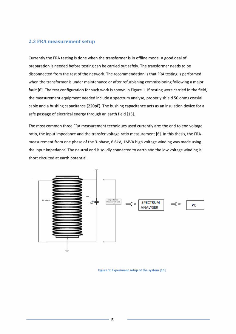
fault [6]. The test configuration for such work is shown in Figure 1. If testing were carried in the field,
the measurement equipment needed include a spectrum analyse, properly shield 50 ohms coaxial
cable and a bushing capacitance (220pF). The bushing capacitance acts as an insulation device for a
safe passage of electrical energy through an earth field [15].
The most common three FRA measurement techniques used currently are: the end to end voltage
ratio, the input impedance and the transfer voltage ratio measurement [6]. In this thesis, the FRA
measurement from one phase of the 3-phase, 6.6kV, 1MVA high voltage winding was made using
the input impedance. The neutral end is solidly connected to earth and the low voltage winding is
short circuited at earth potential.
Figure 1: Experiment setup of the system [15]
6
2.4 Description of 6.6kV transformer
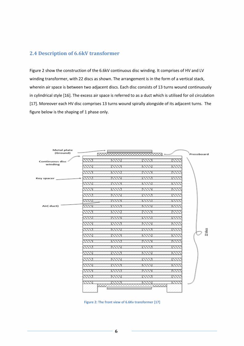
Figure 2 show the construction of the 6.6kV continuous disc winding. It comprises of HV and LV
winding transformer, with 22 discs as shown. The arrangement is in the form of a vertical stack,
wherein air space is between two adjacent discs. Each disc consists of 13 turns wound continuously
in cylindrical style [16]. The excess air space is referred to as a duct which is utilised for oil circulation
[17]. Moreover each HV disc comprises 13 turns wound spirally alongside of its adjacent turns. The
figure below is the shaping of 1 phase only.
Figure 2: The front view of 6.6Kv transformer [17]

7
2.5 Transformer core
The two types of transformer core construction used are shown in Figures 3 and 4. The
configuration of core type is for circular primary and secondary windings to be organized
concentrically around the core leg of significantly circular cross section [18]. The laminations are
stacked and from manufacturing prospective need minimum iron to manufacture. The zero
sequence flux dissipates through the insulation surrounding the core. So in essence this type of core
is useful for balanced load operations [19].
On the other hand the shell type transformer, the magnetic circuit is of rectangular cross section
moulded via stack of lamination of constant width. This core has an appropriate magnetic path for
zero sequence flux. Hence it is suitable for unbalanced operation [19].
In terms of application, the core type is more popular than the shell type for all power system
applications. The shell type finds relevance in very heavy current, low voltage outputs for example
arc furnace or short circuit testing applications. Although shell type is used in countries such as the
USA and France, economic consideration is slow shifting a growing trend towards construction of
core type transformer [19].
Figure 3: The core form type of transformer [19] Figure 4: The shell type of transformer [19]

8
2.6 Transformer material
Paper covered conductor is a popular winding deployed for medium and large power transformers.
These conductors commonly consist of individual strips, bunch or continuously transposed cable
(CTC) type. CTC are used in high current rated transformers on low voltage side (LV) because they
exhibit better spacing factor and reduced eddy current losses in the winding. The epoxy-bonded
types of CTC conductors enhance the short circuit strength [20].
In the low voltage side of transformers, copper and aluminium foil usage are favoured. Properties
such as high temperature and ductility make a copper material attractive use for high current rated
transformers. Conductors with improved thermally upgraded insulating paper are appropriate for
hot-spot temperature of about ~1100 C, they help in managing overload conditions. Moreover,
epoxy diamonded dotted paper improves the mechanical properties and can be utilised as an
interlayer insulation for multilayer windings. High temperature superconductors shall be accessible
commercially in the upcoming years, but economic feasibility and reliability need to be examined
before deployment. [20]

9
2.7 Types of windings
Winding type choice is dependent on the impulse voltage behaviour. Other important considerations
include thermal and current rating of the transformer.
2.7.1 Layer type
Layer winding can extend from a single layer to multiple layers. The single layer or two layer type is
utilised for low voltage windings, with low impulse level and large current. The disadvantage of this
type of winding is the short distance over the top or the bottom of the winding in radial direction.
This distance is meant for the transient voltage creepage path over the winding. “Creepage path
refers to the shortest path between two conducting parts with the voltage difference measured
along the surface of insulation” [21]. The insulation stressed along the surface cannot tolerate
voltage, contrasted to the stress perpendicular to surface.
Improvements can be made to increase the creepage path using tapered layers. This will allow it to
withstand higher nominal voltage withstand because of improved transient voltage distribution.
Figure 5: layer type winding [21]
10
2.7.2 Continuous disc type
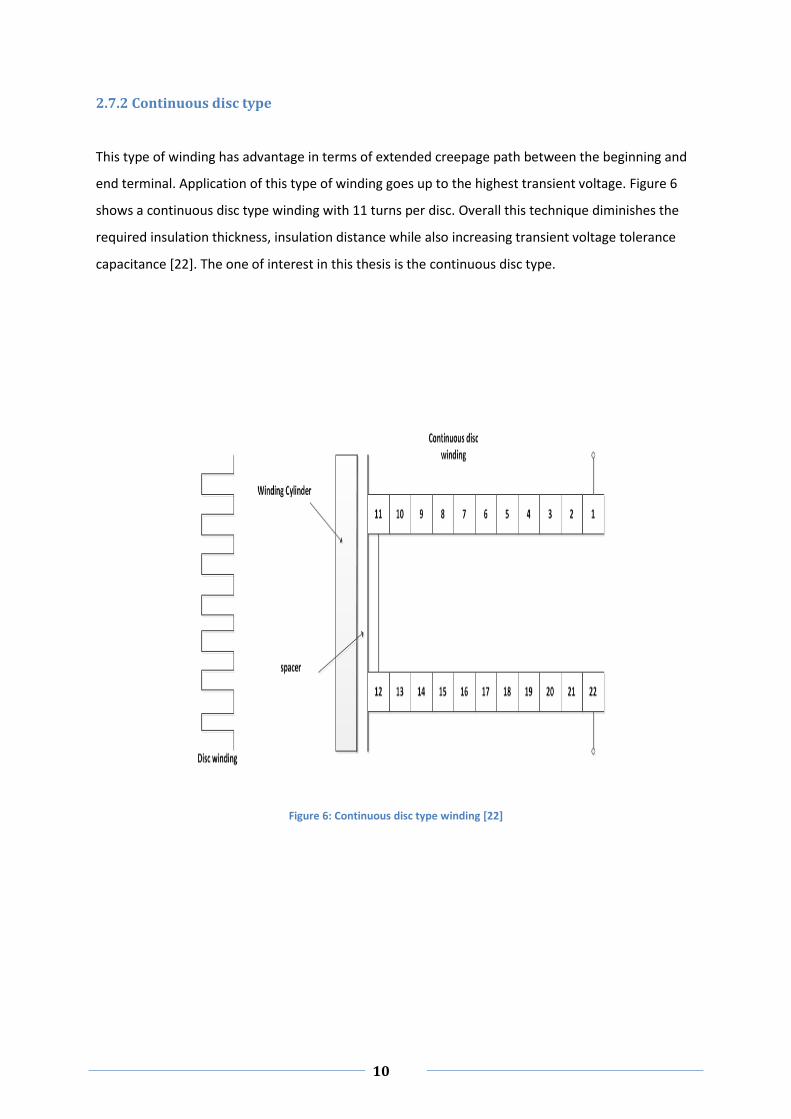
This type of winding has advantage in terms of extended creepage path between the beginning and
end terminal. Application of this type of winding goes up to the highest transient voltage. Figure 6
shows a continuous disc type winding with 11 turns per disc. Overall this technique diminishes the
required insulation thickness, insulation distance while also increasing transient voltage tolerance
capacitance [22]. The one of interest in this thesis is the continuous disc type.
Figure 6: Continuous disc type winding [22]

11
Chapter 3
Electrical Parameter Calculations
3.1 Introduction
Model parameter estimations are usually based on physical arrangements and the dimensions of the
winding. In practice some generalization and approximation of winding geometrical structure can be
considered which will allow for establishing an analytical formula [5]. Through the use of modern
computation, geometric simplification can be circumvented by using the finite element method for
parameter calculation [23]. In both scenarios the frequency dependent behaviour of elements
should be accounted for as well as the frequency dependence of insulation properties.
Under impulse situations, a very fast voltage pulses are injected in to a transformer. This comprises
of high frequency elements, prompting capacitance effect that are absent at normal operating
frequencies [21]. In this thesis, the capacitance and inductance of the lumped circuit model will be
approximated reasonably well by means of an analytical formulae using design specification of the
6.6kV transformer.

12
3.2 Series capacitance
The series capacitance of a physical system is defined by its geometry and relative permittivity of
the dielectric material. The series capacitance is represented by two components: turn to turn
capacitance (Ctt) and disc to disc capacitance (Cdd). The capacitance that exists between two adjacent
conductors separated by dielectric is referred to as turn-turn capacitance and is shown in Figure 7.
The Ctt is determined by using the parallel plate capacitor formula [21]:
(1)
Where is the relatively permittivity of inter-turn insulation, is permittivity of free space (air),
is area of the model and is the single sided inter-turn insulation thickness.
Figure 7: Disc pair of a continuous winding [21]
Similarly, the total disc to disc (axial) capacitance determination is based on two parallel plates with
two dielectrics as depicted in Figure 8. Two capacitances are connected in parallel in the duct,
namely the capacitance of the portion containing the key spacer and the capacitance which consists
of air thickness. The capacitance of the discs can be defined by summation of elementary
capacitance of C1, C2 which are the inter-turn and inter disc capacitance respectively:
The lumped parameter for Cdd is then given by:
(2)

13
Figure 8: Cdd configuration [21]
Once the two components are established namely the inter-turn and inter disc, the total series
capacitance of a continuous winding can be determined by assuming the voltage distribution is non-
linear across within the disc winding [21]. If ND is the number of turns in a disc, then the number of
inter-turn capacitance in each disc is (ND -1). The numbers of inter-section capacitance are equal to
ND. With NDW discs in the winding, the series capacitance for the whole winding can be calculated as
[21]:
(3)

14
3.3 Inductance
In assessing inductance, it is assumed that magnetic flux penetration in the laminated iron is
negligible at frequencies above 1 MHz [19]. So in essence an accurate winding model requires the
calculation of the self –inductance only.
The magnetizing inductance can be calculated with [21]:
(4)
Where N is the number of turns in the winding, R is the reluctance of the magnetic path
(
), is the length of magnetic path. For 2 discs, A is the cross sectional area of disc and
is the permeability of free space.
However, according [15] a more accurate method of modelling inductance is done by using Lyle’s
method. For calculating inductance let us consider Figure 9.
d
h
w
Figure 9: Lyle’s method of calculating inductance for rectangular cross section coils [15]
The following expression can be used to calculate the self-inductance of rectangular coil cross-
section [15]:
2
(5)
Where is the mean radius of the LV and HV for 2 discs, is the number of turns per disc. The
second part of the equation requires dimension of turn conductor turn given by which is the
rectangular transversal section and GMD is the geometrical mean radius given by [15]:
(
)
(
)

15
3.4 Ground Capacitance
The transformer consists of the core, surrounding by LV and HV windings as shown in Figure 10. The
and b symbols signify the inner and outer radius of the LV and HV windings. A configuration for the
calculating capacitance between LV and HV windings is depicted in Figure 11. The ground
capacitance calculations also known as shunt capacitance is based on the dimension of windings.
The windings are treated as concentric cylinders. Appropriate correction factor is needed to account
for the effects of key spacers in between the windings as shown in Figure 12.
a
b
Figure 10: Representation of the LV and HV core [24]
Figure 11: LV and HV calculation configuration [24]

16
s
R1
R2
Figure 12: Portrayal of the spacers [24]
The capacitances between coils in the high voltage winding are computed by considering a
configuration of concentric cylinders by means of [25] and the individual capacitance can be worked
out with the following formulas:
Where is the permittivity of free space, is the number of inter-disc spacers, is the angle
subtended by spacer at centre (given by =
=
), is relative permittivity of
respective cylinder and spacer. is the outer radius of LV winding as illustrated in Figure 11 .
equals plus the thickness of the LV/HV spacers. Similarly equals plus the thickness of the
cylinder between the LV and HV windings and the formulation can be extended to take account of
the thickness of the HV dovetail spacers for . is the outer radius of HV winding.
The calculation of is simpler since the key spacer effect is not present [24]:
The process can then be protracted for and using the above formulas and finally the required
ground capacitance per unit length is obtained as:
(6)

17
The final values of calculated series capacitance, inductance and shunt capacitance are presented
are shown in Table 1.
Table 1: Calculated model parameter values for two discs
Parameter symbol Description Value
Cs Series Capacitance 7.909pF
Cg Shunt Capacitance 13.92pF
Ls Self-Inductance 532.958µH

18
Chapter 4
Modelling a transformer winding
4.1 Introduction
Various analytical methods have been employed in recent decades for transformer modelling. Some
of the methods have drawbacks in terms of detailed depiction of real transformer geometry but
have been utilised due to their simplicity for analysing deformed windings.
On the topic of modelling, suitable methods for determining elementary parameters have to be
studied in order to select the most suitable technique for the thesis objective. For this thesis
frequency range of interest is from 10 kHz to 2MHz.
High frequency behaviour of windings is identified by their resonances (i.e. transfer function maxima
and minima). The introduction of mechanical displacement will alter these characteristic properties.
From an operational requirement, the type and location of faults are imperative. These relations can
be established by measurements on the power transformer or through the use of appropriate model
of the transformer for simulation.
In this chapter, modelling of a high frequency characteristic of a 6.6 kV continuous disc type
transformer winding is presented. The modelling methodology is found on the parameter
formulation derived from the physical geometry and dimension of transformer using data in
Appendix 1. The procedure takes into account winding design and the dependency of losses on
frequency.

19
4.2 Different proposed models
Transformer modelling can be classified into two main categories, the black box (or terminal) models
and detailed (or physical) models. The black box modelling approach finds application in insulation
coordination of HV and EHV systems [24]. The models parameters can be established from
frequency or time domain measurement on complete transformer or otherwise from physical
models [26]. It lacks topological structures and hence outcomes can result in complicated functions
to estimate [26]. The modelling leads to node to node impedance function model [26]. The
admittance matrix represents interaction between terminal nodes of the network. From transformer
design engineer’s perspective, the black box model fails in representing winding displacement, since
it just presents the behaviour of the transformer on its terminals. [24]
On the other hand, detailed (or physical) model comprises of large network of capacitance and
coupled inductance from the discretization of distributed self and mutual winding inductances and
capacitances. Parameter computation involves field problems and necessitates information on the
physical layout and construction details of the transformer. This type of model permits profound
understanding of the observed response and is powerful in the fault diagnosis. Property privileges by
manufacturers may restrict information availability [27]. The physical models can further be
categorised into the following:
Leakage inductance model – the founding work was established by Blume and further
approaches were instigated by others; [28,29]. The three phase multi winding generalisation
was obtainable by Brandwajn et al [30]. Moreover, Dugan and others used this procedure
with the technique for the modelling of multi-section transformers. These models signified
adequately the leakage inductance of the transformer (load or short circuit conditions) but
the iron core is not sufficiently addressed.
Principle of duality model- the approach was presented by Cherry [31] and comprehensively
updated by Slemon [32]. With this model, iron core can be modelled accurately. However,
the disadvantage of such a model is that they inadequately represent the leakage
inductance, while the derivation is based on leakage flux ignoring the thickness of the
winding. Studies by Edelmann and Krahenbuhl et al [30] have amended those inaccuracies
when the magnetic field is assumed axial.

20
Electromagnetic field model- this approach is deployed in the computation design
parameters of massive transformers. The finite element approach is the conventional
numerical solution for field problems [33]. There are also other alternative techniques for
solving the problem according to the following articles [32,34]. This model fails in the
calculation of transients because the simulations are expensive.
The methods discussed above relate mainly to the inductances in the transformer model, since this
presents enormous task in the transformer modelling. The investigations through the literature
study show that among the different approaches of the detail modelling, the lumped parameter
model is the most suitable for modelling of 13 kV/ 275 kV /400 kV ,1000 MVA , continuous disc type
transformer windings with continuous disc type high voltage.
4.3 Lumped parameter model
The lumped parameter model has been used in many work including [7] and is shown that:
A complete lumped-element model of the transformer can be built by means of a series n-
stage ladder network as illustrated in Figure 13. In this equivalent circuit, the elements of
the lumped units are modelled from a continuous disc type winding.
Cs, Cg and Ls denote the series capacitance, ground capacitance and self- inductance, all per
unit length and calculated per turn basis.
The 50Ω resistance is excluded when the simulation is performed in SimPowerSystem in
order to obtain a transient waveshape that is entirely undamped.
The model is utilised in chapter 5 to show the sensitivity of the impedance measurement
and transfer function as a monitoring tool to detect winding movement in transformers.

21
Figure 13: The lumped parameter equivalent electrical network

22
4.4 Measuring methodology
In order to fully understand the SFRA some notions must be introduced [36]:
Measurand: refers to the specific quantity under measurement
Method of measurement: refers to the steps involved in the procedure, termed specifically, is
implemented in the performance of measurement and is derived scientifically
Measurement procedure: fixed actions, detailed specifically, utilised in the performance of the
measurement conferring to a set technique.
4.4.1 SFRA Measurand
There exist two possible potentials of measurand in the application of SFRA method. The transfer
function (Vout/Vin) and trans-impedance measurement (Vin/Iout). Where Vout is the out voltage, Vin is
the input voltage and Iout is the output current. According to literature [37], the transfer function
acquired from voltage ratio (Vout/Vin) has no link with the impedance measurement. The voltage
ratio (Vout/Vin) is the most commonly used as transfer function to the measurand. The purpose for
using the impedance or voltage ratio transfer functions has yet to be concisely explained in
literature.
Although research [38] argues that admittance measurement is typically less sensitive to slight
geometric modification than voltage ratio measurement because the necessary current transformers
rending a small output signal. Similarly [18, 38] use both types of measurement techniques to
establish diagnosis criteria.
23
4.5 Fault diagnosis using SFRA
The sensitivity of SFRA has been broadly tested in numerous works [14, 24 and 37] as a tool for fault
simulation experiments and real case studies of transformer examinations. Numerous types of faults
can be detected by SFRA , this include winding movement, winding deformation, loss of clamping
pressure at the end terminals of windings, inter-turn faults and multiple core grounding etc.
There has been consensus between experts [39,40] that major faults that are caused by large
movements of the core or winding can be identified in the low frequency range. While the minor
faults which include inter-turn faults are identified in the high frequency range.
The disadvantage of the SFRA as a diagnostic method is that there are no standard processes to
analyse and deduce the measurement. Regularly, the diagnosis work is performed by specialists
through the aid of visual inspection and mathematical parameters. The examination depends on
factors such as the type of recording used for comparison, the topographies extracted from the
frequency response etc. These factors are account below:
4.5.1 Types of analysis
The SFRA method is built on the analysis of frequency response recordings taken during the lifespan
of the transformer. There are two prospects [41]:
Analysis with known reference recordings. It is assumed that a set of historical copy offering a
healthy state of the transformer is accessible.
Analysis without reference recordings. If reference recordings are unavailable of the transformer
there are two possibilities:
Analysis using recordings which belong to different phases of the same transformer.
As part of asymmetric character of the transformer, various phases exhibit different
characteristics. This methodology is beneficial in that measurement is made under
the equivalent circumstances.
On the other hand, analysis can be done using a twin transformer. The comparison
is made on the basis of recording from an identical transformer either new or old
with same representation. This present issues since construction characteristic of a
transformer that matches operational conditions are difficult to find.

24
4.6 Frequency range
Table 2 shows a list of references reporting SFRA measurements. The first column displays if the
measured magnitude was an trans-impedance (Vin/Iout) or transfer function (Vout/Vin). The second
column demonstrates the frequency range, which varies from 10 Hz to 10 MHz. From the literature
it is established that the measurement of up to 10 MHz were conducted, but it is concluded that the
upper limit of importance is 2 MHz [38].
Table 2: list of SFRA measurement reporting
Measurement Frequency Reference
Impedance 100 Hz to 1 MHz
[1,43]
Transfer function up to 2 MHz [37,23]
Transfer function 20 kHz to 2 MHz
[35]
Transfer function 1 kHz to 1 MHz [12]
Transfer function 1 kHz to 450 kHz
[21]
Transfer function 10kHz to 3MHz [20]
Impedance/transfer function 1 kHz to 10 MHz
[4]

25
4.7 Frequency response analysis
Transformer winding deformation categories have been highlighted in literature [42] with the
following key points noted:
Frequencies of [<20 kHz], have been attributed to inductive components readily featuring in
the transformer winding response of impedance of transfer function
Frequencies in the range of [20-400 kHz], capacitance and inductive parameter mixtures
yield numerous resonances
Higher frequency range [>400 kHz], the capacitance component leads the frequency
response signature.
Further description of the related fault types are presented in Table 3 [3].
Table 3: Transformer parameter and fault type relationship
Parameter Fault category
Series Capacitance The fault is associated with degrading of the insulation through aging
Shunt Capacitance
Disc breakdown as result of mechanical forces, loss of clamping pressure, disc movements and moisture admission
Inductance Winding short circuits, local degradation and disc deformation

26
Chapter 5
Results
5.1 Introduction
The purpose of this chapter was to introduce discrete changes to series capacitance, inductance and
ground capacitance at designated positions along the windings and plot that simultaneously with the
healthy transformer winding model. The element by element fault simulations for the case studies
are presented in Table 4 as shown below. The first three cases represent terminal impedance
analysis and remaining cases exemplify transfer function analysis. In each case study, the quantum
amendment and its location are known prior, thereby rendering verification of the two analysis
results. The case examples studies are presented as follows:
Table 4: Element by element fault simulation
Fault Fault parameters Fault location Trans-Impedance Transfer Function
Cs1 20% increase in Cs Discs 1-2 Case 1 Case 4
Cs5 20% increase in Cs Discs 9-10
Cs9 20% increase in Cs Discs 17-18
L2 20% increase in L Discs 3-4 Case 2 Case 5
L6 20% increase in L Discs 11-12
L11 20% increase in L Discs 21-22
Cg3 20% increase Cg Discs 5-6 Case 3 Case 6
Cg7 20% increase Cg Discs 13-14
Cg10 20% increase Cg Discs 19-20

27
5.2 Case 1
This example pertains to condition wherein the series capacitance is changed. This is achieved by
increasing the series capacitances at discs 1-2, discs 9-10 and discs 17-18. The series capacitance is
increased by 20% while inductance and ground capacitances remain unchanged. This fault is to
mimic series capacitance changes due to aging of insulation, which diminishes insulation dielectric
strength and hence affects series capacitance. The impedance was measured accordingly using the
Matlab/Simpower code (see appendix E). Figure 14 presents the effect of increase in series
capacitance. As seen from the figure 14, an increase in series capacitance results in reduction in
resonant frequencies of the discs under study and the magnitude and phase characteristics shifts
leftwards at frequencies above 1MHz.
Figure 14: Series capacitance using impedance measurement

28
5.3 Case 2
This is an example wherein the type of fault represented relates to disc deformation through local
breakdown and the parameter affected is inductance. The positions of the windings simulated are
L2, L6 and L11 and the inductance values are increased by 20% at these positions. All other aspects
of the original transformer remain constant. The coded algorithm simulated in Matlab/Simpower for
the impedance measurement is attached (see appendix F).Table 4 summarises the element values
used for the simulation, while Figure 15 depicts the effect of inductance on terminal impedance.
Figure 15 shows the traditional bodeplot of the healthy transformer (blue) and the faulty
transformer signature (green). Increase in inductance has similar effect to that of series capacitance
with reduction in all frequencies at the relevant discs indicated by leftward shift of the green dashed
lines. Compared to changes in Cs, change in L has effect on lower frequencies as well (from 400kHz
upwards).
Figure 15: Effect of inductance using impedance measurement

29
5.4 Case 3
Possibility of detection and location of disc movements, buckling due to large mechanical forces and
moisture ingress will predominantly affect shunt capacitances anywhere along the. This was
examined by increasing the shunt capacitances by 20% at the winding positions Cg3, Cg7 and Cg10.
With these conditions imposed, impedance measurement was computed using Matlab/Simpower
code (see appendix G). Figure 16 shows bodeplot comparison of primary value of Cg (blue) and 20%
increase in Cg values at designated positions (green). It is evident from Figure 16 that increase in Cg
by 20% shifts the magnitude and phase leftward. A change in Cg has affected resonant frequencies
in the impedance. The Effect is marginally visible at around 400kHz and the visibility increases with
increase in frequency.
Figure 16: Effects of ground capacitance on impedance measurement

30
5.5 Case 4
Next, the same procedure for Case 1 was repeated now with transfer function measurement instead
of impedance measurements with changing values of series capacitance. The Matlab/Simpower
code is attached (see appendix H). Figure 17 illustrates the comparison of healthy measurement and
the introduction of the fault, from which we can see that the results are identical to Case 1.
Figure 17: Effects of series capacitance using transfer function

31
5.6 Case 5
As in Case 2, inductance values L2, L6 and L11 are increased by 20%, the transfer function command
is utilised with the implemented code in appendix I. The bodeplot analysis is shown in Figure 18. As it
can be seen, the resonance frequencies change with the presence of the fault. The amplitude
decreases and phase shifts to left.
Figure 18: Effects of increase in inductance on the transfer function

32
5.7 Case 6
To investigate the effects of ground capacitance, the Cg values in winding positions Cg3, Cg7 and
Cg10 are increased by 20%. Transfer function measurements were repeated with the code in
appendix J. The results were identical to Case 3.
Figure 19: Effects of ground capacitance on the transfer function

33
5.8 Discussion
The main body of the thesis results are presented in Table 5.
Table 5: Shows the effect of 20% increase in the various electrical parameter on the Frequency response analysis magnitude and phase (relative to the fingerprint)
Parameter Variation
Frequency range
Low (<20kHz) medium (20-400 kHz) High (>400 kHz)
20% increase in CS No effect No effect
Magnitude and phase resonant frequencies slightly decreased
20% increase in LS
Magnitude and phase resonant frequencies decreased
Magnitude and phase resonant frequencies decreased
Magnitude and phase resonant frequencies decreased
20% increase in Cg No effect No effect
Magnitude and phase resonant frequencies decreased
As a product of these case studies, the results can be summarised as follows:
The equivalent circuit plots with parameter variations taken into account are divided into
three distinct bands of low, medium and high frequency. The frequency response analysis
are obtained using the power_analyze and bodeplot for the impedance measurement
whereas the transfer function are obtained using power_analyze, ss2tf, tf and bodeplot all
from the MATLAB command Signal Processing Toolbox. The function of power_analyze
computes the equivalent state-space model of the specified electrical model built within
SimpowerSystems software. Also the ss2tf converts state space filter parameters to transfer
function form whereas tf command creates transfer function model. Finally the bodeplot
function graphs the magnitude and phase of the dynamic system [43].
The phase response was also considered, although magnitude response for the diagnosis
analysis was the main parameter. If phase response is utilised it must be correctly
represented. When the phase is shown from -90 to +900 (-π/2 and π/2 rad) there are some
jumps when the angle exceeds one of the limits. An algorithm that wraps the phase was
used as a wrap function (MATLAB’s Signal Process Toolbox) [43].

34
Effect of increasing the series capacitance by 20% on the primary circuit in order to mimic
disc deformation, local breakdowns etc. is pronounced of frequencies higher than 1 MHz.
There is slight decrease in magnitude and phase shifts to left.
The principle finding of increasing inductance by 20% starts below 200 kHz frequency and is
more prominent close to 2 MHz. This can be explained by the amount of magnetic flux
probing the transformer core at low frequencies is significant, hence the core characteristic
affect the FRA signature at low frequencies [2]. Similarly at higher frequencies the magnetic
flux encompasses the core and the transformer capacitance components dominate the
response. The 20% increase in inductance imitates winding movement fault. Again
magnitude and phase shift to left to indicate the presence of the fault.
Increase in ground capacitance reflects a winding movement and loss of clamping pressure.
The loss of clamping pressure is associated with aging transformers [13]. It is the result of
mechanical hysteresis in pressboard and paper insulation [13]. Increase in ground
capacitance results in decrease resonant and antiresonant frequencies (i.e. local minimum
and local maximum) with small decrease in magnitude. Additionally the phase shifts to the
left to indicate the fault.

35
Conclusion
Currently, there is great interest in sweep frequency response analysis (SFRA) due its great
sensitivity in detecting mechanical deformation in the power transformers. Moreover the majority of
transformers installed in Australia and worldwide are approaching or have exceeded their life span.
Hence it is vital to identify any winding faults and take suitable direct action. In this thesis, a
simulation model of a continuous disc type 6.6kV transformer was utilised to study frequency
response analysis (FRA) which includes SFRA. The model was based on lumped parameters using
circuit elements of series capacitance, inductance and ground capacitance. Faults were simulated
through change in value of series capacitance, inductance and ground capacitance.
Impedance measurement and transfer function sensitivity analysis were conducted, to evaluate
which of the two methods is more accurate in modelling winding movement. It was found that an
increase of 20% in inductance, which corresponds to disc deformation and local breakdown faults
etc. alters the FRA signature over the entire frequency range (10 Hz-2 MHz). On the other hand a
change in series capacitance and ground capacitance which correlates to disc movement faults
occurs only at frequencies above 400 kHz.
A table listing parameter elements and fault correlations alongside the associated change in FRA
signature was assembled. This information can be a great tool in the preparation of standard codes
for power transformer FRA signature interpretation. Identical trends are observed for the
impedance and transfer function plots indicating that both techniques are very sensitive in the
detection of winding movement in transformer.

36
Recommendations for further work
There are some aspects of this thesis project that can be improved upon. These include a more
comprehensive analysis of the contribution of inductance to the transformer core, model
improvement and use of software package for computation.
The frequency at which core winding impact can be neglected
In this thesis, it was assumed that at higher frequency of 1 MHz or more the contribution of the core
to winding inductance can be considered negligible [4]. It would be more fitting to determine how
the permeability of the transformer core varies with frequency. After that, practical confirmation of
the frequency at which the contribution of the core to inductance is ignored can be determined for
this particular 6.6 kV transformer.
Model improvement
The use of hybrid model for detecting winding deformation has been very promising. This type of
model is more accurate and exceeds the accuracy of the lump parameter model [38]. The model
combines the strength of the lumped parameter model and the multiple transmission line model
(MTL). MTL is based on the principle that every turn of the transformer winding can be treated as a
transmission line. These lines are parallel with each other and with the ground. Moreover, the
windings are also designed as continuous type disc type, thus making it an easy implementation for
future work in this project [38].
Software package for computation
There has been a growing trend towards the use of finite element method (FEM) by engineers. FEM
method, which is a computer software package, allows the computation of parameters and the
calculation is independent of geometry [44]. The calculations of inductance values and electrical field
analysis, which are important phenomena of transformer, have been successfully implemented [37].
It would be very useful if analytical method adopted in this project can be verified by FEM as part of
the thesis objective.

37
Appendices
Appendix A. Transformer data

38
Appendix B. Series capacitance calculation
Turn to turn capacitance
W W
h
τ
d
12
1
2
0.2677 0.230 r= 0.24885
2
0.01375
= single sided inter turn insulation=0.0002
2
1.9548 8.85 10 2 0.24885 0.01375929.8349
2 0.0002
r o
tt
tt
D m
A rhD
where
h
AC
C pF
Disc to disc capacitance
1
12
1
2
12
2
1.9548 8.85 10 2 0.24885 0.0025
0.0002
338.207
1 8.85 10 2 0.24885 0.0025
0.0045
7.686
r o
air o
Ac
c
pF
Ac
d
c
pF

39
Inter disc
1 1 2
1 1 1 1
7.3518 pF
ddc c c c
Series capacitance
2 2
12 12
2 2
( 1)( 1) ( 1)(2 1)24
62
2 (13 1) (22 1) (13 1)(2 13 1)929.8349 10 4 7.35 10
22 6 132 13 22
7.909
DWD D D
s tt dd
DW DD DW
s
S
NN N NC C C
N NN N
C
C pF

40
Appendix C. Inductance Calculation
A general approach 2
7
2
7
=
2 discs
0.01375 2 0.0045 0.032
13 number of turns per disc
D=depth
A=0.032 1
=4 10
26849.487
0.032
4 10 0.032
self
self
self
NL
lwhere
A
L for
l
N
A h D
where
L H
Where o is the permeability constant of 4 710 , N the number of turns per disc and l length
of for 2 discs

41
Lyle’s method for rectangular cross-section coils used for thesis
2
2
2 2 1 1
2 2 2 2
2 2 2 2
7
8( 2)
( 8 2)
1 2 2 ( ) tan tan
2 3 3
25(1 ) (1 )
1212 12
permeability 4 10
turn heigh=13.75mm
w=turn width=2.5mm
radius
m
s o m
s o m m
o
m
RL R NB In
GMD
L R NB In R InGMD
w h h wIn GMD In h w
h w w h
w h h wIn In
h w w h
H
m
h
R
0.2677 0.230
of mean discs= 248.852
for 2 discs=497.7mm
number of turns=13
mm
NB
2 2 1 1
2 2 2 2
2 2 2 2
1 2 0.0025 0.01375 2 0.01375 0.0025 (0.01375 0.0025 ) tan tan
2 3 0.01375 0.0025 3 0.0025 0.01375
0.0025 0.01375 0.01375 0.0025 25(1 ) (1 )
1212 0.01375 0.0025 12 0.0025 0.01375
6.3538
In GMD In
In In
7 24 10 0.4977 13 ( 8 0.4977 ( 6.3538) 2)
532.958
s
s
L In
L H

42
Appendix D. Ground capacitance calculation
2C
bIn
a
s
R1
R2
1
1
1 2
2
S r
S width of spacers
r mean radius
w
R R
1 0.2033
2 1 / 0.2033 0.0103 0.2136
3 2 & 0.2136 0.0103 0.2196
4 3 0.2196 0.0
R outer radius of LV winding
R R thickness of LV HV spacers
R R thickness of cylinder between LV HV
R R thickness of HV dovetail spacers
128 0.2324
5 0.2677R Outer radius of HV winding
a
b

43
0 1 0 1 1
1
2
1
12 12
1
0 1
2
3
2
12
2
0 2 0 3 2
3
4
3
(2 )
0.012 0.0128.85 10 (2 10 ) 8.85 10 4 10
0.20845 0.20845 1434.37900.2136
0.2033
2
8.85 10 4 28029.0290
0.2196
0.2136
(2 )
N NC
RIn
R
C pF
In
CR
InR
C pF
In
N NC
RIn
R
12 12
3
0 4
4
5
4
12
4
1 2 3 4
0.010 0.0108.85 10 (2 10 ) 8.85 10 4 10
0.226 0.226 1188.900.2324
0.2196
2
8.85 10 4 21572.94
0.2677
0.2324
1 1 1 1 1
is the length of electrode for tw
g
C pF
In
CR
InR
C pF
In
C C C C C
where
o discs=0.032
1 1 1 1 1
0.032 1434.3790 8029.0290 1188.900 1572.94
13.92
g
g
C
C pF

44
Appendix E. Matlab code for case 1
Matlab code for case 1
% command returns a state-space model representing the continuous-time % state-space model of the primary electrical circuit sys1=power_analyze('original','ss'); % command returns a state-space model representing the continuous-time % state-space model of 20% increase in Cs, only for discs 1-2, 9-10 and 17-
18 sys2=power_analyze('cs20','ss'); %Defines range frequencies for analysis freq=0:2000000; w=2*pi*freq;
%% plots simulation bodeplot(sys1,'b',sys2,'-.g',w)
leg=legend('sys1','sys2')

45
Appendix F. Matlab code for case 2
Matlab code for case 2
% command returns a state-space model representing the continuous-time % state-space model of the primary electrical circuit sys1=power_analyze('original','ss'); % command returns a state-space model representing the continuous-time % state-space model of 20% increase in Ls, for L2, L6 and L11 sys2=power_analyze('L20','ss'); %Defines range frequencies for analysis freq=10:2000000; w=2*pi*freq;
%% plots simulation bodeplot(sys1,'b',sys2,'-.g',w) leg=legend('sys1','sys2')

46
Appendix G. Matlab code for case 3
% command returns a state-space model representing the continuous-time % state-space model of the primary electrical circuit sys1=power_analyze('original','ss'); % command returns a state-space model representing the continuous-time % state-space model of 20% increase in Cg sys2=power_analyze('cg20','ss'); %Defines range frequencies for analysis freq=10:2000000; w=2*pi*freq;
%% plots simulation bodeplot(sys1,'b',sys2,'-.g',w)
leg=legend('sys1','sys2')

47
Appendix H. Matlab code for case 4
%defines range frequencies for analysis freq = 10:2000000; w = 2*pi.*freq; % command returns a state-space model representing the continuous-time % state-space model of the primary electrical circuit [A,B,C,D] = power_analyze('original'); % command returns a state-space model representing the continuous-time % state-space model of 20% increase in Cs [E,F,G,H] = power_analyze('cs20'); %ss2tf converts a state-space representation of system 1 and 2 to an %equivalent transfer function representation [a,b] = ss2tf(A,B,C,D,1); [c,d] = ss2tf(E,F,G,H,1); % creates a continous-time transfer function with numerator and % denominator specified by a and b for system 1 and c and d respectively
for system 2 sys1=tf(a,b); sys2=tf(c,d);
%% plot h=bodeplot(sys1,'b',sys2,'-.g'); %change units to Hz and make phase plot invisible setoptions(h,'freqUnits','Hz'); axis([0 2000000 -100 250]); leg=legend('sys1','sys2')

48
Appendix I. Matlab code for case 5
%defines range frequencies for analysis freq = 10:2000000; w = 2*pi.*freq; % command returns a state-space model representing the continuous-time % state-space model of the primary electrical circuit [A,B,C,D] = power_analyze('original'); % command returns a state-space model representing the continuous-time % state-space model of 20% increase in Cs [E,F,G,H] = power_analyze('L20'); %ss2tf converts a state-space representation of system 1 and 2 to an %equivalent transfer function representation [a,b] = ss2tf(A,B,C,D,1); [c,d] = ss2tf(E,F,G,H,1); % creates a continuous-time transfer function with numerator and % denominator specified by a and b for system 1 and c and d respectively
for system 2 sys1=tf(a,b); sys2=tf(c,d);
%% plot h=bodeplot(sys1,'b',sys2,'-.g'); %change units to Hz and make phase plot invisible setoptions(h,'freqUnits','Hz'); axis([0 2000000 -100 250]); leg=legend('sys1','sys2')

49
Appendix J. Matlab code for case 6
%defines range frequencies for analysis freq = 10:2000000; w = 2*pi.*freq; % command returns a state-space model representing the continuous-time % state-space model of the primary electrical circuit [A,B,C,D] = power_analyze('original'); % command returns a state-space model representing the continuous-time % state-space model of 20% increase in Cs [E,F,G,H] = power_analyze('cg20'); %ss2tf converts a state-space representation of system 1 and 2 to an %equivalent transfer function representation [a,b] = ss2tf(A,B,C,D,1); [c,d] = ss2tf(E,F,G,H,1); % creates a continuous-time transfer function with numerator and % denominator specified by a and b for system 1 and c and d respectively
for system 2 sys1=tf(a,b); sys2=tf(c,d);
%% plot h=bodeplot(sys1,'b',sys2,'-.g'); %change units to Hz and make phase plot invisible setoptions(h,'freqUnits','Hz'); axis([0 2000000 -100 250]); leg=legend('sys1','sys2')

50
Appendix K. Simpowersystem Block diagrams inputs
Primary circuit
This block shows the series capacitance and inductance values imputed for the primary circuit
simulation
The value of bushing capacitance

51
The value of ground capacitance used for the simulation
Case 1
Shows the value of series capacitance increased by 20% keeping all other parameters constant for
the sensitivity analysis of case 1

52
Case 2
Illustrates the 20% increase in inductance value for the sensitivity study of impedance and transfer
function
Case 3
Displays the ground capacitance value which is increased by 20% for the sensitivity analysis

53
References
[1] Figueroa, EJ. 2009. Managing an aging fleet of transformers. Paper read at Proc. 6th Southern
Africa Regional Conf., CIGRE.
[2] Fogelberg, Thomas. 2008. "Surviving a short-circuit." Behind the plug:24.
[3] Islam, Syed M, and Gerard Ledwich. 1996. Locating transformer faults through sensitivity
analysis of high frequency modeling using transfer function approach. Paper read at
Electrical Insulation, 1996., Conference Record of the 1996 IEEE International Symposium on.
[4] Minhas, MSA, JP Reynders, and PJ De Klerk. 1999. Failures in power system transformers and
appropriate monitoring techniques. Paper read at High Voltage Engineering, 1999. Eleventh
International Symposium on (Conf. Publ. No. 467).
[5] Cigré, WG. "A2/26,“Mechanical condition assessment of transformer windings using
Frequency Response Analysis (FRA)”." Electra (228).
[6] Islam, SM. 2000. Detection of shorted turns and winding movements in large power
transformers using frequency response analysis. Paper read at Power Engineering Society
Winter Meeting, 2000. IEEE.
[7] Hettiwatte, S. N., P. A. Crossley, Z. D. Wang, A. Darwin, and G. Edwards. 2002a. Simulation of
a transformer winding for partial discharge propagation studies. Paper read at Power
Engineering Society Winter Meeting, 2002. IEEE, 2002.
[8] Abeywickrama, KG Nilanga B, Yuriy V Serdyuk, and Stanislaw M Gubanski. 2006. "Exploring
possibilities for characterization of power transformer insulation by frequency response
analysis (FRA)." Power Delivery, IEEE Transactions on no. 21 (3):1375-1382.
[9] Wang, Zhongdong, Jie Li, and Dahlina M Sofian. 2009. "Interpretation of transformer FRA
responses—Part I: Influence of winding structure." Power Delivery, IEEE Transactions on no.
24 (2):703-710.
[10] Shintemirov, A, WJ Tang, WH Tang, and QH Wu. 2010. "Improved modelling of power
transformer winding using bacterial swarming algorithm and frequency response analysis."
Electric Power Systems Research no. 80 (9):1111-1120.
[11] Ji, TY, WH Tang, and QH Wu. 2012. "Detection of power transformer winding deformation
and variation of measurement connections using a hybrid winding model." Electric Power
Systems Research no. 87:39-46.
[12] Bagheri, Mehdi, Mohammad S Naderi, Trevor Blackburn, and Toan Phung. 2012. FRA vs.
short circuit impedance measurement in detection of mechanical defects within large power

54
transformer. Paper read at Electrical Insulation (ISEI), Conference Record of the 2012 IEEE
International Symposium on.
[13] Secue, JR, and E Mombello. 2008. "Sweep frequency response analysis (SFRA) for the
assessment of winding displacements and deformation in power transformers." Electric
Power Systems Research no. 78 (6):1119-1128.
[14] Dick, E. P., and C. C. Erven. 1978. "Transformer Diagnostic Testing by Frequuency Response
Analysis." Power Apparatus and Systems, IEEE Transactions on no. PAS-97 (6):2144-2153.
doi: 10.1109/TPAS.1978.354718.
[15] Hettiwatte, SN, ZD Wang, PA Crossley, A Darwin, and G Edwards. 2002b. Experimental
investigation into the propagation of partial discharge pulses in transformers. Paper read at
Power Engineering Society Winter Meeting, 2002. IEEE.
[16] Gui, Junfeng, Wensheng Gao, Kexiong Tan, and Shengyou Gao. 2003. Deformation analysis of
transformer winding by structure parameter. Paper read at Properties and Applications of
Dielectric Materials, 2003. Proceedings of the 7th International Conference on.
[17] Ang, SP, and MA Salam. 2012. Modeling of high frequency characteristic of a 6.6 kV
transformer. Paper read at Universities Power Engineering Conference (UPEC), 2012 47th
International.
[18] Kim, Jong-Wook, ByungKoo Park, Seung Cheol Jeong, Sang Woo Kim, and PooGyeon Park.
2005. "Fault diagnosis of a power transformer using an improved frequency-response
analysis." Power Delivery, IEEE Transactions on no. 20 (1):169-178.
[19] Khorasani, Pouria G, and Ali Deihimi. 2009. A new modeling of Matlab transformer for
accurate simulation of ferroresonance. Paper read at Power Engineering, Energy and
Electrical Drives, 2009. POWERENG'09. International Conference on.
[20] Kulkarni, Shrikrishna V, and SA Khaparde. 2004. Transformer engineering: design and
practice. Vol. 25: CRC Press.
[21] Popov, Marjan, Bjørn Gustavsen, and Juan A Martinez-Velasco. 2013. "Transformer Modelling
for Impulse Voltage Distribution and Terminal Transient Analysis." Electromagnetic
Transients in Transformer and Rotating Machine Windings:239.
[22] Van Nuys, R. 1978. "Interleaved high-voltage transformer windings." Power Apparatus and
Systems, IEEE Transactions on (5):1946-1954.
[23] Rahimpour, E., J. Christian, K. Feser, and H. Mohseni. 2002. "Transfer Function Method to
Diagnose Axial Displacement and Radial Deformation of Transformer Winding." Power
Engineering Review, IEEE no. 22 (8):70-70. doi: 10.1109/MPER.2002.4312519.

55
[24] Venegas, V., J. L. Guardado, S. G. Maximov, and E. Melgoza. 2009. A computer model for
surge distribution studies in transformer windings. Paper read at EUROCON 2009, EUROCON
'09. IEEE, 18-23 May 2009.
[25] Eslamian, M, B Vahidi, and SH Hosseinian. 2011. "Analytical calculation of detailed model
parameters of cast resin dry-type transformers." Energy Conversion and Management no. 52
(7):2565-2574.
[26] Liu, Yilu, Stephen A Sebo, Ross Caldecott, Donald G Kasten, and SE Wright. 1993. "Modeling
of converter transformers using frequency domain terminal impedance measurements."
Power Delivery, IEEE Transactions on no. 8 (1):66-72.
[27] Shibuya, Yoshio, Shinobu Fujita, and N Hosokawa. 1997. Analysis of very fast transient
overvoltage in transformer winding. Paper read at Generation, Transmission and
Distribution, IEE Proceedings.
[28] Dommel, Hermann W, and W Scott Meyer. 1974. "Computation of electromagnetic
transients." Proceedings of the IEEE no. 62 (7):983-993.
[29] McWhirter, JH, CD Fahrnkopf, and JH Steele. 1956. "Determination of impulse stresses
within transformer windings by computers." Power Apparatus and Systems, Part III.
Transactions of the American Institute of Electrical Engineers no. 75 (3):1267-1274.
[30] De Leon, Francisco, and Adam Semlyen. 1994. "Complete transformer model for
electromagnetic transients." Power Delivery, IEEE Transactions on no. 9 (1):231-239.
[31] Cherry, E Colin. 1949. "The duality between interlinked electric and magnetic circuits and
the formation of transformer equivalent circuits." Proceedings of the Physical Society.
Section B no. 62 (2):101.
[32] Slemon, GR. 1953. "Equivalent circuits for transformers and machines including non-linear
effects." Proceedings of the IEE-Part IV: Institution Monographs no. 100 (5):129-143.
[33] Lian, Gong, Yao Ruoping, and Chen Pizhang. 1987. "An equivalent magnetization surface
current approach of calculation 3-dimensional leakage fields of a transformer." Power
Delivery, IEEE Transactions on no. 2 (3):817-822.
[34] Chari, MVK, J D'Angelo, MA Palmo, and DK Sharma. 1986. "Application of three-dimensional
electromagnetic analysis methods to electrical machinery and devices." Energy Conversion,
IEEE Transactions on (2):145-150.
[35] Yannucci, DA, JB Templeton, and RS Girgis. 1984. "Performance Parameters of Power
Transformers Using 3D Magnetic Field Calculations." Power Apparatus and Systems, IEEE
Transactions on (9):2708-2

56
[36] Chimklai, S, and JR Marti. 1995. "Simplified three-phase transformer model for
electromagnetic transient studies." Power Delivery, IEEE Transactions on no. 10 (3):1316-
1325.
[37] Dommel, Hermann W, and W Scott Meyer. 1974. "Computation of electromagnetic
transients." Proceedings of the IEEE no. 62 (7):983-993.
[38] Sweetser, Charles, and Tony McGrail. 2003. "Sweep frequency response analysis transformer
applications." A technical paper from Doble Engineering.
[39] Hassig, M, R Braunlich, R Gysi, J-J Alff, V Der Houhanessian, and WS Zaengl. 2001. On-site
applications of advanced diagnosis methods for quality assessment of insulation of power
transformers. Paper read at Electrical Insulation and Dielectric Phenomena, 2001 Annual
Report. Conference on.
[40] Csépes, G, and I Kispál. 2003. Case stories of FRA results used to detect the winding
movement and geometric changes in power transformers (Hungarian experience). Paper
read at Cigre SC. A2, Merida Colloquium.
[41] Ryder, Simon A. 2003. "Diagnosing transformer faults using frequency response analysis."
Electrical Insulation Magazine, IEEE no. 19 (2):16-22.
[42] Minhas, MSA, JP Reynders, and PJ De Klerk. 1999. Failures in power system transformers and
appropriate monitoring techniques. Paper read at High Voltage Engineering, 1999. Eleventh
International Symposium on (Conf. Publ. No. 467).
[43] MATLAB, Ver. 2012. "7.14. 0.739 (R2012a), The MathWorks." Inc., Natick, MA.
[44] Bjerkan, E., and H. K. Høidalen. 2007. "High frequency FEM-based power transformer
modeling: Investigation of internal stresses due to network-initiated overvoltages." Electric
Power Systems Research no. 77 (11):1483-1489. doi:
http://dx.doi.org/10.1016/j.epsr.2006.08.031.