Variance Risk Premium Dynamics

in Equity and Option Markets∗

Laurent Barras† Aytek Malkhozov‡

May 26, 2014

Abstract

We analyze the quarterly dynamics of the Variance Risk Premium (VRP) in

both the equity and option markets. For each market, we provide consistent es-

timators of the path followed by the VRP and examine the drivers of its time

variation. Whereas the VRPs in the two markets follow similar patterns, they also

exhibit large, but temporary differences. We find that such differences are largely

explained by changes in the risk-bearing capacity of financial intermediaries, which

only affect the option VRP. These results points to a degree of market segmenta-

tion between the two markets and suggest that the option VRP does not directly

capture changes in the risk attitude of equity investors.

Keywords : Variance Risk Premium, Cross-Section of Stock Returns, Broker-

Dealer Leverage

JEL Classification : G12, G13, C23, C51, C52, C58

∗We would like to thank Lasse Pedersen, Christopher Polk, Olivier Scaillet, Andrea Vedolin, HaoZhou and seminar participants at the 2014 CIRPÉE Applied Financial Time Series Conference, the 2014meeting of the Institute for Mathematical Finance, the Copenhagen Business School, the Federal ReserveBoard, and the University of Sherbrooke. The authors gratefully acknowledge financial support from theMontreal Institute of Structured Finance and Derivatives (IFSID).†McGill, Finance, laurent.barras@mcgill.ca‡McGill, Finance, aytek.malkhozov@mcgill.ca

1

1 Introduction

The Variance Risk Premium (VRP) is the compensation required by investors for holding

assets that perform poorly when stock market volatility rises. Because a version of the

VRP can be easily calculated from option prices as the difference between the expected

realized variance and the squared VIX index, it is often considered to be the most readily

available proxy for fluctuations in investors’ risk aversion, or more colloquially "fear".

As a result, the option VRP is used not only to assess the expected returns on option

strategies, but also as a much broader measure of fluctuations in aggregate discount rates.1

Whereas the wide use of the option VRP relies on the assumption that risk is priced

consistently across markets, previous studies provide evidence of potential mispricing

between equity and option markets and stress the key role played by broker-dealers in

determining option prices.2 Therefore, the sources of variation as well as the informational

content of the VRP in the option market can be quite different from those of the VRP

required by equity market investors.

In this paper, we conduct an in-depth analysis of the quarterly dynamics of the VRP

in both the option and equity markets. Our contributions to the existing literature

are fourfold. First, we develop a new methodology to obtain consistent estimators of

the entire path followed by the VRP in each market. Second, we study the sources of

the time-variation of the VRP using a rich set of macro-finance predictors. Third, we

compare the prices of variance risk in both markets to identify periods when they differ

significantly. Finally, we determine to which extent this difference can be explained by

changes in the risk-bearing capacity of broker-dealers active in the option market.

To preview our main findings, we plot in Figure 1 the paths followed by the equity

and option VRPs (each datapoint provides a conditional estimate of the premium for

the next quarter). First, we see that both series take negative values in most quarters,

1See Bollerslev, Gibson, and Zhou (2011), Drechsler and Yaron (2011), and Bekaert and Hoerova(2014).

2See Constantinides, Jackwerth, and Perrakis (2009) and Bates (2003), Garleanu, Pedersen, andPoteshman (2009) respectively.

2

consistent with the idea that investors are willing to pay a premium for portfolios that

perform well in times of high volatility. Second, the magnitude of both premia is higher

when the market volatility is high (e.g., economic shocks in 1973-74, 1987 crash, recent

financial crisis) and when the economy is in recession. Third, the price of variance risk

is, on average, the same in both markets and approximately equal to -1.50% per year;

however, Figure 1 reveals that in 16 quarters, the gap between the two premia is above

3.00% per year (two times larger than the average premium itself). Therefore, a simple

analysis of the unconditional VRP is not suffi cient to uncover the large, but temporary

differences across the equity and option markets. Fourth, we find that these differences

are largely explained by changes in the risk-bearing capacity of broker-dealers. When the

latter become risk-constrained, option prices become dislocated relative to equity prices

and imply a relatively higher VRP (in absolute value). The opposite phenomenon occurs

when broker-dealers actively expand the size of their balance sheets. These findings are

statistically significant and robust to a wide range of specification changes (set of macro-

finance predictors, proxies for the risk-bearing capacity, and sample period). In short, we

find that the ability of financial institutions to intermediate variance risk mostly affects

the option VRP. These results point to a degree of market segmentation that limits risk

sharing between equity investors and these institutions. In addition, they suggest that

the option VRP does not directly reflect the attitude towards risk of equity investors.

[FIGURE 1 HERE]

We model the VRP consistently across both markets as the difference between the

conditional expectations of the realized variance under the physical and risk-neutral mea-

sures. Each of these conditional expectations is specified as a linear function of lagged

predictive variables that capture both business cycle conditions and the risk-bearing

capacity of financial intermediaries. To estimate these linear coeffi cients, we develop a

unified econometric framework that yields estimators that are both consistent and asymp-

totically normally distributed. For the physical expectation, we obtain the coeffi cients

3

by regressing the quarterly realized variance on the lagged predictors following the recent

studies by Paye (2012) and Campbell, Giglio, Polk, and Turley (2013). For the risk-

neutral expectation, we estimate the coeffi cients separately using either equity or option

data to allow for potential differences between the two markets. In the equity market, we

extract the risk neutral coeffi cients from a conditional two-factor model that includes the

market return and the realized variance. After forming a set of 25 variance portfolios, we

estimate this model using a conditional version of the two-pass cross-sectional regression

developed by Gagliardini, Ossola, and Scaillet (2013). In the option market, the proce-

dure is easier because the squared VIX index provides us with a model-free approximation

for the risk neutral expectation of realized variance (e.g., Britten-Jones and Neuberger

(2000)). Therefore, we can estimate the coeffi cients by regressing the squared VIX index

on the lagged predictors. Because the VIX index is only observed during the second

half of our sample, we apply the Generalized Method of Moments (GMM) for samples of

unequal lengths proposed by Lynch and Wachter (2013) to improve the precision of the

estimated coeffi cients.

We apply our methodology to estimate the risk premia associated with the quarterly

realized variance of SP500 returns. To track business cycle conditions, we use a set of

macro-finance variables that contains the lagged realized variance, the Price/Earnings

(PE) ratio, the default spread, and the quarterly employment and inflation rates. In

addition, we include two predictors that proxy for the risk-bearing capacity of financial

intermediaries. The first one is the leverage ratio of broker-dealers available quarterly

from the Fed Flow of Funds. This is motivated by previous work by Adrian and Shin

(2010), and Adrian and Shin (2013) who provide supporting evidence that financial inter-

mediaries actively manage their leverage in response to the tightness of their Value-at-Risk

constraints. The second one is the quarterly return of the Prime Broker Index (PBI) used

by Boyson, Stahel, and Stulz (2010), among others, to measure the financial standing of

the major players in the brokerage sector, including Citigroup, Goldman Sachs, and UBS.

Examining the drivers of the time-variation of the equity VRP yields several new in-

4

sights. First, we find that the negative spikes documented in Figure 1 are mainly driven

by the lagged realized variance. In volatile periods, investors revise their expectations

about the future realized variance (physical expectation); concurrently, assets that pro-

vide insurance against a rise in future volatility become extremely valuable (risk-neutral

expectation). Because the second effect dominates the first one, the estimated coeffi cient

for the equity VRP is negative and significant. Second, these two effects offset each other

for the default spread and the PE ratio and produce coeffi cients that are not statisti-

cally different from zero. Whereas both variables are important predictors of the future

realized variance (as shown by Campbell, Giglio, Polk, and Turley (2013)), they do not

significantly affect the equity VRP. Finally, both the employment and inflation rates yield

positive estimated coeffi cients, which possibly explains why the magnitude of the VRP is

higher during recessions (as shown in Figure 1).

In the option market, the relationship between the price of variance risk and the

macro-finance variables is similar to the one observed in the equity market and explains

the co-movement between the two VRP series in Figure 1. The major difference comes

from the strong exposure of the option VRP to changes in the risk bearing capacity of

financial intermediaries. When the latter deleverage or suffer from short-term losses, the

magnitude of the VRP increases dramatically in the option market, but stays largely

unchanged in the equity market. For example, the price of variance risk is very high

in the option market in 1998 and in 2009-10 as a consequence of the LTCM collapse

and the recent financial crisis. On the contrary, we observe the opposite phenomenon

when broker-dealers take on leverage, as evidenced by the 2001-2003 monetary easing

period. In both cases, the impact of such changes is economically large: a one-standard

deviation variation in the leverage ratio changes the difference (in absolute value) between

the option and equity VRPs by 1.12% per year—a change nearly as large as the average

premium itself.

Our empirical evidence is consistent with the role played by financial intermediaries

in risk sharing in the option market. Previous studies provide evidence that option prices

5

are determined by market makers who supply options to other market participants and

require a premium in exchange for holding residual risk.3 Therefore, their ability to take

on risk should have a direct impact on the VRP in the option market.4 The fact that we

do not observe the same effect in the equity market and the resulting difference between

the two VRPs constitute an apparent violation of no-arbitrage. From a theoretical point

of view, this result can persist in equilibrium if investors face portfolio constraints that

limit their ability to take advantage of mispricing and induce segmentation between the

two markets (Basak and Croitoru (2000)). Alternatively, identical assets can be priced

differently in equilibrium if investors face funding constraints and different margin re-

quirements across markets (Garleanu and Pedersen (2011)). Whereas both explanations

are likely to play a role, market segmentation seems more consistent with our main find-

ings. First, we find that more direct measures of funding constraints, such as the default

spread and the TED spread, cannot explain the difference between the two VRPs. Sec-

ond, a margin-based explanation cannot easily account for the positive and negative VRP

differences because the margin gap between the equity and option markets is unlikely to

change signs.

This paper also sheds additional light on the effect of monetary policy on investors’

risk-taking behavior and asset prices, which is a major concern for policymakers (e.g.,

Bernanke and Kuttner (2005), Rajan (2006)). We note that during the investigated

period, the leverage of broker-dealers is considerably higher in times when the Federal

Reserve pursues accommodative monetary policy. These episodes are associated with

more risk-taking by financial intermediaries and lower risk premia in the option market

where these institutions trade. This finding resonates with the model recently proposed

by Drechsler, Savov, and Schnabl (2014) in which lower nominal rates result in increased

3See Bates (2003), Bollen and Whaley (2004), Bates (2008), Garleanu, Pedersen, and Poteshman(2009) and Chen, Joslin, and Ni (2013).

4Similar mechanisms are documented in other derivative markets. Cheng, Kirilenko, and Xiong (2012)report that, in normal times, financial traders in commodity futures markets accommodate the demandof commercial hedgers, but reduce the amount of risk sharing in times of distress. Etula (2009) showsthat the risk-bearing capacity of broker-dealers, which is proxied by their leverage, drives risk premia incommodity derivatives markets.

6

bank leverage and lower risk premia.

There is an extensive literature on the role of market volatility risk in pricing the

cross-section of stock returns. Ang, Hodrick, Xing, and Zhang (2006) estimate the un-

conditional VRP from a two-factor model that includes the market return and the VIX

index, whereas Bali and Zhou (2013) use the option VRP as a risk factor that proxies

for fluctuations in aggregate stock market uncertainty. Campbell, Giglio, Polk, and Tur-

ley (2013) and Bansal, Kiku, Shaliastovich, and Yaron (2013) derive an intertemporal

CAPM with stochastic volatility where the realized variance of stock market returns is

an important factor that helps the model to explain the cross-section of average stock

returns. Relative to these papers, we specify and estimate the entire path followed by the

equity VRP over time. Second, several studies examine the time-variation of the VRP

computed from the prices of index options (e.g., Todorov (2010), Bollerslev, Gibson, and

Zhou (2011)). By estimating the path of the VRP using equity instead of option data,

our paper provides new evidence about the informational content of the VRP. Third,

Constantinides, Jackwerth, and Perrakis (2009) who document violations of stochastic

dominance bounds derived the prices of call and put options written on the SP500 in-

dex. We provide one possible reason for this mispricing, namely the difference in the

pricing of variance risk. Fourth, our paper is related to the study by Bekaert, Hoerova,

and Lo Duca (2013) which documents a strong co-movement between the VIX index and

measures of monetary policy stance. Our results link this co-movement with changes

in the risk-taking behaviour of financial intermediaries. Finally, Bates (2008), Adrian

and Shin (2010), and Chen, Joslin, and Ni (2013) show that the risk-bearing capacity of

financial intermediaries is an important driver of option prices. Relative to these papers,

we find that financial intermediaries affect the price of variance risk very differently in

the equity and option markets.

The rest of the paper is organized as follows. Section 2 presents the methodology used

to estimate the VRP dynamics in the equity and option markets. Section 3 describes the

data, whereas Section 4 contains the main empirical results. The appendix contains

7

additional details on the estimation procedure.

2 Empirical Framework

2.1 Specification of the Variance Risk Premium

We denote the conditional VRP in the equity and option markets by λev,t and λov,t, respec-

tively. Following the formulation used in the option literature (e.g., Bollerslev, Tauchen,

and Zhou (2009), and Carr and Wu (2009)), we define each VRP as

λev,t = Et (fv,t+1)− EQet (fv,t+1) , (1)

λov,t = Et (fv,t+1)− EQot (fv,t+1) , (2)

where Et (fv,t+1) is the conditional expectation of the realized variance fv,t+1 under the

physical measure between time t and t + 1, and EQet (fv,t+1) , EQo

t (fv,t+1) are the con-

ditional expectations of fv,t+1 under the risk-neutral measures in the equity and option

markets, respectively.

In a frictionless, no-arbitrage environment, the equity and option VRPs have to be

equal and any difference between them constitutes an arbitrage opportunity that can

be exploited by market participants. However, mispricing between the two markets can

possibly exist in equilibrium in a variety of cases. First, it can be caused by portfolio

constraints that limit the ability of investors to take advantage of arbitrage opportuni-

ties. For instance, Basak and Croitoru (2000) describe a setting in which traders with

heterogeneous preferences face portfolio constraints that limit the size of their positions

in different markets, whereas Gromb and Vayanos (2002) demonstrate that when arbi-

trageurs are capital constrained, they cannot fully correct mispricing between two seg-

mented markets. Second, deviations from the law of one price can also be explained

by different margin requirements, as discussed by Garleanu and Pedersen (2011). In all

8

these cases, the difference between the two premia reflects the shadow cost of portfolio

or margin constraints. Such frictions are potentially important when considering the

equity and option markets. For example, stock market investors may face information

costs or regulatory constraints that prevent them from buying or writing options. In

addition, margin requirements generally differ between the underlying and derivative se-

curities. Motivated by these considerations, we model the risk-neutral expectations in the

two markets (EQet (fv,t+1) and EQo

t (fv,t+1)) separately, thus allowing for a time-varying

difference between the equity and option VRPs.

To determine the path followed by the VRP in each market, we need to specify the dy-

namics of the variance factor. Similar to the previous literature on variance predictability

(e.g., Campbell, Giglio, Polk, and Turley (2013), Paye (2012)), we specify the conditional

expectation of fv,t+1 as a linear function of lagged instruments, i.e.,

Et(fv,t+1) = F ′vzt, (3)

where zt is a J-vector that includes a constant and J−1 centered predictive variables, and

Fv is the J-vector of associated coeffi cients. This framework is not restrictive since non-

linearities can be accounted for by including powers of the predictive variables. Similarly,

we set the risk-neutral expectations of fv,t+1 equal to

EQet (fv,t+1) = V e′

v zt, EQot (fv,t+1) = V o′

v zt, (4)

where V ev and V

ov are the J-vectors that drive the risk-neutral conditional expectations in

the equity and option markets, respectively. Combining Equations (1)-(4), we can write

each VRP as a linear function of the lagged instruments:

λev,t = (Fv − V ev )′ zt, (5)

λov,t = (Fv − V ov )′ zt. (6)

9

The procedure for estimating these two risk premia can be summarized in three steps.

First, we simply run a time-series regression of the realized variance on the predictors

to estimate Fv. Second, we estimate the values taken by V ev and V

ov using data from the

equity and option markets, respectively. Finally, we plug the three estimated vectors,

Fv, Vev and V

ov , into Equations (5) and (6). In the next two sections, we describe the

methodology used to compute the two vectors V ev and V

ov .

2.2 Estimating the Equity Variance Risk Premium

2.2.1 A Two-Factor Model for Equity Returns

Wemodel equity returns using a two-factor representation that includes the market return

fm,t+1, and the variance factor fv,t+1. This specification is used by Ang, Hodrick, Xing,

and Zhang (2006), among others, to estimate the unconditional VRP in the equity market.

To extend their analysis to a conditional setting, we assume the following return dynamics

for each stock j :

rj,t+1 = aj,t + bjm,t · fm,t+1 + bjv,t · fv,t+1 + ej,t+1, (7)

where bjm,t and bjv,t are the time-varying risk loadings on the market and variance factors,

and ej,t+1 is the residual term. Following the large literature on return predictability

(e.g., Keim and Stambaugh (1986), Fama and French (1986), Ferson and Harvey (1991)),

we also write the conditional expectations of the market factor as linear functions of the

predictors, i.e., Et(fm,t+1) = F ′mzt and EQet (fm,t+1) = V e′

m zt. The two-factor model implies

the following restriction on the intercept:

10

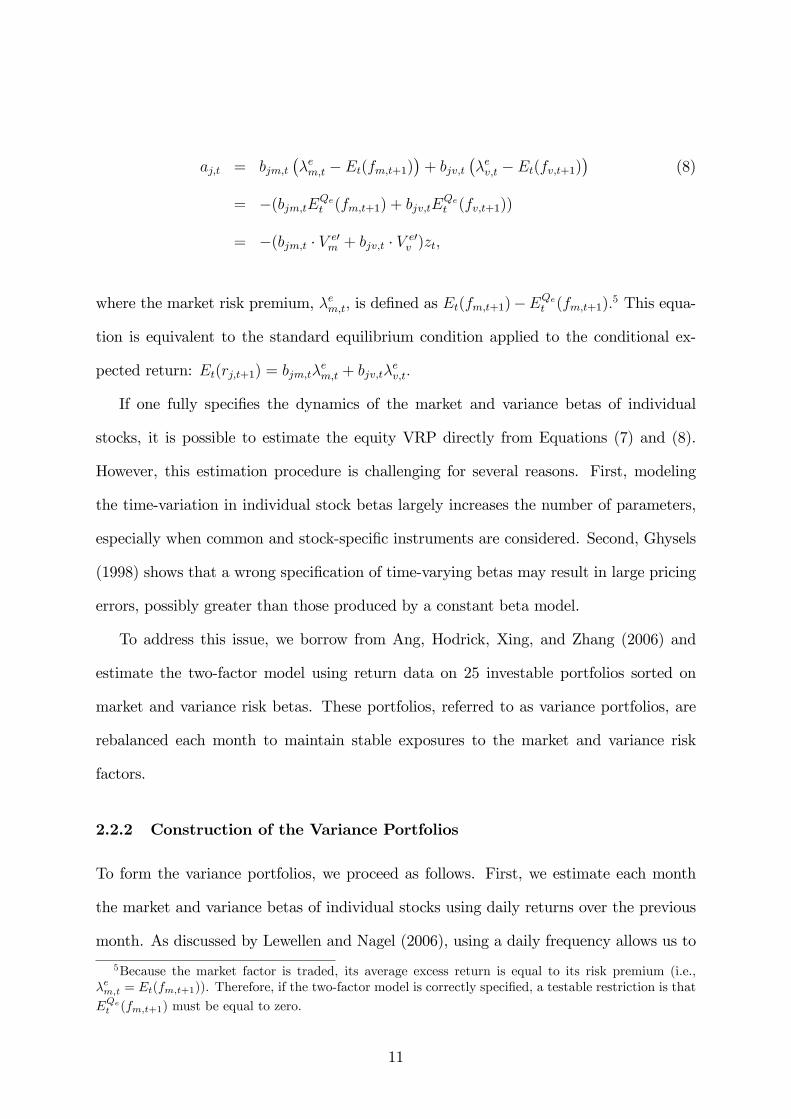
aj,t = bjm,t(λem,t − Et(fm,t+1)

)+ bjv,t

(λev,t − Et(fv,t+1)

)(8)

= −(bjm,tEQet (fm,t+1) + bjv,tE

Qet (fv,t+1))

= −(bjm,t · V e′m + bjv,t · V e′

v )zt,

where the market risk premium, λem,t, is defined as Et(fm,t+1)−EQet (fm,t+1).5 This equa-

tion is equivalent to the standard equilibrium condition applied to the conditional ex-

pected return: Et(rj,t+1) = bjm,tλem,t + bjv,tλ

ev,t.

If one fully specifies the dynamics of the market and variance betas of individual

stocks, it is possible to estimate the equity VRP directly from Equations (7) and (8).

However, this estimation procedure is challenging for several reasons. First, modeling

the time-variation in individual stock betas largely increases the number of parameters,

especially when common and stock-specific instruments are considered. Second, Ghysels

(1998) shows that a wrong specification of time-varying betas may result in large pricing

errors, possibly greater than those produced by a constant beta model.

To address this issue, we borrow from Ang, Hodrick, Xing, and Zhang (2006) and

estimate the two-factor model using return data on 25 investable portfolios sorted on

market and variance risk betas. These portfolios, referred to as variance portfolios, are

rebalanced each month to maintain stable exposures to the market and variance risk

factors.

2.2.2 Construction of the Variance Portfolios

To form the variance portfolios, we proceed as follows. First, we estimate each month

the market and variance betas of individual stocks using daily returns over the previous

month. As discussed by Lewellen and Nagel (2006), using a daily frequency allows us to

5Because the market factor is traded, its average excess return is equal to its risk premium (i.e.,λem,t = Et(fm,t+1)). Therefore, if the two-factor model is correctly specified, a testable restriction is that

EQe

t (fm,t+1) must be equal to zero.

11

pin down the conditional risk loadings without specifying the conditioning information.

Specifically, we regress the return of each stock on the market return and the innovation

of the variance factor. Computing a model-free variance innovation based on intraday

return observations is not feasible because this data is only available in the latter part of

the sample. To address this issue, we model the daily conditional variance of the market

return, σ2d, using a standard GARCH (1,1): σ

2d = γ + ασ2

d−1 + βε2d, where ε

2d is the daily

squared market return. Estimating the parameters γ, α, and β using daily returns over

a one-year rolling window, we compute the daily variance innovation as ε2d− σ

2d−1, where

σ2d−1 is the estimated variance on the previous day.

6

Second, we sort stocks according to their exposures to the market and variance factors.

Since short-window regressions can produce large estimation errors, we use the beta t-

statistics, tjm,t = bjm,t/σbjm,t and tjv,t = biv/σbjv,t , where σbjm,t , σbjv,t denote the estimated

standard deviation of bjm,t and bjv,t, respectively.7 Stocks are ranked first into quintiles

based on the variance t-statistic, and then into quintiles based on the market t-statistic.

Third, we compute the value-weighted return of all stocks in each of the 25 groups.

Repeating these three steps each month over the entire sample period, we obtain return

time-series for 25 investable variance portfolios.

2.2.3 Estimation Procedure

The estimation procedure builds on a recent paper by Gagliardini, Ossola, and Scaillet

(2013) that extends the traditional two-pass regression to the conditional setting exam-

ined here. In the first step, we run a time-series regression of the excess return of each

variance portfolio p (p = 1, ..., 25) on the J-vector of predictors and the two risk factors:

rp,t+1 = β′p1zt + bpm · fm,t+1 + bpv · fv,t+1 + ep,t+1. (9)

6Alternatively, Ang, Hodrick, Xing, and Zhang (2006) use the daily change in the VIX index. Wefollow a different approach for two reasons. First, as noted by these authors, the VIX is a noisy proxy ofthe innovation of the variance factor because it also captures changes in the risk premium itself. Second,data on the VIX is only available in 1990, while our sample begins in 1970.

7Previous papers (e.g., Kosowski, Timmerman, Wermers, and White (2006)) show that the t-statisticallows for an improved ranking because it controls for the precision of the estimated coeffi cient.

12

This formulation is a special case of Equation (7) with constant conditional betas. In the

second step, we exploit the parameter restrictions implied by the equilibrium condition

in Equation (8), which can be rewritten as

βp1 = −(bpm · V em + bpv · V e

v ) = −βp2V e, (10)

where V e is a 2J-vector equal to [V e′m , V

e′v ]′, βp2 is a J×2·J matrix equal to [bpm ·IJ , bpv ·IJ ],

and IJ is the J × J identity matrix. Therefore, if we run a cross-sectional regression of

the estimated J-vector βp1 on the estimated coeffi cient matrix −βp2 = [bpm · IJ , bpv · IJ ],

we obtain an estimator of V e denoted by V e = [V e′m , V

e′v ]′.8

Inserting V ev in Equation (5), we compute the estimated equity VRP as λ

e

v,t =(Fv − V e

v

)′zt. As a by-product of the estimation procedure, we also obtain an estimate of

time-varying market risk premium λe

m,t equal to(Fm − V e

m

)′zt, where Fm is the J-vector

of estimated coeffi cients from a time-series regression of the market excess return on the

predictors. The appendix contains additional details on the estimation procedure and on

the asymptotic properties of the different estimators.

2.3 Estimating the Option Variance Risk Premium

2.3.1 Extracting Information from Option Prices

The option VRP is easier to estimate than the equity VRP because we can use the infor-

mation contained in the VIX index computed from the prices of index options. Specifically,

Britten-Jones and Neuberger (2000), Jiang and Tian (2005), and Carr and Wu (2009)

show that the squared VIX index, or implied variance, provides a model-free approxima-

tion of the risk-neutral expectation of the realized variance. This result has been widely

used in the literature (see for instance Carr and Wu (2009) and Bollerslev, Gibson, and

8Equations (9) and (10) are simply the conditional counterparts to the widely used two-pass regressionused in an unconditional setting: (i) the time-series regression becomes rp,t+1 = a+ bpm · fm,t+1 + bpv ·fv,t+1+ep,t+1; (ii) the cross-sectional regression becomes E(rp,t+1) = bpm ·λm+ bpv ·λv, where E(rp,t+1)is the average portfolio return, and λm, λv are the unconditional risk premia.

13

Zhou (2011)) to estimate a "raw" version of the VRP in which the risk-neutral expecta-

tion of the realized variance is conditioned on all information available to option market

participants: λo,rawv,t = Et (fv,t+1)− ivt = F ′vzt− ivt, where ivt denotes the implied variance

computed from index option prices observed at time t.

This "raw" version of the option VRP is easy to compute and extracts as much

information as possible from option prices. However, it does not allow us to determine to

which extent the predictors zt drive the dynamics of the option VRP. For this purpose,

we rely on the formulation in Equation (6) to estimate the predictor-based option VRP

λov,t defined as (Fv − V ov )′ zt. The only required input is an estimate of the J-vector V o

v

that we obtain by regressing the implied variance on the predictors using the procedure

described below.

2.3.2 Estimation Procedure

The main diffi culty in estimating the vector V ov comes from data limitation. While the

realized variance and predictors are observed over a long period starting in 1970 (i.e., the

long sample), data on the implied variance is only available in the early 90’s (i.e., the

short sample). To address this issue, we use the Generalized Method of Moments (GMM)

extended by Lynch and Wachter (2013) for samples of unequal lengths. The basic idea

behind this approach is to exploit information contained in the long sample to obtain

an estimator of V ov that exhibits lower volatility than the one based on the short sample

only.

The estimation procedure can be described as follows. First, we run a time-series

regression of the implied variance on the predictors over the short sample to obtain

an initial estimate denoted by V ov,S. Second, we compute an adjustment factor, A, that

depends on the estimated vector Fv computed over the long sample. Third, we obtain

the final estimate V ov by taking the difference between V

ov,S and A.

While the general expression for A is not particularly insightful, the intuition behind

this adjustment can be easily illustrated with the following example. Suppose that we

14

just want to estimate the average of the realized and implied variances– in this case, zt

equals 1 and Fv and V ov are scalars equal to the means of fv,t+1 and ivt, respectively. Now

suppose that the estimated mean of fv,t+1 over the short sample is above the more precise

estimate computed over the long sample, i.e., Fv,S > Fv. If fv,t+1 and ivt are positively

correlated, the estimated mean of ivt, V ov,S, is also likely to be above average. Therefore,

A takes a positive value to produce a final estimate V ov that is below V o

v,S. The appendix

contains additional details on the estimation procedure and on the asymptotic properties

of the different estimators.

3 Data Description

3.1 Risk Factors and Predictive Variables

We conduct the empirical analysis using quarterly data between April 1970 and December

2012 (the long sample). The market factor is proxied by the excess return of the CRSP

value-weighted market index, while the variance factor is measured as the sum of the

squared daily returns of the SP500 over each quarter. To compute the quarterly implied

variance of the SP500, we use the squared VIX index computed from three-month option

prices and available between January 1992 and December 2012 (the short sample).

We use a set of five macro-finance predictors to capture the time-variation of the

VRP: the lagged realized variance, the Price/Earnings (PE) ratio, the quarterly inflation

rate, the quarterly growth in aggregate employment, and the default spread (all of them

expressed in log form). This choice is motivated by the recent studies of Bollerslev,

Gibson, and Zhou (2011), Paye (2012), and Campbell, Giglio, Polk, and Turley (2013) in

which these variables contain predictive information on the realized variance.9 Whereas

9Our approach is different from Corsi (2009), and Bekaert and Hoerova (2014) who forecast themonthly realized variance using its lags calculated at different frequencies (monthly, weekly, daily).Here, we follow Paye (2012) and Campbell, Giglio, Polk, and Turley (2013) who show that over a quar-terly horizon, including macro-finance variables in a multivariate regression improves forecast accuracy.In particular, the above-mentioned papers point out that a multivariate forecast can be useful for dis-tinguishing between the short- and long-term variance fluctuations.

15

the lagged realized variance is informative about the persistent component of the variance

process, the remaining variables help capture the fluctuations of aggregate volatility over

the business cycle.10 The PE ratio is downloaded from Robert Shiller’s webpage and

is defined as the price of the SP500 divided by the 10-year trailing moving average of

aggregate earnings. Inflation data is computed from the Producer Price Index (PPI),

aggregate employment is measured by the total number of employees in the nonfarm

sector (seasonally-adjusted), and the default spread is defined as the yield differential

between Moody’s BAA- and AAA-rated bonds. These three series are downloaded from

the Federal Reserve Bank of St. Louis.

In addition to the macro-finance variables mentioned above, we consider two predictors

used by previous studies as proxies for the risk-bearing capacity of financial intermediaries

(both expressed in log form). The first one is the leverage ratio of broker-dealers, defined

as their asset to equity values from the Federal Reserve Flow of Funds Accounts (Table L

128).11 Adrian and Shin (2010) provide supporting evidence that broker-dealers actively

manage their leverage levels. In good times, they increase their leverage and expand their

asset base, possibly because their Value-at-Risk constraints are less tight (see Adrian and

Shin (2013)), whereas they deleverage in bad times. Second, we follow Boyson, Stahel,

and Stulz (2010) and compute the value-weighted index of publicly-traded prime broker

firms, including Goldman Sachs, Morgan Stanley, Bear Stearns, UBS, and Citigroup.

The quarterly return of this index allows us to capture changes in the financial strength

of the major players in the brokerage sector.

Table 1 provides summary statistics for the different predictors. To facilitate compar-

isons across the estimated coeffi cients presented in the empirical section, all the predictors

are standardized.12 The comparison of the persistence levels for the two broker-dealer

10In the sensitivity analysis presented below, we consider an alternative set of macro-finance predictorsthat includes the dividend yield, the quarterly growth rate in industrial production, the business cycleindicator constructed by Aruoba, Diebold, and Scotti (2009), the 3-month Tbill rate, and the termspread. In all these cases, the main results of the paper remain unchanged.11The Federal Reserve defines broker-dealers as financial institutions who buy and sell securities for a

fee, hold and inventory of securities for resale, or do both.12Lettau and VanNieuwerburgh (2008), among others, provide empirical evidence that the mean of

16

variables reveals that they contain information at different frequencies. The leverage

ratio is a slow-moving predictor that proxies for long-term changes in the risk-bearing

capacity of financial intermediaries, whereas the PBI return captures the short-term re-

action of these intermediaries to aggregate losses. It is well known from the previous

literature that persistent variables such as the leverage ratio can create inference biases

in predictive regresssions (e.g., Cavanagh, Elliott, and Stock (1995), Ferson, Sarkissian,

and Simin (2003)). To mitigate this concern, we also run the estimation using the annual

change in the leverage ratio– although this variable is a noisier measure of the leverage

of broker-dealers, its first-order autocorrelation (0.74) is below the levels produced by all

but one predictor (the PBI return).

Perhaps not surprisingly, the two broker-dealer variables also pick up some business

cycle fluctuations– for instance, the correlation between the leverage and PE ratios equals

0.33. To explicitly distinguish between the two sets of predictors, we therefore regress the

leverage ratio and the PBI return on the macro-finance variables and take the residual

components of the two regressions.

[TABLE 1 HERE]

3.2 Variance Portfolios

To create the 25 variance portfolios, we consider all stocks traded on AMEX, NASDAQ

and the NYSE, and impose two filters. First, we exclude tiny-cap stocks to avoid liquidity-

related issues. Using the classification proposed by Fama and French (2008), we select

all existing stocks with a size above the 20th percentile of the market capitalization for

NYSE stocks. Second, we require each stock to have at least 15 daily return observations

over the previous month in order to compute its market and variance betas.

To summarize the properties of the variance portfolios, we take an equally-weighted

average of all portfolios in the same variance beta quintile (Low, 2, 3, 4, High). Overall,

financial ratios exhibit large structural shifts after 1991. Therefore, we follow their recommendation andallow for the possibility that predictors have different means before and after 1991.

17

the results are similar to those reported by Ang, Hodrick, Xing, and Zhang (2006) for

their VIX-based variance portfolios. Panel A of Table 2 shows that the low variance

beta portfolio loads negatively on the variance factor (with a post-ranking beta of -0.30)

and yields an average return of 7.55% per year. As we move toward the high variance

portfolio, the post-ranking beta increases and the average return drops, consistent with

the idea that investors are willing to pay a premium for portfolios that perform well

in times of high volatility. Interestingly, unreported results show that during the five

greatest volatility spikes (Oct. 1987, July 2002, July/Oct. 2008, July 2011), the market-

hedged return of the high minus low variance portfolio is always positive (e.g., it equals

11.31% over the last quarter of 1987), whereas it turns negative during the five quarters

with the lowest realized variance. These findings provide supportive evidence that the

returns of the variance portfolios are exposed to variance risk and can be used to extract

information about the VRP.

Whereas high volatility shocks are associated with stock market declines (i.e., the

correlation between factor innovations equals -0.49), the two factors capture different

dimensions of risk. Specifically, Panel B reveals that using the market factor alone pro-

duces CAPM alphas that exhibit the same pattern as the one observed for average re-

turns. Next, we report the portfolio alphas obtained with the Fama-French model and

two extensions that include the momentum and the Pastor-Stambaugh liquidity factors,

respectively. The results show that the three models generally help reduce the magni-

tude of the alphas compared to the CAPM, but do not fully capture the cross-sectional

variation in average returns.13

[TABLE 2 HERE]

13We reach a similar conclusion over the short sample (1992-2012). Unreported results show that theannual alphas range between -2.8% and 4.1% for the Fama-French (FF) model, between -2.1% and 4.1%for the FF-momentum model, and between -3.0% and 3.2% for the FF-liquidity model.

18

4 Empirical Results

4.1 Realized Variance Predictability

We begin our empirical analysis by measuring the extent of variance predictability. We

regress the quarterly realized variance on the set of predictors over the period 1970-

2012 to estimate the J-vector of coeffi cients Fv. This procedure allows us to estimate

the conditional expectation of the realized variance that we use as input to compute the

equity and option VRPs.

Panel A of Table 3 reports the estimated vector Fv obtained with the (standardized)

macro-finance variables. The first row shows the results when the lagged realized variance

is used as a single predictor. We find that the estimated coeffi cient is positive and highly

significant, i.e., a one-standard deviation increase in past variance increases future vari-

ance by 65% compared to its average level (0.49/0.75). In the second row, we condition on

all macro-finance variables simultaneously. Consistent with Campbell, Giglio, Polk, and

Turley (2013) and Paye (2012), we find a positive and statistically significant relationship

between the default spread and future realized variance. The intuition for this result is

that risky bonds are short the option to default. When expected future variance is above

average, investors bid down the price of risky bonds, which in turn increases the default

spread. Conditional on the other predictors, a high PE ratio also signals above-average

future variance. As noted by Campbell, Giglio, Polk, and Turley (2013), the PE ratio

helps capture episodes during which both stock prices and volatility are high, such as the

dotcom bubble in the late 90’s.

In Figure 2, we plot the evolution of the realized variance and its conditional expec-

tation based on the macro-finance variables. Overall, the fit is good and contrasts with

the relatively low predictive R2 reported in Panel A. This discrepancy is primarily driven

by a few surprise spikes in realized variance, notably in 1987– when we only focus on the

short sample (1992− 2012), the predictive R2 rises to 30.6% (unreported results).

Building on previous work by Brunnermeier and Pedersen (2009), Paye (2012) suggests

19

that financial intermediation possibly amplifies shocks to asset markets in times when

financial intermediaries find themselves in deleveraging spirals. If this relationship holds,

the leverage ratio of broker-dealers and the PBI return should capture information on

future volatility beyond that already contained in the macro-finance variables. Contrary

to this view, Panel B reveals that the incremental power of the broker-dealer variables is

modest because none of the t-statistics is statistically different from zero.

[TABLE 3 HERE]

[FIGURE 2 HERE]

4.2 Equity Variance Risk Premium

Next, we analyze the dynamics of the equity VRP inferred from the cross-section of

variance portfolios. Specifically, we use the conditional two-pass regression approach de-

scribed in Section 2 to estimate of the J-vector V ev that drive the risk-neutral expectation

of the realized variance. Then, we plug the two estimated vectors Fv and V ev into Equation

(5) to compute the equity VRP as λe

v,t = Λe′v zt, where Λe

v = Fv − V ev .

The estimated vector Λev obtained with the macro-finance variables is shown in Panel

A of Table 4. In an multi-period setting, risk-averse investors want to hedge against

increases in aggregate volatility because such changes represent a deterioration in in-

vestment opportunities. Therefore, stocks that do well in times of high volatility should

command lower expected returns (e.g., Campbell, Giglio, Polk, and Turley (2013)). Con-

sistent with this view, the average equity VRP equals −1.48% per year (−0.38 · 4), and

is comparable to the unconditional estimate of −1.00% per year found by Ang, Hodrick,

Xing, and Zhang (2006).

The remaining coeffi cients in Panel A provide new insights into the dynamics of the

equity VRP. First, the lagged realized variance has a significant impact on the VRP, both

economically and statistically– a one-standard deviation increase in realized variance

increases the magnitude of the VRP by 1.32% per year (-0.33 · 4). The intuition for

20

this result is simple: in volatile periods, the price of assets that pay off when future

volatility increases further becomes extremely valuable; this effect dominates the increase

in expected future variance documented in Table 3 (i.e., V e′v zt > F ′vzt). Interestingly,

the physical and risk-neutral expectation effects offset each other for both the PE ratio

and the default spread because the estimated coeffi cients in Panel A are not statistically

significant. Second, the coeffi cients associated with the inflation and employment rates are

both positive. Since both predictors tend to be high in expansions, this result suggests

that the VRP is countercyclical. However, only past inflation exhibits a statistically

significant coeffi cient, possibly because its lower persistence level helps capture higher

frequency business cycle fluctuations. Third, the conditional two-factor model does a

good job at capturing the return dynamics of the 25 variance portfolios. Using the joint

test of Kan, Robotti, and Shanken (2013), we find that the model is not rejected by the

data at conventional significance thresholds.

In Figure 3, we plot the path of the equity VRP obtained with the macro-finance

variables. The premium is negative most of the time and is characterized by transitory

spikes during the 1973-74 economic crisis, the 1987 crash, the burst of the dotcom bubble,

or the 2008 crisis. With an autocorrelation coeffi cient of 0.51, it also inherits some of the

persistence exhibited by the predictors. Finally, there is only a partial overlap between

episodes of highly negative VRP and the NBER recession periods. For instance, the

magnitude of the premium is high throughout late 1990s and early 2000s.

Turning to the analysis of the broker-dealer variables, we observe in Panel B that

none of the coeffi cients associated with the leverage ratio, the change in leverage and the

PBI return is statistically different from zero. These results suggest that the risk-bearing

capacity of financial intermediaries has little influence on the pricing of variance risk

in the equity market– as shown in Figure 4 the equity VRP paths computed with and

without the broker-dealer variables are nearly indistinguishable.

Bates (2000) argues that the probability of negative extreme events as perceived

by investors has increased after the 1987 crash. This change could have potentially

21

contributed to increase the magnitude of the variance risk premium.14 Motivated by

his findings, we examine whether the 1987 crash has triggered a structural change in

the equity market by estimating the VRP over the short sample (1992-2012). Figure 5

reveals that the VRP paths computed over the long and short samples look very similar.

In addition, the estimated coeffi cients associated with the different predictors do not

change dramatically either (unreported results). Taken together, these empirical findings

do not support the hypothesis of a structural break after 1987.

[TABLE 4 HERE]

[FIGURE 3 HERE]

[FIGURE 4 HERE]

[FIGURE 5 HERE]

To conclude this section, we examine the time-variation of the estimated market risk

premium obtained from the two-factor model. As discussed in Section 2, this premium

is defined as Λe′mzt, where Λe

m = Fm − V em, and Fm is the J-vector of coeffi cients from the

time-series regression of the quarterly market excess return on the predictors. Consistent

with the previous literature, Figure (6) shows that the premium rises during recession

periods. This countercyclicality is mostly driven by the PE ratio, which produces the

most significant estimated coeffi cient across all predictors (unreported results).

Studying the time-series properties of the market risk premium provides a second test

of the two-factor model. If the latter is correctly specified, the risk premium of the traded

market factor must be equal to its conditional average return (e.g., Cochrane (2005)). To

see if this restriction holds, we simply test whether the vector V em equals zero. We find

that this equality is not rejected by the data because none of the estimated coeffi cients

in V em is statistically significant at conventional levels (unreported results).

[FIGURE 6 HERE]

14See Bollerslev and Todorov (2011) for how an increase in the risk neutral probability of jumps couldcontribute to increase the magnitude of the VRP.

22

4.3 Option Variance Risk Premium

Previous studies infer the dynamics of the VRP directly from the prices of index options.

Specifically, the implied variance ivt provides an option-based measure of the risk-neutral

expectation of the realized variance. Exploiting this result, we can simply take the dif-

ference between F ′vzt and ivt to estimate the "raw" option VRP (e.g., Bollerslev, Gibson,

and Zhou (2011)). As shown in Figure 1, this premium is mostly negative, which is again

consistent with the idea that investors are willing to accept lower returns to be protected

against positive volatility shocks. In addition, it exhibits spikes that are much larger than

those observed in the equity market. For instance, the magnitude of the premium is as

large as 10% per year in the last quarter of 1998 (LTCM collapse), 2008 (height of the

financial crisis), and 2011 (European debt crisis).

Whereas this simple approach provides a convenient way to determine the fluctuations

of the option VRP, it is not informative about the role played by the different predictors

in driving such fluctuations. To address this issue, we compute a version of the option

VRP that is only conditioned on the predictors. As shown in Equation (6), it is defined

as λo

v,t = Λo′v zt, where Λo

v = Fv − V ov , and the J-vector V

ov is obtained by regressing the

implied variance on the predictors using the GMM approach described in Section 2.

In Panel A of Table 5, we report the estimated vector Λov associated with the macro-

finance variables. Overall, the results are similar to those documented for the equity

VRP, except for the positive and significant estimated coeffi cient associated with the

PE ratio. More importantly, Panel B reveals a strong positive relationship between

the two broker-dealer variables and the option VRP. When broker-dealers deleverage or

suffer short-term losses, the magnitude of the option VRP increases (in absolute value),

whereas the opposite holds when their leverage or their stock returns are above average.

The estimated coeffi cient for the leverage ratio is not only highly significant, it is also

economically large: a one-standard deviation decrease in leverage boosts the magnitude of

the premium by 1.40% per year (-0.36·4). Because the two orthogonalized broker-dealer

23

variables are negatively correlated (-0.26), the predictive information contained in the

PBI return is obscured when this predictor is used alone in the regression. Adding the

leverage ratio cleans up the relationship between the PBI return and the option VRP and

produces a positive and statistically significant coeffi cient (0.18). The rightmost columns

of Panel B confirm that all these results remain unchanged when the leverage ratio is

replaced with the annual change in leverage.

As a further check, Table 6 reports the estimated vector V ov for the predictive re-

gression of the implied variance. Because the implied variance is a measure of option

expensiveness, the coeffi cients in V ov indicate how option prices respond to changes in the

predictor values. The empirical evidence in Panel B is the mirror image of its counterpart

in Table 5, i.e., the coeffi cients are all negative and highly significant, which implies that

options become more expensive when broker-dealer leverage and the PBI return are low.

The overall evidence is consistent with the role played by financial intermediaries in

the risk sharing process. Garleanu, Pedersen, and Poteshman (2009) and Chen, Joslin,

and Ni (2013) show empirically that public investors have a large long net position in

SP500 index options, in particular in deep out of the money put options. By market

clearing, option dealers satisfy this demand by writing options and are, therefore, struc-

turally short variance risk. The risk-bearing capacity of these broker-dealers can change,

possibly because they face more or less tight risk constraints (Etula (2009), Adrian and

Shin (2010)); in particular, Adrian and Shin (2013) find that intermediaries actively

manage their balance sheet in response to Value-at-Risk constraints. When the ability or

willingness of broker-dealers to supply options goes down, the price of options increases

and vice versa.15

Finally, the reported link between broker-dealer variables and option VRP cannot

be fully attributed to an alternative demand-based option pricing mechanism. First,

we would expect demand pressure from hedgers to be at least partially captured by

15For instance, Chen, Joslin, and Ni (2013) show that financial intermediaries became net buyers ofdeep out-of-the-money options during major negative events that followed the onset of the global financialcrisis in 2009. These periods also correspond to spikes in option VRP.

24

aggregate macro-finance variables and be reflected in the price of variance risk in both

equity and option markets. Second, a shift in the demand for options would imply

a positive relationship between the magnitude of the option VRP and risk-taking by

broker-dealers. The data suggest the opposite pattern, which is consistent with a shift in

the supply of options.16

[TABLE 5 HERE]

[TABLE 6 HERE]

4.4 Equity versus Option Variance Risk Premia

The comparison of the equity and the "raw" option VRPs in Figure 1 reveals that the two

series diverge significantly at times– for instance, the magnitude of the option VRP is

much larger during the 2008 and European debt crises, whereas the opposite relationship

is observed in the beginning of 2000. To examine whether the different predictors can

explain these discrepancies, we study the properties of the predictor-based VRP difference

dv,t, defined as λe

v,t−λo

v,t = D′vzt, where Dv is equal to the difference between the J-vectors

Λev and Λo

v that drive the dynamics of the equity and option VRPs (reported in Tables 4

and 5, respectively).

The difference vector Dv is shown in Table 7, along with the vector of t-statistics

computed with the bootstrap approach described in the appendix. There are several

points worth noting. First, the average difference between the equity and option VRPs

is not statistically different from zero. Therefore, a simple analysis of the unconditional

risk premia is not suffi cient to uncover the large, but temporary mispricing across the

two markets. Second, there is significant evidence that the gap between the two premia

varies with the leverage of financial intermediaries. Specifically, the estimated coeffi cient

shown in Panel B is negative and implies that a one-standard deviation drop in leverage

increases the magnitude of the option VRP by 1.12% per year compared to the equity

16A similar conclusion is reached in Chen, Joslin, and Ni (2013), who document a negative relationshipbetween the quantity of options exchanged and their expensiveness.

25

VRP (−0.28 · 4)– a change nearly as large as the average premium itself. Third, the

discrepancy between the two VRPs is also negatively related to the PBI return (-0.20).

As a result, aggregate losses experienced by broker-dealers have a much larger impact

on the option VRP. Fourth, the only relevant macro-finance variable for explaining the

VRP difference is the PE ratio (see Panel A). However, unreported results reveal that

its impact becomes insignificant when we allow the broker-dealer leverage to compete

with the PE ratio (i.e., when we do not orthogonalize leverage). Therefore, the predictive

ability of the PE ratio may arise for its positive correlation with the leverage ratio, in

particular during the late 90’s when both predictors are above-average.

The coeffi cients estimated over the short sample (1992-2012) and documented in Fig-

ure 8 largely support the analysis above. The leverage ratio and the PBI return still

produce coeffi cients that are negative and highly significant.17 Furthermore, none of the

macro-finance variables including the PE ratio explains the difference between the two

markets.

[TABLE 7 HERE]

[TABLE 8 HERE]

Whereas the leverage of broker-dealers helps explain the gap between the equity and

option markets, it remains to be shown that it explains a large fraction of the "raw" VRP

difference displayed in Figure 1. To examine this issue, we first plot both the leverage

ratio and the "raw" difference in Figure 7, and find that the relationship between the

two variables is striking. A high leverage ratio signals periods when the magnitude of

the option VRP is lower than its equity counterpart (in absolute value). This is the case

prior to the monetary policy tightening in 1994, during the 2001-2003 monetary policy

easing, and between 2006 and 2008. On the contrary, episodes when the magnitude of

the option VRP increases dramatically correspond to sharp contractions in broker-dealer

17One difference with Table 7 is that the estimated coeffi cient associated with the change in leverageis not statistically significant. Whereas the magnitude of this coeffi cient is lower during the short sample(-0.11 versus -0.19), the reduction in the sample size (84 versus 171 observations) lowers the precision ofthe estimated coeffi cients.

26

leverage. Interestingly, Figure 7 reveals that the negative relationship between leverage

and the "raw" difference is not only observed during the recent financial crisis.

Second, we measure to which extent the predictor-based VRP difference dv,t tracks

the time-variation of the "raw" difference. As shown in Figure 8, using macro-finance

variables produces an overly-smoothed path that leaves 53% of the variation of the "raw"

difference unexplained. In contrast, adding the two broker-dealer variables allows us to

explain up to 65% of the time-variation of the "raw" difference.

[FIGURE 7 HERE]

[FIGURE 8 HERE]

4.5 Interpreting the Evidence

Our analysis so far reveals that the two proxies for the risk-bearing capacity of financial

intermediaries have a significant impact on the option VRP, but do not drive the price

of variance risk in the equity market. As a result, we observe a time-varying difference

between the two risk premia that constitutes an apparent arbitrage opportunity. Per-

haps the most natural explanation for this discrepancy is the presence of informational or

regulatory constraints that produce market segmentation and limit risk-sharing between

marginal investors in the two markets.18 For instance, retail investors can lack the ex-

pertise required to monitor option positions, whereas mutual funds generally face limits

on the amount of options they can hold in their portfolios. In addition, option trading

desks of financial institutions may be constrained to trade exclusively in the underlying

asset necessary to manage the delta of their positions, but not in other stocks (e.g., only

in SP500 index futures for SP500 index options traders). As a result, the option VRP

is determined by the capacity of broker-dealers to supply options– when they are con-

strained and the option VRP is high (in absolute value), equity investors are not able

18Basak and Croitoru (2000) provide the theoretical foundations for this result. Specifically, theyshow that mispricing between two redundant securities can exist in equilibrium in presence of portfolioconstraints that limit investors positions in the two markets.

27

to write options in suffi cient amount to provide protection against spikes in aggregate

volatility; conversely when broker-dealers are unconstrained, stock market investors do

not fully take advantage of the cheap protection against volatility risk. This explanation

is consistent with our key findings that changes in the risk bearing capacity of broker-

dealers strongly affects the option VRP (but not its equity counterpart), and help explain

both the positive and negative differences between the two VRPs observed in the data.

Alternatively, the gap in the pricing of variance risk may result from different funding

constraints. Specifically, Garleanu and Pedersen (2011) provide a theoretical framework

in which identical assets can exhibit different prices if they are traded in markets with

different margin requirements. Applied to our setting, the theory predicts that the price

of identical cash flows should be lower in the stock market because it exhibits higher

margin requirements than the option market. In addition, this price discrepancy should

increase with the tightness of funding constraints, leading to a time-varying and positive

VRP difference between the equity and option markets. Given that prime brokers provide

financing to institutions such as hedge funds, the two broker-dealer variables may simply

capture the tightness of these funding constraints.19 This story is not supported by the

data when we take more direct measures of funding constraints tightness. First, the

default spread, which is included in the set of macro-finance variables, does not exhibit

a significant relationship with the VRP difference (see Tables 7 and 8). Second, when

we include the TED spread in the set of predictors (on its own or together with broker-

dealer leverage), unreported results reveal that the coeffi cient has the wrong sign and is

not statistically significant either (t-statistics of−0.03 (without leverage) and−0.92 (with

leverage)). More importantly, a margin-based explanation cannot easily account for the

possibility of both positive and negative VRP differences because margin requirements

in the option market are unlikely to be greater than those in the equity market.

Whereas market segmentation seems more consistent with our main findings, it is nat-

19For instance, Adrian, Etula, and Muir (2012) interpret broker-dealer leverage as a proxy for thetightness of funding constraints.

28

ural to consider the role of specialized arbitrageurs who have a strong incentive to correct

any significant price discrepancy induced by segmented markets. For instance, when the

magnitude of option VRP is suffi ciently high, an arbitrageur could write expensive index

options and invest in a portfolio of stocks with a positive beta to the market variance

factor. Our evidence is not entirely consistent with arbitrageurs playing an active role in

correcting the relative mispricing of variance risk, possibly because of high trading costs

associated with rebalancing variance portfolios. If their ability to set up arbitrage trades

is limited by funding constraints, we would expect to observe pronounced differences be-

tween the two VRPs only when broker-dealer leverage and prime broker index returns

are low– that is, when the funding liquidity of arbitrageurs is limited. However, we find

that discrepancies in the pricing of variance risk also arises when financial intermediaries’

leverage and their stock returns are high.

Overall, our evidence leads to a more nuanced view of the informational content

of the VRP computed from option prices. Spikes in the option VRP can arise when

financial intermediaries are in a deleveraging phase, whereas a low price of risk could be

the consequence of an increased willingness of broker-dealers to take on risk. Because of

market segmentation, such fluctuations might not reflect actual changes in investors’risk

aversion in the equity market. Interestingly, we also find that episodes when options seems

cheap relative to the equity market valuation levels correspond to periods of monetary

easing. Figure 7 plots the VRP difference and broker-dealer leverage series against shaded

areas that correspond to periods where the Federal Reserve reduced its target for the

federal funds rate by more than 100 basis points in total and subsequently kept it at this

level. The correlation between the changes in the target federal funds rate and changes

in leverage is equal to -0.29. This suggests a connection between monetary policy, risk-

taking by financial intermediaries, and option prices.

29

4.6 Sensitivity Analysis

To check the robustness of our results, we examine whether the dynamics of the equity

and option VRPs are sensitive to the choice of the macro-finance variables. First, we re-

place the PE ratio with the dividend yield computed from the CRSP index. Second, we

replace the quarterly growth rate in employment with two alternative indicators of real

activity: the (seasonally-adjusted) quarterly growth rate in industrial production, and

the business cycle indicator constructed by Aruoba, Diebold, and Scotti (2009) that ag-

gregates information about employment, industrial production, and interest rates. Third,

we take the initial set of macro-finance variables and add two commonly-used interest

rate variables: the 3-month Tbill rate and the term spread, defined as the difference

between the 10- and 1-year Tbond yields. Finally, we add the quarterly variance of the

inflation rate following recent work by Paye (2012) which shows that this variable helps

forecast quarterly future volatility. The results in Table 9 reveal that the paths followed

by the VRP is extremely stable across the different specifications– in each market, the

correlation with the baseline VRP computed with the initial set of predictors is always

above 0.9.

[TABLE 9 HERE]

The previous analysis reveals that the VRP difference between the equity and option

markets is particularly large during volatile periods. Therefore, it raises the concern that

the explanatory power of the broker-dealer variables is only driven by a few extreme

observations for the volatility process. Unreported results show this is not the case, i.e.,

the coeffi cients that drive the VRP difference remain significant for both predictors when

1% and 2.5% of the most negative and positive variance observations are winsorized.

30

5 Conclusion

In this paper we infer the path of the VRP from the cross-section of stock returns and

compare it to the VRP implied by option prices. Whereas the two premia are in line

with each other on average, we identify episodes when they diverge and find that such

differences are explained to a large extent by changes in the risk-taking behaviour of

financial intermediaries who supply options. More precisely, proxies for broker-dealer

risk-bearing capacity are significant explanatory variables for the option VRP, but come

out as not significant for the equity VRP. Interestingly, we find that times when options

are relatively cheap coincide with periods of monetary easing. The relationship between

monetary policy, financial intermediation, and asset prices is an interesting topic for future

research about which our paper provides novel empirical evidence. In sum, our findings

can be exploited in future theoretical work that attempts to explain the aggregate pricing

of variance risk and model local demand and supply factors in option market.

31

References

Adrian, T., E. Etula, and T. Muir (2012): “Financial Intermediation and the Cross

Section of Asset Returns,”Journal of Finance, forthcoming.

Adrian, T., and H. S. Shin (2010): “Liquidity and Leverage,” Journal of Financial

Intermediation, 19(3), 418—437.

(2013): “Procyclical Leverage and Value-at-Risk,”Review of Financial Studies,

forthcoming.

Ang, A., B. Hodrick, Y. Xing, and X. Zhang (2006): “The Cross-Section of Volatil-

ity and Expected Returns,”Journal of Finance, 61(1), 259—299.

Aruoba, S. B., F. X. Diebold, and C. Scotti (2009): “Real-Time Measurement of

Business Conditions,”Journal of Business and Economic Statistics, 27(4), 417—427.

Bali, T., and H. Zhou (2013): “Risk, Uncertainty, and Expected Returns,”Working

Paper.

Bansal, R., D. Kiku, I. Shaliastovich, and A. Yaron (2013): “Volatility, the

Macroeconomy, and Asset Prices,”Journal of Finance, forthcoming.

Basak, S., and B. Croitoru (2000): “Equilibrium Mispricing in a Capital Market

with Portfolio Constraints,”Review of Financial Studies, 13(3), 715—748.

Bates, D. S. (2000): “Post-’87 Crash Fears in the SP 500 Futures Option Market,”

Journal of Econometrics, 94(1-2), 181—238.

(2003): “Empirical Option Pricing: A Retrospection,”Journal of Econometrics,

116(1-2), 387—404.

(2008): “The Market for Crash Risk,” Journal of Economic Dynamics and

Control, 32(7), 2291—2321.

Bekaert, G., and M. Hoerova (2014): “The VIX, the Variance Premium and Stock

Market Volatility,”Journal of Econometrics, forthcoming.

32

Bekaert, G., M. Hoerova, and M. Lo Duca (2013): “Risk, Uncertainty and Mon-

etary Policy,”Journal of Monetary Economics, 60(7), 771—788.

Bernanke, B. S., and K. N. Kuttner (2005): “What Explains the Stock Market’s

Reaction to Federal Reserve Policy?,”Journal of Finance, 60(3), 1221—1257.

Bollen, N. P. B., and R. E. Whaley (2004): “Does Net Buying Pressure Affect the

Shape of Implied Volatility Functions?,”Journal of Finance, 59(2), 711—753.

Bollerslev, T., M. Gibson, and H. Zhou (2011): “Dynamic Estimation of Volatility

Risk Premia and Investor Risk Aversion from Option-Implied and Realized Volatil-

ities,”Journal of Econometrics, 160(1), 235—245.

Bollerslev, T., G. Tauchen, and H. Zhou (2009): “Expected Stock Returns and

Variance Risk Premia,”Review of Financial Studies, 22(11), 4463—4492.

Bollerslev, T., and V. Todorov (2011): “Tails, Fears and Risk Premia,”Journal

of Finance, 66(6), 2165—2211.

Boyson, N. M., C. W. Stahel, and R. M. Stulz (2010): “Hedge Fund Contagion

and Liquidity Shocks,”Journal of Finance, 65(5), 1789—1816.

Britten-Jones, M., and A. Neuberger (2000): “Option Prices, Implied Price

Processes, and Stochastic Volatility,”Journal of Finance, 55(2), 839—866.

Brunnermeier, M. K., and L. H. Pedersen (2009): “Marker Liquidity and Funding

Liquidity,”Review of Financial Studies, 2(6), 2201—2238.

Campbell, J. Y., S. Giglio, C. Polk, and R. Turley (2013): “An Intertemporal

CAPM with Stochastic Volatility,”Working Paper.

Carr, P., and L. Wu (2009): “Variance Risk Premiums,”Review of Financial Studies,

22(3), 1311—1341.

Cavanagh, C. L., G. Elliott, and J. H. Stock (1995): “Inference in Models with

Nearly Integrated Regressors,”Econometric Theory, 11(5), 1131—1147.

33

Chen, H., S. Joslin, and S. Ni (2013): “Demand for Crash Insurance and Stock

Returns,”Working Paper.

Cheng, I., A. Kirilenko, and W. Xiong (2012): “Convective Risk Flows in Com-

modity Futures Markets,”Working Paper.

Cochrane, J. H. (2005): Asset Pricing. Princeton University Press.

Constantinides, G. M., J. C. Jackwerth, and S. Perrakis (2009): “Mispricing

of SP 500 Index Options,”Review of Financial Studies, 22(3), 1247—1277.

Corsi, F. (2009): “A Simple Approximate Long-Memory Model of Realized Volatility,”

Journal of Financial Econometrics, 7(2), 174—196.

Drechsler, I., A. Savov, and P. Schnabl (2014): “A Model of Monetary Policy and

Risk Premia,”Working Paper.

Drechsler, I., and A. Yaron (2011): “What’s Vol Got to Do With It,”Review of

Financial Studies, 24(1), 1—45.

Etula, E. (2009): “Broker-Dealer Risk Appetite and Commodity Returns,”Journal of

Financial Econometrics, forthcoming.

Fama, E. F., and K. R. French (1986): “Business Conditions and Expected Returns

on Stocks and Bonds,”Journal of Financial Economics, 25(1), 23—49.

(2008): “Dissecting Anomalies,”Journal of Finance, 63(4), 1653—1678.

Ferson, W. E., and C. R. Harvey (1991): “The Variation of Economic Risk Premi-

ums,”Journal of Political Economy, 99(2), 385—415.

Ferson, W. E., S. Sarkissian, and T. Simin (2003): “Spurious regressions in Finan-

cial Economics?,”Journal of Finance, 58(4), 1393—1414.

Gagliardini, P., E. Ossola, and O. Scaillet (2013): “Time-Varying Risk Premium

in Large Cross-Sectional Equity Datasets,”Working Paper.

Garleanu, N., and L. H. Pedersen (2011): “Margin-based Asset Pricing and Devi-

ations from the Law of One Price,”Review of Financial Studies, 24(6), 1980—2022.

34

Garleanu, N., L. H. Pedersen, and A. M. Poteshman (2009): “Demand-Based

Option Pricing,”Review of Financial Studies, 22(10), 4259—4299.

Ghysels, E. (1998): “On Stable Factor Structures in the Pricing of Risk: Do Time-

Varying Betas Help or Hurt?,”Journal of Finance, 53(2), 549—573.

Gromb, D., and D. Vayanos (2002): “Equilibrium and Welfare in Markets with Finan-

cially Constrained Arbitrageurs,” Journal of Financial Economics, 66(2-3), 361—

407.

Jagannathan, R., and Z. Wang (1998): “An Asymptotic Theory for Estimating

Beta-Pricing Models Using Cross-Sectional Regression,”Journal of Finance, 53(4),

1285—1309.

Jiang, G. J., and Y. S. Tian (2005): “The Model-Free Implied Volatility and Its

Information Content,”Review of Financial Studies, 18(4), 1305—1342.

Kan, R., C. Robotti, and J. A. Shanken (2013): “Pricing Model Performance and

the Two-Pass Cross-Sectional Regression Methodology,”Journal of Finance, 68(6),

2617—2649.

Keim, D. B., and R. F. Stambaugh (1986): “Predicting Returns in the Stock and

Bond Makets,”Review of Economics and Statistics, 17(2), 357—390.

Kosowski, R., A. Timmerman, R. Wermers, and H. White (2006): “Can Mutual

Fund Stars Really Pick Stocks? New Evidence from a Bootstrap Analysis,”Journal

of Finance, 61(6), 2551—2595.

Lettau, M., and S. VanNieuwerburgh (2008): “Reconciling the Return Predictabil-

ity Evidence,”Review of Financial Studies, 21(4), 1607—1652.

Lewellen, J., and S. Nagel (2006): “The Conditional CAPM does not Explain Asset-

pricing Anomalies,”Journal of Financial Economics, 82(2), 289—314.

35

Lynch, A. W., and J. A. Wachter (2013): “Using Samples of Unequal Length in Gen-

eralized Method of Moments Estimation,” Journal of Financial and Quantitative

Analysis, 48(1), 277—307.

Paye, B. S. (2012): “Deja vol: Predictive regressions for aggregate stock market volatil-

ity using macroeconomic variables,”Journal of Financial Economics, 106(3), 527—

546.

Rajan, R. G. (2006): “Has Finance Made the World Riskier?,” European Financial

Management, 12(4), 499Ð533.

Stambaugh, R. F. (1997): “Analyzing investments whose histories differ in length,”

Journal of Financial Economics, 45(3), 285—331.

Todorov, V. (2010): “Variance Risk Premium Dynamics,”Review of Financial Studies,

23(1), 345—383.

36

Appendix

A The Equity Variance Risk Premium

A.1 Two-pass Regression in a Conditional Setting

This section explains how to estimate the J-vectors of coeffi cients Fv and V ev that drive

the evolution of the equity VRP. To this end, we use the two-pass regression approach

developed by Gagliardini, Ossola, and Scaillet (2013). In the first step, we estimate,

for each variance portfolio p (p = 1, ..., n), the coeffi cients of the following time-series

regression:

rp,t+1 = β′p,1zt + bp,m · fm,t+1 + bp,v · fv,t+1 + ep,t+1, (A1)

where zt is the J-vector of lagged predictors (including a constant), fm,t+1 is the excess

market return, and fv,t+1 is the variance risk factor. The (J + 2)-vector of coeffi cients,

βp = (β′p,1, bp,m, bv,m)′, is equal to Q−1x E[xt+1rp,t+1], where Qx is a (J+2)× (J+2) matrix

equal to E[xt+1x′t+1], and xt+1 = (z′t, fm,t+1, fv,t+1)′. The OLS estimator is computed as

βp = Q−1x

1

T

T∑t=1

xt+1rp,t+1, (A2)

where T is the total number of return observations, and Qx = 1T

∑Tt=1 xt+1x

′t+1.

In the second step, we compute the estimator of the 2J-vector V e = [V e′m , V

e′v ]′ that

drives the risk-neutral expectations of the two risk factors. Specifically, we use a WLS

approach to estimatethe following cross-sectional regression:

βp1 = −βp2V e, (A3)

where βp2 a J×2J matrix equal to [bp,m·IJ , bp,v ·IJ ], and IJ is the J×J identity matrix. For

each portfolio p, we compute a J×J matrix of weights wp equal to diag(vp)−1, where vp is

37

the J×J covariance matrix of the J-vector of standardized errors εp =√T (βp1− β

′p2V

e),

i.e.,

vp = C ′VQ−1x SppQ

−1x C ′V , (A4)

where Spp is a (J + 2)×(J + 2) matrix equal to E[e2p,t+1xt+1x

′t+1], and CV is a (J + 2)×J

matrix defined as [E ′1 − (IJ ⊗ V e′)JAE′2]′, with E1 = [IJ ,0J×2]′, E2 = [02×J , I2]′, JA =

WJ,J ·2(I2⊗vec(IJ)), 0J×2 is a J×2 matrix of zeros, andWJ,J ·2 is a (J, J ·2)-commutation

matrix.20 The empirical counterpart of Equation (A4) is given by

vp = C ′V1Q−1x SpQ

−1x C ′

V1, (A5)

where Spp = 1T

∑Tt=1 e

2p,t+1xt+1x

′t+1, ep,t+1 = rp,t+1− β

′pxt+1, CV1 = [E ′1− (IJ ⊗ V e′

1 )JAE′2]′,

and V e1 is the first-step OLS estimator of V e obtained using unit weights, i.e., V e

1 =(∑np=1 β

′p2βp2

)−1∑np=1 β

′p2βp1.Using the estimated matrix of weights wp equal to diag(vp)

−1,

we obtain the following estimator of V e :

V e = Q−1βp2

1

n

n∑p=1

β′p2wpβp1, (A6)

where Qβ2is a 2J × 2J matrix equal to 1

n

∑np=1 β

′p,2wpβp,2.

The conditional expectation of the risk factors, ft+1 = (fm,t+1, fv,t+1)′, is given by

F ′zt, where F = [Fm, Fv] is a J × 2 matrix of coeffi cients equal to Q−1z E[ztf

′t+1], with

Qz = E[ztz′t]. To estimate F, we run a time-series regression of the factors on the lagged

predictors to obtain

F = Q−1z

1

T

T∑t=1

ztf′t+1, (A7)

where Qz = 1T

∑Tt=1 ztz

′t. Combining Equations (A6) and (A7), we can determine the

20The commutation matrix Wn,m of order n ·m×n ·m is defined such that Wn,mvec(A) = vec(A′) forany matrix A ∈ Rm×n.

38

path followed by the market and variance risk premia:

λe

m,t =(Fm − V e

m

)′zt,

λe

v,t =(Fv − V e

v

)′zt. (A8)

A.2 Distribution of the Estimated Coeffi cients

In an unconditional setting, Jagannathan and Wang (1998) show that the estimated vec-

tor of unconditional risk premia, λ, is consistent and asymptotically normally distributed.

Its covariance matrix, Σλ, is equal to Σf + 1nΣV , where Σf is the covariance matrix of the

factors, n is the number of test assets, and ΣV is the covariance matrix of the vector of

estimated expectations of the risk factors under the risk-neutral measure.

Gagliardini, Ossola, and Scaillet (2013) show that a similar result holds in a condi-

tional setting. Specifically, the 2J-vector Λe = vec(F ) − V e is consistent and asympoti-

cally normally distributed as

√T(

Λe − Λe)⇒ N(02J×1,ΣΛe). (A9)

The 2J × 2J covariance matrix ΣΛe is the sum of two terms, ΣF + 1nΣV , defined as

ΣF = (IJ ⊗Q−1z )Σu(IJ ⊗Q−1

z ), (A10)

ΣV =

(1

nB′nWnBn

)−11

nB′nWnVnWnBn

(1

nB′nWnBn

)−1

, (A11)

where Σu is a 2J × 2J matrix equal to E(ut+1u′t+1 ⊗ ztz′t) with ut+1 = ft+1 − F ′zt, Bn

is a Jn × 2J matrix defined as [β′12, ..., β′n2]′, Wn is a Jn × Jn block diagonal matrix

with elements [wp]p=1,...,n on its diagonal, and Vn is a Jn× Jn matrix composed of J × J

submatrices [Vpk]p,k=1,...,n with Vpk = C ′VQ−1x SpkQ

−1x C ′V , and Spk = E[ep,t+1ek,t+1xt+1x

′t+1].

A consistent estimator of ΣΛe can be obtained by replacing Σu, Q−1z , Bn, Wn, and Vn with

their empirical counterparts in Equation (A11).

39

A.3 Joint Test of Correct Specification

To test whether the two-factor model is correctly specified, we use the test statistic

proposed by Kan, Robotti, and Shanken (2013). Under the null of correct specification,

the sum of the pricing errors,∑n

p=1

(βp1 − βp2V e

)′ (βp1 − βp2V e

), is equal to zero. The

test is based on the weighted sum of squared residuals,

Qe =1

n

n∑p=1

ε′pwpεp, (A12)

where ep is the J-vector of estimated errors, εp = βp1 − βp2V e. Under the null, the test

statistic, T · Qe, is asymptotically distributed as 1n

∑nJ−2Jp=1 eigpχ

2p, where χ

2p are i.i.d. chi-

square variables with one degree of freedom, and eigp are the non-zero eigenvalues of the

matrix D equal to

D = V 1/2n (Wn −WnBn(B′nWnBn)−1B′nWn)V 1/2

n . (A13)

B The Option Variance Risk Premium

B.1 Treatment of Samples with Unequal Lengths

This section explains how to estimate the J-vectors of coeffi cients, Fv and V ov , that drive

the evolution of the option VRP. To estimate Fv, we simply regress the realized variance

fv,t+1 on the predictors zt. Therefore, the vector of estimated coeffi cients, Fv, is exactly

the same as the one used for the equity VRP (see Equation (A7)).

To estimate V ov , we run a time-series regression of the implied variance ivt on the

predictors. The main issue is that the periods over which fv,t+1, ivt, and zt are observed

have unequal lengths—while fv,t+1 and zt are available since 1970 (i.e., the long sample),

ivt is only observed since the early 90’s (i.e., the short sample). To exploit the information

contained in the long sample, we use the extension of the Generalized Method of Moments

(GMM) developed by Lynch and Wachter (2013).

40

To begin, we denote by g(V ov,S), g(Fv,S) the J-vectors of moments associated with V o

v

and Fv over the short sample, whereas g(Fv) is the J-vector of moments associated with

Fv over the long sample:

g(V ov,S) =

1

λT

λT∑ft(V

ov ) =

1

λT

λT∑ztuiv,t+1 =

1

λT

λT∑zt(ivt+1 − V o′

v zt),

g(Fv,S) =1

λT

λT∑ft(Fv) =

1

λT

λT∑ztuv,t+1 =

1

λT

λT∑zt(fv,t+1 − F ′vzt),

g(Fv) =1

T

T∑ft(Fv) =

1

T

T∑ztuv,t+1 =

1

T

T∑zt(fv,t+1 − F ′vzt), (B1)

where λ is the fraction of the period during which all variables are observed. The proce-

dure proposed by Lynch and Wachter (2013) consists in using a new set of moments to

estimate V ov :

g(V ov ) = g(V o

v,S)−BV ov ,Fv(g(Fv)− g(Fv,S)), (B2)

where each row of the J × J matrix BV ov ,Fv contains the coeffi cients of a regression of

each element in g(V ov,S) on the J-vector g(Fv,S). To estimate this matrix, we compute the

estimated vectors V ov,S and Fv,S over the short sample; then, we use Equations (B1) to

compute the J-vectors ft(V ov,S) and ft(Fv,S) at each time t, and run a time-series regression

of each element in ft(V ov,S) on ft(Fv,S).

By construction, the estimated long sample moment, g(Fv), equals zero because we

use it to compute Fv, wheras the estimated short sample moment, g(Fv,S), is given by

1λTZ ′(Yfv − ZFv), where Z = [z′(1−λ)T+1, ..., z

′T ]′, and Yfv = [fv,(1−λ)T+2, ..., fv,T+1]′. Plug-

ging these estimates into Equation (B2), we have:

g(V ov ) =

1

λTZ ′(Yiv − ZV o

v )− BV ov ,Fv

(1

λTZ ′(Yfv − ZFv)

)=

1

λT

(Z ′(Yiv − ZV o

v )− BV ov ,FvZ′(Yfv − ZFv)

), (B3)

41

where Yiv = [iv(1−λ)T+1, ..., ivT ]′. Therefore, the adjusted estimated vector given by

V ov = (Z ′Z)

−1(Z ′Yiv − D

)= V o

v,S − A, (B4)

where V ov,S is the short sample estimate of V

ov equal to (Z ′Z)−1 Z ′Yiv, and A is the adjust-

ment factor given by (Z ′Z)−1 BV ov ,FvZ′(Yfv −ZFv). Combining the two estimated vectors

Fv and V ov , we can compute the option VRP as (Fv − V o

v )′zt.

B.2 Distribution of the Estimated Coeffi cients

Using the results derived by Lynch and Wachter (2013), we can determine the properties

of the 2J-vector of estimated coeffi cients, Co = [F ′v, Vo′v ]′. Specifically, it is consistent and

asymptotically normally distributed as

√λT(Co − Co

)⇒ N(02J×1,ΣCo). (B5)

The 2J × 2J covariance matrix ΣCo is equal to

ΣCo = (I2 ⊗ E[ztz′t]−1)SA(I2 ⊗ E[ztz

′t]−1), (B6)

where SA is defined as

SA =

λSFv λSFv ,V ov

λSV ov ,Fv SV ov − (1− λ)SV ov ,FvS−1FvSFv ,V ov

, (B7)

with SFv =∑∞

τ=−∞E[ft(Fv)ft−τ (Fv)′], SFv ,V ov =

∑∞τ=−∞E[ft(Fv)ft−τ (V

ov )′], and, finally,

SV ov =∑∞

τ=−∞E[ft(Vov )ft−τ (V

ov )′]. To estimate these elements, we build on the procedure

described by Stambaugh (1997) and Lynch and Wachter (2013). First, we use the White

estimator to compute SFv over the full sample. Then, we use the estimated coeffi cient

matrix BV ov ,Fv and the estimated residual covariance matrix Σ from the regression of

ft(Vov ) on ft(Fv) to compute the remaining terms:

42

SFv ,V ov = SFvB′V ov ,Fv

, (B8)

SV ov = Σ + BV ov ,Fv SFvB′V ov ,Fv

. (B9)

This approach guarantees that the estimator of SA is positive-definite. Plugging this

estimator in Equation (B7) and replacing E[ztz′t] with its estimated value over the long

sample, Qz = 1T

∑Tt=1 ztz

′t, we get a consistent estimator of ΣCo .

Building on Equation (B7), we can also derive the asymptotic distribution of the

J-vector of estimated coeffi cients that drive the option VRP:

√λT (Λo

v − Λov)⇒ N(0J×1,ΣΛov), (B10)

where Λov is equal to the difference between Fv and V

ov . The J ×J covariance matrix ΣΛov

is given by

ΣΛov = Σ1Co + Σ2

Co − 2Σ1,2Co , (B11)

where Σ1Co is the J × J upper block of ΣCo , Σ2

Co is the J × J lower block, and Σ1,2Co is the

off-diagonal block.

C t-Statistics for the Difference in Estimated Coeffi cients

The time-variation of the equity and option VRPs is governed by the two estimated J-

vectors Λev and Λo

v defined above. To determine whether these two vectors differ from each

other, we compute the difference vector, Dv = Λev − Λo

v, and use a bootstrap approach to

determine the t-statistics associated with D. Consistent with the specification chosen to

estimate the equity and option VRPs, we assume that the dynamics of the excess return

of each variance portfolio p (p = 1, ..., 25), the market return, the realized variance, the

43

implied variance, and the vector of predictors is given by:

rp,t+1 = −(bpm · V e′m + bpv · V e′

v )zt + bpm · fm,t+1 + bpv · fv,t+1 + ep,t+1,

fm,t+1 = F ′mzt + um,t+1,

fv,t+1 = F ′vzt + uv,t+1,

ivt+1 = V o′v zt + uiv,t+1,

zt+1 = Φzt + uz,t+1. (C1)

After estimating the different coeffi cients in the system of Equations (C1), we build a

λT ×N matrix of estimated residuals, R = [e, um, uv, uiv, uz], where λT is the number of

observations over the short sample, N = 25 + 3 + (J − 1), um = [um,(1−λ)T+2, ..., um,T+1]′,

uv = [uv,(1−λ)T+2, ..., uv,T+1]′, uiv = [uiv,(1−λ)T+2, ..., uiv,T+1]′, uz = [u′z,(1−λ)T+2, ..., u′z,T+1]′,

and e = [e′(1−λ)T+2, ..., e′T+1]′, where each element et is equal to [e1,t, ..., e25,t].

For each boostrap iteration b (b = 1, ..., 1, 000), we first draw with replacement a

set of T rows from the matrix R. This procedure allows to preserve the cross-sectional

correlation between the residuals. Second, we plug the estimated coeffi cients and the

bootstrapped residuals into Equations (C1) to build, for each time t (t = 1, ..., T ), the

J-vector of predictors zbt , the excess return of the variance portfolios rbp,t+1, the market

return f bm,t+1, and the realized variance, fbv,t+1. Third, we do the same for the implied

variance ivbt+1 using the bootstrapped residuals over the short sample. Fourth, we use

all of these bootstrapped time-series and reestimate the J-vectors of coeffi cients Fv(b),

V ev (b), and V o

v (b) using the approach proposed by Gagliardini, Ossola, and Scaillet (2013)

and Lynch and Wachter (2013). Fifth, we compute Λev(b) as Fv(b) − V e

v (b), Λov(b) as

Fv(b) − V ov (b), and Dv(b) as Λe

v(b) − Λov(b). After repeating these five steps 1,000 times,

we compute the t-statistic of each element, dv,j (j = 1, ..., J), as dv,jσdv,j

, where σdv,j is the

standard deviation of the 1,000 bootstrapped values.

44

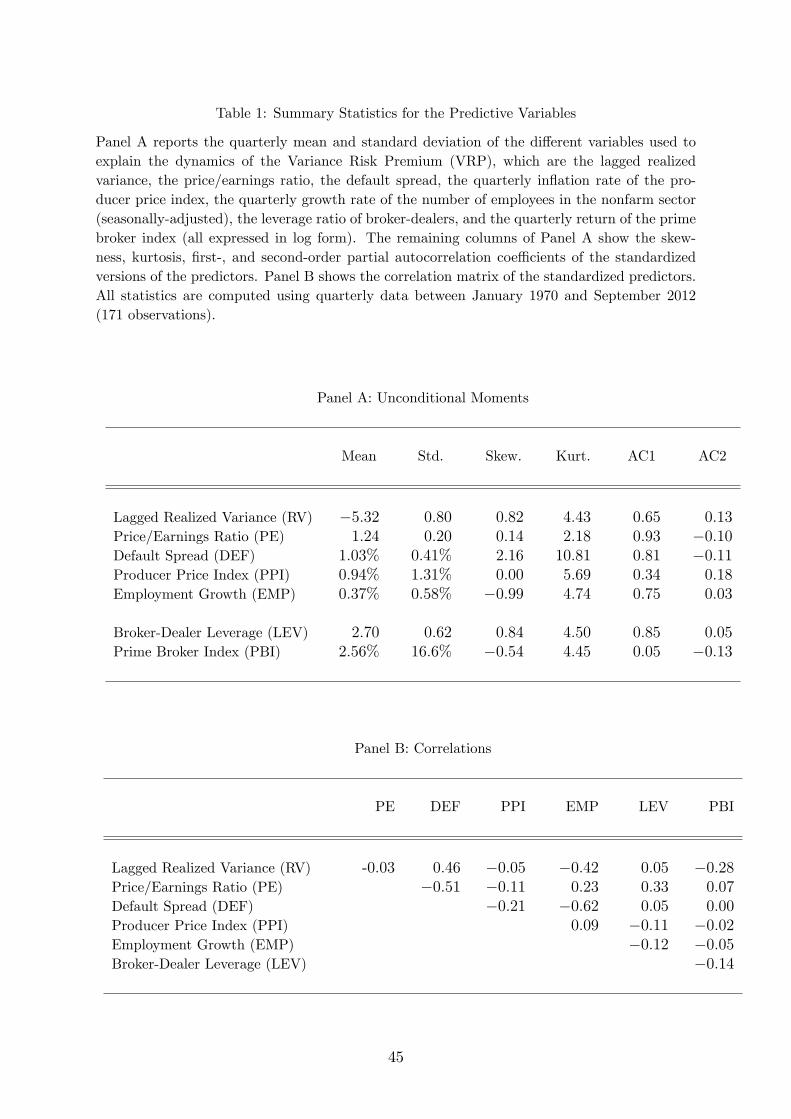
Table 1: Summary Statistics for the Predictive Variables

Panel A reports the quarterly mean and standard deviation of the different variables used toexplain the dynamics of the Variance Risk Premium (VRP), which are the lagged realizedvariance, the price/earnings ratio, the default spread, the quarterly inflation rate of the pro-ducer price index, the quarterly growth rate of the number of employees in the nonfarm sector(seasonally-adjusted), the leverage ratio of broker-dealers, and the quarterly return of the primebroker index (all expressed in log form). The remaining columns of Panel A show the skew-ness, kurtosis, first-, and second-order partial autocorrelation coeffi cients of the standardizedversions of the predictors. Panel B shows the correlation matrix of the standardized predictors.All statistics are computed using quarterly data between January 1970 and September 2012(171 observations).

Panel A: Unconditional Moments

Mean Std. Skew. Kurt. AC1 AC2

Lagged Realized Variance (RV) −5.32 0.80 0.82 4.43 0.65 0.13Price/Earnings Ratio (PE) 1.24 0.20 0.14 2.18 0.93 −0.10Default Spread (DEF) 1.03% 0.41% 2.16 10.81 0.81 −0.11Producer Price Index (PPI) 0.94% 1.31% 0.00 5.69 0.34 0.18Employment Growth (EMP) 0.37% 0.58% −0.99 4.74 0.75 0.03

Broker-Dealer Leverage (LEV) 2.70 0.62 0.84 4.50 0.85 0.05Prime Broker Index (PBI) 2.56% 16.6% −0.54 4.45 0.05 −0.13

Panel B: Correlations

PE DEF PPI EMP LEV PBI

Lagged Realized Variance (RV) -0.03 0.46 −0.05 −0.42 0.05 −0.28Price/Earnings Ratio (PE) −0.51 −0.11 0.23 0.33 0.07Default Spread (DEF) −0.21 −0.62 0.05 0.00Producer Price Index (PPI) 0.09 −0.11 −0.02Employment Growth (EMP) −0.12 −0.05Broker-Dealer Leverage (LEV) −0.14

45

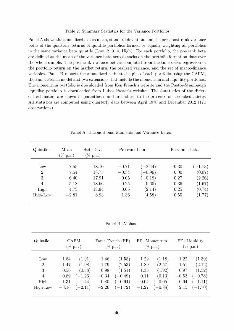
Table 2: Summary Statistics for the Variance Portfolios

Panel A shows the annualized excess mean, standard deviation, and the pre-, post-rank variancebetas of the quarterly returns of quintile portfolios formed by equally weighting all portfoliosin the same variance beta quintile (Low, 2, 3, 4, High). For each portfolio, the pre-rank betaare defined as the mean of the variance beta across stocks on the portfolio formation date overthe whole sample. The post-rank variance beta is computed from the time-series regression ofthe portfolio return on the market return, the realized variance, and the set of macro-financevariables. Panel B reports the annualized estimated alpha of each portfolio using the CAPM,the Fama-French model and two extensions that include the momentum and liquidity portfolios.The momentum portfolio is downloaded from Ken French’s website and the Pastor-Stambaughliquidity portfolio is downloaded from Lubos Pastor’s website. The t-statistics of the differ-ent estimators are shown in parentheses and are robust to the presence of heterokedasticity.All statistics are computed using quarterly data between April 1970 and December 2012 (171observations).

Panel A: Unconditional Moments and Variance Betas

Quintile Mean Std. Dev. Pre-rank beta Post-rank beta(% p.a.) (% p.a.)

Low 7.55 18.10 −0.71 (−2.44) −0.30 (−1.73)2 7.54 18.75 −0.34 (−0.96) 0.00 (0.07)3 6.40 17.91 −0.05 (−0.18) 0.27 (2.26)4 5.18 18.66 0.25 (0.60) 0.36 (1.67)

High 4.75 18.94 0.65 (2.14) 0.25 (0.74)High-Low −2.81 8.93 1.36 (4.58) 0.55 (1.77)

Panel B: Alphas

Quintile CAPM Fama-French (FF) FF+Momentum FF+Liquidity(% p.a.) (% p.a.) (% p.a.) (% p.a.)

Low 1.84 (1.91) 1.46 (1.58) 1.22 (1.18) 1.22 (1.39)2 1.47 (1.98) 1.79 (2.53) 1.89 (2.57) 1.51 (2.12)3 0.56 (0.88) 0.98 (1.51) 1.33 (1.92) 0.97 (1.52)4 −0.89 (−1.26) −0.34 (−0.49) 0.11 (0.13) −0.53 (−0.78)

High −1.31 (−1.44) −0.80 (−0.94) −0.04 (−0.05) −0.94 (−1.11)High-Low −3.16 (−2.11) −2.26 (−1.72) −1.27 (−0.88) 2.15 (−1.70)

46

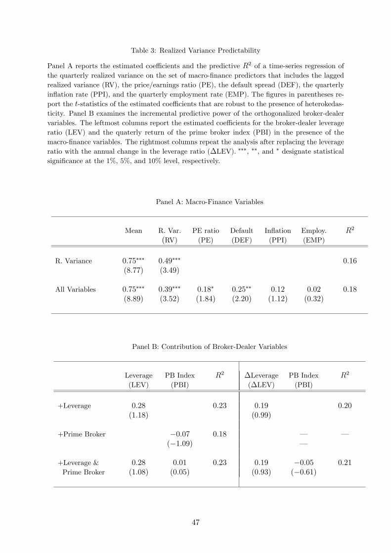
Table 3: Realized Variance Predictability

Panel A reports the estimated coeffi cients and the predictive R2 of a time-series regression ofthe quarterly realized variance on the set of macro-finance predictors that includes the laggedrealized variance (RV), the price/earnings ratio (PE), the default spread (DEF), the quarterlyinflation rate (PPI), and the quarterly employment rate (EMP). The figures in parentheses re-port the t-statistics of the estimated coeffi cients that are robust to the presence of heterokedas-ticity. Panel B examines the incremental predictive power of the orthogonalized broker-dealervariables. The leftmost columns report the estimated coeffi cients for the broker-dealer leverageratio (LEV) and the quaterly return of the prime broker index (PBI) in the presence of themacro-finance variables. The rightmost columns repeat the analysis after replacing the leverageratio with the annual change in the leverage ratio (∆LEV). ∗∗∗, ∗∗, and ∗ designate statisticalsignificance at the 1%, 5%, and 10% level, respectively.

Panel A: Macro-Finance Variables

Mean R. Var. PE ratio Default Inflation Employ. R2

(RV) (PE) (DEF) (PPI) (EMP)

R. Variance 0.75∗∗∗ 0.49∗∗∗ 0.16(8.77) (3.49)

All Variables 0.75∗∗∗ 0.39∗∗∗ 0.18∗ 0.25∗∗ 0.12 0.02 0.18(8.89) (3.52) (1.84) (2.20) (1.12) (0.32)

Panel B: Contribution of Broker-Dealer Variables

Leverage PB Index R2 ∆Leverage PB Index R2

(LEV) (PBI) (∆LEV) (PBI)

+Leverage 0.28 0.23 0.19 0.20(1.18) (0.99)

+Prime Broker −0.07 0.18 – –(−1.09) –

+Leverage & 0.28 0.01 0.23 0.19 −0.05 0.21Prime Broker (1.08) (0.05) (0.93) (−0.61)

47

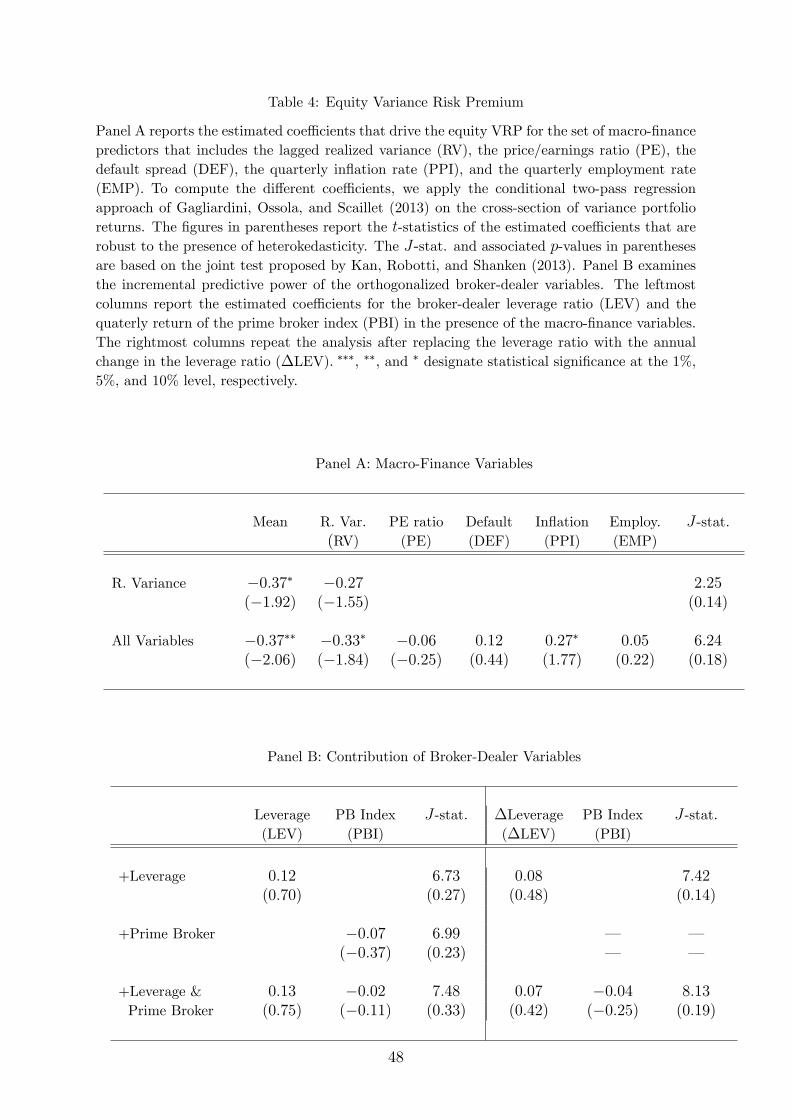
Table 4: Equity Variance Risk Premium

Panel A reports the estimated coeffi cients that drive the equity VRP for the set of macro-financepredictors that includes the lagged realized variance (RV), the price/earnings ratio (PE), thedefault spread (DEF), the quarterly inflation rate (PPI), and the quarterly employment rate(EMP). To compute the different coeffi cients, we apply the conditional two-pass regressionapproach of Gagliardini, Ossola, and Scaillet (2013) on the cross-section of variance portfolioreturns. The figures in parentheses report the t-statistics of the estimated coeffi cients that arerobust to the presence of heterokedasticity. The J-stat. and associated p-values in parenthesesare based on the joint test proposed by Kan, Robotti, and Shanken (2013). Panel B examinesthe incremental predictive power of the orthogonalized broker-dealer variables. The leftmostcolumns report the estimated coeffi cients for the broker-dealer leverage ratio (LEV) and thequaterly return of the prime broker index (PBI) in the presence of the macro-finance variables.The rightmost columns repeat the analysis after replacing the leverage ratio with the annualchange in the leverage ratio (∆LEV). ∗∗∗, ∗∗, and ∗ designate statistical significance at the 1%,5%, and 10% level, respectively.

Panel A: Macro-Finance Variables

Mean R. Var. PE ratio Default Inflation Employ. J -stat.(RV) (PE) (DEF) (PPI) (EMP)

R. Variance −0.37∗ −0.27 2.25(−1.92) (−1.55) (0.14)

All Variables −0.37∗∗ −0.33∗ −0.06 0.12 0.27∗ 0.05 6.24(−2.06) (−1.84) (−0.25) (0.44) (1.77) (0.22) (0.18)

Panel B: Contribution of Broker-Dealer Variables

Leverage PB Index J -stat. ∆Leverage PB Index J -stat.(LEV) (PBI) (∆LEV) (PBI)

+Leverage 0.12 6.73 0.08 7.42(0.70) (0.27) (0.48) (0.14)

+Prime Broker −0.07 6.99 – –(−0.37) (0.23) – –

+Leverage & 0.13 −0.02 7.48 0.07 −0.04 8.13Prime Broker (0.75) (−0.11) (0.33) (0.42) (−0.25) (0.19)

48

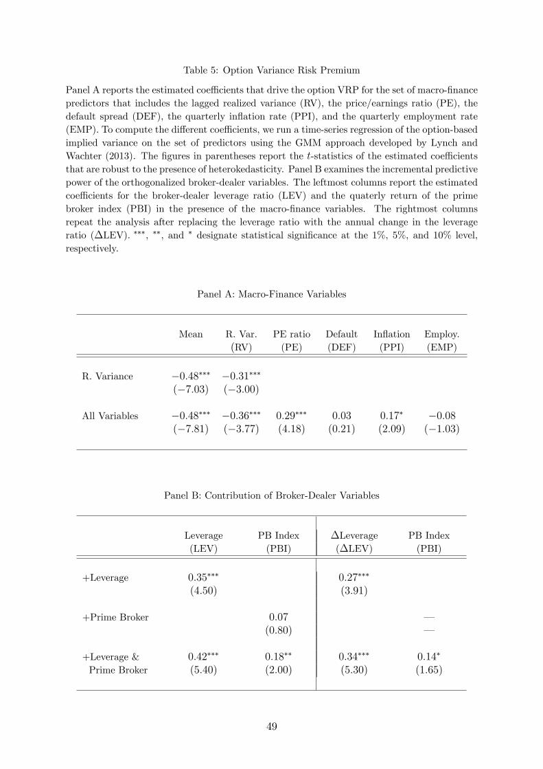
Table 5: Option Variance Risk Premium

Panel A reports the estimated coeffi cients that drive the option VRP for the set of macro-financepredictors that includes the lagged realized variance (RV), the price/earnings ratio (PE), thedefault spread (DEF), the quarterly inflation rate (PPI), and the quarterly employment rate(EMP). To compute the different coeffi cients, we run a time-series regression of the option-basedimplied variance on the set of predictors using the GMM approach developed by Lynch andWachter (2013). The figures in parentheses report the t-statistics of the estimated coeffi cientsthat are robust to the presence of heterokedasticity. Panel B examines the incremental predictivepower of the orthogonalized broker-dealer variables. The leftmost columns report the estimatedcoeffi cients for the broker-dealer leverage ratio (LEV) and the quaterly return of the primebroker index (PBI) in the presence of the macro-finance variables. The rightmost columnsrepeat the analysis after replacing the leverage ratio with the annual change in the leverageratio (∆LEV). ∗∗∗, ∗∗, and ∗ designate statistical significance at the 1%, 5%, and 10% level,respectively.

Panel A: Macro-Finance Variables

Mean R. Var. PE ratio Default Inflation Employ.(RV) (PE) (DEF) (PPI) (EMP)

R. Variance −0.48∗∗∗ −0.31∗∗∗

(−7.03) (−3.00)

All Variables −0.48∗∗∗ −0.36∗∗∗ 0.29∗∗∗ 0.03 0.17∗ −0.08(−7.81) (−3.77) (4.18) (0.21) (2.09) (−1.03)

Panel B: Contribution of Broker-Dealer Variables

Leverage PB Index ∆Leverage PB Index(LEV) (PBI) (∆LEV) (PBI)

+Leverage 0.35∗∗∗ 0.27∗∗∗

(4.50) (3.91)

+Prime Broker 0.07 –(0.80) –

+Leverage & 0.42∗∗∗ 0.18∗∗ 0.34∗∗∗ 0.14∗

Prime Broker (5.40) (2.00) (5.30) (1.65)

49

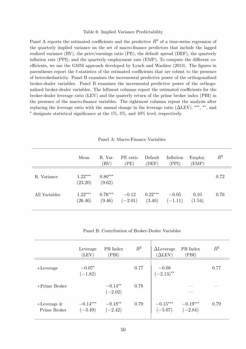
Table 6: Implied Variance Predictability

Panel A reports the estimated coeffi cients and the predictive R2 of a time-series regression ofthe quarterly implied variance on the set of macro-finance predictors that include the laggedrealized variance (RV), the price/earnings ratio (PE), the default spread (DEF), the quarterlyinflation rate (PPI), and the quarterly employment rate (EMP). To compute the different co-effi cients, we use the GMM approach developed by Lynch and Wachter (2013). The figures inparentheses report the t-statistics of the estimated coeffi cients that are robust to the presenceof heterokedasticity. Panel B examines the incremental predictive power of the orthogonalizedbroker-dealer variables. Panel B examines the incremental predictive power of the orthogo-nalized broker-dealer variables. The leftmost columns report the estimated coeffi cients for thebroker-dealer leverage ratio (LEV) and the quaterly return of the prime broker index (PBI) inthe presence of the macro-finance variables. The rightmost columns repeat the analysis afterreplacing the leverage ratio with the annual change in the leverage ratio (∆LEV). ∗∗∗, ∗∗, and∗ designate statistical significance at the 1%, 5%, and 10% level, respectively.

Panel A: Macro-Finance Variables

Mean R. Var. PE ratio Default Inflation Employ. R2

(RV) (PE) (DEF) (PPI) (EMP)

R. Variance 1.22∗∗∗ 0.80∗∗∗ 0.72(23.20) (9.62)

All Variables 1.22∗∗∗ 0.76∗∗∗ −0.12 0.22∗∗∗ −0.05 0.10 0.76(26.46) (9.46) (−2.01) (3.40) (−1.11) (1.54)

Panel B: Contribution of Broker-Dealer Variables

Leverage PB Index R2 ∆Leverage PB Index R2

(LEV) (PBI) (∆LEV) (PBI)

+Leverage −0.07∗ 0.77 −0.08 0.77(−1.82) (−2.13)∗∗

+Prime Broker −0.14∗∗ 0.78 – –(−2.02) –

+Leverage & −0.14∗∗∗ −0.18∗∗ 0.79 −0.15∗∗∗ −0.19∗∗∗ 0.79Prime Broker (−3.49) (−2.42) (−5.07) (−2.84)

50

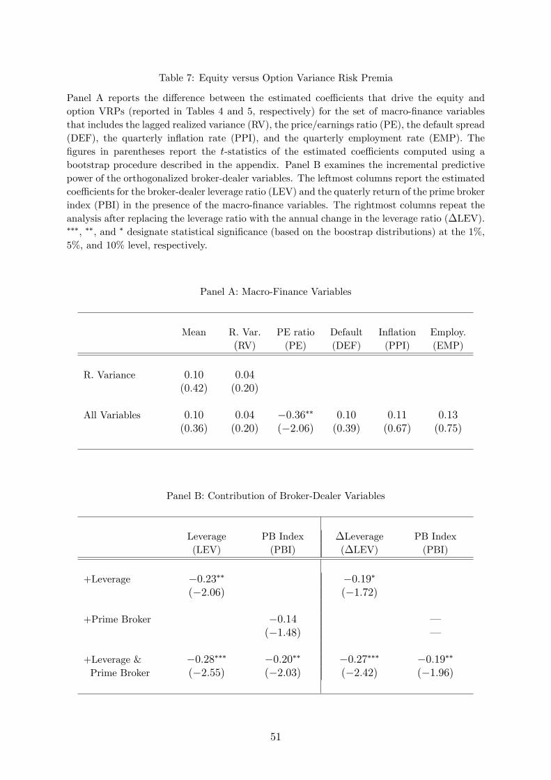
Table 7: Equity versus Option Variance Risk Premia

Panel A reports the difference between the estimated coeffi cients that drive the equity andoption VRPs (reported in Tables 4 and 5, respectively) for the set of macro-finance variablesthat includes the lagged realized variance (RV), the price/earnings ratio (PE), the default spread(DEF), the quarterly inflation rate (PPI), and the quarterly employment rate (EMP). Thefigures in parentheses report the t-statistics of the estimated coeffi cients computed using abootstrap procedure described in the appendix. Panel B examines the incremental predictivepower of the orthogonalized broker-dealer variables. The leftmost columns report the estimatedcoeffi cients for the broker-dealer leverage ratio (LEV) and the quaterly return of the prime brokerindex (PBI) in the presence of the macro-finance variables. The rightmost columns repeat theanalysis after replacing the leverage ratio with the annual change in the leverage ratio (∆LEV).∗∗∗, ∗∗, and ∗ designate statistical significance (based on the boostrap distributions) at the 1%,5%, and 10% level, respectively.

Panel A: Macro-Finance Variables

Mean R. Var. PE ratio Default Inflation Employ.(RV) (PE) (DEF) (PPI) (EMP)

R. Variance 0.10 0.04(0.42) (0.20)

All Variables 0.10 0.04 −0.36∗∗ 0.10 0.11 0.13(0.36) (0.20) (−2.06) (0.39) (0.67) (0.75)

Panel B: Contribution of Broker-Dealer Variables

Leverage PB Index ∆Leverage PB Index(LEV) (PBI) (∆LEV) (PBI)

+Leverage −0.23∗∗ −0.19∗

(−2.06) (−1.72)

+Prime Broker −0.14 –(−1.48) –

+Leverage & −0.28∗∗∗ −0.20∗∗ −0.27∗∗∗ −0.19∗∗

Prime Broker (−2.55) (−2.03) (−2.42) (−1.96)

51

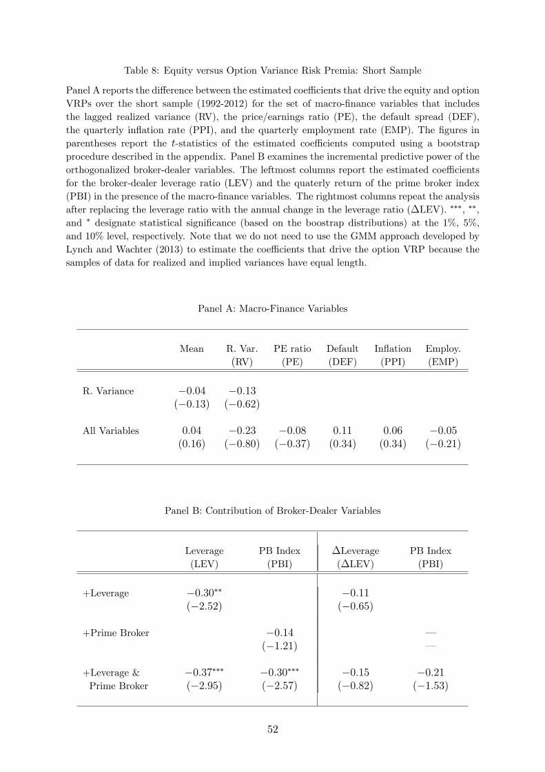
Table 8: Equity versus Option Variance Risk Premia: Short Sample

Panel A reports the difference between the estimated coeffi cients that drive the equity and optionVRPs over the short sample (1992-2012) for the set of macro-finance variables that includesthe lagged realized variance (RV), the price/earnings ratio (PE), the default spread (DEF),the quarterly inflation rate (PPI), and the quarterly employment rate (EMP). The figures inparentheses report the t-statistics of the estimated coeffi cients computed using a bootstrapprocedure described in the appendix. Panel B examines the incremental predictive power of theorthogonalized broker-dealer variables. The leftmost columns report the estimated coeffi cientsfor the broker-dealer leverage ratio (LEV) and the quaterly return of the prime broker index(PBI) in the presence of the macro-finance variables. The rightmost columns repeat the analysisafter replacing the leverage ratio with the annual change in the leverage ratio (∆LEV). ∗∗∗, ∗∗,and ∗ designate statistical significance (based on the boostrap distributions) at the 1%, 5%,and 10% level, respectively. Note that we do not need to use the GMM approach developed byLynch and Wachter (2013) to estimate the coeffi cients that drive the option VRP because thesamples of data for realized and implied variances have equal length.

Panel A: Macro-Finance Variables

Mean R. Var. PE ratio Default Inflation Employ.(RV) (PE) (DEF) (PPI) (EMP)

R. Variance −0.04 −0.13(−0.13) (−0.62)

All Variables 0.04 −0.23 −0.08 0.11 0.06 −0.05(0.16) (−0.80) (−0.37) (0.34) (0.34) (−0.21)

Panel B: Contribution of Broker-Dealer Variables

Leverage PB Index ∆Leverage PB Index(LEV) (PBI) (∆LEV) (PBI)

+Leverage −0.30∗∗ −0.11(−2.52) (−0.65)

+Prime Broker −0.14 –(−1.21) –

+Leverage & −0.37∗∗∗ −0.30∗∗∗ −0.15 −0.21Prime Broker (−2.95) (−2.57) (−0.82) (−1.53)

52

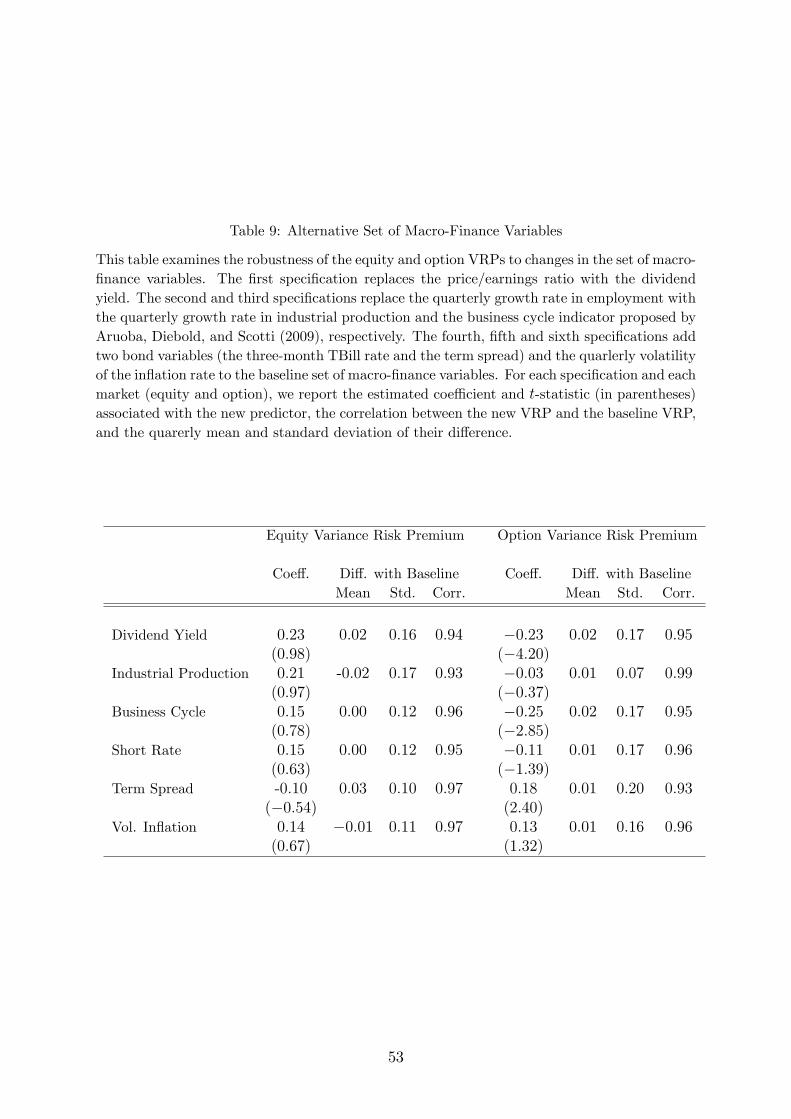
Table 9: Alternative Set of Macro-Finance Variables

This table examines the robustness of the equity and option VRPs to changes in the set of macro-finance variables. The first specification replaces the price/earnings ratio with the dividendyield. The second and third specifications replace the quarterly growth rate in employment withthe quarterly growth rate in industrial production and the business cycle indicator proposed byAruoba, Diebold, and Scotti (2009), respectively. The fourth, fifth and sixth specifications addtwo bond variables (the three-month TBill rate and the term spread) and the quarlerly volatilityof the inflation rate to the baseline set of macro-finance variables. For each specification and eachmarket (equity and option), we report the estimated coeffi cient and t-statistic (in parentheses)associated with the new predictor, the correlation between the new VRP and the baseline VRP,and the quarerly mean and standard deviation of their difference.

Equity Variance Risk Premium Option Variance Risk Premium

Coeff. Diff. with Baseline Coeff. Diff. with BaselineMean Std. Corr. Mean Std. Corr.

Dividend Yield 0.23 0.02 0.16 0.94 −0.23 0.02 0.17 0.95(0.98) (−4.20)

Industrial Production 0.21 -0.02 0.17 0.93 −0.03 0.01 0.07 0.99(0.97) (−0.37)

Business Cycle 0.15 0.00 0.12 0.96 −0.25 0.02 0.17 0.95(0.78) (−2.85)

Short Rate 0.15 0.00 0.12 0.95 −0.11 0.01 0.17 0.96(0.63) (−1.39)

Term Spread -0.10 0.03 0.10 0.97 0.18 0.01 0.20 0.93(−0.54) (2.40)

Vol. Inflation 0.14 −0.01 0.11 0.97 0.13 0.01 0.16 0.96(0.67) (1.32)

53

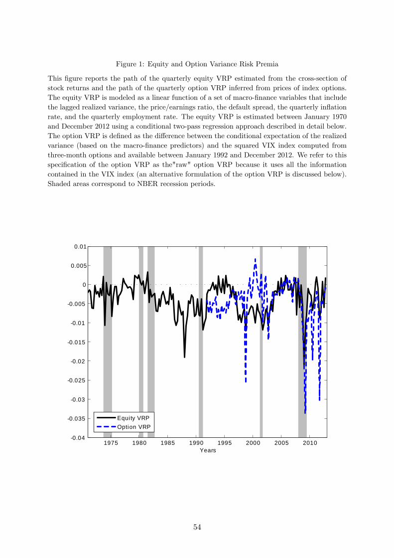
Figure 1: Equity and Option Variance Risk Premia

This figure reports the path of the quarterly equity VRP estimated from the cross-section ofstock returns and the path of the quarterly option VRP inferred from prices of index options.The equity VRP is modeled as a linear function of a set of macro-finance variables that includethe lagged realized variance, the price/earnings ratio, the default spread, the quarterly inflationrate, and the quarterly employment rate. The equity VRP is estimated between January 1970and December 2012 using a conditional two-pass regression approach described in detail below.The option VRP is defined as the difference between the conditional expectation of the realizedvariance (based on the macro-finance predictors) and the squared VIX index computed fromthree-month options and available between January 1992 and December 2012. We refer to thisspecification of the option VRP as the"raw" option VRP because it uses all the informationcontained in the VIX index (an alternative formulation of the option VRP is discussed below).Shaded areas correspond to NBER recession periods.

Years1975 1980 1985 1990 1995 2000 2005 2010

­0.04

­0.035

­0.03

­0.025

­0.02

­0.015

­0.01

­0.005

0

0.005

0.01

Equity VRPOption VRP

54

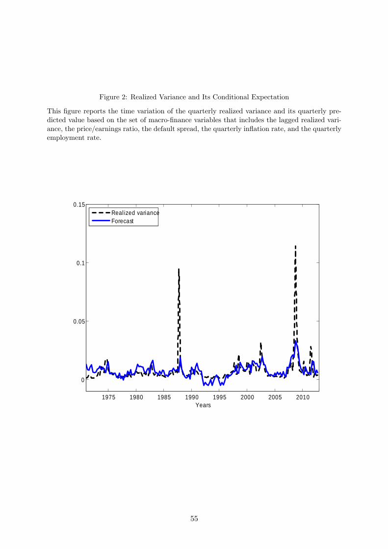
Figure 2: Realized Variance and Its Conditional Expectation

This figure reports the time variation of the quarterly realized variance and its quarterly pre-dicted value based on the set of macro-finance variables that includes the lagged realized vari-ance, the price/earnings ratio, the default spread, the quarterly inflation rate, and the quarterlyemployment rate.

1975 1980 1985 1990 1995 2000 2005 2010

0

0.05

0.1

0.15

Years

Real ized varianceForecast

55

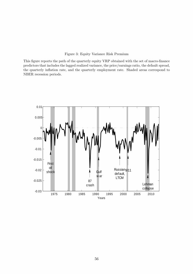
Figure 3: Equity Variance Risk Premium

This figure reports the path of the quarterly equity VRP obtained with the set of macro-financepredictors that includes the lagged realized variance, the price/earnings ratio, the default spread,the quarterly inflation rate, and the quarterly employment rate. Shaded areas correspond toNBER recession periods.

Years1975 1980 1985 1990 1995 2000 2005 2010

­0.03

­0.025

­0.02

­0.015

­0.01

­0.005

0

0.005

0.01

Firstoil

shock 9/11Russiandefault,LTCM

Gulfw ar

87crash Lehman

collapse

56

Figure 4: Equity Variance Risk Premium: Impact of the Broker-Dealer Variables

This figure compares the paths followed by two versions of quarterly equity VRP. The firstversion is based on the set of macro-finance variables that includes the lagged realized variance,the price/earnings ratio, the default spread, the quarterly inflation rate, and the quarterlyemployment rate. The second version is based on the macro-finance predictors and the twobroker-dealer variables, wich are the leverage ratio of broker-dealers and the quarterly returnof the prime broker index.

1975 1980 1985 1990 1995 2000 2005 2010­0.04

­0.035

­0.03

­0.025

­0.02

­0.015

­0.01

­0.005

0

0.005

0.01

Years

Macro­Finance PredictorsAll  Predictors

57

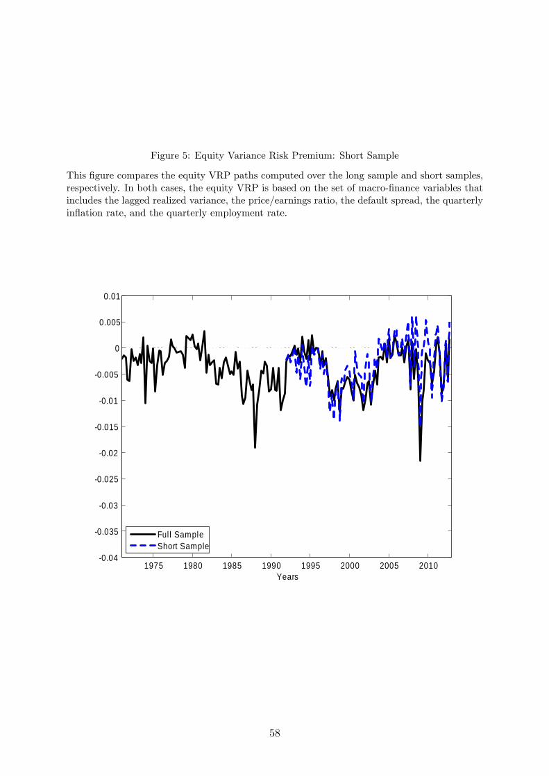
Figure 5: Equity Variance Risk Premium: Short Sample

This figure compares the equity VRP paths computed over the long sample and short samples,respectively. In both cases, the equity VRP is based on the set of macro-finance variables thatincludes the lagged realized variance, the price/earnings ratio, the default spread, the quarterlyinflation rate, and the quarterly employment rate.

1975 1980 1985 1990 1995 2000 2005 2010­0.04

­0.035

­0.03

­0.025

­0.02

­0.015

­0.01

­0.005

0

0.005

0.01

Years

Ful l  SampleShort Sample

58

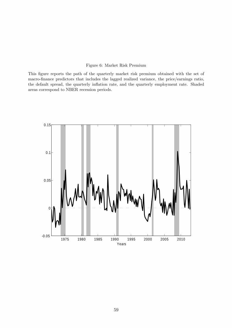
Figure 6: Market Risk Premium

This figure reports the path of the quarterly market risk premium obtained with the set ofmacro-finance predictors that includes the lagged realized variance, the price/earnings ratio,the default spread, the quarterly inflation rate, and the quarterly employment rate. Shadedareas correspond to NBER recession periods.

Years1975 1980 1985 1990 1995 2000 2005 2010

­0.05

0

0.05

0.1

0.15

59

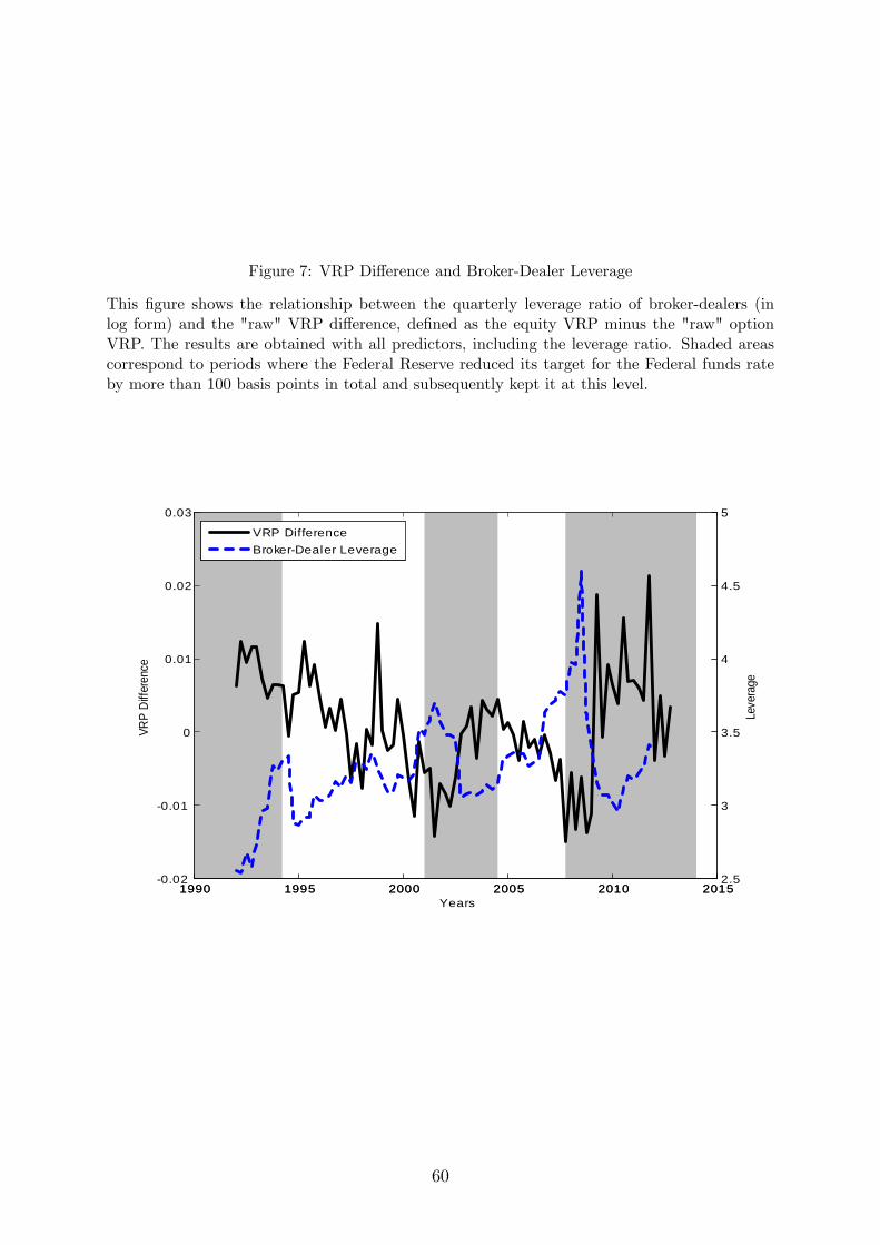
Figure 7: VRP Difference and Broker-Dealer Leverage

This figure shows the relationship between the quarterly leverage ratio of broker-dealers (inlog form) and the "raw" VRP difference, defined as the equity VRP minus the "raw" optionVRP. The results are obtained with all predictors, including the leverage ratio. Shaded areascorrespond to periods where the Federal Reserve reduced its target for the Federal funds rateby more than 100 basis points in total and subsequently kept it at this level.

VRP 

Diffe

renc

e

Years1990 1995 2000 2005 2010 2015

­0.02

­0.01

0

0.01

0.02

0.03

1990 1995 2000 2005 2010 20152.5

3

3.5

4

4.5

5

Leve

rage

VRP DifferenceBroker­Dealer Leverage

60

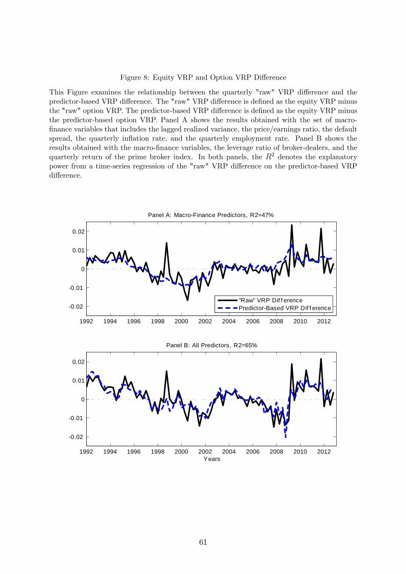
Figure 8: Equity VRP and Option VRP Difference

This Figure examines the relationship between the quarterly "raw" VRP difference and thepredictor-based VRP difference. The "raw" VRP difference is defined as the equity VRP minusthe "raw" option VRP. The predictor-based VRP difference is defined as the equity VRP minusthe predictor-based option VRP. Panel A shows the results obtained with the set of macro-finance variables that includes the lagged realized variance, the price/earnings ratio, the defaultspread, the quarterly inflation rate, and the quarterly employment rate. Panel B shows theresults obtained with the macro-finance variables, the leverage ratio of broker-dealers, and thequarterly return of the prime broker index. In both panels, the R2 denotes the explanatorypower from a time-series regression of the "raw" VRP difference on the predictor-based VRPdifference.

1992 1994 1996 1998 2000 2002 2004 2006 2008 2010 2012

­0.02

­0.01

0

0.01

0.02

Panel A: Macro­Finance Predictors, R2=47%

"Raw" VRP Dif f erencePredictor­Based VRP Dif f erence

1992 1994 1996 1998 2000 2002 2004 2006 2008 2010 2012

­0.02

­0.01

0

0.01

0.02

Panel B: All Predictors, R2=65%

Years

61