energies

Article

Wireless Sliding MPPT Control of PhotovoltaicSystems in Distributed Generation Systems

Aranzazu D. Martin * , Juan M. Cano, Reyes S. Herrera and Jesus R. Vazquez

Departamento de Ingeniería Eléctrica y Térmica, de Diseño y Proyectos, University of Huelva,21004 Huelva, Spain* Correspondence: aranzazu.delgado@die.uhu.es

Received: 26 July 2019; Accepted: 18 August 2019; Published: 21 August 2019

Abstract: The aim of a photovoltaic (PV) system’s control is the extraction of the maximum powereven if the irradiance, the temperature, or the parameters vary. To do that, a maximum powerpoint tracking (MPPT) algorithm is required. In this work, a sliding control is designed to regulatethe PV modules’ output voltage and make the panel work at the maximum power voltage. Thiscontrol is selected to improve the robustness, the transient dynamic response, and the time responseof the system under changeable environmental conditions, adjusting the duty cycle of the DC/DCconverter. The DC/DC converter connected to the PV module output is a buck-boost converter. Thisconfiguration presents the advantage of providing voltages lower or higher than supplied by thephotovoltaic modules to provide the required voltage to the load (including the voltages ceded bytelecommunication loads, amongst others). In addition, a remote sliding control is developed to makethe global supervision of the PV system in distributed generation grids. The designed algorithm istested in an experimental platform, both locally and remotely connected to the base station, to provethe effectiveness of the sliding control. Thus, the communication effect in the control is also analyzed.

Keywords: photovoltaic system; maximum power point tracking (MPPT); sliding mode control;wireless communication

1. Introduction

The main objective of a photovoltaic (PV) system’s control is power maximization. The voltagecorresponding to the maximum power point (maximum power point voltage, MPPV) of eachphotovoltaic module (or set of modules) depends on the weather conditions. Thus, maximumpower point tracking (MPPT) is needed. In plants located in places where there are fast changingenvironmental conditions, the tracking becomes critical [1], as well as in mobile plants, such as thoseassociated to electrical vehicles, boats, or airplanes.

MPPT is an algorithm usually implemented in a power converter connected to the modules,which matches their optimal operating point with the load operation, [2–6]. It must be considered thatload operation conditions can require lower or higher voltages than MPPV. In fact, telecommunicationsapplications are quite suitable to be supplied by PV plants because telecom apparatus powerconsumption is approximately constant. Their nominal voltages work from 36 to 75 V, [7]. The majorityof PV modules provide the output voltage within the range of 36 to 75 V. Thus, considering the availableDC/DC converter topologies, [8], a buck-boost converter would be suitable as the adaptation device, [8].In fact, this last configuration can supply voltages in the required range to the telecom equipment oreven lower or higher voltages if it is necessary. The analysis and design of the buck-boost converterscan be seen in [9,10].

Thus, the MPPT calculates the MPPV and the converter duty cycle (D) to make the modules workat the MPPV. Some algorithms in the technical literature achieves the objective with a control loop

Energies 2019, 12, 3226; doi:10.3390/en12173226 www.mdpi.com/journal/energies

Energies 2019, 12, 3226 2 of 16

as, for example, the perturb and observe (P&O) algorithm, the incremental conductance method, theripple correlation control, or MPP trackers based on artificial neuronal networks, or fuzzy logic, [11–15].These algorithms offer good performance. However, these solutions imply the use of linear controllersthat decrease the bandwidth of the system and commits the global stability. The time response is alsoaffected by that restriction when there are perturbations.

To overcome those problems, it must be considered that, actually, there are two control loopsincluded in the MPPT. The first one calculates the MPPV from the weather conditions and themodules’ characteristics. The second control loop calculates D to make the modules work at the MPPV.Additionally, the dynamic can be improved using specialized tracking algorithms to implement thesecond loop. These algorithms calculate the duty cycle of the DC/DC converter to make the modulesvoltage follow the MPPV previously calculated. Among these algorithms, the back-stepping, thesliding mode control (SMC), or others are considered, [16–19]. The use of one of these algorithmsensures an appropriate performance in the working range, operating in all the bandwidths of thesystem and guaranteeing global stability.

A comprehensive review and comparison of a variety of most-used MPPT methods is in [6,20,21],where the different control algorithms are classified regarding the complexity, true MPPT capability,number of sensors, and the variation of the parameters. The inherent nonlinearity of MPPT controllersmakes it difficult to appreciate if the dynamic performance of each MPPT control algorithm is optimizedor not. Indeed, the maximization of the convergence speed needs a commissioning phase to adjustthe control method to the specific application in experimental implementations. Anyway, a fastconvergence speed is always appreciable.

This paper focuses on the sliding mode control. This controller has been widely used for avariety of applications, such as robot manipulators, spacecrafts, underwater vehicles, electrical motors,etc., [22], and automotive applications such as anti-lock brake control, electronic throttle control,suspension control, and engine fault tolerant control, [23]. Besides, the use of the SMC in powersystems is also extended, [24–29]. References [16,24,25] propose an adaption stage for a DC/DCconverter regulated by a sliding mode control connected to an external MPPT algorithm, supplyingthe appropriate reference to the controller.

Reference [26] is focused on a new sliding mode control to enforce the adequate admittance to thePV array. This admittance is obtained tracking the reference given by an external admittance usinga MPPT algorithm. In addition, the oscillations are mitigated in the DC-link and the use of voltagecontrollers is not required. In this case, a boost converter is used to raise the PV array voltage to therequired value for the grid.

In the same line, [17] presents a fast and efficient MPPT algorithm for a PV system usingback-stepping and sliding mode controllers. In addition, [27] presents a convergence study of a SMCof the MPPT using ripple correlation control. In both cases, the DC/DC converter considered is also aboost converter like in [28,29].

All those references only take into account the boost converter, keeping out important photovoltaicapplications, such as those related to telecommunications, as explained above. To overcome thisproblem, in this paper the SMC is applied to a buck-boost converter integrated in a PV system supplyinga resistive load. The SMC makes the modules track the MPPV calculated by an algorithm whichpreviously obtains it. This algorithm applies a regression plane to obtain the reference voltage using amodified P&O, [30]. It avoids the local maximum points.

As an additional innovation, in this paper the control is implemented remotely and thecommunication effects are analyzed. In fact, a current tendency in the industry is the centralization ofthe control in remote control centers. The plants are monitored and the signals are sent to a serverwhere the set points are calculated and returned to the plant. This tendency facilitates the maintenancerevisions, among other advantages. In this sense, this paper makes a test of the proposed controlimplemented in a remote PC in communication with the local board connected to the converter in theoutside platform.

Energies 2019, 12, 3226 3 of 16

Therefore, this paper is organized according to the next sections: In Section 2, the photovoltaicsystem used to test the algorithms is presented with the results of its simulation in Matlab/Simulink. Inaddition, the complete experimental system, locally or remotely connected, is presented. In Section 3,the proposed sliding control is described in a theoretical way. In Section 4, a use case is presented withthe control implemented locally and in a remote way. Finally, in Section 5, some conclusions are drawn.

2. Photovoltaic System

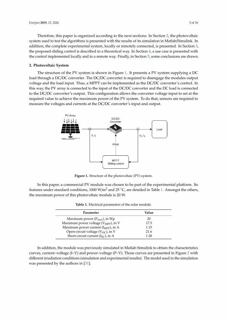
The structure of the PV system is shown in Figure 1. It presents a PV system supplying a DCload through a DC/DC converter. The DC/DC converter is required to disengage the modules outputvoltage and the load input. Thus, a MPPT can be implemented as the DC/DC converter’s control. Inthis way, the PV array is connected to the input of the DC/DC converter and the DC load is connectedto the DC/DC converter’s output. This configuration allows the converter voltage input to set at therequired value to achieve the maximum power of the PV system. To do that, sensors are required tomeasure the voltages and currents at the DC/DC converter’s input and output.

Energies 2019, 12, x 3 of 17

Therefore, this paper is organized according to the next sections: In Section 2, the photovoltaic system used to test the algorithms is presented with the results of its simulation in Matlab/Simulink. In addition, the complete experimental system, locally or remotely connected, is presented. In Section 3, the proposed sliding control is described in a theoretical way. In Section 4, a use case is presented with the control implemented locally and in a remote way. Finally, in Section 5, some conclusions are drawn.

2. Photovoltaic System

The structure of the PV system is shown in Figure 1. It presents a PV system supplying a DC load through a DC/DC converter. The DC/DC converter is required to disengage the modules output voltage and the load input. Thus, a MPPT can be implemented as the DC/DC converter’s control. In this way, the PV array is connected to the input of the DC/DC converter and the DC load is connected to the DC/DC converter’s output. This configuration allows the converter voltage input to set at the required value to achieve the maximum power of the PV system. To do that, sensors are required to measure the voltages and currents at the DC/DC converter’s input and output.

Figure 1. Structure of the photovoltaic (PV) system.

In this paper, a commercial PV module was chosen to be part of the experimental platform. Its features under standard conditions, 1000 W/m2 and 25 °C, are detailed in Table 1. Amongst the others, the maximum power of this photovoltaic module is 20 W.

Table 1. Electrical parameters of the solar module.

Parameter Value Maximum power (Pmax), in Wp 20

Maximum power voltage (VMPP), in V 17.5 Maximum power current (IMPP), in A 1.15

Open-circuit voltage (VOC), in V 21.6 Short-circuit current (ISC), in A 1.28

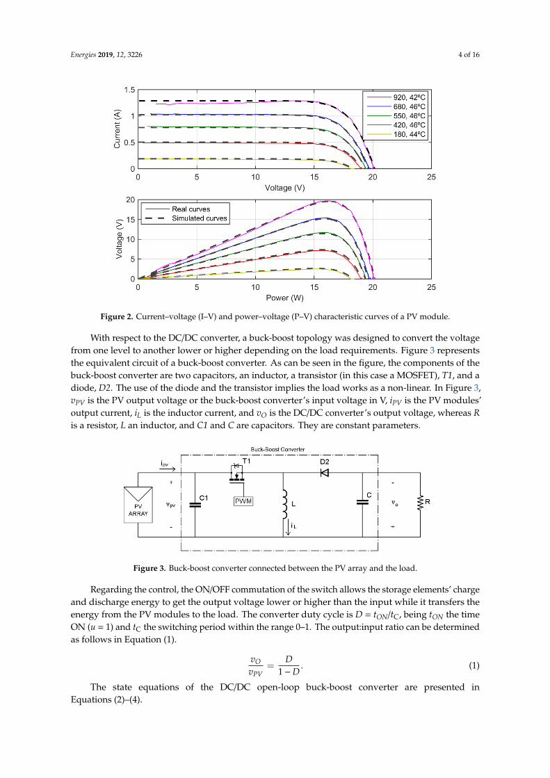
In addition, the module was previously simulated in Matlab-Simulink to obtain the characteristics curves, current – voltage (I-V) and power-voltage (P-V). Those curves are presented in Figure 2 with different irradiation conditions (simulation and experimental results). The model used in the simulation was presented by the authors in [31].

Figure 1. Structure of the photovoltaic (PV) system.

In this paper, a commercial PV module was chosen to be part of the experimental platform. Itsfeatures under standard conditions, 1000 W/m2 and 25 C, are detailed in Table 1. Amongst the others,the maximum power of this photovoltaic module is 20 W.

Table 1. Electrical parameters of the solar module.

Parameter Value

Maximum power (Pmax), in Wp 20Maximum power voltage (VMPP), in V 17.5Maximum power current (IMPP), in A 1.15

Open-circuit voltage (VOC), in V 21.6Short-circuit current (ISC), in A 1.28

In addition, the module was previously simulated in Matlab-Simulink to obtain the characteristicscurves, current–voltage (I–V) and power–voltage (P–V). Those curves are presented in Figure 2 withdifferent irradiation conditions (simulation and experimental results). The model used in the simulationwas presented by the authors in [31].

Energies 2019, 12, 3226 4 of 16Energies 2019, 12, x 4 of 17

Figure 2. current – voltage (I–V) and power-voltage (P–V) characteristic curves of a PV module.

With respect to the DC/DC converter, a buck-boost topology was designed to convert the voltage from one level to another lower or higher depending on the load requirements. Figure 3 represents the equivalent circuit of a buck-boost converter. As can be seen in the figure, the components of the buck-boost converter are two capacitors, an inductor, a transistor (in this case a MOSFET), T1, and a diode, D2. The use of the diode and the transistor implies the load works as a non-linear. In Figure 3, vPV is the PV output voltage or the buck-boost converter’s input voltage in V, iPV is the PV modules’ output current, iL is the inductor current, and vO is the DC/DC converter’s output voltage, whereas R is a resistor, L an inductor, and C1 and C are capacitors. They are constant parameters.

Figure 3. Buck-boost converter connected between the PV array and the load.

Regarding the control, the ON/OFF commutation of the switch allows the storage elements’ charge and discharge energy to get the output voltage lower or higher than the input while it transfers the energy from the PV modules to the load. The converter duty cycle is D = tON/tC, being tON the time ON (u = 1) and tC the switching period within the range 0–1. The output:input ratio can be determined as follows in Equation (1). 𝑣𝑣 = 𝐷1 − 𝐷. (1)

The state equations of the DC/DC open-loop buck-boost converter are presented in Equations (2)–(4).

Figure 2. Current–voltage (I–V) and power–voltage (P–V) characteristic curves of a PV module.

With respect to the DC/DC converter, a buck-boost topology was designed to convert the voltagefrom one level to another lower or higher depending on the load requirements. Figure 3 representsthe equivalent circuit of a buck-boost converter. As can be seen in the figure, the components of thebuck-boost converter are two capacitors, an inductor, a transistor (in this case a MOSFET), T1, and adiode, D2. The use of the diode and the transistor implies the load works as a non-linear. In Figure 3,vPV is the PV output voltage or the buck-boost converter’s input voltage in V, iPV is the PV modules’output current, iL is the inductor current, and vO is the DC/DC converter’s output voltage, whereas Ris a resistor, L an inductor, and C1 and C are capacitors. They are constant parameters.

Energies 2019, 12, x 4 of 17

Figure 2. current – voltage (I–V) and power-voltage (P–V) characteristic curves of a PV module.

With respect to the DC/DC converter, a buck-boost topology was designed to convert the voltage from one level to another lower or higher depending on the load requirements. Figure 3 represents the equivalent circuit of a buck-boost converter. As can be seen in the figure, the components of the buck-boost converter are two capacitors, an inductor, a transistor (in this case a MOSFET), T1, and a diode, D2. The use of the diode and the transistor implies the load works as a non-linear. In Figure 3, vPV is the PV output voltage or the buck-boost converter’s input voltage in V, iPV is the PV modules’ output current, iL is the inductor current, and vO is the DC/DC converter’s output voltage, whereas R is a resistor, L an inductor, and C1 and C are capacitors. They are constant parameters.

Figure 3. Buck-boost converter connected between the PV array and the load.

Regarding the control, the ON/OFF commutation of the switch allows the storage elements’ charge and discharge energy to get the output voltage lower or higher than the input while it transfers the energy from the PV modules to the load. The converter duty cycle is D = tON/tC, being tON the time ON (u = 1) and tC the switching period within the range 0–1. The output:input ratio can be determined as follows in Equation (1). 𝑣𝑣 = 𝐷1 − 𝐷. (1)

The state equations of the DC/DC open-loop buck-boost converter are presented in Equations (2)–(4).

Figure 3. Buck-boost converter connected between the PV array and the load.

Regarding the control, the ON/OFF commutation of the switch allows the storage elements’ chargeand discharge energy to get the output voltage lower or higher than the input while it transfers theenergy from the PV modules to the load. The converter duty cycle is D = tON/tC, being tON the timeON (u = 1) and tC the switching period within the range 0–1. The output:input ratio can be determinedas follows in Equation (1).

vOvPV

=D

1−D. (1)

The state equations of the DC/DC open-loop buck-boost converter are presented inEquations (2)–(4).

Energies 2019, 12, 3226 5 of 16

dvPV

dt=

iPV

C1−

iLC1

u. (2)

diLdt

= −vo

L+

uL(vPV + vo). (3)

dvo

dt=

( iLC−

vo

RC

)−

uiLC

. (4)

The target of our control was to adjust the duty cycle to achieve the optimal voltage and to ensurethe maximum energy extraction of the PV modules. A pulse width modulation (PWM) technique wasused to control the transistor commutation. The output voltage presents the polarity opposite theinput voltage. Figure 4 shows the voltages at the input and at the output of the buck-boost converterwith different D targets.

Energies 2019, 12, x 5 of 17

𝑑𝑣𝑑𝑡 = 𝑖𝐶 − 𝑖𝐶 𝑢. (2) = − + (𝑣 + 𝑣 ). (3) 𝑑𝑣𝑑𝑡 = 𝑖𝐶 − 𝑣𝑅𝐶 − 𝑢𝑖𝐶 . (4)

The target of our control was to adjust the duty cycle to achieve the optimal voltage and to ensure the maximum energy extraction of the PV modules. A pulse width modulation (PWM) technique was used to control the transistor commutation. The output voltage presents the polarity opposite the input voltage. Figure 4 shows the voltages at the input and at the output of the buck-boost converter with different D targets.

Figure 4. DC/DC converter’s input and output voltages for some D values.

The experimental platform contains three photovoltaic modules. The modules feed a built buck-boost converter (as the presented above) working with an input voltage of 10 V as minimum and 70 V as maximum. The maximum output voltage is 100 V. The maximum power that can be transferred is 70 W. The load is a 220 Ω resistor.

A personal computer (PC) is responsible for collecting the measurements and performing the control. LEM sensors are used to make the needed measurements. In this sense, the DC/DC converter includes three LA25NP current sensors to measure the input current, the output current, and the inductor current. Two LV25P voltage sensors measure the DC/DC converter’s input and output voltage. A 12-bit digital analog converter, with a microcontroller 30F4011, manages all the sensors. The data obtained from the experiments is saved in the PC by means of a supervisory control and data acquisition (SCADA) system, which allows the figures to be presented using Matlab. The SCADA was designed in Visual Basic to visualize the data in real time and to implement the sliding controller remotely from a base station. The platform is depicted in Figure 5. Measurements are obtained through an EM203 serial-to-Ethernet module.

Figure 4. DC/DC converter’s input and output voltages for some D values.

The experimental platform contains three photovoltaic modules. The modules feed a builtbuck-boost converter (as the presented above) working with an input voltage of 10 V as minimum and70 V as maximum. The maximum output voltage is 100 V. The maximum power that can be transferredis 70 W. The load is a 220 Ω resistor.

A personal computer (PC) is responsible for collecting the measurements and performing thecontrol. LEM sensors are used to make the needed measurements. In this sense, the DC/DC converterincludes three LA25NP current sensors to measure the input current, the output current, and theinductor current. Two LV25P voltage sensors measure the DC/DC converter’s input and outputvoltage. A 12-bit digital analog converter, with a microcontroller 30F4011, manages all the sensors.The data obtained from the experiments is saved in the PC by means of a supervisory control and dataacquisition (SCADA) system, which allows the figures to be presented using Matlab. The SCADAwas designed in Visual Basic to visualize the data in real time and to implement the sliding controllerremotely from a base station. The platform is depicted in Figure 5. Measurements are obtained throughan EM203 serial-to-Ethernet module.

As a different possibility, a router with a wireless interconnection is included into the platform, tosend the data via Wi-Fi. To do that, the base station running the application is required, with a Wi-Ficommunication system using the user datagram protocol (UDP). Figure 6 presents the scheme of theinterconnected system. The PC is connected to the router that allows the Wi-Fi communication and the

Energies 2019, 12, 3226 6 of 16

DC/DC converter is connected through the Ethernet interface RS232 to the router. The communicationbetween DC/DC converter–PC are by Wi-Fi with a latency of 5 ms, Figure 7.Energies 2019, 12, x 6 of 17

(a)

(b)

Figure 5. Experimental platform. (a) PV modules outside; (b) controller and base station.

As a different possibility, a router with a wireless interconnection is included into the platform, to send the data via Wi-Fi. To do that, the base station running the application is required, with a Wi-Fi communication system using the user datagram protocol (UDP). Figure 6 presents the scheme of the interconnected system. The PC is connected to the router that allows the Wi-Fi communication and the DC/DC converter is connected through the Ethernet interface RS232 to the router. The communication between DC/DC converter–PC are by Wi-Fi with a latency of 5 ms, Figure 7.

Figure 6. Scheme of the interconnected system.

Figure 5. Experimental platform. (a) PV modules outside; (b) controller and base station.

Energies 2019, 12, x 6 of 17

(a)

(b)

Figure 5. Experimental platform. (a) PV modules outside; (b) controller and base station.

As a different possibility, a router with a wireless interconnection is included into the platform, to send the data via Wi-Fi. To do that, the base station running the application is required, with a Wi-Fi communication system using the user datagram protocol (UDP). Figure 6 presents the scheme of the interconnected system. The PC is connected to the router that allows the Wi-Fi communication and the DC/DC converter is connected through the Ethernet interface RS232 to the router. The communication between DC/DC converter–PC are by Wi-Fi with a latency of 5 ms, Figure 7.

Figure 6. Scheme of the interconnected system. Figure 6. Scheme of the interconnected system.

Energies 2019, 12, x 7 of 17

Figure 7. Round-trip latency in the wireless network.

Figure 7 shows the round-trip latency in the wireless network. The round-trip latency statistical value is 5 ms with a typical deviation of 1 ms.

3. Sliding Control

Several algorithms have been used up to now by the authors to control the DC/DC converter as a MPPT. The results of the back-stepping algorithm are presented in [29,30]. In both cases, results show that the controllers ensure maximum power transfer with changing irradiation conditions.

To improve the controller dynamic behavior, this work presents a non-linear sliding control method which is a variable structure controller. The sliding control will be applied to the buck-boost converter of a photovoltaic system because it is a variable structure system with a discontinuous control action, which modifies its structure to reach a set of switching surfaces. In addition, the buck-boost converter has a non-minimum phase structure. Then, the voltage must be controlled through the current.

The sliding control allows the buck-boost converter to work in a wide operating range obtaining a high dynamical performance. It uses a high speed switching law to make the system go to a predetermined sliding surface (or switching function). The switching law also makes the system remains in the surface. The dynamic behavior is given by the designed parameters and equations that define the switching surface. Thus, the sliding control is robust under disturbances and parameter variations.

To apply the sliding control, the buck-boost equations are defined using the state averaging method and the parameter D when it works in continuous conduction mode (CCM). 𝑥 = 𝑖𝐶 − 𝑥𝐶 𝐷. (5) 𝑥 = − 𝑥𝐿 + (𝑥 + 𝑥 )𝐿 𝐷. (6) 𝑥 = 𝑥𝐶 − 𝑥𝑅𝐶 − 𝑥𝐶 𝐷. (7) 𝑥 = 𝑥 (8)

Then, the system equation is presented in (9). 𝑥 = 𝐴𝑥 + 𝛿 + 𝐷(𝐵𝑥 + 𝛾), (9)

Figure 7. Round-trip latency in the wireless network.

Energies 2019, 12, 3226 7 of 16

Figure 7 shows the round-trip latency in the wireless network. The round-trip latency statisticalvalue is 5 ms with a typical deviation of 1 ms.

3. Sliding Control

Several algorithms have been used up to now by the authors to control the DC/DC converter as aMPPT. The results of the back-stepping algorithm are presented in [29,30]. In both cases, results showthat the controllers ensure maximum power transfer with changing irradiation conditions.

To improve the controller dynamic behavior, this work presents a non-linear sliding controlmethod which is a variable structure controller. The sliding control will be applied to the buck-boostconverter of a photovoltaic system because it is a variable structure system with a discontinuouscontrol action, which modifies its structure to reach a set of switching surfaces. In addition, thebuck-boost converter has a non-minimum phase structure. Then, the voltage must be controlledthrough the current.

The sliding control allows the buck-boost converter to work in a wide operating range obtaininga high dynamical performance. It uses a high speed switching law to make the system go to apredetermined sliding surface (or switching function). The switching law also makes the system remainsin the surface. The dynamic behavior is given by the designed parameters and equations that definethe switching surface. Thus, the sliding control is robust under disturbances and parameter variations.

To apply the sliding control, the buck-boost equations are defined using the state averagingmethod and the parameter D when it works in continuous conduction mode (CCM).

.x1 =

iPV

C1−

x2

C1D. (5)

.x2 = −

x3

L+

(x1 + x3)

LD. (6)

.x3 =

x2

C−

x3

RC−

x2

CD. (7)

.x4 = x4 (8)

Then, the system equation is presented in (9).

.x = Ax + δ+ D(Bx + γ), (9)

where x = [x1, x2, x3, x4]T with x1 = vPV; x2 = iL; x3 = vo; x4 =

∫ (vPV − vr

PV

)dt, vr

PV being the referencevoltage to be reached.

These equations are rewritten in a matrix form as shown in Equation (10).

.x = Ax + δ+ D(Bx + γ). (10)

The matrices are shown in Equations (11)–(14).

A =

0 0 0 00 0 −

1L 0

0 1C −

1RC 0

0 0 0 1

. (11)

δ =

ipvC1

000

. (12)

Energies 2019, 12, 3226 8 of 16

B =

0 −

1C1

0 01L 0 1

L 00 −

1C 0 0

0 0 0 0

. (13)

γ =

0000

. (14)

A sliding surface with the dynamic suitable to this application is proposed in (15). Thus,the trajectories around the surface should converge to it and, then, the trajectories must stay on the slidingsurface. In addition, the switching function ensures regulation of the buck-boost converter voltage.

S(x) = k1(x1 − vPVr) + x2 + k2x4, (15)

where k1 and k2 are the sliding design parameters. The sliding surface exists if S(x) = dS/dt = 0.Now, a control law to reach the sliding surface and stay thereafter must be found. It must also

guarantee the existence of the sliding mode. The control input has two components called correctivecontrol, Dc, and equivalent control, Deq. Then, the control signal is presented in Equation (16).

D = Dc + Deq. (16)

The corrective control compensates the deviations from the sliding surface to reach the mentionedsurface as shown in (17). It is a typical choice for this controller.

Dc = −kcsgn(S), (17)

where kc is chosen to be positive. The sign of the sliding surface is defined as shown in Equation (18).

sgn(S) =

+1, S(x) > 0−1, S(x) < 0

. (18)

The equivalent control makes null the time derivative of the sliding surface to remain on thesliding surface. The equation that defines this control is presented in (19).

Deq = −

[∂S∂x

B(x)]−1(

∂S∂x

(Ax + δ)

). (19)

Using Equations (9) and (15)–(17), the equivalent control can be expressed as shown inEquation (20).

Deq =−k1LiPV + C1x3 − k2C1Lx4

−k1Lx2 + C1(x1 + x3). (20)

It must fulfill Equations (21)–(23).

∂S∂x

Bx = −k1x2

C1+

x1 + x3

L, 0. (21)

−

(∂S∂x

Bx)−1

=−C1L

−k1Lx2 + C1(x1 + x3). (22)

Energies 2019, 12, 3226 9 of 16

∂S∂x

(Ax + δ) = (k1, 1, 0, k2)

iPVC1

−x3L

x2C −

x3RC

x4

=Lk1iPV −C1x3 + C1Lk2x4

C1L. (23)

The buck-boost converter is working in CCM. Thus, the inductor current is always positive, x2.Nevertheless, the output voltage is always negative, x3. It is guaranteed if k1 and k2 are positive.

S = 0 is globally asymptotically stable. Thus, using Equations (16), (17), and (19), the control lawis achieved. Its expression is presented in Equation (24).

D =−k1LiPV + C1x3 − k2C1Lx4

−k1Lx2 + C1(x1 + x3)− kcsgn(S). (24)

Now, a Lyapunov function, (25), is used to make the sliding mode control force the system to goto the sliding surface and remain on it.

V =12

S2. (25)

To guarantee the stability of the system, the control D has to be selected to make the time derivativeof the Lyapunov function negative. Thus, the switching function will be attractive. Thus, the timederivative of the Lyapunov function is presented in Equation (26).

.V = S

.S < 0,

.V = S

(∂S∂x (Ax + δ) + ∂S

∂x B(x)D).

(26)

Now, the time derivative of the sliding surface must be calculated, using Equation (27).

.S(x) = k1

( .x1 −

.vr

PV

)+

.x2 + k2

.x4. (27)

The time derivative of the Lyapunov function yields Equation (28).

.V(x) = S

.S = S

[k1

( .x1 −

.vr

PV

)+

.x2 + k2

.x4

]. (28)

The term between square brackets is worked out, obtaining the expression shown in (29).

− k1.vr

PV −(x1 + x3)C1 − x2Lk1

C1Lkc|S|S

. (29)

The first term is considered to be zero. Then the time derivative of the Lyapunov function ispresented in Equation (30).

.V = S

(−

x1C1+x3C1−x2Lk1C1L kc

|S|S

)<

< − x1C1+x3C1−x2Lk1C1L kc|S| < 0.

(30)

The last term is negative. Then:

(x1C1 + x3C1 − x2Lk1)kc < 0. (31)

k1 <(x1 + x3)C1

−x2L. (32)

These two equations close the sliding control.

Energies 2019, 12, 3226 10 of 16

4. Practical Cases

Experimental tests were carried out to validate the previous theoretical analysis of the slidingcontroller under different conditions. The experimental results were obtained with different scopes,both working in the experimental platform described in Section 2. In the first test, the physical systemwas wire connected to the PC and the second test was carried out with Wi-Fi communications, using asynthetic local wireless network.

4.1. Experimental Results with the Controller Connected to the PC by a Wire

The sliding control developed in this paper was implemented in a dsPIC30F4011 low-costmicrocontroller, being supervised via a local internet connection. The sliding control has to regulatethe DC/DC converter’s input voltage to reach the MPP through the MOSFET switching controlling theduty cycle. The PWM frequency is 20 kHz whereas the sampling time of the control is 5 ms.

Experiments under different conditions were conducted to verify the sliding control performance.In this sense, there are different step signals that represent changes in the incident irradiance overthe PV modules. Step signals were used to test the control, although the real irradiation changes aresmooth due to the progressive appearance of the clouds. Thus, we tested the control in even worseconditions to verify the robustness. The system was tested with different irradiances, 670 W/m2 until33 s, 490 W/m2 until 68 s, and 690 W/m2 until 95 s, to finish with an irradiance of 330 W/m2.

Figure 8 depicts the voltage and current transient response when there are step irradiance changes.Figure 8a shows the reference voltage to be achieved by the control at the PV modules’ output orDC/DC converter’s input, even when there are changes in the irradiance. The buck-boost converter’smeasured input voltage is shown in the figure, reaching the reference voltage values in all the cases.The DC/DC converter’s output voltage is also presented in this figure. As expected, the converter’sinput voltage changes with the irradiance; both increase and decrease together.Energies 2019, 12, x 11 of 17

(a)

(b)

Figure 8. Transient response with variable irradiance with wire connection. (a) Converter’s input and output voltage and reference voltage; (b) Inductor’s current and converter’s input and output currents.

The inductor’s current and the converter’s input and output currents are depicted in Figure 8b. These currents also change when the irradiance changes. As in the previous figure, the currents are higher when the irradiance achieves higher values and decrease when the irradiance is lower.

Figure 9 presents the output and input power of the DC/DC converter with the same changes in the irradiance as the voltages and current. This figure also defines the converter efficiency. The buck-boost converter efficiency ranges from 95% to 98.1% in this case. The voltages and the currents and; therefore, the power are robust, obtaining the expected values even when the irradiance changes suddenly, proving the robustness of the sliding control under external perturbation signals.

Figure 9. DC/DC converter’s input and output power under variable irradiance with wire connection.

Results presented in Figures 8 and 9 are also shown in Table 2. In the simulation system, for the irradiance of 670 W/m2, the maximum power is 45.1 W and the power obtained experimentally is 45 W; for 490 W/m2, the maximum power is 30.1 W and the power obtained experimentally is 30.1 W; for 690 W/m2, the maximum power is 46.3 W and the power obtained experimentally is 46.1 W; for 330 W/m2, the values are 16.2 and 16.1 W, respectively. Thus, the MPPT efficiency ranges from 99.5% to 100%.

Table 2. Voltage and power values obtained at the converter’s input and output under different irradiances with wire connection, time (s), G (W/m2), vPVr is the reference voltage (V), vPV is the

Figure 8. Transient response with variable irradiance with wire connection. (a) Converter’s input andoutput voltage and reference voltage; (b) Inductor’s current and converter’s input and output currents.

The inductor’s current and the converter’s input and output currents are depicted in Figure 8b.These currents also change when the irradiance changes. As in the previous figure, the currents arehigher when the irradiance achieves higher values and decrease when the irradiance is lower.

Figure 9 presents the output and input power of the DC/DC converter with the same changesin the irradiance as the voltages and current. This figure also defines the converter efficiency. Thebuck-boost converter efficiency ranges from 95% to 98.1% in this case. The voltages and the currentsand; therefore, the power are robust, obtaining the expected values even when the irradiance changessuddenly, proving the robustness of the sliding control under external perturbation signals.

Energies 2019, 12, 3226 11 of 16

Energies 2019, 12, x 11 of 17

(a)

(b)

Figure 8. Transient response with variable irradiance with wire connection. (a) Converter’s input and output voltage and reference voltage; (b) Inductor’s current and converter’s input and output currents.

The inductor’s current and the converter’s input and output currents are depicted in Figure 8b. These currents also change when the irradiance changes. As in the previous figure, the currents are higher when the irradiance achieves higher values and decrease when the irradiance is lower.

Figure 9 presents the output and input power of the DC/DC converter with the same changes in the irradiance as the voltages and current. This figure also defines the converter efficiency. The buck-boost converter efficiency ranges from 95% to 98.1% in this case. The voltages and the currents and; therefore, the power are robust, obtaining the expected values even when the irradiance changes suddenly, proving the robustness of the sliding control under external perturbation signals.

Figure 9. DC/DC converter’s input and output power under variable irradiance with wire connection.

Results presented in Figures 8 and 9 are also shown in Table 2. In the simulation system, for the irradiance of 670 W/m2, the maximum power is 45.1 W and the power obtained experimentally is 45 W; for 490 W/m2, the maximum power is 30.1 W and the power obtained experimentally is 30.1 W; for 690 W/m2, the maximum power is 46.3 W and the power obtained experimentally is 46.1 W; for 330 W/m2, the values are 16.2 and 16.1 W, respectively. Thus, the MPPT efficiency ranges from 99.5% to 100%.

Table 2. Voltage and power values obtained at the converter’s input and output under different irradiances with wire connection, time (s), G (W/m2), vPVr is the reference voltage (V), vPV is the

Figure 9. DC/DC converter’s input and output power under variable irradiance with wire connection.

Results presented in Figures 8 and 9 are also shown in Table 2. In the simulation system, for theirradiance of 670 W/m2, the maximum power is 45.1 W and the power obtained experimentally is 45 W;for 490 W/m2, the maximum power is 30.1 W and the power obtained experimentally is 30.1 W; for690 W/m2, the maximum power is 46.3 W and the power obtained experimentally is 46.1 W; for 330 W/m2,the values are 16.2 and 16.1 W, respectively. Thus, the MPPT efficiency ranges from 99.5% to 100%.

Table 2. Voltage and power values obtained at the converter’s input and output under differentirradiances with wire connection, time (s), G (W/m2), vPVr is the reference voltage (V), vPV is themeasured voltage at the DC/DC converter input (V), vo is the DC/DC converter output voltage (V),Pref is the reference power (W), Pin is the DC/DC converter input power (W) and Pout is the DC/DCconverter output power (W).

Time G vPVr vPV vo Pref Pin Pout

[0, 33) 670 15.8 15.8 59.5 45.1 45 42.9[33, 68) 490 14.8 14.9 56.5 30.1 30.1 28.6[68, 95) 690 15.9 15.9 58.8 46.3 46.1 43.9[95, 110] 330 14.1 14.2 51.3 16.2 16.1 15.8

Figure 10 presents the control signal obtained using the sliding method. This figure shows thecommuted control actions or the discontinuous actions needed to make the system remain in the slidingsurface. It shows that the control signal changes its value when there is a change in the irradiance. Italso presents the effect of the control non-linearities (the control is discontinuous).

Energies 2019, 12, x 12 of 17

measured voltage at the DC/DC converter input (V), vo is the DC/DC converter output voltage (V), Pref

is the reference power (W), Pin is the DC/DC converter input power (W) and Pout is the DC/DC converter output power (W).

Time G vPVr vPV vo Pref Pin Pout

[0, 33) 670 15.8 15.8 59.5 45.1 45 42.9 [33, 68) 490 14.8 14.9 56.5 30.1 30.1 28.6 [68, 95) 690 15.9 15.9 58.8 46.3 46.1 43.9 [95, 110] 330 14.1 14.2 51.3 16.2 16.1 15.8

Figure 10 presents the control signal obtained using the sliding method. This figure shows the commuted control actions or the discontinuous actions needed to make the system remain in the sliding surface. It shows that the control signal changes its value when there is a change in the irradiance. It also presents the effect of the control non-linearities (the control is discontinuous).

Figure 10. Control signal evolution with variable irradiance.

Figure 10. Control signal evolution with variable irradiance.

Energies 2019, 12, 3226 12 of 16

4.2. Experimental Results with the Controller Connected to the PC by Wireless Communication

To do this new test, the experimental platform used was the same as before. The only differenceis that, now, the control is applied in a 2 GHz·PC with 4 GB·RAM. It is connected to the dsPIC viacommunication (IEEE802.11) through the UDP protocol at a nominal rate of 5 ms. This communicationprotocol is used because it is faster at sending data packets. The SCADA was also designed to implementthe sliding controller remotely from the base station. The application receives the packet with thesensors’ data from the dsPIC and the controller uses those data to calculate the control signal, which ispackaged and sent to the microcontroller to update the PWM that controls the buck-boost converter.

In these new conditions of wireless connection, the sliding control robustness is tested again, usingthe same set of experiments as in the previous case, with the same sudden changes in the irradiance.The irradiance is 200 W/m2 until 1 s, 360 W/m2 until 9 s, 470 W/m2 until 18 s, 760 W/m2 until 24 s,480 W/m2 until 33 s, 780 W/m2 until 36 s, 480 W/m2 until 42 s, and 780 W/m2 again until 45 s.

Figure 11 presents, as in the previous case, the transient response of the voltages, currents, andpowers under sudden changes in the irradiance. Figure 11a presents the reference voltage that has tobe reached, the DC/DC converter’s input voltage that follows the reference voltage, and the buck-boostconverter’s output voltage. Figure 11b depicts the inductor’s current and the DC/DC converter’s inputand output currents.

Energies 2019, 12, x 13 of 17

4.2. Experimental Results with the Controller Connected to the PC by a Wire

To do this new test, the experimental platform used was the same as before. The only difference is that, now, the control is applied in a 2 GHz·PC with 4 GB·RAM. It is connected to the dsPIC via communication (IEEE802.11) through the UDP protocol at a nominal rate of 5 ms. This communication protocol is used because it is faster at sending data packets. The SCADA was also designed to implement the sliding controller remotely from the base station. The application receives the packet with the sensors’ data from the dsPIC and the controller uses those data to calculate the control signal, which is packaged and sent to the microcontroller to update the PWM that controls the buck-boost converter.

In these new conditions of wireless connection, the sliding control robustness is tested again, using the same set of experiments as in the previous case, with the same sudden changes in the irradiance. The irradiance is 200 W/m2 until 1 s, 360 W/m2 until 9 s, 470 W/m2 until 18 s, 760 W/m2 until 24 s, 480 W/m2 until 33 s, 780 W/m2 until 36 s, 480 W/m2 until 42 s, and 780 W/m2 again until 45 s.

Figure 11 presents, as in the previous case, the transient response of the voltages, currents, and powers under sudden changes in the irradiance. Figure 11a presents the reference voltage that has to be reached, the DC/DC converter’s input voltage that follows the reference voltage, and the buck-boost converter’s output voltage. Figure 11b depicts the inductor’s current and the DC/DC converter’s input and output currents.

(a)

(b)

Figure 11. Transient response with variable irradiance with wireless connection. (a) Converter’s input and output voltage and reference voltage; (b) Inductor’s current and converter input and output currents.

Then, Figure 12 shows the power at the input and output buck-boost converter, defining the converter efficiency. In this case, the efficiency of the DC/DC converter ranges from 93.2% to 94%. As in the previous case, the voltage, current, and power values increase when the irradiance increase, whereas the values decreases when the irradiance goes down. Table 3 summarizes those results.

Figure 11. Transient response with variable irradiance with wireless connection. (a) Converter’s input andoutput voltage and reference voltage; (b) Inductor’s current and converter input and output currents.

Then, Figure 12 shows the power at the input and output buck-boost converter, defining theconverter efficiency. In this case, the efficiency of the DC/DC converter ranges from 93.2% to 94%.As in the previous case, the voltage, current, and power values increase when the irradiance increase,whereas the values decreases when the irradiance goes down. Table 3 summarizes those results.

Energies 2019, 12, x 14 of 17

Figure 12. DC/DC converter’s input and output power under variable irradiance with wireless connection.

Table 3. Voltage and power values obtained at the converter’s input and output under different irradiances, time (s), G (W/m2), and V (V) with Wi-Fi.

Time G vPVr vPV vo Pref Pin Pout

[0, 1) 200 11.90 11.90 40.7 9.8 9.7 9.1

[1, 9) 360 14.02 14.02 51.6 17 16.9 15.9

[9, 18) 470 15.01 15.01 56.1 29.2 28.9 27.1

[18, 24) 760 16.1 16.1 59.4 48 47.9 44.8

[24, 33) 480 15.1 15.1 56.2 29.8 29.6 27.6

[33, 36) 780 16.2 16.2 59.2 49 48.8 45.7

[36, 42) 480 15.1 15.1 56.2 29.8 29.7 27.7

[42, 45] 780 16.2 16.2 59.2 49 48.9 45.9

As expected, the wireless communication makes the signals in Figure 12 have more noise than that obtained in the previous case (Figure 9) due to the wireless communication effect. Indeed, this type of communication implies a variable delay in the signal processing and data transmission. The data are packaged with the sensors information to be sent from the DC/DC converter to the base station, and the packaged data with the control signal information are sent from the base station to the buck-boost converter. However, in spite of the higher delay, the control remains stable and the variables converge to the set points. Thus, the sliding control robustness is verified.

The delay in the data processing and the data transmission packets with the packaged data from the microcontroller to the base station, and vice versa, are depicted in Figure 13. These measurements were taken when the experiment was conducted. The values were obtained independently from the PC and from the dsPIC, showing a mean value of time of 5.4 ms.

Figure 12. DC/DC converter’s input and output power under variable irradiance with wireless connection.

Energies 2019, 12, 3226 13 of 16

Table 3. Voltage and power values obtained at the converter’s input and output under differentirradiances, time (s), G (W/m2), and V (V) with Wi-Fi.

Time G vPVr vPV vo Pref Pin Pout

[0, 1) 200 11.90 11.90 40.7 9.8 9.7 9.1[1, 9) 360 14.02 14.02 51.6 17 16.9 15.9[9, 18) 470 15.01 15.01 56.1 29.2 28.9 27.1

[18, 24) 760 16.1 16.1 59.4 48 47.9 44.8[24, 33) 480 15.1 15.1 56.2 29.8 29.6 27.6[33, 36) 780 16.2 16.2 59.2 49 48.8 45.7[36, 42) 480 15.1 15.1 56.2 29.8 29.7 27.7[42, 45] 780 16.2 16.2 59.2 49 48.9 45.9

As expected, the wireless communication makes the signals in Figure 12 have more noise than thatobtained in the previous case (Figure 9) due to the wireless communication effect. Indeed, this type ofcommunication implies a variable delay in the signal processing and data transmission. The data arepackaged with the sensors information to be sent from the DC/DC converter to the base station, andthe packaged data with the control signal information are sent from the base station to the buck-boostconverter. However, in spite of the higher delay, the control remains stable and the variables convergeto the set points. Thus, the sliding control robustness is verified.

The delay in the data processing and the data transmission packets with the packaged data fromthe microcontroller to the base station, and vice versa, are depicted in Figure 13. These measurementswere taken when the experiment was conducted. The values were obtained independently from thePC and from the dsPIC, showing a mean value of time of 5.4 ms.

Energies 2019, 12, x 15 of 17

Figure 13. Delay of the variables time response and number of lost packages.

Figure 14 presents the control signal. As in Figures 11 and 12, it is shown that the control changes when the irradiance changes as well, in order to make the system remain in the sliding surface. It also depicts the effect of the discontinuous control non-linearities, but in this case with more noise.

Figure 14. Control signal evolution with a variable irradiance through wireless communication.

In all the figures presented in this subsection, in the wireless network case, the signals present more oscillations and the efficiency of the DC/DC converter is lower (from 98.1% to 94% as maximum efficiency) than that corresponding to the previous case with wire connection. In fact, control algorithms present a delay due to the time necessary to process the signals and make the suitable operations. The delay grows in wireless connection because of the time necessary to transmit the data. The delay is also affected by the distance between the buck-boost converter and the base station and by the interferences created by other systems that use the same frequency. As the delay increased, the system efficiency decreased. Moreover, the variability of the transmission time provokes a higher noise in all the electrical signals in the case of wireless connection. Even so, the controller reaches the desired values and; therefore, it can be used in centralized systems.

5. Conclusions

In this paper, the sliding mode control was applied to make a set of photovoltaic modules track the maximum power point voltage. The use of this control improved the dynamics of the system and

Figure 13. Delay of the variables time response and number of lost packages.

Figure 14 presents the control signal. As in Figures 11 and 12, it is shown that the control changeswhen the irradiance changes as well, in order to make the system remain in the sliding surface. It alsodepicts the effect of the discontinuous control non-linearities, but in this case with more noise.

Energies 2019, 12, 3226 14 of 16

Energies 2019, 12, x 15 of 17

Figure 13. Delay of the variables time response and number of lost packages.

Figure 14 presents the control signal. As in Figures 11 and 12, it is shown that the control changes when the irradiance changes as well, in order to make the system remain in the sliding surface. It also depicts the effect of the discontinuous control non-linearities, but in this case with more noise.

Figure 14. Control signal evolution with a variable irradiance through wireless communication.

In all the figures presented in this subsection, in the wireless network case, the signals present more oscillations and the efficiency of the DC/DC converter is lower (from 98.1% to 94% as maximum efficiency) than that corresponding to the previous case with wire connection. In fact, control algorithms present a delay due to the time necessary to process the signals and make the suitable operations. The delay grows in wireless connection because of the time necessary to transmit the data. The delay is also affected by the distance between the buck-boost converter and the base station and by the interferences created by other systems that use the same frequency. As the delay increased, the system efficiency decreased. Moreover, the variability of the transmission time provokes a higher noise in all the electrical signals in the case of wireless connection. Even so, the controller reaches the desired values and; therefore, it can be used in centralized systems.

5. Conclusions

In this paper, the sliding mode control was applied to make a set of photovoltaic modules track the maximum power point voltage. The use of this control improved the dynamics of the system and

Figure 14. Control signal evolution with a variable irradiance through wireless communication.

In all the figures presented in this subsection, in the wireless network case, the signals presentmore oscillations and the efficiency of the DC/DC converter is lower (from 98.1% to 94% as maximumefficiency) than that corresponding to the previous case with wire connection. In fact, control algorithmspresent a delay due to the time necessary to process the signals and make the suitable operations.The delay grows in wireless connection because of the time necessary to transmit the data. The delayis also affected by the distance between the buck-boost converter and the base station and by theinterferences created by other systems that use the same frequency. As the delay increased, the systemefficiency decreased. Moreover, the variability of the transmission time provokes a higher noise inall the electrical signals in the case of wireless connection. Even so, the controller reaches the desiredvalues and; therefore, it can be used in centralized systems.

5. Conclusions

In this paper, the sliding mode control was applied to make a set of photovoltaic modules trackthe maximum power point voltage. The use of this control improved the dynamics of the system andits response to perturbations in the load or in the irradiance. The control algorithm was implementedin a buck-boost converter, which is able to supply a voltage lower and higher than the input voltage,as required by telecommunications applications, amongst others. To achieve it, a boost converter isnot suitable. In addition, the algorithm was experimentally tested in a platform with the controllerremotely connected to the photovoltaic systems and the effect of the distance was evaluated. Thesystem proved to be efficient with both wire and wireless communication, and in both cases thedynamic performance was improved. The communications effect provides a higher level of noisealthough the dynamics remain good. In addition, the buck-boost converter’s efficiency decreases from98.1% to 94% in the case of remote control, but the control remains stable and the voltage reference isreached with an efficiency between 99% to 99.8%, proving the wireless control works in centralizedphotovoltaic plants and in distributed generation systems.

Author Contributions: Conceptualization, A.D.M. and J.M.C.; formal analysis, A.D.M. and J.M.C.; investigation,A.D.M., J.M.C., R.S.H. and J.R.V.; methodology, A.D.M. and J.M.C.; project administration, R.S.H. and J.R.V.;resources, R.S.H. and J.R.V.; validation, A.D.M. and J.M.C.; writing—original draft, A.D.M.; writing—review andediting, A.D.M., J.M.C., R.S.H. and J.R.V.

Funding: This research received no external funding.

Conflicts of Interest: The authors declare no conflict of interest.

Energies 2019, 12, 3226 15 of 16

References

1. Çelik, Ö.; Teke, A. A Hybrid MPPT method for grid connected photovoltaic systems under rapidly changingatmospheric conditions. Electr. Power Syst. Res. 2017, 152, 194–210. [CrossRef]

2. Femia, N.; Petrone, G.; Spagnuolo, G.; Vitelli, M. Optimization of perturb and observe maximum powerpoint tracking method. IEEE Trans. Power Electron. 2005, 20, 963–973. [CrossRef]

3. Sera, D.; Mathe, l.; Kerekes, T.; Spataru, S.V.; Teodorescu, R. On the Perturb-and-Observe and IncrementalConductance MPPT Methods for PV Systems. IEEE J. Photovolt. 2013, 3, 1070–1078. [CrossRef]

4. Fernandes, D.; Almeida, R.; Guedes, T.; Filho, A.J.S.; Costa, F.F. State feedback control for DC-photovoltaicsystems. Electr. Power Syst. Res. 2017, 143, 794–801. [CrossRef]

5. Masoum, M.A.S.; Dehbonei, H.; Fuchs, E.F. Theoretical and experimental analyses of photovoltaic systemswith voltage and current-based maximum power-point tracking. IEEE Trans. Energy Convers. 2002, 17,514–522. [CrossRef]

6. Islam, H.; Mekhilef, S.; Shah, N.B.M.; Soon, T.K.; Seyedmahmousian, M.; Horan, B.; Stojcevski, A. PerformanceEvaluation of Maximum Power Point Tracking Approaches and Photovoltaic Systems. Energies 2018, 11, 365.[CrossRef]

7. Ren, X.; Tang, Z.; Ruan, X.; Wei, J.; Hua, G. Four Switch Buck-Boost Converter for Telecom DC-DC powersupply applications. In Proceedings of the Twenty-Third Annual IEEE Applied Power Electronics Conferenceand Exposition, Austin, TX, USA, 24–28 February 2008; pp. 1527–1530.

8. Power Electronics Handbook; Elsevier: Amsterdam, The Netherlands, 2018.9. Pradeep, A.; Yadav, K.; Thirumalia, S.; Haritha, G. Comparison of MPPT Algorithms for DC-DC Converters

Based PV Systems. Int. J. Adv. Res. Electr. Electron. Instrum. Eng. 2012, 1, 18–23.10. Babaei, E.; Mahmoodieh, M.E.S.; Mahery, H.M. Operational Modes and Output-Voltage-Ripple Analysis

and Design Considerations of Buck-Boost DC-DC Converters. IEEE Trans. Ind. Electron. 2012, 59, 381–391.[CrossRef]

11. Tan, B.; Ke, X.; Tang, D.; Yin, S. Improved Perturb and Observation Method Based on Support VectorRegression. Energies 2019, 12, 1151. [CrossRef]

12. Tey, K.S.; Mekhilef, S. Modified incremental conductance MPPT algorithm to mitigate inaccurate responsesunder fast-changing solar irradiation level. Sol. Energy 2014, 101, 333–342. [CrossRef]

13. Esram, T.; Kimball, J.W.; Krein, P.T.; Chapman, P.L.; Midya, P. Dynamic maximum power point trackingof photovoltaic arrays using ripple correlation control. IEEE Trans. Power Electron. 2006, 21, 1282–1291.[CrossRef]

14. Elobaid, L.M.; Abdelsalam, A.K.; Zakzouk, E.E. Artificial neural network-based photovoltaic maximumpower point tracking techniques: A survey. IET Renew. Power Gener. 2015, 9, 1043–1063. [CrossRef]

15. Guenounou, O.; Dahhou, B.; Chabour, F. Adaptive fuzzy controller based MPPT for photovoltaic systems.Energy Convers. Manag. 2014, 78, 843–850. [CrossRef]

16. Montoya, D.G.; Paja, C.A.R.; Giral, R. Maximum power point tracking based on the sliding mode control ofthe average PV admittance. In Proceedings of the 2014 IEEE Emerging Technology and Factory Automation(ETFA), Barcelona, Spain, 16–19 September 2014; pp. 1–5.

17. Dahech, K.; Allouche, M.; Damak, T.; Tadeo, F. Backstepping sliding mode control for maximum power pointtracking of a photovoltaic system. Electr. Power Syst. Res. 2017, 143, 182–188. [CrossRef]

18. Vazquez, J.R.; Martin, A.D. Backstepping Control of a Buck-Boost Converter in an Experimental PV-System.J. Power Electron. 2015, 15, 1584–1592. [CrossRef]

19. Martin, A.D.; Cano, J.M.; Silva, J.F.A.; Vázquez, J.R. Backstepping Control of Smart Grid-ConnectedDistributed Photovoltaic Power Supplies for Telecom Equipment. IEEE Trans. Energy Convers. 2015, 30,1496–1504. [CrossRef]

20. Salah, C.B.; Ouali, M. Comparison of fuzzy logic and neural network in maximum power point tracker forPV systems. Electr. Power Syst. Res. 2011, 81, 43–50. [CrossRef]

21. Ezinwannea, O.; Zhongwena, F.; Zhijunb, L. Energy Performance and Cost Comparison of MPPT Techniquesfor Photovoltaics and other Applications. In Proceedings of the 3rd International Conference on Energy andEnvironment Research (ICEER), Barcelona, Spain, 7–11 September 2016.

22. Wu, L.; Yang, R.; Sun, G.; Zhao, X.; Shi, P. New Developments in Sliding Mode Control and Its Applications.Math. Probl. Eng. 2015. [CrossRef]

Energies 2019, 12, 3226 16 of 16

23. Fu, L.; Özgüner, Ü.; Haskara, I. Automotive Applications of Sliding Mode Control. IFAC Proc. Vol. 2011, 44,1898–1903. [CrossRef]

24. Haroun, R.; Aroudi, A.E.; Cid-Pastor, A.; Garcia, G.; Olalla, C.; Martínez-Salamero, L. Impedance Matchingin Photovoltaic Systems Using Cascaded Boost Converters and Sliding-Mode Control. IEEE Trans. PowerElectron. 2015, 30, 3185–3199. [CrossRef]

25. Mamarelis, E.; Petrone, G.; Spagnuolo, G. A two-steps algorithm improving the P&O steady state MPPTefficiency. Appl. Energy 2014, 113, 414–421.

26. Montoya, D.G.; Paja, C.A.R.; Giral, R. Maximum power point tracking of photovoltaic systems based on thesliding mode control of the module admittance. Electr. Power Syst. Res. 2016, 136, 125–134. [CrossRef]

27. Costabeber, A.; Carraro, M.; Zigliotto, M. Convergence Analysis and Tuning of a Sliding-ModeRipple-Correlation MPPT. IEEE Trans. Energy Convers. 2015, 30, 696–706. [CrossRef]

28. Valencia, P.A.O.; Ramos-Paja, C.A. Sliding-Mode Controller for Maximum Power Point Tracking inGrid-Connected Photovoltaic Systems. Energies 2015, 8, 12363–12387. [CrossRef]

29. Ramos-Paja, C.A.; Montoya, D.G.; Rodriguez, J.D.B. Sliding-Mode Control of Distributed Maximum PowerPoint Tracking Converters Featuring Overvoltage Protection. Energies 2018, 11, 2220. [CrossRef]

30. Martin, A.D.; Vazquez, J.R. Backstepping Controller Design to Track Maximum Power in PhotovoltaicSystems. Automatika 2014, 55, 22–31. [CrossRef]

31. Martin, A.D.; Vazquez, J.R.; Cano, J.M. MPPT in PV Systems under Partial Shading Conditions using ArtificialVision. Electr. Power Syst. Res. 2018, 162, 89–98. [CrossRef]

© 2019 by the authors. Licensee MDPI, Basel, Switzerland. This article is an open accessarticle distributed under the terms and conditions of the Creative Commons Attribution(CC BY) license (http://creativecommons.org/licenses/by/4.0/).