Detection of biogas composition by mid-wavelengthinfrared spectral analysis

João Afonso Ribeiro e Costa Toipa

Thesis to obtain the Master of Science Degree in

Mechanical Engineering

Supervisor: Prof. Edgar Caetano Fernandes

Examination CommitteeChairperson: Prof. Paulo Rui Alves FernandesSupervisor: Prof. Edgar Caetano Fernandes

Member of the Committee: Dr. Luísa Maria Leal da Silva Marques

November 2017

ii

Acknowledgments

First and foremost, I’d like to deeply thank Professor Edgar Fernandes not only for the scientific

guidance, but also for his availability and proximity on a daily basis, never hesitating to take

time to help with any question.

To Professor Teodoro Trindade and Sandra Dias, lab manager of the Laboratory of Ther-

mofluids, Combustion and Energy Systems I’d also like to thank for their experimental guid-

ance.

I’d also like to thank Professor Mario Nuno Berberan e Santos and the LQF laboratory

managers Jorge Teixeira and Marta Coelho for their guidance and availability while doing the

FT-IR spectrometry tests and extend my gratefulness to engineer Claudia Araujo Moreira and

Engineer Ricardo Sousa e Silva of the Sarspec company for their help while completing this

work and supporting the development of this system.

On a personal level, I’d like to acknowledge all my lab mates, who made this one of the

most enjoyable projects I’ve ever been involved with.

To all my house mates, colleagues and friends that have accompanied me on this journey

since the day I entered this university I’d also like to deeply thank you all, with a special mention

to Joao, Marcia and Mariana.

To my girlfriend, Barbara, for all her love and patience, for always having time to hear me

complain, improving my mood and giving me all the support I needed.

Last but not least, to my family, whom I dedicate this thesis to, for their never ending love

and support, without which this journey wouldn’t have reached its end.

iii

iv

Resumo

Neste trabalho e apresentada a avaliacao experimental de um sistema de deteccao de metano e

dioxido de carbono, aplicado num contexto de producao de biogas. Baseia-se nos princıpios

de absorcao de energia e foca-se na regiao infravermelha do espectro eletromagnetico, a gama

em que esses dois gases, os dominantes em misturas de biogas, absorvem a luz incidente. Com

duas configuracoes, este sistema usa uma fonte de luz e sensor, ambos funcionais na regiao do

infravermelho de 1000 nm ate 5000 nm, para medir o sinal de diferentes concentracoes de am-

bos os gases e procura-se encontrar uma correlacao entre o integral do sinal e a concentracao. A

Configuracao A inclui a fonte de luz, uma celula de gas e o sensor, enquanto a configuracao B

adiciona um monocromador a esta configuracao de forma a focar em bandas especıficas. Tendo

em conta as funcoes de transferencia da fonte de luz, sensor infravermelho, monocromador e

gases, e criada uma referencia teorica para a qual os resultados experimentais sao compara-

dos com grande proximidade. Uma correlacao linear clara entre a intensidade do sinal e a

concentracao, bem como a capacidade de analisar bandas estreitas especıficas na configuracao

B, sustentam a viabilidade deste sistema, nomeadamente na sua segunda configuracao.

Palavras-chave: biogas, espectroscopia, absorcao, infravermelho, metano, dioxido

de carbono

v

vi

Abstract

In this work is presented the design, assembly and experimental assessment of a methane and

carbon dioxide evaluation system applied in a biogas production environment. It’s based on the

principles of energy absorption and focused in the infrared region of the electromagnetic spec-

trum, the range where these two gases, the dominant ones in biogas mixtures, absorb the most

incident light. With two configurations, this system uses an infrared light source and sensor,

operating in the wavelength range of 1000 nm to 5000 nm, to measure the signal for different

concentrations of both gases and trying to find a correlation between the signal’s integral and

the concentration. Configuration A includes the light source, a gas cell and the sensor, while

configuration B adds a monochromator to this setup in a way of focusing on specific bands.

Taking into account the transfer functions of the light source, infrared sensor, monochromator

and gases, a theoretical benchmark is created to which the experimental results are compared

with great proximity. A clear linear correlation between signal integral and concentration, as

well as the ability to look into specific narrow bands in configuration B, sustain the viability of

this system, namely in its second configuration.

Keywords: biogas, spectroscopy, infrared, absorption, methane, carbon dioxide

vii

viii

Contents

Acknowledgments . . . . . . . . . . . . . . . . . . . . . . . . . . . . . . . . . . . . iii

Resumo . . . . . . . . . . . . . . . . . . . . . . . . . . . . . . . . . . . . . . . . . v

Abstract . . . . . . . . . . . . . . . . . . . . . . . . . . . . . . . . . . . . . . . . . vii

List of Tables . . . . . . . . . . . . . . . . . . . . . . . . . . . . . . . . . . . . . . xi

List of Figures . . . . . . . . . . . . . . . . . . . . . . . . . . . . . . . . . . . . . . xiii

Nomenclature . . . . . . . . . . . . . . . . . . . . . . . . . . . . . . . . . . . . . . xvii

Glossary . . . . . . . . . . . . . . . . . . . . . . . . . . . . . . . . . . . . . . . . . xix

1 Introduction 1

1.1 Motivation . . . . . . . . . . . . . . . . . . . . . . . . . . . . . . . . . . . . . 1

1.2 Literature Review . . . . . . . . . . . . . . . . . . . . . . . . . . . . . . . . . 2

1.2.1 Biogas . . . . . . . . . . . . . . . . . . . . . . . . . . . . . . . . . . 2

1.2.2 Factors Influencing Biogas Production and Measuring Techniques . . . 4

1.3 Objectives . . . . . . . . . . . . . . . . . . . . . . . . . . . . . . . . . . . . . 10

1.4 Thesis Outline . . . . . . . . . . . . . . . . . . . . . . . . . . . . . . . . . . . 10

2 Experimental Setup 11

2.1 Light Source . . . . . . . . . . . . . . . . . . . . . . . . . . . . . . . . . . . . 12

2.2 Infrared Sensor . . . . . . . . . . . . . . . . . . . . . . . . . . . . . . . . . . 13

2.3 Monochromator . . . . . . . . . . . . . . . . . . . . . . . . . . . . . . . . . . 16

2.4 Gas Cell . . . . . . . . . . . . . . . . . . . . . . . . . . . . . . . . . . . . . . 17

2.5 Configuration A . . . . . . . . . . . . . . . . . . . . . . . . . . . . . . . . . . 23

2.6 Configuration B . . . . . . . . . . . . . . . . . . . . . . . . . . . . . . . . . . 25

2.7 Uncertainty Analysis . . . . . . . . . . . . . . . . . . . . . . . . . . . . . . . 26

ix

3 Results 29

3.1 Configuration A . . . . . . . . . . . . . . . . . . . . . . . . . . . . . . . . . . 29

3.2 Configuration B . . . . . . . . . . . . . . . . . . . . . . . . . . . . . . . . . . 33

4 Conclusions 37

4.1 Future Work . . . . . . . . . . . . . . . . . . . . . . . . . . . . . . . . . . . . 38

Bibliography 39

A FT-IR Spectroscopy Results 43

B Technical Datasheets 57

x

List of Tables

1.1 Biogas composition and qualities for two types of substrate [3]. . . . . . . . . . 3

2.1 Gas containers technical details. . . . . . . . . . . . . . . . . . . . . . . . . . 18

2.2 All samples tested. CH4 mixtures are in the left part of the table and CO2 are

in the right side. . . . . . . . . . . . . . . . . . . . . . . . . . . . . . . . . . . 21

2.3 Integral range, corresponding gas and color code associated with each band. . . 22

2.4 Integral band and corresponding monochromator position . . . . . . . . . . . . 26

2.5 Flow controller associated uncertainties. . . . . . . . . . . . . . . . . . . . . . 27

xi

xii

List of Figures

1.1 Modern biogas plant [1]. . . . . . . . . . . . . . . . . . . . . . . . . . . . . . 2

1.2 Sketch of the experimental setup for absorption-QEPAS [24]. . . . . . . . . . . 6

1.3 Absorption of different molecules across the infrared spectrum. [28] . . . . . . 7

1.4 Individual spectrum of each element of a biogas mixture [29]. . . . . . . . . . 8

1.5 Spectrum of the dominant components of a biogas mixture [29]. . . . . . . . . 9

2.1 Scheme representing both configurations of the system being tested . . . . . . 11

2.2 Infrared light source and spectral behaviour curve. (a) Sarspec LS-MIR. (b)

Spectral radiance vs. λ. . . . . . . . . . . . . . . . . . . . . . . . . . . . . . . 12

2.3 Infrared sensor and spectral behaviour curve. (a) Luxell FPA 256 mounted in

the system structure. (b) Specific detectivity vs. λ. . . . . . . . . . . . . . . . . 13

2.4 Background noise after hardware dark current subtraction is performed. This

error signal is extracted from an average of 200 frames for a typical case of

system operation. . . . . . . . . . . . . . . . . . . . . . . . . . . . . . . . . . 15

2.5 Optical path scheme and photographs of the inside of the monochromator and

diffraction grating. (a) Inside view of the monochromator with optical path

drawn. (b) Oriel monochromator optical design [35]. (c) 77301 diffraction

grating. . . . . . . . . . . . . . . . . . . . . . . . . . . . . . . . . . . . . . . 16

2.6 Monochromator and spectral efficiency curve. (a) Oriel 1/8m hand operated

monochromator. (b) Diffraction grating efficiency vs. λ. . . . . . . . . . . . . 17

2.7 Stainless steel gas cell. . . . . . . . . . . . . . . . . . . . . . . . . . . . . . . 18

2.8 FT-IR experimental setup schematics and photographs. (a) Experimental setup

scheme. (b) Gas filling setup. (c) Bruker ALPHA spectrometer with gas cell

performing a test. . . . . . . . . . . . . . . . . . . . . . . . . . . . . . . . . . 19

2.9 Absorbance spectrum for a biogas mixture given by the FT-IR spectrometer.

Case in point, 40% CO2 and 60% CH4. . . . . . . . . . . . . . . . . . . . . . 20

xiii

2.10 Peak absorbance at λ=3315 nm for CH4 as a function of its percentage in a

CH4/N2 mixture. . . . . . . . . . . . . . . . . . . . . . . . . . . . . . . . . . 21

2.11 Integral bands of Table 2.3 with the respective color code. . . . . . . . . . . . . 22

2.12 Plot of the integral values for CO2 and CH4 in the bands defined in Table 2.3 as

a function of concentration. Each curve corresponds in color to the respective

band following what’s shown in that same table. . . . . . . . . . . . . . . . . . 23

2.13 System configuration A. 1 represents the light source, 2 the gas cell and 3 the

sensor. . . . . . . . . . . . . . . . . . . . . . . . . . . . . . . . . . . . . . . . 24

2.14 Signal detected by the sensor after absorption by the biogas mixture according

to equation 2.1. Case in point: 60% CH4 and 40% CO2. . . . . . . . . . . . . 24

2.15 System configuration with monochromator. 1 represents the light source, 2 the

gas cell, 3 the monochromator and 4 the sensor. . . . . . . . . . . . . . . . . . 25

2.16 Signal integral in the defined intervals of Table 2.4. . . . . . . . . . . . . . . . 26

3.1 Typical signal measured by the software and signal integral area. . . . . . . . . 30

3.2 Comparison of theoretical and experimental values of the CH4 and CO2 inte-

grals as a function of concentration. (a) CH4 analysis. Linear relation for the

experimental values given by Equation 3.3. (b) CO2 analysis. Linear relation

for the experimental values given by Equation 3.5. . . . . . . . . . . . . . . . . 31

3.3 Evolution of the signal integral for configuration A as the gas cell goes from 0%

in volume ofCH4 to 45% to then 75%. The left axis displays the signal integral,

while the right one shows theCH4 concentration calculated in accordance to the

linear correlation calibrated for this case. . . . . . . . . . . . . . . . . . . . . . 33

3.4 Comparison of theoretical and experimental values of the CH4 and CO2 inte-

grals as a function of concentration. (a) CH4 band: 3080 - 3560 nm. Linear

relation for the experimental values given by Equation 3.7. (b) CO2 band: 2520

- 3000 nm. Linear relation for the experimental values given by Equation 3.8.

(c) CO2 band: 4104 - 4584 nm. . . . . . . . . . . . . . . . . . . . . . . . . . . 35

3.5 Evolution of the signal integral for configuration B as the gas cell goes from 0%

in volume of CO2 to 75% and then 45%. The left axis displays the signal inte-

gral, while the right one shows the CO2 concentration calculated in accordance

to the linear correlation calibrated for this case. . . . . . . . . . . . . . . . . . 36

xiv

A.1 5% CH4 . . . . . . . . . . . . . . . . . . . . . . . . . . . . . . . . . . . . . . 43

A.2 10% CH4 . . . . . . . . . . . . . . . . . . . . . . . . . . . . . . . . . . . . . 44

A.3 15% CH4 . . . . . . . . . . . . . . . . . . . . . . . . . . . . . . . . . . . . . 44

A.4 20% CH4 . . . . . . . . . . . . . . . . . . . . . . . . . . . . . . . . . . . . . 44

A.5 25% CH4 . . . . . . . . . . . . . . . . . . . . . . . . . . . . . . . . . . . . . 45

A.6 30% CH4 . . . . . . . . . . . . . . . . . . . . . . . . . . . . . . . . . . . . . 45

A.7 35% CH4 . . . . . . . . . . . . . . . . . . . . . . . . . . . . . . . . . . . . . 45

A.8 40% CH4 . . . . . . . . . . . . . . . . . . . . . . . . . . . . . . . . . . . . . 46

A.9 45% CH4 . . . . . . . . . . . . . . . . . . . . . . . . . . . . . . . . . . . . . 46

A.10 50% CH4 . . . . . . . . . . . . . . . . . . . . . . . . . . . . . . . . . . . . . 46

A.11 55% CH4 . . . . . . . . . . . . . . . . . . . . . . . . . . . . . . . . . . . . . 47

A.12 60% CH4 . . . . . . . . . . . . . . . . . . . . . . . . . . . . . . . . . . . . . 47

A.13 65% CH4 . . . . . . . . . . . . . . . . . . . . . . . . . . . . . . . . . . . . . 47

A.14 75% CH4 . . . . . . . . . . . . . . . . . . . . . . . . . . . . . . . . . . . . . 48

A.15 80% CH4 . . . . . . . . . . . . . . . . . . . . . . . . . . . . . . . . . . . . . 48

A.16 85% CH4 . . . . . . . . . . . . . . . . . . . . . . . . . . . . . . . . . . . . . 48

A.17 90% CH4 . . . . . . . . . . . . . . . . . . . . . . . . . . . . . . . . . . . . . 49

A.18 95% CH4 . . . . . . . . . . . . . . . . . . . . . . . . . . . . . . . . . . . . . 49

A.19 100% CH4 . . . . . . . . . . . . . . . . . . . . . . . . . . . . . . . . . . . . 49

A.20 5% CO2 . . . . . . . . . . . . . . . . . . . . . . . . . . . . . . . . . . . . . . 50

A.21 10% CO2 . . . . . . . . . . . . . . . . . . . . . . . . . . . . . . . . . . . . . 50

A.22 15% CO2 . . . . . . . . . . . . . . . . . . . . . . . . . . . . . . . . . . . . . 50

A.23 20% CO2 . . . . . . . . . . . . . . . . . . . . . . . . . . . . . . . . . . . . . 51

A.24 25% CO2 . . . . . . . . . . . . . . . . . . . . . . . . . . . . . . . . . . . . . 51

A.25 30% CO2 . . . . . . . . . . . . . . . . . . . . . . . . . . . . . . . . . . . . . 51

A.26 35% CO2 . . . . . . . . . . . . . . . . . . . . . . . . . . . . . . . . . . . . . 52

A.27 40% CO2 . . . . . . . . . . . . . . . . . . . . . . . . . . . . . . . . . . . . . 52

A.28 45% CO2 . . . . . . . . . . . . . . . . . . . . . . . . . . . . . . . . . . . . . 52

A.29 50% CO2 . . . . . . . . . . . . . . . . . . . . . . . . . . . . . . . . . . . . . 53

A.30 55% CO2 . . . . . . . . . . . . . . . . . . . . . . . . . . . . . . . . . . . . . 53

A.31 60% CO2 . . . . . . . . . . . . . . . . . . . . . . . . . . . . . . . . . . . . . 53

A.32 65% CO2 . . . . . . . . . . . . . . . . . . . . . . . . . . . . . . . . . . . . . 54

xv

A.33 70% CO2 . . . . . . . . . . . . . . . . . . . . . . . . . . . . . . . . . . . . . 54

A.34 75% CO2 . . . . . . . . . . . . . . . . . . . . . . . . . . . . . . . . . . . . . 54

A.35 80% CO2 . . . . . . . . . . . . . . . . . . . . . . . . . . . . . . . . . . . . . 55

A.36 85% CO2 . . . . . . . . . . . . . . . . . . . . . . . . . . . . . . . . . . . . . 55

A.37 90% CO2 . . . . . . . . . . . . . . . . . . . . . . . . . . . . . . . . . . . . . 55

A.38 95% CO2 . . . . . . . . . . . . . . . . . . . . . . . . . . . . . . . . . . . . . 56

A.39 100% CO2 . . . . . . . . . . . . . . . . . . . . . . . . . . . . . . . . . . . . 56

xvi

Nomenclature

α Molar absorptivity.

λ Wavelength.

ν Wavenumber.

A Absorbance

Ad Detector area.

c Concentration.

Ci Integrator capacity.

D∗ Specific detectivity.

eQ Flow controller associated error.

f Frequency bandwidth.

I Radiation intensity after absorption.

I0 Radiation intensity.

Is Signal measured current.

Irms Root mean square current.

l Path length.

P0 Incident radiant power.

Qm Measured flow.

Qimax Maximum flow capacity.

xvii

RI Responsivity related to measured current.

RV Responsivity related to measured voltage.

ti Integration time.

Vs Signal measured voltage.

Vrms Root mean square voltage.

xviii

Glossary

FPA Focal plane array.

FT-IR Fourier transform infrared spectroscopy.

GHG Greenhouse gases.

LPM Liters-per-minute.

LS Light source.

MWIR or MIR Mid-wavelength infrared.

NEP Noise equivalent power.

NIST National Institute of Standards and Technology.

RMS Root mean square.

SLPM Standard liters-per-minute.

TF Transfer function.

xix

xx

Chapter 1

Introduction

1.1 Motivation

As society evolves and the world’s population grows, the amount of organic waste produced

by human activities is also increasing dramatically. Whether its origin is agriculture, animal

production, municipal waste or sewage, the need for more efficient ways of disposing or trans-

forming this potential source of pollution into something useful grows everyday.

That way, biogas production comes into play as one of the most sensible applications of

organic waste by converting it into usable energy, serving as a more ecological alternative to the

use of fossil fuels, avoiding additional emission of greenhouse gases (GHG) during its inception.

Today’s ideal of decentralized energy sources has brought the potential of local biogas plants

in big agricultural or animal production farms to the forefront of self-sustainable systems. Many

farms nowadays are able to become self-sufficient with the energy produced from small di-

gesters, where all the organic waste they produced can be used as the main source for the

energy that will guarantee its functioning, avoiding the need to buy electricity from the grid. A

model of a modern biogas plant is displayed in Figure 1.1.

Constant evolution in biology and engineering, along with the deployment of numerous

policies favouring the support of renewable energy sources in the European Union has trans-

formed biogas production into an industry producing 10.5 Mtoe/y in Europe alone. Globally,

this value is around 17.2 Mtoe/y, meaning that production in the EU accounts for 60% of the

world’s production [2].

To demonstrate the potential of this energy source, new plants must be built and further im-

provements should be made to the ones currently operating. Only with cutting-edge technology

1

Figure 1.1: Modern biogas plant [1].

can renewable energy sources provide economic value to justify its use vs. the widespread use

of cheap but polluting fossil fuels.

With that in mind, the work here presented strives to contribute to this wave of innovation

and development of new ideas in the energetic field. A parternership between the two faculties

of the Universidade de Lisboa - Instituto Superior Tecnico and Instituto Superior de Agronomia

- brings the focus into the pilot plant located in ISA’s campus, and seeks to upgrade the facil-

ities and technologies in a conjoined effort to improve the quality of biogas produced and its

energetic value.

1.2 Literature Review

1.2.1 Biogas

Biogas is a mixture of methane (CH4) and carbon dioxide (CO2), also containing very small

percentages of a number of different gases such as hydrogen sulphide(H2S), nitrogen (N2),

oxygen (O2), hydrogen (H2), ammonia (NH3) and, evidently, water vapour (H2O). Table 1.1

indicates the presence of each component on a dry basis. Based on the chemical process of

anaerobic digestion, its production can be easily described as the oxygen-less biochemical di-

gestion of organic waste into the mixture of those two gases by action of anaerobic microorgan-

isms.

2

Table 1.1: Biogas composition and qualities for two types of substrate [3].

Gas composites/features Formula UnitsBiogasSewage gas Agricultural gas

Methane CH4 % by vol. 65-75 45-75Carbon dioxide CO2 % by vol. 20-35 25-55Carbon monoxide CO % by vol. <0.2 <0.2Nitrogen N2 % by vol. 3.4 0.01-5.00Oxygen O2 % by vol. 0.5 0.01-2.00Hydrogen H2 % by vol. trace 0.5Hydrogen sulfide H2S mg/Nm3 <8000 10-30Ammonium NH3 mg/Nm3 trace 0.01-2.5Siloxanes mg/Nm3 <0.1-5.0 traceBenzene, Toluene, Xylene mg/Nm3 <0.1-5.0 0.0CFC mg/Nm3 0 20-1000Net Calorific Value kWh/Nm3 6.0-7.5 5.0-7.5Normal Density kg/m3 1.16 1.16Wobbe Index kWh/Nm3 7.3Methane number - 134 124-150

The process of making the organic material suitable for fermentation begins with multiple

treatment operations, such as filtration, thickening, dewatering, drying, hygienization and desin-

tegration, after which it becomes designated as substrate [4]. Inside the digester, a large domed

container, the four key parts of anaerobic digestion naturally occur: hydrolisis, acidogenesis,

acetogenesis and methanogenesis [5].

To allow it to then be used as an energy source, the biogas trapped in the dome of the digester

will be transferred to a gas container and posteriorly it must go through a gas upgrading station

in the plant where CO2 and all the other trace gases are removed from the mixture, leaving

only a concentration of methane that is up to natural gas standards. This process involves two

phases, the first one is cleaning, which is the removal of H2S, due to its corrosive nature,

while the second is the enrichment of CH4, or in other words the removal of CO2 from the

mixture [6, 7].

Besides this, looking from a perspective of self-sustenance for agricultural-based biogas

plants, the waste that’s left after the transformation process is concluded, called digestate, can

also be used as fertilizer, guaranteeing maximum efficiency of the whole process.

Scientific works from the academic and industrial communities, as well as economic reports

from bureaucratic entities, are looking into the possibility of expanding the amount of self-

sustainable farms by harnessing the energetic power of biogas to then independently suppress

3

the farms’ needs [8, 9].

A cattle slaughtering facility in Ireland that incorporates the anaerobic digestion process as

a means of recovering energy (efficiency of over 100% of its energy demands) [10] is one great

example of self-sustainability in agricultural operations. The potential of small-scale biogas

plants as an answer to the energetic demands in bottom-of-the-pyramid and rural populations is

explored in India and presented in the work of Surie, G. (2017) [11].

1.2.2 Factors Influencing Biogas Production and Measuring Techniques

It bears mentioning that the concentration of methane and carbon dioxide can vary based on a

large number of factors, the most important being the type of substrate used and the conditions

inside the digester during production [12, 13, 14]. The concentration of methane can range

from 45% to 75% [3, 4], and it is directly related to the energetic value of biogas, whether it is

combusted or oxidized, therefore it is of great importance maximizing its production. Thus, the

precise detection and determination of each component’s concentration in this mixture is a very

important factor as that’s the only way of knowing what is being produced.

To tackle this need, multiple methods have been tested and implemented in the past years,

not only by way of a direct analysis of the gas itself but also by studying the anaerobic digestion

process by looking at different types of substrates and employing several different techniques

to predict the methane and energetic potential of the mixture before it’s produced [15].

The standard method is the biochemical methane potential (BMP) test which has the purpose

of measuring the anaerobic biodegradability of a certain sample. It is a long duration test that

can last up to 30 days and its aim is to establish the correlation between the specific organic

waste being tested and the amount of methane produced [16].

Alternatively, other methods such as chemical composition analysis take a deeper look at the

substrate whether it’s by looking at its elemental composition or at the components that define

it, such as dry matter, voltatile solids and fatty acids [17].

Spectroscopy and other processes have risen as very valid alternatives to the BMP test as

well, namely in the near infrared (NIR) region, where several studies have shown that the sample

can be identified and categorized by its spectrum, allowing for the theoretical methane output

to be calculated based on empirical mathematical correlations [18, 19, 20].

4

On the other hand, the large amount of variables to be considered in this case such as en-

vironmental conditions and different protocols, as well as distinct substrates and equipments

make the real-time monitoring of CO2 and CH4 percentages the most efficient way of under-

standing the behaviour of anaerobic degradation process [21]. Moreover, the solubilization of

carbon dioxide in the substrate usually means that the theoretical values of methane are lower

than the real ones measured [22].

For direct analysis of the biogas mixtures being produced, gas chromatography is the most

common method, as its precision and reliability, as well as its suitability for the measurement of

gas in contact with its liquid phase, make this an ideal solution [21]. Another common method

is the use of an FT-IR spectrometer to identify the concentration of each component through the

biogas sample spectrum.

However, in a biogas plant it is known that the gas being produced may vary in its compo-

sition through a period of time, therefore real-time monitoring of each species concentration is

of the utmost importance. As the two methods listed above are based on extracting a sample

and studying it in a lab separate from the production line, instant knowledge of what is being

produced is not attainable.

Therefore, while the technology needed to do gas chromatography is costlier and harder

to integrate in the biogas production system, the widespread existence of infrared sensors and

emitters make spectrometry easier to transform into a cost-efficient, small-sized and direct so-

lution of instant, real-time biogas measurement.

Spectrometry has its foundations in the concept of energy absorbance in the infrared region.

All chemical species in nature absorb electromagnetic radiation, meaning the molecules of a

certain sample make a transition from a lower to a higher energy state when bombarded with

light in their respective band of absorption. Each species has a unique fingerprint - a spectrum -

that displays the absorption of radiation by its atoms or molecules as a function of wavelength.

In the case of biogas, this phenomenon is most relevant in the MIR region for its components,

thus the logical interest of investigating the correlation between absorbance in this large band

and the concentration in the mixture.

5

Learning about this correlation, given by the Beer-Lambert Law, allows us to look at the

spectrum of a biogas mixture, finding the total energy absorbed in this band and identifying the

gases present and their percentage.

The Beer-Lambert Law relates radiant power in a beam of electromagnetic radiation to the

length of the path of the beam in an absorbing medium and to the concentration of the absorbing

species, respectively.

Equation 1.1 shows this relation in mathematical terms, where I0 is the incident power and

I the power after absorption; as usual for any figure of power, the unit is the Watt. For the

right part of this equation, l is the path length in cm, c the concentration in mol.dm−3 and α

is the molar absorptivity, given by dm3.mol−1.cm−1. This parameter α is an intrinsic property

of every species and is a function of the wavelength λ [23]. This means absorbance is unitless,

even though it can sometimes be represented in Absorbance Units (AU).

A = −log10(I/I0) = αlc (1.1)

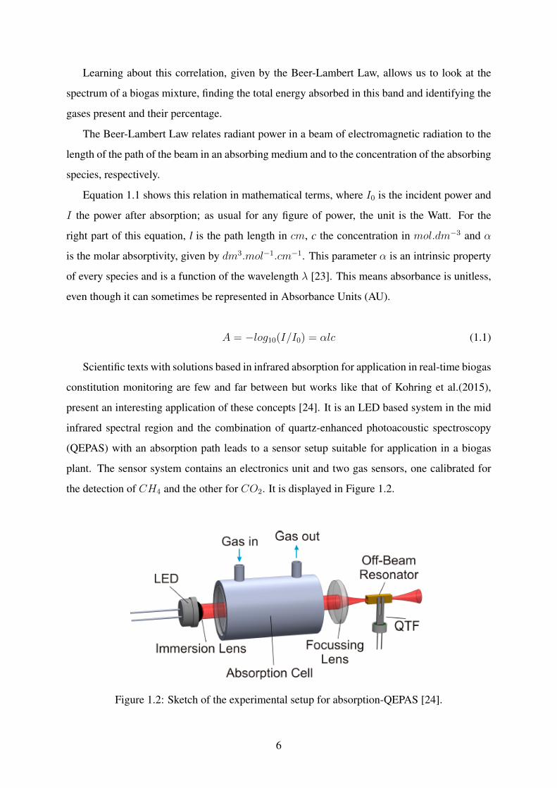
Scientific texts with solutions based in infrared absorption for application in real-time biogas

constitution monitoring are few and far between but works like that of Kohring et al.(2015),

present an interesting application of these concepts [24]. It is an LED based system in the mid

infrared spectral region and the combination of quartz-enhanced photoacoustic spectroscopy

(QEPAS) with an absorption path leads to a sensor setup suitable for application in a biogas

plant. The sensor system contains an electronics unit and two gas sensors, one calibrated for

the detection of CH4 and the other for CO2. It is displayed in Figure 1.2.

Figure 1.2: Sketch of the experimental setup for absorption-QEPAS [24].

6

Using this same principle of absorption-QEPAS, the work of Wu et al. (2015) strives to

detect trace gases in the compositon of biogas instead of the main components [25]. Focusing on

identifying the concentration of NH3 and H2S - two gases that are toxic, reactive and corrosive

-, two well-defined absorption lines with no interference from H2O are identified (6322.45

cm−1 for NH3 and 6328.88 cm−1 for H2S) and the utilized sensor is optimized for detection

in those very same wavenumbers.

Other works like Eichmann et al. (2014) introduce a Raman scattering-based system to anal-

yse all the components of biogas including water vapour [26]. Raman spectroscopy is a tech-

nique with the purpose of measuring vibrational, rotational, and other low-frequency modes

in a system [27]. In this work it is defended that virtually all molecular species can be si-

multaneously studied with a single light source, allowing relative concentration measurements

independent of the laser power [26].

To better understand why MIR spectral analysis is well-suited for evaluation of biogas mix-

tures, Figure 1.3 shows the infrared region and what types of molecules usually absorb in which

bands, immediately showing how almost every biogas component absorbs electromagnetic ra-

diation in the mid-wavelength infrared range.

Figure 1.3: Absorption of different molecules across the infrared spectrum. [28]

Taking the information from Figure 1.3 of each individual gas that composes a biogas mix-

ture and displaying the infrared spectrum of each one it’s easier to see the overlapping of bands

where energy is absorbed between molecules. This is displayed in Figure 1.4 for a limited

wavenumber range.

7

Figure 1.4: Individual spectrum of each element of a biogas mixture [29].

The data here presented is extracted from the NIST Chemistry WebBook [29]. While the

concentration for each gas in Figure 1.4 is unknown, all gases are diluted in N2 in known

pressures:

• 150mmHg of CH4 diluted to 600mmHg;

• 200mmHg of CO2 diluted to 600mmHg;

• 600mmHg of H2S diluted to 600mmHg;

• 50mmHg of NH3 diluted to 600mmHg;

• 400mmHg of CO diluted to 600mmHg

Information on the state of water vapour is not given by NIST.

The first conclusion to be drawn from Figures 1.3 and 1.4 is that O2, N2 and H2 do not

absorb infrared light, therefore making it invisible in the spectrum of any biogas mixture.

Also, it can be seen that water vapour can be a problem for many different reasons, the main

one being that it absorbs all across the spectrum, most noticeably in the range where there is

CO2, NH3, CH4 and H2S presence, meaning it can easily disrupt any measurements. This

explains why dry-basis analysis is preferred when studying and evaluating biogas mixtures.

8

However, taking into account the information in Table 1.1, we can conclude that most of

these gases will not have a relevant presence in spectroscopic analysis of a typical biogas sam-

ple. Therefore, due to the overwhelming concentration of methane and carbon dioxide in biogas

mixtures, those will be the main components to be trialled in this system. In Figure 1.5 both

species’ spectrum is displayed for a wavenumber range between 2000 cm−1 and 4000 cm−1.

Figure 1.5: Spectrum of the dominant components of a biogas mixture [29].

As it can be seen, there is no juxtaposition between both spectrums, therefore the viability

of this solution appears even greater.

Both for CO2 and CH4, the dominant species in biogas, the absorption of energy in the in-

frared region cause the molecules to chaotically oscillate around its nucleus; this is called a vi-

brational molecular state, where small amplitude movements between atoms make the molecule

behave similarly to an harmonic oscillator [30].

In the case of CH4, since it’s an alkane, its behaviour is caused by the existence of stretch-

ing vibrations in the C-H bond in the range of 3000 cm−1 – 2850 cm−1 with the well-defined

energetic transitions due to the rigid rotation of the molecule defining the constant interval be-

tween peaks in this range [31, 32]. For CO2, the peak around 2300 cm−1 is due to assymetrical

stretching in the C=O bonds [33].

9

1.3 Objectives

This work presents the design, assembly, tests and results of a proposed biogas sensor. Its

ultimate goal is the distinction and correct measurement of the two main components in a biogas

mixture, CH4 and CO2, in the absence of H2O vapour.

The proposed way of achieving this is measuring the absorption of infrared light by the gas

samples and establishing a correlation between the signal and the concentration of each species.

To correctly determine the validity and sensitivity of this system, the theoretical value of

incident radiation detected by the signal can be calculated based on the transfer functions of all

the components, so as to have a benchmark to which experimental values can be compared.

1.4 Thesis Outline

This thesis is divided into four chapters. Chapter 1 begins with the motivation for this work

and introduces the central topic of this work, biogas. This chapter also presents the literature

review for the current state of biogas production and the most relevant measurement techniques.

Finally, the objectives for this work are outlined at the end of this chapter.

The experimental setup and instruments description is detailed in Chapter 2, outlining at

the same time the two configurations of the system tested in this work. The absorption spectra

of different CH4 and CO2 concentrations obtained through FT-IR spectrometry tests are also

shown in this chapter.

Results of this system’s behaviour are presented and discussed in Chapter 3 for both config-

urations.

Finally, Chapter 4 is where the conclusions are written alongside some suggestions on the

future expansion of this work.

10

Chapter 2

Experimental Setup

Two distinct configurations were here implemented and tested, as shown in the schematics of

Figure 2.1.

Figure 2.1: Scheme representing both configurations of the system being tested

In configuration A, the sensor integrated in this proposed system detects a signal dependent

on the incident radiant power. This signal is a product of the transfer functions of the light

source, the absorbing gas and the sensor. This is given by Equation 2.1.

TFLS × TFGas × TFSensor = Signal (2.1)

Configuration B of the system sees the introduction of a monochromator as a way to dis-

perse the light so as for the sensor to only receive radiation in a continuous and narrow window,

11

displaying only light in relevant bands where it has been absorved the most. The monochro-

mator also has a curve representing its spectral behaviour, this way the previous equation is

rewritten as Equation 2.2.

TFLS × TFGas × TFMonochromator × TFSensor = Signal (2.2)

So, before testing this system and evaluating its performance as a mean of evaluating bio-

gas mixtures, theoretical values must be assessed so the experimental values obtained can be

compared to them, this way it’s necessary to define the experimental setup and each transfer

function.

2.1 Light Source

The light source is a Sarspec LS-MIR, a Si3N4 (silicon nitride) emitter with an emitting power

of 18W and working wavelength range from 500 nm to 5000 nm. Its spectral behaviour is

shown in Figure 2.2 alongside a picture of the device.

(a) (b)

Figure 2.2: Infrared light source and spectral behaviour curve. (a) Sarspec LS-MIR. (b) Spectralradiance vs. λ.

This equipment is air-cooled and the infrared beam can hit temperatures as high as 1150◦C.

It also includes a shutter to avoid overexposing the sample without turning off the lamp and

an intensity controller to allow for manual regulation of light intensity (although this parameter

was not altered for the whole duration of this work, working at maximum intensity all along).

12

2.2 Infrared Sensor

The sensor implemented in the system is a focal plane array, the NIT Luxell FPA 256, attached

to an electronic device designed to read and process the signal current, the Luxell CORE-S.

The FPA is a vapour phase deposition PbSe (lead selenide) focal plane array with 256 pixels

and response in the 1000 nm to 5000 nm range. After radiant flux is received by the detector, a

signal current is generated. The relation between incident light and signal current needs to take

into account the spectral sensitivity curve. The curve made available by the manufacturer, as

seen in Figure 2.3, displays the specific detectivity (D∗) as a function of wavelength. This is a

figure of merit which has the purpose of characterizing the detector’s performance.

(a) (b)

Figure 2.3: Infrared sensor and spectral behaviour curve. (a) Luxell FPA 256 mounted in thesystem structure. (b) Specific detectivity vs. λ.

Specific detectivity relates the concept of noise equivalent power with the area of the detec-

tor and its frequency bandwidth through Equation 2.3. Its unit is Jones; 1 Jones = 1 [cm.Hz1/2/W] [34].

D∗ =(Adf)1/2

NEP(2.3)

While Ad is the detector area, NEP is the noise equivalent power and the frequency band-

width f is directly computed from the integration time ti defined in the software as shown in

Equation 2.4.

f =1

2ti(2.4)

13

However, specific detectivity appears as an obstacle in establishing the relationship between

radiant intensity emitted by the light source, energy absorbed by the gas sample and signal

detected by the sensor as this figure of merit is not easily correlated with radiant intensity.

Therefore, to better comprehend it, it’s needed to not only introduce the concept of responsivity

but also define noise equivalent power.

NEP is a figure of merit used to characterize the sensitivity of an IR detector and it’s defined

as the minimum radiant incident power that produces a signal equal to the root mean square

noise and is given by Equation 2.5.

NEP =VrmsRV

(2.5a)

NEP =IrmsRI

(2.5b)

Responsivity, R, is a figure of merit that establishes the relation between the output sig-

nal in response to the optical input represented by Equation 2.6. Its units are either A/W or

V/W depending if a current or a voltage is measured, respectively, per Watt of incident radiant

power. It is also a function of the wavelength, meaning it has a different behaviour along the

electromagnetic spectrum.

RV =VsP0

(2.6a)

RI =IsP0

(2.6b)

This is therefore the figure of merit needed to perfectly establish a relation between incident,

absorbed and detected radiation along our system. Further developing the mathematics here

involved show responsivity as directly proportional to the specific detectivity as exhibited by

Equation 2.7.

RV =Vrms√

Ad

2ti

D∗ (2.7a)

RI =Irms√

Ad

2ti

D∗ (2.7b)

14

It is known Ad and f are constant, and even withouth knowing the rms noise voltage or

current, we can infer that there is a direct proportionality between the responsivity and the

specific detectivity. Therefore, the given curve can be used to qualitatively relate all the transfer

functions of this system and evaluate the validity of the experimental results obtained.

In what regards what’s seen in the software, it’s the result of the processing by the Luxell

CORE-S of the signal current converted from the radiant incident power. This hardware has

a dark current subtraction function integrated into it and an integrator amplifier with the gain

formula of Equation 2.8.

V0 = I0tiCi

(2.8)

In this case, I0 is the signal current alongside the residual dark current being directed to the

amplifier, ti the user defined integration time and ci the 10pF integrator capacity. Afterwards,

the corresponding voltage, V0, is digitized by a bipolar 14bit ±10V span analog-to-digital con-

verter. This is what is finally observed in the software connected to the sensor as a real-time

movie, displaying approximately 180 frames per second.

It should be noted that even though the system has an hardware-integrated dark current

subtraction function, a residual background noise is always present. This can be accounted for,

a 200 frame averaged value for this error is taken from a typical system operating case and is

displayed in Figure 2.4.

Figure 2.4: Background noise after hardware dark current subtraction is performed. This errorsignal is extracted from an average of 200 frames for a typical case of system operation.

15

2.3 Monochromator

A monochromator is a manually operated instrument that receives incident light through the

entrance slit with a wide range of wavelengths. Light is then directed by a set of mirrors to a

diffraction grating where it’s diffracted and spatially separated in the same way as a prism sep-

arates visible light into colors. Posteriorly, this light is directed to the exit slit through a similar

set of mirrors. This is an entirely mechanic instrument and the hand operated crank precisely

controls the grating position and, therefore, the narrow wavelength band being outputted by it.

This design is shown in Figure 2.5.

(a)

(b)

(c)

Figure 2.5: Optical path scheme and photographs of the inside of the monochromator anddiffraction grating. (a) Inside view of the monochromator with optical path drawn. (b) Orielmonochromator optical design [35]. (c) 77301 diffraction grating.

16

The instrument here implemented is an Oriel 1/8m hand operated monochromator with in-

terchangeable diffraction gratings; the one used here allows for diffraction in the range of 2500

nm to 8000 nm. The number read on the counter on top of the monochromator is calibrated to

allow identification of the wavelength coming out of it depending on the grating’s factor scale;

the grating here used - Oriel 77301 monochromator grating - has a scaling factor of 8, meaning

the wavelength leaving the center of the slit is 8 times higher than the number displayed. In the

case of this unit, with exit slit fully open it is known that a band of 480 nm is outputted.

This way, it allows for the signal to be detected by the sensor as a spectrum, with each

pixel receiving radiant light in a different wavelength and the full 256 pixels reading a 480 nm

fraction of what is seen in Figure 2.14.

The efficiency of the diffraction grating however is not constant and also a function of

λ. Therefore, its transfer function is the spectral curve presented in Figure 2.6 alongside the

monochromator.

(a) (b)

Figure 2.6: Monochromator and spectral efficiency curve. (a) Oriel 1/8m hand operatedmonochromator. (b) Diffraction grating efficiency vs. λ.

2.4 Gas Cell

The gas cell used to house the samples to be studied is made of stainless steel with a 7cm path

length, 25 mm diameter and 2 mm thickness ZnSe (zinc selenide) windows and two valves for

entrance and exit of the gases and displayed in Figure 2.7.

Monomixtures of both CH4 and CO2 are diluted in N2, a molecule with no relevance in the

17

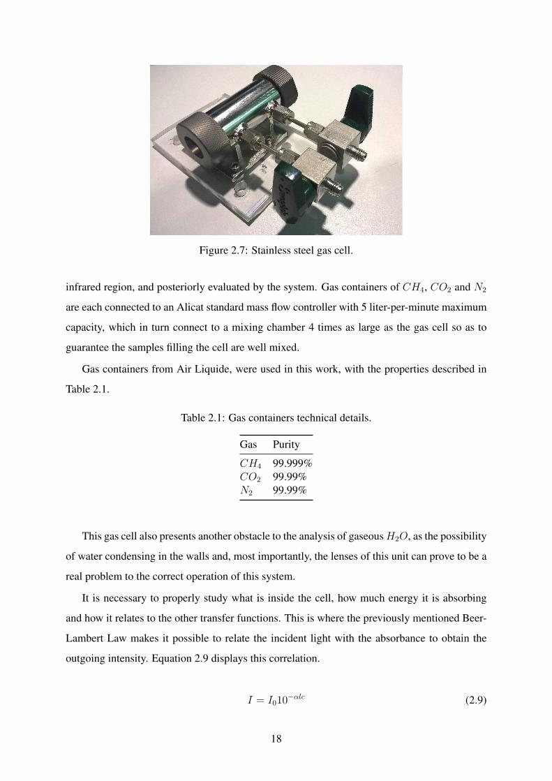
Figure 2.7: Stainless steel gas cell.

infrared region, and posteriorly evaluated by the system. Gas containers of CH4, CO2 and N2

are each connected to an Alicat standard mass flow controller with 5 liter-per-minute maximum

capacity, which in turn connect to a mixing chamber 4 times as large as the gas cell so as to

guarantee the samples filling the cell are well mixed.

Gas containers from Air Liquide, were used in this work, with the properties described in

Table 2.1.

Table 2.1: Gas containers technical details.

Gas Purity

CH4 99.999%CO2 99.99%N2 99.99%

This gas cell also presents another obstacle to the analysis of gaseousH2O, as the possibility

of water condensing in the walls and, most importantly, the lenses of this unit can prove to be a

real problem to the correct operation of this system.

It is necessary to properly study what is inside the cell, how much energy it is absorbing

and how it relates to the other transfer functions. This is where the previously mentioned Beer-

Lambert Law makes it possible to relate the incident light with the absorbance to obtain the

outgoing intensity. Equation 2.9 displays this correlation.

I = I010−αlc (2.9)

18

To obtain the absorbance term, αlc, precise spectroscopic analysis with access to an FT-IR

spectrometer was performed to acquire the needed data.

FT-IR spectrometry is a technique based on the principle of Fourier Transform Spectroscopy,

a technique that uses interference of light rather than dispersion to measure the spectrum of a

substance. The basis of this technique is the Fourier-pair relationship between the interferogram

(interference function) of a substance and its spectrum [36]. What we obtain here, as referred,

is a spectrum of absorbance as a function of wavelength.

The scheme in Figure 2.8 show the new experimental setup implemented to perform this

technique.

(a)

(b) (c)

Figure 2.8: FT-IR experimental setup schematics and photographs. (a) Experimental setupscheme. (b) Gas filling setup. (c) Bruker ALPHA spectrometer with gas cell performing a test.

19

The device used for this was the Bruker ALPHA, with spectral range from 1250 nm to

25000 nm, maximum resolution of 0.95 nm and a wavelength precision of 0.01 nm.

As described by the Beer-Lambert Law, absorbance should be directly proportional to the

concentration, assuming a constant path length, as is the case with this system. However, to

guarantee the absence of absorption saturation outside the peaks, tests were done for both CH4

and CO2, diluted with N2. Figure 2.9 displays an example of a spectrum for a mixture of 60%

CH4 and 40% CO2 obtained with the Bruker ALPHA spectrometer.

Figure 2.9: Absorbance spectrum for a biogas mixture given by the FT-IR spectrometer. Casein point, 40% CO2 and 60% CH4.

The sample concentrations range from 5% to 100% in 5% intervals. Three tests were done

for each concentration and to further guarantee the reliability of the spectrum obtained, each

sample was scanned 16 times by the device and an average spectrum of those scans is pre-

sented. Even though higher numbers of scans were tested with certain samples, it could easily

be confirmed that the results were not affected. The total mixtures tested are displayed in Ta-

ble 2.2. All the corresponding spectra resulting from these tests are displayed in Appendix

A.

However, this equipment has limitations for absorbance values greater than 2.5AU according

to manufacturer recommendations. In the case of both CH4 and CO2, their peaks easily surpass

these values even for low concentrations, therefore saturating in these specific wavelengths,

λCH4 ≈ 3315 nm and λCO2 ≈ 4330 nm. After all spectra are collected it’s important to compare

20

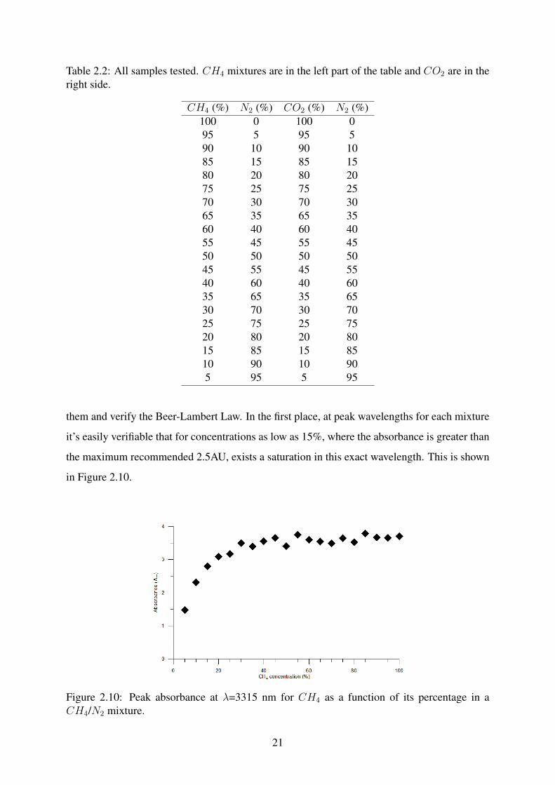
Table 2.2: All samples tested. CH4 mixtures are in the left part of the table and CO2 are in theright side.

CH4 (%) N2 (%) CO2 (%) N2 (%)100 0 100 095 5 95 590 10 90 1085 15 85 1580 20 80 2075 25 75 2570 30 70 3065 35 65 3560 40 60 4055 45 55 4550 50 50 5045 55 45 5540 60 40 6035 65 35 6530 70 30 7025 75 25 7520 80 20 8015 85 15 8510 90 10 905 95 5 95

them and verify the Beer-Lambert Law. In the first place, at peak wavelengths for each mixture

it’s easily verifiable that for concentrations as low as 15%, where the absorbance is greater than

the maximum recommended 2.5AU, exists a saturation in this exact wavelength. This is shown

in Figure 2.10.

Figure 2.10: Peak absorbance at λ=3315 nm for CH4 as a function of its percentage in aCH4/N2 mixture.

21

As the same is known to happen to CO2 in the previously referred peak wavelength, this

shows that what should be looked at are the energetic bands rather than the peak to draw better

conclusions about the concentration. These wavelength intervals are defined in Table 2.3 and

Figure 2.11.

Table 2.3: Integral range, corresponding gas and color code associated with each band.

Gas Color Wavelength band

CH4Red 2105 - 2500 nm

Black 3100 - 3950 nm

CO2Green 2650 - 2860 nmBlue 4100 - 4550 nm

Figure 2.11: Integral bands of Table 2.3 with the respective color code.

After an averaging of the three samples for each concentration, by integrating the spectrum

in these defined bands it is possible to find out that the linear relation established by Beer-

Lambert is followed almost perfectly except for the CO2 peak represented in Figure 2.11 in the

color blue, where the referred absorbance saturation takes a major role in stopping that linearity.

The plot of each integral as a function of concentration can be observed in Figure 2.12 and it

follows the previously established color code.

22

Figure 2.12: Plot of the integral values for CO2 and CH4 in the bands defined in Table 2.3 asa function of concentration. Each curve corresponds in color to the respective band followingwhat’s shown in that same table.

With this information, and comparing it to the data from the NIST Chemical WebBook,

it can be concluded that only one band doesn’t respect the linearity that is expected from the

Beer-Lambert Law, more specifically, the larger CO2 band. It is easy, however, to justify the be-

haviour of the integral curve for this band with the fact that this spectrometer cannot process the

absorbance for values greater than 2.5AU, meaning saturation greatly influences the measured

values here observed.

On the other hand, both CH4 bands and the small CO2 band, the expected linearity is in fact

observed, as higher concentrations of both species are accompanied by a directly proportional

raise in absorbance values.

2.5 Configuration A

The most direct system is composed by the components previously described with the exception

of the monochromator and it is shown in figures 2.13 and 2.1.

In this configuration, light goes through the gas cell, filled with the gas being studied in the

same way as the spectrometry test.

In conclusion, the composed transfer function given by equation 2.1 after the incident light

is detected by the sensor should follow the behaviour shown in Figure 2.14.

23

Figure 2.13: System configuration A. 1 represents the light source, 2 the gas cell and 3 thesensor.

Figure 2.14: Signal detected by the sensor after absorption by the biogas mixture according toequation 2.1. Case in point: 60% CH4 and 40% CO2.

On first sight, it can be inferred that with higher concentrations, the integral of the signal

represented in Figure 2.14 will decrease, following the Beer-Lambert theory, linearly.

As in the case of the FT-IR spectrometry tests, separate samples of CH4 and CO2 are

studied. Tests were done in 5% intervals of gas concentration from 100% to 5% mixed with N2.

24

2.6 Configuration B

This configuration of the system, schematized in Figure 2.1 and shown in Figure 2.15, sees the

introduction of a monochromator to allow it to work as a spectrometer.

Figure 2.15: System configuration with monochromator. 1 represents the light source, 2 the gascell, 3 the monochromator and 4 the sensor.

The intervals to be studied with this configuration of the system aim to show all the relevant

wavelength bands for both gases and are therefore an approximation of the ones shown in Ta-

ble 2.3. Knowing that the window of the monochromator outputs 480 nm of light when the slit

is fully open, the real intervals are defined by the wavelength chosen in the readable counter.

Shorter intervals were avoided as the closure of the exit slit meant the signal read would drop

significantly in intensity. In Table 2.4 these intervals are well defined. As previously referred,

the diffraction grating can’t display the CH4 band in the 2105 - 2500 nm wavelength range.

The product of the four transfer functions given by Equation 2.2 in this configuration of

the system results in the signal of Figure 2.14 with the transfer function of the monochromator

accounted for. Looking at the intervals determined in the above table, the areas of the signal

integrated look like Figure 2.16.

25

Table 2.4: Integral band and corresponding monochromator position

Gas Counter number WavelengthCH4 415 3080 - 3560 nm

CO2345 2520 - 3000 nm543 4104 - 4584 nm

Figure 2.16: Signal integral in the defined intervals of Table 2.4.

The main disadvantage of this configuration is the grating not diffracting light for wave-

lengths lower than 2500 nm, removing the possibility of detecting the band of CH4 in the 2100

nm - 2500 nm range. The much lower signal intensity detected by the sensor with this iteration

of this system is the second biggest disadvantage, in the first place because the light source

is farther away from it meaning there is more dispersion and in the second place because the

diffraction grating has a varying efficiency, resulting in a lower signal for some wavelengths.

2.7 Uncertainty Analysis

Every experimental test has an associated uncertainty. In the case of this system, the flow

controllers and sensor are the two main sources of uncertainty.

The Alicat flow controllers used to control the filling of the gas cell have an associated

uncertainty of 0.8% of the flow measured over 0.2% of its full scale. Therefore, the error eQ is

26

given by Equation 2.10.

eQ = ±(0.008Qm + 0.002Qimax) × 100% (2.10)

It’s evident this uncertainty depends not only on the measured flow rate, Qm, but also on

the maximum operating value of the flow controller i, Qimax, meaning lower capacity flow

controllers have lower associated errors.

The highest measured flow rate was taken into account for all flow controllers in this calcu-

lation and results are presented in Table 2.5.

Table 2.5: Flow controller associated uncertainties.

Gas Qm (SLPM) Qimax (SLPM) eQ (%)

N2 0.2 5 1.16CO2 0.2 1 0.36CH4 0.2 1 0.36

To determine the error of the sensor signal, 200 frames were integrated and the mean value

calculated as a reference value. Afterwards, the root mean square (RMS) deviation was com-

puted and the error values obtained. A typical value of the sensor associated error is 0.9733%,

with a mean value of 241178.57 and an RMS deviation of 2347.44.

27

28

Chapter 3

Results

Experimental results and the respective comparison with theoretical values are presented in this

section. The integrals of both theoretical and experimental signals were integrated with the

trapezoidal numerical method for every case. They are presented here qualitatively as a fraction

of a standard integral value, in both cases when the gas cell is filled with N2, an expressionless

molecule in the infrared region, meaning the signal is absorbed with maximum possible inten-

sity for each configuration. This way, a qualitative analysis can be done to draw conclusions.

3.1 Configuration A

What the software exports is a real-time movie of the signal detected, displaying approximately

180 frames per second. After covering the sensor, 200 frames of the signal are collected to

define the background noise and allow the system to remove it when the test is being processed.

The measured signal, after background noise is removed usually has the format displayed in

Figure 3.1.

With this configuration, the sensor is bombarded with incident light across the whole de-

tected range, from 1000 nm - 5000 nm. However, unlike what happens in configuration B, this

light is not spatially separated and only an intensity is measured.

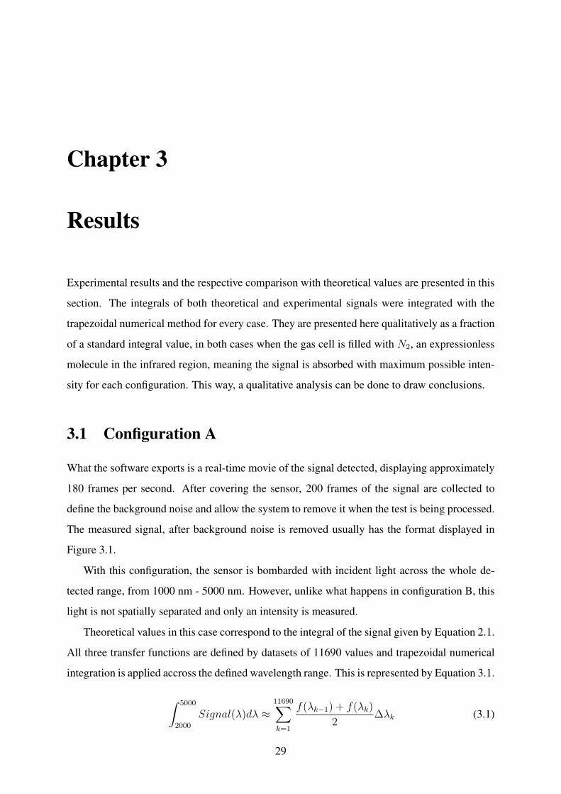
Theoretical values in this case correspond to the integral of the signal given by Equation 2.1.

All three transfer functions are defined by datasets of 11690 values and trapezoidal numerical

integration is applied accross the defined wavelength range. This is represented by Equation 3.1.

∫ 5000

2000

Signal(λ)dλ ≈11690∑k=1

f(λk−1) + f(λk)

2∆λk (3.1)

29

Figure 3.1: Typical signal measured by the software and signal integral area.

On the other hand, experimental values are calculated from a matrix of 200 frames × 256

pixels, where an average of those 200 frames is integrated just as described in Equation 3.2 for

an interval of 256 pixels.

∫ 256

1

Signal(x)dx ≈256∑k=1

f(xk−1) + f(xk)

2∆xk (3.2)

In both Figures 3.2a and 3.2b are presented the theoretical vs. the experimental values.

Looking firstly at the plot of Figure 3.2a, a strong linear correlation between the signal inte-

gral and the concentration can be seen for the experimental values, as described by Equation 3.3,

with a corresponding coefficient of determination of R2 = 0.991865. The theoretical curve also

displays that same linearity - R2 = 0.996541 - however with a different slope than the exper-

imental one. What establishes this dissociation between the two sets of values is the fact that

while the experimental signal is the product of the whole light emitting range, the theoretical

signal is measured in a range of 2000 nm - 5000 nm due to the fact that the FT-IR spectrometer

only outputted noise-free values starting with that wavelength.

%CH4 =

IntegralCH4

IntegralN2− 0.9825

−8.4795 × 10−4(3.3)

RV =VsP0

(3.4a)

30

(a)

(b)

Figure 3.2: Comparison of theoretical and experimental values of the CH4 and CO2 integralsas a function of concentration. (a) CH4 analysis. Linear relation for the experimental valuesgiven by Equation 3.3. (b) CO2 analysis. Linear relation for the experimental values given byEquation 3.5.

RI =IsP0

(3.4b)

This means that for the plot of Figure 3.2b, while showing a great similarity with theoretical

values, it is still being radiated by the same emitter as in the previous case, therefore exper-

imental values should naturally be higher as the integral value needs to account for the extra

1000 nm of energy received by the detector. For concentrations lower than 60% the relation of

integral fraction and concentration of CO2 shows the expected linearity. The linear correlation

between signal integral and CO2 concentration is also represented in Equation 3.5. The coeffi-

31

cient of determination for the theoretical curve in Figure 3.2b is R2 = 0.998666, while for the

experimental curve that value is R2 = 0.862249.

%CO2 =

IntegralCO2

IntegralN2− 0.9747

−3.4015 × 10−4(3.5)

The results from Figure 3.2b however show that the measured CO2 signal follows closely

the one from the theoretical value even though an extra 1000 nm of radiation are being detected

by the sensor as compared to the theory.

This is not a completely valid result however and it may be due to the lower spectral response

of the system in the bands where this species absorbs energy, meaning the detected signal must

be more susceptible to external variables such as temperature and humidity or internal variables

like the sensor noise. This also helps justify the high variance of results for the CO2 measure-

ment as it is an important factor when raising questions about the validity of this system, as the

concentration of a CO2 sample cannot effectively be calculated without stable conditions.

Furthermore, when observing a biogas mixture, this sensor allows no distinction between

CO2 and CH4 as the light incides on it in its full electromanetic spectrum, therefore displaying

the signal after both have absorbed energy with no way of evaluating each species’ weight.

This means that, while this configuration of the system proves to be effective as a way of

identifying the concentration of either CO2 or CH4 when in the presence of other elements

invisible in the infrared region - like N2 -, this is not a valid way of correctly assessing the

quality of the biogas being produced.

To showcase a typical case of system operation in configuration A, tests were done in a pre-

commercial scope. The signal integrals as a function of time resulting of these tests are shown

in Figure 3.3.

It must be noted, however, that these tests were conducted after the system was reassem-

bled, meaning it was therefore subject to a set of calibration tests in order to adjust to the new

conditions of the system and obtain a new linear correlation similar to the ones of Equations 3.3

and 3.5. The calibration process involves as well the definition of the reference integral value,

for when the gas cell is filled with only N2. Only after that can one take an integral value and

immediately find out the gas concentration.

For the case of Figure 3.3, it is evident that the system responds well to the variations in

concentration, showing that the linear relation derived from the calibrations for this case shows

close proximity to the injected values. For example, in the demarked regions of this figure, when

32

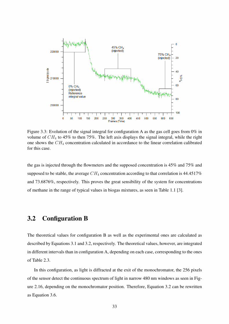
Figure 3.3: Evolution of the signal integral for configuration A as the gas cell goes from 0% involume of CH4 to 45% to then 75%. The left axis displays the signal integral, while the rightone shows the CH4 concentration calculated in accordance to the linear correlation calibratedfor this case.

the gas is injected through the flowmeters and the supposed concentration is 45% and 75% and

supposed to be stable, the average CH4 concentration according to that correlation is 44.4517%

and 73.6876%, respectively. This proves the great sensibility of the system for concentrations

of methane in the range of typical values in biogas mixtures, as seen in Table 1.1 [3].

3.2 Configuration B

The theoretical values for configuration B as well as the experimental ones are calculated as

described by Equations 3.1 and 3.2, respectively. The theoretical values, however, are integrated

in different intervals than in configuration A, depending on each case, corresponding to the ones

of Table 2.3.

In this configuration, as light is diffracted at the exit of the monochromator, the 256 pixels

of the sensor detect the continuous spectrum of light in narrow 480 nm windows as seen in Fig-

ure 2.16, depending on the monochromator position. Therefore, Equation 3.2 can be rewritten

as Equation 3.6.

33

∫ 480

0

Signal(λ)dλ ≈256∑k=1

f(xk−1) + f(xk)

2∆xk (3.6)

Figure 3.4 displays the correlation between theoretical and experimental values based on

this integration method.

Looking at all the plots of Figure 3.4, it becomes apparent that the signal measured by the

sensor in this configuration never follows the theoretical value. However, Figures 3.4a and

3.4b denote the existence of a linear relation between the value of the integrated signal and the

concentration as expected.

Looking at Figure 3.4c on the other hand it’s possible to observe not only a great variance

in the observed values, showing an excess of sensitivity for this band, but also the lack of a

tendency in the experimental values where the diffence to the theoretical values is significant,

making it impossible for the concentration to be calculated. This may be due to the fact that

the sensor as well as the light source have a reduced sensitivity and radiance in this band, as

the curves corresponding to each of those two devices decrease dramatically for wavelengths

greater than 4000 nm.

The linear correlation seen in the other two studied bands should be enough to create a

valid correlation between the measured signal and the concentration of that respective element.

However, the lower intensity of light that reaches the sensor in this configuration means that

the detected signal will be lower and therefore it will be more susceptibile to noise and other

environmental perturbations that can greatly affect the signal being detected.

As it was the case for configuration A, the signal integral relates to the concentration in a

linear way. From the most relevant results, shown in Figures 3.4a and 3.4b, that linear rela-

tion can be written as in Equations 3.7 and 3.8, respectively. For the case of Figure 3.4a, the

coefficient of determination for the theoretical curve is R2 = 0.99638 and R2 = 0.917426 for

the experimental curve, while for Figure 3.4b those same coefficients are R2 = 0.991004 and

R2 = 0.924941 for the theoretical and experimental curves, respectively.

%CH4 =

IntegralCH4

IntegralN2− 0.9168

−1.7925 × 10−3(3.7)

%CO2 =

IntegralCO2

IntegralN2− 0.9468

−8.3645 × 10−4(3.8)

34

(a)

(b)

(c)

Figure 3.4: Comparison of theoretical and experimental values of the CH4 and CO2 integralsas a function of concentration. (a) CH4 band: 3080 - 3560 nm. Linear relation for the exper-imental values given by Equation 3.7. (b) CO2 band: 2520 - 3000 nm. Linear relation for theexperimental values given by Equation 3.8. (c) CO2 band: 4104 - 4584 nm.

35

In a similar manner as in configuration A, in a pre-commercial approach, a typical case

of system operation for fluctuating concentrations of gas is shown in Figure 3.5. Likewise,

calibration tests were done to find a new linear correlation in the same vein as Equations 3.7

and 3.8 and to establish a new integral reference value for 0% gas concentration. In the case

here depicted, the monochromator is in position 415, focused on the CH4 detection band, 3080

- 3560 nm.

Figure 3.5: Evolution of the signal integral for configuration B as the gas cell goes from 0% involume of CO2 to 75% and then 45%. The left axis displays the signal integral, while the rightone shows the CO2 concentration calculated in accordance to the linear correlation calibratedfor this case.

As it can be seen, the system once again responds accordingly to the variation in CH4 con-

centration, showing close proximity to the injected values. The average concentration calculated

through the calibrated correlation in the demarked region of 75% injected CH4 is 72.5654%,

while in the 45% region that value is 48.0539%.

This, once again, proves the quality of configuration B as a means of evaluating the CH4

concentration in biogas mixtures as it behaves well between the typical values of methane con-

centration.

36

Chapter 4

Conclusions

The purpose of this work is the experimental assessment of the validity and applicability of the

system here proposed as a biogas sensor that is able to discretize and evaluate the percentage of

CO2 and CH4 in this mixture after H2O is removed.

Looking at all tests and results, it’s evident that only the second configuration of this system

can ever be considered for use in a biogas plant, as the first one allows no distinction between

each gas that composes the produced biogas. It can also be noted that accross all tests results

follow the linear behaviour that is to be expected.

The use of the monochromator allows for detection of radiant light in the bands where both

gases absorb and presents the only reliable option for identifying specific species in biogas

mixtures. However, the discrete bands observable in this system impose another limitation of

this system because it means that identification of only one gas at a time is possible. To evaluate

the concentration of both gases, two filters designed for operation in two different bands are

needed, more specifically the ones that presented best results: between 2520 nm - 3000 nm for

CO2 and 3080 nm - 3560 nm for CH4.

The linearity observed in the signals for these two bands make possible the calculation of

the percentage of each gas in the mixture, however calibration of the system is of paramount im-

portance to consider the results reliable because of the significant noise values. If this approach

is selected, as the observed signal shows variance, stable conditions are absolutely necessary

in the surroundings of the system, as temperature and humidity play a big part in affecting this

sensor and the measured signal due to the lower intensity of light.

It must also be noted that with this system it is absolutely needed to remove water vapour

from this mixture, namely for CO2 measurement, as the band with best results (2520 nm -

37

3000 nm) for the evaluation of that gas is also where H2O absorbs most energy, as seen in

Figure 1.4. H2S can also be a nuisance as it also absorbs in that range, however, because of its

very corrosive properties it should also be removed before analysis so operation of this system

is not affected.

Finally, the first configuration demonstrates potential use as a sensor for CO2 and CH4 as

long as its diluted in a medium with no species absorbing energy in the 1000 nm to 5000 nm

range. One such application for a sensor like this inside a biogas plant is the evaluation of

biomethane to attest its high quality, as after biogas is processed inside an upgrading station it

becomes free of CO2, H2O vapour and other trace gases. Taking into the excellent measure-

ments for CH4 by this system in its simple configuration it becomes a very cost-efficient sensor

for this purpose.

It should be noted, however, that this system while proving great responsivity to concen-

tration variations needs to go through a set of calibration tests before it becomes available for

commercial use. That way, when installing a system like this in a biogas plant, the system

should be calibrated to the operating conditions first and then sealed and kept untouched to

make sure optimum and stable performance can be achieved, as meddling with it can scramble

the extracted values, making a correct evaluation of the concentration impossible.

4.1 Future Work

This work can be expanded in a number of ways, the most evident being the calibration and

optimization of this system for operation in real biogas plants for methane and carbon dioxide

detection.

The behaviour of this system in regards to the detection of trace gases in biogas mixtures

is also a viable path of investigation, as with access to different instrumentation that allows

the system to focus on the relevant absorbing bands for those species this can become a real

scenario.

Finally, work should be done in designing this system with modifications to the gas cell in

a way that allows for water vapour to be analysed with no fear of it damaging the experimental

setup.

38

Bibliography

[1] Biogas plant scheme. https://balkanengineer.com/news/

second-biogas-power-plant-launched-macedonia. Accessed: 2017-10-09.

[2] M. Raboni and G. Urbini. Production and use of biogas in Europe: a survey of current

status and perspectives. Revista ambiente & agua, 9(2):191–202, 2014.

[3] D. Deublein and A. Steinhauser. Biogas from waste and renewable resources: an intro-

duction. John Wiley Sons, 2011.

[4] O. Razbani. Biogas Fueled Technologies, Solid Oxide Fuel Cells & Internal Combus-

tion Engines. PhD thesis, University of Stavanger, Faculty of Science and Technology,

Department of Petroleum Engineering, 2013.

[5] J. L. Walsh, C. C. Ross, M. Smith, S. Harper, and W. Wilkins. Handbook on biogas uti-

lization. Prepared for US Department of Energy, Southeastern Regional Biomass Energy

Program. Prepared by Georgia Institute of Technology, Engineering Technology Branch.

Atlanta, GA, 1988.

[6] O. Dada and C. Mbohwa. Biogas upgrade to biomethane from landfill wastes: A review.

Procedia Manufacturing, 7:333–338, 2017.

[7] F. Burmeister, J. Senner, and E. Tali. Conditioning of biogas for injection into the natural

gas grid. In Biogas. InTech, 2012.

[8] R. Berruto, V. Boero, P. Busato, A. Calvo, A. Sopegno, L. Venudo, D. Rossi, P. Gomez,

B. Ruiz, and M. Kachniarz. Biogas3: Sustainable and economical production of biogas

from food waste of European agrifood industry. Proceedings in Food System Dynamics,

pages 299–308, 2015.

39

[9] F. Hofmann, L. Gamba, U. Weddige, F. Gerlach, A. Wilinska, V. Jaensch, C. Schneider,

W. E. Baaske, B. Lancaster, M. Tersbøl, et al. Report on analysis of sustainability perfor-

mance for organic biogas plants. SUSTAINGAS Report D, 4, 2013.

[10] A. Ware and N. Power. Biogas from cattle slaughterhouse waste: Energy recovery towards

an energy self-sufficient industry in Ireland. Renewable Energy, 97:541–549, 2016.

[11] G. Surie. Achieving sustainability: Insights from biogas ecosystems in India. Agriculture,

7(2):15, 2017.

[12] T. Amon, B. Amon, V. Kryvoruchko, W. Zollitsch, K. Mayer, and L. Gruber. Biogas

production from maize and dairy cattle manure—Influence of biomass composition on the

methane yield. Agriculture, Ecosystems Environment, 118(1):173–182, 2007.

[13] K. Chae, A. Jang, S. Yim, and I. S. Kim. The effects of digestion temperature and temper-

ature shock on the biogas yields from the mesophilic anaerobic digestion of swine manure.

Bioresource Technology, 99(1):1–6, 2008.

[14] S. Jayaraj, B. Deepanraj, and V. Sivasubramanian. Study on the effect of pH on biogas pro-

duction from food waste by anaerobic digestion. In Proceedings of the 9th International

Green Energy Conference, Tianjin, China, May, pages 25–26, 2014.

[15] M. Lesteur, V. Bellon-Maurel, C. Gonzalez, E. Latrille, J. Roger, G. Junqua, and J. Steyer.

Alternative methods for determining anaerobic biodegradability: a review. Process Bio-

chemistry, 45(4):431–440, 2010.

[16] T. L. Hansen, J. E. Schmidt, I. Angelidaki, E. Marca, J. la Cour Jansen, H. Mosbaek, and

T. H. Christensen. Method for determination of methane potentials of solid organic waste.

Waste Management, 24(4):393–400, 2004.

[17] P. Buffiere, D. Loisel, N. Bernet, and J. Delgenes. Towards new indicators for the predic-

tion of solid waste anaerobic digestion properties. Water Science and Technology, 53(8):

233–241, 2006.

[18] H. F. Jacobi, S. Ohl, E. Thiessen, and E. Hartung. NIRS-aided monitoring and prediction

of biogas yields from maize silage at a full-scale biogas plant applying lumped kinetics.

Bioresource technology, 103(1):162–172, 2012.

40

[19] S. Stromberg, M. Nistor, and J. Liu. Early prediction of Biochemical Methane Potential

through statistical and kinetic modelling of initial gas production. Bioresource technology,

176:233–241, 2015.

[20] A. J. Ward, E. Bruni, M. K. Lykkegaard, A. Feilberg, A. P. Adamsen, A. P. Jensen, and

A. K. Poulsen. Real time monitoring of a biogas digester with gas chromatography, near-

infrared spectroscopy, and membrane-inlet mass spectrometry. Bioresource technology,

102(5):4098–4103, 2011.

[21] P. Parajuli. Biogas measurement techniques and the associated errors. Master’s thesis,

University of Jyvaskyla, Department of Biological and Environmental Science, Renewable

Energy Programme, 2011.

[22] P. Weiland. Biogas production: current state and perspectives. Applied microbiology and

biotechnology, 85(4):849–860, 2010.

[23] D. Swinehart. The Beer-Lambert law. J. Chem. Educ, 39(7):333, 1962.

[24] M. Kohring, S. Bottger, U. Willer, and W. Schade. LED-absorption-QEPAS sensor for

biogas plants. Sensors, 15(5):12092–12102, 2015.

[25] H. Wu, L. Dong, X. Liu, H. Zheng, X. Yin, W. Ma, L. Zhang, W. Yin, and S. Jia. Fiber-

amplifier-enhanced QEPAS sensor for simultaneous trace gas detection of NH3 and H2S.

Sensors, 15(10):26743–26755, 2015.

[26] S. C. Eichmann, J. Kiefer, J. Benz, T. Kempf, A. Leipertz, and T. Seeger. Determination

of gas composition in a biogas plant using a Raman-based sensor system. Measurement

Science and Technology, 25(7):075503, 2014.

[27] P. Graves and D. Gardiner. Practical Raman Spectroscopy. Springer, 1989.

[28] H. P. K. K. Gas measurement devices catalog, January 2017.

[29] P. J. Linstrom and W. G. Mallard. The NIST Chemistry WebBook: A chemical data

resource on the internet. Journal of Chemical & Engineering Data, 46(5):1059–1063,

2001.

[30] M. N. Berberan e Santos. Espectroscopia (Principios de Quimica-Fisica). Instituto Supe-

rior Tecnico, Department of Chemical Engineering, March 2016.

41

[31] C. Bronner and F. Essenberger. Rotation-vibrational spectrum. Freie Universitat Berlin,

Department of Physics, 2008.

[32] Chemistry LibreTexts. https://chem.libretexts.org/Core/Physical_and_

Theoretical_Chemistry/Spectroscopy/Vibrational_Spectroscopy/Infrared_

Spectroscopy/Infrared%3A_Interpretation. Accessed: 2017-10-09.

[33] B. C. Smith. Infrared spectral interpretation: a systematic approach. CRC press, 1998.

[34] P. G. Datskos and N. V. Lavrik. Detectors—figures of merit. Encyclopedia of Optical

Engineering, 349, 2003.

[35] NewportCorporation. Oriel instruments spectroscopy instruments catalog. Oriel 77250

Series 1/8 m Monochromator, Page 1181.

[36] J. Bates. Fourier transform infrared spectroscopy.[Basic principles and current applica-

tions]. Science;(United States), 191(4222), 1976.

42

Appendix A

FT-IR Spectroscopy Results

Figure A.1: 5% CH4

43

Figure A.2: 10% CH4

Figure A.3: 15% CH4

Figure A.4: 20% CH4

44

Figure A.5: 25% CH4

Figure A.6: 30% CH4

Figure A.7: 35% CH4

45

Figure A.8: 40% CH4

Figure A.9: 45% CH4

Figure A.10: 50% CH4

46

Figure A.11: 55% CH4

Figure A.12: 60% CH4

Figure A.13: 65% CH4

47

Figure A.14: 75% CH4

Figure A.15: 80% CH4

Figure A.16: 85% CH4

48

Figure A.17: 90% CH4

Figure A.18: 95% CH4

Figure A.19: 100% CH4

49

Figure A.20: 5% CO2

Figure A.21: 10% CO2

Figure A.22: 15% CO2

50

Figure A.23: 20% CO2

Figure A.24: 25% CO2

Figure A.25: 30% CO2

51

Figure A.26: 35% CO2

Figure A.27: 40% CO2

Figure A.28: 45% CO2

52

Figure A.29: 50% CO2

Figure A.30: 55% CO2

Figure A.31: 60% CO2

53

Figure A.32: 65% CO2

Figure A.33: 70% CO2

Figure A.34: 75% CO2

54

Figure A.35: 80% CO2

Figure A.36: 85% CO2

Figure A.37: 90% CO2

55

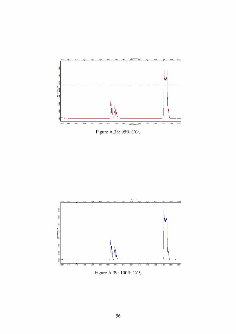
Figure A.38: 95% CO2

Figure A.39: 100% CO2

56

Appendix B

Technical Datasheets

57

Built for IR applicationsWith one 18 W Silicon Nitride emitter, the Light Source LS-MIR

was specially designed for Infrared applications providing a

wavelength range from 500 to 5000+ nm. This is an high flexibility

product that includes shutter, slide filter holder, intensity control

and remote operation.

Slide filter holder, intensity control and shutter for maximum flexibilityThe flexibility of this light source is granted not only for its wide

wavelength range but also for the included slide filter holder

allowing the selection of a specific range. The intensity control

offers the user the possibility to select the correct intensity

for each application. The LS-MIR includes a shutter to avoid

overexpose the sample without turning off the lamp.

Remote operationAll features from LS-MIR can be controlled remotely via the

D-SUB connector and TTL compatible signals, namely the shutter,

intensity control and emitter operation.

Extended emitter lifetimeThe emitter included in this instrument has an estimated lifetime

of 5000 h reducing usage cost.

Large collection opticsThere’s no point in having an high power emitter when a high percentage of light is not coupled into the fiber. For that reason

Sarspec uses 12.7 mm diameter lens offering high efficiency light collection.

LIGHT SOURCES

WWW.SARSPEC.COM WWW.SARSPEC.COM

Typical spectral

radiance for the

LS-MIR

21

LS-MIR Specifications Table

Parameter Value

Wavelength range 500–5000 nm

Emitter Silicon nitride

Power Requirements 15 Vdc / 2 Adc max.

Power Cons. (Max.) 23 W

Warm-Up Time Approx. 5 min

Shutter / Filter holder Yes / Yes

Local Intensity Control Yes

Emitter Power 18 W

Emitter lifetime 5000 h

Emitter Temperature 1150º C

Remote OperationShutter, Emitter operation (TTL compatible signals)

Intensity control (analog and PWM)

Fiber Connector SMA 905

Cooling Air cooling

Dimensions 200 (L) x 92 (D) x 72 (H) mm

Weight 1.1 kg

Ordering Information

Light Source LS-MIR LS-MIR

Replacement emitter for LS-MIR B-MIR

LIGHT SOURCES

WWW.SARSPEC.COM 22

LUXELL FPA Uncooled VPD PbSe, linear array

FPA formats available: Biasing voltage (typ):Pixel size: LUXELL 64, 128 FPA: LUXELL 256 FPA:Pixel pitch: LUXELL 64, 128 FPA: LUXELL 256 FPA:Pixel resistance (typ): LUXELL 64, 128 FPA: LUXELL 256 FPA:Spectral response (typ):Spectral response (LVF version):Peak wavelength of detection:D*(peak) (typ):Responsivity (@Vb=0.5V)(A/W): LUXELL 64, 128 FPA: LUXELL 256 FPA:Quantum effi ciency:Packaging:Dimensions (mm):Operating temperature:Response time:Readout electronics:Readout method:

64, 128 and 256 pixels5 V

1000 μm 600 μm

100 μm 60 μm

300 - 800 k250 - 700 k

1-5 microns3.0 - 4.6 microns

3.7 microns2·109 Jones

0.0250.090

2%SMD, LCC68 footprint

24 x 24 x 2.25C - 70 C

2 microsecondsnot included

multiplexed (blocks of 16 px)

Typical detector spectral response [D*(peak)(500 K, 1000 Hz, 1 Hz)]

Dimensions (mm): 109 x 100 x 73Weight: < 500 gramsFPGA: XILINX VIRTEX 4 (PowerPC + Linux OS embedded)Integration time: > 4.10 μs, selectableFrame rate in lines per second (max): LUXELL 64 FPA: 20,000 LUXELL 128 FPA: 10,000 LUXELL 256 FPA: 5,000Intelligent dark current substractionStart-up time: < 20 secondsOptimum temperature detection range: > 70 CSystem communication and control: Ethernet 10/100Data transmission: TCP/IP, raw format, 16 bitsControl: UDPPower: 12 VDC, 1 ASoftware: LUXELL SOFTWARE SUITE (Acqusition+Visualization SW)

LUXELL CORE-HSCompatible with all LUXELL FPA versions

LUXELL CORE-SCompatible with all LUXELL FPA versions

The LUXELL FPA footprint is LCC68 compatible and is packaged as an SMD component to allow a perfect integration into your circuitry. It has a sapphire window that is replaced with an LVF in the spectroscopy version

Left - FPA dimensions in mm

LUXELL SERIESTypical applications

LUXELL ACQUISITION SOFTWARE

As a part of the LUXELL SOFTWARE SUITE, it allows control of the CORE system and data acquisition to your PC, maximizing the performance of the LUXELL FPA series.

Integration time: 2 - 100 μs, selectableFrame rate (max): LUXELL 64 FPA version: 1,200 lines per second LUXELL 128 FPA version: 600 lines per second LUXELL 256 FPA version: 300 lines per secondIntelligent dark current substractionStart-up time: < 5 secondsDimensions (mm): 60 x 60 x 40Microcontroller: ARM CORTEX M3System communication and control: USB 2.0 full speed, raw format, 14 bitsUSB powered (5 VDC, 0.5 A)Software: LUXELL SW SUITE (Acq+Vis)

The LUXELL SERIES is a product from New Infrared Technologies, S.L.For more information, visit us at www.niteurope.com, or contact us at info@niteurope.com(C) New Infrared Technologies, S.L. - 07/2012 - All rights reserved - The information shown in this document is property of New Infrared Technologies and subject to changes without prior communication.The images shown in this brochure may not reflect the current product appearance.

Quality inspection in production lines: glass container industry

Welding inspection and defect detection: steel industry

High-speed gas fl ow study and characterization

Railway industry: hot-boxes and hot-wheel inspection

Defective welding

1/8 m MONOCHROMATOR GRATINGS

GRATING ASSEMBLY: 77301 1/8 m Monochromator Grating

SPECIFICATIONS

>-o z LU

O Li_ Li-LU

100

90

80

70

60

50

40

30

20

10

1

1 :

/ i \

1

- \ i V - ! : - -: / 1 \ ! i ! i \ ' '

/

/

" "

1 \ - V \

^ \

/ 1 •

1

. ...

\

: i 1 i i

^

\

-I \

ORIEL INSTRUMENTS

SHADED AREA IS BEYOND MECHANICAL LIMIT OF MONOCHROMATOR

1 1 1

py-)) AD(7Pn 1 X/-V r^Dy-»>^WCO

(P-PLANE)

2 3 4 5 6 7 8 9 10 11 12 13 14 15 16 17 18 19 20 21 22 23 24 25

WAVELENGTH (nm)

Line Density:

Blaze Wavelength:

Type:

Reciprocal Dispersion at Blaze Wavelength:

Wavelength Counter Multiplier:

Primary Wavelength Region':

150 I/mm

4nm

Ruled

52 nm/mm

8

2.5-8 nm+

Usable Wavelength Region^: 2.5-8 nm*

77700 Series Monochromator/Spectrograph equivalent grating (page): 77750 (24)

77200 1/4 m Monochromator equivalent grating (page): 77236 (50)

77400 1/8 m Spectrograph equivalent grating (page): N/A

Unmounted equivalent grating (page): 77947/77948 (86)

'Wavelength region where the grating efficiency is >20%. Wavelength region where the grating efficiency is >10%. *The wavelength region is limited at the long wavelength end by the mechanical constraints of the monochromator.

36 250 LONG BEACH BLVD.. P.O. BOX 872, STRATFORD, CT. U.S.A. 06497 - TEL: (203) 377-8282 - FAX: (203) 378-2457 « ELECTRONIC MAIL: 73163.1321@comDuserve.com