Embed Size (px)
Citation preview

INTERNATIONAL JOURNAL FOR NUMERICAL METHODS IN ENGINEERING, VOL. 34, 319-347 (1992)
EFFECTS OF SOFTENING IN ELASTIC-PLASTIC STRUCTURAL DYNAMICS*
G. MAIER AND U. PEREGO
Department of Structural Engineering, Technical University (Politecnico) of Milan, Piazza L. Da Vinci 32, 20133 Milano, Italy
SUMMARY Softening, understood as unstable behaviour of material or structural components, is considered herein for its possible consequences on the overall behaviour of discrete dynamic models of elastic-plastic beam structures, in the absence of geometric effects. It is shown that multiplicity of incremental solutions (response bifurcations) and manifestations of overall instability may occur. The bifurcated responses may exhibit different scenarios for the same excitation: e.g. shakedown or local damage up to failure. An insight into and criteria for such occurrences are achieved by formulating the rate and the finite increment problem as linear complementarity problems. Period doubling and deterministic chaos under harmonic excitation are observed when reversible (holonomic) softening behaviour is assumed. The strong sensitivity of the phenomena investigated with respect to the choice of the structural model is pointed out. The findings are elucidated by illustrative examples.
1. INTRODUCTION
The behaviour of elements or constituents of structures may be characterized by instability in the sense of negative second-order work for some geometry perturbation, i.e. in the sense of a particular violation of Drucker's stability postulate of classical plasticity.', This softening behaviour can be interpreted as a manifestation of material instability and/or as a consequence of geometric effects (influence of deformations on equilibrium) enclosed in the structural component or in the tested specimen.
The local (element) softening behaviour is the one described by the relationships (constitutive models), which are associated with equilibrium and compatibility equations for the analysis of the overall structural response to loads. Examples of local softening are provided by compressed steel members in trusses and by the flexural behaviour of reinforced concrete beams.
Typical possible consequences of constitutive softening on the quasi-static behaviour of elastic-plastic structures, even in the absence of geometric effects, have been shown to be path bifurcation or equilibrium branching and overall instability manifestations such as instability in load-controlled structures and intrinsic instability (or snap-back) occurring under displacement- controlled conditions. These phenomena had been pointed out long ago with reference to trusses, beam systems and discretized ~ o n t i n u a . ~ - ~ Strain localization as a consequence of material
Dedicated to Professor Paul Symonds on his 75th birthday
Mechanics, Stuttgart, August 27-31, 1990 * Presented at the Minisymposium on Structural Failure held within the 2nd World Congress on Computational
0029-5981/92/050319-29s14.50 0 1992 by John Wiley & Sons, Ltd.
Received September 1990 Revised February 1990

320 G. MAIER AND U. PEREGO
unstable behaviour in continua, or finite element models thereof, have been the object of an abundant literature, with recent extensions to rate dependence and inertial effects. Representative authoritative references are e.g. References 7-9.
The effects of softening in dynamics seem to have attracted little attention so far. The investigations on dynamic responses of softening frames by Sanjayan and Darvall" led to
various conclusions of practical interest but did not indicate special mechanical features. Unexpected counterintuitive behaviours have been pointed out by Symonds and co-workers in beam models which may be transformed by plastic strains into shallow arches prone to snap- through instabilities due to geometric effects."-'3 Other meaningful features of instability- affected dynamic behaviour of structures were investigated in Reference 14. These results represent interesting addenda to the recent growth of non-linear structural dynamics partly fostered by deterministic chaos.' 5 , '
The present paper is concerned with possible consequences of softening on the dynamic analysis of structures. Emphasis will be on mechanical aspects which, to our knowledge, were not investigated so far and which can be. interpreted as peculiar overall manifestations due to local softening alone, i.e. in the absence of geometric effects on equilibrium.
In Section 2 we define a class of conventional structural models apt to provide a simple yet meaningful reference for the subsequent developments. Specifically, we generate the relationships which govern the motion of plane frames or beam systems under the following hypotheses: lumped masses and viscous dampers; small deformations; plastic flexural behaviour idealized by the plastic hinge concept with linear or piecewise-linear hardening or softening as in previous quasi-static ~ tud ie s .~ . 5,17, '' Thus the structure is discretized as for dynamic degrees of freedom (d.0.f.) and plastic strains (which localize to plastic rotations, i.e. to generalized strains confined to critical sections), while its elastic deformability remains unprejudiced (and may be modelled, say by finite elements, or dealt with as a continuum).
In Section 3, the analysis problem in terms of velocities or rates, i.e. over an infinitesimal time step 6t, is formulated as a linear complementarity problem and as an equivalent, generally non- convex, quadratic program. Noting that the velocities at the dynamic d.0.f. act as input quantities, we point out and discuss the softening-related possibility of, and criteria for, solution multiplici- ties (i.e. of bifurcations in the dynamic response to loads) and of instability manifestations in form of snap-back phenomena.
Time integration of the non-linear differential governing relationships of Section 2 is dealt with in Sections 4 and 5. In Section 4 we adopt a non-conventional approach based on Duhamel integral representations and developed by various authors,' 9, 2o particularly in recent times by Polizzotto and co-workers.21'22 This choice is due to the fact that such an approach, combined with piecewise-linear plastic laws, leads to linear complementarity and quadratic programming formulations analogous to that of Section 3 (and analogous to those earlier developed by Maier and co-workers in quasi-static plasticity6, 7 , ''). The formal analogy achieved between the problem in infinitesimal increments and the problem in finite increments permits us to transfer the conclusions of Section 3 to Section 4, where various comparative remarks are presented.
For the numerical marching solutions based on the above mentioned approach, a predictor-corrector iterative procedure is developed and discussed in Section 5. The present purpose, however, is not to assess the computational performance of the algorithm, but to investigate the main features of a somewhat anomalous and apparently overlooked subject in modelling dynamical responses of structures.
The theoretical developments expounded in Sections 2-5 are tested and corroborated by the simple examples presented in Sections 6-8. The same single dynamic d.0.f. beam under harmonic excitation used in Section 6 for illustration purposes is reconsidered in Section 7 under the

EFFECTS OF SOFTENING IN ELASTIC-PLASTIC STRUCTURAL DYNAMICS 321
practically unrealistic, but physicaily plausible, hypothesis of reversible (holonomic) softening flexural behaviour, in order to point out typical manifestations of chaos and of routes to it.
Section 9 summarizes the main findings and contains remarks on the limitations of the present study and on future developments of it. In particular, it is pointed out that the structural modelling adopted for the dynamic analysis has a crucial influence on the consequences of softening on the achievable results.
Notation: Bold-face symbols denote matrices and column-vectors; a superscript T marks transpose, a dot time derivative; 0 indicates a vector with all zero entries; inequalities apply componentwise; the symbol = is used in equations which define new symbols.
2. A CLASS OF DYNAMIC ELASTOPLASTIC STRUCTURAL MODELS: GOVERNING RELATIONS
Consider an elastic-plastic plane frame structure or beam system where possible plastic deforma- tions are localized in a number (say m) of critical sections, in the form of relative rotations collected in the m-vector p (plastic hinge hypothesis). The rn-vector Q will encompass the conjugate bending moments in these critical sections. Configuration changes are assumed not to affect equilibrium (small deformation hypothesis) and rigid body motions are ruled out.
Let the n-vector u gather as components all d.o.f., i.e. the displacements or rotations associated with lumped masses and viscous dampers. These are defined by the (diagonal, positive definite) inertia M and damping V matrices of order n. Let K be the (symmetric, positive definite) elastic stiffness matrix of order n of the structure with respect to the d.0.f. defined by u. Let F denote the n-vector of external forces or moments assumed as concentrated on the masses, i.e. conjugate to the d.0.f. u.
Consider now the structure in a first fictitious state (a), with all its dynamic d.0.f. fixed by auxiliary constraints (u, = 0) and acted upon only by imposed rotations pa in the critical sections. Let the following two matrices be generated by a linear elastostatic analysis possibly based on some discrete (e.g. finite element) model: matrix B (of dimensions n x m) which relates to pa the reactive forces Fa provided by the auxiliary fictitious constraints in the above elastic state, Fa = Bp,; matrix D (of order m) which relates to pa the bending moments Q, at the critical sections in the same fictitious elastic state, Q, = Dp,; clearly D is symmetric and negative semidefinite, since the quadratic form - Spf Dp, represents the elastic strain energy stored in the structure in the above specified situation (a).
Consider a second fictitious elastostatic situation (b), where the above auxiliary constraints impose displacements ub in the absence of plastic rotations (pb = 0). Consider the matrix that relates to the imposed displacements ub the bending moments Qb generated by them at the critical sections. The Betti reciprocity theorem of linear elasticity, applied to the fictitious states (a) and (b), implies that this matrix is the transpose of B generated in the preceding state (a): Qb = B'u,.
The initial conditions read (uo and Uo denoting given displacements and velocities):
u(0) = ug, U(0) = Uo (1)
The dynamic equilibrium equation for the structural models in question, having in mind the above fictitious state (a), can be expressed by the equation
(2) Note that excitation due to imposed displacements is easily accommodated in the present description. In fact, movable constraints can merely be simulated by fictitious stiff bar or beam elements subject to variable imposed deformations, say p* (t), which are transformed (through
MU(t) + VU(t) + Ku(t) = F(t) + Bp(t)

322 G. MAIER AND U. PEREGO
matrix B) into an equivalent load vector additional to the vector F of given forces in equation (2) and an addend to the stress vector Q in the subsequent equation (3).
Since the plastic rotations p are unknown, equation (2) must be associated with the plastic constitutive relations concerning all critical sections formulated later (equation (4), etc.) and with the elastostatic equation which relates the bending moments there to the kinematic variables of the model. This equation involves matrices arising from the above fictitious states (a) and (b) and reads
Q ( t ) = BTu(t) + Dp(t) (3) The plastic flexural behaviour idealized as a plastic hinge with linearly, or piecewise Iinearly, hardening (or softening), can be described for all m critical sections simultaneously, by the relation set17
P(t) = Ni(t) (4) + ( t ) = NTQ(t) - Y - Hli.(t) < 0
i ( t ) 3 0, + T ( t ) i ( t ) = 0 (6)
( 5 )
In order to justify this description, note that in a single section, say the hth, two yielding modes are usually envisaged, say sagging and hogging (marked by + and - ). Then the irreversible (non-holonomic) relationship between the rotation Ph and the bending moment Qh reads (see Figure l(b))
Ph = 1; - 1,; 4; = Q h - ?h+(Ah+,r?k) < 0, 4; = - Q h - ?T(Ah+,LL) < 0 (7)
i, '>O, i,>O; 4h+ih+ =0 , c#I[~; = 0 , h = l , . . . , m (8)
A B
C
Figure 1. (a) Single-dynamic-d.0.f.-beam model. (b) Its softening plastic flexural behaviour at sections A and B (bending moment Q versus plastic rotation p )

EFFECTS OF SOFTENING IN ELASTIC-PLASTIC STRUCTURAL DYNAMICS 323
where 9 denotes the current yield limit, 4 the yield function and 1 the internal variable which measures the contribution of the relevant mode to the plastic rotation. Linear hardening means that a (2 x 2) constant hardening matrix H, relates the changes of the yield limit vector 9, to the internal variable vector 1,. The hardening behaviour (e.g. kinematic or isotropic or mixed) of plastic hinge h is defined by this matrix:' a diagonal Hh, as assumed later for the examples, means non-interacting yield modes (Koiter hardening).
By setting, with h running over all m sections,
(9) IT { . . . A+A-. . .}, +T { . . . 4;4h-. . .} h h
1 - 1 0
N E O O l - 11, H E diag[Hh] (10) [ . . . . . .
h
all equations (7) and (8), for h = 1, . . . , m, are rewritten in the more convenient form (4)-(6).
implies i = 0. Therefore, as a consequence of equations (4)-(6), we can write It is worth noting that, for each yield mode at any instant, i > 0 implies 4 = 0, and 4 # 0
= 0, 6 = NTQ - H i (1 1)
Equations (1 l), combined with (4), lead to
Thus, the second-order plastic work d2n turns out to be the quadratic form associated with H (nh being the plastic work performed in the critical section h up to the current instant t).
Local unstable softening (or negatiue hardening) behaviour is characterized by the fact that the hardening matrix H is not positive semidefinite (it is so in stable, hardening or perfectly plastic models). Herein the matrix H will be assumed symmetric, which means that the possible interactions between yielding modes exhibit a reciprocity property (reciprocal hardening). '
The current yield limits pcontained in vector P measure the bending resistance in the relevant sections. The vanishing of at least one such limits, i.e. damage so severe to imply the loss of moment (but not shear) transmission capacity in some section, will be regarded as a threshold of structural failure. In other terms, herein failure is assumed to mean violation of an admissible seruice condition which reads
Y + HI@) > 0 (13) This restriction implies that the identification of plastic work ll with dissipated energy does not contradict the thermodynamic requirement of non-negative dissipation rate.
Equations (1)-(6) represent a complete set of relations governing the dynamic response of the considered structural system (beam or frame model) to a given excitation F(t) which will be assumed a continuous function of time.
3. PATH BIFURCATIONS AND OVERALL INSTABILITY MANIFESTATIONS
3.1. Formulation of the rate problem at a certain instant
Consider a structure modelled as in Section 2 at an instant t k at which the state of motion is defined by the displacement and velocity vectors u(tk) = uk and u ( t k ) = u k , and the plastic strains

324 G. MAIER AND U. PEREGO
by the vector p(tk) = pk, all supposed to be known from some marching solution procedure up to tk. Equation (3) provides the stress state Q k at tk.
Let us formulate the rate problem at t,, i.e. the relations governing the plastic strain increments occurring in an infinitesimal time interval 6t after tk.
It is essential to note that the increments 6u in the dynamic d.0.f. (displacements associated with inertia) must be regarded as assigned in the problem in point. In fact, since impulsive loads are ruled out by the assumed continuity in time of the external forces F, the velocities are continuous functions of time, so that 6u = uk6t.
Knowing Qk, one can distinguish between yielding modes whose yield functions are negative at t , (4( tk) < 0) from those such that 4(tk) = 0 and, hence, can plastically yield or be active in 6t, i.e. are such that 6h may be positive. Subvectors and submatrices concerning only the latter modes and the relevant m, critical sections will be marked by a subscript y whereas the subscript k is dropped for brevity. Clearly, since two yield modes in opposite direction are envisaged for each critical section, N, will be a diagonal matrix (with either + 1 or - 1 as diagonal entries). Thus we can write
Q, = B:U + DyPy, 6, = N:Q, - H,i, < 0
P, = N,h,
i, 3 0, & T i , = 0
Substituting in (15) Q, from (14a) and p, from (14b) gives
having set
6; = N;B;fu, A, = H, - NFD,N, (18)
The relation sets (14H16) and (17) are alternative formulations of the rate problem at the instant tk.
The latter, more compact formulation (17), mathematically speaking, is a linear comple- mentarity problem associated with the symmetric matrix A, in the variables i,, by. Because of its simplicity, an insight into the role of softening and into a variety of its possible consequences on the overall structural response can be easily achieved through the remarks which follow. These are partly based on well known results of linear complementarity or transferred from earlier work on quasi-static plasticity.6. 7 * 2 5
Remark 1. The my-vector b;, equation (18a), of data for the rate problem (17) can be interpreted as containing the yield function rates that one would have in the m, active sections if there were no yielding (i, = 0) in the time increment 6t. Clearly, if 6; < 0, then i, = 0 is a/the solution to (17). The data vector 6; depends only on the current velocities u at the dynamic d.o.f., as noted earlier, not on the rates of external actions acting on the masses. However, external actions not acting on the masses (not explicitly considered herein) would provide a contribution to Q and, hence, to 6;. The dynamical nature and the past dynamic evolution of the system affect the rate problem only through the current velocities u and the set of my active yield modes at t k .
Remark 2. The symmetric matrix A, of order my, equation (18b), which characterizes problem (17), condenses the main mechanical features of the structural model at instant t , . It consists of two addends. The former is the hardening matrix H, which reflects decoupled, local, constitutive plastic features and is: positive definite for hardening plastic bending (in this case, however, the

EFFECTS OF SOFTENING IN ELASTIC-PLASTIC STRUCTURAL DYNAMICS 325
plastic hinge hypothesis becomes more unrealistic); = 0 in ideal plasticity; not positive definite when softening instantaneous bending behaviour is allowed for. The latter addend in (18b), - N:DyNy, reflects the elastostatics and geometric properties of the whole structure with fixed
masses (i.e. with u = 0, as in the fictitious elastic state (a) of Section 2). This matrix is always at least positive semidefinite (it is sometimes definite, also depending on the set of the my active yield modes), since - D is so, as noted in Section 2. Therefore, in the presence of softening, the properties of A, are determined by a trade-off between the above two addends (its sign semidefiniteness is guaranteed only by stable local behaviour, i.e. in case of hardening or perfect plasticity).
In the subsequent subsections each issue (stability, extremum properties, bifurcations) will be discussed separately for (a) hardening, (B) perfectly plastic and (y) softening behaviour, in order to evidence by contrast the peculiarity of the last case. We will characterize the three cases assuming that the instantaneous hardening moduli are positive, zero and negative, respectively, for all the active yield modes at the instant tk ; namely: (a) Hi > 0; (/I) Hi = 0; ( y ) H i < 0, for i = 1, . . . , my. This assumption is adopted in order to keep the discussion shorter and clearer, although hardening flexural behaviour implies spreading plastic strains and makes the plastic hinge model unrealistic and although mixed cases (with active yield modes of various kinds) are quite possible and would require a slightly longer discussion.
3.2, Overall stability and instabilities
Let d2 W be the second-order work required in order to produce an infinitesimal geometry perturbation of a given equilibrium state of the structure (say at time t k ) and performed by the external agency which provides the forces needed to preserve static equilibrium (besides compati- bility and constitutive laws) in the disturbed configuration. The stability criteria adopted herein are formulated as follows: the system is stable (strictly stable) if, and only if, 62 W > 0 (8’ W > 0) for any geometric disturbance; unstable if, and only if, d2 W < 0 for some disturbance.
This notion of stability in the statical sense physically means that the system does not spontaneously abandon the considered state; it was proposed in classical works’, 27 and corro- borated by thermodynamic considerations.28 However, it does not imply necessarily stability of the system evolution in the asymptotic dynamical sense of Lyapunov (e.g. in the presence of follower forces, ruled out here).
It is worth stressing that the second-order work criterion involving virtual kinematic and correlated static perturbations concerns here only the inertialess structural parts supporting the masses in motion. These virtual processes are time-independent, i.e. are conceived as occurring in an ordering variable increment, which can be, but not necessarily is, coincident with the typical time increment 6t.
In the present class of plane frame models, by equating external to internal work, we may write
b h2 W = $i;H,i,6t2 + f E J d 2 dx6t2
Here bending strains only are considered, elastic curvature is denoted by e, elastic stiffness by EJ and the integration variable x represents a space co-ordinate along beam axes over the whole structure S . The former addend in (19) represents, according to equation (12), the second-order plastic work or dissipated energy 6’II in the my critical sections active at t,, as noticed in Section 2. The latter term represents the second-order work associated with incremental elastic deforma- tions in the structure. These deformations (curvatures) consist of an addend d‘ due to external

326 G. MAIER AND U. PEREGO
actions and of an addend iP due to p and related to the concomitant self-stresses Qp: i p = QP(EJ)-’ . Making these addends explicit, equation (19) becomes
By the virtual work principle the third integral vanishes (i”(x) being compatible strains and QP(x) self-equilibrated bending moments); the first integral, which represents the elastic energy locked-in at the structural level due to the onset of plastic rotations p, in view of equations (14) can be expressed as the quadratic form associated with D:
[sEJ(ip)’dx = - p ;DYpY (21)
The non-negative second integral in (20) represents the elastic strain energy 6’ W e that the structure would receive from the external agency promoting the disturbance in a hypothetical purely elastic regime. It is worth noting that d2 W e is strictly positive for any geometric perturbation not coincident with one generated by a virtual 6p alone. As a conclusion, using equation (1 8b),
6’W = $i;A,A,6tZ + 6’ We (22)
In view of (22) and of the above noted fact that 6’ W e 3 0, we may recognize that the following special criterion can be derived, for the present context, from Hill’s general criterion quoted earlier.
Criteria for stability in statical sense. The system is stable at t , if, and only if, matrix A, is copositive, namely iff the sum, say S 2 W, of the dissipated second-order plastic work and locked-in energy is non-negative for all p,:
6’ W = 3i,TA,&6t2 2 0 for any i, 3 0 (23) As an obvious corollary, positive semidefiniteness of A, is sufficient, generally not necessary, for stability in the present sense.
For the three cases envisaged here, taking account of Remarks 1 and 2, Section 3.1, the conclusions are as follows: (a) hardening ( H i > 0): strict stabilty always; (b) perfect plasticity (Hi = 0): stability (generally not strict); (y) softening (Hi < 0): stability not guaranteed.
Remark 3. Let us focus on the softening case, where overall instability can be exhibited only if A, is not positive semidefinite, i.e. its least eigenvalue is negative. When softening is so intense (IHil so large) that the onset of instability is trespassed and, hence, 6’ @ < 0 for some i, > 0, the ensuing phenomena can be described as follows:
(i) along the path p for which 6’ w < 0, the release of elastic energy due to yielding exceeds the energy consumption in the plastic hinge;
(ii) in the absence of any external agency but random disturbances (besides the loads acting on the masses), the supporting structure spontaneously and instantaneously abandons the equilibrium configuration;
(iii) since the geometry change occurs with negligible inertia, the kinematic path is run instantaneously and has finite, though small, amplitude;
(iv) ajurnp in the stress state occurs, implying discontinuity in time of the interactions between masses and supporting structure and, hence, of the acceleration u;

EFFECTS OF SOFTENING IN ELASTIC-PLASTIC STRUCTURAL DYNAMICS 327
the configuration change develops at fixed dynamic d.0.f. (u = 0) and, hence, can be described as a manifestation of internal or snap-back in~tab i l i ty ,~-~ since it is not controll- able through the kinematics (defined by u) which led to its onset as an outcome of the system past dynamic history.
3.3. Extremum properties for the rate solutions
Remark 4. Every solution (if any) to problem (17) solves the following (generally non-convex) quadratic programming problem:
min { Y = i;A,i , - (&)Tiy}, subject to: A y i y 2 &;, i, 2 0 (24) 4 ..
Conversely, every solution 9, i, to this problem, provided 9 = 0, solves problem (17). This equivalence (under the noteworthy condition Y = 0) is easily justified by substituting by,
equation (17a), into the dot product &;iy in (17d) and by observing that this is non-positive under the constraints (17b) and (17c).
Remark 5 . If the matrix A, is positive definite (it is so in hardening cases) problem (17) is equivalent to both the following (strictly convex) quadratic programming problems:
min{Y’ = $i:A,i, - (&;)Tiy}, subject to: i, 2 0
min{Y” = $i;A,i,}, subject to: A,& 3 4; (26)
(25) I ,
LY When the matrix A, is positive semidefinite (not necessarily definite), then the equivalence of problems (24), (25) and (26) still holds, with the only reservation that the solution set of (26) be limited by the condition i, 2 0.
A proof of the stated equivalences (in the sense of identical solutions) is achieved by writing the Kuhn-Tucker optimality conditions for the optimizations (25) and (26) and by noting that they are sufficient (besides necessary) for optimality owing to the convexity of the objective fun- c t i o n ~ , ~ ~ and, finally, by recognizing that they coincide with the complementarity problem (17). Using duality theory in mathematical programming (see e.g. References 23-25) one might show that problems (25) and (26) are dual (to within the change of one to a max). This and other aspects can be found in earlier studies of analogous extremum properties in statics.6’ 17*29
For the present purposes, the conclusions on extremum properties characterizing the rate solution in the three kinds of situations are (a) hardening (Hi > 0): all three optimization problems (24), (25) and (26) are equivalent to the rate problem (17); (p) perfect plasticity (Hi = 0): problems (24) and (25) are equivalent to (17); (y) softening (Hi < 0): only optimization (24) with 9 = 0 is equivalent to problem (17).
3.4. Solutions to the rate problem and path bifurcations
Multiplicity of solutions to the rate problem (17) obviously means that the structure exhibits at time t , a bifurcation of its response to the loads $t least in terms of plastic strains. On the other hand, if problem (17) has a unique solution, say I , , this uniquely defines through the relations of Section 2 all other increments in 6t and path branching is ruled out. Therefore, a discussion of(17) from the standpoint of solution uniqueness is crucial to the present purposes.

328 G. MAIER AND U. PEREGO
Remark 6. If A, is positive definite, the solution to (17) exists and is unique for any data vector +;, i.e. whatever the velocity vector 6 may be. This circumstance can be regarded as a direct consequence of the equivalence between the problems (17) and (25), as the latter exhibits strictly convex objective function and its feasible domain is not empty. The converse can be shown to hold,z3 but is hardly useful here, i.e. solution existence and uniqueness for all data vectors 6; imply that A, is positive definite. The well expected conclusion is that in the hardening case (a) with (Hi > 0) no bifurcation is possible.
Remark 7. As a consequence of a theorem ofi convex quadratic programming (see e.g. Reference 24), when A, is positive semidefinite, then tge entire set of solutions to problem (25), and hence to (17), is generated by adding to a solution A,, if there is any, vectors i; such that
(27) A,i; = 0, (4,) * e T ’ hi = 0, i, + il > 0 - If equatipns (27a, b) have a solution h; 2 0, then the solution set is unbounded, since it contains vectors i, + C I ~ ; for all CI > 0, i.e. it is a feasible ray.
Remark 8. Considering now the perfectly plastic case (b), rewrite equations (27) taking into account H, = 0 and equation (18a):
A
D,N& = 0, B ~ B , N , ~ ; = 0, i, + 2 o S
where: i z s are 1 independent solutions to equation (28a); a, denotes new variables (with s = 1, . . . , 1 ) , 1 > 0 being the defect of D, (N, is here square and non-singular; therefore, if 1 = 0, A, is positive definite and Remark 6 still applies).
Equation (28b) becomes a consequence of (28a), through the virtual work principle, since (28a) means that i; defines a stressless compatible ensemble of plastic strains. These cannot form a feasible ray il > 0, i.e. a collapse mechanism, because, since Y > 0, this would imply a dissipation rate YTi; > 0 while there are no loads (out of the masses) to provide external power. For assigned displacemznts u on a perfectly plastic structure a (finite) plastic strain response and, hence, a solution h; > 0 always exists. Therefore, in the case (b) Hi = 0, the totality of rate solutions represented by equations (28) forms in the i, space a convex closed region which is always non-empty and bounded and has the dimensionality 1 at most. Hence, the rate problem has either a unique solution or an injnity of solutions; these, in view of (28a) and (28c) do not differ in stress state and, as a consequence, give rise to subsequent dynamic responses which are identical except for an immaterial time-independent difference in the deformed configuration of the supporting structure (not in the istantaneous locations of the masses).
Remark 9.. The softening case (y) Hi < 0, turns out to be, by exclusion in view of the preceding remarks, the only one in which actual bifurcations may occur, with dynamic scenarios distinct by time-dependent difference originated by solution multiplicity of the rate problem (1 7) at some instant t. A theoremz6 states that such multiplicity consists of a finite number of bounded solutions if and only if all the principal minors of A, are non-zero.
The main conclusions of the remarks in this section are as follows: (a) in contrast to perfect and hardening plasticity, softening may give rise to alternative distinct dynamic solutions, apart from instabilities; (b) bifurcations and instabilities are governed by a matrix which is related to the static behaviour of the structural model with fixed masses and, hence, is very model-dependent, in the sense that it directly depends on the interpretation and discretization of the inertia effects.
EFFECTS O F SOFTENING IN ELASTIC-PLASTIC STRUCTURAL DYNAMICS 329
4. DUHAMEL INTEGRAL FORMULATION IN TERMS OF FINITE INCREMENTS
4.1. Duhamel integral time integration
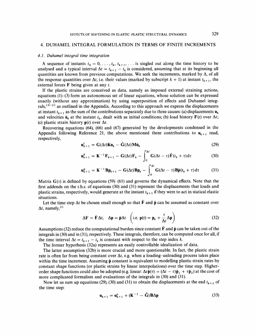
. . . is singled out along the time history to be analysed and a typical interval At = t k + l - t k is considered, assuming that at its beginning all quantities are known from previous computations. We seek the increments, marked by A, of all the response quantities over At, i.e. their values (marked by subscript k + 1) at instant t k + the external forces F being given at any t.
If the plastic strains are conceived as data, namely as imposed external straining actions, equations (1)-(3) form an autonomous set of linear equations, whose solution can be expressed exactly (without any approximation) by using superposition of effects and Duhamel integ- r a l ~ , ' ~ - ~ ' as outlined in the Appendix. According to this approach we express the displacements at instant t k + as the sum of the contributions separately due to three causes: (a) displacements uk and velocities uk at the instant t k , dealt with as initial conditions; (b) load history F(t) over At; (c) plastic strain history p(t) over At.
Recovering equations (64), (66) and (67) generated by the developments condensed in the Appendix following Reference 21, the above mentioned three contributions to uk+ read, respectively,
A sequence of instants to = 0, . . . , t k , t k +
I I : + ~ = G(At)Kuk - G(At)MUk
u,"+, = K - ' F k + , - G(At)Fk -
(29)
(30) G(At - z)F(tk + r)dz loAt Matrix G(z) is defined by equations (59)-(61) and governs the dynamical effects. Note that the first addends on the r.h.s. of equations (30) and (31) represent the displacements that loads and plastic strains, respectively, would generate at the instant t k + if they were to act in statical elastic situations.
Let the time step At be chosen small enough so that F and p can be assumed as constant over At, namely,' '
AF = FAt, Ap = PAt 1.e. p(t) = Pk + -Ap (32) ( At 9 Assumptions (32) reduce the computational burden since constant F and p can be taken out of the integrals in (30) and in (31), respectively. These integrals, therefore, can be computed once for all, if the time interval At = tk+ l - tk is constant with respect to the step index k .
The former hypothesis (32a) represents an easily controllable idealization of data. The latter assumption (32b) is more crucial and more questionable. In fact, the plastic strain
rate is often far from being constant over At, e.g. when a loading-unloading process takes place within the time increment. Assuming p constant is equivalent to modeling plastic strain rates by constant shape functions (or plastic strains by linear interpolations) over the time step. Higher- order shape functions could also be adopted (e.g. linear: Atp(z) = (At - z)pl + zpz) at the cost of more complicated formalism and evaluations of the integrals in (30) and (31).
Now let us sum up equations (29), (30) and (31) to obtain the displacements at the end t k + l of the time step:
uk+l = UE+1 + (K- ' - &)BAp (33)

330 G. MAIER AND U. PEREGO
having set
Clearly, u; + represents the displacements one would have at the dynamic d.0.f. if there were no yielding in At. The state of stress (specifically, bending moments in the critical sections) at instant t k + can be obtained by substituting equations (33) into (3) written for p = Pk + Ap:
The matrix Z transforms increments of plastic rotations into increments of moments by allowing for dynamical effects and is affected by the amplitude of the time interval At. However, like G and G it can be computed only once for all equal time steps At.
Let us suppose that the plastic flow process is regulariy progressive in At (i.e. no unloading occurs in At for a yield mode after it starts yielding at some instant in At). Then the time integration over a time step At of the constitutive plastic relations (4)-(6) is straightforward and equivalent to assuming the following stepwise-holonomic formulation or backward-difference integration scheme:"
where Yk is the vector of current yield limits at instant t k .
based on the association of two ingredients: After the above preliminary developments, any solution method of the step problem may be
(i) linear algebraic equations generated by Duhamel integrals accounting for the dynamical features and involving the whole structure regarded as purely elastic;
(ii) non-linear algebraic relations (37) and (38) generated by a stepwise-holonomic interpreta- tion of the local plastic bending behaviour and involving all the critical sections, separately.
Substituting into equation (37b) equations (37a) and (35) we achieve the finite step formulation proposed by Polizzotto,2' fully analogous to the rate formulation (17), (18) and to the quasi-static finite step formulation proposed in References 17 and 18, namely,
$ k + l = @;+I - &Ah 6 0, A1L 3 0, Cp;+lAh = O (39) Here we have set
t$;+l = NT(BTuE+, + Dp,) - Y,, A(At) s H - NTZ(At)N (40) This particular formulation is useful to the present purposes because it provides further insight into the role of softening and allows easy comparative remarks like those which follow.
4.2. Comparative remarks
Remark 10. Through the formal analogy between (39) and (17), all conclusions on extremum properties and multiplicity presented in Section 3 for the rate problem can directly be transferred to the finite increment problem, the matrix A(At) being the governing factor instead of its

EFFECTS OF SOFTENING IN ELASTIC--PLASTIC STRUCTURAL DYNAMICS 331
counterpart A,. As expected, for At + 0 equations (39) and (40) reduce to equations (17) and
$:+ , Ak = 0, which applies to each ith (i = 1, . . . , 2 m ) component in view of the sign constraints, becomes &+, ALi = 0 -+ #:i'6t + #' i '6 t2 = 0, so that ii = 0 if #: < 0 and, thus, the y poten- tially active modes and sections can be selected and only the corresponding submatrices, marked by subscript y, need be considered (in particular, D reduces to its principal submatrix Dy).
(18). In fact, as At + 0 @:+I + +k + "TBTUk6t; & + I - @k + 6 6 t ; z + D (as + K-');
Remark 11. In the finite increment formulation (39) the state of the motion at tk (and, through it, the past dynamical history) is reflected in the vector +;+ (40a), which is the main factor in the selection of the yielding modes operated by the complementarity relationship; the matrix f defined in (40b), as noted in Section 2, accounts for constitutive softening by H and for the elastic and geometric properties of the element aggregate by means of Z, which, now depends on the time step At as well.
When an approximate time-stepping marching solution is performed, f (At) instead of A,, plays the discriminant role as for possible bifurcations. Therefore, attention should be paid to two influences of the finiteness of At on A:
(i) the dependence of Z on At through the term BT(K-' - G)B additional to D in (36) and
(ii) the dependence of f on the number (say j > 0) of the yield modes potentially active in the vanishing for At + 0;
step At.
The influence (i) might be easily examined using equations (59) and (60) and expanding in MacLaurin series X(t), equation (60). As for (ii), the assumption, tacitly adopted so far for presentation simplicity, that all modes are potentially active in At (i.e. j = 2m 9 y) is untenable in numerical solutions for two reasons: first, because the size of the step problem is unnecessarily increased; second, because the properties of f which are discriminant in softening analysis may be affected (e.g. while A, is positive definite, f may be not). Therefore, the accuracy of time-stepping solutions is enhanced (and the computing effort alleviated), e.g. if one adopts the following size- reduction provision: in the current step At, as a first trial, only the J yield modes will be considered such that 2 - a, h = 1, . . . , j , a being a positive threshold; by the solution thus obtained, each neglected mode, say h', can be checked and considered in a second trial if (&+ I)h' > 0. Note that the above provision, as long as 2a < (Y: + Y;),,, rules out that yielding modes of opposite directions be considered simultaneously in the same section (an occurrence which anyway would not show up in the solution); then m 2 j (and generally j 2 y) and N in (40) becomes a diagonal matrix.
Remark 12. Suppose that the dynamic structural response can be regarded as a small amplitude motion around a pre-existing constant loaded and stressed state which intervenes in the equilibrium equations through a (constant) matrix in an additional term linear in the displacements.6 This kind of linearized geometric effect is exemplified by a beam subjected to transversal dynamic loads in the presence of axial constant loading. Such situations are implicitly covered by what precedes, provided all elastic matrices introduced in Section 2 be computed using the geometric stiffness which captures these second-order geometric effects. It is worth noting that, e.g. the matrix D is altered: in fact, it may become positive definite (stabilizing effect) or non-definite (unstabilizing effect) instead of semidefinite, with meaningful consequences on f and on its discriminant role in the sense of the remarks of Section 3.

332 G. MAIER AND U. PEREGO
Remark 13. Finally, it may be useful to compare the following square matrices, which have in common the role of elastic influence operators relating plastic rotations p in critical sections to the consequent bending moments Q there: Z, of order rn in statical situations (M = 0); Z of order rn defined by equation (36); Z, of order j d rn defined in the preceding remark 11; D of order rn defined in Section 2; D, of order y < rn, defined in Section 3 as a submatrix of D; D to be defined in Section 5, equation (43c). We may write
(41)
(42)
0 6 - - ipTZ,p < - ipTDp < - 2 P 'Dp, for any p; II - D I/ d I1 - Dyll
I( - z I / < I( - Z& - +p;zipp N - - : P p , P ,
Here 1 1 . 1 1 denotes the matrix norm, i.e. the min of its quadratic form over the set of all variable vectors of unit length. These inequalities stem from the energy meaning of the quadratic forms considered (elastic strain energy due to imposed strains in an elastic structure); equations (41 b) and (41c) are due to additional external constraints; the approximation in (42b) rests on the limit relation and the size-reduction provision pointed out in Remarks 10 and 12, respectively.
As a conclusion, from (41) and (42) we notice that both Z, and Z are by their very nature negative semidefinite, but from what precedes it seems reasonable to say, though not in rigorous terms, that Z is much stiffer than Z, and that, therefore, bifurcations can generally occur in statics for a less pronounced softening behaviour than in dynamics. Further, we can qualitatively notice that softening-induced bifurcation phenomena involve in statics the structural behaviour at a global level (through matrix Z,) while in dynamics they are mainly affected by local properties of single structural parts (through matrix D).
5. AN ALGORITHM FOR THE FINITE STEP PROBLEM
The complementarity formulation (39) entails a noteworthy coupling among the variables. Therefore, it generally turns out to be computationally unattractive, even if size-reduction provisions and efficient linear complementarity algorithms can be employed.
For the numerical solution of the problem in Section 4.1, it appears interesting (in view of its peculiar softening-related implications) to adopt here a modified Newton-Raphson strategy of iterations consisting of a linear prediction involving the whole system and a non-linear correction carried out locally in a decoupled system.
To this purpose, note first that the general mathematical model (1)-(6) set up in Section 2 for plane frame structures involves as kinematic variables only the dynamic (mass-related) d.0.f. u and the plastic generalized strains p. All other non-inertial d.0.f. could be interpreted as statically condensed to u and so far needed not be specified. Now let the mass-carrying structure (which might so far have been thought of as a one-dimensional continuum) be conceived as an aggregate of beam finite elements embodying a plastic hinge at an end node wherever required. Denoting by ii and U the vectors of condensed non-inertial and of all d.0.f. respectively, in the assembled element aggregate, we can write
U = { z ] , i i = R u + S p , Q = B T U + D p (43)
where R and S are influence matrices on ii due to u and p respectively, evaluated for the discrete model in the fictitious elastostatic states (b) and (a) of Section 2, respectively; B and D are influence matrices like B and D in equation (3), but evaluated in states (b) and (a) respectively, with fictitious constraints acting on all nodal d.0.f. in U. Clearly, these constraints induce a

EFFECTS OF SOFTENING IN ELASTIC-PLASTIC STRUCTURAL DYNAMICS 333
desirable decoupling of equation (43c), i.e. the matrices B and D are block-diagonal and diagonal respectively, each diagonal block corresponding to an element which includes a critical section.
Making use of equations (43c) and (37a), equations (37b) and (38) become
having set
A = H - N ~ D N
After the above preliminaries, the proposed solution algorithm can be concisely described as follows (the superscript r runs over the iteration sequence concerning the step At from t , to t,+ 1):
1. Initialization. Using known quantities at t k determined in the preceding step and the data
2. Prediction. Compute through equations (33) and (43a, b):
(45)
increments, compute uB+ I equation (34a) and set Ap'=O = suitable guess.
3. Correction. Generating vector uk+ by means of u;,: and iii;: from equations (46), solve the complementarity problem (44) to obtain Ak*+' and a new estimate Ap'" = NAk'+'.
4. Convergence test. If a norm (1 (uk + ),+ ' - (uk+ ), (1 is below a suitable tolerance compute the velocity uk+ as mentioned in the Appendix and go to 1 with new step data; otherwise go to 2 with new estimate Ap"'.
Remark 14. The problem size reduction proposed in Remark 11, for the reasons pointed out there, was tacitly adopted although the symbols of Section 4 were preserved for notation simplicity. Thus, in view of the basic restriction on modelling in Section 2 and of the above definition of ii, the matrices D, N, H and, hence, A in equation (45), are all diagonal of order j < rn (usually j < rn, m being the number of all critical sections). This means that, for the structural model in question, the correction phase (44) is decoupled to trivially solved complementarity problems in scalars and A l h ( h = 1, . . . , j).
Remark 15. The matrix A (not to be confused with & of Section 4) can always be made positive definite (so that equation (44) has a unique solution for any data vector) by a suitable choice of the finite element discretization. A suitable choice consists of taking each beam element which includes a softening critical section sufficiently short (and, hence, stiff ), so that snap-back within it be ruled out at yielding, see inequality (41c). Such provision is peculiar to the present softening context and, basically, exploits at the element level the size efSect on the stability of softening systems. This effect does not concern the response of the overall discrete model. However, internal instability at element level implies a fortiori instability at structural level whereas, clearly, the converse is not true.
Remark 16. Since A is definite positive, the algorithm certainly leads to a unique solution Ap for a given initial vector Ap'='. When the discriminant matrix & of Section 4, equation (40b), is not so and bifurcation is not ruled out by the criteria of Section 3, then diverse initializations are needed to generate alternative solutions to the step problem. This aspect of the present algorithm as well as its convergence and stability properties will be examined elsewhere. Our present aim is to clarify some rather anomalous aspects of dynamical simulation in the title area. To this purpose, after the preceding theoretical framework, it is useful to consider the simple examples analysed by the above procedure in Sections 6-8.

334 G. MAIER A N D U. PEREGO
6. VARIOUS SCENARIOS IN A SINGLE-DYNAMIC-D.O.F. BEAM AS ILLUSTRATIVE EXAMPLE
The (built-in ends) model of Figure l(a) referred to below exhibits the following features: constant elastic bending stiffness EJ; span 21 (AC = CB = 1); a mass M with translational (not rotational) inertia and viscous damper V located at the mid-span section C and acted up on by a load F sinof (of = 2n/T,, T, being the excitation force period).
The plastic hinge linearly-softening flexural behaviour confined to the end sections A and B is defined by the yield limits Y + = Y - = Y, the ultimate rotations p i = p , = pu, as shown in Figure l(b). The resulting hardening moduli are H + = H - = - Y/p , . Interaction (indirect hardening) between the two yielding modes is ruled out.
This elementary system with a single-dynamic d.0.f. u exhibits symmetry of data with respect to the vertical axis through C. The matrices and vectors involved in the governing relationships of Section 2 specialize as follows:
EJ[7 21 1 7 'I 24EJ 6EJ K = - p B=,-[1 11, D = - - 1 (47)
1 - 1 0
N = [ 0 0 1 - 1 i = 1 , . . . , 4 '1, H = diag [GI, YT = ( Y Y Y Y } (48)
The elastic stiffness K at C, the length I , the forcing period Tf and the ultimate rotation p , (in rad) will be used for the non-dimensional formulation which follows.
The dynamic equilibrium equation (2) divided by K1 becomes
M,u: + V,u; + u, = F , sin o f t f B,p, (49)
where subscript n marks non-dimensional quantities (u, = u/l , p, = p/p,) and the primes denote derivatives with respect to the non-dimensional time t, = t / T f . Note that K , = 1 and that the non-dimensional eigenperiod of the linear oscillator described by equation (49) is given by T,, = TE/Tf = 2n JM,/K, = 2n & T, being its dimensional eigenperiod. The non-dimen- sionalized equations (3)-(6), dividing equations (3) and (5) by KZ2/p, and setting 1, = L / p , , read
Q, = BXU, + D,p,, 9, = NTQ, - H,1, - Y, < 0
pn = Nh,, i, 3 0, +Xi,, = 0 (51)
(50)
The coefficients in equations (49) and (50) are defined as a consequence of the above non- dimensionalization to within numerical factors. These have been chosen such that
3 3 f i M,=-TL2, V,=-T; ' , Y , = - - p 2 5 24
These factors were dictated by the search for chaotic manifestations considered in Section 7 and are not meant to simulate any engineering situation.
The amplitude F , = F(KI)-' and the period Tf = 2 x / o , of the excitation force will be fixed for each case, together with the hardening modulus H, = Hp:(K12)- ' . Meaningful quantities of the beam model and natural references for non-dimensionalizations are: the displacement u, and the load F, at the elastic limit (i.e. when Q = Y at A and B in Figure 1 in the elastic regime); the eigenperiod TE = 2 x m of the free elastic vibration.

EFFECTS OF SOFTENING IN ELASTIC-PLASTIC STRUCTURAL DYNAMICS 335
Case I
In non-dimensional terms this case is characterized by: hardening H,, = - p;/30; excitation force F , = 0.06Fe ( K / ) - ’ = 00173; excitation period Tf = TE so that TEn = 1; initial conditions u,(O) = 0, uh(0) = 1.25u:,, where u:, = 1.8138 is the (non-dimensional) initial velocity which would lead to the attainment of the yield limit Y,, at A and B if it were acting alone on the linear oscillator. These values define all quantities needed for the numerical applications of the concepts and methods expounded in Sections 3-4. For instance, equations (52) directly give the non- dimensional mass and viscous damper M , and V,,, while Y, can be derived by noting that H , = - Y,, and, therefore, that one obtains pu = z,,h by comparing equation (52c) with the assumption H , = - &PI. Clearly, the resonance situation assumed in this case prevents plastic deformations from eventually ceasing (an occurrence which will be referred to henceforth as shakedown).
With the above data, matrix A,” of equation (18b) turns out to be always positive definite. Therefore, bifurcations and instabilities can be ruled out a priori (Section 3). The time integration of the governing equations (49)-(51) has been carried out by the algorithm described in Section 4, assuming a time step At = 1/300 T, (At, = 1/300).
Figure 2 depicts the time histories of displacements and plastic rotations up to failure in the sense of Section 2 (vanishing flexural strength), marked by the end dot on the graphs. The decrease of amplitude of the mass motion shown by Figure 2(a) is explained by the gradual reduction of the elastic stages of the motion compared to the intervals along which plastic hinges
1.50
1.25
-1.25 k”? 10 15 20 25 20 35 40 45 50 55 60 65 m , , , , , , . . . . , I . I , . I . I , I I . . / I I , I , I I I I , ~ I . I / I
TIME t/Tr
Figure 2. Case 1: time histories (a) of displacement at mid-span section and (b) of plastic rotations (failure is marked by a dot)

336 G. MAIER AND U. PEREGO
1.25 4 I
i ,- 0.50 Z W 0.25 I g 0.00 "-0.25 Z s-0.50 Z W-0.75 rn
- 1 .oo j L
- 1 . 2 5 ' ~ ~ ~ ~ ' ~ ~ ~ ~ I I - I 1 1 1 1 I I I I
-0102 0.00 0.62 0.64 0.06 0 PLASTIC ROTATION p/pu
Figure 3. Case 1: evolution of bending at end cross sections A and B
are active: this relative reduction make the system to go further and further away from resonance conditions. The growth of the yielding stages is evidenced by Figure 2(b). After the pronounced yielding primarily due to the impulse provided by the initial velocity, one observes in Figure 2(b) an apparent trend toward shakedown, followed by a steady amplitude increase in the oscillation of the plastic strains p = pa = pB up to failure.
The cyclic yielding in A and B with decreasing limit moments is illustrated in Figure 3 (the short increasing segments, which show up there, are due to coarse graphical recording of the output data).
Case 2
H , = - 0.135~:; p,, = F , = 0.367Fe(K1)-' = 0.106; Tf = 1.471 TE(TEn = 0.68); homogeneous initial conditions.
Owing to the system symmetry, the limit moments at A and B will be attained simultaneously so that a rate problem arises in the two variables iA and &. Using the present data, the relevant matrix A, in non-dimesional terms (subscript n) reads
A y , = H yn - D = - (53)
The matrix A,, is non-definite but it is strictly copositive (since all its entries are positive). Therefore, stability of the supporting beam is ensured.
As for the bifurcation possibility envisaged in Section 3, by the Murty theorem26 there must be a discrete number of solutions. It turns out that the rate problem (17) has now three and only three solutions. In fact, referring to the equivalent problem (24), the condition of minimum zero objective function Y,
i A & A + i B & = o (54) can be attained for: (A) iB $A = 0; (B) iA = dB = 0; (S) 4, = & = 0; (E) = iB = 0.
Since all components of 4; (as defined by equation (18a) in Section 3.1) and all entries of A, are positive in the present case, the inequality constraints imply that (A), (B) and (S) correspond to

EFFECTS O F SOFTENING IN ELASTIC-PLASTIC STRUCTURAL DYNAMICS 337
solutions of the problem and that the elastic solution (E) does not. The three solutions in terms of i,, are uniquely determined (det A,, # 0) and read (since 4EA = &zB = 4;):
There cannot be other solutions if the constraints (50b) and (5la) are obeyed, since these require each addend in equation (54) to be non-positive.
Among the three possible solutions, clearly (S) preserves the original symmetry of the structure-load system; (A) and (B) are non-symmetric (but specular to each other). The response one should expect is non-symmetric. In fact, the symmetric rate solution (S), whenever it occurs, has (A) or (B) as alternatives and leads to possible subsequent yielding situations with the same triplet of solutions. On the contrary, a non-symmetric solution (A) or (B) leads to situations where equilibrium branching cannot show up again. Moreover, a slight difference of limit moment at A and B makes (S) unattainable.
The time-stepping solution described in Section 4 has been applied assuming At = (1/300) TF and regarding the rotation a t mid-span C as a condensed d.0.f. (thus satisfying the conditions formulated in Section 4.2). As for the above envisaged multiplicity of solutions (see Remark 16), the bifurcation toward a non-symmetric response has been triggered by setting ALL== = 0 for solution (B) (ALL= = 0 for solution (A)) at the end of the correction phase in the first iteration of the first time step in the plastic range.
Figure 4 shows time histories of the displacement at the mid-point C and of the elastic energy for the structural response after a non-symmetric solution (A) has occurred at first yielding (in the latter graph one notices the sharp energy decreases due to plastic flow). Figure 5(a) represents the evolution of bending moment and plastic rotation in the cross section A during the non- symmetric response starting from the solution (A). Figure 5(b) compares the non-symmetric response (A) to the symmetric one (S) in terms of plastic strain history. It is worth noting that the former leads to failure, whereas the latter implies shakedown to an elastic periodic motion after two yielding processes.
Classijication at increasing softening
It may be interesting to regard as a control variable the slope H of the falling branch in Figure l(b), i.e. the ratio h = - H / ( E J / 2 l ) and to single out various ranges of characteristic features of
1.20 , I
- 1 20 0.0 0.5 1.0 1.5 2.0 2.5 3.0 3.5 4.0
TIME t/Tt
1 .o 0.9
0.8
0.7
0.6
0.5
0.4
0.3
0.2
0.1
0.0 0.0 0.5 1.0 1.5 2.0 2.5 3.0 3.5 4
TIME t/Tf 0
Figure 4. Case 2 time histories of (a) displacements and (b) elastic energy

338
0.6
z 2 0.4 -
v) Z
+ U I-
B-0.0 -
9 0.2 -
I!
4 c
-0.2 - a
. -0.4
G. MAIER AND U. PEREGO
i-: nonsymmetric ;
i i I I I I 6 L-2 I
I symmetric
I
I , !
4 nonsymmetrlc
(bl r 7 8 I r~
Figure 5. Case 2: (a) evolution of bending at end section A in non-symmetric response; (b) time history of plastic rotations at A and B in symmetric and non-symmetric responses
the system of Figure l(a). We consider below matrix A,, for m = 2 yield modes according to (53); bifurcation possibility for $; > 0; stability assessment. These features are as follows, respectively:
0 h < 6: positive definite (hence strictly copositive); unique symmetric incremental solution;
0 h = 6: positive semidefinite, strictly copositive; infinite bounded solutions; stable. 0 6 < h < 8: non-definite, non-singular, copositive; three solutions; stable. 0 h = 8: non-definite, singular, non-copositive; no solution; neutral. 0 h > 8: non-definite, non-singular, non-copositive; no solution; internally unstable (snap-
The above term neutral means that, at fixed mass ( z i = 0, de = 0) there is an infinity of possible configurations and of corresponding mass-beam interactions. Note that the interaction vs. displacement relationship exhibits hardening, perfectly plastic and softening behaviour for h < 2, h = 2 and h > 2, respectively.
stable.
back).
7. PERIOD DOUBLING AND CHAOS IN A HOLONOMIC VERSION OF A SINGLE-DYNAMIC-D.O.F. BEAM
The same elementary beam model of Section 6 (Figure l(a)) is reconsidered here with the following changes in the softening flexural model (Figure l(b)): the moment-plastic rotation constitutive law is assumed as holonomic (instead of non-reversible, elastic-plastic or non- holonomic); the sloping-down linear branches are no longer interrupted by local failure at zero moment.
These additional drastic idealizations make the model hardly plausible to simulate an elastic-plastic structure. However, they are not physically inconsistent (in fact, reversible soften- ing hinges at the end A and B might be materialized by suitable structural devices); their motivation rests on the fairly interesting dynamical scenarios which were found as a consequence of such idealizations.
The negative hardening modulus chosen for the plastic hinges is H, = - (9/100)p: ( p , = (25/54) f i ) which makes A,, positive definite. Therefore, when the peak moment Y is reached

EFFECTS OF SOFTENING IN ELASTIC-PLASTIC STRUCTURAL DYNAMICS 339
at both ends A and B bifurcations are ruled out and the supporting structure is stable in the dynamic sense of Section 3 (no snap-back with respect to fixed mid-point) but unstable with respect to mid-span dead loads, i.e. the reaction provided to the oscillating mass may decrease at increasing displacements. In the above conditions the system becomes a single-d.0.f. trilinear- elastic oscillator with stiffness which may become negative.
To such system, starting from homogeneous initial conditions, a harmonic excitation was applied with fixed forcing period Tf = 1.471 TE and variable amplitude F. Marching solutions obtained by the same algorithm as in Sections 4 and 6, for increasing values of the control variable F (F = F / K l being its non-dimensional value as in Section 6) yielded results partly illustrated by Figures 6-8 and outlined below.
1. F , = 0.857F,(Kl)-1 = 0.247: after the transient load died off due to damping, periodic motion with the same period Tf of the excitation.
2. F , = O.883Fe(Kl)-' = 0.255: periodic motion with double period 2Tf with respect to the forcing load (subharmonic of order 2). This subharmonic response of order 2 is illustrated by the displacement time history of Figure 6(a) and by the phase plane trajectories of Figure 6(b). In the latter figure, the transient part of the trajectory has been ignored in order to make the period doubling visually more evident.
3. F, = 0.896Fe(Kl)-' = 0259: periodic motion with period 4Tf (subharmonic of order 4). 4. F , = 0.901 Fe(Kl) - ' = 0.260: periodic motion with period 6T, (subharmonic of order 6). 5. F, = 0.903Fe(Kl)-' = 0.261: non-periodic motion, which appears to be so from the 35Tf
The chaotic nature of a motion is not easily ascertained. The case of Figure 7 was tested by
(a) Poincare map: Figure 8(a) shows the set of dots representing 1387 Poincare sections at intervals T,; typical folded shape and fractal geometry are quite apparent.
(b) Lyapunov exponent: this measure, say L, of the sensitivity to initial disturbances has been evaluated numerically as average over time intervals 0-t, by the procedure described in Reference 16. As shown in Figure 8(b), L becomes and remains positive. This occurrence reveals divergence of motion starting from slightly different conditions and, hence. the unpredictability of the dynamic response of the system.
window in the time history of Figure 7.
means of the following chaos indicator^.'^, l 6
3 TIME t/Tt
Figure 6. Holonomic case: period doubling for F = 0.883Fe. (a) Time history; (b) phase plane trajectory (steady state motion only)

340 G. MAlER AND U. PEREGO
50 .0 6 0 ' o r- I 3.0 .
3 60.0 > 2.0 2 1.0 h
0.0 F
4-1.0 20.0
3 30.0 W v
0
a g -2.0 10.0
-3.0
-4.0 0.0 0 5 10 15 20 25 30 35 0.0 0.5 1.0 1.5 2.0 2.5 3.0 3.5 4 . 0
TIME t /Tf W/Wf
Figure 7. Holonomic case: chaotic response for F = 0903F,. (a) Time history; (b) frequency spectrum of output (a)
0.2 , I
1 I
DISPLACEMENT u/u.
0.4 I
-0.4 0 3 6 9 1 2
TIME t/Tf
-o.21b, , , , , , , , , , , , ,
5
Figure 8. Holonomic case: chaotic response for F = 0.903Fe. (a) Poincare map; (b) Lyapunov exponent
(c) Frequency spectra: Fourier fast transform applied to the time history of Figure 7 leads to a broad band in the subharmonics range spectrum, with a spike at the frequency of the excitation.
(d) The above described sequence of dynamic scenarios 1-4 with ordered appearances of subharmonics at shrinking time intervals represents per se a chaos indicator; in fact, it is quite apparent it has a resemblance to a Feigenbaum route to chaos (see e.g. Reference 16), whose precise materialization in the present case is not necessary, since Feigenbaum's basic hypotheses are not fulfilled.
Deterministic chaos is often not easy to detect and, in fact, although expected for some parameter combinations, it was found only after fairly extensive parametric study. Despite the abundant recent literature on chaos (e.g. surveyed in References 15 and 16), chaotic motions due to softening in the present piecewise-linear beam model seem to be noteworthy. They will further

EFFECTS OF SOFTENING IN ELASTIC PLASTIC STRUCTURAL DYNAMICS 341
be investigated elsewhere, especially for the influence of the numerical integration scheme (see e.g. Reference 30) and possibly for chaos manifestations in other more realistic structural models exhibiting local softening behaviour (a Duffing's oscillator with softening was studied e.g. in Reference 3 1).
8. A MULTI-D.O.F. EXAMPLE: SHEAR MODEL OF A FRAME STRUCTURE SUBJECTED TO SEISMIC EXCITATION
A four-storey, reinforced concrete building frame has been considered, with the layout and the sectional geometries and material properties assumed in Reference 32, where its design according to seismic codes and its limit analysis under static-equivalent earthquake loadings were pre- sented. For the present purposes of dynamic analysis, a conventional shear model is chosen. This means that the horizontal girders (at slab levels) are assumed as rigid and endowed with concentrated masses, and the columns as inertialess and deformable in bending with plastic strains modelled according to the plastic hinge hypothesis.
Figure 9 shows: (a) the overall geometry and the 24 critical sections at the column ends; (b) the plastic hinge behaviour assumed as equal in the two directions (the cross sections of the columns exhibit symmetry of shape and reinforcement), with non-interactive hardening-softening yield modes in each quadrant, which follow the empirical assumptions in Reference 10 and drastically idealize experimental data presented in Reference 33 (effects of flexural softening idealizations are discussed e.g. in Reference 34, while simplified models of softening flexure can be found in Reference 35). Note that bilinear rather than linear hardening is assumed here (as in Reference 10) for each yield mode; (c) the recorded accelerograph of an earthquake (Friuli 1976) used for the input ground motion. The resulting numerical data for the floors from i = 1 to 4 (top) are, respectively (equal for the columns of each floor):
elastic bending stiffness EJ' (in Nm2 x lo3): 272, 156, 102, 36; yield moment Y' (in Nm x lo3): 550, 310, 170, 110; softening hinge modulus H i (in kNm x lo3): 150, 110, 70, 34. mass M i (in kg x lo3): 40, 16, 16, 11 , associated with zero damping.
In all critical sections the hardening branches (see Figure 9(b)) are defined by the hardening coefficient HI = 100 kN m and by the rotation pm = 0.01 rad corresponding to the maximum bending moment.
In the above described model of the structural system in point, all columns exhibit symmetry with respect to the relevant mid-section and, hence, antisymmetric deformations and bending moment distributions, as long as the (local) flexural behaviour is stable. However, the softening branch in the local deformability model may lead to bifurcations or instability in the sense of Section 3. In fact, with the present data, a preliminary study of the rate problem of Section 3 for each column (similar to that in Section 6) rules out instability but predicts the possibility of three rate solutions: one (symmetric) with equal and opposite plastic flow at both ends; two (non- symmetric) with yielding at either end only. Note that the rigid slab assumption implies a decoupling between columns as for the matrix D, so that the matrix A,, is block-diagonal with blocks of order not larger than 2 since two yield modes at most are simultaneously active in each column.
In view of this circumstance, two dynamic analyses have been carried out on the basis of the above specified data, using the precedure described in Section 4 (with At = 11300 of the fourth eigenperiod) by initializing the iterative algorithm in two distinct ways: (a) the initial plastic multiplier A 1 is assumed zero at the lower end and positive at the upper end of each column, in

342 G. MAIER AND U. PEREGO
3.0 - A Q
“0 2.0
2 1.0 v
z 0.0 t- lx W _I w -2.0 V V
-Y -3.0
b 0 P m PY P 4 -1.0
-4.0 (b) 0.0 1.0 2.0 3.0 4.0 5.0 6.0
TIME (sec)
Figure 9. Shear model of reinforced concrete frame: (a) geometry and critical sections; (b) plastic flexural behaviour; (c) earthquake excitation
order to foster possible non-symmetric solutions; (B) with A2 = 0 at both ends. Clearly, as numerically checked, both initializations lead to the same results as long as the incremental solution is unique.
Figure 10(a) shows the time history obtained by the provision (a), for the displacement of the girder over the third floor (marked in Figure 9(a)). The dot at the end means local failure in the

EFFECTS OF SOFTENING IN ELASTIC PLASTIC STRUCTURAL DYNAMICS 343
- 7.0 0 - 7 I - c D -
6.0 -
v r . 2 - 0
5.0 - Q - I - - 0 . [ r -
0 4.0 - F : -
nonsymmatric v -
Figure 10. Responses of frame model: (a) time history of displacement at 3d slab (b) yielding evolutions of ends of column 17-18 after bifurcation
sense of Section 2 (because of damage up to vanishing bending strength). Figure 10(b) provides details on the plastic rotation histories just before and after the failure instant at t = 5.2 sec. The non-symmetric response, obtained by procedure (a), is illustrated by the dashed line which represents the plastic rotations (positive means tensile strains on the right) at the upper ends of the columns at the third floor and by the dashed-dotted line which represents those at lower ends (positive if tensile strains on the left). The solid line depicts the alternative results obtained by procedure (b), namely the symmetric response implying equal (but opposite) rotations at the two ends of floor 3. It is worth noting that, whereas the former non-symmetric (a) response predicts local failure, the latter (p) predicts shakedown (at least over the time interval examined). The non- symmetric response, whenever it becomes possible, exhibits stability with respect to perturbations for the same reasons discussed with reference to the beam model in Section 6.
9. CLOSING REMARKS
The findings of the foregoing study can be summarized as follows.
(a) Conventional models with concentrated masses for the dynamic elastic-plastic, small- deformation analysis of structures (here specifically plane frames) in the presence of softening iocal plastic (flexural) behaviour may exhibit peculiar features and require caution and special provisions owing to possible effects of softening on the computed overall response.
(b) The main possible consequences of local softening are: (i) bfircations of the equilibrium path of the structure supporting the masses and hence, alternative dynamic evolutions obtainable for the same load history; (ii) intrinsic (snap-back) instability of the supporting structure, and consequent discontinuity in time of the deformation and stress histories. Both these manifestations of softening can be conveniently examined by a rate formulation in terms of a linear complementarity problem (or quadratic, generally non-convex, program). This problem is defined by a vector which depends on the velocities of the masses and by a matrix A, which depends on the hardening or softening moduli of the active yield modes (current plastic hinges) and on influence coefficients of the structure assumed as elastic with fixed masses. This circumstance (fixed masses) makes the onset of bifurcation or instability

344 G. MAIER AND U. PEREGO
and, hence, the computed dynamic evolution, extremely sensitive to the modelling of the mass distribution and the inertial effects.
(c) When alternative incremental solutions become possible, the one which would be the unique solution in the absence of softening (i.e. for perfect or hardening plasticity) may turn out to be so sensitive to perturbations (as in the examples of Sections 6 and 8) that it should be ruled out in favour of one of the bifurcated solutions (the non-symmetric solutions in our examples). This circumstance, combined with that pointed out at the end of the preceding remark (b), confers a noteworthy subjectivity to the results of dynamic analyses based on conventional structural models, with concentrated masses, whenever such models entail bifurcation possibility due to softening (i.e. non-positive semidefinite matrices A,, Section 3). Therefore, unstable constitutiue laws for local deformability require structural models with spread inertia and consistent masses in order to confer to dynamic analyses the same degree of predictive objectivity they exhibit with stable constitutions.
(d) For the time integration of the (non-linear differential) relations governing dynamical systems with constitutive softening, a Duhamel integral approach advantageously permits one to preserve in the finite step problem (in At) essential features of the rate (dt) problem. The main feature is the linear complementarity in the case of piecewise-linear plastic laws. The advantage is that a matrix A(At) , basically consisting of quantities computed once for all equal intervals At, permits one to detect and assess the softening effects mentioned in what precedes in the same fashion as by matrix A, (to which it reduces for At -, 0), provided At be sufficiently small and a suitable size reduction is performed in formulating the step problem.
(e) An iterative predictor-corrector method for solving the Duhamel-formulated step problem has been developed which relegates all non-linear computations to local level (with expected advantages over quadratic programming algorithms proposed in Reference 21). However, though based on a conventional strategy, this method exhibits peculiar softening- related features.
( f ) When the local softening behaviour is assumed as non-linear elastic or holonomic, then the response to periodic excitations may exhibit pre-chaotic phenomena (such as subharmon- ics) and chaotic features (non-periodicity, unpredictability). Such constitutive modification (Section 7) is clearly unrealistic from a structural engineering standpoint. However, it provides, in a sense, a way to relate the present findings concerning softening effects on elastoplastic dynamics to deterministic chaos as a time1.y topic in the broader context of non-linear dynamics (see e.g. Reference 37).
The limitation of the present study to a restricted category of dynamic structural models (plane frames with lumped masses and linearly-softening plastic hinges) can be relaxed to broader categories by formal rather than conceptual complications.
A number of mechanically more important questions remain open and are meant to be pursued elsewhere. These include: the resolution, in terms of computational efficiency, of the trade-off between the advantages, observed in the specific present context, of the Duhamel integral formulation and its general disadvantages caused by limitation to geometric linearity and preliminary modal analysis (though the latter burden can be alkviated as shown in Reference 36); the correlation, as for predictive capacity in the presence of softening, between continuum and discrete models, with regard to both the space and time discretization; the possible unpredict- ability due to softening of, say, residual displacements in elastic-plastic dynamics under impulsive loading as a counterpart, in the present context, to Symonds’ counterintuitive dynamic behaviours and to the chaotic motions in softening holonomic models noticed in Section 7.

EFFECTS OF SOFTENING IN ELASTIC-PLASTIC STRUCTURAL DYNAMICS 345
ACKNOWLEDGEMENTS
The authors wish to express their gratitude to Professor P. S. Symonds for having inspired this work and for useful discussions, to the Division of Engineering of Brown University (where this study was partly carried out) for hospitality in the summers of 1987 and 1990, to Dr G. Borino for making available his software and to their former student G. Calabrese for assistance in computations. The results presented in this paper were obtained in the course of a research sponsored by CNR-GNDT.
APPENDIX
An outline of the Duhamel integral approach to elasto-dynamic analysis
We rewrite below for convenience the relations (1) and (2) which govern the linear elastic dynamic response of discrete structural model of frames (Section 2) to given external loads F ( t ) and to plastic strains p ( t ) conceived as imposed variable dislocations. Assume to know at an instant tk, the displacement uk and velocities uk pertaining to the n dynamic degrees of freedom of the system
(55)
U(tk) = uk, u(tk) uk (56)
MU(t) + V u ( t ) + Ku(t ) = F(t) + Bp(t )
A Duhamel integral method for integrating in time equations (55)-(57) is outlined here, in view of its extension to plastic dynamics developed in References 21 and 22 and adopted to the present purposes in Section 4.
Let @ denote the matrix collecting as columns the II displacement mode-shape vectors and R the diagonal matrix of the relevant eigenfrequencies mi (i = 1, . . . , n, n being the number of dynamical d.0.f.). As usual in structural dynamics (e.g. Reference 38), we assume that
QTM@ = I (57)
mTV@ = diag [I2 [iOi] (58) i
where ii is the damping ratio corresponding to the ith mode. Equation (58) defines these ratios, equation (57) normalizes the eigenvectors.
New symbols are now introduced as follows:
oi = U l i J r n (59)
G(7) = @X(7)QT (61) In view of the linearity of the problem (55), (56), the displacement vector u at an arbitrarily
(a) displacements u1 associated with the free vibration due to the initial conditions uk, u,, setting F ( t ) = 0 and p ( t ) = 0 in equations (55);
(b) displacements u f , pertaining to the forced motions due to loads F ( t ) alone ( p = 0), applied over the interval At = tk+ - t , , with homogeneous initial conditions at tk (uk = 0, u, = 0);
assigned instant, say tk+ can be obtained by the superposition of the following effects:
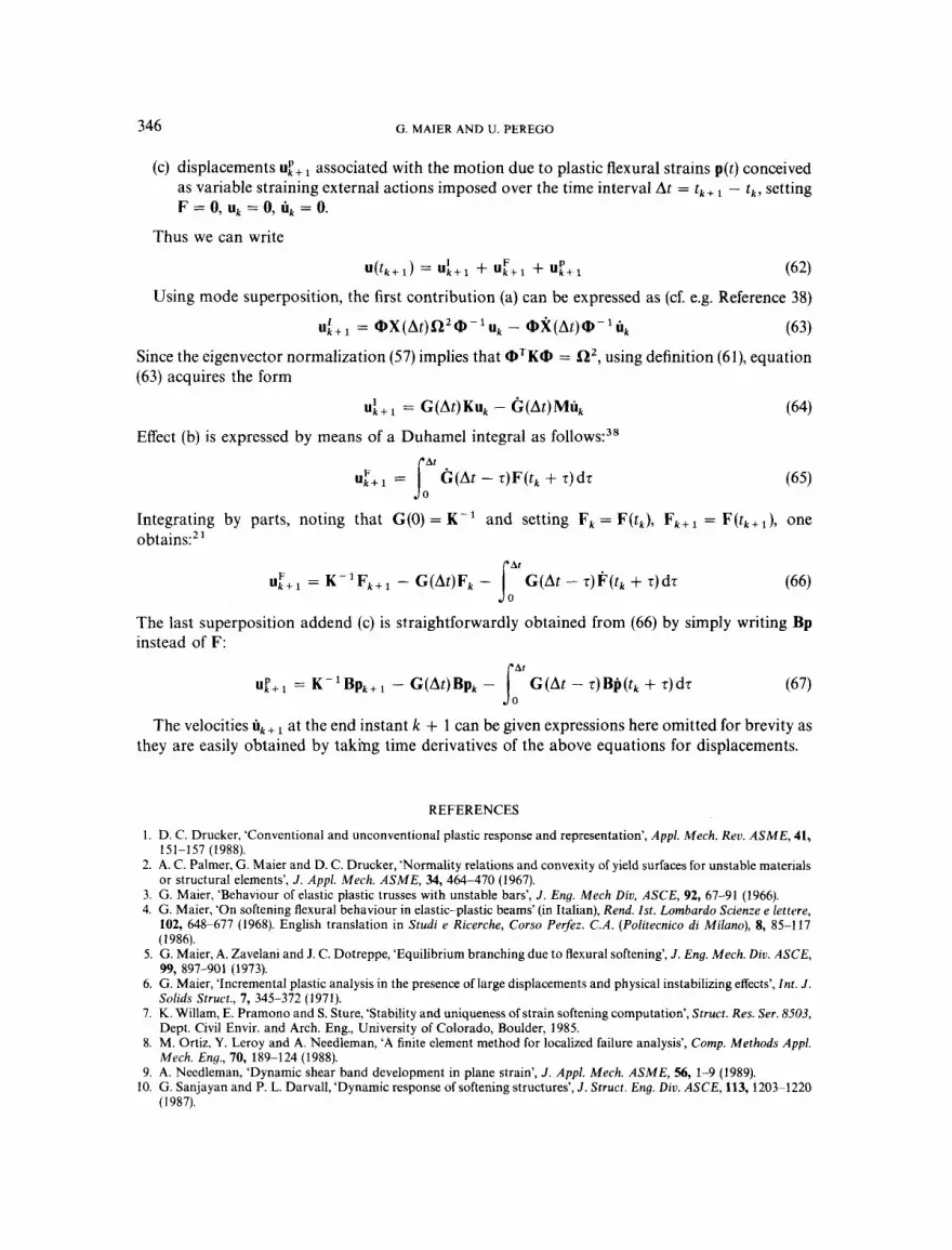
346 G. MAIER AND U. PEREGO
(c) displacements ukp+ associated with the motion due to plastic flexural strains p(t) conceived as variable straining external actions imposed over the time interval At = t k + - t k , setting F = 0, uk = 0, 8, = 0.
Thus we can write
u ( t k + l ) = uL+l + ukF+l + 1 (62)
(63) Since the eigenvector normalization (57) implies that @‘K@ = a’, using definition (61), equation (63) acquires the form
(64)
Using mode superposition, the first contribution (a) can be expressed as (cf. e.g. Reference 38)
U i + l = @ X ( A t ) f i ’ @ - l U k - @k(Al’)@-’Uk
u : + ~ = G(At)Kuk - G(At)MIlk
Effect (b) is expressed by means of a Duhamel integral as follows:38
Integrating by parts, noting that G(0) = K - ’ and setting F, = F(tk), Fk+l = F(tk+l) , one obtains:’ ’
U c + l = K - ’ F k + ’ - G(At)Fk - G(At - T ) P ( t k + t ) d ~ (66) loAf
JoAf The last superposition addend (c) is straightforwardly obtained from (66) by simply writing B p instead of F:
U p + 1 = K-’Bpk+, - G(At)Bpk - G(At -- T)BP(tk + T)dT (67)
The velocities u k + at the end instant k + 1 can be given expressions here omitted for brevity as they are easily obtained by taking time derivatives of the above equations for displacements.
REFERENCES
1. D. C. Drucker, ‘Conventional and unconventional plastic response and representation’, Appl . Mech. Rev. A S M E , 41,
2. A. C. Palmer, G. Maier and D. C. Drucker, ‘Normality relations and convexity of yield surfaces for unstable materials
3. G. Maier, ‘Behaviour of elastic plastic trusses with unstable bars’, J . Eng. Mech Diu. ASCE, 92, 67-91 (1966). 4. G. Maier, ‘On softening flexural behaviour in elastic-plastic beams’ (in Italian), Rend. 1st. Lombardo Scienze e letture,
102, 648-677 (1968). English translation in Studi e Ricerche, Corso Perfez. C.A. (Politecnico di Milano), 8, 85-1 17 ( I 986).
5. G. Maier, A. Zavelani and J. C. Dotreppe, ‘Equilibrium branching due to flexural softening’, J . Eng. Mech. Diu. ASCE,
6. G. Maier, ‘Incremental plastic analysis in the presence of large displacements and physical instabilizing effects’, Int. J .
7. K. Willam, E. Pramono and S. Sture, ‘Stability and uniqueness of strain softening computation’, Struct. Res. Ser. 8503,
8. M. Ortiz, Y. Leroy and A. Needleman, ‘A finite element method for localized failure analysis’, Comp. Methods Appl.
9. A. Needleman, ‘Dynamic shear band development in plane strain’, J . Appl. Mech. ASME, 56, 1-9 (1989).
151-157 (1988).
or structural elements’, J . Appl. Mech. ASME, 34, 464-470 (1967).
99, 897-901 (1973).
Solids Struct., 7, 345-372 (1971).
Dept. Civil Envir. and Arch. Eng., University of Colorado, Boulder, 1985.
Mech. Eng., 70, 189-124 (1988).
10. G. Sanjayan and P. L. Darvall, ‘Dynamic response of softening structures’, J. Struct. Eng. Diu. ASCE, 113,1203-1220 ( I 987).

EFFECTS OF SOFTENING IN ELASTIC-PLASTIC STRUCTURAL DYNAMICS 347
11. P. S. Symonds and T. X. Yu, ‘Counterintuitive behaviour in a problem of elastic-plastic beam dynamics’, J . Appl. Mech. ASME, 52, 517-522 (1985).
12. G. Borino, U. Perego and P. S. Symonds, ‘An energy approach to anomalous damped elastic-plastic response to short pulse loading’, J . Appl. Mech. ASME, 56, 430-438 (1986).
13. P. S. Symonds, U. Perego, G. Borino and F. Genna, ‘Anomalous elastic-plastic response to short pulse loading-An outline of recent progress’, in U. Andreaus et al. (eds.), Omaggio a Giulio Ceradini, Dip. Ing. Strutt. Geotecnica, Uniuersita di Roma, Rome, 1988, pp. 641-648.
14. D. Capecchi and F. Vestroni, ‘Steady state dynamic analysis of hysteretic systems’, J . Eng. Mech. Diu. ASCE, 111,
15. J. M. T. Thompson and H. B. Stewart, Nonlinear Dynamics and Chaos, Wiley, Chichester, U.K., 1986. 16. F. C. Moon, Chaotic Vibrations, Wiley, Chichester, U.K., 1987. 17. G. Maier, ‘A matrix structural theory of piecewise-linear plasticity with interacting yield planes’, Meccanica, 5, 55-66
18. 0. De Donato and G. Maier, ‘Mathematical programming methods for the inelastic analysis of reinforced concrete
19. V. N. Shah, G. J. Bohm and A. N. Nahavardi, Modal superposition method for computationally economical
20. J. A. Stricklin and W. E. Haisler, ‘Formulations and solution procedures for nonlinear structural analysis’, Comp.
21. C. Polizzotto, ‘Elastoplastic analysis method for dynamic agencies’, J . Eng. Mech. Diu. A X E , 112, 293-310 (1986). 22. G. Borino and C. Polizzotto, ‘A mathematical programming approach to dynamic elastoplastic structural analysis’,
23. J. B. Dantzig and R. W. Cottle, ‘Positive (semi-)definite programming’, in J. Abadie (ed.), Nonlinear Programming,
24. H. P. Kunzi and W. Krelle, Nonlinear Programming, Blaisdell, New York, 1966. 25. M. Z. Cohn and G. Maier, Engineering Plasticity by Mathematical Programming, Pergamon Press, New York, 1979. 26. K. G. Murty, ‘On the number of solutions to the complementarity problem and the spanning properties of
27. R. Hill, ‘A general theory of uniqueness and stability in elastic-plastic solids’, J . Mech. Physics Solids, 6, 236-249
28. Z. P. Bazant and L. Cedolin, Stability ofstructures, Oxford University Press, Oxford, 1991. 29. G. Maier, ‘Some theorems for plastic strain rates and plastic strains’, J . Mhcanique, 8, 5-19 (1969). 30. B. H. Tongue, ‘Characteristics of numerical simulations of chaotic behaviour’, J . Appl. Mech. ASME, 54, 695499
31. B. A. Huberman and J. P. Crutchfield, ‘Chaotic states of anhormonic systems in periodic fields’, Phys. Rev. Lett., 43,
32. V. Franciosi, Structural Mechanics, Vol. I V, Limit Analysis (in Italian), Liguori, Napoli, 1974. 33. E. Giuriani and G. Rosati, ‘Experiments on reinforced concrete elements and falling-down branches in
moment-rotation relationship’ (in Italian), in Studi e Ricerche, Corso Perfez. C.A. (Politecnico di Milano), 6, 151-201 (1984).
34. Z. P. Bazant, G. Pijaudier-Cabot and J. Pan, ‘Ductility, snap-back, size effect and redistribution in softening beams or frames’, J . Struct. Eng. Diu. ASCE, 113, 2348-2364 (1987).
35. L. Biolzi, ‘Flexure of beams with elastic-softening behaviour’, Solid Mech. Arch., 13, 177-191 (1988). 36. G. Muscolino, ‘Mode-superposition methods for elastoplastic systems’, J . Eng. Mech. Diu. ASCE, 115, 2199-2215
37. W. Szempliska-Stupnicka, ‘Bifurcations of harmonic solutions leading to chaotic motion in the softening type
38. R. W. Clough and J. Penzien, Dynamics ofStructures, McGraw-Hill, New York, 1975.
1515-1531 (1985).
(1970).
frames allowing for limited rotation capacity’, Int. j . numer. methods eng., 4, 307-329 (1972).
nonlinear structural analysis’, J . Press. Vess. Technol. ASME, 101, 134-141 (1979).
Struct., 7 , 125-136 (1977).
Meccanica, 23, 11-19 (1988).
North-Holland, Amsterdam, 1967.
complementary cones’, Linear Algebra Applic., 5, 65-108 (1972).
(1958).
(1987).
1743-1746 (1979).
(1989).
Duffing’s oscillator’, Int. J . Non-linenr Mech., 23, 257-277 (1988).


