Filter Tests In Nasdaq Stocks

Financial The Review

EFA Eastern Pinance

Association The Financial Review 34 (1999) 45-70

Filter Tests In Nasdaq Stocks Andrew Szakmary*

Wallace N. Davidson III

Thomas V. Schwarz Southern Illinois University

Amturf

~~ ~

Abstract

This study examines the performance of filter and dual moving-average crossover trading rules applied to Nasdaq stocks. We find that trading rules conditioned on a stock's past price history perform poorly, but those based on past movements in the overall Nasdaq Index tend to earn statistically significant abnormal returns. Since there is a high level of transaction costs in this market, these abnormaI returns are generally not economically significant. However, there are indications that pursuing some of these strategies can be worthwhile in carefully selected subsets of stocks.

Keywords: market efficiency, filter tests, Nasdaq JEL classification: G14

1. Introduction

Most financial researchers conclude that the stock market is at least weak-form efficient (Fama, 1991). Weak-form efficiency assumes that excess profits cannot be earned from the knowledge of past and current security prices. Once transaction costs are included, most weak-form tests fail to find opportunities for excess profit.

One test of weak-form efficiency is a filter-rule test. A filter is often described as a trading rule that signals a buy when the market price of a stock rises X% and a sell when the price falls by X%. A filter rule is profitable if stock prices follow a pattern. Alexander (1961, 1964) finds in tests of the Dow Jones Industrial Average

*Corresponding author: Department of Finance, Southern Illinois University, Carbondale, IL 62901; Phone: (618) 453-2459, Fax: (618) 453-5626, E-mail: [email protected]

45

46 A. Szakmary, W.N. Davidson, T.V. SchwardThe Financial Review 34 (1999) 45-70

(DJIA) and Standard & Poor Industrials, that filters outperform simple buy-and- hold strategies. Fama and Blume (1966), by correcting for dividend payments, find that excess profits from filter trading strategies are so small that they disappear, even for floor traders, once transaction costs are considered.

In more recent tests, Sweeney (1988) and Corrado and Lee (1992) find that there is a potential for excess profits from filter tests. Sweeney retests the Fama and Blume (1966) DJIA stocks in a later time period and determines that a floor trader can make excess profits of just under 2% per year. Corrado and Lee, using 120 firms from the Dow Jones and S&P 100, find that filter rules can earn excess profits, but that these profits disappear when transaction costs are approximately 12 basis points.

We re-examine the filter-rule results on a sample of Nasdaq traded stocks. Our use of Nasdaq stocks is motivated by the small-firm effect, which has been well documented but only partially explained in the extant literature (Reinganum, 1981; Roll, 1981, 1983; Lustig and Leinbach, 1983; Schultz, 1983; Stoll and Whaley, 1983; Booth and Smith, 1985, 1987). For example, Kester (1990) demonstrates that small-firm stocks “. . . offer more profitable opportunities for market timing than large-firm stocks.”

One explanation for the small-firm effect is that these firms are neglected by analysts and thus could offer a premium to those willing to investigate them (Arbel, Carvell, and Strebel, 1983; Arbel and Strebel, 1983). Further, the lack of competition in Nasdaq securities may increase the volatility of their spreads (Christie, Harris, and Schulz, 1994; Lau, McCorry, McInish, and Van Ness, 1996).

Most filter-rule studies focus on the Dow Jones 30 or other large-firm stocks, which may be some of the best covered f m s in the market. Our tests are motivated by the potential for trading profits that may exist in smaller or more neglected firms’ stocks. We propose to test for the potential for excess profits using various filter strategies on smaller firms that do not trade on the floors of organized exchanges.

Section 2 describes our sample selection and data analysis technique. Section 3 presents our filter rule and dual moving-average results. In Section 4, we present results for related issues such as the inclusion of transaction costs, the inclusion of firm characteristics, stability of our results across time, and the impact of nonsynchronous information on our results.

2. Procedures for evaluating trading rule returns

2. I. Sample selection

For our tests, we examine the stocks on the Nasdaq CRSP tapes. We select all stocks that are continuously traded on the CRSP tapes from January 1, 1973 to December 31, 1991 and that are not missing any observations. This gives us a sample of 149 f m s .

A. Szakmary, W.N. Davidson, T.V. SchwardThe Financial Review 34 (1999) 45-70 47

To assess whether the profitability of technical trading rules has changed over time as the Nasdaq has matured, we divide our sample into two relatively equal subperiods (January 1, 1973 to June 30, 1982 and July 1, 1982 to December 31, 1991) and also report results for these subperiods. In addition, we re-estimate our results without October 1987 (the crash), and find that the results are not markedly different from those for the full sample. We also re-estimate the returns, deleting January of each year. Once again, our results are qualitatively similar to those of the full sample period.

2.2. Trading rules

Following Sweeney (1988) and Corrado and Lee (1992), we do not take short positions in stocks. All of the trading rules are therefore either “in” (long position) or “out” (neutral) of a stock on any given day.

We use four types of trading strategies. The first is an own-stock filter. Here, we base our buylsell decisions on a stock on the price movement in that stock. We use seven own-stock filter sizes, 0.5%, I%, 2%, 5%, lo%, 20%, and 50%.

The second strategy is a Nasdaq Index filter. In this strategy, we base our buy/ sell decisions in a stock on movements in the Nasdaq Index. We use seven Nasdaq Index filter sizes, 0.25%, 0.5%, 1%, 2%, 5%, lo%, and 20%.

The third strategy is an own-stock dual-moving-average rule, drawn from Brock, Lakonishok, and LeBaron (1992). In a dual-moving average, a buylsell decision occurs from monitoring two moving averages of stock prices. One is a short-term average, and the second long-term. In this strategy, a buy signal occurs when the short-term moving average rises above the long-term moving average. A sell signal occurs when the short-term moving average falls below the long-term moving average. Brock, Lakonishok, and LeBaron (1992) state that “When the short-period moving average penetrates the long-period moving average, a trend is considered to be initiated.”

In an own-stock moving average, we base our moving averages on the stock‘s own prior prices. The dual-moving-average buy signal for a strategy of say, 1/50, triggers a stock purchase when, on day t, the stock’s price is above the average of the last 50 days’ (t - 49 to t) prices. The stock is sold when the price on day t falls below the average on days t - 49 to t. We use the same five moving-average specifications as in Brock, Lakonishok, and LeBaron (1992): 1/50, 1/150,5/150, 1/ 200, and 21200.

Our final strategy is the Nasdaq Index dual-moving average. Here, we base our buy/sell decision on a stock on short- and long-term moving averages of the Nasdaq Index. For the Nasdaq Index dual-moving-average strategy of 1/50, we buy a stock if the value of the Nasdaq Index on day t is above the Index’s average on day t - 49 to day t. We sell the stock when the value of the Nasdaq Index on day t falls below the average for Days t - 49 to day t. Again, we use the moving-average specifications, 1/50, 1/150, 5/150, 1/200, and 2/200.


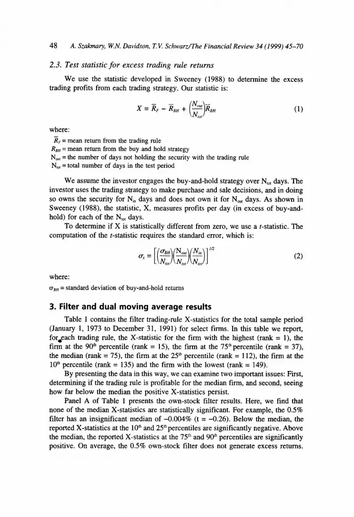
2.3. Test statistic for excess trading rule returns

trading profits from each trading strategy. Our statistic is: We use the statistic developed in Sweeney (1988) to determine the excess

where:

RBH = mean return from the buy and hold strategy No", = the number of days not holding the security with the trading rule N,, =total number of days in the test period

RF = mean return from the trading rule

We assume the investor engages the buy-and-hold strategy over N,,, days. The investor uses the trading strategy to make purchase and sale decisions, and in doing so owns the security for N, days and does not own it for No,, days. As shown in Sweeney (1988), the statistic, X, measures profits per day (in excess of buy-and- hold) for each of the N,,, days.

To determine if X is statistically different from zero, we use a t-statistic. The computation of the t-statistic requires the standard error, which is:

where: uBH = standard deviation of buy-and-hold returns

3. Filter and dual moving average results Table 1 contains the filter trading-rule X-statistics for the total sample period

(January 1, 1973 to December 31, 1991) for select firms. In this table we report, foreeach trading rule, the X-statistic for the firm with the highest (rank = l), the firm at the 90" percentile (rank = 15), the firm at the 751hpercentile (rank = 37), the median (rank = 75), the firm at the 25" percentile (rank = 112), the firm at the lo* percentile (rank = 135) and the firm with the lowest (rank = 149).

By presenting the data in this way, we can examine two important issues: First, determining if the trading rule is profitable for the median firm, and second, seeing how far below the median the positive X-statistics persist.

Panel A of Table 1 presents the own-stock filter results. Here, we find that none of the median X-statistics are statistically significant. For example, the 0.5% filter has an insignificant median of -0.004% (t = -0.26). Below the median, the reported X-statistics at the 10" and 2Sh percentiles are significantly negative. Above the median, the reported X-statistics at the 751h and 90" percentiles are significantly positive. On average, the 0.5% own-stock filter does not generate excess returns.

A. Szakrnary, WN. Davidson, T.V. SchwardThe Financial Review 34 (1999) 45-70 49

As the filter size increases, the highest X-statistic decreases monotonically. The size of X-statistic for the 75" and 901h percentile firms decreases monotonically for increasing filter sizes after the 1% filter.

Panel B of Table 1 shows the X-statistics using the Nasdaq Index filters. Here, we find that for 5% and smaller filters, the medians are significantly positive and remain positive down to loth percentile for 2% and smaller filters. As the filter size increases, the median X-statistic decreases monotonically. Smaller filters outperform the larger filters, and the Nasdaq Index filters outperform the own-stock rules.

Panel A of Table 2 shows the own-stock dual-moving-average X-statistics. We report the same five model specifications as in Brock, Lakonishok, and LeBaron (1992). For these five models, the median X-statistics are statistically insignificant. The own-stock dual-moving-average filter rules do not produce excess returns.

Panel B of Table 2 presents the Nasdaq Index dual-moving-average results. The first two models, 1/50 and 1/150, produce significant median X-statistics. The 1/50 model produces significant X-statistics down to the 25" percentile. With dual- moving-average tests, as with the filters, the Nasdaq Index models outperform the own-stock models.

We divide our sample into two relatively equal time periods, January 1, 1973 to June 30, 1982 and July 1, 1982 to December 31, 1991. For each time period, we recompute the results reported in Table 1. Tables 3 and 4 contain the results for the earlier time period and Tables 5 and 6 show the later time period results.

Panel A of Table 3 shows that in the early time period, own-stock filters from 0.5% to 5% have significant median X-statistics and filters from 0.5% to 2% produce significant X-statistics down to at least the 25" percentile. Panel A of Table 5 shows that in the later time period these filters lose at the median. Filters from 0.5% to 2% have significantly negative median X-statistics.

Panel B, Table 3, shows that for the Nasdaq Index filters, the early-time-period filters produce significantly positive median X-statistics for filters from 0.25% to 5%. Here, the 0.25% to 10% filters produce significantly positive results down to at least the 1Oth-percentile firm.

In Panel B, Table 5, which shows the later time period, Nasdaq Index filters continue to produce positive median X-statistics for the 0.25% to 2% filters. How- ever, the size of the median and 2Sh-percentile firm X-statistics are generally smaller in the later time period. For example, the 2% filter median X-statistic is 0.046% (t = 1.76) in the later period, but is 0.077% (t = 3.29) in the earlier period. The gains from the Nasdaq filter decline in the second half of the sample period.

Panel A of Table 4 and Panel A of Table 6 show that the own-stock dual- moving-average models do not produce significant medians in either time period. However, Panel B of Table 4 shows that the 1/50 and 1/150 Nasdaq Index dual- moving-average models produce significant median X-statistics. The results in Panel B of Table 6 indicate that the X-statistics generally decline in the later time period. Here, the median is not significant for the 1/150 model, and it is only significant

Tabl

e 1

Filte

r ru

le X

-sta

tistic

s: fu

ll s

ampl

e pe

riod

(VW

3 -

12B

1/91

) T

he n

umbe

r in

each

cel

l rep

rese

nts t

he X

-sta

tistic

dev

elop

ed b

y Sw

eene

y (1

988)

that

mea

sure

s exc

ess r

etur

ns fr

om tr

adin

g st

rate

gies

. In

this

tabl

e w

e m

easu

re

tradi

ng s

trat

egie

s bas

ed o

n fi

lter r

ules

. For

thes

e te

sts

the

filte

r rul

es ta

ke o

nly

long

or

neut

ral p

ositi

ons

(no

shor

t sal

es).

We

use

filte

rs b

ased

on

own-

stoc

k pr

ice

mov

emen

ts (P

anel

A)

and

Nas

daq

Inde

x pr

ice

mov

emen

ts (P

anel

B).

The

figu

re in

par

enth

eses

is th

e r-

stat

istic

that

mea

sure

s th

e st

atis

tical

sign

ifica

nce

of t

he X

-sta

tistic

s.

VI

0

Perf

orm

ance

Per

cent

iles

Acr

oss

Cro

ss-S

ectio

n of

Sto

cks

Trad

ing

Rul

e TV

De:

Low

est

l(yh

25"

Med

ian

75'h

90"

Hig

hest

Pane

l A:

Ow

n-St

ock

Filt

ers

0.5%

1%

2%

5%

10%

20%

50%

-0.5

54%

***

(-16.

25)

-0.5

62%

***

(-16.

07)

-0.5

60%

***

(-15.

16)

-0.5

49%

***

(-11.

39)

-0.4

72%

***

(-8.5

9)

-0.3

61%

***

-0.0

88%

***

(-7.3

1)

(-3.2

1)

-0.1

62%

***

-0.1

59%

***

(-8.7

8)

(-8.6

6)

-0.1

58%

***

(-8.4

7)

-om

s%**

* (-5

.42)

-0

.044

%**

* (-2

.35)

-0

.038

%**

(-2

.19)

-0

.021

%

(-1.6

4)

-0.0

83%

***

(-4.

76)

-0.0

86%

***

(-4.

73)

-0.0

75%

***

(-3.9

1)

-0.0

37%

(-1

.60)

-0

.015

%

(-1.0

8)

-0.0

20%

(-1

.32)

-0

.008

%

(-0.5

4)

-0.0

04%

(-0

.26)

-0

.009

%

(-0.4

7)

-0.0

01%

(-0.04)

0.01

2%

(0.9

5)

-o.O

Oo%

(-0

.02)

-0

.005

%

(-0.2

8)

0.00

4%

(0.3

2)

0.06

0%**

* (3

.76)

0.

066%

***

(3.7

1)

0.05

8%**

* (3

.97)

0.

036%

**

(2.3

6)

0.01

9%

(1.0

3)

0.00

9%

(0.5

2)

0.01

3%

(1.0

2)

0.11

3%**

* (7

.36)

0.

1 16

%**

* (6

.97)

0.

102%

***

(5.7

3)

0.05

6%**

* (3

.69)

0.

032%

**

(2.0

2)

0.02

0%

(1.1

4)

0.01

8%

(1.6

2)

0.22

8%**

*

0.21

0%**

*

0.16

9%**

*

0.13

7%**

* (5

.59)

0.

088%

***

(3.5

9)

0.04

7%**

* (2

.73)

0.

043%

***

(4.2

6)

(1 1.

43)

(12.

31)

(10.

18)

P

Tabl

e 1

cont

inue

d P

Pane

l B: N

asda

q In

dex

Filt

ers:

9

0.25

%

-0.0

14%

0.

046%

***

0.07

3%**

* 0.

095%

***

0.11

9%**

* 0.

156%

***

0.19

3%**

* $

0.5%

-0

.013

%

0.040%***

0.71

%**

* 0.090%***

0.11

3%**

* 0.

148%

***

0.19

7%**

* 9 s.

1%

-0

.007

%

0.04

0%**

0.

059%

***

0.08

2%**

* 0.

105%

***

0.12

4%**

* 0.

157%

***

-2 3 M

2%

-0.0

32%

0.

028%

* 0.046%**

0.06

4%**

* 0.

080%

***

0.10

4%**

* 0.

134%

***

S

5%

-0.0

12%

0.

016%

0.

030%

* 0.

042%

**

0.06

0%**

* 0.

075%

***

0.11

4%**

* ' r3

10%

-0

.004

%

0.00

8%

0.01

8%

0.02

7%

0.03

6%**

0.

047%

***

0.08

3%**

* \ 3

20%

-0

.018

%

-0.0

04%

0.

002%

0.

011%

0.

023%

0.

036%

**

0.06

9%**

* (-1

.19)

(-

0.39

) (0

.14)

(0

.67)

(1

.38)

(2

.18)

(4

.24)

z

(-0.

80)

(2.8

5)

(4.0

6)

(5.4

5)

(6.6

7)

(8.3

0)

(1 1.

52)

(-0.

71)

(2.6

7)

(3.9

7)

(5.2

4)

(6.5

6)

(8.1

4)

(11.

19)

(-0.

20)

(2.3

5)

(3.4

9)

(4.W

(5

.81)

(7

.35)

(9

.82)

(-0.99)

(1.7

0)

(2.5

5)

(3.5

6)

(4.7

0)

(5.4

9)

(7.5

9)

(-1.5

2)

(0.9

5)

(1.7

3)

(2.4

9)

(3.3

4)

(4.2

0)

(5.9

1)

(-0.

56)

(0.5

7)

(1.0

3)

(1.5

8)

(2.W

(2

.82)

(4

.75)

2

*** I

ndic

ates

sta

tistic

al s

igni

fican

ce a

t the

0.0

1 le

vel

** In

dica

tes

stat

istic

al s

igni

fican

ce a

t the

0.0

5 le

vel

* Ind

icat

es s

tatis

tical

sig

nific

ance

at t

he 0

.10

leve

l

52 A. Szakmary, W.N. Davidson, T.V. Schwarz/The Financial Review 34 (1999) 45-70

Table 2

Dual-moving-average X-statistics: full sample period (1/1/73 - 12nU91) The number in each cell represents the X-statistic developed by Sweeney (1988) that measures excess returns from trading strategies. In this table we measure trading strategies based on dud-moving-average trading rules. A buy (sell) occurs when a short-term moving average rises above (falls below) a long- term moving average. We base buy or sell decisions on own-stock moving averages (Panel A) and Nasdaq Index moving averages (Panel B). The figure in parentheses is the t-statistic that measures the statistical significance of the X-statistics.

Performance Percentiles Across Cross-Section of Stocks Trading Rule Type: Lowest 1 Oh 25" Median 75h 90Lh Highest

Panel A: Own-Stock DMAC:

1/50 -0.367%*** -0.077%*** -0.034%* O.OOO% 0.024% 0.046%*** 0.080%*** (-10.95) (-4.50) (-1.81) (0.01) (1.47) (2.92) (6.20)

(-6.63) (-2.63) (-1.55) (-0.48) (0.44) (1.46) (4.47) 11150 -0.178%*** -0.049%*** -0.029% -0.007% 0.007% 0.024% 0.078%***

5/150 -0.1 13%** -0.029% -0.018% -0.004% 0.007% 0.021% 0.075%*** (-2.55) (-1.53) (-1.12) (-0.25) (0.47) (1.18) (3.84)

1/200 -0.158%*** -0.048%*** -0.031% -0.008% 0.006% 0.024% 0.077%*** (-6.57) (-2.69) (-1.63) (-0.60) (0.39) (1.34) (4.80)

2/200 -0.1 17%*** -0.033%* -0.021% -0.006% 0.010% 0.022% 0.073%*** (-4.08) (-1.86) (-1.31) (-0.36) (0.60) (1.48) (4.60)

Panel B: Nasdaq Index DMAC:

1/50 -0.010% 0.022% 0.045%** 0.062%*** 0.079%*** 0.094%*** 0.143%*** (-1.30) (1.44) (2.50) (3.32) (4.19) (5.05) (6.53)

(-0.60) (0.61) (1.13) (1.67) (2.35) (3.02) (6.33) 1/150 -0.018% 0.007% 0.018% 0.029%* 0.041%** 0.053%*** 0.119%***

5/150 -0.029% 0.000% 0.008% 0.019% 0.032%* 0.043%** 0.098%*** (-1.09) (0.01) (0.50) (1.09) (1.80) (2.39) (5.46)

(-1.20) (0.33) (0.88) (1.45) (2.16) (2.70) (6.03)

(-1.29) (0.16) (0.68) (1.26) (2.01) (2.79) (5.72)***

1/200 -0.036% 0.004% 0.013% 0.025% 0.037%** 0.054%*** 0.103%***

2/200 -0.039% 0.002% 0.010% 0.022% 0.036%** 0.051% 0.101%***

*** Indicates statistical significance at the 0.01 level ** Indicates statistical significance at the 0.05 level * Indicates statistical significance at the 0.10 level

at the 0.10 level for the 1/50 model. Much of the potential for excess returns decline in the later time period.

Altogether, the results in Tables 1 through 6 suggest that in our sample stocks, trading rules conditioned on a stock's own-price history do not earn positive abnormal returns. However, other specifications based on past movements of the overall Nasdaq Index do show promise.

4. Further issues and tests At this point several questions arise, such as whether any of the abnormal

returns are large enough to be economically significant after transaction costs,


Table 3

Filter rule X-statistics: first half of sample (Yb73 - 6/30/82) The number in each cell represents the X-statistic developed by Sweeney (1988) that measures excess returns from trading strategies. In this table we measure trading strategies based on filter rules. For these tests the filter rules take only long or neutral positions (no short sales). We use filters on own-stock price movements (Panel A) and Nasdaq Index price movements (Panel B). The figure in parentheses is the t-statistic that measures the statistical significance of the X-statistics.

Performance Percentiles Across Cross-Section of Stocks Trading Rule Type: Lowest 10" 25" Median 75" 90" Highest

Panel A: Own-Stock Filters

0.5% -0.133%*** 0.020% 0.068%*** 0.119%*** 0.167%*** 0.207%*** 0.296%***

1% -0.136%*** 0.019% 0.069%*** 0.112%*** 0.157%*** 0.203%*** 0.278%***

2% -0.121%*** 0.016% 0.054%*** 0.096%*** 0.135%*** 0.169%*** 0.245%***

5% -0.144%*** -0.002% 0.023% 0.057%** 0.087%*** 0.1 13%*** 0.208%***

10% -0.149%*** -0.023% -0.003% 0.017% 0.042%* 0.066%*** 0.150%***

20% -0.124%*** -0.038%* -0.018% 0.001% 0.017% 0.036% 0.082%***

50% -0.095%*** -0.019% -0.005% 0.008% 0.026% 0.041%** 0.078%***

(-3.00) (0.58) (3.09) (5.33) (7.34) (8.32) (9.76)

(-3.08) (0.55) (2.97) (5.29) (6.84) (8.05) (9.75)

(-2.76) (0.72) (2.57) (4.17) (5.65) (6.91) (9.03)

(-3.63) (-0.13) (1.17) (2.44) (3.73) (4.55) (6.02)

(-3.73) (-1.09) (-0.16) (0.73) (1.67) (2.91) (4.20)

(-2.85) (-1.70) (-1.01) (0.07) (0.82) (1.48) (3.50)

(-2.69) (-0.93) (-0.31) (0.34) (1.39) (1.98) (3.74)

Panel B: Nasdaq Index Filters:

0.25% -0.025% 0.051%*** 0.086%*** 0.111%*** 0.144%*** 0.193%*** 0.280%***

0.5% -0.029% 0.054%*** 0.084%*** 0.111%*** 0.141%*** 0.184%*** 0.280%***

1% 0.003% 0.047%** 0.079%*** 0.104%*** 0.137%*** 0.165%*** 0.230%***

2% -0.039% 0.032% 0.050%** 0.077%*** 0.103%*** 0.130%*** 0.187%***

5% -0.016% 0.018% 0.031%* 0.056%** 0.079%*** 0.102%*** 0.145%***

10% -0.016% 0.006% 0.017% 0.033% 0.049%** 0.064%*** 0.091%***

20% -0.042%* -0.008% O.OOO% 0.017% 0.034% 0.049%** 0.085%***

(-0.92) (2.83) (3.71) (4.85) (5.96) (7.16) (9.86)

(-1.06) (2.90) (3.83) (4.73) (6.01) (7.06) (8.86)

(0.13) (2.56) (3.47) (4.57) (5.71) (6.83) (8.67)

(-1.44) (1.57) (2.34) (3.29) (4.24) (5.21) (7.38)

(-1.01) (0.92) (1.69) (2.45) (3.28) (4.20) (6.58)

(-0.71) (0.27) (0.94) (1.50) (2.05) (2.93) (4.42)

(-1.89) (-0.35) (0.01) (0.69) (1.48) (2.10) (3.63)***



Table 4

Dual-moving-average X-statistics: first half of sample (1/1/73 - 6/30/82) The number in each cell represents the X-statistic developed by Sweeney (1988) that measures excess returns from trading strategies. In this table we measure trading strategies based on dual-moving-average trading rules. A buy (sell) occurs when a short-term moving average rises above (falls below) a long- term moving average. We base buy or sell decisions on own-stock moving averages (Panel A) and Nasdaq Index moving averages (Panel B). The figure in parentheses is the t-statistic that measures the statistical significance of the X-statistic.

Trading Rule Performance Percentiles Across Cross-Section of Stocks

Type: Lowest 10" 251h Median 75" 90th Highest

Panel A: Own-Stock DMAC: ~ ~~ ~

1/50 -0.097%** -0.008% 0.016% (-2.14) (-0.40) (0.57)

1/150 -0.121%*** -0.029% -0.008% (-2.65) (-1.10) (-0.43)

5/150 -0.081%*** -0.044% -0.019% (-2.94) (-1.62) (-0.97)

1/200 -0.100%** -0.032% -0.01 1% (-2.47) (-1.47) (-0.52)

2/200 -0.105%*** -0.036% -0.017% (-3.26) (-1.56) (-0.84)

0.033% (1.58) 0.007% (0.36) -0.004%

(-0.23) 0.006% (0.30) 0.004%

(0.18)

0.057%** (2.43) 0.025%

(1.24) 0.013%

(0.64) 0.024%

(1.22) 0.020%

(0.93)

0.076%*** 0.132%*** (3.54) (6.00) 0.049%** 0.094%***

(2.43) (4.09) 0.038%* 0.081%***

(1.78) (4.04) 0.050%** 0.092%*** (2.25) (4.85) 0.044%* 0.091%***

(1.90) (4.86)


1/50 -0.021% 0.025% 0.043%** (-1.44) (1.27) (2.09)

(-1.07) (0.19) (0.97) 1/150 -0.044% 0.005% 0.021%

5/150 -0.040% -0.000% 0.013% (-1.50) (-0.02) (0.70)

1/200 -0.056%* -0.002% 0.017% (-1.81) (-0.10) (0.75)

2/200 -0.058%** -0.002% 0.013% (-1.98) (-0.14) (0.68)

0.066%*** 0.093%*** 0.1 19%*** 0.174%*** (2.83) (3.72) (5.10) (6.55) 0.040%* 0.055%*** 0.081%*** 0.145%***

(1.73) (2.58) (3.26) (6.22) 0.029% 0.050%** 0.070%*** 0.145%***

(1.39) (2.11) (2.81) (5.80) 0.032% 0.053%** 0.077%*** 0.129%***

(1.52) (2.44) (3.09) (5.67) 0.030% 0.047%** 0.073%*** 0.126%***

(1.36) (2.27) (2.92) (5.35)***


whether the trading rules are more likely to work for stocks with certain characteristics, whether the results are consistent across subperiods and whether they are influenced by non-synchronous information.

4. I . Transaction costs A critical question in the use of technical trading rules is whether they continue

to work in the presence of transaction costs. To examine this issue, we compute the maximum round-trip transaction cost that would drive a positive X-statistic to zero.

A. Szakmary, W.N. Davidson, T.V. Schwarz/The Financial Review 34 (1999) 45-70 55

We show the results for this statistic for six of the more profitable strategies that include the Nasdaq Index filters from 0.25% to 5% and the 1/50 Nasdaq dual-moving- average strategy. Panel A of Table 7 shows the results for the total sample period. For the 0.25% Nasdaq Index filter, a transaction cost of only 0.746% reduces profits for the median firm to zero. Even for the most profitable sample firm, a transaction cost of only 1.52% negates the excess profits.

For the six strategies shown, the 2% and the 5% Nasdaq Index filters appear to be promising. For the total sample period, transaction costs of 2.141 % for the 2% filter and 4.385% for the 5% filter reduce the median firm’s excess profit to zero.

Panel B of Table 7 shows the maximum round-trip transaction costs for the first half of the sample period. Panel C contains the results for the second half. Previously, we demonstrated that in the early period, the trading strategies were more profitable than in the later period. The transaction cost results in Panels B and C are consistent with the previous findings. That is, the trading strategies can absorb larger transaction costs in the early period than they can in the later period.

Prior research documents transaction cost sizes. Fortin, Grube, and Joy (1990) show that during the period 1980 to 1985, bid-ask spread quarterly means ranged from 7.7% to 12.6% (with medians ranging from 4.5% to 7.3%). Bhardwaj and Brooks (1992) estimate that bid-ask spreads average from 0.899% for stocks selling above $20 per share to 5.953% for stocks selling for $5 or less per share. They also estimate that commission rates range from 1.435% to 14.434% for the two groups of stocks. After adjusting for these transaction costs, it does not appear that the filters we test would be profitable.

In Table 8 we report profitability results for 12 stocks that are likely to have the lowest transaction costs. These 12 stocks have an average stock price greater than $201 share and an average market capitalization greater than $200 million over the full sample period. In Panel A, we report the mean X-statistics for the own-stock filters. Surprisingly, these 12 stocks tend to have, on average, larger X-statistics than the medians reported in Tables 1 through 3. Panel B reports the Nasdaq Index filter results, Panel C reports the own-stock dual-moving-average results, and Panel D reports the Nasdaq Index dual-moving-average results. In each case the X-statistics are somewhat larger than the medians reported earlier.

As noted, Bhardwaj and Brooks (1992) estimated that bid-ask spreads averaged 0.899% and commissions averaged 1.435% for low transaction-cost firms. When we take these statistics into consideration for the 12 firms reported in Table 8, it suggests some room for generating excess profits after transaction costs.

4.2. Firm characteristics

To determine if filters work better for some firms than for others, we perform cross-sectional regression of the X-statistics we describe in Section 2 against six independent variables that we obtain from Compustat and from the S&P OTC Stock Guide. We could find complete data for only 99 of our sample firms.

Tab

le 5

Filter r

ule

X-s

tatis

tics:

seco

nd h

alf

of s

ampl

e (7

/1/8

2 - 12/31/91)

The

num

ber

in e

ach

cell

repr

esen

ts th

e X

-sta

tistic

dev

elop

ed b

y Sw

eene

y (1

988)

that

mea

sure

s exc

ess

retu

rns f

rom

trad

ing

stra

tegi

es. I

n th

is ta

ble

we

mea

sure

tra

ding

str

ateg

ies b

ased

on

filte

r rul

es. F

or th

ese

test

s th

e fi

lter

rule

s ta

ke o

nly

long

or

neut

ral

posi

tions

(no

shor

t sal

es).

We

use

filte

rs b

ased

on

own-

stoc

k pr

ice

mov

emen

ts (

Pane

l A) a

nd N

asda

q In

dex

pric

e m

ovem

ents

(Pan

el B

). T

he fi

gure

in p

aren

thes

es is

the

?-st

atis

tic th

at m

easu

res t

he s

tatis

tical

sign

ific

ance

of

the

X-s

tatis

tics.

Perf

orm

ance

Per

cent

iles A

cros

s C

ross

-Sec

tion

of S

tock

s T

radi

ng R

ule

Type

: Lo

wes

t 10

" 25

Ih

Med

ian

75"

90"

Hig

hest

Pane

l A:

Ow

n-St

ock

Filt

ers

0.5%

-1

.39%

***

(-17.

72)

1%

-1.1

47%

***

(-17.

33)

2%

-1.1

39%

***

(-16

.52)

5%

-1

.053

%**

* (- 1

2.89

) 10

%

-0.8

9 1 %

** *

(-8.2

8)

20%

-0

.666

% * *

* (-6

.45)

(-4.

93)

50%

-0

.150

%**

*

-0.3

80%

***

(-13

.25)

-0

.387

%**

* (-1

3.1

1)

-0.3

72%

***

(-11

.78)

-0

.246

%**

* (-7

.37)

-0

.112

%**

* (-2

.82)

-0

.049

%**

(-

1.93

) -0

.034

%**

(-2

.03)

-0.2

64%

***

(-9.

70)

-0.2

61%

***

(-9.

85)

-0.2

43%

***

(-8.7

3)

-0.1

06%

***

(-3.6

9)

-0.0

39%

(-

1.63

) -0

.027

%

(-1.1

6)

-0.0

19%

(-1

.52)

-0.1

39%

***

(-5.

82)

-0.1

47%

***

(-5.6

6)

(-3.

74)

-0.0

98 %

* * *

-0.0

14%

(-

0.57

) -0

.010

%

(-0.6

0)

-0.0

10%

(-

0.57

) -0

.005

%

(-0.8

9)

-0.0

01%

(-0

.03)

-0

.001

%

(-0.0

3)

0.01

8%

(1.0

1)

0.01

0%

(0.5

1)

0.00

7%

(0.3

6)

0.00

0%

(0.0

3)

O.OO

O%

(-0.

18)

0.07

9%**

* (3

.43)

0.

085%

***

(3.3

9)

0.06

4%**

* (3

.17)

0.

034%

(1

.59)

0.

023%

(1

.10)

0.

017%

(0

.81)

0.

001%

(0

.27)

0.19

9%**

* (8

.65)

0.

181 %

***

(7.4

9)

0.14

4%**

* (6

.69)

0.

095%

***

(2.8

9)

0.05

5%**

(2

.48)

0.

074%

**

(2.2

4)

0.04

0%*

(1.9

1)

P B f.

T: n

Tabl

e 5

cont

inue

d ?

Pane

l B:

Nas

daq

Inde

x F

ilter

s:

0.25

%

-0.0

1 1%

0.5%

-0

.003

%

(-0.4

7)

(-0.

08)

(-1.3

8)

1%

-0.0

62%

2%

-0.0

64%

5%

-0.0

14%

(-

1.59

)

(-1.1

1)

(-1.2

3)

10%

-0

.034

%

20%

-0

.041

%

(-1.

72)

0.02

9%

(1.2

0)

0.02

5%

(0.9

1)

0.01

7%

(0.7

2)

0.00

8%

(0.4

1)

0.00

5%

(0.2

3)

-O.OO

O%

(-0.

02)

-0.0

12%

(-

0.64

)

0.05

0%*

( 1.9

0)

0.045%*

(1.6

7)

0.03

7%

(1.3

2)

0.03

0%

(1.1

2)

0.01

7%

(0.6

7)

0.00

8%

(0.4

0)

-0.0

06%

(-0

.29)

0.07

9%**

* (3

.04)

0.

068%

***

(2.6

7)

0.05

9%**

(2

.21)

0.

046%

* (1

.76)

0.

032%

(1

.30)

0.

020%

(0

.80)

0.

007%

(0

.34)

0.10

3%**

* (4

.26)

0.

090%

***

(3.9

6)

0.07

9% * *

* (3

.21)

0.

066%

***

(2.8

6)

0.045%*

(1.9

3)

0.03

2%

(1.4

8)

0.01

8%

(0.8

6)

0.13

2%**

* (5

.51)

0.

120%

***

(4.9

1)

0.09

%**

* (4

.33)

0.

082%

***

(3.5

9)

0.064%**

(2.4

3)

0.04

6%*

(1.9

0)

0.03

1%

( 1.3

5)

0.1 8

6%**

* (7

.62)

0.

166%

***

(7.1

1)

0.14

3%**

* (5

.62)

0.

138%

***

(5.5

5)

0.11

9%**

* (3

.60)

0.

078%

***

(3.1

3)

0.08

8%**

* (3

.61)

*** I

ndic

ates

sta

tistic

al si

gnifi

canc

e at

the

0.01

leve

l **

Indi

cate

s st

atis

tical

sign

ifica

nce

at t

he 0

.05

leve

l * I

ndic

ates

sta

tistic

al si

gnifi

canc

e at

the

0.1

0 le

vel


Table 6

Dual-moving-average X-statistics: second half of sample (7/1/82 - 12/31/91) The number in each cell represents the X-statistic developed by Sweeney (1988) that measures excess return from trading strategies. In this table we measure trading strategies based on dual-moving-average trading rules. A buy (sell) occurs when a short-term moving average rises above (falls below) a long- term moving average. We use buy or sell decisions on own-stock moving averages (Panel A) and Nasdaq Index moving averages (Panel B). The figure in parentheses is the t-statistic that measures the statistical significance of the X-statistics.

Trading Rule Performance Percentiles Across Cross-Section of Stocks

Type: Lowest 10th 25” Median 75” 90Ih Highest

Panel A: Own-Stock DMAC:

1/50 -0.669%*** -0.173%*** -0.086%*** -0.027% 0.006% (-12.32) (-6.30) (-3.39) (-1.17) (0.27)

1/150 -0.445%*** -0.093%*** -0.051%*** -0.026% -0.001% (-9.23) (-3.58) (-2.60) (-1.20) (-0.07)

5/150 -0.231%*** -0.040%** -0.028% -0.01 1% 0.004% (-3.54) (-2.10) (-1.31) (-0.46) (0.17)

1/200 -0.279%*** -0.098%*** -0.055%*** -0.027% -0.010% (-11.92) (-3.99) (-2.81) (-1.32) (-0.54)

2/200 -0.200%*** -0.063%*** -0.042%** -0.022% -0.004% (-8.62) (-2.89) (-2.02) (-1.1 1) (-0.16)

0.024% ( 1 .OO) 0.012%

(0.58) 0.016% (0.67) 0.004%

(0.26) 0.011%

(0.58)

0.61%*** (3.21) 0.080%**

(2.09) 0.070%**

(2.20) 0.072%**

(2.01) 0.075%**

(2.07)


1/50 -0.009% 0.012% (-0.74) (0.53)

1/150 -0.028% -0.002% (-1.18) (-0.06)

5/150 -0.029% -0.007% (-1.03) (-0.41)

1/200 -0.038% -0.014% (-1.53) (-0.67)

2/200 -0.051%* -0.018% (-1.74) (-0.76)

0.029% (1.17) 0.007%

(0.30) 0.003% (0.11) -0.002%

(-0.13) -0.004%

(-0.20)

0.048%* 0.062%** 0.080%*** 0.151%*** (1.89) (2.66) (3.13) (3.95) 0.022% 0.032% 0.048%** 0.108%***

(0.97) (1.55) (2.13) (3.70) 0.014% 0.027% 0.041%* 0.094%*** (0.62) (1.22) (1.71) (3.08) 0.010% 0.023% 0.038% 0.068%***

(0.51) (1.06) (1.56) (2.64) 0.008% 0.063% 0.036% 0.022%**

(0.33) (1.00) (1.53) (2.54)


The first independent variable is PNZ. It is the percentage of nonzero returns on the CRSP tapes. We use this variable as a proxy for information flow. For example, stocks that rarely change in price on a given day must not have many “news” releases or substantial analyst coverage. We expect firms with less coverage and fewer news releases to have the potential for greater trading profits.

The second independent variable is SRANGE, which is the average annual range in stock price. We compute this as (Annual High - Annual Low)/[(Annual High + Annual Low)/2] and average the result across time. We expect a greater

Tabl

e 7

Rou

nd-tu

rn tr

ansa

ctio

n co

sts

nece

ssar

y to

red

uce

trad

ing

rule

X-S

tatis

tics

to z

ero

The

num

ber i

n th

e ta

ble

repr

esen

ts th

e tra

ding

cos

t tha

t wou

ld e

limin

ate

tradi

ng p

rofi

ts fo

r th

e i'

firm

for a

par

ticul

ar t

radi

ng r

ule.

For

exa

mpl

e, a

tran

sact

ion

cost

of

0.74

6% w

ould

elim

inat

e th

e tra

ding

pro

fits

from

a 0

.25%

Nas

daq

Inde

x Fi

lter

for t

he m

edia

n fir

m.

P

Perf

orm

ance

Per

cent

iles

Acr

oss

Cro

ss-S

ectio

n of

Sto

cks

Trad

ing

Rul

e Ty

pe:

Low

est

10"

25'

Med

ian

75Lh

90

' H

ighe

st

Pane

l A:

Full

Sam

ple

Peri

od (

I/In

3 - 1

2/31

/91)

0.25

% N

asda

q In

dex

Filte

r N

MF

0.35

9%

0.57

4%

0.74

6%

0.94

1%

1.22

6%

1.52

0%

0.5%

Nas

daq

Inde

x Fi

lter

NM

F 0.

449%

0.

790%

1.

008%

1.

262%

1.

656%

2.

193%

1%

Nas

daq

Inde

x Fi

lter

NM

F 0.

740%

1.

110%

1.

530%

1.

968%

2.

327%

2.

935%

2%

Nas

daq

Inde

x Fi

lter

NM

F 0.

944%

1.

515%

2.

141%

2.

647%

3.

453%

4.

466%

1/50

Nas

daq

Inde

x D

MA

C

NM

F 1.

053%

2.

139%

2.

972%

3.

757%

4.

500%

6.

827%

5%

Nas

daq

Inde

x Fi

lter

NM

F 1.

732%

3.

176%

4.

385%

6.

308%

7.

867%

11

.987

%

Pane

l B

: F

irst

Hal

f of

Sam

ple

(I/M

'3 - 6

/30/

82)

~ ~

0.25

% N

asda

q In

dex

Filte

r N

MF

0.39

8%

0.66

5%

0.86

1%

1.11

9%

1.49

9%

2.17

3%

0.5%

Nas

daq

Inde

x Fi

lter

NM

F 0.

604%

0.

950%

1.

247%

1.

591%

2.

069%

3.

147%

1%

Nas

daq

Inde

x Fi

lter

0.06

9%

0.95

5%

1.59

0%

2.08

7%

2.75

9%

3.32

4%

4.62

6%

2% N

asda

q In

dex

Filte

r N

MF

0.99

9%

1.53

0%

2.38

4%

3.18

9%

3.99

9%

5.77

0%

5% N

asda

q In

dex

Filte

r N

MF

1.87

6%

3.16

8%

5.73

6%

8.16

8%

10.5

68%

14

.981

%

1/50

Nas

daq

Inde

x D

MA

C

NM

F 1.

159%

1.

992%

3.

086%

4.

352%

5.

540%

8.

091%

~

~ ~~

~

Pane

l C

: Se

cond

Hal

f of

Sam

ple

(7/1

/82 - 1

2/31

/91)

0.25

% N

asda

q In

dex

Filte

r N

MF

0.23

0%

0.40

3%

0.63

4%

0.82

0%

1.05

6%

1.48

9%

0.5%

Nas

daq

Inde

x Fi

lter

NM

F 0.

27 1

%

0.49

2%

0.75

2%

0.99

5%

1.32

8%

1.83

3%

1% N

asda

q In

dex

Filte

r N

MF

0.29

3%

0.65

5%

1.02

9%

1.38

7%

1.71

2%

2.49

8%

2% N

asda

q In

dex

Filte

r N

MF

0.28

4%

1.09

1%

1.65

4%

2.36

7%

2.93

6%

4.95

8%

5% N

asda

q In

dex

Filte

r N

MF

0.53

9%

1.82

9%

3.45

2%

4.85

2%

6.91

9%

12.7

90%

1/

50 N

asda

q In

dex

DM

AC

N

MF

0.58

8%

1.43

3%

2.33

4%

3.02

0%

3.93

3%

7.42

3%

VI W

60 A. Szakmary, W.N. Davidson, T.V. Schwarz/The Financial Review 34 (1999) 45-70

Table 8

Average of trading rule X-statistics for 12 stocks likely to have low transaction costs The 12 stocks on which X-statistics are reported above are those for which we could obtain yearly prices and market capitalizations, and that had average stock price greater than $20 and average market capitalization greater than $200 million during the full sample period.

Entire Period First Subperiod Second Subperiod Trading Rule Type (1/1/73 - 12/31/91) (1/1/73 - 6/30182) (7/1/82 - 12/31/91)

Panel A: Own-Stock Filters.

0.5% 0.095% 0.156% 0.035% 1% 0.094% 0.145% 0.044% 2% 0.077% 0.114% 0.041% 5% 0.033% 0.056% 0.010%

10% 0.007% 0.024% -0.010% 20% -0.003% -0.001% -0.007% 50% 0.011% 0.025% -0.005%

Panel B: Nasdaq Index Filters:

0.25% 0.107% 0.124% 0.090% 0.5% 0.099% 0.120% 0.078% 1% 0.089% 0.1 17% 0.061% 2% 0.063% 0.078% 0.047% 5% 0.035% 0.05 1 % 0.019%

10% 0.020% 0.029% 0.01 1% 20% 0.012% 0.022% 0.001%

Panel C: Own-Stock DMAC:

1150 11150 51150 1/200 2/200

0.029% 0.048% 0.008% 0.007% 0.014% -0.007%

-0.002% -0.002% -0.011% 0.006% 0.014% -0.011% 0.002% 0.006% -0.01 1%

~ ~

Panel D: Nasdaq Index DMAC:

1/50 0.05 1% 0.062% 0.038% 11150 0.026% 0.037% 0.015% 51150 0.014% 0.028% 0.006% 11200 0.019% 0.029% 0.003% 2/200 0.017% 0.025% 0.001%

potential for trading profits when SRANGE is high, because stocks that have large price movements are more likely to be driven above or below their equilibrium values. We believe trending behavior is more likely to occur in cases in which valuations are not fully rational.

The third variable is SPRICE, the average stock price for the firm. We expect a negative relation between this variable and the X-statistics. Low-priced stocks have higher transaction costs, which makes the arbitrage of inefficiencies more difficult.

A. Szakmary, W.N. Davidson, T.V. SchwarzIThe Financial Review 34 (1999) 45-70 61

The final three variables are SVOL, MVAL, and PB. SVOL is the average daily trading volume of the stock, MVAL is the average market capitalization, and PB is the average price-to-book value ratio.

Table 9 presents the regression results, divided into panels, that correspond to the four types of trading strategies.’ The coefficient for the variable PNZ is significantly positive for the small own-stockfilters, the 1/50 own-stockdual-moving-average strategy, and small Nasdaq Index filters. However, it is significantly negative for the larger Nasdaq Index filters, for the larger own-stock dual-moving averages, and for all the Nasdaq Index dual-moving-average strategies. The smaller filters that are positively related to PNZ perform better for firms with large proportions of nonzero returns. Thus, these smaller filters work better on what might be called the more ‘ ‘news-active’ ’ companies, and the larger filters work better for less news-active stocks.

SRANGE is significantly positive for the Nasdaq Index filters and all but one of the dual-moving-average strategies. Since SRANGE can be interpreted as a proxy for each stock’s tendency to depart from equilibrium, these strategies appear to work best for stocks that are frequently mispriced relative to their fundamental values.

SPRICE tends to be positive but statistically insignificant. However, it is significantly positive for the own-stock dual-moving-average strategies. Similarly, SVOL, average daily trading volume, is significantly positive for several own-stock filters and for most of the own-stock dual-moving averages. The securities’ average price and average volume impact the own-stock strategies but not the Nasdaq strategies.

MVAL, the proxy for market capitalization, is usually insignificant. Combined with the lack of significance in most cases for SPRICE (or positive coefficients in others), the strategies do not work better in smaller firms with smaller stock prices, those firms with typically higher transaction costs.

The coefficient for PB is never significant. Thus, the firms’ growth potential does not appear to impact the strategies.

4.3. Superior pe$ormance across time

In this section, we ask if we can improve our trading results for one period by trading stocks that had a high X-statistic in an earlier period.

’ The 24 regressions that appear in Table 9 are all multiple regressions, including all six independent variables. There are numerous specifications of these regressions with various combinations of independent variables. In an appendix, available from the authors upon request, we regress each of the independent variables separately in simple OLS regressions. For the own-stock filter regressions, SPRICE and MVAL often have significant coefficients in the simple regressions that disappear in the multiple regressions. PNZ and SVOL generally remain significant in both the simple and multiple regressions. For the Nasdaq Index regressions, PNZ is generally significant in both the simple and multiple regressions. However, in several instances, the coefficient on SVOL is positive and significant in the simple regressions and negative but insignificant in the multiple regressions. In the own-stock dual-moving-average filter regressions, MVAL often changes signs in going from the simple to multiple regression. These results suggest that there may be some multicollinearity in the regressions. However, the results for PNZ remain generally consistent for both the simple and multiple regressions.

Tab

le 9

Res

ults

of

cros

s-se

ctio

n reg

ress

ion

of t

radi

ng r

ule

X-s

tatis

tics o

n st

ock

attr

ibut

es

Mod

el: X

STA

T, =

u +

b,PN

Z +

b,SR

AN

GE

+ G

3SPR

ICE

+ b,

SVO

L +

bSM

VA

L + b

6PB

+ e,

?

Inde

pend

ent v

aria

bles

are

as fo

llow

s: P

NZ

= p

erce

nt o

f tra

ding

day

s with

non

zero

retu

rn; S

RA

NG

E =

stoc

k pri

ce ra

nge;

SPR

ICE

= a

vera

ge st

ock p

rice

; SV

OL

=

aver

age d

aily

trad

ing

volu

me;

MV

AL

= a

vera

ge m

arke

t cap

italiz

atio

n; P

B =

ave

rage

pri

ceho

ok ra

tio o

f com

mon

sto

ck. F

igur

es in

par

enth

eses

belo

w c

oeff

icie

nt

estim

ates

are

t-st

atis

tics.

Coe

ffic

ient

On:

Con

stan

t PN

Z SR

AN

GE

SPRZ

CE

SVO

L

MV

AL

PB

R’

Pane

l A:

Ow

n-St

ock

Filte

rs

0.5%

-0

.003

0160

(-4

.974

)***

1%

-0

.002

9125

(-

4.75

2)**

* 2%

-0

.002

5289

(-

4.07

5)**

* 5%

-0

.001

295

0 (-2

.61

1)**

10

%

-0.0

0035

35

(-1,

077)

20

%

-0.0

0000

56

(-0.

028)

50

%

0.00

0211

3 (1

.672

)*

0.00

3519

8 (3

.707

)***

0.

0034

978

0.00

3280

8

0.00

2007

1 (2

.585

)**

0.00

0252

0 (0

.490

) -0

.000

3832

(-

1.22

6)

(3.6

45)*

**

(3.3

77)*

**

-0.0

0009

88

(-0.

499)

0.00

0662

4 (0

.970

) 0.

0005

094

(0.7

38)

0.00

0 106

4 (0

.152

) -0

.000

3775

(-

0.67

6)

-0.0

0018

03

(-0.

488)

-0

.000

01 9

8 (-

0.08

8)

-0.0

0032

56

(-2.

288)

**

0.00

001 6

9 (1

.23 1

) 0.

0000

150

(1.0

78)

O.OO

O0 1

54

(1.0

96)

0.00

0018

2 (1

.617

) 0.

0000

137

(1.8

36)*

0.

0000

073

(1.6

14)

0.0o

ooo1

1 (0

.397

)

0.00

0000

7 (2

.185

)**

O.OO

oooO

6 (2

.039

)**

0.00

0000

5 (1

.702

)*

0.00

0000

4 (1

.629

) 0.

0000

002

(1.3

86)

0.00

0000

2 (2

.281

)**

0.00

0ooo

O

(0.5

14)

0.00

0000

1 (0

.107

) o.

oooo

o02

(0.2

13)

-0.0

00O

ool

(-0.

195)

-0

.000

0008

(-

1.36

9)

-0.0

0000

05

(-1.

360)

-0

.000

0003

o.OO

ooO

01

(0.5

85)

(-1.3

02)

0.00

0039

0 0.

4967

(0

.630

) 0.

0000

521

0.48

56

(0.8

34)

0.00

0066

2 0.

4046

(1

.047

) 0.

0000

234

0.24

81

(0.4

62)

O.oo

oO27

3 0.

1068

(0

.816

)

(-0.

045)

-0

.000

0009

0.

0735

-0.0

0000

72

0.14

56

(-0.

562)

(con

tinue

d)

A. Szakmry, W.N. Davidson, T.V. Schwarz/The Financial Review 34 (1999) 45-70 63

?

Tabl

e 9

cont

inue

d ~

U

Pane

l D

: N

asda

q In

dex

DM

AC

:

1/50

0.

0003

853

-0.0

0062

14

0.00

0997

4 0.

0000

025

0.00

0ooo

o -0

.000

0000

-0

.000

0018

0.

3726

8

0.00

0013

1 0.

3326

S

1/

150

0.00

0108

2 -0

.000

413

1 0.

0006

321

0.00

0002

6 -0

.000

0000

(1

.083

0)

(-2.6

42)*

* (5

.620

)***

(1

.167

) (-0

.275

) (0

.488

) (1

.288

) 5/

150

0.00

0168

0 -0

.000

5425

0.

0004

624

0.00

0003

7 0.

0000

000

-0.0

0000

00

0.00

0011

0 0.

2265

F

(1.5

59)

(-3.

215)

***

(3.8

10)*

**

(1.5

21)

(0.0

38)

(-0.

265)

(1

.004

) a

1120

0 0.

0001

195

-0.0

0048

73

0.00

06 1

7 1

0.00

0002

9 0.

0000

000

-0.0

0000

00

0.00

0013

3 0.

3116

5

(1.1

16)

(-2.9

06)*

**

(5.1

16)*

**

(1.2

07)

(0.0

24)

(-0.0

51)

( 1.2

14)

11

2/20

0 0.

000 1

46 1

-0.0

0053

59

0.00

0554

7 0.

0000

033

-0.0

0000

00

-0.o

0o00

00

0.00

0014

7 0.

2670

(1

.305

) (-3

.057

)**

* (4

.399

)***

(1

.281

) (-0

.038

) (-0

.134

) (1

.29 1

) s. 2.

a, F 1. 2 s 3 2. 3

(2.5

25)*

* (-

2.60

1)**

(5

.804

)***

(0

.713

) (0

.151

) (-0

.100

) (-0

.1 1

7)

0.00

0000

1

2 a 3 **

* Ind

icat

es s

tatis

tical

sign

ifica

nce

at th

e 0.

01 le

vel

* Ind

icat

es s

tatis

tical

sign

ifica

nce

at th

e 0.

10 le

vel

** In

dica

tes

statis

tical

sig

nific

ance

at t

he 0

.05

leve

l

bJ

Q

k

v, - L

Q

CII

I

Tabl

e 10

Pers

iste

nce o

f su

peri

or p

erfo

rman

ce b

y in

divi

dual

stocks a

cros

s su

bsam

ples

Th

e nu

mbe

r in

eac

h ce

ll re

pres

ents

the

X-s

tatis

tic d

evel

oped

by

Swee

ney

(198

8) th

at m

easu

res

the

exce

ss re

turn

s fr

om tr

adin

g st

rate

gies

. In

Pane

ls A

and

B

we

mea

sure

exc

ess

retu

rns

from

filt

er ru

les

and

in P

anel

s C

and

D w

e m

easu

re e

xces

s re

turn

s fr

om d

ual m

ovin

g av

erag

es. I

n th

is t

able

we

com

pare

whe

ther

th

e to

p st

ocks

fro

m e

ach

tradi

ng s

trate

gy in

an

early

per

iod

(1/1

/73 -

6/2

0/82

) con

tinue

to e

arn

exce

ss re

turn

s in

a la

ter p

erio

d (7

/1/8

2 -

12/3

1/91

).

P

Ave

rage

X-s

tatis

tic i

n Su

bper

iod

2 of

Bes

t 8 S

tock

s B

est

15 S

tock

s B

est

38 S

tock

s (T

op 5

%)

in

(Top

10%

) in

(Top

25%

) in

X-s

tatis

tics o

f al

l Sto

cks

in S

ubpe

riod

2:

Trad

ing

Rul

e Ty

pe:

Subp

erio

d 1:

Su

bper

iod

1:

Subp

erio

d 1:

M

edia

n 75

" Pe

rcen

tile

90*

Perc

entil

e

Pane

l A:

Ow

n-St

ock

Filt

ers.

0.07

9%

0.5%

-0

.032

%

-0.0

43%

-0

.072

%

-0.1

39%

1%

-0

.029

%

-0.0

25%

-0

.068

%

-0.1

47%

-0

.001

%

0.08

5%

2%

-0.0

38%

-0

.046

%

-0.1

13%

-0

.098

%

0.01

8%

0.06

4%

5%

4.08

0%

-0.0

92%

-0

.068

%

-0.0

14%

0.

010%

0.

034%

10

%

-0.0

37%

-0

.049

%

-0.0

33%

-0

.010

%

0.00

7%

0.02

3%

20%

-0

.015

%

-0.0

16%

-0

.016

%

-0.0

10%

O.

ooO%

0.

017%

50

%

-0.0

05%

-0

.011

%

-0.0

09%

-0

.005

%

O.oo

O%

0.00

1%

-0.0

01%

Pane

l B:

Nas

ahq

Inde

x F

ilter

:

0.25

%

0.10

1%

0.10

5%

0.10

3%

0.07

9%

0.10

3%

0.13

2%

0.5%

0.

108%

0.

107%

0.

084%

0.

068%

0.

090%

0.

120%

1%

0.

081%

0.

079%

0.

077%

0.

059%

0.

079%

0.

098%

2%

0.

061%

0.

066%

0.

064%

0.

046%

0.

066%

0.

082%

5%

0.

037%

0.

045%

0.

042%

0.

032%

0.

045%

0.

064%

10

%

0.03

3%

0.02

9%

0.02

1%

0.02

0%

0.03

2%

0.04

6%

20%

0.

028%

0.

019%

0.

018%

0.

007%

0.

018%

0.

031%

ui Ta

ble

10

conr

inue

d ch P

Pane

l C

: O

wn-

Stoc

k D

MA

C:

3

1/15

0 -0

.057

%

-0.0

35%

-0

.024

%

-0.0

26%

-0

.001

%

0.01

2%

9 3

1/20

0 -0

.023

%

-0.0

35%

-0

.032

%

-0.0

27%

-0

.010

%

0.00

4%

2 2.

1/50

0.

003%

-0

.021

%

-0.0

53%

-0

.027

%

0.00

6%

0.02

4%

5/15

0 -0

.017

%

-0.0

12%

-0

.012

%

-0.0

11%

0.

004%

0.

016%

2/20

0 -0

.017

%

-0.0

22%

-0

.024

%

-0.0

22%

-0

.004

%

0.01

1%

b

Pane

l D:

Nas

daq

Inde

x D

MA

C:

Et

Y

1/50

1/

150

5/15

0 1/

200

2/20

0

0.05

3%

0.05

7%

0.05

8%

0.04

8%

0.06

2%

0.08

0%

3 0.

028%

0.

022%

0.

020%

0.

014%

0.

027%

0.

041%

s

0.03

4%

0.03

4%

0.02

5%

0.02

2%

0.03

2%

0.04

8%

N

0.02

6%

0.01

8%

0.01

8%

0.01

0%

0.02

3%

0.03

8%

2 0.

030%

0.

016%

0.

014%

0.

008%

0.

022%

0.

036%


We select the top eight stocks (top 5% of the sample) in Subperiod 1 (1/1/73 to 6/30/82) and examine their performance in Subperiod 2 (7/1/82 to 12/31/91). We perform the same tests for the top 15 stocks (top 10% of the sample) and the top 38 stocks (top 25% of the sample). Table 10 shows the results.

The own-stock filters in Panel A and the own-stock dual-moving-average rules in Panel C do not perform well. However, the Nasdaq Index filters in Panel B and the Nasdaq Index dual-moving-average rules perform positively in Period 2 and appear to perform at about the 751h percentile of all stocks in Subperiod 2.

This table suggests that abnormal trading returns can be earned at approximately the level of the 751h percentile for all stocks if we apply some prescreening to the traded stocks. The pre-screening that we use is simplistic and could, perhaps, be improved upon.

4.4. Nonsynchronous information transfer

Ogden (1997) argues that since information processing is not costless and costs may impede trading, there can be a delay in the transmission of new information to security prices. Ogden tests this nonsynchronous information transfer hypothesis by examining whether information reaches all stocks in an index simultaneously. In particular, Ogden structured his tests using the S&P 500 Index. His empirical results “. . . favor the nonsynchronous information transfer hypothesis” as the under- lying cause of positive autocorrelation in stock index returns.

Using the Nasdaq Index and our sample firms, we model our tests after those in Ogden (1997). These results appear in Table 11. This table examines average daily stock returns in any subsequent 15-trading-day period based on whether the Nasdaq Index return is positive or negative and at least 1% on a given day.

The first row presents all of our sample firms. When the Nasdaq Index return is positive and at least 1% on any given day, the average daily return for the subsequent 15 days on our sample firms is 0.218%. These initial results confirm the Index autocorrelation, and the difference between the subsequent 15-day returns for the positive and negative index returns is statistically significant.

The next section of the table compares how the Index return and company returns behave when the Nasdaq Index return on a given day is positive and at least 1%. The return on the stocks in our sample on that day may be either positive or nonpositive. On a portfolio of stocks whose return is positive on the event day, the subsequent 15-day return is 0.21% per day. On a portfolio of stocks whose return on the event day is negative or zero, the subsequent 15-day return is 0.225% per day. Both are significant, and the difference is marginally significant at the 0.10 level.

Because the return on the portfolio with nonpositive event day returns is higher, this evidence is weakly consistent with the nonsynchronous information transfer hypothesis and with the evidence found in Ogden (1997). On a day when the Nasdaq Index is negative and at least 1%, those stocks with positive or zero returns on that day earn a subsequent daily return of -0.108%, and those with a negative return

68 A. Szakmaiy, W.N. Davidson, T.V. SchwardThe Financial Review 34 (1999) 45-70

Table 11

Average daily returns on various equally weighted portfolios of Nasdaq stocks for 15 trading days following “event days” on which the Nasdaq index either rose or fell by 1% or more. This table examines average excess daily stock returns in any subsequent 15-day period following a day when the Nasdaq Index return is at least 1% (positive or negative). The number in the table is the average daily return for the 15-day period followed by a t-statistic to measure the returns’ statistical significance.

Sign of Event Date Return on Individual

Stocks Included in the Portfolio

Any Sign

Positive

Positive or Zero

Negative

Negative or Zero

Paired Sample f-Statistic for Difference in Row Means:

Sign of Nasdaq Index Return on Event Date:

Independent Sample t-Statistic for Difference in

Column Means: Positive Negative

0.218% (12.900)***

0.210% (1 1.500)*** -

0.225% ( 13.419)***

1.645*

-0.082% 1 1.098* ** (-4.054)* * *

-0.108% (-5.743)***

-0.060% (-2.640)***

6.045***

*** Indicates statistical significance at the 0.01 level * Indicates statistical significance at the 0.10 level

Figures in parentheses below subsequent 15 trading day mean daily returns are ?-statistics for a two- tailed test that the mean daily return equals zero.

on that day earn a return of -0.060%. These returns are statistically significant, and their difference is significant at the 0.01 level (t = 6.045). These results are also consistent with the nonsynchronous information transfer hypothesis.

Although the difference in returns between positive and nonpositive return stocks following positive Nasdaq Index days is statistically significant, it may not be economically significant. The total difference over 15 days is 0.225% (0.015% per day). It is hard to imagine that this would lead to trading profits, given the hefty transaction costs in these stocks. Similarly, the difference in daily returns when the Nasdaq Index return is negative is small enough (0.048%) that it is unlikely it could be exploited in these stocks.

5. Conclusion We examine the performance of various filter and dual-moving-average cross-

over trading rules in a sample of 149 Nasdaq stocks. We find that those trading

A. Szakmary, W.N. Davidson, T. V. Schwarz/The Financial Review 34 (1999) 45-70 69

rules that are conditioned on a stock’s past price history perform poorly, but those that are based on past movements in the overall Nasdaq market index appear to earn excess returns for many specifications. However, these excess returns tend to be smaller in the second half of our 19-year sample period, indicating that this market is becoming increasingly efficient with the passage of time.

Given the high transaction costs for these stocks, as reported in previous studies, the excess returns are probably not economically significant. There is some indication that the trading rules might produce economically significant abnormal returns for certain narrow subsets of stocks, e.g., those with higher average prices (and thus lower trading costs), those that typically have a large range of annual price movement, and/or those for which trading rules worked particularly well in an earlier test period.

However, what is perhaps more important is that contrary to our expectations, our results show that the technical trading rules work no better for the low-price, low-market-capitalization, less-news-active stocks than for larger, more actively followed stocks. This conclusion is also apparent if our results are compared to Sweeney (1988) and Corrado and Lee (1992). Our X-statistics are generally lower than are reported in these studies for Dow Jones and/or S&P 100 stocks. We also show some evidence consistent with Ogden (1997) that there may be some nonsynchronous information flow in these Nasdaq stocks, but this is also unlikely to lead to economically significant trading profits. Thus, it appears that if trend- following trading rules have any promise at all, they are more profitably used for the large NYSE stocks than for the small Nasdaq stocks we examine here.

References

Alexander, S.S., 1961. Price movements in speculative markets: Trends or random walks, Industrial Management Review 2, 7-26.

Alexander, S.S., 1964. Price movements in speculative markets: Trends or random walks, No. 2, Industrial Management Review 5, 25-46.

Arbel, A. and P. Strebel, 1983. Pay attention to neglected fms! Even when they’re large, Journal of Portfolio Managemenr 9, 37-42.

Arbel, A,, S. Carvell, and P. Strebel, 1983. Giraffes, institutions and neglected firms, Financial Analysts Journal 39, 57-63.

Bhardwaj, R.K. and L.D. Brooks, 1992. The January anomaly: Effects of low share price, transactions costs, and BID-ASK BIAS, Journal of Finance 47, 553-575.

Booth, J.R. and R.L. Smith, 1987. An examination of the small-firm effect on the basis of skewness preference, Journal of Financial Research 10, 77-86.

Booth, J.R. and R.L. Smith, 1985. The application of error-in-variables methodology to capital market research: Evidence on the small-fm effect, Journal of Financial and Quantitative Analysis 20,

Brock. W., 1. Lakonishok and B. LeBaron, 1992. Simple technical trading rules and the stochastic

Christie, W.G., J.H. Harris, and P.H. Schultz, 1994. Why did Nasdaq market makers stop avoiding odd-

Corrado, C.J. and S.H. Lee, 1992. Filter rule tests of the economic significance of serial dependencies

Fama, E.F., 1991. Efficient capital markets: 11, Journal of Finance 46, 1575-1618. Fama, E.F. and M.E. Blume, 1966. Filter rules and stock-market trading, Journal of Business 39,226-241.

501-515.

properties of stock returns, Journal of Finance 47, 1731-1764.

eighth quotes? Journal of Finance 49, 1841-60.

in daily stock returns, The Journal of Financial Research 15, 369-387.

70 A. Szakrnary, W.N. Davidson, T.V. SchwardThe Financial Review 34 (1999) 45-70

Fortin, R.D., R.C. Grube, and O.M. Joy, 1990. Bid-ask spreads for OTC Nasdaq firms, Financial Analysts

Kester, G.W., 1990. Market timing with small versus large-firm stocks: Potential gains and required

Lau, S.T., M.S. McCorry, T.H. McInish, and R.A. Van Ness, 1996. Trading of Nasdaq stocks on the

Lustig, I.L. and P.A. Leinbach, 1983. The small firm effect, Financial Analyst Journal 39, 46-49. Ogden, J. P., 1997. Empirical analyses of three explanations for the positive autocorrelation of short-

Reinganum, M.R., 1981. Misspecification of capital asset pricing: Empirical anomalies based on earnings’

Roll, R., 1983. On computing mean returns and the small firm premium, Journal ofFinancial Economics

Roll, R., 1981. A possible explanation for the small firm effect, Journal ofFinance 36, 879-888. Schultz, P., 1983. Transaction costs and the small firm effect: A comment, Journal ofFinancial Economics

Stoll, H.R. and R.E. Whaley, 1983. Transaction costs and the small fum effect, Journal of Financial

Sweeney, R.J., 1988. Some new filterrule tests: Methods andresults, JournalofFinancialandQuantitative

Journal, 76-79.

predictive ability, Financial Analysrs Journal 46, 63-69.

Chicago Stock Exchange, Journal of Financial Research 19, 579-584.

horizon stock index returns, Review of Quantitative Finance and Accounting 9, 203-217.

yields and market values, Journal of Financial Economics 9, 19-46.

12, 371-386.

12, 81-88.

Economics 12, 57-79.

Analysis 23, 285-300.

Documents

Filter Tests In Nasdaq Stocks