Embed Size (px)
Citation preview

Filters, Cost Functions, and Controller Structures �
Robert Stengel� Optimal Control and Estimation MAE 546 �
Princeton University, 2015�
Copyright 2015 by Robert Stengel. All rights reserved. For educational use only.�http://www.princeton.edu/~stengel/MAE546.html�
http://www.princeton.edu/~stengel/OptConEst.html�
min�u
J = 12
�xT (t)Q�x(t) + �uT (t)R�u(t)�� ��dt0
�
�subject to��x(t) = F�x(t) +G�u(t)
�� �E:-95/�?E?@19?�-?�8;C�<-??�J8@1>?��� Frequency response of dynamic systems��� Shaping system response�
�� LQ regulators with output vector cost functions��� Implicit model-following��� Cost functions with augmented state vector�
1�
First-Order Low-Pass Filter�
2�

Low-Pass Filter� ;C�<-??�J8@1> passes low frequency signals and
attenuates high-frequency signals�
�x t( ) = �ax t( ) + au t( )a = 0.1, 1, or 10
x s( ) = as + a( )u s( )
x j�( ) = aj� + a( )u j�( )
�� Laplace transform, x(0) = 0�
�� Frequency response, s = j��
3�
Response of 1st-Order Low-Pass Filters to Step Input and Initial
Condition�
�x t( ) = �ax t( ) + au t( )a = 0.1, 1, or 10
Smoothing effect on sharp changes� 4�

Frequency Response of Dynamic Systems�
5�
Response of 1st-Order Low-Pass Filters to Sine-Wave Inputs�
u t( ) =sin t( )sin 2t( )sin 4t( )
�
���
���
�x t( ) = �x t( ) + u t( )
�x t( ) = �10x t( ) +10u t( )
�x t( ) = �0.1x t( ) + 0.1u t( )
Input�
Output�
6�

Response of 1st-Order Low-Pass Filters to White Noise�
�x t( ) = �ax t( ) + au t( )a = 0.1, 1, or 10
7�
Relationship of Input Frequencies to Filter Bandwidth�
u t( ) =sin �t( )sin 2�t( )sin 4�t( )
�
���
���
How do we calculate frequency
response?�
BANDWIDTH�Input frequency at which magnitude =
–3dB�
8�

Bode Plot Asymptotes, Departures, and Phase Angles for 1st-Order Lags�7� General shape of amplitude
ratio governed by asymptotes�7� Slope of asymptotes changes
by multiples of ±20 dB/dec at poles or zeros�7� Actual AR departs from
asymptotes�
7� Phase angle of a real, negative pole�
–� When � = 0, � = 0°�–� When � = �, � =–45°�–� When � -> �, � -> –90°�
7� AR asymptotes of a real pole�–� When � = 0, slope = 0 dB/
dec�–� When � � �, slope = –20 dB/
dec�
x j�( ) = aj� + a( )u j�( )
9�
2nd-Order Low-Pass Filter�
��x t( ) = �2�� n �x t( )�� n2x t( ) +� n
2u t( )Laplace transform, I.C. = 0�
Frequency response, s = j��
x s( ) = � n2
s2 + 2�� ns +� n2 u s( )
x j�( ) = � n2
j�( )2 + 2�� n j�( ) +� n2u j�( )
10�

2nd-Order Step Response�
11�
Amplitude Ratio Asymptotes and Departures of Second-Order Bode
Plots (No Zeros)�7�AR asymptotes of a
pair of complex poles�–� When �� = 0, slope
= 0 dB/dec�–� When �� � ��n,
slope = –40 dB/dec�
7�Height of resonant peak depends on damping ratio�
12�

Phase Angles of Second-Order Bode Plots (No Zeros)�
7�Phase angle of a pair of complex negative poles�
–� When �� = 0, �� = 0°�–� When �� = ��n, �� =–
90°�–� When �� -> �, �� -> –
180°�7�Abruptness of phase
shift depends on damping ratio�
13�
�x(t) = Fx(t)+Gu(t)y(t) = Hxx(t)+Huu(t)
Time-Domain System Equations�
Laplace Transforms of System Equations�
sx(s)� x(0) = Fx(s)+Gu(s)
x(s) = sI� F[ ]�1 x(0)+Gu(s)[ ]y(s) = Hxx(s)+Huu(s)
Transformation of the System Equations �
14�

Transfer Function Matrix �
Transfer Function Matrix relates control input to system output �
with Hu = 0 and neglecting initial condition�
HH (s) = Hx sI � F[ ]�1G (r x m)
Laplace Transform of Output Vector�
y(s) = Hxx(s)+Huu(s) = Hx sI� F[ ]�1 x(0)+Gu(s)[ ]+Huu(s)
= Hx sI� F( )�1G +Hu�� ��u(s)+Hx sI� F[ ]�1 x(0)= Control Effect + Initial Condition Effect
15�
Scalar Frequency Response from Transfer Function Matrix�
Transfer function matrix with s = j����
HH (j� ) = Hx j�I � F[ ]�1G (r x m)
�yi s( )�u j s( ) = HH ij (j� ) = Hxi
j�I� F[ ]�1G j (r x m)
Hxi= ith row of Hx
G j = j th column of G16�

Second-Order Transfer Function �
H(s) = HxA s( )G =h11 h12h21 h22
�
���
�
��
adjs � f11( ) � f12� f21 s � f22( )
�
�
��
�
��
dets � f11( ) � f12� f21 s � f22( )
�
���
�
g11 g12g21 f22
�
���
�
��
(n = m = r = 2)
Second-order transfer function matrix�
r � n( ) n � n( ) n � m( )= r � m( ) = 2 � 2( )
�x t( ) =�x1 t( )�x2 t( )
�
���
�
���=
f11 f12f21 f22
�
���
�
���
x1 t( )x2 t( )
�
���
�
���+
g11 g12g21 f22
�
���
�
���
u1 t( )u2 t( )
�
���
�
���
y t( ) =y1 t( )y2 t( )
�
���
�
���=
h11 h12h21 h22
�
���
�
���
x1 t( )x2 t( )
�
���
�
���
Second-order dynamic system�
17�
Scalar Transfer Function from ��uj to ��yi�
Hij (s) =kijnij (s)�(s)
=kij s
q + bq�1sq�1 + ...+ b1s + b0( )
sn + an�1sn�1 + ...+ a1s + a0( )
# zeros = q�# poles = n�
Just one element of the matrix, H(s)�Denominator polynomial contains n roots�
Each numerator term is a polynomial with q zeros, where q varies from term to term and � n – 1�
=kij s� z1( )ij s� z2( )ij ... s� zq( )ij
s��1( ) s��2( )... s��n( )18�
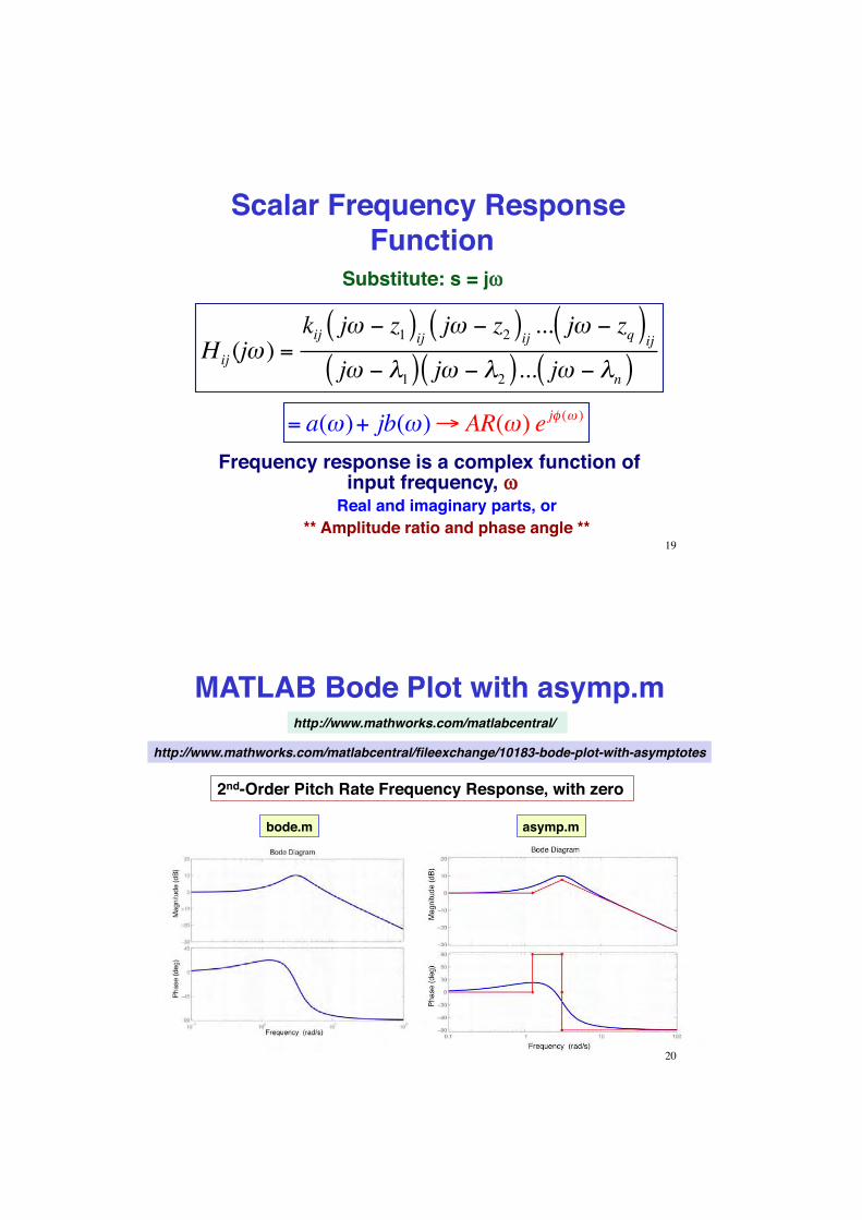
Scalar Frequency Response Function�
Hij (j� ) =kij j� � z1( )ij j� � z2( )ij ... j� � zq( )ij
j� � �1( ) j� � �2( )... j� � �n( )
Substitute: s = j���
Frequency response is a complex function of input frequency, ���
Real and imaginary parts, or�** Amplitude ratio and phase angle **�
= a(�)+ jb(�)� AR(�) e j� (� )
19�
MATLAB Bode Plot with asymp.m�http://www.mathworks.com/matlabcentral/�
http://www.mathworks.com/matlabcentral/3#��/���%��/10183-bode-plot-with-asymptotes�
2nd-Order Pitch Rate Frequency Response, with zero�
asymp.m�bode.m�
20�

7�High gain (amplitude) at low frequency�
–� Desired response is slowly varying�
7� Low gain at high frequency�
–� Random errors vary rapidly�
7�Crossover region is <>;.819�?<1/5J/�
Desirable Open-Loop Frequency Response Characteristics (Bode)�
21�
Examples of Proportional LQ
Regulator Response�
22�

Example: Open-Loop Stable and Unstable 2nd-Order LTI System Response to Initial Condition�
Stable Eigenvalues =� -0.5000 + 3.9686i� -0.5000 - 3.9686i��Unstable Eigenvalues =� 0.2500 + 3.9922i� 0.2500 - 3.9922i�
FS =0 1
�16 �1�
��
�
��
FU = 0 1�16 +0.5
�
��
�
��
23�
Example: Stabilizing Effect of Linear-Quadratic Regulators for Unstable
2nd-Order System�
r = 1�Control Gain (C) =� 0.2620 1.0857��Riccati Matrix (S) =� 2.2001 0.0291� 0.0291 0.1206��Closed-Loop Eigenvalues =� -6.4061� -2.8656�
r = 100�Control Gain (C) =� 0.0028 0.1726��Riccati Matrix (S) =� 30.7261 0.0312� 0.0312 1.9183��Closed-Loop Eigenvalues =� -0.5269 + 3.9683i� -0.5269 - 3.9683i�
minuJ = min
u
12
x12 + x2
2 + ru2( )dt0
�
��
��
�
��
u(t) = � c1 c2��
��
x1(t)x2 (t)
�
���
�
���= �c1x1(t) � c2x2 (t)
For the unstable system�
24�

Example: Stabilizing/Filtering Effect of LQ Regulators for the Unstable 2nd-
Order System�r = 1�Control Gain (C) =� 0.2620 1.0857��Riccati Matrix (S) =� 2.2001 0.0291� 0.0291 0.1206��Closed-Loop Eigenvalues =� -6.4061� -2.8656�
r = 100�Control Gain (C) =� 0.0028 0.1726��Riccati Matrix (S) =� 30.7261 0.0312� 0.0312 1.9183��Closed-Loop Eigenvalues =� -0.5269 + 3.9683i� -0.5269 - 3.9683i�
25�
Example: Open-Loop Response of the Stable 2nd-Order System to
Random Disturbance�
Eigenvalues = -1.1459, -7.8541�
26�
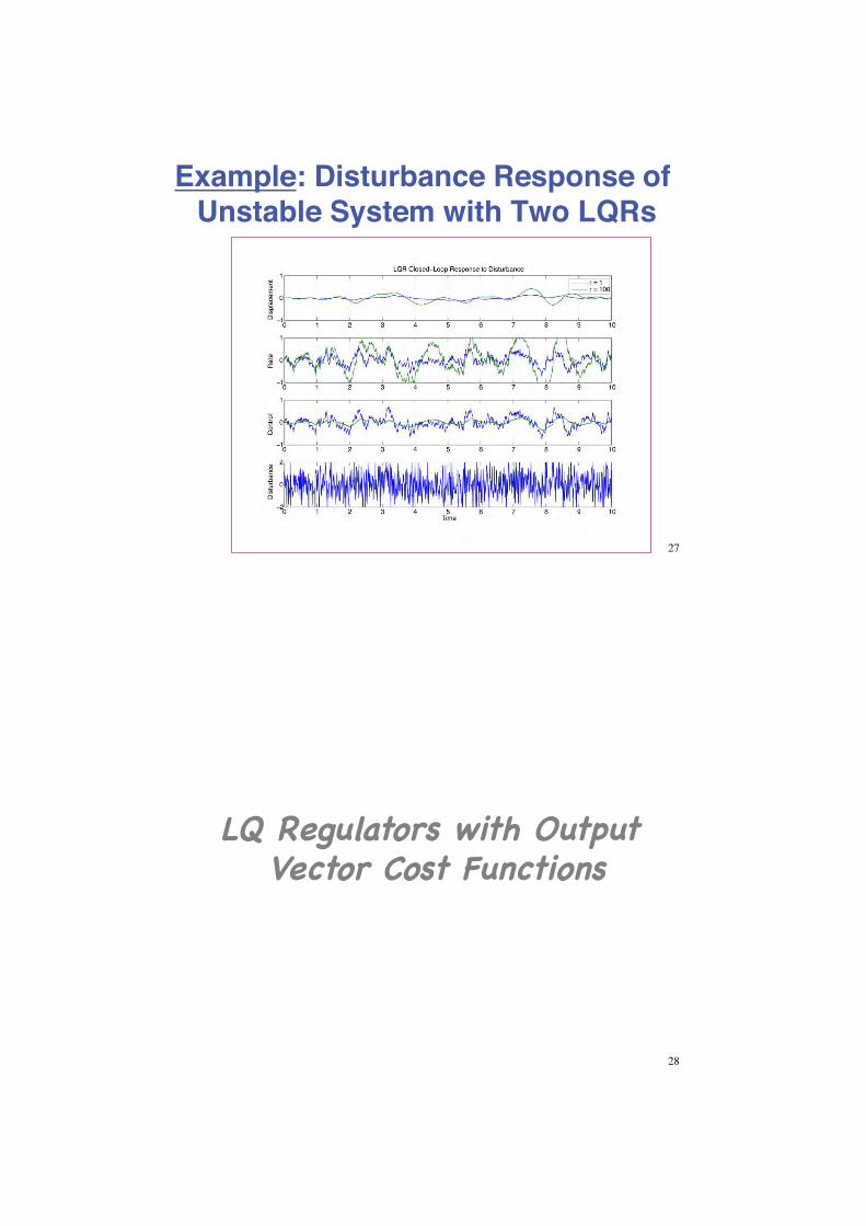
Example: Disturbance Response of Unstable System with Two LQRs�
27�
LQ Regulators with Output Vector Cost Functions�
28�

Quadratic Weighting of the Output�
J = 12
�yT (t)Qy�y(t)�� ��dt0
�
�
= 12
Hx�x(t)+Hu�u(t)[ ]T Qy Hx�x(t)+Hu�u(t)[ ]{ }dt0
�
�
�u(t) = �uC (t) �CO�x t( )
umin J =
umin
12
�xT (t) �uT (t)��
� Hx
TQyHx HxTQyHu
HuTQyHx Hu
TQyHu +Ro
�
�
��
�
��
�x(t)�u(t)
�
���
�
��
��
�
��
�dt
0
�
umin J �
umin
12
�xT (t) �uT (t)��
� QO MO
MOT RO +Ro
�
���
�
��
�x(t)�u(t)
�
���
�
��
��
�
��
�dt
0
�
�y(t) = Hx�x(t) +Hu�u(t)
29�
State Rate Can Be Expressed as an Output
to be Minimized�
J = 1
2�yT (t)Qy�y(t)�� ��dt
0
�
� = 12
��xT (t)Qy��x(t)�� ��dt0
�
�
�u(t) = �uC (t)�CSR�x t( )
��x(t) = F�x(t)+G�u(t)�y(t) = Hx�x(t)+Hu�u(t) � F�x(t)+G�u(t)
Special case of output weighting�
J = 12
�xT (t) �uT (t)��
� FTQyF FTQyG
GTQyF GTQyG +Ro
�
�
��
�
��
�x(t)�u(t)
�
���
�
��
��
�
��
�dt
0
�
�12
�xT (t) �uT (t)��
� QSR MSR
MSRT RSR +Ro
�
���
�
��
�x(t)�u(t)
�
���
�
��
��
�
��
�dt
0
�
30�

Implicit Model-Following LQ Regulator�
�u(t) = �uC (t)�CIMF�x t( )
��x(t) = F�x(t) +G�u(t)Simulator aircraft dynamics�
��xM (t) = FM�xM (t)Ideal aircraft dynamics�
Feedback control law�
Another special case of output weighting�31�
Implicit Model-Following LQ Regulator�
��x(t) = F�x(t)+G�u(t)��xM (t) = FM�xM (t)
If simulation is successful,�xM (t) � �x(t)
and��xM (t) � FM�x(t)
32�

Implicit Model-Following LQ Regulator�
J = 1
2��x(t)� ��xM (t)[ ]T QM ��x(t)� ��xM (t)[ ]{ }dt
0
�
�
�u(t) = �uC (t)�CIMF�x t( )
Cost function penalizes difference between actual and ideal model dynamics�
Therefore, ideal model is implicit in the optimizing feedback control law�
J = 12
�x(t) �u(t)��
��T F � FM( )T QM F � FM( ) F � FM( )T QMG
GTQM F � FM( ) GTQMG +Ro
�
�
��
�
�
�x(t)�u(t)
�
���
�
�
��
��
�dt
0
�
�
�12
�x(t) �u(t)��
��T QIMF M IMF
M IMFT R IMF +Ro
�
���
�
�
�x(t)�u(t)
�
���
�
�
��
��
�dt
0
�
�
33�
Proportional-Derivative Control�Basic LQ regulators provide proportional control�
�u(t) = �C�x t( ) + �uC (t)
How can proportional-derivative (PD) control be implemented with
an LQ regulator?�
Derivative feedback can either quicken or slow system response (��lead�� or ��lag��), depending on the control gain sign�
�u(t) = �CP�x t( ) �CD��x t( ) + �uC (t)
34�

Explicit Proportional-Derivative Control�
Substitute for the derivative� �u(t) = �CP�x t( ) ±CD��x t( ) + �uC (t)
�u(t) = I �CDG[ ]�1 � CP �CDF( )�x t( ) + �uC (t)�� ��
� �CPD�x t( ) + I �CDG[ ]�1�uC (t)
Structure is the same as that of proportional control�
Implement as ad hoc�9;05J/-@5;:�;2�proportional LQ control, e.g., � CD = �CPLQ
�u(t) = �CP�x t( ) ±CD F�x(t)+G�u(t)[ ]+ �uC (t)I �CDG[ ]�u(t) = �CP�x t( ) ±CDF�x(t)+ �uC (t)
Inverse Problem: Given a stabilizing gain matrix, CPD, does it minimize some (unknown) cost function? [TBD]� 35�
Implicit Proportional-Derivative Control�Add state rate, i.e., the derivative, to a standard cost function�
Include system dynamics in the cost function�
J = 1
2�xT (t)Qx�x(t)± ��xT (t)Q �x��x(t)+ �uT (t)R�u(t)�� ��dt
0
�
�
J = 12
�xT (t)Qx�x(t)± F�x t( ) +G�u t( )�� � T Q �x F�x t( ) +G�u t( )�� � + �uT (t)R�u(t){ }dt
0
�
�12
�xT (t) �uT (t)��
� QPD MPD
MPDT RPD
�
���
�
��
�x(t)�u(t)
�
���
�
��
��
�
��
�dt
0
�
�u(t) = �CPD�x t( ) + �uC (t)
Penalty/reward for fast motions��
Must verify guaranteed stability criteria��
36�

Cost Functions with Augmented State Vector�
37�
Integral Compensation Can Reduce Steady-State Errors�
��x(t) = F�x(t)+G�u(t)
���� t( ) = H I�x(t)
�� Selector matrix, HI, can reduce or mix integrals in feedback�
�� Sources of Steady-State Error��� Constant disturbance��� Errors in system dynamic model�
38�

LQ Proportional-Integral (PI) Control �
�u(t) = �CB�x t( )�CI H I�x �( )d�0
t
�� �CB�x t( )�CI��� t( ) + �uC (t)
where the integral state is
�� t( ) � H I�x �( )d�0
t
�dim H I( ) = m � n
define � t( ) ��x t( )�� t( )
�
���
�
��
39�
Integral State is Added to the Cost Function and the Dynamic Model�
min�u
J = 12
�xT (t)Qx�x(t)+ ���T t( )Q����� t( ) + �uT (t)R�u(t)�� �dt0
�
�
= 12
���T (t)Qx 00 Q��
�
���
����(t)+ �uT (t)R�u(t)
�
�
��
�
dt
0
�
�
subject to ����(t) = F�����(t)+G���u(t)
�u(t) = �C����(t)+ �uC (t)
= �CB�x t( )�CI��� t( ) + �uC (t)40�

Integral State is Added to the Cost Function and the Dynamic Model�
�u(t) = �C����(t)+ �uC (t)
= �CB�x t( )�CI��� t( ) + �uC (t)
�u(s) = �C����(s)+ �uC (s)
= �CB�x s( )�CI��� s( ) + �uC (s)
= �CB�x s( )�CIHx�x s( )
s+ �uC (s)
�u(s) = �CBs�x s( ) +CIHx�x s( )
s+ �uC (s)
= �CBs +CIHx[ ]
s�x s( ) + �uC (s)
Form of (m x n) Bode Plots
from �x to �u?�41�
Actuator Dynamics and Proportional-Filter LQ
Regulators�
42�

Proportional LQ Regulator: High-Frequency Control in Response to
High-Frequency Disturbances�2nd-Order System Response with Perfect Actuator�
Good disturbance rejection, but may high bandwidth may be unrealistic�43�
Actuator Dynamics May Impact System Response�
44�

Actuator Dynamics May Affect System Response�
��x(t)� �u(t)
�
���
�
���= F G
0 �K�
��
�
��
�x(t)�u(t)
�
���
�
���+ 0
I�
��
�
���v(t)
Control variable is actuator forcing function�
Augment state dynamics to include actuator dynamics�
�v(t) = � �uIntegrator (t) = �CB�x t( ) + �vC (t) is sub -optimal45�
LQ Regulator with Actuator Dynamics�
min�u
J = 12
�xT (t)Qx�x(t)+ �uT (t)Ru�u(t)+ �vT (t)Rv�v(t)�� �dt0
�
�
= 12
���T (t)Qx 00 Ru
�
���
�
���(t)+ �vT (t)Rv�v(t)
�
���
�
dt
0
�
�subject to ����(t) = F�����(t)+G���v(t)
Cost function is minimized with re-01J:10�?@-@1�-:0�/;:@>;8�B1/@;>?�
���(t) =�x(t)�u(t)
�
���
�
��; F�� =
F G0 �K
�
��
�
�; G�� =
0I
�
��
�
�
46�

LQ Regulator with Actuator Dynamics�
�v(t) = �C����(t)+ �vC (t)
= �CB�x t( )�CA�u(t)+ �vC (t)
�v(s) = �CB�x s( )�CA�u(s)+ �vC (s)
Control Force�
47�
LQ Regulator with Actuator Dynamics�
Control Displacement�
� �u(t) = �K�u(t)�CA�u(t)�CB�x t( ) + �vC (t)s�u(s) = �K�u(s)�CA�u(s)�CB�x s( ) + �vC (s)+ �u(0)
sI+K +CA[ ]�u(s) = �CB�x s( ) + �vC (s)
�u(s) = sI+K +CA[ ]�1 �CB�x s( ) + �vC (s)�� ��48�

%�&13A8-@;>�C5@4��>@5J/5-8�Actuator Dynamics�
��x(t)� �u(t)
�
���
�
���= F G
0 0�
��
�
��
�x(t)�u(t)
�
���
�
���+ 0
I�
��
�
���v(t)
�v(t) = � �uInt (t) = �CB�x t( )�CA�u(t)+ �vC (t)
CA� %+)&�,��*��)+ 3� �#���+,�+&)��0%�$ �*�
LQ control variable is derivative of actual system control�
49�
Proportional-Filter (PF) LQ Regulator�
���(t) =�x(t)�u(t)
�
���
�
���; F�� =
F G0 0
�
��
�
��; G�� =
0I
�
��
�
��
�v(t) = � �uIntegrator (t) = �C����(t)+ �vC (t)
CA provides #&.�'�**�3#+�) %�������+ on the control input �
�u(s) = sI+CA[ ]�1 �CB�x s( ) + �vC (s)�� ��
Optimal LQ Regulator�
50�

Proportional-Filter LQ Regulator Reduces High-Frequency Control
Signals �2nd-Order System Response�
... at the expense of decreased disturbance rejection� 51�
Next Time: �Linear-Quadratic Control
System Design�
52�

53�
Implicit Model-Following Linear-Quadratic Regulator�
Model the response of one airplane with another using feedback control�
54�

Princeton Variable-Response Research Aircraft (VRA)�
55�