HOW ACCURATE IS MOLECULAR DYNAMICS?

CHRISTIAN BAYER, HAKON HOEL, PETR PLECHAC, ANDERS SZEPESSY, AND RAUL TEMPONE

Abstract. Born-Oppenheimer dynamics is shown to provide an accurate approximation of time-independentSchrodinger observables for a molecular system with an electron spectral gap, in the limit of large ratio of

nuclei and electron masses, without assuming that the nuclei are localized to vanishing domains. Thederivation, based on a Hamiltonian system interpretation of the Schrodinger equation and stability of the

corresponding Hamilton-Jacobi equation, bypasses the usual separation of nuclei and electron wave func-

tions, includes caustic states and gives a different perspective on the Born-Oppenheimer approximation,Schrodinger Hamiltonian systems and numerical simulation in molecular dynamics modeling at constant

energy microcanonical ensembles.

Contents

1. Motivation for error estimates of molecular dynamics 12. The Schrodinger and molecular dynamics models 33. A time-independent Schrodinger WKB-solution 63.1. Exact Schrodinger dynamics 63.2. Born-Oppenheimer dynamics 93.3. Equations for the density 93.4. Construction of the solution operator 104. Computation of observables 115. Molecular dynamics approximation of Schrodinger observables 125.1. The Born-Oppenheimer approximation error 125.2. Why do symplectic numerical simulations of molecular dynamics work? 136. Analysis of the molecular dynamics approximation 136.1. Continuation of the construction of the solution operator 146.2. Stability from perturbed Hamiltonians 156.3. The Born-Oppenheimer approximation 177. Fourier integral WKB states including caustics 207.1. A preparatory example with the simplest caustic 207.2. A general Fourier integral ansatz 238. Numerical examples 298.1. Example 1: A single WKB state 298.2. Example 2: A caustic state 319. The stationary phase expansion 36References 37

1. Motivation for error estimates of molecular dynamics

Molecular dynamics is a computational method to study molecular systems in materials science, chemistryand molecular biology. The simulations are used, for example, in designing and understanding new materials

2000 Mathematics Subject Classification. Primary: 81Q20; Secondary: 82C10.Key words and phrases. Born-Oppenheimer approximation, WKB expansion, caustics, Fourier integral operators,

Schrodinger operators.The research of P.P. and A.S. was partially supported by the National Science Foundation under the grant NSF-DMS-

0813893 and Swedish Research Council grant 621-2010-5647, respectively.

1

arX

iv:1

104.

0953

v1 [

mat

h-ph

] 5

Apr

201

1

or for determining biochemical reactions in drug design, [13]. The wide popularity of molecular dynamicssimulations relies on the fact that in many cases it agrees very well with experiments. Indeed when we haveexperimental data it is easy to verify correctness of the method by comparing with experiments at certainparameter regimes. However, if we want the simulation to predict something that has no comparing experi-ment, we need a mathematical estimate of the accuracy of the computation. In the case of molecular systemswith few particles such studies are made by directly solving the Schrodinger equation. A fundamental andstill open question in classical molecular dynamics simulations is how to verify the accuracy computationally,i.e., when the solution of the Schrodinger equation is not a computational alternative.

The aim of this paper is to derive qualitative error estimates for molecular dynamics and present newmathematical methods which could be used also for a more demanding quantitive accuracy estimation,without solving the Schrodinger solution. Having molecular dynamics error estimates opens, for instance,the possibility of systematically evaluating which density functionals or empirical force fields are good ap-proximations and under what conditions the approximation properties hold. Computations with such errorestimates could also give improved understanding when quantum effects are important and when they arenot, in particular in cases when the Schrodinger equation is too computational complex to solve.

The first step to check the accuracy of a molecular dynamics simulation is to know what to compare with.Here we compare with the value of any observable g(X), of nuclei positions X, for the time-independentSchrodinger eigenvalue equation HΦ = EΦ, so that the approximation error we study is

(1.1)

∫R3(N+n)

g(X)Φ(x,X)∗Φ(x,X) dx dX − limT→∞

1

T

∫ T

0

g(Xt)dt ,

for a molecular dynamics path Xt, with total energy equal to the Schrodinger eigenvalue E. The observablecan be, for instance, the local potential energy, used in [34] to determine phase-field partial differential equa-tions from molecular dynamics simulations, see Figure 1. The time-independent Schrodinger equation hasa remarkable property of accurately predicting experiments in combination with no unknown data, therebyforming the foundation of computational chemistry. However, the drawback is the high dimensional solutionspace for nuclei-electron systems with several particles, restricting numerical solution to small molecules. Inthis paper we study the time-independent setting of the Schrodinger equation as the reference. The pro-posed approach has the advantage of avoiding the difficulty of finding the initial data for the time-dependentSchrodinger equation.

Figure 1. A Lennard-Jones molecular dynamics simulation of a phase transition with pe-riodic boundary conditions, from [34]. The left part is solid and the right is liquid. Thecolor measures the local potential energy.

The second step to check the accuracy is to derive error estimates. We have three types of error: time dis-cretization error, sampling error and modeling error. The time discretization error comes from approximatingthe differential equation for molecular dynamics with a numerical method, based on replacing time deriva-tives with difference quotients for a positive step size ∆t. The sampling error is due to truncating the infiniteT and using a finite value of T in the integral in (1.1). The modeling error (also called coarse-graining error)

2

originates from eliminating the electrons in the Schrodinger nuclei-electron system and replacing the nucleidynamics with their classical paths; this approximation error was first analyzed by Born and Oppenheimerin their seminal paper [2].

The time discretization and truncation error components are in some sense simple to handle by comparingsimulations with different choice of ∆t and T , although it can, of course, be difficult to know that the behaviordoes not change with even smaller ∆t and larger T . The modeling error is more difficult to check since a directapproach would require to solve the Schrodinger equation. Currently the Schrodinger partial differentialequation can only be solved with few particles, therefore it is not an option to solve the Schrodinger equationin general. The reason to use molecular dynamics is precisely in avoiding solution of the Schrodinger equation.Consequently the modeling error requires mathematical error analysis. In the literature there seems to be noerror analysis that is precise, simple and constructive enough so that a molecular dynamics simulation canuse it to asses the modeling error. Our alternative error analysis presented here is developed with the aim toallow the construction of algorithms that estimate the modeling error in molecular dynamics computations.Our analysis differs from previous ones by using

- the time-independent Schrodinger equation as the reference model to compare molecular dynamicswith,

- an amplitude function in a WKB-Ansatz that depends only on position coordinates (x,X) (and noton momentum coordinates (p, P )) for caustic states,

- actual solutions of the Schrodinger equation (and not only asymptotic solutions),- the theory of Hamilton-Jacobi partial differential equations to derive estimates for the corresponding

Hamiltonian systems, i.e., the molecular dynamics systems.

Understanding both the exact Schrodinger model and the molecular dynamics model through Hamiltoniansystems allows us to obtain bounds for the difference of the solutions by well-established comparison resultsfor the solutions of Hamilton-Jacobi equations, by regarding the Schrodinger Hamiltonian and the moleculardynamics Hamiltonians as perturbations of each others. The Hamilton-Jacobi theory applied to Hamiltoniansystems is inspired by the error analysis of symplectic methods for optimal control problems for partialdifferential equations, [28]. The result is that the modeling error can be estimated based on the difference ofthe Hamiltonians, for the molecular dynamics system and the Schrodinger system, along the same solutionpath, see Theorem 5.1 and Section 6.2.

2. The Schrodinger and molecular dynamics models

In deriving the approximation of the solutions to the full Schrodinger equation the heavy particles areoften treated within classical mechanics, i.e., by defining the evolution of their positions and momenta byequations of motions of classical mechanics. Therefore we denote Xt : [0,∞)→ R3N and Pt : [0,∞)→ R3N

time-dependent functions of positions and momenta with time derivatives denoted by

Xt =dXt

dt, Xt =

d2Xt

dt2.

We denote the Euclidean scalar product on R3N by

X · Y =

3N∑i=1

XiY i .

Furthermore, we use the notation ∇Xψ(x,X) = (∇X1ψ(x,X), . . . ,∇XNψ(x,X)), and as customary ∇Xiψ =(∂Xi1ψ, ∂Xi2ψ, ∂Xi3ψ).

On the other hand, the light particles are treated within the quantum mechanical description and thefollowing complex valued bilinear map 〈· , ·〉 : L2(R3n × R3N ) × L2(R3n × R3N ) → L2(R3N ) will be used inthe subsequent calculations

(2.1) 〈φ, ψ〉 =

∫R3n

φ(x,X)∗ψ(x,X) dx .

The notation ψ(x,X) = O(M−α) is also used for complex valued functions, meaning that |ψ(x,X)| =O(M−α) holds uniformly in x and X.

3

The time-independent Schrodinger equation

(2.2) H(x,X)Φ(x,X) = EΦ(x,X)

models many-body (nuclei-electron) quantum systems and is obtained from minimization of the energy inthe solution space of wave functions, see [30, 29, 1, 32, 7]. It is an eigenvalue problem for the energy E ∈ Rof the system in the solution space, described by wave functions, Φ : R3n×R3N → C, depending on electroncoordinates x = (x1, . . . , xn) ∈ R3n, nuclei coordinates X = (X1, . . . , XN ) ∈ R3N , and the Hamiltonianoperator H(x,X)

(2.3) H(x,X) = V(x,X)− 1

2M−1

N∑n=1

∆Xn .

We assume that a quantum state of the system is fully described by the wave function Φ : R3n × R3N → Cwhich is an element of the Hilbert space of wave functions with the standard complex valued scalar product

〈〈Φ,Ψ〉〉 =

∫R3n×R3N

Φ(x,X)∗Ψ(x,X) dx dX ,

and the operator H is self-adjoint in this Hilbert space. The Hilbert space is then a subset of L2(R3n×R3N )with symmetry conditions based on the Pauli exclusion principle for electrons, see [7, 21].

In computational chemistry the operator V, the electron Hamiltonian, is independent of M and it isprecisely determined by the sum of the kinetic energy of electrons and the Coulomb interaction betweennuclei and electrons. We assume that the electron operator V(·, X) is self-adjoint in the subspace with theinner product 〈·, ·〉 of functions in (2.1) with fixed X coordinate and acts as a multiplication on functions thatdepend only on X. An essential feature of the partial differential equation (2.2) is the high computationalcomplexity of finding the solution in an antisymmetric/symmetric subset of the Sobolev spaceH1(R3n×R3N ).The mass of the nuclei, which are much greater than one (electron mass), are the diagonal elements in thediagonal matrix M .

In contrast to the Schrodinger equation, a molecular dynamics model of N nuclei X : [0, T ] → R3N ,with a given potential Vp : R3N → R, can be computationally studied for large N by solving the ordinarydifferential equations

(2.4) MXt = −∇XVp(Xt) .

This computational and conceptual simplification motivates the study to determine the potential and itsimplied accuracy compared with the the Schrodinger equation, as started already in the 1920’s with theBorn-Oppenheimer approximation [2]. The purpose of our work is to contribute to the current understandingof such derivations by showing convergence rates under new assumptions. The precise aim in this paper isto estimate the error

(2.5)

∫R3N+3n g(X)Φ(x,X)∗Φ(x,X) dx dX∫

R3N+3n Φ(x,X)∗Φ(x,X) dx dX− limT→∞

1

T

∫ T

0

g(Xt) dt

for a position dependent observable g(X) of the time-indepedent Schrodinger equation (2.2) approximated

by the corresponding molecular dynamics observable limT→∞ T−1∫ T

0g(Xt) dt, which is computationally

cheaper to evaluate with several nuclei. The Schrodinger eigenvalue problem may typically have multipleeigenvalues and the aim is to find an eigenfunction Φ and a molecular dynamics system that can be compared.There may be eigenfunctions that we cannot approximate, but with some assumptions on the spectrum ofV(·, X) the molecular dynamics in fact approximates the observable corresponding to one eigenfunction.

The main step to relate the Schrodinger wave function and the molecular dynamics solution is the so-calledzero-order Born-Oppenheimer approximation, whereXt solves the classical ab initio molecular dynamics (2.4)with the potential Vp : R3N → R determined as an eigenvalue of the electron Hamiltonian V(·, X) for a givennuclei position X. That is Vp(X) = λ0(X) and

V(·, X)ΨBO(·, X) = λ0(X)ΨBO(·, X) ,

for an electron eigenfunction ΨBO(·, X) ∈ L2(R3n), for instance, the ground state. The Born-Oppenheimerexpansion [2] is an approximation of the solution to the time-independent Schrodinger equation which isshown [14, 18] to solve the time-independent Schrodinger equation approximately. This expansion, analyzed

4

by the methods of multiple scales, pseudo-differential operators and spectral analysis in [14, 18, 12], can beused to study the approximation error (2.5). However, in the literature it is easier to find precise statementson the error in observables for the setting of the time-dependent Schrodinger equation, since the stabilityissue is more subtle in the eigenvalue setting.

Instead of an asymptotic expansion we use a different method based on a Hamiltonian dynamics formu-lation of the time-independent Schrodinger eigenfunction and the stability of the corresponding perturbedHamilton-Jacobi equations viewed as a hitting problem. This approach makes it possible to reduce the errorpropagation on the infinite time interval to finite time excursions from a certain co-dimension one hittingset. A motivation for our method is that it forms a sub-step in trying to estimate the approximation errorusing only information available in molecular dynamics simulations.

The related problem of approximating observables to the time-dependent Schrodinger equation by theBorn-Oppenheimer expansions is well studied, theoretically [4, 26] and computationally [19] using the Egorovtheorem. The Egorov theorem shows that finite time observables of the time-dependent Schrodinger equationare approximated with O(M−1) accuracy by the zero-order Born-Oppenheimer dynamics with an electroneigenvalue gap. In the special case of a position observable and no electrons (i.e., V = V (X) in (2.3)), theEgorov theorem states that

(2.6)

∣∣∣∣∫R3N

g(X)Φ(X, t)∗Φ(X, t) dX −∫R3N

g(Xt)Φ(X0, 0)∗Φ(X0, 0) dX0

∣∣∣∣ ≤ CtM−1 ,

where Φ(X, t) is a solution to the time-dependent Schrodinger equation

iM−1/2∂tΦ(·, t) = HΦ(·, t)

with the Hamiltonian (2.3) and the path Xt is the nuclei coordinates for the dynamics with the Hamiltonian12 |X|

2 +V (X). If the initial wave function Φ(X, 0) is the eigenfunction in (2.2) the first term in (2.6) reducesto the first term in (2.5) and the second term can also become the same in an ergodic limit. However, sincewe do not know that the parameter Ct (bounding an integral over (0, t)) is bounded for all time we cannotdirectly conclude an estimate for (2.5) from (2.6).

In our perspective studying the time-independent instead of the time-dependent Schrodinger equation hasthe important differences that

- the infinite time study of the Born-Oppenheimer dynamics can be reduced to a finite time hittingproblem,

- the computational and theoretical problem of specifying initial data for the Schrodinger equation isavoided, and

- computationally cheap evaluation of the position observable g(X) is possible using the time average

limT→∞1T

∫ T0g(Xt) dt along the solution path Xt.

In this paper we derive the Born-Oppenheimer approximation from the time-independent Schrodingerequation (2.2) and we establish convergence rates for molecular dynamics approximations to time-independentSchrodinger observables under simple assumptions including the so-called caustic points, where the Jacobiandeterminant det J(Xt) ≡ det(∂Xt/∂X0) of the Eulerian-Lagrangian transformation of X-paths vanish. Asmentioned previously, the main new analytical idea is an interpretation of the time-independent Schrodingerequation (2.2) as a Hamiltonian system and the subsequent analysis of the approximations by comparingHamiltonians. This analysis employs the theory of Hamilton-Jacobi partial differential equations. The prob-lematic infinite-time evolution of perturbations in the dynamics is solved by viewing it as a finite-time hittingproblem for the Hamilton-Jacobi equation, with a particular hitting set. In contrast to the traditional rigor-ous and formal asymptotic expansions we analyze the transport equation as a time-dependent Schrodingerequation.

The main inspiration for this paper is [25, 6, 5] and the semi-classical WKB analysis in [23]: the works

[25, 6, 5] derive the time-dependent Schrodinger dynamics of an x-system, iΨ = H1Ψ, from the time-independent Schrodinger equation (with the Hamiltonian H1(x) + εH(x,X)) by a classical limit for theenvironment variable X, as the coupling parameter ε vanishes and the mass M tends to infinity; in particular[25, 6, 5] show that the time derivative enters through the coupling of Ψ with the classical velocity. Here werefine the use of characteristics to study classical ab initio molecular dynamics where the coupling does not

5

vanish, and we establish error estimates for Born-Oppenheimer approximations of Schrodinger observables.The small scale, introduced by the perturbation

−(2M)−1∑k

∆Xk

of the potential V, is identified in a modified WKB eikonal equation and analyzed through the correspondingtransport equation as a time-dependent Schrodinger equation along the eikonal characteristics. This modifiedWKB formulation reduces to the standard semi-classical approximation, see [23], in the case of the potentialfunction V = V (X) ∈ R, depending only on nuclei coordinates, but becomes different in the case of operator-valued potentials studied here. The global analysis of WKB functions was initiated by Maslov in the 1960’,[23], and lead to the subject Geometry of Quantization, relating global classical paths to eigenfunctions ofthe Schrodinger equation, see [10]. The analysis presented in this paper is based on a Hamiltonian systeminterpretation of the time-independent Schrodinger equation. Stability of the corresponding Hamilton-Jacobiequation, bypasses the usual separation of nuclei and electron wave functions in the time-dependent self-consistent field equations, [3, 22, 33].

Theorem 5.1 demonstrates that observables from the zero-order Born-Oppenheimer dynamics approxi-mate observables for the Schrodinger eigenvalue problem with the error of order O(M−1+δ), for any δ > 0,assuming that the electron eigenvalues satisfy a spectral gap condition. The result is based on the Hamilton-ian (2.3) with any potential V that is smooth in X, e.g., a regularized version of the Coulomb potential. Thederivation does not assume that the nuclei are supported on small domains; in contrast derivations basedon the time-dependent self-consistent field equations require nuclei to be supported on small domains. Thereason that the small support is not needed here comes from the combination of the characteristics and sam-pling from an equilibrium density. In other words, the nuclei paths behave classically although they may notbe supported on small domains. Section 4 shows that caustics couple the WKB modes, as is well-known fromgeometric optics, see [17, 23], and generate non-orthogonal WKB modes that are coupled in the Schrodingerdensity. On the other hand, without caustics the Schrodinger density is asymptotically decoupled into asimple sum of individual WKB densities. Section 7 constructs a WKB-Fourier integral Schrodinger solutionfor caustic states. Section 5.2 relates the approximation results to the accuracy of symplectic numericalmethods for molecular dynamics.

A unique property of the time-independent Schrodinger equation we use is the interpretation that thedynamics Xt ∈ R3N can return to a co-dimension one surface I which then can reduce the dynamics toa hitting time problem with finite-time excursions from I. Another advantage of viewing the moleculardynamics as an approximation of the eigenvalue problem is that stochastic perturbations of the electronground state can be interpreted as a Gibbs distribution of degenerate nuclei-electron eigenstates of theSchrodinger eigenvalue problem (2.2), see [31]. The time-independent eigenvalue setting also avoids the issueon “wave function collapse” to an eigenstate, present in the time-dependent Schrodinger equation.

We believe that these ideas can be further developed to better understanding of molecular dynamicssimulations. For example, it would be desirable to have more precise conditions on the data (i.e. molec-ular dynamics initial data and potential V) instead of our implicit assumption on finite hitting time andconvergence of the Born-Oppenheimer power series approximation in Lemma 6.2.

3. A time-independent Schrodinger WKB-solution

3.1. Exact Schrodinger dynamics. For the sake of simplicity we assume that all nuclei have the same

mass. If this is not the case, we can introduce new coordinates M1/21 Xk = M

1/2k Xk, which transform the

Hamiltonian to the form we want V(x,M1/21 M−1/2X) − (2M1)−1

∑Nk=1 ∆Xk . The singular perturbation

−(2M)−1∑k ∆Xk of the potential V introduces an additional small scale M−1/2 of high frequency oscilla-

tions, as shown by a WKB-expansion, see [27, 16, 15, 24]. We shall construct solutions to (2.2) in such aWKB-form

(3.1) Φ(x,X) = φ(x,X)eiM1/2θ(X) ,

where the amplitude function φ : R3n × R3N → C is complex valued, the phase θ : R3N → R is realvalued, and the factor M1/2 is introduced in order to have well-defined limits of φ and θ as M → ∞.Note that it is trivially always possible to find funtions φ and θ satisfying (3.1), even in the sense of a true

6

equality. Of course, the ansatz only makes sense if φ and θ do not have strong oscillations for large M .The standard WKB-construction, [23, 15], is based on a series expansion in powers of M1/2 which solvesthe Schrodinger equation with arbitrary high accuracy. Instead of an asymptotic solution, we introduce anactual solution based on a time-dependent Schrodinger transport equation. This transport equation reducesto the formulation in [23] for the case of a potential function V = V (X) ∈ R, depending only on nucleicoordinates X ∈ R3N , and modifies it for the case of a self-adjoint potential operator V(·, X) on the electronspace L2(R3n) which is the primary focus of our work here. In Sections 4 and 7 we use a linear combinationof WKB-eigensolutions, but first we study the simplest case of a single WKB-eigensolution.

3.1.1. A first WKB-solution. The WKB-solution satisfies the Schrodinger equation (2.2) provided that

0 = (H− E)φ eiM1/2θ(X)

=

((1

2|∇Xθ|2 + V − E)φ − 1

2M∆Xφ−

i

M1/2(∇Xφ · ∇Xθ +

1

2φ∆Xθ)

)eiM

1/2θ(X) ,(3.2)

where we use the notation ∆X =∑j ∆Xj . We shall see that only eigensolutions Φ that correspond to

dynamics without caustics correspond to such a single WKB-mode, as for instance when the eigenvalue E isinside an electron eigenvalue gap. Solutions in the presence of caustics use a Fourier integral of such WKB-modes, and we treat this case in detail in Section 7. To understand the behavior of θ, we multiply (3.2) by

φ∗e−iM1/2θ(X) and integrate over R3n. Similarly we take the complex conjugate of (3.2), and multiply by

φ eiM1/2θ(X) and integrate over R3n. By adding these two expressions we obtain

0 = 2(1

2|∇Xθ|2 − E

)〈φ, φ〉+ 〈φ,Vφ〉+ 〈Vφ, φ〉︸ ︷︷ ︸

=2〈φ,Vφ〉

− 1

2M(〈φ,∆Xφ〉+ 〈∆Xφ, φ〉)

− i

M1/2

(〈φ,∇Xφ · ∇Xθ〉 − 〈∇Xφ · ∇Xθ, φ〉

)︸ ︷︷ ︸=2iIm 〈φ,∇Xφ·∇Xθ〉

+i

2M1/2

(〈φ, φ〉 − 〈φ, φ〉

)︸ ︷︷ ︸=0

∆Xθ .(3.3)

The purpose of the phase function θ is to generate an accurate approximation in the limit as M → ∞. Apossible and natural definition of θ would be the formal limit of (3.3) as M → ∞, which is the Hamilton-Jacobi equation, also called the eikonal equation

(3.4)1

2|∇Xθ|2 = E − V0 ,

where the function V0 : R3N → R is

(3.5) V0 :=〈φ,Vφ〉〈φ, φ〉

.

The solution to the Hamilton-Jacobi eikonal equation can be constructed from the associated Hamiltoniansystem

Xt = Pt

Pt = −∇XV0(Xt)(3.6)

through the characteristics path (Xt, Pt) satisfying ∇Xθ(Xt) =: Pt. The amplitude function φ can bedetermined by requiring the ansatz (3.2) to be a solution, which gives

0 = (H− E)φ eiM1/2θ(X)

=(

(1

2|∇Xθ|2 + V0 − E)︸ ︷︷ ︸

=0

φ

− 1

2M∆Xφ+ (V − V0)φ− i

M1/2(∇Xφ · ∇Xθ +

1

2φ∆Xθ)

)eiM

1/2θ(X) ,

so that by using (3.4) we have

− 1

2M∆Xφ+ (V − V0)φ− i

M1/2(∇Xφ · ∇Xθ +

1

2φ∆Xθ) = 0 .

7

The usual method for determining φ from this so-called transport equation uses an asymptotic expansion

φ '∑Kk=0M

−k/2φk, see [14], [18] and the beginning of Section 6. An alternative is to write it as a Schrodingerequation, similar to [23]: we apply the characteristics in (3.6) to write

d

dtφ(Xt) = ∇Xφ · Xt = ∇Xφ · ∇Xθ ,

and define the weight function G by

(3.7)d

dtlogGt =

1

2∆Xθ(Xt) ,

and the variable ψt := φ(Xt)Gt. We use the notation φ(X) instead of the more precise φ(·, X), so that e.g.ψt = ψt(x) = φ(x,Xt)Gt. Then the transport equation becomes a Schrodinger equation

(3.8) iM−1/2ψt = (V − V0)ψt −Gt2M

∆X

(ψtGt

).

In conclusion, equations (3.4)-(3.8) determine the WKB-ansatz (3.1) to be a solution to the Schrodingerequation (2.2).

Theorem 3.1. The Hamilton-Jacobi equation, with the corresponding Hamiltonian,

HS(X,P ) :=1

2|P |2 +

〈ψ(X),V(X)ψ(X)〉〈ψ(X), ψ(X)〉︸ ︷︷ ︸

=:V0(X)

−E = 0 ,

based on the primal variable X and the dual variable P = P (X) = ∇Xθ(X), generates a solution to thetime-independent Schrodinger equation (H− E)Φ = 0, in the sense that

Φ(Xt, x) = G−1(Xt)ψ(x,Xt)eiM1/2θ(Xt)

solves the equation (2.2), where ψ(Xt) := ψt satisfies the transport equation (3.8) and

G(Xt) = Gt ,

d

dtlogGt =

1

2∆Xθ(Xt) ,

(Xt, Pt) solves the Hamiltonian system (3.6) corresponding to HS.

Note that the nuclei density, using G, can be written

(3.9) ρ :=〈φ, φ〉∫

R3N 〈φ, φ〉 dX=

〈ψ, ψ〉 G−2∫R3N 〈ψ, ψ〉 G−2 dX

,

and since each time t determines a unique point (Xt, Pt) = (Xt,∇Xθ(Xt)) in the phase space the functions

G and ψ are well defined.

3.1.2. Liouville’s Formula. In this section we verify Liouville’s formula

(3.10)G2

0

G2t

= e−∫ t0

Tr (∇XP (Xt)) dt =

∣∣∣∣det∂(X0)

∂(Xt)

∣∣∣∣ ,given in [23]. The characteristic Xt = P (Xt) implies d

dtJ(Xt) = ∇XP J(X), where J(X)ij = ∂Xit/∂X

j0

denotes the first variation with respect to perturbations of the initial data. The logarithmic derivative thensatisfies d/dt

(log J(X)

)ij

= ∂XjPi(Xt) = ∂XiXjθ(X) which implies that log J(Xt) is symmetric and shows

that (3.10) holds

divP = Tr∇XP =d

dtTr log J(X) =

d

dtlog detJ(X) .

The last step uses that J(X) can be diagonalized by an orthogonal transformation and that the trace isinvariant under orthogonal transformations.

8

3.1.3. Data for the Hamiltonian system. For the energy E chosen larger than the potential energy, that issuch that E ≥ V0, the Hamiltonian system (3.6) yields a solution (X,P ) : [0, T ] → U × R3N to the eikonalequation (3.4) locally in a neighborhood U ⊆ R3N , for regular compatible data (X0, P0) given on a 3N − 1dimensional ”inflow”-domain I ⊂ U . Typically, the domain I and the data (X0, P0)|I are not given (exceptthat its total energy is E), unless it is really an inflow domain and characteristic paths do not return to I asin a scattering problem. If paths leaving from I return to I, there is an additional compatibility of data onI: assume X0 ∈ I and Xt ∈ I, then the values Pt are determined from P0; continuing the path to subsequenthitting points Xtj ∈ I, j = 1, 2, . . . determines Ptj from P0. The characteristic path (Xt, Pt), t > 0, generatesa manifold in the phase space (X,P ), which is smooth under our assumptions. This manifold is in generalonly locally of the form (X,P (X)), but in the case of no caustics it is globally of this form and then thereis a phase function X 7→ θ(X) such that P (X) = ∇Xθ(X) globally. In Section 7 we study phase spacemanifolds with caustics.

Remark 3.2. The integrating factor G and its derivative ∂XiG can be determined from (P, ∂XiP, ∂XiXjP )along the characteristics by the following characteristic equations obtained from (3.4) by differentiation withrespect to X

d

dt∂XrP

k =

∑j

P j∂XjXrPk =

∑j

P j∂XrXkPj

= −

∑j

∂XrPj∂XkP

j − ∂XrXkV0 ,

d

dt∂XrXqP

k =

∑j

P j∂XjXrXqPk +

∑j

P j∂XrXkXqPj

= −

∑j

∂XrPj∂XkXqP

j −∑j

∂XrXqPj∂XkP

j − ∂XrXkXqV0 ,

(3.11)

and similarly ∂XiXjG can be determined from (P, ∂XiP, ∂XiXjP, ∂XiXjXkP ).

3.2. Born-Oppenheimer dynamics. The Born-Oppenheimer approximation leads to the standard for-mulation of ab initio molecular dynamics, in the micro-canonical ensemble with the constant number ofparticles, volume and energy, for the nuclei positions X = XBO,

Xt = Pt ,

Pt = −∇Xλ0(Xt) ,(3.12)

by using that the electrons are in the eigenstate ψ = ΨBO with eigenvalue λ0 to V, in L2(dx) for fixed X,i.e., V(X)ΨBO = λ0(X)ΨBO. The corresponding Hamiltonian is HBO(X,P ) := |P |2/2 + λ0(X) with theeikonal equation

(3.13)1

2|∇XθBO(X)|2 + λ0(X) = E .

3.3. Equations for the density. We note that

φ = G−1ψ =

(ρ

〈ψ, ψ〉/∫〈ψ, ψ〉G−2 dX

)1/2

ψ ,

shows that G and ψ determine the density

(3.14) ρS = ρ =〈ψ, ψ〉|G|−2∫〈ψ, ψ〉 |G|−2dX

,

defined in (3.9). Using the Born-Oppenheimer approximation in Lemma 6.2 we have 〈ψ, ψ〉 = 1 +O(M−1)

in the case of a spectral gap. Therefore the weight function |G|−2 approximates the density and we know

from Theorem 3.1 that |G|−2 is determined by the phase function θ.9

The Born-Oppenheimer dynamics generates an approximate solution ΨBOG−1BOe

iM1/2θBO which yields thedensity

(3.15) ρBO = |GBO|−2,

whered

dtlog |GBO|−2 = −∆XθBO(X) .

This representation can also be obtained from the conservation of mass

0 = div(ρBO∇XθBO)

implying

(3.16)d

dtρBO(Xt) = ∇XρBO(Xt) · Xt = −ρBO(Xt) div∇XθBO ,

with the solution

(3.17) ρBO(Xt) =C

|GBO(Xt)|2,

where C is a positive constant for each characteristic. Note that the derivation of this classical density doesnot need a corresponding WKB equation but uses only the conservation of mass that holds for classical pathssatisfying a Hamiltonian system. The classical density corresponds precisely to the Eulerian-Lagrangianchange of coordinates |Gt|2/|G0|2 = det(∂Xt/∂X0) in (3.10).

3.4. Construction of the solution operator. The WKB Ansatz (3.1) is meaningful when ψ does notinclude the full small scale. In Lemma 6.2 we present conditions for ψ to be smooth.

To construct the solution operator it is convenient to include a non interacting particle in the system, i.e.,a particle without charge, and assume that this particle moves with a constant, high speed dX1

1/dt = P 11 � 1

(or equivalently with the unit speed and a large mass). Such a non interacting particle does not affect theother particles. The additional new coordinate X1

1 is helpful in order to simply relate the time-coordinate tand X1

1 . We add the corresponding kinetic energy (P 11 )2/2 to E in order not to change the original problem

(2.2) and write the equation (3.8) in the fast time scale τ = M1/2t

id

dτψ = (V − V0)ψ − 1

2MG∑j

∆Xj (G−1ψ) .

Furthermore, we change to the coordinates

(τ,X∗) := (τ,X12 , X

13 , X

2, . . . , XN ) ∈ [0,∞)× I , instead of (X1, X2, . . . , XN ) ∈ R3N ,

where Xj = (Xj1 , X

j2 , X

j3) ∈ R3. Hence we obtain

(3.18) iψ +1

2(P 11 )2

ψ = (V − V0)ψ − 1

2MG∑j

∆Xj∗(G−1ψ) =: Vψ ,

using the notation w = dw/dτ in this section. In Section 6.1 we show that the left hand side can be reduced

to iψ as P 11 → ∞, by choosing special initial data. Note also that G is independent of the first component

in X1. We see that the operator

V := G−1VG = G−1(V − V0)G︸ ︷︷ ︸=V−V0

− 1

2M

∑j

∆Xj∗

is symmetric on L2(R3n+3N−1). Assume now the data (X0, P0, Z0) for X0 ∈ R3N−1 is (LZ)3N−1-periodic,then also (Xτ , Pτ , Zτ ) is (LZ)3N−1-periodic, for Zt = θ(Xt) and Pt = ∇Xθ(Xt). To simplify the notationfor such periodic functions, define the periodic circle

T := R/(LZ) .

We seek a solution Φ of (2.2) which is (LZ)3(n+N)−1-periodic in the (x,X∗)-variable. The Schrodingeroperator V(·, Xτ ) has, for each τ , real eigenvalues {λm(τ)} with a complete set of eigenvectors {ζm(x,X∗, τ)}orthogonal in the space of x-anti-symmetric functions in L2(T3n+3N−1), see [1]. The proof uses that the

10

operator Vτ + γI generates a compact solution operator in the Hilbert space of x-anti-symmetric func-tions in L2(T3n+3N−1), for the constant γ ∈ (0,∞) chosen sufficiently large. The discrete spectrum andthe compactness comes from Fredholm theory for compact operators and the fact that the bilinear form∫T3(n+N)−1 vVτw+γvw dx dX∗ is continuous and coercive on H1(T3(n+N)−1), see [11]. We see that V has the

same eigenvalues {λm(τ)} and the eigenvectors {Gτζm(τ)}, orthogonal in the weighted L2-scalar product∫T3N−1

〈v, w〉 G−2 dX∗ .

The construction and analysis of the solution operator continues in Section 6.1 based on the spectrum.

Remark 3.3 (Boundary conditions). The eigenvalue problem (2.2) makes sense not only in the periodicsetting but also with alternative boundary conditions from interaction with an external environment, e.g.,for scattering problems.

4. Computation of observables

Suppose the goal is to compute a real-valued observable∫T3N

〈Φ, AΦ〉 dX

for a given bounded linear multiplication operator A = A(X) on L2(T3N ) and a solution Φ =∑k φke

iM1/2θk

of (2.2). We have

(4.1)

∫T3N 〈Φ, AΦ〉dX =

∑k,l

∫T3N 〈AφkeiM

1/2θk(X), φleiM1/2θl(X)〉 dX

=∑k,l

∫T3N Ae

iM1/2(θl(X)−θk(X))〈φk, φl〉 dX .

The integrand is oscillatory for k 6= l, hence critical points of the phase difference give the main contribution.The stationary phase method, see [10, 23] and Section 9, shows that these integrals are small, boundedby O(M−3N/4), in the case when the phase difference has non degenerate critical points (or no criticalpoint) and the functions A〈φk, φl〉 and θl are sufficiently smooth. A critical point Xc ∈ R3N satisfies∇Xθl(Xc) − ∇Xθk(Xc) = 0, which means that the two different paths, generated by θl and θk, passingthrough X = Xc also have the same momentum P at this point. Consequently the critical point must be acaustic point since otherwise the paths are the same. That the critical point is non degenerate means thatthe Hessian matrix ∂XiXj (θk − θl)(Xc) is non singular.

We see that WKB terms, with smooth phases and coefficients avoiding caustics, are asymptotically or-thogonal, so that the density of a linear combination of them separates asymptotically to a sum of densitiesof the individual WKB terms

(4.2)

∫T3N

〈Φ, AΦ〉dX =

k∑k=1

∫T3N

A 〈φk, φk〉︸ ︷︷ ︸=ρk

dX +O(M−1) ,

in the case of multiple eigenstates, k > 1, and∫T3N

〈Φ, AΦ〉 dX =

∫T3N

A〈φ1, φ1〉 dX

for a single eigenstate. In the next section we will study molecular dynamics approximations of a single state

(4.3)

∫T3N

A〈φk, φk〉 dX =

∫T3N

A(X)ρk(X) dX .

In the presence of a caustic, the WKB terms can be asymptotically non orthogonal, since their coefficientsand phases typically are not smooth enough to allow the integration by parts to gain powers of M−1/2.Non-orthogonal WKB functions tell how the caustic couples the WKB modes.

Regarding the inflow density ρk∣∣I

there are two situations: either the characteristics return often to theinflow domain or not. If they do not return we have a scattering problem and it is reasonable to define the

11

inflow-density ρk∣∣I

as an initial condition. If characteristics return, the dynamics can be used to estimate

the return-density ρk∣∣I

as follows: Assume that the following limits exist

(4.4) limT→∞

1

T

∫ T

0

A(Xt) dt =

∫T3N

A(X)ρk(X) dX

which bypasses the need to find ρk∣∣I

and the quadrature in the number of characteristics. A way to thinkabout this limit is to sample the return points Xt ∈ I and from these samples construct an empirical return-density, converging to ρk

∣∣I

as the number of return iterations tends to infinity. We shall use this perspective

to view the eikonal equation (3.4) as a hitting problem on I, with hitting times τ (i.e., return times). Weallow the density ρ|I to depend on the initial position X0. The more restrictive property having ρ|I constantas a function of X0 is called ergodicity. An example of a hitting surface is the co-dimension one surface wherethe first component X11 in X1 = (X11, X12, X13) is equal to its initial value X11(0). The dynamics does notalways have such a hitting surface: for instance if all particles are close initially and then are scattered awayfrom each other, as in an explosion, no co-dimension one hitting surface exists.

5. Molecular dynamics approximation of Schrodinger observables

A numerical computation of an approximation to∑k

∫T3N 〈φk, Aφk〉 dX has the main ingredients:

(1) to approximate the exact characteristics by molecular dynamics characteristics (3.6),(2) to discretize the molecular dynamics equations, and

(3a) if ρ∣∣I

is an inflow-density, to introduce quadrature in the number of characteristics, or

(3b) if ρ∣∣I

is a return-density, to replace the ensemble average by a time average using the property (4.4).

This section presents a derivation of the approximation error in the step (1) in the case of a return density andcomments on the time-discretization of step (2) treated in Section 5.2. The third and fourth discretizationsteps, which are not described here, are studied, for instance, in [8, 7, 20].

5.1. The Born-Oppenheimer approximation error. This section states our main result of molecu-lar dynamics approximating Schrodinger observables. We formulate it using the assumption of the Born-Oppenheimer property

(5.1) ‖ψt −ΨBO(Xt)‖L2(dx) = O(M−1/2) , uniformly in t.

This assumption is then proved in Lemma 6.2 based on a setting with a spectral gap.The spectral gap condition. The electron eigenvalues {λk} satisfy, for some positive c, the spectral gapcondition

(5.2) infk 6=0, Y ∈D

|λk(Y )− λ0(Y )| > c ,

where D := {XS(t) | t ≥ 0} ∪ {XBO(t) | t ≥ 0} is the set of all nuclei positions obtained from the Schrodingercharacteristics X = XS in Theorem 3.1 and from the Born-Oppenheimer dynamics X = XBO in (3.12), forall considered initial data.

Theorem 5.1. Assume that the phase functions θS and θBO are smooth solutions to the eikonal equations(3.4) and (3.13) and that the Born-Oppenheimer property (5.1) holds, then the zero-order Born-Oppenheimerdynamics (3.12), assumed to have bounded hitting times τ in (6.11), (6.14) and (6.18), approximates time-independent Schrodinger observables, generated by Theorem 3.1 or the caustic case in Section 7.2, with errorbounded by O(M−1+δ)

(5.3)

∫T3N

g(X)ρBO(X) dX =

∫T3N

g(X)ρS(X) dX +O(M−1+δ) , for any δ > 0.

The proof is given in Sections 6 and 7.2.12

5.2. Why do symplectic numerical simulations of molecular dynamics work? The derivation of theapproximation error for the Born-Oppenheimer dynamics, in Theorem 5.1, also allows to study perturbedsystems. For instance, the perturbed Born-Oppenheimer dynamics

Xt = Pt +∇PHε(Xt, Pt)

Pt = −∇Xλ0(Xt)−∇XHε(Xt, Pt) ,

generated from a perturbed Hamiltonian HBO(X,P ) +Hε(X,P ) = E, with the perturbation satisfying

(5.4) ‖Hε‖L∞ ≤ ε for some ε ∈ (0,∞)

yields through (6.13) and (6.19) an additional error term O(ε) to the approximation of observables in (5.3).So called symplectic numerical methods are precisely those that can be written as perturbed Hamiltoniansystems, see [28], and consequently we have a method to precisely analyze their numerical error by com-bining an explicit construction of Hε with the stability condition (5.4) to obtain O(M−1+δ + ε) accurateapproximations. The popular Stormer-Verlet method is symplectic and the positions X coincides with thoseof the symplectic Euler method, for which Hε is explicitly constructed in [28] with ε proportional to thetime step. The construction in [28] is not using the modified equation and formal asymptotics, instead apiecewise linear extension of the solution generates Hε.

6. Analysis of the molecular dynamics approximation

Before we proceed with the analysis of the approximation error we motivate our results by a significantlysimpler case of a system without electrons. We use the densities (3.14) and (3.15) and we show heuristicallyhow the characteristics can be used to estimate the difference ρS − ρBO, leading to O(M−1) accurate Born-Oppenheimer approximations of Schrodinger observables∫

g(X) ρS(X)︸ ︷︷ ︸〈Φ,Φ〉

dX =

∫g(X)ρBO(X) dX +O(M−1) .

In the special case of no electrons, the dynamics of X does not depend on ψ and therefore XBO = XS = Xand consequently GBO = GS. The difference ψS − ψBO can be understood from iterative approximations of(3.8)

(6.1)i

M1/2ψk+1 − (V − V0)ψk+1 =

1

2MG∆X(G−1ψk)

with ψ0 = 0. Then ψBO = ψ1 is the Born-Oppenheimer approximation and formally we have the iterationsapproaching the full Schrodinger solution ψk → ψS as k →∞.

In the special case of no electrons, there holds V = V0, thus the transport equation iψ1 = 0 has constantsolutions. We let ψ1 = 1 and then ψ2 − ψ1 is imaginary with its absolute value bounded by O(M−1/2). Wewrite the iterations of ψk by integrating (6.1) as the linear mapping

ψk+1 = 1 + iM−1/2S(ψk) =

k∑l=0

ilM−l/2Sl(ψ1) ,

which formally shows that

|ψS|2 = |ψ1|2 + 2Re 〈ψS − ψ1, ψ1〉+ |ψS − ψ1|2 = 1 +O(M−1) .

Consequently this special Born-Oppenheimer density satisfies

(6.2) ρBO = G−2S 〈ψS, ψS〉︸ ︷︷ ︸

=ρS

+O(M−1) ,

since GBO = GS and X do not depend on ψ.In the general case with electrons and a spectral gap, we show in Lemma 6.2 that there is a solution ψS

satisfying

(6.3) ‖ψS −ΨBO‖L2(dx) = O(M−1/2) ,13

for the electron eigenfunction ΨBO, satisfying

V(·, X)ΨBO(·, X) = λ0(X)ΨBO(·, X)

and the eigenvalue λ0(X) ∈ R with a (fixed) nuclei position X. Then the state ψ1 equal to a constant, inthe case of no electrons, corresponds to the electron eigenfunction ΨBO in the case with electrons present.In the general case the X dynamics for the Schrodinger and the Born-Oppenheimer dynamics are not thesame, but we will show that (6.3) implies that the Hamiltonians HS and HBO are O(M−1) close. Usingstability of Hamilton-Jacobi equations, the phase functions θS and θBO are then also close in the maximumnorm, which, combined with an assumption of smooth phase functions, show that |GS−GBO| = O(M−1+δ)for any δ > 0. Lemma 6.2 also shows that |〈ψS, ψS〉 − 1| = O(M−1) and consequently the density bound|ρS − ρBO| = O(M−1+δ) holds. To obtain the estimate (6.3) the important new property, compared to noelectrons, is to use oscillatory cancellation in directions orthogonal to ΨBO.

6.1. Continuation of the construction of the solution operator. This section continues the construc-tion of the solution operator started in Section 3.4. Assume for a moment that V is independent of τ . Thenthe solution to (3.18) can be written as a linear combination of the two exponentials

aeiτA+ + beiτA−

where the two characteristic roots are the operators

A± = (P 11 )2

(−1± (1− 2(P 1

1 )−2V)1/2).

We see that eiτA− is a highly oscillatory solution on the fast τ -scale with

limP 1

1→∞

1

(P 11 )2A− = −2Id ,

while

(6.4) limP 1

1→∞A+ = −V .

Therefore we chose initial data

(6.5) iψ|τ=0 = −A+ψ|τ=0

to have b = 0, which eliminates the fast scale, and the limit P 11 → ∞ determines the solution by the

Schrodinger equation

iψ = Vψ .The next section presents an analogous construction for the slowly, in τ , varying operator V.

6.1.1. Spectral decomposition. Write (3.18) as the first order system

iψ = π

iπ = −2(P 11 )2(Vψ − π) ,

which for ψ := (ψ, π) takes the form

˙ψ = iBψ , B :=

(0 −1

2(P 11 )2V −2(P 1

1 )2

),

where the eigenvalues Λ± , right eigenvectors Q± and left eigenvectors Q−1± of the real “matrix” operator B

are

Λ± := (P 11 )2

(−Id±

(Id− 2(P 1

1 )−2V)1/2

),

Q+ :=

(Id−Λ+

), Q− :=

(−Λ−1−

Id

),

Q−1+ := (Id− Λ+Λ−1

− )−1

(Id

Λ−1−

), Q−1

− := (Id− Λ+(Λ−)−1)−1

(Λ+

Id

).

14

We see that limP 11→∞ Λ+ = −V and limP 1

1→∞(P 11 )−2Λ− = −2Id. The important property here is that

the left eigenvector limit limP 11→∞Q

−1+ = (Id, 0) is constant, independent of τ , which implies that the Q+

component Q−1+ ψ = ψ decouples. We obtain in the limit P 1

1 →∞ the time-dependent Schrodinger equation

iψ(τ) = id

dτ(Q−1

+ ψτ ) = iQ−1+

d

dτψτ = −Q−1

+ Bτ ψτ

= − Λ+(τ)Q−1+ ψτ = − Λ+(τ)ψ(τ) = Vτψ(τ) ,

where the operator Vτ depends on τ and (x,X0), and we define the solution operator S

(6.6) ψ(τ) = Sτ,0ψ(0) .

As in (6.5) we can view this as choosing special initial data for ψ(0). From now on we only consider suchdata.

The operator V can be symmetrized

(6.7) Vτ := G−1τ VτGτ = (V − V0)τ −

1

2M

∑j

∆Xj∗,

with real eigenvalues {λm} and orthonormal eigenvectors {ζm} in L2(dx dX∗), satisfying

Vτζm(τ) = λm(τ)ζm(τ) .

Therefore Vτ has the same eigenvalues and the eigenvectors ζm := Gτζm, which establishes the spectral

representation

(6.8) Vτψ(·, τ, ·) =∑m

λm(τ)

∫T3N−1

〈ψ(·, τ, ·), ζm〉G−2τ dX∗ ζ

m(τ) .

We note that the weight G−2 on the co-dimension one surface T3N−1 appears precisely because the operatorV is symmetrized by G−2 and the weight G−2 corresponds to the Eulerian-Lagrangian change of coordinates(3.10)

(6.9)

∫T3N−1

〈ψ, ζm〉G−2τ dX∗ =

∫T3N−1

〈ψ, ζm〉 dX0 .

The existence of the orthonormal set of eigenvectors and real eigenvalues makes the operator V self-adjoint inthe Lagrangian coordinates and hence the solution operator S becomes unitary in the Lagrangian coordinates.

6.2. Stability from perturbed Hamiltonians. In this section we derive error estimates of the weightfunctions G when the corresponding Hamiltonian system is perturbed. To derive the stability estimate weconsider the Hamilton-Jacobi equation

H(∇Xθ(X), X) = 0

in an optimal control perspective with the corresponding Hamiltonian system

Xt = ∇PH(Pt, Xt)

Pt = −∇XH(Pt, Xt) .

We define the “value” function

θ(X0) = θ(Xt)−∫ t

0

h(Ps, Xs) ds ,

where the “cost” function defined by

h(P,X) := P · ∇PH(P,X)−H(P,X)

satisfies the Pontryagin principle (related to the Legendre transform)

(6.10) H(P,X) = supQ

(P · ∇QH(Q,X)− h(Q,X)

).

15

Let θ∣∣∣I

be defined by the hitting problem

θ(X0) = θ(Xτ )−∫ τ

0

h(Ps, Xs) ds

using the hitting time τ on the return surface I

(6.11) τ := inf{t |X0 ∈ I, Xt ∈ I & t > 0} .

For a perturbed Hamiltonian H and its dynamics (Xt, Pt) we define analogously the value function θ and

the cost function h.We can think of the difference θ − θ as composed by a perturbation of the boundary data (on the return

surface I) and perturbations of the Hamiltonians. The difference of the value functions due to the perturbedHamiltonian satisfies the stability estimate

θ(X0)− θ(X0) ≥ θ(Xτ )− θ(Xτ ) +

∫ τ

0

(H − H)(∇Xθ(Xt), Xt

)dt

θ(X0)− θ(X0) ≤ θ(Xτ )− θ(Xτ ) +

∫ τ

0

(H − H)(∇X θ(Xt), Xt

)dt

(6.12)

with a difference of the Hamiltonians evaluated along the same solution path. This result follows by dif-ferentiating the value function along a path and using the Hamilton-Jacobi equations, see Remark 6.1 and[9].

We assume that

(6.13) sup(P,X)=(∇X θ(Xt),Xt), (P,X)=(∇Xθ(Xt),Xt)

|(H − H)(P,X)| = O(M−1) .

We choose the hitting set as

(6.14) I := {X ∈ T3N | θ(X) = θ(X)}on which the two phases coincide. Now assume that I forms a codimension one set in T3N and that themaximal hitting time τ for characteristics starting on I is bounded; the fact that I is a codimension one setholds, for instance, locally if |∇X(θ − θ)| is nonzero. In fact, it is sufficient to assume that there exists a

function γ : T3N → R, satisfying γ = O(M−1), and such that the set I := {X ∈ T3N | θ(X)− θ(X) = γ(X)}is a codimension one set with bounded hitting times. Then the representation (6.12), for any time t replacing

τ and τ , together with the stability of the Hamiltonians (6.13) and the initial data (θ − θ)|I = 0 obtainedfrom (6.14) imply that

(6.15) ‖θ − θ‖L∞ = O(M−1) ,

provided the maximal hitting time τ is bounded, which we assume.When the value functions θ and θ are smoothly differentiable in X with derivatives bounded uniformly in

M , the stability estimate (6.12) implies that also the difference of the second derivatives has the bound

(6.16) ‖∆Xθ −∆X θ‖L∞ = O(M−1+δ) , for any δ > 0.

Our goal is to analyze the density function ρ = |G|−2〈ψ,ψ〉 with G defined in (3.7). The Born-Oppenheimer approximation (5.1) yields 〈ψ,ψ〉 = 1 + O(M−1) thus it remains to estimate the weightfunction |G|−2. This weight function satisfies the Hamilton-Jacobi equation

(6.17) HG(∇X log |G|−2, X) := ∇Xθ(X) · ∇X log |G|−2 + ∆Xθ(X) = 0 .

The stability of Hamilton-Jacobi equations can then be applied to (6.17), as in (6.12), using now the hittingset

(6.18) I := {X ∈ T3N | log |G(X)|−2 = log |G(X)|−2}and the assumption of bounded hitting times τ in the hitting problem, and we obtain

(6.19) ‖ log |G|−2 − log |G|−2‖L∞ ≤ C‖HG −HG‖L∞ = O(M−1+δ) .

In this sense we will use that an O(M−1) perturbation of the Hamiltonian yields an error estimate of almostthe same order for the difference of the corresponding densities ρ− ρ.

16

The Hamiltonians we use are

HS =|P |2

2+〈ψ(X),V(X)ψ(X)〉〈ψ(X), ψ(X)〉

− E ,

HBO =|P |2

2+ λ0(X)− E ,

based on the cost functions

hS = E +|P |2

2− 〈ψ(X),V(X)ψ(X)〉

〈ψ(X), ψ(X)〉,

hBO = E +|P |2

2− λ0(X) .

For the Born-Oppenheimer case the electron wave function is the eigenstate ΨBO.

Remark 6.1. This remark derives the stability estimate (6.12). The definitions of the value functions imply

θ(Xτ )−∫ τ

0

h(Pt, Xt) dt︸ ︷︷ ︸θ(X0)

−(θ(Xτ )−

∫ τ

0

h(Pt, Xt) dt

)︸ ︷︷ ︸

θ(X0)

= −∫ τ

0

h(Pt, Xt) dt+ θ(Xτ )− θ(X0)︸ ︷︷ ︸θ(X0)

+θ(Xτ )− θ(Xτ )

= −∫ τ

0

h(Pt, Xt) dt+

∫ τ

0

dθ(Xt) + θ(Xτ )− θ(Xτ )

=

∫ τ

0

−h(Pt, Xt) +∇Xθ(Xt) · ∇P H(Pt, Xt)︸ ︷︷ ︸≤H(∇Xθ(Xt),Xt)

dt+ θ(Xτ )− θ(Xτ )

≤∫ τ

0

(H −H)(∇Xθ(Xt), Xt

)dt+ θ(Xτ )− θ(Xτ ) ,

(6.20)

where the Pontryagin principle (6.10) yields the inequality and we use the Hamilton-Jacobi equation

H(∇Xθ(Xt), Xt) = 0 .

To establish the lower bound we replace θ along with Xt by θ and Xt and repeat the derivation above.

6.3. The Born-Oppenheimer approximation. The purpose of this section is to present a case when theBorn-Oppenheimer approximation holds in the sense that ‖ψ −ΨBO‖L2(dx) is small.

We know from Section 6.1.1 that the solution ψt = St,0ψ0 is bounded in L2(dx dX), since S is unitaryin the Lagrangian coordinates. This unitary S implies that the integral in the Lagrangian coordinates∫T3N−1〈ψt, ψt〉 dX0 is constant in time. We consider the co-dimension one set

Iψ := {X ∈ R3N | 〈ψ(X), ψ(X)〉 =

∫T3N−1

〈ψ(t,X0), ψ(t,X0)〉 dX0/

∫T3N−1

dX0} ,

where the point values of 〈ψ(X), ψ(X)〉 coincides with its L2 average. We choose a time t such that Xt ∈ Iψand assume that the time τ∗ it takes to hit Iψ the next time is bounded, i.e.,

τ∗ := inf{τ |Xt ∈ Iψ, τ > 0 & Xt+τ ∈ Iψ} = O(1) .

We also assume that all functions of X are smooth.

17

Lemma 6.2. Assume that iψ = M1/2Vψ holds, then there exists initial data for ψ such that the L2(dx)orthogonal decomposition ψ = ψ0 ⊕ ψ⊥0 , where ψ0 = αΨBO for some α ∈ C satisfies

‖ψ⊥0 (t)‖L2(dx)

‖ψ0(t)‖L2(dx)

= O(M−1/2)

|〈ψt, ψt〉 − 1| = O(M−1)

‖ψt −ΨBO(Xt)‖L2(dx) = O(M−1/2)

(6.21)

uniformly in time t, provided the spectral gap condition (5.2) holds, the smoothness estimate (6.28) is satisfiedand the hitting time τ∗ is bounded.

Proof. We consider the decomposition ψ = ψ0 ⊕ ψ⊥0 , where ψ0(τ) is an eigenfunction of V(Xτ ) in L2(dx),satisfying V(Xτ )ψ0(τ) = λ0(τ)ψ0(τ) for the eigenvalue λ0(τ) ∈ R. This ansatz is motivated by the zeroresidual

(6.22) Rψ := ψ + iM1/2Vψ = 0

and the small residual for the eigenfunction

〈Π( ˙ψ0), ψ0〉 = 0

M1/2Vψ0 = O(M−1/2) ,

where

(6.23) w(X) = 〈ΨBO(X), w(X)〉ΨBO(X)⊕Πw(X)

denotes the orthogonal decomposition in the eigenfunction direction ΨBO and its orthogonal complementin L2(dx). We consider first the linear operator R in (6.22) with a given function V0 and then we use acontraction setting to show that V0 = 〈ψ,Vψ〉/〈ψ,ψ〉 also works since ‖ψ⊥0 ‖L2(dx) is small. The orthogonal

splitting ψ = ψ0 ⊕ ψ⊥0 and the projection Π(·) in (6.23) imply

0 = Π(R(ψ0 + ψ⊥0 )

)= Π

(R(ψ0)

)+ Π

(R(ψ⊥0 )

)= Π(Rψ0) + ψ0

⊥+ iM1/2(V − V0)ψ⊥0 + iΠ

(GM−1/2

2∆X(G−1ψ⊥0 )

),

where the last step follows from the orthogonal splitting

Π((V − V0)ψ⊥0

)= (V − V0)ψ⊥0

together with the second order change in the subspace projection

ψ⊥0 (τ + ∆τ) = Π(τ + ∆τ)(ψ⊥0 (τ + ∆τ)

)= Π(τ)

(ψ⊥0 (τ + ∆τ)

)+O(∆τ2)

which yields Π(ψ⊥0 ) = ψ⊥0 ; here Π(τ)· denotes the projection on the orthogonal complement to the eigen-vector ψ0(τ). To explain the second order change start with a function v satisfying 〈v,ΨBO(Xτ )〉 = 0 andΨBO(Xσ) = ΨBO(Xτ ) +O(∆τ) for σ ∈ [τ, τ + ∆τ ] to obtain

Π(σ)(Π(τ + ∆τ)v −Π(τ)v

)= Π(σ)

(〈v,ΨBO(Xτ )〉ΨBO(Xτ )− 〈v,ΨBO(Xτ+∆τ )〉ΨBO(Xτ+∆τ )

)= Π(σ)O(∆τ2) + Π(σ)

(〈v,O(∆τ)〉ΨBO(Xτ )

)= O(∆τ2) +O(∆τ)

(ΨBO(Xτ )− 〈ΨBO(Xτ ),ΨBO(Xσ)〉ΨBO(Xσ)

)= O(∆τ2).

Let Sτ,σ be the solution operator from time σ to τ for the generator

v 7→ iM1/2(V − V0)v + iΠ

(GM−1/2

2∆X(G−1v)

)=: iM1/2Vv .

18

Consequently, the perturbation ψ⊥0 can be determined from the projected residual

ψ⊥0 = −iM1/2Vψ⊥0 −Π(Rψ0)

and we have the solution representation

(6.24) ψ⊥0 (τ) = Sτ,0ψ⊥0 (0)−∫ τ

0

Sτ,σΠ(Rψ0(σ)

)dσ .

Integration by parts introduces the factor M−1/2 we seek∫ τ

0

Sτ,σΠRψ0(σ) dσ =

∫ τ

0

iM−1/2 d

dσ(Sτ,σ)V−1ΠRψ0(σ) dσ

=

∫ τ

0

iM−1/2 d

dσ

(Sτ,σV−1ΠRψ0(σ)

)dσ

−∫ τ

0

iM−1/2Sτ,σd

dσ

(V−1(Xσ)ΠRψ0(σ)

)dσ

= iM−1/2V−1ΠRψ0(τ)− iM−1/2Sτ,0V−1ΠRψ0(0)

−∫ t

0

iM−1/2Sτ,σd

dσ

(V−1(Xσ)ΠRψ0(σ)

)dσ .

(6.25)

To analyze the integral in the right hand side we will use the fact

V−1 =(I + (V − V0)−1

[V − (V − V0)

])−1

(V − V0)−1,

which can be verified by multiplying both sides from the left by I + (V − V0)−1[V − (V − V0)

]. A spectral

decomposition in L2(dx), based on the electron eigenpairs {λk, ψk}∞k=1 and satisfying Vψk = λkψk, thenimplies

V−1(Rψ0)⊥ =(I + (V − V0)−1

[V − (V − V0)

])−1

(V − V0)−1(Rψ0)⊥

=∑k 6=0

(I + (V − V0)−1

[V − (V − V0)

])−1

(λk − V0)−1ψk〈(Rψ0)⊥, ψk〉

=∑k 6=0

(λk − V0)−1ψk〈(Rψ0)⊥, ψk〉+O(M−1)

(6.26)

which applied to the integral in the right hand side of (6.25) shows that ‖ψ⊥0 ‖L2(dx) = O(M−1/2) on abounded time interval, when the spectral gap condition holds and ψk are smooth.

The evolution on longer times requires an additional idea: one can integrate by parts recursively in (6.25)to obtain ∫ τ

0

Sτ,σΠRψ0(σ) dσ =

[Sτ,σ

(BR − B d

dσ(BR) + B d

dσ

(B d

dσ(BR)

)− . . .

)]σ=τ

σ=0

,

B := iM−1/2V−1 , R := ΠRψ0(σ) ,

so that by (6.24) we have

ψ⊥0 (τ) = Sτ,0ψ⊥0 (0)−[Sτ,σ

(BR − B d

dσ(BR) + B d

dσ

(B d

dσ(BR)

)− . . .

)]σ=τ

σ=0

.

By choosing

ψ⊥0 (σ)∣∣∣σ=0

= −(BR(σ)− B d

dσ(BR)(σ) + B d

dσ

(B d

dσ(BR)

)(σ)− . . .

)∣∣∣σ=0

we get

(6.27) ψ⊥0 (τ) = −∞∑n=0

Bn0R0(τ) ,

19

where B0 := −iM−1/2V−1 ddτ and R0 := iM−1/2V−1R. We assume this expansion (6.27) is convergent in

L2(dx) for each τ , which follows from the smoothness estimate

(6.28) ‖Bn0R0(τ)‖L2(dx) → 0 as n→∞

and (6.26).The next step, verifying that also the non linear problem for V0 works, is based on the contraction obtained

from

V0 − λ0 =〈ψ, (V − λ0)ψ〉〈ψ,ψ〉

= O(‖ψ⊥0 ‖L2(dx))

and that ψ⊥0 depends on V0 in (6.24), (6.25) and (6.26) with a multiplicative factor O(M−1/2).Finally, to conclude that |〈ψ,ψ〉 − 1| = O(M−1), we use the evolution equation

d

dt〈ψ,ψ〉 = M−1/2|G|2Im 〈∆ψ

G,ψ

G〉 = O(M−1)

where the last equality uses the obtained bound of ψ⊥0 in the first part of (6.21). The assumption of a finitehitting time τ∗ then implies that |〈ψ,ψ〉−1| = O(τ∗M−1) = O(M−1), since we may assume that 〈ψ,ψ〉 = 1on Iψ. �

Remark 6.3 (Error estimates for the densities). We have the densities

ρS = G−2S 〈ψ,ψ〉 for the Schrodinger equation,(6.29)

ρBO = G−2BO for the Born-Oppenheimer dynamics.(6.30)

From the stability of the Hamilton-Jacobi equation for log(|G|−2) and the estimate ‖∂XiXj (θ − θ)‖L∞ =O(M−1+δ) in (6.16) we have

G−2S = G−2

BO +O(M−1+δ) ,

and Lemma 6.2 implies

(6.31) 〈ψ,ψ〉 = 1 +O(M−1) ,

which proves

ρS = ρBO +O(M−1+δ) .

7. Fourier integral WKB states including caustics

7.1. A preparatory example with the simplest caustic. As an example of a caustic, we study first thesimplest example of a fold caustic based on the Airy function A : R→ R which solves

(7.1) − ∂xxA(x) + xA(x) = 0 .

The scaled Airy function

u(x) = C A(M1/3x)

solves the Schrodinger equation

(7.2) − 1

M∂xxu(x) + xu(x) = 0 ,

for any constant C. In our context an important property of the Airy function is the fact that it is theinverse Fourier transform of the function

A(p) =

√2

πeip

3/3 ,

i.e.,

(7.3) A(x) =1

π

∫Rei(xp+p

3/3) dp .

20

In the next section, we will consider a general Schrodinger equation and determine a WKB Fourier integralcorresponding to (7.3) for the Airy function; as an introduction to the general case we show how the derive(7.3): by taking the Fourier transform of the ordinary differential equation (7.1)

(7.4) 0 =

∫R

(−∂xx + x) A(x)e−ixp dx = (p2 + i∂p)A(p) ,

we obtain an ordinary differential equation for the Fourier transform A(p) with the solution A(p) = Ceip3

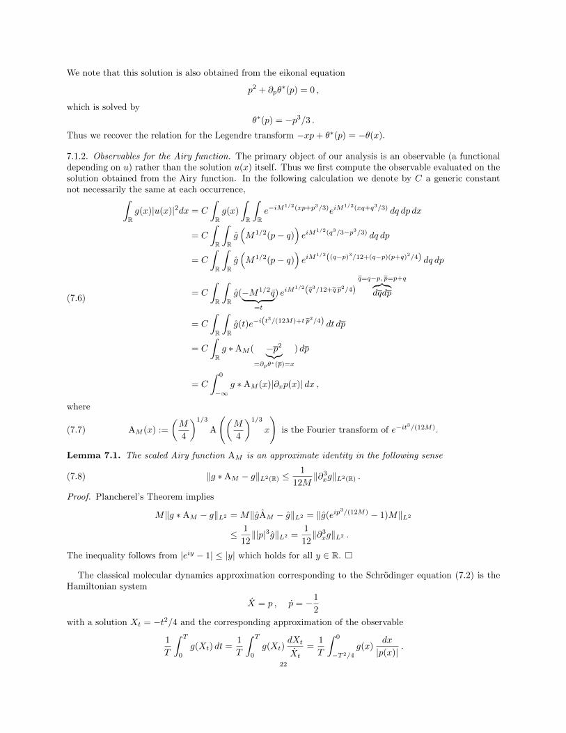
, forany constant C. Then, by differentiation, it is clear that the scaled Airy function u solves (7.2). Furthermore,the stationary phase method, cf. Section 9, shows that to the leading order u is approximated by

u(x) ' C(−xM1/3

)−1/4

cos(M1/2(−x)3/2 − π/4

), for x < 0 ,

and u(x) ' 0 to any order (i.e., O(M−K) for any positive K) when x > 0. The behaviour of the Airyfunction is illustrated in Figure 2.

−30 −25 −20 −15 −10 −5 0 5 10 15 20−0.8

−0.6

−0.4

−0.2

0

0.2

0.4

0.6

Figure 2. The Airy function.

7.1.1. Molecular dynamics for the Airy function. The eikonal equation corresponding to (7.2) is

p2 + x = 0

with solutions for x ≤ 0, which leads to the phase

(7.5) p = θ′(x) = ±(−x)1/2 , and θ(x) = ∓2

3(−x)3/2 .

We compute the Legendre transformθ∗(p) = xp− θ(x)

where by (7.5) and −x = p2 we obtain

θ∗(p) = −p2p+2

3p3 = −p

3

3.

21

We note that this solution is also obtained from the eikonal equation

p2 + ∂pθ∗(p) = 0 ,

which is solved by

θ∗(p) = −p3/3 .

Thus we recover the relation for the Legendre transform −xp+ θ∗(p) = −θ(x).

7.1.2. Observables for the Airy function. The primary object of our analysis is an observable (a functionaldepending on u) rather than the solution u(x) itself. Thus we first compute the observable evaluated on thesolution obtained from the Airy function. In the following calculation we denote by C a generic constantnot necessarily the same at each occurrence,∫

Rg(x)|u(x)|2dx = C

∫Rg(x)

∫R

∫Re−iM

1/2(xp+p3/3)eiM1/2(xq+q3/3) dq dp dx

= C

∫R

∫Rg(M1/2(p− q)

)eiM

1/2(q3/3−p3/3) dq dp

= C

∫R

∫Rg(M1/2(p− q)

)eiM

1/2((q−p)3/12+(q−p)(p+q)2/4) dq dp

= C

∫R

∫Rg(−M1/2q︸ ︷︷ ︸

=t

) eiM1/2(q3/12+q p2/4)

q=q−p, p=p+q︷︸︸︷dqdp

= C

∫R

∫Rg(t)e−i(t

3/(12M)+t p2/4) dt dp

= C

∫Rg ∗AM ( −p2︸︷︷︸

=∂pθ∗(p)=x

) dp

= C

∫ 0

−∞g ∗AM (x)|∂xp(x)| dx ,

(7.6)

where

(7.7) AM (x) :=

(M

4

)1/3

A

((M

4

)1/3

x

)is the Fourier transform of e−it

3/(12M).

Lemma 7.1. The scaled Airy function AM is an approximate identity in the following sense

(7.8) ‖g ∗AM − g‖L2(R) ≤1

12M‖∂3xg‖L2(R) .

Proof. Plancherel’s Theorem implies

M‖g ∗AM − g‖L2 = M‖gAM − g‖L2 = ‖g(eip3/(12M) − 1)M‖L2

≤ 1

12‖|p|3g‖L2 =

1

12‖∂3xg‖L2 .

The inequality follows from |eiy − 1| ≤ |y| which holds for all y ∈ R. �

The classical molecular dynamics approximation corresponding to the Schrodinger equation (7.2) is theHamiltonian system

X = p , p = −1

2

with a solution Xt = −t2/4 and the corresponding approximation of the observable

1

T

∫ T

0

g(Xt) dt =1

T

∫ T

0

g(Xt)dXt

Xt

=1

T

∫ 0

−T 2/4

g(x)dx

|p(x)|.

22

In this specific case the phase satisfies |p(x)| = |x|1/2 and |∂xp| = |x|−1/2/2, and hence the non-normalizeddensity |p|−1 is in this case equal to 2|∂xp|. Equation (7.6) and Lemma 7.1 imply

|∫Rg|u|2 dx−

∫Rg∂xp(x) dx| = O(M−1)

and consequently for two different observables g1 and g2 we have that Schrodinger observables are approxi-mated by the classical observables with the error O(M−1)

(7.9)

∫R g1|u|2 dx∫R g2|u|2 dx

−∫R g1|∂xxθ| dx∫R g2|∂xxθ| dx

= O(M−1) ,

using ∂xp(x) = ∂xxθ(x). The reason we compare two different observables with a compact support is that∫R u

2(x) dx =∞ in the case of the Airy function.We note that in (7.6) we used

1

3(q3 − p3) = θ∗(p)− θ∗(q) = (p− q)∂pθ∗

(1

2(p+ q)

)+

1

3∂3θ∗

(1

2(p+ q)

)(1

2(p− q)

)3

which in the next section is generalized to other caustics. For the Airy function there holds

1

3∂3θ∗

(1

2(p+ q)

)= −2

3.

7.2. A general Fourier integral ansatz. In order to treat a more general case with a caustic of thedimension d we use the Fourier integral ansatz

(7.10) Φ(X,x) =

∫Rdφ(X,x)e−iM

1/2Θ(X,X,P ) dP

and we write

X = (X, X) , P = (P , P )

X · P =

d∑j=1

XjP j , X · P =

N∑j=d+1

XjP j

Θ(X, X, P ) = X · P − θ∗(X, P ) ,

based on the Legendre transform

θ∗(X, P ) = minX

(X · P − θ(X, X)

).

If the function θ∗(X, P ) is not defined for all P ∈ Rd, but only for P ∈ U ⊂ Rd we replace the integral overRd by integration over U using a smooth cut-off function χ(P ). The cut-off function is zero outside U andequal to one in a large part of the interior of U , see Section 7.2.3. The ansatz (7.10) is inspired by Maslov’s

work [23], although it is not the same since our amplitude function φ depends on (X, X, x) but not on P .We emphasize that our modification consisting in having an amplitude function that is not dependent on Pis essential in the construction of the solution and for determining the accuracy of observables based on thissolution.

7.2.1. Making the ansatz for a Schrodinger solution. In this section we construct a solution to the Schrodingerequation from the ansatz (7.10). The constructed solution will be an actual solution and not only anasymptotic solution as in [23]. We consider first the case when the integration is over Rd and then concludein the end that the cut-off function χ(P ) can be included in all integrals without changing the property of

the Fourier integral ansatz being a solution in the X-domain where X = ∇P θ∗(X, P ) for some P satisfying

χ(P ) = 1.23

The requirement to be a solution means that there should hold

0 = (H− E)Φ

=

∫Rd

(1

2|∇Xθ

∗(X, P )|2 +1

2|P |2 + V0(X)− E

)φ(X,x)e−iM

1/2Θ(X,X,P ) dP

−∫Rd

(iM−1/2(∇Xφ · ∇Xθ

∗ −∇Xφ · P +1

2φ∆Xθ

∗)− (V − V0)φ+1

2M∆Xφ

)e−iM

1/2Θ(X,X,P ) dP .

(7.11)

Comparing this expression to the previously discussed case of a single WKB-mode we see that the zero orderterm is now ∆Xθ

∗ instead of ∆Xθ and that we have −∇Xφ · P instead of ∇Xφ · ∇Xθ. However, the maindifference is that the first integral is not zero (only the leading order term of its stationary phase expansion iszero, cf. (9.1)). Therefore, the first integral contributes to the second integral. The goal is now to determine

a function F (X, X, P ) satisfying∫Rd

(1

2|∇Xθ

∗|2 +1

2|P |2 + V0(X)− E

)e−iM

1/2Θ(X,X,P ) dP

= iM−1/2

∫RdF (X, X, P ) e−iM

1/2Θ(X,X,P ) dP ,

(7.12)

and verify that it is bounded.

Lemma 7.2. There holds F = F0 + F1 where

F0 =1

2

∑i,j

∂XiXjV0

(∇P θ

∗(P ))∂P j P iθ

∗(P ) ,

F1 = iM−1/2

∫ 1

0

∫ 1

0

∫Rd

∑i,j,k

t(1− t)∂Pk[∂XiXjXkV0

(∇P θ

∗(P ) + s t δθ∗(P ))∂Pj Pi∇P θ

∗(P )]dt ds .

Proof. The function θ∗(X, P ) is defined as a solution to the Hamilton-Jacobi (eikonal) equation

(7.13)1

2|∇Xθ

∗(X, P )|2 +1

2|P |2 + V0

(X,∇P θ

∗(X, P ))− E = 0

for all (X, P ). Consequently, the integral on the left hand side of (7.12) is∫Rd

(V0(X, X)− V0(X,∇P θ

∗(X, P ))e−iM

1/2(X·P−θ∗(X,P )) dP .

Let P0(X) be any solution to the stationary phase equation X = ∇P θ∗(X, P0) and introduce the notation

Θ′(X, X, P ) := ∇P θ∗(X, P0) · P − θ∗(X, P ) .

Then by writing a difference as V (y1)−V (y2) =∫ 1

0∂yV (y2 + t(y1− y2))dt · (y1− y2), identifying a derivative

∂Pi and integrating by parts the integral can be written∫Rd

(V0(X,∇P θ

∗(X, P0))− V0(X,∇P θ∗(X, P )

)e−iM

1/2Θ′(X,X,P ) dP

=

∫ 1

0

∫Rd

∑i

∂XiV0

(∇P θ

∗(P ) + t[∇P θ

∗(P0)−∇P θ∗(P )

])×

×(∂P iθ

∗(P0)− ∂P iθ∗(P )

)e−iM

1/2Θ′(X,X,P ) dP dt

= −iM−1/2

∫ 1

0

∫Rd

∑i

∂XiV0

(∇P θ

∗(P ) + t[∇P θ

∗(P0)−∇P θ∗(P )

])∂Pie

−iM1/2Θ′(X,X,P ) dP dt

= iM−1/2

∫ 1

0

∫Rd

∑i

∂Pi∂XiV0

(∇P θ

∗(P ) + t[∇P θ

∗(P0)−∇P θ∗(P )

])e−iM

1/2Θ′(X,X,P ) dP dt .

24

Therefore the leading order term in F =: F0 + F1 is

F0 :=

∫ 1

0

∑i,j

(1− t)∂XiXjV0

(∇P θ

∗(P ))∂P j P iθ

∗(P ) dt

=1

2

∑i,j

∂XiXjV0

(∇P θ

∗(P ))∂P j P iθ

∗(P ) .

Denoting δθ∗(P ) = ∇P θ∗(P0)−∇P θ∗(P ) the remainder becomes

− iM−1/2

∫ 1

0

∫Rd

∑i,j

[∂XiXjV0

(∇P θ

∗(P ))− ∂XiXjV0

(∇P θ

∗(P ) + t δθ∗(P ))]

× (1− t)∂P j P iθ∗(P ) e−iM

1/2Θ′(X,X,P ) dP dt

= iM−1/2

∫ 1

0

∫ 1

0

∫Rd

∑i,j,k

t(1− t)∂XiXjXkV0

(∇P θ

∗(P ) + s t δθ∗(P ))∂P j P iθ

∗(P )

×(∂Pkθ

∗(P0)− ∂Pkθ∗(P )

)e−iM

1/2Θ′(X,X,P ) dP dt ds

= − 1

M

∫ 1

0

∫ 1

0

∫Rd

∑i,j,k

t(1− t)∂Pk[∂XiXjXkV0

(∇P θ

∗(P ) + s t δθ∗(P ))∂P j P iθ

∗(P )]

× e−iM1/2Θ′(X,X,P ) dP dt ds ,

hence the function F1 is purely imaginary and small

F1 = iM−1/2

∫ 1

0

∫ 1

0

∫Rd

∑i,j,k

t(1− t)∂Pk[∂XiXjXkV0

(∇P θ

∗(P ) + s t δθ∗(P ))∂Pj Pi∇P θ

∗(P )]dt ds ,

and

(7.14) 2ReF =∑i,j

∂XiXjV0

(∇P θ

∗(P ))∂P j P iθ

∗(P ) .

�

The eikonal equation (7.13) and the requirement that (H− E)Φ = 0 in (7.11) then imply that

0 =

∫Rd

[iM−1/2

(∇Xφ · ∇Xθ

∗ −∇Xφ · P +1

2φ(∆Xθ

∗ − 2F (X, P )))

−(V − V0)φ+1

2M∆Xφ

]e−iM

1/2Θ(X,X,P ) dP .

(7.15)

The Hamilton-Jacobi eikonal equation (7.13), in the primal variable (X, P ) with the corresponding dual

variable P , X), can be solved by the characteristics

˙X = P

˙P = −∇XV0(X, X)

˙X = −P˙P = ∇XV0(X, X) ,

(7.16)

using the definition

∇Xθ∗(X, P ) = P

∇P θ∗(X, P ) = X .

The characteristics gived

dtφ = ∇Xφ · ∇Xθ

∗ −∇Xφ · P ,25

so that the Schrodinger transport equation becomes, as in (3.8),

(7.17) iM−1/2

(φ+ φ

G

G

)= (V − V0)φ− 1

2M∆Xφ

and for ψ = Gφ

(7.18) iM−1/2ψ = (V − V0)ψ − G

2M∆X

ψ

G

with the complex valued weight function G defined by

(7.19)d

dtlogGt =

1

2∆Xθ

∗(Xt, Pt)− F (Xt, Pt) .

This transport equation is of the same form as the transport equation for a single WKB-mode, with amodification of the weight function G.

Differentiation of the second equation in the Hamiltonian system (7.16) implies that the first variation∂Pt/∂X0 satisfies

d

dt

(∂P it∂X0

)=∑j,k

∂XiXjV0(X, Xt)∂P j Pkθ∗(P )

∂P kt∂X0

,

which by the Liouville formula (3.10) and the equality

2ReF =∑i,j

∂XiXjV0∂P j P iθ∗ = Tr (

∑j

∂XiXjV0∂P j Pkθ∗)

in (7.14) yields the relation,

(7.20) e−2∫ t0

ReF dt′ = C

∣∣∣∣det∂Pt

∂X0

∣∣∣∣ ,for the constant C := |det ∂X0

∂P0|. We use relation (7.20) to study the density in the next section.

Remark 7.3. The conclusion in this section holds also when all integrals over dP in Rd are replaced byintegrals with the measure χ(P ) dP . Then there holds 2ReF =

∑ij ∂XiXjV∂P i(χ∂P jθ∗). We use that the

observable g is zero when the cut-off function χj is not one, see Section 7.2.3. In Section 7.2.5 we showhow to construct a global solution by connecting the Fourier integral solutions, valid in a neighborhoodwhere det ∂(X)/∂(P ) vanishes (and χ(P ) = 1), to a sum of WKB-modes, valid in neighborhoods wheredet ∂(P )/∂(X) vanishes (and χ(P ) < 1).

7.2.2. The Schrodinger density for caustics. In this section we study the density generated by the solution

Φ(X,x) =

∫Rdφ(X,x) e−iM

1/2(X·P−θ∗(X,P )) dP .

The analysis of the density generalizes the calculations for the Airy function in Section 7.1.2. We have, usingthe notation ˆg for the Fourier transform of g with respect to the X variable, and by introducing the notationR = 1

2 (P + Q) and S = P − Q26

∫g(X)|Φ(x,X)|2 dxdX =

∫g(X)〈φ, φ〉︸ ︷︷ ︸

=:g(X)

eiM1/2(X·P−θ∗(X,P )) e−iM

1/2(X·Q−θ∗(X,Q)) dP dQ dX

=

∫ˆg(X,M1/2S) eiM

1/2(θ∗(X,Q)−θ∗(X,P )) dP dQ dX

=

∫ˆg(X,M1/2S) eiM

1/2 16 (S·∇P )3θ∗(X,R+γS/2)×

× eiM1/2S·∇P θ

∗(X,R) dS dR dX

=

(1

2π

)d/2M−1/2

∫g ∗AM

(X,∇P θ

∗(X, R︸ ︷︷ ︸=X

))dRdX

=

(1

2π

)d/2M−1/2

∫g ∗AM (X, X)

∣∣∣∣det∂(P )

∂(X)

∣∣∣∣ dX .

(7.21)

In the convolution g ∗AM , the function AM , analogous to (7.7), is the Fourier transform of

ei1M (ω·∇P )3θ∗(X,P )

∣∣∣P=R+γω

with respect to ω ∈ Rd and the integration in X is with respect to the range of ∇P θ∗(X, ·). As a next stepwe evaluate the Fourier transform and its derivatives at zero and obtain∫

RdAM (X) dX = 1 ,

∫RdXiAM (X) dX = 0 ,∫

RdXiXjAM (X) dX = 0 , M

∫RdXiXjXkAM (X) dX = O(1).

Here we use that both differentiation with respect to (ω · ∇P )3 and θ∗(X, R + γω) yield factors of ω whichvanish. The vanishing moments of AM imply that

(7.22) ‖g ∗AM − g‖L2(dX) = O(M−1)

as in (7.8), so that up to O(M−1) error the convolution with AM can be neglected.

7.2.3. Integration over a compact set in P . In the case when the integration is over U ⊂ Rd instead of Rd,we use a smooth cut-off function χ(P ), which is zero outside U and restrict our analysis to the case when

the smooth observable mapping P 7→ g(X,∇P θ∗(X, P )) is compactly supported in the domain where χ is

one. In this way g(X,∇P θ∗(X, P )) is zero when ∇Pχ(P ) is non zero. The integrand is thus equal to

(g(X) 〈φ, φ〉)χ(P )χ(Q)

and we use the convergent Taylor expansion

χ(R+M−1/2ω︸ ︷︷ ︸P

)χ(R−M−1/2ω︸ ︷︷ ︸Q

) =

∞∑k=0

|ω|2k

Mkak(R) .

Then the observable becomes

(2π)−d/2M−1/2∞∑k=0

∫ (ak (M−1∆X)kg

)∗AM

(X,∇P θ

∗(X, R))dR dX .

27

As in (7.22) we can remove the convolution with AM by introducing an error O(M−1) and since for k > 0

we have ak(R)g(X,∇P θ∗(X, R)) = 0 and a0 = 1, we obtain the same observable as before∞∑k=0

∫ (ak (M−1∆X)kg

)∗AM

(X,∇P θ

∗(X, R))dR dX

=

∞∑k=0

∫ (ak (M−1∆X)kg

) (X,∇P θ

∗(X, R))dR dX +O(M−1)

=

∫g(X,∇P θ

∗(X, R))dR dX +O(M−1)

=

∫g(X, X)

∣∣∣∣det∂(P )

∂(X)

∣∣∣∣ dX +O(M−1) .

7.2.4. Comparing the Schrodinger and molecular dynamics densities. We compare the Schrodinger densityto the molecular dynamics density generated by the continuity equation

0 = div(ρ∇θ) = ∇ρ · ∇θ + ρdiv(∇θ) = ρ+ ρdiv(∇θ)which yields the density

e−∫

div(∇θ) dt .

We have P = ∇θ, so that ∂(P )∂(X) = ∂XXθ. The Liouville formula (3.10) implies the molecular dynamics

density

ρBO = e−∫ t0

div(∇θ) dt′ = det∂X0,BO

∂Xt,BO.(7.23)

The observable for the Schrodinger equation has, by (7.21), the density

(g〈φ, φ〉) ∗AM

∣∣∣∣det∂(P )

∂(X)

∣∣∣∣ .We want to compare it with the molecular dynamics density ρBO. The convolution with AM gives an errorterm of the order O(M−1), as in (7.8), and following the proof of Theorem 5.1 for a single WKB-state inSection 6 (now based on the Hamilton-Jacobi equation (7.13), the Schrodinger transport equation (7.17)and the definition of the weight G in (7.19)), the amplitude function satisfies, by (7.18) and (7.19) and theBorn-Oppenheimer approximation Lemma 6.2,

〈φ, φ〉 = |G|2〈ψ,ψ〉 = e∫

2Re F−∆Xθ∗ dt +O(M−1),

so that by (7.20)

(g〈φ, φ〉) ∗AM |det∂(P )

∂(X)| = (g〈φ, φ〉)|det

∂(P )

∂(X)|+O(M−1)

= g e∫

2ReF−∆Xθ∗ dt |det

∂(P )

∂(X)|+O(M−1)

= g |det∂(X0)

∂(P )| |det

∂(X0)

∂(X)| |det

∂(P )

∂(X)|+O(M−1) ,

= g |det∂(X0)

∂(X)| |det

∂(X0)

∂(X)|+O(M−1) ,

= g |det∂(X0)

∂(X)|+O(M−1) .

(7.24)

When we restrict the domain to U with the cut-off function χ as in Remark 7.3 we use the fact thatg(X,∇P θ∗(X, P )) is zero when ∇Pχ(P ) is non zero and obtain the same. The representations (7.24) and(7.23) show that the density generated in the caustic case with a Fourier integral also takes the same form,to the leading order, as the molecular dynamics density and the remaining discrepancy is only due to θ∗ = θ∗Sand θ∗ = θ∗BO being different. This difference is, as in the single mode WKB expansion, of size O(M−1)

28

which is estimated by the difference in Hamiltonians of the Schrodinger and molecular dynamics eikonalequations. The estimate of the difference of the phase functions uses the Hamilton-Jacobi equation (7.13)

for θ∗S(X, P ) and a similar Hamilton-Jacobi equation for θ∗BO(X, P ) with V0 = λBO +O(M−1) replaced by

λBO. The difference in the weight functions log(|G(X, P )|−2) is estimated by the Hamilton-Jacobi equation(∇Xθ

∗S(X, P ) · ∇X −∇XV0(X, X) · ∇P

)log |GS(X, P )|−2 −∆Xθ

∗S(X, P ) + ReF (X, P ) = 0 ,

where ReF is given in (7.14), and by the similar Hamilton-Jacobi equation with V0 = λBO + O(M−1)replaced by λBO and θ∗S by θ∗BO.

7.2.5. A global construction coupling caustics with single WKB-modes. We see that the weight function G,in (3.10), based on a single WKB-mode (3.1) blows up at caustics, where det(∂(X)/∂(P )) = 0, and thatthe weight function G in (7.17) for the Fourier integral (7.10) blows up at points where det(∂(P )/∂(X))

vanishes. Therefore, in neighborhoods around caustic points we need to use the representation θ∗(X, P ) ofthe phase based on the Fourier integrals, while around points where det(∂(P )/∂(X)) vanishes we apply the

representation θ(X, X) based on the Legendre transform, as pointed out by Maslov [23].One way to make a global construction of a WKB solution, which is slightly different than in [23], is to

use the characteristics and a partition of the phase-space as follows, also explained constructively by thenumerical algorithm 8.2 in the next section. Start with a Fourier integral representation in a neighborhoodU of a caustic point, which gives a representation of the Schrodinger solution Φ in U . Then we use thestationary phase expansion, see Section 9, to find an asymptotic approximation Φ (accurate to any orderN ∈ N) at the boundary points X of U as a sum of single WKB-modes with phase functions θj∫

Rdχ(P )e−iM

1/2(X·P−θ∗(X,P )) dP =∑j

e−iM1/2θj(X)φj(X) +O(M−N )

where each phase function θj(X) := X · PX,j − θ∗(X, PX,j) corresponds to a branch of the boundary and

the index j corresponds to different solutions PX,j of the stationary phase equation X = ∇P θ∗(X, PX).

The single WKB-modes φ(x,X)eiM1/2θ(X) are then constructed along the characteristics to be Schrodinger

solutions in a domain around the point where det(∂(P )/∂(X)) vanishes, following the construction in The-

orem 3.1 using the initial data of Φ at ∂U . We note that the tiny error of size O(M−N ) that we make in

the initial data for φ also yields a tiny perturbation error in φ of size O(M−N ) along the path, due to theassumption of the finite hitting times. A small error we make in the expansion therefore leads to a negligibleerror in the Schrodinger solution and the corresponding density.

When a characteristic leaves the domain and enters another region around a caustic we again use thestationary phase method at the boundary to give initial data for (X,P, φ,G). When the characteristic finallyreturns to the first boundary ∂U , there is a compatibility condition to have a global solution that restrictsthe possible solutions to a discrete set of energies E, i.e., the eigenvalues, and therefore the compatibilitycondition is called a quantization condition. In this way we define the (X,P, φ,G) globally, for the eigenvalueenergies E. To evaluate observables we use a partition of unity to restrict the observable to a domain witha single representation, either a Fourier integral representation for a caustic or a single WKB-mode whendet(∂(P )/∂(X)) = 0.

8. Numerical examples

In order to demonstrate the presented theory we consider two different low dimensional Schrodingerproblems. For both of these problems we show that there exists a Schrodinger eigenfunction density whichconverges weakly to the corresponding molecular dynamics density as M → ∞ with a convergence ratewithin the upper bound predicted in the theoretical part of this paper.

8.1. Example 1: A single WKB state. The first problem we consider is the time-independent Schrodingerequation

(8.1) HΦ :=

(− 1

2M∂XX + V

)Φ = EΦ

29

with heavy coordinate X ∈ (−π, π] and two-state light coordinate x ∈ {x−, x+}. Periodicity is assumed overthe heavy coordinate, Φ(X,x) = Φ(X + 2π, x), and the potential operator V is defined by the matrix

(8.2) V(X) =

[V (X) 1

2V (X)e(X) + c12V (X)e(X) + c 0

],

where we have chosen V (X) = −2 cos(X) + cos(4X), e(X) = 1 + X2 and c to be a non-negative constantrelating to the size of the spectral gap of V. The action VΦ is thus defined by

(VΦ)(X, ·) ≡ V(X)

(Φ(X,x−)Φ(X,x+)

).

For each X the potential matrix (8.2) gives rise to the eigenvalue problem

V(X)υ = λ±(X)υ

with the eigenvalues

λ±(X) =1

2

(V (X)± Sgn(X)

√V (X)2 + 4

(V (X)e(X)/2 + c

)2),

where Sgn(X) = ±1 as defined below. When constructing the molecular dynamics density for this problem

ρMD(X) =C√

2(E − λ(X)),

one has to determine on which of the two eigenfunctions λ± to base this density. When c = 0 the difficultythat the eigenvalue functions λ+ and λ− can cross is added to the problem. In order to determine thecontinuation of eigenvalue functions at the crossings we introduce a function Sgn(X) which is a sign functionwith Sgn(−π) = 1 that changes sign at points where

V (X)2 + 4

(1

2V (X)e(X) + c

)2

= 0 .

Since this situation can only occur when c = 0, it is possible to set

Sgn(X) := sgn(V (−π))sgn(V (X)) .

See Figure 3 for a typical eigenvalue function crossing, which makes the function λ± : R → R smooth (incontrast to the choice Sgn ≡ 1).

To solve (8.1) numerically, we use the finite difference method to discretise the operator H on a grid{Xj}Nj=1 × {x−, x+} with the step-size h = 2π/N and Xj = jh. The discrete eigenvalue problem

H(h)Υj = EjΥj

is solved for the 10 eigenvalues being closest to the fixed energy E and a molecular dynamics approximationof the eigensolution is constructed by

ΦMD(X,x) :=√ρMD(X) eiM

1/2Θ(X)υ(X,x) ,

where υ(X, ·) is one of the eigenvectors of V(X) and

(8.3) Θ(X) :=

∫ X

0

√2(E1 − λ(s)) ds

is approximated by a trapezoidal quadrature yielding Θ(h). Thereafter a Schrodinger eigensolution Φ(h) whichis close to the molecular dynamics eigensolution is obtained by projecting ΦMD onto the subspace spannedby {Υ}Jj=1 as described in Algorithm 2. By denoting ρΦ(h)(X) = 〈Φ(h),Φ(h)〉 and ρMD(X) = 〈ΦMD,ΦMD〉,the observables g1(X) = X2 and g2(X) = V (X) are used to compute the convergence rate of

(8.4)

∣∣∣∣∣∫ π−π gi(X)ρMD(X) dX −

∫ π−π gi(X)ρΦ(h)(X) dX∫ π

−π gi(X)ρMD(X) dX

∣∣∣∣∣ ,as M increases. Further details of the numerical solution idea are described in Algorithm 1.

30

Plots of the results for the test case with the spectral gap c = 5 and E = 0, and for the test case withcrossing eigenvalue functions when c = 0 and E = 1.2 are given below. Most noteworthy is Figure 6, whichdemonstrates that the obtained convergence rate for (8.4) is O(M−1) for both scenarios.

−3 −2 −1 0 1 2 3

−6

−4

−2

0

2

4

6

8

10

X

Plot of eignvalue functions

λ+(X)

λ−(X)

S(X)

−3 −2 −1 0 1 2 3

−4

−3

−2

−1

0

1

2

3

4

5

X

Plot of eignvalue functions

λ+(X)

λ−(X)

S(X)

Figure 3. Left plot: Eigenvalue functions when c = 5. There is a spectral gap whichmakes the sign function constant S = 1. Right plot: Eigenvalue functions when c = 0. Theeigenvalue functions exhibit crossing, consequently the function S changes its sign from ±1to ∓1 at the crossing points.

−4 −2 0 2 40.08

0.1

0.12

0.14

0.16

0.18

0.2

X

Density comparison when M=90

MD density

Schrodinger Density

−4 −2 0 2 40.08

0.1

0.12

0.14

0.16

0.18

0.2

X

Density comparison when M=724

MD density

Schrodinger Density

Figure 4. Plot of the MD density ρMD and the Schrodinger projection density ρΦ(h) in thecase c = 5 and E = 0 for the two different masses M = 90 (left plot) and M = 724 (rightplot) illustrating the convergence of the densities.

8.2. Example 2: A caustic state. Next, we consider the one dimensional, time independent, periodicSchrodinger equation

(8.7)

(− 1

2M∂XX + V

)Φ = EΦ , X ∈ (−2

√E, 2√E)

with V (X) = X2 and E = 1. The eikonal equation corresponding to (8.7) is

(8.8)1

2P 2 + V (X) = E .

31

Algorithm 1 Algorithm for problems in Example 1

Input: Energy E; potential functions V , e and c; mass M ; number of grid points N and grid {Xi}Ni=1.Output: Schrodinger projection density ρΦ(h) .

1. Construct the discrete operator H(h) from (8.1) using finite differences and solve the eigenvalue problem

H(h)Υi = EiΥi

for the 10 eigenvalues being closest to E by using MATLAB eigs(H,10,E).

2. Sort the eigenvalues and eigenvectors by distance from E and keep only the Eis which are less thanM−1/2 away from E. Let J be the number of kept eigenvalues and E0 the eigenvalue closest to E.

3.for i = 1 to N do

Solve the eigenvalue problem

V(Xi, ·)υ±(Xi, ·) = λ±(Xi)υ±(Xi, ·) ,where V is the matrix defined in (8.2).

end for

4. Construct the molecular dynamics density according to the formula

ρMD(X) =(E0 − λ(X))

−1/2∫[0,2π]

(E0 − λ(X))−1/2

dX,

where we choose λ(X) above from the two eigenvalues λ±(X) by the criterion that the eigenvalue chosenmust fulfil ‖λ‖∞ < E0.

5. Construct a discrete molecular dynamics approximation to the eigenfunction

(8.5) ΦMD(X,x) =√ρMD(X)eiM

1/2Θ(X)υ(X,x) ,

where υ(X,x) is one of the eigenvectors υ±,

(8.6) Θ(X) :=

∫ X

0

√2(E1 − λ(s)) ds ,

and we approximate Θ by a trapezoidal quadrature Θ(h).

6. Project the molecular dynamics solution ΦMD onto the eigenspace {Υi}Ji=1, J ≤ 10 by Algorithm 2 toobtain a projection solution Φ(h).

7. Derive the Schrodinger projection density byfor i = 1 to N do

ρΦ(h)(Xi) = |Φ(h)(Xi, x−)|2 + |Φ(h)(Xi, x+)|2 ,end forand scaling ρΦ(h) = ρΦ(h)/‖ρΦ(h)‖.

As in Example 1, we would like to use the eikonal equation to construct a numerical approximate solutionof (8.7) whose density converges weakly as M → ∞ to the density generated from a solution of (8.7).The molecular dynamics density corresponding to this eikonal equation becomes by (3.15) ρBO = C(E −V (X))−1/2. The density ρBO goes to infinity at the caustics X = V −1(E) = ±

√E and the approach in

Example 1 does not work directly. We will instead construct the numerical approximate solution using thestationary phase method as outlined below based on the WKB Fourier integral ansatz.

By the Legendre transform

θ∗(P ) = minX

(XP − θ(X)

)an invertible mapping between the momentum and position coordinates fulfilling X = ∇P θ∗(P ) is con-structed. Using equation (8.8), one sees that ∇P θ∗(P ) = V −1(E − P 2/2). Since θ∗(0) = 0, one can derive

32

Algorithm 2 Projection algorithm

Input: Mass M ; wave solution Φ; eigenvalues {Ei}Ji=1 and corresponding eigenvectors {Υi}Ji=1.Output: Schrodinger projection wave solution Φ(h).

1. Organize eigenvalues by multiplicity by a numerical approximation. Construct a J × J , zero matrix Awhich keeps track of multiplicity relations as follows:for i = 1 to J dofor j = i to J doif |Ei − Ej | < M−3/4 then

Consider eigenvalues equal since the expected spectral gap is O(M−1/2), and store this relation byif Akj = 0 for all k < i then

Set Aij = 1.end if

end ifend for

end for

2. For vectors b ∈ {0, 1}J , define the projection

Φ(h,b) :=

J∑j,k=1

bkAk,j〈〈Φ,Υj〉〉Υj

and, letting ρ and ρΦ(h,b) denote the densities generated by Φ and Φ(h,b) respectively, set

b∗ = arg minb∈{0,1}J

‖ρ− ρΦ(h,b)‖.

3. Return the projection Φ(h) := Φ(h,b∗).

−4 −2 0 2 40

0.1

0.2

0.3

0.4

0.5

0.6

0.7

X

Density comparison when M=724

MD density

Schrodinger Density

−4 −2 0 2 40

0.1

0.2

0.3

0.4

0.5

0.6

0.7

X

Density comparison when M=5792

MD density

Schrodinger Density

Figure 5. Plot of the MD density ρMD and Schrodinger projection density ρΦ(h) in thecase c = 0 and E = 1.2 for the two different masses M = 724 (left plot) and M = 5792(right plot).

that for this particular choice of V

θ∗(P ) =

∫ P

0

√E − s2/2 ds =

E√2

[sin−1

(P√2E

)+

P√2E

√1− P 2

2E

].

33

101

102

103

104

105

10−5

10−4

10−3

10−2

10−1

Mass M

Relative error for densities

Diff. for obs g1(X)

Diff. for obs g2(X)

M−1

101

102

103

104

105

10−5

10−4

10−3

10−2

10−1

100

Mass M

Relative error for densities

Diff. for obs g1(X)

Diff. for obs g2(X)

M−1

Figure 6. Left plot: Plot of the observable density errors given in (8.4) with an eigenvaluegap, when c = 5 and E = 0. Right plot: Plot of the observable density errors given in (8.4)with an eigenvalue crossing, when c = 0 and E = 1.2.

In neighbourhoods of the caustics [−2E1/2,−X0) and (X0, 2E1/2], we construct the approximate solution

by

Φ(X) =u(X)√|∇XV (X)|

where u is the inverse Fourier transform

u(X) :=

∫ 2√E

−2√E

eiM1/2(−XP+θ∗(P )) dP

and X0 ∈ (−V −1(E), V −1(E)) is a value yet to be chosen. In the region (−X0, X0) the approximate solutionis constructed by

(8.9) Φ(X) = Cu(X)

(E − V (X))1/4.

Here

(8.10) u(X) := e−iM1/2θ(X)ψ+ + eiM

1/2θ(X)ψ− ,

with, according to the Legendre transform, θ(X) := X√

2(E − V (X)) − θ∗(√

2(E − V (X)))

and ψ± de-

termined by the stationary phase method:

1. Set P (p) = P0 + p with P0 =√

2(E − V (X0)) and let

Y (p) := sgn(p)

√2−X(P0 + p) + θ∗(P0 + p) + θ(X0)

∂PP θ∗(P0),

using

(8.11) θ(X) := X√

2(E0 − V (X))− θ∗(√

2(E0 − V (X))),

and determine its inverse p(Y ) in a neighbourhood of Y = 0 by computing (pi, Y (pi)) on a gridaround p = 0 and, for k ≥ 3, fit a 3k + 1th degree polynomial to the values (Y (pi), pi) using themethod of least squares.

34

2. Evaluate the stationary phase expansion

u(X0) =∑

p0=±√

2(E−V (X0))

eiπsgn(∂PP θ∗(P0))/4

[∣∣∣∣12∂PP θ∗(P0)

∣∣∣∣−1/2

e−iM1/2θ(X0)

×k∑j=0

M−j/2

j!

(i

(1

2∂PP θ

∗(P0)

)−1

∂Y Y

)j|∂Y p|

∣∣∣∣∣∣Y=0

+O(M−j/2)

](8.12)

to obtain

u(X−0 ) = eiM1/2θ(X0)(ψ+ +O(M−k/2)) + e−iM

1/2θ(X0)(ψ− +O(M−k/2)) ,

where

ψ± := eiπsgn(∂PP θ∗(±P0))/4

∣∣∣∣12∂PP θ∗(±P0)

∣∣∣∣−1/2 3∑k=0

M−k/2

k!

(i

(∂PP θ

∗(±p0)

2

)−1

∂Y Y

)k|∂Y p|

∣∣∣Y=0

.

−1 −0.8 −0.6 −0.4 −0.2 0 0.2 0.4 0.6 0.8 10

0.5

1

1.5

2

2.5

X

u(X)u(X)gluingpoints

Figure 7. Plot illustrating the gluing procedure of the functions u(X) and u(X) at thepoints ±X0.

The constant C in (8.9) is chosen so that the wave solution parts are continuous at the gluing point,Φ(±X−0 ) = Φ(±X+

0 ). It is most easy to determine C when X0 is chosen so that |u(X0)| is at a localmaximum; see Figure 7 for an illustration of the gluing procedure.

At the end a Schrodinger eigenfunction solution Φ(h) is obtained by projecting Φ onto the space spannedby a set of eigensolutions to the discretized version of the Schrodinger problem, {Υj}Jj=1, as is described inAlgorithm 2.

Two convergence results are needed to make the method work. First, the density generated from thestationary phase based on the approxmiate solution ρ(X) := |Φ|2(X)/‖Φ‖22 must converge weakly to theSchrodinger projection based density ρΦ(h)(X) := |Φ(h)|2(X)/‖Φ(h)‖22 as M → ∞; see Figure 8 for anillustration of how these functions converge. Second, ρΦ(h) must converge to the molecular dynamics densityρMD(X) := C(E − V (X))−1/2 as M increases; see Figure 9.

A numerical test of the convergence rate of

(8.13)

∣∣∣∣∣∣∫ 2√E0

−2√E0g1(X)ρMD(X) dX∫ 2

√E0

−2√E0g2(X)ρMD(X) dX

−∫ 2√E0

−2√E0g1(X)ρΦ(h)(X) dX∫ 2

√E0

−2√E0g2(X)ρΦ(h)(X) dX

∣∣∣∣∣∣35

−1 −0.5 0 0.5 10

0.5

1

1.5

2Density comparison when M =200

Schrodinger density

Stationary phase density

−1 −0.5 0 0.5 10

0.5

1

1.5

2Density comparison when M =800

Schrodinger density

Stationary phase density

Figure 8. Comparison of the approximate solution based density ρ and the Schrodingerprojection based solution ρΦ(h) for M = 200 (left plot) and M = 800 (right plot).

−2 −1 0 1 20

0.5

1

1.5

2Density comparison when M= 200

Schrodinger densityMD density

−1.5 −1 −0.5 0 0.5 1 1.50

0.5

1

1.5

2Density comparison when M= 6400

Schrodinger densityMD density

Figure 9. Comparision of the Schrodinger projection density ρΦ(h) and the molecular dy-namics density ρMD for M = 200 (left plot) and M = 6400 (right plot).

as M increases is illustrated in Figure 10 for the observables

(8.14) g1(X) =(1.5−X)6(1.5 +X)6(1 + e−X

2

)

1.512and g2(X) =

(1.5−X)6(1.5 +X)6(1−X2 +X4)

1.512.

Further details of the solution procedure in Exampe 2 are given in Algorithm 3.

9. The stationary phase expansion

Consider the phase function X · P − θ∗(X, P ) and let P0(X) be any solution to the stationary phase

equation X = ∇P θ∗(X, P0). We rewrite the phase function

X · P − θ∗(X, P ) = X · P0 − θ∗(X, P0)︸ ︷︷ ︸=θ(X,X)

+(P − P0) ·∫ 1

0

(1− t)∂PP θ∗(P0 + t[P − P0]

)dt [P − P0] .

The relation

1

2Y · ∂PP θ(P0)Y = (P − P0) ·

∫ 1

0

(1− t)∂PP θ(P0 + t[P − P0]

)dt [P − P0]

36

102

103

104

10−6

10−5

10−4

10−3

10−2

M

observable error

M−1

Figure 10. Convergence rate of (8.13) for the observables g1 and g2 as defined in (8.14).

defines the function Y (P ), and its inverse P (Y ), so that the phase is a quadratic function in Y . Thestationary phase expansion of an integral takes the form, see [10],∫

Rdw(P ) e−iM

1/2(X·P−θ∗(X,P )) dP

'∑

∇P θ∗(P0)=X

(2πM−1/2)d/2∣∣∣∣det

∂(P )

∂(X)

∣∣∣∣1/2 eiπ4 sgn(∂PP θ∗(P0)) e−iM

1/2θ(X,X)

×∞∑k=0

M−k/2

k!

∑l,j

i(∂P lP jθ∗)−1(P0)∂Y lY j

k (w(P (Y ))

∣∣∣∣det∂(P )

∂(Y )

∣∣∣∣) .

(9.1)

References

[1] F.A. Berezin and M.A. Shubin, The Schrodinger equation, Kluwer Academic Publishers, 1991.[2] M. Born and R. Oppenheimer, Zur quantentheorie der molekeln, Ann. Physik (1927), no. 84, 4571–484.

[3] F.A. Bornemann, P. Nettesheim, and C. Schutte, Quantum-classical molecular dynamics as an approximation to fullquantum dynamics, J. Chem. Phys. 105 (1996), 1074–1083.

[4] A. Bouzounia and D. Robert, Uniform semiclassical estimates for the propagation of quantum observables, Duke Math. J.

111 (2002), 223–252.

[5] J. Briggs, S. Boonchui, and S. Khemmani, The derivation of the time-dependent Schrodinger equation, J. Phys. A: Math.Theor. 40 (2007), 1289–1302.

[6] J. Briggs and J.M. Rost, On the derivation of the time-dependent equation of Schrodinger, Foundations of Physics 31(2001), 693–712.

[7] E. Cances, M. Defranceschi, W. Kutzelnigg, C. LeBris, and Y. Maday, Computational chemistry: a primer, Handbook of

Numerical Analysis, vol. X, North-Holland, 2007.

[8] E. Cances, F. Legoll, and G. Stolz, Theoretical and numerical comparison of some sampling methods for molecular dy-namics, Math. Model. Num. Anal. 41 (2007), 351–389.

[9] J. Carlsson, M. Sandberg, and A. Szepessy, Symplectic Pontryagin approximations for optimal design, Math. Model. Num.Anal. 43 (2009), 3–32.

[10] J.J. Duistermaat, Fourier integral operators, Courant Institute, 1973.

[11] L.C. Evans, Partial differential equation, American Mathematical Society, Providence, RI, 1998.[12] C. Fefferman and L. Seco, Eigenvalues and eigenfunctions of ordinary differential operators, Adv. Math. 95 (1992), 145–

305.

[13] D. Frenkel and B. Smith, Understanding molecular simulation, Academic Press, 2002.[14] G.A. Hagedorn, High order corrections to the time-independent Born-Oppenheimer approximation II: diatomic Coulomb

systems, Comm. Math. Phys. 116 (1988), 23–44.

37

Algorithm 3 Algorithm for Example 2

Input: An energy E, an one-dimensional potential function V , mass M , Schrodinger equation (8.7).Output: The Schrodinger projection density ρΦ(h) .

1. Identify the right caustic point X+ > 0 satisfying X+ = V −1(E). For a fixed E ∈ R, consider theperiodic eigenvalue problem. Solve (8.7) numerically by constructing the discretised operator form of−(2M)−1∂XX + V using finite differences and denoted H(h), and solve the eigenvalue problem

(8.15) H(h)Pi = EiPi

for the 10 eigenvalues closest to E using the Matlab eigenvalue solver eigs(H,10,E). Let E0 denote theeigenvalue closest to E and consider from now on solving (8.7) for the energy E0 and its correspondingeikonal equation 1

2P2 + V (X) = E0.

2. Determine θ∗(P ) by

θ∗(P ) =

∫ P

0

∇P θ∗(p) dp

3. Evaluate the Fourier integral

(8.16) u(X) :=

∫ 2√E

−2√E

eiM1/2(−XP+θ∗(P )) dP , |X| > X0 ,

where X0 is chosen as the smallest value X > X+/2 such that |u(X)| is at a local maximum, and for|X| ≤ X0 compute u by (8.10) using the stationary phase method.

4. Construct the approximate solution

Φ(X) :=

{Cu(X)(E0 − V (X))−1/4 |X| ≤ X0 ,

u(X)/√|∇XV (X)| |X| ≥ X0 ,

with

C =u(X0)(E0 − V (X0))1/4√|∇XV (X0)|u(X0)

.

5.Project Φ onto the eigenspace {Υi}Ji=1, J ≤ 10 by Algorithm 2 to obtain a projection solution Φ(h) andcompute its corresponding approximate density

ρΦ(h) =|Φ(h)|2(X)

‖Φ(h)‖22.

[15] B. Helffer, Semi-classical analysis for the Schrodinger operator and applications, Lecture Notes in Mathematics, vol. 1336,Springer Verlag, 1988.

[16] H. Jeffreys, On certain approximate solutions of linear differential equations of the second order, Proc. London Math. Soc.23 (1924), 428–436.

[17] J. B. Keller, Corrected Bohr-Sommerfeld quantum conditions for nonseparable systems, Ann. Phys. 4 (1958), 180–188.

[18] M. Klein, A. Martinez, R. Seiler, and X. P. Wang, On the Born-Oppenheimer expansion for polyatomic molecules, Comm.Math. Phys. 143 (1992), 607–639.

[19] C. Lasser and S. Roblitz, Computing expectations values for molecular quantum dynamics, SIAM J. Sci. Comput. 32(2010), 1465–1483.

[20] C. LeBris, Computational chemistry from the perspective of numerical analysis, Acta Numerica, vol. 14, pp. 363–444, CUP,

2005.[21] E. Lieb and R. Seiringer, The stability of matter in quantum mechanics, CUP, 2010.

[22] D. Marx and J. Hutter, Ab initio molecular dynamics: Theory and implementation, modern methods and algorithms ofquantum chemistry, Tech. report, John von Neumann Institute for Computing, Julich, 2001.

[23] V. P. Maslov and M. V. Fedoriuk, Semi-classical approximation in quantum mechanics, D. reidel Publishing Company,1981.

[24] M.Dimassi and J. Sjostrand, Spectral asymptotics in the semiclassical limit, LMS Lecture Note Series, vol. 268, CUP, 1999.[25] N. F. Mott, On the theory of excitation by collision with heavy particles, Proc. Camb. Phil. Soc. 27 (1931), 553–560.[26] G. Panati, H. Spohn, and S. Teufel, Space-adiabatic perturbation theory, Adv. Theor. Math. Phys. 7 (2003), 145–204.

38

[27] Rayleigh, On the propagation of waves through a stratified medium, with special reference to the question of reflection,Proc. Roy. Soc. (London) Series A 86 (1912), 207–226.

[28] M. Sandberg and A. Szepessy, Convergence rates of symplectic Pontryagin approximations in optimal control theory, Math.

Model. Num. Anal. 40 (2006), 149–173.[29] L. Schiff, Quantum mechanics, McGraw-Hill, 1968.

[30] E. Schrodinger, Collected papers on wave mechanics, Blackie and Son, London, 1928.

[31] A. Szepessy, Langevin molecular dynamics derived from Ehrenfest dynamics, Tech. Report arXiv:0712.3656, 2010.[32] D. J. Tanner, Introduction to quantum mechanics: A time-dependent perspective, University Science Books, 2006.

[33] J. C. Tully, Mixed quantum-classical dynamics, Faraday Discuss. 110 (1998), 407–419.[34] E. von Schwerin and A. Szepessy, A stochastic phase-field model determined from molecular dynamics, Math. Model. Num.

Anal. 44 (2010), 627–646.

Department of Mathematics University of Vienna Nordbergstrae 15 1090 Wien, Austria

E-mail address: christian.bayer@univie.ac.at

Department of Numerical Analysis, Kungl. Tekniska Hogskolan, 100 44 Stockholm, Sweden

E-mail address: hhoel@kth.se

Department of Mathematical Sciences, University of Delaware, Newark, DE 19716, USA

E-mail address: plechac@math.udel.edu

Department of Mathematics, Kungl. Tekniska Hogskolan, 100 44 Stockholm, Sweden

E-mail address: szepessy@kth.se

Division of Mathematics, King Abdullah University of Science and Technology, Thuwal 23955-6900, Kingdom

of Saudi Arabia

E-mail address: raul.tempone@kaust.edu.sa

39