Embed Size (px)
Citation preview
Impact of Electric Power Sector Reforms on Farm Incomes in India*
Rimjhim Aggarwal Department of Agriculture and Resource Economics
University of Maryland, College Park [email protected]
Dina Umali-Deininger
Senior Agriculture Economist South Asia Rural Development Unit
World Bank [email protected]
Tulika A. Narayan
Department of Agriculture and Resource Economics University of Maryland, College Park
May 15th 2001
Selected Paper to be presented in AAEA Summer Meetings, August 2001
Abstract: The supply of electricity to the agricultural sector (largely for pumping groundwater) is heavily subsidized in India. Using data from a household survey in the state of Haryana, a profit function estimated to analyze the impact of increase in tariffs accompanied by improvement in conditions of supply on farm incomes.
Copyright 2000 by Rimjhim Aggarwal, Dina Umali- Deininger and Tulika A. Narayan. All rights reserved. Readers may make verbatim copies of this document for non-commercial purposes by any means, provided that this copyright notice appears on all such copies.
* The authors wish to thank Lucio Monari, Djamal Mostefai, Bhavna Bhatia, Sunil Khosla, Sudarshan Raheja and Pedro Olinto for their valuable comments and suggestions. The effort of Operations Research Group (Baroda, India) in the data collection work is also gratefully acknowledged. The findings, interpretations and conclusions expressed in this paper are those of the authors; they do no necessarily reflect the views of the World Bank or the countries it represents.
I. Introduction
The power sector exerts a critical influence on the performance of the agricultural sector in India
as it influences farmers’ access to and use of electricity for a variety of agricultural operations,
particularly for pumping groundwater. In the north Indian state of Haryana, for instance, about
42 percent of the total net irrigated area in 1998-99 was irrigated using groundwater, extracted
mainly using electric pumps (CMIE, 1999). There were 352,875 electric pumps registered in the
State in 2000. The price of electricity in the state is heavily subsidized to the extent that the total
electricity subsidy amounted to about 1.2 percent of the state’s gross domestic product in fiscal
year 2000/2001. These subsidies have contributed to the financial crisis in the state utility,
reducing its ability to undertake required investments to respond to rising local demand and to
maintain a smooth and reliable service. For the agricultural sector, the supply of electricity has
been characterized by rationing, frequent power interruptions, and voltage fluctuations that raise
the real cost of electricity to farmers and affect their production activities in several ways.
The Government of Haryana initiated reforms in the power sector in 1997-98, with World
Bank assistance. A central agenda of power sector reforms is to link the adjustment of electricity
tariffs in agricultural sector with improvement in its availability and quality. However, increases
in electricity tariffs and associated elimination of subsidies have elicited substantial opposition
from politically powerful agricultural interest groups. To facilitate a meaningful policy
discussion, there is need for a rigorous analysis of the impact of tariff adjustments and
improvements in power supply conditions in the agricultural sector.
At present, however, there are hardly any empirical studies, which have analyzed these
issues with sufficient depth. The present study attempts to fill this gap and specifically aims to
answer the following questions. What is the current burden of nominal electricity tariffs and what
is the effective burden of tariffs including the cost of poor quality? What are the determinants of
farmers’ net income, and in particular, how do electricity supply conditions affect it? And finally,
what would be the willingness to pay (WTP) by farmers for improvements in availability (as
3
measured by the average duration of scheduled power supply during the day), unreliability (as
measured by the duration of unscheduled power cuts during the day) and quality (as measured by
an index of voltage fluctuations). In what follows, section II presents details on the electricity
supply conditions in Haryana, section III presents the data and sample characteristics, in section
IV the tariff burden on farmers is evaluated, section V presents the econometric results, section
VI presents the WTP measures and in section VII we conclude.
II. Electricity Supply Conditions
Since the primary focus of this paper is to look at the impact of electricity supply conditions on
farm incomes, it is useful to define the supply indicators used in the study and provide a brief
background on electricity supply conditions in Haryana. As a result of overall shortages, power
supply to agriculture is heavily rationed in Haryana. The three-phase power supply required to
operate electric pumps is typically rostered amongst the various electricity feeders for a specified
number of hours during the day and night. The three-phase supply during the scheduled timings
of the roster is referred to as the “scheduled supply.” The actual availability of three-phase
supply to farmers differs from the scheduled supply on two accounts. First, there are frequent
power cuts during the scheduled hours of supply. Second, it is also common for power to be
available outside the scheduled hours.
Given this situation, the following two aspects of power supply are likely to be important
from the farmers’ perspective. First, the total number of hours of actual availability of power
(both during scheduled and unscheduled period), on average at the farm level, every day during
each season. This aspect will be referred to as the “availability” of power supply. Average
availability in the sample is reported in Table1.
The second aspect relates to the “unreliability” of actual supply and will be defined as the
total duration of power cuts during the scheduled hours of power supply. An important reason for
power cuts during scheduled periods of power supply is frequent transformer burnouts.
4
Another important characteristic of power supply is the magnitude of voltage and its
variability (below or above the norms established by the utility). This is often referred to as the
“quality” of power supply. Poor quality increases farmers’ costs for three reasons. First, low
voltage implies that water delivered by the pump per unit of time is reduced (generally @square
of voltage), other things remaining the same. Second, poor quality also leads to motor burnouts.
Apart from the costs of getting the motor rewound, production activities need to be readjusted and
there is potential loss of output in the time period it takes to get the motor reinstalled. Poor
quality of supply may also cause the electricity transformer to fail, further interrupting the supply
of power until the time it takes to repair it. Third there is also some evidence to suggest that
given the poor quality of supply, farmers tend to select robust motors that have thicker armature
coil windings. These motors reduce the frequency of motor burnouts but have a lower overall
efficiency. Moreover, to ensure that the flow rate of water is not reduced due to low voltage,
farmers often over-invest in pumps with higher capacity rating. From the farmer’s viewpoint, a
10 hp motor operating under low voltage conditions is likely to perform as well as a 5 hp motor
(Padmanabhan and Govindarajalu, 1999).
III. Data and Sample Characteristics
This study is based on a detailed World Bank survey of 1,659 farmers in Haryana for the
complete one-year agricultural cycle in 1999-2000. The sampling of farmers was done using a 2-
stage stratified random sampling procedure with villages as the primary stage units (PSU) and
farmers as the second stage units (SSU). Information on plot level cultivation was collected for
the three seasons summer (April–June), kharif (July-mid November) and rabi (mid-November-
March). Apart from information on prices and input-output use by farmers, the data is first of its
kind for India, in that it has state representative detailed information on power availability,
unreliability and quality conditions at the farm level.
5
The survey covered farmers who use electric pumps for irrigation and farmers
dependent on other sources of irrigation such as canal and/or diesel pumps together with the pure
rainfed farmers. Since the primary focus of this study is on farmers who own electric pumps, this
category was over-sampled. The distribution of farmers across different irrigation type is given
in Table 2. Of the total of 1,659 farmers surveyed, there were 777 electric pump owners, 249
non-electric diesel pump owners, 251 non-pump canal users, 245 non-pump water purchasers and
137 rainfed farmers. Of the 777 electric pump owners in the sample, around 80% use electric
pumps as the sole source of irrigation, around 10% use diesel pumps conjunctively with canal,
7% use electric pumps with diesel pumps and 3% use electric pumps with both canal and diesel
pumps.
Farmers in each of the above defined irrigation categories were further classified into the
following four size categories according to the land owned: (i) marginal if they owned less than 1
hectare (ha.); (ii) small if they owned greater than 1 but less than 2 ha; (iii) medium if they owned
greater than 2 but less than 5 ha; (iv) large if they owned greater than 5 ha. Using this
classification, farmers in the study were distributed according to the following proportions:
marginal--35%, small--22%, medium--28%, large --16% (table 2).
It is interesting to note that, pump ownership is not confined to only the larger sized
farms in Haryana (table 2). In the sample category of electric pump owners, 21% of farmers were
observed to be marginal and 19% were small. Similarly, in the sample category of non-electric
diesel pump owners, 24% of farmers were marginal and 26% were small. As expected, the
proportion of small and marginal farmers is much higher in the non-pump categories. Around
65% of non-pump canal users were small or marginal farmers, while about a quarter were
medium farmers. Non-pump water purchasers and rainfed farmers were observed to be largely
marginal or small. Small and marginal farmers not only have less number of pumps on average
than large farmers, but also their total installed capacity (as measured by horsepower of pump) is
6
lower. 1 The average horsepower of electric and diesel pumps per hectare of cultivated area for
large farmers is around 0.3 and 0.6 respectively, compared to 1.8 and 1.4 respectively for
marginal farmers (table 3).
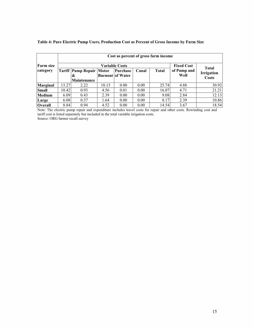
IV. Tariff Burden
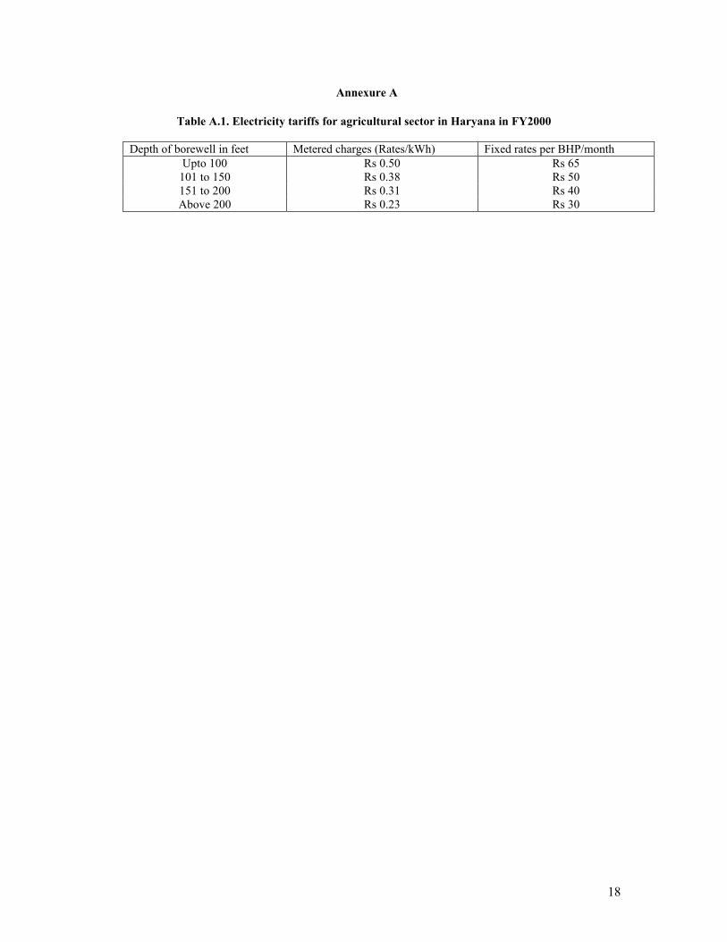
Farmers in Haryana have the choice of being charged for their consumption either on the basis of
per unit of consumption (metered rate) or on the basis of a flat rate per installed HP per month.2
The majority (80%) of farmers in Haryana in year 2000, however, were under the flat rate tariff. 3
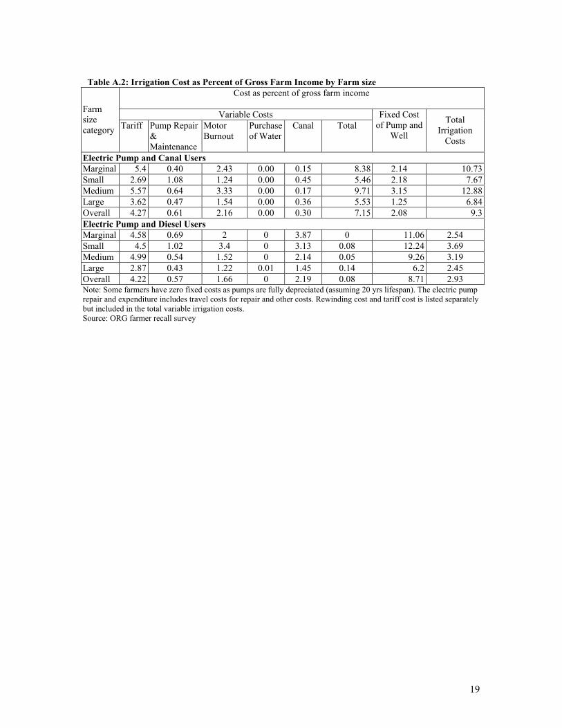
Using the official tariff rates, we calculated the tariff burden for each farm size category and
found that flat rate tariff is regressive (table 4). Electricity tariffs account for a larger proportion
of the gross farm income of marginal farmers: more than 13 per cent for those farmers who only
use electric pumps, and 2.5 per cent for users of electric pumps with diesel pumps (see annexure
A, table A.2 for details on other categories of electric farmers). 4 In contrast, electricity tariffs
account for only about 1 per cent to 6 per cent of gross income for larger farmers. For the
average electric pump owner in the sample, electricity tariff accounts from about 1 per cent (for
those who use electric with diesel pumps) to 9 per cent (for those using electric pumps only) of
gross income.
The poor quality of electricity supply imposes an additional cost to the farmers in the
form of expenditures to repair burned out electric pumps. On average, motor burnout costs
account for about 2-4.5% of gross income of electric pump owners. It is especially critical for
pure electric pump owners, and in particular, for marginal farmers for whom it amounts to as
much as 10% of gross farm income. Hence, although farmers are paying quite low tariffs, their
1 The following procedure was used to calculate total HP per farmer. If a farmer owned one 5 HP pump individually and had half ownership share in a 10 HP pump then his total HP was calculated as 10. 2 Official tariffs in Haryana are reported in annexure A, table A.1 3 In our data more than 90% of the farmers paid flat tariff and all the farmers in the regression sample paid flat tariff. 4 Gross farm income is defined as the sum of the price times the volume of all crops produced during the survey year, irrespective of whether these are self-consumed or sold in the market. The gross farm income does not include proceeds from the sale of crop by-products, non-crop activities (e.g. livestock) and sale of water. Total crop production was
7
effective costs are considerably higher due to these additional indirect costs. Note that the poor
quality of supply has several other important effects on farmers besides resulting in additional
expenditures on motor rewindings. Thus, for instance, the loss in crop yields due to lack of water
in the time period it takes to get the motor rewound also needs to be taken into account. The loss
in income due to these yield losses is estimated in the econometric model that is presented in the
section below.
V. Impact of Power supply conditions on Net Farm Income of electric pump owners
An econometric model was developed using the survey data to analyze how electricity supply
conditions affect net farm incomes of electric pump owners, controlling for other factors. Since
the decision to own an electric pump is endogenous, a correction for sample selection bias needs
to be made, if only the sample of electric pump owners is considered. The Heckman two-step
procedure was used to correct for this bias in the following way. First a probit estimation was
done to explain the choice of electric pumps (results presented in annexure A, table A.3), then the
estimate of inverse mills ratio from this equation was included amongst the set of repressors to
explain net farm income.
Net farm income is defined as the gross value of farm production minus annualized fixed
cost and all variable costs (except the imputed cost of family labor and land). Thus this income
regression estimates the determinants of net returns to own labor and land. Since the effect of
power and other farm and region specific factors on net farm incomes are likely to differ across
farmers belonging to different size categories, a net farm income equation was estimated
taken into account here irrespective of whether it was used for self-consumption, as seed for next year or as marketable surplus. Crop production was valued at the price as reported by farmer for the marketed portion
8
separately for a pooled sample of marginal and small farmers and pooled sample of medium and
large farmers.5
In the short run, net farm income is likely to be influenced by the pumping technology used
by the farmer. The technology variables include the total installed HP at the farm level and
whether it is allocated to electric pumps alone or also to diesel pumps. These technology
variables are included amongst the set of regressors and thus this equation estimates the effect of
power and other farm and region specific factors on short run incomes (keeping irrigation
technology constant). It can be argued, however, that both total HP and choice to invest in a
supplemental diesel pump are endogenous to the farm income regression. The greater the farm
income the greater the ability to invest in larger horsepower pumps and supplemental diesel
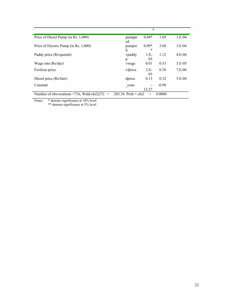
pumps. Hausman test of exogeniety test led us to reject the exogeniety of total horsepower in
both the farm income regressions. However, we failed to reject the exogeniety of the choice to
invest in a supplemental diesel pump. Instrument variable method was used to correct for
endogeneity of total HP. The instruments used to explain the choice of horsepower were the
information on past conditions of electricity supply.6 Past conditions of electricity supply would
clearly have no impact on the current farm incomes but would explain the choice of total
horsepower. The regression explaining the choice of horsepower is presented in annexure A,
table A.4.
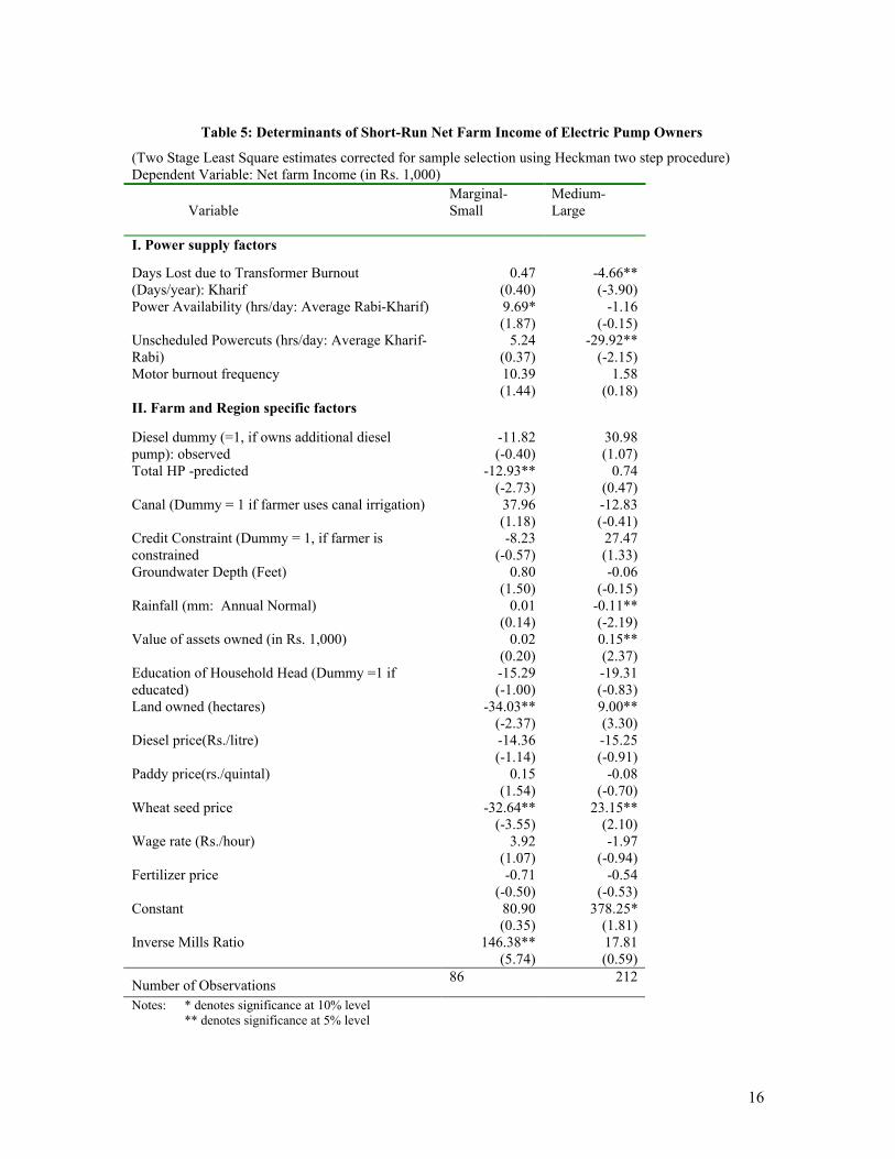
The results of the income equation show that the effect of power supply factors differs
significantly amongst farmers belonging to different size categories (table 5). Thus, for instance,
days lost due to transformer burnout during the kharif season was found to have a significant
negative effect on net farm incomes of medium and large farmers but not the small and marginal
farmers. It is during the kharif season that rice, a highly water intensive crop, is cultivated in
5 Separate income equations were first estimated for all the four size categories. The results for small and marginal were found to be qualitatively similar, and so also the results for medium and large farmers. Given the small regression sample size for each category taken separately, two pooled samples were examined finally.
9
many areas. It is likely that when power is interrupted for a long stretch of time (it took on
average of around 10 days to rectify a burnt transformer in kharif-99), there is significant
reduction in yields of water intensive crops, such as rice, due to water shortage. The effect of
transformer burnouts was not found to be significant in the other seasons. 7 A table on the
marginal willingness to pay for improvements in different power supply indicators is given in the
next section.
Power availability during the two main growing seasons of kharif and rabi was found to have
a significant positive effect on net incomes of only the marginal and small farmers. This suggests
that in the short run when irrigation capital is held constant, only marginal and small farmers feel
constrained by available power supply. Thus the potential of increasing net farm incomes in the
short run by increasing availability seems to be limited to only the smaller sized farmers.
Unreliability of supply was found to have a significant negative effect on net incomes of only
the medium and large farmers. In the short run, the net incomes of marginal and small farmers
are not significantly affected by the reliability of supply. It is possible that given their limited
capacity to bear shocks due to unreliability of supply, they make exante technology choices (such
as investing in larger sized pumps, annexure A) or cropping choices so as to insulate themselves
from these shocks more than the larger sized farms. Over the long run, improvements in
reliability of supply are likely to lead them to invest in smaller sized pumps and thus increase
their long run incomes.
The effect of poor quality of supply (as measured by the frequency of motor burnouts) was
not found to be significant for any of the size categories. Field investigators have observed that in
areas where motor burnouts are frequent (generally water intensive cropping areas with poor
quality of supply), the motor repair mechanics keep some old motors for use as rolling stock and
6 A separate attitude survey on electric pump owners’ perception of past conditions of electricity supply was conducted before the start of the seasonal recall surveys. Data on electricity supply conditions from this attitude survey were used in the technology regressions. Around 80% of farmers in the recall survey were also included in the attitude survey.
10
provide these to the farmers when their motor burns as a stop gap arrangement on a minimal rent
basis. This ensures that farmers do not suffer much loss in crop production on account of motor
burnout and the only income loss is in the form of expenses incurred in getting the motor
rewound and rental for a temporary motor.
To test for the possibility of non-linear effects of power supply indicators, squared terms of
the power supply indicators were also included as explanatory variables. However, the effects
were not found to be significant. Several interaction effects such as that between power supply
indicators and technology variables were also tried but not found to be significant. Amongst the
other farm and region specific factors, land and non-land assets owned by the farmer were found
to have a significant positive effect on net incomes of medium and large farmers. Interestingly,
the education of the household head was not found to have a significant effect on farm incomes of
any of the size categories. Amongst the various input prices that were tried, only wheat seed
price was found to have a significant effect on farm incomes of small and marginal farmers.
None of the output prices was found to have a significant effect apart from rice, which had a
significant positive effect for small and marginal farmers. Wheat is also an important crop, but its
price does not show much cross-sectional variability because of the government’s procurement
policies. Thus the wheat price elasticity could not be estimated.
Besides the above-discussed variables, several infrastructure variables, such as road density
(length of road/ sq km) and market development (number of markets/sq km) at the district level
were also tried, but the effects were not significant. The groundwater quality (percentage of fresh
water in the aquifer), soil quality (dummy equal to one for saline districts) and annual rainfall
variables were also not found to be significant.
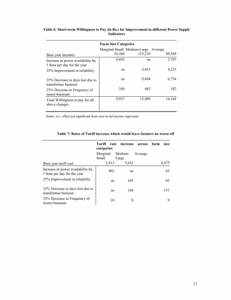
VI. How much do farmers value improvements in conditions of power supply
7 The frequency of transformer burnouts in kharif-99 season was around 0.92, which is somewhat higher than that
11
As discussed before, a central objective of this study was to find out how much farmers value
improvements in conditions of supply. There are two ways of addressing this issue. One is to
find out farmers’ willingness to pay for power supply improvements. Second is to find out how
much tariffs could be increased, if power supply conditions are improved, without making any set
of farmers worse off. Both these measures could provide useful inputs to policy makers in
proposing alternative policy scenarios.
To begin with, it would be useful to evaluate the marginal willingness to pay (MWTP) for
improvement in different power supply indicators in the short run. If Y is the short run net farm
income and I is a power supply indicator, then MWTP is defined as MWTP = ∂Y/∂I
These MWTP estimates are therefore the coefficients on the power supply indicators in the net
income regressions presented in table 5. Amongst the different power supply indicators, first
consider the willingness to pay for an hour’s increase in power availability per day through out
the year. Here note that the short run supply curve of electric pump owners has a mirrored L
shape. This implies that for farmers whose demand curve intersects this supply curve on the
horizontal part, the MWTP is equal to zero because these farmers are unconstrained and value
water (and hence power) at zero value at the margin. On the other hand, for some other farmers it
may be possible that their demand curve intersects their supply curve at the vertical part in which
case they are constrained by available power supply and have a positive valuation for power.
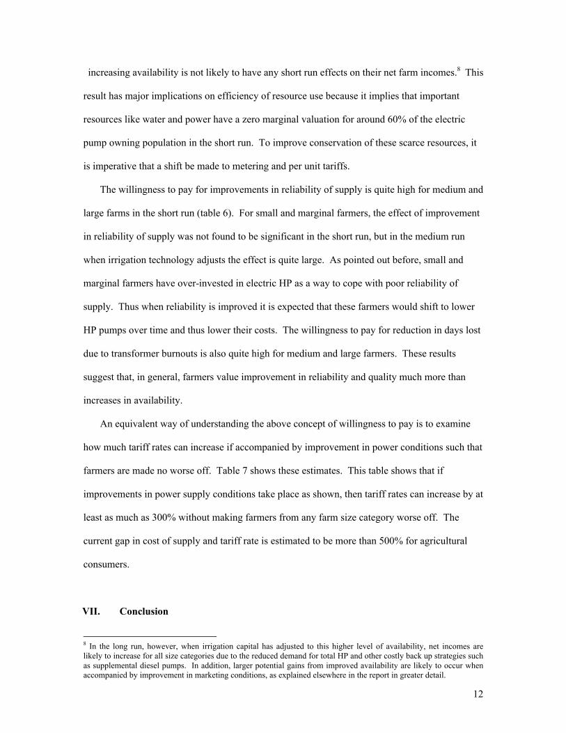
Table 6 below shows the willingness to pay for different farm size categories in the sample.
As shown in this table, marginal and small farmers are willing to pay Rs. 9692 for an hour/per
day increase in availability of power in the short run. However, medium and large farmers seem
to have a zero valuation for power availability at the margin. This implies that given their
technology choices, they are not currently constrained by the available power supply. Thus
reported for the other seasons in the survey year (summer=0.7 ; rabi=0.8). The days taken for repair was also reported to be higher in kharif (10 days) as opposed to other seasons during the survey year (summer:8 days, rabi: 6 days ).
12
increasing availability is not likely to have any short run effects on their net farm incomes.8 This
result has major implications on efficiency of resource use because it implies that important
resources like water and power have a zero marginal valuation for around 60% of the electric
pump owning population in the short run. To improve conservation of these scarce resources, it
is imperative that a shift be made to metering and per unit tariffs.
The willingness to pay for improvements in reliability of supply is quite high for medium and
large farms in the short run (table 6). For small and marginal farmers, the effect of improvement
in reliability of supply was not found to be significant in the short run, but in the medium run
when irrigation technology adjusts the effect is quite large. As pointed out before, small and
marginal farmers have over-invested in electric HP as a way to cope with poor reliability of
supply. Thus when reliability is improved it is expected that these farmers would shift to lower
HP pumps over time and thus lower their costs. The willingness to pay for reduction in days lost
due to transformer burnouts is also quite high for medium and large farmers. These results
suggest that, in general, farmers value improvement in reliability and quality much more than
increases in availability.
An equivalent way of understanding the above concept of willingness to pay is to examine
how much tariff rates can increase if accompanied by improvement in power conditions such that
farmers are made no worse off. Table 7 shows these estimates. This table shows that if
improvements in power supply conditions take place as shown, then tariff rates can increase by at
least as much as 300% without making farmers from any farm size category worse off. The
current gap in cost of supply and tariff rate is estimated to be more than 500% for agricultural
consumers.
VII. Conclusion
8 In the long run, however, when irrigation capital has adjusted to this higher level of availability, net incomes are likely to increase for all size categories due to the reduced demand for total HP and other costly back up strategies such as supplemental diesel pumps. In addition, larger potential gains from improved availability are likely to occur when accompanied by improvement in marketing conditions, as explained elsewhere in the report in greater detail.
13
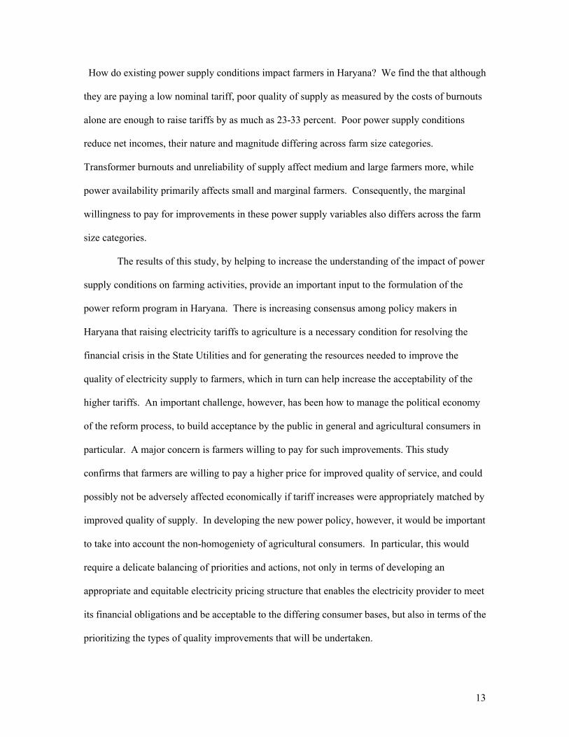
How do existing power supply conditions impact farmers in Haryana? We find the that although
they are paying a low nominal tariff, poor quality of supply as measured by the costs of burnouts
alone are enough to raise tariffs by as much as 23-33 percent. Poor power supply conditions
reduce net incomes, their nature and magnitude differing across farm size categories.
Transformer burnouts and unreliability of supply affect medium and large farmers more, while
power availability primarily affects small and marginal farmers. Consequently, the marginal
willingness to pay for improvements in these power supply variables also differs across the farm
size categories.
The results of this study, by helping to increase the understanding of the impact of power
supply conditions on farming activities, provide an important input to the formulation of the
power reform program in Haryana. There is increasing consensus among policy makers in
Haryana that raising electricity tariffs to agriculture is a necessary condition for resolving the
financial crisis in the State Utilities and for generating the resources needed to improve the
quality of electricity supply to farmers, which in turn can help increase the acceptability of the
higher tariffs. An important challenge, however, has been how to manage the political economy
of the reform process, to build acceptance by the public in general and agricultural consumers in
particular. A major concern is farmers willing to pay for such improvements. This study
confirms that farmers are willing to pay a higher price for improved quality of service, and could
possibly not be adversely affected economically if tariff increases were appropriately matched by
improved quality of supply. In developing the new power policy, however, it would be important
to take into account the non-homogeniety of agricultural consumers. In particular, this would
require a delicate balancing of priorities and actions, not only in terms of developing an
appropriate and equitable electricity pricing structure that enables the electricity provider to meet
its financial obligations and be acceptable to the differing consumer bases, but also in terms of the
prioritizing the types of quality improvements that will be undertaken.
Table 1: Availability of Power in Haryana – Responses from the Attitude and Recall Survey
Hours of power supply reported by farmers Season Recall Survey Attitude Survey
Rabi season 6.3 8 Summer season 7.3 7 Kharif season 9.7 7
Source : ORG Survey Table 2: Summary statistics on sample irrigation technology groups (table below summarizes the main points)
Pump owners Non-pump owners
Particulars Electric pump owners
Non-electric diesel pump owners
Canal users Water purchasers Rainfed
Total
Total number in sample
777 249 251 245 137 1,659
Marginal 165 60 90 168 95 578 Small 148 66 78 47 23 362 Medium 274 87 65 27 17 470 Large 190 36 18 3 2 249
Average Land Owned Average land owned (ha.)
4.0 2.8 1.9 1.0 1.1 2.8
Notes: This table includes only those sample farmers for whom complete land and cultivation data is available Source: ORG farmers’ recall data
Table 3: Average Horsepower per Unit of Gross Cultivated area by Farmer Size ( HP/gross cultivated hectare)
Farm size categories Pump type Marginal Small Medium Large All Diesel 1.8 1.1 0.7 0.3 0.9 Electric 1.4 0.8 0.6 0.6 0.8
Source: ORG farmers’ recall data
15
Table 4: Pure Electric Pump Users, Production Cost as Percent of Gross Income by Farm Size
Cost as percent of gross farm income
Variable Costs Farm size category Tariff Pump Repair
& Maintenance
Motor Burnout
Purchase of Water
Canal Total Fixed Cost
of Pump and Well
Total Irrigation
Costs
Marginal 13.27 2.22 10.15 0.00 0.00 25.74 4.88 30.92 Small 10.42 0.93 4.56 0.01 0.00 16.07 4.71 21.21 Medium 6.09 0.43 2.39 0.00 0.00 9.08 2.84 12.13 Large 6.08 0.37 1.64 0.00 0.00 8.17 2.39 10.86 Overall 8.84 0.94 4.52 0.00 0.00 14.54 3.67 18.54 Note: The electric pump repair and expenditure includes travel costs for repair and other costs. Rewinding cost and tariff cost is listed separately but included in the total variable irrigation costs. Source: ORG farmer recall survey
16
Table 5: Determinants of Short-Run Net Farm Income of Electric Pump Owners
(Two Stage Least Square estimates corrected for sample selection using Heckman two step procedure) Dependent Variable: Net farm Income (in Rs. 1,000) Variable
Marginal-Small
Medium-Large
I. Power supply factors
Days Lost due to Transformer Burnout (Days/year): Kharif
0.47 (0.40)
-4.66** (-3.90)
Power Availability (hrs/day: Average Rabi-Kharif) 9.69* (1.87)
-1.16 (-0.15)
Unscheduled Powercuts (hrs/day: Average Kharif- Rabi)
5.24 (0.37)
-29.92** (-2.15)
Motor burnout frequency 10.39 (1.44)
1.58 (0.18)
II. Farm and Region specific factors
Diesel dummy (=1, if owns additional diesel pump): observed
-11.82 (-0.40)
30.98 (1.07)
Total HP -predicted -12.93** (-2.73)
0.74 (0.47)
Canal (Dummy = 1 if farmer uses canal irrigation) 37.96 (1.18)
-12.83 (-0.41)
Credit Constraint (Dummy = 1, if farmer is constrained
-8.23 (-0.57)
27.47 (1.33)
Groundwater Depth (Feet) 0.80 (1.50)
-0.06 (-0.15)
Rainfall (mm: Annual Normal) 0.01 (0.14)
-0.11** (-2.19)
Value of assets owned (in Rs. 1,000) 0.02 (0.20)
0.15** (2.37)
Education of Household Head (Dummy =1 if educated)
-15.29 (-1.00)
-19.31 (-0.83)
Land owned (hectares) -34.03** (-2.37)
9.00** (3.30)
Diesel price(Rs./litre) -14.36 (-1.14)
-15.25 (-0.91)
Paddy price(rs./quintal) 0.15 (1.54)
-0.08 (-0.70)
Wheat seed price -32.64** (-3.55)
23.15** (2.10)
Wage rate (Rs./hour) 3.92 (1.07)
-1.97 (-0.94)
Fertilizer price -0.71 (-0.50)
-0.54 (-0.53)
Constant
80.90 (0.35)
378.25* (1.81)
Inverse Mills Ratio 146.38** (5.74)
17.81 (0.59)
Number of Observations 86 212
Notes: * denotes significance at 10% level ** denotes significance at 5% level
17
Table 6: Short-term Willingness to Pay (in Rs.) for Improvement in different Power Supply Indicators
Farm Size Categories Marginal-Small Medium-Large Average
Base year incomes 36,360 125,210 99,569
Increase in power availability-by 1 hour per day for the year
9,692 ns 2,797
25% Improvement in reliability ns 5,953 4,235
25% Decrease in days lost due to transformer burnout-
ns 9,494 6,754
25% Decrease in Frequency of motor-burnouts
244 462 382
Total Willingness to pay for all above changes
9,937 15,909 14,168
Notes: n.s.: effect not significant from zero in net income regression
Table 7: Rates of Tariff increase which would leave farmers no worse off
Tariff rate increase across farm size categories
Marginal-Small
Medium-Large
Average
Base year tariff cost 2,413 5,652 4,475
Increase in power availability-by 1 hour per day for the year
402 ns 63
25% Improvement in reliability ns 105 95
25% Decrease in days lost due to transformer burnout-
ns 168 151
25% Decrease in Frequency of motor-burnouts
10 8 9
18
Annexure A
Table A.1. Electricity tariffs for agricultural sector in Haryana in FY2000
Depth of borewell in feet Metered charges (Rates/kWh) Fixed rates per BHP/month Upto 100 Rs 0.50 Rs 65
101 to 150 Rs 0.38 Rs 50 151 to 200 Rs 0.31 Rs 40 Above 200 Rs 0.23 Rs 30
19
Table A.2: Irrigation Cost as Percent of Gross Farm Income by Farm size
Cost as percent of gross farm income
Variable Costs Farm size category Tariff Pump Repair
& Maintenance
Motor Burnout
Purchase of Water
Canal Total Fixed Cost
of Pump and Well
Total Irrigation
Costs
Electric Pump and Canal Users Marginal 5.4 0.40 2.43 0.00 0.15 8.38 2.14 10.73 Small 2.69 1.08 1.24 0.00 0.45 5.46 2.18 7.67 Medium 5.57 0.64 3.33 0.00 0.17 9.71 3.15 12.88 Large 3.62 0.47 1.54 0.00 0.36 5.53 1.25 6.84 Overall 4.27 0.61 2.16 0.00 0.30 7.15 2.08 9.3 Electric Pump and Diesel Users Marginal 4.58 0.69 2 0 3.87 0 11.06 2.54 Small 4.5 1.02 3.4 0 3.13 0.08 12.24 3.69 Medium 4.99 0.54 1.52 0 2.14 0.05 9.26 3.19 Large 2.87 0.43 1.22 0.01 1.45 0.14 6.2 2.45 Overall 4.22 0.57 1.66 0 2.19 0.08 8.71 2.93 Note: Some farmers have zero fixed costs as pumps are fully depreciated (assuming 20 yrs lifespan). The electric pump repair and expenditure includes travel costs for repair and other costs. Rewinding cost and tariff cost is listed separately but included in the total variable irrigation costs. Source: ORG farmer recall survey
20
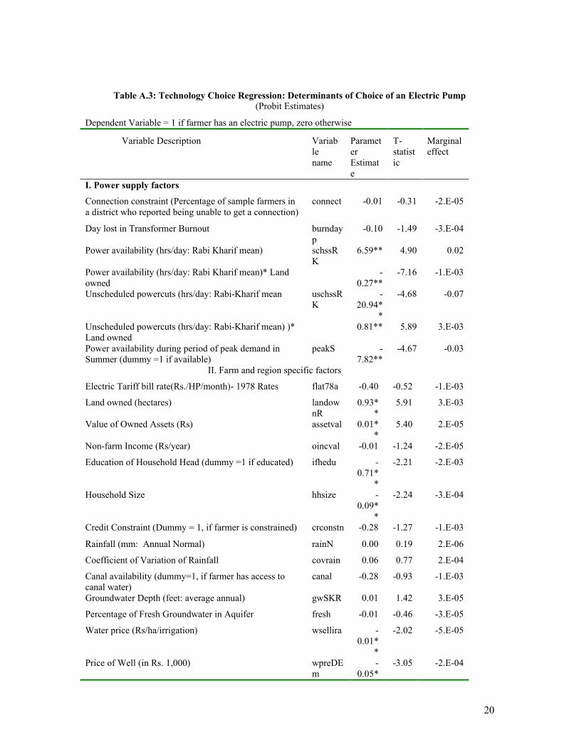
Table A.3: Technology Choice Regression: Determinants of Choice of an Electric Pump (Probit Estimates)
Dependent Variable = 1 if farmer has an electric pump, zero otherwise
Variable Description Variable name
Parameter Estimate
T-statistic
Marginal effect
I. Power supply factors
Connection constraint (Percentage of sample farmers in a district who reported being unable to get a connection)
connect -0.01 -0.31 -2.E-05
Day lost in Transformer Burnout burndayp
-0.10 -1.49 -3.E-04
Power availability (hrs/day: Rabi Kharif mean) schssRK
6.59** 4.90 0.02
Power availability (hrs/day: Rabi Kharif mean)* Land owned
-0.27**
-7.16 -1.E-03
Unscheduled powercuts (hrs/day: Rabi-Kharif mean uschssRK
-20.94*
*
-4.68 -0.07
Unscheduled powercuts (hrs/day: Rabi-Kharif mean) )* Land owned
0.81** 5.89 3.E-03
Power availability during period of peak demand in Summer (dummy =1 if available)
peakS -7.82**
-4.67 -0.03
II. Farm and region specific factors
Electric Tariff bill rate(Rs./HP/month)- 1978 Rates flat78a -0.40 -0.52 -1.E-03
Land owned (hectares) landownR
0.93**
5.91 3.E-03
Value of Owned Assets (Rs) assetval 0.01**
5.40 2.E-05
Non-farm Income (Rs/year) oincval -0.01 -1.24 -2.E-05
Education of Household Head (dummy =1 if educated) ifhedu -0.71*
*
-2.21 -2.E-03
Household Size hhsize -0.09*
*
-2.24 -3.E-04
Credit Constraint (Dummy = 1, if farmer is constrained) crconstn -0.28 -1.27 -1.E-03
Rainfall (mm: Annual Normal) rainN 0.00 0.19 2.E-06
Coefficient of Variation of Rainfall covrain 0.06 0.77 2.E-04
Canal availability (dummy=1, if farmer has access to canal water)
canal -0.28 -0.93 -1.E-03
Groundwater Depth (feet: average annual) gwSKR 0.01 1.42 3.E-05
Percentage of Fresh Groundwater in Aquifer fresh -0.01 -0.46 -3.E-05
Water price (Rs/ha/irrigation) wsellira -0.01*
*
-2.02 -5.E-05
Price of Well (in Rs. 1,000)
wpreDEm
-0.05*
-3.05 -2.E-04
21
*
Price of Diesel Pump (in Rs. 1,000)
pumppred
0.04* 1.69 1.E-04
Price of Electric Pump (in Rs. 1,000)
pumpreE
0.09**
3.60 3.E-04
Paddy price (Rs/quintal) vpaddyp
1.E-03
1.12 4.E-06
Wage rate (Rs/day) vwage 0.01 0.53 5.E-05
Ferilizer price vfprice 2.E-03
0.30 7.E-06
Diesel price (Rs/liter) dprice 0.13 0.32 5.E-04
Constant _cons -12.27
-0.98
Number of obsverations =716, Wald chi2(27) = 203.34 Prob > chi2 = 0.0000
Notes: * denotes significance at 10% level ** denotes significance at 5% level
22
Table A.4: Determinants of Total Horsepower for Farmers with Electric Pump (Ordinary Least Square estimates corrected for sample selection using Heckman two step procedure)
Dependent Variable: Natural Log of Total Horsepower
Variable
Parameter Estimate
T-Statistic Elasticity
I. Power supply factors
Days Lost due to Transformer Burnout (Days/year) -3.E-04 -0.06 -3.E-03 Power Availability (hrs/day: Average Rabi-Kharif) -0.70** -4.93 -5.49 Power Availability (hrs/day: Average Rabi-Kharif)* Landowned
0.11** 4.68 3.76
Power Availability (hrs/day:Summer) 0.48** 3.80 3.37 Power Availability (hrs/day:Summer)* Landown -0.09** -3.88 -2.74 Unscheduled Powercuts (hrs/day: Average Kharif- Rabi)
0.87** 3.38 1.14
Unscheduled Powercuts (hrs/day: Average Kharif- Rabi)*Landowned
-0.08** -2.72 -0.47
Availability during period of peak demand (Kharif) 1.66** 2.98 0.38 Availability during period of peak demand (Rabi) -2.67** -8.37 -1.15 Availability during period of peak demand (Summer) 0.84* 1.85 0.13
II. Farm and region specific factors
Electric Tariff bill rate(Rs./HP/month) -0.04** -2.32 -0.93 Electric Tariff bill Rate * Groundwater Depth 5.E-04** 2.35 0.80 Canal (Dummy = 1 if farmer uses canal irrigation) -0.23 -1.29 -0.04 Percentage Fresh Groundwater in Aquifer 0.01** 3.29 0.77 Groundwater Depth (Feet) -0.01** -2.32 -0.84 Rainfall (mm: Annual Normal) -2.E-03** -2.12 -0.96 Coefficient of Variation of Rainfall 3.E-03 0.19 0.08 Land owned (hectares) -0.03 -1.11 -0.16 Rental Price of Land (Rs/hectare) 3.E-05** 3.65 0.25 Household size 0.02* 1.66 0.16 Education of Household Head (Dummy =1 if educated)
0.06 0.56 0.04
Constant 3.57** 3.63
N=334
Log likelihood = -316.0357
Wald chi2(21) = 329.44 Prob > chi2 = 0.0000
Notes: * denotes significance at 10% level ** denotes significance at 5% level

23
References
1. Center for Monitoring Indian Economy, 1999, Agriculture, Bombay: CMIE. 2. Padmanabhan, S. and Govindarajalu, C., 1999, “Power supply to agriculture: Cost
minimization options”, Inception Report, World Bank, Washington D.C.