IMRT planning on adaptive volume structures - a decisive reduction in computational complexity

INSTITUTE OF PHYSICS PUBLISHING PHYSICS IN MEDICINE AND BIOLOGY

Phys. Med. Biol. 50 (2005) 2033–2053 doi:10.1088/0031-9155/50/9/008

IMRT planning on adaptive volume structures—adecisive reduction in computational complexity

Alexander Scherrer1, Karl-Heinz Kufer1, Thomas Bortfeld2,Michael Monz1 and Fernando Alonso1

1 Department of Optimization, Fraunhofer Institut for Industrial Mathematics,Gottlieb-Daimler-Straße 49, 67663 Kaiserslautern, Germany2 Department of Radiation Oncology, Massachusetts General Hospital and Harvard MedicalSchool, 30 Fruit Street, Boston, MA 02114, USA

E-mail: [email protected], [email protected], [email protected], [email protected] [email protected]

Received 18 March 2004, in final form 21 February 2005Published 20 April 2005Online at stacks.iop.org/PMB/50/2033

AbstractThe objective of radiotherapy planning is to find a compromise between thecontradictive goals of delivering a sufficiently high dose to the target volumewhile widely sparing critical structures. The search for such a compromiserequires the computation of several plans, which mathematically means solvingseveral optimization problems. In the case of intensity modulated radiotherapy(IMRT) these problems are large-scale, hence the accumulated computationalexpense is very high. The adaptive clustering method presented in this paperovercomes this difficulty. The main idea is to use a preprocessed hierarchyof aggregated dose–volume information as a basis for individually adaptedapproximations of the original optimization problems. This leads to a decisivelyreduced computational expense: numerical experiments on several sets of realclinical data typically show computation times decreased by a factor of about10. In contrast to earlier work in this field, this reduction in computationalcomplexity will not lead to a loss in accuracy: the adaptive clustering methodproduces the optimum of the original optimization problem.

(Some figures in this article are in colour only in the electronic version)

1. Introduction

In intensity-modulated radiotherapy (IMRT) planning the oncologist faces the challenging taskof finding a treatment plan that he considers to be an ideal compromise between the inherentlycontradictive goals of delivering a sufficiently high dose to the target while widely sparingcritical structures. The search for this a priori unknown compromise typically requiresthe computation of several plans, i.e. the solution of several optimization problems. This

0031-9155/05/092033+21$30.00 © 2005 IOP Publishing Ltd Printed in the UK 2033

http://dx.doi.org/10.1088/0031-9155/50/9/008

http://stacks.iop.org/pb/50/2033

2034 A Scherrer et al

accumulates to a high computational expense due to the large scale of these problems—aconsequence of the 3D discretization of the relevant volume and the large number of parametersrepresenting the intensity maps to be computed. An overview of the various aspects of IMRTis given in Webb (2001) and a description of the state-of-the-art and current research topicscan be found in IMRT Collaborative Working Group (2001). Zelefsky et al (2001), Pollackand Price (2003) and Chao and Blanco (2003) give some clinical aspects of IMRT.

This paper presents the adaptive clustering method as a new algorithmic concept for thesolution of such problems. The computations are performed on an individually adapted volumestructure rather than on the original voxels, leading to a decisively reduced computationalexpense. In contrast to many other similar concepts, the typical tradeoff between a reductionin computational complexity and a loss in exactness can be avoided: the adaptive clusteringmethod produces the optimum of the original problem. Despite its original invention for thelinear max and mean equivalent uniform dose (EUD) model, cf Thieke et al (2002), in amulti-criteria optimization concept, cf Kufer et al (2003), this flexible method can be appliedto both single- and multi-criteria convex optimization methods. The extension to non-convexproblems is a topic of future research.

The paper is organized as follows. Section 1.1 provides the basic ideas of the adaptiveclustering method. Section 2 first introduces the mathematical notation and terminology (2.1),then formulates the adaptive clustering principle including an argument of correctness (2.2)and explains its algorithmic realization in the form of the adaptive clustering method (2.3)with a discussion of the computational complexity. Section 3 gives evidence of the practicalrelevance by comparing CPU times required for computations on adapted volume structuresversus regular voxel grids for two clinical cases.

Sections 1.1 and 3 are sufficient for a first understanding of the basic ideas and impressionof the obtained results, whereas section 2 is essential for a deeper understanding of thetheoretical and algorithmic concepts.

1.1. The basic idea of the adaptive clustering method

The optimization problem of IMRT planning, i.e. the computation of a plan of the best possiblequality is based on the information about the dose distribution and its evaluation in the differentclinical structures involved. Typically, during a plan computation the dose distribution willattain an acceptable shape in most of the volume, such that the final quality of a treatment planstrongly depends on the shape in some small volume parts, where e.g. the descent of radiationfrom the cancerous to the healthy structures implies undesirable dose–volume effects.

Based on this problem characteristic, several approaches to reduce the computationalcomplexity of the problem by manipulations in the volume have been tried, cf the listing inZakarian and Deasy (2004). These manipulations are done by heuristic means in advance ofthe computations and incorporate e.g. the use of large voxels in less critical volume parts, arestriction to the voxels located in pre-defined regions of interest or a physically motivatedselection of voxels. However, such heuristic problem modifications will possibly lead to aninsufficient control on the dose distribution during the computation and a thus uncontrollablyworsened plan quality.

The adaptive clustering method overcomes these defects by means of a non-heuristicadaptation in the volume, performed during the plan computation. In a preprocessing step,the original dose–volume information is successively aggregated to clusters consisting ofmerged voxels with their corresponding dose information, forming a cluster hierarchy withdifferent levels. This hierarchical clustering process is independent of how dose distributionsare evaluated. Performed only once for an IMRT planning problem, the resulting cluster

IMRT planning on adaptive volume structures 2035

Figure 1. The original volume structure consisting of voxels (left) and the adapted volume structurebased on clusters (right).

hierarchy will then serve as a ‘construction kit’ to generate adapted volume structures for allthe plan computations required. Each computation starts on a coarse clustering that consistsof clusters of the upper hierarchy levels. While the computation runs, the algorithm graduallydetects the volume parts with an undesirable shape of the dose distribution and replaces thecorresponding clusters in local refinement steps by smaller ones of the lower levels to improvethe local control on the dose distribution. Such structures with clusters from different levelsare called adapted clusterings. Due to the individual adaptation of the volume structure duringthis local refinement process, the computation yields an optimum of the original problem, butwith a significantly smaller expense than straightforward computation based on the voxelswould have required. Numerical experiments on several sets of real clinical data typicallyshow computation times decreased by a factor of about 10.

Figure 1 shows for a clinical head neck case the original volume structure of voxels in atransversal slice and the adapted volume structure in the same slice that was generated withthe adaptive clustering method. Computations on both structures yield plans with very similarand (numerically) identically evaluated dose distributions and almost identical dose–volumehistograms, but with a significantly smaller computational expense for the adaptive clusteringmethod.

2. Material and methods

2.1. The IMRT planning problem

2.1.1. Basic notation. A treatment plan is physically determined by the irradiation geometry,which is assumed to be already given, and the intensity map for the different beams. LetB = ⋃

i Bi denote the partition of the total beam area B into the beamlets Bi and V = ⋃j Vj

the partition of the relevant part V of the body volume into the voxels Vj . Furthermore, letX denote the space containing all intensity maps, i.e. the vectors x = (xi) � 0 containingthe intensities for the beamlets Bi of all beams. The realization of intensity maps withmultileaf collimators or other devices cf Webb (1997), is not discussed in this paper. The dosedistribution in the volume for an intensity map x attains the form of a vector d(x) = (d(Vj )(x))

with the dose values d(Vj )(x) in the voxels Vj . These values follow as

d(Vj )(x) = p(Vj ) · x, (1)

where the entries of the dose information vector p(Vj ) denote the dose deposits of the differentbeamlets Bi into the corresponding voxel Vj when radiating with unit intensity. With the dose


information matrix P as the combination of the vectors p(Vj ), the dose distribution follows asd(x) = P · x.

2.1.2. Typical evaluation functions. The quality of a treatment plan determined by anintensity vector x with respect to a clinical structure is modelled by an evaluation function f

that maps the corresponding dose distribution d(x) to a real value f (d(x)). Standard evaluationfunctions include those that measure deviations from a desired dose value L in the target T

f (d(x)) = maxVj ⊆T

|L − d(Vj )(x)|, (2)

or functions which penalize voxel doses exceeding an upper bound U in an organ at risk R

f (d(x)) = ∑

Vj ⊆R

(d(Vj )(x) − U)q+

1q

, q ∈ [1,∞). (3)

Another choice are functions which take account of the whole shape of a dose distribution bymeans of an EUD, cf e.g. Brahme (1984). Using for example Niemierko’s EUD (Niemierko1997), the deviation for the organ at risk R from U is measured by

f (d(x)) = 1

U

|R|−1

∑Vj ⊆R

d(Vj )q(x)

1q

, q ∈ [1,∞), (4)

where |R| denotes the number of voxels in R. The basic property of all such evaluationfunctions is convexity. Due to the favourable numerical properties of the resulting problems,the restriction to a convex setting, has proven to be a very reasonable way to compute plansof high clinical quality, whose final evaluation by the physician may nevertheless be done onthe basis of non-convex criteria like DVH constraints. However, since the adaptive clusteringconcept is physically well motivated, it will possibly extend well to non-convex problems, atopic for future research.

Nevertheless, since the evaluation functions typically take account of all the voxels in aclinical structure with their corresponding dose values (1) and each structure typically consistsof several ten thousand or hundred thousand voxels, multiple computations of an evaluationfunction during the optimization are very expensive and the corresponding optimizationproblems thus have a high computational complexity.

2.1.3. The optimization method. Based on the structure related evaluation functions, theoptimization problem is formulated either in a single- or a multi-criteria way. Classicalsingle-criteria approaches introduce an objective function by means of weighted scalarization,e.g.

f (d(x)) =∑k∈K

µkfk(d(x)) (5)

with some weight factors µk > 0, where the fk denote the evaluation functions for the differentclinical structures, that are enumerated by k ∈ K. Throughout the paper, a clinical structuredenotes a volume of interest with a single evaluation function. Volumes of interest with two ormore evaluation functions are thus duplicated and considered as separate clinical structures.In modern multi-criteria approaches, cf e.g. Yu (1997) and Cotrutz et al (2001), the fk enteras separate objective functions. Multi-criteria optimization can be done in many differentways, cf e.g. Steuer (1985), that are all somehow based on a reasonably chosen reductionto a single-criteria optimization problem. In the single-criteria as well as the multi-criteria


approach, some clinical structures may also be excluded from the objective function(s) andenter the optimization problem as hard constraints, e.g. for the target T with the index k(T ),

fk(T )(d(x)) = Lk(T ) − minVj ⊆T

d(Vj )(x) � 0 (6)

with the strict lower dose bound Lk(T ).

2.1.4. The necessity for repeated plan computations. Since the treatment possibilities ofIMRT strongly depend on the specific clinical case and are thus not completely known at thebeginning, the search for an optimal treatment plan typically requires the solution of severaloptimization problems in order to explore the limitations set by the introduced hard constraintsand to study the remaining possibilities, e.g. the trade-off between different structure-relatedplanning goals, cf Hunt et al (2002). This is often done in a human iteration loop, where in eachiterative step a plan is computed with the current objective function and, provided it does notsatisfy all clinical goals, the objective function is modified for the next step, e.g. by modificationof the weight vector in the single-criteria approach or some goal programming technique forthe multi-criteria approach. Another option especially in the case of the multi-criteria approachis a precomputation of sufficiently many clinically reasonable plans in advance to choose fromafterwards, cf Kufer et al (2000, 2003). Combinations of these two main options, which sharethe need for repeated plan computations, are also possible.

2.1.5. The geometry of the convex optimization problem. The problems resulting from thedifferent evaluation models and mathematical approaches above imply convex optimizationproblems. To keep the notation simple, we restrict our theoretical considerations to the caseof a target with the hard constraint (6) and a single organ at risk R with the evaluation function(4) serving as the objective function. The feasible region, i.e. the set of all intensity vectors,whose corresponding dose distributions d(x) fulfil the hard constraint in the target, is denoted

Xfeas = {0 � x ∈ X : fk(T )(d(x)) � 0}. (7)

Concerning the organ at risk R, the level set for the objective value s, i.e. the set of allintensity vectors, whose dose distributions obtain the same evaluation s when considered inR, is denoted

Xobj(s) = {0 � x ∈ X : fk(R)(d(x)) = s}. (8)

Solving the resulting convex optimization problem means finding an intensity vector x∗, thatfulfils the hard constraint (6) and is thus contained in Xfeas and is at the same time evaluatedbest among all elements of Xfeas, i.e. fk(R)(d(x)) attains for x∗ its minimum s∗ on Xfeas. Thegeometrical meaning of this in the space X containing all intensity maps is illustrated infigure 2, where each coordinate axis corresponds to one of the typically many hundred orseveral thousand beamlets: s∗ is the smallest value, such that the level set Xobj(s), whoseshape and position in X varies depending on the value of s, intersects the feasible region Xfeas.The convex optimization problem can thus be written as

CP : s → Min subject to (9)

Xfeas ∩ Xobj(s) �= ∅.

The typically non-unique optima then form the intersection

Xfeas ∩ Xobj(s∗) = {0 � x∗ ∈ X : x∗ optimum of CP}. (10)


feas

(s*)obj

(s), s>s*obj

x*

(s), s<s*obj

xi

xi'

Figure 2. The set-based illustration of the optimization problem.

2.2. The principle of adaptive clustering

This section contains an explanation of the underlying principles of the adaptive clusteringmethod and an informal argument of its correctness.

2.2.1. The clustering technique. To ensure a uniform notation, the voxels are supplementedwith an upper index (0), i.e. V (0)

j . The whole family of voxels with their corresponding vectorsis denoted as

C(0) := {(V (0)

ι , p(V (0)

ι

)): ι ∈ J (0)

}. (11)

Since the photon pencil beam is smooth due to scattering effects, a family of voxelsV (0)

ι , ι ∈ J (0)j ⊂ J (0) of the same clinical structure, that are in the vicinity of each other

receive similar dose contributions from most of the beamlets. Hence, depending on the shapeof the intensity vector, they are likely to have similar dose values (1) and may be merged to

V(1)j :=

⋃

ι∈J (0)j

V (0)ι (12)

with the mean dose value d(V

(1)j

)(x) = ∣∣J (0)

j

∣∣−1 ∑ι∈J (0)

jp(V (0)

ι

) · x =: p(V

(1)j

) · x and the

mean dose information vector p(V

(1)j

)fulfilling

d(V

(1)j

)(x) ≈ d

(V (0)

ι

)(x) for all voxels V (0)

ι ⊆ V(1)j . (13)

Partitioning both structures R and T into such families of voxels and merging them yields aclustering

C(1) := {(V

(1)j , p

(V

(1)j

)): j ∈ J (1)

}, (14)

with the clusters(V

(1)j , p

(V

(1)j

)), cf figure 4. According to (13), the original dose vector

dC(0)

(x) = (d(V (0)

ι

)(x)

)with the dose values attained in the voxels V (0)

ι is quite similar to

the vector dC(1)

(x) = (d(V

(1)

j (ι)

)(x)

), that is derived from dC(0)

(x) by replacing the dose value

d(V (0)

ι

)(x) of each voxel by the mean dose value d

(V

(1)

j (ι)

)(x) of the corresponding cluster(

V(1)

j (ι), p(V

(1)

j (ι)

)), that contains this voxel. Hence applying e.g. the evaluation function of R to

both vectors yields almost the same values, i.e.

fk(R)

(dC(0)

(x)) ≈ fk(R)

(dC(1)

(x)). (15)


x*

(s*)obj

(0)

(s*)obj

(1)

(s*)obj

xi

xi'

Figure 3. The original level set, its approximation and the local adaptation around x∗.

However, the evaluation of a treatment plan on the basis of dC(1)

(x), i.e.

fk(R)

(dC(1)

(x)) = 1

U

|J (0)|−1

∑

V(1)j ⊆R

∣∣J (0)j

∣∣d(V

(1)j

)q(x)

1q

(16)

is much cheaper, since only the mean dose values for the few clusters are required insteadof the dose values for the many voxels. Obviously, the better the cluster related mean doseapproximates the dose values of the voxels of R in (13), the smaller are the cluster relatederrors ∑

ι∈J (0)j

d(V (0)

ι

)q(x) − ∣∣J (0)

j

∣∣d(V

(1)j

)q(x) (17)

and the more exact is approximation (15). A similar argument holds for the evaluation in T

based on dC(1)

(x), i.e.

fk(T )

(dC(1)

(x)) = L − min

V(1)j ⊆T

d(V

(1)j

)(x). (18)

This means, the clustering process, i.e. the merger of voxels to clusters allows an approximate,but much simpler representation for the dose distribution based on the mean dose values in theclusters, whose evaluation can be computed with a significantly smaller expense at the cost ofan only moderate approximation error.

2.2.2. Approximation aspects of clustering. Figure 3 illustrates the geometrical effect of theclustering on the level set

XC(0)

obj (s∗) = {0 � x ∈ X : fk(R)

(dC(0)

(x)) = s∗} (19)

of all intensity vectors x, whose voxel related dose vectors dC(0)

(x) attain the evaluation s∗ withrespect to R. Typically, the evaluation of an optimum x∗C(1) ∈ XC(1)

obj (s∗) based on the clusterrelated mean dose values differs slightly from s∗ according to (15). Hence x∗ is not containedin the approximate level set

XC(1)

obj (s∗) = {0 � x ∈ X : fk(R)

(dC(1)

(x)) = s∗} (20)


of all intensity vectors x, whose cluster related dose vectors dC(1)

(x) attain the evaluation s∗.This set passes somewhere nearby in some spatial distance depending on the exactness of(15). This means, the transition from the evaluation based on the voxel related dose valuesto the evaluation based on the cluster related mean dose values changes the level sets of theoptimization problem (2). In particular for x∗, the cluster related mean doses approximate thedose values of the contained voxels in (13) very well for the vast majority of the clusters, i.e.∣∣∣∣∣∣∣

∑

ι∈J (0)j

d(V (0)

ι

)q(x∗) − ∣∣J (0)

j

∣∣d(V

(1)j

)q(x∗)

∣∣∣∣∣∣∣� εk(R) (21)

with some small εk(R) > 0. It would thus make no real difference in the evaluation of x∗, ifsuch voxels with their dose values were replaced by the corresponding clusters with the clusterrelated mean doses. Only in very few clusters, where large dose gradients appear, e.g. in someparts of R adjacent to the target T , (13) is rather inexact implying large cluster related errors(17). Using these clusters and their mean doses instead of the contained voxels and their dosevalue worsens the approximation (15) significantly. Hence, the approximation error for thelevel set around x∗ has a local origin: there is a direct correspondence between the change inthis part of the level set and some volume part, where the discrepancy between the dose valuesby the cluster related mean doses is rather large.

The situation is analogous for T : in volume parts with dose values much higher than theminimal dose, the transition from voxels to clusters does not affect the evaluation at all. Alsothe use of clusters with dose values close to the lower dose bound L, but

maxι∈J (0)

j

∣∣∣d(V

(1)j

)(x∗) − d

(V (0)

ι

)(x∗)

∣∣∣ � εk(T ) (22)

with some small εk(T ) > 0 instead of the corresponding voxels would also make no realdifference in the evaluation of x∗. This means, the approximation error around x∗ traces backto small volume parts, in which the dose distribution attains its minimum and the clusterrelated dose values give a rather inexact approximation.

2.2.3. Local adaptation by means of adaptive clustering. According to the previousconsiderations, the evaluation error for x∗ could thus be almost avoided using voxels incritical volume parts of R and T and clusters everywhere else. This combination A of voxelsand clusters is called an adapted clustering, cf figure 4. The evaluation of the dose distributionin R based on A then fulfils∣∣fk(R)

(dC(0)

(x∗)) − fk(R)(dA(x∗))

∣∣ → 0 (23)

for εk(R) → 0 in (21). The effect on the level set is shown in figure 3: the original set (19) andthe adapted set

XAobj(s

∗) = {0 � x ∈ X : fk(R)(dA(x)) = s∗} (24)

based on A match very well close to x∗. Analogously for T , εk(T ) → 0 and consideration ofsufficiently many clusters with small dose values yields∣∣fk(T )

(dC(0)

(x∗)) − fk(T )(dA(x∗))

∣∣ → 0, (25)

and a matching for the boundaries bdXAfeas and bdXC(0)

feas of the feasible regions. This implies

Theorem. The adapted clustering A implies an adapted optimization problem

CPA : s → Min subject to(26)

XAfeas ∩ XA

obj(s) �= ∅,


Figure 4. The different partitions of a clinical structure consisting of the voxels (left) and theclusters (middle). An adapted clustering (right) consists of voxels in critical volume parts andclusters elsewhere.

x*

bd feas

(s*)obj

bd feas

(0)

(s*)obj

(0)

xi'

xi

Figure 5. The original problem and an adapted problem.

with a solution s∗A and optima

XAfeas ∩ XA

obj(s∗A) = {0 � x∗A ∈ X : x∗A optimum of CPA}, (27)

that approach the solution s∗ and optima (10) of the original problem (9) for εk(R), εk(T ) → 0.

This is illustrated in figure 5: the optima of the adapted and the original problem cannot reallybe distinguished from each other, hence in principle

XAfeas ∩ XA

obj(s∗A) = XC(0)

feas ∩ XC(0)

obj (s∗) (28)

and an optimum x∗A of the adapted problem can be considered as an optimum of the originalproblem. However, the adapted optimization problem can be solved with a much smallercomputational expense, since the number of volume elements |A| that have to be consideredin CPA is significantly smaller than the number of voxels |C(0)| occurring in CP.


x*

x*bd feas

(0)

bd feas

(1)

(s*)obj

(0)(s* )obj

(1)

xi'

xi

(1)

(1)

Figure 6. The solutions of the original and the approximate optimization problem.

2.3. The adaptive clustering method

In this section, the algorithmic realization of the previous results in the form of the adaptiveclustering method is presented.

2.3.1. The local refinement principle. According to the preceding section, the constructionof A requires at least some coarse knowledge about the optima x∗ and their correspondingcritical volume parts. An exact x∗ is not available, but can be approximately revealed bysolving the approximate optimization problem

CPC(1)

: s → Min subject to(29)

XC(1)

feas ∩ XC(1)

obj (s) �= ∅that yields the solution s∗C(1) ≈ s∗ and an optimum x∗C(1) ∈ XC(1)

feas ∩ XC(1)

obj

(s∗C(1))

quite close to

x∗, cf figure 6. Hence the dose distributions corresponding to x∗C(1)

and x∗ are quite similar,in particular they have large dose gradients in almost the same part of the organ at risk R

and attain their minima in the target T in almost the same volume part. This means, theapproximations (13) for both dose distributions get coarse in almost the same volume partsand analysing the behaviour of the cluster related errors (17) for the distribution correspondingto x∗C(1)

thus reveals which clusters might not fulfil the error bound (21). Analogously for T ,one detects the clusters in which the minimal dose might be attained, for which (22) mightnot be fulfilled. This yields the desired information about the critical volume parts in R andT in order to construct the adapted clustering A. This transition in some volume parts fromthe clusters back to the voxels is called local refinement.

2.3.2. The hierarchical clustering process. In the most desirable situation, one would solvean approximate problem CPC(1)

of very small computational complexity due to a small numberof clusters to be considered, obtain precise information about the position of x∗, then performa local refinement in small volume parts, i.e. split up only a few clusters to obtain A and obtainthe optimum x∗ by solving an adapted problem CPA of only slightly increased computationalcomplexity. However, this cannot be achieved: a small number of clusters in C(1) implies large


(0)

(1)

(2)

....

Figure 7. The level structure of the cluster hierarchy.

Figure 8. The levels 0 (left), 1 (middle) and 2 (right) of the cluster hierarchy in a clinical structure.

errors (17) causing strong approximation errors for the sets and thus a large spatial distancebetween x∗C(1)

and x∗. This gives less accurate information about x∗ and typically yields manyclusters to be refined. On the other hand, a large number of clusters in C(1) already gives CPC(1)

a comparably high computational complexity, hence the gain by solving two comparably largeproblems instead of the large original problem CP is not as large as desired. This drawbackcan be overcome by a refinement from the large clusters not directly down to the voxels, butto something ‘in between’. This possibility is provided by a cluster hierarchy.

Having constructed the clustering C(1) of level 1 consisting of comparably manysmall clusters, one continues iteratively by merging these clusters, resulting in the level2-clustering C(2), and so on up to some maximal level lmax with a desirably small numberof large clusters. This hierarchical clustering process yields a sequence of clusteringsC(l) := {(

V(l)j , p

(V

(l)j

)): j ∈ J (l)

}, l = 0, . . . , lmax, that combine to a cluster hierarchy⋃

l=0,...,lmaxC(l), cf figures 7 and 8.

2.3.3. The local refinement process. The process starts with a coarse clustering, e.g. that ofthe highest hierarchy level, A(0) := C(lmax), the corresponding approximate problem

CPA(0)


XA(0)

feas ∩ XA(0)

obj (s) �= ∅and yields the solution x∗A(0)

as a first approximation of an original optimum x∗. Accordingto the local refinement principle, this solution reveals some information about the locationof x∗, that is rather coarse due to the big clusters in A(0) with mostly large cluster relatederrors. In order to avoid a refinement of an unacceptably large number of clusters, the localrefinement is applied only to those clusters whose errors might exceed reasonably large error


(0)

(1)

(2)

....

Figure 9. The refinement step from A(t) to A(t+1) in the cluster hierarchy.

Figure 10. The refinement step from A(t) (left) to A(t+1) (right) in a clinical structure.

bounds ε(0)

k(R) and ε(0)

k(T ) in x∗. These clusters are then split up into their subclusters of somelower level to improve the control on the evaluation error, cf (23). Together with the retainedclusters, these subclusters form the finer adapted clustering A(1) with an only moderatelyincreased number of elements. The solution x∗A(1)

of the corresponding problem CPA(1)

then provides more exact information about x∗. The iterative execution of local refinementsteps with decreasing error bounds is called local refinement process and yields a series ofadapted clusterings A(t), t = 0, 1, . . . , of increasing resolution, cf figures 9 and 10, and thecorresponding approximate problems

CPA(t)


XA(t)

feas ∩ XA(t)

obj (s) �= ∅with s∗A(t)

and x∗A(t)

, cf figure 11. Let εk(R) and εk(T ) denote the error bounds derived fromthe solver’s criterion for numerical optimality of an x with respect to the original problemCP. The process then terminates at some step tstop with ε

(tstop)

k(R) � εk(R) and ε(tstop)

k(T ) � εk(T ). The

number of steps depends on how the error bounds ε(t)

k(R) and ε(t)

k(T ) are chosen for the specificevaluation functions.

Theorem. The local refinement process terminates at tstop with the problem CPA(tstop)

, such

that s∗A(tstop)

is numerically equal to s∗ and

XA(tstop)

feas ∩ XA(tstop)

obj

(s∗A(tstop))

(32)

are numerical optima of the original problem (9).


x* x*x* bd feas

(0)

(s*)obj

(0)

(s* )obj

(t )stop

xi

xi'

(s* )obj

(0) (0)

(s* )obj

(1) (1) (t )stop

(1)

(0)

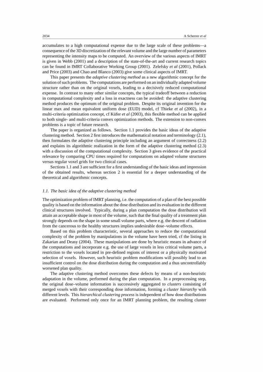
Figure 11. The geometrical illustration of the local refinement process.

According to the physical meaning of the local refinement, the cluster structure is graduallyrefined in those volume parts of R, where large dose gradients occur, and those parts of T

where the minimal dose is attained, until a sufficient exactness in (13) is obtained. Hence, thelocal refinement process gradually reveals the position of the optima of the original problem(9) while keeping the number of elements in the adapted clustering A(tstop) moderately low.

Although the computation of x∗A(tstop)

requires the solution of the several approximateproblems CPA(0)

, . . . , CPA(tstop)

, the accumulated computational expense is still much smallerthan the expense for a straightforward computation of (9) due to the fact that the numberof clusters contained even in the largest adapted clustering A(tstop) is much smaller than thenumber of voxels in C(0).

2.3.4. The job sharing effect. The real strength of the adaptive clustering method isrevealed in the case of repeated plan computations. The computational expense for thehierarchical clustering process itself is rather small compared with the expense for a singleplan computation using the voxels, which makes the whole method highly effective even fora single plan computation using the voxels. Performed only once in advance of the repeatedplan computations, the expense for the construction of the cluster hierarchy is thus negligiblysmall compared with the accumulated expense of these computations, which all use the samehierarchy as a ‘construction kit’ for their local refinement processes.

2.4. Embedding the method in a general mathematical framework

The adaptive clustering method merges theoretically well-founded techniques from differentfields of mathematics:

Clustering techniques originating from the wide field of classification, (IFCS web site),are used in mathematical programming, cf. e.g. Hansen and Jaumard (1997), with a specialfocus on large scale handling by means of aggregation/disaggregation techniques (Evans et al1991). They can be effectively adapted to the discretized IMRT planning problems due to thecontinuous problem background.


In applied mathematics, the numerical solution of e.g. partial differential and integralequations is done by means of adaptive multigrid methods, cf Hackbusch (2003). The conceptof constructive grid adaptation known from there can be generalized to the non-regular gridstructures suitable for IMRT planning.

3. Results and discussion

3.1. Numerical results on real clinical data

The following numerical examples based on real clinical data provided by the German CancerResearch Center (DKFZ), Heidelberg (Germany), show the high practicability of the adaptiveclustering method. The computations were performed on a 1.7 GHz Pentium VI with 3 GBRAM. Since the choice of evaluation functions and dose bounds is a very individual one, theproblem formulations of the examples might not appeal to everyone. However, the relativeimprovement in the computational expense, on which the main focus shall be put, is notaffected by this.

3.1.1. Clinical example 1: a carcinoma in the head and neck region. The first clinicalexample is a carcinoma in the head and neck region. The planning target volume is classifiedinto a boost volume and the surrounding remaining target volume. The critical structuresinvolved are the spinal cord, brain stem and right parotid gland, the two eyes and the unclassifiedtissue. The irradiation geometry is a coplanar arrangement of seven equidistantly positionedbeams with 1896 active beamlets altogether, and the partition of the relevant body volumeconsists of 306 742 voxels. The dose information matrix contained 12.4% non-zero entries.The IMRT planning problem in this specific clinical case was modelled in the following way,whereas the dose bounds for the involved structures were chosen according to protocol RTOGH-0022, cf (RTOG web site).

The set of indices K enumerating the different clinical structures divides into the indexset Kfeas for the clinical structures, whose evaluation functions imply a hard constraint andthus determine the feasible region and Kobj for the clinical structures, that enter the objectivefunction. The first set

Kfeas := {k ∈ K : fk implies a hard constraint} = {k′(B), k′(T )} (33)

contained the indices k′(B) of the boost volume B with its condition on the minimal dose in B

fk′(B)(d(x)) := Lk′(B) − minVj ⊆B

d(Vj )(x) � 0, (34)

with the prescription dose Lk′(B) = 72 Gy as the isodose that shall encompass at least 95% ofB, and k′(T ) of the target volume T with the analogous condition on the minimal dose withLk′(T ) = 66 Gy. The second set

Kobj := {k ∈ K : fk enters the objective function} = K \ Kfeas (35)

contained the indices k(B) of the boost volume B with the homogeneity condition on the dose

fk(B)(d(x)) = maxVj ⊆B d(Vj )(x)

Uk(B)

(36)

and the ideal upper dose bound Uk(B) = 78 Gy, and k(T ) of the target volume T with theanalogous homogeneity condition on the dose with Uk(T ) = 72 Gy. For the organs at risk withindices k ∈ K, account was taken on both the mean dose deposit and the local appearance of


Table 1. The parameters and ideal dose bounds chosen for the organs at risk.

Organ at risk qk q ′k αk Uk

Spinal cord 3.0 8.0 0.80 30Brain stem 3.0 8.0 0.75 35Parotid gland 3.0 8.0 0.99 25Right eye 3.0 8.0 0.70 10Left eye 3.0 8.0 0.70 10Unclassified tissue 1.1 3.0 0.01 15

high dose values by means of the evaluation function

fk(d(x)) = (1 − αk)1

Uk

|Rk|−1

∑Vj ⊆Rk

(d(Vj )(x))qk

1qk

+ αk

1

U ′k

|Rk|−1

∑Vj ⊆Rk

(d(Vj )(x))q′k

1q′k

. (37)

The first term with a comparably small qk and the ideal upper dose bound Uk measures the meandose, while the second term with larger q ′

k and the ideal upper dose bound U ′k measures the

tail of the dose distribution in the clinical structure Rk . The parameter αk ∈ [0, 1] determineswhether there is more emphasis put on the mean dose or on the tail. For the subsequentexample, Uk = U ′

k was set and the ideal dose bounds and mode parameters were chosenas shown in table 1. The values for αk originate from a parameter fitting of the max andmean EUD concept cf Thieke et al (2002), to the normal tissue tolerance data (Emami et al1991). The explicit choice of qk and q ′

k is of minor influence for the computation, hence some‘standard setting’ was used. The main focus was put on the dose bounds and in particular theirratio, since these physical parameters are the most important ones for the optimization.

At the common boundaries of boost and target and the unclassified tissue, the conditionson the dose distribution were slightly relaxed to steer the decay of dose deposits from the highvalues in boost and target to the low ones in the critical structures into a small volume passingalong these boundaries with acceptably small dose volume effects. In accordance with (9),the optimization problem was formulated as

CP : s → Min subject to (38)

fk′(d(x)) � 0, k′ ∈ Kfeas (39)

fk(d(x)) � s, k ∈ Kobj (40)

with (39) representing the hard constraints on the minimal dose in boost and target and (40)representing the planning goals in form of the best possible homogeneity in boost and targetand the best possible evaluation in the organs at risk.

Concerning the cluster hierarchy, the number of levels and the level related number ofclusters in the different clinical structures are shown in table 2. For boost and target, theclustering process stopped on level 3, since due to the superposition of seven beams in thesestructures, the dose inhomogeneities in big clusters on higher levels tend to be rather large,hence almost all these clusters would be refined, unnecessarily increasing the computational


Figure 12. The clusterings C(l) of the levels l = 0, . . . , 2 in a transversal voxel layer. In this layer,the boost volume is located on the right side, the target on the left and the spinal cord in the centre.The remainder is the unclassified tissue.

Table 2. The number of levels and level related number of clusters of the cluster hierarchy.

Clinical structure |C(0)| |C(1)| |C(2)| |C(3)| . . . |C(lmax)|Boost 13 914 6957 1439 294Target 42 070 21 035 5330 1424Spinal cord 2346 1173 272 73Brain stem 1200 600 134 38Parotid gland 1270 635 206 129 . . . 101, lmax = 5Right eye 144 72 16Left eye 48 24 9Unclassified tissue 245 750 122 875 23 384 4831 . . . 286, lmax = 8

expense. In the other clinical structures, the method continued until the number of clusterswas sufficiently small or the rate of reduction was too low. The proceeding of the hierarchicalclustering process in a transversal voxel layer is shown in figure 12. The appearance ofseemingly small clusters and single voxels even on high levels might be a bit misleading inview of the strongly reduced cluster numbers, but typically the clusters span over severallayers containing only few voxels in each one. The local refinement process took four stepsto yield an x∗A(4)

that approximates the optimum of the original problem in such a way thatthe corresponding dose distributions differ only locally by at most 0.5 Gy, attain numericallyidentical evaluations and have dose–volume curves without any significant differences. Thechange of the adapted clusterings during this process is documented by the number of clustersused in the different entities at the different process steps, cf table 3. Even the final and thuslargest adapted clustering A(4) consisted of 18 524 clusters, which is only 6.0% of the originalnumber of 306 742 voxels. The shape of these adapted clusterings in the transversal voxellayer is shown in figure 13. The change of an intensity map for a single beam during the localrefinement process as shown in figure 14 illustrates, how the approximate solutions approachthe original solution x∗A(4)

. Besides some minor modifications of the intensity especially onthe left side of the intensity map, its general shape does not change. The low volatility ofthe intensity values over the beamlets is due to the smoothing effect of the local refinementprocess. This typically also contributes to the delivery efficiency of the plan.

It is self-evident that the slight modifications of the intensity maps induce only minorchanges of the dose–volume histograms for x∗A(t)

, t = 0, . . . , 4, cf figure 15. The followingtables illustrate the change of the characteristic values of the dose–volume curves duringthe local refinement process and with the corresponding RTOG H-0022 requirements.


Figure 13. The refinement process and the adapted clusterings A(t), t = 0, . . . , 2, in a transversalvoxel layer. The further refinement steps do not alter the cluster structure in this layer. The filledclusters are the ones that were refined in the previous step. The refinements of some clustershappen in other layers and are thus not visible in the given one.

Figure 14. The intensity maps of x∗A(t), t = 0, . . . , 4 for one beam.

Table 3. The number of clusters of the adapted clusterings constructed in the local refinementprocess.

Clinical structure |A(0)| |A(1)| |A(2)| |A(3)| |A(4)|Boost 294 1394 4456 4456 4456Target 1424 4922 12 928 12 928 12 928Spinal cord 73 207 376 514 514Brain stem 38 38 38 38 38Parotid gland 101 107 118 134 180Right eye 16 16 16 16 16Left eye 9 9 9 9 9Unclassified tissue 286 383 383 383 383Whole volume 2241 7076 18 324 18 478 18 524

Table 4 contains the percentages of boost and target volume, in which the prescription doserespectively 93% and 110% of it are exceeded. The changes in these values over the firsttwo steps of the local refinement process, especially the 110%-values correspond to the majorrefinements performed in these structures, cf table 3. The maximal dose values attained inboost and target change only slightly, cf table 5. More significant are the changes in thespinal cord and the parotid gland. An increase of the maximal dose attained in the spinalcord is accompanied by a gradually increasing number of clusters, cf table 5, and a correctevaluation of the dose–volume criterion in the parotid gland, where more than 50% shouldattain less than 30 Gy, cf table 6, causes moderate local refinements. The CPU times of table 7give an impression of the computational complexity of the adaptive clustering method: the


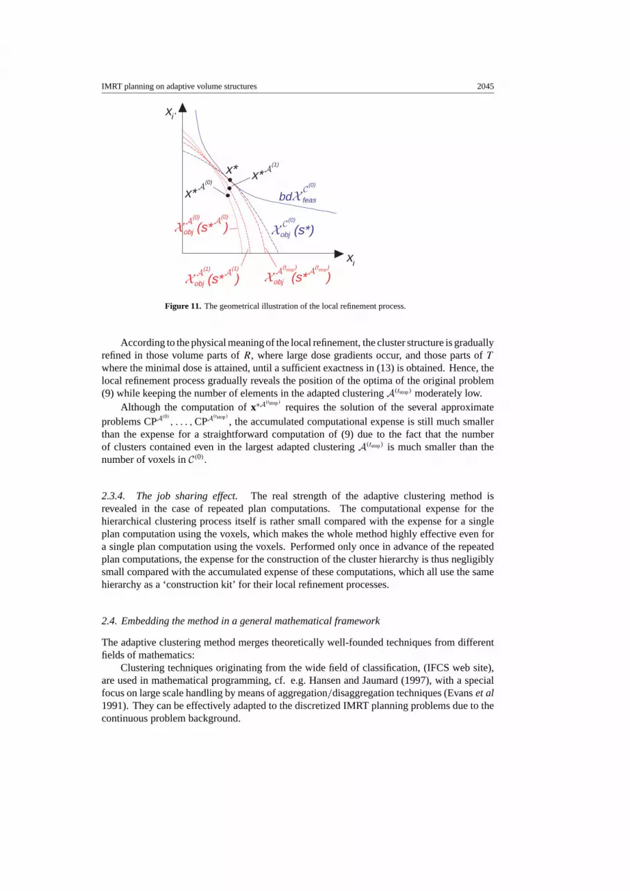
Figure 15. The dose–volume histograms of x∗A(t), t = 0, . . . , 4.

Table 4. The volume percentages of target and boost with certain percentages of the prescriptiondose exceeded for each step of the local refinement process.

Volume percentage with valid criterion

Structure Dose criterion t = 0 t = 1 t = 2 t = 3 t = 4 RTOG

Boost d � 0.93 · LB 97.9 99.0 99.5 99.4 99.3 �99.0Boost d � 1.00 · LB 89.3 92.5 93.2 93.9 95.0 �95.0Boost d � 1.10 · LB 31.1 19.7 15.0 14.3 12.6 �25.0Target d � 0.93 · LT 98.1 98.2 99.0 99.3 99.7 �99.0Target d � 1.00 · LT 89.1 92.7 92.7 94.2 95.0 �95.0Target d � 1.10 · LT 29.3 28.6 27.1 27.4 25.2 �25.0

local refinement process required only 19.0% of the CPU time needed for the straightforwardcomputation on the voxels.

3.1.2. Clinical example 2: a prostate carcinoma. The second clinical example is a case of aprostate carcinoma. Besides boost and target volume, the bladder, rectum, the two femurs andthe unclassified tissue are involved, cf figure 16 (left). The irradiation geometry is a coplanararrangement of five equidistantly located beams with 400 active beamlets altogether, and the


Figure 16. Left: the organ geometry with boost and target (centre), the adjacent bladder (abovetarget) and rectum (below target) and the two femurs. The lines heading towards the isocenter(cross in the centre) visualize the beam directions. Right: the clustering structure on level 3, whichwell represents the beam directions.

Table 5. The maximal dose values attained in the different clinical structures in each step of thelocal refinement process.

Attained maximal dose values

Structure t = 0 t = 1 t = 2 t = 3 t = 4 RTOG

Boost 84.8 83.0 85.2 85.0 85.0 –Target 81.0 79.7 79.7 79.2 78.2 –Spinal cord 41.0 41.0 43.0 43.9 44.0 45 GyBrain stem 33.8 34.4 35.3 36.3 36.4 54 GyNon-target volume 73.0 72.8 72.8 72.7 72.8 72.6 Gy

Table 6. The valid dose–volume criterion in the parotid gland in each step of the local refinementprocess.

Volume percentage with valid criterion

Structure Dose criterion t = 0 t = 1 t = 2 t = 3 t = 4 RTOG

Parotid gland d � 30 Gy 80.2 80.6 77.7 75.4 75.1 >50.0

Table 7. The CPU times (in seconds) for the head neck case required for the voxel-basedcomputation and for the computation with the adaptive clustering method.

Process CPU time (s)

Voxel-based computation: 525Adaptive clustering method: 200

Hierarchical clustering process 100Local refinement process 100

partition of the relevant body volume consists of 435 501 voxels. The dose information matrixcontained 12.0% non-zero entries.


Table 8. The CPU times (in seconds) for the prostate case required for the voxel-based computationand for the computation with the adaptive clustering method.

Process CPU time (s)

Voxel-based computation: 403Adaptive clustering method: 49

Hierarchical clustering process 38Local refinement process 11

This case is well suited to demonstrate how the construction of the clusters performs.Figure 16 (right) shows the clustering C(3) of an upper level in the transversal voxel layerthrough the isocenter. Comparison with figure 16 (left) illustrates that the shapes of theclusters well represent the irradiation geometry, i.e. they pass along the beam directions. Thecluster hierarchy contained 3–8 levels depending on the organ. The local refinement processterminated after tstop = 2 steps with an adapted clustering consisting of 4369 clusters, whichis 1% of the original number of voxels. Performing the local refinement process in this caserequired only 2.7% of the CPU time needed for the straightforward computation on the voxels,cf table 8.

4. Conclusion

The presented adaptive clustering method leads to a decisive speed-up in plan computationallowing a more efficient use of the limited time that is available in IMRT treatment planning tofind a desirable therapy. Possible extensions of this flexible method to more general, namelynon-convex problem settings, and several other questions in the field of IMRT treatmentplanning, e.g. a fast plan adaptation to a changed organ geometry or the integration of thesequencing, i.e. the generation of fitting aperture arrangements for the beams into the plancomputation, are future research topics.

Acknowledgments

The authors are grateful to the members of the Department of Medical Physics in RadiationOncology of Wolfgang Schlegel and the Clinical Cooperation Unit Radiation Oncology ofJurgen Debus at the German Cancer Research Center (DKFZ), Heidelberg (Germany), fora successful scientific cooperation. Special thanks are addressed to Christian Thieke andUwe Oelfke for a long lasting teamwork and to Christoph Thilmann for the helpful consultingin clinical questions.

References

Brahme A 1984 Dosimetric precision requirements in radiation therapy Acta Radiol. Oncol. 23 379–91Chao K S C and Blanco A I 2003 Intensity-modulated radiation therapy for head and neck cancer Intensity-Modulated

Radiation Therapy: The State of the Art ed J R Palta and T R Mackie (Medical Physics Publishing) pp 631–44Cotrutz C, Lahanas M, Kappas K and Baltas D 2001 A multiobjective gradient based dose optimization algorithm for

external beam conformal radiotherapy Phys. Med. Biol. 46 2161–75Emami B, Lyman J, Brown A, Coia L, Goitein M, Munzenrider J E, Shank B, Solin L J and Wesson M 1991 Tolerance

of normal tissue to therapeutic irradiation Int. J. Radi. Oncol. Biol. and Phys. 21 109–22Evans J, Plante R D, Rogers D F and Wong R T 1991 Aggregation and disaggregation techniques and methodology

in optimization Oper. Res. 39 553–82


Hackbusch W 2003 Multi-Grid Methods and Applications (Berlin: Springer)Hansen P and Jaumard B 1997 Cluster analysis and mathematical programming Math. Program. 79 191–215Hunt M A, Hsiung C-Y, Spirou S V, Chui C-S, Amols H I and Ling C C 2002 Evaluation of concave dose distributions

created using an inverse planning system Int. J. Radi. Oncol. Biol. Phys. 54 953–62International Federation of Classification Societies (IFCS) http://www.classification-society.orgIMRT Collaborative Working Group 2001 Intensity-modulated radiotherapy: current status and issues of interest Int.

J. Radiat. Oncol. Biol. Phys. 51 880–914Kufer K-H, Hamacher H W and Bortfeld T R 2000 A multicriteria optimization approach for inverse radiotherapy

planning Proc. XIIIth ICCR (Heidelberg 2000) ed Thomas R Bortfeld and Wolfgang Schlegel, pp 26–9Kufer K-H, Scherrer A, Monz M, Alonso F, Trinkaus H, Bortfeld T and Thieke C 2003 Intensity-modulated

radiotherapy—a large scale multi-criteria programming problem OR Spectr. 25 223–49Niemierko A 1997 Reporting and analysing dose distributions: a concept of equivalent uniform dose Med. Phys. 24

103–10Pollack A and Price R A 2003 IMRT for prostate cancer Intensity-Modulated Radiation Therapy: The State of the

Art ed J R Palta and T R Mackie (Medical Physics Publishing) pp 617–30Radiation Therapy Oncology Group (RTOG) http://www.rtog.orgSteuer R E 1985 Multicriteria Optimization: Theory, Computation and Applications (NewYork: Wiley)Thieke C, Bortfeld T and Kufer K-H 2002 Characterization of dose distributions through the max and mean dose

concept Acta Oncol. 41 158–61Webb S 1997 The Physics of Conformal Radiotherapy—Advances in Technology (Medical Science Series) (Bristol:

Institute of Physics Publishing)Webb S 2001 Intensity-Modulated Radiation Therapy (Series in Medical Physics) (Bristol: Institute of Physics

Publishing)Yu Y 1997 Multiobjective decision theory for computational optimization in radiation therapy Med. Phys. 24 1445–54Zakarian C and Deasy J O 2004 Beamlet dose distribution compression and reconstruction using wavelets for intensity

modulated treatment planning Med. Phys. 31 368–75Zelefsky M J, Fuks Z, Hunt M A, Yamada Y, Marion C, Ling C C, Amols H I, Venkatraman E S and Leibel S A 2001

High-dose intensity modulated radiation therapy for prostate cancer: early toxicity and biochemical outcome in772 patients Int. J. Radiat. Oncol. Biol. Phys. 53 1111–6

Documents

IMRT planning on adaptive volume structures - a decisive reduction in computational complexity