Embed Size (px)
Citation preview

Infrared Radiation in the Mesosphere and LowerThermosphere: Energetic Effects and Remote Sensing
Artem G. Feofilov • Alexander A. Kutepov
Received: 5 March 2012 / Accepted: 18 September 2012� Springer Science+Business Media Dordrecht 2012
Abstract This paper discusses the formation mechanisms of infrared radiation in the
mesosphere and lower thermosphere (MLT), the energetic effects of the radiative
absorption/emission processes, and the retrieval of atmospheric parameters from infrared
radiation measurements. In the MLT and above, the vibrational levels of the molecules
involved in radiative transitions are not in local thermodynamic equilibrium (LTE) with the
surrounding medium, and this then requires specific theoretical treatment. The non-LTE
models for CO2, O3, and H2O molecules are presented, and the radiative cooling/heating
rates estimated for five typical atmospheric scenarios, from polar winter to polar summer,
are shown. An optimization strategy for calculating the cooling/heating rates in general
circulation models is proposed, and its accuracy is estimated for CO2. The sensitivity of the
atmospheric quantities retrieved from infrared observations made from satellites to the
non-LTE model parameters is shown.
Keywords Infrared energy � Radiative transfer � Mesosphere lower thermosphere
1 Introduction
In this paper, we concentrate on (a) the role of the infrared (IR) radiation in the energy
budget of the mesosphere and lower thermosphere (MLT) as well as (b) on the IR radiation
emerging from the atmosphere, which is observed with various instruments from space.
Both topics are strongly linked and require detailed consideration of formation and
A. G. Feofilov (&)Laboratory of Dynamical Meteorology, Ecole Polytechnique, Palaiseau, Francee-mail: [email protected]
A. A. KutepovThe Catholic University of America, Washington, DC, USA
A. A. KutepovNASA Goddard Space Flight Center, Greenbelt, MD, USA
123
Surv GeophysDOI 10.1007/s10712-012-9204-0

propagation of the IR radiation in the MLT and its interactions with the various compo-
nents of the atmosphere.
The translational degrees of freedom of all atmospheric molecular and atomic gaseous
compounds represent the heat reservoir. This reservoir obtains or loses energy due to a
number of sources and sinks, among them heating and cooling related to various types of
mass motions, redistribution of energy released in the course of various photochemical
reactions (the translational energy, the chemical energy and the nascent electronic,
vibration and rotational energy of the reaction products), and absorption and emission of
the IR radiation. In the latter case, one usually speaks about the interaction between matter
and the IR radiative field, which, for the case of the MLT, includes the atmospheric
radiation formed in these layers, the upwelling radiation from the ground and lower
atmosphere, and, during daytime, the IR solar radiation.
Our primary interest here is with the interaction of the heat reservoir and the IR
radiative field. The energy exchange between them is carried out through an intermediate
reservoir of vibrational and rotational energy of molecular atmospheric compounds: the
photons are absorbed and emitted by molecules of optically active gases through the
processes of spontaneous and stimulated emission and absorption in a large variety of
molecular rotational-vibration and rotational transitions. In this respect, the MLT has a
significant peculiarity related to the fact that the vibrational (and in its upper part also
rotational) excitation of the molecules does not obey Boltzmann’s law with the local
kinetic temperature. As a result, the IR radiation (which is often called ‘‘thermal radia-
tion’’) emitted in these layers does not reflect the thermal state of matter. This situation is
referred to as the breakdown of local thermodynamic equilibrium (LTE) for the vibrational
or rotational–vibrational degrees of freedom. Detailed treatment of non-LTE plays a
crucial role for the estimation of the thermal effects of the IR radiation and for the
diagnostics of space-based IR observations.
In the book by Lopez-Puertas and Taylor (2001), the discussion of both topics was
presented relying on the current status of research at that time. Since then, many research
papers have been published in this field. For example, the recent paper of Funke et al.
(2012) contains an updated compilation of the non-LTE models for the most important
atmospheric infrared emitters. However, no reviews discussing the current status of
methodologies and indicating the directions for further studies have been published for
quite a while. This paper is intended (at least partly) to fill this gap. The storyline is built
around the studies in which both authors took part and, naturally, other works that to our
mind had a significant impact on the field.
The paper is organized as follows. First, we consider the mechanisms of the IR radiation
generation in the MLT, discuss the conditions for LTE breakdown using an example of a
two-level atom (Sect. 2), and introduce the radiative cooling/heating rate (called ‘‘heating
rate’’ throughout this paper, see the definition in Sect. 2.2.4), which is the characteristic
essential for understanding the energetic balance in the MLT. This section also contains a
description of the research code that is used for all test calculations shown in this work.
Section 3 provides the current status of our non-LTE model for carbon dioxide, ozone, and
water vapor, the three most important molecules for the IR heating of the MLT. For each of
the molecules considered, the calculated heating rates for five typical atmospheric sce-
narios, from subarctic summer to subarctic winter, are shown. We pay specific attention to
the problem of the quenching rate coefficient for energy exchange during CO2–O collisions
and provide details of the most recent study on this topic. We discuss the O2/O3 photolysis
scheme and the coupling of the photolysis products’ energy levels with the system of water
vapor vibrational levels. At the end of Sect. 3, we consider an interesting aspect of the
Surv Geophys
123

radiative cooling in the MLT that is related to the combined effect of the small-scale
temperature and trace gas concentration fluctuations associated with gravity waves, and to
the radiative transfer in the 15 lm CO2 band. Section 4 deals with the optimization of the
heating rate calculations necessary for atmospheric modeling. Besides the well-known
parameterization methods, we also present an approach that provides accuracy comparable
to line-by-line calculations but is faster by a factor of *103–104. Section 5 describes the
most common techniques of IR sounding of the MLT and peculiarities of the atmospheric
parameter retrievals related to the non-LTE character of radiation emitted from this region.
Section 6 presents the conclusions of this work.
2 IR Radiation in the MLT: Generation Mechanisms and Interaction with Matter
2.1 Overview
Optically active molecular gases at any given height in the atmosphere absorb and emit
radiation. With respect to the radiative energy transformations, the MLT area can be
considered as a mixture of gases exposed to (a) the solar irradiance from the top, (b) the
reflected solar radiation from below, (c) the terrestrial IR radiation from below, and (d) the
radiation emitted by the molecules in other atmospheric layers (Fig. 1). Solar energy is
absorbed primarily by O2 and O3 molecules, and their photolysis leads to atmospheric
heating both directly (through the formation of translationally hot products) and by cre-
ating electronically and vibrationally excited products that later will heat the atmosphere
through a set of energy exchange processes. The solar near-infrared radiation in the
spectral range with wavelengths k B 5 lm is also absorbed by a number of molecules to
provide the heating of the MLT; among them, the most noteworthy are the CO2 2.0, 2.7,
and 4.3 lm bands. Another source of the MLT heating is the absorption of atmospheric
radiation emitted from other atmospheric layers. This heating is accompanied by cooling
due to the emission of radiation, mainly in the CO2 15 lm band, O3 9.6 lm band, and H2O
rotational and 6.3 lm vibrational bands (e.g., see Brasseur and Solomon 2005). In this
work, we will focus mainly on the IR part of the spectra that corresponds to the rotational–
vibrational (also called ro-vibrational) transitions of the atmospheric molecules.
If a molecule (or atom) is formed in an excited state due to absorption of a radiation
quantum or due to chemical or photochemical processes, then the energy of excitation may
be (a) emitted to the atmosphere; (b) transferred to another excited state of the same
molecule through an intra-molecular energy exchange induced by collision with another
molecule or atom; (c) transferred to other molecules by intermolecular vibrational–
vibrational (V–V) or (d) electronic-vibrational (E–V) energy exchange processes; or
(e) converted to kinetic energy of atmospheric molecules and atoms via collision (vibra-
tional–translational energy exchange, V–T). A simplified scheme of the interactions
between the atmospheric molecules is shown in Fig. 2. In general, each molecule
exchanges energy with the heat reservoir through the V–T collisions and interacts with
other molecules through a set of V–V and E–V energy exchanges.
To calculate the absorbing and emitting characteristics of the optically active molecules
and to estimate the balance between the IR cooling and heating one needs to know the
populations of the corresponding ro-vibrational levels. However, as mentioned above, the
vibrational levels of the molecules under consideration are not in thermodynamic equi-
librium with the surrounding medium in the MLT. The next section provides the back-
ground necessary for understanding the non-LTE effects in the atmosphere.
Surv Geophys
123

2.2 LTE and Non-LTE
2.2.1 The Two-Level Atom
For simplicity, let us first consider a case of a plane-parallel atmosphere that contains just
one optically active component: a two-level hypothetical atom. Let us assume that we
Fig. 1 Diagram showing radiative processes affecting the MLT region: solar irradiance, reflected andscattered solar radiation (by clouds and from the ground), terrestrial IR radiation, and radiation emitted byother atmospheric layers
Fig. 2 Diagram illustrating those molecules and atoms whose ro-vibrational and/or electronic levels areinvolved in the generation of IR emissions in the MLT region. Energy exchange and transformationprocesses involve absorption of radiation quanta (see Fig. 1), emission to the atmosphere, and collision-induced intra- and inter-molecular V–V, E–V, and V–T energy exchange
Surv Geophys
123

consider a steady state of the atomic gas, which means that pressure, temperature, and the
degree of excitation (the ratio of the upper-level population to the lower-level population)
do not change with time. For this atom, one can write the steady-state equation (SSE),
which describes the various processes populating and de-populating each level of the atom
at any given altitude, as
ðR21 þ C21Þ � n2 ¼ ðR12 þ C12Þ � n1; ð1Þ
where n1 and n2 are the populations of the first and second levels, respectively, C12 and C21
are the coefficients of collisional population and de-population of the second level, and
R21 ¼ A21 þ B21 � �JðzÞ; R12 ¼ B12 � �JðzÞ ð2Þ
are the radiative terms, where A21, B21, and B12 are, respectively, the Einstein coefficients
for spontaneous emission, stimulated emission, and absorption, and
�JðzÞ ¼ 1
4p
Z
X
dXZþ1
�1
IlmðzÞuðm; zÞdm ¼Z1
�1
Zþ1
�1
IlmðzÞuðm; zÞdmdl ð3Þ
is the integrated mean intensity of the radiation at the considered altitude. Here, Ilm (z) is the
monochromatic radiation intensity, which satisfies the radiative transfer equation (RTE)
ldIlmðzÞ
dz¼ �vlmðzÞIlmðzÞ þ glmðzÞ; ð4Þ
where Ilm (z) is the monochromatic radiation intensity, l = cos(h) is the direction cosine, vis the frequency of the radiation, vlm (z) and glm (z) are the total opacity and emissivity,
respectively, and u(m, z) is the normalized spectral line profile function, which satisfies
Zþ1
�1
uðm; zÞdm ¼ 1: ð5Þ
It is important to note that the opacity and emissivity terms in (4) are expressed through the
populations of the upper and lower levels as vðzÞ ¼ hm4p ðn1ðzÞB12 � n2ðzÞB21Þ and
gðzÞ ¼ hm4p n2ðzÞA21, respectively. In order to find n1 and n2, one must supplement Eq. (1) by
the particle conservation law
n1 þ n2 ¼ 1: ð6Þ
In general, �JðzÞ in the radiative terms R21 and R12 in (2) in the MLT is the combination
of solar radiation, terrestrial radiation, radiation scattered by the clouds, and the atmo-
spheric radiation (see Fig. 1). The system of steady-state Eqs. (1) and (6) can be solved for
the populations n1 and n2 if all the coefficients A21, B21, B12, C21, C12, and �JðzÞ are known.
On the other hand, finding �JðzÞ requires solving and integrating the radiative transfer Eq.
(4), which depends on the populations n1 and n2. As a result, one has to search for the joint
solution of (1), (6) and (3), (4) (e.g., see Ivanov 1973; Mihalas 1978). There are various
approaches to solving this joint system in atmospheric studies: the Curtis method (e.g., see
Goody and Yung 1995), Lambda Iterations (e.g., see Wintersteiner et al. 1992), Modified
Curtis Method (e.g., see Lopez-Puertas and Taylor 2001; Funke et al. 2012), Accelerated
Lambda Iterations (e.g., see Kutepov et al. 1998; Gusev and Kutepov 2003). We will refer
to them in Sect. 4.1 with respect to the calculation optimization schemes.
Surv Geophys
123

In further consideration of the two-level system, one has to keep in mind that the
coefficients C12 and C21 in (1) are linked by the detailed balance equation
C21 ¼ C12
g2
g1
e�E21=kT ; ð7Þ
where k is Boltzmann’s constant, E21 is the energy difference between the levels, and T is
the local temperature. This results from the validity of the Maxwellian distribution for the
translational degrees of freedom for molecules and atoms of the atmospheric constituents
in the MLT. Correspondingly, if the terms R12 and R21 in Eq. (1) are negligible in com-
parison with C12 and C21 or if n1R12 % n2R21, then the populations n1 and n2 will obey
Boltzmann’s law. Since the collisional term is proportional to the concentration of the
collisional partner, the former situation is typical for the lower atmosphere. The latter
situation is possible in the cores of optically thick lines. This is also more typical for the
lower atmosphere due to high concentrations of the absorbing gas. We will refer to such
conditions as ‘‘LTE’’ (local thermodynamic equilibrium) and we will denote the corre-
sponding level populations as the ‘‘LTE populations’’. If the frequency of collisions is low
and n1R12 = n2R21, then the populations will be sensitive to the radiative field. This
situation is called ‘‘non-LTE’’.
2.2.2 The Multi-Level Non-LTE Problem
In reality, the number of levels involved in energy exchange processes in the atmosphere is
far greater than two (see Figs. 7, 11, 14 below). In this case, the system of SSE (1), (6) and
RTE (4) must be extended to the other levels. Correspondingly, a complete system for NV
vibrational levels will include NV steady-state equations, one of which must be replaced by a
particle conservation equation similar to (6). In the case of a multi-level problem, the
collisional terms are divided into two groups: V–T, for which the vibrational state of only one
collisional partner changes, and V–V energy exchange processes, for which both of the
collisional partners change their vibrational states. In general form, the steady-state equation
for a multilevel problem involving chemical production P and losses L can be written as:
nl Ll þXl 6¼l0
ðRll0 þ Cll0 Þ !
¼Xl6¼l0
nl0 ðRl0l þ Cl0lÞ þ Pl ðl ¼ 1; 2; . . .; NVÞ: ð8Þ
Each of the molecules considered is characterized by a set of radiation coefficients, usually
obtained from the HITRAN spectroscopic database described in Rothman et al. (2009), and
by a set of V–T and V–V rates representing a compilation of the most up-to-date mea-
surements and theoretical calculations.
For the case of a multilevel problem with rotational substructure of vibrational levels,
the integrated mean intensity calculation (3) and the radiative transfer Eq. (4) must take
into account the ro-vibrational structure of the optical molecular band. In general, for any
given pair of ro-vibrational levels (l, l0), where l0 is the lower level index and l is the upper
level index, the emissivity gll0(m) and opacity vll0(m) at the frequency m are given by
gll0 ðmÞ ¼hmll0
4pnlAll0ull0 ðmÞ; vll0 ðmÞ ¼
hmll0
4pðnl0Bl0l � nlBll0 Þull0 ðmÞ; ð9Þ
where mll0 is the line center frequency, All0, Bl0l, and Bll0 are the Einstein coefficients, and
ull0(m) is the normalized line profile (see (5)). The total emissivity and opacity expressed in
terms of line quantities (9) are
Surv Geophys
123

gðmÞ ¼Xl;l0
gll0 ðmÞ; vðmÞ ¼Xl;l0
vll0 ðmÞ: ð10Þ
In the traditional approach, the radiative transfer equation is solved for each line sep-
arately, and the resulting integrated mean intensities are summed for the molecular band
considered. This type of radiative transfer calculations is called LBL (for line-by-line) and
is used as a reference because of its high accuracy. The computational cost is high, due to
the large number of individual lines involved. In addition, each line in this approach must
be well resolved at all altitudes, which means that a large number of spectral points must be
considered. In the lower atmosphere, the problem is complicated by line overlapping,
which requires a finer spectral grid. Fortunately, in the Earth’s atmosphere, line overlap-
ping effects are essentially separated from the non-LTE effects: the lower the pressure, the
narrower is the line and the stronger the non-LTE effects. In this work, we will consider
only non-overlapping lines, which is a reasonable approximation for the MLT. We will
address the computational cost issues and the optimization strategy in the Sect. 4. For more
details regarding solving the multi-level non-LTE problem, we refer the reader to the
works of Kutepov et al. (1998), Lopez-Puertas and Taylor (2001), and Gusev and Kutepov
(2003).
2.2.3 Non-LTE Populations and Vibrational Temperatures
Figure 3 illustrates the typical cases of non-LTE. The levels selected for this demonstration
are the upper ones in optically thick (main isotope of CO2) and optically thin (the fifth in
abundance CO2 isotope) fundamental m2 (15 lm) and m3 (4.3 lm), and the vibrational level
pumped by direct solar radiance absorption in the 2.0 lm band. In this work, we mark the
vibrational levels in accordance with the nomenclature used in the HITRAN spectroscopic
database: m1, m2, l, m3, nF where m1, m2, and m3 denote the number of the corresponding
vibrational quanta, the l symbol refers to the angular momentum quantum number, and the
nF symbol denotes the number of the level in a subgroup of levels close in energy and
linked by Fermi resonance. The isotopes are marked using the lower digit of the atomic
weight: 16O12C16O corresponds to 626, 16O13C18O is marked as 638, 1H16O1H becomes
161, and so on.
The vibrational-level populations are traditionally shown as vibrational temperatures
that give an insight into the pumping and quenching mechanisms for a given level. The
vibrational temperatures Tvib describe the excitation degree of the level l against the ground
level 0:
nl
n0
¼ gl
g0
e�ðEl�E0Þ=kTvib ; ð11Þ
where El is the energy of the level l and E0 is the ground-level energy. If the level is in
LTE, then Tvib = Tkin. If Tvib [ Tkin then the net pumping of the level is larger than that
under LTE conditions. Similarly, if Tvib \ Tkin, the level is populated less efficiently and/or
depopulated faster than at LTE.
Let us comment on the behavior of the corresponding Tvib in Fig. 3 and explain the
physics involved: the temperature difference between the stratopause and the mesopause is
not high enough to ensure significant pumping of the 01101 levels by radiation coming
from below (see the right-hand panel of Fig. 3); the high optical thickness of the main
isotope’s m2 transitions and frequent atmospheric collisions keep the 626(01101) level in
LTE up to *80 km altitude; the 638(01101) level is characterized by optically thinner
Surv Geophys
123

‘‘photon escape paths’’ that leads to LTE breakdown for this level at lower altitudes; the
absorption of solar radiation and its further redistribution to the 00011 levels moves them
out of LTE at *55 km altitude. The level 20012 is efficiently pumped by solar radiance
absorption in the 2.0-lm band and is in non-LTE even at low altitudes. Following this
logic, one may explain the Tvib behavior in other cases.
2.2.4 Radiative Cooling and Heating Rates
Radiative cooling and heating are essential energetic characteristics of the atmosphere that
show the amount of energy acquired or lost by an atmospheric layer due to the integrated
effects of radiative energy absorption and emission. The radiative flux divergence defines
the rate at which energy is added to the radiative field per unit volume, that is the rate at
which energy is lost by the matter. Following the standard way (see, e.g., Goody et al.
1989), we introduce the radiative heating rate h for this process as the radiative flux
divergence taken with the minus sign. In the plane-parallel atmosphere at the altitude z, the
flux divergence is obtained by integrating Eq. (4) over frequency and solid angle
hðzÞ ¼ � 1
4p
Z
X
dXZþ1
�1
ldIlmðzÞ
dzdm: ð12Þ
Since the main effect of interaction between the infrared radiation and the atmosphere is
cooling, h(z) is often called ‘‘cooling rate’’, even though it is a heating rate by definition. One
has to keep in mind that h(z) may be both positive (heating) and negative (cooling) depending
on the dominating term in the right-hand side of Eq. (12). Throughout this paper, we will call
Fig. 3 Explanation of non-LTE effects in the middle and upper atmosphere. Left: Vertical temperaturedistribution in the atmosphere, with a large ([75 K) temperature difference between the stratopause and themesopause, typical for the high latitude summer atmosphere (latitude = 70�N, solar zenith angle = 46.5�).The non-LTE populations on this plot and below are represented as vibrational temperatures (see text). 626is the main CO2 isotope (16O12C16O); 638 is the fifth in abundance (4.4 9 10-2) CO2 isotope (16O13C18O);01101 and 00011 are first m2- and m3 vibrational levels, respectively. The 20012 is the solar-pumpedvibrational level (see also Fig. 7). Right: diagram of energy transformation for the simplified two-level casein a layered plane-parallel atmosphere (i is the index of the layer corresponding to the stratopause, andi ? m defines the mesopause level)
Surv Geophys
123

h(z) ‘‘heating rate’’. The units of h(z) in (12) are (W/m3). To convert the h(z) values to units
more commonly used in atmospheric physics (K/day), one has to apply the formula
hðzÞðK/day) ¼ hðzÞðW/m3Þ 24 � 60 � 60
CpðzÞqðzÞ; ð13Þ
where Cp(z) is the heat capacity at constant pressure in (J/kg/K), and q(z) is the density in
(kg/m3). We note here that heating rate in (K/day) should not be treated as daily averages;
‘‘day’’ is used as time unit while h(z) can (and does) vary during the day. We suppose that
the integral over frequency in (12) covers the entire IR range and will show the altitude
distributions for the net heating rate h(z). The sign of h(z) tells whether the atmosphere is
cooled or heated at the given altitude z, and its magnitude provides an estimate of the
importance of a given molecule for the energetic balance of the region. The heating rate
distributions will be accompanied by plots showing the nl(z) distributions for the most
important vibrational levels. In Sect. 3, we will consider the non-LTE radiative heating
rates for the main contributors to the MLT radiative energy budget: CO2, O3, H2O, and the
kinetics of the O2/O3 photolysis products.
2.3 ALI-ARMS Research Code
All calculations presented in this work were performed with the help of the ALI-ARMS
(for Accelerated Lambda Iterations for Atmospheric Radiation and Molecular Spectra)
non-LTE code package described in detail in Kutepov et al. (1998), Gusev and Kutepov
(2003), and Gusev (2003). Compared to the other non-LTE codes applied in the studies of
the Earth’s and planetary atmospheres, the ALI-ARMS code solves the multi-level prob-
lem (8) by means of the accelerated lambda iteration (ALI) technique developed in stellar
astrophysics (e.g., see Rybicki and Hummer 1991, 1992; Pauldrach et al. 1994, 2001;
Pauldrach 2003; Hubeny and Lanz 2003; Hubeny et al. 2003) for calculating non-LTE
populations of atomic and ionic levels (see also Sect. 4.1 of this paper).
The code in its current version can treat an arbitrary number of molecules of arbitrary
structures in a given planetary atmosphere provided by the prescribed format inputs of
(a) planetary atmosphere profile that consists of pressure, temperature, volume mixing ratios
(VMRs) of molecules at all altitudes, (b) solar spectra, (c) vibrational and ro-vibrational
energies, (d) spectroscopic information (the Einstein coefficients for ro-vibrational or rota-
tional transitions, line half-widths), and (e) collisional rate coefficients for specified sets of
E–V, V–T, and V–V transitions. The code produces populations of ro-vibrational levels and
radiative flux divergences (radiative cooling and heating) in the lines and bands involved.
The current inputs of V–T and V–V rates are described in Shved et al. (1998),
Manuilova et al. (1998) and summarized in the Ph.D. thesis by Gusev (2003). These inputs
include the interactions between the following molecules: N2, O2, CO2, O3, H2O, CO, OH,
and NO (Fig. 2). The reference model (Fig. 4) includes 350 vibrational levels and 200,000
ro-vibrational lines of the CO2 molecule and its isotopes (Sect. 3.1), 23 vibrational levels
and 150,000 ro-vibrational lines of ozone (Sect. 3.2), 14 vibrational levels and 20,000 lines
of the H2O molecule (Sect. 3.4), and 7 vibrational levels of N2 molecule. The model also
incorporates the kinetic model of O2/O3 photolysis products (Sect. 3.3) developed by
Yankovsky and Manuilova (2006) and interactions of the photolysis products with
vibrational levels of H2O, N2, and CO2 molecules.
The ALI-ARMS code has been successfully applied to the interpretation of the 4.3- and
9.6-lm spectral Earth’s limb radiation measured by the Cryogenic Infrared Spectrometers
and Telescopes for the Atmosphere (CRISTA) instrument (see Offermann et al. 1999;
Surv Geophys
123

Grossmann et al. 2002) in the studies by Kaufmann et al. (2002, 2003) who retrieved the
first global CO2 and O3 density distributions in the Earth’s MLT. Later Gusev et al. (2006)
applied the ALI-ARMS model to the analysis of the CRISTA 15 lm spectral radiation data
and performed temperature retrievals in the MLT. The ALI-ARMS code was used for
the analysis (see Maguire et al. 2002) of the seasonal, altitude, and latitude variations of the
10 lm CO2 limb emissions measured by the Thermal Emission Spectrometer onboard the
Mars Global Surveyor (TES/MGS), as well as to study the infrared radiative heating of
the middle and upper atmospheres of Mars (see Hartogh et al. 2005) and Earth (e.g., see
Kutepov et al. 2007).
The ALI-ARMS code was also used (see Kutepov et al. 2006, Feofilov et al. 2009,
Rezac 2011) for the validation of the operational retrieval algorithms applied to processing
broadband 15 and 4.7 lm CO2 and 6.3 lm H2O Earth’s limb emissions measured by the
SABER (Sounding of the Atmosphere using Broadband Emission Radiometry) instrument
(see Russell et al. 1999) on board the NASA TIMED (Thermosphere Ionosphere Meso-
sphere Energetics and Dynamics) satellite (see Yee et al. 1999). It was also used for the
analysis of the MGS-TES 15 lm limb observations to extend temperature retrievals in
Martian atmosphere up to *90 km altitude (see Feofilov et al. 2012b) and for developing
the two-channel algorithm for simultaneous retrieval of pressures/temperatures and CO2
VMRs in the MLT from the SABER limb 15 and 4.3 lm radiation (see Rezac 2011).
2.4 Test Atmospheres Used in Study
To demonstrate the variability of the infrared energy budget components in the MLT, we
used five typical atmospheric scenarios. The time of the year for all of the test profiles was
Fig. 4 Vibrational energy levels diagram for molecules considered in this study, which are included in thecurrent ALI-ARMS reference model. Levels for CH4 and N2O molecules, which are also part of the model,are not shown. Thin black lines: vibrational levels. Blue lines with arrows: major fundamental and hotoptical transitions. Dashed orange line: the vibrational level manifold pumped by the absorption of near-IRsolar radiation (thick orange arrow). The vibrational levels are linked by a variety of V–T and V–V energyexchanges (not shown here, see Sect. 3 for more details)
Surv Geophys
123

set to the summer solstice in the Northern hemisphere. The time of the day was set to local
noon. Pressure/temperature profiles, O2, and N2 VMR profiles were obtained from the
MSIS-E-90 database (http://omniweb.gsfc.nasa.gov/vitmo/msis_vitmo.html). The CO2
VMRs were taken from WACCM model outputs (http://waccm.acd.ucar.edu/). Because
the O3, O3(P), and O1(D) values are highly variable and are interdependent, we used
the correspondent VMRs obtained from the SABER V1.07 ‘‘instantaneous’’ retrievals
(http://saber.gats-inc.com/). The H2O VMRs are July averages retrieved from all ACE-FTS
measurements (see Bernath et al. 2005). In this work, we will use abbreviated names for
these five atmospheric scenarios: SAW for subarctic winter, MLW for midlatitude winter,
TROP for the tropical atmosphere, MLS for midlatitude summer, and SAS for subarctic
summer. The latitudes and solar zenith angles for local noon, hz, and the SABER 2010
orbits and record numbers are listed in Table 1.
Figure 5 shows the temperature profiles used in the study. These profiles cover most of
the situations that are observed in the atmosphere, unperturbed by gravity waves (GW, see
Sect. 3.5).
Even though the area of our primary interest is the MLT, pressure/temperature and trace
gases VMR distributions in the lower atmosphere are also necessary due to non-local
effects and pumping the molecular levels in the MLT by radiation coming from below.
Some features of the selected profiles are worth noting: the stratopause temperature varies
from 255 K (MLW) to 281 K (SAS), the mesopause temperature changes from 140 K
(SAS) to 200 K (SAW) (see the discussion in Smith 2012), and the hz changes from 16.5�(MLS) to 93.5� (SAW). One has to keep in mind that even though hz = 93.5� [ 90.0�means night on the ground, the SAW atmosphere is in shadow only up to *12 km while,
above this point, the atmosphere is still illuminated so this specific case is called ‘‘twilight’’
in Table 1. The maximum of the solar pumping and O2/O3 photodissociation in this case
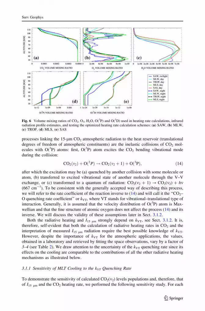
moves up, contrary to the low hz case for MLS atmospheric scenario. Figure 6 shows the
vertical distributions of the CO2, O3, H2O, O(3P), and O(1D) VMRs. It is essential to
include both daytime and nighttime ozone profiles because of the second ozone maximum
at *90 km during the nighttime.
Table 1 Atmospheric scenarios used in this study
Name SAW MLW TROP MLS SASDay/night Twilight/night Day/night Day/night Day/night Days
Noon hz 93.5� 63.5� 23.5� 16.5� 46.5�Latitude 70�S 40�S 0� 40�N 70�N
SABER day
DOY 193 194 193 193 193
Latitude 69.4�S 39.8�S 0.1�N 38.0�N 68.4�N
Longitude 180.6� 158.2� 210.2� 14.7� 95.8�hz 92.24� 63.1� 28.3� 25.3� 49.7�
SABER night
DOY 194 194 192 192
Latitude 68.14�S 40.0�S 0.1�S 38.1�N –
Longitude 208.1� 273.5� 318.6� 175.9�hz 131.0� 154.8� 154.5� 119.4�
Surv Geophys
123

3 Radiative Cooling and Heating in the MLT
The main objective of this section is to provide an overview of CO2, O3, O2, and H2O
contributions to the energy budget of the MLT, and to discuss the energy transformation
mechanism in which these molecules are involved. This requires considering the non-LTE
models for the CO2, O3, and H2O molecules as well as the model of O2/O3 photolysis
products kinetics.
3.1 Carbon Dioxide
Carbon dioxide is an optically active linear triatomic molecule. It has the three vibrational
modes: linear symmetric and asymmetric stretch vibrations referred to as m1 and m3,
respectively, and bending mode (m2). The vibrational quanta energies are 1,388, 667, and
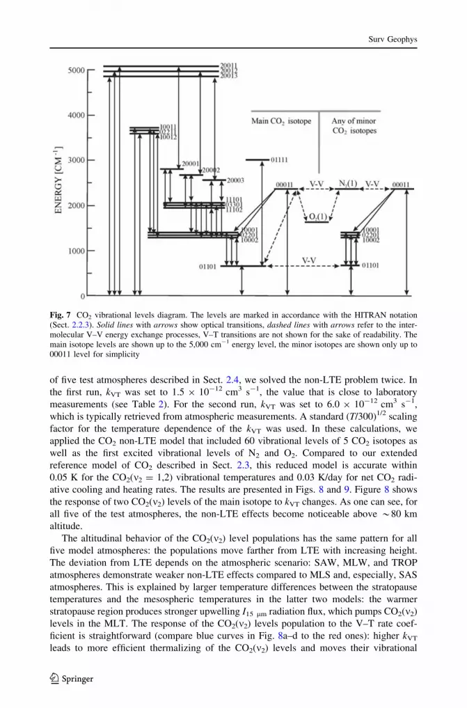
2,349 cm-1 for m1, m2, and m3 modes, respectively. The CO2 vibrational levels diagram
with the main optical transitions and processes of V–V exchange is shown in Fig. 7. The
levels on this diagram are marked in accordance with the HITRAN notation described in
Sect. 2.2.3. A CO2 molecule takes part in the following processes essential for the MLT
energetics: solar radiation absorption in 1–4.3-lm bands, CO2 atmospheric radiation
absorption and emission, and redistribution of the excitation among various vibrational
levels in a series of V–V, V–T, and emission processes.
Let us consider in detail the 15-lm infrared emission (I15 lm) formation. This emission
is the dominant cooling mechanism in the Earth’s MLT (e.g., see Gordiets 1976; Dickinson
1984; Goody and Yung 1995; Sharma and Wintersteiner 1990). On Earth, the magnitude of
the MLT cooling affects both the mesopause temperature and height; the stronger the
cooling, the colder and higher is the mesopause (see Bougher et al. 1994). The main
Fig. 5 Atmospheric temperature profiles used for heating rate calculations, infrared radiation profilesestimates, and testing the optimized heating rate calculation schemes: SAW denotes subarctic winter, 70�S,solar zenith angle hz = 93.5�; MLW denotes midlatitude winter, 40�S, hz = 63.5�; TROP stands for tropicalprofile, 0�, hz = 23.5�; MLS denotes midlatitude summer, 40�N, hz = 16.5�; SAS stands for subarcticsummer, 70�N, hz = 46.5�
Surv Geophys
123
processes linking the 15-lm CO2 atmospheric radiation to the heat reservoir (translational
degrees of freedom of atmospheric constituents) are the inelastic collisions of CO2 mol-
ecules with O(3P) atoms: first, O(3P) atom excites the CO2 bending vibrational mode
during the collision:
CO2ðm2Þ þ Oð3PÞ ! CO2ðm2 þ 1Þ þ Oð3PÞ; ð14Þ
after which the excitation may be (a) quenched by another collision with some molecule or
atom, (b) transferred to excited vibrational state of another molecule through the V–V
exchange, or (c) transformed to a quantum of radiation: CO2(m2 ? 1) ? CO2(m2) ? hm(667 cm-1). To be consistent with the generally accepted way of describing this process,
we will refer to the rate coefficient of the reaction inverse to (14) and will call it the ‘‘CO2–
O quenching rate coefficient’’ or kVT, where VT stands for vibrational–translational type of
interaction. Generally, it is assumed that the velocity distribution of O(3P) atom is Max-
wellian and that the fine structure of atomic oxygen does not affect the process (14) and its
inverse. We will discuss the validity of these assumptions later in Sect. 3.1.2.
Both the radiative heating and I15 lm strongly depend on kVT, see Sect. 3.1.2. It is,
therefore, self-evident that both the calculation of radiative heating rates in CO2 and the
interpretation of measured I15 lm radiation require the best possible knowledge of kVT.
However, despite the importance of kVT for the atmospheric applications, the values,
obtained in a laboratory and retrieved by fitting the space observations, vary by a factor of
3–4 (see Table 2). We draw attention to the uncertainty of the kVT quenching rate since its
effects on the cooling are comparable to the contributions of all the other radiative heating
mechanisms as illustrated below.
3.1.1 Sensitivity of MLT Cooling to the kVT Quenching Rate
To demonstrate the sensitivity of calculated CO2(m2) levels populations and, therefore, that
of I15 lm and the CO2 heating rate, we performed the following sensitivity study. For each
Fig. 6 Volume mixing ratios of CO2, O3, H2O, O(3P) and O(1D) used in heating rate calculations, infraredradiation profile estimates, and testing the optimized heating rate calculation schemes: (a) SAW, (b) MLW,(c) TROP, (d) MLS, (e) SAS
Surv Geophys
123
of five test atmospheres described in Sect. 2.4, we solved the non-LTE problem twice. In
the first run, kVT was set to 1.5 9 10-12 cm3 s-1, the value that is close to laboratory
measurements (see Table 2). For the second run, kVT was set to 6.0 9 10-12 cm3 s-1,
which is typically retrieved from atmospheric measurements. A standard (T/300)1/2 scaling
factor for the temperature dependence of the kVT was used. In these calculations, we
applied the CO2 non-LTE model that included 60 vibrational levels of 5 CO2 isotopes as
well as the first excited vibrational levels of N2 and O2. Compared to our extended
reference model of CO2 described in Sect. 2.3, this reduced model is accurate within
0.05 K for the CO2(m2 = 1,2) vibrational temperatures and 0.03 K/day for net CO2 radi-
ative cooling and heating rates. The results are presented in Figs. 8 and 9. Figure 8 shows
the response of two CO2(m2) levels of the main isotope to kVT changes. As one can see, for
all five of the test atmospheres, the non-LTE effects become noticeable above *80 km
altitude.
The altitudinal behavior of the CO2(m2) level populations has the same pattern for all
five model atmospheres: the populations move farther from LTE with increasing height.
The deviation from LTE depends on the atmospheric scenario: SAW, MLW, and TROP
atmospheres demonstrate weaker non-LTE effects compared to MLS and, especially, SAS
atmospheres. This is explained by larger temperature differences between the stratopause
temperatures and the mesospheric temperatures in the latter two models: the warmer
stratopause region produces stronger upwelling I15 lm radiation flux, which pumps CO2(m2)
levels in the MLT. The response of the CO2(m2) levels population to the V–T rate coef-
ficient is straightforward (compare blue curves in Fig. 8a–d to the red ones): higher kVT
leads to more efficient thermalizing of the CO2(m2) levels and moves their vibrational
Fig. 7 CO2 vibrational levels diagram. The levels are marked in accordance with the HITRAN notation(Sect. 2.2.3). Solid lines with arrows show optical transitions, dashed lines with arrows refer to the inter-molecular V–V energy exchange processes, V–T transitions are not shown for the sake of readability. Themain isotope levels are shown up to the 5,000 cm-1 energy level, the minor isotopes are shown only up to00011 level for simplicity
Surv Geophys
123

Table 2 Historic review of the kVT quenching rate coefficient laboratory measurements and atmosphericretrievals at T = 300 K
kVT (cm3 s-1) Reference Comments
3–30 9 10-14 Crutzen (1970) First guess
2.4 9 10-14 Taylor (1974), Center (1973) Laboratory measurements
5.0 9 10-13 Sharma and Nadile (1981) Atmospheric retrieval
1.0 9 10-12 Gordiets et al. (1982) Numerical experiment
2.0 9 10-13 Kumer and James (1983) Atmospheric retrieval
2.0 9 10-13 Dickinson (1984); Allen et al. (1980) Laboratory measurements
5.2 9 10-12 Stair et al. (1985) Atmospheric retrieval
3.5 9 10-12 Sharma (1987) Atmospheric retrieval
3–9 9 10-12 Sharma and Wintersteiner (1990) Atmospheric retrieval
1.5 9 10-12 Shved et al. (1991) Laboratory measurements
1.3 9 10-12 Pollock et al. (1993) Laboratory measurements
3–6 9 10-12 Lopez-Puertas et al. (1992) Atmospheric retrieval
5.0 9 10-12 Ratkowski et al. (1994) Atmospheric retrieval
5.0 9 10-13 Lilenfeld (1994) Laboratory measurements
1.5 9 10-12 Vollmann and Grossmann (1997) Atmospheric retrieval
1.4 9 10-12 Khvorostovskaya et al. (2002) Laboratory measurements
1.8 9 10-12 Castle et al. (2006) Laboratory measurements
6.0 9 10-12 Gusev et al. (2006) Atmospheric retrieval
1.5 9 10-12 Huestis et al. (2008) Recommended value
1.3–2.7 9 10-12 Castle et al. (2012) Laboratory measurements
Fig. 8 Sensitivity of 01101 and 02201 vibrational levels population to kVT for the five test daytimeatmospheres: (a) SAW (twilight case), (b) MLW, (c) TROP, (d) MLS, e SAS. Solid black lines: kinetictemperature; red lines: calculations with kVT = 6.0 9 10-12 cm3 s-1; blue lines: calculations withkVT = 1.5 9 10-12 cm3 s-1; solid red and blue lines: populations of 01101 level, dashed red and bluelines: populations of 02201 level
Surv Geophys
123

temperatures closer to the kinetic temperature profiles. The net heating rates for the five
test atmospheres and their sensitivity to kVT are presented in Fig. 9a–d. As one can see, the
absolute values of the net heating in the MLT are sensitive both to kVT and to the type of
atmosphere. The latter is explained not only by temperature profile differences but also by
variability of atomic oxygen VMR profiles. The kVT value and the atomic oxygen con-
centration are both equally important for the estimation of the MLT CO2 radiative cooling
and I15 lm since the CO2(m2) quenching term contains their product (see Eq. (15) below).
The strongest MLT cooling in Fig. 9 corresponds to high altitudes, high kVT rate, and polar
latitudes in the summer hemisphere. The sensitivity to kVT grows with increasing altitude
because the atomic oxygen concentration increases with height. Since the process (14)
plays an important role in the MLT cooling, the best possible knowledge of kVT is required
for adequate infrared cooling calculations. In the next section, we demonstrate an example
of estimating kVT from atmospheric measurements and discuss the result with respect to the
MLT energetics.
3.1.2 Estimating kVT Quenching Rate from Atmospheric Observations
The laboratory measurements of rate coefficients for various energy exchange processes by
inelastic collisions of molecules and atoms suffer from difficulties with reproducing
conditions close to those in the MLT in which molecules and atoms of various compounds
interact. This is particularly true for laboratory studies of reactions involving oxygen atoms
due to their extremely high chemical activity. On the other hand, the large variety of space
and ground-based observations of the MLT available today provides an opportunity to
utilize the MLT as ‘‘a natural laboratory’’ for retrieving these critical parameters. Below
we discuss a recent example of the kVT retrieval which utilizes the synergy of coincidental
satellite and lidar observations of the MLT. The advantage of utilizing the lidar (e.g., see
Weitkamp 2005) for such experiments is that the lidar temperature retrievals T(z) do not
depend on the non-LTE model parameters and, therefore, can be used as references. The
detailed description of the approach is given elsewhere (see Feofilov et al. 2012a). The
Fig. 9 Sensitivity of net CO2 heating rate to the value of the kVT{CO2–O} quenching rate for the five testdaytime atmospheres: (a) SAW (twilight case), (b) MLW, (c) TROP, (d) MLS, (e) SAS. Blue lines:calculations with kVT = 1.5 9 10-12 cm3 s-1; red lines: calculations with kVT = 6.0 9 10-12 cm3 s-1
Surv Geophys
123

comparison of the SABER temperature retrievals with lidar measurements has already
been performed by Remsberg et al. (2008), and the quenching rate coefficient used in that
study was estimated to be equal to (6.0 ± 3.0) 9 10-12 cm3 s-1. Applying stringent
overlapping criteria and treating the individual altitude layers of the overlapping region
separately, one can increase the accuracy and get into more detail of the MLT physics.
The general idea of the kVT retrieval is in minimizing the difference between the
measured and simulated 15-lm radiation by varying the product of kVT and O(3P) VMR.
For the study described, the measured radiation was provided by the SABER instrument
that also provides O(3P)(z) (see Smith et al. 2010) and CO2(z)(see Rezac 2011) VMRs.
This dataset was supplemented with T(z) in 80–110 km altitude range measured by the Fort
Collins lidar (see She et al. 2003). For these temperature profiles, the I15 lm limb radiation
was simulated at each tangent height in the 85–105 km altitude interval, and the ‘‘v2’’
deviations (see Chap. 15 in Press et al. 2002) for the measured and simulated radiation
were built for the kVT varying from 1.0 9 10-12 cm3 s-1 to 1.0 9 10-11 cm3 s-1 with a
5.0 9 10-13 cm3 s-1 step. Figure 10 shows the averaged kVT(z) ‘‘profile’’ obtained by
Feofilov et al. (2012a) that minimizes the radiation deviation.
Overall, the kVT values shown in Fig. 10 fit the atmospheric retrievals well: the aver-
aged kVT = (6.5 ± 1.5) 9 10-12 cm3 s-1. However, Fig. 10 also shows the altitudinal
variability of kVT that goes beyond its uncertainties in the 85–105 km altitude range.
Obviously, this variability does not imply that the rate coefficient depends on altitude.
Possible reasons for the kVT ‘‘variability’’ are discussed in Feofilov et al. (2012a) and
include collisions with thermal and non-thermal hydrogen, electronically excited O(1S),
charged components, multi-quantum excitation of CO2 by thermal oxygen (Ogibalov
2000), and temperature dependence of the kVT. The authors suggest that the observed
phenomenon may be explained by the simplicity of the currently utilized CO2 non-LTE
model with respect to CO2–O collisions. That might also be a clue to the ‘‘atmospheric/
laboratory’’ difference of the kVT values. The standard pumping term in the non-LTE
Fig. 10 Solid line: kVT(z) vertical distribution retrieved from minimizing the differences between thecalculated and measured I15 lm (z) radiation profiles (from Feofilov et al. 2012a). Dashed lines: uncertainties
Surv Geophys
123

model, which describes the total production of CO2 (m2) in the state with the number of
bending mode quanta m2 due to collisions with the O(3P) atoms, has the form of
Ym2¼ nOð3PÞfnm2�1km2�1;m2
� nm2km2;m2�1g; ð15Þ
where nOð3PÞ is the O(3P) density, nm2�1 and nm2are the vibrational states populations, and
km2�1;m2and km2;m2�1 are rate coefficients for one-quantum excitation and de-excitation,
respectively.
In the current non-LTE models, including the one applied in this study, it is usually
assumed that km2�1;m2¼ k0;1 and km2;m2�1 ¼ k1;0 ¼ kVT . It follows from Huestis et al. (2008)
that if the velocity distribution of O(3P) atoms is Maxwellian and their fine structure is
thermalized, then the laboratory measured k0,1 and k1,0 are linked by the detailed balance
relation:
k0;1 ¼ k1;0g1
g0
e� E1�E0ð Þ=kT ; ð16Þ
where E1 is the vibrational energy of the first m2 vibrational level and E0 is the energy of
ground vibrational level. Sharma et al. (1994) showed that both aforementioned conditions
are valid for O(3P) atoms in the Earth’s atmosphere up to at least 400 km, which seems to
justify usage of (16) in the non-LTE models. However, as Balakrishnan et al. (1998) and
Kharchenko et al. (2005) show, the non-thermal O(3P) and O(1D) atoms are produced by
O2 and O3 photolysis and Oþ2 dissociative recombination reactions in the MLT. These
‘‘hot’’ atoms may serve as an additional source of CO2(m2) level excitation. Therefore, the
expression (15) may need to be replaced by an expression like
Ym2¼ nOð3PÞ ð1� aÞfnm2�1km2�1;m2
� nm2km2;m2�1gþ a
Xm
nm2�mkhotm2�m;m2
� nm2
Xm
khotm2;m2�m
( )( );
ð17Þ
where a is the altitude dependent fraction of total O(3P) density that corresponds to hot
atoms and khotm2�m;m2
and khotm2;m2�m are the rate coefficients for excitation and de-excitation of
CO2 molecules, respectively, due to collisions with hot atoms, assuming also multi-
quantum processes. These rate coefficients are not related by the detailed balance since hot
O(3P) atoms are not thermalized. Comparing (15), which is applied in the model used in
the present study, with (17), one can see that the rate coefficient values retrieved in this
work and also in earlier atmospheric studies are some sort of effective rate coefficients that
include the contribution of hot O(3P) atoms, which may be expressed as
kretrVT ðzÞ ¼ kretr
m2;m2�1ðzÞ ¼ ð1� aðzÞÞ � km2�1;m2þ aðzÞ �
Xm
nm2khotm2�m;m2
: ð18Þ
These ‘‘hot’’ atoms may serve as an additional source of CO2(m2) level excitation that
would explain the difference between the laboratory measurements and atmospheric ret-
rievals of kVT. The increasing hot O(3P) atoms density with increasing altitude in the MLT
may also explain the altitude dependence of the retrieved ‘‘efficient’’ kVT. We stress here
that these important questions remain open and require further studies, both theoretical and
experimental. The negative temperature dependence of kVT that was found recently (see
Castle et al. 2012) makes this problem more complicated since the altitude gradient of the
kVT parameter would be even higher if this ‘‘new’’ temperature dependence was to be used
in the kVT retrieval.
Surv Geophys
123

3.2 Ozone
The ozone molecule in its ground electronic state is a bent three-atomic molecule that has
three vibrational modes: symmetric and asymmetric stretching modes (m1 and m3, respec-
tively), and a bending mode (m2). The m1 and m3 vibrations are close in energy (1,103 and
1,043 cm-1, respectively) and are coupled through a near-resonant V–V exchange. The
radiative transitions corresponding to m1 and m3 quanta change are responsible for infrared
cooling in the 9.6 lm O3 band. The m2 band transitions (705 cm-1) are weak and overlap
with 15 lm CO2 emissions. The transitions from the combination level (101) to the ground
and hot transitions of the type (m1, m2, m3) ? (m1 - 1, m2, m3 - 1) give rise to a strong 4.8-
lm band. In modern non-LTE models of O3 (e.g., see Lopez-Puertas and Taylor 2001;
Kaufmann et al. 2006; Fernandez et al. 2009, 2010), the total number of vibrational levels
considered is more than a hundred, up to the dissociation limit (*8,500 cm-1), and
includes many combination vibrational states. A simplified diagram of the first 22 vibra-
tional levels of ozone and interactions between them is shown in Fig. 11. The non-LTE
model for O3 molecule involves intra-molecular energy exchange processes:
O3ðm1; m2; m3Þ þMðN2;O2;OÞ$kint1
O3ðm1 � 1; m2; m3 þ 1Þ þM ð19Þ
O3ðm1; m2; m3Þ þMðN2;O2;OÞ$kint2
O3ðm1 � 1; m2 þ 1; m3Þ þM ð20Þ
O3ðm1; m2; m3Þ þMðN2;O2;OÞ$kint3
O3ðm1; m2 þ 1; m3 � 1Þ þM ð21Þ
as well as V–T processes:
O3ðm1; m2; m3Þ þMðN2;O2;OÞ$kVT1
O3ðm1; m2 � 1; m3Þ þM ð22Þ
O3ðm1; m2; m3Þ þMðN2;O2;OÞ$kVT2
O3ðm1 � 1; m2; m3Þ þM ð23Þ
O3ðm1; m2; m3Þ þMðN2;O2;OÞ$kVT3
O3ðm1; m2; m3 � 1Þ þM ð24Þ
and intermolecular V–V processes:
O3ð000Þ þ N2ðv ¼ 1Þ$kVV1O3ð200Þ þ N2ðv ¼ 0Þ þ 130 cm�1 ð25Þ
O3ð000Þ þ O2ðv ¼ 1Þ$kVV2O3ð100Þ þ O2ðv ¼ 0Þ þ 456 cm�1 ð26Þ
O3ð000Þ þ O2ðv ¼ 1Þ$kVV3O3ð001Þ þ O2ðv ¼ 0Þ þ 517 cm�1 ð27Þ
O3ð102Þ þ O2ðv ¼ 0Þ$kVV4O3ð000Þ þ O2ðv ¼ 2Þ � 4:9 cm�1: ð28Þ
A review of the rate coefficients for kint1 - kint3 (internal conversion of vibrational energy),
kVT1 - kVT3 (V–T processes), and kVV1 - kVV4 (V–V processes) is given in Manuilova and
Shved (1992), Manuilova et al. (1998), and Lopez-Puertas and Taylor (2001). The relation
between the rate coefficients is the following: kint1 � kint2 & kint3 & kVT1 & kVT2 � kVT3.
Besides these processes and the radiative transitions shown in Fig. 11, the O3 vibrational levels
are populated in the process of chemical recombination of ozone in the presence of a third body:
O2 þ Oð3PÞ þM ! O3ðm1; m2; m3Þ þM; ð29Þ
where M is N2, O2 or atomic oxygen. The energetics of this process is:
Surv Geophys
123

DH0f ðO2Þ þ DH0
f ðOð3PÞÞ ¼ DH0f ðO3Þ þ Evib þ Etransl ð30Þ
Evib þ Etransl ¼ 106:5 kJ/mol ¼ � 8; 900 cm�1; ð31Þ
where DH0f is the enthalpy of formation of gas at standard conditions, Evib is the vibrational
energy of O3, and Etransl is the total translational (kinetic) energy of O3 and M. The values
of DH0f ðO2Þ, DH0
f ðOð3PÞÞ, and DH0f ðO3Þ used for estimating Evib ? Etransl in (30) were
taken from the NIST Standard Reference Database (http://webbook.nist.gov/chemistry/).
As one can see from (31), the chemical energy released in the recombination process
(29) can populate the O3 vibrational levels up to its dissociation limit. In reality, the
fractioning between the Evib and Etransl is complicated. Several models have been sug-
gested for the nascent Evib distributions. In a widely used ‘‘zero surprisal’’ model (e.g., see
Levine and Bernstein 1974; Gil-Lopez et al. 2005), it is assumed that only O3(0, 0, m3)
levels are excited with the probability given by the formula:
f ðvÞ ¼ ð1� Em=DeÞ1:5P7v¼1 ð1� Em=DeÞ1:5
; ð32Þ
where m and Em are the level number and energy of m3, respectively, and De is the disso-
ciation energy. In other models (see Kaufmann et al. 2006), it is considered that all the
excitation goes to a single level m3 = 3, 5, or 8. Fernandez et al. (2009, 2010) assume that
the branching ratio between the Evib and Etransl is 7:3 and that the vibrational excitation
energy goes to m3 = 6. One can also assume that the chemical energy of the reaction (29) is
used to excite the O3(m1, m2, m3) levels near the dissociation limit (the so-called ‘‘Top-8’’
model in Lopez-Puertas and Taylor 2001).
The comparison of the effects of the nascent distribution model on the O3(m3) levels
population is given in Lopez-Puertas and Taylor (2001, Ch. 7.3.6, p. 211) where the vibra-
tional temperatures for the first 7 m3 levels obtained with the zero surprisal model are
Fig. 11 Ozone molecule vibrational levels diagram (Manuilova et al. 1998). Solid lines optical transitions,dashed lines V–V and V–T transitions
Surv Geophys
123

compared with that obtained with ‘‘Top-8’’ model where the excitation is distributed among
the uppermost vibrational levels below the dissociation limit. The study shows the high
sensitivity of the corresponding m3 level populations to the model chosen. In the zero surprisal
model, the atmospheric emission from the low m3 levels is higher compared to that in the
‘‘Top-8’’ model and vice versa, the emissions from the high m3 levels in the zero surprisal
model are lower than that in the ‘‘Top 8’’ model. We have to stress here that if one assumes
that the process (29) populates the O3 levels close to the dissociation limit, then the rate
coefficients for the processes (19)–(24) need to be determined since the rate coefficients
kint1 - kint3 and kVT1 – kVT3 cannot be applied to high-energy levels due to anharmonicity of
the vibrations and due to the complicated physics of closely spaced vibrational levels.
The uncertainty of the nascent population model is currently the most challenging
problem for the interpretation of O3 radiation measured in the hot bands (Manuilova,
private communication, 2012). For example, if the O3 VMR profile is retrieved from the
radiation in the (010–000), (100–000) and (001–000) transitions that are less sensitive to
the nascent populations model and then used for the interpretation of the 4.8-lm hot bands
radiation measurements (see Kaufmann et al. 2006), an inconsistency arises: the calculated
4.8-lm radiation is 2–3 times lower than the measured one in the 50–75 km altitude
interval. Correspondingly, Kaufmann et al. (2006) had to assume that either the ozone is
formed at the levels around 3,000 cm-1 (levels 003, 102, 201, or 300), like Manuilova
et al. (1998) did, or that the kint2, kint3 rate coefficients for hot band transitions have to be
reduced by a factor three or four to fit the MIPAS measurements. From the point of view of
the infrared energy budget, the branching ratio between the Evib and Etransl energies is
noteworthy since the latter term directly adds to the atmospheric heating while the Evib is
partially radiated back to the atmosphere and partially quenched and transformed to
translational energy. This contribution to the heat reservoir may be found only by detailed
solution of the non-LTE problem which accounts for the emission, propagation, absorption
and re-distribution of radiative energy.
Figure 12 shows the vibrational temperatures of the (100) and (001) vibrational levels
for the daytime and nighttime conditions calculated using the model of Manuilova et al.
(1998). For most of the atmospheric scenarios, the breakdown of LTE for these levels starts
at *65–70 km altitude. The vibrational temperatures shown in Fig. 12 are higher than the
kinetic ones because of the recombination process (29) and the radiative pumping of the
(100) and (001) levels by the absorption of radiation coming from the lower atmospheric
layers and from the ground. The daytime increase of the vibrational temperatures shown in
Fig. 12 is explained by a combined effect of higher daytime atomic oxygen VMR, higher
O3 VMR at 30–40 km, and lower O3 VMR in the 50–75 km altitude interval.
The radiative pumping effects can be seen in Fig. 13 which shows that the net radiative
effect of O3 in the MLT area is heating that maximizes at *95 km altitude and varies from
*0 K/day for the daytime cases to 3.0 K/day for the nighttime scenarios. Low absolute
values of the net heating by O3 in the MLT during daytime are explained by low O3 VMRs
(see solid lines in Fig. 6b). The energetic effects of ozone photolysis and subsequent
energy transformation processes in the system of electronic-vibrational oxygen energy
levels O2ðb3Rþg ; vÞ, O2ða1Dg; vÞ, and O2ðX3R�; vÞ will be considered in the next section.
3.3 Molecular Oxygen and Ozone Photolysis
Absorption of solar ultraviolet radiation by O2 and O3 in the MLT leads to a whole chain of
energy conversion processes. The first commonly accepted model of electronic kinetics of
Surv Geophys
123

O2/O3 photolysis products was developed by Harris and Adams (1983) and Thomas et al.
(1984) and was significantly improved by Mlynczak et al. (1993). Later, this model was
substantially extended by Yankovsky and Manuilova (2006). The updates and optimiza-
tions of this model may be found in Yankovsky and Babaev (2010) and Yankovsky et al.
(2011). In this section, we will refer to the model of Yankovsky and Manuilova (2006) and
demonstrate its coupling with the system of vibrational levels presented in Fig. 4.
The upper panel of Fig. 14 shows that the molecular oxygen photolysis caused by absorption
of radiation in the Schumann-Runge continuum (175–205 nm) and Lyman-alpha (Ly-a) line
leads to producing the electronically excited oxygen atoms O(1D). These atoms are also pro-
duced as a result of O3 photolysis in the Hartley band (200–310 nm). The collisions of O(1D)
with molecular oxygen in the ground electronic state, O2 (X3R-, 0), and the transfer of its
electronic energy to O2 give rise to the populations of electronically vibrationally excited
molecular oxygen O2ðb3Rþg ; vÞ with the subsequent redistribution of excitation energy to
O2(a1Dg, m) and O2 (X3R-, m) electronic-vibrational levels. These levels are also directly
populated by O3 photolysis in the Hartley band, Huggins bands (310–350 nm), and Chappuis
bands (410–750 nm) and by resonance absorption of solar radiation at 762, 689, 629 nm and
1.27 lm. At each electronic-vibrational level, the deposited energy can be either quenched by
a collision with one of the atmospheric species (mainly with N2, O2, and O) or radiated to the
atmosphere. The net effect of solar absorption leading to O2/O3 photolysis is heating (hO2=O3)
since the energy is deposited in the respective region, and only part of it escapes through
radiation in the 1.27 lm and 762 nm O2 bands (see the cooling components in Fig. 15). The
total energy budget of O2/O3 photolysis may be represented in the following form:
hO2;O3ðzÞ ¼ 1
CpðzÞqðzÞ
�Zka2
ka1
EaðkÞUsolðk; zÞraðkÞdkþZkb2
kb1
EbðkÞUsolðk; zÞrbðkÞdk�X
i
hmiUiðzÞ
264
375;
ð33Þ
Fig. 12 Nighttime and daytime (twilight for the SAW case) populations of O3(100) and O3(001) vibrationallevels in a form of vibrational temperatures for the five test atmospheres: (a) SAW, (b) MLW, (c) TROP,(d) MLS, (e) SAS
Surv Geophys
123

where Cp(z) is the air heat capacity at constant pressure, q(z) is the density, the indices a
and b are related to O2 and O3 photodissociation, respectively, E(k) is the energetic effect
of one photodissociation act calculated from the energy of the absorbed quantum and DH0f
values of the participating atoms and molecules, and the amount of Usol(k, z) is the
incoming solar flux for wave length k at the altitude z, r(k) is the absorption cross section,
Ui(z) and hmi are the integrated volume emission rates at the altitude z and the energies of
emission quanta that correspond to 630, 629, 689, 762, and 1.27 lm radiation (Fig. 14,
upper panel).
Cross-sections for O2 photodissociation have been the subject of numerous laboratory
studies. Based on these studies, the parameterization schemes and tables for different
spectral areas have been built: see Chabrillat and Kockarts (1997) for Ly-a radiation
absorption; Minschwaner et al. (1992) and Kockarts (1994) for O2 absorption in Schu-
mann-Runge bands (175–205 nm); Nee and Lee (1997) and DeMajistre et al. (2001) for
the absorption in Schumann-Runge continuum. Regarding the O3 absorption cross-sections
one can refer to: DeMore et al. (1997) for the absorption in Hartley band; Malicet et al.
(1995) for Huggins bands; Brion et al. (1998) for Chappuis bands. The estimates of terms
in (33) for the heating by the absorption of the UV solar radiation by O2 and O3 and for the
1.27 lm and 762 nm bands cooling (main cooling terms in (33)) are shown in Fig. 15. The
cooling component is calculated from the 762 nm and 1.27 lm Ui(z) fluxes measured in
the METEORS experiment (see Mlynczak et al. 2001). Heating rates due to O2 and O3
photodissociation for tropical conditions were estimated by Fomichev (2009) using the
method suggested by Mlynczak and Solomon (1993) and Mlynczak and Marshall (1996).
Overall, the net MLT heating due to photochemical effects of solar radiation on O2 and O3
is quite significant and can reach values of about 8 K/day at *95 km altitude. At the same
altitude, both O2 bands provide significant cooling of about 3.5 K/day.
The model of the O2/O3 photolysis product kinetics shown in the upper panel of Fig. 14
is implemented in the ALI-ARMS code (see Sect. 2.3). It allows simultaneous self-con-
sistent solution of the non-LTE problem for the set of vibrational levels of molecules
(Fig. 4) and the system of electronic-vibrational levels of the O2 and O3 molecules and
electronic levels of O atoms. The coupling of the O2/O3 system of levels of Fig. 14 with
Fig. 13 Nighttime and daytime (twilight for the SAW case) net heating rates of ozone in the MLT regionfor the five test atmospheres: (a) SAW, (b) MLW, (c) TROP, (d) MLS, (e) SAS
Surv Geophys
123

Fig. 14 Joint scheme of O2/O3 photolysis products kinetics (upper panel, after Yankovsky and Manuilova(2006)) and H2O vibrational levels (lower panel). In the upper panel thick horizontal lines correspond toelectronic states of atomic and molecular oxygen; thin horizontal lines represent the vibrational substructureof the corresponding electronic state; lines with arrows in the upper part of the panel denote the O2 and O3
photolysis after absorption of radiation in the Schumann-Runge continuum (JSRC), Lyman-a line (JLya),Hartley (JH), Huggins (JHu), and Chappuis (JCh) bands (see text for more details). In the lower panel thickhorizontal lines correspond to vibrational states of the H2O molecule; optical transitions are shown as thinsolid lines; dashed lines represent V–T processes, and thick dashed lines with arrows correspond to V–Venergy exchange processes. Note the V–V coupling of the O2 (X, v = 1) level in the upper panel andH2O(010) level in the lower panel
Surv Geophys
123

the molecular levels shown in Fig. 4 is realized through the V–V exchanges. In addition,
the photochemical model is linked to the system of molecular levels shown in Figs. 2 and 4
through the O(1D) energy transfer to N2(m) vibrational levels, which are also pumped from
the OH(m) during nighttime. The V–V exchange between O2(1), N2(1) and H2O(010)
shown in Fig. 14 dominates among these energy transfers and is important for the H2O
model discussed in the next section.
3.4 Water Vapor
Water vapor cools the atmosphere in rotational and vibrational bands. The direct energetic
effect of H2O on the MLT cooling is tertiary, compared to that of CO2 and O3. However,
besides the direct effects of infrared cooling, H2O influences the composition and energy
budget of the MLT area in a number of ways. Being a source for chemically active
constituents, such as OH, O(1D), H2, and H (e.g., see Brasseur and Solomon 2005), it
participates in the so-called ‘‘zero-cycle’’ reactions where the absorption of solar short-
wave radiation leads to H2O photodissociation with subsequent recombination in a number
of processes that result in heating of the atmosphere (e.g., see Sonnemann et al. 2005). The
existence of water molecules at sufficiently low temperatures near the polar summer
mesopause leads to the nucleation of ice particles in the MLT region (e.g., see Rapp and
Thomas 2006, and references therein). These particles are responsible for such phenomena
as noctilucent clouds (NLCs) and polar mesospheric summer echoes (PMSEs). Because of
high sensitivity to local kinetic temperatures, the NLC and PMSE phenomena can be used
as temperature probes for these regions (e.g., see Lubken et al. 2007; Petelina and Zasetsky
2009) and as possible indicators of climate change (e.g., see Thomas 2003).
In the gas phase, water molecule vibrations involve combinations of symmetric stretch
(m1), covalent bond bending (m2), and asymmetric stretch (m3) modes with the band strength
Fig. 15 Heating effects due to solar absorption by O2 (Lyman-a, Schumann-Runge bands, and Schumann-Runge continuum) and O3 (Hartley, Huggins, and Chappuis bands) after Fomichev (2009). Cooling in the1.27 lm and 762 nm bands is estimated from the corresponding volume emission rates measured by theMETEORS experiment (Mlynczak et al. 2001)
Surv Geophys
123

ratio for the fundamental bands of the main H2O isotope being 0.07/1.50/1.00 for the m1,
m2, and m3 vibrations, respectively (e.g., see Goody and Yung 1995, and references therein,
and Rothman et al. 2009). The diagram in the lower panel of Fig. 14 shows the ground
level and various excited vibrational levels of the H2O molecule up to 7,445 cm-1. The
levels are marked in accordance with the number of vibrational quanta m1m2m3. The rota-
tional levels of H2O are considered to be in LTE in the MLT while the vibrational levels
start deviating from LTE above *50 km. The detailed description and sensitivity studies
for the H2O non-LTE model may be found in Lopez-Puertas and Taylor (2001), Manuilova
et al. (2001), and Feofilov et al. (2009). The highest sensitivity of the H2O(m2) vibrational
levels population is to the rate coefficient kVV of the V–V exchange process:
H2Oðm2Þ þ O2ðX3R�; 1Þ�!kVVH2Oðm2 þ 1Þ þ O2ðX3R�; 0Þ: ð34Þ
This sensitivity is bilateral: O2(X3R-, 1) is pumped in a series of processes shown in the
upper panel of Fig. 14 and reducing the value of the kVV coefficient may lead to a decrease in
H2O(m2) pumping. On the other hand, O2(X3R-, 0) serves as a vibrational energy ‘‘reservoir’’
for H2O(m2) quanta; reducing the kVV leads to decoupling of H2O(m2) system from this
reservoir and to an increase of H2O(m2) populations. This issue is especially important when
dealing with the interpretation of 6.6 lm H2O radiation that will be described in Sect. 5.2.2.
The kVV value estimated by different groups varies from 5.5 9 10-13 cm3 s-1 (see Huestis
2006) through 1.0 9 10-12 cm3s-1 (see Koukouli et al. 2006) and 1.2 9 10-12 cm3 s-1 (see
Feofilov et al. 2009) to 1.7 9 10-12 cm3 s-1 (see Garcıa-Comas et al. 2002); see also
Table 2 in Feofilov et al. (2009) for a historical review of this rate coefficient.
Figure 16 shows the contributions of the main isotope H2O rotational band (associated
with the ground vibrational level) and vibrational bands to radiative heating of the MLT.
As one can see, the net effect of the radiative transfer in the vibrational band in this region
is heating since H2O absorbs the radiation coming up from below where the net radiative
effect is cooling (not shown in the figure due to the selected vertical axis limits). The
vibrational band is responsible for a maximum of 0.5 K/day at *70 km altitude for the
MLS and SAS profiles. On the other hand, the rotational band cools the mesosphere at
70–80 km and provides 0.6–1.5 K/day cooling in its maximum. It is interesting to note
both quantitative and qualitative differences between the rotational cooling profiles for the
SAW, MLW, TROP and MLS, SAS atmospheric scenarios. For the latter two, the cooling
in the cold mesopause is compensated by absorption of the radiation coming from below.
Summing up the profiles of the vibrational and rotational heating rates leads to reduction of
the cooling effect of the rotational band in the 75–85 km altitude range to 1.5 K/day for the
SAW, 1.1 K/day for the MLW and the TROP, 0.5 K/day for the MLS, and 0.2 K/day for
the SAS atmospheric scenario. Above *85 km altitude, the H2O contribution to the MLT
energy budget becomes negligible for the SAW, MLW, TROP, and MLS scenarios due to
the rapidly decreasing H2O VMR. For the SAS atmosphere, the rotational band cooling at
100 km altitude remains on the order of 0.5 K/day due both to higher SAS temperatures
here and higher summer H2O VMR that is explained by the upward transport by vertical
winds (see Garcia and Solomon 1994; Korner and Sonnemann 2001).
3.5 Radiative Cooling of the MLT Associated with Gravity Wave-Induced
Atmospheric Fluctuations
An interesting aspect of the radiative cooling in the MLT is the combined effect of the
small-scale fluctuations in the atmospheric vertical structure, and radiative transfer in the
Surv Geophys
123

15 lm CO2 band. First described by Kutepov et al. (2007) for T(z) variations, it was later
extended to the variation of T(z), CO2(z), and O(3P)(z) distributions (see Kutepov et al.
2012). The additional cooling in the MLT caused by this phenomenon is comparable with
the heating effects of O3 and H2O, so we go into some detail regarding its mechanism. As
one can see from the Sect. 3 of this work, the heating rates in the atmosphere strongly
depend on the distributions of temperature and of radiatively active atmospheric
components.
In the middle atmosphere, instantaneous profiles are highly irregular due to disturbances
associated with gravity waves (GWs). The GW amplitude increases with height and the
r.m.s. of temperature fluctuations is about 20 K at 90 km altitude (e.g., see Whiteway and
Carswell 1995; Smith 2012). The wavelengths k � 2pH, where H is a scale height, are
usually not well resolved in modern GCMs, and the dynamic effects of these ‘‘sub-grid’’
GWs are usually taken into account in the form of a ‘‘GW drag’’ parameterization (see
Fritts and Alexander 2003). On the other hand, the atmospheric parameter fluctuations
caused by GWs affect the radiative transfer and the corresponding heating rates. These
effects, however, are usually omitted in GCMs because (a) small-scale GWs are not well
resolved and (b) radiative heating rates h(z) parameterizations (see also Sect. 4) utilize a
grid coarser than the grid of the GCM.
In the MLT, the trace gases CO2 and O(3P) can be considered as conservative tracers so
that the GW-induced variations are entirely due to adiabatic displacements of air parcels.
In this case, one can express the trace gas VMR variation, f0, as a function of temperature
variation T0:
f0 ¼ cT 0; c ¼ dfdz� dT
dzþ RT
cpH
� ��1
; ð35Þ
where f is the mean VMR, T is the mean temperature profile, and R is the gas constant. If
the model for T0 fluctuations is known, one can perform a numerical experiment to identify
the effects of GW-induced fluctuations on mean radiative heating rate. This experiment
was carried out for the five atmospheric scenarios. For each case, 1,000 individual GWs
were generated in accordance with the statistical model described in Kutepov et al. (2007).
Fig. 16 Net heating rates of H2O in vibrational bands and in the rotational band for the five daytime testatmospheres: (a) SAW (twilight), (b) MLW, (c) TROP, (d) MLS, (e) SAS
Surv Geophys
123

The f0 values were calculated in accordance with (35), and the non-LTE problem was run
for each of the individual atmospheric profiles of T, O(3P), and CO2. After that, the
differences of the heating rates DhðzÞ ¼ �hðzÞ � haver:atm:ðzÞ were calculated where �hðzÞrepresents the h(z) averaged over 1,000 profiles and haver:atm:ðzÞ is the heating rate calcu-
lated for an averaged atmospheric profile. The r.m.s. profile of the temperature fluctuations
rT ¼ 1N
PNi¼1
ðT 0i Þ2
� �1=2
for SAW atmospheric scenario is shown in Fig. 17a. The results
presented in Fig. 17b show the combined effect of T, O(3P) and CO2 fluctuations on the
CO2 radiative heating. As one can see, the main effect of GW-induced fluctuations is an
additional cooling of up to 3 K/day (for SAW and MLW) in the altitude region 80–95 km
and a slight additional warming up to 1 K/day (for MLS). The observed effect is mainly
related to temperature fluctuations and is explained by increased mean local thermal
emission with respect to emission for the non-disturbed temperature due to strong non-
linear temperature dependence of the Planck function (see Kutepov et al. 2007).
Accounting for fCO2and fOð3PÞ fluctuations leads to changes in DhðzÞ compared to the
results obtained in Kutepov et al. (2007): fOð3PÞ fluctuation increases the additional cooling
in the 85–100 km area by a maximum of *1 K/day (SAW) while the fCO2fluctuation has
the opposite effect, decreasing the h(z) in 88–100 km by *1.7 K/day. These effects and
their signs are related to f gradients in the MLT: according to (35), large f gradients lead to
large f0 values, and in the MLT the fOð3PÞ rapidly increases with height while the fCO2
decreases with height (see Fig. 6a, d, respectively).
A more detailed explanation for the Dh(z) behavior with respect to temperature, fCO2,
and fO3fluctuations as well as its parameterization with respect to average temperature
variation rT, and fCO2ðzÞ and fOð3PÞðzÞ distributions is given in Kutepov et al. (2012) who
show that the net effect of these fluctuations can cause an additional cooling of up to
4 K/day near the mesopause.
4 Optimization of Heating Rate Calculation for GCMs
Let us assume that there are NV vibrational levels involved in the problem and that the
atmosphere is discretized at ND altitude grid points. Solving the steady state equations (8)
for this system requires solving the radiative transfer equation (4) for NR spectral lines in
the NB ro-vibrational molecular bands. In the LBL approach for the non-overlapping lines,
each line must be resolved in NF frequency points to include the changes of the line shape
with respect to atmospheric pressure and temperature. The above-mentioned parameters in
modern models for molecules considered above are of the following order: NV = 10 - 100,
ND & 100, NB = 10 - 1,000, NR = 100 - 105, NF = 10 - 100. Naturally, the exact non-
LTE calculations performed in this manner cannot be used to estimate the heating rates
h(z) in GCMs. Instead, the h(z) in molecular bands are usually calculated with the help of
some parameterizations that take into account the main physical mechanism responsible for
the radiative cooling or heating for each particular molecule. Obviously, there is a trade-off
between accuracy and efficiency of these algorithms, most of which are described in the
review paper of Fomichev (2009). Among these methods, one has to highlight the CO2
infrared cooling parameterizations by Fomichev et al. (1993) and Fomichev et al. (1998a),
which cover both LTE and non-LTE region starting from 15 km up to the altitudes in
thermosphere. The non-LTE fraction of this algorithm (see Kutepov and Fomichev 1993)
Surv Geophys
123

evolved from the second-order escape probability approximation of Frisch and Frisch (1975)
and was later supplemented by the parameterization of heating by the CO2 absorption of the
near-infrared solar radiation (see Fomichev et al. 2004). The accuracy of this method in the
MLT region is reported to be about 1 K/day if kVT = 1.5 9 10-12 cm3 s-1 is utilized (see
Fomichev 2009).
The 9.6 lm O3 cooling effects have not been parameterized yet due to the complexity of
the O3 non-LTE model and its relatively small effect during the day. The same is also true
for H2O. However, during the nighttime, the contribution of O3 to the MLT energy budget
becomes noticeable (up to ?3 K/day at *95 km altitude, see Fig. 13), which calls for its
parameterization in the GCM. The absence of this term might create a negative temper-
ature bias at 85–100 km altitude.
Because of the increasing requirements for accuracy and flexibility of the radiative
heating estimates in GCMs, it is unlikely that the parameterizations based on different
approximate treatments of the non-LTE radiative transfer like various order escape
probability approximations or matrix approaches (see Fomichev et al. 1993, 1998a) will
satisfy the users. On the other hand, computer processor capacities as well as those of
multi-core and parallel processing computers are continually increasing. This is supple-
mented also by the dramatic progress in the efficiency of exact multiple scattering non-
LTE radiative transfer algorithms (see Gusev and Kutepov 2003).
This allows turning from developing the radiative cooling parameterizations for GCMs
to utilizing the exact non-LTE radiative transfer algorithms. Below, we describe an
approach developed first for calculating h(z) in the 15 lm CO2 bands in the Martian
atmosphere (see Hartogh et al. 2005, Feofilov et al. 2006) and apply it to the terrestrial
atmosphere. Since this scheme is based on our exact reference non-LTE model and the
ALI-ARMS code, it is potentially applicable to any significant atmospheric molecule in the
planetary atmosphere, given that the non-LTE reference model for this molecule exists.
Fig. 17 Additional cooling caused by atmospheric vertical structure fluctuations associated with gravitywaves. (a) r.m.s. of the temperature variation caused by gravity waves for the SAW atmospheric scenario;(b) net effect of T(z), CO2(z), and O(z) variations on heating of the MLT region for the five testatmospheres: (a) SAW (twilight), (b) MLW, (c) TROP, (d) MLS, (e) SAS
Surv Geophys
123

The acceleration approach consists of the three steps: (a) applying the ALI (for Acceler-
ated Lambda Iteration) technique for radiative transfer; (b) replacing the radiative transfer
in the NR individual lines of the NB molecular bands by radiative transfer in the molecular
bands themselves by utilizing the opacity distribution function (ODF) method; and
(c) reducing the NV involved into the steady-state Eq. (8). The peculiarities of each step are
discussed below.
4.1 Methods of Solving the Non-LTE Problem: The ALI Technique
The most straightforward way of solving the joint system of the SSE (8) and the RTE (4) is to
iterate between them. This approach is traditionally called the ‘‘lambda iteration’’ (LI) and
has been studied in detail in the astrophysical context since the 1920s (see Unsold 1968). In
atmospheric science, the straightforward application of this technique was described by
Wintersteiner et al. (1992). This approach numerically simulates the multiple scattering of
photons and is attractive since it involves ND matrices of NV 9 NV size. However, as
Kutepov et al. (1998) showed, the convergence of the LI method is slow since the photons are
‘‘trapped’’ in the cores of optically thick lines. Kutepov et al. (1998) and Gusev and Kutepov
(2003) studied the LI approach in detail for non-LTE problems in the Earth’s and planetary
atmospheres and demonstrated that its convergence rate could be so slow that false solutions
appear to be stable and/or the accumulation of numerical errors causes the process to diverge.
They showed that the LI approach is particularly inefficient for the solution of the non-LTE
problem in molecular bands, like those, for instance, for CO2 in the Earth’s and Martian
atmospheres, since the general non-local and nonlinear nature of the non-LTE problem is
aggravated here by the additional nonlinearity introduced by the V–V energy exchanges
whose rates depend on the products of level populations.
An alternative way of solving the non-LTE problem is treating the SSE (8) and the RTE
(4) simultaneously by discretizing the RTE with respect to an optical depth or pressure grid
to get a matrix representation of the radiative terms in the SSE. In this approach (see, e.g.,
Lopez-Puertas and Taylor 2001; Funke et al. 2012), the non-local radiative terms are
expressed in terms of populations and the problem is solved iteratively as a set of non-local
linear problems. The convergence of this method is usually fast (see Gusev and Kutepov
2003), but the time for filling out and inverting the matrices is large because of their size
(NV 9 ND) 9 (NV 9 ND). From the point of view of computation time, one matrix iter-
ation is roughly equivalent to ND lambda iterations. However, if both ND and NV are large,
each matrix iteration is very expensive in computer time; the same result may be achieved
faster with LI or its accelerated version discussed below.
The problems related to the application of standard LI or matrix approaches outlined above
are overcome by utilizing the so-called ‘‘accelerated lambda iteration’’ (ALI) method devel-
oped in stellar astrophysics (see Rybicki and Hummer 1991, 1992 and references therein). The
family of ALI methods is based on the operator splitting of the form K = K* ? (K - K*),
where K is the monochromatic lambda operator Klm along the ray with direction l defined
by the formal solution of the RTE (4) Ilm = Klm[Sm], where Sm = glm/vlm is the source
function and the square brackets mean ‘‘acting on’’. The splitting of the operator leads to the
following iteration scheme: Iilm ¼ K�i�1
lm ½Sim þ ðK
i�1lm � K�i�1
lm Þ½Si�1m ¼ K�i�1
lm ½Sim þ Ieff i�1
lm ,
where i and i-1 indices denote the current and the previous iterations, respectively, and
Ieff i�1lm ¼ ðKi�1
lm � K�i�1lm Þ½Si�1
m is the ‘‘effective’’ intensity. Although this equation is only
approximate at each iteration, it becomes exact for the converged solution, for which
Surv Geophys
123

Sim ¼ Si�1
m , K�ilm ¼ K�i�1lm , and Ki
lm ¼ Ki�1lm . This iteration scheme describes a whole class of
methods, each specified by the choice of a particular approximate lambda operator K�lm. The
simplest choice is to use the diagonal part of the matrix representation of the exact lambda
operator as it is done in the ALI-ARMS research code. Using a ‘‘preconditioning’’ approach
(see Rybicki and Hummer 1991, 1992), one can rewrite the radiative rate coefficients in such
a way that much of the transfer in the optically thick ‘‘core’’ of the line, described by the local
part of the lambda operator, is canceled analytically: Reffll0 ¼ All0 ð1� K�i�1
ll0 Þ þ Bll0�Jeff i�1ll0 ,
where K�ll0 and �Jeffll0 are obtained from K�lm and Ieff
lm by applying double integration
1�
4pR
dlR
/ll0 ðmÞdm. As a result, the ALI method converges much faster than the LI method
while it still utilizes ND matrices of NV 9 NV size. The convergence speed of LI, matrix, and
ALI methods has been studied in detail by Kutepov et al. (1998) who showed the superiority
of ALI over the two other approaches for the atmospheres of Earth and Mars.
4.2 Optimizing the Radiative Transfer Calculations in Molecular Bands: Reducing
the Number of Frequency Points
Additional significant computational time savings may be reached by optimizing the
radiative transfer calculations. The latter linearly depends on the number of frequency and
angle points in the angle and frequency integrals in (3). Whereas the number of angle
points usually does not exceed 4, the number of frequency points is very large: the
algorithm needs to treat the radiative transfer adequately in NF points within each of NR ro-
vibrational lines for each of NB bands considered. If one considers the g(m) and v(m) (see
Eq. (10)) for a group of lines belonging to one molecular band branch and builds them
using the contributions of NR individual lines gll0(m) and vll0(m), one will obtain the
‘‘spectral profile’’ characterized by non-monotonic behavior. In order to evaluate the
integral of type (3), one has to consider this profile for a large number of frequency points.
One of the ways of optimizing the radiative transfer for a molecular band would be to
reduce the NR by retaining strong lines and omitting weak lines. However, this will barely
help and may lead to undesirable results for optically dense media since in this case the
radiative transfer occurs mostly in the weak lines and partly in the far wings of strong lines.
In the LTE area, the reduction of frequency points number is usually achieved by
utilizing the so-called CKD (correlated k-distribution) method that is based on grouping
the gaseous spectral transmittances in accordance with the absorption coefficient k. In this
method, it is assumed that the k-distributions built for atmospheric layers with different
pressure and temperature provide the spectral frequency correlation required for ade-
quately reproducing the radiative transfer at any given frequency. In reality, the method
appears to be accurate only in the case of radiative transfer between adjacent vertical levels
or in the cases of low vertical temperature gradients. For flux calculations in the LTE area,
it was found that the method is accurate to within 1 % (see Goody et al. 1989; Lacis and
Oinas 1991; Fu and Liou 1992). However, the k-correlation scheme is not applicable in the
case of non-LTE because the vibrational level populations involved in the building of
k-distributions (and calculated in the LTE according to Boltzmann’s law for a local
temperature) are unknown and depend on the solution of RTE.
In the context of non-LTE, one may use the idea of opacity distribution function (ODF),
as discussed by Anderson (1987) and Mihalas (1978). In this approach, the absorption
cross section is re-sampled to yield a monotonic function of frequency that can be rep-
resented by a relatively small number of frequency points. Though the idea is similar to the
k-correlation, in this method, the absorption and emission profiles and the populations are
Surv Geophys
123

treated separately, which allows accounting for the non-LTE conditions. There are two
potential problems associated with this approach. First, the positions of the lines in the
original and re-sampled v(m) distributions may be not the same since the re-ordering
depends on the rotational distribution function in the ro-vibrational band, which, in turn,
depends on temperature. The second problem is linked with the overlapping of two or more
different molecular bands. Fortunately, these issues have little effect on the populations of
the vibrational levels and radiative cooling and heating rates. The first problem is effi-
ciently masked by photon trapping in the cores of thick lines and by relatively small
changes in the temperature from layer to layer. The effects of the second problem can be
neglected due to the validity of the non-overlapping lines approximation for the majority of
applications in the MLT (see Lopez-Puertas and Taylor 2001).
Since the use of the ODF approach for treating molecular bands is new, we provide
some background information on it. If one considers a simple case of the non-overlapping
branches of molecular bands, one can write the opacity and emissivity distributions for
these spectral ‘‘profiles’’ as
gbvv0 ðmÞ ¼
hvvv0
4pnvAb
vv0 ðTÞuevv0 ðmÞ ð36Þ
vbvv0 ðmÞ ¼
hvvv0
4pnv0B
bv0vðTÞua
v0vðmÞ � nvBbvv0 ðTÞus
vv0 ðmÞ� �
; ð37Þ
where Abvv0 ðTÞ, Bb
vv0 ðTÞ, and Bbv0vðTÞ are the temperature-dependent Einstein coefficients for
the branch, and uevv0 ðmÞ, ua
vv0 ðmÞ, and usvv0 ðmÞ are the normalized branch profile functions for
emission, absorption, and stimulated emissions, respectively. We draw the reader’s
attention to the fact that, compared to the CKD approach, the vibrational levels populations
do not enter these branch profile functions. These profile functions are highly non-
monotonic since they are constructed as superpositions of individual line profiles presented
by the Voigt functions and weighted with the normalized rotational distribution.
Let us now define the /(m) functions as re-sampled and sorted /vv0 ðmÞ profiles and also
define normalized distributions
aðxÞ ¼ 1
/ð0Þ/vv01
/ð0Þ x� �
; ð38Þ
where x = m�/(0), and for which a(0) = 1,Rþ10
aðxÞdx ¼ 1. We have built and analyzed
several hundreds of these functions for linear molecules CO2, N2O and CO fundamental
and hot branches for broad ranges of pressure and temperature variations (P = 10-9 -
1 bar, T = 150-600 K).
Two principal conclusions, which followed from this analysis, are:
1) uevv0 ðmÞ, ua
vv0 ðmÞ, and usvv0 ðmÞ profiles for emission, absorption and stimulated emission
of each branch nearly coincide (their relative differences do not exceed a few fractions
of percent), and, therefore, may be represented by a single function a(x), which we
will call ‘‘ODF cross section’’ or simply ‘‘ODF’’. Similar to the case of the complete
frequency redistribution within a single line, when line absorption, emission, and
stimulated emission in the line are described by the same Voight function, this effect
can be called ‘‘complete frequency redistribution’’ within the branch.
2) For the majority of the considered molecular bands of various molecules, the ODF
cross-sections a(x) for P, Q and R branches of perpendicular bands or those for P and
Surv Geophys
123

R branches of parallel bands are remarkably close. Although in the pressure and
temperature ranges considered their relative differences in narrow intervals Dx may
reach 25 %, this has no significant effect on estimation of integrals of type (3). It
allows operating with the single ODF cross section a(x) for each branch of any band of
any of the linear molecules considered.
If the shape of the a(x) profile is known, then the Eqs. (36) and (37) may be rewritten for
/(m), which is a monotonic function that can be represented in a small number of fre-
quency (or better to say ‘‘pseudo-frequency’’) points NF. This means that the ODF
approach allows each branch to be replaced by a single ‘‘superline’’ of a special shape,
which may be parameterized with respect to variations of pressure and temperature.
Further analysis has shown that the ‘‘superline’’ can be approximated by a function similar
to the Voigt function, in which exp(-y2) is replaced by exp(-|y|).
The tests show that NF required for the sufficient accuracy of the RTE calculations when
applying ODF is approximately equal to the number of frequency points for a single line in
the LBL approach. Therefore, the acceleration factor that can be reached by utilizing the
ODF approach is roughly equal to the number of spectral lines within the branch (*100
for CO2, *1,000 for O3). The accuracy of the ODF approach with respect to heating rate
calculations is shown in Fig. 18. As one can see, the errors for the net heating rate in CO2
do not exceed ±0.15 K/day compared to the reference LBL data for all test atmospheres.
This high accuracy of the radiative flux divergence calculations, which are extremely
sensitive to the radiative transfer treatment, means that the ODF approach in its version
outlined above significantly exceeds the CKD approach in its flexibility. Compared to
CKD which provides reasonable accuracy only for adjacent atmospheric levels with low
temperature gradient, the ODF approach demonstrates high accuracy over the wide altitude
range of the MLT, where the temperature exhibits large changes with altitude.
We found that the higher accuracy of the ODF approach is explained by the much
stronger dependence of the ‘‘superline’’ profile wing on temperature: the wing of the
‘‘superline’’ is proportional to T-1 while the single Voigt line wing is proportional to T-1/2.
This temperature dependence efficiently compensates for the differences between the ODF
and LBL approaches, associated with the radiative energy exchange between distant
atmospheric layers having different temperatures.
4.3 Reducing the Number of Levels
For any of the methods described in Sect. 4.1, the time required for solving the problem
depends on N2V; thus, reducing the number of vibrational levels involved in the non-LTE
problem is desirable. On the other hand, the vibrational levels are involved in complicated
chains of V–V, V–T, and radiative transfer processes, so any optimization should be
performed with particular care. We have investigated the accuracy of day- and nighttime
h(z) calculations with respect to the number of vibrational levels involved. This study
performed for five test atmospheres shows that for daytime non-LTE models of CO2 the
reduced set of vibrational levels that guarantees the 1 K/day accuracy (which is a typical
requirement of modern GCMs) even for high values of CO2–O quenching rate
kVT = 6.0 9 10-12cm3 s-1 (see Sect. 3.1.2) includes 15 excited levels, some of which (so
called ‘‘super-levels’’) consist of vibrational levels closely spaced in energy and coupled by
intensive intra-molecular V–V exchange. For these levels, we will use the notation (m1,2,
m3) where m1,2 = 2m1 ? m2. In this notation, the levels for 626-th isotope are: (1,0); (2,0);
(3,0); (0,1); (4,0); (1,1); (2,1); (3,1); (4,1). For 636 and 628, the levels are (1,0); (2,0); and
Surv Geophys
123

(3,0). For the nighttime non-LTE model of CO2, this set reduces to 11 excited levels and
‘‘super-levels’’: (1,0); (2,0); (3,0); (0,1); (4,0); (1,1); (2,1) for 626 and (1,0) and (2,0) for
636 and 628. Figure 18 shows the accuracy of this approach for daytime calculations
performed for five test atmospheres. In this plot, the non-LTE heating rates obtained in an
optimized model are compared to that obtained for our ‘‘reference’’ model (5 isotopes, 60
vibrational levels). The blue lines in Fig. 18 show that the errors introduced by using an
optimized model in 65–105 km interval do not exceed 0.3 K/day while the acceleration
coefficient achieved is *15 for daytime and *25 for nighttime.
In summary, the total error associated with utilizing an optimized set of vibrational
levels and applying the ODF technique for radiative transfer calculation in the molecular
bands does not exceed ±0.35 K/day for any of the test atmospheres. The method is free
from any constraints on the input profiles and can provide the h(z) profiles for any altitude
grid. The acceleration factor of *103 compared to the ‘‘reference’’ LBL calculations
allows its utilization in modern GCMs. The same approach may be used for optimizing the
h(z) calculations in O3 and H2O. The acceleration factor for ozone will be another order of
magnitude higher because of the larger number of lines in the O3 bands.
5 Infrared Sounding of the MLT Region
In Sect. 3, we primarily considered the energetic effects of the radiation emission and
absorption on the atmosphere. The emission and absorption in molecular bands can also be
used to estimate the atmospheric properties like temperature, pressure, concentration of
optically active atmospheric components and even the concentration of optically passive
components if these components affect the populations of the rotational and vibrational
states of optically active molecules. The information about these characteristics is carried
by the radiation that can be registered and processed to retrieve the desired atmospheric
quantities. However, the MLT is a challenging region for measurements due to a number of
Fig. 18 Errors in CO2 heating rates related to using an ODF in the radiative transfer calculations and anoptimized set of vibrational levels. The panels correspond to the five test atmospheres: (a) SAW, (b) MLW,(c) TROP, (d) MLS, (e) SAS. The optimized heating rate calculation schemes are compared to the referenceone (full model: 5 isotopes, 60 vibrational levels, radiative transfer calculated in line-by-line (LBL)approach). See text for ODF approach and an optimized set of levels
Surv Geophys
123

reasons: (a) these heights cannot be reached by balloons or aircraft; (b) the total density
and consequently the concentrations of atmospheric gases are low; (c) the vibrational,
rotational, and spin levels populations start to depart from LTE thus reducing the
‘‘information content’’ of the radiation concerning these atmospheric layers; and (d) the
temporal and spatial variability of the MLT region is high, which imposes certain criteria
on the duration of the measurement. On the other hand, the high sensitivity of this region
both to local and to non-local energy sources makes it a good indicator of atmospheric
changes and attracts the attention of the researchers.
5.1 Atmospheric Observations in the MLT
The MLT observations can be separated into three groups: ground-based, in situ, and
remote sensing from space. The measurements of the first two groups are confined to a
local area while the satellite observations provide better coverage, up to global coverage.
Direct ground-based sensing of the MLT region by measuring the atmospheric radiation
coming to the ground is difficult because of the strong atmospheric absorption in the lower
atmosphere. Lidars (for Light Detection and Ranging) overcome these difficulties by
means of active sounding of the atmosphere at certain wavelengths and measuring the
Rayleigh scattering, Raman scattering or fluorescence (e.g., see the overview book of
Weitkamp (2005)). Using the time-resolved backscatter signal, one can retrieve the vertical
distribution of the corresponding atmospheric property, such as kinetic temperature or the
concentration of the trace gas. The typical accumulation time for the backscattered signal
in modern lidars is on the order of tens of minutes, which is comparable to or is greater
than the lifetime of the structures created by GW. Another limitation of the ground-based
lidar techniques is the size of the area that can be observed (±100 km from the lidar setup).
On the other hand, lidar techniques are robust, and the retrievals do not depend on
sophisticated non-LTE models that makes the lidar measurements an excellent reference
dataset in the MLT. Other reference data can be obtained from the in situ measurements
performed by rockets (e.g., Goldberg et al. 2004 and references therein). The atmospheric
observations of this type are also limited in space and time and cannot be used for building
global distributions of pressure–temperature profiles or trace gas concentrations. In this
respect, the satellite-based measurements look attractive since the absorption in the upper
atmospheric layers is small compared to that in the lower atmosphere, and the coverage is
global. As a result, in the past two decades, satellite instruments have become the dominant
source of information regarding the Earths’ atmosphere in general and the MLT region in
particular.
Figure 19 shows the three most common types of spaceborne observation techniques:
detecting the atmospheric emissions in the limb scanning mode, registering the solar (or
stellar) radiation attenuation by atmospheric absorption (the so-called occultation mea-
surement mode), and measuring the atmospheric emissions and absorption of the terrestrial
radiation in the nadir viewing mode. Compared to the other two techniques, the nadir mode
is less suitable for the MLT observations. In this mode, the vertical distribution of the
atmospheric properties is retrieved using the spectrally resolved radiation. The retrieval
approach usually utilizes one of the modifications of Chahine’s method (e.g., see Chahine
1968, 1970, 1972; Smith 1970; Barcilon 1975; Houghton et al. 1984). In this approach, a
thorough selection of a set of spectral channels is needed to reduce the background radi-
ation effects and ensure proper contributions of the layers within the altitude measurement
range.
Surv Geophys
123

In solar or stellar occultation measurements, the atmospheric parameters like density or
trace gas VMRs are retrieved from the absorption profile. An obvious limitation of the
occultation methods is the spatial and temporal coverage: typically the satellite instruments
scan the atmosphere at sunset and sunrise once per orbit, with limited longitudinal cov-
erage in each hemisphere. On the other hand, these methods are robust since the retrievals,
in general, do not depend on the sophisticated non-LTE models: for a given molecular gas,
the absorption is almost always defined by the transition from the ground state of the
molecule, the concentration of which is much higher than that of other states of this
molecule. The emission in the same band, which ‘‘reduces’’ the absorption, can be cal-
culated in the LTE assumption for most of the cases. However, it was found that the non-
LTE radiation contribution to the absorbed radiation measured by the SOFIE instrument
(see Gordley et al. 2009) onboard the AIM platform (see Russell et al. 2009) is not
negligible, and accounting for the non-LTE contribution in the 4.3 lm CO2 band is needed
to extend the temperature retrievals up to *110 km (see Marshall et al. 2011). Overall, the
solar occultation instruments like HALOE (see Russell et al. 1993), ACE-FTS (see Bernath
et al. 2005) and SOFIE have demonstrated a long-term record of reliable observations that
can serve as an excellent reference dataset, with far better spatio-temporal coverage than
may be obtained from local measurements.
The next step toward global measurements in the upper atmosphere is to study atmo-
spheric emissions in the limb scanning mode. In this mode, collecting the atmospheric
radiation along the long limb line of sight increases the signal-to-noise ratio; pointing to
space instead of pointing to the ground in the nadir observation mode removes the intense
background; the vertical resolution is defined by the optical properties of the observation
setup and is about 2 km for modern instruments; the spatio-temporal coverage is limited
only by the orbit of the satellite. Satellite limb measurements of atmospheric thermal
emissions date back to the 1970s and instruments like the Limb Radiance Inversion
Radiometer (LRIR) (see Gille et al. 1980), the Stratosphere and Mesosphere Sounder
(SAMS) (see Drummond et al. 1980) and the Limb Infrared Monitor of the Stratosphere
(LIMS) (see Gille and Russell 1984). Later on, the altitude range for this type of mea-
surements was extended, and the infrared emissions affected by non-LTE were observed
by the Cryogenic Limb Array Etalon Spectrometer (CLAES) (see Roche et al. 1993), the
Improved Stratosphere and Mesosphere Sounder (ISAMS) (see Taylor et al. 1993), and the
Fig. 19 Diagram illustrating atmospheric observations from space: 1) Satellite instrument registersatmospheric emissions in the limb scanning mode; 2) Satellite instrument registers solar radiation inoccultation mode; 3) Nadir viewing mode; 4) Sun
Surv Geophys
123

Michelson Interferometer for Passive Atmospheric Sounding (MIPAS) (see Fischer et al.
2008), the CRISTA, and the SABER.
Figure 20 shows an example of atmospheric limb emissions measured by the SABER
radiometers for daytime and nighttime conditions. The interpretation of these measure-
ments requires the use of a corresponding non-LTE model and an inversion algorithm.
Following the general formalism (see, e.g., Rodgers 2000), the relationship between the
observed radiation profile I~and the state vector X~, which is the concentration, temperature
or the VMR of the atmospheric constituent, can be described as:
I~¼ F~ðX~Þ þ DI~; ð39Þ
where F~ðX~Þ is a nonlinear functional, which represents the forward radiance calculations
in limb geometry and which includes known vertical distributions of atmospheric com-
ponents and non-LTE model parameters, and DI~ is measurement error. We refer the reader
to Rodgers (2000) for the review of inverse methods for atmospheric sounding. Here we
consider the problem (39) in application to the MLT infrared measurements in limb
geometry. The inversion of (39) in this case may be complicated due to the following
reasons: (a) if the radiation at given tangent height depends on the radiation coming from
other atmospheric layers, which is typical for the non-LTE conditions, the ‘‘information
content’’ of the tangent point is reduced; (b) if the observed molecular band is optically
thick, then the observed radiation remains constant or even decreases with decreasing
tangent height, and the problem becomes ill-conditioned; (c) the response of limb radiation
to a change in state vector (for example, an increase of temperature) can be positive (higher
local temperature leads to higher population of the emitting levels) or negative (for hot
bands, an increase in population of the lower level associated with higher temperature
means an increase of the absorption).
Several research groups have developed retrieval algorithms for the infrared MLT
observations: see, for example, Rinsland et al. (1992) for temperature, CO2, and CO
retrieval from ATMOS observations, Lopez-Valverde et al. (1996) for CO retrieval from
ISAMS measurements, Zaragoza et al. (2000) for the global distribution of CO2 in the
upper mesosphere from UARS/ISAMS observations, Mertens et al. (2001) and Gusev et al.
(2006) for temperature retrievals from the SABER and CRISTA measurements, respec-
tively, Kaufmann et al. (2002) for CO2 and Grossmann et al. (2006) for CO retrieval from
CRISTA measured spectra, Kaufmann et al. (2003) and Gil-Lopez et al. (2005) for O3
retrieval, Funke et al. (2009) for CO retrieval, Bermejo-Pantaleon et al. (2011) for tem-
perature and NO, and Garcıa-Comas et al. (2011) for temperature retrievals in the MLT
from MIPAS spectra, Mlynczak et al. (2007) for O3 retrieval and Feofilov et al. (2009) for
H2O retrieval from the SABER, and Funke et al. (2005) for NO and NO2 retrieval from the
MIPAS measurements.
The majority of retrieval techniques applied for limb observations are based on the so-
called ‘‘onion peeling’’ approach. This utilizes the specifics of limb geometry, namely that
(neglecting aerosol scattering) atmospheric layers lying below the tangent height do not
contribute to the measured signal. In this case, one only needs to solve a set of triangular
matrices in order to get corrections to the chosen set of parameters. However, since in
many cases, the tangent points are not observable (see case b) above), the rows of these
matrices become linearly dependent, and the entire process collapses. In order to avoid this
situation, various regularizations as well as a priori information are required to search for
the so-called ‘‘physical solution’’, which is one of pre-calculated solutions predicting the
outgoing radiation within the accuracy of measurements. The search for such a solution is
Surv Geophys
123

usually organized as an iterative process. If the problem is nonlinear, then it is linearized,
and the iterative search for the solution includes a latent iterative solution of the nonlinear
problem, which often leads to time-consuming calculations and instabilities.
These complications stimulate the replacement of this inversion technique by more
stable and reliable iterative forward-fit algorithm, in which the retrieval is performed
iteratively. This approach avoids matrix inversion and relies on the stable and fast forward
radiation calculations, a technique similar to the method described in Gordley and Russell
(1981). Another advantage of the forward-fitting algorithm is that it allows straightforward
accounting for the non-LTE conditions. The process starts with an initial guess for the X~
profile assuming that the remaining atmospheric parameters are known and fixed. The non-
LTE populations are calculated and used for the limb radiation calculations. The resulting
simulated radiation vector I~calc is compared to the measured radiation I~meas at each tangent
height, and X~ is iterated using the following relaxation scheme:
X~iþ1 ¼ X~
i þ ðI~meas � I~i
calcÞ �W ; ð40Þ
where i and i ? 1 denote two subsequent iterations and W is a diagonal matrix, elements of
which are inversely proportional to numerically calculated derivatives of the radiation
produced by the forward model with respect to X~ (see case c) above). After the X~iþ1
vector
is updated, it is used to calculate new non-LTE populations, and the radiation is simulated
again. The iterations are repeated until the differences between the simulated and measured
radiation become equal to the radiation noise for a given instrument. The computational
cost of this method is higher than that of a standard inversion procedure. The approximate
deceleration coefficient is roughly equal to the number of iterations (7–10 depending on the
radiation noise and the molecule). However, the forward-fitting algorithms demonstrate
Fig. 20 Example of the SABER/TIMED limb emissions for the tropical atmosphere (2008, day 198,lat = 0 ± 5�). Left panel nighttime measurements (hz [ 120� to exclude the effects of partial illuminationof the upper atmosphere); right panel daytime measurements (hz \ 85� to exclude twilight conditions)
Surv Geophys
123

stable convergence and are less prone to false solutions (see Rezac et al. 2011 for recent
findings on the convergence of relaxation type retrieval algorithms).
This method has been successfully applied by Gusev et al. (2006) to the non-LTE
temperature retrievals in the Earths MLT from the CRISTA 15 lm spectral limb radiances,
by Feofilov et al. (2009) to the H2O retrievals and Rezac (2011) to the CO2 retrievals from
the SABER radiation measurements, as well as to the temperature retrievals in the Martian
atmosphere from the MGS-TES observations (see Feofilov et al. 2012b).
5.2 Peculiarities of the Atmospheric Properties Retrievals from the Non-LTE Infrared
Radiation Measurements
In this section, we demonstrate two examples of the non-LTE retrievals from the infrared
radiation observations in the MLT. These retrievals are single-channel retrievals that are
not complicated by the cross-correlation of the two or more channels (e.g., see Rezac
2011). Still, they show the complexity of the problem and the importance of the proper
modeling of all the sinks and sources for the populations of the levels responsible for the
radiation formation.
5.2.1 Importance of the m2-Quanta V–V Exchange Between the CO2 Isotopesfor Temperature Retrievals from 15 lm Radiation
For this example, we refer to Figs. 3, 7 and 8e of this work. It has been noticed that the
retrieved SABER V1.06 temperatures for the polar summer mesospheric conditions (red
curve in Fig. 5) differed significantly from those obtained from coincident falling sphere
(FS) measurements taken during the 1–5 July 2002 summer MaCWAVE (for Mountain
and Convective Waves Ascending VErtically) campaign (see Goldberg et al. 2004) and
from the climatological profiles presented by Lubken (1999) for early July (compare the
black, red, and green curves in Fig. 21b). Further evidence of a temperature discrepancy
was obtained from the comparison of these temperatures with lidar data (e.g., see She et al.
2002; Fritts et al. 2004). One has to note that the polar summer temperature profile
provides an excellent test bed for non-LTE codes due to a large difference between the
mesopause and stratopause temperatures that may reach 150–180 K. Kutepov et al. (2006)
have found that the discrepancy between the SABER V1.06 temperature retrievals and
other measurements was caused by neglecting the V–V m2-quanta exchange
COi2ð01101Þ þ CO
j2ð0Þ $ COi
2ð0Þ þ COj2ð01101Þ ð41Þ
between the CO2(m2) isotopic levels in the SABER V1.06 operational model, where i and j
denote different isotopes. One has to note that the abundances of the CO2 isotopes in the
Earth’s atmosphere are 0.98 for 626, 1.1 9 10-2 for 636, 3.9 9 10-3 for 628, 7.3 9 10-4
for 627, and 4.4 9 10-5 for 638 isotope. The low abundance of minor isotopes makes their
spectral lines optically thin, which is crucial for the problem under consideration. In the
summer polar atmosphere, the upwelling radiation from the warm stratosphere is absorbed
by CO2 molecules of minor isotopes in and around the very cold mesopause, making Tvib
of the 01101 minor isotopic levels there significantly warmer than the kinetic temperature.
This is, however, not true for the 01101 level of main isotope 626: the fundamental 15 lm
band of this isotope is optically thick—allowing the exchange of radiation only between
the adjacent altitude levels and keeping this Tvib much closer to the kinetic temperature
(see Sect. 2.2).
Surv Geophys
123

The radiative energy transferred to the mesopause in the optically thin isotopic bands
populates the 01101 isotopic levels, which can radiate the 15 lm quanta, lose it in the
collision with atomic oxygen or in the process of V–V energy transfer to the 01101 levels
of the main isotope. The contributions of different isotopes to the 15 lm broadband limb
radiation measured by the radiometer are shown in Fig. 21a. If the isotopic V–V exchange
is not included in the model (it can be done for the convergence process acceleration,
which is linked with the treatment of strongly coupled levels, see also Sect. 4.1), the
isotopic 01101 levels become overpopulated and ‘‘produce’’ stronger 15 lm radiation in
the model. Since the local temperature still has an effect on the populations of these levels
(although weaker than in the LTE case), the retrieval algorithm decreases the local tem-
perature to compensate for the increased radiation. The hydrostatic adjustment of pressure
distribution in accordance with the new temperature profile moves the mesopause level
downward. After the V–V exchange between CO2 isotopes was implemented into the
SABER non-LTE operational model, significant reductions of the differences between the
SABER retrievals and other measurements were observed (compare the blue and magenta
curves with the green and red curves in Fig. 21b). This effect is noticeable at latitudes
higher than 40� in both hemispheres in the summer period (June–August in the Northern
hemisphere and December-February in the Southern hemisphere).
5.2.2 V–V Coupling of H2O(010) with O2(1) and the Effects of O2(1) Level Pumping
In Sect. 3.3, we considered a model of O2/O3 photolysis products and its coupling with the
system of H2O vibrational levels (Fig. 14) through the V–V exchange process:
O2ðX3R�; v ¼ 1Þ þ H2Oðm2Þ $ O2ðX3R�; v ¼ 0Þ þ H2Oðm2 þ 1Þ: ð42Þ
The importance of the V–V coupling of H2O(m2) with O2 (X3R-, m = 1) or, for simplicity,
O2(1) level for correct estimating the H2O(010) level population and, therefore, for an
adequate retrieval of the H2O VMR from the 6.3 lm radiation is well known (see Sect.
3.4).
Figure 22a shows the sensitivity of the H2O(010) population to the process (42) esti-
mated for four test atmospheric scenarios (see Yankovsky et al. 2011). The most prominent
Fig. 21 The effects of m2-quanta V–V exchange between CO2 isotopes on temperature retrievals from15 lm broadband radiation (Kutepov et al. 2006) for the polar summer MLT: (a) contributions to broadband15 lm limb radiation measured by SABER radiometer; (b) an individual temperature profile retrieved fromthe SABER measurements under different assumptions is compared to the collocated falling spheresmeasurement (Goldberg et al. 2004) and to climatology (Lubken 1999)
Surv Geophys
123

influence of processes (42) on the population of 010 is connected with the deactivation of
vibrational levels 010, 020, 030, 110, 011, 040, 120 and 021 at near-resonance V–V energy
exchange with O2(1) above 70 km, which leads to a significant decrease of the 010 level
population at 80–85 km, in comparison with the population of the H2O(010) calculated
without taking this process into account. Since the H2O and O2 systems are coupled, the
next step is to include the pumping of O2(1) level through a set of processes shown in the
upper panel of Fig. 14 and described in detail in Yankovsky and Manuilova (2006).
However, including all these processes into the operational retrieval algorithm is too
complicated and computationally expensive. Instead, the approximate quantum yield e for
O2(1) molecules production per one act of O3 photolysis is used (e.g., see Lopez-Puertas
and Taylor 2001). In this approach, the value of quantum yield is equal to 4 and does not
change with altitude. Recently, Yankovsky et al. (2011) used the model of Yankovsky and
Manuilova (2006) and studied the behavior of the quantum yield e with respect to latitude,
season, solar zenith angle, and O3 photolysis in the Hartley, Huggins, Chappuis and Wulf
bands (200–900 nm). They found that e depends weakly on latitude, season, and solar
zenith angle, and they suggested a simple parameterization formula for the altitude
dependence of this parameter:
e ¼ eaþbðlnðPÞÞ2þc�P; ð43Þ
where a = 2.1370 ± 0.0328, b = -0.0366 ± 0.00207, and c = -0.1099 ± 0.0720 are
the parameterization coefficients, and P is pressure in hPa.
The comparisons of variable e versus fixed e = 4 calculations are shown in Fig. 22b.
The behavior of the H2O(010) in this figure requires some comment. The 3–5 % increase
in H2O(010) population at 60–70 km altitude is due to an increased pumping from O2(1)
since e is greater than 4 here. However, the region above 80 km altitude also experiences
an increase in H2O(010) population even though e is less than 4 at these heights. This is
explained by the non-local nature of radiation in the MLT region: the H2O(010) levels in
the mesopause are sensitive to radiation coming from other parts of the atmosphere.
Increased quantum yield at 60–70 km altitudes leads to stronger pumping of the H2O(010)
levels and, therefore, to an increase in 6.3 lm radiation coming up to the mesopause
region. Correspondingly, this increased radiation leads to stronger excitation of the
H2O(010) levels in the mesopause region. Neglecting the variability of e will lead to an
overestimate of the retrieved H2O VMR in the MLT area by at least 5 %. The approach
described has been incorporated into the H2O non-LTE model in the SABER operational
code and will be used for H2O VMR retrievals in the next release of the SABER data.
6 Summary
This paper discusses the formation mechanisms of infrared radiation and its interaction
with the matter in the mesosphere and lower thermosphere. A distinctive feature of this
region is the breakdown of local thermodynamic equilibrium for the vibrational levels of
the molecules involved in these mechanisms. Therefore, we concentrate mainly on the
discussing the non-LTE models of IR radiation formation as well as on the methodology of
the non-LTE problem solution with an aim to overview the current status of this meth-
odology and corresponding applications for the energy budget calculations and interpre-
tation of space observations, and indicate important, to our mind, directions of further
activities.
Surv Geophys
123

The non-LTE models for three most important (for the MLT energy budget) molecules
CO2, O3, and H2O are described in detail, and the contributions of these molecules to the
radiative energy budget are estimated for five test atmospheres, ranging from polar winter
to polar summer. As it was shown in a number of studies, CO2 is the main cooler of the
MLT: the cooling increases with increasing altitude up to about 110–130 km (depending
on the atmospheric model) reaching maxima of the order of tens of K/day. The LTE
breakdown for CO2(v2) levels occurs at altitudes above *85 km and the magnitude of the
cooling strongly depends on the CO2(v2)-O quenching rate coefficient. However, there is
an unresolved discrepancy between the laboratory measurements and atmospheric retri-
evals of this rate coefficient. We address this problem and describe recent attempt to
estimate this coefficient from atmospheric measurements, which obviously indicates the
need for further theoretical and experimental studies of this collisional process.
For O3, the net effect is cooling at altitudes below *70 km and heating above *75 km,
which reaches 2–3 K/day at *90–95 km altitude. The combined effect of the rotational
and vibrational H2O bands in the MLT region is a cooling of *1.0–1.5 K/day at *75 km;
this cooling decreases with increasing altitude. We also address a new term of the energy
budget, namely, the additional radiative cooling caused by fluctuations of the atmospheric
vertical structure induced by small-scale (sub-grid) gravity waves, which are poorly
resolved in the current GCMs and show that it can reach *4 K/day at the mesopause
altitude.
Another problem addressed in this paper is the efficiency and accuracy of the IR
radiative heating rate estimations. The radiative heating rates in modern GCMs are usually
parameterized. A number of efficient parameterization schemes have been developed up to
now, which, however, have limited accuracy and flexibility. In this paper, we propose a
way for optimizing exact algorithms of the non-LTE heating rate calculations for further
usage in GCMs aimed at keeping the accuracy and flexibility of LBL calculations. Three
key steps of this optimization are (a) utilizing accelerated lambda iterations (ALI) as the
most advanced technique for solving the non-LTE problem, (b) using the opacity distri-
bution function (ODF) approach for treating the branches of molecular bands as single
Fig. 22 Tests (Yankovsky et al. 2011) showing the importance of correctly accounting for the V–Vexchanges with O2(X, v = 1) in the H2O non-LTE model: (a) sensitivity of H2O(010) level population toH2O(010)–O2(X, v = 1) coupling for four test atmospheric scenarios; (b) sensitivity of H2O(010) levelpopulation to the efficiency of O2(X, v = 1) level pumping from the O2/O3 photolysis products (Sect. 3.3);the H2O(010) populations computed with variable quantum yield e are compared with the H2O(010)populations estimated with e = 4 (see text)
Surv Geophys
123

spectral ‘‘super-lines’’, and (c) reducing the number of vibrational levels. As we show,
these three features ensure an efficient and flexible calculation algorithm with controlled
accuracy that can be used in modern GCMs as a replacement for parameterizations.
Another important aspect addressed in the paper is the quality of non-LTE models
applied for the interpretation of the infrared emissions observations of the MLT region.
These models require precise and detailed accounting for all known mechanism of
molecular vibration excitation, exchange and quenching. To illustrate that, we use the
SABER infrared limb observations in the 15 lm and 6.3 lm channels and the corre-
sponding T(z) and H2O(z) retrievals. We show that omission of the process of V–V v2
quanta exchange between the main and ‘‘minor’’ CO2 isotopes (*1.5 % in abundance in
total) leads to a *10 K underestimate of the mesopause temperature for polar summer
conditions. We also demonstrate how simplification of the O2(1) level pumping in the O2/
O3 photolysis products kinetics scheme leads to an underestimate of the 6.3 lm H2O
radiation between 50 and 70 km altitude and, correspondingly, to 5–10 % overestimate of
H2O VMR retrieved from 6.3 lm radiation measured in this region.
Acknowledgments We would like to thank our colleagues for the discussions related to various aspects ofthis work: Richard Goldberg, David Huestis, Vassily Kharchenko, Rada Manuilova, Alexander Medvedev,William D. Pesnell, Svetlana Petelina, Richard Picard, Ladislav Rezac, James Russell III, Anne Smith, GaryThomas, Jeremy Winick, Peter Wintersteiner, and Valentine Yankovsky. We thank two anonymousreviewers for their comprehensive and valuable comments. Finally, we thank Erich Becker, Michael Ry-croft, Frank Schmidlin, and Anne Smith for proof reading the manuscript.
References
Allen DC, Scragg T, Simpson CJSM (1980) Low temperature fluorescence studies of the deactivation of thebend-stretch manifold of CO2. Chem Phys 51:279–298
Anderson LS (1987) An algorithm for the simultaneous solution of thousands of transfer equations underglobal constraints. In: Kalkofen W (ed) Numerical radiative transfer. Cambridge University Press,Cambridge, pp 163–190
Balakrishnan N, Kharchenko V, Dalgarno A (1998) Slowing of energetic O(3P) atoms in collisions with N2.J Geophys Res 103:23393–23398
Barcilon TV (1975) On Chahine’s relaxation method for the radiative transfer equation. J Atmos Sci32:1626–1630
Bermejo-Pantaleon D, Funke B, Lopez-Puertas M, Garcıa-Comas M, Stiller G, von Clarmann T, Linden A,Grabowski U, Hopfner M, Kiefer M, Glatthor N, Kellmann S, Lu G (2011) Global observations ofthermospheric temperature and nitric oxide from MIPAS spectra at 5.3 lm. J Geophys Res116(A10):A10313
Bernath PF, McElroy CT, Abrams MC, Boone CD, Butler M, Camy-Peyret C, Carleer M, Clerbaux C,Coheur PF, Colin R, DeCola P, DeMaziere M, Drummond JR, Dufour D, Evans WFJ, Fast H, FussenD, Gilbert K, Jennings DE, Llewellyn EJ, Lowe RP, Mahieu E, McConnell JC, McHugh M, McLeodSD, Michaud R, Midwinter C, Nassar R, Nichitiu F, Nowlan C, Rinsland CP, Rochon YJ, Rowlands N,Semeniuk K, Simon P, Skelton R, Sloan JJ, Soucy MA, Strong K, Tremblay P, Turnbull D, WalkerKA, Walkty I, Wardle DA, Wehrle V, Zander R, Zou J (2005) Atmospheric chemistry experiment(ACE): mission overview. Geophys Res Lett 32:L15S01. doi:10.1029/2005GL022386
Bougher SW, Hunten DM, Roble RG (1994) CO2 cooling in terrestrial planet thermospheres. J Geophys Res99:14609–14622
Brasseur GP, Solomon S (2005) Aeronomy of the middle atmosphere. Springer, New YorkBrion J, Chakir A, Charbonnier J, Daumont D, Parisse C, Malicet J (1998) Absorption spectra measurements
for the ozone molecule in the 350–830 nm region. J Atm Chem 30:291–299Castle KJ, Kleissas KM, Rhinehart JM, Hwang ES, Dodd JA (2006) Vibrational relaxation of CO2(m2) by
atomic oxygen. J Geophys Res 111(A09303). doi:10.1029/2006JA011736Castle KJ, Black LA, Simione MW, Dodd JA (2012) Vibrational relaxation of CO2(m2) by O(3P) in the
142–490 K temperature range. J Geophys Res. doi:10.1029/2012JA017519
Surv Geophys
123

Center RE (1973) Vibrational relaxation of CO2 by O atoms. J Chem Phys 59(7):3523–3528Chabrillat S, Kockarts G (1997) Simple parameterization of the absorption of the solar Lyman-a line.
Geophys Res Lett 24:2659–2662Chahine MT (1968) Determination of the temperature profile in an atmosphere from its outgoing radiance.
J Opt Soc Am 58:1634–1637Chahine MT (1970) Inverse problems in radiative transfer: determination of atmospheric parameters.
J Atmos Sci 27:960–967Chahine MT (1972) A general relaxation method for inverse solution of the full radiative transfer equation.
J Atmos Sci 29:741–747Crutzen PJ (1970) Discussion of paper ‘‘Absorption and emission by carbon dioxide in the atmosphere’’ by
JT Houghton. Quart J R Met Soc 96:767–770DeMajistre R, Yee JH, Zhu X (2001) Parameterizations of oxygen photolysis and energy deposition rates
due to solar energy absorption in the Schumann-Runge continuum. Geophys Res Lett28(16):3163–3166
DeMore WB, Golden DM, Hampson RF, Howard CJ, Kolb CE, Molina MJ (1997) Chemical kinetics andphoto-chemical data for use in stratospheric modeling. JPL Publ 97–4:1–128
Dickinson RE (1984) Infrared radiative cooling in the mesosphere and lower thermosphere. J Atmos SolTerr Phys 46:995–1008
Drummond JR, Houghton JT, Peskett GD, Rodgers CD, Wale MJ, Whitney J, Williamson EJ (1980) Thestratospheric and mesospheric sounder on nimbus 7. Philos Trans R Soc Lond A296:219–241
Feofilov AG, Kutepov AA, Medvedev AS, Hartogh P (2006) New technique for calculating the non-LTEinfrared radiative cooling/heating rates in the Martian GCM. In: Forget F, Lopez-Valverde MA,Desjean MC, Huot JP, Lefevre F, Lebonnois S, Lewis SR, Millour E, Read PL, Wilson RJ (eds) Secondworkshop on Mars atmosphere modelling and observations, held February 27–March 3, 2006. LMD,IAA, AOPP, CNES, ESA, Granada, Spain, pp 614–617
Feofilov AG, Kutepov AA, Pesnell WD, Goldberg RA, Marshall BT, Gordley LL, Garcıa-Comas M, Lopez-Puertas M, Manuilova RO, Yankovsky VA, Petelina SV, Russell JM III (2009) Daytime SABER/TIMED observations of water vapor in the mesosphere: retrieval approach and first results. AtmosChem Phys 9:8139–8158
Feofilov AG, Kutepov AA, She C-Y, Smith AK, Pesnell WD, Goldberg RA (2012a) CO2(m2)-O quenchingrate coefficient derived from coincidental SABER/TIMED and Fort Collins lidar observations of themesosphere and lower thermosphere. Atmos Chem Phys 12:9013–9023. doi:10.5194/acp-12-9013-2012
Feofilov AG, Kutepov AA, Rezac L, Smith MD (2012b) Extending MGS-TES temperature retrievals inthe Martian atmosphere up to 90 km: retrieval approach and results. Icarus 221:949–959. doi:10.1016/j.icarus.2012.09.033
Fernandez RP, Kaufmann M, Toselli BM (2009) Relative importance of ozone energy transfer processes inthe middle atmosphere. J Atmos Sol Terr Phys 71:805–815
Fernandez RP, Kaufmann M, Toselli BM (2010) Effects of the inclusion of bending-to-stretching transitionsin the non-LTE modeling of ozone vibrational temperatures. J Atmos Sol Terr Phys 72:890–899
Fischer H, Birk M, Blom C, Carli B, Carlotti M, von Clarmann T, Delbouille L, Dudhia A, Ehhalt D,Endemann M, Flaud JM, Gessner R, Kleinert A, Koopman R, Langen J, Lopez-Puertas M, Mosner P,Nett H, Oelhaf H, Perron G, Remedios J, Ridolfi M, Stiller G, Zander R (2008) MIPAS: an instrumentfor atmospheric and climate research. Atmos Chem Phys 8:2151–2188
Fomichev VI (2009) The radiative energy budget of the middle atmosphere and its parameterization ingeneral circulation models. J Atmos Sol Terr Phys 71:1577–1585
Fomichev VI, Kutepov AA, Akmaev RA, Shved GM (1993) Parameterization of the 15 lm CO2 bandcooling in the middle atmosphere (15–115 km). J Atmos Terr Phys 55:7
Fomichev VI, Blanchet J-P, Turner DS (1998) Matrix parameterization of the 15 lm CO2 band cooling inthe middle and upper atmosphere for variable CO2 concentration. J Geophys Res 103(D10):11505–11528
Fomichev VI, Ogibalov VP, Beagley SR (2004) Solar heating by the near-IR CO2 bands in the mesosphere.Geophys Res Lett 31:L21102
Frisch U, Frisch H (1975) Non-LTE transfer, He revised. Mon Not R Astron Soc 173:167–182Fritts DC, Alexander MJ (2003) Gravity wave dynamics and effects in the middle atmosphere. Rev Geophys
41(1):1003–1067. doi:10.1029/2001RG000106Fritts DC, Williams BP, She C-Y, Vance JD, Rapp M, Lubken F-J, Mullemann A, Schmidlin FJ, Goldberg
RA (2004) Observations of extreme temperature and wind gradients near the summer mesopauseduring the MaCWAVE/MIDAS rocket campaign. Geophys Res Lett 31:L24S06. doi:10.1029/2003GL019389
Surv Geophys
123

Fu K, Liou KN (1992) On the correlated k-distribution method for radiative transfer in nonhomogeneousatmospheres. J Atmos Sci 49:2139–2156
Funke B, Lopez-Puertas M, von Clarmann T, Stiller GP, Fischer H, Glatthor N, Grabowski U, Hopfner M,Kellmann S, Kiefer M, Linden A, Mengistu Tsidu G, Milz M, Steck T, Wang DY (2005) Retrieval ofstratospheric NOx from 5.3 and 6.2 lm nonlocal thermodynamic equilibrium emissions measured byMichelson Interferometer for Passive Atmospheric Sounding (MIPAS) on Envisat. J Geophys Res110:D09302. doi:10.1029/2004JD005
Funke B, Lopez-Puertas M, Garcıa-Comas M, Stiller G, von Clarmann T, Hopfner M, Glatthor N, Gra-bowski U, Kellmann S, Linden A (2009) Carbon monoxide distributions from the upper troposphere tothe mesosphere inferred from 4.7 lm non-local thermal equilibrium emissions measured by MIPAS onEnvisat. Atmos. Chem Phys 9(7):2387–2411
Funke B, Lopez-Puertas M, Garcıa-Comas M, Kaufmann M, Hopfner M, Stiller GP (2012) GRANADA: ageneric radiative transfer and non-LTE population algorithm. J Quant Spectrosc Radiat Transf113(14):1771–1817
Garcia RR, Solomon S (1994) A new numerical model of the middle atmosphere. 2. Ozone and relatedspecies. J Geophys Res 99(D6):12937–12951
Garcıa-Comas M, Lopez-Puertas M, Mertens CJ, Mlynczak MG, Russell JM III, Remsberg EE, Gordley LL,Kalogerakis KS, Copeland RA, Slanger TG (2002) The role of the quenching of O2(1) by atomicoxygen on 6.3 lm atmospheric radiances and its impact on the retrieval of water vapour. AGU FallMeet Abstr A512?
Garcıa-Comas M, Funke B, Lopez-Puertas M, Bermejo-Pantaleon D, Glatthor N, von Clarmann T, Stiller G,Grabowski U, Boone CD, French WJR, Leblanc T, Lopez-Gonzalez MJ, Schwartz MJ (2011) On thequality of MIPAS kinetic temperature in the middle atmosphere. Atmos Chem Phys Discuss11(8):24233–24312
Gille JC, Russell JM III (1984) The limb infrared monitor of the stratosphere—experiment description,performance, and results. J Geophys Res 89(D4):5125–5140
Gille JC, Bailey PL, Russell JM III (1980) Temperature and composition measurements from the LRIR andLIMS experiments on Nimbus 6 and 7. Philos Trans R Soc A 89:205–218
Gil-Lopez S, Lopez-Puertas M, Kaufmann M, Funke B, Garcıa-Comas M, Koukouli ME, Glatthor N,Grabowski U, Hopfner M, Stiller GP, von Clarmann T (2005) Retrieval of stratospheric and meso-spheric O3 from high resolution MIPAS spectra at 15 and 10 lm. Adv Sp Res 36(5):943–951
Goldberg RA, Fritts DC, Williams BP, Lubken F-J, Rapp M, Singer W, Latteck R, Hoffmann P, MullemannA, Baumgarten G, Schmidlin FJ, She C-Y, Krueger DA (2004) The MaCWAVE/MIDAS rocket andground-based measurements of polar summer dynamics: overview and mean state structure. GeophysRes Lett 31:L24S02. doi:10.1029/2004GL019411
Goody RM, Yung YL (1995) Atmospheric radiation: theoretical basis. Oxford University Press, USAGoody RM, West R, Chen L, Crisp D (1989) The correlated-k method for radiation calculations in non-
homogeneous atmospheres. J Quant Spectr Rad Trans 42:539–550Gordiets BF (1976) A model of the upper atmosphere radiating in infrared spectrum. Kratkie Soobsch Fiz
6:40Gordiets BF, Kulikov YuN, Markov MN, Marov MYa (1982) Numerical modelling of the thermospheric
heat budget. J Geophys Res 87(A6):4504–4514Gordley LL, Russell JM III (1981) Rapid inversion of limb radiance using an emissivity growth approxi-
mation. Appl Opt 20:807–813Gordley LL, Hervig M, Fish C, Russell JM III, Cook J, Hanson S, Shumway A, Bailey S, Paxton G, Deaver
L, Marshall BT, Burton J, Magill B, Brown C, Thompson E, Kemp J (2009) The solar occultation forice experiment (SOFIE). J Atmos Sol Terr Phys 71:285–299. doi:10.1016/JjastP2008.07.012
Grossmann KU, Offermann D, Gusev O, Oberheide J, Riese M, Spang R (2002) The CRISTA-2 mission.J Geophys Res 107(D23):8173–8185. doi:10.1029/2001JD000667
Grossmann KU, Gusev O, Knieling P (2006) The distribution of carbon monoxide in the upper mesosphereand lower thermosphere during CRISTA-1 and CRISTA-2. J Atm Sol Terr Phys 68(15):1764–1780.doi:10.1016/JjastP2006.05.022
Gusev OA (2003) Non-LTE diagnostics of infrared observations of the planetary atmospheres. PhD thesis.University of Munich, http://deposiTddBde/cgi-bin/dokserv?idn=968893651&dok_var = d1&dok_ext = pdf&filename = 968893651.pdf
Gusev OA, Kutepov AA (2003) Non-LTE gas in planetary atmospheres. In: Hubeny I, Mihalas D, Werner K(eds) Stellar atmosphere modeling, ASP conference series, vol 288, pp 318–330
Gusev O, Kaufmann M, Grossmann KU, Schmidlin FJ, Shepherd MG (2006) Atmospheric neutral tem-perature distribution at the mesopause/turbopause altitude. J Atmos Sol Terr Phys 68(15):1684–1697.doi:10.1016/JjastP2005.12.010
Surv Geophys
123

Harris RD, Adams GW (1983) Where does the O(1D) energy go? J Geophys Res 88(A6):4918–4928Hartogh P, Medvedev AS, Kuroda T, Saito R, Feofilov AG, Kutepov AA, Berger U (2005) Description and
climatology of a new general circulation model of the Martian atmosphere. J Geophys Res110:E11008. doi:10.1029/2005JE002498
Houghton JT, Taylor FW, Rodgers CD (1984 republished 2009) Remote soundings of atmospheres,Cambridge University Press, Cambridge, New York, Series title: Cambridge planetary science series,343 pp
Hubeny I, Lanz T (2003) Model photospheres with accelerated lambda iteration. In: Hubeny I, Mihalas D,Werner K (eds) Stellar atmosphere modeling, ASP conference series, vol 288, pp 51–68
Hubeny I, Mihalas D, Werner K (eds) (2003) Stellar atmosphere modeling, ASP Conference Series, vol 288,697 pp
Huestis DL (2006) Vibrational energy transfer and relaxation in O2 and H2O. J Phys Chem A110:6638–6642
Huestis DL, Bougher SW, Fox JL, Galand M, Johnson RE, Moses JI, Pickering JC (2008) Cross sections andreaction rates for comparative planetary aeronomy. Space Sci Rev 139:63–105. doi:10.1007/s11214-008-9383-7
Ivanov VV (1973) Transfer of radiation in spectral lines. National Bureau of Standards Special PublicationN385, US Government Printing Office, Washington, DC
Kaufmann M, Gusev OA, Grossmann KU, Roble RG, Hagan ME, Hartsough C, Kutepov AA (2002) Thevertical and horizontal distribution of CO2 densities in the upper mesosphere and lower thermosphereas measured by CRISTA. J Geophys Res D107:8182–8200. doi:10.1029/2001JD000704
Kaufmann M, Gusev OA, Grossmann KU, Martin-Torres FJ, Marsh DR, Kutepov AA (2003) Satelliteobservations of daytime and nighttime ozone in the mesosphere and lower thermosphere. J GeophysRes 108(D9):4272–4285. doi:10.1029/2002JD002800
Kaufmann M, Gil-Lopez S, Lopez-Puertas M, Funke B, Garcıa-Comas M, Glatthor N, Grabowski U,Hopfner M, Stiller GP, von Clarmann T, Koukouli ME, Hoffmann L, Riese M (2006) Vibrationallyexcited ozone in the middle atmosphere. J Atmos Sol Terr Phys 68(2):202–212
Kharchenko V, Dalgarno A, Fox JL (2005) Thermospheric distribution of fast O(1D) atoms. J Geophys Res110:A12305–A12313. doi:10.1029/2005JA011232
Khvorostovskaya LE, Potekhin IYu, Shved GM, Ogibalov VP, Uzyukova TV (2002) Measurement of therate constant for quenching CO2(0110) by atomic oxygen at low temperatures: reassessment of the rateof cooling by the CO2 15-lm emission in the lower thermosphere. Izvestiya Atmos Ocean Phys38:613–624
Kockarts G (1994) Penetration of solar radiation in the Schumann-Runge bands of moleculated oxygen: arobust approximation. Ann Geophys 12:1207–1217
Korner U, Sonnemann GR (2001) Global three-dimensional modeling of the water vapor concentration ofthe mesosphere-mesopause region and implications with respect to the noctilucent cloud region.J Geophys Res 106(9):9639–9651
Koukouli M, Lopez-Puertas M, Gil-Lopez S, Funke B, Milz M, for the IAA/IMK MIPAS/ENVISAT team(2006) Water vapour profiles and non-LTE parameters from its mesospheric emissions derived fromMIPAS/ENVISAT. In: Geophys Res Abstr 8: 03303, SRef-ID: 1607-7962/gra/EGU06-A-03303
Kumer JB, James TC (1983) SPIRE data evaluation and nuclear IR fluorescence processes, ReportDNAOOI-79-C-0033. AFGL, Bedford
Kutepov AA, Fomichev VI (1993) Application of the second-order escape probability approximation to thesolution of the NLTE vibration–rotation band radiative transfer problem. J Atmos Terr Phys 55:1–6
Kutepov AA, Gusev OA, Ogibalov VP (1998) Solution of the non-LTE problem for molecular gas inplanetary atmospheres: superiority of accelerated lambda iteration. J Quant Spectrosc Radiat Transf60:199–220
Kutepov AA, Feofilov AG, Marshall BT, Gordley LL, Pesnell WD, Goldberg RA, Russell JM III (2006)SABER temperature observations in the summer polar mesosphere and lower thermosphere: impor-tance of accounting for the CO2 m2 quanta V–V exchange. Geophys Res Lett 33:L21809–L21813. doi:10.1029/2006GL026591
Kutepov AA, Feofilov AG, Medvedev AS, Pauldrach AWA, Hartogh P (2007) Small-scale temperaturefluctuations associated with gravity waves cause additional radiative cooling of the mesopause region.Geophys Res Lett 34:L24807–L24811. doi:10.1029/2007GL032392
Kutepov AA, Feofilov AG, Medvedev AS, Berger U, Kaufmann M, Pauldrach AWA (2012) Infra-redradiative cooling/heating of the mesosphere and lower thermosphere due to the small-scale temperaturefluctuations associated with gravity waves. In: Lubken FJ (ed) Climate and weather of the sun-earthsystem (CAWSES), Springer, pp 429–442
Surv Geophys
123
Lacis AA, Oinas VA (1991) Description of the correlated k-distribution method for modeling nongreygaseous absorption, thermal emission, and multiple scattering in vertically inhomogeneous atmo-spheres. J Geophys Res 96:9027–9063
Levine RD, Bernstein RB (1974) Energy disposal and energy consumption in elementary chemical reac-tions: the information theoretic approach. Acc Chem Res 7(12):393–400
Lilenfeld HV (1994) Deactivation of vibrationally-excited NO and CO2 by O-atoms. Final technical rept, 28Sep 89-15 Jun 94, http://handlEdtiCmil/100.2/ADA298581, ADA298581
Lopez-Puertas M, Taylor FW (2001) Non-LTE radiative transfer in the atmosphere. World ScientificPublishing Co, River Edge
Lopez-Puertas M, Lopez-Valverde MA, Rinsland CP, Gunson MR (1992) Analysis of the upper atmosphereCO2(v2) vibrational temperatures retrieved from ATMOS/Spacelab 3 observations. J Geophys Res97(D18):20,469–20,478
Lopez-Valverde MA, Lopez-Puertas M, Remedios JJ, Rodgers CD, Taylor FW, Zipf EC, Erdman PW(1996) Validation of measurements of carbon monoxide from the improved stratospheric and meso-spheric sounder. J Geophys Res 101(D):9929–9956. doi:10.1029/95JD01715
Lubken F-J (1999) Thermal structure of the Arctic summer mesosphere. J Geophys Res 104:9135–9149Lubken F-J, Rapp M, Strelnikova I (2007) The sensitivity of mesospheric ice layers to atmospheric back-
ground temperatures and water vapor. Adv Space Res 40:794–801Maguire WC, Pearl JC, Smith MD, Conrath BJ, Kutepov AA, Kaelberer MS, Winter E, Christensen PR
(2002) Observation of high altitude, CO2 hot bands on Mars by the orbiting thermal emission Spec-trometer. J Geophys Res E107:5063–5067. doi:10.1029/2001JE001516
Malicet J, Daumont D, Charbonnier J, Parisse C, Chakir A, Brion J (1995) Ozone UV spectroscopyabsorption cross-sections and temperature dependence. J Atmos Chem 21(4):263–273. doi:10.1007/BF00696758
Manuilova RO, Shved GM (1992) The 4.8 and 9.6 lm ozone band emissions in the middle atmosphere.J Atmos Terr Phys 54(9):1149–1168
Manuilova RO, Gusev OA, Kutepov AA, Von Clarmann T, Oelhaf H, Stiller GP, Wegner A, Lopez-PuertasM, Martin-Torres FJ, Zaragoza Gand Flaud JM (1998) Modelling of non-LTE Limb spectra of IRozone bands for the MIPAS space experiment. J Quant Spect Radiat Transf 59(3–5):405–422
Manuilova RO, Yankovsky VA, Semenov AO, Gusev OA, Kutepov AA, Sulakshina ON, Borkov YuG(2001) Non-equilibrium emission of the middle atmosphere in the IR ro-vibrational water vapor bands.Atmos Ocean Opt 14:864–867
Marshall BT, Deaver LE, Thompson RE, Gordley LL, McHugh MJ, Hervig ME, Russell JM III (2011)Retrieval of temperature and pressure using broadband solar occultation: SOFIE approach and results.Atmos Meas Tech 4:893–907. doi:10.5194/amt-4-893-2011
Mertens CJ, Mlynczak MG, Lopez-Puertas M, Wintersteiner PP, Picard RH, Winick JR, Gordley LL,Russell JM III (2001) Retrieval of mesospheric and lower thermospheric kinetic temperature frommeasurements of CO2 15 lm Earth limb emission under non-LTE conditions. Geophys Res Lett28(7):1391–1394
Mihalas D (1978) Stellar atmospheres, 2nd edn. Freeman and Co, San FranciscoMinschwaner K, Anderson GP, Hall LA, Yoshino K (1992) Polynomial coefficients for calculating O2
Schumann-Runge cross sections at 0.5 cm-1 resolution. J Geophys Res 97:10103–10108Mlynczak MG, Marshall BT (1996) A reexamination of the role of solar heating in the O2 atmospheric and
infrared atmospheric bands. Geophys Res Lett 23:657–660Mlynczak MG, Solomon S (1993) A detailed evaluation of the heating efficiency in the middle atmosphere.
J Geophys Res 98:10517–10541Mlynczak MG, Solomon SC, Zaras DS (1993) An updated model for O2(1Dg) concentrations in the
mesosphere and lower thermosphere and implications for remote sensing of ozone at 1.27 lm.J Geophys Res D 98:18639–18648
Mlynczak MG, Morgan F, Yee J-H, Espy P, Murtagh D, Marshall B, Schmidlin F (2001) Simultaneousmeasurements of the O2(1D) and O2(1R) airglows and ozone in the daytime mesosphere. Geophys ResLett 28(6):999–1002
Mlynczak MG, Marshall BT, Martin-Torres FJ, Russell JM III, Thompson RE, Remsberg EE, Gordley LL(2007) Sounding of the atmosphere using broadband emission radiometry observations of daytimemesospheric O2 (1D) 1.27 lm emission and derivation of ozone, atomic oxygen, and solar andchemical energy deposition rates. J Geophys Res 112(D15306). doi:10.1029/2006JD008355
Nee JB, Lee PC (1997) Detection of O(1D) produced in the photodissociation of O2 in the Schumann-Rungecontinuum. J Phys Chem A 101(36):6653–6657
Surv Geophys
123

Offermann D, Grossmann KU, Barthol P, Knieling P, Riese M, Trant R (1999) Cryogenic infrared spec-trometers and telescopes for the atmosphere (CRISTA) experiment and middle atmosphere variability.J Geophys Res 104:16311–16325
Ogibalov VP (2000) The CO2 non-LTE problem taking account of the Multiquantum transitions on the m2-mode during CO2-O collisions. Phys Chem Earth (B) 25(5–6):493–499
Pauldrach AWA (2003) Hot stars: old-fashioned or trendy? Rev Modern Astron 16:133–170Pauldrach AWA, Kudritzki RP, Puls J, Butler K, Hunsinger J (1994) Radiation driven winds of hot luminous
stars—XII. A first step towards detailed UV line diagnostics of O-stars. Astron Astrophys 283:525–560Pauldrach AWA, Hoffmann TL, Lennon M (2001) Radiation driven winds of hot luminous stars—XIII. A
description of NLTE line blocking and blanketing towards realistic models for expanding atmospheres.Astron Astrophys 375:161–202. doi:10.1051/0004-6361:20021443
Petelina SV, Zasetsky AY (2009) Temperature of mesospheric ice retrieved from the O-H stretch band.Geophys Res Lett 36:L15804. doi:10.1029/2009GL038488
Pollock DS, Scott GBI, Phillips LF (1993) Rate constant for quenching of CO2(010) by atomic oxygen.Geophys Res Lett 20:727–729
Press WH, Teukolsky SA, Vetterling WT, Flannery BP (2002) Numerical recipes in C ??, the art ofscientific computing, 2nd edn. Cambridge University Press, Cambridge
Rapp M, Thomas GE (2006) Modeling the microphysics of mesospheric ice particles: assessment of currentcapabilities and basic sensitivities. J Atmos Sol Terr Phys 68(7):715–744
Ratkowski AJ, Picard RH, Winick JR, Grossmann KU, Homann D, Ulwick JC, Paboojian AJ (1994) Lower-thermospheric infra-red emissions from minor species during high-latitude twilight—B: analysis of15 lm emission and comparison with non-LTE models. J Atmos Terr Phys 56:1899–1914
Remsberg EE, Marshall BT, Garcia-Comas M, Krueger D, Lingenfelser GS, Martin-Torres J, MlynczakMG, Russell JM III, Smith AK, Zhao Y, Brown C, Gordley LL, Lopez-Gonzalez MJ, Lopez-PuertasM, She C-Y, Taylor MJ, Thompson RE (2008) Assessment of the quality of the Version 1.07 tem-perature-versus-pressure profiles of the middle atmosphere from TIMED/SABER. J Geophys Res113(D17):1–27. doi:10.1029/2008JD010013
Rezac L (2011) Simultaneous retrieval of T(p) and CO2 volume mixing ratio from limb observations ofinfrared radiance under non-LTE conditions, PhD thesis, http://dl.dropbox.com/u/44230060/Ladislav-Rezac-PhD-thesis-2011.pdf, Hampton University of Virginia, 163 pp
Rezac L, Kutepov AA, Feofilov AG, Russell JM III (2011) On limb radiance calculations and convergenceof relaxation type retrieval algorithms. Appl Opt 50(28):5499–5502
Rinsland C, Gunson MR, Zander R, Lopez-Puertas M (1992) Middle and upper atmosphere pressure-temperature profiles and the abundances of CO2 and CO in the upper atmosphere from ATMOS/Spacelab 3 observations. J Geophys Res 97:20479
Roche AE, Kumer JB, Merganthaler JL, Ely GA, Ulpinger WG, Potter JF, James TC, Sterrit LW (1993) Thecryogenic limb array etalon spectrometer (CLAES). J Geophys Res 98(10):10763–10775
Rodgers CD (2000) Inverse methods for atmospheric sounding: theory and practice. World ScientificPublishing Co, River Edge, 238 pp
Rothman LS, Gordon IE, Barbe A, Benner DC, Bernath PF, Birk M, Boudon V, Brown LR, Campargue A,Champion J-P, Chance K, Coudert LH, Dana V, Devi VM, Fally S, Flaud J-M, Gamache RR, GoldmanA, Jacquemart D, Kleiner I, Lacome N, Lafferty WJ, Mandin J-Y, Massie ST, Mikhailenko ST, MillerCE, Moazzen-Ahmadi N, Naumenko OV, Nikitin AV, Orphal J, Perevalov VI, Perrin A, Predoi-CrossA, Rinsland CP, Rotger M, Simeckova M, Smith MAH, Sung K, Tashkun SA, Tennyson J, Toth RA,Vandaele AC, Vander Auwera J (2009) The HITRAN 2008 molecular spectroscopic database. J QuantSpectrosc Radiat Transf 110:533–572
Russell JM III, Gordley LL, Park JH, Drayson SR, Hesketh DH, Cicerone RJ, Tuck AF, Frederick JE,Harries JE, Crutzen PJ (1993) The halogen occultation experiment. J Geophys Res 98(D6):10777–10797
Russell JM III, Mlynczak MG, Gordley LL, Tansock JJ, Esplin R (1999) Overview of the SABERexperiment and preliminary calibration results. Proc SPIE, Opt Spectr Tech Instrum Atmos Space ResIII 3756:277–288
Russell JM III, Bailey SM, Horanyi M, Gordley LL, Rusch DW, Hervig ME, Thomas GE, Randall CE,Siskind DE, Stevens MH, Summers ME, Taylor MI, Englert CR, Espy PJ, McClintock WE, MerkelAW (2009) Aeronomy of ice in the mesosphere (AIM): overview and early science result. J Atmos SolTerr Phys 79:289–299. doi:10.1016/JjastP2008.08.011
Rybicki GB, Hummer DG (1991) An accelerated lambda iteration method for multilevel radiative transfer.I—Non-overlapping lines with background continuum. Astron Astrophys 245:171–181
Rybicki GB, Hummer DG (1992) An accelerated lambda iteration method for multilevel radiative transfer.II—Overlapping transitions with full continuum. Astron Astrophys 262:209–215
Surv Geophys
123
Sharma RD (1987) Infrared airglow, progress in atmospheric physics. In: Rodrigo R, Lopez-Moreno JJ,Lopez-Puertas M, Molina A (eds) Proceedings of the 15th annual meeting on atmospheric studies byoptical methods. Kluwer, Boston, pp 177–186
Sharma RD, Nadile RM (1981) Carbon dioxide (v2) radiance results using a new nonequilibrium model,presented at 19th aerospace sciences meeting, Am Inst Aeronaut Astronaut, St Louis MO, Jan 12–15
Sharma RD, Wintersteiner PP (1990) Role of carbon dioxide in cooling planetary thermospheres. GeophysRes Lett 17:2201–2204
Sharma R, Zygelman B, von Esse F, Dalgarno A (1994) On the relationship between the population of thefine structure levels of the ground electronic state of atomic oxygen and the translational temperature.Geophys Res Lett 21:1731–1734
She C-Y, Vance JD, Williams BP, Krueger DA, Moosmuller H, Gibson-Wilde D, Fritts D (2002) Lidarstudies of atmospheric dynamics near polar mesopause. EOS Trans AGU 83(27):289–293
She C-Y, Sherman YJ, Yuan T, Williams BP, Arnold K, Kawahara TD, Li T, Xu LF, Vance JD, Acott P,Krueger DA (2003) The first 80-hour continuous lidar campaign for simultaneous observation ofmesopause region temperature and wind. Geophys Res Lett 30:1319–1323. doi:10.1029/2002GL016412
Shved GM, Khvorostovskaya LE, Potekhin IYu, Demyanikov AI, Kutepov AA, Fomichev VI (1991)Measurement of the quenching rate constant for collisions CO2(0110)–O: the importance of the rateconstant magnitude for the thermal regime and radiation of the lower thermosphere. Izvest AtmosOcean Phys 27:431–437
Shved GM, Kutepov AA, Ogibalov VP (1998) Non-local thermodynamic equilibrium in CO2 in the middleatmosphere. I. Input data and populations of the v3 mode manifold states. J Atmos Sol Terr Phys60:289–314
Smith WL (1970) Iterative solution of the radiative transfer equation for the temperature and absorbing gasprofile of an atmosphere. Appl Opt 9:1993–1999
Smith AK (2012) Global dynamics of the MLT. Surv Geophys. doi:10.1007/s10712-012-9196-9Smith AK, Marsh DR, Mlynczak MG, Mast JC (2010) Temporal variations of atomic oxygen in the upper
mesosphere from SABER. J Geophys Res 115:D18309–D18326. doi:10.1029/2009JD013434Sonnemann GR, Grygalashvyly M, Berger U (2005) Autocatalytic water vapor production as a source of
large mixing ratios within the middle to upper mesosphere. J Geophys Res 110:D1530310. doi:10.1029/2004JD005593
Stair AT Jr, Sharma RD, Nadile RM, Baker DJ, Grieder WF (1985) Observations of limb radiance withcryogenic spectral infrared rocket experiment. J Geophys Res 90(A10):9763–9775
Taylor R (1974) Energy transfer processes in the stratosphere. Can J Chem 52:1436–1451Taylor FW, Rodgers CD, Whitney JG, Werrett ST, Barnett JJ, Peskett GD, Venters P, Ballard J, Palmer
CWP, Knight RJ, Morris P, Nightingale T, Dudhia A (1993) Remote sensing of the atmosphericstructure and composition by pressure modulator radiometry from space: the ISAMS experiment onUARS. J Geophys Res 98(D6):10799–10814. doi:10.1029/92JD03029
Thomas G (2003) Are noctilucent clouds harbingers of global change in the middle atmosphere? Adv SpaceRes 32(9):1737–1746
Thomas RJ, Barth CA, Rusch DW, Sanders RW (1984) Solar mesosphere explorer near-infrared spec-trometer: measurements of 1.27 lm radiances and the interference of mesospheric ozone. J GeophysRes 89:9569–9580
Unsold A (1968) Physik der Sternatmospharen, Springer-Verlag Berlin, Heidelberg, New York, 866 ppVollmann K, Grossmann KU (1997) Excitation of 4.3 lm CO2 emissions by O(1D) during twilight. Adv
Space Res 20(6):1185–1189Weitkamp C (2005) Lidar, range-resolved optical remote sensing of the atmosphere. Springer, New YorkWhiteway JA, Carswell AI (1995) Lidar observations of gravity wave activity in the upper stratosphere over
Toronto. J Geophys Res 100:14113–14124Wintersteiner PP, Picard RH, Sharma RD, Winick JR, Joseph RA (1992) Line-by-line radiative excitation
model for the non-equilibrium atmosphere: application to CO2 15 lm emission. J Geophys Res D97:18083–18117
Yankovsky VA, Babaev AS (2010) Specified calculation of the distribution of molecules of O2 (X,v = 1–30) in the mesosphere using new data on the quenching rate constant of reaction O2(X, v) withatomic oxygen. Atmos Ocean Opt 23(8):640–649 (in Russian)
Yankovsky VA, Manuilova RO (2006) Model of daytime emissions of electronically-vibrationally excitedproducts of O3 and O2 photolysis: application to ozone retrieval. Ann Geophys 24(11):2823–2839
Yankovsky V, Manuilova R, Babaev A, Feofilov A, Kutepov A (2011) Model of electronic-vibrationalkinetics of the O3 and O2 photolysis products in the middle atmosphere: applications to water vapor
Surv Geophys
123

retrievals from SABER/TIMED 6.3 lm radiance measurements. Int J Rem Sens, ‘‘Atmospheric studiesby optical methods 36AM’’ special issue, pp 3065–3078
Yee J-H, Cameron GE, Kusnierkiewicz DY (1999) Overview of TIMED. SPIE 3756:244–254Zaragoza G, Lopez-Puertas M, Lopez-Valverde MA, Taylor FW (2000) Global distribution of CO2 in the
upper mesosphere as derived from UARS/ISAMS measurements. J Geophys Res 105(19829). doi:10.1029/2000JD900243
Surv Geophys
123


