Embed Size (px)
Citation preview

Quantifying networks complexity from information geometry viewpointDomenico Felice, Stefano Mancini, and Marco Pettini
Citation: Journal of Mathematical Physics 55, 043505 (2014); doi: 10.1063/1.4870616 View online: http://dx.doi.org/10.1063/1.4870616 View Table of Contents: http://scitation.aip.org/content/aip/journal/jmp/55/4?ver=pdfcov Published by the AIP Publishing Articles you may be interested in A generalized statistical complexity measure: Applications to quantum systems J. Math. Phys. 50, 123528 (2009); 10.1063/1.3274387 Generalized synchronization of complex dynamical networks via impulsive control Chaos 19, 043119 (2009); 10.1063/1.3268587 Optimization of synchronization in complex clustered networks Chaos 18, 013101 (2008); 10.1063/1.2826289 From Information Geometry to Newtonian Dynamics AIP Conf. Proc. 954, 165 (2007); 10.1063/1.2821259 Extraction of phase information in daily stock prices AIP Conf. Proc. 519, 711 (2000); 10.1063/1.1291646
This article is copyrighted as indicated in the article. Reuse of AIP content is subject to the terms at: http://scitation.aip.org/termsconditions. Downloaded to IP:
87.11.17.118 On: Tue, 15 Apr 2014 14:31:29
JOURNAL OF MATHEMATICAL PHYSICS 55, 043505 (2014)
Quantifying networks complexity from informationgeometry viewpoint
Domenico Felice,1,2,a) Stefano Mancini,1,2 and Marco Pettini31School of Science and Technology, University of Camerino, I-62032 Camerino, Italy2INFN-Sezione di Perugia, Via A. Pascoli, I-06123 Perugia, Italy3Centre de Physique Theorique, UMR7332, and Aix-Marseille University, Luminy Case 907,13288 Marseille, France
(Received 30 October 2013; accepted 23 March 2014; published online 15 April 2014)
We consider a Gaussian statistical model whose parameter space is given by thevariances of random variables. Underlying this model we identify networks by inter-preting random variables as sitting on vertices and their correlations as weighted edgesamong vertices. We then associate to the parameter space a statistical manifold en-dowed with a Riemannian metric structure (that of Fisher-Rao). Going on, in analogywith the microcanonical definition of entropy in Statistical Mechanics, we introducean entropic measure of networks complexity. We prove that it is invariant under net-works isomorphism. Above all, considering networks as simplicial complexes, weevaluate this entropy on simplexes and find that it monotonically increases with theirdimension. C© 2014 AIP Publishing LLC. [http://dx.doi.org/10.1063/1.4870616]
I. INTRODUCTION
The notion of complexity is central in many branches of science. Common understanding tellsus what is simple and complex, however formalizing this rather elusive notion results a dauntingtask.1 That has led to a variety of definitions and measures of complexity. Among them one canconsider the statistical ones2 with an example provided by the Fisher-Shannon information.3
The notion of complexity is also relevant when dealing with networks. Actually complexnetworks have become one of the prominent tools in the study of social, technological, and biologicalscience.4 In particular, the statistical approach to complex networks is a dominant paradigm indescribing natural and societal systems.5 By means of statistical complexity there is the possibilityto consider both information about and structure of networks.6
Information geometry concerns the possibility of dealing with statistical models by usingdifferential geometry tools.7 This is realized by analyzing the spaces of probability distributionsas Riemannian differentiable manifolds. Information geometry has been already used to study thecomplexity of informational geodesic flows on curved statistical manifolds8, 9 and to formalize theidea that in a complex system the whole is more than the sum of its parts.10
Here, we resort to information geometry to introduce a statistical measure of networks com-plexity. We start considering a statistical model with underlying network by interpreting randomvariables as sitting on vertices and their correlations as weighted edges among vertices. Specifically,from Sec. II on, we shall focus on Gaussian statistical models, motivated by the fact that very oftenin real world random variables are Gaussian distributed (with parameter space given by the variancesof random variables). For the sake of simplicity we shall consider presence/absence of correlationsthus taking weights of edges simply equal to 1 or 0. Since Gaussian probability distributions areparametrized by real-valued variables it is possible to provide a C∞-differentiable structure upon thisset. In this way, we are able to consider a differentiable statistical manifold.7 The information of thesystem underlying the manifold is provided by the Fisher information matrix which also provides
0022-2488/2014/55(4)/043505/13/$30.00 C©2014 AIP Publishing LLC55, 043505-1
This article is copyrighted as indicated in the article. Reuse of AIP content is subject to the terms at: http://scitation.aip.org/termsconditions. Downloaded to IP:
87.11.17.118 On: Tue, 15 Apr 2014 14:31:29
043505-2 Felice, Mancini, and Pettini J. Math. Phys. 55, 043505 (2014)
a Riemannian metric to the parameter space. The reason of this choice is that the properties of agiven network, that is a discrete object, are lifted to the geometric structure of a manifold, that is adifferentiable object.
Then, in Sec. III we introduce a measure of complexity related to the volume of the manifold. Thisis inspired by the microcanonical definition of thermodynamical entropy in Statistical Mechanicsas the logarithm of the phase space volume. After dealing with the difficulty of defining a propervolume on a manifold that results noncompact, we show that the introduced measure of complexityis invariant under networks isomorphism.
Finally, in Sec. IV we consider networks as simplicial complexes, we evaluate the measure ofcomplexity on simplexes and show that it increases with their dimension. This reveals its sensitivityto topological network features, in contrast for example to the Fisher-Shannon information whichdoes not distinguish among Gaussian models.
II. GAUSSIAN STATISTICAL MANIFOLDS AND NETWORKS
We start considering a set of n random variables x1, . . . , xn defined on the continuous realalphabet with a joint probability distribution p, a function p : Rn → R satisfying the conditions
p(x) ≥ 0 (∀x ∈ Rn) and∫Rn
dx p(x) = 1.
Next we consider a familyP of such probability distributions parametrized by m real-valued variables(θ1, . . . , θm) so that
P = {pθ = p(x ; θ )|θ = (θ1, . . . , θm) ∈ �},where � ⊆ Rm and the mapping θ → pθ is injective. Intended in such a way P is an m-dimensionalstatistical model on Rn .
The mapping ϕ : P → Rm defined by ϕ(pθ ) = θ allows us to consider ϕ = [θ i] as a coordinatesystem for P . Assuming parametrizations which are C∞ we can turn P into a C∞ differentiablemanifold (P is thus called statistical manifold).7
Let P = {pθ |θ ∈ �} be an m-dimensional statistical model. Given a point θ , the Fisher infor-mation matrix of P in θ is the m × m matrix G(θ ) = [gμν], where the μν entry is defined by
gμν(θ ) :=∫Rn
dxp(x |θ )∂μ log p(x |θ )∂ν log p(x |θ ), (1)
with ∂μ standing for ∂∂θμ . The matrix G(θ ) is symmetric, positive semidefinite and determines a
Riemannian metric on the parameter space �.7
From here on we assume to deal with an n-variate Gaussian probability distribution for the nrandom variables, i.e.,
p(x |θ ) = 1√(2π )n det C
exp
[−1
2xt C−1x
], (2)
where C denotes the covariance matrix and t the transposition. Furthermore, assume that the param-eters are the variances of the random variables
θ i =∫Rn
dx p(x |θ )x2i , i = 1, . . . , m = n,
while it is assumed that the random variables have zero mean. Generally speaking the parameterscan be regarded as the pieces of information about the system (random variables) one can access.
Then the statistical manifold is determined by
� = {θ ∈ Rn|C(θ ) > 0}. (3)
At this point we can interpret random variables as sitting on vertices of a network and correlationsof random variables as weighted edges among vertices of such a network. For the sake of simplicitywe shall consider the weights, i.e., the non-diagonal entry cij of the covariance matrix C, to be either1 or 0.
This article is copyrighted as indicated in the article. Reuse of AIP content is subject to the terms at: http://scitation.aip.org/termsconditions. Downloaded to IP:
87.11.17.118 On: Tue, 15 Apr 2014 14:31:29
043505-3 Felice, Mancini, and Pettini J. Math. Phys. 55, 043505 (2014)
Given the formal definition of the Fisher-Rao metric tensor (1), in order to make it of practicaluse it is crucial to try to work out a simple and more explicit analytical relation between the entriesof the matrix G and those of the covariance matrix C. It turns out that such a simple relation actuallyexists. Let us see how things proceed.
Because of Eq. (2) we note that Eq. (1) involves a Gaussian integral. However, before evaluatingit, let us study the function
fμν(x) : = ∂μ log p(x |θ )∂ν log p(x |θ ). (4)
By means of logarithm’s properties we can write
log[p(x |θ )] = −1
2
[log[(2π )n det C(θ )] +
n∑α,β=1
c−1αβ (θ )xαxβ
], (5)
where c−1αβ is the entry αβ of the inverse of the covariance matrix C. Then the derivative ∂μ of
Eq. (5) reads
∂μ log[p(x |θ )] = −1
2
[∂μ(det C)
det C+
n∑α,β=1
∂μ(c−1αβ )xαxβ
].
Recall that the following relations hold
∂μ(det C(θ )) = det C(θ )Tr(C(θ ) ∂μ(C(θ )));
∂μ(C(θ )) =[∂ci j
∂θμ
]i j.
Hence, observing that the only nonzero entries of the matrix ∂μ(C(θ )) are ∂cμμ
∂θμ = 1, we find
∂μ det(C(θ )) = c−1μμ(θ ) det(C(θ )). (6)
Furthermore, for any invertible matrix A it is well-known the following relation about thederivative of the inverse matrix11
∂μ(A−1(θ )) = −A−1(∂μ(A)
)A−1.
Then the derivative of the inverse of the covariance matrix C reads ∂μ(C−1(θ )) = −[c−1
iμ (θ )c−1jμ (θ )
]i j,
and so the entry ij is given by the relation
∂μ(c−1i j )(θ ) = −c−1
iμ (θ )c−1jμ (θ ). (7)
Thanks to Eqs. (6) and (7) we obtain
∂μ log[p(x |θ )] = −1
2
[c−1μμ −
n∑α,β=1
c−1αμc−1
βμxαxβ
]. (8)
We are now going to evaluate the Gaussian integrals in Eq. (1). Using Eq. (8), the functionfμν(x) of Eq. (4) reads
fμν(x) = 1
4
[c−1μμ −
n∑α,β=1
c−1αμc−1
βμxαxβ
][c−1νν −
n∑α,β=1
c−1αν c−1
βν xαxβ
]. (9)
For a differentiable function f(x) and a symmetric definite-positive n × n matrix A = (aij) itresults ∫
dx f (x) exp[
− 1
2
n∑i, j=1
ai j xi x j
]=√
(2π )n
det Aexp
⎡⎣1
2
n∑i, j=1
a−1i j
∂
∂xi
∂
∂x j
⎤⎦ f |x=0, (10)
This article is copyrighted as indicated in the article. Reuse of AIP content is subject to the terms at: http://scitation.aip.org/termsconditions. Downloaded to IP:
87.11.17.118 On: Tue, 15 Apr 2014 14:31:29
043505-4 Felice, Mancini, and Pettini J. Math. Phys. 55, 043505 (2014)
where a−1i j is the entry ij of the inverse of the matrix A and the exponential means the power series
over its argument (the differential operator).Substituting expression (2) into the relation (1) and employing Eq. (10) we find
gμν = 1√(2π )n det C
∫dx fμν(x) exp
[−1
2xt C−1x
]
= exp
⎡⎣1
2
n∑i, j=1
ci j∂
∂xi
∂
∂x j
⎤⎦ fμν |x=0. (11)
Lemma 1. Let us set D : = 12
∑ni, j=1 ci j
∂∂xi
∂∂xi
; expanding the right-hand side of (11) we havethat
gμν(θ ) = fμν(0) + D fμν |x=0 + 1
2D2 fμν |x=0, (12)
with
D fμν |x=0 = −1
4
n∑i, j=1
ci j (c−1iμ c−1
jμc−1νν + c−1
iν c−1jν c−1
μμ), (13)
and
1
2D2 fμν |x=0 = 1
8
( n∑i, j,h,k=1
ci j chk∂
∂xi
∂
∂x j
∂
∂xh
∂
∂xk
)fμν |x=0
= 1
8
n∑i, j,h,k=1
ci j chk
(c−1
iμ c−1jμc−1
hν c−1kν + c−1
kμ c−1jμc−1
hν c−1iν + c−1
hμc−1jμc−1
kν c−1iν
+ c−1kμ c−1
iμ c−1hν c−1
jν + c−1hμc−1
iμ c−1kν c−1
jν + c−1iν c−1
jν c−1hμc−1
kμ
). (14)
Proof. Letting i, j ∈ {1, . . . , n}, by a straightforward calculation, we have
∂
∂xi
(∂ fμν
∂x j
)(x) = −1
2c−1
iμ c−1jμc−1
νν + 1
2c−1
iμ c−1jμ
n∑α,β=1
c−1αν c−1
βν xαxβ
+n∑
α=1
c−1αμc−1
jμ xα
n∑α=1
c−1αν c−1
iν xα +n∑
α=1
c−1αμc−1
iμ xα
n∑α=1
c−1αν c−1
jν xα
− 1
2c−1
iν c−1jν c−1
μμ + 1
2c−1
iν c−1jν
n∑α,β=1
c−1αμc−1
βμxαxβ.
Taking the sum over i, j ∈ {1, . . . , n} and evaluating the above expression for x = 0, we obtainEq. (13).
Then, letting i, j, h, k ∈ {1, . . . , n}, we have
∂
∂xh
(∂
∂xk
∂
∂xi
∂
∂x jfμν
)(x) = c−1
iμ c−1jμc−1
hν c−1kν + c−1
kμ c−1jμc−1
hν c−1iν + c−1
hμc−1jμc−1
kν c−1iν
+ c−1kμ c−1
iμ c−1hν c−1
jν + c−1hμc−1
iμ c−1kν c−1
jν + c−1iν c−1
jν c−1hμc−1
kμ .
Taking the sum over i, j, h, k ∈ {1, . . . , n} Eq. (14) straightforwardly follows.
This article is copyrighted as indicated in the article. Reuse of AIP content is subject to the terms at: http://scitation.aip.org/termsconditions. Downloaded to IP:
87.11.17.118 On: Tue, 15 Apr 2014 14:31:29
043505-5 Felice, Mancini, and Pettini J. Math. Phys. 55, 043505 (2014)
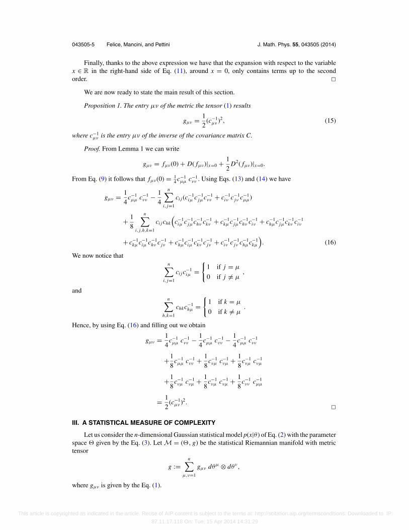
Finally, thanks to the above expression we have that the expansion with respect to the variablex ∈ R in the right-hand side of Eq. (11), around x = 0, only contains terms up to the secondorder. �
We are now ready to state the main result of this section.
Proposition 1. The entry μν of the metric the tensor (1) results
gμν = 1
2(c−1
μν )2, (15)
where c−1μν is the entry μν of the inverse of the covariance matrix C.
Proof. From Lemma 1 we can write
gμν = fμν(0) + D( fμν)|x=0 + 1
2D2( fμν)|x=0.
From Eq. (9) it follows that fμν(0) = 14 c−1
μμ c−1νν . Using Eqs. (13) and (14) we have
gμν = 1
4c−1μμ c−1
νν − 1
4
n∑i, j=1
ci j (c−1iμ c−1
jμc−1νν + c−1
iν c−1jν c−1
μμ)
+ 1
8
n∑i, j,h,k=1
ci j chk
(c−1
iμ c−1jμc−1
hν c−1kν + c−1
kμ c−1jμc−1
hν c−1iν + c−1
hμc−1jμc−1
kν c−1iν
+ c−1kμ c−1
iμ c−1hν c−1
jν + c−1hμc−1
iμ c−1kν c−1
jν + c−1iν c−1
jν c−1hμc−1
kμ
). (16)
We now notice thatn∑
i, j=1
ci j c−1iμ =
{1 if j = μ
0 if j = μ,
andn∑
h,k=1
chkc−1hμ =
{1 if k = μ
0 if k = μ.
Hence, by using Eq. (16) and filling out we obtain
gμν = 1
4c−1μμ c−1
νν − 1
4c−1μμ c−1
νν − 1
4c−1μμ c−1
νν
+1
8c−1μμ c−1
νν + 1
8c−1νμ c−1
νμ + 1
8c−1νμ c−1
νμ
+1
8c−1νμ c−1
νμ + 1
8c−1νμ c−1
νμ + 1
8c−1νν c−1
μμ
= 1
2(c−1
μν )2. �III. A STATISTICAL MEASURE OF COMPLEXITY
Let us consider the n-dimensional Gaussian statistical model p(x|θ ) of Eq. (2) with the parameterspace � given by the Eq. (3). Let M = (�, g) be the statistical Riemannian manifold with metrictensor
g :=n∑
μ,ν=1
gμν dθμ ⊗ dθν,
where gμν is given by the Eq. (1).
This article is copyrighted as indicated in the article. Reuse of AIP content is subject to the terms at: http://scitation.aip.org/termsconditions. Downloaded to IP:
87.11.17.118 On: Tue, 15 Apr 2014 14:31:29
043505-6 Felice, Mancini, and Pettini J. Math. Phys. 55, 043505 (2014)
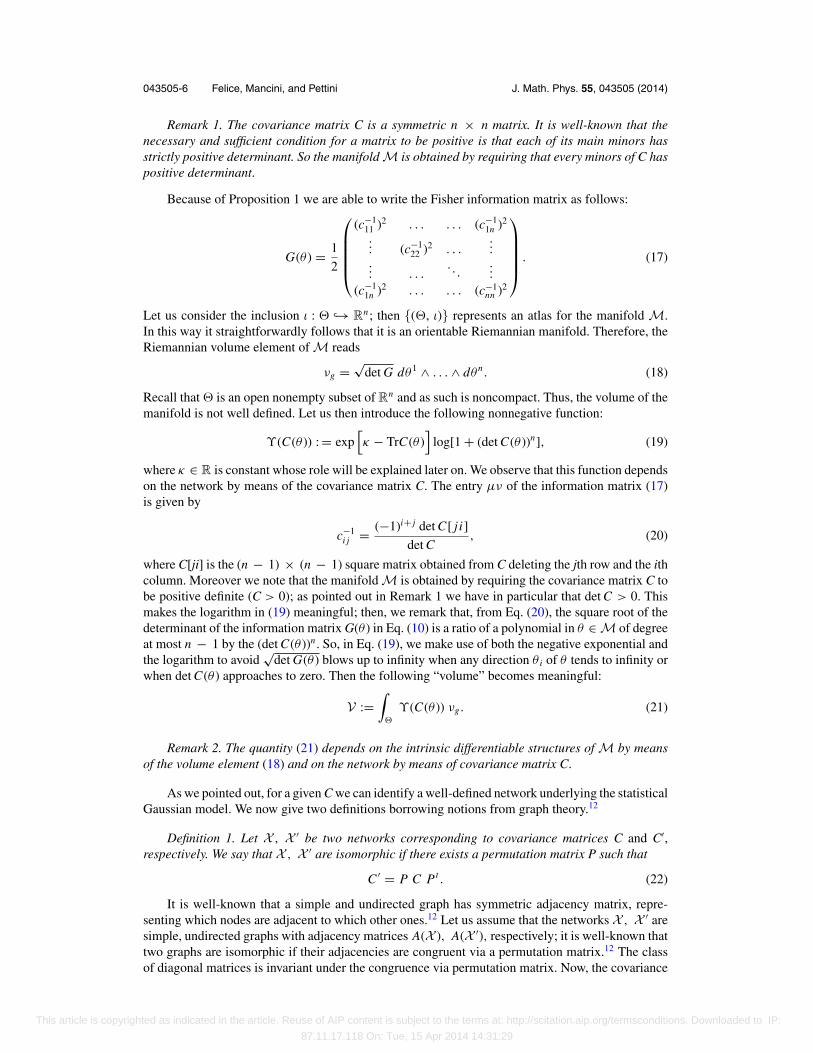
Remark 1. The covariance matrix C is a symmetric n × n matrix. It is well-known that thenecessary and sufficient condition for a matrix to be positive is that each of its main minors hasstrictly positive determinant. So the manifold M is obtained by requiring that every minors of C haspositive determinant.
Because of Proposition 1 we are able to write the Fisher information matrix as follows:
G(θ ) = 1
2
⎛⎜⎜⎜⎜⎝
(c−111 )2 . . . . . . (c−1
1n )2
... (c−122 )2 . . .
...... . . .
. . ....
(c−11n )2 . . . . . . (c−1
nn )2
⎞⎟⎟⎟⎟⎠ . (17)
Let us consider the inclusion ι : � ↪→ Rn; then {(�, ι)} represents an atlas for the manifold M.In this way it straightforwardly follows that it is an orientable Riemannian manifold. Therefore, theRiemannian volume element of M reads
νg =√
det G dθ1 ∧ . . . ∧ dθn. (18)
Recall that � is an open nonempty subset of Rn and as such is noncompact. Thus, the volume of themanifold is not well defined. Let us then introduce the following nonnegative function:
ϒ(C(θ )) : = exp[κ − TrC(θ )
]log[1 + (det C(θ ))n], (19)
where κ ∈ R is constant whose role will be explained later on. We observe that this function dependson the network by means of the covariance matrix C. The entry μν of the information matrix (17)is given by
c−1i j = (−1)i+ j det C[ j i]
det C, (20)
where C[ji] is the (n − 1) × (n − 1) square matrix obtained from C deleting the jth row and the ithcolumn. Moreover we note that the manifold M is obtained by requiring the covariance matrix C tobe positive definite (C > 0); as pointed out in Remark 1 we have in particular that det C > 0. Thismakes the logarithm in (19) meaningful; then, we remark that, from Eq. (20), the square root of thedeterminant of the information matrix G(θ ) in Eq. (10) is a ratio of a polynomial in θ ∈ M of degreeat most n − 1 by the (det C(θ ))n . So, in Eq. (19), we make use of both the negative exponential andthe logarithm to avoid
√det G(θ ) blows up to infinity when any direction θ i of θ tends to infinity or
when det C(θ ) approaches to zero. Then the following “volume” becomes meaningful:
V :=∫
�
ϒ(C(θ )) νg. (21)
Remark 2. The quantity (21) depends on the intrinsic differentiable structures of M by meansof the volume element (18) and on the network by means of covariance matrix C.
As we pointed out, for a given C we can identify a well-defined network underlying the statisticalGaussian model. We now give two definitions borrowing notions from graph theory.12
Definition 1. Let X , X ′ be two networks corresponding to covariance matrices C and C′,respectively. We say that X , X ′ are isomorphic if there exists a permutation matrix P such that
C ′ = P C Pt . (22)
It is well-known that a simple and undirected graph has symmetric adjacency matrix, repre-senting which nodes are adjacent to which other ones.12 Let us assume that the networks X , X ′ aresimple, undirected graphs with adjacency matrices A(X ), A(X ′), respectively; it is well-known thattwo graphs are isomorphic if their adjacencies are congruent via a permutation matrix.12 The classof diagonal matrices is invariant under the congruence via permutation matrix. Now, the covariance
This article is copyrighted as indicated in the article. Reuse of AIP content is subject to the terms at: http://scitation.aip.org/termsconditions. Downloaded to IP:
87.11.17.118 On: Tue, 15 Apr 2014 14:31:29
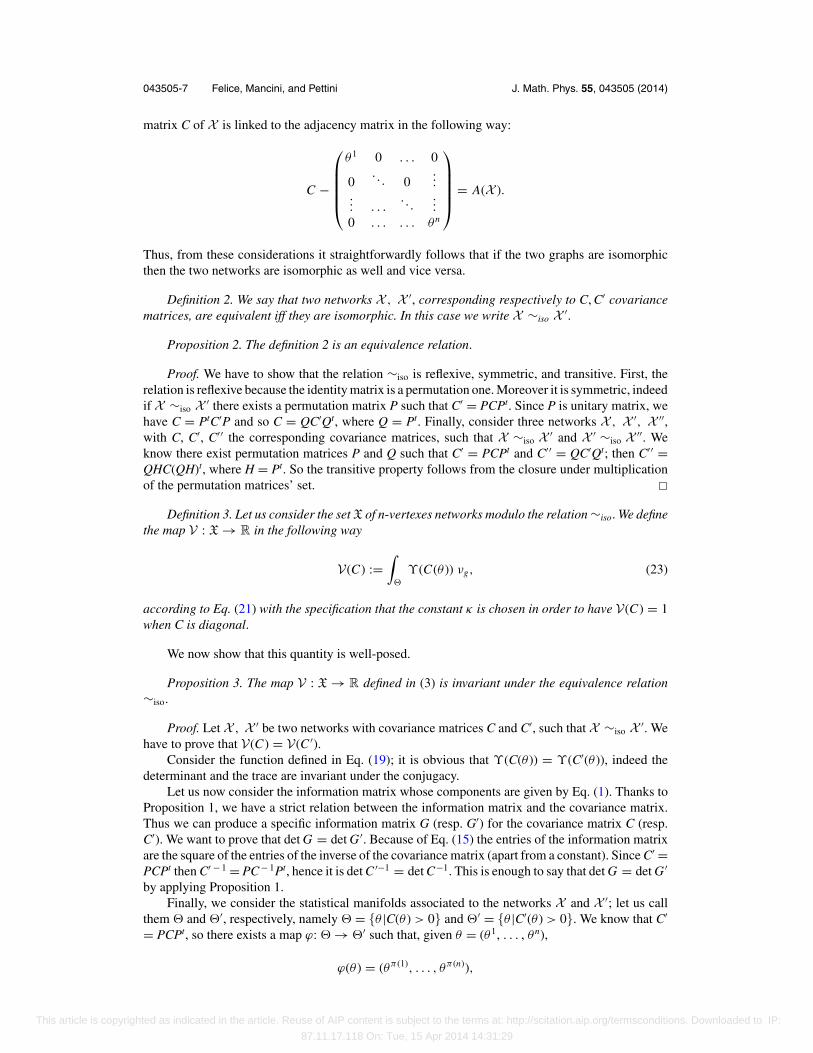
043505-7 Felice, Mancini, and Pettini J. Math. Phys. 55, 043505 (2014)
matrix C of X is linked to the adjacency matrix in the following way:
C −
⎛⎜⎜⎜⎜⎝
θ1 0 . . . 0
0. . . 0
...... . . .
. . ....
0 . . . . . . θn
⎞⎟⎟⎟⎟⎠ = A(X ).
Thus, from these considerations it straightforwardly follows that if the two graphs are isomorphicthen the two networks are isomorphic as well and vice versa.
Definition 2. We say that two networks X , X ′, corresponding respectively to C, C′ covariancematrices, are equivalent iff they are isomorphic. In this case we write X ∼iso X ′.
Proposition 2. The definition 2 is an equivalence relation.
Proof. We have to show that the relation ∼iso is reflexive, symmetric, and transitive. First, therelation is reflexive because the identity matrix is a permutation one. Moreover it is symmetric, indeedif X ∼iso X ′ there exists a permutation matrix P such that C′ = PCPt. Since P is unitary matrix, wehave C = PtC′P and so C = QC′Qt, where Q = Pt. Finally, consider three networks X , X ′, X ′′,with C, C′, C′′ the corresponding covariance matrices, such that X ∼iso X ′ and X ′ ∼iso X ′′. Weknow there exist permutation matrices P and Q such that C′ = PCPt and C′′ = QC′Qt; then C′′ =QHC(QH)t, where H = Pt. So the transitive property follows from the closure under multiplicationof the permutation matrices’ set. �
Definition 3. Let us consider the set X of n-vertexes networks modulo the relation ∼iso. We definethe map V : X → R in the following way
V(C) :=∫
�
ϒ(C(θ )) νg, (23)
according to Eq. (21) with the specification that the constant κ is chosen in order to have V(C) = 1when C is diagonal.
We now show that this quantity is well-posed.
Proposition 3. The map V : X → R defined in (3) is invariant under the equivalence relation∼iso.
Proof. Let X , X ′ be two networks with covariance matrices C and C′, such that X ∼iso X ′. Wehave to prove that V(C) = V(C ′).
Consider the function defined in Eq. (19); it is obvious that ϒ(C(θ )) = ϒ(C′(θ )), indeed thedeterminant and the trace are invariant under the conjugacy.
Let us now consider the information matrix whose components are given by Eq. (1). Thanks toProposition 1, we have a strict relation between the information matrix and the covariance matrix.Thus we can produce a specific information matrix G (resp. G′) for the covariance matrix C (resp.C′). We want to prove that det G = det G ′. Because of Eq. (15) the entries of the information matrixare the square of the entries of the inverse of the covariance matrix (apart from a constant). Since C′ =PCPt then C′ − 1 = PC− 1Pt, hence it is det C ′−1 = det C−1. This is enough to say that det G = det G ′
by applying Proposition 1.Finally, we consider the statistical manifolds associated to the networks X and X ′; let us call
them � and �′, respectively, namely � = {θ |C(θ ) > 0} and �′ = {θ |C′(θ ) > 0}. We know that C′
= PCPt, so there exists a map ϕ: � → �′ such that, given θ = (θ1, . . . , θn),
ϕ(θ ) = (θπ(1), . . . , θπ(n)),
This article is copyrighted as indicated in the article. Reuse of AIP content is subject to the terms at: http://scitation.aip.org/termsconditions. Downloaded to IP:
87.11.17.118 On: Tue, 15 Apr 2014 14:31:29
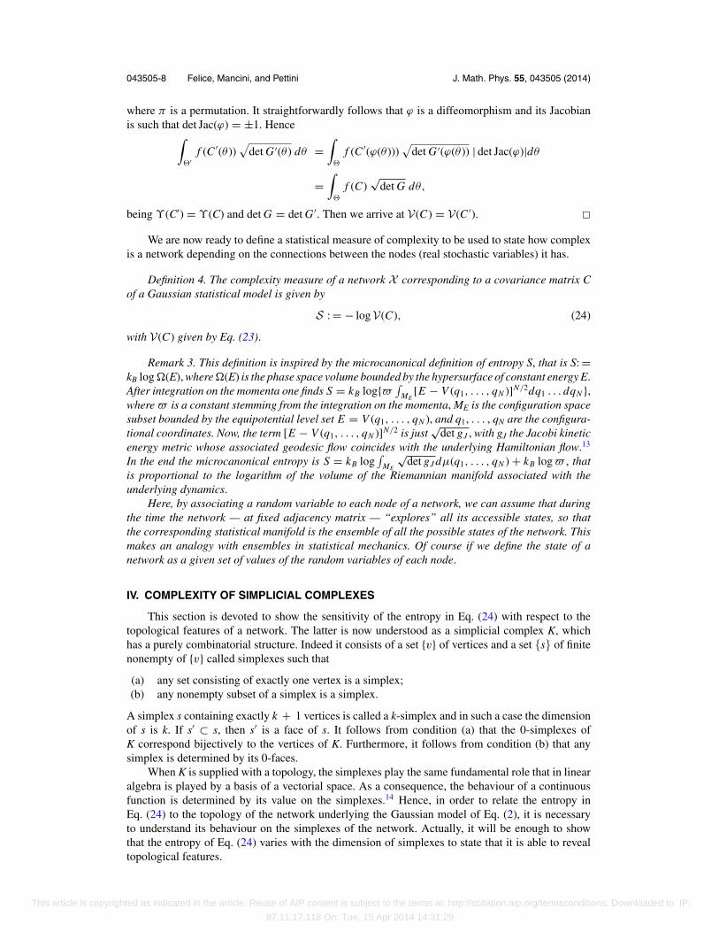
043505-8 Felice, Mancini, and Pettini J. Math. Phys. 55, 043505 (2014)
where π is a permutation. It straightforwardly follows that ϕ is a diffeomorphism and its Jacobianis such that det Jac(ϕ) = ±1. Hence∫
�′f (C ′(θ ))
√det G ′(θ ) dθ =
∫�
f (C ′(ϕ(θ )))√
det G ′(ϕ(θ )) | det Jac(ϕ)|dθ
=∫
�
f (C)√
det G dθ,
being ϒ(C′) = ϒ(C) and det G = det G ′. Then we arrive at V(C) = V(C ′). �We are now ready to define a statistical measure of complexity to be used to state how complex
is a network depending on the connections between the nodes (real stochastic variables) it has.
Definition 4. The complexity measure of a network X corresponding to a covariance matrix Cof a Gaussian statistical model is given by
S : = − logV(C), (24)
with V(C) given by Eq. (23).
Remark 3. This definition is inspired by the microcanonical definition of entropy S, that is S: =kB log �(E), where �(E) is the phase space volume bounded by the hypersurface of constant energy E.After integration on the momenta one finds S = kB log{� ∫
ME[E − V (q1, . . . , qN )]N/2dq1 . . . dqN },
where � is a constant stemming from the integration on the momenta, ME is the configuration spacesubset bounded by the equipotential level set E = V (q1, . . . , qN ), and q1, . . . , qN are the configura-tional coordinates. Now, the term [E − V (q1, . . . , qN )]N/2 is just
√det gJ , with gJ the Jacobi kinetic
energy metric whose associated geodesic flow coincides with the underlying Hamiltonian flow.13
In the end the microcanonical entropy is S = kB log∫
ME
√det gJ dμ(q1, . . . , qN ) + kB log � , that
is proportional to the logarithm of the volume of the Riemannian manifold associated with theunderlying dynamics.
Here, by associating a random variable to each node of a network, we can assume that duringthe time the network — at fixed adjacency matrix — “explores” all its accessible states, so thatthe corresponding statistical manifold is the ensemble of all the possible states of the network. Thismakes an analogy with ensembles in statistical mechanics. Of course if we define the state of anetwork as a given set of values of the random variables of each node.
IV. COMPLEXITY OF SIMPLICIAL COMPLEXES
This section is devoted to show the sensitivity of the entropy in Eq. (24) with respect to thetopological features of a network. The latter is now understood as a simplicial complex K, whichhas a purely combinatorial structure. Indeed it consists of a set {v} of vertices and a set {s} of finitenonempty of {v} called simplexes such that
(a) any set consisting of exactly one vertex is a simplex;(b) any nonempty subset of a simplex is a simplex.
A simplex s containing exactly k + 1 vertices is called a k-simplex and in such a case the dimensionof s is k. If s′ ⊂ s, then s′ is a face of s. It follows from condition (a) that the 0-simplexes ofK correspond bijectively to the vertices of K. Furthermore, it follows from condition (b) that anysimplex is determined by its 0-faces.
When K is supplied with a topology, the simplexes play the same fundamental role that in linearalgebra is played by a basis of a vectorial space. As a consequence, the behaviour of a continuousfunction is determined by its value on the simplexes.14 Hence, in order to relate the entropy inEq. (24) to the topology of the network underlying the Gaussian model of Eq. (2), it is necessaryto understand its behaviour on the simplexes of the network. Actually, it will be enough to showthat the entropy of Eq. (24) varies with the dimension of simplexes to state that it is able to revealtopological features.
This article is copyrighted as indicated in the article. Reuse of AIP content is subject to the terms at: http://scitation.aip.org/termsconditions. Downloaded to IP:
87.11.17.118 On: Tue, 15 Apr 2014 14:31:29
043505-9 Felice, Mancini, and Pettini J. Math. Phys. 55, 043505 (2014)
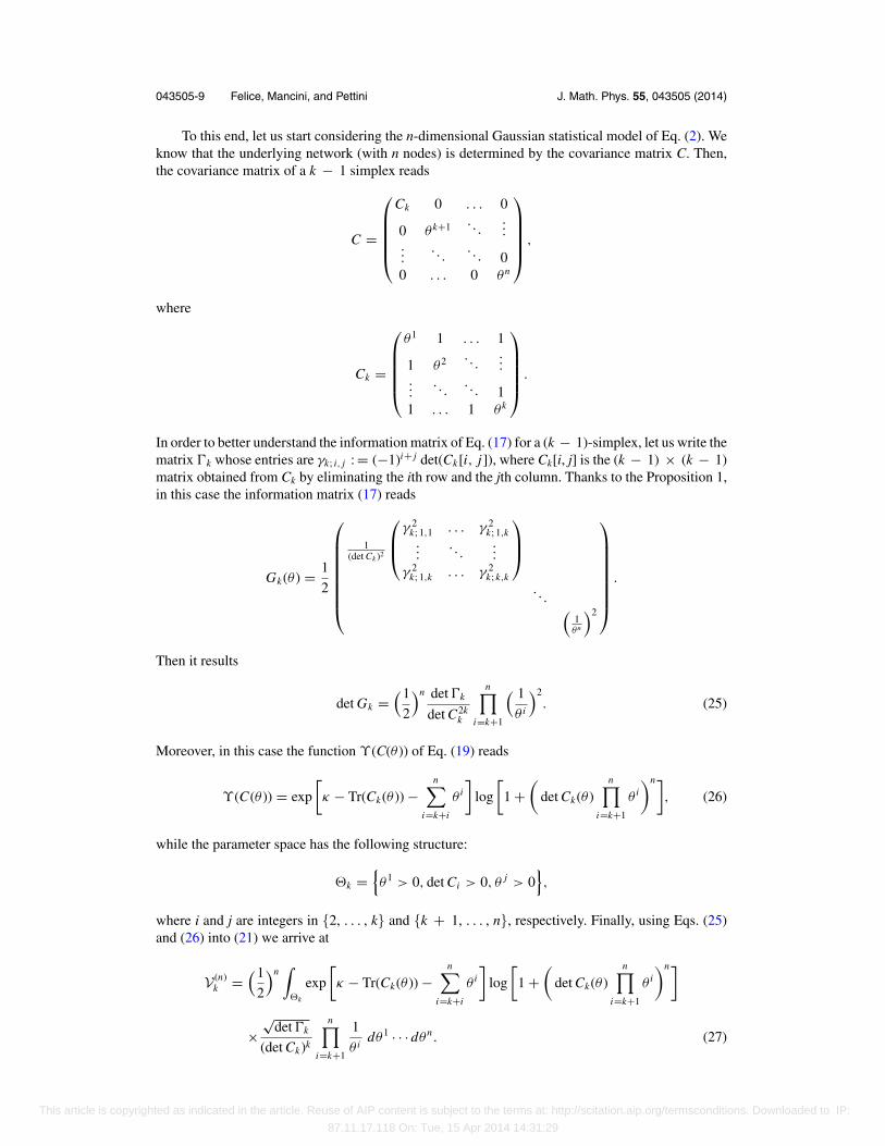
To this end, let us start considering the n-dimensional Gaussian statistical model of Eq. (2). Weknow that the underlying network (with n nodes) is determined by the covariance matrix C. Then,the covariance matrix of a k − 1 simplex reads
C =
⎛⎜⎜⎜⎜⎝
Ck 0 . . . 0
0 θ k+1 . . ....
.... . .
. . . 00 . . . 0 θn
⎞⎟⎟⎟⎟⎠ ,
where
Ck =
⎛⎜⎜⎜⎜⎝
θ1 1 . . . 1
1 θ2 . . ....
.... . .
. . . 11 . . . 1 θ k
⎞⎟⎟⎟⎟⎠ .
In order to better understand the information matrix of Eq. (17) for a (k − 1)-simplex, let us write thematrix �k whose entries are γk; i, j : = (−1)i+ j det(Ck[i, j]), where Ck[i, j] is the (k − 1) × (k − 1)matrix obtained from Ck by eliminating the ith row and the jth column. Thanks to the Proposition 1,in this case the information matrix (17) reads
Gk(θ ) = 1
2
⎛⎜⎜⎜⎜⎜⎜⎜⎝
1(det Ck )2
⎛⎜⎝
γ 2k; 1,1 . . . γ 2
k; 1,k...
. . ....
γ 2k; 1,k . . . γ 2
k; k,k
⎞⎟⎠
. . . (1θn
)2
⎞⎟⎟⎟⎟⎟⎟⎟⎠
.
Then it results
det Gk =(1
2
)n det �k
det C2kk
n∏i=k+1
( 1
θ i
)2. (25)
Moreover, in this case the function ϒ(C(θ )) of Eq. (19) reads
ϒ(C(θ )) = exp
[κ − Tr(Ck(θ )) −
n∑i=k+i
θ i
]log
[1 +
(det Ck(θ )
n∏i=k+1
θ i
)n], (26)
while the parameter space has the following structure:
�k ={θ1 > 0, det Ci > 0, θ j > 0
},
where i and j are integers in {2, . . . , k} and {k + 1, . . . , n}, respectively. Finally, using Eqs. (25)and (26) into (21) we arrive at
V (n)k =
(1
2
)n∫
�k
exp
[κ − Tr(Ck(θ )) −
n∑i=k+i
θ i
]log
[1 +
(det Ck(θ )
n∏i=k+1
θ i
)n]
×√
det �k
(det Ck)k
n∏i=k+1
1
θ idθ1 · · · dθn. (27)
This article is copyrighted as indicated in the article. Reuse of AIP content is subject to the terms at: http://scitation.aip.org/termsconditions. Downloaded to IP:
87.11.17.118 On: Tue, 15 Apr 2014 14:31:29
043505-10 Felice, Mancini, and Pettini J. Math. Phys. 55, 043505 (2014)
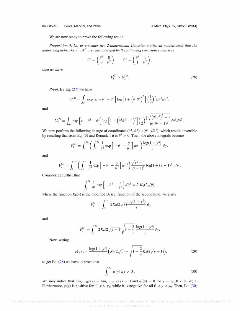
We are now ready to prove the following result.
Proposition 4. Let us consider two 2-dimensional Gaussian statistical models such that theunderlying networks X ′,X ′′ are characterized by the following covariance matrices
C ′ =(
θ1 00 θ2
)C ′′ =
(θ1 11 θ2
),
then we have
V (2)1 > V (2)
2 . (28)
Proof. By Eq. (27) we have
V (2)1 =
∫�′
exp[κ − θ1 − θ2
]log[1 +
(θ1θ2
)2] (1
2
) 12dθ1dθ2,
and
V (2)2 =
∫�′′
exp[κ − θ1 − θ2
]log[1 +
(θ1θ2 − 1
)2](1
2
) 12
√(θ1θ2
)2 − 1
(θ1θ2 − 1)2dθ1dθ2 .
We now perform the following change of coordinates (θ1, θ2) �→(θ1, y/θ1), which results invertibleby recalling that from Eq. (3) and Remark 1 it is θ1 > 0. Then, the above integrals become
V (2)1 =
∫ ∞
0
(∫ ∞
0
1
θ1exp[
− θ1 − y
θ1
]dθ1
)log(1 + y2)
ydy,
and
V (2)2 =
∫ ∞
1
(∫ ∞
0
1
θ1exp[
− θ1 − y
θ1
]dθ1
)√y2 − 1
(y − 1)2log[1 + (y − 1)2] dy .
Considering further that ∫ ∞
0
1
θ1exp[
− θ1 − y
θ1
]dθ1 = 2 K0(2
√y),
where the function K0(y) is the modified Bessel function of the second kind, we arrive
V (2)1 =
∫ ∞
02K0(2
√y)
log(1 + y2)
ydy
and
V (2)2 =
∫ ∞
02K0(2
√y + 1)
√1 + 2
y
log(1 + y2)
ydy.
Now, setting
ϕ(y) : = log(1 + y2)
y
(K0(2
√y) −
√1 + 2
yK0(2
√y + 1)
), (29)
to get Eq. (28) we have to prove that ∫ ∞
0ϕ(y) dy > 0 . (30)
We may notice that limy → 0ϕ(y) = limy → ∞ ϕ(y) = 0 and ϕ′(y) = 0 for y = y0, 0 < y0 � 1.Furthermore, ϕ(y) is positive for all y > y0, while it is negative for all 0 < y < y0. Then, Eq. (30)
This article is copyrighted as indicated in the article. Reuse of AIP content is subject to the terms at: http://scitation.aip.org/termsconditions. Downloaded to IP:
87.11.17.118 On: Tue, 15 Apr 2014 14:31:29
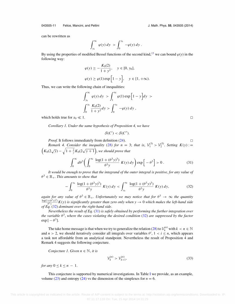
043505-11 Felice, Mancini, and Pettini J. Math. Phys. 55, 043505 (2014)
can be rewritten as ∫ ∞
y0
ϕ(y) dy >
∫ y0
0−ϕ(y) dy .
By using the properties of modified Bessel functions of the second kind,15 we can bound ϕ(y) in thefollowing way:
ϕ(y) ≥ − K0(2)
1 + y2, y ∈ [0, y0],
ϕ(y) ≥ ϕ(1) exp[1 − y
], y ∈ [1,+∞).
Thus, we can write the following chain of inequalities:∫ ∞
y0
ϕ(y) dy >
∫ ∞
1ϕ(1) exp
[1 − y
]dy >
∫ y0
0
K0(2)
1 + y2dy >
∫ y0
0−ϕ(y) dy ,
which holds true for x0 � 1. �Corollary 1. Under the same hypothesis of Proposition 4, we have
S(C ′) < S(C ′′).
Proof. It follows immediately from definition (24). �Remark 4. Consider the inequality (28) for n = 3; that is, V (3)
1 > V (3)2 . Setting K (y) : =(
K0(2√
y) −√
1 + 2y K0(2
√y + 1
), we should prove that
∫ ∞
0dθ3
(∫ ∞
0
log(1 + (θ3 y)3)
θ3 yK (y) dy
)exp[
− θ3]
> 0 . (31)
It would be enough to prove that the integrand of the outer integral is positive, for any value ofθ3 ∈ R+. This amounts to show that
−∫ y0
0
log(1 + (θ3 y)3)
θ3 yK (y) dy <
∫ ∞
y0
log(1 + (θ3 y)3)
θ3 yK (y) dy, (32)
again for any value of θ3 ∈ R+. Unfortunately we may notice that for θ3 → ∞ the quantitylog(1+(θ3 y)3)
θ3 y K (y) is significantly greater than zero only when y → 0 which makes the left-hand sideof Eq. (32) dominant over the right-hand side.
Nevertheless the result of Eq. (31) is safely obtained by performing the further integration overthe variable θ3, where the cases violating the desired condition (32) are suppressed by the factorexp [ − θ3].
The take home message is that when we try to generalize the relation (28) toV (n)k with k < n ∈ N
and n > 2, we should iteratively consider all integrals over variables θ i, 1 < i ≤ n, which appearsa task not affordable from an analytical standpoint. Nevertheless the result of Proposition 4 andRemark 4 suggests the following conjecture.
Conjecture 1. Given n ∈ N, it is
V (n)k > V (n)
k+1, (33)
for any 0 ≤ k ≤ n − 1.
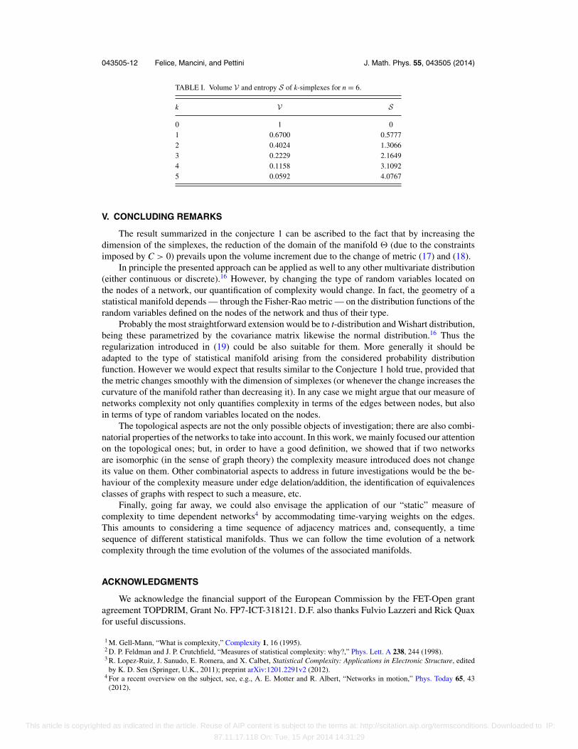
This conjecture is supported by numerical investigations. In Table I we provide, as an example,volume (23) and entropy (24) vs the dimension of the simplexes for n = 6.
This article is copyrighted as indicated in the article. Reuse of AIP content is subject to the terms at: http://scitation.aip.org/termsconditions. Downloaded to IP:
87.11.17.118 On: Tue, 15 Apr 2014 14:31:29
043505-12 Felice, Mancini, and Pettini J. Math. Phys. 55, 043505 (2014)
TABLE I. Volume V and entropy S of k-simplexes for n = 6.
k V S
0 1 01 0.6700 0.57772 0.4024 1.30663 0.2229 2.16494 0.1158 3.10925 0.0592 4.0767
V. CONCLUDING REMARKS
The result summarized in the conjecture 1 can be ascribed to the fact that by increasing thedimension of the simplexes, the reduction of the domain of the manifold � (due to the constraintsimposed by C > 0) prevails upon the volume increment due to the change of metric (17) and (18).
In principle the presented approach can be applied as well to any other multivariate distribution(either continuous or discrete).16 However, by changing the type of random variables located onthe nodes of a network, our quantification of complexity would change. In fact, the geometry of astatistical manifold depends — through the Fisher-Rao metric — on the distribution functions of therandom variables defined on the nodes of the network and thus of their type.
Probably the most straightforward extension would be to t-distribution and Wishart distribution,being these parametrized by the covariance matrix likewise the normal distribution.16 Thus theregularization introduced in (19) could be also suitable for them. More generally it should beadapted to the type of statistical manifold arising from the considered probability distributionfunction. However we would expect that results similar to the Conjecture 1 hold true, provided thatthe metric changes smoothly with the dimension of simplexes (or whenever the change increases thecurvature of the manifold rather than decreasing it). In any case we might argue that our measure ofnetworks complexity not only quantifies complexity in terms of the edges between nodes, but alsoin terms of type of random variables located on the nodes.
The topological aspects are not the only possible objects of investigation; there are also combi-natorial properties of the networks to take into account. In this work, we mainly focused our attentionon the topological ones; but, in order to have a good definition, we showed that if two networksare isomorphic (in the sense of graph theory) the complexity measure introduced does not changeits value on them. Other combinatorial aspects to address in future investigations would be the be-haviour of the complexity measure under edge delation/addition, the identification of equivalencesclasses of graphs with respect to such a measure, etc.
Finally, going far away, we could also envisage the application of our “static” measure ofcomplexity to time dependent networks4 by accommodating time-varying weights on the edges.This amounts to considering a time sequence of adjacency matrices and, consequently, a timesequence of different statistical manifolds. Thus we can follow the time evolution of a networkcomplexity through the time evolution of the volumes of the associated manifolds.
ACKNOWLEDGMENTS
We acknowledge the financial support of the European Commission by the FET-Open grantagreement TOPDRIM, Grant No. FP7-ICT-318121. D.F. also thanks Fulvio Lazzeri and Rick Quaxfor useful discussions.
1 M. Gell-Mann, “What is complexity,” Complexity 1, 16 (1995).2 D. P. Feldman and J. P. Crutchfield, “Measures of statistical complexity: why?,” Phys. Lett. A 238, 244 (1998).3 R. Lopez-Ruiz, J. Sanudo, E. Romera, and X. Calbet, Statistical Complexity: Applications in Electronic Structure, edited
by K. D. Sen (Springer, U.K., 2011); preprint arXiv:1201.2291v2 (2012).4 For a recent overview on the subject, see, e.g., A. E. Motter and R. Albert, “Networks in motion,” Phys. Today 65, 43
(2012).
This article is copyrighted as indicated in the article. Reuse of AIP content is subject to the terms at: http://scitation.aip.org/termsconditions. Downloaded to IP:
87.11.17.118 On: Tue, 15 Apr 2014 14:31:29

043505-13 Felice, Mancini, and Pettini J. Math. Phys. 55, 043505 (2014)
5 R. Albert and A.-L. Barabasi, “Statistical mechanics of complex networks,” Rev. Mod. Phys. 74, 47 (2002); S. N.Dorogovtsev, A. V. Goltsev, and J. F. F. Mendes, “Critical phenomena in complex networks,” ibid. 80, 1275 (2008).
6 R. Lopez-Ruiz, H. L. Mancini, and X. Calbet, “A statistical measure of complexity,” Phys. Lett. A 209, 321 (1995).7 S. Amari and H. Nagaoka, Methods of Information Geometry (Oxford University Press, 2000).8 C. Cafaro, “Works on an information geometrodynamical approach to chaos,” Chaos, Solitons Fractals 41, 886 (2009).9 S. A. Ali, C. Cafaro, D.-H. Kim, and S. Mancini, “The effect of the microscopic correlations on the information geometric
complexity of Gaussian statistical models,” Physica A 389, 3117 (2010).10 N. Ay, E. Olbrich, N. Bertschinger, and J. Jost, “A geometric approach to complexity,” Chaos 21, 037103 (2011).11 T. H. Corman, C. E. Leiserson, R. L. Rivest, and C. Stein, Introduction to Algorithms (McGraw-Hill, 2009).12 R. Distel, Graph Theory (Springer-Verlag, 2000).13 M. Pettini, Geometry and Topology in Hamiltonian Dynamics and Statistical Mechanics (Springer-Verlag, 2007).14 E. H. Spanier, Algebraic Topology (McGraw-Hill, 1966).15 G. N. Watson, Theory of Bessel Functions (Cambridge University Press, 1952).16 T. W. Anderson, An Introduction to Multivariate Statistical Analysis (Wiley, 2003).
This article is copyrighted as indicated in the article. Reuse of AIP content is subject to the terms at: http://scitation.aip.org/termsconditions. Downloaded to IP:
87.11.17.118 On: Tue, 15 Apr 2014 14:31:29


