Embed Size (px)
Citation preview

Water Rights Analysis Package (WRAP) Modeling System Reference Manual
by Ralph A. Wurbs Texas A&M University
TR-255 Texas Water Resources Institute College Station, Texas March 2008
Water Rights Analysis Package (WRAP) Modeling System
Reference Manual
by
Ralph A. Wurbs Department of Civil Engineering and
Texas Water Resources Institute Texas A&M University
for the
Texas Commission on Environmental Quality Austin, Texas 78711-3087
under
TCEQ/TWRI Contract 9880074800 (1997-2003) TCEQ/TEES Contract 582-6-77422 (2005-2008)
Cosponsored with Supplemental Funding Support
from the
Texas Water Development Board Fort Worth District, U.S. Army Corps of Engineers
Texas Water Resources Institute, Texas A&M University System
Technical Report No. 255 Texas Water Resources Institute
The Texas A&M University System College Station, Texas 77843-2118
First Edition, August 2003 Second Edition, April 2005
Third Edition, September 2006 Fourth Edition, March 2008

ii
TABLE OF CONTENTS Acknowledgements ................................................................................................................. vii
Chapter 1 Introduction ......................................................................................................... 1
WRAP Documentation ....................................................................................................... 1 WRAP Programs ................................................................................................................ 3 Auxiliary Software ............................................................................................................. 5 Texas WAM System ........................................................................................................... 7 Model Development Background ...................................................................................... 11 Organization of the Reference and Users Manuals ............................................................ 14
Chapter 2 Overview of the Simulation Model ................................................................... 15
Modeling Capabilities ......................................................................................................... 15 Water Availability Modeling Process ................................................................................. 16 Long-Term, Yield-Reliability, and Conditional Reliability Modeling Modes ................... 17 Control Point Representation of Spatial Configuration ...................................... ............... 18 Simulation Input ................................................................................................................. 19 Simulation Results .............................................................................................................. 20 Units of Measure ................................................................................................................. 21 Organization of the Simulation Computations .................................................................. 22 Constructing a Model with WRAP .................................................................................... 30 Measures of Water Availability and Reliability ................................................................. 38 Program SIM Options Involving Cyclic Repetitions of the Simulation ............................. 41
Chapter 3 Hydrology Features ............................................................................................ 43
Naturalized Stream Flow .................................................................................................... 44 Reservoir Evaporation-Precipitation .................................................................................. 46 Program HYD Hydrology Data Manipulation Capabilities ............................................... 47 HYD Features for Developing Evaporation-Precipitation Datasets .................................. 50 Regression Equation to Adjust Flows and/or Evaporation-Precipitation Depths ............... 50 HYD Features for Developing Stream Flow Datasets ........................................................ 51 Allocation of Stream Flow within SIM .............................................................................. 55 Channel Losses .................................................................................................................... 56 Methods for Establishing Stream Flow Inflows ................................................................. 60 Distribution of Naturalized Flows from Gaged to Ungaged Control Points ...................... 61 Use of GIS to Determine Spatial Connectivity and Watershed Parameters ....................... 73 Negative Incremental Naturalized Stream Flows ............................................................... 74
Chapter 4 Water Management Features ............................................................................. 89
Water Rights ........................................................................................................................ 89 Water Right Priorities ......................................................................................................... 91 Water Availability within the Priority-Based Water Rights Computation Loop ............... 93 Specifying Targets and Rules for Meeting the Targets ..................................................... 94 Setting Diversion, Instream Flow, and Hydropower Targets ............................................ 96 River/Reservoir System Operating Rules for Meeting Water Use Requirements ............. 102 Reservoir Storage ............................................................................................................... 107 Multiple-Reservoir and Multiple-Right Reservoir Systems .............................................. 110
iii
TABLE OF CONTENTS (Continued) Multiple Reservoir System Operations ............................................................................... 112 Iterative Reservoir Volume Balance Computations ........................................................... 116 Multiple Rights Associated with the Same Reservoir ........................................................ 117 Water Supply Diversions ..................................................................................................... 123 Return Flows ...................................................................................................................... 123 Other Inflows and Outflows .............................................................................................. 125 Hydroelectric Energy Generation ...................................................................................... 126 Instream Flow Requirements ............................................................................................. 131 Dual Simulation Options ................................................................................................... 140 Options for Circumventing the Priority Sequence ............................................................. 142
Chapter 5 Organization and Analysis of Simulation Results ............................................ 151
OUT, SOU, and DSS Files ................................................................................................. 151 SIM Simulation Results Variables ..................................................................................... 153 Organization of SIM OUT Output File .............................................................................. 158 Types of TABLES Tabulations .......................................................................................... 165 Time Series Tables and Tabulations ................................................................................. 167 Reliability and Frequency Tables ....................................................................................... 170 Water Supply and Hydropower Reliability ........................................................................ 171 Flow and Storage Frequency Analyses ............................................................................. 175 Reservoir Contents, Drawdown Duration, and Storage Reliability .................................. 179 Summary Tables ................................................................................................................. 181 Water Budget Tables ......................................................................................................... 183
Chapter 6 Auxiliary Special-Purpose Modeling Features ............................................... 189
SIM Output Files ................................................................................................................ 189 Auxiliary Software ............................................................................................................. 192 Yield versus Reliability Relationships Including Firm Yield ........................................... 194 Stream Flow Availability in Water Rights Priority Sequence ........................................... 197 Beginning-Ending Storage Options ................................................................................... 202 Tables Summarizing Water Right, Control Point, and Reservoir Input Data ................... 204 General Modeling Framework for Applying WRAP ......................................................... 204 HYD Stream Flow Adjustments Using SIM Simulation Results to Develop SIM Hydrology Datasets ................................................................................ 206
Chapter 7 Detecting Errors and Irregularities in Data Files ............................................ 213
Locating Errors in SIM Input Data .................................................................................... 213 Locating Errors in the SIM Output File ............................................................................. 224 Locating Errors in TABLES Input Data ............................................................................ 226 Locating Errors in HYD Input Data .................................................................................. 226 HEC-DSS Trace Messages ................................................................................................. 231
References ............................................................................................................................... 233 Appendix A Glossary ............................................................................................................ 235 Appendix B SIM/TABLES Examples ................................................................................. 243 Appendix C HYD Examples ................................................................................................ 283
iv
LIST OF FIGURES 1.1 Texas WAM System River Basins ................................................................................. 8 1.2 Major Rivers of Texas .................................................................................................... 10 2.1 Reservoir/River System Schematic ................................................................................ 18 2.2 Outline of WRAP-SIM Simulation ................................................................................ 23 2.3 Control Point Schematic for Example 1 ........................................................................ 26 2.4 Control Point Schematic for Example 2 ........................................................................ 32 3.1 Gage (Known-Flow) and Ungaged (Unknown Flow) Control Points .......................... 63 3.2 System with Negative Incremental Stream Flows ........................................................ 75 4.1 Reservoir Pools and Zones ............................................................................................ 111 4.2 Storage Zones for Defining Multiple-Reservoir Release Rules ................................... 112 4.3 Multiple Reservoir System ............................................................................................ 115 4.4 System Schematic for Example 10 in Appendix B ...................................................... 145 5.1 Time Series Plot Created with HEC-DSSVue .............................................................. 170
LIST OF TABLES 1.1 WRAP Programs ............................................................................................................ 3 1.2 Texas WAM System Models ......................................................................................... 9 2.1 Variables in the WRAP-SIM Output File ...................................................................... 20 2.2 Organization of Model Documentation ......................................................................... 22 2.3 Water Rights Information for Example 1 ....................................................................... 26 2.4 Water Rights Simulation Results for Example 1 ........................................................... 27 2.5 Streamflow for the Month at Each Control Point for Example 1 .................................. 27 2.6 WRAP-SIM Input File for Example 2 ........................................................................... 34 2.7 TABLES Input File for Example 2 ................................................................................ 34 2.8 First Year of SIM Output File for Example 2 ................................................................ 35 2.9 TABLES Output File for Example 2 ............................................................................. 36 3.1 Capabilities Provided by Program HYD ....................................................................... 49 3.2 Methods for Establishing Stream Flow Inflows ........................................................... 60 3.3 Incremental Naturalized Streamflow Example ............................................................. 76 3.4 Available Stream Flows for the Example ...................................................................... 76 4.1 Classification of Water Right Features .......................................................................... 95 4.2 Water Right Types 1, 2, 3, 4, 5, 6, and 7 ...................................................................... 104 4.3 Hydropower Factor for Alternative Sets of Units ........................................................ 129 5.1 Summary of SIM Simulation Results Variables in OUT File Output Records ........... 159 5.2 Organization of Main SIM Output File ......................................................................... 160 5.3 Water Right Output Record .......................................................................................... 160 5.4 Control Point Output Record ........................................................................................ 161 5.5 Reservoir/Hydropower Output Record ......................................................................... 161 5.6 Beginning of OUT File for Example in Fundamentals Manual ................................... 163
v
LIST OF TABLES (Continued) 5.7 Outline of Program TABLES Features ......................................................................... 166 5.8 Example of a Time Series Table with Annual Rows and Monthly Columns ............. 168 5.9 Example of a Time Series Table with Columnar Format ............................................. 169 5.10 Reliability Table from the Example in the Fundamentals Manual .............................. 173 5.11 Hydropower Reliability Table from the Example in the Fundamentals Manual ......... 173 5.12 2FRE Frequency Table from the Example in the Fundamentals Manual ................... 176 5.13 2FRQ Frequency Table from the Example in the Fundamentals Manual ................... 176 5.14 Frequency Factors for the Normal Probability Distribution ........................................ 178 5.15 Beginning of Table of Reservoir Storage Content as Percentage of Capacity ............ 180 5.16 Reservoir Storage Drawdown Duration Table ............................................................ 181 5.17 Reservoir Storage Reliability Table .............................................................................181 5.18 Summary Table for a Control Point ............................................................................ 182 5.19 Beginning of Control Point Water Budget Tabulation ................................................. 184 5.20 River Basin Water Budget for Example in Fundamentals Manual ............................. 184 5.21 Monthly Volumes in the Control Point Water Budget Table ....................................... 185 5.22 Summary Water Budget for the Entire River Basin(s) ................................................. 186 6.1 SIM Output Files .......................................................................................................... 190 6.2 Example SIM Yield-Reliability Output Table .............................................................. 195 6.3 Beginning of Example ZZZ File Created with ZZ Record .......................................... 198 6.4 4ZZZ Time Series Table for the Example ................................................................... 200 6.5 4ZZF Frequency Analysis Table for the Example ...................................................... 201 7.1 SIM Trace Messages on Monitor ................................................................................ 214 7.2 Information Recorded in Message File for Various Values of ICHECK .................... 215 7.3 SIM Trace Messages Written to Message File ............................................................. 216 7.4 SIM Error Messages ……............................................................................................ 219 7.5 SIM Warning Messages ……....................................................................................... 222 7.6 HYD Trace Displayed on Monitor .............................................................................. 227 7.7 Trace Information Copied to Message File for Various Values of ICHECK .............. 227 7.8 HYD Trace Messages Written to HMS File ................................................................ 228 7.9 HYD Error Messages ................................................................................................... 230 7.10 HYD Warning Messages ............................................................................................. 231 7.11 DSS Message Levels .................................................................................................... 232
vi
ACKNOWLEDGEMENTS Development of the WRAP modeling system has been an evolutionary process accomplished under the auspices of several sponsors. Many agencies, firms, and individuals have contributed to development and improvement of the model. The original WRAP, initially called TAMUWRAP, stemmed from a 1986-1988 research project at Texas A&M University, entitled Optimizing Reservoir System Operations, which was sponsored by a federal/state cooperative research program administered by the U.S. Geological Survey and Texas Water Resources Institute. The Brazos River Authority served as the nonfederal sponsor. Major improvements in the model were accomplished during 1990-1994 in conjunction with TAMU research projects sponsored by the Texas Water Development Board through the TWRI and by the Texas Advanced Technology Program administered by the Texas Higher Education Coordinating Board. Texas Natural Resource Conservation Commission support of WRAP actually began in 1996 before the 1997 Senate Bill 1. The model was greatly expanded and improved during 1997-2003 under TNRCC/TCEQ sponsorship pursuant to the 1997 Senate Bill 1 enacted by the Texas Legislature and subsequent legislation. The TNRCC was renamed the Texas Commission on Environmental Quality in 2002. The U.S. Army Corps of Engineers Fort Worth District during 2001-2005 also sponsored continued development of modeling capabilities. WRAP is being further expanded and improved during 2005-2008 under the auspices of the TCEQ. The TWDB also sponsored additional improvements during 2007-2008. WRAP was applied to the 23 river basins of Texas by several consulting engineering firms working for the TNRCC/TCEQ, in coordination with the TWDB and Texas Parks and Wildlife Department, during development of the statewide Water Availability Modeling (WAM) System authorized by the 1997 Senate Bill 1. The Center for Research in Water Resources at the University of Texas at Austin provided GIS support for this effort. Since completion of the WAM System river basin models, the agencies and consulting firms are continuing to apply the models in support of permitting, planning, and other water management activities. The experience gained by the water management professionals of these agencies and consulting firms and their ideas for model improvements have greatly contributed to the development of WRAP. Many graduate students at Texas A&M University have used WRAP in courses and research projects. The former students acknowledged here made major contributions to development of the modeling system working as graduate research assistants and focusing their thesis or dissertation research on WRAP related topics. Publications resulting from their work are cited in Chapter 1. Former graduate student researchers contributing to WRAP development include: W. Brian Walls, M.S. 1988; David D. Dunn, M.S. 1993; Anilkumar R. Yerramreddy, M.S. 1993; Gerardo Sanchez-Torres, Ph.D. 1994; Emery D. Sisson, M.S. 1999; A. Andres Salazar, Ph.D. 2002, Hector E. Olmos, M.S. 2004, and Ganesh Krishnamurthy, M.S., 2005. Ph.D. students Richard J. Hoffpauir, Chi Hun Lee, and Tae Jin Kim are currently working on further improvements to WRAP. Richard Hoffpauir has worked for several years both as a researcher expanding WRAP capabilities and as a consultant applying the modeling system. David Dunn, P.E., has contributed to the evolution of WRAP since the early 1990's, initially as a graduate student at TAMU, followed by an employment period at the USGS, and since then at HDR Engineering, Inc., participating in the TCEQ WAM System development and various planning and research studies. Andres Salazar and Hector Olmos have also upon graduation continued WRAP development/application efforts as civil engineers at Freese and Nichols, Inc.
vii

viii
CHAPTER 1 INTRODUCTION
The Water Rights Analysis Package (WRAP) modeling system simulates management of
the water resources of a river basin or multiple-basin region under priority-based water allocation systems. In WRAP terminology, river/reservoir system water management requirements and capabilities are called water rights. The model facilitates assessments of hydrologic and institutional water availability/reliability in satisfying requirements for instream flows, water supply diversions, hydroelectric energy generation, and reservoir storage. Reservoir system operations for flood control can be simulated. Capabilities are also provided for tracking salinity loads and concentrations. Basin-wide impacts of water resources development projects and management practices are modeled. The modeling system is generalized for application anywhere, with input datasets being developed for the particular river basins of concern.
WRAP is incorporated in the Water Availability Modeling (WAM) System implemented and maintained by the Texas Commission on Environmental Quality (TCEQ). The Texas WAM System includes databases of water rights and related information, geographical information system (GIS) and other data management software, and WRAP input files and simulation results for the 23 river basins of Texas, as well as the generalized WRAP simulation model. The WRAP modeling system may be applied either independently of or in conjunction with the Texas WAM System. The set of reports documenting WRAP, including this Reference Manual, focus on the generalized WRAP, rather than the overall Texas WAM System.
WRAP simulation studies combine a specified scenario of river/reservoir system management and water use with river basin hydrology represented by sequences of naturalized stream flows and reservoir evaporation-precipitation rates at pertinent locations for each monthly or sub-monthly interval of a hydrologic period-of-analysis. Model application consists of:
1. compiling water management and hydrology input data for the river system 2. simulating alternative water resources development, management, and use scenarios 3. developing water supply reliability and stream flow and storage volume frequency
relationships and otherwise organizing and analyzing simulation results
Input datasets for the river basins of Texas are available through the TCEQ WAM System. WRAP users modify these data files to model the alternative water resources development projects, river regulation strategies, and water use scenarios being investigated in their studies. For river basins outside of Texas, model users must develop the input datasets required for their particular applications.
WRAP Documentation
This Reference Manual and companion Users Manual, a Supplemental Manual covering additional features, and an introductory Fundamentals Manual document WRAP.
Reference Manual for the Water Rights Analysis Package (WRAP) Modeling System, TWRI TR-255, Fourth Edition, March 2008.
Users Manual for the Water Rights Analysis Package (WRAP) Modeling System, TWRI TR-256, Fourth Edition, March 2008.
Chapter 1 Introduction 1
Fundamentals of Water Availability Modeling with WRAP, TWRI TR-283, Fourth Edition, March 2008. (Fundamentals Manual)
Conditional Reliability, Sub-Monthly Time Step, Flood Control, and Salinity Features of WRAP, TWRI TR-284, First Edition, September 2006. (Supplemental Manual)
The Texas WAM System was implemented during 1997-2003 based on the WRAP modeling capabilities covered by this Reference Manual and accompanying Users Manual. These first two reports in the preceding list cover the WRAP modeling features reflected in the original WAM System datasets plus various enhancements. Modeling capabilities documented by the basic Reference and Users Manuals are designed for assessing water availability for existing and proposed water rights under alternative water management and use scenarios based on a hydrologic simulation period covering many years with a monthly computational time step. The Fundamentals Manual is designed as an introductory tutorial allowing new users to learn the basics of the modeling system quickly. With this abbreviated manual covering only select basic features, within a few hours, first-time users can become proficient in fundamental aspects of applying WRAP. The other manuals and experience in applying the modeling system are required for proficiency in implementing broader ranges of modeling options. The Fundamentals Manual also serves as a quick reference to basics for experienced users. WRAP applications range from simple to quite complex. Complexities are due primarily to requirements for flexibility in modeling diverse water management strategies and reservoir/river system operating practices, extensive physical infrastructure, and complex institutional systems allocating water between numerous water users. Modeling flexibility is provided through many optional features that are documented in detail in the Reference, Users, and Supplemental Manuals. However, easy-to-learn fundamentals covered in the Fundamentals Manual account for a significant portion of practical modeling applications. Additional features of the WRAP modeling system developed during 2002-2008 provide expanded capabilities for conditional reliability, flood control, and salinity modeling, and use of smaller time steps in the simulation. Daily or other sub-monthly time step options may be used along with flow forecasting and routing features. The expanded modeling capabilities are documented in the fourth report listed above which serves as a supplemental combined reference and users manual. The features covered in the Supplemental Manual build upon and extend the modeling capabilities covered by the basic Reference and Users Manuals. Numerous computer models for analyzing reservoir/river system management have been reported in the published literature and unpublished agency documents. A state-of-the-art review of reservoir/river system modeling capabilities is presented in the report (Wurbs 2005):
Comparative Evaluation of Generalized Reservoir/River System Models, Texas Water Resources Institute, Technical Report 282, April 2005.
This review is designed to (1) assist practitioners in selecting and applying generalized models in various types of situations and (2) support continuing research and development efforts in improving modeling capabilities. Modeling methods and strategies are explored and several generalized river/reservoir management modeling systems, including WRAP, are compared.
Chapter 1 Introduction 2
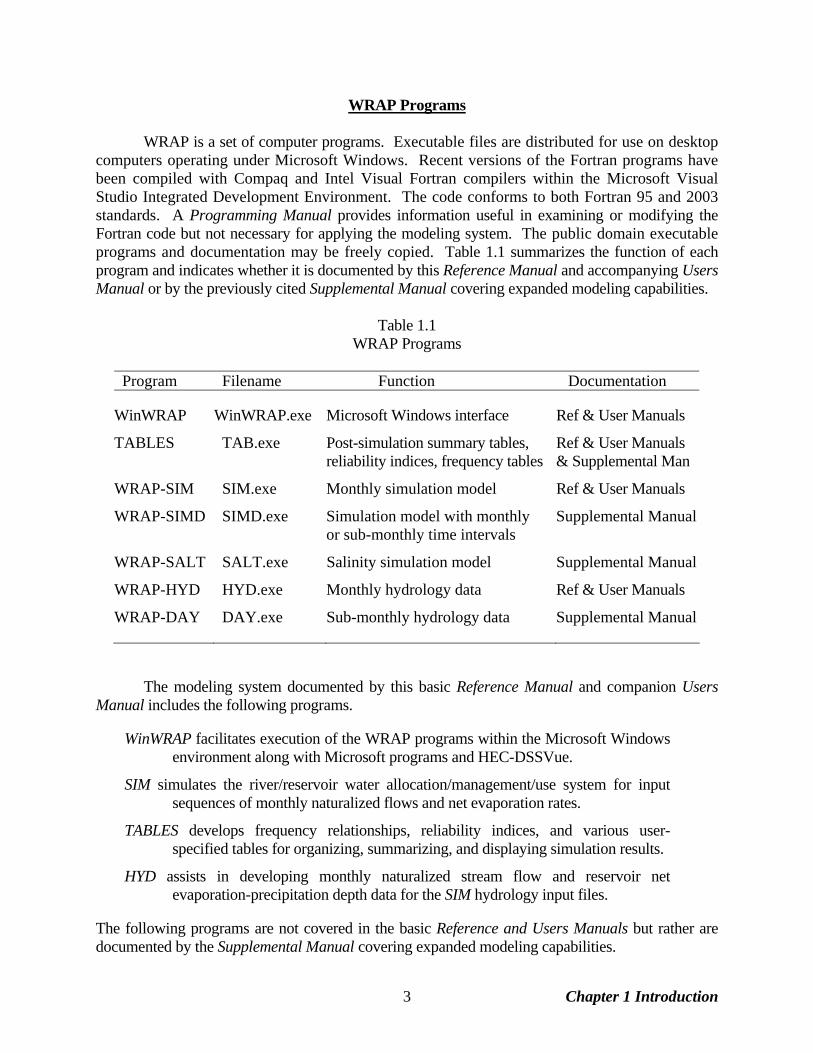
WRAP Programs WRAP is a set of computer programs. Executable files are distributed for use on desktop computers operating under Microsoft Windows. Recent versions of the Fortran programs have been compiled with Compaq and Intel Visual Fortran compilers within the Microsoft Visual Studio Integrated Development Environment. The code conforms to both Fortran 95 and 2003 standards. A Programming Manual provides information useful in examining or modifying the Fortran code but not necessary for applying the modeling system. The public domain executable programs and documentation may be freely copied. Table 1.1 summarizes the function of each program and indicates whether it is documented by this Reference Manual and accompanying Users Manual or by the previously cited Supplemental Manual covering expanded modeling capabilities.
Table 1.1 WRAP Programs
Program Filename Function Documentation
WinWRAP WinWRAP.exe Microsoft Windows interface Ref & User Manuals
TABLES TAB.exe Post-simulation summary tables, reliability indices, frequency tables
Ref & User Manuals & Supplemental Man
WRAP-SIM SIM.exe Monthly simulation model Ref & User Manuals
WRAP-SIMD SIMD.exe Simulation model with monthly or sub-monthly time intervals
Supplemental Manual
WRAP-SALT SALT.exe Salinity simulation model Supplemental Manual
WRAP-HYD HYD.exe Monthly hydrology data Ref & User Manuals
WRAP-DAY DAY.exe Sub-monthly hydrology data Supplemental Manual
The modeling system documented by this basic Reference Manual and companion Users Manual includes the following programs.
WinWRAP facilitates execution of the WRAP programs within the Microsoft Windows environment along with Microsoft programs and HEC-DSSVue.
SIM simulates the river/reservoir water allocation/management/use system for input sequences of monthly naturalized flows and net evaporation rates.
TABLES develops frequency relationships, reliability indices, and various user-specified tables for organizing, summarizing, and displaying simulation results.
HYD assists in developing monthly naturalized stream flow and reservoir net evaporation-precipitation depth data for the SIM hydrology input files.
The following programs are not covered in the basic Reference and Users Manuals but rather are documented by the Supplemental Manual covering expanded modeling capabilities.
Chapter 1 Introduction 3
SIMD (D for daily) is an expanded version of SIM that includes features for sub-monthly time steps, flow disaggregation, flow forecasting and routing, and flood control operations along with all of the capabilities of SIM.
DAY assists in developing sub-monthly (daily) time step hydrology input for SIMD
including disaggregating monthly flows to sub-monthly time intervals and determining routing parameters.
SALT reads a SIM or monthly SIMD output file and a salinity input file and tracks salt
constituents through the river/reservoir/water use system. WinWRAP User Interface
The Fortran programs are compiled as separate individual programs, which may be executed independently of each other without WinWRAP. However, the WinWRAP user interface program facilitates running all of the WRAP programs within Microsoft Windows in an integrated manner along with use of Microsoft programs to access and edit input and output files and use of HEC-DSSVue to plot and/or otherwise analyze simulation results. The WinWRAP interface connects executable programs and data files. The model user must create or obtain previously created files describing hydrology and water management for the river basin or region of concern along with other related information. The programs are connected through various input/output files. Certain programs create files with intermediate results to be read by other programs. File access occurs automatically, controlled by the software. SIM and SIMD Versions of the Simulation Model
The simulation program SIM performs the river/reservoir/use system water allocation computations using a monthly time step. SIMD contains all of the capabilities of the monthly time step SIM, plus options for synthesizing sub-monthly time step stream flows, flow forecasting and Muskingum routing, and simulating reservoir operations for flood control. Although any sub-monthly time interval may be used in SIMD, the model is called the daily version of SIM since the day is the default sub-monthly time step expected to be adopted most often.
SIMD duplicates simulation results for datasets prepared for SIM. The expanded version
SIMD may be viewed as replacing SIM. However, SIM is being maintained as a separate program. The SIM program is complex, and the additional features make SIMD significantly more complex. SIM has been applied extensively as a component of the Texas WAM System. The basic SIM may continue to be used in ongoing applications of the Texas WAM System datasets that do not need the expanded modeling capabilities.
The conditional reliability modeling features covered in the supplemental expanded capabilities manual are incorporated in both SIM and SIMD. The SIMD sub-monthly time step, disaggregation of monthly to daily flows, flow forecasting, flow routing, and flood control reservoir operations features covered in the supplemental manual are provided only by SIMD, not SIM. SIMD flow forecasting involves consideration of future stream flows over a specified forecast period in making water supply diversion and multiple-purpose reservoir system operating decisions. Methodologies are provided for routing of stream flow adjustments.
Chapter 1 Introduction 4

HYD and DAY Pre-Simulation Hydrology Programs
Program HYD assists in developing hydrology input for SIM, which consists of sequences of monthly naturalized stream flows and reservoir net evaporation-precipitation rates. HYD is the only program not affected by the expanded capabilities covered in the Supplemental Manual.
The program DAY documented in the Supplemental Manual provides a set of computational routines that facilitate developing SIMD hydrology input related to sub-monthly time steps. The DAY routines facilitate disaggregation of monthly flows to sub-monthly time intervals and calibrating routing parameters. SALT Simulation Model The program SALT is applied in combination with either SIM or SIMD to simulate salinity. SALT is designed for use with a monthly time step. SALT obtains monthly water quantities by reading the main SIM or SIMD output file, obtains water quality data by reading a separate salinity input file, and tracks the water quality constituents through the river/reservoir system. All of the simulation capabilities of SIM/SIMD are preserved while adding salt balance accounting features. TABLES Organization of Simulation Results
The program TABLES provides a comprehensive array of tables and tabulations in user-specified formats for organizing, summarizing, analyzing, and displaying simulation results from SIM, SIMD, and SALT. Many of the options provided by TABLES involve rearranging simulation results into convenient tables for reports and analyses or as tabulations for export to Microsoft Excel or HEC-DSSVue. TABLES also provides an assortment of computational options for developing tables of water supply reliability indices and flow and storage frequency relationships.
Auxiliary Software
The WRAP programs provide comprehensive computational capabilities but have no editing or graphics capabilities. The user's choice of auxiliary editing and graphics software may be adopted for use with WRAP. The only required auxiliary software is an editor such as Microsoft WordPad. However, WRAP modeling and analysis capabilities are enhanced by use of other supporting software for developing input datasets and plotting simulation results, such as Microsoft Excel, HEC-DSSVue, and ArcGIS. Microsoft Programs
Programs distributed by the Microsoft Corporation with its Windows and Office Systems are widely used. WordPad and Notepad are used routinely in editing WRAP input files and viewing simulation results. Excel provides both graphics and computational capabilities and has been extensively applied with WRAP. These programs are accessed directly from the WinWRAP interface. TABLES has options for tabulating essentially any of the time series variables included in the SIM, SIMD, and SALT simulation results in a format designed to be conveniently accessed by Microsoft Excel for plotting or other purposes.
Chapter 1 Introduction 5
Hydrologic Engineering Center HEC-DSS and HEC-DSSVue The Hydrologic Engineering Center (HEC) of the U.S. Army Corps of Engineers (USACE) has developed a suite of generalized hydrologic, hydraulic, and water management simulation models that are applied extensively by numerous agencies and consulting firms throughout the United States and abroad. The HEC-DSS (Data Storage System) is used routinely with HEC simulation models and with other non-HEC modeling systems as well. Multiple simulation models share the same graphics and data management software as well as a set of basic statistical and arithmetic routines. A HEC-DSS Excel data exchange add-in is also available from the HEC for transporting data between Microsoft Excel and HEC-DSS (Hydrologic Engineering Center 2003). Database management and graphics capabilities provided by the HEC-DSS are oriented particularly toward voluminous sets of sequential data such as time series (Hydrologic Engineering Center 1995). The HEC-DSS Visual Utility Engine (HEC-DSSVue) is a graphical user interface program for viewing, editing, and manipulating data in HEC-DSS files (Hydrologic Engineering Center 2005). The public domain HEC-DSSVue software and documentation may be downloaded from the Hydrologic Engineering Center website. http://www.hec.usace.army.mil/ The WRAP Fortran programs are linked during compilation to DSS routines from a static library file provided by the Hydrologic Engineering Center that allow access to DSS files. The WRAP executable programs include options for writing the SIM, SIMD, or SALT simulation results as HEC-DSS files. Hydrology input data stored as a DSS file can also be read by the WRAP simulation programs. HEC-DSSVue provides very convenient capabilities for graphical displays of WRAP simulation results. The many HEC-DSSVue mathematical and statistical computational routines may also be pertinent to manipulation and analysis of WRAP simulation results. HEC-DSSVue can be accessed directly through WinWRAP. ArcGIS and ArcMap WRAP Display Tool
Geographic information systems (GIS) such as ESRI's ArcGIS (http://www.esri.com) are useful in dealing with spatial aspects of compiling WRAP input data and displaying simulation results. Arc Hydro is a data model that operates within ArcGIS and provides a set of tools designed specifically for hydrology and water resources applications (http://www.crwr.utexas.edu/giswr/; Maidment 2002). Gopalan (2003) describes development of ArcGIS tools at the Center for Research in Water Resources at the University of Texas to determine drainage areas and other watershed parameters and the spatial connectivity of control points for the WRAP input datasets for the Texas WAM System. Use of GIS tools to develop WRAP input data for the Texas WAM System is noted in the following section and discussed further in Chapter 3.
An ArcGIS tool for displaying WRAP simulation results was initially developed at Texas
A&M University (Olmos 2004) and subsequently expanded at the University of Texas (Center for Research in Water Resources 2007) for the TCEQ. The WRAP Display Tool functions as a toolbar within the ArcMap component of ArcGIS. Ranges of water supply reliabilities, flow and storage frequencies, and other simulation results are displayed by control point locations as a color coded map. Time series graphs of WRAP-SIM output variables can also be plotted. Customization capabilities as well as standard WRAP output data features are provided.
Chapter 1 Introduction 6
Texas WAM System Senate Bill 1, Article VII of the 75th Texas Legislature in 1997 directed the Texas Natural Resource Conservation Commission (TNRCC) to develop water availability models for the 22 river basins of the state, excluding the Rio Grande. Models for six river basins were to be completed by January 2000, and the 16 others completed by January 2002. Subsequent legislation authorized modeling of the Rio Grande Basin. The Water Availability Modeling (WAM) Project was conducted collaboratively by the TNRCC (as lead agency), Texas Water Development Board (TWDB), Texas Parks and Wildlife Department (TPWD), consulting engineering firms, and university researchers, in coordination with the water management community. Effective September 2002, the TNRCC was renamed the Texas Commission on Environmental Quality (TCEQ). The resulting WAM System includes databases and data management systems, the generalized WRAP model, input datasets, and simulation results for all of the river basins of Texas (TNRCC 1998; Sokulsky, Dacus, Bookout, Patek 1998; Wurbs 2005). The water management and engineering professionals from the agencies and consulting firms responsible for implementing the Texas WAM System contributed numerous ideas for expanding and improving WRAP along with testing methodologies through actual applications. During 1997-1998, the TNRCC, TWDB, TPWD, and a team of consulting firms evaluated available river/reservoir system simulation models to select a generalized model to adopt for the statewide water availability modeling system (TNRCC 1998). This study resulted in adoption of WRAP, along with recommendations for modifications. WRAP was greatly expanded and improved during 1997-2003 and 2005-2008 at Texas A&M University under interagency agreements between the TNRCC/TCEQ and Texas A&M University System. Consulting engineering firms working under contracts with the TCEQ developed WRAP input datasets and performed simulation studies for all of the river basins of the state during 1998-2003. Parsons Engineering Science, R. J. Brandes Company, HDR Engineering, Freese and Nichols, Inc., Espey Consultants, Inc., and Brown and Root were the primary contractors. Other consulting firms assisted as subcontractors. Individual firms or teams of firms modeled individual river basins or groups of adjacent basins. The Sulphur, Neches, Nueces, San Antonio, and Guadalupe were the initial river basins modeled during 1998-1999. Work on the Trinity and San Jacinto River Basins and adjoining coastal basins was initiated in 1999. Work on the Brazos River Basin was initiated in early 2000, with the remainder of the 22 basins following shortly thereafter. Initial modeling of the 22 river basins was completed by 2002. The Rio Grande, the 23rd and last basin, was modeled in 2002-2003. Upon completion of the models for each river basin, water rights permit holders were provided information regarding reliabilities associated with their water rights. WRAP input datasets and reports documenting the simulation studies are available from the TCEQ. The Center for Research in Water Resources (CRWR) at the University of Texas, under contract with the TCEQ, developed an ArcView/ArcInfo based geographic information system for delineating the spatial connectivity of pertinent sites and determining watershed parameters required for distributing naturalized stream flows (Hudgens and Maidment 1999; Mason and Maidment 2000; Figurski and Maidment 2001), which was later updated/improved using the new ArcGIS Hydro Data Model (Maidment 2002; Gopalan 2003). The watershed parameters are drainage area,
Chapter 1 Introduction 7
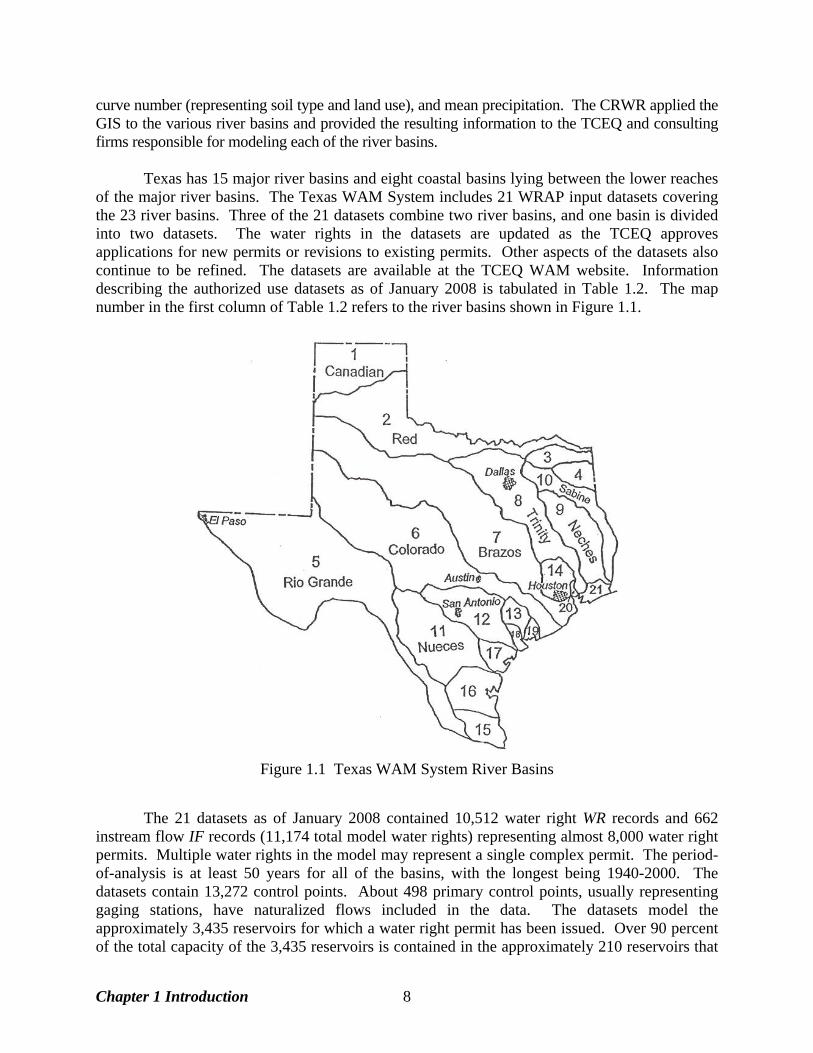
curve number (representing soil type and land use), and mean precipitation. The CRWR applied the GIS to the various river basins and provided the resulting information to the TCEQ and consulting firms responsible for modeling each of the river basins. Texas has 15 major river basins and eight coastal basins lying between the lower reaches of the major river basins. The Texas WAM System includes 21 WRAP input datasets covering the 23 river basins. Three of the 21 datasets combine two river basins, and one basin is divided into two datasets. The water rights in the datasets are updated as the TCEQ approves applications for new permits or revisions to existing permits. Other aspects of the datasets also continue to be refined. The datasets are available at the TCEQ WAM website. Information describing the authorized use datasets as of January 2008 is tabulated in Table 1.2. The map number in the first column of Table 1.2 refers to the river basins shown in Figure 1.1.
Figure 1.1 Texas WAM System River Basins The 21 datasets as of January 2008 contained 10,512 water right WR records and 662 instream flow IF records (11,174 total model water rights) representing almost 8,000 water right permits. Multiple water rights in the model may represent a single complex permit. The period-of-analysis is at least 50 years for all of the basins, with the longest being 1940-2000. The datasets contain 13,272 control points. About 498 primary control points, usually representing gaging stations, have naturalized flows included in the data. The datasets model the approximately 3,435 reservoirs for which a water right permit has been issued. Over 90 percent of the total capacity of the 3,435 reservoirs is contained in the approximately 210 reservoirs that
Chapter 1 Introduction 8
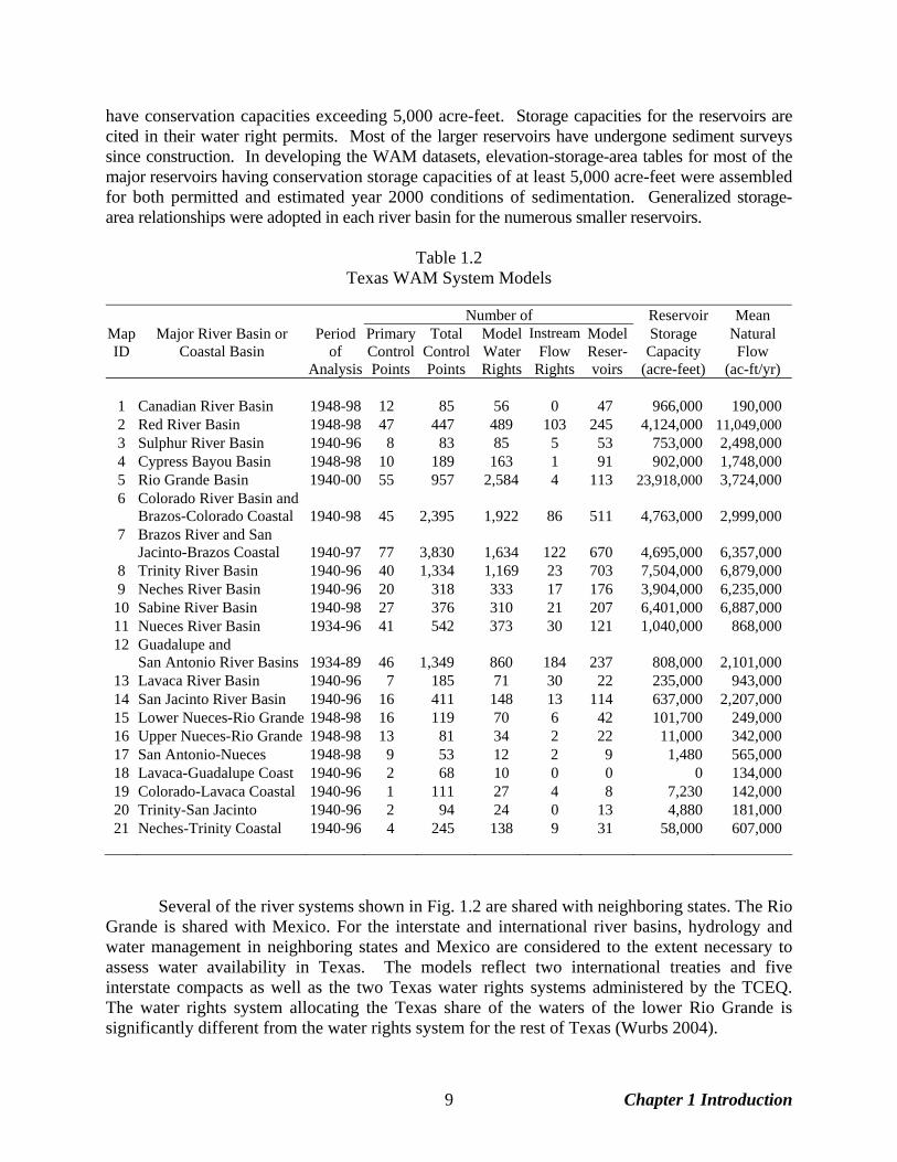
have conservation capacities exceeding 5,000 acre-feet. Storage capacities for the reservoirs are cited in their water right permits. Most of the larger reservoirs have undergone sediment surveys since construction. In developing the WAM datasets, elevation-storage-area tables for most of the major reservoirs having conservation storage capacities of at least 5,000 acre-feet were assembled for both permitted and estimated year 2000 conditions of sedimentation. Generalized storage-area relationships were adopted in each river basin for the numerous smaller reservoirs.
Table 1.2 Texas WAM System Models
Number of Reservoir Mean
Map Major River Basin or Period Primary Total Model Instream Model Storage Natural ID Coastal Basin of Control Control Water Flow Reser- Capacity Flow
Analysis Points Points Rights Rights voirs (acre-feet) (ac-ft/yr)
1 Canadian River Basin 1948-98 12 85 56 0 47 966,000 190,000 2 Red River Basin 1948-98 47 447 489 103 245 4,124,000 11,049,000 3 Sulphur River Basin 1940-96 8 83 85 5 53 753,000 2,498,000 4 Cypress Bayou Basin 1948-98 10 189 163 1 91 902,000 1,748,000 5 Rio Grande Basin 1940-00 55 957 2,584 4 113 23,918,000 3,724,000 6 Colorado River Basin and
Brazos-Colorado Coastal 1940-98 45 2,395 1,922
86 511 4,763,000 2,999,000 7 Brazos River and San
Jacinto-Brazos Coastal 1940-97 77 3,830 1,634
122 670 4,695,000 6,357,000 8 Trinity River Basin 1940-96 40 1,334 1,169 23 703 7,504,000 6,879,000 9 Neches River Basin 1940-96 20 318 333 17 176 3,904,000 6,235,000
10 Sabine River Basin 1940-98 27 376 310 21 207 6,401,000 6,887,000 11 Nueces River Basin 1934-96 41 542 373 30 121 1,040,000 868,000 12 Guadalupe and
San Antonio River Basins 1934-89 46 1,349 860
184 237 808,000 2,101,000 13 Lavaca River Basin 1940-96 7 185 71 30 22 235,000 943,000 14 San Jacinto River Basin 1940-96 16 411 148 13 114 637,000 2,207,000 15 Lower Nueces-Rio Grande 1948-98 16 119 70 6 42 101,700 249,000 16 Upper Nueces-Rio Grande 1948-98 13 81 34 2 22 11,000 342,000 17 San Antonio-Nueces 1948-98 9 53 12 2 9 1,480 565,000 18 Lavaca-Guadalupe Coast 1940-96 2 68 10 0 0 0 134,000 19 Colorado-Lavaca Coastal 1940-96 1 111 27 4 8 7,230 142,000 20 Trinity-San Jacinto 1940-96 2 94 24 0 13 4,880 181,000 21 Neches-Trinity Coastal 1940-96 4 245 138 9 31 58,000 607,000
Several of the river systems shown in Fig. 1.2 are shared with neighboring states. The Rio Grande is shared with Mexico. For the interstate and international river basins, hydrology and water management in neighboring states and Mexico are considered to the extent necessary to assess water availability in Texas. The models reflect two international treaties and five interstate compacts as well as the two Texas water rights systems administered by the TCEQ. The water rights system allocating the Texas share of the waters of the lower Rio Grande is significantly different from the water rights system for the rest of Texas (Wurbs 2004).
Chapter 1 Introduction 9
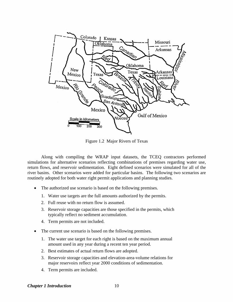
Figure 1.2 Major Rivers of Texas
Along with compiling the WRAP input datasets, the TCEQ contractors performed simulations for alternative scenarios reflecting combinations of premises regarding water use, return flows, and reservoir sedimentation. Eight defined scenarios were simulated for all of the river basins. Other scenarios were added for particular basins. The following two scenarios are routinely adopted for both water right permit applications and planning studies.
• The authorized use scenario is based on the following premises.
1. Water use targets are the full amounts authorized by the permits. 2. Full reuse with no return flow is assumed. 3. Reservoir storage capacities are those specified in the permits, which
typically reflect no sediment accumulation. 4. Term permits are not included.
• The current use scenario is based on the following premises.
1. The water use target for each right is based on the maximum annual amount used in any year during a recent ten year period.
2. Best estimates of actual return flows are adopted. 3. Reservoir storage capacities and elevation-area-volume relations for
major reservoirs reflect year 2000 conditions of sedimentation. 4. Term permits are included.
Chapter 1 Introduction 10
The WAM System is applied by water management agencies and their consultants in planning studies and preparation of permit applications. TCEQ staff applies the modeling system in evaluating the permit applications. The TWDB, regional planning committees, and their consultants apply the modeling system in regional and statewide planning studies also established by the 1997 Senate Bill 1. Agencies and consulting firms use the modeling system in various other types of studies as well.
Model Development Background The primary objectives guiding development of the WRAP modeling system have been:
• to provide capabilities for assessing hydrologic and institutional water availability and reliability within the framework of the priority-based Texas water rights system
• to develop a flexible generalized computer model for simulating the complexities of
surface water management, which can be adapted by water management agencies and consulting firms to a broad range of applications
Early Versions of the WRAP Programs A university research project, entitled Optimizing Reservoir Operations in Texas, was performed in 1986-1988 as a part of the cooperative federal/state research program of the Texas Water Resources Institute and U.S. Geological Survey. The Brazos River Authority served as the nonfederal sponsor. The research focused on formulating and evaluating storage reallocations and other reservoir system operating strategies and developing improved modeling capabilities for analyzing hydrologic and institutional water availability. A system of 12 reservoirs in the Brazos River Basin, operated by the U.S. Army Corps of Engineers Fort Worth District and the Brazos River Authority, provided a case study. Several computer simulation models were applied. The need for a generalized water rights analysis model became evident. The original version of the WRAP model, called the Texas A&M University Water Rights Analysis Program (TAMUWRAP), was developed and applied in the portion of the Brazos River Basin study documented by Wurbs, Bergman, Carriere, and Walls (1988), Walls (1988), and Wurbs and Walls (1989). A package composed of WRAP2, WRAP3, and TABLES became the second and third generations of TAMUWRAP. These programs as well as WRAPNET and WRAPSALT cited next were developed during 1990-1994 in conjunction with research projects sponsored by the Texas Water Resources Institute (TWRI), Texas Water Development Board (TWDB), U.S. Geological Survey (USGS), and the Texas Advanced Technology Program (TATP) administered by the Texas Higher Education Coordinating Board. These studies focused on natural salt pollution, water rights, and reservoir system operations. The original TAMUWRAP was replaced by WRAP2 and TABLES, reflecting significant improvements building on the same fundamental concepts. The computational algorithms were refined, additional capabilities were added, the input data format was changed, and the output format was totally restructured. WRAP3 was more complex than WRAP2 and provided expanded capabilities, particularly in regard to simulating multiple-reservoir, multiple-purpose reservoir system operations. The revisions involved coding completely new computer programs. Model
Chapter 1 Introduction 11
development and application to the Brazos River Basin are described by Dunn (1993) and Wurbs, Sanchez-Torres, and Dunn (1994). Further minor revisions were made in conjunction with a water availability modeling project for the San Jacinto River Basin performed at TAMU for the TNRCC in 1996. The WRAP2, WRAP3, and TABLES package is documented by Wurbs and Dunn (1996). WRAPNET was developed in conjunction with a research study to evaluate the relative advantages and disadvantages of adopting a generic network flow programming algorithm for WRAP as compared to ad hoc algorithms developed specifically for WRAP (Yerramreddy 1993; Wurbs and Yerramreddy 1994). Network flow programming is a special computationally efficient form of linear programming that has been adopted for a number of other similar models (Wurbs 2005). WRAPNET reads the same input files as WRAP2 and provides the same output, but the simulation computations are performed using a network flow programming algorithm. TABLES is used with WRAPNET identically as with WRAP2 or WRAP3 or the later WRAP-SIM. Although network flow programming was demonstrated to be a viable alternative modeling approach, the model-specific algorithms were concluded to be advantageous for the WRAP model. Development of WRAP-SALT was motivated by natural salt pollution in Texas and neighboring states (Wurbs et al. 1994; Sanchez-Torres 1994; Wurbs and Sanchez-Torres 1996, Wurbs 2002). The model was applied to the Brazos River Basin. The initial WRAP-SALT was an expanded version of WRAP3 and TABLES with features added for simulating salt concentrations and their impacts on water supply reliabilities. Sequences of monthly salt loads were input along with the naturalized stream flows. Water availability was constrained by both salt concentrations and water quantities. The current SALT provides similar modeling capabilities but has been completely rewritten. Whereas the original WRAP-SALT integrated the salinity computations internally within WRAP3, the current SALT is a separate program that reads a SIM output file. Texas WAM System Development of WRAP has been motivated by the implementation of a water rights permit system in Texas during the 1970's and 1980's and the creation of the previously discussed statewide Water Availability Modeling (WAM) System during 1997-2003 to support administration of the water rights system. Surface water law in Texas evolved historically over several centuries (Wurbs 2004). Early water rights were granted based on various versions of the riparian doctrine. A prior appropriation system was later adopted and then modified. The Water Rights Adjudication Act of 1967 merged the riparian water rights into the prior appropriation system. The allocation of surface water has now been consolidated into a unified permit system. The water rights adjudication process required to transition to the permit system was initiated in 1967 and was essentially completed by the late 1980's. As previously discussed, the 1997 Senate Bill 1 was a comprehensive water management legislative package addressing a wide range of issues including the need to expand statewide water availability modeling capabilities. The TCEQ, its partner agencies, and contractors developed the Texas WAM System during 1997-2003 pursuant to the 1997 Senate Bill 1 to support water rights regulatory and regional and statewide planning activities. Texas WAM System implementation efforts resulted in extensive modifications and many evolving versions of WRAP developed under 1997-2003 and 2005-2008 contracts between the TCEQ and Texas A&M University System.
Chapter 1 Introduction 12
Modeling Capabilities Added Since Implementation of WAM System The TCEQ has continued to improve and expand WRAP since implementation of the WAM System. The Fort Worth District of the U.S. Army Corps of Engineers also cosponsored ongoing efforts at TAMU during 2001-2005 to further expand WRAP under its congressionally authorized Texas Water Allocation Assessment Project. The TWDB sponsored additional improvements during 2007-2008. The TWRI and TAMU Civil Engineering Department have continued to support WRAP expansion efforts. The modeling capabilities covered by this Reference Manual and accompanying Users Manual include many significant improvements and new features added since completion of the initial TCEQ WAM System implementation project. The following additional major new modeling capabilities documented by the Supplemental Manual (Wurbs, Hoffpauir, Olmos, and Salazar 2006) are not covered in the Reference and Users Manuals. Conditional reliability modeling (CRM) provides estimates of the likelihood of meeting diversion, instream flow, hydropower, and storage targets during specified time periods of one month to several months or a year into the future, given preceding storage levels. CRM uses the same input datasets as conventional WRAP applications. CRM is based on dividing the several-decade-long hydrologic sequences into multiple shorter sequences. SIM or SIMD repeats the simulation computations with each of the sequences, starting with the same specified initial reservoir storage conditions. TABLES determines reliabilities for meeting water right requirements and storage-frequency relationships based on the SIM or SIMD simulation results. The original WRAP uses a monthly time step. The expanded version allows each of the 12 months to be subdivided into any number of time intervals with the default being daily. Model input may either include daily or other sub-monthly time interval naturalized flows, or options may be activated for disaggregating monthly flows to smaller time intervals. An adaptation of the Muskingum routing method has been added for use with smaller computational time steps. Calibration methods for determining routing parameters are included in the software package. Future time steps extending over a forecast period are considered in determining water availability. TABLES develops frequency relationships and reliability indices reflecting the sub-monthly time interval. SIMD sub-monthly results may also be aggregated to monthly values. Any number of flood control reservoirs may be operated in SIMD either individually or as multiple-reservoir systems to reduce flooding at any number of downstream control points. Operating rules are based on emptying flood control pools expeditiously while assuring that releases do not contribute to flows exceeding specified flood flow limits at downstream control points during a specified future forecast period. Flood frequency analyses of annual peak naturalized flow, regulated flow, and reservoir storage are performed with TABLES based on the log-Pearson type III probability distribution. Natural salt pollution (Wurbs 2002) in several major river basins in Texas and neighboring states motivated addition of capabilities for tracking salt concentrations through river/reservoir systems for alternative water management/use scenarios. SALT reads water quantity data from a SIM or SIMD output file along with additional input data regarding salt concentrations and loads of flows entering the river system. The model computes concentrations of the water quality constituents in the regulated stream flows, diversions, and reservoir storage contents throughout the river basin. Options in TABLES organize the salinity simulation results.
Chapter 1 Introduction 13

Organization of the Reference and Users Manuals This Reference Manual and accompanying Users Manual cover the WRAP modeling system exclusive of the expanded modeling capabilities noted in the preceding section. As previously noted, a third Supplemental Reference/Users Manual documents the additional features not covered in the basic Reference and Users Manuals. The Programming Manual documenting the Fortran code for all the WRAP programs is designed to support software maintenance and improvement but is not necessary in applying the executable programs. The companion Reference Manual and Users Manual are designed for different types of use. This Reference Manual describes WRAP capabilities and methodologies. The Reference Manual introduces the model to the new user and serves as an occasional reference for the experienced user. The Users Manual provides the operational logistics required any time anyone is working with WRAP input files. Application of WRAP requires developing and modifying files of input records. The primary purpose of the Users Manual is to provide the detailed explanation of file and record content and format required for building and revising input files. The Users Manual is organized by computer program with separate chapters for SIM, TABLES, and HYD. Chapters 1 and 2 and Appendix A of this Reference Manual provide a general overview of WRAP. Chapter 1 introduces the model and its documentation and describes its origins. Chapter 2 covers modeling capabilities and methodologies from a general overview perspective. Appendix A is a glossary of terms used in the manuals. Essentially all aspects of WRAP can be categorized as dealing with either natural hydrology or human water resources development, allocation, management, and use (water rights). Hydrology and water right features, respectively, are described in detail in Chapters 3 and 4 of this Reference Manual. From a WRAP perspective, hydrology (Chapter 3) consists of natural stream flows at gaged and ungaged sites, reservoir net evaporation minus precipitation depths, and channel losses. Likewise, from a WRAP perspective, water rights (Chapter 4) include constructed infrastructure and institutional arrangements for managing and using the water flowing in rivers and stored in reservoirs. Water rights include storage and conveyance, water supply diversions and return flows, hydroelectric energy generation, environmental instream flow requirements, reservoir/river system operating policies and practices, and water allocation rules and priorities. Chapters 5 and 6 describe SIM simulation results and the use of TABLES and auxiliary software to organize and analyze simulation results. The time series variables computed in the SIM simulation are defined. Special SIM auxiliary analysis features are outlined. Capabilities provided by TABLES for developing simulation results tables, summaries, water budgets, reliability indices, frequency relationships, and tabulations for transport to Excel and HEC-DSSVue are explained. Appendix B consists of input and output for several SIM and TABLES examples. Examples illustrating HYD are presented as Appendix C. The Fundamentals Manual presents a larger, more realistic example. The input files for the examples are available in electronic format along with the executable programs. Learning WRAP is greatly facilitated by experimenting with the examples. The simulation computations can be readily tracked by examining simulation results. The examples provide simple datasets with easy-to-track numbers to which additional modeling options of interest can be added to explore their functionality.
Chapter 1 Introduction 14
CHAPTER 2 OVERVIEW OF THE SIMULATION MODEL
Modeling Capabilities WRAP is designed for use by water management agencies, consulting firms, and university researchers in the modeling and analysis of river/reservoir system operations. The modeling system may be applied in a wide range of planning and management situations to evaluate alternative water resources development and river regulation strategies. As discussed in the preceding chapter, water availability modeling studies are routinely performed in Texas to support regional and statewide planning activities and the preparation and evaluation of water right permit applications. Model results are used to analyze the capability of a river basin to satisfy specified water use requirements. Basin-wide impacts of changes in water management and use are assessed. Multiple-purpose reservoir system operations may be investigated in operational planning studies for existing facilities and/or feasibility studies for constructing new projects. WRAP incorporates priority-based water allocation schemes in modeling river regulation and water management. Stream flow and reservoir storage are allocated among water users based on specified priorities. WRAP was motivated by and developed within the framework of the Texas water rights permit system. However, the flexible generalized model is applicable to essentially any water allocation systems and also to situations where water is managed without a structured water rights system. WRAP is applied to river basins that have hundreds of reservoirs, thousands of water supply diversions, complex water use requirements, and complex water management practices. However, it is also applicable to simple systems with one, several, or no reservoirs. The generalized computer model provides capabilities for simulating a river/reservoir/use system involving essentially any stream tributary configuration. Interbasin transfers of water can be included in the simulation. Closed loops such as conveying water by pipeline from a downstream location to an upstream location on the same stream or from one tributary to another tributary can be modeled. Water management/use may involve reservoir storage, water supply diversions, return flows, environmental instream flow requirements, hydroelectric power generation, and flood control. Multiple-reservoir system operations and off-channel storage may be simulated. Flexibility is provided for modeling the various rules specified in water rights permits and/or other institutional arrangements governing water allocation and management. There are no limits on the number of water rights, control point locations, reservoirs, and other system components included in a model. There is no limit on the number of years included in the hydrologic period-of-analysis. The SIM model is an accounting system for tracking stream flow sequences, subject to reservoir storage capacities and operating rules and water supply diversion, hydroelectric power, and instream flow requirements. Water balance computations are performed in each time step of the simulation. Typically, a simulation will be based on combining (1) a repetition of historical hydrology with (2) a specified scenario of river basin development, water use requirements, and reservoir system operating rules. A broad spectrum of hydrologic and water management scenarios may be simulated. Numerous optional features have been incorporated into the generalized modeling system to address complexities in the variety of ways that people manage and use water. The Fortran programs are designed to facilitate adding new features and options as needs arise.
Chapter 2 Overview 15
Water Availability Modeling Process The conventional water availability modeling process consists of two phases:
1. developing sequences of monthly naturalized stream flows covering the hydrologic period-of-analysis at all pertinent locations
a. developing sequences of naturalized flows at stream gaging stations [WRAP-HYD]
b. extending record lengths and filling in gaps to develop complete sequences at all selected gages covering the specified period-of-analysis [Not included in WRAP]
c. distributing naturalized flows from gaged to ungaged locations [HYD or SIM]
2. simulating the rights/reservoir/river system, given the input sequences of naturalized flows, to determine regulated and unappropriated flows, storage, reliability indices, flow-frequency relationships and related information regarding water supply capabilities
a. simulating the rights/reservoir/river system [WRAP-SIM]
b. computing water supply reliability and stream flow frequency indices and otherwise organizing/summarizing/displaying simulation results [TABLES]
Naturalized or unregulated stream flows represent historical hydrology without the effects of reservoirs and human water management/use. Naturalized flows at gaging stations are determined by adjusting gaged flows to remove the historical effects of human activities. Various gaging stations in a river basin are installed at different times and have different periods-of-record. Gaps with missing data may occur. Record lengths are extended and missing data reconstituted by regression techniques using data from other gages and other months at the same gage. Naturalized flows at ungaged sites are synthesized based upon the naturalized flows at gaged sites and watershed characteristics.
HYD includes options to assist in adjusting gaged flows to obtain naturalized flows (Task 1a above). Naturalized flows may be distributed from gaged (or known-flow) locations to ungaged (unknown-flow) locations (Task 1c above) within either HYD or SIM. WRAP does not include regression methods to extend records or reconstitute missing data (Task 1b). Readily available spreadsheet and statistical software packages include regression analyses. Naturalized flows have been developed (Tasks 1a and 1b) for the Texas WAM System and are readily available for further application. Watershed parameters for distributing flows (Task 1c) are also incorporated in the Texas WAM System datasets.
A WRAP-SIM simulation starts with known naturalized flows provided in the hydrology
input file and computes regulated flows and unappropriated flows at all pertinent locations. Regulated and unappropriated flows computed within SIM reflect the effects of reservoir storage and water use associated with the water rights included in the input. Regulated flows represent physical flows at a location, some or all of which may be committed to meet water rights requirements. Unappropriated flows are the stream flows remaining after all water rights have received their allocated share of the flow to refill reservoir storage and meet diversion and instream flow requirements. Unappropriated flows represent uncommitted water still available for additional water right permit applicants.
Chapter 2 Overview 16
Water is allocated to meet diversion, instream flow, hydroelectric energy, and reservoir storage requirements based on water right priorities. In the Texas WAM System, priorities are based on seniority dates specified in the water right permits. Various other schemes for establishing relative priorities may be adopted as well. Water availability is evaluated in simulation studies from the perspectives of (1) reliabilities in satisfying existing and proposed water use requirements, (2) effects on the reliabilities of other water rights in the river basin, (3) regulated instream flows, and (4) unappropriated flows available for additional water right applicants. Reservoir storage and stream flows are simulated. WRAP may be used to evaluate water supply capabilities associated with alternative water resources development projects, water management plans, water use scenarios, demand management strategies, regulatory requirements, and reservoir system operating procedures.
Long-Term Simulation, Yield-Reliability, and Conditional Reliability Modeling Modes
The WRAP simulation program SIM may be applied in the following alternative modes.
1. A single long-term simulation is the default mode.
2. The yield-reliability analysis option activated by the FY record is based on repetitions of the long-term simulation to develop a diversion target (yield) versus reliability table that includes the firm yield if a firm (100% reliability) yield is feasible.
3. The conditional reliability modeling (CRM) option activated by the CR record is based on many short-term simulations starting with the same initial storage condition.
In the conventional long-term SIM simulation mode, a specified water management and use scenario is combined with naturalized flows and net reservoir evaporation rates covering the entire hydrologic period-of-analysis in a single simulation. The user specifies the storage content of all reservoirs at the beginning of the simulation, defaulting to full to capacity. Optionally, a storage cycling feature described in Chapter 6 is based on repeating the simulation setting beginning-of-simulation storages equal to end-of-simulation storages. Water supply reliability and flow and storage frequency statistics developed by TABLES from the SIM simulation results represent long-term probabilities or percent-of-time estimates. SIM has a yield-reliability analysis option described in Chapter 6 that is activated by the FY record. The long-term simulation is iteratively repeated multiple times with specified water use targets incremented in each simulation to develop a table of diversion target versus period and volume reliability. The resulting yield-reliability table is written as a SIM output file. The table ends with the firm (100% reliability) yield if a firm yield can be obtained. In the SIM conditional reliability modeling (CRM) mode activated by a CR record, the long period-of-analysis hydrology is divided into many short sequences defined by options specified by the model-user. The SIM simulation is automatically repeated with each hydrologic sequence starting with the same user-specified initial reservoir storage contents. Program TABLES develops reliability and frequency relationships from the simulation results. Options are provided in TABLES for assigning probabilities to each hydrologic sequence. Water supply reliability and stream flow and storage frequency relationships for periods of a month to several
Chapter 2 Overview 17
months or a year into the future are conditioned upon the preceding storage condition. The CRM mode supports short-term operational planning studies and seasonal or real-time reservoir/river system management. CRM procedures are explained in the Supplemental Reference/Users Manual (Wurbs, Hoffpauir, Olmos, and Salazar 2006).
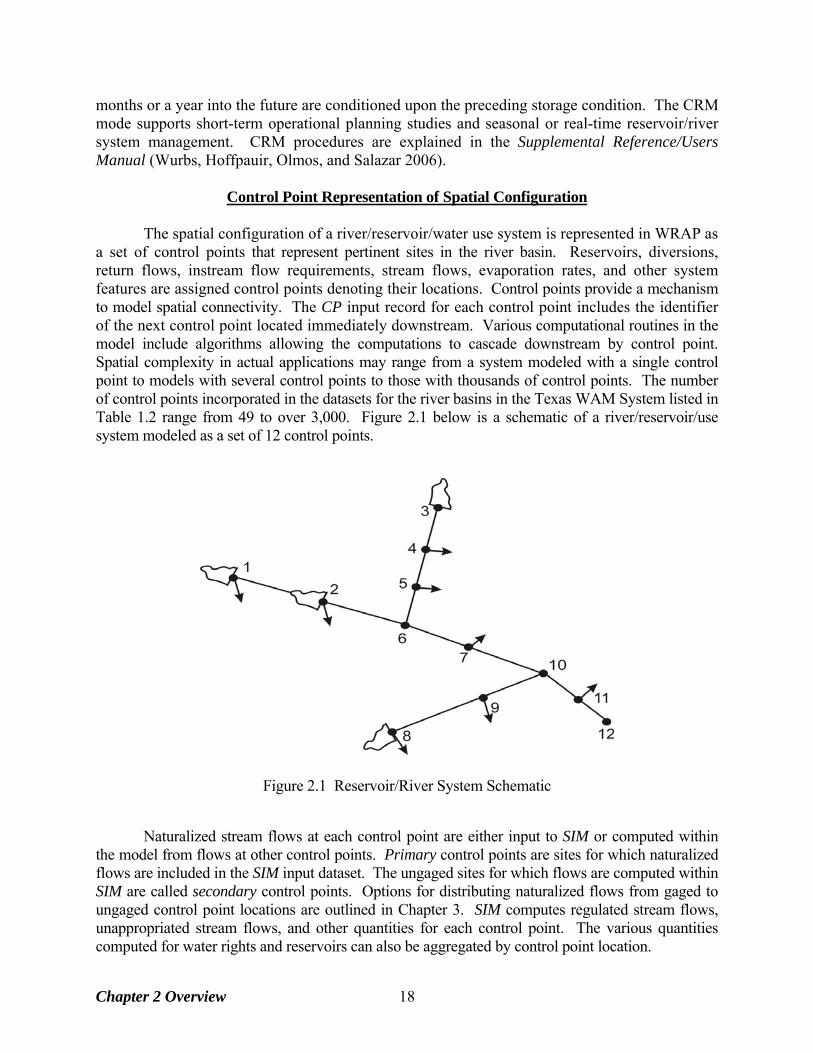
Control Point Representation of Spatial Configuration The spatial configuration of a river/reservoir/water use system is represented in WRAP as a set of control points that represent pertinent sites in the river basin. Reservoirs, diversions, return flows, instream flow requirements, stream flows, evaporation rates, and other system features are assigned control points denoting their locations. Control points provide a mechanism to model spatial connectivity. The CP input record for each control point includes the identifier of the next control point located immediately downstream. Various computational routines in the model include algorithms allowing the computations to cascade downstream by control point. Spatial complexity in actual applications may range from a system modeled with a single control point to models with several control points to those with thousands of control points. The number of control points incorporated in the datasets for the river basins in the Texas WAM System listed in Table 1.2 range from 49 to over 3,000. Figure 2.1 below is a schematic of a river/reservoir/use system modeled as a set of 12 control points.
Figure 2.1 Reservoir/River System Schematic Naturalized stream flows at each control point are either input to SIM or computed within the model from flows at other control points. Primary control points are sites for which naturalized flows are included in the SIM input dataset. The ungaged sites for which flows are computed within SIM are called secondary control points. Options for distributing naturalized flows from gaged to ungaged control point locations are outlined in Chapter 3. SIM computes regulated stream flows, unappropriated stream flows, and other quantities for each control point. The various quantities computed for water rights and reservoirs can also be aggregated by control point location.
Chapter 2 Overview 18
Each water right must be assigned a main control point indicating the location at which the right has access to available stream flow. This site is referred to as the control point of the water right though various components of the right such as return flows and multiple reservoirs may be assigned other control point locations. Any number of water rights can be assigned to the same control point. Rights can be grouped such that the rights assigned to a given control point include all those located along specified stream reaches. Multiple water rights at the same control point all have access, in priority order, to the stream flow available at the control point. Any number of reservoirs can be associated with a single control point, but each control point is limited to one set of reservoir net evaporation-precipitation rates. Stream flow depletions and return flows associated with a water right affect stream flows at other control points located downstream.
Simulation Input
Input data for the WRAP programs are provided as records in a set of files as described in
the Users Manual. The system for organizing the input includes an identifier for each type of record that is placed at the beginning of the records. The SIM hydrology input files include sequences of monthly naturalized stream flows (IN records) and net reservoir evaporation minus precipitation rates (EV records). Naturalized stream flows may be distributed from gaged (known-flow) to ungaged (unknown-flow) control points in either SIM or HYD using optional alternative methods. Watershed parameters for distributing flows to ungaged water rights sites are provided on FD, FC, and WP records in a flow distribution input file.
Input describing water rights includes control point location, annual diversion amount,
instream flow requirements, hydroelectric energy demand, storage capacity, type of water use, return flow, and priority specifications. A set of 12 monthly water use distribution factors may be input for each water use type. Diversion, instream flow, and hydropower targets optionally may be specified as a function of reservoir storage or stream flow. Return flows may be specified as a fraction of diversions or as a constant amount, return flow location, and whether the return flows occur the same month as the diversion or the next month.
Water right priority numbers may be entered for each individual right on WR or IF
records or for water use type groups on UP records. Optionally, water use demands may be met in upstream-to-downstream order. Priority numbers may reflect priority dates specified in the permit for each right. For example, a water right established as of May 1, 1972 is represented by a priority number of 19720501, which is a smaller number than the priority of more junior rights. The model-user can adopt other schemes for assigning relative priorities to fit the particular application. The model provides considerable flexibility for applying ingenuity in combining water right modeling options to simulate a particular water management/use scenario.
Reservoirs are described by elevation versus storage volume and surface area
relationships, storage capacity allocations, and multiple-reservoir release rules for any reservoirs operated as a system. Storage-area relationships may be input in either tabular form or as coefficients for an equation. Multiple-reservoir system operations are based on balancing the percentage full of specified zones in each reservoir included in the system for a particular right. Although reservoirs on rivers and off-channel reservoirs are treated basically the same, certain modeling features are more relevant to each of these two types of reservoirs.
Chapter 2 Overview 19
Simulation Results The voluminous output for each month of a WRAP-SIM simulation includes:
• naturalized, regulated, and unappropriated flows for each control point • return flows from diversions that are returned at each control point • channel losses and loss credits for the stream reach below each control point • diversions, diversion shortages, and return flows for each water right • hydroelectric energy generated and energy shortages • instream flow targets and shortages • storage and net evaporation-precipitation for each reservoir, right, and control point • amount of water available and stream flow depletions for each right
Simulation results are written to a SIM output file, which is read by TABLES. The program TABLES computes reliability indices, including volume and period reliabilities, and stream flow and storage frequency relationships and organizes the simulation results as tables of information in various user-specified optional formats. SIM results can be easily plotted with HEC-DSSVue.
Table 2.1
Variables in the WRAP-SIM Output File WR Record Rights Instream Flow Rights Control Points Reservoir/Hydropower
diversion or energy target instream flow target diversion target energy generated diversion/energy shortage flow shortage diversion shortage energy shortage storage volume storage volume storage volume secondary energy evap-precip volume evap-precip volume evap-precip volume storage volume available stream flow available stream flow unappropriated flow evap-precip volume stream flow depletion stream flow depletion stream flow depletion evap-precip depth reservoir releases required res release naturalized flow adjusted evap-prec depthreturn flow reservoir release regulated flow reservoir inflow available flow increase reservoir release shortage reservoir releases reservoir release water right identifier water right identifier return flow turbine flow first group identifier channel loss water surface elevation second group identifier channel loss credit reservoir identifier control point identifier
For each month of a SIM simulation, output records are written for user-selected water rights (WR record rights and instream flow IF rights), control points, and reservoir/hydropower projects. These records contain the data listed in Tables 2.1 and 5.1. Some data are unique to water right, control point, or reservoir/hydropower output records. For example, naturalized, regulated, and unappropriated flows, and channel losses are associated only with control points. Other data are repeated on two or three of the record types. For example, reservoir storage and evaporation are written to all three records. If one water right with one reservoir is located at a control point, reservoir storage will be identical on all three records. However, the control point records contain the summation of storage contents of all reservoirs assigned to the control point. Likewise, multiple water rights may be assigned to the same reservoir. Diversions and shortages on
Chapter 2 Overview 20

a control point record are the totals for all the rights assigned to the control point. The diversions and shortages on a water right output record are associated with a single WR input record. As discussed in Chapter 5, the time series of monthly values of the variables listed in Table 2.1 are read by the post-simulation program TABLES, which in turn creates user-specified tables to organize, display, and summarize the simulation results. Some of the TABLES routines simply rearrange and tabulate, with appropriate table headings, selected data read from SIM input or output files. Other routines include computational algorithms, which may range from simple sums or statistics to more complex arithmetic operations. A reliability table for water supply diversion or hydroelectric energy targets includes volume reliabilities and period reliabilities for meeting various percentages of the target demands. Frequency tables are developed for naturalized flows, regulated flows, unappropriated flows, reservoir storage, and instream flow shortages. Reservoir storage may be also displayed as comparative tables of percentages of capacity and drawdown-duration tables. TABLES also creates tables organizing and summarizing water rights data read from a SIM input file. Options in TABLES also allow data to be tabulated in formats designed to facilitate convenient import to Microsoft Excel or HEC-DSSVue for further computations or graphs.
Units of Measure Any units may be adopted. However, the set of all input data units and conversion factors must be computationally consistent. The various flows (volume per month or volume per year) must have the same volume units as the reservoir storage volume. Most of the input data are volumes, areas, or depths, including annual and monthly diversion volumes, volume/month stream flow rates, reservoir storage volume and surface area, and net evaporation-precipitation depths. Net evaporation volumes are depths multiplied by reservoir water surface areas. An example of a set of computationally consistent (feet× acre = acre-feet) English units is as follows:
• acre-feet for storage volume and volume/month or volume/year quantities • acres for reservoir surface area • feet for monthly net reservoir surface evaporation-precipitation rates
A set of computationally consistent (meters×km2 = million m3) metric units is as follows:
• million cubic meters for the reservoir storage and volume/month or volume/year quantities • square kilometers for reservoir surface area • meters for monthly net reservoir surface evaporation-precipitation rates
For many WRAP applications, all input is entered in consistent units without needing conversions within the model. However, as described in the Users Manual, several input variables are multipliers that may be used as unit conversions. Most of these unit conversion factors are entered on the SIM or HYD multiplier factor XL record described in the Users Manual. Computations within TABLES do not depend on units, but an option allows the user to specify units to be written in the table headings. The hydroelectric power factor entered on the SIM multiplier factor XL record entails unit conversions and specific weight and is described later in the hydropower section of Chapter 4. A multiplier factor entered on the XL record associated with the curve number method for distributing flows from gaged to ungaged control points is defined in Chapter 3.
Chapter 2 Overview 21
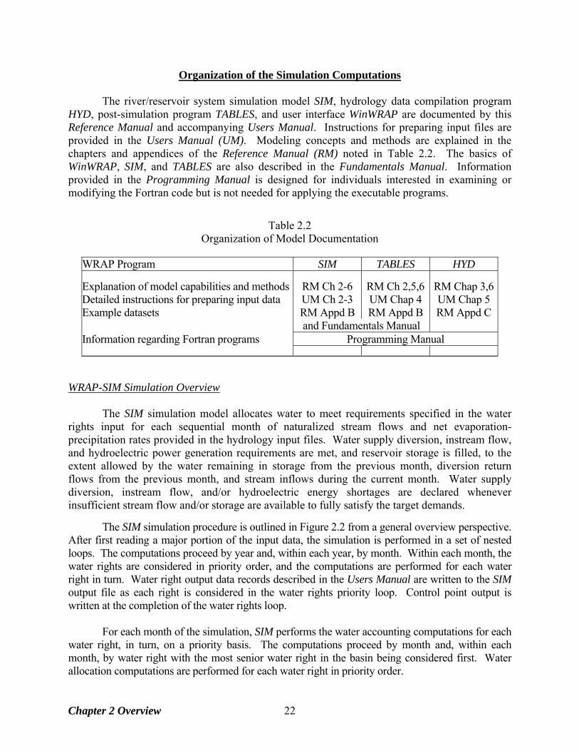
Organization of the Simulation Computations
The river/reservoir system simulation model SIM, hydrology data compilation program HYD, post-simulation program TABLES, and user interface WinWRAP are documented by this Reference Manual and accompanying Users Manual. Instructions for preparing input files are provided in the Users Manual (UM). Modeling concepts and methods are explained in the chapters and appendices of the Reference Manual (RM) noted in Table 2.2. The basics of WinWRAP, SIM, and TABLES are also described in the Fundamentals Manual. Information provided in the Programming Manual is designed for individuals interested in examining or modifying the Fortran code but is not needed for applying the executable programs.
Table 2.2
Organization of Model Documentation
WRAP Program SIM TABLES HYD Explanation of model capabilities and methods RM Ch 2-6 RM Ch 2,5,6 RM Chap 3,6Detailed instructions for preparing input data UM Ch 2-3 UM Chap 4 UM Chap 5 Example datasets RM Appd B RM Appd B RM Appd C and Fundamentals Manual Information regarding Fortran programs Programming Manual
WRAP-SIM Simulation Overview
The SIM simulation model allocates water to meet requirements specified in the water rights input for each sequential month of naturalized stream flows and net evaporation-precipitation rates provided in the hydrology input files. Water supply diversion, instream flow, and hydroelectric power generation requirements are met, and reservoir storage is filled, to the extent allowed by the water remaining in storage from the previous month, diversion return flows from the previous month, and stream inflows during the current month. Water supply diversion, instream flow, and/or hydroelectric energy shortages are declared whenever insufficient stream flow and/or storage are available to fully satisfy the target demands. The SIM simulation procedure is outlined in Figure 2.2 from a general overview perspective. After first reading a major portion of the input data, the simulation is performed in a set of nested loops. The computations proceed by year and, within each year, by month. Within each month, the water rights are considered in priority order, and the computations are performed for each water right in turn. Water right output data records described in the Users Manual are written to the SIM output file as each right is considered in the water rights priority loop. Control point output is written at the completion of the water rights loop. For each month of the simulation, SIM performs the water accounting computations for each water right, in turn, on a priority basis. The computations proceed by month and, within each month, by water right with the most senior water right in the basin being considered first. Water allocation computations are performed for each water right in priority order.
Chapter 2 Overview 22
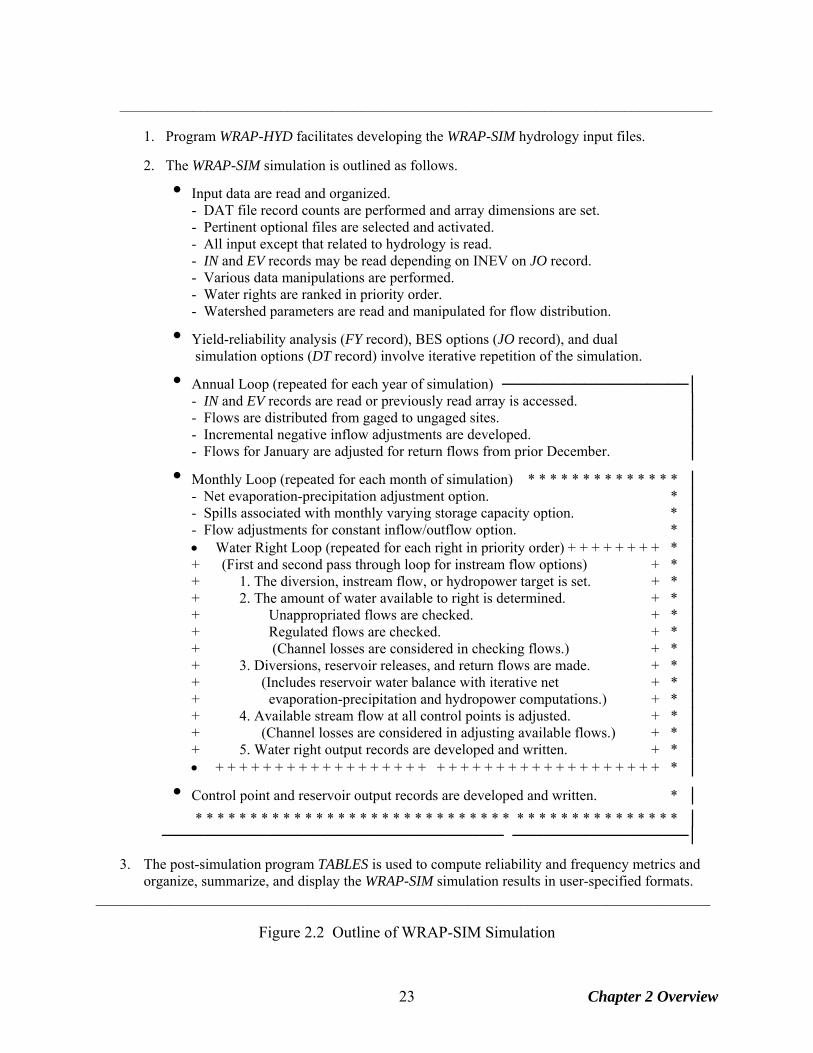
_________________________________________________________________________________
1. Program WRAP-HYD facilitates developing the WRAP-SIM hydrology input files.
2. The WRAP-SIM simulation is outlined as follows.
• Input data are read and organized. - DAT file record counts are performed and array dimensions are set. - Pertinent optional files are selected and activated. - All input except that related to hydrology is read. - IN and EV records may be read depending on INEV on JO record. - Various data manipulations are performed. - Water rights are ranked in priority order. - Watershed parameters are read and manipulated for flow distribution.
• Yield-reliability analysis (FY record), BES options (JO record), and dual simulation options (DT record) involve iterative repetition of the simulation.
• Annual Loop (repeated for each year of simulation) ──────────────────│ - IN and EV records are read or previously read array is accessed. │ - Flows are distributed from gaged to ungaged sites. │ - Incremental negative inflow adjustments are developed. │ - Flows for January are adjusted for return flows from prior December. │
• Monthly Loop (repeated for each month of simulation) * * * * * * * * * * * * * * │ - Net evaporation-precipitation adjustment option. * │ - Spills associated with monthly varying storage capacity option. * │ - Flow adjustments for constant inflow/outflow option. * │
• Water Right Loop (repeated for each right in priority order) + + + + + + + + * │ + (First and second pass through loop for instream flow options) + * │ + 1. The diversion, instream flow, or hydropower target is set. + * │ + 2. The amount of water available to right is determined. + * │ + Unappropriated flows are checked. + * │ + Regulated flows are checked. + * │ + (Channel losses are considered in checking flows.) + * │ + 3. Diversions, reservoir releases, and return flows are made. + * │ + (Includes reservoir water balance with iterative net + * │ + evaporation-precipitation and hydropower computations.) + * │ + 4. Available stream flow at all control points is adjusted. + * │
+ (Channel losses are considered in adjusting available flows.) + * │ + 5. Water right output records are developed and written. + * │ • + + + + + + + + + + + + + + + + + + + + + + + + + + + + + + + + + + + + + * │
• Control point and reservoir output records are developed and written. * │
* * * * * * * * * * * * * * * * * * * * * * * * * * * * * * * * * * * * * * * * * * * * │ ───────────────────────────────── ─────────────────│
3. The post-simulation program TABLES is used to compute reliability and frequency metrics and organize, summarize, and display the WRAP-SIM simulation results in user-specified formats.
____________________________________________________________________________________
Figure 2.2 Outline of WRAP-SIM Simulation
Chapter 2 Overview 23
As SIM considers each water right, pertinent computational algorithms are activated to make water management decisions and perform volume balance accounting computations. Diversions and diversion shortages are computed. Environmental instream flow requirements are considered. Reservoir storage capacity is filled to the extent allowed by available stream flow. Reservoir net evaporation-precipitation volume is computed and incorporated in the water balance. Return flows are computed and re-enter the stream at user-specified control points. An accounting is maintained of storage levels in each reservoir and stream flow still available at each control point. Considerable flexibility is provided for specifying water right requirements. The following features of the computational algorithms are fundamental to representing water rights requirements in the monthly time step SIM model. As discussed in the Supplemental Manual, SIMD also has flow forecasting and routing routines connecting time steps. • The simulation progresses sequentially by month. The following model features connect a
month with the preceding month. The computed end-of-period reservoir storage for a month becomes the given beginning-of-period storage for the next month. An option allows return flows from diversions in a given month to be returned to the stream the next month. Hydropower releases may also be made available at downstream locations optionally the following month. Targets may be set based on cumulative flows. Options limit cumulative annual or seasonal diversions, withdrawals from storage, and stream flow depletions.
• A water rights priority loop is embedded within the monthly computational loop. In a
particular month, the water rights are considered in priority order. Thus, in general, each water right is affected only by more senior rights, with the following exceptions. Reservoir storage is affected by computations for previous months. Next-month return flow options allow senior rights access to junior return flows. Instream flow requirements may be considered in an optional dual loop within the water rights loop, allowing junior rights to affect regulated flow constraints on water availability for more senior rights.
Steps in the WRAP-SIM Simulation All input data is read at the beginning of a SIM execution, except naturalized flows and net evaporation rates and the optional flow adjustment file that are read during each year of the simulation. Various manipulations of the water rights input data read at the beginning are performed prior to starting the monthly simulation. This includes a ranking mechanism for identifying the priority order of the water rights based on priority specifications from the input data. The annual loop begins with reading the stream flow and evaporation data for each of the 12 months of that year and distributing flows from gaged to ungaged control points. The computations are then performed on a monthly basis. The data in the control point and reservoir/hydropower output records listed in Table 2.1 reflect the effects of all the rights and are outputted each month at the completion of the water rights loop. The simulation proceeds by month and, within each month, by water right in priority order with the most senior right in the basin being considered first. Thus, if supplies are insufficient to meet all demands in a given month, the water available to a particular water right is not adversely affected by other rights that are more junior in priority. Most of the system
Chapter 2 Overview 24
simulation computations are performed within the water rights priority loop. For each individual water right in turn, the computations are performed in four stages. 1. The diversion, instream flow, or hydropower generation target is set based on specifications
read from water right WR, instream flow IF, water use coefficient UC, supplemental options SO, target options TO, flow switch FS, time series TS, and drought index DI/IS/IP records.
2. The amount of stream flow available to the right is determined. Stream flow availability is
determined as the lesser of the stream flow availability array amounts at the control point of the water right and at each of the control points located downstream.
3. Water volume balance computations are performed to compute the stream flow depletion, net
reservoir evaporation, end-of-period storage, return flow, diversion and diversion shortage, and hydroelectric energy generated and shortage. The interrelationships between the variables necessitate an iterative algorithm. For multiple reservoir system operations, the releases and storages for all the system reservoirs are computed.
4. The stream flow availability array values at the control point of the water right and at
downstream control points are decreased by a stream flow depletion and increased by a return flow or hydropower release, with adjustments for channel losses or loss credits. Upon completion of the water rights computation loop, regulated and unappropriated flows are determined from the stream flow availability array as adjusted for the effects of the water rights.
Figure 2.2 and the present discussion outline a single simulation. Various options discussed later in this manual involve two or more repetitions of the simulation. As explained in Chapter 4, instream flow options may activate a second pass through the water rights loop in a particular month. Multiple repetitions of the entire simulation may be performed automatically within SIM for purposes of using stream flow depletions determined in an initial simulation as an upper limit constraining depletions in a subsequent simulation (Chapter 4), developing yield-reliability relationships (Chapter 6), or setting beginning storage equal to ending storage (Chapter 6). Example 1 - Stages Repeated for Each Right Within Water Rights Priority Loop The objective of Example 1 is to illustrate the basic computational stages within the water rights loop. Data for the example are presented in Figure 2.3 and Tables 2.3, 2.4, and 2.5. The example focuses on the computations for just one month of a simulation. The spatial configuration of the system is represented by five control points shown in Figure 2.3. Information for each of three water rights is provided in Table 2.3. Water right WR-A includes reservoir storage as well as a diversion. Water rights WR-B and WR-C are run-of-river diversion rights. A SIM simulation consists of allocating available water to water rights in priority order. Available water consists of stream flow during the month and reservoir storage content at the beginning of the month. For this particular month, naturalized stream flow is 100 acre-feet at control point CP5 with lesser amounts at the four other control points located upstream of CP5 as tabulated in column 2 of Table 2.5. The beginning-of-month storage in the WR-A reservoir at CP4 is 195 ac-ft as shown in column 6 of Table 2.3. These naturalized flows and beginning-of-
Chapter 2 Overview 25
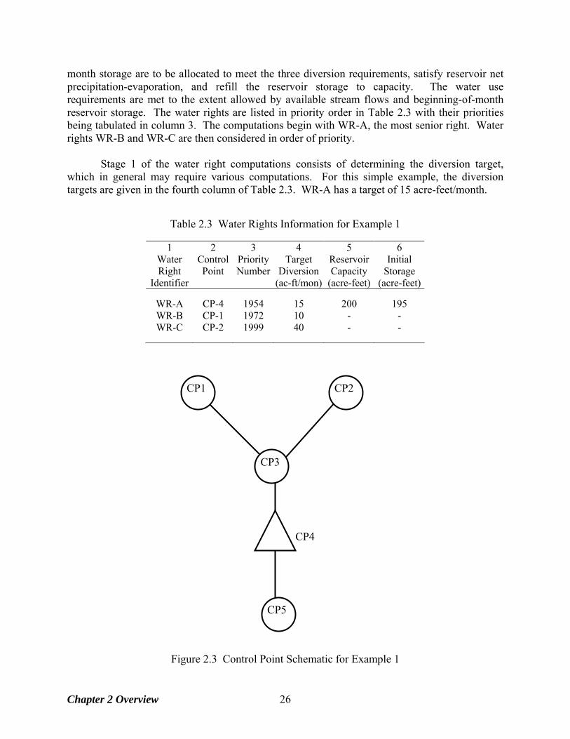
month storage are to be allocated to meet the three diversion requirements, satisfy reservoir net precipitation-evaporation, and refill the reservoir storage to capacity. The water use requirements are met to the extent allowed by available stream flows and beginning-of-month reservoir storage. The water rights are listed in priority order in Table 2.3 with their priorities being tabulated in column 3. The computations begin with WR-A, the most senior right. Water rights WR-B and WR-C are then considered in order of priority.
Stage 1 of the water right computations consists of determining the diversion target, which in general may require various computations. For this simple example, the diversion targets are given in the fourth column of Table 2.3. WR-A has a target of 15 acre-feet/month.
Table 2.3 Water Rights Information for Example 1
1 2 3 4 5 6 Water Control Priority Target Reservoir Initial Right Point Number Diversion Capacity Storage
Identifier (ac-ft/mon) (acre-feet) (acre-feet)
WR-A CP-4 1954 15 200 195 WR-B CP-1 1972 10 - - WR-C CP-2 1999 40 - -
Figure 2.3 Control Point Schematic for Example 1
CP2
CP3
CP1
CP5
CP4
Chapter 2 Overview 26
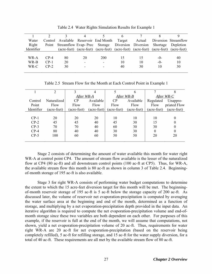
Table 2.4 Water Rights Simulation Results for Example 1
1 2 3 4 5 6 7 8 9 Water Control Available Reservoir End Month Target Actual Diversion StreamflowRight Point Streamflow Evap- Prec Storage Diversion Diversion Shortage Depletion
Identifier (acre-feet) (acre-feet) (acre-feet) (acre-feet) (acre-feet) (acre-feet) (acre-feet)
WR-A CP-4 80 20 200 15 15 -0- 40 WR-B CP-1 20 - - 10 10 -0- 10 WR-C CP-2 30 - - 40 30 10 30
Table 2.5 Stream Flow for the Month at Each Control Point in Example 1
1 2 3 4 5 6 7 8 After WR-A After WR-B After WR-C
Control Naturalized CP Available CP Available Regulated Unappro- Point Flow Flow Flow Flow Flow Flow priated Flow
Identifier (acre-feet) (acre-feet) (acre-feet) (acre-feet) (acre-feet) (acre-feet) (acre-feet)
CP-1 20 20 20 10 10 10 0 CP-2 45 45 40 45 30 15 0 CP-3 70 70 40 60 30 30 0 CP-4 80 40 40 30 30 0 0 CP-5 100 60 60 50 50 20 20
Stage 2 consists of determining the amount of water available this month for water right WR-A at control point CP4. The amount of stream flow available is the lesser of the naturalized flow at CP4 (80 ac-ft) and all downstream control points (100 ac-ft at CP5). Thus, for WR-A, the available stream flow this month is 80 ac-ft as shown in column 3 of Table 2.4. Beginning-of-month storage of 195 ac-ft is also available.
Stage 3 for right WR-A consists of performing water budget computations to determine the extent to which the 15 acre-feet diversion target for this month will be met. The beginning-of-month reservoir storage of 195 ac-ft is 5 ac-ft below the storage capacity of 200 ac-ft. As discussed later, the volume of reservoir net evaporation-precipitation is computed by averaging the water surface area at the beginning and end of the month, determined as a function of storage, and multiplying by a net evaporation-precipitation depth provided in the input data. An iterative algorithm is required to compute the net evaporation-precipitation volume and end-of-month storage since these two variables are both dependent on each other. For purposes of this example, if the reservoir is full at the end of the month, we will assume that computations, not shown, yield a net evaporation-precipitation volume of 20 ac-ft. Thus, requirements for water right WR-A are 20 ac-ft for net evaporation-precipitation (based on the reservoir being completely refilled), 5 ac-ft for refilling storage, and 15 ac-ft for the water supply diversion, for a total of 40 ac-ft. These requirements are all met by the available stream flow of 80 ac-ft.
Chapter 2 Overview 27
Stage 4 consists of adjusting the stream flows at CP4 and CP5 to reflect the stream flow depletion of 40 ac-ft at CP4. Prior to considering WR-A, the available (yet unappropriated) stream flows at CP4 and CP5 are the naturalized flows of 80 and 100 ac-ft. Reducing the flows at CP4 and CP5 by the WR-A stream flow depletion of 40 ac-ft results in the water availability array values of control point (CP) flows shown in column 3 of Table 2.5. The now available (still unappropriated) stream flows at each control point are tabulated in column 4 of Table 2.5. Water right WR-B at CP1 is next in the water rights loop. Stage 1 consists of setting the run-of-river diversion requirement of 10 ac-ft from Table 2.3. Stage 2 consists of determining the amount of stream flow available to WR-B as the lesser of the CP flows at CP-1 (20 ac-ft) and the downstream CP3 (70 ac-ft), CP4 (40 ac-ft), and CP5 (60 ac-ft). Thus, 20 ac-ft is available for WR-B. Stage 3 consists of allocating water to satisfy the 10 ac-ft diversion target. Stage 4 consists of adjusting flows at CP1 and all downstream control points to reflect the WR-B stream flow depletion of 10 ac-ft at CP1. Water right WR-C at CP2 is next in the water rights loop. Stage 1 consists of setting the run-of-river diversion target of 40 ac-ft. Stage 2 consists of determining the amount of stream flow available to WR-C as the lesser of the CP flows at CP2 (45 ac-ft) and the downstream CP3 (60 ac-ft), CP4 (30 ac-ft), and CP5 (50 ac-ft). Thus, 30 ac-ft is available for WR-C. Stage 3 consists of allocating water to meet the run-of-river diversion requirement of 40 ac-ft. The actual diversion is limited to the available stream flow of 30 ac-ft, and a shortage of 10 ac-ft is declared. Stage 4 consists of adjusting flows at CP1 and all downstream control points to reflect the WR-B stream flow depletion of 30 ac-ft at CP2. The computed water right diversions, shortage, and end-of-month storage are tabulated in Table 2.4. The final regulated flows and unappropriated flows at each control point are shown in columns 7 and 8 of Table 2.5. Water Accounting Procedures Thus, as illustrated by the preceding example, for a given month, as the computations are performed for each water right in priority order, an accounting is maintained of the amount of regulated and unappropriated flow remaining at each control point location. Stream flow is treated as total flows rather than incremental or local flows. An intermediate computational water availability array of stream flows at each control point begins as the naturalized flow and is adjusted to reflect the effects of each water right located at the control point or upstream. As each water right is considered in priority order, the amount of stream flow available to the right is determined as the minimum of this flow at each of the individual downstream control points and the control point of the water right. After the stream flow depletion, return flow, and other variable values are determined for a water right, the water availability array values for that control point and each downstream control point are adjusted appropriately. Flows are decreased by depletions made to fill reservoir storage and meet diversion requirements. Flows are increased by return flows, hydropower releases, and reservoir releases. Channel losses may be included in the computations.
The stream flow depletion for a water right with reservoir storage will include the net
volume of evaporation less precipitation. The stream flow depletion may also include water
Chapter 2 Overview 28
taken to refill previously drawn-down reservoir storage. Conversely, water use requirements may be met by withdrawals from reservoir storage. The water accounting computations for a storage right include computation of reservoir net evaporation-precipitation volume. An input net evaporation minus precipitation depth is applied to the average water surface area, which is determined as a function of average storage during the period, determined by averaging the storage at the beginning and end of the period. An iterative algorithm is used since evaporation volume depends on end-of-period storage, which is a function of evaporation. Likewise, an iterative algorithm is used to determine hydroelectric power releases, which depend on head, which is a function of end-of-month storage. The end-of-period reservoir storage content for a particular period becomes the beginning storage content for the next period in the period computation loop. The end-of-period reservoir storage content ST is computed in the model based on the water volume balance equation: ST-1 + DSF = WWS + R + E + ST (2.1)where: ST-1 - reservoir storage content at the end of the previous time period T-1 ST - reservoir storage content at the end of the current time period T DSF - stream flow depletion during the time period T WWS - water supply withdrawal or diversion from the reservoir during period T R - release for hydropower, instream flow, or other downstream requirements E - net reservoir surface evaporation less precipitation during time period T The term stream flow depletion (DSF) refers to the amount of stream flow appropriated by a water right to meet water use requirements and refill reservoir storage, while accounting for net evaporation-precipitation. SIM works with total flows, rather than incremental flows, at each control point. Stream flow depletions represent the water taken by the right from available stream flow. The effects of senior rights as well as naturalized flows are incorporated in the available stream flow. Reservoir spills are also reflected in the available stream flow, though not actually computed except for releases resulting from lowering the pool level for the seasonal rule curve option. Determination of net evaporation volumes and hydropower releases necessitate an iterative algorithm with the water balance computations being repeated until a stop criterion is met.
Any number of water rights may include storage capacity in the same reservoir. Each right
allows storage to be refilled to a specified cumulative storage capacity with a specified priority. The storage capacity associated with refilling by junior rights must equal or exceed refill capacities associated with more senior rights. All rights associated with a reservoir have access to all water in their active pools for use in meeting diversion, instream flow, and hydropower requirements. An inactive pool capacity may also be specified for each right, from which the right can not take water. An option associated with the evaporation allocation EA record is described in Chapter 4 that allows a reservoir with multiple owners to be modeled as multiple water rights and multiple reservoirs.
End-of-period storage depends upon all the rights associated with the reservoir. For a senior
water right, the beginning-of-period storage can be impacted by the computations for the previous month for junior rights at the same reservoir. For a hydropower right, the actual beginning-of-period and end-of-period storages are used in the computations, even if the capacity associated with the right is exceeded due to other rights. For a diversion right, the beginning-of-period and end-of-
Chapter 2 Overview 29
period storages used in the computations for that particular right are limited to not exceed the storage capacity associated with the right. Thus, the storage capacity for a junior right at a reservoir must be equal to or greater than the storage capacity of any senior right at the reservoir.
Constructing a Model with WRAP
Building a WRAP model for a particular river basin consists of developing input information in the format of records that are stored in files. Required input files must be developed prior to running the programs. Model-users create and revise various input files in the format outlined in the Users Manual using their choice of editor, spreadsheet program, and/or other software. Microsoft Excel, Word, WordPad, and Notepad are popular programs that may be used to create, edit, and manipulate text files used in WRAP. These Microsoft programs may be accessed directly from WinWRAP. Certain other input files are created by the WRAP programs. HYD output files become SIM input files, and SIM output files become TABLES input files. The Users Manual describes the data to be entered in each field of each type of record. Each HYD and SIM input record begins with a two-character identifier. TABLES input records begin with a four-character identifier. The manuals cite record types by these identifiers. The record types and associated identifiers provide a mechanism for organizing and labeling the input data. For example, a control point CP record is required for each control point to store certain information. In WRAP, a water right is defined as the information provided on a water right WR record or instream flow IF record and other supporting records associated with the WR or IF record. In terms of number of records, the majority of the SIM input for a typical application usually consists of the naturalized stream flows stored on inflow IN records and net evaporation-precipitation rates on evaporation EV records. Many types of records are described in the Users Manual. Most are optional. Switches for activating options as well as input describing the system being modeled are entered in the various fields of the different types of records. The size of a SIM input dataset may vary from a few records to many thousands of records. The smallest possible SIM model would contain one each of the JD, CP, WR, IN, and ED records described in the Users Manual. Actual applications may involve datasets with less than a hundred records, but many typical applications involve several thousand records. A SIM model with 500 control points, a 50-year period-of-analysis, naturalized stream flows at 20 gaged control points, and evaporation-precipitation rates at 20 control points includes: 500 CP records; 1,000 IN records (50 for each of 20 control points); 1,000 EV records; 480 FD and WP records for distributing flows from 20 gaged to 480 ungaged control points; and many hundreds of water rights WR records and other records of various types. WRAP applications may be simple. A SIM input dataset may involve only a few types of records using relatively simple options. On the other hand, applications may be quite complex. River basin hydrology, water control facilities, water use requirements, institutional water allocation procedures, and management policies/practices for major river basins are complicated. Many varied options are incorporated in the generalized WRAP modeling system in order to provide flexible capabilities for analyzing a comprehensive range of river basin management situations. Complexities in applying WRAP are related primarily to (1) the numerous optional features available for modeling various complexities of water management and (2) the need to compile and
Chapter 2 Overview 30
manage large amounts of data. Ingenuity is required to combine the appropriate WRAP options to model complex systems of rivers, reservoirs, and water rights. Significant time, effort, and expertise may be required to compile the voluminous input data, perform a simulation study, and analyze and interpret results. Understanding WRAP requires carefully studying the Reference and Users Manuals as well as gaining experience in actually applying the model. Even for experienced users, the Users Manual must be referenced frequently in developing and modifying input data. Input files for Example 2 below and the examples presented in Appendices B and C and the Fundamentals Manual are distributed with the programs. An effective aid in becoming familiar with the model is to experiment with the examples by modifying them to include various features of interest, rerunning, and examining the results. Comparison of model results with a few selected pencil/calculator computations provides a good way to confirm your understanding of particular computational algorithms in the model. All of the computations in WRAP are trackable. In applying particular aspects of the model, experimenting with a simple data set with easy-to-track numbers is often worthwhile prior to tackling the complex real world river basin modeling problem. The following Example 2 is a simple hypothetical application presented to introduce basic features of SIM and TABLES. The example combines title T1, T2, comment **, job control data JD, use coefficient UC, control point CP, instream flow IF, water right WR, water right reservoir storage WS, storage volume SV versus surface area SA, end of data ED, inflow IN, and evaporation EV records, all stored in a DAT file with the filename Exam1.dat. This represents only 13 of the 50 SIM input record types outlined in the Users Manual, and many of the fields of these records remain blank, meaning various optional features are not used. However, the fundamental record types introduced by this simple example may be the only records needed to construct real-world models. A large river basin with many pertinent sites simply means more CP records. The models for the larger river basins in the Texas WAM System have thousands of control points. A greater number of reservoirs and water rights translate to more IF, WR, WS, SV, and SA records. A several decade long hydrologic period-of-analysis requires many more IN and EV records. As the complexity of the river basin management system increases and/or various other modeling situations are encountered, the various optional features described in subsequent chapters are incorporated into the modeling application. Most water management situations may be modeled using simple basic features of WRAP. However, optional capabilities are provided to model a comprehensive range of complicated water rights and water management scenarios. Example 2: A Simple WRAP-SIM Model Illustrating Basic Modeling Features A system consisting of a reservoir, two water supply diversions, and an environmental instream flow requirement, is modeled using a three year hydrologic period-of-analysis. The WRAP-SIM input file (filename Exam2.DAT) and the first part of the output file (Exam2.OUT) are reproduced as Tables 2.6 and 2.8. To save space, only the first eleven months of the simulation results are included in Table 2.8. TABLES input and output files (filenames Tab2.TIN and Tab2.TAB) are shown in Tables 2.7 and 2.9. Information entered in each field of each SIM and TABLES input record is explained in the SIM and TAB chapters, respectively of the Users Manual. The data in the SIM output file are defined in Tables 5.1 through 5.5 of Chapter 5. Several tables
Chapter 2 Overview 31
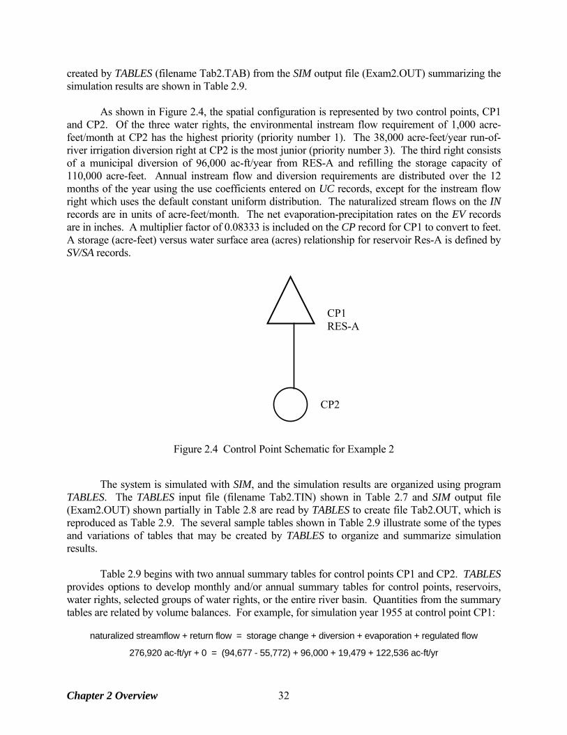
created by TABLES (filename Tab2.TAB) from the SIM output file (Exam2.OUT) summarizing the simulation results are shown in Table 2.9. As shown in Figure 2.4, the spatial configuration is represented by two control points, CP1 and CP2. Of the three water rights, the environmental instream flow requirement of 1,000 acre-feet/month at CP2 has the highest priority (priority number 1). The 38,000 acre-feet/year run-of-river irrigation diversion right at CP2 is the most junior (priority number 3). The third right consists of a municipal diversion of 96,000 ac-ft/year from RES-A and refilling the storage capacity of 110,000 acre-feet. Annual instream flow and diversion requirements are distributed over the 12 months of the year using the use coefficients entered on UC records, except for the instream flow right which uses the default constant uniform distribution. The naturalized stream flows on the IN records are in units of acre-feet/month. The net evaporation-precipitation rates on the EV records are in inches. A multiplier factor of 0.08333 is included on the CP record for CP1 to convert to feet. A storage (acre-feet) versus water surface area (acres) relationship for reservoir Res-A is defined by SV/SA records.
CP1 RES-A
CP2
Figure 2.4 Control Point Schematic for Example 2 The system is simulated with SIM, and the simulation results are organized using program TABLES. The TABLES input file (filename Tab2.TIN) shown in Table 2.7 and SIM output file (Exam2.OUT) shown partially in Table 2.8 are read by TABLES to create file Tab2.OUT, which is reproduced as Table 2.9. The several sample tables shown in Table 2.9 illustrate some of the types and variations of tables that may be created by TABLES to organize and summarize simulation results. Table 2.9 begins with two annual summary tables for control points CP1 and CP2. TABLES provides options to develop monthly and/or annual summary tables for control points, reservoirs, water rights, selected groups of water rights, or the entire river basin. Quantities from the summary tables are related by volume balances. For example, for simulation year 1955 at control point CP1:
naturalized streamflow + return flow = storage change + diversion + evaporation + regulated flow
276,920 ac-ft/yr + 0 = (94,677 - 55,772) + 96,000 + 19,479 + 122,536 ac-ft/yr
Chapter 2 Overview 32
Stream flow depletions are:
streamflow depletion = diversion + evaporation + storage refilling
CP1 1955 streamflow depletion = 96,000 + 19,479 + (94,677 - 55,772) = 154,384 ac-ft/yr
CP2 1955 streamflow depletion = diversion = 38,000 ac-ft/yr Since CP2 is the most downstream gage, the 1955 annual volume balance may be expressed as:
naturalized flows + return flows = CP1 and CP2 streamflow depletions + CP2 regulated flows
345,380 + 38,400 = 154,384 + 38,000 + 191,396 A reliability summary table is also included in Table 2.9. This type of table may be developed for diversion or hydropower requirements for individual rights, groups of rights, or all rights at control points or reservoirs. The 96,000 ac-ft/yr diversion target at CP1 has no shortages and thus period and volume reliabilities of 100.0%. The monthly diversion requirements for the 38,000 ac-ft/yr diversion at CP2 were met during 16 months of the 24-months for which permitted targets were non-zero, with shortages occurring in the other eight months. The period and volume reliabilities shown in Table 2.9 are computed as:
period reliability = [(24-8)/24] 100% = 66.67%
volume reliability = [(38,000-6,877)/38,000] 100% = 81.90% The reliability table shows that the diversion at CP2 equals or exceeds 50 percent of the monthly target in 91.7 percent of the months. The annual diversion equals or exceeds 34,200 ac-ft/yr (90% of the annual target of 38,000 ac-ft/yr) during 33.3% of the three years of the period-of-analysis. The first flow-frequency table in Table 2.9 (bottom of page 36) indicates that regulated monthly stream flows at CP2 vary from 1,000 ac-ft to 80,526 ac-ft, with a mean of 7,650 ac-ft. The regulated flow equals or exceeds 2,168 ac-ft during 75% of the 36 months. The second flow-frequency table is in an alternate format in which exceedance frequencies are determined for user-specified flow amounts. Frequency tables may be developed for naturalized, regulated, and unappropriated stream flows, reservoir storage, and instream flow shortage. The last six tables in Table 2.9 on are illustrative of TABLES time series tables of naturalized, regulated, and unappropriated flows; stream flow depletions; diversions, diversion or instream flow shortages; channel losses; or reservoir storage for either control points, reservoirs, water rights, or water right groups. The data may be tabulated as annual rows with monthly columns (page 37) and alternatively in a columnar format (page 38) to facilitate manipulation and plotting in a spreadsheet program such as Microsoft Excel. TABLES can also write the time series variables from the SIM simulation results, with or without optional adjustments, as binary DSS files which are read by HEC-DSSVue (Hydrologic Engineering Center 2005). SIM can also record results directly in a DSS file. DSS files can be read only by HEC-DSSVue or other HEC-DSS software. The primary motivation for converting SIM simulation results to records in a DSS file is to facilitate convenient plotting using HEC-DSSVue. However, the full spectrum of other HEC-DSS capabilities are available as well as graphics.
Chapter 2 Overview 33
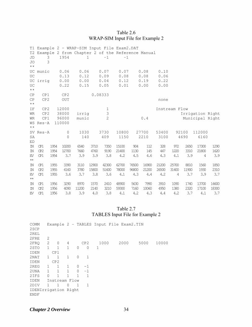
Table 2.6 WRAP-SIM Input File for Example 2
T1 Example 2 - WRAP-SIM Input File Exam2.DAT T2 Example 2 from Chapter 2 of the Reference Manual JD 3 1954 1 -1 -1 JO 3 ** UC munic 0.06 0.06 0.07 0.07 0.08 0.10 UC 0.13 0.12 0.09 0.08 0.08 0.06 UC irrig 0.00 0.00 0.04 0.12 0.19 0.22 UC 0.22 0.15 0.05 0.01 0.00 0.00 ** CP CP1 CP2 0.08333 CP CP2 OUT none ** IF CP2 12000 1 Instream Flow WR CP2 38000 irrig 3 Irrigation Right WR CP1 96000 munic 2 0.4 Municipal Right WS Res-A 110000 ** SV Res-A 0 1030 3730 10800 27700 53400 92100 112000 SA 0 140 409 1150 2210 3100 4690 6160 ED IN CP1 1954 10200 6540 3710 7350 15100 904 112 328 972 2650 17300 1290 IN CP2 1954 12700 7660 4760 9190 21400 1130 145 447 1220 3310 21800 1620 EV CP1 1954 3.7 3.9 3.9 3.8 4.2 4.5 4.6 4.3 4.1 3.9 4 3.9 ** IN CP1 1955 3390 3110 12900 42300 62700 76500 16900 21200 25700 8810 1560 1850 IN CP2 1955 4160 3780 15800 51600 78000 96800 21200 26500 31400 11900 1930 2310 EV CP1 1955 3.6 3.7 3.8 3.6 4.1 4.3 4.4 4.2 4 3.7 3.9 3.7 ** IN CP1 1956 3290 8970 1570 2410 48900 5630 7990 3910 1090 1740 13700 14600 IN CP2 1956 4090 11200 2140 3210 59300 7160 10060 4950 1380 2320 17100 18300 EV CP1 1956 3.8 3.9 4.0 3.8 4.1 4.2 4.3 4.4 4.2 3.7 4.1 3.7
Table 2.7
TABLES Input File for Example 2
COMM Example 2 - TABLES Input File Exam2.TIN 2SCP 2REL 2FRE 2 2FRQ 2 0 4 CP2 1000 2000 5000 10000 2STO 1 1 1 0 0 1 IDEN CP1 2NAT 1 1 1 0 1 IDEN CP2 2REG 1 1 1 0 -1 2UNA 1 1 1 0 -1 2IFS 0 1 1 1 1 IDEN Instream Flow 2DIV 1 1 0 1 1 IDENIrrigation Right ENDF
Chapter 2 Overview 34
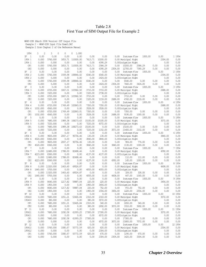
Table 2.8 First Year of SIM Output File for Example 2
WRAP-SIM (March 2008 Version) OUT Output File Example 2 - WRAP-SIM Input File Exam2.DAT Example 2 from Chapter 2 of the Reference Manual 1954 3 2 3 0 0 0 1.000 IF 1 0.00 0.00 0.00 0.00 0.00 0.00 0.00 Instream Flow 1000.00 0.00 1 1954 1954 1 0.000 5760.000 1853.71 110000.00 7613.71 10200.00 0.00 Municipal Right 2304.00 0.00 1954 1 0.000 0.000 0.00 0.00 0.00 6390.29 0.00Irrigation Right 0.00 0.00 CP1 0.000 5760.000 1853.71 110000.00 7613.71 2586.29 0.00 10200.00 2586.29 0.00 0.00 0.00 CP2 0.000 0.000 0.00 0.00 0.00 6390.29 2304.00 12700.00 7390.29 0.00 0.00 0.00 IF 2 0.00 0.00 0.00 0.00 0.00 0.00 0.00 Instream Flow 1000.00 0.00 2 1954 1954 2 0.000 5760.000 1939.98 108840.02 6540.00 6540.00 0.00 Municipal Right 2304.00 0.00 1954 2 0.000 0.000 0.00 0.00 0.00 2424.00 0.00Irrigation Right 0.00 0.00 CP1 0.000 5760.000 1939.98 108840.02 6540.00 0.00 0.00 6540.00 0.00 0.00 0.00 0.00 CP2 0.000 0.000 0.00 0.00 0.00 2424.00 2304.00 7660.00 3424.00 0.00 0.00 0.00 IF 3 0.00 0.00 0.00 0.00 0.00 0.00 0.00 Instream Flow 1000.00 0.00 3 1954 1954 3 0.000 6720.000 1867.51 103962.50 3710.00 3710.00 0.00 Municipal Right 2688.00 0.00 1954 3 0.000 1520.000 0.00 0.00 1520.00 2738.00 0.00Irrigation Right 0.00 0.00 CP1 0.000 6720.000 1867.51 103962.50 3710.00 0.00 0.00 3710.00 0.00 0.00 0.00 0.00 CP2 0.000 1520.000 0.00 0.00 1520.00 1218.00 2688.00 4760.00 2218.00 0.00 0.00 0.00 IF 4 0.00 0.00 0.00 0.00 0.00 0.00 0.00 Instream Flow 1000.00 0.00 4 1954 1954 4 0.000 6720.000 1749.49 102843.01 7350.00 7350.00 0.00 Municipal Right 2688.00 0.00 1954 4 1032.000 4560.000 0.00 0.00 3528.00 3528.00 0.00Irrigation Right 0.00 0.00 CP1 0.000 6720.000 1749.49 102843.01 7350.00 0.00 0.00 7350.00 0.00 0.00 0.00 0.00 CP2 1032.000 4560.000 0.00 0.00 3528.00 0.00 2688.00 9190.00 1000.00 0.00 0.00 0.00 IF 5 0.00 0.00 0.00 0.00 0.00 0.00 0.00 Instream Flow 1000.00 0.00 5 1954 1954 5 0.000 7680.000 1989.38 108273.63 15100.00 15100.00 0.00 Municipal Right 3072.00 0.00 1954 5 0.000 7220.000 0.00 0.00 7220.00 8372.00 0.00Irrigation Right 0.00 0.00 CP1 0.000 7680.000 1989.38 108273.63 15100.00 0.00 0.00 15100.00 0.00 0.00 0.00 0.00 CP2 0.000 7220.000 0.00 0.00 7220.00 1152.00 3072.00 21400.00 2152.00 0.00 0.00 0.00 IF 6 0.00 0.00 0.00 0.00 0.00 0.00 0.00 Instream Flow 1000.00 0.00 6 1954 1954 6 0.000 9600.000 2047.17 96756.46 130.00 130.00 0.00 Municipal Right 3840.00 0.00 1954 6 4520.000 8360.000 0.00 0.00 3840.00 3840.00 0.00Irrigation Right 0.00 0.00 CP1 0.000 9600.000 2047.17 96756.46 130.00 0.00 0.00 904.00 774.00 0.00 0.00 0.00 CP2 4520.000 8360.000 0.00 0.00 3840.00 0.00 3840.00 1130.00 1000.00 0.00 0.00 0.00 IF 7 0.00 0.00 0.00 0.00 0.00 0.00 0.00 Instream Flow 1000.00 0.00 7 1954 1954 7 0.000 12480.000 1788.00 82488.46 0.00 0.00 0.00 Municipal Right 4992.00 0.00 1954 7 4223.000 8360.000 0.00 0.00 4137.00 4137.00 0.00Irrigation Right 0.00 0.00 CP1 0.000 12480.000 1788.00 82488.46 0.00 0.00 0.00 112.00 112.00 0.00 0.00 0.00 CP2 4223.000 8360.000 0.00 0.00 4137.00 0.00 4992.00 145.00 1000.00 0.00 0.00 0.00 IF 8 0.00 0.00 0.00 0.00 0.00 0.00 0.00 Instream Flow 1000.00 0.00 8 1954 1954 8 0.000 11520.000 1443.60 69524.87 0.00 0.00 0.00 Municipal Right 4608.00 0.00 1954 8 1645.000 5700.000 0.00 0.00 4055.00 4055.00 0.00Irrigation Right 0.00 0.00 CP1 0.000 11520.000 1443.60 69524.87 0.00 0.00 0.00 328.00 328.00 0.00 0.00 0.00 CP2 1645.000 5700.000 0.00 0.00 4055.00 0.00 4608.00 447.00 1000.00 0.00 0.00 0.00 IF 9 0.00 0.00 0.00 0.00 0.00 0.00 0.00 Instream Flow 1000.00 0.00 9 1954 1954 9 0.000 8640.000 1217.82 59887.04 220.00 220.00 0.00 Municipal Right 3456.00 0.00 1954 9 0.000 1900.000 0.00 0.00 1900.00 3456.00 0.00Irrigation Right 0.00 0.00 CP1 0.000 8640.000 1217.82 59887.04 220.00 752.00 0.00 972.00 752.00 0.00 0.00 0.00 CP2 0.000 1900.000 0.00 0.00 1900.00 1556.00 3456.00 1220.00 2556.00 0.00 0.00 0.00 IF 10 0.00 0.00 0.00 0.00 0.00 0.00 0.00 Instream Flow 1000.00 0.00 10 1954 195410 0.000 7680.000 1051.21 53465.84 2310.00 2310.00 0.00 Municipal Right 3072.00 0.00 195410 0.000 380.000 0.00 0.00 380.00 3072.00 0.00Irrigation Right 0.00 0.00 CP1 0.000 7680.000 1051.21 53465.84 2310.00 340.00 0.00 2650.00 340.00 0.00 0.00 0.00 CP2 0.000 380.000 0.00 0.00 380.00 2692.00 3072.00 3310.00 3692.00 0.00 0.00 0.00 IF 11 0.00 0.00 0.00 0.00 0.00 0.00 0.00 Instream Flow 1000.00 0.00 11 1954 195411 0.000 7680.000 1092.58 61993.25 17300.00 17300.00 0.00 Municipal Right 3072.00 0.00 195411 0.000 0.000 0.00 0.00 0.00 6572.00 0.00Irrigation Right 0.00 0.00 CP1 0.000 7680.000 1092.58 61993.25 17300.00 0.00 0.00 17300.00 0.00 0.00 0.00 0.00 CP2 0.000 0.000 0.00 0.00 0.00 6572.00 3072.00 21800.00 7572.00 0.00 0.00 0.00 IF 12 0.00 0.00 0.00 0.00 0.00 0.00 0.00 Instream Flow 1000.00 0.00 12 1954 195412 0.000 5760.000 1080.67 55772.59 620.00 620.00 0.00 Municipal Right 2304.00 0.00 195412 0.000 0.000 0.00 0.00 0.00 2304.00 0.00Irrigation Right 0.00 0.00 CP1 0.000 5760.000 1080.67 55772.59 620.00 670.00 0.00 1290.00 670.00 0.00 0.00 0.00 CP2 0.000 0.000 0.00 0.00 0.00 2304.00 2304.00 1620.00 3304.00 0.00 0.00 0.00
Chapter 2 Overview 35
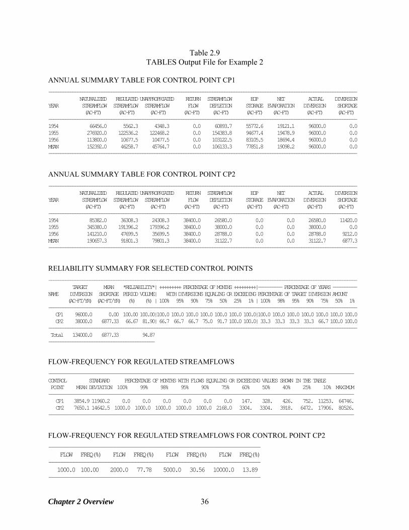
Table 2.9 TABLES Output File for Example 2
ANNUAL SUMMARY TABLE FOR CONTROL POINT CP1
-------------------------------------------------------------------------------------------------------------------------------- NATURALIZED REGULATED UNAPPROPRIATED RETURN STREAMFLOW EOP NET ACTUAL DIVERSION YEAR STREAMFLOW STREAMFLOW STREAMFLOW FLOW DEPLETION STORAGE EVAPORATION DIVERSION SHORTAGE (AC-FT) (AC-FT) (AC-FT) (AC-FT) (AC-FT) (AC-FT) (AC-FT) (AC-FT) (AC-FT) -------------------------------------------------------------------------------------------------------------------------------- 1954 66456.0 5562.3 4348.3 0.0 60893.7 55772.6 19121.1 96000.0 0.0 1955 276920.0 122536.2 122468.2 0.0 154383.8 94677.4 19478.9 96000.0 0.0 1956 113800.0 10677.5 10477.5 0.0 103122.5 83105.5 18694.4 96000.0 0.0 MEAN 152392.0 46258.7 45764.7 0.0 106133.3 77851.8 19098.2 96000.0 0.0 --------------------------------------------------------------------------------------------------------------------------------
ANNUAL SUMMARY TABLE FOR CONTROL POINT CP2
-------------------------------------------------------------------------------------------------------------------------------- NATURALIZED REGULATED UNAPPROPRIATED RETURN STREAMFLOW EOP NET ACTUAL DIVERSION YEAR STREAMFLOW STREAMFLOW STREAMFLOW FLOW DEPLETION STORAGE EVAPORATION DIVERSION SHORTAGE (AC-FT) (AC-FT) (AC-FT) (AC-FT) (AC-FT) (AC-FT) (AC-FT) (AC-FT) (AC-FT) -------------------------------------------------------------------------------------------------------------------------------- 1954 85382.0 36308.3 24308.3 38400.0 26580.0 0.0 0.0 26580.0 11420.0 1955 345380.0 191396.2 179396.2 38400.0 38000.0 0.0 0.0 38000.0 0.0 1956 141210.0 47699.5 35699.5 38400.0 28788.0 0.0 0.0 28788.0 9212.0 MEAN 190657.3 91801.3 79801.3 38400.0 31122.7 0.0 0.0 31122.7 6877.3 --------------------------------------------------------------------------------------------------------------------------------
RELIABILITY SUMMARY FOR SELECTED CONTROL POINTS
-------------------------------------------------------------------------------------------------------------------------------- TARGET MEAN *RELIABILITY*| +++++++++ PERCENTAGE OF MONTHS +++++++++|---------- PERCENTAGE OF YEARS ---------- NAME DIVERSION SHORTAGE PERIOD VOLUME| WITH DIVERSIONS EQUALING OR EXCEEDING PERCENTAGE OF TARGET DIVERSION AMOUNT (AC-FT/YR) (AC-FT/YR) (%) (%) | 100% 95% 90% 75% 50% 25% 1% | 100% 98% 95% 90% 75% 50% 1% -------------------------------------------------------------------------------------------------------------------------------- CP1 96000.0 0.00 100.00 100.00|100.0 100.0 100.0 100.0 100.0 100.0 100.0|100.0 100.0 100.0 100.0 100.0 100.0 100.0 CP2 38000.0 6877.33 66.67 81.90| 66.7 66.7 66.7 75.0 91.7 100.0 100.0| 33.3 33.3 33.3 33.3 66.7 100.0 100.0 -------------------------------------------------------------------------------------------------------------------------------- Total 134000.0 6877.33 94.87 --------------------------------------------
FLOW-FREQUENCY FOR REGULATED STREAMFLOWS
------------------------------------------------------------------------------------------------------------------------ CONTROL STANDARD PERCENTAGE OF MONTHS WITH FLOWS EQUALING OR EXCEEDING VALUES SHOWN IN THE TABLE POINT MEAN DEVIATION 100% 99% 98% 95% 90% 75% 60% 50% 40% 25% 10% MAXIMUM ------------------------------------------------------------------------------------------------------------------------ CP1 3854.9 11960.2 0.0 0.0 0.0 0.0 0.0 0.0 147. 328. 426. 752. 11253. 64746. CP2 7650.1 14642.5 1000.0 1000.0 1000.0 1000.0 1000.0 2168.0 3304. 3304. 3918. 6472. 17906. 80526. ------------------------------------------------------------------------------------------------------------------------
FLOW-FREQUENCY FOR REGULATED STREAMFLOWS FOR CONTROL POINT CP2
------------------------------------------------------------------------ FLOW FREQ(%) FLOW FREQ(%) FLOW FREQ(%) FLOW FREQ(%) ------------------------------------------------------------------------ 1000.0 100.00 2000.0 77.78 5000.0 30.56 10000.0 13.89 ------------------------------------------------------------------------
Chapter 2 Overview 36
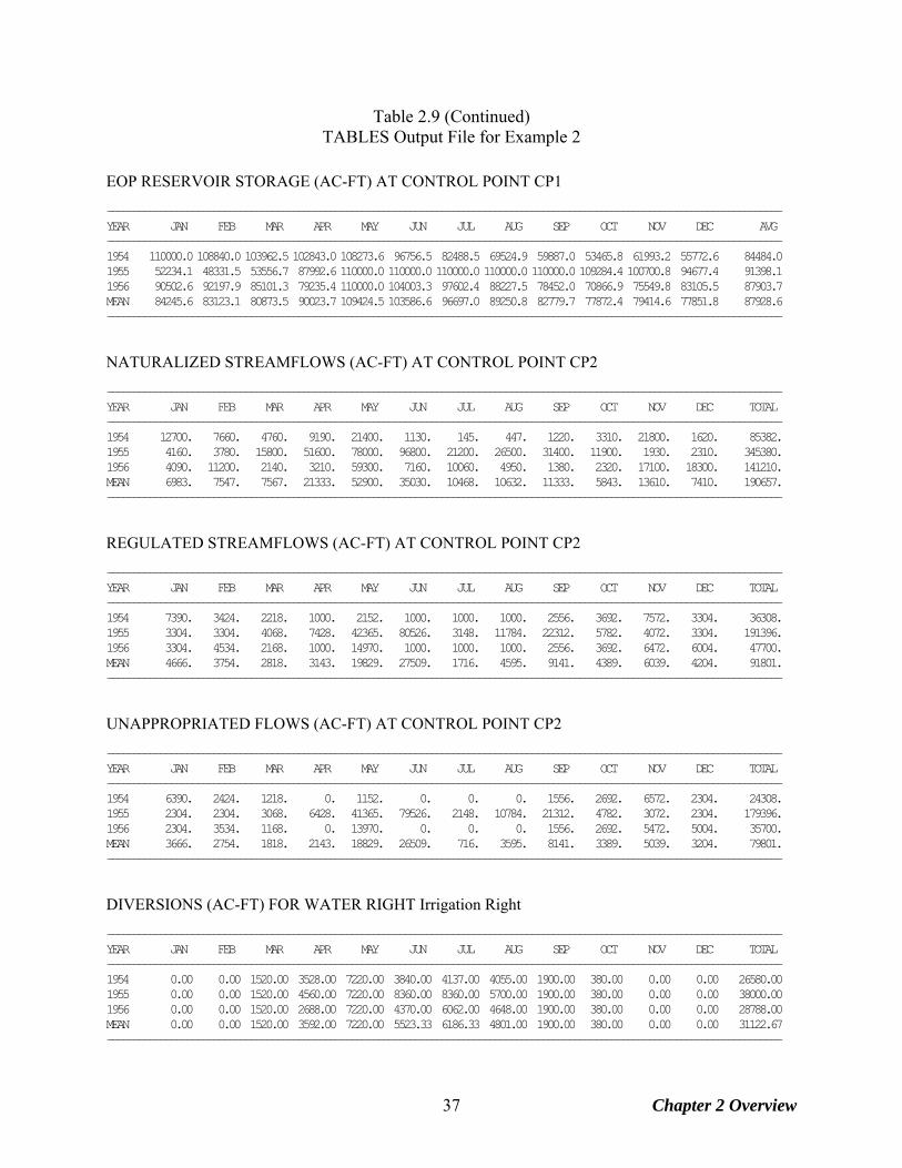
Table 2.9 (Continued) TABLES Output File for Example 2
EOP RESERVOIR STORAGE (AC-FT) AT CONTROL POINT CP1 ------------------------------------------------------------------------------------------------------------------------------- YEAR JAN FEB MAR APR MAY JUN JUL AUG SEP OCT NOV DEC AVG ------------------------------------------------------------------------------------------------------------------------------- 1954 110000.0 108840.0 103962.5 102843.0 108273.6 96756.5 82488.5 69524.9 59887.0 53465.8 61993.2 55772.6 84484.0 1955 52234.1 48331.5 53556.7 87992.6 110000.0 110000.0 110000.0 110000.0 110000.0 109284.4 100700.8 94677.4 91398.1 1956 90502.6 92197.9 85101.3 79235.4 110000.0 104003.3 97602.4 88227.5 78452.0 70866.9 75549.8 83105.5 87903.7 MEAN 84245.6 83123.1 80873.5 90023.7 109424.5 103586.6 96697.0 89250.8 82779.7 77872.4 79414.6 77851.8 87928.6 -------------------------------------------------------------------------------------------------------------------------------
NATURALIZED STREAMFLOWS (AC-FT) AT CONTROL POINT CP2 ------------------------------------------------------------------------------------------------------------------------------- YEAR JAN FEB MAR APR MAY JUN JUL AUG SEP OCT NOV DEC TOTAL ------------------------------------------------------------------------------------------------------------------------------- 1954 12700. 7660. 4760. 9190. 21400. 1130. 145. 447. 1220. 3310. 21800. 1620. 85382. 1955 4160. 3780. 15800. 51600. 78000. 96800. 21200. 26500. 31400. 11900. 1930. 2310. 345380. 1956 4090. 11200. 2140. 3210. 59300. 7160. 10060. 4950. 1380. 2320. 17100. 18300. 141210. MEAN 6983. 7547. 7567. 21333. 52900. 35030. 10468. 10632. 11333. 5843. 13610. 7410. 190657. -------------------------------------------------------------------------------------------------------------------------------
REGULATED STREAMFLOWS (AC-FT) AT CONTROL POINT CP2 ------------------------------------------------------------------------------------------------------------------------------- YEAR JAN FEB MAR APR MAY JUN JUL AUG SEP OCT NOV DEC TOTAL ------------------------------------------------------------------------------------------------------------------------------- 1954 7390. 3424. 2218. 1000. 2152. 1000. 1000. 1000. 2556. 3692. 7572. 3304. 36308. 1955 3304. 3304. 4068. 7428. 42365. 80526. 3148. 11784. 22312. 5782. 4072. 3304. 191396. 1956 3304. 4534. 2168. 1000. 14970. 1000. 1000. 1000. 2556. 3692. 6472. 6004. 47700. MEAN 4666. 3754. 2818. 3143. 19829. 27509. 1716. 4595. 9141. 4389. 6039. 4204. 91801. -------------------------------------------------------------------------------------------------------------------------------
UNAPPROPRIATED FLOWS (AC-FT) AT CONTROL POINT CP2 ------------------------------------------------------------------------------------------------------------------------------- YEAR JAN FEB MAR APR MAY JUN JUL AUG SEP OCT NOV DEC TOTAL ------------------------------------------------------------------------------------------------------------------------------- 1954 6390. 2424. 1218. 0. 1152. 0. 0. 0. 1556. 2692. 6572. 2304. 24308. 1955 2304. 2304. 3068. 6428. 41365. 79526. 2148. 10784. 21312. 4782. 3072. 2304. 179396. 1956 2304. 3534. 1168. 0. 13970. 0. 0. 0. 1556. 2692. 5472. 5004. 35700. MEAN 3666. 2754. 1818. 2143. 18829. 26509. 716. 3595. 8141. 3389. 5039. 3204. 79801. -------------------------------------------------------------------------------------------------------------------------------
DIVERSIONS (AC-FT) FOR WATER RIGHT Irrigation Right ------------------------------------------------------------------------------------------------------------------------------- YEAR JAN FEB MAR APR MAY JUN JUL AUG SEP OCT NOV DEC TOTAL ------------------------------------------------------------------------------------------------------------------------------- 1954 0.00 0.00 1520.00 3528.00 7220.00 3840.00 4137.00 4055.00 1900.00 380.00 0.00 0.00 26580.00 1955 0.00 0.00 1520.00 4560.00 7220.00 8360.00 8360.00 5700.00 1900.00 380.00 0.00 0.00 38000.00 1956 0.00 0.00 1520.00 2688.00 7220.00 4370.00 6062.00 4648.00 1900.00 380.00 0.00 0.00 28788.00 MEAN 0.00 0.00 1520.00 3592.00 7220.00 5523.33 6186.33 4801.00 1900.00 380.00 0.00 0.00 31122.67 -------------------------------------------------------------------------------------------------------------------------------
Chapter 2 Overview 37
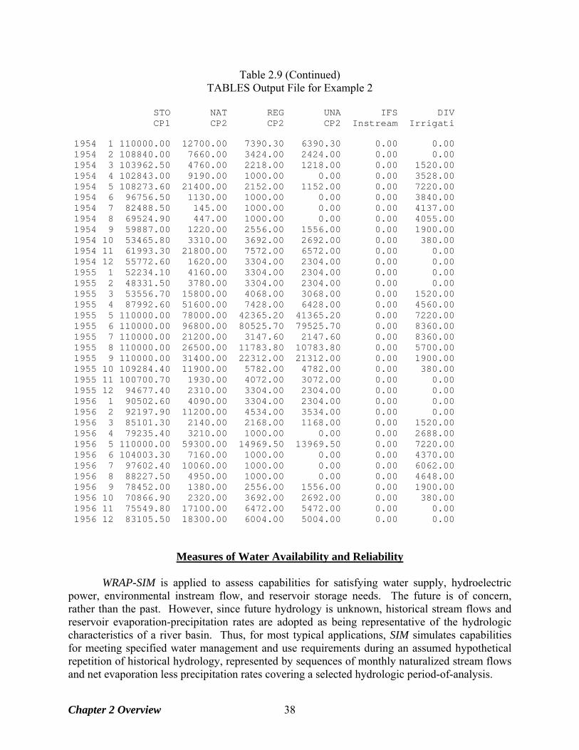
Table 2.9 (Continued) TABLES Output File for Example 2
STO NAT REG UNA IFS DIV CP1 CP2 CP2 CP2 Instream Irrigati 1954 1 110000.00 12700.00 7390.30 6390.30 0.00 0.00 1954 2 108840.00 7660.00 3424.00 2424.00 0.00 0.00 1954 3 103962.50 4760.00 2218.00 1218.00 0.00 1520.00 1954 4 102843.00 9190.00 1000.00 0.00 0.00 3528.00 1954 5 108273.60 21400.00 2152.00 1152.00 0.00 7220.00 1954 6 96756.50 1130.00 1000.00 0.00 0.00 3840.00 1954 7 82488.50 145.00 1000.00 0.00 0.00 4137.00 1954 8 69524.90 447.00 1000.00 0.00 0.00 4055.00 1954 9 59887.00 1220.00 2556.00 1556.00 0.00 1900.00 1954 10 53465.80 3310.00 3692.00 2692.00 0.00 380.00 1954 11 61993.30 21800.00 7572.00 6572.00 0.00 0.00 1954 12 55772.60 1620.00 3304.00 2304.00 0.00 0.00 1955 1 52234.10 4160.00 3304.00 2304.00 0.00 0.00 1955 2 48331.50 3780.00 3304.00 2304.00 0.00 0.00 1955 3 53556.70 15800.00 4068.00 3068.00 0.00 1520.00 1955 4 87992.60 51600.00 7428.00 6428.00 0.00 4560.00 1955 5 110000.00 78000.00 42365.20 41365.20 0.00 7220.00 1955 6 110000.00 96800.00 80525.70 79525.70 0.00 8360.00 1955 7 110000.00 21200.00 3147.60 2147.60 0.00 8360.00 1955 8 110000.00 26500.00 11783.80 10783.80 0.00 5700.00 1955 9 110000.00 31400.00 22312.00 21312.00 0.00 1900.00 1955 10 109284.40 11900.00 5782.00 4782.00 0.00 380.00 1955 11 100700.70 1930.00 4072.00 3072.00 0.00 0.00 1955 12 94677.40 2310.00 3304.00 2304.00 0.00 0.00 1956 1 90502.60 4090.00 3304.00 2304.00 0.00 0.00 1956 2 92197.90 11200.00 4534.00 3534.00 0.00 0.00 1956 3 85101.30 2140.00 2168.00 1168.00 0.00 1520.00 1956 4 79235.40 3210.00 1000.00 0.00 0.00 2688.00 1956 5 110000.00 59300.00 14969.50 13969.50 0.00 7220.00 1956 6 104003.30 7160.00 1000.00 0.00 0.00 4370.00 1956 7 97602.40 10060.00 1000.00 0.00 0.00 6062.00 1956 8 88227.50 4950.00 1000.00 0.00 0.00 4648.00 1956 9 78452.00 1380.00 2556.00 1556.00 0.00 1900.00 1956 10 70866.90 2320.00 3692.00 2692.00 0.00 380.00 1956 11 75549.80 17100.00 6472.00 5472.00 0.00 0.00 1956 12 83105.50 18300.00 6004.00 5004.00 0.00 0.00
Measures of Water Availability and Reliability WRAP-SIM is applied to assess capabilities for satisfying water supply, hydroelectric power, environmental instream flow, and reservoir storage needs. The future is of concern, rather than the past. However, since future hydrology is unknown, historical stream flows and reservoir evaporation-precipitation rates are adopted as being representative of the hydrologic characteristics of a river basin. Thus, for most typical applications, SIM simulates capabilities for meeting specified water management and use requirements during an assumed hypothetical repetition of historical hydrology, represented by sequences of monthly naturalized stream flows and net evaporation less precipitation rates covering a selected hydrologic period-of-analysis.
Chapter 2 Overview 38
The main simulation results from a WRAP-SIM simulation as organized by Program TABLES are discussed in Chapter 5. Additional auxiliary WRAP-SIM simulation results and analysis capabilities are covered in Chapter 6. Many different optional analysis methods and variations thereof are provided by WRAP for assessing water availability and reliability. Key fundamental concepts related to these simulation and analysis methods are introduced in this section of the present Chapter 2. Program SIM simulation results include hydrologic period-of-analysis sequences of monthly values for the variables listed in Table 2.1 and defined in detail in Chapter 5. A majority of the variables associated with water rights can be summed within SIM by control point or reservoir. Program TABLES allows simulation results associated with water rights to be aggregated by specified groups of rights. TABLES reads SIM input and output files, computes reliability indices and frequency relationships, and creates tables organizing and summarizing the simulation results as discussed in Chapters 5 and 6. Simulation studies are organized in a variety of ways to develop an understanding of the river basin system. Model runs demonstrate the effects of alternative water use scenarios and management strategies. Simulation results may be organized in various formats including: the entire time sequences of monthly values of various variables; annual summaries; period-of-analysis means; monthly, annual, or period-of-analysis water budgets; reliability indices; and frequency relationships. These forms of information may all be useful in analyzing, interpreting, and applying the results of a simulation study to support decision-making processes. Simulation results are typically viewed from the perspectives of frequency, probability, percent-of-time, or reliability of meeting water supply, instream flow, hydropower, and/or reservoir storage targets. Volume and Period Reliability Concise measures of reliability are useful in analyzing and displaying simulation results. A reliability summary is specified in TABLES with a 2REL record as illustrated by Table 2.9. This table may be created for either water supply diversion or hydroelectric energy generation targets for individual water rights, the aggregation of all rights associated with individual reservoirs or control points, groups of selected rights, or the aggregation of all rights in the model. TABLES computes both period reliabilities based on percent-of-time and volume reliabilities based on diversion volumes or hydroelectric energy amounts. Volume reliability is the percentage of the total target demand amount that is actually supplied. For water supply diversions, the amounts are volumes. For hydroelectric power, the amounts are kilowatt-hours of energy generated. Volume reliability (RV) is the ratio of volume supplied or energy supplied (v) to the volume or energy target (V), converted to a percentage.
(100%)VvRV =
(2.2)
Equivalently, for water supply, RV is the mean actual diversion rate as a percentage of the mean target diversion rate. For hydropower, RV is the mean actual rate of energy production as a percentage of the mean target energy production rate.
Chapter 2 Overview 39
Period reliability is based on counting the number of periods of the simulation during which the specified demand target is either fully supplied or a specified percentage of the target is equaled or exceeded. A reliability summary includes tabulations of period reliabilities expressed both as the percentage of months and the percentage of years during the simulation during which water supply diversions (or hydroelectric energy produced) equaled or exceeded specified magnitudes expressed as a percentage of the target demand. The various variations of period reliability (RP) are computed by TABLES from the results of a SIM simulation as:
PnR = (100%)N
(2.3)
where n denotes the number of periods during the simulation for which the specified percentage of the demand target is met, and N is the total number of periods. 2REL record options allow N and n to be defined either considering all months or only months with non-zero demand targets. A TABLES reliability summary includes tabulations of period reliabilities expressed both as the percentage of months and the percentage of years during the simulation during which diversions (or energy produced) equaled or exceeded specified magnitudes expressed as a percentage of the target demand. For example, the table shows the percentage of months in the simulation for which the computed diversion equals or exceeds 75% of the monthly diversion target. It also shows the percentage of years for which the total diversions during the year equal or exceed 75% of the annual permitted amount. The table also shows the percentage of months for which the demand is fully 100% met, without shortage. Thus, period reliability RP is an expression of the percentage of time that the full demand target or a specified portion of the demand target can be supplied. Equivalently, RP represents the likelihood or probability of the target being met in any randomly selected month or year. The period reliability RP is the complement (RP=1-F) of the risk of failure (F) that the demand target or specified percentage of the target will not be met. The firm (safe or dependable) yield associated with a particular water supply diversion or hydroelectric power production target is defined as the maximum annual demand target that can be met with a reliability of 100.0 percent based on all the premises reflected in the model. Firm yields may be determined by iteratively adjusting a target amount and rerunning SIM until the value meeting the definition of firm yield is found. As discussed in Chapter 6, the FY record activates a SIM option that automates this procedure. Flow-Frequency and Storage-Frequency Relationships Frequency tables created with TABLES 2FRE and 2FRQ records are also included in Table 2.9. These tables may be developed for naturalized flow, regulated flow, unappropriated flow, and reservoir storage for specified control points, instream flow shortages and reservoir storage for specified water rights, and storage volume and water surface elevation for specified reservoirs. The frequency tables may be for a specified month of the year such as August or for all months. Exceedance frequency is an expression of the percentage of time that particular flow or storage amounts can be expected to occur. Equivalently, the exceedance frequency represents the likelihood or probability of a certain amount of water being available.
Chapter 2 Overview 40
Exceedance frequencies may be determined with Eq. 2.4 based on ranking and counting.
nExceedance Frequency = (100%)N
(2.4)
where n is the number of months during the simulation that a particular flow or storage amount is equaled or exceeded, and N is the total number of months considered. Alternatively, 2FRE record options include modeling the frequency relationship with the log-normal or normal probability distributions based on the computed parameters mean and standard deviation. The 2FRE table includes the mean and standard deviation, minimum and maximum, and the flow or storage amounts that are equaled or exceeded specified percentages of the time. The 2FRQ table also develops a flow-frequency, storage-frequency, elevation-frequency, or instream flow shortage-frequency relationship. However, the model-user enters specified flow or storage values of interest. TABLES simply counts the number of months for which a specified amount was equaled or exceeded and applies Equation 2.4 to assign a frequency.
Program SIM Options Involving Cyclic Repetitions of the Simulation The SIM simulation computations outlined in Figure 2.2 are discussed earlier in this chapter. A specified scenario of water resources development, allocation, management, and use is simulated during each sequential month of a hydrologic period-of-analysis with stream flow inflows and reservoir net evaporation rates representing historical hydrology for natural conditions or some other specified condition of river basin development. For example, the hydrologic period-of-analysis might be 1940-2005, covering a sequence of 792 months. The simulation begins with January 1940 naturalized stream flows and net evaporation rates and proceeds through the 792 months. In many typical applications, a particular execution of SIM involves a single simulation covering the hydrologic period-of-analysis once. However, SIM has several optional features that involve two or more repetitions of the hydrologic period-of-analysis simulation automated within a single execution of SIM. With one or more of the following optional features activated, the simulation is automatically repeated two or more times with a single execution of SIM.
• Dual simulation options activated by the JO, SO or PX records and described in Chapter 4 of this Reference Manual.
• Yield-reliability analysis routine activated by the FY record as outlined in Chapter 6.
• Beginning-ending storage options activated by the JO record and described in Chapter 6 of this Reference Manual.
• Monthly cycle option of conditional reliability modeling explained in Chapter 2 of the Supplemental Manual.
The dual simulation and beginning-ending storage features each involve two simulations. The yield-reliability analysis routine may iteratively repeat the simulation any number of times. The conditional reliability modeling routine may also activate multiple repetitions of the simulation.
Chapter 2 Overview 41

The simulation is repeated in its entirety from the beginning to the end of the hydrologic period-of-analysis with the four routines noted in the preceding paragraph. Another different SIM modeling feature involves a second pass through the water rights priority sequence simulation repeated within individual months. Second pass options activated by instream flow IF record field 7 or JO record field 10 and outlined in Chapter 4 involve dual passes through the water right priority loop. As indicated in Figure 2.2, the two passes through the water right computations are embedded within the monthly loop.
Chapter 2 Overview 42
CHAPTER 3 HYDROLOGY FEATURES
River basin hydrology is represented in WRAP-SIM by input sequences of naturalized stream flows and reservoir net evaporation-precipitation depths for each month of the hydrologic period-of-analysis at each pertinent location. WRAP-HYD is designed to facilitate developing hydrology-related WRAP-SIM input data sets. Both programs include routines for incorporating channel losses in various computations, based on including loss factors for pertinent stream reaches in the input data. The model is based on total stream flows, rather than incremental inflows. However, options are provided in HYD and SIM to address the issue of negative incremental flows. These hydrology-related features of the model described in this chapter involve stream flow and/or reservoir water surface evaporation less precipitation. Most of the chapter focuses on stream flow. Chapter 4 covers aspects of the model dealing with water rights requirements including reservoir storage and water management, allocation, and use.
WRAP-SIM allocates naturalized stream flows to meet specified water right requirements subject to channel losses and losses or gains associated with evaporation from and precipitation onto reservoir water surfaces. A conventional application of SIM is based on:
• simulating capabilities for fulfilling specified river regulation and water use requirements for a specified scenario of water resources development infrastructure, reservoir system operating rules, and water allocation practices
• during an assumed hypothetical repetition of historical hydrology represented by sequences of monthly naturalized stream flows and reservoir net evaporation-precipitation rates covering a selected hydrologic period-of-analysis.
The future is of concern, rather than the past. However, future hydrology is unknown. Historical stream flows and reservoir evaporation less precipitation rates are adopted as being representative of the hydrologic characteristics of a river basin that can be expected to continue into the future. A typical hydrologic period-of-analysis used for studies in Texas is 1940 to near the present. This period includes the 1950-1957 most severe drought-of-record as well as a full range of fluctuating wet and dry periods. Water resources are highly variable and highly stochastic (random), subject to extremes of droughts and floods as well as continuous more normal fluctuations. Major droughts typically involve long periods with sequences of many months of low flows. A basic premise of the conventional modeling approach is that historical naturalized stream flows and evaporation-precipitation rates for an adequately long period-of-analysis capture the essential statistical characteristics of river basin hydrology. WRAP is a river/reservoir system model with little capability for simulating groundwater or surface/subsurface water interactions. However, some interactions between stream flow and subsurface water may be modeled. Channel loss features are described in this chapter. Water supply return flows covered in Chapter 4 may originate from groundwater sources. Groundwater return flows may be modeled using constant inflow CI records or as a WR record type 4 right. Changes in spring flows or stream base flows associated with aquifer pumping or management scenarios, simulated with a groundwater model, may be treated as adjustments to naturalized stream flows contained in a WRAP-SIM flow adjustment file.
Chapter 3 Hydrology 43
Naturalized Stream Flow A WRAP-SIM simulation begins with homogeneous sequences of monthly stream flow volumes covering the hydrologic period-of-analysis at all control points. Program HYD provides a set of optional routines for developing homogeneous stream flow datasets for input to SIM. For each control point, stream flows must be either provided as input to SIM or computed within SIM from flows at one or more other control points using the flow distribution techniques that are incorporated in both HYD and SIM and described later in this chapter. No limits are imposed on the length of the period-of-analysis. Any units may be used in combination with appropriate conversion factors. Typical English units for stream flow are acre-feet/month. Typical metric units for stream flow are thousand cubic meters per month. Homogeneous Stream Flow Sequences Homogeneous means that the flows represent a specified uniform condition of watershed and river system development, long-term climate, and water use. Non-homogeneities in historical gaged stream flows are typically caused primarily by construction of reservoir projects, growth or changes in water use, and other changes in water management practices over time. However, watershed land use changes, climate changes, and other factors may also affect the homogeneity of recorded stream flow measurements. Flows observed at gaging stations during past years may be adjusted to develop flow sequences representing a specified scenario of water resources development and management, water use, watershed land use, climate, and hydrologic conditions. The stream flows in the SIM input dataset (IN records in FLO file or DSS file) may be naturalized flows representing natural hydrology unaffected by water resources development and management. Alternatively, the stream flow inflows input to the river/reservoir system simulation model may represent some other specified homogeneous condition of river basin development. The basic concept is to provide a homogeneous set of flows as input to SIM representing hydrology for a specified condition of river basin development. The stream flows in the SIM input dataset should represent flows unaffected by the reservoirs, diversions, return flows, and other water management practices and water use reflected in the SIM water rights input dataset. Typically, SIM stream flow input datasets represent natural hydrology without human impact but alternatively may reflect other scenarios of river basin hydrology, depending on the particular application. The term naturalized flow may be applied generically to refer to any stream flows adopted for a SIM input dataset. The objective of the stream flow naturalization process is to develop a homogeneous set of flows representing natural river basin hydrology. Historical observed flows are adjusted to remove nonhomogeneities caused by human activities. Naturalized stream flows represent the natural flows that would have occurred in the absence of the water users and water management facilities and practices reflected in the WRAP-SIM water rights input dataset. Developing naturalized flows typically represents a major portion of the effort required for a creating a SIM input dataset. The extent to which observed historical flows are naturalized is based largely on judgment. In extensively developed river basins, quantifying and removing all effects of human activities is not possible. For sites with relatively undeveloped watersheds, little or no adjustments may be necessary.
Chapter 3 Hydrology 44
Sequences of monthly flows representing historical natural hydrology are typically developed by adjusting recorded flows at gaging stations to remove the past impacts of upstream major reservoirs, water supply diversions, return flows from surface and ground water sources, and possibly other factors. In most typical major river basins, numerous smaller reservoirs have been constructed over many decades, but most of the storage capacity is contained in a relatively few large reservoirs. Decisions are required regarding which reservoirs to include in the adjustments. Major water supply diversions and return flows are typically also included in the flow adjustments. Other types of adjustments may be made as well. For example, land use changes such as clearing forests and urbanization or climate change due to global warming may significantly affect stream flow. A watershed model such as the Soil and Water Assessment Tool (SWAT) may be used to quantify the impacts of land use changes on stream flows. Wurbs, Muttiah, and Felden (2005) outline an approach for using a global circulation model reflecting climate change in combination with the SWAT precipitation-runoff model to adjust WRAP naturalized stream flows for alternative scenarios of future long-term climate change. Without adequate historical gaged stream flow records, naturalized flows representing a specified condition of watershed development may be synthesized from precipitation data with a watershed precipitation-runoff model such as SWAT. However, adjusting gaged flows to remove nonhomogeneities is generally more accurate than synthesizing flows with a watershed model. WRAP Features for Developing Flow Datasets The following tasks are involved in developing the sequences of monthly naturalized flows covering the hydrologic period-of-analysis at all control points required for a SIM simulation.
1. developing sequences of naturalized flows at stream gaging stations using HYD
2. synthesizing flows for gaps of missing data and extending record lengths outside of WRAP
3. distributing naturalized flows from gaged to ungaged locations within either HYD or SIM WRAP includes routines to assist with the first and third task, but not the second. Various gaging stations have different periods-of-record, and there may be gaps with missing data. The second task consists of extending flow sequences and reconstituting missing data using regression techniques with data from other gages and other months at the same gage. Regression analysis capabilities are readily available in other computer software packages and are not incorporated in WRAP. As discussed later in this chapter, program HYD provides various hydrology data compilation capabilities, which among other capabilities include options for:
• converting observed gaged stream flows to naturalized stream flows using techniques described later in this chapter
• distributing flows from gaged to ungaged locations using techniques described later in this chapter
• otherwise adjusting stream flows as described in Chapter 6 HYD writes stream flows as a set of inflow IN records in a text file or as binary records in a Data Storage System (DSS) file for input to SIM.
Chapter 3 Hydrology 45
Reservoir Evaporation-Precipitation Evaporation from a reservoir and precipitation falling directly on the reservoir water surface are combined as a net evaporation minus precipitation. Net evaporation less precipitation volumes are computed by multiplying the reservoir water surface area by net evaporation-precipitation rates provided on EV records in dimensions of depth/month. Various units may be used. Typical units include water surface area in acres, evaporation-precipitation rates in feet/month, and volumetric rates in acre-feet/month. Computation of evaporation-precipitation volumes are incorporated in HYD and SIM reservoir volume accounting routines. The SIM evaporation computations are described in the Chapter 5 section entitled Iterative Reservoir Volume Balance Computations. Within HYD, the computations are performed in conjunction with reservoir adjustments for converting gaged stream flow to naturalized stream flow. HYD also provides optional capabilities for combining sets of evaporation and/or precipitation depths to develop EV records. Precipitation depths may be subtracted from evaporation depths or sets of evaporation, precipitation, or net evaporation-precipitation depths may be averaged. Within SIM, net evaporation minus precipitation volume is included in the monthly water accounting computations performed in the water rights simulation loop. Average water surface area is determined as a function of storage content at the beginning and end of the month. Since both end-of-month storage and net evaporation-precipitation volumes are unknowns in the computations, an iterative solution algorithm is required. Adjusted Net Evaporation-Precipitation
SIM and HYD include options to account for the fact that a portion of the precipitation falling on the reservoir water surface is also reflected in the naturalized stream flows. Without a reservoir, the runoff from the land area of the non-existent reservoir contributes to stream flow. However, only a portion of the precipitation falling at the reservoir site contributes to stream flow. The remainder is lost through infiltration and other hydrologic abstractions. With the reservoir in place, all of the precipitation falling on the water surface is inflow to the reservoir.
SIM and HYD options include adjustments in the reservoir volume balance computations for the runoff from the land area covered by a reservoir that would have occurred without the reservoir. This adjustment in HYD may be incorporated with other adjustments in removing the historical effects of reservoirs in the process of converting gaged stream flows to naturalized flows. The option in SIM accounts for the portion of the reservoir surface precipitation that is already reflected in the naturalized stream flow inflows. In a typical application mode, the HYD adjustment is added to historical stream flows to determine naturalized stream flows. In SIM, the adjustment reduces available water amounts to prevent double-counting which would occur inappropriately if the runoff from the reservoir site is included in both the naturalized stream flows (IN records) and precipitation falling on the reservoir water surface (EV records).
The procedure in SIM for adjusting net evaporation-precipitation depths for runoff from reservoir sites are outlined as follows. The HYD version is outlined later in this chapter.
Chapter 3 Hydrology 46
• Net evaporation minus precipitation depths are input on EV records in an EVA file or as binary records in a DSS file.
• A precipitation-runoff adjustment term is computed within SIM to prevent double-counting
the reservoir surface precipitation that is already in the IN record naturalized flows. JD record field 10 (EPADJ) and CP record field 9 (EWA) activates this option. The JD record field 10 sets the default option applied to all control points for which the CP record field 9 is left blank. An entry for EWA on a CP record overrides the default option set by EPADJ on the JD record. Without the JD and CP record entries, the adjustment option is not applied.
• The precipitation-runoff adjustment requires a drainage area and corresponding naturalized
stream flows. An effective total watershed area may be input as a positive number in CP record field 9 for use with the total naturalized flows at that control point. Alternatively, the incremental or total watershed area and corresponding incremental or total naturalized flows for either the ungaged (FD record field 2) or gaged (FD record field 3) control points may be used by entering a –1 or –2 in CP record field 9 (applicable to that control point) or JD record field 10 (default for all control points). Incremental flows and watershed areas determined based on information from the FD and WP records are identically the same for the rainfall-runoff adjustments as for distributing stream flows from gaged to ungaged sites.
Within SIM, the portion of the naturalized stream flows derived from precipitation falling on dry land, that is now in the model covered by the reservoir, is determined by an algorithm that is conceptually identical to the drainage area ratio method for transferring stream flow. Although a drainage area ratio is not actually computed, the method is conceptually the same. SIM performs the adjustment computations for each month as follows. 1. A stream flow per unit drainage area or runoff depth (in feet/month) is computed by dividing
the total or incremental monthly naturalized stream flow (in acre-feet/month) by the watershed area from the CP record or FD/WP records.
2. The runoff depth computed in step 1 above is added to the net evaporation-precipitation rate
read from an EV record. Thus, the adjusted net evaporation-precipitation rate is the evaporation rate minus precipitation rate plus rainfall-runoff depth computed in step 1 above.
3. The algorithms for determining net evaporation volumes and performing the reservoir
volume accounting remain unchanged. The only difference is that the EV record net evaporation-precipitation rates input to the computations have been adjusted as noted above. The net evaporation-precipitation volume is determined by multiplying the reservoir water surface area by the adjusted net evaporation-precipitation depth.
Program HYD Hydrology Data Manipulation Capabilities
Program HYD is designed to facilitate developing hydrology-related input data for SIM. The HYDrology data program provides a set of optional routines to read, modify, and create sequences of naturalized or otherwise adjusted monthly stream flow volumes and net reservoir surface monthly evaporation less precipitation depths. HYD output files are read by SIM as input files. HYD has certain computational routines that are also available in SIM and others that are not.
Chapter 3 Hydrology 47
Data may be simply read from HYD input files and written to a HYD output file with no adjustments other than changing the organization and/or format of the dataset. Alternatively, the data may undergo a variety of adjustments and manipulations employing various computational options. Capabilities are provided for performing the tasks outlined in Table 3.1 and discussed in the following paragraphs. The tasks are listed in Table 3.1 generally in the order in which they are performed within HYD. All tasks are optional. The model-user specifies any number of tasks to be performed in a particular execution of HYD through entries on the JC, CP, EP, OI, AN, AS, RS and EQ input records which are described in Chapter 5 of the Users Manual. The various HYD options involve reading data from HYD input files or a SIM output file and performing computations to create stream flow and/or evaporation-precipitation datasets stored in new files. HYD options also include developing several related tables as well as sets of IN and EV records or DSS records. A single execution of HYD may include any number of data adjustments. Alternatively, in order to sequence the adjustments certain ways, multiple runs may be made with the output file from one run being read as the input file for the next. Files may also be transported back and forth between HYD and spreadsheet programs. Many of the computations performed by HYD are also adaptable to spreadsheet programs. Initial Data Manipulations The following optional initial tasks are activated by parameters entered on XL, CP, and MF records described in Chapter 5 of the Users Manual.
• The flows and/or evaporation-precipitation rates are multiplied by factors specified on XL, CP, and MF records. The monthly factors on MF records may also be added.
• Stream flows and/or evaporation-precipitation rates may be assigned to a control point by either verbatim repeating data from another control point or by multiplying the repeated flows by the factors from the CP records.
The XL and CP record factors in HYD are essentially the same as the factors in SIM covered in Chapter 3 of the Users Manual. The factors may be used for unit conversions, such as converting stream flows from second-feet-day (ft3/s×day) to acre-feet or net evaporation-precipitation depths from inches to feet. Also, the same stream flow or evaporation-precipitation rates may be conveniently assigned to multiple control points as appropriate. Drainage area ratios may be applied to transfer flows from gaged to ungaged sites. These data adjustments occurring immediately after the original data are read are then followed by the other optional tasks listed in Table 3.1. Changing the Organization and Format of the Datasets HYD reads input files near the beginning of program execution before the data handling and computational tasks and writes to output files near the end. The organization and format for the output files may be different than that of the input files. Datasets may also be converted between text files and Data Storage System (DSS) files and between SIM/HYD files and Microsoft Excel spreadsheet files. Text files may be reorganized. Options listed in Table 3.1 allow reading input files in alternative formats and converting to another selected format. The alternative formats are further discussed in Chapter 5 of the Users Manual.
Chapter 3 Hydrology 48
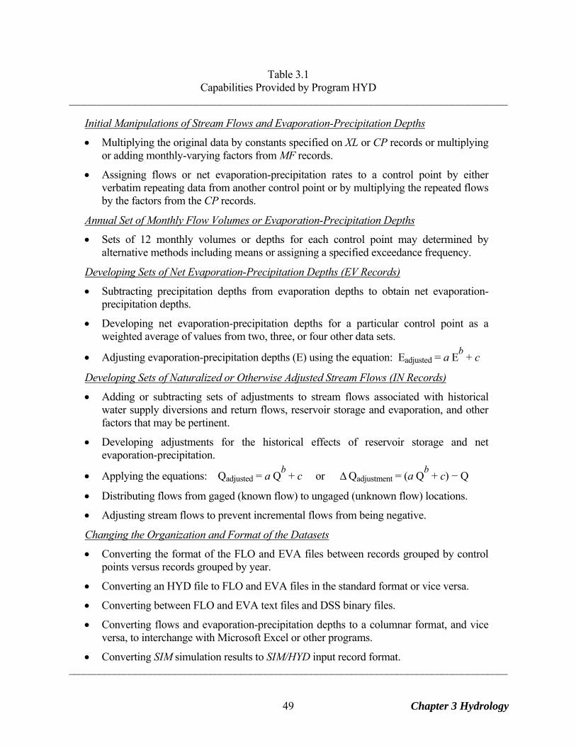
Table 3.1 Capabilities Provided by Program HYD
_______________________________________________________________________________________
Initial Manipulations of Stream Flows and Evaporation-Precipitation Depths
• Multiplying the original data by constants specified on XL or CP records or multiplying or adding monthly-varying factors from MF records.
• Assigning flows or net evaporation-precipitation rates to a control point by either verbatim repeating data from another control point or by multiplying the repeated flows by the factors from the CP records.
Annual Set of Monthly Flow Volumes or Evaporation-Precipitation Depths
• Sets of 12 monthly volumes or depths for each control point may determined by alternative methods including means or assigning a specified exceedance frequency.
Developing Sets of Net Evaporation-Precipitation Depths (EV Records)
• Subtracting precipitation depths from evaporation depths to obtain net evaporation-precipitation depths.
• Developing net evaporation-precipitation depths for a particular control point as a weighted average of values from two, three, or four other data sets.
• Adjusting evaporation-precipitation depths (E) using the equation: Eadjusted = a Eb + c
Developing Sets of Naturalized or Otherwise Adjusted Stream Flows (IN Records)
• Adding or subtracting sets of adjustments to stream flows associated with historical water supply diversions and return flows, reservoir storage and evaporation, and other factors that may be pertinent.
• Developing adjustments for the historical effects of reservoir storage and net evaporation-precipitation.
• Applying the equations: Qadjusted = a Qb + c or ΔQadjustment = (a Qb + c) − Q
• Distributing flows from gaged (known flow) to ungaged (unknown flow) locations.
• Adjusting stream flows to prevent incremental flows from being negative.
Changing the Organization and Format of the Datasets
• Converting the format of the FLO and EVA files between records grouped by control points versus records grouped by year.
• Converting an HYD file to FLO and EVA files in the standard format or vice versa.
• Converting between FLO and EVA text files and DSS binary files.
• Converting flows and evaporation-precipitation depths to a columnar format, and vice versa, to interchange with Microsoft Excel or other programs.
• Converting SIM simulation results to SIM/HYD input record format. _______________________________________________________________________________________
Chapter 3 Hydrology 49
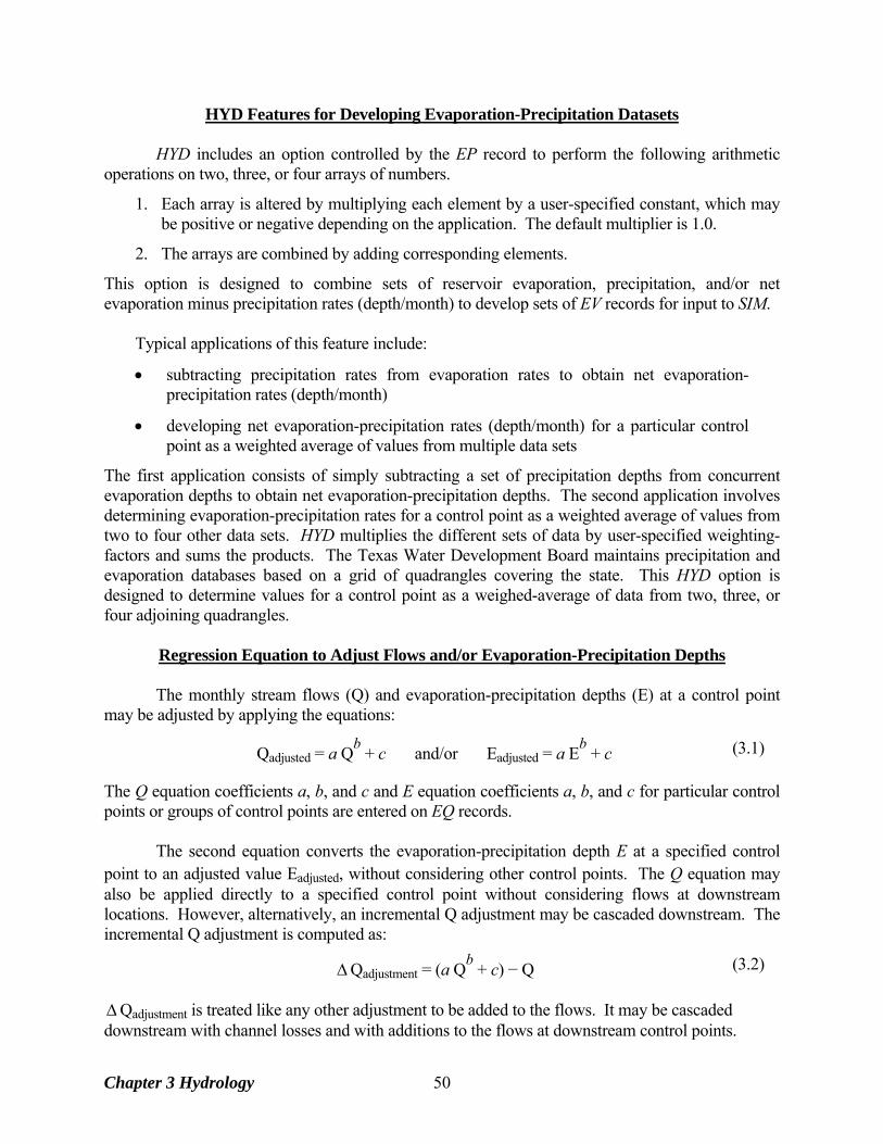
HYD Features for Developing Evaporation-Precipitation Datasets
HYD includes an option controlled by the EP record to perform the following arithmetic operations on two, three, or four arrays of numbers.
1. Each array is altered by multiplying each element by a user-specified constant, which may be positive or negative depending on the application. The default multiplier is 1.0.
2. The arrays are combined by adding corresponding elements.
This option is designed to combine sets of reservoir evaporation, precipitation, and/or net evaporation minus precipitation rates (depth/month) to develop sets of EV records for input to SIM.
Typical applications of this feature include:
• subtracting precipitation rates from evaporation rates to obtain net evaporation-precipitation rates (depth/month)
• developing net evaporation-precipitation rates (depth/month) for a particular control point as a weighted average of values from multiple data sets
The first application consists of simply subtracting a set of precipitation depths from concurrent evaporation depths to obtain net evaporation-precipitation depths. The second application involves determining evaporation-precipitation rates for a control point as a weighted average of values from two to four other data sets. HYD multiplies the different sets of data by user-specified weighting-factors and sums the products. The Texas Water Development Board maintains precipitation and evaporation databases based on a grid of quadrangles covering the state. This HYD option is designed to determine values for a control point as a weighed-average of data from two, three, or four adjoining quadrangles.
Regression Equation to Adjust Flows and/or Evaporation-Precipitation Depths
The monthly stream flows (Q) and evaporation-precipitation depths (E) at a control point may be adjusted by applying the equations:
Qadjusted = a Qb + c and/or Eadjusted = a Eb + c (3.1)
The Q equation coefficients a, b, and c and E equation coefficients a, b, and c for particular control points or groups of control points are entered on EQ records.
The second equation converts the evaporation-precipitation depth E at a specified control point to an adjusted value Eadjusted, without considering other control points. The Q equation may also be applied directly to a specified control point without considering flows at downstream locations. However, alternatively, an incremental Q adjustment may be cascaded downstream. The incremental Q adjustment is computed as:
ΔQadjustment = (a Qb + c) − Q (3.2) ΔQadjustment is treated like any other adjustment to be added to the flows. It may be cascaded downstream with channel losses and with additions to the flows at downstream control points.
Chapter 3 Hydrology 50
The regression equation feature may be used in various ways. It was incorporated into HYD particularly for use with a precipitation-runoff watershed simulation model such as the Soil and Water Assessment Tool (SWAT) developed at the USDA Agricultural Research Service and Texas Agricultural Experiment Station Research Center in Temple, Texas. The precipitation-runoff model may be used to quantify the effects of watershed land use changes. SWAT and WRAP have also been applied in combination on a research project assessing the impacts of climate change on water management (Wurbs et al. 2005). Stream flow is computed with SWAT for given precipitation and other climatic data and watershed characteristics. Changes in land use are modeled by changing watershed parameter values. Changes in climate are reflected in precipitation, temperature, and other climatic variables. The precipitation-runoff model is applied to compute stream flows for scenarios with and without climate or watershed changes. Regression analyses are then applied to flows computed with the two different scenarios to obtain a set of a, b, c coefficients for input to WRAP-HYD. As discussed later in this chapter, a regression equation likewise may be used with FD/FC records to distribute flows from gaged to ungaged locations.
HYD Features for Developing Stream Flow Datasets The following HYD capabilities are provided to facilitate developing the monthly flow volumes which are input to SIM as IN records in a FLO file or DSS records in a DSS file.
1. adding or subtracting sets of adjustments to flows with the flow adjustments being obtained from various sources and optionally cascading downstream
2. developing flow adjustments for the historical effects of reservoirs
3. applying the equations: Qadjusted = a Qb + c or ΔQadjustment = (a Qb + c) − Q
4. distributing flows from gaged (known flow) to ungaged (unknown flow) locations
5. adjusting stream flows to prevent incremental flows from being negative The objective of the stream flow adjustment routines in HYD is to provide a flexible generic set of options to facilitate adjusting a set of stream flows to reflect changes in river basin development. The most typical application is converting historical stream flows to naturalized flows. However, conversions between other scenarios of watershed development may also be of interest. HYD is designed to be flexible for application to various situations including those discussed in Chapter 6 as well as the type of applications noted in the present Chapter 3. Manipulation of flow data may involve combined use of HYD, Microsoft Excel or other spreadsheet programs, and HEC-DSSVue. Stream Flow Naturalization Adjustments Naturalized stream flows are gaged flows adjusted to remove the effects of human water management and use. HYD has options for modifying stream flows by adding or subtracting any number of data sets of flow adjustments. Typically, the original unadjusted stream flows will be historical gaged flows. Typical adjustments include historical water supply diversions, return flows from surface and/or groundwater diversions, reservoir storage changes, and reservoir surface evaporation/precipitation. Other types of adjustments may be added or subtracted as well. For
Chapter 3 Hydrology 51
example, changes in spring flows or stream base flows determined with a groundwater model and associated with alternative aquifer management strategies may be treated as adjustments to naturalized stream flows. The adjustment data sets are simply time series of numbers to be added to the stream flows. The flow adjustments may be positive, negative, or zero. An option allows an adjustment data set to be multiplied by a user-specified factor prior to being added to the flows. Any number of sets of adjustments may be applied at a particular control point. The data sets are added at a specified control point and optionally at all downstream control points. If the channel loss factor field of the control point CP record is non-zero, channel losses are reflected in cascading the adjustments downstream. Options are provided for setting the final adjusted flows to zero if the computations result in negative values. Particular adjustments may cover all or any portion of the hydrologic period-of-analysis. The adjustments to be combined with the stream flows may consist of either constant annual sequences of 12 monthly values or longer multiple-year time series. Adjustments for the effects of reservoirs are computed within HYD and then handled the same as the other adjustments read from input files. The following types of sets of adjustments may be added to the stream flows.
1. A constant may be entered on the AS record to add to the flows.
2. A set of 12 adjustments for each of the 12 months of the year to be repeated annually during a specified span of years are input on constant inflow CI records.
3. Multiple-year time series of adjustments are entered on flow adjustment FA records.
4. Variables read from the SIM output file may serve as flows and flow adjustments.
5. Adjustments for the effects of reservoirs may be computed within HYD.
All five types of adjustments are handled the same. An adjustment specification AS record provides the following information for each set of adjustments.
• control point identifier • beginning and ending year of adjustments • source of adjustments • whether adjustments are to be applied to all downstream control points • factor by which adjustments are multiplied • selection of option for dealing with possibility of negative stream flows
Adjustments may result in negative stream flows. Options are available to either maintain
the negative flows as the adjustments accumulate or set them equal to zero. For multiple sets of adjustments, the negative values in the cumulatively adjusted stream flows may be set to zero after any specified adjustment. If negative flows are changed to zero, an option allows flow in the next month to be decreased by the amount of the negative flow. Another option limits the adjustment to the amount of stream flow. For example, if an adjustment of 25 acre-feet/month is to be subtracted from a stream flow of 15 acre-feet/month, the adjustment is changed to 15 acre-feet/month. The 15 acre-feet (not 25 acre-feet) adjustment is applied at each control point as the adjustment cascades downstream.
Chapter 3 Hydrology 52
Stream Flow Adjustments for the Effects of Reservoirs Input data required to compute adjustments for the effects of reservoirs on stream flow include historical end-of-month storage content (SC records) and storage-area relationships (SV/SA or RS records), and net evaporation-precipitation rates (EV records). The adjustments include the following user-specified component parts that are combined to obtain a total adjustment that is applied to the flows at the control of the reservoir and optionally at downstream control points.
• increases in reservoir storage content (RS record field 3; default: adjustment to be added to stream flows)
• decreases in conservation storage content (RS record field 4; default: adjustment to be subtracted from stream flows)
• decreases in storage above a specified storage capacity which represent spills or flood releases (RS field 5; default: adjustment to be subtracted from stream flows)
• net evaporation minus precipitation volumes (RS record field 6; default: adjustment to be added to stream flows)
• portion of naturalized stream flow representing runoff from land area covered by reservoir that would have occurred without the reservoir (RS record field 7; default: adjustment to be added to stream flows)
The model-user specifies on the reservoir storage RS record which component parts to include in the total adjustment. HYD combines the component parts to obtain a total adjustment which is applied just like other flow adjustment FA or constant inflow CI record adjustments to adjust the stream flows at the control point of the reservoir and optionally at each downstream control point. RS record field 8 specifies creation of a table showing the component parts of the monthly reservoir adjustments.
Each component part of the adjustment may be either added to or subtracted from the stream
flow, with defaults shown in parentheses in the preceding list. The defaults represent the conventional process of naturalizing gaged flows. However, flexibility is provided to model various situations. For example, water supply diversion data, normally input on flow adjustment FA records, may not be available. Decreases in conservation storage is caused by evaporation and downstream releases as well as lakeside diversions. However, if conservation storage decreases are caused primarily by diversions, and diversion data are unavailable and thus not included in the naturalization process, the decreases in conservation storage may be omitted as partial compensation for the missing FA record diversion data. HYD computes net evaporation-precipitation volumes by applying rates (depth/month) to the average water surface area during the month determined by combining storage contents with the storage-area relationship for the reservoir. Net evaporation-precipitation depths are either read from EV records or computed as specified by EP records based on data read from EV records. The format for entering reservoir storage volume versus water surface area relationships is the same in both HYD and SIM. A storage-area relationship may be provided as either a table on SV and SA records or as equation coefficients entered on a RS record (rather than SIM WS record).
Chapter 3 Hydrology 53
As discussed earlier in this chapter, HYD has an option for increasing the naturalized stream flows to account for runoff derived from precipitation falling on dry land that historically was actually covered by the reservoir. The precipitation falling on the reservoir is removed in the flow naturalization process with the net evaporation less precipitation adjustments. The adjustment for the portion of the stream flow representing runoff from the land area covered by a reservoir that would have occurred without the reservoir is incorporated in both SIM and HYD and is conceptually the same as the drainage area method for transferring flows. The adjustment is computed by multiplying the naturalized stream flow by the ratio of reservoir water surface area to watershed drainage area. Since the current value for naturalized flow at the control point is used, this adjustment should be made after other relevant adjustments. JC record field 17 (EPADJ), CP record field 9 (EWA), and RS record field 7 (RS(5)) activate this HYD option. RS(5) specifies whether the site runoff is included in a particular reservoir adjustment. JC field 12 sets the default option applied to all control points for which the CP field 9 is left blank. An entry for EWA on a CP record overrides the default option set by EPADJ on the JC record. The precipitation-runoff adjustment requires a drainage area. An effective total watershed area may be input as a positive number in CP field 9 for use with the total naturalized flows at that control point. Alternatively, the incremental or total watershed area and corresponding incremental or total flows for either the ungaged (FD record field 2) or gaged (FD field 3) control points may be used by entering a –1 or –2 in CP field 9 (for that control point) or JC field 17 (default for all control points). Incremental flows and watershed areas determined based on information from the FD and WP records are identically the same for the rainfall-runoff adjustments as for distributing flows from gaged to ungaged sites. The increase or decrease in reservoir storage content during each month is computed from the end-of-month storage contents provided on SC records. Storage increases, decreases, or both may be included in the adjustment. Storage decreases occurring above and below a specified storage capacity are determined separately. The user-specified storage capacity is typically the full conservation storage. Storage above this capacity represents flood storage, and corresponding storage reductions represent spills or flood releases. Flood control pool spills are shown as a separate column in the table created by RS record field 8. With the reservoir storage RS record default options, flood spills are handled the same as decreases in conservation pool storage in the final adjustments. However, if water supply diversion data is lacking, conservation pool storage decreases may be omitted to compensate for omissions of diversions in the adjustments. Distributing Flows from Gaged to Ungaged Locations Naturalized flows are typically developed for locations of gaging stations by adjusting the recorded observed flows. Naturalized flows at numerous ungaged sites of water rights are then estimated based on combining the concurrent naturalized flows at gaging stations with parameters characterizing the watersheds above the gaged and ungaged sites. Alternative methods for transferring naturalized flows from gaged (known flow) to ungaged (unknown flow) locations are outlined in detail later in this chapter. These techniques include the drainage area ratio method, a modified version of the NRCS curve number methodology, and other related approaches. Watershed parameters are entered on FD, FC, and WP records in a DIS file. HYD includes an
Chapter 3 Hydrology 54
option for developing tables displaying the watershed parameters including both values inputted on WP records and values for incremental watersheds computed within HYD.
The same flow distribution techniques are incorporated in both HYD and SIM, but the computed flows are stored in different formats. HYD stores the flows computed for the ungaged control points as IN records along with the original IN records for the known-flow control points. SIM writes synthesized naturalized flows to its output file just like all the other simulation results. In a typical major river basin application, recorded flows may be used from perhaps 10 to 25 gaging stations. Naturalized flows developed at the gage sites may then be distributed to several other key control points (perhaps another 10-25 sites) within HYD with the results permanently stored as IN records in the HYD output (SIM input) file. Within SIM, naturalized flows may be distributed to several hundred other sites internally without further enlarging the file of IN records. Negative Incremental Stream Flow Adjustments Total, rather than incremental, naturalized river flows are provided as SIM input. All computational and data handling procedures in SIM and HYD are based on total flows. Negative incremental stream flows are an indication of complexities that perhaps could cause inaccuracies in the simulation. The incremental local flow at a control point is defined as the total flow at the control point minus the corresponding flow at control point(s) located immediately upstream. Since flows normally increase going downstream, incremental flows are usually positive. However, flows may be greater upstream than downstream for various reasons. HYD and SIM include options to identify negative incremental flows and adjust the naturalized flows to alleviate negative incrementals. The negative incremental flow adjustments may be written to a file for information.
Options for dealing with negative incremental flows are outlined in the last section of this chapter. Negative incremental inflow options 1, 2, 3, and 4 specified on the HYD JC record or SIM JD record are the same in either program. HYD adjusts the IN records for options 2, 3, and 4. Options 3 and 4 involve the same flow adjustments applied in a different manner. Option 5 involves computations performed within the SIM water rights loop that are not pertinent to HYD.
Allocation of Stream Flow within SIM
The WRAP-SIM simulation process is outlined in Figure 2.2 of Chapter 2. A SIM simulation begins each month with sequences of monthly stream flow volumes at each control point representing natural hydrology or some other specified condition of river basin development. These stream flows typically represent unregulated natural historical hydrology and are called naturalized flows. For each month of the simulation, stream flows are allocated to meet the water rights requirements described in Chapter 4. Regulated and unappropriated flows are computed for each control point for each month of the period-of-analysis. Available flows and stream flow depletions are computed for each water right for each month of the period-of-analysis. The basic stream flow-related variables computed within SIM are defined as follows. Regulated flows represent the actual physical stream flow at a control point location after
accounting for all of the water rights. Given all of the water right requirements and other premises reflected in the model, the regulated flows are the monthly stream flow volumes that would be measured by a gaging station at the control point.
Chapter 3 Hydrology 55
Unappropriated flows represent the monthly flow volumes still available for appropriation after considering all water rights requirements. In a particular month, the unappropriated flow at a control point may be less than the regulated flow because a portion or all of the flow may have been committed to meet instream flow requirements at that control point or for use further downstream. The unappropriated flow is the portion of the regulated flow that is not needed to meet the water rights requirements included in the simulation. Unappropriated flows represent water available for additional new water right applicants.
Available flows represent the amount of water available to a particular water right in the priority
based water rights allocation. The available flow for a right is affected by more senior rights and is determined based on the still uncommitted flows at the right's control point and all downstream control points. At the beginning of the monthly simulation loop, the available flow for the most senior water right is the naturalized flow plus return flow from the previous month, if any. At the completion of the water rights computational loop, after considering the most junior water right, available flows become the unappropriated flows.
Stream flow depletions are the stream flow amounts appropriated to meet diversion requirements,
account for reservoir net evaporation-precipitation, and/or refill reservoir storage. A stream flow depletion volume in a given month will often include refilling of reservoir storage capacity depleted during previous months. A negative stream flow depletion may occur if the input net evaporation less precipitation depth is negative, meaning precipitation falling on a reservoir water surface exceeds evaporation. A negative stream flow depletion means that reservoir surface precipitation volume added to the stream flow exceeds the evaporation, diversion, and reservoir refilling volumes that deplete the stream flow. Each stream flow depletion is associated with a particular water right. Unappropriated flows are the portions of the naturalized flows still remaining after accounting for stream flow depletions, instream flow requirements, and return flows for all water rights.
A SIM simulation begins with hydrologic period-of-analysis sequences of monthly naturalized (unregulated) flow volumes at each control point provided as input or computed within SIM using flow distribution methods covered later in this chapter. Regulated and unappropriated flow volumes are computed from the naturalized flows through a series of adjustments reflecting the effects of water rights requirements and associated reservoir storage. As illustrated in Figure 2.2, the SIM water allocation computations are performed in a water rights loop embedded with a period (monthly time step) loop. SIM computes available flows and stream flow depletions associated with each water right and unregulated and unappropriated stream flows associated with each control point. As each water right is considered, the available stream flow is determined based on yet uncommitted flows at its control point and all downstream control points. After the stream flow depletion for the right is determined, the flows at the control point and all downstream control points are adjusted for the flow depletion and return flow.
Channel Losses Channel losses represent the portion of the stream flow in the reach between two control points that is loss through infiltration, evapotranspiration, and diversions not reflected in the water rights. The naturalized flows input on IN records are typically determined based on adjusting observed flows at gaging stations to remove the effects of human water management.
Chapter 3 Hydrology 56
Thus, the naturalized flows should already reflect natural channel losses. In SIM, a stream flow depletion (diversion and/or refilling reservoir storage) at a control point results in a reduction in the water available at that control point and all downstream control points. In reality, a portion of the water diverted or stored may not reach the downstream sites anyway due to channel losses. Also, diversion return flows and reservoir releases may be diminished prior to reaching downstream locations. Channel losses are included in several SIM routines to address these situations. Channel losses may also be included in the HYD stream flow naturalization adjustments discussed earlier in this chapter. A channel loss option is also included in the flow distribution methods, described later in this chapter, incorporated in both HYD and SIM.
Channel loss L is treated as a linear function of the flow Qupstream at the control point defining the upstream end of the channel reach. L = FCL Qupstream (3.3) By definition, the channel loss coefficient FCL should range from 0.0 to 1.0. FCL for the river reach below a control point is input as variable CL in field 10 of the control point CP record. All control points are internally assigned a default CL of zero, with the user providing the CL on the CP records for any control points with non-zero values. As discussed below, this linear stream flow versus loss relationship and CP record loss factor is incorporated in several routines in programs SIM and HYD. Channel Losses in WRAP-SIM Channel losses affect regulated flows, unappropriated flows, available flows, and other variables computed within SIM. Channel losses are reflected in the simulation from two perspectives.
1. Channel losses reduce the stream flows associated with return flows, CI and FA record positive inflows, releases from reservoir storage for downstream diversions or hydroelectric power generation. These losses represent decreases in stream flows to result from incorporation of channel losses in the model.
2. Channel loss credits represent the ″reduction in the reduction″ in stream flows at
downstream locations associated with upstream stream flow depletions for diversion and storage rights and CI record outflows (negative inflows). Credits represent increases in stream flows to result from incorporation of channel losses in the model. In the simulation computations, flows at downstream control points are reduced by the amount of upstream stream flow depletions for diversions and filling reservoir storage. Credits represent the amount of the stream flow depletion that would not have reached the downstream location anyway due to channel losses.
Both channel loss credits and channel losses are computed and written to the output file
within the SIM water rights and period loops. The total of the channel loss credits for each month at each control point are written in the control point output record. Likewise, the total monthly channel losses are written in field 12 of the control point records in the SIM output file. Program TABLES reads the SIM output file and builds user-specified tables which may include
Chapter 3 Hydrology 57
the channel losses and credits. The difference between the credits tabulated by a 2CLC record and losses tabulated by a 2CLO record is as follows.
• The monthly flows in a table developed by a channel loss credit 2CLC record for a
specified control point represent the total channel losses in the reach below the control point associated with stream flow depletions at upstream control points for diversions and refilling reservoir storage. These loss credits represent channel losses reflected in the IN record stream flows that did not actually occur in the simulation because the diversion or reservoir refilling reduced the downstream flows and corresponding channel losses.
• The monthly flows in a table developed by a channel loss 2CLO record for a
specified control point represent the total channel losses in the reach below the control point associated with diversion return flows, CI record constant inflows, and releases from reservoir storage. These flows represent reductions in stream flow in the model.
Computational algorithms related to channel losses are incorporated in flow adjustment, available flow determination, flow distribution and other routines. As previously discussed, in SIM, regulated flows and unappropriated flows are computed through a series of cumulative adjustments starting with the naturalized flows provided as input. The stream flow volumes change in response to the effects of each water right as it is considered in turn in the water rights computation loop. The channel loss computations are performed in conjunction with (1) determining the amount of water available to a right and (2) making adjustments to regulated and unappropriated flows at each downstream control point reflecting the effects of upstream:
• stream flow depletions for diversions and/or refilling of reservoir storage • constant inflows or outflow input on CI or FA records • return flows • releases from storage in secondary reservoirs at upstream control points
for diversions downstream • releases from reservoir storage for hydroelectric power generation • reservoir spills associated with seasonal rule curve operations
Releases may be made from reservoirs located some distance upstream of a diversion site as necessary to supplement the stream flow available at the diversion site. SIM considers channel losses in determining the amount to release from the reservoir or multiple reservoirs. The reservoir release amount is set to meet the diversion requirement after channel losses.
As discussed later in this chapter, channel losses may also be incorporated in the computational routines for distributing naturalized flows from gaged to ungaged locations. The flow distribution routines are the same in this respect in SIM and HYD. The channel loss credit computations for adjustments to regulated and unappropriated flows associated with stream flow depletions for diversion and storage rights are described below. Similar algorithms compute channel losses associated with return flows and releases
Chapter 3 Hydrology 58
from reservoir storage. Channel losses are also considered in another computation. In the water rights computational loop, as each right is considered in turn, the allocation computations begin by calling the subroutine that determines the amount of water available to the right. The amount of water available depends on yet unappropriated flows at the control point of the water right and at all downstream control points. Channel loss credits for stream flow depletions associated with the right are included in determining the amount of water available to the right. The effects of a stream flow depletion D, for a diversion or refilling storage, are carried downstream by reducing the amount of water available A at all downstream control points by the amount of the stream flow depletion D. Without channel losses, the amount of water available Aadjusted at a control point is adjusted for a stream flow depletion D occurring upstream as follows.
Aadjusted = A – D (3.4) With channel losses, the water available A at downstream control points is reduced by the upstream depletion D less the channel loss L, where L=CLD. Aadjusted = A − (D – FCL D) = A − (1.0 − FCL) D (3.5)
The term (1.0 − FCL) is a delivery factor defined as the fraction of the flow at the upstream control point that reaches the next downstream control point. For control points in series, the channel losses in each individual reach (Li = FCLiD) are considered in adjusting water availability to reflect upstream diversions and storage. The water available A at the Nth control point below the stream flow depletion is adjusted as follows, where FCL1, FCL2, FCL3, ..., FCLN denote the channel loss coefficients for each of the N individual reaches between the control point at which the stream flow depletion D occurs and the control point at which the amount of available water A is being adjusted.
Aadjusted = A − [(1.0 − FCL1) (1.0 − FCL2) (1.0 − FCL3) ... (1.0 − FCLN)] D (3.6) The effects of channel losses on return flows, hydropower releases, and releases from secondary reservoirs are handled similarly. With respect to return flows and hydropower releases, the channel losses are reflected in the adjustments to the regulated and unappropriated flows at all downstream control points. Releases from secondary reservoirs, with associated channel losses, affect regulated flows at control points located below the reservoir but above the diversion. Channel Losses in WRAP-HYD Channel losses are incorporated in the following routines in HYD.
1. stream flow naturalization adjustments
2. distribution of flows from gaged to ungaged locations In developing naturalized flows, the adjusted flow Fadjusted at the control point of the diversion, reservoir, or other adjustment is the original flow F plus an adjustment amount AF. Without channel losses:
Chapter 3 Hydrology 59

Fadjusted = F + AF (3.7) The stream flow at the Nth control point below the diversion, reservoir, or other adjustment is adjusted as follows, where CL1, CL2, CL3, ..., CLN denote the channel loss coefficients for each of the N individual reaches between the control point at which the flow adjustment AF occurs and the control point at which the stream flow Fadjusted is being adjusted. Fadjusted = F + [(1.0 − FCL1) (1.0 − FCL2) (1.0 − FCL3) ... (1.0 − FCLN)] AF (3.8)
Methods for Establishing Stream Flow Inflows A SIM simulation begins with river system inflows representing natural hydrology or some other specified condition of river basin development. Since these flows typically represent natural hydrology, they are called naturalized flows. Stream flow operations within HYD typically involve computational adjustments to convert historical gaged flows to naturalized flows, which may then be transferred within either HYD or SIM to ungaged control points.
The input variable INMETHOD(cp) on the SIM control point CP record controls selection of the options listed in Table 3.2 for assigning naturalized flows to each control point. Option 1 consists of providing flows in a SIM input file for a control point, which is called a primary control point. Options 2 through 8 involve distributing flows from a primary control point to a secondary control point. The same INMETHOD(cp) options 1 through 8 are also selected on the HYD control point CP record. Inflow options 1 and 2 and the flow distribution methods (options 3-8) are the same in HYD and SIM. Option 9 is applicable only to SIM.
Table 3.2 Methods for Establishing Stream Flow Inflows
______________________________________________________________________ 1 Naturalized flows at the control point are provided as input data.
2 Flows from another control point are repeated without change except for a multiplier.
3 Equation 3.10 is used to compute flows: Qungaged = a (Qgaged)b + c
4 The modified NRCS CN method is used. The computed flows at the ungaged control point are limited to not exceed the flows at the gaged (known-flow) control point.
5 The modified NRCS CN method is used. The computed flows at the ungaged control point are not constrained to not exceed the flows at the gaged (known-flow) CP.
6 Equation 3.11 incorporating a channel loss coefficient into the drainage area ratio method is used. Drainage areas are entered on WP records. FCL is from CP record.
7 Simple ratio of drainage areas from WP records is used. Qungaged = Qgaged RDA
8 An iterative algorithm incorporates channel losses in the NRCS CN method.
9 Flows are not provided for this control point. ______________________________________________________________________
Chapter 3 Hydrology 60
The CP record field 4 default option 1 listed in Table 3.2 consists of providing flows for the control point as input for either SIM or HYD, which may be in the form of inflow IN records in a text file (FLO, DAT, HYD files) or as binary records a DSS file. At least one SIM control point must be assigned flows based on option 1. The term SIM primary control point is applied to control points for which flows are provided as input. Secondary control points have flows computed within SIM based on flows at primary control points provided in a SIM input file.
Option 2 for either SIM or HYD consists of repeating the flows already input or computed for another control point identified in CP record field 7, with the option of applying the multiplication factor entered in the CP record field 4. The multiplication factor could be a unit conversion factor, drainage area ratio, or other flow distribution factor. With the default multiplication factor of 1.0, the flows at the primary control point are duplicated at the secondary control point without modification. CP record field 7 also allows values of zero to be assigned to the naturalized flows at a secondary control point. Option 9 applicable only to SIM allows a control point to be included in the input dataset without being assigned stream flows. In most typical applications, there is no need for including control points in the model without assigning stream flows. Water rights and reservoirs are assigned to appropriate control point locations that define the stream flow available to them. However, option 9 is available for unusual situations in which control points are included in a model without stream flows being assigned. Option 9 is very different than assigning zero values for stream flows. Option 9 affects the basic SIM simulation computations as follows. As each water right is considered in priority sequence in the simulation, the amount of stream flow available to the water right is computed considering flows at the control point of the right and all downstream control points with the exception of option 9 control points. Any control point assigned option 9 in CP record field 6 is skipped (not considered) in determining stream flow availability for water rights. The naturalized, regulated, and unappropriated flows are zero at an option 9 control point, but this does not constrain flow availability for water rights. Flows available to water rights located at an option 9 control point are controlled only by flows at downstream control points. Likewise, an option 9 control point does not affect flow availability for upstream rights.
Distribution of Naturalized Flows from Gaged to Ungaged Control Points
The term flow distribution refers to the computation within SIM or HYD of naturalized stream flows at a control point based upon known naturalized flows at one or more other control points. As discussed in the preceding section, SIM and HYD control point CP record field 4 controls the specification of method for assigning flows. The alternative methods for distributing naturalized flows from gaged (known-flow) to ungaged (unknown-flow) control points are listed as options 3 through 8 in Table 3.2. Input parameters are provided on flow distribution FD, flow distribution coefficients FC, and watershed parameter WP records stored in a DIS file.
The flow distribution computations are the same in HYD and SIM, but the computed
flows are output in a different format. HYD provides capabilities for developing SIM hydrology datasets (IN and EV records in text files or binary records in a DSS file) for specified control
Chapter 3 Hydrology 61
points from given inflow IN and evaporation rate EV records at other control points. The synthesized flows are output along with the known flows. Conversely, if naturalized flows are synthesized within SIM, the inputted and computed naturalized flows are output to the SIM output file and read by TABLES just like all the other simulation output.
Stream flows may be distributed from gaged (known-flow) to ungaged (unknown-flow) control points within either programs HYD or SIM using the same methodologies. The computations are the same, but the computed flows are output in a different format. HYD provides capabilities for developing SIM hydrology (IN and EV record) files at specified control points from given inflow IN and evaporation rate EV records at other control points. The synthesized flows are output on IN records along with the known flows. Conversely, if naturalized flows are synthesized within SIM, the inputted and computed naturalized flows are output to the SIM output file and read by TABLES just like all the other simulation output. Incremental Watersheds The alternative flow distribution methods may be applied to either local incremental stream flows or the total flows at the pertinent control points. The local incremental subwatersheds above the gaged and ungaged control points are delineated by specifying upstream control points. If local incremental subwatersheds are adopted, the unknown flow at an ungaged control point is determined from the known flow at a gaged control point in three steps.
1. The incremental flow at the gage is computed by subtracting the total flow at the gage from the sum of flows at appropriate upstream gages, adjusted for channel losses if channel loss factors are non-zero.
2. The incremental flow at the gage, computed in step (1), is distributed to the ungaged
site using one of the alternative methods described later. 3. The incremental flow at the ungaged site, computed in step (2), is added to the flows
at appropriate upstream control points, adjusted for channel losses, to obtain the total flows at the ungaged site.
Watershed parameters for distributing flows are provided on flow distribution coefficient FC and watershed parameter WP records. The inputted watershed parameters may correspond to either the entire watershed above a control point or to the incremental local watershed between control points. The flag INWS(cp) on the CP record for the ungaged control point indicates whether the parameters on the FC or WP record are for the total watershed or incremental watershed. If the inputted watershed parameters are for total watersheds, parameter values for incremental watersheds are computed by the model as required. If the watershed parameters provided as input are for incremental watersheds, the user must specify the corresponding control points for computing incremental stream flows.
The schematic and equations shown in Figure 3.1 illustrate the scheme by which HYD and SIM allow the user to define incremental watersheds on FD records for use in distributing flows. Figure 3.1 also serves as the schematic for an example in Appendix J that demonstrates flow distribution features. In Figure 3.1, flows are known at gaged control points (CPs) J, K, L,
Chapter 3 Hydrology 62
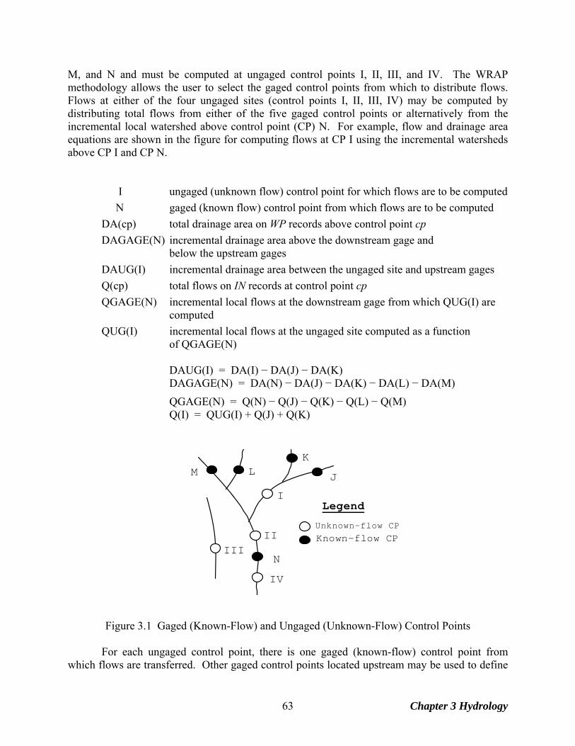
M, and N and must be computed at ungaged control points I, II, III, and IV. The WRAP methodology allows the user to select the gaged control points from which to distribute flows. Flows at either of the four ungaged sites (control points I, II, III, IV) may be computed by distributing total flows from either of the five gaged control points or alternatively from the incremental local watershed above control point (CP) N. For example, flow and drainage area equations are shown in the figure for computing flows at CP I using the incremental watersheds above CP I and CP N.
I ungaged (unknown flow) control point for which flows are to be computed
N gaged (known flow) control point from which flows are to be computed
DA(cp) total drainage area on WP records above control point cp
DAGAGE(N) incremental drainage area above the downstream gage and below the upstream gages
DAUG(I) incremental drainage area between the ungaged site and upstream gages
Q(cp) total flows on IN records at control point cp
QGAGE(N) incremental local flows at the downstream gage from which QUG(I) are computed
QUG(I) incremental local flows at the ungaged site computed as a function of QGAGE(N)
DAUG(I) = DA(I) − DA(J) − DA(K) DAGAGE(N) = DA(N) − DA(J) − DA(K) − DA(L) − DA(M)
QGAGE(N) = Q(N) − Q(J) − Q(K) − Q(L) − Q(M) Q(I) = QUG(I) + Q(J) + Q(K)
Legend
Unknown-flow CP
Known-flow CPIII
M LK
J
I
II
N
IV
Figure 3.1 Gaged (Known-Flow) and Ungaged (Unknown-Flow) Control Points For each ungaged control point, there is one gaged (known-flow) control point from which flows are transferred. Other gaged control points located upstream may be used to define
Chapter 3 Hydrology 63
the local incremental watersheds for both the gaged source CP and the ungaged CP. The following information is provided on the flow distribution FD record of the control point for which flows are being generated.
• control point identifier of ungaged (unknown-flow) control point to which flows are being distributed
• control point identifier of gaged (known-flow) control point from which flows are being distributed
• control point identifiers of the upstream control points used to compute incremental flows
• the number of upstream control points used to compute the incremental flows at the ungaged (unknown-flow) control point
The gaged control point from which flows are computed will be called the source CP. As illustrated by Fig. 3.1, the ungaged site may be either upstream of the source CP, downstream of the source CP, or on a different tributary. Any of the upstream control points may also be used to define the incremental watershed above the ungaged CP. The variable NGAGE on the FD record indicates how many of the gaged CPs above the source CP are also located above the ungaged site. For example, the flows at CP I in Fig. 3.1 may be determined from the flows at source CP N. Upstream CPs K, J, M, and L are listed on the FD record to define an incremental watershed for source CP N. NGAGE(I) is 2, indicating that the first two upstream CPs listed (CPs K and J) define the incremental watershed above ungaged CP I. NGAGE(II) is 4 for transferring incremental flows below J-K-L-M from N to II. NGAGE(III) is zero for computing flows at control point III from either total or incremental flows at control point N. For simplicity, the flow equations are shown in Fig. 3.1 without channel loss adjustments.
A NGAGE of −1 on a FD record indicates that flows at an ungaged site are computed from flows at a source control point located upstream. For example, referring to Fig. 3.1, for NGAGE(IV) = −1, the incremental flow at IV [QUG(IV)] is computed as a function of incremental or total flow at N [QGAGE(N)] and added to the total flow at N [Q(N)] to obtain the total flow at IV [Q(IV)], where:
DAUG(IV) = DA(IV) − DA(N) Q(IV) = QUG(IV) + Q(N)
As noted previously, if INWS(cp) on the CP record is blank or zero, the parameters on the
WP record are for the total watershed above the gaged CP, and the parameters for the incremental watershed are computed using the other control points. A positive integer for INWS(cp) indicates that the watershed parameters on the WP record correspond to the incremental watersheds. In this case [INWS(cp)>0], caution must be exercised to assure that incremental flows correspond to precisely the same control points as the incremental watersheds.
Flow Distribution Methods Methods for distributing naturalized stream flows from gaged or known-flow locations to ungaged sites are explored by Wurbs and Sisson (1999). The same flow synthesis methods in both HYD and SIM are activated by CP record field 4 and are based on parameters provided on FD, FC, and WP records in a DIS file. The flow distribution methods may be applied to either
Chapter 3 Hydrology 64
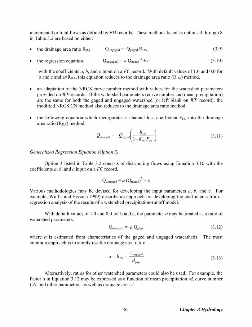
incremental or total flows as defined by FD records. These methods listed as options 3 through 8 in Table 3.2 are based on either: • the drainage area ratio RDA Qungaged = Qgaged RDA (3.9) • the regression equation Qungaged = a Qgaged b + c (3.10)
with the coefficients a, b, and c input on a FC record. With default values of 1.0 and 0.0 for b and c and a=RDA, this equation reduces to the drainage area ratio (RDA) method.
• an adaptation of the NRCS curve number method with values for the watershed parameters
provided on WP records. If the watershed parameters (curve number and mean precipitation) are the same for both the gaged and ungaged watershed (or left blank on WP record), the modified NRCS CN method also reduces to the drainage area ratio method.
• the following equation which incorporates a channel loss coefficient FCL into the drainage
area ratio (RDA) method.
⎟⎟⎠
⎞⎜⎜⎝
⎛−
=CLDA
DAgagedungaged FR
RQQ1
(3.11)
Generalized Regression Equation (Option 3) Option 3 listed in Table 3.2 consists of distributing flows using Equation 3.10 with the coefficients a, b, and c input on a FC record.
Qungaged = a (Qgaged)b + c
Various methodologies may be devised for developing the input parameters a, b, and c. For example, Wurbs and Sisson (1999) describe an approach for developing the coefficients from a regression analysis of the results of a watershed precipitation-runoff model.
With default values of 1.0 and 0.0 for b and c, the parameter a may be treated as a ratio of watershed parameters.
Qungaged = a Qgage (3.12) where a is estimated from characteristics of the gaged and ungaged watersheds. The most common approach is to simply use the drainage area ratio:
gage
ungagedDA A
ARa == (3.13)
Alternatively, ratios for other watershed parameters could also be used. For example, the factor a in Equation 3.12 may be expressed as a function of mean precipitation M, curve number CN, and other parameters, as well as drainage area A.
Chapter 3 Hydrology 65
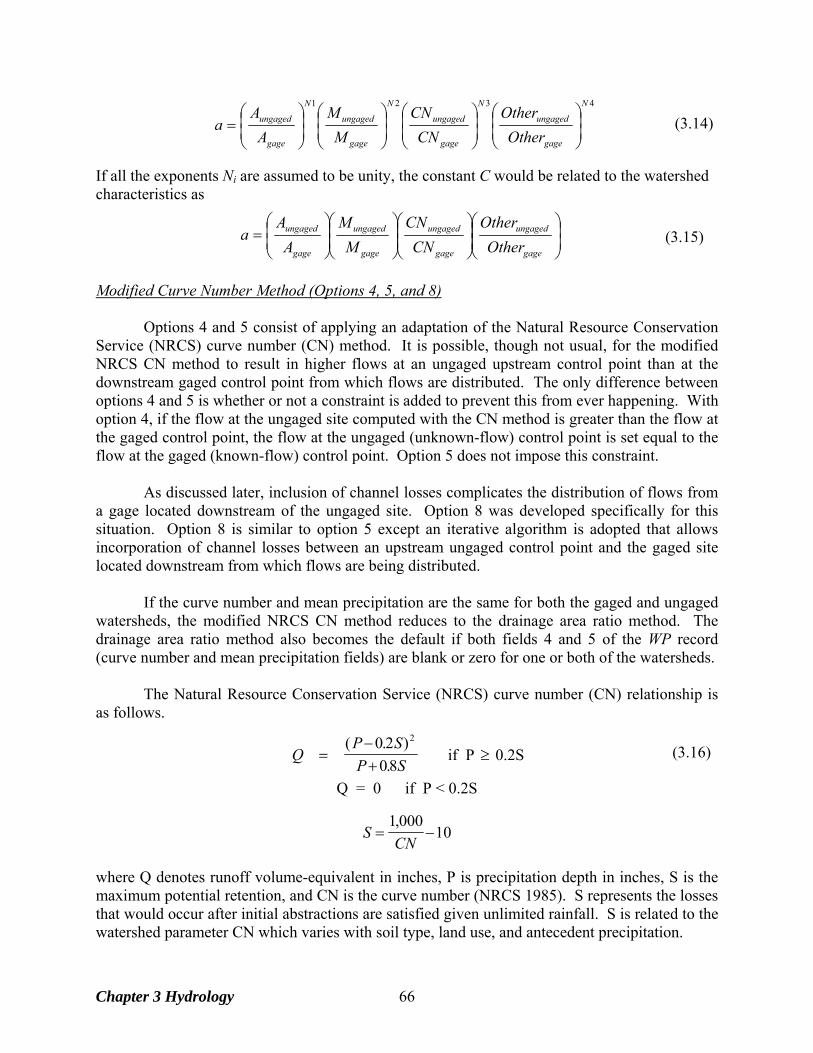
4321 N
gage
ungaged
N
gage
ungaged
N
gage
ungaged
N
gage
ungaged
OtherOther
CNCN
MM
AA
a ⎟⎟⎠
⎞⎜⎜⎝
⎛⎟⎟⎠
⎞⎜⎜⎝
⎛⎟⎟⎠
⎞⎜⎜⎝
⎛⎟⎟⎠
⎞⎜⎜⎝
⎛=
(3.14)
If all the exponents Ni are assumed to be unity, the constant C would be related to the watershed characteristics as
⎟⎟⎠
⎞⎜⎜⎝
⎛⎟⎟⎠
⎞⎜⎜⎝
⎛⎟⎟⎠
⎞⎜⎜⎝
⎛⎟⎟⎠
⎞⎜⎜⎝
⎛=
gage
ungaged
gage
ungaged
gage
ungaged
gage
ungaged
OtherOther
CNCN
MM
AA
a
(3.15)
Modified Curve Number Method (Options 4, 5, and 8) Options 4 and 5 consist of applying an adaptation of the Natural Resource Conservation Service (NRCS) curve number (CN) method. It is possible, though not usual, for the modified NRCS CN method to result in higher flows at an ungaged upstream control point than at the downstream gaged control point from which flows are distributed. The only difference between options 4 and 5 is whether or not a constraint is added to prevent this from ever happening. With option 4, if the flow at the ungaged site computed with the CN method is greater than the flow at the gaged control point, the flow at the ungaged (unknown-flow) control point is set equal to the flow at the gaged (known-flow) control point. Option 5 does not impose this constraint.
As discussed later, inclusion of channel losses complicates the distribution of flows from a gage located downstream of the ungaged site. Option 8 was developed specifically for this situation. Option 8 is similar to option 5 except an iterative algorithm is adopted that allows incorporation of channel losses between an upstream ungaged control point and the gaged site located downstream from which flows are being distributed.
If the curve number and mean precipitation are the same for both the gaged and ungaged watersheds, the modified NRCS CN method reduces to the drainage area ratio method. The drainage area ratio method also becomes the default if both fields 4 and 5 of the WP record (curve number and mean precipitation fields) are blank or zero for one or both of the watersheds.
The Natural Resource Conservation Service (NRCS) curve number (CN) relationship is
as follows.
Q
P SP S
=−+
( . ).
0 208
2
if P 0.2S ≥
(3.16)
Q = 0 if P < 0.2S
SCN
= −1 000
10,
where Q denotes runoff volume-equivalent in inches, P is precipitation depth in inches, S is the maximum potential retention, and CN is the curve number (NRCS 1985). S represents the losses that would occur after initial abstractions are satisfied given unlimited rainfall. S is related to the watershed parameter CN which varies with soil type, land use, and antecedent precipitation.
Chapter 3 Hydrology 66
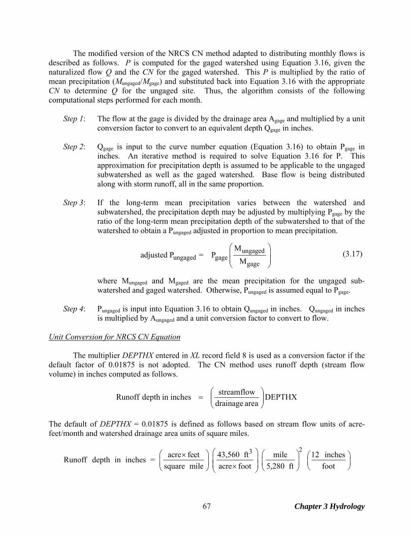
The modified version of the NRCS CN method adapted to distributing monthly flows is described as follows. P is computed for the gaged watershed using Equation 3.16, given the naturalized flow Q and the CN for the gaged watershed. This P is multiplied by the ratio of mean precipitation (Mungaged/Mgage) and substituted back into Equation 3.16 with the appropriate CN to determine Q for the ungaged site. Thus, the algorithm consists of the following computational steps performed for each month.
Step 1: The flow at the gage is divided by the drainage area Agage and multiplied by a unit conversion factor to convert to an equivalent depth Qgage in inches.
Step 2: Qgage is input to the curve number equation (Equation 3.16) to obtain Pgage in
inches. An iterative method is required to solve Equation 3.16 for P. This approximation for precipitation depth is assumed to be applicable to the ungaged subwatershed as well as the gaged watershed. Base flow is being distributed along with storm runoff, all in the same proportion.
Step 3: If the long-term mean precipitation varies between the watershed and
subwatershed, the precipitation depth may be adjusted by multiplying Pgage by the ratio of the long-term mean precipitation depth of the subwatershed to that of the watershed to obtain a Pungaged adjusted in proportion to mean precipitation.
ungaged
ungaged gagegage
Madjusted P = P
M
⎛ ⎞⎜ ⎟⎜ ⎟⎝ ⎠
(3.17)
where Mungaged and Mgaged are the mean precipitation for the ungaged sub-
watershed and gaged watershed. Otherwise, Pungaged is assumed equal to Pgage.
Step 4: Pungaged is input into Equation 3.16 to obtain Qungaged in inches. Qungaged in inches is multiplied by Aungaged and a unit conversion factor to convert to flow.
Unit Conversion for NRCS CN Equation
The multiplier DEPTHX entered in XL record field 8 is used as a conversion factor if the default factor of 0.01875 is not adopted. The CN method uses runoff depth (stream flow volume) in inches computed as follows.
DEPTHXareadrainage
streamflowinchesindepthRunoff ⎟⎟⎠
⎞⎜⎜⎝
⎛=
The default of DEPTHX = 0.01875 is defined as follows based on stream flow units of acre-feet/month and watershed drainage area units of square miles.
23acre feet 43,560 ft mile 12 inchesRunoff depth in inches =square mile acre foot 5,280 ft foot
⎛ ⎞⎛ ⎞ ⎛ ⎞× ⎛ ⎞⎜ ⎟⎜ ⎟ ⎜ ⎟ ⎜ ⎟⎜ ⎟× ⎝ ⎠⎝ ⎠ ⎝ ⎠⎝ ⎠
Chapter 3 Hydrology 67
streamflow in acre feetRunoff depth in inches = 0.01875drainage area in square miles
⎛ ⎞×⎜ ⎟⎝ ⎠
If units for stream flow other than acre-feet/month and/or drainage area units other than
square miles are used, an appropriate DEPTHX is entered on the XL record to convert the monthly runoff depth to inches. A conversion factor on the watershed parameter WP record allows converting units for watershed area. For example, for stream flow in thousand cubic meters (1,000 m3) and watershed area in square kilometers, DEPTHX is 0.03937 determined as follows:
23
21,000 m km 39.37 inchesRunoff depth in inches =
1,000m meterkm
⎛ ⎞ ⎛ ⎞ ⎛ ⎞⎜ ⎟ ⎜ ⎟ ⎜ ⎟⎜ ⎟ ⎝ ⎠⎝ ⎠⎝ ⎠
3
2streamflow in 1,000mRunoff depth in inches = 0.03937drainage area in km
⎛ ⎞⎜ ⎟⎜ ⎟⎝ ⎠
The mean precipitation depth MP is used only to obtain ratios of MPungaged to MPgaged. Thus, any depth unit may be used as long as the same unit is used for all watersheds. Bounds on Curve Number (CN), Mean Precipitation (MP), and Flow
The SIM and HYD subroutine FLDIST distributes flows from gaged to ungaged locations for options 3 through 8 listed in Table 3.2. Subroutine IACNP reads the FD and WP records from the DIS file and computes incremental drainage areas (A), curve numbers (CN), and mean precipitation (MP) for use in subroutine FLDIST. The CN and MP for a incremental watershed are computed from the CN's and MP's read from the WP records for total watersheds. The basic premise in computing the CN and MP for an incremental watershed is that the CN or MP for a total watershed equals the area-weighted average of the values for all its subwatersheds.
Situations may occur in which the CN or MP input for total watersheds are unrealistically low or high. Unrealistic values may also result for the computed CN's or MP's for small incremental subwatersheds. Problems may be related to preciseness of the CN's and MP's relative to the size of incremental subwatersheds that are a very small portion of the total watershed. The CN may be negative or exceed 100, violating the definition of CN and resulting in negative flows from the CN method algorithm.
WRAP-SIM has an option for placing bounds on the curve numbers CN and mean
precipitation MP used in synthesizing flows. If in determining flows for any particular ungaged control point, the CN or MP for either the gaged or ungaged incremental or total watershed falls outside the specified lower and upper bounds, the drainage area ratio method is used instead of the NRCS CN method. Under these conditions, INMETHOD options 4 and 5 revert to option 7 (drainage area ratio method without channel losses), and option 8 reverts to option 6 (with channel losses). Only flows at ungaged control points with watershed parameters violating the bounds are affected by this feature. This will likely affect only a very small portion, if any, of the control points in any particular river basin.
Chapter 3 Hydrology 68
Warning messages are written to the message file for each control point total or incremental watershed for which either the CN or MP violates either the lower or upper bounds. Negative watershed areas are treated as errors that result in an error message and termination of program execution.
The default lower and upper bounds are zero and 100 for CN's. The default bounds are zero and 100 units (inches or other units) for MP's. Optionally, the bounds may be specified in the XL record.
Incremental flows at a gaged control point are computed in subroutine FLDIST by subtracting flows at upstream control points specified on a FD record. Incremental flows are used in distributing flows from gaged to ungaged control points. The incremental flows may be computed as negative numbers. Negative incremental flows are converted to zeros for all flow distribution options except option 8. Also, after the flow distribution computations, any negative total flows computed for ungaged control points are converted to zero, except for option 8. With option 8, negative incremental flows trigger reverting to option 6. Thus, for option 8, a negative incremental flow has the same effect as a CN or MP violating lower or upper bounds. Incorporation of Channel Losses in Flow Distribution Options 3, 4, 5, 6, 7 and 8 Flow distribution is one of several aspects of a WRAP simulation for which channel losses may be pertinent. Channel losses are discussed earlier in this chapter. All of the channel loss routines in the model use a channel loss coefficient FCL for the river reach below a control point, that is entered as variable CL(cp) in the CP record. FCL is defined by Equation 3.3. The alternative flow distribution methods previously cited may be applied to either local incremental subwatersheds or the total watersheds above the gaged and ungaged control points. If incremental stream flow is used, the unknown total flow at an ungaged control point is determined from the known flow at a gaged control point in three steps.
1. The incremental flow at the gage is computed by subtracting the total flow at the gage from the sum of flows at appropriate upstream gages adjusted to remove the effects of channel losses.
2. The incremental flows at the gage, computed in step (1), are distributed to the
ungaged site using one of the optional methods described here. 3. The incremental flows at the ungaged site, computed in step (2), are added to the
flows at appropriate upstream control points, adjusted for channel losses, to obtain the total flows at the ungaged site.
Channel losses are included in steps 1 and 3 for all of the flow distribution options as long as the FCL for the pertinent reaches are non-zero. All of the flow distribution options may be applied concurrently with channel loss factors FCL under appropriate circumstances in cases where the ungaged site is located downstream of the source control point or on a different tributary. However, options 6 and 8 are designed specifically to address the situation described below.
Chapter 3 Hydrology 69
Ungaged Control Point Located Upstream of Source Gaged Control Point Options 6 and 8 in Table 3.2 are designed to be applied specifically and only for the situation in which the ungaged control point is located upstream of the source gaged site with channel losses occurring in between. This situated is complicated by the fact that the flow at the ungaged site is a function of the flow at the gaged site Qgaged plus channel losses FCLQungaged Qungaged = f(Qgaged+FCLQungaged) (3.18) and channel losses are a function of Qungaged (loss = FCLQungaged). Thus, Qungaged is on both sides of Equation 3.18. This complexity in incorporating channel losses in the flow distribution algorithms is illustrated by referring to Figure 3.1 and assuming that flows at CP I and CP II are computed from either the total or incremental flow at CP N. If incremental flows at N are used, the channel losses in the reaches below M, L, K, J, I, and II are considered in computing the incremental flow at N. The complexity is that the channel loss in the reach below CP II depends upon the unknown flow at CP II. The flow at control point II is a function of flow at N plus channel losses.
QII = f(QN+FCLQII) This function is expressed as follows for the drainage area ratio method.
QII = RDA (QN + FCLQII) Likewise, with flows being distributed from CP N to CP I, the channel losses in the reaches between I and II and between II and N depend upon the unknown flows at control points I and II. Thus, channel losses may occur in multiple reaches between the gaged and upstream ungaged sites. For multiple reaches in series, the total channel loss is determined by multiplying the flow at the most upstream control point by an equivalent N-reach FCL determined by combining the channel losses FCLi for each reach as follows:
Equivalent (1.0 − FCL) = (1.0 − FCL1) (1.0 − FCL2) (1.0 − FCL3) ... (1.0 − FCLN) (3.19) Options 6 and 8 are modifications of the drainage area ratio and NRCS CN methods to
incorporate channel losses between an upstream ungaged (unknown flow) control point and a gaged (known flow) site located downstream from which flows are being distributed. Options 6 and 8 are applicable only in cases where:
• The ungaged site is located upstream of the source gaged control point.
• Channel losses occurring between the ungaged and gaged control points are significantly greater than otherwise captured by the CN or DA methods.
Options 6 and 8 incorporating the channel loss factor (FCL) are applicable if the channel losses in the reach between the ungaged and gaged control point are significantly greater than in the other streams in the watershed and thus not adequately reflected in the flow proportioning of the CN
Chapter 3 Hydrology 70
and drainage area ratio methods without the FCL. Incorporating a FCL results in higher estimates of the flow amounts at the ungaged control point. Option 6 - Drainage Area Ratio with Channel Losses
As noted above, the drainage ratio method may be expressed as
Qungaged = RDA (Qgaged + FCLQungaged) (3.20)
for a situation with a ungaged control point located upstream of a gaged control point, with the channel losses occurring between the ungaged and gaged control point being significantly greater than reflected in proportioning flows based on the RDA alone. RDA is the drainage area ratio (Aungaged/Agage), and FCL is the channel loss coefficient. Qungaged and Qgaged denote the naturalized flow (either total or incremental) at the two control points. (Qgaged+ FCLQungaged) denotes the flow at the gage adjusted to remove the effect of channel losses in the reach between the ungaged and gaged sites. If intermediate control points are located between these locations, the FCL is an equivalent multiple-reach channel loss factor determined as noted earlier. This equation is algebraically rearranged to obtain the previously noted Equation 3.11.
⎟⎟⎠
⎞⎜⎜⎝
⎛−
=CLDA
DAgagedungaged FR
RQQ1
(3.11)
INMETHOD(cp) option 6 in Table 3.2 consists of applying Equation 3.11. The model obtains FCL from the CP record for the ungaged control point and the watershed areas from the appropriate WP records. For multiple intermediate control points between the gaged and ungaged sites, an equivalent FCL is determined as previously noted. Option 6 is applicable only in situations where the ungaged control point is located upstream of the gaged control point and the channel losses between the control points are greater than otherwise reflected in the simple drainage area ratio method of Equation 3.9. Option 8 - NRCS CN Method with Channel Losses Referring to Figure 3.1, options 4 and 5 applying the NRCS CN method is applicable for transferring flow from source control point N to either control points III or IV. Options 4 and 5 are applicable in the situation of the ungaged CP being located above the gaged control point, such as in transferring flows from control point N to control points I and II, if channel loss factors for control point I and control point II are zero. Option 8 is pertinent in situations in which the ungaged site is located upstream of the gaged site with channel losses occurring in between that are greater than otherwise reflected in options 4 and 5. Option 8 is pertinent only in situations in which the ungaged site is located upstream of the gaged site with channel losses occurring in between. Option 8 consists of combining Equations 3.21 and 3.22
Qungaged = f(Qgaged+FCLQungaged) (3.21)
Equivalent (1.0 − FCL) = (1.0 − FCL1) (1.0 − FCL2) (1.0 − FCL3) ... (1.0 − FCLN) (3.22)
Chapter 3 Hydrology 71
with the NRCS CN method. If the known flow Qgaged is zero, then the unknown flow Qungaged is set equal to zero. Otherwise, the following iterative algorithm is employed.
1. For the initial iteration, the channel loss FCLQungaged is set equal to zero, and thus (Qgaged+FCLQungaged) is set equal to Qgaged.
2. The CN method based on Equations 3.16 and 3.17 is applied following the steps
previously outlined identically as with Option 5 to compute an intermediate value for Qungaged.for the given (Qgaged+FCLQungaged) from steps 1 and 3.
3. Given the Qungaged.computed in step 2 above, FCLQungaged and thus
(Qgaged+FCLQungaged) are determined.
Steps 2 and 3 are repeated iteratively until a stop criterion is met. The stop criterion is that the change in successive values of Qungaged is less than 0.5 percent. The algorithm is terminated after 100 iterations with the following warning message.
WARNING: Convergence criterion of 0.5% was not met for flow distribution option 8
after 100 iterations at ungaged CP _____ for year _____, month _____. Last flow computed of ______ was adopted.
Multipliers and Control Point Identifiers on CP Record (Option 2) HYD and SIM CP records include the variables CPIN(cp) and CPEV(cp) which specify other control points with flows or net evaporation-precipitation rates, respectively, which are to be used for control point cp. Thus, the flow at another control point can be used without change or multiplied by CPDT(cp,1). The approach is referred to as option 2 in Table 3.2. Also, zero flows can be specified on the CP record. Multipliers CPDT(cp,1) and CPDT(cp,2) are also input on the CP record. The naturalized flows and net precipitation-evaporation rates are multiplied by these factors. CPDT(cp,1) and CPDT(cp,2) are typically used for unit conversion factors. However, the flow multiplier CPDT(cp,1) can also include a drainage area ratio or other flow distribution parameter. This provides another convenient alternative means for applying the drainage area ratio method for distributing flow. The approach is applicable only for total flows, not for incremental flows. Watershed Flow Option WRAP-SIM includes an alternative simplified option for dealing with water right diversions and storage at many remote ungaged locations throughout the watersheds above the control points. The watershed flow option supplements the control point network in delineating the location of water rights. All rights are assigned a control point and, in the model computations, affect unappropriated flows and water availability at that control point and downstream control points. Multiple rights may be assigned to the same control point. The watershed flow option is used for rights at locations in the watersheds above their assigned control points. The site in the watershed at
Chapter 3 Hydrology 72
which the right is actually located has no CP record and is not treated as a control point. WRAP-SIM limits water available to each of these rights to the lesser of:
• naturalized stream flows at the site
• yet unappropriated flows at the control point assigned to the right and downstream control points.
The naturalized stream flows at the watershed sites are determined by multiplying the naturalized stream flows at the control point by a user-specified factor. The drainage area ratio or other flow multiplier for a water right is provided as variable WSHED(wr) on the SO record.
Use of GIS to Determine Spatial Connectivity and Watershed Parameters The usefulness of a geographic information system (GIS) in developing input data for WRAP depends largely on the number of control points incorporated in the model and the methodology adopted for transferring naturalized stream flows from gaged to ungaged locations. Development of the Texas WAM System involved thousands of control points and parameters for thousands of subwatersheds for distributing naturalized flows. Thus, a GIS was essential. In developing the WRAP input datasets for the river basins of Texas for the TCEQ WAM System described in Chapter 1, a GIS methodology based on the ESRI software products ArcView and ArcInfo was developed and applied to determine spatial connectivity and estimate values for watershed parameters (Hudgens and Maidment 1999; Mason and Maidment 2000; Figurski and Maidment 2001). Later improvements in the ESRI ArcGIS software include expanded Arc Hydro capabilities for developing river basin data (Maidment 2002). Gopalan (2003) describes Arc Hydro procedures adopted specifically for developing watershed parameters for input to WRAP. In a WRAP model of a river basin, every control point except the basin outlet has another control point located immediately downstream. The control point CP record for each control point includes an entry for the identifier of the next downstream control point. The computational routines within WRAP use the next downstream control point designated for each control point to define spatial connectivity. For river basins with hundreds of control points, a GIS is very useful for developing a list of the next downstream control point associated with each control point. Watershed drainage areas are required for all of the methods for distributing naturalized flows from gaged to ungaged sites. The curve number CN and mean precipitation MP are also required if the NRCS CN method adaptation is used for distributing flows. The following datasets were used to develop these watershed parameters for the Texas WAM System.
• digital elevation models of land surface terrain available from the U.S. Geological Survey • set of USGS stream gaging station locations • stream network available from the U.S. Environmental Protection Agency • set of water right locations developed by TCEQ and consulting firms • grid of mean annual precipitation from the PRISM project developed at Oregon State
University for the USDA Natural Resource Conservation Service • grid of curve numbers developed by the TAES Blackland Research Center for the
HUMUS Project sponsored by the USDA NRCS
Chapter 3 Hydrology 73
The curve number (CN) database was previously produced by the Texas Agricultural Experiment Station of the Texas A&M University System for the Hydrologic Unit Modeling of the United States (HUMUS) project sponsored by the USDA Natural Resource Conservation Service (NRCS). The CN grid was developed by intersecting maps of land use and soil type and combining the results with a CN table to determine the CN for each grid cell.
Negative Incremental Naturalized Stream Flows SIM naturalized stream flow input, computational algorithms, computed regulated and unappropriated flows, and associated variables are all based on total flows, rather than incremental flows. Although incremental watersheds and incremental flows may be used in distributing flows from gaged to ungaged locations, the final synthesized flows used in the simulation are total flows. Thus, a simulation is based on total stream flows, not incremental inflows. However, situations in which naturalized flows at a particular control point are less than concurrent flows at upstream locations are described in terms of negative incremental inflows. The relevance of negative incremental flows and options for dealing with them are addressed in this section. The incremental inflow between a control point and control point(s) located upstream is the naturalized flow at the downstream location minus the concurrent flow at the upstream location(s). Since stream flow usually increases going downstream, incremental inflows are typically positive. However, situations with flows at upstream locations exceeding concurrent flows at a downstream location are not unusual. Negative incrementals for actual observed stream flows at gaging stations may result from: channel seepage and evapotranspiration losses; recorded or unrecorded diversions; large travel times causing the effects of precipitation events to reach adjacent control points in different time periods; and/or measuring inaccuracies or data recording errors. Computational adjustments to convert gaged flows to naturalized flows introduce other inaccuracies that may contribute to incremental naturalized stream flows being negative. Example 3 - Negative Incremental Stream flows An example is provided in Figure 3.2 and Tables 3.3 and 3.4. Naturalized flows at each control point for a particular month are tabulated in column 2 of Table 3.3 and also shown in the figure. The incremental inflows between each control point and its adjacent upstream control points are shown in column 3. Incremental flows are negative at control point CP-2 (incremental flow = 81−90 = −9) and control point 6 (incremental flow = 80−100−8 = −28). As illustrated by columns 4 and 6 of Table 3.3 and discussed later, negative incremental flows alternatively may be defined considering all control points located either upstream or downstream of a particular control point. As illustrated by columns 5 and 7 and also discussed later, negative incremental flows may be eliminated by adjusting the flows at pertinent control points. Significance of Negative Incremental Naturalized Stream Flows The amount of water available to a water right and the unappropriated stream flow at a control point may be affected by the magnitude of the naturalized stream flows at that control point and all downstream control points. The relevance of flows being smaller downstream than upstream (negative incremental) and associated adjustments are related to the effects on the amount
Chapter 3 Hydrology 74
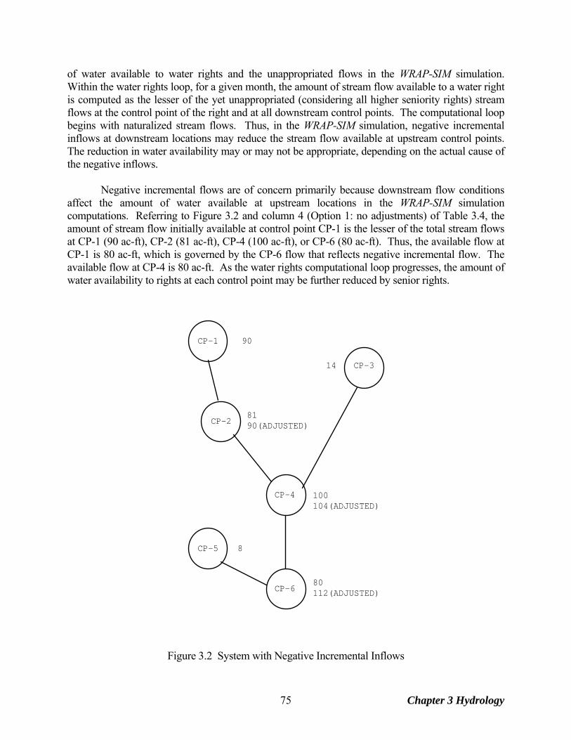
of water available to water rights and the unappropriated flows in the WRAP-SIM simulation. Within the water rights loop, for a given month, the amount of stream flow available to a water right is computed as the lesser of the yet unappropriated (considering all higher seniority rights) stream flows at the control point of the right and at all downstream control points. The computational loop begins with naturalized stream flows. Thus, in the WRAP-SIM simulation, negative incremental inflows at downstream locations may reduce the stream flow available at upstream control points. The reduction in water availability may or may not be appropriate, depending on the actual cause of the negative inflows. Negative incremental flows are of concern primarily because downstream flow conditions affect the amount of water available at upstream locations in the WRAP-SIM simulation computations. Referring to Figure 3.2 and column 4 (Option 1: no adjustments) of Table 3.4, the amount of stream flow initially available at control point CP-1 is the lesser of the total stream flows at CP-1 (90 ac-ft), CP-2 (81 ac-ft), CP-4 (100 ac-ft), or CP-6 (80 ac-ft). Thus, the available flow at CP-1 is 80 ac-ft, which is governed by the CP-6 flow that reflects negative incremental flow. The available flow at CP-4 is 80 ac-ft. As the water rights computational loop progresses, the amount of water availability to rights at each control point may be further reduced by senior rights.
CP-1
CP-2
CP-3
CP-4
CP-6
CP-5
90
8190(ADJUSTED)
100104(ADJUSTED)
80112(ADJUSTED)
8
14
Figure 3.2 System with Negative Incremental Inflows
Chapter 3 Hydrology 75
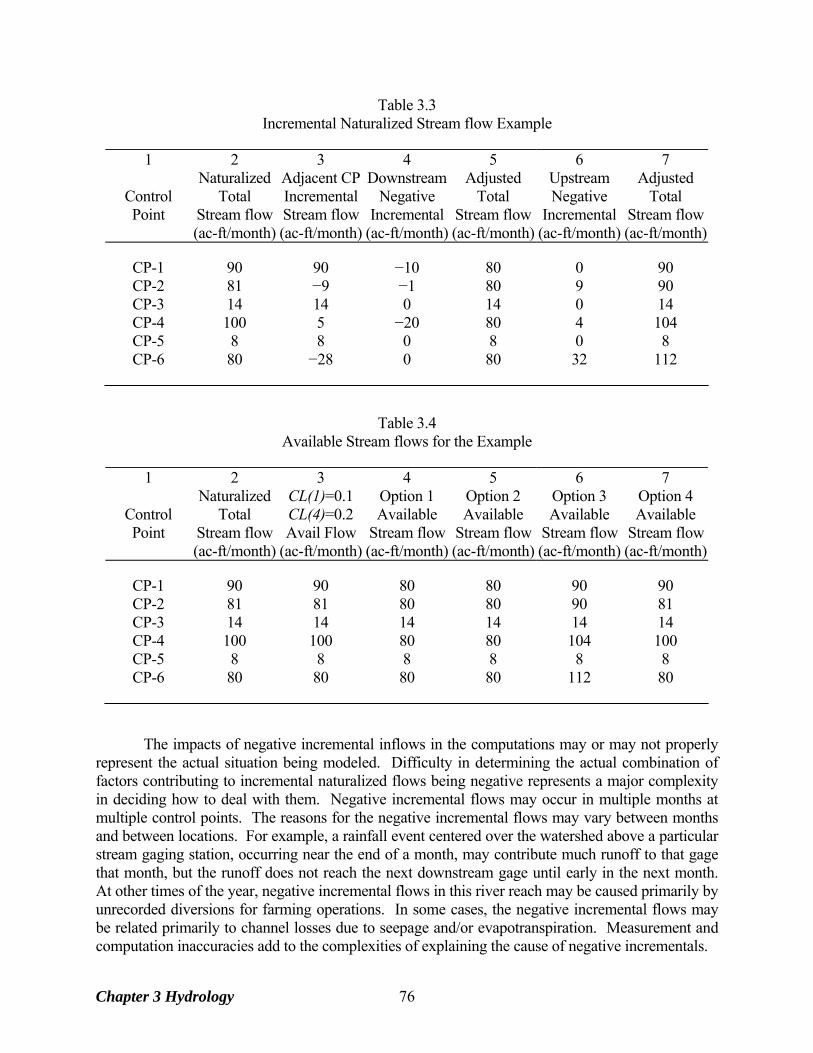
Table 3.3 Incremental Naturalized Stream flow Example
1 2 3 4 5 6 7 Naturalized Adjacent CP Downstream Adjusted Upstream Adjusted
Control Total Incremental Negative Total Negative Total Point Stream flow Stream flow Incremental Stream flow Incremental Stream flow
(ac-ft/month) (ac-ft/month) (ac-ft/month) (ac-ft/month) (ac-ft/month) (ac-ft/month)
CP-1 90 90 −10 80 0 90 CP-2 81 −9 −1 80 9 90 CP-3 14 14 0 14 0 14 CP-4 100 5 −20 80 4 104 CP-5 8 8 0 8 0 8 CP-6 80 −28 0 80 32 112
Table 3.4 Available Stream flows for the Example
1 2 3 4 5 6 7 Naturalized CL(1)=0.1 Option 1 Option 2 Option 3 Option 4
Control Total CL(4)=0.2 Available Available Available Available Point Stream flow Avail Flow Stream flow Stream flow Stream flow Stream flow
(ac-ft/month) (ac-ft/month) (ac-ft/month) (ac-ft/month) (ac-ft/month) (ac-ft/month)
CP-1 90 90 80 80 90 90 CP-2 81 81 80 80 90 81 CP-3 14 14 14 14 14 14 CP-4 100 100 80 80 104 100 CP-5 8 8 8 8 8 8 CP-6 80 80 80 80 112 80
The impacts of negative incremental inflows in the computations may or may not properly represent the actual situation being modeled. Difficulty in determining the actual combination of factors contributing to incremental naturalized flows being negative represents a major complexity in deciding how to deal with them. Negative incremental flows may occur in multiple months at multiple control points. The reasons for the negative incremental flows may vary between months and between locations. For example, a rainfall event centered over the watershed above a particular stream gaging station, occurring near the end of a month, may contribute much runoff to that gage that month, but the runoff does not reach the next downstream gage until early in the next month. At other times of the year, negative incremental flows in this river reach may be caused primarily by unrecorded diversions for farming operations. In some cases, the negative incremental flows may be related primarily to channel losses due to seepage and/or evapotranspiration. Measurement and computation inaccuracies add to the complexities of explaining the cause of negative incrementals.
Chapter 3 Hydrology 76
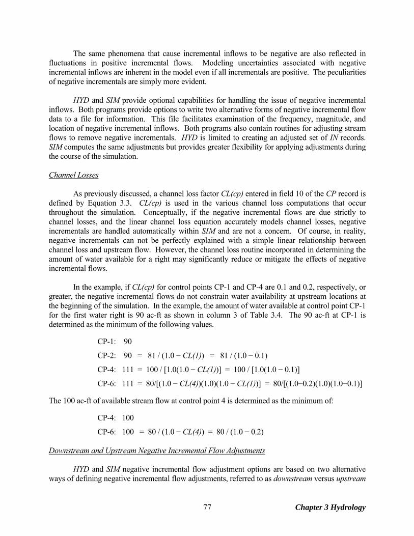
The same phenomena that cause incremental inflows to be negative are also reflected in fluctuations in positive incremental flows. Modeling uncertainties associated with negative incremental inflows are inherent in the model even if all incrementals are positive. The peculiarities of negative incrementals are simply more evident. HYD and SIM provide optional capabilities for handling the issue of negative incremental inflows. Both programs provide options to write two alternative forms of negative incremental flow data to a file for information. This file facilitates examination of the frequency, magnitude, and location of negative incremental inflows. Both programs also contain routines for adjusting stream flows to remove negative incrementals. HYD is limited to creating an adjusted set of IN records. SIM computes the same adjustments but provides greater flexibility for applying adjustments during the course of the simulation. Channel Losses As previously discussed, a channel loss factor CL(cp) entered in field 10 of the CP record is defined by Equation 3.3. CL(cp) is used in the various channel loss computations that occur throughout the simulation. Conceptually, if the negative incremental flows are due strictly to channel losses, and the linear channel loss equation accurately models channel losses, negative incrementals are handled automatically within SIM and are not a concern. Of course, in reality, negative incrementals can not be perfectly explained with a simple linear relationship between channel loss and upstream flow. However, the channel loss routine incorporated in determining the amount of water available for a right may significantly reduce or mitigate the effects of negative incremental flows. In the example, if CL(cp) for control points CP-1 and CP-4 are 0.1 and 0.2, respectively, or greater, the negative incremental flows do not constrain water availability at upstream locations at the beginning of the simulation. In the example, the amount of water available at control point CP-1 for the first water right is 90 ac-ft as shown in column 3 of Table 3.4. The 90 ac-ft at CP-1 is determined as the minimum of the following values. CP-1: 90
CP-2: 90 = 81 / (1.0 − CL(1)) = 81 / (1.0 − 0.1)
CP-4: 111 = 100 / [1.0(1.0 − CL(1))] = 100 / [1.0(1.0 − 0.1)]
CP-6: 111 = 80/[(1.0 − CL(4))(1.0)(1.0 − CL(1))] = 80/[(1.0−0.2)(1.0)(1.0−0.1)] The 100 ac-ft of available stream flow at control point 4 is determined as the minimum of: CP-4: 100
CP-6: 100 = 80 / (1.0 − CL(4)) = 80 / (1.0 − 0.2) Downstream and Upstream Negative Incremental Flow Adjustments HYD and SIM negative incremental flow adjustment options are based on two alternative ways of defining negative incremental flow adjustments, referred to as downstream versus upstream
Chapter 3 Hydrology 77
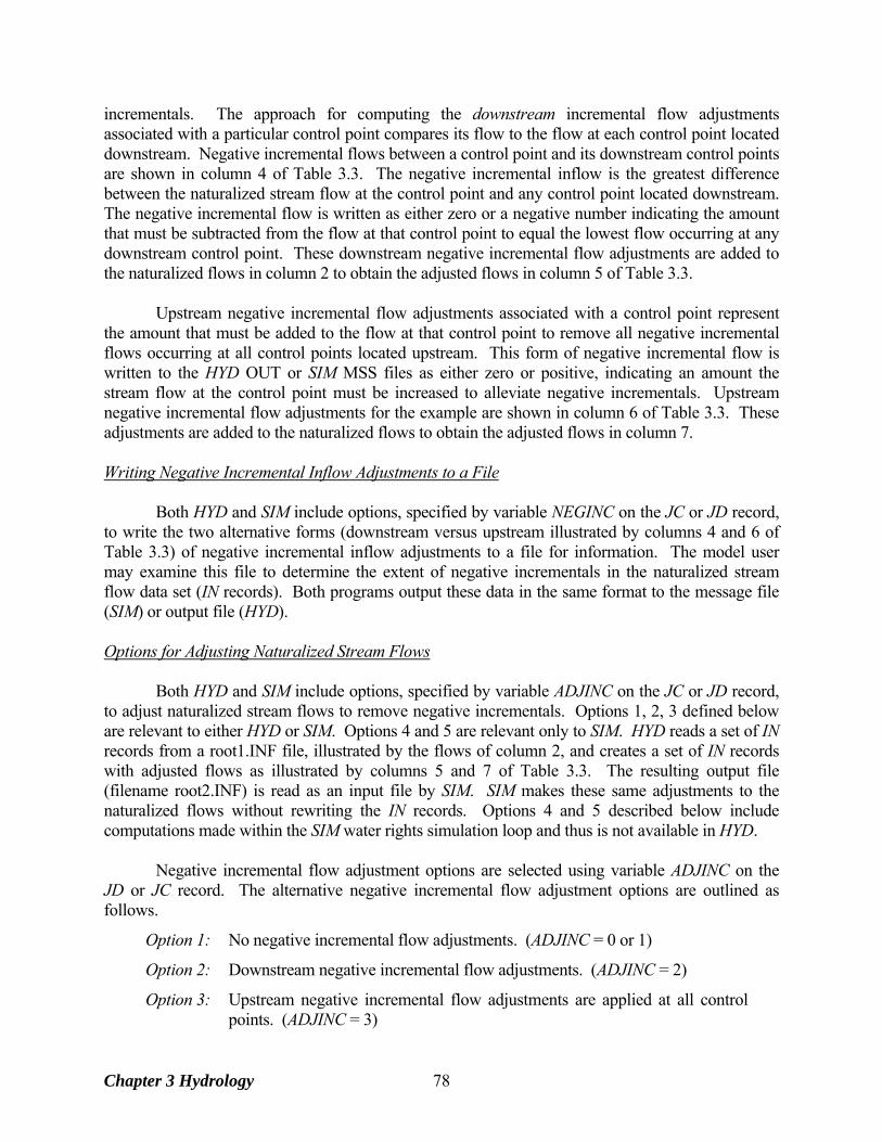
incrementals. The approach for computing the downstream incremental flow adjustments associated with a particular control point compares its flow to the flow at each control point located downstream. Negative incremental flows between a control point and its downstream control points are shown in column 4 of Table 3.3. The negative incremental inflow is the greatest difference between the naturalized stream flow at the control point and any control point located downstream. The negative incremental flow is written as either zero or a negative number indicating the amount that must be subtracted from the flow at that control point to equal the lowest flow occurring at any downstream control point. These downstream negative incremental flow adjustments are added to the naturalized flows in column 2 to obtain the adjusted flows in column 5 of Table 3.3. Upstream negative incremental flow adjustments associated with a control point represent the amount that must be added to the flow at that control point to remove all negative incremental flows occurring at all control points located upstream. This form of negative incremental flow is written to the HYD OUT or SIM MSS files as either zero or positive, indicating an amount the stream flow at the control point must be increased to alleviate negative incrementals. Upstream negative incremental flow adjustments for the example are shown in column 6 of Table 3.3. These adjustments are added to the naturalized flows to obtain the adjusted flows in column 7. Writing Negative Incremental Inflow Adjustments to a File Both HYD and SIM include options, specified by variable NEGINC on the JC or JD record, to write the two alternative forms (downstream versus upstream illustrated by columns 4 and 6 of Table 3.3) of negative incremental inflow adjustments to a file for information. The model user may examine this file to determine the extent of negative incrementals in the naturalized stream flow data set (IN records). Both programs output these data in the same format to the message file (SIM) or output file (HYD). Options for Adjusting Naturalized Stream Flows Both HYD and SIM include options, specified by variable ADJINC on the JC or JD record, to adjust naturalized stream flows to remove negative incrementals. Options 1, 2, 3 defined below are relevant to either HYD or SIM. Options 4 and 5 are relevant only to SIM. HYD reads a set of IN records from a root1.INF file, illustrated by the flows of column 2, and creates a set of IN records with adjusted flows as illustrated by columns 5 and 7 of Table 3.3. The resulting output file (filename root2.INF) is read as an input file by SIM. SIM makes these same adjustments to the naturalized flows without rewriting the IN records. Options 4 and 5 described below include computations made within the SIM water rights simulation loop and thus is not available in HYD. Negative incremental flow adjustment options are selected using variable ADJINC on the JD or JC record. The alternative negative incremental flow adjustment options are outlined as follows.
Option 1: No negative incremental flow adjustments. (ADJINC = 0 or 1)
Option 2: Downstream negative incremental flow adjustments. (ADJINC = 2)
Option 3: Upstream negative incremental flow adjustments are applied at all control points. (ADJINC = 3)
Chapter 3 Hydrology 78
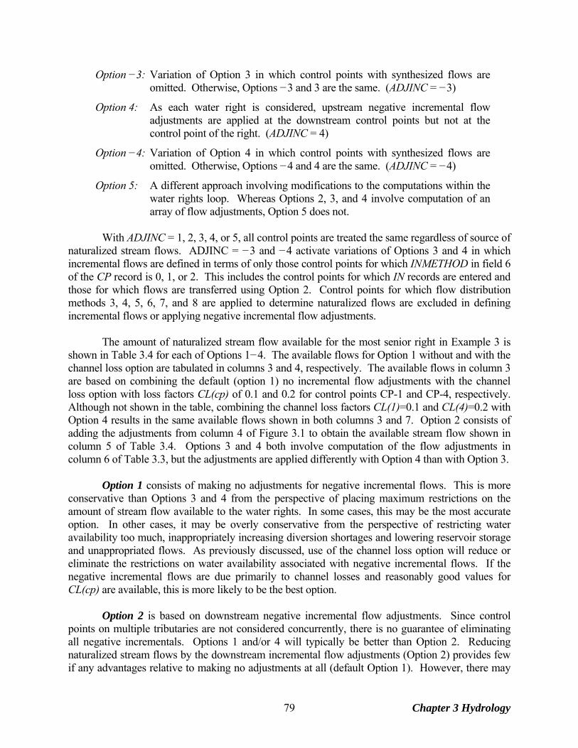
Option −3: Variation of Option 3 in which control points with synthesized flows are omitted. Otherwise, Options −3 and 3 are the same. (ADJINC = −3)
Option 4: As each water right is considered, upstream negative incremental flow adjustments are applied at the downstream control points but not at the control point of the right. (ADJINC = 4)
Option −4: Variation of Option 4 in which control points with synthesized flows are omitted. Otherwise, Options −4 and 4 are the same. (ADJINC = −4)
Option 5: A different approach involving modifications to the computations within the water rights loop. Whereas Options 2, 3, and 4 involve computation of an array of flow adjustments, Option 5 does not.
With ADJINC = 1, 2, 3, 4, or 5, all control points are treated the same regardless of source of naturalized stream flows. ADJINC = −3 and −4 activate variations of Options 3 and 4 in which incremental flows are defined in terms of only those control points for which INMETHOD in field 6 of the CP record is 0, 1, or 2. This includes the control points for which IN records are entered and those for which flows are transferred using Option 2. Control points for which flow distribution methods 3, 4, 5, 6, 7, and 8 are applied to determine naturalized flows are excluded in defining incremental flows or applying negative incremental flow adjustments. The amount of naturalized stream flow available for the most senior right in Example 3 is shown in Table 3.4 for each of Options 1−4. The available flows for Option 1 without and with the channel loss option are tabulated in columns 3 and 4, respectively. The available flows in column 3 are based on combining the default (option 1) no incremental flow adjustments with the channel loss option with loss factors CL(cp) of 0.1 and 0.2 for control points CP-1 and CP-4, respectively. Although not shown in the table, combining the channel loss factors CL(1)=0.1 and CL(4)=0.2 with Option 4 results in the same available flows shown in both columns 3 and 7. Option 2 consists of adding the adjustments from column 4 of Figure 3.1 to obtain the available stream flow shown in column 5 of Table 3.4. Options 3 and 4 both involve computation of the flow adjustments in column 6 of Table 3.3, but the adjustments are applied differently with Option 4 than with Option 3. Option 1 consists of making no adjustments for negative incremental flows. This is more conservative than Options 3 and 4 from the perspective of placing maximum restrictions on the amount of stream flow available to the water rights. In some cases, this may be the most accurate option. In other cases, it may be overly conservative from the perspective of restricting water availability too much, inappropriately increasing diversion shortages and lowering reservoir storage and unappropriated flows. As previously discussed, use of the channel loss option will reduce or eliminate the restrictions on water availability associated with negative incremental flows. If the negative incremental flows are due primarily to channel losses and reasonably good values for CL(cp) are available, this is more likely to be the best option. Option 2 is based on downstream negative incremental flow adjustments. Since control points on multiple tributaries are not considered concurrently, there is no guarantee of eliminating all negative incrementals. Options 1 and/or 4 will typically be better than Option 2. Reducing naturalized stream flows by the downstream incremental flow adjustments (Option 2) provides few if any advantages relative to making no adjustments at all (default Option 1). However, there may
Chapter 3 Hydrology 79
be circumstances when option 2 might be considered. It is the most conservative option since stream flows are reduced rather than increased or left unaltered. If Option 2 is used in combination with the channel loss option, the loss factors CL(cp) are reflected in the computation of downstream negative incremental flow adjustments. The channel loss option is treated as an integral part of Option 2, and these two modeling features may be used in combination. Option 3 consists of adjusting the naturalized stream flows at all control points by adding the downstream flow adjustments. All negative incrementals are alleviated. The adjusted total flows are determined prior to the simulation and simply replace the original naturalized flows. The adjusted total flows are treated in the simulation just like any naturalized flows. The stream flows can be adjusted by either SIM or HYD. This approach makes the maximum amount of water available to the water rights. The problem is that water is being arbitrarily added to the system, likely resulting in inappropriately high indications of water supply availability/reliability. Option 3 includes no features for integrating it with the channel loss option. Option 3 and the channel loss option should not be used in combination because adjustments to remove the effects of channel losses will be reflected twice. Option 4 involves the same flow adjustments as option 3. However, in considering each water right in turn, the flow adjustment is made available at downstream control points but not at the control point of the right. For example, referring to column 7 of Table 3.4, the available flow of 81 ac-ft at CP-2 is determined as the minimum of the following values. CP-2: 81
CP-4: 104 = 100 + 4
CP-6: 112 = 80 + 32 Adjustments are added to the flows at the downstream CP-4 and CP-6 but not at the location (CP-2) of the water right. Thus, negative incrementals occurring downstream do not affect the amount of water available to a right. However, negative incrementals in the reaches upstream of the water right do affect its water availability. Option 4 will be the most realistic assumption in many actual river basin modeling situations. Option 4 includes the following other special features which are not included in Option 3.
• With Option 4, if pertinent channel loss factors CL(cp) are non-zero, the amount of water available to a water right is determined as the greater of the amount considering either the channel loss factors or negative flow adjustment but not both.
• With Option 4, the negative incremental flow adjustments are not applied to regulated flows. The negative incremental flow adjustments affect the amount of stream flow available to a water right and affect unappropriated flows but do not affect regulated stream flows. Regulated flows logically should not be adjusted for negative incremental inflows occurring downstream. The channel loss option may be used in combination with negative incremental adjustment Option 4. However, the negative incremental flow adjustment is a correction for channel losses as well as other factors. Therefore, in the water rights computational loop, in determining water availability for a particular right in a particular month, the channel losses factors CL(cp) and
Chapter 3 Hydrology 80
negative incremental flow adjustments are not both applied concurrently. Rather, each is applied individually, and the method providing the greatest water availability is adopted. As previously discussed, the model checks available stream flow at all downstream control points as well as at the control point at which the right is located. At each downstream control point, water availability is determined alternatively (1) using the CL(cp) to cascade back upstream and (2) applying the incremental flow adjustment. The method yielding the highest water availability is selected. Channel losses are identically the same with ADJINC of either −4 or 4. Channel losses are computed for all control points with non-zero CL(cp) either way. In Example 3 presented in Figure 3.2 and Tables 3.3 and 3.4, if CL(cp) for control points CP-1 and CP-4 are 0.1 and 0.2, respectively, the available flow of 90 ac-ft at CP-2 is determined as the minimum of the following values. CP-1: 90
CP-2: 90 = maximum of: 81 / [1.0(1.0 − CL(1))] = 81 / 0.9 = 90 81 + 9 = 90
CP-4: 111 = maximum of: 100 / [1.0(1.0 − CL(1))] = 100 / 0.9 = 111 100 + 4 = 104
CP-6: 112 = maximum of: 80 / [(1.0 − CL(4))(1.0)(1.0 − CL(1))] = 80/[(0.8)(0.9)] = 111 80 + 32 = 112 The available flow of 81 ac-ft at CP-2 is determined as the minimum of the following values. CP-2: 81
CP-4: 111 = maximum of: 100 / [1.0(1.0 − CL(1))] = 100 / 0.9 = 111 100 + 4 = 104
CP-6: 112 = maximum of: 80 / [(1.0 − CL(4))(1.0)(1.0 − CL(1))] = 80/[(0.8)(0.9)] = 111 80 + 32 = 112 The available flow of 100 ac-ft at CP-4 is determined as the minimum of the following values. CP-4: 100
CP-6: 112 = maximum of: 80 / (1.0 − 0.2) = 100 80 + 32 = 112 Option 5 consists of computations within the water rights simulation. Regardless of negative incremental flow option, in WRAP-SIM, as each water right is considered in turn, the simulation proceeds through three steps:
1. The amount of water available to that right is determined based on stream flows at its control point and all downstream control points.
2. Water accounting computations are performed to determine stream flow depletion, reservoir evaporation, storage, diversion, shortage, and the other relevant quantities.
3. Stream flows at downstream control points are adjusted for the effects of the water right.
Chapter 3 Hydrology 81
Option 5 is a modified version of the algorithms for steps 1 and 3 above. Incremental flows are not actually computed, and there is no negative flow adjustment array developed prior to the simulation like the other options.
Option 5 as well as Option 1 are based on the premise that upstream flow must be committed to satisfying downstream negative incremental flows along with senior downstream water right requirements. However, unlike Option 1, with Option 5 this premise is not adopted if: (1) there is no downstream senior water right that affects upstream water availability or (2) there is a discontinuity of flow between the CP of the downstream senior right and the upstream CP for which water availability is being determined. With no senior rights located downstream, water availability is not affected by negative incrementals at downstream control points. However, with senior rights located downstream and no flow discontinuity, Option 5 is equivalent to Option 1. Comparison of Options 1, 4, and 5
Option 1 is the most conservative, and Option 3 the least conservative, from the perspective of limiting the amount of water available at an upstream location. Option 4 falls between Options 1 and 3. Option 5 falls in between Options 1 and 4 in the sense of being equivalent to Option 1 except where circumstances dictate switching to being essentially equivalent to Option 4.
The term excess negative incremental flow is adopted here to refer to the portion of a
negative incremental flow not accounted for by the channel loss factor. • Option 1 is based on the premise that flow at upstream locations must be committed to
mitigating excess negative incremental flows at downstream control points prior to meeting downstream water right requirements.
• Option 5 is likewise based on the premise that upstream flow must be used to supply excess
negative incremental flow prior to meeting downstream water right requirements, unless: (1) there is no downstream senior water right that affects upstream water availability or (2) there is a discontinuity of flow between the control point of the downstream senior right and the upstream control point for which water availability is being determined.
• Option 4 is based on the premise that negative incremental flows at downstream control
points do not affect water availability at an upstream control point. Flows have to be passed to meet water right requirements at downstream control points, adjusted by CL channel loss factors. However, water availability at an upstream control point is not reduced for negative incremental flows assigned to other control points located downstream of it.
The other key difference between the options relates to flow adjustments for the effects of
a stream flow depletion. In cascading flow reductions downstream, Options 1 and 4 will allow the flow at a downstream CP to be reduced more than the total regulated flow of another intermediate CP located upstream. Conversely, Option 5 limits the flow adjustment to not exceed the regulated flow at the intermediate CP.
Chapter 3 Hydrology 82
The following Examples A-D are used for illustration. Referring to Example A, with either Option 1, 4, or 5:
• With CL = 0.5 for CP2, a senior stream flow depletion of 80 at CP1 would reduce the flow at CP3 from 40 to zero. A CP1 depletion of 50 would reduce the CP3 flow to 15.
• The maximum amount of water available at CP3 is 40.
• A senior right of up to 40 at CP3 will be met without shortage. Options 1 and 5 are based on the premise that the monthly flow of 40 at CP3 in Example A came totally from the same-month flow of 100 at CP1 and 110 at CP2. None of the 40 was derived from the incremental watershed between CP1 and CP3 or from previous-month flow at CP3. With Option 1, water availability at CP1 is limited by the flow at CP3 regardless of whether there is a senior right at CP3. With Option 5, water availability at CP1 is limited by the flow at CP3 only if there is a senior right at CP3. With Option 4, water availability at CP1 is not limited by negative incremental flow occurring downstream. Example A. CP3 is downstream of CP2 and CP1. Naturalized flows at CP1, CP2, and CP3 are 100, 110, and 40. Thus, the Option 4 incremental flow adjustment at CP3 is 70. The CP2 channel loss factor CL is 0.50 for reach CP2-CP3. The amount available for a senior right at CP3 is 40 for all three options. The effect of a water right diversion of 30 at CP3 on the amount of water available for a water right at CP1 is shown as follows for negative incremental inflow options 1, 4, and 5.
CP1: 100
↓
CP2: 110
↓
CP3: 40
Amount of Water Available to a Water Right WR1 at Upstream CP1
Negative Incremental Flow Option Option 1 Option 4 Option 5
WR1 at CP1 is senior to diversion of 30 at CP3 80 100 100 WR1 at CP1 is junior to diversion of 30 at CP3 20 80 20
computed as follows
Option 1 Option 4 Option 5
40/0.5=80 Min[100 and maximum of (40+70=110 and 40/0.5=80)] = 100 100 at CP1 10/0.5=20 Min[100 and maximum of (10+70=80 and 10/0.5=20)] = 80 10/0.5=20
Chapter 3 Hydrology 83
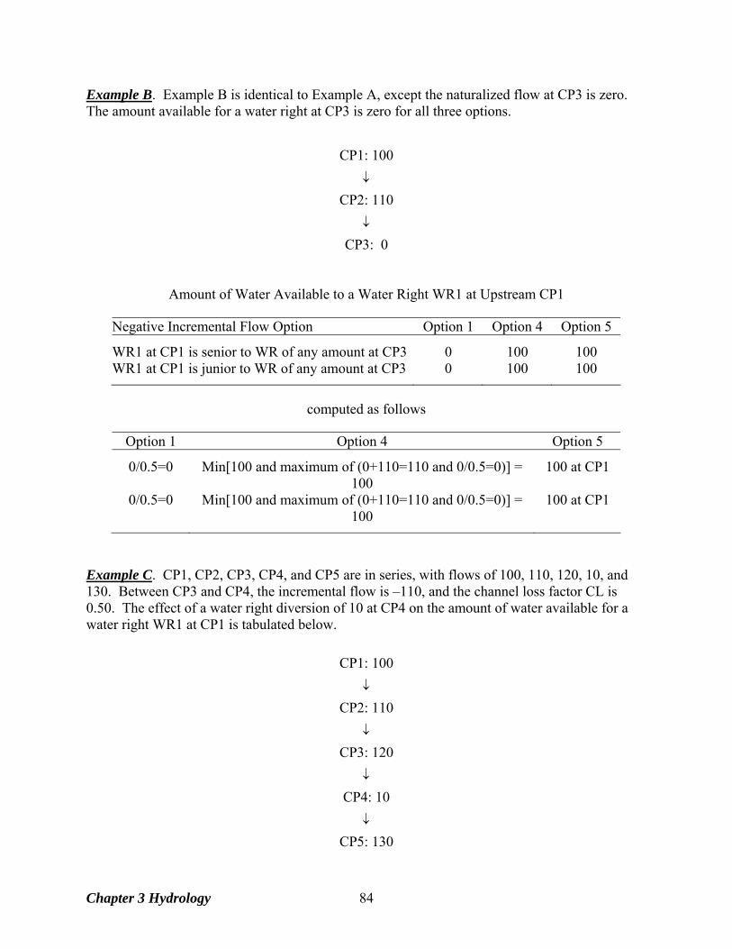
Example B. Example B is identical to Example A, except the naturalized flow at CP3 is zero. The amount available for a water right at CP3 is zero for all three options.
CP1: 100
↓
CP2: 110
↓
CP3: 0
Amount of Water Available to a Water Right WR1 at Upstream CP1
Negative Incremental Flow Option Option 1 Option 4 Option 5
WR1 at CP1 is senior to WR of any amount at CP3 0 100 100 WR1 at CP1 is junior to WR of any amount at CP3 0 100 100
computed as follows
Option 1 Option 4 Option 5
0/0.5=0 Min[100 and maximum of (0+110=110 and 0/0.5=0)] = 100
100 at CP1
0/0.5=0 Min[100 and maximum of (0+110=110 and 0/0.5=0)] = 100
100 at CP1
Example C. CP1, CP2, CP3, CP4, and CP5 are in series, with flows of 100, 110, 120, 10, and 130. Between CP3 and CP4, the incremental flow is –110, and the channel loss factor CL is 0.50. The effect of a water right diversion of 10 at CP4 on the amount of water available for a water right WR1 at CP1 is tabulated below.
CP1: 100
↓
CP2: 110
↓
CP3: 120
↓
CP4: 10
↓
CP5: 130
Chapter 3 Hydrology 84
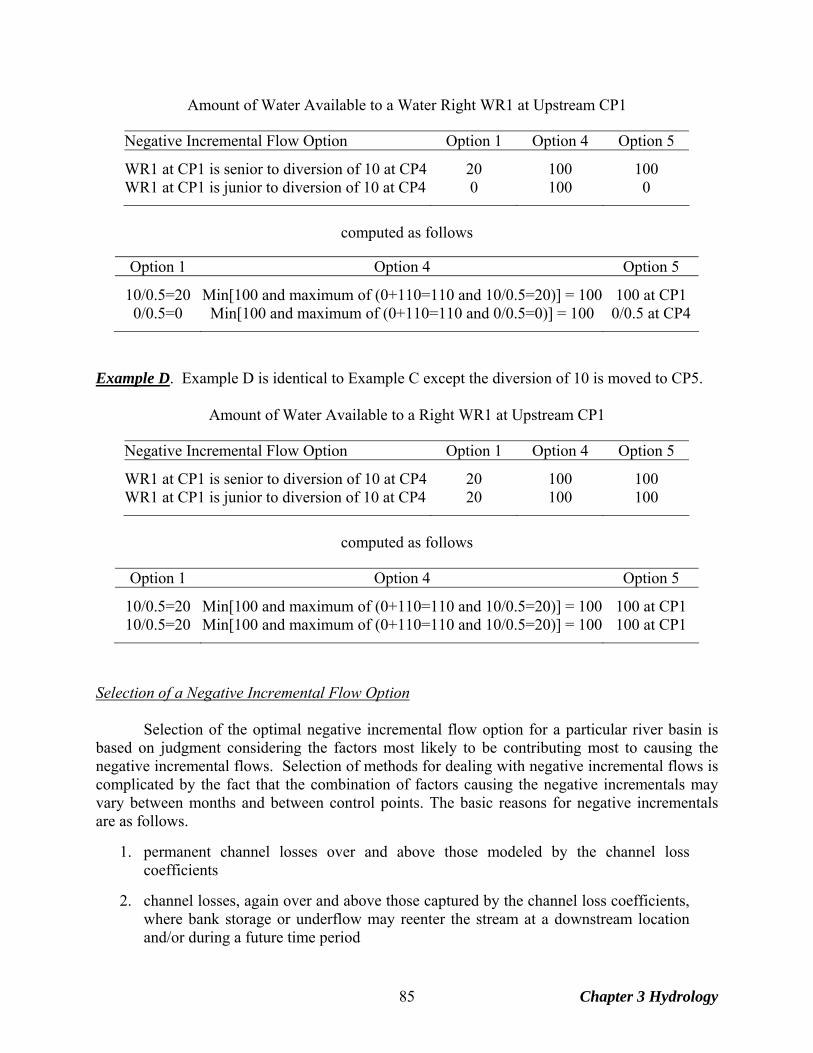
Amount of Water Available to a Water Right WR1 at Upstream CP1
Negative Incremental Flow Option Option 1 Option 4 Option 5
WR1 at CP1 is senior to diversion of 10 at CP4 20 100 100 WR1 at CP1 is junior to diversion of 10 at CP4 0 100 0
computed as follows
Option 1 Option 4 Option 5
10/0.5=20 Min[100 and maximum of (0+110=110 and 10/0.5=20)] = 100 100 at CP1 0/0.5=0 Min[100 and maximum of (0+110=110 and 0/0.5=0)] = 100 0/0.5 at CP4
Example D. Example D is identical to Example C except the diversion of 10 is moved to CP5.
Amount of Water Available to a Right WR1 at Upstream CP1
Negative Incremental Flow Option Option 1 Option 4 Option 5
WR1 at CP1 is senior to diversion of 10 at CP4 20 100 100 WR1 at CP1 is junior to diversion of 10 at CP4 20 100 100
computed as follows
Option 1 Option 4 Option 5
10/0.5=20 Min[100 and maximum of (0+110=110 and 10/0.5=20)] = 100 100 at CP1 10/0.5=20 Min[100 and maximum of (0+110=110 and 10/0.5=20)] = 100 100 at CP1
Selection of a Negative Incremental Flow Option
Selection of the optimal negative incremental flow option for a particular river basin is
based on judgment considering the factors most likely to be contributing most to causing the negative incremental flows. Selection of methods for dealing with negative incremental flows is complicated by the fact that the combination of factors causing the negative incrementals may vary between months and between control points. The basic reasons for negative incrementals are as follows.
1. permanent channel losses over and above those modeled by the channel loss
coefficients 2. channel losses, again over and above those captured by the channel loss coefficients,
where bank storage or underflow may reenter the stream at a downstream location and/or during a future time period
Chapter 3 Hydrology 85
3. timing effects of the runoff from a rainfall event reaching an upstream control point in a particular month but reaching a downstream control point early the next month
4. errors and lack of precision in stream flow measurements at the gages and in
computations to convert gaged flows to naturalized flows
The uncertainties associated with combinations of the factors listed above are inherent in the model even if all incremental flows are positive. Negative incremental flows simply result in the effects being more obvious. Simulation results should be identical for all of the negative incremental flow options if there are no negative incremental flows.
With options 1 and 5, the amount of water available to a right is reduced by negative incremental flows occurring at downstream control points. With options 3 and 4, water availability is not affected by negative incremental flows assigned to control points located downstream. A key hydrologic question is as follows. In order for sufficient water to be physically available for senior water right requirements at downstream locations, must upstream water rights allow sufficient stream flows to pass their locations to cover the negative incremental flows (assumed to be channel losses) occurring in river reaches in between. A policy question to be considered in comparing options is as follows. Is a water right required to allow stream flows to pass its location in order to mitigate negative incremental flows (assumed to be channel losses) occurring in river reaches located downstream. In all cases, stream flows are allowed to "pass through" to accommodate senior water rights located downstream. However, does the amount of flow committed to the downstream rights include channel losses as well as diversion, instream flow, hydropower, and storage requirements? In the extreme case, curtailment of an upstream junior right may, due to channel losses, result in little or no increase in water available to the downstream senior right. Senior rights are protected in SIM regardless of negative incremental flow option. The options differ in regard to how protection of a senior downstream right affects water available to upstream more junior rights.
Default negative incremental flow Option 1 includes no provisions designed specifically to address the issue of negative incremental flows. Options 2, 3, and 4 are based on computing incremental flows at the beginning of the simulation. Options 2 and 3 adjust the naturalized flows to remove the negative incrementals at the beginning of the simulation and thus do not require modifications to the routines in the water rights priority loop. Option 4 computes an adjustment array at the beginning that is used during the simulation in several routines in the model. Option 5 is a modified version of the water right simulation algorithms. With Option 5, incremental flows are not actually computed, and there is no negative flow adjustment array.
The types of circumstances for which each option is most applicable is subject to investigation and debate. However, the following general observations are reasonably valid. • Option 1 is the most conservative in limiting available flows. It provides the conservatively
low extreme of water availability estimates. Option 1 is useful if the model-user chooses to be conservative (under-estimate the amount of water available to rights) with respect to the effects of negative incremental flows. It is also useful in sensitivity study runs testing the effects of the other options on simulation results.
Chapter 3 Hydrology 86
• Option 2 is similar to the approach mentioned below involving adjustments with spreadsheet computations to remove the negative incremental flows prior to applying WRAP. Option 2 is useful for sensitivity studies but would seldom, if ever, be adopted for a final simulation.
• Option 3 is the opposite extreme to Option 1. Option 3 provides high estimates of water
availability. Negative incremental flows have no effect in regard to reducing water availability. Option 3 is useful for sensitivity studies but would seldom, if ever, be adopted for a final simulation.
• Option 4 is generally the optimal choice for most situations. • Option 5 relates best to situations characterized by both of the following conditions:
1. The dominant cause of negative incremental flows is permanent channel losses not modeled by the channel loss factors.
2. The water rights system requires that upstream junior water users curtail their use to
allow pass-by flows to mitigate downstream channel losses in addition to meeting downstream senior water right diversion, instream flow, and storage amounts.
Option 1 is also applicable in these situations, but Option 5 is less overly conservative than option 1.
Another approach for dealing with negative incremental naturalized flows is to adjust
flows with spreadsheet computations to remove the negative incrementals prior to applying WRAP. Flows subtracted in one month may be added back in the next month. WRAP Option 2 similarly reduces flows to remove negative incrementals but does not add the reductions to the next month flows. Options 4 and 5 are probably almost always better than making adjustments outside of WRAP-SIM. Options 3 and 4 routines for computing incremental flows are too complicated to perform conveniently with a spreadsheet program. Options 4 and 5 computations are an integral part of the simulation and can not be performed external to WRAP-SIM.
Chapter 3 Hydrology 87

Chapter 3 Hydrology 88
CHAPTER 4 WATER MANAGEMENT FEATURES
A WRAP-SIM simulation combines
∗ sequences of naturalized stream flows and reservoir net evaporation-precipitation rates representing river basin hydrology, as discussed in the preceding Chapter 3, with
∗ water rights information representing the manner in which water resources are developed, regulated, allocated, and used, as discussed in the present Chapter 4.
WRAP is motivated by the Texas prior appropriation water right permit system but provides flexible capabilities for modeling water management situations anywhere that may or may not involve actual water rights. A broad spectrum of water allocation schemes may be simulated. Constructed facilities, water use requirements, and river/reservoir system operating practices are referred to generically as water rights in WRAP. This chapter describes capabilities provided by WRAP-SIM for modeling a water resources development/management/use system consisting of:
• reservoir projects operated to regulate and conserve river flow, off-channel storage reservoirs, pumping/conveyance facilities, and hydroelectric power plants
• international treaties, interstate compacts, interagency contracts, and other agreements
• requirements specified in water right permits
• river/reservoir system operating policies and rules
• water use characteristics and practices
Water Rights In WRAP terminology, a water right is a set of water management capabilities and use requirements associated with either a water right WR record or an instream flow IF record. UC, UP, DI, IS, IP, RF, WS, OR, HP, SO, ML, TO, FS, TS, and PX records are connected to specific WR or IF records to provide additional information regarding water management and use specifications. Refilling reservoir storage, water supply diversions, and hydroelectric energy generation are specified as WR record rights. Environmental instream flow requirements are specified as IF record rights. SIMD flood control operations covered in the Supplemental Manual are defined as FC/FF record rights. The number of rights counted by SIM is simply the number of WR and IF records in the input file. In modeling a permit system, the total number of rights (WR and IF records) counted by the model typically does not correspond to the number of actual water right permits. A key aspect of applying WRAP is ingenuity in combining water right WR, instream flow IF, and supporting input records to model a particular water management situation. The model provides considerable flexibility in defining water management/use requirements and capabilities. An actual water right permit may be represented by any number of model water rights. A single appropriator holding a single water right permit may have several model rights representing different features of the water right permit. For example, a water right that includes three different uses, such as municipal, industrial, and irrigation, would be treated as three separate WR record rights, since the monthly water use distribution factors are different for the various uses. A water
Chapter 4 Water Management 89

supply diversion and storage capacity can be assigned different priorities by treating them as two separate rights, a diversion right with no storage capacity and a storage right with a zero diversion. A reservoir may have several rights with different combinations of priority dates and storage capacities. Any number of rights may be associated with the same reservoir. Likewise, multiple reservoirs may be associated with a single right. Also, in certain applications, several actual permitted water rights may be combined and inputted to the model as a single aggregate water right. The set of information specifying the water management and use requirements defining a particular water right may include the following.
• identifiers of the control point locations of pertinent components • priority number or information that assigns a priority number • annual diversion target • return flow specifications • instream flow specifications • annual hydroelectric energy generation target • set of monthly water use distribution coefficients • set of rules for varying diversion, instream flow, and hydroelectric energy targets as a function of stream flow subject to specified limits • drought index for varying targets as a function of reservoir storage • active and inactive reservoir storage capacity • reservoir storage volume versus surface area relationship • reservoir water surface elevation versus storage volume relationship • reservoir/river system operating rules • off-channel reservoir storage • interbasin or intrabasin conveyance • annual and monthly limits on stream flow depletions • annual limits on total diversions or diversions from storage • identifiers for labeling rights and aggregating simulation results for groups of related rights
Most of the records and record fields for entering water rights information are optional. The control point location and priority number are actually the only required information for a water right. The priority number field may be left blank but will then default to zero. Each control point identifier on WR or IF records must match an identifier on a CP record. Control point identifiers are required to define the spatial connectivity of a river basin system. Water right identifiers are also entered on WR and IF records for use in labeling input and output data and aggregating simulation results for groups of related rights. However, water right identifiers are not actually required in the simulation computations. Water supply diversion, hydroelectric energy generation, and instream flow requirements are specified in terms of an annual amount input on a WR or IF record combined with a set of 12 monthly use coefficients specified on UC records for distributing the annual amount over the 12 months of the year. Thus, water use requirements may be expressed as monthly targets that may vary each month from January through December but are constant from year to year. Model options also allow targets to be defined as a function of reservoir storage and/or stream flow.
Chapter 4 Water Management 90

Water Right Priorities The allocation of water among water rights in WRAP-SIM is based on priority numbers. The integer priority numbers serve the important function of setting the order in which the rights are considered in the water rights computational loop that allocates water, but are used in no other way. Diversion, instream flow, hydropower, and storage refilling targets for each right are met to the extent allowed by available stream flow and storage prior to considering the requirements of more junior rights. A fundamental concept of the model is that available stream flow is allocated to each water right in turn in ranked priority order. The seniority of a right relative to other rights is expressed by their priority numbers. A smaller priority number means higher priority, rank, or seniority. In comparing two rights, the senior right has a lower priority number than the junior right. Junior and senior are relative terms used in the context of comparing the priority of two rights. Within the SIM computations, the magnitude of the priority numbers for each of the rights relative to each other govern the sequencing of computations and thus water allocation among the rights. In the Texas prior appropriation water rights permit system, priority numbers typically represent dates specified in the permits. For example, a priority date of June 25, 1978 specified in a water right permit is entered in field 5 of the WR record as the integer 19780625, which is a larger number than the priority corresponding to any earlier date. However, with a little ingenuity, the model-user can devise various other schemes for using the priority numbers to model relative priorities for allocating water. WRAP also has alternative options other than water right WR and IF input records for assigning priorities and also has options for circumventing the priority system. Priorities are integer numbers specified for each water right. Smaller integers mean rights are considered earlier in the priority-based computational sequence (Figure 2.2). With the standard default system for assigning priorities, the model-user assigns each water right its own unique priority by entries in WR and IF record field 5. This standard default and other optional alternative methods for ranking all water rights (WR and IF records) in priority order are described as follows. 1. A priority number for each water right is entered in field 5 of its WR or IF records. A blank
field 5 is read as a priority number of zero. If two or more rights have the same priority number, they are ranked in the same order as their WR or IF records are entered in the input file.
2. Factors entered on a use priority UP record replace or modify the WR/IF field 5 priority numbers for all WR and IF records having the same water use type identifier as the UP record.
3. JO record field 9 activates optional methods for assigning priorities that replace the priorities assigned in WR and IF record field 5. These options set priorities either automatically in upstream-to-downstream order (JO record field 9 option 1) or based on the order in which WR/IF records (option 2) or CP records (option 3) are placed in the DAT input file.
4. Options provided on PX/AV and EA/EF/AF records allow two or more rights to share the same priority. Stream flow and storage are allocated between these rights in accordance with rules governed by parameters provided as input by the model-user.
Water use types serve the primary purpose of specifying coefficients for distributing annual use targets over the 12 months of the year but also can be used in specifying priorities for groups of rights. Examples of possible water use types include municipal, various types of industrial, various
Chapter 4 Water Management 91
types of agricultural, mining, or any other categories of interest. Field 4 of the WR and IF records provides a water use identifier that connects the right with water use distribution coefficient (UC) and use priority (UP) records. The following factors may be entered on a UP record.
• integer priority number that overrides the WR/IF record priority number
• integer number to be added to the WR/IF record priority numbers
• factor by which the target diversion, instream flow, or hydropower target amounts from the WR/IF records are to be multiplied
These factors are applied to all rights that have the pertinent use type identifier on the WR or IF record. For example, the effects of making municipal rights senior to all other rights may be conveniently simulated by subtracting some integer from the priorities for all municipal rights that makes them smaller and thus senior to all other rights. Likewise, an alternative simulation examining the effects of a 20 percent reduction in municipal water use targets could be easily made. The following options replace the priorities entered in WR and IF record field 5. The WR/IF field 5 priority number is ignored. The switch parameter NPOPT in JO record field 9 activates three alternative options for setting priorities. JO record field 9 option 1 provides the capability to conveniently simulate water management in a river basin that has no water allocation priority system. Without a water rights permit system or some other regulatory mechanism to allocate water, water availability for each water user is affected by other water users located upstream but not by those downstream. Priorities may be manually assigned to each water right to simulate this upstream-to-downstream natural priority system. However, JO record option 1 allows the upstream-to-downstream priorities to be activated automatically. SIM internally assigns priority numbers to water rights based on the location of their control points. The control points are automatically assigned integer priority numbers starting with 100 and increasing in increments of 100 following the criterion that the integer assigned to any control point is smaller than the number assigned to any other control point located downstream. For control points on parallel tributaries, those listed in the input file first are considered first in the algorithm and get the smaller priority number. Each water right is then assigned the number associated with its control point. For multiple rights at the same control point, the priority number is incremented based relative priorities on their WR and/or IF records. For example, four water rights at a control point with priority number 800 will be assigned priority numbers 800, 801, 802, 803 based upon the relative priorities on their WR or IF records. With JO record option 2, priorities are based simply on the order in which WR and IF records are placed in the DAT input files. The first right read by SIM from the input file is most senior with the priority number 1. The second and third WR or IF records have priorities 2 and 3. With JO record option 3, priorities are based on the order that control point CP records are placed in the input file. For multiple water rights located at the same control point, relative priority rankings are based on the order of the WR and IF records in the input file. PX/AV and EA/EF/AF record options described later in this chapter allocate water between rights sharing the same priority. Capabilities are provided for circumventing the priority system.
Chapter 4 Water Management 92

Water Availability within the Priority-Based Water Rights Computation Loop
The WRAP-SIM simulation approach is built on the fundamental concept of water
allocation computations being performed in a water rights loop in which the requirements of each individual right are met in priority order. Thus, senior rights affect the amount of water available to junior rights but are not adversely affected by the junior rights. However, the simulation is complicated by situations in which junior rights may increase the amount of water available to senior rights. Fluctuating decreases and increases in water availability are a complexity in applying SIM that must be considered in applying the methods outlined in this chapter. Modeling difficulties may occur involving senior rights not getting access to water made available by junior rights through:
1. same-month return flows from diversions from storage
2. same-month hydroelectric power releases
3. contributions to meeting instream flow requirements at intermediate control points made by releases from upstream reservoirs to meet diversions at downstream locations
As each water right is considered in priority order in the water rights computational loop,
regulated flows and the flows available to more-junior rights usually decrease but may also increase. Diversions and filling reservoir storage decrease flows at their control point and at downstream control points. Conversely, flows are increased by hydropower releases and return flows from diversions from storage. Reservoir releases may increase flows at intermediate control points between the reservoir and downstream diversion site. A diversion and/or storage right may be unnecessarily curtailed (shorted) due to computationally not having access to water made available by more junior rights in the form of return flows or hydropower releases. Likewise, reservoir releases that increase flows at intermediate control points between the reservoir and downstream diversion site may not be properly credited as contributing to instream flows at the intermediate control points. Junior diversion and storage rights may be unnecessarily curtailed to maintain senior instream flow requirements.
The following SIM options have been adopted in practice to deal with the complexities of
fluctuating decreases and increases in water availability in the water rights priority loop. These options involve model features described throughout the remainder of this chapter. The next-month return flow option makes the return flows available in the next month at the beginning of the water rights loop. Likewise, modeling return flows as constant inflows on CI records makes the flows available at the beginning of the water right computations. Thus, all rights have access to the return flows in priority order. The next-month hydropower option serves this same purpose for power releases. The optional second-pass feature associated with IF record rights addresses this same complexity for the perspective of instream flow requirements. Since return flows and hydropower releases are usually handled with next-month options and CI record inflows, the second pass instream flow option is probably most relevant for situations in which reservoir releases increase flows at intermediate control points between the reservoir and downstream diversion site. The transient priority XP option 1 on the PX record allows the return flow to be assigned a priority that is different than the diversion priority. Other PX record options are designed to circumvent the priority sequence for other purposes.
Chapter 4 Water Management 93
Specifying Targets and Rules for Meeting the Targets WRAP-SIM provides considerable flexibility in modeling complex water management practices and associated water right permits. Water use requirements, reservoir/river system operating rules, and storage and conveyance structures are modeled in association with water rights. Water rights are addressed here from the perspective of input data records and associated computations performed by the model. An actual water management scheme and associated water right permit can be modeled by a combination of any number of water right input records. The various water right modeling features can be combined in a variety of ways to represent each particular aspect of a reservoir/river/use system. Modeling water rights may be very simple or quite complex depending on the particular application. Table 4.1 provides a categorization of the different types and features of water rights. The input records used to activate the various features are also shown. In WRAP terminology, a water right is a water management scheme described by the information entered on either a WR record or IF record along with auxiliary records tied to the WR or IF record. WR records specify requirements for water supply diversions and return flows or hydroelectric energy generation. WR records are also used to refill/maintain storage in reservoirs at specified capacities subject to water availability. IF records are used to establish instream flow targets, typically associated with environmental needs, and optionally may include releases from storage to meet flow targets. A WR record right, with associated WS record, may include refilling storage in one reservoir called its primary reservoir. An instream flow, water supply diversion, or hydroelectric energy generation requirement may be met by stream flow and/or releases/withdrawals from the primary reservoir and multiple secondary reservoirs. Secondary means the reservoir releases to meet instream flow, diversion or hydropower targets associated with the water right, but its storage is not refilled in association with that particular right. It is refilled by one or more other rights (sets of WR/WS records). Multiple rights with different priorities may refill storage to different levels in the same reservoir. Run-of-river diversion or hydroelectric energy generation rights may be modeled by specifying zero active storage capacity. WR/WS records may also specify a storage-only right with zero entered for the diversion target. An instream flow target is a minimum regulated flow at a control point. Water rights junior to the IF record right are curtailed as necessary to maintain the target minimum flow. An instream flow requirement (IF record) may be specified either without or with associated reservoir storage (WS record). Either way, inflows to reservoirs associated with junior rights are passed through the reservoirs as necessary to maintain the instream flow target. However, releases from storage to meet instream flow requirements are made only from reservoirs associated with the IF record by attached WS records. Reservoir storage parameters on WS records and operating rules on OR records may be associated with either WR or IF records. Diversion, instream flow, and hydropower requirements are typically specified by entering an annual target amount along with a set of 12 monthly distribution factors. The targets may also be altered internally within the model as a user-specified function of storage or stream flow. Alternatively, multiple-year time series of targets may by provided as input. Target setting options may be combined in a variety of ways.
Chapter 4 Water Management 94
Table 4.1 Classification of Water Right Features
_______________________________________________________________________________________ Water rights are categorized as either water right WR record or instream flow IF record rights.
• WR record rights include requirements for diversions and return flows, hydroelectric energy generation, and/or filling reservoir storage.
• IF record rights set requirements for minimum instream flows.
Water rights may include the following optional features for specifying diversion, instream flow, hydropower, and storage targets.
• constant annual amount combined with monthly distribution factors (WR/IF fields 3-4, UC)
• target series that vary between years as well as between months of the year (TS record)
• specification of diversion and instream flow targets as a function of naturalized/regulated/ unappropriated flows, reservoir storage, and/or stream flow depletions (TO, FS records)
• drought index that allows diversion, instream flow, and hydropower requirements to vary as a function of reservoir storage (DI, IS, IP records; IF record field 8; WR record field 10)
Water rights may also include the following optional features for specifying system operating rules.
• secondary backup right that supplies shortages incurred by other rights (BU record)
• stream flow depletions from alternate locations (SO record field 5)
• annual or seasonal limits on diversions (SO record fields 10, 11, 12)
• monthly/seasonal/annual limits on stream flow depletions (SO fields 3-4, 11-12; ML record)
• monthly/seasonal/annual limits on withdrawals from reservoir storage (SO fields 7-8, 11-12)
• monthly varying reservoir storage capacity (MS record)
• multiple entities sharing storage capacity in the same reservoir (EA record)
• multiple reservoir system operations (WS and OR records)
• hydroelectric power operations (HP record)
• water management schemes that circumvent the priority system (PX record)
WR record water rights are categorized as either Type 1, 2, 3, 4, 5, 6, or 7 in WR record field 6.
Type 1: default standard right may include diversion and return flow, refilling storage in one reservoir, and releases from any number of reservoirs. Diversion requirements are met from reservoir storage if and only if sufficient stream flow is not available.
Type 2: same as type 1 except that refilling of reservoir storage is not allowed
Type 3: same as type 2 except diversions can be supplied only from reservoir storage
Type 4: flow is discharged into the stream
Type 5: hydropower right, same as type 1 except a hydroelectric energy generation requirement is specified instead of a diversion requirement
Type 6: hydropower right with stream flow depletions not allowed, meaning electric energy is generated only from releases from reservoir storage and the reservoir is not refilled
Type 7: reservoir storage refilling target is determined and applied _______________________________________________________________________________________
Chapter 4 Water Management 95
In addition to the features listed in Table 4.1, a watershed flow option for distributing naturalized flows may be activated by the SO record. The watershed flow option is described in Chapter 3 along with the other flow distribution methods. It is different than the other methods in regard to being associated with a water right (WR record) rather than a control point (CP record). Water management and use requirements are based on meeting:
• reservoir storage demands/needs/targets • water supply diversion demands/needs/targets • hydroelectric energy production demands/needs/targets • instream flow demands/needs/targets
to the extent allowed by available water subject to the water rights priority system, operating rules and practices, and the configuration and capacities of storage and conveyance facilities. The terms targets, demands, needs, and requirements are used interchangeably in this report. The organization of the SIM simulation algorithms is outlined by Figure 2.2 and the accompanying discussion in Chapter 2. In a given month, in considering each individual right in priority order in the water rights computation loop, the following tasks are performed by the model for each right in turn. Task 1: The diversion, hydropower, storage, or instream flow target for the month is set.
Task 2: The amount of stream flow available to a WR record right is determined.
Task 3: Water allocation algorithms determine stream flow depletions, reservoir releases and storage changes, net evaporation-precipitation volumes, and the portion of the diversion and hydropower targets that are met and associated shortages.
Task 4: Unappropriated and regulated stream flows are adjusted for the effects of the right. The next section outlines the system for setting water management/use targets (Task 1). Features for modeling operating rules for meeting the targets (Tasks 2 & 3) are then described. The chapter then covers the details of reservoir system storage and operations, water supply diversions and return flows, hydroelectric energy generation, environmental instream flow requirements, and modeling water management schemes that circumvent the priority sequence.
Setting Diversion, Instream Flow, and Hydropower Targets In many typical modeling applications, targets are defined by simply entering an annual target amount on a WR or IF record and a set of 12 monthly distribution factors on UC records. The targets vary seasonally but are constant from year to year. However, targets may also be entered for each individual month of the multiple-year period-of-analysis, varying from year to year as well as seasonally. Options also provide flexibility for defining targets as a function of reservoir storage, current or accumulated past river flows and/or stream flow depletions appropriated by specified rights, as well as month of the year. Water use requirements may be specified by a single option in SIM, or alternatively, requirements may be computed within the model by combining multiple optional features. For
Chapter 4 Water Management 96

most typical water rights, targets are defined by simply entering an annual target amount on a WR or IF record and monthly distribution factors on UC records. However, ingenuity may be applied to combine several options to model complex water management situations. In a given month of the simulation, as the water rights are considered in turn in priority order, SIM builds monthly diversion, instream flow, or hydroelectric energy targets in sequential steps as outlined below. Embedded within the other sequentially ordered steps governed by WR/IF/UC, BU, DI/IS/IP, TO, TS, FS, and SO records, step 4 below may also be a series of target building steps with each step being governed by a separate TO record. 1. The model combines the annual diversion, hydroelectric energy, or instream flow
requirement amount entered in a WR or IF record with monthly distribution coefficients from UC records to obtain a target for each of the 12 months of the year. UC records are not required if the monthly target is constant over the year.
2. The backup option activated by the BU record allows a water right to serve as a supplemental
backup right for one or more other rights. Shortages incurred by the other rights are added to the target of the backup right. The shortage may be added at this step or as step 9.
3. The optional drought index defined by a set of DI/IS/IP records modifies the target as a
function of the storage content of specified reservoirs. The drought index may be applied here as step 3 or later as step 6. The location of the drought index adjustment in the computational sequence is specified with the DINDEX entry on the IF or WR record.
4. SIM uses several variables entered on one or multiple TO records to build diversion and
instream flow targets. Targets may be a function of naturalized, regulated, or unappropriated flow multiplied by a factor. The target may be set based on reservoir storage or stream flow depletions incurred by other rights, which may also be multiplied by a factor. Upper and lower bounds on the target may be applied in two different ways here in the repetitive step 4.
Several TO records may be used to build a target step-by-step. The first TO record results in a target to be combined with the target determined in the preceding steps outlined above. Each subsequent TO record results in another target to be combined with the preceding cumulative target. The two intermediate targets are combined in each step by either (a) selecting either the maximum or minimum or (b) adding them. The target developed in this manner may be a function of the summation of naturalized, regulated, and/or unappropriated stream flow at multiple control point locations, stream flows at various locations, reservoir storage, stream flow depletions by other water rights, and/or user specified lower and upper bounds. Flexibility is provided for combining these features as needed.
5. A time series of monthly diversion, hydroelectric energy, or instream flow targets for each
month of the hydrologic period-of-analysis may be entered on TS records. The TS record may be the only option used for a particular water right, or TS record targets may be combined with the other options. Either (a) the greater or lesser or (b) the summation or product of the steps 1−4 versus step 5 values for a particular month is adopted depending on the value for TSL entered in the second field of the TS record for the first year.
Chapter 4 Water Management 97
6. A drought index defined by a set of DI/IS/IP records modifies the target determined above as a function of the storage content of specified reservoirs. The drought index may be applied at this step in the sequence or as step 3 above.
7. The target may be constrained by upper and lower limits entered on a TO record. 8. A flow switch FS record may modify the target based on accumulated regulated, naturalized,
or unappropriated flow, diversions or stream flow depletions, or control point inflows. One of two alternative multipliers are applied to the target depending on whether the defined flow variable at a specified control point during the current month or accumulated during the past period of any number of months fall within a specified range.
9. The backup option activated by the BU record may be applied as either steps 2 or 9. The
backup right’s own target is first determined as outlined above, and then shortages incurred by one or more specified other rights are added.
The options outlined above are applied in sequential order within SIM to set targets.
Other parameters on a SO record may limit the amount of water available to a water right. Water availability for a right may be limited by monthly or cumulative seasonal or annual limits on stream flow depletions and the amount of water that may be withdraw from reservoir storage. An annual or seasonal diversion limit may also be placed on the total water diverted by a right.
Diversion and Instream Flow Targets as a Function of Stream Flow, Storage, and Other Rights
The target options TO record provides options described as Step 4 on the preceding page for computing monthly diversion or instream flow targets as functions of (a) naturalized, regulated, or unappropriated stream flow, (b) reservoir storage or storage drawdown, (c) water taken from stream flow or reservoir storage by other rights, and (d) user-specified upper and lower bounds. Storage drawdown is capacity less storage content. The targets may be functions of stream flows or storage optionally in either the previous month or current month. If the current month option is adopted, unappropriated stream flow is the flow that is still unappropriated at the step in the water rights priority loop computations at which the right is considered. Likewise, with the current month option, the regulated flow and end-of-period storage reflect only the effects of senior rights.
Considerable flexibility is provided to creatively combine target-building features in a
variety of ways to model a broad range of possible water management situations. Targets could be computed by the model by adding and/or subtracting stream flows at any number of locations; combining other types of flows at other locations; adopting the minimum or maximum of these values; and placing upper and lower bounds on the flows. Stream flow falling within different bounds may be multiplied by different factors. A reservoir may be refilled with a diversion with the target determined based on the reservoir drawdown limited by regulated flows. Targets may depend upon the amount of water taken by other water rights. The TO record options may also be combined with drought index DI/IP/IS, flow switch FS, and target series TS records. Innovative strategies for combining options may be adopted to model complex and unique water management situations.
Chapter 4 Water Management 98
The following simple example illustrates the general approach of applying TO records. Examples in Appendix B provide further illustration. ______________________________________________________________________________ Example: Subject to water availability, regulated flows at control point CP1 are maintained to not fall below the minimum level defined by the following instream flow target. The target is set as a function of naturalized flows at CP1 and the summation of available flows at CP2 and CP3. Available flows are the unappropriated stream flows considering all water rights that are senior to this right. For each month, the target is set at 25 percent of the total sum of the unappropriated flows at CP2 and CP3, except the target can not exceed the naturalized flow at CP1. Another feature of the instream flow requirement is that the target must fall within the range of 100 to 500 acre-feet/month, regardless of the flows at CP1, CP2, and CP3. This target is specified by the following IF and TO records. ** ** Record Fields **⏐ 2 ⏐ 3 ⏐ 4 ⏐ 5 ⏐ 6 ⏐ 7 ⏐ 8 ⏐ 9 ⏐ 10 ** IF CP1 1985 TO 3 0.25 CP2 CONT TO 3 .25 ADD CP3 CONT TO 1 CP1 MIN 100. 500. ** Although each TO record results in a cumulative intermediate target, only the final target
is used in the simulation computations. For purposes of illustration, assume that in a particular month of the simulation, the naturalized flow at CP1 is 635 ac-ft and WRAP-SIM computes available flows of 800 and 400 ac-ft at CP2 and CP3. The target is set by WRAP-SIM step-by-step as follows.
IF CP1 1985 TO 3 0.25 CP2 CONT
The first intermediate target is computed as: (0.25)(800) = 200 ac-ft TO 3 .25 ADD CP3 CONT
The target is computed as: 200 + (0.25)(400) = 300 ac-ft TO 1 CP1 MIN 100. 500.
The target is the minimum of 300 or (1.0)(635)=635 which is 300 ac-ft. The target is the maximum of 300 or the lower limit 100 which is 300 ac-ft The target is the minimum of 300 or upper limit of 500 which is 300 ac-ft.
Thus, in the example, SIM determines a minimum instream flow target of 300 ac-ft for that month. This target was built step-by-step by combining several options. ______________________________________________________________________________
Chapter 4 Water Management 99
Diversion, Hydropower, and Instream Flow Targets Series Entered on TS Records The purpose of the target series TS record option is to provide flexibility for diversion, instream flow, or hydropower targets to be developed outside of the model and entered as input. The targets entered on TS records may be determined by various means independently of SIM or perhaps from previous simulations performed with the model. The TS record targets may be the only requirements specified for a particular water right or alternatively may be integrated with the other options. Targets from TS records are integrated into the sequential step-by-step SIM target building scheme as Step 5 as previously outlined. TS records may be used to modify targets computed within the model with other options. Targets may be arithmetically manipulated by adding, subtracting, or multiplying numbers from TS records. The target series TS records allow monthly diversion, instream flow, and hydropower demands to be specified that vary between years as well as seasonally. If the TS option is adopted, targets cover every month of the hydrologic period-of-analysis. However, the number of TS records may range from one to the total number of years in the simulation. The 12 monthly targets entered on a TS record may represent just one year or be repeated for any group of years or the entire simulation period. Drought or Storage Index The various options activated by the WR, IF, SO, TO, FS, TS, and DI/IP/IS records may be combined in a myriad of ways to define diversion, instream flow, and hydropower targets. The drought or storage index option defined by DI, IP, and IS records may be combined with the other records in the target building process or alternatively may be applied independently. The term drought index is adopted because depleted storage is viewed as an indicator of prolonged dry conditions with diminished water resources. The drought index option allows instream flow, diversion, and hydropower requirements to vary with reservoir storage content. The drought index option may be used as a mechanism for modeling reservoir system operations. However, more generically, a drought index can be used to allow any water use target to vary as a function of storage content, including instream flow, run-of-river diversion, and other water use requirements not met by releases from the reservoirs included in the drought index. This feature may be adopted for any application in which water use requirements are expressed as a function of reservoir storage. JO record field 8 is a switch allowing either beginning-of-month storage or the latest end-of-month storage computed in the water right priority loop to be used for the index. Drought indices are assigned integer identifiers (1, 2, 3, ...) in the sequential order that the DI/IS/IP records for each index are entered in the input file. Entering one of these integer identifiers in field 8 of an IF record or field 10 of a WR record connects a water right to a drought index. Any number of water rights can be assigned the same drought index, and there can be any number of drought indices. Each drought index consists of a drought index reservoirs DI record and drought index storage IS versus percentage IP records. The DI record specifies the selection of reservoirs upon which to base the index. Either all of the reservoirs in the model or a selection of up to 12 reservoirs
Chapter 4 Water Management 100

may be specified. The IS and IP records provide a table of reservoir storage versus percentage. The reservoir storage values on the IS record refer to the total storage content of the reservoirs specified by the DI record. The corresponding percentage on the IP record are factors by which the instream flow, diversion, and/or hydroelectric energy requirements are multiplied. The inclusion of certain reservoirs in the drought index assigned to particular water rights does not otherwise associate the reservoirs with the water rights. WS and OR records are connected to WR and IF records identically the same with or without assigning a drought index to the WR record. Instream flow, diversion, and hydropower generation requirements associated with a water right may be determined as a function of a particular drought index without the DI record reservoirs making releases for these requirements or being otherwise associated with the right. Drought indices are incorporated in the SIM simulation computations as follows. 1. A parameter entered in JO record field 8 allows either beginning-of-month storage or the latest
end-of-month storage computed in the water right priority loop to be used for the index. Either at the beginning of the month or at the pertinent point in the priority sequence, the storage contents of the specified reservoirs are summed to obtain a total storage for the drought index. All of the reservoirs in the model or up to 12 reservoirs can be selected for each drought index.
2. Linear interpolation is applied in combining the total storage associated with a particular
drought index with the storage versus percentage relationship from the IS/IP records to obtain a multiplier factor expressed as a percentage.
3. The percentage converted to a fraction is multiplied by the permitted instream flow, diversion,
and/or hydroelectric energy targets for each right assigned to a particular drought index. 4. After adjusting the target instream flow, diversion, and hydropower amounts in the previous
step, all computations proceed normally without any other change related to the drought index. A drought index is normally used to express a diversion, instream flow, or hydropower target as a function of the storage content of one or more actual reservoirs. However, other innovative types of applications are also possible. For example, a drought index may be used to specify targets as a function of cumulative flows or diversions. A diversion may be a function of the cumulative total amount previously diverted that year by certain water rights. Freshwater inflows into a bay and estuarine system may be expressed as a function of cumulative inflows to date that year. A computational reservoir with zero evaporation may be placed at the basin outlet to model the accumulation of inflows into a bay or estuary. The zero-evaporation, zero-inflow computational reservoir could be assigned a control point not connected to the system to model a sink or accumulation of diversions that are transported to the computational reservoir as return flows. The switching-variable EMPTY of the DI record is designed to facilitate this type of application. The reservoir may be emptied either every month or annually on a specified month of the year. In the model, the water from the reservoir is loss from the system. Flow Switch for Adjusting Targets Based on Accumulated Flow Volumes The flow switch FS record activates a feature allowing instream flow, diversion, and hydropower targets to be switched on/off or otherwise adjusted depending on whether the
Chapter 4 Water Management 101
accumulated volume of a selected flow variable in the current and/or any number of preceding months falls within a specified range. The primary motivation for this feature is flexibility in modeling instream flow requirements that are expressed as a function of whether current and/or accumulated past flows at a specified location fall within a specified range. However, the FS record options may be also applied in setting water supply diversion, hydropower generation, and reservoir storage targets. SIM keeps track of the total volume of the defined flow variable at a specified control point that has accumulated over the preceding user-defined number of months. Any number of months may be specified. The FS record target setting rules are based on specifying two different factors which may be zero, 1.0, or any other number. The target is multiplied by one of the two alternative factors each month. The choice of factor depends on whether or not the cumulated flow falls within a user-specified range.
River/Reservoir System Operating Rules for Meeting Water Use Requirements Modeling river/reservoir/use system operations may range from very simple to quite complex. Flexible options are provided to model the rules by which stream flow and reservoir storage is allocated to meet the water use targets described in the preceding section. Table 4.1 outlines the optional water rights features for modeling various complexities or different situations. The preceding section focuses on options for setting targets modeling water supply diversion, environmental instream flow, and hydroelectric energy production targets (demands, needs, requirements). The following discussion describes options to be adopted in various combinations to model the manner in which the river/reservoir system is managed to meet these water use targets. Secondary Backup Right The secondary backup option allows diversion, instream flow, or hydropower shortages associated with a water right to be supplied by another right called a backup right. The backup option is activated by a BU record assigned to the right providing the backup. The WR or IF record right with a BU record serves as a backup for any number of other rights. The diversion, instream flow, or hydropower shortages computed for the one or more specified other water rights are added to the target of the backup right. The computations then proceed normally without any other change related to the backup feature. In each month, the target for the backup right is the shortage of the rights being backed up plus the target amount determined by its own WR/IF/UC records and target setting options on associated SO/TO/TS/DI/FS records. A backup right may also be combined with the PX record control point limit option discussed in the last section of this chapter. Shortages incurred by the specified rights are added to the target of the BU record right within in the water rights priority loop computational sequence. If the other right is senior to the backup right, its shortage is added to the target of the backup right in the same month. If the other right is junior, its shortage is added to the backup right target in the next month.
A backup right may backup another backup right. Any number of backup rights may be placed in sequence. Each adds any shortage amount computed for the preceding backup right to its own target. Thus, a single diversion requirement can be shared by multiple rights.
Chapter 4 Water Management 102
Though rendered obsolete with introduction of the expanded features provided by the newer BU and PX records, SO record field 6 is still functional. The SO record field 6 option with RETURN entered may be used in combination with a type 4 right to assign a priority to a return flow that is different than the corresponding diversion right. A WR record for a type 4 right along with its SO record may be placed behind the WR and supporting records for a more senior diversion right. The diversion shortage for the first right will be applied in computing the amount AMTRF that the second right (type 4 right) returns to the stream as follows:
( )( )4 4 4type right type right previous right type rightAMTRF T S RFAC= −
where the target amount T for the type 4 right is computed as normal and then adjusted for the shortage S from the previous right. The more recently added transient water right XP option 1 activated by the PX record provides a simpler means to assign a different priority to return flows. Stream Flow Depletions from Multiple Locations Stream flow depletions to meet diversion requirements and refill reservoir storage normally occur at the control point to which the water right is assigned. This control point is specified in the second field of the WR record. Diversion and reservoir refilling requirements can also be met by releases from storage from one or multiple secondary reservoirs identified on WS records with system operating rules specified on OR records. An option allows reservoir storage to be refilled from stream flow depletions at other control points. The input variable ACPID (alternate control point identifier) entered in the SO record specifies the location from which flow depletions are made. Any number of WR/SO records, and thus alternate control point locations, can be associated with a particular reservoir. There are no restrictions on which control points to use to refill storage. The computations are based on using the alternate control point in lieu of the default control point specified in the second field of the WR record. A typical application of this feature would be a storage reservoir located on a small tributary that is filled by pumping water from a nearby major river as well as the inflows from its own watershed. A WR/WS/SO record set allows the reservoir to be refilled from inflows from the small stream on which it is located. In months in which these inflows are insufficient to fill the reservoir to capacity, a second WR/WS/SO record set with an alternate control point allows the reservoir to pump water from the other stream. Limits on Stream Flow Depletions, Diversions, and Diversions from Storage SO record variables MRW and ARW are limits on monthly and seasonal or annual withdrawals from reservoir storage. An annual or seasonal diversion limit ADL may also be entered on the SO record. For annual limits, starting in the first month of each year, the model maintains a record of the total cumulative stream flow depletions, diversions, and the amount of the diversions that came from reservoir storage that year associated with the specified water right. Upon reaching a specified limit, no more water is available to the diversion right until the beginning of the next year. Likewise, the limit months LM(wr,1) and LM(wr,2) entered on the SO record define beginning and ending months of a season for which the limits apply.
Chapter 4 Water Management 103
Water right permits associated with off-channel reservoirs often limit the total cumulative amount of stream flow that may be taken each year to refill reservoir storage. Pumping and conveyance facilities as well as water rights permits may limit the amount of stream flow withdrawn each month. Options allow monthly and annual limits to be imposed on stream flow depletions associated with a water right. Without specifying this option, reservoir storage is refilled to capacity each month as long as sufficient stream flow is available to a right. The options for specifying flow depletion limits are motivated primarily by constraints on refilling off-channel reservoir storage but are applicable to major main-stream reservoirs and diversions as well. SIM does not explicitly differentiate between on-channel and off-channel reservoirs, and these options may be applied to either.
A stream flow depletion is the amount of water taken from stream flow by a right to meet diversion requirements, net evaporation-precipitation requirements, and refill reservoir storage. The input variable ANNDEP of the SO record is a limit on the cumulative annual flow depletion that a right is allowed. Starting in the first month each year, the model maintains a record of the total stream flow depletions that a right has accumulated that year. Reservoir storage refilling and diversion associated with the right (WR/WS records) is curtailed whenever the ANNDEP limit is reached. The limit is treated as another constraint on water availability. Monthly limits on the stream flow depletions associated with a water right can also be imposed. The input variable MONDEP of the SO record is a constant limit imposed each of the 12 months of the year. The amount of stream flow available to a right is constrained to not exceed MONDEP) in any month. Alternatively, a set of 12 monthly varying limits may be specified for a right on a ML record. Specifying River/Reservoir System Operating Rules Based on Water Right Types 1 to 7 As indicated by Tables 4.1 and 4.2, all WR record water rights are categorized as being either type 1, 2, 3, 4, 5, 6, or 7 by the entry in field 6 of the WR record. This scheme of water right types is used to specify certain basic rules for meeting diversion or hydroelectric energy requirements from stream flow and reservoir storage and for refilling reservoir storage. The kinds of river/reservoir system operations associated with each type of water right are summarized in Table 4.2 and described in the following paragraphs.
Table 4.2
Water Right Types 1, 2, 3, 4, 5, 6, and 7
Water Right Type (WR Record Field 6) River/Reservoir System Operation 1 2 3 4 5 6 7 water supply diversion from stream flow yes yes − − − − − hydroelectric power generation − − − − yes yes − releases from one or multiple reservoirs yes yes yes − yes yes − refill storage in one reservoir yes − − − yes − yes discharge of inflows into the river − − − yes − − −
Chapter 4 Water Management 104
Type 1, 2, 3, 5, and 6 rights allow releases from reservoirs to meet either diversion (types 1, 2, 3) or hydropower (types 5, 6) requirements specified on WR and associated records. However, reservoir storage may be refilled only by type 1, 5, and 7 rights. Thus, at least one type 1, 5, or 7 right must be connected to every reservoir. A type 1 right is often used to refill a reservoir from which draw-downs are made by type 2, 3, and/or 6 rights and perhaps other type 1 or type 5 rights. Refilling storage may be assigned a different priority than withdrawals and releases from storage. If one or more WS records are connected to an IF record, reservoir operation is equivalent to WR record type 2. Releases are made from the reservoirs to meet the instream flow requirement. However, an IF record does not refill storage. In general, all junior rights must pass inflows through their reservoirs to meet downstream instream flow requirements. Using one or more WS records to assign reservoir storage to an IF record right is relevant only if releases from storage are required, in addition to passing reservoir inflows, to meet instream flow requirements. Type 1 right.- Most water rights in a typical river basin will likely be represented as type 1 rights. A type 1 right allows a diversion to be met from stream flow depletions and/or storage in one or more reservoirs. A diversion requirement is met first from stream flow, if available, and then from reservoir storage if stream flow is not available. One reservoir, called the primary reservoir, can be refilled from stream flow depletions or releases from other reservoirs in the system. The one primary reservoir that can be refilled and the diversion, if any, associated with that WR record must be located at the same control point. The other reservoirs in the system, from which releases or withdrawals are made, can be located at any of the control points. A storage-only right may simply refill storage in the one reservoir, having a diversion requirement of zero. A run-of-river diversion right can be represented as a type 1 or type 2 right with zero active reservoir storage capacity. Type 2 right.- A type 2 right is identical to a type 1 right except that reservoir storage is not refilled. Reservoirs may be used along with stream flow to meet diversion requirements, but other rights are used to refill storage. Another type 1 right refills the reservoir storage. A type 1 right allows both a diversion and refilling of storage, but the diversion and reservoir must be at the same location. If a diversion is at a location different than the location of the reservoir, a type 2 or 3 right with an operating rules OR record is required. Type 3 right.- A type 3 right is identical to a type 2 right except the diversion target can be met only by releases or withdrawals from reservoir storage. For example, a diversion could be met by releases from one or more upstream reservoirs without allowing diversion of unregulated stream flow entering the river below the dams. Unlike a type 3 right, a type 1 or 2 right makes reservoir releases only after the stream flow at the diversion location is depleted. Type 4 right.- With a type 4 right, the annual amount AMT entered in WR record field 3 is discharged into the stream. The stream inflow amounts resulting from type 4 rights are found in the simulation results as return flows. A type 4 right may model an interbasin transfer of water through conveyance facilities, return flow from groundwater sources, or other situations involving discharge of water into the river system within the water rights priority computation loop sequence. The target amount is computed for a type 4 right just like any other type of right. The difference is that a type 4 right is not a diversion from the stream, but rather an inflow to the stream. After the monthly amount is determined just like a diversion target, it is then multiplied
Chapter 4 Water Management 105
by the return flow factor RFAC from WR field 8 and treated computationally as a return flow. RFAC is assigned a default of 1.0 if the RFAC field is blank. All return flow options are valid, except monthly return factors (RF records) can not be used. Water availability computations are not relevant and are not performed for a type 4 right. The flow is entered into the stream system; it is not taken from stream flow, reservoir storage, or any other source included in the model. Type 5 right.- A hydropower right is identical to a type 1 right except a hydroelectric energy requirement is specified rather than a diversion. A 5 or −1 is entered in WR record field 6 for a hydropower right. A run-of-river hydropower right can be represented as a type 5 right with one reservoir with inactive but no active storage capacity. Hydropower rights are not affected by IF record rights. Use of separate WR record type 1 rights to refill reservoir storage at a hydropower reservoir project may be required to protect IF record instream flow requirements. Type 6 right.- A type 6 hydropower right is analogous to a type 3 diversion right. A 6 or −3 is entered in WR record field 6. The only difference between types 5 and 6 is that type 6 does not allow access to stream flow. Stream flow depletions are zero and thus storage can not be refilled. Type 7 right.- A type 7 right refills storage in a reservoir based on a storage target computed in identically the same manner as a diversion target. Options for setting diversion targets using WR, UC, DI/IS/IP, TO, TS, FS, and SO record options are applied in exactly the same way to set a type 7 right storage target starting with AMT in WR record field 3 which is distributed over the 12 months of the year. However, the target is a storage capacity to which the reservoir is filled subject to water availability and the constraint of not exceeding the capacity entered in WS record field 3. Thus, as long as the target does not exceed the normal WS record field 3 capacity, the target is treated as the storage capacity. There is no diversion or hydropower generation associated with a type 7 water right. A type 7 right does nothing but refill reservoir storage. Primary and Secondary Reservoirs A water right can be associated with any number of reservoirs. A WS record for each reservoir must follow the WR record. Only one reservoir, called the primary reservoir, is allowed to refill storage with that particular right. The water right diversion and primary reservoir must be located at the same control point. Types 1, 5, and 7 rights are the only water rights allowed to refill storage. A type 1 right or hydropower right may have either zero or one primary reservoir and any number of secondary reservoirs. A type 7 right must have one primary reservoir and may have any number of secondary reservoirs. The primary reservoir must be cited on the WS record immediately following the WR record. All reservoirs on the second and subsequent WS records are termed secondary reservoirs and can only make releases for the water right, not be refilled by it. All reservoirs associated with type 2, 3, or 6 rights are classified as secondary reservoirs. These reservoirs are refilled by other rights. Likewise, IF record rights do not refill reservoir storage. Water Right Types 1, 2, 3, and 7 in the WRAP-SIM Simulation The water right type specified on the WR record guides the computations within the WRAP-SIM water rights loop. The type specification primarily affects the determination of the target requirement for the right and the manner in which the requirement is to be met. The available
Chapter 4 Water Management 106
stream flow is calculated the same regardless of water right type, except hydropower rights are not subject to instream flow requirements. The target stream flow depletion is then computed according to the type of right. For type 1 rights, the target stream flow depletion is the permitted diversion amount plus the volume needed to refill storage in the primary reservoir, if one exists. A right is allowed to refill storage only in its primary reservoir, and only up to the storage capacity of the right. A stream flow depletion is then made to meet the target. If the available stream flow is greater than the target, the target stream flow depletion is taken from the available flow, and the computations continue on to the next right in priority order. If there is not enough available stream flow to meet the target, the additional amount is released from reservoir storage. The permitted diversion amount for a type 1 right is given priority over refilling of reservoir storage when the amount of water available is insufficient to supply both. The computations to replenish storage in the primary reservoir are based on the total capacity associated with that water right. Subsequent junior rights may have storage capacities that are higher than the right in question, but this extra storage capacity is ignored by the current right in refilling storage. Computations for a type 2 right are identical to a type 1 right except a type 2 right is not allowed a primary reservoir in which to replenish storage. The target depletion for a type 2 right is simply the permitted diversion amount. Although a type 2 right can not refill storage, it can meet its diversion requirement from releases from storage from one or more reservoirs. The target requirement for a type 3 right is computed identically to a type 2 right, but a type 3 right is not allowed to make a stream flow depletion. The available stream flow is by definition zero. The permitted diversion is treated as an additional amount to be released from system reservoirs. For water right types 1, 2, and 3, diversion shortages are calculated as the difference between the permitted diversion amount and the amount of the diversion target actually met. With a type 7 right, a target is computed just like for a type 1 diversion. The simulation computations for a type 7 right are identical to a type 1 right except for the use of this target. With a type 7 right, the target replaces the total storage capacity at top of conservation from the WS record field 3 as long as the target does not exceed the WS record capacity. In any month in which the computed target exceeds the conventional WS record storage capacity, the target is ignored and the computations are identical to a type 1 right with zero diversion.
Reservoir Storage Reservoir storage parameters are provided on the storage WS record associated with a water right WR record or an instream flow IF record if one of the storage options (IFMETH options 3 or 4) is activated. Any number of water rights can be associated with a single reservoir. Multiple reservoirs may also be associated with a single water right. However, a right may include a storage capacity to be refilled in only one reservoir, called its primary reservoir. Secondary reservoirs supply water use requirements but are not refilled by the right. The WS record includes the total storage capacity volume at the top of conservation pool and at the top of the inactive pool. Each individual water right associated with a reservoir has its own conservation and inactive capacities.
Chapter 4 Water Management 107
The storage capacity at the top of conservation pool specified in WS record field 3 (or the alternative storage target for a type 7 right if less than WS record field 3 capacity) defines:
1. The pool from which that right can divert or release water. The right has access to the volume of water stored above its top of inactive pool and below its top of conservation pool storage levels. (Applicable for water right types 1, 2, 3, 4, 5, 6, and IF rights.)
2. The total cumulative capacity to which the reservoir can be refilled under the priority of that water right, assuming the reservoir has been drawn down in current and previous months and stream flow is now available for refilling. (Types 1, 5, 7 only.)
In the simulation, a water right can make no releases or diversions from its inactive pool. The reservoir storage level is allowed to fall below the top of inactive pool only due to evaporation. Storage Capacity Versus Surface Area and Elevation Relationships A storage volume versus water surface area relationship is provided as input for each reservoir for use in the net evaporation-precipitation computations. The net evaporation-precipitation volume for a given month is the computed average water surface area during the month times the appropriate net evaporation-precipitation depth. Two optional formats are provided for inputting a reservoir storage volume versus surface area relationship. A table of storage volume versus surface area can be inputted on SV/SA records. The model applies linear interpolation to the table to determine the area corresponding to a computed storage volume. Alternatively, values of the coefficients a, b, and c can be provided on the WS record for use in the following equation incorporated in the model:
A = aSb + c (4.1) where S and A denote reservoir storage volume and surface area. Typically, storage volume versus surface area tables are provided on SV/SA records for major reservoirs. These data are usually readily available for large reservoirs. A generic set of coefficients (a, b, c) for Equation 4.1 may be developed from data available for a few representative small reservoirs and then applied to numerous smaller reservoirs for which storage-area data are not available. A water surface elevation versus storage volume table is provided on PE/PV records for any reservoir associated with hydropower for use in determining head. A PE/PV record elevation-volume table may also be input for reservoirs without hydropower to tabulate water surface elevations for information purposes. Monthly Varying Limits on Storage Capacity The monthly varying storage capacity option is motivated primarily by seasonal reallocations of storage capacity between flood control and water supply in multiple-purpose reservoirs. Seasonal rule curve operating rules consist of varying the top-of-conservation pool or other designated pool levels with season of the year. Probably the most common use of seasonal rule curve operations is in allocating storage capacity in multiple-purpose reservoirs between flood control and conservation pools, based on seasonally varying characteristics of water supply
Chapter 4 Water Management 108
and flood risk. The flood control pool consists of storage capacity above the designated top of conservation pool elevation that is keep empty except during and following major flood events. The bottom of the flood control pool coincides with the top of the conservation pool. A seasonal rule curve consists of varying the specified top of conservation pool elevation over the year. Monthly varying upper limits on reservoir storage capacity are specified on MS records. A storage capacity limit is specified for each of the 12 months of the year. The monthly storage MS record supplements the WR, WS, and OR records. Reservoirs are refilled to the capacities specified on WS records. Multiple WR and WS records, representing refilling storage capacity to various levels with different priorities may be associated with a single reservoir. Likewise, multiple diversion rights may obtain water from a single reservoir or multiple-reservoir system. The monthly storage option simply places a limit on the maximum storage in a reservoir for each of the 12 months of the year. Reservoirs are filled to the capacities specified on the WS records subject to the constraint of not exceeding the limits specified on the MS records. The monthly varying limits on storage capacity (MS record) option is reflected in the simulation in two ways. 1. Each month, prior to the water rights computation loop, the beginning-of-period storage
content of each reservoir is limited to the capacity specified on the MS records. If the end-of-period storage content from the previous month exceeds the capacity limit, the excess water in storage is released back to stream flow, subject to an optional maximum release capacity limit specified on the MS record. The optional release capacity limit may result in longer than one month being required to lower the seasonal pool level. The spill from lowering the pool level is treated identically to the inflows entered on CI records. The flow at the control point of the water right is increased by the amount of the spill. The stream flow at all downstream control points is increased by the amount of the spill adjusted for channel losses.
2. As reservoir storage is refilled in the water rights loop, the end-of-period storage content is
constrained to not exceed the specified monthly varying maximum storage limit. Reservoir Storage Content at the Beginning of the Simulation By default, all reservoirs are assumed to be full to their maximum storage capacity at the beginning of the simulation. If not specified otherwise, reservoirs start the simulation full. A less than capacity beginning storage content for any reservoir may be specified on its WS record. Another set of beginning-ending storage (BES) options is described in Chapter 2 that allows the storage at the beginning and end of the simulation to be the same, representing an infinite recycling of the hydrologic period-of-analysis. Any other beginning storage can also be defined in a BES file. Reservoir/River System Operations With a little ingenuity and imaginative creativity, SIM water right options may be integrated in a variety of ways to model a comprehensive range of reservoir system operating scenarios. Considerable flexibility is provided to simulate complex system operations by combining:
• a storage WS record for each reservoir associated with a water right defining storage capacities and operating parameters
Chapter 4 Water Management 109

• previously discussed water right features associated with WR and IF records and auxiliary SO, ML, TO, FS, BU, and TS records including the river/reservoir system operating rules specified by categorizing a right as type 1, 2, 3, 4, 5, 6, or 7 (WR record field 6), target setting options, and various other types of options specified on the auxiliary records
• previously discussed drought indices allowing diversion, instream flow, hydropower, and storage targets to be specified as a function of reservoir storage content (DI/IS/IP records)
• previously discussed monthly varying limits on storage capacity (MS record)
• multiple reservoir system operating rules discussed next (OR record)
• multiple owners sharing storage in the same reservoir discussed later (EA record)
• hydroelectric power features of a project discussed later (HP record)
• priority sequence circumvention options discussed in the last section of this chapter (PX records)
Most aspects of modeling water rights covered in the preceding sections of this chapter are relevant to reservoir system operations. The following discussion focuses on (1) multiple rights associated with the same reservoir and (2) multiple reservoirs associated with a single right.
Multiple-Reservoir and Multiple-Right Reservoir Systems A WRAP-SIM water right may include:
1. maintaining (refilling) the storage in one reservoir
2. meeting diversion, hydropower, or instream flow requirements by diverting or releasing from storage in one or multiple reservoirs
In constructing a model, these two activities can be viewed as being essentially separate. A particular right may include either, neither, or both. Reservoir storage capacity is provided on the WS record associated with a water right. Any number of water rights can be associated with a single reservoir, with each right filling the reservoir to a different storage capacity and/or using the reservoir to meet its water use requirements. SIM allows releases from multiple reservoirs to meet the one diversion, hydropower, or instream flow target and maintain storage in the one reservoir specified by a single water right. As discussed later, the model includes options for specification of multiple-reservoir/river system operating rules (OR record). Multiple reservoirs can each have one or more separate rights to maintain their individual storages. Reservoir system operations may be defined by combining any number of WR/WS records and other supporting records. Each reservoir is associated with at least one water right. Each reservoir is assigned a control point. Multiple rights and multiple reservoirs may be assigned to the same control point. Each water right has access, in priority order, to the stream flow inflows at the control point. Each right may have multiple reservoirs (one primary and the others secondary).
Chapter 4 Water Management 110
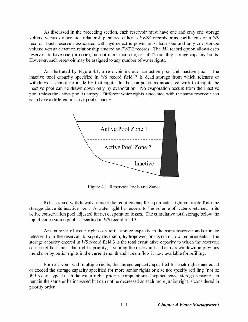
As discussed in the preceding section, each reservoir must have one and only one storage volume versus surface area relationship entered either as SV/SA records or as coefficients on a WS record. Each reservoir associated with hydroelectric power must have one and only one storage volume versus elevation relationship entered as PV/PE records. The MS record option allows each reservoir to have one (or none), but not more than one, set of 12 monthly storage capacity limits. However, each reservoir may be assigned to any number of water rights. As illustrated by Figure 4.1, a reservoir includes an active pool and inactive pool. The inactive pool capacity specified in WS record field 7 is dead storage from which releases or withdrawals cannot be made by that right. In the computations associated with that right, the inactive pool can be drawn down only by evaporation. No evaporation occurs from the inactive pool unless the active pool is empty. Different water rights associated with the same reservoir can each have a different inactive pool capacity.
Active Pool Zone 1
Active Pool Zone 2
Inactive
Figure 4.1 Reservoir Pools and Zones Releases and withdrawals to meet the requirements for a particular right are made from the storage above its inactive pool. A water right has access to the volume of water contained in its active conservation pool adjusted for net evaporation losses. The cumulative total storage below the top of conservation pool is specified in WS record field 3. Any number of water rights can refill storage capacity in the same reservoir and/or make releases from the reservoir to supply diversion, hydropower, or instream flow requirements. The storage capacity entered in WS record field 3 is the total cumulative capacity to which the reservoir can be refilled under that right’s priority, assuming the reservoir has been drawn down in previous months or by senior rights in the current month and stream flow is now available for refilling. For reservoirs with multiple rights, the storage capacity specified for each right must equal or exceed the storage capacity specified for more senior rights or else not specify refilling (not be WR record type 1). In the water rights priority computational loop sequence, storage capacity can remain the same or be increased but can not be decreased as each more junior right is considered in priority order.
Chapter 4 Water Management 111
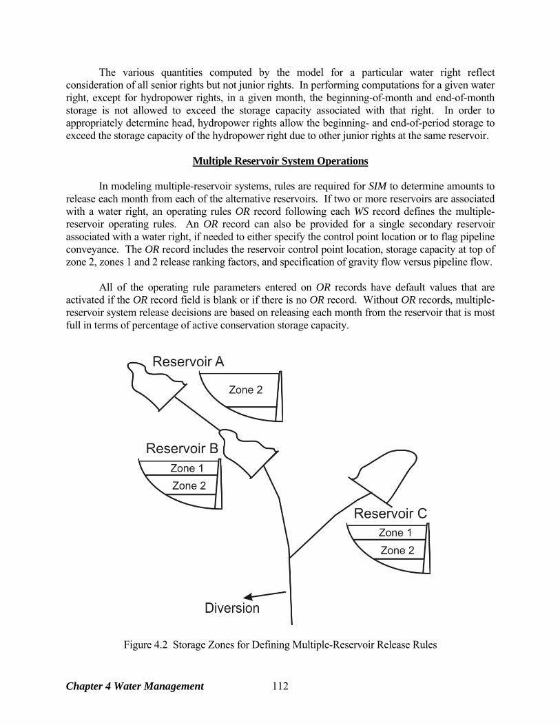
The various quantities computed by the model for a particular water right reflect consideration of all senior rights but not junior rights. In performing computations for a given water right, except for hydropower rights, in a given month, the beginning-of-month and end-of-month storage is not allowed to exceed the storage capacity associated with that right. In order to appropriately determine head, hydropower rights allow the beginning- and end-of-period storage to exceed the storage capacity of the hydropower right due to other junior rights at the same reservoir.
Multiple Reservoir System Operations In modeling multiple-reservoir systems, rules are required for SIM to determine amounts to release each month from each of the alternative reservoirs. If two or more reservoirs are associated with a water right, an operating rules OR record following each WS record defines the multiple-reservoir operating rules. An OR record can also be provided for a single secondary reservoir associated with a water right, if needed to either specify the control point location or to flag pipeline conveyance. The OR record includes the reservoir control point location, storage capacity at top of zone 2, zones 1 and 2 release ranking factors, and specification of gravity flow versus pipeline flow. All of the operating rule parameters entered on OR records have default values that are activated if the OR record field is blank or if there is no OR record. Without OR records, multiple-reservoir system release decisions are based on releasing each month from the reservoir that is most full in terms of percentage of active conservation storage capacity.
Figure 4.2 Storage Zones for Defining Multiple-Reservoir Release Rules
Chapter 4 Water Management 112
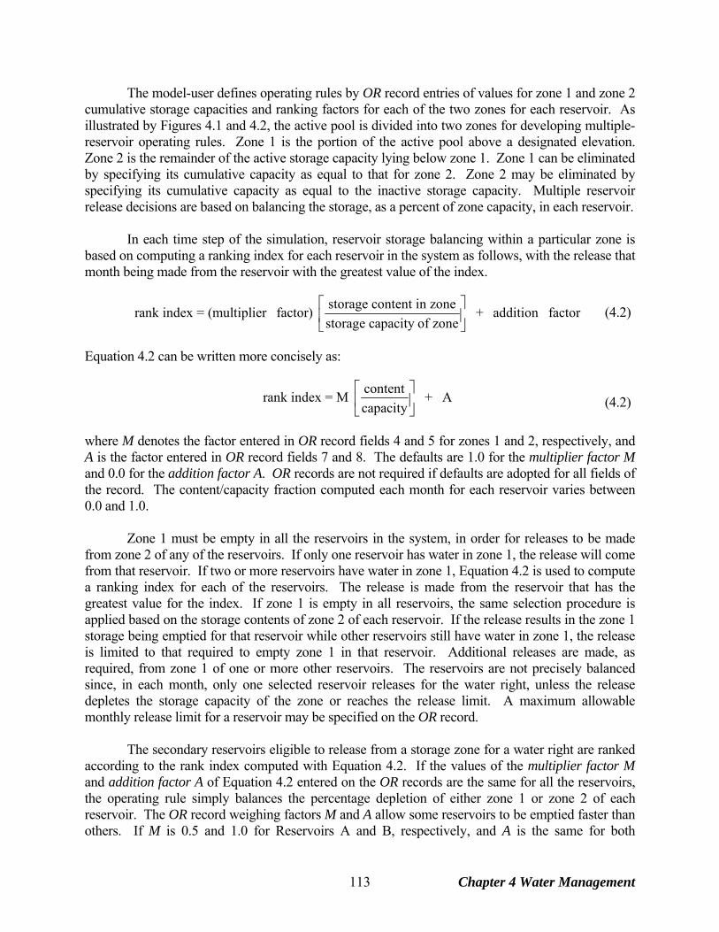
The model-user defines operating rules by OR record entries of values for zone 1 and zone 2 cumulative storage capacities and ranking factors for each of the two zones for each reservoir. As illustrated by Figures 4.1 and 4.2, the active pool is divided into two zones for developing multiple-reservoir operating rules. Zone 1 is the portion of the active pool above a designated elevation. Zone 2 is the remainder of the active storage capacity lying below zone 1. Zone 1 can be eliminated by specifying its cumulative capacity as equal to that for zone 2. Zone 2 may be eliminated by specifying its cumulative capacity as equal to the inactive storage capacity. Multiple reservoir release decisions are based on balancing the storage, as a percent of zone capacity, in each reservoir. In each time step of the simulation, reservoir storage balancing within a particular zone is based on computing a ranking index for each reservoir in the system as follows, with the release that month being made from the reservoir with the greatest value of the index. storage content in zonerank index = (multiplier factor) + addition factor
storage capacity of zone⎡ ⎤⎢ ⎥⎣ ⎦
(4.2)
Equation 4.2 can be written more concisely as: contentrank index = M + A
capacity⎡ ⎤⎢ ⎥⎣ ⎦
(4.2)
where M denotes the factor entered in OR record fields 4 and 5 for zones 1 and 2, respectively, and A is the factor entered in OR record fields 7 and 8. The defaults are 1.0 for the multiplier factor M and 0.0 for the addition factor A. OR records are not required if defaults are adopted for all fields of the record. The content/capacity fraction computed each month for each reservoir varies between 0.0 and 1.0. Zone 1 must be empty in all the reservoirs in the system, in order for releases to be made from zone 2 of any of the reservoirs. If only one reservoir has water in zone 1, the release will come from that reservoir. If two or more reservoirs have water in zone 1, Equation 4.2 is used to compute a ranking index for each of the reservoirs. The release is made from the reservoir that has the greatest value for the index. If zone 1 is empty in all reservoirs, the same selection procedure is applied based on the storage contents of zone 2 of each reservoir. If the release results in the zone 1 storage being emptied for that reservoir while other reservoirs still have water in zone 1, the release is limited to that required to empty zone 1 in that reservoir. Additional releases are made, as required, from zone 1 of one or more other reservoirs. The reservoirs are not precisely balanced since, in each month, only one selected reservoir releases for the water right, unless the release depletes the storage capacity of the zone or reaches the release limit. A maximum allowable monthly release limit for a reservoir may be specified on the OR record. The secondary reservoirs eligible to release from a storage zone for a water right are ranked according to the rank index computed with Equation 4.2. If the values of the multiplier factor M and addition factor A of Equation 4.2 entered on the OR records are the same for all the reservoirs, the operating rule simply balances the percentage depletion of either zone 1 or zone 2 of each reservoir. The OR record weighing factors M and A allow some reservoirs to be emptied faster than others. If M is 0.5 and 1.0 for Reservoirs A and B, respectively, and A is the same for both
Chapter 4 Water Management 113
reservoirs, the storage content of Reservoir A, expressed as a fraction (ranging from 0.0 to 1.0) of zone capacity, must be at least twice that of Reservoir B in order for the release to be made from Reservoir A. Likewise, if M is the same for both reservoirs, and A is 0.0 and 0.5 for Reservoirs A and B, respectively, the storage content of Reservoir A, expressed as a fraction of zone capacity, must be greater by 0.5 than Reservoir B in order for the release to be made from Reservoir A. JO record field 7 allows selection between two options regarding the storage to use in the multiple reservoir release decision computations: (1) the beginning-of-period storage or (2) the intermediate end-of-period storage at that point in the water rights priority loop computations, which is subject to change due to more junior water rights. Gravity Flow in River Channels versus Pipeline/Canal/Pump Conveyance By default, reservoir operation is based on assuming conveyance by gravity flow in river channels. Reservoir releases can meet diversion requirements at the control point of the reservoir or at any control point located downstream of the reservoir. OR record field 6 is used to remove the gravity flow constraint. A pipeline or canal, with pumps as needed, is assumed to convey water from the reservoir to the control point of the water right diversion, which can be any location. Releases for Downstream Senior Rights Reservoirs located upstream of a diversion are assumed to make direct releases to supply the diversion requirement. The pump/pipeline/canal option activated by OR record field 6 allows diversions from a reservoir to be conveyed to any control point. However, without the pump/pipeline/canal option, reservoirs that are physically able to release only to control points that are downstream of the diversion location may still contribute to system operations. These reservoirs, referred to as downstream reservoirs, are limited to mitigating stream flow depletions made by senior rights downstream of the diversion location. The amount of water that a downstream reservoir may release is limited to the flow that has been passed through the diversion location to meet senior water right requirements as illustrated by the following example. Figure 4.3 illustrates a system composed of four reservoirs and one diversion, which is subject to the constraint of another more senior water right. The system diversion can be met from stream flow depletions at control point CP-4 and releases from reservoirs RES-A, RES-B, RES-C, and RES-D located at control points CP-1, CP-2, CP-3, and CP-5. Since reservoir RES-D at control point CP-5 is not located upstream of the system diversion location at control point CP-4, its role is limited to minimizing the adverse impacts on water availability of the senior right at control point CP-6. In each month of the simulation, the computations include determination of the amount of water to release from each subcomponent of the four-reservoir system to meet the diversion at CP-4, based on balancing storage depletions in the reservoirs. The multiple reservoir system release rules may involve interactions with other more senior rights in the river basin. For example, the senior right at control point CP-6 in Figure 4.3 is not part of the four-reservoir/one-diversion system but impacts the water available to the system. The model maintains an accounting of the amount by which the senior right at CP-6 reduces water availability at the other control points and allows releases to be made from reservoir RES-D, as well as RES-A,
Chapter 4 Water Management 114
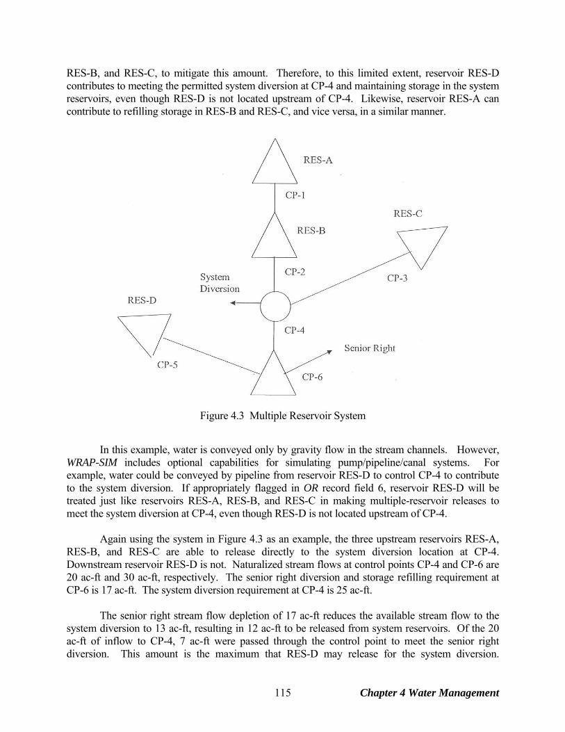
RES-B, and RES-C, to mitigate this amount. Therefore, to this limited extent, reservoir RES-D contributes to meeting the permitted system diversion at CP-4 and maintaining storage in the system reservoirs, even though RES-D is not located upstream of CP-4. Likewise, reservoir RES-A can contribute to refilling storage in RES-B and RES-C, and vice versa, in a similar manner.
Figure 4.3 Multiple Reservoir System In this example, water is conveyed only by gravity flow in the stream channels. However, WRAP-SIM includes optional capabilities for simulating pump/pipeline/canal systems. For example, water could be conveyed by pipeline from reservoir RES-D to control CP-4 to contribute to the system diversion. If appropriately flagged in OR record field 6, reservoir RES-D will be treated just like reservoirs RES-A, RES-B, and RES-C in making multiple-reservoir releases to meet the system diversion at CP-4, even though RES-D is not located upstream of CP-4. Again using the system in Figure 4.3 as an example, the three upstream reservoirs RES-A, RES-B, and RES-C are able to release directly to the system diversion location at CP-4. Downstream reservoir RES-D is not. Naturalized stream flows at control points CP-4 and CP-6 are 20 ac-ft and 30 ac-ft, respectively. The senior right diversion and storage refilling requirement at CP-6 is 17 ac-ft. The system diversion requirement at CP-4 is 25 ac-ft. The senior right stream flow depletion of 17 ac-ft reduces the available stream flow to the system diversion to 13 ac-ft, resulting in 12 ac-ft to be released from system reservoirs. Of the 20 ac-ft of inflow to CP-4, 7 ac-ft were passed through the control point to meet the senior right diversion. This amount is the maximum that RES-D may release for the system diversion.
Chapter 4 Water Management 115
Effectively, it is releasing the 7 ac-ft to the senior right, freeing that amount of water for use by the system diversion. Of course, any of the upstream reservoirs RES-A, RES-B, and RES-C may release all of the 12 ac-ft if the storage content is sufficient. The downstream release constraint is determined on a control point basis. If a second system diversion exists at control point CP-4 that is junior to the first, the amount that RES-D may release for the second system diversion is constrained by the amount that RES-D released for the first. If RES-D released 4 ac-ft for the first system diversion, then it is limited to releasing 3 ac-ft for the second because a total of 7 ac-ft were passed through the control point to the senior water right. SIM maintains an accounting of depletions at and releases to each control point as well as an accounting at each control point of releases made from downstream reservoirs to determine the downstream releases constraints. Negative incremental inflows may cause inaccuracies in the flow accounting.
Iterative Reservoir Volume Balance Computations Reservoir water budget computations are performed within SIM for each individual water right that has reservoir storage, within the water right priority sequence, which is repeated within the monthly time step sequence. The following three volumes are computed simultaneously:
• end-of-month reservoir storage volume • reservoir outflow (releases and withdrawals) volume during the month • net water surface evaporation less adjusted precipitation volume during the month
Since, the monthly storage, outflow, and net evaporation volumes are all dependent on each other, an iterative computational algorithm is required. Net water surface evaporation-precipitation is discussed in the preceding Chapter 3. The net evaporation volume is computed each month by multiplying a net evaporation depth times the average water surface area determined as a function of storage volume. The reservoir surface area is a simple average of the areas at the beginning and end of the month. The beginning-of-month area is determined as a function of the known beginning-of-month storage volume. However, the unknown end-of-month reservoir storage volume depends upon the net evaporation volume. Thus, the estimated end-of-month reservoir surface area changes during the course of iterative computations along with the improvements in the end-of-month storage volume and net evaporation volume estimates. The stop criteria for the iterative algorithm is based on comparing successive computed end-of-month storage volumes. The computations stop if the difference between successive end-of-month storage volumes is less than either 0.1 unit (acre-foot) or 0.01 percent. The computations also stop upon completion of a maximum of 50 iterations, with a warning message written to the message file that the 50 iteration maximum was reached and the last storage computed was adopted. As discussed later in this chapter, hydroelectric energy generation is a function of head as well as discharge. Average head is a function of the end-of-month storage, which is also being computed, as well as the known beginning storage. The hydropower routine iteratively activates the iterative reservoir routine described above in its own iterative routine to meet a energy target.
Chapter 4 Water Management 116

The following previously-computed known amounts are provided to the SIM routine that performs the iterative computations to determine reservoir outflow, net evaporation, and end-of-month storage volumes for a particular reservoir for a particular water right.
• beginning-of-month storage • stream inflows into the reservoir from stream flow depletions for senior rights • inflows into the reservoir from releases from upstream reservoirs for senior rights • available stream flow still remaining for appropriation by the current water right • outflows (releases and diversions) for other more senior water rights • outflow target for the current water right
The reservoir volume balance computations like other aspects of SIM must be understood within the framework of the priority sequence. Stream flow depletions, releases from upstream system reservoirs, and diversions and releases from this reservoir are accumulated in memory and incorporated into the water budget computations associated with other more junior rights at the same reservoir. In the water right priority sequence simulation, the water accounting computations for a particular water right include consideration of the diversions and releases at the same reservoir previously determined for more senior rights. However, the evaporation and end-of-month storage previously computed for the senior rights at the reservoir is not considered. With multiple rights at the same reservoir, SIM computes the total net evaporation volume along with end-of-month storage content from scratch for each water right in turn in the priority sequence, not the incremental decrease or increase in evaporation. The actual correct evaporation volume and end-of-month storage for a reservoir are the amounts computed for the last right in the priority sequence at the reservoir. However, intermediate evaporation and end-of-month storage estimates computed during the priority sequence are used in determining the amount of water available from reservoir storage for individual rights. The determination of the amount of water available to a particular water right from reservoir storage is based on information currently known at that point in the priority sequence. Likewise, for hydropower rights, head available to generate hydroelectric energy is based on information currently known at that point in the priority sequence. Evaporation and storage volumes are written to the output file for types 1 and 7 and hydropower (types 5 and 6) rights but not for types 2 and 3 rights.
Multiple Rights Associated with the Same Reservoir Any number of diversion, hydropower generation, or instream flow requirements may be supplied from the same reservoir. A particular reservoir may be assigned to any number of water rights. Storage may be refilled to different levels by multiple rights connected to a reservoir. A particular right may refill storage, divert/release from storage, or both. A reservoir may be the primary reservoir for several rights and a secondary reservoir for other rights. The water use requirements for each right associated with a reservoir are supplied from the total active storage content of the reservoir below the top of conservation pool of that right regardless of how the reservoir is refilled. An inactive storage capacity may be specified for each right, from which withdrawals can not be made for that right. However, storage capacity associated with a reservoir is not otherwise allocated among multiple rights in SIM. Thus, a senior right may replenish storage depleted by a junior right in previous months. A junior water right could empty its
Chapter 4 Water Management 117
active storage pool, even though the depleted storage capacity affects water available to a senior right at the same reservoir during the next month. However, as discussed below, this issue may be addressed by modeling a shared multiple-owner reservoir as multiple separate reservoirs. Modeling a Single Reservoir as Multiple Reservoirs Two or more river authorities, water districts, cities, or other entities may share the same reservoir. If the owners all have equal access to the total storage shared in common, their water use may be aggregated and the reservoir modeled as a single reservoir using the basic WR and WS record features. However, the reservoir operation problem is more complicated if each entity individually owns or contractually controls a specified portion of the storage capacity in the one reservoir. If each owner has a dedicated storage capacity from which the other owners are not allowed access, the multiple-owner reservoir may be treated as multiple separate reservoirs located at the same control point. Each component reservoir has its own storage capacity, diversion/release targets, and operating rules. If nonlinearities of the area-volume relationship used in the evaporation computations are not of concern and if the different owners can be assigned different priorities, a single reservoir with multiple owners can be modeled as separate reservoirs easily within SIM without having to activate additional special computational methods. However, with net evaporation-precipitation modeled as a nonlinear function of storage, a scheme for its allocation among the multiple reservoir owners is required. Priorities or an alternative allocation scheme are also required to define the order in which the multiple owners have access to inflows to fill their storage and meet their water use requirements. The evaporation allocation EA record facilitates allocating the net evaporation-precipitation volumes among the otherwise computationally separate reservoirs. If the rights share the same priority, AF record parameters are also provided to allocate available stream flow. SIM can automatically handle the allocation of the total net evaporation volume between multiple component reservoirs without needing the EA record evaporation allocation routines if the following two premises are accepted as being valid.
1. The storage versus area relationship defined by either the SV/SA record table or the coefficients on the WS record is linear. The storage versus area relationship adopted for each component reservoir is a linear relationship representing the actual single reservoir.
2. The evaporation volume is allocated between the different entities in direct proportion to their beginning-of-month and end-of-month storage contents.
The EA record evaporation allocation routine allows a nonlinear storage-area relationship for the actual reservoir to be applied to each of the individual component reservoirs representing different owners and allows specification of alternative strategies for allocating evaporation. Evaporation Allocation Methodologies Activated by the EA Record The multiple computational reservoirs representing each entity's share of the storage capacity in the single actual reservoir are listed on an evaporation allocation EA record along with selection of allocation method The computational reservoirs listed on an EA record represent the multiple storage components of the single actual reservoir.
Chapter 4 Water Management 118
Each component reservoir listed on an EA record must be associated with a type 1 or 7 right that refills storage in that reservoir. The evaporation allocation routine is applied only to type 1 or 7 rights. However, any number of type 2, 3, 5, or 6 rights or IF record rights may also withdraw or release water from the reservoir. Thus, the evaporation allocation may be associated with essentially any reservoir operating scenario. With multiple rights at the same reservoir, evaporation computations are repeated in the water rights loop priority sequence, with the last computed evaporation volume replacing amounts determined as more senior rights were considered. Thus, the EA record evaporation allocation should be performed with the most junior right at each component reservoir, which must be type 1 or 7 rights, controlling the refilling of storage. Total net evaporation-precipitation volume is computed based on the total area determined as a function of total storage content. Total storage determined by summing the contents of the component reservoirs is combined with a storage-area relationship to obtain the water surface area. Although not required by SIM, component reservoirs will normally share the same storage versus area relationship (SV/SA records) in the model. A component reservoir's share of the evaporation-precipitation volume is computed by one of the alternative methods listed below.
Option 1. Incremental Based on Water Right Priorities.- As the water rights are considered in priority order, the most senior right with a reservoir on the EA record is allocated the net evaporation computed prior to considering the other junior rights. Each subsequent water right with a reservoir on the EA record is allocated its incremental additional net evaporation in the priority sequence. The concept is to determine evaporation unaffected by junior rights in the priority sequence.
Options 2 and 22. Proportional to Storage Content.- The evaporation-precipitation
volume is allocated among the component reservoirs in proportion to beginning-of-month storage. If the beginning-of-month storage is zero in all reservoirs, net evaporation associated with refilling during the month is divided equally between the reservoirs. Options 2 and 22 are the same except for the last reservoir.
Options 3 and 33. User-Specified Factors.- The net evaporation-precipitation volume is
allocated among the component reservoirs based on multiplier factors entered on an EF record. Thus, the model-user defines a fixed proportion for each reservoir. The computations switch to option 2 above if beginning-of-month storage drops below a limiting level specified on the EF record. The difference between options 2 and 3 is that the multiplier factors for option 2 are the ratio of beginning-of-month storage content to storage capacity and for option 3 are specified on an EF record. Options 3 and 33 are identical except for handling of the last reservoir.
Option 4. Priority Adjusted with Multiplier Factors.- The net evaporation volume is first
determined in the same manner as option 1 and then multiplied by a factor from the EF record. The computations switch to option 2 above if the beginning-of-month storage drops below a limiting storage level specified on the EF record. With factors of 1.0 and no switching limit, option 4 is identical to option 1.
Method (option) 1 models the fundamental principle of a prior appropriation water right priority system. The method 1 computations are based on accumulating storage and evaporation
Chapter 4 Water Management 119
volumes as the simulation progresses through the priority sequence. Component reservoirs associated with junior rights in the priority sequence are not considered when determining the evaporation for a particular more senior water right. Method 4 is a variation of method 1 providing additional flexibility for adjusting the allocation. Methods 2, 22, 3, and 33 consist of multiplying an estimate of the total net evaporation-precipitation volume by a computed or given factor for each reservoir. With methods 2 and 22, SIM computes the factors as the ratio of beginning-of-month storage in each component reservoir to the total for all the reservoirs. With methods 3 and 33, the model-user provides the factors on EF records. Options 22 and 33 are identical to options 2 and 3 except for the feature described below. Since the evaporation allocation computations occur in the water rights priority sequence, end-of-month storage for junior rights has not yet been computed when a particular more senior right is considered. Net evaporation-precipitation volumes are always computed in SIM based on an average water surface area determined from both end-of-month and beginning-of-month storage. End-of-month storage is a function of net evaporation, which is a function of end-of-month storage. Thus, an iterative algorithm is required. The evaporation allocation algorithm is integrated into the normal iterative computational procedure described earlier in this chapter for simultaneously determining reservoir outflow, net evaporation, and end-of-month storage volumes. However, in applying the storage-area relationship to determine water surface area, the best estimate of end-of-month storage at that point in the priority sequence calculations is used for the allocation algorithm. For any component reservoir for which end-of-month storage has not yet been computed, the end-of-month storage is estimated as the beginning-of-month storage. In order to ensure that the combined total net evaporation volume is correct, for methods 2 and 3 defined above, the volume for the last reservoir listed on an EA record is computed as the final correct total net evaporation-precipitation volume less the amounts previously determined for the other reservoirs. This option 2 and 3 feature for forcing the evaporation for the component reservoirs to sum to the correct total is not applied with options 22 and 33. With options 22 and 33, all component reservoirs listed on the EA record are treated the same, and thus the evaporation volume for the component reservoirs will typically not sum to the correct final total. With method 1, the correct total evaporation is computed at each point in the priority sequence and the incremental evaporation assigned to the right is determined by subtracting the cumulative incrementals previously assigned to senior rights. Thus, the evaporation for the component reservoirs automatically sum to the correct total. The problem associated with options 22 and 33 that is described in the preceding paragraph is also pertinent to option 4. Multiple Rights at the Same Component Reservoir The following are key basic concepts in combining multiple rights at the same component reservoir listed on an EA record. With multiple water rights at the same reservoir, diversions and releases associated with senior rights are accumulated in memory and incorporated into the water budget computations associated with the other more junior rights at that same reservoir. In the water right priority sequence simulation, the water accounting computations for a particular water right includes consideration of the diversions and releases at
Chapter 4 Water Management 120
the same reservoir previously determined for more senior rights. However, the evaporation and end-of-month storage volumes previously computed for any senior rights at the reservoir are not considered. Net evaporation and end-of-month storage volumes are computed again from scratch as each right is considered in the priority sequence. Total hydroelectric energy generation is also recomputed from scratch for multiple hydropower rights at the same reservoir. The following routines are applied in the water rights simulation when considering a water right located at a reservoir listed on an EA record.
1. For type 1 and 7 rights (WR record field 6), the net evaporation-precipitation volume is computed based on evaporation allocation methods activated by the EA record options outlined in the preceding two pages. The evaporation allocation methods are applied only to type 1 and 7 rights.
2. For hydropower rights, the head used in the hydropower computations corresponds to the
summation of the storage contained in all of the component reservoirs listed on the EA record. Likewise, the elevation of the bottom of the power pool refers to total storage capacity summed for all the reservoirs. Storage in all EA record reservoirs is summed in the computation of head and specification of bottom of power pool for all hydropower rights. However, the EA record evaporation allocation routines are not applied for hydropower rights. Evaporation is determined by the conventional SIM routine.
3. The stream flow availability allocation routine activated by the AF record is applied to all
water rights associated with all reservoirs listed on the EA record. Storage and evaporation are not relevant to the AF record stream flow availability routine.
The EA record evaporation allocation routines are activated within SIM only for type 1 and 7 rights. However, with caution, any number of water rights of any of the types can be applied at EA record reservoirs. Evaporation allocation options 2, 3, 22, and 33 are different than options 1 and 4 in regard to dealing with multiple rights at the same component reservoir. Reservoir storage is filled only by types 1, 5, and 7 rights (WR record field 6). Thus, with or without EA records, every reservoir must have at least one type 1, 5, or 7 water right or the reservoir will never refill. Typically, with multiple rights at the same reservoir, the most junior right will be a type 1 right that performs the final refilling in the priority sequence. Likewise, for EA record reservoirs, the final evaporation allocation typically will be determined with a type 1 right at each reservoir listed on the EA record. Since with or without EA records, type 2 and 3 rights do not refill storage, the final end-of-month storage is yet unknown, and evaporation volumes are approximate. Since type 2 and 3 rights do not activate the EA record routine, water surface areas determined from the nonlinear storage-area relationship are approximate. The degree of inaccuracy depends on the nonlinearity of the storage-area relationship. This evaporation volume is used only in the determination of the amount of water available to the right from reservoir storage. The evaporation affects the diversion only if the reservoir empties. The actual final evaporation volume for the reservoir should be determined later in the priority sequence in association with a type 1 right that activates the EA record evaporation allocation routine.
Chapter 4 Water Management 121
Likewise, the evaporation volume computed for hydropower rights is approximate, but serves only in the determination of the amount of water available to the hydropower right from reservoir storage if followed in the priority sequence by a type 1 or 7 right. However, as a separate issue for hydropower rights, SIM uses the total storage summed for all the EA record reservoirs in the determination of head and minimum power pool elevation. Evaporation allocation options 1 and 4 are based on incremental evaporation volumes. With options 1 and 4, storage and evaporation volumes are accumulated. The evaporation computed for the most senior component reservoir treats the other junior component reservoirs as not existing. Thus, there must be a priority sequence with one type 1 or 7 water right at each EA record reservoir. For example, with three reservoirs listed on an EA record, there must be exactly three type 1 or 7 water rights representing the three reservoirs. There can not be two type 1 rights at the same reservoir interrupting the priority sequence storage and evaporation volume accumulation. There can be any number of complete sets of three type 1 or 7 rights as long as there is no intermingling between the sets of three rights in the priority sequence. Any other types of rights at the EA record reservoirs should be senior to the type 1 and 7 rights driving the evaporation allocation algorithm. These option 1 and 4 requirements are not applicable for options 2, 22, 3, and 33. Options 2 and 3 use the last reservoir listed on the EA record to assure that the evaporation for the component reservoirs sum to the correct total for the actual real reservoir. Thus, a type 1 or 7 right junior to all the other rights associated with the EA record reservoirs must be assigned to the last reservoir listed on the EA record. This requirement is not applicable to options 22 and 33. Options 22 and 33 are the most flexible of all the evaporation allocation options in dealing with multiple rights at the same component reservoirs. Allocation of Available Stream Inflow to the Reservoirs Water right priority numbers set the order in which rights are considered in the computations and thus have access to available stream flow. However, two or more of the reservoir owners may share the same priority. With multiple rights having the same priority, an alternative methodology is adopted to allocate available flow between water rights. The AF record serves this purpose. With the EA/AF record option activated, the amount of stream flow available to a water right is determined in the water rights priority loop computations as follows. If the parameters MIN and MAX are not used, the algorithm consists simply of multiplying the available stream flow by the factor AFX from the AF record.
• The available stream flow volume (A1) is first determined in the normal manner and then adjusted by the AF record parameters as follows.
• If the minimum limit (input parameter MIN) is not zero, the adjusted available stream flow is set at A1 as long as A1 does not exceed MIN.
• If A1 exceeds MIN, an input multiplier factor AFX is applied as follows
adjusted available stream flow = MIN + (A1 − MIN) × AFX
• If maximum limit (input parameter MAX) is not zero, the adjusted available flow is set at MAX if the volume computed by the equation above exceeds MAX.
Chapter 4 Water Management 122
The AF and AX records both serve the same purpose and are based on the same simulation algorithm. The stream flow availability allocation factors AFX record connected to the EA record is designed for modeling multiple-owner reservoirs. The flow availability AX record connected to the priority circumvention PX record discussed in the last section of this chapter can be more generically applied to any water right. The PX/AX option allows allocation factors to vary monthly throughout the year, while the EA/AF option is limited to a constant factor for the entire year.
Water Supply Diversions A monthly water supply diversion target is determined by combining an annual diversion amount from a WR record with the appropriate monthly distribution factor from an UC record. The water use type on the WR record connects the diversion right with the appropriate monthly use coefficients. If a use type is not entered in field 4 of the IF or WR record, the default of a constant uniform distribution (1/12 of total in each month) is adopted. An entry of NDAYS distributes the annual target in proportion to the number of days in each month (28, 30, or 31 days/month). As previously discussed, a variety of other options may be employed in setting a diversion target. A series of diversion targets that vary annually as well as monthly may be entered on target series TS records. The drought index option (DI record) allows diversion targets to be adjusted as a function of storage content in selected reservoirs. A multiplier factor, as a percentage, is determined by combining the beginning-of-month storage with a storage versus multiplier factor relationship defined by IS/IP records. The diversion target can also be modified as a function on stream flow, storage, and specified upper and lower limits by options controlled with supplemental options SO and target options TO records. Intermediate targets may be computed with the various target setting options. Only one target and shortage are included in the simulation results recorded for each water right for each period. In the case of adopting multiple options resulting in multiple intermediate targets, SO record field 9 allows selection of which diversion target and shortage to include in the output file. In the SIM simulation, in the water rights priority loop, diversion requirements are satisfied to the extent allowed by available stream flow and reservoir storage. A diversion shortage is declared any time the diversion target can not be fully met. A diversion shortage is computed as the monthly target described in the preceding paragraphs less the computed actual diversion amount as limited by water availability. The priority number sets the seniority of the diversion relative to other rights. A diversion requirement may be run-of-river with zero storage. Alternatively, a diversion requirement may be met by stream flow supplemented by releases from one or more reservoirs.
Return Flows Return flows can represent water discharged back into the stream after use, such as municipal and industrial wastewater treatment plant effluent or irrigation return flows. Return flows can also represent water transported through conveyance facilities such as canals, pipelines, and pumping plants from other control points which may be located any place. The control points of origin and destination of the diversion return flow can be located in different river basins. Intrabasin or interbasin transfers may be simulated in this manner. Alternatively, such transfers of water may
Chapter 4 Water Management 123
also be modeled as a type 4 right (WR record field 6) or by using the alternate control point (SO record), pipeline (OR record), or constant inflow (CI record) options described elsewhere in this chapter. Transient right XP option 1 on the PX record allows return flows computed as a function of actual diversion amounts to have a priority that is different than the diversion. Return flow priorities affect the order in which other water rights have access to the return flow. Return flows from water uses supplied by groundwater sources are often modeled as constant inflows on CI records rather than using the WR record return flow options described below. CI record flows are discharged at the beginning of the priority sequence. The previously discussed type 4 right allows return flows from groundwater to be assigned any priority. Return flows are computed in the model as a user-specified fraction of computed actual (rather than target) diversion amounts. A diversion return flow can reenter at any user-specified control point, which could be located downstream or upstream of the diversion location or on a different stream. The diversion amount, return flow factor, and return flow control point location are part of the water right WR record input data. Timing of return flows is also a user-specified option. The return flows may be returned during the same month as the water right diversion or during the next month. Since water rights are considered in priority order, the return flows associated with a junior water right will not affect the water available to a senior right unless the return flow is carried over to the next month. PX record XP option 1 allows return flows to have a priority that is different than the diversion. Return flow specifications provided on the WR record for each water right include the return flow factor, the control point location to which flows are returned, and whether return flows occur in the same month as the diversion or the next month. Return flows are computed in SIM by multiplying a computed diversion by a return flow factor, which may be either a constant specified on the WR record for the water right or optionally a set 12 monthly return flow factors specified on RF records associated with a specified type of water use. The variable RFMETH entered as either 0, 1, 2, 3, or 4 in WR record field 7 specifies the return flow method adopted for the water right as follows. 0, 1, blank A constant return flow factor RFAC is specified in WR record field 8. The
return flow occurs in the same month as the diversion. 2 A constant return flow factor RFAC is specified in WR record field 8. The
return flow occurs in the next month after the diversion. 3 An alphanumeric identifier RFIDWR is specified in WR record field 8 which
connects the water right to a set of 12 monthly return flow factors input on RF records. The return flow occurs in the same month as the diversion.
4 An alphanumeric identifier RFIDWR is specified in WR record field 8 which
connects the water right to a set of 12 monthly return flow factors input on RF records. The return flow occurs in the next month after the diversion.
Chapter 4 Water Management 124
Options 3 and 4 require that a set of 12 monthly return flow factors be input on RF records. Identifiers input in the WR and RF records connect the water rights to the appropriate return flow factors. Options 1 and 2 both include a value for RFAC on the WR record, so RF records are not required. If the RFAC field is left blank, there is no return flow. Hydroelectric power releases through turbines are also treated as return flows using the same options applied to diversions. The default for hydropower is to return 100 percent of the hydropower release at the next downstream control point during the same month as the release. However, the next month option, return to another control point, and the other options available for diversions are computationally applied to turbine flows in the same manner.
Other Inflows and Outflows
Stream flow adjustments may be specified as either FA or CI records. Constant inflow CI records consist of 12 inflows or outflows, for the 12 months of the year, which are repeated each year. Flow adjustment FA records are used to input multiple-year sequences of inflows or outflows, with the monthly flows varying each year. The adjustments from the FA or CI records are applied by the model in essentially the same manner. The following discussion focuses on CI record adjustments but is also pertinent to FA record adjustments. As discussed in the Users Manual, WRAP-HYD provides more flexible options for applying CI and FA record adjustments, which includes the SIM methodology discussed below and variations thereof. The constant inflow/outflow (CI record) option allows input of 12 flows, for the 12 months of the year, associated with a specified control point. This option may be used to model:
• return flows not otherwise included in the return flow options, such as return flows from water supply withdrawals from groundwater aquifers
• diversions not otherwise included in the water rights
• channel losses not otherwise included in the channel loss option
• interbasin transfers of water to the control point
• interactions between groundwater and stream flow associated with aquifer pumping Sets of 12 inflows may be entered for any control points on pairs of constant inflow CI records. An outflow is entered as a negative value of inflow. The constant inflows are added to the flows at the control point designated on the CI record and at all control points located downstream. If channel loss factors are input on pertinent CP records, the CI record inflows/outflows are adjusted by channel losses at downstream control points. Sequences of inflows for each control point provided as input on IN records typically consist of naturalized stream flows. The next-period return flow option allows diversion return flows to be added to the naturalized flows for the next month after the diversion. At the beginning of the monthly simulation loop, prior to performing the water allocation computations, SIM combines the inflows/outflows from the CI records with the naturalized flows from the IN records and return flows from the previous month. The constant inflows/outflows are added after the optional negative incremental flow adjustments.
Chapter 4 Water Management 125
A constant monthly outflow may be input as a negative value on a CI record. Negative inflows are not allowed to reduce the total stream flow to below zero. If an outflow (negative inflow) is greater than the combined IN-record naturalized flow plus return flows from the previous month, the combined total of all three components is set equal to zero. The reduced value of negative inflow at the designated control point is carried downstream. The negative CI-record inflow is also restricted from reducing the total flows at the downstream control points to below zero. A CI-record outflow (negative inflow) is essentially equivalent to a diversion that is senior to all the water rights on the WR and IF records.
Hydroelectric Energy Generation
Hydroelectric energy production rights are similar to diversion rights in WRAP-SIM. Both hydropower (types 5 and 6) rights and diversion (types 1, 2, and 3) rights are activated with a water right WR record. An energy generation target is entered on the WR record for a hydropower right. Reservoir storage and hydropower operation information is specified on WS and HP records. A reservoir storage volume versus water surface elevation table (PV/PE records) and constant tailwater elevation (HP record) or tailwater elevation versus discharge table (TE/TQ records) are input to allow the model to compute head. Hydroelectric power is generated with all water that is available to the turbines in the priority-sequenced simulation computations, which includes reservoir releases and pass-through flows associated with senior water supply rights, available unregulated stream flows, and releases from reservoirs made specifically to meet the hydropower generation target. If multiple hydropower rights are assigned to the same reservoir/hydropower project, the energy generation associated with each right is the total energy that can generated with all the water available at that point in the priority sequence. Unlike multiple diversions at the same reservoir which can be summed to obtain a total diversion amount, each of the hydropower energy production amounts are already a cumulative total. Thus, energy production associated with multiple hydropower rights at the same reservoir can not be added. Energy generation target, actual production, and shortage amounts may be written to reservoir/hydropower project and/or water right output records. If only one hydropower right is associated with a particular reservoir/hydropower plant, the energy amounts are the same on the reservoir/hydropower and water right output records. With multiple hydropower rights at the same reservoir/hydropower project, the multiple water right output records contain the cumulative energy amounts associated with each water right. The reservoir/hydropower project output record shows the cumulative energy amount associated with the most junior hydropower right at the reservoir. For each period of the simulation, the energy production target is met as long as sufficient water and head is available from stream flow and reservoir storage. An energy shortage occurs if sufficient water is not available to meet the user-specified energy requirement. The model also computes secondary or surplus energy. Secondary energy represents additional energy, above the specified energy target, that potentially could be generated by passing reservoir releases for downstream diversions through the turbines. Only reservoir releases for water rights senior to the hydropower right are considered in computing secondary energy. Secondary energy is treated by
Chapter 4 Water Management 126
the model as a negative energy shortage. No releases from storage or stream flow depletions are made if previous releases for senior rights are sufficient to meet or exceed the energy requirement. Power generation may be constrained by both an optional turbine discharge capacity and a maximum monthly energy amount specified on the HP record. Minimum reservoir storage levels allowing power generation are also specified. Flows through hydroelectric power turbines are returned to the river computationally in the same manner as water supply diversion return flows. Return flow options specified by WR record fields 7−9 (RFMETH, RFAC, RFIDWR, RCP) are applied to hydropower releases the same as to diversions. The default is to return 100 percent of the turbine flow at the next downstream control point below the control point of the water right during the same month as the release. However, hydropower releases may contribute to downstream flows optionally either the same or next month. The flows may enter the river at any specified control point. Input Data for Hydropower Rights A hydroelectric energy generation right is represented by the following input data:
• control point location [WR record field 2]
• annual energy generation target [WR record field 3]
• set of 12 monthly energy target distribution factors [WR record field 4, UC records]
• drought index for varying energy target as a function of reservoir storage [DI/IS/IP records]
• optional series of monthly energy generation targets that vary between years [TS record]
• priority number [WR record field 5]
• water right type [WR record field 6]
• active and inactive reservoir storage capacities [WS record fields 3 and 7]
• parameter LAKESD for diversion rights indicating whether diversions can be released through hydropower turbines and thus contribute to power generation [WS record field 11]
• plant efficiency factor [HP record field 2]
• tailwater elevation [HP record field 3] or tailwater rating table [TE/TQ records]
• turbine inlet invert elevation [HP record field 4]
• turbine discharge capacity [HP record field 5]
• maximum limit on secondary energy generation [HP record field 6]
• reservoir storage versus water surface elevation table [PV/PE records]
• multiple-reservoir system operating rules [OR records]
• turbine discharge return flow specifications [WR record fields 7, 8, 9]
• multiplier factor POWFCT [XL record field 7]
Chapter 4 Water Management 127
Energy Equation and Multiplier Factor Hydroelectric energy computations are based on the following equations:
E = P t (4.3) P = γ Q H e (unit conversion factors) (4.4)
E = γ Q H e t (unit conversion factors) = Q H e t (POWFCT) (4.5)
where the terms are defined with examples of typical units in brackets as follows: E − energy generated [Watt-hour (W-hr) = 3,600 Newton meters = 2,650 ft-lbs; megaWatt-hr (MW-hr) = 1,000,000 W-hr = 1,000 kiloWatt-hr (kW-hr)] P − power generated [Watt (W) = Nm/second; MW = 1,000,000 W = 1,000 kW; horsepower = 550 ft-lb/s = 0.7457 kW]
γ − unit weight of water [lb/ft3, kN/m3] Q − discharge through turbines during time period [ac-ft/month; 103 m3/month] H − head [feet, meters] = mean reservoir water surface elevation for period minus tailwater elevation e − plant efficiency [dimensionless] t − time period (one month) POWFCT = power factor used in WRAP-SIM In the SIM model, hydroelectric energy (E) produced is represented as:
E = Q H e t (POWFCT) (4.6) where: POWFCT = γ (unit conversion factors) (4.7) POWFCT is a multiplier factor that reflects unit conversions and the unit weight of water. Values of POWFCT for several alternative sets of units are tabulated in Table 4.3 and may be computed for any other set of units. SIM uses a default POWFCT of 0.0010237 corresponding to the units shown in the last column of Table 4.3. Thus, the default POWFCT = 0.0010237 automatically used by SIM is appropriate if the variables are expressed in the following units:
POWFCT = 0.0010237 energy (E) in megawatt-hours (MW-hrs)
discharge (Q) in acre-feet/month head (H) in feet
If other units are adopted, a value for POWFCT must be entered in field 7 of the multiplier factor XL record.
Chapter 4 Water Management 128
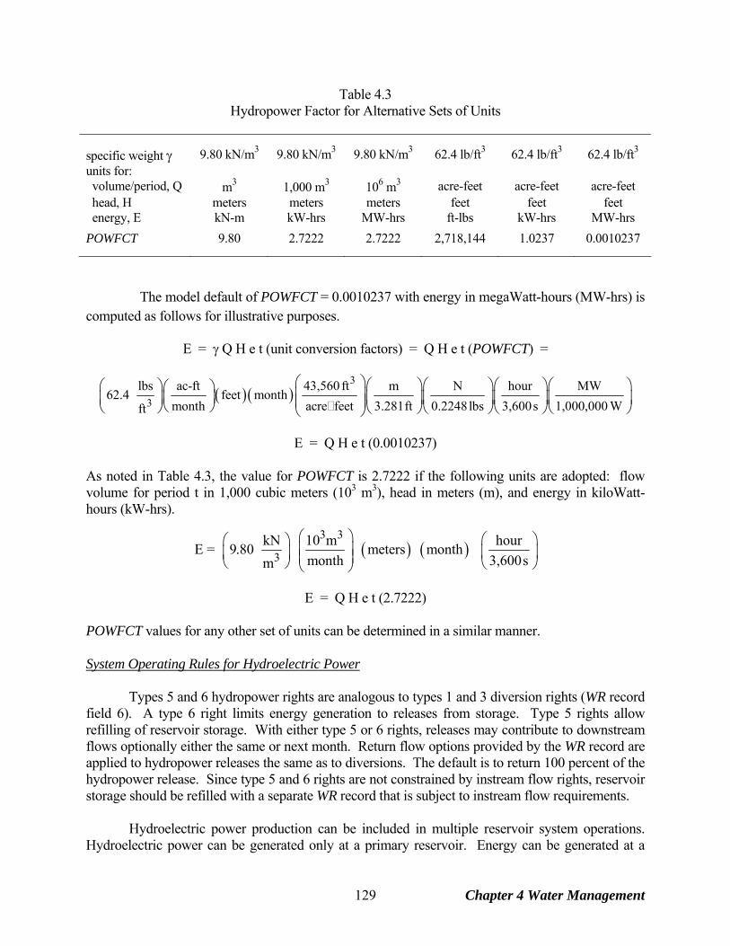
Table 4.3 Hydropower Factor for Alternative Sets of Units
specific weight γ 9.80 kN/m3 9.80 kN/m3 9.80 kN/m3 62.4 lb/ft3 62.4 lb/ft3 62.4 lb/ft3
units for: volume/period, Q m3 1,000 m3 106 m3 acre-feet acre-feet acre-feet head, H meters meters meters feet feet feet energy, E kN-m kW-hrs MW-hrs ft-lbs kW-hrs MW-hrs
POWFCT 9.80 2.7222 2.7222 2,718,144 1.0237 0.0010237 The model default of POWFCT = 0.0010237 with energy in megaWatt-hours (MW-hrs) is computed as follows for illustrative purposes.
E = γ Q H e t (unit conversion factors) = Q H e t (POWFCT) =
( )( )3
3lbs ac-ft 43,560 ft m N hour MW
62.4 feet monthmonth acre feet 3.281ft 0.2248lbs 3,600s 1,000,000 Wft
⎛ ⎞⎛ ⎞⎛ ⎞⎛ ⎞⎛⎛ ⎞⎛ ⎞ ⎜ ⎟⎜ ⎟ ⎜ ⎟⎜ ⎟⎜ ⎟⎜⎜ ⎟ ⎜ ⎟⎝ ⎠⎝ ⎠ ⎝ ⎠⎝ ⎠⎝ ⎠⎝⎝ ⎠
⎞⎟⎠
E = Q H e t (0.0010237)
As noted in Table 4.3, the value for POWFCT is 2.7222 if the following units are adopted: flow volume for period t in 1,000 cubic meters (103 m3), head in meters (m), and energy in kiloWatt-hours (kW-hrs).
( ) ( )3 3
3kN 10 m hourE = 9.80 meters month
month 3,600sm
⎛ ⎞ ⎛ ⎞⎛ ⎞⎜ ⎟ ⎜ ⎟⎜ ⎟ ⎜ ⎟⎝ ⎠ ⎝ ⎠⎝ ⎠
E = Q H e t (2.7222)
POWFCT values for any other set of units can be determined in a similar manner. System Operating Rules for Hydroelectric Power Types 5 and 6 hydropower rights are analogous to types 1 and 3 diversion rights (WR record field 6). A type 6 right limits energy generation to releases from storage. Type 5 rights allow refilling of reservoir storage. With either type 5 or 6 rights, releases may contribute to downstream flows optionally either the same or next month. Return flow options provided by the WR record are applied to hydropower releases the same as to diversions. The default is to return 100 percent of the hydropower release. Since type 5 and 6 rights are not constrained by instream flow rights, reservoir storage should be refilled with a separate WR record that is subject to instream flow requirements. Hydroelectric power production can be included in multiple reservoir system operations. Hydroelectric power can be generated only at a primary reservoir. Energy can be generated at a
Chapter 4 Water Management 129
hydroelectric plant as a type 5 or 6 right using flows from releases from multiple reservoirs. A run-of-the-river hydropower right is modeled as a type 5 water right with the total storage capacity equal to the inactive capacity. By default, all diversions and releases from a reservoir contribute to power generation for junior hydropower rights at the reservoir, unless otherwise specified. When a non-hydropower water right diversion is met from a primary reservoir and/or secondary reservoirs, the water is released either through the reservoir hydropower turbines or directly from the reservoir pool, not passing through the turbines, depending upon the input specifications (WS record field 11). The hydropower release is computed as the additional release amount needed to meet the energy target, considering all releases for more senior rights that pass incidentally through the turbines. Because the energy produced is a function of both the flow through the turbines and the average head on the turbines, hydropower rights are handled differently than diversion rights in regard to assumptions regarding refilling reservoir storage. The non-hydropower convention of ignoring storage above the storage capacity of the water right in a multiple-right reservoir is not applicable to hydropower. A type 5 hydropower right will make stream flow depletions and receive releases from secondary reservoirs to meet its energy requirement as well as refill storage up to its storage capacity. If the storage in the reservoir is above the capacity of the right, the right will make stream flow depletions and reservoir releases necessary to just maintain the storage level while meeting the energy requirement. The target stream flow depletion is computed as the additional water that must be passed through the hydropower turbines assuming that the end-of-period storage is either the water right storage capacity or the current storage level, whichever is higher, plus the amount needed to refill storage. The actual energy produced must be computed in an iterative manner if the reservoir is drawn-down by releases through the turbines since the monthly release volume required depends on head but head depends on the release volume. Multiple Hydropower Rights at the Same Reservoir Any number of hydropower rights may be associated with the same reservoir, but certain physical characteristics of the reservoir are fixed, remaining constant for all rights. The tables describing volume-area (SV/SA records), volume-elevation (PV/PE records), and tailwater discharge-elevation (TQ/TE records) relationships are fixed for a reservoir. These tables are provided only once for each reservoir. The turbine inlet capacity, turbine discharge capacity, and maximum limit on energy production are fixed by the first HP record read that is connected to the reservoir and can not be changed between rights. However, each of the multiple hydropower rights assigned to a single reservoir has its own energy target and priority set by its WR and auxiliary records, own efficiency (HP record), and own inactive and total storage capacities (WS record). The cumulative total energy generated at a reservoir/hydropower project is recomputed for each right. The energy value reported on a reservoir/hydropower record in the main OUT output file represents the energy produced by the most junior hydropower right at the reservoir. The intermediate values of energy for senior rights are recorded on OUT file water right output records and listed in the reservoir/hydropower HRR output file. The storage used in the computations is the current end-of-period storage for that reservoir. Junior rights associated with the reservoir may increase or decrease the storage amount, changing the energy actually produced at the reservoir.
Chapter 4 Water Management 130
Instream Flow Requirements In WRAP, an instream flow requirement activated by an IF record is a target minimum regulated flow rate at a control point location. The objective is to maintain regulated flows equal to or greater than the monthly instream flow targets. The units for instream flow targets are the same as the other flow rate terms in WRAP, such as acre-feet/month or other volume/month units. Instream flow requirements typically represent environmental flow needs for preservation and enhancement of ecosystems, fisheries, and wildlife habitat and but may also serve various other purposes such as recreation, aesthetics, water quality, and water supply.
Instream flow targets are determined step-by-step within SIM following the procedure outlined earlier in this chapter in the section entitled Setting Diversion, Instream Flow, and Hydropower Targets. The target setting procedure is addressed further in the Users Manual. Instream flow targets are specified in a SIM input file using an instream flow IF record and supporting water use coefficient UC, drought index DI/IS/IP, target options TO, supplemental options SO, flow switch FS, target series TS, reservoir storage WS, and multiple-reservoir operating rules OR records. An IF record is required for each instream flow requirement. The other optional auxiliary records activate various options. Any number of IF records may be input for a particular control point, with the next more junior instream flow target replacing the latest more senior target in the priority-based water rights computational loop.
Water allocation routines in SIM are based on user-assigned priorities for all rights, which include instream flow requirements as well as diversion, storage, and hydroelectric energy requirements. Instream flow requirements may be assigned to any or all control points. Any number of instream flow requirements (IF records) may be input for a particular control point, with the next more junior IF record target replacing the latest more senior target in the priority-based water rights loop sequence. Thus, as each water right is considered in turn based on priority, the only instream flow target at a control point constraining water availability is the last IF record target set based on priority. However, this instream flow target may be replaced by a more junior IF record instream flow target later in the priority loop.
Two types of actions may occur in the simulation in order to prevent or minimize failures (shortages) in meeting the instream flow requirements.
1. Constraints placed on the amount of stream flow available to diversion and storage rights, that are junior to an instream flow requirement, may result in these rights being curtailed to minimize shortages in meeting the instream flow target.
2. Releases from reservoirs identified by WS records associated with the IF record
may be made specifically to meet instream flow requirements. In the SIM water rights computation loop, with or without instream flow requirements,
the amount of water available to a right is based on yet unappropriated flows at the control point of the right and at all downstream control points. Instream flow requirements add constraints limiting water availability based on regulated flow targets. Diversion and storage rights that are junior to an instream flow target may have the amount of water available to them constrained, thus resulting in curtailment of stream flow depletions for diversions and reservoir storage.
Chapter 4 Water Management 131
Reservoirs Associated with IF Record Rights Junior diversion rights are curtailed and inflows are passed through junior upstream reservoirs to meet an instream flow requirement, regardless of whether or not storage rights (WS record) are attached to the instream flow right (IF record). Without WS records connected to the IF record, the releases each month through the outlet works of reservoirs associated with junior rights resulting from senior IF record rights do not exceed reservoir inflows that month. Only inflows are passed through reservoirs.
Reservoir storage WS records must follow the IF record in the SIM input file if releases from storage in one or more reservoirs associated with the instream flow right are to be used to prevent regulated flows from falling below the minimum levels specified by the instream flow targets. Any number of reservoirs identified with WS records may be operated with releases from storage to maintain instream flow requirements at control points located at or downstream of the dams.
Releases from reservoir storage (WS and OR records) may be incorporated with instream flow rights (IF records) just the same as with type 2 diversion rights (WR records). However, IF record rights do not refill storage. Water right types are not specified on the IF record, but all IF record rights are equivalent to type 2 rights defined on the WR record. Reservoir releases are made as necessary to meet the target minimum regulated flow, but storage is not refilled. Type 1 WR record rights must be included in the dataset to refill storage in reservoirs. Interactions Between Hydropower and Instream Flow Rights
Hydroelectric power releases contribute to downstream regulated flows. The algorithms in the computer code automatically prevent hydropower rights from being curtailed as a result of instream flow requirements. Hydropower rights ignore instream flow requirements. For hydropower reservoirs, storage and energy requirements may be entered as separate WR records, if necessary, so that the reservoir storage (type 1 right) is constrained by instream flow limits on downstream water availability, but the turbine releases (type 5 or 6 right) are not.
Hydropower releases increase regulated and unappropriated flows at downstream control
points. However, a next-month return flow option allows hydropower rights to appropriate stream flow one month and return it to the stream the next. This could allow storage associated with hydropower to reduce rather than increase downstream flows in a particular month. Special Conditions An option is activated by SO record field 13 that allows a water right to not be constrained by instream flow requirements. This option facilitates convenient assessment of the impacts of instream flow requirements on particular water rights.
Instream flow limits are normally compared to the total regulated flow at specified locations in determining water available to junior water rights. However, an option is activated by IF record field 7 that allows the instream flow limits to be compared to regulated flows
Chapter 4 Water Management 132
exclusive of reservoir releases made from upstream reservoirs to meet water rights requirements at locations further downstream. This option allows modeling of situations in which reservoir releases for other purposes are not given credit for contributing to instream flows between the dam and downstream point of diversion. Specification of Instream Flow Requirements
Monthly instream flow targets are set similarly as diversion and hydropower targets as discussed earlier in this chapter. An annual instream flow target amount from an IF record is combined with a set of 12 monthly distribution factors provided on UC records to develop monthly regulated flow targets. TO records allow the monthly target to be adjusted as a function of river flows or diversions. The FS record activates options that either adjust or switch the instream flow requirement on or off based on whether a total regulated flow volume accumulated of a specified length of time at a particular control point falls within a defined range. The instream target can also be set as a function of reservoir storage using DI/IS/IP records. A time series of instream flow targets may be input on time series TS records. A water right consists of either an IF or a WR record, which may be accompanied by other records providing associated information. The model-user combines one or more IF and/or WR records along with other records as necessary to model a particular water right permit or set of water management/use requirements. The instream flow IF record is similar to the water right WR record. In a SIM input file, IF and WR records are grouped together in any order. IF records may be grouped together and placed either before or after the WR records or interspersed between WR records. UC, DI/IS/IP, TO, SO, FS, TS, WS, and OR records are associated with IF records the same as with WR records.
The instream flow amount AMT from the IF record is handled differently in the simulation than the diversion amount AMT in the same field of the WR record. The instream flow amount is a target minimum regulated flow at a control point. Without an instream flow requirement, the amount of water available to each right in the priority sequence is based on yet unappropriated flows. The instream flow target adds another constraint, based on regulated flows, on the amount of water available to all the water rights with priority numbers junior to that of the instream flow requirement. Types of Instream Flow Computations The computational method associated with a particular instream flow requirement is specified as variable IFMETH in IF record field 7. PASS2 entered in JO record field 10 allows a second pass to be activated regardless of IFMETH. Otherwise, the options are as follows. 0, 1 Junior rights are curtailed as necessary to meet the instream flow requirements during a
single pass through the water rights loop. The minimum instream flow (regulated flow) targets result in constraints on the amount of water available to junior rights. At any point in priority sequence, regulated flow reflects only the effects of senior rights.
2 Junior rights are curtailed as necessary to meet instream flow requirement during a
second pass through the water rights loop. The first pass through the water rights loop is
Chapter 4 Water Management 133
used to compute regulated flows and instream flow shortages without limiting the amount of water available for other rights. The second pass is made only if at least one instream flow failure (shortage) occurs during the first pass.
−2 Junior rights are curtailed as necessary to meet instream flow requirements during both
the first and second passes through the water rights loop. 3 Option 3 is the same as Option 1 except reservoir releases are used as necessary to meet
instream flow requirements. Option 3 requires that a reservoir storage WS record follow immediately behind the IF record. The WS record may be followed by OR records.
4 Option 4 is the same as Option 2 except reservoir releases are used as necessary to meet
instream flow requirements. Option 4 requires that a reservoir storage WS record follow immediately behind the IF record. The WS record may be followed by OR records.
−4 Option –4 is the same as Option –2 except reservoir releases are used as necessary to
meet instream flow requirements. Example - Set of Records Specifying Instream Flow Requirements For purposes of illustrating the WRAP-SIM strategy for modeling instream flow requirements, the computations to result from the input records shown below are discussed. Only the portion of the input file relevant to instream flow requirements is shown.
various input records of various types various UC records
UCseason 0 0 0 0 0 0.25 UC 0.5 0.25 0 0 0 0 UC irrig 0 0 0 0.1 0.1 0.3 UC 0.4 0.1 0 0.0 0.0 0.0 other UC records various other types of records IF CP7 6000 19850501 2 IF1 IF CP15 5200 season19720801 2 IF2 IF CP7 12000 19910215 2 IF3 IF CP12 1800 19880601 2 IF4 WR CP12 7800 irrig19880601 0.25 WR7 WS Res-A 125000 -1 IF CP12 0 19880601 2 IF5 IF CP7 9000 99999999 4 IF6 WS Res-B 50000 -1 many other records of various types Water is allocated to all IF and WR rights in turn, in priority order, as the simulation proceeds through the water rights loop for January of the first year. Instream flow requirement IF2 at control point CP15, with a priority date of 1 August 1972 (19720801) is the most senior of the rights shown and therefore the first to be considered. Multiplying the annual instream flow target of 5,200 ac-ft/yr by a January distribution factor of 0.0 results in a January target of zero.
Chapter 4 Water Management 134
Instream flow requirement IF1 at control point CP7, with a priority of 19850501 (1 May 1985), is considered next. The January instream flow target is 1/12 of 6,000 ac-ft/yr or 500 ac-ft/month. This 500 ac-ft/month regulated flow target serves as a constraint on the amount of water available to water rights with a priority junior to 1 May 1985. Instream flow requirement IF3, with a priority of 19910215 (15 February 1991), raises the instream flow target at control point CP7 from 500 ac-ft/month, set by IF1, to 1,000 ac-ft/month. Thus, all rights with a priority date between 1 May 1985 and 14 February 1991 are subject to an instream flow requirement at CP7 of 500 ac-ft/month, and those with priority dates of 15 February 1991 or later are subject to an instream flow requirement of 1,000 ac-ft/month. Rights IF4, WR7, and IF5 at control point CP12 all have a priority of 19880601 (1 June 1988). Multiple rights with the same priority number are considered in the order they are entered in the input file. IF4 sets an instream flow target of 150 ac-ft/month, which constrains the amount of water available to water right WR7. IF5 resets the instream flow target back to zero. Thus, the 150 ac-ft/month instream flow requirement at CP12 affects only water right WR7.
Instream flow requirement IF6 changes the minimum regulated flow target at control point CP7 from 1,000 ac-ft/month, set previously by IF3, to 750 ac-ft/month. Since the IF6 priority of 99999999 is junior to all other water rights, this target has no affect on the amount of water available to the other rights. If the regulated flow at CP7 is less than 750 ac-ft/month, releases from reservoir Res-B will be made to increase it to 750 ac-ft/month, as specified by the WS record following the IF record for IF6. Multiple IF Record Rights at the Same Control Point Multiple IF records may be used to model a particular set of instream flow requirements. Any number of instream flow IF records can be connected to the same control point. As each IF record water right is considered in the priority loop, the target set by that IF record right is compared with the target previously set by the preceding IF record right in the priority sequence at the same control point. An option controlled by the parameter in IF record field 3 allows selection between three options. The default option 1 is for the junior target to replace the senior target. Options 2 and 3 are to adopt the larger or smaller of the two targets. This procedure of comparing the latest two targets computed in the priority loop can be applied to any number of IF records at the same control point. Instream flow Computations IF record instream flow targets are set within the SIM water rights priority sequence in essentially the same manner as WR record diversion and hydropower targets, but the targets are used differently. The amount of water available to a WR record right is determined based on unappropriated and regulated flows at the control point of the right and downstream control points. IF record instream flow targets are minimum limits on regulated flows used in defining water availability for junior WR record rights. For each month of the simulation, the SIM instream flow routines perform the following tasks. The IF record field 6 IFMETH options for which the tasks are relevant are shown in parenthesis.
Chapter 4 Water Management 135
• Setting the Instream Flow Target for the Month (Options 0, 1, 2, 3, and 4)
SIM determines the monthly instream flow target following the procedures previously outlined based on information entered on IF, UC, DI/IS/IP, TO, FS, SO, and/or TS records. An instream flow target is determined the same way as a diversion target and expressed in the same units as a diversion target, such as acre-feet/month or other volume/month units. • Writing Instream flow Shortages to the Output File (Options 0, 1, 2, 3, and 4) The instream flow requirement is a target minimum regulated flow. For a given month, at the completion of the water rights loop, the instream flow target for each IF record right is compared with the regulated flows at the appropriate control point to determine whether failures to meet the targets occur and to compute the shortage amounts. A shortage occurs when the regulated flow is less then the instream flow target. The shortage, in volume/month, is the difference between the instream flow target and the regulated flow. The targets and shortages are written to the main SIM output OUT file. Program TABLES reads the SIM output file and builds instream flow shortage tables in the same manner as the other tables are developed. • Initial Pass through Water Rights Loop (Options 2 and 4) With the dual pass options 2 and 4 activated, in the initial pass through the water rights computational loop, regulated flow constraints are not placed on the amount of water available to each WR record water right. Thus, junior rights are not curtailed to prevent instream flow shortages from occurring. If one or more failures to meet instream flow targets occur, a second pass through the computational loop is made. If no failures to meet instream flow targets occur in the first pass, there is no second pass; the simulation proceeds to the next month. For options 2 and 4, the first pass through the water rights loop serves the following purposes.
1. A determination is made of whether or not failures to meet instream flow requirements
occur if no other diversion and storage rights are curtailed. The second pass through the water rights loop described below occurs only if one or more failures to meet instream flow targets occur in the first pass. This guarantees that junior rights are not unnecessarily curtailed due to instream flow requirements, in those months in which all instream flow requirements can be met without curtailing junior rights.
2. The regulated flows reflecting all the water rights are determined in this first pass. These
regulated flows are used in the second pass as a lower limit on the regulated flows used to define water availability. This prevents junior rights from being curtailed more than necessary in those months in which instream flow requirements do constrain junior rights.
• Second Pass through Water Rights Loop (Options 2 and 4)
If instream flow shortages occur during the first pass through the water rights loop described above, a second pass is performed. In the second pass, instream flow requirements result in constraints on the amount of water available to all rights that are junior to the instream flow requirements, except hydropower rights. The constraints on water availability result in junior rights being curtailed as necessary to prevent or minimize instream flow shortages.
Chapter 4 Water Management 136
Within the priority-based water rights loop, an instream flow requirement establishes a minimum regulated flow target at a specified control point that results in a constraint on water availability for junior water rights. The regulated flow is compared with the instream flow target to determine the limit on water availability. The regulated flow constraint is incorporated in subroutine AVALB for computing the amount of water available to each right in the priority loop.
Intermediate regulated flows computed during the second pass, with a minimum limit set
by the final regulated flows at the completion of the first pass, are combined with the instream flow requirements to determine the constraints on water availability. As each water right is considered in turn, the intermediate estimate of regulated flow reflects only the effects of more senior rights, since the junior rights have not yet been considered in the priority-based water rights loop. However, the algorithm in SIM limits the regulated flow during the second pass to not drop below the final regulated flow computed at the completion of the first pass.
• Second Pass through Water Rights Loop (Options -2 and -4)
IF record field 6 IFMETH options –2 and –4 in combination with PASS2 from the JO record provide variations of the procedure allowing curtailment of junior rights in all months regardless of conditions and always requiring a second pass. These options provide capabilities for experimentation on the effects of the instream flow algorithms. • Single Pass through Water Rights Loop (Options 1 and 3)
Options 1 and 3 involve only one pass through the water rights priority sequence simulation loop. The instream flow requirements result in constraints on the amount of water available to junior water rights. • Reservoir Storage for Meeting Instream flow Requirements (Options 3 and 4) Options 3 and 4 involve using releases from reservoir storage to meet instream flow targets. Options 3 and 4 consist of adding reservoir storage to options 1 and 2, respectively. A WS record must follow the IF record for an option 3 or 4 instream flow requirement. Multiple-reservoir operating rules OR records may follow the WS record as appropriate. Instream flow shortages are determined in the water rights loop. Whenever the instream flow target exceeds the monthly regulated flow at a control point, a shortage is computed as the instream flow target minus the regulated flow. For an IF record right with reservoir storage (option 3 or 4), the instream flow shortage is mimicked as a diversion right with return flow factor of 1.0. The 100 percent return flow occurs at the same control point as the dummy diversion (instream flow shortage). Thus, if an instream shortage occurs, a diversion target equal to the shortage is created, and the corresponding return flow factor is assigned a value of 1.0. The IF record right is then processed through the water right computations just like a WR record right. The simulation results recorded in the SIM output file for IF record and WR record water rights can be compared in Table 5.3 of Chapter 5. The reservoir release, storage, and net evaporation volumes are non-zero for instream flow output records only for IF record rights with IFMETH option 3 or 4.
Chapter 4 Water Management 137
Regulated Flows and Instream Flow Targets For a given month, water is allocated to each water right in turn, in priority order, in the water rights computational loop priority sequence. At the beginning of the water rights loop, the regulated flow at a control point is the summation of:
• the naturalized flows from the IN records • return flows from the previous month if the next-month return flow option is used • gains or losses from an optional CI record
During the water rights allocation computations, the regulated flows are diminished by stream flow depletions for diversions and refilling reservoir storage. The regulated flows may be increased by return flows from diversions from reservoir storage, hydropower releases, or upstream reservoir releases for downstream diversions. The intermediate regulated flows and unappropriated flows in effect, when a particular water right is considered in the priority-based water allocation computation loop, depend upon the effects of the more senior rights that have already been considered. From the perspective of WRAP-SIM, an instream flow requirement is a target minimum regulated flow at a control point. Any number of IF records may be associated with a control point, allowing the target minimum regulated flow to change in the priority sequence as the various water rights are considered. An actual instream flow requirement is modeled by combining as many IF records as necessary. An instream flow shortage occurs if the regulated flow falls below a minimum flow target. SIM computes and outputs the monthly instream flow shortages for each IF record right. Actions to Prevent or Reduce Instream flow Shortages
The following two approaches are incorporated in WRAP to model regulatory actions in
maintaining instream flow requirements. 1. In the water rights loop, as each water right is considered in turn, a first step is to compute
the amount of water available to the right. The instream flow target is a constraint on the amount of water available to junior WR record rights. Reductions in water availability may result in curtailment of stream flow depletions for meeting diversion requirements and refilling reservoir storage associated with these junior rights.
2. An instream flow right (IF record) may also have its own reservoir storage (WS record).
Releases from storage are made as necessary to prevent or minimize instream flow shortages at downstream control points. The IF record right allows only releases, not refilling of storage. In the model computations, the instream flow shortage is converted to a dummy diversion with 100% return flow, which is then handled the same as a WR record diversion.
Single Versus Dual Passes through the Water Rights Computational Loop Modeling the effects of instream flow requirements on the numerous other diversion and storage rights in a river basin is complicated by the combination of the following two considerations.
Chapter 4 Water Management 138
1. Available stream flow is allocated to water rights based on priorities. Thus, the water rights are considered in priority order in the water rights computation loop.
2. Diversion and storage rights may either increase or decrease the regulated flows at a control
point. Diversions and refilling reservoir storage decrease regulated flows at downstream control points. Conversely, regulated flows may be increased by (1) return flows from diversions from storage, (2) hydropower releases, or (3) upstream reservoir releases for downstream diversions.
As discussed earlier, in the priority-based water rights computational loop, restrictions on water availability due to instream flow requirements may result in shortages in meeting diversion and/or storage requirements that are not necessary. For example, the regulated flows may have dropped below the target level, thus restricting water availability, when a particular diversion right is considered. Thus, the diversion right incurs a shortage. However, more junior rights considered later in the computations may result in return flows from diversions from reservoir storage that raise the regulated flow above the instream flow target. The sole purpose for performing two passes through the water rights computation loop is to address this complication. IFMETH options 1 and 3 perform the water allocation computations during a single pass through the water rights loop. The instream flow shortages computed by this approach are accurate. However, diversions and refilling of reservoir storage associated with other rights may have been curtailed more than necessary to prevent or reduce instream flow shortages. The dual-pass approach of options 2 and 4 provides protection against erroneously over restricting the amount of water available to other water rights in the following two regards. However, they do not guarantee that junior rights are not over-restricted. 1. In the dual pass approach, the first pass is used to compute regulated flows without allowing
instream flow requirements to restrict the amount of water available to junior rights. The second pass occurs only if the first pass results in one or more instream flow shortages. Thus, option 2 guarantees that junior rights are not affected in any month in which instream flow targets are met anyway without restricting the amount of water available to other rights.
2. At completion of the first pass, the regulated flows reflect the effects of all water rights, but
the rights are unrestricted by instream flow targets. In option 2, these final first-pass regulated flows are used in the second pass to set a lower limit on regulated flows used in the water availability computations. This prevents junior rights from being curtailed more than necessary in those months in which instream flow requirements do limit the amount of water available to junior rights.
An erroneous instream flow shortage could possibly occur in a situation in which a diversion right actually increased regulated flows in the first pass but is curtailed in the second pass. Consider a diversion downstream of the instream flow target control point made from releases from a reservoir located upstream. The reservoir release increases the regulated flow at the instream flow target control point prior to being diverted downstream. For purposes of reducing instream flow shortages, this particular diversion right should not be curtailed. The model-user can handle this situation by bracketing the WR record in the input file with IF
Chapter 4 Water Management 139
records, with the same priority as the diversion right, that turn the instream flow requirement off and then back on again just before and after consideration of the WR record right. The second pass IF record option could possibly cause irregularities in simulation results when used with various complex combinations of other SIM modeling features and thus should be applied cautiously. In general, the single pass options 1 and 3 should be adopted unless specific reasons are clearly identified warranting the more complicated dual pass options 2 and 4. With IFMETH options 2 and 4, instream flow requirements are imposed only during the second pass through the water rights computation loop. Thus, another problem with options 2 and 4 is that the final unappropriated flows do not reflect instream flow requirements in those months in which all requirements are met without necessitating a second pass.
The only reason for the IF record dual pass options is to deal with the problems of senior rights not getting access to water made available by junior rights through same-month return flows from diversions from storage and same-month hydroelectric power releases and obtaining credit for contributions to meeting instream flow requirements at intermediate control points made by releases from upstream reservoirs to meet diversions at downstream locations. As previously discussed, CI record return flow, next-month return flow, and next-month hydropower options are typically adopted to deal with return flows and hydropower releases. Thus, the dual pass option is applicable primarily in situations involving senior IF record instream flow requirements located between a junior WR record right's reservoir and its downstream water supply diversion. The second pass options would be adopted to prevent unnecessary curtailments by other WR record rights located between the dam and diversion with priorities falling between the senior IF record right and junior WR record right.
Dual Simulation Options The dual simulation feature is designed primarily for applications where multiple rights with different priorities divert water from the same reservoir system. Without the dual simulation, reservoir draw-downs associated with junior diversions may be inappropriately refilled in subsequent months by senior rights at the same reservoir. The set of dual simulation options allow stream flow depletions computed during an initial simulation to be used as upper limits constraining depletions during a second simulation. Selected water rights may be switched on or off during either the initial or second simulations. Dual simulations may be performed automatically during a single execution of SIM. Alternatively, SIM may be executed once to develop a set of stream flow depletions, which are then incorporated into a SIM input file as time series TS records for use in further simulations. The dual simulation feature is discussed in the next section from the perspective of its application as a priority circumvention mechanism. Logistics of its use are outlined as follows. The dual simulation options are activated for individual water rights as specified by either SO record field 14 or PX record field 2. A default dual option may be set for all rights in JO record field 11, subject to being over-ridden for individual rights by the SO or PX records. The options available for application to one or any number of water rights are as follows.
Chapter 4 Water Management 140
Option 1: The water right is activated only during the initial simulation. Option 2: The water right is activated only during the second simulation and is not subject to an
initial simulation stream flow depletion constraint. Option 3 with variations 33 and 333: A dual simulation is automatically performed. Stream
flow depletions computed during the first simulation serve as upper limits on water availability during the second simulation. The stream flow depletions computed during the initial simulation may optionally be written to the message file.
Option 4: The water right is activated only during the initial simulation. A stream flow depletion
array is developed. If an option 5 right follows this right, the depletions serve as upper limits on water availability for the option 5 right during the second simulation. The stream flow depletions may optionally be written to the message file.
Option 5 with variations 55 and 555: A dual simulation is performed with this water right being
activated only during the second simulation. The stream flow depletion array from the preceding option 4 right serves as an upper limit on depletions for this option 5 right.
A second simulation is automatically performed if and only if option 3 or 5 is selected for one or more rights. Alternatively, the simulation may be performed once to develop a set of stream flow depletions, which are then incorporated into an input file as TS records for use in further simulations. Options 3 and 4 depletions may also be written to the message file. With dual options 3 and 5, stream flow depletions each month for a right determined during the first simulation serve as a maximum limit on stream flow depletions during the second simulation. The stream flow depletion for a given month during the second simulation is not allowed to exceed the depletion for that month occurring during the initial simulation. Options 33, 333, 55, and 555 are variations of options 3 and 5 that allow the depletion constraints to be relaxed somewhat by allowing flexibility in the timing of the depletions. Dual options 33 and 55 are the same as options 3 and 5 except the constraints applied during the second simulation are based on cumulative stream flow depletions rather than depletions in each individual month. For any month, for a particular right, the total cumulative stream flow depletions since the beginning of the second simulation can not exceed the corresponding cumulative depletions occurring in the initial simulation. With options 333 and 555, for water rights that refill reservoir storage (types 1 and 7 rights described in Chapter 5), the limit during the second simulation is the accumulative stream flow depletions since the reservoir was last full. During the second simulation, the accumulation of initial simulation depletions is zeroed any time the reservoir contents are full to capacity. For other water right types, the options 333 and 555 limits applied during the second simulation are the first simulation depletion for the current month plus any excess depletion from the immediately preceding month. Unused stream flow depletions below the constraining limits are carried into the next month but no further.
Chapter 4 Water Management 141

Options for Circumventing the Priority Sequence As discussed throughout this manual, the WRAP-SIM modeling strategy is based on simulating water management/allocation/use in a priority-based water rights loop computational sequence. In general, senior rights affect the amount of water available to junior rights but are not affected by the junior rights. However, in some applications, various needs may arise for evading the priority sequence. For example, as previously discussed, same-month return flows from water supply diversions from storage associated with a junior right are not available to senior rights located downstream but should be. The next-month diversion return flow option is designed to address this issue. Likewise, the next-month hydropower option allows senior rights access to hydropower releases. Second pass instream flow IF record options involving a repeat of the water rights loop within a given month are discussed in the preceding section. Multiple rights with the same priority, agreements that subordinate a senior right to a junior right, reservoir storage priority complexities, and various other aspects of water management may motivate circumvention of the water right priority loop sequencing in the simulation computations. Four different sets of options activated by the priority circumvention PX record and stream flow availability factor AX record are designed to facilitate evasion of the normal SIM priority sequence based allocation of available water. The options may also serve other purposes not necessarily related to evading the restrictions of the priority system. The different PX record options may be applied either independently or in combination with each other and combined with various other SIM features. Strategies for their use are governed by the water management situation being modeled and the ingenuity and creativity of the model-user. The PX record described in the Users Manual provides the following four different types of modeling features which are described by the remainder of this chapter.
1. The dual simulation feature is actually designed to contribute to maintaining the priority system though discussed here in the context of priority circumvention applications. A set of dual simulation options allow a repeat of the simulation for the entire hydrologic period-of-analysis. Water rights may be selected for activation or deactivation during either the first or second simulation. [JO record field 11, PX record field 2, or SO record field 14]
2. For multiple rights sharing the same priority, the allocation of available stream flow
may be based on parameters provided as input. [PX record field 3 and AX record]
3. All downstream control points are normally considered in both determining the amount of water available to a water right and adjusting water availability for the effects of the right. A downstream control point limit option allows the model-user to adjust the manner in which these computations cascade downstream. [PX record fields 4 and 5]
4. Transient priority XP options allow a computational water right to be activated and
deactivated at different points in the priority sequence. The simplest XP option allows a return flow to occur later in the priority sequence than the corresponding
Chapter 4 Water Management 142
diversion. A second more complex XP option allows all features of a water right to be activated and deactivated at different points in the computational sequence based on two different assigned priorities. [PX record fields 6−12]
Dual Simulation Feature The SIM dual simulation feature described in the preceding section of this chapter allows stream flow depletions determined during an initial simulation to serve as upper limits on flow depletions during a second simulation. Selected water rights may be activated or deactivated during either of the two simulations. Dual simulations may be performed automatically during a single execution of SIM. Alternatively, SIM may be executed once to develop a set of stream flow depletions, which are then incorporated into a SIM input file as time series TS records for use in further simulations. The basic concept of the dual simulation feature is to establish a set of stream flow depletions for selected water rights during an initial simulation representing a specified water management scenario, which then serve as upper limits on the stream flow available to those rights during a second simulation reflecting an altered or different water management scenario. The SIM dual simulation options activated by the PX record were originally motivated primarily by applications where multiple rights with different priorities divert water from the same reservoir. The dual simulation feature is designed to preserve the priority system by preventing actions of junior rights in a current month from adversely affecting more senior rights in future months through the delayed affects of reservoir storage draw-downs and refilling. Without the dual simulation options, reservoir draw-downs associated with junior diversions may be refilled in subsequent months by senior rights at the same reservoir. For example, junior diversion right XX draws the reservoir down in July. During August, senior right YYY at the same reservoir refills storage with stream flow that otherwise would have supplied other third-party rights with priorities falling between the priorities of senior right YYY and junior right XX. Thus, the diversion by junior right XX from reservoir storage in July results in other senior third-party rights having stream flow availability inappropriately reduced in August and later months when senior right YYY refills the reservoir. With activation of the dual simulation option, an initial simulation is made without junior right XX to determine the proper stream flow depletions during each month of the period-of-analysis for senior right YYY. The dual simulation option allows the senior right YYY stream flow depletions computed during the initial simulation without junior XX to be used as upper limits constraining senior right YYY depletions during a second simulation in which junior right XX is also activated. An additional junior WR record may also be added to allow senior right YYY to further refill storage with excess flows not appropriared by any other rights. Allocation of Available Stream Flow A fundamental concept of WRAP-SIM is that available stream flow is allocated to each water right in turn in the water rights computation loop priority sequence. Since the computational procedure is based on considering water rights one at a time, for purposes of sequencing rights in the computations, no two rights can be assigned the same priority.
Chapter 4 Water Management 143
However, water rights actually having the same priority and located at the same control point or different control points with access to approximately the same stream flow may be modeled as adjacent rights in the priority sequence with the available stream flow allocated between them based on user-specified parameters entered on the PX and AX records. Water right priorities govern access to available stream flow. However, when multiple water rights have the same priority, another strategy must be adopted to allocate available stream flow between the rights. The PX record stream flow availability allocation option uses multiplier factors. Either a constant multiplier factor may be entered on the PX record or factors for each of the 12 months of the year may be entered on AF records. The amount of stream flow available to a right is first determined in the normal manner and then multiplied by the pertinent factor from the PX or AX record. The model-user must select appropriate multiplier factors. For example, consider a water management situation in which three WR record diversion and/or storage rights located at the same control point have equal access to available stream flow. One-third of the available flow is to be allocated to each water right. The three rights are assigned priorities allowing them to be adjacent in the priority sequence. The most senior right is assigned a multiplier factor of 0.33333 on the PX record, allowing it access to one-third of the available stream flow. The second right is assigned a factor of 0.50 allowing it access to half of the remaining two-thirds of the available stream flow. The most junior of the three rights is assigned a factor of 1.0 allowing it access to the remainder of the available stream flow. The methodology is explained in the Users Manual. The same available stream flow allocation procedure is also implemented by an EA/AF record option described earlier in this chapter in the section on multiple rights associated with the same reservoir. Downstream Control Point Limit As outlined in Figure 2.2 and discussed in Chapter 2, the SIM simulation is organized based on a water rights priority loop embedded within the monthly time step loop. Within the water rights priority loop, as each individual water right is considered in turn, the computations are performed in four stages. Task 1: A water supply diversion, hydropower generation, or other type of target is set. Task 2: The amount of stream flow available to the right is determined. Stream flow availability is
determined as the lesser of the stream flow availability array amounts at the control point of the water right and at each of the control points located downstream.
Task 3: Water volume balance computations are performed to compute the stream flow depletion,
net reservoir evaporation, end-of-period storage, return flow, diversion and diversion shortage, and hydroelectric energy generated and shortage.
Task 4: The stream flow availability array values at the control point of the water right and at
downstream control points are decreased by a flow depletion and increased by a return flow or hydropower release, with adjustments for channel losses or loss credits.
Chapter 4 Water Management 144
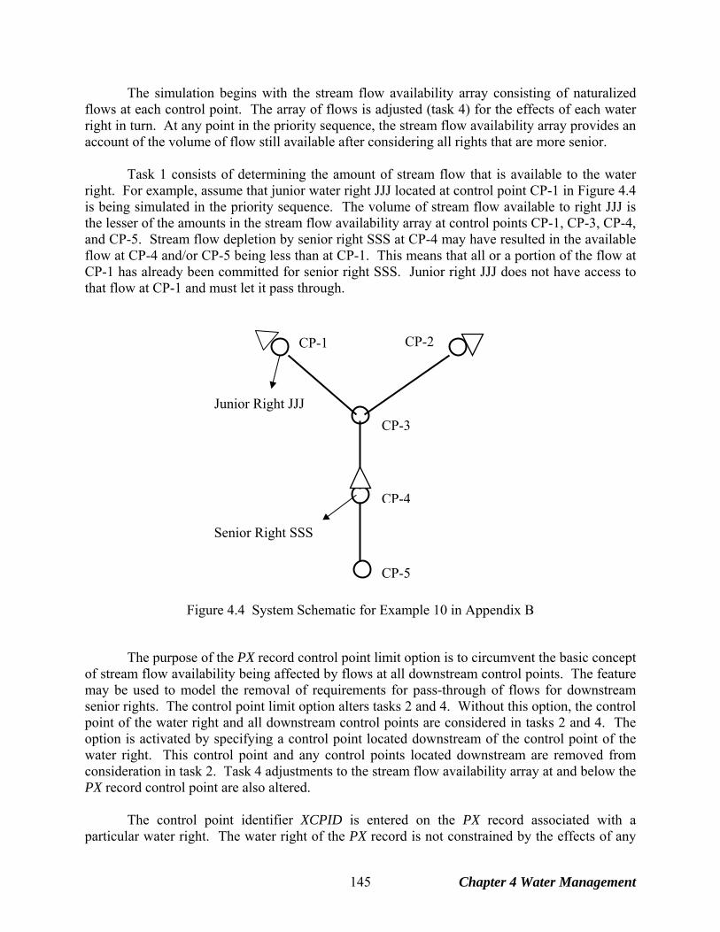
The simulation begins with the stream flow availability array consisting of naturalized flows at each control point. The array of flows is adjusted (task 4) for the effects of each water right in turn. At any point in the priority sequence, the stream flow availability array provides an account of the volume of flow still available after considering all rights that are more senior. Task 1 consists of determining the amount of stream flow that is available to the water right. For example, assume that junior water right JJJ located at control point CP-1 in Figure 4.4 is being simulated in the priority sequence. The volume of stream flow available to right JJJ is the lesser of the amounts in the stream flow availability array at control points CP-1, CP-3, CP-4, and CP-5. Stream flow depletion by senior right SSS at CP-4 may have resulted in the available flow at CP-4 and/or CP-5 being less than at CP-1. This means that all or a portion of the flow at CP-1 has already been committed for senior right SSS. Junior right JJJ does not have access to that flow at CP-1 and must let it pass through.
CP-3
CP-2
Junior Right JJJ
CP-1
CP-5
Senior Right SSS
CP-4
Figure 4.4 System Schematic for Example 10 in Appendix B The purpose of the PX record control point limit option is to circumvent the basic concept of stream flow availability being affected by flows at all downstream control points. The feature may be used to model the removal of requirements for pass-through of flows for downstream senior rights. The control point limit option alters tasks 2 and 4. Without this option, the control point of the water right and all downstream control points are considered in tasks 2 and 4. The option is activated by specifying a control point located downstream of the control point of the water right. This control point and any control points located downstream are removed from consideration in task 2. Task 4 adjustments to the stream flow availability array at and below the PX record control point are also altered. The control point identifier XCPID is entered on the PX record associated with a particular water right. The water right of the PX record is not constrained by the effects of any
Chapter 4 Water Management 145
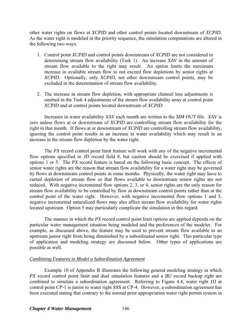
other water rights on flows at XCPID and other control points located downstream of XCPID. As the water right is modeled in the priority sequence, the simulation computations are altered in the following two ways.
1. Control point XCPID and control points downstream of XCPID are not considered in determining stream flow availability (Task 1). An increase XAV in the amount of stream flow available to the right may result. An option limits the maximum increase in available stream flow to not exceed flow depletions by senior rights at XCPID. Optionally, only XCPID, not other downstream control points, may be excluded in the determination of stream flow availability.
2. The increase in stream flow depletion, with appropriate channel loss adjustments is
omitted in the Task 4 adjustments of the stream flow availability array at control point XCPID and at control points located downstream of XCPID.
Increases in water availability XAV each month are written to the SIM OUT file. XAV is zero unless flows at or downstream of XCPID are controlling stream flow availability for the right in that month. If flows at or downstream of XCPID are controlling stream flow availability, ignoring the control point results in an increase in water availability which may result in an increase in the stream flow depletion by the water right. The PX record control point limit feature will work with any of the negative incremental flow options specified in JD record field 8, but caution should be exercised if applied with options 1 or 5. The PX record feature is based on the following basic concept. The effects of senior water rights are the reason that stream flow availability for a water right may be governed by flows at downstream control points in some months. Physically, the water right may have to curtail depletion of stream flow so that flows available to downstream senior rights are not reduced. With negative incremental flow options 2, 3, or 4, senior rights are the only reason for stream flow availability to be controlled by flow at downstream control points rather than at the control point of the water right. However, with negative incremental flow options 1 and 5, negative incremental naturalized flows may also affect stream flow availability for water rights located upstream. Option 5 may particularly complicate the simulation in this regard. The manner in which the PX record control point limit options are applied depends on the particular water management situation being modeled and the preferences of the modeler. For example, as discussed above, the feature may be used to prevent stream flow available to an upstream junior right from being diminished by a subordinated senior right. This particular type of application and modeling strategy are discussed below. Other types of applications are possible as well. Combining Features to Model a Subordination Agreement Example 10 of Appendix B illustrates the following general modeling strategy in which PX record control point limit and dual simulation features and a BU record backup right are combined to simulate a subordination agreement. Referring to Figure 4.4, water right JJJ at control point CP-1 is junior to water right SSS at CP-4. However, a subordination agreement has been executed stating that contrary to the normal prior appropriation water right permit system in
Chapter 4 Water Management 146
effect in general, as an exception, water right JJJ is not required to curtail diversions or storage to pass inflows through its reservoir to maintain stream flows for senior right SSS. The agreement is not applicable to the other water rights at various locations in the river basin, some of which have priorities falling between those of senior right SSS and junior right JJJ. With CP-4 specified for XCPID on the PX record for junior right JJJ, its stream flow availability is not affected by the requirement to pass flow through CP-1 for senior right SSS at CP-4. Since in the model senior right SSS has already made its stream flow depletion, junior right JJJ is appropriating water that is not available. Thus, there is an excess appropriation. In performing task 4, SIM omits the portion of the junior right JJJ stream flow depletion that is an excess appropriation, adjusted for channel losses, from the stream flow availability array adjustments at and below the PX record control point XCPID. Thus, the PX record control point limit option allows junior right JJJ to appropriate stream flow without being constrained by senior right SSS. Stated more precisely, junior right JJJ is not constrained by the effects of any other water rights on flows at CP-4 and the downstream CP-5. However, a problem occurs in that the junior right JJJ stream flow depletion may include an amount over the volume of stream flow that is actually available. The excess stream flow depletion amount at CP-1 is reduced by channel losses to an equivalent amount at CP-4. The strategy described below for dealing with the excess stream flow depletion uses the backup right option activated by a BU record. With reservoir storage associated with senior right SSS, the dual simulation option may also be activated to protect other water rights. A new water right is created for the sole purpose of serving as a backup right to account for the excess stream flow depletion XD2. The backup right is junior to junior right JJJ, is located at control point CP-4, and diverts from the same reservoir as senior right SSS. If storage is sufficient, the XD2 results in a draw-down of the reservoir. Otherwise, a diversion shortage is declared which represents a diversion shortage to be incurred by senior right SSS. A BU record backup right normally adds a shortage incurred by another right to its target. However, with a BU record combined with the PX downstream control limit activated for a right, WRAP-SIM adds the excess stream flow depletion, instead of shortage, to the target of the backup right. Assume the procedure outlined above results in a drawdown in reservoir storage in June to mitigate the junior right JJJ excess stream flow depletion. This means that a certain volume of stream flow was appropriated by junior right JJJ at CP-1 rather than passing the flow on down to senior right SSS. Thus, senior right SSS's reservoir is lower than it would have been otherwise at the end of June. Other rights not bound by the subordination agreement may be affected when senior right SSS refills its reservoir in July or some later month. This is the complexity discussed in the prior section describing the dual simulation feature. The dual simulation feature is activated to address this concern. An initial simulation without the PX record control point limit feature and BU record backup feature activated establishes a sequence of stream flow depletions for senior right SSS that serve as upper limits in the second simulation. Application of the dual option may possibly limit access of water right SSS to unappropriated stream flows. A WR/WS record type 1 reservoir refilling right junior to all other rights may be added to capture any remaining available flow at the end of the priority sequence.
Chapter 4 Water Management 147
The strategy for modeling this particular type of subordination agreement situation is summarized as follows. Step 1: The PX record control point option prevents the stream flow available to an upstream
junior right from being diminished by a subordinated senior right located downstream. Step 2: Step 1 above may result in an increase in stream flow depletions by the upstream junior
right that must be mitigated by the subordinated senior right. A junior backup BU record right is created for this purpose. The incremental addition in stream flow depletion by the junior right is treated as a diversion target by the backup right. The backup right may supply its diversion target from the reservoir of the subordinated senior right. Diversion shortages incurred by the backup right are treated as diversion shortages associated with the subordinated senior right.
Step 3: Step 2 above may result in drawdown of reservoir storage in the reservoir of the
subordinated senior right. Refilling during future months may inappropriately affect other rights that are not connected to the subordination agreement. The PX record dual simulation capability is adopted to deal with this complexity.
Step 4: Step 3 could result in constraining the filling of the senior right's reservoir more than
necessary. There could possibly be unappropriated stream flows to which the senior reservoir is inappropriately denied access. This problem may be partially addressed by adopting dual simulation options 33, 333, 55, and 555 described in Chapter 2. Alternatively, an extra right junior to all other pertinent rights may be added solely to refill storage with any unappropriated stream flow that may still be available after considering all relevant water rights.
The strategy outlined above for modeling subordination agreements is designed to prevent third-party rights from being affected, including by actions in a current month causing effects in future months through reservoir storage draw-down and refilling. However, other aspects of the simulation may still result in third-party rights being affected. Next-month return flows and next-month power releases circumvent the priority sequence. Next-month return flows and next-month power releases associated with rights either connected or unconnected to the subordination agreement rights may cause third-party rights to be affected by the subordination. Target setting options applied for third-party rights based on stream flows or storage likewise complicate the simulation in this regard. The objective of the strategy outlined above is to model agreements between certain parties to circumvent the priority system without affecting other water users (third-parties) in the river basin. The difficulty is that in complex real-world river/reservoir systems, water management actions have unintended consequences. Modeling studies may very well involve attempts at preventing effects on third parties in the simulation model that can not be prevented in the real world. Thus, these types of modeling strategies must be applied with caution.
Chapter 4 Water Management 148

Transient Water Right Options The PX record transient water right features provide additional capabilities for circumventing the water right priority sequence. A WR/PX record combination creates a pair of computational water rights. The first and second components of the water right duo are assigned priorities from WR field 5 and PX field 8, respectively. The PX record activates two types of dual switching priority (XP) water rights. The first type assigns a priority to return flows that is different than the diversion priority. The second involves activation and deactivation of an entire water right at different points in the priority sequence. With XP option 1, return flows may occur at points in the priority loop sequence different than the corresponding diversion. This option may be used to control which other rights have first access to return flows based on the priority placement of the return flows. The second internal component right does nothing but the return flow. If the return flow priority entered in the PX record is junior to the priority in the WR record, the return flow occurs in the same month as its diversion. Otherwise, the return flow occurs in the next month which is the next time its priority is reached in the priority based simulation computations. PX record XP option 2 is motivated by subordination agreements designed to evade the priority system. A computational right is activated and deactivated at different points in the computations based on assigned priorities. The objective is to constrain water availability for other rights bracketed by the two priorities. A right is activated based on the senior priority from its WR record. Its stream flow depletion, return flow, and storage change are later reversed automatically within the model as a second component right at a priority from the PX record. Stream flow depletions are returned to the stream as return flows. Return flows are reversed as stream flow depletions. In typical subordination applications, the actual water right will be modeled with another WR record with its actual junior priority. The mechanisms of applying these options are explained in the Users Manual.
Chapter 4 Water Management 149

Chapter 4 Water Management 150
CHAPTER 5 ORGANIZATION AND ANALYSIS OF SIMULATION RESULTS
This chapter describes the WRAP-SIM simulation results recorded in the OUT, SOU, and
DSS output files and the further organization and analysis of the SIM output with the program TABLES. The OUT file is accessed with TABLES. The SOU and DSS files store the same simulation results output data as the OUT file but in different formats, neither of which are read with TABLES. The YRO, ZZZ, BES, BRS, and HRR files are other special purpose SIM output files that are discussed in Chapter 6. Whereas Chapter 5 covers the main simulation results stored in the OUT, SOU, and DSS files and organized with TABLES, Chapter 6 covers the simulation results provided in the other auxiliary SIM output files. Simulation results are typically extremely voluminous. The role of the post-simulation program TABLES is to convert the extensive time series of SIM simulation output data into meaningful information. TABLES also provides capabilities for converting the simulation results into formats that facilitate further organization and display with Microsoft Excel, HEC-DSSVue, and ArcGIS. TABLES reads SIM input and output files, computes reliability and frequency metrics, performs various other data manipulations, and develops a variety of tables and data tabulations. Although TABLES also contains options for tabulating SIM input data, its primary role is organizing, analyzing, summarizing, and displaying simulation results. Chapter 4 of the Users Manual provides instructions for using TABLES.
Programs SIM and TABLES and their combined application are addressed in this Reference Manual and this chapter. As discussed in the Supplemental Manual, program TABLES also provides similar capabilities for organizing, analyzing, summarizing, and displaying programs SIMD and SALT simulation results.
OUT, SOU, and DSS Output Files The model-user selects the control points, water rights, and/or reservoir/hydropower projects for which monthly time series of simulation results are to be recorded in the main SIM output files, which have filename extensions OUT, SOU, and DSS, following instructions provided in Chapter 2 of the Users Manual. Any or all of the three output files are activated with the optional output files OF record described in Chapter 3 of the Users Manual, with the default being to activate only the OUT file. The OUT, SOU, and DSS files store the same SIM simulation results output data, but in different formats.
The OUT file may be created in either text or binary format and is designed to be accessed by program TABLES in either format. The default text file version of the OUT file can be read directly with Microsoft Word or WordPad as well as read by TABLES. The binary unformatted machine language version of the OUT file activated by the parameter OUTFILE on the JD record is read only by TABLES. The advantages of the binary option are a signification reduction in the size of the OUT file and, for simulations with large amounts of output, a significant reduction in computer execution time. Also, since simulation results are stored on the computer hard drive in the same form as computed by the processor, there is no loss in precision. The data in the text file version of the OUT file are stored with the number of digits to the right
Chapter 5 Simulation Results 151
of decimal shown in Tables 5.3-5.5 presented later in this chapter, which results in decreasing precision for small numbers.
Not all editors read the OUT file. All of the WRAP output files that are created as text files, except the OUT file, can be directly read with essentially any editor including either Microsoft NotePad or WordPad. The text version of the OUT file is written by SIM in a direct access format designed to be efficiently read by TABLES. The OUT file contains line breaks that are read fine by Microsoft WordPad and Word but are not recognized by NotePad.
The SIM output SOU file is an ordinary text file read directly with any editor, but is not accessible with TABLES. Although the OUT file can also be read directly without TABLES, it is designed for efficient data management focused on connecting with TABLES. The purpose of the SOU file is to present simulation results in a convenient-to-read columnar format designed to be examined directly with Microsoft WordPad, NotePad, or other editor or to be transported to Microsoft Excel or other spreadsheet program without intervention with TABLES.
The SIM DSS output file is read with HEC-DSSVue. The Hydrologic Engineering Center (HEC) Data Storage System (DSS) is described in Chapter 1 and discussed further in Chapter 6. DSS files are in a binary format accessible only by DSS software. DSS routines provided by the Hydrologic Engineering Center are incorporated into the WRAP programs allowing creation of and access to DSS files. The purpose for recording the SIM simulation results in a DSS file is to allow access to the graphics and data management capabilities provided by the HEC-DSS Visual Utility Engine (HEC-DSSVue). WRAP-SIM simulation results are conveniently plotted with HEC-DSSVue. Computational capabilities provided by HEC-DSSVue may also be useful in analyzing WRAP-SIM simulation results. SIM simulation results may be stored by SIM in their entirety directly as a DSS file. Alternatively, the same output data may be stored as an OUT file and read by TABLES. The program TABLES also has options for writing the SIM simulation results to a DSS file either without modification or after further computational manipulations.
As illustrated in Figure 2.2 of Chapter 2, the SIM simulation proceeds month-by-month sequentially through the hydrologic period-of-analysis. A water rights loop is embedded within the monthly time-step simulation loop. Within each month, water rights are simulated in priority order. Water right, control point, and reservoir/hydropower output records are written to the OUT file as the computations proceed by month and within each month by water right. Water right output records are created in the OUT file as each individual right is considered in the priority sequence. Control point and reservoir/hydropower output records are created each month at the completion of the water rights sequence prior to advancing to the next month. The same simulation results data are stored in memory and recorded in the SOU and DSS files at the completion of the entire simulation.
The SIM simulation results are time series of monthly amounts for a variety of variables
associated with either control points, water rights, or reservoir/hydropower projects. The model-user selects the control points, water rights, and/or reservoir/hydropower projects for which monthly time series of simulation results are to be recorded in the OUT, SOU, and/or DSS files.
Chapter 5 Simulation Results 152
SIM Simulation Results Variables The variables included in the SIM simulation results are listed as follows. As discussed in the preceding section, the same output data are stored in different formats in the OUT, SOU, and DSS files. All of the variables are time series of monthly amounts. All are monthly volumes except for monthly evaporation-precipitation depths tabulated with the TABLES 2EPD and 2EVR records and reservoir surface elevations associated with the 2WSE record. As explained in Chapter 4 of the Users Manual, program TABLES is controlled by input records with 4-character identifiers. The TABLES input record identifiers associated with standard time series tables are adopted here to label the SIM output variables. The TABLES input record identifiers are shown in parenthesis below and are also referenced in the subsequent Tables 5.1−5.5. The TABLES time series records cover all of the variables included in the SIM OUT file and two other variables computed from the OUT file data. Most of the SIM output variables are incorporated in various other types of tables created by TABLES as well. The SOU (filename extension SOU) output file consists of tables for either control points, water rights, and/or reservoirs, with the first two columns being the year and month and the remaining columns being each of the time series variables. Table headings in the SOU file include the identifiers shown in parenthesis below without the initial numeral 2. The identifiers are also incorporated in the DSS record pathnames when the data are stored in a DSS file. These time series data stored in a DSS file (filename extension DSS) can be tabulated, plotted, and otherwise manipulated with the program HEC-DSSVue. Stream Flow at a Control Point
naturalized flows (2NAT) − Inflows to the river system at each control point are either read by SIM from IN records or DSS records or computed within SIM with the flow distribution methods described in Chapter 3. The inflows are typically developed by adjusting gaged flows to represent natural hydrology and are thus called naturalized flows. The SIM water rights simulation converts naturalized stream flows to regulated and unappropriated flows.
regulated flows (2REG) − Regulated stream flows are the actual sequence of physical stream flows at a control point after all the water rights are allocated their water.
unappropriated flows (2UNA) − Unappropriated flows are uncommitted flows still remaining after all the water rights are allocated their water. Unappropriated stream flows may be less than regulated flows due to instream flow requirements at the control point and requirements for passing flows through the control point for water rights located downstream.
Changes in Channel Loss in the Reach Downstream of a Control Point
channel loss (2CLO) − Channel loss adjustments based on loss factors entered on CP records for a river reach below a control point as defined in Chapter 3 and the Appendix A Glossary. Channel losses are losses of return flows, hydropower releases, and other inflows.
channel loss credits (2CLC) − Channel loss credits based on loss factors on CP records for the river reach below a control point. Channel loss credits are adjustments applied in determining effects on downstream flows resulting stream flow depletions occurring upstream.
Chapter 5 Simulation Results 153
Specific Components of Regulated Flow at a Control Point
return flows (2RFR) − Return flows returning at this control point are the summation of return flows from all diversions that reenter the stream system at this control point. Reservoir releases for hydropower, releases from storage for downstream instream flow requirements, and water right type 4 inflows are also treated as return flows and included in this variable.
releases (2URR) − This portion of the regulated flow consists of the summation of releases from reservoirs located at this control point and upstream control points that were made to meet water right requirements at other control points located downstream. The releases are from secondary reservoirs located upstream of diversion, hydropower, or instream flow rights.
control point inflows (2CPI) − The 2CPI record data are the total monthly inflow to a control point excluding releases from secondary reservoirs located upstream of the control point for diversion or hydropower rights that are located downstream. Inflows to a control point are not included in the OUT file but rather are computed within TABLES by combining other variables from the OUT file. The 2CPI inflow is computed by adding the stream flow depletion (2DEP) at the control point to the regulated flow (2REG) less secondary reservoir releases (2URR). If there are no water rights at the control point or downstream control points that have secondary reservoirs located upstream of the control point, the 2CPI inflow represents the total actual inflow at the control point. The inflow includes stream inflows, diversion return flows returned to that control point, and hydropower releases returned to that control point. The inflows referenced in TO record fields 5 & 6 and FS record field 2 are conceptually the same but are computed at a point within the water right priority sequence. The 2CPI record contains the final values after considering all water rights.
Reservoir Storage and Net Evaporation Volumes for a Control Point, Right, or Reservoir
storage (2STO) − End-of-month reservoir storage may be for an individual water right, reservoir, or control point. For a reservoir, the storage is the actual total volume of water stored in the reservoir at the end of the month. For a control point, it is the summation of storage for all reservoirs located at that same control point. For a water right, the level to which the individual right filled the reservoir is reported.
net evaporation-precipitation (2EVA) − Reservoir net water surface evaporation less precipitation volume may be the cumulative total for an individual water right or for an individual reservoir. For a control point, the net evaporation-precipitation volume is the summation of final reservoir amounts for all reservoirs assigned to that same control point.
Water Right Quantities Reported by Right and Also Aggregated by Control Point
stream flow depletion (2DEP) − As defined in Chapter 3 and the Glossary of Appendix A, the stream flow depletion is the amount of water appropriated by a water right to meet diversion requirements and maintain reservoir storage. The amount reported for a control point is the summation of stream flow depletions for all water rights assigned to the control point.
diversion target (2TAR) − A diversion target is set for a water right in a series of steps governed by the WR, UC, SO, TO, TS, FS, DI, and other SIM input records. SO record field 9 specifies
Chapter 5 Simulation Results 154
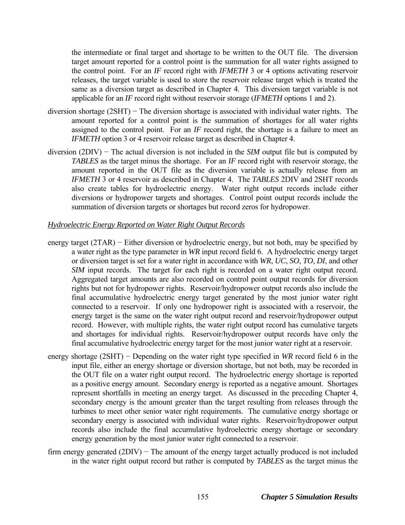
the intermediate or final target and shortage to be written to the OUT file. The diversion target amount reported for a control point is the summation for all water rights assigned to the control point. For an IF record right with IFMETH 3 or 4 options activating reservoir releases, the target variable is used to store the reservoir release target which is treated the same as a diversion target as described in Chapter 4. This diversion target variable is not applicable for an IF record right without reservoir storage (IFMETH options 1 and 2).
diversion shortage (2SHT) − The diversion shortage is associated with individual water rights. The amount reported for a control point is the summation of shortages for all water rights assigned to the control point. For an IF record right, the shortage is a failure to meet an IFMETH option 3 or 4 reservoir release target as described in Chapter 4.
diversion (2DIV) − The actual diversion is not included in the SIM output file but is computed by TABLES as the target minus the shortage. For an IF record right with reservoir storage, the amount reported in the OUT file as the diversion variable is actually release from an IFMETH 3 or 4 reservoir as described in Chapter 4. The TABLES 2DIV and 2SHT records also create tables for hydroelectric energy. Water right output records include either diversions or hydropower targets and shortages. Control point output records include the summation of diversion targets or shortages but record zeros for hydropower.
Hydroelectric Energy Reported on Water Right Output Records
energy target (2TAR) − Either diversion or hydroelectric energy, but not both, may be specified by a water right as the type parameter in WR input record field 6. A hydroelectric energy target or diversion target is set for a water right in accordance with WR, UC, SO, TO, DI, and other SIM input records. The target for each right is recorded on a water right output record. Aggregated target amounts are also recorded on control point output records for diversion rights but not for hydropower rights. Reservoir/hydropower output records also include the final accumulative hydroelectric energy target generated by the most junior water right connected to a reservoir. If only one hydropower right is associated with a reservoir, the energy target is the same on the water right output record and reservoir/hydropower output record. However, with multiple rights, the water right output record has cumulative targets and shortages for individual rights. Reservoir/hydropower output records have only the final accumulative hydroelectric energy target for the most junior water right at a reservoir.
energy shortage (2SHT) − Depending on the water right type specified in WR record field 6 in the input file, either an energy shortage or diversion shortage, but not both, may be recorded in the OUT file on a water right output record. The hydroelectric energy shortage is reported as a positive energy amount. Secondary energy is reported as a negative amount. Shortages represent shortfalls in meeting an energy target. As discussed in the preceding Chapter 4, secondary energy is the amount greater than the target resulting from releases through the turbines to meet other senior water right requirements. The cumulative energy shortage or secondary energy is associated with individual water rights. Reservoir/hydropower output records also include the final accumulative hydroelectric energy shortage or secondary energy generation by the most junior water right connected to a reservoir.
firm energy generated (2DIV) − The amount of the energy target actually produced is not included in the water right output record but rather is computed by TABLES as the target minus the
Chapter 5 Simulation Results 155

shortage. Firm energy generated equals target minus shortage. The TABLES 2DIV record creates tables of either diversions or hydroelectric energy in the same manner.
Additional Variables Recorded Only on Water Right Output Records
instream flow target (2IFT) − Instream flow targets are specified by IF input records and supporting input records as described in Reference Manual Chapter 4 and Users Manual Chapter 3. SO record field 9 specifies the intermediate or final target and shortage written to the OUT file.
instream flow shortage (2IFS) − An instream flow shortage is the amount by which the monthly regulated flow volume falls below the instream flow target.
return flow (2RFL) − The return flow volume for this particular water right is the portion of the diversion volume that is returned to the river system following WR record specifications.
secondary reservoir releases (2ROR) − Total volume released from secondary reservoirs this month for this water right following OR input record multiple-reservoir system operating rules.
available stream flow (2ASF) − The amount of stream flow available to a water right is computed as each right is considered in the water rights priority loop.
increase in available flow (2XAV) − The increase in available stream flow to result from the PX record control point limit option described in the last section of Chapter 4. This variable is recorded only if this PX input record field 4 & 5 option is activated.
Additional Variables Recorded on Reservoir/Hydropower Output Records
energy shortage (2HPS) − Both shortages in firm energy and additional secondary energy are recorded as the same variable in the OUT file. The hydroelectric energy shortage is reported as a positive energy amount. Secondary energy is reported as a negative amount. Shortages represent shortfalls in meeting an energy target. Secondary energy is the amount greater than the target resulting from releases through the turbines for other senior water rights.
energy generated (2HPE) − The actual energy generated represents the portion of the energy target that was supplied. Only the firm energy target, not secondary energy, is included. The hydroelectric energy recorded on the reservoir/hydropower output record is the accumulated total energy generated by the most junior hydropower right associated with the reservoir.
flow depletions (2RID) − Stream flow depletions associated with a reservoir include all the water taken from stream flow to meet water right requirements at the reservoir.
reservoir inflows (2RIR) − Reservoir inflows from other reservoirs consist of releases from secondary reservoirs to meet water right requirements at this reservoir.
releases (2RAH) − Releases from the reservoir that can be used to generate hydropower. The parameter LAKESD entered on the WS input records of other non-hydropower rights controls whether or not water supply releases from a reservoir can be passed through hydropower turbines. The default option is for hydropower to access water supply releases.
releases (2RNA) − Releases from the reservoir that are not accessible to the turbines for use in generating hydropower as governed by the parameter LAKESD entered on the WS input record. Diversions for water rights flagged as lakeside do not pass through the turbines.
Chapter 5 Simulation Results 156
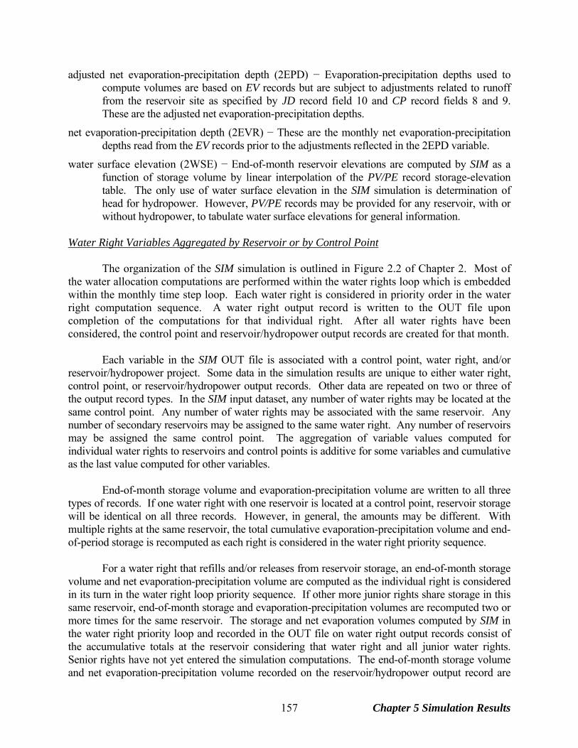
adjusted net evaporation-precipitation depth (2EPD) − Evaporation-precipitation depths used to compute volumes are based on EV records but are subject to adjustments related to runoff from the reservoir site as specified by JD record field 10 and CP record fields 8 and 9. These are the adjusted net evaporation-precipitation depths.
net evaporation-precipitation depth (2EVR) − These are the monthly net evaporation-precipitation depths read from the EV records prior to the adjustments reflected in the 2EPD variable.
water surface elevation (2WSE) − End-of-month reservoir elevations are computed by SIM as a function of storage volume by linear interpolation of the PV/PE record storage-elevation table. The only use of water surface elevation in the SIM simulation is determination of head for hydropower. However, PV/PE records may be provided for any reservoir, with or without hydropower, to tabulate water surface elevations for general information.
Water Right Variables Aggregated by Reservoir or by Control Point The organization of the SIM simulation is outlined in Figure 2.2 of Chapter 2. Most of the water allocation computations are performed within the water rights loop which is embedded within the monthly time step loop. Each water right is considered in priority order in the water right computation sequence. A water right output record is written to the OUT file upon completion of the computations for that individual right. After all water rights have been considered, the control point and reservoir/hydropower output records are created for that month. Each variable in the SIM OUT file is associated with a control point, water right, and/or reservoir/hydropower project. Some data in the simulation results are unique to either water right, control point, or reservoir/hydropower output records. Other data are repeated on two or three of the output record types. In the SIM input dataset, any number of water rights may be located at the same control point. Any number of water rights may be associated with the same reservoir. Any number of secondary reservoirs may be assigned to the same water right. Any number of reservoirs may be assigned the same control point. The aggregation of variable values computed for individual water rights to reservoirs and control points is additive for some variables and cumulative as the last value computed for other variables. End-of-month storage volume and evaporation-precipitation volume are written to all three types of records. If one water right with one reservoir is located at a control point, reservoir storage will be identical on all three records. However, in general, the amounts may be different. With multiple rights at the same reservoir, the total cumulative evaporation-precipitation volume and end-of-period storage is recomputed as each right is considered in the water right priority sequence. For a water right that refills and/or releases from reservoir storage, an end-of-month storage volume and net evaporation-precipitation volume are computed as the individual right is considered in its turn in the water right loop priority sequence. If other more junior rights share storage in this same reservoir, end-of-month storage and evaporation-precipitation volumes are recomputed two or more times for the same reservoir. The storage and net evaporation volumes computed by SIM in the water right priority loop and recorded in the OUT file on water right output records consist of the accumulative totals at the reservoir considering that water right and all junior water rights. Senior rights have not yet entered the simulation computations. The end-of-month storage volume and net evaporation-precipitation volume recorded on the reservoir/hydropower output record are
Chapter 5 Simulation Results 157
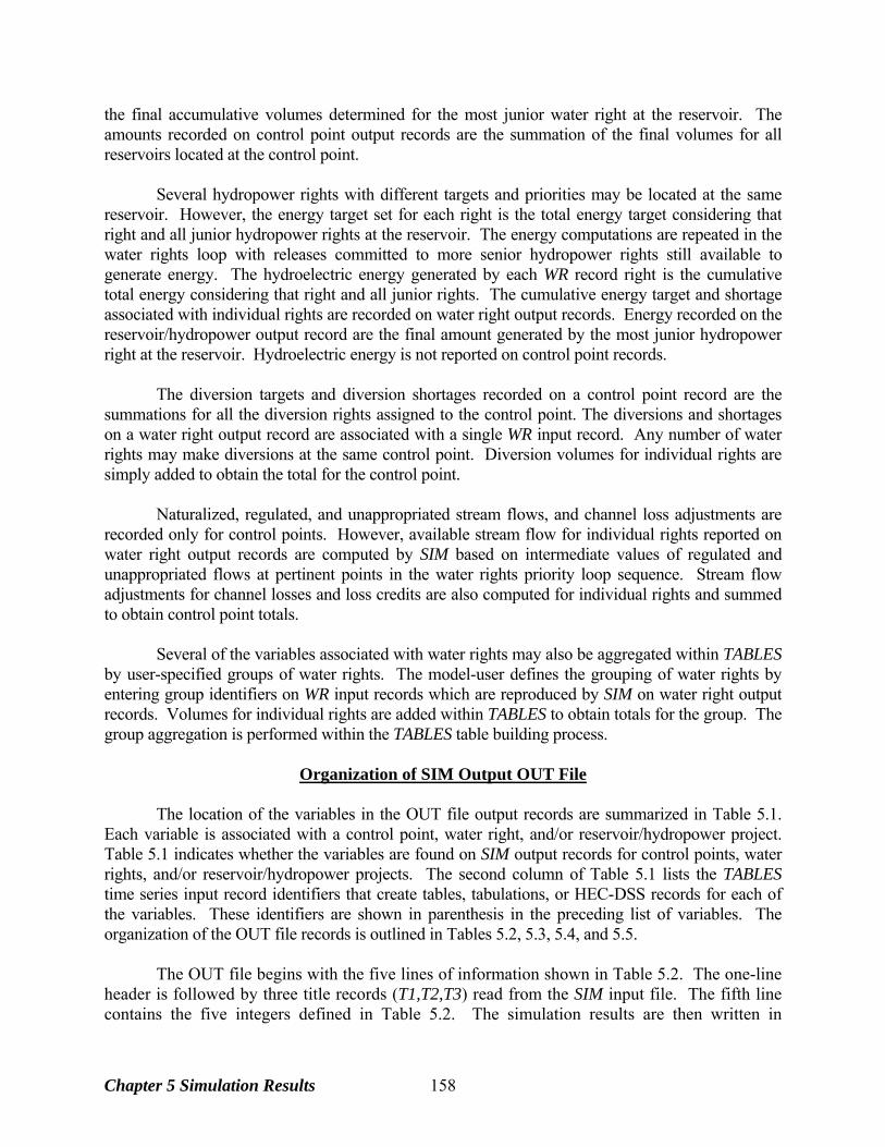
the final accumulative volumes determined for the most junior water right at the reservoir. The amounts recorded on control point output records are the summation of the final volumes for all reservoirs located at the control point. Several hydropower rights with different targets and priorities may be located at the same reservoir. However, the energy target set for each right is the total energy target considering that right and all junior hydropower rights at the reservoir. The energy computations are repeated in the water rights loop with releases committed to more senior hydropower rights still available to generate energy. The hydroelectric energy generated by each WR record right is the cumulative total energy considering that right and all junior rights. The cumulative energy target and shortage associated with individual rights are recorded on water right output records. Energy recorded on the reservoir/hydropower output record are the final amount generated by the most junior hydropower right at the reservoir. Hydroelectric energy is not reported on control point records. The diversion targets and diversion shortages recorded on a control point record are the summations for all the diversion rights assigned to the control point. The diversions and shortages on a water right output record are associated with a single WR input record. Any number of water rights may make diversions at the same control point. Diversion volumes for individual rights are simply added to obtain the total for the control point. Naturalized, regulated, and unappropriated stream flows, and channel loss adjustments are recorded only for control points. However, available stream flow for individual rights reported on water right output records are computed by SIM based on intermediate values of regulated and unappropriated flows at pertinent points in the water rights priority loop sequence. Stream flow adjustments for channel losses and loss credits are also computed for individual rights and summed to obtain control point totals. Several of the variables associated with water rights may also be aggregated within TABLES by user-specified groups of water rights. The model-user defines the grouping of water rights by entering group identifiers on WR input records which are reproduced by SIM on water right output records. Volumes for individual rights are added within TABLES to obtain totals for the group. The group aggregation is performed within the TABLES table building process.
Organization of SIM Output OUT File
The location of the variables in the OUT file output records are summarized in Table 5.1. Each variable is associated with a control point, water right, and/or reservoir/hydropower project. Table 5.1 indicates whether the variables are found on SIM output records for control points, water rights, and/or reservoir/hydropower projects. The second column of Table 5.1 lists the TABLES time series input record identifiers that create tables, tabulations, or HEC-DSS records for each of the variables. These identifiers are shown in parenthesis in the preceding list of variables. The organization of the OUT file records is outlined in Tables 5.2, 5.3, 5.4, and 5.5. The OUT file begins with the five lines of information shown in Table 5.2. The one-line header is followed by three title records (T1,T2,T3) read from the SIM input file. The fifth line contains the five integers defined in Table 5.2. The simulation results are then written in
Chapter 5 Simulation Results 158
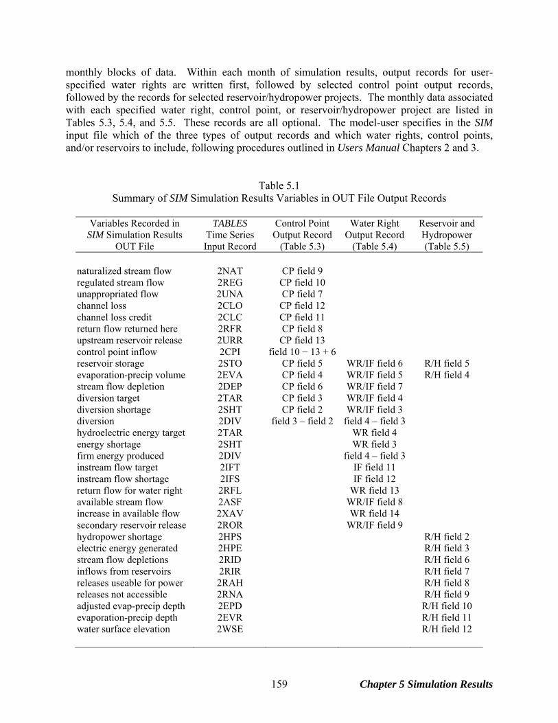
monthly blocks of data. Within each month of simulation results, output records for user-specified water rights are written first, followed by selected control point output records, followed by the records for selected reservoir/hydropower projects. The monthly data associated with each specified water right, control point, or reservoir/hydropower project are listed in Tables 5.3, 5.4, and 5.5. These records are all optional. The model-user specifies in the SIM input file which of the three types of output records and which water rights, control points, and/or reservoirs to include, following procedures outlined in Users Manual Chapters 2 and 3.
Table 5.1 Summary of SIM Simulation Results Variables in OUT File Output Records
Variables Recorded in TABLES Control Point Water Right Reservoir and
SIM Simulation Results Time Series Output Record Output Record Hydropower OUT File Input Record (Table 5.3) (Table 5.4) (Table 5.5)
naturalized stream flow 2NAT CP field 9 regulated stream flow 2REG CP field 10 unappropriated flow 2UNA CP field 7 channel loss 2CLO CP field 12 channel loss credit 2CLC CP field 11 return flow returned here 2RFR CP field 8 upstream reservoir release 2URR CP field 13 control point inflow 2CPI field 10 − 13 + 6 reservoir storage 2STO CP field 5 WR/IF field 6 R/H field 5 evaporation-precip volume 2EVA CP field 4 WR/IF field 5 R/H field 4 stream flow depletion 2DEP CP field 6 WR/IF field 7 diversion target 2TAR CP field 3 WR/IF field 4 diversion shortage 2SHT CP field 2 WR/IF field 3 diversion 2DIV field 3 – field 2 field 4 – field 3 hydroelectric energy target 2TAR WR field 4 energy shortage 2SHT WR field 3 firm energy produced 2DIV field 4 – field 3 instream flow target 2IFT IF field 11 instream flow shortage 2IFS IF field 12 return flow for water right 2RFL WR field 13 available stream flow 2ASF WR/IF field 8 increase in available flow 2XAV WR field 14 secondary reservoir release 2ROR WR/IF field 9 hydropower shortage 2HPS R/H field 2 electric energy generated 2HPE R/H field 3 stream flow depletions 2RID R/H field 6 inflows from reservoirs 2RIR R/H field 7 releases useable for power 2RAH R/H field 8 releases not accessible 2RNA R/H field 9 adjusted evap-precip depth 2EPD R/H field 10 evaporation-precip depth 2EVR R/H field 11 water surface elevation 2WSE R/H field 12
Chapter 5 Simulation Results 159
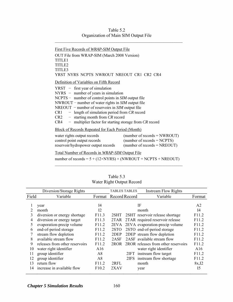
Table 5.2 Organization of Main SIM Output File
______________________________________________________________ First Five Records of WRAP-SIM Output File
OUT File from WRAP-SIM (March 2008 Version) TITLE1 TITLE2 TITLE3 YRST NYRS NCPTS NWROUT NREOUT CR1 CR2 CR4
Definition of Variables on Fifth Record
YRST − first year of simulation NYRS − number of years in simulation NCPTS − number of control points in SIM output file NWROUT − number of water rights in SIM output file NREOUT − number of reservoirs in SIM output file CR1 − length of simulation period from CR record CR2 − starting month from CR record CR4 − multiplier factor for starting storage from CR record
Block of Records Repeated for Each Period (Month)
water rights output records (number of records = NWROUT) control point output records (number of records = NCPTS) reservoir/hydropower output records (number of records = NREOUT)
Total Number of Records in WRAP-SIM Output File
number of records = 5 + (12×NYRS) × (NWROUT + NCPTS + NREOUT) ______________________________________________________________
Table 5.3
Water Right Output Record
Diversion/Storage Rights TABLES TABLES Instream Flow Rights Field Variable Format Record Record Variable Format
1 year I4 IF A2 2 month I2 month I4 3 diversion or energy shortage F11.3 2SHT 2SHT reservoir release shortage F11.2 4 diversion or energy target F11.3 2TAR 2TAR required reservoir release F11.2 5 evaporation-precip volume F11.2 2EVA 2EVA evaporation-precip volume F11.2 6 end-of-period storage F11.2 2STO 2STO end-of-period storage F11.2 7 stream flow depletion F11.2 2DEP 2DEP stream flow depletion F11.2 8 available stream flow F11.2 2ASF 2ASF available stream flow F11.2 9 releases from other reservoirs F11.2 2ROR 2ROR releases from other reservoirs F11.2
10 water right identifier A16 water right identifier A16 11 group identifier A8 2IFT instream flow target F11.2 12 group identifier A8 2IFS instream flow shortage F11.2 13 return flow F11.2 2RFL month 8x,I2 14 increase in available flow F10.2 2XAV year I5
Chapter 5 Simulation Results 160
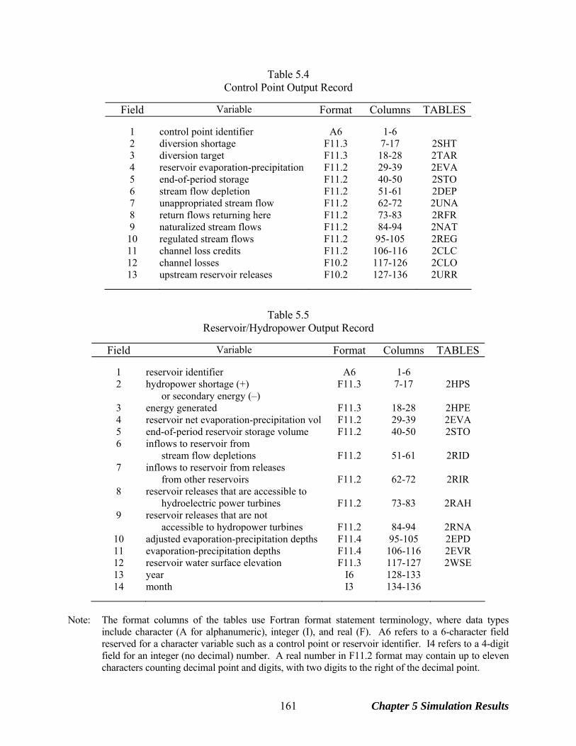
Table 5.4 Control Point Output Record
Field Variable Format Columns TABLES
1 control point identifier A6 1-6 2 diversion shortage F11.3 7-17 2SHT 3 diversion target F11.3 18-28 2TAR 4 reservoir evaporation-precipitation F11.2 29-39 2EVA 5 end-of-period storage F11.2 40-50 2STO 6 stream flow depletion F11.2 51-61 2DEP 7 unappropriated stream flow F11.2 62-72 2UNA 8 return flows returning here F11.2 73-83 2RFR 9 naturalized stream flows F11.2 84-94 2NAT
10 regulated stream flows F11.2 95-105 2REG 11 channel loss credits F11.2 106-116 2CLC 12 channel losses F10.2 117-126 2CLO 13 upstream reservoir releases F10.2 127-136 2URR
Table 5.5
Reservoir/Hydropower Output Record
Field Variable Format Columns TABLES
1 reservoir identifier A6 1-6 2 hydropower shortage (+)
or secondary energy (–) F11.3 7-17 2HPS
3 energy generated F11.3 18-28 2HPE 4 reservoir net evaporation-precipitation vol F11.2 29-39 2EVA 5 end-of-period reservoir storage volume F11.2 40-50 2STO 6 inflows to reservoir from
stream flow depletions
F11.2
51-61
2RID 7 inflows to reservoir from releases
from other reservoirs
F11.2
62-72
2RIR 8 reservoir releases that are accessible to
hydroelectric power turbines
F11.2
73-83
2RAH 9 reservoir releases that are not
accessible to hydropower turbines
F11.2
84-94
2RNA 10 adjusted evaporation-precipitation depths F11.4 95-105 2EPD 11 evaporation-precipitation depths F11.4 106-116 2EVR 12 reservoir water surface elevation F11.3 117-127 2WSE 13 year I6 128-133 14 month I3 134-136
Note: The format columns of the tables use Fortran format statement terminology, where data types
include character (A for alphanumeric), integer (I), and real (F). A6 refers to a 6-character field reserved for a character variable such as a control point or reservoir identifier. I4 refers to a 4-digit field for an integer (no decimal) number. A real number in F11.2 format may contain up to eleven characters counting decimal point and digits, with two digits to the right of the decimal point.
Chapter 5 Simulation Results 161
Simulation results from the example presented in the Fundamentals Manual are used for illustration throughout the remainder of this chapter. Table 5.6 reproduces the beginning of the OUT file showing the output records for the two instream flow rights, 28 WR record water rights, eleven control points, and six reservoirs for the first month of the 696-month 1940-1997 simulation. The OUT file is designed to compactly store the voluminous output data in the order in which it is computed. Water right records are written in order of priority as each water right is considered in the computational loop. Control point output records are in the same order as the CP records in the input file. Likewise, reservoir/hydropower records are in the order that reservoirs are first read in the input file. Examination of the OUT file may be useful occasionally for tracking problems, but the format is not convenient for routinely interpreting simulation results. The SOU file is designed to be much easier for people to read than the OUT file but does not record the output data in the exact order that is computed like the OUT file. Program TABLES provides an array of options for organizing, tabulating, analyzing, summarizing, and displaying the simulation results in a variety of formats. The data in the SIM OUT file are incorporated into various tables created by TABLES including standard time series tables as well as the other types of tables described later in this chapter. The TABLES input records that build standard time series tables for each type of data shown in parenthesis in the preceding list of variable definitions and listed in the second column of Table 5.1, middle columns of Table 5.3, and last column of Tables 5.4 and 5.5. Water Right Output Records Each record provides data for a water right for a given month. The records for all of the water rights are grouped together for a given month. As shown in Table 5.3, the water right output record for an IF input record instream flow right is different than the record for a WR input record right. The variables are stored in the format indicated by the following Fortran format statements. WR record water rights: Format (I4, I2, 2F11.3, 5F11.2, A16, 2A8, F11.2, F10.2) IF record instream flow rights: Format (A2, I4, 7F11.2, A16, 2F11.2, 8x, I2, I5) Each WR record water right output record contains: year and month, shortage and target, net evaporation-precipitation volume, end-of-period reservoir storage, stream flow depletion by the water right, stream flow available to the right before the stream flow depletion, all water that was released from secondary reservoirs to meet the diversion and/or refill storage, the three identifiers from the WR input record, return flows, and an available flow increase generated only in conjunction with a PX record option. The actual diversion volume or hydroelectric production is computed within TABLES as the target less the shortage. Depending on the water right type specified in WR record field 6 in the input file, either an energy shortage, diversion shortage, or storage shortage, may be recorded in the OUT file on a water right output record. The same variable is used to report both energy shortages and secondary energy. The hydroelectric energy shortage is reported as a positive energy amount. Secondary energy is reported as a negative amount. Shortages represent shortfalls in meeting an energy target. Secondary energy is the amount greater than the target resulting from releases through the turbines to meet other senior water right requirements.
Chapter 5 Simulation Results 162
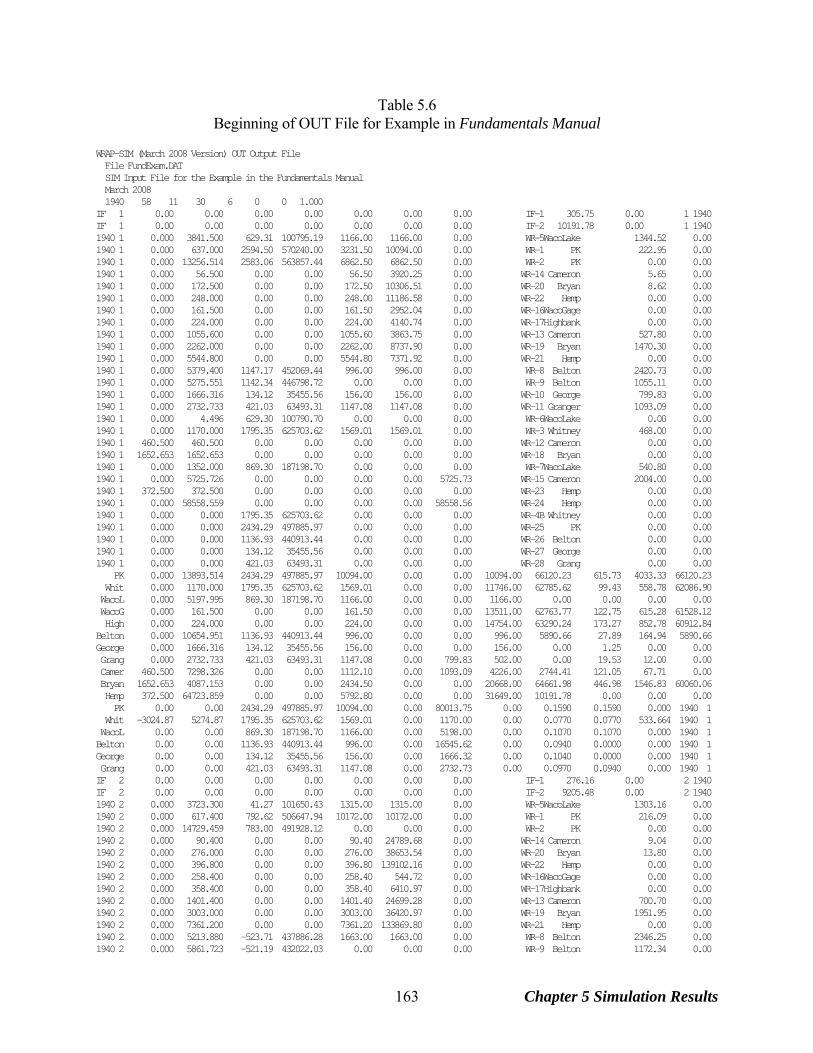
Table 5.6 Beginning of OUT File for Example in Fundamentals Manual
WRAP-SIM (March 2008 Version) OUT Output File File FundExam.DAT SIM Input File for the Example in the Fundamentals Manual March 2008 1940 58 11 30 6 0 0 1.000 IF 1 0.00 0.00 0.00 0.00 0.00 0.00 0.00 IF-1 305.75 0.00 1 1940 IF 1 0.00 0.00 0.00 0.00 0.00 0.00 0.00 IF-2 10191.78 0.00 1 1940 1940 1 0.000 3841.500 629.31 100795.19 1166.00 1166.00 0.00 WR-5WacoLake 1344.52 0.00 1940 1 0.000 637.000 2594.50 570240.00 3231.50 10094.00 0.00 WR-1 PK 222.95 0.00 1940 1 0.000 13256.514 2583.06 563857.44 6862.50 6862.50 0.00 WR-2 PK 0.00 0.00 1940 1 0.000 56.500 0.00 0.00 56.50 3920.25 0.00 WR-14 Cameron 5.65 0.00 1940 1 0.000 172.500 0.00 0.00 172.50 10306.51 0.00 WR-20 Bryan 8.62 0.00 1940 1 0.000 248.000 0.00 0.00 248.00 11186.58 0.00 WR-22 Hemp 0.00 0.00 1940 1 0.000 161.500 0.00 0.00 161.50 2952.04 0.00 WR-16WacoGage 0.00 0.00 1940 1 0.000 224.000 0.00 0.00 224.00 4140.74 0.00 WR-17Highbank 0.00 0.00 1940 1 0.000 1055.600 0.00 0.00 1055.60 3863.75 0.00 WR-13 Cameron 527.80 0.00 1940 1 0.000 2262.000 0.00 0.00 2262.00 8737.90 0.00 WR-19 Bryan 1470.30 0.00 1940 1 0.000 5544.800 0.00 0.00 5544.80 7371.92 0.00 WR-21 Hemp 0.00 0.00 1940 1 0.000 5379.400 1147.17 452069.44 996.00 996.00 0.00 WR-8 Belton 2420.73 0.00 1940 1 0.000 5275.551 1142.34 446798.72 0.00 0.00 0.00 WR-9 Belton 1055.11 0.00 1940 1 0.000 1666.316 134.12 35455.56 156.00 156.00 0.00 WR-10 George 799.83 0.00 1940 1 0.000 2732.733 421.03 63493.31 1147.08 1147.08 0.00 WR-11 Granger 1093.09 0.00 1940 1 0.000 4.496 629.30 100790.70 0.00 0.00 0.00 WR-6WacoLake 0.00 0.00 1940 1 0.000 1170.000 1795.35 625703.62 1569.01 1569.01 0.00 WR-3 Whitney 468.00 0.00 1940 1 460.500 460.500 0.00 0.00 0.00 0.00 0.00 WR-12 Cameron 0.00 0.00 1940 1 1652.653 1652.653 0.00 0.00 0.00 0.00 0.00 WR-18 Bryan 0.00 0.00 1940 1 0.000 1352.000 869.30 187198.70 0.00 0.00 0.00 WR-7WacoLake 540.80 0.00 1940 1 0.000 5725.726 0.00 0.00 0.00 0.00 5725.73 WR-15 Cameron 2004.00 0.00 1940 1 372.500 372.500 0.00 0.00 0.00 0.00 0.00 WR-23 Hemp 0.00 0.00 1940 1 0.000 58558.559 0.00 0.00 0.00 0.00 58558.56 WR-24 Hemp 0.00 0.00 1940 1 0.000 0.000 1795.35 625703.62 0.00 0.00 0.00 WR-4B Whitney 0.00 0.00 1940 1 0.000 0.000 2434.29 497885.97 0.00 0.00 0.00 WR-25 PK 0.00 0.00 1940 1 0.000 0.000 1136.93 440913.44 0.00 0.00 0.00 WR-26 Belton 0.00 0.00 1940 1 0.000 0.000 134.12 35455.56 0.00 0.00 0.00 WR-27 George 0.00 0.00 1940 1 0.000 0.000 421.03 63493.31 0.00 0.00 0.00 WR-28 Grang 0.00 0.00 PK 0.000 13893.514 2434.29 497885.97 10094.00 0.00 0.00 10094.00 66120.23 615.73 4033.33 66120.23 Whit 0.000 1170.000 1795.35 625703.62 1569.01 0.00 0.00 11746.00 62785.62 99.43 558.78 62086.90 WacoL 0.000 5197.995 869.30 187198.70 1166.00 0.00 0.00 1166.00 0.00 0.00 0.00 0.00 WacoG 0.000 161.500 0.00 0.00 161.50 0.00 0.00 13511.00 62763.77 122.75 615.28 61528.12 High 0.000 224.000 0.00 0.00 224.00 0.00 0.00 14754.00 63290.24 173.27 852.78 60912.84 Belton 0.000 10654.951 1136.93 440913.44 996.00 0.00 0.00 996.00 5890.66 27.89 164.94 5890.66 George 0.000 1666.316 134.12 35455.56 156.00 0.00 0.00 156.00 0.00 1.25 0.00 0.00 Grang 0.000 2732.733 421.03 63493.31 1147.08 0.00 799.83 502.00 0.00 19.53 12.00 0.00 Camer 460.500 7298.326 0.00 0.00 1112.10 0.00 1093.09 4226.00 2744.41 121.05 67.71 0.00 Bryan 1652.653 4087.153 0.00 0.00 2434.50 0.00 0.00 20668.00 64661.98 446.98 1546.83 60060.06 Hemp 372.500 64723.859 0.00 0.00 5792.80 0.00 0.00 31649.00 10191.78 0.00 0.00 0.00 PK 0.00 0.00 2434.29 497885.97 10094.00 0.00 80013.75 0.00 0.1590 0.1590 0.000 1940 1 Whit -3024.87 5274.87 1795.35 625703.62 1569.01 0.00 1170.00 0.00 0.0770 0.0770 533.664 1940 1 WacoL 0.00 0.00 869.30 187198.70 1166.00 0.00 5198.00 0.00 0.1070 0.1070 0.000 1940 1 Belton 0.00 0.00 1136.93 440913.44 996.00 0.00 16545.62 0.00 0.0940 0.0000 0.000 1940 1 George 0.00 0.00 134.12 35455.56 156.00 0.00 1666.32 0.00 0.1040 0.0000 0.000 1940 1 Grang 0.00 0.00 421.03 63493.31 1147.08 0.00 2732.73 0.00 0.0970 0.0940 0.000 1940 1 IF 2 0.00 0.00 0.00 0.00 0.00 0.00 0.00 IF-1 276.16 0.00 2 1940 IF 2 0.00 0.00 0.00 0.00 0.00 0.00 0.00 IF-2 9205.48 0.00 2 1940 1940 2 0.000 3723.300 41.27 101650.43 1315.00 1315.00 0.00 WR-5WacoLake 1303.16 0.00 1940 2 0.000 617.400 792.62 506647.94 10172.00 10172.00 0.00 WR-1 PK 216.09 0.00 1940 2 0.000 14729.459 783.00 491928.12 0.00 0.00 0.00 WR-2 PK 0.00 0.00 1940 2 0.000 90.400 0.00 0.00 90.40 24789.68 0.00 WR-14 Cameron 9.04 0.00 1940 2 0.000 276.000 0.00 0.00 276.00 38653.54 0.00 WR-20 Bryan 13.80 0.00 1940 2 0.000 396.800 0.00 0.00 396.80 139102.16 0.00 WR-22 Hemp 0.00 0.00 1940 2 0.000 258.400 0.00 0.00 258.40 544.72 0.00 WR-16WacoGage 0.00 0.00 1940 2 0.000 358.400 0.00 0.00 358.40 6410.97 0.00 WR-17Highbank 0.00 0.00 1940 2 0.000 1401.400 0.00 0.00 1401.40 24699.28 0.00 WR-13 Cameron 700.70 0.00 1940 2 0.000 3003.000 0.00 0.00 3003.00 36420.97 0.00 WR-19 Bryan 1951.95 0.00 1940 2 0.000 7361.200 0.00 0.00 7361.20 133869.80 0.00 WR-21 Hemp 0.00 0.00 1940 2 0.000 5213.880 -523.71 437886.28 1663.00 1663.00 0.00 WR-8 Belton 2346.25 0.00 1940 2 0.000 5861.723 -521.19 432022.03 0.00 0.00 0.00 WR-9 Belton 1172.34 0.00
Chapter 5 Simulation Results 163
Instream flow rights may include releases from reservoir storage to meet the regulated flow target. The release from storage required to meet the instream flow requirement is recorded in field 4 in lieu of diversion target, and the shortage in supplying the reservoir release is recorded in field 3. The net evaporation-precipitation volume and end-of-period storage volume in fields 5 and 6 are the values determined prior to considering any other junior rights that are associated with the reservoir. The amounts written for the most junior right at the reservoir are the actual values that occur for the reservoir. Any amounts recorded for senior rights at the reservoir are intermediate values only. The reservoir net evaporation minus precipitation volume is positive if evaporation rate exceeds precipitation and negative if precipitation is greater. The stream flow depletion in field 7 represents the monthly stream flow volume that the water right appropriated to supply the diversion target, account for reservoir net evaporation-precipitation, and/or refill storage. In months with a negative net evaporation-precipitation depth, the stream flow depletion may be a negative number. In this case, the water right actually makes water available to the river system by catching precipitation that falls onto the reservoir surface. Releases from other reservoirs in field 9 are from secondary reservoirs to meet the storage and diversion requirements of the right. Releases from the primary reservoir are not included. Control Point Output Records Control point records for all of the control points included in the OUT file are grouped together for a given month. The 136-character record contains 13 variables stored in the format indicated by the following Fortran format statement.
Format (A6, 2F11.3, 8F11.2, 2F10.2) As indicated in Table 5.4, each record begins with the control point identifier, sum of the shortages and diversion targets for all diversion rights, evaporation-precipitation and end-of-period storage for all reservoirs, and stream flow depletions for all rights located at the control point. The next four fields contain the unappropriated flow remaining at the control point after all stream flow depletions have been made, the sum of the return flow returned at the control point from the current and previous month, and the naturalized and regulated stream flow. Fields 11 and 12 contain adjustments applied for channel loss credits and channel losses. The last field has the portion of the regulated flow that originates as releases made from reservoirs located at this control point or upstream to meet water right requirements at control points located further downstream. Reservoir/Hydropower Output Records Each record provides data for a reservoir and/or hydroelectric power plant for a given month. All the reservoir/hydropower records are grouped together for a given period. The variables include energy shortage at the reservoir, energy produced at the reservoir, evaporation-precipitation, end-of-period storage, stream flow depletions made available to the reservoir, releases from other reservoirs made available, releases from the reservoir through the outlet works, lakeside releases from the reservoir, net evaporation-precipitation depths with and without runoff
Chapter 5 Simulation Results 164
adjustments, reservoir water surface elevation, year, and month. The 136 character record outlined in Table 5.5 contains 12 variables stored in the following format.
Format (A6, 2F11.3, 6F11.2, 2F11.4, F11.3, I6, I3) The hydroelectric energy produced at the reservoir in each month is calculated from the average water surface elevation of the reservoir, the tailwater elevation for the most junior hydropower right associated with the reservoir, and the total flow through the outlet works for all hydropower rights and other senior rights. Either a turbine flow capacity may be specified or the power produced may be computed assuming that the turbine capacity is unlimited. Hydropower shortages are calculated as the algebraic difference between energy target and the energy produced. Positive shortage values signify that insufficient water was released from the reservoir to produce the energy requirement of the most junior hydropower right at the reservoir. Negative shortages represent secondary energy that was produced by releases through the outlet works to meet senior water right diversion and storage requirements. Stream flow depletions include amounts for diversions as well as depletions to refill storage and account for net evaporation less precipitation. Depletions for diversions are assumed to enter a primary reservoir and then are either diverted lakeside or released through the reservoir outlet works. The releases written to a reservoir output record include releases made both as a primary and as a secondary reservoir.
Types of TABLES Tabulations The TABLES input TIN file specifies the tables and/or other types of information to be created and written to the TABLES output TOU file. The TIN file records begin with the four character identifiers shown in parenthesis in Table 5.7. Each record activates routines that create sets of tables and/or tabulations in a variety of user-specified formats. Chapter 4 of the Users Manual explains TABLES types 1, 2, 3, and 4 input records and resulting output tables or listings. The Supplemental Manual provides instructions for applying TABLES types 5, 6, 7, and 8 options. The following general description of types 1, 2, 3, and 4 features is followed by a more in depth presentation of capabilities provided by TABLES type 2 options for organizing and analyzing SIM simulation results. Type 1 input records activate routines that read the main SIM input DAT file and organize selected data. The 1REC routine simply lists SIM input records of user-selected types. The 1SUM record instructs TABLES to create water right summary tables organized in user-selected formats. A 1SRT record creates a listing of water rights sorted in priority order or a listing by type of use, control point, water right type, or water right group in priority order. The 1CPT record provides options for rearranging control point records in upstream-to-downstream order and developing listings of control points with user-specified information. Type 2 routines provide an array of formats for organizing, analyzing, summarizing, and displaying SIM simulation results. Most of the types 5, 6, 7, and 8 options described in the Supplemental Manual are analogous to the type 2 features covered in the Users Manual. Basic concepts reflected in type 2 routines are described in the following sections of this chapter.
Chapter 5 Simulation Results 165
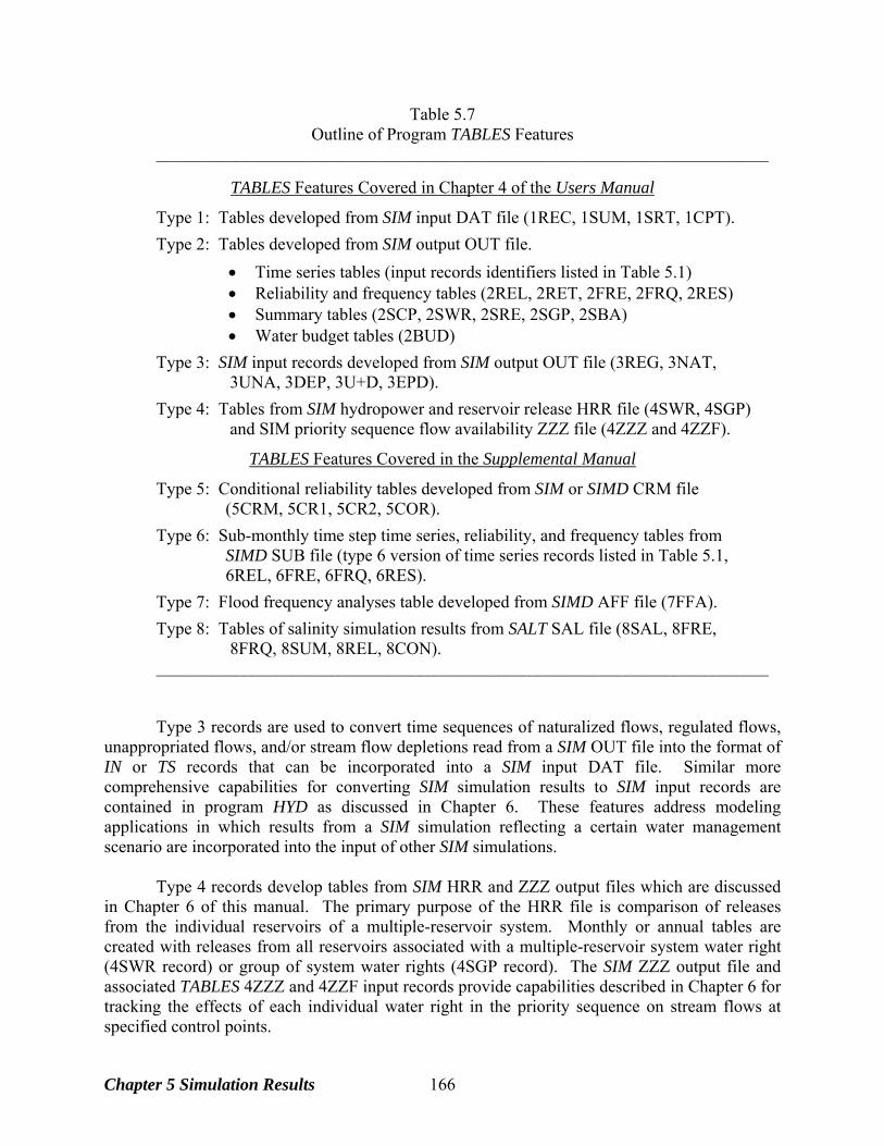
Table 5.7 Outline of Program TABLES Features
_____________________________________________________________________________
TABLES Features Covered in Chapter 4 of the Users Manual
Type 1: Tables developed from SIM input DAT file (1REC, 1SUM, 1SRT, 1CPT).
Type 2: Tables developed from SIM output OUT file.
• Time series tables (input records identifiers listed in Table 5.1) • Reliability and frequency tables (2REL, 2RET, 2FRE, 2FRQ, 2RES) • Summary tables (2SCP, 2SWR, 2SRE, 2SGP, 2SBA) • Water budget tables (2BUD)
Type 3: SIM input records developed from SIM output OUT file (3REG, 3NAT, 3UNA, 3DEP, 3U+D, 3EPD).
Type 4: Tables from SIM hydropower and reservoir release HRR file (4SWR, 4SGP) and SIM priority sequence flow availability ZZZ file (4ZZZ and 4ZZF).
TABLES Features Covered in the Supplemental Manual
Type 5: Conditional reliability tables developed from SIM or SIMD CRM file (5CRM, 5CR1, 5CR2, 5COR).
Type 6: Sub-monthly time step time series, reliability, and frequency tables from SIMD SUB file (type 6 version of time series records listed in Table 5.1, 6REL, 6FRE, 6FRQ, 6RES).
Type 7: Flood frequency analyses table developed from SIMD AFF file (7FFA).
Type 8: Tables of salinity simulation results from SALT SAL file (8SAL, 8FRE, 8FRQ, 8SUM, 8REL, 8CON). _____________________________________________________________________________ Type 3 records are used to convert time sequences of naturalized flows, regulated flows, unappropriated flows, and/or stream flow depletions read from a SIM OUT file into the format of IN or TS records that can be incorporated into a SIM input DAT file. Similar more comprehensive capabilities for converting SIM simulation results to SIM input records are contained in program HYD as discussed in Chapter 6. These features address modeling applications in which results from a SIM simulation reflecting a certain water management scenario are incorporated into the input of other SIM simulations. Type 4 records develop tables from SIM HRR and ZZZ output files which are discussed in Chapter 6 of this manual. The primary purpose of the HRR file is comparison of releases from the individual reservoirs of a multiple-reservoir system. Monthly or annual tables are created with releases from all reservoirs associated with a multiple-reservoir system water right (4SWR record) or group of system water rights (4SGP record). The SIM ZZZ output file and associated TABLES 4ZZZ and 4ZZF input records provide capabilities described in Chapter 6 for tracking the effects of each individual water right in the priority sequence on stream flows at specified control points.
Chapter 5 Simulation Results 166
Time Series Tables and Tabulations The time series data read from the SIM simulation results OUT file may be written by TABLES to the tables in the TABLES output TOU file and/or as records to a DSS file. Optionally, moving averages or moving accumulative totals of the data for a user-specified number of months may be computed and written to the TOU file and/or the DSS file. The data may also be adjusted by a multiplier factor, such as unit conversion factors, or subtracted from a given constant, such as computing reservoir drawdown as capacity minus storage content.
The original SIM simulation results or computed moving averages, moving totals, or otherwise adjusted time series data may be transformed by TABLES to the following formats.
• A text file with the filename extension TOU has each time series organized into a separate table with annual rows and monthly columns with headings illustrated by Table 5.8. Each of the variables selected from the 32 variables listed in Table 5.1 is presented as a set of separate tables for each selected water right, control point, or reservoir/hydropower project. This format is designed for report preparation and convenient viewing of simulation results.
• Each variable of interest may be tabulated as one column of a table written to the
TOU file along with the tables described above. Either monthly simulation results or annual totals may be tabulated. A monthly table would be 12 times longer than the table of annual totals shown in Table 5.9. Any of the 32 variables and any water right, control point, or reservoir/hydropower project may be selected for inclusion in the up to 100 column tabulation. This format is designed for convenient transport to Microsoft Excel or other spreadsheet programs for plotting or further computations.
• A binary file with the filename extension DSS has each time series variable of
interest stored as a HEC-DSS record. This format is designed to allow the data to be read by HEC-DSSVue for plotting or further computations. Figure 5.1 is a plot of monthly regulated flows created with HEC-DSSVue from a DSS file created with TABLES. Monthly or annual time series of any of the variables listed in Table 5.1 may be converted by TABLES to DSS records and plotted with HEC-DSSVue.
All SIM and TABLES input and output files except DSS files are in standard text format that can be read and viewed with Microsoft WordPad or other editors. The TABLES columnar format option facilitates importing the time series into Microsoft Excel or other spreadsheet programs. TABLES also converts the time series to records stored in a DSS file to be read by HEC-DSSVue. SIM simulation results can be stored directly by SIM as DSS or SOU files, but TABLES also allows the data manipulations noted above. HEC-DSSVue can be downloaded from the Hydrologic Engineering Center website and activated directly from WinWRAP. The Hydrologic Engineering Center (2005) provides detailed instructions in its use. A primary motivation for connecting HEC-DSSVue to WRAP is its capabilities for plotting time series graphs like Figure 5.1. However, HEC-DSSVue provides an array of other graphics, data tabulation, statistics, and computational capabilities that may also be useful for organizing and analyzing WRAP simulation results.
Chapter 5 Simulation Results 167
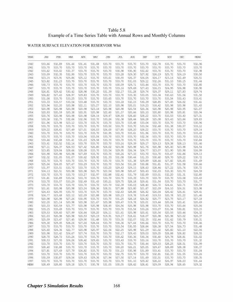
Table 5.8 Example of a Time Series Table with Annual Rows and Monthly Columns
WATER SURFACE ELEVATION FOR RESERVOIR Whit ------------------------------------------------------------------------------------------------------------------------------- YEAR JAN FEB MAR APR MAY JUN JUL AUG SEP OCT NOV DEC MEAN ------------------------------------------------------------------------------------------------------------------------------- 1940 533.66 532.89 531.44 531.41 531.08 533.70 533.70 533.70 533.70 532.78 533.70 533.70 532.96 1941 533.70 533.70 533.70 533.70 533.70 533.70 533.70 533.70 533.70 533.70 533.70 533.70 533.70 1942 533.62 533.02 532.37 533.70 533.70 533.70 530.98 530.90 532.62 533.70 533.70 533.70 532.98 1943 533.09 532.35 532.90 533.70 533.70 533.70 533.28 529.30 527.92 526.19 525.72 524.19 530.50 1944 523.15 523.91 525.86 525.12 533.70 533.61 530.55 526.37 526.05 524.17 523.16 522.49 526.51 1945 523.82 531.23 533.70 533.70 533.70 533.70 533.70 531.03 529.12 532.26 531.10 530.15 531.44 1946 530.73 533.70 533.70 533.70 533.70 533.70 530.09 529.71 533.44 533.70 533.70 533.70 532.80 1947 533.70 533.70 533.70 533.70 533.70 533.70 533.16 529.69 527.63 526.15 524.95 526.98 530.90 1948 526.81 529.62 530.42 528.98 530.20 531.39 532.17 531.28 529.74 529.37 529.11 527.83 529.74 1949 526.82 527.43 528.97 529.83 533.70 533.70 533.70 533.30 533.05 533.34 532.63 531.56 531.50 1950 531.08 533.70 533.25 533.70 533.70 533.65 533.70 533.70 533.70 533.70 533.54 533.43 533.41 1951 533.33 533.57 533.54 533.48 533.70 533.70 533.18 532.15 530.39 528.85 527.45 526.02 531.61 1952 523.94 522.20 520.98 522.11 525.27 522.10 520.98 520.01 519.23 518.42 520.98 520.98 521.43 1953 520.98 520.98 520.98 520.98 523.14 520.98 520.98 520.54 520.36 520.98 520.98 520.95 521.07 1954 520.93 520.59 520.38 520.91 520.98 522.60 521.57 520.66 520.10 520.80 520.98 520.81 520.94 1955 520.76 520.98 520.98 520.98 528.14 529.47 528.93 528.60 528.22 533.70 533.53 533.40 527.31 1956 533.36 532.75 532.66 532.96 533.70 533.26 532.38 528.44 526.28 525.08 523.43 523.66 529.83 1957 521.96 523.98 523.12 533.70 533.70 533.70 533.70 533.48 533.04 533.70 533.70 533.70 530.96 1958 533.70 533.70 533.70 533.70 533.70 533.50 533.70 533.70 533.54 532.48 531.38 530.57 533.12 1959 529.22 528.61 527.49 527.01 526.03 526.00 527.85 528.20 528.22 533.70 533.70 533.70 529.14 1960 533.70 533.70 533.70 533.70 533.70 532.95 533.70 533.61 531.96 533.70 533.70 533.70 533.49 1961 533.70 533.70 533.70 533.56 533.04 533.70 533.70 533.70 532.34 533.70 533.70 533.70 533.52 1962 533.46 532.68 531.41 531.03 529.58 533.70 533.70 533.70 533.70 533.70 533.70 533.70 532.84 1963 533.41 532.52 532.14 533.70 533.70 533.70 533.16 529.39 529.17 529.13 529.38 528.13 531.46 1964 527.11 526.37 526.53 527.42 526.80 524.02 523.08 520.98 521.76 520.98 525.40 523.98 524.54 1965 523.85 529.04 528.66 528.08 533.70 533.54 529.95 526.34 524.77 523.07 521.90 520.98 526.99 1966 520.98 520.98 520.98 527.69 533.70 533.70 530.26 527.33 533.70 533.70 533.67 532.86 529.13 1967 532.32 531.05 531.07 530.62 529.92 531.33 531.08 530.44 531.33 530.60 529.70 529.22 530.72 1968 533.70 533.70 533.70 533.70 533.70 533.70 533.70 531.38 529.89 528.66 527.82 526.65 531.69 1969 525.04 524.05 527.67 533.29 533.70 533.70 533.56 531.28 530.88 531.81 531.37 531.58 530.66 1970 531.97 533.51 533.70 533.70 533.70 533.20 529.63 529.15 528.63 528.46 527.22 525.76 530.72 1971 524.13 522.51 520.98 520.98 522.75 522.54 520.98 520.67 520.43 532.03 533.30 533.70 524.59 1972 533.70 533.70 533.70 533.27 532.97 532.88 532.41 531.79 532.69 533.01 532.20 531.31 532.80 1973 531.81 532.89 533.56 533.70 533.70 533.70 533.70 533.39 533.70 533.70 533.70 533.58 533.43 1974 533.70 533.57 533.29 532.49 531.43 530.21 529.75 528.18 529.61 531.54 533.70 533.70 531.77 1975 533.70 533.70 533.70 533.70 533.70 533.70 532.39 530.03 528.40 526.72 524.61 522.71 530.59 1976 521.61 520.98 520.98 523.24 528.36 528.51 527.88 523.80 521.67 522.09 524.10 524.51 523.98 1977 524.43 526.93 533.70 533.70 533.70 533.70 532.63 528.86 526.42 526.04 526.42 526.41 529.41 1978 524.77 523.68 522.12 522.09 522.88 520.98 520.23 519.78 519.40 519.53 520.78 521.22 521.46 1979 520.98 520.98 527.26 530.95 533.70 533.70 531.25 528.18 526.52 525.77 523.75 523.17 527.18 1980 522.20 521.14 520.98 520.98 521.67 520.98 520.47 519.78 520.01 519.64 520.04 520.41 520.69 1981 520.33 520.59 521.77 520.98 520.98 528.45 524.56 520.98 520.98 533.70 533.70 533.64 525.06 1982 533.15 533.49 533.70 533.70 533.70 533.70 533.70 533.54 533.26 533.07 531.94 530.81 533.15 1983 529.53 528.60 527.99 526.64 528.20 526.11 521.61 520.98 520.61 520.56 520.55 520.46 524.32 1984 521.03 520.98 520.98 520.53 520.19 519.91 519.17 518.61 518.07 520.98 520.98 523.02 520.37 1985 525.09 523.47 527.45 529.90 531.48 533.70 533.35 532.07 532.35 532.44 531.62 530.79 530.31 1986 529.30 529.45 528.24 527.04 528.04 533.70 530.36 527.64 530.66 533.70 533.70 533.70 530.46 1987 533.70 533.70 533.70 533.70 533.70 533.70 533.54 530.55 528.84 528.38 527.54 526.73 531.48 1988 525.60 524.36 522.77 520.98 520.97 522.56 522.25 520.98 521.29 521.02 520.82 521.10 522.06 1989 520.98 522.42 526.67 527.74 533.70 533.70 532.17 529.43 529.03 529.05 528.88 528.82 528.55 1990 528.70 528.73 533.24 533.70 533.70 533.70 530.62 530.36 530.34 530.60 529.78 528.81 531.02 1991 528.53 527.93 526.26 528.42 529.65 533.70 533.43 533.70 533.16 533.70 533.70 533.70 531.32 1992 533.70 533.70 533.70 533.70 533.70 533.70 533.70 531.75 530.44 529.03 528.25 528.51 531.99 1993 528.40 532.88 533.70 533.70 533.70 533.70 530.20 526.21 525.05 529.67 528.89 528.38 530.37 1994 527.81 527.69 527.79 526.82 533.70 533.70 531.23 530.98 531.89 533.41 533.70 533.70 531.04 1995 533.70 533.70 533.70 533.70 533.70 533.70 532.75 533.70 533.70 532.81 532.33 531.55 533.26 1996 530.59 530.87 529.56 529.63 529.36 527.94 527.50 527.14 531.69 532.51 533.70 533.70 530.35 1997 533.70 533.70 533.70 533.70 533.70 533.70 533.70 531.10 529.42 528.22 526.97 528.03 531.64 MEAN 528.49 528.80 529.18 529.71 530.78 531.05 530.05 528.62 528.41 529.09 528.94 528.65 529.32 -------------------------------------------------------------------------------------------------------------------------------
Chapter 5 Simulation Results 168

Table 5.9 Example of a Time Series Table with Columnar Format
WSE REG REG REG REG REG REG REG REG REG REG REG Whit PK Whit WacoL WacoG High Belton George Grang Camer Bryan Hemp 1940 533. 609001. 960729. 272764. 1592601. 2088888. 395017. 90464. 318032. 1673082. 4072310. 5233300. 1941 534. 3258658. 4088860. 699272. 5244092. 6021732. 1331568. 119541. 400520. 2898893. 9376748. 10171189. 1942 533. 1091776. 2162636. 696321. 3502712. 3980242. 1031677. 18169. 94254. 1761355. 5969242. 6136762. 1943 531. 190736. 226388. 24203. 536425. 654845. 180429. 19033. 50010. 338995. 1217041. 600518. 1944 527. 0. 94946. 370771. 1183318. 1949815. 796638. 63172. 224077. 2088508. 4954642. 6322829. 1945 531. 61891. 773248. 705926. 2255380. 2933956. 748221. 41483. 191520. 1844566. 5524224. 7162484. 1946 533. 348926. 805975. 257017. 1392210. 1935124. 480651. 37325. 160531. 1375068. 4159842. 5896686. 1947 531. 553023. 758965. 126544. 1181960. 1433612. 220417. 34533. 128228. 779966. 2485817. 3061788. 1948 530. 406386. 381596. 0. 645960. 693067. 183038. 11389. 54936. 237293. 1013219. 397094. 1949 532. 287670. 600204. 45949. 958580. 1100793. 39896. 249. 802. 300974. 1472027. 1964502. 1950 533. 314369. 565292. 0. 731368. 825645. 30539. 0. 0. 111466. 1181134. 1696867. 1951 532. 492834. 594196. 627. 736029. 748034. 6238. 223. 978. 21261. 762074. 126380. 1952 521. 0. 11527. 0. 301461. 363544. 37013. 5406. 27467. 126417. 534828. 428901. 1953 521. 311565. 291259. 108286. 649666. 917422. 67617. 9972. 57283. 534193. 1914404. 2324499. 1954 521. 578358. 565974. 4078. 649065. 659504. 0. 240. 12957. 34112. 705734. 152468. 1955 527. 745181. 652723. 0. 717706. 808218. 43469. 146. 12752. 204306. 1120174. 510484. 1956 530. 343302. 418073. 0. 665599. 693564. 65422. 739. 4630. 63273. 737057. 169016. 1957 531. 2715611. 4254029. 609612. 5447402. 6306072. 748348. 71377. 268591. 2463207. 9528487. 10685191. 1958 533. 518696. 1069313. 283077. 1657103. 2065564. 427078. 53821. 193706. 1371932. 3798908. 3860195. 1959 529. 273430. 627180. 326553. 1271860. 1616798. 306078. 52926. 202144. 1000589. 2850414. 3111920. 1960 533. 311038. 584303. 239145. 1080570. 1580928. 382114. 50367. 188995. 1461118. 3632746. 4294280. 1961 534. 591993. 1141560. 817534. 2390424. 2979373. 738507. 55451. 201449. 1958046. 5335313. 6541116. 1962 533. 694479. 994063. 31741. 1354522. 1439817. 11625. 0. 19485. 270185. 1727754. 1126383. 1963 531. 613488. 615538. 0. 763675. 785106. 189043. 216. 2494. 235751. 1007895. 382515. 1964 525. 122763. 132318. 43432. 550366. 637213. 203862. 163. 19716. 359312. 862942. 315011. 1965 527. 0. 208857. 538955. 1428944. 2146742. 637731. 68183. 225582. 2242896. 4883964. 5402762. 1966 529. 695300. 798695. 283049. 1666939. 2183906. 291691. 1828. 187516. 1061780. 3537392. 3567118. 1967 531. 439206. 444808. 0. 730825. 914203. 167957. 349. 782. 318507. 1287434. 377211. 1968 532. 287264. 1225955. 757064. 2607601. 3177232. 626998. 79461. 307200. 1989678. 5734862. 7766706. 1969 531. 668832. 1048807. 236752. 1801859. 1969023. 78857. 41141. 208235. 733593. 3063535. 3656947. 1970 531. 235701. 620229. 278053. 1277054. 1508217. 419334. 81372. 171150. 1172574. 2981807. 3005670. 1971 525. 333644. 507111. 177482. 985347. 1160851. 208661. 0. 20804. 325489. 1560941. 815262. 1972 533. 448806. 554935. 62499. 748877. 857168. 78196. 1064. 37360. 272324. 1281969. 711239. 1973 533. 83781. 769603. 266385. 1628162. 2463495. 0. 10433. 146182. 735907. 3743544. 5633755. 1974 532. 260274. 481128. 174757. 1177118. 1818234. 96502. 111768. 239928. 934101. 3156029. 4265922. 1975 531. 316221. 860809. 271856. 1628336. 2172774. 369974. 93849. 262443. 1574277. 4063340. 4678672. 1976 524. 39809. 9841. 167668. 876002. 1488695. 43976. 63295. 140827. 831278. 3006385. 3630270. 1977 529. 297033. 744426. 474512. 1807740. 2197667. 639257. 34926. 200225. 1452385. 4120546. 4514329. 1978 521. 609751. 468970. 0. 630613. 659486. 139523. 3341. 3360. 155424. 870878. 344397. 1979 527. 0. 372135. 215100. 1093170. 1762521. 0. 24250. 151045. 1085282. 3997048. 5404661. 1980 521. 426556. 388273. 41256. 738370. 956981. 127513. 27233. 104708. 466906. 1698384. 1585621. 1981 525. 685823. 856586. 83442. 1355592. 1715633. 0. 87725. 250433. 849662. 2869096. 2988590. 1982 533. 1607361. 2167872. 145748. 2394058. 2568173. 0. 35526. 131093. 306179. 2915530. 2533518. 1983 524. 191484. 163325. 55563. 560223. 695848. 17860. 40139. 115256. 404536. 1346579. 2010297. 1984 520. 46664. 56488. 36582. 282652. 468065. 25950. 2382. 2265. 183677. 794367. 1607746. 1985 530. 367031. 320034. 159843. 881109. 1231743. 1215. 22194. 158277. 643469. 2303526. 2959296. 1986 530. 452877. 498598. 303508. 1365598. 1901962. 229203. 50417. 193414. 1145286. 3595308. 4067372. 1987 531. 691856. 1381713. 175483. 1869920. 2275772. 525823. 75313. 324569. 1748907. 4556556. 5071964. 1988 522. 371189. 346594. 24601. 630163. 662609. 307705. 9034. 19695. 344352. 1074862. 319499. 1989 529. 218059. 1068293. 325789. 1885435. 2270481. 21940. 0. 9927. 123254. 2612692. 2231878. 1990 531. 1204822. 2450521. 335400. 3209152. 3518046. 424260. 0. 0. 594848. 4467988. 4138865. 1991 531. 1167444. 2327877. 712304. 3727072. 4294449. 510276. 21007. 183376. 1762694. 6872109. 8052059. 1992 532. 1556231. 2750723. 774352. 4184471. 5254312. 1477800. 198648. 546823. 3987261. 10868120. 13084108. 1993 530. 118002. 308810. 220067. 991424. 1452050. 427565. 69719. 232379. 1246096. 3379547. 4530224. 1994 531. 325227. 527942. 302651. 1297480. 1396384. 281615. 0. 0. 513484. 2152835. 3194309. 1995 533. 15956. 1044952. 753256. 2398259. 2565618. 492667. 0. 48989. 931663. 3921200. 3822911. 1996 530. 243565. 394157. 75725. 821366. 960674. 317437. 439. 16099. 444554. 1570224. 581159. 1997 532. 351445. 1745997. 966384. 3537467. 4253932. 1152960. 99832. 455040. 2977848. 8052053. 7977756.
Chapter 5 Simulation Results 169
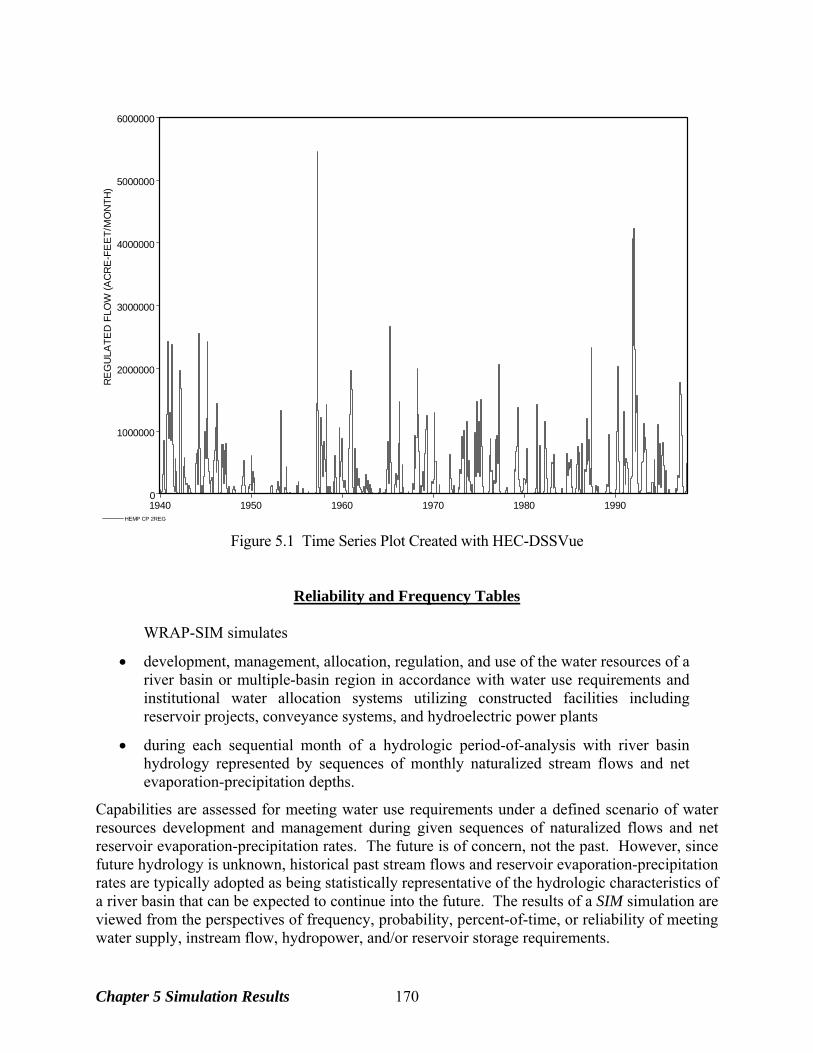
1940 1950 1960 1970 1980 1990
RE
GU
LATE
D F
LOW
(AC
RE
-FE
ET/
MO
NTH
)
0
1000000
2000000
3000000
4000000
5000000
6000000
HEMP CP 2REG
Figure 5.1 Time Series Plot Created with HEC-DSSVue
Reliability and Frequency Tables WRAP-SIM simulates
• development, management, allocation, regulation, and use of the water resources of a river basin or multiple-basin region in accordance with water use requirements and institutional water allocation systems utilizing constructed facilities including reservoir projects, conveyance systems, and hydroelectric power plants
• during each sequential month of a hydrologic period-of-analysis with river basin hydrology represented by sequences of monthly naturalized stream flows and net evaporation-precipitation depths.
Capabilities are assessed for meeting water use requirements under a defined scenario of water resources development and management during given sequences of naturalized flows and net reservoir evaporation-precipitation rates. The future is of concern, not the past. However, since future hydrology is unknown, historical past stream flows and reservoir evaporation-precipitation rates are typically adopted as being statistically representative of the hydrologic characteristics of a river basin that can be expected to continue into the future. The results of a SIM simulation are viewed from the perspectives of frequency, probability, percent-of-time, or reliability of meeting water supply, instream flow, hydropower, and/or reservoir storage requirements.
Chapter 5 Simulation Results 170
Concise measures of water availability/reliability are useful in analyzing and displaying simulation results and assessing water management capabilities. TABLES options described in the Users Manual include the following metrics for concisely summarizing SIM results.
• volume and period reliability tables for water supply diversion and hydroelectric energy generation targets [TABLES 2REL record]
• frequency tables for naturalized, regulated, and unappropriated flows, reservoir storage volumes and water surface elevations, and instream flow shortages [TABLES 2FRE and 2FRQ records]
• reservoir drawdown-duration and storage-reliability tables [2RES record] The reliability and frequency tables may be developed either considering all months or alternatively for a specified individual month of the year such as July or November.
Water Supply and Hydropower Reliability Reliability tables for meeting water supply diversion and hydroelectric energy generation requirements are developed with the 2REL record. A reliability table contains both volume and period reliabilities. Volume and Period Reliabilities Volume reliability is the percentage of the total target demand amount that is actually supplied. For water supply diversions, the amounts are volumes. For hydroelectric power, the amounts are kilowatt-hours of energy generated. Volume reliability (RV) is the ratio of volume of water supplied or the energy produced (v) to the target (V), converted to a percentage.
(100%)VvRV =
(5.1)
Equivalently, for water supply, RV is the mean actual diversion rate as a percentage of the mean target diversion rate. For hydropower, RV is the mean actual rate of energy production as a percentage of the mean target energy production rate. Period reliability is the percentage of the total number of periods of the simulation during which the specified demand target is either fully supplied or at least a specified percentage of the target is supplied. The various variations of period reliability (RP) are computed by TABLES from the results of a SIM simulation as:
PnR = (100%)N
(5.2)
where n denotes the number of periods during the simulation for which the specified percentage of the demand target is met, and N is the total number of periods considered. The 2REL record develops a reliability table with periods defined alternatively in terms of both months and years. The 2REL record allows N and n to be defined on a monthly basis optionally either considering
Chapter 5 Simulation Results 171
all months or only months with non-zero demand targets. The 6REL record described in the Supplemental Manual allows use of SIMD results with a sub-monthly time step such as a day. Whereas volume reliabilities are based on total diversion volumes or hydroelectric energy amounts, period reliabilities are based on percent-of-time. Period reliability RP is an expression of the percentage of time that the full demand target or a specified portion of the demand target can be supplied. Equivalently, RP represents the likelihood or probability of the target being met in any randomly selected month or year. The volume reliability RV provides a greater focus on the relative magnitude of the shortage amounts. TABLES 2REL Tables The tables reproduced here to illustrate the format of tables produced with TABLES are from the example presented in the Fundamentals Manual. The complete dataset of SIM and TABLES input and output files is presented in the Fundamentals Manual. Tables 5.10 and 5.11 illustrate the format of water supply diversion and hydropower reliability tables created with a 2REL record. Water supply diversion reliabilities may be tabulated for individual water rights, the aggregation of all rights associated with individual control points, or user-selected groups of water rights. The user selects which water rights, control points, or water rights groups to include in a diversion reliability table. Reliabilities for diversion targets for each of the individual water rights included in the example are tabulated in Table 5.10. A reliability table for aggregated diversion targets and shortages for defined groups of water rights has the same format. Likewise, diversion targets and shortages for all water rights located at each control point are summed for a control point reliability table which has the same format except the first column is a list of control points. Table 5.11 illustrates the format of reliability tables for reservoir/hydropower projects. The table may contain any number of reservoir/hydropower projects with their individual reliabilities. However, the energy targets/shortages and corresponding reliabilities can not be aggregated by control point or other grouping. As indicated in Table 5.1, hydroelectric energy targets and shortages are stored on both reservoir/hydropower output records and water right records. Multiple water rights with different priorities may generate energy at the same reservoir. However, only the cumulative total energy associated with the most junior right, which is computed last in the priority sequence, is written to the OUT file on reservoir/hydropower records and included in a 2REL record reliability table for reservoir/hydropower projects. The intermediate cumulative energy amounts generated by the senior rights are recorded on water right output records and may be included in a water right reliability table. The reliabilities may be for a specified single month of the year such as August or for all 12 months. The reliabilities in Table 5.10 are for all months as indicated by no month being identified in the table headings. The reliabilities represent probabilities of supplying demands irrespective of season of the year. If August tends to be dry, reliabilities of meeting demands in August computed based on frequency counts considering only August will be lower.
Chapter 5 Simulation Results 172
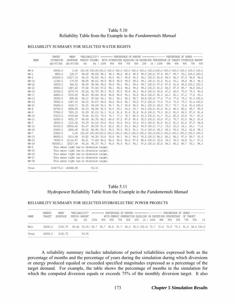
Table 5.10 Reliability Table from the Example in the Fundamentals Manual
RELIABILITY SUMMARY FOR SELECTED WATER RIGHTS ---------------------------------------------------------------------------------------------------------------------------------- TARGET MEAN *RELIABILITY*| +++++++++ PERCENTAGE OF MONTHS +++++++++|------- PERCENTAGE OF YEARS ------- NAME DIVERSION SHORTAGE PERIOD VOLUME| WITH DIVERSIONS EQUALING OR EXCEEDING PERCENTAGE OF TARGET DIVERSION AMOUNT (AC-FT/YR) (AC-FT/YR) (%) (%) | 100% 95% 90% 75% 50% 25% 1% | 100% 98% 95% 90% 75% 50% ---------------------------------------------------------------------------------------------------------------------------------- WR-6 60000.0 0.00 100.00 100.00|100.0 100.0 100.0 100.0 100.0 100.0 100.0|100.0 100.0 100.0 100.0 100.0 100.0 WR-1 9800.0 128.37 98.28 98.69| 98.3 98.3 98.4 98.6 98.9 98.9 100.0| 87.9 89.7 89.7 93.1 100.0 100.0 WR-2 245000.0 10227.33 94.25 95.83| 94.3 94.5 94.7 94.8 95.3 96.1 100.0| 82.8 84.5 84.5 87.9 94.8 96.6 WR-14 11300.0 179.59 98.85 98.41| 98.9 98.9 98.9 99.0 99.0 99.1 100.0| 91.4 91.4 93.1 94.8 98.3 98.3 WR-20 34500.0 364.52 98.99 98.94| 99.0 99.0 99.1 99.1 99.4 99.7 100.0| 87.9 87.9 91.4 96.6 100.0 100.0 WR-22 49600.0 1487.60 97.84 97.00| 97.8 98.1 98.4 98.6 99.0 99.0 100.0| 81.0 84.5 87.9 89.7 94.8 100.0 WR-16 32300.0 2679.74 95.26 91.70| 95.3 95.5 95.5 95.8 96.3 96.4 100.0| 63.8 67.2 69.0 75.9 79.3 96.6 WR-17 44800.0 4720.00 94.83 89.46| 94.8 94.8 94.8 95.1 95.8 96.6 100.0| 60.3 62.1 62.1 67.2 77.6 93.1 WR-13 18200.0 808.66 96.12 95.56| 96.1 96.1 96.1 96.3 96.7 96.8 100.0| 77.6 77.6 77.6 79.3 91.4 100.0 WR-19 39000.0 1687.55 96.55 95.67| 96.6 96.6 96.6 96.7 96.8 97.0 100.0| 75.9 75.9 75.9 79.3 91.4 100.0 WR-21 95600.0 5169.71 95.55 94.59| 95.5 95.7 95.7 95.8 96.0 96.1 100.0| 69.0 70.7 70.7 72.4 91.4 100.0 WR-8 82760.0 4896.89 92.53 94.08| 92.5 92.5 93.1 93.4 93.7 94.5 100.0| 81.0 81.0 84.5 86.2 89.7 96.6 WR-9 97500.0 7655.33 91.09 92.15| 91.1 91.4 91.4 91.4 91.8 91.8 100.0| 79.3 81.0 81.0 84.5 87.9 91.4 WR-10 25610.0 4709.84 76.44 81.61| 76.4 76.7 77.3 78.7 80.9 83.3 100.0| 51.7 55.2 60.3 63.8 70.7 81.0 WR-11 42000.0 4052.37 86.49 90.35| 86.5 86.6 87.2 87.9 90.4 92.5 100.0| 63.8 67.2 70.7 81.0 86.2 91.4 WR-3 18000.0 1231.56 93.39 93.16| 93.4 93.4 93.4 93.4 93.4 93.5 100.0| 81.0 81.0 81.0 81.0 87.9 94.8 WR-12 92100.0 28924.62 81.47 68.59| 81.5 82.2 82.3 83.3 86.2 90.9 100.0| 17.2 19.0 22.4 24.1 43.1 77.6 WR-18 25400.0 2806.28 90.52 88.95| 90.5 90.5 90.5 90.5 91.1 91.4 100.0| 48.3 48.3 50.0 55.2 82.8 98.3 WR-7 20800.0 0.00 100.00 100.00|100.0 100.0 100.0 100.0 100.0 100.0 100.0|100.0 100.0 100.0 100.0 100.0 100.0 WR-15 88000.0 5014.48 93.82 94.30| 93.8 93.8 94.1 94.3 94.5 95.0 100.0| 86.2 86.2 86.2 87.9 89.7 91.4 WR-23 74500.0 21116.87 86.21 71.66| 86.2 86.2 86.2 86.6 87.6 88.6 100.0| 32.8 34.5 34.5 44.8 51.7 67.2 WR-24 900000.1 32627.69 95.26 96.37| 95.3 95.4 95.4 95.5 96.1 97.6 100.0| 82.8 84.5 86.2 89.7 93.1 98.3 WR-5 This water right has no diversion target. WR-25 This water right has no diversion target. WR-26 This water right has no diversion target. WR-27 This water right has no diversion target. WR-28 This water right has no diversion target. ---------------------------------------------------------------------------------------------------------------------------------- Total 2106770.0 140488.98 93.33 ----------------------------------------------------
Table 5.11 Hydropower Reliability Table from the Example in the Fundamentals Manual
RELIABILITY SUMMARY FOR SELECTED HYDROELECTRIC POWER PROJECTS -------------------------------------------------------------------------------------------------------------------------------- ENERGY MEAN *RELIABILITY* +++++++++ PERCENTAGE OF MONTHS +++++++++|---------- PERCENTAGE OF YEARS ---------- NAME TARGET SHORTAGE PERIOD AMOUNT WITH ENERGY GENERATION EQUALING OR EXCEEDING PERCENTAGE OF TARGET (%) (%) 100% 95% 90% 75% 50% 25% 1% | 100% 98% 95% 90% 75% 50% 1% -------------------------------------------------------------------------------------------------------------------------------- Whit 36000.0 2192.75 90.66 93.91| 90.7 90.7 90.8 91.7 94.4 95.5 100.0| 70.7 72.4 75.9 79.3 91.4 96.6 100.0 -------------------------------------------------------------------------------------------------------------------------------- Total 36000.0 2192.75 93.91 --------------------------------------------
A reliability summary includes tabulations of period reliabilities expressed both as the percentage of months and the percentage of years during the simulation during which diversions or energy produced equaled or exceeded specified magnitudes expressed as a percentage of the target demand. For example, the table shows the percentage of months in the simulation for which the computed diversion equals or exceeds 75% of the monthly diversion target. It also
Chapter 5 Simulation Results 173
shows the percentage of years for which the total diversions during the year equal or exceed 75% of the annual target amount. The table also shows the percentage of months for which the demand is fully 100% supplied, without any shortage. Water right WR-1 in Table 5.10 has a mean annual diversion target of 9,800 acre-feet/year, mean annual shortage of 128.37 acre-feet/year, and a corresponding (Equation 5.1) volume reliability of 98.69 percent. Period reliabilities are based on Equation 5.2. The monthly diversion targets are fully met during 98.28 percent of the 696 months of the 1940-1997 hydrologic period of analysis. At least 90 percent of the monthly target is supplied during 98.4% of the 696 months. At least 90 percent of the annual target is supplied during 93.1% of the 58 years of the simulation. Reliabilities for hydroelectric power generation at Whitney Reservoir (reservoir identifier Whit) are shown in Table 5.11. The monthly hydropower targets sum to a total annual target of 36,000 kilowatt-hours/year. The mean annual shortage is 2,192.5 kilowatt-hours/year, and thus the mean annual energy production from Equation 5.1 is 93.91 percent of the target. The energy target is fully met during 90.66 percent of the 696 months (Equation 5.2). Energy production equals or exceeds 75 percent of the target during 91.7 percent of 696 months and during 91.4 percent of the 58 years of the simulation.
These frequency statistics may be interpreted as follows. The WR-1 diversion shown in Table 5.10 equals or exceeds 90 percent of the monthly target an estimated 98.4 percent of the time. At least 90 percent of the annual demand is supplied an estimated 93.1 percent of the time. The estimated probability of supplying at least 90 percent of the monthly target in any randomly selected future month is 0.984. The estimated probability of supplying at least 90 percent of the annual target in any randomly selected future year is 0.931. These estimates reflect all of the premises and approximations incorporated into the modeling system and thus are necessarily approximate. For example, hydrologic variables such as river flows are highly variable, stochastic, and uncertain. The model and resulting reliabilities are typically based on the premise that historical hydrology is statistically representative of the climatic and hydrologic characteristics of the river basin to be expected in the future. Data describing the physical and institutional features of water management systems as well as river basin hydrology are also necessarily approximate. Uncertainties are inherent in modeling water management and use practices. The reliabilities computed by TABLES must be interpreted in the context of the targets selected for inclusion in the SIM simulation results output file. SIM has a variety of options for specifying diversion and hydroelectric energy targets as a function of reservoir storage and stream flow. An option activated by the SO record allows specification of which original, intermediate, or final target developed during the target building process is written to the SIM output file. The default is to write the last target and shortage amount to the output file. TABLES reads the values written in the SIM output file and computes the water supply diversion or energy generated as the target less the shortage. A 2REL record allows specification of the target to be adopted by TABLES for volume reliability computations. The firm yield associated with a particular water supply diversion or hydroelectric power production target is defined as the maximum annual demand target that can be met with a reliability of 100.0 percent. Firm yields may be determined by iteratively adjusting a target
Chapter 5 Simulation Results 174
amount and rerunning SIM until a value meeting the definition of firm yield at a prescribed level of precision is found. As discussed in Chapter 6, The FY record activates a SIM option that automates this procedure. The reliabilities computed by the FY record yield-reliability routine in SIM are based on Equations 5.1 and 5.2 just like the TABLES 2REL record reliability routine. The difference is that the FY record routine computes reliabilities for one single diversion right with the target incremented multiple times. Any number of diversion rights may be included in a TABLES 2REL record reliability table, but all diversion targets are fixed at set values. A procedure for applying ArcGIS to display SIM simulation results is noted in Chapter 6 of this manual. A map of the river/reservoir system has color coded symbols indicating ranges in which reliabilities and frequencies fall at control locations.
Flow and Storage Frequency Analyses Exceedance frequency is an expression of the percentage-of-time or equivalently the likelihood or probability that a variable of interest will equal or exceed a certain amount. Exceedance frequency tables may be created with TABLES 2FRE and 2FRQ records for:
• naturalized flow, regulated flow, unappropriated flow, and reservoir storage volume for specified control points
• instream flow shortages and reservoir storage volume for specified water rights • reservoir storage volume and water surface elevation for specified reservoirs • other variables such as reservoir draw-downs computed from these variables
The frequencies may be based on considering all months or alternatively be developed for a specified month of the year such as May or August. Applications of TABLES 2FRE frequency analysis capabilities may deal directly with the time series data read from the SIM simulation results OUT file. Optionally, the frequency analysis may be applied to moving averages or moving accumulative totals of the data computed for a user-specified number of months. The data may be adjusted by a multiplier factor, which may be a unit conversion factor or serve other purposes. The data may be added or subtracted from a constant entered on the 2FRE record. For example, the time series data for a frequency analysis of reservoir draw-downs is developed by subtracting water surface elevations from the inputted top of conservation pool elevation or storage volume may be subtracted from capacity. Likewise, deviations of regulated flows from a specified flow amount may be analyzed. Table 5.12 illustrates the default standard format of a 2FRE frequency table. The 2FRE table includes the mean and standard deviation, minimum and maximum, and the flow or storage amounts that are equaled or exceeded specified percentages of the time. The 2FRE record also includes an option to write the frequencies and corresponding amounts as columns rather than rows. The alternative columnar format is convenient for transporting the tabulations to Microsoft Excel for plotting and also contains several more frequencies. The 2FRQ record also develops a frequency table for the same types of flow or storage variables, but in a different format illustrated by Table 5.13. The model-user enters specified flow or storage values of interest on the 2FRQ record. TABLES counts the number of months for
Chapter 5 Simulation Results 175
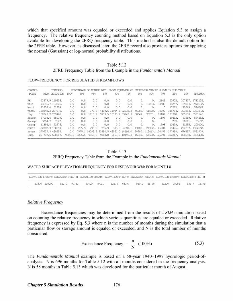
which that specified amount was equaled or exceeded and applies Equation 5.3 to assign a frequency. The relative frequency counting method based on Equation 5.3 is the only option available for developing the 2FRQ frequency table. This method is also the default option for the 2FRE table. However, as discussed later, the 2FRE record also provides options for applying the normal (Gaussian) or log-normal probability distributions.
Table 5.12 2FRE Frequency Table from the Example in the Fundamentals Manual
FLOW-FREQUENCY FOR REGULATED STREAMFLOWS -------------------------------------------------------------------------------------------------------------------------- CONTROL STANDARD PERCENTAGE OF MONTHS WITH FLOWS EQUALING OR EXCEEDING VALUES SHOWN IN THE TABLE POINT MEAN DEVIATION 100% 99% 98% 95% 90% 75% 60% 50% 40% 25% 10% MAXIMUM -------------------------------------------------------------------------------------------------------------------------- PK 43379.9 119616. 0.0 0.0 0.0 0.0 0.0 0.0 0. 0. 2643. 50903. 107827. 1782155. Whit 73686.7 183326. 0.0 0.0 0.0 0.0 0.0 0.0 0. 10233. 38502. 78247. 189804. 2970632. WacoL 21636.4 51914. 0.0 0.0 0.0 0.0 0.0 0.0 0. 0. 0. 17515. 71069. 526063. WacoG 128848.3 237675. 0.0 0.0 379.8 4409.6 11904.6 32638.3 45087. 61528. 75692. 115784. 303863. 3361572. High 158249.7 269466. 0.0 0.0 1118.7 5733.5 16778.2 39742.9 58647. 73201. 96101. 137398. 385570. 3581146. Belton 27018.6 65029. 0.0 0.0 0.0 0.0 0.0 0.0 0. 0. 1194. 19413. 92619. 524452. George 3004.7 7642. 0.0 0.0 0.0 0.0 0.0 0.0 0. 0. 0. 283. 10841. 65552. Grang 11394.4 23276. 0.0 0.0 0.0 0.0 0.0 0.0 0. 0. 1598. 10439. 41255. 200100. Camer 82002.9 150359. 42.0 295.9 295.9 295.9 305.8 4587.1 13109. 24392. 45981. 90476. 214237. 1392558. Bryan 270525.3 430255. 0.0 7575.1 14093.2 32484.5 48061.0 68692.0 98980. 113463. 130459. 277893. 676897. 4521903. Hemp 297707.6 538387. 9205.5 9205.5 9863.0 9863.0 9863.0 10191.8 15647. 54660. 125291. 392267. 888598. 5455438. --------------------------------------------------------------------------------------------------------------------------
Table 5.13 2FRQ Frequency Table from the Example in the Fundamentals Manual
WATER SURFACE ELEVATION-FREQUENCY FOR RESERVOIR Whit FOR MONTH 8 ------------------------------------------------------------------------------------------------------------------------------ ELEVATION FREQ(%) ELEVATION FREQ(%) ELEVATION FREQ(%) ELEVATION FREQ(%) ELEVATION FREQ(%) ELEVATION FREQ(%) ELEVATION FREQ(%) ------------------------------------------------------------------------------------------------------------------------------ 518.0 100.00 520.0 94.83 524.0 79.31 528.0 68.97 530.0 48.28 532.0 25.86 533.7 13.79 ------------------------------------------------------------------------------------------------------------------------------
Relative Frequency Exceedance frequencies may be determined from the results of a SIM simulation based on counting the relative frequency in which various quantities are equaled or exceeded. Relative frequency is expressed by Eq. 5.3 where n is the number of months during the simulation that a particular flow or storage amount is equaled or exceeded, and N is the total number of months considered.
nExceedance Frequency = (100%)N
(5.3)
The Fundamentals Manual example is based on a 58-year 1940−1997 hydrologic period-of-analysis. N is 696 months for Table 5.12 with all months considered in the frequency analysis. N is 58 months in Table 5.13 which was developed for the particular month of August.
Chapter 5 Simulation Results 176
In developing the 2FRE table for the predefined exceedance frequencies shown in the heading of Table 5.12, TABLES sorts and searches the flow or storage data to find a value that is equaled or exceeded during the specified percentage of the months of the simulation. If a single monthly flow value does not precisely match that frequency, linear interpolation is applied to the two flow values that bracket the specified frequency. In developing the 2FRQ table for user-specified flow or storage amounts, TABLES simply counts the number of months for which a specified amount (518 ft, 520 ft, 524 ft, 528 ft, 530 ft in Table 5.13) was equaled or exceeded. Table 5.12 is frequency table for regulated stream flows based on considering all months. At the Bryan control point, the minimum and maximum regulated flow during the 696-month 1940-1997 simulation period is 0.0 and 4,521,903 acre-feet/month, respectively. The mean and standard deviation of regulated flows at the Bryan control point are 270,525 and 430,255 acre-feet/month, respectively. A flow of 14,093 ac-ft/month is equaled or exceeded during 98 percent of the 696 months of the hydrologic period-of-analysis. The regulated flow volume is at least 98,980 acre-feet during 60 percent of the 696 months. Thus, flows equal or exceed 98,980 ac-ft/month an estimated 60 percent of the time. The estimated probability that the flow volume at the Bryan control point will be at least 98,980 acre-feet in any randomly selected month is 0.60 for the water management and use scenario and modeling premises incorporated in the WRAP-SIM simulation model and input dataset. Normal and Log-Normal Probability Distributions
Alternatively, the TABLES 2FRE record provides options to apply the normal (Eq. 5.4) or log-normal (Eq. 5.5) probability distribution to the series of flow and storage amounts generated by SIM or adjustments thereto.
X = X + z S (5.4) log X = log X + z Slog X (5.5)
The frequency factor (z) is derived from a normal probability table. X and S denote the mean and standard deviation of the data read from the SIM output file. log X and Slog X are the mean and standard deviation of the logarithms of these data. The log-normal distribution consists of the normal distribution applied to the logarithms of X, with Eq. 5.4 expressed as Eq. 5.5 with z still derived from the normal probability distribution. The random variable X in Equations 5.4 and 5.5 is the naturalized flows, regulated flows, unappropriated flows, instream flow shortages, reservoir storage volumes, or reservoir water surface elevations from the SIM simulation results or variations thereof reflecting adjustments made within TABLES. The mean X and standard deviation S, computed from these data using Equations 5.6 and 5.7, are the parameters used to model frequency relationship as the log-normal or normal probability distributions. n
ii=1
1X = Xn
∑
(5.6)
Chapter 5 Simulation Results 177
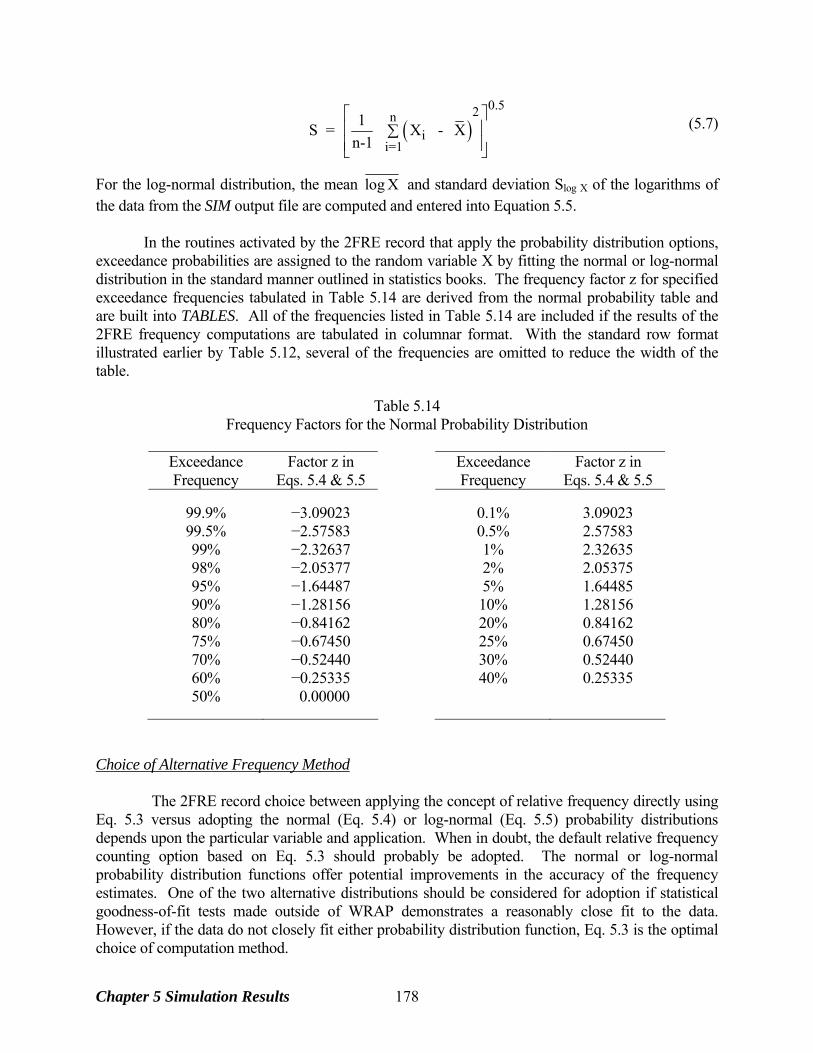
( )0.52n
ii=1
1S = X - Xn-1
⎡ ⎤⎢ ⎥∑⎢ ⎥⎣ ⎦
(5.7)
For the log-normal distribution, the mean log X and standard deviation Slog X of the logarithms of the data from the SIM output file are computed and entered into Equation 5.5. In the routines activated by the 2FRE record that apply the probability distribution options, exceedance probabilities are assigned to the random variable X by fitting the normal or log-normal distribution in the standard manner outlined in statistics books. The frequency factor z for specified exceedance frequencies tabulated in Table 5.14 are derived from the normal probability table and are built into TABLES. All of the frequencies listed in Table 5.14 are included if the results of the 2FRE frequency computations are tabulated in columnar format. With the standard row format illustrated earlier by Table 5.12, several of the frequencies are omitted to reduce the width of the table.
Table 5.14 Frequency Factors for the Normal Probability Distribution
Exceedance Factor z in Exceedance Factor z in Frequency Eqs. 5.4 & 5.5 Frequency Eqs. 5.4 & 5.5
99.9% −3.09023 0.1% 3.09023 99.5% −2.57583 0.5% 2.57583 99% −2.32637 1% 2.32635 98% −2.05377 2% 2.05375 95% −1.64487 5% 1.64485 90% −1.28156 10% 1.28156 80% −0.84162 20% 0.84162 75% −0.67450 25% 0.67450 70% −0.52440 30% 0.52440 60% −0.25335 40% 0.25335 50% 0.00000
Choice of Alternative Frequency Method The 2FRE record choice between applying the concept of relative frequency directly using Eq. 5.3 versus adopting the normal (Eq. 5.4) or log-normal (Eq. 5.5) probability distributions depends upon the particular variable and application. When in doubt, the default relative frequency counting option based on Eq. 5.3 should probably be adopted. The normal or log-normal probability distribution functions offer potential improvements in the accuracy of the frequency estimates. One of the two alternative distributions should be considered for adoption if statistical goodness-of-fit tests made outside of WRAP demonstrates a reasonably close fit to the data. However, if the data do not closely fit either probability distribution function, Eq. 5.3 is the optimal choice of computation method.
Chapter 5 Simulation Results 178
A conventional frequency plot on normal probability paper of the data or logarithms of the data versus frequency calculated based on Eq. 5.3 provides a subjective measure of the closeness-of-fit of the probability distributions. If the normal or log-normal distribution accurately models the probability characteristics of the flow or storage variable of interest, the resulting frequency relationship will be close to the frequencies computed with Eq. 5.3 for a large sample size N, with the fit improving with increasing N. The probability distributions perhaps may be more useful for frequency analyses for a particular month where the sample size N is only 1/12 of the size when considering all months. Conditional reliability modeling (CRM) is described in the Supplemental Manual. The random variable is defined differently in CRM versus conventional simulations. The log-normal or normal distribution options may be particularly relevant for CRM applications. The log-normal distribution allows the random variable to range from zero upward with no defined upper limit, which is consistent with stream flows. The normal distribution is symmetric about the mean with no lower and upper limits. The log-normal distribution will typically be a reasonably valid model for monthly naturalized stream flow volumes. Regulated and unappropriated flows are affected by water management practices that may invalidate application of the log-normal distribution. Storage capacity sets an upper limit on storage volumes that likely prevents proper fitting of either the normal or log-normal distributions, except perhaps for reservoirs that are never or seldom completely full or completely empty during the simulation. The distributions may be more appropriately applied to storage draw-downs rather than storage.
Reservoir Contents, Drawdown Duration, and Storage Reliability Reservoir storage frequency tables may be developed using 2FRE or 2FRQ records for either water rights, control points, or reservoirs as discussed in the preceding section. The 2RES record provides an alternative format for storage frequency analyses based on storage volumes from reservoir/ hydropower output records. The 2RES record results in three tables for selected reservoirs:
1. storage contents as a percentage of storage capacity 2. drawdown-duration relationships 3. storage-reliability relationships
The first table is a tabulation of end-of-month storage content expressed as a percentage
of the storage capacity of a user-specified zone. The storage content as a percentage is (100%)
CCCScapacityofpercentage ascontent storage
21
2
−−
=
(5.8)
where C1 and C2 are the user-specified total storage capacity below the water surface elevations defining the top and bottom of the storage zone or pool being considered. Often C1 will be the total conservation storage capacity and C2 will be entered as zero. C1 may be the total conservation capacity, and C2 the inactive storage capacity. Other zones may be analyzed as well. The storage percentage is negative for a storage content less than C2 and greater than 100% for a storage content greater than C1. The table format is illustrated by Table 5.15 which shows only the first 14 months
Chapter 5 Simulation Results 179
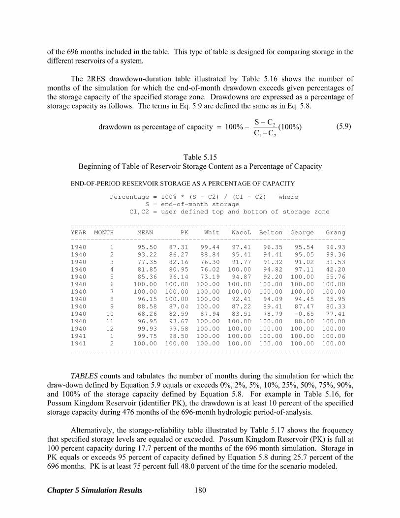
of the 696 months included in the table. This type of table is designed for comparing storage in the different reservoirs of a system.
The 2RES drawdown-duration table illustrated by Table 5.16 shows the number of months of the simulation for which the end-of-month drawdown exceeds given percentages of the storage capacity of the specified storage zone. Drawdowns are expressed as a percentage of storage capacity as follows. The terms in Eq. 5.9 are defined the same as in Eq. 5.8.
(100%)CCCS100%capacityofpercentageasdrawdown
21
2
−−
−=
(5.9)
Table 5.15
Beginning of Table of Reservoir Storage Content as a Percentage of Capacity
END-OF-PERIOD RESERVOIR STORAGE AS A PERCENTAGE OF CAPACITY Percentage = 100% * (S - C2) / (C1 - C2) where S = end-of-month storage C1,C2 = user defined top and bottom of storage zone ---------------------------------------------------------------------- YEAR MONTH MEAN PK Whit WacoL Belton George Grang ---------------------------------------------------------------------- 1940 1 95.50 87.31 99.44 97.41 96.35 95.54 96.93 1940 2 93.22 86.27 88.84 95.41 94.41 95.05 99.36 1940 3 77.35 82.16 76.30 91.77 91.32 91.02 31.53 1940 4 81.85 80.95 76.02 100.00 94.82 97.11 42.20 1940 5 85.36 96.14 73.19 94.87 92.20 100.00 55.76 1940 6 100.00 100.00 100.00 100.00 100.00 100.00 100.00 1940 7 100.00 100.00 100.00 100.00 100.00 100.00 100.00 1940 8 96.15 100.00 100.00 92.41 94.09 94.45 95.95 1940 9 88.58 87.04 100.00 87.22 89.41 87.47 80.33 1940 10 68.26 82.59 87.94 83.51 78.79 -0.65 77.41 1940 11 96.95 93.67 100.00 100.00 100.00 88.00 100.00 1940 12 99.93 99.58 100.00 100.00 100.00 100.00 100.00 1941 1 99.75 98.50 100.00 100.00 100.00 100.00 100.00 1941 2 100.00 100.00 100.00 100.00 100.00 100.00 100.00 ----------------------------------------------------------------------
TABLES counts and tabulates the number of months during the simulation for which the draw-down defined by Equation 5.9 equals or exceeds 0%, 2%, 5%, 10%, 25%, 50%, 75%, 90%, and 100% of the storage capacity defined by Equation 5.8. For example in Table 5.16, for Possum Kingdom Reservoir (identifier PK), the drawdown is at least 10 percent of the specified storage capacity during 476 months of the 696-month hydrologic period-of-analysis. Alternatively, the storage-reliability table illustrated by Table 5.17 shows the frequency that specified storage levels are equaled or exceeded. Possum Kingdom Reservoir (PK) is full at 100 percent capacity during 17.7 percent of the months of the 696 month simulation. Storage in PK equals or exceeds 95 percent of capacity defined by Equation 5.8 during 25.7 percent of the 696 months. PK is at least 75 percent full 48.0 percent of the time for the scenario modeled.
Chapter 5 Simulation Results 180
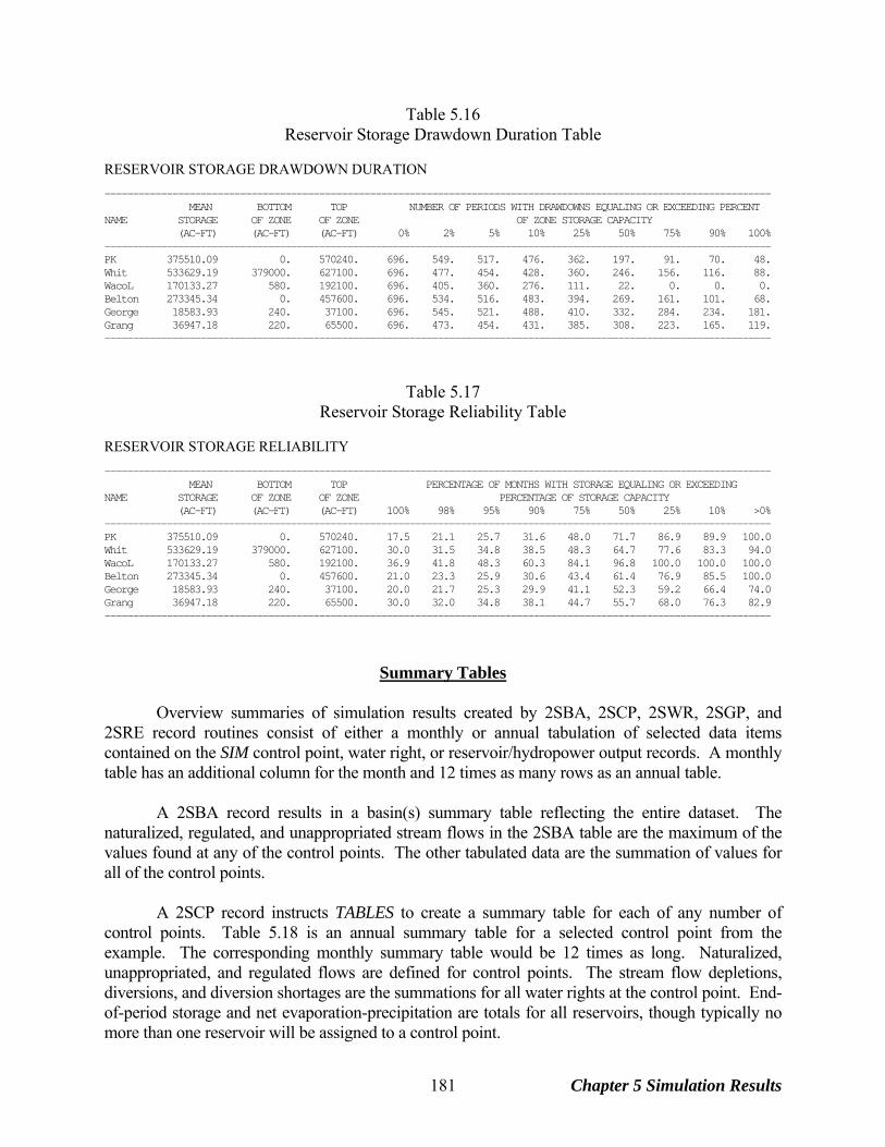
Table 5.16 Reservoir Storage Drawdown Duration Table
RESERVOIR STORAGE DRAWDOWN DURATION ---------------------------------------------------------------------------------------------------------------------- MEAN BOTTOM TOP NUMBER OF PERIODS WITH DRAWDOWNS EQUALING OR EXCEEDING PERCENT NAME STORAGE OF ZONE OF ZONE OF ZONE STORAGE CAPACITY (AC-FT) (AC-FT) (AC-FT) 0% 2% 5% 10% 25% 50% 75% 90% 100% ---------------------------------------------------------------------------------------------------------------------- PK 375510.09 0. 570240. 696. 549. 517. 476. 362. 197. 91. 70. 48. Whit 533629.19 379000. 627100. 696. 477. 454. 428. 360. 246. 156. 116. 88. WacoL 170133.27 580. 192100. 696. 405. 360. 276. 111. 22. 0. 0. 0. Belton 273345.34 0. 457600. 696. 534. 516. 483. 394. 269. 161. 101. 68. George 18583.93 240. 37100. 696. 545. 521. 488. 410. 332. 284. 234. 181. Grang 36947.18 220. 65500. 696. 473. 454. 431. 385. 308. 223. 165. 119. ----------------------------------------------------------------------------------------------------------------------
Table 5.17 Reservoir Storage Reliability Table
RESERVOIR STORAGE RELIABILITY ---------------------------------------------------------------------------------------------------------------------- MEAN BOTTOM TOP PERCENTAGE OF MONTHS WITH STORAGE EQUALING OR EXCEEDING NAME STORAGE OF ZONE OF ZONE PERCENTAGE OF STORAGE CAPACITY (AC-FT) (AC-FT) (AC-FT) 100% 98% 95% 90% 75% 50% 25% 10% >0% ---------------------------------------------------------------------------------------------------------------------- PK 375510.09 0. 570240. 17.5 21.1 25.7 31.6 48.0 71.7 86.9 89.9 100.0 Whit 533629.19 379000. 627100. 30.0 31.5 34.8 38.5 48.3 64.7 77.6 83.3 94.0 WacoL 170133.27 580. 192100. 36.9 41.8 48.3 60.3 84.1 96.8 100.0 100.0 100.0 Belton 273345.34 0. 457600. 21.0 23.3 25.9 30.6 43.4 61.4 76.9 85.5 100.0 George 18583.93 240. 37100. 20.0 21.7 25.3 29.9 41.1 52.3 59.2 66.4 74.0 Grang 36947.18 220. 65500. 30.0 32.0 34.8 38.1 44.7 55.7 68.0 76.3 82.9 ----------------------------------------------------------------------------------------------------------------------
Summary Tables Overview summaries of simulation results created by 2SBA, 2SCP, 2SWR, 2SGP, and 2SRE record routines consist of either a monthly or annual tabulation of selected data items contained on the SIM control point, water right, or reservoir/hydropower output records. A monthly table has an additional column for the month and 12 times as many rows as an annual table. A 2SBA record results in a basin(s) summary table reflecting the entire dataset. The naturalized, regulated, and unappropriated stream flows in the 2SBA table are the maximum of the values found at any of the control points. The other tabulated data are the summation of values for all of the control points. A 2SCP record instructs TABLES to create a summary table for each of any number of control points. Table 5.18 is an annual summary table for a selected control point from the example. The corresponding monthly summary table would be 12 times as long. Naturalized, unappropriated, and regulated flows are defined for control points. The stream flow depletions, diversions, and diversion shortages are the summations for all water rights at the control point. End-of-period storage and net evaporation-precipitation are totals for all reservoirs, though typically no more than one reservoir will be assigned to a control point.
Chapter 5 Simulation Results 181
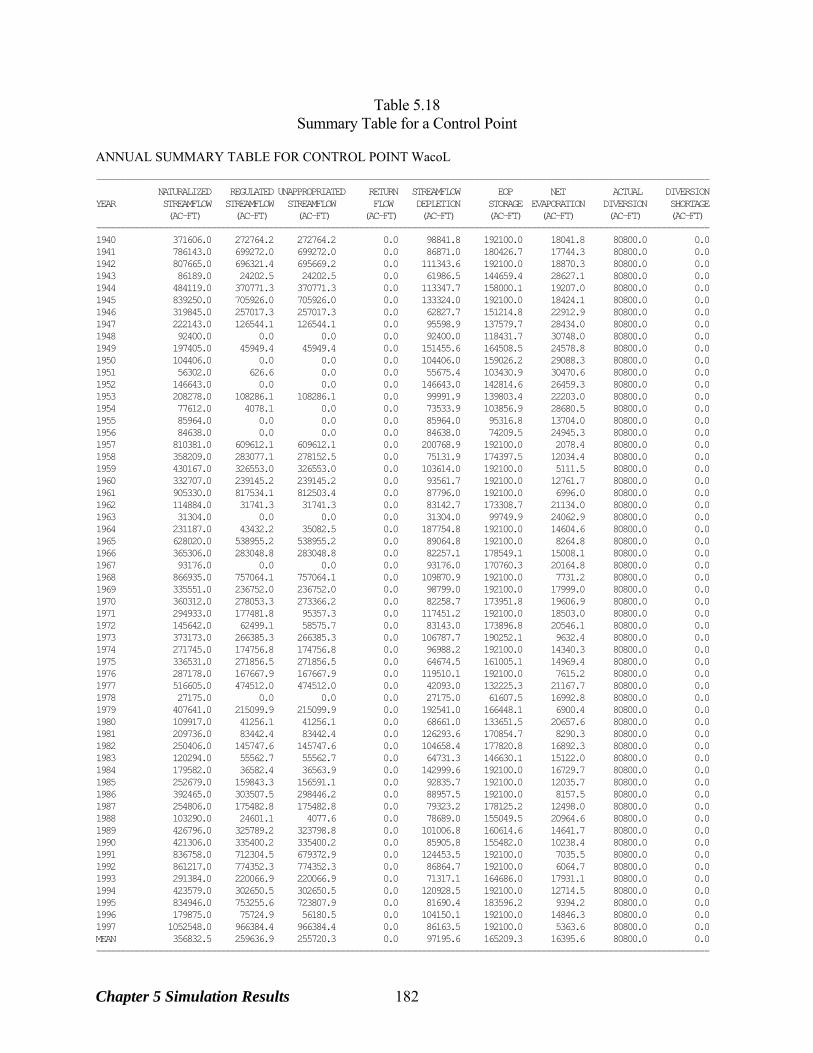
Table 5.18 Summary Table for a Control Point
ANNUAL SUMMARY TABLE FOR CONTROL POINT WacoL -------------------------------------------------------------------------------------------------------------------------------- NATURALIZED REGULATED UNAPPROPRIATED RETURN STREAMFLOW EOP NET ACTUAL DIVERSION YEAR STREAMFLOW STREAMFLOW STREAMFLOW FLOW DEPLETION STORAGE EVAPORATION DIVERSION SHORTAGE (AC-FT) (AC-FT) (AC-FT) (AC-FT) (AC-FT) (AC-FT) (AC-FT) (AC-FT) (AC-FT) -------------------------------------------------------------------------------------------------------------------------------- 1940 371606.0 272764.2 272764.2 0.0 98841.8 192100.0 18041.8 80800.0 0.0 1941 786143.0 699272.0 699272.0 0.0 86871.0 180426.7 17744.3 80800.0 0.0 1942 807665.0 696321.4 695669.2 0.0 111343.6 192100.0 18870.3 80800.0 0.0 1943 86189.0 24202.5 24202.5 0.0 61986.5 144659.4 28627.1 80800.0 0.0 1944 484119.0 370771.3 370771.3 0.0 113347.7 158000.1 19207.0 80800.0 0.0 1945 839250.0 705926.0 705926.0 0.0 133324.0 192100.0 18424.1 80800.0 0.0 1946 319845.0 257017.3 257017.3 0.0 62827.7 151214.8 22912.9 80800.0 0.0 1947 222143.0 126544.1 126544.1 0.0 95598.9 137579.7 28434.0 80800.0 0.0 1948 92400.0 0.0 0.0 0.0 92400.0 118431.7 30748.0 80800.0 0.0 1949 197405.0 45949.4 45949.4 0.0 151455.6 164508.5 24578.8 80800.0 0.0 1950 104406.0 0.0 0.0 0.0 104406.0 159026.2 29088.3 80800.0 0.0 1951 56302.0 626.6 0.0 0.0 55675.4 103430.9 30470.6 80800.0 0.0 1952 146643.0 0.0 0.0 0.0 146643.0 142814.6 26459.3 80800.0 0.0 1953 208278.0 108286.1 108286.1 0.0 99991.9 139803.4 22203.0 80800.0 0.0 1954 77612.0 4078.1 0.0 0.0 73533.9 103856.9 28680.5 80800.0 0.0 1955 85964.0 0.0 0.0 0.0 85964.0 95316.8 13704.0 80800.0 0.0 1956 84638.0 0.0 0.0 0.0 84638.0 74209.5 24945.3 80800.0 0.0 1957 810381.0 609612.1 609612.1 0.0 200768.9 192100.0 2078.4 80800.0 0.0 1958 358209.0 283077.1 278152.5 0.0 75131.9 174397.5 12034.4 80800.0 0.0 1959 430167.0 326553.0 326553.0 0.0 103614.0 192100.0 5111.5 80800.0 0.0 1960 332707.0 239145.2 239145.2 0.0 93561.7 192100.0 12761.7 80800.0 0.0 1961 905330.0 817534.1 812503.4 0.0 87796.0 192100.0 6996.0 80800.0 0.0 1962 114884.0 31741.3 31741.3 0.0 83142.7 173308.7 21134.0 80800.0 0.0 1963 31304.0 0.0 0.0 0.0 31304.0 99749.9 24062.9 80800.0 0.0 1964 231187.0 43432.2 35082.5 0.0 187754.8 192100.0 14604.6 80800.0 0.0 1965 628020.0 538955.2 538955.2 0.0 89064.8 192100.0 8264.8 80800.0 0.0 1966 365306.0 283048.8 283048.8 0.0 82257.1 178549.1 15008.1 80800.0 0.0 1967 93176.0 0.0 0.0 0.0 93176.0 170760.3 20164.8 80800.0 0.0 1968 866935.0 757064.1 757064.1 0.0 109870.9 192100.0 7731.2 80800.0 0.0 1969 335551.0 236752.0 236752.0 0.0 98799.0 192100.0 17999.0 80800.0 0.0 1970 360312.0 278053.3 273366.2 0.0 82258.7 173951.8 19606.9 80800.0 0.0 1971 294933.0 177481.8 95357.3 0.0 117451.2 192100.0 18503.0 80800.0 0.0 1972 145642.0 62499.1 58575.7 0.0 83143.0 173896.8 20546.1 80800.0 0.0 1973 373173.0 266385.3 266385.3 0.0 106787.7 190252.1 9632.4 80800.0 0.0 1974 271745.0 174756.8 174756.8 0.0 96988.2 192100.0 14340.3 80800.0 0.0 1975 336531.0 271856.5 271856.5 0.0 64674.5 161005.1 14969.4 80800.0 0.0 1976 287178.0 167667.9 167667.9 0.0 119510.1 192100.0 7615.2 80800.0 0.0 1977 516605.0 474512.0 474512.0 0.0 42093.0 132225.3 21167.7 80800.0 0.0 1978 27175.0 0.0 0.0 0.0 27175.0 61607.5 16992.8 80800.0 0.0 1979 407641.0 215099.9 215099.9 0.0 192541.0 166448.1 6900.4 80800.0 0.0 1980 109917.0 41256.1 41256.1 0.0 68661.0 133651.5 20657.6 80800.0 0.0 1981 209736.0 83442.4 83442.4 0.0 126293.6 170854.7 8290.3 80800.0 0.0 1982 250406.0 145747.6 145747.6 0.0 104658.4 177820.8 16892.3 80800.0 0.0 1983 120294.0 55562.7 55562.7 0.0 64731.3 146630.1 15122.0 80800.0 0.0 1984 179582.0 36582.4 36563.9 0.0 142999.6 192100.0 16729.7 80800.0 0.0 1985 252679.0 159843.3 156591.1 0.0 92835.7 192100.0 12035.7 80800.0 0.0 1986 392465.0 303507.5 298446.2 0.0 88957.5 192100.0 8157.5 80800.0 0.0 1987 254806.0 175482.8 175482.8 0.0 79323.2 178125.2 12498.0 80800.0 0.0 1988 103290.0 24601.1 4077.6 0.0 78689.0 155049.5 20964.6 80800.0 0.0 1989 426796.0 325789.2 323798.8 0.0 101006.8 160614.6 14641.7 80800.0 0.0 1990 421306.0 335400.2 335400.2 0.0 85905.8 155482.0 10238.4 80800.0 0.0 1991 836758.0 712304.5 679372.9 0.0 124453.5 192100.0 7035.5 80800.0 0.0 1992 861217.0 774352.3 774352.3 0.0 86864.7 192100.0 6064.7 80800.0 0.0 1993 291384.0 220066.9 220066.9 0.0 71317.1 164686.0 17931.1 80800.0 0.0 1994 423579.0 302650.5 302650.5 0.0 120928.5 192100.0 12714.5 80800.0 0.0 1995 834946.0 753255.6 723807.9 0.0 81690.4 183596.2 9394.2 80800.0 0.0 1996 179875.0 75724.9 56180.5 0.0 104150.1 192100.0 14846.3 80800.0 0.0 1997 1052548.0 966384.4 966384.4 0.0 86163.5 192100.0 5363.6 80800.0 0.0 MEAN 356832.5 259636.9 255720.3 0.0 97195.6 165209.3 16395.6 80800.0 0.0 --------------------------------------------------------------------------------------------------------------------------------
Chapter 5 Simulation Results 182

Likewise, 2SWR and 2SRE records create summary tables for specified water rights or reservoirs. A 2SGP record results in a summation of certain data on the SIM water right output records of multiple rights with the same group identifier in fields 12 or 13 of the WR input records. The water right group summary table has the summation of the stream flow depletions, diversions, and diversion shortages associated with all water rights with the specified group identifier.
Water Budget Tables A 2BUD record develops two types of tables.
1. A monthly water budget tabulation may be created for a selected control point or all control points for each month of the simulation. This is a very lengthy tabulation.
2. A river basin water budget is a very concise summary table aggregating data computed
for all individual control points and all months into period-of-analysis basin totals. Monthly computations are performed for all control points in developing the 2BUD total river basin water budget table. The 2SBA, 2SCP, 2SWR, 2SGP, and 2SRE summary tables described above tabulate SIM simulation results with only minor additional computations. The 2BUD routine uses SIM input and output data in relatively extensive computations which are required to develop all components of a complete water budget. The water budgets are tabulations of the individual components of inflows to and outflows from the control point or river basin along with changes in reservoir storage. The following water budget equation is confirmed.
sum of all inflows − sum of all outflows = change in storage The water budget routines were initially developed with the program SALT. The detailed accounting of inflow and outflow components is required for tracking salt loads and concentrations through the system. The water budget routines within SALT are an integral part of the simulation. The same basic computations are consolidated into the TABLES 2BUD record routine. The two types of tables created by the 2BUD record have general utility in analyzing simulation results. The TABLES 2BUD water budget computations are based on reading the simulation results from a SIM output OUT file containing output records for all control points included in the SIM DAT file. Additional information is also read from the SIM DAT file. Two different types of water budget tables may be developed, river basin and individual control point. Computations are performed for all control points in the process of developing the river basin water budget table. Results associated with individual control points are recorded in the individual control point water budget table. The computations step sequentially through time and, for each month, are performed by control point in upstream-to-downstream order. Table 5.19 shows the first 24 months of a water budget table for the Waco Lake control point. The entire tabulation is 696 months long. Table 5.20 is the complete water budget summary table for the entire river basin for the entire hydrologic period-of-analysis. The variables in the control point water budget tabulation and the river basin summary water budget table are defined in Tables 5.21 and 5.22, respectively. The variable names used in the Fortran code are adopted in Tables 5.21 and 5.22 and the following discussion.
Chapter 5 Simulation Results 183
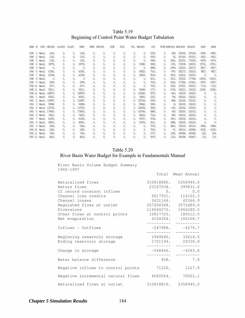
Table 5.19 Beginning of Control Point Water Budget Tabulation
YEAR M CPID NAT(CP) CLC(CP) CL(CP) FNAT FREG RET(CP) CINF FCLC FCL REG(CP) DIV FOTH EVAP(CP) BSTO(CP) STO(CP) XSTO XSUM 1940 1 WacoL 1166. 0. 0. 1166. 0. 0. 0. 0. 0. 0. 5252. 0. 869. 192100. 187145. -4955. -4955. 1940 2 WacoL 1315. 0. 0. 1315. 0. 0. 0. 0. 0. 0. 5090. 0. 56. 187145. 183313. -3831. -3831. 1940 3 WacoL 1182. 0. 0. 1182. 0. 0. 0. 0. 0. 0. 5494. 0. 2661. 183313. 176339. -6974. -6974. 1940 4 WacoL 36755. 0. 0. 36755. 0. 0. 0. 0. 0. 15680. 5818. 0. -503. 176339. 192100. 15761. 15761. 1940 5 WacoL 0. 0. 0. 0. 0. 0. 0. 0. 0. 0. 6868. 0. 2959. 192100. 182273. -9827. -9827. 1940 6 WacoL 61991. 0. 0. 61991. 0. 0. 0. 0. 0. 45625. 7514. 0. -975. 182273. 192100. 9827. 9827. 1940 7 WacoL 41936. 0. 0. 41936. 0. 0. 0. 0. 0. 28529. 9534. 0. 3872. 192100. 192100. 0. 0. 1940 8 WacoL 0. 0. 0. 0. 0. 0. 0. 0. 0. 0. 9211. 0. 5321. 192100. 177568. -14532. -14532. 1940 9 WacoL 2999. 0. 0. 2999. 0. 0. 0. 0. 0. 0. 7676. 0. 5260. 177568. 167631. -9937. -9937. 1940 10 WacoL 2477. 0. 0. 2477. 0. 0. 0. 0. 0. 0. 7030. 0. 2563. 167631. 160515. -7116. -7116. 1940 11 WacoL 93211. 0. 0. 93211. 0. 0. 0. 0. 0. 59268. 5737. 0. -3378. 160515. 192100. 31585. 31585. 1940 12 WacoL 128574. 0. 0. 128574. 0. 0. 0. 0. 0. 123662. 5575. 0. -663. 192100. 192100. 0. 0. 1941 1 WacoL 45901. 0. 0. 45901. 0. 0. 0. 0. 0. 39855. 5252. 0. 794. 192100. 192100. 0. 0. 1941 2 WacoL 129987. 0. 0. 129987. 0. 0. 0. 0. 0. 125764. 5090. 0. -868. 192100. 192100. 0. 0. 1941 3 WacoL 94948. 0. 0. 94948. 0. 0. 0. 0. 0. 89462. 5494. 0. -8. 192100. 192100. 0. 0. 1941 4 WacoL 133705. 0. 0. 133705. 0. 0. 0. 0. 0. 128068. 5818. 0. -180. 192100. 192100. 0. 0. 1941 5 WacoL 174843. 0. 0. 174843. 0. 0. 0. 0. 0. 167566. 6868. 0. 409. 192100. 192100. 0. 0. 1941 6 WacoL 76423. 0. 0. 76423. 0. 0. 0. 0. 0. 68016. 7514. 0. 892. 192100. 192100. 0. 0. 1941 7 WacoL 61285. 0. 0. 61285. 0. 0. 0. 0. 0. 47837. 9534. 0. 3913. 192100. 192100. 0. 0. 1941 8 WacoL 46901. 0. 0. 46901. 0. 0. 0. 0. 0. 32704. 9211. 0. 4986. 192100. 192100. 0. 0. 1941 9 WacoL 5494. 0. 0. 5494. 0. 0. 0. 0. 0. 0. 7676. 0. 4802. 192100. 185116. -6984. -6984. 1941 10 WacoL 1926. 0. 0. 1926. 0. 0. 0. 0. 0. 0. 7030. 0. -72. 185116. 180084. -5032. -5032. 1941 11 WacoL 7916. 0. 0. 7916. 0. 0. 0. 0. 0. 0. 5737. 0. 1955. 180084. 180308. 224. 224. 1941 12 WacoL 6814. 0. 0. 6814. 0. 0. 0. 0. 0. 0. 5575. 0. 1120. 180308. 180427. 119. 119.
Table 5.20
River Basin Water Budget for Example in Fundamentals Manual
River Basin Volume Budget Summary 1940-1997 Total Mean Annual Naturalized flows 310818880. 5358946.0 Return flows 23167034. 399431.6 CI record constant inflows 0. 0.0 Channel loss credits 6617931. 114102.3 Channel losses 2631164. 45364.9 Regulated flows at outlet 207204368. 3572489.0 Diversions 114044272. 1966280.5 Other flows at control points 10817725. 186512.5 Net evaporation 6154304. 106108.7 ---------- ---------- Inflows - Outflows -247988. -4275.7 ---------- ---------- Beginning reservoir storage 1949640. 33614.5 Ending reservoir storage 1701194. 29330.9 ---------- ---------- Change in storage -248446. -4283.6 ---------- ---------- Water balance difference 458. 7.9 Negative inflows to control points 71220. 1227.9 Negative incremental natural flows 4060064. 70001.1 Naturalized flows at outlet 310818816. 5358945.0
Chapter 5 Simulation Results 184
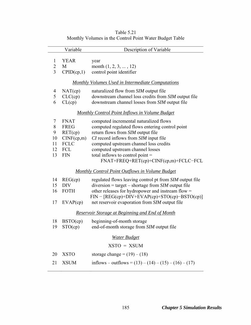
Table 5.21 Monthly Volumes in the Control Point Water Budget Table
Variable Description of Variable 1 YEAR year 2 M month (1, 2, 3, ... , 12) 3 CPID(cp,1) control point identifier
Monthly Volumes Used in Intermediate Computations
4 NAT(cp) naturalized flow from SIM output file 5 CLC(cp) downstream channel loss credits from SIM output file 6 CL(cp) downstream channel losses from SIM output file
Monthly Control Point Inflows in Volume Budget
7 FNAT computed incremental naturalized flows 8 FREG computed regulated flows entering control point 9 RET(cp) return flows from SIM output file 10 CINF(cp,m) CI record inflows from SIM input file 11 FCLC computed upstream channel loss credits 12 FCL computed upstream channel losses 13 FIN total inflows to control point = FNAT+FREQ+RET(cp)+CINF(cp,m)+FCLC−FCL
Monthly Control Point Outflows in Volume Budget
14 REG(cp) regulated flows leaving control pt from SIM output file 15 DIV diversion = target – shortage from SIM output file 16 FOTH other releases for hydropower and instream flow = FIN − [REG(cp)+DIV+EVAP(cp)+STO(cp)−BSTO(cp)]
17 EVAP(cp) net reservoir evaporation from SIM output file
Reservoir Storage at Beginning and End of Month
18 BSTO(cp) beginning-of-month storage 19 STO(cp) end-of-month storage from SIM output file
Water Budget
XSTO = XSUM
20 XSTO storage change = (19) – (18)
21 XSUM inflows – outflows = (13) – (14) – (15) – (16) – (17)
Chapter 5 Simulation Results 185
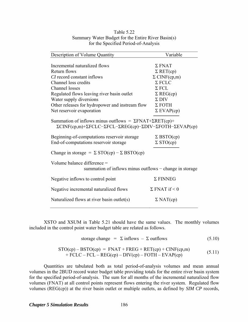
Table 5.22 Summary Water Budget for the Entire River Basin(s)
for the Specified Period-of-Analysis
Description of Volume Quantity Variable Incremental naturalized flows Σ FNAT Return flows Σ RET(cp) CI record constant inflows Σ CINF(cp,m) Channel loss credits Σ FCLC Channel losses Σ FCL Regulated flows leaving river basin outlet Σ REG(cp) Water supply diversions Σ DIV Other releases for hydropower and instream flow Σ FOTH Net reservoir evaporation Σ EVAP(cp) ───────── Summation of inflows minus outflows = ΣFNAT+ΣRET(cp)+
ΣCINF(cp,m)+ΣFCLC−ΣFCL−ΣREG(cp)−ΣDIV−ΣFOTH−ΣEVAP(cp) Beginning-of-computations reservoir storage Σ BSTO(cp) End-of-computations reservoir storage Σ STO(cp) ───────── Change in storage = Σ STO(cp) − Σ BSTO(cp) Volume balance difference =
summation of inflows minus outflows − change in storage Negative inflows to control point Σ FINNEG Negative incremental naturalized flows Σ FNAT if < 0 Naturalized flows at river basin outlet(s) Σ NAT(cp)
XSTO and XSUM in Table 5.21 should have the same values. The monthly volumes included in the control point water budget table are related as follows. storage change = Σ inflows – Σ outflows (5.10) STO(cp) – BSTO(cp) = FNAT + FREG + RET(cp) + CINF(cp,m)
+ FCLC – FCL – REG(cp) – DIV(cp) – FOTH – EVAP(cp)
(5.11)
Quantities are tabulated both as total period-of-analysis volumes and mean annual volumes in the 2BUD record water budget table providing totals for the entire river basin system for the specified period-of-analysis. The sum for all months of the incremental naturalized flow volumes (FNAT) at all control points represent flows entering the river system. Regulated flow volumes (REG(cp)) at the river basin outlet or multiple outlets, as defined by SIM CP records,
Chapter 5 Simulation Results 186
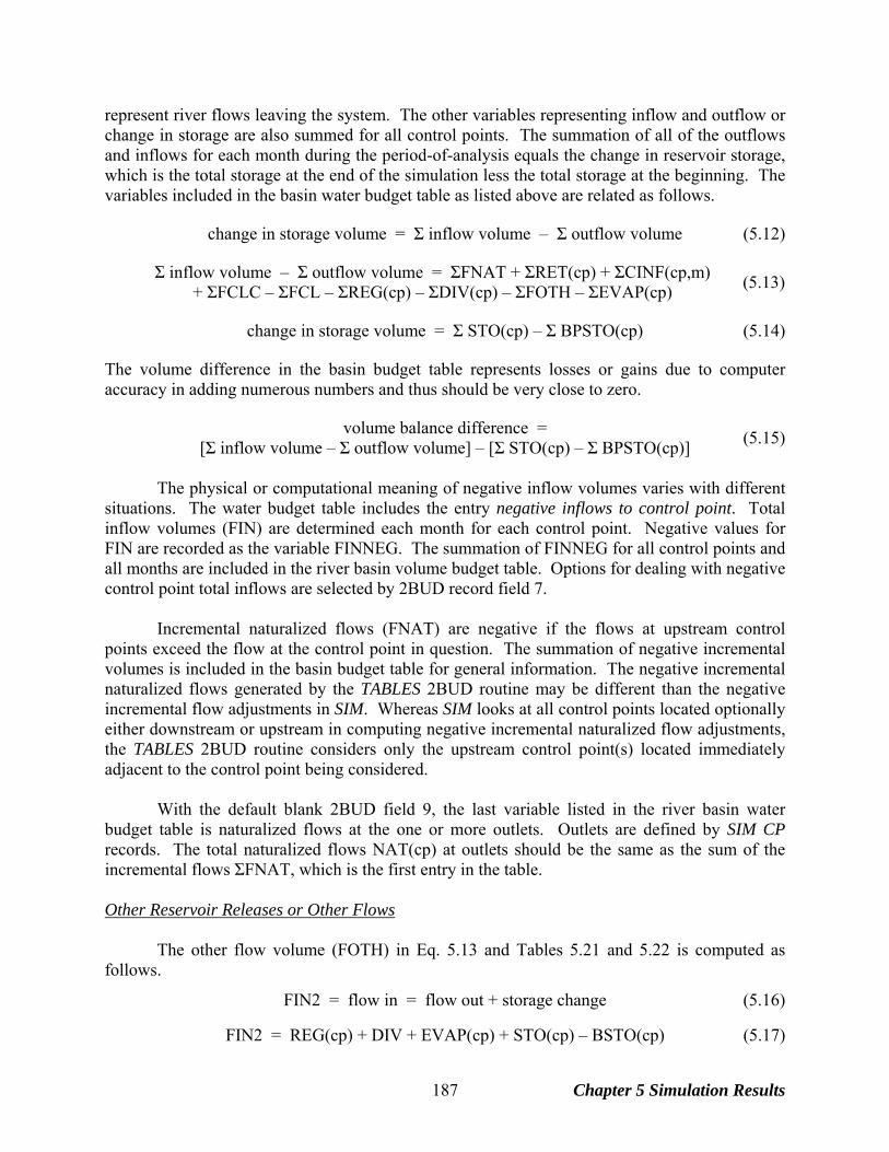
represent river flows leaving the system. The other variables representing inflow and outflow or change in storage are also summed for all control points. The summation of all of the outflows and inflows for each month during the period-of-analysis equals the change in reservoir storage, which is the total storage at the end of the simulation less the total storage at the beginning. The variables included in the basin water budget table as listed above are related as follows. change in storage volume = Σ inflow volume – Σ outflow volume (5.12) Σ inflow volume – Σ outflow volume = ΣFNAT + ΣRET(cp) + ΣCINF(cp,m)
+ ΣFCLC – ΣFCL – ΣREG(cp) – ΣDIV(cp) – ΣFOTH – ΣEVAP(cp)
(5.13)
change in storage volume = Σ STO(cp) – Σ BPSTO(cp) (5.14) The volume difference in the basin budget table represents losses or gains due to computer accuracy in adding numerous numbers and thus should be very close to zero. volume balance difference =
[Σ inflow volume – Σ outflow volume] – [Σ STO(cp) – Σ BPSTO(cp)]
(5.15)
The physical or computational meaning of negative inflow volumes varies with different situations. The water budget table includes the entry negative inflows to control point. Total inflow volumes (FIN) are determined each month for each control point. Negative values for FIN are recorded as the variable FINNEG. The summation of FINNEG for all control points and all months are included in the river basin volume budget table. Options for dealing with negative control point total inflows are selected by 2BUD record field 7. Incremental naturalized flows (FNAT) are negative if the flows at upstream control points exceed the flow at the control point in question. The summation of negative incremental volumes is included in the basin budget table for general information. The negative incremental naturalized flows generated by the TABLES 2BUD routine may be different than the negative incremental flow adjustments in SIM. Whereas SIM looks at all control points located optionally either downstream or upstream in computing negative incremental naturalized flow adjustments, the TABLES 2BUD routine considers only the upstream control point(s) located immediately adjacent to the control point being considered. With the default blank 2BUD field 9, the last variable listed in the river basin water budget table is naturalized flows at the one or more outlets. Outlets are defined by SIM CP records. The total naturalized flows NAT(cp) at outlets should be the same as the sum of the incremental flows ΣFNAT, which is the first entry in the table. Other Reservoir Releases or Other Flows The other flow volume (FOTH) in Eq. 5.13 and Tables 5.21 and 5.22 is computed as follows.
FIN2 = flow in = flow out + storage change (5.16) FIN2 = REG(cp) + DIV + EVAP(cp) + STO(cp) – BSTO(cp) (5.17)
Chapter 5 Simulation Results 187
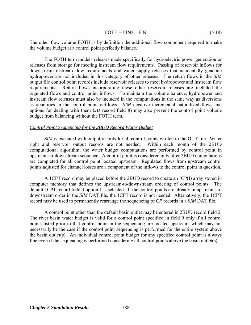
FOTH = FIN2 – FIN (5.18) The other flow volume FOTH is by definition the additional flow component required to make the volume budget at a control point perfectly balance.
The FOTH term models releases made specifically for hydroelectric power generation or releases from storage for meeting instream flow requirements. Passing of reservoir inflows for downstream instream flow requirements and water supply releases that incidentally generate hydropower are not included in this category of other releases. The return flows in the SIM output file control point records include reservoir releases to meet hydropower and instream flow requirements. Return flows incorporating these other reservoir releases are included the regulated flows and control point inflows. To maintain the volume balance, hydropower and instream flow releases must also be included in the computations in the same way as diversions as quantities in the control point outflows. SIM negative incremental naturalized flows and options for dealing with them (JD record field 8) may also prevent the control point volume budget from balancing without the FOTH term. Control Point Sequencing for the 2BUD Record Water Budget SIM is executed with output records for all control points written to the OUT file. Water right and reservoir output records are not needed. Within each month of the 2BUD computational algorithm, the water budget computations are performed by control point in upstream-to-downstream sequence. A control point is considered only after 2BUD computations are completed for all control point located upstream. Regulated flows from upstream control points adjusted for channel losses are a component of the inflows to the control point in question. A 1CPT record may be placed before the 2BUD record to create an ICP(I) array stored in computer memory that defines the upstream-to-downstream ordering of control points. The default 1CPT record field 3 option 1 is selected. If the control points are already in upstream-to-downstream order in the SIM DAT file, the 1CPT record is not needed. Alternatively, the 1CPT record may be used to permanently rearrange the sequencing of CP records in a SIM DAT file. A control point other than the default basin outlet may be entered in 2BUD record field 2. The river basin water budget is valid for a control point specified in field 9 only if all control points listed prior to that control point in the sequencing are located upstream, which may not necessarily be the case if the control point sequencing is performed for the entire system above the basin outlet(s). An individual control point budget for any specified control point is always fine even if the sequencing is performed considering all control points above the basin outlet(s).
Chapter 5 Simulation Results 188
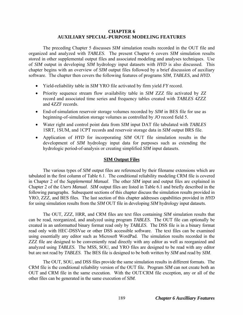
CHAPTER 6 AUXILIARY SPECIAL-PURPOSE MODELING FEATURES
The preceding Chapter 5 discusses SIM simulation results recorded in the OUT file and organized and analyzed with TABLES. The present Chapter 6 covers SIM simulation results stored in other supplemental output files and associated modeling and analyses techniques. Use of SIM output in developing SIM hydrology input datasets with HYD is also discussed. This chapter begins with an overview of SIM output files followed by a brief discussion of auxiliary software. The chapter then covers the following features of programs SIM, TABLES, and HYD.
• Yield-reliability table in SIM YRO file activated by firm yield FY record. • Priority sequence stream flow availability table in SIM ZZZ file activated by ZZ
record and associated time series and frequency tables created with TABLES 4ZZZ and 4ZZF records.
• End-of-simulation reservoir storage volumes recorded by SIM in BES file for use as beginning-of-simulation storage volumes as controlled by JO record field 5.
• Water right and control point data from SIM input DAT file tabulated with TABLES 1SRT, 1SUM, and 1CPT records and reservoir storage data in SIM output BRS file.
• Application of HYD for incorporating SIM OUT file simulation results in the development of SIM hydrology input data for purposes such as extending the hydrologic period-of-analysis or creating simplified SIM input datasets.
SIM Output Files
The various types of SIM output files are referenced by their filename extensions which are tabulated in the first column of Table 6.1. The conditional reliability modeling CRM file is covered in Chapter 2 of the Supplemental Manual. The other SIM input and output files are explained in Chapter 2 of the Users Manual. SIM output files are listed in Table 6.1 and briefly described in the following paragraphs. Subsequent sections of this chapter discuss the simulation results provided in YRO, ZZZ, and BES files. The last section of this chapter addresses capabilities provided in HYD for using simulation results from the SIM OUT file in developing SIM hydrology input datasets. The OUT, ZZZ, HRR, and CRM files are text files containing SIM simulation results that can be read, reorganized, and analyzed using program TABLES. The OUT file can optionally be created in an unformatted binary format read only by TABLES. The DSS file is in a binary format read only with HEC-DSSVue or other DSS accessible software. The text files can be examined using essentially any editor such as Microsoft WordPad. The simulation results recorded in the ZZZ file are designed to be conveniently read directly with any editor as well as reorganized and analyzed using TABLES. The MSS, SOU, and YRO files are designed to be read with any editor but are not read by TABLES. The BES file is designed to be both written by SIM and read by SIM. The OUT, SOU, and DSS files provide the same simulation results in different formats. The CRM file is the conditional reliability version of the OUT file. Program SIM can not create both an OUT and CRM file in the same execution. With the OUT/CRM file exception, any or all of the other files can be generated in the same execution of SIM.
Chapter 6 Auxilliary Features 189
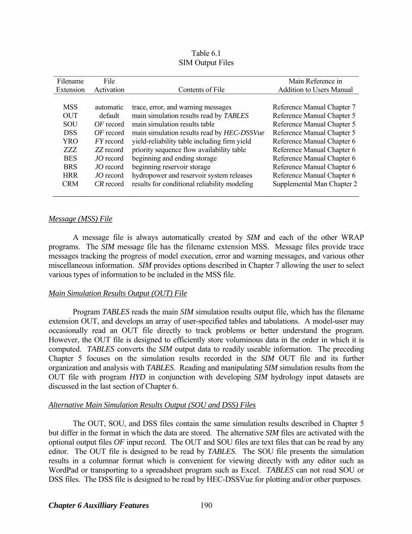
Table 6.1 SIM Output Files
Filename File Main Reference in Extension Activation Contents of File Addition to Users Manual
MSS automatic trace, error, and warning messages Reference Manual Chapter 7 OUT default main simulation results read by TABLES Reference Manual Chapter 5 SOU OF record main simulation results table Reference Manual Chapter 5 DSS OF record main simulation results read by HEC-DSSVue Reference Manual Chapter 5 YRO FY record yield-reliability table including firm yield Reference Manual Chapter 6 ZZZ ZZ record priority sequence flow availability table Reference Manual Chapter 6 BES JO record beginning and ending storage Reference Manual Chapter 6 BRS JO record beginning reservoir storage Reference Manual Chapter 6 HRR JO record hydropower and reservoir system releases Reference Manual Chapter 6 CRM CR record results for conditional reliability modeling Supplemental Man Chapter 2
Message (MSS) File A message file is always automatically created by SIM and each of the other WRAP programs. The SIM message file has the filename extension MSS. Message files provide trace messages tracking the progress of model execution, error and warning messages, and various other miscellaneous information. SIM provides options described in Chapter 7 allowing the user to select various types of information to be included in the MSS file. Main Simulation Results Output (OUT) File Program TABLES reads the main SIM simulation results output file, which has the filename extension OUT, and develops an array of user-specified tables and tabulations. A model-user may occasionally read an OUT file directly to track problems or better understand the program. However, the OUT file is designed to efficiently store voluminous data in the order in which it is computed. TABLES converts the SIM output data to readily useable information. The preceding Chapter 5 focuses on the simulation results recorded in the SIM OUT file and its further organization and analysis with TABLES. Reading and manipulating SIM simulation results from the OUT file with program HYD in conjunction with developing SIM hydrology input datasets are discussed in the last section of Chapter 6. Alternative Main Simulation Results Output (SOU and DSS) Files The OUT, SOU, and DSS files contain the same simulation results described in Chapter 5 but differ in the format in which the data are stored. The alternative SIM files are activated with the optional output files OF input record. The OUT and SOU files are text files that can be read by any editor. The OUT file is designed to be read by TABLES. The SOU file presents the simulation results in a columnar format which is convenient for viewing directly with any editor such as WordPad or transporting to a spreadsheet program such as Excel. TABLES can not read SOU or DSS files. The DSS file is designed to be read by HEC-DSSVue for plotting and/or other purposes.
Chapter 6 Auxilliary Features 190
Yield versus Reliability Output (YRO) File As discussed later in this chapter, the firm yield FY record activates a routine to develop a yield-reliability table for a diversion, which is written to the YRO file (filename extension YRO). The firm yield is the last entry in the table. SIM creates this yield-reliability table directly as the simulation is iteratively repeated multiple times. TABLES is not involved in any way with the YRO file table. However, TABLES creates other reliability tables for fixed targets from the results of a single simulation that are discussed in the preceding Chapter 5. Priority Sequence Stream Flow Availability (ZZZ) File Simulation results stored in the ZZZ file activated by the ZZ record are also discussed later in this chapter. Regulated flows, available flows, and upstream reservoir releases at specified control points are tabulated in a ZZZ file after each individual water right is simulated in the priority loop. The SIM output ZZZ file table may be read directly with any editor. The TABLES 2ZZZ and 2ZZF records activate TABLES routines for reading a ZZZ file and organizing the simulation results in optional time series formats or developing frequency tables. Beginning-Ending Storage (BES) File End-of-simulation reservoir storage contents may be saved for subsequent use as beginning-of-simulation reservoir storage. Beginning-ending storage (BES) options are described later in this chapter. A BES file may be both created and read by SIM. Program TABLES does not deal in any way with BES files. Beginning Reservoir Storage (BRS) File The optional BRS file is a table listing all reservoirs with the following data: reservoir identifier, control point location, storage capacity, and beginning-of-simulation storage content. Program SALT and a TABLES conditional reliability modeling routine, both described in the Supplemental Manual, contain options to read beginning-of-simulation storage from a BRS file. The BRS file may also be useful for general information. Hydropower and Reservoir Release (HRR) File The HRR file is used primarily for comparing releases from individual reservoirs of a multiple-reservoir system operated for the same water right. Simulation results in the OUT file (or SOU or DSS files) include data related to reservoirs and hydropower. However, multiple-reservoir system secondary reservoir releases, not found in the OUT file, are recorded in the optional hydropower and multiple-reservoir system release HRR file. Hydroelectric power generation is included in the HRR as well as OUT files. Tables created by TABLES as specified by 4SWR and 4SGP input records organize these data into a more convenient-to-read tabular format. The HRR file lists releases from primary and secondary reservoirs for each month of the simulation for each water right selected for output. The release from a primary reservoir is simply the diversion supplied by the water right, which is also recorded in the OUT file. For multiple-
Chapter 6 Auxilliary Features 191

reservoir systems, the HRR file also provides a tabulation of the releases from each of the individual secondary reservoirs associated with a water right. Unlike the HRR file, the OUT file records only the aggregated total release from all of the secondary reservoirs. The HRR file also contains the hydroelectric energy target and amount of energy generated, which are also found in the OUT file. Conditional Reliability Modeling (CRM) File Conditional reliability modeling (CRM) is covered in Chapter 2 of the Supplemental Manual. The CRM file activated by a CR record is described in the Supplemental Manual. The CRM file is the conditional reliability modeling version of the OUT file. SIM creates either an OUT file or CRM file, but not both. The same simulation result variables are contained in either the OUT or CRM file. However, the CRM file reflects the subdivision of the hydrologic period-of-analysis into multiple sequences associated with conditional reliability modeling.
Auxiliary Software As discussed initially in Chapter 1 and noted throughout this manual, use of other readily available software along with the WRAP programs serve various purposes. Other non-WRAP programs are used along with TABLES to organize and display WRAP simulation results. Microsoft Programs Microsoft WordPad and NotePad are used to create WRAP input files and to read and edit input and output files. Tables created with TABLES are transported into Microsoft Word documents when preparing reports. Excel is used to plot simulation results and perform various computational manipulations. Both SIM and TABLES create output files in optional columnar formats for convenient transport to spreadsheet programs such as Microsoft Excel. These Microsoft programs can be accessed directly from the WinWRAP interface. Hydrologic Engineering Center HEC-DSS and HEC-DSSVue The HEC-DSS (Data Storage System) was developed by the Hydrologic Engineering Center (HEC) of the U.S. Army Corps of Engineers (USACE) for use with its own generalized hydrologic, hydraulic, and water management simulation models. The HEC-DSS is used with other non-HEC modeling systems as well. Multiple simulation models share the same graphics and data management software as well as a set of basic statistical and arithmetic routines. HEC-DSS database management and graphics capabilities are designed particularly for sequential time series data such as WRAP simulation results and hydrology input data. The HEC-DSS Visual Utility Engine (HEC-DSSVue) is a graphical user interface program for viewing, editing, and manipulating data in DSS files. The public domain HEC-DSSVue software and documentation may be downloaded from the Hydrologic Engineering Center website. http://www.hec.usace.army.mil/ The WRAP Fortran programs are linked during compilation to DSS routines from a static library file provided by the Hydrologic Engineering Center that allows access to DSS files. The WRAP executable programs include options for writing the SIM, SIMD, or SALT simulation results as HEC-DSS files and reading and writing hydrology data. DSS files store data is a binary format
Chapter 6 Auxilliary Features 192
that is accessible only by HEC-DSSVue and programs such as the HEC simulation models and WRAP programs that incorporate DSS routines from the HEC-DSS library in the computer code. HEC-DSSVue can be accessed directly from the WinWRAP interface. The WRAP programs store the following types of data in DSS files: (1) hydrology input data consisting of stream flows and net evaporation rates and (2) simulation results including essentially all of the time series variables. Naturalized stream flows and net evaporation-precipitation depths may be both read from and written to DSS files by either WRAP-SIM/SIMD or WRAP-HYD. Reading of hydrology data by SIM from a DSS file rather than the default FLO and EVA files is controlled by JO record field 2. Creation of a hydrology DSS file with SIM is activated by OF record field 6. Program HYD JC record parameters control reading and writing hydrology data by HYD in a DSS file. The SIM, SIMD, and SALT simulation programs have options for storing simulation results as DSS files. The post-simulation program TABLES also includes options for writing the time series variables from the simulation results as DSS records and may also perform various arithmetic operations prior to writing the resulting adjusted simulation results as DSS records. SIM output files OF input record field 4 activates the option of storing SIM simulation results in a DSS file. As discussed in Chapter 5, all of the SIM simulation results that can be stored in an OUT or SOU file can also be stored by SIM in a DSS file. The TABLES time series records include options for writing SIM OUT file data or other data computed based on the SIM output data to a DSS file. TABLES can also store SIM results read from a ZZZ file as a DSS file. The purpose for storing WRAP simulation results as DSS files is to allow application of HEC-DSSVue primarily to develop time series graphs. HEC-DSSVue provides convenient capabilities for plotting SIM, SIMD, and SALT simulation results or hydrology input data. In addition to graphics, HEC-DSSVue also provides an array of data management and computation options. HEC-DSSVue statistical analyses and mathematical operations can be applied to the WRAP time series data. HEC-DSSVue is documented in detail by a users manual (Hydrologic Engineering Center 2005) which is available along with the software from the HEC website. WRAP Display Tool for ArcGIS ArcMap
Geographic information system (GIS) software is useful in dealing with spatial aspects of compiling WRAP input data and displaying simulation results. The ArcGIS software system marketed by the Environmental Systems Research Institute (http://www.esri.com) is a particularly popular GIS. Use of ArcGIS to develop WRAP input datasets is noted in Chapters 1 and 3.
An ArcGIS tool for displaying WRAP-SIM simulation results originally developed by
Olmos (2004) was later improved by the Center for Research in Water Resources (2007) at the University of Texas for the TCEQ. The WRAP Display Tool is applied as an ArcMap toolbar. Flow and storage frequencies, water supply reliabilities, and other percentage-based indices derived from SIM simulation results are displayed by range as color coded symbols on a map. Time series graphs of SIM output data can also be plotted. The tool includes features for customizing applications along with its standard SIM output file manipulation and display capabilities. The WRAP Display Tool is available from the TCEQ as an executable setup file along with a users manual (CRWR 2007). It is designed for use with ArcGIS version 9.2.
Chapter 6 Auxilliary Features 193
Yield Versus Reliability Relationships Including Firm Yield
The annual water supply diversion target or hydroelectric energy generation target is entered in the SIM water right WR record field 3 as the input variable AMT. Model applications may require computing volume and period reliabilities (defined by Equations 5.1 and 5.2 in Chapter 5) for a range of different values for AMT. The firm yield, defined as the maximum value of AMT that has a computed reliability of 100.0 percent, also may be of interest. The reliabilities associated with various annual yields, represented by the variable AMT, that includes the firm yield (100% reliability), may be developed simply by running SIM multiple times, manually changing the AMT entry in WR record field 3 for each run. An option activated by the FY record automates this procedure. In a single SIM execution, multiple simulations are repeated with the annual target amount being systematically changed. The resulting yield-reliability table is written as a SIM output file with the filename extension YRO.
The SIM routine to develop a yield versus reliability relationship is controlled with the
firm yield FY record. The firm yield is the last entry in the resulting YRO file yield-reliability table, assuming a non-zero firm yield is possible. In some situations, any non-zero diversion target results in a reliability of less than 100 percent. The diversion or hydropower yield may be associated with a single water right or a set of any number of rights. If associated with multiple water rights, two options are available for allocating the annual yield amount between rights.
1. With the first option (MFY=1 on FY record), the yield is allocated between rights in
proportion to target amounts entered in field 3 of the water right WR records. Thus, the total yield is multiplied by fractions set by the model-user to determine the proportion of the total yield assigned to each water right as illustrated by the following example.
2. The second option (MFY=2 on FY record) is based on the priorities from field 7 of the
WR records. The yield is assigned to the most senior priority right up to the target amount specified in field 3 of its WR record. Any yield remaining is assigned to the next most senior priority right up to its target amount, and so forth. Upon reaching the most junior right, the remaining portion of the yield, if any, is assigned to the most junior right regardless of its WR record target amount.
The yield-reliability table reproduced as Table 6.2 is provided to illustrate the automated
yield-reliability/firm yield option. This YRO file table is created with the following entries on a FY record:
FYIN(1) = 0.92 FYIN(2) = 200,000 acre-feet/year FYIN(3) = 10,000 acre-feet/year FYIN(4) = 1,000 acre-feet/year FYIN(5) = 100 acre-feet/year Either FYWRID = Jones Reservoir and/or FYGROUP = yield
MFY = 1
The yield-reliability table shown as Table 6.2 begins with a list of the water rights for which the target amounts are adjusted. FYWRID and FYGROUP from FY record fields 7 and 8
Chapter 6 Auxilliary Features 194
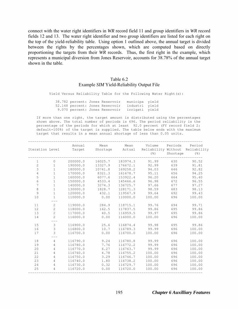
connect with the water right identifiers in WR record field 11 and group identifiers in WR record fields 12 and 13. The water right identifier and two group identifiers are listed for each right on the top of the yield-reliability table. Using option 1 outlined above, the annual target is divided between the rights by the percentages shown, which are computed based on directly proportioning the targets from their WR records. Thus, the first right in the example, which represents a municipal diversion from Jones Reservoir, accounts for 38.78% of the annual target shown in the table.
Table 6.2 Example SIM Yield-Reliability Output File
Yield Versus Reliability Table for the Following Water Right(s): 38.782 percent: Jones Reservoir municipa yield 52.148 percent: Jones Reservoir industri yield 9.070 percent: Jones Reservoir irrigati yield If more than one right, the target amount is distributed using the percentages shown above. The total number of periods is 696. The period reliability is the percentage of the periods for which at least 92.0 percent (FY record field 2; default=100%) of the target is supplied. The table below ends with the maximum target that results in a mean annual shortage of less than 0.05 units. ----------------------------------------------------------------------------------- Annual Mean Mean Volume Periods Period Iteration Level Target Shortage Actual Reliability Without Reliability (%) Shortage (%) ----------------------------------------------------------------------------------- 1 0 200000.0 16025.7 183974.3 91.99 630 90.52 2 1 190000.0 13327.9 176672.1 92.99 639 91.81 3 1 180000.0 10741.8 169258.2 94.03 646 92.82 4 1 170000.0 8321.3 161678.7 95.11 656 94.25 5 1 160000.0 6077.6 153922.4 96.20 664 95.40 6 1 150000.0 4533.4 145466.6 96.98 672 96.55 7 1 140000.0 3274.3 136725.7 97.66 677 97.27 8 1 130000.0 1828.7 128171.3 98.59 683 98.13 9 1 120000.0 432.1 119567.9 99.64 692 99.43 10 1 110000.0 0.00 110000.0 100.00 696 100.00 --- 11 2 119000.0 284.9 118715.1 99.76 694 99.71 12 2 118000.0 162.5 117837.5 99.86 695 99.86 13 2 117000.0 40.5 116959.5 99.97 695 99.86 14 2 116000.0 0.00 116000.0 100.00 696 100.00 --- 15 3 116900.0 25.6 116874.4 99.98 695 99.86 16 3 116800.0 10.7 116789.3 99.99 696 100.00 17 3 116700.0 0.00 116700.0 100.00 696 100.00 --- 18 4 116790.0 9.24 116780.8 99.99 696 100.00 19 4 116780.0 7.76 116772.2 99.99 696 100.00 20 4 116770.0 6.27 116763.7 99.99 696 100.00 21 4 116760.0 4.78 116755.2 100.00 696 100.00 22 4 116750.0 3.29 116746.7 100.00 696 100.00 23 4 116740.0 1.80 116738.2 100.00 696 100.00 24 4 116730.0 0.32 116729.7 100.00 696 100.00 25 4 116720.0 0.00 116720.0 100.00 696 100.00 -----------------------------------------------------------------------------------
Chapter 6 Auxilliary Features 195
Each line in the YRO file table represents the results of a SIM simulation. The annual target amount AMT is the only input variable that changes between simulations. No other features of WRAP-SIM are affected. All other features remain in effect. FYIN(1) entered in FY record field 2 is the fraction of the monthly target that must be met in order for the routine to not declare that month a failure in the computation of period reliability. FYIN(1) might be set at 0.92 for an analysis based on the premise that a 8% reduction in water use through demand management measures is acceptable during dry periods. The FYIN(1) default is 1.0, meaning the entire target must be met in order to not declare a failure in meeting the target that month. FYIN(1) affects only the period reliability (last two columns of table). It is not used in the volume reliability computations (columns 3, 4, 5). The firm yield criterion for stopping the iterative routine is based on reaching a total shortage of essentially zero, defined as less than 0.05 unit of the units being used (for example 0.05 acre-feet/year). If FYIN(1) is non-zero, the 100% period reliability yield may be larger than the 100% volume reliability yield. Both are shown in the yield-reliability table. In the example with FYIN(5)=0.92, the volume reliability firm yield is 116,720 ac-ft/yr and the period reliability firm yield is 116,800 ac-ft/yr.
The iterative simulations are organized as follows. 1. The total annual target amount AMT equals FYIN(2) (=200,000 ac-ft/yr) from the FY record
for the first simulation. With MFY option 1, AMT for the initial and all subsequent iterations is distributed to multiple water rights in proportion to WR record field 3 AMTs, with resulting percentages listed at the top of the table, to determine the individual AMT for each of the rights. The following steps are identical regardless of which of the two MFY options is activated in FY field 9 for distributing the target amount between water rights.
2. The total annual target amount AMT is decreased by FYIN(3) for each subsequent level 1
iteration until either no shortages occur or the target is finally decreased to zero or less. 3. If both FYIN(4) and FYIN(5) are zero, the computations stop. If FYIN(4) is not zero, the
computations proceed to level 2. In the example, since FYIN(4) of 1,000 ac-ft has been entered on the FY record, the computations proceed to level 2.
4. For level 2, the initial target amount AMT is set equal to the next-to-last target amount from
the level 1 iterations (120,000 ac-ft). AMT is decreased by FYIN(4) (1,000 ac-ft) for each level 2 iteration until either no shortages occur or the target AMT reaches zero.
5. If FYIN(5) is zero, the computations stop without proceeding to levels 3 and 4. Otherwise,
level 3 iterations are performed using FYIN(5) as the incremental decrease in AMT. For the example, FYIN(5) is 100 ac-ft.
6. If FYIN(5) is not zero, upon completion of the level 3 iterations, an extra level 4 set of
iterations is performed with the incremental decrease set at 10 percent of FYIN(5).
The FY record computations are performed for only one annual diversion or hydropower amount. A single annual target amount is adjusted during the iterative routine. However, this amount may be shared by any number of water rights (WR records). The water right identifier in
Chapter 6 Auxilliary Features 196
FY record field 7 is matched with the identifiers entered in water right WR record field 11. The water right group identifier in FY record field 8 is matched with the identifiers entered in water right WR record fields 12 and 13. The annual amount is divided between multiple rights based on the choice of two optional method specified by MFY in FY record field 9. For those rights designated by FYWRID and FYGROUP on the WR record, this is the only use made of the amounts entered in field 3 of their WR records. If only one right is designated by the FY record, an amount entered in field 3 of its WR record is not used for anything in the computations. The example in the Fundamentals Manual further illustrates the methodology. The Fundamentals Manual is organized focusing on an example with complete dataset provided, which includes application of the firm yield FY record yield-reliability analysis feature of SIM.
Stream Flow Availability in the Water Rights Priority Sequence A SIM feature controlled by the ZZ record and associated TABLES routines controlled by the 4ZZZ and 4ZZF records are designed to facilitate assessments of the effects of other water rights located throughout the river basin on the amount of stream flow that is available to water users at particular locations of concern. For each control point specified with a SIM ZZ record, regulated flows, available flows, and upstream reservoir releases are tabulated in a ZZZ file after each individual water right is simulated in the priority loop. These monthly flows are recorded at the beginning of the water rights loop and after each individual water right is simulated in the priority sequence. TABLES reads the ZZZ file and organizes the flow information. All SIM output OUT file variables are defined in Chapter 5 and listed in Table 5.1. An identifying label is listed in the second column of Table 5.1. Three of these previously defined variables (regulated flows, available stream flows, and upstream reservoir releases), labeled 2REG, 2ASF, and 2URR in Table 5.1, are included in the ZZZ file. Intermediate available stream flows (2ASF in Table 5.1) in the water rights priority sequence become unappropriated flows (2UNA) after the most junior water right is simulated. The reservoir releases (2URR) included in the ZZZ table are a component of regulated flows (2REG) and include only releases from reservoirs located at or upstream of a control point that are made to meet water right diversion, storage, or instream flow requirements at a control point located further downstream. The ZZZ file table may be read directly with any editor. The TABLES 4ZZZ and 4ZZF records activate TABLES options for reading a ZZZ file and organizing the simulation results in optional time series formats or developing frequency tables. The 4ZZZ record builds time series tables in optional formats or DSS files, and the 4ZZF record creates frequency analysis tables similar to the 2FRE record frequency tables discussed in Chapter 5. During each month of the SIM simulation, flows at designated control points are tabulated in the ZZZ file at the beginning of the water rights priority loop and after each water right is simulated in the priority sequence. By default, all water rights from the most senior to most junior are included in the tabulation. However, an optional parameter entered on the ZZ record sets a minimum flow change required for a water right to be included in the table. Monthly flow volumes are tabulated after a water right is simulated only if the change in either the regulated flow, available flow, or upstream release equals or exceeds the specified limit at
Chapter 6 Auxilliary Features 197
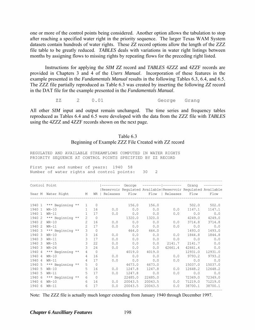
one or more of the control points being considered. Another option allows the tabulation to stop after reaching a specified water right in the priority sequence. The larger Texas WAM System datasets contain hundreds of water rights. These ZZ record options allow the length of the ZZZ file table to be greatly reduced. TABLES deals with variations in water right listings between months by assigning flows to missing rights by repeating flows for the preceding right listed. Instructions for applying the SIM ZZ record and TABLES 4ZZZ and 4ZZF records are provided in Chapters 3 and 4 of the Users Manual. Incorporation of these features in the example presented in the Fundamentals Manual results in the following Tables 6.3, 6.4, and 6.5. The ZZZ file partially reproduced as Table 6.3 was created by inserting the following ZZ record in the DAT file for the example presented in the Fundamentals Manual.
ZZ 2 0.01 George Grang All other SIM input and output remain unchanged. The time series and frequency tables reproduced as Tables 6.4 and 6.5 were developed with the data from the ZZZ file with TABLES using the 4ZZZ and 4ZZF records shown on the next page.
Table 6.3
Beginning of Example ZZZ File Created with ZZ record REGULATED AND AVAILABLE STREAMFLOWS COMPUTED IN WATER RIGHTS PRIORITY SEQUENCE AT CONTROL POINTS SPECIFIED BY ZZ RECORD First year and number of years: 1940 58 Number of water rights and control points: 30 2 ---------------------------------------------------------------------------------------------- Control Point |--------- George ---------|--------- Grang --------- |Reservoir Regulated Available|Reservoir Regulated Available Year M Water Right M WR | Releases Flow Flow | Releases Flow Flow ----------------------------------------------------------------------------------------------
1940 1 *** Beginning ** 1 0 156.0 156.0 502.0 502.0 1940 1 WR-10 1 16 0.0 0.0 0.0 0.0 1147.1 1147.1 1940 1 WR-11 1 17 0.0 0.0 0.0 0.0 0.0 0.0 1940 2 *** Beginning ** 2 0 1320.0 1320.0 4249.0 4249.0 1940 2 WR-10 2 16 0.0 0.0 0.0 0.0 3714.8 3714.8 1940 2 WR-11 2 17 0.0 0.0 0.0 0.0 0.0 0.0 1940 3 *** Beginning ** 3 0 464.0 464.0 1493.0 1493.0 1940 3 WR-10 3 16 0.0 0.0 0.0 0.0 1844.8 1844.8 1940 3 WR-11 3 17 0.0 0.0 0.0 0.0 0.0 0.0 1940 3 WR-15 3 22 0.0 0.0 0.0 2141.7 2141.7 0.0 1940 3 WR-24 3 24 0.0 0.0 0.0 42661.4 42661.4 0.0 1940 4 *** Beginning ** 4 0 4019.0 4019.0 12931.0 12931.0 1940 4 WR-10 4 16 0.0 0.0 0.0 0.0 9793.2 9793.2 1940 4 WR-11 4 17 0.0 0.0 0.0 0.0 0.0 0.0 1940 5 *** Beginning ** 5 0 4673.0 4673.0 15037.0 15037.0 1940 5 WR-10 5 16 0.0 1247.8 1247.8 0.0 12648.2 12648.2 1940 5 WR-11 5 17 0.0 1247.8 0.0 0.0 0.0 0.0 1940 6 *** Beginning ** 6 0 22485.0 22485.0 72349.0 72349.0 1940 6 WR-10 6 16 0.0 20043.5 20043.5 0.0 71219.0 71219.0 1940 6 WR-11 6 17 0.0 20043.5 20043.5 0.0 38700.1 38700.1 ---------------------------------------------------------------------------------------------- Note: The ZZZ file is actually much longer extending from January 1940 through December 1997.
Chapter 6 Auxilliary Features 198
The ZZZ file covers the entire period-of-analysis which is 1940-1997 for the example in the Fundamentals Manual. Only the first six months are shown in Table 6.3. The year and month are tabulated in the first two columns of the ZZZ file table. The month (M) in the second column is an integer between 1 and 12 repeating each year, and the month (M) in the fourth column is an integer between 1 and 696 covering the 696 months in the 1940-1997 period-of-analysis. The third column is the water right identifier. The sixth column with heading WR is the integer water right index with 1 denoting the most senior water right in the SIM input dataset. The table includes flows at control points with identifiers George and Grang. The ZZZ table is constructed as the simulation proceeds through the water rights priority sequence each month. The default is to include all water rights in the table. However, in creating the ZZZ file of Table 6.3, a ZZ record option was used that allows specification of a minimum flow change required to include a water right in the table. A minimum limit of 0.01 acre-feet was entered on the ZZ record for this example, which essentially means a non-zero change. Thus, an additional row is added to the ZZZ file table only if at least one of the flows in the row is different from the preceding row of the table in an amount of at least 0.01 acre-feet. With a total of 30 water rights in the example, this option greatly reduces the length of the table. Using the third month (March 1940) as an example, the ZZZ file is interpreted as follows. The purpose of the ZZZ file is to display the impacts of all water rights on regulated and available flows at each of the two control points with identifiers George and Grang. At the beginning of the water rights priority loop for the third month, prior to simulating any of the water rights, the March 1940 regulated and available flow are both 464.0 acre-feet/month at control point George and 1,493.0 acre-feet/month at control point Grang. The initial flows are always naturalized flows plus, if next-month return flow or next-month hydropower options are activated, any return flows or hydropower releases from the preceding month.
In month 3 (March 1940), one or more of the flows are affected by water rights WR-10, WR-11, WR-15, and WR-24. The relative priority rankings of these four water rights are 16, 17, 22, and 24. The 15 other rights senior to WR-10 do not affect the flows at Grang. After simulating water right WR-10, the regulated and available flows are reduced to 0.0 at George and are increased to 1,844.8 acre-feet at Grang. The increase at Grang is due to return flow from a diversion at George located upstream. Water right WR-11 reduces the regulated and available flows to zero at both George and Grang. The flows at George remain zero throughout the reminder of the priority sequence simulation. Water rights WR-15 and WR-24 increase the regulated flows at Grang to 2,141.7 and 42,661.4 acre-feet. WR-15 and WR-24 are diversions at a downstream control point for which releases are made from the reservoir at control point Grang. The reservoir release column of the ZZZ file table is a component of regulated flow, which for the 2,141.7 and 42,661.4 acre-feet flows happen to account for the total regulated flow. With the 4ZZZ and 4ZZF input records reproduced below, TABLES reads the ZZZ file of Table 6.3 and creates the tables reproduced as Tables 6.4 and 6.5 which are stored in the TABLES output TOU file. Only tables for control point Grang are shown in Tables 6.4 and 6.5. 24ZZZ 1 0 0 3 2 WR-15
IDEN George Grang 4ZZF 3 0 -2
Chapter 6 Auxilliary Features 199
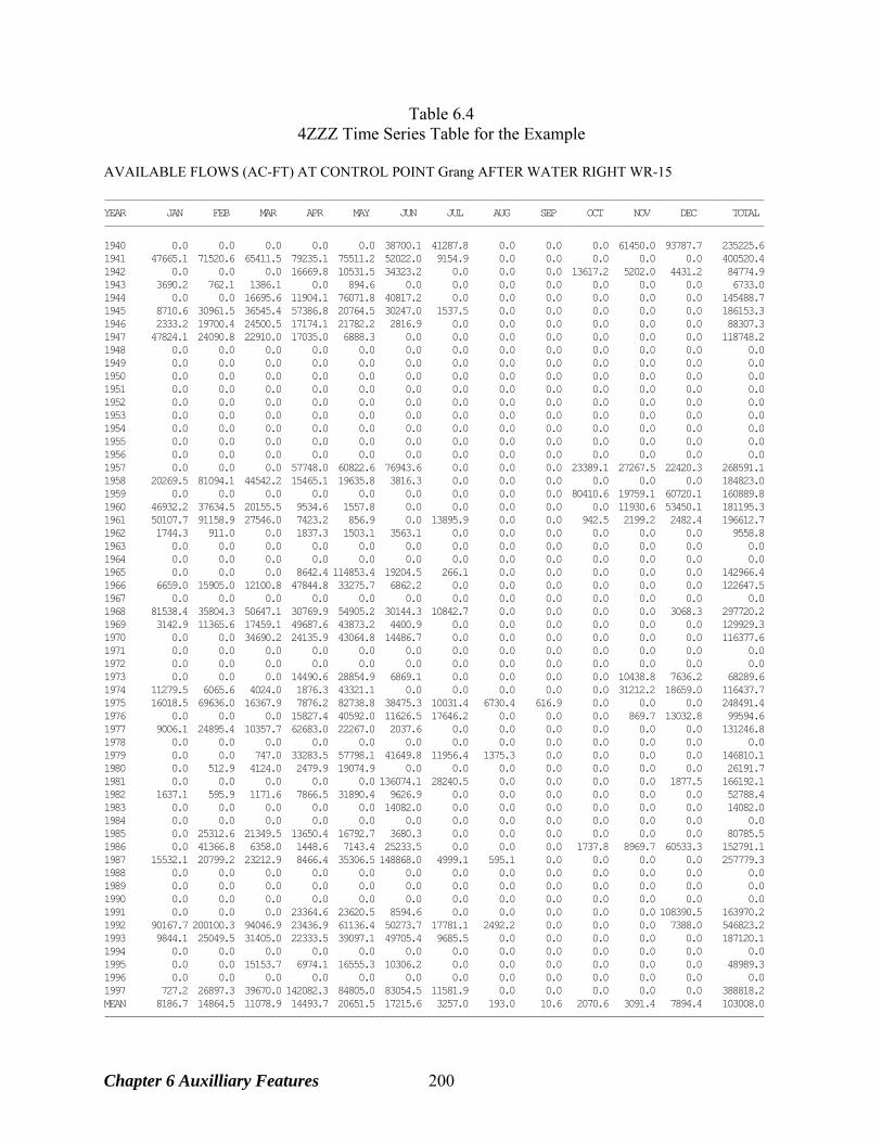
Table 6.4 4ZZZ Time Series Table for the Example
AVAILABLE FLOWS (AC-FT) AT CONTROL POINT Grang AFTER WATER RIGHT WR-15 ------------------------------------------------------------------------------------------------------------------------------- YEAR JAN FEB MAR APR MAY JUN JUL AUG SEP OCT NOV DEC TOTAL -------------------------------------------------------------------------------------------------------------------------------
1940 0.0 0.0 0.0 0.0 0.0 38700.1 41287.8 0.0 0.0 0.0 61450.0 93787.7 235225.6 1941 47665.1 71520.6 65411.5 79235.1 75511.2 52022.0 9154.9 0.0 0.0 0.0 0.0 0.0 400520.4 1942 0.0 0.0 0.0 16669.8 10531.5 34323.2 0.0 0.0 0.0 13617.2 5202.0 4431.2 84774.9 1943 3690.2 762.1 1386.1 0.0 894.6 0.0 0.0 0.0 0.0 0.0 0.0 0.0 6733.0 1944 0.0 0.0 16695.6 11904.1 76071.8 40817.2 0.0 0.0 0.0 0.0 0.0 0.0 145488.7 1945 8710.6 30961.5 36545.4 57386.8 20764.5 30247.0 1537.5 0.0 0.0 0.0 0.0 0.0 186153.3 1946 2333.2 19700.4 24500.5 17174.1 21782.2 2816.9 0.0 0.0 0.0 0.0 0.0 0.0 88307.3 1947 47824.1 24090.8 22910.0 17035.0 6888.3 0.0 0.0 0.0 0.0 0.0 0.0 0.0 118748.2 1948 0.0 0.0 0.0 0.0 0.0 0.0 0.0 0.0 0.0 0.0 0.0 0.0 0.0 1949 0.0 0.0 0.0 0.0 0.0 0.0 0.0 0.0 0.0 0.0 0.0 0.0 0.0 1950 0.0 0.0 0.0 0.0 0.0 0.0 0.0 0.0 0.0 0.0 0.0 0.0 0.0 1951 0.0 0.0 0.0 0.0 0.0 0.0 0.0 0.0 0.0 0.0 0.0 0.0 0.0 1952 0.0 0.0 0.0 0.0 0.0 0.0 0.0 0.0 0.0 0.0 0.0 0.0 0.0 1953 0.0 0.0 0.0 0.0 0.0 0.0 0.0 0.0 0.0 0.0 0.0 0.0 0.0 1954 0.0 0.0 0.0 0.0 0.0 0.0 0.0 0.0 0.0 0.0 0.0 0.0 0.0 1955 0.0 0.0 0.0 0.0 0.0 0.0 0.0 0.0 0.0 0.0 0.0 0.0 0.0 1956 0.0 0.0 0.0 0.0 0.0 0.0 0.0 0.0 0.0 0.0 0.0 0.0 0.0 1957 0.0 0.0 0.0 57748.0 60822.6 76943.6 0.0 0.0 0.0 23389.1 27267.5 22420.3 268591.1 1958 20269.5 81094.1 44542.2 15465.1 19635.8 3816.3 0.0 0.0 0.0 0.0 0.0 0.0 184823.0 1959 0.0 0.0 0.0 0.0 0.0 0.0 0.0 0.0 0.0 80410.6 19759.1 60720.1 160889.8 1960 46932.2 37634.5 20155.5 9534.6 1557.8 0.0 0.0 0.0 0.0 0.0 11930.6 53450.1 181195.3 1961 50107.7 91158.9 27546.0 7423.2 856.9 0.0 13895.9 0.0 0.0 942.5 2199.2 2482.4 196612.7 1962 1744.3 911.0 0.0 1837.3 1503.1 3563.1 0.0 0.0 0.0 0.0 0.0 0.0 9558.8 1963 0.0 0.0 0.0 0.0 0.0 0.0 0.0 0.0 0.0 0.0 0.0 0.0 0.0 1964 0.0 0.0 0.0 0.0 0.0 0.0 0.0 0.0 0.0 0.0 0.0 0.0 0.0 1965 0.0 0.0 0.0 8642.4 114853.4 19204.5 266.1 0.0 0.0 0.0 0.0 0.0 142966.4 1966 6659.0 15905.0 12100.8 47844.8 33275.7 6862.2 0.0 0.0 0.0 0.0 0.0 0.0 122647.5 1967 0.0 0.0 0.0 0.0 0.0 0.0 0.0 0.0 0.0 0.0 0.0 0.0 0.0 1968 81538.4 35804.3 50647.1 30769.9 54905.2 30144.3 10842.7 0.0 0.0 0.0 0.0 3068.3 297720.2 1969 3142.9 11365.6 17459.1 49687.6 43873.2 4400.9 0.0 0.0 0.0 0.0 0.0 0.0 129929.3 1970 0.0 0.0 34690.2 24135.9 43064.8 14486.7 0.0 0.0 0.0 0.0 0.0 0.0 116377.6 1971 0.0 0.0 0.0 0.0 0.0 0.0 0.0 0.0 0.0 0.0 0.0 0.0 0.0 1972 0.0 0.0 0.0 0.0 0.0 0.0 0.0 0.0 0.0 0.0 0.0 0.0 0.0 1973 0.0 0.0 0.0 14490.6 28854.9 6869.1 0.0 0.0 0.0 0.0 10438.8 7636.2 68289.6 1974 11279.5 6065.6 4024.0 1876.3 43321.1 0.0 0.0 0.0 0.0 0.0 31212.2 18659.0 116437.7 1975 16018.5 69636.0 16367.9 7876.2 82738.8 38475.3 10031.4 6730.4 616.9 0.0 0.0 0.0 248491.4 1976 0.0 0.0 0.0 15827.4 40592.0 11626.5 17646.2 0.0 0.0 0.0 869.7 13032.8 99594.6 1977 9006.1 24895.4 10357.7 62683.0 22267.0 2037.6 0.0 0.0 0.0 0.0 0.0 0.0 131246.8 1978 0.0 0.0 0.0 0.0 0.0 0.0 0.0 0.0 0.0 0.0 0.0 0.0 0.0 1979 0.0 0.0 747.0 33283.5 57798.1 41649.8 11956.4 1375.3 0.0 0.0 0.0 0.0 146810.1 1980 0.0 512.9 4124.0 2479.9 19074.9 0.0 0.0 0.0 0.0 0.0 0.0 0.0 26191.7 1981 0.0 0.0 0.0 0.0 0.0 136074.1 28240.5 0.0 0.0 0.0 0.0 1877.5 166192.1 1982 1637.1 595.9 1171.6 7866.5 31890.4 9626.9 0.0 0.0 0.0 0.0 0.0 0.0 52788.4 1983 0.0 0.0 0.0 0.0 0.0 14082.0 0.0 0.0 0.0 0.0 0.0 0.0 14082.0 1984 0.0 0.0 0.0 0.0 0.0 0.0 0.0 0.0 0.0 0.0 0.0 0.0 0.0 1985 0.0 25312.6 21349.5 13650.4 16792.7 3680.3 0.0 0.0 0.0 0.0 0.0 0.0 80785.5 1986 0.0 41366.8 6358.0 1448.6 7143.4 25233.5 0.0 0.0 0.0 1737.8 8969.7 60533.3 152791.1 1987 15532.1 20799.2 23212.9 8466.4 35306.5 148868.0 4999.1 595.1 0.0 0.0 0.0 0.0 257779.3 1988 0.0 0.0 0.0 0.0 0.0 0.0 0.0 0.0 0.0 0.0 0.0 0.0 0.0 1989 0.0 0.0 0.0 0.0 0.0 0.0 0.0 0.0 0.0 0.0 0.0 0.0 0.0 1990 0.0 0.0 0.0 0.0 0.0 0.0 0.0 0.0 0.0 0.0 0.0 0.0 0.0 1991 0.0 0.0 0.0 23364.6 23620.5 8594.6 0.0 0.0 0.0 0.0 0.0 108390.5 163970.2 1992 90167.7 200100.3 94046.9 23436.9 61136.4 50273.7 17781.1 2492.2 0.0 0.0 0.0 7388.0 546823.2 1993 9844.1 25049.5 31405.0 22333.5 39097.1 49705.4 9685.5 0.0 0.0 0.0 0.0 0.0 187120.1 1994 0.0 0.0 0.0 0.0 0.0 0.0 0.0 0.0 0.0 0.0 0.0 0.0 0.0 1995 0.0 0.0 15153.7 6974.1 16555.3 10306.2 0.0 0.0 0.0 0.0 0.0 0.0 48989.3 1996 0.0 0.0 0.0 0.0 0.0 0.0 0.0 0.0 0.0 0.0 0.0 0.0 0.0 1997 727.2 26897.3 39670.0 142082.3 84805.0 83054.5 11581.9 0.0 0.0 0.0 0.0 0.0 388818.2 MEAN 8186.7 14864.5 11078.9 14493.7 20651.5 17215.6 3257.0 193.0 10.6 2070.6 3091.4 7894.4 103008.0 -------------------------------------------------------------------------------------------------------------------------------
Chapter 6 Auxilliary Features 200
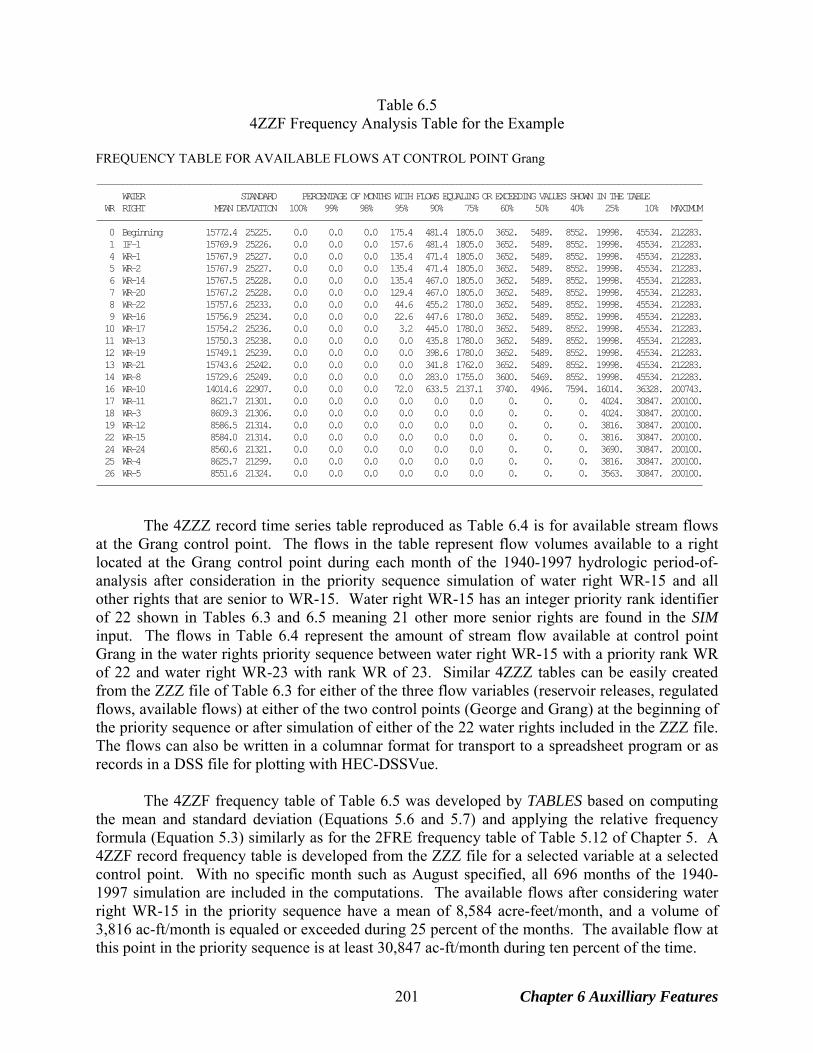
Table 6.5 4ZZF Frequency Analysis Table for the Example
FREQUENCY TABLE FOR AVAILABLE FLOWS AT CONTROL POINT Grang ------------------------------------------------------------------------------------------------------------------------------------------ WATER STANDARD PERCENTAGE OF MONTHS WITH FLOWS EQUALING OR EXCEEDING VALUES SHOWN IN THE TABLE WR RIGHT MEAN DEVIATION 100% 99% 98% 95% 90% 75% 60% 50% 40% 25% 10% MAXIMUM ------------------------------------------------------------------------------------------------------------------------------------------ 0 Beginning 15772.4 25225. 0.0 0.0 0.0 175.4 481.4 1805.0 3652. 5489. 8552. 19998. 45534. 212283. 1 IF-1 15769.9 25226. 0.0 0.0 0.0 157.6 481.4 1805.0 3652. 5489. 8552. 19998. 45534. 212283. 4 WR-1 15767.9 25227. 0.0 0.0 0.0 135.4 471.4 1805.0 3652. 5489. 8552. 19998. 45534. 212283. 5 WR-2 15767.9 25227. 0.0 0.0 0.0 135.4 471.4 1805.0 3652. 5489. 8552. 19998. 45534. 212283. 6 WR-14 15767.5 25228. 0.0 0.0 0.0 135.4 467.0 1805.0 3652. 5489. 8552. 19998. 45534. 212283. 7 WR-20 15767.2 25228. 0.0 0.0 0.0 129.4 467.0 1805.0 3652. 5489. 8552. 19998. 45534. 212283. 8 WR-22 15757.6 25233. 0.0 0.0 0.0 44.6 455.2 1780.0 3652. 5489. 8552. 19998. 45534. 212283. 9 WR-16 15756.9 25234. 0.0 0.0 0.0 22.6 447.6 1780.0 3652. 5489. 8552. 19998. 45534. 212283. 10 WR-17 15754.2 25236. 0.0 0.0 0.0 3.2 445.0 1780.0 3652. 5489. 8552. 19998. 45534. 212283. 11 WR-13 15750.3 25238. 0.0 0.0 0.0 0.0 435.8 1780.0 3652. 5489. 8552. 19998. 45534. 212283. 12 WR-19 15749.1 25239. 0.0 0.0 0.0 0.0 398.6 1780.0 3652. 5489. 8552. 19998. 45534. 212283. 13 WR-21 15743.6 25242. 0.0 0.0 0.0 0.0 341.8 1762.0 3652. 5489. 8552. 19998. 45534. 212283. 14 WR-8 15729.6 25249. 0.0 0.0 0.0 0.0 283.0 1755.0 3600. 5469. 8552. 19998. 45534. 212283. 16 WR-10 14014.6 22907. 0.0 0.0 0.0 72.0 633.5 2137.1 3740. 4946. 7594. 16014. 36328. 200743. 17 WR-11 8621.7 21301. 0.0 0.0 0.0 0.0 0.0 0.0 0. 0. 0. 4024. 30847. 200100. 18 WR-3 8609.3 21306. 0.0 0.0 0.0 0.0 0.0 0.0 0. 0. 0. 4024. 30847. 200100. 19 WR-12 8586.5 21314. 0.0 0.0 0.0 0.0 0.0 0.0 0. 0. 0. 3816. 30847. 200100. 22 WR-15 8584.0 21314. 0.0 0.0 0.0 0.0 0.0 0.0 0. 0. 0. 3816. 30847. 200100. 24 WR-24 8560.6 21321. 0.0 0.0 0.0 0.0 0.0 0.0 0. 0. 0. 3690. 30847. 200100. 25 WR-4 8625.7 21299. 0.0 0.0 0.0 0.0 0.0 0.0 0. 0. 0. 3816. 30847. 200100. 26 WR-5 8551.6 21324. 0.0 0.0 0.0 0.0 0.0 0.0 0. 0. 0. 3563. 30847. 200100. ------------------------------------------------------------------------------------------------------------------------------------------
The 4ZZZ record time series table reproduced as Table 6.4 is for available stream flows at the Grang control point. The flows in the table represent flow volumes available to a right located at the Grang control point during each month of the 1940-1997 hydrologic period-of-analysis after consideration in the priority sequence simulation of water right WR-15 and all other rights that are senior to WR-15. Water right WR-15 has an integer priority rank identifier of 22 shown in Tables 6.3 and 6.5 meaning 21 other more senior rights are found in the SIM input. The flows in Table 6.4 represent the amount of stream flow available at control point Grang in the water rights priority sequence between water right WR-15 with a priority rank WR of 22 and water right WR-23 with rank WR of 23. Similar 4ZZZ tables can be easily created from the ZZZ file of Table 6.3 for either of the three flow variables (reservoir releases, regulated flows, available flows) at either of the two control points (George and Grang) at the beginning of the priority sequence or after simulation of either of the 22 water rights included in the ZZZ file. The flows can also be written in a columnar format for transport to a spreadsheet program or as records in a DSS file for plotting with HEC-DSSVue. The 4ZZF frequency table of Table 6.5 was developed by TABLES based on computing the mean and standard deviation (Equations 5.6 and 5.7) and applying the relative frequency formula (Equation 5.3) similarly as for the 2FRE frequency table of Table 5.12 of Chapter 5. A 4ZZF record frequency table is developed from the ZZZ file for a selected variable at a selected control point. With no specific month such as August specified, all 696 months of the 1940-1997 simulation are included in the computations. The available flows after considering water right WR-15 in the priority sequence have a mean of 8,584 acre-feet/month, and a volume of 3,816 ac-ft/month is equaled or exceeded during 25 percent of the months. The available flow at this point in the priority sequence is at least 30,847 ac-ft/month during ten percent of the time.
Chapter 6 Auxilliary Features 201
Beginning-Ending Storage Options
SIM has several options for specifying storage content of each reservoir at the beginning of the simulation. The default beginning-of-simulation storage content is the maximum storage capacity entered on a WS record for a water right associated with the reservoir. Optionally, the initial storage content may be entered on the WS record for each reservoir. If not otherwise specified, the storage at the beginning of the simulation is set equal to the reservoir storage capacity by default.
SIM also includes a set of beginning-ending storage (BES) options activated by an entry
on the JO record. The BES options provide capabilities for setting beginning storages for numerous reservoirs more conveniently than using the WS record for each individual reservoir. Though setting beginning storages for other types of applications may be useful as well, the beginning-ending storage (BES) feature is motivated primarily by situations in which beginning storage is set equal to ending storage.
In past Texas WAM System applications of WRAP, beginning-of-simulation reservoir
storage has typically been set at capacity for all reservoirs. The hydrologic period of analysis has been selected to begin with a series of relative wet years during which the assumption of initially full reservoirs is reasonable. However, beginning-of-simulation storage may be an issue in some applications. The initial storage content less the storage content at the end of the simulation represents extra water that could result in estimated reliabilities being higher than they should.
The BES feature is based on setting beginning and ending storages equal, which reflects
the concept of a cycling hydrologic simulation period. A fixed simulation period is assumed to conceptually repeat forever. For example, hydrology may be represented by a set of naturalized flows and evaporation rates covering a 1940-2007 period-of-analysis. The 68-year hydrologic sequence is assumed to repeat forever. The sequences of naturalized flows and evaporation rates starting in January 1940 are assumed to repetitively follow completion of the sequences in December 2007. Cycling results in a steady state condition with the storages at the beginning and ending of the 68 year hydrologic cycle being identical. The cycling premise is incorporated into models by setting the storages at the beginning and ending of the simulation equal.
One approach for setting the beginning and ending storages equal is to perform the simulation two or more times. The first simulation is based on assumed beginning storages, such as assuming reservoirs are full to capacity. For the second and subsequent (as needed) simulations, the beginning storage is set equal to ending storage from the previous simulation. One iteration may be sufficient to achieve the same beginning and ending storage conditions in some cases. Additional iterations may be necessary. The beginning-ending storage (BES) switch on the JO record activates options that are based on an initial simulation just to determine the storage at the end of the simulation. A second simulation begins with the beginning storages set equal to these ending storages. The ending storages may be recorded in a file and read as beginning storages with the process manually repeated iteratively. A second simulation may also be repeated automatically within SIM either with or without recording the storages in a BES file. Thus, the model user can quickly run SIM multiple times to iteratively determine a set of beginning storage content levels that result in the simulation ending with the same storage levels.
Chapter 6 Auxilliary Features 202
SIM also has options in which diversion return flows and hydropower releases are returned to the stream system the next month after the water supply diversion or hydropower release occurs. The BES options include a feature that also cycles the next-month option return flows and hydropower releases. The flows from the last month of the initial simulation re-enter the stream system at the beginning of the repeat simulation. The beginning-ending storage options are selected by the parameter BES in JO record field 5. The six alternative options are as follows.
1. BES of 1 specifies that the storage content of each reservoir at the end of the simulation be written to a file with the filename extension BES.
2. BES of 2 specifies that initial storages at the beginning of the simulation be read from the
BES file.
3. For BES = 3, the storages at the beginning of the simulation are read from the BES file, and the storages at the end of the simulation are written to the BES file. Thus, option 3 combines options 1 and 2.
4. With BES = 4, the simulation is performed twice; the storages at the end of the first
simulation are written to the BES file; and the storages at the beginning of the second simulation are read from the BES file. Thus, the storages at the beginning of the second simulation are set equal to the storages at the end of the first simulation. The BES file contains the storages at the end of the first simulation and beginning of the second simulation. The final output file contains the results of the second simulation.
5. BES = 5 performs a dual simulation identical to option 5 except the BES file is not
created. The storages at the end of the first simulation become the storages at the beginning of the first simulation without being written to a file.
6. BES = 6 creates a listing with reservoir-related water rights information added that cannot
be read by SIM, but rather is designed just for information for the model-user. BES options 4 and 5 also address return flows and hydropower releases. With the next-month return flow and next-month hydropower options in effect, BES options 4 and 5 return the return flows at the end of the simulation back to the beginning. Options 1, 2, 3, and 4 involve writing ending storages to a file and/or reading beginning storages from the file. Using options 1, 2, and 3, two or more simulations may be performed by repeated runs of WRAP-SIM. Options 4 and 5 involve an automatic second simulation with second simulation beginning storages set equal to the storages at the end of the first simulation. Options 4 and 5 also return next-month option hydropower releases and return flows from the end of the simulation back to the beginning. All options except option 5 require activation of a BES file, which is opened automatically. A BES file written by SIM includes all reservoirs listed in the conventional order established when the DAT file was read. A BES file read by SIM may include any number of the reservoirs but they must be listed in the order of the numeric identifiers. The BES file may be
Chapter 6 Auxilliary Features 203

manually edited to change storage amounts or delete/add reservoirs. A reservoir may be removed either by entering a −1 for its storage amount or by deleting its entry from the file. If a BES file is read, for any reservoirs not included in the file, beginning storages are set by WS record fields 3 and 8 in the conventional manner.
Tables Summarizing Water Right, Control Point, or Reservoir Input Data Organizing the SIM input data into easier-to-read tables is often useful for display and analysis purposes. Use of the program TABLES is covered in Chapter 4 of the Users Manual. Though most TABLES routines deal with SIM simulation results, TABLES Type 1 input records create tables that organize the data read from a SIM input DAT file.
A 1SUM record builds a water rights summary table with the number or rights, diversion targets, number of reservoirs, storage capacities, and priority ranges summed optionally by control point, water use type, water right type, or specified water right groupings. The 1SRT record provides a tabulation of water rights listed in priority order with pertinent data for each right. The 1SRT tabulation is typically much longer than the 1SUM table since a row of data is included for each individual water right rather than for water right groupings. Control point data are provided on CP records that may be stored in the DAT input file in any order. The TABLES 1CPT record activates a routine that rearranges control point records in upstream-to-downstream order. The rearranged CP records may be written to a file with no change other than the re-sequencing. Options are also provided to build tables of pertinent information for the control points listed in upstream-to-downstream order. The SIM beginning reservoir storage BRS file activated by a switch on the JO record is a tabulation with the following four columns: (1) reservoir identifier, (2) control point location, (3) storage capacity, and (4) beginning-of-simulation storage content. The BRS file is designed to provide beginning storage contents for program SALT and a TABLES conditional reliability modeling routine, both described in the Supplemental Manual. However, the reservoir storage table may also be useful for general information.
General Framework for Applying WRAP WRAP is a flexible modeling system that can be applied in various ways depending on the particular situation. Conventional strategies for applying the WRAP programs SIM and TABLES adopted in the past are briefly discussed in this section. The next and last section of this chapter outlines newer proposed approaches for combining SIM and HYD in developing hydrology datasets that have not yet been routinely applied. The Water Availability Modeling (WAM) System discussed in Chapter 1 combines the generalized WRAP and input datasets listed in Table 1.2 for all of the river basins of Texas. Implementation of the WAM System during 1997-2003 consisted of developing input datasets and modeling a specified set of water management and use scenarios for each of the river basins. The WRAP programs were greatly expanded and improved in response to challenges encountered and experience gained in modeling the diverse individual river basins of the state.
Chapter 6 Auxilliary Features 204
The SIM and TABLES features outlined in this Reference Manual and companion Users Manual have been extensively applied by the water management community in Texas. Most of the features outlined in Chapters 1 through 5 of this Reference Manual are in routine use. However, the additional more recently developed modeling capabilities documented by the Supplemental Manual have not yet as of March 2008 reached the stage of being routinely applied. The WRAP features covered in the Supplemental Manual are purposely documented separately and are not addressed in this Reference Manual and accompanying Users Manual.
WRAP is routinely applied in regional and statewide planning studies and water rights regulatory activities in Texas using the input datasets from the TCEQ WAM System. WRAP users employed by water agencies, consulting firms, and universities modify these data files to model the alternative water resources development projects, river regulation strategies, and water use scenarios being investigated in their studies. The WAM System datasets are periodically updated by the Texas Commission on Environmental Quality (TCEQ) to reflect changes in water right permits and water management practices and refinements in modeling capabilities.
WRAP is applicable essentially any place in the world for modeling a comprehensive range of water resources development, management, and allocation practices and river/reservoir system configurations and operations. For river basins outside of Texas, model users must develop the input datasets required for their particular applications. New and different input datasets may also be developed for different types of applications in Texas.
Developing a SIM simulation input dataset can be a major effort. The program HYD is designed to assist in developing the hydrology files of stream flows and net evaporation-precipitation depths for the SIM input dataset. Most of the hydrology datasets for the Texas WAM System were completed prior to completion of the program HYD. Microsoft Excel was used for most of the computational tasks that have since been incorporated into HYD. The original program WRAP-HYD developed during 1998-2000 was significantly improved during 2007-2008. Potential new applications for HYD are discussed in the next section of this chapter.
A simulation study typically involves many executions of SIM and TABLES modeling alternative water resources development, management, allocation, and use scenarios. The river/reservoir system is simulated with SIM with the results reorganized with TABLES for display and analysis purposes. The primary SIM simulation time series results recorded in the OUT file are input to TABLES to perform user-specified reliability, frequency, water accounting, and other analyses. The same SIM simulation time series output is optionally recorded in a SIM DSS output file for transfer to HEC-DSSVue for plotting graphs or other analysis. Options in TABLES also allow SIM output with or without further TABLES adjustments to be transported to HEC-DSSVue. The simulation results may also be transferred to ArcGIS for spatial display. The preceding Chapter 5 focuses on the time series variables of SIM simulation results stored in the OUT, SOU, and DSS output files and TABLES capabilities for reorganizing these data and performing frequency, reliability, and water budget analyses. The preceding sections of Chapter 6 discuss organization and analyses of SIM simulation results associated with other SIM output files. The following final section of Chapter 6 addresses other innovative ways of using SIM simulation results in an OUT file with HYD to further expand modeling capabilities.
Chapter 6 Auxilliary Features 205
HYD Stream Flow Adjustments Using SIM Simulation Results to Develop SIM Hydrology Datasets
Program HYD capabilities are outlined in Chapter 3 of this Reference Manual and Chapter 5 of the Users Manual. HYD is a set of routines designed to assist in developing hydrology input datasets for SIM. The description of HYD features in Chapter 3 of this Reference Manual is primarily from the perspective of conventional applications in which SIM input files of naturalized stream flows and evaporation-precipitation depths are developed prior to application of SIM and thus without reference to SIM simulation results. The following discussion deals with special applications in which SIM simulation results from an OUT output file are incorporated in developing SIM hydrology input data. The following two types of applications are discussed.
• extension of the hydrologic period-of-analysis • development of simplified datasets with a reduced
number of control points, water rights, and reservoirs Extending the Hydrologic Period-of-Analysis
The hydrologic simulation periods for the Texas Water Availability Modeling (WAM) System datasets listed in Table 1.2 of Chapter 1 all begin in either 1934, 1940, or 1948 and end in either 1989, 1996, 1997, 1998, or 2000. As of March 2008, these original hydrologic periods-of-record had not yet been extended forward toward the present. A possible methodology for extending the naturalized stream flows is outlined in this section. The methodology is based on using an adjusted current use SIM input dataset from the WAM System to convert gaged stream flows to naturalized flows. The WAM System current use scenario is defined in Chapter 1. Capabilities are incorporated in HYD for performing the computations necessary to implement this strategy. The naturalized flow datasets for the Texas WAM System were originally developed by adjusting observed flows at gaging stations to remove the effects of historical reservoir storage and operations, water supply diversions, return flows from diversions from surface and ground water sources, and other factors. This same approach could be adopted for extending the period-of-analysis covered by the naturalized flows. Program HYD provides capabilities for performing the computations. However, much time and effort is required to compile and manipulate the voluminous data describing actual water management and use that is required for the flow adjustments. The objective of the alternative approach outlined below is to greatly reduce the required effort by using the existing current use scenario datasets from the TCEQ WAM System.
As an example to illustrate this alternative procedure, assume that the hydrologic simulation period is 1940 through 1997 for a particular river basin. Our hypothetical example dataset has about 1,000 control points of which 50 are primary control points with naturalized flows provided in the SIM input. The task addressed here is to develop naturalized monthly flows at the 50 primary control points for the period 1998-2007.
A proposed procedure for extending a naturalized flow dataset to cover the period 1998-2007 at pertinent primary control points consists of combining two datasets.
Chapter 6 Auxilliary Features 206
• 1998-2007 sequences of monthly flows at pertinent gaging stations compiled from available USGS gage records of observed daily flows
• SIM input DAT file representing 1998-2007 actual water management and use developed based on modifying the TCEQ WAM System current use input dataset
The procedure consists of iteratively adjusting gaged flows at USGS gaging stations with the differences between naturalized (unregulated) flows and regulated flows from a SIM simulation with a modified current use dataset. An iterative procedure is required because naturalized flows are computed as a function of flow adjustments but the flow adjustments are computed as a function of naturalized flows. The iterative procedure begins with a statistically based set of 1998-2007 naturalized flows determined from the 1940-1997 naturalized flows that serves the sole purpose of determining an initial estimate of flow adjustments which are later updated. The SIM simulation with the modified current use DAT input file serves the sole purpose of computing regulated flows allowing the differences between naturalized and regulated flows to be computed for use as adjustments in converting gaged flows to naturalized flows. The accuracy of the procedure depends upon the accuracy of the flow differences rather the accuracy of the naturalized and regulated flows themselves. The flows are defined as followed.
naturalized (unregulated) flows − gaged flows adjusted to remove the effects of water resources development, management, and use. Naturalized or unregulated stream flows represent natural conditions without the effects of the human activities modeled by the information contained in the SIM input DAT file.
regulated flows − flows computed by SIM by adjusting naturalized flows for the effects of the human activities modeled by the information contained in a SIM input DAT file. Regulated flows are the actual flows at a site which would be measured by a stream flow gage if the information in the SIM input file perfectly modeled actual water resources development, management, and use during each month of the simulation.
The difference between the naturalized flows provided as input to a SIM simulation and the regulated flows computed by the SIM simulation is the summation of stream flow depletions, return flows, reservoir releases, inflows or outflows from constant inflow CI records or flow adjustment FA records which are each appropriately cascaded to downstream control points while accounting for channel losses. Thus, the SIM variables represented by the differences between regulated and unregulated (naturalized) flows are defined as follows.
stream flow depletion − volume appropriated by a water right to meet diversion requirements and/or refill reservoir storage while also accounting for evaporation
return flow − portion of stream flow depletion that is returned to the stream
reservoir releases − those releases from reservoir storage made specifically for a water right to meet a diversion, instream flow, or refilling target at a control point located further downstream or releases for hydroelectric energy generation
other inflows − inflows representing water supply return flows, interbasin transport, or other considerations that are input on CI and/or FA records
Chapter 6 Auxilliary Features 207
The difference between regulated and naturalized flows at a particular control point consist of the accumulation of stream flow depletions, return flows, reservoir releases, and CI and FA record flows occurring at that control point and all upstream control points properly cascaded downstream with adjustments for channel losses. Thus, the accuracy of the flow adjustments in the proposed flow extension procedure is basically the accuracy of the SIM computation of stream flow depletions, return flows, and reservoir releases.
Subtracting regulated flows from naturalized flows at a control point may result in positive differences in some months and negative differences in other months. The naturalized less regulated flow difference is usually positive if stream flow depletions exceed return flows and upstream reservoir releases and negative otherwise.
Regulated flows are computed from a set of naturalized flows, but regulated flows are required for the flow adjustments (naturalized − regulated flows) used to determine the naturalized flows. Thus, an iterative procedure is required. An initial set of adjustments is developed based on an initial approximation of naturalized flows. These initial flow adjustments are used to convert gaged flows to naturalized flows, which are then used to develop a better estimate of flow adjustments. Program HYD can be used to perform the computations.
The proposed procedure for extending a naturalized flow dataset to cover the period 1998-2007 at pertinent primary control points includes the following tasks. 1. Available gaged daily flow data for 1998-2007 at gaging stations are compiled and
aggregated to monthly flows. HEC-DSSVue may be used to assist with this task. 2. A set of 1998-2007 monthly net evaporation-precipitation depths are compiled for all
pertinent control points that have reservoirs. 3. An actual use SIM input dataset is developed that has a 1998-2007 simulation period. The
original current use water rights input dataset already approximates 1998-2007 conditions of water management and use but is modified to further improve the representation of actual 1998-2007 water management/use. Although the current use DAT file may be used with minimal or no modifications, the following adjustments will improve accuracy in better representing actual 1998-2007 water management and use.
• The upstream-to-downstream natural priority option may be adopted to replace the permit priorities. This is a simple option switch in SIM.
• Beginning of 1998-2007 simulation reservoir storage volumes are compiled as follows. A SIM execution of the modified dataset with the 1940-1997 hydrology results in end-of-simulation December 2007 storage volumes for the many reservoirs. These amounts are used to set the beginning of January 1998 reservoir storage using the SIM beginning reservoir storage (BRS) option. For the larger reservoirs, available observations from gage records are used to replace the SIM simulated beginning of January 1998 storage volumes. These are the beginning-of-simulation reservoir storage volumes for the 1998-2007 SIM simulation DAT file.
• For the larger reservoirs with readily available gaged sequences of 1998-2007 end-of-month storage volume observations, the actual storages for all months are incorporated
Chapter 6 Auxilliary Features 208
into the SIM DAT file with the type 7 storage right feature combined with TS record sequences of the actual 1998-2007 gaged storage volumes.
• Diversion targets and return flows in the DAT file are not changed for many of the water rights due to lack of data, the effort required to update, and minimal impact on final results. However, considering data availability, any number of the larger diversion targets and return flow specifications may be updated with actual 1998-2007 observations. The time series of updated diversions may be entered on TS records or alternatively representative annual targets may be entered on WR records.
• Any other modifications may be made to the DAT file dataset to more closely model actual 1998-2007 water management and use.
4. A FLO file with 1998-2007 naturalized flows is required for the SIM input dataset.
However, 1998-2007 naturalized flows are the unknown data that the overall procedure is designed to compute. An initial set of 1998-2007 naturalized flows is developed as follows solely for use in developing the initial estimate of flow adjustments. Although mean flows, median flows, or any other exceedance frequency flows could be adopted, the 75 percent exceedance frequency flows are proposed as being reasonably likely flows on the conservatively low side of mean flows. Using the 1940-1997 naturalized flows at a particular control point, the flow volume that is equaled or exceeded in 75% of the 58 years is determined for each of the 12 months January through December. The resulting set of 12 naturalized flow volumes for January−December are repeated for each of the ten years during 1998−2007.
5. The SIM simulation model is executed with the 1998-2007 period-of-analysis input dataset
consisting of the DAT file developed in the preceding Task 3, EVA file from Task 2, and FLO file from Task 4. The objective is to simulate regulated flows that can be used to develop an initial estimate of flow adjustments consisting of naturalized (unregulated) flows minus regulated flows at the pertinent control points.
6. HYD reads the SIM output OUT file developed as Task 5 and the gaged flows from Task 1.
The following computations are performed.
• Flow adjustments are computed as the difference in naturalized flows minus regulated flows read by HYD from the SIM output OUT file.
• Naturalized flows are computed by subtracting the flow adjustments from the gaged flows read by HYD from another HYD input file in either text file or DSS file format.
Task 6 results in a set of 1998-2007 naturalized flows at the pertinent primary control points. The naturalized flows are approximate since the flow adjustments were determined based on the 1998-2007 naturalized flow dataset developed as Task 4 which are statistically based on 1940-1997 historical flows rather than adjustments to 1998-2007 actual gaged flows.
7. The naturalized flows developed in Task 6 above are stored as a FLO or DSS file which
replaces the FLO or DSS file used in Task 5 above. SIM is executed again to obtain an updated set of regulated flows which when differenced with the corresponding latest update of naturalized flows provides a better estimate of flow adjustments.
Chapter 6 Auxilliary Features 209
8. HYD is run again with the new SIM output file from Task 7 and the original gaged flows from Task 1. The following computations previously performed in Task 6 are repeated.
• Flow adjustments are computed by subtracting regulated flows from naturalized flows read by HYD from the SIM output OUT file.
• Naturalized flows are computed by subtracting the flow adjustments from the gaged flows.
The result is a FLO or DSS file with the final naturalized flows for 1998-2007.
Developing a Simplified Input Dataset The larger Texas WAM System datasets listed in Table 1.2 of Chapter 1 contain hundreds of water rights, control points, and reservoirs. These large complex datasets are necessary for the regional and statewide planning and water right permitting applications for which the datasets were developed. However, simpler datasets are advantageous for certain other applications. A methodology is presented here for simplifying SIM input datasets for particular applications. Selected water rights, control points, and reservoirs are removed with their effects retained in the adopted stream inflow input data for the simplified dataset. For example, assume that a large SIM input dataset contains 1,650 diversions, 510 reservoirs, and 2,150 control points. Naturalized flows are input on inflow IN records for 32 primary control points located at gaging stations and distributed within SIM to the other 2,118 ungaged secondary control points. The hydrologic period-of-analysis is 1940-2006. A water management agency operates a system of ten reservoirs in this river basin with 25 water supply diversions occurring at the ten reservoirs and five other downstream control points. This particular system of interest is a component part of the larger complete dataset. A simplified dataset is developed that contains only the 15 control points, 10 reservoirs, and 25 diversion rights. Impacts of the other 500 reservoirs and 1,625 diversion rights are reflected in the IN record river flows developed for the simplified SIM input dataset. The objective is to develop a simplified SIM input dataset for purposes of studying or providing decision support for a particular system, which in this example consists of ten reservoirs and 25 diversions with associated river/reservoir/use system operating rules. The motivation is simply that input datasets and corresponding output datasets with dramatically fewer control points, water rights, and reservoirs are much more manageable to use in modeling studies. The simplified dataset is our example consists of the following SIM input files.
• DAT file with information for ten reservoirs and 25 diversions at 15 control points
• FLO or DSS file with 1940-2006 sequences of monthly flows representing conditions of river system development that includes all of the water rights and associated reservoirs in the original complete DAT file except the 25 diversions and ten reservoirs contained in the simplified dataset DAT file
• EVA or DSS file with 1940-2006 sequences of monthly net evaporation-precipitation depths for the ten control points at which the ten reservoirs are located
Chapter 6 Auxilliary Features 210
The simplified dataset should adopt the same net evaporation-precipitation depths for the ten reservoirs as used in the original complete dataset SIM simulation. SIM includes an option for adjusting net evaporation-precipitation depths for the precipitation runoff from the portion of the watershed covered by the reservoir. In this case, net evaporation-precipitation depths should be obtained from the OUT file for the complete simulation rather than using the original evaporation-precipitation depth input dataset. The accuracy achieved in the development of a simplified dataset can be checked by comparing simulation results with the original complete dataset. The monthly diversion amounts and reliabilities computed for the diversions included in the simplified dataset should be the same as in the simulation with the original complete dataset. Likewise, the 1940-2006 sequences of monthly reservoir storage volumes and regulated and unappropriated stream flows at the 15 control points will be the same. Near perfect correspondence between simulation results with the simplified versus complete datasets should be expected.
The input data vary as follows between the original and simplified SIM input datasets.
• In the original complete input dataset, the stream flows at the 32 primary control points provided on inflow IN records in a FLO file are naturalized flows representing river basin hydrology under natural conditions with no reservoirs and no diversions. The DAT input file contains 2,150 control points, 1,650 diversion rights, and 510 reservoirs. Watershed parameters are provided in a flow distribution DIS file for the 2,118 secondary control points.
• In the simplified input dataset, the stream flows at the 15 primary control points provided on the FLO file IN records represent conditions with the 500 reservoirs and 1,625 diversions that were removed from the DAT file being in operation but without the others that remain in the DAT file. The DAT input file contains 15 control points, 25 diversion rights, and 10 reservoirs. There is no DIS file.
The methodology for developing a simplified dataset is based on developing flows at the selected control points that represent stream inflow amounts available to the selected system that reflect the impacts of all of the water rights and accompanying reservoirs removed from the original complete dataset. Stream flows are provided on IN records in either a FLO input file or a hydrology input DSS file for the simplified dataset. These stream flows represent flows available to the selected system modeled in the water right DAT input file considering the effects of all the other water rights in the river basin contained in the original complete DAT file that are not included in the simplified DAT file. The stream inflows input on IN records in a FLO file or DSS records in a DSS file for the simplified dataset include stream flow depletions made for the selected water rights less return flows plus unappropriated flows. Hydropower releases and reservoir releases made specifically to meet instream flow requirements are also appropriately incorporated in the flows. Summation and cascading operations are applied in developing the stream flow input data. The methodology for developing the stream flow data (FLO or DSS file) for the simplified dataset is outlined as follows.
Chapter 6 Auxilliary Features 211
1. SIM is executed with the original complete dataset.
2. HYD is applied to read pertinent stream flow depletions, return flows, unappropriated flows, and any other pertinent variables from the SIM output OUT file and combine these variables as required to develop the stream flow FLO or DSS input file for the simplified dataset. Combining the time sequences of flow volumes include summations and cascading operations that may include channel losses. HYD reads the necessary control point information from an input file. Options are also provided in HYD for dealing with the issue of computed flows being negative numbers.
Referring again to the example, stream flows developed for the 15 control points consist of the following 1940-2006 sequences of monthly volumes of the following variables obtained from the OUT file created by SIM with the original complete input dataset. The computations can be performed with HYD.
• Stream flow depletions made by each of the 25 water rights with their 10 reservoirs are included in the flows being developed. These flow volumes are placed at the control point of the stream flow depletion and at all downstream control points. Channel losses are considered in cascading the stream flow depletions downstream.
• Return flows from the diversion component of the stream flow depletions are
subtracted from the flows. These flow volumes are placed at the control point at which the return flow is returned to the stream and at all downstream control points. Channel losses are considered in cascading the return flows downstream.
• Unappropriated flows at each of the 15 control points are added to the flows. Since
unappropriated flows are cumulative total flows, these flows are not cascaded downstream
• Any releases from the 10 selected reservoirs made specifically for instream flow
rights are subtracted at the control point of the reservoir and cascaded downstream in the normal manner which includes consideration of channel losses.
• Any hydroelectric power releases from the 10 selected reservoirs are likewise
subtracted at the control point of the reservoir and cascaded downstream in the normal manner which includes consideration of channel losses.
As previously discussed, the accuracy of the procedure is confirmed by reproducing the sequences of monthly diversions, storage contents, regulated flows, unappropriated flows, and other pertinent variables contained in the SIM simulation results associated with the ten reservoirs, 25 diversions, and 15 control points. These SIM simulation results should be same with the simplified dataset versus the original complete dataset. The system of ten reservoirs and 25 diversions must be operated the same in both the simplified and complete datasets for the comparison simulations. After completing the comparison to confirm that the dataset is correct, the simplified dataset can be used to simulate alternative river/reservoir system operating rules and water management and use scenarios for the system of ten reservoirs and associated diversions at the 15 control points.
Chapter 6 Auxilliary Features 212
CHAPTER 7 DETECTING ERRORS AND IRREGULARITES IN DATA FILES
Blunders are inevitable in compiling voluminous input datasets. Detecting and correcting input errors is fundamental to computer modeling. The WRAP programs include features designed to help detect missing and erroneous records in input files. The modeling system features outlined in this chapter facilitate finding many types of errors that violate format rules or result in detectable inconsistencies. However, the discussion in this chapter does not pertain to those situations in which incorrect simulation results are obtained from reasonable but wrong numbers being input in the proper format. The following features of SIM, TABLES, and HYD facilitate locating errors.
• tracking of progress in reading input and performing computations • error messages accompanied by termination of program execution • warning messages alerting users to possible peculiarities without stopping execution
The system for tracing progress and for checking and reporting errors and irregularities is similar in all of the WRAP programs. An array of checking routines is coded into the programs that write error and warning messages. Program execution is terminated in conjunction with error messages but continues with warning messages. The programs all create message files that should be routinely examined by model users.
Locating Errors in SIM Input Data The progress of the SIM simulation is tracked by trace messages written to the monitor and message MSS file. Simulation results are written to the OUT file as computed, providing a mechanism for detailed tracking of the simulation computations. Numerous error and warning checks automatically detect irregularities in input data. Tracking Simulation Progress The following features trace the progress of the SIM simulation.
• Messages appearing on the monitor during model execution provide a general overview of simulation progress.
• Input trace messages written to the message file confirm that various input records were read and various other tasks were accomplished.
• The OUT output file shows intermediate results of the simulation computations. SIM execution begins with an interactive session, which may be managed through WinWRAP, in which the roots of the filenames are entered and the files are opened. The program checks to confirm that the specified files do exist. If an input file is missing, a message to that effect appears on the monitor, and execution is terminated. An optional feature alerts the user if files with the output filenames already exist. The program requests verification from the user that these files are to be overwritten. The messages shown in Table 7.1 then appear on the
Chapter 7 Detecting Errors 213
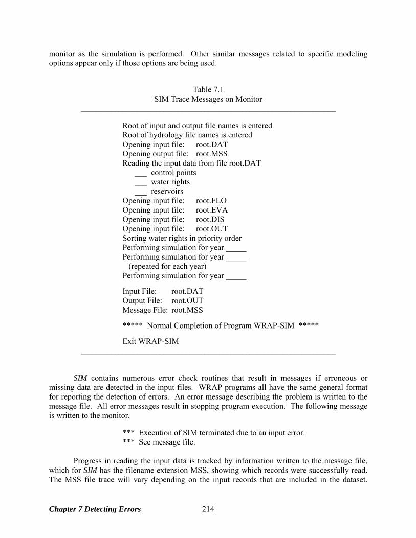
monitor as the simulation is performed. Other similar messages related to specific modeling options appear only if those options are being used.
Table 7.1
SIM Trace Messages on Monitor ____________________________________________________________________
Root of input and output file names is entered Root of hydrology file names is entered Opening input file: root.DAT Opening output file: root.MSS Reading the input data from file root.DAT ___ control points ___ water rights ___ reservoirs Opening input file: root.FLO Opening input file: root.EVA Opening input file: root.DIS Opening input file: root.OUT Sorting water rights in priority order Performing simulation for year _____ Performing simulation for year _____ (repeated for each year) Performing simulation for year _____
Input File: root.DAT Output File: root.OUT Message File: root.MSS
***** Normal Completion of Program WRAP-SIM *****
Exit WRAP-SIM
____________________________________________________________________ SIM contains numerous error check routines that result in messages if erroneous or missing data are detected in the input files. WRAP programs all have the same general format for reporting the detection of errors. An error message describing the problem is written to the message file. All error messages result in stopping program execution. The following message is written to the monitor. *** Execution of SIM terminated due to an input error. *** See message file. Progress in reading the input data is tracked by information written to the message file, which for SIM has the filename extension MSS, showing which records were successfully read. The MSS file trace will vary depending on the input records that are included in the dataset.
Chapter 7 Detecting Errors 214
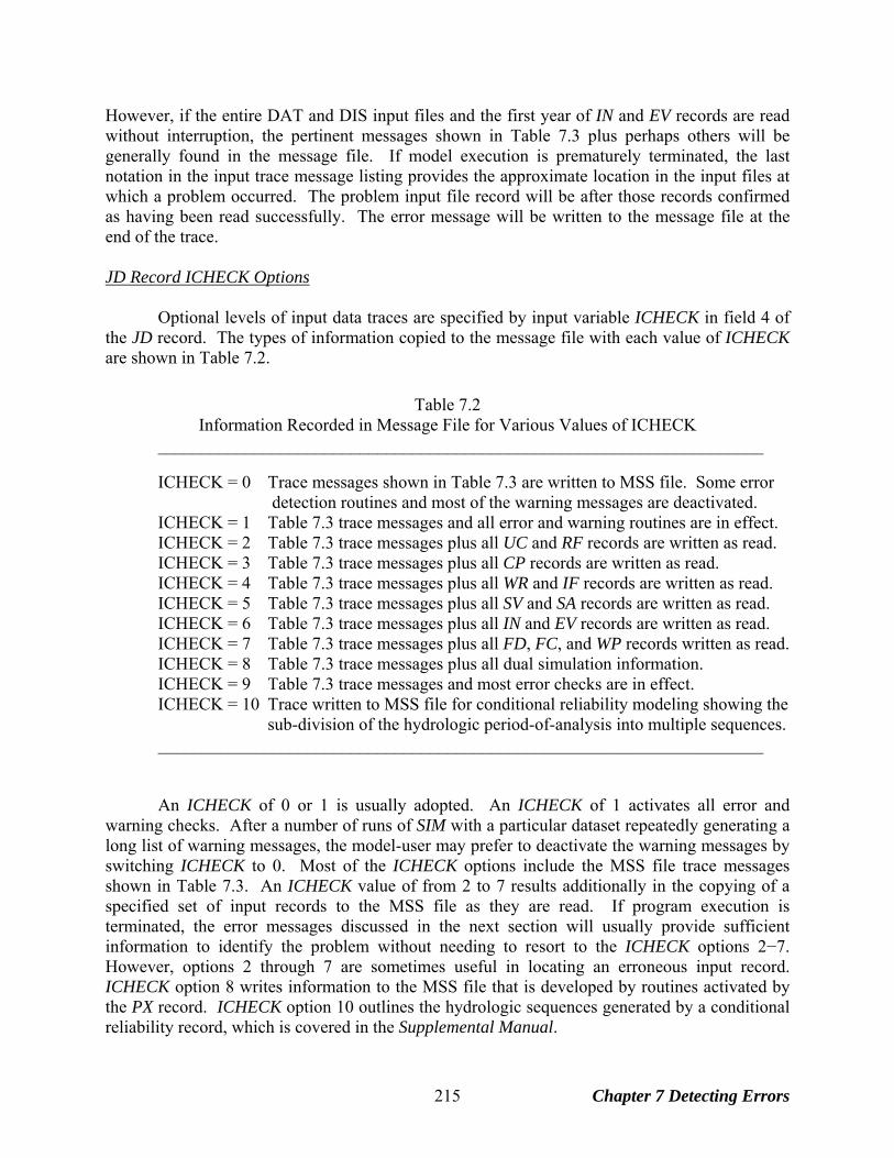
However, if the entire DAT and DIS input files and the first year of IN and EV records are read without interruption, the pertinent messages shown in Table 7.3 plus perhaps others will be generally found in the message file. If model execution is prematurely terminated, the last notation in the input trace message listing provides the approximate location in the input files at which a problem occurred. The problem input file record will be after those records confirmed as having been read successfully. The error message will be written to the message file at the end of the trace. JD Record ICHECK Options Optional levels of input data traces are specified by input variable ICHECK in field 4 of the JD record. The types of information copied to the message file with each value of ICHECK are shown in Table 7.2.
Table 7.2
Information Recorded in Message File for Various Values of ICHECK _____________________________________________________________________ ICHECK = 0 Trace messages shown in Table 7.3 are written to MSS file. Some error detection routines and most of the warning messages are deactivated. ICHECK = 1 Table 7.3 trace messages and all error and warning routines are in effect. ICHECK = 2 Table 7.3 trace messages plus all UC and RF records are written as read. ICHECK = 3 Table 7.3 trace messages plus all CP records are written as read. ICHECK = 4 Table 7.3 trace messages plus all WR and IF records are written as read. ICHECK = 5 Table 7.3 trace messages plus all SV and SA records are written as read. ICHECK = 6 Table 7.3 trace messages plus all IN and EV records are written as read. ICHECK = 7 Table 7.3 trace messages plus all FD, FC, and WP records written as read. ICHECK = 8 Table 7.3 trace messages plus all dual simulation information. ICHECK = 9 Table 7.3 trace messages and most error checks are in effect. ICHECK = 10 Trace written to MSS file for conditional reliability modeling showing the sub-division of the hydrologic period-of-analysis into multiple sequences. _____________________________________________________________________
An ICHECK of 0 or 1 is usually adopted. An ICHECK of 1 activates all error and warning checks. After a number of runs of SIM with a particular dataset repeatedly generating a long list of warning messages, the model-user may prefer to deactivate the warning messages by switching ICHECK to 0. Most of the ICHECK options include the MSS file trace messages shown in Table 7.3. An ICHECK value of from 2 to 7 results additionally in the copying of a specified set of input records to the MSS file as they are read. If program execution is terminated, the error messages discussed in the next section will usually provide sufficient information to identify the problem without needing to resort to the ICHECK options 2−7. However, options 2 through 7 are sometimes useful in locating an erroneous input record. ICHECK option 8 writes information to the MSS file that is developed by routines activated by the PX record. ICHECK option 10 outlines the hydrologic sequences generated by a conditional reliability record, which is covered in the Supplemental Manual.
Chapter 7 Detecting Errors 215
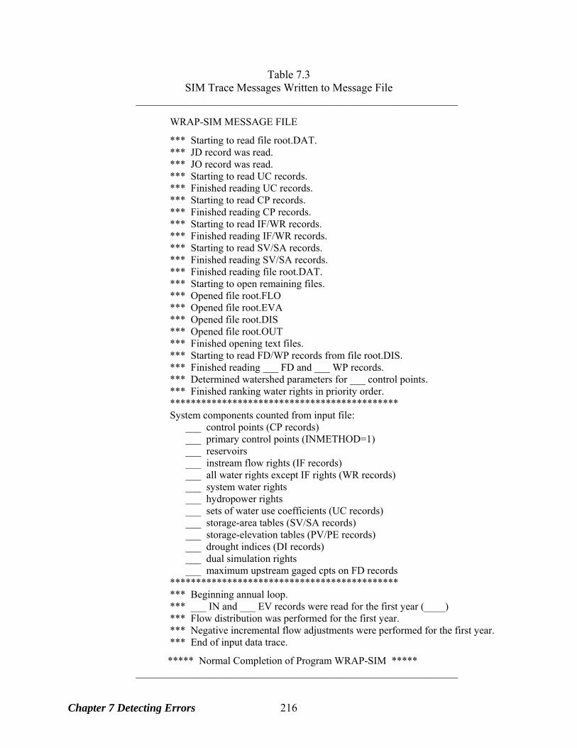
Table 7.3 SIM Trace Messages Written to Message File
______________________________________________________________ WRAP-SIM MESSAGE FILE
*** Starting to read file root.DAT. *** JD record was read. *** JO record was read. *** Starting to read UC records. *** Finished reading UC records. *** Starting to read CP records. *** Finished reading CP records. *** Starting to read IF/WR records. *** Finished reading IF/WR records. *** Starting to read SV/SA records. *** Finished reading SV/SA records. *** Finished reading file root.DAT. *** Starting to open remaining files. *** Opened file root.FLO *** Opened file root.EVA *** Opened file root.DIS *** Opened file root.OUT *** Finished opening text files. *** Starting to read FD/WP records from file root.DIS. *** Finished reading ___ FD and ___ WP records. *** Determined watershed parameters for ___ control points. *** Finished ranking water rights in priority order. ******************************************** System components counted from input file: ___ control points (CP records) ___ primary control points (INMETHOD=1) ___ reservoirs ___ instream flow rights (IF records) ___ all water rights except IF rights (WR records) ___ system water rights ___ hydropower rights ___ sets of water use coefficients (UC records) ___ storage-area tables (SV/SA records) ___ storage-elevation tables (PV/PE records) ___ drought indices (DI records) ___ dual simulation rights ___ maximum upstream gaged cpts on FD records ******************************************** *** Beginning annual loop. *** ___ IN and ___ EV records were read for the first year (____) *** Flow distribution was performed for the first year. *** Negative incremental flow adjustments were performed for the first year. *** End of input data trace.
***** Normal Completion of Program WRAP-SIM ***** ______________________________________________________________
Chapter 7 Detecting Errors 216
An ICHECK of one should normally be selected whenever a new or revised dataset is initially run. If the model runs correctly, changing ICHECK to zero (blank JD record field 4) will save a little computer time by not performing the more time-consuming error checks and deactivating most warning messages. With ICHECK option 1, warning messages may be repeated numerous times resulting in a large MSS file, which may be prevented by switching to option zero. For ICHECK options 2 through 8, most of the error checks for ICHECK=1 are in effect. However, most warning message checks and several of the error checks are in effect only if ICHECK is one. An ICHECK of 9 or 10 will deactivate many warning messages without affecting error checks. Program execution may be terminated due to a problem in an input record. Error messages normally provide sufficient information to locate the problem without the ICHECK options 2 through 7 input record reproduction routines noted in Table 7.2. However, ICHECK options 2−7 provide an additional tool to facilitate finding an erroneous record. SIM reads all the records in sequential order starting with the DAT file. The ICHECK=1 trace is used to find the general location of the problem record based on where the trace stops with an error message. The program is then rerun with a different ICHECK value to check which records in the groups cited in Table 7.2 are read and copied correctly. With ICHECK options 2 through 7, the records are written to the MSS file immediately after each record is read. The records are copied to the MSS file almost verbatim as read, except most real numbers are written in a F8.0 Fortran format with zero digits to the right of the decimal point. If the program reads some but not all records of a particular record type, the problem will typically be associated with either the last record read and copied to the MSS file or more likely the next record in the input file. The types of records listed in Table 7.2 account for many but not all of the records in a SIM input set. ICHECK=6 applies to IN/EV records stored in DAT, FLO/EVA, or DSS files but does not apply to a input file with filename extension HYD. ICHECK option 8 relates to the PX record dual simulation option. ICHECK=8 writes a list of rights with the dual option activated by the PX record and the array of initial simulation stream flow depletions for rights with DUAL options of 3 or 4. Simulation results are written to the main output file (filename extension OUT) both as each individual water right is considered in the priority loop and at the end of each simulation month upon completion of the water rights priority loop. Thus, if execution is terminated after the input is read and the simulation computations begin, the computations can be tracked to approximately the point just before the computational problem. The OUT or SOU file may also be useful in analyzing computational problems that do not terminate execution. Error and Warning Messages All of the WRAP programs have a similar system for managing error and warning checks. Error messages are always accompanied by automatic termination of program execution, but execution continues with warning messages. Various error checks are performed as the input files are read and the simulation computations are performed. If data are missing or in the wrong format or inconsistencies are detected, program execution is stopped and an error
Chapter 7 Detecting Errors 217
message is written to the message MSS file. Warning messages identify potential problems and are also written to the message file, but program execution is not terminated. Warning routines simply write messages without affecting the simulation. Thus, the message file should be checked for warning messages even if the program runs to a normal completion. Error messages in all of the WRAP programs are written with two components. First an individualized statement written to the message file provides information regarding the particular type of error detected. Then a standard message is written to both the monitor and message file followed by termination of program execution. Error messages in all of the programs are generated in two different ways:
1. The Fortran input/output status specifier IOSTAT is included in essentially all of the read statements.
2. Numerous other specific error check algorithms are coded into various
data input and computational routines. If violation of a Fortran rule is indicated by the IOSTAT variable in a read statement, messages are written to the monitor and MSS file along with the program being terminated. IOSTAT errors result in variations of the following message being written to the monitor. *** Execution of SIM terminated due to an input error. *** IOSTAT status variable (error code) = ___ *** ___ record contains data in wrong format. *** End of file was reached without finding data record. *** End of __ record was reached without finding data. *** See message file. The first and last line of the message are displayed on the monitor with any error. The second and one of the three or similar lines are added for IOSTAT errors. When IOSTAT errors occur in reading the DAT file, the following message may be written to the message file along with the last two records read. ERROR: Fortran IOSTAT error occurred reading an input record with identifier CD of ___ IOSTAT status variable = ____
The first 82 characters of each of the last two records read are as follows: The monitor and MSS file messages indicate the value for the IOSTAT variable as defined within the Fortran language compiler. A negative one (−1) means the end of file was reached without finding the data record. A −2 indicates the end of the record was reached without finding the data. A positive integer refers to Fortran error condition messages provided by the compiler. The most common values for the IOSTAT variable are 61 and 64, which mean input data is in the wrong format, such as a letter in a real or integer numeric field or a decimal in an integer field.
Many other error checking routines are coded into SIM with error or warning messages that are written to the message file. Error messages are accompanied by termination of model
Chapter 7 Detecting Errors 218
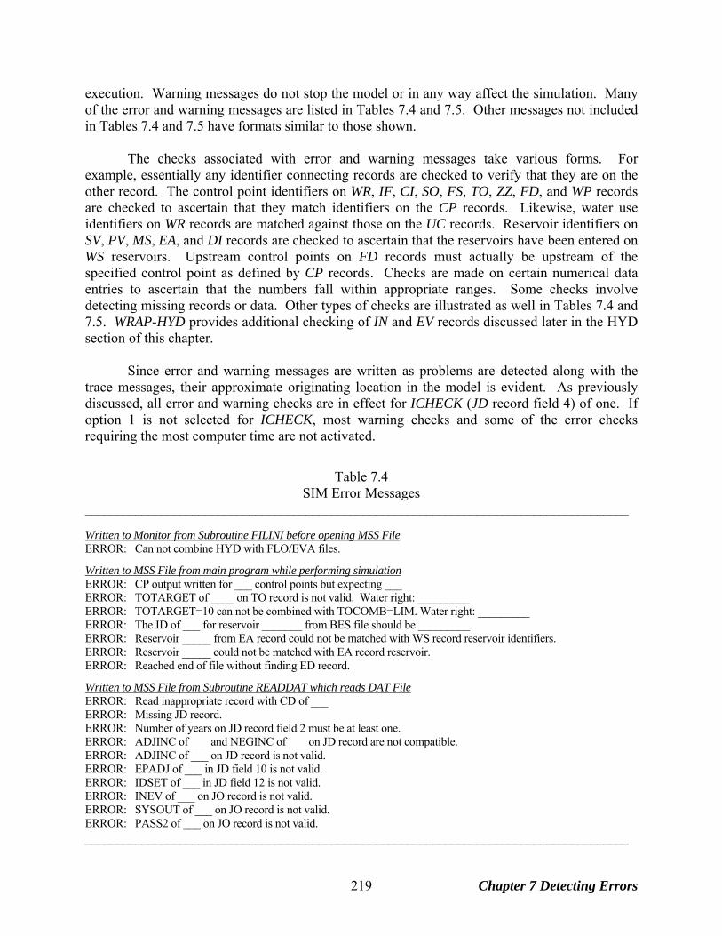
execution. Warning messages do not stop the model or in any way affect the simulation. Many of the error and warning messages are listed in Tables 7.4 and 7.5. Other messages not included in Tables 7.4 and 7.5 have formats similar to those shown.
The checks associated with error and warning messages take various forms. For
example, essentially any identifier connecting records are checked to verify that they are on the other record. The control point identifiers on WR, IF, CI, SO, FS, TO, ZZ, FD, and WP records are checked to ascertain that they match identifiers on the CP records. Likewise, water use identifiers on WR records are matched against those on the UC records. Reservoir identifiers on SV, PV, MS, EA, and DI records are checked to ascertain that the reservoirs have been entered on WS reservoirs. Upstream control points on FD records must actually be upstream of the specified control point as defined by CP records. Checks are made on certain numerical data entries to ascertain that the numbers fall within appropriate ranges. Some checks involve detecting missing records or data. Other types of checks are illustrated as well in Tables 7.4 and 7.5. WRAP-HYD provides additional checking of IN and EV records discussed later in the HYD section of this chapter. Since error and warning messages are written as problems are detected along with the trace messages, their approximate originating location in the model is evident. As previously discussed, all error and warning checks are in effect for ICHECK (JD record field 4) of one. If option 1 is not selected for ICHECK, most warning checks and some of the error checks requiring the most computer time are not activated.
Table 7.4 SIM Error Messages
______________________________________________________________________________________ Written to Monitor from Subroutine FILINI before opening MSS File ERROR: Can not combine HYD with FLO/EVA files.
Written to MSS File from main program while performing simulationERROR: CP output written for ___ control points but expecting ___ ERROR: TOTARGET of ____ on TO record is not valid. Water right: _________ ERROR: TOTARGET=10 can not be combined with TOCOMB=LIM. Water right: _________ ERROR: The ID of ___ for reservoir _______ from BES file should be _________ ERROR: Reservoir _____ from EA record could not be matched with WS record reservoir identifiers. ERROR: Reservoir _____ could not be matched with EA record reservoir. ERROR: Reached end of file without finding ED record.
Written to MSS File from Subroutine READDAT which reads DAT FileERROR: Read inappropriate record with CD of ___ ERROR: Missing JD record. ERROR: Number of years on JD record field 2 must be at least one. ERROR: ADJINC of ___ and NEGINC of ___ on JD record are not compatible. ERROR: ADJINC of ___ on JD record is not valid. ERROR: EPADJ of ___ in JD field 10 is not valid. ERROR: IDSET of ___ in JD field 12 is not valid. ERROR: INEV of ___ on JO record is not valid. ERROR: SYSOUT of ___ on JO record is not valid. ERROR: PASS2 of ___ on JO record is not valid. ______________________________________________________________________________________
Chapter 7 Detecting Errors 219
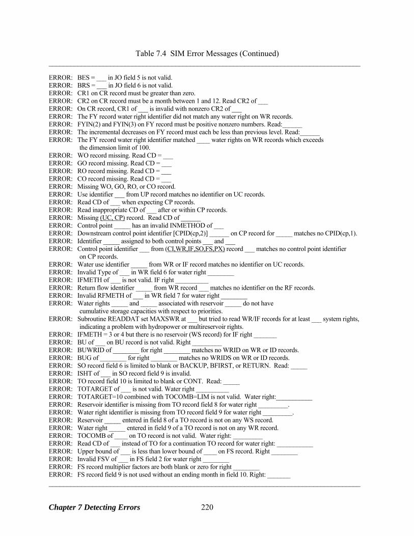
Table 7.4 SIM Error Messages (Continued) ______________________________________________________________________________________ ERROR: BES = ___ in JO field 5 is not valid. ERROR: BRS = ___ in JO field 6 is not valid. ERROR: CR1 on CR record must be greater than zero. ERROR: CR2 on CR record must be a month between 1 and 12. Read CR2 of ___ ERROR: On CR record, CR1 of ___ is invalid with nonzero CR2 of ___ ERROR: The FY record water right identifier did not match any water right on WR records. ERROR: FYIN(2) and FYIN(3) on FY record must be positive nonzero numbers. Read:______ ERROR: The incremental decreases on FY record must each be less than previous level. Read:______ ERROR: The FY record water right identifier matched ____ water rights on WR records which exceeds the dimension limit of 100. ERROR: WO record missing. Read CD = ___ ERROR: GO record missing. Read CD = ___ ERROR: RO record missing. Read CD = ___ ERROR: CO record missing. Read CD = ___ ERROR: Missing WO, GO, RO, or CO record. ERROR: Use identifier ___ from UP record matches no identifier on UC records. ERROR: Read CD of ___ when expecting CP records. ERROR: Read inappropriate CD of ___ after or within CP records. ERROR: Missing (UC, CP) record. Read CD of ______ ERROR: Control point _____ has an invalid INMETHOD of ___ ERROR: Downstream control point identifier [CPID(cp,2)] ______ on CP record for _____ matches no CPID(cp,1). ERROR: Identifier _____ assigned to both control points ___ and ___ ERROR: Control point identifier ___ from (CI,WR,IF,SO,FS,PX) record ___ matches no control point identifier on CP records. ERROR: Water use identifier _____ from WR or IF record matches no identifier on UC records. ERROR: Invalid Type of ___ in WR field 6 for water right ________ ERROR: IFMETH of ___ is not valid. IF right __________ ERROR: Return flow identifier _____ from WR record ___ matches no identifier on the RF records. ERROR: Invalid RFMETH of ___ in WR field 7 for water right ________ ERROR: Water rights _____ and _____ associated with reservoir _____ do not have cumulative storage capacities with respect to priorities. ERROR: Subroutine READDAT set MAXSWR at ___ but tried to read WR/IF records for at least ___ system rights, indicating a problem with hydropower or multireservoir rights. ERROR: IFMETH = 3 or 4 but there is no reservoir (WS record) for IF right _______ ERROR: BU of ___ on BU record is not valid. Right _________ ERROR: BUWRID of ________ for right ________ matches no WRID on WR or ID records. ERROR: BUG of ________ for right ________ matches no WRIDS on WR or ID records. ERROR: SO record field 6 is limited to blank or BACKUP, BFIRST, or RETURN. Read: _____ ERROR: ISHT of ___ in SO record field 9 is invalid. ERROR: TO record field 10 is limited to blank or CONT. Read: _____ ERROR: TOTARGET of ___ is not valid. Water right __________ ERROR: TOTARGET=10 combined with TOCOMB=LIM is not valid. Water right:___________ ERROR: Reservoir identifier is missing from TO record field 8 for water right _________. ERROR: Water right identifier is missing from TO record field 9 for water right _________. ERROR: Reservoir _____ entered in field 8 of a TO record is not on any WS record. ERROR: Water right _____ entered in field 9 of a TO record is not on any WR record. ERROR: TOCOMB of ____ on TO record is not valid. Water right: _________ ERROR: Read CD of ___ instead of TO for a continuation TO record for water right: ___________ ERROR: Upper bound of ___ is less than lower bound of ____ on FS record. Right ________ ERROR: Invalid FSV of ___ in FS field 2 for water right ________ ERROR: FS record multiplier factors are both blank or zero for right ________ ERROR: FS record field 9 is not used without an ending month in field 10. Right: _______ ______________________________________________________________________________________
Chapter 7 Detecting Errors 220
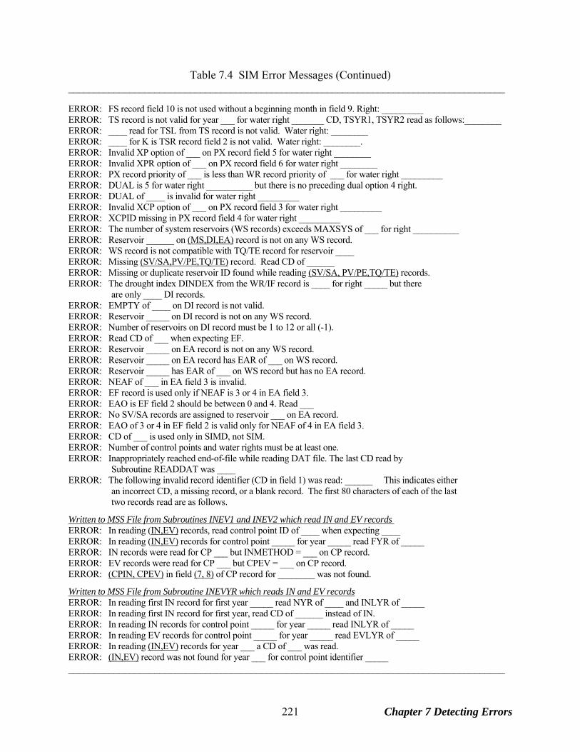
Table 7.4 SIM Error Messages (Continued) ______________________________________________________________________________________ ERROR: FS record field 10 is not used without a beginning month in field 9. Right: _________ ERROR: TS record is not valid for year ___ for water right _______ CD, TSYR1, TSYR2 read as follows:________ ERROR: ____ read for TSL from TS record is not valid. Water right: ________ ERROR: ____ for K is TSR record field 2 is not valid. Water right: ________. ERROR: Invalid XP option of ___ on PX record field 5 for water right ________ ERROR: Invalid XPR option of ___ on PX record field 6 for water right ________ ERROR: PX record priority of ___ is less than WR record priority of ___ for water right _________ ERROR: DUAL is 5 for water right __________ but there is no preceding dual option 4 right. ERROR: DUAL of ____ is invalid for water right _________ ERROR: Invalid XCP option of ___ on PX record field 3 for water right _________ ERROR: XCPID missing in PX record field 4 for water right _________ ERROR: The number of system reservoirs (WS records) exceeds MAXSYS of ___ for right __________ ERROR: Reservoir ______ on (MS,DI,EA) record is not on any WS record. ERROR: WS record is not compatible with TQ/TE record for reservoir ____ ERROR: Missing (SV/SA,PV/PE,TQ/TE) record. Read CD of ______ ERROR: Missing or duplicate reservoir ID found while reading (SV/SA, PV/PE,TQ/TE) records. ERROR: The drought index DINDEX from the WR/IF record is ____ for right _____ but there are only ____ DI records. ERROR: EMPTY of ____ on DI record is not valid. ERROR: Reservoir _____ on DI record is not on any WS record. ERROR: Number of reservoirs on DI record must be 1 to 12 or all (-1). ERROR: Read CD of ___ when expecting EF. ERROR: Reservoir _____ on EA record is not on any WS record. ERROR: Reservoir _____ on EA record has EAR of ___ on WS record. ERROR: Reservoir _____ has EAR of ___ on WS record but has no EA record. ERROR: NEAF of ___ in EA field 3 is invalid. ERROR: EF record is used only if NEAF is 3 or 4 in EA field 3. ERROR: EAO is EF field 2 should be between 0 and 4. Read ___ ERROR: No SV/SA records are assigned to reservoir ___ on EA record. ERROR: EAO of 3 or 4 in EF field 2 is valid only for NEAF of 4 in EA field 3. ERROR: CD of ___ is used only in SIMD, not SIM. ERROR: Number of control points and water rights must be at least one. ERROR: Inappropriately reached end-of-file while reading DAT file. The last CD read by Subroutine READDAT was ____ ERROR: The following invalid record identifier (CD in field 1) was read: ______ This indicates either an incorrect CD, a missing record, or a blank record. The first 80 characters of each of the last two records read are as follows.
Written to MSS File from Subroutines INEV1 and INEV2 which read IN and EV records ERROR: In reading (IN,EV) records, read control point ID of ____ when expecting ____ ERROR: In reading (IN,EV) records for control point _____ for year _____ read FYR of _____ ERROR: IN records were read for CP ___ but INMETHOD = ___ on CP record. ERROR: EV records were read for CP ___ but CPEV = ___ on CP record. ERROR: (CPIN, CPEV) in field (7, 8) of CP record for ________ was not found.
Written to MSS File from Subroutine INEVYR which reads IN and EV recordsERROR: In reading first IN record for first year _____ read NYR of ____ and INLYR of _____ ERROR: In reading first IN record for first year, read CD of ______ instead of IN. ERROR: In reading IN records for control point _____ for year _____ read INLYR of _____ ERROR: In reading EV records for control point _____ for year _____ read EVLYR of _____ ERROR: In reading (IN,EV) records for year ___ a CD of ___ was read. ERROR: (IN,EV) record was not found for year ___ for control point identifier _____ ______________________________________________________________________________________
Chapter 7 Detecting Errors 221
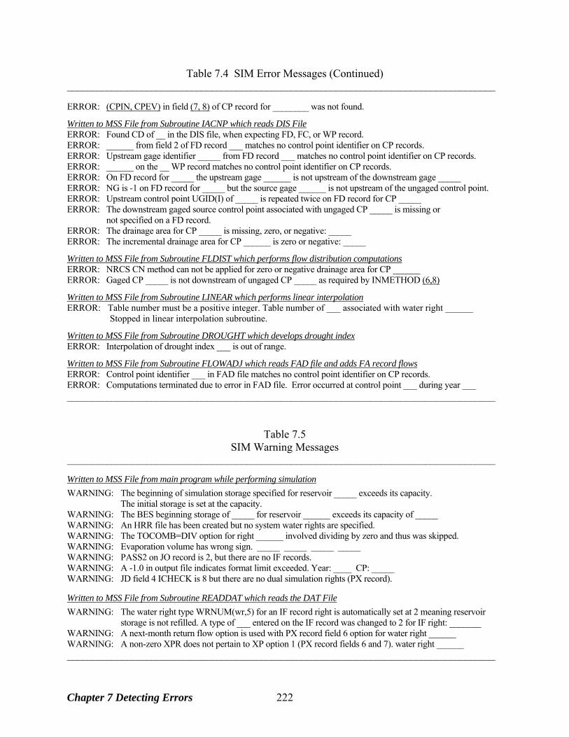
Table 7.4 SIM Error Messages (Continued) ______________________________________________________________________________________ ERROR: (CPIN, CPEV) in field (7, 8) of CP record for ________ was not found.
Written to MSS File from Subroutine IACNP which reads DIS File ERROR: Found CD of __ in the DIS file, when expecting FD, FC, or WP record. ERROR: ______ from field 2 of FD record ___ matches no control point identifier on CP records. ERROR: Upstream gage identifier _____ from FD record ___ matches no control point identifier on CP records. ERROR: ______ on the __ WP record matches no control point identifier on CP records. ERROR: On FD record for _____ the upstream gage ______ is not upstream of the downstream gage _____ ERROR: NG is -1 on FD record for _____ but the source gage ______ is not upstream of the ungaged control point. ERROR: Upstream control point UGID(I) of _____ is repeated twice on FD record for CP _____ ERROR: The downstream gaged source control point associated with ungaged CP _____ is missing or not specified on a FD record. ERROR: The drainage area for CP _____ is missing, zero, or negative: _____ ERROR: The incremental drainage area for CP ______ is zero or negative: _____
Written to MSS File from Subroutine FLDIST which performs flow distribution computations ERROR: NRCS CN method can not be applied for zero or negative drainage area for CP ______ ERROR: Gaged CP _____ is not downstream of ungaged CP _____ as required by INMETHOD (6,8)
Written to MSS File from Subroutine LINEAR which performs linear interpolation ERROR: Table number must be a positive integer. Table number of ___ associated with water right ______ Stopped in linear interpolation subroutine.
Written to MSS File from Subroutine DROUGHT which develops drought index ERROR: Interpolation of drought index ___ is out of range.
Written to MSS File from Subroutine FLOWADJ which reads FAD file and adds FA record flows ERROR: Control point identifier ___ in FAD file matches no control point identifier on CP records. ERROR: Computations terminated due to error in FAD file. Error occurred at control point ___ during year ___ ______________________________________________________________________________________
Table 7.5 SIM Warning Messages
______________________________________________________________________________________ Written to MSS File from main program while performing simulation
WARNING: The beginning of simulation storage specified for reservoir _____ exceeds its capacity. The initial storage is set at the capacity. WARNING: The BES beginning storage of _____ for reservoir ______ exceeds its capacity of _____ WARNING: An HRR file has been created but no system water rights are specified. WARNING: The TOCOMB=DIV option for right ______ involved dividing by zero and thus was skipped. WARNING: Evaporation volume has wrong sign. _____ _____ _____ _____ WARNING: PASS2 on JO record is 2, but there are no IF records. WARNING: A -1.0 in output file indicates format limit exceeded. Year: ____ CP: _____ WARNING: JD field 4 ICHECK is 8 but there are no dual simulation rights (PX record). Written to MSS File from Subroutine READDAT which reads the DAT File
WARNING: The water right type WRNUM(wr,5) for an IF record right is automatically set at 2 meaning reservoir storage is not refilled. A type of ___ entered on the IF record was changed to 2 for IF right: _______ WARNING: A next-month return flow option is used with PX record field 6 option for water right ______ WARNING: A non-zero XPR does not pertain to XP option 1 (PX record fields 6 and 7). water right ______ ______________________________________________________________________________________
Chapter 7 Detecting Errors 222
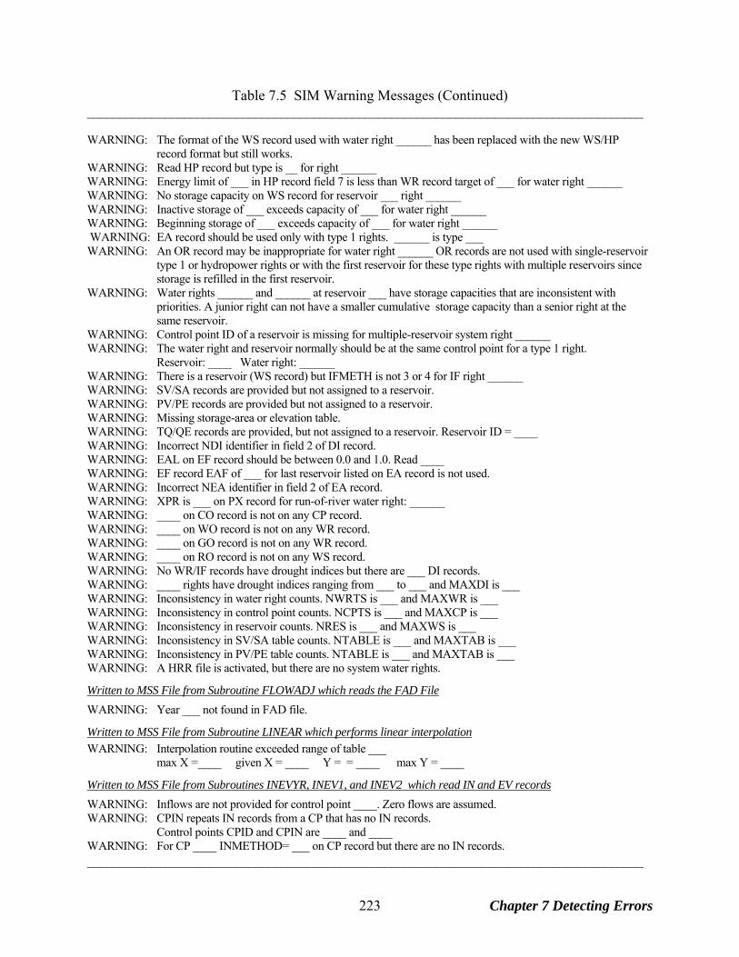
Table 7.5 SIM Warning Messages (Continued) ______________________________________________________________________________________ WARNING: The format of the WS record used with water right ______ has been replaced with the new WS/HP record format but still works. WARNING: Read HP record but type is __ for right ______ WARNING: Energy limit of ___ in HP record field 7 is less than WR record target of ___ for water right ______ WARNING: No storage capacity on WS record for reservoir ___ right ______ WARNING: Inactive storage of ___ exceeds capacity of ___ for water right ______ WARNING: Beginning storage of ___ exceeds capacity of ___ for water right ______ WARNING: EA record should be used only with type 1 rights. ______ is type ___ WARNING: An OR record may be inappropriate for water right ______ OR records are not used with single-reservoir type 1 or hydropower rights or with the first reservoir for these type rights with multiple reservoirs since storage is refilled in the first reservoir. WARNING: Water rights ______ and ______ at reservoir ___ have storage capacities that are inconsistent with priorities. A junior right can not have a smaller cumulative storage capacity than a senior right at the same reservoir. WARNING: Control point ID of a reservoir is missing for multiple-reservoir system right ______ WARNING: The water right and reservoir normally should be at the same control point for a type 1 right. Reservoir: ____ Water right: ______ WARNING: There is a reservoir (WS record) but IFMETH is not 3 or 4 for IF right ______ WARNING: SV/SA records are provided but not assigned to a reservoir. WARNING: PV/PE records are provided but not assigned to a reservoir. WARNING: Missing storage-area or elevation table. WARNING: TQ/QE records are provided, but not assigned to a reservoir. Reservoir ID = ____ WARNING: Incorrect NDI identifier in field 2 of DI record. WARNING: EAL on EF record should be between 0.0 and 1.0. Read ____ WARNING: EF record EAF of ___ for last reservoir listed on EA record is not used. WARNING: Incorrect NEA identifier in field 2 of EA record. WARNING: XPR is ___ on PX record for run-of-river water right: ______ WARNING: ____ on CO record is not on any CP record. WARNING: ____ on WO record is not on any WR record. WARNING: ____ on GO record is not on any WR record. WARNING: ____ on RO record is not on any WS record. WARNING: No WR/IF records have drought indices but there are ___ DI records. WARNING: ____ rights have drought indices ranging from ___ to ___ and MAXDI is ___ WARNING: Inconsistency in water right counts. NWRTS is ___ and MAXWR is ___ WARNING: Inconsistency in control point counts. NCPTS is ___ and MAXCP is ___ WARNING: Inconsistency in reservoir counts. NRES is ___ and MAXWS is ___ WARNING: Inconsistency in SV/SA table counts. NTABLE is ___ and MAXTAB is ___ WARNING: Inconsistency in PV/PE table counts. NTABLE is ___ and MAXTAB is ___ WARNING: A HRR file is activated, but there are no system water rights.
Written to MSS File from Subroutine FLOWADJ which reads the FAD File
WARNING: Year ___ not found in FAD file.
Written to MSS File from Subroutine LINEAR which performs linear interpolation
WARNING: Interpolation routine exceeded range of table ___ max X =____ given X = ____ Y = = ____ max Y = ____
Written to MSS File from Subroutines INEVYR, INEV1, and INEV2 which read IN and EV records
WARNING: Inflows are not provided for control point ____. Zero flows are assumed. WARNING: CPIN repeats IN records from a CP that has no IN records. Control points CPID and CPIN are ____ and ____ WARNING: For CP ____ INMETHOD= ___ on CP record but there are no IN records. ______________________________________________________________________________________
Chapter 7 Detecting Errors 223
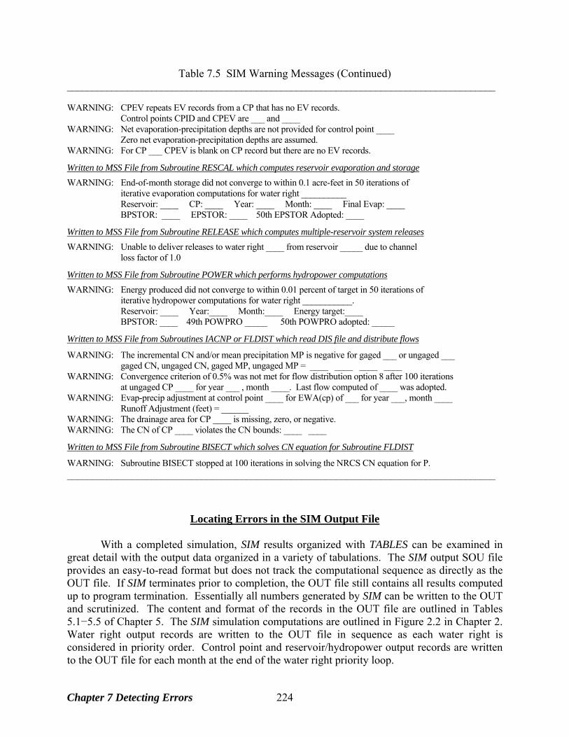
Table 7.5 SIM Warning Messages (Continued) ______________________________________________________________________________________ WARNING: CPEV repeats EV records from a CP that has no EV records. Control points CPID and CPEV are ___ and ____ WARNING: Net evaporation-precipitation depths are not provided for control point ____ Zero net evaporation-precipitation depths are assumed. WARNING: For CP ___ CPEV is blank on CP record but there are no EV records.
Written to MSS File from Subroutine RESCAL which computes reservoir evaporation and storage
WARNING: End-of-month storage did not converge to within 0.1 acre-feet in 50 iterations of iterative evaporation computations for water right __________ Reservoir: ____ CP: ____ Year: ____ Month: ____ Final Evap: ____ BPSTOR: ____ EPSTOR: ____ 50th EPSTOR Adopted: ____
Written to MSS File from Subroutine RELEASE which computes multiple-reservoir system releases
WARNING: Unable to deliver releases to water right ____ from reservoir _____ due to channel loss factor of 1.0
Written to MSS File from Subroutine POWER which performs hydropower computations
WARNING: Energy produced did not converge to within 0.01 percent of target in 50 iterations of iterative hydropower computations for water right ___________. Reservoir: ____ Year:____ Month:____ Energy target:____ BPSTOR: ____ 49th POWPRO _____ 50th POWPRO adopted: _____
Written to MSS File from Subroutines IACNP or FLDIST which read DIS file and distribute flows
WARNING: The incremental CN and/or mean precipitation MP is negative for gaged ___ or ungaged ___ gaged CN, ungaged CN, gaged MP, ungaged MP = ____ ____ ____ ____ WARNING: Convergence criterion of 0.5% was not met for flow distribution option 8 after 100 iterations at ungaged CP ____ for year ___ , month ____. Last flow computed of ____ was adopted. WARNING: Evap-precip adjustment at control point ____ for EWA(cp) of ___ for year ___, month ____ Runoff Adjustment (feet) = ______ WARNING: The drainage area for CP ____ is missing, zero, or negative. WARNING: The CN of CP ____ violates the CN bounds: ____ ____
Written to MSS File from Subroutine BISECT which solves CN equation for Subroutine FLDIST
WARNING: Subroutine BISECT stopped at 100 iterations in solving the NRCS CN equation for P. ______________________________________________________________________________________
Locating Errors in the SIM Output File With a completed simulation, SIM results organized with TABLES can be examined in great detail with the output data organized in a variety of tabulations. The SIM output SOU file provides an easy-to-read format but does not track the computational sequence as directly as the OUT file. If SIM terminates prior to completion, the OUT file still contains all results computed up to program termination. Essentially all numbers generated by SIM can be written to the OUT and scrutinized. The content and format of the records in the OUT file are outlined in Tables 5.1−5.5 of Chapter 5. The SIM simulation computations are outlined in Figure 2.2 in Chapter 2. Water right output records are written to the OUT file in sequence as each water right is considered in priority order. Control point and reservoir/hydropower output records are written to the OUT file for each month at the end of the water right priority loop.
Chapter 7 Detecting Errors 224

The following discussion addresses the situation in which TABLES will not read an OUT file from an apparently successful execution of SIM even though the TABLES input file is completely correct. This situation should be encountered by model users seldom, if ever. After a SIM input dataset has been successfully debugged, irregularities in the SIM output OUT file should be rare. Program TABLES includes a routine activated by the TEST record that performs a series of checks on a SIM output file. The TEST option in TABLES is designed for use in the unusual situation in which TABLES can not read an OUT file from a successful SIM simulation. The following tests are performed. The tests are applicable only to an OUT file created as a text file rather than as the optional unformatted binary file specified by JD record field 7. TABLES reads the first record of the OUT file, and an error message is written to the TMS message file if irregularities are encountered. The problem will most likely be that TABLES is expecting a text file but the OUT file is not an ordinary text file. The only type of text file that can be read by TABLES is an ordinary text file with no enhancements. The Fortran code in SIM always creates a text file in the correct format. However, if the model-user reads the OUT text file with WordPad or some other editor and inadvertently saves the file in another format that adds formatting characters, TABLES will not be able to read the file. The TEST routine will detect the problem. Most of the data in an OUT file are numbers. The TEST routine checks whether letters or other characters appear in the fields that should be numbers. Error messages are written to the TMS file if improper characters are found. The most likely problem is the occurrence of either NaN or ********* in the OUT file. The SIM code includes checks to prevent these situations from occurring. The TABLES TEST routine provides another backup check. The term NaN, meaning not a number, is written by a Fortran program when an arithmetic operation is not defined. The undefined operation is usually dividing by zero. A number can not be divided by zero. The SIM code is written with checks to prevent divisions in which the denominator could be zero. However, if the safeguards fail, a NaN could written to the OUT file and detected by the TABLES TEST routine. Format specifications for the variables written to the OUT file are described in Chapter 5 of the Reference Manual. If a computed number has more digits than is allowed by a Fortran format statement, the number is replaced by the program with asterisks (***********) in the output file. SIM includes safeguards to prevent this situation along with warning messages. However, the TABLES TEST routine will detect asterisks if they occur. The TEST routine also checks that all water right output records in the OUT file are in the correct chronological order by year and month. For control point and reservoir output records, the control point and reservoir identifiers are read for the first month and checked for consistency in all subsequent months. Thus, an incorrect ordering of records or incorrect number of records will be detected. SIM should always write the correct number of records in the proper sequence. However, this test feature provides yet another check in exploring a corrupted file or occurrence of a strange unexplained problem.
Chapter 7 Detecting Errors 225
Locating Errors in TABLES Input Data Instructions for applying the WRAP program TABLES are provided by Chapter 4 of the Users Manual. TABLES is very modular. Operations are controlled by records entered in an input file with filename extension TIN. TABLES reads one record of the TIN input file, performs the specified operations, records the results, and then proceeds to the next record in the TIN file. Trace messages are written to the message TMS file as each TIN file input record is read. Thus, if an input problem occurs, the input record causing the problem is evident. All of the WRAP programs have the same basic system for recording error and warning messages on the monitor and in the message file. TABLES is the same as SIM and HYD in this regard. Checks are embedded in various routines in TABLES. Program execution is terminated with error messages but is not terminated with warning messages.
Locating Errors in HYD Input Data
WRAP-HYD contains features similar to those of WRAP-SIM to help detect missing records or inconsistencies and locate erroneous records that cause program execution to terminate due to illegal computer operations. These features do not pertain to those situations in which reasonable but incorrect data are input in the right format. Tracking Program Progress Tracing the progress of reading input records and performing computations up to program termination may be useful in locating the input record causing the problem. The following HYD features trace the progress of the simulation. HYD execution begins with an interactive session in which the user supplies the root of the input and output filenames, and the files are opened. The program checks whether the specified files exist, writes a message to the monitor if an input file is missing, and allows the user to confirm overwriting of existing output files. The messages shown in Table 7.6 then appear on the monitor as various tasks are performed. Progress is tracked in more detail by notes the program writes to the message file, which has the filename extension HMS. If program execution is terminated prior to completion the specified tasks, the trace messages help locate the input record causing the problem. Optional levels of input data traces are specified by input variable ICHECK in field 4 of the JC record. The basic trace (ICHECK ≥ 0) consists of printing the messages shown in Table 7.7 to the HMS file. Only those messages associated with options included in the HYD application will be written to the message file. If model execution is prematurely terminated, the last message provides the approximate location in the input files at which a problem occurred. Additional information noted in Table 7.7 may also be written to the message file as specified by ICHECK in field 4 of the JC record. The ICHECK = 1 trace shown in Table 7.7 is used to find the general location of the problem record based on where the trace stops. The program is then rerun with a different ICHECK value to check which records in the groups noted in Table 7.7 are read and copied correctly.
Chapter 7 Detecting Errors 226
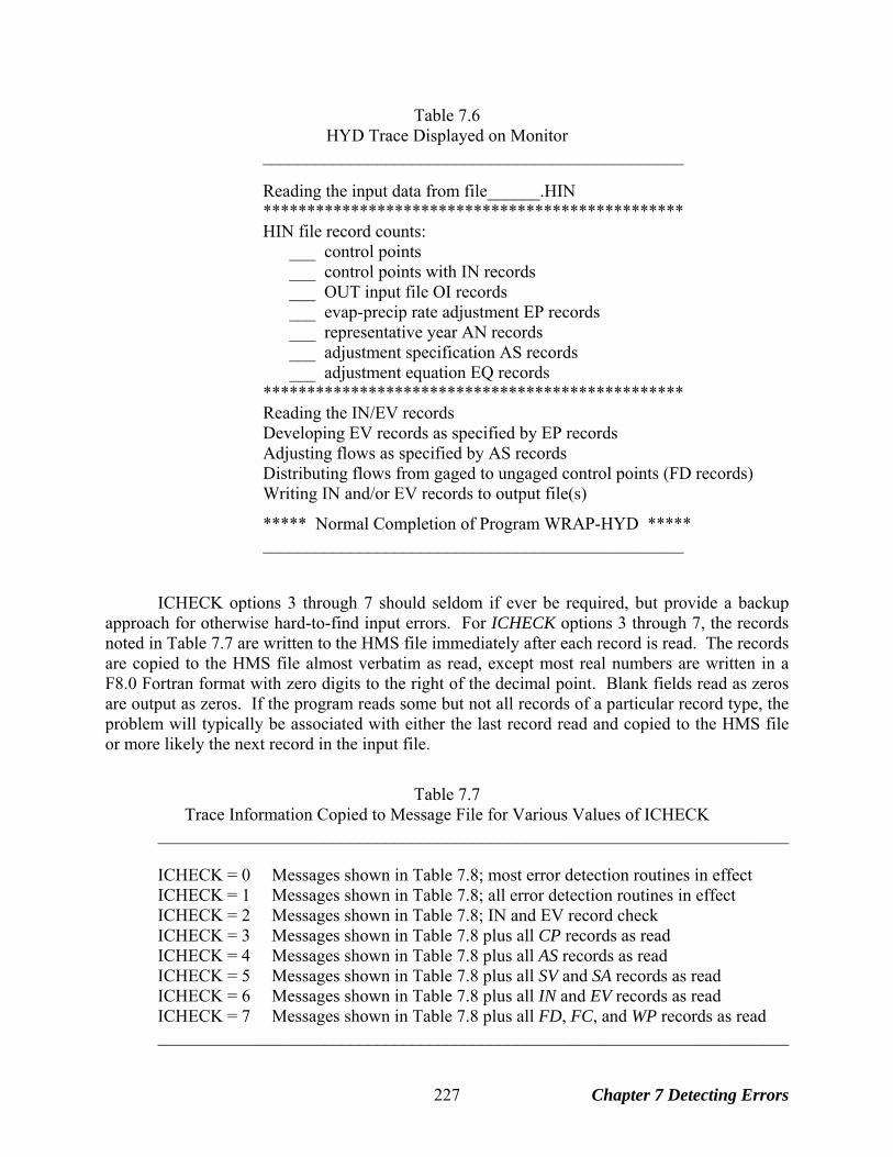
Table 7.6 HYD Trace Displayed on Monitor
________________________________________________
Reading the input data from file______.HIN ************************************************ HIN file record counts: ___ control points ___ control points with IN records ___ OUT input file OI records ___ evap-precip rate adjustment EP records ___ representative year AN records ___ adjustment specification AS records ___ adjustment equation EQ records ************************************************ Reading the IN/EV records Developing EV records as specified by EP records Adjusting flows as specified by AS records Distributing flows from gaged to ungaged control points (FD records) Writing IN and/or EV records to output file(s)
***** Normal Completion of Program WRAP-HYD ***** ________________________________________________
ICHECK options 3 through 7 should seldom if ever be required, but provide a backup approach for otherwise hard-to-find input errors. For ICHECK options 3 through 7, the records noted in Table 7.7 are written to the HMS file immediately after each record is read. The records are copied to the HMS file almost verbatim as read, except most real numbers are written in a F8.0 Fortran format with zero digits to the right of the decimal point. Blank fields read as zeros are output as zeros. If the program reads some but not all records of a particular record type, the problem will typically be associated with either the last record read and copied to the HMS file or more likely the next record in the input file.
Table 7.7
Trace Information Copied to Message File for Various Values of ICHECK ________________________________________________________________________ ICHECK = 0 Messages shown in Table 7.8; most error detection routines in effect ICHECK = 1 Messages shown in Table 7.8; all error detection routines in effect ICHECK = 2 Messages shown in Table 7.8; IN and EV record check ICHECK = 3 Messages shown in Table 7.8 plus all CP records as read ICHECK = 4 Messages shown in Table 7.8 plus all AS records as read ICHECK = 5 Messages shown in Table 7.8 plus all SV and SA records as read ICHECK = 6 Messages shown in Table 7.8 plus all IN and EV records as read ICHECK = 7 Messages shown in Table 7.8 plus all FD, FC, and WP records as read ________________________________________________________________________
Chapter 7 Detecting Errors 227
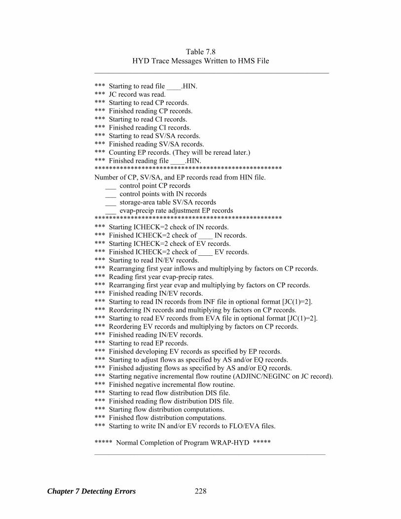
Table 7.8 HYD Trace Messages Written to HMS File
_________________________________________________________________
*** Starting to read file ____.HIN. *** JC record was read. *** Starting to read CP records. *** Finished reading CP records. *** Starting to read CI records. *** Finished reading CI records. *** Starting to read SV/SA records. *** Finished reading SV/SA records. *** Counting EP records. (They will be reread later.) *** Finished reading file ____.HIN. **************************************************** Number of CP, SV/SA, and EP records read from HIN file. ___ control point CP records ___ control points with IN records ___ storage-area table SV/SA records ___ evap-precip rate adjustment EP records **************************************************** *** Starting ICHECK=2 check of IN records. *** Finished ICHECK=2 check of ____ IN records. *** Starting ICHECK=2 check of EV records. *** Finished ICHECK=2 check of ____ EV records. *** Starting to read IN/EV records. *** Rearranging first year inflows and multiplying by factors on CP records. *** Reading first year evap-precip rates. *** Rearranging first year evap and multiplying by factors on CP records. *** Finished reading IN/EV records. *** Starting to read IN records from INF file in optional format [JC(1)=2]. *** Reordering IN records and multiplying by factors on CP records. *** Starting to read EV records from EVA file in optional format [JC(1)=2]. *** Reordering EV records and multiplying by factors on CP records. *** Finished reading IN/EV records. *** Starting to read EP records. *** Finished developing EV records as specified by EP records. *** Starting to adjust flows as specified by AS and/or EQ records. *** Finished adjusting flows as specified by AS and/or EQ records. *** Starting negative incremental flow routine (ADJINC/NEGINC on JC record). *** Finished negative incremental flow routine. *** Starting to read flow distribution DIS file. *** Finished reading flow distribution DIS file. *** Starting flow distribution computations. *** Finished flow distribution computations. *** Starting to write IN and/or EV records to FLO/EVA files. ***** Normal Completion of Program WRAP-HYD *****
________________________________________________________________
Chapter 7 Detecting Errors 228
ICHECK Option 2 IN and EV Record Checks SIM and HYD performed similar checks when reading inflow IN and evaporation EV records with ICHECK option 1 selected in JD or JC record field 4. ICHECK option 2 in HYD activates a routine that performs a series of checks of IN and EV records that includes several extra checks in addition to those performed with ICHECK option 1. The HYD ICHECK option 2 checks are performed on INF and EVA files that may serve as input files for either HYD or SIM. The ICHECK=2 routine is applicable to INF and EVA files but not a HYD file. Checks performed for ICHECK option 2 result in the normal error messages for Fortran IOSTAT errors and result in warning messages written to the HMS file if the following irregularities are detected.
• Control point identifiers on IN and EV records must match identifiers on CP records. • IN records should correspond to INMETHOD(cp) option 1 on the CP records. • EV records should correspond to a blank CPEV(cp) on the CP records. • Years on IN and EV records should fall within the period-of-analysis defined by
JC(1) and JC(2). • Years on IN and EV records should increase sequentially in chronological order. • The number of IN and EV records should be consistent for each year and each
control point. The total numbers of IN and EV records are recorded.
The routine reads the control point identifiers entered in field 2 of the IN and EV records and matches them against those on the CP records. The following warning message is written to the HMS file for each IN or EV record that does not match a CP record.
WARNING: Control point ___ on (IN or EV) record matches no identifier on CP records. If IN records are provided, the variable INMETHOD in field 6 of the CP record should be zero or one. If this is not the case, the following message is written. WARNING: INMETHOD is ___ on CP record for control point _____ on IN record. If EV records are provided, field 8 of the CP record (CPEV) should be blank. If this is not the case, the following message is written. WARNING: CPEV is _____ on CP record for control point ______ on EV record. Similar warning messages are activated by other ICHECK=2 checks. Error and Warning Messages HYD contains a variety of other error and warning checks that are applied with the other ICHECK options in addition to the ICHECK option 2 checks noted above. Most are performed as the input files are read. If data are missing or in the wrong format, program execution is stopped and an error message is written. Warning messages identify potential problems, but program execution is not terminated. Error and warning messages are written to the HMS file. HYD and SIM both generate two types of error messages:
Chapter 7 Detecting Errors 229
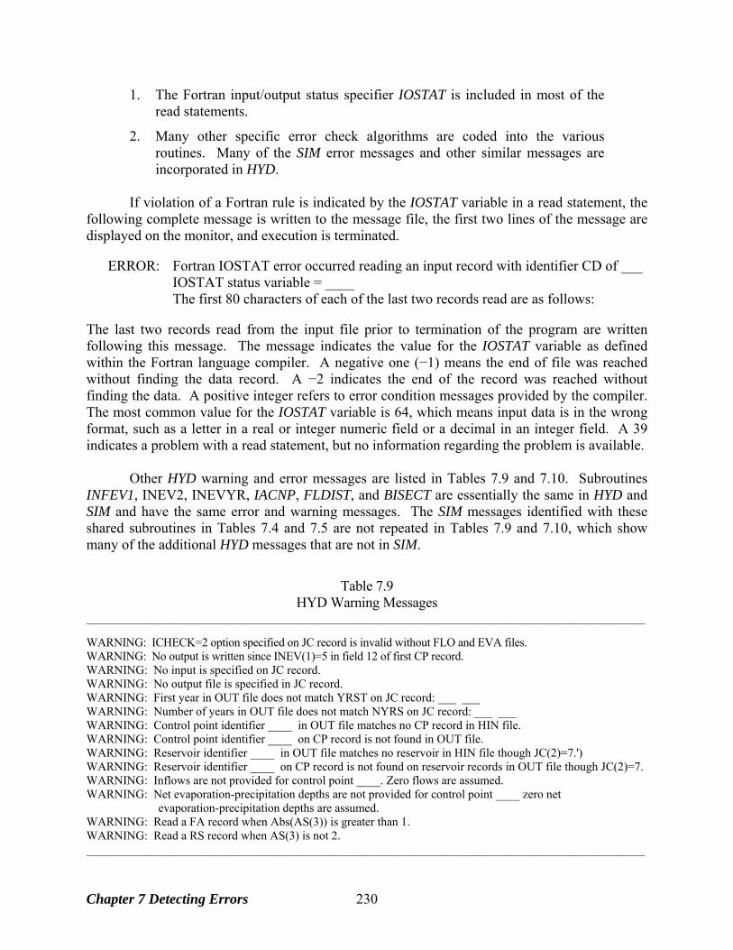
1. The Fortran input/output status specifier IOSTAT is included in most of the read statements.
2. Many other specific error check algorithms are coded into the various routines. Many of the SIM error messages and other similar messages are incorporated in HYD.
If violation of a Fortran rule is indicated by the IOSTAT variable in a read statement, the following complete message is written to the message file, the first two lines of the message are displayed on the monitor, and execution is terminated. ERROR: Fortran IOSTAT error occurred reading an input record with identifier CD of ___ IOSTAT status variable = ____
The first 80 characters of each of the last two records read are as follows: The last two records read from the input file prior to termination of the program are written following this message. The message indicates the value for the IOSTAT variable as defined within the Fortran language compiler. A negative one (−1) means the end of file was reached without finding the data record. A −2 indicates the end of the record was reached without finding the data. A positive integer refers to error condition messages provided by the compiler. The most common value for the IOSTAT variable is 64, which means input data is in the wrong format, such as a letter in a real or integer numeric field or a decimal in an integer field. A 39 indicates a problem with a read statement, but no information regarding the problem is available. Other HYD warning and error messages are listed in Tables 7.9 and 7.10. Subroutines INFEV1, INEV2, INEVYR, IACNP, FLDIST, and BISECT are essentially the same in HYD and SIM and have the same error and warning messages. The SIM messages identified with these shared subroutines in Tables 7.4 and 7.5 are not repeated in Tables 7.9 and 7.10, which show many of the additional HYD messages that are not in SIM.
Table 7.9
HYD Warning Messages ________________________________________________________________________________________________ WARNING: ICHECK=2 option specified on JC record is invalid without FLO and EVA files. WARNING: No output is written since INEV(1)=5 in field 12 of first CP record. WARNING: No input is specified on JC record. WARNING: No output file is specified in JC record. WARNING: First year in OUT file does not match YRST on JC record: ___ ___ WARNING: Number of years in OUT file does not match NYRS on JC record: ___ ___ WARNING: Control point identifier ____ in OUT file matches no CP record in HIN file. WARNING: Control point identifier ____ on CP record is not found in OUT file. WARNING: Reservoir identifier ____ in OUT file matches no reservoir in HIN file though JC(2)=7.') WARNING: Reservoir identifier ____ on CP record is not found on reservoir records in OUT file though JC(2)=7. WARNING: Inflows are not provided for control point ____. Zero flows are assumed. WARNING: Net evaporation-precipitation depths are not provided for control point ____ zero net evaporation-precipitation depths are assumed. WARNING: Read a FA record when Abs(AS(3)) is greater than 1. WARNING: Read a RS record when AS(3) is not 2. ________________________________________________________________________________________________
Chapter 7 Detecting Errors 230
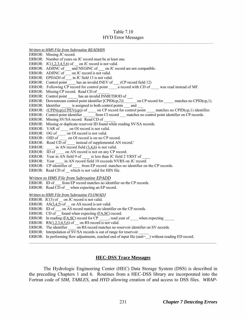
Table 7.10 HYD Error Messages
_______________________________________________________________________________________________________________________ Written to HMS File from Subroutine READHIN ERROR: Missing JC record. ERROR: Number of years on JC record must be at least one. ERROR: JC(1,2,3,4,5,6) of __ on JC record is not valid. ERROR: ADJINC of ___ and NEGINC of ___ on JC record are not compatible. ERROR: ADJINC of ___ on JC record is not valid. ERROR: EPDADJ of ___ in JC field 13 is not valid. ERROR: Control point ____ has an invalid INEV of ___ (CP record field 12) ERROR: Following CP record for control point ____ a record with CD of ____ was read instead of MF. ERROR: Missing CP record. Read CD of ______ ERROR: Control point _____ has an invalid INMETHOD of ___ ERROR: Downstream control point identifier [CPID(cp,2)] ______ on CP record for _____ matches no CPID(cp,1). ERROR: Identifier _____ is assigned to both control points ___ and ___ ERROR: (CPIN(cp),CPEV(cp)) of ____ on CP record for control point ____ matches no CPID(cp,1) identifier. ERROR: Control point identifier ______ from CI record ___ matches no control point identifier on CP records. ERROR: Missing SV/SA record. Read CD of ______ ERROR: Missing or duplicate reservoir ID found while reading SV/SA records. ERROR: VAR of ____ on OI record is not valid. ERROR: OG of ____ on OI record is not valid. ERROR: OID of ____ on OI record is on no CP record. ERROR: Read CD of ____ instead of supplemental AN record.' ERROR: ____ in AN record field (3,4,6) is not valid. ERROR: ID of ____ on AN record is not on any CP record. ERROR: Year in AN field 9 of ____ is less than JC field 2 YRST of ____ ERROR: Year ____ in AN record field 10 exceeds NYRS on JC record. ERROR: CP identifier of ____ from EP record matches no identifier on the CP records. ERROR: Read CD of __ which is not valid for HIN file.
Written to HMS File from Subroutine EPADD ERROR: ID of ___ from EP record matches no identifier on the CP records. ERROR: Read CD of __ when expecting an EP record.
Written to HMS File from Subroutine FLOWADJ ERROR: JC(3) of __ on JC record is not valid. ERROR: AS(3,4,5) of __ on AS record is not valid. ERROR: ID of ___ on AS record matches no identifier on the CP records. ERROR: CD of __ found when expecting (FA,SC) record. ERROR: In reading (FA,SC) record for CP _____, read year of ____ when expecting _____ ERROR: RS(1,2,3,4,5,6) of __ on RS record is not valid. ERROR: The identifier ____ on RS record matches no reservoir identifier on SV records. ERROR: Interpolation of SV/SA records is out of range for reservoir _____ ERROR: In performing flow adjustments, reached end of input file (unit=__) without reading ED record. ________________________________________________________________________________________________
HEC-DSS Trace Messages The Hydrologic Engineering Center (HEC) Data Storage System (DSS) is described in the preceding Chapters 1 and 6. Routines from a HEC-DSS library are incorporated into the Fortran code of SIM, TABLES, and HYD allowing creation of and access to DSS files. WRAP-
Chapter 7 Detecting Errors 231
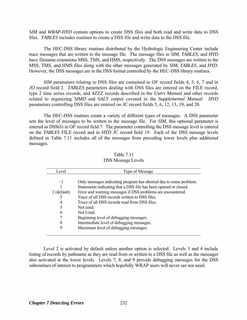
SIM and WRAP-HYD contain options to create DSS files and both read and write data to DSS files. TABLES includes routines to create a DSS file and write data to the DSS file. The HEC-DSS library routines distributed by the Hydrologic Engineering Center include trace messages that are written to the message file. The message files in SIM, TABLES, and HYD have filename extensions MSS, TMS, and HMS, respectively. The DSS messages are written to the MSS, TMS, and HMS files along with the other messages generated by SIM, TABLES, and HYD. However, the DSS messages are in the DSS format controlled by the HEC-DSS library routines. SIM parameters relating to DSS files are contained in OF record fields 4, 5, 6, 7 and in JO record field 2. TABLES parameters dealing with DSS files are entered on the FILE record, type 2 time series records, and 4ZZZ records described in the Users Manual and other records related to organizing SIMD and SALT output covered in the Supplemental Manual. HYD parameters controlling DSS files are entered on JC record fields 5, 6, 12, 13, 19, and 20. The HEC-DSS routines create a variety of different types of messages. A DSS parameter sets the level of messages to be written to the message file. For SIM, this optional parameter is entered as DSS(6) in OF record field 7. The parameter controlling the DSS message level is entered on the TABLES FILE record and in HYD JC record field 19. Each of the DSS message levels defined in Table 7.11 includes all of the messages from preceding lower levels plus additional messages.
Table 7.11 DSS Message Levels
Level Type of Message
−1 Only messages indicating program has aborted due to some problem. 1 Statements indicating that a DSS file has been opened or closed.
2 (default) Error and warning messages if DSS problems are encountered. 3 Trace of all DSS records written to DSS files. 4 Trace of all DSS records read from DSS files. 5 Not used. 6 Not Used. 7 Beginning level of debugging messages. 8 Intermediate level of debugging messages. 9 Maximum level of debugging messages.
Level 2 is activated by default unless another option is selected. Levels 3 and 4 include listing of records by pathname as they are read from or written to a DSS file as well as the messages also activated at the lower levels. Levels 7, 8, and 9 provide debugging messages for the DSS subroutines of interest to programmers which hopefully WRAP users will never see nor need.
Chapter 7 Detecting Errors 232
REFERENCES Center for Research in Water Resources, University of Texas at Austin, WRAP Display Tool, Users
Manual and Operating Instructions, Prepared for the Texas Commission on Environmental Quality, Austin, Texas, December 2007.
Dunn, David D., Incorporation of System Operation Strategies in Water Rights Modeling and Analysis, Master of Science Thesis, Texas A&M University, August 1993.
Figurski, Melissa J., and David R. Maidment, GIS Algorithms for Large Watersheds with Non-contributing Areas, Center for Research in Water Resources, University of Texas at Austin, Online Report 01-7, December 2001. http://www.crwr.utexas.edu/online.shtml
Gopalan, Hema, WRAP Hydro Data Model: Finding Input Parameters for the Water Rights Analysis Package, Texas Water Resources Institute, Technical Report 233, Center for Research in Water Resources, University of Texas at Austin, Online Report 03-3, May 2003.
Hudgens, Bradley T., and David R. Maidment, Geospatial Data in Water Availability Modeling, Center for Research in Water Resources, University of Texas at Austin, Online Report 99-4, December 1999. http://www.crwr.utexas.edu/online.shtml
Hydrologic Engineering Center, HECDSS Users Guide and Utility Programs Manuals, U.S. Army Corps of Engineers, Davis, CA, March 1995.
Hydrologic Engineering Center, HECDSS Microsoft Excel Data Exchange Add-In, U.S. Army Corps of Engineers, Davis, CA, November 2003.
Hydrologic Engineering Center, HEC-DSSVue HEC Data Storage System Visual Utility Engine, User’s Manual, Version 1.2, U.S. Army Corps of Engineers, Davis, CA, May 2005.
Maidment, David R. (Editor), Arc Hydro GIS for Water Resources, ESRI Press, 2002. Mason, David, and David R. Maidment, An Analysis Methodology for Generating Watershed
Parameters Using GIS, Center for Research in Water Resources, University of Texas at Austin, Online Report 00-3, May 2000. http://www.crwr.utexas.edu/online.shtml
Olmos Alejo, Hector E., Improving Capabilities for Dealing with Key Complexities of Water Availability Modeling, M.S. Thesis, Texas A&M University, December 2004.
Sanchez-Torres, Gerardo, Reservoir System Reliability Considering Water Rights and Water Quality, Ph.D. Dissertation, Texas A&M University, December 1994.
Salazar, A. Andres, Conditional Reliability Modeling to Support Short Term River Basin Management Decisions, Ph.D. Dissertation, Texas A&M University, May 2002.
Sokulsky, Kariann, Tina Dacus, Lann Bookout, and Jim Patek, "Water Availability Modeling Project: Year 1 - Concept Plan, Overview of the New Modeling System and Its Role in Regional Planning," Proceedings of the 25th Water for Texas Conference, Water Planning Strategies for Senate Bill 1 (Edited by R. Jensen), Texas Water Resources Institute, Dec. 1998.
Texas Natural Resource Conservation Commission, Water Availability Modeling: An Overview, GI-245, July 1998.
Walls, W. Brian, Application of a Water Rights Analysis Program to Reservoir System Yield Calculations, Master of Science Thesis, Texas A&M University, August 1988.
Wurbs, R.A., C.E. Bergman, P.E. Carriere, P.E., and W.B. Walls, Hydrologic and Institutional Water Availability in the Brazos River Basin, Technical Report 144, Texas Water Resources Institute, August 1988.
References 233
Wurbs, R.A., and W.B. Walls, "Water Rights Modeling and Analysis," Journal of Water Resources Planning and Management, American Society of Civil Engineers, Vol. 115, No. 4, July 1989.
Wurbs, R.A., G. Sanchez-Torres, and D.D. Dunn, Reservoir/River System Reliability Considering Water Rights and Water Quality, TR-165, Texas Water Resources Institute, March 1994.
Wurbs, R.A. and A.K. Yerramreddy, "Reservoir/River System Analysis Models: Conventional Simulation versus Network Flow Programming," International Journal of Water Resources Development, Carfax Publishing, Vol. 10, No. 2, 1994.
Wurbs, R.A., and D.D. Dunn, Water Rights Analysis Package (TAMUWRAP), Model Description and Users Manual, TR-146, TWRI, March 1993, revised October 1996.
Wurbs, R.A., and E.D. Sisson, Evaluation of Methods for Distributing Naturalized Streamflows from Gaged Watersheds to Ungaged Subwatersheds, TR-179, TWRI, August 1999.
Wurbs, R.A., Water Rights Analysis Package (WRAP), Model Description and Users Manual, Technical Report 180, Texas Water Resources Institute, First Edition August 1999, Second Edition October 2000, Third Edition July 2001.
Wurbs, R.A., "Assessing Water Availability under a Water Rights Priority System," Journal of Water Resources Planning and Management, American Society of Civil Engineers, Vol. 127, No. 4, July/August 2001.
Wurbs, R.A., “Water Allocation Systems in Texas,” International Journal of Water Resources Development, Carfax Publishing, Vol. 20, No. 2, June 2004.
Wurbs, R.A., "Natural Salt Pollution Control in the Southwest," Journal of the American Water Works Association, Vol. 94, No. 12, December 2002.
Wurbs, R.A., "Modeling River/Reservoir System Management, Water Allocation, and Supply Reliability, " Journal of Hydrology, Elsevier Science Publishers, Vol. 300, 2005.
Wurbs, R.A., "Texas Water Availability Modeling System," Journal of Water Resources Planning and Management, American Society of Civil Engineers, Vol. 131, No. 4, July/August 2005.
Wurbs, R.A., R.S. Muttiah, F. Felden, "Incorporation of Climate Change in Water Availability Modeling," Journal of Hydrologic Engineering, American Society of Civil Engineers, Vol. 131, No. 5, September/October 2005.
Wurbs, R.A., "Methods for Developing Naturalized Monthly Flows at Gaged and Ungaged Sites," Journal of Hydrologic Engineering, American Society of Civil Engineers, Vol. 11, No. 1, January/February 2006.
Wurbs, R.A., Comparative Evaluation of Generalized Reservoir/River System Models, Technical Report 282, Texas Water Resources Institute, April 2005.
Wurbs, R.A., Water Rights Analysis Package Modeling System Users Manual, Technical Report 256, Texas Water Resources Institute, Fourth Edition, March 2008.
Wurbs, R.A., Fundamentals of Water Availability Modeling with WRAP, Technical Report 283, Texas Water Resources Institute, Fourth Edition, March 2008.
Wurbs, R.A., R.J. Hoffpauir, H.E. Olmos, and A.A. Salazar, Conditional Reliability, Sub-Monthly Time Step, Flood Control, and Salinity Features of WRAP, Technical Report 284, Texas Water Resources Institute, September 2006.
Yerramreddy, Anil R., Comparative Evaluation of Network Flow Programming and Conventional Reservoir System Simulation Models, M.S. Thesis, Texas A&M University, August 1993.
References 234
APPENDIX A GLOSSARY
Each of the terms included in this glossary is defined and discussed in more detail in various parts of the manual. Terms are defined specifically from the perspective of their use in this manual. active pool – reservoir storage zone from which releases and withdrawals are made.
adjusted net evaporation-precipitation – JD record field 10 and CP record field 9 activates a SIM option to account for the portion of the reservoir water surface evaporation-precipitation that is also reflected in the naturalized streamflow inflows. The ratio of reservoir surface area to watershed area is used to determine the proportion of the naturalized streamflow that is runoff from the land now covered by the reservoir. The net evaporation-precipitation rate is adjusted to prevent double-counting this inflow.
available streamflow – The streamflow available to a water right is computed by SIM as an initial step as each right is considered in the water rights priority loop which is embedded within the monthly loop.
backup right – A backup water right activated by a BU record adds any shortage incurred by the other right being backed-up to its own target. Thus, multiple rights may be assigned to meet a particular target. The secondary backup right supplies the target only to the extent that the other right can not due to insufficient water availability.
channel loss credits – Credits represent increases in streamflow to result from incorporating channel losses in SIM. For example, diversions reduce streamflows at downstream control points less if channel losses are considered.
channel loss factor – The channel loss factor CL entered on the CP record is used to determine channel losses in the river reach below a control point as follows where Qupstream is the flow at the control point: channel loss = CL Qupstream
channel losses – Channel losses represent the portion of the streamflow in the reach between two control points that is loss through infiltration, evapotranspiration, and diversions not reflected in the water rights. Channel loss L is treated as a linear function of the flow Qupstream at the control point defining the upstream end of the reach [L = CL Qupstream] where CL is a channel loss coefficient provided as HYD or SIM input.
conditional reliability modeling – An optional modeling approach activated by SIM CR record and TABLES type 5 records analyzes water supply reliabilities and flow and storage frequencies over relatively short periods of a month to a year conditioned upon specified preceding reservoir storage conditions.
constant inflow or outflow – An option allows a set of 12 flows for the 12 months of the year entered on CI records to be either added or subtracted from streamflow each year. This flows may represent intrabasin or interbasin water transport, return flows from groundwater sources, losses or other flows not otherwise reflected in the water rights input.
control point – Control points are stations or nodes which provide a modeling mechanism for representing the spatial connectivity of system components. The locations of system features are defined by control points. The spatial configuration of the system is delineated by specifying the control point located immediately downstream of each control point.
Appendix A − Glossary 235
curve number method adaptation – This method of distributing flows described in Chapter 3 is based on a modified version of the Natural Resource Conservation Service (NRCS) rainfall-runoff modeling methodology which uses the curve number CN to represent the land cover and soil types of the watersheds.
delivery factor – In considering channel losses, the delivery factor is one minus the channel loss factor (DF = 1 − CL) and represents the fraction of the flow at the upstream control point that reaches the next downstream control point.
diversion – Computed by SIM as a diversion target limited by water availability. The water supply diversion requirement minus the computed diversion is the computed shortage.
drainage area ratio method – Naturalized flows at an ungaged site are estimated from flows at a gaged location based on proportioning the flows in proportion to the drainage areas of the gaged and ungaged watersheds. Qungaged = RDA Qgaged where RDA is the drainage area ratio
drought index – A drought or storage index (DI/IP/IS records) allows diversion, instream flow, and hydropower requirements to be specified as a function of the storage content of specified reservoirs. The drought index is expressed in the format of a table of storage content versus a percentage multiplier which is applied to the target diversion, instream flow, or hydropower amount associated with a water right.
DSS file – WRAP programs create, read, and write to DSS files in the direct access binary format of the Data Storage System (DSS) developed by the USACE Hydrologic Engineering Center.
dual simulation option – An automated dual simulation activated by the JO, SO or PX record allows streamflow depletions during a first simulation with specified water rights to serve as a limit on streamflow depletions during a second simulation with modified water rights.
energy requirement – An annual hydroelectric energy target in units of megawatt hours per year or similar units is entered in WR record field 3. SIM determines a monthly energy target by combining the annual target with monthly distribution factors (UC records) and other optional target setting records. An energy target is determined the same as a diversion target.
evaporation – Evaporation from the water surface of reservoirs is included in the volume accounting computations by combining depths from EV records with water surface areas determined as a function of storage volume. The evaporation in WRAP is actually a net evaporation minus precipitation depth or volume.
evaporation-precipitation – Net evaporation minus precipitation depth or volume. Evaporation represents a loss of water from the reservoir. Conversely, precipitation is a gain.
evaporation-precipitation rate – Monthly rates expressed as depths of evaporation minus precipitation are provided as model input in inches, feet, or other units of depth per month.
evaporation-precipitation volume – In the water volume accounting computations, the monthly net evaporation-precipitation volume is determined as the rate (depth/month) multiplied by the average surface area of the reservoir for the month.
exceedance frequency – The percentage of the total months in the overall simulation period-of-analysis that a particular amount is equaled or exceeded. TABLES develops exceedance frequency relationships for naturalized, regulated, and unappropriated streamflow, instream flow shortage, reservoir storage, and reservoir water surface elevation.
Appendix − A Glossary 236
firm yield – The maximum water supply diversion or hydropower electric energy generation that can be achieved with a volume and period reliability of one-hundred percent (to a defined level of precision) based on the premises reflected in the model. The SIM firm yield FY record activates an automated iterative search for the firm yield.
flow distribution methods – Several alternative methods are described in Chapter 3 for synthesizing naturalized streamflows at ungaged (unknown flow) control points based on known flows at other control points read from IN records and watershed parameters from a flow distribution DIS file.
flow distribution equation – Qungaged = a (Qgaged)b + c with coefficients a, b, and c input on FC records is one of several flow distribution methods. With default values of one and zero for b and c and the drainage area ratio used for the coefficient a, the equation reduces to the drainage area ratio method.
Fundamentals Manual – TWRI Technical Report 283 entitled Fundamentals of Water Availability Modeling with WRAP provides an introductory overview of WRAP.
head – The vertical water surface elevation difference between upstream and downstream of the turbines used in the power equation (Equation 4-4). SIM computes head as a reservoir water surface elevation minus tailwater elevation.
HEC-DSS – The Hydrologic Engineering Center (HEC) Data Storage System (DSS) developed by the HEC of the U.S. Army Corps of Engineers is a database management system used with both HEC and non-HEC simulation models including WRAP.
HEC-DSSVue – The USACE Hydrologic Engineering Center HEC-DSS Visual Utility Engine is a user-friendly software package for managing, plotting, and manipulating data in DSS files. WRAP programs write simulation results to DSS files for transport to HEC-DSSVue.
HYD – see WRAP-HYD
hydrologic simulation period – In a WRAP simulation, specified annual water use requirements, distributed over the 12 months of the year, are met, subject to water availability, during a hypothetical repetition of historical hydrology represented by sequences of naturalized streamflows and net evaporation-precipitation rates for each month of a multiple-year hydrologic simulation period, which is also called the period-of-analysis.
inactive pool – The bottom pool of a reservoir from which releases or withdrawals cannot be made except by evaporation. The inactive pool storage capacity is entered in WS record field 7.
incremental streamflows – An incremental flow is the difference between total flows at adjacent control points. WRAP computational algorithms, as well as input and output data, are based on total flows rather than incremental inflows. However, HYD and SIM include options for checking for negative incremental naturalized streamflows and adjusting the flows to remove the negative incrementals. Incremental flow options are controlled by JD record fields 8 and 9.
inflows to a control point – This quantity referenced in TO record fields 5 and 6 and FS record field 2 and tabulated by the 2CPI record represents inflows into a control point excluding releases from secondary reservoirs located upstream for water rights located downstream of the control point. The inflow is computed as the regulated flow plus streamflow depletion at the control point minus secondary reservoir releases.
Appendix A − Glossary 237
instream flow requirement – A water right requirement entered on an IF record consists of placing a minimum target limit on the regulated flows at a control point. The objective is to maintain regulated streamflows at or greater than the target if feasible.
junior right – see senior or junior rights
lakeside versus downstream water supply release – WS record field 11 allows specification of whether or not water supply diversions are used to generate energy for more junior hydropower rights. By default, diversions for senior water rights are allowed to pass through the turbines to generate power for junior hydropower rights. However, the lakeside diversion option activated by WS record field 11 for a diversion right results in the diversion bypassing the turbines and not contributing to power generation.
multiple-reservoir system operations – A single water right diversion, instream flow, or hydroelectric power target may be met by releases from multiple reservoirs following rules specified on OR records. Multiple-reservoir release rules are based upon balancing the storage content expressed as a percentage of capacity in specified vertical active pool zones of each system reservoir.
natural priority option – Water right priorities are ordered internally within SIM in upstream to downstream order if the natural priority option is specified in the JO record. This ranked order is used in lieu of the water right priorities entered on WR records.
naturalized streamflows – Sequences of monthly streamflows representing natural hydrology are developed by adjusting historical gaged streamflow data to remove the impacts of reservoir construction, water use, and other human activities. Naturalized streamflows are provided as SIM input data on inflow IN records.
period reliability – The reliability index reflected in Equation 5.2 is the percentage of the total months or years (periods) in the overall simulation period-of-analysis that a specified percentage of a diversion target or hydroelectric energy target is met.
permitted, authorized, or target diversion – The diversion requirement or target amount of water to be appropriated from streamflow at a control point location and reservoir storage at the same or other locations.
permitted, authorized, or target energy requirement – Hydroelectric energy generation target.
precipitation – Precipitation falling directly on the water surface of reservoirs is included in the reservoir volume accounting computations through the net evaporation-precipitation depth.
primary and secondary control points – Naturalized streamflows are input to SIM on IN records for primary (known-flow or gaged) control points. Secondary control points are locations for which naturalized streamflows are computed in SIM from flows at one or more primary control points and watershed parameters used methods outlined in Chapter 3.
primary and secondary reservoirs – The terms primary reservoir and secondary reservoir are defined in the context of water rights. Primary reservoirs are refilled by the water right in question; secondary reservoirs are not refilled. Any number of reservoirs can be associated with each water right. However, storage capacity can be refilled in only one primary reservoir. The other secondary reservoirs make releases to meet diversion, instream flow, or hydropower requirements but cannot be refilled by the water right. A secondary reservoir for one water right can be a primary reservoir for another water right and vice versa.
Appendix − A Glossary 238
priority – An integer value associated with a water right indicating the seniority of the right relative to all the other rights. In each period of the simulation, water rights are considered in turn and available water appropriated in order of their relative priorities. Priorities are entered on the WR and IF records and may be adjusted by options on the UP records or replaced by the natural priority option activated with the JO record.
priority circumvention options – The PX record controls four different modeling features designed to deal with water management situations in which the normal priority system is not applicable. Water management actions evade the priority sequence in the model.
Reference Manual – WRAP is documented by this Reference Manual and the Users Manual, Fundamentals Manual, and Supplemental Manual.
regulated streamflows –SIM computed regulated flows, associated with a particular control point, represent the physical streamflow after accounting for all the water rights. The SIM simulation starts with naturalized flows and computes regulated flows. Regulated flows may be greater than unappropriated flows because a portion of the regulated flows may be committed to meet instream flow requirements or downstream diversion or storage rights.
record – Data is recorded in input and output files as records. A record is one line of data in a text file or a time series referenced by a pathname in a DSS file. Input records are described in the Users Manual. Output records are described in Chapter 5 of this Reference Manual.
return flow – An amount of water computed as the diversion multiplied by an inputted return flow factor is returned to the stream system at a user-specified control point in either the same month as the diversion or the next month as specified by the WR record. Return flows may also be modeled as constant inflows entered on CI records.
run-of-river water right – A water right with zero reservoir storage capacity.
SALT – see WRAP-SALT
seasonal rule curve operations – A model option activated by the MS record allows the storage capacity of a reservoir to vary monthly over the 12 months of the year. The primary application of this option is modeling reservoirs with operating plans based on seasonal allocations of storage capacity between flood control and conservation pools.
secondary control points – See primary and secondary control points.
secondary energy – Additional hydroelectric energy, above the permitted energy target, which could be generated incidentally by pass-through flows and releases for more senior water right diversions.
secondary reservoirs – See primary and secondary reservoirs.
senior or junior rights – A water right is senior or junior relative to another water right depending on the priority number included in the input data for each right. A senior right has the highest priority, which is represented by the smallest priority number (earliest date or other priority indicator) and is considered first in the water allocation computations.
shortage – Diversion target minus actual diversion or energy target minus actual energy produced. A shortage is the amount of a diversion or energy target not supplied due to insufficient streamflow and/or reservoir storage being available to meet the full target.
Appendix A − Glossary 239
storage-area relationship – A relationship between reservoir storage volume and water surface area is required in the computation of net evaporation-precipitation volumes. This relationship may be input alternatively as a storage versus area table (SV/SA records) or as coefficients for an equation (WS record fields 4, 5, 6).
storage-elevation relationship – A relationship between reservoir storage volume and water surface elevation is required in the computation of head in the hydropower routine. This relationship is input as a storage volume versus elevation table (PV/PE records).
streamflow depletion limit – Limits may be placed on the amount of streamflow a right can appropriate in a year, season, or month of the year to meet streamflow and storage targets using options on the SO record.
streamflow depletion –SIM computed streamflow depletions are the amounts appropriated to meet water right diversions, account for reservoir net evaporation-precipitation, and/or refill reservoir storage. Each streamflow depletion is associated with a particular right.
Supplemental Manual – TWRI Technical Report 254 entitled Conditional Reliability, Sub-Monthly Time Step, Flood Control, and Salinity Features of WRAP documents these features which are not covered in the basic Reference and Users Manuals.
TABLES – This post-simulation program develops tables, data listings, and reliability indices from SIM input and output files that organize/summarize the simulation results.
tailwater – The water surface elevation downstream of a hydropower plant is used in computing head. The tailwater elevation may be entered as a constant on a HP record, or alternatively a table of tailwater elevation versus discharge (TE/TQ records) may be entered.
TAMUWRAP – The original 1988 version of the WRAP model was called the Texas A&M University Water Rights Analysis Program (TAMUWRAP).
target – Diversion, instream flow, or hydroelectric power generation demand/need/requirement associated with a water right. WR, UC, DI, SO, TO, TS, and FS records provide options for use in setting targets. The water right type 7 feature (WR record field 6) allows reservoir storage targets to be set in the same manner as diversion targets but limited to not exceed the conservation storage capacity. Targets are met to the extent allowed by water availability.
target series – Diversion, instream flow, and hydropower requirements are typically modeled as varying seasonally but being constant from year to year. However, the target series TS record allows specifying targets that vary between years as well as between months.
time interval – The version of WRAP documented by this manual uses a computational time step of one month. Expanded features documented by the Supplemental Manual allow use of a daily or other sub-monthly time interval.
transient priority water right – options activated by the PX record assign two priorities to a water right. Transient priority option 1 allows a return flow to be assigned a priority different than the diversion. Transient priority option 2 allows a right to be activated and deactivated at different points in the priority sequence.
turbine capacity – An optional discharge capacity entered on the HP record in volume/month may be input as an upper limit on the amount of water that can be released through the turbines to
Appendix − A Glossary 240
generate energy each month. If not otherwise specified the turbine discharge capacity is assumed to be unlimited.
turbine inlet elevation – The optional inlet elevation entered on a HP record sets a minimum pool level below which power generation is curtailed. Power generation with all releases for all rights is constrained by the turbine inlet invert. Releases for a particular right are also constrained by the specified inactive pool. For a hydropower right with the inactive pool set higher than the turbine inlet, power generation with pass-through flows and water supply releases for other rights are constrained only by the turbine inlet elevation. Additional releases for the hydropower right are also constrained by the specified inactive pool.
type – The water right type defined in WR record field 6 specifies certain water management tasks and rules associated with the water right.
type 1 water right – allows a water supply diversion target and/or storage target in one reservoir to be met from streamflow depletions and releases from one or multiple reservoirs.
type 2 water right – is the same as a type 1 right except a reservoir storage target (refilling of storage capacity in the one reservoir) is not allowed.
type 3 water right – is the same as a type 2 right except the permitted diversion target can be met only from reservoir releases from storage, not streamflow.
type 4 water right – the target amount of water is discharged into the stream.
type 5 water right – is the same as a type 1 right except a hydroelectric energy generation target is specified rather than a diversion. Hydropower rights are either type 5 and or type 6.
type 6 water right – is the same as a type 3 right except a hydroelectric energy generation target is specified rather than a diversion. Same as type 5 except not allowed streamflow depletions.
type 7 water right – sets a reservoir storage target.
unappropriated streamflows –SIM computed unappropriated flows, associated with a particular control point, are the portions of the naturalized streamflows still remaining after the streamflow depletions are made and return flows are returned for all the water rights included in the simulation. The SIM simulation starts with naturalized flows and computes regulated and unappropriated flows. Unappropriated flows may be less than regulated flows because a portion of the regulated flows may be committed to meet instream flow requirements or downstream diversion or storage rights.
Users Manual – TWRI Technical Report 256 entitled Water Rights Analysis Package Modeling System Users Manual provides instructions for working with input files and records.
volume reliability – The total volume of actual diversions or total hydroelectric energy generated during the simulation period-of-analysis expressed as a percentage of the corresponding total permitted diversion or hydroelectric energy targets. Computed based on Equation 5.1.
water right – A WRAP water right is a set of water management capabilities and water use requirements associated with either a water right WR record or instream flow IF record and supplemental records associated with the WR or IF record. A water right may include specifications for water supply diversion, return flow, hydroelectric energy generation, instream flow, and/or reservoir storage.
Appendix A − Glossary 241
water use distribution coefficients – Each annual diversion, instream flow, and hydropower target is distributed over the 12 months of the year by a set of 12 multiplier factors entered on UC records.
water surface elevation – Reservoir water surface elevations determined based on linear interpolation of PV/PE record table are included in the OUT file on reservoir/hydropower records for all reservoirs for which PV/PE records are entered regardless of whether hydropower rights are associated with the reservoir. Reservoir water surface elevations are tabulated by the TABLES 2WSE record.
watershed flow option – This SIM option restricts the amount of water available to a water right to naturalized streamflow at its location computed by multiplying the naturalized flows input for the control point assigned to the water right by a factor which typically will be a drainage area ratio. Multiple water rights assigned to the same control point can have different limits on the amount of naturalized streamflow available to them.
WinWRAP – The user interface facilitates executing the WRAP programs within Microsoft Windows in combination with other Microsoft programs.
WRAP – The term Water Rights Analysis Package (WRAP) refers to the set of computer programs, WinWRAP, TABLES, SIM, SIMD, HYD, DAY, and SALT and associated documentation.
WRAP2 and WRAP3 – The 1992 Water Rights Analysis Program-Version 2 (WRAP2) in combination with TABLES replaced the original TAMUWRAP and was superceded by WRAP3 which provided essentially all the capabilities of WRAP2 plus multiple-reservoir system operation, hydroelectric power, and other optional features not available in WRAP2. WRAP3 is superseded by WRAP-SIM.
WRAP-DAY – Pre-simulation utility program used to develop hydrology input for WRAP-SIMD.
WRAP-HYD – Pre-simulation utility program is used to develop hydrology input for WRAP-SIM.
WRAPNET – WRAPNET completed in 1993 provides the same modeling capabilities as WRAP2, but the internal computations are performed using network flow programming, a computationally efficient form of linear programming.
WRAP-SALT – The original WRAPSALT completed in 1994 expands WRAP3 to incorporate features for considering salinity in assessing water supply reliability. A completely redesigned WRAP-SALT completed in 2004-2006 reads a SIM output file and salinity input file and tracks salt loads and concentrations through the river/reservoir system.
WRAP-SIM – This main program simulates a river/reservoir/use water allocation system.
WRAP-SIMD – This expanded version of SIM has sub-monthly time step, flow forecasting, flow routing, and flood control operations added.
WRAPVIEW – The TNRCC and USGS developed WRAPVIEW in 1996 by combining WRAP with the ArcView Geographical Information System (GIS) software package. WRAPVIEW was never fully operational and is now obsolete.
zones 1 and 2 – For purposes of specifying multiple-reservoir operating rules, reservoir active pools may be divided into an upper and lower zones illustrated in Figures 4.1 and 4.2 by use of OR records. Release decisions are based on balancing the storage contents of comparable zones in multiple reservoirs in terms of contents as a percentage of zone capacity.
Appendix − A Glossary 242
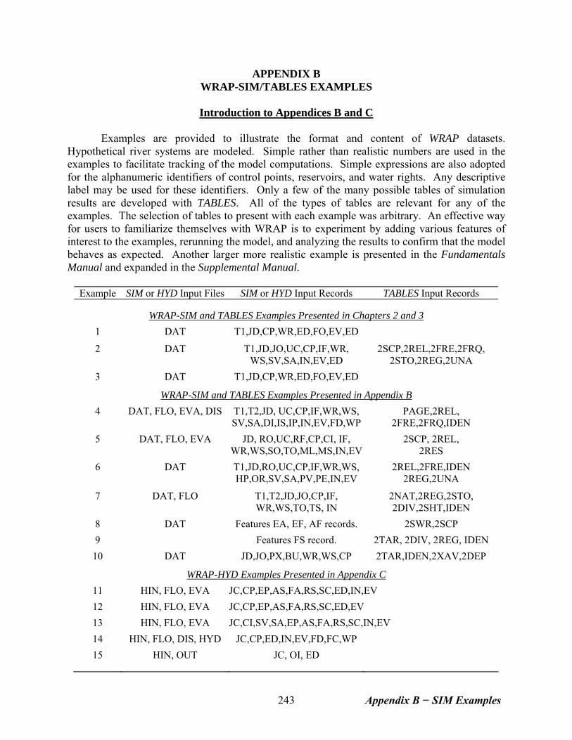
APPENDIX B WRAP-SIM/TABLES EXAMPLES
Introduction to Appendices B and C
Examples are provided to illustrate the format and content of WRAP datasets.
Hypothetical river systems are modeled. Simple rather than realistic numbers are used in the examples to facilitate tracking of the model computations. Simple expressions are also adopted for the alphanumeric identifiers of control points, reservoirs, and water rights. Any descriptive label may be used for these identifiers. Only a few of the many possible tables of simulation results are developed with TABLES. All of the types of tables are relevant for any of the examples. The selection of tables to present with each example was arbitrary. An effective way for users to familiarize themselves with WRAP is to experiment by adding various features of interest to the examples, rerunning the model, and analyzing the results to confirm that the model behaves as expected. Another larger more realistic example is presented in the Fundamentals Manual and expanded in the Supplemental Manual.
Example SIM or HYD Input Files SIM or HYD Input Records TABLES Input Records
WRAP-SIM and TABLES Examples Presented in Chapters 2 and 3
1 DAT T1,JD,CP,WR,ED,FO,EV,ED
2 DAT T1,JD,JO,UC,CP,IF,WR, WS,SV,SA,IN,EV,ED
2SCP,2REL,2FRE,2FRQ, 2STO,2REG,2UNA
3 DAT T1,JD,CP,WR,ED,FO,EV,ED
WRAP-SIM and TABLES Examples Presented in Appendix B
4 DAT, FLO, EVA, DIS T1,T2,JD, UC,CP,IF,WR,WS,SV,SA,DI,IS,IP,IN,EV,FD,WP
PAGE,2REL, 2FRE,2FRQ,IDEN
5 DAT, FLO, EVA JD, RO,UC,RF,CP,CI, IF, WR,WS,SO,TO,ML,MS,IN,EV
2SCP, 2REL, 2RES
6 DAT T1,JD,RO,UC,CP,IF,WR,WS,HP,OR,SV,SA,PV,PE,IN,EV
2REL,2FRE,IDEN 2REG,2UNA
7 DAT, FLO T1,T2,JD,JO,CP,IF, WR,WS,TO,TS, IN
2NAT,2REG,2STO, 2DIV,2SHT,IDEN
8 DAT Features EA, EF, AF records. 2SWR,2SCP
9 Features FS record. 2TAR, 2DIV, 2REG, IDEN
10 DAT JD,JO,PX,BU,WR,WS,CP 2TAR,IDEN,2XAV,2DEP
WRAP-HYD Examples Presented in Appendix C
11 HIN, FLO, EVA JC,CP,EP,AS,FA,RS,SC,ED,IN,EV
12 HIN, FLO, EVA JC,CP,EP,AS,FA,RS,SC,ED,EV
13 HIN, FLO, EVA JC,CI,SV,SA,EP,AS,FA,RS,SC,IN,EV
14 HIN, FLO, DIS, HYD JC,CP,ED,IN,EV,FD,FC,WP
15 HIN, OUT JC, OI, ED
Appendix B − SIM Examples 243
The input files for the 15 examples are distributed with the software. Examples 1 and 2 are presented in Chapter 2. Example 3 is discussed in Chapter 3. Appendix B consists of Examples 4, 5, 6, 7, 8, 9, and 10 illustrating SIM and TABLES. Five examples demonstrating use of HYD are presented in Appendix C. HYD and SIM both contain several of the same computational routines. Thus, some of the HYD options, such as transferring stream flows from gaged to ungaged sites, illustrated by the HYD examples are also pertinent to SIM and vice versa.
WRAP-SIM and TABLES Examples 1, 2, 3
The SIM and TABLES input and output data for Example 2 are included in the presentation in Chapter 2. The input files for Examples 1 and 3 are distributed with the other examples. However, the discussions of Examples 1 and 3 in Chapters 2 and 3 focus on specific aspects of the simulation computations and do not include actual data files. Example 1 addresses fundamental water rights loop computational algorithms in SIM. Example 3 focuses specifically on negative incremental flow adjustments. The set of example input files distributed with the model also includes a modified version of Example 3 revised to include synthesized stream flows. All of the SIM examples include the required T1, JD, CP, WR or IF, ED, and IN records. Examples 1 and 3 are limited to these basic types of records along with JO and EV records. The other examples include various other input records and associated modeling features.
WRAP-SIM and TABLES Example 4
Default input and output files are used in Example 4; thus, a JO record INEV entry is not required. Input data files are printed on the following pages. Filenames are exam4.DAT, exam4H.FLO, exam4H.EVA, and exam4H.DIS. SIM creates output files with filenames exam4.OUT and exam4.MSS. Neither is reproduced here. The message file (filename exam4.MSS) provides the trace messages shown in the Users Manual indicating the simulation progressed to a normal completion. TABLES reads the file exam4.OUT and organizes the simulation into selected tables. TABLES input and output files (filenames exam4.TIN and exam4.TOU) are reproduced here following the SIM input. The spatial configuration of the river basin system is shown in the schematic on the next page. Hydrology for Example 4 A 3-year 1996-1998 hydrologic period-of-analysis is adopted. A 50 to 80 year period-of-analysis would be more representative of actual modeling applications, but we need to keep the examples small. Naturalized stream flows, in acre-feet/month, are provided as input on IN records for control points CP-2, CP-3, and CP-5. Naturalized stream flows at CP-1 are synthesized by transferring flows from CP-2 using the modified NRCS CN method. Flows at CP-4 are synthesized by applying the drainage area ratio method with channel losses to the incremental flows at CP-5 from the subwatershed below CP-2 and CP-3. Channel loss factors of 0.10, 0.12, and 0.15, respectively, are entered on the CP records for CP-2, CP-3, and CP-4. Net evaporation-precipitation depths in inches are provided on EV records for CP-2. These depths are converted to feet by the multiplier factor in field 5 of the CP record. Net
Appendix B − SIM Examples 244
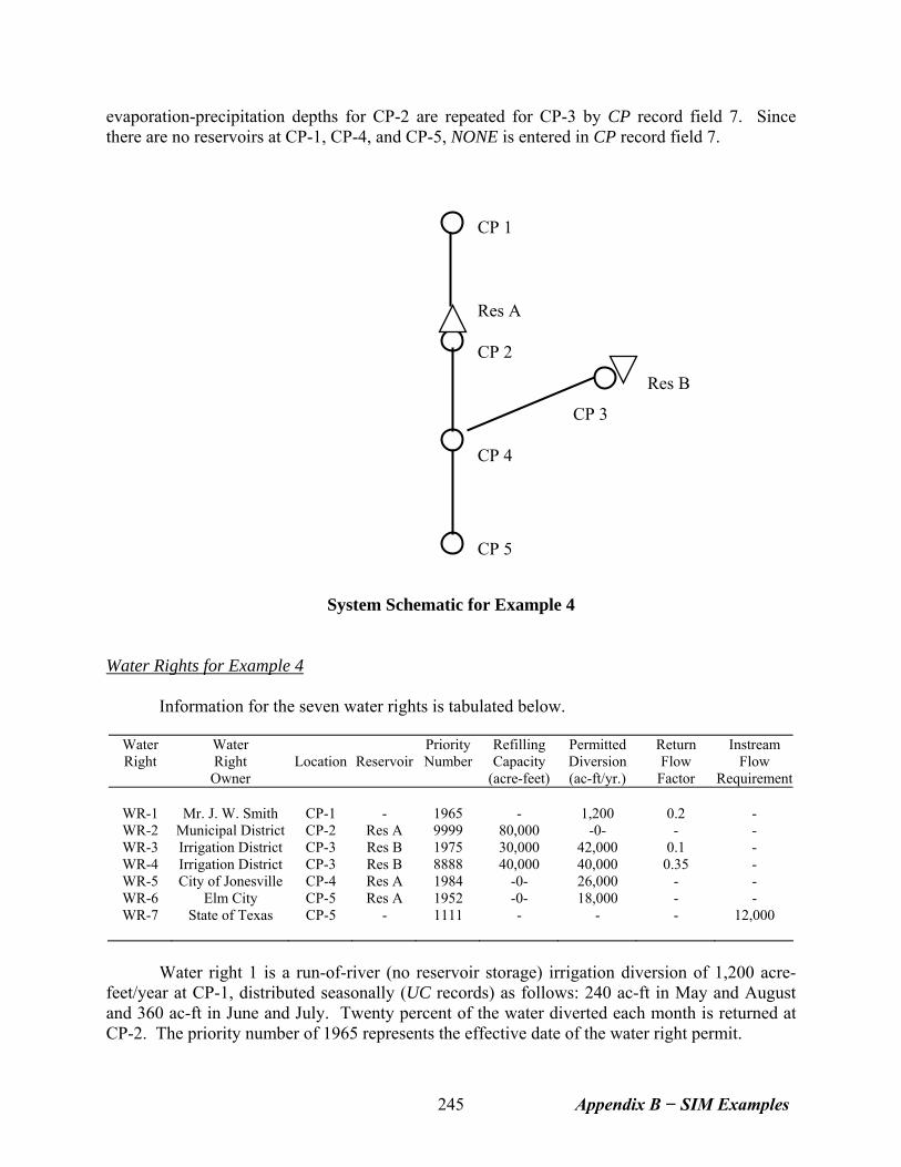
evaporation-precipitation depths for CP-2 are repeated for CP-3 by CP record field 7. Since there are no reservoirs at CP-1, CP-4, and CP-5, NONE is entered in CP record field 7.
Res A
CP 1
CP 5
Res B
CP 3
CP 4
CP 2
System Schematic for Example 4 Water Rights for Example 4 Information for the seven water rights is tabulated below.
Water Water Priority Refilling Permitted Return Instream Right Right Location Reservoir Number Capacity Diversion Flow Flow
Owner (acre-feet) (ac-ft/yr.) Factor Requirement
WR-1 Mr. J. W. Smith CP-1 - 1965 - 1,200 0.2 - WR-2 Municipal District CP-2 Res A 9999 80,000 -0- - - WR-3 Irrigation District CP-3 Res B 1975 30,000 42,000 0.1 - WR-4 Irrigation District CP-3 Res B 8888 40,000 40,000 0.35 - WR-5 City of Jonesville CP-4 Res A 1984 -0- 26,000 - - WR-6 Elm City CP-5 Res A 1952 -0- 18,000 - - WR-7 State of Texas CP-5 - 1111 - - - 12,000
Water right 1 is a run-of-river (no reservoir storage) irrigation diversion of 1,200 acre-feet/year at CP-1, distributed seasonally (UC records) as follows: 240 ac-ft in May and August and 360 ac-ft in June and July. Twenty percent of the water diverted each month is returned at CP-2. The priority number of 1965 represents the effective date of the water right permit.
Appendix B − SIM Examples 245
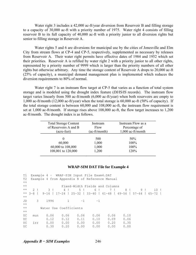
Water right 3 includes a 42,000 ac-ft/year diversion from Reservoir B and filling storage to a capacity of 30,000 ac-ft with a priority number of 1975. Water right 4 consists of filling reservoir B to its full capacity of 40,000 ac-ft with a priority junior to all diversion rights but senior to filling storage in Reservoir A.
Water rights 5 and 6 are diversions for municipal use by the cities of Jonesville and Elm City from stream flows at CP-4 and CP-5, respectively, supplemented as necessary by releases from Reservoir A. Their water right permits have effective dates of 1984 and 1952 which set their priorities. Reservoir A is refilled by water right 2 with a priority junior to all other rights, represented by a priority number of 9999 which is larger than the priority numbers of all other rights but otherwise arbitrary. Any time the storage content of Reservoir A drops to 20,000 ac-ft (25% of capacity), a municipal demand management plan is implemented which reduces the diversion requirements to 80% of normal. Water right 7 is an instream flow target at CP-5 that varies as a function of total system storage and is modeled using the drought index feature (DI/IS/IS records). The instream flow target varies linearly from 500 ac-ft/month (6,000 ac-ft/year) when both reservoirs are empty to 1,000 ac-ft/month (12,000 ac-ft/year) when the total storage is 60,000 ac-ft (50% of capacity). If the total storage content is between 60,000 and 108,000 ac-ft, the instream flow requirement is set at 1,000 ac-ft/month. If storage rises above 108,000 ac-ft, the flow target increases to 1,200 ac-ft/month. The drought index is as follows.
Total Storage Content Instream Instream Flow as a of Reservoirs A and B Flow Percentage of
(acre-feet) (ac-ft/month) 1,000 ac-ft/month
0 500 50% 60,000 1,000 100%
60,000 to 108,000 1,000 100% 108,001 to 120,000 1,200 120%
WRAP-SIM DAT File for Example 4 T1 Example 4 - WRAP-SIM Input File Exam4.DAT T2 Example 4 from Appendix B of Reference Manual ** ** Fixed-Width Fields and Columns ** 2 ! 3 ! 4 ! 5 ! 6 ! 7 ! 8 ! 9 ! 10 ! ** 3-8 ! 9-16 ! 17-24 ! 25-32 ! 33-40 ! 41-48 ! 49-56 ! 57-64 ! 65-72 ! ** JD 3 1996 1 -1 -1 ** ** Water Use Coefficients ** UC mun 0.06 0.06 0.06 0.06 0.06 0.10 UC 0.12 0.12 0.11 0.10 0.09 0.06 UC irr 0.00 0.00 0.00 0.00 0.20 0.30 UC 0.30 0.20 0.00 0.00 0.00 0.00
Appendix B − SIM Examples 246
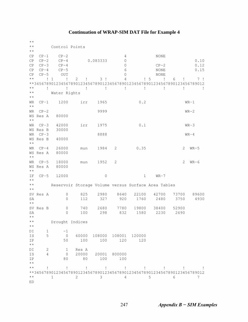
Continuation of WRAP-SIM DAT File for Example 4 ** ** Control Points ** CP CP-1 CP-2 4 NONE CP CP-2 CP-4 0.083333 0 0.10 CP CP-3 CP-4 0 CP-2 0.12 CP CP-4 CP-5 6 NONE 0.15 CP CP-5 OUT 0 NONE ** ! 1 ! 2 ! 3 ! 4 ! 5 ! 6 ! 7 ! **3456789012345678901234567890123456789012345678901234567890123456789012 ** ! ! ! ! ! ! ! ! ! ** Water Rights ** WR CP-1 1200 irr 1965 0.2 WR-1 ** WR CP-2 9999 WR-2 WS Res A 80000 ** WR CP-3 42000 irr 1975 0.1 WR-3 WS Res B 30000 WR CP-3 8888 WR-4 WS Res B 40000 ** WR CP-4 26000 mun 1984 2 0.35 2 WR-5 WS Res A 80000 ** WR CP-5 18000 mun 1952 2 2 WR-6 WS Res A 80000 ** IF CP-5 12000 0 1 WR-7 ** ** Reservoir Storage Volume versus Surface Area Tables ** SV Res A 0 825 2980 8640 22100 42700 73700 89600 SA 0 112 327 920 1760 2480 3750 4930 ** SV Res B 0 740 2680 7780 19800 38400 52900 SA 0 100 298 832 1580 2230 2690 ** ** Drought Indices ** DI 1 -1 IS 5 0 60000 108000 108001 120000 IP 50 100 100 120 120 ** DI 2 1 Res A IS 4 0 20000 20001 800000 IP 80 80 100 100 ** ** ! ! ! ! ! ! ! ! ! **3456789012345678901234567890123456789012345678901234567890123456789012 ** 1 2 3 4 5 6 7 ED
Appendix B − SIM Examples 247
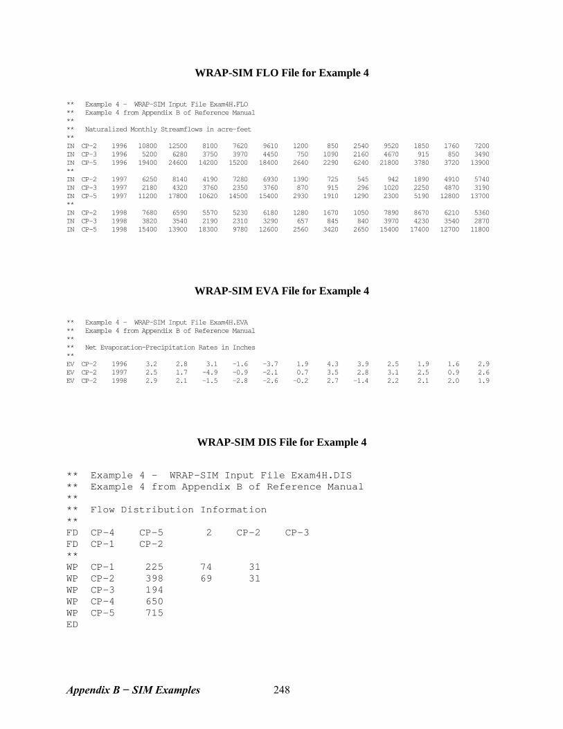
WRAP-SIM FLO File for Example 4
** Example 4 - WRAP-SIM Input File Exam4H.FLO ** Example 4 from Appendix B of Reference Manual ** ** Naturalized Monthly Streamflows in acre-feet ** IN CP-2 1996 10800 12500 8100 7620 9610 1200 850 2540 9520 1850 1760 7200 IN CP-3 1996 5200 6280 3750 3970 4450 750 1090 2160 4670 915 850 3490 IN CP-5 1996 19400 24600 14200 15200 18400 2640 2290 6240 21800 3780 3720 13900 ** IN CP-2 1997 6250 8140 4190 7280 6930 1390 725 545 942 1890 4910 5740 IN CP-3 1997 2180 4320 3760 2350 3760 870 915 296 1020 2250 4870 3190 IN CP-5 1997 11200 17800 10620 14500 15400 2930 1910 1290 2300 5190 12800 13700 ** IN CP-2 1998 7680 6590 5570 5230 6180 1280 1670 1050 7890 8670 6210 5360 IN CP-3 1998 3820 3540 2190 2310 3290 657 845 840 3970 4230 3540 2870 IN CP-5 1998 15400 13900 18300 9780 12600 2560 3420 2650 15400 17400 12700 11800
WRAP-SIM EVA File for Example 4
** Example 4 - WRAP-SIM Input File Exam4H.EVA ** Example 4 from Appendix B of Reference Manual ** ** Net Evaporation-Precipitation Rates in Inches ** EV CP-2 1996 3.2 2.8 3.1 -1.6 -3.7 1.9 4.3 3.9 2.5 1.9 1.6 2.9 EV CP-2 1997 2.5 1.7 -4.9 -0.9 -2.1 0.7 3.5 2.8 3.1 2.5 0.9 2.6 EV CP-2 1998 2.9 2.1 -1.5 -2.8 -2.6 -0.2 2.7 -1.4 2.2 2.1 2.0 1.9
WRAP-SIM DIS File for Example 4
** Example 4 - WRAP-SIM Input File Exam4H.DIS ** Example 4 from Appendix B of Reference Manual ** ** Flow Distribution Information ** FD CP-4 CP-5 2 CP-2 CP-3 FD CP-1 CP-2 ** WP CP-1 225 74 31 WP CP-2 398 69 31 WP CP-3 194 WP CP-4 650 WP CP-5 715 ED
Appendix B − SIM Examples 248
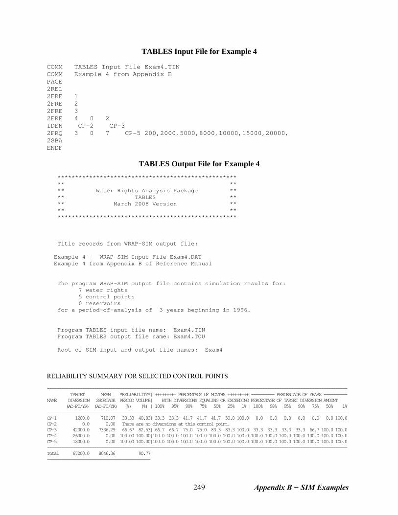
TABLES Input File for Example 4 COMM TABLES Input File Exam4.TIN COMM Example 4 from Appendix B PAGE 2REL 2FRE 1 2FRE 2 2FRE 3 2FRE 4 0 2 IDEN CP-2 CP-3 2FRQ 3 0 7 CP-5 200,2000,5000,8000,10000,15000,20000, 2SBA ENDF
TABLES Output File for Example 4 *************************************************** ** ** ** Water Rights Analysis Package ** ** TABLES ** ** March 2008 Version ** ** ** *************************************************** Title records from WRAP-SIM output file: Example 4 - WRAP-SIM Input File Exam4.DAT Example 4 from Appendix B of Reference Manual The program WRAP-SIM output file contains simulation results for: 7 water rights 5 control points 0 reservoirs for a period-of-analysis of 3 years beginning in 1996. Program TABLES input file name: Exam4.TIN Program TABLES output file name: Exam4.TOU Root of SIM input and output file names: Exam4 RELIABILITY SUMMARY FOR SELECTED CONTROL POINTS -------------------------------------------------------------------------------------------------------------------------------- TARGET MEAN *RELIABILITY*| +++++++++ PERCENTAGE OF MONTHS +++++++++|---------- PERCENTAGE OF YEARS ---------- NAME DIVERSION SHORTAGE PERIOD VOLUME| WITH DIVERSIONS EQUALING OR EXCEEDING PERCENTAGE OF TARGET DIVERSION AMOUNT (AC-FT/YR) (AC-FT/YR) (%) (%) | 100% 95% 90% 75% 50% 25% 1% | 100% 98% 95% 90% 75% 50% 1% -------------------------------------------------------------------------------------------------------------------------------- CP-1 1200.0 710.07 33.33 40.83| 33.3 33.3 41.7 41.7 41.7 50.0 100.0| 0.0 0.0 0.0 0.0 0.0 0.0 100.0 CP-2 0.0 0.00 There are no diversions at this control point. CP-3 42000.0 7336.29 66.67 82.53| 66.7 66.7 75.0 75.0 83.3 83.3 100.0| 33.3 33.3 33.3 33.3 66.7 100.0 100.0 CP-4 26000.0 0.00 100.00 100.00|100.0 100.0 100.0 100.0 100.0 100.0 100.0|100.0 100.0 100.0 100.0 100.0 100.0 100.0 CP-5 18000.0 0.00 100.00 100.00|100.0 100.0 100.0 100.0 100.0 100.0 100.0|100.0 100.0 100.0 100.0 100.0 100.0 100.0 -------------------------------------------------------------------------------------------------------------------------------- Total 87200.0 8046.36 90.77 --------------------------------------------
Appendix B − SIM Examples 249
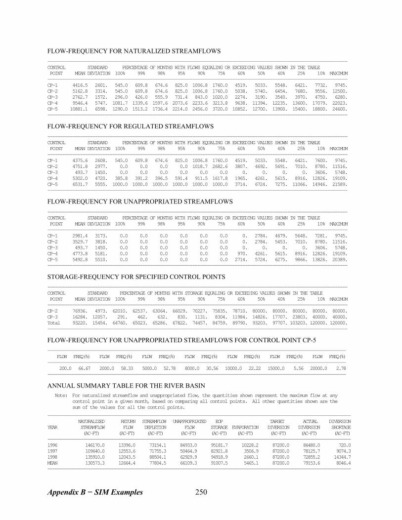
FLOW-FREQUENCY FOR NATURALIZED STREAMFLOWS
------------------------------------------------------------------------------------------------------------------------ CONTROL STANDARD PERCENTAGE OF MONTHS WITH FLOWS EQUALING OR EXCEEDING VALUES SHOWN IN THE TABLE POINT MEAN DEVIATION 100% 99% 98% 95% 90% 75% 60% 50% 40% 25% 10% MAXIMUM ------------------------------------------------------------------------------------------------------------------------ CP-1 4416.5 2601. 545.0 609.8 674.6 825.0 1006.8 1760.0 4519. 5033. 5548. 6421. 7732. 9745. CP-2 5162.8 3314. 545.0 609.8 674.6 825.0 1006.8 1760.0 5038. 5740. 6454. 7680. 9556. 12500. CP-3 2762.7 1572. 296.0 426.0 555.9 731.4 843.0 1020.0 2274. 3190. 3540. 3970. 4750. 6280. CP-4 9546.4 5747. 1081.7 1339.6 1597.6 2073.6 2233.6 3213.8 9638. 11394. 12235. 13600. 17079. 22023. CP-5 10881.1 6598. 1290.0 1513.2 1736.4 2214.0 2456.0 3720.0 10852. 12700. 13900. 15400. 18800. 24600. ------------------------------------------------------------------------------------------------------------------------
FLOW-FREQUENCY FOR REGULATED STREAMFLOWS
------------------------------------------------------------------------------------------------------------------------ CONTROL STANDARD PERCENTAGE OF MONTHS WITH FLOWS EQUALING OR EXCEEDING VALUES SHOWN IN THE TABLE POINT MEAN DEVIATION 100% 99% 98% 95% 90% 75% 60% 50% 40% 25% 10% MAXIMUM ------------------------------------------------------------------------------------------------------------------------ CP-1 4375.6 2608. 545.0 609.8 674.6 825.0 1006.8 1760.0 4519. 5033. 5548. 6421. 7600. 9745. CP-2 4751.8 2977. 0.0 0.0 0.0 0.0 1018.7 2682.6 3807. 4692. 5691. 7010. 8780. 11516. CP-3 493.7 1450. 0.0 0.0 0.0 0.0 0.0 0.0 0. 0. 0. 0. 3606. 5748. CP-4 5302.0 4720. 385.8 391.2 396.5 591.4 911.5 1617.8 1965. 4261. 5615. 8916. 12826. 19109. CP-5 6531.7 5555. 1000.0 1000.0 1000.0 1000.0 1000.0 1000.0 3714. 6724. 7275. 11066. 14946. 21589. ------------------------------------------------------------------------------------------------------------------------
FLOW-FREQUENCY FOR UNAPPROPRIATED STREAMFLOWS
------------------------------------------------------------------------------------------------------------------------ CONTROL STANDARD PERCENTAGE OF MONTHS WITH FLOWS EQUALING OR EXCEEDING VALUES SHOWN IN THE TABLE POINT MEAN DEVIATION 100% 99% 98% 95% 90% 75% 60% 50% 40% 25% 10% MAXIMUM ------------------------------------------------------------------------------------------------------------------------ CP-1 2981.4 3173. 0.0 0.0 0.0 0.0 0.0 0.0 0. 2784. 4679. 5648. 7281. 9745. CP-2 3529.7 3818. 0.0 0.0 0.0 0.0 0.0 0.0 0. 2784. 5453. 7010. 8780. 11516. CP-3 493.7 1450. 0.0 0.0 0.0 0.0 0.0 0.0 0. 0. 0. 0. 3606. 5748. CP-4 4773.8 5181. 0.0 0.0 0.0 0.0 0.0 0.0 970. 4261. 5615. 8916. 12826. 19109. CP-5 5492.8 5510. 0.0 0.0 0.0 0.0 0.0 0.0 2714. 5724. 6275. 9866. 13826. 20389. ------------------------------------------------------------------------------------------------------------------------
STORAGE-FREQUENCY FOR SPECIFIED CONTROL POINTS
------------------------------------------------------------------------------------------------------------------------ CONTROL STANDARD PERCENTAGE OF MONTHS WITH STORAGE EQUALING OR EXCEEDING VALUES SHOWN IN THE TABLE POINT MEAN DEVIATION 100% 99% 98% 95% 90% 75% 60% 50% 40% 25% 10% MAXIMUM ------------------------------------------------------------------------------------------------------------------------ CP-2 76936. 4973. 62010. 62537. 63064. 66029. 70227. 75835. 78710. 80000. 80000. 80000. 80000. 80000. CP-3 16284. 12057. 291. 462. 632. 830. 1131. 8304. 11984. 14826. 17707. 23803. 40000. 40000. Total 93220. 15454. 64760. 65023. 65286. 67822. 74457. 84759. 89790. 93203. 97707. 103203. 120000. 120000. ------------------------------------------------------------------------------------------------------------------------
FLOW-FREQUENCY FOR UNAPPROPRIATED STREAMFLOWS FOR CONTROL POINT CP-5
------------------------------------------------------------------------------------------------------------------------------ FLOW FREQ(%) FLOW FREQ(%) FLOW FREQ(%) FLOW FREQ(%) FLOW FREQ(%) FLOW FREQ(%) FLOW FREQ(%) ------------------------------------------------------------------------------------------------------------------------------ 200.0 66.67 2000.0 58.33 5000.0 52.78 8000.0 30.56 10000.0 22.22 15000.0 5.56 20000.0 2.78 ------------------------------------------------------------------------------------------------------------------------------
ANNUAL SUMMARY TABLE FOR THE RIVER BASIN
Note: For naturalized streamflow and unappropriated flow, the quantities shown represent the maximum flow at any control point in a given month, based on comparing all control points. All other quantities shown are the sum of the values for all the control points.
-------------------------------------------------------------------------------------------------------------------------------- NATURALIZED RETURN STREAMFLOW UNAPPROPRIATED EOP TARGET ACTUAL DIVERSION YEAR STREAMFLOW FLOW DEPLETION FLOW STORAGE EVAPORATION DIVERSION DIVERSION SHORTAGE (AC-FT) (AC-FT) (AC-FT) (AC-FT) (AC-FT) (AC-FT) (AC-FT) (AC-FT) (AC-FT) -------------------------------------------------------------------------------------------------------------------------------- 1996 146170.0 13396.0 73154.1 84933.0 95181.7 10228.2 87200.0 86480.0 720.0 1997 109640.0 12553.6 71755.3 50464.9 82921.8 3506.9 87200.0 78125.7 9074.3 1998 135910.0 12043.5 88504.1 62929.9 94918.9 2660.1 87200.0 72855.2 14344.7 MEAN 130573.3 12664.4 77804.5 66109.3 91007.5 5465.1 87200.0 79153.6 8046.4 --------------------------------------------------------------------------------------------------------------------------------
Appendix B − SIM Examples 250
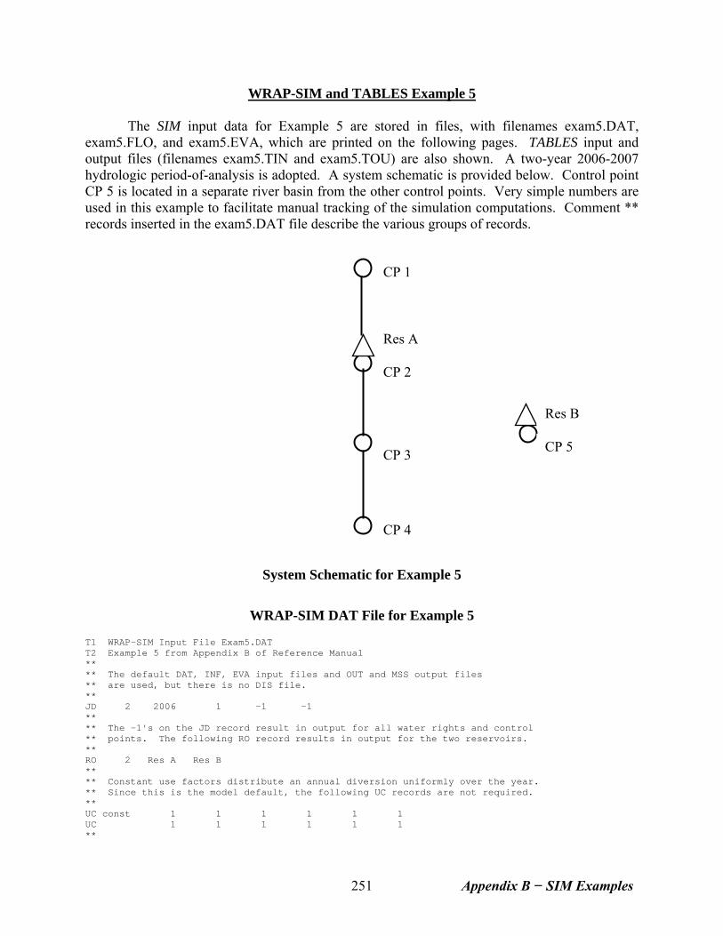
WRAP-SIM and TABLES Example 5
The SIM input data for Example 5 are stored in files, with filenames exam5.DAT, exam5.FLO, and exam5.EVA, which are printed on the following pages. TABLES input and output files (filenames exam5.TIN and exam5.TOU) are also shown. A two-year 2006-2007 hydrologic period-of-analysis is adopted. A system schematic is provided below. Control point CP 5 is located in a separate river basin from the other control points. Very simple numbers are used in this example to facilitate manual tracking of the simulation computations. Comment ** records inserted in the exam5.DAT file describe the various groups of records.
CP 2
Res A
CP 1
CP 3
CP 4
CP 5
Res B
System Schematic for Example 5
WRAP-SIM DAT File for Example 5
T1 WRAP-SIM Input File Exam5.DAT T2 Example 5 from Appendix B of Reference Manual ** ** The default DAT, INF, EVA input files and OUT and MSS output files ** are used, but there is no DIS file. ** JD 2 2006 1 -1 -1 ** ** The -1's on the JD record result in output for all water rights and control ** points. The following RO record results in output for the two reservoirs. ** RO 2 Res A Res B ** ** Constant use factors distribute an annual diversion uniformly over the year. ** Since this is the model default, the following UC records are not required. ** UC const 1 1 1 1 1 1 UC 1 1 1 1 1 1 **
Appendix B − SIM Examples 251
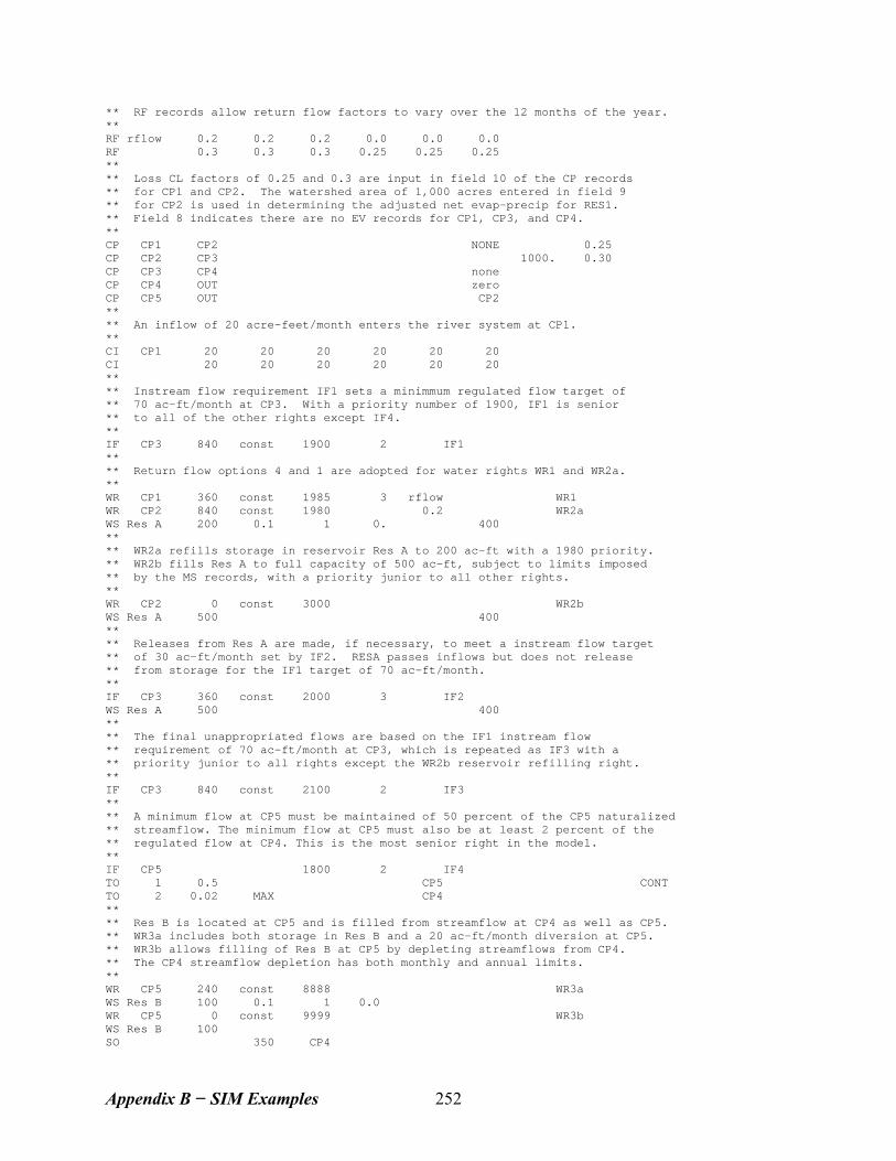
** RF records allow return flow factors to vary over the 12 months of the year. ** RF rflow 0.2 0.2 0.2 0.0 0.0 0.0 RF 0.3 0.3 0.3 0.25 0.25 0.25 ** ** Loss CL factors of 0.25 and 0.3 are input in field 10 of the CP records ** for CP1 and CP2. The watershed area of 1,000 acres entered in field 9 ** for CP2 is used in determining the adjusted net evap-precip for RES1. ** Field 8 indicates there are no EV records for CP1, CP3, and CP4. ** CP CP1 CP2 NONE 0.25 CP CP2 CP3 1000. 0.30 CP CP3 CP4 none CP CP4 OUT zero CP CP5 OUT CP2 ** ** An inflow of 20 acre-feet/month enters the river system at CP1. ** CI CP1 20 20 20 20 20 20 CI 20 20 20 20 20 20 ** ** Instream flow requirement IF1 sets a minimmum regulated flow target of ** 70 ac-ft/month at CP3. With a priority number of 1900, IF1 is senior ** to all of the other rights except IF4. ** IF CP3 840 const 1900 2 IF1 ** ** Return flow options 4 and 1 are adopted for water rights WR1 and WR2a. ** WR CP1 360 const 1985 3 rflow WR1 WR CP2 840 const 1980 0.2 WR2a WS Res A 200 0.1 1 0. 400 ** ** WR2a refills storage in reservoir Res A to 200 ac-ft with a 1980 priority. ** WR2b fills Res A to full capacity of 500 ac-ft, subject to limits imposed ** by the MS records, with a priority junior to all other rights. ** WR CP2 0 const 3000 WR2b WS Res A 500 400 ** ** Releases from Res A are made, if necessary, to meet a instream flow target ** of 30 ac-ft/month set by IF2. RESA passes inflows but does not release ** from storage for the IF1 target of 70 ac-ft/month. ** IF CP3 360 const 2000 3 IF2 WS Res A 500 400 ** ** The final unappropriated flows are based on the IF1 instream flow ** requirement of 70 ac-ft/month at CP3, which is repeated as IF3 with a ** priority junior to all rights except the WR2b reservoir refilling right. ** IF CP3 840 const 2100 2 IF3 ** ** A minimum flow at CP5 must be maintained of 50 percent of the CP5 naturalized ** streamflow. The minimum flow at CP5 must also be at least 2 percent of the ** regulated flow at CP4. This is the most senior right in the model. ** IF CP5 1800 2 IF4 TO 1 0.5 CP5 CONT TO 2 0.02 MAX CP4 ** ** Res B is located at CP5 and is filled from streamflow at CP4 as well as CP5. ** WR3a includes both storage in Res B and a 20 ac-ft/month diversion at CP5. ** WR3b allows filling of Res B at CP5 by depleting streamflows from CP4. ** The CP4 streamflow depletion has both monthly and annual limits. ** WR CP5 240 const 8888 WR3a WS Res B 100 0.1 1 0.0 WR CP5 0 const 9999 WR3b WS Res B 100 SO 350 CP4
Appendix B − SIM Examples 252
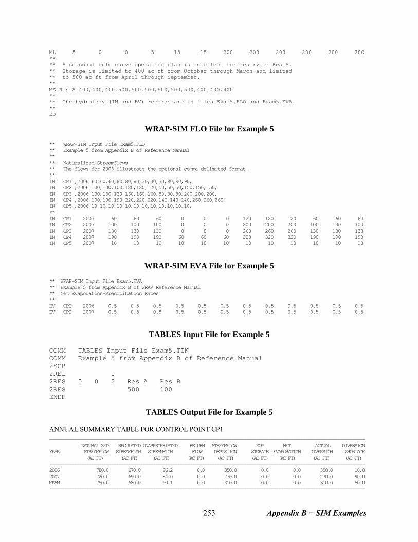
ML 5 0 0 5 15 15 200 200 200 200 200 200 ** ** A seasonal rule curve operating plan is in effect for reservoir Res A. ** Storage is limited to 400 ac-ft from October through March and limited ** to 500 ac-ft from April through September. ** MS Res A 400,400,400,500,500,500,500,500,500,400,400,400 ** ** The hydrology (IN and EV) records are in files Exam5.FLO and Exam5.EVA. ** ED
WRAP-SIM FLO File for Example 5 ** WRAP-SIM Input File Exam5.FLO ** Example 5 from Appendix B of Reference Manual ** ** Naturalized Streamflows ** The flows for 2006 illustrate the optional comma delimited format. ** IN CP1 ,2006 60,60,60,80,80,80,30,30,30,90,90,90, IN CP2 ,2006 100,100,100,120,120,120,50,50,50,150,150,150, IN CP3 ,2006 130,130,130,160,160,160,80,80,80,200,200,200, IN CP4 ,2006 190,190,190,220,220,220,140,140,140,260,260,260, IN CP5 ,2006 10,10,10,10,10,10,10,10,10,10,10,10, ** IN CP1 2007 60 60 60 0 0 0 120 120 120 60 60 60 IN CP2 2007 100 100 100 0 0 0 200 200 200 100 100 100 IN CP3 2007 130 130 130 0 0 0 260 260 260 130 130 130 IN CP4 2007 190 190 190 60 60 60 320 320 320 190 190 190 IN CP5 2007 10 10 10 10 10 10 10 10 10 10 10 10
WRAP-SIM EVA File for Example 5
** WRAP-SIM Input File Exam5.EVA ** Example 5 from Appendix B of WRAP Reference Manual ** Net Evaporation-Precipitation Rates ** EV CP2 2006 0.5 0.5 0.5 0.5 0.5 0.5 0.5 0.5 0.5 0.5 0.5 0.5 EV CP2 2007 0.5 0.5 0.5 0.5 0.5 0.5 0.5 0.5 0.5 0.5 0.5 0.5
TABLES Input File for Example 5
COMM TABLES Input File Exam5.TIN COMM Example 5 from Appendix B of Reference Manual 2SCP 2REL 1 2RES 0 0 2 Res A Res B 2RES 500 100 ENDF
TABLES Output File for Example 5
ANNUAL SUMMARY TABLE FOR CONTROL POINT CP1
-------------------------------------------------------------------------------------------------------------------------------- NATURALIZED REGULATED UNAPPROPRIATED RETURN STREAMFLOW EOP NET ACTUAL DIVERSION YEAR STREAMFLOW STREAMFLOW STREAMFLOW FLOW DEPLETION STORAGE EVAPORATION DIVERSION SHORTAGE (AC-FT) (AC-FT) (AC-FT) (AC-FT) (AC-FT) (AC-FT) (AC-FT) (AC-FT) (AC-FT) -------------------------------------------------------------------------------------------------------------------------------- 2006 780.0 670.0 96.2 0.0 350.0 0.0 0.0 350.0 10.0 2007 720.0 690.0 84.0 0.0 270.0 0.0 0.0 270.0 90.0 MEAN 750.0 680.0 90.1 0.0 310.0 0.0 0.0 310.0 50.0 --------------------------------------------------------------------------------------------------------------------------------
Appendix B − SIM Examples 253
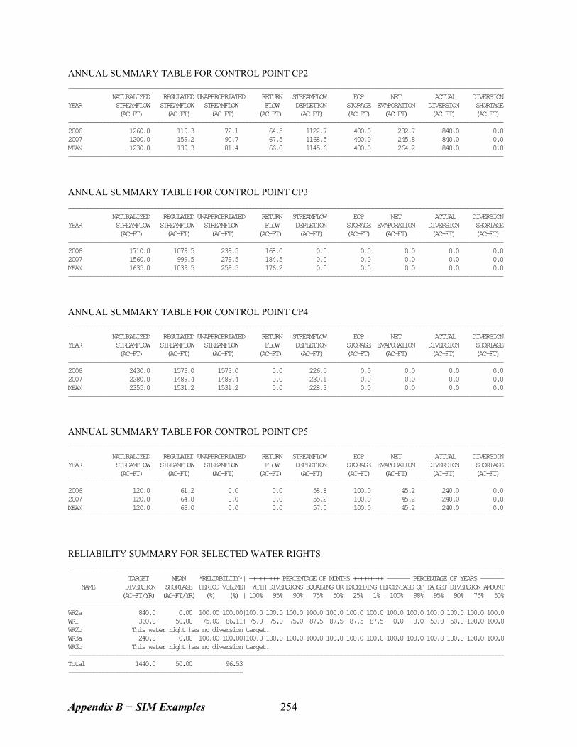
ANNUAL SUMMARY TABLE FOR CONTROL POINT CP2
-------------------------------------------------------------------------------------------------------------------------------- NATURALIZED REGULATED UNAPPROPRIATED RETURN STREAMFLOW EOP NET ACTUAL DIVERSION YEAR STREAMFLOW STREAMFLOW STREAMFLOW FLOW DEPLETION STORAGE EVAPORATION DIVERSION SHORTAGE (AC-FT) (AC-FT) (AC-FT) (AC-FT) (AC-FT) (AC-FT) (AC-FT) (AC-FT) (AC-FT) -------------------------------------------------------------------------------------------------------------------------------- 2006 1260.0 119.3 72.1 64.5 1122.7 400.0 282.7 840.0 0.0 2007 1200.0 159.2 90.7 67.5 1168.5 400.0 245.8 840.0 0.0 MEAN 1230.0 139.3 81.4 66.0 1145.6 400.0 264.2 840.0 0.0 -------------------------------------------------------------------------------------------------------------------------------- ANNUAL SUMMARY TABLE FOR CONTROL POINT CP3 -------------------------------------------------------------------------------------------------------------------------------- NATURALIZED REGULATED UNAPPROPRIATED RETURN STREAMFLOW EOP NET ACTUAL DIVERSION YEAR STREAMFLOW STREAMFLOW STREAMFLOW FLOW DEPLETION STORAGE EVAPORATION DIVERSION SHORTAGE (AC-FT) (AC-FT) (AC-FT) (AC-FT) (AC-FT) (AC-FT) (AC-FT) (AC-FT) (AC-FT) -------------------------------------------------------------------------------------------------------------------------------- 2006 1710.0 1079.5 239.5 168.0 0.0 0.0 0.0 0.0 0.0 2007 1560.0 999.5 279.5 184.5 0.0 0.0 0.0 0.0 0.0 MEAN 1635.0 1039.5 259.5 176.2 0.0 0.0 0.0 0.0 0.0 -------------------------------------------------------------------------------------------------------------------------------- ANNUAL SUMMARY TABLE FOR CONTROL POINT CP4 -------------------------------------------------------------------------------------------------------------------------------- NATURALIZED REGULATED UNAPPROPRIATED RETURN STREAMFLOW EOP NET ACTUAL DIVERSION YEAR STREAMFLOW STREAMFLOW STREAMFLOW FLOW DEPLETION STORAGE EVAPORATION DIVERSION SHORTAGE (AC-FT) (AC-FT) (AC-FT) (AC-FT) (AC-FT) (AC-FT) (AC-FT) (AC-FT) (AC-FT) -------------------------------------------------------------------------------------------------------------------------------- 2006 2430.0 1573.0 1573.0 0.0 226.5 0.0 0.0 0.0 0.0 2007 2280.0 1489.4 1489.4 0.0 230.1 0.0 0.0 0.0 0.0 MEAN 2355.0 1531.2 1531.2 0.0 228.3 0.0 0.0 0.0 0.0 -------------------------------------------------------------------------------------------------------------------------------- ANNUAL SUMMARY TABLE FOR CONTROL POINT CP5 -------------------------------------------------------------------------------------------------------------------------------- NATURALIZED REGULATED UNAPPROPRIATED RETURN STREAMFLOW EOP NET ACTUAL DIVERSION YEAR STREAMFLOW STREAMFLOW STREAMFLOW FLOW DEPLETION STORAGE EVAPORATION DIVERSION SHORTAGE (AC-FT) (AC-FT) (AC-FT) (AC-FT) (AC-FT) (AC-FT) (AC-FT) (AC-FT) (AC-FT) -------------------------------------------------------------------------------------------------------------------------------- 2006 120.0 61.2 0.0 0.0 58.8 100.0 45.2 240.0 0.0 2007 120.0 64.8 0.0 0.0 55.2 100.0 45.2 240.0 0.0 MEAN 120.0 63.0 0.0 0.0 57.0 100.0 45.2 240.0 0.0 --------------------------------------------------------------------------------------------------------------------------------
RELIABILITY SUMMARY FOR SELECTED WATER RIGHTS ---------------------------------------------------------------------------------------------------------------------------------- TARGET MEAN *RELIABILITY*| +++++++++ PERCENTAGE OF MONTHS +++++++++|------- PERCENTAGE OF YEARS ------- NAME DIVERSION SHORTAGE PERIOD VOLUME| WITH DIVERSIONS EQUALING OR EXCEEDING PERCENTAGE OF TARGET DIVERSION AMOUNT (AC-FT/YR) (AC-FT/YR) (%) (%) | 100% 95% 90% 75% 50% 25% 1% | 100% 98% 95% 90% 75% 50% ---------------------------------------------------------------------------------------------------------------------------------- WR2a 840.0 0.00 100.00 100.00|100.0 100.0 100.0 100.0 100.0 100.0 100.0|100.0 100.0 100.0 100.0 100.0 100.0 WR1 360.0 50.00 75.00 86.11| 75.0 75.0 75.0 87.5 87.5 87.5 87.5| 0.0 0.0 50.0 50.0 100.0 100.0 WR2b This water right has no diversion target. WR3a 240.0 0.00 100.00 100.00|100.0 100.0 100.0 100.0 100.0 100.0 100.0|100.0 100.0 100.0 100.0 100.0 100.0 WR3b This water right has no diversion target. ---------------------------------------------------------------------------------------------------------------------------------- Total 1440.0 50.00 96.53 ----------------------------------------------------
Appendix B − SIM Examples 254
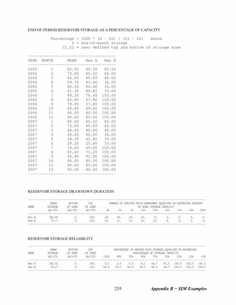
END-OF-PERIOD RESERVOIR STORAGE AS A PERCENTAGE OF CAPACITY Percentage = 100% * (S - C2) / (C1 - C2) where S = end-of-month storage C1,C2 = user defined top and bottom of storage zone -------------------------------------- YEAR MONTH MEAN Res A Res B -------------------------------------- 2006 1 82.50 80.00 85.00 2006 2 73.00 80.00 66.00 2006 3 64.00 80.00 48.00 2006 4 59.70 83.40 36.00 2006 5 60.30 86.60 34.00 2006 6 61.30 89.60 33.00 2006 7 89.20 78.40 100.00 2006 8 83.90 67.80 100.00 2006 9 78.90 57.80 100.00 2006 10 84.80 69.60 100.00 2006 11 90.00 80.00 100.00 2006 12 90.00 80.00 100.00 2007 1 82.50 80.00 85.00 2007 2 73.00 80.00 66.00 2007 3 64.00 80.00 48.00 2007 4 48.40 60.80 36.00 2007 5 38.30 42.60 34.00 2007 6 29.20 25.40 33.00 2007 7 74.50 49.00 100.00 2007 8 85.60 71.20 100.00 2007 9 95.90 91.80 100.00 2007 10 90.00 80.00 100.00 2007 11 90.00 80.00 100.00 2007 12 90.00 80.00 100.00 -------------------------------------- RESERVOIR STORAGE DRAWDOWN DURATION ---------------------------------------------------------------------------------------------------------------------- MEAN BOTTOM TOP NUMBER OF PERIODS WITH DRAWDOWNS EQUALING OR EXCEEDING PERCENT NAME STORAGE OF ZONE OF ZONE OF ZONE STORAGE CAPACITY (AC-FT) (AC-FT) (AC-FT) 0% 2% 5% 10% 25% 50% 75% 90% 100% ---------------------------------------------------------------------------------------------------------------------- Res A 365.42 0. 500. 24. 24. 24. 23. 8. 3. 0. 0. 0. Res B 75.17 0. 100. 24. 12. 12. 12. 10. 8. 0. 0. 0. ---------------------------------------------------------------------------------------------------------------------- RESERVOIR STORAGE RELIABILITY ---------------------------------------------------------------------------------------------------------------------- MEAN BOTTOM TOP PERCENTAGE OF MONTHS WITH STORAGE EQUALING OR EXCEEDING NAME STORAGE OF ZONE OF ZONE PERCENTAGE OF STORAGE CAPACITY (AC-FT) (AC-FT) (AC-FT) 100% 98% 95% 90% 75% 50% 25% 10% >0% ---------------------------------------------------------------------------------------------------------------------- Res A 365.42 0. 500. 0.0 0.0 0.0 4.2 66.7 87.5 100.0 100.0 100.0 Res B 75.17 0. 100. 50.0 50.0 50.0 50.0 58.3 66.7 100.0 100.0 100.0 ----------------------------------------------------------------------------------------------------------------------
Appendix B − SIM Examples 255
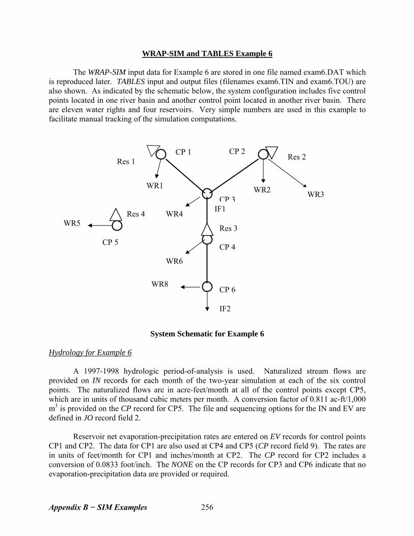
WRAP-SIM and TABLES Example 6 The WRAP-SIM input data for Example 6 are stored in one file named exam6.DAT which is reproduced later. TABLES input and output files (filenames exam6.TIN and exam6.TOU) are also shown. As indicated by the schematic below, the system configuration includes five control points located in one river basin and another control point located in another river basin. There are eleven water rights and four reservoirs. Very simple numbers are used in this example to facilitate manual tracking of the simulation computations.
CP 6
WR6
WR5
CP 3 IF1
CP 4 CP 5
Res 4
CP 2
WR1
WR4
Res 3
CP 1 Res 1 Res 2
WR3 WR2
WR8 IF2
System Schematic for Example 6 Hydrology for Example 6 A 1997-1998 hydrologic period-of-analysis is used. Naturalized stream flows are provided on IN records for each month of the two-year simulation at each of the six control points. The naturalized flows are in acre-feet/month at all of the control points except CP5, which are in units of thousand cubic meters per month. A conversion factor of 0.811 ac-ft/1,000 m3 is provided on the CP record for CP5. The file and sequencing options for the IN and EV are defined in JO record field 2.
Reservoir net evaporation-precipitation rates are entered on EV records for control points CP1 and CP2. The data for CP1 are also used at CP4 and CP5 (CP record field 9). The rates are in units of feet/month for CP1 and inches/month at CP2. The CP record for CP2 includes a conversion of 0.0833 foot/inch. The NONE on the CP records for CP3 and CP6 indicate that no evaporation-precipitation data are provided or required.
Appendix B − SIM Examples 256
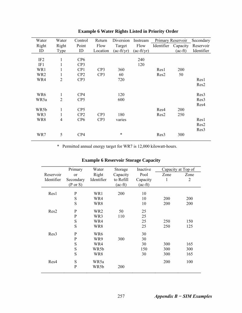
Example 6 Water Rights Listed in Priority Order
Water Water Control Return Diversion Instream Primary Reservoir SecondaryRight Right Point Flow Target Flow Identifier Capacity Reservoir
ID Type ID Location (ac-ft/yr) (ac-ft/yr) (ac-ft) Identifier
IF2 1 CP6 240 IF1 1 CP3 120
WR1 1 CP1 CP3 360 Res1 200 WR2 1 CP2 CP3 60 Res2 50 WR4 2 CP3 720 Res1
Res2
WR6 1 CP4 120 Res3 WR5a 2 CP5 600 Res3
Res4 WR5b 1 CP5 Res4 200 WR3 1 CP2 CP3 180 Res2 250 WR8 4 CP6 CP3 varies Res1
Res2 Res3
WR7 5 CP4 * Res3 300
* Permitted annual energy target for WR7 is 12,000 kilowatt-hours.
Example 6 Reservoir Storage Capacity
Primary Water Storage Inactive Capacity at Top of Reservoir or Right Capacity Pool Zone Zone Identifier Secondary Identifier to Refill Capacity 1 2
(P or S) (ac-ft) (ac-ft)
Res1 P WR1 200 10 S WR4 10 200 200 S WR8 10 200 200
Res2 P WR2 50 25 P WR3 110 25 S WR4 25 250 150 S WR8 25 250 125
Res3 P WR6 30 P WR9 300 30 S WR4 30 300 165 S WR5b 150 300 300 S WR8 30 300 165
Res4 S WR5a 200 100 P WR5b 200
Appendix B − SIM Examples 257
Volume versus Area Relationships for the Example 6 Reservoirs A storage volume versus water surface area relationship is required for each of the four reservoirs for use in the evaporation computations. A table of storage volume, in acre-feet, versus area, in acres, is provided on SV and SA records for reservoir Res4.
The storage-volume relationships for the other three reservoirs are provided by the alternative option of entering the coefficients for Equation 7-1 in fields 4, 5, and 6 of the WS record. With values of 0.1, 1.0, and 0.0 for coefficients a, b, and c, respectively, for each of these reservoirs, Equation 7-1 reduces to:
area in acres = 0.1 (storage volume in acre-feet) Water Rights for Example 6 Information associated with each water right is summarized in the tables on the next page. Diversion, instream flow, and hydropower requirements are provided in the first table. Reservoir storage capacities are tabulated in the second table. Water Rights IF1 and IF2. - Water rights IF1 and IF2 are instream flow requirements at control points CP3 and CP6, respectively, of 120 ac-ft/year (10 ac-ft/month) and 240 ac-ft/year (20 ac-ft/month). With priority numbers of 191805 (May 1918) and 191803 (March 1918), these are the two most senior rights in the system. Water Right WR1. - Water right WR1 located at control point CP1 has a permitted diversion of 360 ac-ft/yr, priority number of 192602 representing February 1926, and same-month return flow of 20% reentering the river at CP3. The annual diversion amount is converted to monthly diversions using the default constant monthly use factors. WR1 is a type 1 right with RES1 being its primary and only reservoir. Reservoir Res1 can be filled to a capacity of 200 ac-ft and supply water for the WR1 diversion until the storage level drops below the inactive pool capacity of 10 ac-ft. The volume-area relationship coefficients must be entered with WR1 since this is the first time Res1 is cited but do not have to be repeated on subsequent Res1 WS records. Water Rights WR2 and WR3. - Res2 is the primary (and only) reservoir for both WR2 and WR3, which can refill it to total cumulative capacities of 50 and 250 ac-ft, respectively. WR2 and WR3 have permitted annual diversion amounts of 60 and 180 ac-ft/yr, respectively, which are met by CP2 inflows as long as yet unappropriated stream flow is available and then withdrawals from Res2 as long as the storage is above the inactive pool capacity of 25 ac-ft. WR3 is junior to WR2. Several other rights at other locations have priorities which fall between WR2 and WR3. Water Right WR4. - WR4 is a type 2 right with two secondary reservoirs but no primary reservoir. The WR4 diversion target is 720 ac-ft/yr or 60 ac-ft/month at CP3. Return flows of 40% the diversion amount renter the river at the default next downstream control point. The WR4 diversion target is met first by available stream flow at CP3 and then, as necessary, by releases from reservoirs Res1 and Res2. WR4 is denoted a type 2 right since
Appendix B − SIM Examples 258
(unlike a type 1 right) it does not refill reservoir storage and (like a type 1 but unlike a type 3 right) it makes releases from Res1 and Res2 only if sufficient stream flow is not available at CP3 for the diversion. Multiple-reservoir system operations are based on balancing the storage, as a percent of zone capacity, in each reservoir. WRAP-SIM computes a ranking index for each reservoir using Equation 4.2.
storage content in zonerank index = (multiplier factor) + addition factorstorage capacity of zone⎡ ⎤⎢ ⎥⎣ ⎦
(4.2)
The release is made from the reservoir with the greatest value for the rank index. The reservoir zones are defined by Figure 4.1. Zone 1 must be empty in all the reservoirs in the system in order for releases to be made from zone 2 of any of the reservoirs. The weighting factors used in the above formula are entered for each reservoir on the OR records. Weighting factors of either 1.0 or zero are used for the two zones of all reservoirs in the example. Since only the relative magnitude between reservoirs matters, replacing the 1.0’s with any positive constant number will yield the same result. Since the zeroes are assigned to zones with zero storage capacity, any other number will yield the same result. For water right WR4, the Res2 cumulative storage capacities at the top of inactive zone, active zone 2, and active zone 1 are 25 ac-ft, 125 ac-ft, and 250 ac-ft. Thus, zones 1 and 2 have capacities of 125 ac-ft (250-125), and 100 ac-ft (125-25), respectively. Res1 has cumulative storage capacities at the top of inactive zone, active zone 2, and active zone 1 of 10, 200, and 200 ac-ft, respectively. Since WS record field 3 and OR record field 3 both contain values of 200 ac-ft, Res1 zone 1 contains zero storage capacity. In order for a release to be made from Res1, the storage contents of Res2 must be below 125 ac-ft. Water Rights WR5a and WR5b. Since multiple-reservoir release decisions are pertinent only to secondary reservoirs and storage capacity can be replenished only in a primary reservoir, WR5 is treated as two separate water rights WR5a and WR5b. Water right WR5a has a diversion of 50 ac-ft/month (600 ac-ft/yr.) located at CP5 which is met by available stream flow at CP5 supplemented by releases from reservoirs Res3 and Res4. WR5b refills storage in Res4 from available stream flow. WR5b is assigned a priority junior to WR5a so that the Res4 storage capacity is refilled after, rather than before, the WR5a diversion and associated release decisions are completed. With the exception of Res4, the reservoirs are full at the beginning of the simulation on 1 January 1997. The storage content of Res4 is 100 ac-ft when the simulation begins. The WR5a diversion is supplied by water from the following sources in the order listed:
(1) stream flows at CP5 (inflows to Res4) until the stream flow is depleted
(2) releases or withdrawals from Res4 until the reservoir is emptied to less than half of its storage capacity
Appendix B − SIM Examples 259
(3) releases and withdrawals from both Res3 and Res4 until Res3 is emptied to less than half of its storage capacity and Res4 is empty
When both Res3 and Res4 are supplying water, release decisions are based on balancing the percent full (or percent depleted) of specified zones consisting of the lower half of Res4 and the upper half of Res3. Shortages occur if the indicated stream flow and reservoir storage is insufficient to meet the permitted diversion. This WR5a multiple-reservoir operating policy is defined in the WRAP-SIM input file as follows. Active pool zone 1 (Figure 4-1) in Res4 has a capacity of 100 ac-ft since the total cumulative capacities at the top of zone 1 is 200 ac-ft and at the top of zone 2 (bottom of zone 1) is 100 ac-ft. The inactive pool has zero storage. Thus, the Res4 storage capacity is divided in half, with 100 ac-ft in the upper zone 1 and 100 ac-ft in the lower zone 2. For WR5a, reservoir Res3 has cumulative capacities at the top of inactive pool, active pool zone 2, and zone 1 of 150 ac-ft, 300 ac-ft, and 300 ac-ft. Thus, zone 1 in Res3 has zero capacity. Res4 must be half empty before water is taken from Res3. Likewise, water is not withdrawn from Res3 for WR5 if the storage content of Res3 falls below 150 ac-ft. CP5 is located in a different river basin than the other control points. Water withdrawn from Res3 and CP4 is conveyed by pipeline (or some means other than the gravity flow in river channels) to the WR5a diversion site at CP5. Consequently, a negative one is entered in field 6 of the OR record. A negative integer in this field has the effect of acting as a switch to allow a reservoir to release to a diversion with a control point location which is not downstream of the reservoir. Field 11 of the WS record is also flagged with a negative integer indicating that the WR5a releases from Res3 do not pass through the hydroelectric power plant associated with water right WR7. Water Right WR6. - WR6 diverts 120 ac-ft/yr at CP4 from available stream flow and Res3 storage. Since WR6 is not permitted to refill storage, a type 2 right is specified. Water Right WR7. - WR7 generates hydroelectric power and refills storage in Res3. With a POWFCT value of 1.0237, the energy units are kilowatt-hours. The permitted firm energy is a constant 12,000 kW-hr. The cumulative total storage capacity and inactive pool (bottom of power pool) capacity are 300 ac-ft and 30 ac-ft respectively. The tailwater elevation is 5.0 feet, and the plant efficiency is 85%. All flows through control point CP4 can be diverted through the hydroelectric turbines except for the lakeside withdrawals from Res3 for WR5. WR7 is a type 5 right with Res3 as the primary (and only) reservoir. Res3 storage versus elevation data, used to compute the head term of the power equation, are provided on PV and PE records. The elevation is assumed to vary linearly from zero to 100 feet as storage varies from zero to 300 ac-ft. Water Right WR8. - WR8 is a type 3 diversion right with the permitted diversion amount being supplied only by reservoirs Res1, Res2, and Res3 without appropriating stream flows at CP6. The diversion target is a function of month of the year (WR record field 4 and UC records). The permitted diversion is zero during the months from September through April (UC records). During the remaining four months, the permitted diversion is ac-ft/month.
Appendix B − SIM Examples 260
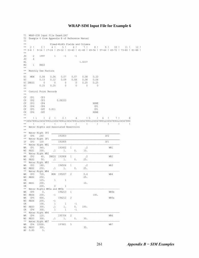
WRAP-SIM Input File for Example 6 T1 WRAP-SIM Input File Exam6.DAT T2 Example 6 from Appendix B of Reference Manual ** ** Fixed-Width Fields and Columns ** 2 ! 3 ! 4 ! 5 ! 6 ! 7 ! 8 ! 9 ! 10 ! 11 ! 12 ! ** 3-8 ! 9-16 ! 17-24 ! 25-32 ! 33-40 ! 41-48 ! 49-56 ! 57-64 ! 65-72 ! 73-80 ! 81-88 ! ** JD 2 1997 1 -1 -1 JO 4 XL 1.0237 RO 1 RES3 ** ** Monthly Use Factors ** UC MUN 0.06 0.06 0.07 0.07 0.08 0.10 UC 0.13 0.12 0.09 0.08 0.08 0.06 UC IRRIG 0 0 0 0 0.25 0.25 UC 0.25 0.25 0 0 0 0 ** ** Control Point Records ** CP CP1 CP3 CP CP2 CP3 0.08333 CP CP3 CP4 NONE CP CP4 CP6 CP1 CP CP5 OUT 0.811 CP1 CP CP6 OUT NONE ** ** ! 1 ! 2 ! 3 ! 4 ! 5 ! 6 ! 7 ! 8 **345678901234567890123456789012345678901234567890123456789012345678901234567890 ** ! ! ! ! ! ! ! ! ! ! ** Water Rights and Associated Reservoirs ** ** Water Right IF2 ___________________________________________________ IF CP6 240 191803 IF2 ** Water Right IF1 ___________________________________________________ IF CP3 120 191805 IF1 ** Water Right WR1 --------------------------------------------------- WR CP1 360. 192602 1 .2 WR1 WS RES1 200. .1 1. 0. 10. ** Water Right WR2 --------------------------------------------------- WR CP2 60. IRRIG 193908 1 .2 WR2 WS RES2 50. .1 1. 0. 25. ** Water Right WR3 --------------------------------------------------- WR CP2 180. 196506 1 .2 WR3 WS RES2 250. .1 1. 0. 25. ** Water Right WR4 --------------------------------------------------- WR CP3 720. MUN 195207 2 0.4 WR4 WS RES2 250. 25. OR 125. 1 1 WS RES1 200. 10. OR 200. 0 1 ** Water Rights WR5a and WR5b ---------------------------------------- WR CP5 0. 196213 1 WR5b WS RES4 200. -1 100. WR CP5 600. 196212 2 WR5a WS RES4 200. -1 OR 100. 1 1 -1 WS RES3 300. .1 1. 0. 150. OR CP4 300. 1 1 -1 ** Water Right WR6 --------------------------------------------------- WR CP4 120. 195704 2 WR6 WS RES3 300. .1 1. 0. 30. ** Water Right WR7 --------------------------------------------------- WR CP4 12000. 197801 5 WR7 WS RES3 300. 30. HP 0.85 5.
Appendix B − SIM Examples 261
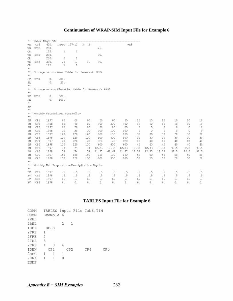
Continuation of WRAP-SIM Input File for Example 6 ** Water Right WR8 --------------------------------------------------- WR CP6 400. IRRIG 197412 3 2 WR8 WS RES2 250. 25. OR 125. 1 1 WS RES1 200. 10. OR 200. 0 1 WS RES3 300. .1 1. 0. 30. OR 165. 1 1 ** ** Storage versus Area Table for Reservoir RES4 ** SV RES4 0. 200. SA 0. 20. ** ** Storage versus Elevation Table for Reservoir RES3 ** PV RES3 0. 300. PE 0. 100. ** ED ** ** Monthly Naturalized Streamflow ** IN CP1 1997 60 60 60 60 60 60 10 10 10 10 10 10 IN CP1 1998 60 60 60 300 300 300 10 10 10 10 10 10 IN CP2 1997 20 20 20 20 20 20 0 0 0 0 0 0 IN CP2 1998 20 20 20 100 100 100 0 0 0 0 0 0 IN CP3 1997 120 120 120 100 100 100 30 30 30 30 30 30 IN CP3 1998 120 120 120 500 500 500 30 30 30 30 30 30 IN CP4 1997 120 120 120 120 120 120 40 40 40 40 40 40 IN CP4 1998 120 120 120 600 600 600 40 40 40 40 40 40 IN CP5 1997 74 74 74 12.33 12.33 12.33 12.33 12.33 12.33 92.5 92.5 92.5 IN CP5 1998 74 74 74 61.67 61.67 61.67 12.33 12.33 12.33 92.5 92.5 92.5 IN CP6 1997 150 150 150 180 180 180 50 50 50 50 50 50 IN CP6 1998 150 150 150 900 900 900 50 50 50 50 50 50 ** ** Monthly Net Evaporation-Precipitation Depths ** EV CP1 1997 .5 .5 .5 .5 .5 .5 .5 .5 .5 .5 .5 .5 EV CP1 1998 .5 .5 .5 .5 .5 .5 .5 .5 .5 .5 .5 .5 EV CP2 1997 6. 6. 6. 6. 6. 6. 6. 6. 6. 6. 6. 6. EV CP2 1998 6. 6. 6. 6. 6. 6. 6. 6. 6. 6. 6. 6.
TABLES Input File for Example 6 COMM TABLES Input File Tab6.TIN COMM Example 6 2REL 2REL 2 1 IDEN RES3 2FRE 1 2FRE 2 2FRE 3 2FRE 4 0 4 IDEN CP1 CP2 CP4 CP5 2REG 1 1 1 2UNA 1 1 0 ENDF
Appendix B − SIM Examples 262
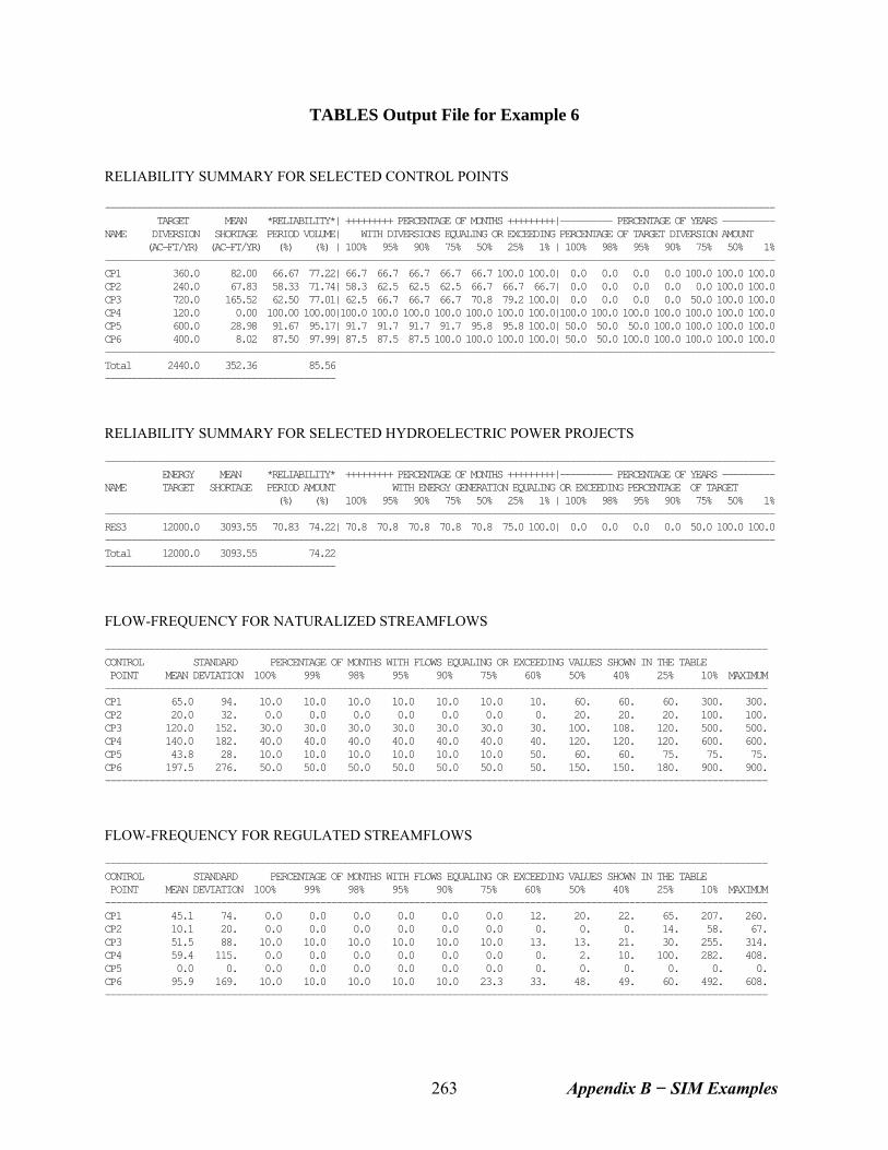
TABLES Output File for Example 6
RELIABILITY SUMMARY FOR SELECTED CONTROL POINTS -------------------------------------------------------------------------------------------------------------------------------- TARGET MEAN *RELIABILITY*| +++++++++ PERCENTAGE OF MONTHS +++++++++|---------- PERCENTAGE OF YEARS ---------- NAME DIVERSION SHORTAGE PERIOD VOLUME| WITH DIVERSIONS EQUALING OR EXCEEDING PERCENTAGE OF TARGET DIVERSION AMOUNT (AC-FT/YR) (AC-FT/YR) (%) (%) | 100% 95% 90% 75% 50% 25% 1% | 100% 98% 95% 90% 75% 50% 1% -------------------------------------------------------------------------------------------------------------------------------- CP1 360.0 82.00 66.67 77.22| 66.7 66.7 66.7 66.7 66.7 100.0 100.0| 0.0 0.0 0.0 0.0 100.0 100.0 100.0 CP2 240.0 67.83 58.33 71.74| 58.3 62.5 62.5 62.5 66.7 66.7 66.7| 0.0 0.0 0.0 0.0 0.0 100.0 100.0 CP3 720.0 165.52 62.50 77.01| 62.5 66.7 66.7 66.7 70.8 79.2 100.0| 0.0 0.0 0.0 0.0 50.0 100.0 100.0 CP4 120.0 0.00 100.00 100.00|100.0 100.0 100.0 100.0 100.0 100.0 100.0|100.0 100.0 100.0 100.0 100.0 100.0 100.0 CP5 600.0 28.98 91.67 95.17| 91.7 91.7 91.7 91.7 95.8 95.8 100.0| 50.0 50.0 50.0 100.0 100.0 100.0 100.0 CP6 400.0 8.02 87.50 97.99| 87.5 87.5 87.5 100.0 100.0 100.0 100.0| 50.0 50.0 100.0 100.0 100.0 100.0 100.0 -------------------------------------------------------------------------------------------------------------------------------- Total 2440.0 352.36 85.56 -------------------------------------------- RELIABILITY SUMMARY FOR SELECTED HYDROELECTRIC POWER PROJECTS -------------------------------------------------------------------------------------------------------------------------------- ENERGY MEAN *RELIABILITY* +++++++++ PERCENTAGE OF MONTHS +++++++++|---------- PERCENTAGE OF YEARS ---------- NAME TARGET SHORTAGE PERIOD AMOUNT WITH ENERGY GENERATION EQUALING OR EXCEEDING PERCENTAGE OF TARGET (%) (%) 100% 95% 90% 75% 50% 25% 1% | 100% 98% 95% 90% 75% 50% 1% -------------------------------------------------------------------------------------------------------------------------------- RES3 12000.0 3093.55 70.83 74.22| 70.8 70.8 70.8 70.8 70.8 75.0 100.0| 0.0 0.0 0.0 0.0 50.0 100.0 100.0 -------------------------------------------------------------------------------------------------------------------------------- Total 12000.0 3093.55 74.22 -------------------------------------------- FLOW-FREQUENCY FOR NATURALIZED STREAMFLOWS ------------------------------------------------------------------------------------------------------------------------ CONTROL STANDARD PERCENTAGE OF MONTHS WITH FLOWS EQUALING OR EXCEEDING VALUES SHOWN IN THE TABLE POINT MEAN DEVIATION 100% 99% 98% 95% 90% 75% 60% 50% 40% 25% 10% MAXIMUM ------------------------------------------------------------------------------------------------------------------------ CP1 65.0 94. 10.0 10.0 10.0 10.0 10.0 10.0 10. 60. 60. 60. 300. 300. CP2 20.0 32. 0.0 0.0 0.0 0.0 0.0 0.0 0. 20. 20. 20. 100. 100. CP3 120.0 152. 30.0 30.0 30.0 30.0 30.0 30.0 30. 100. 108. 120. 500. 500. CP4 140.0 182. 40.0 40.0 40.0 40.0 40.0 40.0 40. 120. 120. 120. 600. 600. CP5 43.8 28. 10.0 10.0 10.0 10.0 10.0 10.0 50. 60. 60. 75. 75. 75. CP6 197.5 276. 50.0 50.0 50.0 50.0 50.0 50.0 50. 150. 150. 180. 900. 900. ------------------------------------------------------------------------------------------------------------------------ FLOW-FREQUENCY FOR REGULATED STREAMFLOWS ------------------------------------------------------------------------------------------------------------------------ CONTROL STANDARD PERCENTAGE OF MONTHS WITH FLOWS EQUALING OR EXCEEDING VALUES SHOWN IN THE TABLE POINT MEAN DEVIATION 100% 99% 98% 95% 90% 75% 60% 50% 40% 25% 10% MAXIMUM ------------------------------------------------------------------------------------------------------------------------ CP1 45.1 74. 0.0 0.0 0.0 0.0 0.0 0.0 12. 20. 22. 65. 207. 260. CP2 10.1 20. 0.0 0.0 0.0 0.0 0.0 0.0 0. 0. 0. 14. 58. 67. CP3 51.5 88. 10.0 10.0 10.0 10.0 10.0 10.0 13. 13. 21. 30. 255. 314. CP4 59.4 115. 0.0 0.0 0.0 0.0 0.0 0.0 0. 2. 10. 100. 282. 408. CP5 0.0 0. 0.0 0.0 0.0 0.0 0.0 0.0 0. 0. 0. 0. 0. 0. CP6 95.9 169. 10.0 10.0 10.0 10.0 10.0 23.3 33. 48. 49. 60. 492. 608. ------------------------------------------------------------------------------------------------------------------------
Appendix B − SIM Examples 263
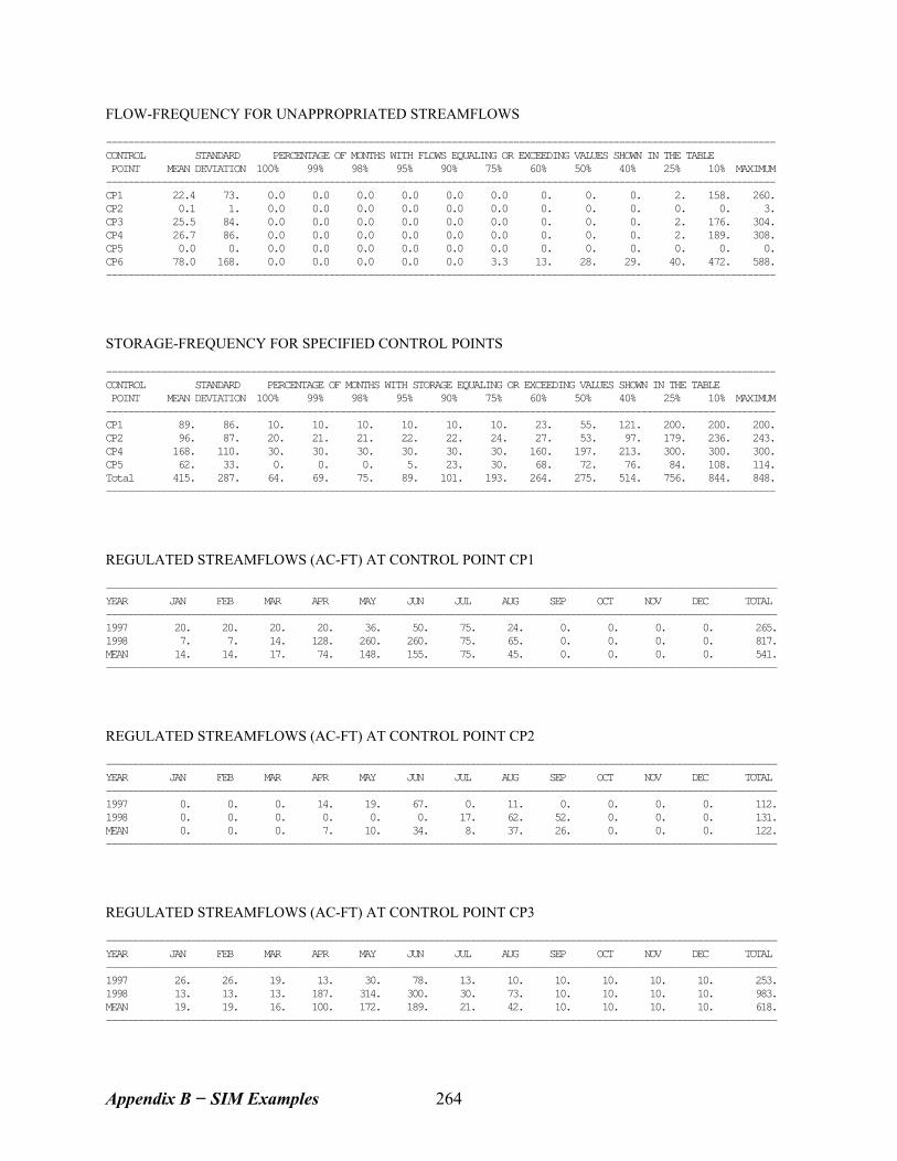
FLOW-FREQUENCY FOR UNAPPROPRIATED STREAMFLOWS ------------------------------------------------------------------------------------------------------------------------ CONTROL STANDARD PERCENTAGE OF MONTHS WITH FLOWS EQUALING OR EXCEEDING VALUES SHOWN IN THE TABLE POINT MEAN DEVIATION 100% 99% 98% 95% 90% 75% 60% 50% 40% 25% 10% MAXIMUM ------------------------------------------------------------------------------------------------------------------------ CP1 22.4 73. 0.0 0.0 0.0 0.0 0.0 0.0 0. 0. 0. 2. 158. 260. CP2 0.1 1. 0.0 0.0 0.0 0.0 0.0 0.0 0. 0. 0. 0. 0. 3. CP3 25.5 84. 0.0 0.0 0.0 0.0 0.0 0.0 0. 0. 0. 2. 176. 304. CP4 26.7 86. 0.0 0.0 0.0 0.0 0.0 0.0 0. 0. 0. 2. 189. 308. CP5 0.0 0. 0.0 0.0 0.0 0.0 0.0 0.0 0. 0. 0. 0. 0. 0. CP6 78.0 168. 0.0 0.0 0.0 0.0 0.0 3.3 13. 28. 29. 40. 472. 588. ------------------------------------------------------------------------------------------------------------------------ STORAGE-FREQUENCY FOR SPECIFIED CONTROL POINTS ------------------------------------------------------------------------------------------------------------------------ CONTROL STANDARD PERCENTAGE OF MONTHS WITH STORAGE EQUALING OR EXCEEDING VALUES SHOWN IN THE TABLE POINT MEAN DEVIATION 100% 99% 98% 95% 90% 75% 60% 50% 40% 25% 10% MAXIMUM ------------------------------------------------------------------------------------------------------------------------ CP1 89. 86. 10. 10. 10. 10. 10. 10. 23. 55. 121. 200. 200. 200. CP2 96. 87. 20. 21. 21. 22. 22. 24. 27. 53. 97. 179. 236. 243. CP4 168. 110. 30. 30. 30. 30. 30. 30. 160. 197. 213. 300. 300. 300. CP5 62. 33. 0. 0. 0. 5. 23. 30. 68. 72. 76. 84. 108. 114. Total 415. 287. 64. 69. 75. 89. 101. 193. 264. 275. 514. 756. 844. 848. ------------------------------------------------------------------------------------------------------------------------ REGULATED STREAMFLOWS (AC-FT) AT CONTROL POINT CP1 ------------------------------------------------------------------------------------------------------------------------------- YEAR JAN FEB MAR APR MAY JUN JUL AUG SEP OCT NOV DEC TOTAL ------------------------------------------------------------------------------------------------------------------------------- 1997 20. 20. 20. 20. 36. 50. 75. 24. 0. 0. 0. 0. 265. 1998 7. 7. 14. 128. 260. 260. 75. 65. 0. 0. 0. 0. 817. MEAN 14. 14. 17. 74. 148. 155. 75. 45. 0. 0. 0. 0. 541. ------------------------------------------------------------------------------------------------------------------------------- REGULATED STREAMFLOWS (AC-FT) AT CONTROL POINT CP2 ------------------------------------------------------------------------------------------------------------------------------- YEAR JAN FEB MAR APR MAY JUN JUL AUG SEP OCT NOV DEC TOTAL ------------------------------------------------------------------------------------------------------------------------------- 1997 0. 0. 0. 14. 19. 67. 0. 11. 0. 0. 0. 0. 112. 1998 0. 0. 0. 0. 0. 0. 17. 62. 52. 0. 0. 0. 131. MEAN 0. 0. 0. 7. 10. 34. 8. 37. 26. 0. 0. 0. 122. ------------------------------------------------------------------------------------------------------------------------------- REGULATED STREAMFLOWS (AC-FT) AT CONTROL POINT CP3 ------------------------------------------------------------------------------------------------------------------------------- YEAR JAN FEB MAR APR MAY JUN JUL AUG SEP OCT NOV DEC TOTAL ------------------------------------------------------------------------------------------------------------------------------- 1997 26. 26. 19. 13. 30. 78. 13. 10. 10. 10. 10. 10. 253. 1998 13. 13. 13. 187. 314. 300. 30. 73. 10. 10. 10. 10. 983. MEAN 19. 19. 16. 100. 172. 189. 21. 42. 10. 10. 10. 10. 618. -------------------------------------------------------------------------------------------------------------------------------
Appendix B − SIM Examples 264
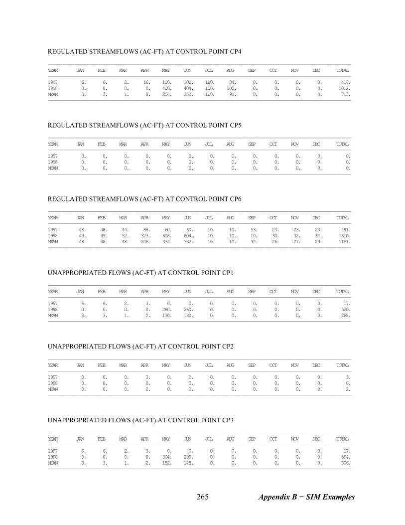
REGULATED STREAMFLOWS (AC-FT) AT CONTROL POINT CP4 ------------------------------------------------------------------------------------------------------------------------------- YEAR JAN FEB MAR APR MAY JUN JUL AUG SEP OCT NOV DEC TOTAL ------------------------------------------------------------------------------------------------------------------------------- 1997 6. 6. 2. 16. 100. 100. 100. 84. 0. 0. 0. 0. 414. 1998 0. 0. 0. 0. 408. 404. 100. 100. 0. 0. 0. 0. 1012. MEAN 3. 3. 1. 8. 254. 252. 100. 92. 0. 0. 0. 0. 713. ------------------------------------------------------------------------------------------------------------------------------- REGULATED STREAMFLOWS (AC-FT) AT CONTROL POINT CP5 ------------------------------------------------------------------------------------------------------------------------------- YEAR JAN FEB MAR APR MAY JUN JUL AUG SEP OCT NOV DEC TOTAL ------------------------------------------------------------------------------------------------------------------------------- 1997 0. 0. 0. 0. 0. 0. 0. 0. 0. 0. 0. 0. 0. 1998 0. 0. 0. 0. 0. 0. 0. 0. 0. 0. 0. 0. 0. MEAN 0. 0. 0. 0. 0. 0. 0. 0. 0. 0. 0. 0. 0. ------------------------------------------------------------------------------------------------------------------------------- REGULATED STREAMFLOWS (AC-FT) AT CONTROL POINT CP6 ------------------------------------------------------------------------------------------------------------------------------- YEAR JAN FEB MAR APR MAY JUN JUL AUG SEP OCT NOV DEC TOTAL ------------------------------------------------------------------------------------------------------------------------------- 1997 48. 48. 44. 88. 60. 60. 10. 10. 53. 23. 23. 23. 491. 1998 49. 49. 52. 323. 608. 604. 10. 10. 10. 30. 32. 34. 1810. MEAN 48. 48. 48. 206. 334. 332. 10. 10. 32. 26. 27. 29. 1151. ------------------------------------------------------------------------------------------------------------------------------- UNAPPROPRIATED FLOWS (AC-FT) AT CONTROL POINT CP1 ------------------------------------------------------------------------------------------------------------------------------- YEAR JAN FEB MAR APR MAY JUN JUL AUG SEP OCT NOV DEC TOTAL ------------------------------------------------------------------------------------------------------------------------------- 1997 6. 6. 2. 3. 0. 0. 0. 0. 0. 0. 0. 0. 17. 1998 0. 0. 0. 0. 260. 260. 0. 0. 0. 0. 0. 0. 520. MEAN 3. 3. 1. 2. 130. 130. 0. 0. 0. 0. 0. 0. 268. ------------------------------------------------------------------------------------------------------------------------------- UNAPPROPRIATED FLOWS (AC-FT) AT CONTROL POINT CP2 ------------------------------------------------------------------------------------------------------------------------------- YEAR JAN FEB MAR APR MAY JUN JUL AUG SEP OCT NOV DEC TOTAL ------------------------------------------------------------------------------------------------------------------------------- 1997 0. 0. 0. 3. 0. 0. 0. 0. 0. 0. 0. 0. 3. 1998 0. 0. 0. 0. 0. 0. 0. 0. 0. 0. 0. 0. 0. MEAN 0. 0. 0. 2. 0. 0. 0. 0. 0. 0. 0. 0. 2. ------------------------------------------------------------------------------------------------------------------------------- UNAPPROPRIATED FLOWS (AC-FT) AT CONTROL POINT CP3 ------------------------------------------------------------------------------------------------------------------------------- YEAR JAN FEB MAR APR MAY JUN JUL AUG SEP OCT NOV DEC TOTAL ------------------------------------------------------------------------------------------------------------------------------- 1997 6. 6. 2. 3. 0. 0. 0. 0. 0. 0. 0. 0. 17. 1998 0. 0. 0. 0. 304. 290. 0. 0. 0. 0. 0. 0. 594. MEAN 3. 3. 1. 2. 152. 145. 0. 0. 0. 0. 0. 0. 306. -------------------------------------------------------------------------------------------------------------------------------
Appendix B − SIM Examples 265
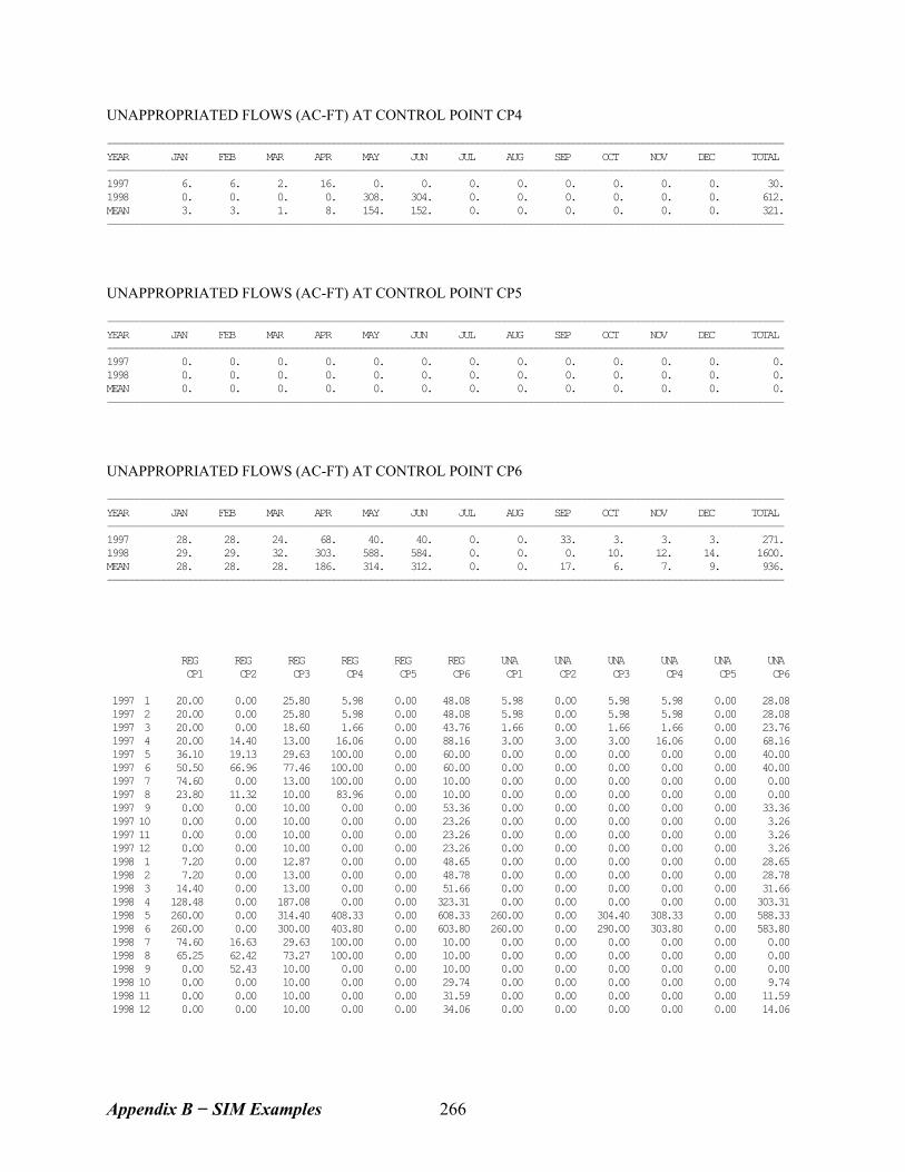
UNAPPROPRIATED FLOWS (AC-FT) AT CONTROL POINT CP4 ------------------------------------------------------------------------------------------------------------------------------- YEAR JAN FEB MAR APR MAY JUN JUL AUG SEP OCT NOV DEC TOTAL ------------------------------------------------------------------------------------------------------------------------------- 1997 6. 6. 2. 16. 0. 0. 0. 0. 0. 0. 0. 0. 30. 1998 0. 0. 0. 0. 308. 304. 0. 0. 0. 0. 0. 0. 612. MEAN 3. 3. 1. 8. 154. 152. 0. 0. 0. 0. 0. 0. 321. ------------------------------------------------------------------------------------------------------------------------------- UNAPPROPRIATED FLOWS (AC-FT) AT CONTROL POINT CP5 ------------------------------------------------------------------------------------------------------------------------------- YEAR JAN FEB MAR APR MAY JUN JUL AUG SEP OCT NOV DEC TOTAL ------------------------------------------------------------------------------------------------------------------------------- 1997 0. 0. 0. 0. 0. 0. 0. 0. 0. 0. 0. 0. 0. 1998 0. 0. 0. 0. 0. 0. 0. 0. 0. 0. 0. 0. 0. MEAN 0. 0. 0. 0. 0. 0. 0. 0. 0. 0. 0. 0. 0. ------------------------------------------------------------------------------------------------------------------------------- UNAPPROPRIATED FLOWS (AC-FT) AT CONTROL POINT CP6 ------------------------------------------------------------------------------------------------------------------------------- YEAR JAN FEB MAR APR MAY JUN JUL AUG SEP OCT NOV DEC TOTAL ------------------------------------------------------------------------------------------------------------------------------- 1997 28. 28. 24. 68. 40. 40. 0. 0. 33. 3. 3. 3. 271. 1998 29. 29. 32. 303. 588. 584. 0. 0. 0. 10. 12. 14. 1600. MEAN 28. 28. 28. 186. 314. 312. 0. 0. 17. 6. 7. 9. 936. ------------------------------------------------------------------------------------------------------------------------------- REG REG REG REG REG REG UNA UNA UNA UNA UNA UNA CP1 CP2 CP3 CP4 CP5 CP6 CP1 CP2 CP3 CP4 CP5 CP6 1997 1 20.00 0.00 25.80 5.98 0.00 48.08 5.98 0.00 5.98 5.98 0.00 28.08 1997 2 20.00 0.00 25.80 5.98 0.00 48.08 5.98 0.00 5.98 5.98 0.00 28.08 1997 3 20.00 0.00 18.60 1.66 0.00 43.76 1.66 0.00 1.66 1.66 0.00 23.76 1997 4 20.00 14.40 13.00 16.06 0.00 88.16 3.00 3.00 3.00 16.06 0.00 68.16 1997 5 36.10 19.13 29.63 100.00 0.00 60.00 0.00 0.00 0.00 0.00 0.00 40.00 1997 6 50.50 66.96 77.46 100.00 0.00 60.00 0.00 0.00 0.00 0.00 0.00 40.00 1997 7 74.60 0.00 13.00 100.00 0.00 10.00 0.00 0.00 0.00 0.00 0.00 0.00 1997 8 23.80 11.32 10.00 83.96 0.00 10.00 0.00 0.00 0.00 0.00 0.00 0.00 1997 9 0.00 0.00 10.00 0.00 0.00 53.36 0.00 0.00 0.00 0.00 0.00 33.36 1997 10 0.00 0.00 10.00 0.00 0.00 23.26 0.00 0.00 0.00 0.00 0.00 3.26 1997 11 0.00 0.00 10.00 0.00 0.00 23.26 0.00 0.00 0.00 0.00 0.00 3.26 1997 12 0.00 0.00 10.00 0.00 0.00 23.26 0.00 0.00 0.00 0.00 0.00 3.26 1998 1 7.20 0.00 12.87 0.00 0.00 48.65 0.00 0.00 0.00 0.00 0.00 28.65 1998 2 7.20 0.00 13.00 0.00 0.00 48.78 0.00 0.00 0.00 0.00 0.00 28.78 1998 3 14.40 0.00 13.00 0.00 0.00 51.66 0.00 0.00 0.00 0.00 0.00 31.66 1998 4 128.48 0.00 187.08 0.00 0.00 323.31 0.00 0.00 0.00 0.00 0.00 303.31 1998 5 260.00 0.00 314.40 408.33 0.00 608.33 260.00 0.00 304.40 308.33 0.00 588.33 1998 6 260.00 0.00 300.00 403.80 0.00 603.80 260.00 0.00 290.00 303.80 0.00 583.80 1998 7 74.60 16.63 29.63 100.00 0.00 10.00 0.00 0.00 0.00 0.00 0.00 0.00 1998 8 65.25 62.42 73.27 100.00 0.00 10.00 0.00 0.00 0.00 0.00 0.00 0.00 1998 9 0.00 52.43 10.00 0.00 0.00 10.00 0.00 0.00 0.00 0.00 0.00 0.00 1998 10 0.00 0.00 10.00 0.00 0.00 29.74 0.00 0.00 0.00 0.00 0.00 9.74 1998 11 0.00 0.00 10.00 0.00 0.00 31.59 0.00 0.00 0.00 0.00 0.00 11.59 1998 12 0.00 0.00 10.00 0.00 0.00 34.06 0.00 0.00 0.00 0.00 0.00 14.06
Appendix B − SIM Examples 266
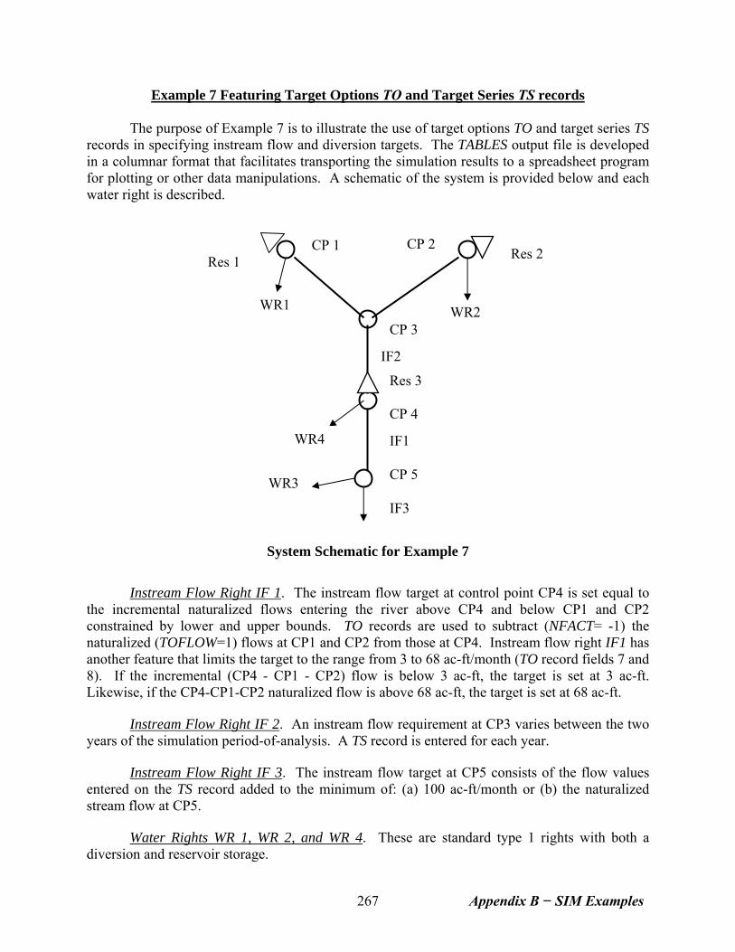
Example 7 Featuring Target Options TO and Target Series TS records
The purpose of Example 7 is to illustrate the use of target options TO and target series TS records in specifying instream flow and diversion targets. The TABLES output file is developed in a columnar format that facilitates transporting the simulation results to a spreadsheet program for plotting or other data manipulations. A schematic of the system is provided below and each water right is described.
WR3
WR4 IF1
IF2
Res 3
CP 4
CP 3
CP 2
WR2 WR1
Res 1 CP 1 Res 2
CP 5
IF3
System Schematic for Example 7
Instream Flow Right IF 1. The instream flow target at control point CP4 is set equal to
the incremental naturalized flows entering the river above CP4 and below CP1 and CP2 constrained by lower and upper bounds. TO records are used to subtract (NFACT= -1) the naturalized (TOFLOW=1) flows at CP1 and CP2 from those at CP4. Instream flow right IF1 has another feature that limits the target to the range from 3 to 68 ac-ft/month (TO record fields 7 and 8). If the incremental (CP4 - CP1 - CP2) flow is below 3 ac-ft, the target is set at 3 ac-ft. Likewise, if the CP4-CP1-CP2 naturalized flow is above 68 ac-ft, the target is set at 68 ac-ft.
Instream Flow Right IF 2. An instream flow requirement at CP3 varies between the two
years of the simulation period-of-analysis. A TS record is entered for each year. Instream Flow Right IF 3. The instream flow target at CP5 consists of the flow values entered on the TS record added to the minimum of: (a) 100 ac-ft/month or (b) the naturalized stream flow at CP5. Water Rights WR 1, WR 2, and WR 4. These are standard type 1 rights with both a diversion and reservoir storage.
Appendix B − SIM Examples 267
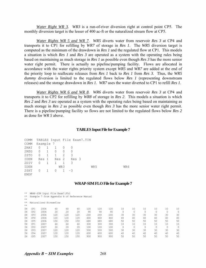
Water Right WR 3. WR3 is a run-of-river diversion right at control point CP5. The monthly diversion target is the lesser of 400 ac-ft or the naturalized stream flow at CP5. Water Rights WR 5 and WR 7. WR5 diverts water from reservoir Res 3 at CP4 and transports it to CP1 for refilling by WR7 of storage in Res 1. The WR5 diversion target is computed as the minimum of the drawdown in Res 1 and the regulated flow at CP1. This models a situation is which Res 1 and Res 3 are operated as a system with the operating rules being based on maintaining as much storage in Res 1 as possible even though Res 3 has the more senior water right permit. There is actually no pipeline/pumping facility. Flows are allocated in accordance with the water rights priority system except WR5 and WR7 are added at the end of the priority loop to reallocate releases from Res 1 back to Res 1 from Res 3. Thus, the WR5 dummy diversion is limited to the regulated flows below Res 1 (representing downstream releases) and the storage drawdown in Res 1. WR7 uses the water diverted to CP1 to refill Res 1. Water Rights WR 6 and WR 8. WR6 diverts water from reservoir Res 3 at CP4 and transports it to CP2 for refilling by WR8 of storage in Res 2. This models a situation is which Res 2 and Res 3 are operated as a system with the operating rules being based on maintaining as much storage in Res 2 as possible even though Res 3 has the more senior water right permit. There is a pipeline/pumping facility so flows are not limited to the regulated flows below Res 2 as done for WR 5 above.
TABLES Input File for Example 7 COMM TABLES Input File Exam7.TIN COMM Example 7 2NAT 0 1 1 0 0 2REG 0 1 0 0 0 2STO 0 1 1 2 3 IDEN Res 1 Res 2 Res 3 2DIV 0 1 1 1 3 IDEN WR3 WR5 WR6 2SHT 0 1 0 1 -3 ENDF
WRAP-SIM FLO File for Example 7 ** WRAP-SIM Input File Exam7.FLO ** Example 7 from Appendix B of Reference Manual ** ** Naturalized Streamflow ** IN CP1 2006 60 60 60 120 120 120 10 10 10 10 10 10 IN CP2 2006 20 20 20 90 90 90 0 0 0 0 0 0 IN CP3 2006 120 120 120 240 240 240 30 30 30 30 30 30 IN CP4 2006 120 120 120 460 460 460 40 40 40 40 40 40 IN CP5 2006 150 150 150 680 680 680 50 50 50 50 50 50 IN CP1 2007 60 60 60 300 300 300 10 10 10 10 10 10 IN CP2 2007 20 20 20 100 100 100 0 0 0 0 0 0 IN CP3 2007 120 120 120 500 500 500 30 30 30 30 30 30 IN CP4 2007 120 120 120 600 600 600 40 40 40 40 40 40 IN CP5 2007 150 150 150 900 900 900 50 50 50 50 50 50
Appendix B − SIM Examples 268
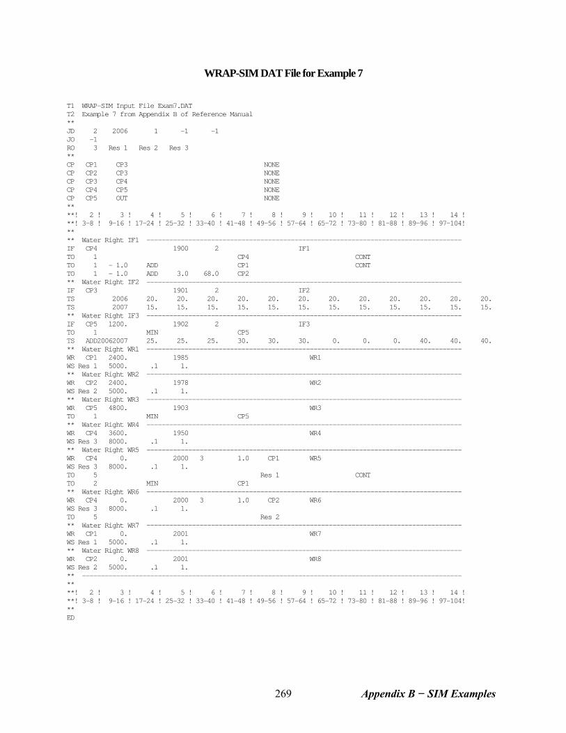
WRAP-SIM DAT File for Example 7 T1 WRAP-SIM Input File Exam7.DAT T2 Example 7 from Appendix B of Reference Manual ** JD 2 2006 1 -1 -1 JO -1 RO 3 Res 1 Res 2 Res 3 ** CP CP1 CP3 NONE CP CP2 CP3 NONE CP CP3 CP4 NONE CP CP4 CP5 NONE CP CP5 OUT NONE ** **! 2 ! 3 ! 4 ! 5 ! 6 ! 7 ! 8 ! 9 ! 10 ! 11 ! 12 ! 13 ! 14 ! **! 3-8 ! 9-16 ! 17-24 ! 25-32 ! 33-40 ! 41-48 ! 49-56 ! 57-64 ! 65-72 ! 73-80 ! 81-88 ! 89-96 ! 97-104! ** ** Water Right IF1 ----------------------------------------------------------------------------------- IF CP4 1900 2 IF1 TO 1 CP4 CONT TO 1 - 1.0 ADD CP1 CONT TO 1 - 1.0 ADD 3.0 68.0 CP2 ** Water Right IF2 ----------------------------------------------------------------------------------- IF CP3 1901 2 IF2 TS 2006 20. 20. 20. 20. 20. 20. 20. 20. 20. 20. 20. 20. TS 2007 15. 15. 15. 15. 15. 15. 15. 15. 15. 15. 15. 15. ** Water Right IF3 ----------------------------------------------------------------------------------- IF CP5 1200. 1902 2 IF3 TO 1 MIN CP5 TS ADD20062007 25. 25. 25. 30. 30. 30. 0. 0. 0. 40. 40. 40. ** Water Right WR1 ----------------------------------------------------------------------------------- WR CP1 2400. 1985 WR1 WS Res 1 5000. .1 1. ** Water Right WR2 ----------------------------------------------------------------------------------- WR CP2 2400. 1978 WR2 WS Res 2 5000. .1 1. ** Water Right WR3 ----------------------------------------------------------------------------------- WR CP5 4800. 1903 WR3 TO 1 MIN CP5 ** Water Right WR4 ----------------------------------------------------------------------------------- WR CP4 3600. 1950 WR4 WS Res 3 8000. .1 1. ** Water Right WR5 ----------------------------------------------------------------------------------- WR CP4 0. 2000 3 1.0 CP1 WR5 WS Res 3 8000. .1 1. TO 5 Res 1 CONT TO 2 MIN CP1 ** Water Right WR6 ----------------------------------------------------------------------------------- WR CP4 0. 2000 3 1.0 CP2 WR6 WS Res 3 8000. .1 1. TO 5 Res 2 ** Water Right WR7 ----------------------------------------------------------------------------------- WR CP1 0. 2001 WR7 WS Res 1 5000. .1 1. ** Water Right WR8 ----------------------------------------------------------------------------------- WR CP2 0. 2001 WR8 WS Res 2 5000. .1 1. ** ---------------------------------------------------------------------------------------------------- ** **! 2 ! 3 ! 4 ! 5 ! 6 ! 7 ! 8 ! 9 ! 10 ! 11 ! 12 ! 13 ! 14 ! **! 3-8 ! 9-16 ! 17-24 ! 25-32 ! 33-40 ! 41-48 ! 49-56 ! 57-64 ! 65-72 ! 73-80 ! 81-88 ! 89-96 ! 97-104! ** ED
Appendix B − SIM Examples 269
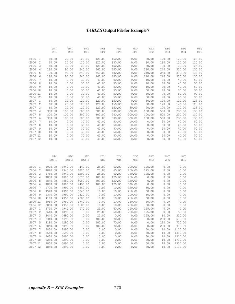
TABLES Output File for Example 7 NAT NAT NAT NAT NAT REG REG REG REG REG CP1 CP2 CP3 CP4 CP5 CP1 CP2 CP3 CP4 CP5 2006 1 60.00 20.00 120.00 120.00 150.00 0.00 80.00 120.00 120.00 125.00 2006 2 60.00 20.00 120.00 120.00 150.00 0.00 80.00 120.00 120.00 125.00 2006 3 60.00 20.00 120.00 120.00 150.00 0.00 80.00 120.00 120.00 125.00 2006 4 120.00 90.00 240.00 460.00 680.00 0.00 210.00 240.00 310.00 130.00 2006 5 120.00 90.00 240.00 460.00 680.00 0.00 210.00 240.00 310.00 130.00 2006 6 120.00 90.00 240.00 460.00 680.00 0.00 210.00 240.00 310.00 130.00 2006 7 10.00 0.00 30.00 40.00 50.00 0.00 10.00 30.00 40.00 50.00 2006 8 10.00 0.00 30.00 40.00 50.00 0.00 10.00 30.00 40.00 50.00 2006 9 10.00 0.00 30.00 40.00 50.00 0.00 10.00 30.00 40.00 50.00 2006 10 10.00 0.00 30.00 40.00 50.00 0.00 50.00 70.00 80.00 90.00 2006 11 10.00 0.00 30.00 40.00 50.00 0.00 50.00 70.00 80.00 90.00 2006 12 10.00 0.00 30.00 40.00 50.00 0.00 50.00 70.00 80.00 90.00 2007 1 60.00 20.00 120.00 120.00 150.00 0.00 80.00 120.00 120.00 125.00 2007 2 60.00 20.00 120.00 120.00 150.00 0.00 80.00 120.00 120.00 125.00 2007 3 60.00 20.00 120.00 120.00 150.00 60.00 20.00 120.00 120.00 125.00 2007 4 300.00 100.00 500.00 600.00 900.00 300.00 100.00 500.00 230.00 130.00 2007 5 300.00 100.00 500.00 600.00 900.00 300.00 100.00 500.00 230.00 130.00 2007 6 300.00 100.00 500.00 600.00 900.00 300.00 100.00 500.00 230.00 130.00 2007 7 10.00 0.00 30.00 40.00 50.00 10.00 0.00 30.00 40.00 50.00 2007 8 10.00 0.00 30.00 40.00 50.00 10.00 0.00 30.00 40.00 50.00 2007 9 10.00 0.00 30.00 40.00 50.00 10.00 0.00 30.00 40.00 50.00 2007 10 10.00 0.00 30.00 40.00 50.00 10.00 0.00 30.00 40.00 50.00 2007 11 10.00 0.00 30.00 40.00 50.00 10.00 0.00 30.00 40.00 50.00 2007 12 10.00 0.00 30.00 40.00 50.00 10.00 0.00 30.00 40.00 50.00 STO STO STO DIV DIV DIV SHT SHT SHT Res 1 Res 2 Res 3 WR3 WR5 WR6 WR3 WR5 WR6 2006 1 4920.00 4940.00 7440.00 25.00 60.00 200.00 125.00 0.00 0.00 2006 2 4840.00 4940.00 6820.00 25.00 60.00 260.00 125.00 0.00 0.00 2006 3 4760.00 4940.00 6200.00 25.00 60.00 260.00 125.00 0.00 0.00 2006 4 4800.00 4880.00 5670.00 400.00 120.00 260.00 0.00 0.00 0.00 2006 5 4840.00 4880.00 5080.00 400.00 120.00 320.00 0.00 0.00 0.00 2006 6 4880.00 4880.00 4490.00 400.00 120.00 320.00 0.00 0.00 0.00 2006 7 4700.00 4990.00 3860.00 0.00 10.00 320.00 50.00 0.00 0.00 2006 8 4520.00 4990.00 3340.00 0.00 10.00 210.00 50.00 0.00 0.00 2006 9 4340.00 4990.00 2820.00 0.00 10.00 210.00 50.00 0.00 0.00 2006 10 4160.00 4950.00 2300.00 0.00 10.00 210.00 50.00 0.00 0.00 2006 11 3980.00 4950.00 1740.00 0.00 10.00 250.00 50.00 0.00 0.00 2006 12 3800.00 4950.00 1180.00 0.00 10.00 250.00 50.00 0.00 0.00 2007 1 3720.00 4940.00 570.00 25.00 60.00 250.00 125.00 0.00 0.00 2007 2 3640.00 4890.00 0.00 25.00 60.00 210.00 125.00 0.00 50.00 2007 3 3440.00 4690.00 0.00 25.00 0.00 0.00 125.00 60.00 310.00 2007 4 3310.00 4490.00 0.00 400.00 70.00 0.00 0.00 230.00 510.00 2007 5 3180.00 4290.00 0.00 400.00 70.00 0.00 0.00 230.00 710.00 2007 6 3050.00 4090.00 0.00 400.00 70.00 0.00 0.00 230.00 910.00 2007 7 2850.00 3890.00 0.00 0.00 0.00 0.00 50.00 10.00 1110.00 2007 8 2650.00 3690.00 0.00 0.00 0.00 0.00 50.00 10.00 1310.00 2007 9 2450.00 3490.00 0.00 0.00 0.00 0.00 50.00 10.00 1510.00 2007 10 2250.00 3290.00 0.00 0.00 0.00 0.00 50.00 10.00 1710.00 2007 11 2050.00 3090.00 0.00 0.00 0.00 0.00 50.00 10.00 1910.00 2007 12 1850.00 2890.00 0.00 0.00 0.00 0.00 50.00 10.00 2110.00
Appendix B − SIM Examples 270
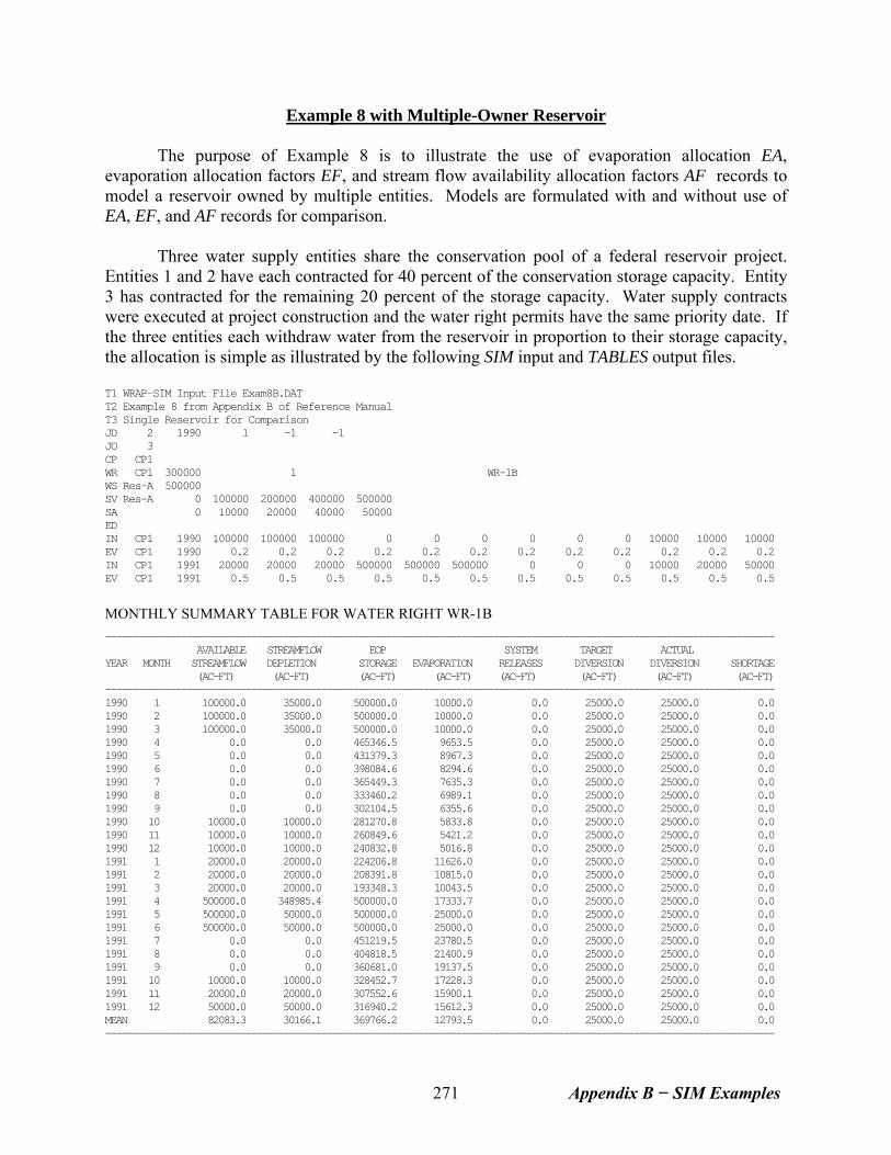
Example 8 with Multiple-Owner Reservoir The purpose of Example 8 is to illustrate the use of evaporation allocation EA, evaporation allocation factors EF, and stream flow availability allocation factors AF records to model a reservoir owned by multiple entities. Models are formulated with and without use of EA, EF, and AF records for comparison. Three water supply entities share the conservation pool of a federal reservoir project. Entities 1 and 2 have each contracted for 40 percent of the conservation storage capacity. Entity 3 has contracted for the remaining 20 percent of the storage capacity. Water supply contracts were executed at project construction and the water right permits have the same priority date. If the three entities each withdraw water from the reservoir in proportion to their storage capacity, the allocation is simple as illustrated by the following SIM input and TABLES output files. T1 WRAP-SIM Input File Exam8B.DAT T2 Example 8 from Appendix B of Reference Manual T3 Single Reservoir for Comparison JD 2 1990 1 -1 -1 JO 3 CP CP1 WR CP1 300000 1 WR-1B WS Res-A 500000 SV Res-A 0 100000 200000 400000 500000 SA 0 10000 20000 40000 50000 ED IN CP1 1990 100000 100000 100000 0 0 0 0 0 0 10000 10000 10000 EV CP1 1990 0.2 0.2 0.2 0.2 0.2 0.2 0.2 0.2 0.2 0.2 0.2 0.2 IN CP1 1991 20000 20000 20000 500000 500000 500000 0 0 0 10000 20000 50000 EV CP1 1991 0.5 0.5 0.5 0.5 0.5 0.5 0.5 0.5 0.5 0.5 0.5 0.5
MONTHLY SUMMARY TABLE FOR WATER RIGHT WR-1B
---------------------------------------------------------------------------------------------------------------------------- AVAILABLE STREAMFLOW EOP SYSTEM TARGET ACTUAL YEAR MONTH STREAMFLOW DEPLETION STORAGE EVAPORATION RELEASES DIVERSION DIVERSION SHORTAGE (AC-FT) (AC-FT) (AC-FT) (AC-FT) (AC-FT) (AC-FT) (AC-FT) (AC-FT) ---------------------------------------------------------------------------------------------------------------------------- 1990 1 100000.0 35000.0 500000.0 10000.0 0.0 25000.0 25000.0 0.0 1990 2 100000.0 35000.0 500000.0 10000.0 0.0 25000.0 25000.0 0.0 1990 3 100000.0 35000.0 500000.0 10000.0 0.0 25000.0 25000.0 0.0 1990 4 0.0 0.0 465346.5 9653.5 0.0 25000.0 25000.0 0.0 1990 5 0.0 0.0 431379.3 8967.3 0.0 25000.0 25000.0 0.0 1990 6 0.0 0.0 398084.6 8294.6 0.0 25000.0 25000.0 0.0 1990 7 0.0 0.0 365449.3 7635.3 0.0 25000.0 25000.0 0.0 1990 8 0.0 0.0 333460.2 6989.1 0.0 25000.0 25000.0 0.0 1990 9 0.0 0.0 302104.5 6355.6 0.0 25000.0 25000.0 0.0 1990 10 10000.0 10000.0 281270.8 5833.8 0.0 25000.0 25000.0 0.0 1990 11 10000.0 10000.0 260849.6 5421.2 0.0 25000.0 25000.0 0.0 1990 12 10000.0 10000.0 240832.8 5016.8 0.0 25000.0 25000.0 0.0 1991 1 20000.0 20000.0 224206.8 11626.0 0.0 25000.0 25000.0 0.0 1991 2 20000.0 20000.0 208391.8 10815.0 0.0 25000.0 25000.0 0.0 1991 3 20000.0 20000.0 193348.3 10043.5 0.0 25000.0 25000.0 0.0 1991 4 500000.0 348985.4 500000.0 17333.7 0.0 25000.0 25000.0 0.0 1991 5 500000.0 50000.0 500000.0 25000.0 0.0 25000.0 25000.0 0.0 1991 6 500000.0 50000.0 500000.0 25000.0 0.0 25000.0 25000.0 0.0 1991 7 0.0 0.0 451219.5 23780.5 0.0 25000.0 25000.0 0.0 1991 8 0.0 0.0 404818.5 21400.9 0.0 25000.0 25000.0 0.0 1991 9 0.0 0.0 360681.0 19137.5 0.0 25000.0 25000.0 0.0 1991 10 10000.0 10000.0 328452.7 17228.3 0.0 25000.0 25000.0 0.0 1991 11 20000.0 20000.0 307552.6 15900.1 0.0 25000.0 25000.0 0.0 1991 12 50000.0 50000.0 316940.2 15612.3 0.0 25000.0 25000.0 0.0 MEAN 82083.3 30166.1 369766.2 12793.5 0.0 25000.0 25000.0 0.0 ----------------------------------------------------------------------------------------------------------------------------
Appendix B − SIM Examples 271
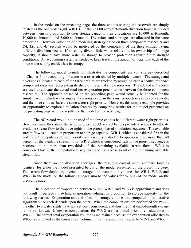
In the model on the preceding page, the three entities sharing the reservoir are simply treated as the one water right WR-1B. If the 25,000 acre-feet/month diversion target is divided between them in proportion to their storage capacity, their allocations are 10,000 ac-ft/month, 10,000 ac-ft/month, and 5,000 ac-ft/month. Diversions and shortages are allocated in the same proportion. However, adoption of a modeling strategy based on three component reservoirs and EA, EF, and AF records would be motivated by the complexity of the three entities having different diversion needs. If an entity diverts little water relative to its ownership of storage capacity, it should have more water in storage to provide protection against future drought conditions. An accounting system is needed to keep track of the amount of water that each of the three water supply entities has in storage. The following model formulation illustrates the component reservoir strategy described in Chapter 4 for accounting for water in a reservoir shared by multiple owners. The storage and diversions allocated to each of the three entities are tracked by assigning each a "computational" component reservoir representing its share of the actual single reservoir. The EA and EF records are used to allocate the actual total net evaporation-precipitation between the three component reservoirs. The approach presented on the preceding page would actually be adopted for the simple case in which water supply diversions occur in the same proportion as storage capacity, and the three entities share the same water right priority. However, this simple example provides an opportunity to explore simulation features by comparing results for the model presented on the preceding page with the results for the model on the next page. The AF record would not be used if the three entities had different water right priorities. However, since they share the same priority, the AF record factors provide a scheme to allocate available stream flow to the three rights in the priority-based simulation sequence. The available stream flow is allocated in proportion to storage capacity. WR-1, which is considered first in the water right computational loop priority sequence, is restricted to appropriate no more than 40 percent of the available stream flow. WR-2 which is considered next in the priority sequence is restricted to no more than two-thirds of the remaining available stream flow. WR-3 is considered last in the computational sequence and has access to all of the remaining available stream flow. Since there are no diversion shortages, the resulting control point summary table is identical for either the model presented below or the model presented on the presenting page. The stream flow depletion, diversion, storage, and evaporation volumes for WR-1, WR-2, and WR-3 in the model on the following pages sum to the values for WR-1B of the model on the preceding page. The allocation of evaporation between WR-1, WR-2, and WR-3 is approximate and does not result in perfectly matching evaporation volumes in proportion to storage capacity for the following reason. Evaporation and end-of-month storage volumes are computed in an iterative algorithm since each depends upon the other. When the computations are performed for WR-1, the other two water rights have not yet been considered, and thus the final end-of-month storage is not yet known. Likewise, computations for WR-2 are performed prior to consideration of WR-3. The correct total evaporation volume is maintained because the evaporation allocated to WR-3 is computed as the correct total volume minus the amounts allocated to WR-1 and WR-2.
Appendix B − SIM Examples 272
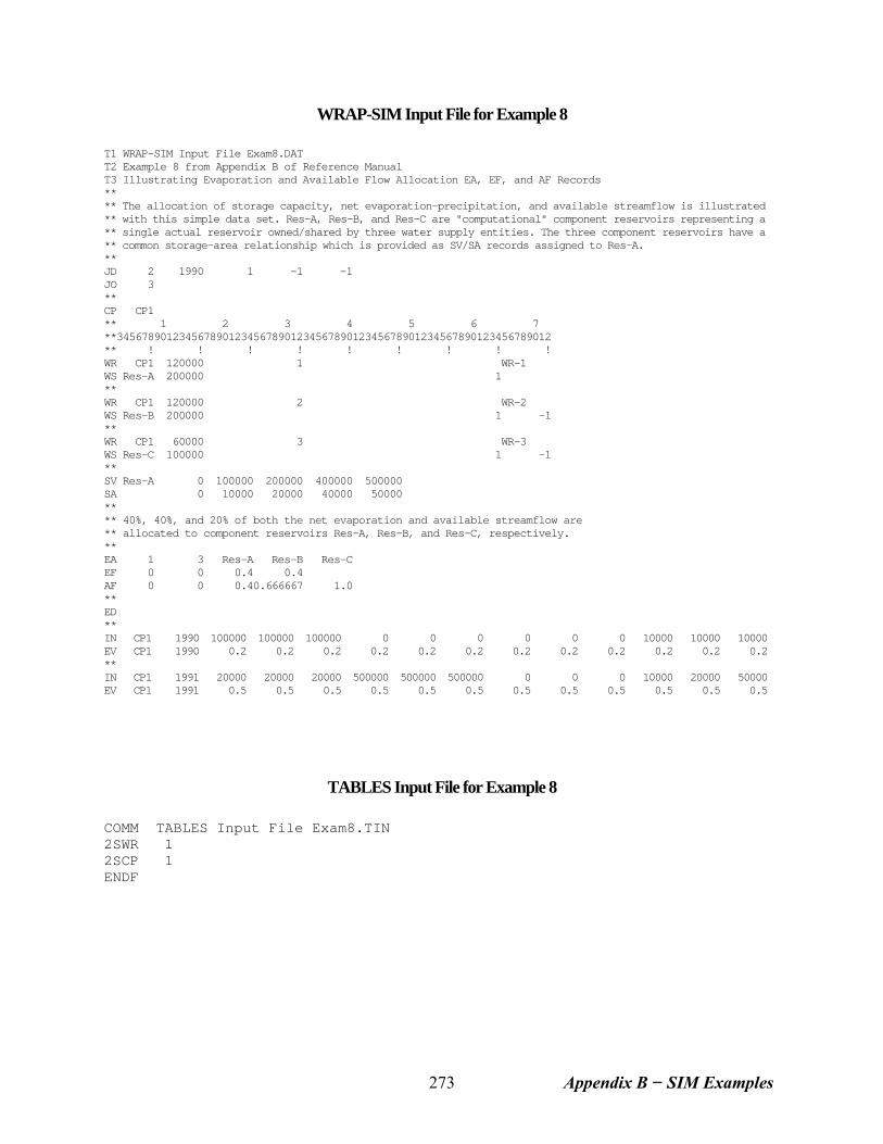
WRAP-SIM Input File for Example 8 T1 WRAP-SIM Input File Exam8.DAT T2 Example 8 from Appendix B of Reference Manual T3 Illustrating Evaporation and Available Flow Allocation EA, EF, and AF Records ** ** The allocation of storage capacity, net evaporation-precipitation, and available streamflow is illustrated ** with this simple data set. Res-A, Res-B, and Res-C are "computational" component reservoirs representing a ** single actual reservoir owned/shared by three water supply entities. The three component reservoirs have a ** common storage-area relationship which is provided as SV/SA records assigned to Res-A. ** JD 2 1990 1 -1 -1 JO 3 ** CP CP1 ** 1 2 3 4 5 6 7 **3456789012345678901234567890123456789012345678901234567890123456789012 ** ! ! ! ! ! ! ! ! ! WR CP1 120000 1 WR-1 WS Res-A 200000 1 ** WR CP1 120000 2 WR-2 WS Res-B 200000 1 -1 ** WR CP1 60000 3 WR-3 WS Res-C 100000 1 -1 ** SV Res-A 0 100000 200000 400000 500000 SA 0 10000 20000 40000 50000 ** ** 40%, 40%, and 20% of both the net evaporation and available streamflow are ** allocated to component reservoirs Res-A, Res-B, and Res-C, respectively. ** EA 1 3 Res-A Res-B Res-C EF 0 0 0.4 0.4 AF 0 0 0.40.666667 1.0 ** ED ** IN CP1 1990 100000 100000 100000 0 0 0 0 0 0 10000 10000 10000 EV CP1 1990 0.2 0.2 0.2 0.2 0.2 0.2 0.2 0.2 0.2 0.2 0.2 0.2 ** IN CP1 1991 20000 20000 20000 500000 500000 500000 0 0 0 10000 20000 50000 EV CP1 1991 0.5 0.5 0.5 0.5 0.5 0.5 0.5 0.5 0.5 0.5 0.5 0.5
TABLES Input File for Example 8 COMM TABLES Input File Exam8.TIN 2SWR 1 2SCP 1 ENDF
Appendix B − SIM Examples 273
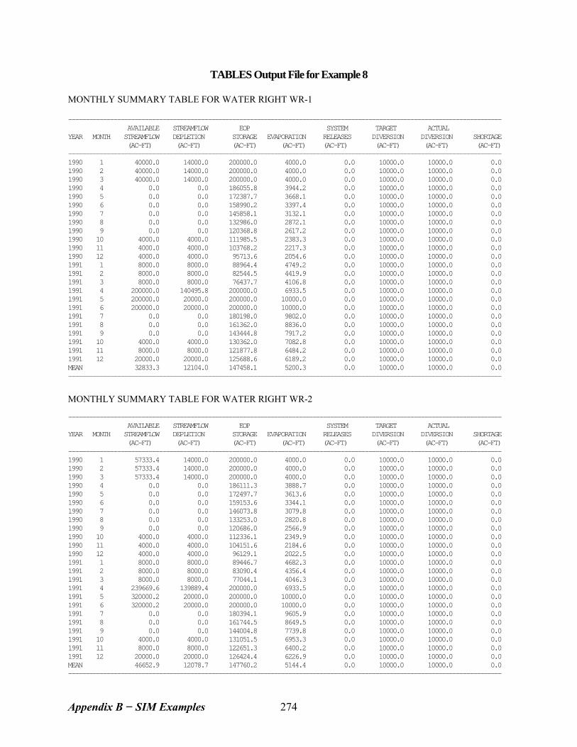
TABLES Output File for Example 8 MONTHLY SUMMARY TABLE FOR WATER RIGHT WR-1 ---------------------------------------------------------------------------------------------------------------------------- AVAILABLE STREAMFLOW EOP SYSTEM TARGET ACTUAL YEAR MONTH STREAMFLOW DEPLETION STORAGE EVAPORATION RELEASES DIVERSION DIVERSION SHORTAGE (AC-FT) (AC-FT) (AC-FT) (AC-FT) (AC-FT) (AC-FT) (AC-FT) (AC-FT) ---------------------------------------------------------------------------------------------------------------------------- 1990 1 40000.0 14000.0 200000.0 4000.0 0.0 10000.0 10000.0 0.0 1990 2 40000.0 14000.0 200000.0 4000.0 0.0 10000.0 10000.0 0.0 1990 3 40000.0 14000.0 200000.0 4000.0 0.0 10000.0 10000.0 0.0 1990 4 0.0 0.0 186055.8 3944.2 0.0 10000.0 10000.0 0.0 1990 5 0.0 0.0 172387.7 3668.1 0.0 10000.0 10000.0 0.0 1990 6 0.0 0.0 158990.2 3397.4 0.0 10000.0 10000.0 0.0 1990 7 0.0 0.0 145858.1 3132.1 0.0 10000.0 10000.0 0.0 1990 8 0.0 0.0 132986.0 2872.1 0.0 10000.0 10000.0 0.0 1990 9 0.0 0.0 120368.8 2617.2 0.0 10000.0 10000.0 0.0 1990 10 4000.0 4000.0 111985.5 2383.3 0.0 10000.0 10000.0 0.0 1990 11 4000.0 4000.0 103768.2 2217.3 0.0 10000.0 10000.0 0.0 1990 12 4000.0 4000.0 95713.6 2054.6 0.0 10000.0 10000.0 0.0 1991 1 8000.0 8000.0 88964.4 4749.2 0.0 10000.0 10000.0 0.0 1991 2 8000.0 8000.0 82544.5 4419.9 0.0 10000.0 10000.0 0.0 1991 3 8000.0 8000.0 76437.7 4106.8 0.0 10000.0 10000.0 0.0 1991 4 200000.0 140495.8 200000.0 6933.5 0.0 10000.0 10000.0 0.0 1991 5 200000.0 20000.0 200000.0 10000.0 0.0 10000.0 10000.0 0.0 1991 6 200000.0 20000.0 200000.0 10000.0 0.0 10000.0 10000.0 0.0 1991 7 0.0 0.0 180198.0 9802.0 0.0 10000.0 10000.0 0.0 1991 8 0.0 0.0 161362.0 8836.0 0.0 10000.0 10000.0 0.0 1991 9 0.0 0.0 143444.8 7917.2 0.0 10000.0 10000.0 0.0 1991 10 4000.0 4000.0 130362.0 7082.8 0.0 10000.0 10000.0 0.0 1991 11 8000.0 8000.0 121877.8 6484.2 0.0 10000.0 10000.0 0.0 1991 12 20000.0 20000.0 125688.6 6189.2 0.0 10000.0 10000.0 0.0 MEAN 32833.3 12104.0 147458.1 5200.3 0.0 10000.0 10000.0 0.0 ----------------------------------------------------------------------------------------------------------------------------
MONTHLY SUMMARY TABLE FOR WATER RIGHT WR-2 ---------------------------------------------------------------------------------------------------------------------------- AVAILABLE STREAMFLOW EOP SYSTEM TARGET ACTUAL YEAR MONTH STREAMFLOW DEPLETION STORAGE EVAPORATION RELEASES DIVERSION DIVERSION SHORTAGE (AC-FT) (AC-FT) (AC-FT) (AC-FT) (AC-FT) (AC-FT) (AC-FT) (AC-FT) ---------------------------------------------------------------------------------------------------------------------------- 1990 1 57333.4 14000.0 200000.0 4000.0 0.0 10000.0 10000.0 0.0 1990 2 57333.4 14000.0 200000.0 4000.0 0.0 10000.0 10000.0 0.0 1990 3 57333.4 14000.0 200000.0 4000.0 0.0 10000.0 10000.0 0.0 1990 4 0.0 0.0 186111.3 3888.7 0.0 10000.0 10000.0 0.0 1990 5 0.0 0.0 172497.7 3613.6 0.0 10000.0 10000.0 0.0 1990 6 0.0 0.0 159153.6 3344.1 0.0 10000.0 10000.0 0.0 1990 7 0.0 0.0 146073.8 3079.8 0.0 10000.0 10000.0 0.0 1990 8 0.0 0.0 133253.0 2820.8 0.0 10000.0 10000.0 0.0 1990 9 0.0 0.0 120686.0 2566.9 0.0 10000.0 10000.0 0.0 1990 10 4000.0 4000.0 112336.1 2349.9 0.0 10000.0 10000.0 0.0 1990 11 4000.0 4000.0 104151.6 2184.6 0.0 10000.0 10000.0 0.0 1990 12 4000.0 4000.0 96129.1 2022.5 0.0 10000.0 10000.0 0.0 1991 1 8000.0 8000.0 89446.7 4682.3 0.0 10000.0 10000.0 0.0 1991 2 8000.0 8000.0 83090.4 4356.4 0.0 10000.0 10000.0 0.0 1991 3 8000.0 8000.0 77044.1 4046.3 0.0 10000.0 10000.0 0.0 1991 4 239669.6 139889.4 200000.0 6933.5 0.0 10000.0 10000.0 0.0 1991 5 320000.2 20000.0 200000.0 10000.0 0.0 10000.0 10000.0 0.0 1991 6 320000.2 20000.0 200000.0 10000.0 0.0 10000.0 10000.0 0.0 1991 7 0.0 0.0 180394.1 9605.9 0.0 10000.0 10000.0 0.0 1991 8 0.0 0.0 161744.5 8649.5 0.0 10000.0 10000.0 0.0 1991 9 0.0 0.0 144004.8 7739.8 0.0 10000.0 10000.0 0.0 1991 10 4000.0 4000.0 131051.5 6953.3 0.0 10000.0 10000.0 0.0 1991 11 8000.0 8000.0 122651.3 6400.2 0.0 10000.0 10000.0 0.0 1991 12 20000.0 20000.0 126424.4 6226.9 0.0 10000.0 10000.0 0.0 MEAN 46652.9 12078.7 147760.2 5144.4 0.0 10000.0 10000.0 0.0 ----------------------------------------------------------------------------------------------------------------------------
Appendix B − SIM Examples 274
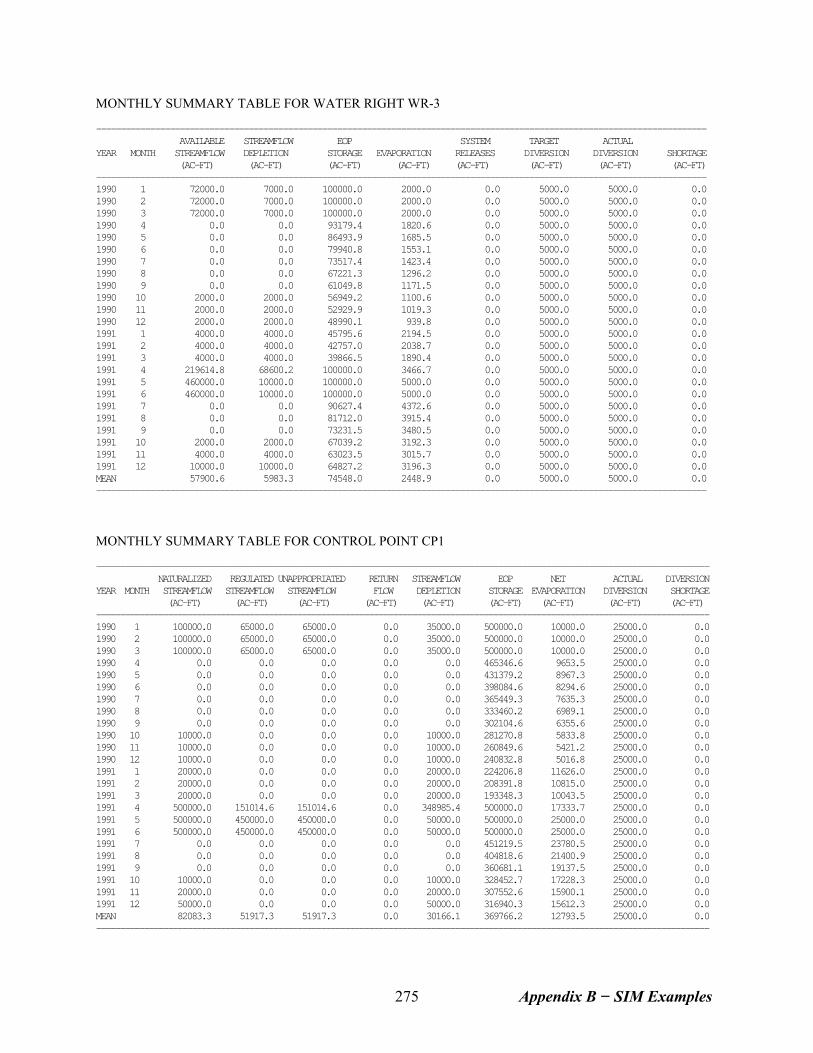
MONTHLY SUMMARY TABLE FOR WATER RIGHT WR-3 ---------------------------------------------------------------------------------------------------------------------------- AVAILABLE STREAMFLOW EOP SYSTEM TARGET ACTUAL YEAR MONTH STREAMFLOW DEPLETION STORAGE EVAPORATION RELEASES DIVERSION DIVERSION SHORTAGE (AC-FT) (AC-FT) (AC-FT) (AC-FT) (AC-FT) (AC-FT) (AC-FT) (AC-FT) ---------------------------------------------------------------------------------------------------------------------------- 1990 1 72000.0 7000.0 100000.0 2000.0 0.0 5000.0 5000.0 0.0 1990 2 72000.0 7000.0 100000.0 2000.0 0.0 5000.0 5000.0 0.0 1990 3 72000.0 7000.0 100000.0 2000.0 0.0 5000.0 5000.0 0.0 1990 4 0.0 0.0 93179.4 1820.6 0.0 5000.0 5000.0 0.0 1990 5 0.0 0.0 86493.9 1685.5 0.0 5000.0 5000.0 0.0 1990 6 0.0 0.0 79940.8 1553.1 0.0 5000.0 5000.0 0.0 1990 7 0.0 0.0 73517.4 1423.4 0.0 5000.0 5000.0 0.0 1990 8 0.0 0.0 67221.3 1296.2 0.0 5000.0 5000.0 0.0 1990 9 0.0 0.0 61049.8 1171.5 0.0 5000.0 5000.0 0.0 1990 10 2000.0 2000.0 56949.2 1100.6 0.0 5000.0 5000.0 0.0 1990 11 2000.0 2000.0 52929.9 1019.3 0.0 5000.0 5000.0 0.0 1990 12 2000.0 2000.0 48990.1 939.8 0.0 5000.0 5000.0 0.0 1991 1 4000.0 4000.0 45795.6 2194.5 0.0 5000.0 5000.0 0.0 1991 2 4000.0 4000.0 42757.0 2038.7 0.0 5000.0 5000.0 0.0 1991 3 4000.0 4000.0 39866.5 1890.4 0.0 5000.0 5000.0 0.0 1991 4 219614.8 68600.2 100000.0 3466.7 0.0 5000.0 5000.0 0.0 1991 5 460000.0 10000.0 100000.0 5000.0 0.0 5000.0 5000.0 0.0 1991 6 460000.0 10000.0 100000.0 5000.0 0.0 5000.0 5000.0 0.0 1991 7 0.0 0.0 90627.4 4372.6 0.0 5000.0 5000.0 0.0 1991 8 0.0 0.0 81712.0 3915.4 0.0 5000.0 5000.0 0.0 1991 9 0.0 0.0 73231.5 3480.5 0.0 5000.0 5000.0 0.0 1991 10 2000.0 2000.0 67039.2 3192.3 0.0 5000.0 5000.0 0.0 1991 11 4000.0 4000.0 63023.5 3015.7 0.0 5000.0 5000.0 0.0 1991 12 10000.0 10000.0 64827.2 3196.3 0.0 5000.0 5000.0 0.0 MEAN 57900.6 5983.3 74548.0 2448.9 0.0 5000.0 5000.0 0.0 ----------------------------------------------------------------------------------------------------------------------------
MONTHLY SUMMARY TABLE FOR CONTROL POINT CP1 -------------------------------------------------------------------------------------------------------------------------------- NATURALIZED REGULATED UNAPPROPRIATED RETURN STREAMFLOW EOP NET ACTUAL DIVERSION YEAR MONTH STREAMFLOW STREAMFLOW STREAMFLOW FLOW DEPLETION STORAGE EVAPORATION DIVERSION SHORTAGE (AC-FT) (AC-FT) (AC-FT) (AC-FT) (AC-FT) (AC-FT) (AC-FT) (AC-FT) (AC-FT) -------------------------------------------------------------------------------------------------------------------------------- 1990 1 100000.0 65000.0 65000.0 0.0 35000.0 500000.0 10000.0 25000.0 0.0 1990 2 100000.0 65000.0 65000.0 0.0 35000.0 500000.0 10000.0 25000.0 0.0 1990 3 100000.0 65000.0 65000.0 0.0 35000.0 500000.0 10000.0 25000.0 0.0 1990 4 0.0 0.0 0.0 0.0 0.0 465346.6 9653.5 25000.0 0.0 1990 5 0.0 0.0 0.0 0.0 0.0 431379.2 8967.3 25000.0 0.0 1990 6 0.0 0.0 0.0 0.0 0.0 398084.6 8294.6 25000.0 0.0 1990 7 0.0 0.0 0.0 0.0 0.0 365449.3 7635.3 25000.0 0.0 1990 8 0.0 0.0 0.0 0.0 0.0 333460.2 6989.1 25000.0 0.0 1990 9 0.0 0.0 0.0 0.0 0.0 302104.6 6355.6 25000.0 0.0 1990 10 10000.0 0.0 0.0 0.0 10000.0 281270.8 5833.8 25000.0 0.0 1990 11 10000.0 0.0 0.0 0.0 10000.0 260849.6 5421.2 25000.0 0.0 1990 12 10000.0 0.0 0.0 0.0 10000.0 240832.8 5016.8 25000.0 0.0 1991 1 20000.0 0.0 0.0 0.0 20000.0 224206.8 11626.0 25000.0 0.0 1991 2 20000.0 0.0 0.0 0.0 20000.0 208391.8 10815.0 25000.0 0.0 1991 3 20000.0 0.0 0.0 0.0 20000.0 193348.3 10043.5 25000.0 0.0 1991 4 500000.0 151014.6 151014.6 0.0 348985.4 500000.0 17333.7 25000.0 0.0 1991 5 500000.0 450000.0 450000.0 0.0 50000.0 500000.0 25000.0 25000.0 0.0 1991 6 500000.0 450000.0 450000.0 0.0 50000.0 500000.0 25000.0 25000.0 0.0 1991 7 0.0 0.0 0.0 0.0 0.0 451219.5 23780.5 25000.0 0.0 1991 8 0.0 0.0 0.0 0.0 0.0 404818.6 21400.9 25000.0 0.0 1991 9 0.0 0.0 0.0 0.0 0.0 360681.1 19137.5 25000.0 0.0 1991 10 10000.0 0.0 0.0 0.0 10000.0 328452.7 17228.3 25000.0 0.0 1991 11 20000.0 0.0 0.0 0.0 20000.0 307552.6 15900.1 25000.0 0.0 1991 12 50000.0 0.0 0.0 0.0 50000.0 316940.3 15612.3 25000.0 0.0 MEAN 82083.3 51917.3 51917.3 0.0 30166.1 369766.2 12793.5 25000.0 0.0 --------------------------------------------------------------------------------------------------------------------------------
Appendix B − SIM Examples 275
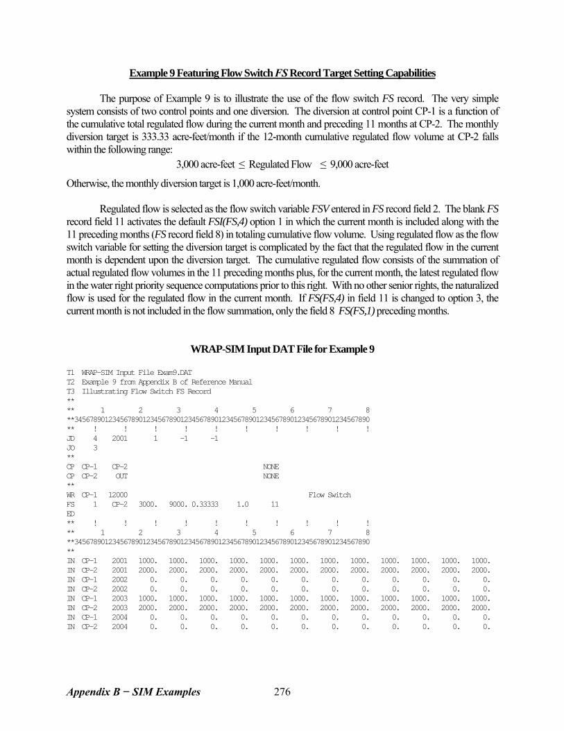
Example 9 Featuring Flow Switch FS Record Target Setting Capabilities The purpose of Example 9 is to illustrate the use of the flow switch FS record. The very simple system consists of two control points and one diversion. The diversion at control point CP-1 is a function of the cumulative total regulated flow during the current month and preceding 11 months at CP-2. The monthly diversion target is 333.33 acre-feet/month if the 12-month cumulative regulated flow volume at CP-2 falls within the following range:
3,000 acre-feet ≤ Regulated Flow ≤ 9,000 acre-feet
Otherwise, the monthly diversion target is 1,000 acre-feet/month. Regulated flow is selected as the flow switch variable FSV entered in FS record field 2. The blank FS record field 11 activates the default FSI(FS,4) option 1 in which the current month is included along with the 11 preceding months (FS record field 8) in totaling cumulative flow volume. Using regulated flow as the flow switch variable for setting the diversion target is complicated by the fact that the regulated flow in the current month is dependent upon the diversion target. The cumulative regulated flow consists of the summation of actual regulated flow volumes in the 11 preceding months plus, for the current month, the latest regulated flow in the water right priority sequence computations prior to this right. With no other senior rights, the naturalized flow is used for the regulated flow in the current month. If FS(FS,4) in field 11 is changed to option 3, the current month is not included in the flow summation, only the field 8 FS(FS,1) preceding months.
WRAP-SIM Input DAT File for Example 9
T1 WRAP-SIM Input File Exam9.DAT T2 Example 9 from Appendix B of Reference Manual T3 Illustrating Flow Switch FS Record ** ** 1 2 3 4 5 6 7 8 **345678901234567890123456789012345678901234567890123456789012345678901234567890 ** ! ! ! ! ! ! ! ! ! ! JD 4 2001 1 -1 -1 JO 3 ** CP CP-1 CP-2 NONE CP CP-2 OUT NONE ** WR CP-1 12000 Flow Switch FS 1 CP-2 3000. 9000. 0.33333 1.0 11 ED ** ! ! ! ! ! ! ! ! ! ! ** 1 2 3 4 5 6 7 8 **345678901234567890123456789012345678901234567890123456789012345678901234567890 ** IN CP-1 2001 1000. 1000. 1000. 1000. 1000. 1000. 1000. 1000. 1000. 1000. 1000. 1000. IN CP-2 2001 2000. 2000. 2000. 2000. 2000. 2000. 2000. 2000. 2000. 2000. 2000. 2000. IN CP-1 2002 0. 0. 0. 0. 0. 0. 0. 0. 0. 0. 0. 0. IN CP-2 2002 0. 0. 0. 0. 0. 0. 0. 0. 0. 0. 0. 0. IN CP-1 2003 1000. 1000. 1000. 1000. 1000. 1000. 1000. 1000. 1000. 1000. 1000. 1000. IN CP-2 2003 2000. 2000. 2000. 2000. 2000. 2000. 2000. 2000. 2000. 2000. 2000. 2000. IN CP-1 2004 0. 0. 0. 0. 0. 0. 0. 0. 0. 0. 0. 0. IN CP-2 2004 0. 0. 0. 0. 0. 0. 0. 0. 0. 0. 0. 0.
Appendix B − SIM Examples 276
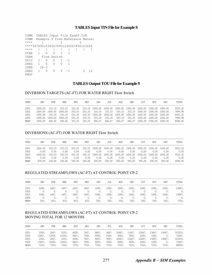
TABLES Input TIN File for Example 9
COMM TABLES Input File Exam9.TIN COMM Example 9 from Reference Manual **** 1 2 3 ****56789012345678901234567890123456 **** ! ! ! ! ! ! ! ! 2TAR 1 0 0 1 1 IDEN Flow Switch 2DIV 1 0 0 1 -1 2REG 1 0 0 0 1 IDEN CP-2 2REG 1 0 0 0 -1 2 12 ENDF
TABLES Output TOU File for Example 9
DIVERSION TARGETS (AC-FT) FOR WATER RIGHT Flow Switch ------------------------------------------------------------------------------------------------------------------------------- YEAR JAN FEB MAR APR MAY JUN JUL AUG SEP OCT NOV DEC TOTAL ------------------------------------------------------------------------------------------------------------------------------- 2001 1000.00 333.33 333.33 333.33 333.33 1000.00 1000.00 1000.00 1000.00 1000.00 1000.00 1000.00 9333.32 2002 1000.00 1000.00 1000.00 333.33 333.33 333.33 333.33 333.33 333.33 1000.00 1000.00 1000.00 7999.98 2003 1000.00 333.33 333.33 333.33 333.33 1000.00 1000.00 1000.00 1000.00 1000.00 1000.00 1000.00 9333.32 2004 1000.00 1000.00 1000.00 333.33 333.33 333.33 333.33 333.33 333.33 1000.00 1000.00 1000.00 7999.98 MEAN 1000.00 666.66 666.66 333.33 333.33 666.67 666.67 666.67 666.67 1000.00 1000.00 1000.00 8666.65 -------------------------------------------------------------------------------------------------------------------------------
DIVERSIONS (AC-FT) FOR WATER RIGHT Flow Switch ------------------------------------------------------------------------------------------------------------------------------- YEAR JAN FEB MAR APR MAY JUN JUL AUG SEP OCT NOV DEC TOTAL ------------------------------------------------------------------------------------------------------------------------------- 2001 1000.00 333.33 333.33 333.33 333.33 1000.00 1000.00 1000.00 1000.00 1000.00 1000.00 1000.00 9333.32 2002 0.00 0.00 0.00 0.00 0.00 0.00 0.00 0.00 0.00 0.00 0.00 0.00 0.00 2003 1000.00 333.33 333.33 333.33 333.33 1000.00 1000.00 1000.00 1000.00 1000.00 1000.00 1000.00 9333.32 2004 0.00 0.00 0.00 0.00 0.00 0.00 0.00 0.00 0.00 0.00 0.00 0.00 0.00 MEAN 500.00 166.66 166.66 166.66 166.66 500.00 500.00 500.00 500.00 500.00 500.00 500.00 4666.66 -------------------------------------------------------------------------------------------------------------------------------
REGULATED STREAMFLOWS (AC-FT) AT CONTROL POINT CP-2 ------------------------------------------------------------------------------------------------------------------------------- YEAR JAN FEB MAR APR MAY JUN JUL AUG SEP OCT NOV DEC TOTAL ------------------------------------------------------------------------------------------------------------------------------- 2001 1000. 1667. 1667. 1667. 1667. 1000. 1000. 1000. 1000. 1000. 1000. 1000. 14667. 2002 0. 0. 0. 0. 0. 0. 0. 0. 0. 0. 0. 0. 0. 2003 1000. 1667. 1667. 1667. 1667. 1000. 1000. 1000. 1000. 1000. 1000. 1000. 14667. 2004 0. 0. 0. 0. 0. 0. 0. 0. 0. 0. 0. 0. 0. MEAN 500. 833. 833. 833. 833. 500. 500. 500. 500. 500. 500. 500. 7333. -------------------------------------------------------------------------------------------------------------------------------
REGULATED STREAMFLOWS (AC-FT) AT CONTROL POINT CP-2 MOVING TOTAL FOR 12 MONTHS ------------------------------------------------------------------------------------------------------------------------------- YEAR JAN FEB MAR APR MAY JUN JUL AUG SEP OCT NOV DEC TOTAL ------------------------------------------------------------------------------------------------------------------------------- 2001 1000. 2667. 4333. 6000. 7667. 8667. 9667. 10667. 11667. 12667. 13667. 14667. 103333. 2002 13667. 12000. 10333. 8667. 7000. 6000. 5000. 4000. 3000. 2000. 1000. 0. 72667. 2003 1000. 2667. 4333. 6000. 7667. 8667. 9667. 10667. 11667. 12667. 13667. 14667. 103333. 2004 13667. 12000. 10333. 8667. 7000. 6000. 5000. 4000. 3000. 2000. 1000. 0. 72667. MEAN 7333. 7333. 7333. 7333. 7333. 7333. 7333. 7333. 7333. 7333. 7333. 7333. 88000. -------------------------------------------------------------------------------------------------------------------------------
Appendix B − SIM Examples 277
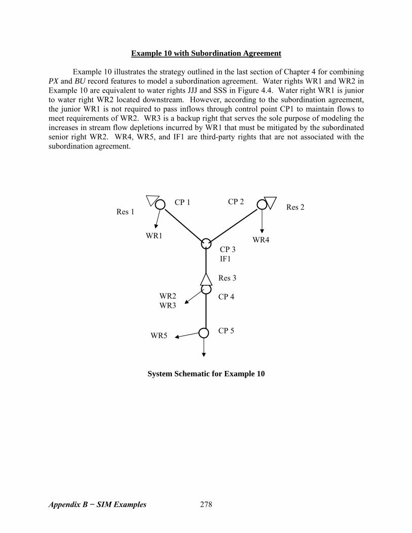
Example 10 with Subordination Agreement Example 10 illustrates the strategy outlined in the last section of Chapter 4 for combining PX and BU record features to model a subordination agreement. Water rights WR1 and WR2 in Example 10 are equivalent to water rights JJJ and SSS in Figure 4.4. Water right WR1 is junior to water right WR2 located downstream. However, according to the subordination agreement, the junior WR1 is not required to pass inflows through control point CP1 to maintain flows to meet requirements of WR2. WR3 is a backup right that serves the sole purpose of modeling the increases in stream flow depletions incurred by WR1 that must be mitigated by the subordinated senior right WR2. WR4, WR5, and IF1 are third-party rights that are not associated with the subordination agreement.
WR5
WR2 WR3
CP 3 IF1
CP 2
WR4 WR1
Res 1 CP 1
Res 3
CP 4
Res 2 CP 5
System Schematic for Example 10
Appendix B − SIM Examples 278
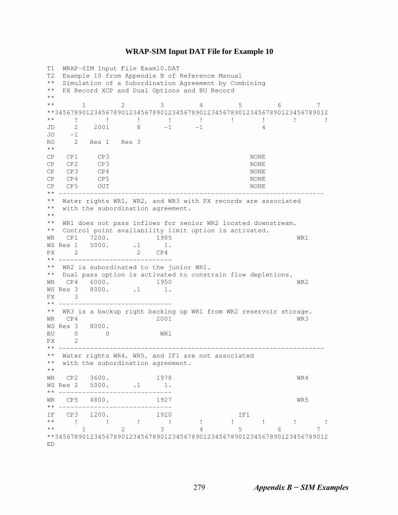
WRAP-SIM Input DAT File for Example 10 T1 WRAP-SIM Input File Exam10.DAT T2 Example 10 from Appendix B of Reference Manual ** Simulation of a Subordination Agreement by Combining ** PX Record XCP and Dual Options and BU Record ** ** 1 2 3 4 5 6 7 **3456789012345678901234567890123456789012345678901234567890123456789012 ** ! ! ! ! ! ! ! ! ! JD 2 2001 8 -1 -1 4 JO -1 RO 2 Res 1 Res 3 ** CP CP1 CP3 NONE CP CP2 CP3 NONE CP CP3 CP4 NONE CP CP4 CP5 NONE CP CP5 OUT NONE ** -------------------------------------------------------------------- ** Water rights WR1, WR2, and WR3 with PX records are associated ** with the subordination agreement. ** ** WR1 does not pass inflows for senior WR2 located downstream. ** Control point availability limit option is activated. WR CP1 7200. 1985 WR1 WS Res 1 5000. .1 1. PX 2 2 CP4 ** ----------------------------- ** WR2 is subordinated to the junior WR1. ** Dual pass option is activated to constrain flow depletions. WR CP4 6000. 1950 WR2 WS Res 3 8000. .1 1. PX 3 ** ----------------------------- ** WR3 is a backup right backing up WR1 from WR2 reservoir storage. WR CP4 2001 WR3 WS Res 3 8000. BU 0 0 WR1 PX 2 ** -------------------------------------------------------------------- ** Water rights WR4, WR5, and IF1 are not associated ** with the subordination agreement. ** WR CP2 3600. 1978 WR4 WS Res 2 5000. .1 1. ** ----------------------------- WR CP5 4800. 1927 WR5 ** ----------------------------- IF CP3 1200. 1920 IF1 ** ! ! ! ! ! ! ! ! ! ** 1 2 3 4 5 6 7 **3456789012345678901234567890123456789012345678901234567890123456789012 ED
Appendix B − SIM Examples 279
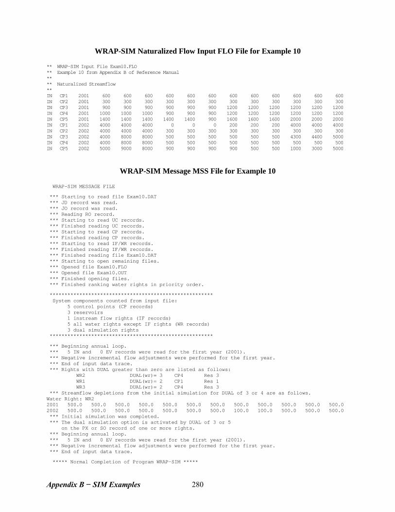
WRAP-SIM Naturalized Flow Input FLO File for Example 10 ** WRAP-SIM Input File Exam10.FLO ** Example 10 from Appendix B of Reference Manual ** ** Naturalized Streamflow ** IN CP1 2001 600 600 600 600 600 600 600 600 600 600 600 600 IN CP2 2001 300 300 300 300 300 300 300 300 300 300 300 300 IN CP3 2001 900 900 900 900 900 900 1200 1200 1200 1200 1200 1200 IN CP4 2001 1000 1000 1000 900 900 900 1200 1200 1200 1200 1200 1200 IN CP5 2001 1400 1400 1400 1400 1400 900 1600 1600 1600 2000 2000 2000 IN CP1 2002 4000 4000 4000 0 0 0 200 200 200 4000 4000 4000 IN CP2 2002 4000 4000 4000 300 300 300 300 300 300 300 300 300 IN CP3 2002 4000 8000 8000 500 500 500 500 500 500 4300 4400 5000 IN CP4 2002 4000 8000 8000 500 500 500 500 500 500 500 500 500 IN CP5 2002 5000 9000 8000 900 900 900 900 500 500 1000 3000 5000
WRAP-SIM Message MSS File for Example 10 WRAP-SIM MESSAGE FILE *** Starting to read file Exam10.DAT *** JD record was read. *** JO record was read. *** Reading RO record. *** Starting to read UC records. *** Finished reading UC records. *** Starting to read CP records. *** Finished reading CP records. *** Starting to read IF/WR records. *** Finished reading IF/WR records. *** Finished reading file Exam10.DAT *** Starting to open remaining files. *** Opened file Exam10.FLO *** Opened file Exam10.OUT *** Finished opening files. *** Finished ranking water rights in priority order. ******************************************************* System components counted from input file: 5 control points (CP records) 3 reservoirs 1 instream flow rights (IF records) 5 all water rights except IF rights (WR records) 3 dual simulation rights ******************************************************* *** Beginning annual loop. *** 5 IN and 0 EV records were read for the first year (2001). *** Negative incremental flow adjustments were performed for the first year. *** End of input data trace. *** Rights with DUAL greater than zero are listed as follows: WR2 DUAL(wr)= 3 CP4 Res 3 WR1 DUAL(wr)= 2 CP1 Res 1 WR3 DUAL(wr)= 2 CP4 Res 3 *** Streamflow depletions from the initial simulation for DUAL of 3 or 4 are as follows. Water Right: WR2 2001 500.0 500.0 500.0 500.0 500.0 500.0 500.0 500.0 500.0 500.0 500.0 500.0 2002 500.0 500.0 500.0 500.0 500.0 500.0 500.0 100.0 100.0 500.0 500.0 500.0 *** Initial simulation was completed. *** The dual simulation option is activated by DUAL of 3 or 5 on the PX or SO record of one or more rights. *** Beginning annual loop. *** 5 IN and 0 EV records were read for the first year (2001). *** Negative incremental flow adjustments were performed for the first year. *** End of input data trace. ***** Normal Completion of Program WRAP-SIM *****
Appendix B − SIM Examples 280
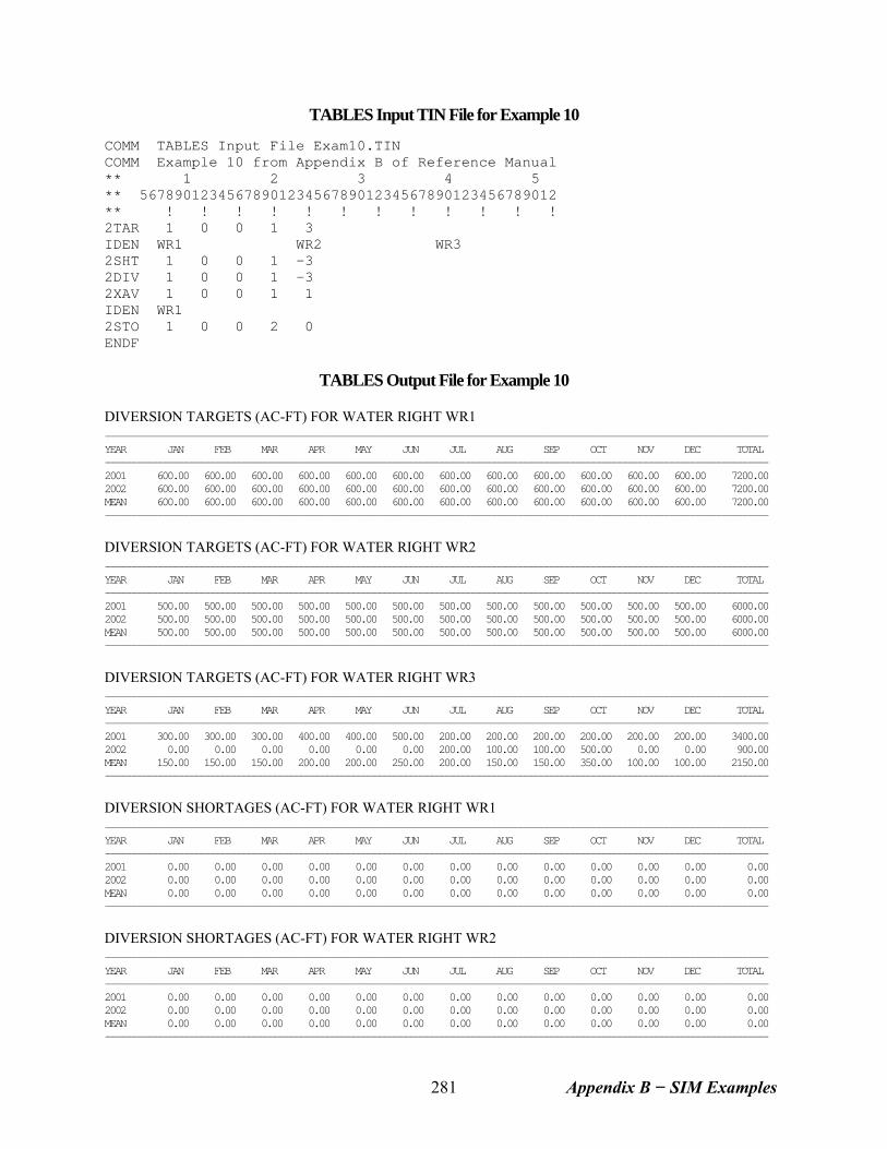
TABLES Input TIN File for Example 10 COMM TABLES Input File Exam10.TIN COMM Example 10 from Appendix B of Reference Manual ** 1 2 3 4 5 ** 567890123456789012345678901234567890123456789012 ** ! ! ! ! ! ! ! ! ! ! ! ! 2TAR 1 0 0 1 3 IDEN WR1 WR2 WR3 2SHT 1 0 0 1 -3 2DIV 1 0 0 1 -3 2XAV 1 0 0 1 1 IDEN WR1 2STO 1 0 0 2 0 ENDF
TABLES Output File for Example 10 DIVERSION TARGETS (AC-FT) FOR WATER RIGHT WR1
------------------------------------------------------------------------------------------------------------------------------- YEAR JAN FEB MAR APR MAY JUN JUL AUG SEP OCT NOV DEC TOTAL ------------------------------------------------------------------------------------------------------------------------------- 2001 600.00 600.00 600.00 600.00 600.00 600.00 600.00 600.00 600.00 600.00 600.00 600.00 7200.00 2002 600.00 600.00 600.00 600.00 600.00 600.00 600.00 600.00 600.00 600.00 600.00 600.00 7200.00 MEAN 600.00 600.00 600.00 600.00 600.00 600.00 600.00 600.00 600.00 600.00 600.00 600.00 7200.00 ------------------------------------------------------------------------------------------------------------------------------- DIVERSION TARGETS (AC-FT) FOR WATER RIGHT WR2
------------------------------------------------------------------------------------------------------------------------------- YEAR JAN FEB MAR APR MAY JUN JUL AUG SEP OCT NOV DEC TOTAL ------------------------------------------------------------------------------------------------------------------------------- 2001 500.00 500.00 500.00 500.00 500.00 500.00 500.00 500.00 500.00 500.00 500.00 500.00 6000.00 2002 500.00 500.00 500.00 500.00 500.00 500.00 500.00 500.00 500.00 500.00 500.00 500.00 6000.00 MEAN 500.00 500.00 500.00 500.00 500.00 500.00 500.00 500.00 500.00 500.00 500.00 500.00 6000.00 ------------------------------------------------------------------------------------------------------------------------------- DIVERSION TARGETS (AC-FT) FOR WATER RIGHT WR3
------------------------------------------------------------------------------------------------------------------------------- YEAR JAN FEB MAR APR MAY JUN JUL AUG SEP OCT NOV DEC TOTAL ------------------------------------------------------------------------------------------------------------------------------- 2001 300.00 300.00 300.00 400.00 400.00 500.00 200.00 200.00 200.00 200.00 200.00 200.00 3400.00 2002 0.00 0.00 0.00 0.00 0.00 0.00 200.00 100.00 100.00 500.00 0.00 0.00 900.00 MEAN 150.00 150.00 150.00 200.00 200.00 250.00 200.00 150.00 150.00 350.00 100.00 100.00 2150.00 ------------------------------------------------------------------------------------------------------------------------------- DIVERSION SHORTAGES (AC-FT) FOR WATER RIGHT WR1
------------------------------------------------------------------------------------------------------------------------------- YEAR JAN FEB MAR APR MAY JUN JUL AUG SEP OCT NOV DEC TOTAL ------------------------------------------------------------------------------------------------------------------------------- 2001 0.00 0.00 0.00 0.00 0.00 0.00 0.00 0.00 0.00 0.00 0.00 0.00 0.00 2002 0.00 0.00 0.00 0.00 0.00 0.00 0.00 0.00 0.00 0.00 0.00 0.00 0.00 MEAN 0.00 0.00 0.00 0.00 0.00 0.00 0.00 0.00 0.00 0.00 0.00 0.00 0.00 ------------------------------------------------------------------------------------------------------------------------------- DIVERSION SHORTAGES (AC-FT) FOR WATER RIGHT WR2
------------------------------------------------------------------------------------------------------------------------------- YEAR JAN FEB MAR APR MAY JUN JUL AUG SEP OCT NOV DEC TOTAL ------------------------------------------------------------------------------------------------------------------------------- 2001 0.00 0.00 0.00 0.00 0.00 0.00 0.00 0.00 0.00 0.00 0.00 0.00 0.00 2002 0.00 0.00 0.00 0.00 0.00 0.00 0.00 0.00 0.00 0.00 0.00 0.00 0.00 MEAN 0.00 0.00 0.00 0.00 0.00 0.00 0.00 0.00 0.00 0.00 0.00 0.00 0.00 -------------------------------------------------------------------------------------------------------------------------------
Appendix B − SIM Examples 281
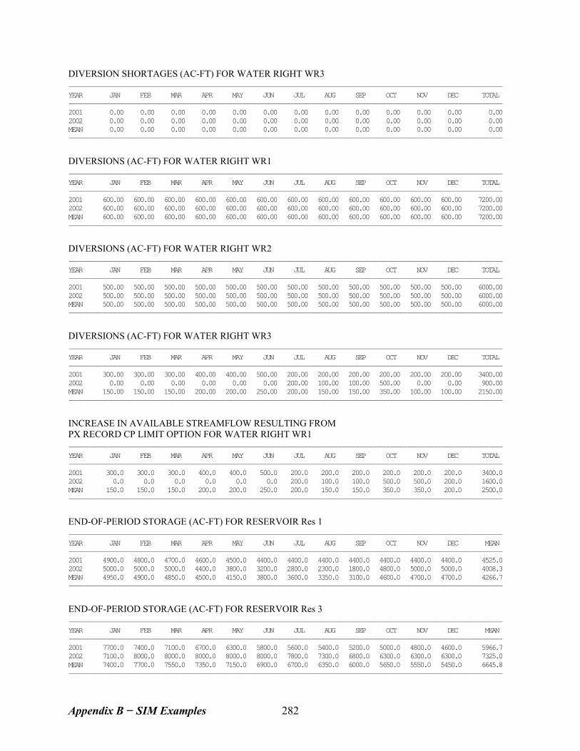
DIVERSION SHORTAGES (AC-FT) FOR WATER RIGHT WR3
------------------------------------------------------------------------------------------------------------------------------- YEAR JAN FEB MAR APR MAY JUN JUL AUG SEP OCT NOV DEC TOTAL ------------------------------------------------------------------------------------------------------------------------------- 2001 0.00 0.00 0.00 0.00 0.00 0.00 0.00 0.00 0.00 0.00 0.00 0.00 0.00 2002 0.00 0.00 0.00 0.00 0.00 0.00 0.00 0.00 0.00 0.00 0.00 0.00 0.00 MEAN 0.00 0.00 0.00 0.00 0.00 0.00 0.00 0.00 0.00 0.00 0.00 0.00 0.00 -------------------------------------------------------------------------------------------------------------------------------
DIVERSIONS (AC-FT) FOR WATER RIGHT WR1
------------------------------------------------------------------------------------------------------------------------------- YEAR JAN FEB MAR APR MAY JUN JUL AUG SEP OCT NOV DEC TOTAL ------------------------------------------------------------------------------------------------------------------------------- 2001 600.00 600.00 600.00 600.00 600.00 600.00 600.00 600.00 600.00 600.00 600.00 600.00 7200.00 2002 600.00 600.00 600.00 600.00 600.00 600.00 600.00 600.00 600.00 600.00 600.00 600.00 7200.00 MEAN 600.00 600.00 600.00 600.00 600.00 600.00 600.00 600.00 600.00 600.00 600.00 600.00 7200.00 -------------------------------------------------------------------------------------------------------------------------------
DIVERSIONS (AC-FT) FOR WATER RIGHT WR2
------------------------------------------------------------------------------------------------------------------------------- YEAR JAN FEB MAR APR MAY JUN JUL AUG SEP OCT NOV DEC TOTAL ------------------------------------------------------------------------------------------------------------------------------- 2001 500.00 500.00 500.00 500.00 500.00 500.00 500.00 500.00 500.00 500.00 500.00 500.00 6000.00 2002 500.00 500.00 500.00 500.00 500.00 500.00 500.00 500.00 500.00 500.00 500.00 500.00 6000.00 MEAN 500.00 500.00 500.00 500.00 500.00 500.00 500.00 500.00 500.00 500.00 500.00 500.00 6000.00 -------------------------------------------------------------------------------------------------------------------------------
DIVERSIONS (AC-FT) FOR WATER RIGHT WR3
------------------------------------------------------------------------------------------------------------------------------- YEAR JAN FEB MAR APR MAY JUN JUL AUG SEP OCT NOV DEC TOTAL ------------------------------------------------------------------------------------------------------------------------------- 2001 300.00 300.00 300.00 400.00 400.00 500.00 200.00 200.00 200.00 200.00 200.00 200.00 3400.00 2002 0.00 0.00 0.00 0.00 0.00 0.00 200.00 100.00 100.00 500.00 0.00 0.00 900.00 MEAN 150.00 150.00 150.00 200.00 200.00 250.00 200.00 150.00 150.00 350.00 100.00 100.00 2150.00 -------------------------------------------------------------------------------------------------------------------------------
INCREASE IN AVAILABLE STREAMFLOW RESULTING FROM PX RECORD CP LIMIT OPTION FOR WATER RIGHT WR1
------------------------------------------------------------------------------------------------------------------------------- YEAR JAN FEB MAR APR MAY JUN JUL AUG SEP OCT NOV DEC TOTAL ------------------------------------------------------------------------------------------------------------------------------- 2001 300.0 300.0 300.0 400.0 400.0 500.0 200.0 200.0 200.0 200.0 200.0 200.0 3400.0 2002 0.0 0.0 0.0 0.0 0.0 0.0 200.0 100.0 100.0 500.0 500.0 200.0 1600.0 MEAN 150.0 150.0 150.0 200.0 200.0 250.0 200.0 150.0 150.0 350.0 350.0 200.0 2500.0 -------------------------------------------------------------------------------------------------------------------------------
END-OF-PERIOD STORAGE (AC-FT) FOR RESERVOIR Res 1
------------------------------------------------------------------------------------------------------------------------------- YEAR JAN FEB MAR APR MAY JUN JUL AUG SEP OCT NOV DEC MEAN ------------------------------------------------------------------------------------------------------------------------------- 2001 4900.0 4800.0 4700.0 4600.0 4500.0 4400.0 4400.0 4400.0 4400.0 4400.0 4400.0 4400.0 4525.0 2002 5000.0 5000.0 5000.0 4400.0 3800.0 3200.0 2800.0 2300.0 1800.0 4800.0 5000.0 5000.0 4008.3 MEAN 4950.0 4900.0 4850.0 4500.0 4150.0 3800.0 3600.0 3350.0 3100.0 4600.0 4700.0 4700.0 4266.7 -------------------------------------------------------------------------------------------------------------------------------
END-OF-PERIOD STORAGE (AC-FT) FOR RESERVOIR Res 3
------------------------------------------------------------------------------------------------------------------------------- YEAR JAN FEB MAR APR MAY JUN JUL AUG SEP OCT NOV DEC MEAN ------------------------------------------------------------------------------------------------------------------------------- 2001 7700.0 7400.0 7100.0 6700.0 6300.0 5800.0 5600.0 5400.0 5200.0 5000.0 4800.0 4600.0 5966.7 2002 7100.0 8000.0 8000.0 8000.0 8000.0 8000.0 7800.0 7300.0 6800.0 6300.0 6300.0 6300.0 7325.0 MEAN 7400.0 7700.0 7550.0 7350.0 7150.0 6900.0 6700.0 6350.0 6000.0 5650.0 5550.0 5450.0 6645.8 -------------------------------------------------------------------------------------------------------------------------------
Appendix B − SIM Examples 282
APPENDIX C WRAP-HYD EXAMPLES
An "Introduction to Appendices B and C" is presented at the beginning of Appendix B. The examples illustrate the content and format of the input and output. They also provide a starting point for creating other datasets containing other features of interest to model users. Model users should experiment with simple datasets to become proficient with various modeling features prior to application to complex real world river basins. Model results with simplified data are easily trackable. Users can compare computer results with manual computational checks to confirm that the programs work as expected. Five simple examples are provided to illustrate WRAP-HYD input and output datasets. Examples 11, 12, and 13 demonstrate basic AS, FA, RS, SC, CI record stream flow adjustment features and also include EP record evaporation-precipitation manipulations. Examples 11 and 12 are identical except for the format of the input and output. Example 12 is included to further illustrate input/output format options. IN and EV records in Examples 11 and 13 are input in the optional control point grouping format and output in standard format. Example 12 uses the columnar table format for the stream flow input file rather than IN records. Example 14 focuses on distribution of stream flows from gaged to ungaged control points. IN records for Example 14 are provided alternatively as a standard-format FLO file and an old-format root1.HYD file. Example 15 employs the OI record to convert WRAP-SIM simulation results from an OUT file to SIM or HYD input records written to a HYD output HOT file.
Example 11 The Example 11 river basin configuration is represented by four control points (labeled CP-1, CP-2, CP-3, CP-4) representing actual locations in the river system. Two other control points (CP1E and CP2P) serve as identifiers for evaporation (CP1E) and precipitation (CP1P) datasets for reservoir Res located at CP-1. An input file with filename Exam11.DAT contains:
• job control JC and control point CP records
• an EP record activating an evaporation-precipitation combining operation
• adjustment specifications (AS records) and information for adjusting the flows for a FA record series of inflows/outflows and for the effects of a reservoir described by RS and SC records
Evaporation and precipitation depths (EV records) are provided in file Exam11.EVA with
the control point identifiers CP1E and CP1P. The same sets of 12 monthly evaporation and precipitation depths are repeated for each of the three years of the period-of-analysis. An EP record in the DAT file specifies that the precipitation be subtracted from the evaporation, and that the resulting net evaporation-precipitation depths be assigned to control point CP-1. The output file Exam11OUT.EVA contains only the computed EV records for CP-1. EV records for all other control points are omitted from the output file as specified by parameter INEV on the CP records. The net evaporation-precipitation depths are also used in the reservoir evaporation-precipitation computations performed in adjusting stream flows as instructed by the RS record.
Appendix C − HYD Examples 283
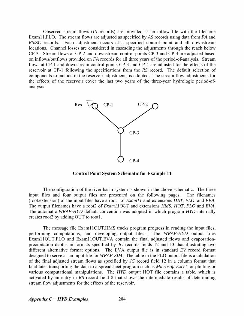
Observed stream flows (IN records) are provided as an inflow file with the filename Exam11.FLO. The stream flows are adjusted as specified by AS records using data from FA and RS/SC records. Each adjustment occurs at a specified control point and all downstream locations. Channel losses are considered in cascading the adjustments through the reach below CP-3. Stream flows at CP-2 and downstream control points CP-3 and CP-4 are adjusted based on inflows/outflows provided on FA records for all three years of the period-of-analysis. Stream flows at CP-1 and downstream control points CP-3 and CP-4 are adjusted for the effects of the reservoir at CP-1 following the specifications from the RS record. The default selection of components to include in the reservoir adjustments is adopted. The stream flow adjustments for the effects of the reservoir cover the last two years of the three-year hydrologic period-of-analysis. CP-2 CP-1 Res
CP-3
CP-4
Control Point System Schematic for Example 11
The configuration of the river basin system is shown in the above schematic. The three input files and four output files are presented on the following pages. The filenames (root.extension) of the input files have a root1 of Exam11 and extensions DAT, FLO, and EVA. The output filenames have a root2 of Exam11OUT and extensions HMS, HOT, FLO and EVA. The automatic WRAP-HYD default convention was adopted in which program HYD internally creates root2 by adding OUT to root1.
The message file Exam11OUT.HMS tracks program progress in reading the input files,
performing computations, and developing output files. The WRAP-HYD output files Exam11OUT.FLO and Exam11OUT.EVA contain the final adjusted flows and evaporation-precipitation depths in formats specified by JC records fields 12 and 13 that illustrating two different alternative format options. The EVA output file is in standard EV record format designed to serve as an input file for WRAP-SIM. The table in the FLO output file is a tabulation of the final adjusted stream flows as specified by JC record field 12 in a column format that facilitates transporting the data to a spreadsheet program such as Microsoft Excel for plotting or various computational manipulations. The HYD output HOT file contains a table, which is activated by an entry in RS record field 8 that shows the intermediate results of determining stream flow adjustments for the effects of the reservoir.
Appendix C − HYD Examples 284
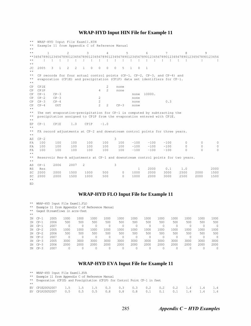
WRAP-HYD Input HIN File for Example 11 ** WRAP-HYD Input File Exam11.HIN ** Example 11 from Appendix C of Reference Manual ** ** 1 2 3 4 5 6 7 8 9 **3456789012345678901234567890123456789012345678901234567890123456789012345678901234567890123456 ** ! ! ! ! ! ! ! ! ! ! ! ! ! ! ! ! ! ! ! ! ! ** JC 2005 3 1 2 2 1 0 0 0 0 5 1 0 1 ** ** CP records for four actual control points (CP-1, CP-2, CP-3, and CP-4) and ** evaporation (CP1E) and precipitation (CP1P) data set identifiers for CP-1. ** CP CP1E 2 none CP CP1P 4 2 none CP CP-1 CP-3 none 10000. CP CP-2 CP-3 2 none CP CP-3 CP-4 2 none 0.3 CP CP-4 OUT 2 2 CP-3 none ** ** The net evaporation-precipitation for CP-1 is computed by subtracting the ** precipitation assigned to CP1P from the evaporation entered with CP1E. ** EP CP-1 CP1E 1.0 CP1P -1.0 ** ** FA record adjustments at CP-2 and downstream control points for three years. ** AS CP-2 3 FA 100 100 100 100 100 100 -100 -100 -100 0 0 0 FA 100 100 100 100 100 100 -100 -100 -100 0 0 0 FA 100 100 100 100 100 100 -100 -100 -100 0 0 0 ** ** Reservoir Res-A adjustments at CP-1 and downstream control points for two years. ** AS CP-1 2006 2007 2 3 RS Res 1 2000 0.1 1.0 2000 SC 2000 2000 1500 1000 500 0 1000 2000 3000 2500 2000 1500 SC 2000 2000 1500 1000 500 0 1000 2000 3000 2500 2000 1500 ** ED
WRAP-HYD FLO Input File for Example 11
** WRAP-HYD Input File Exam11.FLO ** Example 11 from Appendix C of Reference Manual ** Gaged Streamflows in acre-feet ** IN CP-1 2005 1000 1000 1000 1000 1000 1000 1000 1000 1000 1000 1000 1000 IN CP-1 2006 500 500 500 500 500 500 500 500 500 500 500 500 IN CP-1 2007 0 0 0 0 0 0 0 0 0 0 0 0 IN CP-2 2005 1000 1000 1000 1000 1000 1000 1000 1000 1000 1000 1000 1000 IN CP-2 2006 500 500 500 500 500 500 500 500 500 500 500 500 IN CP-2 2007 0 0 0 0 0 0 0 0 0 0 0 0 IN CP-3 2005 3000 3000 3000 3000 3000 3000 3000 3000 3000 3000 3000 3000 IN CP-3 2006 2000 2000 2000 2000 2000 2000 2000 2000 2000 2000 2000 2000 IN CP-3 2007 0 0 0 0 0 0 0 0 0 0 0 0
WRAP-HYD EVA Input File for Example 11 ** WRAP-HYD Input File Exam11.EVA ** Example 11 from Appendix C of Reference Manual ** Evaporation (CP1E) and Precipitation (CP1P) for Control Point CP-1 in feet ** EV CP1E20052007 1.5 1.5 1.5 0.3 0.3 0.3 0.2 0.2 0.2 1.4 1.4 1.4 EV CP1P20052007 0.5 0.5 0.5 0.8 0.8 0.8 0.1 0.1 0.1 1.4 1.4 1.4
Appendix C − HYD Examples 285
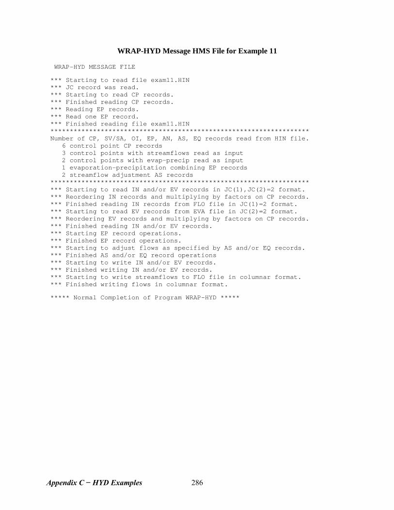
WRAP-HYD Message HMS File for Example 11 WRAP-HYD MESSAGE FILE *** Starting to read file exam11.HIN *** JC record was read. *** Starting to read CP records. *** Finished reading CP records. *** Reading EP records. *** Read one EP record. *** Finished reading file exam11.HIN ******************************************************************* Number of CP, SV/SA, OI, EP, AN, AS, EQ records read from HIN file. 6 control point CP records 3 control points with streamflows read as input 2 control points with evap-precip read as input 1 evaporation-precipitation combining EP records 2 streamflow adjustment AS records ******************************************************************* *** Starting to read IN and/or EV records in JC(1),JC(2)=2 format. *** Reordering IN records and multiplying by factors on CP records. *** Finished reading IN records from FLO file in JC(1)=2 format. *** Starting to read EV records from EVA file in JC(2)=2 format. *** Reordering EV records and multiplying by factors on CP records. *** Finished reading IN and/or EV records. *** Starting EP record operations. *** Finished EP record operations. *** Starting to adjust flows as specified by AS and/or EQ records. *** Finished AS and/or EQ record operations *** Starting to write IN and/or EV records. *** Finished writing IN and/or EV records. *** Starting to write streamflows to FLO file in columnar format. *** Finished writing flows in columnar format. ***** Normal Completion of Program WRAP-HYD *****
Appendix C − HYD Examples 286
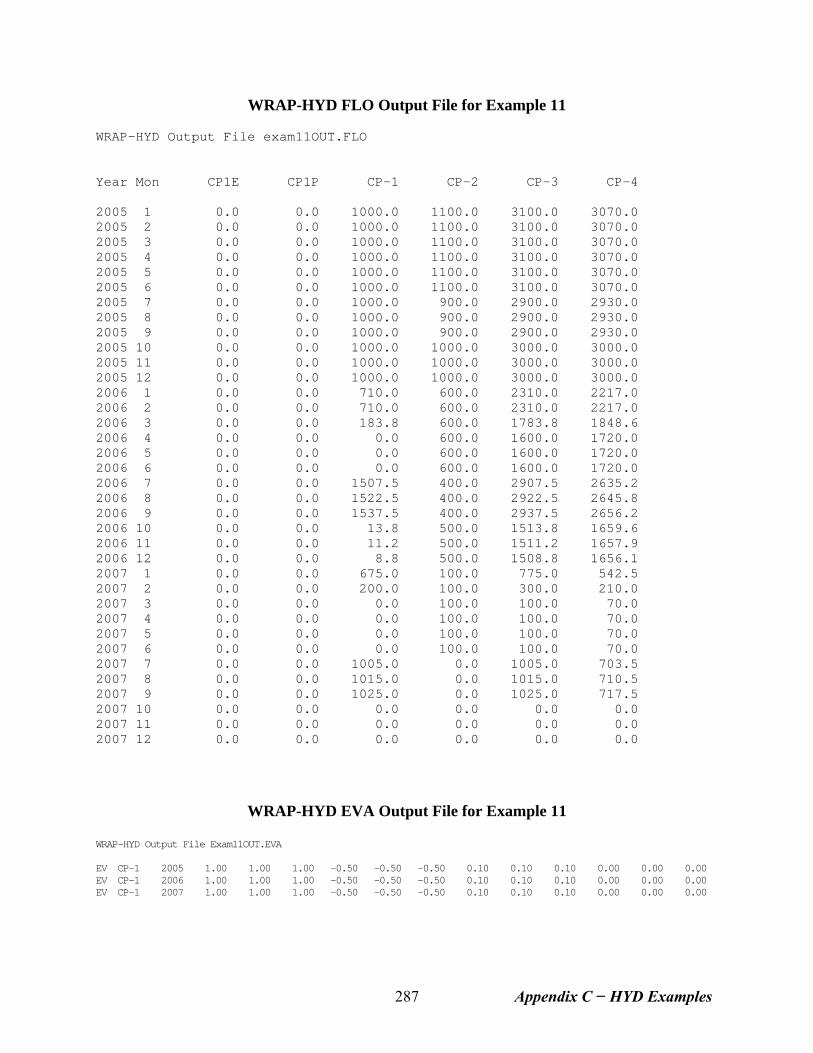
WRAP-HYD FLO Output File for Example 11 WRAP-HYD Output File exam11OUT.FLO Year Mon CP1E CP1P CP-1 CP-2 CP-3 CP-4 2005 1 0.0 0.0 1000.0 1100.0 3100.0 3070.0 2005 2 0.0 0.0 1000.0 1100.0 3100.0 3070.0 2005 3 0.0 0.0 1000.0 1100.0 3100.0 3070.0 2005 4 0.0 0.0 1000.0 1100.0 3100.0 3070.0 2005 5 0.0 0.0 1000.0 1100.0 3100.0 3070.0 2005 6 0.0 0.0 1000.0 1100.0 3100.0 3070.0 2005 7 0.0 0.0 1000.0 900.0 2900.0 2930.0 2005 8 0.0 0.0 1000.0 900.0 2900.0 2930.0 2005 9 0.0 0.0 1000.0 900.0 2900.0 2930.0 2005 10 0.0 0.0 1000.0 1000.0 3000.0 3000.0 2005 11 0.0 0.0 1000.0 1000.0 3000.0 3000.0 2005 12 0.0 0.0 1000.0 1000.0 3000.0 3000.0 2006 1 0.0 0.0 710.0 600.0 2310.0 2217.0 2006 2 0.0 0.0 710.0 600.0 2310.0 2217.0 2006 3 0.0 0.0 183.8 600.0 1783.8 1848.6 2006 4 0.0 0.0 0.0 600.0 1600.0 1720.0 2006 5 0.0 0.0 0.0 600.0 1600.0 1720.0 2006 6 0.0 0.0 0.0 600.0 1600.0 1720.0 2006 7 0.0 0.0 1507.5 400.0 2907.5 2635.2 2006 8 0.0 0.0 1522.5 400.0 2922.5 2645.8 2006 9 0.0 0.0 1537.5 400.0 2937.5 2656.2 2006 10 0.0 0.0 13.8 500.0 1513.8 1659.6 2006 11 0.0 0.0 11.2 500.0 1511.2 1657.9 2006 12 0.0 0.0 8.8 500.0 1508.8 1656.1 2007 1 0.0 0.0 675.0 100.0 775.0 542.5 2007 2 0.0 0.0 200.0 100.0 300.0 210.0 2007 3 0.0 0.0 0.0 100.0 100.0 70.0 2007 4 0.0 0.0 0.0 100.0 100.0 70.0 2007 5 0.0 0.0 0.0 100.0 100.0 70.0 2007 6 0.0 0.0 0.0 100.0 100.0 70.0 2007 7 0.0 0.0 1005.0 0.0 1005.0 703.5 2007 8 0.0 0.0 1015.0 0.0 1015.0 710.5 2007 9 0.0 0.0 1025.0 0.0 1025.0 717.5 2007 10 0.0 0.0 0.0 0.0 0.0 0.0 2007 11 0.0 0.0 0.0 0.0 0.0 0.0 2007 12 0.0 0.0 0.0 0.0 0.0 0.0
WRAP-HYD EVA Output File for Example 11
WRAP-HYD Output File Exam11OUT.EVA EV CP-1 2005 1.00 1.00 1.00 -0.50 -0.50 -0.50 0.10 0.10 0.10 0.00 0.00 0.00 EV CP-1 2006 1.00 1.00 1.00 -0.50 -0.50 -0.50 0.10 0.10 0.10 0.00 0.00 0.00 EV CP-1 2007 1.00 1.00 1.00 -0.50 -0.50 -0.50 0.10 0.10 0.10 0.00 0.00 0.00
Appendix C − HYD Examples 287
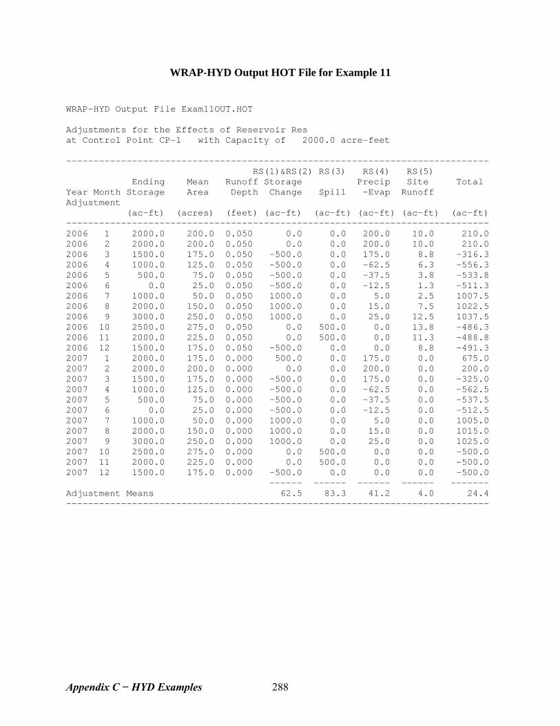
WRAP-HYD Output HOT File for Example 11 WRAP-HYD Output File Exam11OUT.HOT Adjustments for the Effects of Reservoir Res at Control Point CP-1 with Capacity of 2000.0 acre-feet ----------------------------------------------------------------------------- RS(1)&RS(2) RS(3) RS(4) RS(5) Ending Mean Runoff Storage Precip Site Total Year Month Storage Area Depth Change Spill -Evap Runoff Adjustment (ac-ft) (acres) (feet) (ac-ft) (ac-ft) (ac-ft) (ac-ft) (ac-ft) ----------------------------------------------------------------------------- 2006 1 2000.0 200.0 0.050 0.0 0.0 200.0 10.0 210.0 2006 2 2000.0 200.0 0.050 0.0 0.0 200.0 10.0 210.0 2006 3 1500.0 175.0 0.050 -500.0 0.0 175.0 8.8 -316.3 2006 4 1000.0 125.0 0.050 -500.0 0.0 -62.5 6.3 -556.3 2006 5 500.0 75.0 0.050 -500.0 0.0 -37.5 3.8 -533.8 2006 6 0.0 25.0 0.050 -500.0 0.0 -12.5 1.3 -511.3 2006 7 1000.0 50.0 0.050 1000.0 0.0 5.0 2.5 1007.5 2006 8 2000.0 150.0 0.050 1000.0 0.0 15.0 7.5 1022.5 2006 9 3000.0 250.0 0.050 1000.0 0.0 25.0 12.5 1037.5 2006 10 2500.0 275.0 0.050 0.0 500.0 0.0 13.8 -486.3 2006 11 2000.0 225.0 0.050 0.0 500.0 0.0 11.3 -488.8 2006 12 1500.0 175.0 0.050 -500.0 0.0 0.0 8.8 -491.3 2007 1 2000.0 175.0 0.000 500.0 0.0 175.0 0.0 675.0 2007 2 2000.0 200.0 0.000 0.0 0.0 200.0 0.0 200.0 2007 3 1500.0 175.0 0.000 -500.0 0.0 175.0 0.0 -325.0 2007 4 1000.0 125.0 0.000 -500.0 0.0 -62.5 0.0 -562.5 2007 5 500.0 75.0 0.000 -500.0 0.0 -37.5 0.0 -537.5 2007 6 0.0 25.0 0.000 -500.0 0.0 -12.5 0.0 -512.5 2007 7 1000.0 50.0 0.000 1000.0 0.0 5.0 0.0 1005.0 2007 8 2000.0 150.0 0.000 1000.0 0.0 15.0 0.0 1015.0 2007 9 3000.0 250.0 0.000 1000.0 0.0 25.0 0.0 1025.0 2007 10 2500.0 275.0 0.000 0.0 500.0 0.0 0.0 -500.0 2007 11 2000.0 225.0 0.000 0.0 500.0 0.0 0.0 -500.0 2007 12 1500.0 175.0 0.000 -500.0 0.0 0.0 0.0 -500.0 ------ ------ ------ ------ ------- Adjustment Means 62.5 83.3 41.2 4.0 24.4 -----------------------------------------------------------------------------
Appendix C − HYD Examples 288
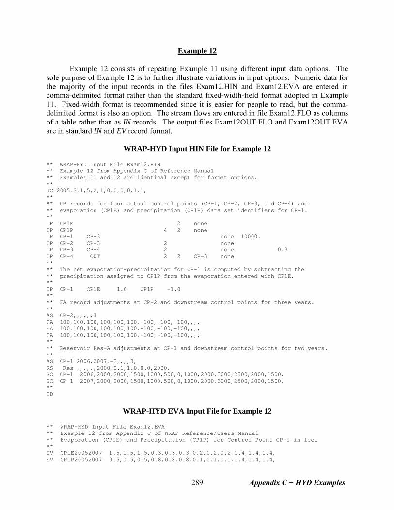
Example 12 Example 12 consists of repeating Example 11 using different input data options. The sole purpose of Example 12 is to further illustrate variations in input options. Numeric data for the majority of the input records in the files Exam12.HIN and Exam12.EVA are entered in comma-delimited format rather than the standard fixed-width-field format adopted in Example 11. Fixed-width format is recommended since it is easier for people to read, but the comma-delimited format is also an option. The stream flows are entered in file Exam12.FLO as columns of a table rather than as IN records. The output files Exam12OUT.FLO and Exam12OUT.EVA are in standard IN and EV record format.
WRAP-HYD Input HIN File for Example 12 ** WRAP-HYD Input File Exam12.HIN ** Example 12 from Appendix C of Reference Manual ** Examples 11 and 12 are identical except for format options. ** JC 2005,3,1,5,2,1,0,0,0,0,1,1, ** ** CP records for four actual control points (CP-1, CP-2, CP-3, and CP-4) and ** evaporation (CP1E) and precipitation (CP1P) data set identifiers for CP-1. ** CP CP1E 2 none CP CP1P 4 2 none CP CP-1 CP-3 none 10000. CP CP-2 CP-3 2 none CP CP-3 CP-4 2 none 0.3 CP CP-4 OUT 2 2 CP-3 none ** ** The net evaporation-precipitation for CP-1 is computed by subtracting the ** precipitation assigned to CP1P from the evaporation entered with CP1E. ** EP CP-1 CP1E 1.0 CP1P -1.0 ** ** FA record adjustments at CP-2 and downstream control points for three years. ** AS CP-2,,,,,,3 FA 100,100,100,100,100,100,-100,-100,-100,,,, FA 100,100,100,100,100,100,-100,-100,-100,,,, FA 100,100,100,100,100,100,-100,-100,-100,,,, ** ** Reservoir Res-A adjustments at CP-1 and downstream control points for two years. ** AS CP-1 2006,2007,-2,,,,3, RS Res ,,,,,,2000,0.1,1.0,0.0,2000, SC CP-1 2006,2000,2000,1500,1000,500,0,1000,2000,3000,2500,2000,1500, SC CP-1 2007,2000,2000,1500,1000,500,0,1000,2000,3000,2500,2000,1500, ** ED
WRAP-HYD EVA Input File for Example 12
** WRAP-HYD Input File Exam12.EVA ** Example 12 from Appendix C of WRAP Reference/Users Manual ** Evaporation (CP1E) and Precipitation (CP1P) for Control Point CP-1 in feet ** EV CP1E20052007 1.5,1.5,1.5,0.3,0.3,0.3,0.2,0.2,0.2,1.4,1.4,1.4, EV CP1P20052007 0.5,0.5,0.5,0.8,0.8,0.8,0.1,0.1,0.1,1.4,1.4,1.4,
Appendix C − HYD Examples 289
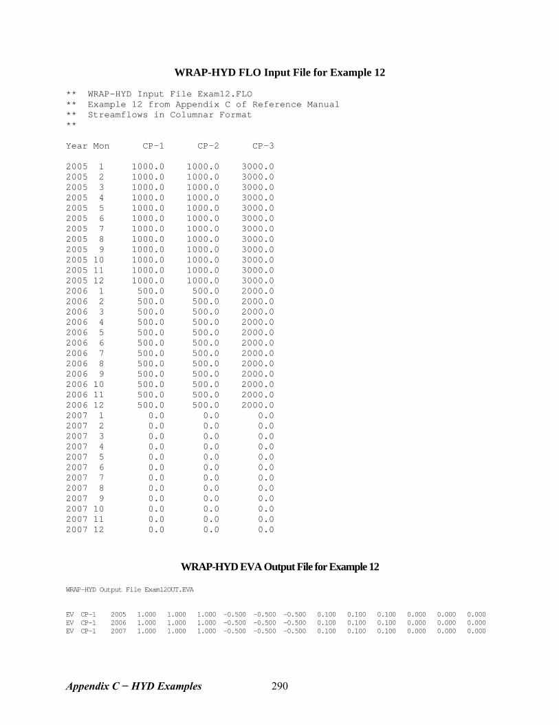
WRAP-HYD FLO Input File for Example 12 ** WRAP-HYD Input File Exam12.FLO ** Example 12 from Appendix C of Reference Manual ** Streamflows in Columnar Format ** Year Mon CP-1 CP-2 CP-3 2005 1 1000.0 1000.0 3000.0 2005 2 1000.0 1000.0 3000.0 2005 3 1000.0 1000.0 3000.0 2005 4 1000.0 1000.0 3000.0 2005 5 1000.0 1000.0 3000.0 2005 6 1000.0 1000.0 3000.0 2005 7 1000.0 1000.0 3000.0 2005 8 1000.0 1000.0 3000.0 2005 9 1000.0 1000.0 3000.0 2005 10 1000.0 1000.0 3000.0 2005 11 1000.0 1000.0 3000.0 2005 12 1000.0 1000.0 3000.0 2006 1 500.0 500.0 2000.0 2006 2 500.0 500.0 2000.0 2006 3 500.0 500.0 2000.0 2006 4 500.0 500.0 2000.0 2006 5 500.0 500.0 2000.0 2006 6 500.0 500.0 2000.0 2006 7 500.0 500.0 2000.0 2006 8 500.0 500.0 2000.0 2006 9 500.0 500.0 2000.0 2006 10 500.0 500.0 2000.0 2006 11 500.0 500.0 2000.0 2006 12 500.0 500.0 2000.0 2007 1 0.0 0.0 0.0 2007 2 0.0 0.0 0.0 2007 3 0.0 0.0 0.0 2007 4 0.0 0.0 0.0 2007 5 0.0 0.0 0.0 2007 6 0.0 0.0 0.0 2007 7 0.0 0.0 0.0 2007 8 0.0 0.0 0.0 2007 9 0.0 0.0 0.0 2007 10 0.0 0.0 0.0 2007 11 0.0 0.0 0.0 2007 12 0.0 0.0 0.0
WRAP-HYD EVA Output File for Example 12 WRAP-HYD Output File Exam12OUT.EVA EV CP-1 2005 1.000 1.000 1.000 -0.500 -0.500 -0.500 0.100 0.100 0.100 0.000 0.000 0.000 EV CP-1 2006 1.000 1.000 1.000 -0.500 -0.500 -0.500 0.100 0.100 0.100 0.000 0.000 0.000 EV CP-1 2007 1.000 1.000 1.000 -0.500 -0.500 -0.500 0.100 0.100 0.100 0.000 0.000 0.000
Appendix C − HYD Examples 290
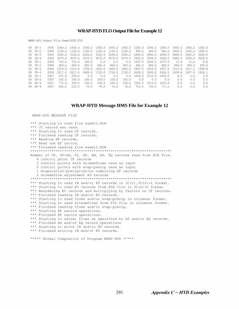
WRAP-HYD FLO Output File for Example 12 WRAP-HYD Output File Exam12OUT.FLO IN CP-1 2005 1000.0 1000.0 1000.0 1000.0 1000.0 1000.0 1000.0 1000.0 1000.0 1000.0 1000.0 1000.0 IN CP-2 2005 1100.0 1100.0 1100.0 1100.0 1100.0 1100.0 900.0 900.0 900.0 1000.0 1000.0 1000.0 IN CP-3 2005 3100.0 3100.0 3100.0 3100.0 3100.0 3100.0 2900.0 2900.0 2900.0 3000.0 3000.0 3000.0 IN CP-4 2005 3070.0 3070.0 3070.0 3070.0 3070.0 3070.0 2930.0 2930.0 2930.0 3000.0 3000.0 3000.0 IN CP-1 2006 710.0 710.0 183.8 0.0 0.0 0.0 1507.5 1522.5 1537.5 13.8 11.2 8.8 IN CP-2 2006 600.0 600.0 600.0 600.0 600.0 600.0 400.0 400.0 400.0 500.0 500.0 500.0 IN CP-3 2006 2310.0 2310.0 1783.8 1600.0 1600.0 1600.0 2907.5 2922.5 2937.5 1513.8 1511.2 1508.8 IN CP-4 2006 2217.0 2217.0 1848.6 1720.0 1720.0 1720.0 2635.2 2645.8 2656.2 1659.6 1657.9 1656.1 IN CP-1 2007 675.0 200.0 0.0 0.0 0.0 0.0 1005.0 1015.0 1025.0 0.0 0.0 0.0 IN CP-2 2007 100.0 100.0 100.0 100.0 100.0 100.0 0.0 0.0 0.0 0.0 0.0 0.0 IN CP-3 2007 775.0 300.0 100.0 100.0 100.0 100.0 1005.0 1015.0 1025.0 0.0 0.0 0.0 IN CP-4 2007 542.5 210.0 70.0 70.0 70.0 70.0 703.5 710.5 717.5 0.0 0.0 0.0
WRAP-HYD Message HMS File for Example 12 WRAP-HYD MESSAGE FILE *** Starting to read file exam12.HIN *** JC record was read. *** Starting to read CP records. *** Finished reading CP records. *** Reading EP records. *** Read one EP record. *** Finished reading file exam12.HIN ******************************************************************* Number of CP, SV/SA, OI, EP, AN, AS, EQ records read from HIN file. 6 control point CP records 3 control points with streamflows read as input 2 control points with evap-precip read as input 1 evaporation-precipitation combining EP records 2 streamflow adjustment AS records ******************************************************************* *** Starting to read IN and/or EV records in JC(1),JC(2)=2 format. *** Starting to read EV records from EVA file in JC(2)=2 format. *** Reordering EV records and multiplying by factors on CP records. *** Finished reading IN and/or EV records. *** Starting to read flows and/or evap-precip in columnar format. *** Starting to read streamflows from FLO file in columnar format. *** Finished reading flows and/or evap-precip. *** Starting EP record operations. *** Finished EP record operations. *** Starting to adjust flows as specified by AS and/or EQ records. *** Finished AS and/or EQ record operations *** Starting to write IN and/or EV records. *** Finished writing IN and/or EV records. ***** Normal Completion of Program WRAP-HYD *****
Appendix C − HYD Examples 291
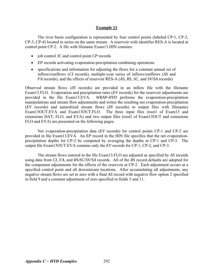
Example 13 The river basin configuration is represented by four control points (labeled CP-1, CP-2, CP-3, CP-4) located in series on the same stream. A reservoir with identifier RES-A is located at control point CP-2. A file with filename Exam13.HIN contains:
• job control JC and control point CP records
• EP records activating evaporation-precipitation combining operations
• specifications and information for adjusting the flows for a constant annual set of inflows/outflows (CI records), multiple-year series of inflows/outflows (AS and FA records), and the effects of reservoir RES-A (AS, RS, SC, and SV/SA records)
Observed stream flows (IN records) are provided in an inflow file with the filename Exam13.FLO. Evaporation and precipitation rates (EV records) for the reservoir adjustments are provided in the file Exam13.EVA. WRAP-HYD performs the evaporation-precipitation manipulations and stream flow adjustments and writes the resulting net evaporation-precipitation (EV records) and naturalized stream flows (IN records) to output files with filenames Exam13OUT.EVA and Exam13OUT.FLO. The three input files (root1 of Exam13 and extensions DAT, FLO, and EVA) and two output files (root2 of Exam13OUT and extensions FLO and EVA) are presented on the following pages.
Net evaporation-precipitation data (EV records) for control points CP-1 and CP-2 are provided in file Exam13.EVA. An EP record in the HIN file specifies that the net evaporation-precipitation depths for CP-2 be computed by averaging the depths at CP-1 and CP-3. The output file Exam13OUT.EVA contains only the EV records for CP-1, CP-2, and CP-3. The stream flows entered in the file Exam13.FLO are adjusted as specified by AS records using data from CI, FA, and RS/SC/SV/SA records. All of the RS record defaults are adopted for the component adjustments for the effects of the reservoir at CP-2. Each adjustment occurs at a specified control point and all downstream locations. After accumulating all adjustments, any negative stream flows are set to zero with a final AS record with negative flow option 2 specified in field 9 and a constant adjustment of zero specified in fields 5 and 11.
Appendix C − HYD Examples 292
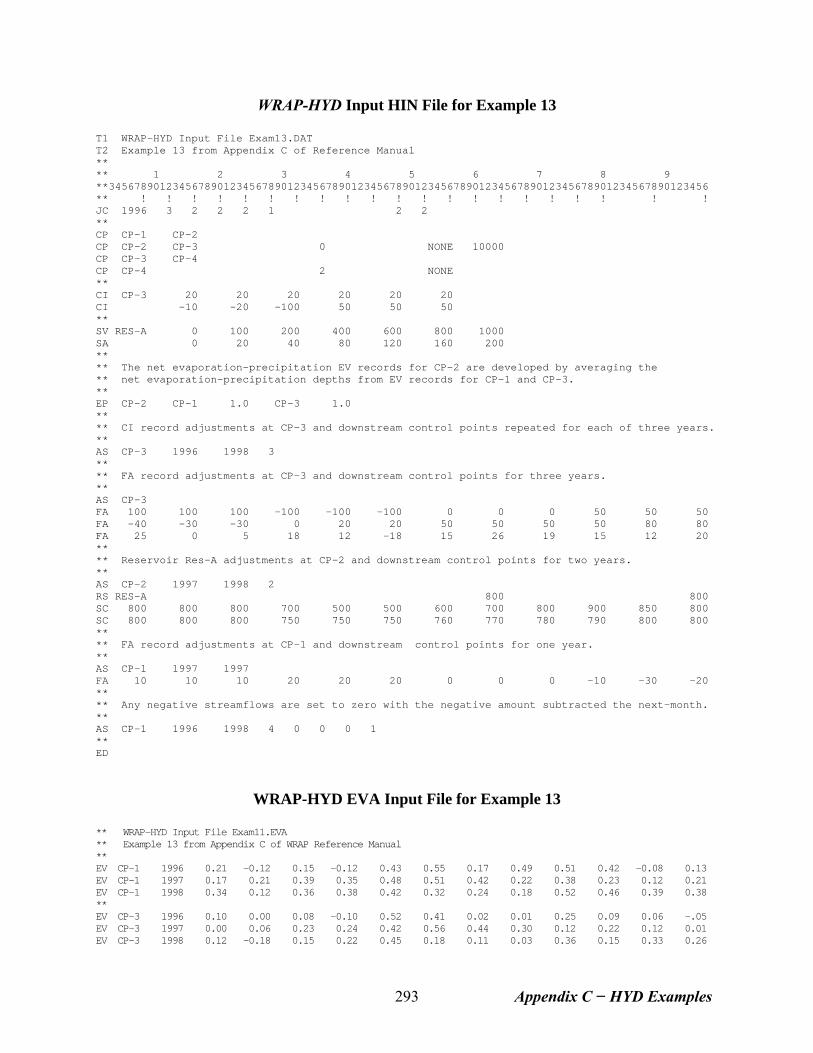
WRAP-HYD Input HIN File for Example 13 T1 WRAP-HYD Input File Exam13.DAT T2 Example 13 from Appendix C of Reference Manual ** ** 1 2 3 4 5 6 7 8 9 **3456789012345678901234567890123456789012345678901234567890123456789012345678901234567890123456 ** ! ! ! ! ! ! ! ! ! ! ! ! ! ! ! ! ! ! ! ! ! JC 1996 3 2 2 2 1 2 2 ** CP CP-1 CP-2 CP CP-2 CP-3 0 NONE 10000 CP CP-3 CP-4 CP CP-4 2 NONE ** CI CP-3 20 20 20 20 20 20 CI -10 -20 -100 50 50 50 ** SV RES-A 0 100 200 400 600 800 1000 SA 0 20 40 80 120 160 200 ** ** The net evaporation-precipitation EV records for CP-2 are developed by averaging the ** net evaporation-precipitation depths from EV records for CP-1 and CP-3. ** EP CP-2 CP-1 1.0 CP-3 1.0 ** ** CI record adjustments at CP-3 and downstream control points repeated for each of three years. ** AS CP-3 1996 1998 3 ** ** FA record adjustments at CP-3 and downstream control points for three years. ** AS CP-3 FA 100 100 100 -100 -100 -100 0 0 0 50 50 50 FA -40 -30 -30 0 20 20 50 50 50 50 80 80 FA 25 0 5 18 12 -18 15 26 19 15 12 20 ** ** Reservoir Res-A adjustments at CP-2 and downstream control points for two years. ** AS CP-2 1997 1998 2 RS RES-A 800 800 SC 800 800 800 700 500 500 600 700 800 900 850 800 SC 800 800 800 750 750 750 760 770 780 790 800 800 ** ** FA record adjustments at CP-1 and downstream control points for one year. ** AS CP-1 1997 1997 FA 10 10 10 20 20 20 0 0 0 -10 -30 -20 ** ** Any negative streamflows are set to zero with the negative amount subtracted the next-month. ** AS CP-1 1996 1998 4 0 0 0 1 ** ED
WRAP-HYD EVA Input File for Example 13
** WRAP-HYD Input File Exam11.EVA ** Example 13 from Appendix C of WRAP Reference Manual ** EV CP-1 1996 0.21 -0.12 0.15 -0.12 0.43 0.55 0.17 0.49 0.51 0.42 -0.08 0.13 EV CP-1 1997 0.17 0.21 0.39 0.35 0.48 0.51 0.42 0.22 0.38 0.23 0.12 0.21 EV CP-1 1998 0.34 0.12 0.36 0.38 0.42 0.32 0.24 0.18 0.52 0.46 0.39 0.38 ** EV CP-3 1996 0.10 0.00 0.08 -0.10 0.52 0.41 0.02 0.01 0.25 0.09 0.06 -.05 EV CP-3 1997 0.00 0.06 0.23 0.24 0.42 0.56 0.44 0.30 0.12 0.22 0.12 0.01 EV CP-3 1998 0.12 -0.18 0.15 0.22 0.45 0.18 0.11 0.03 0.36 0.15 0.33 0.26
Appendix C − HYD Examples 293
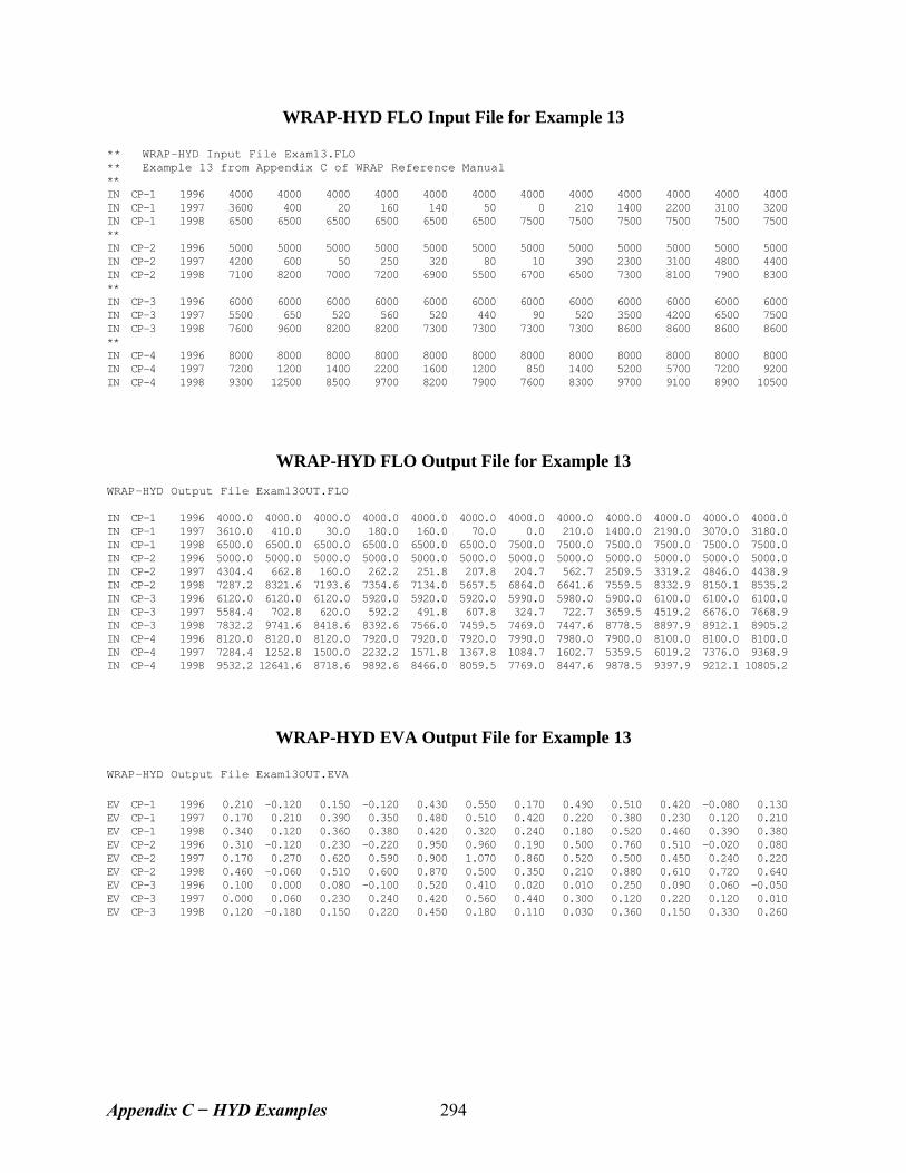
WRAP-HYD FLO Input File for Example 13 ** WRAP-HYD Input File Exam13.FLO ** Example 13 from Appendix C of WRAP Reference Manual ** IN CP-1 1996 4000 4000 4000 4000 4000 4000 4000 4000 4000 4000 4000 4000 IN CP-1 1997 3600 400 20 160 140 50 0 210 1400 2200 3100 3200 IN CP-1 1998 6500 6500 6500 6500 6500 6500 7500 7500 7500 7500 7500 7500 ** IN CP-2 1996 5000 5000 5000 5000 5000 5000 5000 5000 5000 5000 5000 5000 IN CP-2 1997 4200 600 50 250 320 80 10 390 2300 3100 4800 4400 IN CP-2 1998 7100 8200 7000 7200 6900 5500 6700 6500 7300 8100 7900 8300 ** IN CP-3 1996 6000 6000 6000 6000 6000 6000 6000 6000 6000 6000 6000 6000 IN CP-3 1997 5500 650 520 560 520 440 90 520 3500 4200 6500 7500 IN CP-3 1998 7600 9600 8200 8200 7300 7300 7300 7300 8600 8600 8600 8600 ** IN CP-4 1996 8000 8000 8000 8000 8000 8000 8000 8000 8000 8000 8000 8000 IN CP-4 1997 7200 1200 1400 2200 1600 1200 850 1400 5200 5700 7200 9200 IN CP-4 1998 9300 12500 8500 9700 8200 7900 7600 8300 9700 9100 8900 10500
WRAP-HYD FLO Output File for Example 13 WRAP-HYD Output File Exam13OUT.FLO IN CP-1 1996 4000.0 4000.0 4000.0 4000.0 4000.0 4000.0 4000.0 4000.0 4000.0 4000.0 4000.0 4000.0 IN CP-1 1997 3610.0 410.0 30.0 180.0 160.0 70.0 0.0 210.0 1400.0 2190.0 3070.0 3180.0 IN CP-1 1998 6500.0 6500.0 6500.0 6500.0 6500.0 6500.0 7500.0 7500.0 7500.0 7500.0 7500.0 7500.0 IN CP-2 1996 5000.0 5000.0 5000.0 5000.0 5000.0 5000.0 5000.0 5000.0 5000.0 5000.0 5000.0 5000.0 IN CP-2 1997 4304.4 662.8 160.0 262.2 251.8 207.8 204.7 562.7 2509.5 3319.2 4846.0 4438.9 IN CP-2 1998 7287.2 8321.6 7193.6 7354.6 7134.0 5657.5 6864.0 6641.6 7559.5 8332.9 8150.1 8535.2 IN CP-3 1996 6120.0 6120.0 6120.0 5920.0 5920.0 5920.0 5990.0 5980.0 5900.0 6100.0 6100.0 6100.0 IN CP-3 1997 5584.4 702.8 620.0 592.2 491.8 607.8 324.7 722.7 3659.5 4519.2 6676.0 7668.9 IN CP-3 1998 7832.2 9741.6 8418.6 8392.6 7566.0 7459.5 7469.0 7447.6 8778.5 8897.9 8912.1 8905.2 IN CP-4 1996 8120.0 8120.0 8120.0 7920.0 7920.0 7920.0 7990.0 7980.0 7900.0 8100.0 8100.0 8100.0 IN CP-4 1997 7284.4 1252.8 1500.0 2232.2 1571.8 1367.8 1084.7 1602.7 5359.5 6019.2 7376.0 9368.9 IN CP-4 1998 9532.2 12641.6 8718.6 9892.6 8466.0 8059.5 7769.0 8447.6 9878.5 9397.9 9212.1 10805.2
WRAP-HYD EVA Output File for Example 13 WRAP-HYD Output File Exam13OUT.EVA EV CP-1 1996 0.210 -0.120 0.150 -0.120 0.430 0.550 0.170 0.490 0.510 0.420 -0.080 0.130 EV CP-1 1997 0.170 0.210 0.390 0.350 0.480 0.510 0.420 0.220 0.380 0.230 0.120 0.210 EV CP-1 1998 0.340 0.120 0.360 0.380 0.420 0.320 0.240 0.180 0.520 0.460 0.390 0.380 EV CP-2 1996 0.310 -0.120 0.230 -0.220 0.950 0.960 0.190 0.500 0.760 0.510 -0.020 0.080 EV CP-2 1997 0.170 0.270 0.620 0.590 0.900 1.070 0.860 0.520 0.500 0.450 0.240 0.220 EV CP-2 1998 0.460 -0.060 0.510 0.600 0.870 0.500 0.350 0.210 0.880 0.610 0.720 0.640 EV CP-3 1996 0.100 0.000 0.080 -0.100 0.520 0.410 0.020 0.010 0.250 0.090 0.060 -0.050 EV CP-3 1997 0.000 0.060 0.230 0.240 0.420 0.560 0.440 0.300 0.120 0.220 0.120 0.010 EV CP-3 1998 0.120 -0.180 0.150 0.220 0.450 0.180 0.110 0.030 0.360 0.150 0.330 0.260
Appendix C − HYD Examples 294
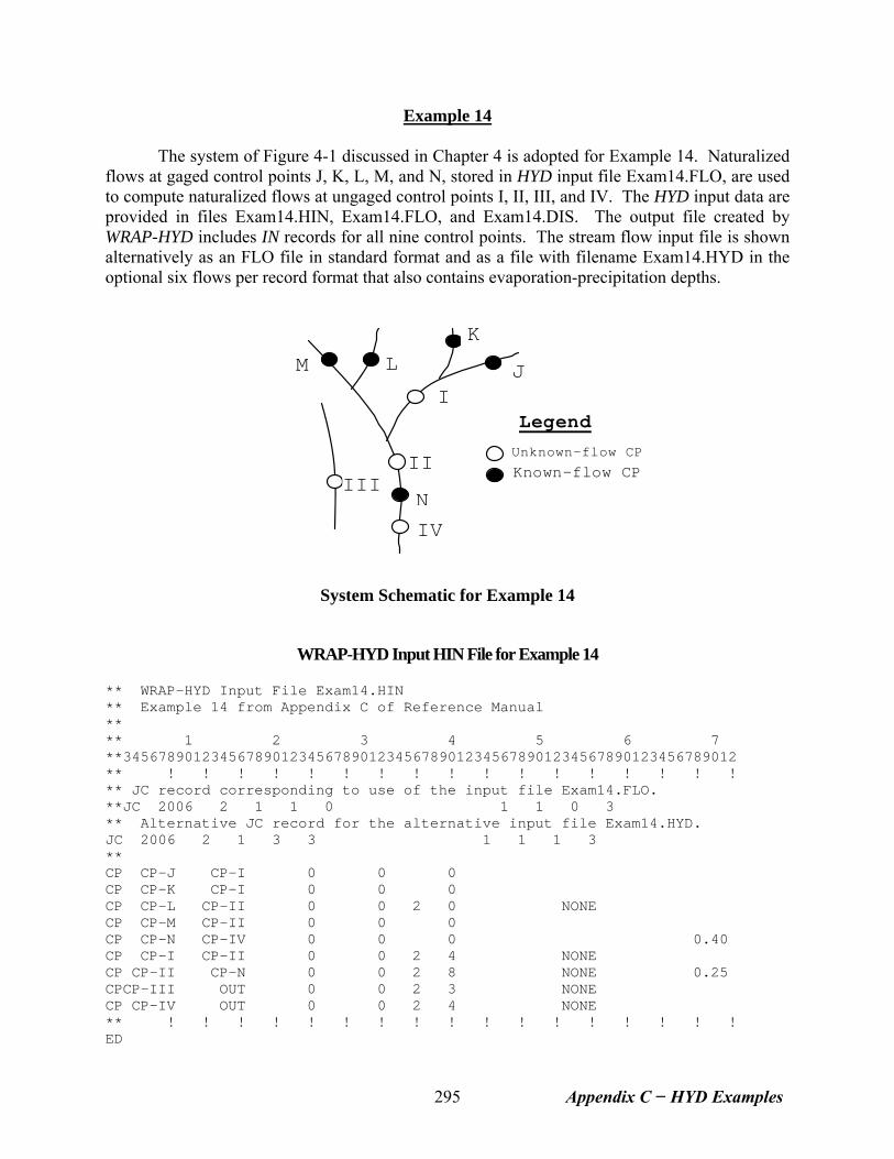
Example 14 The system of Figure 4-1 discussed in Chapter 4 is adopted for Example 14. Naturalized flows at gaged control points J, K, L, M, and N, stored in HYD input file Exam14.FLO, are used to compute naturalized flows at ungaged control points I, II, III, and IV. The HYD input data are provided in files Exam14.HIN, Exam14.FLO, and Exam14.DIS. The output file created by WRAP-HYD includes IN records for all nine control points. The stream flow input file is shown alternatively as an FLO file in standard format and as a file with filename Exam14.HYD in the optional six flows per record format that also contains evaporation-precipitation depths.
Legend
Unknown-flow CP
Known-flow CPIII
M LK
JI
II
NIV
System Schematic for Example 14
WRAP-HYD Input HIN File for Example 14 ** WRAP-HYD Input File Exam14.HIN ** Example 14 from Appendix C of Reference Manual ** ** 1 2 3 4 5 6 7 **3456789012345678901234567890123456789012345678901234567890123456789012 ** ! ! ! ! ! ! ! ! ! ! ! ! ! ! ! ! ! ** JC record corresponding to use of the input file Exam14.FLO. **JC 2006 2 1 1 0 1 1 0 3 ** Alternative JC record for the alternative input file Exam14.HYD. JC 2006 2 1 3 3 1 1 1 3 ** CP CP-J CP-I 0 0 0 CP CP-K CP-I 0 0 0 CP CP-L CP-II 0 0 2 0 NONE CP CP-M CP-II 0 0 0 CP CP-N CP-IV 0 0 0 0.40 CP CP-I CP-II 0 0 2 4 NONE CP CP-II CP-N 0 0 2 8 NONE 0.25 CPCP-III OUT 0 0 2 3 NONE CP CP-IV OUT 0 0 2 4 NONE ** ! ! ! ! ! ! ! ! ! ! ! ! ! ! ! ! ! ED
Appendix C − HYD Examples 295
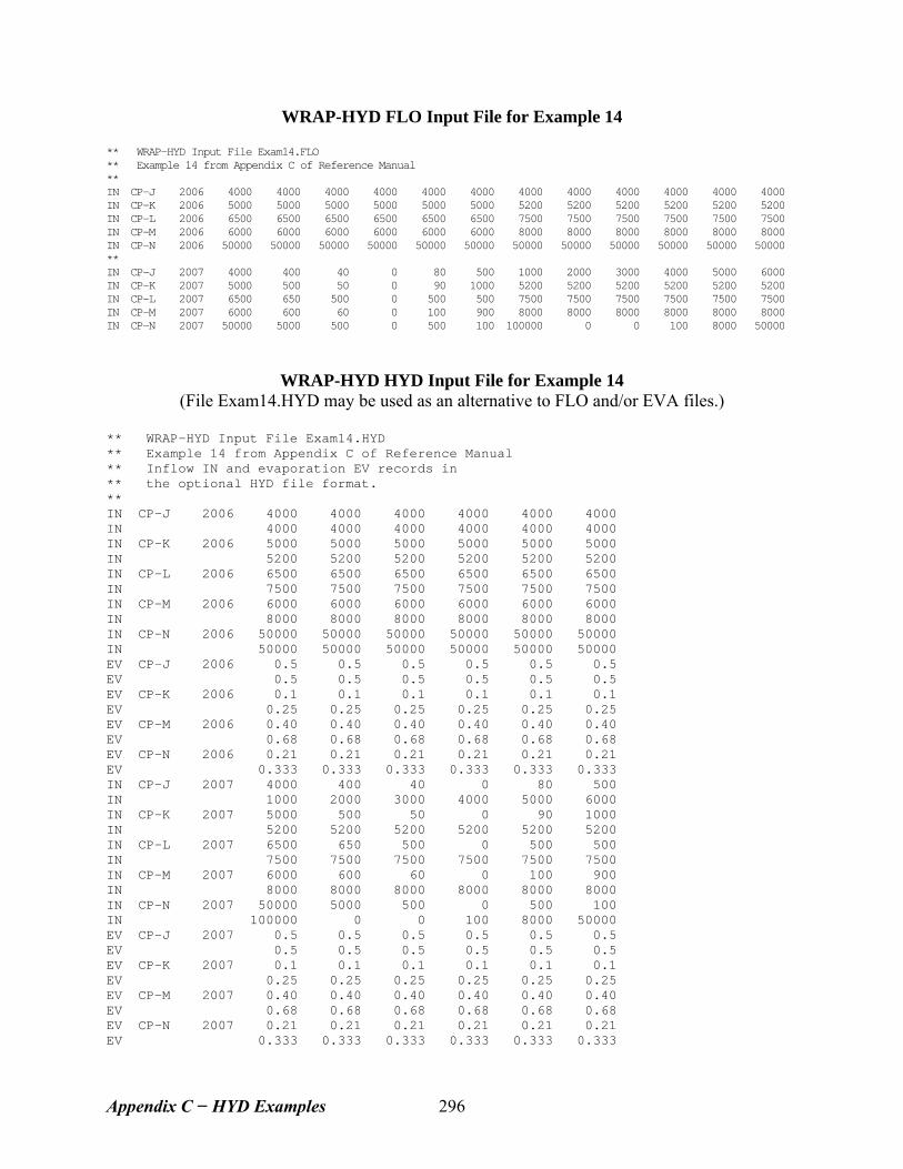
WRAP-HYD FLO Input File for Example 14
** WRAP-HYD Input File Exam14.FLO ** Example 14 from Appendix C of Reference Manual ** IN CP-J 2006 4000 4000 4000 4000 4000 4000 4000 4000 4000 4000 4000 4000 IN CP-K 2006 5000 5000 5000 5000 5000 5000 5200 5200 5200 5200 5200 5200 IN CP-L 2006 6500 6500 6500 6500 6500 6500 7500 7500 7500 7500 7500 7500 IN CP-M 2006 6000 6000 6000 6000 6000 6000 8000 8000 8000 8000 8000 8000 IN CP-N 2006 50000 50000 50000 50000 50000 50000 50000 50000 50000 50000 50000 50000 ** IN CP-J 2007 4000 400 40 0 80 500 1000 2000 3000 4000 5000 6000 IN CP-K 2007 5000 500 50 0 90 1000 5200 5200 5200 5200 5200 5200 IN CP-L 2007 6500 650 500 0 500 500 7500 7500 7500 7500 7500 7500 IN CP-M 2007 6000 600 60 0 100 900 8000 8000 8000 8000 8000 8000 IN CP-N 2007 50000 5000 500 0 500 100 100000 0 0 100 8000 50000
WRAP-HYD HYD Input File for Example 14 (File Exam14.HYD may be used as an alternative to FLO and/or EVA files.)
** WRAP-HYD Input File Exam14.HYD ** Example 14 from Appendix C of Reference Manual ** Inflow IN and evaporation EV records in ** the optional HYD file format. ** IN CP-J 2006 4000 4000 4000 4000 4000 4000 IN 4000 4000 4000 4000 4000 4000 IN CP-K 2006 5000 5000 5000 5000 5000 5000 IN 5200 5200 5200 5200 5200 5200 IN CP-L 2006 6500 6500 6500 6500 6500 6500 IN 7500 7500 7500 7500 7500 7500 IN CP-M 2006 6000 6000 6000 6000 6000 6000 IN 8000 8000 8000 8000 8000 8000 IN CP-N 2006 50000 50000 50000 50000 50000 50000 IN 50000 50000 50000 50000 50000 50000 EV CP-J 2006 0.5 0.5 0.5 0.5 0.5 0.5 EV 0.5 0.5 0.5 0.5 0.5 0.5 EV CP-K 2006 0.1 0.1 0.1 0.1 0.1 0.1 EV 0.25 0.25 0.25 0.25 0.25 0.25 EV CP-M 2006 0.40 0.40 0.40 0.40 0.40 0.40 EV 0.68 0.68 0.68 0.68 0.68 0.68 EV CP-N 2006 0.21 0.21 0.21 0.21 0.21 0.21 EV 0.333 0.333 0.333 0.333 0.333 0.333 IN CP-J 2007 4000 400 40 0 80 500 IN 1000 2000 3000 4000 5000 6000 IN CP-K 2007 5000 500 50 0 90 1000 IN 5200 5200 5200 5200 5200 5200 IN CP-L 2007 6500 650 500 0 500 500 IN 7500 7500 7500 7500 7500 7500 IN CP-M 2007 6000 600 60 0 100 900 IN 8000 8000 8000 8000 8000 8000 IN CP-N 2007 50000 5000 500 0 500 100 IN 100000 0 0 100 8000 50000 EV CP-J 2007 0.5 0.5 0.5 0.5 0.5 0.5 EV 0.5 0.5 0.5 0.5 0.5 0.5 EV CP-K 2007 0.1 0.1 0.1 0.1 0.1 0.1 EV 0.25 0.25 0.25 0.25 0.25 0.25 EV CP-M 2007 0.40 0.40 0.40 0.40 0.40 0.40 EV 0.68 0.68 0.68 0.68 0.68 0.68 EV CP-N 2007 0.21 0.21 0.21 0.21 0.21 0.21 EV 0.333 0.333 0.333 0.333 0.333 0.333
Appendix C − HYD Examples 296
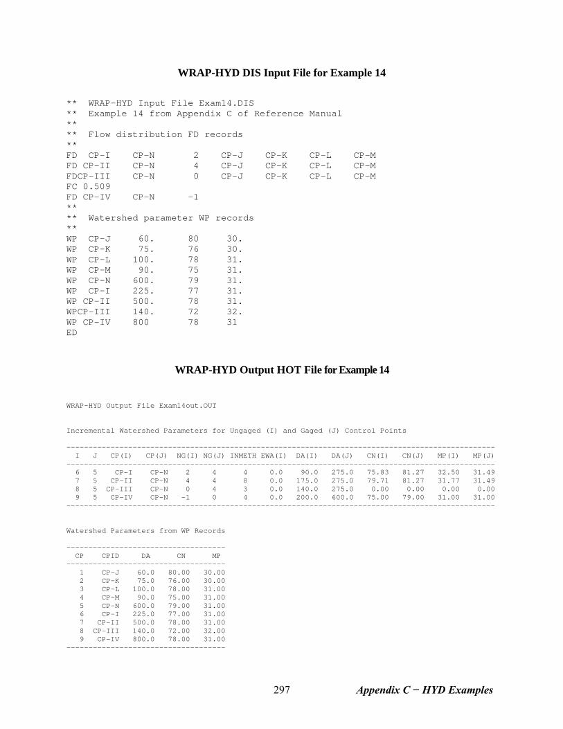
WRAP-HYD DIS Input File for Example 14
** WRAP-HYD Input File Exam14.DIS ** Example 14 from Appendix C of Reference Manual ** ** Flow distribution FD records ** FD CP-I CP-N 2 CP-J CP-K CP-L CP-M FD CP-II CP-N 4 CP-J CP-K CP-L CP-M FDCP-III CP-N 0 CP-J CP-K CP-L CP-M FC 0.509 FD CP-IV CP-N -1 ** ** Watershed parameter WP records ** WP CP-J 60. 80 30. WP CP-K 75. 76 30. WP CP-L 100. 78 31. WP CP-M 90. 75 31. WP CP-N 600. 79 31. WP CP-I 225. 77 31. WP CP-II 500. 78 31. WPCP-III 140. 72 32. WP CP-IV 800 78 31 ED
WRAP-HYD Output HOT File for Example 14 WRAP-HYD Output File Exam14out.OUT Incremental Watershed Parameters for Ungaged (I) and Gaged (J) Control Points ------------------------------------------------------------------------------------------------- I J CP(I) CP(J) NG(I) NG(J) INMETH EWA(I) DA(I) DA(J) CN(I) CN(J) MP(I) MP(J) ------------------------------------------------------------------------------------------------- 6 5 CP-I CP-N 2 4 4 0.0 90.0 275.0 75.83 81.27 32.50 31.49 7 5 CP-II CP-N 4 4 8 0.0 175.0 275.0 79.71 81.27 31.77 31.49 8 5 CP-III CP-N 0 4 3 0.0 140.0 275.0 0.00 0.00 0.00 0.00 9 5 CP-IV CP-N -1 0 4 0.0 200.0 600.0 75.00 79.00 31.00 31.00 ------------------------------------------------------------------------------------------------- Watershed Parameters from WP Records ------------------------------------ CP CPID DA CN MP ------------------------------------ 1 CP-J 60.0 80.00 30.00 2 CP-K 75.0 76.00 30.00 3 CP-L 100.0 78.00 31.00 4 CP-M 90.0 75.00 31.00 5 CP-N 600.0 79.00 31.00 6 CP-I 225.0 77.00 31.00 7 CP-II 500.0 78.00 31.00 8 CP-III 140.0 72.00 32.00 9 CP-IV 800.0 78.00 31.00 ------------------------------------
Appendix C − HYD Examples 297
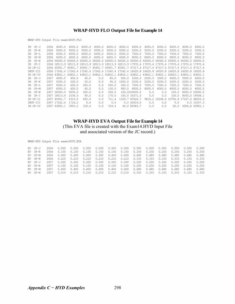
WRAP-HYD FLO Output File for Example 14
WRAP-HYD Output File exam14OUT.FLO IN CP-J 2006 4000.0 4000.0 4000.0 4000.0 4000.0 4000.0 4000.0 4000.0 4000.0 4000.0 4000.0 4000.0 IN CP-K 2006 5000.0 5000.0 5000.0 5000.0 5000.0 5000.0 5200.0 5200.0 5200.0 5200.0 5200.0 5200.0 IN CP-L 2006 6500.0 6500.0 6500.0 6500.0 6500.0 6500.0 7500.0 7500.0 7500.0 7500.0 7500.0 7500.0 IN CP-M 2006 6000.0 6000.0 6000.0 6000.0 6000.0 6000.0 8000.0 8000.0 8000.0 8000.0 8000.0 8000.0 IN CP-N 2006 50000.0 50000.0 50000.0 50000.0 50000.0 50000.0 50000.0 50000.0 50000.0 50000.0 50000.0 50000.0 IN CP-I 2006 18513.9 18513.9 18513.9 18513.9 18513.9 18513.9 17970.6 17970.6 17970.6 17970.6 17970.6 17970.6 IN CP-II 2006 45901.7 45901.7 45901.7 45901.7 45901.7 45901.7 47317.4 47317.4 47317.4 47317.4 47317.4 47317.4 INCP-III 2006 17242.4 17242.4 17242.4 17242.4 17242.4 17242.4 16020.8 16020.8 16020.8 16020.8 16020.8 16020.8 IN CP-IV 2006 43852.1 43852.1 43852.1 43852.1 43852.1 43852.1 43852.1 43852.1 43852.1 43852.1 43852.1 43852.1 IN CP-J 2007 4000.0 400.0 40.0 0.0 80.0 500.0 1000.0 2000.0 3000.0 4000.0 5000.0 6000.0 IN CP-K 2007 5000.0 500.0 50.0 0.0 90.0 1000.0 5200.0 5200.0 5200.0 5200.0 5200.0 5200.0 IN CP-L 2007 6500.0 650.0 500.0 0.0 500.0 500.0 7500.0 7500.0 7500.0 7500.0 7500.0 7500.0 IN CP-M 2007 6000.0 600.0 60.0 0.0 100.0 900.0 8000.0 8000.0 8000.0 8000.0 8000.0 8000.0 IN CP-N 2007 50000.0 5000.0 500.0 0.0 500.0 100.0100000.0 0.0 0.0 100.0 8000.0 50000.0 IN CP-I 2007 18513.9 1536.5 90.0 0.0 170.0 100.0 31671.0 0.0 0.0 100.0 8000.0 19508.1 IN CP-II 2007 45901.7 4319.0 650.0 0.0 711.4 1329.7 83526.7 9816.2 10248.6 10756.8 17167.6 48203.6 INCP-III 2007 17242.4 1724.2 6.4 0.0 0.0 0.0 42616.0 0.0 0.0 0.0 0.0 15257.3 IN CP-IV 2007 43852.1 3953.2 318.4 0.0 318.4 60.0 89383.7 0.0 0.0 60.0 6506.8 43852.1
WRAP-HYD EVA Output File for Example 14 (This EVA file is created with the Exam14.HYD Input File
and associated version of the JC record.) WRAP-HYD Output File exam14OUT.EVA EV CP-J 2006 0.500 0.500 0.500 0.500 0.500 0.500 0.500 0.500 0.500 0.500 0.500 0.500 EV CP-K 2006 0.100 0.100 0.100 0.100 0.100 0.100 0.250 0.250 0.250 0.250 0.250 0.250 EV CP-M 2006 0.400 0.400 0.400 0.400 0.400 0.400 0.680 0.680 0.680 0.680 0.680 0.680 EV CP-N 2006 0.210 0.210 0.210 0.210 0.210 0.210 0.333 0.333 0.333 0.333 0.333 0.333 EV CP-J 2007 0.500 0.500 0.500 0.500 0.500 0.500 0.500 0.500 0.500 0.500 0.500 0.500 EV CP-K 2007 0.100 0.100 0.100 0.100 0.100 0.100 0.250 0.250 0.250 0.250 0.250 0.250 EV CP-M 2007 0.400 0.400 0.400 0.400 0.400 0.400 0.680 0.680 0.680 0.680 0.680 0.680 EV CP-N 2007 0.210 0.210 0.210 0.210 0.210 0.210 0.333 0.333 0.333 0.333 0.333 0.333
Appendix C − HYD Examples 298
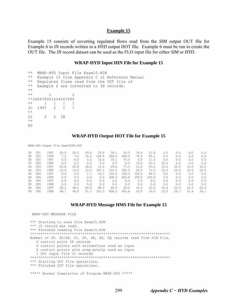
Example 15 Example 15 consists of coverting regulated flows read from the SIM output OUT file for Example 6 to IN records written to a HYD output HOT file. Example 6 must be run to create the OUT file. The IN record dataset can be used as the FLO input file for either SIM or HYD.
WRAP-HYD Input HIN File for Example 15 ** WRAP-HYD Input File Exam15.HIN ** Example 15 from Appendix C of Reference Manual ** Regulated flows read from the OUT file of ** Example 6 are converted to IN records. ** ** 1 2 **345678901234567890 ** ! ! ! ! JC 1997 2 1 7 ** OI 2 2 IN ** ED
WRAP-HYD Output HOT File for Example 15 WRAP-HYD Output File Exam15OUT.HOT IN CP1 1997 20.0 20.0 20.0 20.0 36.1 50.5 74.6 23.8 0.0 0.0 0.0 0.0 IN CP1 1998 7.2 7.2 14.4 128.5 260.0 260.0 74.6 65.2 0.0 0.0 0.0 0.0 IN CP2 1997 0.0 0.0 0.0 14.4 19.1 67.0 0.0 11.3 0.0 0.0 0.0 0.0 IN CP2 1998 0.0 0.0 0.0 0.0 0.0 0.0 16.6 62.4 52.4 0.0 0.0 0.0 IN CP3 1997 25.8 25.8 18.6 13.0 29.6 77.5 13.0 10.0 10.0 10.0 10.0 10.0 IN CP3 1998 12.9 13.0 13.0 187.1 314.4 300.0 29.6 73.3 10.0 10.0 10.0 10.0 IN CP4 1997 6.0 6.0 1.7 16.1 100.0 100.0 100.0 84.0 0.0 0.0 0.0 0.0 IN CP4 1998 0.0 0.0 0.0 0.0 408.3 403.8 100.0 100.0 0.0 0.0 0.0 0.0 IN CP5 1997 0.0 0.0 0.0 0.0 0.0 0.0 0.0 0.0 0.0 0.0 0.0 0.0 IN CP5 1998 0.0 0.0 0.0 0.0 0.0 0.0 0.0 0.0 0.0 0.0 0.0 0.0 IN CP6 1997 48.1 48.1 43.8 88.2 60.0 60.0 10.0 10.0 53.4 23.3 23.3 23.3 IN CP6 1998 48.7 48.8 51.7 323.3 608.3 603.8 10.0 10.0 10.0 29.7 31.6 34.1
WRAP-HYD Message HMS File for Example 15 WRAP-HYD MESSAGE FILE *** Starting to read file Exam15.HIN *** JC record was read. *** Finished reading file Exam15.HIN ******************************************************************* Number of CP, SV/SA, OI, EP, AN, AS, EQ records read from HIN file. 0 control point CP records 0 control points with streamflows read as input 0 control points with evap-precip read as input 1 OUT input file OI records ******************************************************************* *** Starting OUT file operations. *** Finished OUT file operations. ***** Normal Completion of Program WRAP-HYD *****
Appendix C − HYD Examples 299