ScholarWorks - Boise State University

Boise State UniversityScholarWorks

Mathematics Faculty Publications and Presentations Department of Mathematics

1-1-2013

x2 Tests for the Choice of the RegularizationParameter in Nonlinear Inverse ProblemsJ. L. MeadBoise State University

C. C. HammerquistBoise State University

First published in SIAM Journal on Matrix Analysis and Applications in Vol. 34(3) 2013, published by the Society of Industrial and Applied Mathematics(SIAM). Copyright © by SIAM. Unauthorized reproduction of this article is prohibited.

https://scholarworks.boisestate.edu

https://scholarworks.boisestate.edu/math_facpubs

https://scholarworks.boisestate.edu/math

Copyright © by SIAM. Unauthorized reproduction of this article is prohibited.

SIAM J. MATRIX ANAL. APPL. c© 2013 Society for Industrial and Applied MathematicsVol. 34, No. 3, pp. 1213–1230

χ2 TESTS FOR THE CHOICE OF THE REGULARIZATIONPARAMETER IN NONLINEAR INVERSE PROBLEMS∗

J. L. MEAD† AND C. C. HAMMERQUIST†

Abstract. We address discrete nonlinear inverse problems with weighted least squares andTikhonov regularization. Regularization is a way to add more information to the problem whenit is ill-posed or ill-conditioned. However, it is still an open question as to how to weight thisinformation. The discrepancy principle considers the residual norm to determine the regularizationweight or parameter, while the χ2 method [J. Mead, J. Inverse Ill-Posed Probl., 16 (2008), pp. 175–194; J. Mead and R. A. Renaut, Inverse Problems, 25 (2009), 025002; J. Mead, Appl. Math. Comput.,219 (2013), pp. 5210–5223; R. A. Renaut, I. Hnetynkova, and J. L. Mead, Comput. Statist. DataAnal., 54 (2010), pp. 3430–3445] uses the regularized residual. Using the regularized residual hasthe benefit of giving a clear χ2 test with a fixed noise level when the number of parameters is equalto or greater than the number of data. Previous work with the χ2 method has been for linearproblems, and here we extend it to nonlinear problems. In particular, we determine the appropriateχ2 tests for Gauss–Newton and Levenberg–Marquardt algorithms, and these tests are used to find aregularization parameter or weights on initial parameter estimate errors. This algorithm is applied toa two-dimensional cross-well tomography problem and a one-dimensional electromagnetic problemfrom [R. C. Aster, B. Borchers, and C. Thurber, Parameter Estimation and Inverse Problems,Academic Press, New York, 2005].

Key words. least squares, regularization, nonlinear, covariance

AMS subject classifications. 92E24, 65F22, 65H10, 62J02

DOI. 10.1137/12088447X

1. Introduction. We address nonlinear inverse problems of the form F(x) = d,where d ∈ R

m represents measurements and F ∈ Rm×n represents a nonlinear model

that depends on parameters x ∈ Rn. It is fairly straightforward, although possibly

computationally demanding, to recover parameter estimates x from data d for alinear operator F = A when A is well-conditioned. If A is ill-conditioned, typicallyconstraints or penalties are added to the problem, and the problem is regularized.The most common regularization technique is Tikhonov regularization, where leastsquares is used to minimize

||d−Ax||22 + α2||Lx||22.(1.1)

The minimum occurs at x̂,

x̂ = (ATA+ α2LTL)−1ATd,

if the invertibility condition

N (A) ∩ N (L) �= ∅is satisfied. When x̂ is written explicitly in this manner, it is clear how appropriatechoice of α creates a well-conditioned problem. Popular methods for choosing α are

∗Received by the editors July 13, 2012; accepted for publication (in revised form) by J. G. NagyMay 30, 2013; published electronically August 6, 2013. This work was supported by NSF grant DMS1043107.

http://www.siam.org/journals/simax/34-3/88447.html†Department of Mathematics, Boise State University, Boise, ID 83725-1555 (jmead@boisestate.

edu, [email protected]).

1213


1214 J. L. MEAD AND C. C. HAMMERQUIST

the discrepancy principle, L-curve, and generalized cross validation (GCV) [5], whileL can be chosen to be the identity matrix, or a discrete approximation to a derivativeoperator. The problem with this approach is that large values of α may significantlychange the problem or create undesired smooth solutions.

Nonlinear problems have the same issues but have the added burden of linearapproximations [10]. The parameter estimate of the regularized nonlinear problemminimizes

||d− F(x)||22 + α2||Lx||22.(1.2)

In [3] it is shown that this regularized problem is stable and that there is a weakconnection between the ill-posedness of the nonlinear problem and the linearization.The authors of [3] and [12] prove the well-posedness of the regularized problem andconvergence of regularized solutions.

The least squares estimate can be viewed as the maximum a posteriori (MAP)estimate [13] when the data and the initial parameter estimate xp have errors that arenormally distributed with error covariances Cε and Cf , respectively. Regularizationin this case takes the form of adding a priori information about the parameters. Theregularized maximum likelihood estimate minimizes the following objective function:

J = (d− F(x))TC−1ε (d− F(x)) + (x− xp)

TC−1f (x− xp).(1.3)

The difficulty with this viewpoint is that the distribution of the data and initial pa-rameter errors may be unknown, or not normal. In addition, good estimates of Cε

and Cf can be difficult to acquire. However, different norms or functionals can besampled which represent error distributions other than normal, and scientific knowl-edge can be used to form prior error covariance matrices. Empirical Bayes methods[2] can also be used to find hyperparameters, i.e., parameters which define the priordistribution.

In this work we use the least squares estimator and weight the squared errors withinverse covariances matrices but do not assume the errors are normally distributed.Matrix weights alleviate the problem of undesired smooth solutions because they givepiecewise smooth solutions; thus discontinuous parameters can be obtained. In pre-liminary work [7, 9] diagonal matrix weights Cf were found, and future work involvesmore robust methods for finding Cf . In this initial work on nonlinear problems, weapproximate the unknown error covariance matrix with a scalar times the identitymatrix, but future work involves finding more dense matrices. To find the scalar weuse the χ2 method, which is similar to the discrepancy principle.

The discrepancy principle can be viewed as a χ2 test on the data residual, but thisis not possible when the number of parameters is greater than or equal to the numberof data because the degrees of freedom in the χ2 test are zero or negative. Thisissue is typically not recognized because the degrees of freedom in the discrepancyprinciple are often taken to be m, the number of data, while they should be reducedby the number of parameters, i.e., reduced to m − n. The reduction is necessarybecause parameter estimates are found using the data, and hence their dependencyshould be subtracted from the degrees of freedom. This difference can be significantwhen the number of parameters is significantly different from the number of data.Alternatively we suggest applying the χ2 test to the regularized residual (1.1), inwhich case the degrees of freedom are equal to the number of data [1]. This is calledthe χ2 method, and previous work with the method applied to linear problems hasbeen done [7, 8, 9, 11].


NONLINEAR χ2 METHOD 1215

The χ2 method is described in section 2, where we also develop it for nonlinearproblems. In this work χ2 tests are developed for Gauss–Newton and Levenberg–Marquardt algorithms, rather than for the nonlinear functional, because we havefound that the statistical tests on the theoretical functional are not satisfied when theoptimum value is approximated. We will explain how iterations in these nonlinearalgorithms form a sequence of linear least squares problems and show how to apply theχ2 principle at each iterate. From these tests we determine a regularization parameter,and this can be viewed as an estimate of the error covariance matrices. In section 3 wegive results on benchmark problems from [1] and compare the nonlinear χ2 methodto other methods. In section 4 we give conclusions and future work.

2. Nonlinear χ2 method. We formulate the problem as minimizing weightederrors ε and f in a least squares sense where the errors are defined as

d = F(x) + ε,(2.1)

x = xp + f .(2.2)

The weighted least squares fit of the measurements d and initial parameter estimatexp is found by minimizing the objective function in (1.3). This means the weightsare chosen to be the inverse covariance matrices for the respective errors. Statisticalinformation comes in the form of error covariance matrices, but they are used onlyto weight the errors or residuals and are not used in the sense of Bayesian inferencebecause the errors may not be Gaussian.

An initial estimate xp is required for this method, but this often comes from someunderstanding of the problem. The goal is then to find a way to weight this initialestimate. The elements in Cf should reflect whether xp is a good or poor estimateand ideally quantify the correlation in the parameter errors. Estimation of Cf is thusa challenge with limited understanding of the parameters, but regularization methodsare an approach to its approximation. In this work we use a modified form of thediscrepancy principle, called the χ2 method [7], to estimate it.

It is well known that when the objective function (1.3) is applied to a linearmodel, it follows a χ2 distribution [1, 7], and this fact is often used to also check thevalidity of estimates. This property is given in the following theorem.

Theorem 1. If F(x) = Ax, d, and x are independent and identically distributed

random variables from unknown distributions with ε = f = 0, εεT = Cε, ffT = Cf ,

and εT f = 0, and the number of data m is large, then the minimum value of (1.3)asymptotically follows a χ2 distribution with m degrees of freedom.

A proof of this is given in [7]. In the case that xp is not the mean of x, then (1.3)

follows a noncentral χ2 distribution as shown in [11]. The requirement that εT f = 0assumes that the errors in d and xp are uncorrelated, and hence we do not get xp

from d.The χ2 method is used to find weights for misfits in the initial parameter esti-

mates, Cf , or data, Cε, and is based on the χ2 tests given in Theorem 1. The methodcan also be used to find weights for the regularization term when it contains a first orsecond derivative operator L. In this case the inverse covariance matrix is viewed asweighting the error in an initial estimate of the appropriate derivative. The minimumvalue of (1.3) is

J (x̂) = rT (ACfAT +Cε)

−1r

with r = d−Axp [7]. Its expected value is the number of degrees of freedom, whichis the number of measurements in d. The χ2 method thus estimates scalar weight Cf



or Cε by solving the nonlinear equation

rT (ACfAT +Cε)

−1r = m.(2.3)

For example, with d given by the data and xp an initial parameter estimate (possibly0), if we have estimates of data uncertainty Cε, we can solve for Cf (alternatively wecan solve for Cε given Cf ). This differs from the discrepancy principle in that theregularized residual is used for the χ2 test rather than just the data residual. Oneadvantage of this approach over the discrepancy principle is that it can be appliedwhen the number of parameters is greater than or equal to the number of data.Results from the χ2 method for the case when Cf = σ2

fI, i.e., the scalar χ2 method,are given in [8, 11]. It is shown there that this is an attractive alternative to the L-curve, GCV, and the discrepancy principle among other methods. Preliminary workfor more dense estimates of Cε or Cf has been done in [7, 9], and future work involvesefficient solution of nonlinear systems similar to (2.3) to estimate more dense Cf orCε.

Here we extend the estimation of Cf or Cε by χ2 tests to nonlinear problems.It has been shown that the nonlinear data residual has properties similar to those ofthe linear data residual [10]. In particular, it behaves like a χ2 random variable withm−n degrees of freedom. Here we show that when Newton-type methods are used tofind the minimum of (1.3), the corresponding cost functions at each iterate are alsoχ2, and we give the χ2 tests for both the Gauss–Newton and Levenberg–Marquardtmethods.

2.1. Gauss–Newton method. The Gauss–Newtonmethod uses Newton’s methodto estimate the minimum value of a function. When used to find parameters that min-imize (1.3), the following estimate is obtained at each iterate:

xk+1 = xk + (JTk C

−1ε Jk +C−1

f )−1(JTk C

−1ε rk −C−1

f �xk),(2.4)

where Jk is the Jacobian of F(x) about the previous estimate xk, rk = d − F(xk),and �xk = xk−xp. Iteratively regularized Gauss–Newton updates the regularizationparameter at each estimate so that C−1

f = αkI. At each iterate, this can be viewedas an estimate that minimizes the following functional:

J (x) ≈ J̃k(x) = (d̃k − Jkx)TC−1

ε (d̃k − Jkx) + αk(x− xp)T (x− xp),(2.5)

with d̃k = d − F(xk) + Jkxk. With this view, at each iterate the Gauss–Newtonfunctional minimizes weighted errors εk and fk defined by

d̃k = Jkx+ εk,(2.6)

x = xp + fk,(2.7)

where εk = υk + ε, υk represents error in linear approximation at step k, i.e.,

υk = F(x) − F(xk)− Jk(x− xk),

and fkfTk−1

= αkI.Inverse methods typically identify error in data, but it is less common to account

for error in the numerical approximation of the model. In most applications, bias indata error is subtracted out so that ε = 0 is a reasonable assumption. In the followingtheorem we will assume that εk = 0, which is not valid unless we remove the bias in



the linearization error. Estimating bias in the linearization error is a topic for futurework; however, we continue with the theoretical development using this assumption.The fact that the regularization parameter is iteratively adjusted helps to alleviatethe effects of this linearization error.

The linear cost function (2.5) is the basis for the linear χ2 method, which statesthat

‖d̃k − Jkx̂‖C−1εk

+ ‖x̂− xp‖C−1fk

= rTP−1k r ∼ χ2

m

with Pk = JkCfkJTk + Cεk and r = d̃k − Jkxp. The Gauss–Newton method can

be viewed as optimizing the linear cost function at each iterate, but the algorithmis not completely linear in that the optimal estimate at each iterate is xk+1 in (2.4)rather than x̂. The difference is that xk+1 depends on the estimate at the previousiteration; i.e., x̂ is (2.4) with �xk = 0. We will show in the following theorem thatunder specific assumptions, the linear cost function at the Gauss–Newton iterate alsofollows a χ2 distribution with m degrees of freedom:

‖d̃k − Jkxk+1‖C−1εk

+ ‖xk+1 − xp‖C−1fk

= rTP−1k r ∼ χ2

m.

Theorem 2. Let εk = fk = 0, εTk fk = 0, εkεTk = Cεk , and fkfTk = Cfk ; then thevalue of (2.5) at each iterate is

J̃k(xk+1) = (rk + Jk�xk)TP−1

k (rk + Jk�xk)(2.8)

with Pk = JkCfkJTk +Cεk , and J̃k(xk+1) follows a χ2 distribution with m degrees of

freedom.Proof. The estimate xk+1 and is given by (2.4).Define Qk = JT

k C−1εk Jk +C−1

f so that

xk+1 = xk + (JkCf )TP−1

k rk −Q−1k C−1

f �xk.(2.9)

The linear cost function (2.5) at this estimate is

J̃k(xk+1) = rTk P−1k rk + 2�xT

k JTk P

−1k rk +�xT

kC−1f

(Cf −Q−1

k

)C−1

f �xk.(2.10)

Simplifying further, we note that

C−1f

(Cf −Q−1

k

)C−1

f = C−1f (CfQk − I)Q−1

k C−1f

= C−1f

(CfJ

TkC

−1εk JkQ

−1k

)C−1

f

= JTk

(C−1

f Q−1k JT

kC−1εk

)T

= JTk (J

Tk P

−1k )T ,

where the last equality uses the fact that CfJTk P

−1k = Q−1

k JTkC

−1εk . Now we have the

quadratic form

J̃k(xk+1) = (rk + Jk�xk)TP−1

k (rk + Jk�xk)

= kTk,

where rk + Jk�xk = d̃k − Jkxp = P1/2k k. The square root of Pk is defined since Cεk

and Cfk are covariance matrices, and hence Pk is symmetric positive definite.



The mean of k is

k = P−1/2k (fk + εk),

which is zero under our assumptions. In addition, the covariance of k is

kkT = P−1/2k

(JkCfkJ

Tk +Cεk

)P

−1/2k

= I.

Note that Cεk = Cυk+Cε and Cυk

can be approximated using the Hessian Hk

at each iterate; i.e.,

Cνk ≈ Hk

2cov((x − xk)

2)HT

k

2.(2.11)

2.2. Occam’s method. Occam’s method estimates parameters that minimizethe nonlinear functional (1.3) by updating xp with xk found by minimizing the linearfunctional (2.5). The regularization parameter is chosen according to the discrepancyprinciple at each step, and C−1

f = α2kLL

T with the operator L typically chosen torepresent the second derivative [1]. The discrepancy principle finds the value of αk

for which ||d− F(xk+1)||2C−1ε

≤ ||ε||22.The goal in Occam’s inversion is to find smooth parameters that fit the data [4].

When xp, and hence the second derivate estimate, is chosen to be 0, smooth resultsare obtained. Guessing the second derivative of the parameter values to be zero maybe a good choice for prior information, if little information is known about xp. Thediscrepancy principle is then applied where a χ2 test for the data residual is used tofind weights αk. The χ2 test in Theorem 2 differs from Occam’s inversion in that theregularized residual is used to find the weights αk, and the Gauss–Newton updaterather than the optimum for the linearized cost function is used for the test. Whenthe operator L is not full rank, the degrees of freedom in the χ2 test change [8]. Thisleads to the following Corollary to Theorem 2.

Corollary 3. Let

J̃L(x) = (d̃k − Jkx)TC−1

εk(d̃k − Jkx) + (x− xp)

TLT (CLf )

−1L(x− xp),(2.12)

and assume the invertibility condition

N (Jk) ∩N (L) �= ∅,(2.13)

where N (Jk) is the null space of matrix Jk. In addition, let the assumptions in

Theorem 2 hold except that Lf(Lf)T = CLf . If L has rank q, the minimum value of

the functional (1.2) follows a χ2 distribution with m− n+ q degrees of freedom.Proof. The proof for linear problems is given in [8].

2.3. Levenberg–Marquardt method. With the Gauss–Newton method itmay be the case that the objective function does not decrease, or it may decreaseslowly at each iteration. The solution can be incremented in the direction of steepestdescent by introducing the damping parameter λk. The iterate in this case at eachstep is

xk+1 = xk + (JTk C

−1εk

Jk +C−1f + λkI)

−1(JTk C

−1εk

rk −C−1f �xk).(2.14)



In [1] it is stated that this approach differs from Tikhonov regularization because itdoes not alter the objective function (1.3). However, at each iterate it does minimize

an altered form of J̃k(x) in (2.5); i.e., it minimizes

J̃ LMk (x) = J̃k(x) + λk(x− xk)

T (x− xk).(2.15)

This cost function minimizes the weighted errors εk, f , and δk defined by

d̃k = Jkx+ εk,

x = xp + f ,

x = xk + δk,

where δk represents the error in the parameter estimate at step k.Theorem 4. With the same assumptions as in Theorem 2, and if δk = 0,

δkδTk = λ−1I, εδTk = 0, and fδT

k = 0, then the minimum value of (2.15) at eachiterate is

J̃ LMk (xk+1) = (rk + JkBk�xk)

T(Pλ

k )−1 (rk + JkBk�xk)− sk

with Bk = (C−1f + λkI)

−1C−1f , sk = �xT

k C−1f (Bk − I)�xk, and Pλ

k = JkBkCfJTk +

Cεk . Here J̃ LMk (xk+1) + sk follows a χ2 distribution with m degrees of freedom.

Proof. The proof follows similarly as that of Theorem 2; however, we defineQλ

k = Qk + λkI so that

xk+1 = xk + (JkBkCf )T (Pλ

k)−1rk −Q−1

k C−1f �xk.(2.16)

The minimum value is

J̃ LMk (xk+1) = rTk (P

λk)

−1rk+2�xTk (JkBk)

T(Pλ

k)−1k rk+�xT

k C−1f

(Cf −Q−1

k

)C−1

f �xk.

Now here the last term in J̃ LMk (xk+1) does not lead to a quadratic functional. How-

ever, the first two terms suggest the quadratic form kTλkλ with

kλ = (Pλk)

−1/2 (rk + JkBk�xk) .

To determine sk we note that

(JkBk)T (Pλ

k)−1JkBk = (JkBk)

T (C−1f Q−1JTC−1

εk )T

= (Jk(C−1f + λkI)

−1C−1f )TC−1

εkJkQ

−1k C−1

f

= C−1f

((C−1

f + λkI)−1JT

k C−1εk

JQ−1)C−1

f

= C−1f

((C−1

f + λkI)−1Q− I

)Q−1C−1

f

= C−1f

((C−1

f + λkI)−1 −Q−1

)C−1

f ,

where the first equality uses the fact that Q−1k JT

k C−1εk

= (C−1f +λkI)

−1JTkP

−1k . Unfor-

tunately, this is not C−1f

(Cf −Q−1

k

)C−1

f , which would give J̃ LMk (xk+1) quadratic

form, but we can use it to find sk. Since

Cf −Q−1k =

((C−1

f + λkI)−1 −Q−1

)−((C−1

f + λkI)−1 −Cf

),



we have that

sk = �xTk C

−1f

((C−1

f + λkI)−1 −Cf

)C−1

f �xk

= �xTk C

−1f (Bk − I)�xk.

Finally, we now show that the mean and covariance of the quadratic part of thefunctional kT

λkλ are zero and the identity matrix, respectively. First, we note that iff = δk = 0, then �xk = δk − f = 0, and hence kλ = 0. For the covariance, note that

rk + JkBk�xk = d̃− Jxk + JkBk�xk

= ε+ Jkδ + JkBk(f − δ).

With the assumption that the errors are not correlated, we thus have

E((rk + JkBk�xk)(rk + JkBk�xk)

T)

= Cεk + Jk(1/λI− 1/λBTk +BkCfB

Tk − 1/λBk + 1/λBkB

Tk )J

T .

Simplifying further, we get

1/λI− 1/λBTk +BkCfB

Tk − 1/λBk + 1/λBkB

Tk

= Bk

(1/λB−1

k − 1/λB−1k BT

k +CfBTk − 1/λI+ 1/λBT

k

)= Bk

(Cf + (Cf + 1/λI− 1/λB−1

k )BTk

)= BkCf ,

where the second equality uses the fact that B−1k BT

k = I both in the second andfourth terms in the previous equality. Thus

E(kλkTλ ) = P−1/2

(Cεk + J(C−1

f + λI)−1JT)P−1/2 = I.

We note here that by setting λk = 0 we get the same result as in Theorem 2.The assumptions in Theorem 4 may be difficult to verify or may not hold exactly.

For example, we assume that the damping parameter λk represents the inverse of theerror covariance for the parameter estimate at step k. The damping parameter is notchosen to estimate the covariance but rather to shorten the step in the Gauss–Newtoniteration. There is a problem with its interpretation as the inverse of the standarddeviation for the error because as λk decreases to zero the covariance is undefined.Alternatively, we take the view that when λk ≈ 0, infinite weight is given to x − xk

in the objective function since xk is considered a good estimate of x. In section 3 wegive histograms of J̃k(x) and J̃ LM

k (x) and show experimentally that these theoremshold.

3. Numerical experiments. We present two problems to illustrate both thevalidity of the χ2 tests and the applicability of these tests to solving nonlinear inverseproblems. The nonlinear problems are from Chapter 10 of [1], where the authors notonly describe and illustrate solutions to these problems, but also provide correspond-ing MATLAB codes that both set up the forward problems and find solutions to theinverse problems. In particular, we used the m-files available with the text to computeapproximations using Gauss–Newton with the discrepancy principle as described inAlgorithm 1 and Occam’s method as described in Algorithm 2.



Algorithm 1 (Gauss–Newton with discrepancy principle).

Input L, Cε, xp

for i = 1, 2, 3, . . . doGenerate logarithmically spaced αi

for k = 1, 2, 3, . . . do

Calculate xk+1 =(JTk C

−1ε Jk + α2

iLTL

)−1(JT

k C−1ε d̃k − α2

iLTLxp)

if |xk+1 − xk| < tol thenxi = xk+1

breakend if

end forCalculate J i

data = ‖d− F(xi)‖2C−1ε

end forChoose i for smallest value of |J i

data −m|x ≈ xi.

Algorithm 2 (Occam’s inversion [1]).

Input L, Cε, x0, δfor k = 1, 2, 3, . . . , 30 doCalculate Jk and d̃k

Define xk+1 =(JTk C

−1ε Jk + α2

kLTL

)−1JTkC

−1ε d̃k

while ‖xk−xk−1‖‖xk‖ > 5e− 3 or ‖d− F(xk+1)‖2C−1

ε> 1.01δ2 do

Choose largest value of αk such ‖d− F(xk+1)‖2C−1ε

≤ m

If no such αk exists, then chose a αk that minimizes ‖d− F(xk+1)‖2C−1ε

end whileend for

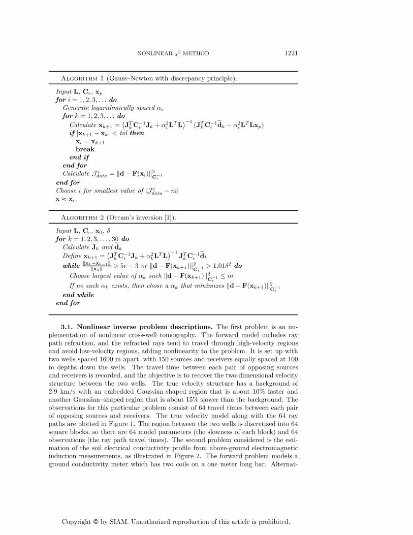
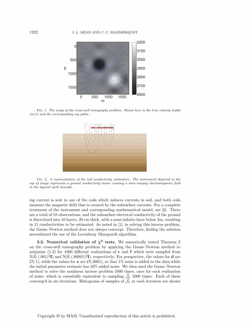
3.1. Nonlinear inverse problem descriptions. The first problem is an im-plementation of nonlinear cross-well tomography. The forward model includes raypath refraction, and the refracted rays tend to travel through high-velocity regionsand avoid low-velocity regions, adding nonlinearity to the problem. It is set up withtwo wells spaced 1600 m apart, with 150 sources and receivers equally spaced at 100m depths down the wells. The travel time between each pair of opposing sourcesand receivers is recorded, and the objective is to recover the two-dimensional velocitystructure between the two wells. The true velocity structure has a background of2.9 km/s with an embedded Gaussian-shaped region that is about 10% faster andanother Gaussian–shaped region that is about 15% slower than the background. Theobservations for this particular problem consist of 64 travel times between each pairof opposing sources and receivers. The true velocity model along with the 64 raypaths are plotted in Figure 1. The region between the two wells is discretized into 64square blocks, so there are 64 model parameters (the slowness of each block) and 64observations (the ray path travel times). The second problem considered is the esti-mation of the soil electrical conductivity profile from above-ground electromagneticinduction measurements, as illustrated in Figure 2. The forward problem models aground conductivity meter which has two coils on a one meter long bar. Alternat-



m

m

0 500 1000 1500

0

500

1000

1500

2600

2700

2800

2900

3000

3100

3200

Fig. 1. The setup of the cross-well tomography problem. Shown here is the true velocity model(m/s) and the corresponding ray paths.

Fig. 2. A representation of the soil conductivity estimation. The instrument depicted in thetop of image represents a ground conductivity meter creating a time-varying electromagnetic fieldin the layered earth beneath.

ing current is sent in one of the coils which induces currents in soil, and both coilsmeasure the magnetic field that is created by the subsurface currents. For a completetreatment of the instrument and corresponding mathematical model, see [6]. Thereare a total of 18 observations, and the subsurface electrical conductivity of the groundis discretized into 10 layers, 20 cm thick, with a semi-infinite layer below 2m, resultingin 11 conductivities to be estimated. As noted in [1], in solving this inverse problem,the Gauss–Newton method does not always converge. Therefore, finding the solutionnecessitated the use of the Levenberg–Marquardt algorithm.

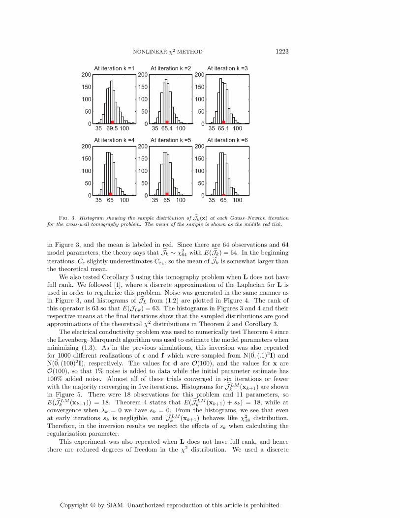
3.2. Numerical validation of χ2 tests. We numerically tested Theorem 2on the cross-well tomography problem by applying the Gauss–Newton method tominimize (1.3) for 1000 different realizations of ε and f which were sampled fromN(�0, (.001)2I) and N(�0, (.00001)2I), respectively. For perspective, the values for d areO(.1), while the values for x are O(.0001), so that 1% noise is added to the data whilethe initial parameter estimate has 10% added noise. We then used the Gauss–Newtonmethod to solve the nonlinear inverse problem 1000 times, once for each realizationof noise, which is essentially equivalent to sampling J̃k 1000 times. Each of theseconverged in six iterations. Histograms of samples of J̃k at each iteration are shown



35 69.5 1000

50

100

150

200At iteration k =1

35 65.4 1000

50

100

150


35 65.1 1000

50

100

150


35 65 1000

50

100

150


35 65 1000

50

100

150


35 65 1000

50

100

150


Fig. 3. Histogram showing the sample distribution of ˜Jk(x) at each Gauss–Newton iterationfor the cross-well tomography problem. The mean of the sample is shown as the middle red tick.

in Figure 3, and the mean is labeled in red. Since there are 64 observations and 64model parameters, the theory says that J̃k ∼ χ2

64 with E(J̃k) = 64. In the beginning

iterations, Cε slightly underestimates Cεk , so the mean of J̃k is somewhat larger thanthe theoretical mean.

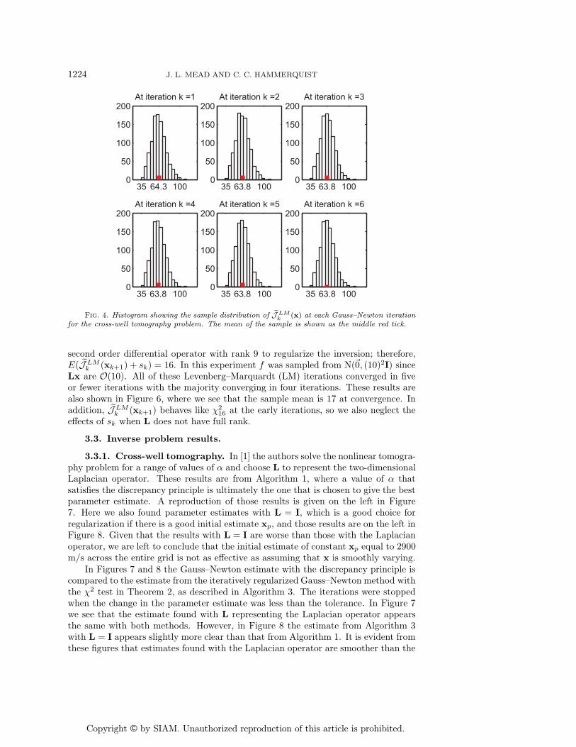
We also tested Corollary 3 using this tomography problem when L does not havefull rank. We followed [1], where a discrete approximation of the Laplacian for L isused in order to regularize this problem. Noise was generated in the same manner asin Figure 3, and histograms of J̃L from (1.2) are plotted in Figure 4. The rank ofthis operator is 63 so that E(JLk) = 63. The histograms in Figures 3 and 4 and theirrespective means at the final iterations show that the sampled distributions are goodapproximations of the theoretical χ2 distributions in Theorem 2 and Corollary 3.

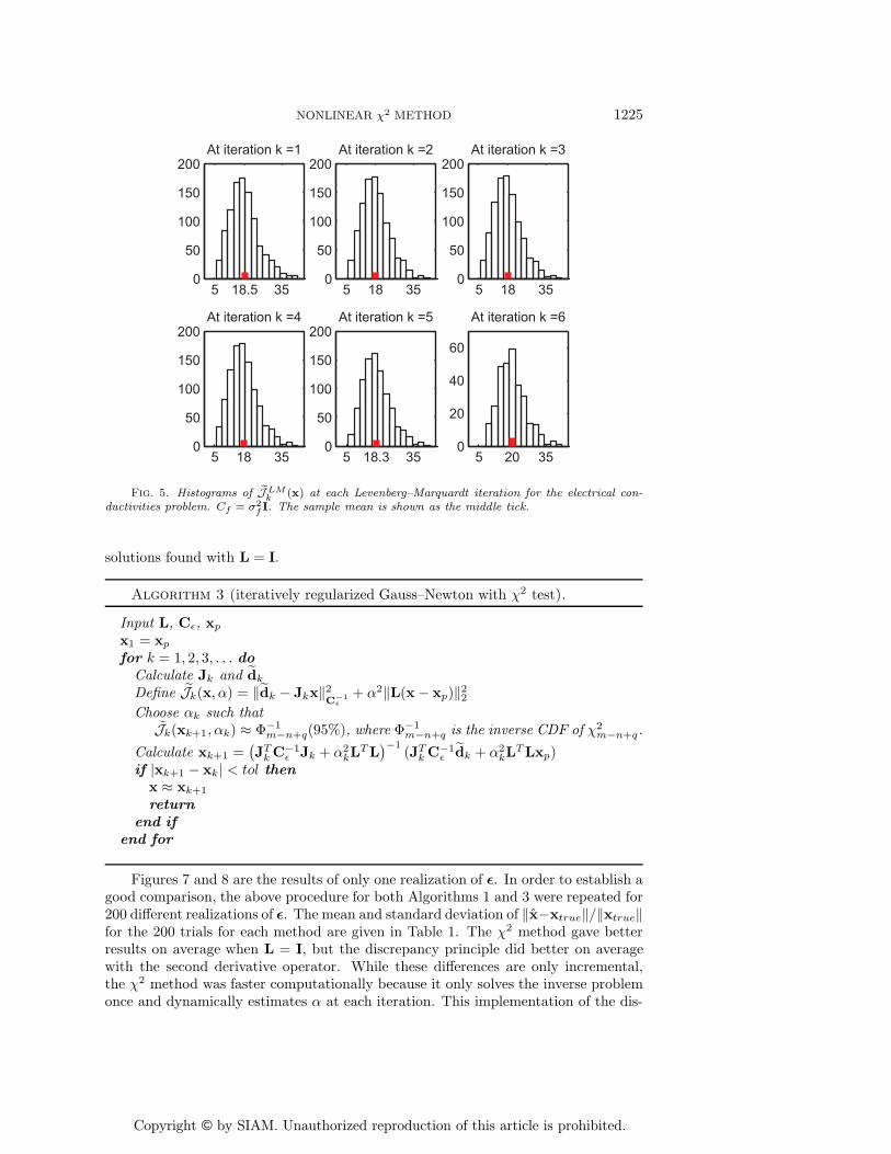
The electrical conductivity problem was used to numerically test Theorem 4 sincethe Levenberg–Marquardt algorithm was used to estimate the model parameters whenminimizing (1.3). As in the previous simulations, this inversion was also repeatedfor 1000 different realizations of ε and f which were sampled from N(�0, (.1)2I) andN(�0, (100)2I), respectively. The values for d are O(100), and the values for x areO(100), so that 1% noise is added to data while the initial parameter estimate has100% added noise. Almost all of these trials converged in six iterations or fewerwith the majority converging in five iterations. Histograms for J̃ LM

k (xk+1) are shownin Figure 5. There were 18 observations for this problem and 11 parameters, soE(J̃ LM

k (xk+1)) = 18. Theorem 4 states that E(J̃ LMk (xk+1) + sk) = 18, while at

convergence when λk = 0 we have sk = 0. From the histograms, we see that evenat early iterations sk is negligible, and J̃ LM

k (xk+1) behaves like χ218 distribution.

Therefore, in the inversion results we neglect the effects of sk when calculating theregularization parameter.

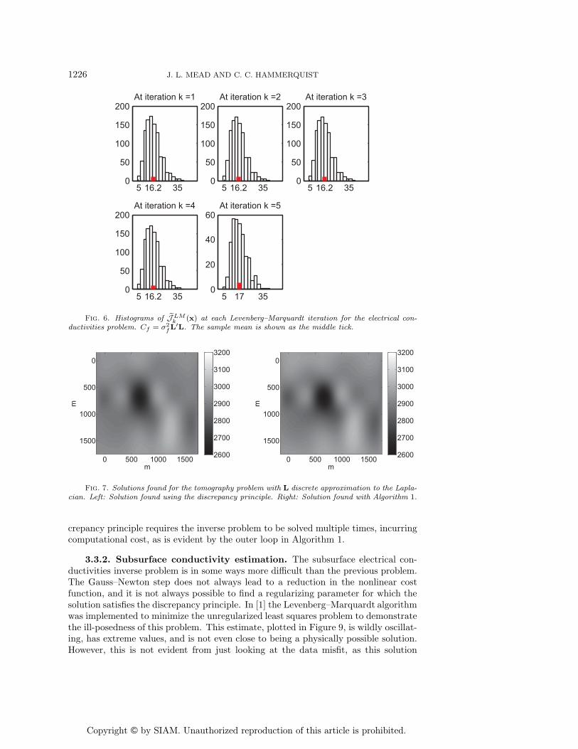
This experiment was also repeated when L does not have full rank, and hencethere are reduced degrees of freedom in the χ2 distribution. We used a discrete



35 64.3 1000

50

100

150


35 63.8 1000

50

100

150


35 63.8 1000

50

100

150


35 63.8 1000

50

100

150


35 63.8 1000

50

100

150


35 63.8 1000

50

100

150


Fig. 4. Histogram showing the sample distribution of ˜J LMk (x) at each Gauss–Newton iteration

for the cross-well tomography problem. The mean of the sample is shown as the middle red tick.

second order differential operator with rank 9 to regularize the inversion; therefore,E(J̃ LM

k (xk+1) + sk) = 16. In this experiment f was sampled from N(�0, (10)2I) sinceLx are O(10). All of these Levenberg–Marquardt (LM) iterations converged in fiveor fewer iterations with the majority converging in four iterations. These results arealso shown in Figure 6, where we see that the sample mean is 17 at convergence. Inaddition, J̃ LM

k (xk+1) behaves like χ216 at the early iterations, so we also neglect the

effects of sk when L does not have full rank.

3.3. Inverse problem results.

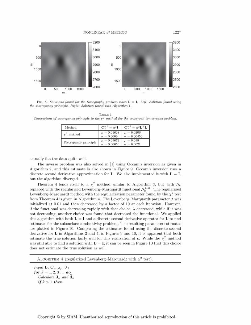
3.3.1. Cross-well tomography. In [1] the authors solve the nonlinear tomogra-phy problem for a range of values of α and choose L to represent the two-dimensionalLaplacian operator. These results are from Algorithm 1, where a value of α thatsatisfies the discrepancy principle is ultimately the one that is chosen to give the bestparameter estimate. A reproduction of those results is given on the left in Figure7. Here we also found parameter estimates with L = I, which is a good choice forregularization if there is a good initial estimate xp, and those results are on the left inFigure 8. Given that the results with L = I are worse than those with the Laplacianoperator, we are left to conclude that the initial estimate of constant xp equal to 2900m/s across the entire grid is not as effective as assuming that x is smoothly varying.

In Figures 7 and 8 the Gauss–Newton estimate with the discrepancy principle iscompared to the estimate from the iteratively regularized Gauss–Newton method withthe χ2 test in Theorem 2, as described in Algorithm 3. The iterations were stoppedwhen the change in the parameter estimate was less than the tolerance. In Figure 7we see that the estimate found with L representing the Laplacian operator appearsthe same with both methods. However, in Figure 8 the estimate from Algorithm 3with L = I appears slightly more clear than that from Algorithm 1. It is evident fromthese figures that estimates found with the Laplacian operator are smoother than the



5 18.5 350

50

100

150


5 18 350

50

100

150


5 18 350

50

100

150


5 18 350

50

100

150


5 18.3 350

50

100

150


5 20 350

20

40

60

At iteration k =6

Fig. 5. Histograms of ˜JLMk (x) at each Levenberg–Marquardt iteration for the electrical con-

ductivities problem. Cf = σ2f I. The sample mean is shown as the middle tick.

solutions found with L = I.

Algorithm 3 (iteratively regularized Gauss–Newton with χ2 test).

Input L, Cε, xp

x1 = xp

for k = 1, 2, 3, . . . doCalculate Jk and d̃k

Define J̃k(x, α) = ‖d̃k − Jkx‖2C−1ε

+ α2‖L(x− xp)‖22Choose αk such that

J̃k(xk+1, αk) ≈ Φ−1m−n+q(95%), where Φ−1

m−n+q is the inverse CDF of χ2m−n+q.

Calculate xk+1 =(JTk C

−1ε Jk + α2

kLTL

)−1(JT

k C−1ε d̃k + α2

kLTLxp)

if |xk+1 − xk| < tol thenx ≈ xk+1

returnend if

end for

Figures 7 and 8 are the results of only one realization of ε. In order to establish agood comparison, the above procedure for both Algorithms 1 and 3 were repeated for200 different realizations of ε. The mean and standard deviation of ‖x̂−xtrue‖/‖xtrue‖for the 200 trials for each method are given in Table 1. The χ2 method gave betterresults on average when L = I, but the discrepancy principle did better on averagewith the second derivative operator. While these differences are only incremental,the χ2 method was faster computationally because it only solves the inverse problemonce and dynamically estimates α at each iteration. This implementation of the dis-



5 16.2 350

50

100

150


5 16.2 350

50

100

150


5 16.2 350

50

100

150


5 16.2 350

50

100

150


5 17 350

20

40

60At iteration k =5

Fig. 6. Histograms of ˜JLMk (x) at each Levenberg–Marquardt iteration for the electrical con-

ductivities problem. Cf = σ2fL

′L. The sample mean is shown as the middle tick.

m

m

0 500 1000 1500

0

500

1000

1500

2600

2700

2800

2900

3000

3100

3200

m

m

0 500 1000 1500

0

500

1000

1500

2600

2700

2800

2900

3000

3100

3200

Fig. 7. Solutions found for the tomography problem with L discrete approximation to the Lapla-cian. Left: Solution found using the discrepancy principle. Right: Solution found with Algorithm 1.

crepancy principle requires the inverse problem to be solved multiple times, incurringcomputational cost, as is evident by the outer loop in Algorithm 1.

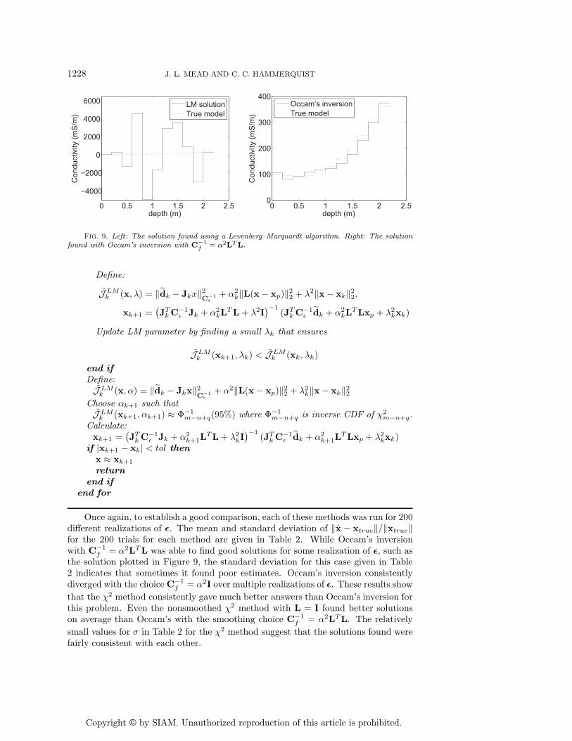
3.3.2. Subsurface conductivity estimation. The subsurface electrical con-ductivities inverse problem is in some ways more difficult than the previous problem.The Gauss–Newton step does not always lead to a reduction in the nonlinear costfunction, and it is not always possible to find a regularizing parameter for which thesolution satisfies the discrepancy principle. In [1] the Levenberg–Marquardt algorithmwas implemented to minimize the unregularized least squares problem to demonstratethe ill-posedness of this problem. This estimate, plotted in Figure 9, is wildly oscillat-ing, has extreme values, and is not even close to being a physically possible solution.However, this is not evident from just looking at the data misfit, as this solution



m

m

0 500 1000 1500

0

500

1000

1500

2600

2700

2800

2900

3000

3100

3200

m

m

0 500 1000 1500

0

500

1000

1500

2600

2700

2800

2900

3000

3100

3200

Fig. 8. Solutions found for the tomography problem when L = I. Left: Solution found usingthe discrepancy principle. Right: Solution found with Algorithm 1.

Table 1

Comparison of discrepancy principle to the χ2 method for the cross-well tomography problem.

Method C−1f = α2I C−1

f = α2LTL

χ2 methodμ = 0.01628 μ = 0.0206σ = 0.0006 σ = 0.00456

Discrepancy principleμ = 0.01672 μ = 0.018σ = 0.00050 σ = 0.0021

actually fits the data quite well.

The inverse problem was also solved in [1] using Occam’s inversion as given inAlgorithm 2, and this estimate is also shown in Figure 9. Occam’s inversion uses adiscrete second derivative approximation for L. We also implemented it with L = I,but the algorithm diverged.

Theorem 4 lends itself to a χ2 method similar to Algorithm 3, but with J̃k

replaced with the regularized Levenberg–Marquardt functional J̃ LMk . The regularized

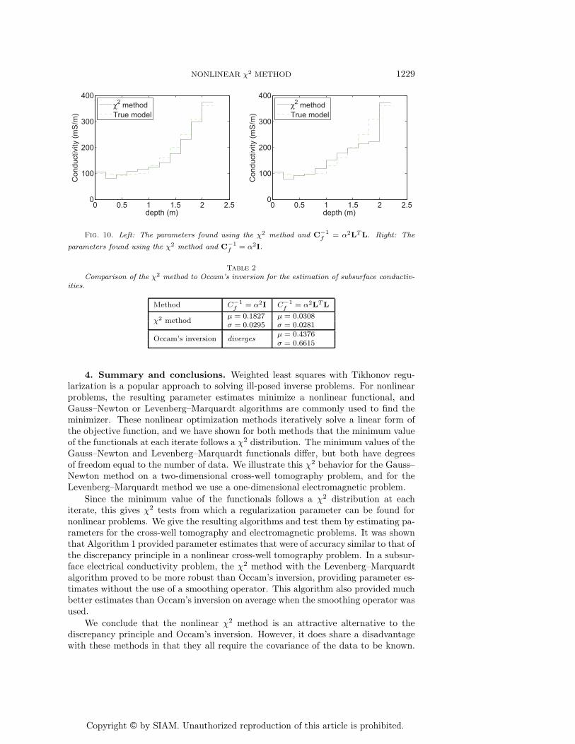
Levenberg–Marquardt method with the regularization parameter found by the χ2 testfrom Theorem 4 is given in Algorithm 4. The Levenberg–Marquardt parameter λ wasinitialized at 0.01 and then decreased by a factor of 10 at each iteration. However,if the functional was decreasing rapidly with that choice, λ decreased, while if it wasnot decreasing, another choice was found that decreased the functional. We appliedthis algorithm with both L = I and a discrete second derivative operator for L to findestimates for the subsurface conductivity problem. The resulting parameter estimatesare plotted in Figure 10. Comparing the estimates found using the discrete secondderivative for L in Algorithms 2 and 4, in Figures 9 and 10, it is apparent that bothestimate the true solution fairly well for this realization of ε. While the χ2 methodwas still able to find a solution with L = I, it can be seen in Figure 10 that this choicedoes not estimate the true solution as well.

Algorithm 4 (regularized Levenberg–Marquardt with χ2 test).

Input L, Cε, xp, λ1

for k = 1, 2, 3 . . . doCalculate Jk and d̃k

if k > 1 then



0 0.5 1 1.5 2 2.5

−4000

−2000

0

2000

4000

6000

depth (m)

Con

duct

ivity

(mS

/m)

LM solutionTrue model

0 0.5 1 1.5 2 2.50

100

200

300

400

depth (m)

Con

duct

ivity

(mS

/m)

Occam’s inversionTrue model

Fig. 9. Left: The solution found using a Levenberg–Marquardt algorithm. Right: The solutionfound with Occam’s inversion with C−1

f = α2LTL.

Define:

J̃ LMk (x, λ) = ‖d̃k − Jkx‖2C−1

ε+ α2

k‖L(x− xp)‖22 + λ2‖x− xk‖22,xk+1 =

(JTkC

−1ε Jk + α2

kLTL+ λ2I

)−1(JT

k C−1ε d̃k + α2

kLTLxp + λ2

kxk)

Update LM parameter by finding a small λk that ensures

J̃ LMk (xk+1, λk) < J̃ LM

k (xk, λk)

end ifDefine:J̃ LMk (x, α) = ‖d̃k − Jkx‖2C−1

ε+ α2‖L(x− xp)‖22 + λ2

k‖x− xk‖22Choose αk+1 such thatJ̃ LMk (xk+1, αk+1) ≈ Φ−1

m−n+q(95%) where Φ−1m−n+q is inverse CDF of χ2

m−n+q.Calculate:xk+1 =

(JTk C

−1ε Jk + α2

k+1LTL+ λ2

kI)−1

(JTk C

−1ε d̃k + α2

k+1LTLxp + λ2

kxk)if |xk+1 − xk| < tol thenx ≈ xk+1

returnend if

end for

Once again, to establish a good comparison, each of these methods was run for 200different realizations of ε. The mean and standard deviation of ‖x̂ − xtrue‖/‖xtrue‖for the 200 trials for each method are given in Table 2. While Occam’s inversionwith C−1

f = α2LTL was able to find good solutions for some realization of ε, such asthe solution plotted in Figure 9, the standard deviation for this case given in Table2 indicates that sometimes it found poor estimates. Occam’s inversion consistentlydiverged with the choiceC−1

f = α2I over multiple realizations of ε. These results show

that the χ2 method consistently gave much better answers than Occam’s inversion forthis problem. Even the nonsmoothed χ2 method with L = I found better solutionson average than Occam’s with the smoothing choice C−1

f = α2LTL. The relatively

small values for σ in Table 2 for the χ2 method suggest that the solutions found werefairly consistent with each other.



0 0.5 1 1.5 2 2.50

100

200

300

400

depth (m)

Con

duct

ivity

(mS

/m)

χ2 methodTrue model

0 0.5 1 1.5 2 2.50

100

200

300

400

depth (m)

Con

duct

ivity

(mS

/m)

χ2 methodTrue model

Fig. 10. Left: The parameters found using the χ2 method and C−1f = α2LTL. Right: The

parameters found using the χ2 method and C−1f = α2I.

Table 2

Comparison of the χ2 method to Occam’s inversion for the estimation of subsurface conductiv-ities.

Method C−1f = α2I C−1

f = α2LTL

χ2 methodμ = 0.1827 μ = 0.0308σ = 0.0295 σ = 0.0281

Occam’s inversion divergesμ = 0.4376σ = 0.6615

4. Summary and conclusions. Weighted least squares with Tikhonov regu-larization is a popular approach to solving ill-posed inverse problems. For nonlinearproblems, the resulting parameter estimates minimize a nonlinear functional, andGauss–Newton or Levenberg–Marquardt algorithms are commonly used to find theminimizer. These nonlinear optimization methods iteratively solve a linear form ofthe objective function, and we have shown for both methods that the minimum valueof the functionals at each iterate follows a χ2 distribution. The minimum values of theGauss–Newton and Levenberg–Marquardt functionals differ, but both have degreesof freedom equal to the number of data. We illustrate this χ2 behavior for the Gauss–Newton method on a two-dimensional cross-well tomography problem, and for theLevenberg–Marquardt method we use a one-dimensional electromagnetic problem.

Since the minimum value of the functionals follows a χ2 distribution at eachiterate, this gives χ2 tests from which a regularization parameter can be found fornonlinear problems. We give the resulting algorithms and test them by estimating pa-rameters for the cross-well tomography and electromagnetic problems. It was shownthat Algorithm 1 provided parameter estimates that were of accuracy similar to that ofthe discrepancy principle in a nonlinear cross-well tomography problem. In a subsur-face electrical conductivity problem, the χ2 method with the Levenberg–Marquardtalgorithm proved to be more robust than Occam’s inversion, providing parameter es-timates without the use of a smoothing operator. This algorithm also provided muchbetter estimates than Occam’s inversion on average when the smoothing operator wasused.

We conclude that the nonlinear χ2 method is an attractive alternative to thediscrepancy principle and Occam’s inversion. However, it does share a disadvantagewith these methods in that they all require the covariance of the data to be known.



If an estimate of the data covariance is not known, then the nonlinear χ2 method willnot be appropriate for solving such a problem. Future work includes estimating morecomplex covariance matrices for the parameter estimates. In [9] Mead shows that itis possible to use multiple χ2 tests to estimate such a covariance, and it seems likelythat this could also be extended to solving nonlinear problems.

REFERENCES

[1] R. C. Aster, B. Borchers, and C. Thurber, Parameter Estimation and Inverse Problems,Academic Press, New York, 2005, p. 301.

[2] P. C. Carline and T. A. Louis, Bayes and Empirical Bayes Methods for Data Analysis,Chapman and Hall, London, 1996, p. 397.

[3] H. W. Engl, K. Kunisch, and A. Neubauer, Convergence rates for Tikhonov regularisationof nonlinear ill-posed problems, Inverse Problems, 5 (1989), pp. 523–540.

[4] W. P. Gouveia and J. A. Scales, Resolution of seismic waveform inversion: Bayes versusOccam, Inverse Problems, 13 (1997), pp. 323–349.

[5] P. C. Hansen, Rank-Deficient and Discrete Ill-Posed Problems: Numerical Aspects of LinearInversion, SIAM Monogr. Math. Model. Comput. 4, SIAM, Philadelphia, 1998.

[6] J. M. H. Hendrickx, B. Borchers, D. L. Corwin, S. M. Lesch, A. C. Hilgendorf, and

J. Schule, Inversion of soil conductivity profiles from electromagnetic induction measure-ments: Theory and experimental verification, Soil Sci. Soc. Amer. J., 66 (2002), pp. 673–685.

[7] J. Mead, Parameter estimation: A new approach to weighting a priori information, J. InverseIll-Posed Probl., 16 (2008), pp. 175–194.

[8] J. Mead and R. A. Renaut, A Newton root-finding algorithm for estimating the regularizationparameter for solving ill-conditioned least squares problems, Inverse Problems, 25 (2009),025002.

[9] J. Mead, Discontinuous parameter estimates with least squares estimators, Appl. Math. Com-put., 219 (2013), pp. 5210–5223.

[10] A. Rieder, On the regularization of nonlinear ill-posed problems via inexact Newton iterations,Inverse Problems, 15 (1999), pp. 309–327.

[11] R. A. Renaut, I. Hnetynkova, and J. L. Mead, Regularization parameter estimation for largescale Tikhonov regularization using a priori information, Comput. Statist. Data Anal., 54(2010), pp. 3430–3445.

[12] T. I. Seidman and C. R. Vogel, Well-posedness and convergence of some regularisationmethods for non-linear ill posed problems, Inverse Problems, 5 (1989), pp. 227–238.

[13] A. Tarantola, Inverse Problem Theory and Methods for Model Parameter Estimation, SIAM,Philadelphia, 2005.

Documents

ScholarWorks - Boise State University