The Role of Filter Banks in

Sinusoidal Frequency Estimation

Andre Tkacenko and P. P. Vaidyanathan

California Institute of Technology

136-93 Moore

Pasadena, CA 91125

E-mail: andre@systems.caltech.edu, ppvnath@systems.caltech.edu

Abstract

The problem of estimating the frequencies of sinusoids buried in noise has been one of great interest

to the signal processing community for many years, especially to those involved in the field of array

processing. While many methods have been proposed to solve this problem, most involve processing

in the fullband. In this paper, we investigate the effects of carrying out estimation in the subbands

of an analysis bank of a multirate filter bank and show that there are some benefits to be reaped. In

particular, we observe that with properly chosen analysis filters, the local signal-to-noise ratio (SNR)

and line resolution in the subbands will exceed that in the fullband. Also, through the use of the spectral

flatness measure, we show that if the input noise is colored, then the noise processes seen in the subbands

will be more flat on average. This can be useful if the exact statistics of the input noise process are not

known. Various examples are shown giving evidence to the fact that estimation in the subbands is

superior to that in the fullband. 1

Keywords: sinusoidal frequency estimation, pseudospectra, filter banks, subband estimation, spectral flat-

ness measure

1Work supported in part by the ONR grant N00014-99-1-1002.

1

I. Introduction

A classical problem of statistical signal processing [16, 7, 2] is that of determining the frequencies of sinusoids

buried in noise. Such a problem arises in array processing [6, 10, 3], for example, when we wish to estimate

the direction of arrival (DOA) of a narrowband electromagnetic signal incident on a uniform linear array.

In this application, the radial angle of arrival plays the role of digital frequency. Another field in which this

problem arises is in digital telephony [13] when we wish to estimate one of a number of possible Caller ID

tones.

While many approaches have been proposed to solve this problem, most suffer from certain basic short-

comings. For example, most require a large SNR and perform poorly if the lines are too close to one another.

In this paper, we investigate how filter banks can be used to overcome these shortcomings. For a uniform

maximally decimated power complementary analysis bank, we will see that locally in the subbands, the SNR

and the line resolution increase by a factor equal to the decimation ratio. Examples will then be shown to

demonstrate the usefulness of our claims. Afterwards, we will show that if the input noise is colored, then

the noise processes seen in the subbands will be more white on the average in a certain quantitative sense.

This will be shown heuristically and also analytically in terms of the spectral flatness measure. In particular,

we will prove that for the class of maximally decimated power complementary analysis banks, the geometric

mean of the flatness measures of the subband signals will exceed the flatness of the fullband signal. This

is a generalization of a result given in [12], in which only ideal filters were considered. Examples of this

result will also be shown and it will be seen that in many practical scenarios, we can assume the noise to be

approximately white in the subbands, even though this may not be the case in the fullband. This will be

useful if the statistics of the input noise are not known, which perhaps is more often the case than not.

A. Notations

Throughout the paper, we will use the notations described in [18]. In particular, boldface lowercase and

uppercase letters will be used to represent vectors and matrices, respectively. The superscripts (∗), (T ),

(†), (+), and (+(P)) will be used to represent, respectively, the conjugate, transpose, conjugate transpose,

Moore-Penrose pseudoinverse [4], and rank P pseudoinverse [16] of a given matrix. We will use the notation

[G(ejω)]↓M to denote the Fourier transform of g(Mn). Finally, we will say that a signal f(n), or its Fourier

transform F (ejω), is Nyquist(M) if f(Mn) = δ(n) or equivalently [F (ejω)]↓M = 1.

2

B. Outline

In Section II, we briefly review some of the more classical methods for sinusoidal frequency estimation, in-

cluding the Pisarenko harmonic decomposition [11], the MUSIC algorithm [14], and the principal components

linear prediction method [17]. In Section III, we analyze the effect of carrying out frequency estimation in

the subbands of a uniform filter bank with ideal analysis filters for the case of white noise. It is shown there

that the local SNR and line resolution increase by a factor equal to the decimation ratio. To substantiate

our results, in Section IV, examples are given in which estimation in the subbands performs better than

in the fullband. In Section V, we discuss some of the consequences involved when we deal with finite data

records and show that the advantages mentioned above do not come without a price. Since in practice we

must estimate correlation functions using only a finite amount of data, the estimated subband correlation

functions will be more erroneous than the fullband one. In Section VI, we examine the effects of colored

noise and show there that the geometric mean of the spectral flatnesses in the subbands exceeds that of the

fullband for a particular class of filter banks. Examples are shown supporting this theorem in Section VII.

In addition, we then compare estimation in the subbands to that in the fullband when the statistics of the

noise are not known and the noise is incorrectly assumed to be white. It is seen there that estimation in the

subbands continues to be superior to that in the fullband. In Section VIII, we conclude by mentioning some

of the open problems still present.

II. Problem Statement and Previous Work

Regarding the problem of estimating sinusoids buried in noise, we have the following discrete time signal

model x(n).

x(n) =P∑i=1

Aisi(n) + η(n) , si(n) = ejωin , Ai = |Ai|ejφi (1)

Here, we have P sinusoidal signals si(n), each scaled by an amount Ai, and buried in the complex noise

process η(n). The goal here is to determine the frequencies ωi of the sinusoidal signals given Ns observations

of one particular instance of the random process x(n). The complex amplitudes Ai are assumed to have

unknown but constant magnitudes |Ai| and phase angles φi each uniformly distributed over the interval

[−π, π). For sake of stationarity, it is assumed that the phase angles are pairwise independent, i.e. φi and

φj are independent for all i �= j. The noise process η(n) is assumed to be a zero mean wide sense stationary

(WSS) random process uncorrelated with the sinusoidal signals. Ideally, to estimate the frequencies given only

Ns observations, we would use the maximum likelihood estimate. However, it turns out that if P > 1, this

3

problem becomes computationally intractable [7] as it involves finding the location of the global maximum

of a highly nonlinear function. If Ns is sufficiently large, then the frequencies can be estimated by looking

at the peaks of the magnitude of the Fourier transform of the observed signal, even if the power of the noise

is significant. This is due to the fact that the sinusoids will have a Dirac type distribution in the frequency

domain, whereas the observed noise signal will most likely not have such strong support in these regions.

However, if Ns is relatively small, then these peaks will be smeared out in the frequency domain on account

of the noticable windowing effect in the time domain. Since the approximate frequency resolution will vary as

2π/Ns, lines that are close to each other (in particular, closer than 2π/Ns) will become indistinguishable and

will be observed as only one wide peak. Instead what is typically done in this case is to exploit the special

properties of the autocorrelation function of x(n). This can be done since under the above assumptions,

x(n) is ergodic in the mean and autocorrelation [7]. It follows that x(n) is a zero mean WSS process with

the following autocorrelation function.

Rxx(k) =P∑i=1

Piejωik +Rηη(k) , Pi � |Ai|2 (2)

Here, Pi denotes the power of the i-th sinusoidal signal. At this point, we define two figures of merit for

estimating the frequencies, namely the individual or local signal-to-noise ratio of the i-th sinusoid with

respect to the noise, denoted as SNRind,i and the net signal-to-noise ratio SNRnet. These are defined as

follows.

SNRind,i � PiRηη(0)

, SNRnet �

P∑i=1

Pi

Rηη(0)

The local SNR is a good figure of merit of how likely we will be able to estimate a particular frequency

correctly. As we would heuristically expect, it can be shown [7, 10] that as this ratio increases for some

sinusoid, indeed we will statistically estimate this sinusoid more correctly. The net SNR, on the other hand,

is a measure of how likely we will be able to estimate the frequencies on average. Continuing from (2), the

N ×N autocorrelation matrix of x(n), namely Rx, is as follows.

Rx =P∑i=1

Pisis†i + Rη = Rs + Rη , si � [ 1 ejωi · · · ej(N−1)ωi ]T (3)

Here, the matrices Rs and Rη denote, respectively, the autocorrelation matrices corresponding to the purely

harmonic process consisting of the P sinusoids and the noise process. As Rs is simply a sum of dyadic

4

matrices of the form vv†, it can be shown [7] that if the frequencies ωi are all distinct modulo 2π and if the

size of the autocorrelation matrix N is chosen such that N > P, then Rs has rank P. Furthermore, the

set of P eigenvectors {vk} for k = 1, . . . ,P corresponding to the nonzero eigenvalues {λk} span the same

space as the signal vectors {si}. The space spanned by the signal vectors {si} is commonly referred to as

the signal subspace. The remaining N − P eigenvectors vk for k = P + 1, . . . , N corresponding to the zero

eigenvalue are orthogonal to all of the signal vectors, i.e. s†ivk = 0 for all i = 1, . . . ,P and k = P + 1, . . . , N .

The space spanned by the eigenvectors {vk} for k = P + 1, . . . , N is commonly called the noise subspace.

Define the eigenfilter corresponding to vk = [ vk(0) vk(1) · · · vk(N − 1) ]T as,

Vk(z) �N−1∑n=0

vk(n)z−n

Then, for k = P + 1, . . . , N , it follows that Vk(z) has zeros at z = ejω1 , . . . , ejωP . If the input noise process

η(n) is white with variance σ2η, then Rη = σ2

ηI, and so we have,

Rx = Rs + σ2ηI

In this case, the eigenvectors of Rx are the same as those of Rs, namely vk for k = 1, . . . , N . The corre-

sponding eigenvalues µk are given below as follows.

µk =

λk + σ2

η , k = 1, . . . ,P

σ2η , k = P + 1, . . . , N

As Rx can be estimated by observations of x(n), the frequencies of the sinusoids can be estimated by finding

the roots of the eigenfilters Vk(z) for k = P+1, . . . , N ideally on (or in practice nearest) the unit circle. This is

the basis behind many of the classical techniques for sinusoidal frequency estimation which we discuss briefly

below, such as the Pisarenko harmonic decomposition [11], the MUSIC algorithm [14], and the principal

components linear prediction (PCLP) method [17]. These algorithms only work if the input noise is white.

In Section VI, we address what must be done if the noise is colored.

A. Pisarenko Harmonic Decomposition

In 1973, V. F. Pisarenko became the first person to observe and exploit the interesting eigenstructure of

the autocorrelation matrix Rx for the purpose of frequency estimation. In his classic paper [11], he used

5

an autocorrelation matrix of size N = P + 1 and estimated the frequencies as the peaks of the following

frequency estimation function commonly referred to now as the “pseudospectrum” [16, 7, 2] corresponding

to the Pisarenko harmonic decomposition.

SPHD(ejω) =1

|VP+1(ejω)|2 , where VP+1(z) =P∑n=0

vP+1(n)z−n

Ideally, all of the zeros of VP+1(z) lie on the unit circle at angles corresponding to the frequencies of the

sinusoids sent. Thus, the frequencies are estimated as the locations of the peaks of SPHD(ejω) or the zeros

of VP+1(z). Though this method works in theory, in practice it unfortunately performs poorly, even at large

SNRs [16, 7, 2]. The reason for this is that with finite data records, the variance of SPHD(ejω) is quite large

on account of the small size of the autocorrelation matrix used [7]. By using a larger size, as is the case with

the MUSIC algorithm and the PCLP method, we obtain frequency estimators which come much closer to

the Cramer-Rao bound than the Pisarenko harmonic decomposition.

B. MUSIC Algorithm

The MUltiple SIgnal Classification or MUSIC algorithm introduced by R. Schmidt in 1979 [14] is a gen-

eralization of the Pisarenko harmonic decomposition, which experimentally has been shown to be a major

improvement over that method. Here, the size of the autocorrelation matrix Rx is chosen to be N > P + 1

and the pseudospectrum is obtained by reciprocating the sum of the magnitude squared responses of the

eigenfilters Vk(z) for k = P + 1, . . . , N , as is shown below.

SMUSIC(ejω) =1

N∑k=P+1

|Vk(ejω)|2

As before, the frequencies of the sinusoids are estimated to be where the peaks of the function above occur.

However, note now that Vk(z) is a polynomial of degree N − 1 > P for all k. Thus, while each Vk(z) for

k = P + 1, . . . , N will have P roots on the unit circle corresponding to the frequencies of the sinusoids sent,

it will also have N − P − 1 roots, deemed spurious roots, which can lie anywhere in the complex plane,

including the unit circle. Though this may appear to be a dilemma, it is highly unlikely that the spurious

zeros of all of the eigenfilters will coincide, and so adding the magnitude responses in the denominator of the

pseudospectrum above has the effect of moving these spurious roots away from the unit circle [16, 2]. This

method has been shown to perform well provided that the SNR is moderately large [16, 7, 2] and is still used

6

today on account of its low complexity. However, the PCLP method, which elegantly takes care of the issue

of spurious roots, has been shown experimentally to perform better, as will soon be discussed.

C. Principal Components Linear Prediction

In 1982, D. Tufts and R. Kumaresan introduced a novel approach to estimate the frequencies of the sinusoids

buried in noise [17]. They started from the known premise that for the harmonic process consisting of just

the P sinusoids, whose autocorrelation matrix is simply Rs, a prediction error filter could be found such that

the prediction error variance is identically zero [16], provided that the size of the autocorrelation matrix N

was such that N > P. That is, if a � [a(0) a(1) · · · a(N − 1)]T represents the vector of prediction error

filter coefficients, then the normal equations to determine an optimal prediction filter are as follows [16].

Rsa = 0 (4)

From this, we observe that the vector a is an eigenvector corresponding to the zero eigenvalue and hence is

orthogonal to the signal subspace. It turns out that for N > P + 1, there is not a unique solution to (4),

and as a result, the eigenfilter corresponding to a, namely A(z), will have P of its roots on the unit circle

corresponding to the frequencies of the sinusoids sent and N −P − 1 spurious roots which may lie anywhere

in the complex plane. This is similar to what was observed above for the eigenfilters Vk(z) in the case of the

MUSIC algorithm. It turns out, however [16], that this problem can be overcome if we take a to be monic,

i.e. a(0) = 1, and minimize the l2-norm of the vector a subject to the constraint (4). By minimizing this

norm, the problem becomes akin to solving for an optimum prediciton error filter by the autocorrelation

method. As a result, all spurious roots will be guaranteed to lie strictly inside the unit circle. Partitioning

a as a = [1 aT ]T and Rs as Rs = [rs Rs], we have from (4),

Rsa = −rs

and so the unique optimal choice of a which minimizes the l2-norm of a and hence a is given by [16],

a = −R+s rs (5)

where R+s is the Moore-Penrose pseudoinverse [4] of the matrix Rs. Tufts and Kumaresan noted [17] that

by choosing a as in (5), the spurious roots of A(z) had a tendency to be uniformly distributed around a

7

circle (with radius less than unity of course) concentric with the unit circle at angles away from those which

corresponded to the frequencies of the sinusoids sent. While this approach elegantly handles the spurious

roots of the eigenfilter A(z), in practice, we will only have an estimate for the autocorrelation matrix of the

observed process Rx. A naive approach to this problem is to partition Rx as Rx = [rx Rx] and choose a as

a = −R+x rx. However, Tufts and Kumaresan showed that the presence of the noise in Rx had a tendency

to significantly perturb a from its optimum value given in (5). Instead, they showed [17] that the following

choice of a had the effect of nullifying the perturbation due to the present noise.

a = −R+(P)x rx

where R+(P)x is the rank P pseudoinverse [16] of the matrix Rx obtained by preserving only the P largest

singular values of R+x and zeroing out the rest. This choice of a forms the foundation for the principal

components linear prediction method or PCLP method for estimating the frequencies of the sinusoids. In

particular, if a = [a(1) a(2) · · · a(N − 1)]T , the frequencies are estimated as the P roots of the prediction

error filter,

A(z) = 1 +N−1∑n=1

a(n)z−n

on or nearest the unit circle. Graphically, the frequencies are estimated as the peaks of the pseudospectrum,

SPCLP =1

|A(ejω)|2 (6)

While this method is computationally more complex than the MUSIC algorithm, there is evidence to support

its superiority. In [7], it is shown for the case of two sinusoids that the PCLP method comes much closer

to the Cramer-Rao bound for frequency estimation than does the MUSIC algorithm. It is also mentioned

there that the choice of N ≈ 34Ns has been shown experimentally to give the lowest variance estimate.

Furthermore, in [17, 16], it is shown that the method of (6) is relatively insensitive to an overestimation of

the number of sinusoids in the received signal. Namely, if the number of sinusoids buried in the noise is

not known a priori and is estimated erroneously to be P0 > P, then provided that the noise power is of

a moderate level, there will be only P dominant peaks observed in the pseudospectrum of (6). It is this

property which allows estimation in the subbands of a filter bank to be possible, as we will soon see, since

the number of sinusoids present in any one subband will not be known a priori. As the PCLP method has

been shown experimentally to approach the Cramer-Rao bound for frequency estimation closer than other

8

techniques [7], we have opted to use this method for estimation in the subbands. At this point, we will

proceed to analyze what happens when the model signal given in (1) is input to a filter bank.

III. Analysis of Subband Frequency Estimation

A. Introduction

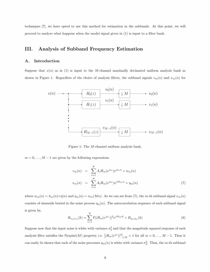
Suppose that x(n) as in (1) is input to the M -channel maximally decimated uniform analysis bank as

shown in Figure 1. Regardless of the choice of analysis filters, the subband signals vm(n) and xm(n) for

x(n) � �

�

�

�

�

�

�

�

�

�

� HM−1(z)

H1(z)

H0(z) �

�

�vM−1(n)

v1(n)

v0(n)↓ M

↓ M

↓ M

�

�

�

x0(n)

x1(n)

xM−1(n)

Figure 1: The M -channel uniform analysis bank.

m = 0, . . . ,M − 1 are given by the following expressions.

vm(n) =P∑i=1

AiHm(ejωi)ejωin + wm(n)

xm(n) =P∑i=1

AiHm(ejωi)ejMωin + ηm(n) (7)

where wm(n) = hm(n)∗η(n) and ηm(n) = wm(Mn). As we can see from (7), the m-th subband signal xm(n)

consists of sinusoids buried in the noise process ηm(n). The autocorrelation sequence of each subband signal

is given by,

Rxmxm(k) =

P∑i=1

Pi|Hm(ejωi)|2ejMωik +Rηmηm(k) (8)

Suppose now that the input noise is white with variance σ2η and that the magnitude squared response of each

analysis filter satisfies the Nyquist(M) property, i.e.[|Hm(ejω)|2]↓M = 1 for all m = 0, . . . ,M − 1. Then it

can easily be shown that each of the noise processes ηm(n) is white with variance σ2η. Thus, the m-th subband

9

signal xm(n) is nothing more than a set of sinusoids buried in the white noise process ηm(n). It is clear here

in this case that the subband signals xm(n) are intrinsically of the same form as the input signal x(n). The

only differences are that the sinusoids are scaled by the frequency responses of the analysis filters and the

frequencies of the sinusoids themselves are mapped to different locations, namely ωi →Mωi mod 2π. It will

be seen shortly that these two very important differences make estimation in the subbands advantageous

compared to that in the fullband.

B. Advantages of Estimation in the Subbands

1. SNR Amplification

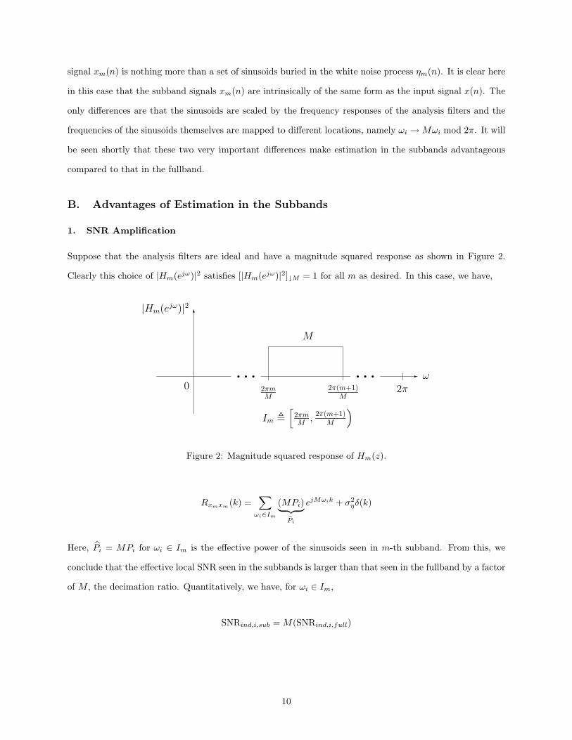
Suppose that the analysis filters are ideal and have a magnitude squared response as shown in Figure 2.

Clearly this choice of |Hm(ejω)|2 satisfies [|Hm(ejω)|2]↓M = 1 for all m as desired. In this case, we have,

�

� � � � � � �

2πω

0

|Hm(ejω)|2

2πmM

2π(m+1)M

Im �[

2πmM , 2π(m+1)

M

)

M

Figure 2: Magnitude squared response of Hm(z).

Rxmxm(k) =

∑ωi∈Im

(MPi)︸ ︷︷ ︸Pi

ejMωik + σ2ηδ(k)

Here, Pi = MPi for ωi ∈ Im is the effective power of the sinusoids seen in m-th subband. From this, we

conclude that the effective local SNR seen in the subbands is larger than that seen in the fullband by a factor

of M , the decimation ratio. Quantitatively, we have, for ωi ∈ Im,

SNRind,i,sub = M(SNRind,i,full)

10

where SNRind,i,sub and SNRind,i,full are the local SNRs of the i-th sinusoid in the m-th subband and in the

fullband, respectively. As there is an increase of the local SNR seen in the subbands, we expect to estimate

the frequencies seen in the subbands more accurately than those seen in the fullband. As the intervals

{Im} form a partition of [0, 2π), each sinusoid present in the original signal will appear in one and only one

subband.

2. Increase of Line Resolution

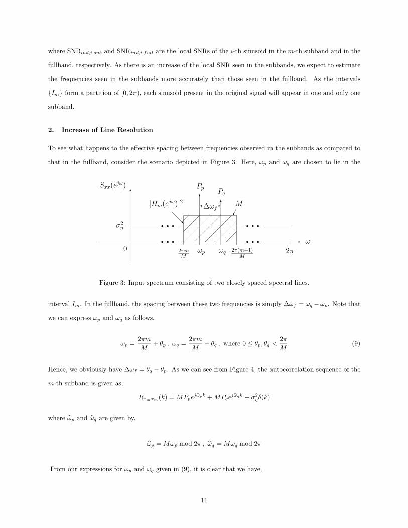
To see what happens to the effective spacing between frequencies observed in the subbands as compared to

that in the fullband, consider the scenario depicted in Figure 3. Here, ωp and ωq are chosen to lie in the

�

σ2η

0

Sxx(ejω)

� ω2π

��|Hm(ejω)|2

�

M

�

2πmM

2π(m+1)M

ωp ωq

PpPq

∆ωf� �

Figure 3: Input spectrum consisting of two closely spaced spectral lines.

interval Im. In the fullband, the spacing between these two frequencies is simply ∆ωf = ωq − ωp. Note that

we can express ωp and ωq as follows.

ωp =2πmM

+ θp , ωq =2πmM

+ θq , where 0 ≤ θp, θq <2πM

(9)

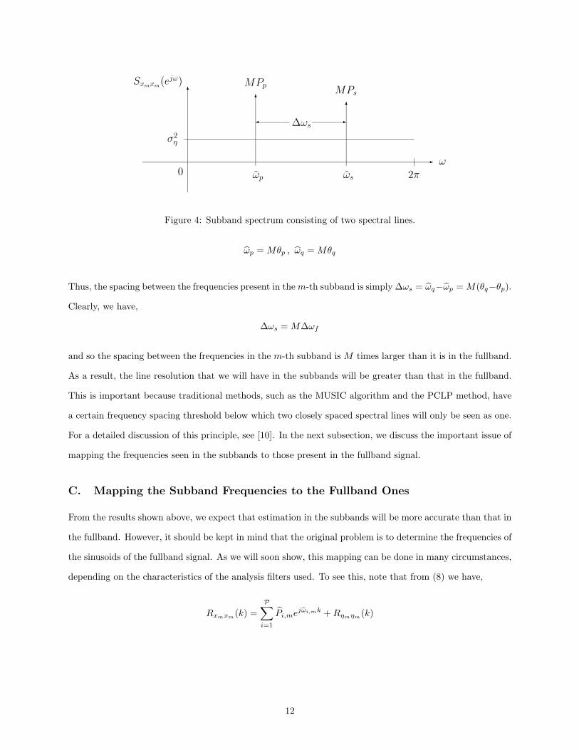
Hence, we obviously have ∆ωf = θq − θp. As we can see from Figure 4, the autocorrelation sequence of the

m-th subband is given as,

Rxmxm(k) = MPpe

jωpk +MPqejωqk + σ2

ηδ(k)

where ωp and ωq are given by,

ωp = Mωp mod 2π , ωq = Mωq mod 2π

From our expressions for ωp and ωq given in (9), it is clear that we have,

11

�

�

σ2η

0

Sxmxm(ejω)

ω2π

��

ωp ωs

MPpMPs

∆ωs� �

Figure 4: Subband spectrum consisting of two spectral lines.

ωp = Mθp , ωq = Mθq

Thus, the spacing between the frequencies present in them-th subband is simply ∆ωs = ωq−ωp = M(θq−θp).Clearly, we have,

∆ωs = M∆ωf

and so the spacing between the frequencies in the m-th subband is M times larger than it is in the fullband.

As a result, the line resolution that we will have in the subbands will be greater than that in the fullband.

This is important because traditional methods, such as the MUSIC algorithm and the PCLP method, have

a certain frequency spacing threshold below which two closely spaced spectral lines will only be seen as one.

For a detailed discussion of this principle, see [10]. In the next subsection, we discuss the important issue of

mapping the frequencies seen in the subbands to those present in the fullband signal.

C. Mapping the Subband Frequencies to the Fullband Ones

From the results shown above, we expect that estimation in the subbands will be more accurate than that in

the fullband. However, it should be kept in mind that the original problem is to determine the frequencies of

the sinusoids of the fullband signal. As we will soon show, this mapping can be done in many circumstances,

depending on the characteristics of the analysis filters used. To see this, note that from (8) we have,

Rxmxm(k) =

P∑i=1

Pi,mejωi,mk +Rηmηm

(k)

12

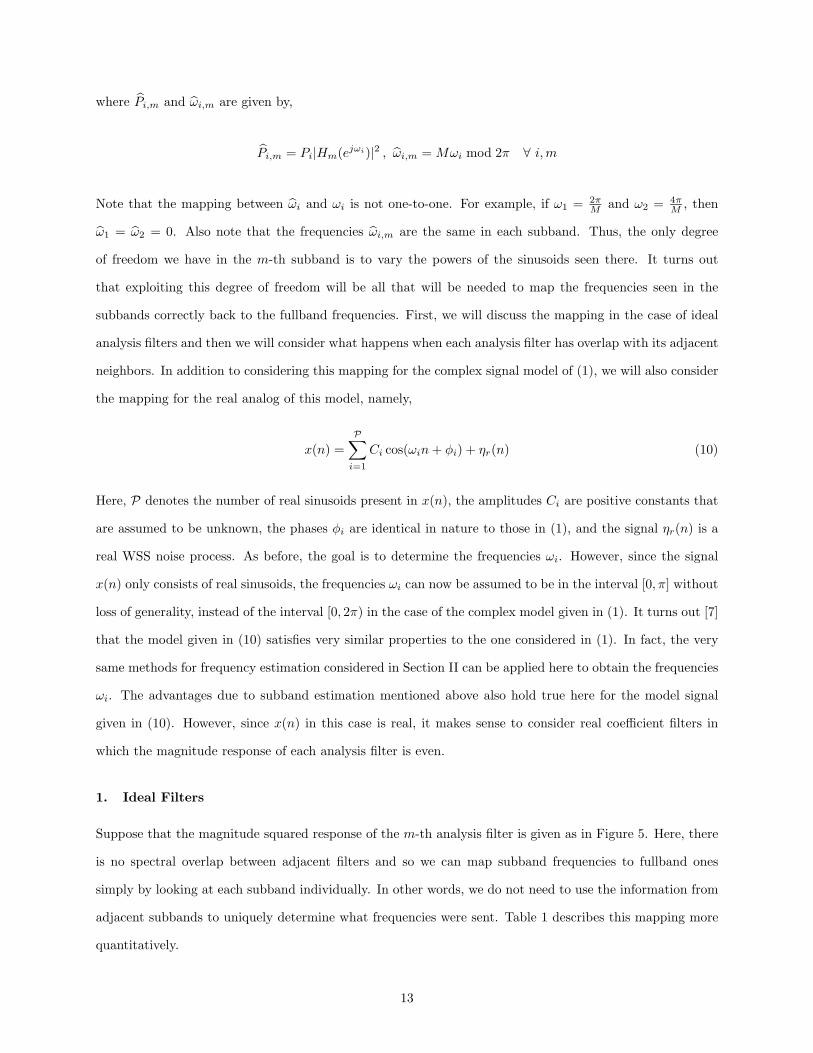
where Pi,m and ωi,m are given by,

Pi,m = Pi|Hm(ejωi)|2 , ωi,m = Mωi mod 2π ∀ i,m

Note that the mapping between ωi and ωi is not one-to-one. For example, if ω1 = 2πM and ω2 = 4π

M , then

ω1 = ω2 = 0. Also note that the frequencies ωi,m are the same in each subband. Thus, the only degree

of freedom we have in the m-th subband is to vary the powers of the sinusoids seen there. It turns out

that exploiting this degree of freedom will be all that will be needed to map the frequencies seen in the

subbands correctly back to the fullband frequencies. First, we will discuss the mapping in the case of ideal

analysis filters and then we will consider what happens when each analysis filter has overlap with its adjacent

neighbors. In addition to considering this mapping for the complex signal model of (1), we will also consider

the mapping for the real analog of this model, namely,

x(n) =P∑i=1

Ci cos(ωin+ φi) + ηr(n) (10)

Here, P denotes the number of real sinusoids present in x(n), the amplitudes Ci are positive constants that

are assumed to be unknown, the phases φi are identical in nature to those in (1), and the signal ηr(n) is a

real WSS noise process. As before, the goal is to determine the frequencies ωi. However, since the signal

x(n) only consists of real sinusoids, the frequencies ωi can now be assumed to be in the interval [0, π] without

loss of generality, instead of the interval [0, 2π) in the case of the complex model given in (1). It turns out [7]

that the model given in (10) satisfies very similar properties to the one considered in (1). In fact, the very

same methods for frequency estimation considered in Section II can be applied here to obtain the frequencies

ωi. The advantages due to subband estimation mentioned above also hold true here for the model signal

given in (10). However, since x(n) in this case is real, it makes sense to consider real coefficient filters in

which the magnitude response of each analysis filter is even.

1. Ideal Filters

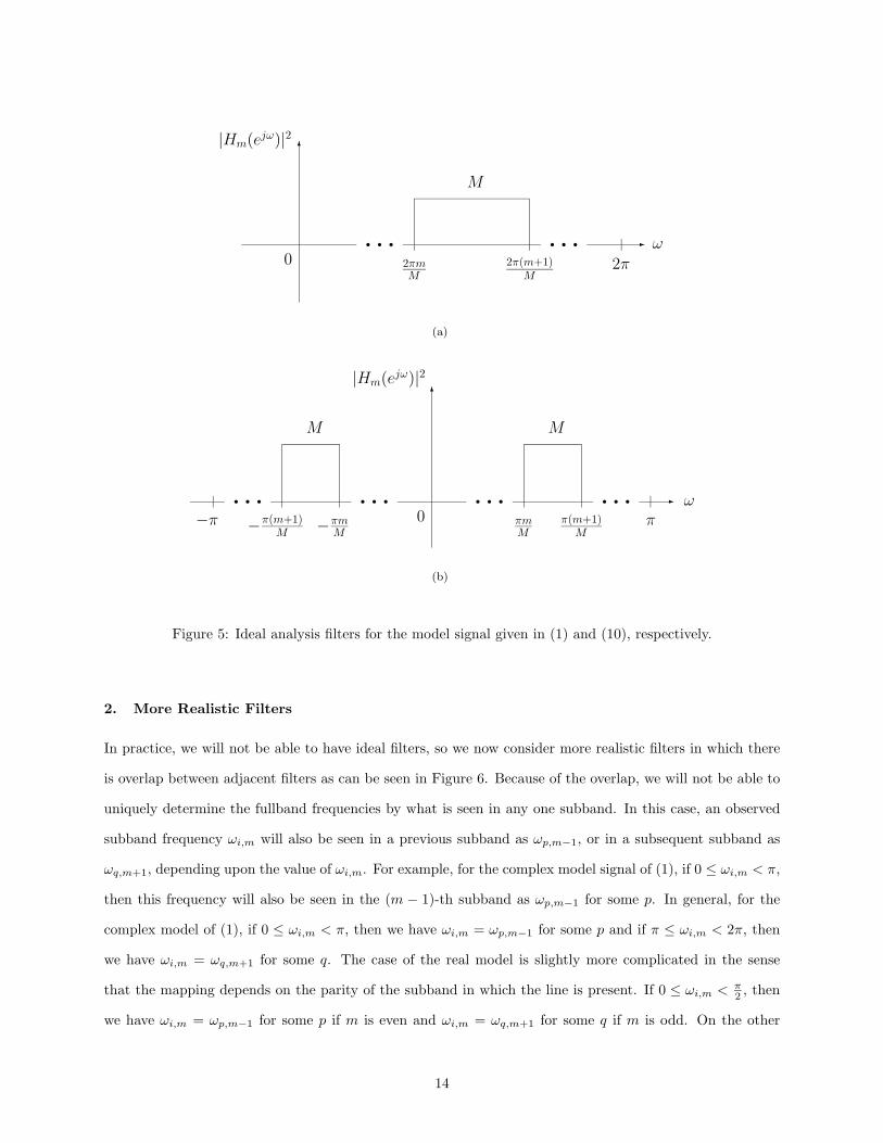
Suppose that the magnitude squared response of the m-th analysis filter is given as in Figure 5. Here, there

is no spectral overlap between adjacent filters and so we can map subband frequencies to fullband ones

simply by looking at each subband individually. In other words, we do not need to use the information from

adjacent subbands to uniquely determine what frequencies were sent. Table 1 describes this mapping more

quantitatively.

13

�

� � � � � � �

2πω

0

|Hm(ejω)|2

2πmM

2π(m+1)M

M

(a)

�

0

|Hm(ejω)|2

� � � � � � � ωπ

M

πmM

π(m+1)M

������

−π

M

−πmM−π(m+1)

M

(b)

Figure 5: Ideal analysis filters for the model signal given in (1) and (10), respectively.

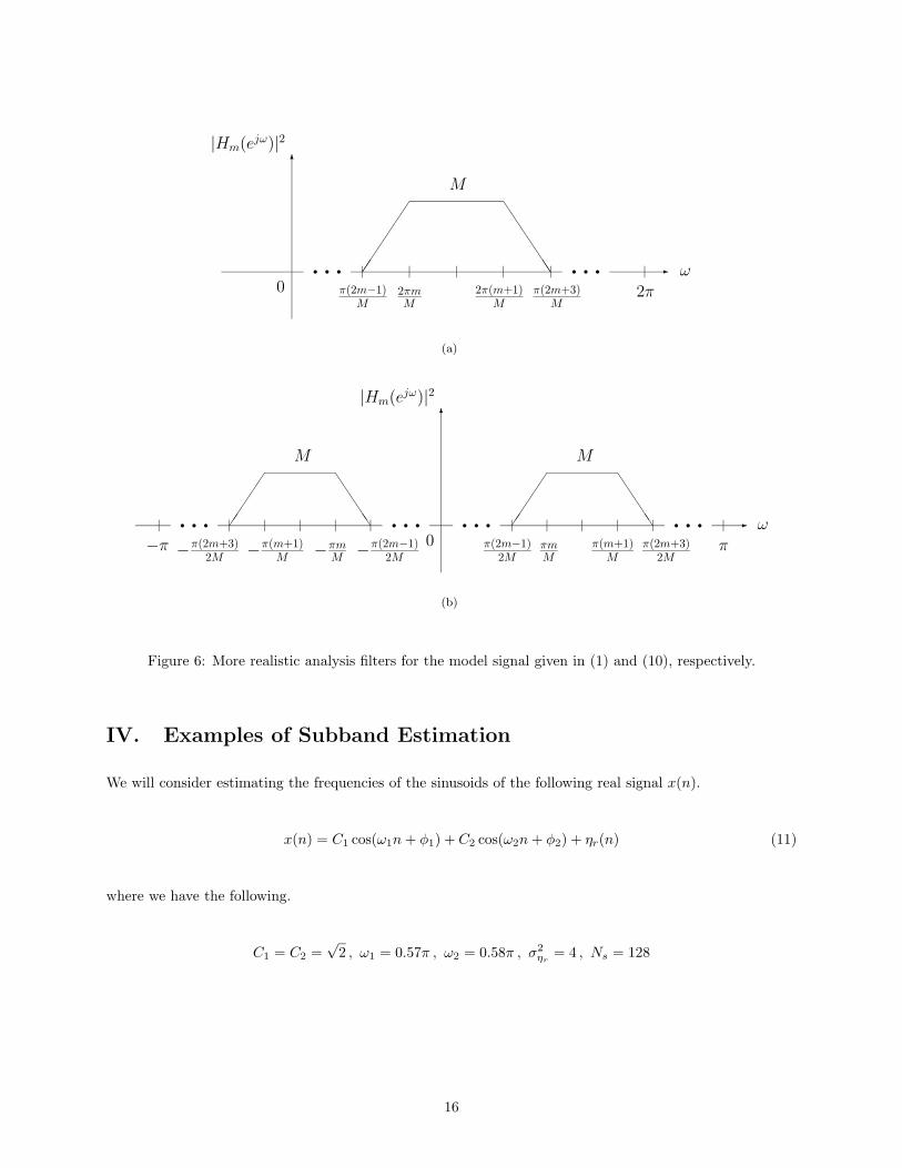
2. More Realistic Filters

In practice, we will not be able to have ideal filters, so we now consider more realistic filters in which there

is overlap between adjacent filters as can be seen in Figure 6. Because of the overlap, we will not be able to

uniquely determine the fullband frequencies by what is seen in any one subband. In this case, an observed

subband frequency ωi,m will also be seen in a previous subband as ωp,m−1, or in a subsequent subband as

ωq,m+1, depending upon the value of ωi,m. For example, for the complex model signal of (1), if 0 ≤ ωi,m < π,

then this frequency will also be seen in the (m − 1)-th subband as ωp,m−1 for some p. In general, for the

complex model of (1), if 0 ≤ ωi,m < π, then we have ωi,m = ωp,m−1 for some p and if π ≤ ωi,m < 2π, then

we have ωi,m = ωq,m+1 for some q. The case of the real model is slightly more complicated in the sense

that the mapping depends on the parity of the subband in which the line is present. If 0 ≤ ωi,m < π2 , then

we have ωi,m = ωp,m−1 for some p if m is even and ωi,m = ωq,m+1 for some q if m is odd. On the other

14

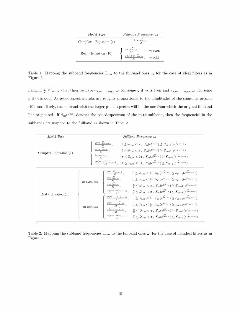
Model Type Fullband Frequency: ωl

Complex - Equation (1) 2πm+ωi,m

M

Real - Equation (10)

πm+ωi,m

M , m evenπ(m+1)−ωi,m

M , m odd

Table 1: Mapping the subband frequencies ωi,m to the fullband ones ωl for the case of ideal filters as inFigure 5.

hand, if π2 ≤ ωi,m < π, then we have ωi,m = ωq,m+1 for some q if m is even and ωi,m = ωp,m−1 for some

p if m is odd. As pseudospectra peaks are roughly proportional to the amplitudes of the sinusoids present

[10], most likely, the subband with the larger psuedospectra will be the one from which the original fullband

line originated. If Sm(ejω) denotes the psuedospectrum of the m-th subband, then the frequencies in the

subbands are mapped to the fullband as shown in Table 2.

Model Type Fullband Frequency: ωl

Complex - Equation (1)

2πm−ωp,m−1M , 0 ≤ ωi,m < π , Sm(ejωi,m) ≤ Sm−1(ejωp,m−1)

2πm+ωi,m

M , 0 ≤ ωi,m < π , Sm(ejωi,m) ≥ Sm−1(ejωp,m−1)2πm+ωi,m

M , π ≤ ωi,m < 2π , Sm(ejωi,m) ≥ Sm+1(ejωq,m+1)2π(m+2)−ωq,m+1

M , π ≤ ωi,m < 2π , Sm(ejωi,m) ≤ Sm+1(ejωq,m+1)

Real - Equation (10)

m even =⇒

πm−ωp,m−1M , 0 ≤ ωi,m < π

2 , Sm(ejωi,m) ≤ Sm−1(ejωp,m−1)πm+ωi,m

M , 0 ≤ ωi,m < π2 , Sm(ejωi,m) ≥ Sm−1(ejωp,m−1)

πm+ωi,m

M , π2 ≤ ωi,m < π , Sm(ejωi,m) ≥ Sm+1(ejωq,m+1)

π(m+2)−ωq,m+1M , π

2 ≤ ωi,m < π , Sm(ejωi,m) ≤ Sm+1(ejωq,m+1)

m odd =⇒

π(m+1)+ωq,m+1M , 0 ≤ ωi,m < π

2 , Sm(ejωi,m) ≤ Sm+1(ejωq,m+1)π(m+1)−ωi,m

M , 0 ≤ ωi,m < π2 , Sm(ejωi,m) ≥ Sm+1(ejωq,m+1)

π(m+1)−ωi,m

M , π2 ≤ ωi,m < π , Sm(ejωi,m) ≥ Sm−1(ejωp,m−1)

π(m−1)+ωp,m−1M , π

2 ≤ ωi,m < π , Sm(ejωi,m) ≤ Sm−1(ejωp,m−1)

Table 2: Mapping the subband frequencies ωi,m to the fullband ones ωl for the case of nonideal filters as inFigure 6.

15

�

0

|Hm(ejω)|2

� � � � � � �

��

��

���

��

��

��� ω

2π

M

π(2m−1)M

π(2m+3)M

2πmM

2π(m+1)M

(a)

�

0

|Hm(ejω)|2

� � � � � � � ωπ

��

���

��

���

M

π(2m−1)2M

π(2m+3)2M

πmM

π(m+1)M

������

−π

��

���

��

���

M

−π(2m−1)2M−π(2m+3)

2M −πmM−π(m+1)

M

(b)

Figure 6: More realistic analysis filters for the model signal given in (1) and (10), respectively.

IV. Examples of Subband Estimation

We will consider estimating the frequencies of the sinusoids of the following real signal x(n).

x(n) = C1 cos(ω1n+ φ1) + C2 cos(ω2n+ φ2) + ηr(n) (11)

where we have the following.

C1 = C2 =√

2 , ω1 = 0.57π , ω2 = 0.58π , σ2ηr

= 4 , Ns = 128

16

In this case, we have,

SNRind,1 = SNRind,2 = −6.02 (dB) , SNRnet = −3.01 (dB)

It should be noted here that as there are only Ns = 128 observations of x(n) and the two frequencies are

spaced out by 0.01π < 2π128 , we cannot find the frequencies by taking the Fourier transform of the observed

signal. As the input signal x(n) is real like the model given in (10), we will consider only cosine modulated

analysis filter banks. In order to keep the number of observed samples seen in the subbands relatively

moderate (see Part E of this section), the value of M is chosen to be 8. In the examples that follow, the

estimation was carried out 50 times using a different observation of x(n) each time.

Example 1. Kaiser-Window Based Prototype Cosine Modulated Filter Bank

In this example, the impulse responses of the analysis filters are given by [18],

hk(n) = 2p0(n) cos[π

M

(k +

12

)(n− Np

2

)+ (−1)k

π

4

](12)

for all k, n. Here, the sequence p0(n) is an FIR prototype filter of length Np so that hk(n) has length Np as

well. The choice of p0(n) dictates the type of filter bank that we have. In this case, p0(n) was designed using

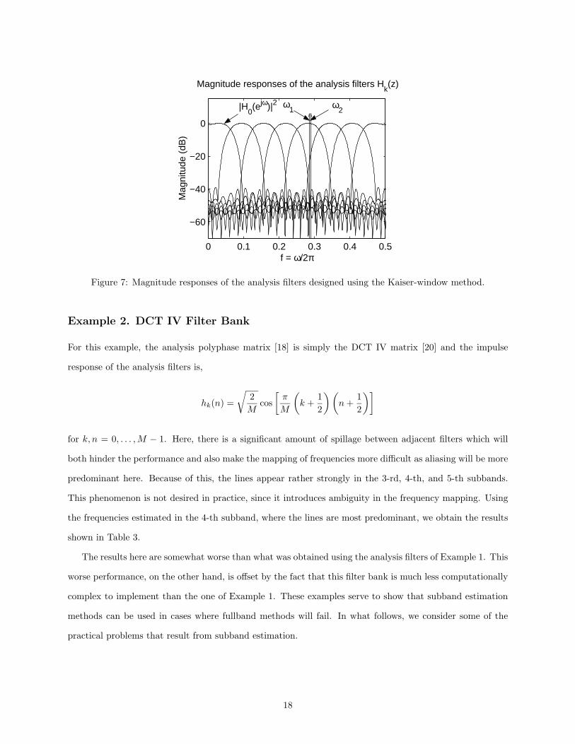
the Kaiser-window method as described in [8]. The length of each analysis filter here is Np = 40. Figure 7

shows the magnitude responses of the analysis filters. As we can see, the frequencies of the sinusoids present

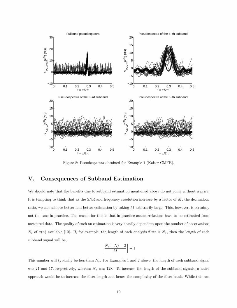
in (11) fall predominantly in the 3-rd, 4-th, and 5-th subbands. The pseudospecta obtained here for the

fullband, as well as the 3-rd, 4-th, and 5-th subbands are shown in Figure 8. As we can see, the pseudospecta

seen in the fullband only appear to consist of one predominant peak and we are not able to resolve both

sinusoids. However, in the subband pseudospectra, we can clearly see the presence of two distinct lines. As

the analysis filters provide good attenuation in the stopband, there is little overlap between adjacent filters

and so the lines present in the 4-th subband are heavily attenuated in the adjacent 3-rd and 5-th subbands,

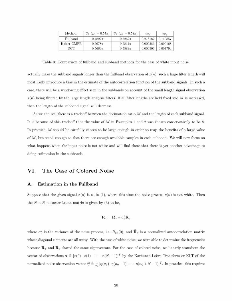
as is desired here. Performing the frequency mapping described in the previous section, we obtain the mean

and standard deviation of the estimates of ω1 and ω2 shown in Table 3. Included in Table 3 are the results

obtained by carrying out the estimation in the fullband. Here, we see that estimation in the subbands yielded

better results.

17

0 0.1 0.2 0.3 0.4 0.5

−60

−40

−20

0

f = ω/2π

Mag

nitu

de (

dB)

Magnitude responses of the analysis filters Hk(z)

|H0(ejω)|2 ω

1 ω2

Figure 7: Magnitude responses of the analysis filters designed using the Kaiser-window method.

Example 2. DCT IV Filter Bank

For this example, the analysis polyphase matrix [18] is simply the DCT IV matrix [20] and the impulse

response of the analysis filters is,

hk(n) =

√2M

cos[π

M

(k +

12

)(n+

12

)]

for k, n = 0, . . . ,M − 1. Here, there is a significant amount of spillage between adjacent filters which will

both hinder the performance and also make the mapping of frequencies more difficult as aliasing will be more

predominant here. Because of this, the lines appear rather strongly in the 3-rd, 4-th, and 5-th subbands.

This phenomenon is not desired in practice, since it introduces ambiguity in the frequency mapping. Using

the frequencies estimated in the 4-th subband, where the lines are most predominant, we obtain the results

shown in Table 3.

The results here are somewhat worse than what was obtained using the analysis filters of Example 1. This

worse performance, on the other hand, is offset by the fact that this filter bank is much less computationally

complex to implement than the one of Example 1. These examples serve to show that subband estimation

methods can be used in cases where fullband methods will fail. In what follows, we consider some of the

practical problems that result from subband estimation.

18

0 0.1 0.2 0.3 0.4 0.5−10

0

10

20

30

f = ω/2π

SP

CLP

,full(e

jω)

(dB

)

Fullband pseudospectra

0 0.1 0.2 0.3 0.4 0.5−10

−5

0

5

10

15

20

f = ω/2π

SP

CLP

,4(e

jω)

(dB

)

Pseudospectra of the 4−th subband

0 0.1 0.2 0.3 0.4 0.5−10

−5

0

5

10

15

20

f = ω/2π

SP

CLP

,3(e

jω)

(dB

)

Pseudospectra of the 3−rd subband

0 0.1 0.2 0.3 0.4 0.5−10

−5

0

5

10

15

20

f = ω/2π

SP

CLP

,5(e

jω)

(dB

)

Pseudospectra of the 5−th subband

Figure 8: Pseudospectra obtained for Example 1 (Kaiser CMFB).

V. Consequences of Subband Estimation

We should note that the benefits due to subband estimation mentioned above do not come without a price.

It is tempting to think that as the SNR and frequency resolution increase by a factor of M , the decimation

ratio, we can achieve better and better estimation by taking M arbitrarily large. This, however, is certainly

not the case in practice. The reason for this is that in practice autocorrelations have to be estimated from

measured data. The quality of such an estimation is very heavily dependent upon the number of observations

Ns of x(n) available [10]. If, for example, the length of each analysis filter is Nf , then the length of each

subband signal will be, ⌊Ns +Nf − 2

M

⌋+ 1

This number will typically be less than Ns. For Examples 1 and 2 above, the length of each subband signal

was 21 and 17, respectively, whereas Ns was 128. To increase the length of the subband signals, a naive

approach would be to increase the filter length and hence the complexity of the filter bank. While this can

19

Method ω1 (ω1 = 0.57π) ω2 (ω2 = 0.58π) σω1 σω2

Fullband 0.4892π 0.6262π 0.278182 0.110857Kaiser CMFB 0.5678π 0.5817π 0.000286 0.000168

DCT 0.5664π 0.5883π 0.000506 0.001794

Table 3: Comparison of fullband and subband methods for the case of white input noise.

actually make the subband signals longer than the fullband observation of x(n), such a large filter length will

most likely introduce a bias in the estimate of the autocorrelation function of the subband signals. In such a

case, there will be a windowing effect seen in the subbands on account of the small length signal observation

x(n) being filtered by the large length analysis filters. If all filter lengths are held fixed and M is increased,

then the length of the subband signal will decrease.

As we can see, there is a tradeoff between the decimation ratio M and the length of each subband signal.

It is because of this tradeoff that the value of M in Examples 1 and 2 was chosen conservatively to be 8.

In practice, M should be carefully chosen to be large enough in order to reap the benefits of a large value

of M , but small enough so that there are enough available samples in each subband. We will now focus on

what happens when the input noise is not white and will find there that there is yet another advantage to

doing estimation in the subbands.

VI. The Case of Colored Noise

A. Estimation in the Fullband

Suppose that the given signal x(n) is as in (1), where this time the noise process η(n) is not white. Then

the N ×N autocorrelation matrix is given by (3) to be,

Rx = Rs + σ2ηRη

where σ2η is the variance of the noise process, i.e. Rηη(0), and Rη is a normalized autocorrelation matrix

whose diagonal elements are all unity. With the case of white noise, we were able to determine the frequencies

because Rx and Rs shared the same eigenvectors. For the case of colored noise, we linearly transform the

vector of observations x � [x(0) x(1) · · · x(N − 1)]T by the Karhunen-Loeve Transform or KLT of the

normalized noise observation vector η � 1ση

[η(n0) η(n0 + 1) · · · η(n0 +N − 1)]T . In practice, this requires

20

first estimating Rη. The KLT is given by [16] as the following.

y � R− 12

η x

This transformation diagonalizes Rη. We have,

Ry = E[yy†] = E[R− 1

2η xx†R− 1

2η

]= R− 1

2η RxR

− 12

η

where we have exploited the fact that R− 12

η is Hermitian. As Rx can be estimated from the data, then we

can form an estimate of Ry provided that we know the coloring of the noise process as manifested in the

matrix Rη. To determine the frequencies of the original sinusoids, note that from (3) we have,

Ry =P∑i=1

Pitit†i︸ ︷︷ ︸

Rt

+σ2ηI (13)

where the vectors ti are defined to be,

ti � R− 12

η si (14)

As the vectors si are assumed to be linearly independent, assuming that the frequencies present in the input

signal x(n) are all distinct modulo 2π [7], the vectors ti are all linearly independent. Thus, provided that

N > P, the matrix Rt in (13) is of rank P and furthermore the P eigenvectors {uk} for k = 1, . . . ,Pwhich correspond to the nonzero eigenvalues of Rt span the same subspace as the set of vectors {ti}. This

was the same phenomenon observed in Rs in Section II. Also, the eigenvectors of Rt which correspond to

the zero eigenvalue, {uk} for k = P + 1, . . . , N , are orthogonal to the vectors ti, namely t†iuk = 0 for all

i = 1, . . . ,P and k = P + 1, . . . , N . Using (14), this means that s†i (R− 1

2η uk) = 0 or that the generalized

eigenfilter corresponding to R− 12

η uk = [wk(0) wk(1) · · · wk(N − 1) ]T , namely,

Wk(z) �N−1∑n=0

wk(n)z−n

has a zero at z = ejωi for all i = 1, . . . ,P and k = P + 1, . . . , N . From this property, we can obtain the

original frequencies using either the MUSIC algorithm or PCLP method.

It should be noted that we can estimate the frequencies only if we know the noise autocorrelation matrix

Rη. In practice, however, we may not know the exact statistics of the input noise. Despite this stumbling

21

block, we will soon show that if the signal x(n) is input to a particular kind of analysis bank, then, on average,

the noise processes seen in the subbands will be more white in terms of the spectral flatness measure. There

will even be some instances in which the flatness in each subband is strictly larger than that seen in the

fullband. Hence, if we do not know the exact statistics of the noise process η(n), then assuming that the

noise is white in the subbands will be less erroneous than assuming that it is in the fullband. This will be

illustrated with examples.

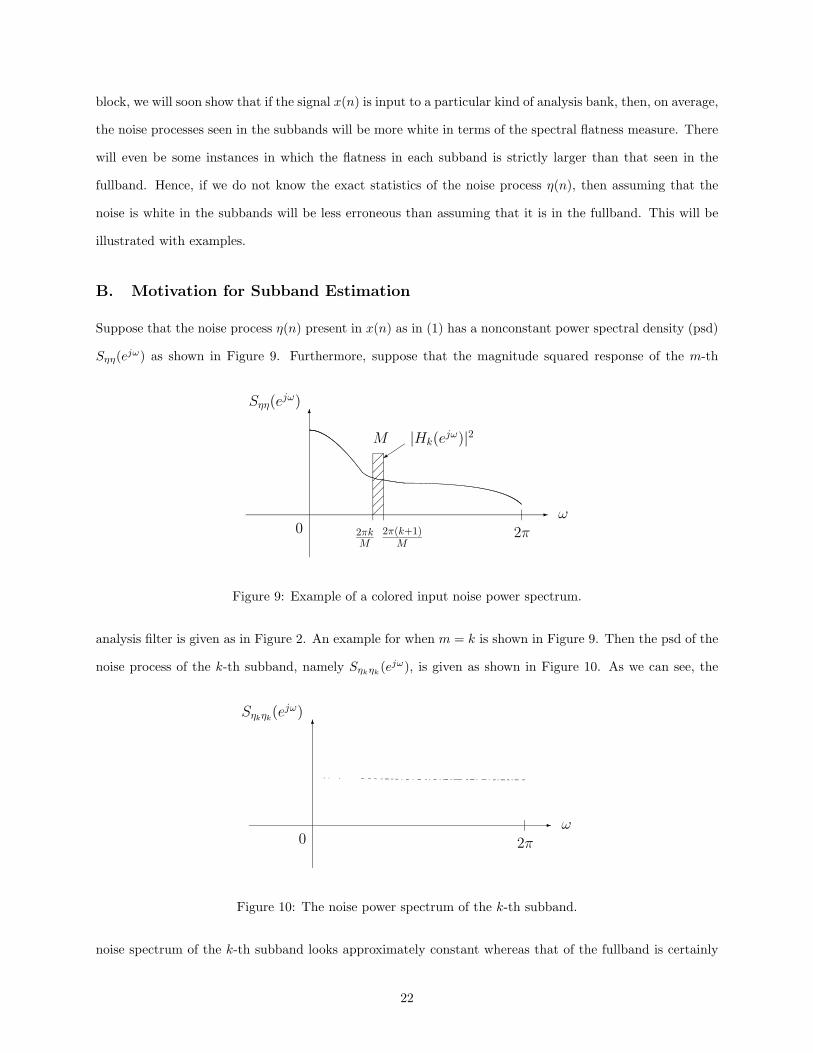
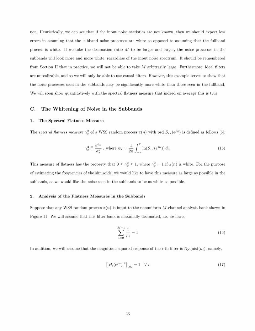
B. Motivation for Subband Estimation

Suppose that the noise process η(n) present in x(n) as in (1) has a nonconstant power spectral density (psd)

Sηη(ejω) as shown in Figure 9. Furthermore, suppose that the magnitude squared response of the m-th

�

�

0

Sηη(ejω)

ω2π2πk

M2π(k+1)

M

M |Hk(ejω)|2

�

Figure 9: Example of a colored input noise power spectrum.

analysis filter is given as in Figure 2. An example for when m = k is shown in Figure 9. Then the psd of the

noise process of the k-th subband, namely Sηkηk(ejω), is given as shown in Figure 10. As we can see, the

�

�

0

Sηkηk(ejω)

ω2π

Figure 10: The noise power spectrum of the k-th subband.

noise spectrum of the k-th subband looks approximately constant whereas that of the fullband is certainly

22

not. Heuristically, we can see that if the input noise statistics are not known, then we should expect less

errors in assuming that the subband noise processes are white as opposed to assuming that the fullband

process is white. If we take the decimation ratio M to be larger and larger, the noise processes in the

subbands will look more and more white, regardless of the input noise spectrum. It should be remembered

from Section II that in practice, we will not be able to take M arbitrarily large. Furthermore, ideal filters

are unrealizable, and so we will only be able to use causal filters. However, this example serves to show that

the noise processes seen in the subbands may be significantly more white than those seen in the fullband.

We will soon show quantitatively with the spectral flatness measure that indeed on average this is true.

C. The Whitening of Noise in the Subbands

1. The Spectral Flatness Measure

The spectral flatness measure γ2x of a WSS random process x(n) with psd Sxx(ejω) is defined as follows [5].

γ2x � eψx

σ2x

, where ψx =12π

∫ π

−πln(Sxx(ejω)) dω (15)

This measure of flatness has the property that 0 ≤ γ2x ≤ 1, where γ2

x = 1 if x(n) is white. For the purpose

of estimating the frequencies of the sinusoids, we would like to have this measure as large as possible in the

subbands, as we would like the noise seen in the subbands to be as white as possible.

2. Analysis of the Flatness Measures in the Subbands

Suppose that any WSS random process x(n) is input to the nonuniform M -channel analysis bank shown in

Figure 11. We will assume that this filter bank is maximally decimated, i.e. we have,

M−1∑i=0

1ni

= 1 (16)

In addition, we will assume that the magnitude squared response of the i-th filter is Nyquist(ni), namely,

[|Hi(ejω)|2]↓ni= 1 ∀ i (17)

23

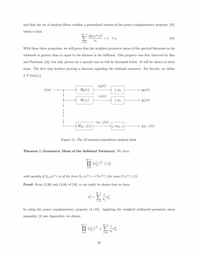
and that the set of analysis filters satisfies a generalized version of the power complementary property [19],

which is that,M−1∑i=0

|Hi(ejω)|2ni

= 1 ∀ ω (18)

With these three properties, we will prove that the weighted geometric mean of the spectral flatnesses in the

subbands is greater than or equal to the flatness in the fullband. This property was first observed by Rao

and Pearlman [12], but only proven for a special case as will be discussed below. It will be shown in three

steps. The first step involves proving a theorem regarding the subband variances. For brevity, we define

L � lcm{ni}.

x(n) � �

�

�

�

�

�

�

�

�

�

� HM−1(z)

H1(z)

H0(z) �

�

�vM−1(n)

v1(n)

v0(n)↓ n0

↓ n1

↓ nM−1

�

�

�

y0(n)

y1(n)

yM−1(n)

Figure 11: The M -channel nonuniform analysis bank.

Theorem 1 (Geometric Mean of the Subband Variances) We have,

M−1∏i=0

(σ2yi

) 1ni ≤ σ2

x ,

with equality if Sxx(ejω) is of the form Sxx(ejω) = C(ejLω) for some C(ejω) ≥ 0.

Proof: From (3.36) and (3.40) of [19], it can easily be shown that we have,

σ2x =

M−1∑i=0

1niσ2yi

by using the power complementary property of (18). Applying the weighted arithmetic-geometric mean

inequality [4] (see Appendix), we obtain,

M−1∏i=0

(σ2yi

) 1ni ≤

M−1∑i=0

1niσ2yi

24

which then proves the inequality. If Sxx(ejω) = C(ejLω), for some C(ejω) ≥ 0, note that we have, for any

i = 0, . . . ,M − 1 and l = 0, . . . , ni − 1,

Sxx

(ej(

ω−2πlni

))= C(ejNi(ω−2πl)) = C(ejNiω)

where Ni � Lni

is an integer for all i. Then, it can easily be shown that,

Syiyi(ejω) = C(ejNiω)

using the Nyquist(ni) property from (17). From this, a straightforward calculation shows that,

σ2yi

= σ2x

from which we obtain,

M−1∏i=0

(σ2yi

) 1ni =

(σ2x

)M−1∑i=0

1ni = σ2

x

The last step here follows from the fact that the filter bank is maximally decimated (16). This completes

the proof.���

We now prove a result regarding the quantity ψ given in (15).

Theorem 2 (Arithmetic Mean of the Subband ψ’s) We have,

M−1∑i=0

1niψyi

≥ ψx ,

with equality iff Sxx(ejω) is of the form Sxx(ejω) = C(ejLω) for some C(ejω) ≥ 0.

Proof: From the log-sum inequality [1] (see Appendix), if al and bl are nonnegative numbers for l ∈ I, where

I is some index set, and the sequence {al} is a probability density function (pdf) such that∑l∈I al = 1,

then we have,

ln

(∑l∈I

bl

)≥∑l∈I

al lnblal

25

with equality iff bl = Kal for all l and for some K ≥ 0. Hence, for any pdf {al,i} such that∑l∈Ii

al,i = 1 for

all i = 0, . . . ,M − 1, where Ii = {0, . . . , ni − 1}, we have, as the psd of any random process is nonnegative,

ln

(1ni

ni−1∑l=0

Svivi

(ej(

ω−2πlni

)))≥ni−1∑l=0

al,i ln

1niSvivi

(ej(

ω−2πlni

))al,i

∀ ω, i

with equality iff 1niSvivi

(ej(

ω−2πlni

))= Kial,i for all l, i where Ki ≥ 0 for all i. Let us choose al,i as

al,i = 1ni

∣∣∣∣Hi

(ej(

ω−2πlni

))∣∣∣∣2 for all l, i. This choice is valid since by (17), we have,

1ni

ni−1∑l=0

∣∣∣∣Hi

(ej(

ω−2πlni

))∣∣∣∣2 = 1 ∀ i

and so indeed {al,i} is a pdf for all i. With this choice, we have, for all ω, i.

ln

(1ni

ni−1∑l=0

Svivi

(ej(

ω−2πlni

)))≥

ni−1∑l=0

1ni

∣∣∣∣Hi

(ej(

ω−2πlni

))∣∣∣∣2 ln

1niSvivi

(ej(

ω−2πlni

))1ni

∣∣∣∣Hi

(ej(

ω−2πlni

))∣∣∣∣2

=1ni

ni−1∑l=0

∣∣∣∣Hi

(ej(

ω−2πlni

))∣∣∣∣2 ln(Sxx

(ej(

ω−2πlni

)))(19)

with equality iff Sxx

(ej(

ω−2πlni

))= Ki for all ω, l, i. This condition for equality is equivalent to saying that

Sxx(ejω) is periodic with period 2πL . As the above is true for all ω, we thus have the following.

ψyi=

12π

∫ π

−πln

(1ni

ni−1∑l=0

Svivi

(ej(

ω−2πlni

)))dω

≥ 12πni

ni−1∑l=0

∫ π

−π

∣∣∣∣Hi

(ej(

ω−2πlni

))∣∣∣∣2 ln(Sxx

(ej(

ω−2πlni

)))dω

=12π

ni−1∑l=0

∫ π−2πlni

−π−2πlni

|Hi(ejλ)|2 ln(Sxx(ejλ)) dλ

=12π

∫ π

−π|Hi(ejω)|2 ln(Sxx(ejω)) dω (20)

26

It should be noted that this is true for all i with equality iff Sxx(ejω) is of the form Sxx(ejω) = C(ejLω) for

some C(ejω) ≥ 0. As (20) is true for all i, we have,

M−1∑i=0

1niψyi

≥ 12π

∫ π

−π

(M−1∑i=0

|Hi(ejω)|2ni

)ln(Sxx(ejω)) dω

=12π

∫ π

−πln(Sxx(ejω)) dω = ψx (21)

Here, (21) follows from the generalized power complementary property (18). As we have equality iff Sxx(ejω)

is of the form Sxx(ejω) = C(ejLω), this completes the proof of Theorem 2.���

From Theorem 2, we have the following important corollary if the input process x(n) is Gaussian. This is

important from the point of view of information theory. It is a generalization of a result given originally

by Rao and Pearlman [12], in which only ideal analysis filters were considered and the authors eventually

restricted the ni’s to be identical for all i.

Corollary 1 (Differential Entropy Rate) If the input x(n) to the nonuniform filter bank in Figure 11 is

a Gaussian WSS process and hx and hyidenote, respectively, the differential entropy rates of x(n) and the

i-th subband process yi(n), then we have,M−1∑i=0

1nihyi

≥ hx

with equality iff Sxx(ejω) is of the form Sxx(ejω) = C(ejLω) for some C(ejω) ≥ 0.

Proof: If x(n) is Gaussian, then its differential entropy rate is given by [1] to be,

hx =12

ln(2πe) +14π

∫ π

−πln(Sxx(ejω)) dω =

12

ln(2πe) +12ψx

As x(n) is assumed Gaussian, it follows that the signals vi(n) are also Gaussian, since the analysis filters

{Hi(z)} are linear. Furthermore, as vi(n) is Gaussian for all i, it follows that yi(n) is Gaussian for all i as

well, since decimators are also linear systems. Hence, the differential entropy rate of yi(n) is given by,

hyi=

12

ln(2πe) +12ψyi

So, using Theorem 2 and the fact that the filter bank is maximally decimated (16), we immediately obtain,

M−1∑i=0

1nihyi

≥ 12

ln(2πe) +12ψx = hx

27

with equality iff Sxx(ejω) = C(ejLω). This completes the proof.���

We now conclude this section with the main result regarding the geometric mean of the flatness measures of

the subband signals.

Theorem 3 (Geometric Mean of the Subband Flatness Measures) Let the input to the analysis fil-

ter bank of Figure 11 be a WSS random process x(n) with spectral flatness measure γ2x. If the filter bank is

such that (16), (17), and (18) hold, then we have,

γ2y �

M−1∏i=0

(γ2yi

) 1ni ≥ γ2

x

with equality if Sxx(ejω) is of the form Sxx(ejω) = C(ejLω) for some C(ejω) ≥ 0 where L = lcm{ni}.

Proof: We have the following.

γ2y =

exp

(M−1∑i=0

1niψyi

)M−1∏i=0

(σ2yi

) 1ni

≥exp

(M−1∑i=0

1niψyi

)σ2x

≥ eψx

σ2x

= γ2x (22)

Here, (22) results from first using Theorem 1 and then using Theorem 2 and the fact that the exponential

function is a monotonic increasing function. As a sufficient condition for equality in (22) is that Sxx(ejω) =

C(ejLω) for some C(ejω) ≥ 0, this completes the proof.���

This theorem is a generalization and a correction of a result given by Rao and Pearlman [12]. In that

paper, only ideal analysis filters were considered and their expression for the analysis filter responses given

in Equation (1) was erroneous. At this point, we now proceed to present various examples of Theorem 3.

VII. Examples of Noise Flattening in the Subbands

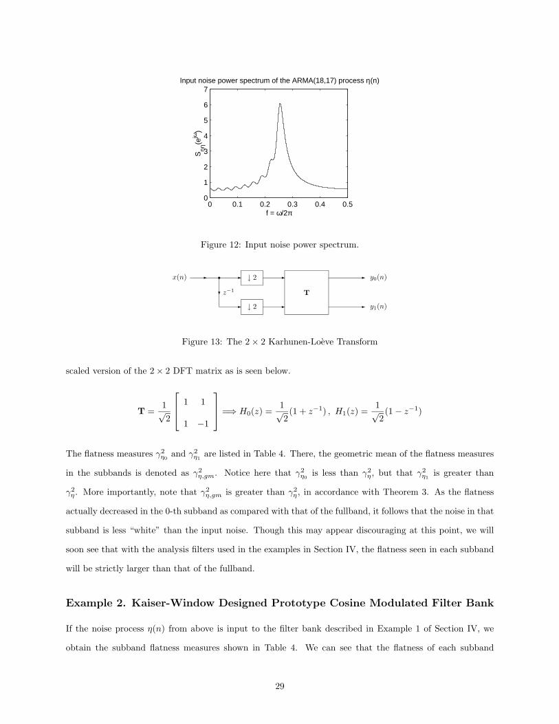
In all of the following examples, we will assume that the noise process η(n) is a real ARMA(18,17) process

with psd shown in Figure 12. The spectral flatness measure for this particular process was calculated

numerically to be γ2η = 0.7680.

Example 1. The 2 × 2 Karhunen-Loeve Transform

Consider the 2 × 2 paraunitary filter bank shown in Figure 13. Here, T is the 2 × 2 KLT which is simply a

28

0 0.1 0.2 0.3 0.4 0.50

1

2

3

4

5

6

7

f = ω/2π

Sηη

(ejω

)

Input noise power spectrum of the ARMA(18,17) process η(n)

Figure 12: Input noise power spectrum.

x(n) � �

�

�

�

z−1

�

�

T

↓ 2

↓ 2

�

�

y0(n)

y1(n)

Figure 13: The 2 × 2 Karhunen-Loeve Transform

scaled version of the 2 × 2 DFT matrix as is seen below.

T =1√2

1 1

1 −1

=⇒ H0(z) =1√2(1 + z−1) , H1(z) =

1√2(1 − z−1)

The flatness measures γ2η0 and γ2

η1 are listed in Table 4. There, the geometric mean of the flatness measures

in the subbands is denoted as γ2η,gm. Notice here that γ2

η0 is less than γ2η , but that γ2

η1 is greater than

γ2η . More importantly, note that γ2

η,gm is greater than γ2η , in accordance with Theorem 3. As the flatness

actually decreased in the 0-th subband as compared with that of the fullband, it follows that the noise in that

subband is less “white” than the input noise. Though this may appear discouraging at this point, we will

soon see that with the analysis filters used in the examples in Section IV, the flatness seen in each subband

will be strictly larger than that of the fullband.

Example 2. Kaiser-Window Designed Prototype Cosine Modulated Filter Bank

If the noise process η(n) from above is input to the filter bank described in Example 1 of Section IV, we

obtain the subband flatness measures shown in Table 4. We can see that the flatness of each subband

29

increased quite substantially over that of the fullband. Note that γ2η,gm is greater than γ2

η in accordance with

Theorem 3, even though properties (17) and (18) are only approximately satisfied for this choice of analysis

bank.

Example 3. DCT IV Filter Bank

Applying η(n) from above to the filter bank described in Example 2 of Section IV, we obtain the subband

flatness measures shown in Table 4. As with the Kaiser-window designed filter bank, the flatness of each

subband is significantly larger than that of the fullband. Note that γ2η,gm is greater than γ2

η , further verifying

Theorem 3.

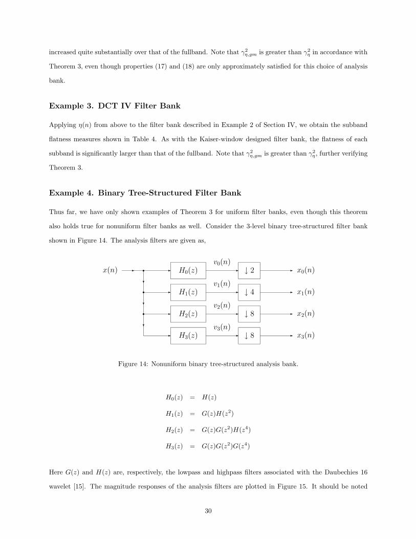
Example 4. Binary Tree-Structured Filter Bank

Thus far, we have only shown examples of Theorem 3 for uniform filter banks, even though this theorem

also holds true for nonuniform filter banks as well. Consider the 3-level binary tree-structured filter bank

shown in Figure 14. The analysis filters are given as,

x(n) � �

�

�

�

�

�

�

�

�

� H3(z)

H2(z)

H1(z)

H0(z) �

�

�

�v3(n)

v2(n)

v1(n)

v0(n)↓ 2

↓ 4

↓ 8

↓ 8

�

�

�

�

x0(n)

x1(n)

x2(n)

x3(n)

Figure 14: Nonuniform binary tree-structured analysis bank.

H0(z) = H(z)

H1(z) = G(z)H(z2)

H2(z) = G(z)G(z2)H(z4)

H3(z) = G(z)G(z2)G(z4)

Here G(z) and H(z) are, respectively, the lowpass and highpass filters associated with the Daubechies 16

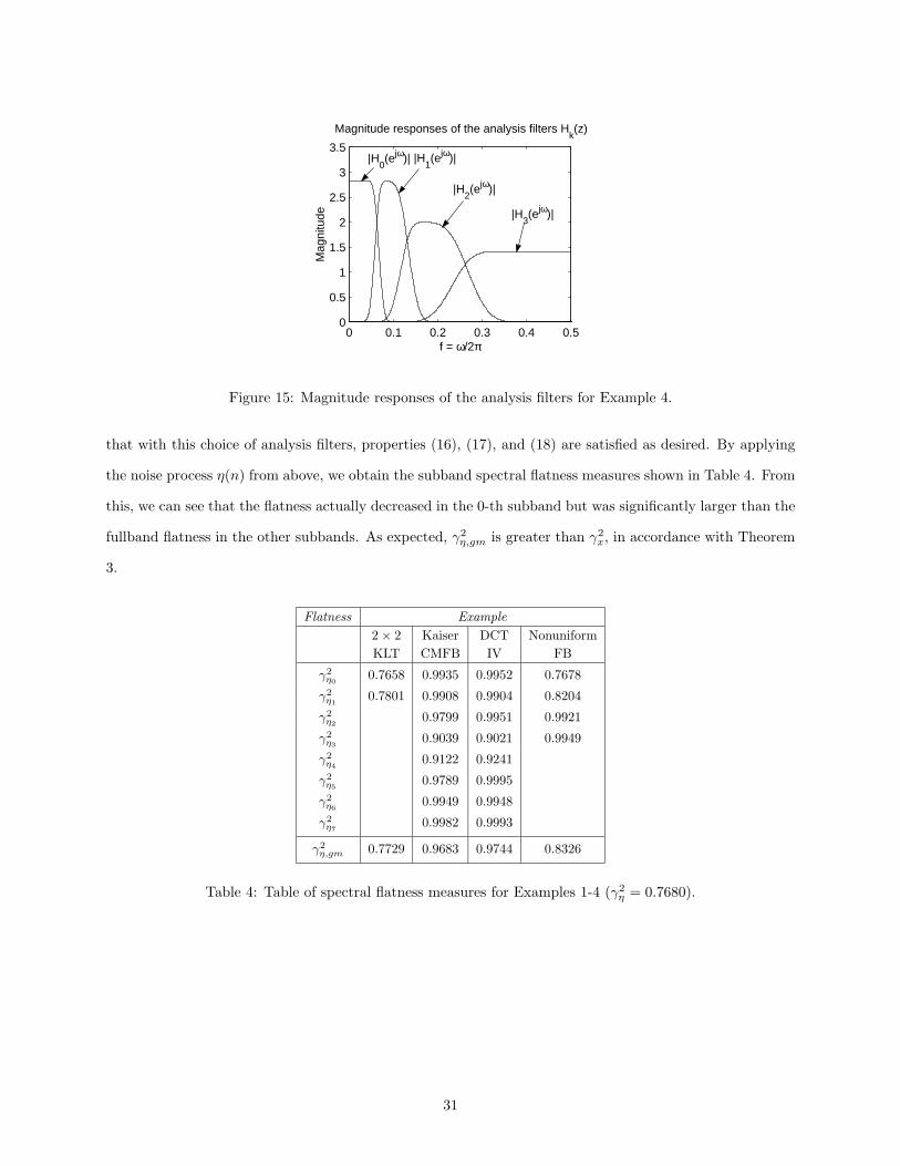
wavelet [15]. The magnitude responses of the analysis filters are plotted in Figure 15. It should be noted

30

0 0.1 0.2 0.3 0.4 0.50

0.5

1

1.5

2

2.5

3

3.5

f = ω/2π

Mag

nitu

de

Magnitude responses of the analysis filters Hk(z)

|H0(ejω)| |H

1(ejω)|

|H2(ejω)|

|H3(ejω)|

Figure 15: Magnitude responses of the analysis filters for Example 4.

that with this choice of analysis filters, properties (16), (17), and (18) are satisfied as desired. By applying

the noise process η(n) from above, we obtain the subband spectral flatness measures shown in Table 4. From

this, we can see that the flatness actually decreased in the 0-th subband but was significantly larger than the

fullband flatness in the other subbands. As expected, γ2η,gm is greater than γ2

x, in accordance with Theorem

3.

Flatness Example2 × 2 Kaiser DCT NonuniformKLT CMFB IV FB

γ2η0 0.7658 0.9935 0.9952 0.7678

γ2η1 0.7801 0.9908 0.9904 0.8204

γ2η2 0.9799 0.9951 0.9921

γ2η3 0.9039 0.9021 0.9949

γ2η4 0.9122 0.9241

γ2η5 0.9789 0.9995

γ2η6 0.9949 0.9948

γ2η7 0.9982 0.9993

γ2η,gm 0.7729 0.9683 0.9744 0.8326

Table 4: Table of spectral flatness measures for Examples 1-4 (γ2η = 0.7680).

31

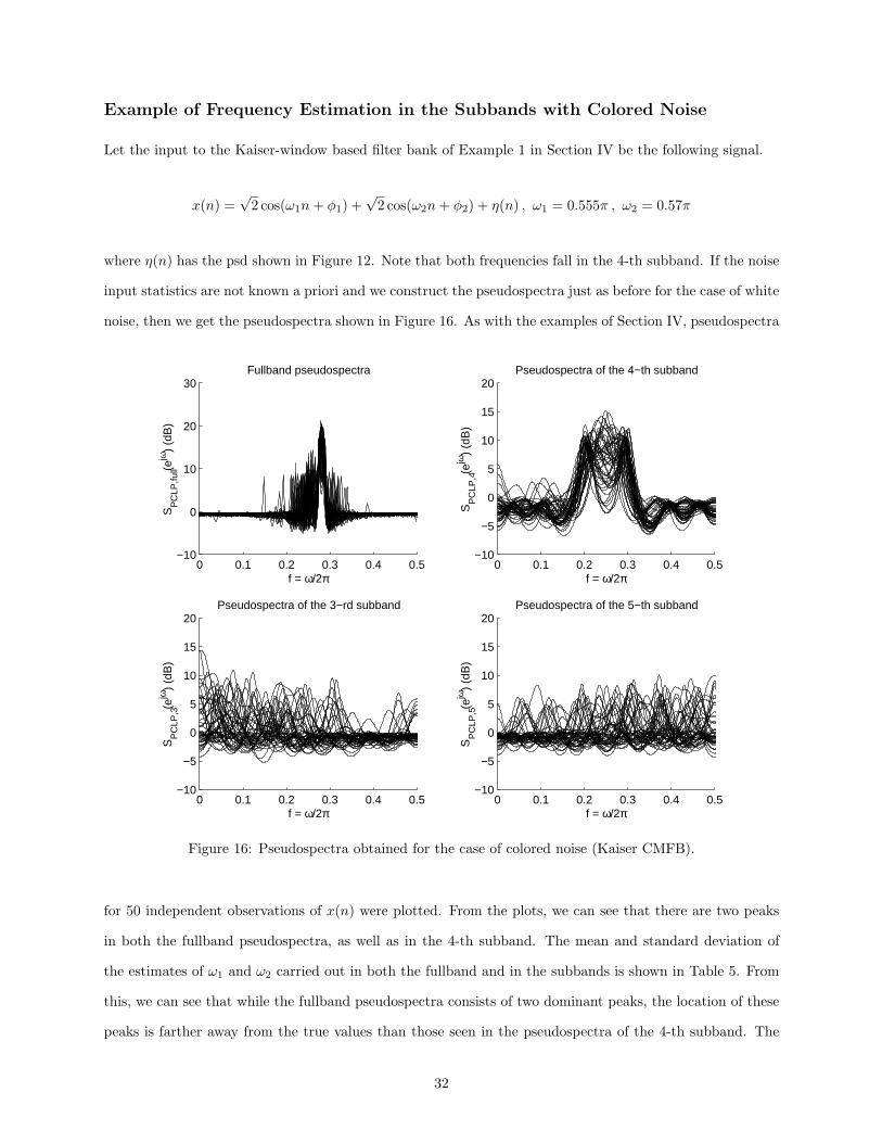
Example of Frequency Estimation in the Subbands with Colored Noise

Let the input to the Kaiser-window based filter bank of Example 1 in Section IV be the following signal.

x(n) =√

2 cos(ω1n+ φ1) +√

2 cos(ω2n+ φ2) + η(n) , ω1 = 0.555π , ω2 = 0.57π

where η(n) has the psd shown in Figure 12. Note that both frequencies fall in the 4-th subband. If the noise

input statistics are not known a priori and we construct the pseudospectra just as before for the case of white

noise, then we get the pseudospectra shown in Figure 16. As with the examples of Section IV, pseudospectra

0 0.1 0.2 0.3 0.4 0.5−10

0

10

20

30

f = ω/2π

SP

CLP

,full(e

jω)

(dB

)

Fullband pseudospectra

0 0.1 0.2 0.3 0.4 0.5−10

−5

0

5

10

15

20

f = ω/2π

SP

CLP

,4(e

jω)

(dB

)

Pseudospectra of the 4−th subband

0 0.1 0.2 0.3 0.4 0.5−10

−5

0

5

10

15

20

f = ω/2π

SP

CLP

,3(e

jω)

(dB

)

Pseudospectra of the 3−rd subband

0 0.1 0.2 0.3 0.4 0.5−10

−5

0

5

10

15

20

f = ω/2π

SP

CLP

,5(e

jω)

(dB

)

Pseudospectra of the 5−th subband

Figure 16: Pseudospectra obtained for the case of colored noise (Kaiser CMFB).

for 50 independent observations of x(n) were plotted. From the plots, we can see that there are two peaks

in both the fullband pseudospectra, as well as in the 4-th subband. The mean and standard deviation of

the estimates of ω1 and ω2 carried out in both the fullband and in the subbands is shown in Table 5. From

this, we can see that while the fullband pseudospectra consists of two dominant peaks, the location of these

peaks is farther away from the true values than those seen in the pseudospectra of the 4-th subband. The

32

Method ω1 (ω1 = 0.555π) ω2 (ω2 = 0.57π) σω1 σω2

Fullband 0.5207π 0.5747π 0.01501 0.00928Subband 0.5535π 0.5708π 0.000092 0.000098

Table 5: Comparison of fullband and subband methods for the case of colored input noise.

flatter noise seen in the subbands perturbed the peaks in their pseudospectra less than the heavily colored

input noise perturbed the peaks of the fullband pseudospectra. This example justifies the notion that there

indeed are cases where we may assume that the noise in the subbands is practically white, even though this

may not be the case in the fullband.

VIII. Concluding Remarks

We have shown various ways in which frequency estimation in the subbands of a filter bank can perform

better than conventional methods in the fullband, both theoretically and with numerous examples. It should

be noted, however, that there are still a number of open problems that remain regarding this subject. For

example, the statistical bias and variance of the frequency estimates have not been calculated and it is not

known quantitatively how close the variance comes to the Cramer-Rao bound for frequency estimation. Such

analysis will most likely shed more light on the precise tradeoff between the analysis filters and decimation

ratios used and the number of observation samples available at each subband.

Another open problem stems from the result proven in Theorem 3. Given that the geometric mean of

the flatness measures of the subband signals is always greater than or equal to that of the fullband input

signal, provided that (16), (17), and (18) are satisfied, the question then arises as to how to choose the

analysis filters such that this geometric mean in maximized. This problem is probably more of theoretical

than practical importance. The reason for this is because the optimal choice of analysis filters will most

likely depend on the input statistics, which we have assumed here are not known a priori.

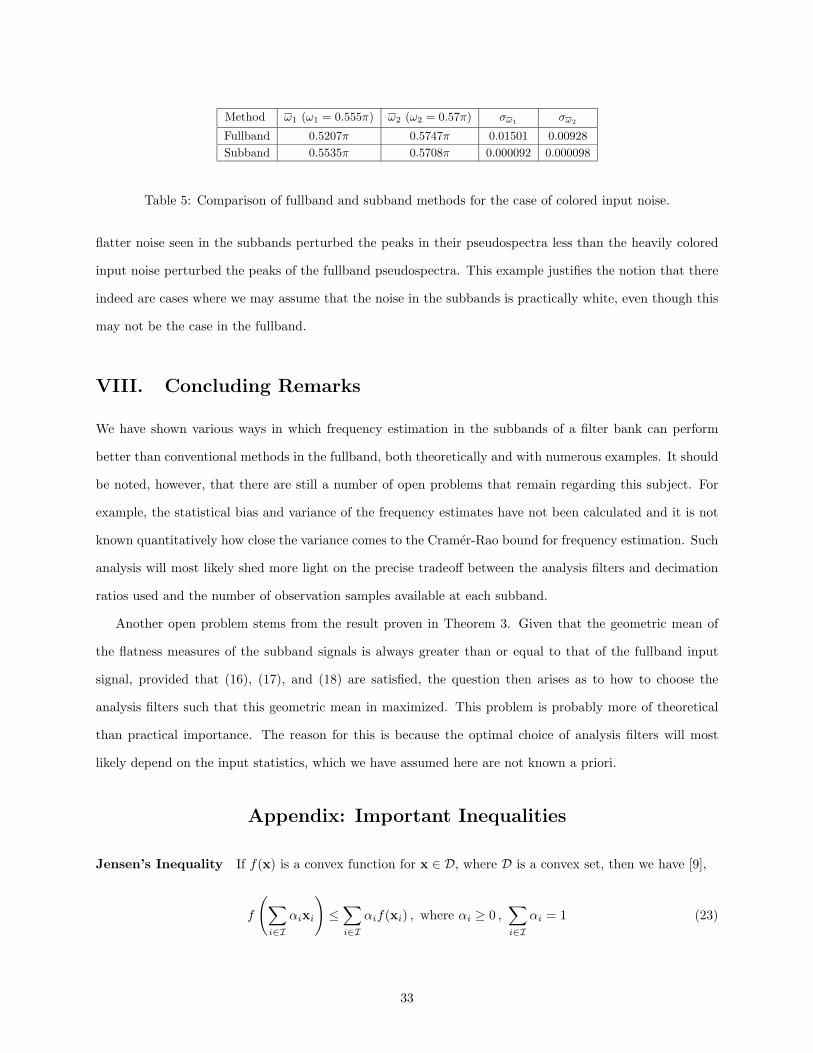
Appendix: Important Inequalities

Jensen’s Inequality If f(x) is a convex function for x ∈ D, where D is a convex set, then we have [9],

f

(∑i∈I

αixi

)≤∑i∈I

αif(xi) , where αi ≥ 0 ,∑i∈I

αi = 1 (23)

33

Here, I is an index set and xi ∈ D for all i. Moreover, equality holds in (23) iff either the set of αis is

degenerate in the sense that αi = 1 for a particular i and is zero for the rest, or if xk = xl for all k, l.

Examples of convex functions are f(x) = x2 and f(x) = ex.

Weighted Arithmetic-Geometric Mean Inequality Applying Jensen’s inequality to the strictly con-

vex function f(x) = − lnx over the interval (0,∞) yields the following important inequality [4].

∑i∈I

αixi ≥∏i∈I

xαii

where the αis are as in (23) and xi ≥ 0 for all i. The conditions for equality are the same as those for

Jensen’s inequality.

Log-Sum Inequality From [1], we have the following inequality, which results from applying Jensen’s

inequality to the strictly convex function f(x) = x lnx over the interval (0,∞).

∑i∈I

ai lnaibi

≥(∑i∈I

ai

)ln

∑i∈I

ai∑i∈I

bi

Here ai, bi ≥ 0 for all i and we have equality iff bi = Kai for all i and for some K ≥ 0. If the sequence {ai}is a pdf in the sense that

∑i∈I ai = 1, we obtain, ln

(∑i∈I bi

) ≥∑i∈I ai lnbi

ai.

References

[1] T. M. Cover and J. A. Thomas. Elements of Information Theory. John Wiley & Sons, Inc., New York,

NY, 1991.

[2] M. H. Hayes. Statistical Digital Signal Processing and Modeling. John Wiley & Sons, Inc., New York,

NY, 1996.

[3] S. Haykin, editor. Array Signal Processing. Prentice-Hall, Inc., Englewood Cliffs, NJ, 1985.

[4] R. A. Horn and C. R. Johnson. Matrix Analysis. Cambridge Univ. Press, Cambridge, U.K., 1985.

[5] N. S. Jayant and P. Noll. Digital Coding of Waveforms. Prentice-Hall, Inc., Englewood Cliffs, NJ, 1984.

34

[6] D. H. Johnson and D. E. Dudgeon. Array Signal Processing. Prentice-Hall, Inc., Englewood Cliffs, NJ,

1993.

[7] S. M. Kay. Modern Spectral Estimation. Prentice-Hall, Inc., Englewood Cliffs, NJ, 1988.

[8] Y. P. Lin and P. P. Vaidyanathan. A Kaiser window approach for the design of prototype filters of

cosine modulated filterbanks. IEEE Signal Processing Letters, 5(6):132–134, Jun. 1998.

[9] D. S. Mitrinovic. Analytic Inequalities. Springer-Verlag, Inc., New York, NY, 1970.

[10] S. U. Pillai. Array Signal Processing. Springer-Verlag, Inc., New York, NY, 1989.

[11] V. F. Pisarenko. The retrieval of harmonics from a covariance function. Geophysical Journal of the

Royal Astronomical Society, 33:347–366, 1973.

[12] S. Rao and W. A. Pearlman. Analysis of linear prediction, coding, and spectral estimation from sub-

bands. IEEE Trans. Inform. Theory, 42(4):1160–1178, Jul. 1996.

[13] A. Samant and S. Shearman. High-resolution frequency analysis with a small data record. IEEE

Spectrum, pages 82–86, Sep. 1999.

[14] R. Schmidt. Multiple emitter location and signal parameter estimation. In Proc. RADC Spectrum

Estimation Workshop, pages 243–258, 1979.

[15] G. Strang and T. Q. Nguyen. Wavelets and Filter Banks. Wellesly-Cambridge Press, Wellesly, MA,

1996.

[16] C. W. Therrien. Discrete Random Signals and Statistical Signal Processing. Prentice-Hall, Inc., Engle-

wood Cliffs, NJ, 1992.

[17] D. W. Tufts and R. Kumaresan. Singular value decomposition and improved frequency estimation using

linear prediction. IEEE Trans. Acoust., Speech, Signal Process., ASSP-30:671–675, Aug. 1982.

[18] P. P. Vaidyanathan. Multirate Systems and Filter Banks. Prentice-Hall, Inc., Englewood Cliffs, NJ,

1993.

[19] P. P. Vaidyanathan. Orthonormal and biorthonormal filter banks as convolvers, and convolutional

coding gain. IEEE Trans. Signal Processing, 41(6):2110–2130, Jun. 1993.

[20] P. Yip and K. R. Rao. Discrete Cosine Transform: Algorithms, Advantages, Applications. Springer-

Verlag, Inc., New York, NY, 1997.

35