Embed Size (px)
Citation preview

International Journal of Applied Engineering Research ISSN 0973-4562 Volume 12, Number 14 (2017) pp. 4708-4722
© Research India Publications. http://www.ripublication.com
4708
An Energy Efficient Scheme for Detecting Redundant Readings in
Cluster-based Model of Integrated RFID and Wireless Sensor Networks
Dongcheon Shin1 and Seikwon Park2
1Professor, Department of Industrial Security, Chung-Ang University, 84 Heukseok-ro, Dongjak-gu, Seoul-06974, Korea.
2Professor, Business School, Chung-Ang University, 84 Heukseok-ro, Dongjak-gu, Seoul-06974, Korea. (Corresponding author)
Abstract
For efficient detection of redundant readings by the
overlapped reading ranges, by avoiding the unnecessary
transmission of reading data and unsuccessful detection
attempts, detecting the redundant readings as early as possible
is critical for energy efficiency in the integrated RFID and
WSNs. In this paper, we propose a cluster-based efficient
detection scheme called ASER (Aggregation-based Scheme
for Eliminating Redundancy) for detecting redundant readings
with the purpose of attaining energy efficiency in integrated
RFID and WSNs. ASER is based on a 2-Phase Aggregation
(2PA) scheme whose main purpose is to localize the detection
attempts without traversing nodes in the network. ASER can
minimize the unnecessary overhead by detecting redundant
readings in advance before they traverse along the routing
path. According to results of performance evaluation, ASER
shows considerable improvement in reduction of both
communication cost and computational detection overhead to
detect the redundancy
Keywords: RFID, WSN, Redundant Reading, Energy
Efficiency, Cluster, Data Filtering
INTRODUCTION
The wireless and mobile paradigm in computing and
communication has rapidly emerged in many our daily life
environments. In accordance with this trend, the integration of
RFID and wireless sensor networks (WSNs) gets to play very
fundamental roles in the near future. RFID technology enables
large volumes of data to be captured for monitoring,
identifying, and locating objects at high speed. This makes
RFID technology suitable for a variety applications such as
supply chain management, manufacturing and distribution
logistics, healthcare, security, agricultural applications and so
on [1]. WSNs are networks of sensor nodes equipped with
wireless interface through which they can communicate with
each other in order to cooperate for gathering sensed
information [2]. WSNs can be introduced in many applications
such as environment monitoring, health observation, security
and other commercial applications [3].
RFID systems usually consist of tags, readers, and host
computers. The reader reads tag data attached to objects
through communication with tags using RF signals. The host
computer stores and manages the data read and transmitted by
the reader. It also submits queries to readers for data needed to
run applications. To manage RFID data stream, which has
nature of seamless and dynamic massiveness, has posed
several challenges for RFID systems to get more widespread
use in diverse applications [4], [5]. Sensor nodes in WSNs are
typically characterized by low power, small memory capacity,
and low communication range. WSNs, however, easily
achieve a large scale and dense deployment so that they can
extend the coverage of area and improve the fault tolerance or
robustness. Therefore, conditions or circumstances of objects
can be effectively captured by sensor nodes in decentralized
and large scale environments.
While RFID is suitable for identifying and monitoring objects
with relative low cost, WSN are usually suitable for gathering
detailed information about object conditions with networked
sensors. This complementary aspects makes RFID systems to
operate in a multi-hop fashion together with detailed
conditions of objects especially in large scale and distributed
environments. This implies that integration of RFID and
WSNs (RFID/WSNs) can be useful for various applications
[6], [7], [8], [9]. In particular, integration helps to implement
smart environments such as Internet of Things [10] where
physical objects are seamlessly identified, producing useful
information over the Internet for applications [11], [12].
However, to promote RFID/WSNs, there exist several
challenges including energy consumption, data cleaning, time
delay and so on [13], [14], [15].
Since wireless devices have very limited battery life, low
energy consumption has been one of crucial problems in
RFID/WSNs. As the number of sensors increases, the time
delay also increases. Hence, by efficient use of network
bandwidth, satisfying time constraints is of importance
especially in real time applications. The need for data cleaning
stems from the inherent unreliability of RFID readers and
overlapped reading areas among them which makes it very
likely to produce redundant readings. Redundant readings

International Journal of Applied Engineering Research ISSN 0973-4562 Volume 12, Number 14 (2017) pp. 4708-4722
© Research India Publications. http://www.ripublication.com
4709
need to be filtered out for the correct monitoring and tracking
of tagged objects. Actually, the goal of data cleaning is to
maintain integrity of RFID data streams in order to delivery
clean data to applications. Many related works on data
cleaning can be founded in the literatures [16], [17], [18], [19],
[20], [21].
The redundant readings in RFID/WSNs are more likely to
occur since sensor nodes are densely deployed and
consequently have more overlapped reading areas with
surrounding sensor nodes. The redundant readings are
unavoidable as long as overlapped areas exist. As a result, to
detect redundant readings as soon as possible without
unnecessary transmissions of them and meaningless attempts
to detect them at each node is a very critical point for
successful integration. Many works for filtering redundant
readings in relation to the RFID or/and WSNs appear in the
literatures [22], [23], [24], [25], [15], [26], [27]. Most of them,
however, address filtering problems at a reader level or a host
node level. That is, energy efficient filtering by reducing
transmissions of redundant readings by sensor nodes may be
not of their major concerns for RFID/WSNs.
The key point to detect redundant readings in RFID/WSNs is
to acquire the complete knowledge of such readings among
surrounding nodes. One easy way to acquire the knowledge
for redundant readings is to transmit of redundant data to the
sink node along the routing path. Such transmission of
redundant readings in energy-constrained RFID/WSNs incurs
very undesirable effects because it consumes the unnecessary
power and network bandwidth. Therefore, energy efficient
schemes need to be developed to prolong network life.
Many works address the problem of energy efficient scheme
for reducing transmission of redundant data in RFID/WSNs
integration. In-network aggregation techniques are proposed to
deal with distributed processing of data generated by different
sensors [28], [29]. Though they contribute to the reduction in
communication among sensors, eventually leading to
reduction in the energy consumed from the batteries, they
have specific purposes for only data gathering queries and also
suffer from the computation overhead for data processing.
Several algorithms for dealing with redundant readers also
proposed to detect and eliminate redundant readers from the
network for the purpose of posing a minimal communication
overhead [30], [31], [32]. However, this problem is basically
an NP-hard so that most of them take heuristic approaches to
obtain the optimal solutions.
A series of interesting works related in-network RFID data
filtering to deal with the redundant readings by multiple
readers have also proposed to prolong the life of the energy-
constrained WSNs [33], [34], [35]. In [34], they propose an
INPFM (In-Network Phased Filtering Mechanism) to filter the
global redundant readings. In INPFM, data transmission
follows the routing path on WSNs, trying to filter redundant
data at nodes on the path. Since INPFM is subject to a multi-
hop routing, it needs to check the redundancy at every node
along the routing path until the redundancy is detected. This is
undesirable because it incurs much computational overhead
and transmission overhead which are accompanied by high
power consumption. In densely deployed WSNs, it is evident
that it aggravates WSNs system. CLIF (Cluster-based In-
network Filtering scheme) in [35] introduces clustering of
nodes in which one node is designated as a cluster head node
(CH) to whom other nodes involved in the same cluster send
the data. Therefore, CHs will perform the filtering and then
forward data along the routing path towards the host
(base/sink) node connected to the host computer. In the case of
intra-cluster redundancy which results from the nodes in the
same cluster, CLIF can reduce the computation overhead and
consequent transmission overhead, compared to INPFM by
sending data to the head node. On the contrary, in the case of
inter-cluster redundancy which results from the nodes with
overlapped area even in the different clusters, CLIF also
imposes computation overhead and consequent transmission
overhead, since CHs follows the similar scenario to that of
INPFM. EIFS (Energy Efficient In-Network RFID Data
Filtering Scheme) in [33] improves CLIF by using a feedback
message. If an intermediate CH on the routing path detects the
inter-cluster redundancy, it sends a feedback message to
surrounding CHs whose member nodes generated the
redundant data. Thereafter, those CHs transmit the inter-
cluster redundant data to the near CH by changing the routing
paths of them. This allows EIFS to avoid unnecessary
comparisons and redundant transmissions from a source CH to
the detecting intermediate CH. They prove EIFS is a more
energy efficient scheme than other ones such as INPFM and
CLIF through simulations.
To avoid frequent feedback messages, EIFS sets a condition
for sending feedback messages, which depends on the network
size, number of cluster, or distance of a node. Apart from the
cost of sending feedback messages, even if EIFS gains the
energy-efficiency as compared to preceding schemes, it also
suffers from some shortcomings. First the inter-cluster
redundant data are transmitted to the intermediate CHs along
the routing paths until the source CH which is involved in
sending the redundant data receives the feedback message to
change the routing path towards their surrounding CHs.
Second, until the inter-cluster redundancy is detected, each
intermediate CH on the routing path also tries to check the
inter-cluster redundancy as in preceding works. Third, since
nodes involved in the same cluster can have overlapped
reading areas with nodes in distinct clusters, the feedback
message is not immediately effective for some inter-redundant
readings. Fourth, in case one particular source CH among the
surrounding CHs happens to take over the responsibility of
checking all inter-cluster redundancy generated by its
surrounding CHs, the CH relatively consumes significant
energy.
It is obvious that the undesirable overhead for detecting and
International Journal of Applied Engineering Research ISSN 0973-4562 Volume 12, Number 14 (2017) pp. 4708-4722
© Research India Publications. http://www.ripublication.com
4710
transmitting redundant readings can be considerably reduced if
redundancy can be detected in advance before CH of a node
starts to transmit redundant reading data to the intermediate
CHs along the routing path. We think the best way is to detect
redundancy at a node’s CH without traversing nodes along the
routing path. To make this possible, the CH should have the
complete knowledge of redundant readings by all surrounding
nodes of nodes that belong to its cluster. For the acquisition of
such knowledge, CHs of surrounding nodes should send their
own redundant readings to the one CH among them.
Therefore, the first important thing is to figure out a group of
those associated CHs, which we call cluster head aggregation.
However, to build a complete aggregation is not trivial
because a surrounding node of a node can be also a
surrounding node of another node which belongs to different
CH from its CH. This implies that it needs to consider the
transitive surrounding relationships of nodes as well as direct
surrounding relationships, in order to achieve efficiency owing
to early detection as much as possible. Otherwise, it is likely
to miss detection of some redundancies in advance because of
partial aggregation of the cluster heads. Our previous work in
[36] addresses to solve this problem and proposes 2-Phase
Aggregation (2PA) scheme in order to build the effective
aggregation.
In this paper, to solve the shortcomings of previous works, we
propose an energy efficiency scheme called ASER
(Aggregation-based Scheme for Eliminating Redundancy) for
detecting redundant readings in RFID/WSNs. ASER also
introduces clustering of sensor nodes, and is based on the
notion of cluster head aggregation scheme called 2PA appears
in our previous work. Owing to the notion of aggregation,
with ASER the unnecessary transmission of redundant data
and useless detection attempts can be reduced, contributing to
the improvement of energy efficiency after all. Then, we
evaluate the performance of ASER through simulation
approach.
The remainder of this paper is as follows. Section 2 briefly
introduces preliminaries needed for presenting ASER,
including problem overview. In Section 3, we describe our
previous work called 2PA scheme to produce the aggregation.
ASER is proposed in Section 4. Section 5 shows the
simulation results for performance evaluation. The
conclusions and future works appear in Section 6.
PRELIMINARIES
Cluster-based System Model of RFID/WSNs
In accordance with the intended purposes, there may be
different approaches to integration of RFID and WSNs [37, 38,
39]. Without losing generality, we can consider a simple
model of RFID/WSNs in which each wireless sensor node is
integrated with one RFID reader and there is one base sensor
node connected directly to the server running applications.
Figure 1 shows our simplified model. A sensor node delivers
RFID data by the reader and sensing data by the sensor to the
server for applications via WSNs in a multi-hop fashion along
the routing path to the destination.
In our WSNs, we do not pose any limitation on the
deployment of sensor nodes. Sensor nodes may be positioned
dynamically and arbitrarily according to the situation. That is,
their positions may be static or dynamic, dense or sparse to
meet the application purposes. A group of sensor nodes forms
one cluster with unique identification number and one sensor
node belongs to one cluster. Though we can consider the
clustering criteria such as the number of nodes in the cluster
and cluster’s coverage distance, in this paper we do not
address how to cluster nodes. One sensor node in each cluster
is designated as a cluster head node (CH). Of course, CH may
be changed for balancing the energy consumption. Each
member nodes can communicate with its own CH directly so
that it transmit tag data to its CH. Tags in the reading region of
a node are read multiple times, and tags in the overlapped
region by multiple nodes are also read multiple times. A CH
performs data filtering in order to eliminate the redundant
data, and then forwards data to other CHs on the routing path
towards the base node in a multi-hop communication via
WSNs.
Figure 1: Cluster-based System Model
Problem Overview
A node reads data like the identity label of tags in its vicinity.
We represent tag data as 3 fields: d(Tid, Nid, Ts). Tid refers to
the unique tag identifier like EPC (Electronic Product Data)
standard. Nid refers the unique identifier of a node that read
the tag of Tid. Ts is the timestamp that the node of Nid read
tag of Tid. Due to the possible latency, we need to include
timestamp to denote tag data. Otherwise, the incorrect filtering
may deliver inappropriate data to applications, especially to
query-based or event-based applications. We need to define
redundant data clearly at reader level in our work.

International Journal of Applied Engineering Research ISSN 0973-4562 Volume 12, Number 14 (2017) pp. 4708-4722
© Research India Publications. http://www.ripublication.com
4711
Definition 1 (Redundant data): For two arbitrary tag data
di(Tidi, Nidi, Tsi) and dj(Tidj, Nidj, Tsj), if the following
conditions satisfy at the same time, di(Tidi, Nidi, Tsi) and
dj(Tidj, Nidj, Tsj) are defined to be redundant data.
a) Tidi, = Tidj,
b) Nidi, ≠ Nidj,
c) | Tsi - Tsj | ≤ Δ, where Δ is the time threshold to be
acceptable
In the cluster-based model, we consider two types of readings.
A local reading and a global reading are produced by a local
node and a global node, respectively. A local node refers to
one that does not have the overlapped area with nodes which
belong to other different clusters from its cluster. Of course, it
has the overlapped area with nodes in the same cluster as its
cluster, producing the local redundancy readings. A global
node refers to one that does have the overlapped area with
nodes which belong to other distinct clusters, producing the
global redundancy readings.
Definition 2 (A local node and a global node): Let SNi = {Nj, i∈1, 2,….n, j∈1, 2,….n, i≠j} be a set of nodes that response
to the enquiry of a node Ni. CIi and CIj denote the cluster
identifier of a node Ni and Nj, respectively. A node Ni is a
local node if CIi= CIj holds for all j. Otherwise, it is a global
node.
Redundant readings occur when reading ranges of different
nodes are overlapped. Redundant readings are classified into
local redundant readings and global redundant readings as
shown in Figure 2. Local redundant readings are ones among
local nodes, whereas global redundant readings are ones
among global nodes. The tag data read by a node is delivered
to its CH, and then CH checks whether tag data is redundant
or not. The local redundant data can be locally detected and
removed at its CH through some filtering process. This is
possible because CH can have the knowledge of all local
redundant readings within its cluster.
The global redundant data, however, cannot be obviously
detected at its CH because CH can have no idea of other
global redundant readings originated from nodes involved in
different clusters. The other global redundant readings by
nodes in different clusters must have delivered to their
respective CH. As a result, the CH has no choice but to
transmit the redundant data to next CH along the routing path.
This evidently incurs redundant transmission that entails
energy consumption and communication delay. This
redundant transmission stops at last only after some distant
CH on the routing path happens to detect the global
redundancy. In other words, the transmission of redundant
data continues at all intermediate CHs, traversing along the
routing path until redundancy is detected at one of the
intermediate CHs. Moreover, the intermediate CHs have to put
up with computation overhead to check the possible global
redundancy. Since global redundant readings are likely to
increase in accordance with increased tags and degree of dense
deployment of nodes, to devise an efficient scheme for
checking global redundancy in advance without traverse is
fundamental to the improvement of overall system
performance.
(a) Local redundant readings (b) Global redundant readings
Figure 2: Two types of redundant readings
As an example, consider Figure 3. Assume that CH1 and CH2
have the global redundant readings for the same tags due to
the overlapped reading range of nodes that belong to the
different cluster 1 and cluster 2. The redundant global reading
data at CH1 arrives at the intermediate CH10 through CH3,
CH6 and CH9 along the routing path, while the redundant
global reading data at CH2 also arrives at CH10 through CH4
and CH8 along the routing path. Now, the global redundancy
can be detected at CH10 at the expense of the duplicate
transmission of redundant data, leading to the energy
consumption and communication delay in many intermediate
CHs. Moreover, the intermediate CHs have to execute the
filtering process to find out the incoming redundant global
data to them. Those executions are in fact useless in that
redundancy cannot be detected at such CHs because the
redundant data are traversed along the different routing paths.
Eventually, the attempts to run the filtering process also
contribute to the wasteful consumption of energy.
Figure 3: Detection of global redundancy readings at
distant CH

International Journal of Applied Engineering Research ISSN 0973-4562 Volume 12, Number 14 (2017) pp. 4708-4722
© Research India Publications. http://www.ripublication.com
4712
On the other hand, it may be worthy of notice that tag data
sent by a global node can also have the possibility of local
redundancy. This fact makes it difficult to detect the
redundancy generated by a global node, since CH cannot
distinguish the local redundancy and global redundancy by the
same global node. This implies that a scheme to consider this
situation needs to be devised for eliminating the global
redundancy. Figure 4 illustrates this. A global node can also
have the overlapped areas with one or more its local nodes,
which implies that tag data by a global node may have a local
redundancy and/or global redundancy.
Figure 4: Local redundancy and global redundancy by one
node
2-PHASE AGGREGATION SCHEME (2PA)
To minimize the undesirable overhead, it is necessary to detect
the global redundancy without traversing the intermediate CHs
along the routing path. We think the best way is, at the very
beginning, to detect global redundancy at one of CHs which
are associated with the global redundancy. In this section, we
present the cluster head aggregation scheme called 2PA in our
previous work [36].
Determining Node Type
To detect global redundancy, it is certainly necessary to
exchange knowledge about global readings among global
nodes. As a result, we need to know whether a node is a local
node or a global node. To determine the node type, a node
communicates with its surrounding nodes to obtain their
cluster identifier. The surrounding nodes may belong to the
same cluster as a node, or belong to the different cluster. If all
surrounding nodes are exactly discovered, in our approach the
unnecessary transmission of redundant data can be minimized
to the highest level. However, even if some surrounding nodes
are missing for some reasons, our approach is sufficiently
reasonable because most of global redundancy seems to be
detected without traversing along the routing path. The exact
discovery of surrounding nodes is not a problem of
correctness, but is a matter of efficiency degree in relation to
unnecessary data retransmission. That is, it is deeply related
with minimization level of unnecessary overhead.
In our approach, as one of tasks for system configuration after
cluster establishment among nodes, each node sends an
enquiry messages to its surrounding nodes in order to figure
out their cluster identifiers. When a node receives such an
enquiry message, it gives an answer with its node identifier
plus its cluster identifier, <Nid CI>. Once a node receives
answers from its surrounding nodes, according to Definition 2,
it can determine whether it is a local node or not. If all cluster
identifiers received from its surrounding nodes are same as its
own cluster identifier, it becomes a local node. Otherwise, it
becomes a global node. It is obvious that the answering
surrounding nodes with different cluster identifiers are also
global nodes and other answering surrounding nodes are local
nodes. We define the answering nodes with different cluster
identifiers to be direct surrounding global nodes of the
enquiring node (Definition 3). Note that if a node A is a direct
surrounding node of a node B, a node B is also a direct
surrounding node of a node A. After determining the node
type, each global node can keep the information about its
direct surrounding global nodes and their clusters.
Definition 3 (A direct surrounding global node)): The global
node that responds to the enquiry of a node N is defined to be
a direct surrounding global node of node N.
To show an example, consider Figure 5. Each node receives
answers from its surrounding nodes as follows.
Node A: [<B,CH2>, <D,CH3> ] Node B: [<A,CH1>,
<C,CH2>, <D,CH3>, <E,CH2>]
Node C: [<B, CH2>, <E, CH2> ] Node D: [<A,CH1>,
<B,CH2> ]
Node E: [<B,CH2>, <C,CH2>]
Global nodes are A, B, and D since they have surrounding
nodes with different cluster identifiers from their own cluster
identifiers, respectively. Other nodes C and E are local nodes.
Now, global nodes can keep the information of its direct
surrounding global nodes such as node identifiers and cluster
identifiers as follows.
Node A: [<B,CH2>, <D,CH3>]
Node B: [<A,CH1>, <D,CH3>]
Node D: [<A,CH1>, <B,CH2>]
Note that one global node can become a direct surrounding
global node of several different global nodes with different
clusters. For example, in figure 5, we can know that a global
node B becomes two different global node A and D with
different clusters.

International Journal of Applied Engineering Research ISSN 0973-4562 Volume 12, Number 14 (2017) pp. 4708-4722
© Research India Publications. http://www.ripublication.com
4713
Figure 5: Sample configuration of clusters
Aggregation Scheme
When a node sends tag data to its CH, it attaches its
determined node type to tag data. So, tag data consists of 4
fields including the additional field Ntype: d(Tid, Ntype, Nid, Ts). Ntype has one value of ‘L’ and ‘G’, representing local
node type and global node type, respectively. Based on the
node type, CH can distinguish the local redundancy from the
global redundancy. Hence, CH performs its function to deal
with tag data, depending on the node type. It can detect local
redundancy with its own knowledge. However, to check and
detect global redundancy, it requires the global knowledge of
tag readings from its direct surrounding global nodes. To get
the needed global knowledge, it should communicate with
other CHs of its direct surrounding global because those CHs
have the knowledge of global tag readings generated by their
direct surrounding global nodes.
It is very important to realize that surrounding global nodes of
a global node can belong to different clusters from each other.
In Figure 5, a global node A have overlapped reading areas
with other global nodes <B, D> which belong to different
clusters from each other. Similarly, the global node B has
overlapped reading areas with other global nodes <A, D>.
Finally, the global node D has overlapped reading areas with
other global nodes <A, B>. Since each global node sends tag
data to its CH, in order to detect the global redundancy, CH
requires tag data read by surrounding global nodes. As an
example, if CH1 has the knowledge of other global readings
by global nodes B and D, it can detect the global redundancy
among A, B, and D. Similarly, CH2 and CH3 also detect the
global redundancy among A, B, and D by communication with
each other. Consequently, CH1, CH2, and CH3 form one
group which we call an aggregation of CH for a global node.
Note that, since local redundancies can be detected by CH
without communication with other CHs, aggregation needs to
be built for only global nodes. Furthermore, one aggregation is
needed for each global node.
An aggregation for a global node consists of cluster identifiers
of its surrounding global nodes. In the above example, global
node A, B, and D happens to have the same aggregation,
<CH1, CH2, CH3>. Through communication among only
CHs appeared in the aggregation, each CH can detect the
global redundancy. The fundamental motivation of
introducing the notion of aggregation for a global node is, at
the beginning before traversal for detecting global
redundancy, to confine communication overheads to only CHs
in which its direct surrounding global nodes are involved. In
the above example, communication among CH1, CH2, and
CH3 is evidently more efficient for detecting global
redundancies among global node A, B, and D, compared to
sending global redundant tag data to other CHs besides CH1,
CH2, and CH3. As you know, sending global redundant data
to other CHs can result in undesirable transmission and
computation costs because detection of global redundancy is
likely to be impeded until some another CH on the routing
path happens to have the needed global redundant tag
readings.
On the other hand, if associated direct surrounding global
nodes have the same aggregation, in order to detect the global
redundancy, there is no need for each CH appeared in the
aggregation to send its global readings to each other. It is
sufficient for one of CHs to have knowledge of total global
readings. Therefore, one of CHs appeared in an aggregation
needs to be designated as a master head node (MH). For
example, in Figure 5, global nodes A, B, and D happen to
have the same aggregations <CH1, CH2, CH3>. If one of
CH1, CH2, and CH3 is designated as a MH, then other CHs
send its global readings to MH at which detection of the global
redundancy is attempted and the global redundancy can be
detected if there exists.
In relation to the aggregations for associated direct
surrounding global nodes, it is very important to notice that
each direct surrounding global node should have the same
aggregation. Otherwise, CH is likely to incur undesirable
anomaly when it sends global readings to the designated MH.
In Figure 5, global nodes A, B, and D happen to have the same
aggregation <CH1, CH2, CH3>. Unfortunately, the initial
aggregations of associated direct surrounding global nodes are
not always same. This occurs because a global node has
overlapped area with one more global nodes involved in
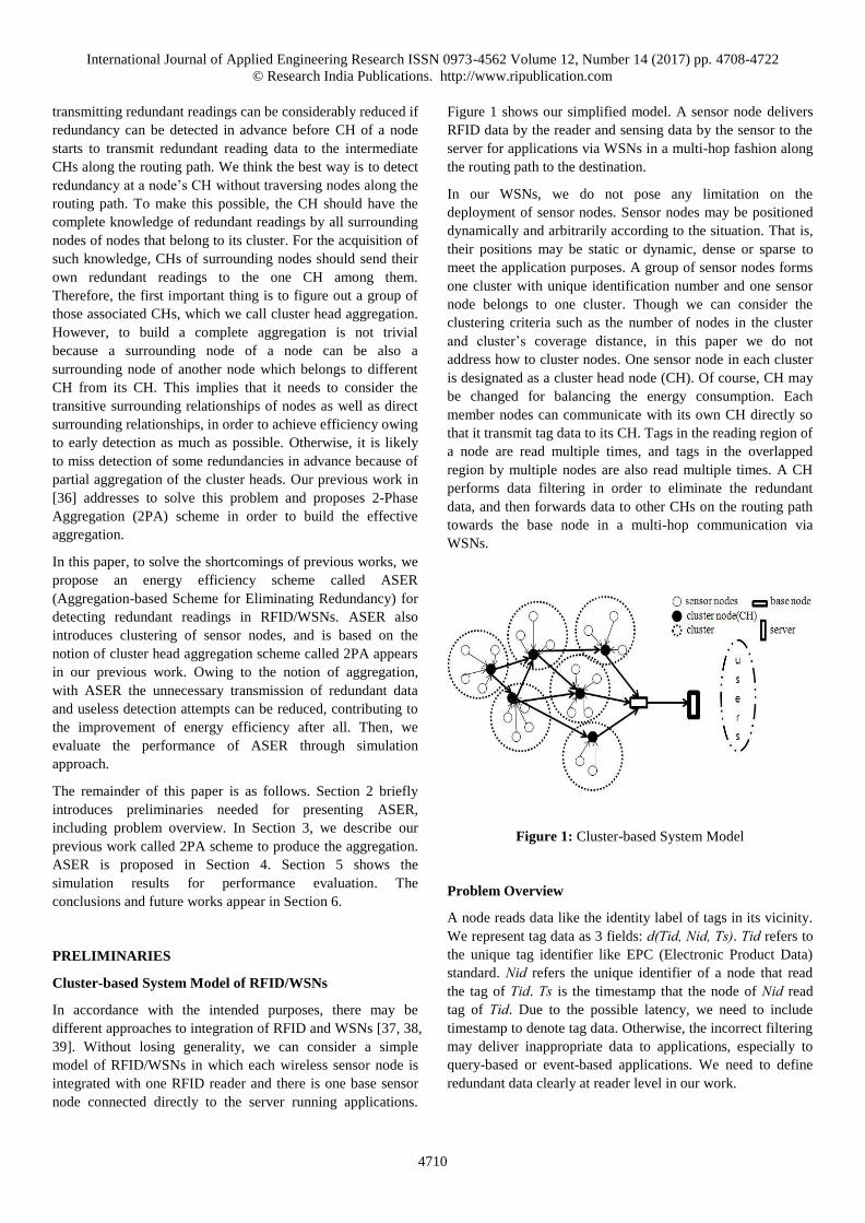
different clusters. To demonstrate the undesirable anomaly
when surrounding global nodes does not have the same
aggregation, consider Figure 6. The initial aggregations for
node A, B, C, and D are as follows:
Node A: <CH1, CH2, CH3> Node B: <CH1,CH4,CH2>
Node C: <CH1, CH3> Node D:<CH2, CH4>
If CH receives aggregations like the above, CH cannot
determine where it sends the global readings. This occurs
because a global node has overlapped area with one more
International Journal of Applied Engineering Research ISSN 0973-4562 Volume 12, Number 14 (2017) pp. 4708-4722
© Research India Publications. http://www.ripublication.com
4714
global nodes involved in different clusters. For example, node
A is overlapped area with both node B and C which belong to
different clusters, cluster 2 and cluster 3. As a result, to detect
global redundancies among node A, B, and C, assume that
CH1 is a MH. In this case, CH2 and CH3 must send respective
global readings generated by node B and node C. CH2 also
sends other global readings of B which overlapped with node
D to MH (CH1). Unless CH4 for node D sends its global
readings which also overlapped with node B to CH1, global
redundancy between node B and node D cannot be detected at
this stage. Note that <CH1, CH4, CH2> and <CH2, CH4> are
aggregations of node B and node D, respectively. This
demonstrates that each associated direct surrounding global
node should have the same aggregation in order to prevent this
undesirable anomaly. To build the same aggregations for
associated direct surrounding global nodes, it needs to
consider the transitive surrounding relationships among direct
surrounding global nodes (definition 4). Note that the fact that
a node A is a transitive surrounding node of a node C implies
that a node C is also a transitive surrounding node of
a node A.
Figure 6: Transitive surrounding relationships of global nodes
Definition 4 (A transitive surrounding global node): If a
node A is a direct surrounding global node of a node B, and a
node B is a direct surrounding global node of a node C, then a
node A is defined to be a transitive surrounding global node of
a node C.
Definition 5 (An aggregation for a global node): An
aggregation for a global node consists of cluster identifiers of
its all direct and/or transitive surrounding global nodes
including its cluster identifiers.
Our 2PA scheme consists of 2 phases. In the first phase, the
initial aggregation for each global node is built. Each node
sends an enquiry message to its surrounding nodes. On
receiving the enquiry message, each surrounding node
responds by sending an answer message including its node
identifier and cluster head identifier. Each node determines its
direct surrounding global node from answers and its node type
can be also determined. From the answers from the direct
surrounding global nodes, the first initial aggregation for each
global node, can be built. To build the same aggregations
among associated direct surrounding global nodes, a second-
round communication begins in the second phase.
In the second phase, each global node sends its own current
aggregation to its direct surrounding global nodes. On
receiving the other aggregations from its direct surrounding
global nodes, each global node combines its current
aggregation with other aggregations received from its direct
surrounding global nodes by eliminating the duplicate cluster
head identifiers. If the current aggregation is subset of the new
built aggregation, it means that there must have been also
some other transitive surrounding global nodes which belong
to different clusters from those which appear in the current
aggregation. Then, the global node should send its new built
aggregation to its direct surrounding global nodes in order to
propagate the transitive relationships. On receiving the
additional aggregations, each global node again makes a
combined new aggregation. Now, the second-round
communication ends. If any new aggregation is built again on
the second round communication, then similarly third-round
communication begins by sending the new current aggregation
to their direct surrounding global nodes. The next round
communication may continue until no more newly built
aggregation exists. In the long run, each direct or transitive
surrounding global nodes can have the same aggregation.
To take an example, consider again Figure 6. The initial
aggregations for each global node are formed in the first phase
as follows (Figure 7-a).
Node A: <CH1, CH2, CH3> Node B: <CH1, CH4, CH2>
Node C: <CH1, CH3> Node D: <CH2, CH4>
In the second phase, each node sends its initial aggregation to
its surrounding nodes. Then, each node makes a temporary
aggregation by unification (Figure 7-b). Then, it sends its
initial aggregation to the nodes whose CHs newly appear in
the united temporary aggregation (Figure 7-c). Again, each
node makes a temporary aggregation, <CH1, CH2, CH3,
CH4>, which is the final aggregation in this example (Figure
7-d).

International Journal of Applied Engineering Research ISSN 0973-4562 Volume 12, Number 14 (2017) pp. 4708-4722
© Research India Publications. http://www.ripublication.com
4715
(a) Initial aggregations (b) New built aggregations
(c) Sending to direct surrounding nodes (d) Final aggregations
Figure 7: Sketches of 2PA scheme
Proposition 1: 2PA guarantees the same aggregation among
global nodes with direct and/or transitive surrounding
relationships
< proof > Suppose that there are n global nodes G1, G2,…, Gn
(n>1) which belongs to the different clusters whose cluster
heads are CH1, CH2,…., CHn, respectively.
● Case 1: N=2
In this case, two nodes must be a direct surrounding
relationship between them. Therefore, it is obvious that they
have the same aggregation consisting of their CHs.
● Case 2: N=3
Let 3 nodes be Gi-1, Gi, and Gi+1 (1<i<n).They have either
only direct surrounding relationships or both of direct
relationship and transitive relationship among them. In case
only the direct surrounding relationships among them exist,
each node has the direct relationships with other two nodes.
Therefore, it is obvious that they have the same aggregation
consisting of their CHs. For a transitive relationship among
them, one node must have the direct surrounding relationship
with other two nodes. Assume that Gi has the direct
surrounding relationships with Gi-1 and Gi+1. Therefore, Gi-
1and Gi+1 have the transitive surrounding relationships through
Gi. In the 1st phase, Gi-1, Gi, and Gi+1 have the initial
aggregations <CHi-1, CHi>, <CHi-1, CHi, CHi+1>, and <CHi,
CHi+1>, respectively. In the first round in the 2nd phase, each
node sends its initial aggregation to its direct surrounding
global nodes. Owing to the first round, Gi-1 and Gi+1 get to
build the new aggregation <CHi-1, CHi, CHi+1> and <CHi-1,
CHi, CHi+1>, respectively. Note that the aggregation for Gi
have no change. Eventually, all nodes with both types of
surrounding relationship can have the same aggregation <CHi-
1, CHi, CHi+1>.
For the generalization, we make m (n=3*m) virtual global
nodes V1, V2……Vm. According to Case 2, three global nodes
in each virtual node can have the same aggregation. Consider
some two virtual nodes Vs and Vt (s, t∈1, 2….m, s≠t) which
contain 3 global nodes [Gs-1, Gs, Gs+1] and [Gt-1, Gt, Gt+1],
respectively. Suppose that Vs and Vt get to have the direct
surrounding relationships. This is possible if only one global
node in Vs gets to have the direct surrounding relationship
with only one global node in Vt. Let Gs and Gt be those global
nodes. According to Case 1, through the additional-round
communication, Gs and Gt build the new same aggregation.
Then, according to Case 2, Gs-1, Gs, and Gs+1 have the same
aggregation, while Gt-1, Gt, Gt+1 also have the same
aggregation. After all, all global nodes in Gs and Gt can have
the same aggregation. It is obvious that this is true even if
there are one more direct surrounding relationships among
global nodes in Gs and Gt. In this case, the only difference
consists in the number of round communication needed to
obtain the same aggregation. The same way can be applied to
the remaining virtual nodes recursively. This fact
demonstrates that all global nodes can have the same
aggregation. ■
1, 2 3, 4
1, 2 3, 4
1, 2 3, 4
1, 2 3, 4
1, 2, 3, 4
1, 2 3, 4 1, 2
3 1, 2 3, 4
1, 2 3, 4
1, 2 3, 4
1, 2 3
1, 2 4
1, 2 4
1, 2 3, 4

International Journal of Applied Engineering Research ISSN 0973-4562 Volume 12, Number 14 (2017) pp. 4708-4722
© Research India Publications. http://www.ripublication.com
4716
It is worthy of attention to consider the worst case in 2PA
scheme. The worst case is to have numerous successive
transitive surrounding relationships among global nodes.
Consider Figure 8. Since each node has a successive
transitivity, according to 2PA scheme, the final aggregation
for each global node would include all cluster identifiers after
several round communications in the second phase. In the
worst case, the result is equivalent to that of other schemes
which do not introduce the notion of aggregation. However,
since there are generally a number of nodes in one cluster and
the reading scope is noticeably narrow as compared with the
cluster area, we think such successive transitivity is very
unusual and unrealistic
Figure 8: Successive transitive surrounding global
relationships
DETECTION OF GLOBAL REDUNDANCIES
In our scheme, each CH maintains two main data repositories
to store information for detecting redundancy. A tag table
consists of tag entries d(Tid, Ntype, Nid, Ts) to which CH
refers in order to check both the local redundancy and the
global redundancy. Each CH maintains tag entries for tag data
delivered to it. An incoming tag data is turned out to be a
redundant tag data if it matches with any entry in tag table
according to conditions in Definition 1. The discussion of
efficient methods to check the redundancy is out of our scope,
and as introduced in Section 1, many works related to the
issue already exist. In addition, since discussion about
implementing tag table efficiently is also out of our main
purposes, we do not deal with the related mechanisms to
exploit known techniques such as indexing, hashing, bit map,
pruning table, and so on. Needless to say, the above issues can
be separate research issues.
Master Cluster Head (MH)
According to 2PA scheme, surrounding global nodes
ultimately get to have the same aggregation. Therefore,
instead of sending global readings to each other, it is
reasonable for one of CHs appeared in the aggregation to have
total global readings. This node is designated as a master head
node (MH) for the global nodes involved in the aggregation.
Hence, each global node sends its aggregation to its CH. If CH
receives the aggregation for a global node, it stores the
aggregation into another repository called an aggregation list.
An aggregation list is maintained for each global node in some
order according to the cluster identifiers. The primary role of
MH is to check the global redundancy. On behalf of global
nodes, since every other CH which appear in an aggregation
sends global readings to MH, MH gets to have knowledge of
all global readings by global nodes. In pursuit of balanced
power consumption, the role of MH may rotate among CHs.
There may be several strategies. For example, CH with the
longest-remaining power may be selected as next MH. Every
CH may take over the role during its time quantum assigned to
it. Time quantum for each CH may be also fixed or varied in
length.
Without losing the main purpose of minimizing the redundant
transmission, in this section, we address an illustrative
strategy. We may choose round-robin rotation. Each CH has
its time quantum which is a small unit of time, and time
quantum is assigned on the basis of the number of nodes
included in the cluster. That is, time quantum is inversely
proportional to the number of nodes. The smaller time
quantum is assigned to CH with more nodes. Initially one of
CHs in an aggregation plays the role of MH. Since each CH is
probably to participate in several aggregations for its global
nodes, from the beginning, it is also possible to distribute the
roles of MH among them. After expiration of time quantum,
CH declares the end of role to other CHs in the aggregation.
Then, the next CH takes over the role of MH. To support the
round-robin scheme, the aggregation list is implemented as a
linked list as shown in Figure 9.
In Figure 9-a, global nodes are A, B, D, E, and G. According
to 2PA scheme, nodes A, B, and G have the same aggregation
[<CH1>,<CH2>,<CH5>], whereas nodes D and E also have
the same aggregation [<CH2>,<CH3>]. Figure 9-b shows the
illustrative implementation of aggregation lists. Each CH
maintains aggregation list of its global nodes. For example,
CH2 maintains two aggregation lists for global nodes B and
D. The head pointer and tail pointer point to the first node and
the last node, respectively. The node pointed by head pointer
plays the role of MH. Initially, CH1 plays the role of MH for
the global nodes A, B, and G, while CH2 plays the role of MH
for the global nodes D and E. As an example, if time quantum
of CH1 expires, it informs CH2 and CH5 of the fact. Then,
CH1, CH2, and CH5 delete the first node and attach it to the
last node, adjusting the corresponding pointers. So CH2
becomes the new MH.

International Journal of Applied Engineering Research ISSN 0973-4562 Volume 12, Number 14 (2017) pp. 4708-4722
© Research India Publications. http://www.ripublication.com
4717
(a) Illustrative sample of configuration (b) Linked list implementation
Figure 9: Aggregation list implemented as a linked list
Detection Scheme
In ASER, tag data received by a particular CH usually
originates from two major sources. Since every node sends its
tag data to its CH, both local nodes and global nodes are one
of sources. Other CHs are another sources, since other CHs
send tag data due to participation in aggregation or just
forwarding the non-redundant data towards next CH along the
routing path. Incoming tag data from other CHs due to
participation in the aggregation should be checked whether it
is globally redundant or not. On the contrary, if the incoming
tag data come from the CHs for forwarding, it must have
already turned out to be non-redundant. Considering tag data
from CHs with these two cases, we add additional two types
of node, ‘A’ and ‘N’, to existing node type. Types ‘A’ and ‘N’
represent for tag data from CHs for participating in
aggregation and forwarding non-redundant tag data,
respectively. Note that types ‘L’ and ‘G’ represent for tag data
from local nodes and global nodes, respectively.
When CH receives tag data, first of all, CH examines the node
type attached to the incoming tag data. If node type is ‘N’, it
just send the tag data to the next hop node without checking
the redundancy, since tag data has already turned out to be
non-redundant. Of course, it is not necessary to store the tag
entry into tag table for later redundancy check.
In case node type is ‘L’, CH checks local redundancy of tag
data by referring to the tag table. CH can make a decision
about the redundancy according to the conditions in Definition 1. If redundancy is detected, it is sufficient for CH simply to
discard the local redundant data. Otherwise, it just send tag
data to the next hop node, after updating Ntype as ‘N’ and
storing the tag entry, d(Tid, Ntype, Nid, Ts), into the tag table
for using local redundancy check later.
If node type is ‘G’, first of all, CH refers to the tag table in
order to check local redundancy against tag data by its other
local nodes. If CH detects redundancy, it simply discards the
local redundant data. If CH does not detect the local
redundancy, two cases to consider still remain. First, tag data
from a global node happens to arrive at CH first before other
local redundant tag data by local nodes arrive at CH. Second,
the tag data may have the global redundancy with tag data
read by global nodes belong to different clusters. Consider
Figure 10. Node B in cluster 1 is a global node overlapped
with node C in cluster 2. Reading Tag 1 by node B may have a
local redundancy with reading Tag 1 by a local node A. At the
same time, reading Tag 2 by node B may have a global
redundancy with reading Tag 2 by a global node C. If reading
Tag 1 by node B arrives at CH1 before reading Tag 1 by node
A arrives, CH1 decide the reading Tag 1 by node B as non-
redundant data. In this case, tag entry of Tag 1 by node B
should be stored into tag table for checking the local
redundancy with reading Tag 1 by node A. Then, it should be
sent to the next hop node. In contrast, CH1 sends reading Tag
2 by node B to CH2 (if it is a MH) because reading Tag 2 by
node B has global redundancy with reading Tag by node C.
Moreover, storing tag entry of Tag 2 by node B is not needed
because the global redundancy is checked at its MH.
Figure 10: Difficulties in readings of a global node

International Journal of Applied Engineering Research ISSN 0973-4562 Volume 12, Number 14 (2017) pp. 4708-4722
© Research India Publications. http://www.ripublication.com
4718
The above example demonstrates that two cases require
different mechanisms for redundancy check. Unfortunately,
however, it is impossible to distinguish the two cases
generated by the same global node unless there is some
additional knowledge about tag such as tag location. If we can
know additionally whether overlapped area occurs due to
nodes in the same cluster or not, it is possible to distinguish
two cases. For example, if we know that Tag 1 is located in
the overlapped area between a local node A and a global node
B, we can decide that reading Tag 1 by global node B have
only local redundancy. However, we think that maintenance of
such knowledge is impractical, even simply considering the
huge number of tags in the systems. Therefore, in this paper,
we treat two cases without distinguishing them. In either case,
CH stores the tag entry into the tag table for using redundancy
check later, then sends tag data to MH for the global node.
In order to identify MH, CH examines the front node of
aggregation list for the global node because the front node
pointed by a head pointer is MH. Therefore, CH can know
whether it is a MH or not. If it is not a MH, it first updates
Ntype as ‘A’, and stores the tag entry into the tag table.
Updating Ntype as ‘A’ is an important prerequisite to sending
tag data to MH. This makes it possible for MH to recognize
the need for global redundancy check among readings by
global nodes associated with the aggregation. Next, CH should
send tag data with type of ‘A’ to MH for the global node so
that the tag data can be checked against the global redundancy
at MH. If it is a MH, it should update Ntype as ‘N’ and store
the tag entry into the tag table for using redundancy check
later. Then, it sends tag data to the next hop node.
Lastly, consider the case of node type ‘A’. The CH received
tag data with type value of ‘A’ must be a MH for the
corresponding global node. In the long run, the CH can have
the total global readings by surrounding global nodes since
other CHs also send the global readings to MH. Therefore, CH
can check global redundancy.
ASER is outlined in Figure 11. As you figures out, in case of
node type ‘G’, some cost may be paid instead of avoiding the
impractical approach. That is, tag entries for readings by
global nodes are likely to be stored both at a CH and MH,
which may increase the maintenance overhead of tag table. In
addition, tag data with no possibility of the global redundancy
may be also unnecessarily sent to MH and then MH checks
redundancy. However, an efficient scheme for pruning tag
table can relive the overhead of tag table. Note that
unnecessary sending and checking is performed just once.
According to ASER, for example, in Figure 10 tag entry for
Tag 2 by node B is stored at CH1 and CH2 (if CH2 is a MH).
In addition, unnecessarily reading Tag 1 by node B is sent to
CH2 (if CH2 is a MH) and checked for redundancy. Note that
we pay some overhead for node type ‘G’ only when CH itself
is not a MH.
while ( 1 ) {
Find NodeType from incoming tag data;
switch(NodeType) {
case ‘N’:
Send tag data to the next hop node; //forwards to next hop
break;
case ‘L’:
case ‘A’:
Perform redundancy check;
if (is_redundancy(tag_data )) // is_redundancy( ) returns 1 if
redundant, otherwise returns 0
then Discard the tag data;
else {Update NodeType as ‘N’; // non-redundant tag data
Store tag entry into tag table;
Send tag data to the next hop node;
}
break;
case ‘G’:
Perform redundancy check; //for both local and global redundancy
if (is_redundancy(tag_data ))
then Discard the tag data;
else if (is_MH( )) //is_MH( ) returns 1 if CH itself is MH,
otherwise returns 0
then {Update NodeType as ‘N’; // non-redundant local or
global tag data
Store tag entry into tag table;
Send tag data to the next hop node; //forwards to next hop
}
else {Update NodeType as ‘A’; //may need for global
redundancy check at MH
Store tag entry into tag table; //may need for local redundancy check
at CH itself later
Send tag data to MH for the global node; //send to MH for global
redundancy check
}
break;
} // end while
Figure 11: Outline of ASER

International Journal of Applied Engineering Research ISSN 0973-4562 Volume 12, Number 14 (2017) pp. 4708-4722
© Research India Publications. http://www.ripublication.com
4719
PERFORMANCE EVALUATION
Authors in [33] proved that EIFS performs better than INPFM
[34] and CLIF [35] in terms of communication cost and
computational overhead, saving power efficiently. To evaluate
the performance of ASER, we compare ASER with EIFS
through simulation approach. Since both redundant data
transmission and redundancy checking contribute to the waste
node power, we consider 2 measures for comparison: number
of redundant transmission and number of redundancy
checking. Table 1 shows parameters used for the simulation.
Each cluster consists of the same number of nodes which are
located uniformly in a cluster, whereas tags are distributed
randomly over reading area of nodes. The overlapped ratio
means the ratio of overlapped reading area among nodes.
Table 1: Parameters of the simulation
Parameter Value
clusters 25 (in number)
nodes per cluster 9 (in number)
overlapped ratio 20 ~ 60 (%)
tag 500 ~ 2000 (in number)
Figure 12 shows that ASER is better than EIFS in terms of
redundant transmission and global redundancy checking for 4
cases with tag numbers of 500, 1000, 1500, and 2000. These
results stems from the notion of aggregation with which
ASER can detect the global redundancy at near CHs of
surrounding global nodes without traversal. Figure 12(a)
shows that, as the overlapped rate increases, the difference in
the redundant transmission of ASER and EFIS inversely
decrease. This owes the fact that the successive transitive
surrounding global nodes also increase as the overlapped rate
increases, which increases the number of CHs participated in
one aggregation and makes the aggregation bigger. Note that
the increased CHs in one aggregation need more transmission
to their MH before global redundancy is detected at MH. This
demonstrates that the notion of aggregation is effective in
cluster-based redundancy detection scheme. In contrast, as the
overlapped rate increases, the difference in redundancy
checking also slightly increase (Figure 12(b)). This is a natural
consequence because in our scheme the global redundancy is
checked at MH instead of individual participating CH, though
the number of participating CHs in one aggregation increases.
In addition, as tags and overlapped ratio increase, both
redundant transmission and redundancy checking also increase
in both ASER and EIFS due to the increased possibility of
both global and local redundancy. In short, ASER has more
efficiency in power savings than EIFS especially in larger
densely deployed networks.
(a) Redundant transmission

International Journal of Applied Engineering Research ISSN 0973-4562 Volume 12, Number 14 (2017) pp. 4708-4722
© Research India Publications. http://www.ripublication.com
4720
(b) Redundancy checking
Figure 12: Evaluation results
CONCLUSIONS
Since RFID and WSNs are complementary technologies,
integration of two can contribute to implement smart and
dynamic environments such as Internet of Things. To
eliminate the redundancy helps to save the power
consumption. In particular, since elimination of global
redundancy needs to have knowledge about all global readings
by surrounding nodes, it is very important to minimize
redundant transmission and redundancy checking to detect the
global redundancy. In this paper, we propose an aggregation-
based low power scheme for eliminating redundancy in the
integrated RFID and WSNs.
For developing ASER, we first introduce the notion of
aggregation and then propose a 2-phase aggregation (2PA)
scheme to build the aggregations for the global nodes. In the
first phase, node type is determined and the initial
aggregations for surrounding global nodes are drawn. Since
aggregations for global surrounding nodes should be same, in
the second phase the same final aggregations are drawn. In
ASER, to eliminate global redundancy, one of CHs
participated in the aggregation is designated as a master head
node (MH). The MH can play the role of detecting global
redundancy, since other CHs send their global readings to it.
ASER can minimize the redundant transmission and
redundancy checking of global redundant data, which
contributes to prevention of wasteful power consumption.
We evaluate ASER to see how much ASER can reduce the
communication cost and computation overhead, thereby
savings the node power. Redundant retransmission and global
redundancy checking are taken into consideration as measures
for performance evaluation. According to simulation results,
ASER considerably contributes to reduction in the undesirable
overheads, as compared with previous related works. The
contribution basically results from the notion of aggregation.
That is, by detecting global redundancy at near CHs for
surrounding global nodes instead of distant intermediate CHs
along the routing path, ASER can avoid the redundant
transmission cost and redundancy checking overhead.
REFERENCES
[1] Ahsan, K., Shah, H. and Kingston, P., 2010, “RFID
Applications: An Introductory and Exploratory
Study,“ International Journal of Computer Science,
Vol. 7, pp. 1-7.
[2] Janiffer Y., Biswanath, M. and Dipak, G., 2008,
“Wireless Sensor Network Survey,” Computer

International Journal of Applied Engineering Research ISSN 0973-4562 Volume 12, Number 14 (2017) pp. 4708-4722
© Research India Publications. http://www.ripublication.com
4721
Networks, Vol. 52, pp. 2292-2330.
[3] Borges, L. M., Velez, F.J. and Lebres, A.S., 2014,
“Survey on the Characterization and Classification of
Wireless Sensor Network Applications,” IEEE
Communications Surveys and Tutorials, Vol. 16, pp.
1869-1890.
[4] Aggarwal, C. C. and Han, J., 2013, “A Survey of RFID
Data Processing. Managing and Mining Sensor Data,”
C. C. Aggarwal eds., Springer US, pp. 349-382.
[5] Derakhshan, R., Orlowska, M. E. and Li, X., 2007,
“RFID Data Management: Challenges and
Opportunities,” IEEE Int. Conf. on RFID, pp. 175-182.
[6] Garcia-Ansola, P., Garcia, A. and Morenas, J. Z., 2011,
“Improving Visibility in Industrial Environments by
Combining WSN and RFID,” Journal of Zhejing Univ.
Science A (Applied Physics and Engineering), Vol. 12,
pp. 849-859.
[7] Mark, L., McKelvin, Jr., Mitchel, L. W. and Nina, M.
B., 2005, “Integrated Radio Frequency Identification
and Wireless Sensor Network Architecture for
Automated Inventory Management and Tracking
Applications,” Proc. of the 2005 Conf. on Diversity in
Computing.
[8] Mitrokotsa, A. and Douligeris, C., 2009, “Integrated
RFID and Sensor Networks: Architecture and
Applications,” Y. Zhang et al., eds., RFID and Sensor
Networks, CRC press, pp. 511-535.
[9] Zhu, J. and Sun, N., 2011, “Research on Integration of
WSN and RFID Technology for Agricultural Product
Inspection. American Journal of Engineering
Technology Research,” Vol. 11, pp. 2299-2305.
[10] Omar, S. and Mehedl, M., 2013, “Towards Internet of
Things: Survey and Future Vision,” International
Journal of Computer Networks, Vol. 5, pp.1-17.
[11] Tomas, S. L., Daeyoung, K., Gonzalo, H. C. and
Koudjo, K., 2009, “Integrating Wireless Sensors and
RFID Tags into Energy-Efficient and Dynamic Context
Networks,” The Computer Journal, Vol. 52, pp. 240-
267.
[12] Zhang, L. and Wang, Z., 2006, “Integration of RFID
into Wireless Sensor Networks: Architecture,
Opportunities and Challenging Problem,” Proc of 5th
Int. Conf. on Grid Cooperative Computing Workshops,
pp. 463-469.
[13] Gamba, G., Tramarin, F. and Willing, A., 2010,
“Retransmission Strategies for Cyclic Polling over
Wireless Channels in the Presence of Interference,”
IEEE Transactions on Industrial Informatics, Vol. 6, pp.
405-415.
[14] Haase, J., Molina, J. M. and Dietrich, D., 2011,
“Power-aware System Design of Wireless Sensor
Networks: Power Estimation and Power Profiling
Strategies,” IEEE Transactions on Industrial
Informatics, Vol. 7, 2011, pp. 601-613.
[15] Wang, L., L. D., Xu, Bi Z. and Xu, Y., 2014, “Data
Cleaning for RFID and WSN Integration,” IEEE
Transactions on Industrial Informatics, Vol. 10, pp.
408-418.
[16] Chen, H., Ku, W. S., Wang, H. and Sun, M.T., 2010,
“Leveraging Spatio-Temporal Redundancy for RFID
Data Cleansing,” ACM SIGMOD Conference, pp. 51-
62.
[17] Jeffery, S. R., Garofalakis, M. and Franklin, M. J., 2008,
“Adaptive Cleaning for RFID Data Streams, ” VLDB
Journal, Vol. 17, pp. 265-289.
[18] Liao, G., Li J., Chen, L. and Wen, C., 2011, “KLEAP:
An Efficient Cleaning Method to Remove Cross-Reads
in RFID Data Streams,” ACM CIKM(Conf. on
Information and Knowledge Management), pp. 2209-
2212.
[19] Mahdin, H. and Abawajy, C., 2011, “An Approach for
Removing Redundant Data from RFID Data Streams,”
Sensors, pp. 9863-9877.
[20] Massawe, L. V., Vernaak, H. and Kinyua, J. D. M.,
2012, “An Adaptive Data Cleaning Scheme for
Reducing False Negative Reads in RFID Data Streams,”
IEEE Int. Conference on RFID, pp. 157-164.
[21] Shin, D., Oh D., Ryu, S. and Park, S., 2014, “A
Smoothing Data Cleaning based on Adaptive Window
Sliding for Intelligent RFID Middleware Systems,”
Journal of Intelligence and Information Systems, Vol.
20, 2014, pp. 1-18.
[22] Bashier, A. K., Lim, S. J., Hussain, C. S. and Park M.
S., 2011, “Energy Efficient In-network RFID Data
Filtering Scheme in Wireless Sensor Networks,”
Sensors, pp. 7004-7021.
[23] Choi, W., Eric, N. and Wendy, T., 2008, “The Tag
Duplication Problem in an Integrated WSN for RFID-
based Item-level Inventory Monitoring,” Int. Conf. on
Networked Sensing System, pp.59-62.
[24] Hairulnizam, M. and Jemal, A., 2011, “An Approach
for Removing Redundant Data from RFID Data
Streams,” Sensors, pp. 9863-9877.
[25] Hongli, D., Zidong, W., Steven, X. D. and Huijiun G.,
2014, “A Survey on Distributed Filtering and Fault
Detection for Sensor Networks,” Mathematical
Problems in Engineering, pp. 1-7.
[26] Wang, L., Xu, L. D., Bi, Z. and Xu, Y., 2014, “Data

International Journal of Applied Engineering Research ISSN 0973-4562 Volume 12, Number 14 (2017) pp. 4708-4722
© Research India Publications. http://www.ripublication.com
4722
Cleaning for RFID and WSN Integration,” IEEE
Transactions on Industrial Informatics, Vol. 10, pp.
408-418.
[27] Xiaowei, W., Qiang, Z. and Yan, J., 2008, “Efficiently
Filtering Duplicates over Distributed Data Streams,”
Int. Conf. on Computer Science and Software
Engineering, pp. 631-634.
[28] Elena, F., Michele, R., Jorg, W. and Michele Z., 2007,
“In-Network Aggregation Techniques for Wireless
Sensor Networks: a Survey,” IEEE Wireless
Communications, Vol. 14, pp. 70-87.
[29] Weifa, L. and Yuzhen, L., (2007, “Online Data
Gathering for Maximizing Network Lifetime in Sensor
Networks,” IEEE Transactions on Mobile Computing,
pp. 2-11.
[30] Ali, K. B., Hassanein, H. S. and Alsalih, W., 2011,
“Using Neighbor and Tag Estimations for Reductions
for Redundant Reader Eliminations in RFID Networks,”
Proc. of IEEE Wireless Communications and
networking Conference, pp. 832-837.
[31] Irfan, N. and Yagoup M. C. E., 2010, “Efficient
Approach for Redundant Reader Elimination in Large-
Scale RFID Networks,” IEEE Int. Conf. on Integrated
Intelligent Computing, pp. 102-107.
[32] Meng, M., Ping, W. and Cho, H. C., 2013, ”A Novel
Distributed Algorithm for Redundant Reader
Elimination in RFID Networks,” IEEE Int. Conf. on
RFID-Technologies and Applications, pp. 1-6.
[33] Ali, K. B., Lee, S. J., Chauhdary S. H. and Park M. S.,
2011, “Energy Efficient In-network RFID Data
Filtering Scheme in Wireless Sensor Networks,”
Sensors, pp. 7004-7021.
[34] Choi, W.I. and Park, M. S., 2007, “In-Network Phased
Filtering Mechanism for a Large-Scale RFID Inventory
Application,” Proc. of 4th Int. Conf. on IT &
Applications, pp. 401-405.
[35] Kim, D. S., Ali, K., Xue, M., Kim, J. H. and Park, M. S.,
2008, “Energy Efficient In-Network Phase RFID Data
filtering Scheme,” Proc. of 5th Int. Conf. on Ubiquitous
Intelligence and Computing, pp. 311-322.
[36] Shin, D. C. and Park, S. K., 2016, “A Cluster Head
Aggregation Scheme for Early Elimination of Global
Redundancy In a Cluster-based Model of Integrated
RFID and Wireless Sensor Networks,” International
Journal of Applied Engineering Research, Volume 11,
Number 15, pp. 8631-8640.
[37] Abdulrahman, A., Ashraf, E. A., Sharief, M. A. O. and
Hossam, S. H., 2013, “Selective Context Fusion
Utilizing an Integrated RFID-WSN Architecture,” 10th
Annual IEEE-CCNC Smart Spaces and Sensor
Networks, pp. 317-322.
[38] Cho, J., Shim, Y., Kwon, T., Choi, Y., Pack, S. and
Kim, S., 2007, “SARIF: A Novel Framework for
Integrating Wireless Sensor and RFID Networks,”
IEEE Wireless Communication, Vol. 14, pp. 50-56.
[39] Hai, H., Miodrag, B., Amiya, N. and Ivan, S., 2008,
“Taxonomy and Challenges of the Integration of RFID
and Wireless Sensor Networks,” IEEE Network,
Vol.22, pp. 26-32.