Embed Size (px)
Citation preview

EFFECTS OF INEQUALITY, FAMILY INVESTMENT AND EARLY
CHILDHOOD INTERVENTIONS ON CHILDREN COGNITIVE AND SOCIO-
EMOTIONAL WELLBEING IN INDONESIA
Amelia Maika
Thesis submitted in fulfilment of the requirement for the degree
of Doctor of Philosophy
July 2016
School of Public Health
University of Adelaide
Australia

Contents Thesis summary ................................................................................................................. i
Declaration ....................................................................................................................... v
Publications contributing to this thesis ............................................................................ vi
Conference presentation arising from this thesis............................................................vii
Acknowledgements ......................................................................................................... ix
Abbreviations ................................................................................................................... x
CHAPTER 1 ..................................................................................................................... 1
Introduction ...................................................................................................................... 1
1.1. Introduction ............................................................................................................... 2
1.2. Thesis objective ......................................................................................................... 7
1.3. Thesis outline............................................................................................................. 8
CHAPTER 2 ................................................................................................................... 11
Literature Review ........................................................................................................... 11
2.1. The Indonesian Context ........................................................................................... 11
2.1.1. Indonesian standards of living and access to education ................................... 13
2.1.2. Indonesian government policies to improve access to education ..................... 15
2.2. Examining inequalities in children’s cognitive and socio-emotional wellbeing ..... 18
2.2.1. Household socio-economic position ................................................................. 20
2.2.2. Maternal mental health ..................................................................................... 23
2.2.3. Parenting styles ................................................................................................. 25
2.2.4. The relations between household SEP, parental mental health, parenting and children’s cognitive and socio-emotional wellbeing .................................................. 26
2.3. Early childhood interventions and strategies for effective implementation of intervention ..................................................................................................................... 28
2.3.1. Income supports for poor families .................................................................... 28
2.3.2. Improving household standards of living ......................................................... 30
2.3.3. Maternal mental health and parenting interventions......................................... 31
2.3.4. Strategies for effective implementation of interventions .................................. 33
2.4. Conclusions ............................................................................................................. 35
CHAPTER 3 ................................................................................................................... 37
Methods .......................................................................................................................... 37
3.1. Data sources............................................................................................................. 38

3.1.1. The Indonesian Family Life Survey ................................................................. 38
3.1.2. The Early Childhood Education and Development (ECED) ........................... 40
3.2. Measures ................................................................................................................. 43
3.2.1. Outcomes .......................................................................................................... 43
3.2.2. Exposures ......................................................................................................... 45
3.2.3. Covariates ......................................................................................................... 48
3.3. Methodological Approach and Statistical Analysis ................................................ 50
3.3.1. Study 1: measuring inequality in children’s cognitive function ...................... 50
3.3.2. Studies 2-4: using observational longitudinal data to aid causal interpretation 57
3.3.3. Study 2: estimating the effect of household expenditure and cash transfer intervention on children’s cognitive function ............................................................ 68
3.3.4. Study 3: estimating the associations of early and later childhood poverty on children’s cognitive function ...................................................................................... 75
3.3.5. Study 4: estimating the effect of hypothetical interventions on children’s school readiness and socio-emotional wellbeing ....................................................... 94
CHAPTER 4 ................................................................................................................ 107
Changes in Socioeconomic Inequality in Indonesian Children’s Cognitive Function From 2000 to 2007: .................................................................................................. 107
A Decomposition Analysis ........................................................................................ 107
4.1. Preface................................................................................................................... 108
4.2. Statement of authorship ........................................................................................ 109
4.3. Abstract ................................................................................................................. 111
4.4. Introduction ........................................................................................................... 113
4.5. Methods................................................................................................................. 114
4.6. Results ................................................................................................................... 123
4.7. Discussion ............................................................................................................. 129
CHAPTER 5 ................................................................................................................ 135
Effect on Child Cognitive Function of Increasing Household Expenditure in Indonesia: Application of a Marginal Structural Model and Simulation of a Cash Transfer Programme ....................................................................................... 135
5.1. Preface................................................................................................................... 136
5.2. Statement of authorship ........................................................................................ 137
5.3. Abstract ................................................................................................................. 138
5.4. Introduction ........................................................................................................... 141
5.5 Methods.................................................................................................................. 142

5.6 Results .................................................................................................................... 156
5.7. Discussion.............................................................................................................. 160
CHAPTER 6 ................................................................................................................. 165
Associations of Early and Later Childhood Poverty with Child Cognitive Function in Indonesia: Effect Decomposition in the Presence of Exposure-Induced Mediator-Outcome Confounding ................................................................................................. 165
6.1. Preface ................................................................................................................... 166
6.2. Abstract.................................................................................................................. 167
6.3. Introduction ........................................................................................................... 168
6.4. Materials and Methods .......................................................................................... 170
6.5. Results ................................................................................................................... 180
6.6. Discussion.............................................................................................................. 182
6.7. Chapter 6 Appendices ............................................................................................ 186
6.7.1. Web Table 1. Characteristics of study participants from response sample in each IFLS survey 2000 and 2007, n=6,680 .............................................................. 187
6.7.2. Web Table 2. Estimates of the association between household per capita expenditure at 0-7 and cognitive function at 7-14 years. IFLS 2000 and 2007, complete cases, n=4,245 ........................................................................................... 190
6.7.3. Web Table 3. Estimates of the association between household per capita expenditure at 7-14 and cognitive function at 7-14 years. IFLS 2000 and 2007, complete cases, n=4,245 ........................................................................................... 190
6.7.4. Web Table 4. Crude associations between poverty at 0-7 years (X), poverty at 7-14 years (M), schooling/home environment (L) and cognitive function at 7-14 years (Y), IFLS 2000 and 2007, complete cases, n=4245. ........................................ 191
6.7.5. Web Appendix 1 ............................................................................................. 192
6.7.6. Web Figure 1 .................................................................................................. 193
6.7.7. Web Appendix 2 ............................................................................................. 194
6.7.8. Web Appendix 3 ............................................................................................. 196
6.7.9. Web Appendix 4 ............................................................................................. 201
6.7.10. Web Appendix 5 ........................................................................................... 203
6.7.11. Web Appendix 6. .......................................................................................... 207
6.7.12. Web Table 5. Estimates for the association of poverty at 0-7 with cognitive function at 7-14 from conventional regression analysis, IFLS 2000 and 2007, complete cases, n=4,245 ........................................................................................... 208
6.7.13. Web Appendix 7. .......................................................................................... 209
6.7.14. Web Table 6. Results of the sensitivity analysis. IFLS 2000 and 2007, complete cases, n=4,245 .......................................................................................... 212
CHAPTER 7 ................................................................................................................ 213
Effects of Hypothetical Interventions on Children’s School Readiness and Socio-emotional wellbeing in Rural Indonesia: Application of Parametric G-Formula ........ 213
7.1. Preface................................................................................................................... 214
7.2. Introduction ........................................................................................................... 215
7.3. Methods................................................................................................................. 216
7.4. Results ................................................................................................................... 228
7.5. Discussion ............................................................................................................. 241
CHAPTER 8 ................................................................................................................ 247
Discussion and Conclusion .......................................................................................... 247
8.1. Synthesis of the findings ....................................................................................... 248
8.2. Limitations and future research ............................................................................ 253
8.3. Concluding remarks .............................................................................................. 257
REFERENCES ............................................................................................................ 258
APPENDIX .................................................................................................................. 274
Published Papers .......................................................................................................... 274

Table of figures
Figure 1. Poverty rates Indonesia 1970-2013 (Source: National Bureau Statistics Indonesia).................................................................................................................................................. 11 Figure 2. Proportion of households with improved sanitation and drinking water source, Indonesia 1993-2015 (Source: National Bureau Statistics Indonesia) .................................... 13 Figure 3. The conceptual model representing the overall research framework ....................... 19 Figure 4. Rates of return to human capital investment (Source; Doyle et al. 2000) ................ 34 Figure 5. The Indonesian Family Life Survey enumeration areas ........................................... 39 Figure 6. The Early Childhood Education and Development enumeration areas .................... 42 Figure 7. Example of item in Raven Progressive Matrices as appeared in IFLS questionnaire.................................................................................................................................................. 44 Figure 8. Concentration curve.................................................................................................. 51 Figure 9. Causal diagram representing the association between confounder, exposure and outcome, where each variable is measured at a different time point ....................................... 58 Figure 10. Causal diagram representing the association between confounder, time-varying exposure and outcome.............................................................................................................. 59 Figure 11. Causal diagram representing the association between time-varying exposure, confounding and outcome ........................................................................................................ 60 Figure 12. Causal diagram for estimating the cumulative effect of exposure (Xt1 and Xt2) in the presence of time-varying confounding and outcome ......................................................... 61 Figure 13. Causal diagram representing the association between confounder, time-varying exposure, mediator-outcome confounder and outcome ........................................................... 62 Figure 14 Causal diagram representing potential pathways between exposure and outcome in effect decomposition analysis. ................................................................................................. 63 Figure 15. Direct acyclic graph (DAG) representing the hypothesized causal structure in estimating the effect of household per capita expenditure on cognitive function. .................. 69 Figure 16. Directed Acyclic Graph representing the associations between baseline confounders, poverty at 0-7 and poverty at 7-14 years, poor home environment not attending school at 7-14, and cognitive function at 7-14 ......................................................................... 76 Figure 17 Sequential randomization in the intervention analogue approach. .......................... 89 Figure 18. Causal diagram for estimating the effect of hypothetical intervention on children’s school readiness and socio-emotional wellbeing at age 8. ...................................................... 94 Figure 19. Relative concentration curve for inequality in children's cognitive function using complete cases analysis, Indonesia 2000 and 2007 ............................................................... 124 Figure 20. Trends in school enrolment, Indonesia 1971-2010 .............................................. 131 Figure 21. Trends in GDP growth and improved sanitation facilities, Indonesia 2000-2011133 Figure 22. Flow chart of sample selection ............................................................................. 143 Figure 23. Direct acyclic graph (DAG) representing the relations between confounders, household per capita expenditure and child cognitive function ............................................. 147

Figure 24 National statistics on average monthly per capita expenditure, Indonesia 2000-2013................................................................................................................................................ 161 Figure 25 Sample selection from the Indonesian Family Life Survey, 2000 and 2007......... 171 Figure 26 DAG Directed Acyclic Graph representing the associations of baseline confounders, poverty at 0-7 and poverty at 7-14 years, poor home environment/not attending school at 7-14, and cognitive function at 7-14. ...................................................................... 174 Figure 27 Flow of study participants, children aged 4 in 2009 follow up aged 5 in 2010 and aged 8 in 2013 ........................................................................................................................ 217 Figure 28. Causal diagram for estimating the effects of hypothetical interventions on children's school readiness and socio-emotional wellbeing .................................................. 221 Figure 29. IFLS 1-4 Enumeration areas ................................................................................. 254 Figure 30. IFLS-East enumeration areas ............................................................................... 255
Tables
Table 1. Summary statistics for cognitive function and its contributors using complete case analysis, 2000 and 2007 ......................................................................................................... 121 Table 2. Comparison between complete cases and multiple imputation ............................... 124 Table 3. Decomposition of inequality in children's cognitive function ranked by contribution in 2000 ................................................................................................................................... 125 Table 4. Oaxaca-type decomposition for change in children's cognitive function inequality, 2000 and 2007 ........................................................................................................................ 128 Table 5. Characteristics of study participants, IFLS 1993, 1997, 2000 and 2007 ................. 154 Table 6. Estimates for the stabilized weight and the inverse probability of treatment weighting (IPTW) .................................................................................................................. 157 Table 7. Estimates for the effect of per capita expenditure on children's cognitive function (n=6136) ................................................................................................................................. 157 Table 8. Results of the sensitivity analysis ............................................................................ 159 Table 9. Characteristics of study participants, IFLS 2000 and 2007, n=4,245 ...................... 178 Table 10. The associations of poverty at 0-7 and poverty at 7-14 years with cognitive function at 7-14 years, IFLS 2000 and 2007, n=4,245 ......................................................................... 180 Table 11. Decomposition of the effect of poverty status at 0-7 years on cognitive function at 7-14 years from VVR analysis, IFLS 2000 and 2007, n=4,245 ............................................ 181 Table 12. Characteristics of study participants, ECED 2009, 2010 and 2013 ....................... 230 Table 13. Estimates for the risk of being vulnerable in one or more domains under different hypothetical interventions (complete case EDI, n=2906) ...................................................... 234 Table 14. Estimates for the risk of being vulnerable in each EDI domain under different hypothetical intervention scenarios (complete case EDI, n=2906) ....................................... 235 Table 15. Estimates for the mean of internalising and externalising behaviour scores under different hypothetical interventions (complete case SDQ, n=2955) ...................................... 239


Thesis summary
Background
Understanding inequality in children’s health and development is important because
effects of disadvantage early in life may contribute to health disparities throughout life.
Evidence shows that children who live in poorer families tend to have poorer cognitive
outcomes and higher risk of behavioural problems compared to their peers from non-
poor families. In low and middle income countries, children from poor families are
more likely to be exposed to a multitude of risk factors that compromise healthy child
development including lack of access to safe drinking water and improved sanitation,
lack of access to health and education services, as well as inadequate learning
environment at home. Whilst parental investment in children’s health and development
often relies on resources that are available at home, effective interventions may protect
children from negative consequences of living in poverty and increase investment in
children’s health and development.
Aims
The overall aim of this thesis is to investigate inequalities in cognitive function and
socio-emotional well-being among Indonesian children, and how early childhood
interventions might reduce these inequalities. The specific research questions are as
follows:
1. What is the magnitude of socioeconomic inequality in Indonesian children’s
cognitive function in 2000 and 2007? What factors contribute to the inequality? Does
i

the inequality in children’s cognitive functioning change between 2000 and 2007 and
what factors contribute to the change in inequality?
2. What is the effect of household per capita expenditure on Indonesian children
cognitive function and does a cash transfer intervention increase cognitive function
scores?
3. What is the association of poverty at ages 0-7 and poverty at 7-14 with
children’s cognitive function at 7-14 years? What is the direct effect of poverty at 0-7
years on cognitive function at 7-14 years, and is this effect mediated through poverty at
7-14 and through school attendance and aspects of the child’s home environment?
4. What is the relative and combined effect of different hypothetical interventions
such as improving standard of living through provision of piped water and improved
sanitation, maternal mental health and a parenting program on children’s school
readiness and socio-emotional wellbeing in Indonesia?
Methods
This thesis used data from the Indonesian Family Life Survey (IFLS) and the Early
Childhood Education and Development (ECED) project. IFLS was used in studies 1-3,
where the study participants consisted of two cohorts who were recruited for cognitive
testing, comprising children aged 7-14 in 2000 (born between 1993 and 1986) and
children aged 7-14 in 2007 (born between 2000 and 1993). In study 4, data from the
ECED was used. Herein, the study participants included children aged 4 in 2009 and
followed up at ages 5 and 8. This thesis used a range of statistical approaches to answer
the aims of this thesis including the relative concentration index, decomposition of
concentration index, Oaxaca-type decomposition of change, an inverse probability of
ii

treatment weight of a marginal structural model, conventional regression analysis,
decomposition analysis (direct and indirect effects) and parametric g-formula. Multiple
imputation analysis was also performed where applicable.
Results
In the first study, there were substantial reductions in inequality in children’s cognitive
function between 2000 and 2007, but the burden of poor cognitive function was still
higher among the disadvantaged. In both 2000 and 2007, household per capita
expenditure was the largest single contributor to inequality in children’s cognitive
function. However, improvements in maternal education, access to improved sanitation
and household per capita expenditure were the main contributors to reductions in
inequality in children’s cognitive function from 2000 to 2007.
In study two, greater household per capita expenditure was associated with higher
cognitive function but the effect size was small. Based on simulations of a hypothetical
cash transfer intervention, an additional US$ 6-10/month of cash transfer for children
from the poorest households in 2000 increased the mean cognitive function score by
6% but there was no overall effect of cash transfers at the total population level.
In the third study, being exposed to poverty was associated with poor cognitive
function score at any age, however, there was no evidence that being exposed to
poverty at 0-7 had a larger effect on cognitive function than poverty at 7-14 years.
From decomposition analysis, poverty at 0-7 had a larger direct effect on children’s
cognitive function at 7-14 years than the effect of poverty at 0-7 that was mediated
through poverty, school attendance and aspects of the child’s home environment at 7-14
years. Moreover, the effect of poverty at 0-7 on cognitive function at 7-14 years was
iii

largely mediated through pathways involving child’s home environment, school
attendance and poverty at 7-14 than the mediated effect through poverty at 7-14 alone.
From the final study, providing access to piped water as the main drinking water
source, improved sanitation, maternal mental health and a parenting education program
had positive effects on children’s school readiness and socio-emotional wellbeing in
rural Indonesia. Intervention that combined multiple programs had a larger effect than
any single intervention. In this study, a combination of provision of piped drinking
water, improved sanitation, maternal mental health and a parenting education program
is likely yield the largest effect, however, most of the effect was driven by provision of
piped drinking water and improved sanitation.
Conclusions
This thesis provides some evidence to fill the knowledge gap on inequalities in
children’s cognitive and socio-emotional wellbeing in Indonesia. It has also attempted
to generate evidence that is relevant for policy intervention that may help to reduce
these inequalities. Providing early childhood intervention that combined multiple
programs is likely to have the largest effect. More importantly, the early childhood
intervention in Indonesia should start with providing greater access to piped drinking
water and improved sanitation.
iv

Declaration
This thesis contains no material which has been accepted for the award of any other
degree or diploma in any university or other institution and affirms that to the best of
my knowledge, the thesis contains no material previously published or written by
another person, except where due reference is made in the text of thesis. In addition, I
certify that no part of this work will, in the future be used in a submission for any other
degree or diploma in any university or other tertiary institution without the prior
approval of the University of Adelaide and where applicable, any partner institution
responsible for the joint-award of this degree.
I give consent to this copy of my thesis, when deposited in the University Library,
being made available for loan and photocopying, subject to the provisions of the
Copyright Act 1968.
The author acknowledges that copyright of published works contained within this
thesis, (as listed on the next page) resides with the copyright holder(s) of those works.
I also give permission for the digital version of my thesis to be made available on the
web, via the University’s digital research repository, the Library catalogue, the
Australasian Digital Theses Program (ADTP) and also through web search engines,
unless permission has been granted by the University to restrict access for a period of
time.
Signed ..........................................................................
Amelia Maika (Candidate)
Date:
v
Publications contributing to this thesis
1. Maika A, Mittinty MN, Brinkman S, Harper S, Satriawan E, Lynch, J. Changes
in Socioeconomic Inequality in Indonesian Children’s Cognitive Function from
2000 to 2007: A Decomposition Analysis. PLOS ONE 2013 8(10): e78809.
doi:10.1371/journal.pone.0078809
2. Maika A, Mittinty NM, Brinkman S, Lynch J. Effect on child cognitive function
of increasing household expenditure in Indonesia: application of a marginal
structural model and simulation of a cash transfer programme. Int. J.
Epidemiology (2015) 44(1):218-228.
3. Maika A, Mittinty NM, Brinkman S, Lynch J. Associations of early and later
childhood poverty with child cognitive function in Indonesia: Effect
decomposition in the presence of exposure-induced mediator-outcome
confounding. American Journal of Epidemiology (in press).
vi

Conference presentation arising from this thesis
1. Maika A, Brinkman S, Pradhan M, Satriawan E, Adaptation of the Early
Development Instrument in Indonesia, The 2012 Biennial Meeting, The
International Society for the Study of Behavioural Development, 8th – 12th July
2012, Edmonton, Alberta, Canada.
2. Maika A, Mittinty, N Murthy, Brinkman S, Harper S, Satriawan E, Lynch J.
Changes in Socioeconomic Inequality in Indonesian Children’s Cognitive
Function from 2000 to 2007: A Decomposition Analysis. The 7th Annual
Faculty of Health Postgraduate Research Conference. University of Adelaide,
29th August 2013, Adelaide, Australia. Received the award for the winner from
the School of Population Health.
3. Maika A, Mittinty N Murthy., Brinkman S., Harper S, Satriawan E, Lynch J.
Changes in Socioeconomic Inequality in Indonesian Children’s Cognitive
Function from 2000 to 2007: A Decomposition Analysis. The 2013 State
Population Health Conference, 26th October 2013, Adelaide, Australia.
Received special mention for poster presentation.
4. Maika A, Mittinty N Murthy, Brinkman S, Lynch J. Effect Decomposition in
the Presence of Exposure-Induced Mediator-Outcome Confounding : An
Application for Estimating Effects of Early and Later Childhood Poverty on
Child Cognitive Function in Indonesia. Young Statisticians Conference 2015,
5th – 6th February 2015, Adelaide, Australia.
vii

5. Maika A, Mittinty N Murthy, Brinkman S, Lynch J. Effects of Maternal Mental
Health on Child Cognitive and Behavioural Outcomes in Indonesia: An
Application of a Marginal Structural Model. The Australian Development
Census 2015 National Conference, 18th -20th February 2015, Glenelg, South
Australia.
viii

Acknowledgements
In the name of Allah, the Beneficent, the Merciful.
I would sincerely thank to the following people for their guidance, support and encouragement throughout my PhD.
`“What is the expected my PhD outcomes would be if I did not have John Lynch, Murthy Mittinty and Sally Brinkman as my supervisors and mentors”. It has been my privilege to work closely with the highly respected people in the field.
My husband Boedhi Adhitya for being there all the way.
My daughter Anindya, you are my true inspiration.
To my family, Ibu-Bapak, Mamah-Bapak, my sisters and their families
To my wonderful PhD fellows and friends, Angela Gialamas, Maoyi Xu, and Kerri Beckman – for all the highs and lows. We did it!
BetterStart research group, Lisa, Cathy, Alyssa, Rhiannon, Megan, Shiau, Veronica. You guys are genuinely wonderful people and my role models in research.
School of Public Health, University of Adelaide, and Faculty of Social and Political Science, Gadjah Mada University.
ix

Abbreviations
CCT Conditional Cash Transfer CDE Controlled Direct Effect DE Direct Effect ECED Early Childhood Education and Development GEE General Estimating Equation HICs High Income Countries IE Indirect Effect IFLS Indonesian Family Life Survey IPTW Inverse Probability of Treatment Weights IPW Inverse Probability of Weights LMICs Lower and Middle Income Countries MAR Missing at Random MCAR Missing Completely at Random MICE Multiple Imputation by Chained Equation MSM Marginal Structural Model NDE Natural Direct Effect NIE Natural Direct Effect NMAR Not Missing Not at Random OECD Organization for Economic Cooperation and Development PCE Per Capita Expenditure PKH Program Keluarga Harapan RCI Relative Concentration Index RCT Randomized Controlled Trial SD INPRES Sekolah Dasar Instruksi Presiden (Presidential Instruction on Primary
School program) SW Stabilized Weight TCE Total Causal Effect UNICEF United Nations Children’s Fund WHO World Health Organization
x

CHAPTER 1
Introduction

Chapter 1
1.1. Introduction
Inequality in children’s health and development outcomes has received international
attention because they contribute to health disparities throughout life (1, 2). Evidence
from both high income (HICs) and lower-middle income countries (LMICs) shows that
children who live in poorer families have poorer health (3-5), poorer cognitive
outcomes and higher risk of behavioural problems (6-8) compare to their peers from
non-poor families. Being exposed to poverty in early childhood also has a long-term
effect on various outcomes in adulthood. For example, children who are exposed to
poverty tend to have less education (9), less earnings (10, 11), and poorer health (9, 12-
14). Inequalities in children’s health and development in LMICs are larger and more
pronounced compared to HICs (15). This is because children from poor families in
LMICs are more likely to be exposed to a multitude of risk factors that compromise
healthy child development (16, 17) including lack of access to safe drinking water and
improved sanitation, malnutrition, poor immunization, micronutrient deficiencies such
as iodine and iron deficiencies, lack of access to health and education services, as well
as inadequate learning environment at home (18, 19).
Many Indonesian children are exposed to poverty, poor housing conditions and lack of
access to education services, which may affect their poor developmental outcomes.
Recent statistics (20) suggest that 28.55 million (11%) of the Indonesian population
lived below the poverty line in 2013 (equivalent to 308 826 rupiah or about US$
25.21/month in the year 2013 exchange rates). In 2013, 61% of households used
improved sanitation and less than half of households had access to either piped (11%),
pumped (15%) or protected well (23%) as the main drinking water source, which also
reflects the poor hygiene conditions in Indonesia. Inadequate access to improved
2

Chapter 1 sanitation and safe drinking water source is associated with poor growth and higher
prevalence of diarrhoea, which is a leading contributor to under five mortality in
Indonesia (21).
In terms of access to education services, many Indonesian children under 6 do not have
access to an early childhood education and development (ECED) centre. Estimates
suggest that only 18% of children aged 3-6 years participated in an ECED program in
2006 (22), and those that did mainly lived in urban areas and rich districts (23). In
contrast, access to primary education (ages 7-12 years) is almost universal for both
urban and rural, however, social inequalities in school enrolment widen after age 10
(24). Household financial resources (24, 25), distance to school and the cost of
transportation (24) are common factors that contribute to inequality in school enrolment
in Indonesia. In order to reduce inequality in school enrolment, the Indonesian
government has implemented several programs including providing a community based
ECED project throughout the country especially in rural areas (26) and provision of
cash transfer for the poor families (23, 27).
Parental investment and benefits of early childhood interventions
Children’s health and development outcomes partly rely on resources that are available
at home and are invested in children (28). Children from lower income families tend to
have poorer outcomes because their families may not have the resources to provide an
adequate home environment that can support healthy child development including less
stimulating activities at home and fewer visits to health checks. Children from poor
families are also more likely to have mothers with mental health problems (29-31) and
poor parenting behaviour (30). Parents from low income families and having poor
3

Chapter 1 mental health tend to be less nurturing and engaged with their children, which in turn
affects poor development outcomes (6).
Evidence from HICs (32-35) and LMICs (19, 36, 37) indicates that effective
interventions can protect children from negative consequences of living in poverty (36)
and increase investment in children’s health and development (1). Investing in early
childhood has long-term benefits not only for individuals but also for the society and the
country. Investing in early childhood improves cognitive ability, reduces the risk of
behavioural problems, increases education attainment and earnings, reduces social
problems such as delinquency and crimes in society, as well as increases government
saving through higher tax revenue and reduced social welfare spending (35).
Among LMICs, effective early childhood interventions have been characterized by
programs that targeted younger children and their families, had a mixed component of
health, education and income support, and combined provision of high quality services
with high intensity and longer duration (19, 36, 37). In HICs research in neuroscience
(38) and economics (33) suggests that early childhood intervention yields better results
than intervention in later childhood and is even more effective if it is followed up by
later investment (39). Even when evidence for intervention effectiveness does exist, (19,
34, 36, 37) effective implementation of early childhood intervention is challenged by
capacities in resourcing, targeting, and translating evidence-based policy into the actual
programs and practices that directly touch poor children (40). For example, although
there is a growing interest of the importance of ECED, financial resources for ECED
programs are still limited. Whilst most countries spend less than 10% of their education
budget for ECED programs (36), in Indonesia the allocation for preschool education
was less than 1% of the national education budget (24). Funding from international
4

Chapter 1 organisations has provided support for the government to scale up intervention that
could benefit the whole population (36, 41). Moreover, in LMICs interventions are
often limited not only financially but also with the availability of supporting system in
the community, and hence in some cases effective intervention in LMICs is more
plausible when using community-based intervention by integrating the intervention into
existing systems and staff to promote sustainability of the program (32, 42).
Previous studies about children’s development outcomes in Indonesia
For the past decade, research about Indonesian children has largely focussed on
traditional health outcomes. For example a recent systematic review by Schröders et al
(21) identified 83 studies about inequities in children’s health outcomes in Indonesia
including immunisation and nutritional status, prevalence of diarrhoea and mortality.
According to Schröders et al (21) determinants of inequity in children’s health in
Indonesia include place of residence, poor access to improved sanitation and clean
piped drinking water, income, parental education, access and utilization of health care
use and quality of health care system.
This thesis focuses on two child’s development outcomes; cognitive and socio-
emotional wellbeing. There is a great deal of empirical evidence showing that higher
cognitive function is associated with better academic achievement (43, 44), physical and
mental health (45-48), and economic outcomes such as occupational status, and
earnings (49-52). Children’s poor socio-emotional wellbeing are also associated with
poorer academic achievement, poorer mental health at adolescence (42) and in
adulthood (53).
Research examining children’s cognitive and socio-emotional wellbeing in Indonesia is
extremely limited. What evidence does exist comes from mostly small, cross sectional
5

Chapter 1 studies (54-57). In regards to socio-emotional wellbeing, current studies examining
children’s socio-emotional well-being in Indonesia often focus on children living in a
specific environmental setting. For example, Tol et al., (58) examined post-traumatic
stress of children living in armed-conflict area in Poso, Indonesia, whilst Graham et al.,
(59) and Jordan et al., (60) investigated common mental health disorder (depression and
anxiety) of children who were left behind by the migrating parents. Moreover, there are
a couple of studies that examined posttraumatic stress of children living in the areas that
were affected by natural disaster (61, 62).
There is also limited research examining the effects of early childhood interventions on
children’s cognitive and socio-emotional wellbeing in Indonesia. Recently, three
randomized trials examined the effect of provision of micronutrient intervention for
mothers (63), an educational media intervention for children (64) and school based
psychosocial intervention (58) on Indonesian children’s cognitive and emotional
wellbeing. Although these trials provide valuable information regarding the effects of
different early childhood interventions on children' cognitive and socio-emotional
development, these trials only included one intervention component and had small
sample sizes (ranging between 160 and 495).
This thesis provides some evidence to fill the knowledge gap on inequalities in
children’s cognitive and socio-emotional wellbeing in Indonesia using a large sample of
children from two longitudinal studies. It also provides evidence about the type of early
childhood interventions that may help to reduce the inequalities in children’s
development in Indonesia.
6

Chapter 1 1.2. Thesis objective
The overall aim of this thesis is to investigate inequalities in cognitive function and
socio-emotional well-being among Indonesian children, and how early childhood
interventions might reduce these inequalities. The specific research questions are as
follows
1. What is the magnitude of socioeconomic inequality in Indonesian children’s
cognitive function in 2000 and 2007? What factors contribute to the inequality? Does
the inequality in children’s cognitive functioning change between 2000 and 2007 and
what factors contribute to the change in inequality?
2. What is the effect of household per capita expenditure on Indonesian children
cognitive function and does a cash transfer intervention increase cognitive function
scores?
3. What is the association of poverty at ages 0-7 and poverty at 7-14 with
children’s cognitive function at 7-14 years? What is the direct effect of poverty at 0-7
years on cognitive function at 7-14 years, and is this effect mediated through poverty at
7-14 and through school attendance and aspects of the child’s home environment?
4. What are the relative and combined effects of different hypothetical
interventions (e.g., provision of piped water and improved sanitation, maternal mental
health, and parenting program) on children’s school readiness and socio-emotional
wellbeing in Indonesia?
7

Chapter 1 1.3. Thesis outline
The remainder of the thesis is organised as follows. Chapter 2 describes the background
context of Indonesian society and its development, followed by a literature review about
factors that contribute to inequality in children’s cognitive and socio-emotional
wellbeing and provides the relevant interventions that may reduce inequality in
children’s cognitive and socio-emotional wellbeing. Chapter 3 describes the various
data sources, measures, methodological and statistical approaches used to address each
of the research questions. Chapter 4 addresses the first research question, which
describes the magnitude of socioeconomic inequality in children’s cognitive function in
Indonesia, factors that contribute to the inequality and changes in the inequality between
2000 and 2007. Chapter 4 was published as a research article in a peer-reviewed journal
(65).
Chapter 5 addresses the second research question, which discusses the effects of
household expenditure on children’s cognitive function and results from simulation of a
hypothetical cash transfer intervention on children’s cognitive function. Chapter 5 was
also published in a peer-reviewed journal (66). Chapter 6 addresses the third research
question, which presents the associations of early (at 0-7 years) and later childhood
poverty (at 7-14 years) on cognitive function at 7-14 years and examines the mechanism
through which early year’s poverty could affect cognitive function at 7-14. Chapter 6 is
accepted to be published in a peer-reviewed journal. Chapter 7 addresses the fourth
research question, which describes the effects of various hypothetical interventions on
children’s school readiness and socio-emotional wellbeing in Indonesia. This chapter
will be prepared for submission to a peer-reviewed journal after completion of the PhD.
8

Chapter 1 Chapter 8 provides a summary from the overall thesis, synthesis of the findings, and
agenda for future research.
9


CHAPTER 2
Literature Review


Chapter 2 The structure of this chapter is as follows. Section 2.1 describes the background context
of Indonesian society and related economic development. Section 2.2 presents a
literature review about inequalities in children’s cognitive and socio-emotional
wellbeing. Section 2.3 presents relevant interventions that may reduce inequalities in
children’s cognitive and socio-emotional wellbeing, followed by a conclusion.
2.1. The Indonesian Context
Indonesia is a South East Asian nation with an estimated population of 248.8 million
people (20). About half of the population live in Java Island and urban areas. Many
Indonesians live in poverty. The first poverty rate was recorded in 1970, suggesting that
70 million (about 60%) of the population lived in poverty, placing Indonesia amongst
the poorest countries in the world (67). Poverty rates have decreased substantially from
60% in 1970 to 11% in 1996 (Figure 1).
Figure 1. Poverty rates Indonesia 1970-2013 (Source: National Bureau Statistics Indonesia)
0.00
10.00
20.00
30.00
40.00
50.00
60.00
70.00
urban rural total
11
Chapter 2
However, in 1997, Indonesia was hit by the Asian financial crisis (68). The rupiah
devaluation to the US dollar resulted in millions of people losing their jobs, as roughly
2,000 companies having foreign debts went bankrupt. As a result, the poverty rate rose
from 11% in 1996 to 19% in 2000. After the year 2000, the poverty rate decreased by
less than 1% per year indicating no substantial progress in poverty reduction. Since
2010, economic growth has moved Indonesia from being among the poorest to a lower
middle income country (LMIC) (23). According to a recent World Bank report (69) the
national Gross Domestic Product (GDP) is expected to grow by 5.5% in 2015 indicating
a moderate level of economic growth. In terms of macroeconomics, economic growth
provides financial resources to improve living standards and reduce poverty (70).
Recent statistics (20) suggest that 28.55 million (11%) of the Indonesian population
lived below the poverty line in 2013 (equivalent to 308 826 rupiah or about US$
25.21/month in the year 2013 exchange rates). In comparison with other provinces,
Papua has the highest prevalence of poverty, which is more than triple the national
average, whereas Jakarta, the capital city of Indonesia has the lowest poverty levels at
4% (20).
Figure 1 shows that poverty rates are higher in rural than in urban areas, suggesting that
economic growth in Indonesia is not distributed equally across the country. Regional
disparities are often characterized by geographical isolation, low resource base, harsh
climate conditions, and lack of public services, transportation and infrastructure (71).
These characteristics are mostly found in rural areas and provinces outside Java Island,
especially in the Eastern part of Indonesia. Regional disparities are not only reflected in
poverty rates as shown in Figure 1, but also in standards of living and access to
education. The following section provides evidence regarding factors related to living
standards and access to education in Indonesia.
12
Chapter 2 2.1.1. Indonesian standards of living and access to education
Standards of living
In terms of living standards, this review only focuses on household access to electricity,
sanitation and drinking water source. Currently, 93% of Indonesian households have
access to electricity, but many of them live with a lack of access to improved sanitation
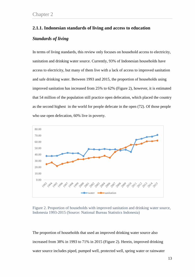
and safe drinking water. Between 1993 and 2015, the proportion of households using
improved sanitation has increased from 25% to 62% (Figure 2), however, it is estimated
that 54 million of the population still practice open defecation, which placed the country
as the second highest in the world for people defecate in the open (72). Of those people
who use open defecation, 60% live in poverty.
Figure 2. Proportion of households with improved sanitation and drinking water source, Indonesia 1993-2015 (Source: National Bureau Statistics Indonesia)
The proportion of households that used an improved drinking water source also
increased from 38% in 1993 to 71% in 2015 (Figure 2). Herein, improved drinking
water source includes piped, pumped well, protected well, spring water or rainwater
0.00
10.00
20.00
30.00
40.00
50.00
60.00
70.00
80.00
water sanitation
13

Chapter 2
where distance between the source and sewage system is more than 10 metres. In terms
of drinking water sources, currently less than half of all households had access to either
piped (11%), pumped (15%) or protected well (23%) as the main drinking water source.
At the provincial level, the proportion of households that used piped water as their main
drinking water source ranged from 20% in Bali to 4% in Papua (20).
Inadequate access to improved drinking water and sanitation is associated with poor
growth and higher prevalence of diarrhoea, which is a leading contributor to under five
mortality in Indonesia (21). National statistics suggest that 1 in 25 children under five
dies before age 5 but estimates in the Eastern provinces is higher, suggesting that 1 for
every 14 children under five dies in that region (73). Children in the poorest households
are more than three times more likely to die during the first five years of life compared
to the richest households.
Access to education
Regional disparities are also reflected in terms of access to education services. Overall,
children from poorer households and who live in rural areas have lower access to
education services compared to their peers from richer households, and those who live
in urban areas. Many Indonesian children under 6 do not have access to early childhood
education and development (ECED) services. Estimates suggest that only 18% of
children aged 3-6 years participated in an ECED program in 2006 (22), and those that
did mainly lived in urban areas and rich districts (23). Access to primary education
(ages 7-12 years) is almost universal for both urban and rural, however, social
inequalities in school enrolment widen after age 10 (24). For example, in 2010 of
children aged 15, school enrolment rates in rural areas were 70% compared to 85% in
urban areas. Children aged 13-15 years from the poorest families are four times more
14
Chapter 2 likely to drop out from school (72). Household financial resources (24, 25), distance to
school and the cost of transportation(24) are common factors that contribute to
inequality in school enrolment in Indonesia. Almost all primary education students live
within four kilometres from a school and about 20% of junior secondary education
students have to travel four or more kilometres to school. Distance to senior secondary
education and higher education is even farther, which implies higher transportation
costs. In 2010, the poorest income quintile spent about 205,000 rupiah/child (about
US$26 using the year 2010 currency rate) for primary education, which is equivalent to
a 15% of per capita household expenditure. The average cost for senior secondary
education is about 1.2 million rupiah/child/year (about US$150) or equivalent to about
50% of per capita household expenditure (24). This is an enormous economic strain on
most families, and maybe one reason why many children from poor families do not
continue onto secondary education. Over the years, the Indonesian government has
implemented several policies to improve universal access to education for its citizens
(23, 24). Increasing access to education services also has been included as part of the
national poverty reduction program. Some of these programs are presented in the
following section.
2.1.2. Indonesian government policies to improve access to education
This section presents an overview of the government policy interventions aimed to
improve access to education services in Indonesia including the school construction
program, the ECED centre, and cash transfer programs.
The school construction program
The first program that aimed to improve access to education was the school construction
program, also known as SD INPRES (Sekolah Dasar Instruksi Presiden – Presidential
15

Chapter 2
Instruction for Primary School Program) (67). The school construction program was
implemented in the 1970s, which aimed to improve access to primary education and to
reduce poverty in the long run. Between 1973-1974 and 1978-1979, the Indonesian
government built more than 61,000 primary schools across the country. On average two
schools were built per 1000 children aged 5-14 years in 1971 (10), and more schools
were built in the areas where there were higher proportions of school drop outs or lower
participation rates in schooling. According to the World Bank, it was the fastest school
construction on record (67). The school construction program successfully increased
enrolment rates from 69% in 1973 to 83% in 1978. According to Duflo (10), the school
construction program increased the average years of education by 0.12 to 0.19 years of
education, and increased wages by 1.5 to 2.7% for each primary school constructed per
1000 children. Using evidence from the Indonesian Family Life Survey (IFLS),
Pettersson (74) reported similar findings. He also found that children from lower
socioeconomic position (SEP) and women benefitted more from the program than their
peers from higher SEP families and men.
Early childhood Education and Development (ECED) program
As mentioned in section 2.1.1 many Indonesian children under 6 do not have access to
an ECED centre. In the past decade, access to ECED services has been concentrated in
urban and rich districts. In order to increase participation in the ECED services and
improve children’s developmental potential and transition to more formal education,
between 2006 and 2012 the Indonesian government launched a community-based
ECED project throughout the country (26). The ECED program targeted about 738,000
children aged 0-6 years and their primary caregivers living in 3000 villages within 50
poor districts (26). A recent World Bank report (75) indicates that children living in the
16

Chapter 2 project area had a 7% higher chance to enrol in an ECED centre compared to those
children living outside the project areas. The ECED project also had positive effects on
children’s school readiness and socio-emotional wellbeing, but no impact on nutritional
status.
Cash transfer programs
As shown in section 2.1.1, household finances (24, 25) are a major contributor to
inequality in school enrolment rates in Indonesia. The Indonesian government has rolled
out several programs to provide financial assistance for poor families, including
conditional (Program Keluarga Harapan PKH), and unconditional cash transfers
(Bantuan Langsung Tunai BLT), scholarships for poor students (Bantuan Siswa Miskin
BSM) (23), and recently the Indonesian Smart Card program (Kartu Indonesia Pintar
KIP) (27). Of these programs, only the conditional cash transfer program PKH has both
health and education components. The PKH program targeted poor households with
pregnant and/or lactating women, children between 0-15 years, or children between 16-
18 years, but who had not completed 9 years of basic education upon participation on
local health and education services. The first pilot of the PKH program was conducted
in 2007 and, targeted 300,000 poor households in 7 provinces (76). The targeted
households received cash transfers ranging from 600,000 (US$ 21) to 2.2 million rupiah
(US$ 232) per year, depending on the number of children in the household and
children’s age. Findings from the impact evaluation study of PKH (76) suggest that
PKH households used the cash transfer to increase their spending in food, health and
non-food expenditure, increase utilization in health services but not educational
services.
17

Chapter 2
In November 2014, the Indonesian government introduced a new cash transfer program,
known as the Indonesian Smart Card program (Kartu Indonesia Pintar KIP). KIP
provides cash transfers to poor families who have children between 7 and 18 years of
age (27). The additional income from KIP should only be used for the purpose of
children’s education, for example to pay additional costs of education such as uniforms,
reading materials, and the costs of transportation. Currently there is no study that has
evaluated the effect of KIP on educational outcomes.
In summary, section 2.1 provides an overview of Indonesian society and related
economic development. Indonesia continues to have significant economic growth,
which has moved Indonesia from a lower to a middle-income country. However, the
review of the literature suggests regional disparities in poverty rates, standards of living
and access to education. People, who live in Java or in urban areas tend to have lower
poverty rates, better standards of living and access to education services compared to
the population who live outside Java or in rural areas. Several examples of policy
interventions to improve access to education in Indonesia were presented.
2.2. Examining inequalities in children’s cognitive and socio-emotional wellbeing
The aim of this thesis was to investigate inequalities in children’s cognitive and socio-
emotional wellbeing in Indonesia, and interventions that might reduce these
inequalities. This review focuses on three factors that contribute to inequalities in
children’s cognitive and socio-emotional wellbeing including household socio-
economic position (SEP), parental mental health and parenting styles. Figure 3 shows a
conceptual model that represents the overall research framework. This graph shows that
children’s cognitive and socio-emotional wellbeing is affected by household SEP,
18

Chapter 2 maternal mental health and parenting styles. Household SEP may have a direct effect on
children’s cognitive and socio-emotional wellbeing and an indirect effect mediated
through parental mental health and parenting styles. Moreover, parental mental health
may have a direct effect on children’s cognitive and socio-emotional wellbeing and
indirect effect mediated through parenting styles confounded by household SEP.
Finally, parenting has a direct effect on children’s cognitive and socio-emotional
wellbeing, confounded by household SEP and parental mental health. Figure 3 also
shows that whether a child lives in poorer SEP, has parents with poor mental health or
poor parenting styles affects the likelihood of receiving intervention to improve
household’s economic condition, parental mental health or parenting styles, and in turn
improving children’s cognitive and socio-emotional wellbeing. Section 2.2 presents a
review of the literature about the associations of household SEP, parental mental health
and parenting styles with children’s cognitive and socio-emotional wellbeing.
Figure 3. The conceptual model representing the overall research framework
19

Chapter 2
2.2.1. Household socio-economic position
Extensive studies in high-income countries (HICs) and LMICs have examined the
association of household SEP with children’s cognitive and socio-emotional wellbeing.
SEP is commonly used as an indicator of individual or family position based on their
financial resources and/or social position in the society. There are various definitions
and measures of SEP including income, expenditure, housing conditions, assets,
education and occupation (77). Lower SEP is associated with lower household income
or expenditure, lower parental education, and poor housing conditions, i.e. lack of
access to improved sanitation and safe drinking water. Researchers have measured SEP
in a number of ways, either as single or composite variables. The decision of which
measure to be used in a study may rely on the context of the study and the availability
of data (78-80). For example, ’income’ is commonly used as a direct measure of SEP in
HICs, however, in LMICs ‘consumption expenditure’ is preferable for both conceptual
and practical reasons (81). In LMICs, many households are employed in the informal
sector such as home production. In addition, many households in LMICs may have
multiple sources of income, and as a result household income often fluctuates over time.
Hence, use of consumption expenditure is preferred in LMICS partly because this
measure is more stable than income.
In some studies, household ‘standard of living’ is used as a measure of SEP. This
measure is useful especially when information about income or expenditure is not
available (80). Household standards of living could be measured through housing
conditions and household assets (82). Housing conditions may include access to
drinking water supply, sanitation facilities, electricity, types of flooring, roof, wall and
kitchen, cooking fuel and number of rooms in the house. Household assets may include
owning a television, radio, refrigerator, vehicle and house tenure. Together these
20

Chapter 2 variables can be combined to provide a summary of standard of living or wealth index,
which is generated using either a factor analysis or principal component analysis (80,
82).
Despite various ways to measure SEP, there is clear evidence indicating that children
who live in higher SEP have better cognitive functioning (7, 83-89) and fewer socio-
emotional problems (6-8, 90-92) compared to children from lower SEP. Results about
the association of SEP with children’s cognitive and socio-emotional wellbeing from
HICs and LMICs are presented below.
Association of household SEP with children’s cognitive and socio-emotional wellbeing in high income countries
Numerous studies in HICs have examined the association between household income,
and children’s cognitive and socio-emotional wellbeing (8, 86, 87, 92). Most studies
show that higher income is associated with better cognitive function, however, the
effect size is relatively small. For example, Dahl et al., (86) used an instrumental
variable method to estimate the association of income with children’s language and
math scores from an observational study in the United States (US). They found that for
every US$ 1000/year increase in current income was associated with a 6% standard
deviation (SD) units increase in language and math scores for children aged 8-14 years,
and a larger effect was found among the lowest quartile income group (86). From a
cohort study in the UK, the association of income with children’s cognitive test scores
ranged from 0.22 to 0.37 SD units for every £10,000 increase in the average annual
family income at age 3 (8).
Studies that used a composite measure of SEP also showed similar patterns. Household
income and assets were the largest contributors of inequality in reading and math
21

Chapter 2
assessment for children aged 3-17 years in the US (93), and associated with children’s
socio-emotional wellbeing in eleven European countries (90). A systematic review by
Reiss et al., (91) used evidence from cross sectional and longitudinal studies to examine
the association of SEP (measured by household income and parental education) with
internalising and externalising problems in children and adolescence. From this review,
Reiss et al., (91) showed that children from lower SEP were three times more likely to
develop internalising and externalising problems compared to their peers from higher
SEP. Reiss et al., (91) also showed the association of SEP was stronger with
externalising than with internalising problems, and was stronger in children aged 4-11
than in children aged 12-18 years.
Association of household SEP with children’s cognitive and socio-emotional wellbeing in LMICs
Several studies from LMICs used the term ’household wealth’ to define household
standards of living. Wehby and McCarthy (88) used principal component analysis to
generate a household wealth index based on housing conditions and assets in a sample
of children in Argentina, Brazil, Chile and Ecuador. They examined the association of
household wealth in the first two years of life with children’s cognitive function
(measured by Bayley Infant Neurodevelopmental Screener). Results showed that in all
countries included in the study, children from higher wealth quintiles had higher
cognitive scores after controlling for maternal age, education, and marital status,
children’s ethnicity and sex, and number of adults in the household. In Wehby and
McCarthy’s (88) study, the effect size of the association between household wealth and
children’s cognitive function was relatively small (ranged from 0.06 SD in Argentina to
0.15 SD in Ecuador). Another study that used data from community-randomized trials
in India, Indonesia, Peru and Senegal (94) also showed similar results, suggesting that
22
Chapter 2 children from wealthier households had better cognitive function than their peers from
poorer households. In this study (94), having a mother who completed 9 years of
education or more was also associated with better cognitive function scores compared to
those who had a mother who never attended formal education (effect size ranged
between 0.26 and 0.48 of a SD score after controlling household wealth and other
covariates).
Evidence from a nationally representative sample of poor children in poor communities
In Madagascar suggested that household wealth and maternal education were associated
with cognitive function and language development in children aged 3-6 years (89). In
this study, children from the richest quintile group had a 0.72 SD higher receptive
language (vocabulary) score compared to children from the poorest quintile, controlling
for maternal education, residential area (urban-rural), household crowding (household
size and number of rooms in the household), and children’s sex, age and birth order.
Furthermore the association of maternal education with children’s receptive language
score was smaller than household wealth. Children whose mothers had a secondary or
higher education had a 0.39 SD higher receptive vocabulary score than children whose
mothers had never received a formal education.
The following sections present evidence about the associations of parental mental health
and parenting styles with children’s cognitive and socio-emotional wellbeing.
2.2.2. Maternal mental health
Association of maternal mental health with children’s cognitive and socio-emotional wellbeing in HICs
Studies about the associations of parental mental health and parenting with children’s
cognitive and socio-emotional wellbeing in HICs are well documented. Studies show
23

Chapter 2
children living in households with parents with poor mental health tend to have poorer
cognitive and socio-emotional wellbeing (6, 7, 95-97). For example, evidence from the
Millennium Cohort Study (MCS) in the UK suggested that poor maternal mental health
at age 3 was associated with a 0.13 SD units increase in internalizing problems, and a
0.22 SD unit increase in externalizing problems (6). In this cohort, the association of
maternal mental health with children’s cognitive function was much smaller (-0.01 SD)
than with socio-emotional wellbeing. A nationally representative sample in the US
findings showed that the association of maternal depression with cognitive scores
ranged from -0.18 to -0.42 SD for children age 13-50 months (7). Mothers who had
mental health problems were more likely to have lower income, lower education,
younger age, unmarried and unemployed, which are markers of economic and social
disadvantage (7, 98-100).
Association of maternal mental health with children’s cognitive and socio-emotional wellbeing in LMICs
Studies about the association of parental mental health with children’s cognitive and
socio-emotional wellbeing are often under-reported in LMICs. Women in LMICs are
less likely to self-report having mental health problems and this is partly because their
perception of mental health is shaped by cultural constraints such as stigma within the
community (101). Although evidence from LMICs is more limited, findings from
observational and RCT studies in LMICs also suggest that poor maternal mental health
are associated with children’s poor cognitive and socio-emotional wellbeing (102-104).
24
Chapter 2 2.2.3. Parenting styles
Association of parenting styles with children’s cognitive and socio-emotional wellbeing in HICs
In terms of parenting styles, positive parenting was associated with improved child
temperament, lowered behavioral problems or disruptive behavior, better social
emotional competence and higher language scores (8, 30). Findings from the UK
showed that among children aged 3-5 years, warm parenting was associated with a 0.06
SD units increase in cognitive scores and a 0.15 SD units decrease in externalizing
behavior problems, whereas punitive parenting was associated with a 0.08 SD units
decreased cognitive scores (30).
Associations of parenting styles with children’s cognitive and socio-emotional wellbeing in LMICs Cultural variations in parental styles were also found in Bornstein, et al., (105) study,
conducted in nine countries i.e. China, Colombia, Italy, Jordan, The Philippines,
Kenya, Sweden, Thailand and the US. This study found that parents from Kenya,
Colombia and the Philippines were more likely to have authoritarian attitudes, whereas
parents from the US, Sweden, Thailand, China and Jordan were more likely to have
progressive attitudes even after controlling for parent’s age, education and potential
reporting bias. In terms of the characteristics, authoritarian parents demanded children
to be respectful and obedient towards parents, whereas progressive parents encouraged
children to think independently, and to speak their minds. A survey of 273 Indonesian
parents of children aged 2-12 years reported a positive correlation between poor
parenting and children’s emotional and behavioral problems (106). In this study, parents
who reported low levels of children’s emotional and behavioral problems not only tend
25

Chapter 2
to have better parenting but also greater self-efficacy and less mental health problem
than parents who reported high levels of children’s emotional and behavioral problems.
Long term effects of household SEP, parental mental health and parenting
Longitudinal studies have showed long term effects of being exposed to poverty, having
parents with poor mental health, and poor parenting ability. Children exposed to poverty
in the first year of life tend to have poor cognitive (83, 107) and socio-emotional
problems (107, 108) at later childhood and adolescence, and those who were exposed to
longer periods of poverty had poorer outcomes compared to the children who only
experienced poverty at one point in time (107). Evidence showed parental mental health
(measured through depression) in the first year of life was associated with poorer
children’s behavioural problems at age under five (109, 110), at preschool (97) and
increased the risk of depression at age 16 (111). Moreover, low maternal warmth was
associated with more socio-emotional problems at younger ages and at adolescence
(112, 113).
2.2.4. The relations between household SEP, parental mental health, parenting and children’s cognitive and socio-emotional wellbeing
This review of the literature demonstrates consistent findings from both HIC and
LMICs that children from lower SEP families tend to have poorer cognitive and socio-
emotional wellbeing compared to their peers living in families from higher SEP.
Household SEP such as income represents financial resources that are available in the
family, and the extent to which these resources are invested in children’s development
(28). As outline in section 2.1.1 poor financial resources limit parental investment on
children’s education in Indonesia. Children from lower income families tend to have
26

Chapter 2 poorer development outcomes because their families were less likely to engage in
cognitive stimulating activities and had fewer visits to health checks (29, 30, 92).
The relations between poverty, parental mental health and parenting are well
documented, although most evidence comes from HICs. Evidence from a systematic
review and cohort studies (6, 8, 30, 114, 115) suggest that the association of SEP with
children’s cognitive and socio-emotional wellbeing was potentially mediated by
parental mental health and parenting styles. A cohort study in the UK found a direct
effect of income on cognitive ability and socio-emotional wellbeing at age 9 months, 3
years and 5 years, and an indirect effect mediated through parental stress (8). Among
mothers, higher income and higher education are associated with positive psychological
functioning because educated mothers usually have greater self-esteem and optimism,
and therefore show fewer symptoms of depression (116). In contrast, low income may
affect emotional distress in parents, and reduce their capability to interact and to build
healthy relationships with children (117). Parents from low income families who had
poor mental health tended to be less nurturing and engaged with their children, which in
turn affects poor development in children (6).
In summary, section 2.2 shows a great deal of research pointing to the importance of
household and parental characteristics, parental mental health, and parenting skills on
children’s cognitive and socio-emotional wellbeing. The following section presents
evidence from relevant policy interventions that could reduce inequalities in children’s
cognitive and socio-emotional wellbeing and strategies for effective implementation of
these interventions.
27

Chapter 2
2.3. Early childhood interventions and strategies for effective implementation of intervention
Evidence from HICs (32-35) and LMICs (19, 36, 37) indicates that effective
interventions can protect children from negative consequences of living in poverty (36)
and increase investment in children’s health and development (1). The final section of
this chapter presents several examples from relevant early childhood interventions that
might reduce inequalities in children’s cognitive and socio-emotional wellbeing. This
review focuses on interventions that aim to enhance family investment in children,
maternal mental health and parenting skills, followed by evidence about effective
interventions.
2.3.1. Income supports for poor families
There is clear evidence that children from poor income families tend to have poorer
cognitive ability, and higher risk of behavioural problems compared to their peers from
higher income families. One of the strategies to support parental investment in children
is through providing financial intervention to poor families. In HICs, financial
intervention could be in the form of direct cash payments or tax benefits. A systematic
review by Lucas et al., (118) used evidence from RCTs and quasi-randomised trials to
examine the effect of a financial intervention (through direct cash payments or tax
benefit) for poor families in HICs on children’s health, socio-emotional and educational
outcomes. Despite strong evidence of the association between family income and
children’s health, socio-emotional and educational outcomes, they could not find
evidence of the effect of financial interventions on the overall outcomes. Moreover,
Lucas et al., (118) argued that on the basis of current evidence, they could not show
28
Chapter 2 whether providing financial interventions are effective to reduce inequalities in
children’s development outcomes in HICs.
In LMICs, providing financial intervention through conditional cash transfer (CCT)
programs is widely used to help parental investment in children’s health and education,
and reduce poverty in the long run (119). In general, CCT target poor households with
pregnant or lactating women, and children aged 0-18 years. In CCT program, the money
was transferred to households conditional upon their compliance with regular visits to
health clinics, and attendance in primary or secondary school depending on the child’s
age.
Evidence from the CCT program in Mexico, Oportunidades, suggested that children
who received CCT had better nutritional status, better motor skills, higher cognitive
scores, and lower socio-emotional problems (120). A study by Fernald et al., (121)
examined long terms effects of the Oportunidades on various child outcomes and
showed that this program continue to have a positive effects on children’s health,
cognitive and socio-emotional wellbeing even after ten years of its implementation.
Evidence from various cash transfer program in LMICs showed that cash transfer
intervention had improved children’s health, cognitive functioning, schooling and socio-
emotional wellbeing (37, 76, 120-124) but the effect size was small. For example,
Paxson and Schady (125) examined the effect of cash transfer on children’s cognitive
and socio-emotional wellbeing in Ecuador. In Ecuador, the average effect size of cash
transfer program on children’s cognitive and socio-emotional wellbeing was about 5%
of a SD score for an additional $15 of cash transfer (an equivalent to a 10% increase in
household expenditure for the average eligible households). Another example is from
Nores and Barnett (37) who conducted a meta-analysis on the benefits of early
29

Chapter 2
childhood interventions in LMICs particularly studies that used quasi-experimental or
random assignment. In their meta-analysis, Nores and Barnett (37) reported the average
Cohen d effect size of cash transfer programs on children’s cognitive function ranged
between 0.08 and 0.30, whereas the effect of cash transfer on socio-emotional
wellbeing ranged between 0.10 and 0.39.
2.3.2. Improving household standards of living
As shown in section 2.2.1 housing conditions are commonly used as an indicator of
household standards of living in LMICs. Many poor children in LMICs including
Indonesia are exposed to poor housing conditions including lack of access to clean
water and improved sanitation, which effects their health and development (18, 19, 21).
Children living in poor housing conditions tend to have poorer cognitive function (88,
94), less likely to be able to read paragraphs (126) and lower levels of education (127)
compared to their peers who live in better housing conditions. There is a growing
recognition by international organisations that improving daily living conditions is one
of the key recommendations to reduce inequalities in children’s healthy development (1,
2, 128). One of the strategies to improve housing conditions is through provision of
clean water and sanitation intervention for the poorest population.
Nowadays, providing water and sanitation interventions could be more relevant for the
poorest population living in LMICs than for those living in HICs. However, the benefits
of water and sanitation intervention in HICs have been recorded since the early 19th
century. For example, two studies from the US showed that water and sanitation
intervention between 1880 and 1915 contributed to a 35% reduction in infant mortality
rate (129), whereas provision of public water and sewage system between 1900 and
1940 reduced mortality by 20%.
30

Chapter 2 Cochrane Database of Systematic Reviews showed extensive evidence about the
benefits of water and sanitation intervention on children’s health including better
nutritional status (130) and a reduction in diarrhoea (131) but little is known about the
effect of this intervention on children’s cognitive and socio-emotional wellbeing.
Recent evidence from the Total Sanitation Campaign (TSC) in rural India suggested
that every improved sanitation built in the community at age 1 was associated with a
0.75 SD increased in the mean literacy scores at age 6 and similar effect size for the
math score (126).
The effect of water and sanitation interventions on children’s cognitive function is
potentially mediated through children’s health status. Poor sanitation and hygiene is
associated with higher prevalence of diarrhoea and infectious diseases, which links to
the children’s nutritional status, and in turn affects their poor cognitive functioning and
reduced years of schooling (17, 18). Studies showed providing water and sanitation
interventions promoted better overall health, eliminated diarrhoea and typhoid,
improved immune system function to fight disease due to poor sanitation (130-132).
Moreover, providing water and sanitation in the household may also reduce stress (132)
and less time to travel to get water or use communal sanitation facilities (133).
2.3.3. Maternal mental health and parenting interventions
As outlined in section 2.2.4 evidence shows that poverty is often associated with poor
mental health status. Using data from RCT, non-randomized intervention and cohort
studies in LMICs Lundt, et al., (134) conducted two systematic reviews to examined the
effect of poverty alleviation interventions on individual and family or caregiver mental
health status and vice versa. In the first review they identified poverty alleviation
programs that focused on providing financial support including cash transfer,
31

Chapter 2
microfinance, loans, social insurance, debt management and financial services. Results
show that only interventions to provide cash transfer and accumulation of assets in the
family had a greater effect to reduce mental health problems compared to other financial
interventions. The second part of the systematic review examined the effect of mental
health interventions on economic outcomes such as employment status. In the second
review, they identified a wide range of mental health interventions including personal,
community-based rehabilitation program, preventive program, medication and some of
their combination. Results show that all mental health interventions were associated
with improved household economic conditions.
Based on a systematic review of evidence from RCT and observational studies (135)
mental health interventions for parents also had benefits for children. Parents who
received mental health intervention had fewer children with or suffering from
internalising and externalising problems and learning difficulties (135). Moreover,
evidence from systematic reviews suggests that parenting interventions in HICs and
LMICS have several benefits for both families and their children including reduced
family stress and maternal ill health (136), and improved women’s perception for
existing social support (137), reduced harsh or abusive parenting and increased
parenting practices (138-140), improved home learning environment (137), more visits
to library (32), improved children’s overall health, higher immunization rates, better
infant feeding patterns, better fine motor skills and cognitive functioning (32, 140), and
better socio-emotional wellbeing (140).
32

Chapter 2 2.3.4. Strategies for effective implementation of interventions
Timing for intervention
A review of the literature showed that the association of household SEP with children’s
cognitive and socio-emotional wellbeing are stronger in younger children (37, 114, 141,
142), suggesting that early childhood interventions may have greater effect than
intervention in later childhood (19, 37). In HICs research in neuroscience (38) and
economics (33) support the argument that early childhood intervention yields better
results than intervention in later childhood. In terms of cost-effectiveness, Doyle et al.,
(33) provide a summary of benefit for investing in early childhood based on the rates of
return in human capital investment (Figure 4). As shown in figure 4, assuming the costs
of interventions are held constant across all ages, early years interventions would yield
the highest rates of return. Rates of return can be defined as economic benefits in the
form of individual’s earnings, higher education, better physical and mental health,
whereas at community level the rates of return of early intervention may include higher
government savings and revenues from taxes, as well as reduce crime and delinquency
(33, 35). In terms of benefit-cost ratios, an example from a meta-analysis of early
childhood interventions in the US estimated that using a 3% of annual discount rate,
every dollar invested in children had benefit of about USD 1.27 to USD 17.7 for society
(35). The largest benefit was associated with programs that had long term follow up
(35) and followed by late investment (39).
33

Chapter 2
Coverage of intervention
Effectiveness of early childhood intervention could also be influenced by the
interventional approaches and coverage of the program. A universal approach may
reduce inequalities in early childhood development by providing equal access to all
social groups in a defined population (1). A meta-analysis in HICs and LMICs
suggested that provision of universal interventions on education had greater effect for
improving children’s cognitive outcome than targeted interventions (37). Although
universal intervention is costly, some would argue that the benefit is greater than the
cost (32, 143).
In contrast, targeted interventions were more effective to improve children’s socio-
emotional wellbeing (37), maternal mental health (144) and parenting skills (137, 139,
140). Evidence from RCTs about parenting interventions in HICs suggested that an
intervention targeted young and unmarried mothers from low socioeconomic position is
Figure 4. Rates of return to human capital investment (Source; Doyle et al. 2000)
34

Chapter 2 the most effective to improve parenting skills and in turn affect healthier children’s
developmental outcomes (137, 139, 140). Despite the advantage, targeted intervention
may limit participation and create stigma among people who were targeted for an
intervention (32). Universal approaches may be costly but reach a much larger
population and remove stigma associated with targeted programs (32, 143).
Evidence from HICs and LMICs also showed that provision of intervention that had a
mixed component early childhood program may yield greater benefit to improve
children’s cognitive function than a single intervention. For example, in Nores and
Barnett meta-analysis of quasi-experiments and RCTs (37) the average effect size of
cash transfer programs on children’s cognition was 0.17 (SD 0.06), whereas the average
effect size of intervention that combined cash transfer, nutrition and an educational
program was 0.35 (SD 0.22). Finally, evidence about effective implementation of
parenting intervention is also found in HICs and LMICs. Studies showed that the most
effective parenting intervention was characterized by a program that combined home
visits, clinic care and educational program for both parents and children, workshops or
public health campaign or mass media education and (32, 137, 140, 145), and focused
on specific behavioural change including promoting positive mother-child relationships
(32, 36, 140).
2.4. Conclusions
There is evidence to show that inequalities in children’s cognitive and socio-emotional
wellbeing are influenced by a range of household and parental characteristics including
household SEP, parental mental health status and parenting styles. Interventions that
provide support for family investment in children, improve housing conditions, enhance
maternal mental health and parenting skills may improve children’s cognitive and socio-
35

Chapter 2
emotional wellbeing. In order to have greater benefit, the intervention should be
conducted at early ages (e.g. under seven) and have multiple components of
intervention such as cash transfer, nutrition and an educational program.
This research will seek to identify the magnitude of, and contributors to socioeconomic
inequality experienced by children in Indonesia. We then investigate the mediating
effect of early vs late poverty on cognitive function, and the simulated effect of different
types of interventions designed to improve cognitive function and socio-emotional
wellbeing. These studies extend previous work by providing context specific evidence
that can contribute to the implementation of evidence based interventions, to improve
child health and development in Indonesia.
36

CHAPTER 3
Methods

Chapter 3 The overall aim of this thesis is to investigate inequalities in cognitive function and
socio-emotional well-being among Indonesian children, and how early childhood
interventions might reduce these inequalities. Four studies were conducted to address
this overall aim. This chapter provides an overview of data used in this thesis, the
measures, the methodological and the statistical approaches in each study including how
to address the uncertainties due to missing data and unmeasured confounding.
3.1. Data sources
3.1.1. The Indonesian Family Life Survey
The first data source used in this thesis was the Indonesian Family Life Survey (IFLS).
IFLS is an ongoing longitudinal survey, which was first conducted in 1993 and
subsequently in 1997, 2000 and 2007 (146-149). In 1993, 13 of the 27 provinces were
selected purposively due to logistical reasons but to still maximize representation of the
population, and capture the cultural and socioeconomic diversity. These provinces
spread across Indonesia including the islands of Sumatera, Java, Bali, West Nusa
Tenggara, Kalimantan and Sulawesi (Figure 5). The sampling scheme was stratified on
provinces and urban rural areas, where within each province the enumeration area was
selected randomly. In IFLS1 over 7000 households and 22,000 individuals were
interviewed. This sample was considered to be representative of 83% of the Indonesian
population (146). In the most current data collection (IFLS4), over 13,000 households
and 44,000 individuals were interviewed.
38
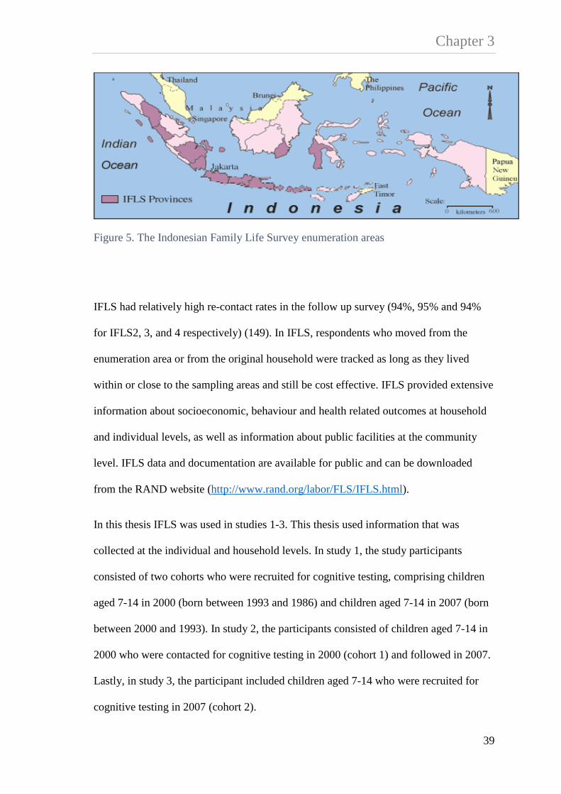
Chapter 3
Figure 5. The Indonesian Family Life Survey enumeration areas
IFLS had relatively high re-contact rates in the follow up survey (94%, 95% and 94%
for IFLS2, 3, and 4 respectively) (149). In IFLS, respondents who moved from the
enumeration area or from the original household were tracked as long as they lived
within or close to the sampling areas and still be cost effective. IFLS provided extensive
information about socioeconomic, behaviour and health related outcomes at household
and individual levels, as well as information about public facilities at the community
level. IFLS data and documentation are available for public and can be downloaded
from the RAND website (http://www.rand.org/labor/FLS/IFLS.html).
In this thesis IFLS was used in studies 1-3. This thesis used information that was
collected at the individual and household levels. In study 1, the study participants
consisted of two cohorts who were recruited for cognitive testing, comprising children
aged 7-14 in 2000 (born between 1993 and 1986) and children aged 7-14 in 2007 (born
between 2000 and 1993). In study 2, the participants consisted of children aged 7-14 in
2000 who were contacted for cognitive testing in 2000 (cohort 1) and followed in 2007.
Lastly, in study 3, the participant included children aged 7-14 who were recruited for
cognitive testing in 2007 (cohort 2).
39

Chapter 3 3.1.2. The Early Childhood Education and Development (ECED)
The ECED data was used in study 4, which investigated the relative and combined
effect of different hypothetical interventions on children’s school readiness and socio-
emotional wellbeing. Study 4 used information that was collected at the individual
(children and caregiver) as well as household levels and was analysed as a cohort study
of children aged 4 in 2009 and followed up at ages 5 and 8.
Background to ECED Study
There is a growing awareness about the importance of early childhood education and
development (ECED) programs in Indonesia (150), however, access to ECED services
remains very low and are more concentrated in urban areas and rich districts. Estimates
from the World Development Indicators 2006 suggest that the total ECED participation
rate among children ages 3-6 years in Indonesia was 18%, which is lower than the
global average in low income countries (27%) (22). To provide greater access to ECED
services in the country, between 2006 and 2012 the Indonesian government through the
Ministry of National Education and Culture (formerly the Ministry of National
Education MoNE) implemented a community based ECED project, which aimed to
improve children’s development and readiness for transition to formal education (26).
This project was financed through multiple sources including the World Bank, the
government of the Netherlands and the Indonesian government with a total cost of US$
127.7 million. The ECED project targeted about 738,000 children ages 0-6 years and
their primary caregivers living in 3000 villages within 50 poor districts that were
selected based on low participation rates in ECED services, high poverty rates, and
commitment to developing, managing and financing the ECED project in their area.
Within each district, 60 villages were selected based on high numbers of children aged
40

Chapter 3 0-6 years, had high poverty rates and had shown interest in the ECED project. In each
district, the project was implemented in three waves with 20 new villages receiving the
program per implementation wave, each nine months apart.
The Indonesian government also received technical support from the World Bank to
conduct a cluster randomized controlled trial (RCT) to evaluate the impact of the ECED
project on children’s developmental outcomes and factors that contribute to the
effectiveness of the program (26). The RCT also aimed to increase awareness and
generate discussion among policy makers and the general public about the importance
of ECED and effective implementation to improve ECED programs. Evidence from this
project may then be used to scale up the coverage of ECED services for poor children in
Indonesia (26). After the implementation of the ECED project, in late 2013 the
Indonesian government initiated a national program “Satu Desa Satu PAUD” (one
village one ECED centre) to provide greater access to ECED services especially in rural
areas. This could be evidence that scaling up ECED interventions in the country is
already in progress.
For the RCT, the Indonesian government selected 10 out of 50 districts based on their
willingness to randomize villages into the implementation waves and still represent
geographic diversity. The randomization did not take place at the district level because
many districts had already allocated villages to a particular wave. Prior to the first data
collection in 2009, one district was dropped from the study due to non-compliance. The
final sample in the RCT consisted of 310 villages in 9 districts including Sarolangun,
North Bengkulu, East Lampung, Majalengka, Rembang, Kulon Progo, Sidenreng
Rappang (Sidrap), Ketapang and Middle Lombok (Figure 6).
41

Chapter 3
Figure 6. The Early Childhood Education and Development enumeration areas
The ECED study comprised cohorts aged 1 and 4 in 2009 with follow up in 2010 and
2013. Additionally, the study also collected information at the household and
community levels. At the follow up in 2010, 99% of children were successfully
recontacted. The reason the ECED project had high recontact rates was partly because
children who moved to another village were tracked as long as they lived within the
study sample (26). For this thesis, access to ECED data was obtained through the World
Bank.
42
Chapter 3 3.2. Measures
The following section describes the various measures used in the thesis.
3.2.1. Outcomes
Raven Progressive Matrices – Cognitive Ability
The Raven’s Progressive Matrices (RPM) was used as a measure of cognitive function
or general intelligence (151). The RPM was available in IFLS collected from children
aged 7-14 in 2000 and aged 7-14 in 2007. Children who took the test in 2000 were
interviewed again in 2007 when they were 14-22 years. In IFLS, the questions were
reduced in number due to logistical constraints. The test comprised 12 shapes with a
missing part where children selected the correct part to complete the shape (Figure 7).
Each correct answer was coded 1 or 0 otherwise and scores combined as the total raw
scores. The total raw scores increased with age and had skewed distributions towards
the left tail. The total raw scores were then transformed into an age-specific z-score.
Because the total scores were skewed, the mean and the variance of score distributions
were calculated by taking into account the range, median and the sample size using the
formula from Hozo, et al., (152) and used the estimated mean and standard deviation to
create an age specific z-score. The RPM was used as the cognitive function outcome in
studies 1-3.
43

Chapter 3
Figure 7. Example of item in Raven Progressive Matrices as appeared in IFLS questionnaire
Early Development Instrument (EDI)
The Early Development Instrument (EDI) was used as a measure of school readiness
and comprised five major developmental domains including physical health and well-
being, social competence, emotional maturity, language and cognitive development, as
well as communication skills and general knowledge (153, 154). For each domain the
score ranged from 0 to 10, where a higher score indicated better outcomes. A child
whose score was in the lowest 10% in each domain was classified as developmentally
vulnerable in that specific domain (coded as 1 or 0 otherwise). The scores were summed
to define whether a child was developmentally vulnerable in one or more domains
(coded as 1 or 0 otherwise). The EDI was available in ECED collected on children aged
4 in 2009 and follow up at ages 5 and 8.
44

Chapter 3 Strengths and Difficulties Questionnaire (SDQ)
The Strengths and Difficulties Questionnaire (SDQ) was used as a measure of
children’s socio-emotional wellbeing (155). The SDQ comprises five subscales
including emotional symptoms, conduct problems, hyperactivity/inattention, peer
relation problem and prosocial behaviour. For each subscale the score ranged from 0 to
10. With the exception of prosocial behavior, higher scores in emotional symptoms,
conduct problems, hyperactivity/inattention and peer problems indicated poorer
behavioural outcomes. The scores of emotional and peer problems subscales were
combined to define internalising behaviour, whereas the scores of conduct problems and
hyperactivity/inattention subscales were combined to define externalising behaviour.
According to Goodman, et al., (156) use of internalising and externalising problems
subscales is more appropriate in epidemiological studies and to define children’s
behavioural problems in low risk populations. The SDQ was available in ECED
collected on children aged 4 and follow up at ages 5 and 8.
Both the EDI and the SDQ were used as the outcomes in study 4. This analysis only
used the EDI and the SDQ that were measured at age 8 based on caregiver’s report.
3.2.2. Exposures
Household expenditures
Household per capita expenditure (PCE) was used as an indicator of relative
socioeconomic position and resources for parental investment in children. Information
about household PCE was only available in IFLS. Household PCE was constructed by
summing the monthly total household food and non-food expenditures divided by the
number of household members (157). This variable was used in continuous form, where
45

Chapter 3 higher PCE indicated higher socioeconomic position and the potential for more
financial resources invested in children. This thesis used information about household
PCE that was collected in 2000 and 2007. Household PCE collected in 2000 and 2007
was used as the exposure in studies 1 and 2. Additionally, a new variable was
constructed to define poverty status based on the distribution of household PCE in the
population. Following the World Bank and WHO proposition, the poorest 40% of the
population was considered as in “poverty” for the purpose of determining access to
universal health coverage (158). Herein, poor households were defined as those living
in the bottom 40% of PCE (coded as 1 or 0 otherwise). Poverty status was used to
identify the target population for cash transfer intervention (study 2) and children who
lived in poverty (study 3). Moreover, in study 3, poverty status in 2000 (children ages
0-7 years) was defined as the exposure and poverty status in 2007 (children ages 7-14
years) was defined as the mediator.
In study 4, three exposures that affect children’s school readiness and socio-emotional
wellbeing were identified based on the literature review in chapter 2, the availability of
data in the ECED study and feasibility of intervention. These exposures included
household standards of living (126, 129), maternal mental health (6, 145) and parenting
styles (32, 36, 138, 140, 159).
Household standards of living
Household standards of living is commonly used as a measure of economic status and is
useful especially when information about income or consumption expenditure is not
available in the data (80). Herein, a household standard of living was measured using
two indicators including access to improved drinking water source and sanitation.
Access to improved drinking water source was measured through whether the child
46

Chapter 3 lived in a household that used piped water as the main drinking water source (coded as
1 and 0 otherwise), whereas access to improved sanitation was measured through
whether the child lived in a household that owned a private toilet connected to septic
tank (coded as 1 and 0 otherwise).
Maternal mental health intervention
Maternal mental health was measured using Kessler 10 (K10) (160), which is a self-
reported questionnaire that was designed to measure non-specific psychological
distress. K10 comprises 10 items of feelings of anxiety and depression in the past four
weeks and their frequency. Each response item was reported on a 3-point scale where
the score ranges from 1 “never”, 3”sometimes” and 5”often”. All the 10 items were
combined to generate a total mental health score, where higher score is associated with
poorer mental health (scores ranging 10-50).
Parenting styles
Parenting styles was measured using 24 items describing parent-child relationships such
as warmth, consistency and hostility. This measure was adapted from the Longitudinal
Study of Australian Children (LSAC) study (161). For each item, the response was
reported on a 5-point scale, which ranges from never to always. All 23 items were
combined to generate a total parenting score, where higher score indicated better
parenting styles. This variable was used in continuous form (scores ranging 23-115).
47

Chapter 3 3.2.3. Covariates
A series of covariates were selected a priori as potential confounding based on the
literature review in chapter 2.
Child characteristics
Child characteristics included age, gender, and education (30, 56, 151). Age was
reported in years and was used in continuous form. Gender was coded as 1 for male and
0 for female. Child’s education was measured using two indicators. For children aged 7-
14, education was measured as whether the child was currently attending school. For
those children who were interviewed at follow up (aged 14-22), education was
measured as whether the child completed at least 8 years of education.
Parent characteristics
Parent characteristics were measured separately for mother and father including
education (30, 83, 90, 162, 163), employment status (164) and mental health (6, 95,
141, 165). In IFLS, education was measured as the highest level of education attended,
(categorized as none, primary school, junior high school, senior high school and
diploma/university degree). In ECED, education was measured as the highest education
completed (categorized as none or not completed primary school, primary school, junior
high school, senior high school and diploma/university). Employment status was
measured as whether parent was working in the past week.
Mental health was also measured in IFLS3 and 4. In IFLS3, the measure consisted of
eight items of feelings experienced in the past 4 weeks, with responses in three categories
ranging from never to often. In IFLS4, the measure was adapted from the shorter version
of the Centre for Epidemiological Studies-Depression scales (CES-D) (166) consisting of
48

Chapter 3 10 items of symptoms or feelings experienced in the past week, with responses in five
categories ranging from not at all, rarely (<=1 day), some days (1–2 days), occasionally
(3–4 days) and most of the time (5–7 days). For both measures, each item was scored
from 0 to 3 and summed as the total mental health score separately for 2000 (scores
ranging 0–24) and 2007 (scores ranging 0–30) (167-169). The variable was used in
continuous form, where a higher score indicated poorer mental health. Last, maternal age
(30, 83, 108) was reported in years and used in continuous form.
Household characteristics
Household characteristics included household size (continuous) (30), the number of
self-reported economic hardships experienced by household (continuous) (102),
residential area (categorized as urban or rural and Java/Bali or otherwise) (30), housing
conditions and assets (23, 88, 126, 162, 163). Housing conditions were measured as
whether the household had electricity, used piped or pumped well as the main drinking
water source, and improved sanitation (defined as a toilet that was connected to a septic
tank).
In study 4, factor analysis (170, 171) was used to construct a standard of living index
based on housing conditions and household assets. Housing conditions included
whether the household had electricity, separate kitchen, used non-earth floor, and type
of cooking fuel (used wood, kerosene or gas/electricity). Household assets included
whether the household had telephone, radio, television, refrigerator, bike, motorcycle
and car. The standards of living index was estimated as the sum of the variables
weighted by the elements of the first eigenvector, which was the first linear combination
of the variables. The total score was then classified into quintiles, which ranged from
the poorest (quintile 1) to the richest (quintile 5).
49

Chapter 3 3.3. Methodological Approach and Statistical Analysis
The following section describes the various methodological and statistical approaches
used in the four studies presented in the thesis. This section also discusses methods used
to address missing data and unmeasured confounding.
3.3.1. Study 1: measuring inequality in children’s cognitive function
Study 1 aimed to address the following questions, (1) what is the magnitude of
socioeconomic inequality among Indonesian children’s cognitive function in 2000 and
2007; (2) what factors contribute to the inequality; (3) does the inequality in children’s
cognitive function change between 2000 and 2007 and what factors contribute to the
change in inequality? In study 1, measuring inequality in socioeconomic position is of
more interest because it has a broader concept than poverty. Poverty is defined by
comparing individual’s income or expenditure with some defined threshold in the
population. For example, individuals whose expenditure is below a certain poverty line
are classified as being poor. In contrast, inequality focuses on the distribution of
expenditure across the whole population (from the poorest to the riches) rather than only
focus on the poor (71).
In study 1, data from IFLS was used. The study participants were children aged 7-14 in
2000 and aged 7-14 in 2007. The Relative Concentration Index (RCI) (81, 172, 173)
was used to estimate the magnitude of relative socioeconomic inequality in child’s
cognitive function. This method has advantages; first the RCI estimates the magnitude
of inequality across all levels of socioeconomic position in the population (from the
poorest to the richest) rather than compares inequality between two groups, e.g., poor
versus non-poor. Second, the RCI can be decomposed into factors that contribute to the
inequality.
50

Chapter 3 Concentration curve
The RCI is derived from a concentration curve, which gives a graphical illustration of
the magnitude of inequality (Figure 8). The concentration curve is drawn by comparing
the cumulative percent of people ranked by their relative socioeconomic position for
example income or expenditure (x-axis) from the poorest (left hand side) to the richest
(right hand side), against the cumulative percent of the outcome Y (y-axis) – in this case
children’s cognitive function. The diagonal line is defined as the line of equality.
Figure 8. Concentration curve
The upper (a) and lower (b) curve indicates that inequality exists in the population.
Equality exists when the outcome Y is distributed proportionately across the
socioeconomic groups, for example when ranked by household expenditure 20 percent
51

Chapter 3 of children with lower outcome scores live in the poorest 20th percent of households. In
contrast, inequality exists when there is a disproportionate distribution of people with
lower or higher scores across socioeconomic groups, for example, where 35 percent of
children with poorer cognitive function scores live among the poorest 20% of household
PCE. The magnitude of inequality is shown as the distance between the line of equality
(the diagonal) and the curve (a or b). The farther the curve is from the line of equality,
the bigger the magnitude of inequality. If the outcome variable indicates a poor
outcome, for example malnutrition, then the inequality is shown by the curve that lies
above the diagonal line (curve a in Figure 8) indicating higher malnutrition rates are
concentrated among the poorer socioeconomic groups. On the other hand, if the
outcome variable indicates a positive outcome, for example cognitive function scores
then the curve lies below the diagonal (curve b) indicating children with poorer
cognitive function scores are concentrated among the poorer socioeconomic groups.
The Relative Concentration Index
The RCI was used to estimate the magnitude of inequality, and is defined as twice the
area between the line of equality and the curve. A value of zero in the RCI indicates
there is no inequality. The RCI values are commonly bounded between -1 and +1,
however, if the outcome is a dichotomous, the bounds depend on the mean of the
outcome ( 1−µ for the lower and µ−1 for the upper bound) (174). If the outcome
variable takes negative as well as positive values, the RCI is not bounded. The RCI
(172) can be defined as
52

Chapter 3
Equation 1. Relative Concentration Index
121
−= ∑=
i
n
ii Ry
nRCI
µ
Where μ is the mean of the outcome y (cognitive function score), and Ri is the relative
rank of the ith person in the socioeconomic distribution (household PCE). Delta method
was used to estimate the standard error, followed by the 95% confidence interval (CI)
estimation (81).
Decomposition of the RCI
The RCI can be decomposed into factors that contribute to the inequality. Suppose that
the outcome Y is a continuous score with a set of k contributors (x1, …xk), then equation
2 shows the statistical model to estimate the association between a set of k contributors
and outcome Y including child’s gender, current’s school attendance, parental
education, employment status, mental health scores, housing conditions (access to
improved drinking water, improved sanitation, and electricity) and residential areas
(living in urban or rural areas, and Java/Bali or otherwise).
Equation 2. Linear regression model
iikk
ki xY εβα ++= ∑
Let βk equal the coefficients of k contributors and iε is an error term, obtained from
equation 2, and then for decomposition analysis the RCI is estimated as the sum of
53

Chapter 3 relative concentration index of the contributors weighted by the elasticity ( kη ) of y with
respect to each contributor (equation 3).
Equation 3. Decomposition of the concentration index
µη ε /GCCRCIk
kk +=∑
Where µ
βη kk
kx
=
Where kβ is the estimated coefficient of kth contributor, kx is the mean of kth
contributor, μ is the mean of outcome y, Ck is the concentration index for each of the kth
contributor and GCε is the generalized concentration index for the error term. In other
words, GCε is the unexplained residual or unknown contributors to the concentration
index. For each kth contributor, decomposition of the RCI provides information on the
magnitude of the association between kth contributor and the outcome, the elasticity, the
RCI, its contribution and the percent contribution to the overall inequality. Elasticity (
kη ) is a unit free measure of “responsiveness” of change in y as a response to the
change in the kth contributor. In order to have a large contribution to the total inequality,
a factor should have either large elasticity or large relative concentration index (Ck) or
both. For decomposition of RCI, the 95% CI was estimated using Gibb’s re-sampling
method of Markov Chain Monte Carlo (MCMC) simulation (175). This was chosen
over bootstrap methods because it allows use of the survey weights without requiring
any additional computational complexity. The 95% confidence interval was calculated
using the equal tail method, where the interval runs from 2.5th percentile and 97.5th
percentile of the posterior distributions (176).
54

Chapter 3 Oaxaca-type decomposition
Oaxaca-type decomposition was used to decompose factors contributing to the change in
inequality (81, 177). As in equation 4, the Oaxaca-type decomposition is defined as
Equation 4. Oaxaca-type decomposition of change
)/()()( 111 ttktktk
ktk
ktktkt GCCCCC µηηη ε∆+−+−=∆ −−− ∑∑
Where ktη and 1−ktη is the elasticity of kth contributor at time t and t-1 respectively, ktC
and 1−ktC is the concentration index of kth contributor at time t and t-1, respectively,
kGCε is the concentration index for the error term at time t and tµ is the mean of y at
time t.
Missing data
Missing data is common in observational studies. In longitudinal studies, missing data
could be in the form of attrition or loss to follow up, and non-response to an item where
an individual cannot be contacted during data collection, refusal and for other unknown
reasons. One of the methods to address the problem with missing values is multiple
imputation (178). In study 1, Multiple Imputation by Chained Equation (MICE)
procedure was performed to minimize bias due to attrition and missing responses to
questions under the assumption that the imputed data were missing at random (179,
180).
55

Chapter 3 The steps in conducting multiple imputation are as follows.
• First, generate m complete dataset using a specified imputation model. This
process is conducted by running a series of sequential regression models for
each variable with missing data conditional upon other variables in the data.
Each variable is modelled according to its distribution, for example logistic
regression was used to model binary variables, linear regression was used to
model continuous variables and multinomial logistic regression was used to
model categorical variables. The process was repeated fifty times (cycles) to
generate one imputed data set. Van Buuren defined this process as regression
switching (180). In the analysis, a total of twenty imputed datasets was
generated using fifty cycles of regression switching.
• Second, perform analysis in each separate m dataset.
• Finally, combine and analyse the result from imputed dataset using Rubin’s rule
(181).
An extension of this method of imputation is known as ‘multiple imputation then
deletion’ (MID) of the imputed outcome. This method was introduced Von Hippel
(182), who argued that using imputed outcomes will not provide additional information
to the imputation model and may bring noises to the estimates. For that reason, imputed
outcomes should not be included in the final analysis. Subsequent to our first study
being published this approach has been questioned in statistical literature (183).
In study 1, both MICE and MID were used for estimating the RCI. However, for both
decomposition analyses, analysis was restricted to the complete case sample. This is
because there is no current method available to combine estimates from decomposition
analysis using Rubin’s rule. Findings from study 1 are presented in chapter 4.
56

Chapter 3 3.3.2. Studies 2-4: using observational longitudinal data to aid causal interpretation
This thesis used data from longitudinal observational studies wherein data were
collected at multiple time points. This thesis took advantage of having repeated
measures in the data in a number of ways. First, the change in inequality in children’s
cognitive function between 2000 and 2007 (study 1) was estimated. Second, the
cumulative effect of time varying exposures (study 2) was estimated. Third, the effect of
time specific exposure (study 2 and 3) and finally, the effect of hypothetical
interventions at ages 4, 5, and 8 on children’s school readiness and socio-emotional
wellbeing at age 8 (study 4) was estimated. The following section provides graphical
illustrations of data structures commonly presented in longitudinal studies.
Directed Acyclic Graphs (DAGs)
Directed acyclic graphs (DAGs) provide graphical representations of data structure and
show the hypothesized causal relationships between variables of interest (184, 185). All
causal diagrams presented in this thesis were drawn using DAGitty 2.0, a computer
based program recently developed by Textor et al., (186), for drawing and analysing
causal diagrams. This section starts with a simple DAG followed by more complex data
structures, which may affect the statistical methods used in the analysis.
Figure 5 is an example of a causal diagram, which represents the association between
confounder, exposure and outcome in longitudinal studies. Let t be the time variable
representing the period of data collection, C be the confounder, X be the exposure and Y
be the outcome. This implies that each variable C, X and Y in figure 5 is measured at a
different time point. Suppose that the parameter of interest is exposure X measured at t1
and the causal effect to be estimated is the effect of X on an outcome Y measured at t2,
57
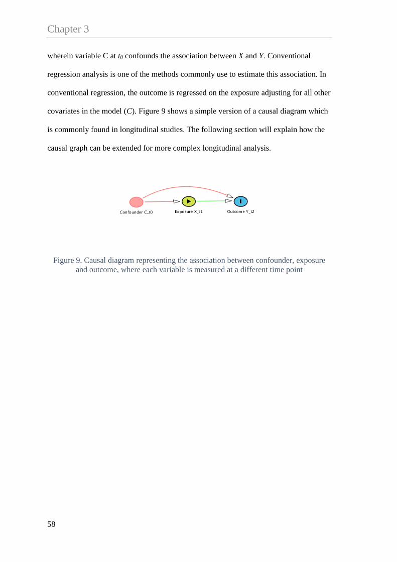
Chapter 3 wherein variable C at t0 confounds the association between X and Y. Conventional
regression analysis is one of the methods commonly use to estimate this association. In
conventional regression, the outcome is regressed on the exposure adjusting for all other
covariates in the model (C). Figure 9 shows a simple version of a causal diagram which
is commonly found in longitudinal studies. The following section will explain how the
causal graph can be extended for more complex longitudinal analysis.
Figure 9. Causal diagram representing the association between confounder, exposure and outcome, where each variable is measured at a different time point
58

Chapter 3 Time varying exposure
In longitudinal studies data are collected at multiple time points, which brings both
potential advantages and complexities to the analysis. For simplicity, suppose that both
exposure and outcome are measured at two time points then the causal diagram in figure
9 can be extended as follow.
Figure 10. Causal diagram representing the association between confounder, time-varying exposure and outcome
Figure 10 shows that both exposures and outcomes are time varying, where covariate C
is the confounder. Suppose that the parameters of interest are X_t1 and X_t2, then
conventional regression analysis, such as generalized equation estimation (GEE), might
be used to estimate the effect of X on Y. In a scenario where all information about time
varying confounding (Lt) is also collected in the study, then the data structure in figure
10 can be extended as follows.
59

Chapter 3
Figure 11. Causal diagram representing the association between time-varying exposure, confounding and outcome
Figure 11 shows that the data structure is now more complex with the need to account
for all time varying confounding, exposures and outcomes. Figure 12 has the same data
structure as Figure 11 with an additional black circle to indicate the parameter of
interest in the analysis. A caveat in using conventional regression to estimate the effect
of time varying exposures on outcome in longitudinal studies is when the covariate that
was affected by prior exposure also predicts the subsequent exposure and outcome
(187-190). Herein, covariate L is considered as time dependent (or time varying)
confounding because it affects subsequent exposure (X_t2) and outcome (Y_t2). In the
presence of time varying confounding, conventional regression analysis would
introduce bias whether or not L is adjusted in the model. Intuitively, L should be
included in the analysis because it confounds the association between the exposure and
the outcome, however, adjusting L_t1 would block the path from exposure (X_t1) to
outcome (Y_t2) and opens the potential backdoor path other than X_t1 - L_t1 - Y_t2. In this
case, using conventional regression adjusting for time-varying confounding may lead to
“collider stratification bias” and does not have a clear causal interpretation (184, 191).
60

Chapter 3
Figure 12. Causal diagram for estimating the cumulative effect of exposure (Xt1 and Xt2) in the presence of time-varying confounding and outcome
Methods that can be used to aid causal interpretation from complex longitudinal
observational studies include g-formula (187, 188, 192), g-estimation of the structural
nested models (SNMs) (189) and marginal structural models (MSMs) (189, 190, 193,
194). These are collectively known as “g-methods” or the generalization of
standardization for time varying exposures and confounders. The g-formula can be used
to estimate the potential outcome of Y by simulating the joint distributions of exposure
X, confounding L and outcome Y. Whilst g-estimation of the structural nested model
also uses simulation models of X, L and Y, the potential outcome is estimated under the
assumption that the effect of exposure varies for different levels of confounding, in
other words there is effect measure modification by L. Finally, MSMs use the inverse
probability of treatment weight to control the potential bias due to confounding L. In
this thesis, study 2 has the same data structure with figures 11 and 12, which aimed to
estimate the effect of household expenditure and cash transfer intervention on children’s
cognitive function. In study 2, the effect of cumulative time varying exposures
61

Chapter 3 (household expenditure and cash transfer) were estimated using MSMs. Details about
the statistical analysis in study 2 will be discussed in section 3.3.3.
Time specific exposure
The previous section shows how to take advantage of having repeated measures to
estimate the effect of time varying exposures on outcome in the analysis. This section
explains another way of using repeated measure by partitioning the effect of exposure
into several potential pathways, which can be illustrated in the following graphs.
Figure 13. Causal diagram representing the association between confounder, time-varying exposure, mediator-outcome confounder and outcome
62

Chapter 3
Figure 14 Causal diagram representing potential pathways between exposure and
outcome in effect decomposition analysis.
Suppose that the exposures are measured at two time points and the outcome is
measured at the end of the study, then the relations between the exposures, covariates
and outcome can be presented in Figure 13. Herein, the exposure at time 2 (X_t2) can be
defined as the mediator because it is in the pathway between X_t1 and outcome Y_t2. In
addition, the covariate L_t1 is a confounder of X_t2 and Y_t2, which is also affected by the
past exposure (X_t1). In other words, L_t1 is an exposure-induced mediator-outcome
confounder. Suppose that the parameter of interest is the exposure at time 1 (X_t1) then
there are at least four potential pathways that can be identified to estimate the causal
effect of X_t1 on Y (Figure 14).
The first potential pathway is to estimate the direct effect of exposure on outcome
(pathway 1 X_t1 → Y_t2). Second, to estimate the indirect effect of exposure on outcome
mediated through the second exposure (pathway 2 X_t1 →X_t2 →Y_t2). Third, to estimate
the indirect effect of exposure on outcome mediated through covariate L (pathway 3
63

Chapter 3 X_t1→L_t1→Y_t2), and finally to estimate the indirect effect of exposure at time 1 on
outcome mediated through covariate L and exposure at time 2 (pathway 4
X_t1→L_t1→X_t2→Y_t2).
To estimate the effect of exposure on outcome by adjusting for covariates using
conventional mediation analysis, such as Baron and Kenny (195) would yield bias in the
effect estimation and may fail to have causal interpretation (196, 197). In conventional
mediation analysis, direct and indirect effects of exposure on outcome were estimated
from a sequential regression analysis. In the first model, the outcome was regressed on
exposure adjusting for covariates. The coefficient of the exposure in model 1 was
defined as the direct effect. In the second model, the outcome was regressed on
exposure adjusted for covariates and the mediator. The difference between the
coefficients of the exposure in the first and second models was then defined as the
indirect effect of the exposure through the mediator. However, as shown in figure 14 in
conventional regression adjusting the mediator X_t2 would open the backdoor path from
X_t1→L_t1→Y_t2 (pathway 3) in addition to X_t1→X_t2→Y_t2 (pathway 2). On the other
hand, because L_t1 is affected by X_t1 then adjusting L_t1 would block the backdoor path
from X_t1→L_t1→Y_t2 (pathway 3).In these situation, conventional regression results in
“collider stratification bias” (184). In other words, Lt1 can be defined as an exposure-
induced mediator-outcome confounder.
Under a potential outcome approach, effect of exposure on outcome can be decomposed
into direct and indirect effects under the following assumptions
1. the effect of X on Y is unconfounded given C, ),( CXYx
64

Chapter 3
2. the effect of M on Y is unconfounded given X, C ),|( , CXMY mx
3. the effect of X on M is unconfounded given C ),( CXM x
4. there is no exposure-induced mediator-outcome confounding )( *, CMY xmx
In the presence of mediator-outcome confounding that is affected by exposure, methods
to estimate the causal effect of exposure on outcome without introducing bias in the
effect estimation include MSM (194) and g-computation (187, 188). In so-called
“causal mediation analysis”, MSM is used to estimate the controlled direct effect (CDE)
of exposure on outcome (198). MSM provides robust estimation for the effect of
exposure on outcome by controlling the mediator and mediator-outcome confounding
properly through inverse probability of weighting and is useful when the substantive
interest is only the CDE of exposure on outcome. However, MSM cannot be used for
effect decomposition (197). Estimation of CDE only requires the first two
assumptions;(1) the effect of X on Y is unconfounded given C, and (2) the effect of M
on Y is unconfounded given X, C. In other words, there are no unmeasured confounding
of the association between exposure and outcome, and there are no unmeasured
confounding of the association between mediator and outcome.
G-computation is useful for decomposing the total effect of exposure into direct and
indirect effects. However, because the estimation of g-computation is conducted under
sequential non-parametric models there is potential risk of bias if there is
misspecification of the link function (i.e., X-Y link) in the working models (for example
by not including a product term in the model when there is an interaction between the
exposure and mediator) (199). In addition, although g-computation controls the
65

Chapter 3 potential bias due to exposure-induced mediator-outcome confounder L, this method
can only be used to partition the effect mediated through mediator M but not through L.
The most recent effect decomposition analysis was introduced by Vanderweele,
Vansteelandt and Robins (VVR) (200) in 2014, which include joint mediators, path
specific and interventional analogues approaches. This thesis used the VVR approach in
study 3.
In this thesis, study 3 used a similar causal graph as Figure 13, which aimed to estimate
the direct effect of poverty at 0-7 years on cognitive function at 7-14 years and whether
the effect is mediated through poverty at 7-14 and school attendance/home
environment. Details about the statistical analysis used in study 3 will be explained in
section 3.3.4.
Potential outcome or counterfactual framework
This thesis aimed to estimate the causal associations between exposure and outcome
from observational studies via the potential outcome (counterfactual) framework. Use of
a potential outcome framework in observational studies is intended to mimic a
randomized control trial where the individuals are assigned to a potential intervention.
The idea of potential outcomes in observational studies is that each subject in a
population of interest could experience different types of exposure even though she/he
only has one observed outcome at any time point. The potential outcome or
counterfactual can be defined as the expected outcome an individual would have had,
contrary to fact, that the same individual had the observed exposure (201). Suppose that
the exposure is binary, i.e. whether a child is poor or not poor, then for a subject who is
poor his potential outcome can be defined as what would happen if the same subject is
not poor and vice versa.
66
Chapter 3 Formally, let x be the value of the observed exposure and x* be the alternative exposure,
then the causal effect is estimated as the difference between the outcome under the
observed value and the counterfactual value )( *ixix YY − Since each subject can only have
one observed value, this implies that causal effect cannot be directly estimated from the
data. Estimation of a causal effect under the potential outcome framework depends on
several assumptions, and proper analytical methods that can provide unbiased
estimation to move closer towards causal interpretation.
Under a potential outcome framework, estimation of causal effects in observational
studies is dependent on the following assumptions (189, 201)
1. Consistency, which means the individual’s potential outcome depends only on
his/her own exposure history and was not influenced by treatment applied to
other individuals. Rubin (202) defined this assumption as the stable unit
treatment value assumption (SUTVA).
2. Conditional exchangeability, which means that the mean of outcome Y given
exposure is independent of the individual’s exposure given covariates. In other
words, conditional exchangeability assumes there is no unmeasured
confounding.
3. Positivity, which means both exposed and unexposed individuals are present at
every level of any confounders. In other words, the exposure is not
deterministically assigned within any levels of covariates. i.e., probability of
exposure does not equal one or zero. Probability of exposure in a standard RCT
is 0.5.
Although estimation of causal effects may be plausible, the assumptions on which it is
based are not guaranteed by design and cannot be tested in observational studies (189).
67
Chapter 3 In a randomized experiment, the causal effect can be estimated directly from the data as
the difference in the outcome between the treatment and control group. In contrast, in
observational studies the causal effect cannot be directly estimated because the studies
were not designed to estimate the causal association between the exposure and outcome.
Hence a priori knowledge about the association between the exposure and outcome is
important to determine their causal relations (203). Proper understanding about the
association between the exposure and outcome would be useful to generate well-defined
interventions (204).
As mentioned earlier, under a potential outcome (counterfactual) framework, methods
that can be used to assess causality from complex longitudinal observational studies
include g-formula (187, 188, 192), g-estimation of the structural nested models (SNMs)
(189) and marginal structural models (MSMs) (189, 190, 193, 194).
3.3.3. Study 2: estimating the effect of household expenditure and cash transfer intervention on children’s cognitive function
Study 2 aimed to address the following questions, (1) what is the effect of household
PCE on Indonesian children’s cognitive function; and (2) does a cash transfer
intervention increase cognitive function scores? Assuming there is no unmeasured
confounding of all the associations between C, X, L, Y Figure 15 shows the
hypothesized causal diagram for study 2, representing associations between
confounders, household PCE and children’s cognitive function.
68
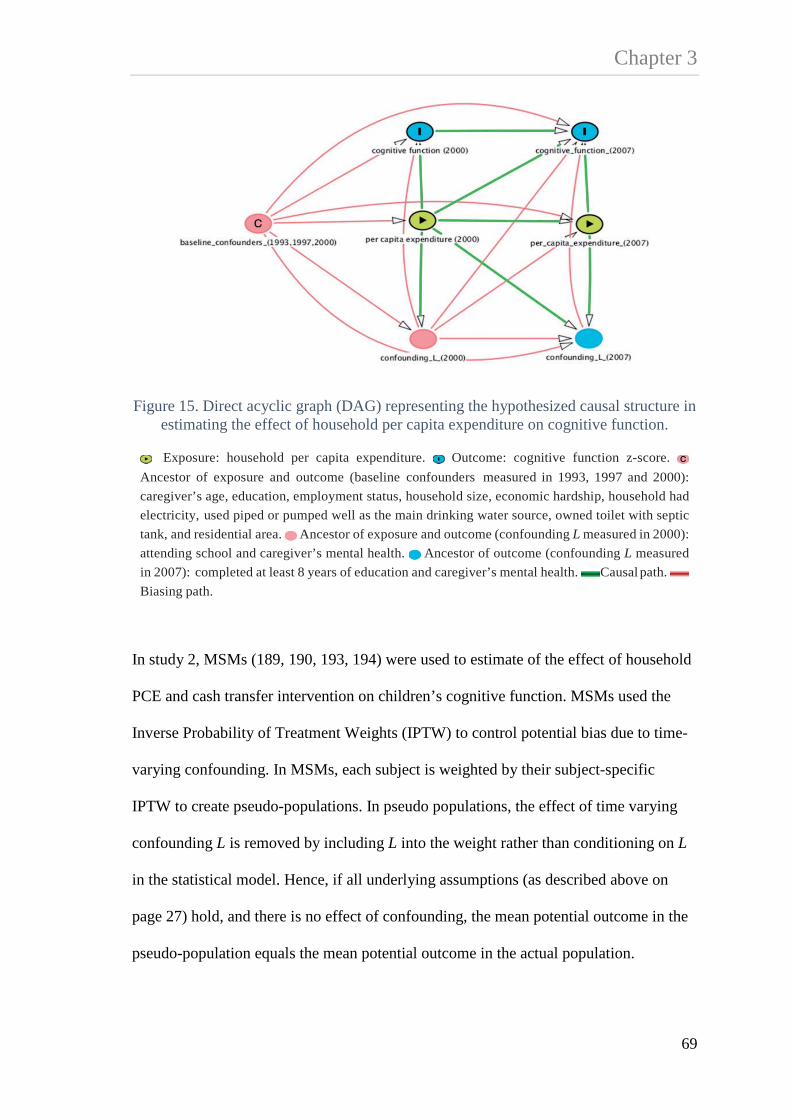
Chapter 3
Figure 15. Direct acyclic graph (DAG) representing the hypothesized causal structure in estimating the effect of household per capita expenditure on cognitive function.
Exposure: household per capita expenditure. Outcome: cognitive function z-score. Ancestor of exposure and outcome (baseline confounders measured in 1993, 1997 and 2000): caregiver’s age, education, employment status, household size, economic hardship, household had electricity, used piped or pumped well as the main drinking water source, owned toilet with septic tank, and residential area. Ancestor of exposure and outcome (confounding L measured in 2000): attending school and caregiver’s mental health. Ancestor of outcome (confounding L measured in 2007): completed at least 8 years of education and caregiver’s mental health. Causal path. Biasing path.
In study 2, MSMs (189, 190, 193, 194) were used to estimate of the effect of household
PCE and cash transfer intervention on children’s cognitive function. MSMs used the
Inverse Probability of Treatment Weights (IPTW) to control potential bias due to time-
varying confounding. In MSMs, each subject is weighted by their subject-specific
IPTW to create pseudo-populations. In pseudo populations, the effect of time varying
confounding L is removed by including L into the weight rather than conditioning on L
in the statistical model. Hence, if all underlying assumptions (as described above on
page 27) hold, and there is no effect of confounding, the mean potential outcome in the
pseudo-population equals the mean potential outcome in the actual population.
69

Chapter 3 Steps for estimation of the weights are as follows:
1. Generate the time-specific stabilized weight.
Let Xit be the exposure for individual i at time t, X and L be the history of exposure
and time varying confounding, respectively then the construction of the stabilized
weight for each individual i at time t (SWit) defined as (194)
Equation 5. Stabilized weight
∏= −−
−=T
t ititit
ititit CLXXf
XXfSW0 ,1,1
1
)|()|(
Where each factor in numerator in equation 5 is the probability density function that the
subject received his/her observed exposure conditional on her/his past exposure, and the
denominator is the probability density function that the subject received her/his
exposure given his/her past exposure and covariates, which include both time varying
confounding and baseline confounder.
Another approach of weight creation is using non-stabilized weight. In contrast with
stabilized weight, the numerator of non-stabilized weight is not estimated from the
observed value of exposure at each time point given the past exposure but replaced by
the value of 1, whereas the denominator of non-stabilized weight is estimated similar to
denominator in stabilized weight (the probability of density function that a subject
received his/her exposure given past exposure and covariates). Use of stabilized weight
is preferable over non-stabilized weight because the former has smaller variance,
narrower confidence interval and better coverage rates than the later (194). For each
time point, the mean of the weight is expected to be one because the size of the pseudo
70

Chapter 3 population equals the study population and has a small range suggesting positivity or
there is no misspecification of the weight model (205). To reduce potential bias if the
weight model is miss-specified, weights with large variance or extreme values were
truncated at the 1st and 99th percentile or at the 5th and 95th percentile.
71

Chapter 3 In the analysis, the stabilized weight is defined as
Equation 6. Stabilized weight for the exposure in 2000
)|()(
2000
20002000
ii
ii CXf
XfSW =
Equation 7. Stabilized weight for the exposure in 2007
),,|()|(
20002007
200020072007
iiii
iii LCXXf
XXfSW =
Equations 6 and 7 show the stabilized weight for the exposure in 2000 (SWi2000) and
2007 (SWi2007), respectively. The numerator in equation 6 is the marginal density of the
exposure (household PCE) in 2000 (Xi2000), and the denominator is the conditional
density function of Xi2000 given the history of confounders ( iC ) up to 2000 including
caregiver and household characteristics. The numerator in equation 7 is the conditional
density function of the exposure in 2007 (Xi2007) given Xi2000, and the denominator is the
density function of X2007 given X2000, history of confounders ( iC ), and time varying
confounders ( iL ) which includes the child attending school and their caregiver’s mental
health in 2000, and the child’s completion of at least 8 years of education and their
caregiver’s mental health in 2007.
2. Generate IPTW for the marginal structural mean model
IPTW was estimated as the product of time-specific SW (equation 8), which is defined as
Equation 8. The inverse probability of treatment weighting
20072000 SWSWIPTW ×=
72

Chapter 3 In study 2, the MSM was estimated using generalized estimating equations (GEE) with
an independent working correlations matrix (206, 207), defined as
Equation 9. Marginal Structural Mean Model
xitxitit cumcumYE 10)|( ββ +=
Where itY is the expected mean potential outcome of cognitive function z-score given
the observed cumulative household PCE over two time points )( xitcum weighted by the
individual’s subject specific weight (IPTW).
Sensitivity analysis for unmeasured confounding
Causal analysis in observational studies is conducted under the assumption of no
unmeasured confounding. Although this assumption cannot be tested, unmeasured
confounding may lead to bias in effect estimation. To address this issue, Robins (190)
argued that conducting sensitivity analysis is important to quantify how effect
estimation may vary as a function of the magnitude of unmeasured confounding.
In study 2, sensitivity analysis was conducted to estimate bias in the causal effect of
household PCE on cognitive function due to unmeasured confounding of the exposure
(U). In sensitivity analysis, U was defined as a binary variable and it was assumed that
the association between U and cognitive function did not vary across levels of
household PCE i.e., no effect measure modification of U and X. Following
VanderWeele and Arah (208), the sensitivity parameter δ was defined as the effect of U
on cognitive function (U-Y) and the sensitivity parameter γ was defined as the
prevalence of U for given level of X (household PCE). These two quantities define the
73

Chapter 3 strength of potential confounding by U of the X-Y association. Equation 10 shows
formula for sensitivity analysis, where the magnitude of potential bias (dx+) in the
estimated X-Y association was estimated as the product of δ and γ.
Equation 10 Formula for sensitivity analysis
δγ=+xd
)0,,|()1,,|(
)},|)0(),|)1({
=Ε−=Ε=
=−==
UcxYUcxY
cxUPcxUPwhere
γ
δ
Equation 10 also shows the effect of U on cognitive function Y (δ) was estimated as the
difference between the probability of U given the exposure and covariates, whereas the
prevalence of U (γ) was estimated as the difference in cognitive function Y given
exposure, covariates and U. The magnitude of potential bias (dx+) was then estimated
over several simulations of plausible levels of δ and γ.
Missing data
Similar to study 1, in study 2 the Multiple Imputation by Chained Equation (MICE)
procedure was performed to minimize bias due to attrition and missing responses to
questions under the assumption that the imputed data were missing at random (179,
180). In this study, a total of twenty imputed datasets was generated using fifty cycles of
regression switching. Rubin’s rule (181) was used to combine and analyse imputed
74

Chapter 3 datasets. In addition, the method of multiple imputation then deletion of the imputed
outcome (MID) as derived by Von Hippel (182) was also performed as part of the
sensitivity analysis.
Findings from study 2 are presented in chapter 5.
3.3.4. Study 3: estimating the associations of early and later childhood poverty on children’s cognitive function
Study 3 aimed to address the following questions, (1) what is the effect of poverty at 0-7
and poverty at 7-14 years on cognitive function at 7-14 years; (2) what is the direct
effect of poverty at 0-7 on cognitive function at 7-14 years, and (3) is this effect
mediated through poverty at 7-14 and through school attendance and aspects of the
child’s home environment, children’s living conditions and school attendance? This
study was motivated to better estimate the optimal timing for intervention and the
mechanism by which poverty earlier in life at 0-7 could affect cognitive function at 7-14
years.
Figure 16 shows the causal diagram for estimating the effect of poverty at 0-7 on
cognitive function at 7-14. The hypothetical structure of the DAG suggests that
household poverty at 0-7 (exposure, reflecting household expenditure on children)
would affect both household poverty at 7-14 years (mediator), children’s living
conditions and the opportunity to attend school at ages 7-14 (exposure induced time-
varying confounder of the mediator-outcome association), which subsequently would
affect both family expenditure on children and their cognitive function at 7-14. In
Indonesia, social inequalities in school enrolment widen after age 10, likely due to costs
of schooling (209) The cost burden of education is higher among the poor and those
living in rural areas. For example, in 2010 about 44% of students who dropped-out of
75

Chapter 3 school at ages 13-15 years were from the poorest quintile of households. Among this
group, the average cost of education is about 500,000 rupiah/child/year (about US$59),
representing about a quarter of annual household expenditure.
Figure 16. Directed Acyclic Graph representing the associations between baseline confounders, poverty at 0-7 and poverty at 7-14 years, poor home environment not attending school at 7-14, and cognitive function at 7-14
Legend
Ancestor of exposure and outcome (baseline confounders measured at 0-7 years): caregiver’s age, education, employment status, household size, economic hardship, household had electricity, used piped or pumped well as the main drinking water source, improved sanitation and residential area. Exposure: poverty status at 0-7 years. Ancestor of outcome (mediator): poverty status at 7-14 years.
Ancestor of outcome (exposure-induced mediator-outcome confounders): latent variable (child is attending school, caregiver’s employment status, household had electricity, used piped or pumped well as the main drinking water source, improved sanitation, house tenure, types of cooking fuel, had television and residential area). Outcome: cognitive function z-score at 7-14 years. Causal path. Biasing path
Assuming there is no unmeasured confounding of all the associations of C, X, L, M and
Y, the DAG in Figure 16 shows exposure X (poverty at 0-7) has a direct effect on
outcome Y (cognitive function score at 7-14). The path from X to Y is potentially
76

Chapter 3 mediated through poverty at 7-14 (M). In addition children’s living conditions and
school attendance (L) is a potential mediator-outcome confounder, which is also
affected by the exposure.
Conventional regression analysis
Conventional regression analysis was used to answer the first objective, which
examined the associations of early poverty (at 0-7) and later childhood poverty (at 7-14
years) with cognitive function at 7-14 years. Herein, equation 11 shows the regression
model estimating the association of poverty at 0-7 (X) with cognitive function adjusting
for baseline confounders (C). Equation 12 shows the regression model estimating the
association of poverty at 7-14 (M) adjusting for all covariates including poverty at 0-7
(X), baseline confounders (C) and schooling/home environment (L).
Equation 11. Model for estimating the association of poverty at 0-7 with cognitive function at 7-14 years
CXCXYE 210),|( βββ ++=
Equation 12. Model for estimating the association of poverty at 7-14 with cognitive function at 7-14 years
LCXMLCXMYE 43210),,,|( βββββ ++++=
Decomposition Analysis
To estimate the effect of poverty at 0-7 years on cognitive function by adjusting for
covariates using conventional mediation analysis, such as Baron and Kenny (195)
would yield bias in the effect estimation and may lack causal interpretation (196, 197).
77

Chapter 3 Limitations of using conventional mediation analysis were explained in section 3.3.2.
Briefly, in the presence of exposure induced mediator outcome confounder (L) in
conventional regression adjusting M would open the backdoor path from X→L→Y in
addition to X→M→Y. On the other hand, because L is affected by X then adjusting L
would block the backdoor path from X→L→Y, however, not adjusting L would generate
bias in estimates because it confounds the association of M with Y. In this situation,
conventional regression would result in “collider stratification bias” (184).
Estimation of effect decomposition requires the following assumptions
1. the effect of X on Y is unconfounded given C, ),( CXYx
2. the effect of M on Y is unconfounded given X, C ),|( , CXMY mx
3. the effect of X on M is unconfounded given C ),( CXM x
4. there is no exposure-induced mediator-outcome confounding )( *, CMY xmx
The fourth assumption is known as the “cross-world independence assumption” (210).
There have been criticisms concerning estimation of direct and indirect effects that
involve the cross-world independence assumption (211). Cross-world independence
assumes that the joint effect of the observed exposure and the mediator on the outcome
is independent of the effect of the mediator under the counterfactual exposure (X=x*)
given C, which implies that each individual has both observed and counterfactual
exposures. Avin et al., (210) showed that estimation of direct and indirect effects that
involve the cross world assumption is unidentifiable even when the exposure-induced
mediator-outcome confounder is observed in the data. Furthermore, Naimi et al., (211)
argued that the estimation of direct and indirect effects that involves a cross-world
independence assumption involves a logical inconsistency in the two states required for
78

Chapter 3 its calculation and so has no sensible real world interpretation but is rather a product of
purely mathematical formulations.
Under a potential outcome approach (212, 213) the total causal effect (TCE), the natural
direct (NDE), indirect effect (NIE) and the controlled direct effect (CDE) are defined as
follows.
Equation 13. Total Causal Effect
][ *)(*,)(, xMxxMx YYETCE −=
Equation 13 shows the TCE is the expected potential outcome (child cognitive function
z-score) in children exposed to poverty at 0-7 (X=x) and the mediator (poverty at 7-14,
M(x)) is set at the level it would be among those who were exposed to poverty at age 0-
7, minus, the expected potential outcome in children not exposed to poverty at 0-7, and
the mediator is set at the level it would be among those who were unexposed to poverty
at 0-7 (M(x*)).
Equation 14. Natural Direct Effect
][ *)(*,*)(, xMxxMx YYENDE −=
In equation 14, the NDE is the expected potential outcome in children exposed to
poverty at 0-7 (X=x) and the mediator is set at the level it would be among those who
were not exposed to poverty at 0-7 (M(x*)), minus, the expected outcome in the
unexposed to poverty at 0-7, and the mediator is set at the level it would be among those
who were unexposed to poverty at 0-7 (M(x*)). Intuitively, the NDE estimates the effect
79

Chapter 3 of poverty at 0-7 on cognitive function through pathways that do not involve poverty at
7-14 years.
Equation 15. Natural Indirect Effect
][ *)(,)(, xMxxMx YYENIE −=
In equation 15, the NIE is the expected potential outcome in children exposed to
poverty at 0-7 and the mediator is set at the level it would be among those who were
exposed to poverty at 0-7 (M(x)) minus the expected potential outcome in children
exposed to poverty at 0-7 and the mediator is set at the level it would be among those
who were unexposed to poverty at 0-7 (M(x*)). This algebra invokes the cross-world
assumption because NIE requires the mediator to simultaneously take on values under
X=x and X=x* i.e., M cannot take on its value under x and x* simultaneously and so is
logically inconsistent and requires X to exist in two worlds to observe the NIE (211).
Nevertheless, intuitively, the NIE estimates the effect of poverty at 0-7 on cognitive
function through poverty at 7-14 years.
Equation 16. Controlled Direct Effect
][ *,, mMxmMx YYECDE == −=
In equation 16, CDE is the difference in the expected potential outcome between
children who were exposed (X=x) and not exposed to poverty at 0-7 (X=x*) with the
mediator set at some level M=m for all individuals in the population. This approach is
used in MSM and effectively blocks any variation in M by setting it to some plausible
level m. It shows why MSMs cannot be used to decompose direct and indirect effects
80

Chapter 3 because M is essentially blocked at one level for all individuals and so cannot vary
across X or Y.
The VanderWeele, Vanstelandt and Robins (2014) approach to effect
decomposition
The most recent approach to effect decomposition is derived by Vanderweele,
Vansteelandt and Robins (hereafter VVR) (200). VVR introduced three approaches to
effect decomposition that partially overcome the identification limitations due to
exposure induced mediator-outcome confounding. The three VVR approaches to effect
decomposition do not estimate the “natural” direct and indirect effects but they provide
insight into mediation and pathways when exposure induced mediator-outcome
confounding exists. This included a) the joint mediators, b) the path specific and c) the
interventional analogue approaches.
a) Joint mediators
In the joint mediators approach, the direct effect (X→Y) is defined as the effect of
poverty at 0-7 (X) that is not through poverty at 7-14 (M) or schooling/home
environment L. The indirect effect is defined as the effect of X that is mediated through
M or L or both. Under the joint mediator approach, M and L are considered as joint
mediators, the fourth assumption is modified as CMLY xxxlm |)( **, and is effectively
satisfied. In other words in Figure 16 there is no effect of exposure X that confounds the
relationship between the joint mediator (L, M). This approach is useful if partitioning
the indirect effect of X through M or L was not of interest so that both poverty at 7-14
81

Chapter 3 (M) and schooling/home environment (L) were assumed to be equally important as
mechanisms by which poverty at 0-7 (X) affects cognitive function at 7-14 (Y).
Let X be the exposure (poverty at 0-7 years), where X=x is defined as exposure set to the
child being poor and X=x* is defined as the exposure being set to child not being poor at
0-7. Let M be the mediator (poverty at 7-14 years), where Mx* is defined as the value of
observed poverty status at 7-14 years and poverty at 0-7 is set to being not poor. Let Lx*
be defined as the value of observed mediator-outcome confounder (home
environment/schooling) and poverty at 0-7 is set to being not poor. Equation 17 shows
formula for estimating the direct effect (DE) in joint mediators approach.
Equation 17. Estimation of direct effect for the joint mediator approach
∑ −=−=→ mlcMxLxxMxxLxYX cPcxmlPcmlxYEcmlxYEYYEDE,,***** )()*,|,(]},,*,|[],,,|{[][
In this approach, the DE is the sum of the products of three statistical models. The first
model ],,*,|[],,,|[ cmlxYEcmlxYE − estimates the difference between two potential
outcomes, (1) the expected cognitive function z-score Y given the child is poor at 0-7
(X=x), home environment/schooling (L), poverty at 7-14 (M) and baseline confounders
C (caregiver’s age, education, employment status, household size, economic hardship,
household had electricity, used piped or pumped well as the main drinking water source,
improved sanitation and residential area); minus (2) the expected cognitive function z-
score given the child is not poor at 0-7(X=x*), home environment/schooling, poverty at
7-14 and confounders. The second part of the model estimates the joint )*,|,( cxmlP
82

Chapter 3 probabilities that the child is living in poor home environment (L) and poverty at 7-14
given the child is not poor at 0-7 (X=x*), and C. The final statistical model
estimates the probability of confounders.
Equation 18 shows the formula for estimating the indirect effect (IE) in joint mediators
approach.
Equation 18. Estimation for the indirect effect for the joint mediator approach
∑ −=−=→→ mlcMxxLxxLxMxYMX cPcxmlPcxmlPcmlxYEYYEIE,,** )()}*,|,(),|,(]{,,,|[][
In equation 18, the joint mediators approach estimates the indirect effect (IE) as the sum
of the product of three statistical models. The first model ],,,|[ cmlxYE estimates the
expected cognitive function z-score Y given the child is poor at 0-7 (X=x), home
environment/schooling, poverty at 7-14 and confounders. The second part of the model
)*,|,(),|,( cxmlPcxmlP − estimates the difference between two joint probabilities;
(1) the joint probability of the child is living in poor home environment/schooling (L)
and poverty at 7-14 (M) given the child is poor at 0-7 (X=x) and C, minus (2) the joint
probability of L and M given the child is not poor at 0-7 (X=x*) and C. The final model
)(cP estimates the probability of confounders.
In the VVR method, effect decomposition was estimated using a combination of
sequential simulations of parametric models for Y, X, M, and L and inverse-probability
of weighting for probabilities of X, M and L. Combination of sequential simulations and
weighting may overcome the issue of model compatibility (214). In study 3, effect
)(cP
83

Chapter 3 decomposition was estimated under the assumption of no interaction between the
exposure and the mediator. Assuming the parametric models for Y, X, M and L are
correctly specified, the simulation was run under restricted models by not included the
interaction terms of X and M in the simulation model. However, if there is in fact an
interaction between X and M then estimates of direct and indirect effects could be
biased because the model was misspecified. The weighting and duplication of the
exposure method allows for estimation of the effect of exposure on outcome that was
partly through the mediator and sequentially through the change in mediator under
specified exposure level without adding interaction terms in the model.
In VVR, the sequential simulation was started by generated duplicates of the exposure
data and added variables that represent counterfactual of the exposure. For example, in
joint mediators approach, two copies of the data were generated and a variable of
exposure X* was added to each of the new data set. Herein, in the first replicate the
value of X* was set to 0 and in the second replicate the value of X* was set to 1.
Intuitively, in each replicate a child will have one observed value of the exposure (X)
and one counterfactual value of the exposure (X*). Both data were then combined to
generate person specific weight.
The construction of the weight for the joint mediators approach is as follow.
Equation 19. Weight for the joint mediator approach
),,|(),|()|()*,,|()*,|(
1 cxlmPcxlPcxPcxlmPcxlPW =
84

Chapter 3 In equation 19, the numerator is the product of two statistical models; (1) the probability
of schooling/home environment (L) given poverty at 0-7 is set to x* and C, and the
probability of poverty at 7-14 (M) given schooling/home environment, poverty at 0-7 is
set to x* and C. The denominator is the product of three statistical models; (1) the
probability of the observed poverty 0-7 (X=x) given C; (2) the probability of
schooling/home environment given the observed poverty at 0-7 and C; and (3) the
probability of poverty at 7-14 given schooling/home environment, the observed poverty
at 0-7, and C.
Effect decomposition was then estimated using a weighted regression. To estimate the
direct effect, the cognitive function Y was regressed on the observed X among X*=0. Of
those children who were poor at 0-7 years (X=1), a weighted regression of Y on X* was
used to estimate the indirect effect of poverty at 0-7 years that was mediated through
poverty at 7-14 or home environment/schooling or both.
b) Path specific
Assuming that the above four assumptions of unmeasured confounding (1-4) hold, the
identifiable path specific effects (210) are XY, XLY, XMY. The path specific
approach is more relevant if the substantive question is to estimate the relative
importance of specific pathways by partitioning the indirect effects of poverty at 0-7
through poverty at 7-14 (X→M→Y) and through pathways that involve schooling/home
environment at 7-14 (X→LY), which is the combination of X→L→M→Y and X→L→Y.
Thus the path specific approach can be used to estimate whether the effect of poverty at
0-7 is largely mediated through poverty at 7-14 (M) only or through schooling/home
environment (L).
85

Chapter 3 Similar to the joint mediators approach, the path specific effect defines DE as the effect
of exposure on outcome that is not through M or L (See equation 17 above). In the path
specific approach, the indirect effect of poverty at 0-7 through poverty at 7-14
(X→M→Y) defined as
Equation 20. Estimation for the indirect effect through mediator in the path specific approach
∑ −=→→ mlcYMX cPcxlPclxmPclxmPcmlxYEIE,,
)()*,|()},*,|(),,|(]{,,,|[
In equation 20, IE X→M→Y is estimated as the sum of the product of four statistical
models. The first model ],,,|[ cmlxYE estimates the expected cognitive function z-
score given the child is poor at 0-7, home environment/schooling, poverty at 7-14 and
confounders. The second part of the model ),*,|(),,|( clxmPclxmP − estimates the
difference between two probabilities; (1) the probability of poverty at 7-14 given the
child is poor at 0-7, home environment/schooling and confounders, minus, (2) the
probability of poverty at 7-14 given the child is not poor at 7-14, home
environment/schooling and confounders. The third part of the model )*,|( cxlP
estimates the probability of living in poor home environment/schooling given the child
is not poor at 0-7 and confounders. The fourth part of the model )(cP estimates the
probability of confounders.
Equation 21 shows the indirect effect of poverty at 0-7 that involving pathway through
home environment/schooling X→LY defined as
86

Chapter 3
Equation 21. Estimation of the indirect effect mediated through confounding L in the path specific approach
∑ −=→ mlcLYX cPcxlPcxlPclxmPcmlxYEIE,,
)()}*,|(),|(){,,|(),,,|(
In equation 21, the IE is estimated as the sum of the product of four statistical models.
The first model ),,,|( cmlxYE estimates the expected potential cognitive function z-
score given the child is not poor at 0-7, home environment/schooling, poverty at 7-14
and confounders. The second part of the model ),,|( clxmP estimates the probability of
poverty at 7-14 given the child is not poor at 0-7, home environment/schooling and
confounders. The third part of the model )*,(),|( cxPcxlP − estimate the difference
between two probability models; (1) the probability of the child is living in poor home
environment/schooling given the child is poor at 0-7 and covariates, minus, (2) the
probability of the child is living in poor home environment/schooling given the child is
not poor at 0-7 and confounders. The fourth part of the model )(cP estimates the
probability of confounders.
For path specific effect, three copies of the data were generated and two variables X*
and X** were added to each data set. In the first replicate of data, both variables X* and
X** were set to the same value of observed exposure X (X*=x and X**=x). In the
second replicate of data, variable X* was set to 1-x and X** was set to the observed
exposure. Lastly, in the third replicate of data variable X* is set to 1 and X** is set to 1-
x. The copies of the data set were merged to generate a person specific weight for the
path specific effect (equation 22).
87

Chapter 3 The construction of the weight for the identifiable path specific effects is as follows.
Equation 22. Weight for the path specific approach
),,|(),|()|()*,*,|()*,|(
2 cxlmPcxlPcxPcxlmPcxlPW =
In equation 22, the numerator is the product of two statistical models; (1) the probability
of schooling/home environment (L) given poverty at 0-7 is set to x* and C, and (2) the
probability of poverty at 7-14 given poverty at 0-7 is set to x** and C. The denominator
is the product of three statistical models; (1) the probability of poverty at 0-7 given C;
(2) the probability of schooling/home environment given the observed poverty at 0-7
(X=x) and C; and (3) the probability of poverty at 7-14 years given schooling/home
environment, the observed poverty at 0-7 and C. Herein, x* represents potential
outcome for the X→LY path, whereas x** represents potential outcome for the X→M→
Y path.
In the path specific effect, a weighted regression of Y on the observed X (X=x) was used
to estimate the direct effect of poverty at 0-7 on cognitive function among those who
were not poor at 0-7 years in both in the replicate data set (X*=0 and X**=0). Estimates
of the indirect effect of poverty at 0-7 mediated through poverty at 7-14 (M) years was
calculated from a weighted regression of Y on X** among those who were observed
being poor at 0-7 but not poor on the counterfactual exposure in the replicate data
(X*=1).
A weighted regression of Y on X* was used to estimate the indirect effect of poverty at
0-7 on cognitive function that was mediated through home environment/schooling L
88

Chapter 3 and poverty at 7-14. Herein, the weighted regression was estimated among those who
were poor at 0-7 in both observed and replicate data (X=1 and X**=1). Although the
VVR can be used to estimate the indirect effect of exposure that was through L and M
(X→LY), the current method cannot be used to estimate the indirect effect of X that was
only mediated through L alone (X→L→Y).
Figure 17 Sequential randomization in the intervention analogue approach.
c) Intervention Analogue
Effect decomposition carried out under the intervention analogue approach is similar to
a sequential randomized trial (Figure 17) (185, 212, 215). The randomized intervention
analogue of the natural direct effect is defined as the difference in potential outcome
Poverty at 0-7 (X)
(A) X=1 (poor)
(C) Poverty at 7-14, M=1 (poor)
Y1M1
(D) M=0 (not-poor)Y1M0
(B) X=0 (not-poor)
(E) M=1 (poor)Y0M1
(F) M=0 (not-poor)Y0M0
89

Chapter 3 between children who were exposed and not exposed to poverty at 0-7, where in both
cases the value of the mediator (poverty at 7-14) was randomly drawn from the
distribution of the mediators amongst children who were not exposed to poverty at 0-7
(Y1m0-Y0m0).
The randomized intervention analogue of the indirect effect is defined as the difference
in potential outcome in children who were exposed to poverty at 0-7 where the value of
the mediator was first randomly drawn from the distribution of the mediator amongst
children who were exposed to poverty at 0-7 ( )( 11MY in Figure 17) and then the value of
the mediator was randomly drawn from the distribution of mediator amongst children
who were not exposed to poverty at 0-7 ( )( 01MY in Figure 17), thus simulating an RCT
of the mediator (poverty at 7-14). Subtraction of these two quantities estimates the
intervention analogue of the indirect effect (See equation 24). Thus effect
decomposition conducted as an analogue of sequential randomization of the mediator,
requires only the first three assumptions.
In the third approach, effect decomposition is estimated as the difference between two
potential outcomes where the value of the mediator (poverty at 7-14) is randomly drawn
from the distribution of exposure level (poverty at 0-7). Equation 23 shows the
estimation of DE in the intervention analogue approach.
Equation 23. Estimation of the direct effect in the intervention analogue approach
∑ ×−=
−=→
mlc
GxxGYX
cPcxmPcxlPcmlxYEcxlPcmlxYE
YEYEDEcxcx
,,
*
)()*,|()}*,|(),,*,|(),|(),,,|({
)()(|*|
90
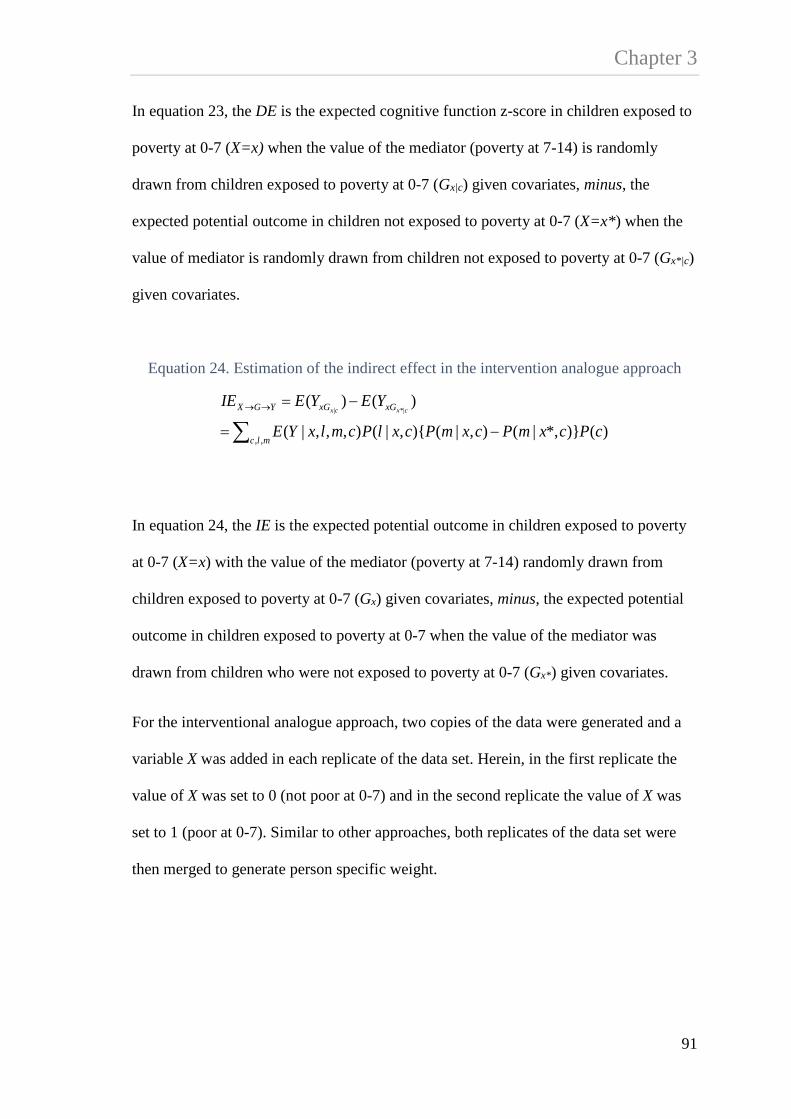
Chapter 3 In equation 23, the DE is the expected cognitive function z-score in children exposed to
poverty at 0-7 (X=x) when the value of the mediator (poverty at 7-14) is randomly
drawn from children exposed to poverty at 0-7 (Gx|c) given covariates, minus, the
expected potential outcome in children not exposed to poverty at 0-7 (X=x*) when the
value of mediator is randomly drawn from children not exposed to poverty at 0-7 (Gx*|c)
given covariates.
Equation 24. Estimation of the indirect effect in the intervention analogue approach
∑ −=
−=→→
mlc
xGxGYGX
cPcxmPcxmPcxlPcmlxYE
YEYEIEcxcx
,,)()}*,|(),|(){,|(),,,|(
)()(|*|
In equation 24, the IE is the expected potential outcome in children exposed to poverty
at 0-7 (X=x) with the value of the mediator (poverty at 7-14) randomly drawn from
children exposed to poverty at 0-7 (Gx) given covariates, minus, the expected potential
outcome in children exposed to poverty at 0-7 when the value of the mediator was
drawn from children who were not exposed to poverty at 0-7 (Gx*) given covariates.
For the interventional analogue approach, two copies of the data were generated and a
variable X was added in each replicate of the data set. Herein, in the first replicate the
value of X was set to 0 (not poor at 0-7) and in the second replicate the value of X was
set to 1 (poor at 0-7). Similar to other approaches, both replicates of the data set were
then merged to generate person specific weight.
91

Chapter 3 The construction of the weight for the intervention analogue approach is as follow.
Equation 25. Weight for the intervention analogue approach
In equation 25, the numerator is the sum of the product of two statistical models; (1) the
probability of poverty at 7-14 (M) given schooling/home environment/, poverty at 0-7 is
set to x* and C, and (2) the probability of schooling/home environment/ given poverty
at 0-7 is set to x* and C. The denominator is the product of two statistical models; (1)
the probability of poverty 0-7 years given C, and (2) the probability of poverty at 7-14
given schooling/home environment, the observed poverty at 0-7 years, and C.
To estimate the direct effect in the interventional analogue approach, the cognitive
function Y was regressed on the observed X among children who were not poor at 0-7
(X=0), whereas of those children who were poor at 0-7 years (X=1), a weighted
regression of Y on X was used to estimate the indirect effect of poverty at 0-7 years that
was mediated through poverty at 7-14.
The 95% CI was estimated based on a bootstrap of 1000 resamples. Analyses using the
VVR approach were conducted in SAS 9.4 (SAS Institute, Cary, North Carolina).
),,|()|(
),|(),,|( **
3 cxlmPcxP
cxlPcxlmPW l
∑=
92

Chapter 3 Complete case analysis
The analysis in study 3 was restricted to complete cases (178). Complete case analysis
was conducted by deleting observations that had missing information in any variables of
interest (confounder, exposure, mediator and outcome). Using complete case analysis
has several well-known limitations including reduction of the sample size, loss of
precision and potential bias in the estimates if the missing mechanism is not missing
completely at random (MCAR), suggesting that the missing data is not related to any
variables in the dataset (178, 181, 216). The reason analysis in study 3 was restricted to
complete cases was because there is no current method available to combine estimates
from VVR approach to effect decomposition using Rubin’s rule.
Sensitivity analysis for potential unmeasured confounding
Potential bias in effect estimation is still plausible if there is potential unmeasured
confounding. Sensitivity analysis method (217) was used to estimate bias in effect
decomposition due to unmeasured mediator-outcome confounding. The sensitivity
analysis that was developed by Vander Weele and Chiba was conducted as a non-
parametric approach, which can be applied for any effect decomposition method
including the method that has an exposure-induced mediator-outcome confounding.
Findings from study 3 are presented in chapter 6.
93

Chapter 3 3.3.5. Study 4: estimating the effect of hypothetical interventions on children’s school readiness and socio-emotional wellbeing
Study 4 aimed to investigate the relative and combined effects of different hypothetical
interventions on children’s school readiness and socio-emotional wellbeing at age 8.
Assuming there is no unmeasured confounder; Figure 18 shows a DAG representing the
associations between baseline confounders at age 4, exposure X and covariates L. In this
DAG, both exposure X and confounding L are time-varying because they were
measured at ages 4, 5 and 8. As outline in section 3.2, children’s school readiness was
measured using the Early Development Instrument (EDI), whereas socio-emotional
wellbeing were measured using SDQ internalising and externalising behaviour scores.
Moreover, four variables were identified as the exposure in study 4 including whether a
child lived in a household that used piped water as the main drinking water source,
improved sanitation, maternal mental health and parenting styles.
Figure 18. Causal diagram for estimating the effect of hypothetical intervention on children’s school readiness and socio-emotional wellbeing at age 8.
94

Chapter 3 Under a potential outcome approach, study 4 aimed to estimate (1) the risk of being
vulnerable in one or more EDI domains; (2) the risk of being vulnerable in each of the
school readiness domains (EDI) and (3) the mean of internalising and externalising
behaviour scores at age 8 that would have been observed under each of the following
specified hypothetical intervention scenario.
Scenario 1 Improving household standards of living
In LMICs, household standards of living is commonly used as an indicator of poverty
particularly when information about income or expenditure is not available in the data
(80, 82). Evidence suggests that children living in poor housing conditions tend to have
poorer cognitive function (88, 94), less likely to be able to read paragraphs (126) and
lower levels of education (127) compared to their peers who live in a better housing
condition. Improving daily living conditions is one of the key recommendations to
reduce inequalities in children’s healthy development (1, 2, 128).
Scenario 1 has two components of intervention including provision of piped water as
the main drinking water source and improved sanitation. Studies show a combination of
improved water and sanitation intervention would generate a greater effect than a single
intervention (129, 218), hence in scenario 1 provision of piped water and improved
sanitation were considered as a joint intervention. Hypothetically, provision of piped
water as the main drinking water source and improved sanitation would enhance
housing conditions and in turn would have positive effect on children’s school readiness
and socio-emotional wellbeing. Under scenario 1, all children would have access to
piped water and improved sanitation.
95

Chapter 3 Scenario 2 Maternal mental health intervention
Poor maternal mental health is one of the risk factors that associated with children’s
poor cognitive and socio-emotional wellbeing (6, 95, 109-111). A systematic review
that used evidence from RCTs and observational studies (135) suggest that mental
health intervention for mothers had benefit for both mothers and their children, i.e.
mothers who received mental health intervention had fewer children’s internalising and
externalising problems and learning difficulties. In terms of coverage of intervention,
there was no evidence that a universal program of mental health intervention had a
greater effect compare to targeted interventions (144). In terms of the prevalence of the
population with mental health problems, a study by Bahar et al., (219) reported that
20% of 1670 adults in Indonesia were classified as having mental health problems
(measured by General Health Questionnaire). Patel and Kleinman (220) systematically
reviewed evidence of the association between poverty and common mental health
disorder in LMICs. They reported that the median prevalence rates of common mental
disorder in LMICs ranged between 20% and 30%.
Hence, under scenario 2, a mother whose score was in the highest 20% of the K10 score
was targeted for mental health intervention (score 17 or above from the observed data).
Hypothetically, the targeted mothers received mental health intervention in the form of
community based intervention to promote good mental health, which is commonly
conducted in LMICs in the setting where access to mental health services are limited
(32, 42). In LMICs, intervention programs were often integrated into existing services
in the community. In this study setting, this typical mental health intervention is
plausible to be implemented by integrating mental health intervention as part of services
provided by community-based ECED center.
96
Chapter 3 Scenario 3 Parenting intervention
Poverty and poor maternal mental health is also associated with poor parenting
behaviour (30), which in turn affects poor cognitive and socio-emotional (6, 8, 30, 221).
A great deal of evidence suggests that parenting interventions benefits both parents and
children. Parenting intervention reduce harsh or abusive parenting and increase
parenting practices (138, 139, 222), reduce family stress and maternal ill health (223),
improve the home learning environment (137), improve children’s overall health, better
fine motor skills and cognitive functioning (32, 222), and socio-emotional wellbeing
(222). In scenario 3, hypothetically mothers received parenting intervention in a form of
a parenting education program to improve caregiving behaviour (parent-child
relationship), which is shown as an effective intervention in LMICs (36, 138, 222). The
parenting intervention in LMICs (32) was relatively low cost because they often
combined this with other programs such as food supplementation and was integrated
into the existing program (222) .
In scenario 3, a mother whose score was in the lowest 20% of the total parenting scores
was targeted for intervention (scores 75 or lower based on the observed data).
Hypothetically, mothers who received parenting interventions improved their
relationships with the child and this may reduce harsh or abusive parenting, which in
turn will improve children’s school readiness and socio-emotional wellbeing (32, 36,
222). Similar to scenario 2, this parenting education program is likely to be
implemented in Indonesia by using the community-based ECED center to promote
positive parenting behavior.
97

Chapter 3 Scenario 4 Joint intervention of maternal mental health and parenting education program
Nores and Barnett (37) conducted a meta-analysis on the benefits of early childhood
interventions in LMICs and found interventions that combined several programs had a
greater benefits than single intervention. This study was also interested to estimate the
joint effects of maternal mental health and parenting education program interventions
on children’s school readiness and socio-emotional wellbeing.
Scenario 5 Joint intervention of improving standards of living, maternal mental health and parenting program
Under scenario 5, this study examined the joint effects of interventions on providing
piped water as the main drinking water source, improved sanitation, maternal mental
health and parenting education program (scenario 1-3 above). This is an example of
intervention that has components of progressive universalism (40) where all children
would have access to a decent standard of living and more support is provided for
children’s whose mothers need mental health and parenting interventions.
Statistical analysis
Notation
Let t be the time variable where t0, t1 and t2 is defined as the time when data was
collected (ages 4, 5 and 8, respectively). Let Y2 be the outcome (school readiness and
socio-emotional wellbeing) that was measured at age 8. Let d=(d1, d2, d3, d4, d5) be the
intervention scenario (regime). Let fd be the density function under a particular
intervention d. Let X=(X1, X2, X3, X4) be the exposure, where X1 is defined as used
piped water as the main drinking water source, X2 defined as used improved sanitation,
98

Chapter 3 X3 defined as maternal mental health score, and X4 defined as parenting scores. Let *
tx is
the observed value of exposure under no intervention at time t. Let tx be the value of
exposure under intervention d at time t. Let L=(L1, L2, L3, L4) be confounding, where L1
defined as used piped water as the main drinking water source, L2 defined as used
improved sanitation, L3 defined as maternal mental health score, and L4 defined as
parenting scores. Let tl be the value of confounding at time t. Let variables with over
bars ( )ttt lxx ,, * represent the history of the intervention, observed exposure and
covariates up to time t, respectively. Let c be a vector of baseline confounders
measured at time 0 (age 4) including maternal age and education, household size, the
number of self-reported economic hardships in the past year, standard of living index
and whether the child is living in a village that receive the ECED program or otherwise.
Study 4 used observational longitudinal data where both exposure and confounding
were measured at multiple time points (ages 4, 5, and 8). As shown in section 3.3.2,
methods that can be used to aid causal interpretation from complex longitudinal
observational studies include g-formula (187, 188, 192), g-estimation of the structural
nested models (SNMs) (189) and marginal structural models (MSMs) (189, 190, 193,
194). MSMs use the inverse probability of treatment weight to control the potential bias
due to confounding L. G-estimation of the structural nested model uses simulation
models of X, L and Y, to estimate the potential outcome under the assumption that the
effect of exposure varies for different levels of confounding L. Finally, the g-formula
can be used to estimate the potential outcome of Y by simulating the joint distributions
of exposure X, confounding L and outcome Y (equation 26).
99

Chapter 3 G-formula
The earlier version of g-formula was derived by Robins (187, 188) to estimate the effect
of time-varying exposure in the presence of time-varying confounding through
standardization modelling. The original g-formula is a nonparametric method because
the estimation did not require a priori restrictions on the value of the effect estimates.
Equation 26. Statistical model for g-formula
),|(),|()|( 10 0
11, tt
T
t
T
tttttttobs lxxfxllfLXYff −
= =−−∏ ∏××=
Equation 26 shows that g-formula estimates the potential outcome of Y under a joint
density of conditional probabilities of the observed exposure X, confounder L and Y at
time t given the history of the observed X and L. G-formula is useful to estimate the
effect of time varying exposure in the presence of time varying confounders that are
also affected by the past exposure. However, in the case where data has many
confounders (high dimensional data), g-formula can only be estimated under parametric
modelling assumptions and uses a Monte Carlo simulation to estimate the sum over all
histories of covariates (224). Moreover, the earlier version of g-formula cannot be used
to estimate the potential outcome of Y under joint interventions of multiple exposures.
To estimate the relative effect of specified hypothetical interventions on children’s
school readiness and socio-emotional wellbeing, this study used an extended version of
g-formula, which also known as parametric g formula (224-226).
100
Chapter 3 Parametric g formula
Parametric g-formula (224-226) is the extended version of nonparametric g-formula
(187, 188). This method was firstly introduced by Robins, Hernan and Siebert (224) for
estimation of the potential outcome under several types of hypothetical interventions
(regimes). By definition, intervention (treatment regime) can be in the form of single
(intervention on one risk factor) or joint interventions (intervention on multiple risk
factors), and static or dynamic interventions. An intervention is defined as “static
deterministic” if the assignment of intervention did not depend on the past treatment or
covariates. This approach is also known as non-dynamic intervention because all
subject receive the same value of intervention irrespective of the past exposure or
covariates. In contrast, intervention where assignment was based on past treatment or
covariates is classified as “dynamic intervention”.
The steps in parametric g-formula are as follows.
Step 1. Parametric modelling
Specify four parametric models of each covariate L=l in the following order; whether a
child was exposed to pumped water as the main drinking water source (l1), improved
sanitation (l2), maternal mental health (l3) and parenting scores (l4).
In Model 1, ),,,,|Pr( 141312,211 cllllll ttttitt −−−− logistic regression was used to estimate the
conditional probability of the child exposed to piped water as the main drinking water
source at time t )( 1 itt lL = given whether the child used piped water in the past, the
101

Chapter 3 history of other covariates up to time t-1 tL (improved sanitation, maternal mental
health and parenting scores) and baseline confounders C.
In Model 2, ),,,,,|Pr( 1413111122 cllllll tttttt −−−− logistic regression was used to estimate the
conditional probability of the child exposed to improved sanitation at time t )( 22 tt lL =
given whether the child used improved sanitation in the past, the history other
covariates up to time t-1 (used piped water as the main drinking water source, maternal
mental health and parenting scores) and baseline C.
In Model 3, ),,,,,,|( 14122111133 clllllllE ttttttt −−−− linear regression was used to estimate
the conditional density function of maternal mental health scores at time t )( 33 tt lL =
given the cumulative mean of maternal mental health score in the past, the history of
other covariates up to time t-1 (whether a children used piped water, improved
sanitation and parenting score) and baseline C.
In Model 4, ),,,,,,|( 13122111144 clllllllE ttttttt −−−− linear regression was used to estimate
the conditional density function of parenting score at time t )( 44 tt lL = given the
cumulative mean of parenting score in the past, the history of other covariates up to
time t-1 (whether a child used piped water as the main drinking water source, improved
sanitation and maternal mental health score) and baseline C.
102

Chapter 3 Fit a model for each outcome
Model ],,|Pr[ 1 clxY ttit+ used logistic regression to estimate the risk of being vulnerable
in each EDI domain (or vulnerable in one or more EDI domains) at age 8 given the
history of exposure, confounding and baseline C.
Model [ ]clxYE ttt ,,|1+ used linear regression to estimate the expectation of internalising
(or externalising) score at age 8 given the history of exposure, confounding and baseline
C.
103

Chapter 3 Step 2. Monte Carlo simulation
For each time t generate the intervention d value for each covariate, “provide piped
water as the main drinking water source and improved sanitation” (scenario 1); “set
maternal mental health score to a maximum value of 17” (scenario 2); and “set
parenting score to a minimum value of 75” (scenario 3). Monte Carlo simulation with a
full sample samples (n=2906 for the EDI and n=2955 for the SDQ) was conducted to
estimate parametric models in step 1 and was used to estimate the outcome under each
intervention.
Step 3. Estimation of the outcome under each intervention
Under the assumption of conditional exchangeability, positivity and consistency,
parametric g-formula was used to estimate the potential outcome under each
hypothetical intervention above, defined as
Equation 27. Parametric g-formula
[ ]∑∑∑∑=
+
T
t x x lttt
t t t
clxY0
1*
,,|Pr
( )cxxlxf tttd ,,,| 1*
−×
( )cxllf ttt ,,| 11 −−×
( )cxlxf ttt ,,| 1*
−
For school readiness outcomes, the model in equation 27 can be defined as the risk of
being vulnerable in each EDI domain (or vulnerable in one or more domains) given the
history of specified intervention d, covariates and observed exposure under no
intervention. For socio-emotional wellbeing, the model can be replaced by
104

Chapter 3 [ ]clxYE ttt ,,|1+ defined as the expectation of internalising (or externalising) behaviour
scores given the history of specified intervention d, covariates and observed exposure
under no intervention.
This process (steps 1-3) was repeated sequentially for each scenario and for each
different outcome. The 95% CI was estimated based on a bootstrap of 1000 resamples.
Analysis of parametric g formula was conducted in SAS 9.4 (SAS Institute, Cary, North
Carolina). The algorithm for parametric g-formula was adapted from SAS macro
program version June 2015 that is available from
www.hsph.harvard.edu/causal/software.
Complete case analysis
Analysis in study 4 was also restricted to complete cases (178) because of there is no
current method available to combine estimates from parametric g-formula using
Rubin’s rule.
Findings from study 4 are presented in chapter 7.
105


CHAPTER 4
Changes in Socioeconomic Inequality in Indonesian Children’s Cognitive Function From 2000 to 2007:
A Decomposition Analysis

Chapter 4 4.1. Preface
This chapter contains the first study of the thesis, which examined the magnitude of
socioeconomic inequality in Indonesian children’s cognitive function in 2000 and 2007,
factors contribute to the inequality, whether the inequality in children’s cognitive
functioning change between 2000 and 2007 and factors contribute to the change in
inequality. This chapter has been published in PLOS One.
108

Chapter 4
4.2. Statement of authorship
109

Chapter 4
110

Chapter 4 4.3. Abstract
Background
Measuring social inequalities in health is common, however, research examining
inequalities in child cognitive function is more limited. We investigated household
expenditure-related inequality in children’s cognitive function in Indonesia in 2000 and
2007, the contributors to inequality in both time periods, and changes in the contributors
to cognitive function inequalities between the periods.
Methods
Data from the 2000 and 2007 round of the Indonesian Family Life Survey (IFLS) were
used. Study participants were children aged 7-14 years (n=6179 and n=6680 in 2000
and 2007, respectively). The relative concentration index (RCI) was used to measure the
magnitude of inequality. Contribution of various contributors to inequality was
estimated by decomposing the concentration index in 2000 and 2007. Oaxaca-type
decomposition was used to estimate changes in contributors to inequality between 2000
and 2007.
Results
Expenditure inequality decreased by 45% from an RCI=0.29 (95% CI 0.22 to 0.36) in
2000 to 0.16 (95% CI 0.13 to 0.20) in 2007 but the burden of poorer cognitive function
was higher among the disadvantaged in both years. The largest contributors to
inequality in child cognitive function were inequalities in per capita expenditure, use of
improved sanitation and maternal high school attendance. Changes in maternal high
school participation (27%), use of improved sanitation (25%) and per capita
111

Chapter 4 expenditures (18%) were largely responsible for the decreasing inequality in children’s
cognitive function between 2000 and 2007.
Conclusions
Government policy to increase basic education coverage for women along with
economic growth may have influenced gains in children’s cognitive function and
reductions in inequalities in Indonesia.
112

Chapter 4
4.4. Introduction
In 1970 Indonesia was among the poorest countries in the world with 60% of the
population living in absolute poverty (67). In the decade from 2003, the poverty rate in
Indonesia decreased from 17% to 12% and economic growth in the past decade has
moved Indonesia from a low to a middle-income country (227). Despite this overall
progress, regional and socioeconomic disparities within the country are still evident,
driven by inequalities in economic, infrastructure and human resources (228, 229). For
example, the mean years of schooling for the household head in poor families was 5
compared to 8 years for non-poor families (229). Fewer than half of the households in
2011 had access to safe drinking water and only about 56% had access to a latrine
connected to septic tank or a composting toilet (230).
Measuring inequalities in health related outcomes is relatively common (177, 231, 232),
but research examining inequalities in children’s development is more limited. Children
under five living in poorer socioeconomic circumstances in low and middle income
countries are often exposed to a multitude of risk factors such as poverty, malnutrition,
poor housing conditions and sanitation that influence their opportunities for healthy
child development (16, 17). There is growing interest in the influences of children’s
health, learning and well-being, on their later school readiness, academic achievement
and labor force participation (51). Cognitive function is an important aspect of healthy
child development as it has both short and longer terms effects. Higher cognitive
function is associated with better academic achievement (43, 44) physical and mental
health (45, 46, 233) and in the long-term economic outcomes such as higher
occupational status, earnings and may influence national economic performance (49,
50). Early life social disadvantage has been associated with poorer cognitive outcomes
113

Chapter 4 and neurodevelopment in richer and poorer countries (6-8, 88, 89, 234). Among school
aged children, inequality in early life socioeconomic circumstances also contributes to
inequality in children’s cognitive outcomes as measured through literacy (93, 235) and
math scores (93, 236).
The aim of the current study was to quantify household expenditure-related inequality in
Indonesian children’s cognitive function in 2000 and 2007. We also investigated the
contributions of child, parental and household characteristics to inequality in both
periods and changes in contributions to children’s cognitive function inequalities
between 2000 and 2007.
4.5. Methods
Ethics statement
This research has been approved by Human Research Ethics Committee the University
of Adelaide.
114

Chapter 4 Data
We used data from the 2000 and 2007 round of the Indonesia Family Life Survey
(IFLS), which is an ongoing longitudinal survey in Indonesia. IFLS was conducted in
1993, 1997, 2000 and 2007. IFLS provided extensive information about
socioeconomic, behavior and health related outcomes at household and individual
levels, as well as information about public facilities at the community level. IFLS used
multi-stage sampling. Stratified sampling was used to select province, which covers 13
out of 27 provinces in 1993. Random sampling was used to select households within
these provinces. The sample of households represented 83% of the Indonesian
population living in the 13 provinces in 1993 (146). In this study, we used data from the
third (2000) and fourth (2007) round of the IFLS (148, 149). We selected participants
aged 7 to 14 years who were interviewed for cognitive assessment in 2000 (n=6179) and
aged 7 to 14 in 2007 (n=6680). The response rate for this cognitive test was 96% for
each year. The data was analyzed as a repeated cross sectional study and was weighted
using cross-sectional person sampling weights provided in the IFLS datasets for 2000
and 2007.
Cognitive function
Cognitive function was measured using a subset from the Raven’s Progressive Matrices,
comprising 12 shapes with a missing part where children selected the correct part to
complete the shape (151). Each correct answer was coded 1 or 0 otherwise and scores
combined as the total raw score. The distributions of the total raw scores were skewed
towards the left tail at all ages, and as expected also increased with age. Because scores
were highly skewed, we calculated the mean and the variance by taking into account the
115

Chapter 4 range, median and the sample size using the formula from Hozo, et al., (152) and used
the estimated mean and standard deviation to create an age specific z-score.
Per capita expenditure
We used the log of per capita expenditure which was constructed from the monthly total
household expenditures divided by the number of household members (157).
Covariates
A range of child, parental and household characteristics was selected a priori as
contributors to inequality in children’s cognitive function. Children’s characteristics
included gender and whether the child was currently attending school (151, 237, 238).
Parental characteristics were measured separately for father and mother including
education, employment and mental health (6-8, 162, 239). Parental education was
measured as the highest level of education attended and was recoded in three categories,
none or primary, high school, or university. Parental primary employment was defined
whether parents were working in the past week, categorized as “yes” and “no”. Parental
mental health was measured using the short version of the Centre for Epidemiology
Studies Depression Scale (CES-D) (166). For this study we used mental health as a
continuous variable from total scores of the CES-D measure, where higher score is
associated with poorer mental health symptoms. Household characteristics included
whether the household had electricity, used an improved drinking water source (defined
as piped water, electric or hand pumps boreholes and bottled water) and improved
sanitation (defined as toilet with septic tank) (162, 240, 241). Residential area included
whether the household was in a rural area and province of residence, categorized as Java
Bali or otherwise.
116

Chapter 4 Missing data
In 2000, of the 6179 children, 2023 children had missing data in one or more variables
of interest (exposure, outcome or covariate) leaving 4156 children with complete
information. In 2007, of the 6680 children, 2389 children had missing data in one or
more variable of interest and 4291 children had complete information. We performed
Multiple Imputation by Chained Equation (MICE) procedure in STATA to impute all
the missing variables under the assumption that the data are missing at random (181).
We generated a total of twenty imputed datasets using fifty cycles of regression
switching. Children who do not have either one or both parents, due to death or were
not residing in the same household were excluded from the imputation analysis.
Imputations were conducted for each study year separately. Multiple imputation was
only used for the estimation of the RCI not in the decomposition. That is because there
are currently no methods for combining the estimates in the decomposition part of the
analysis.
Analysis
The magnitude of the inequality in children’s cognitive function
The concentration curve is a graphical illustration of the magnitude of the inequality in
children’s cognitive function. The relative concentration curve can be drawn by plotting
the cumulative share of the population ranked by the log of per capita expenditures
(starting from the lowest to the highest) on the x-axis, against the cumulative share of
cognitive function z-score on the y-axis. We used the relative concentration index (RCI)
to calculate the magnitude of the inequality, defined as twice the area between the curve
and the line of equality (172, 177). The RCI can be written as
117
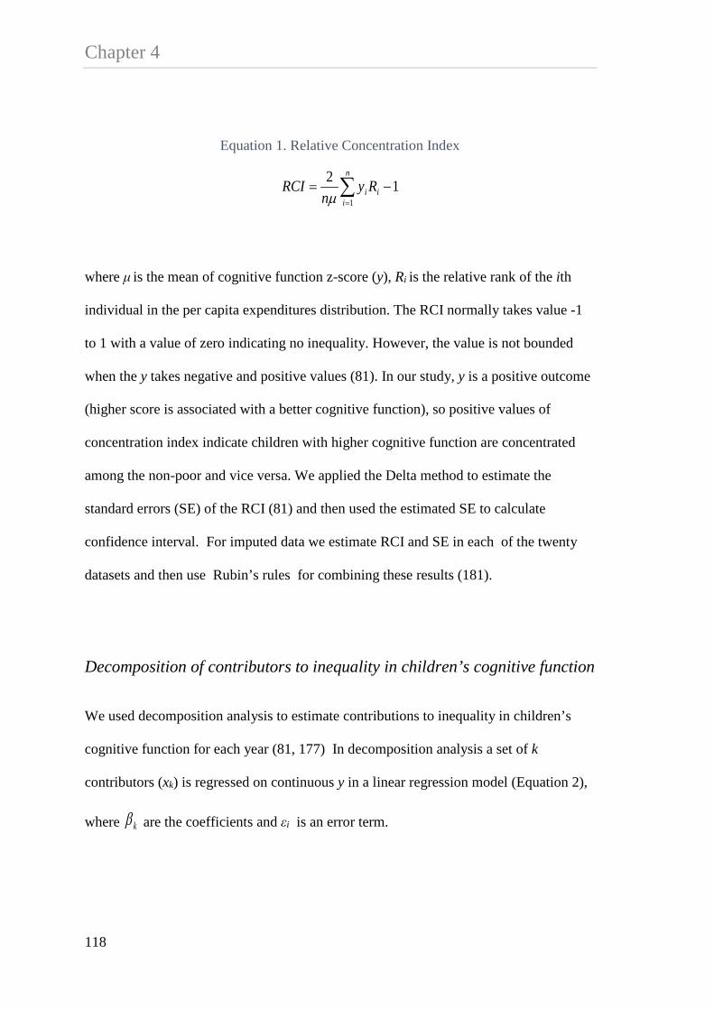
Chapter 4
Equation 1. Relative Concentration Index
121
−= ∑=
i
n
ii Ry
nRCI
µ
where μ is the mean of cognitive function z-score (y), Ri is the relative rank of the ith
individual in the per capita expenditures distribution. The RCI normally takes value -1
to 1 with a value of zero indicating no inequality. However, the value is not bounded
when the y takes negative and positive values (81). In our study, y is a positive outcome
(higher score is associated with a better cognitive function), so positive values of
concentration index indicate children with higher cognitive function are concentrated
among the non-poor and vice versa. We applied the Delta method to estimate the
standard errors (SE) of the RCI (81) and then used the estimated SE to calculate
confidence interval. For imputed data we estimate RCI and SE in each of the twenty
datasets and then use Rubin’s rules for combining these results (181).
Decomposition of contributors to inequality in children’s cognitive function
We used decomposition analysis to estimate contributions to inequality in children’s
cognitive function for each year (81, 177) In decomposition analysis a set of k
contributors (xk) is regressed on continuous y in a linear regression model (Equation 2),
where kβ are the coefficients and εi is an error term.
118

Chapter 4
Equation 2. Linear regression model
iikk
ki XY εβα ++= ∑
Given the relationship between yi and xik in Equation 2, the RCI is estimated as the
sum of the relative concentration index of the determinants weighted by the
elasticity ( kη ) of y with respect to each determinant. The formula can be written as
Equation 3. Decomposition of the concentration index
µη ε /GCCRCIk
kk +=∑
µβ
η kkk
X=
where kβ is the estimated coefficient of k contributor, kx is the mean of k, μ is the
mean of y, Ck is the relative concentration index for k contributor, and GCε is the
generalized concentration index for the error term. The contribution of each factor is a
function of the elasticity of cognitive function with respect to the particular contributor
and the degree of per capita expenditures-related inequality. Therefore, in order to have
a large contribution to the total inequality, a factor should have either large elasticity or
large relative concentration index (Ck) or both.
For estimating the uncertainty in the decomposition we used Markov chain Monte
Carlo (MCMC) simulation method (175). This was chosen over bootstrap methods
because it allows use of the survey weights without requiring any additional
computational complexity. In MCMC we used the Gibbs re-sampling method. The 95%
119

Chapter 4 confidence interval was calculated using the equal tail method. The equal tail interval
runs from 2.5th percentile and 97.5th percentile of the posterior distributions (176). The
decomposition analysis is limited to complete case because the methodology for
estimating the SE of percent contribution of each determinant is not yet available, which
in-turn limits the use of Rubin’s rule for combining the imputed data.
Decomposition of changes in the inequality in children’s cognitive function
We also examined changes in per capita expenditure inequality in cognitive function
between 2000 and 2007. We used the Oaxaca-type decomposition to measure changes
in inequality in the contributors to cognitive function inequality and changes in the
elasticity of cognitive function with respect to these contributors (81, 177). The formula
can be written as
Equation 4. Oaxaca-type decomposition of change
)/()()( 111 ttktktk
ktk
ktktkt GCCCCC µηηη ε∆+−+−=∆ −−− ∑∑
where ktη is the elasticity of k contributor at time t and Ckt is the relative concentration
index of k at time t. Similar to decomposition analysis, the decomposition of change is
also restricted to complete case.
120

Chapter 4 Table 1. Summary statistics for cognitive function and its contributors using complete case analysis, 2000 and 2007
2000 2007
n=4156 n=4291
% or Mean (SD) % or Mean (SD)
Outcome
cognitive function (z-score) 0.24 (0.79) 0.34 (0.66)
Children characteristics
Age 10.5 (2.28) 10.2 (2.31)
Gender
Male 51 52
Female 49 48
Primary activity
-attending school 91 95
Parental characteristics
Father education
- none or primary 60 45
- high school 32 44
-university 8 11
Mother education
-none or primary 69 50
-high school 26 42
-university 5 7
Father primary activity
-working 93 95
-others 7 5
121

Chapter 4
Table 1. Continued
2000 2007
n=4156 n=4291
% or Mean (SD) % or Mean (SD)
Mother education
-none or primary 69 50
-high school 26 42
-university 5 7
Father primary activity
-working 93 95
-others 7 5
Mother primary activity
-working 53 49
-others 47 51
Mental health
-Father 2.03 (2.98) 3.29 (3.18)
-Mother 2.56 (3.50) 3.53 (3.48)
Household characteristics
Residential area
-Living in rural 57 49
-Living in urban 43 51
-Living in Java or Bali 58 59
-Living in outside Java or Bali 42 41
Log per capita expenditures 11.93 (0.70) 12.82 (0.65)
Has electricity 89 96
Improved drinking water 51 55
Improved sanitation 44 64
122

Chapter 4 4.6. Results
Table 1 shows the summary statistics of cognitive function and its contributors. The average
child cognitive function z-score increased from 0.24 (SD 0.79) in 2000 to 0.34 (SD 0.66) in
2007. Of the 4156 children in 2000, 51% were males and 91% of them were still attending
school. In 2007, of the 4251 children 95% were still attending school. In terms of parental
education, the mothers had lower education than the fathers in both years. In 2000, 69% of
mothers had no or primary education, whereas in 2007 this had dropped to 50%. There was
also improvement in fathers’ education, 60% of fathers had no or primary education in 2000
down to 45% in 2007. The average log per capita expenditures was 11.93 rupiah (SD 0.70) in
2000 and 12.82 rupiah (SD 0.65) in 2007, which is equivalent to an increase from
approximately 16 to 37 USD per month. In 2000, the proportion of households that had
electricity was 89%, used an improved drinking water source was 51% and used improved
sanitation was 44%, whereas in 2007, the proportion was 96%, 55% and 64%, respectively.
123

Chapter 4
Figure 19. Relative concentration curve for inequality in children's cognitive function using complete cases analysis, Indonesia 2000 and 2007
The relative concentration curves for inequality in children’s cognitive function in 2000 and
2007 based on complete case analysis are shown in Figure 19. Using complete case analysis,
the RCI in 2000 was 0.29 (95% CI 0.22-0.36) and was 0.16 (95% CI 0.13-0.20) in 2007,
showing the burden of poorer cognitive function was higher among the disadvantaged in both
years.
Table 2. Comparison between complete cases and multiple imputation
2000 2007 Sample
N=6179 RCI (95% CI) Sample
N=6680 RCI (95% CI)
Complete case 4156 0.29 (0.22-0.36) 4291 0.16 (0.13-0.20) Multiple imputation 5079 0.32 (0.24-0.41) 5560 0.20 (0.15-0.25)
124

Chapter 4 Table 2 shows the comparison of RCI and their confidence interval for 2000 and 2007
between complete case analysis and multiple imputation analysis. The magnitude of the RCI
from multiple imputation analysis were 0.3 and 0.4 higher than using complete case analysis,
for 2000 and 2007 respectively,
Table 3. Decomposition of inequality in children's cognitive function ranked by contribution in 2000
Contributors
2000
β Elasticity concentration
contribution 95% CI
index lower upper
Log per capita expenditures 0.08 3.38 0.03 37% 19% 55%
Use improved sanitation 0.14 0.21 0.26 18% 11% 26%
Mother attended high school 0.18 0.16 0.33 18% 11% 24%
Father attended university 0.12 0.03 0.67 7% 0% 14%
Mother attended university 0.17 0.03 0.69 7% 1% 12%
Has electricity 0.20 0.65 0.03 6% 4% 9%
Living in rural -0.07 -0.16 -0.10 6% 2% 9%
Child is attending school 0.17 0.56 0.02 3% 2% 5%
Living in Java/Bali 0.13 0.37 0.02 3% 1% 4%
Father's mental health scores -0.01 -0.04 -0.06 1% 0% 2%
Mother's mental health scores -0.01 -0.06 -0.03 1% 2% 9%
Father attended high school 0.00 0.00 0.20 0% -4% 5%
Father is working 0.04 0.13 0.01 0% 0% 1%
Mother is working 0.01 0.02 0.01 0% 0% 0%
Use improved drinking water 0.00 0.00 0.16 0% -5% 5%
Child is male 0.10 0.19 -0.02 -1% -2% -1%
Residual 0.00 0.00 -5%
125

Chapter 4 Table 3. Continued
Contributors
2007
β elasticity concentration
contribution 95% CI
index lower upper
Log per capita expenditures 0.10 3.09 0.03 52% 33% 70%
Use improved sanitation 0.09 0.14 0.13 12% 6% 18%
Mother attended high school 0.10 0.09 0.16 9% 4% 13%
Father attended university 0.10 0.02 0.57 9% 2% 15%
Mother attended university 0.07 0.01 0.64 5% -2% 11%
Has electricity 0.25 0.60 0.01 5% 3% 70%
Living in rural -0.03 -0.05 -0.09 3% -1% 7%
Child is attending school 0.09 0.22 0.02 2% 0% 4%
Living in Java/Bali 0.14 0.29 0.00 0% 0% 0%
Father's mental health scores -0.01 -0.05 -0.03 1% 0% 2%
Mother's mental health scores 0.00 -0.03 -0.03 1% 0% 2%
Father attended high school 0.04 0.04 0.11 3% 0% 6%
Father is working -0.13 -0.31 0.01 -2% -3% -1%
Mother is working 0.05 0.07 0.07 3% 1% 5%
Use improved drinking water 0.04 0.05 0.09 3% 0% 6%
Child is male 0.05 0.06 -0.01 0% -1% 0%
Residual 0.00 0.00 -3%
126
Chapter 4 Table 3 shows the decomposition of the inequality in cognitive function for 2000 and
2007 ranked by the contribution in 2000. The β coefficient shows the association
between cognitive function and each contributor. Being male, still attending school,
living with a parent who had higher education, and living in Java-Bali were all
associated with higher cognitive function scores. Whereas higher parental mental
health score and living in a rural area are associated with a lower cognitive function
score. The elasticity shows how sensitive cognitive function is to each contributor.
The largest elasticity was the log of per capita expenditure (3.38 in 2000 and 3.09 in
2007). The concentration index shows the magnitude of inequality in cognitive
function with respect to each contributor. The concentration indices for parental
education were all positive, indicating parents with higher education were more
concentrated among the higher economic groups. For example, in 2000 the
concentration index for the father’s university attendance was 0.67 and was 0.69 for
mothers. The concentration indices for parental mental health were negative,
indicating that parents with higher mental health scores were more concentrated
among the higher economic groups.
The largest contribution to inequality in cognitive function was inequality in per
capita expenditures, accounting for 37% and 52% of the total inequality in 2000 and
2007, respectively. Inequality in using improved sanitation accounted for 18% (in
2000) and 12% (in 2007) of the total inequality in children’s cognitive function. As an
important determinant of child cognitive function, parental education
disproportionately contributed to the total inequality with maternal high school
attendance having the largest contribution in 2000 (18%) and having equal
contribution with fathers’ university attendance in 2007 (9%). Although residential
location made a very small contribution to the total inequality, children residing in
127

Chapter 4 rural areas or outside Java-Bali had poorer cognitive function compared to their urban
peers or those children residing in Java-Bali.
Table 4. Oaxaca-type decomposition for change in children's cognitive function inequality, 2000 and 2007
Contributors change in inequality
change in elasticity
total %
Mother attended high h l
-0.02 -0.02 -0.04 27%
Use improved sanitation -0.02 -0.02 -0.03 25%
Log per capita expenditures -0.02 -0.01 -0.02 18%
Living in rural 0.00 -0.01 -0.01 8%
Mother attended university 0.00 -0.01 -0.01 8%
Has electricity -0.01 0.00 -0.01 7%
Father attended university 0.00 -0.01 -0.01 5%
Living in Java/Bali -0.01 0.00 -0.01 5%
Child is attending school 0.00 -0.01 -0.01 4%
Father is working 0.00 0.00 0.00 3%
Father's mental health scores
0.00 0.00 0.00 1%
Mother's mental health scores
0.00 0.00 0.00 0%
Residual 0.00 0.00 0.00 0%
Father attended high school 0.00 0.01 0.00 -2%
Child is male 0.00 0.00 0.00 -3%
Mother is working 0.00 0.00 0.00 -3%
Use improved drinking water
0.00 0.01 0.00 -3%
Total -0.07 -0.07 -0.14 100%
There was 0.13 (45%) decrease in inequality in children’s cognitive function between
2000 and 2007. Table 4 shows the decomposition for change in inequality in
children’s cognitive function. The first column shows changes in the magnitude of
inequality in the contributors and the second column shows changes in the elasticity
128

Chapter 4 of the cognitive function with respect to these contributors. The total change for each
determinant and the percent change are presented in the last two columns. Overall,
changing inequalities and changing elasticities contributed equally to the reduction in
inequality in cognitive function. Although inequality in per capita expenditures
accounted for the largest contribution to the total inequality for each year, it only
contributed 18% to decreasing inequality. Changes in maternal participation in high
school (27%), use of improved sanitation (25%) and increases in per capita
expenditures were largely responsible for changes in inequality in children’s cognitive
function.
4.7. Discussion
Inequality in Indonesian children’s cognitive function favored more advantaged
households in both 2000 and 2007. However, children aged 7-14 years in 2007 had
higher cognitive scores than the cohort of 7-14 year olds in 2000. Importantly,
although pro-rich inequality remains, inequality in cognitive function decreased by
45% between 2000 and 2007. Inequalities in per capita expenditures, maternal high
school attendance and use of improved sanitation were the largest contributors to
inequality for each year, suggesting that the change in cognitive function is most
sensitive to these three important determinants. Children living in households with
higher per capita expenditures, having a mother with high school education and using
improved sanitation were more concentrated among the higher economic groups.
Between 2000 and 2007, inequality in the social distribution of children with mothers
who attended high school and used improved sanitation decreased. In these data, these
were the main contributors to reduction in inequalities in children’s cognitive
function. Our findings are consistent with the recent Program for International Student
129

Chapter 4 Assessment’s (PISA) results, indicating Indonesia was among the small number of
countries where the level of socioeconomic inequality decreased and the average
student’s performance improved between 2000 and 2009 (242).
The decomposition analysis presented here is descriptive rather than causal, partly
because we are limited by the factors included in the ILFS survey to examine as
contributors. To triangulate our findings, we examined the national statistics on
school participation, population with access to improved sanitation and GDP growth
(243) as well as policy trends that may shed light on what we found to be the three
largest contributors to reduction in cognitive function inequality. Statistics on trends
in school participation show that between 1971 and 2010 both primary and secondary
school enrolments have increased, with a substantial increase between 1971 and 1987
for primary school and between 1978 and 1987 for secondary school enrolment
(Figure 20).
130

Chapter 4
Figure 20. Trends in school enrolment, Indonesia 1971-2010
One possible explanation is related to government policy to provide universal access
to basic education through the school construction program in 1973-1979 and the
elimination of primary school fees in 1978 (67). Through the Presidential Instruction
for Primary School program (SD Inpres), the government doubled the number of
primary schools by building more than 61,000 new primary schools between 1973
and 1979. The number of schools constructed in each district was proportional to the
number of primary school aged children not enrolled in schools in 1972 (10). SD
Inpres was not only the largest school construction program in the country’s history,
but also the fastest increase in school provision in the world (67). A study by Duflo
(10) suggested that this program had more impact on the cohort aged 7 or younger in
1974 but not the cohort born in 1962 or before. The same study also found this
131

Chapter 4 program had more impact in poor provinces and increased the probability of
completing primary school by 12% among the affected children.
Using data from the IFLS 2000, Petterson (244) found that women and students from
low socioeconomic groups received more benefits from the school construction
program in Indonesia. Following that program, in 1984 the government passed the
first law of compulsory basic education (Wajib Belajar), where every child aged 7-12
had to attend six years basic education.
Our results show that reduction in the inequality in maternal high school attendance
made the largest contribution to decreasing inequality in children’s cognitive function
between 2000 and 2007. This is consistent with the evidence from developing
countries that shows increasing school availability at the local level has greater benefit
for educational achievement in females although the Indonesian program was not
specifically targeting girls (245). In our study, the mean age of mothers was 37 (SD
6.61 for 2000 and 6.58 for 2007). With the assumption that the cohort born after 1962
received more benefit from the school construction program, we estimated 85% of the
mothers in 2007 were among the cohort who were more likely to benefit from the
school construction program and the laws making six years basic education
compulsory, compared to 55% of the mothers in 2000. In addition to change in
inequality in maternal high school attendance, reduction in cognitive function
inequality was also sensitive to change in household access to improved sanitation
and change in per capita expenditures. Figure 21 shows steadily increasing trends in
the proportion of the population with access to improved sanitation and improvements
in the average GDP in 2000 and 2011.
132

Chapter 4
Figure 21. Trends in GDP growth and improved sanitation facilities, Indonesia 2000-
2011
A great deal of evidence shows that increasing pro-equity public service coverage
including health and education programs could help reduce health related inequalities
at the population level (246-248). A systematic review by Gakidou, et al., (249) found
increases in women’s educational attainment reduced gender gaps in education and
contributed about 51% to decreasing under five mortality in 175 countries between
1970-2009. Evidence from Japan shows universal access to primary education in the
early 1900s increased primary school attendance and reduced gender inequality in
education, which in the longer term also had benefits on population health through
reduction of infant mortality and increased life expectancy (250). Qualitatively similar
processes resulting in reductions in infant mortality on increasing life expectancy has
also been demonstrated in South Korea (245).
133

Chapter 4 The limitations of this study include that it is a descriptive analysis of cross sectional
data in 2000 and 2007. Estimates of the magnitude and contribution to inequality
calculated in these data are based on the socioeconomic measure used - in this case,
per capita household expenditure. Other indicators of socioeconomic inequality may
yield different estimates, especially for the contributions (81, 251). Results from the
decomposition analysis are sensitive to which determinants are selected for inclusion
in the model. Remaining cognizant that our findings cannot be considered causal, we
argue that pro-equity government policy and investment in education, particularly for
women, improved sanitation and to a lesser extent economic growth are plausible
important contributors to overall improvements and decreased inequalities in
children’s cognitive function in Indonesia.
134

CHAPTER 5
Effect on Child Cognitive Function of Increasing Household Expenditure in Indonesia: Application of a Marginal Structural Model and Simulation of a Cash Transfer Programme

Chapter 5 5.1. Preface
As outlined in chapter 4, findings from study one suggested that the burden of poor
cognitive function was higher among the disadvantages. In both 2000 and 2007,
household per capita expenditure was the largest single contributor to inequality in
children’s cognitive function. This chapter presents the second aim of this thesis, which
examined the effects of household per capita expenditure on children’s cognitive
function and whether a cash transfer intervention increased cognitive function scores. In
study two, the effects of household expenditure and cash transfer intervention were
estimated using an inverse probability of treatment weight in a marginal structural
model. Under a potential outcome approach, marginal structural models provide robust
estimates for better causal interpretation. Simulations of hypothetical cash transfer
interventions were modelled using the Indonesian conditional cash transfer program
(Program Keluarga Harapan PKH). Findings from this study provide evidence whether
cash transfer intervention could be used as an effective intervention to improve
children’s cognitive function in Indonesia.
This chapter has been published in the International Journal of Epidemiology.
136

Chapter 5
5.2. Statement of authorship
137

Chapter 5
138

Chapter 5 5.3. Abstract
Background
Parental investments in children are an important determinant of human capability
formation. We investigated the causal effect of household expenditure on Indonesian
children’s cognitive function between 2000 and 2007. We also investigated the effect
of change in mean cognitive function from a simulation of a hypothetical cash
transfer intervention.
Methods
A longitudinal analysis using data from the Indonesian Family Life Survey (IFLS)
was conducted using 6136 children aged 7 to 14 years in 2000 and still alive in 2007.
We used the inverse probability of treatment weighting of a marginal structural
model to estimate the causal effect of household expenditure on children’s cognitive
function.
Results
Cumulative household expenditure was positively associated with cognitive function
z-score. From the marginal structural model, a 74534 rupiah/month (about US$9)
increase in household expenditure resulted in a 0.03 increase in cognitive function z-
score (β=0.32, 95% CI 0.30 – 0.35). Based on our simulations, among children in
the poorest households in 2000, an additional about US$6-10 of cash transfer
resulted in a 0.01 unit increase cognitive function z-score, equivalent to about 6%
increase from the mean z-score prior to cash transfer. In contrast, children in the
poorest household in 2007 did not benefit from an additional about US$10 cash
transfer. We found no overall effect of cash transfers at the total population level.
139

Chapter 5 Conclusion
Greater household expenditure had a small causal effect on children’s cognitive
function. Although cash transfer interventions had a positive effect for poor children,
this effect was quite small. Multi-faceted interventions that combine nutrition, cash
transfer, improved living conditions and women’s education are required to benefit
children’s cognitive development in Indonesia.
Key Messages
• Household expenditure is weakly associated with higher cognitive function • From our hypothetical intervention, small cash transfers (e.g. US$6-
10/months) for the poorest households had a very small effect in improving child cognitive function but no overall effect at the population level.
• Multi-faceted interventions that combine nutrition, cash transfer, improved living conditions and women’s education are required to benefit children’s cognitive development in Indonesia.
140
Chapter 5
5.4. Introduction
Parental investments in children are an important determinant of human capability
formation. These investments include economic, learning, social, cultural and
behavioural resources that help create the early life supports for the accumulation of
capabilities over the life course. Parental investments rely on the resources in the
household that can be deployed, and transferred to their children (28). The unequal
distribution of resources in society limits people’s freedom to fully function and may
lead to capability deprivation (252). The Commission on Social Determinants of
Health’s indicated that investing in early childhood interventions was a major driver of
improving health disparities over the life course (1). Even when evidence for
intervention effectiveness does exist (34, 37), effective implementation of early
childhood intervention is challenged by capacities in resourcing, targeting, and
translating evidence-based policy into practice (40).
Conditional Cash Transfer (CCT) programs are a welfare strategy generally aimed at
families to alleviate poverty through conditional actions. In relation to children, the cash
transfers are commonly conditional on immunization and/or primary school enrolment.
Such CCT programs have been widely used in developing countries, including
Indonesia. CCT programs combine redistribution of resources to poor households and
have been shown to promote greater investment in human capital of children, which is
expected to, in turn reduce long-term poverty (119). Evidence from Mexico’s CCT
program, Opportunidades suggests that CCT had both short and long-term positive
effects on children’s cognitive function (120, 121). The CCT program in Indonesia,
Program Keluarga Harapan, successfully increased food consumption expenditure,
141

Chapter 5 especially high protein food and increased participation in local health services but had
little effect on education services (76).
Our recent study (65) found that among Indonesian children aged 7-14 years, the burden
of poorer cognitive function was higher among disadvantaged groups. This inequality,
however, reduced markedly between 2000 and 2007. Decreasing inequality in children’s
cognitive function was mainly driven by changes in maternal education, use of
improved sanitation and household per capita expenditure. Decomposition of the
inequality showed that household expenditure was the largest single contributor to
socioeconomic inequality in 2000 and 2007 (65). The aim of the current study was to
estimate the causal effect of household expenditure on Indonesian children’s cognitive
function between 2000 and 2007, and then simulate the effect of a hypothetical CCT on
change in cognitive function after a plausible intervention.
5.5 Methods
Data
We used data from four waves of the Indonesian Family Life Survey (IFLS). IFLS is an
ongoing longitudinal survey in Indonesia, which was first conducted in 1993 and
subsequently in 1997, 2000 and 2007 (146-149). The IFLS sample is considered to be
representative of 83% of the whole Indonesian population. The sample was collected
from households in 13 of the 27 provinces in Indonesia in 1993,and specific details of
the sampling methodology are detailed elsewhere (146). During follow-up, the IFLS
tracked not only individuals who resided in the original household in 1993, but also
individuals who had moved out from the original household but still live within the
IFLS provinces. For our study, we selected children aged 7 to 14 years in 2000 and still
142
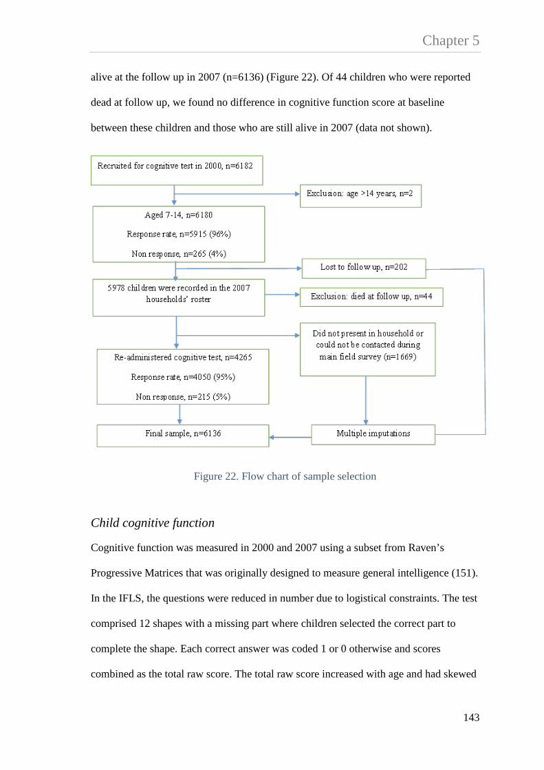
Chapter 5 alive at the follow up in 2007 (n=6136) (Figure 22). Of 44 children who were reported
dead at follow up, we found no difference in cognitive function score at baseline
between these children and those who are still alive in 2007 (data not shown).
Figure 22. Flow chart of sample selection
Child cognitive function
Cognitive function was measured in 2000 and 2007 using a subset from Raven’s
Progressive Matrices that was originally designed to measure general intelligence (151).
In the IFLS, the questions were reduced in number due to logistical constraints. The test
comprised 12 shapes with a missing part where children selected the correct part to
complete the shape. Each correct answer was coded 1 or 0 otherwise and scores
combined as the total raw score. The total raw score increased with age and had skewed
143

Chapter 5 distributions towards the left tail. The total raw scores were then transformed into an
age-specific z-score. Because the total scores were skewed, we calculated the mean and
the variance of score distributions by taking into account the range, median and the
sample size using the formula from Hozo, et al., (152) and used the estimated mean and
standard deviation to create an age specific z-score (65).
Household Expenditure
We used the log of household per capita expenditure (PCE) constructed from the
monthly total household expenditures divided by the number of household
members.(157) The cumulative household PCE was constructed by summing PCE in
2000 and 2007. The PCE was reported in Indonesian rupiah value. To aid interpretation
we also report PCE in US dollar (US$) at the year 2000 exchange rates (1 US$=8422
rupiah).
Confounding
A series of child, caregiver and household characteristics measured variously in 1993,
1997, 2000 and 2007 was selected a priori based on the directed acyclic graph (DAG)
in Fig.2 as representing baseline and time-varying confounding of the associations
between household PCE and child cognitive function in 2000 and 2007. Child
characteristics included age (continuous), whether the child was attending school in
2000 and had completed at least 8 years of education by 2007. Caregiver characteristics
included maternal age (continuous), the highest level of education attended (categorized
as none, primary school, junior high school, senior high school and diploma/university),
whether the mother was working in the past week, and self-reported mental health. All
144

Chapter 5 information about caregiver characteristics was measured in 1993, 1997 and 2000
except for mental health. Maternal self-reported mental health was measured in 2000
and 2007. The measure in 2000 consisted of eight items of feelings experienced in the
past four weeks with response in three categories ranging from never to often. In 2007,
the measure was adapted from the shorter version of Centre for Epidemiological
Studies-Depression scales (CES-D) (166) consisting of 10 items of symptoms or
feelings experienced in the past week with response in five categories ranging from not
at all, rarely (<=1 day), some days (1-2 days), occasionally (3-4 days) and most of the
time (5-7 days). For both measures, each item was scored ranging from 0 to 3 and
summed as the total mental health score separately for 2000 (scores ranging 0-24) and
2007 (scores ranging 0-30). In the analysis, we used the total mental health score where
a higher score indicated poorer mental health.
In 1993, 96% of caregivers were the mothers and the proportion slightly decreased in
1997 and 2000 (92% and 90%, respectively). For each survey round, if a mother was
not present in the household, either because she was living elsewhere or was reported
dead, other family members who took the role as the child’s main caregiver provided
information. However, information about caregiver was only collected for children
under 15 years of age. In 2007, 5626 (92%) children were between 15 and 22 years of
age. Of these, 1116 (20%) children in the sample did not have associated information on
their mothers. In this circumstance caregiver’s mental health was replaced by the father,
but when both parents were not present; this information was replaced by the household
head.
Household characteristics include household size (continuous), the number of economic
hardships experienced in the past five years (continuous), whether the household had
145

Chapter 5 electricity, used piped water or a pumped well as the main drinking water source, owned
a toilet connected to septic tank, and place of residence (categorized as urban or rural).
All information about household characteristics was measured in 1993, 1997 and 2000,
except for economic hardship. We used information about economic hardship collected
in 1993 and 2000.
Missing data
Of the children in the IFLS who were administered the cognitive test, the response rate
was 96% and 95% in 2000 and 2007, respectively. The proportion of children with
missing information on the exposure was 0.7% in 2000 and 7% in 2007. Of the 6136
children, only 5305 (86%) were recorded as a member of the original household in
1993, whereas 831 children were recorded as either a new member of the original
household or a member of the split off households who were included in 1997 and 2000
survey. As such, data related to all confounders in 1993 were not available for 831
(14%) children. Additionally, 1669 children were either not present in household or
could not be contacted during the main field survey in 2007. To minimize bias due to
attrition and missing responses to questions, we performed the Multiple Imputation by
Chained Equation (MICE) procedure in STATA under the assumption that the imputed
data were missing at random (179, 180). We generated twenty imputed datasets using
fifty cycles of regression switching. We used Rubin’s rule to combine and analyse
imputed datasets (181). We used all imputed outcomes in our analysis. As a sensitivity
analysis, we conducted the method of multiple imputation then deletion of outcomes as
described by von Hippel (182) and the results did not change.
146

Chapter 5
Figure 23. Direct acyclic graph (DAG) representing the relations between confounders, household per capita expenditure and child cognitive function
Exposure: household per capita expenditure. Outcome: cognitive function z-score. Ancestor of exposure and outcome (baseline confounders measured in 1993, 1997 and 2000): caregiver’s age, education, employment status, household size, economic hardship, household had electricity, used piped or pumped well as the main drinking water source, owned toilet with septic tank, and residential area. Ancestor of exposure and outcome (confounding L measured in 2000): attending school and caregiver’s mental health. Ancestor of outcome (confounding L measured in 2007): completed at least 8 years of education and caregiver’s mental health. Causal path. Biasing path.
Analysis
We used observational data to investigate a potential causal link between household
PCE and children’s cognitive function. For this analysis we used the inverse probability
of treatment weighting (IPTW) of a marginal structural model (MSM) based on the
assumptions of consistency, no unmeasured confounders (exchangeability) and
positivity (189, 194). Under the assumption of no unmeasured confounders, the causal
DAG (184) shown in figure 23 presents the association between confounders, exposure
and outcome. This causal graph was drawn using DAGitty program version 2.0 (186).
Both the exposure and the outcome were measured at two time points (2000 and 2007),
147

Chapter 5 whereas a series of baseline confounders were measured in 1993, 1997 and 2000. The
confounders included - caregiver’s age, education, employment status, household size,
economic hardship, housing conditions (access to electricity, the main drinking water
source and type of toilet) and place of residence. The use of confounding information
measured at three survey rounds allowed for the situations where a child was raised by a
different caregiver, or lived in different housing environments over the course of the
study period. This model specification may also help to reduce measurement error by
having multiple indicators over time. In the DAG, the child’s current schooling and
caregiver’s mental health in 2000 were included because they indicate the presence of
time varying confounding so that given past household PCE, current schooling and
maternal mental health predict subsequent exposure and outcome. In addition, the DAG
reflects the proposition that a child’s current schooling affects completion of at least
eight years of education and also affects cognitive function in 2007. Similarly,
caregiver’s mental health in 2000 affects mental health and in turn affects child’s
cognitive function in 2007.
In the presence of time varying confounding, the use of conventional regression lacks a
causal interpretation and may introduce collider stratification bias (184, 191). Therefore
in this study, we use a MSM to estimate the causal effect of household PCE on
children’s cognitive function.
Construction of the Inverse Probability of Treatment Weighting (IPTW)
We used the inverse probability of treatment weighting (IPTW) to adjust for
confounding in the marginal structural model (194). The weighting method creates a
pseudo population, based on the child’s potential exposure at each time point. The
weight was estimated based on the probability of an individual having the observed
148

Chapter 5 exposure given their covariates. Because the exposure variable was in continuous form,
we used stabilized weight (SW) to reduce large variance in the weight (194, 205). The
weight was calculated separately for 2000 and 2007, which can be defined as follow;
Equation 6. Stabilized weight for the exposure in 2000
)|()(
2000
20002000
ii
ii CXf
XfSW =
Equation 7 Stabilized weight for the exposure in 2007
),,|()|(
20002007
200020072007
iiii
iii LCXXf
XXfSW =
where the numerator in equation 6 is the marginal density of the exposure in 2000
(Xi2000), and the denominator is the conditional density function of Xi2000 given the
history of confounders ( iC ) up to 2000 including caregiver and household
characteristics. The numerator in equation 7 is the conditional density function of the
exposure in 2007 (Xi2007) given Xi2000, and the denominator is the density function of
X2007 given X2000, history of confounders ( iC ), and time varying confounders ( iL )
which includes the child attending school and their caregiver’s mental health in 2000,
and the child’s completion of at least 8 years of education and their caregiver’s mental
health in 2007. The mean weight was expected to be around one, suggesting no
misspecification of the weight model (nonpositivity) (205). To test whether there is a
bias in our causal estimation due to nonpositivity, we truncated the weight at the 1st and
149

Chapter 5 the 99th percentile as well as at the 5th and the 95th percentile of the weight distributions
(205).
The last step was the creation of the final weight;
Equation 8. The inverse probability of treatment weights
20072000 SWSWIPTW ×=
Marginal structural mean model
Since we have repeated measures on both the exposure and the outcome, we used the
generalized estimating equations model (GEE) (253) to estimate the effect of household
PCE on cognitive function. We specified an independent working correlation structure
and calculated the 95% confidence interval (CI) using robust variance estimator. Use of
the independent correlation structure is preferable in the GEE when using IPTW
because although there is potential that the working correlation structure is miss-
specified the independent correlation structure still gives consistent estimation (206,
207). All analyses were conducted using STATA 13 (254).
The marginal structural mean model can be defined as
Equation 9. Marginal Structural Mean Model
xitxitit cumcumYE 10)|( ββ +=
150

Chapter 5 Where itY is the expected mean potential outcome of cognitive function z-score given
the observed cumulative household PCE )( xitcum . We present three types of GEE
models. The first model is the standard (unadjusted) regression GEE model estimating
the effect of cumulative household PCE on cognitive function. The second model
estimated the effect of cumulative household PCE on cognitive function using standard
regression adjusted covariates. Finally, we present the GEE from a MSM estimating the
causal effect of cumulative household PCE on cognitive function, accounting for
confounding by the IPTW.
Hypothetical intervention on household PCE
We used the Indonesian CCT program, Program Keluarga Harapan (PKH or Hopeful
Families Program), as a hypothetical intervention to estimate the effect of change in
household PCE on mean cognitive function after a plausible cash transfer intervention.
The PKH provided cash transfer to very poor households with children ages 0-6 years
conditional on their participation in the local health service to ensure the child was fully
immunized, took Vitamin A capsules a minimum of twice a year, and attended growth
monitoring check-ups. The PKH also provided cash transfer to very poor households
with children ages 6-15 conditional on enrolment in school and ensured attendance for
minimum of 85% of school days. Lastly, PKH provided cash transfer to very poor
households with children ages 16-18 years but who had not completed 9 years of basic
education conditional on their school enrolment to finish a full 9 years of education. In
PKH, the money was transferred quarterly. The compliance of conditions were
monitored and verified through health and education service providers report. Non-
151

Chapter 5 compliance of these conditions would result in a warning, 10% discount of benefit and
even discontinuity of the cash transfer (76).
For this study, we modelled the hypothetical intervention on the PKH education
program, which targeted very poor household with children ages 6-15 years and ages
16-18 years but who had not completed 9 years of education. This program provided a
fixed amount of 200,000 rupiah/household/year and an additional of 400,000
rupiah/year for each child aged 6-12 years and 800,000 rupiah/year for each child aged
13-15 years (255). Based on results from a World Bank report, the first batch of PKH
beneficiaries in 2007, increased their average household per capita income by 19000
rupiah/month (about $2) or by 10% compared to prior to the program (76). At the
national level, the transfer was equivalent to about 5% of the average PCE in 2007
(353421 rupiah or about US$42/month) (256).
Our simulated intervention focused on the poorest 40% of the population, which is
similar to the target group that was proposed by the World Bank and WHO for the
equity goal in universal health coverage (158). Herein, the poorest household were
defined as those having children living in the bottom 40% of PCE. We simulated the
intervention in both 2000 and 2007 to examine whether a CCT at ages 7-14 had a larger
effect than in adolescence at ages 14-18 years.(39) In step one, we targeted the poorest
households in 2000 who had children aged 7-14 years. Of the total population, 2456
(40%) children were eligible to receive a CCT in 2000. In 2000, all eligible children
received 200,000 rupiah/year. In addition, each child aged 7-12 received 400,000
rupiah/year and each child aged 13-14 received 800,000 rupiah/year. Assuming this
money was transferred monthly, each child aged 7-12 received 50000 rupiah/month
(about US$6) whereas each child aged 13-14 received about 83333 rupiah/month (about
152

Chapter 5 US$10). In step two, we targeted the poorest households in 2007 and who had children
aged 14-15 years as well those who had children aged 16-18 but who had not completed
9 years of education. Of the total population, 961 (16%) children were eligible to
receive a CCT in 2007. In 2007, each eligible child received 200,000 rupiah/year and an
additional 800,000 rupiah/year. Similar to step one, assuming this money was
transferred monthly each child received 83333 rupiah/month (about US$10). Our
hypothetical intervention assumed that all the increased income from the CCT was
invested in the child’s education.
Sensitivity analysis for unmeasured confounding
We conducted sensitivity analysis to estimate bias in the causal effect of household PCE on cognitive function due to unmeasured confounding (U). In sensitivity analysis, we defined U as a binary variable and assumed that the association between U and cognitive function did not vary across levels of household PCE. Following VanderWeele and Arah (208), we defined the sensitivity parameter δ as the effect of U on cognitive function and the sensitivity parameter γ as the prevalence of U. The magnitude of bias dx+ was then estimated as the product of δ and γ.
153

Chapter 5 Table 5. Characteristics of study participants, IFLS 1993, 1997, 2000 and 2007
1993 1997 2000 2007 Outcome Cognitive function z-score, median (IQR) 0.41 (-0.29 – 0.82) 0.53 (0.10 – 0.83) Exposure Log of per capita expenditure/month (PCE), mean (SD) 11.91 (0.71) 12.94 (0.70)
-PCE in rupiah, median (IQR) 142231
(91831 – 227202) 394682
(254286 – 644316) -PCE in US$ (1US$=8422 rupiah), median (IQR) 17 (11 -27) 47 (30 – 77) Log of cumulative PCE, mean (SD) 13.29 (0.65)
-cumulative PCE in rupiah, median (IQR) 560852
(374714 – 887050) -cumulative PCE in US$, median (IQR) 67 (44 – 105) Covariates Children’s characteristics Gender: male, n (%) 3129 (51) Age, mean (SD) 3.76 (2.33) 7.71 (2.29) 10.53 (2.30) 17.89 (2.36) Currently attending school, n (%) 5461 (89) Completed at least 8 years education, n (%) 4503 (73) Caregiver’s characteristics Caregiver’s age, median (IQR) 31 (23 – 39) 35 (26 – 45) 37 (33 – 42) Highest education attended, n (%) -None 2270 (37) 1391 (23) 858 (14) -Primary (grade 1-6) 2635 (43) 3009 (49) 3434 (56) -Junior high school (grade 7-9) 533 (9) 806 (13) 761 (12) -Senior high school (grade 10-12) 544 (9) 723 (12) 805 (13) -Diploma/university 154 (2) 207 (3) 278 (5)
154

Chapter 5
Table 5. Continued
1993 1997 2000 2007 Caregiver’s characteristics Working in the past week, n (%) 1901 (31) 3319 (54) 3472 (56) Mental health scores, median (IQR) 2 (0 – 7) Mental health scores (CES-D), median (IQR) 3 (1 – 5) Household’s characteristics Household size, mean (SD) 5.93 (2.21) 5.76 (2.04) 5.59 (1.93) The number of economic hardship in the past five years, mean (SD) 0.43 (0.70) 0.46 (0.71) Had electricity, n (%) 3970 (65) 5043 (82) 5412 (88) Drinking water source: piped or pump well, n (%) 1984 (32) 2623 (43) 3037 (50) Owned toilet with septic tank, n (%) 1652 (27) 2426 (39) 2611 (43) Place of residence: urban, n (%) 2576 (42) 2516 (41) 2540 (41)
155

Chapter 5
5.6 Results
Table 5 shows the characteristics of study participants in all survey rounds based on multiple
imputed data. The median of cognitive function z-score was 0.41 (interquartile range IQR -
0.29 to 0.82) in 2000 and was 0.53 (IQR 0.10 to 0.83) in 2007, suggesting improvement. In
the same period, the mean of log PCE also increased from 11.91 (SD 0.71) to 12.94 (SD
0.70) equivalent to 49985 rupiah/month/year (about $6), slightly higher than the national
average (Figure 24).
The median age of caregiver in 1993 was 31 years (IQR 23 – 39). In terms of education, we
found a small number of caregivers improved their education, for example the proportion of
caregivers with a diploma or attended university increased from 2% in 1993 to 3% in 1997
and 5% in 2000. Among mothers who were found in the follow up, we found some
discordance in the level of education reported. To test whether bias in reporting education
was affecting the estimates of our MSM, we conducted sub-group analysis for children whose
caregiver reporting was consistent and the result showed no substantial difference. We also
tested whether using education as a continuous instead of a categorical variable changed the
estimate and the result suggested no substantial difference.
The proportion of caregivers who reported working in the past week increased substantially
from 31% in 1993 to 51% in 1997 and steadily increased to 56% in 2000. The substantial
increase found between 1993 and 1997 might be influenced by the economic crisis that hit
Indonesia in 1997 forcing more women to participate in the labour force (257). The median
mental health score was 2 (IQR 0 – 7) and 3 (IQR 1 – 5) in 2000 and 2007, respectively.
At the household level, the proportion of children who had access to electricity, drinking
water from piped water or a pumped well and improved sanitation increased over the years.
156
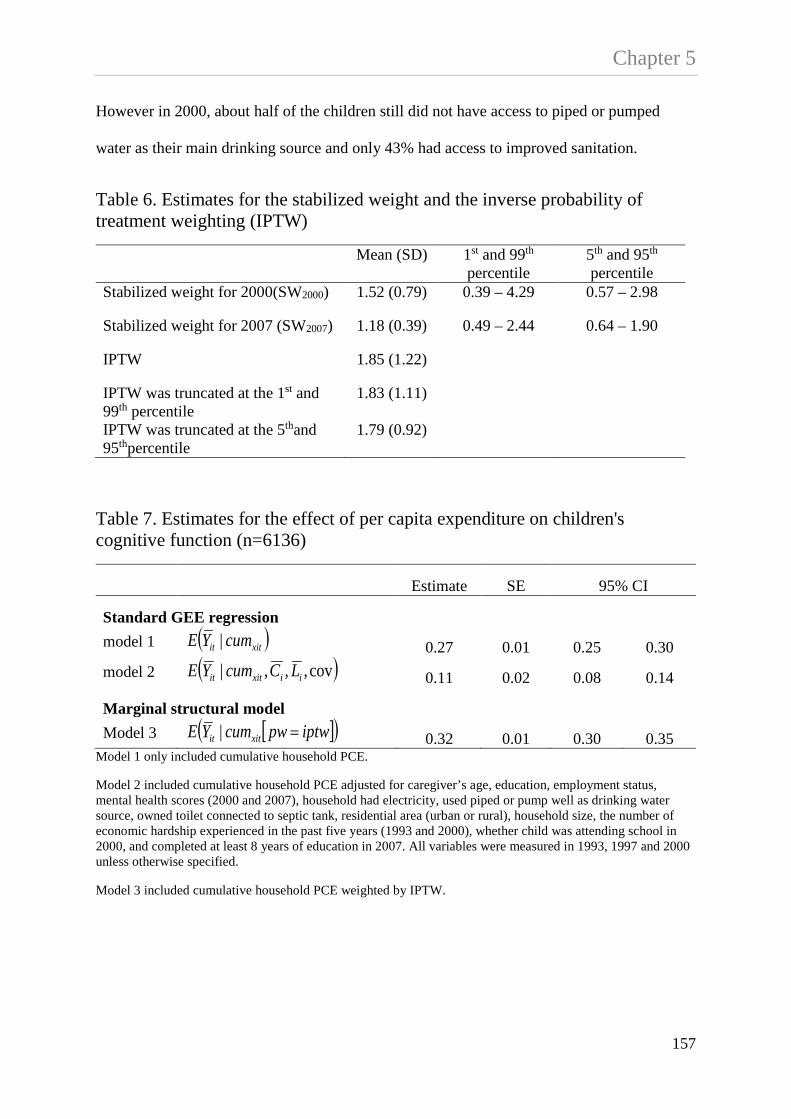
Chapter 5 However in 2000, about half of the children still did not have access to piped or pumped
water as their main drinking source and only 43% had access to improved sanitation.
Table 6. Estimates for the stabilized weight and the inverse probability of treatment weighting (IPTW)
Mean (SD) 1st and 99th percentile
5th and 95th percentile
Stabilized weight for 2000(SW2000) 1.52 (0.79) 0.39 – 4.29 0.57 – 2.98
Stabilized weight for 2007 (SW2007) 1.18 (0.39) 0.49 – 2.44 0.64 – 1.90
IPTW 1.85 (1.22)
IPTW was truncated at the 1st and 99th percentile
1.83 (1.11)
IPTW was truncated at the 5thand 95thpercentile
1.79 (0.92)
Table 7. Estimates for the effect of per capita expenditure on children's cognitive function (n=6136)
Estimate SE 95% CI
Standard GEE regression model 1 ( )xitit cumYE | 0.27 0.01 0.25 0.30 model 2 ( )cov,,,| iixitit LCcumYE 0.11 0.02 0.08 0.14
Marginal structural model Model 3 [ ]( )iptwpwcumYE xitit =| 0.32 0.01 0.30 0.35
Model 1 only included cumulative household PCE.
Model 2 included cumulative household PCE adjusted for caregiver’s age, education, employment status, mental health scores (2000 and 2007), household had electricity, used piped or pump well as drinking water source, owned toilet connected to septic tank, residential area (urban or rural), household size, the number of economic hardship experienced in the past five years (1993 and 2000), whether child was attending school in 2000, and completed at least 8 years of education in 2007. All variables were measured in 1993, 1997 and 2000 unless otherwise specified.
Model 3 included cumulative household PCE weighted by IPTW.
157
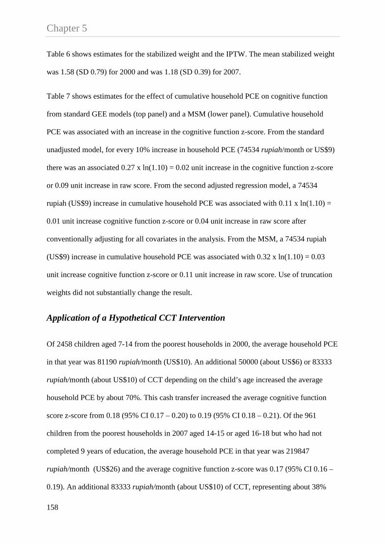
Chapter 5 Table 6 shows estimates for the stabilized weight and the IPTW. The mean stabilized weight
was 1.58 (SD 0.79) for 2000 and was 1.18 (SD 0.39) for 2007.
Table 7 shows estimates for the effect of cumulative household PCE on cognitive function
from standard GEE models (top panel) and a MSM (lower panel). Cumulative household
PCE was associated with an increase in the cognitive function z-score. From the standard
unadjusted model, for every 10% increase in household PCE (74534 rupiah/month or US$9)
there was an associated 0.27 x ln(1.10) = 0.02 unit increase in the cognitive function z-score
or 0.09 unit increase in raw score. From the second adjusted regression model, a 74534
rupiah (US$9) increase in cumulative household PCE was associated with 0.11 x ln(1.10) =
0.01 unit increase cognitive function z-score or 0.04 unit increase in raw score after
conventionally adjusting for all covariates in the analysis. From the MSM, a 74534 rupiah
(US$9) increase in cumulative household PCE was associated with 0.32 x ln(1.10) = 0.03
unit increase cognitive function z-score or 0.11 unit increase in raw score. Use of truncation
weights did not substantially change the result.
Application of a Hypothetical CCT Intervention
Of 2458 children aged 7-14 from the poorest households in 2000, the average household PCE
in that year was 81190 rupiah/month (US$10). An additional 50000 (about US$6) or 83333
rupiah/month (about US$10) of CCT depending on the child’s age increased the average
household PCE by about 70%. This cash transfer increased the average cognitive function
score z-score from 0.18 (95% CI 0.17 – 0.20) to 0.19 (95% CI 0.18 – 0.21). Of the 961
children from the poorest households in 2007 aged 14-15 or aged 16-18 but who had not
completed 9 years of education, the average household PCE in that year was 219847
rupiah/month (US$26) and the average cognitive function z-score was 0.17 (95% CI 0.16 –
0.19). An additional 83333 rupiah/month (about US$10) of CCT, representing about 38%
158
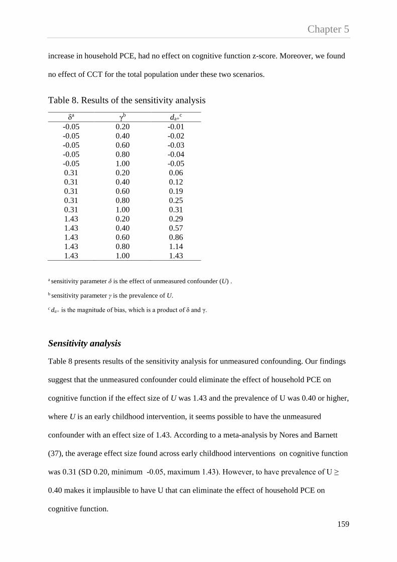
Chapter 5 increase in household PCE, had no effect on cognitive function z-score. Moreover, we found
no effect of CCT for the total population under these two scenarios.
Table 8. Results of the sensitivity analysis
a sensitivity parameter δ is the effect of unmeasured confounder (U) .
b sensitivity parameter γ is the prevalence of U.
c da+ is the magnitude of bias, which is a product of δ and γ.
Sensitivity analysis
Table 8 presents results of the sensitivity analysis for unmeasured confounding. Our findings
suggest that the unmeasured confounder could eliminate the effect of household PCE on
cognitive function if the effect size of U was 1.43 and the prevalence of U was 0.40 or higher,
where U is an early childhood intervention, it seems possible to have the unmeasured
confounder with an effect size of 1.43. According to a meta-analysis by Nores and Barnett
(37), the average effect size found across early childhood interventions on cognitive function
was 0.31 (SD 0.20, minimum -0.05, maximum 1.43). However, to have prevalence of U ≥
0.40 makes it implausible to have U that can eliminate the effect of household PCE on
cognitive function.
δa γb da+c
-0.05 0.20 -0.01 -0.05 0.40 -0.02 -0.05 0.60 -0.03 -0.05 0.80 -0.04 -0.05 1.00 -0.05 0.31 0.20 0.06 0.31 0.40 0.12 0.31 0.60 0.19 0.31 0.80 0.25 0.31 1.00 0.31 1.43 0.20 0.29 1.43 0.40 0.57 1.43 0.60 0.86 1.43 0.80 1.14 1.43 1.00 1.43
159

Chapter 5 5.7. Discussion
Our results suggest that cumulative household expenditure has a small causal effect on
cognitive function in Indonesian children aged 7-14 and 14-22 in 2000 and 2007. Our
findings are consistent with evidence suggesting CCT programs have a positive but small
effect on children’s cognitive function (120, 121). From our hypothetical intervention, a CCT
involving increased household expenditure of 50000 (about US$6) to 83333 rupiah/month
(about US$10) in 2000 increased the average cognitive function score by 0.01 SD; a small
effect size by traditional metrics. This represents about 6% increase from the average
cognitive function z-score prior to cash transfer. We also found that a CCT in 2000 had a
larger effect than a CCT in 2007, possibly because a CCT in 2000 had a larger contribution to
the average household PCE (70% vs 38%) and higher levels of coverage of children in the
population (40% vs 16%). According to the World Bank, one of the reasons PKH had a small
effect on participation in education services such as enrolment rates and transitions to higher
grades, was partly because the cash transfer was too small to benefit the target children (76).
For example, to send a student to secondary school in Indonesia costs on average 2.8 million
rupiah/year for education (equivalent to about $US28/month), which represents about 30% of
the total household expenditure for those living in the poorest quintile of households.
160

Chapter 5
Figure 24 National statistics on average monthly per capita expenditure, Indonesia 2000-2013
Source: Statistics Indonesia, Trends of selected socio economic indicators of Indonesia. Data for 2002-2013 are available at http://www.bps.go.id/eng/aboutus.php?65tahun=1 (accessed 18 May 2014).
Given the effect size of hypothetical cash transfer in this study, a cash transfer would need to
be much larger than those used to have a substantial impact on children’s cognitive function.
Under our first scenario, the estimated amount of cash transfer to shift the average cognitive
function score of the poorest children in 2000 to the average population score is about
825356 rupiah/child/month (about US$98). The national statistics show that the average
annual growth of PCE between 2000 and 2013 has been about US$5/month (Figure 24). At
current levels of national growth in PCE, assuming that household expenditure remains
consistent across groups and assuming that the remainder of the population stay at current
levels of cognitive ability then it will take 20 years to reduce cognitive inequality between
children in the bottom 40% of households and the reminder of the population. However, since
it is unlikely that expenditure growth is equally distributed across the population, it may take
longer for the poorest children to increase their cognitive score to the average level. For this
0
10
20
30
40
50
60
70
80
90
0
100000
200000
300000
400000
500000
600000
700000
800000
2000 2001 2002 2005 2007 2008 2009 2010 2011 2012 2013
rupiah
US$
161
Chapter 5 reason investment in child human capital through cash transfer alone could be very
expensive. It is important to find other types of intervention programs that may be more
efficient in closing the inequality in children’s cognitive function. Our recent study found
that in addition to household PCE, the largest contributors to inequality in Indonesian
children’s cognitive function include access to improved sanitation and maternal education
(65). Numerous studies suggest that early intervention programs that have an educational
component for children, caregivers or both, have a positive effect on various cognitive
development outcomes in both low and middle income countries (19) as well as in high
income countries (258).
Another potential intervention that benefits child cognitive function are nutrition programs,
which may involve nutrition supplementation and nutrition education. Evidence from Nores
and Barnett (37) suggest that nutrition interventions had a larger effect on child cognitive
function than cash transfer programs (mean effect size was 0.26, SD 0.16 for nutrition, and
was 0.17, SD 0.06, for cash transfer). They also found provision of an integrated early
childhood program may yield greater benefit than a single intervention. However, a recent
systematic review by Grantham-McGregor, et al., (259) failed to find any evaluations of
programs delivered at scale in which the effects of integrating psychosocial stimulation into
health and nutrition services on children’s growth and development were assessed. They
argued that this is an urgent need. An integrated intervention program that combined
provision of nutrition, cash transfer, improved living conditions and educational components
especially for young women may yield a greater effect on improving the Indonesian
children’s cognitive function. To a large extent, such an integrated intervention program
could also become part of a strategic plan to promote a better understanding of the social
determinants of health and improving health equity in Indonesia (1).
162

Chapter 5 Our study is subject to limitations. First, our measure of cognitive function was limited to
data that were available in the IFLS, which might not be the best measure to capture the true
cognitive ability of Indonesian children. Second, our findings should be interpreted with care.
Use of standard regression models to estimate the effect of household PCE does not generally
have a causal interpretation and may yield biased effect estimates. The first GEE model
presented a crude association between household PCE on cognitive function, assuming there
were no other factors that potentially confounded this association. Although the second
model included all potential measured confounders, use of standard regression could not
control the potential bias in the presence of time varying confounding. Therefore our use of
the MSM presents a more robust estimation with causal interpretation. However, estimates
for our causal inferences are only true under the assumption of consistency, exchangeability
and positivity, which are not guaranteed by design when using observational data (189, 260).
Third, it is plausible that there are variables that confound the relationship between household
PCE and cognitive function but were not included in the analysis. To address the issue of
potential bias in effect estimation due to unmeasured confounding, we conducted the
sensitivity analysis. Fourth, our estimates assume that financial investment in children’s
capability are drawn from their household’s expenditure. In our hypothetical CCT we assume
that targeted families would spend their CCT funds on their children’s education. When
considering these two assumptions together, it is important to point out that the effect sizes
could indeed be different if increases in household income were not invested in their
children’s education (as we have assumed with the CCT).
163

Chapter 5 In summary, household expenditure had a small positive effect on children’s cognitive
function. Although a hypothetical cash transfer intervention had a positive effect on
children’s cognitive function, the effect was very small. Interventions that combine cash
transfer, improved living conditions and educational opportunities especially for young
women may have greater benefit for the future of children’s cognitive development in
Indonesia.
164

CHAPTER 6
Associations of Early and Later Childhood Poverty with Child Cognitive Function in Indonesia: Effect Decomposition in the Presence of Exposure-Induced Mediator-Outcome Confounding

Chapter 6 6.1. Preface
As shown in chapter five, greater household per capita expenditure was associated with
higher cognitive function score but the effect size was small. Based on simulations of a
hypothetical cash transfer intervention, an additional US$ 6-10/month of cash transfer for
children from the poorest households in 2000 increased the mean cognitive function score by
6% but there was no overall effect of cash transfers at the total population level. This chapter
presents the third study of this thesis, which investigated the associations of poverty at ages
0-7 and poverty at 7-14 on children’s cognitive function at 7-14 years. Using decomposition
analysis, this study also examined the direct and indirect effects of poverty at 0-7 years on
cognitive function at 7-14 years mediated through poverty at 7-14 and school attendance and
aspects of the child’s home environment. This study was motivated to better estimate the
optimal timing for intervention and the mechanism by which poverty earlier in life at 0-7
could affect cognitive function at 7-14 years.
This chapter has been accepted for publication in the American Journal of Epidemiology.
166

Chapter 6 6.2. Abstract
The amount of family financial resources available in early-life influences child health and
development. Using data from the Indonesian Family Life Survey 2000 and 2007, we
estimated the effects of early-life poverty (at 0-7 years) and poverty in later childhood (7-14
years) on cognitive function at 7-14. Our analysis provides little support for the idea that an
early intervention to support household income has a larger effect than intervention later in
childhood, both seem equally important. We also decomposed the effect of poverty at 0-7
into direct and indirect effects mediated through poverty and schooling/home environment at
7-14. For decomposing the effects we used three approaches; joint mediators, path specific
and intervention analogue. Being exposed to poverty under 7 had a larger direct effect on
child cognitive function at 7-14 (i.e. joint mediator β = -0.07, 95% confidence interval: -0.12,
-0.02) than the indirect effects mediated through later poverty at 7-14 (β = -0.01, 95%
confidence interval: -0.04, 0.01) and school attendance/home environment at 7-14. However,
the effect of poverty on cognitive function was small. Providing a comprehensive early
childhood development intervention that combines cash transfer, enhanced nutrition and
education may yield greater benefit on cognitive functioning of Indonesian children than
income transfer alone.
Keywords: poverty, cognitive function, Indonesia, potential outcome, effect decomposition
167

Chapter 6
6.3. Introduction
Greater family financial resources are one of the key factors enabling parental
investment in health and development of children. Extensive evidence shows that
children of families with fewer financial resources have poorer cognitive function at
young ages (6, 8, 261) and in middle childhood (85). In low and middle-income
countries fewer financial resources may contribute directly to poor child outcomes
through poor housing conditions, limited access to health care, nutrition and schooling
costs (18, 19, 28). Evidence from Indonesia shows that during the financial crisis in
1997-1998, average household expenditure on children’s education decreased, and
poorer households protected the education of their older children at the expense of
younger children (25). While a recent World Bank report (209) shows near universal
enrolment rates for primary school in Indonesia, social inequalities in school enrolment
widen after age 10, likely due to costs of schooling. The cost burden of education is
higher among the poor and those living in rural areas. In 2010 about 44% of students
who dropped-out of school at ages 13-15 years were from the poorest quintile of
households. Among this group, the average cost of education is about 500,000
rupiah/child/year (about US$59), representing about a quarter of annual household
expenditure. Financial incentive programs such as conditional cash transfers are widely
used in LMIC, including Indonesia, to help poor families invest in children’s human
capability formation (23, 119).
We previously examined changes in socioeconomic inequality in Indonesian children’s
cognitive function in 2000 and 2007 (65). Decomposing the relative concentration index
showed that household expenditure was the largest single contributor to inequality in
Indonesian children’s cognitive function (65). In this study we used household
168

Chapter 6 expenditure as a measure of poverty. This is consistent with many international studies
that favour expenditure measures over income as indicators of economic resources that
convert household economic inputs into health and development enhancing investments
(262). The aim of the current study was twofold. First, we examined the association of
early poverty, measured as being in the poorest 40% of household expenditure at 0-7
years and later childhood poverty (at 7-14) with cognitive function. This is important for
understanding the optimal timing for intervention. Second, we decomposed the direct
and indirect effects of poverty at 0-7 on cognitive function at 7-14 years. Estimation of
direct and indirect effects is of policy interest for better understanding the mechanisms
by which early-life poverty could affect cognitive function at 7-14.
Conventional mediation and effect decomposition analysis (195) has been used to
estimate natural direct and indirect effects but extensive argument has shown these
conventional methods often generate biased estimates and lack causal interpretation
(196, 197). Decomposing natural direct and indirect effects requires satisfying four
assumptions;
1. effect of exposure X on outcome Y is unconfounded given covariates C,
2. effect of M on Y is unconfounded given X, C,
3. effect of X on M is unconfounded given C, and
4. there is no exposure-induced mediator-outcome confounding (L),
)|( * CMY Xxm .
The fourth assumption can be stated as the joint effect of the observed exposure and the
mediator on the outcome is independent of the effect of the mediator under the
counterfactual exposure (X=x*) given C, )|( * CMY Xxm . This is known as the ‘cross-
world’ independence assumption. There have been criticisms concerning estimation of
169

Chapter 6 direct and indirect effects that involve the cross-world independence assumption. Avin,
et al.,(210) showed that estimation of direct and indirect effects that involve the cross-
world assumption is unidentifiable even when the exposure-induced mediator-outcome-
confounding is observed. Furthermore, Naimi, et al.,(211) argued that the estimation of
natural direct and indirect effects that involves a cross-world independence assumption
has no real world interpretation but is rather a product of purely mathematical
formulations that cannot be observed or estimated from any randomised controlled trial.
In this paper we have utilised recently developed methods by VanderWeele,
Vansteelandt, and Robins (hereafter VVR) (200) for effect decomposition, that partially
overcome the identification limitations due to exposure-induced mediator-outcome
confounding. The three VVR approaches to effect decomposition do not estimate the
“natural” direct and indirect effects but they provide insight into mediation and
pathways when exposure-induced mediator-outcome confounding exists. In this study
we hypothesized that household poverty at 0-7 (exposure, reflecting household
expenditure on children) would affect both household poverty at 7-14 (mediator),
children’s living conditions and the opportunity to attend school at ages 7-14 (exposure-
induced mediator-outcome confounding), which subsequently would affect both family
expenditure on children and their cognitive function at 7-14.
6.4. Materials and Methods
Study population
Our analysis uses data from the 2000 and 2007 waves of the Indonesian Family Life
Survey (IFLS) (148, 149). IFLS is an ongoing longitudinal survey conducted in 1993,
1997, 2000 and 2007. A random sample was collected from households spread across
170

Chapter 6 13 of the 27 provinces on the islands of Java, Kalimantan, Sulawesi, West Nusa
Tenggara, Bali, and Sumatra in 1993. Together these provinces contain 83% of the
Indonesian population (146). Our analysis used 6680 children aged between 7 and 14
years who were contacted for cognitive tests in 2007 (Figure 25). Of these, 6400
children (96%) participated in the test, with 280 children not responding (119 refusals,
56 unavailable and 75 others). The youngest children in this cohort were aged less than
1 year in 2000. These children then turned 7 in 2007 so there are 7 year olds in both
2000 and 2007. Distributions of variables in the complete case sample are consistent
with the response sample (Web Table 1). Despite the importance of multiple imputation
for missing data, given the technical complexity of the decomposition methods used in
this paper the analysis is restricted to complete cases (n=4,245).
Children Aged 7-14 Years Contacted for Cognitive Test in 2007
(n = 6,680)
Test Participants
(n = 6,400)
Participants with Complete Information
(n = 4,245)
Total Analytical Sample
(n = 4,245)
Excluded Due to No Response
(n = 4,245)
Excluded Due to Missing in 1 or More Covariates
(n = 4,245)
Figure 25 Sample selection from the Indonesian Family Life Survey, 2000 and 2007
171
Chapter 6 Cognitive function
Cognitive function was measured using a subset from the Raven’s Progressive Matrices
(151). The test comprises 12 shapes with a missing part where children selected the
correct part to complete the shape. Each correct answer was coded 1 or 0 and combined
as the total raw score. The total raw score increased with age as expected and had
skewed distributions towards the left tail. We generated an age-specific z-score and
used this variable in continuous form where a higher score is associated with better
outcome (65).
Poverty
Household per capita expenditure (PCE) was used as an indicator of poverty. PCE was
constructed from the monthly total household expenditures divided by the number of
household members (157). The PCE was reported in Indonesian rupiah value. To aid
interpretation we also report PCE in US dollars in 2000 exchange rates (1 US$=8422
rupiah). We reported association of PCE in 2000 with cognitive function in Web Table
2 and association of PCE in 2007 with cognitive function in Web Table 3. The World
Bank and WHO (158) have proposed that the poorest 40% of the population be
considered as in ‘poverty’ for the purposes of determining access to universal health
coverage. We defined poor households as those living in the bottom 40% of PCE (about
US$14/month or less for 2000 and about US$36/month or less for 2007). We considered
poverty at 0-7 years as the main exposure and poverty at 7-14 years as the mediator.
Confounding
A series of child’s (151), maternal (162-164), and household characteristics (88, 126,
162, 263) were selected a priori as potentially confounding associations between
172

Chapter 6 poverty and cognitive function at 0-7 and as time-varying covariates at 7-14. Child’s
characteristics included age (continuous) and whether they currently attended school.
Maternal characteristics included age (continuous), the highest level of education
attended (categorized as none, primary school, junior high school, senior high school
and diploma/university degree), and whether the mother was working in the past week.
Household characteristics included household size (continuous), the number of self-
reported economic hardships in the past five years (continuous), whether the household
had electricity, used piped or pumped well water as the main drinking source, improved
sanitation (defined as owned a toilet that was connected to a septic tank) and place of
residence as urban or rural. We defined maternal age, education and employment status
and household characteristics that were measured in 2000 as potential baseline
confounders. We defined child’s current schooling, maternal employment status and the
household characteristics that were measured in 2007 as intermediate confounding (L)
affected by the exposure. In 2007, household characteristics included whether
household had electricity, used piped or pumped well water, improved sanitation, place
of residence, types of cooking fuel, house tenure and had television. We used factor
analysis (170, 171) to construct a home environment score based on the variables
included in L. We defined poor home environment as those having the lowest 40% of
the total home environment score.
173
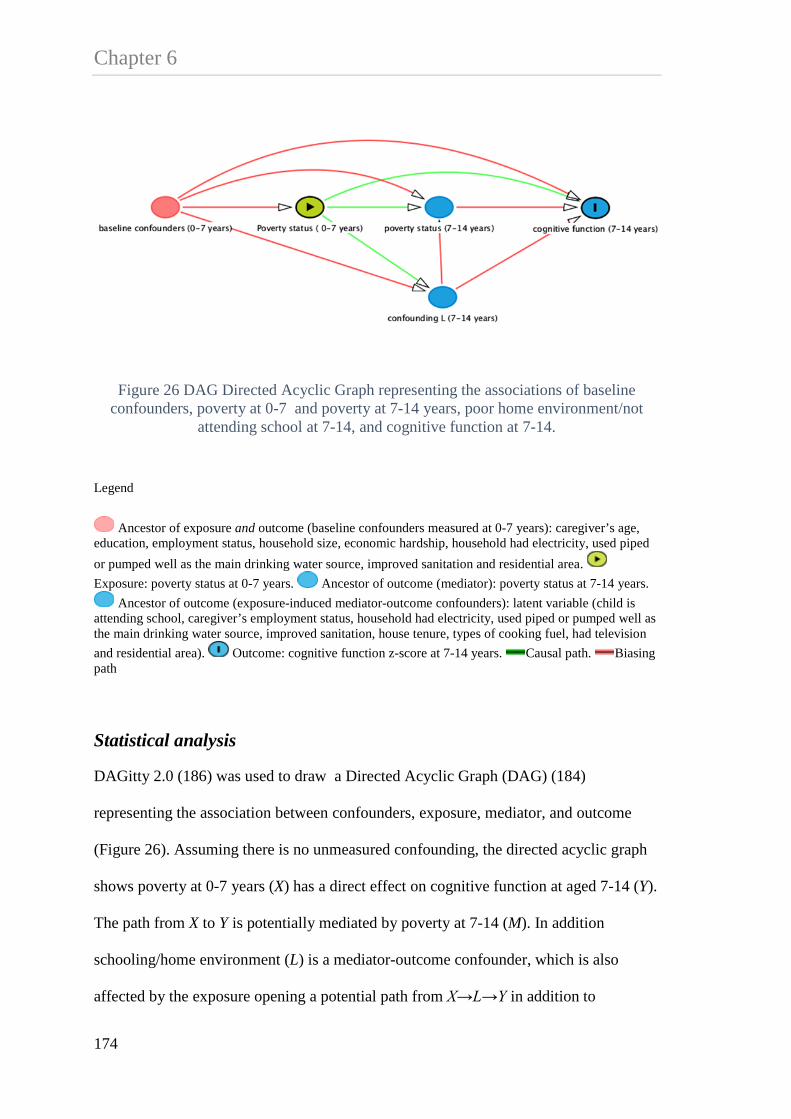
Chapter 6
Figure 26 DAG Directed Acyclic Graph representing the associations of baseline confounders, poverty at 0-7 and poverty at 7-14 years, poor home environment/not
attending school at 7-14, and cognitive function at 7-14.
Legend
Ancestor of exposure and outcome (baseline confounders measured at 0-7 years): caregiver’s age, education, employment status, household size, economic hardship, household had electricity, used piped or pumped well as the main drinking water source, improved sanitation and residential area. Exposure: poverty status at 0-7 years. Ancestor of outcome (mediator): poverty status at 7-14 years.
Ancestor of outcome (exposure-induced mediator-outcome confounders): latent variable (child is attending school, caregiver’s employment status, household had electricity, used piped or pumped well as the main drinking water source, improved sanitation, house tenure, types of cooking fuel, had television and residential area). Outcome: cognitive function z-score at 7-14 years. Causal path. Biasing path
Statistical analysis
DAGitty 2.0 (186) was used to draw a Directed Acyclic Graph (DAG) (184)
representing the association between confounders, exposure, mediator, and outcome
(Figure 26). Assuming there is no unmeasured confounding, the directed acyclic graph
shows poverty at 0-7 years (X) has a direct effect on cognitive function at aged 7-14 (Y).
The path from X to Y is potentially mediated by poverty at 7-14 (M). In addition
schooling/home environment (L) is a mediator-outcome confounder, which is also
affected by the exposure opening a potential path from X→L→Y in addition to
174

Chapter 6 X→M→Y. We described the magnitude of associations along all paths between X, M, L
and Y using regression analysis (Web Table 4).
We examined the association of poverty at 0-7 and poverty at 7-14 with cognitive
function at 7-14 using conventional regression analysis (Web Appendix 1). Figure 26
shows there is mediator-outcome confounding (schooling/home environment) induced
by the exposure. In this case, we hypothesized that the extent of financial resources
available at ages 0-7 could plausibly influence whether a child was attending school and
living in poor home environment at age 7-14. Because of this intermediate confounding,
we used the method for effect decomposition derived by VVR (200) who introduced
three approaches for effect decomposition in the presence of exposure-induced
mediator-outcome confounding. These are a) joint mediators, b) path-specific, and c)
intervention analogue.
a) Joint mediators
In the joint mediators approach, the direct effect (X→Y) is defined as the effect of
poverty at 0-7 (X) that is not through poverty at 7-14 (M) or schooling/home
environment (L). The indirect effect is defined as the effect of X that is mediated
through M or L or both. Under the joint mediator approach, where M and L are
considered as joint mediators, the fourth assumption is modified as CMLY xxxlm |)( **
and is effectively satisfied. In other words in Figure 26 there is no effect of exposure
that confounds the relationship between the joint mediator (L, M). This approach is
useful if partitioning the indirect effect of X through M or L was not of interest so that
both poverty at 7-14 and schooling/home environment were assumed to be equally
important as mechanisms by which poverty at 0-7 affects cognitive function at 7-14 (Y).
175

Chapter 6
b) Path specific
Assuming that the above four assumptions of unmeasured confounding (1-4) hold, the
identifiable path specific effects (210) are XY, XLY, XMY. The path specific
approach is more relevant if the substantive question is to estimate the relative
importance of specific pathways by partitioning the indirect effects of poverty at 0-7
through poverty at 7-14 (X→M→Y) and through pathways that involving
schooling/home environment at 7-14 (X→LY), which is the combination of
X→L→M→Y and X→L→Y. Thus the path specific approach can be used to estimate
whether the effect of poverty at 0-7 is largely mediated through poverty at 7-14 only or
through schooling/home environment.
c) Intervention Analogue
Effect decomposition carried out under the intervention analogue approach is similar to
a sequential randomized trial (Web Figure 1) (185, 212, 215). The randomized
intervention analogue of the direct effect is defined as the difference in potential
outcome between children who were exposed and not exposed to poverty at 0-7, where
in both cases the value of the mediator (poverty at 7-14) was randomly drawn from the
distribution of the mediators amongst children who were not exposed to poverty at 0-7.
The randomized intervention analogue of the indirect effect is defined as the difference
in potential outcome in children who were exposed to poverty at 0-7 where the value of
the mediator was first randomly drawn from the distribution of the mediator amongst
children who were exposed to poverty at 0-7 ( 11MY ) and then the value of the mediator
was randomly drawn from the distribution of mediator amongst children who were not
exposed to poverty at 0-7 ( 01MY ), thus simulating an RCT of the mediator. Subtraction
of these two quantities estimates the intervention analogue of the indirect effect (See
176
Chapter 6 equation e11). Thus effect decomposition conducted as an analogue of sequential
randomization of the mediator, requires only the first three assumptions.
In the VVR approach, effect decomposition was estimated using inverse-probability
weights. Analyses using the VVR approach were conducted in SAS 9.1 (SAS Institute,
Cary, North Carolina). We presented details about formula for estimating effect
decomposition in Web Appendix 2, the VVR methods in Web Appendix 3, construction
of the weights in Web Appendix 4 and the SAS code in Web Appendix 5. Despite its
documented limitations, for comparative purposes, we estimated effect decomposition
using conventional sequential regression analysis (Web Appendix 6) and presented the
results in Web Table 5.
177

Chapter 6 Table 9. Characteristics of study participants, IFLS 2000 and 2007, n=4,245
Abbreviations: IFLS, Indonesian Family Life Survey; IQR, inter quartile range; PCE, per capita expenditure; SD, standard deviation.
Variables 2000
2007
No. % Median (IQR) Mean (SD) No. % Median (IQR) Mean (SD) Outcome Cognitive function z-score 0.53 (-0.07 - 0.83) Exposure and mediator Child is poor 1,698 40 1,698 40 Household per capita expenditure per month (PCE), Rupiah
-the poor 83,273 (65,112 – 99,362)
214,376 (171,561 – 258,117)
-the non-poor 200,644 (150,156 – 280,083)
500,119 (382,821 – 713,208)
Household PCE per month, US$ (1 US$=8422 rupiah)
-the poor 10 (8 – 12) 25 (20 – 31) -the non-poor 24 (18 – 33) 59 (45 – 85) Covariates Child’s characteristics Child is male 2,177 51 Age 3.24
(2.24) 10.60 (2.22)
Attending school 4,008 94 Caregiver’s characteristics Age 30 (25 - 35)
178

Chapter 6
Table 9. Continued
Variables 2000
2007
No. % Median (IQR) Mean (SD) No. % Median (IQR) Mean (SD) Highest education attended None 259 6 Primary school (Grade 1-6) 2,038 48 Junior high school (Grade 7-9) 776 18 Senior high school (Grade 10-12) 935 22 Diploma/university 237 6 Working in the past week 1,750 41 1,784 42 Household characteristics Household size 5.41 (2.06) Economic hardship experience in the past 5 years
0.45 (0.72)
Had electricity 3,787 89 4,091 96 Used piped or pumped well as the main drinking water source
2,169 51 2,345 55
Improved sanitation 1,875 44 2,668 63 Residential area -urban 1,877 44 2,094 49 -Java/Bali 2,557 60 Type of cooking fuel -gas/electricity 738 17 -kerosene 1,800 43 -wood/coal 1,707 40 Had television 3,412 80 House tenure: own house 3,406 80
179

Chapter 6
6.5. Results
Table 9 shows the characteristics of study participants using the complete-case sample. The
median age-specific cognitive function z-score was 0.53 (interquartile range IQR -0.07 –
0.83). Between 2000 and 2007, the median PCE among the poor households increased from
83,273 rupiah /month (about US$10) to 21,4376 rupiah/month (about US$25). Although this
indicates overall improvement, the gap in PCE between the poor and non-poor during this
time period increased. About half (48%) of the children lived with a mother with only
primary school education. Overall, the household living conditions improved from 2000 to
2007, however, only 55% of children had access to piped and pumped well as the main
drinking water source and 63% used improved sanitation in 2007.
Table 10. The associations of poverty at 0-7 and poverty at 7-14 years with cognitive function at 7-14 years, IFLS 2000 and 2007, n=4,245
Model β 95% CI
The effect of poverty at 0-7 yearsa -0.08 -0.13, -0.03
The effect of poverty at 7-14 yearsb -0.07 -0.11, -0.02 Abbreviations: CI, confidence interval; IFLS, Indonesian Family Life Survey.
a Model included the effect of poverty at 0-7 adjusted for baseline confounders.
b Model included the effect of poverty at 7-14 adjusted for poverty at 0-7, baseline confounders and schooling/home environment.
Table 10 shows results from conventional regression where the association of poverty at 0-7
with cognitive function was -0.08 (95% confidence interval (CI): -0.13, -0.03) after
accounting for baseline confounders. The association of poverty at 7-14 was -0.07 (95% CI: -
0.11, -0.02) after adjusting for poverty at 0-7, baseline and time-varying confounding
180

Chapter 6 Table 11. Decomposition of the effect of poverty status at 0-7 years on cognitive function at 7-14 years from VVR analysis, IFLS 2000 and 2007, n=4,245
Model The direct effect
of poverty at 0-
7a
95% CI The indirect
effect through
poverty
at 7-14
95% CI The indirect
effect through
home
environment
95% CI
Approach 1:
Joint Mediators
-0.07 -0.12, -0.02 -0.01b -0.04, 0.01
Approach 2:
Path Specific
-0.07 -0.12, -0.02 -0.003c -0.03, 0.02 -0.01d -0.02, -0.0004
Approach 3:
Intervention
Analogue
-0.08 -0.13, -0.03 -0.003e -0.03, 0.02
Abbreviation: CI, confidence interval; IFLS, Indonesian Family Life Survey.
a The effect of poverty at 0-7 years on cognitive function at 7-14 years (X→Y).
b The effect of poverty at 0-7 years on cognitive function at 7-14 years through poverty at 7-14 (X→M→Y) or home environment/schooling (X→L→Y) or both.
c,e The effect of poverty at 0-7 on cognitive function at 7-14 years mediated through poverty at 7-14 years (X→M→Y).
d The effect of poverty at 0-7 on cognitive function at 7-14 years mediated home environment/schooling (X→L→Y), as well as through home environment/schooling and poverty at 7-14 years (X→L→M→Y).
181

Chapter 6 Table 11 shows the estimates for the effect decomposition of poverty at 0-7 on cognitive
function at 7-14 years. The joint mediator approach showed the direct effect of poverty
at 0-7 on cognitive function was -0.07 (95% CI: -0.12, - 0.02), which is similar with the
estimate from the path specific effect. The direct effect of poverty at 0-7 from the
intervention analogue approach was slightly higher (β = -0.08, 95% CI: -0.13, -0.03).
The indirect effect of poverty at 0-7 mediated through poverty at 7-14 for the joint
mediator approach was -0.01 (95% CI: -0.04, 0.01). We used McKinnon et al (264)
method to estimate CI for the ratio mediated effect. This suggests 18% (95% CI 7, 29)
of the total effect was mediated indirectly. From both path specific effect and
intervention analogue, the indirect effect of poverty at 0-7 mediated through poverty at
7-14 was smaller (β = -0.003, 95% CI: -0.03, 0.02). Furthermore, the path specific
approach showed the effect of poverty at 0-7 mediated through schooling/home
environment was -0.01 (95% CI: -0.02, -0.0004).
For comparison, Web Table 5 shows results from a conventional sequential regression
analysis where the direct effect of poverty at 0-7 on cognitive function was -0.08 (95%
CI: -0.13,-0.03). After further adjustment for poverty and schooling/home environment
at 7-14, the direct effect was -0.05 (95% CI: -0.10, -0.002). The change in the
coefficient for the direct effect ((-0.03)/(-0.08)=0.37) showed that 37% the effect of
poverty at 0-7 on cognitive function was explained by M and L.
6.6. Discussion
Our goal was to obtain an estimate of the optimal timing for a potential poverty
alleviating financial intervention, and the mechanisms by which poverty in early-life at
0-7 years could affect cognitive function at 7-14. From conventional regression, the
effect of early-life poverty was similar to the effect of poverty in later childhood. From
182

Chapter 6 effect decomposition, we found that poverty at 0-7 had a bigger direct effect on
cognitive function than via its mediated effect through poverty at 7-14. Moreover, the
mediated effect of poverty at 0-7 years was stronger through pathways that involving
schooling/home environment and poverty at 7-14 than through poverty at age 7-14
alone.
Although conventional mediation analysis (195) can be used to estimate direct and
indirect effects, this method may generate biased estimates, especially for indirect
effects in the presence of exposure-induced mediator outcome confounding (196, 197).
In terms of the magnitude of the effect, conventional regression may yield similar
estimates for the direct effect of poverty at 0-7 with the VVR approach, however,
conventional regression does not deal properly with time-varying confounding and
mediation. Results of the ‘mediated effect’ from conventional regression suggest 37%
of the total effect is mediated (95% CI 36, 38) compared to 18% (95% CI 7, 29) from
the VVR approach. Thus, conventional regression over-estimates the amount of
mediation by a factor of two compared to the VVR method.
Our findings have several implications. First, our findings are qualitatively consistent
with other studies suggesting that children exposed to poverty from birth to 14 years
have lower cognitive function (85, 265). Second, and contrary to our a priori
expectations, our findings provide little support for the idea that an early intervention to
support household income has a larger effect than intervention later in childhood, both
seem equally important (33, 266). Third, the direct effect of poverty at 0-7 on cognitive
function at 7-14 was small. In this study a US$14 difference in the median household
expenditure between the poor and the non-poor was associated with a 0.07 unit lower
cognitive function z-score. Small effects were also reported by Paxson and Schady
183

Chapter 6 (125), suggesting that a $15 cash transfer intervention was associated with a 5% SD
increase in cognitive score among children under 7 in Ecuador. The estimated effect
size in our study is about half that reported in a recent systematic review and meta-
analysis of experimental and quasi-experimental evaluations of early childhood
interventions in low and middle=income countries (37) which found cash transfer
programs had a mean effect size 0.17 (SD 0.06) on cognitive ability. Our study thus
adds to evidence about the financial costs of cash-transfer interventions and the likely
effects on improving cognitive function in children, which may in turn have flow on
effects on individual earnings and economic growth (267, 268). In our data, the
mechanism by which poverty under 7 affects cognitive function is largely mediated
through schooling/home environment and subsequent childhood poverty (ages 7-14)
than mediated through poverty at 7-14 alone, which supports the argument that family
financial resources contribute to children’s development outcomes through direct
parental investments of time and attention, and through expenditure on their skills,
health, and education (28).
Use of effect decomposition provides estimates for direct and indirect effects by
controlling confounding appropriately even in the presence of exposure-induced
mediator-outcome confounding. We present three approaches to effect decomposition in
the presence of exposure-induced mediator-outcome confounding (L). Although our
estimates show similar results, each method can be applied in different contexts. If there
is L, the joint mediators approach does not violate the fourth assumption because both
the mediator and the mediator-outcome confounder were considered as joint mediators.
The path specific approach is useful to partition the indirect effect of exposure on
outcome, which is mediated through confounding L in addition to the pathway
involving the mediator. Finally, in the intervention analogue approach, effect
184

Chapter 6 decomposition is estimated as an analogue of a sequentially randomized mediator based
on the exposure level, which effectively removes L.
We are fully aware that there are other potential mechanisms by which poverty at 0-7
years could affect cognitive function at 7-14 years including but not limited to access to
health care, nutrition, cognitive stimulating environment, parental stress and parenting
practices but we did not have such measures in the IFLS data (269, 270). To estimate
potential bias due to unmeasured mediator-outcome confounding (U), we conducted
sensitivity analysis (Web Appendix 7). We found the effect of U would be small to
explain away the direct effect of poverty at 0-7 on cognitive function (Web Table 6).
In summary, exposure to poverty at 0-7 had similar effects on child cognitive function
at 7-14 as child poverty at 7-14. Despite the small effect size, cash-transfer intervention
may improve children’s cognitive function.
185

Chapter 6
6.7. Chapter 6 Appendices
186

Chapter 6 6.7.1. Web Table 1. Characteristics of study participants from response sample in each IFLS survey 2000 and 2007, n=6,680
Variables 2000 2007 Response sample
No. % Median (IQR) Mean (SD)
Response sample
No. % Median (IQR) Mean (SD)
Outcome Cognitive function z-score 6,247 0.53
(-0.08 - 0.83)
Exposure and mediator Household per capita expenditure per month (PCE), Rupiah
5,571 140,253 (92,019 – 223,942)
6,510 351,408 (231,881 - 545,340)
-the poor 2,229 83,490 (65,154 – 100,229)
2,604 209,875 (166,700 - 253,713)
-the non-poor 3,342 202,459 (152,642 – 287,258)
3,906 493,752 (377,815 - 713,920)
Household PCE per month, US$ (1 US$=8422 rupiah)
5,571 6,510
-the poor 2,229 8 (12 - 17) 2,604 25 (20 – 30) -the non-poor 3,342 21 (14 - 32) 3,906 45 (30 – 85) Covariates Child’s characteristics Child is male 5,595 2,879 51 6,680 3,431 51 Age, mean (SD) 5,595 3.22
(2.24) 6,680 10.31
(2.32) Attending school 6,678 6,220 93
187

Chapter 6
Web Table 1. Continued
Variables 2000 2007 Response sample
No. % Median (IQR)
Mean (SD)
Response sample
No. % Median (IQR) Mean (SD)
Caregiver’s characteristics Age, median (IQR) 5,578 30 (25 – 35) Highest education attended 5,563 None 364 7 Primary school (Grade 1-6) 2,620 47 Junior high school (Grade 7-9)
1,016 18
Senior high school (Grade 10-12)
1,241 22
Diploma/university 322 6 Working in the past week 5,543 2,300 41 5,427 2,270 42 Household characteristics Household size, mean (SD) 5,589 89 5.41
(2.06)
Economic hardship experience in the past 5 years, mean (SD)
5,588 51 0.45 (0.71)
Had electricity 5,588 4,981 44 6,659 6,391 96 Used piped or pumped well as the main drinking water source
5,588 2,852 6,659 3,653 55
Improved sanitation 5,588 2,482 44 6,659 4,163 63
188

Chapter 6
Web Table 1. Continued
Variables 2000 2007 Response sample
No. % Median (IQR)
Mean (SD)
Response sample
No. % Median (IQR) Mean (SD)
-urban 5,595 2,462 47 6,666 3,302 50 -Java/Bali 6,666 3,894 58 Type of cooking fuel 6,634 -gas/electricity 1,197 18 -kerosene 2,779 42 -wood/coal 2,658 40 Had television 6,633 5,276 80 House tenure: own house 6,659 5,244 79
Abbreviations: IFLS, Indonesian Family Life Survey; IQR, inter quartile range; PCE, per capita expenditure; SD, standard deviation.
189

Chapter 6 6.7.2. Web Table 2. Estimates of the association between household per capita expenditure at 0-7 and cognitive function at 7-14 years. IFLS 2000 and 2007, complete cases, n=4,245
Decile US$ β 95% CI
1 ≤ 7.73 ref
2 7.74 – 9.89 0.07 -0.03 0.16
3 9.90 – 11.80 0.06 -0.03 0.15
4 11.81 – 13.87 0.06 -0.03 0.15
5 13.89 – 16.54 0.14 0.04 0.23
6 16.55 – 19.50 0.18 0.09 0.28
7 19.51 – 23.82 0.20 0.11 0.29
8 23.83 – 28.86 0.24 0.14 0.33
9 28.93 – 41.49 0.31 0.22 0.40
10 ≥ 42 0.40 0.31 0.49
6.7.3. Web Table 3. Estimates of the association between household per capita expenditure at 7-14 and cognitive function at 7-14 years. IFLS 2000 and 2007, complete cases, n=4,245
Decile US$ Β 95% CI
1 ≤ 20.37 Ref
2 20.42 – 25.45 0.14 0.05 0.23
3 25.46 – 30.65 0.16 0.07 0.25
4 30.65 – 35.92 0.19 0.09 0.28
5 35.93 – 42.20 0.20 0.11 0.30
6 42.27 – 49.34 0.22 0.13 0.31
7 49.37 – 59.38 0.31 0.22 0.40
8 59.46 – 72.57 0.34 0.24 0.43
9 72.63 – 101.72 0.40 0.31 0.49
10 ≥ 102 0.49 0.40 0.58
190

Chapter 6 6.7.4. Web Table 4. Crude associations between poverty at 0-7 years (X), poverty at 7-14 years (M), schooling/home environment (L) and cognitive function at 7-14 years (Y), IFLS 2000 and 2007, complete cases, n=4245.
Model OR β 95% Confidence
Interval
Pr (M|X) 5.51 4.81 6.30
Pr (L|X) 4.20 3.69 4.79
Pr (M|L) 4.73 4.14 5.39
E (Y|X) -0.20 -0.24 -0.15
E (Y|M) -0.21 -0.25 -0.16
E (Y|L) -0.24 -0.28 -0.19
Abbreviations: IFLS, Indonesian Family Life Survey; OR, odds ratio.
191

Chapter 6 6.7.5. Web Appendix 1
THE ASSOCIATIONS OF EARLY (AT 0-7 YEARS) AND LATER CHILDHOOD
POVERTY (AT 7-14 YEARS) WITH COGNITIVE FUNCTION AT 7-14 YEARS
We used conventional regression analysis to examine the associations of early poverty (at 0-
7) and later childhood poverty (at 7-14 years) with cognitive function at 7-14 years. Herein,
equation e1 shows the regression model estimated the association of poverty at 0-7 (X) with
cognitive function adjusting for baseline confounders (C). Equation e2 shows the regression
model estimated the association of poverty at 7-14 (M) adjusting for all covariates including
poverty at 0-7 (X), baseline confounders (C) and schooling/home environment (L).
CXCXYE 210),|( βββ ++= (e1)
LCXMLCXXYE 43210),,,|( βββββ ++++= (e2)
192

Chapter 6 6.7.6. Web Figure 1
Web Figure 1. Sequential randomization in the intervention analogue approach
Poverty at 0-7 (X)
(A) X=1 (poor)
(C) Poverty at 7-14, M=1 (poor)
Y1M1
(D) M=0 (not-poor)Y1M0
(B) X=0 (not-poor)
(E) M=1 (poor)Y0M1
(F) M=0 (not-poor)Y0M0
193

Chapter 6 6.7.7. Web Appendix 2
EFFECT DECOMPOSITION UNDER POTENTIAL OUTCOME APPROACH
In general, a potential outcome approach (212, 213) decomposes the total causal effect
(TCE), into the natural direct (NDE) and indirect effects (NIE). In this study, effect
decomposition can be defined as
][ *)(*,)(, xMxxMx YYETCE −= (e3)
][ *)(*,*)(, xMxxMx YYENDE −= (e4)
][ *)(,)(, xMxxMx YYENIE −= (e5)
In equation e3 TCE is the expected potential outcome (child cognitive function z-score)
in children exposed to poverty at 0-7 (X=x) and the mediator (poverty at 7-14, M(x)) is
set at the level it would be among those who were exposed to poverty at age 0-7, minus,
the expected potential outcome in children not exposed to poverty at 0-7, and the
mediator is set at the level it would be among those who were unexposed to poverty at
0-7 (M(x*)). In equation e4, the NDE is the expected potential outcome in children
exposed to poverty at 0-7 (X=x) and the mediator is set at the level it would be among
those who were not exposed to poverty at 0-7 (M(x*)), minus, the expected outcome in
the unexposed and the mediator is set at the level it would be among those who were
unexposed to poverty at 0-7 (M(x*)). Intuitively, the NDE estimates the effect of
poverty at 0-7 on cognitive function through pathways that do not involve poverty at 7-
14 years. In equation e5, the NIE is the potential outcome in children exposed to
poverty at 0-7 when the mediator is set at the level it would be among those who were
exposed to poverty at 0-7 (M(x)) minus the potential outcome in children exposed to
194

Chapter 6 poverty at 0-7 and the mediator is set at the level it would be among those who were
unexposed to poverty at 0-7 (M(x*)). This algebra invokes the cross-world assumption
because NIE requires the mediator to simultaneously take on values under X=x and
X=x* i.e., M cannot take on its value under x and x* simultaneously (211). Nevertheless,
intuitively, the NIE estimates the effect of poverty at 0-7 on cognitive function through
poverty at 7-14 years.
195

Chapter 6 6.7.8. Web Appendix 3
FORMULA FOR EFFECT DECOMPOSITION IN VVR METHODS
a) Joint Mediators Approach
Let X be the exposure (poverty at 0-7 years), where X=x is defined as exposure set to the
child being poor and X=x* is defined as the exposure being set to child not being poor at
0-7. Equation e1 shows formula for estimating the direct effect (DE) in joint mediators
approach.
∑ −=→ mlcYX cPcxmlPcmlxYEcmlxYEDE,,
)()*,|,(]},,*,|[],,,|{[ (e6)
In this approach, the DE is the sum of the products of three statistical models. The first
model estimates the difference between two potential
outcomes, (1) the expected cognitive function z-score Y given the child is poor at 0-7
(X=x), home environment/schooling (L), poverty at 7-14 (M) and baseline confounders
C (caregiver’s age, education, employment status, household size, economic hardship,
household had electricity, used piped or pumped well as the main drinking water source,
improved sanitation and residential area); minus (2) the expected cognitive function z-
score given the child is not poor at 0-7(X=x*), home environment/schooling, poverty at
7-14 and confounders. The second part of the model estimates the joint
probabilities that the child is living in poor home environment (L) and poverty at 7-14
given the child is not exposed (X=x*), in our case not poor at 0-7 and C. The final
statistical model estimates the probability of confounders.
],,*,|[],,,|[ cmlxYEcmlxYE −
)*,|,( cxmlP
)(cP
196

Chapter 6
Equation e7 shows the formula for estimating the indirect effect (IE) in joint mediators
approach.
(e7)
In equation e7, the joint mediators approach estimates the indirect effect (IE) as the sum
of the product of three statistical models. The first model estimates the
expected cognitive function z-score Y given the child is poor at 0-7 (X=x), home
environment/schooling, poverty at 7-14 and confounders. The second part of the model
estimates the difference between two joint probabilities; (1)
the joint probability of the child is living in poor home environment/schooling (L) and
poverty at 7-14 (M) given the child is not poor at 0-7 and C, minus (2) the joint
probability of L and M given the child is not poor at 0-7 (X=x*) and C. The final model
)(cP estimates the probability of confounders.
b) Path Specific Approach
Similar to the joint mediators approach, the path specific effect defines DE as the effect
of exposure on outcome that is not through M or L. In the path specific approach, the
indirect effect of poverty at 0-7 through poverty at 7-14 (X→M→Y) defined as
(e8)
∑−
=→→ mlcYMX cPcxmlPcxmlPcmlxYE
IE,, )()}*,|,(
),|,(]{,,,|[
],,,|[ cmlxYE
)*,|,(),|,( cxmlPcxmlP −
)()*,|()},*,|(
),,|(]{,,,|[,,
cPcxlPclxmP
clxmPcmlxYEIEmlcYMX −= ∑→→
197

Chapter 6 In equation e8, IE X→M→Y is estimated as the sum of the product of four statistical
models. The first model estimates the expected cognitive function z-score
given the child is poor at 0-7, home environment/schooling, poverty at 7-14 and
confounders. The second part of the model estimates the
difference between two probabilities; (1) the probability of poverty at 7-14 given the
child is poor at 0-7, home environment/schooling and confounders, minus, (2) the
probability of poverty at 7-14 given the child is not poor at 7-14, home
environment/schooling and confounders. The third part of the model
estimates the probability of living in poor home environment/schooling given the child
is not poor at 0-7 and confounders. The fourth part of the model )(cP estimates the
probability of confounders.
Equation e9 shows the indirect effect of poverty at 0-7 that involving pathway through
home environment/schooling X→LY defined as
∑ −=→ mlcLYX cPcxlPcxlPclxmPcmlxYEIE,,
)()}*,|(),|(){,,|(),,,|(
(e9)
In equation e9, the IE is estimated as the sum of the product of four statistical models.
The first model ),,,|( cmlxYE estimates the expected potential cognitive function z-
score given the child is not poor at 0-7, home environment/schooling, poverty at 7-14
and confounders. The second part of the model ),,|( clxmP estimates the probability
of poverty at 7-14 given the child is not poor at 0-7, home environment/schooling and
),,,|( cmlxYE
),*,|(),,|( clxmPclxmP −
)*,|( cxlP
198

Chapter 6 confounders. The third part of the model )*,(),|( cxPcxlP − estimate the difference
between two probability models; (1) the probability of the child is living in poor home
environment/schooling given the child is poor at 0-7 and covariates, minus, (2) the
probability of the child is living in poor home environment/schooling given the child is
not poor at 0-7 and confounders. The fourth part of the model )(cP estimates the
probability of confounders.
c) Intervention Analogue Approach
In the third approach, effect decomposition is estimated as the difference between two
potential outcomes where the value of the mediator (poverty at 7-14) is randomly drawn
from the distribution of exposure level (poverty at 0-7). Equation e10 shows the
estimation of DE in the intervention analogue approach.
∑ ×−=
−=→
mlc
GxxGYX
cPcxmPcxlPcmlxYEcxlPcmlxYE
YEYEDEcxcx
,,
*
)()*,|()}*,|(),,*,|(),|(),,,|({
)()(|*|
(e10)
In equation e10, the DE is the expected cognitive function z-score in children exposed
to poverty at 0-7 (X=x) when the value of the mediator (poverty at 7-14) is randomly
drawn from children exposed to poverty at 0-7 (Gx|c) given covariates, minus, the
expected potential outcome in children not exposed to poverty at 0-7 (X=x*) when the
value of mediator is randomly drawn from children not exposed to poverty at 0-7 (Gx*|c)
given covariates.
199
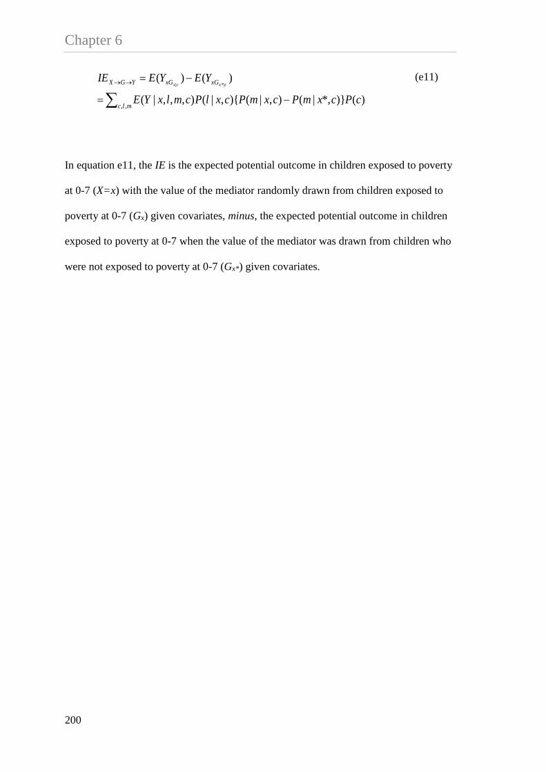
Chapter 6
∑ −=
−=→→
mlc
xGxGYGX
cPcxmPcxmPcxlPcmlxYE
YEYEIEcxcx
,,)()}*,|(),|(){,|(),,,|(
)()(|*|
(e11)
In equation e11, the IE is the expected potential outcome in children exposed to poverty
at 0-7 (X=x) with the value of the mediator randomly drawn from children exposed to
poverty at 0-7 (Gx) given covariates, minus, the expected potential outcome in children
exposed to poverty at 0-7 when the value of the mediator was drawn from children who
were not exposed to poverty at 0-7 (Gx*) given covariates.
200

Chapter 6 6.7.9. Web Appendix 4
FORMULA FOR THE INVERSE PROBABILITY OF WEIGHTS IN VVR
METHODS
The construction of the weight for the joint mediators approach is as follow.
),,|(),|()|()*,,|()*,|(
1 cxlmPcxlPcxPcxlmPcxlPW = (e12)
In equation e12, the numerator is the product of two statistical models; (1) the
probability of schooling/home environment (L) given poverty at 0-7 is set to x* and C,
and the probability of poverty at 7-14 (M) given schooling/home environment, poverty
at 0-7 is set to x* and C. The denominator is the product of three statistical models; (1)
the probability of the observed poverty 0-7 (X=x) given C; (2) the probability of
schooling/home environment given the observed poverty at 0-7 and C; and (3) the
probability of poverty at 7-14 given schooling/home environment, the observed poverty
at 0-7, and C.
The construction of the weight for the identifiable path specific effects is as follows.
),,|(),|()|()*,*,|()*,|(
2 cxlmPcxlPcxPcxlmPcxlPW = (e13)
In equation e13, the numerator is the product of two statistical models; (1) the
probability of schooling/home environment (L) given poverty at 0-7 is set to x* and C,
and (2) the probability of poverty at 7-14 given poverty at 0-7 is set to x** and C. The
denominator is the product of three statistical models; (1) the probability of poverty at
201

Chapter 6 0-7 given C; (2) the probability of schooling/home environment given the observed
poverty at 0-7 (X=x) and C; and (3) the probability of poverty at 7-14 years given
schooling/home environment, the observed poverty at 0-7 and C. Herein, x* represents
potential outcome for the X→LY path, whereas x** represents potential outcome for the
X→M→Y path.
The construction of the weight for the intervention analogue approach is as follow.
(e14)
In equation e14, the numerator is the sum of the product of two statistical models; (1)
the probability of poverty at 7-14 (M) given schooling/home environment/, poverty at 0-
7 is set to x* and C, and (2) the probability of schooling/home environment/ given
poverty at 0-7 is set to x* and C. The denominator is the product of two statistical
models; (1) the probability of poverty 0-7 years given C, and (2) the probability of
poverty at 7-14 given schooling/home environment, the observed poverty at 0-7 years,
and C.
We estimated the 95% CI based on a bootstrap of 1000 resamples.
),,|()|(
),|(),,|( **
3 cxlmPcxP
cxlPcxlmPW l
∑=
202

Chapter 6 6.7.10. Web Appendix 5
SAS CODE FOR EFFECT DECOMPOSITION IN THE PRESENCE OF
EXPOSURE-INDUCED MEDIATOR-OUTCOME CONFOUNDER
/* Definition of terms
Y= outcome (cognitive function at 7-14 years).
X= exposure (poverty status at 0-7 years).
M=mediator (poverty status at 7-14 years).
L= exposure-induced mediator-outcome confounder (home environment/schooling at 7-14).
C1-C9=baseline confounders (caregiver’s age, education, employment status, household size, economic hardship, household had electricity, used piped or pumped well as the main drinking water source, improved sanitation and residential area).
*/
/*Prepare the data and create duplicates of the data set
For approach 1 and 3, generate two copies of the data and add variable X=0 for the first replicate and X=1 for the second replicate.
For approach 2, generate three copies of the data set and add two variables X* and X**. In the first replicate X*=X**=the observed x. In the second replicate, X*=1-x and X**=the observed x. In the third replicate X*=1 and X**=1-x. */
proc surveyselect data=mydata out=mydatab seed=3022 method=urs samprate=1 outhits rep=1000 noprint; run;
data mydata0; set mydatab; x = 0; by Replicate; output; run;
data mydata1; set mydatab; x = 1; by Replicate; output; run;
proc logistic data = mydatab noprint;
model x = c1 c2 c3 c4 c5 c6 c7 c8 c9; by Replicate; score data = mydatab out = preda; run;
data preda; set preda; pa1 = P_1; by Replicate; run;
proc logistic data = mydatab noprint; model l = x c1 c2 c3 c4 c5 c6 c7 c8 c9; by Replicate; score data = mydata1 out = predl1;
score data = mydata0 out = predl0; run;
data predl1; set predl1; pl1 = P_1; by Replicate; run;
data predl0; set predl0; pl10 = P_1; by Replicate; run;
data mydata00; set mydatab; x = 0; l = 0; by Replicate; output; run;
203

Chapter 6 data mydata10; set mydatab; x = 1; l = 0; by Replicate; output; run;
data mydata01; set mydatab; x = 0; l = 1; by Replicate; output; run;
data mydata11; set mydatab; x = 1; l = 1; by Replicate; output; run;
proc logistic data = mydatab noprint; model m = x l c1 c2 c3 c4 c5 c6 c7 c8 c9; by Replicate;
score data = mydata1 out = predm1;
score data = mydata0 out = predm0;
score data = mydata00 out = predm00;
score data = mydata01 out = predm01;
score data = mydata10 out = predm10;
score data = mydata11 out = predm11;
run;
data predm1; set predm1; pm1 = P_1; by Replicate; run;
data predm0; set predm0; pm10 = P_1; by Replicate; run;
data predm00; set predm00; pm100 = P_1; by Replicate; run;
data predm10; set predm10; pm110 = P_1; by Replicate; run;
data predm01; set predm01; pm101 = P_1; by Replicate; run;
data predm11; set predm11; pm111 = P_1; by Replicate; run;
data mydataw;
merge preda predl1 predl0 predm1 predm0 predm00 predm01 predm10 predm11 mydatab; by Replicate; run;
*/This part will generate the weight for the joint mediator approach */
data mydatanew; set mydataw; xstar = x; w1 = x/pa1+(1-x)/(1-pa1); output; xstar = 1-x;
if x = 0 then w1 = (1/(1-pa1))*(l*pl1/pl10+(1-l)*(1-pl1)/(1-pl10))
*((1-m)*(1-pm1)/(1-pm10) + m*pm1/pm10);
if x = 1 then w1 = (1/pa1)*((l*pl10/pl1+(1-l)*(1-pl10)/(1-pl1))
*((1-m)*(1-pm10)/(1-pm1) + m*pm10/pm1));
by Replicate; output; run;
*/This part will generate the weight for the intervention analogue */
data mydatanew; set mydatanew;
204

Chapter 6 if (x = 0) & (xstar = 0) & (m = 1) then
w3 = (1/(1-pa1))*(pm100*(1-pl10)+pm101*pl10)/pm10;
if (x = 0) & (xstar = 0) & (m = 0) then
w3 = (1/(1-pa1))*((1-pm100)*(1-pl10)+(1-pm101)*pl10)/(1-pm10);
if (x = 0) & (xstar = 1) & (m = 1) then
w3 = (1/(1-pa1))*(pm110*(1-pl1)+pm111*pl1)/pm10;
if (x = 0) & (xstar = 1) & (m = 0) then
w3 = (1/(1-pa1))*((1-pm110)*(1-pl1)+(1-pm111)*pl1)/(1-pm10);
if (x = 1) & (xstar = 0) & (m = 1) then
w3 = (1/pa1)*(pm100*(1-pl10)+pm101*pl10)/pm1;
if (x = 1) & (xstar = 0) & (m = 0) then
w3 = (1/pa1)*((1-pm100)*(1-pl10)+(1-pm101)*pl10)/(1-pm1);
if (x = 1) & (xstar = 1) & (m = 1) then
w3 = (1/pa1)*(pm110*(1-pl1)+pm111*pl1)/pm1;
if (x = 1) & (xstar = 1) & (m = 0) then
w3 = (1/pa1)*((1-pm110)*(1-pl1)+(1-pm111)*pl1)/(1-pm1);
by Replicate; run;
*/Estimation of effect decomposition under the joint mediator approach*/
proc reg data = mydatanew outest=estw1x noprint;
where xstar = 0; model y = x; weight w1; by Replicate; run;
proc reg data = mydatanew outest=estw1xs noprint; where x = 1; model y = xstar; weight w1; by Replicate;
run;
data estfw1; merge estw1x estw1xs; by Replicate; run;
proc univariate data=estfw1; var x xstar;
output out=cilw1 pctlpts=2.5, 50, 97.5 pctlpre=x xstar;
run;
*/Estimation of effect decomposition under the intervention analogue */
proc reg data = mydatanew outest=estw3x noprint;
where xstar = 0; model y = x; weight w3; by Replicate; run;
205

Chapter 6 proc reg data = mydatanew outest=estw3xs noprint; where x = 1; model y = xstar; weight w3; by Replicate;
run;
data estfw3; merge estw3x estw3xs; by Replicate; run;
proc univariate data=estfw3; var x xstar;
output out=cilw3 pctlpts=2.5, 50, 97.5 pctlpre=x xstar;
run;
*/This part will generate the weight for the path specific effect */
data mydatanew2; set mydataw;
xstar = x; xstarstar = x; w2 = x/pa1+(1-x)/(1-pa1); output;
xstar = 1-x; xstarstar = x;
w2 = (x/pa1)*(l*pl10/pl1+(1-l)*(1-pl10)/(1-pl1)) +
((1-x)/(1-pa1))*(l*pl1/pl10+(1-l)*(1-pl1)/(1-pl10)); output;
xstar = 1-x; xstarstar = 1-x;
w2 = (x/pa1)*(l*(pl10/pl1)*(m*(pm101/pm111)+(1-m)*(1-pm101)/(1-pm111))
+(1-l)*((1-pl10)/(1-pl1))*(m*(pm100/pm110)+(1-m)*(1-pm100)/(1-pm110)))
+((1-x)/(1-pa1))*(l*(pl1/pl10)*(m*(pm111/pm101)+(1-m)*(1-pm111)/(1-pm101))
+(1-l)*((1-pl1)/(1-pl10))*(m*(pm110/pm100)+(1-m)*(1-pm110)/(1-pm100))); output; by Replicate; run;
*/Estimation of effect decomposition under the path specific effect */
proc reg data = mydatanew2 outest=est noprint;
where (xstar = 0) & (xstarstar = 0); model y = x; weight w2; by Replicate; run;
proc reg data = mydatanew2 outest=est2 noprint;
where (x = 1) & (xstarstar = 1); model y = xstar; weight w2; by Replicate; run;
proc reg data = mydatanew2 outest=est3 noprint;
where (x = 1) & (xstar = 0); model y = xstarstar; weight w2; by Replicate; run;
data estf; merge est est2 est3; by Replicate; run;
proc univariate data=estf; var x xstar xstarstar;
output out=cilw2 pctlpts=2.5, 50, 97.5 pctlpre=x xstar xstarstar;
206

Chapter 6 run;
6.7.11. Web Appendix 6.
DECOMPOSITION OF THE EFFECT OF POVERTY AT 0-7 AND POVERTY
AT 7-14 YEARS FROM CONVENTIONAL SEQUENTIAL REGRESSION
ANALYSIS
For comparative purpose, we conducted a conventional sequential regression analysis to
estimate the effect of poverty at 0-7 and at 7-14 on children’s cognitive function. Web
Table 5 presents estimates for the association of poverty at 0-7 with cognitive function
from a sequential regression analysis. In this table, the coefficient 1α in model 1 can be
interpreted as a direct effect, whereas the difference between 1α and 1φ represents an
indirect effect by controlling for M (poverty 7-14) and L (poor home environment and
school attendance 7-14). The adjusted (model 1) effect of poverty at 0-7 on cognitive
function was -0.08 z-score units of cognitive ability, and the adjusted effect (model 3)
was (-0.08)-(-0.05) = -0.03 in cognitive function z-score. Thus the proportion
“explained” was ((-0.03)/(-0.08))*100 = 38%. This can be interpreted as 38% of the
effect of poverty at 0-7 was “mediated” through poverty and poor home environment
and school attendance at 7-14 years of age.
207

Chapter 6 6.7.12. Web Table 5. Estimates for the association of poverty at 0-7 with cognitive function at 7-14 from conventional regression analysis, IFLS 2000 and 2007, complete cases, n=4,245
Coefficient
of the
exposure
95% CI
Model 1 CXCXYE 210),|( ααα ++= -0.08 -0.13 -0.033
Model 2 MCXMCXYE 3210),,|( ββββ +++= -0.06 -0.11 -0.009
Model 3 LMCXLMCXYE 43210),,,|( φφφφφ ++++=
-0.05 -0.10 -0.002
Model 1 included poverty at 0-7 years (X) and baseline confounders (C)
Model 2 included model 1 and poverty at 7-14 years (M)
Model 3 included model 2 and home environment/schooling at 7-14 years (L)
208
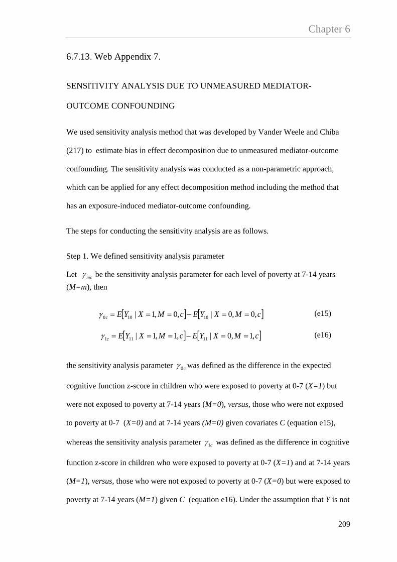
Chapter 6 6.7.13. Web Appendix 7.
SENSITIVITY ANALYSIS DUE TO UNMEASURED MEDIATOR-
OUTCOME CONFOUNDING
We used sensitivity analysis method that was developed by Vander Weele and Chiba
(217) to estimate bias in effect decomposition due to unmeasured mediator-outcome
confounding. The sensitivity analysis was conducted as a non-parametric approach,
which can be applied for any effect decomposition method including the method that
has an exposure-induced mediator-outcome confounding.
The steps for conducting the sensitivity analysis are as follows.
Step 1. We defined sensitivity analysis parameter
Let mcγ be the sensitivity analysis parameter for each level of poverty at 7-14 years (M=m), then
[ ] [ ]cMXYEcMXYEc ,0,0|,0,1| 10100 ==−===γ
(e15)
[ ] [ ]cMXYEcMXYEc ,1,0|,1,1| 11111 ==−===γ (e16)
the sensitivity analysis parameter c0γ was defined as the difference in the expected
cognitive function z-score in children who were exposed to poverty at 0-7 (X=1) but
were not exposed to poverty at 7-14 years (M=0), versus, those who were not exposed
to poverty at 0-7 (X=0) and at 7-14 years (M=0) given covariates C (equation e15),
whereas the sensitivity analysis parameter c1γ was defined as the difference in cognitive
function z-score in children who were exposed to poverty at 0-7 (X=1) and at 7-14 years
(M=1), versus, those who were not exposed to poverty at 0-7 (X=0) but were exposed to
poverty at 7-14 years (M=1) given C (equation e16). Under the assumption that Y is not
209
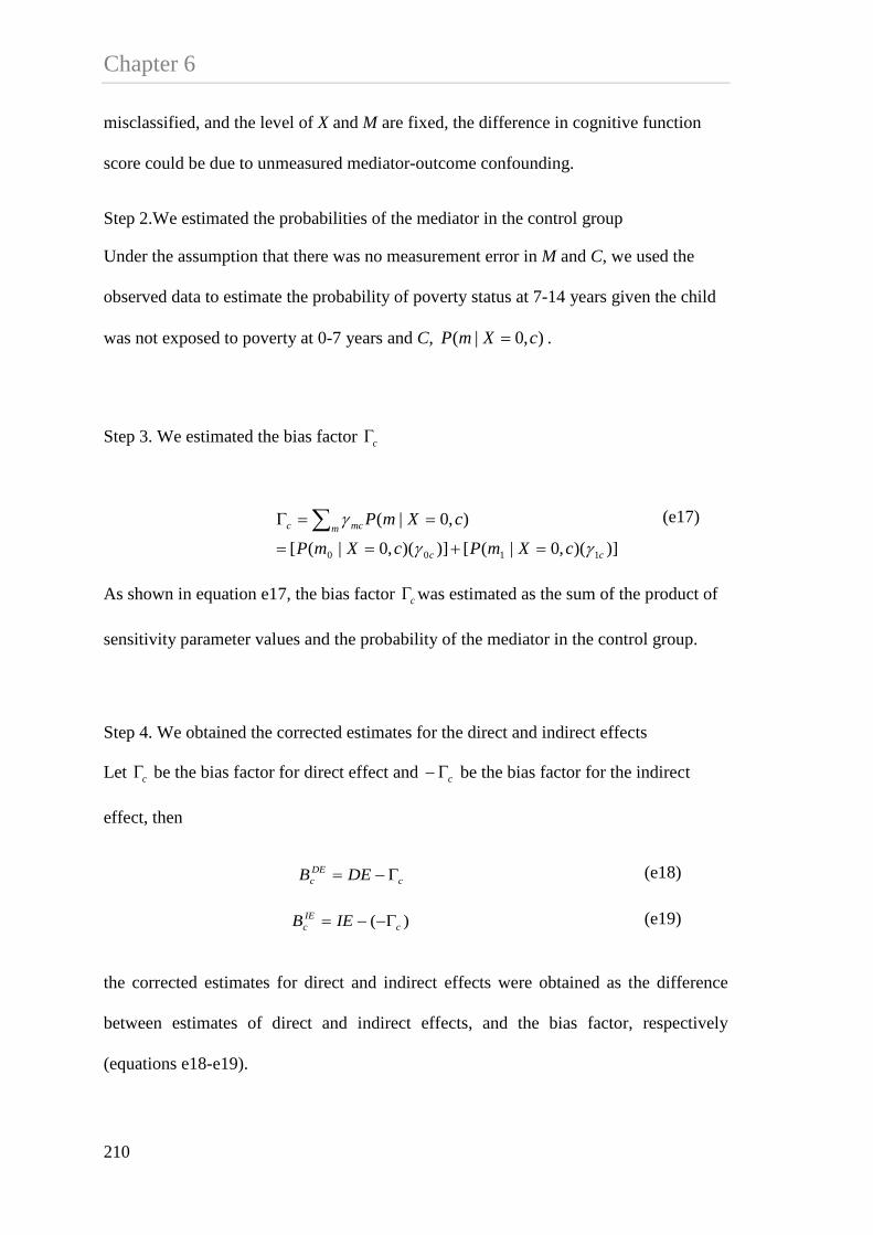
Chapter 6 misclassified, and the level of X and M are fixed, the difference in cognitive function
score could be due to unmeasured mediator-outcome confounding.
Step 2.We estimated the probabilities of the mediator in the control group
Under the assumption that there was no measurement error in M and C, we used the
observed data to estimate the probability of poverty status at 7-14 years given the child
was not exposed to poverty at 0-7 years and C, ),0|( cXmP = .
Step 3. We estimated the bias factor cΓ
)])(,0|([)])(,0|([
),0|(
1100 cc
m mcc
cXmPcXmP
cXmP
γγ
γ
=+==
==Γ ∑
(e17)
As shown in equation e17, the bias factor cΓ was estimated as the sum of the product of
sensitivity parameter values and the probability of the mediator in the control group.
Step 4. We obtained the corrected estimates for the direct and indirect effects
Let cΓ be the bias factor for direct effect and cΓ− be the bias factor for the indirect
effect, then
cDEc DEB Γ−=
(e18)
)( cIEc IEB Γ−−= (e19)
the corrected estimates for direct and indirect effects were obtained as the difference
between estimates of direct and indirect effects, and the bias factor, respectively
(equations e18-e19).
210

Chapter 6 Results of the sensitivity analysis are presented in Web table 6. As illustration, we
specified the values of sensitivity parameters at 0.03, 0.07, 0.10 and 0.14, representing
about 5%, 10%, 15% and 20% SD of cognitive function z-score, respectively. We used
estimates of direct and indirect effects of poverty at 0-7 from the VVR joint mediators
approach. Under different values of specified sensitivity parameters, we found that the
sensitivity analysis values and the bias factor would be small to explain away the direct
effect of poverty at 0-7 on cognitive function at 7-14 years (scenario 12). This also
implies that the magnitude of the effect of unmeasured mediator-outcome confounding
is relatively small to eliminate the effect of exposure on outcome.
211

Chapter 6 6.7.14. Web Table 6. Results of the sensitivity analysis. IFLS 2000 and 2007, complete cases, n=4,245
c0γ a
c1γ b ccXmP ),0|( 0 = dcXmP ),0|( 1 = DEe IEf gcΓ h
cΓ− icDE Γ−
jcIE )( Γ−−
1 -0.03 -0.07 0.76 0.24 -0.07 -0.01 -0.04 0.04 -0.03 -0.05
2 -0.03 -0.10 0.76 0.24 -0.07 -0.01 -0.05 0.05 -0.02 -0.06
3 -0.07 -0.03 0.76 0.24 -0.07 -0.01 -0.06 0.06 -0.01 -0.07
4 -0.03 -0.14 0.76 0.24 -0.07 -0.01 -0.06 0.06 -0.01 -0.07
5 -0.07 -0.07 0.76 0.24 -0.07 -0.01 -0.07 0.07 0.00 -0.08
6 0.03 0.10 0.76 0.24 -0.07 -0.01 0.05 -0.05 -0.12 0.04
7 0.07 0.03 0.76 0.24 -0.07 -0.01 0.06 -0.06 -0.13 0.05
8 0.03 0.14 0.76 0.24 -0.07 -0.01 0.06 -0.06 -0.13 0.05
9 0.07 0.10 0.76 0.24 -0.07 -0.01 0.08 -0.08 -0.15 0.07
10 0.10 0.03 0.76 0.24 -0.07 -0.01 0.08 -0.08 -0.15 0.07
11 0.07 0.14 0.76 0.24 -0.07 -0.01 0.09 -0.09 -0.16 0.08
12 0.10 0.07 0.76 0.24 -0.07 -0.01 0.09 -0.09 -0.16 0.08
a sensitivity parameter c0γ is the difference in cognitive function z-score between two subgroups, where the first group is children who were poor at 0-7 (X=1) but not poor at
7-14 years (M=0), and second those who were not poor both at 0-7 (X=0) and at 7-14 (M=0) given covariates. b sensitivity parameter c1γ is the difference in cognitive function z-score between two subgroups, where the first group is children who were poor both at 0-7 (X=1) and at 7-14 (M=1), and second those who were not poor at 0-7 (X=0) but poor at 7-14 (M=1) given covariates. c-d the probability of poverty status at 7-14 years in the control group. e-f estimates for the natural direct and indirect effects of poverty status at 0-7 years on cognitive function, respectively. g-h bias factor for DE and IE, respectively. i-j the corrected estimate for DE and IE, respectively.
212

CHAPTER 7
Effects of Hypothetical Interventions on Children’s School Readiness and Socio-emotional wellbeing in Rural Indonesia: Application of Parametric G-Formula

Chapter 7 7.1. Preface
This chapter contains the final study of this thesis, which investigated the relative and
combined effects of different hypothetical interventions on children’s school readiness
and socio-emotional wellbeing in rural Indonesia. As outline in chapter 4, findings from
study 1 suggested that household per capita expenditure was the largest contributor to
inequality in children’s cognitive function in 2000 and 2007. Between 2000 and 2007,
substantial reductions in inequality in children’s cognitive function were mainly driven
by improvements in maternal education, access to improved sanitation and household
per capita expenditure. In study 2, the effects of household per capita expenditure and
cash transfer intervention on children’s cognitive function were examined (chapter 5).
Findings from study 2 suggested that a cash transfer intervention for the poorest
households in 2000 increased children’s cognitive function score by 6% but there was
no overall effect of cash transfers at the population level because the cash transfer was
too small to benefit the target children. This implies that providing cash transfer alone is
not effective in improving children’s cognitive function at the population level. Hence,
the current study aimed to examine the relative and combined strategies of interventions
that potentially could improve children’s development outcomes in rural Indonesia.
214

Chapter 7 7.2. Introduction
Since 2010, economic growth has moved Indonesia from being among the poorest to a
lower middle income country (23). Despite this progress, many Indonesian households
still live in poor standards of living. The current national statistics suggest that only
11% of the Indonesian population used piped water as the main drinking water source
and 70% had private toilet (271). In low and middle income countries (LMICs)
inadequate access to water and sanitation is associated with poverty, increased maternal
poor mental health and poor parenting behaviour (16, 17), which in turn may affect
children’s cognitive and socio-emotional wellbeing (6, 8, 30, 221). Evidence from
LMICs also suggests that children living in poor housing conditions tend to have poorer
cognitive function (88, 272), and are less likely to be able to read paragraphs (126) and
have lower levels of education (127) compared to children who live in better housing
conditions. Evidence from a range of studies also shows that effective interventions can
protect children from multiple negative consequences of living in poverty (36), improve
maternal mental health (145) and parenting behaviour (138, 140).
Our recent study examined the effect of a hypothetical cash transfer intervention on
children’s cognitive function (66). Based on simulations of a plausible hypothetical cash
transfer intervention, we found that a US$ 6-10/month of cash transfer for children from
the poorest 40% of household expenditure increased the mean cognitive function score
by 6% but there was no overall effect of cash transfers at the total population level
because the cash transfer was too small to benefit the target children. Given the small
effect size of cash transfer intervention in our previous study, a stand-alone cash transfer
would need to be much larger to have a substantial impact on children’s cognitive
function (66). This implies that providing cash transfer alone is not an effective
215

Chapter 7 intervention to improve children’s cognitive function in Indonesia. Moreover, evidence
from systematic review and meta-analysis (37, 259) that examined effectiveness
implementation of early childhood interventions suggested that an intervention that
combined multiple programs may yield greater effect than single intervention.
The current study examined the relative and combined effects of a range of hypothetical
interventions at ages 4, 5 and 8 years on a holistic measure of children’s school
readiness and socio-emotional wellbeing at age 8 among children living in rural
Indonesia. In this study, we focused on interventions that provide piped water as the
main drinking water source and improved sanitation (126, 129), improve maternal
mental health (6, 141, 145, 165) and parenting behaviour (32, 36, 138, 140).
7.3. Methods
Data
We used data from a pragmatic clustered randomized controlled trial (RCT) evaluating
the impact of community-based Early Childhood Education and Development (ECED)
intervention in rural communities in Indonesia (26). In this study, we used information
about whether or not a village was randomized to receive an ECED project as a baseline
confounder. The ECED project was implemented by the Indonesian government, which
aimed to provide greater access to ECED services in the community and improve
children’s development and readiness for transition to formal education (26). The ECED
project targeted about 738,000 children ages 0-6 years and their primary caregivers
living in 3000 villages within 50 poor districts. These districts were selected based on
low participation rates in ECED services, high poverty rates, and commitment to
developing, managing and financing the ECED project in their area. Within each
216

Chapter 7 district, 60 villages were selected based on high numbers of children aged 0-6 years,
high poverty rates and had shown interest in the ECED project.
The RCT was conducted in 310 villages in 9 districts including Sarolangun, North
Bengkulu, East Lampung, Majalengka, Rembang, Kulon Progo, Sidenreng Rappang
(Sidrap), Ketapang and Middle Lombok. The first data collection was conducted in
2009 and subsequently in 2010 and 2013. The ECED study comprised cohorts aged 1
(n=3118) and 4 (n=3251) in 2009 with follow up in 2010 and 2013. In this study, we
selected participants aged 4 in 2009 and followed up at ages 5 and 8 who had complete
information about variables of interest (Figure 27).
Figure 27 Flow of study participants, children aged 4 in 2009 follow up aged 5 in 2010 and aged 8 in 2013
217

Chapter 7 Measures
Outcome
School readiness
The Early Development Instrument (EDI) is a holistic measure of child development at
school entry that comprises that five major developmental domains including physical
health and well-being, social competence, emotional maturity, language and cognitive
development, as well as communication skills and general knowledge (153, 154). For
each domain the score ranged from 0 to 10, where a higher score indicated better
outcomes. According to standard practice, a child whose score was in the lowest 10% in
each domain was classified as developmentally vulnerable in that specific domain
(coded as 1 or 0 otherwise) (154). The scores were summed to define whether a child
was developmentally vulnerable in one or more domains (coded as 1 or 0 otherwise).
We used the classification of being vulnerable in one or more domains as the primary
outcome, which is consistent with its use in national population survey (273, 274).
Socio-emotional wellbeing
The second main outcome used the Strengths and Difficulties Questionnaire (SDQ) as a
measure of children’s socio-emotional wellbeing (155). The SDQ comprises five
subscales including emotional symptoms, conduct problems, hyperactivity/inattention,
peer relation problem and prosocial behaviour. For each subscale the score ranged from
0 to 10. With the exception of prosocial behavior sub-scale, higher scores are associated
with poorer behavioural outcomes. Consistent with standard practice, the scores of
emotional and peer problems subscales were combined to define internalising
behaviour, whereas the scores of conduct problems and hyperactivity/inattention
218

Chapter 7 subscales were combined to define externalising behaviour (156). In the analysis both
internalising and externalising behaviour problems were used as continuous scores.
Exposure
Household standards of living
Household standards of living were measured using two indicators. First, whether the
child lived in a household that used piped water as the main drinking water source
(coded as 1 and 0 otherwise). Second, whether the child lived in a household that used
improved sanitation, defined as owned a toilet that was connected to a septic tank
(coded as 1 and 0 otherwise).
Maternal mental health
Maternal mental health was measured using Kessler 10 (K10) (160), which is a self-
reported questionnaire that was designed to measure non-specific psychological distress.
K10 comprises 10 items of feelings of anxiety and depression in the past four weeks and
their frequency. Each response item was reported on a 3-point scale where the score
ranged from 1 “never”, 3”sometimes” and 5”often”. All the 10 items were combined to
generate a total mental health score, where higher score is associated with poorer mental
health (scores ranging 10-50).
Parenting styles
Parenting style was measured using 24 items describing parent-child relationships such
as warmth, consistency and hostility. This measure was adapted from the Longitudinal
Study of Australian Children (LSAC) study (161). For each item, the response was
reported on a 5-point scale, which ranged from never to always. All 23 items were
combined to generate a total parenting score, where higher score indicated better
219

Chapter 7 parenting styles. This variable was treated as a continuous variable (scores ranging 23-
115).
Covariates
A series of covariates were selected a priori as baseline confounders (C) that were
measured at age 4 including maternal age (83, 108) and education (83, 90, 162, 163).
Maternal age was measured in years and used as continuous variable. Maternal
education was measured as the highest education completed (categorized as none or not
completed primary school, primary school, junior high school, senior high school and
diploma/university). Household characteristics include household size (continuous)
(30), the number of self-reported economic hardships experienced by household
(continuous) (102), housing conditions and assets (23, 88, 126, 162) and whether the
child is living in a village that receive the ECED program or otherwise.
Factor analysis (170, 171) was used to construct a standard of living index based on
housing conditions and household assets at aged 4. Housing conditions include whether
the household had electricity, separate kitchen, used non-earth floor, and type of
cooking fuel (used wood, kerosene or gas/electricity). Household assets include whether
the household had telephone, radio, television, refrigerator, bike, motorcycle and car.
The standards of living index was estimated as the weighted sum of the scores on these
variables, where the weights are the eigen values. The latent variable/factor score was
then classified into quintiles, which ranged from the poorest (quintile 1) to the richest
(quintile 5).
220

Chapter 7 Statistical analysis
Assuming there is no unmeasured confounding, Figure 18 shows a Directed Acyclic
Graph (DAG) representing the associations between baseline confounders (C), exposure
X and covariates L on children’s school readiness and socio-emotional wellbeing at age
8.
In this DAG, both exposure X and confounding L are time-varying because they were
measured at ages 4, 5 and 8, whereas a series of baseline confounders (maternal age,
education, economic hardships, whether a child is living in the ECED program and
household standards of living) were measured at aged 4.
Figure 28. Causal diagram for estimating the effects of hypothetical interventions on children's school readiness and socio-emotional wellbeing
We examined the relative and combined effects of different interventions at ages 4, 5,
and 8 on children’s school readiness and socio-emotional wellbeing at age 8 under the
following hypothetical intervention scenario.
221

Chapter 7 Scenario 1. Improving household standards of living
Scenario 1 has two components of intervention provision of piped water as the main
drinking water source and improved sanitation. Studies show a combination of
improved water and sanitation intervention would generate a greater effect than a single
intervention (129, 218), hence in scenario 1 provision of piped water and improved
sanitation were considered as a joint intervention. Hypothetically, provision of piped
water as the main drinking water source and improved sanitation would enhance
housing conditions and in turn would have positive effect on children’s school readiness
and socio-emotional wellbeing. Under scenario 1, all children would have access to
piped water and improved sanitation.
Scenario 2. Maternal mental health intervention
In scenario 2, we generated a hypothetical community-based mental health intervention
to promote good mental health, which is commonly conducted in LMICs in the setting
where accesses to mental health services are limited (32, 42). In this scenario, a mother
whose score was in the highest 20% of the K10 score was targeted for mental health
intervention (score 17 or above from the observed data). The 20% cut off for our
intervention coverage was based on the prevalence of common mental health disorder in
Indonesia (219) and in LMICs (220). Hypothetically, mental health intervention for
mothers had benefit both mothers and their children (145).
Scenario 3. Parenting intervention
In scenario 3, we generated a hypothetical parenting education program to improve
caregiving behaviour, which has been shown as an effective parenting intervention in
LMICs (36, 138, 140). Under this scenario, a mother whose score was in the lowest
222

Chapter 7 20% of the total parenting scores was targeted for intervention (scores 75 or lower based
on the observed data). Hypothetically, mothers who received parenting interventions
improve their relationships with the child and this may reduce harsh or abusive
parenting, which in turn will improve children’s school readiness and socio-emotional
wellbeing (32, 36, 140).
Scenarios 4-5. Joint interventions
A great deal of evidence shows that interventions that combined several programs had
greater benefits than a single intervention (37, 259), hence under scenario 4 and 5, we
generated hypothetical intervention that combined multiple programs. In scenario 4, we
estimated the joint effects of intervention that combined maternal mental health and a
parenting education program (scenario 2 and 3). In scenario 5, we estimated the joint
effects of all interventions from scenarios 1-3 above that combined provision of piped
water as the main drinking water source, improved sanitation, maternal mental health
and parenting education program.
Using a potential outcome approach, we estimated the risk of being vulnerable in one or
more EDI domains and the average of internalising and externalising behaviour scores
(SDQ) at age 8 that would have been observed under each of the specified hypothetical
interventions at ages 4, 5 and 8. In the presence of time-varying exposure and
confounding, use of conventional regression may yield bias in effect estimation (187-
190). Methods that can be used to assess causality from complex longitudinal
223

Chapter 7 observational studies include g-formula, g-estimation of the structural nested models
(SNMs) and marginal structural models (MSMs) (189).
We used parametric g-formula (224-226) for estimating the potential outcome under the
specified hypothetical interventions. Parametric g-formula (59-61) is the extended
version of nonparametric g-formula (55, 56). The earlier version of g-formula is useful
to estimate the effect of time-varying exposure in the presence of time-varying
confounding through standardization modelling. The original g-formula is a
nonparametric method because the estimation did not require a priori specification of
distributions to link restrictions on the value of the effect estimates. Estimates from g-
formula were based on the joint distributions of the observed exposure X, confounding L
and outcome Y in the population. However, in the case where data has many
confounders (high dimensional data), g-formula can only be estimated under parametric
modelling assumptions and uses a Monte Carlo simulation to estimate the sum over all
histories of covariates.
Notation
Let t be the time variable where t0, t1 and t2 is defined as the time when data was
collected (ages 4, 5 and 8, respectively). Let Y2 be the outcome (school readiness and
socio-emotional wellbeing) that was measured at age 8. Let d=(d1, d2, d3, d4, d5) be the
different intervention scenarios . Let fd be the density function under a particular
intervention d. Let X=(X1, X2, X3, X4) be the exposure, where X1 is defined as used
piped water as the main drinking water source, X2 defined as used improved sanitation,
X3 defined as maternal mental health score, and X4 defined as parenting scores. Let *tx is
the observed value of exposure under no intervention at time t. Let tx be the value of
exposure under intervention d at time t. Let L=(L1, L2, L3, L4) be confounding, where L1
224

Chapter 7 defined as used piped water as the main drinking water source, L2 defined as used
improved sanitation, L3 defined as maternal mental health score, and L4 defined as
parenting scores. Herein, when X1 is defined as piped water then other covariates
(improved sanitation, maternal mental health and parenting) are used as confounding L
(L2, L3, L4), which implies that there are multiple Xs and Ls.
Let tl be the value of confounding at time t. Let variables with over bars ( )ttt lxx ,, *
represent the history of the intervention, observed exposure and covariates up to time t,
respectively. Let c be a vector of baseline confounders measured at time 0 (age 4)
including maternal age and education, household size, the number of self-reported
economic hardships in the past year, standard of living index and whether the child is
living in a village that receive the ECED program or otherwise.
The steps in parametric g-formula are as follows.
Step 1. Parametric modelling
We specified four parametric models of each covariate in the following order; whether a
child was exposed to pumped water as the main drinking water source, improved
sanitation, maternal mental health and parenting scores.
In Model 1, ),,,,|Pr( 141312,211 cllllll ttttitt −−−− logistic regression was used to estimate the
conditional probability of the child exposed to piped water as the main drinking water
source at time t )( 1 itt lL = given whether the child used piped water in the past, the
history of other covariates up to time t-1 tL (improved sanitation, maternal mental
health and parenting scores) and baseline confounders C.
225

Chapter 7 In Model 2, ),,,,,|Pr( 1413111122 cllllll tttttt −−−− logistic regression was used to estimate the
conditional probability of the child exposed to improved sanitation at time t )( 22 tt lL =
given whether the child used improved sanitation in the past, the history other covariates
up to time t-1 (used piped water as the main drinking water source, maternal mental
health and parenting scores) and baseline C.
In Model 3, ),,,,,,|( 14122111133 clllllllE ttttttt −−−− linear regression was used to estimate the
conditional density function of maternal mental health scores at time t )( 33 tt lL = given
the cumulative mean of maternal mental health score in the past, the history of other
covariates up to time t-1 (whether a children used piped water, improved sanitation and
parenting score) and baseline C.
In Model 4, ),,,,,,|( 13122111144 clllllllE ttttttt −−−− linear regression was also used to
estimate the conditional density function of parenting score at time t )( 44 tt lL = given
the cumulative mean of parenting score in the past, the history of other covariates up to
time t-1 (whether a child used piped water as the main drinking water source, improved
sanitation and maternal mental health score) and baseline C.
Fit a model for each outcome
Model ],,|Pr[ 1 clxY ttit+ used logistic regression to estimate the risk of being vulnerable
in one or more EDI domains) at age 8 given the history of exposure, confounding and
baseline C.
Model [ ]clxYE ttt ,,|1+ used linear regression to estimate the expectation of internalising
(or externalising) score at age 8 given the history of exposure, confounding and baseline
C.
226

Chapter 7 Step 2. Monte Carlo simulation
For each time t generate the intervention value for each covariate, “provide piped water
as the main drinking water source and improved sanitation” (scenario 1); “set maternal
mental health score to a maximum value of 17” (scenario 2); and “set parenting score to
a minimum value of 75” (scenario 3). Monte Carlo simulation with a full sample
samples (n=2906 for the EDI and n=2955 for the SDQ) was conducted to estimate
parametric models in step 1 and was used to estimate the outcome under each
intervention. The 95% CI was estimated based on a bootstrap of 1000 re-samples.
Step 3. Estimation of the outcome under each intervention
The statistical model for parametric g formula is defined as
Equation 26 Parametric g-formula
[ ]∑∑∑∑=
+
T
t x x lttt
t t t
clxY0
1*
,,|Pr
( )cxxlxf tttd ,,,| 1*
−×
( )cxllf ttt ,,| 11 −−×
( )cxlxf ttt ,,| 1*
−
For school readiness outcomes the model in equation 26 can be defined as the risk of
being vulnerable in vulnerable in one or more domains given the history of specified
intervention d, covariates and observed exposure under no intervention. For socio-
emotional wellbeing, the model can be replaced by [ ]clxYE ttt ,,|1+ defined as the
227

Chapter 7 expectation of internalising (or externalising) behaviour scores given the history of
specified intervention d, covariates and observed exposure under no intervention.
Under the assumption of conditional exchangeability, positivity and consistency,
parametric g-formula (224-226) was estimated as a weighted sum of the outcome (i.e.
the risk of being vulnerable in EDI or the mean of internalising behaviour scores)
conditional on the specified intervention, time varying exposure and covariates.
Analysis of parametric g formula was conducted in SAS 9.4 (SAS Institute, Cary, North
Carolina).
Complete case analysis
Currently there is no method available for estimating parametric g-formula using
multiple imputed data. Due to complexity of the method used in this study, analysis was
restricted to complete cases (178).
7.4. Results
Table 12 shows the characteristics of study participants. Of the 2906 children with
complete EDI and covariates, 37% of children were classified as vulnerable in one or
more EDI domains. In terms of specific domains, 28% of children were classified as
vulnerable in the emotional maturity domain and in contrast only 2% of children were
classified as vulnerable in the language and cognitive development and another 1% of
children were classified as vulnerable in the communication skills and general
knowledge domain. Whilst EDI was originally designed for children ages 4-7 years
(154), our analysis was conducted using information that was collected on children’s at
age 8. This could be the reason there were very few children being classified as
vulnerable in some of the EDI domains. Most of early childhood interventions had
228

Chapter 7 multiple outcomes (37, 259), hence we used the classification of being vulnerable in one
or more EDI domains, children’s internalising and externalising behaviour scores as the
primary outcomes. Of the 2955 children with complete SDQ and covariates, the mean
of internalising behaviour scores was 6.16 (SD 3.06) and externalising behaviour scores
was 7.77 (SD 2.66).
The proportion of households that used piped water as the main drinking water source
increased from 7% in 2009 to 11% in 2013, which is similar to the national average
(271). The proportion of households that used improved sanitation also increased from
44% in 2009 to 61% in 2013, but it is slightly lower than the national average (70%). In
2009, the median maternal mental health score was 14 (inter quartile range IQR 12 -16)
and the mean parenting score was 0.42 (SD 7.19). Both estimates did not change
substantially at follow up. Finally, about half of the children lived with caregiver who
either had none or completed primary school (18% and 38% respectively).
229

Chapter 7 Table 12. Characteristics of study participants, ECED 2009, 2010 and 2013
Complete case EDI (n=2906) Complete case SDQ (n=2955)
2009 2010 2013 2009 2010 2013
Child is male, n (%) 1454 (50) 1479 (50) Age, mean (SD) 4 (0.04) 5.23 (0.42) 7.81 (0.39) 4 (0.04) 5.24 (0.42) 7.83 (0.42) Outcomes Early Development Instrument (EDI), n (%)
-Vulnerable in 1 or more domains 1074 (37) EDI domains -Vulnerable in physical health and wellbeing
230 (8)
-Vulnerable in social competence 233 (8) -Vulnerable in emotional maturity 826 (28) -Vulnerable in language & cognitive development
72 (2)
-Vulnerable in communication skills and general knowledge
30 (1)
Strengths and Difficulties Questionnaire (SDQ)
-Internalising behaviour scores, mean (SD)
6.16 (3.06)
-Externalising behaviour scores, mean (SD)
7.77 (2.66)
230

Chapter 7 Table 12. Continued
Complete case EDI (n=2906) Complete case SDQ (n=2955) 2009 2010 2013 2009 2010 2013 Exposures Main drinking water source -piped water 197 (7) 222 (8) 310 (11) 203 (7) 224 (8) 314 (11) -pump well 433 (15) 634 (22) 716 (24) 435 (15) 642 (22) 729 (24) -well 1666 (57) 1383 (47) 1196 (41) 1694 (57) 1402 (47) 1211 (41) -springs 368 (13) 398 (14) 314 (11) 375 (13) 406 (14) 320 (11) -others 242 (8) 269 (9) 370 (13) 248 (8) 281 (9) 381 (13) Household had improved sanitation 1271 (44) 1422 (49) 1780 (61) 1291 (44) 1441 (49) 1807 (61) Caregiver mental health scores (K10) (range 10-50), median (IQR)
14 (12 – 16) 14 (12 – 17) 14 (12 – 17) 14 (12 – 16) 14 (12 – 17) 14 (12 – 17)
Total parenting scores (range 23-120), mean (SD)
80.42 (7.19) 79.73 (7.06) 80.56 (7.28) 80.39 (7.19) 79.73 (7.09) 80.55 (7.27)
Covariates Village receive ECED project 2092 (72) 2122 (72) Caregiver characteristics Age, median (IQR) 30 (26 - 36) 30 (26 - 36) Education, n (%) -None/not completed primary school
534 (18) 550 (18)
-Primary school (grade 1-6) 1099 (38) 1118 (38) -Junior high school (grade 7-9) 663 (23) 673 (23) -Senior high school (grade 10-12) 491 (17) 494 (17) -Diploma/university 119 (4) 120 (4)
231
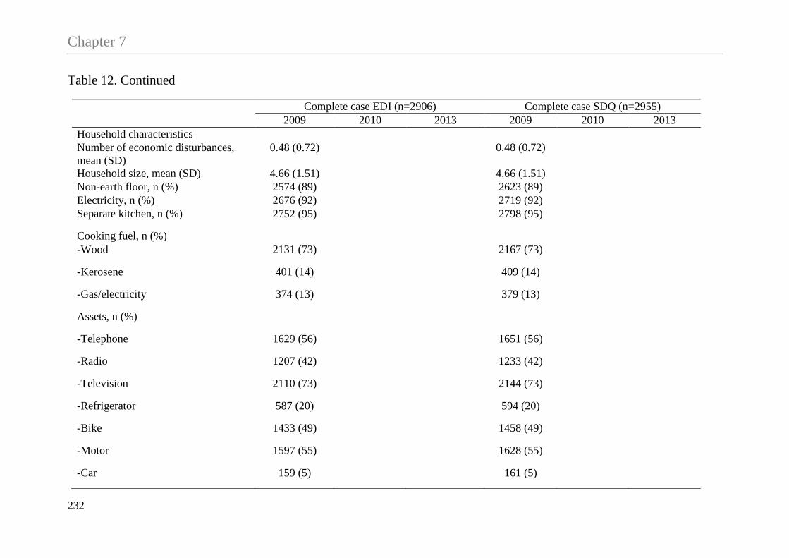
Chapter 7 Table 12. Continued
Complete case EDI (n=2906) Complete case SDQ (n=2955) 2009 2010 2013 2009 2010 2013 Household characteristics Number of economic disturbances, mean (SD)
0.48 (0.72) 0.48 (0.72)
Household size, mean (SD) 4.66 (1.51) 4.66 (1.51) Non-earth floor, n (%) 2574 (89) 2623 (89) Electricity, n (%) 2676 (92) 2719 (92) Separate kitchen, n (%) 2752 (95) 2798 (95)
Cooking fuel, n (%) -Wood 2131 (73) 2167 (73)
-Kerosene 401 (14) 409 (14)
-Gas/electricity 374 (13) 379 (13)
Assets, n (%)
-Telephone 1629 (56) 1651 (56)
-Radio 1207 (42) 1233 (42)
-Television 2110 (73) 2144 (73)
-Refrigerator 587 (20) 594 (20)
-Bike 1433 (49) 1458 (49)
-Motor 1597 (55) 1628 (55)
-Car 159 (5) 161 (5)
232

Chapter 7 Table 13 shows the estimated risk of being vulnerable in one or more EDI domains under the
specified hypothetical interventions. The estimated risk under no intervention was 37.62%
(95% CI 35.61, 39.35). Under scenario 1, if all children were exposed to piped water as the
main drinking water source and improved sanitation, the risk was 28.90% (95% CI 23.77,
33.98). This implies that intervention that provide piped water and improved sanitation
reduced the risk of being vulnerable in one or more domains by 23% (8.71/37.62=0.23)
compared to no intervention. Providing a hypothetical maternal mental health intervention
(scenario 2) reduced the risk by 6%, whereas a parenting education program (scenario 3)
reduced the risk by 8%. Under scenario 4, we found a 14% reduction in the risk of being
vulnerable in one or more domains if all mothers who had the poorest 20% of mental health
scores and the poorest 20% of parenting scores received intervention to improve their mental
health and parenting behaviour compared to no intervention. Under scenario 5, intervention
that combined provision of piped water, improved sanitation, maternal mental health
intervention and parenting education program had the largest effect on reducing the risk of
being vulnerable in one or more domains (36%).
We also present the estimated risk of being vulnerable in each of the EDI domains under the
hypothetical interventions as our secondary outcome (Table 14). Overall, table 3 shows
combined interventions (scenario 4 and 5) had the largest positive effect on reducing the risk
of being vulnerable in the physical health and wellbeing, social competence and emotional
maturity domains. Providing piped water and improved sanitation reduced the risk of being
vulnerable in emotional maturity by 20% but there is no evidence of the effect on other
domains.
233
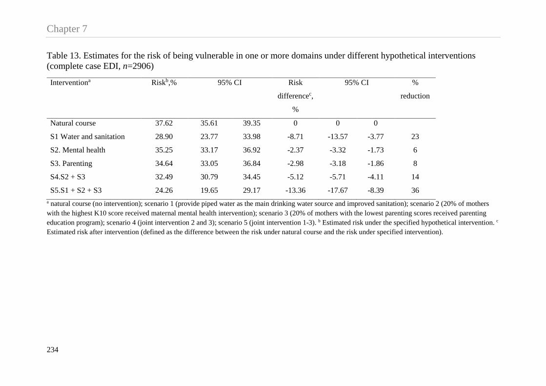
Chapter 7 Table 13. Estimates for the risk of being vulnerable in one or more domains under different hypothetical interventions (complete case EDI, n=2906)
Interventiona Riskb,% 95% CI Risk
differencec,
%
95% CI %
reduction
Natural course 37.62 35.61 39.35 0 0 0
S1 Water and sanitation 28.90 23.77 33.98 -8.71 -13.57 -3.77 23
S2. Mental health 35.25 33.17 36.92 -2.37 -3.32 -1.73 6
S3. Parenting 34.64 33.05 36.84 -2.98 -3.18 -1.86 8
S4.S2 + S3 32.49 30.79 34.45 -5.12 -5.71 -4.11 14
S5.S1 + S2 + S3 24.26 19.65 29.17 -13.36 -17.67 -8.39 36 a natural course (no intervention); scenario 1 (provide piped water as the main drinking water source and improved sanitation); scenario 2 (20% of mothers with the highest K10 score received maternal mental health intervention); scenario 3 (20% of mothers with the lowest parenting scores received parenting education program); scenario 4 (joint intervention 2 and 3); scenario 5 (joint intervention 1-3). b Estimated risk under the specified hypothetical intervention. c Estimated risk after intervention (defined as the difference between the risk under natural course and the risk under specified intervention).
234

Chapter 7 Table 14. Estimates for the risk of being vulnerable in each EDI domain under different hypothetical intervention scenarios (complete case EDI, n=2906)
Interventiona Riskb , % 95% CI Risk
differencec , %
95% CI %
reduction
physical health and wellbeing
Natural course 7.96 7.03 9.02 0 0 0
S1. Water and sanitation 6.65 4.15 9.65 -1.31 -3.83 1.59 16
S2. Mental health 6.77 5.83 7.66 -1.19 -1.72 -0.85 15
S3. Parenting 7.42 6.55 8.55 -0.54 -0.84 -0.14 7
S4.S2 + S3 6.38 5.49 7.30 -1.58 -2.09 -1.20 20
S5.S1 + S2 + S3 5.44 3.31 8.03 -2.53 -4.73 -0.18 32
Social competence
Natural course 8.09 7.08 9.02 0 0 0
S1. Water and sanitation 7.29 4.46 10.30 -0.80 -3.55 2.31 10
S2. Mental health 7.68 6.65 8.64 -0.41 -0.75 -0.01 5
S3. Parenting 6.76 5.95 7.80 -1.33 -1.62 -0.83 16
S4.S2 + S3 6.58 5.64 7.48 -1.51 -1.93 -1.06 19
S5.S1 + S2 + S3 5.79 3.55 8.59 -2.30 -4.48 0.43 28
235
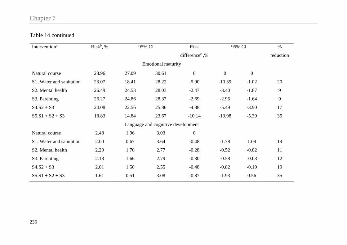
Chapter 7 Table 14.continued
Interventiona Riskb, % 95% CI Risk
differencec ,%
95% CI %
reduction
Emotional maturity
Natural course 28.96 27.09 30.61 0 0 0
S1. Water and sanitation 23.07 18.41 28.22 -5.90 -10.39 -1.02 20
S2. Mental health 26.49 24.53 28.03 -2.47 -3.40 -1.87 9
S3. Parenting 26.27 24.86 28.37 -2.69 -2.95 -1.64 9
S4.S2 + S3 24.08 22.56 25.86 -4.88 -5.49 -3.90 17
S5.S1 + S2 + S3 18.83 14.84 23.67 -10.14 -13.98 -5.39 35
Language and cognitive development
Natural course 2.48 1.96 3.03 0
S1. Water and sanitation 2.00 0.67 3.64 -0.48 -1.78 1.09 19
S2. Mental health 2.20 1.70 2.77 -0.28 -0.52 -0.02 11
S3. Parenting 2.18 1.66 2.79 -0.30 -0.58 -0.03 12
S4.S2 + S3 2.01 1.50 2.55 -0.48 -0.82 -0.19 19
S5.S1 + S2 + S3 1.61 0.51 3.08 -0.87 -1.93 0.56 35
236

Chapter 7 Table 14.continued
Interventiona Riskb, % 95% CI Risk
differencec ,%
95% CI %
reduction
Communication skills and general knowledge
Natural course 1.03 0.68 1.42 0 0 0
S1. Water and sanitation 0.94 0.00 2.16 -0.09 -1.01 0.96 9
S2. Mental health 0.88 0.54 1.26 -0.15 -0.33 0.01 15
S3. Parenting 1.00 0.65 1.41 -0.03 -0.19 0.08 3
S4.S2 + S3 0.86 0.51 1.26 -0.16 -0.36 0.86 16
S5.S1 + S2 + S3 0.81 0.00 1.85 -0.22 -1.03 0.71 21 a natural course (no intervention); scenario 1 (provide piped water as the main drinking water source and improved sanitation); scenario 2 (20% of mothers with the highest K10 score received maternal mental health intervention); scenario 3 (20% of mothers with the lowest parenting scores received parenting education program); scenario 4 (joint intervention 2 and 3); scenario 5 (joint intervention 1-3). b Estimated risk under the specified hypothetical intervention. c Estimated risk after intervention (defined as the difference between the risk under natural course and the risk under specified intervention).
237

Chapter 7 Table 15 shows the estimated mean of internalising and externalising behaviour scores (SDQ)
under the specified hypothetical interventions. For internalising behaviour, the estimated
mean under no intervention was 6.23 (95% CI 6.12, 6.35). Intervention that combined
provision of piped water, improved sanitation, mental health intervention and a parenting
education program (scenario 5) had the largest effect on reducing the mean of internalising
behaviour scores. Under this scenario, the estimated mean of internalising behaviour score
was 5.42 (95% CI 5.11, 5.75), which equals a 13% (0.81/6.23=0.13) reduction on the mean
score compared to no intervention. In contrast, a parenting education program had the
smallest effect on reducing the internalising behaviour score (mean difference -0.09, 95% CI
-0.13, -0.04).
For externalising behaviour, the estimated mean under no intervention was 7.81 (95% 7.71,
7.91). We found a 4% (0.34/7.81=0.04) reduction on the mean score under scenario 5, which
is somewhat similar (due to rounding) with the proportion of reduction in the mean score
under scenario 4. This may suggests that scenario 4 and 5 are equally important to reduce
children’s externalising problems. Examining cost effectiveness of intervention is beyond the
scope of this study, however, based on the number of intervention components, scenario 4
may be more cost effective than scenario 5. Last, maternal mental health intervention had the
smallest effect on reducing the mean of externalising behaviour score (0.11/7.81=0.01).
238

Chapter 7 Table 15. Estimates for the mean of internalising and externalising behaviour scores under different hypothetical interventions (complete case SDQ, n=2955)
Interventiona Meanb 95% CI Mean
differencec
95% CI %
reduction
Internalising behaviour scores
Natural course 6.23 6.12 6.35 0 0 0
S1. Water and sanitation 5.72 5.41 6.05 -0.51 -0.82 -0.17 8
S2. Mental health 5.97 5.85 6.08 -0.26 -0.31 -0.22 4
S3. Parenting 6.13 6.03 6.26 -0.09 -0.13 -0.04 1
S4.S2 + S3 5.89 5.78 5.99 -0.34 -0.39 -0.29 5
S5.S1 + S2 + S3 5.42 5.11 5.75 -0.81 -1.12 -0.48 13
Externalising behaviour scores
Natural course 7.81 7.71 7.91 0 0 0
S1. Water and sanitation 7.75 7.47 8.03 -0.06 -0.33 0.22 1
S2. Mental health 7.71 7.59 7.78 -0.11 -0.17 -0.08 1
S3. Parenting 7.64 7.54 7.74 -0.18 -0.21 -0.13 2
S4.S2 + S3 7.53 7.42 7.63 -0.29 -0.33 -0.24 4
S5.S1 + S2 + S3 7.48 7.19 7.75 -0.34 -0.60 -0.07 4 a natural course (no intervention); scenario 1 (provide piped water as the main drinking water source and improved sanitation); scenario 2 (20% of mothers with the highest K10 score received maternal mental health intervention); scenario 3 (20% of mothers with the lowest parenting scores received parenting education program); scenario 4 (joint intervention 2 and 3); scenario 5 (joint intervention 1-3). b Estimated mean outcome under the specified hypothetical
239

Chapter 7 intervention. c Estimated mean outcome after intervention (defined as the difference between the mean under natural course and the mean under specified intervention).
240

Chapter 7
7.5. Discussion
We investigated the relative and combined effects of a range of hypothetical
interventions on children’s school readiness and socio-emotional wellbeing in rural
Indonesia. In this study, we defined five hypothetical scenarios of intervention including
provision of piped water as the main drinking water source, improved sanitation,
maternal mental health intervention, a parenting education program and their
combination.
Effects on Overall Child Development
Not surprisingly, combined interventions had the largest positive effects on both
primary outcomes. For instance scenario 5 shows that provision of piped water,
improved sanitation, maternal mental health and a parenting education program reduced
the risk of being vulnerable in one or more EDI domains by 36%. In contrast, we
estimated a 6% reduction on the risk of being vulnerable in one or more EDI domains if
intervention only focused on mothers who had mental health problems. Based on our
hypothetical interventions, our findings support evidence that shows interventions that
combined multiple programs had a greater effect on children’s development outcomes
compared to single intervention (37, 259).
Interestingly, we found that the joint effects of combined interventions (scenario 5) on
children’s school readiness was largely driven by provision of piped water and
improved sanitation. Herein, providing piped water and improved sanitation reduced the
risk of being vulnerable in one or more EDI domains by 23%, but they contribute to a
63% (23/36=0.63) of the total reduction on the risk of being vulnerable in one or more
EDI domains if all interventions were combined. This adds to the evidence that
241

Chapter 7 providing piped water and improved sanitation for rural households had positive effect
on different aspect of child’s development outcome other than health (130, 131) and
cognitive ability (126). In rural Indonesia, inadequate access to improved sanitation and
safe drinking water is associated with poor growth and higher prevalence of diarrhoea,
which is a leading contributor to under five mortality in Indonesia (21). Diarrhoeal
disease is also linked to malnutrition and leads to poor cognitive function among
Indonesian children (56, 57). The burden of inadequate access to safe water and
sanitation is higher among children and women. Many Indonesian people who do not
have access to improved drinking water source and sanitation facilities have to walk
long distance to get water or use communal sanitation facilities (133). This implies that
mothers may have less time spent providing adequate care and attention for children.
Effects on Socio-emotional Development
In terms of socio-emotional wellbeing, combined interventions also had the largest
positive effects on children’s socio-emotional wellbeing, however, the percentage of
reduction on the average score is larger for the internalising (13%) than for the
externalising behaviour scores (4%). Our findings support evidence from RCTs and
observational studies (140, 145), suggesting that mental health intervention for mothers
had positive effect on children’s internalising and externalising behaviour problems.
Moreover, a combination of maternal mental health and parenting education
intervention also reduced the average externalising behaviour score by 4%, which
supports evidence about the benefits of maternal mental health intervention and
parenting education program on socio-emotional wellbeing (32, 36, 140, 145).
In terms of coverage of intervention, we used various approaches to intervention. For
example, both maternal mental health and parenting interventions targeted specific
242

Chapter 7 group of mothers in the population, defined as mothers who had the poorest 20% of
mental health score or the poorest 20% of parenting score or both. Targeted intervention
was chosen over a universal program because there was no evidence that universal
maternal mental health intervention had a greater effect compare to targeted
interventions (144). However, targeted intervention have some limitations, for example
the target mothers can be stigmatizing for being classified as having poor mental health
or poor parenting (15, 42). We found intervention that has components of progressive
universalism (40) yields the greatest effect on improving children’s school readiness
and socio-emotional wellbeing. In this case, the greatest reduction on the risk of being
vulnerable in school readiness or poor socio-emotional wellbeing occur if all children
have access to piped water and improved sanitation and more support is provided for
children’s whose mothers need mental health and parenting interventions.
All specified intervention in this study had potential to be implemented in Indonesia,
however, one of the challenges for effective implementation of intervention may related
to the government capacities to provide resources in communities (40). In Indonesia,
improving access to sanitation has received increasing attention from the government.
The Indonesian government has put additional resources to finance sanitation programs
but the allocation for sanitation remains insubstantial representing about 0.03% of the
annual government budget (275). Studies in the US recorded evidence from the early
19th century about the contribution of providing public safe water and sewerage system
interventions on reduction of mortality among the US population (129, 132). With a
growing evidence of the benefits of having access to piped water as the main drinking
water source and improved sanitation on child’s health and development outcomes, the
Indonesian government may need to invest more resources for providing improved
sanitation.
243

Chapter 7 Limitations
Findings from this analysis need to be interpreted with care. First, we used parametric g-
formula (224-226) to estimate the relative effects of a range of interventions on
children’s school readiness and socio-emotional wellbeing in rural Indonesia from
observational data. Parametric g-formula is a robust method to estimate the effects of
multiple interventions on outcome when using observational data in the presence of
time varying exposure and confounding. Our estimates are made under the assumptions
of consistency, conditional exchangeability, and positivity (no misspecification in the
model). Although estimation of causal effects may be plausible, the assumptions on
which it is based are not guaranteed by design and cannot be tested in observational
studies (189). Therefore, although the method can provide a robust estimate, it cannot
guarantee causal interpretation. In order to support our analysis, we specified our
hypothetical interventions based on a priori knowledge about the associations between
housing conditions, maternal mental health, parenting behaviour and children’s
development. Proper understanding about the association between our specified
exposure and outcome are important to generate well-defined interventions (204).
Second, this analysis did not taken into account measurement error in the data. We used
the EDI as a measure of children’s school readiness, which is originally designed for
children ages 4-7 years (154). In this study, we used the EDI that was collected on
children at age 8, which may not reflect the true school readiness outcome.
In summary, providing access to piped water as the main drinking water source,
improved sanitation, maternal mental health and a parenting education program had
positive effect on children’s school readiness and socio-emotional wellbeing in rural
Indonesia. The effect of interventions on school readiness outcome ranged between 6%
244

Chapter 7 and 36%, whereas the effect on socio-emotional wellbeing ranged between 1% and
13%. Intervention that combined multiple programs had a larger effect than any single
intervention. For example, provision of piped water, improved sanitation, maternal
mental health and a parenting education program reduced the risk of being vulnerable in
one or more EDI domains by 36%. In contrast, we estimated a 6% reduction on the risk
of being vulnerable in one or more EDI domains if intervention only focused on
mothers who had mental health problems. In this study, a combination of provision of
piped drinking water, improved sanitation, maternal mental health and a parenting
education program is likely yield the largest effect, however, most of the effect was
driven by provision of piped drinking water and improved sanitation. This is perhaps
understandable given the population was largely rural. Providing early childhood
intervention that combined multiple programs may improve children’s school readiness
and socio-emotional wellbeing in rural Indonesia but more importantly the intervention
should start with providing greater access to piped drinking water and improved
sanitation.
245


CHAPTER 8
Discussion and Conclusion
Chapter 8 This thesis investigated inequalities in children’s cognitive and socio-emotional
wellbeing in Indonesia, and interventions that might reduce these inequalities. Studies
arising from this thesis add to the limited evidence about children’s development in
Indonesia, which to date is still limited. This final chapter provides a synthesis of the
findings, limitations of the studies and potential future research.
8.1. Synthesis of the findings
Inequality in children’s cognitive function in Indonesia
The first study of this thesis investigated the magnitude of socioeconomic inequality
among Indonesian children’s cognitive function in 2000 and 2007, and factors that
contribute to the inequality. It also examined whether the inequality in children’s
cognitive function changed between 2000 and 2007, and the factors contributing to the
change in the inequality. Using data from the Indonesian Family Life Survey (IFLS),
the results showed that the burden of poor cognitive function was higher among the
disadvantaged. From the decomposition analysis, we found that household per capita
expenditure was the largest single contributor of inequality in children’s cognitive
function in both 2000 and in 2007. We also found substantial reductions in the
inequality in children’s cognitive function, which was largely driven by changes in
maternal high school attendance, access to improved sanitation and household per capita
expenditure. As discussed in chapter 4, one possible explanation for maternal education
being the largest contributor of decreasing inequality in children’s cognitive function
between 2000 and 2007 was related to the Indonesian government policy of school
construction in the 1970s. The school construction program was the first national
program, which aimed to provide universal access to primary education in Indonesia.
Previous studies showed the school construction program had successfully increased
248
Chapter 8 school enrolment in Indonesia, where women and students from low socioeconomic
groups received more benefits from this program (10, 244). This is consistent with the
evidence from low and middle income countries (LMICs) that shows increasing school
availability at the local level has greater benefit for educational achievement in females,
although the Indonesian program was not specifically targeting girls (245).
As also shown in chapter 4, whilst maternal education was the largest contributor to the
change in inequality in children’s cognitive function between 2000 and 2007, however,
household per capita expenditure was the largest contributor of inequality in children’s
cognitive function in both 2000 and 2007, which led us to investigate the effect of
household per capita expenditure on children’s cognitive function. Moreover, we
simulated a hypothetical cash transfer intervention, and estimated the change in
cognitive function after a plausible cash intervention.
Cash transfer intervention for the poorest households increased cognitive function score by 6% but no overall effect for the population
Whilst study 1 was conducted as a descriptive analysis, in study 2 we used a more
complex analytical approach to determine the effect of household per capita expenditure
and whether cash transfer intervention could increase cognitive function score. This is
partly because of the complexity of the data structure as shown in our causal DAG
(Figure 13 chapter 5), indicating the presence of time varying exposure and
confounding. Hence, a potential outcome approach was used in this thesis to aid causal
interpretation while using observational data. In this thesis the potential outcome
approach was used in studies 2-4. However, this method has limitations. Under a
potential outcome approach, our estimates were made under the assumptions of
consistency, conditional exchangeability, and positivity. None of these assumptions are
guaranteed by design nor can they be tested in observational studies. In study 2, we used
249
Chapter 8 an inverse probability of treatment weight of a marginal structural model (MSM), which
allowed us to better handle the potential bias in our effect estimation due to time
varying confounding.
As presented in chapter 5, consistent with studies from high income (HICs) and LMICs,
we found that greater household per capita expenditure was associated with higher
cognitive function scores, but the effect size was small. Based on simulations of a
hypothetical cash transfer intervention, an additional US$ 6-10/month of cash transfer
for children from the poorest households in 2000 increased the mean cognitive function
score by 6%, however, there was no overall effect of cash transfers at the total
population level because the cash transfer was too small to benefit the target children.
This implies that a cash transfer would need to be much larger to have a substantial
impact on children’s cognitive function.
The first study of thesis showed while household per capita expenditure was an
important factor that influenced children’s cognitive function in Indonesia, in study 2
there was little evidence of the benefit of a plausible cash transfer intervention on
increasing children’s cognitive function. This finding is very relevant to the Indonesian
context. In the past decade, the Indonesian government has implemented various cash
transfer programs for poor families. Findings from this thesis suggest that providing
cash transfers may not be an effective intervention to improve children’s cognitive
function in Indonesia.
Study 2 examined the effect of household per capita expenditure as a cumulative
exposure on children’s cognitive function, whereas in study 3, the effect of household
per capita expenditure at different time points was examined. In study 3, household per
capita expenditure was used as a binary rather than a continuous variable to define
250

Chapter 8 whether a child was classified as being poor or non-poor based on distribution of
household per capita expenditure in the population.
Little evidence for a larger effect from earlier intervention, and poverty at 0-7 had a larger direct effect on cognitive function than the mediated effect through schooling, the home environment and poverty at 7-14
The third study of this thesis investigated the effects of poverty at 0-7 and at 7-14 on
children’s cognitive function at 7-14 years. Ideally, it would allow us to obtain an
estimate for the optimal timing for a potential poverty alleviating financial intervention.
However, use of conventional regression analysis to obtain this estimate has limitation
because it does not allow us to handle confounding properly. In study 3, we also
examined the direct effect of poverty at 0-7 on cognitive function at 7-14 years, and
whether this effect was mediated through poverty at 7-14, and through school
attendance, and aspects of the child’s home environment. Use of effect decomposition
analysis allowed us to examine the mechanism by which poverty in early-life at 0-7
years could affect cognitive function at 7-14 years.
Consistent with other studies from both HICs and LMICs, the results showed that being
exposed to poverty was associated with poor cognitive function score at any time
period; however, there was no evidence that being exposed to poverty at 0-7 had a
larger effect than being exposed to poverty at 7-14 years. From the decomposition
analysis, we found that poverty at 0-7 years had a bigger direct effect on cognitive
function than via its mediated effect through poverty at 7-14. Moreover, the mediated
effect of poverty at 0-7 years was stronger through pathways that involved
schooling/home environment and poverty at 7-14 than through poverty at age 7-14
alone.
251

Chapter 8 In this study, the magnitude of the direct effect of poverty at 0-7 years was small,
implying that policies providing stand-alone income interventions for poor families may
not be sufficient to achieve intended changes in children’s cognitive function (chapter
6). A study that examined the effect of early childhood interventions on various aspects
of children’s development (37) found that provision of a comprehensive early childhood
program had a greater effect than any single intervention. Hence, it is necessary to
examine the combined strategies of interventions that potentially improve children’s
development in Indonesia.
Combined interventions had the largest effect on reducing poor developmental outcomes
The final study of this thesis investigated the relative and combined effects of different
hypothetical interventions on children’s school readiness and socio-emotional
wellbeing. This study was motivated by the results from studies 2-3, suggesting that
cash transfer a lone intervention may not be an effective strategy to improve children’s
cognitive function in Indonesia. Using data from the ECED project, this final study
identified four components of interventions and generated five hypothetical
interventions including provision of piped water as the main drinking water source,
improved sanitation, maternal mental health, parenting education program and a
combination of these programs. The analysis was conducted using parametric g-
formula, which allowed us to estimate the effects of multiple interventions from a
complex data structure (high dimensional data).
In general, most of the specified interventions had a positive effect on children’s school
readiness and socio-emotional wellbeing, however, the relative effect of each
intervention may not be equally important. Our findings support evidence suggesting
that combined multiple programs had a greater effect on children’s cognitive and socio-
252

Chapter 8 emotional wellbeing compared to single intervention. For example, provision of piped
water, improved sanitation, maternal mental health and a parenting education program
reduced the risk of being vulnerable in one or more EDI domains by 36%. In contrast,
we estimated a 6% reduction on the risk of being vulnerable in one or more EDI
domains if intervention only focused on mothers who had mental health problems. In
this study, a combination of provision of piped drinking water, improved sanitation,
maternal mental health and a parenting education program showed the largest effect on
children’s school readiness and socio-emotional wellbeing, however, most of the effect
was driven by provision of piped drinking water and improved sanitation. This is
perhaps understandable given the population was largely rural.
Again, this thesis is very relevant to the Indonesian context. Despite growing
commitment from the Indonesian government to increase population access to improved
sanitation, the financial resources that have been invested in the sanitation program
remain insignificant. With growing evidence of the benefits of having access to piped
water as the main drinking water source and improved sanitation on children’s health
and development, the Indonesian government may need to invest more resources for
sanitation. Furthermore, providing early childhood interventions that combine multiple
programs may also improve children’s school readiness and socio-emotional wellbeing,
but more importantly any intervention should start with providing greater access to
piped drinking water and improved sanitation.
8.2. Limitations and future research
The limitations of each study were discussed in the relevant chapters. This section
discusses the limitations of this thesis in general and potential future research.
253

Chapter 8 Data source
This thesis used data from two sources, the Indonesian Family Life Survey (IFLS) and
the early Childhood Education and Development (ECED) project. From the first data
source, IFLS 1-4 was used to address research aims in studies 1-3. IFLS 1-4 were
conducted in 13 out of 27 provinces in Indonesia including the islands of Sumatera,
Java, Bali, West Nusa Tenggara, Kalimantan and Sulawesi (Figure 29) (146). These
provinces are mainly located in the Western and Central part of Indonesia and were
selected purposively due to logistical reasons, but to still maximize representation of the
population, and capture the cultural and socioeconomic diversity. The sample in IFLS 1-
4 was considered to be representative of 83% of the Indonesian population, but they did
not have information about the population living in the Eastern provinces of Indonesia.
Only recently the IFLS-East was conducted in 2012 to capture the characteristics of the
population living in the Eastern provinces including East Kalimantan, East Nusa
Tenggara, Maluku, Southeast Sulawesi, Papua and West Papua (Figure 30) (276). The
IFLS-East data was released for public access in 2014. The new IFLS data could be
used for future research to examine the characteristics of families and children’s
outcomes from the Eastern provinces of Indonesia.
Figure 29. IFLS 1-4 Enumeration areas
254

Chapter 8
Figure 30. IFLS-East enumeration areas
From the second data source, the ECED data was used in study 4. The ECED data
collected baseline information for children aged 1 and 4 in 2009 and followed up in
2010 (aged 2 and 4) and 2013 (aged 6 and 8). However, this thesis only used
information that was collected for children aged 4 in 2009 and followed up at ages 5 and
8. This is because our outcome of interest (school readiness and socio-emotional
wellbeing) was firstly collected on children at aged 4 in 2009. Further research could be
conducted using information from the younger cohort.
Aspect of child’s development
Whilst most previous research about Indonesian children has focused on health related
outcomes, this thesis examined two understudied aspects of children’s development,
cognitive ability (studies 1-3) and socio-emotional wellbeing (study 4). In addition, a
small component of this thesis examined children’s school readiness as a measure of
overall development (study 4). Both IFLS and ECED data contain extensive information
255
Chapter 8 at the individual, household and community level. This thesis only utilized data that was
collected at individual and household level. Further research could examine other
aspects of child’s health and development, and the extent to which community
characteristics may influence children’s development outcomes in Indonesia.
Early childhood interventions
This thesis examined the effects of various hypothetical interventions that may improve
children’s cognitive and socio-emotional wellbeing in Indonesia. These interventions
were selected based on relevance with the study, availability of data, and potential for
implementation in the Indonesian context. In this thesis, the hypothetical interventions
included provision of cash transfer (study 2), piped water as the main drinking water
source, improved sanitation, maternal mental health and a parenting education program
(study 4). Although most of the interventions had a positive effect on children’s
development, the effect size of these interventions was small to modest. Hence, further
research is required to examine other interventions that potentially yield larger effects
on improving children’s health and development in Indonesia.
Statistical analysis
This thesis used various methodological and statistical approaches in the analysis, which
were challenging and time consuming. For example, this thesis did not take into account
potential bias due to measurement error or misclassification of using binary rather than
a continuous variable. Particularly in study 2 and 4, this thesis did not examine the
effect of censoring on the effect estimation, which could be conducted as part of a
sensitivity analysis. These are all the potential areas for future research.
256

Chapter 8 8.3. Concluding remarks
This thesis presents a rigorous and comprehensive analysis about inequalities in
Indonesian children’s cognitive and socio-emotional wellbeing, and potential early
childhood interventions that may reduce these inequalities. Whilst most previous
research about Indonesian children has focused on health related outcomes, this thesis
has filled a significant gap in knowledge about the effect of inequalities on children’s
cognitive and socio-emotional development in Indonesia. This thesis has used the best
available methodological and statistical approaches to provide robust estimates.
This thesis began with a discussion about inequality in children’s cognitive function and
identifying factors that contribute to the inequality as well as to the change in inequality
in children’s cognitive function. These findings were then followed by examining the
effect of poverty on inequality in children’s cognitive function and the mechanism by
which early years exposure affects cognitive function at later childhood. Finally, various
potential interventions were examined to find the most effective strategy to improve
children’s cognitive and socio-emotional wellbeing in Indonesia. These results could
inform the Indonesian government policy to enhance children’s health and development
and to reduce these inequalities in the long term.
257

REFERENCES
1. CSDH. Closing the gap in a generation:health equity through action on the social determinants of health. Final report of the Commission on Social Determinants of Health. Geneva: World Health Organization, 2008. 2. UNICEF. 25 Years of the Convention of the Rights of the Child: Is the World a Better Place for Children? New York: UNICEF, November 2014. 3. Mohanty SK. Multidimensional poverty and child survival in India. PLoS One. 2011;6(10):e26857. PubMed PMID: 22046384. eng. 4. Mostafa KS. Socio-economic determinants of severe and moderate stunting among under-five children of rural Bangladesh. Malays J Nutr. 2011 Apr;17(1):105-18. PubMed PMID: 22135870. eng. 5. Urke HB, Bull T, Mittelmark MB. Socioeconomic status and chronic child malnutrition: Wealth and maternal education matter more in the Peruvian Andes than nationally. Nutr Res. 2011;31(10):741-7. PubMed PMID: 22074798. eng. 6. Kiernan KE, Huerta MC. Economic deprivation, maternal depression, parenting and children's cognitive and emotional development in early childhood. Br J Sociol. 2008;59(4):783-806. PubMed PMID: 19035922. 7. Petterson SM, Albers AB. Effects of poverty and maternal depression on early child development. Child Dev. 2001;72(6):1794-813. 8. Violato M, Petrou S, Gray R, Redshaw M. Family income and child cognitive and behavioural development in the United Kingdom: does money matter? Health Econ. 2011;20(10):1201-25. PubMed PMID: 20945340. eng. 9. Duncan GJ, Ziol-Guest KM, Kalil A. Early-Childhood Poverty and Adult Attainment, Behavior, and Health. Child Dev. 2010;81(1):306-25. 10. Duflo E. Schooling and labor market consequences of school construction in Indonesia: Evidence from an unusual policy experiment. Am Econ Rev. 2001 Sep;91(4):795-813. PubMed PMID: WOS:000171104900003. English. 11. Duncan G, Magnuson K, Kalil A, Ziol-Guest K. The Importance of Early Childhood Poverty. Soc Indic Res. 2012;108(1):87-98. English. 12. Lynch J, Smith GD. A Life Course Approach to Chronic Disease Epidemiology. Annu Rev Public Health. 2005;26(1):1-35. PubMed PMID: 15760279. 13. Galobardes B, Lynch JW, Smith GD. Is the association between childhood socioeconomic circumstances and cause-specific mortality established? Update of a systematic review. J Epidemiol Commun H. 2008;62(5):387-90. 14. McLaughlin KA, Breslau J, Green JG, Lakoma MD, Sampson NA, Zaslavsky AM, et al. Childhood socio-economic status and the onset, persistence, and severity of DSM-IV mental disorders in a US national sample. Soc Sci Med. 2011;73(7):1088-96. 15. Victora CG, Wagstaff A, Schellenberg JA, Gwatkin D, Claeson M, Habicht JP. Applying an equity lens to child health and mortality: more of the same is not enough. Lancet. 2003;362(9379):233-41. 16. Walker SP, Wachs TD, Grantham-McGregor S, Black MM, Nelson CA, Huffman SL, et al. Inequality in early childhood: risk and protective factors for early child development. Lancet. 2011;378(9799):1325-38. 17. Grantham-McGregor S, Cheung Y, Cueto S, Glewwe P, Richter L, Strupp B. Developmental potential in the first 5 years for children in developing countries. Lancet. 2007;369(9555):60-70.

18. Walker SP, Wachs TD, Gardner JM, Lozoff B, Wasserman GA, Pollitt E, et al. Child development: risk factors for adverse outcomes in developing countries. Lancet. 2007;369(9556):145-57. PubMed PMID: 17223478. eng. 19. Engle PL, Black MM, Behrman JR, Cabral de Mello M, Gertler PJ, Kapiriri L, et al. Strategies to avoid the loss of developmental potential in more than 200 million children in the developing world. Lancet. 2007;369(9557):229-42. 20. Statistics Indonesia. Statistical Yearbook of Indonesia 2014. Jakarta: Badan Pusat Statistik; 2014. 21. Schröders J, Wall S, Kusnanto H, Ng N. Millennium Development Goal Four and Child Health Inequities in Indonesia: A Systematic Review of the Literature. PLoS One. 2015
10(5):e0123629. 22. World Bank. World Development Indicators 2006. Washington D.C: World Bank, 2006. 23. UNICEF, BAPPENAS, SMERU. Child Poverty and Disparities in Indonesia: Challenges for Inclusive Growth Jakarta, Indonesia: UNICEF, December 2012. 24. World Bank. Spending more or spending better: Improving education financing in Indonesia. Public Expenditure Review. Jakarta: 2013. 25. Thomas D, Beegle K, Frankenberg E, Sikoki B, Strauss J, Teruel G. Education in a crisis. J Dev Econ. 2004 Jun;74(1):53-85. PubMed PMID: WOS:000221001800004. English. 26. Pradhan M, Brinkman SA, Beatty A, Maika A, Satriawan E, de Ree J, et al. Evaluating a community-based early childhood education and development program in Indonesia: study protocol for a pragmatic cluster randomized controlled trial with supplementary matched control group. Trials. 2013;14:259. PubMed PMID: 23953975. Pubmed Central PMCID: 3751636. 27. TNP2K. Kartu Indonesia Pintar 2015 [1/2/2015]. Available from: http://www.tnp2k.go.id/id/program/program-membangun-keluarga-produktif/kartu-indonesia-pintar/. 28. Becker GS, Tomes N. Human Capital and the Rise and Fall of Families. J Labor Econ. 1986;4(3):S1-39. PubMed PMID: 0199988 Alternate Accession Number: EP4661349. 29. Berger LM, Paxson C, Waldfogel J. Income and child development. Child Youth Serv Rev. 2009;31(9):978-89. PubMed PMID: 20368763. Pubmed Central PMCID: 2847736. Eng. 30. Yeung WJ, Linver MR, Brooks–Gunn J. How Money Matters for Young Children's Development: Parental Investment and Family Processes. Child Dev. 2002;73(6):1861-79. 31. Kelly Y, Sacker A, Del Bono E, Francesconi M, Marmot M. What role for the home learning environment and parenting in reducing the socioeconomic gradient in child development? Findings from the Millennium Cohort Study. Archives of Disease in Childhood. 2011 September 1, 2011;96(9):832-7. 32. Morrison J, Pikhart H, Ruiz M, Goldblatt P. Systematic review of parenting interventions in European countries aiming to reduce social inequalities in children's health and development. BMC Public Health. 2014 2014/10/06;14(1):1040. PubMed PMID: 25287010. Pubmed Central PMCID: 4203958. English. 33. Doyle O, Harmon CP, Heckman JJ, Tremblay RE. Investing in early human development: Timing and economic efficiency. Econ Hum Biol. 2009 Mar;7(1):1-6. PubMed PMID: WOS:000265802100001. English. 34. Duncan GJ, Magnuson K. Investing in Preschool Programs. J Econ Perspect. 2013 Spring;27(2):109-32. PubMed PMID: 1361976 Alternate Accession Number: EP87447781. 35. Karoly L, Killburn MR, Cannon JS. Early Childhood Interventions: Proven Results, Future Promise Santa Monica, CA: RAND Corporation; 2005.
259

36. Engle PL, Fernald LCH, Alderman H, Behrman J, O'Gara C, Yousafzai A, et al. Strategies for reducing inequalities and improving developmental outcomes for young children in low-income and middle-income countries. Lancet. 2011;378(9799):1339-53. 37. Nores M, Barnett WS. Benefits of early childhood interventions across the world: (Under) Investing in the very young. Economics of Education Review. 2010;29(2):271-82. 38. National Research Council, Institute of Medicine. From Neurons to Neighborhoods: The Science of Early Childhood Development. Shonkoff JP, Phillips DA, editors. Washington, D.C.: National Academy Press; 2000. 39. Cunha F, Heckman J. The technology of skill formation. Am Econ Rev. 2007;97(2):31-47. 40. Lynch JW, Law C, Brinkman S, Chittleborough C, Sawyer M. Inequalities in child healthy development: some challenges for effective implementation. Soc Sci Med. 2010;71(7):1244-8. 41. Yamey G. Scaling up global health interventions: a proposed framework for success. PLoS Med. 2011;8(6):e1001049. 42. Kieling C, Baker-Henningham H, Belfer M, Conti G, Ertem I, Omigbodun O, et al. Child and adolescent mental health worldwide: evidence for action. Lancet. 2011;378(9801):1515-25. 43. Bull R, Espy KA, Wiebe SA. Short-term memory, working memory, and executive functioning in preschoolers: longitudinal predictors of mathematical achievement at age 7 years. Dev Neuropsychol. 2008;33(3):205-28. PubMed PMID: 18473197. Pubmed Central PMCID: 2729141. eng. 44. D'Angiulli A, Warburton W, Dahinten S, Hertzman C. Population-level associations between preschool vulnerability and grade-four basic skills. PLoS One. 2009;4(11):e7692. 45. Franz CE, Lyons MJ, O'Brien R, Panizzon MS, Kim K, Bhat R, et al. A 35-year longitudinal assessment of cognition and midlife depression symptoms: the Vietnam Era Twin Study of Aging. Am J Geriatr Psychiatry. 2011 Jun;19(6):559-70. PubMed PMID: 21606899. Pubmed Central PMCID: 3101375. eng. 46. Henderson M, Richards M, Stansfeld S, Hotopf M. The association between childhood cognitive ability and adult long-term sickness absence in three British birth cohorts: a cohort study. BMJ Open. 2012;2(2):e000777. PubMed PMID: 22466159. Pubmed Central PMCID: 3323804. eng. 47. Martin LT, Kubzansky LD, LeWinn KZ, Lipsitt LP, Satz P, Buka SL. Childhood cognitive performance and risk of generalized anxiety disorder. Int J Epidemiol. 2007 Aug;36(4):769-75. PubMed PMID: 17470490. 48. Jokela M, Batty GD, Deary IJ, Gale CR, Kivimäki M. Low Childhood IQ and Early Adult Mortality: The Role of Explanatory Factors in the 1958 British Birth Cohort. Pediatrics. 2009;124(3):e380-e8. 49. Hanushek EA, Woessmann L. The role of cognitive skills in economic development. Journal of Economic Literature. 2008;46(3):607-68. 50. Kerckhoff A, Raudenbush S, Glennie E. Education, cognitive skill, and labor force outcomes. Sociology of Education. 2001;74(1):1-24. 51. Conti G, Heckman J. The economics of child well-being. NBER Working Paper No.18466; 2012. 52. Forrest L, Hodgson S, Parker L, Pearce M. The influence of childhood IQ and education on social mobility in the Newcastle Thousand Families birth cohort. BMC Public Health. 2011;11(1):1-9. 53. Thapar A, Collishaw S, Pine DS, Thapar AK. Depression in adolescence. Lancet. 2012;379(9820):1056-67.
260
54. Warsito O, Khomsan A, Hernawati N, Anwar F. Relationship between nutritional status, psychosocial stimulation, and cognitive development in preschool children in Indonesia. Nutr Res Pract. 2012;6(5):451-7. 55. Eisenberg N, Pidada S, Liew J. The Relations of Regulation and Negative Emotionality to Indonesian Children's Social Functioning. Child Dev. 2001;72(6):1747-63. 56. Webb KE, Horton NJ, Katz DL. Parental IQ and cognitive development of malnourished Indonesian children. Eur J Clin Nutr. 2005;59(4):618-20. PubMed PMID: 15688080. eng. 57. Cheung YB. Growth and cognitive function of Indonesian children: Zero-inflated proportion models. Stat Med. 2006;25(17):3011-22. 58. Tol WA, Komproe IH, Susanty D, Jordans MD, Macy RD, De Jong JM. School-based mental health intervention for children affected by political violence in indonesia: A cluster randomized trial. JAMA. 2008;300(6):655-62. 59. Graham E, Jordan LP, Yeoh BSA. Parental migration and the mental health of those who stay behind to care for children in South-East Asia. Soc Sci Med. 2015;132(0):225-35. 60. Jordan LP, Graham E. Resilience and Well-Being Among Children of Migrant Parents in South-East Asia. Child Dev. 2012;83(5):1672-88. 61. Siswa Widyatmoko C, Tan ET, Conor Seyle D, Haksi Mayawati E, Cohen Silver R. Coping with natural disasters in Yogyakarta, Indonesia: The psychological state of elementary school children as assessed by their teachers. School Psychol Int. 2011;32(5):484-97. 62. Lee C, Du YB, Christina D, Palfrey J, O'Rourke E, Belfer M. Displacement as a predictor of functional impairment in tsunami-exposed children. Disasters. 2015;39(1):86-107. 63. Prado EL, Alcock KJ, Muadz H, Ullman MT, Shankar AH. Maternal Multiple Micronutrient Supplements and Child Cognition: A Randomized Trial in Indonesia. Pediatrics. 2012 September 1, 2012;130(3):e536-e46. 64. Borzekowski DLG, Henry HK. The impact of Jalan Sesama on the educational and healthy development of Indonesian preschool children: An experimental study. Int J Behav Dev. 2011 Mar;35(2):169-79. PubMed PMID: WOS:000288380800009. English. 65. Maika A, Mittinty MN, Brinkman S, Harper S, Satriawan E, Lynch JW. Changes in Socioeconomic Inequality in Indonesian Children's Cognitive Function from 2000 to 2007: A Decomposition Analysis. PLoS One. 2013;8(10):e78809. PubMed PMID: 24205322. Pubmed Central PMCID: 3813588. 66. Maika A, Mittinty MN, Brinkman S, Lynch J. Effect on child cognitive function of increasing household expenditure in Indonesia: application of a marginal structural model and simulation of a cash transfer programme. Int J Epidemiol. 2015;44(1):218-28. 67. World Bank. Indonesia, Strategy for a Sustained Reduction in Poverty. Washington, DC: World Bank,, 1990 10009. 68. Strauss J, Beegle K, Dwiyanto A, Herawati Y, Pattinasarany D, Satriawan E, et al. Indonesian Living Standards Before and After the Financial Crisis. Singapore: ISEAS; 2004. 69. World Bank. Indonesia Economic Quarterly: High Expectations Jakarta: World Bank,, 2015 March 2015. Report No. 70. Suryahadi A, Suryadarma D, Sumarto S. The effects of location and sectoral components of economic growth on poverty: Evidence from Indonesia. Journal of Development Economics. 2009;89(1):109-17. 71. Haughton J, Khandker SR. Handbook on Poverty and Inequality. Washington DC: The World Bank; 2009. 72. UNICEF. The Indonesian Story. Jakarta, Indonesia: UNICEF, 2014. 73. UNICEF. Indonesia Annual Report. Jakarta, Indonesia: UNICEF, 2013.
261

74. Petterson G. Do supply-side education programmes work? The impact of increased school supply on schooling and wages in Indonesia revisited. University of Sussex Department of Economics Working Paper Series No.49-2012.; 2012. 75. World Bank. Early Childhood Education and Development in Poor Villages of Indonesia, Strong Foundations Later Success. Hasan A, Hyson M, Chu Chang M, editors. Wahington, DC: The World Bank; 2013. 76. Alatas V. Program Keluarga Harapan: impact evaluation of Indonesia's pilot household conditional cash transfer program. Washington DC: World Bank, 2011 Contract No.: 72506. 77. Shaw M, Galobardes B, Lawlor DA, Lynch J, Wheeler B, Smith GD. The handbook of inequality and socioeconomic position, concepts and measures. Bristol: The Policy Press; 2007. 78. Galobardes B, Shaw M, Lawlor DA, Lynch JW. Indicators of socioeconomic position (part 1). J Epidemiol Commun Health. 2006;60(1):7-12. 79. Galobardes B, Shaw M, Lawlor DA, Lynch JW. Indicators of socioeconomic position (part 2). J Epidemiol Commun Health. 2006;60(2):95-101. 80. Filmer D, Pritchett L. Estimating Wealth Effects Without Expenditure Data—Or Tears: An Application To Educational Enrollments In States Of India*. Demography. 2001;38(1):115-32. 81. O' Donnell O, Van Doorslaer E, Wagstaff A, Lindelow M. Analyzing health equity using household survey data, a guide to techniques and their implementation. Washington DC: The World Bank; 2008. 82. Vyas S, Kumaranayake L. Constructing socio-economic status indices: how to use principal components analysis. Health Policy Plann. 2006 November 1, 2006;21(6):459-68. 83. Lawlor DA, Najman JM, Batty GD, O'Callaghan MJ, Williams GM, Bor W. Early life predictors of childhood intelligence: findings from the Mater-University study of pregnancy and its outcomes. Paediatr Perinat Ep. 2006;20(2):148-62. 84. Najman JM, Aird R, Bor W, O’Callaghan M, Williams GM, Shuttlewood GJ. The generational transmission of socioeconomic inequalities in child cognitive development and emotional health. Social Science & Medicine. 2004 3//;58(6):1147-58. 85. Najman JM, Hayatbakhsh MR, Heron MA, Bor W, O'Callaghan MJ, Williams GM. The Impact of Episodic and Chronic Poverty on Child Cognitive Development. J Pediatr. 2009 Feb;154(2):284-9. PubMed PMID: WOS:000263228300030. English. 86. Dahl GB, Lochner L. The Impact of Family Income on Child Achievement: Evidence from the Earned Income Tax Credit. American Economic Review. 2012;102(5):1927-56. 87. Milligan K, Stabile M. Do Child Tax Benefits Affect the Well-Being of Children? Evidence from Canadian Child Benefit Expansions. American Economic Journal: Economic Policy. 2011;3(3):175-205. 88. Wehby GL, McCarthy AM. Economic gradients in early child neurodevelopment: A multi-country study. Soc Sci Med. 2013;78(0):86-95. 89. Fernald LC, Weber A, Galasso E, Ratsifandrihamanana L. Socioeconomic gradients and child development in a very low income population: evidence from Madagascar. Dev Sci. 2011 Jul;14(4):832-47. PubMed PMID: 21676102. Epub 2011/06/17. eng. 90. Rajmil L, Herdman M, Ravens-Sieberer U, Erhart M, Alonso J. Socioeconomic inequalities in mental health and health-related quality of life (HRQOL) in children and adolescents from 11 European countries. Int J Public Health. 2014;59(1):95-105. 91. Reiss F. Socioeconomic inequalities and mental health problems in children and adolescents: A systematic review. Soc Sci Med. 2013;90(0):24-31. 92. Kelly Y, Sacker A, Del Bono E, Francesconi M, Marmot M. What role for the home learning environment and parenting in reducing the socioeconomic gradient in child
262

development? Findings from the Millennium Cohort Study. Arch Dis Child. 2011;96(9):832-7. PubMed PMID: WOS:000293791200013. English. 93. Sastry N, Pebley A. Family and neighborhood sources of socioeconomic inequality in children’s achievement. Demography. 2010 2010/08/01;47(3):777-800. English. 94. Fernald LCH, Kariger P, Hidrobo M, Gertler PJ. Socioeconomic gradients in child development in very young children: Evidence from India, Indonesia, Peru, and Senegal. P Natl Acad Sci USA. 2012 Oct 16;109:17273-80. PubMed PMID: WOS:000310510500021. English. 95. Weinfield N, Ingerski L, Moreau S. Maternal and paternal depressive symptoms as predictors of toddler adjustment. Journal of Child and Family Studies. 2009;18(1):39-47. 96. Weitzman M, Rosenthal DG, Liu YH. Paternal depressive symptoms and child behavioral or emotional problems in the United States. Pediatrics. 2011;128(6):1126-34. 97. Fletcher RJ, Feeman E, Garfield C, Vimpani G. The effects of early paternal depression on children's development. Med J Aust. 2011;195(11-12):685-9. 98. Javo C, Ronning JA, Heyerdahl S, Rudmin FW. Parenting correlates of child behavior problems in a multiethnic community sample of preschool children in northern Norway. Eur Child Adolesc Psychiatry. 2004;13(1):8-18. PubMed PMID: 14991427. 99. Kashala E, Lundervold A, Sommerfelt K, Tylleskar T, Elgen I. Co-existing symptoms and risk factors among African school children with hyperactivity-inattention symptoms in Kinshasa, Congo. Eur Child Adolesc Psychiatry. 2006;15(5):292-9. 100. Wang L, Wu T, Anderson JL, Florence JE. Prevalence and risk factors of maternal depression during the first three years of child rearing. J Womens Health 2011;20(5):711-8. 101. Halbreich U, Karkun S. Cross-cultural and social diversity of prevalence of postpartum depression and depressive symptoms. J Affect Disord. 2006;91(2-3):97-111. 102. Lam C. Psychological Stress and Parenting Behavior Among Chinese Families: Findings from a Study on Parent Education for Economically Disadvantaged Families. Soc Indic Res. 2011;100(3):451-62. English. 103. Paxson C, Schady N. Cognitive Development among Young Children in Ecuador. J Hum Resour. 2007;42(1):49-84. PubMed PMID: 23860592. 104. Rahman A, Fisher J, Bower P, Luchters S, Tran T, Yasamy MT, et al. Interventions for common perinatal mental disorders in women in low- and middle-income countries: a systematic review and meta-analysis. B World Health Organ. 2013;91(8):593-601I. PubMed PMID: 104215158. Language: English. Entry Date: 20130823. Revision Date: 20150711. Publication Type: Journal Article. 105. Bornstein MH, Putnick DL, Lansford JE. Parenting Attributions and Attitudes in Cross-Cultural Perspective. Parent Sci Pract. 2011;11(2-3):214-37. 106. Sumargi A, Sofronoff K, Morawska A. Understanding Parenting Practices and Parents’ Views of Parenting Programs: A Survey Among Indonesian Parents Residing in Indonesia and Australia. Journal of Child and Family Studies. 2015;24(1):141-60. 107. Najman JM, Hayatbakhsh MR, Heron MA, Bor W, O'Callaghan MJ, Williams GM. The impact of episodic and chronic poverty on child cognitive development. The Journal of Pediatrics. 2009;154(2):284-9. 108. Najman JM, Aird R, Bor W, O’Callaghan M, Williams GM, Shuttlewood GJ. The generational transmission of socioeconomic inequalities in child cognitive development and emotional health. Soc Sci Med. 2004;58(6):1147-58. 109. Ramchandani P, Stein A, Evans J, O'Connor TG. Paternal depression in the postnatal period and child development: a prospective population study. Lancet. 2005;365(9478):2201-5.
263

110. Maughan A, Cicchetti D, Toth SL, Rogosch FA. Early-occurring maternal depression and maternal negativity in predicting young children's emotion regulation and socioemotional difficulties. J Abnorm Child Psychol. 2007;35(5):685-703. 111. Murray L, Arteche A, Fearon P, Halligan S, Goodyer I, Cooper P. Maternal postnatal depression and the development of depression in offspring up to 16 years of age. J Am Acad Child Adolesc Psychiatry. 2011;50(5):460-70. 112. Eisenberg N, Zhou Q, Spinrad TL, Valiente C, Fabes RA, Liew J. Relations Among Positive Parenting, Children's Effortful Control and Externalizing Problems: A Three-Wave Longitudinal Study. Child Dev. 2005;76(5):1055-71. 113. van der Molen E, Hipwell AE, Vermeiren R, Loeber R. Maternal characteristics predicting young girls' disruptive behavior. J Clin Child Adolesc Psychol. 2011;40(2):179-90. PubMed PMID: 21391016. Pubmed Central PMCID: 3063126. Epub 2011/03/11. eng. 114. Reiss F. Socioeconomic inequalities and mental health problems in children and adolescents: A systematic review. Soc Sci Med. 2013 Aug;90:24-31. PubMed PMID: 23746605. 115. Lovejoy MC, Graczyk PA, O'Hare E, Neuman G. Maternal depression and parenting behavior: a meta-analytic review. Clin Psychol Rev. 2000 Aug;20(5):561-92. PubMed PMID: 10860167. Epub 2000/06/22. eng. 116. Brody GH, Murry VM, Kim S, Brown AC. Longitudinal pathways to competence and psychological adjustment among African American children living in rural single-parent households. Child Dev. 2002;73(5):1505-16. 117. Elder GH, Caspi A. Economic Stress in Lives: Developmental Perspectives. J Soc Issues. 1988;44(4):25-45. 118. Lucas P, McIntosh K, Petticrew M, Robert H, Shiell A. Financial benefits for child health and well being in low income or socially disadvantaged families in developed countries. Cochrane Database Syst Rev. 2008 (2). 119. Das J, Do Q-T, Ozler B. Reassessing conditional cash transfer programs. The World Bank research observer. 2005 Spring 2005;20(1):57-80. 120. Fernald LCH, Gertler PJ, Neufeld LM. Role of cash in conditional cash transfer programmes for child health, growth, and development: an analysis of Mexico's Oportunidades. Lancet. 2008 Mar 8;371(9615):828-37. PubMed PMID: WOS:000253866500030. English. 121. Fernald LCH, Gertler PJ, Neufeld LM. 10-year effect of Oportunidades, Mexico's conditional cash transfer programme, on child growth, cognition, language, and behaviour: a longitudinal follow-up study. Lancet. 2009 Dec 12;374(9706):1997-2005. PubMed PMID: WOS:000272727000023. English. 122. Fernald LC, Hidrobo M. Effect of Ecuador's cash transfer program (Bono de Desarrollo Humano) on child development in infants and toddlers: a randomized effectiveness trial. Soc Sci Med. 2011;72(9):1437-46. 123. Lagarde M, Haines A, Palmer N. Conditional cash transfers for improving uptake of health interventions in low- and middle-income countries: a systematic review. JAMA. 2007 Oct 24;298(16):1900-10. PubMed PMID: 17954541. Epub 2007/10/24. eng. 124. Filmer D, Schady N. Does more cash in conditional cash transfer programs always lead to larger impacts on school attendance? Journal of Development Economics. 2011 Sep;96(1):150-7. PubMed PMID: WOS:000291832900013. English. 125. Paxson C, Schady N. Does Money Matter? The Effects of Cash Transfers on Child Development in Rural Ecuador. Econ Dev Cult Change 2010 Oct;59(1):187-229. PubMed PMID: WOS:000281583300006. English.
264

126. Spears D, Lamba S. Effects of early-life exposure to sanitation on childhood cognitive skills, Evidence from India's Total Sanitation Campaign. World Bank Research Research Working Paper 6659; October 2013. 127. En WL, Gan GL. Factors associated with use of improved water sources and sanitation among rural primary schoolchildren in Pursat Province, Cambodia. Southeast Asian J Trop Med Public Health. 2011;42(4):1022-31. 128. World Health Organisation, United Nations Children's Funds. Meeting the MDG Drinking Water and Sanitation Target the Urban and Rural Challange of the Decade Switzerland: WHO UNICEF, 2006. 129. Alsan M, Goldin C. Watersheds in infant mortality: the role of effective water and sewerage infrastructure, 1880 to 1915. NBER Working Paper Series 21263; June 2015. 130. Dangour A, Watson L, Yan Che, Velleman Y, Uauy R. Interventions to improve water quality and supply, sanitation and hygiene practices, and their effects on the nutritional status on the children. Cochrane Database Syst Rev. 2013 (8). 131. Clasen T, Robert I, Rabie T, Schmidt W, Cairncross s. Interventions to improve water quality for preventing diarrheoa. Cochrane Database Syst Rev. 2006 (4). 132. Troesken W. Water, Race and Disease. Cambridge, Massachusetts: The MIT Press; 2004. 133. World Bank. Economic Assessment of Sanitation Interventions in Indonesia. Jakarta: World Bank,, November 2011. 134. Lund C, De Silva M, Plagerson S, Cooper S, Chisholm D, Das J, et al. Poverty and mental disorders: breaking the cycle in low-income and middle-income countries. Lancet. 2011;378(9801):1502-14. 135. Gunlicks ML, Weissman MM. Change in Child Psychopathology With Improvement in Parental Depression: A Systematic Review. Journal of the American Academy of Child & Adolescent Psychiatry. 2008;47(4):379-89. 136. Barlow J, Smailagic N, Huband N, Roloff V, Bennett C. Group-based parent training programmes for improving parental psychosocial health. Cochrane Db Syst Rev. 2012 (6). PubMed PMID: WOS:000305192400015. English. 137. Katz K, Jarrett M, El-Mohandes AE, Schneider S, McNeely-Johnson D, Kiely M. Effectiveness of a Combined Home Visiting and Group Intervention for Low Income African American Mothers: The Pride in Parenting Program. Matern Child Hlth J. 2011;15(1):75-84. 138. Knerr W, Gardner F, Cluver L. Improving Positive Parenting Skills and Reducing Harsh and Abusive Parenting in Low- and Middle-Income Countries: A Systematic Review. Prevention Science. 2013 2013/08/01;14(4):352-63. English. 139. Kaminski JW, Perou R, Visser SN, Smith DC, Danielson ML, Scott KG, et al. Behavioral and Socioemotional Outcomes Through Age 5 Years of the Legacy for Children Public Health Approach to Improving Developmental Outcomes Among Children Born Into Poverty. Am J Public Health. 2013;103(6):1058-66. 140. Eshel N, Daelmans B, de Mello MC, Martines J. Responsive parenting: interventions and outcomes. B World Health Organ. 2006 Dec;84(12):991-8. PubMed PMID: WOS:000242431900014. English. 141. Lovejoy MC, Graczyk PA, O'Hare E, Neuman G. Maternal depression and parenting behavior: A meta-analytic review. Clinical Psychology Review. 2000;20(5):561-92. 142. Morrison J, Pikhart H, Ruiz M, Goldblatt P. Systematic review of parenting interventions in European countries aiming to reduce social inequalities in children’s health and development. BMC Public Health. 2014 2014/10/06;14(1):1-13. English. 143. Barnett WS. Universal and Targeted Approaches to Preschool Education in the United States. International Journal of Child Care and Education Policy. 2010 2010//;4(1):1-12.
265

144. Shaw E, Levitt C, Wong S, Kaczorowski J, The McMaster University Postpartum Research G. Systematic Review of the Literature on Postpartum Care: Effectiveness of Postpartum Support to Improve Maternal Parenting, Mental Health, Quality of Life, and Physical Health. Birth. 2006;33(3):210-20. 145. Gunlicks ML, Weissman MM. Change in child psychopathology with improvement in parental depression: a systematic review. J Am Acad Child Adolesc Psychiatry. 2008 Apr;47(4):379-89. PubMed PMID: 18388766. Epub 2008/04/05. eng. 146. Frankenberg E, Karoly L. The 1993 Indonesian Family Life Survey: Overview and Field Report. RAND, November 1995 DRU-1195/1-NICHD/AID. 147. Frankenberg E, Thomas D. The Indonesia Family Life survey (IFLS): Study Design and Results from Waves 1 and 2 1997 DRU-2238/1-NIA/NICHD. 148. Strauss J, Beegle K, B.Sikoki, Dwiyanto A, Herawati Y, F.Witoelar. The Third Wave of The Indonesia Family Life Survey (IFLS3): Overview and Field Report. March 2004 WR-144/1-NIA/NICHD. 149. Strauss J, F.Witoelar, B.Sikoki, A.M.Wattie. The Fourth Wave of The Indonesia Family Life Survey (IFLS4): Overview and Field Report. RAND, April 2009 WR-675/1-NIA/NICHD. 150. World Bank. Early Childhood Education and Development in Indonesia Jakarta: World Bank, 2006. 151. Raven J. The Raven's progressive matrices: change and stability over culture and time. Cogn Psychol. 2000 Aug;41(1):1-48. PubMed PMID: 10945921. Epub 2000/08/18. eng. 152. Hozo SP, Djulbegovic B, Hozo I. Estimating the mean and variance from the median, range, and the size of a sample. BMC Med Res Methodol. 2005;5:13. PubMed PMID: 15840177. Pubmed Central PMCID: 1097734. eng. 153. Janus M, editor Early Development Instrument: An Indicator of Developmental Health At School Entry. The International Conference on Measuring Early Child Development; 2006; Vaudreuil Quebec, April, 2006: Offord Centre for Child Studies, McMaster University. 154. Janus M, Brinkman S, Duku E, Hertzman C, Santos R, Sayers M, et al. The Early Development Instrument: A Population-based Measure for Communities A Handbook on Development, Properties, and Use. Offord Center for Child Studies, McMaster University 2007. 155. Goodman G. The Strengths and Difficulties Questionnaire: A Research Note. J Child Psychol Psyc. 1997;38:581-6. 156. Goodman A, Lamping DL, Ploubidis GB. When to use broader internalising and externalising subscales instead of the hypothesised five subscales on the Strengths and Difficulties Questionnaire (SDQ): data from British parents, teachers and children. J Abnorm Child Psychol. 2010 Nov;38(8):1179-91. PubMed PMID: 20623175. Epub 2010/07/14. eng. 157. Witoelar F. Note on the construction of the IFLS consumption expenditure aggregates [Internet] Santa Monica, California: RAND,; 2009 [updated 5/11/2014August 2012]. Available from: http://www.rand.org/labor/FLS/IFLS/download.html. 158. World Health Organisation, World Bank. Monitoring Progress towards Universal Health Coverage at Country and Global Levels: A Framework. Joint WHO/World Bank Group Discussion Paper, December 2013. 159. Love JM, Kisker EE, Ross C, Raikes H, Constantine J, Boller K, et al. The effectiveness of early head start for 3-year-old children and their parents: lessons for policy and programs. Dev Psychol. 2005;41(6):885-901. PubMed PMID: 16351335. eng.
266

160. Kessler RC, Andrews G, Colpe LJ, Hiripi E, Mroczek DK, Normand ST, et al. Short screening scales to monitor population prevalences and trends in non-specific psychological distress. Psychol Med. 2002;32(06):959-76. 161. Zubrick SR, Smith GJ, Nicholson JM, Sanson AV, Jackiewicz TA, The LSAC Research Consortium. Parenting and families in Australia. Australian Government of Families, Housing, Community Services amd Indigeneous Affairs, 2008 Social Policy Research Paper No 34. 162. Santos DN, Assis AM, Bastos AC, Santos LM, Santos CA, Strina A, et al. Determinants of cognitive function in childhood: a cohort study in a middle income context. BMC Public Health. 2008;8:202. PubMed PMID: 18534035. Pubmed Central PMCID: 2442073. eng. 163. Schady N. Parents' Education, Mothers' Vocabulary, and Cognitive Development in Early Childhood: Longitudinal Evidence From Ecuador. Am J Public Health. 2011;101(12):2299-307. PubMed PMID: 2011398747. Language: English. Entry Date: 20120113. Revision Date: 20120727. Publication Type: journal article. 164. Goldberg WA, Prause J, Lucas-Thompson R, Himsel A. Maternal employment and children's achievement in context: a meta-analysis of four decades of research. Psychol Bull. 2008;134(1):77-108. PubMed PMID: 18193996. eng. 165. Silverstein M, Augustyn M, Cabral H, Zuckerman B. Maternal depression and violence exposure: double jeopardy for child school functioning. Pediatrics. 2006;118(3):e792-800. 166. Radloff L. The CES-D Scale. Applied Psychological Measurement. 1977 June 1, 1977;1(3):385-401. 167. Miller WC, Anton HA, Townson AF. Measurement properties of the CESD scale among individuals with spinal cord injury. Spinal Cord. 2008 Apr;46(4):287-92. PubMed PMID: 17909558. Epub 2007/10/03. eng. 168. Andresen EM, Malmgren JA, Carter WB, Patrick DL. Screening for depression in well older adults: evaluation of a short form of the CES-D (Center for Epidemiologic Studies Depression Scale). Am J Prev Med. 1994 Mar-Apr;10(2):77-84. PubMed PMID: 8037935. Epub 1994/03/01. eng. 169. SCIRE Project. Center for Epidemiological Studies Depression Scale (CES-D) 2010. Available from: http://www.scireproject.com/outcome-measures/center-epidemiological-studies-depression-scale-ces-d. 170. Cox DR, Wermuth N. On Some Models for Multivariate Binary Variables Parallel in Complexity with the Multivariate Gaussian Distribution. Biometrika. 2002;89(2):462-9. 171. Sahn DE, Stifel DC. Poverty Comparisons Over Time and Across Countries in Africa. World Dev. 2000;28(12):2123-55. 172. Kakwani N, Wagstaff A, van Doorslaer E. Socioeconomic inequalities in health: measurement, computation, and statistical inference. Journal of Econometrics. 1997;77(1):87-103. 173. Harper S, Lynch J. Methods for measuring cancer disparities : using data relevant to Healthy People 2010 cancer-related objectives. Washington, D.C.: National Cancer Institute; 2005. v, 79 p. p. 174. Wagstaff A. The bounds of the concentration index when the variable of interest is binary, with an application to immunization inequality. Health Econ. 2005;14(4):429-32. 175. Chib S. Markov Chain Monte Carlo Methods: Computation and Inference. In: Heckman J, Leamer E, editors. Handbook of Econometrics. 5. Amsterdam: Elsevier; 2001. p. 3569-649. 176. Schafer JL. Analysis of Incomplete Multivariate Data. Boca Raton: Chapman and Hall/CRC; 1997.
267
177. Wagstaff A, van Doorslaer E, Watanabe N. On decomposing the causes of health sector inequalities with an application to malnutrition inequalities in Vietnam. Journal of Econometrics. 2003;112(1):207-23. 178. Little RJA, Rubin DB. Statistical Analysis with Missing Data. 2nd ed. Hoboken, New Jersey: Wiley-Interscience; 2002. 179. Royston P. Multiple imputation of missing values: update. Stata J. 2005;5(2):188-201. PubMed PMID: WOS:000231710800004. English. 180. van Buuren S, Boshuizen HC, Knook DL. Multiple imputation of missing blood pressure covariates in survival analysis. Stat Med. 1999 Mar 30;18(6):681-94. PubMed PMID: 10204197. 181. Rubin DB. Multiple Imputation for Nonresponse in Surveys. New York: John Wiley; 1987. 182. von Hippel PT. Regression with Missing Ys: An Improved Strategy for Analyzing Multiply Imputed Data. Sociol Methodol. 2007;37:83-117. PubMed PMID: WOS:000268397700004. English. 183. Sullivan TR, Salter AB, Ryan P, Lee KJ. Bias and Precision of the “Multiple Imputation, Then Deletion” Method for Dealing With Missing Outcome Data. Am J Epidemiol. 2015. Epub 2 September 2015. 184. Glymour MM, Greenland S. Causal Diagrams. In: Rothman K, Greenland S, Lash TL, editors. Modern Epidemiology. 3rd ed. Philadelphia: Wolters Kluwer Health/Lippincott Williams & Wilkins; 2008. p. 183-209. 185. Pearl J. Causal diagrams for empirical research. Biometrika. 1995 Dec;82(4):669-88. PubMed PMID: WOS:A1995TT22800001. English. 186. Textor J, Hardt J, Knuppel S. DAGitty: a graphical tool for analyzing causal diagrams. Epidemiology. 2011 Sep;22(5):745. PubMed PMID: 21811114. 187. Robins JM. A New Approach to Causal Inference in Mortality Studies with a Sustained Exposure Period - Application to Control of the Healthy Worker Survivor Effect. Math Modelling. 1986;7(9-12):1393-512. PubMed PMID: WOS:A1986F488000016. English. 188. Robins JM. The control of confounding by intermediate variables. Stat Med. 1989;8(6):679-701. 189. Robins J, Hernan M. Estimation of the causal effects of time varying exposure. In: Fitzmaurice G, Davidian M, Verbeke G, Molenberghs G, editors. Longitudinal Data Analysis: Handbooks of Modern Statistical Methods. Boca Raton, FL: Chapman & Hall/CRC; 2009. p. 553-99. 190. Robins JM. Association, causation, and marginal structural models. Synthese. 1999 Nov;121(1-2):151-79. PubMed PMID: WOS:000086030500007. English. 191. Hernán MA, Hernández-Díaz S, Robins JM. A Structural Approach to Selection Bias. Epidemiology. 2004;15(5):615-25. 192. Robins JM. Addendum to “a new approach to causal inference in mortality studies with a sustained exposure period—application to control of the healthy worker survivor effect”. Computers & Mathematics with Applications. 1987 //;14(9–12):923-45. 193. Robins JM. Marginal Structural Models 1997 Proceedings of the American Statistical Association, Section on Bayesian Statistical Science American Statistical Association; 1998. p. 1-10. 194. Robins JM, Hernan MA, Brumback B. Marginal structural models and causal inference in epidemiology. Epidemiology. 2000;11(5):550-60. PubMed PMID: 10955408. 195. Baron RM, Kenny DA. The Moderator Mediator Variable Distinction in Social Psychological-Research - Conceptual, Strategic, and Statistical Considerations. J Pers Soc Psychol. 1986 Dec;51(6):1173-82. PubMed PMID: WOS:A1986F285400010. English.
268

196. Richiardi L, Bellocco R, Zugna D. Mediation analysis in epidemiology: methods, interpretation and bias. Int J Epidemiol. 2013 October 1, 2013;42(5):1511-9. 197. VanderWeele TJ, Vansteelandt S. Conceptual issues concerning mediation, interventions and composition. Stat Interface. 2009;2(4):457-68. PubMed PMID: WOS:000282651000008. English. 198. VanderWeele TJ. Marginal Structural Models for the Estimation of Direct and Indirect Effects. Epidemiology. 2009;20(1):18-26. PubMed PMID: WOS:000261930800006. English. 199. Vansteelandt S. Estimating Direct Effects in Cohort and Case–Control Studies. Epidemiology. 2009;20(6):851-60. 200. VanderWeele TJ, Vansteelandt S, Robins JM. Effect Decomposition in the Presence of an Exposure-Induced Mediator-Outcome Confounder. Epidemiology. 2014 Mar;25(2):300-6. PubMed PMID: WOS:000331098600022. English. 201. Hernán MA. A definition of causal effect for epidemiological research. J Epidemiol Commun Health. 2004;58(4):265-71. 202. Rubin DB. Randomization Analysis of Experimental Data: The Fisher Randomization Test Comment. J Am Stat Assoc. 1980;75(371):591-3. 203. Hernán MA, Hernández-Díaz S, Werler MM, Mitchell AA. Causal Knowledge as a Prerequisite for Confounding Evaluation: An Application to Birth Defects Epidemiology. Am J Epidemiol. 2002;155(2):176-84. 204. Hernán MA, Taubman SL. Does obesity shorten life? The importance of well-defined interventions to answer causal questions. Int J Obesity. 2008;32:S8-S14. PubMed PMID: 33630961. 205. Cole SR, Hernan MA. Constructing inverse probability weights for marginal structural models. Am J Epidemiol. 2008;168(6):656-64. PubMed PMID: 18682488. Pubmed Central PMCID: 2732954. 206. Tchetgen Tchetgen EJ, Glymour MM, Jennifer W, Robins AJ. A cautionary note on specification of the correlation structure in inverse-probability-weighted estimation for repeated measures. Harvard University Biostatistics Working Paper Series 2012;140. 207. Robins JM, Greenland S, Hu FC. Estimation of the causal effect of a time-varying exposure on the marginal mean of a repeated binary outcome. Journal of the American Statistical Association. 1999;94(447):687-700. PubMed PMID: WOS:000082756400006. English. 208. VanderWeele TJ, Arah OA. Bias Formulas for Sensitivity Analysis of Unmeasured Confounding for General Outcomes, Treatments, and Confounders. Epidemiology. 2011 Jan;22(1):42-52. PubMed PMID: WOS:000285187300008. English. 209. The World Bank office Jakarta. Spending more or spending better: Improving education financing in Indonesia. Public Expenditure Review. Jakarta: 2013 March, 2013. Report No. 210. Avin C, Shpitser I, Pearl J, editors. Identifiability of Path-Specific Effects. International Joint Conference on Artificial Intelligence; 2005; Edinburgh, Scotland. 211. Naimi AI, Kaufman JS, MacLehose RF. Mediation misgivings: ambiguous clinical and public health interpretations of natural direct and indirect effects. Int J Epidemiol. 2014 Oct;43(5):1656-61. PubMed PMID: 24860122. 212. Robins J, Greenland S. Identifiability and Exchangeability for Direct and Indirect Effects. Epidemiology. 1992;3(2):143-55. 213. Pearl J. Direct and indirect effects. the Seventeenth Conference on Uncertainty in Artificial Intelligence San Francisco, CA: Morgan Kaufmann; 2001. p. 411-20.
269

214. Hong G, Deutsch J, Hill HD. Ratio-of-Mediator-Probability Weighting for Causal Mediation Analysis in the Presence of Treatment-by-Mediator Interaction. J Educ Behav Stat. 2015 June 1, 2015;40(3):307-40. 215. Robins J. Semantics of causal DAG models and the identification of direct and indirect effects. In: P.Greens, N.Hjort, S.Richardson, editors. Highly Structured Stochastics Systems. New York: Oxford University Press; 2003. 216. Greenland S, Finkle WD. A Critical Look at Methods for Handling Missing Covariates in Epidemiologic Regression Analyses. Am J Epidemiol. 1995;142(12):1255-64. 217. VanderWeele TJ, Chiba Y. Sensitivity analysis for direct and indirect effects in the presence of exposure-induced ediator-outcome confounders. Epidemiology Biostatistics and Public Health. 2014;11(2):e9027. 218. Fewtrell L, Kaufmann RB, Kay D, Enanoria W, Haller L, Colford Jr JM. Water, sanitation, and hygiene interventions to reduce diarrhoea in less developed countries: a systematic review and meta-analysis. The Lancet Infectious Diseases. 2005 1//;5(1):42-52. 219. Bahar E, Henderson AS, Mackinnon AJ. An epidemiological study of mental health and socioeconomic conditions in Sumatera, Indonesia. Acta Psychiat Scand. 1992;85(4):257-63. 220. Patel V, Kleinman A. Poverty and common mental disorders in developing countries. Bull World Health Organ. 2003;81(8):609-15. PubMed PMID: 2005027720. Language: English. Entry Date: 20050128. Revision Date: 20091218. Publication Type: journal article. 221. NICHD Early Child Care Research Network. Early child care and children's development prior to school entry: results from the NICHD study of early child care. American Educational Research Journal. 2002;39(1):133-64. 222. Eshel N, Daelmans B, de Mello MC, Martines J. Responsive parenting: interventions and outcomes. Bull World Health Organ. 2006;84(12):991-8. 223. Barlow J, Smailagic N, Huband N, Roloff V, Bennett C. Group-based parent training programmes for improving parental psychosocial health. The Cochrane database of systematic reviews. 2012;6:CD002020. 224. Robins J, Hernan M, Siebert U. Effects of Multiple Interventions. In: Ezzati M, Lopez AD, Rodgers A, Murray CJL, editors. Comparative Quantification of health Risks: Global and Regional Burden of Disease Attribution to Selected Major Risk Factors Geneva: World Health Organisation; 2004. 225. Taubman SL, Robins JM, Mittleman MA, Hernan MA. Intervening on risk factors for coronary heart disease: an application of the parametric g-formula. Int J Epidemiol. 2009;38(6):1599-611. PubMed PMID: WOS:000272464700022. English. 226. Young JG, Hernán MA, Robins JM. Identification, Estimation and Approximation of Risk under Interventions that Depend on the Natural Value of Treatment Using Observational Data. Epidemiologic Methods. 2014;3(1):1. 227. World Bank. Country Partnership Strategy for Indonesia FY2013-2015 Jakarta: The World Bank, Indonesia Office, 13 December 2013 December 13, 2012. Report No.: 76501. 228. World Bank. Indonesia Economic Quarterly: Policies in Focus. The World Bank, December 2012 December 2012. Report No. 229. Statistics Indonesia. Statistical yearbook of Indonesia 2012. In: Badan Pusat Statistik, editor. Jakarta2012. 230. Ministry of National Development Planning. Report on The Achievement of Millenium Development Goals in Indonesia 2011. Jakarta: Ministry of National Development Planning/National Development Planning Agency (BAPPENAS), 2012. 231. Wagstaff A. Socioeconomic inequalities in child mortality: comparisons across nine developing countries. Bull World Health Organ. 2000;78(1):19-29. PubMed PMID: 10686730. Pubmed Central PMCID: 2560599 5 years by consumption in Brazil, Cote
270
d'Ivoire, Ghana, Nepal, Nicaragua, Pakistan, the Philippines, South Africa, and Vietnam. Data were gathered from the Living Standards Measurement Study and Cebu Longitudinal Health and Nutrition Survey. Mortality rates were estimated directly where complete fertility histories were available. Comparisons of mortality distributions between countries by means of concentration curves and concentration indices: dominance checks, standard errors, and tests of inter-country differences in inequality were performed. The analysis revealed that the application of concentration curves and indices to the data showed that inequalities in infant and under age 5 years mortality favor the better off, and that these inequalities vary between countries. Under age 5 years mortality inequalities were especially high in Brazil and rather high in Nicaragua and the Philippines. They were lower in Cote d'Ivoire, Nepal, and South Africa, but higher in these countries than in Ghana, Pakistan, and Vietnam. Epub 2000/02/25. eng. 232. Hosseinpoor AR, Van Doorslaer E, Speybroeck N, Naghavi M, Mohammad K, Majdzadeh R, et al. Decomposing socioeconomic inequality in infant mortality in Iran. Int J Epidemiol. 2006 Oct;35(5):1211-9. PubMed PMID: 16987848. Epub 2006/09/22. eng. 233. Singh-Manoux A, Ferrie JE, Lynch JW, Marmot M. The role of cognitive ability (intelligence) in explaining the association between socioeconomic position and health: evidence from the Whitehall II prospective cohort study. Am J Epidemiol. 2005 May 1;161(9):831-9. PubMed PMID: 15840615. Epub 2005/04/21. eng. 234. Brooks-Gunn J, Duncan GJ. The effects of poverty on children. Future Child. 1997 Summer-Fall;7(2):55-71. PubMed PMID: 9299837. Epub 1997/07/01. eng. 235. Siddiqi A, Kawachi I, Berkman L, Subramanian SV, Hertzman C. Variation of socioeconomic gradients in children's developmental health across advanced capitalist societies: Analysis of 22 OECD nations. Int J Health Serv. 2007;37(1):63-87. PubMed PMID: WOS:000245718300004. English. 236. Martins L, Veiga P. Do inequalities in parents’ education play an important role in PISA students’ mathematics achievement test score disparities? Economics of Education Review. 2010 12//;29(6):1016-33. 237. Brouwers SA, Van de Vijver FJR, Van Hemert DA. Variation in Raven's Progressive Matrices scores across time and place. Learning and Individual Differences. 2009 Sep;19(3):330-8. PubMed PMID: WOS:000268876300002. English. 238. Lynn R, Kanazawa S. A longitudinal study of sex differences in intelligence at ages 7, 11 and 16 years. Personality and Individual Differences. 2011 Aug;51(3):321-4. PubMed PMID: WOS:000292675400019. English. 239. Goldberg WA, Prause J, Lucas-Thompson R, Himsel A. Maternal employment and children's achievement in context: A meta-analysis of four decades of research. Psychological Bulletin. 2008 Jan;134(1):77-108. PubMed PMID: WOS:000252005800004. English. 240. Bradley RH, Putnick DL. Housing Quality and Access to Material and Learning Resources Within the Home Environment in Developing Countries. Child Dev. 2012;83(1):76-91. PubMed PMID: WOS:000299465000006. English. 241. Bangirana P, John CC, Idro R, Opoka RO, Byarugaba J, Jurek AM, et al. Socioeconomic Predictors of Cognition in Ugandan Children: Implications for Community Interventions. Plos One. 2009;4(11). PubMed PMID: WOS:000272004600004. English. 242. Montt G. Are countries moving towards more equitable education systems? February 2013 ed: OECD Publishing; 2013. 243. Databank.worldbank.org [Internet]. World Bank. [cited 28 February 2013]. Available from: databank.worldbank.org. 244. Pettersson G. Do supply-side education programmes work? The impact of increased school supply on schooling and wages in Indonesia revisited. 2012.
271
245. Yang S, Khang YH, Harper S, Davey Smith G, Leon DA, Lynch J. Understanding the rapid increase in life expectancy in South Korea. Am J Public Health. 2010;100(5):896-903. PubMed PMID: 20299661. Pubmed Central PMCID: 2853609. 246. Knaul FM, Gonzalez-Pier E, Gomez-Dantes O, Garcia-Junco D, Arreola-Ornelas H, Barraza-Llorens M, et al. The quest for universal health coverage: achieving social protection for all in Mexico. Lancet. 2012 Oct 6;380(9849):1259-79. PubMed PMID: WOS:000309817500033. English. 247. Victora CG, Barros AJ, Axelson H, Bhutta ZA, Chopra M, Franca GV, et al. How changes in coverage affect equity in maternal and child health interventions in 35 Countdown to 2015 countries: an analysis of national surveys. Lancet. 2012 Sep 29;380(9848):1149-56. PubMed PMID: 22999433. 248. Ikeda N, Saito E, Kondo N, Inoue M, Ikeda S, Satoh T, et al. Japan: Universal Health Care at 50 Years 1 What has made the population of Japan healthy? Lancet. 2011 Sep 17;378(9796):1094-105. PubMed PMID: WOS:000295548900026. English. 249. Gakidou E, Cowling K, Lozano R, Murray CJL. Increased educational attainment and its effect on child mortality in 175 countries between 1970 and 2009: a systematic analysis. Lancet. 2010 Sep 18;376(9745):959-74. PubMed PMID: WOS:000282247600028. English. 250. Hasegawa T. Japan: Historical and current Dimensions of Health and Health Equity. In: Evans A, Whitehead M, Diderichsen F, Bhuiya A, Wirth M, editors. Challenging Inequities In Health From Ethics to Action. New York: Oxford University Press; 2001. p. 90-103. 251. Lindelow M. Sometimes more equal than others: how health inequalities depend on the choice of welfare indicator. Health Econ. 2006;15(3):263-79. PubMed PMID: WOS:000235911000003. English. 252. Sen A. Development as Freedom. New York: Alfred A. Knopf; 2000. 253. Zeger SL, Liang KY. Longitudinal Data-Analysis for Discrete and Continuous Outcomes. Biometrics. 1986;42(1):121-30. PubMed PMID: WOS:A1986C904700010. English. 254. STATACorp. Stata Statistical Software: Release 13. TX: StataCorp LP: College Station; 2013. 255. World Bank. PKH conditional cash transfer: Social assistance program and public expenditure review 6. Washington, DC: World Bank, 2012. 256. Statistics Indonesia. Trends of selected socio economic indicators of Indonesia, March 2008. Jakarta: Statistics Indonesia; 2008. 257. Smith JP. Wages, Employment and Economic Shocks: Evidence from Indonesia. J Popul Econ. 2002;15(1):161-93. PubMed PMID: 0604147 Alternate Accession Number: EP5980502 Partial authors List. 258. Nowak CN. A Comprehensive Meta-Analysis of Triple P-Positive Parenting Program Using Hierarchical Linear Modeling: Effectiveness and Moderating Variables. Clinical Child & Family Psychology Review. 2008;11(3):114-44. PubMed PMID: 34044975. 259. Grantham-McGregor SM, Fernald LCH, Kagawa RMC, Walker S. Effects of integrated child development and nutrition interventions on child development and nutritional status. Annals of the New York Academy of Sciences. 2014;1308(1):11-32. 260. Hernan MA, Robins JM. Estimating causal effects from epidemiological data. J Epidemiol Commun H. 2006;60(7):578-86. PubMed PMID: WOS:000238437200011. English. 261. Duncan GJ, Morris PA, Rodrigues C. Does money really matter? Estimating impacts of family income on young children's achievement with data from random-assignment experiments. Dev Psychol. 2011 Sep;47(5):1263-79. PubMed PMID: 21688900. Pubmed Central PMCID: 3208322.
272

262. Deaton A, Grosh M. Consumption. Washington,DC: World Bank, 2000 Contract No.: 5. 263. Yeung WJ, Linver MR, Brooks-Gunn J. How Money Matters for Young Children's Development: Parental Investment and Family Processes. Child Dev. 2002;73(6):1861-79. 264. Mackinnon DP, Wharsi G, Dwayer JH. A simulation study of mediated effect measures. Multivariate Behavioural. 1995;30(1):41-6. 265. National Institute of Child Health, Human Development Early Child Care Research Network. Duration and Developmental Timing of Poverty and Children's Cognitive and Social Development From Birth Through Third Grade. Child Dev. 2005;76(4):795-810. 266. Heckman JJ. Skill Formation and the Economics of Investing in Disadvantaged Children. Science. 2006;312(5782):1900-2. 267. Burhan NAS, Mohamad MR, Kurniawan Y, Sidek AH. The impact of low, average, and high IQ on economic growth and technological progress: Do all individuals contribute equally? Intelligence. 2014;46(September-October 2014):1-8. 268. Rindermann H. Intellectual classes, technological progress and economic development: The rise of cognitive capitalism. Pers Indiv Differ. 2012;53(2):108-13. 269. Bradley RH, Corwyn RF. Socioeconomic status and child development. Annu Rev Psychol. 2002;53:371-99. PubMed PMID: WOS:000174039200015. English. 270. Gershoff ET, Aber JL, Raver CC, Lennon MC. Income is not enough: Incorporating material hardship into models of income associations with parenting and child development. Child Dev. 2007 Jan-Feb;78(1):70-95. PubMed PMID: WOS:000244517400005. English. 271. Statistics Indonesia. Statistical Yearbook of Indonesia 2014. In: Statistik BP, editor. Jakarta2014. 272. Fernald LCH, Kariger P, Hidrobo M, Gertler PJ. Socioeconomic gradients in child development in very young children: Evidence from India, Indonesia, Peru, and Senegal. Proceedings of the National Academy of Sciences. 2012;109(Supplement 2):17273-80. 273. Brinkman S, Gregory T, Harris J, Hart B, Blackmore S, Janus M. Associations Between the Early Development Instrument at Age 5, and Reading and Numeracy Skills at Ages 8, 10 and 12: a Prospective Linked Data Study. Child Indic Res. 2013;6(4):695-708. English. 274. Brinkman SA, Gialamas A, Rahman A, Mittinty MN, Gregory TA, Silburn S, et al. Jurisdictional, socioeconomic and gender inequalities in child health and development: analysis of a national census of 5-year-olds in Australia. BMJ Open. 2012;2(5). PubMed PMID: 22952161. Pubmed Central PMCID: 3437432. eng. 275. World Bank. Economic assessment of sanitation interventions in Indonesia. Jakarta, Indonesia: World Bank,, 2011 November 2011. Report No. 276. Sikoki B, Witoelar F, Strauss J, Meijer E, Suriastini W. IFLS-East User's Guide and Field Report. Survey Meter and University of Southern California December 2013.
273

APPENDIX
Published Papers
1. Maika A, Mittinty MN, Brinkman S, Harper S, Satriawan E, Lynch, J. Changes in
Socioeconomic Inequality in Indonesian Children’s Cognitive Function from 2000 to 2007: A
Decomposition Analysis. PLOS ONE 2013 8(10): e78809. doi:10.1371/journal.pone.0078809
2. Maika A, Mittinty NM, Brinkman S, Lynch J. Effect on child cognitive function of increasing household expenditure in Indonesia: application of a marginal structural model and simulation of a cash transfer programme. Int. J. Epidemiology (2015) 44(1):218-228.
274

275

Maika, A., Mittinty, N.M., Brinkman, S. & Lynch, J. (2015). Effect on child cognitive function of increasing household expenditure in Indonesia: application of a marginal structural model and simulation of a cash transfer programme. International Journal of Epidemiology, 44(1), 218-228.
NOTE:
This publication is included on page 276 in the print copy of the thesis held in the University of Adelaide Library.
It is also available online to authorised users at:
http://dx.doi.org/10.1093/ije/dyu264