European Journal of Operational Research 207 (2010) 1327–1340

Contents lists available at ScienceDirect

European Journal of Operational Research

journal homepage: www.elsevier .com/locate /e jor

Production, Manufacturing and Logistics

A proactive approach for simultaneous berth and quay crane schedulingproblem with stochastic arrival and handling time

Xiao-le Han *, Zhi-qiang Lu, Li-feng XiDepartment of Industrial Engineering and Management, Shanghai Jiao Tong University, 800 Dong Chuan Rd, Shanghai 200240, China

a r t i c l e i n f o a b s t r a c t

Article history:Received 18 June 2009Accepted 17 July 2010Available online 23 July 2010

Keywords:Genetic AlgorithmStochastic simulationBerth and quay crane schedulingUncertainty

0377-2217/$ - see front matter � 2010 Elsevier B.V. Adoi:10.1016/j.ejor.2010.07.018

* Corresponding author. Tel.: +86 13585930507; faE-mail addresses: hanxl@sjtu.edu.cn (X.-l. Han),

Lu), lfxi@sjtu.edu.cn (L.-f. Xi).

For a container terminal system, efficient berth and quay crane (QC) schedules have great impact on theimprovement of both operation efficiency and customer satisfaction. In this paper we address berth andquay crane scheduling problems in a simultaneous way, with uncertainties of vessel arrival time and con-tainer handling time. The berths are of discrete type and vessels arrive dynamically with different servicepriorities. QCs are allowed to move to other berths before finishing processing on currently assigned ves-sels, adding more flexibility to the terminal system. A mixed integer programming model is proposed,and a simulation based Genetic Algorithm (GA) search procedure is applied to generate robust berthand QC schedule proactively. Computational experiment shows the satisfied performance of our devel-oped algorithm under uncertainty.

� 2010 Elsevier B.V. All rights reserved.

1. Introduction

Container transportation has been the mainstream of modernlogistics, and seaport container terminals are considered as keynodes of international transportation. High performance is vitalfor a container terminal due to its high capitalization and fiercecompetition with others. A container terminal system utilizesspace resources such as quay berths and yards, as well as trans-shipment equipment such as cranes and trucks to perform desig-nated container loading/unloading and transit tasks (Vis and deKoster, 2003). A well functional container terminal system requireseffective and collaborative decision making processes for resourceallocation and equipment scheduling. Typical decision problemsinclude ship planning process related to task arrangement andcoordination of arriving vessels, storage and stacking logistics inyard, and transport optimization of container transshipmentequipment (Steenken et al., 2004).

When container vessels are sailing to the destination port, theyperiodically update their ETA (estimated time of arrival) to theport, and the terminal acquires information about container load-ing/unloading tasks from vessel company and cargo agentsthrough EDI (electronic data interchange). Based on this informa-tion the container terminal generates predictive ship operationplan. After the container vessel arrives at the terminal, it first waitsat anchor ground until its planned berth space becomes available.Then this vessel is berthed at the designated quay position, and

ll rights reserved.

x: +86 21 34206782.zhiqianglu@sjtu.edu.cn (Z.-q.

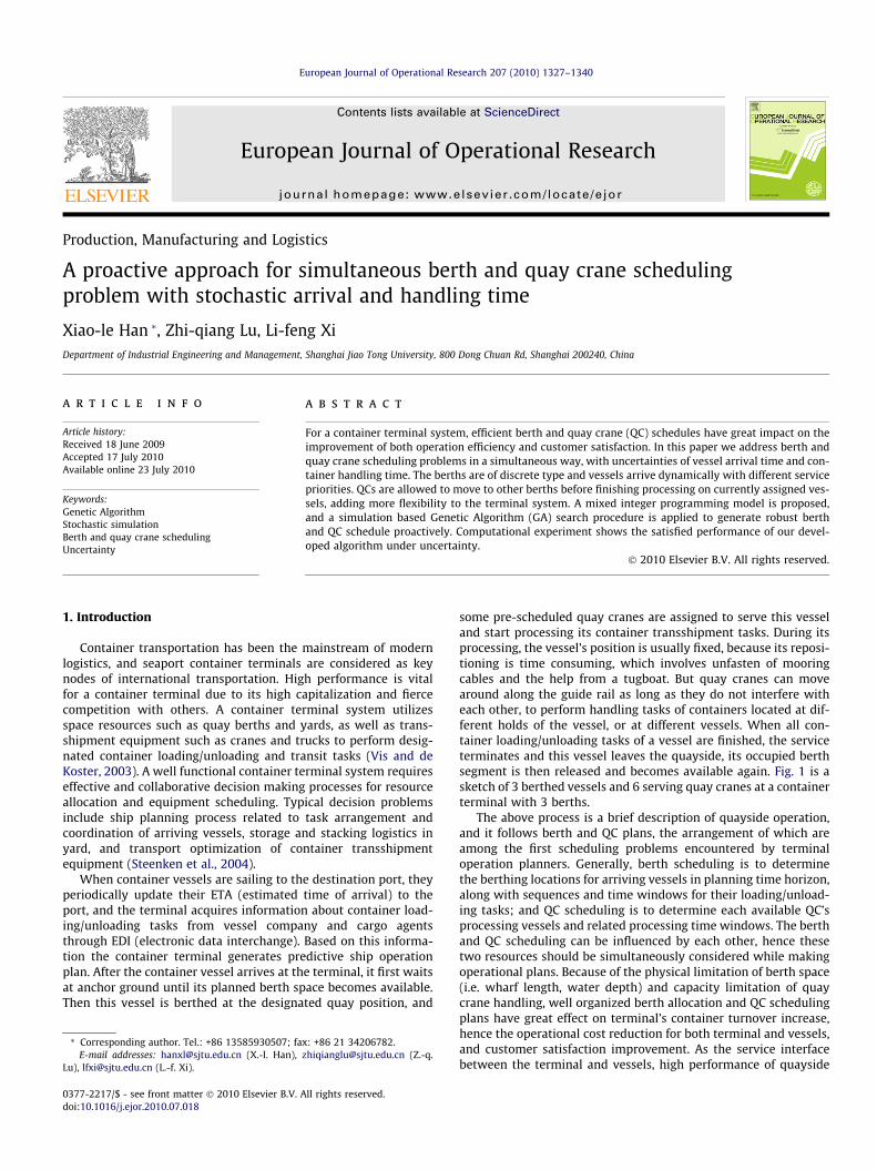
some pre-scheduled quay cranes are assigned to serve this vesseland start processing its container transshipment tasks. During itsprocessing, the vessel’s position is usually fixed, because its reposi-tioning is time consuming, which involves unfasten of mooringcables and the help from a tugboat. But quay cranes can movearound along the guide rail as long as they do not interfere witheach other, to perform handling tasks of containers located at dif-ferent holds of the vessel, or at different vessels. When all con-tainer loading/unloading tasks of a vessel are finished, the serviceterminates and this vessel leaves the quayside, its occupied berthsegment is then released and becomes available again. Fig. 1 is asketch of 3 berthed vessels and 6 serving quay cranes at a containerterminal with 3 berths.

The above process is a brief description of quayside operation,and it follows berth and QC plans, the arrangement of which areamong the first scheduling problems encountered by terminaloperation planners. Generally, berth scheduling is to determinethe berthing locations for arriving vessels in planning time horizon,along with sequences and time windows for their loading/unload-ing tasks; and QC scheduling is to determine each available QC’sprocessing vessels and related processing time windows. The berthand QC scheduling can be influenced by each other, hence thesetwo resources should be simultaneously considered while makingoperational plans. Because of the physical limitation of berth space(i.e. wharf length, water depth) and capacity limitation of quaycrane handling, well organized berth allocation and QC schedulingplans have great effect on terminal’s container turnover increase,hence the operational cost reduction for both terminal and vessels,and customer satisfaction improvement. As the service interfacebetween the terminal and vessels, high performance of quayside

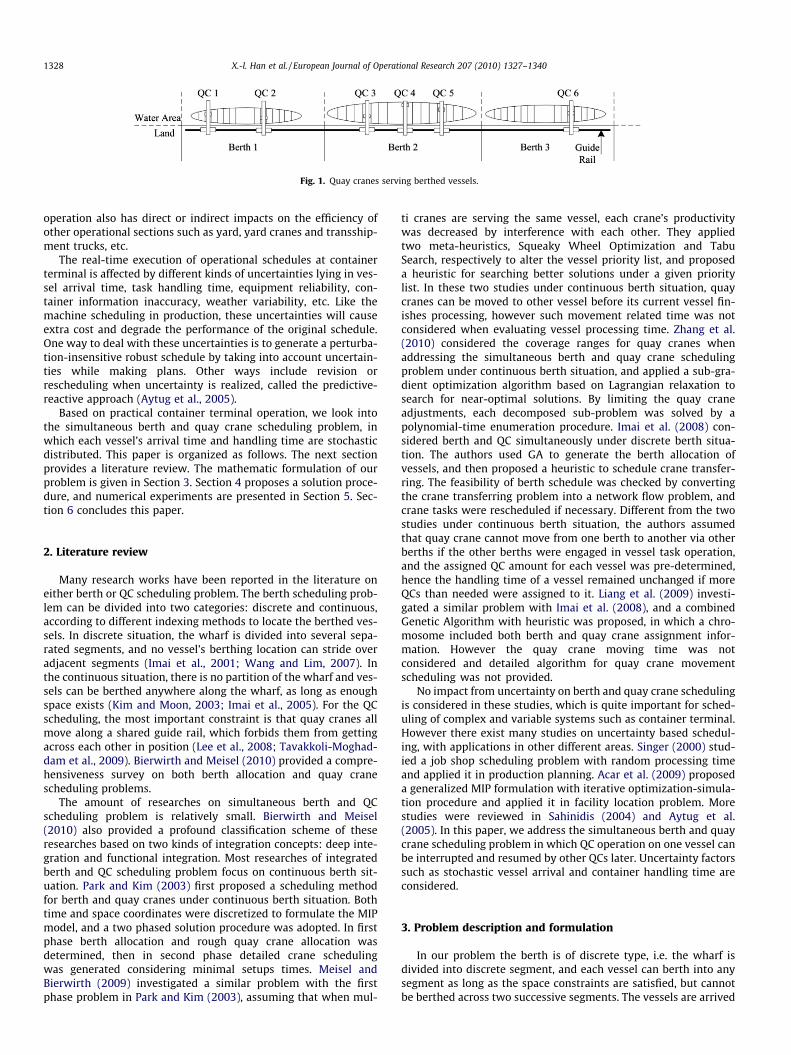
Fig. 1. Quay cranes serving berthed vessels.

1328 X.-l. Han et al. / European Journal of Operational Research 207 (2010) 1327–1340

operation also has direct or indirect impacts on the efficiency ofother operational sections such as yard, yard cranes and transship-ment trucks, etc.

The real-time execution of operational schedules at containerterminal is affected by different kinds of uncertainties lying in ves-sel arrival time, task handling time, equipment reliability, con-tainer information inaccuracy, weather variability, etc. Like themachine scheduling in production, these uncertainties will causeextra cost and degrade the performance of the original schedule.One way to deal with these uncertainties is to generate a perturba-tion-insensitive robust schedule by taking into account uncertain-ties while making plans. Other ways include revision orrescheduling when uncertainty is realized, called the predictive-reactive approach (Aytug et al., 2005).

Based on practical container terminal operation, we look intothe simultaneous berth and quay crane scheduling problem, inwhich each vessel’s arrival time and handling time are stochasticdistributed. This paper is organized as follows. The next sectionprovides a literature review. The mathematic formulation of ourproblem is given in Section 3. Section 4 proposes a solution proce-dure, and numerical experiments are presented in Section 5. Sec-tion 6 concludes this paper.

2. Literature review

Many research works have been reported in the literature oneither berth or QC scheduling problem. The berth scheduling prob-lem can be divided into two categories: discrete and continuous,according to different indexing methods to locate the berthed ves-sels. In discrete situation, the wharf is divided into several sepa-rated segments, and no vessel’s berthing location can stride overadjacent segments (Imai et al., 2001; Wang and Lim, 2007). Inthe continuous situation, there is no partition of the wharf and ves-sels can be berthed anywhere along the wharf, as long as enoughspace exists (Kim and Moon, 2003; Imai et al., 2005). For the QCscheduling, the most important constraint is that quay cranes allmove along a shared guide rail, which forbids them from gettingacross each other in position (Lee et al., 2008; Tavakkoli-Moghad-dam et al., 2009). Bierwirth and Meisel (2010) provided a compre-hensiveness survey on both berth allocation and quay cranescheduling problems.

The amount of researches on simultaneous berth and QCscheduling problem is relatively small. Bierwirth and Meisel(2010) also provided a profound classification scheme of theseresearches based on two kinds of integration concepts: deep inte-gration and functional integration. Most researches of integratedberth and QC scheduling problem focus on continuous berth sit-uation. Park and Kim (2003) first proposed a scheduling methodfor berth and quay cranes under continuous berth situation. Bothtime and space coordinates were discretized to formulate the MIPmodel, and a two phased solution procedure was adopted. In firstphase berth allocation and rough quay crane allocation wasdetermined, then in second phase detailed crane schedulingwas generated considering minimal setups times. Meisel andBierwirth (2009) investigated a similar problem with the firstphase problem in Park and Kim (2003), assuming that when mul-

ti cranes are serving the same vessel, each crane’s productivitywas decreased by interference with each other. They appliedtwo meta-heuristics, Squeaky Wheel Optimization and TabuSearch, respectively to alter the vessel priority list, and proposeda heuristic for searching better solutions under a given prioritylist. In these two studies under continuous berth situation, quaycranes can be moved to other vessel before its current vessel fin-ishes processing, however such movement related time was notconsidered when evaluating vessel processing time. Zhang et al.(2010) considered the coverage ranges for quay cranes whenaddressing the simultaneous berth and quay crane schedulingproblem under continuous berth situation, and applied a sub-gra-dient optimization algorithm based on Lagrangian relaxation tosearch for near-optimal solutions. By limiting the quay craneadjustments, each decomposed sub-problem was solved by apolynomial-time enumeration procedure. Imai et al. (2008) con-sidered berth and QC simultaneously under discrete berth situa-tion. The authors used GA to generate the berth allocation ofvessels, and then proposed a heuristic to schedule crane transfer-ring. The feasibility of berth schedule was checked by convertingthe crane transferring problem into a network flow problem, andcrane tasks were rescheduled if necessary. Different from the twostudies under continuous berth situation, the authors assumedthat quay crane cannot move from one berth to another via otherberths if the other berths were engaged in vessel task operation,and the assigned QC amount for each vessel was pre-determined,hence the handling time of a vessel remained unchanged if moreQCs than needed were assigned to it. Liang et al. (2009) investi-gated a similar problem with Imai et al. (2008), and a combinedGenetic Algorithm with heuristic was proposed, in which a chro-mosome included both berth and quay crane assignment infor-mation. However the quay crane moving time was notconsidered and detailed algorithm for quay crane movementscheduling was not provided.

No impact from uncertainty on berth and quay crane schedulingis considered in these studies, which is quite important for sched-uling of complex and variable systems such as container terminal.However there exist many studies on uncertainty based schedul-ing, with applications in other different areas. Singer (2000) stud-ied a job shop scheduling problem with random processing timeand applied it in production planning. Acar et al. (2009) proposeda generalized MIP formulation with iterative optimization-simula-tion procedure and applied it in facility location problem. Morestudies were reviewed in Sahinidis (2004) and Aytug et al.(2005). In this paper, we address the simultaneous berth and quaycrane scheduling problem in which QC operation on one vessel canbe interrupted and resumed by other QCs later. Uncertainty factorssuch as stochastic vessel arrival and container handling time areconsidered.

3. Problem description and formulation

In our problem the berth is of discrete type, i.e. the wharf isdivided into discrete segment, and each vessel can berth into anysegment as long as the space constraints are satisfied, but cannotbe berthed across two successive segments. The vessels are arrived

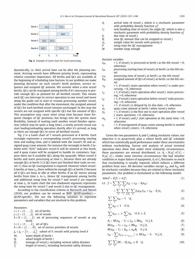
Fig. 2. Example of Gantt chart for vessel processing.

X.-l. Han et al. / European Journal of Operational Research 207 (2010) 1327–1340 1329

dynamically, i.e. their arrival time can be after the planning mo-ment. Arriving vessels have different priority levels, representingrelative customer importance. All berths and QCs are available atthe beginning of scheduling time horizon. In our problem we makeplanning decisions on each vessel’s berth position, service se-quence and assigned QC amount. We assume when a new vesselberths, QCs can be reassigned among berths if it’s necessary to pro-vide enough QCs as planned for all berthed vessels. This meanseach QC can interrupt its service operation to one vessel and movealong the guide rail to start or resume processing another vessel,under the condition that after the movement, the assigned amountof QCs for each berthed vessel remains unchanged. In this way thevessels are not assigned with specific QCs but the amount of QCs.This assumption may cause more setup time because more fre-quent changes of QC positions, but brings into the system moreflexibility. Instead of waiting until another vessel finishes opera-tion (which may be quite a long time), a newly arrived vessel canstart loading/unloading operation shortly after it’s arrived, as longas there are enough QCs to serve all berthed vessels.

Fig. 2 is a Gantt chart of 7 vessels processed at 4 berths. Eachrectangle represents a corresponding vessel’s processing startingtime and ending time, and is labeled with the vessel’s ID and as-signed quay crane amount. For instance the rectangle in berth-2 la-beled with ‘‘6(4)” indicates vessel-6 will be moored at this berth,and 4 quay cranes will be assigned to handle its containers. Sup-pose there are 6 available QCs along the quayside. When vessel-3berths and starts processing at time t1, because there are alreadyenough QCs at berth-3 (2 QCs have just finished their tasks on ves-sel-1), thus no QC reassignment is required. However when vessel-6 berths at time t2, there willnot be enough QCs at berth-2 becauseall 6 QCs are busy or idle at other berths, if no QC moves amongberths from time t1 to t2. Hence QC reassignment among berthsand additional setup time for vessel-7 and vessel-2 are requiredat time t2. In Gantt chart the two shadowed segments representsthe setup time for vessel-7 and vessel-2 due to QC reassignment.

According to the classification scheme in Bierwirth and Meisel(2010), our problem can be viewed as BAP; QCAPðnumberÞ �QCAPðspecificÞ. We use the following notation to representparameters and variables that are involved in this problem:

Parametersi 2 I ¼ f1; . . . ;eIg set of berthsj 2 J ¼ f1; . . . ;eJg set of vesselsk 2 K ¼ f1; . . . ;eJg set of processing sequences of vessels at any

berthl 2 L ¼ f1; . . . ; eLg set of QCsh 2 H ¼ f1; . . . ; eHg set of service priorities of vessels

jh 2 Jh ¼ 1; . . . ; eJh

n osubset of V, vessels with priority level h

Wi water depth of berth iQi wharf length of berth iDj tonnage of vessel j, including vertical safety distanceTj length of vessel j, including horizontal safety distance

Aj arrival time of vessel j, which is a stochastic parameterwith probability density function uA

jCj task handling time of vessel j by single QC, which is also a

stochastic parameter with probability density function uCj

Ej due time of vessel jBj max QC amount that can be assigned to vessel jbh weight value for vessels with priority hP setup time for QC reassignmentM number large enough

Decision variablesxijk = 1, if vessel j is processed at berth i as the kth vessel; = 0,

otherwisetijk processing starting time of vessel j at berth i as the kth ves-

selcijk processing time of vessel j at berth i as the kth vesselbijk assigned amount of QCs of vessel j at berth i as the kth ves-

selv jj0 = 1, if vessel j starts operation when vessel j0 is under pro-

cessing; = 0, otherwiserjj0 = 1, if vessel j starts operation after vessel j0 starts process-

ing; = 0, otherwisesjj0 = 1, if vessel j starts operation before vessel j0 ends process-

ing; = 0, otherwiseej = 1, if vessel j is delayed by its due date; = 0, otherwisenji quay crane amount at berth i when vessel j entersujj0 = 1, if vessel j is the first one to start operation after vessel

j0 starts operation; = 0, otherwisewjj0 = 1, if vessel j and j0 start operation at the same time; = 0,

otherwisezj = 1, if reassignment of quay cranes among berths is needed

when vessel j enters; = 0, otherwise

Given the two parameters Aj and Cj taking stochastic values, ourobjective is to proactively plan a robust berth and QC schedulewhich has statistically good performance under these uncertaintieswithout rescheduling. Survey and analysis of actual terminaloperation data show that under most ordinarily circumstances,these parameters are normal distributed, i.e. Aj � NðlA

j ;rAj ÞCj �

NðlCj ;rC

j Þ. Under some extreme circumstances like bad weathercondition or major failure of equipment, Aj or Cj fluctuates so muchthat rescheduling is usually required, which induces a differentproblem from ours. All decision variables except xijk and bijk willbe stochastic variables because they are related to these stochasticparameters. Our problem is formulated as the following model:

min Z ¼ Eðf Þ þ rðf Þ ð1Þs:t: f ¼

Xi

Xj

Xk

ðtijk þ cijk � AjxijkÞ

þX

h

Xi

Xj2Vh

Xk

bhxijkðtijk þ cijk � EjÞej; ð2Þ

Xi

Xk

xijk ¼ 1 8j; ð3ÞXj

xijk 6 1 8i; k; ð4ÞXj

xijðk�1Þ PX

j

xijk 8i; k P 2; ð5Þ

Aj þMðxijk � 1Þ 6 tijk 6 Mxijk 8i; j; k; ð6ÞMðxijk � 1Þ < cijk 6 Mxijk 8i; j; k; ð7ÞMðxijk � 1Þ < bijk 6 xijkBj 8i; j; k; ð8Þtijk �

Xj0ðtij0ðk�1Þþcij0 ðk�1Þ

ÞP Mðxijk � 1Þ 8i; j; k; ð9Þ

Xi

Xk

ðWi � DjÞxijk P 0 8j; ð10Þ

1330 X.-l. Han et al. / European Journal of Operational Research 207 (2010) 1327–1340

Xi

Xk

ðQ i � TjÞxijk P 0 8j; ð11Þ

ðrjj0 � 1ÞM 6X

i

Xk

tijk �X

i

Xk

tij0k < rjj0M 8j – j0; ð12Þ

ðsjj0 � 1ÞM <X

i

Xk

ðtij0k þ cij0kÞ �X

i

Xk

tijk 6 sjj0M 8j – j0;

ð13Þ0:5ðrjj0 þ sjj0 � 1Þ 6 v jj0 6 0:5ðrjj0 þ sjj0 Þ 8j – j0; ð14Þ0:5ðv jj0 þ v j0j � 1Þ 6 wjj0 6 0:5ðv jj0 þ v j0jÞ 8j – j0; ð15ÞX

i

nji 6eL 8j; ð16Þ

Mðej � 1Þ <X

i

Xk

ðtijk þ cijkÞ � Ej 6 Mej 8j; ð17Þ

nji PXj0–j

Xk

v jj0bij0k þX

k

bijk 8j; i; ð18Þ

rjj0 P ujj0 8j – j0; ð19Þujj0 P rjj0 � rjj00 8j – j0 – j00; ð20ÞMzj P nji �

Xj0–j

nj0 iujj0 8j; i; ð21Þ

cijk � Cj

Xi0

Xk0

bi0jk0 � PXj0–j

v j0 jzj0

,�

Yj00¼1;...;j0�1

wj0 j00 P ðxijk � 1ÞM 8i; j; k; ð22Þ

xijk 2 f0;1g 8i; j; k; ð23Þtijk; cijk; bijk;nji P 0 8i; j; k; ð24Þv jj0 ; rjj0 ; sjj0 ; ej;ujj0 ;wjj0 ; zj 2 f0;1g 8j – j; ð25Þxij0 ¼ 0; tij0 ¼ 0; cij0 ¼ 0; bij0 ¼ 0 8i; j: ð26Þ

The objective function (1) is to minimize the expected value plusstandard deviation of total service time and weighted tardinesstime for all vessels in a planning time horizon. The service time isdefined in first part of (2) as the difference between vessel process-ing finishing time and arrival time. It consists of waiting time andprocessing time, and represents the operational efficiency of thecontainer terminal. The tardiness time is defined in second part of(2) as the difference between vessel processing finishing time anddue time, representing the customer satisfaction. To evaluate theperformance and robustness of berth and QC plans, both expectedvalue and standard deviation objectives are considered. Constraint(3) ensures each vessel has to be processed by exact one berth. Con-straint (4) ensures that at most one vessel can be processed by oneberth at the same time. Constraint (5) is the physical interpretationof processing sequence. Constraint (6) ensures if xijk = 0, tijk = 0; elsethe processing of vessel j should start after its arrival. Constraint (7)

Fig. 3. Procedure of sim

ensures if xijk = 0, cijk = 0; else the processing time of vessel j shouldbe positive. Constraint (8) ensures if xijk = 0, bijk = 0; else the as-signed QC amount for vessel j should be positive and below theup-limit. Constraint (9) ensures each vessel starts processing afterthe leaving of its predecessor at the same berth. Constraints (10)and (11) are space constraints. The vessel size cannot exceed itsberth size in vertical or horizontal dimension. Constraints (12)–(15) are definitions of rjj0 ; sjj0 ; v jj0 and wjj0 . Constraint (16) ensureseach time a new vessel is berthed, the total amount of neededQCs will not exceed the up-limit of all available QCs at containerterminal. Constraint (17) is the definition of ej. Constraint(18) isthe definition of nji. Constraints (19) and (20) are definition forujj0 . Constraint (21) is the definition of zj. Constraint (22) ensureseach vessel’s processing time consists of task handling time andneeded setup time when QC reassignment happens. Here we as-sume the handling task can be equally assigned to each QC withsame handling ability, so the task handling time of a vessel can beaveraged by its assigned QC amount, as in Liang et al. (2009). Thesetup time is set to a fixed amount P, which is enough for cranemovement between any two berths according to the quay lengthand QC moving speed. In this way the detailed quay crane positionand movement are not modeled for simplification, and results ofour problem can be viewed as an upper bound for the actualproblem.

4. Simulation based GA search

Our problem is formulated as a non-liner mixed integer pro-gramming problem, with stochastic parameters and statistical val-ued objective. We adopt a simulation based Genetic Algorithmprocedure to search for robust solutions. Our procedure applies aGA framework, and incorporates a simulation module using MonteCarlo sampling to evaluate the performance of each single chromo-some. The search procedure terminates when the max number ofgenerations is achieved. The flowchart for this procedure is shownin Fig. 3.

4.1. Representation

The solution the problem is represented as a chromosomewhich is a string consists of 2ðeI þeJ � 1Þ integer items. In such achromosome, the first ðeI þeJ � 1Þ items represent berth assignmentand service sequence for vessels, and the last ðeI þeJ � 1Þ items rep-resent each vessel’s assigned QC amount. The items in the berthsegment are vessel IDs ordered by their processing sequences ateach berth, with 0 items representing the switch from one berthto another. The items in the QC segment represent assigned QC

ulation based GA.

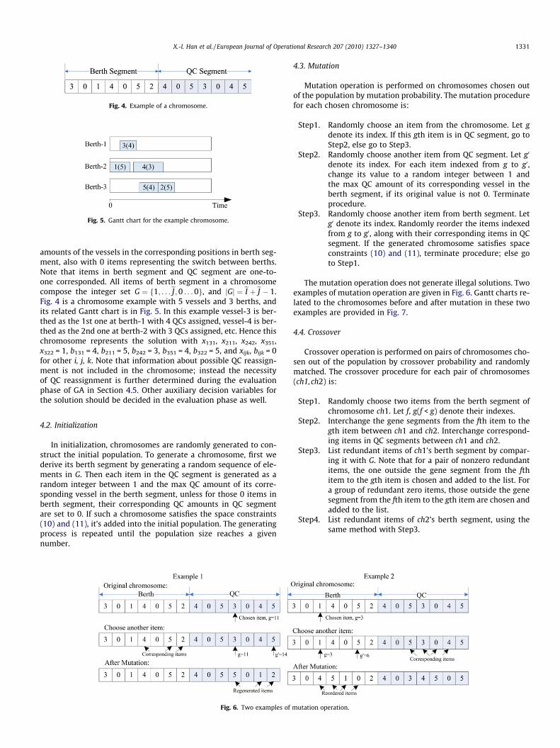
Fig. 4. Example of a chromosome.

Fig. 5. Gantt chart for the example chromosome.

X.-l. Han et al. / European Journal of Operational Research 207 (2010) 1327–1340 1331

amounts of the vessels in the corresponding positions in berth seg-ment, also with 0 items representing the switch between berths.Note that items in berth segment and QC segment are one-to-one corresponded. All items of berth segment in a chromosomecompose the integer set G ¼ f1; . . .eJ;0 . . . 0g, and jGj ¼ eI þeJ � 1.Fig. 4 is a chromosome example with 5 vessels and 3 berths, andits related Gantt chart is in Fig. 5. In this example vessel-3 is ber-thed as the 1st one at berth-1 with 4 QCs assigned, vessel-4 is ber-thed as the 2nd one at berth-2 with 3 QCs assigned, etc. Hence thischromosome represents the solution with x131, x211, x242, x351,x322 = 1, b131 = 4, b211 = 5, b242 = 3, b351 = 4, b322 = 5, and xijk, bijk = 0for other i, j, k. Note that information about possible QC reassign-ment is not included in the chromosome; instead the necessityof QC reassignment is further determined during the evaluationphase of GA in Section 4.5. Other auxiliary decision variables forthe solution should be decided in the evaluation phase as well.

4.2. Initialization

In initialization, chromosomes are randomly generated to con-struct the initial population. To generate a chromosome, first wederive its berth segment by generating a random sequence of ele-ments in G. Then each item in the QC segment is generated as arandom integer between 1 and the max QC amount of its corre-sponding vessel in the berth segment, unless for those 0 items inberth segment, their corresponding QC amounts in QC segmentare set to 0. If such a chromosome satisfies the space constraints(10) and (11), it’s added into the initial population. The generatingprocess is repeated until the population size reaches a givennumber.

Fig. 6. Two examples of

4.3. Mutation

Mutation operation is performed on chromosomes chosen outof the population by mutation probability. The mutation procedurefor each chosen chromosome is:

Step1. Randomly choose an item from the chromosome. Let gdenote its index. If this gth item is in QC segment, go toStep2, else go to Step3.

Step2. Randomly choose another item from QC segment. Let g0

denote its index. For each item indexed from g to g0,change its value to a random integer between 1 andthe max QC amount of its corresponding vessel in theberth segment, if its original value is not 0. Terminateprocedure.

Step3. Randomly choose another item from berth segment. Letg0 denote its index. Randomly reorder the items indexedfrom g to g0, along with their corresponding items in QCsegment. If the generated chromosome satisfies spaceconstraints (10) and (11), terminate procedure; else goto Step1.

The mutation operation does not generate illegal solutions. Twoexamples of mutation operation are given in Fig. 6. Gantt charts re-lated to the chromosomes before and after mutation in these twoexamples are provided in Fig. 7.

4.4. Crossover

Crossover operation is performed on pairs of chromosomes cho-sen out of the population by crossover probability and randomlymatched. The crossover procedure for each pair of chromosomes(ch1,ch2) is:

Step1. Randomly choose two items from the berth segment ofchromosome ch1. Let f, g(f < g) denote their indexes.

Step2. Interchange the gene segments from the fth item to thegth item between ch1 and ch2. Interchange correspond-ing items in QC segments between ch1 and ch2.

Step3. List redundant items of ch1’s berth segment by compar-ing it with G. Note that for a pair of nonzero redundantitems, the one outside the gene segment from the fthitem to the gth item is chosen and added to the list. Fora group of redundant zero items, those outside the genesegment from the fth item to the gth item are chosen andadded to the list.

Step4. List redundant items of ch2’s berth segment, using thesame method with Step3.

mutation operation.

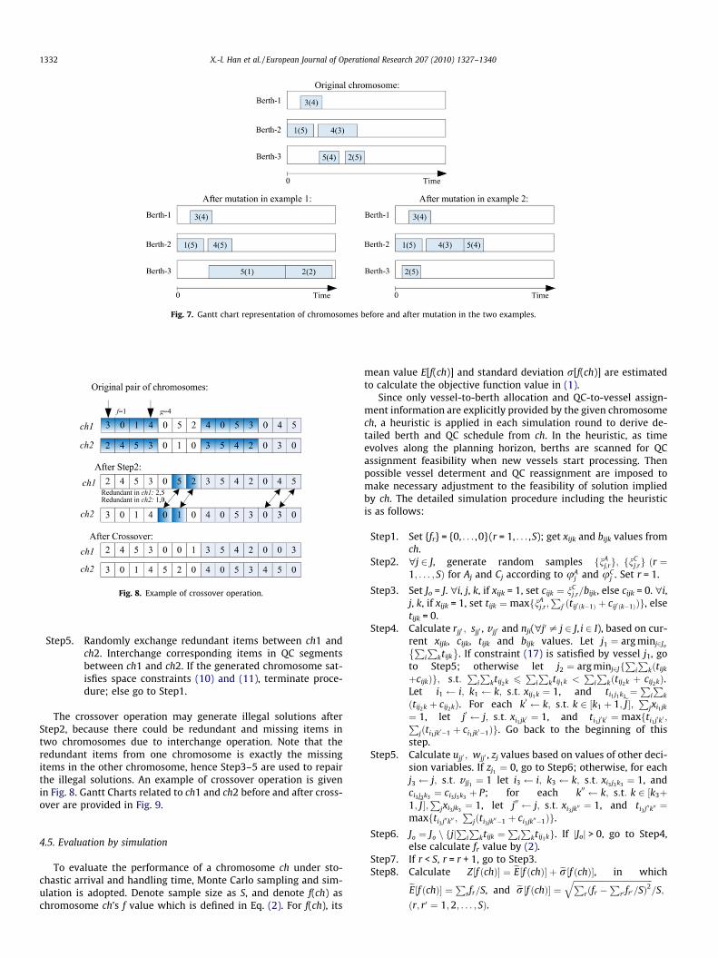
Fig. 7. Gantt chart representation of chromosomes before and after mutation in the two examples.

Fig. 8. Example of crossover operation.

1332 X.-l. Han et al. / European Journal of Operational Research 207 (2010) 1327–1340

Step5. Randomly exchange redundant items between ch1 andch2. Interchange corresponding items in QC segmentsbetween ch1 and ch2. If the generated chromosome sat-isfies space constraints (10) and (11), terminate proce-dure; else go to Step1.

The crossover operation may generate illegal solutions afterStep2, because there could be redundant and missing items intwo chromosomes due to interchange operation. Note that theredundant items from one chromosome is exactly the missingitems in the other chromosome, hence Step3–5 are used to repairthe illegal solutions. An example of crossover operation is givenin Fig. 8. Gantt Charts related to ch1 and ch2 before and after cross-over are provided in Fig. 9.

4.5. Evaluation by simulation

To evaluate the performance of a chromosome ch under sto-chastic arrival and handling time, Monte Carlo sampling and sim-ulation is adopted. Denote sample size as S, and denote f(ch) aschromosome ch’s f value which is defined in Eq. (2). For f(ch), its

mean value E[f(ch)] and standard deviation r[f(ch)] are estimatedto calculate the objective function value in (1).

Since only vessel-to-berth allocation and QC-to-vessel assign-ment information are explicitly provided by the given chromosomech, a heuristic is applied in each simulation round to derive de-tailed berth and QC schedule from ch. In the heuristic, as timeevolves along the planning horizon, berths are scanned for QCassignment feasibility when new vessels start processing. Thenpossible vessel determent and QC reassignment are imposed tomake necessary adjustment to the feasibility of solution impliedby ch. The detailed simulation procedure including the heuristicis as follows:

Step1. Set {fr} = {0, . . . ,0} (r = 1, . . . ,S); get xijk and bijk values fromch.

Step2. "j 2 J, generate random samples fnAj;rg; fn

Cj;rg ðr ¼

1; . . . ; SÞ for Aj and Cj according to uAj and uC

j . Set r = 1.

Step3. Set Jo = J. "i, j, k, if xijk = 1, set cijk ¼ nCj;r=bijk, else cijk = 0. "i,

j, k, if xijk = 1, set tijk ¼maxfnAj;r ;P

j0 ðtij0 ðk�1Þ þ cij0 ðk�1ÞÞg, elsetijk = 0.

Step4. Calculate rjj0 ; sjj0 , v jj0 and nji("j0 – j 2 J, i 2 I), based on cur-rent xijk, cijk, tijk and bijk values. Let j1 ¼ arg minj2JoP

i

Pktijk

� �. If constraint (17) is satisfied by vessel j1, go

to Step5; otherwise let j2 ¼ arg minj2JfP

i

Pkðtijk

þcijkÞg; s:t:P

i

Pktij2k 6

Pi

Pktij1k <

Pi

Pkðtij2k þ cij2kÞ.

Let i1 i; k1 k; s:t: xij1k ¼ 1, and ti1 j1k1 ¼P

i

Pk

ðtij2k þ cij2kÞ. For each k0 k; s:t: k 2 ½k1 þ 1;eJ�; Pjxi1 jk

¼ 1, let j0 j; s:t: xi1 jk0 ¼ 1, and ti1 j0k0 ¼maxfti1j0k0 ;Pjðti1jk0�1 þ ci1 jk0�1Þg. Go back to the beginning of this

step.Step5. Calculate ujj0 ; wjj0 , zj values based on values of other deci-

sion variables. If zj1 ¼ 0, go to Step6; otherwise, for eachj3 j; s:t: v jj1 ¼ 1 let i3 i; k3 k; s:t: xi3 j3k3 ¼ 1, andci3 j3k3 ¼ ci3 j3k3 þ P; for each k00 k; s:t: k 2 ½k3þ1;eJ�;Pjxi3 jk3

¼ 1, let j00 j; s:t: xi3 jk00 ¼ 1, and ti3j00k00 ¼maxfti3j00k00 ;

Pjðti3 jk00�1 þ ci3jk00�1Þg.

Step6. Jo ¼ Jo n fjjP

i

Pktijk ¼

Pi

Pktij1kg. If jJoj > 0, go to Step4,

else calculate fr value by (2).Step7. If r < S, r = r + 1, go to Step3.Step8. Calculate Z½f ðchÞ� ¼ eE½f ðchÞ� þ er½f ðchÞ�, in whicheE½f ðchÞ� ¼

Prfr=S, and er½f ðchÞ� ¼

ffiffiffiffiffiffiffiffiffiffiffiffiffiffiffiffiffiffiffiffiffiffiffiffiffiffiffiffiffiffiffiffiffiffiffiffiffiffiPrðfr �

Pr0 fr0=SÞ2

q=S;

ðr; r0 ¼ 1;2; . . . ; SÞ.

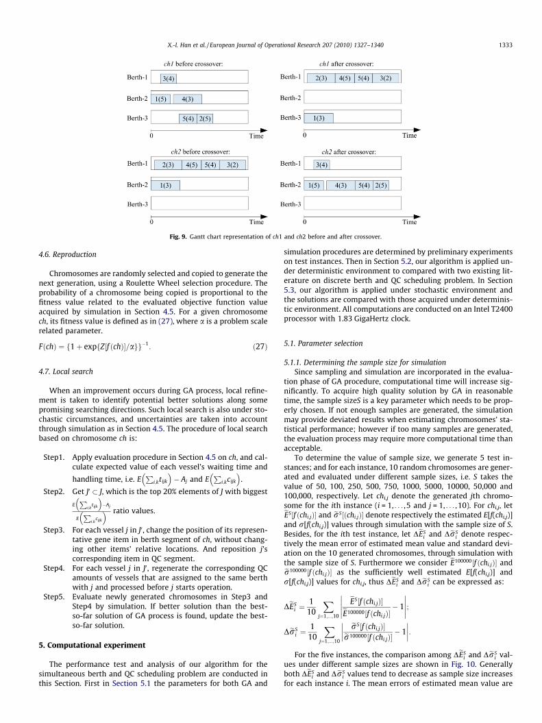
Fig. 9. Gantt chart representation of ch1 and ch2 before and after crossover.

X.-l. Han et al. / European Journal of Operational Research 207 (2010) 1327–1340 1333

4.6. Reproduction

Chromosomes are randomly selected and copied to generate thenext generation, using a Roulette Wheel selection procedure. Theprobability of a chromosome being copied is proportional to thefitness value related to the evaluated objective function valueacquired by simulation in Section 4.5. For a given chromosomech, its fitness value is defined as in (27), where a is a problem scalerelated parameter.

FðchÞ ¼ f1þ expfZ½f ðchÞ�=agg�1: ð27Þ

4.7. Local search

When an improvement occurs during GA process, local refine-ment is taken to identify potential better solutions along somepromising searching directions. Such local search is also under sto-chastic circumstances, and uncertainties are taken into accountthrough simulation as in Section 4.5. The procedure of local searchbased on chromosome ch is:

Step1. Apply evaluation procedure in Section 4.5 on ch, and cal-culate expected value of each vessel’s waiting time and

handling time, i.e. EP

i;ktijk

� �� Aj and E

Pi;kcijk

� �.

Step2. Get J0 � J, which is the top 20% elements of J with biggest

EP

i;ktijk

� ��Aj

EP

i;kcijk

� � ratio values.

Step3. For each vessel j in J0, change the position of its represen-tative gene item in berth segment of ch, without chang-ing other items’ relative locations. And reposition j’scorresponding item in QC segment.

Step4. For each vessel j in J0, regenerate the corresponding QCamounts of vessels that are assigned to the same berthwith j and processed before j starts operation.

Step5. Evaluate newly generated chromosomes in Step3 andStep4 by simulation. If better solution than the best-so-far solution of GA process is found, update the best-so-far solution.

5. Computational experiment

The performance test and analysis of our algorithm for thesimultaneous berth and QC scheduling problem are conducted inthis Section. First in Section 5.1 the parameters for both GA and

simulation procedures are determined by preliminary experimentson test instances. Then in Section 5.2, our algorithm is applied un-der deterministic environment to compared with two existing lit-erature on discrete berth and QC scheduling problem. In Section5.3, our algorithm is applied under stochastic environment andthe solutions are compared with those acquired under determinis-tic environment. All computations are conducted on an Intel T2400processor with 1.83 GigaHertz clock.

5.1. Parameter selection

5.1.1. Determining the sample size for simulationSince sampling and simulation are incorporated in the evalua-

tion phase of GA procedure, computational time will increase sig-nificantly. To acquire high quality solution by GA in reasonabletime, the sample sizeS is a key parameter which needs to be prop-erly chosen. If not enough samples are generated, the simulationmay provide deviated results when estimating chromosomes’ sta-tistical performance; however if too many samples are generated,the evaluation process may require more computational time thanacceptable.

To determine the value of sample size, we generate 5 test in-stances; and for each instance, 10 random chromosomes are gener-ated and evaluated under different sample sizes, i.e. S takes thevalue of 50, 100, 250, 500, 750, 1000, 5000, 10000, 50,000 and100,000, respectively. Let chi,j denote the generated jth chromo-some for the ith instance (i = 1, . . . ,5 and j = 1, . . . ,10). For chi,j, leteES½f ðchi;jÞ� and erS½ðchi;jÞ� denote respectively the estimated E[f(chi,j)]and r[f(chi,j)] values through simulation with the sample size of S.Besides, for the ith test instance, let DeES

i and DerSi denote respec-

tively the mean error of estimated mean value and standard devi-ation on the 10 generated chromosomes, through simulation withthe sample size of S. Furthermore we consider eE100000½f ðchi;jÞ� ander100000½f ðchi;jÞ� as the sufficiently well estimated E[f(chi,j)] andr[f(chi,j)] values for chi,j, thus DeES

i and DerSi can be expressed as:

DeESi ¼

110

Xj¼1;...;10

eES½f ðchi;jÞ�eE100000½f ðchi;jÞ�� 1

����������;

DerSi ¼

110

Xj¼1;...;10

erS½f ðchi;jÞ�er100000½f ðchi;jÞ�� 1

���� ����:For the five instances, the comparison among DeES

i and DerSi val-

ues under different sample sizes are shown in Fig. 10. Generallyboth DeES

i and DerSi values tend to decrease as sample size increases

for each instance i. The mean errors of estimated mean value are

15

35

55

75

95

115

135

155

175

1 101 201 301 401 501 601 701 801 901 1001

obje

ctiv

e fu

ncti

on v

alue

generation

crossover rate=0.1crossover rate=0.2crossover rate=0.4crossover rate=0.6crossover rate=0.8

Fig. 12. Performance comparison of different crossover rates for an instance underpopulation size of 50 and mutation rate of 0.8.

15

35

55

75

95

115

135

155

175

195

1 101 201 301 401 501 601 701 801 901 1001

obje

ctiv

e fu

ncti

on v

alue

s

Generation

mutation rate=0.1mutation rate=0.2mutation rate=0.4mutation rate=0.6mutation rate=0.8

Fig. 11. Performance comparison of different mutation rates for an instance underpopulation size of 50 and crossover rate of 0.8.

15

35

55

75

95

115

135

155

175

1 101 201 301 401 501 601 701 801 901

obje

ctvi

e fu

ncti

on v

alue

generation

population=30population=50population=70population=100

Fig. 13. Performance comparison of different population sizes for an instance undercrossover rate of 0.8 and mutation rate of 0.8.

0

0.01

0.02

0.03

0.04

0.05

0.06

0.07

0.08

0.09

0.1

0.11

50 100 250 500 750 1000 5000 10000 50000

Mea

n er

rors

Sample size S

5S

σΔ

4S

σΔ

3S

σΔ

2S

σΔ

1S

σΔ

4S

EΔ

2S

EΔ

5S

EΔ

3S

EΔ

1S

EΔ

Fig. 10. Mean errors of estimated mean value and standard deviation for fiveinstances under different sample sizes.

1334 X.-l. Han et al. / European Journal of Operational Research 207 (2010) 1327–1340

within 2% for all instances and sample sizes, while the mean errorsof estimated standard deviation are within 2% for all instanceswhen sample size exceeds 750, which implies that 750 sampleswill be sufficient for the estimation of stochastic environment. Asa result we set S = 750 for the simulation process.

5.1.2. Determining the GA parametersGA searches with different parameter settings are applied on

the five instances to select an effective parameter combinationfor our problem. The population size takes the value of 30, 50, 70and 90, respectively, and both the crossover rate and mutationrates take the value of 0.1, 0.2, 0.4, 0.6 and 0.8, respectively. EachGA terminates until 1000 generations are reproduced, and thesample size S takes the value of 750, as determined in Section 5.1.1.

Figs. 11–13 illustrate some comparisons among these differentparameter settings. Fig. 11 shows the convergence curves on differ-ent mutation rates for a typical instance with the crossover rate of0.8 and population size of 50. Fig. 12 shows the convergence curveson different crossover rates for the instance with the mutation rateof 0.8 and population size of 50. Fig. 13 shows the convergencecurves on different population sizes for the instance with the cross-over rate of 0.8 and mutation rate of 0.8. The mutation rate of 0.8outperforms other values in Fig. 11, and the crossover rate of 0.8outperforms other values in Fig. 12. Hence we set mutation rateand crossover rate to 0.8 in GA search. In these two figures, theobjective function values are not improved after 500 generationswhen crossover and mutation rate are set to 0.8, so the maximumgeneration of 500 will be sufficient to acquire a near-optimal solu-tion. Besides, in Fig. 13, the objective function values of the bestfound solutions after 500 generations are close to each other underpopulation size of 50, 70 and 90, so the population size is set to 50for GA search.

5.2. Performance under deterministic circumstance

In literature, Imai et al. (2008) and Liang et al. (2009) studiedthe simultaneous berth and QC scheduling problem with no allow-ing of quay crane reassignment during any vessel’s processing,which is a main difference from our assumption. The considerationbehind our proposal is that by allowing quay crane reassignment,the quay side handling system is given higher flexibility, althoughat the risk of more frequent setup. To examine the influence of add-ing such flexibility into the problem, computational results of ouralgorithm under deterministic environment are compared withthese two literatures, respectively.

5.2.1. Computational experiment on a real caseWe first apply our algorithm to the problem demonstrated in

Liang et al. (2009), which is a real case. The calculation is per-formed under deterministic circumstance, i.e. the simulation isperformed only once when evaluating each chromosome, and each

X.-l. Han et al. / European Journal of Operational Research 207 (2010) 1327–1340 1335

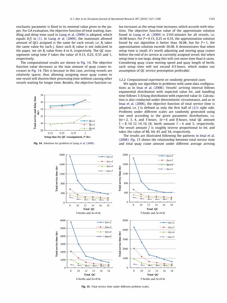
stochastic parameter is fixed to its nominal value given in the pa-per. For GA evaluation, the objective function of total waiting, han-dling and delay time used in Liang et al. (2009) is adopted, whichequals E(f) in (1). In Liang et al. (2009), the maximum allowedamount of QCs assigned is the same for each vessel, i.e. Bj takesthe same value for each j. Since such Bj value is not indicated inthe paper, we set Bj value from 4 to 6, respectively. The QC reas-signment setup time P takes the value of 0.15, 0.25, 0.35 and 1,respectively.

The computational results are shown in Fig. 14. The objectivefunction value decreases as the max amount of quay cranes in-creases in Fig. 14. This is because in this case, arriving vessels arerelatively sparse, thus allowing assigning more quay cranes toone vessel will shorten their processing time without causing othervessels waiting for longer time. Besides, the objective function va-

4 berths and Se

4 berths and Se=8 hr

=6 hr

0

400

800

1200

1600

2000

8 10 12 14 16 18

Tot

al s

ervi

ce t

ime

(hr)

Total QC

Int=2

Int=3

Int=4

Int=5

0

1000

2000

3000

4000

5000

6000

8 10 12 14 16 18

Tot

al s

ervi

ce t

ime

(hr)

Total QC

Int=2

Int=3

Int=4

Int=5

Fig. 15. Total service time unde

28

30

32

34

36

38

0.15 0.25 0.35 1

Tot

al s

ervi

ce a

nd d

elay

tim

e (h

r)

Setup time for QC reassignment, P (hr)

Bj=4Bj=5Bj=6

Fig. 14. Solutions for problem in Liang et al. (2009).

lue increases as the setup time increases, which accords with intu-ition. The objective function value of the approximate solutionfound in Liang et al. (2009) is 2165 minutes for all vessels, i.e.36.08 hours. For P = 0.15, 0.25 or 0.35, the approximation solutionfound by our algorithm is better than 36.08, but for P = 1, theapproximation solution exceeds 36.08. It demonstrates that whensetup time is small, it’s worth adjusting and moving quay cranesbefore the end of its service at currently assigned vessel, but whensetup time is too large, doing this will cost more time than it saves.Considering quay crane moving speed and quay length of berth,such setup time will not exceed 0.5 hours, which makes ourassumption of QC service preemption preferable.

5.2.2. Computational experiment on randomly generated casesWe apply our algorithm to problems with same data configura-

tions as in Imai et al. (2008): Vessels’ arriving interval followsexponential distribution with expected value Int, and handlingtime follows 3-Erlang distribution with expected value Se. Calcula-tion is also conducted under deterministic circumstance, and as inImai et al. (2008), the objective function of total service time isadopted, i.e. f is defined as only the first half of (2)’s right side.Problems under different scales are randomly generated usingone seed according to the given parameter distributions, i.e.Int = 2, 3, 4, and 5 hours, Se = 6 and 8 hours, total QC amounteL ¼ 8;10;12;14;16;18, berth amount eI ¼ 4 and 5, respectively.The vessel amount eJ is roughly inverse proportional to Int, andtakes the value of 88, 64, 45 and 34, respectively.

The results are illustrated following the patterns in Imai et al.(2008): Fig. 15 shows the relationship between total service timeand total quay crane amount under different average arriving

Se=6 hr

5 berths and

5 berths and Se=8 hr

0

400

800

1200

1600

2000

8 10 12 14 16 18

Tot

al s

ervi

ce t

ime

(hr)

Total QC

Int=2

Int=3

Int=4

Int=5

0

1000

2000

3000

4000

5000

8 10 12 14 16 18

Tot

al s

ervi

ce t

ime

(hr)

Total QC

Int=2

Int=3

Int=4

Int=5

r different problem scales.

4 berths and Se=6 hr 5 berths and Se=6 hr

0

5

10

15

20

25

2 3 4 5

Ave

rage

ser

vice

tim

e (h

r)

Average arriving interval, Int (hr)

Total QC=8

Total QC=10

Total QC=12

Total QC=14

Total QC=16

Total QC=18

0

5

10

15

20

25

2 3 4 5

Ave

rage

ser

vice

tim

e (h

r)

Average arriving interval, Int (hr)

Total QC=8

Total QC=10

Total QC=12

Total QC=14

Total QC=16

Total QC=18

4 berths and Se=8 hr 5 berths and Se=8 hr

0

10

20

30

40

50

60

70

2 3 4 5

Ave

rage

ser

vice

tim

e (h

r)

Average arriving interval, Int (hr)

Total QC=8

Total QC=10

Total QC=12

Total QC=14

Total QC=16

Total QC=18

0

10

20

30

40

50

60

2 3 4 5

Ave

rage

ser

vice

tim

e (h

r)

Average arriving interval, Int (hr)

Total QC=8Total QC=10Total QC=12Total QC=14Total QC=16Total QC=18

Fig. 16. Average service time under different problem scales.

1

1.1

1.2

1.3

1.4

1.5

1.6

8 10 12 14 16 18

Rat

io o

f S2

and

S1’s

f v

alue

s

Total QC

Int=2

Int=3

Int=4

Int=5

Fig. 17. Ratio of S2 and S1’s f values under deterministic circumstance (5 berths andSe = 8 hours).

1336 X.-l. Han et al. / European Journal of Operational Research 207 (2010) 1327–1340

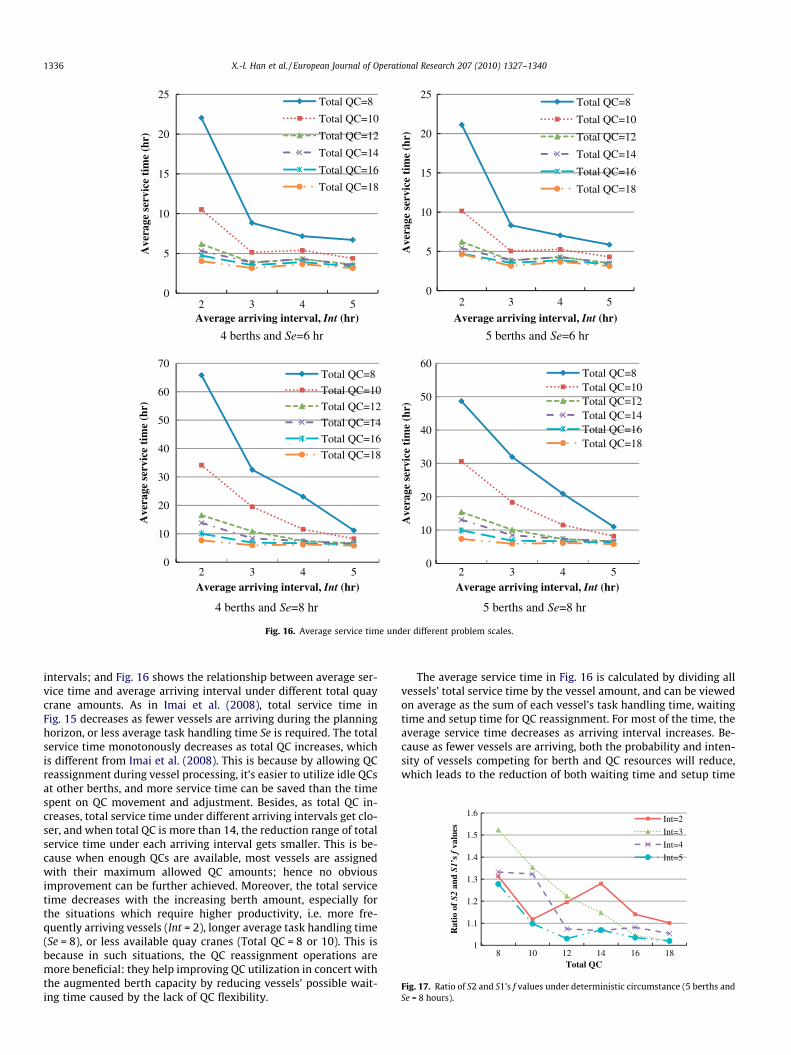
intervals; and Fig. 16 shows the relationship between average ser-vice time and average arriving interval under different total quaycrane amounts. As in Imai et al. (2008), total service time inFig. 15 decreases as fewer vessels are arriving during the planninghorizon, or less average task handling time Se is required. The totalservice time monotonously decreases as total QC increases, whichis different from Imai et al. (2008). This is because by allowing QCreassignment during vessel processing, it’s easier to utilize idle QCsat other berths, and more service time can be saved than the timespent on QC movement and adjustment. Besides, as total QC in-creases, total service time under different arriving intervals get clo-ser, and when total QC is more than 14, the reduction range of totalservice time under each arriving interval gets smaller. This is be-cause when enough QCs are available, most vessels are assignedwith their maximum allowed QC amounts; hence no obviousimprovement can be further achieved. Moreover, the total servicetime decreases with the increasing berth amount, especially forthe situations which require higher productivity, i.e. more fre-quently arriving vessels (Int = 2), longer average task handling time(Se = 8), or less available quay cranes (Total QC = 8 or 10). This isbecause in such situations, the QC reassignment operations aremore beneficial: they help improving QC utilization in concert withthe augmented berth capacity by reducing vessels’ possible wait-ing time caused by the lack of QC flexibility.

The average service time in Fig. 16 is calculated by dividing allvessels’ total service time by the vessel amount, and can be viewedon average as the sum of each vessel’s task handling time, waitingtime and setup time for QC reassignment. For most of the time, theaverage service time decreases as arriving interval increases. Be-cause as fewer vessels are arriving, both the probability and inten-sity of vessels competing for berth and QC resources will reduce,which leads to the reduction of both waiting time and setup time

0.65

0.7

0.75

0.8

0.85

0.9

0.95

1

1.05

1.1

8 10 12 14 16 18

Rat

io o

f S2

and

S1’

s ex

pect

ed f

valu

es

Total QC

Int=2

Int=3

Int=4

Int=5

Fig. 18. Ratio of S2 and S1’s expected f values under stochastic circumstance (5berths and Se = 8 hours).

X.-l. Han et al. / European Journal of Operational Research 207 (2010) 1327–1340 1337

for QC reassignment. However a partial increasing trend can be ob-served when the arriving interval changes from 3 to 4 hours, whichimplies the increasing of task handling time offsets the reductionof waiting time and setup time. Similar to the total service time,average service time tend to be steady when total QC is more than14, indicating the redundancy of available quay cranes.

5.3. Performance under stochastic circumstance

In previous Section 5.2, solutions are acquired under determin-istic circumstance, and we denote them by S1. In this section, ouralgorithm is applied under stochastic environment, i.e. the simula-tion during evaluation phase is performed for S iterations based on

Arrving interval=2

Arrving interval=4

0

1000

2000

3000

4000

5000

6000

7000

8000

8 10 12 14 16 18

[µ-σ

, µ+σ

] ra

nge

of S

1 an

d S2

’f

valu

es

Total QC

S2

S1

0

200

400

600

800

1000

1200

1400

1600

1800

2000

8 10 12 14 16 18

[ µ- σ

, µ+σ

] ra

nge

of S

1 an

d S2

’s f

val

ues

Total QC

S2

S1

Fig. 19. Statistical range of S1 and S2’s f values under s

the sampled vessel arriving time and task handling time, and thesesolutions found under such stochastic circumstance are denoted asS2. To restrict the computational time, the sample size S is set to750 during GA search as previously determined.

After both S1 and S2 have been acquired, the statistic perfor-mance of S1 and S2 are compared by applying simulation proce-dure on them and setting S to 100,000. To differentiate betweenthe f values of a given solution ch(ch = S1 or S2) under two kindsof circumstances, we denote fdet(ch) and fsto(ch) as the f(ch) valuesunder deterministic and stochastic circumstances, respectively. Forfsto(ch), its expected value and standard deviation, i.e. E[fsto(ch)] andr[fsto(ch)] can be estimated by the simulation procedure in Section4.5, and the sample size S is set to 100,000 in order to provide moreaccurate estimations for statistic performance comparison. Corre-spondingly, fdet(ch), the f(ch) value under deterministic circum-stance can be calculated after a single-iteration simulation withnominal parameter values.

5.3.1. Comparing the statistical performance of S1 and S2’sThe generated cases in Section 5.2.2 with 8 hours of average

handling time and 5 berths are used in this section. SetP = 0.25and bh = 1 for each h in (2). Vessels’ arrival and task handling timeare assumed to follow normal distributions with rC

j ¼ lCj =3 and

rAj ¼ Int=3. The detailed procedure of fAS

j;r;CSj;rg sample generation

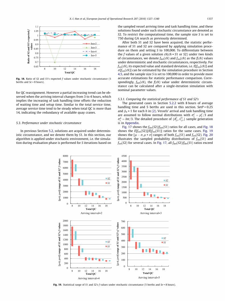
is in Appendix.Fig. 17 shows the fdet(S2)/fdet(S1) ratios for all cases, and Fig. 18

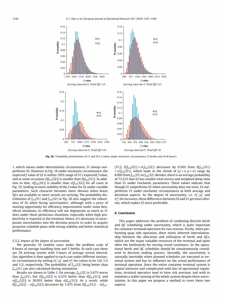
shows the E[fsto(S2)]/E[fsto(S1)] ratios for the same cases. Fig. 19shows the [l � r,l + r] ranges of both fsto(S1) and fsto(S2). Fig. 20illustrates the sampled probability distributions of fsto(S1) andfsto(S2) for several cases. In Fig. 17, all fdet(S2)/fdet(S1) ratios exceed

Arrving interval=3

Arrving interval=5

0

500

1000

1500

2000

2500

3000

3500

4000

4500

8 10 12 14 16 18

[µ-σ

, µ+σ

] ra

nge

of S

1 an

d S2

’s f

val

ues

Total QC

S2

S1

0

100

200

300

400

500

600

700

8 10 12 14 16 18

[ µ-σ

, µ+σ

] ra

nge

of S

1 an

d S2

’s f

val

ues

Total QC

S2

S1

tochastic circumstance (5 berths and Se = 8 hours).

Arrving interval=2, Total QC=14 Arrving interval=3, Total QC=12

Arrving interval=4, Total QC=10 Arrving interval=5, Total QC=8

0

0.02

0.04

0.06

0.08

0.1

0.12

0.14

0.16

1150 1650 2150 2650 3150 3650

Pro

babi

lity

f value

S1

S2

0

0.02

0.04

0.06

0.08

0.1

0.12

0.14

590 915 1240 1565 1890 2215 2540

Pro

babi

lity

f value

S1S2

0

0.05

0.1

0.15

0.2

0.25

450 725 1000 1275 1550 1825 2100

Pro

babi

lity

f value

S1S2

0

0.02

0.04

0.06

0.08

0.1

0.12

0.14

0.16

0.18

330 450 570 690 810 930 1050 1170

Pro

babi

lity

f value

S1S2

Fig. 20. Probability distributions of S1 and S2’s f values under stochastic circumstance (5 berths and Se=8 hours).

1338 X.-l. Han et al. / European Journal of Operational Research 207 (2010) 1327–1340

1, which means under deterministic circumstance, S1 always out-performs S2. However in Fig. 18 under stochastic circumstance, theexpected f value of S2 is within 105% range of S1’s expected f value,and in some occasions E[fsto(S2)] is smaller than E[fsto(S1)]. In addi-tion to that, r[fsto(S2)] is smaller than r[fsto(S2)] for all cases inFig. 19, leading to more stability of the f value for S2 under variableparameters. Such character becomes more obvious when fewerQCs are available or more vessels are arriving. The probability dis-tributions of fsto(S1) and fsto(S2) in Fig. 20 also suggest the robust-ness of S2 when facing uncertainties: although with a price ofwasting opportunity for efficiency improvement under some ben-eficial situations, its efficiency will not degenerate as much as S1does under those pernicious situations, especially when high pro-ductivity is required at the terminal. Hence, it’s necessary to incor-porate uncertainties into the decision process in order to acquireproactive schedule plans with strong stability and better statisticalperformance.

5.3.2. Impact of the degree of uncertaintyWe generate 10 random cases under the problem scale of

8 hours of average handling time and 5 berths. In each case thereare 34 arriving vessels with 5 hours of average arrival interval.Our algorithm is then applied to each case under different stochas-tic circumstances by setting rC

j =lCj and rA

j =Int values to be 1/4, 1/3and 1/2, respectively. The probability of fsto(S2) being better thanfsto(S1) can also calculated during simulation.

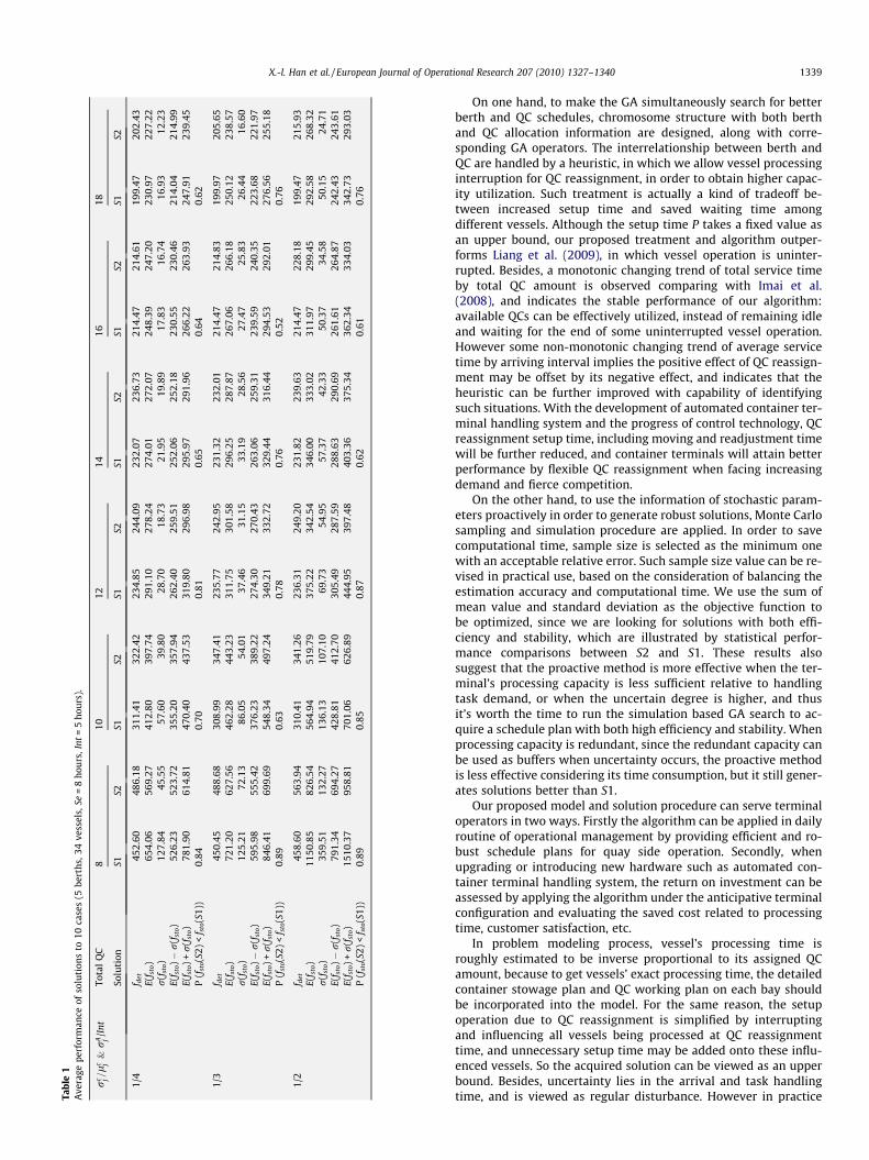
Results are shown in Table 1. On average, fdet(S2) is 5.67% worsethan fdet(S1), but E[fsto(S2)] is 6.27% better than E[fsto(S1)], andr[fsto(S2)] is 30.05% better than r[fsto(S1)]. As a result, whileE[fsto(S2)] � r[fsto(S2)] decreases by 1.47% from E[fsto(S1)] � r[fsto-

(S1)], E[fsto(S2)) + r(fsto(S2)) decreases by 9.56% from E[fsto(S1))+ r(fsto(S1)), which leads to the shrink of [l + r,l + r] range by8.09% from fsto(S1) to fsto(S2). Besides, there is an average probabilityof 73.21% that S2 has smaller total service and weighted delay timethan S1 under stochastic parameters. These values indicate thatthough S1 outperforms S2 when uncertainty does not exist, S2 out-performs S1 under stochastic circumstances in both average anddeviation aspects. As the degree of uncertainty, i.e. rC

j =lCj and

rAj =Int increases, these differences between S2 and S1 get more obvi-

ous, which makes S2 more preferable.

6. Conclusion

This paper addresses the problem of combining discrete berthand QC scheduling under uncertainty, which is quite importantfor container terminal operation for two reasons. Firstly, when per-forming quay side operation, there exists inherent interrelation-ship between the allocation and utilization of berth and QCs,which are the major valuable resources of the terminal and quiteoften the bottlenecks for serving vessel customers. So the opera-tional berth and QC schedules should be simultaneously consid-ered in decision making process. Secondly, the uncertainty isnaturally inevitable when planned schedules are executed in ter-minal system and has its influence on the actual performance ofterminal operation. Since the entire container terminal system iscapital intensive and complicated with lots of operational regula-tions, terminal operators tend to have risk aversion, and wish tomaintain a stable running of the whole system despite these uncer-tainties. In this paper we propose a method to cover these twoaspects.

Tabl

e1

Ave

rage

perf

orm

ance

ofso

luti

ons

to10

case

s(5

bert

hs,3

4ve

ssel

s,Se

=8

hour

s,In

t=

5ho

urs)

.

rc j=

lc j

&r

A j/I

ntTo

tal

QC

810

1214

1618

Solu

tion

S1S2

S1S2

S1S2

S1S2

S1S2

S1S2

1/4

f det

452.

6048

6.18

311.

4132

2.42

234.

8524

4.09

232.

0723

6.73

214.

4721

4.61

199.

4720

2.43

E(f s

to)

654.

0656

9.27

412.

8039

7.74

291.

1027

8.24

274.

0127

2.07

248.

3924

7.20

230.

9722

7.22

r(f

sto)

127.

8445

.55

57.6

039

.80

28.7

018

.73

21.9

519

.89

17.8

316

.74

16.9

312

.23

E(f s

to)�

r(f

sto)

526.

2352

3.72

355.

2035

7.94

262.

4025

9.51

252.

0625

2.18

230.

5523

0.46

214.

0421

4.99

E(f s

to)

+r

(fst

o)

781.

9061

4.81

470.

4043

7.53

319.

8029

6.98

295.

9729

1.96

266.

2226

3.93

247.

9123

9.45

P(f

sto(S

2)<

f sto

(S1)

)0.

840.

700.

810.

650.

640.

62

1/3

f det

450.

4548

8.68

308.

9934

7.41

235.

7724

2.95

231.

3223

2.01

214.

4721

4.83

199.

9720

5.65

E(f s

to)

721.

2062

7.56

462.

2844

3.23

311.

7530

1.58

296.

2528

7.87

267.

0626

6.18

250.

1223

8.57

r(f

sto)

125.

2172

.13

86.0

554

.01

37.4

631

.15

33.1

928

.56

27.4

725

.83

26.4

416

.60

E(f s

to)�

r(f

sto)

595.

9855

5.42

376.

2338

9.22

274.

3027

0.43

263.

0625

9.31

239.

5924

0.35

223.

6822

1.97

E(f s

to)

+r

(fst

o)

846.

4169

9.69

548.

3449

7.24

349.

2133

2.72

329.

4431

6.44

294.

5329

2.01

276.

5625

5.18

P(f

sto(S

2)<

f sto

(S1)

)0.

890.

630.

780.

760.

520.

76

1/2

f det

458.

6056

3.94

310.

4134

1.26

236.

3124

9.20

231.

8223

9.63

214.

4722

8.18

199.

4721

5.93

E(f s

to)

1150

.85

826.

5456

4.94

519.

7937

5.22

342.

5434

6.00

333.

0231

1.97

299.

4529

2.58

268.

32r

(fst

o)

359.

5113

2.27

136.

1310

7.10

69.7

354

.95

57.3

742

.33

50.3

734

.58

50.1

524

.71

E(f s

to)�

r(f

sto)

791.

3469

4.27

428.

8141

2.70

305.

4928

7.59

288.

6329

0.69

261.

6126

4.87

242.

4324

3.61

E(f s

to)

+r

(fst

o)

1510

.37

958.

8170

1.06

626.

8944

4.95

397.

4840

3.36

375.

3436

2.34

334.

0334

2.73

293.

03P

(fst

o(S

2)<

f sto

(S1)

)0.

890.

850.

870.

620.

610.

76

X.-l. Han et al. / European Journal of Operational Research 207 (2010) 1327–1340 1339

On one hand, to make the GA simultaneously search for betterberth and QC schedules, chromosome structure with both berthand QC allocation information are designed, along with corre-sponding GA operators. The interrelationship between berth andQC are handled by a heuristic, in which we allow vessel processinginterruption for QC reassignment, in order to obtain higher capac-ity utilization. Such treatment is actually a kind of tradeoff be-tween increased setup time and saved waiting time amongdifferent vessels. Although the setup time P takes a fixed value asan upper bound, our proposed treatment and algorithm outper-forms Liang et al. (2009), in which vessel operation is uninter-rupted. Besides, a monotonic changing trend of total service timeby total QC amount is observed comparing with Imai et al.(2008), and indicates the stable performance of our algorithm:available QCs can be effectively utilized, instead of remaining idleand waiting for the end of some uninterrupted vessel operation.However some non-monotonic changing trend of average servicetime by arriving interval implies the positive effect of QC reassign-ment may be offset by its negative effect, and indicates that theheuristic can be further improved with capability of identifyingsuch situations. With the development of automated container ter-minal handling system and the progress of control technology, QCreassignment setup time, including moving and readjustment timewill be further reduced, and container terminals will attain betterperformance by flexible QC reassignment when facing increasingdemand and fierce competition.

On the other hand, to use the information of stochastic param-eters proactively in order to generate robust solutions, Monte Carlosampling and simulation procedure are applied. In order to savecomputational time, sample size is selected as the minimum onewith an acceptable relative error. Such sample size value can be re-vised in practical use, based on the consideration of balancing theestimation accuracy and computational time. We use the sum ofmean value and standard deviation as the objective function tobe optimized, since we are looking for solutions with both effi-ciency and stability, which are illustrated by statistical perfor-mance comparisons between S2 and S1. These results alsosuggest that the proactive method is more effective when the ter-minal’s processing capacity is less sufficient relative to handlingtask demand, or when the uncertain degree is higher, and thusit’s worth the time to run the simulation based GA search to ac-quire a schedule plan with both high efficiency and stability. Whenprocessing capacity is redundant, since the redundant capacity canbe used as buffers when uncertainty occurs, the proactive methodis less effective considering its time consumption, but it still gener-ates solutions better than S1.

Our proposed model and solution procedure can serve terminaloperators in two ways. Firstly the algorithm can be applied in dailyroutine of operational management by providing efficient and ro-bust schedule plans for quay side operation. Secondly, whenupgrading or introducing new hardware such as automated con-tainer terminal handling system, the return on investment can beassessed by applying the algorithm under the anticipative terminalconfiguration and evaluating the saved cost related to processingtime, customer satisfaction, etc.

In problem modeling process, vessel’s processing time isroughly estimated to be inverse proportional to its assigned QCamount, because to get vessels’ exact processing time, the detailedcontainer stowage plan and QC working plan on each bay shouldbe incorporated into the model. For the same reason, the setupoperation due to QC reassignment is simplified by interruptingand influencing all vessels being processed at QC reassignmenttime, and unnecessary setup time may be added onto these influ-enced vessels. So the acquired solution can be viewed as an upperbound. Besides, uncertainty lies in the arrival and task handlingtime, and is viewed as regular disturbance. However in practice

1340 X.-l. Han et al. / European Journal of Operational Research 207 (2010) 1327–1340

there is another kind of irregular uncertainty of accidental events,like equipment break down or major delay caused by bad weather,etc. To incorporate such uncertainty into the problem may requiredifferent approaches like reactive or rescheduling. These two as-pects are our future research directions.

Acknowledgements

This research is supported by National Natural Science Founda-tion of China (Nos. 70771065, 70802040) and National High Tech-nology Research and Development Program of China (863Program) (Nos. 2009AA043000, 2009AA043001). Thanks are dueto two anonymous reviewers for comments that improved thequality of this paper.

Appendix. Sample generation procedure for stochasticparameters following normal distribution

The sample generation procedure for fnAj;rg; fn

Cj;rg ðr ¼ 1; . . . ; S;

j 2 eJÞ is as follows. uAj and uC

j are specified to be normal distribu-tion in computation experiment.

Step1. Generate 4 sets of [0,1] Uniform distributed numbers:fe1

1; . . . ; e1eJsg, fe2

1; . . . ; e2eJsg, fe3

1; . . . ; e3eJsg and fe4

1; . . . ; e4eJsg,

using 4 different seeds.Step2. Let

nAj;r ¼ lA

j þ rAj

ffiffiffiffiffiffiffiffiffiffiffiffiffiffiffiffiffiffiffiffiffiffiffiffiffiffiffiffi�2 ln e1

rþsðj�1Þ

qsinð2pe2

rþsðj�1ÞÞ;

nCj;r ¼lC

j þrCj

ffiffiffiffiffiffiffiffiffiffiffiffiffiffiffiffiffiffiffiffiffiffiffiffiffiffiffi�2lne3

rþsðj�1Þ

qsinð2pe4

rþsðj�1ÞÞðr¼1; . . .S; j2 JÞ:

References

Acar, Y., Kadipasaoglu, S.N., Day, J.M., 2009. Incorporating uncertainty in optimaldecision making: Integrating mixed integer programming and simulation to

solve combinatorial problems. Computers & Industrial Engineering 56 (1), 106–112.

Aytug, H., Lawley, M.A., McKay, K., Mohan, S., Uzsoy, R., 2005. Executing productionschedules in the face of uncertainties: A review and some future directions.European Journal of Operational Research 161 (1), 86–110.

Bierwirth, C., Meisel, F., 2010. A survey of berth allocation and quay cranescheduling problems in container terminals. European Journal of OperationalResearch 202 (3), 615–627.

Imai, A., Nishimura, E., Papadimitriou, S., 2001. The dynamic berth allocationproblem for a container port. Transportation Research Part B: Methodological35 (4), 401–417.

Imai, A., Sun, X., Nishimura, E., Papadimitriou, S., 2005. Berth allocation in acontainer port: Using a continuous location space approach. TransportationResearch Part B: Methodological 39 (3), 199–221.

Imai, A., Chen, H.C., Nishimura, E., Papadimitriou, S., 2008. The simultaneous berthand quay crane allocation problem. Transportation Research Part E: Logisticsand Transportation Review 44 (5), 900–920.

Kim, K.H., Moon, K.C., 2003. Berth scheduling by simulated annealing.Transportation Research Part B: Methodological 37 (6), 541–560.

Lee, D.H., Wang, H.Q., Miao, L., 2008. Quay crane scheduling with non-interferenceconstraints in port container terminals. Transportation Research Part E:Logistics and Transportation Review 44 (1), 124–135.

Liang, C., Huang, Y., Yang, Y., 2009. A quay crane dynamic scheduling problem byhybrid evolutionary algorithm for berth allocation planning. Computers &Industrial Engineering 56 (3), 1021–1028.

Meisel, F., Bierwirth, C., 2009. Heuristics for the integration of crane productivity inthe berth allocation problem. Transportation Research Part E: Logistics andTransportation Review 45 (1), 196–209.

Park, Y.M., Kim, K.H., 2003. A scheduling method for berth and quay cranes. ORSpectrum 25 (1), 1–23.

Sahinidis, N.V., 2004. Optimization under uncertainty: State-of-the-art andopportunities. Computers & Chemical Engineering 28 (6–7), 971–983.

Singer, M., 2000. Forecasting policies for scheduling a stochastic due date job shop.International Journal of Production Research 38 (15), 3623–3637.

Steenken, D., Voß, S., Stahlbock, R., 2004. Container terminal operation andoperations research – A classification and literature review. OR Spectrum 26(1), 3–49.

Tavakkoli-Moghaddam, R., Makui, A., Salahi, S., Bazzazi, M., Taheri, F., 2009. Anefficient algorithm for solving a new mathematical model for a quay cranescheduling problem in container ports. Computers & Industrial Engineering 56(1), 241–248.

Vis, I.F.A., de Koster, R., 2003. Transshipment of containers at a container terminal:An overview. European Journal of Operational Research 147 (1), 1–16.

Wang, F., Lim, A., 2007. A stochastic beam search for the berth allocation problem.Decision Support Systems 42 (4), 2186–2196.

Zhang, C., Zheng, L., Zhang, Z., Shi, L., Armstrong, A.J., 2010. The allocation of berthsand quay cranes by using a sub-gradient optimization technique. Computers &Industrial Engineering 58 (1), 40–50.