FDI and International Portfolio Investment - Complements ... · control position FDI yields a higher return than FPI. Hence, there is a trade-o⁄ between ⁄exibility and higher

FDI and International Portfolio Investment -Complements or Substitutes?

Barbara Pfe¤erUniversity of Siegen

pfe¤[email protected]

August 21, 2007

Abstract

We show in a dynamic investment setting whether �rms choose FDIor international portfolio investment (FPI) in the presence of stochasticproductivity taking into account di¤erences in �exibility of both invest-ments. Isolated FPI and FDI investments are compared to combined FPIand FDI investments. FDI requires higher investment speci�c costs thanFPI. Thus, it is not possible to adjust FDI to environmental changes everyperiod. In contrast, FPI bears lower �xed costs and can be adjusted im-mediately to short-term changes in the environment. Additionally, as aresult of the investors� control position FDI yields a higher return thanFPI. Hence, there is a trade-o¤ between �exibility and higher return for�rms deciding between FDI and FPI. We explore whether as a consequenceof higher investment speci�c �xed costs and lower �exibility in the caseof FDI, small �rms prefer FPI and larger �rms invest in FDI. We showthat a combined strategy dominates the isolated strategy always in time.Further, combined international investment comprises a higher incentivefor �rms to invest in R&D-investment and consequently �rm productivityincrease faster than with isolated international investment. Depending onthe success-probability and the correlation between the various investmentpossibilities, even small �rms (low productivity) invest in FDI.

1

PreliminaryPlease, do not quote

1 Introduction

The recent World Investment Report 2006 highlights that Foreign Direct In-vestment (FDI) �ows and growing FDI stocks are now at an unparalleled levelwith most going to industrial countries. At the same time �ows of internationalportfolio investments (FPI) exceeded FDI �ows twice at the beginning of thenineties while more recently FPI growth slowed down and both capital �owsconverged.1 What are the motives for �rms to invest in one or the other andhow are they to be explained?Previous studies on FDI explained the motives for FDI with di¤erential

rates of return, di¤erences in interest rates and risk diversi�cation.2 FollowingAndersen and Hainaut (1998) these determinants lost explanatory power andrecent theoretical and empirical studies document that FDI is undertaken toexploit cost advantages (vertical FDI)3 or to serve di¤erent markets locally toavoid trade costs (horizontal FDI).4 If FDI no longer serves risk diversi�cation,does FPI then �ll the gap and are these capital �ows complements rather thansubstitutes?In the present paper we analyse whether �rms choose FDI or FPI in the

presence of stochastic productivity taking into account di¤erences in �exibilityof both investments. In particular FDI is less �exible than FPI and this reduced�exibility entails a higher rigidity of FDI. As FDI requires higher investmentspeci�c costs it is not possible to adjust FDI to environmental changes every pe-riod.5 In contrast, FPI bears lower �xed costs and can be adjusted immediatelyto short-term changes in the environment. However, as a result of the investors�control position FDI yields a higher return than FPI. Hence, there is a trade-o¤between �exibility and higher return for �rms deciding between FDI and FPI.We explore whether as a consequence of higher investment speci�c �xed costsand lower �exibility in the case of FDI, small �rms prefer FPI and larger �rmsinvest in FDI.We show that the combined investement strategy (FDI and FPI at the same

time) always starts the international investment activity earlier in time thanthe isolated strategy (FDI or FPI). Additionally, with combined internationalinvestment, there is a higher incentive for �rms to invest in R&D-investment andconsequently �rm productivity increases faster than with isolated international

1See WTO News, October 1996.2See for example Dunning (1973).3Grossman, Helpman, Szeidl (2005) discuss in which states �rms decide to outsource or

o¤shore some of their production stages. Acemoglu, Aghion,Gri¢ th and Zilibotti show thatvertical integration is more common if the technology intensity di¤ers signi�cantly.

4See Helpman, Melitz, Yeaple (2003) for a detailed survey whether �rms decide to servea foreign market through export or FDI. Studies of complex FDI strategies can be found forexample in Helpman (2006) or Grossman, Helpmann, Szeidl (2003).

5See Goldstein and Razin (2005) for a discussion of the di¤erent costs for FDI and FPI.

2

investment. Depending on the success-probability and the correlation betweenthe various investment possibilities, even small �rms (low productivity) investin FDI.To model �rm behaviour we use a monopolistic competition framework with

uncertain �rm productivity in combination with a dynamic investment approachover a �nite investment horizon. There are three countries, home and twoforeign countries. The �rms are located in the home country and decide toinvest via FDI or FPI in the foreign countries. Thereby, they face uncertaintyabout their future productivity and returns on the respective investment. Inparticular, �rm productivity is endogenous and follows a Poisson process. Theproductivity of the di¤erent investment opportunities are correlated with eachother. Di¤erences in correlation between FDI and home production account fordi¤erent forms of FDI.6

The reminder of the paper is organized as follows. In section two, we givea short overview of the recent literature and emphasize our contribution toit. Section three outlines the theoretical framework and derives the optimalityconditions for the various investments strategies. Following this, we present thenumerical solution of the model and discuss the results in section four. Finally,section �ve concludes.

2 The Literature

In the paper we link the information based trade-o¤ literature between FDI andFPI by Goldstein and Razin (2005) (RG) and Albuquerque (2003) with the �rm-level Export and FDI approaches by Grossman, Helpman and Szeidl (2003) andHelpman, Melitz and Yeaple (2003). RG analyse the investors�decision betweenFDI and FPI under asymmetric information in a static model.7 As a result ofthe information asymmetry the project revenue from FDI is higher than fromFPI. In the case of FDI the investor is also the manager of the foreign �rm.Hence, he has a higher control over the production processes and can ensurethat the �rm is run according to the investors�interests. If the investor choosesFPI the investor has no control over the foreign production process and theexpected return is lower. We use these di¤erent characteristics shown by RGto motivate the costs, �exibility and return of the di¤erent investment possi-bilities in the present paper. Additionally, we consider the �ndings of Chuhan,Perez-Quiraz and Popper (1996). They provide an empirical analysis on thedi¤erent characteristics of short term and long term capital �ows. Furthermore,in contrast to RG, we introduce a long-term investor in a dynamic setting. Thisinvestor has the possibility to adjust his portfolio periodically with rigidity inFDI-shares. Hence, we also account for the di¤erent grades of �exibility of bothinvestments.

6Aizenman and Marion (2001) as well as Markusen and Maskus (2001) show that horizontalFDI is established in countries similar in size and endowments, while vertical FDI is thepreferred investment in countries with di¤erent characteristics as the source country.

7See also Razin, Mody and Sadka (2002) and Razin (2002).

3

Alburquerque (2003) analyses from a country perspective the risk-sharingcharacter of FDI and non-FDI capital �ows for countries with di¤erent degreesof �nancial constraints. Thereby, non-FDI �ow adjustments arise from shocksin the receiving country. One result is that for �nancially constrained countriesFDI is less volatile than non-FDI �ows. With perfect enforcement, the di¤erencein volatility diminishes. We modify this approach by taking the �rm perspectiveand consider shocks on �rm level as well as on host country level. Actually, wealways �nd a higher volatility of non-FDI �ows (FPI) than FDI �ows in our�rm-level perspective. The �rm reacts to any short-term environment changeby adjusting FPI. Precisely, FPI has the main function to smooth risk whereasFDI mainly exploits gains from technology transfers.Uncertain �rm productivity is decisive for the results of our model. This

leads to the literature around Melitz (2003) or Grossman, Helpman and Szeidl(2003). They motivate the �rms�choice to export or engage in FDI with dif-fering �rm productivity. Melitz (2003) shows that with heterogeneous �rmsonly the large �rms (with higher productivity) export. Small �rms serve thedomestic market only. Furthermore, Helpman, Melitz and Yeaple (2003) extendthis and �nd that �rms with higher productivity use higher integrated organi-sational production structures. They show that less productive �rms only servethe domestic market, with increasing productivity �rms start to export and �-nally the most productive �rms engage in FDI. In contrast to this literature, inthe present paper �rm productivity is endogenous. Firms can push their pro-ductivity by investing in research and development (R&D). The success of theR&D-investment is uncertain. Moreover, we extend these models by introducingFPI as a new form of investment possibility.

3 Theoretical Framework

The dynamic methodology in the model follows roughly the models of Abel(1973) and Holt (2003).Firms optimize their investment decisions in a continuous-time model. In-

spired by Melitz (2003), the model is based on monopolistic competition withstochastic �rm productive. Domestic demand is exogenous and the consumershave Dixit-Stiglitz preferences. There are three countries. Two of these coun-tries are northern countries West (home country) and East (foreign). The thirdcountry is a southern country (foreign). In the eastern country, cultural back-ground, production and cost structure are similar to the home country. Hence,the productivities in these countries are positive correlated. On the opposite,the South has di¤erent cultural background, production and cost structure thanthe home and the eastern country. Consequently, the productivity correlationsbetween South and home or South and East are negative.We consider a setting in which a representative �rm faces a choice between

performing activities at home (production and R&D-investment) and engagingin two alternative foreign investments: foreign portfolio investment (FPI) orforeign direct investment (FDI). The initial position of each �rm is home pro-

4

duction and home R&D investment. Based on these home activities the �rm canadditionally choose to invest internationally. Whether a �rm decides to investinternationally depends on the �rm�s speci�c productivity �. In particular, the�rm can increase its speci�c productivity by investing in home research and de-velopment (R&D). Whether R&D-investment increases the �rm�s productivity isuncertain. The change of � through R&D-investment follows a Poisson-Process

d� =

�(1� �) �t

Kt

��dq. (1)

In (1) � is the capital invested in R&D and K is the total stock of capitalavailable to the �rm. As obsolete technologies have to be replaced, patent lawsare renewed etc., even in case of successful R&D-investment, the growing rateof � is smaller than the invested rate of capital. These costs correspond todepreciation and are depicted by � . Finally q is a random variable that equals1 with probability � and 0 otherwise. Hence, if R&D-investment is successful, �

increases byh(1� �) �K

i�. With probability (1� �) R&D-investment fails and

� stays unchanged.As every �rm, no matter whether it engages in FDI, FPI or not, produces

at home and serves the home market, we start with the analysis of the homecountry.

3.1 Home

3.1.1 Production

The �rm uses a single factor, capital, to produce output at home xh

xh (�) = �h�kh��. (2)

The superscript h states that these are the values in the isolated "Home"-scenario.8 According to (1), �rms also can use capital to invest in R&D andincrease their productivity

K = kh + �. (3)

As a consequence of monopolistic competition, �rms choose the pro�t maximising-price

pt =1

'�t. (4)

Where the rent for capital is set equal to one, 1' is the pro�t maximizing markup and 1

�tare the marginal costs of a �rm with productivity �t. Furthermore,

the �rm has �xed costs of home production equal to fh and costs of R&D-investment equal to �. Hence, the pro�t of the �rm at home in period t is

�t (�t) = pt�t�kht�� fh + xht

�t+ �t

�, 0 < � < 1. (5)

8The following scenarios with isolated FPI, FDI and the combined investments are identi-�ed by the superscripts p, d, and c respectively.

5

The �rst term on the right hand side equals the revenue from production andsales at the home market, rht . The second term on the right hand side summa-rizes the costs of home production and R&D investment.The expected value of �rm pro�ts is

V h (�t) = maxkhs ; �s

Et

TZt

�s (�s) e��(s�t)ds. (6)

subject to (2) - (4). Modi�cation of (6) yields:

�V h (�t) dt = maxkhs ; �s

�t (�t) dt+ Et�dV h

�(7)

which states that the mean required return of a �rm equals the expected return.In period t, the expected return consist of the maximized pro�t at t and theexpected gain or loss of the future pro�t �ow.To calculate the expected capital �ow, we substitute (1) into dV h:

Et�dV h

�= �

�V h ( �)� V h (�)

�dt (8)

with � (1� �) �K .9 Equation (8) is the expected capital �ow. The expected

capital �ow is a perpetual �ow of the di¤erence between the capital �ow in caseof successful R&D investment V h ( �) and without successfull R&D investmentV h (�) weigthed with the success-probability. Substituting (8) back into (7) anddivide by dt leads to

�V h (�) = maxkhs ; �s

�� (�) + �

�V h ( �)� V h (�)

�. (9)

There are two important features about (9) which one should keep in mindthorough the following analysis. Firstly, all important information about thepast concerning current or future decisions are summarized in �. How the �rmreached the present productivity does not matter at all. Secondly, choosing theoptimal production and R&D-investment strategy with respect to the problemstarting at the current productivity level � that results from the initial �rmstrategies, is the optimal strategy no matter what the initial strategy of the�rm was.

3.1.2 Optimality Conditions for R&D-Investment and ProductionStrategies

From (9) we can derive the optimality conditions for �rm-strategies for R&D-investment and home production.

9For a detailed derivation see Appendix A.

6

R&D-Investment Deriving the marginal valuation of R&D-investment from(9) yields

�� (�) + �Vh� ( �) = 0. (10)

The second part of the brackets of (9) disappears, as V h (�) does not depend onthe current �. Rearranging (10) delivers:10

V h� ( �) =1

�

"1�

rh� (�)

!

#. (11)

The marginal valuation of R&D-investment is a perpetual �ow equal to one mi-nus the revenue changes caused by �, discounted by the probability of successfulR&D-investment.

Home Production Di¤erentiating the right hand side of (9) with respect tokh, we obtain

�kh (�) + ��V hkh ( �)� V

hkh (�)

�= 0

rkh (�)

!+ �

�V hkh ( �)� V

hkh (�)

�= 0

V hh ( �) = V hh (�)�1

�

�rhh (�)

!

�. (12)

The subscripts unequal to t stand for the partial derivation. For simplicity, inthe following cases the derivation subscripts are shortened to h for the derivationwith respect to capital invested in home production (respectively p for invest-ment in FPI, d for investment in FDI) instead of kh (respectively kp; kd). Themarginal valuation of production-investment, in the case of R&D-investmentequals the marginal valuation of production-investment with no R&D- invest-ment minus the marginal revenue stream resulting from increased capital inproduction - discounted with the probability of successful R&D-investment. Itis V hh (�) minus the revenue stream, as the valuation of k

h in case of additionalinvestment in R&D is examined. Analysing just the valuation of kh without theincreased productivity would be V hh (� ) plus the revenue stream.An optimal strategy requires that the marginal valuation of investment in

production equals the marginal valuation of R&D-investment. We can derivean explicit marginal valuation for investment in production by equating (12)and (11), namely

V hh (�) =1

�

"1 +

rhh � rh�!

#. (13)

Similar to (11) the marginal valuation of investment in production equals a �owconsisting of one plus the di¤erence between the revenue change caused by thetwo investment decisions. Again, this �ow is discounted by the probability ofsuccessful R&D investment.10For mathematical details see Appendix B.

7

There is a trade-o¤ between investing in R&D or not. First of all, investingin R&D reduces the capital available to invest in domestic production. Thise¤ect is negative. But secondly, R&D-investment increases productivity andhigher productivity enforces the output of the employed production-capital anddecreases the variable production costs x

� . Hence, there is also a positive ef-fect of R&D-investment on the marginal valuation of capital invested in home-production. These considerations are re�ected in the second part of (13).

3.2 Home and Foreign Portfolio Investment

3.2.1 Production and FPI

Now, we analyse the investment decision of the �rm and give it an additionalinvestment alternative, namely foreign portfolio investment (FPI). With FPIequation (3) changes to

Kt = kht + kpt + �t. (14)

This shows that the total capital available to a �rm can be used to invest indomestic production, R&D-investment (the same as in the scenario above) andadditionally kp is the capital invested in FPI. As the �rm invests in FPI, it gainsownership on a foreign �rm. But the domestic �rm has no - or only in�nitelysmall - possibility to exert control over the foreign production and managementprocess. Thus the domestic �rm can not directly in�uence the foreign revenueand the gained dividend

rpt = �t (kpt ) . (15)

�t is the return rate from FPI (or the productivity of capital invested in FPI).It varies with

d�

�= ��dz� (16)

where dz is a Wiener process with mean zero and unit variance. Following (15)and (16), the only impact the home �rm has on the foreign investment, is thedecision of how much capital to invest in FPI.Investment in FPI requires to buy assets, time to select the appropriate

assets, additional administration systems and e¤orts etc. All these e¤orts aresummarized as �xed costs fpt for this investment. Yet the pro�t function for the�rm (5) changes to


�t+ �t

�+ rpt � f

pt . (17)

Following the steps in the home-scenario we get the multi-period optimizationproblem for the �rm

�V p (�t) dt = maxkhs ;k

pt ; �s

�t (�t) dt+ Et (dVp) (18)

subject to (2), (4) and (14) - (16). As the �rm is now in the FPI-scenario, thesuperscript changed to p and there is one more control variable, namely kpt . The

8

expected future capital �ow depends on two state variables �t and �t:

dV p = V p� d� + Vp� d�+

1

2V p�� (d�)

2+ V p�� (d�) (d�) . (19)

Thus in case of FPI investment, the expectation of the change in the expectedcapital �ow consists of three parts

E (dV p) = � [V p ( �)� V p (�)] dt+�1

2�2�2�V

p��

�dt+

hV p�� ( �) (��) �

pidt.

(20)The �rst part is similar to the expected capital �ow in the Home-scenario.Additionally, the variations of the foreign return impacts V p. This impact occursin the second term. Finally, the third term accounts for common variationsof home productivity and foreign productivity that can result from global orindustry shocks. The direction of this correlation depends on �p � (dq) (dz�) 6=0. If the �rm invests FPI in the East, �p is positive and is negative with FPI inthe southern country.In case of FPI, the present value of the �rm pro�t �ows is

�V p (�) = maxkhs ;k

pt ; �s

[�p (�) + � [V p ( �)� V p (�)] + "] (21)

with " � "1 + "2, "1 � 12�

2�2�Vp�� and "

2 � V p�� ( �) (��) �p. The uncertain

foreign productivity in�uences the present value of the pro�t �ows twice. Firstly,the isolated variation of the foreign productivity "1 enters the capital �ows andsecondly, the common variation of home and foreign productivity "2 changes thecapital �ows. Whereas, the home productivity change is a discrete shock and" is continuous. Similar to (9), all necessary information for any decision aresummarised in � and �. Further, any optimality of future decision on FPI, homeproduction or R&D-investment is independent of the �rms�initial decision.

3.2.2 Optimality Conditions with FPI

R&D-Investment With FPI the marginal valuation of R&D-investment changesto

V p� ( �) =1

�

"1�

rh�!� �

#(22)

where � =@(V p

��12�

2�2�)@� +

@(V p��( �)(��)��)

@� . FPI does not have any direct impacton the R&D-investment. In comparison to the pure Home-scenario, the marginalvaluation of R&D-investment is reduced by �. This e¤ect arises through thecommon variation of the home and foreign productivities. If the �rm invests intoclosely related industries or even in the same industry (eastern country) then theown risk is not reduced. Thus � is positive and reduces the marginal valuation ofR&D-investment slightly but never completely compensates it. Contrary, withinvestment in a dissimilar industry (South) the risk of R&D failure is diversi�ed.� is negative and increases the valuation of R&D-investment.

9

Home Production The direct valuation of home production is unchanged

V ph ( �) = V hh (�)��1

�

rhh (�)

!

�. (23)

Following the optimality principle, we can equate the marginal valuation ofinvestment in home production with the marginal valuation of R&D-investmentand get

V ph (�) =1

�

"1 +

rhh � rh�!

� �#. (24)

Similar to (22), the valuation changes by �. Again, the change depends on theindustry invested in.

FPI Optimality requires that the marginal valuation of FPI also equals themarginal valuation of investment in home production and R&D-investment.Therefore we di¤erentiate (21) with respect to kprearranging delivers

V pp ( �) = V pp (�)�1

�

�rpp + "p

�. (25)

Valuation of FPI is lower with investment located in the East (similar produc-tion and cost structure, "p > 0) than with investment located in the South(di¤erent factor endowment, production and cost structure "p < 0). Obviously,the diversi�cation of the risk increases the valuation of the investment abroad.

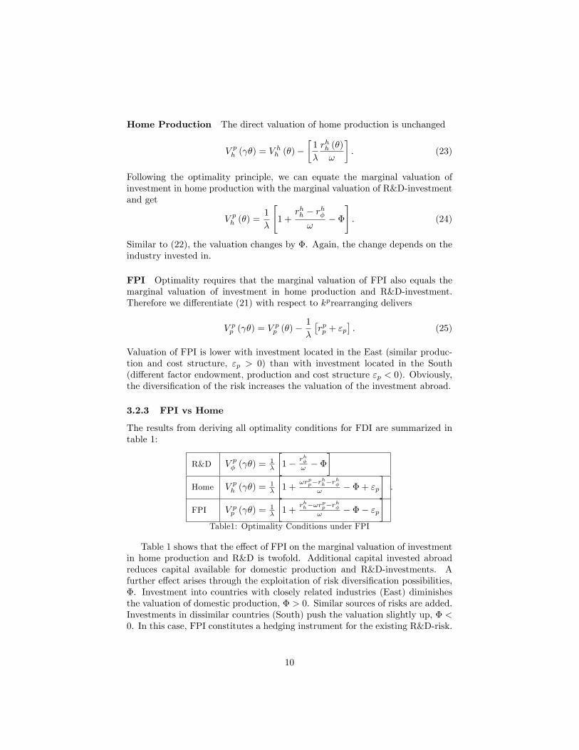
3.2.3 FPI vs Home

The results from deriving all optimality conditions for FDI are summarized intable 1:

R&D V p� ( �) =1�

�1� rh�

! � ��

Home V ph ( �) =1�

�1 +

!rpp�rhh�r

h�

! � �+ "p�

FPI V pp ( �) =1�

�1 +

rhh�!rpp�r

h�

! � �� "p� .

Table1: Optimality Conditions under FPI

Table 1 shows that the e¤ect of FPI on the marginal valuation of investmentin home production and R&D is twofold. Additional capital invested abroadreduces capital available for domestic production and R&D-investments. Afurther e¤ect arises through the exploitation of risk diversi�cation possibilities,�. Investment into countries with closely related industries (East) diminishesthe valuation of domestic production, � > 0. Similar sources of risks are added.Investments in dissimilar countries (South) push the valuation slightly up, � <0. In this case, FPI constitutes a hedging instrument for the existing R&D-risk.

10

Finally, the additional variation of a further unit capital invested in FPI,"p, impacts the valuation of home production. At the same time, "p a¤ectsthe valuation of FPI in the opposite direction. The marginal valuation of homeproduction increases with further FPI in the East, "p > 0 and decreases with ad-ditional southern FPI. Eastern FPI delivers additional variation and risk. Homeproduction is valued higher as it is a more secure source of future capital �ows.11

FPI in the South hedges existing home risk and consequently the valuation ofhome production decreases, "p < 0.12 Additional southern FPI dampens theR&D risk and enforces further R&D investments. The �rm withdraws capitalfrom home production and invests the available capacities into southern FPI.Hence, with isolated investment possibilities the �rm will engage in southern

FPI.

3.3 Home and Foreign Direct Investment

In the case of FDI, the home �rm takes ownership as well as control over the for-eign �rm and thus can in�uence the pro�t of its FDI-investment. In the presentpaper, the �rm only transfers capital to the foreign �rm. No intermediate goodsare traded. However, the choice of the FDI receiving country has a signi�cantimpact on the valuation of FDI.If the home �rm decides for FDI it also transfers intangible assets, as for

example managerial skills, technology..., to the foreign �rm. As a side e¤ect ofthis asset transfer a part of the home productivity directly enters the return ofFDI

rdt = 2t �1at

�kdt�; 0 < a < 1. (26)

Home productivity � does not impact the foreign investment to the same extent,than home production. This can be caused by country speci�c conditions orincomplete mobility of some home skills.13 The impact of home productivityon FDI return increases with country similarity. is the foreign productivitywhich is stochastic and varies with

d = � dz . (27)

Again, dz is Wiener process with mean zero and unit variance. The amountof capital invested in FDI is kd. Hence equation (3) becomes

Kt = kht + kdt + �t. (28)

Further, FDI requires some speci�c up-front costs like country and market re-search, a merger or building a new plant. All these activities are costly andsummarized in fd, as the �xed costs arising from FDI. Now the modi�ed pro�tfunction of the home �rm is


�t+ �t

�+rdt!� fdt . (29)

11FPI valuation decreases through the same e¤ect.12 In this case, the valuation of FPI increases.13With a!1, the FDI scenario would be the same than the FPI scenario.

11

It is important to keep in mind, that the FDI �x costs, fd exceed the FPI �xcosts, fp.The dynamic optimization problem of the home �rm is

�V d (�) dt = maxkh;kd;�

��d (�) dt+ Et

�dV d

��. (30)

Equation (30) is a function of the state variables home productivity � as wellas foreign productivity : The control variables are the three investment pur-poses, kh; kd; �. The derivation of the functional equation from (30) is analogueto the steps in the FPI-scenario. Thus, we get

�V d (�) = maxkh;kd;�

��d + �

�V d ( �)� V d (�)

�+ �

�(31)

with � � �1+�2, �1 � 12�

2

2V d , �2 � V d � ( � ) ( �) �

d and �d � (dz )(dq).Analogue to the FPI scenario, the uncertainty of the foreign productivity hastwo impacts on the present value of the pro�t �ows: the variation of the for-eign productivity �1 and the common variation of the foreign and the homeproductivity �2. All necessary information for any decision is included in � and .

3.3.1 Optimality Conditions with FDI

R&D-Investment Following the same steps as in the two previous scenarioswe get the marginal valuation of additional R&D-investment

V d� ( �) =1

�

"1�

rh� � !rd�!

� {#. (32)

First, there is a additional impact of FDI on the marginal valuation of R&D-investment. It is a very small positive e¤ect through a slight increase in theforeign revenue. In comparison to the isolated home-scenario, this marginalchange in rd again increases the marginal valuation of R&D-investment.Secondly, the in�uence of � on the foreign productivity is included in { �

@�1

@� +@�2

@� . The sign of { is not de�nite. The degree (1a ) of the home productivity

in�uence on foreign revenue is decisive for {.

Proposition 1 If a is su¢ cient high (low control over foreign �rm - low impactof � on rd), then { in the case of eastern FDI { < 0 and with FDI in the South{ > 0.

The overall e¤ect of eastern FDI increases the valuation of domestic R&D-investment, southern FDI decreases it. Horizontal FDI is mostly undertakenamong industrial countries (East). For these countries, production structure,factor endowments and business-culture are relatively similar. Thus, increasedproductivity at home transfers very easily to the foreign a¢ liate. On the otherhand, technology transfer with horizontal FDI in countries with di¤ering pro-duction and cost structures is rather complicated and depends strongly on the

12

cost structure of the di¤erent countries.14 Therefore, the implementation of newtechnologies - developed for domestic production - is not as easy with FDI inthe South as in the case of eastern FDI.

Proposition 2 If a is su¢ cient low (high control over foreign �rm - high impactof � on rd), then { in the case of eastern FDI { > 0 and with FDI in the South{ < 0.

A strong control position and high skills facilitate the entering of new mar-kets even in the south. High control is not necessary for FDI in a very similarinvestment location.

Home Production As expected from the previous section, home productionstays unchanged again

V dh ( �) = V dh (�)�1

�

�rhh (�)

!

�. (33)

Substituting equation (32) into the marginal valuation of investment in homeproduction delivers

V dh (�) =1

�

"1 +

rhh � rh� � !rd�!

� {#. (34)

The changes in � a¤ect directly the FDI revenue and indirectly the variationsof the productivity of FDI. The reduction of the marginal valuation of theinvestment in home production is not as high as under FPI. In the current case,R&D-investment does not only diminish the capital available for FDI it alsoincreases the productivity of capital invested in the foreign �rm. Further, thesign of { depends on the FDI location.

FDI To derive the optimality condition for FDI, we di¤erentiate (31) withrespect to kd. This yields

V dd ( �) = V dd (�)�1

�

�rdd + �d

�. (35)

Equation (35) shows that the marginal valuation of FDI in case of successfulR&D-investment depends again on the FDI location. If the �rm invests ineastern FDI then the term in the brackets remains positive and hence reducesthe valuation. On the other hand, if the �rm undertakes southern FDI thesign of � changes. But the indirect e¤ect through � is weaker than the directe¤ect of the changed revenue. Thus the valuation is still reduced but not asmuch as in the case of FDI in the East. Generally, we observe a decreasingmarginal product of capital either invested in domestic production or investedin foreign production. With a negative correlation between domestic and foreignproductivity at hand, the decrease of the marginal product invested in FDI isdamped.14Grossman, Helpman and Szeidl (2003) show that under di¤erent cost structures in the

observed countries, �rm strategies changes from horizontal to vertical FDI and vice versa.

13

3.3.2 FDI vs Home

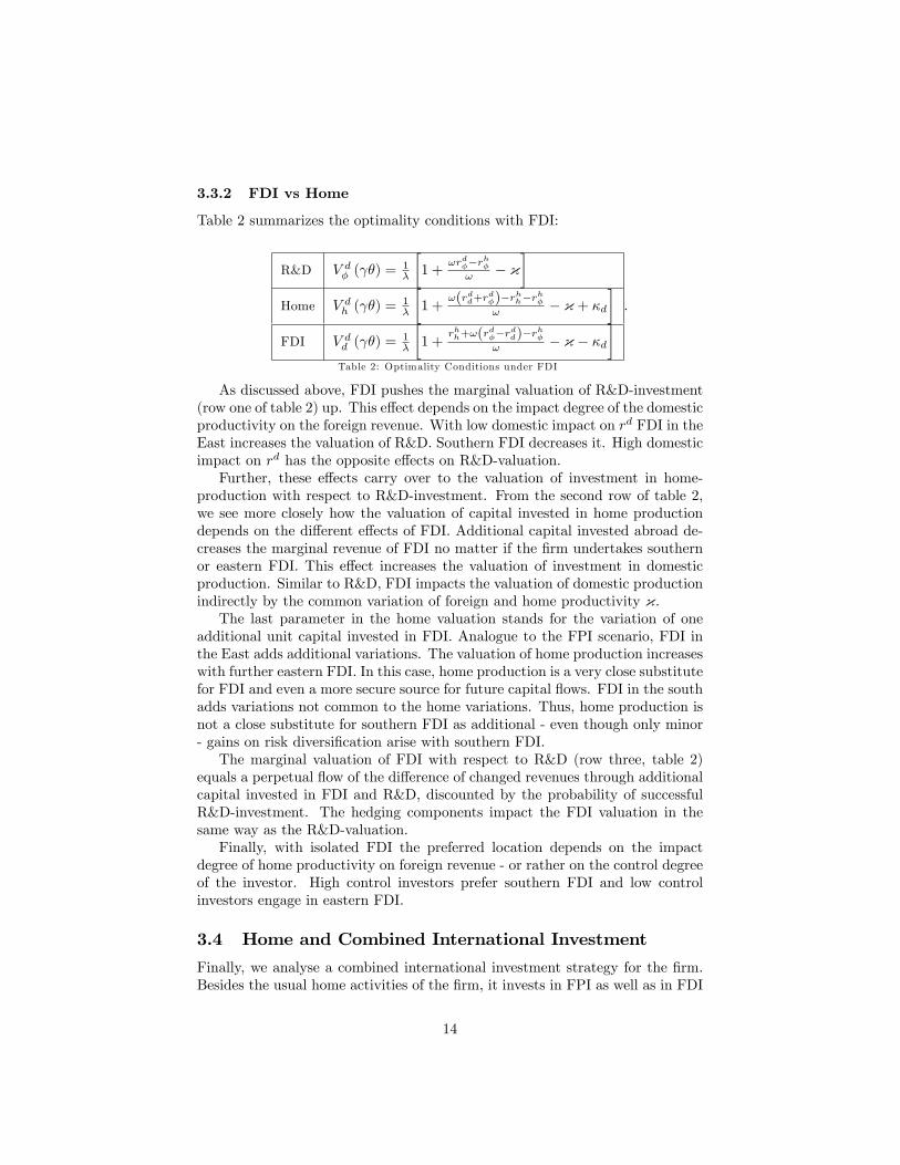
Table 2 summarizes the optimality conditions with FDI:

R&D V d� ( �) =1�

�1 +

!rd��rh�

! � {�

Home V dh ( �) =1�

�1 +

!(rdd+rd�)�r

hh�r

h�

! � { + �d�

FDI V dd ( �) =1�

�1 +

rhh+!(rd��r

dd)�r

h�

! � { � �d�

Table 2: Optimality Conditions under FDI

.

As discussed above, FDI pushes the marginal valuation of R&D-investment(row one of table 2) up. This e¤ect depends on the impact degree of the domesticproductivity on the foreign revenue. With low domestic impact on rd FDI in theEast increases the valuation of R&D. Southern FDI decreases it. High domesticimpact on rd has the opposite e¤ects on R&D-valuation.Further, these e¤ects carry over to the valuation of investment in home-

production with respect to R&D-investment. From the second row of table 2,we see more closely how the valuation of capital invested in home productiondepends on the di¤erent e¤ects of FDI. Additional capital invested abroad de-creases the marginal revenue of FDI no matter if the �rm undertakes southernor eastern FDI. This e¤ect increases the valuation of investment in domesticproduction. Similar to R&D, FDI impacts the valuation of domestic productionindirectly by the common variation of foreign and home productivity {.The last parameter in the home valuation stands for the variation of one

additional unit capital invested in FDI. Analogue to the FPI scenario, FDI inthe East adds additional variations. The valuation of home production increaseswith further eastern FDI. In this case, home production is a very close substitutefor FDI and even a more secure source for future capital �ows. FDI in the southadds variations not common to the home variations. Thus, home production isnot a close substitute for southern FDI as additional - even though only minor- gains on risk diversi�cation arise with southern FDI.The marginal valuation of FDI with respect to R&D (row three, table 2)

equals a perpetual �ow of the di¤erence of changed revenues through additionalcapital invested in FDI and R&D, discounted by the probability of successfulR&D-investment. The hedging components impact the FDI valuation in thesame way as the R&D-valuation.Finally, with isolated FDI the preferred location depends on the impact

degree of home productivity on foreign revenue - or rather on the control degreeof the investor. High control investors prefer southern FDI and low controlinvestors engage in eastern FDI.

3.4 Home and Combined International Investment

Finally, we analyse a combined international investment strategy for the �rm.Besides the usual home activities of the �rm, it invests in FPI as well as in FDI

14

at the same time. Because there are four di¤erent investment alternatives forcapital, (3) changes to

Kt = kht + kpt + k

dt + �t. (36)

The return functions of the international investments are similar to the returnfunctions under isolated international investment. Hence, the �rms�pro�t func-tion with combined international investment is15

�ct (�t) = pt�t�kht�� fh + xht

�t+ �t

�+ rpt � f

pt + r

dt � fdt . (37)

and the dynamic �rm problem is:16

�V c (�) dt = maxkh;kp;kd;�

[�c (�) dt+ Et (dVc)] . (38)

The control variables in the dynamic combined optimization problem are thevarious investment purposes: investment in domestic production kh, R&D-investment � and the two international investment alternatives FPI kp andFDI kd. Further, in the combined scenario the present value of the �rms capital�ows is a function of the three state variables: home productivity �, productiv-ity of the portfolio investments � and the productivity of the direct investment . These three variables summarize all the necessary information for an optimalinvestment-decision in the present period. We need the functional equation ofthe optimizing problem (38) to derive the optimality conditions. Again, thesteps are very similar to the isolated investment strategies and therefore, weneglect them and directly turn to the functional equation

�V c (�) = maxkh;kd;�

[�c + � [V c ( �)� V c (�)] + "+ �+ �] (39)

where � � V c� (��) ( � ) �c and �c � (dz�) (dz ). In (39) we have the invest-

ment e¤ects of the isolated international strategies combined. Additionally, thecommon variation of the two international investments is included through �.

3.4.1 Optimality Conditions with Combined International Invest-ment

R&D-Investment Following (39), the optimality condition for R&D-investmentchanges slightly in comparison to the isolated scenarios:

V c� ( �) =1

�

"1�

rhc� � !rdc�!

� �� { � ��

#. (40)

The �rst part of the bracket stays unchanged. Also, the isolated e¤ects ofthe di¤erent investment possibilities, � and {, are the same as above. But the15We have to keep in mind that fd > fp still holds.16We will keep the detailed transforming-steps very short as the necessary steps for the

transformation are similar to the steps undertaken in the previous isolated section.

15

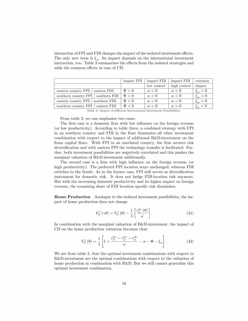
interaction of FPI and FDI changes the impact of the isolated investment e¤ects.The only new term is ��. Its impact depends on the international investmentinteraction, too. Table 3 summarizes the e¤ects from the isolated strategies andadds the common e¤ects in case of CII.

impact FPI impact FDI impact FDI commonlow control high control impact

eastern country FPI / eastern FDI � > 0 { < 0 { > 0 �� > 0

southern country FPI / southern FDI � < 0 { > 0 { < 0 �� > 0

eastern country FPI / southern FDI � > 0 { > 0 { < 0 �� < 0

southern country FPI / eastern FDI � < 0 { < 0 { > 0 �� < 0Table 3: Impact of di¤erent International Investment Possibilities

From table 3, we can emphasize two cases.The �rst case is a domestic �rm with low in�uence on the foreign revenue

(or low productivity). According to table three, a combined strategy with FPIin an southern country and FDI in the East dominates all other investmentcombination with respect to the impact of additional R&D-investment on the�rms capital �ows. With FPI in an unrelated country, the �rm secures riskdiversi�cation and with eastern FPI the technology transfer is facilitated. Fur-ther, both investment possibilities are negatively correlated and this pushes themarginal valuation of R&D-investment additionally.The second case is a �rm with high in�uence on the foreign revenue (or

high productivity). The preferred FPI location stays unchanged; whereas FDIswitches to the South. As in the former case, FPI still serves as diversi�cationinstrument for domestic risk. It does not hedge FDI-location risk anymore.But with the increasing domestic productivity and its higher impact on foreignrevenue, the remaining share of FDI location speci�c risk diminishes.

Home Production Analogue to the isolated investment possibilities, the im-pact of home production does not change

V ch ( �) = V ch (�)�1

�

�rhch (�)

!

�. (41)

In combination with the marginal valuation of R&D-investment, the impact ofCII on the home production valuation becomes clear

V ch (�) =1

�

"1 +

rhch � rhc� � rdc�!

� { � ��

#. (42)

We see from table 3, that the optimal investment combinations with respect toR&D-investment are the optimal combinations with respect to the valuation ofhome production in combination with R&D. But we still cannot generalize thisoptimal investment combination.

16

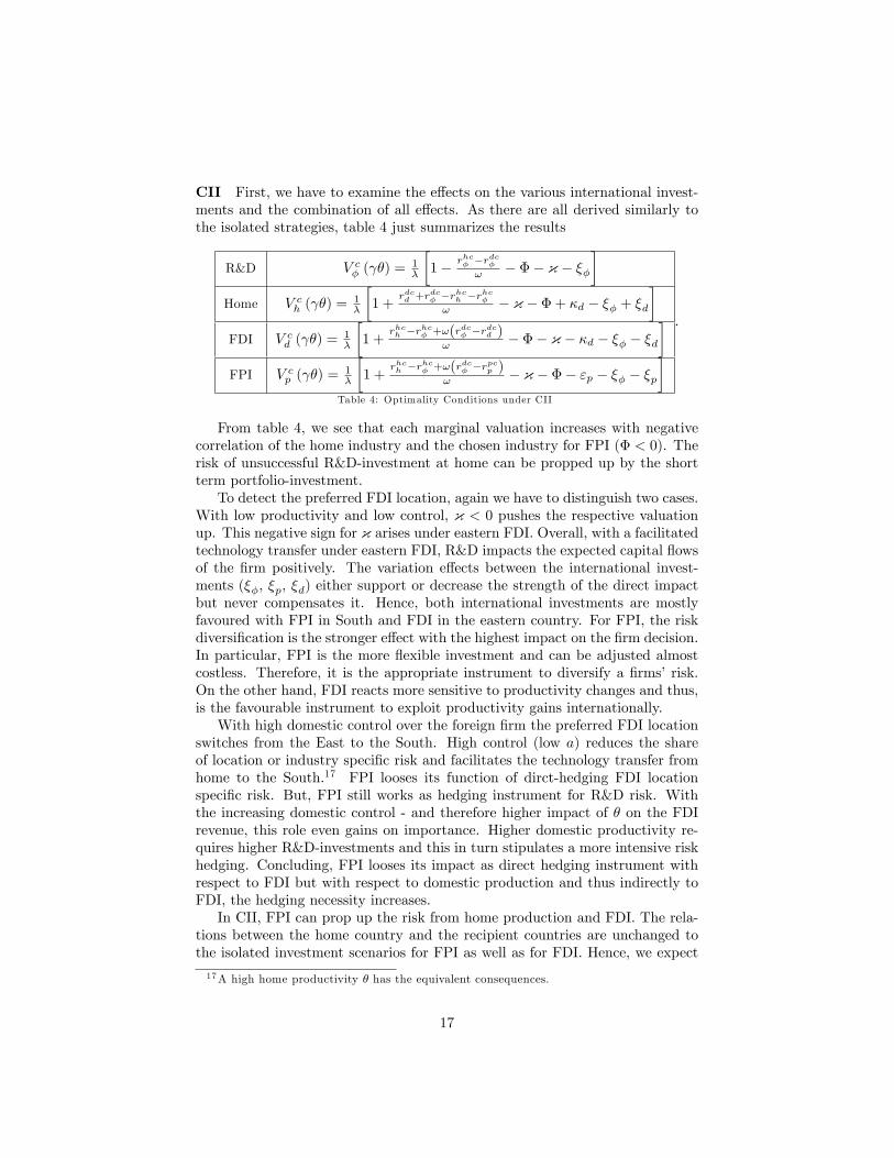
CII First, we have to examine the e¤ects on the various international invest-ments and the combination of all e¤ects. As there are all derived similarly tothe isolated strategies, table 4 just summarizes the results

R&D V c� ( �) =1�

�1� rhc� �rdc�

! � �� { � ��

Home V ch ( �) =1�

�1 +

rdcd +rdc� �rhch �rhc�! � { � �+ �d � �� + �d

�FDI V cd ( �) =

1�

�1 +

rhch �rhc� +!(rdc� �rdcd )! � �� { � �d � �� d

�FPI V cp ( �) =

1�

�1 +

rhch �rhc� +!(rdc� �rpcp )! � { � �� "p � �� p

�Table 4: Optimality Conditions under CII

.

From table 4, we see that each marginal valuation increases with negativecorrelation of the home industry and the chosen industry for FPI (� < 0). Therisk of unsuccessful R&D-investment at home can be propped up by the shortterm portfolio-investment.To detect the preferred FDI location, again we have to distinguish two cases.

With low productivity and low control, { < 0 pushes the respective valuationup. This negative sign for { arises under eastern FDI. Overall, with a facilitatedtechnology transfer under eastern FDI, R&D impacts the expected capital �owsof the �rm positively. The variation e¤ects between the international invest-ments (��, �p, �d) either support or decrease the strength of the direct impactbut never compensates it. Hence, both international investments are mostlyfavoured with FPI in South and FDI in the eastern country. For FPI, the riskdiversi�cation is the stronger e¤ect with the highest impact on the �rm decision.In particular, FPI is the more �exible investment and can be adjusted almostcostless. Therefore, it is the appropriate instrument to diversify a �rms�risk.On the other hand, FDI reacts more sensitive to productivity changes and thus,is the favourable instrument to exploit productivity gains internationally.With high domestic control over the foreign �rm the preferred FDI location

switches from the East to the South. High control (low a) reduces the shareof location or industry speci�c risk and facilitates the technology transfer fromhome to the South.17 FPI looses its function of dirct-hedging FDI locationspeci�c risk. But, FPI still works as hedging instrument for R&D risk. Withthe increasing domestic control - and therefore higher impact of � on the FDIrevenue, this role even gains on importance. Higher domestic productivity re-quires higher R&D-investments and this in turn stipulates a more intensive riskhedging. Concluding, FPI looses its impact as direct hedging instrument withrespect to FDI but with respect to domestic production and thus indirectly toFDI, the hedging necessity increases.In CII, FPI can prop up the risk from home production and FDI. The rela-

tions between the home country and the recipient countries are unchanged tothe isolated investment scenarios for FPI as well as for FDI. Hence, we expect

17A high home productivity � has the equivalent consequences.

17

in CII the share of FPI to adjust to short-term environment changes whereasFDI stays unchanged. It is not possible to derive an explicit analytical solutionfor the respective international investment shares. The de�nite shares of FPIand FDI will be derived numerically.

4 Optimal Investment Strategies

As for both FDI investor scenarios - low and high control on the foreign �rm,the results emphasize that FPI works as diversi�cation instrument and the �rmuses FDI as a technology transfer channel. These �ndings are valid for theisolated strategies as well as for the combined strategy. To proof or reject these�ndings clearly in the following analysis we consider FDI in the East and FPIin the South.Unfortunately, the problem has no tractable closed form solution. Hence,

the solution must be approximated by numerical methods. We use recursivepolicy function iteration.18 The �rst run computes the solution for the isolatedinternational investment strategies and determines the cut-o¤s at which the �rmchanges from one strategy to another (home, FPI or FDI). In the second run,we repeat the same steps for the combined international investment strategy.Precisely, with CII the �rm changes its strategy only once: from isolated homeproduction to FPI and FDI at the same time.We derive a benchmark case with a depreciation of � = 0; 3. A higher

depreciation pushes the start of international activity backwards in time and alower depreciation pulls it forward. The general results stay the same. Further,the probability for successful R&D-investment varies and shows a signi�cantimpact on the �rms�decision to invest internationally or not.

4.1 Isolated International Investment

4.1.1 Start of International Actvitiy

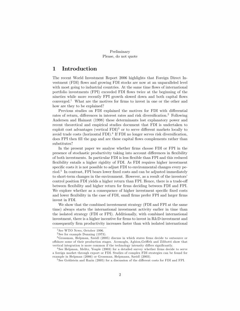
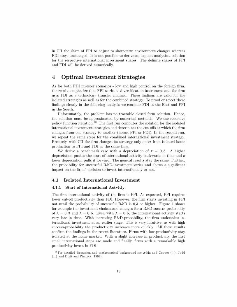
The �rst international activity of the �rm is FPI. As expected, FPI requireslower cut-o¤ productivity than FDI. However, the �rm starts investing in FPInot until the probability of successful R&D is 0,3 or higher. Figure 1 showsfor example the investment choices and changes for a R&D-success probabilityof � = 0; 3 and � = 0; 5. Even with � = 0; 5, the international activity startsvery late in time. With increasing R&D-probability, the �rm undertakes in-ternational investment at an earlier stage. This is very intuitive, as with highsuccess-probability the productivity increases more quickly. All these resultscon�rm the �ndings in the recent literature. Firms with low productivity stayisolated at the home market. With a slight increase in productivity the �rstsmall international steps are made and �nally, �rms with a remarkable highproductivity invest in FDI.

18For detailed discussion and mathematical background see Adda and Cooper (...), Judd(...) and Dixit and Pindyck (1994).

18

investmentshares with r&d successprobability 0,5

0%

20%

40%

60%

80%

100%

1,00

000

1,03

500

1,07

122

1,34

923

1,68

896

1,92

541

1,82

043

1,60

578

1,71

819

1,83

846

productivity/time

shar

e

r&dfdifpihome


0%

20%

40%

60%

80%

100%

1,00

000

1,02

100

1,04

244

1,06

433

1,08

668

1,35

727

1,62

247

1,75

875

1,90

649

1,73

300

productivity/time

shar

er&dfdifpihome

a b


0%

20%

40%

60%

80%

100%

1,00

000

1,03

500

1,07

122

1,34

923

1,68

896

1,92

541

1,82

043

1,60

578

1,71

819

1,83

846

productivity/time

shar

e

r&dfdifpihome


0%

20%

40%

60%

80%

100%

1,00

000

1,03

500

1,07

122

1,34

923

1,68

896

1,92

541

1,82

043

1,60

578

1,71

819

1,83

846

productivity/time

shar

e

r&dfdifpihome


0%

20%

40%

60%

80%

100%

1,00

000

1,02

100

1,04

244

1,06

433

1,08

668

1,35

727

1,62

247

1,75

875

1,90

649

1,73

300

productivity/time

shar

er&dfdifpihome


0%

20%

40%

60%

80%

100%

1,00

000

1,02

100

1,04

244

1,06

433

1,08

668

1,35

727

1,62

247

1,75

875

1,90

649

1,73

300

productivity/time

shar

er&dfdifpihome

a b

Figure 1

4.1.2 Variation of Foreign Productivity

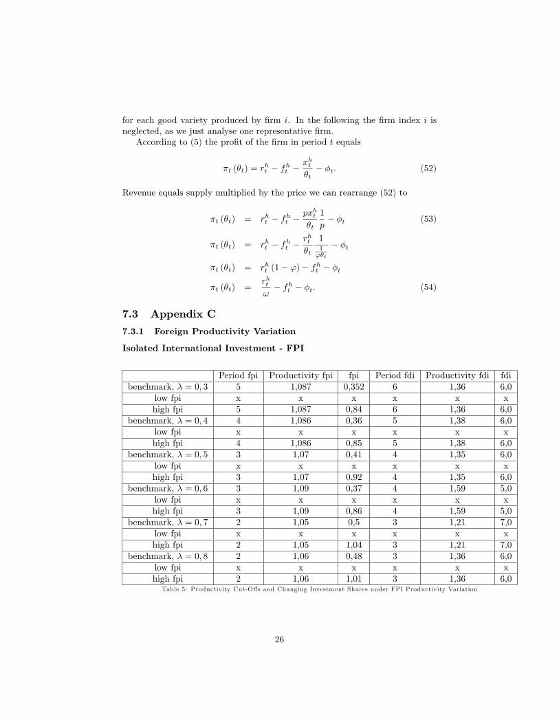
Firstly, we observe changes in the FPI productivity. Table 5 in Appendix Cshows that neither the productivity cut o¤s nor the cut-o¤ time change withvariations in FPI productivity. One might have expected that with higher for-eign productivity the �rm engages earlier in international investment. This isnot the case. The �rm �rst secures the home production process and then goesabroad.Further, the �rm does not reduce or increase its share in FDI. Only the

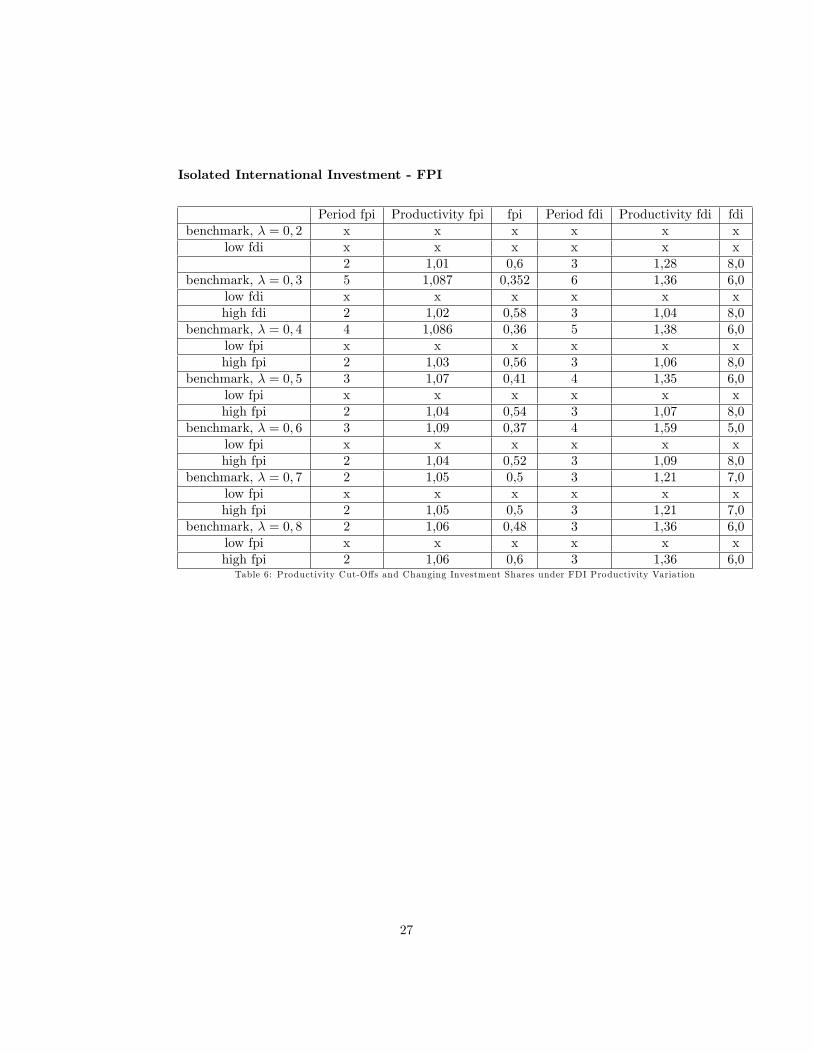
FPI shares increase with higher FPI productivity. This might seem intuitive,as only the FPI-productivity changes. Hence, the FDI shares are independentof the FPI productivity. Let�s take a closer look on FDI-productivity changes,to see whether this independence also hold in the opposite direction and we cancon�rm FPI as the more �exibel instrument.Table 6 in Appendix C shows that with a high FDI-productivity the �rm

engages in international investment at an earlier stage in time, than with alower FDI-productivity. Further, the productivity cut-o¤ is lower than with thebenchmark productivity. The only exceptions are the cases with a very highsuccess probability of R&D investment. For these cases the cut-o¤s are thesame as for the benchmark case and the high FDI-productivity.Finally, with varying FDI-productivity both international shares change in

comparison to the benchmark case. In particular, the FPI shares do not onlyvary in comparison to the benchmark case. They also change between the vari-ous cases of high FDI-productivity while the FDI shares stay almost the same.Again, only with the high R&D-probability the FDI shares change between thedi¤erent cases, but they don�t change with respect to the benchmark case. So,we �nd again FPI as the �exible instrument adjusting to short-term changeswhile FDI reacts more sluggishly. These are only results for the isolated invest-ment scenario.

4.2 Combined International Investment

In contrast to the isolated international investment strategy, the �rm starts itsinternational activities with both investment alternatives FPI and FDI at the

19

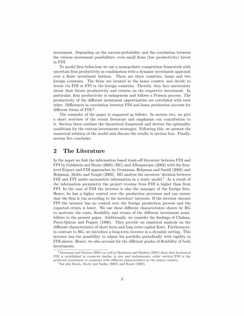
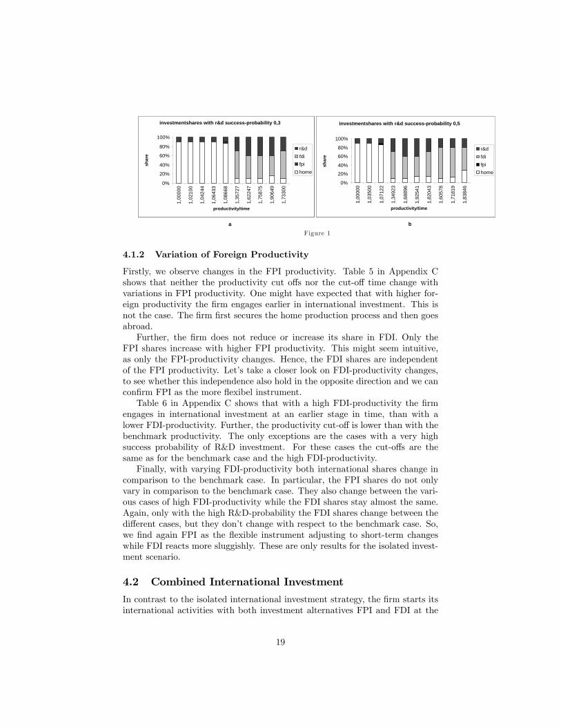
same time. Figure 2a shows that even with a low R&D-probability, the �rmengages in its �rst international investment. However, we have to distinguishbetween the �rst international investment and the investment in FDI. In bothcases, the �rst international activity under CII (CII FDI and FPI vs isolatedFPI) takes place at an earlier date in time than the �rst international �rmactivity under an isolated international investment strategy. Additionally, the�rst international activity at all requires a lower R&D-probability under CIIthan for the isolated international investments.At a moderate probability, the �rm switches from home to international

investment (isol. FPI and combined FPI-FDI respectively at the same time).With increasing probability the isolated investment even dominates the com-bined strategy in time. We have to keep in mind, that we are comparing the�rm starting isolated FPI against the �rm starting combined FPI and FDI underCII.

first international activity

012345678

0 1

perio

d

switch ci 02

switch iso fpi

λ

FDI switch

012345678

0 1

perio

dswitch ciiswitch iso

λ

a b


012345678

0 1

perio

d

switch ci 02

switch iso fpi

λ


012345678

0 1

perio

d

switch ci 02

switch iso fpi

λ

FDI switch

012345678

0 1

perio


λ

FDI switch

012345678

0 1

perio


λ

a b

Figure 2

Now, we turn to the comparison of isolated FDI and the combined interna-tional investment.For the switch to FDI the picture changes as shown in �gure 2b. Under

CII the �rm switches from home production to international investment at alower R&D-probability and at an earlier stage in time. Further, with increasingsuccess-probability, CII still dominates the isolated investments in time.But, CII does not always dominate isolated FDI in productivity. Particu-

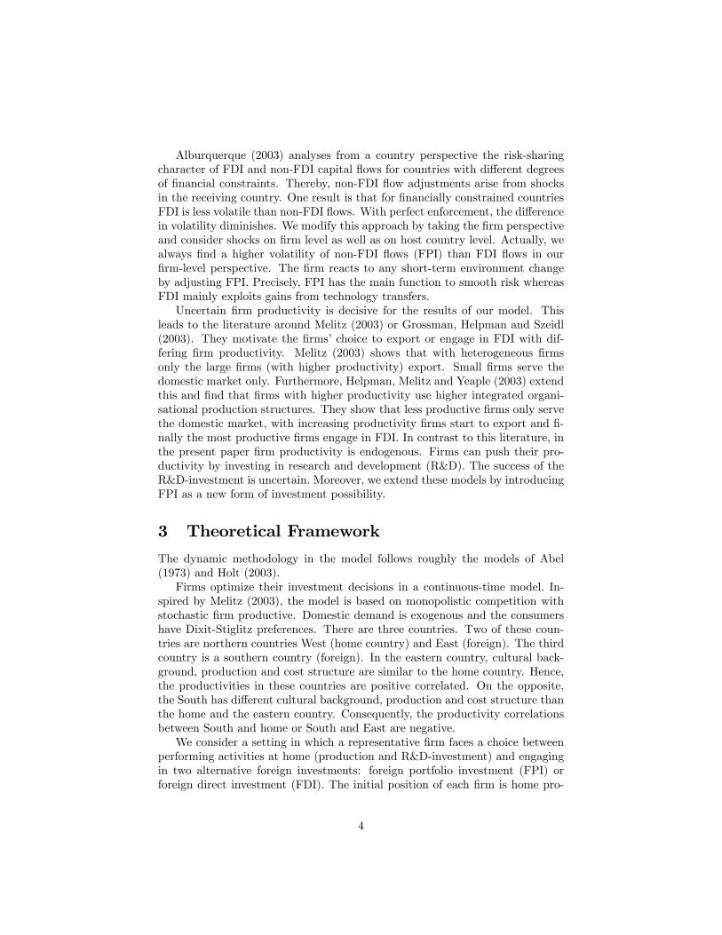
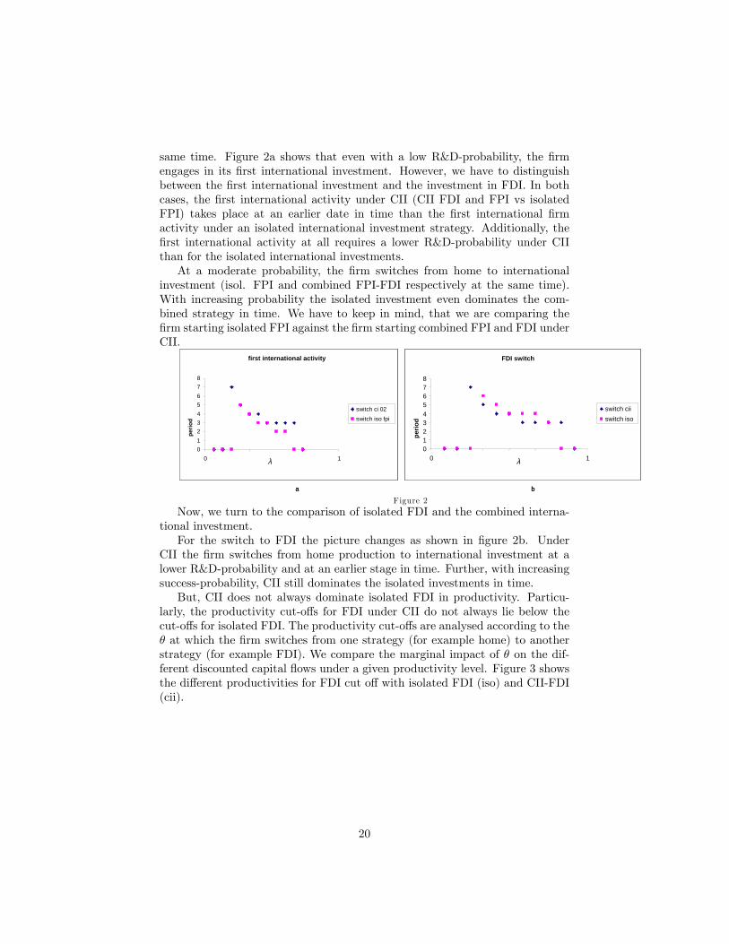
larly, the productivity cut-o¤s for FDI under CII do not always lie below thecut-o¤s for isolated FDI. The productivity cut-o¤s are analysed according to the� at which the �rm switches from one strategy (for example home) to anotherstrategy (for example FDI). We compare the marginal impact of � on the dif-ferent discounted capital �ows under a given productivity level. Figure 3 showsthe di¤erent productivities for FDI cut o¤ with isolated FDI (iso) and CII-FDI(cii).

20

prod

uctiv

ity

0

0,20,40,60,8

11,2

1,41,61,8

0 01 02 03 04 05 06 07 08 09

iso

cii

positive correlation

FDI cut off

apr

oduc

tivity

λ

0

0,2

0,4

0,6

0,8

1

1,2

1,4

1,6

1,8

0 01 02 03 04 05 06 07 08 09

iso

cii

low negative correlation

b

prod

uctiv

ity

λ

0

0,2

0,4

0,6

0,8

1

1,2

1,4

1,6

0 01 02 03 04 05 06 07 08 09

iso

cii

high negative correlation

cλ

prod

uctiv

ity

0

0,20,40,60,8

11,2

1,41,61,8

0 01 02 03 04 05 06 07 08 09

iso

cii


FDI cut off

apr

oduc

tivity

λ

0

0,20,40,60,8

11,2

1,41,61,8

0 01 02 03 04 05 06 07 08 09

iso

cii


FDI cut off

apr

oduc

tivity

λ

0

0,2

0,4

0,6

0,8

1

1,2

1,4

1,6

1,8

0 01 02 03 04 05 06 07 08 09

iso

cii


b

prod

uctiv

ity

λ

0

0,2

0,4

0,6

0,8

1

1,2

1,4

1,6

1,8

0 01 02 03 04 05 06 07 08 09

iso

cii


0

0,2

0,4

0,6

0,8

1

1,2

1,4

1,6

1,8

0 01 02 03 04 05 06 07 08 09

iso

cii

0

0,2

0,4

0,6

0,8

1

1,2

1,4

1,6

1,8

0 01 02 03 04 05 06 07 08 09

iso

cii


b

prod

uctiv

ity

λ

0

0,2

0,4

0,6

0,8

1

1,2

1,4

1,6

0 01 02 03 04 05 06 07 08 09

iso

cii


cλ

0

0,2

0,4

0,6

0,8

1

1,2

1,4

1,6

0 01 02 03 04 05 06 07 08 09

iso

cii


cλ

Figure 3

The domination of the isolated investment strategy might be unexpected.CII implicates a higher incentive to invest in R&D. This in turn pushes domesticproductivity up and also the cut o¤ productivities.

4.2.1 Variation of Foreign Productivity

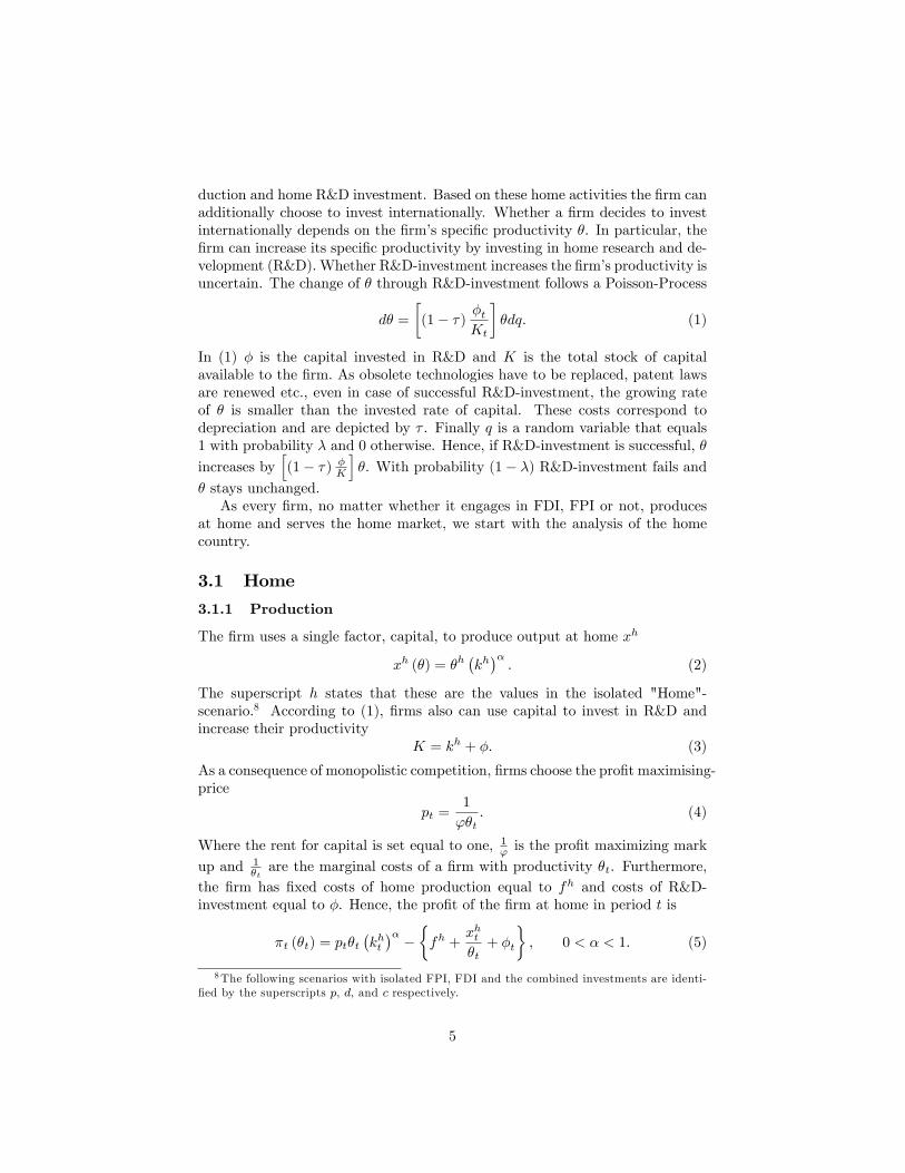
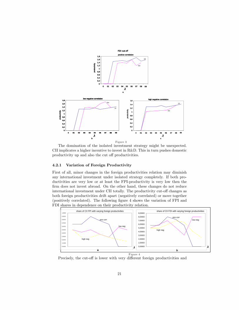
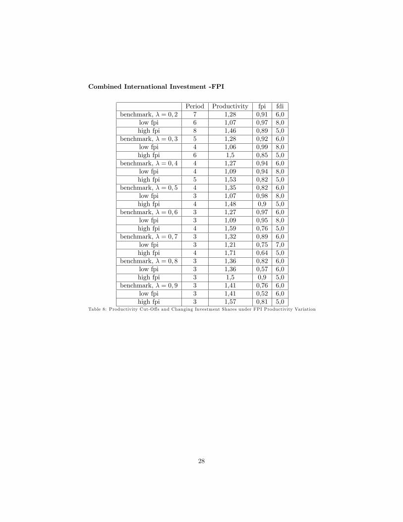
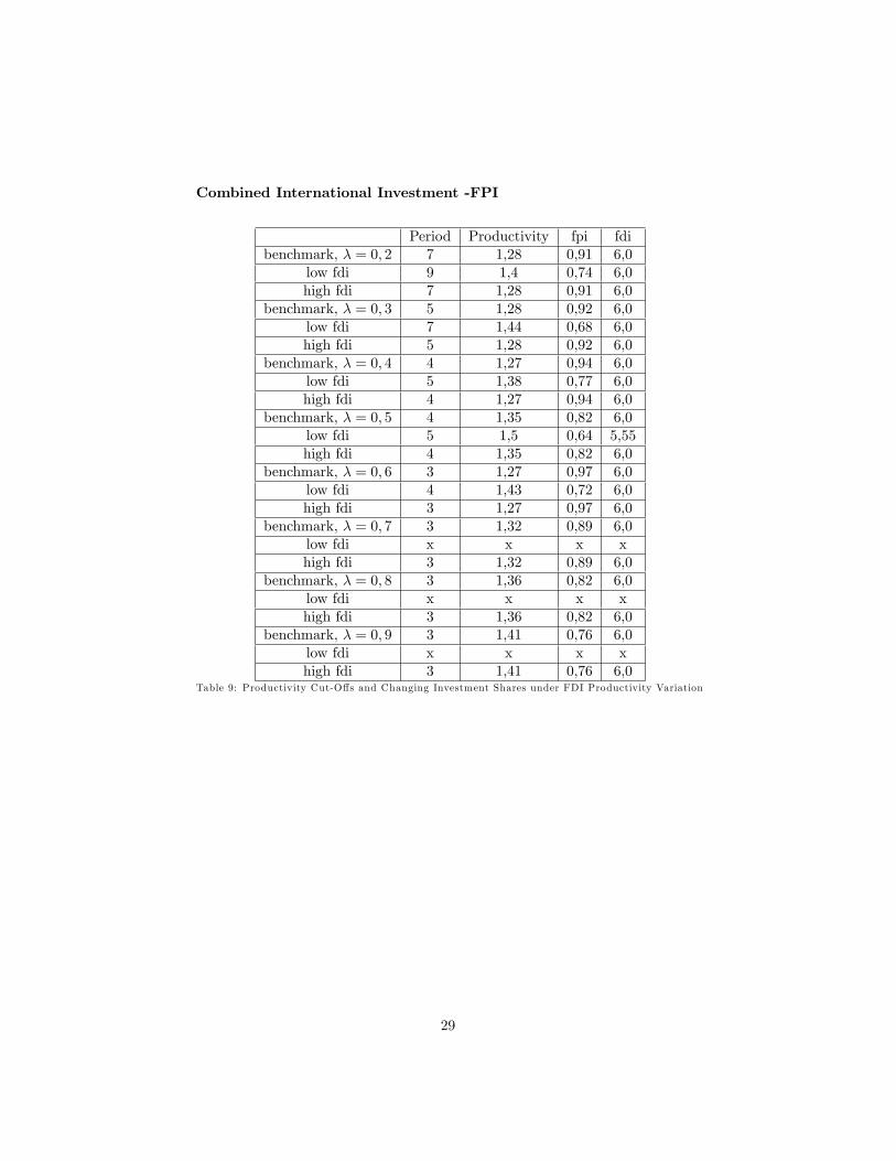
First of all, minor changes in the foreign productivities relation may diminishany international investment under isolated strategy completely. If both pro-ductivities are very low or at least the FPI-productivity is very low then the�rm does not invest abroad. On the other hand, these changes do not reduceinternational investment under CII totally. The productivity cut-o¤ changes asboth foreign productivities drift apart (negatively correlated) or move together(positively correlated). The following �gure 4 shows the variation of FPI andFDI shares in dependence on their productivity relation.

0,00000

0,10000

0,20000

0,30000

0,40000

0,50000

0,60000

0,70000

0,80000

0,90000

1,00000share of CII FPI with varying foreign productivities

aλ

b0,00000

1,00000

2,00000

3,00000

4,00000

5,00000

6,00000

7,00000

8,00000

9,00000share of CII FDI with varying foreign productivities

λ

pos corrpos corr

low neg

low neg

high neg

high neg

0,00000

0,10000

0,20000

0,30000

0,40000

0,50000

0,60000

0,70000

0,80000

0,90000


aλ

b0,00000

1,00000

2,00000

3,00000

4,00000

5,00000

6,00000

7,00000

8,00000


λ0,00000

0,10000

0,20000

0,30000

0,40000

0,50000

0,60000

0,70000

0,80000

0,90000


aλ

b0,00000

1,00000

2,00000

3,00000

4,00000

5,00000

6,00000

7,00000

8,00000


λ

pos corrpos corr

low neg

low neg

high neg

high neg

Figure 4

Precisely, the cut-o¤ is lower with very di¤erent foreign productivities and

21

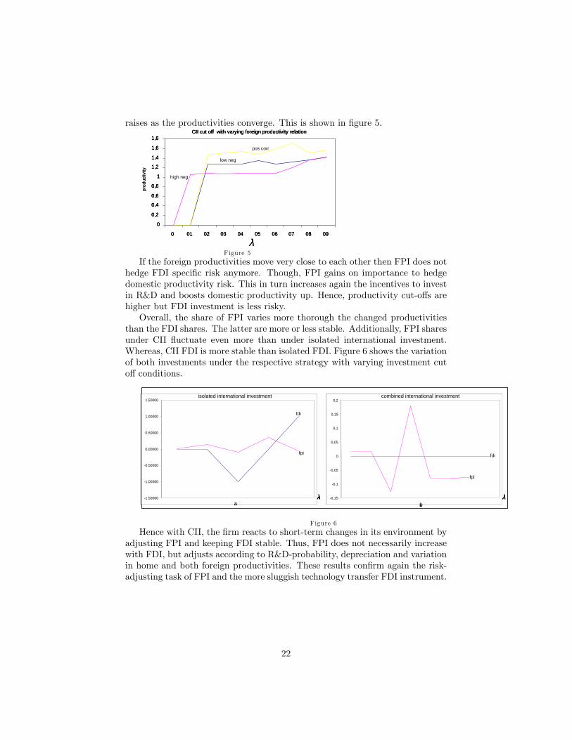
raises as the productivities converge. This is shown in �gure 5.CII cut off with varying foreign productivity relation

0

0,2

0,4

0,6

0,8

1

1,2

1,4

1,6

1,8

0 01 02 03 04 05 06 07 08 09

high neg

low neg

pos corrpr

oduc

tivity

λ

CII cut off with varying foreign productivity relation

0

0,2

0,4

0,6

0,8

1

1,2

1,4

1,6

1,8

0 01 02 03 04 05 06 07 08 09

high neg

low neg

pos corr

CII cut off with varying foreign productivity relation

0

0,2

0,4

0,6

0,8

1

1,2

1,4

1,6

1,8

0 01 02 03 04 05 06 07 08 09

high neg

low neg

pos corrpr

oduc

tivity

λFigure 5

If the foreign productivities move very close to each other then FPI does nothedge FDI speci�c risk anymore. Though, FPI gains on importance to hedgedomestic productivity risk. This in turn increases again the incentives to investin R&D and boosts domestic productivity up. Hence, productivity cut-o¤s arehigher but FDI investment is less risky.Overall, the share of FPI varies more thorough the changed productivities

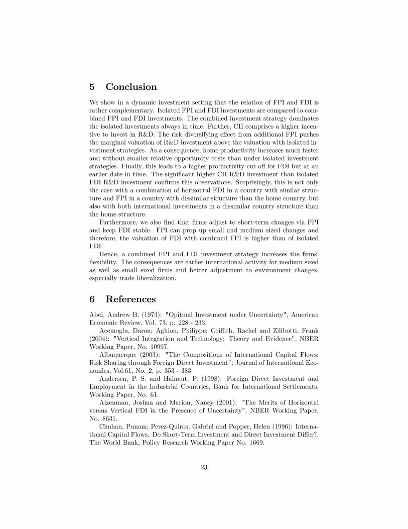
than the FDI shares. The latter are more or less stable. Additionally, FPI sharesunder CII �uctuate even more than under isolated international investment.Whereas, CII FDI is more stable than isolated FDI. Figure 6 shows the variationof both investments under the respective strategy with varying investment cuto¤ conditions.

1,50000

1,00000

0,50000

0,00000

0,50000

1,00000

1,50000

a

fpi

fdi

isolated international investment

λ 0,15

0,1

0,05

0

0,05

0,1

0,15

0,2

b

fpi

fdi

combined international investment

λ1,50000

1,00000

0,50000

0,00000

0,50000

1,00000

1,50000

a

fpi

fdi


λ 0,15

0,1

0,05

0

0,05

0,1

0,15

0,2

b

fpi

fdi


λ1,50000

1,00000

0,50000

0,00000

0,50000

1,00000

1,50000

a

fpi

fdi


λ1,50000

1,00000

0,50000

0,00000

0,50000

1,00000

1,50000

a

fpi

fdi


λ 0,15

0,1

0,05

0

0,05

0,1

0,15

0,2

b

fpi

fdi


λ0,15

0,1

0,05

0

0,05

0,1

0,15

0,2

b

fpi

fdi


λ

Figure 6

Hence with CII, the �rm reacts to short-term changes in its environment byadjusting FPI and keeping FDI stable. Thus, FPI does not necessarily increasewith FDI, but adjusts according to R&D-probability, depreciation and variationin home and both foreign productivities. These results con�rm again the risk-adjusting task of FPI and the more sluggish technology transfer FDI instrument.

22

5 Conclusion

We show in a dynamic investment setting that the relation of FPI and FDI israther complementary. Isolated FPI and FDI investments are compared to com-bined FPI and FDI investments. The combined investment strategy dominatesthe isolated investments always in time. Further, CII comprises a higher incen-tive to invest in R&D. The risk diversifying e¤ect from additional FPI pushesthe marginal valuation of R&D investment above the valuation with isolated in-vestment strategies. As a consequence, home productivity increases much fasterand without smaller relative opportunity costs than under isolated investmentstrategies. Finally, this leads to a higher productivity cut o¤ for FDI but at anearlier date in time. The signi�cant higher CII R&D investment than isolatedFDI R&D investment con�rms this observations. Surprisingly, this is not onlythe case with a combination of horizontal FDI in a country with similar struc-ture and FPI in a country with dissimilar structure than the home country, butalso with both international investments in a dissimilar country structure thanthe home structure.Furthermore, we also �nd that �rms adjust to short-term changes via FPI

and keep FDI stable. FPI can prop up small and medium sized changes andtherefore, the valuation of FDI with combined FPI is higher than of isolatedFDI.Hence, a combined FPI and FDI investment strategy increases the �rms�

�exibility. The consequences are earlier international activity for medium sizedas well as small sized �rms and better adjustment to environment changes,especially trade liberalization.

6 References

Abel, Andrew B. (1973): "Opitmal Investment under Uncertainty", AmericanEconomic Review, Vol. 73, p. 228 - 233.Acemoglu, Daron; Aghion, Philippe; Gri¢ th, Rachel and Zilibotti, Frank

(2004): "Vertical Integration and Technology: Theory and Evidence", NBERWorking Paper, No. 10997.Albuquerque (2003): "The Compositions of International Capital Flows:

Risk Sharing through Foreign Direct Investment"; Journal of International Eco-nomics, Vol.61, No. 2, p. 353 - 383.Andersen, P. S. and Hainaut, P. (1998): Foreign Direct Investment and

Employment in the Industrial Countries, Bank for International Settlements,Working Paper, No. 61.Aizenman, Joshua and Marion, Nancy (2001): "The Merits of Horizontal

versus Vertical FDI in the Presence of Uncertainty", NBER Working Paper,No. 8631.Chuhan, Punam; Perez-Quiros, Gabriel and Popper, Helen (1996): Interna-

tional Capital Flows. Do Short-Term Investment and Direct Investment Di¤er?,The World Bank, Policy Research Working Paper No. 1669.

23

Dixit, Avinash K. and Pindyck, Robert S. (1994):"Investment under Uncer-tainty", Princeton University Press.Dixit, Avinash K. and Stiglitz, J. (1977): "Monopolistic Competition and

Optimum Product Diversity", American Economic Review, Vol. 67, No. 3, 297- 308.Dunning, John H. (1973): "The Determinants of International Production",

Oxford Economic Papers, New Series, Vol. 25, No. 3 , p. 289-336.Goldstein, Itay and Razin, Assaf (2005): Foreign Direct Investment vs For-

eign Portfolio Investment, NBER Working Paper, No. 11047.Grossman, Gene M.; Helpman, Elhanan and Szeidl, Adam (2003): "Optimal

Integration Strategies for the Multinational Firm", NBER Working Paper, No.10189.Grossman, Gene; Helpman, Elhanan and Szeidl, Adam (2005): "Comple-

mentarities between Outsourcing and Foreign Sourcing", American EconomicReview, Vol. 95 (2), p. 19 - 24.Helpman, Elhanan (2006): Trade, FDI, and the Organization of Firms, Jour-

nal of Economic Literature, Vol. 64 (3), p. 589 - 630.Helpman, Elhanan ;Melitz, Marc J.and Yeaple, Stephen R. (2003): Eport

versus FDI, NBER Working Paper, No. 9439.Holt, Richard W.P. (2003): "Investment and dividends under irreversibility

and �nancial constraints", Journal of Economic Dynamics and Control, Vol. 27,p. 467 - 502.Markusen, James R. and Maskus, Keith E. (2001): "General-Equilibrium

Approaches to the Multinational Firm: A Review of Theory adn Evidence",NBER Working Paper, No. 8334.Melitz, Marc J. (2003):"The Impact of Trade on Intra-Industry Reallocations

and Aggregate Industry Productivity", Econometrica, Vol. 71, No. 6, 1695 -1725.Mody, Ashoka; Razin, Assaf and Sadka, Efraim (2002): The Role of In-

formation in driving FDI: Theory and Evidence, NBER Working Paper, No.9255.Razin, Assaf (2002): FDI Contribution to Capital FLows and Investment in

Capacity, NBER Working Paper, No. 9204.WTO (1996): Trade and foreign direct investment, New Report by WTO,www.wto.org/English/news_e/pres96_e/pr057_e.htm.UNCTAD (2006): World Investment Report 2006, http://www.unctad.org/en/docs/wir2006_en.pdf.

24

7 Appendix

7.1 Appendix A

7.1.1 Derivation of Expected Capital Flow

The value of the �rm in the case without international investment is a functionof the state variable � (productivity).

dV h = V h� d� (43)

The state variable follows a Poisson process with q = 1 with prob. �dt andq = 0 with prob. (1� �dt):

) d� =

�(1� �) �

K

��dq (44)

) E�dV h

�= �

�V h��(1� �) �

K

��

�� V (�)

�dt| {z }

change of capital �ow caused by increased � weighted with the probability

(45)

+ (1� �dt)�V h (�)� V h (�)

�| {z }change of capital �ow in the case of unchanged � weighted with respective probability

(46)

) E�dV h

�= +�

�V h ( �)� V h (�)

�dt (47)

with

��(1� �) �

K

�(48)

For a general discussion of Poisson processes in continuous time see Dixit andPindyck (1994).

7.2 Appendix B

7.2.1 Derivation of the Pro�t Function with Variable Revenue

Domestic consumers have Dixit-Stiglitz preferences for di¤erentiated goods withelasticity of substitution ! = 1

1�' > 1. The price index for the home country is

P =

�Zj2J

p (j)1�!

dj

� 11�!

(49)

and the demand level is

A =

�Zj2J

x (j)'dj

� 1'

. (50)

From (49) and (50) we derive the demand function

xi = Ap�!i (51)

25

for each good variety produced by �rm i. In the following the �rm index i isneglected, as we just analyse one representative �rm.According to (5) the pro�t of the �rm in period t equals

�t (�t) = rht � fht �xht�t� �t. (52)

Revenue equals supply multiplied by the price we can rearrange (52) to

�t (�t) = rht � fht �pxht�t

1

p� �t (53)

�t (�t) = rht � fht �rht�t

11'�t

� �t

�t (�t) = rht (1� ')� fht � �t

�t (�t) =rht!� fht � �t. (54)

7.3 Appendix C

7.3.1 Foreign Productivity Variation

Isolated International Investment - FPI

Period fpi Productivity fpi fpi Period fdi Productivity fdi fdibenchmark, � = 0; 3 5 1,087 0,352 6 1,36 6,0

low fpi x x x x x xhigh fpi 5 1,087 0,84 6 1,36 6,0

benchmark, � = 0; 4 4 1,086 0,36 5 1,38 6,0low fpi x x x x x xhigh fpi 4 1,086 0,85 5 1,38 6,0




benchmark, � = 0; 8 2 1,06 0,48 3 1,36 6,0low fpi x x x x x xhigh fpi 2 1,06 1,01 3 1,36 6,0Table 5: Productivity Cut-O¤s and Changing Investment Shares under FPI Productivity Variation

26

Isolated International Investment - FPI

Period fpi Productivity fpi fpi Period fdi Productivity fdi fdibenchmark, � = 0; 2 x x x x x x

low fdi x x x x x x2 1,01 0,6 3 1,28 8,0

benchmark, � = 0; 3 5 1,087 0,352 6 1,36 6,0low fdi x x x x x xhigh fdi 2 1,02 0,58 3 1,04 8,0





benchmark, � = 0; 8 2 1,06 0,48 3 1,36 6,0low fpi x x x x x xhigh fpi 2 1,06 0,6 3 1,36 6,0Table 6: Productivity Cut-O¤s and Changing Investment Shares under FDI Productivity Variation

27

Combined International Investment -FPI

Period Productivity fpi fdibenchmark, � = 0; 2 7 1,28 0,91 6,0

low fpi 6 1,07 0,97 8,0high fpi 8 1,46 0,89 5,0

benchmark, � = 0; 3 5 1,28 0,92 6,0low fpi 4 1,06 0,99 8,0high fpi 6 1,5 0,85 5,0







Table 8: Productivity Cut-O¤s and Changing Investment Shares under FPI Productivity Variation

28

Combined International Investment -FPI

Period Productivity fpi fdibenchmark, � = 0; 2 7 1,28 0,91 6,0

low fdi 9 1,4 0,74 6,0high fdi 7 1,28 0,91 6,0

benchmark, � = 0; 3 5 1,28 0,92 6,0low fdi 7 1,44 0,68 6,0high fdi 5 1,28 0,92 6,0




benchmark, � = 0; 7 3 1,32 0,89 6,0low fdi x x x xhigh fdi 3 1,32 0,89 6,0



Table 9: Productivity Cut-O¤s and Changing Investment Shares under FDI Productivity Variation

29

Documents

FDI and International Portfolio Investment - Complements ... · control position FDI yields a higher return than FPI. Hence, there is a trade-o⁄ between ⁄exibility and higher